67

ESTIMATING LONG RUN RELATIONSHIPS BETWEEN THE TRADE BALANCE AND THE TERMS OF TRADE IN

SELECTED CARICOM COUNTRIES

By

Ryan Straughn Central Bank of Barbados

1

Estimating Long Run Relationships Between the Trade Balance and the terms of trade in Selected CARICOM countries.

by Ryan Straughn

Research Department, Central Bank of Barbados, Bridgetown

ABSTRACT

This paper examines the impact of the terms of trade on the trade balance in 3 Caribbean Community and Common Market (CARICOM) countries, with the inclusion of the real national income and the real stock of money in the model. The econometric procedure employed is the Johansen approach to estimation of multivariate cointegration systems with the aim of testing the empirical validity of the Bickerdike-Robinson-Metzler (BRM) and Marshall-Lerner (ML) condition, as well as the examination of the absorption and monetary approaches. The results indicate that there exists a significant long run “statistical equilibrium” between the trade balance, the terms of trade, the real national income and the real money stock for all three countries. However, these findings along with the impulse response functions indicated that neither the BRM nor the ML condition is supported by the data for any of the three countries, whilst the findings with respect to income and money did not uniformly reject or accept the hypotheses of the absorption or monetary approaches in the long run.

Keywords: Marshall-Lerner Conditions, Cointegration, Vector Autoregression, Impulse Response Functions.

68

2

1. INTRODUCTION

Despite the voluminous literature, the effects of changes in exchange rate regimes on

the balance of payments, particularly those in relation to the trade balance, are still to be

understood clearly. There is still much debate as to whether devaluation or depreciation1 of

country’s (domestic) currency actually improves the trade balance, and if so, does it do so in

the long run? In the Caribbean, this issue is especially critical against the backdrop of

ongoing trade negotiations for the creation of the Free Trade Area of the Americas (FTAA).

Therefore, it is relevant for formulation of sound policy to understand the short-run and long

run relationship between such variables. Over the years, the use of nominal devaluations have

been a key component of many structural adjustment programmes by various economic

authorities to correct external imbalances and/or misalignment in exchange rates, or to

improve a country’s international industrial competitiveness. For many a developing country,

the proper investigation of this area is especially important, since the lack of properly

developed capital markets has meant trade flows have continued to drive the balance of

payment account.

Conventional wisdom says that a nominal devaluation will improve a country’s trade

balance. This effect is deeply rooted in a static and partial approach to the balance of

payments that has come to be known as the elasticities approach. The Bickerdike-Robinson-

Metzler (BRM) model has been recognised in the literature as proving a sufficient condition

(the BRM condition) for trade balance improvement when exchange rates devalue. The

Marshall-Lerner (ML) condition, a particular solution of the BRM condition, hypothesises

that currency depreciation or devaluation can improve a country’s trade balance. The ML

1 Devaluation is defined as the administered reduction in the exchange rate of a currency against other currencies under a FIXED EXCHANGE-RATE SYSTEM; whilst depreciation is defined as a fall in the value of a currency against other currencies under a FLOATING EXCHANGE-RATE SYSTEM.

3

condition states that for a positive effect on the trade balance, and implicitly for a stable

foreign exchange market, the absolute value of the sum of the demand elasticities for imports

and exports must exceed unity. Accordingly, if the ML condition holds, there is excess

supply of foreign exchange when the exchange rate is above the equilibrium level and excess

demand when it is below. Thus the BRM and ML conditions have become the underlying

assumptions for those who support devaluation as a means to stabilise the foreign exchange

market.

The primary objective of this paper is to examine the role of the terms of trade in

determining the long run trade balance behaviour for Barbados, Jamaica and Trinidad and

Tobago in a model that includes the real national income and the real stock of money.

Specifically, the author will examine whether the trade balance is affected by the terms of

trade, through changes in exchange rates and whether the hypotheses such as the BRM or the

ML conditions hold for the current data. The empirical relevance of the absorption and

monetary approaches are also tested indirectly for the current data.

The remainder of the paper is organised as follows. Section 2 gives a brief review of the

literature. Section 3 outlines some methodological issues related to three approaches to

balance of payment adjustment and examines the time series properties of the data. Section 4

presents empirical cointegration results along with the simulated impulse response functions.

Section 5 concludes the paper.

2. REVIEW OF THE LITERATURE

Within the body of literature on international trade, it is not surprising to still find

arguments about whether currency deprecation or devaluation will improve the balance of

trade. The three main approaches that have been identified in the literature are the elasticities,

69

4

absorption and monetary approaches; all bare testimony to this with each having its own

arguments. Paraphrasing Miles (1979), proponents of the elasticities approach describe the

necessary and sufficient conditions for an improvement in the trade balance in terms of the

elasticities of demand and supply. If the demand and supply elasticities are sufficiently large

and small respectively, then depreciation should improve the trade balance. Proponents of the

absorption approach, describe how devaluation may change the terms of trade, increase

production, switch expenditures from foreign to domestic goods, or have some other effect in

reducing domestic absorption relative to production and thus improve the trade balance.

International monetarists such as Mundell (1971), Dornbusch (1973) Frenkel and Rodriguez

(1975) all argue that devaluation reduces the real value of cash balances and/or changes the

relative price of traded and nontraded goods, thus improving both the balance of trade and the

balance of payments.

Whilst there is an abundance of empirical evidence to suggest that the Marshall-Lerner

conditions are indeed met, at least for industrial countries, there have also been circumstances

under which devaluation has not been successful. One famous case was the deterioration of

the U.S. trade balance in 1972 following the devaluation in 1971. This effect was termed the

“J-curve” phenomenon2 because of the path the trade balance would follow over time.

Krueger (1983) argued that the phenomenon emanates from the fact that at the time of

devaluation, goods already in transit and under contract have been purchased, and the

completion of those transactions dominates the short-term change in the trade balance. Junz

2 The J-curve effect is the tendency for a country’s balance of payments deficit to initially worsen following a devaluation of its currency before moving into a surplus. This is because the full adjustment of trade volumes to devaluation involves a time lag:there is an immediate fall in export prices and a rise in import prices so that current exports earn less foreign exchange and current imports absorb more foreign exchange, thereby increasing the size of the payment deficit (the downturn of the J-curve). Over time, the lower export prices will increase overseas demand and exports earning will rise, while higher import prices reduces domestic demand for imports, leading to an improvement in the balance of payments (the upturn of the J-curve).

5

and Rhomberg (1973) identified at least five lags in the process between exchange rate

changes and their ultimate effects on real trade: lags in recognition of the changed situation,

in the decision to change real variables, in delivery time, in the replacement of inventories

and materials, and in production. Their empirical evidence supports lags of up to five years in

the effects of changes in exchange rates on market shares of countries in world trade.

Bahmani-Oskooee (1985) in his study of the experiences of Greece, India, Korea and

Thailand concluded that although the elasticities condition is no longer interpreted to imply

that devaluation or depreciation might fail, there is an alternative basis on which questions

have been raised about the short-term effects of exchange rate changes on the trade balance.

The ML condition often requires the estimation of export and import demand models,

which can be tedious and often requires proxying world export prices, effective exchange

rates, and identifying trading partners, etc. For many countries especially those Caribbean

Community and Common Market (CARICOM) countries under investigation in this paper,

the relevant data for constructing such variables are not readily available. Studies by Miles

(1979) and Bahmani-Oskooee (1985), rather than examining price elasticities, attempted to

establish a link between the real effective exchange rate and the trade balance. These

approaches have relied upon estimating reduced form models and have failed to examine the

time series properties of the data. Arize (1994) has shown that there is a long run relation

between the trade balance and the real effective exchange rate using data for nine Asian

developing countries.

Past contributions to the econometric literature provide the tools with which to

determine whether there is a long run relationship between variables that contain unit roots.

The existence of a long run relationship between the trade balance and the terms of trade can

be tested by estimating an ordinary least squares (OLS) regression and examining the

70

6

residuals from this regression for stationarity. According to Engle and Granger (1987), such a

regression will suffice to yield consistent estimates of the long-run coefficients, regardless of

the dynamic structure of the model and regardless of whether any of the right-hand side

variables are correlated with the disturbances.

Using the Engle and Granger approach, Bahmani-Oskooee (1991) found for Argentina,

the Bahamas, Greece and the Philippines that there exists a long run relationship between the

trade balance and the real effective exchange rate, thus showing that the approach can be

considered an alternative to testing the ML conditions. Cointegration links the economic

notion of a long run relationship between economic variables to a statistical model of those

variables. Bahmani-Oskooee (1985) also pointed out that “the fact that the cointegration

approach could be considered an alternative to the elasticities approach increases our scope of

analysis, especially for LDCs for which estimating elasticities require data for import and

export prices, income, etc. These data are not readily available for some LDCs…world

income has to be proxied for all countries”. Testing for cointegration between the trade

balance and the terms of trade is consistent with examining “the statistical links between the

two series” as suggested by Haynes and Stone (1982:704). In addition, cointegration is

considered an alternative to testing the ML conditions because both the cointegration

approach and the ML conditions are indeed long run analyses.

3. THEORETICAL CONSIDERATIONS

In this section the Bickerdike-Robinson-Metzler (BRM) model and its theoretical

implications are presented along with those of the Marshall-Lerner conditions. Also,

presented here is some discussion of the literature that has interpreted, reformulated and

7

criticised the elasticities approach. There will be some focus on the absorption and the

monetary approaches to the balance of payments.

The Elasticities Approach

The BRM model is a partial equilibrium version of a standard two-country (domestic

and foreign), two-goods (exports and imports) model, where the effects of exchange rate

changes are analysed through the separation of markets for exports and imports. The model is

thus defined as follows. The domestic demand for foreign exports (imports) is a function of

the nominal price of imports measured in domestic currency,

� � )1.3(.mdd PMM �

Here, *mm EPP � , where E is the nominal exchange rate, (the domestic price of foreign

currency) and *mP is the foreign currency price (level) of domestic imports. Likewise, the

foreign demand for domestic exports can be similarly defined as,

� � )2.3(.***

xdd PMM �

where*dM is the quantity of foreign imports and *

xP is the foreign currency price (level) of

domestic exports. Analogously, EPP xx �* where xP is the domestic currency price (level)

of exports. Similar to the demand functions, the exports supply functions are defined

depending only on nominal prices. The domestic and foreign exports supply function are

defined as,

)3.3()( mss PXX �

)4.3()( ***

mss PXX �

where sX and*sX are the quantity of domestic and foreign supplies of exports, respectively.

The market equilibrium conditions for exports and imports are then,

71

8

)5.3(*sd XM �

)6.3(* sd XM �

From equations (3.1) through to (3.4), the domestic trade balance, in domestic currency

is,

)7.3(dm

sx MPXPB ��

In order to properly illustrate the model in equation (3.7), a comparative-static

framework with two separate markets for domestic demand for imports and supply of exports

is used when the functions are assumed to be normal downward and upward sloped,

respectively. With the assumption of an initial equilibrium, that is, B=0, the question is, does

devaluation of the domestic currency improve the trade balance as defined by (3.7)? In the

current model, there are two important points to be noted about exchange rates. Firstly, since

non-traded goods do not exist, the real exchange rate is measured by the terms of trade.

Secondly, any nominal devaluation (assumed to be exogenous) becomes a real devaluation

since domestic and foreign price levels are assumed to remain constant, or they are

determined exogenously.

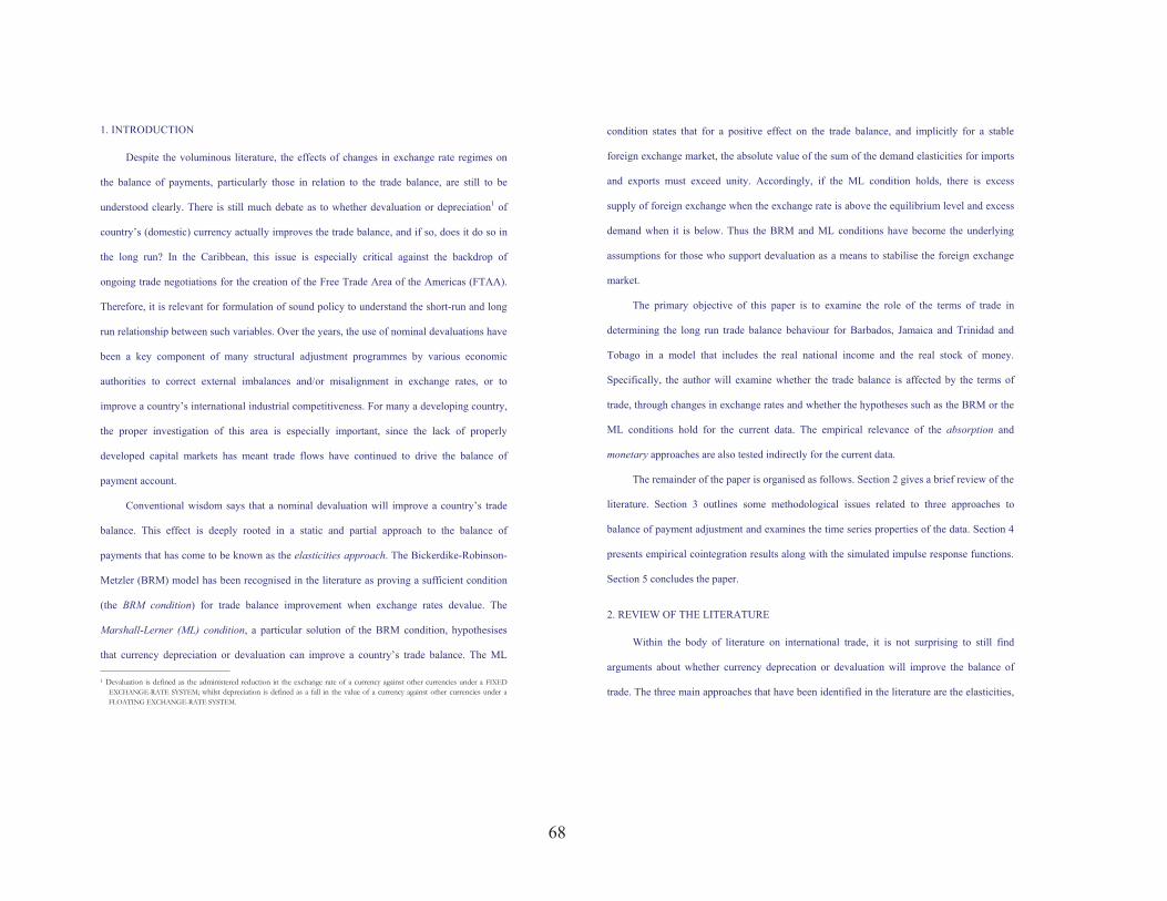
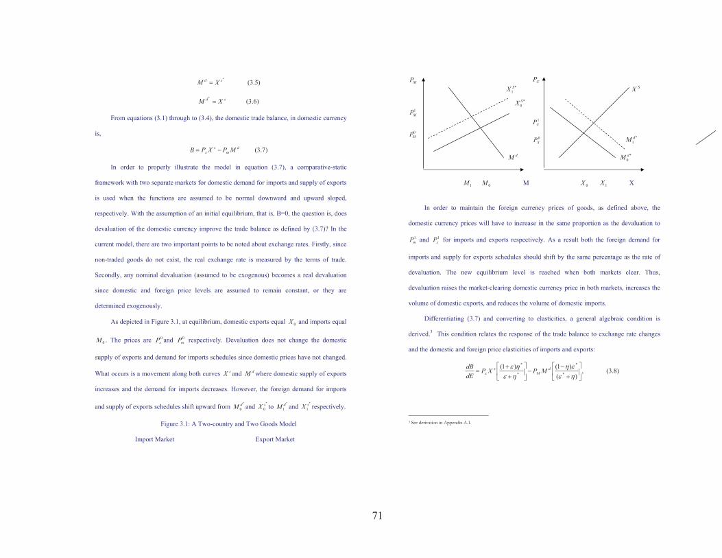
As depicted in Figure 3.1, at equilibrium, domestic exports equal 0X and imports equal

0M . The prices are 0xP and 0

mP respectively. Devaluation does not change the domestic

supply of exports and demand for imports schedules since domestic prices have not changed.

What occurs is a movement along both curves sX and dM where domestic supply of exports

increases and the demand for imports decreases. However, the foreign demand for imports

and supply of exports schedules shift upward from *

0dM and

*

0sX to

*

1dM and

*

1sX respectively.

Figure 3.1: A Two-country and Two Goods Model

Import Market Export Market

9

XP*

1SX SX

1XP

0XP *

1dM

dM *0dM

1M 0M M 0X 1X X

In order to maintain the foreign currency prices of goods, as defined above, the

domestic currency prices will have to increase in the same proportion as the devaluation to

1mP and 1

xP for imports and exports respectively. As a result both the foreign demand for

imports and supply for exports schedules should shift by the same percentage as the rate of

devaluation. The new equilibrium level is reached when both markets clear. Thus,

devaluation raises the market-clearing domestic currency price in both markets, increases the

volume of domestic exports, and reduces the volume of domestic imports.

Differentiating (3.7) and converting to elasticities, a general algebraic condition is

derived.3 This condition relates the response of the trade balance to exchange rate changes

and the domestic and foreign price elasticities of imports and exports:

)8.3(,)(

)1()1(*

*

*

*

��

���

�

��

���

���

�

��

�����

���� d

Ms

x MPXPdEdB

3 See derivation in Appendix A.1.

MP

*0SX

1MP

0MP

72

10

where � and � denote the price elasticities (in absolute values) of domestic demand for

imports and supply of exports. By Walras’s Law, it is sufficient to find equilibrium in one

market since by the market clearing conditions of (3.5) and (3.6) the excess demand in any

one market would be offset by the excess of supply in the other market. Thus without the loss

of generality, the solution could be given in terms of any of the two markets. Analogously, �*

and �* denote respective foreign price elasticities. As can be shown, if B=0 (initial

equilibrium), then 0�dEdB if and only if:

)9.3(,0))((

)1()1(**

****

���

���������

��������

The particular case of interest is the “small country” case where, ��� ** �� (Lindert

and Kindleberger, 1982, ch. 15), which implies that the foreign export supply and export

demand are perfectly elastic and the left hand side of condition (3.9) becomes )( �� � .

Another way to state this case is to say that a country is a price-taker in both its import and

export markets and accordingly, currency devaluation (depreciation) has no effect on world

prices (in foreign currency), or its exports and imports. This implies that only changes in

volumes affect its trade balance.

From condition (3.9) letting ��� and ��*� implies that the left-hand side of (3.9)

becomes 1* ���� . This is the so-called Marshall-Lerner condition (Marshall 1923; Lerner

1944). Thus, for a trade balance improvement after currency devaluation, 1* ���� must

hold. The standard presentation of the ML condition is 1|| * ���� . This simply states that

if domestic and foreign supply elasticities are strictly elastic and if income remains constant,

then a devaluation causes an improvement in the balance of trade when the domestic plus the

11

foreign import demand elasticities, in absolute value, exceeds one. This has been considered

in the literature as a sufficient condition for stability in the foreign exchange market.

The Absorption Approach

The core of this approach is the proposition that any improvement in the trade balance

requires an increase of income over total domestic expenditures, that is, it focuses its analysis

mainly on economic aggregates, typical of the Keynesian analysis, whilst the elasticities

approach based its results on the effects of exchange rate changes on individual

microeconomic behaviour (Marshallian supply and demand analysis).

The theory of the trade balance can be defined in terms of a basic macroeconomic

identity, which expresses the different links between the trade balance and the

macroeconomic aggregates. Assuming no transfers or services (the total national income

becomes the gross domestic product and the current account the trade balance) one can write

the following,

)10.3(dcdcdc MXTBAY ����

where Y is the gross domestic product, A is absorption4, dcTB is the trade balance in domestic

currency, dcX and dcM are the value of exports and imports, respectively, in domestic

currency. The absorption approach analyses the direct effects of exchange rate changes on

relative prices, income, and absorption, and ultimately on the trade balance. This approach

takes implicitly the Keynesian income-expenditure assumption that exports volumes are

independent (autonomous) of national income, and that imports depend directly and positive

on national income. This positive dependence is said to occur in two ways. One is that often

a country’s production needs imported inputs; the other is that imports respond to total

4 Absorption is the total demand for goods and services by all residents (consumers, producers and government) of a country (as opposed to total demand for the country’s output).

73

12

absorption (Alexander, 1952). The more a country spends on goods and services, the more a

country will be inclined to spend on that portion that is bought from abroad. This behaviour is

summarised by the well-known Keynesian foreign trade multiplier.

Under the absorption approach, it is assumed that there is the existence of the

Keynesian short-run world and the nominal and real effects of devaluation can be stated as

follows. Devaluation reduces the relative prices of domestic goods in domestic currency and

produces two effects. Firstly, there is a substitution effect that causes a shift in the

composition from foreign goods towards domestic goods; that is, the exchange rate change

causes an expenditure-substituting effect, and with the usual Keynesian assumption of

unemployment, domestic production increases. Secondly, there is an income effect, which

would increase absorption, and then reduce the trade balance. The income effect is related to

both the increase in domestic output (income), which acts through the “marginal propensity

to absorb” (consume) and “marginal propensity to invest,” and the change in the terms of

trade. In general, this approach argues that a country’s devaluation causes a deterioration in

its terms of trade, and thus a deterioration in its national income. The presumption is that

devaluation will result in a decrease in the price of exports measured in foreign currency5.

However, the fact that the terms of trade deteriorates does not necessarily imply that the trade

balance is also going to deteriorate. “It can worsen the trade balance if the foreign currency

price of exports sinks far enough relative to the price of imports to outweigh the trade balance

improvement implied by the rise in export volumes and the drop in import volumes” (Lindert

and Kindleberger, 1982, p. 312). In all, the final effect of a devaluation on the trade balance

5 Since countries are assumed “large” with elastic supplies, then under the assumption of constant domestic prices, a devaluation will reduce the relative price of domestic exports in foreign currency. The price of imports in foreign currency remains constant, or it can decrease if the foreign supply is not perfectly elastic. The key condition for a worsening of the domestic terms of trade is that the decrease in the price of exports is greater than the decrease of the price of imports.

13

will depend on the combined substitution and income effects. As predicted by the absorption

approach, the trade balance will improve, but it would be smaller (because of the income

effect on absorption) than that predicted by the BRM model.

The Monetary Approach

Since the 1950s, two monetary perspectives have been distinguished in the literature:

the monetary approach and the Keynesian monetary view. Some of the basic assumptions

underlying each of these perspectives are the following. With regard to the former: (1) there

is full employment; (2) there are perfect substitutes for domestic and foreign goods and

assets. This approach has been called the “global monetarist” (Whitman, 1975). With regard

to the Keynesian view: (1) there is unemployment; (2) price sluggishness occurs so that

purchasing power parity may not hold; and (3) money is a close substitute for other assets.

The monetary approach utilises the balance of payment identity is written here as

)11.3(FKACA ���

where CA is the current account, KA is the capital account and F� is the change in a

country’s foreign reserves, denominated in foreign currency. Note, however, that the identity

only holds under a fixed exchange rate regime. “This is in marked contrast with the

Keynesian view of the balance of payments namely that the monetary authorities sterilise the

impact on the domestic money supply of international reserve flows ensuing from payments

imbalance” (Hallwood and MacDonald, 1994, p. 140). Under a clean-floating regime the

central bank refrains from intervention in the foreign exchange market. Accordingly, 0��F .

The absorption approach, the monetary approach can be defined in terms of basic

identities, here, in terms of the central bank’s balance sheet. Simplified, it can be written as

)12.3(CRMBFD dc ����

74

14

where the left-hand side represents the assets and the right-hand side the liabilities. MB is the

monetary base, or high-powered money, D is the domestic credit (or the domestic asset

component of MB), dcF is the stock of foreign reserves (or the foreign-backed component) in

domestic currency, R is the money reserves and C is the currency in public hands. Now, let M

be the domestic money supply and to simplify, let MBM � (the money multiplier is

implicitly assumed constant and equal one), then

)13.3(MFD dc �� .

In an open economy, this identity means that the residents “can have an influence on

the total quantity of money via their ability to convert domestic money into foreign goods and

securities or conversely turn domestic goods and securities into domestic money backed by

foreign exchange reserves” (Hallwood and MacDonald, 1994, p. 137). Taking first

differences of (3.13) and rearranging, we get

)14.3(DMFdc �����

where M� is the flow demand of money balances or hoarding. Therefore, it follows that if

the balance of payments identity in equation (3.11) holds, then the following equality has to

be satisfied.

)15.3(DMFKACA dcdcdc �������

where dcCA and dcKA are CA and KA in domestic currency, respectively. The left-hand side

of (3.15) states that if a country has a deficit in both the current and the capital account, then

it has to be losing foreign reserves, whilst the right-hand side implies that it loses foreign

reserves when domestic credit exceeds hoarding.

In comparison with the elasticity and absorption approaches, and assuming that

0�dcKA and consider dcdc TBCA � , then the following identity must also hold.

15

)16.3(DMFTBAYMX dcdcdcdc ����������

This is a fundamental identity that puts together the elasticity, absorption and monetary

approaches to the balance of payments. Therefore, according to Mundell (1968), if one

considers all the variables in (3.16) in an ex post sense, the three approaches are equivalent. It

is worthy to note, however, that this identity omits reference to the underlying behavioural

relationships and adjustment mechanisms in each of these approaches.

What makes the monetary approach different from the elasticities and absorption

approaches is that the role of the exchange rate is reduced to its temporary effect on the

money supply. The reason being that the monetary approach assumes “a change in the

exchange rate will not systematically alter relative prices of domestic and foreign goods and

it will have only a transitory effect on the balance of payments” (Whitman, 1975, p. 494).

Of particular interest in this research paper is the question, what is the ‘transitory’ (or

short run) effect of the devaluation under the monetary approach? In the short run, this

approach predicts that an increase in prices, as caused by a nominal devaluation, may reduce

the real money stock, and then improve the trade balance. The mechanism works as follows.

A devaluation will proportionally increase the domestic prices6, then people will reduce

spending/absorption relative to income in order to restore their real money balances and

holding of other financial assets. In brief, hoarding will increase7. As a result, the trade

balance, and directly the money account, will improve. As stated above, this effect will be

entirely temporary. Once people have restored their desired financial holdings, real money

balances “ expenditures will rise again and…[any] new surplus…[in the stock of money

caused by the trade balance surplus] will be undermined” (Cooper, 1971, p.7). This result

6 The small country assumption is implicit here. 7 Notice, however, that if the monetary authorities increase the money supply, for example, through an increase in the domestic

credit, the effect on the money account may be undermined.

75

16

assumes that the monetary authority keeps the domestic credit constant. This is a typical

presumption of the IMF’s type of stabilisation programmes for developing countries. If

domestic credit increases after a devaluation to satisfy the new demand for money, the effects

of the devaluation on the trade balance would be undermined.

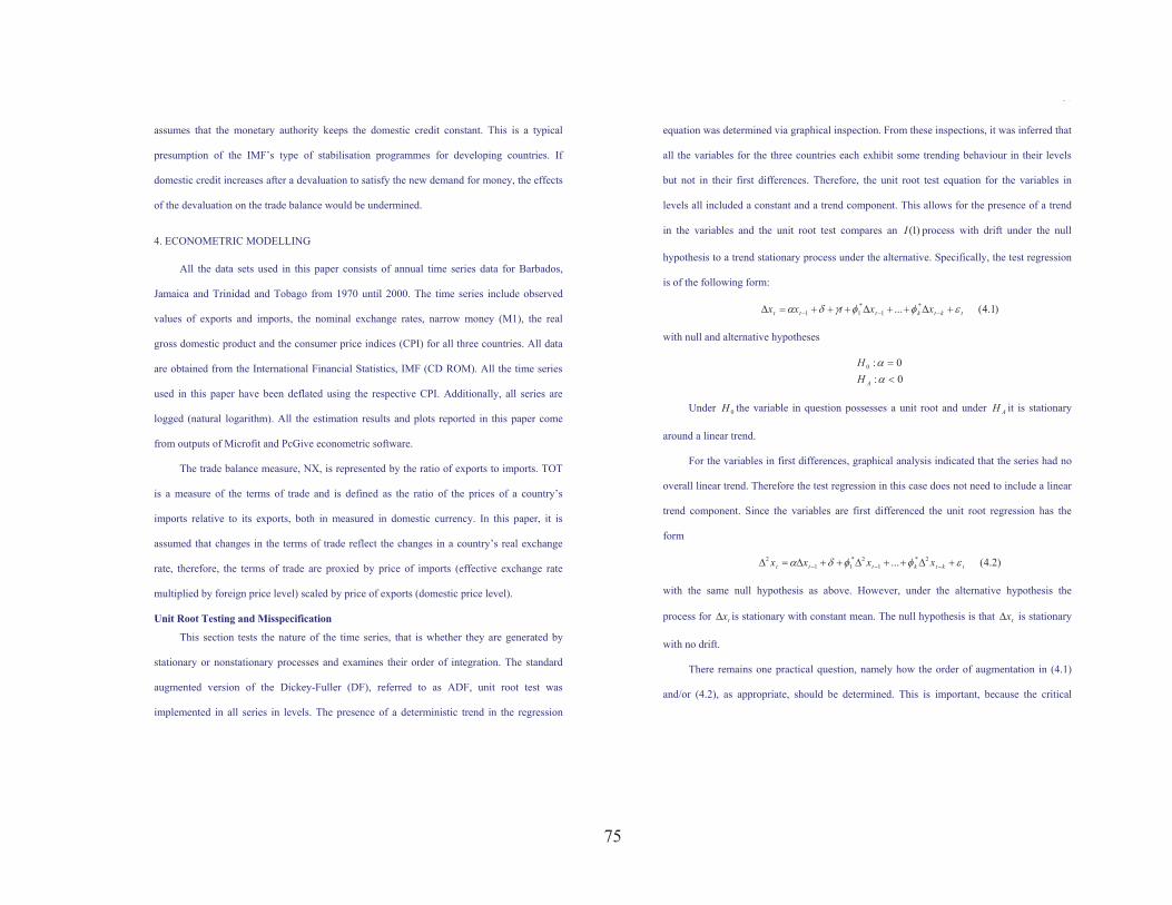
4. ECONOMETRIC MODELLING

All the data sets used in this paper consists of annual time series data for Barbados,

Jamaica and Trinidad and Tobago from 1970 until 2000. The time series include observed

values of exports and imports, the nominal exchange rates, narrow money (M1), the real

gross domestic product and the consumer price indices (CPI) for all three countries. All data

are obtained from the International Financial Statistics, IMF (CD ROM). All the time series

used in this paper have been deflated using the respective CPI. Additionally, all series are

logged (natural logarithm). All the estimation results and plots reported in this paper come

from outputs of Microfit and PcGive econometric software.

The trade balance measure, NX, is represented by the ratio of exports to imports. TOT

is a measure of the terms of trade and is defined as the ratio of the prices of a country’s

imports relative to its exports, both in measured in domestic currency. In this paper, it is

assumed that changes in the terms of trade reflect the changes in a country’s real exchange

rate, therefore, the terms of trade are proxied by price of imports (effective exchange rate

multiplied by foreign price level) scaled by price of exports (domestic price level).

Unit Root Testing and Misspecification

This section tests the nature of the time series, that is whether they are generated by

stationary or nonstationary processes and examines their order of integration. The standard

augmented version of the Dickey-Fuller (DF), referred to as ADF, unit root test was

implemented in all series in levels. The presence of a deterministic trend in the regression

17

equation was determined via graphical inspection. From these inspections, it was inferred that

all the variables for the three countries each exhibit some trending behaviour in their levels

but not in their first differences. Therefore, the unit root test equation for the variables in

levels all included a constant and a trend component. This allows for the presence of a trend

in the variables and the unit root test compares an )1(I process with drift under the null

hypothesis to a trend stationary process under the alternative. Specifically, the test regression

is of the following form:

)1.4(... *1

*11 tktkttt xxtxx ������ ���������� ���

with null and alternative hypotheses

0:0:0

��

��

AHH

Under 0H the variable in question possesses a unit root and under AH it is stationary

around a linear trend.

For the variables in first differences, graphical analysis indicated that the series had no

overall linear trend. Therefore the test regression in this case does not need to include a linear

trend component. Since the variables are first differenced the unit root regression has the

form

)2.4(... 2*1

2*11

2tktkttt xxxx ����� ���������� ���

with the same null hypothesis as above. However, under the alternative hypothesis the

process for tx� is stationary with constant mean. The null hypothesis is that tx� is stationary

with no drift.

There remains one practical question, namely how the order of augmentation in (4.1)

and/or (4.2), as appropriate, should be determined. This is important, because the critical

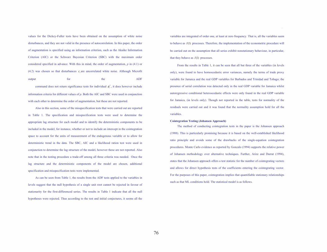
76

18

values for the Dickey-Fuller tests have been obtained on the assumption of white noise

disturbances, and they are not valid in the presence of autocorrelation. In this paper, the order

of augmentation is specified using an information criterion, such as the Akaike Information

Criterion (AIC) or the Schwarz Bayesian Criterion (SBC) with the maximum order

considered specified in advance. With this in mind, the order of augmentation, p in (4.1) or

(4.2) was chosen so that disturbances t� are uncorrelated white noise. Although Microfit

output for the ADF

command does not return significance tests for individual *i� , it does however include

information criteria for different values of p. Both the AIC and SBC were used in conjunction

with each other to determine the order of augmentation, but these are not reported.

Also in this section, some of the misspecification tests that were carried out are reported

in Table 1. The specification and misspecification tests were used to determine the

appropriate lag structure for each model and to identify the deterministic components to be

included in the model, for instance, whether or not to include an intercept in the cointegration

space to account for the units of measurement of the endogenous variable or to allow for

deterministic trend in the data. The SBC, AIC and a likelihood ration test were used in

conjunction to determine the lag structure of the model, however these are not reported. Also

note that in the testing procedure a trade-off among all three criteria was needed. Once the

lag structure and the deterministic components of the model are chosen, additional

specification and misspecification tests were implemented.

As can be seen from Table 1, the results from the ADF tests applied to the variables in

levels suggest that the null hypothesis of a single unit root cannot be rejected in favour of

stationarity for the first-differenced series. The results in Table 1 indicate that all the null

hypotheses were rejected. Thus according to the test and initial conjectures, it seems all the

19

variables are integrated of order one, at least at zero frequency. That is, all the variables seem

to behave as )1(I processes. Therefore, the implementation of the econometric procedure will

be carried out on the assumption that all series exhibit nonstationary behaviour, in particular,

that they behave as )1(I processes.

From the results in Table 1, it can be seen that all but three of the variables (in levels

only), were found to have homoscedastic error variances, namely the terms of trade proxy

variable for Jamaica and the real GDP variables for Barbados and Trinidad and Tobago; the

presence of serial correlation was detected only in the real GDP variable for Jamaica whilst

autoregressive conditional heteroscedastic effects were only found in the real GDP variable

for Jamaica, (in levels only). Though not reported in the table, tests for normality of the

residuals were carried out and it was found that the normality assumption hold for all the

variables.

Cointegration Testing (Johansen Approach)

The method of conducting cointegration tests in the paper is the Johansen approach

(1988). This is particularly promising because it is based on the well-established likelihood

ratio principle and avoids some of the drawbacks of the single-equation cointegration

procedures. Monte Carlo evidence as reported by Gonzalo (1994) supports the relative power

of Johansen methodology over alternative techniques. Further, Arize and Durrat (1994),

states that the Johansen approach offers a test statistic for the number of cointegrating vectors

and allows for direct hypothesis tests of the coefficients entering the cointegrating vector.

For the purposes of this paper, cointegration implies that quantifiable stationary relationships

such as that ML conditions hold. The statistical model is as follows.

77

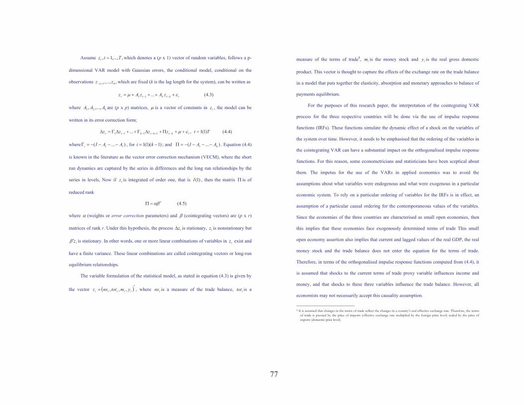
20

Assume ,,...,1, Ttzt � which denotes a (p x 1) vector of random variables, follows a p-

dimensional VAR model with Gaussian errors, the conditional model, conditional on the

observations ,,..., 01 zz k�� which are fixed (k is the lag length for the system), can be written as

)3.4(...11 tktktt zAzAz �� ����� ��

where kAAA ,...,, 21 are (p x p) matrices, � is a vector of constants in tz , the model can be

written in its error correction form;

)4.4()1(1,... 1111 Ttzzzz tktktktt ������������� ����� ��

where )...( 1 ii AAI ������ , for )1)(1(1 �� ki ; and )...( 1 kAAI ������ . Equation (4.4)

is known in the literature as the vector error correction mechanism (VECM), where the short

run dynamics are captured by the series in differences and the long run relationships by the

series in levels, Now if tz is integrated of order one, that is )1(I , then the matrix � is of

reduced rank

)5.4(�� ���

where � (weights or error correction parameters) and � (cointegrating vectors) are (p x r)

matrices of rank r. Under this hypothesis, the process tz� is stationary, tz is nonstationary but

tz� � is stationary. In other words, one or more linear combinations of variables in tz exist and

have a finite variance. These linear combinations are called cointegrating vectors or long-run

equilibrium relationships.

The variable formulation of the statistical model, as stated in equation (4.3) is given by

the vector � ��� ttttt ymtotnxz ,,, , where tnx is a measure of the trade balance, ttot is a

21

measure of the terms of trade8, tm is the money stock and ty is the real gross domestic

product. This vector is thought to capture the effects of the exchange rate on the trade balance

in a model that puts together the elasticity, absorption and monetary approaches to balance of

payments equilibrium.

For the purposes of this research paper, the interpretation of the cointegrating VAR

process for the three respective countries will be done via the use of impulse response

functions (IRFs). These functions simulate the dynamic effect of a shock on the variables of

the system over time. However, it needs to be emphasised that the ordering of the variables in

the cointegrating VAR can have a substantial impact on the orthogonalised impulse response

functions. For this reason, some econometricians and statisticians have been sceptical about

them. The impetus for the use of the VARs in applied economics was to avoid the

assumptions about what variables were endogenous and what were exogenous in a particular

economic system. To rely on a particular ordering of variables for the IRFs is in effect, an

assumption of a particular causal ordering for the contemporaneous values of the variables.

Since the economies of the three countries are characterised as small open economies, then

this implies that these economies face exogenously determined terms of trade This small

open economy assertion also implies that current and lagged values of the real GDP, the real

money stock and the trade balance does not enter the equation for the terms of trade.

Therefore, in terms of the orthogonalised impulse response functions computed from (4.4), it

is assumed that shocks to the current terms of trade proxy variable influences income and

money, and that shocks to these three variables influence the trade balance. However, all

economists may not necessarily accept this causality assumption.

8 It is assumed that changes in the terms of trade reflect the changes in a country’s real effective exchange rate. Therefore, the terms of trade is proxied by the price of imports (effective exchange rate multiplied by the foreign price level) scaled by the price of exports (domestic price level).

78

22

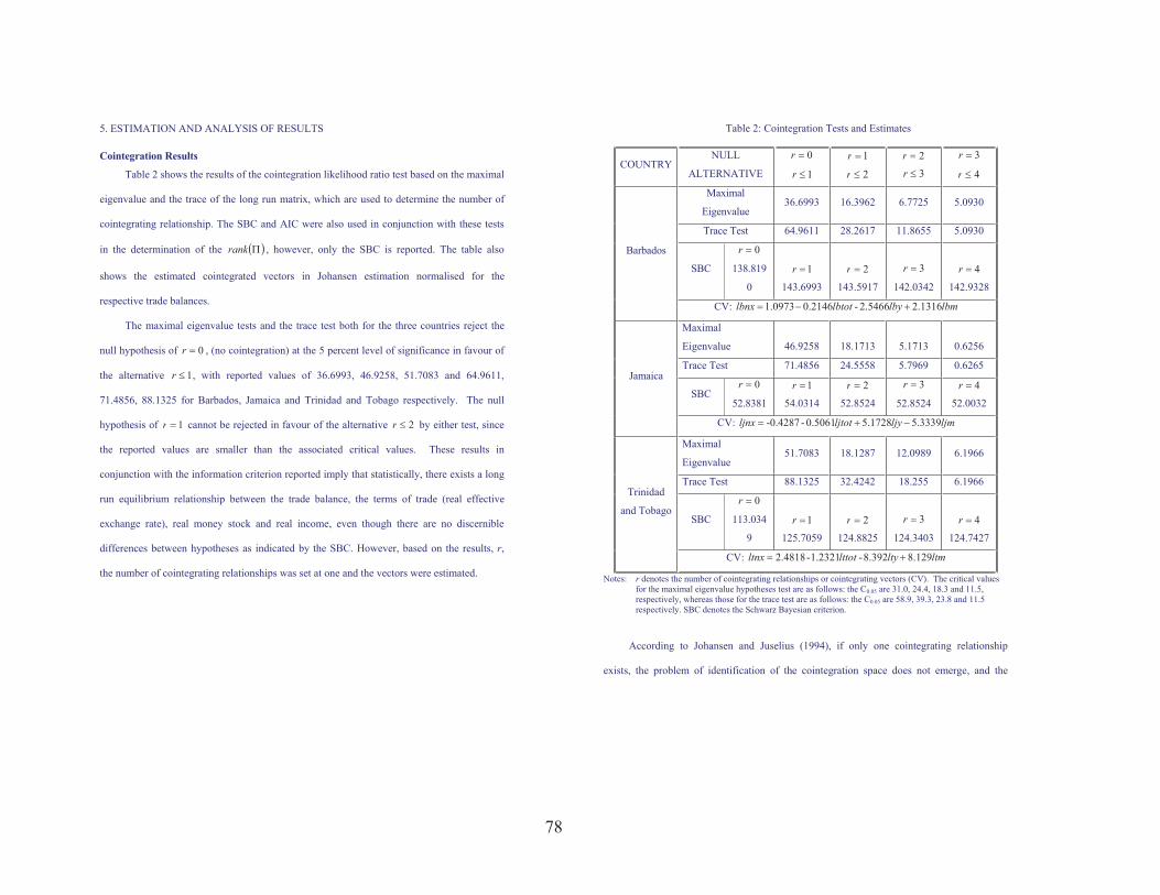
5. ESTIMATION AND ANALYSIS OF RESULTS

Cointegration Results

Table 2 shows the results of the cointegration likelihood ratio test based on the maximal

eigenvalue and the trace of the long run matrix, which are used to determine the number of

cointegrating relationship. The SBC and AIC were also used in conjunction with these tests

in the determination of the � ��rank , however, only the SBC is reported. The table also

shows the estimated cointegrated vectors in Johansen estimation normalised for the

respective trade balances.

The maximal eigenvalue tests and the trace test both for the three countries reject the

null hypothesis of 0�r , (no cointegration) at the 5 percent level of significance in favour of

the alternative 1�r , with reported values of 36.6993, 46.9258, 51.7083 and 64.9611,

71.4856, 88.1325 for Barbados, Jamaica and Trinidad and Tobago respectively. The null

hypothesis of 1�r cannot be rejected in favour of the alternative 2�r by either test, since

the reported values are smaller than the associated critical values. These results in

conjunction with the information criterion reported imply that statistically, there exists a long

run equilibrium relationship between the trade balance, the terms of trade (real effective

exchange rate), real money stock and real income, even though there are no discernible

differences between hypotheses as indicated by the SBC. However, based on the results, r,

the number of cointegrating relationships was set at one and the vectors were estimated.

23

Table 2: Cointegration Tests and Estimates

COUNTRY NULL

ALTERNATIVE

0�r

1�r

1�r

2�r

2�r3�r

3�r

4�r

Maximal

Eigenvalue 36.6993 16.3962 6.7725 5.0930

Trace Test 64.9611 28.2617 11.8655 5.0930

SBC

0�r

138.819

0

1�r

143.6993

2�r

143.5917

3�r

142.0342

4�r

142.9328

Barbados

CV: lbmlbylbtotlbnx 2.13162.5466-.214601.0973 ���

Maximal

Eigenvalue 46.9258 18.1713 5.1713 0.6256

Trace Test 71.4856 24.5558 5.7969 0.6265

SBC 0�r

52.8381

1�r

54.0314

2�r

52.8524

3�r

52.8524

4�r

52.0032

Jamaica

CV: ljmljyljtotljnx 5.33395.17280.5061--0.4287 ���

Maximal

Eigenvalue51.7083 18.1287 12.0989 6.1966

Trace Test 88.1325 32.4242 18.255 6.1966

SBC

0�r

113.034

9

1�r

125.7059

2�r

124.8825

3�r

124.3403

4�r

124.7427

Trinidad

and Tobago

CV: ltmltylttotltnx 8.1298.392-1.2321-2.4818 ��

Notes: r denotes the number of cointegrating relationships or cointegrating vectors (CV). The critical values for the maximal eigenvalue hypotheses test are as follows: the C0.05 are 31.0, 24.4, 18.3 and 11.5, respectively, whereas those for the trace test are as follows: the C0.05 are 58.9, 39.3, 23.8 and 11.5 respectively. SBC denotes the Schwarz Bayesian criterion.

According to Johansen and Juselius (1994), if only one cointegrating relationship

exists, the problem of identification of the cointegration space does not emerge, and the

79

80

26

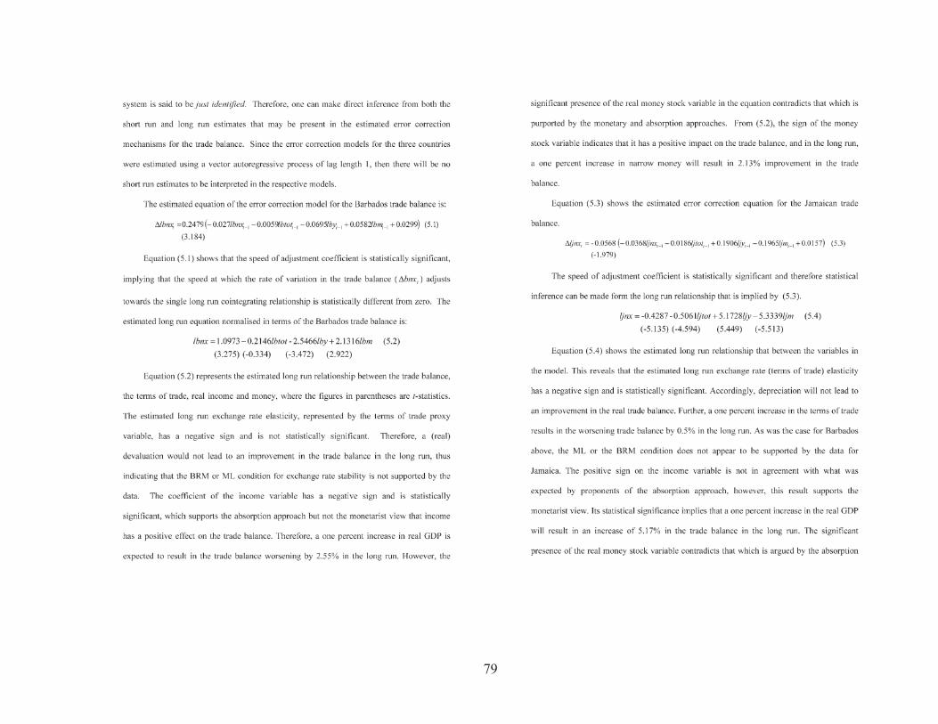
approach. Since Jamaica employs a ‘floating’9 exchange rate policy, the significant presence

of the money variable does not necessarily contradict the view of the monetary approach, and

therefore, a one-percent increase in the real money stock in the long run results in 5.33%

decline in the trade balance.

In the case of Trinidad and Tobago, the error correction equation for the trade balance

is as follows.

)5.5()-2.905()0719.02355.02431.00356.00289.0(4677.0 1111 ������� ���� ttttt ltmltylttotltnxltnx

As was the case for Barbados and Jamaica, the speed of adjustment coefficient was

significantly different from zero and the estimated long run equation normalised in terms of

the Trinidad and Tobago trade balance is

5.641)()-4.974()-0.124()2.968()6.5(8.1298.392-1.2321-2.4818 ltmltylttotltnx ��

Equation (5.6) reveals that the estimated long-run exchange-rate (terms of trade)

elasticity has a negative sign and it is not statistically significant. Therefore, a real

depreciation is not expected to improve the balance of trade in the long run, even though the

coefficient is greater than unity in absolute terms. Thus, indicating that the BRM condition or

the ML condition does not hold for Trinidad and Tobago, as was the case for Barbados and

Jamaica. Further, the sign of the income variable is also negative, which supports the view

argued by proponents of the absorption approach. Statistical significance of the income

variable implies that a one percent increase results in a decline in the trade balance of 8.39%

in the long run. With regard to the real money stock variable, its significant presence in the

estimated long run equation contradicts the view of both the absorption and monetary

9 The Government of Jamaica maintains its exchange rate within a predetermined bandwidth, therefore, this regime can be considered to be a fixed one.

27

approaches, which argues the point of money neutrality in the long run. Note here, that even

though Trinidad and Tobago employs a floating exchange rate regime, it is not a necessarily

clean one, as is the case for Jamaica. Thus, in the long run, a one percent increase in the real

money stock improves the real trade balance by 8.13%.

Table 3 reports the results of the specification and misspecification tests carried out on

the residuals of the VECM representations. No serial correlation was found to be present in

the residuals for any of the three countries. The models were also found to have good

functional form, homoscedasticity and no ARCH effects. All the VECM residuals were also

found to be stationary and the normality assumption also holds. Thus, indicating that the

performance of the VECM representations of the actual data is generally satisfactory.

Table 3: Misspecification Tests for the VECM representations of the trade balances.

DIAGNOSTIC TEST BARBADOS JAMAICA TRINIDAD AND TOBAGO

A: Serial Correlation � �12� = 0.596 (0.440)

� �12� = 0.012(0.909)

� �12� = 0.377 (0.539)

B: Functional Form � �12� = 0.882 (0.595)

� �12� = 0.442 (0.837)

� �12� = 0.889 (0.346)

C: Normality � �22� = 5.048 (0.080)

� �22� = 3.605 (0.165)

� �22� = 0.449 (0.799)

D: Heteroscedasticity � �12� = 1.757 (0.185)

� �12� = 0.014 (0.905)

� �12� =0.158(0.691)

E: ARCH (k) � �12� = 0.642 (0.423)

� �12� = 0.588 (0.443)

� �12� = 0.022 (0.882)

F: ADF -5.379 -5.396 -4.569 Notes: A: Lagrange Multiplier test of residual serial correlation. B: Ramsey’s RESET test using fitted the square of the fitted values. C: Based of a test of skewness and kurtosis of residuals. D: Based on the regression of squared of squared fitted values. E: Engle’s ARCH test of residuals (OLS) case. F: Dickey-Fuller unit root tests for residuals. The 95% asymptotic critical value is -4.182. The figures in parentheses are the statistics associated probability values.

81

28

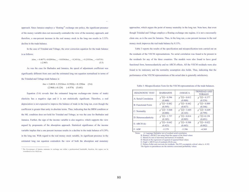
4.2 Impulse Response Functions (IRFs) Analysis

In this section the impulse response functions obtained from the error correction

mechanisms of the cointegration VAR model are used to evaluate the empirical plausibility

of the various theoretical approaches. However, it is not the aim of the author to promote the

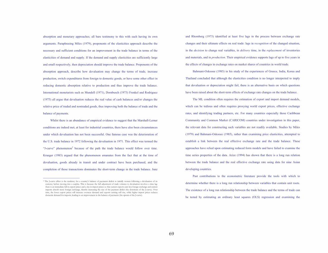
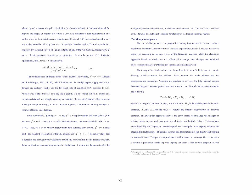
views of any one approach over any of the others. Figure 4.1 shows the empirical orthogonal

impulse response functions for all the variables in the system to a shock in the terms of trade

equation, ceteris paribus, for Barbados, Jamaica and Trinidad and Tobago respectively.

A positive shock to the Barbados term of trade equation reveals that the trade balance

will decline and that the shock would persist for approximately ten years. Similar results are

reported for the real GDP and real money stock variables. For Jamaica, a negative shock to

the terms of trade equation persist for approximately three years and is accompanied by a

worsening of the trade balance. However, the negative shocks affect the real GDP positively

and the real money stock negatively, persisting for approximately three years. In the case of

Trinidad and Tobago, a negative shock to the terms of trade persists for approximately twelve

years and is accompanied by a decline in the trade balance. Nevertheless, the negative shock

affects both the real GDP and the real money stock variables positively.

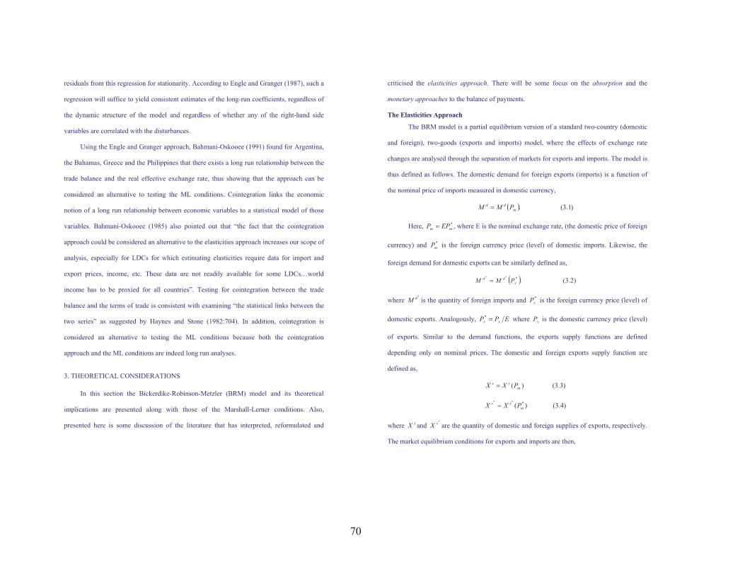
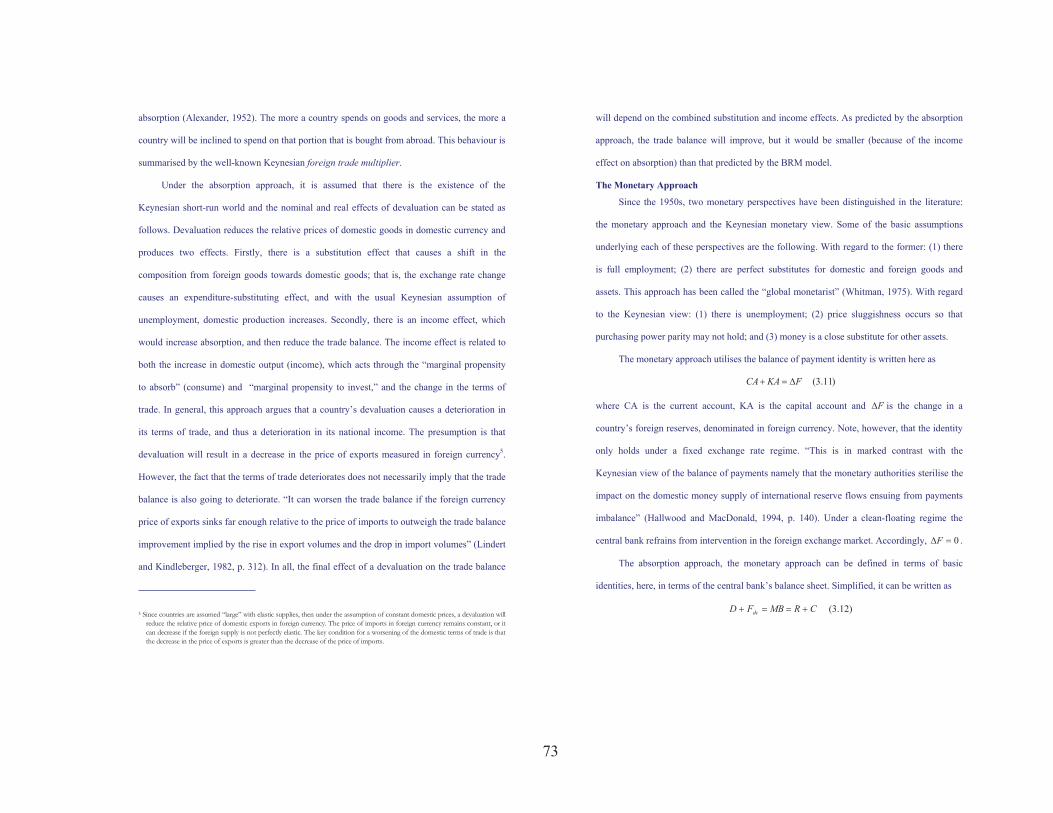
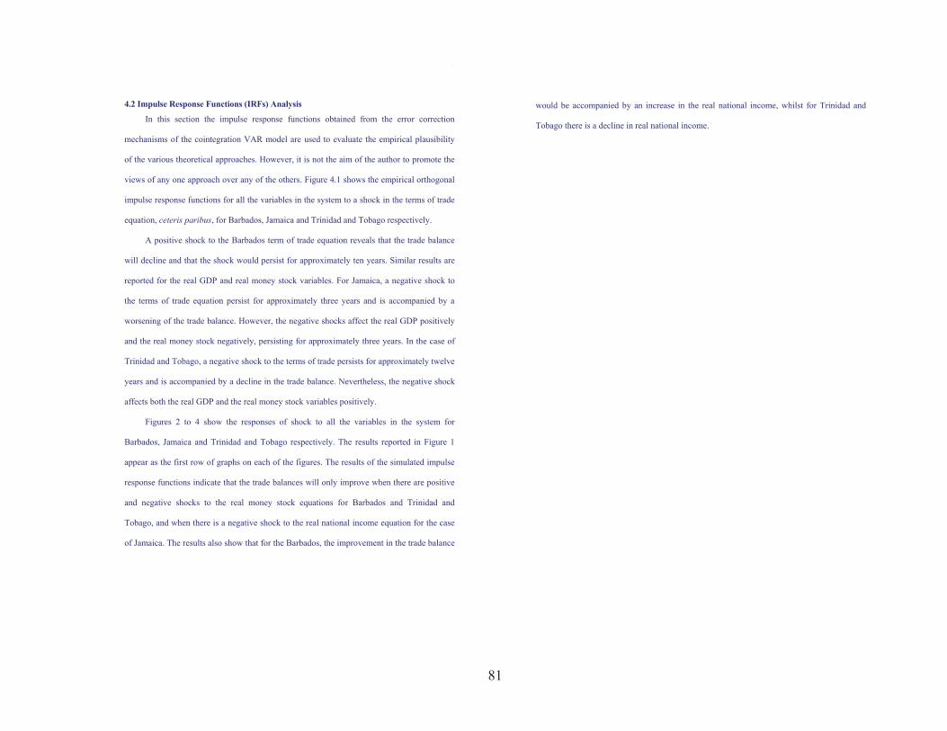
Figures 2 to 4 show the responses of shock to all the variables in the system for

Barbados, Jamaica and Trinidad and Tobago respectively. The results reported in Figure 1

appear as the first row of graphs on each of the figures. The results of the simulated impulse

response functions indicate that the trade balances will only improve when there are positive

and negative shocks to the real money stock equations for Barbados and Trinidad and

Tobago, and when there is a negative shock to the real national income equation for the case

of Jamaica. The results also show that for the Barbados, the improvement in the trade balance

29

would be accompanied by an increase in the real national income, whilst for Trinidad and

Tobago there is a decline in real national income.

82

30

Figure 1: shows the Orthogonal Impulse Response functions of a Terms of Trade shock for Barbados, Jamaica and Trinidad & Tobago. From left to right, the graphs represent the terms of trade, the real national income, the real money stock and the trade balance equations respectively.

0 5 10 15 20 25

05

10

15

20

25

BTOT (BTOT eqn)

0 5 10 15 20 25

-0.075

-0.050

-0.025

0.000

LBY (BTOT eqn)

0 5 10 15 20 25

5

0

5

00

LBM (BTOT eqn)

0 5 10 15 20 25

-0.015

-0.010

-0.005

0.000

BNX (BTOT eqn)

0 5 10 15 20 25

0.8

0.9

1.0

JTOT (JTOT eqn)

0 5 10 15 20 25

0.001

0.002

0.003

LJY (JTOT eqn)

0 5 10 15 20 25

0.06

0.04

0.02

0.00

LJM (JTOT eqn)

0 5 10 15 20 25

-0.020

-0.015

-0.010

-0.005

0.000

JNX (JTOT eqn)

0 5 10 15 20 259925

9950

9975

0000

TTOT (TTOT eqn)

0 5 10 15 20 25

0.025

0.050

0.075

0.100

0.125

LTY (TTOT eqn)

0 5 10 15 20 25

0.05

0.10

0.15

0.20

LTM (TTOT eqn)

0 5 10 15 20 25

-0.06

-0.04

-0.02

0.00

TNX (TTOT eqn)

31

Figure 2: Orthogonalised response of the system to shocks in all equations for Barbados. The first, second, third and fourth lines respectively represent the response of the system variables to shocks in the terms of trade, the real national income, the real money stock and the trade balance equations.

0 10 20 30

1.01

1.02B T T (B T T eqn )

0 10 20 30

-0.075-0.050-0.0250.000

L B Y (B T T e qn )

0 10 20 30-0.015-0.010-0.0050.000

L B M (B T T e qn )

0 10 20 30

-0.01

0.00

B N X (B T T eqn )

0 10 20 30

0.1

0.2

0.3

B T T ( L B Y eqn )

0 10 20 30

0.0

0.5

1.0

L B Y (L B Y eqn )

0 10 20 30

-0.15-0.10-0.050.00

L B M ( L BY e qn )

0 10 20 30

-0.2

-0.1

0.0B N X ( L B Y e qn )

0 10 20 30

-0.2

-0.1

0.0B T T ( L B M eqn )

0 10 20 30

0.250.500.751.00

L B Y (L B M eqn )

0 10 20 30

1.051.101.15

L B M ( L B M e qn )

0 10 20 30

0.1

0.2

B N X ( L B M eqn )

0 10 20 30

0.05

0.10B T T ( B N X eqn )

0 10 20 30

-0.4

-0.2

0.0L B Y ( B N X eqn )

0 10 20 30

-0.050-0.0250.000

L B M ( B N X eqn )

0 10 20 30

0.9250.9500.9751.000

B N X ( B N X eqn )

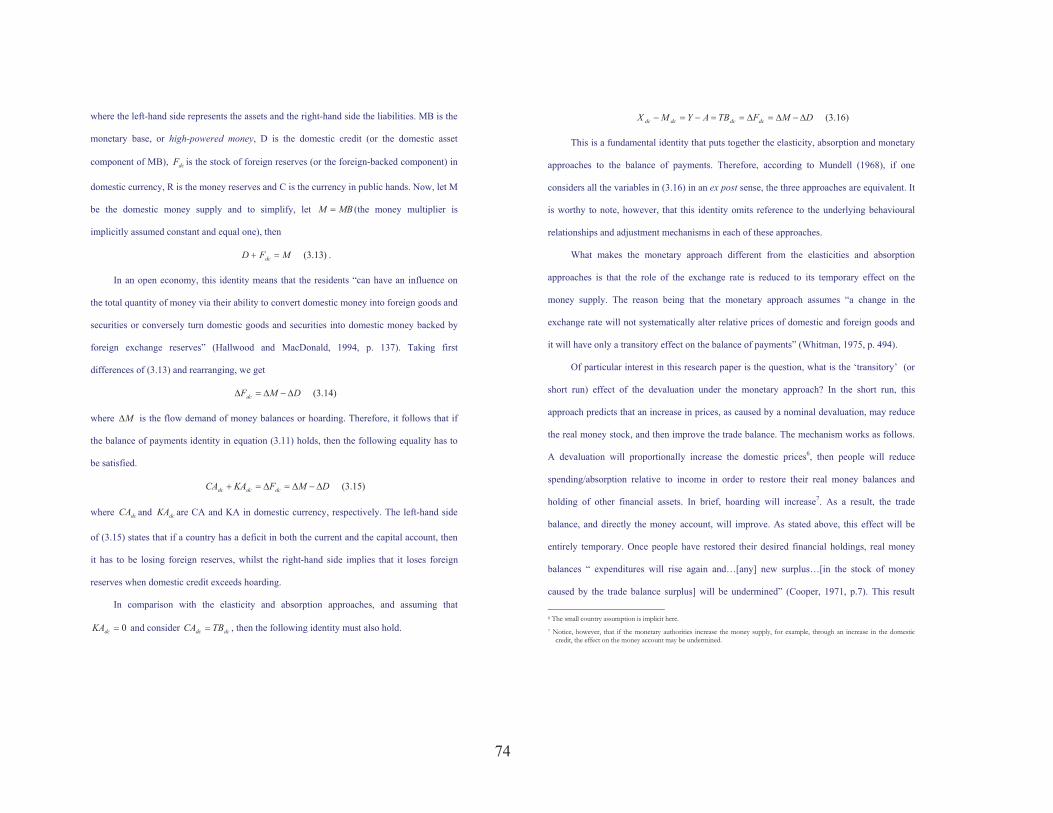
Figure 3: Orthogonalised response of the system to shocks in all equations for Jamaica. The first, second, third and fourth lines respectively represent the response of the system variables to shocks in the terms of trade, the real national income, the real money stock and trade balance equations.

0 10 20 30

0.8

0.9

1.0

JT T (JT T eqn)

0 10 20 30

0.0010.0020.003

LJY (JT T eqn)

0 10 20 30

-0.050-0.0250.000

LJM (JT T eqn)

0 10 20 30

-0.02

-0.01

0.00

JNX (JT T eqn)

0 10 20 30

1

2

3

JT T (LJY eqn )

0 10 20 300.970.980.991.00

LJY (LJY eqn)

0 10 20 30

0.25

0.50

0.75

LJM (LJY eqn)

0 10 20 30

0.1

0.2JNX (LJY eqn)

0 10 20 30

-2

-1

0

JT T (LJM eqn)

0 10 20 30

0.010.020.03

LJY (LJM eqn)

0 10 20 30

0.50

0.75

1.00

LJM (LJM eqn)

0 10 20 30

-0.2

-0.1

0.0JNX (LJM eqn)

0 10 20 30

-0.4

-0.2

0.0JT T (JNX eqn)

0 10 20 30

0.0025

0.0050

0.0075

LJY (JNX eqn)

0 10 20 30

-0.10-0.050.00

LJM (JNX eqn)

0 10 20 30

0.96

0.98

1.00

JNX (JNX eqn)

83

32

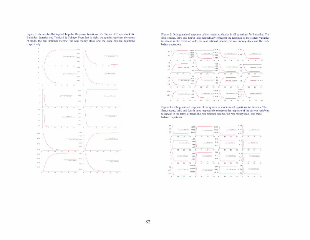
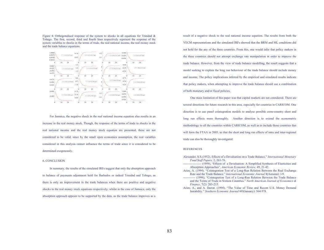
Figure 4: Orthogonalised response of the system to shocks in all equations for Trinidad & Tobago. The first, second, third and fourth lines respectively represent the response of the system variables to shocks in the terms of trade, the real national income, the real money stock and the trade balance equations.

0 10 200.99250.99500.99751.0000

T T T (T T T eqn)

0 10 20

0.05

0.10LT Y (T T T eqn)

0 10 20

0.1

0.2LT M (T T T eqn)

0 10 20

-0.050-0.0250.000

T NX (T T T eqn)

0 10 20-0.075-0.050-0.0250.000

T T T (LT Y eqn)

0 10 20

1.5

2.0

2.5

LT Y (LT Y eqn)

0 10 20

1

2LT M (LT Y eqn)

0 10 20

-0.50

-0.25

0.00T NX (LT Y eqn)

0 10 20

0.0250.0500.075

T T T (LT M eqn)

0 10 20

-1.0

-0.5

0.0

LT Y (LT M eqn)

0 10 20

-1

0

1LT M (LT M eqn)

0 10 20

0.25

0.50

0.75

T NX (LT M eqn)

0 10 20

-0.005

0.000

T T T (T NX eqn)

0 10 20

0.05

0.10

0.15

LT Y (T NX eqn)

0 10 20

0.1

0.2LT M (T NX eqn)

0 10 200.9250.9500.9751.000

T NX (T NX eqn)

For Jamaica, the negative shock in the real national income equation also results in an

increase in the real money stock. Though, the response of the terms of trade to shocks in the

real national income and the real money stock equation are presented, these are not

considered to be valid, since by the small open economies assumption, the real variables

considered in this analysis cannot influence the terms of trade since it is considered to be

determined exogenously.

6. CONCLUSION

In summary, the results of the simulated IRFs suggest that only the absorption approach

to balance of payments adjustment hold for Barbados or indeed Trinidad and Tobago, as

there is only an improvement in the trade balances when there are positive and negative

shocks to the real money stock equations respectively; whilst in the case of Jamaica, only the

absorption approach appears to be supported by the data, as the trade balance improves as a

33

result of a negative shock to the real national income equation. The results from both the

VECM representations and the simulated IRFs showed that the BRM and ML conditions did

not hold for the any of the three countries. From this, one would infer that policy makers in

the three countries should not attempt exchange rate manipulation in order to improve the

trade balance. However, from the view of trade balance modelling, the result suggests that a

model seeking to explain the long run behaviour of the trade balance should include money

and income. The policy implications inferred by the empirical and simulated results indicate

that policy makers, when attempting to improve the trade balance should use a combination

of both monetary and/or fiscal policies.

One main limitation of this paper was that capital markets are not considered. There are

several directions for future research in this area, especially for countries in CARICOM. One

direction is to use panel cointegration models to analyse possible cross-country short and

long run effects more thoroughly. Another direction is to extend the econometric

methodology to all the countries within CARICOM, as well as to include those countries that

will form the FTAA in 2005, so that the short and long run effects of intra and inter-regional

trade can also be thoroughly investigated.

REFERENCES

Alexander, S.S.(1952), Effects of a Devaluation on a Trade Balance,” International Monetary Fund Staff Papers, 2, 263-78.

------------------ (1959), “Effects of a Devaluation: A Simplified Synthesis of Elasticities and Absorption Approaches”, American Economic Review, 49, 21-42.

Arize, A. (1994). “Cointegration Test of a Long-Run Relation Between the Real Exchange Rate and the Trade Balance.” International Economic Journal 8(Autumn): l-9.

------------ (1996), “Cointegration Test of a Long-Run Relation Between the Trade Balance and the Terms of Trade in Sixteen Countries.” North American Journal of Economics & Finance, 7(2): 203-215.

Arize, A., and A. Darrat. (1994). “The Value of Time and Recent U.S. Money Demand Instability.” Southern Economic Journal 6O(January): 564-578.

84

34

Backus, D. K., P. J. Kehoe, F. Kydland (1994), “Dynamics of the Trade Balance and the Terms of Trade: The J-Curve?” American Economic Review, 84, 1, 84-103.

Bahmani-Oskooee, M. (1991), “Is There a Long-run Relation Between the Trade Balance and the Real Effective Exchange Rate of LDCs?” Economic Letters, August, 403-407.

---------------------------- (1985), “Devaluation and the J-curve: Some Evidence from LDCs,” The Review of Economics and Statistics, August, 500-504.

Bahmani-Oskooee, M. and L. Alse (1994), “Short-Run Versus Long-Run Effects of Devaluation: Error-Correction Modelling and Cointegration,” Eastern Economic Journal, 20, 4, 453-64.

Campbell, John Y., and Pierre Perron. (1991) “Pitfalls and Opportunities: What Macroeconomists Should Know about Unit Roots.” Pp. 144-201 in NBER (National Bureau of Economic Research) Macroeconomics Annual, edited by Oliver Jean Blanchard and Stanley Fisher. Cambridge, MA: MIT Press.

Cooper, R. N. (1971), “Currency Devaluation in Developing Countries,” Essays in International Finance, No. 86, Princeton University.

Corden, W. M. (1994), Economic Policy, Exchange Rates and the International System, The University of Chicago Press.

Dornbusch, R. (1973), “Devaluation, Money, and Nontraded Goods,” American Economic Review, 5, 871-880.

----------------- (1975), “Exchange Rates and Fiscal Policy in a Popular Model of International Trade,” American Economic Review, 65, 859-871.

Enders, Walter. 1995. Applied Economic Time Series. New York, NY: John Wiley. Engle, R. F. (1982), “Autoregressive Conditional Heteroscedasticity with Estimates of the

Variance of United Kingdom Inflation,” Econometrica, Vol. 50, 987-1007. Engle, R. F., and C. W. Granger (1987), “ Co-integration and Error Correction: Representation,

Estimation, and Testing,” Econometrica, Vol. 55, 251-276. Frenkel, J. A., and H. G. Johnson (1977), “The Monetary Approach to the Balance of

Payments”, in J. A. Frenkel and H. G. Johnson (eds.), The Monetary Approach to the Balance of Payments.

Frenkel, J.A, and C. Rodriguez (1975), “Portfolio Equilibrium and the Balance of Payments: A Monetary Approach,” American Economic Review, 65, no. 4 (September): 674-88

Gonzalo, Jesus. (1994). “Five Alternative Methods of Estimating Long-Run Equilibrium Relationship.” Journal of Econometrics, 60, 203-233.

Granger, C.W., and R.F. Engle, eds., (1991), Long-run Economic Relationships: Readings in Cointegration, Oxford.

Hallwood, C. P., and R. MacDonald (1994), International Money and Finance, Second Edition, Blackwell.

Harberger, A.C. (1950), “Currency Depreciation, Income, and the Balance of Trade,” Journalof Political Economy, 58, 47-60.

Haynes, Stephen E., and Joe A. Stone. (1982). “Impact of the Terms of Trade on the U.S. Trade Balance: A Reexamination.” The Review of Economics and Statistics 64(November):702-706.

Johansen, S. (1988), “Statistical Analysis of Cointegration Vectors,” Journal of Economic Dynamics and Control, Vol. 12, 231-254.

-------------- (1991), “Estimation and Hypothesis Testing of Cointegration Vectors in Gaussian

35

Vector Autoregressive Models,” Econometrica, 59, 1551-1580. Johansen, S. and K. Juselius (1990), “Maximum Likelihood Estimation and Inference on

Cointegration with Applications to the Demand for Money,” Oxford Bulletin of Economicsand Statistics, 52, 169-210.

----------------------------------------- (1992), “Testing Structural Hypothesis in a Multivariate Cointegration Analysis of the PPP and the UIP for UK,” Journal of Econometrics, 53, 211-244.

----------------------------------------- (1994), “Identification of the Long-Run and the Short-Run Structure: An Application of the ISLM model,” Journal of Econometrics, 63, 7-36.

Junz, H. B., and R. R. Rhomberg (1973), “Price Competitiveness in Export Trade among Industrial Countries,” American Economic Review, 63, 412-18.

Kemp, M. C. (1970), “The Balance of Payments and the Terms of Trade in Relation to Financial Controls,” Review of Economic Studies, 37, 25-31.

Kenen, P.B. (1985), “Macroeconomic Theory and Policy: How was the Closed Economy Model Opened,” in R. Jones and P. Kenen (eds.), Handbook of International Economics, Vol. 2, Amsterdam, North-Holland, 625-77.

Krueger, A. O. (1983), Exchange Rate Determination, Cambridge University Press. Laffer, A. B., “Exchange Rates, the Terms of Trade, and the Trade Balance,” in Effects of

Exchange Rate Adjustments (Washington D.C.: Treasury Dept., OASIA Res., (1974). Lerner, A. P. (1944), The Economics of Control: Principles of Welfare Economics, The

Macmillan Company, N.Y. Lindert, Peter H., and Charles P. Kindleberger. (1982). International Economics. New York,

NY: Irwin. Magee, S. (1973), “Currency Contracts, Pass-Through, and Devaluation,” Brookings Papers

of Economic Activity, 1, 303-23. Mamingi, Nlandu (1999), “Lecture Notes in EC36D Econometrics II”, Department of

Economics, The University of the West Indies, Cave Hill Campus. Marshall, A. (1923), Money, Credit and Commerce, London, Macmillan. McPheters, Lee R., and William B. Stronge. (1979). “Impact of the Terms of Trade on the

US. Trade Balance: A Cross-Spectral Analysis.” The Review of Economics and Statistics 61:45 l-455.

Miles, M. A. (1979), “The Effects of Devaluation on the Trade Balance and the Balance of Payments: Some new Results,” Journal of Political Economy, June, 600-620.

Mundell, R. A. (1968), International Economics, NY, Macmillan. ------------------ (1971), Monetary Theory, Pacific Palisades, Goodyear. Nelson, C. R., and C.I. Plosser (1982), “Trends and Random Walks in Macroeconomic Time

Series: Some Evidence and Implications,” Journal of Monetary Economics, 10, 139-62. Rincón, Hernán C., (1998), “Testing the Short-and-Long-Run Exchange Rate Effects on

Trade Balance: The Case of Columbia”, submitted as part of a Ph.D. dissertation at the University of Illinois at Urbana-Champaign.

Rose, A. K. and J. L. Yellen (1989), “Is There a J-curve?” Journal of Monetary Economics,24, 53-68.

Whitman, M. V. (1975), “Global Monetarism and the Monetary Approach to the Balance of Payments,” Brookings Papers on Economic Activity, 3, 491-536.

85

36

Appendix

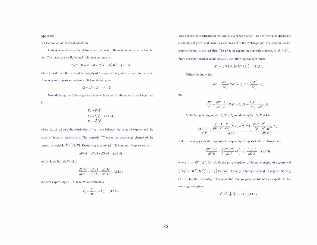
A.1 Derivation of the BRM condition

Only new notation will be defined here, the rest of the notation is as defined in the

text. The trade balance B, defined in foreign currency is,

)1.1.(** AMPXPMXMSB dm

sx ������ ;

where D and S are the demand and supply of foreign currency and are equal to the value

if imports and exports respectively. Differentiating gives

)2.1.(AdDdSdB �� .

Now defining the following elasticities with respect to the nominal exchange rate

E:

EDE

AESE

EBE

D

S

B

ˆˆ)3.1.(ˆˆ

ˆˆ

�

�

�

,

where DSB EEE ,, are the elasticities of the trade balance, the value of exports and the

value of imports, respectively. The symbols “^” states the percentage change of the

respective variable � �EdEE �ˆ . Expressing equation (A.1.2) in terms of exports so that

)4.1.(AMdDMdSMdB ��

and dividing by EdE yields

)5.1.(AEdEMdD

EdEMdS

EdEMdB

��

and now expressing (A.1.5) in terms of elasticities

)6.1.(AEEMXE DSB �� .

37

This defines the elasticities in the foreign exchange market. The next step is to define the

elasticities of prices and quantities with respect to the exchange rate. The solution for the

exports market is derived first. The price of exports in domestic currency is *xx EPP � .

From the export market condition (3.6), the following can de written:

� � � � )7.1.(. *** APMPEXX xd

xSS �� .

Differentiating yields

� � **

**x

x

d

xxx

ss dP

PMdEPEdP

PXdX

��

����

�

or,

� � **

*** 11

xdx

d

xxsx

s

s

s

dPMP

MdEPEdPXP

XX

dX��

����

� .

Multiplying throughout by *xx PEP � and dividing by EdE yields

� �EdE

dPMP

PP

M

EdE

dEPEdPEPP

XPX

EdEXdX xd

x

x

x

d

xxx

xs

x

s

ss*

**

****

*

11��

��

��

� ;

and rearranging yields the response of the quantity if exports to the exchange rate,

)8.1.(1**

***

AEdEPdP

EdEPdP

EdEXdX xxxx

ss

�� ����

����

��� ;

where � �xxss PPXX ����� is the price elasticity of domestic supply of exports and

� �******xx

dd PPMM ����� the price elasticity of foreign demand for imports. Solving

(A.1.8) for the percentage change of the foreign price of (domestic) exports to the

exchange rate gives

� �� � )9.1.(ˆˆ ** AEPx ��� ��

86

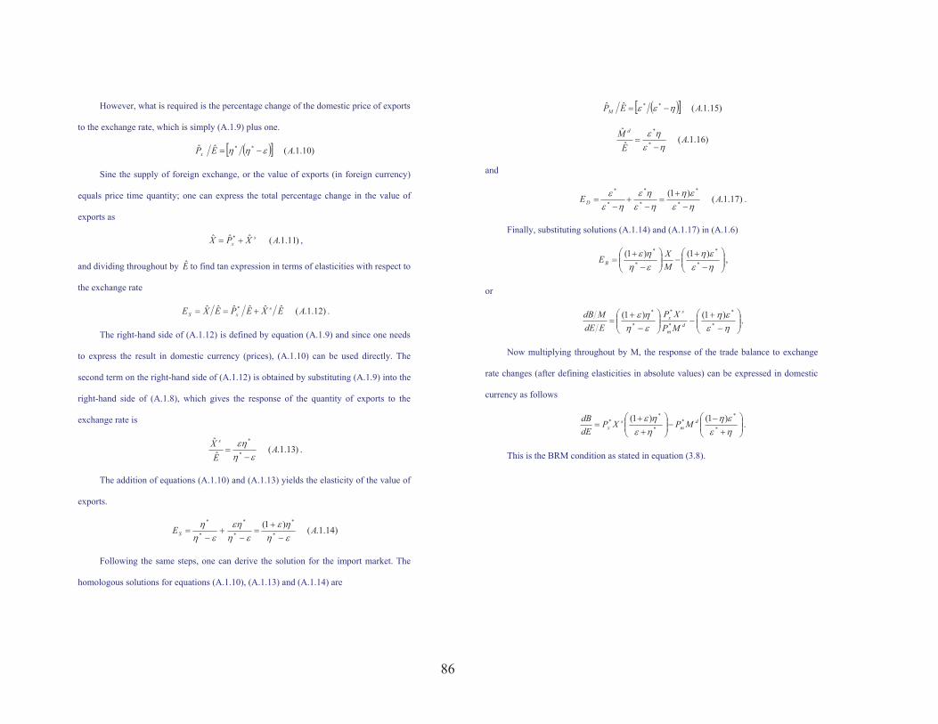
38

However, what is required is the percentage change of the domestic price of exports

to the exchange rate, which is simply (A.1.9) plus one.

� �� � )10.1.(ˆˆ ** AEPx ��� ��

Sine the supply of foreign exchange, or the value of exports (in foreign currency)

equals price time quantity; one can express the total percentage change in the value of

exports as

)11.1.(ˆˆˆ * AXPX sx �� ,

and dividing throughout by E to find tan expression in terms of elasticities with respect to

the exchange rate

)12.1.(ˆˆˆˆˆˆ * AEXEPEXE sxS ��� .

The right-hand side of (A.1.12) is defined by equation (A.1.9) and since one needs

to express the result in domestic currency (prices), (A.1.10) can be used directly. The

second term on the right-hand side of (A.1.12) is obtained by substituting (A.1.9) into the

right-hand side of (A.1.8), which gives the response of the quantity of exports to the

exchange rate is

)13.1.(ˆˆ

*

*

AE

X s

�����

� .

The addition of equations (A.1.10) and (A.1.13) yields the elasticity of the value of

exports.

)14.1.()1(*

*

*

*

*

*

AES ����

����

���

��

��

��

�

Following the same steps, one can derive the solution for the import market. The

homologous solutions for equations (A.1.10), (A.1.13) and (A.1.14) are

39

� �� � )15.1.(ˆˆ ** AEPM ��� ��

)16.1.(ˆˆ

*

*

AE

M d

�����

�

and

)17.1.()1(*

*

*

*

*

*

AED ����

����

���

��

��

��

� .

Finally, substituting solutions (A.1.14) and (A.1.17) in (A.1.6)

���

����

�

��

����

����

�

��

�����

����

*

*

*

* )1()1(MXEB ,

or

���

����

��

����

�

����

��

��

����

����

*

*

*

*

*

* )1()1(d

m

sx

MPXP

EdEMdB .

Now multiplying throughout by M, the response of the trade balance to exchange

rate changes (after defining elasticities in absolute values) can be expressed in domestic

currency as follows

���

����

�

��

����

����

�

��

�����

����

*

**

*

** )1()1( d

ms

x MPXPdEdB .

This is the BRM condition as stated in equation (3.8).