• Current News Exercises —Every week, current microeconomic and macroeconomic news articles or videos, with accompanying exercises, are posted to Pearson MyLab Economics. Assignable and auto-graded, these multi-part exercises ask students to recognize and apply economic concepts to real-world events.

• Real-Time Data Analysis Exercises—Using current macro data to help students understand the impact of changes in economic variables, Real-Time Data Analysis Exercises communicate directly with the Federal Reserve Bank of St. Louis’s FRED® site and update as new data are available.

• Experiments—Flexible, easy-to-assign, auto-graded, and available in Single Player and Multiplayer versions, Experiments in Pearson MyLab Economics make learning fun and engaging.

• Reporting Dashboard—View, analyze, and report learning outcomes clearly and easily. Available via the Gradebook and fully mobile-ready, the Reporting Dashboard presents student performance data at the class, section, and program levels in an accessible, visual manner.

• Mobile Ready—Students and instructors can access multimedia resources and complete assessments right at their fingertips, on any mobile device.

• LMS Integration—Link from any LMS platform to access assignments, rosters, and resources, and synchronize MyLab grades with your LMS gradebook. For students, new direct, single sign-on provides access to all the personalized learning MyLab resources that make studying more efficient and effective.

with Pearson MyLab Economics®

A L W A Y S L E A R N I N G

A01_KRUG6355_11_GE_FM.indd 1 14/10/2017 08:41

The Pearson series in economics

Abel/Bernanke/CroushoreMacroeconomics*†

Acemoglu/Laibson/ListEconomics*†

Bade/ParkinFoundations of Economics*†

Berck/HelfandThe Economics of the Environment

Bierman/FernandezGame Theory with Economic Applications

BlanchardMacroeconomics*†

BoyerPrinciples of Transportation Economics

BransonMacroeconomic Theory and Policy

BrucePublic Finance and the American Economy

Carlton/PerloffModern Industrial Organization

Case/Fair/OsterPrinciples of Economics*†

ChapmanEnvironmental Economics: Theory, Application, and Policy

Daniels/VanHooseInternational Monetary & Financial Economics

DownsAn Economic Theory of Democracy

FarnhamEconomics for Managers†

FroyenMacroeconomics: Theories and Policies

FusfeldThe Age of the Economist

GerberInternational Economics*†

GordonMacroeconomics*†

GreeneEconometric Analysis†

Gregory/StuartRussian and Soviet Economic Performance and Structure

Hartwick/OlewilerThe Economics of Natural Resource Use

Heilbroner/MilbergThe Making of the Economic Society

Heyne/Boettke/PrychitkoThe Economic Way of Thinking

Hubbard/O’BrienEconomics*†

InEconMoney, Banking, and the Financial System*

Hubbard/O’Brien/RaffertyMacroeconomics*†

Hughes/CainAmerican Economic History

Husted/MelvinInternational Economics

Jehle/RenyAdvanced Microeconomic Theory

Keat/Young/ErfleManagerial Economics

KleinMathematical Methods for Economics

Krugman/Obstfeld/MelitzInternational Economics: Theory & Policy*†

LaidlerThe Demand for Money

LynnEconomic Development: Theory and Practice for a Divided World

MillerEconomics Today*

Miller/BenjaminThe Economics of Macro Issues

Miller/Benjamin/NorthThe Economics of Public Issues

MishkinThe Economics of Money, Banking, and Financial Markets*†

The Economics of Money, Banking, and Financial Markets, Business School Edition*Macroeconomics: Policy and Practice*

MurrayEconometrics: A Modern Introduction

O’Sullivan/Sheffrin/PerezEconomics: Principles, Applications and Tools*†

ParkinEconomics*†

PerloffMicroeconomics*†

Microeconomics: Theory and Applications with Calculus*†

Perloff/BranderManagerial Economics and Strategy*†

Pindyck/RubinfeldMicroeconomics*†

Riddell/Shackelford/Stamos/Schneider

Economics: A Tool for Critically Understanding Society

RobertsThe Choice: A Fable of Free Trade and Protection

SchererIndustry Structure, Strategy, and Public Policy

SchillerThe Economics of Poverty and Discrimination

ShermanMarket Regulation

Stock/WatsonIntroduction to Econometrics†

StudenmundA Practical Guide to Using Econometrics†

Todaro/SmithEconomic Development

Walters/Walters/Appel/Callahan/Centanni/Maex/O’Neill

Econversations: Today’s Students Discuss Today’s Issues

WilliamsonMacroeconomics†

*denotes availability of Pearson MyLab Economics titles Log onto www.myeconlab.com to learn more.†denotes availability of Global Edition titles

A01_KRUG6355_11_GE_FM.indd 2 14/10/2017 08:41

International TradeTheorY & PoLicY

eLeVenTh eDiTion

GLoBaL eDiTion

Paul R. KrugmanPrinceton University

Maurice ObstfeldUniversity of California, Berkeley

Marc J. MelitzHarvard University

Harlow, England • London • New York • Boston • San Francisco • Toronto • Sydney • Dubai • Singapore • Hong Kong Tokyo • Seoul • Taipei • New Delhi • Cape Town • São Paulo • Mexico City • Madrid • Amsterdam • Munich • Paris • Milan

A01_KRUG6355_11_GE_FM.indd 3 14/10/2017 08:41

Vice President, Business Publishing: Donna BattistaDirector of Portfolio Management: Adrienne D’AmbrosioPortfolio Manager: Ashley BryanAssociate Acquisitions Editor, Global Edition: Ananya SrivastavaAssociate Project Editor, Global Edition: Paromita BanerjeeEditorial Assistant: Nicole NedwidekVice President, Product Marketing: Roxanne McCarleyDirector of Strategic Marketing: Brad ParkinsStrategic Marketing Manager: Deborah StricklandProduct Marketer: Tricia MurphyManager of Field Marketing: Adam GoldsteinField Marketing Manager: Carlie MarvelField Marketing Assistant: Kristen ComptonProduct Marketing Assistant: Jessica QuazzaVice President, Production and Digital Studio, Arts and Business: Etain O’DeaDirector of Production, Business: Jeff HolcombManaging Producer, Business: Alison Kalil

Content Producer: Nancy FreihoferContent Producer, Global Edition: Nikhil RakshitSenior Manufacturing Controller, Global Edition: Kay HolmanOperations Specialist: Carol MelvilleCreative Director: Blair BrownManager, Learning Tools: Brian SuretteManaging Producer, Digital Studio, Arts and Business: Diane LombardoDigital Studio Producer: Melissa HonigDigital Studio Producer: Alana ColesDigital Content Team Lead: Noel LotzDigital Content Project Lead: Courtney KamaufManager, Media Production, Global Edition: Vikram KumarFull-Service Project Management and Composition: SPi GlobalInterior Design: SPi GlobalCover Design: Lumina DatamaticsCover Art: Liu zishan/Shutterstock

For robin—P.K.For my family—m.o.For clair, Benjamin, and max—m.m.

Acknowledgments of third-party content appear on the appropriate page within the text or on page 366, which constitutes an extension of this copyright page.

FRED® is a registered trademark and the FRED® Logo and ST. LOUIS FED are trademarks of the Federal Reserve Bank of St. Louis. http://research.stlouisfed.org/fred2/

PEARSON, ALWAYS LEARNING, and PEARSON MYLAB ECONOMICS® are exclusive trademarks owned by Pearson Education, Inc. or its affiliates in the U.S. and/or other countries.

Unless otherwise indicated herein, any third-party trademarks, logos, or icons that may appear in this work are the property of their respective owners, and any references to third-party trademarks, logos, icons, or other trade dress are for demonstrative or descriptive purposes only. Such references are not intended to imply any sponsorship, endorsement, authorization, or promotion of Pearson’s products by the owners of such marks, or any relationship between the owner and Pearson Education, Inc., or its affiliates, authors, licensees, or distributors.

Pearson Education LimitedKAO TwoKAO ParkHarlowCM17 9NAUnited Kingdomand Associated Companies throughout the world

Visit us on the World Wide Web at: www.pearsonglobaleditions.com

© Pearson Education Limited 2018

The rights of Paul R. Krugman, Maurice Obstfeld, and Marc J. Melitz, to be identified as the authors of this work, have been asserted by them in accordance with the Copyright, Designs and Patents Act 1988.

Authorized adaptation from the United States edition, entitled International Trade: Theory & Policy, 11th Edition, ISBN 978-0-13-451955-5 by Paul R. Krugman, Maurice Obstfeld, and Marc J. Melitz, published by Pearson Education © 2018.

All rights reserved. No part of this publication may be reproduced, stored in a retrieval system, or transmitted in any form or by any means, electronic, mechanical, photocopying, recording or otherwise, without either the prior written permission of the pub-lisher or a license permitting restricted copying in the United Kingdom issued by the Copyright Licensing Agency Ltd, Saffron House, 6–10 Kirby Street, London EC1N 8TS.

All trademarks used herein are the property of their respective owners. The use of any trademark in this text does not vest in the author or publisher any trademark ownership rights in such trademarks, nor does the use of such trademarks imply any affiliation with or endorsement of this book by such owners. For information regarding permissions, request forms, and the appropriate con-tacts within the Pearson Education Global Rights and Permissions department, please visit www.pearsoned.com/permissions/.

ISBN 10: 1-292-21635-2ISBN 13: 978-1-292-21635-5

British Library Cataloguing-in-Publication DataA catalogue record for this book is available from the British Library

10 9 8 7 6 5 4 3 2 1

Typeset in Times NR MT Pro by SPi GlobalPrinted and bound by Vivar in Malaysia

A01_KRUG6355_11_GE_FM.indd 4 19/10/2017 14:49

5

Contents 7Preface 13

1 Introduction 23

PART 1 International Trade Theory 32

2 World Trade: An Overview 32 3 Labor Productivity and Comparative Advantage:

The Ricardian Model 46 4 Specific Factors and Income Distribution 73 5 Resources and Trade: The Heckscher-Ohlin Model 109 6 The Standard Trade Model 145 7 External Economies of Scale and the International

Location of Production 173 8 Firms in the Global Economy: Export Decisions,

Outsourcing, and Multinational Enterprises 192

PART 2 International Trade Policy 237

9 The Instruments of Trade Policy 237 10 The Political Economy of Trade Policy 268 11 Trade Policy in Developing Countries 305 12 Controversies in Trade Policy 320

Mathematical Postscripts 343Postscript to Chapter 5: The Factor-Proportions Model ...................................................... 343Postscript to Chapter 6: The Trading World Economy ......................................................... 347Postscript to Chapter 8: The Monopolistic Competition Model ........................................... 355

Index 357Credits 366

Brief Contents

A01_KRUG6355_11_GE_FM.indd 5 14/10/2017 08:41

This page intentionally left blank

7

Preface ............................................................................................................................... 13

1 Introduction 23What Is International Economics About? ............................................................................. 25

The Gains from Trade ............................................................................................................ 26The Pattern of Trade .............................................................................................................. 27How Much Trade? .................................................................................................................. 27Balance of Payments .............................................................................................................. 28Exchange Rate Determination ............................................................................................... 29International Policy Coordination .......................................................................................... 29The International Capital Market ........................................................................................... 30

International Economics: Trade and Money ......................................................................... 31

PART 1 International Trade Theory 32

2 World Trade: An Overview 32Who Trades with Whom? ..................................................................................................... 32

Size Matters: The Gravity Model ........................................................................................... 33Using the Gravity Model: Looking for Anomalies ................................................................. 35Impediments to Trade: Distance, Barriers, and Borders ......................................................... 36

The Changing Pattern of World Trade ................................................................................. 38Has the World Gotten Smaller? .............................................................................................. 38What Do We Trade? ............................................................................................................... 40Service Offshoring .................................................................................................................. 41

Do Old Rules Still Apply? .................................................................................................... 43Summary ............................................................................................................................. 44

3 Labor Productivity and Comparative Advantage: The Ricardian Model 46The Concept of Comparative Advantage ............................................................................... 47A One-Factor Economy ....................................................................................................... 48

Relative Prices and Supply...................................................................................................... 50Trade in a One-Factor World ............................................................................................... 51

Determining the Relative Price after Trade ............................................................................. 52box: Comparative Advantage in Practice: The Case of Usain Bolt ........................................ 55

The Gains from Trade ............................................................................................................ 56A Note on Relative Wages ...................................................................................................... 57

box: Economic Isolation and Autarky over Time and Space .................................................. 58Misconceptions about Comparative Advantage ..................................................................... 59

Productivity and Competitiveness .......................................................................................... 59box: Do Wages Reflect Productivity? ................................................................................... 60

The Pauper Labor Argument ................................................................................................. 61Exploitation ........................................................................................................................... 61

Comparative Advantage with Many Goods ........................................................................... 62Setting Up the Model ............................................................................................................. 62Relative Wages and Specialization .......................................................................................... 62Determining the Relative Wage in the Multigood Model ....................................................... 64

Contents

A01_KRUG6355_11_GE_FM.indd 7 14/10/2017 08:41

8 Contents

Adding Transport Costs and Nontraded Goods ..................................................................... 66Empirical Evidence on the Ricardian Model ......................................................................... 67Summary ............................................................................................................................. 70

4 Specific Factors and Income Distribution 73The Specific Factors Model .................................................................................................. 74box: What Is a Specific Factor? ............................................................................................ 75

Assumptions of the Model ..................................................................................................... 75Production Possibilities .......................................................................................................... 76Prices, Wages, and Labor Allocation ...................................................................................... 79Relative Prices and the Distribution of Income ...................................................................... 83

International Trade in the Specific Factors Model ................................................................ 85Income Distribution and the Gains from Trade ..................................................................... 86The Political Economy of Trade: A Preliminary View ........................................................... 89

Income Distribution and Trade Politics .................................................................................. 90case study: Trade and Unemployment ................................................................................... 90International Labor Mobility ............................................................................................... 94case study: Wage Convergence in the European Union .......................................................... 96case study: Immigration and the U.S. Economy: Future Prospects ......................................... 98Summary ........................................................................................................................... 101

5 Resources and Trade: The Heckscher-Ohlin Model 109Model of a Two-Factor Economy ....................................................................................... 110

Prices and Production .......................................................................................................... 110Choosing the Mix of Inputs ................................................................................................. 113Factor Prices and Goods Prices ............................................................................................ 115Resources and Output .......................................................................................................... 118

Effects of International Trade between Two-Factor Economies ........................................... 119Relative Prices and the Pattern of Trade ............................................................................... 120Trade and the Distribution of Income .................................................................................. 121

case study: North-South Trade and Income Inequality ........................................................ 122Skill-Biased Technological Change and Income Inequality .................................................. 124

box: The Declining Labor Share of Income and Capital-Skill Complementarity ................. 128Factor-Price Equalization ..................................................................................................... 129

Empirical Evidence on the Heckscher-Ohlin Model ............................................................ 130Trade in Goods as a Substitute for Trade in Factors: Factor Content of Trade .................... 131Patterns of Exports between Developed and Developing Countries ..................................... 134Implications of the Tests ...................................................................................................... 136

Summary ........................................................................................................................... 137

6 The Standard Trade Model 145A Standard Model of a Trading Economy .......................................................................... 146

Production Possibilities and Relative Supply ........................................................................ 146Relative Prices and Demand ................................................................................................. 147The Welfare Effect of Changes in the Terms of Trade .......................................................... 150Determining Relative Prices ................................................................................................. 151

case study: Unequal Gains from Trade across the Income Distribution ................................ 151Economic Growth: A Shift of the RS Curve ........................................................................ 154Growth and the Production Possibility Frontier ................................................................... 154World Relative Supply and the Terms of Trade .................................................................... 156International Effects of Growth ........................................................................................... 157

A01_KRUG6355_11_GE_FM.indd 8 14/10/2017 08:41

Contents 9

case study: Has the Growth of Newly Industrializing Economies Hurt Advanced Nations? ................................................................................................ 158

Tariffs and Export Subsidies: Simultaneous Shifts in RS and RD ....................................... 160Relative Demand and Supply Effects of a Tariff .................................................................. 160Effects of an Export Subsidy ................................................................................................ 161Implications of Terms of Trade Effects: Who Gains and Who Loses? .................................. 162

International Borrowing and Lending ................................................................................. 163Intertemporal Production Possibilities and Trade ................................................................. 163The Real Interest Rate .......................................................................................................... 164Intertemporal Comparative Advantage ................................................................................ 166

Summary ........................................................................................................................... 166

7 External Economies of Scale and the International Location of Production 173Economies of Scale and International Trade: An Overview ................................................. 174Economies of Scale and Market Structure .......................................................................... 175The Theory of External Economies .................................................................................... 176Specialized Suppliers.......................................................................................................... 176Labor Market Pooling ....................................................................................................... 177Knowledge Spillovers .......................................................................................................... 178

External Economies and Market Equilibrium ...................................................................... 179External Economies and International Trade ...................................................................... 180

External Economies, Output, and Prices .............................................................................. 180External Economies and the Pattern of Trade ...................................................................... 181

box: Holding the World Together ....................................................................................... 183Trade and Welfare with External Economies ........................................................................ 184Dynamic Increasing Returns ................................................................................................ 185

Interregional Trade and Economic Geography .................................................................... 186box: Soccer and the English Premiere League .................................................................... 188Summary ........................................................................................................................... 189

8 Firms in the Global Economy: Export Decisions, Outsourcing, and Multinational Enterprises 192The Theory of Imperfect Competition ................................................................................ 193

Monopoly: A Brief Review .................................................................................................. 194Monopolistic Competition ................................................................................................... 196

Monopolistic Competition and Trade ................................................................................. 201The Effects of Increased Market Size ................................................................................... 201Gains from an Integrated Market: A Numerical Example .................................................... 202The Significance of Intra-Industry Trade ............................................................................. 206

case study: Automobile Intra-Industry Trade within ASEAN-4: 1998–2002 ........................ 208Firm Responses to Trade: Winners, Losers, and Industry Performance ............................... 209

Performance Differences across Producers ........................................................................... 210The Effects of Increased Market Size ................................................................................... 212

Trade Costs and Export Decisions ...................................................................................... 214Dumping ............................................................................................................................ 216case study: Antidumping as Protectionism .......................................................................... 217Multinationals and Outsourcing ......................................................................................... 219case study: Patterns of FDI Flows around the World .......................................................... 219

A01_KRUG6355_11_GE_FM.indd 9 16/10/2017 21:51

10 Contents

The Firm’s Decision Regarding Foreign Direct Investment .................................................. 223Outsourcing ......................................................................................................................... 224

box: Whose Trade Is It? ..................................................................................................... 225case study: Shipping Jobs Overseas? Offshoring and Labor Market

Outcomes in Germany ................................................................................................... 227Consequences of Multinationals and Foreign Outsourcing .................................................. 230

Summary ........................................................................................................................... 231

PART 2 International Trade Policy 237

9 The Instruments of Trade Policy 237Basic Tariff Analysis ......................................................................................................... 237

Supply, Demand, and Trade in a Single Industry ................................................................. 238Effects of a Tariff ................................................................................................................. 240Measuring the Amount of Protection .................................................................................. 241

Costs and Benefits of a Tariff ............................................................................................ 243Consumer and Producer Surplus .......................................................................................... 243Measuring the Costs and Benefits ........................................................................................ 245

box: Tariffs and Retaliation ............................................................................................... 247Other Instruments of Trade Policy ..................................................................................... 249

Export Subsidies: Theory ..................................................................................................... 249case study: Europe’s Common Agricultural Policy .............................................................. 250

Import Quotas: Theory ........................................................................................................ 251case study: Tariff-Rate Quota Origin and its Application in Practice with Oilseeds ............. 252

Voluntary Export Restraints................................................................................................. 255case study: A Voluntary Export Restraint in Practice ......................................................... 256

Local Content Requirements ................................................................................................ 257box: Healthcare Protection with Local Content Requirements ............................................ 258

Other Trade Policy Instruments............................................................................................ 259The Effects of Trade Policy: A Summary ........................................................................... 259Summary ........................................................................................................................... 260

10 The Political Economy of Trade Policy 268The Case for Free Trade .................................................................................................... 269

Free Trade and Efficiency ..................................................................................................... 269Additional Gains from Free Trade ....................................................................................... 270Rent Seeking ........................................................................................................................ 271Political Argument for Free Trade ........................................................................................ 271

National Welfare Arguments against Free Trade ................................................................ 272The Terms of Trade Argument for a Tariff .......................................................................... 272The Domestic Market Failure Argument against Free Trade ................................................ 273How Convincing Is the Market Failure Argument? .............................................................. 275

Income Distribution and Trade Policy ................................................................................ 276Electoral Competition .......................................................................................................... 277Collective Action .................................................................................................................. 278

box: Politicians for Sale: Evidence from the 1990s .............................................................. 279Modeling the Political Process .............................................................................................. 280Who Gets Protected? ............................................................................................................ 280

International Negotiations and Trade Policy ...................................................................... 282The Advantages of Negotiation ........................................................................................... 283International Trade Agreements: A Brief History ................................................................ 284

A01_KRUG6355_11_GE_FM.indd 10 14/10/2017 08:41

Contents 11

The Uruguay Round ............................................................................................................ 286Trade Liberalization ............................................................................................................. 286Administrative Reforms: From the GATT to the WTO ........................................................ 287Benefits and Costs ................................................................................................................ 288

box: Settling a Dispute—And Creating One ....................................................................... 289case study: Testing the WTO’s Metal ................................................................................. 290The End of Trade Agreements? .......................................................................................... 291box: Do Agricultural Subsidies Hurt the Third World? ....................................................... 292

Preferential Trading Agreements .......................................................................................... 293box: Free Trade Area Versus Customs Union ..................................................................... 294box: Brexit ........................................................................................................................ 295case study: Trade Diversion in South America .................................................................... 296

The Trans-Pacific Partnership .............................................................................................. 297Summary ........................................................................................................................... 298

11 Trade Policy in Developing Countries 305Import-Substituting Industrialization ................................................................................. 306

The Infant Industry Argument ............................................................................................. 306Promoting Manufacturing through Protection ..................................................................... 308

case study: Export-Led Strategy ........................................................................................ 310Results of Favoring Manufacturing: Problems of Import-Substituting Industrialization ...... 311Trade Liberalization since 1985 .......................................................................................... 313Trade and Growth: Takeoff in Asia .................................................................................... 315box: India’s Boom .............................................................................................................. 317Summary ........................................................................................................................... 317

12 Controversies in Trade Policy 320Sophisticated Arguments for Activist Trade Policy ............................................................. 321

Technology and Externalities ............................................................................................... 321Imperfect Competition and Strategic Trade Policy ............................................................... 324

box: A Warning from Intel’s Founder ................................................................................. 326case study: When the Chips Were Up ................................................................................. 327Globalization and Low-Wage Labor ................................................................................... 329

The Anti-Globalization Movement ...................................................................................... 329Trade and Wages Revisited ................................................................................................... 330Labor Standards and Trade Negotiations ............................................................................. 332Environmental and Cultural Issues ....................................................................................... 332The WTO and National Independence ................................................................................. 333

case study: A Tragedy in Bangladesh .................................................................................. 334Globalization and the Environment ..................................................................................... 335

Globalization, Growth, and Pollution .................................................................................. 335The Problem of “Pollution Havens” ..................................................................................... 337The Carbon Tariff Dispute ................................................................................................... 338

Trade Shocks and Their Impact on Communities ................................................................ 339Summary ........................................................................................................................... 340

Mathematical Postscripts 343Postscript to Chapter 5: The Factor-Proportion Model ....................................................... 343

Factor Prices and Costs ........................................................................................................ 343Goods Prices and Factor Prices ............................................................................................ 345Factor Supplies and Outputs ................................................................................................ 346

A01_KRUG6355_11_GE_FM.indd 11 16/10/2017 21:51

12 Contents

Postscript to Chapter 6: The Trading World Economy ........................................................ 347Supply, Demand, and Equilibrium ....................................................................................... 347Supply, Demand, and the Stability of Equilibrium ............................................................... 349Effects of Changes in Supply and Demand .......................................................................... 351Economic Growth ................................................................................................................ 351A Transfer of Income ........................................................................................................... 352A Tariff ................................................................................................................................ 353

Postscript to Chapter 8: The Monopolistic Competition Model ........................................... 355

Index 357

Credits 366

ONLINE APPENDICES (www.pearsonglobaleditions.com/Krugman)Appendix A to Chapter 6: International Transfers of Income and the Terms of Trade

The Transfer ProblemEffects of a Transfer on the Terms of TradePresumptions about the Terms of Trade Effects of Transfers

Appendix B to Chapter 6: Representing International Equilibrium with Offer CurvesDeriving a Country’s Offer CurveInternational Equilibrium

Appendix A to Chapter 9: Tariff Analysis in General EquilibriumA Tariff in a Small CountryA Tariff in a Large Country

A01_KRUG6355_11_GE_FM.indd 12 14/10/2017 08:41

13

PrefaceYears after the global financial crisis that broke out in 2007–2008, the world economy is still afflicted by tepid economic growth and, for many people, stagnating incomes. The United States has more or less returned to full employment, but it is growing more slowly than it did before the crisis. Nonetheless, it has been relatively fortunate. Europe’s com-mon currency project faces continuing strains and the European Union is itself under stress, given Britain’s June 2016 vote to withdraw and a surge in anti-immigration senti-ment. Japan continues to face deflation pressures and a sky-high level of public debt. Emerging markets, despite impressive income gains in many cases, remain vulnerable to the ebb and flow of global capital and the ups and downs of world commodity prices. Uncertainty weighs on investment globally, driven not least by worries about the future of the liberal international trade regime built up so painstakingly after World War II.

This eleventh edition therefore comes out at a time when we are more aware than ever before of how events in the global economy influence each country’s economic fortunes, policies, and political debates. The world that emerged from World War II was one in which trade, financial, and even communication links between countries were limited. Nearly two decades into the 21st century, however, the picture is very dif-ferent. Globalization has arrived, big time. International trade in goods and services has expanded steadily over the past six decades thanks to declines in shipping and communication costs, globally negotiated reductions in government trade barriers, the widespread outsourcing of production activities, and a greater awareness of foreign cultures and products. New and better communications technologies, notably the Inter-net, have revolutionized the way people in all countries obtain and exchange informa-tion. International trade in financial assets such as currencies, stocks, and bonds has expanded at a much faster pace even than international product trade. This process brings benefits for owners of wealth but also creates risks of contagious financial insta-bility. Those risks were realized during the recent global financial crisis, which spread quickly across national borders and has played out at huge cost to the world economy. Of all the changes on the international scene in recent decades, however, perhaps the biggest one remains the emergence of China—a development that is already redefin-ing the international balance of economic and political power in the coming century.

Imagine how astonished the generation that lived through the depressed 1930s as adults would have been to see the shape of today’s world economy! Nonetheless, the economic concerns that drive international debate have not changed that much from those that dominated the 1930s, nor indeed since they were first analyzed by economists more than two centuries ago. What are the merits of free trade among nations compared with protectionism? What causes countries to run trade surpluses or deficits with their trading partners, and how are such imbalances resolved over time? What causes bank-ing and currency crises in open economies, what causes financial contagion between economies, and how should governments handle international financial instability? How can governments avoid unemployment and inflation, what role do exchange rates play in their efforts, and how can countries best cooperate to achieve their economic goals? As always in international economics, the interplay of events and ideas has led to new modes of analysis. In turn, these analytical advances, however abstruse they may seem at first, ultimately do end up playing a major role in governmental policies, in international negotiations, and in people’s everyday lives. Globalization has made citizens of all countries much more aware than ever before of the worldwide economic

A01_KRUG6355_11_GE_FM.indd 13 14/10/2017 08:41

14 Preface

forces that influence their fortunes, and globalization is here to stay. As we shall see, globalization can be an engine of prosperity, but like any powerful machine it can do damage if managed unwisely. The challenge for the global community is to get the most out of globalization while coping with the challenges that it raises for economic policy.

New to the Eleventh EditionFor this edition as for the last one, we are offering an Economics volume as well as Trade and Finance splits. The goal with these distinct volumes is to allow professors to use the book that best suits their needs based on the topics they cover in their International Economics course. In the Economics volume for a two-semester course, we follow the standard practice of dividing the book into two halves, devoted to trade and to monetary questions. Although the trade and monetary portions of international economics are often treated as unrelated subjects, even within one textbook, similar themes and meth-ods recur in both subfields. We have made it a point to illuminate connections between the trade and monetary areas when they arise. At the same time, we have made sure that the book’s two halves are completely self-contained. Thus, a one-semester course on trade theory can be based on Chapters 2 through 12, and a one-semester course on inter-national monetary economics can be based on Chapters 13 through 22. For professors’ and students’ convenience, however, they can now opt to use either the Trade or the Finance volume, depending on the length and scope of their course.

We have thoroughly updated the content and extensively revised several chapters. These revisions respond both to users’ suggestions and to some important develop-ments on the theoretical and practical sides of international economics. The most far-reaching changes are the following:

■■ Chapter 4, Specific Factors and Income Distribution Import competition from devel-oping countries—especially from China—is often singled out in both the press and by politicians as the main culprit for declines in manufacturing employment in the United States. This chapter’s case study on trade and unemployment has been signifi-cantly expanded and discusses the potential links between these two trends. A new Case Study documents the trend toward greater wage convergence in the European Union following its expansion to the East.

■■ Chapter 5, Resources and Trade: The Heckscher-Ohlin Model Over the past half century, the compensation of capital owners relative to workers has increased in the United States. A new box reviews this evidence and explains why it is best explained by a process of technological change exhibiting capital-skill complementarity rather than by increased trade between the United States and newly industrializing economies.

■■ Chapter 6, The Standard Trade Model A new box discusses some recent evidence showing that the gains from trade have a pro-poor bias—because consumers with relatively lower incomes tend to consume a relatively higher share of their income on goods that are more widely traded.

■■ Chapter 8, Firms in the Global Economy: Export Decisions, Outsourcing, and Mul-tinational Enterprises Increasingly, the goods we consume are produced in “Global Value Chains” that stretch around the world. A new box explains how this recent offshoring trend leads to very misleading statistics for bilateral trade deficits. Using the example of Apple’s iPhone 7, the box describes how recorded imports of the iPhone from China (where it is assembled) actually represent imports from many countries around the world (including the United States) that contribute key com-ponents used in the final assembly.

A01_KRUG6355_11_GE_FM.indd 14 14/10/2017 08:41

Preface 15

■■ Chapter 10, The Political Economy of Trade Policy Recent years have seen some significant setbacks to the march toward freer trade. The revised chapter reviews the failure of the Doha Round of trade negotiations to reach agreement, and the appar-ent failure of the Trans-Pacific Partnership. A new box discusses “Brexit,” Britain’s startling vote to leave the European Union.

■■ Chapter 12, Controversies in Trade Policy With the backlash against globalization achieving considerable political traction, a new section describes new research sug-gesting that rapid changes in international trade flows, such as the “China shock” after 2000, have larger adverse effects on workers than previously realized.

In addition to these structural changes, we have updated the book in other ways to maintain current relevance. Thus, we discuss the impact of the Automobile Intra-Industry Trade within the Association of Southeast Asian Nations-4 (ASEAN-4), namely Indonesia, Malaysia, the Philippines, and Thailand between 1998–2002 (Chapter 8); and the origin of tariff-rate quotas and its practical application with oil-seeds, noting that tariff quotas for these goods are more often applied than those for the traditionally protected products, like dairy or sugar (Chapter 9).

About the BookThe idea of writing this book came out of our experience in teaching international eco-nomics to undergraduates and business students since the late 1970s. We perceived two main challenges in teaching. The first was to communicate to students the exciting intel-lectual advances in this dynamic field. The second was to show how the development of international economic theory has traditionally been shaped by the need to understand the changing world economy and analyze actual problems in international economic policy.

We found that published textbooks did not adequately meet these challenges. Too often, international economics textbooks confront students with a bewildering array of special models and assumptions from which basic lessons are difficult to extract. Because many of these special models are outmoded, students are left puzzled about the real-world relevance of the analysis. As a result, many textbooks often leave a gap between the somewhat antiquated material to be covered in class and the exciting issues that dominate current research and policy debates. That gap has widened dramatically as the importance of international economic problems—and enrollments in interna-tional economics courses—have grown.

This book is our attempt to provide an up-to-date and understandable analytical framework for illuminating current events and bringing the excitement of international economics into the classroom. In analyzing both the real and monetary sides of the sub-ject, our approach has been to build up, step by step, a simple, unified framework for com-municating the grand traditional insights as well as the newest findings and approaches. To help the student grasp and retain the underlying logic of international economics, we motivate the theoretical development at each stage by pertinent data and policy questions.

The Place of This Book in the Economics CurriculumStudents assimilate international economics most readily when it is presented as a method of analysis vitally linked to events in the world economy, rather than as a body of abstract theorems about abstract models. Our goal has therefore been to stress con-cepts and their application rather than theoretical formalism. Accordingly, the book does not presuppose an extensive background in economics. Students who have had a

A01_KRUG6355_11_GE_FM.indd 15 14/10/2017 08:41

course in economic principles will find the book accessible, but students who have taken further courses in microeconomics or macroeconomics will find an abundant supply of new material. Specialized appendices and mathematical postscripts have been included to challenge the most advanced students.

Some Distinctive FeaturesThis book covers the most important recent developments in international econom-ics without shortchanging the enduring theoretical and historical insights that have traditionally formed the core of the subject. We have achieved this comprehensiveness by stressing how recent theories have evolved from earlier findings in response to an evolving world economy. The book is divided into a core of chapters focused on theory and their empirical implications, followed by chapters applying the theory to major policy questions, past and current.

In Chapter 1, we describe in some detail how this book addresses the major themes of international economics. Here we emphasize several of the topics that previous authors failed to treat in a systematic way.

Increasing Returns and Market StructureEven before discussing the role of comparative advantage in promoting international exchange and the associated welfare gains, we visit the forefront of theoretical and empirical research by setting out the gravity model of trade (Chapter 2). We return to the research frontier (in Chapters 7 and 8) by explaining how increasing returns and product differentiation affect trade and welfare. The models explored in this discussion capture significant aspects of reality, such as intraindustry trade and shifts in trade pat-terns due to dynamic scale economies. The models show, too, that mutually beneficial trade need not be based on comparative advantage.

Firms in International TradeChapter 8 also summarizes exciting new research focused on the role of firms in inter-national trade. The chapter emphasizes that different firms may fare differently in the face of globalization. The expansion of some and the contraction of others shift overall production toward more efficient producers within industrial sectors, raising overall productivity and thereby generating gains from trade. Those firms that expand in an environment of freer trade may have incentives to outsource some of their production activities abroad or take up multinational production, as we describe in the chapter.

Politics and Theory of Trade PolicyStarting in Chapter 4, we stress the effect of trade on income distribution as the key political factor behind restrictions on free trade. This emphasis makes it clear to stu-dents why the prescriptions of the standard welfare analysis of trade policy seldom prevail in practice. Chapter 12 explores the popular notion that governments should adopt activist trade policies aimed at encouraging sectors of the economy seen as cru-cial. The chapter includes a theoretical discussion of such trade policy based on simple ideas from game theory.

Learning FeaturesThis book incorporates a number of special learning features that will maintain stu-dents’ interest in the presentation and help them master its lessons.

16 Preface

A01_KRUG6355_11_GE_FM.indd 16 14/10/2017 08:41

Case StudiesCase studies that perform the threefold role of reinforcing material covered earlier, illustrating its applicability in the real world, and providing important historical infor-mation often accompany theoretical discussions.

Special BoxesLess central topics that nonetheless offer particularly vivid illustrations of points made in the text are treated in boxes. Among these are the discussions on economic isola-tion and autarky using Francisco Franco Spain and the era of the “Spanish Miracle” (Chapter 3) and the astonishing ability of disputes over banana trade to generate acri-mony among countries far too cold to grow any of their own bananas (Chapter 10).

Captioned DiagramsMore than 200 diagrams are accompanied by descriptive captions that reinforce the discussion in the text and help the student in reviewing the material.

Learning GoalsA list of essential concepts sets the stage for each chapter in the book. These learning goals help students assess their mastery of the material.

Summary and Key TermsEach chapter closes with a summary recapitulating the major points. Key terms and phrases appear in boldface type when they are introduced in the chapter and are listed at the end of each chapter. To further aid student review of the material, key terms are italicized when they appear in the chapter summary.

ProblemsEach chapter is followed by problems intended to test and solidify students’ compre-hension. The problems range from routine computational drills to “big picture” ques-tions suitable for classroom discussion. In many problems we ask students to apply what they have learned to real-world data or policy questions.

Further ReadingsFor instructors who prefer to supplement the textbook with outside readings, and for stu-dents who wish to probe more deeply on their own, each chapter has an annotated bibliog-raphy that includes established classics as well as up-to-date examinations of recent issues.

Pearson MyLab Economics

Pearson MyLab EconomicsPearson MyLab Economics is the premier online assessment and tutorial system, pairing rich online content with innovative learning tools. Pearson MyLab Economics includes comprehensive homework, quiz, test, and tutorial options, allowing instructors to manage all assessment needs in one program. Key innovations in the Pearson MyLab Economics course for the eleventh edition of International Trade: Theory & Policy include the following:

■■ Real-Time Data Analysis Exercises, marked with , allow students and instructors to use the latest data from FRED, the online macroeconomic data bank from the Federal Reserve Bank of St. Louis. By completing the exercises, students become

Preface 17

A01_KRUG6355_11_GE_FM.indd 17 14/10/2017 08:41

familiar with a key data source, learn how to locate data, and develop skills to inter-pret data.

■■ The Pearson eText gives students access to their textbook anytime, anywhere. In addition to note-taking, highlighting, and bookmarking, the Pearson eText offers interactive and sharing features. Students actively read and learn through auto-graded practice, real-time data-graphs, figure animations, author videos, and more. Instructors can share comments or highlights, and students can add their own, for a tight community of learners in any class.

■■ Current News Exercises—Every week, current microeconomic and macroeconomic news articles or videos, with accompanying exercises, are posted to Pearson MyLab Economics. Assignable and auto-graded, these multi-part exercises ask students to recognize and apply economic concepts to real-world events.

Students and Pearson MyLab EconomicsThis online homework and tutorial system puts students in control of their own learn-ing through a suite of study and practice tools correlated with the online, interactive version of the textbook and learning aids such as animated figures. Within Pearson MyLab Economics’s structured environment, students practice what they learn, test their understanding, and then pursue a study plan that Pearson MyLab Economics generates for them based on their performance.

Instructors and Pearson MyLab EconomicsPearson MyLab Economics provides flexible tools that allow instructors easily and effec-tively to customize online course materials to suit their needs. Instructors can create and assign tests, quizzes, or homework assignments. Pearson MyLab Economics saves time by automatically grading all questions and tracking results in an online gradebook. Pearson MyLab Economics can even grade assignments that require students to draw a graph.

After registering for Pearson MyLab Economics instructors have access to down-loadable supplements such as an instructor’s manual, PowerPoint lecture notes, and a test bank. The test bank can also be used within Pearson MyLab Economics, giving instructors ample material from which they can create assignments—or the Custom Exercise Builder makes it easy for instructors to create their own questions.

Weekly news articles, video, and RSS feeds help keep students updated on current events and make it easy for instructors to incorporate relevant news in lectures and homework.

For more information about Pearson MyLab Economics or to request an instructor access code, visit www.myeconlab.com.

Additional Supplementary ResourcesA full range of additional supplementary materials to support teaching and learning accompanies this book.

■■ The Online Instructor’s Manual—updated by Hisham Foad of San Diego State Uni-versity—includes chapter overviews and answers to the end-of-chapter problems.

■■ The Online Test Bank offers a rich array of multiple-choice and essay questions, including some mathematical and graphing problems, for each textbook chapter. It is available in Word, PDF, and TestGen formats. This Test Bank was carefully revised and updated by Van Pham of Salem State University.

18 Preface

A01_KRUG6355_11_GE_FM.indd 18 14/10/2017 08:41

■■ The Computerized Test Bank reproduces the Test Bank material in the TestGen software that is available for Windows and Macintosh. With TestGen, instructors can easily edit existing questions, add questions, generate tests, and print the tests in a variety of formats.

■■ The Online PowerPoint Presentation with Tables, Figures, & Lecture Notes was revised by Amy Glass of Texas A&M University. This resource contains all text figures and tables and can be used for in-class presentations.

■■ The Companion Web Site at www.pearsonglobaleditions.com/Krugman contains additional appendices. (See page 12 of the Contents for a detailed list of the Online Appendices.)

Instructors can download supplements from our secure Instructor’s Resource Center. Please visit www.pearsonglobaleditions.com/Krugman.

AcknowledgmentsOur primary debt is to Ashley Bryan, the Pearson Portfolio Manager in charge of the project. We also are grateful to the Pearson Content Producer, Nancy Freihofer, the Pearson Managing Producer, Alison Kalil, and the Editorial Project Manager at SPi Global, Carla Thompson. Julie Kidd’s efforts as Project Manager with SPi Global were essential and efficient. We would also like to thank the digital product team at Pearson—Brian Surette, Noel Lotz, Courtney Kamauf, and Melissa Honig—for all their hard work on the Pearson MyLab Economics course for the eleventh edition. Last, we thank the other editors who helped make the first ten editions of this book as good as they were.

We also wish to acknowledge the sterling research assistance of Lydia Cox and Mauricio Ulate. We thank the following reviewers, past and present, for their recom-mendations and insights:

Jaleel Ahmad, Concordia UniversityLian An, University of North FloridaAnthony Paul Andrews, Governors State

UniversityMyrvin Anthony, University of Strathclyde, U.K.Michael Arghyrou, Cardiff UniversityRichard Ault, Auburn UniversityAmitrajeet Batabyal, Rochester Institute of

TechnologyTibor Besedes, Georgia TechGeorge H. Borts, Brown UniversityRobert F. Brooker, Gannon UniversityFrancisco Carrada-Bravo, W.P. Carey School of

Business, ASUDebajyoti Chakrabarty, University of SydneyAdhip Chaudhuri, Georgetown UniversityJay Pil Choi, Michigan State UniversityJaiho Chung, National University of SingaporeJonathan Conning, Hunter College and The Grad-

uate Center, The City University of New YorkBrian Copeland, University of British Columbia

Kevin Cotter, Wayne State UniversityBarbara Craig, Oberlin CollegeSusan Dadres, University of North TexasRonald B. Davies, University College DublinAnn Davis, Marist CollegeGopal C. Dorai, William Paterson UniversityRobert Driskill, Vanderbilt UniversityGerald Epstein, University of Massachusetts at

AmherstJoAnne Feeney, State University of New York at

AlbanyRobert Foster, American Graduate School of

International ManagementPatrice Franko, Colby CollegeDiana Fuguitt, Eckerd CollegeByron Gangnes, University of Hawaii at ManoaRanjeeta Ghiara, California State University, San

MarcosNeil Gilfedder, Stanford UniversityMark Gius, Quinnipiac UniversityAmy Glass, Texas A&M University

Preface 19

A01_KRUG6355_11_GE_FM.indd 19 14/10/2017 08:41

Patrick Gormely, Kansas State UniversityThomas Grennes, North Carolina State UniversityBodil Olai Hansen, Copenhagen Business SchoolMichael Hoffman, U.S. Government Accountabil-

ity OfficeHenk Jager, University of AmsterdamArvind Jaggi, Franklin & Marshall CollegeMark Jelavich, Northwest Missouri State UniversityPhilip R. Jones, University of Bath and University

of Bristol, U.K.Tsvetanka Karagyozova, Lawrence UniversityHugh Kelley, Indiana UniversityMichael Kevane, Santa Clara UniversityMaureen Kilkenny, University of NevadaHyeongwoo Kim, Auburn UniversityStephen A. King, San Diego State University,

Imperial ValleyFaik Koray, Louisiana State UniversityCorinne Krupp, Duke UniversityBun Song Lee, University of Nebraska, OmahaDaniel Lee, Shippensburg UniversityFrancis A. Lees, St. Johns UniversityJamus Jerome Lim, World Bank GroupRodney Ludema, Georgetown UniversityA. G. Malliaris, Quinlan School of Business,

Loyola University ChicagoStephen V. Marks, Pomona CollegeMichael L. McPherson, University of North TexasMarcel Mérette, University of OttawaShannon Mitchell, Virginia Commonwealth Uni-

versityKaz Miyagiwa, Emory UniversityShahriar Mostashari, Campbell UniversityShannon Mudd, Ursinus CollegeMarc-Andreas Muendler, University of California,

San DiegoTon M. Mulder, Erasmus University, RotterdamRobert G. Murphy, Boston CollegeE. Wayne Nafziger, Kansas State UniversitySteen Nielsen, University of AarhusDmitri Nizovtsev, Washburn UniversityTerutomo Ozawa, Colorado State University

Arvind Panagariya, Columbia UniversityNina Pavcnik, Dartmouth CollegeLourenco Paz, Baylor UniversityIordanis Petsas, University of ScrantonVan Pham, Salem State UniversityGina Pieters, Trinity UniversityThitima Puttitanun, San Diego State UniversityPeter Rangazas, Indiana University-Purdue

University IndianapolisJames E. Rauch, University of California, San

DiegoMichael Ryan, Western Michigan UniversityDonald Schilling, University of Missouri,

ColumbiaPatricia Higino Schneider, Mount Holyoke

CollegeRonald M. Schramm, Columbia UniversityCraig Schulman, Texas A&M UniversityYochanan Shachmurove, University of

PennsylvaniaMargaret Simpson, The College of William and

MaryEnrico Spolaore, Tufts UniversityRobert Staiger, University of Wisconsin-MadisonJeffrey Steagall, University of North FloridaRobert M. Stern, University of MichiganAbdulhamid Sukar, Cameron UniversityRebecca Taylor, University of Portsmouth, U.K.Scott Taylor, University of British ColumbiaAileen Thompson, Carleton UniversitySarah Tinkler, Portland State UniversityArja H. Turunen-Red, University of New OrleansDick vander Wal, Free University of AmsterdamGerald Willmann, University of KielSusan Wolcott, State University of New York,

BinghamtonRossitza Wooster, California State University,

SacramentoBruce Wydick, University of San FranciscoJiawen Yang, The George Washington UniversityKevin H. Zhang, Illinois State University

Although we have not been able to make each and every suggested change, we found reviewers’ observations invaluable in revising the book. Obviously, we bear sole respon-sibility for its remaining shortcomings.

Paul R. KrugmanMaurice Obstfeld

Marc J. MelitzJanuary 2017

20 Preface

A01_KRUG6355_11_GE_FM.indd 20 14/10/2017 08:41

Global Edition AcknowledgmentsWe want to thank the following people for their contributions:

Viktorija Cohen, Vilnius UniversityFlorian Kaulich, Vienna University of Economics

and Business

Archontis Pantsios, Liverpool Hope UniversityGabriela Sterian, Romanian-American UniversityPatrick Terroir, Sciences Po

We would also like to thank the following people for reviewing the Global Edition and sharing their insightful comments and suggestions:

Valentin Cojanu, The Bucharest Academy of Economic Studies

Michael Graff, KOF Swiss Economic InstituteKwan Wai KO, The Chinese University of

Hong Kong

Carsten Küchler, Lucerne School of BusinessMario Pezzino, The University of Manchester

Preface 21

A01_KRUG6355_11_GE_FM.indd 21 14/10/2017 08:41

This page intentionally left blank

23

Introduction

You could say that the study of international trade and finance is where the discipline of economics as we know it began. Historians of economic thought

often describe the essay “Of the Balance of Trade” by the Scottish philosopher David Hume as the first real exposition of an economic model. Hume published his essay in 1758, almost 20 years before his friend Adam Smith published The Wealth of Nations. And the debates over British trade policy in the early 19th century did much to convert economics from a discursive, informal field to the model-oriented subject it has been ever since.

Yet the study of international economics has never been as important as it is now. In the early 21st century, nations are more closely linked than ever before through trade in goods and services, flows of money, and investment in each other’s economies. And the global economy created by these linkages is a turbu-lent place: Both policy makers and business leaders in every country, including the United States, must now pay attention to what are sometimes rapidly changing economic fortunes halfway around the world.

A look at some basic trade statistics gives us a sense of the unprecedented importance of international economic relations. Figure 1-1 shows the levels of U.S. exports and imports as shares of gross domestic product from 1960 to 2015. The most obvious feature of the figure is the long-term upward trend in both shares: International trade has roughly tripled in importance compared with the economy as a whole.

Almost as obvious is that, while both imports and exports have increased, imports have grown more, leading to a large excess of imports over exports. How is the United States able to pay for all those imported goods? The answer is that the money is supplied by large inflows of capital—money invested by foreigners will-ing to take a stake in the U.S. economy. Inflows of capital on that scale would once have been inconceivable; now they are taken for granted. And so the gap between imports and exports is an indicator of another aspect of growing international link-ages—in this case the growing linkages between national capital markets.

Finally, notice that both imports and exports took a plunge in 2009. This decline reflected the global economic crisis that began in 2008 and is a reminder of the close links between world trade and the overall state of the world economy.

C H A P T E R 1

M01_KRUG6355_11_GE_C01.indd 23 14/10/2017 08:41

24 CHAPTER 1    ■   Introduction

If international economic relations have become crucial to the United States, they are even more crucial to other nations. Figure 1-2 shows the average of imports and exports as a share of GDP for a sample of countries. The United States, by virtue of its size and the diversity of its resources, relies less on interna-tional trade than almost any other country.

This text introduces the main concepts and methods of international econom-ics and illustrates them with applications drawn from the real world. Much of the text is devoted to old ideas that are still as valid as ever: The 19th-century trade theory of David Ricardo and even the 18th-century monetary analysis of David Hume remain highly relevant to the 21st-century world economy. At the same time, we have made a special effort to bring the analysis up to date. In particular, the economic crisis that began in 2007 threw up major new challenges for the global economy. Economists were able to apply existing analyses to some of these challenges, but they were also forced to rethink some important concepts. Furthermore, new approaches have emerged to old questions, such as the impacts of changes in monetary and fiscal policy. We have attempted to convey the key ideas that have emerged in recent research while stressing the continuing useful-ness of old ideas.

FIGURE 1-1

Exports and Imports as a Percentage of U.S. National Income (Shaded areas indicate U.S. recessions.)Both imports and exports have risen as a share of the U.S. economy, but imports have risen more.

Source: U.S. Bureau of Economic Analysis, 2015. research.stlouisfed.org

1970 1975 1980 1985 1990 1995 2000 2005 2010 20151960 1965

Exports

Imports

Exports, imports(percent of U.S.national income)

Shaded areas indicate U.S. recessions

0

2.5

5.0

7.5

10.0

12.5

15.0

17.5

20.0

Real-time data

M01_KRUG6355_11_GE_C01.indd 24 14/10/2017 08:41

CHAPTER 1    ■   Introduction 25

LEARNING GOALS

After reading this chapter, you will be able to:■■ Distinguish between international and domestic economic issues.■■ Explain why seven themes recur in international economics, and discuss

their significance.■■ Distinguish between the trade and monetary aspects of international

economics.

What Is International Economics About?International economics uses the same fundamental methods of analysis as other branches of economics because the motives and behavior of individuals are the same in international trade as they are in domestic transactions. Gourmet food shops in Florida sell coffee beans from both Mexico and Hawaii; the sequence of events that brought those beans to the shop is not very different, and the imported beans traveled a much shorter distance than the beans shipped within the United States! Yet interna-tional economics involves new and different concerns because international trade and investment occur between independent nations. The United States and Mexico are sov-ereign states; Florida and Hawaii are not. Mexico’s coffee shipments to Florida could

FIGURE 1-2

Average of Exports and Imports as Percentages of National Income in 2015International trade is even more important to most other countries than it is to the United States.

Source: World Bank.

0

10

20

30

40

50

60

70

80

90

100

U.S. Canada Mexico Germany SouthKorea

Belgium

Exports, imports(percent ofnational income)

M01_KRUG6355_11_GE_C01.indd 25 14/10/2017 08:41

26 CHAPTER 1    ■   Introduction

be disrupted if the U.S. government imposed a quota that limits imports; Mexican coffee could suddenly become cheaper to U.S. buyers if the peso were to fall in value against the dollar. By contrast, neither of those events can happen in commerce within the United States because the Constitution forbids restraints on interstate trade and all U.S. states use the same currency.

The subject matter of international economics, then, consists of issues raised by the special problems of economic interaction between sovereign states. Seven themes recur throughout the study of international economics: (1) the gains from trade, (2) the pat-tern of trade, (3) protectionism, (4) the balance of payments, (5) exchange rate determi-nation, (6) international policy coordination, and (7) the international capital market.

The Gains from TradeEverybody knows that some international trade is beneficial—for example, nobody thinks that Norway should grow its own oranges. Many people are skeptical, however, about the benefits of trading for goods that a country could produce for itself. Shouldn’t Americans buy American goods whenever possible to help create jobs in the United States?

Probably the most important single insight in all of international economics is that there are gains from trade—that is, when countries sell goods and services to each other, this exchange is almost always to their mutual benefit. The range of circumstances under which international trade is beneficial is much wider than most people imagine. For example, it is a common misconception that trade is harmful if large dispari-ties exist between countries in productivity or wages. On one side, businesspeople in less technologically advanced countries, such as India, often worry that opening their economies to international trade will lead to disaster because their industries won’t be able to compete. On the other side, people in technologically advanced nations where workers earn high wages often fear that trading with less advanced, lower-wage coun-tries will drag their standard of living down—one presidential candidate memorably warned of a “giant sucking sound” if the United States were to conclude a free trade agreement with Mexico.

Yet the first model this text presents of the causes of trade (Chapter 3) demonstrates that two countries can trade to their mutual benefit even when one of them is more efficient than the other at producing everything and when producers in the less-efficient country can compete only by paying lower wages. We’ll also see that trade provides benefits by allowing countries to export goods whose production makes relatively heavy use of resources that are locally abundant while importing goods whose production makes heavy use of resources that are locally scarce (Chapter 5). International trade also allows countries to specialize in producing narrower ranges of goods, giving them greater efficiencies of large-scale production.

Nor are the benefits of international trade limited to trade in tangible goods. Inter-national migration and international borrowing and lending are also forms of mutu-ally beneficial trade—the first a trade of labor for goods and services (Chapter 4), the second a trade of current goods for the promise of future goods (Chapter 6). Finally, international exchanges of risky assets such as stocks and bonds can benefit all coun-tries by allowing each country to diversify its wealth and reduce the variability of its income. These invisible forms of trade yield gains as real as the trade that puts fresh fruit from Latin America in Toronto markets in February.

Although nations generally gain from international trade, it is quite possible that international trade may hurt particular groups within nations—in other words, that international trade will have strong effects on the distribution of income. The effects of

M01_KRUG6355_11_GE_C01.indd 26 14/10/2017 08:41

CHAPTER 1    ■   Introduction 27

trade on income distribution have long been a concern of international trade theorists who have pointed out that:

International trade can adversely affect the owners of resources that are “specific” to industries that compete with imports, that is, cannot find alternative employment in other industries. Examples would include specialized machinery, such as power looms made less valuable by textile imports, and workers with specialized skills, like fishermen who find the value of their catch reduced by imported seafood.

Trade can also alter the distribution of income between broad groups, such as workers and the owners of capital.

These concerns have moved from the classroom into the center of real-world policy debate as it has become increasingly clear that the real wages of less-skilled work-ers in the United States have been declining—even though the country as a whole is continuing to grow richer. Many commentators attribute this development to growing international trade, especially the rapidly growing exports of manufactured goods from low-wage countries. Assessing this claim has become an important task for interna-tional economists and is a major theme of Chapters 4 through 6.

The Pattern of TradeEconomists cannot discuss the effects of international trade or recommend changes in government policies toward trade with any confidence unless they know their theory is good enough to explain the international trade that is actually observed. As a result, attempts to explain the pattern of international trade—who sells what to whom—have been a major preoccupation of international economists.

Some aspects of the pattern of trade are easy to understand. Climate and resources clearly explain why Brazil exports coffee and Saudi Arabia exports oil. Much of the pattern of trade is more subtle, however. Why does Japan export automobiles, while the United States exports aircraft? In the early 19th century, English economist David Ricardo offered an explanation of trade in terms of international differences in labor productivity, an explanation that remains a powerful insight (Chapter 3). In the 20th century, however, alternative explanations also were proposed. One of the most influ-ential explanations links trade patterns to an interaction between the relative supplies of national resources such as capital, labor, and land on one side and the relative use of these factors in the production of different goods on the other. We present this theory in Chapter 5. We then discuss how this basic model must be extended in order to generate accurate empirical predictions for the volume and pattern of trade. Also, some international economists have proposed theories that suggest a substantial ran-dom component, along with economies of scale, in the pattern of international trade, theories that are developed in Chapters 7 and 8.

How Much Trade?If the idea of gains from trade is the most important theoretical concept in interna-tional economics, the seemingly eternal debate over how much trade to allow is its most important policy theme. Since the emergence of modern nation-states in the 16th century, governments have worried about the effect of international competition on the prosperity of domestic industries and have tried either to shield industries from foreign competition by placing limits on imports or to help them in world competition by subsidizing exports. The single most consistent mission of international economics has been to analyze the effects of these so-called protectionist policies—and usually,

M01_KRUG6355_11_GE_C01.indd 27 14/10/2017 08:41

28 CHAPTER 1    ■   Introduction

though not always, to criticize protectionism and show the advantages of freer inter-national trade.

The debate over how much trade to allow took a new direction in the 1990s. After World War II the advanced democracies, led by the United States, pursued a broad policy of removing barriers to international trade; this policy reflected the view that free trade was a force not only for prosperity but also for promoting world peace. In the first half of the 1990s, several major free trade agreements were negotiated. The most notable were the North American Free Trade Agreement (NAFTA) between the United States, Canada, and Mexico, approved in 1993, and the so-called Uruguay Round agreement, which established the World Trade Organization in 1994.

Since then, however, there has been considerable backlash against “globalization.” In 2016, Britain shocked the political establishment by voting to leave the European Union, which guarantees free movement of goods and people among its members. In that same year, claims that competition from imports and unfair trade deals have cost jobs played an important role in the U.S. presidential campaign. One consequence of this anti-globalization backlash is that free trade advocates are under greater pressure than ever before to find ways to explain their views.

As befits both the historical importance and the current relevance of the protec-tionist issue, roughly a quarter of this text is devoted to this subject. Over the years, international economists have developed a simple yet powerful analytical framework for determining the effects of government policies that affect international trade. This framework helps predict the effects of trade policies, while also allowing for cost- benefit analysis and defining criteria for determining when government intervention is good for the economy. We present this framework in Chapters 9 and 10 and use it to discuss a number of policy issues in those chapters and in Chapters 11 and 12.

In the real world, however, governments do not necessarily do what the cost-benefit analysis of economists tells them they should. This does not mean that analysis is use-less. Economic analysis can help make sense of the politics of international trade policy by showing who benefits and who loses from such government actions as quotas on imports and subsidies to exports. The key insight of this analysis is that conflicts of interest within nations are usually more important in determining trade policy than conflicts of interest between nations. Chapters 4 and 5 show that trade usually has very strong effects on income distribution within countries, while Chapters 10 through 12 reveal that the relative power of different interest groups within countries, rather than some measure of overall national interest, is often the main determining factor in gov-ernment policies toward international trade.

Balance of PaymentsIn 1998, both China and South Korea ran large trade surpluses of about $40 billion each. In China’s case, the trade surplus was not out of the ordinary—the country had been running large surpluses for several years, prompting complaints from other countries, including the United States, that China was not playing by the rules. So is it good to run a trade surplus and bad to run a trade deficit? Not according to the South Koreans: Their trade surplus was forced on them by an economic and financial crisis, and they bitterly resented the necessity of running that surplus.

This comparison highlights the fact that a country’s balance of payments must be placed in the context of an economic analysis to understand what it means. It emerges in a variety of specific contexts: in discussing foreign direct investment by multinational corporations, in relating international transactions to national income accounting, and in discussing virtually every aspect of international monetary policy.

M01_KRUG6355_11_GE_C01.indd 28 14/10/2017 08:41

CHAPTER 1    ■   Introduction 29

Like the problem of protectionism, the balance of payments has become a central issue for the United States because the nation has run huge trade deficits every year since 1982.

Exchange Rate DeterminationIn September 2010, Brazil’s finance minister, Guido Mantegna, made headlines by declaring that the world was “in the midst of an international currency war.” The occa-sion for his remarks was a sharp rise in the value of Brazil’s currency, the real, which was worth less than 45 cents at the beginning of 2009 but had risen to almost 60 cents when he spoke (and would rise to 65 cents over the next few months). Mantegna accused wealthy countries—the United States in particular—of engineering this rise, which was devastating to Brazilian exporters. However, the surge in the real proved short-lived; the currency began dropping in mid-2011, and by the summer of 2013 it was back down to only 45 cents.

A key difference between international economics and other areas of economics is that countries usually have their own currencies—the euro, which is shared by a number of European countries, being the exception that proves the rule. And as the example of the real illustrates, the relative values of currencies can change over time, sometimes drastically.

For historical reasons, the study of exchange rate determination is a relatively new part of international economics. For much of modern economic history, exchange rates were fixed by government action rather than determined in the marketplace. Before World War I, the values of the world’s major currencies were fixed in terms of gold; for a generation after World War II, the values of most currencies were fixed in terms of the U.S. dollar. The analysis of international monetary systems that fix exchange rates remains an important subject. Some of the world’s most important exchange rates fluctuate minute by minute and the role of changing exchange rates remains at the center of the international economics story.

International Policy CoordinationThe international economy comprises sovereign nations, each free to choose its own economic policies. Unfortunately, in an integrated world economy, one country’s eco-nomic policies usually affect other countries as well. For example, when Germany’s Bundesbank raised interest rates in 1990—a step it took to control the possible infla-tionary impact of the reunification of West and East Germany—it helped precipitate a recession in the rest of Western Europe. Differences in goals among countries often lead to conflicts of interest. Even when countries have similar goals, they may suffer losses if they fail to coordinate their policies. A fundamental problem in international economics is determining how to produce an acceptable degree of harmony among the international trade and monetary policies of different countries in the absence of a world government that tells countries what to do.

For almost 70 years, international trade policies have been governed by an interna-tional agreement known as the General Agreement on Tariffs and Trade (GATT). Since 1994, trade rules have been enforced by an international organization, the World Trade Organization, that can tell countries, including the United States, that their policies violate prior agreements. We discuss the rationale for this system in Chapter 9 and look at whether the current rules of the game for international trade in the world economy can or should survive.

While cooperation on international trade policies is a well-established tradition, coordination of international macroeconomic policies is a newer and more uncertain

M01_KRUG6355_11_GE_C01.indd 29 14/10/2017 08:41

30 CHAPTER 1    ■   Introduction

topic. Attempts to formulate principles for international macroeconomic coordination date to the 1980s and 1990s and remain controversial to this day. Nonetheless, attempts at international macroeconomic coordination are occurring with growing frequency in the real world.

The International Capital MarketIn 2007, investors who had bought U.S. mortgage-backed securities—claims on the income from large pools of home mortgages—received a rude shock: As home prices began to fall, mortgage defaults soared, and investments they had been assured were safe turned out to be highly risky. Since many of these claims were owned by financial institutions, the housing bust soon turned into a banking crisis. And here’s the thing: It wasn’t just a U.S. banking crisis, because banks in other countries, especially in Europe, had also bought many of these securities.

The story didn’t end there: Europe soon had its own housing bust. And while the bust mainly took place in southern Europe, it soon became apparent that many north-ern European banks—such as German banks that had lent money to their Spanish counterparts—were also very exposed to the financial consequences.

In any sophisticated economy, there is an extensive capital market: a set of arrange-ments by which individuals and firms exchange money now for promises to pay in the future. The growing importance of international trade since the 1960s has been accompanied by a growth in the international capital market, which links the capital markets of individual countries. Thus in the 1970s, oil-rich Middle Eastern nations placed their oil revenues in banks in London or New York, and these banks in turn lent money to governments and corporations in Asia and Latin America. During the 1980s, Japan converted much of the money it earned from its booming exports into investments in the United States, including the establishment of a growing number of U.S. subsidiaries of Japanese corporations. Nowadays, China is funneling its own export earnings into a range of foreign assets, including dollars that its government holds as international reserves.

International capital markets differ in important ways from domestic capital mar-kets. They must cope with special regulations that many countries impose on foreign investment; they also sometimes offer opportunities to evade regulations placed on domestic markets. Since the 1960s, huge international capital markets have arisen, most notably the remarkable London Eurodollar market, in which billions of dollars are exchanged each day without ever touching the United States.

Some special risks are associated with international capital markets. One risk is cur-rency fluctuations: If the euro falls against the dollar, U.S. investors who bought euro bonds suffer a capital loss. Another risk is national default: A nation may simply refuse to pay its debts (perhaps because it cannot), and there may be no effective way for its creditors to bring it to court. Fears of default by highly indebted European nations have been a major concern in recent years.

The growing importance of international capital markets and their new problems demand greater attention than ever before. Two issues arising from international capi-tal are the functioning of global asset markets and foreign borrowing by developing countries.

M01_KRUG6355_11_GE_C01.indd 30 14/10/2017 08:41

CHAPTER 1    ■   Introduction 31

International Economics: Trade and MoneyThe economics of the international economy can be divided into two broad subfields: the study of international trade and the study of international money. International trade analysis focuses primarily on the real transactions in the international economy, that is, transactions involving a physical movement of goods or a tangible commitment of economic resources. International monetary analysis focuses on the monetary side of the international economy, that is, on financial transactions such as foreign purchases of U.S. dollars. An example of an international trade issue is the conflict between the United States and Europe over Europe’s subsidized exports of agricultural products; an example of an international monetary issue is the dispute over whether the foreign exchange value of the dollar should be allowed to float freely or be stabilized by gov-ernment action.

In the real world, there is no simple dividing line between trade and monetary issues. Most international trade involves monetary transactions, while, as the examples in this chapter already suggest, many monetary events have important consequences for trade. Nonetheless, the distinction between international trade and international money is useful. This text covers international trade issues. Part One ( Chapters 2 through 8) develops the analytical theory of international trade, and Part Two ( Chapters 9 through 12) applies trade theory to the analysis of government policies toward trade.

Pearson MyLab Economics Can Help You Get a Better GradeIf your exam were tomorrow, would you be ready? For each chapter, Pearson

MyLab Economics Practice Tests and Study Plans pinpoint sections you have mastered and those you need to study. That way, you are more efficient with your study time, and you are better prepared for your exams.

Here’s how it works:1. Make sure you have a Course ID from your instructor. Register and

log in at www.myeconlab.com2. Click on “Study Plan” and select the “Practice” button for the first

section in this chapter.3. Work the Practice questions. Pearson MyLab Economics will grade

your work automatically.4. The Study Plan will serve up additional Practice Problems and tutori-

als to help you master the specific areas where you need to focus. By practicing online, you can track your progress in the Study Plan.

5. If you do well on the practice questions, the “Quiz Me” button will become highlighted. Work the Quiz questions.

6. Once you have mastered a section via the “Quiz Me” test, you will receive a Mastery Point and be directed to work on the next section.

Pearson MyLab Economics

M01_KRUG6355_11_GE_C01.indd 31 14/10/2017 08:41

3232

World Trade: An Overview

In 2015, the world as a whole produced goods and services worth about $74 trillion at current prices. Of this total, about 30 percent was sold across

national borders: World trade in goods and services exceeded $21 trillion. That’s a whole lot of exporting and importing.

In later chapters, we’ll analyze why countries sell much of what they pro-duce to other countries and why they purchase much of what they consume from other countries. We’ll also examine the benefits and costs of international trade and the motivations for and effects of government policies that restrict or encourage trade.

Before we get to all that, however, let’s begin by describing who trades with whom. An empirical relationship known as the gravity model helps to make sense of the value of trade between any pair of countries and sheds light on the impedi-ments that continue to limit international trade even in today’s global economy.

We’ll then turn to the changing structure of world trade. As we’ll see, recent decades have been marked by a large increase in the share of world output sold internationally, by a shift in the world’s economic center of gravity toward Asia, and by major changes in the types of goods that make up that trade.

LEARNING GOALS

After reading this chapter, you will be able to:■■ Describe how the value of trade between any two countries depends on

the size of these countries’ economies and explain the reasons for that relationship.

■■ Discuss how distance and borders reduce trade.■■ Describe how the share of international production that is traded has fluctu-

ated over time and why there have been two ages of globalization.■■ Explain how the mix of goods and services that are traded internationally

has changed over time.

Who Trades with Whom?Figure 2-1 shows the total value of trade in goods—exports plus imports—between the United States and its top 15 trading partners in 2015. (Data on trade in services are less well broken down by trading partner; we’ll talk about the rising importance of trade in

PART

ON

EIn

tern

atio

nal T

rade

The

ory

C H A P T E R 2

M02_KRUG6355_11_GE_C02.indd 32 14/10/2017 08:40

CHAPTER 2   ■   World Trade: An Overview 33

services, and the issues raised by that trade, later in this chapter.) Taken together, these 15 countries accounted for 75 percent of the value of U.S. trade in that year.

Why did the United States trade so much with these countries? Let’s look at the factors that, in practice, determine who trades with whom.

Size Matters: The Gravity ModelThree of the top 15 U.S. trading partners are European nations: Germany, the United Kingdom, and France. Why does the United States trade more heavily with these three European countries than with others? The answer is that these are the three largest European economies. That is, they have the highest values of gross domestic product (GDP), which measures the total value of all goods and services produced in an econ-omy. There is a strong empirical relationship between the size of a country’s economy and the volume of both its imports and its exports.

Figure 2-2 illustrates this relationship by showing the correspondence between the size of different European economies—specifically, America’s 15 most important

FIGURE 2-1

Total U.S. Trade with Major Partners, 2015U.S. trade—measured as the sum of imports and exports—is mostly with 15 major partners.

Source: U.S. Department of Commerce.

0 50 100 150 250200 300 350 400 450 500 550 600 650 700Total trade,$ billion

Switzerland

Belgium

Netherlands

Brazil

Italy

India

Taiwan

France

United Kingdom

Korea, South

Germany

Japan

Mexico

Canada

China

M02_KRUG6355_11_GE_C02.indd 33 14/10/2017 08:40

34 PART ONE   ■   International Trade Theory

FIGURE 2-2

The Size of European Economies and the Value of Their Trade with the United States

Source: U.S. Department of Commerce, European Commission.

0

5

10

15

20

25

30

0 5 10 15 20 25

Percent of EU GDP

Percent of U.S.trade with EU

Germany

United Kingdom

France

Italy

SpainSweden

Austria

Denmark

Poland

Netherlands

Belgium

Western European trading partners in 2012—and those countries’ trade with the United States in that year. On the horizontal axis is each country’s GDP, expressed as a percentage of the total GDP of the European Union; on the vertical axis is each country’s share of the total trade of the United States with the EU. As you can see, the scatter of points is clustered around the dotted 45-degree line—that is, each country’s share of U.S. trade with Europe was roughly equal to that country’s share of Western European GDP. Germany has a large economy, accounting for 20 percent of Western European GDP; it also accounts for 24 percent of U.S. trade with the region. Sweden has a much smaller economy, accounting for only 3.2 percent of European GDP; cor-respondingly, it accounts for only 2.3 percent of U.S.–Europe trade.

Looking at world trade as a whole, economists have found that an equation of the following form predicts the volume of trade between any two countries fairly accurately,

Tij = A * Yi * Yj>Dij, (2-1)

where A is a constant term, Tij is the value of trade between country i and country j, Yi is country i’s GDP, Yj is country j’s GDP, and Dij is the distance between the two countries. That is, the value of trade between any two countries is proportional, other things equal, to the product of the two countries’ GDPs and diminishes with the dis-tance between the two countries.

An equation such as (2-1) is known as a gravity model of world trade. The reason for the name is the analogy to Newton’s law of gravity: Just as the gravitational attraction between any two objects is proportional to the product of their masses and diminishes

M02_KRUG6355_11_GE_C02.indd 34 14/10/2017 08:40

CHAPTER 2   ■   World Trade: An Overview 35

with distance, the trade between any two countries is, other things equal, proportional to the product of their GDPs and diminishes with distance.

Economists often estimate a somewhat more general gravity model of the following form:

Tij = A * Yia * Yj

b >Dijc . (2-2)

This equation says that the three things that determine the volume of trade between two countries are the size of the two countries’ GDPs and the distance between the countries, without specifically assuming that trade is proportional to the product of the two GDPs and inversely proportional to distance. Instead, a, b, and c are chosen to fit the actual data as closely as possible. If a, b, and c were all equal to 1, equation (2-2) would be the same as equation (2-1). In fact, estimates often find that (2-1) is a pretty good approximation.

Why does the gravity model work? Broadly speaking, large economies tend to spend large amounts on imports because they have large incomes. They also tend to attract large shares of other countries’ spending because they produce a wide range of prod-ucts. So, other things equal, the trade between any two economies is larger—the larger is either economy.

What other things aren’t equal? As we have already noted, in practice countries spend much or most of their income at home. The United States and the European Union each account for about 25 percent of the world’s GDP, but each attracts only about 2 percent of the other’s spending. To make sense of actual trade flows, we need to consider the factors limiting international trade. Before we get there, however, let’s look at an important reason why the gravity model is useful.

Using the Gravity Model: Looking for AnomaliesIt’s clear from Figure 2-2 that a gravity model fits the data on U.S. trade with European countries pretty well—but not perfectly. In fact, one of the principal uses of gravity models is that they help us to identify anomalies in trade. Indeed, when trade between two countries is either much more or much less than a gravity model predicts, econo-mists search for the explanation.

Looking again at Figure 2-2, we see that the Netherlands, Belgium, and Ireland trade considerably more with the United States than a gravity model would have predicted. Why might this be the case?

For Ireland, the answer lies partly in cultural affinity: Not only does Ireland share a language with the United States, but tens of millions of Americans are descended from Irish immigrants. Beyond this consideration, Ireland plays a special role as host to many U.S.-based corporations; we’ll discuss the role of such multinational corpora-tions in Chapter 8.

In the case of both the Netherlands and Belgium, geography and transport costs probably explain their large trade with the United States. Both countries are located near the mouth of the Rhine, Western Europe’s longest river, which runs past the Ruhr, Germany’s industrial heartland. So the Netherlands and Belgium have traditionally been the point of entry to much of northwestern Europe; Rotterdam in the Nether-lands is the most important port in Europe, as measured by the tonnage handled, and Antwerp in Belgium ranks second. The large trade of Belgium and the Netherlands suggests, in other words, an important role of transport costs and geography in deter-mining the volume of trade. The importance of these factors is clear when we turn to a broader example of trade data.

M02_KRUG6355_11_GE_C02.indd 35 14/10/2017 08:40

36 PART ONE   ■   International Trade Theory

Impediments to Trade: Distance, Barriers, and BordersFigure 2-3 shows the same data as Figure 2-2—U.S. trade as a percentage of total trade with Western Europe in 2012 versus GDP as a percentage of the region’s total GDP—but adds two more countries: Canada and Mexico. As you can see, the two neighbors of the United States do a lot more trade with the United States than European economies of equal size. In fact, Canada, whose economy is roughly the same size as Spain’s, trades as much with the United States as all of Europe does.

Why does the United States do so much more trade with its North American neigh-bors than with its European partners? One main reason is the simple fact that Canada and Mexico are much closer.

All estimated gravity models show a strong negative effect of distance on interna-tional trade; typical estimates say that a 1 percent increase in the distance between two countries is associated with a fall of 0.7 to 1 percent in the trade between those countries. This drop partly reflects increased costs of transporting goods and services. Economists also believe that less tangible factors play a crucial role: Trade tends to be intense when countries have close personal contact, and this contact tends to diminish when distances are large. For example, it’s easy for a U.S. sales representative to pay a quick visit to Toronto, but it’s a much bigger project for that representative to go to Paris. Unless the company is based on the West Coast, it’s an even bigger project to visit Tokyo.

FIGURE 2-3

Economic Size and Trade with the United StatesThe United States does markedly more trade with its neighbors than it does with European economies of the same size.

Source: U.S. Department of Commerce, European Commission.

0

10

20

30

40

50

60

70

80

90

100

0 5 10 15 20 25

Canada

Mexico

Germany

United Kingdom

FranceItaly

Spain

Netherlands

Belgium

Percent of EU GDP

Percent of U.S.trade with EU

M02_KRUG6355_11_GE_C02.indd 36 14/10/2017 08:40

CHAPTER 2   ■   World Trade: An Overview 37

In addition to being U.S. neighbors, Canada and Mexico are part of a trade agreement with the United States, the North American Free Trade Agreement, or NAFTA, which ensures that most goods shipped among the three countries are not subject to tariffs or other barriers to international trade. We’ll analyze the effects of barriers to interna-tional trade in Chapters 8 and 9, and the role of trade agreements such as NAFTA in Chapter 10. For now, let’s notice that economists use gravity models as a way of assess-ing the impact of trade agreements on actual international trade: If a trade agreement is effective, it should lead to significantly more trade among its partners than one would otherwise predict given their GDPs and distances from one another.

It’s important to note, however, that although trade agreements often end all formal barriers to trade between countries, they rarely make national borders irrelevant. Even when most goods and services shipped across a national border pay no tariffs and face few legal restrictions, there is much more trade between regions of the same country than between equivalently situated regions in different countries. The Canadian–U.S. border is a case in point. The two countries are part of a free trade agreement (indeed, there was a Canadian–U.S. free trade agreement even before NAFTA); most Canadians speak English; and the citizens of either country are free to cross the border with a minimum of formalities. Yet data on the trade of individual Canadian provinces both with each other and with U.S. states show that, other things equal, there is much more trade between provinces than between provinces and U.S. states.

Table 2-1 illustrates the extent of the difference. It shows the total trade (exports plus imports) of the Canadian province of British Columbia, just north of the state of Washington, with other Canadian provinces and with U.S. states, measured as a percentage of each province or state’s GDP. Figure 2-4 shows the location of these provinces and states. Each Canadian province is paired with a U.S. state that is roughly the same distance from British Columbia: Washington State and Alberta both border British Columbia; Ontario and Ohio are both in the Midwest; and so on. With the exception of trade with the far eastern Canadian province of New Brunswick, intra-Canadian trade drops off steadily with distance. But in each case, the trade between British Columbia and a Canadian province is much larger than trade with an equally distant U.S. state.

Economists have used data like those shown in Table 2-1, together with estimates of the effect of distance in gravity models, to calculate that the Canadian–U.S. border, although it is one of the most open borders in the world, has as much effect in deterring trade as if the countries were between 1,500 and 2,500 miles apart.

Why do borders have such a large negative effect on trade? That is a topic of ongo-ing research.

TABLE 2-1 Trade with British Columbia, as Percent of GDP, 2009

Canadian Province

Trade as Percent of GDP

Trade as Percent of GDP

U.S. State at Similar Distance

from British ColumbiaAlberta 6.9 2.6 WashingtonSaskatchewan 2.4 1.0 MontanaManitoba 2.0 0.3 CaliforniaOntario 1.9 0.2 OhioQuebec 1.4 0.1 New YorkNew Brunswick 2.3 0.2 Maine

Source: Statistics Canada, U.S. Department of Commerce.

M02_KRUG6355_11_GE_C02.indd 37 14/10/2017 08:40

38 PART ONE   ■   International Trade Theory

The Changing Pattern of World TradeWorld trade is a moving target. The direction and composition of world trade is quite different today from what it was a generation ago and even more different from what it was a century ago. Let’s look at some of the main trends.

Has the World Gotten Smaller?In popular discussions of the world economy, one often encounters statements that modern transportation and communications have abolished distance, so that the world has become a small place. There’s clearly some truth to these statements: The Internet makes instant and almost free communication possible between people thou-sands of miles apart, while jet transport allows quick physical access to all parts of the globe. On the other hand, gravity models continue to show a strong negative relationship between distance and international trade. But have such effects grown weaker over time? Has the progress of transportation and communication made the world smaller?

FIGURE 2-4

Canadian Provinces and U.S. States That Trade with British Columbia

Source: Statistics Canada, U.S. Department of Commerce.

M02_KRUG6355_11_GE_C02.indd 38 14/10/2017 08:40

CHAPTER 2   ■   World Trade: An Overview 39

The answer is yes—but history also shows that political forces can outweigh the effects of technology. The world got smaller between 1840 and 1914, but it got bigger again for much of the 20th century.

Economic historians tell us that a global economy, with strong economic linkages between even distant nations, is not new. In fact, there have been two great waves of globalization with the first wave relying not on jets and the Internet but on railroads, steamships, and the telegraph. In 1919, the great economist John Maynard Keynes described the results of that surge of globalization:

What an extraordinary episode in the economic progress of man that age was which came to an end in August 1914! . . . The inhabitant of London could order by telephone, sipping his morning tea in bed, the various products of the whole earth, in such quantity as he might see fit, and reasonably expect their early delivery upon his doorstep.

Notice, however, Keynes’s statement that the age “came to an end” in 1914. In fact, two subsequent world wars, the Great Depression of the 1930s and widespread protectionism, did a great deal to depress world trade. Figure 2-5 shows one measure of international trade: the ratio of an index of world exports of manufactured goods to an index of world industrial production. World trade grew rapidly in the decades

FIGURE 2-5

The Fall and Rise of World TradeThe ratio of world exports of manufactured goods to world industrial production—shown here as an index with 1953 = 1— rose in the decades before World War I but fell sharply in the face of wars and protectionism. It didn’t return to 1913 levels until the 1970s but has since reached new heights.

Source: UN Monthly Bulletin of Statistics, World Trade Organization.

Ratio of manufacturestrade to production

0

1

2

3

4

5

6

7

1900

1905

1910

1915

1920

1925

1930

1935

1940

1945

1950

1955

1960

1965

1970

1975

1980

1985

1990

1995

2000

2005

2010

M02_KRUG6355_11_GE_C02.indd 39 14/10/2017 08:40

40 PART ONE   ■   International Trade Theory

leading up to World War I but then fell significantly. As you can see, by this measure globalization didn’t return to pre-World-War-I levels until the early 1970s.

Since then, however, world trade as a share of world production has risen to unprec-edented heights. Much of this rise in the value of world trade reflects the so-called “vertical disintegration” of production: Before a product reaches the hands of consum-ers, it often goes through many production stages in different countries. For example, consumer electronic products—cell phones, iPods, and so on—are often assembled in low-wage nations such as China from components produced in higher-wage nations like Japan. Because of the extensive cross-shipping of components, a $100 product can give rise to $200 or $300 worth of international trade flows.

What Do We Trade?When countries trade, what do they trade? For the world as a whole, the main answer is that they ship manufactured goods such as automobiles, computers, and clothing to each other. However, trade in mineral products—a category that includes every-thing from copper ore to coal, but whose main component in the modern world is oil—remains an important part of world trade. Agricultural products such as wheat, soybeans, and cotton are another key piece of the picture, and services of various kinds play an important role and are widely expected to become more important in the future.

Figure 2-6 shows the percentage breakdown of world exports in 2015. Manufactured goods of all kinds make up the lion’s share of world trade. Most of the value of mining goods consists of oil and other fuels. Trade in agricultural products, although crucial in feeding many countries, accounts for only a small fraction of the value of modern world trade.

Meanwhile, service exports include traditional transportation fees charged by airlines and shipping companies, insurance fees received from foreigners, and spending by foreign tourists. In recent years, new types of service trade, made pos-sible by modern telecommunications, have drawn a great deal of media attention. The most famous example is the rise of overseas call and help centers: If you call

FIGURE 2-6

The Composition of World Trade, 2015Most world trade is in manufactured goods, but minerals—mainly oil—remain important.

Source: World Trade Organization.

Fuels and miningproducts

12%

Agriculturalproducts

8%

Manufactures56.5%

Commercialservices23.5%

M02_KRUG6355_11_GE_C02.indd 40 14/10/2017 08:40

CHAPTER 2   ■   World Trade: An Overview 41

an 800 number for information or technical help, the person on the other end of the line may well be in a remote country (the Indian city of Bangalore is a particu-larly popular location). So far, these exotic new forms of trade are still a relatively small part of the overall trade picture, but as explained below, that may change in the years ahead.

The current picture, in which manufactured goods dominate world trade, is relatively new. In the past, primary products—agricultural and mining goods—played a much more important role in world trade. Table 2-2 shows the share of manufactured goods in the exports and imports of the United Kingdom and the United States in 1910 and 2015. In the early 20th century, Britain, while it overwhelmingly exported manufactured goods (manufactures), mainly imported primary products. Today, manufactured goods dominate both sides of its trade. Meanwhile, the United States has gone from a trade pattern in which primary products were more important than manufactured goods on both sides to one in which manufactured goods dominate.

A more recent transformation has been the rise of third-world exports of man-ufactured goods. The terms third world and developing countries are applied to the world’s poorer nations, many of which were European colonies before World War II. As recently as the 1970s, these countries mainly exported primary products. Since then, however, they have moved rapidly into exports of manufactured goods. Figure 2-7 shows the shares of agricultural products and manufactured goods in developing-country exports from 1960 to 2001. There has been an almost complete reversal of relative importance. For example, more than 90 percent of the exports of China, the largest developing economy and a rapidly growing force in world trade, consists of manufactured goods.

Service OffshoringOne of the hottest disputes in international economics right now is whether modern information technology, which makes it possible to perform some economic functions at long range, will lead to a dramatic increase in new forms of international trade. We’ve already mentioned the example of call centers, where the person answering your request for information may be 8,000 miles away. Many other services can also be done in a remote location. When a service previously done within a country is shifted to a foreign location, the change is known as service offshoring (sometimes known as service outsourcing). In addition, producers must decide whether they should set up a foreign subsidiary to provide those services (and operate as a multinational firm) or outsource those services to another firm. In Chapter 8, we describe in more detail how firms make these important decisions.

TABLE 2-2 Manufactured Goods as Percent of Merchandise Trade

United Kingdom United StatesExports Imports Exports Imports

1910 75.4 24.5 47.5 40.72015 72.3 73.6 74.8 78.4

Source: 1910 data from Simon Kuznets, Modern Economic Growth: Rate, Structure and Speed. New Haven: Yale Univ. Press, 1966. 2015 data from World Trade Organization.

M02_KRUG6355_11_GE_C02.indd 41 14/10/2017 08:40

42 PART ONE   ■   International Trade Theory

In a famous Foreign Affairs article published in 2006, Alan Blinder, an economist at Princeton University, argued that

“in the future, and to a great extent already in the present, the key distinction for inter-national trade will no longer be between things that can be put in a box and things that cannot. It will, instead, be between services that can be delivered electronically over long distances with little or no degradation of quality, and those that cannot.”

For example, the worker who restocks the shelves at your local grocery has to be on site, but the accountant who keeps the grocery’s books could be in another country, keeping in touch over the Internet. The nurse who takes your pulse has to be nearby, but the radiologist who reads your X-ray could receive the images electronically anywhere that has a high-speed connection.

At this point, service outsourcing gets a great deal of attention precisely because it’s still fairly rare. The question is how big it might become, and how many workers who currently face no international competition might see that change in the future. One way economists have tried to answer this question is by looking at which services are traded at long distances within the United States. For example, many financial services are provided to the nation from New York, the country’s financial capital; much of the country’s software publishing takes place in Seattle, home of Microsoft; much of America’s (and the world’s) Internet search services are provided from the Googleplex in Mountain View, California, and so on.

Figure 2-8 shows the results of one study that systematically used data on the location of industries within the United States to determine which services are and are not tradable

FIGURE 2-7

The Changing Composition of Developing-Country ExportsOver the past 50 years, the exports of developing countries have shifted toward manufactures.

Source: United Nations Council on Trade and Development.

Percent of exports

1960 1970 1980 1990 2001

70

0

10

20

30

40

50

60Manufactures

Agricultural

M02_KRUG6355_11_GE_C02.indd 42 14/10/2017 08:40

CHAPTER 2   ■   World Trade: An Overview 43

at long distances. As the figure shows, the study concluded that about 60 percent of total U.S. employment consists of jobs that must be done close to the customer, making them nontradable. But the 40 percent of employment that is in tradable activities includes more service than manufacturing jobs. This suggests that the current dominance of world trade by manufactures, shown in Figure 2-6, may be only temporary. In the long run, trade in services, delivered electronically, may become the most important component of world trade. We discuss the implication of these trends for U.S. employment in Chapter 8.

Do Old Rules Still Apply?We begin our discussion of the causes of world trade in Chapter 3 with an analysis of a model originally put forth by the British economist David Ricardo in 1819. Given all the changes in world trade since Ricardo’s time, can old ideas still be relevant? The answer is a resounding yes. Even though much about international trade has changed, the fundamental principles discovered by economists at the dawn of a global economy still apply.

It’s true that world trade has become harder to characterize in simple terms. A  century ago, each country’s exports were obviously shaped in large part by its cli-mate and natural resources. Tropical countries exported tropical products such as

FIGURE 2-8

Tradable Industries’ Share of EmploymentEstimates based on trade within the United States suggest that trade in services may eventually become bigger than trade in manufactures.

Source: J. Bradford Jensen and Lori. G. Kletzer, “Tradable Services: Understanding the Scope and Impact of Services Outsourcing,” Peterson Institute of Economics Working Paper 5–09, May 2005.

Agriculture 1%

Mining, Utilities, Construction1%

Manufacturing12%

Retail/Wholesale7%

ProfessionalServices

14%

Education/Health0%

Personal Services2%

Other Services1%

Nontradable60%

Public Administration2%

M02_KRUG6355_11_GE_C02.indd 43 14/10/2017 08:40

44 PART ONE   ■   International Trade Theory

coffee and cotton; land-rich countries such as the United States and Australia exported food to densely populated European nations. Disputes over trade were also easy to explain: The classic political battles over free trade versus protectionism were waged between English landowners who wanted protection from cheap food imports and English manufacturers who exported much of their output.

The sources of modern trade are more subtle. Human resources and human-created resources (in the form of machinery and other types of capital) are more important than natural resources. Political battles over trade typically involve workers whose skills are made less valuable by imports—clothing workers who face competition from imported apparel and tech workers who now face competition from Bangalore.

The underlying logic of international trade remains the same. Economic models devel-oped long before the invention of jet planes or the Internet remain key to understanding the essentials of 21st-century international trade.

SUMMARY

1. The gravity model relates the trade between any two countries to the sizes of their economies. Using the gravity model also reveals the strong effects of distance and international borders—even friendly borders like that between the United States and Canada—in discouraging trade.

2. International trade is at record levels relative to the size of the world economy, thanks to falling costs of transportation and communications. However, trade has not grown in a straight line: The world was highly integrated in 1914, but trade was greatly reduced by economic depression, protectionism, and war, and took decades to recover.

3. Manufactured goods dominate modern trade today. In the past, however, primary products were much more important than they are now; recently, trade in services has become increasingly important.

4. Developing countries, in particular, have shifted from being mainly exporters of primary products to being mainly exporters of manufactured goods.

KEY TERMS

developing countries, p. 41gravity model, p. 34gross domestic product

(GDP), p. 33

service offshoring (service outsourcing), p. 41

third world, p. 41trade agreement, p. 37

PROBLEMS

1. The gravity model is often used to not only explain trade between two countries, but also to investigate the reasons why they don’t. Illustrate this anomaly with suitable examples and reasons.

2. Ireland and Belgium have very similar trading patterns. Both trade considerably more with the United States than with the European Union (EU), even though they are EU members and are closer to the EU common market than the American market. Explain this anomaly using the gravity model.

3. Equation (2.1) says that trade between any two countries is proportional to the product of their GDPs. Does this mean that if the GDP of every country in the world doubled, world trade would quadruple?

Pearson MyLab Economics

M02_KRUG6355_11_GE_C02.indd 44 14/10/2017 08:40

CHAPTER 2   ■   World Trade: An Overview 45

4. Over the past few decades, East Asian economies have increased their share of world GDP. Similarly, intra–East Asian trade—that is, trade among East Asian nations—has grown as a share of world trade. More than that, East Asian coun-tries do an increasing share of their trade with each other. Explain why, using the gravity model.

5. A century ago, most British imports came from relatively distant locations: North America, Latin America, and Asia. Today, most British imports come from other European countries. How does this fit in with the changing types of goods that make up world trade?

FURTHER READINGS

Paul Bairoch. Economics and World History. London: Harvester, 1993. A grand survey of the world economy over time.

Alan S. Blinder. “Offshoring: The Next Industrial Revolution?” Foreign Affairs, March/April 2006. An influential article by a well-known economist warning that the growth of trade in services may expose tens of millions of previously “safe” jobs to international competition. The article created a huge stir when it was published.

Frances Cairncross. The Death of Distance. London: Orion, 1997. A look at how technology has made the world smaller.

Keith Head. “Gravity for Beginners.” A useful guide to the gravity model, available at http://pacific.commerce.ubc.ca/keith/gravity.pdf

Harold James. The End of Globalization: Lessons from the Great Depression. Cambridge: Harvard University Press, 2001. A survey of how the first great wave of globalization ended.

J. Bradford Jensen and Lori G. Kletzer. “Tradable Services: Understanding the Scope and Impact of Services Outsourcing.” Peterson Institute Working Paper 5–09, May 2005. A systematic look at which services are traded within the United States, with implications about the future of international trade in services.

World Bank. World Development Report 1995. Each year the World Bank spotlights an important global issue; the 1995 report focused on the effects of growing world trade.

World Trade Organization. World Trade Report. An annual report on the state of world trade. Each year’s report has a theme; for example, the 2004 report focused on the effects on world trade of domestic policies such as spending on infrastructure.

Pearson MyLab Economics Can Help You Get a Better GradeIf your exam were tomorrow, would you be ready? For each chapter, Pearson

MyLab Economics Practice Tests and Study Plans pinpoint sections you have mastered and those you need to study. That way, you are more efficient with your study time, and you are better prepared for your exams.To see how it works, turn to page 31 and then go towww.myeconlab.com

Pearson MyLab Economics

M02_KRUG6355_11_GE_C02.indd 45 14/10/2017 08:40

46

3

Labor Productivity and Comparative Advantage: The Ricardian Model

Countries engage in international trade for two basic reasons, each of which contributes to their gains from trade. First, countries trade because they are

different from each other. Nations, like individuals, can benefit from their differ-ences by reaching an arrangement in which each does the things it does relatively well. Second, countries trade to achieve economies of scale in production. That is, if each country produces only a limited range of goods, it can produce each of these goods at a larger scale and hence more efficiently than if it tried to produce everything. In the real world, patterns of international trade reflect the interaction of both these motives. As a first step toward understanding the causes and effects of trade, however, it is useful to look at simplified models in which only one of these motives is present.

The next four chapters develop tools to help us to understand how differences between countries give rise to trade between them and why this trade is mutually beneficial. The essential concept in this analysis is that of comparative advantage.

Although comparative advantage is a simple concept, experience shows that it is a surprisingly hard concept for many people to understand (or accept). Indeed, the late Paul Samuelson—the Nobel laureate economist who did much to develop the models of international trade discussed in Chapters 4 and 5—once described comparative advantage as the best example he knows of an economic principle that is undeniably true yet not obvious to intelligent people.

In this chapter, we begin with a general introduction to the concept of compara-tive advantage and then proceed to develop a specific model of how comparative advantage determines the pattern of international trade.

LEARNING GOALS

After reading this chapter, you will be able to:■■ Explain how the Ricardian model, the most basic model of international

trade, works and how it illustrates the principle of comparative advantage.

C H A P T E R

M03_KRUG6355_11_GE_C03.indd 46 14/10/2017 08:40

CHAPTER 3   ■   Labor Productivity and Comparative Advantage: The Ricardian Model 47

■■ Demonstrate gains from trade and refute common fallacies about interna-tional trade.

■■ Describe the empirical evidence that wages reflect productivity and that trade patterns reflect relative productivity.

The Concept of Comparative AdvantageOn Valentine’s Day, 1996, which happened to fall less than a week before the crucial February 20 primary in New Hampshire, Republican presidential candidate Patrick Buchanan stopped at a nursery to buy a dozen roses for his wife. He took the occasion to make a speech denouncing the growing imports of flowers into the United States, which he claimed were putting American flower growers out of business. And it is indeed true that a growing share of the market for winter roses in the United States is supplied by imports flown in from South American countries, Colombia in particular. But is that a bad thing?

The case of winter roses offers an excellent example of the reasons why interna-tional trade can be beneficial. Consider first how hard it is to supply American sweet-hearts with fresh roses in February. The flowers must be grown in heated greenhouses, at great expense in terms of energy, capital investment, and other scarce resources. Those resources could be used to produce other goods. Inevitably, there is a trade-off. In order to produce winter roses, the U.S. economy must produce fewer of other things, such as computers. Economists use the term opportunity cost to describe such trade-offs: The opportunity cost of roses in terms of computers is the number of computers that could have been produced with the resources used to produce a given number of roses.

Suppose, for example, that the United States currently grows 10 million roses for sale on Valentine’s Day and that the resources used to grow those roses could have produced 100,000 computers instead. Then the opportunity cost of those 10 million roses is 100,000 computers. (Conversely, if the computers were produced instead, the opportunity cost of those 100,000 computers would be 10 million roses.)

Those 10 million Valentine’s Day roses could instead have been grown in Colombia. It seems extremely likely that the opportunity cost of those roses in terms of comput-ers would be less than it would be in the United States. For one thing, it is a lot easier to grow February roses in the Southern Hemisphere, where it is summer in February rather than winter. Furthermore, Colombian workers are less efficient than their U.S. counterparts at making sophisticated goods such as computers, which means that a given amount of resources used in computer production yields fewer computers in Colombia than in the United States. So the trade-off in Colombia might be something like 10 million winter roses for only 30,000 computers.

This difference in opportunity costs offers the possibility of a mutually beneficial rearrangement of world production. Let the United States stop growing winter roses and devote the resources this frees up to producing computers; meanwhile, let Colom-bia grow those roses instead, shifting the necessary resources out of its computer indus-try. The resulting changes in production would look like Table 3-1.

Look what has happened: The world is producing just as many roses as before, but it is now producing more computers. So this rearrangement of production, with the United States concentrating on computers and Colombia concentrating on roses, increases the size of the world’s economic pie. Because the world as a whole is produc-ing more, it is possible in principle to raise everyone’s standard of living.

M03_KRUG6355_11_GE_C03.indd 47 14/10/2017 08:40

48 PART ONE   ■   International Trade Theory

The reason that international trade produces this increase in world output is that it allows each country to specialize in producing the good in which it has a comparative advantage. A country has a comparative advantage in producing a good if the oppor-tunity cost of producing that good in terms of other goods is lower in that country than it is in other countries.

In this example, Colombia has a comparative advantage in winter roses and the United States has a comparative advantage in computers. The standard of living can be increased in both places if Colombia produces roses for the U.S. market, while the United States produces computers for the Colombian market. We therefore have an essential insight about comparative advantage and international trade: Trade between two countries can benefit both countries if each country exports the goods in which it has a comparative advantage.

This is a statement about possibilities—not about what will actually happen. In the real world, there is no central authority deciding which country should produce roses and which should produce computers. Nor is there anyone handing out roses and computers to consumers in both places. Instead, international production and trade are determined in the marketplace, where supply and demand rule. Is there any reason to suppose that the potential for mutual gains from trade will be realized? Will the United States and Colombia actually end up producing the goods in which each has a comparative advantage? Will the trade between them actually make both countries better off ?

To answer these questions, we must be much more explicit in our analysis. In this chapter, we will develop a model of international trade originally proposed by British economist David Ricardo, who introduced the concept of comparative advantage in the early 19th century.1 This approach, in which international trade is solely due to international differences in the productivity of labor, is known as the Ricardian model.

A One-Factor EconomyTo introduce the role of comparative advantage in determining the pattern of interna-tional trade, we begin by imagining that we are dealing with an economy—which we call Home—that has only one factor of production. (In Chapter 4 we extend the analysis to models in which there are several factors.) We imagine that only two goods, wine and cheese, are produced. The technology of Home’s economy can be summarized by labor productivity in each industry, expressed in terms of the unit labor requirement, the number of hours of labor required to produce a pound of cheese or a gallon of wine. For example, it might require one hour of labor to produce a pound of cheese and two hours to produce a gallon of wine. Notice, by the way, that we’re defining unit labor requirements as the inverse of productivity—the more cheese or wine a worker

1The classic reference is David Ricardo, The Principles of Political Economy and Taxation, first published in 1817.

Million Roses Thousand ComputersUnited States -10 +100Colombia +10 -30Total 0 +70

Hypothetical Changes in ProductionTABLE 3-1

M03_KRUG6355_11_GE_C03.indd 48 14/10/2017 08:40

CHAPTER 3   ■   Labor Productivity and Comparative Advantage: The Ricardian Model 49

can produce in an hour, the lower the unit labor requirement. For future reference, we define aLW and aLC as the unit labor requirements in wine and cheese production, respectively. The economy’s total resources are defined as L, the total labor supply.

Production Possibilities Because any economy has limited resources, there are limits on what it can produce, and there are always trade-offs; to produce more of one good, the economy must sacrifice some production of another good. These trade-offs are illustrated graphically by a production possibility frontier (line PF in Figure 3-1), which shows the maximum amount of wine that can be produced once the decision has been made to produce any given amount of cheese, and vice versa.

When there is only one factor of production, the production possibility frontier of an economy is simply a straight line. We can derive this line as follows: If QW is the economy’s production of wine and QC its production of cheese, then the labor used in producing wine will be aLWQW, and the labor used in producing cheese will be aLCQC. The production possibility frontier is determined by the limits on the economy’s resources—in this case, labor. Because the economy’s total labor supply is L, the limits on production are defined by the inequality

aLCQC + aLWQW … L. (3-1)

Suppose, for example, that the economy’s total labor supply is 1,000 hours, and that it takes 1 hour of labor to produce a pound of cheese and 2 hours of labor to produce a gallon of wine. Then the total labor used in production is (1 * pounds of cheese produced) + (2 * gallons of wine produced), and this total must be no more than the 1,000 hours of labor available. If the economy devoted all its labor to cheese production, it could, as shown in Figure 3-1, produce L>aLC pounds of cheese (1,000 pounds). If it devoted all its labor to wine production instead, it could produce L>aLW gallons—1,000>2 = 500 gallons—of wine. And it can produce any mix of wine and cheese that lies on the straight line connecting those two extremes.

FIGURE 3-1

Home’s Production Possibility FrontierThe line PF shows the maximum amount of cheese Home can produce given any production of wine, and vice versa.

Home wineproduction, QW ,in gallons

L/aLW(500gallonsin ourexample)

L/aLC(1,000 pounds in our example)

Home cheeseproduction, QC,in pounds

F

Absolute value of slope equals opportunity cost of cheese in terms of wine

P

M03_KRUG6355_11_GE_C03.indd 49 14/10/2017 08:40

50 PART ONE   ■   International Trade Theory

When the production possibility frontier is a straight line, the opportunity cost of a pound of cheese in terms of wine is constant. As we saw in the previous section, this opportunity cost is defined as the number of gallons of wine the economy would have to give up in order to produce an extra pound of cheese. In this case, to produce another pound would require aLC person-hours. Each of these person-hours could in turn have been used to produce 1>aLW gallons of wine. Thus, the opportunity cost of cheese in terms of wine is aLC>aLW. For example, if it takes one person-hour to make a pound of cheese and two hours to produce a gallon of wine, the opportunity cost of each pound of cheese is half a gallon of wine. As Figure 3-1 shows, this opportunity cost is equal to the absolute value of the slope of the production possibility frontier.

Relative Prices and SupplyThe production possibility frontier illustrates the different mixes of goods the economy can produce. To determine what the economy will actually produce, however, we need to look at prices. Specifically, we need to know the relative price of the economy’s two goods, that is, the price of one good in terms of the other.

In a competitive economy, supply decisions are determined by the attempts of indi-viduals to maximize their earnings. In our simplified economy, since labor is the only factor of production, the supply of cheese and wine will be determined by the move-ment of labor to whichever sector pays the higher wage.

Suppose, once again, that it takes one hour of labor to produce a pound of cheese and two hours to produce a gallon of wine. Now suppose further that cheese sells for $4 a pound, while wine sells for $7 a gallon. What will workers produce? Well, if they produce cheese, they can earn $4 an hour. (Bear in mind that since labor is the only input into production here, there are no profits, so workers receive the full value of their output.) On the other hand, if workers produce wine, they will earn only $3.50 an hour, because a $7 gallon of wine takes two hours to produce. So if cheese sells for $4 a pound while wine sells for $7 a gallon, workers will do better by producing cheese—and the economy as a whole will specialize in cheese production.

But what if cheese prices drop to $3 a pound? In that case, workers can earn more by producing wine, and the economy will specialize in wine production instead.

More generally, let PC and PW be the prices of cheese and wine, respectively. It takes aLC person-hours to produce a pound of cheese; since there are no profits in our one-factor model, the hourly wage in the cheese sector will equal the value of what a worker can produce in an hour, PC>aLC. Since it takes aLW person-hours to produce a gallon of wine, the hourly wage rate in the wine sector will be PW>aLW. Wages in the cheese sector will be higher if PC>PW 7 aLC>aLW; wages in the wine sector will be higher if PC>PW 6 aLC>aLW. Because everyone will want to work in whichever indus-try offers the higher wage, the economy will specialize in the production of cheese if PC>PW 7 aLC>aLW. On the other hand, it will specialize in the production of wine if PC>PW 6 aLC>aLW. Only when PC >PW is equal to aLC>aLW will both goods be produced.

What is the significance of the number aLC>aLW? We saw in the previous section that it is the opportunity cost of cheese in terms of wine. We have therefore just derived a crucial proposition about the relationship between prices and production: The economy will specialize in the production of cheese if the relative price of cheese exceeds its oppor-tunity cost in terms of wine; it will specialize in the production of wine if the relative price of cheese is less than its opportunity cost in terms of wine.

In the absence of international trade, Home would have to produce both goods for itself. But it will produce both goods only if the relative price of cheese is just equal to its opportunity cost. Since opportunity cost equals the ratio of unit labor requirements

M03_KRUG6355_11_GE_C03.indd 50 14/10/2017 08:40

CHAPTER 3   ■   Labor Productivity and Comparative Advantage: The Ricardian Model 51

in cheese and wine, we can summarize the determination of prices in the absence of international trade with a simple labor theory of value: In the absence of international trade, the relative prices of goods are equal to their relative unit labor requirements.

Trade in a One-Factor WorldTo describe the pattern and effects of trade between two countries when each country has only one factor of production is simple. Yet the implications of this analysis can be surprising. Indeed, to those who have not thought about international trade, many of these implications seem to conflict with common sense. Even this simplest of trade models can offer some important guidance on real-world issues, such as what consti-tutes fair international competition and fair international exchange.

Before we get to these issues, however, let us get the model stated. Suppose there are two countries. One of them we again call Home and the other we call Foreign. Each of these countries has one factor of production (labor) and can produce two goods, wine and cheese. As before, we denote Home’s labor force by L and Home’s unit labor requirements in wine and cheese production by aLW and aLC, respectively. For Foreign, we will use a convenient notation throughout this text: When we refer to some aspect of Foreign, we will use the same symbol that we use for Home, but with an asterisk. Thus Foreign’s labor force will be denoted by L*, Foreign’s unit labor requirements in wine and cheese will be denoted by aLW* and aLC* , respectively, and so on.

In general, the unit labor requirements can follow any pattern. For example, Home could be less productive than Foreign in wine but more productive in cheese, or vice versa. For the moment, we make only one arbitrary assumption: that

aLC>aLW 6 aLC* >aLW* (3-2)

or, equivalently, that

aLC>aLC* 6 aLW>aLW* . (3-3)

In words, we are assuming that the ratio of the labor required to produce a pound of cheese to that required to produce a gallon of wine is lower in Home than it is in Foreign. More briefly still, we are saying that Home’s relative productivity in cheese is higher than it is in wine.

But remember that the ratio of unit labor requirements is equal to the opportunity cost of cheese in terms of wine; and remember also that we defined comparative advan-tage precisely in terms of such opportunity costs. So the assumption about relative productivities embodied in equations (3-2) and (3-3) amounts to saying that Home has a comparative advantage in cheese.

One point should be noted immediately: The condition under which Home has this comparative advantage involves all four unit labor requirements, not just two. You might think that to determine who will produce cheese, all you need to do is com-pare the two countries’ unit labor requirements in cheese production, aLC and aLC* . If aLC 6 aLC* , Home labor is more efficient than Foreign in producing cheese. When one country can produce a unit of a good with less labor than another country, we say that the first country has an absolute advantage in producing that good. In our example, Home has an absolute advantage in producing cheese.

What we will see in a moment, however, is that we cannot determine the pattern of trade from absolute advantage alone. One of the most important sources of error in dis-cussing international trade is to confuse comparative advantage with absolute advantage.

M03_KRUG6355_11_GE_C03.indd 51 14/10/2017 08:40

52 PART ONE   ■   International Trade Theory

Given the labor forces and the unit labor requirements in the two countries, we can draw the production possibility frontier for each country. We have already done this for Home, by drawing PF in Figure 3-1. The production possibility frontier for Foreign is shown as P*F* in Figure 3-2. Since the slope of the production possibility frontier equals the opportunity cost of cheese in terms of wine, Foreign’s frontier is steeper than Home’s.

In the absence of trade, the relative prices of cheese and wine in each country would be determined by the relative unit labor requirements. Thus, in Home the relative price of cheese would be aLC>aLW; in Foreign it would be aLC* >aLW* .

Once we allow for the possibility of international trade, however, prices will no lon-ger be determined purely by domestic considerations. If the relative price of cheese is higher in Foreign than in Home, it will be profitable to ship cheese from Home to For-eign and to ship wine from Foreign to Home. This cannot go on indefinitely, however. Eventually, Home will export enough cheese and Foreign enough wine to equalize the relative price. But what determines the level at which that price settles?

Determining the Relative Price after TradePrices of internationally traded goods, like other prices, are determined by supply and demand. In discussing comparative advantage, however, we must apply supply-and-demand analysis carefully. In some contexts, such as some of the trade policy analysis in Chapters 9 through 12, it is acceptable to focus only on supply and demand in a single market. In assessing the effects of U.S. import quotas on sugar, for example, it is reasonable to use partial equilibrium analysis, that is, to study a single market, the sugar market. When we study comparative advantage, however, it is crucial to keep track of the relationships between markets (in our example, the markets for wine and cheese). Since Home exports cheese only in return for imports of wine, and Foreign exports wine in return for cheese, it can be misleading to look at the cheese and wine markets

FIGURE 3-2

Foreign’s Production Possibility FrontierBecause Foreign’s relative unit labor requirement in cheese is higher than Home’s (it needs to give up many more units of wine to produce one more unit of cheese), its production possibility frontier is steeper.

Foreign wineproduction, QW,in gallons

L*/aLW

L*/aLC Foreign cheeseproduction, QC,in pounds

P*

**

*

* F*

M03_KRUG6355_11_GE_C03.indd 52 14/10/2017 08:40

CHAPTER 3   ■   Labor Productivity and Comparative Advantage: The Ricardian Model 53

in isolation. What is needed is general equilibrium analysis, which takes account of the linkages between the two markets.

One useful way to keep track of two markets at once is to focus not just on the quantities of cheese and wine supplied and demanded but also on the relative supply and demand, that is, on the number of pounds of cheese supplied or demanded divided by the number of gallons of wine supplied or demanded.

Figure 3-3 shows world supply and demand for cheese relative to wine as functions of the price of cheese relative to that of wine. The relative demand curve is indicated by RD; the relative supply curve is indicated by RS. World general equilibrium requires that relative supply equal relative demand, and thus the world relative price is determined by the intersection of RD and RS.

The striking feature of Figure 3-3 is the funny shape of the relative supply curve RS: It’s a “step” with flat sections linked by a vertical section. Once we understand the deri-vation of the RS curve, we will be almost home-free in understanding the whole model.

First, as drawn, the RS curve shows that there would be no supply of cheese if the world price dropped below aLC>aLW. To see why, recall that we showed that Home will specialize in the production of wine whenever PC>PW 6 aLC>aLW. Similarly, Foreign will specialize in wine production whenever PC>PW 6 aLC* >aLW* . At the start of our discussion of equation (3-2), we made the assumption that aLC>aLW 6 aLC* >aLW* . So at relative prices of cheese below aLC>aLW , there would be no world cheese production.

Next, when the relative price of cheese PC>PW is exactly aLC>aLW, we know that workers in Home can earn exactly the same amount making either cheese or wine. So Home will be willing to supply any relative amount of the two goods, producing a flat section to the supply curve.

We have already seen that if PC>PW is above aLC>aLW, Home will specialize in the production of cheese. As long as PC>PW 6 aLC* >aLW* , however, Foreign will continue to specialize in producing wine. When Home specializes in cheese production, it produces

FIGURE 3-3

World Relative Supply and DemandThe RD and RD’ curves show that the demand for cheese relative to wine is a decreasing function of the price of cheese relative to that of wine, while the RS curve shows that the supply of cheese relative to wine is an increasing function of the same relative price.

Relative priceof cheese, PC/PW

aLC /aLW

L /aLC Relative quantity

of cheese,

RD

*

RD

L*/aLW*

Q

*

aLC /aLW

QC + QC

QW +QW*

1

2

RS

*

(2 in ourexample)

(1/2 in ourexample)

M03_KRUG6355_11_GE_C03.indd 53 14/10/2017 08:40

54 PART ONE   ■   International Trade Theory

L>aLC pounds. Similarly, when Foreign specializes in wine, it produces L*>aLW* gallons. So for any relative price of cheese between aLC>aLW and aLC* >aLW* , the relative supply of cheese is

(L>aLC)>(L*>aLW* ). (3-4)

At PC>PW = aLC* >aLW* , we know that Foreign workers are indifferent between pro-ducing cheese and wine. Thus, here we again have a flat section of the supply curve.

Finally, for PC>PW 7 aLC* >aLW* , both Home and Foreign will specialize in cheese production. There will be no wine production, so that the relative supply of cheese will become infinite.

A numerical example may help at this point. Let’s assume, as we did before, that in Home it takes one hour of labor to produce a pound of cheese and two hours to pro-duce a gallon of wine. Meanwhile, let’s assume that in Foreign it takes six hours to pro-duce a pound of cheese—Foreign workers are much less productive than Home workers when it comes to cheesemaking—but only three hours to produce a gallon of wine.

In this case, the opportunity cost of cheese production in terms of wine is 1�2 in Home—that is, the labor used to produce a pound of cheese could have produced half a gallon of wine. So the lower flat section of RS corresponds to a relative price of 1�2.

Meanwhile, in Foreign the opportunity cost of cheese in terms of wine is 2: The six hours of labor required to produce a pound of cheese could have produced two gallons of wine. So the upper flat section of RS corresponds to a relative price of 2.

The relative demand curve RD does not require such exhaustive analysis. The down-ward slope of RD reflects substitution effects. As the relative price of cheese rises, consumers will tend to purchase less cheese and more wine, so the relative demand for cheese falls.

The equilibrium relative price of cheese is determined by the intersection of the relative supply and relative demand curves. Figure 3-3 shows a relative demand curve RD that intersects the RS curve at point 1, where the relative price of cheese is between the two countries’ pretrade prices—say, at a relative price of 1, in between the pretrade prices of 1�2 and 2. In this case, each country specializes in the production of the good in which it has a comparative advantage: Home produces only cheese, while Foreign produces only wine.

This is not, however, the only possible outcome. If the relevant RD curve were RD′, for example, relative supply and relative demand would intersect on one of the horizon-tal sections of RS. At point 2, the world relative price of cheese after trade is aLC>aLW, the same as the opportunity cost of cheese in terms of wine in Home.

What is the significance of this outcome? If the relative price of cheese is equal to its opportunity cost in Home, the Home economy need not specialize in producing either cheese or wine. In fact, at point 2 Home must be producing both some wine and some cheese; we can infer this from the fact that the relative supply of cheese (point Q′ on the horizontal axis) is less than it would be if Home were in fact completely specialized. Since PC>PW is below the opportunity cost of cheese in terms of wine in Foreign, however, Foreign does specialize completely in producing wine. It therefore remains true that if a country does specialize, it will do so in the good in which it has a comparative advantage.

For the moment, let’s leave aside the possibility that one of the two countries does not completely specialize. Except in this case, the normal result of trade is that the price of a traded good (e.g., cheese) relative to that of another good (wine) ends up somewhere in between its pretrade levels in the two countries.

M03_KRUG6355_11_GE_C03.indd 54 14/10/2017 08:40

CHAPTER 3   ■   Labor Productivity and Comparative Advantage: The Ricardian Model 55

The effect of this convergence in relative prices is that each country specializes in the production of that good in which it has the relatively lower unit labor requirement. The rise in the relative price of cheese in Home will lead Home to specialize in the pro-duction of cheese, producing at point F in Figure 3-4a. The fall in the relative price of cheese in Foreign will lead Foreign to specialize in the production of wine, producing at point F* in Figure 3-4b.

The great majority of track-and-field experts would agree that the Jamaican sprinter Usain

Bolt is the greatest of all time. Bolt has won a total of eight Olympic gold medals, including the 100 m, 200 m, and 4X100 m relay races. Bolt also achieved the extraordinary feat of the “triple double”, winning gold medals in the 100 m and 200m races in three consecutive Summer Olym-pics, starting in Beijing in 2008, and repeating the astounding feats in the London (2012) and Rio (2016) Olympics. He is also the first person to hold the world records both for the 100 m and 200 m races.

Bolt showed exceptional promise at a young age by excelling both as a cricket player and as a sprinter and he has confessed that his big loves were cricket and football. Perhaps Bolt could have been very good at playing cricket or foot-ball, but he chose to focus on his exceptional talent and rare skills as a sprinter. Why? It’s all about the principles of absolute and comparative advantage. Bolt could have been a great football or cricket player but his talent as a sprinter in relative terms was even greater. He was so good at sprinting that his comparative advantage was to specialize in track-and-field and “run like the wind!” The football and cricket world may have lost a great star, but world track-and-field won the

COMPARATIVE ADVANTAGE IN PRACTICE: THE CASE OF USAIN BOLT

most brilliant sprinter ever, setting world sprint-ing records that will probably remain untouched for a long time to come. Who knows, after Bolt retires from competitive running, we may see him wearing the colors of Manchester United or of the Melbourne Stars. According to Bolt, “When I finish with track and field, I’ll change sports and move on. If I can’t race at the top level by 2016, then I want to turn my hand to another game – football because I can play and with enough effort I can get better.”*

The principles of absolute and comparative advantage were also put to the test during the Bei-jing Olympics. While the 100 m and 200 m sprints are purely individual races, the relay races involve teamwork and strategy. Instead of choosing the traditional sequence of runners from slowest to fastest, Bolt was assigned to run in the third leg of the Jamaican team rather than the Anchor (last) one. Bolt was faster than any of his other teammates (he had an absolute advantage), but since he could only be assigned to run one leg, he was given to run the leg for which he had a lower opportunity cost (in other words a comparative advantage) when compared to teammate Asafa Powell who run the Anchor leg. The Jamaican team crossed the finish line first by about a full second!**

*Mail Today Reporter, “Olympic Sprinter Bolt Dreamed of Being a Cricketing Hero. . . But Now has His Eye on a Football Career,” Mail Online India , 15 October, 2013, www.dailymail.co.uk.**For a specific calculation of the opportunity costs of the runners in the 4X100 m relay race, see Liam Lenten, “The Economics of Comparative Advantage and Usain Bolt,” The Conversation July 11, 21012.

M03_KRUG6355_11_GE_C03.indd 55 14/10/2017 08:40

56 PART ONE   ■   International Trade Theory

The Gains from TradeWe have now seen that countries whose relative labor productivities differ across industries will specialize in the production of different goods. We next show that both countries derive gains from trade from this specialization. This mutual gain can be demonstrated in two alternative ways.

The first way to show that specialization and trade are beneficial is to think of trade as an indirect method of production. Home could produce wine directly, but trade with Foreign allows it to “produce” wine by producing cheese and then trading the cheese for wine. This indirect method of “producing” a gallon of wine is a more efficient method than direct production.

Consider our numerical example yet again: In Home, we assume that it takes one hour to produce a pound of cheese and two hours to produce a gallon of wine. This means that the opportunity cost of cheese in terms of wine is 1�2. But we know that the relative price of cheese after trade will be higher than this, say 1. So here’s one way to see the gains from trade for Home: Instead of using two hours of labor to produce a gallon of wine, it can use that labor to produce two pounds of cheese, and trade that cheese for two gallons of wine.

More generally, consider two alternative ways of using an hour of labor. On one side, Home could use the hour directly to produce 1>aLW gallons of wine. Alternatively, Home could use the hour to produce 1>aLC pounds of cheese. This cheese could then be traded for wine, with each pound trading for PC>PW gallons, so our original hour

FIGURE 3-4

Trade Expands Consumption PossibilitiesInternational trade allows Home and Foreign to consume anywhere within the colored lines, which lie outside the countries’ production frontiers.

(b) Foreign(a) Home

Quantityof wine, QW

P*

F*

T*

P

F

T

Quantityof wine, QW*

Quantityof cheese, QC

Quantityof cheese, QC*

M03_KRUG6355_11_GE_C03.indd 56 14/10/2017 08:40

CHAPTER 3   ■   Labor Productivity and Comparative Advantage: The Ricardian Model 57

of labor yields (1>aLC)(PC>PW) gallons of wine. This will be more wine than the hour could have produced directly as long as

(1>aLC)(PC>PW) 7 1>aLW, (3-5)

or

PC>PW 7 aLC>aLW.

But we just saw that in international equilibrium, if neither country produces both goods, we must have PC>PW 7 aLC>aLW. This shows that Home can “produce” wine more efficiently by making cheese and trading it than by producing wine directly for itself. Similarly, Foreign can “produce” cheese more efficiently by making wine and trading it. This is one way of seeing that both countries gain.

Another way to see the mutual gains from trade is to examine how trade affects each country’s possibilities for consumption. In the absence of trade, consumption possibili-ties are the same as production possibilities (the solid lines PF and P*F* in Figure 3-4). Once trade is allowed, however, each economy can consume a different mix of cheese and wine from the mix it produces. Home’s consumption possibilities are indicated by the colored line TF in Figure 3-4a, while Foreign’s consumption possibilities are indicated by T*F* in Figure 3-4b. In each case, trade has enlarged the range of choice, and therefore it must make residents of each country better off.

A Note on Relative WagesPolitical discussions of international trade often focus on comparisons of wage rates in different countries. For example, opponents of trade between the United States and Mexico often emphasize the point that workers in Mexico are paid only about $6.50 per hour, compared with more than $35 per hour for the typical worker in the United States. Our discussion of international trade up to this point has not explicitly compared wages in the two countries, but it is possible in the context of our numerical example to determine how the wage rates in the two countries compare.

In our example, once the countries have specialized, all Home workers are employed producing cheese. Since it takes one hour of labor to produce one pound of cheese, workers in Home earn the value of one pound of cheese per hour of their labor. Simi-larly, Foreign workers produce only wine; since it takes three hours for them to produce each gallon, they earn the value of 1�3 of a gallon of wine per hour.

To convert these numbers into dollar figures, we need to know the prices of cheese and wine. Suppose that a pound of cheese and a gallon of wine both sell for $12; then Home workers will earn $12 per hour, while Foreign workers will earn $4 per hour. The relative wage of a country’s workers is the amount they are paid per hour, compared with the amount workers in another country are paid per hour. The relative wage of Home workers will therefore be 3.

Clearly, this relative wage does not depend on whether the price of a pound of cheese is $12 or $20, as long as a gallon of wine sells for the same price. As long as the relative price of cheese—the price of a pound of cheese divided by the price of a gallon of wine—is 1, the wage of Home workers will be three times that of Foreign workers.

Notice that this wage rate lies between the ratios of the two countries’ productivities in the two industries. Home is six times as productive as Foreign in cheese, but only one-and-a-half times as productive in wine, and it ends up with a wage rate three times

M03_KRUG6355_11_GE_C03.indd 57 14/10/2017 08:40

58 PART ONE   ■   International Trade Theory

as high as Foreign’s. It is precisely because the relative wage is between the relative productivities that each country ends up with a cost advantage in one good. Because of its lower wage rate, Foreign has a cost advantage in wine even though it has lower productivity. Home has a cost advantage in cheese, despite its higher wage rate, because the higher wage is more than offset by its higher productivity.

We have now developed the simplest of all models of international trade. Even though the Ricardian one-factor model is far too simple to be a complete analysis of

Our discussion of the gains from trade took the form of a “thought experiment” in which

we compared two situations: one in which coun-tries do not trade at all and another in which they have free trade. It’s a hypothetical case that helps us to understand the principles of international economics, but it does not have much to do with actual events. After all, countries don’t suddenly go from no trade to free trade or vice versa. Or do they?

Historical examples abound of countries that experimented with nontrade and autarky either fully or partially, either for longer or shorter time-periods. Such examples include the Islamic State of Afghanistan under the Taliban rule (1996–2001), the People’s Republic of Albania (1976–1991), Myanmar (1962–1988), Cambo-dia under the Khmer Rouge (1975–1979), Nazi Germany (began four-year Plan in 1936), India (1950–1991), Japan (during “Edo Period” up to 1850s), Guyana under Forbes Burnham (1970-1985), South Africa, partial autarky during Apartheid period, Spain under Franco (1939-1958), and the United States under President Jef-ferson (1807–1809). In all such cases, countries eventually opened up their economies and lifted most trade restrictions.

Spain, under Francisco Franco is a prime example of a country with closed economic bor-ders for 15 years before taking steps to realize the potential benefits of trade and usher the era of the “Spanish Miracle.” Spain was embroiled in a bitter Civil War between 1936 and 1939 among

ECONOMIC ISOLATION AND AUTARky OVER TIME AND SPACE

the Republicans and the Nationalists under General Franco, who staged a coup against the leftist government and ultimately established a dictatorship.

Despite assistance from Nazi Germany and Italy’s Mussolini during the Civil War, Spain remained neutral during WWII, but due to its government’s origins was shunned by the post-war international political and economic order. Spain was left out of the European Recovery Plan (ERP—“Marshal Plan”) and was ostra-cised from numerous European and world organ-isations and institutions. At the same time, due to the nationalist ideology of Franco, the new regime itself followed a policy of isolation and economic self-reliance that compounded on the economic problems emanating from international ostracism.

Spain made the first timid efforts to return to the international community in the early to mid-1950s by signing the Madrid Treaty with the United States, which opened up the prospect of collaboration between the two countries. Domes-tic developments a few years later led to a new government formed mostly by technocrats who foresaw the advantages of a more open economy. The move from isolation to economic cooperation was crowned in 1959 when U.S. President Eisen-hower paid an official visit to Spain.

It is estimated that during the 1940–1958 isola-tion era, the Spanish economy suffered a welfare loss equivalent to 8 percent of its total real GDP over this period.*

* José Antonio Carrasco-Gallego, “The Spanish Autarky and the Marshall Plan: A Welfare Loss Analysis,” Department of Economics, University College Cork Working Paper Series, Working Paper 08-01, 2011.

M03_KRUG6355_11_GE_C03.indd 58 14/10/2017 08:40

CHAPTER 3   ■   Labor Productivity and Comparative Advantage: The Ricardian Model 59

either the causes or the effects of international trade, a focus on relative labor produc-tivities can be a very useful tool for thinking about trade issues. In particular, the simple one-factor model is a good way to deal with several common misconceptions about the meaning of comparative advantage and the nature of the gains from free trade. These misconceptions appear so frequently in public debate about international economic policy, and even in statements by those who regard themselves as experts, that in the next section we take time out to discuss some of the most common misunderstandings about comparative advantage in light of our model.

Misconceptions about Comparative AdvantageThere is no shortage of muddled ideas in economics. Politicians, business leaders, and even economists frequently make statements that do not stand up to careful economic analysis. For some reason this seems to be especially true in international economics. Open the business section of any Sunday newspaper or weekly news magazine and you will probably find at least one article that makes foolish statements about international trade. Three misconceptions in particular have proved highly persistent. In this section we will use our simple model of comparative advantage to see why they are incorrect.

Productivity and CompetitivenessMyth 1: Free trade is beneficial only if your country is strong enough to stand up to foreign competition. This argument seems extremely plausible to many people. For example, a well-known historian once criticized the case for free trade by asserting that it may fail to hold in reality: “What if there is nothing you can produce more cheaply or efficiently than anywhere else, except by constantly cutting labor costs?” he worried.2

The problem with this commentator’s view is that he failed to understand the essential point of Ricardo’s model—that gains from trade depend on comparative rather than absolute advantage. He is concerned that your country may turn out not to have anything it produces more efficiently than anyone else—that is, that you may not have an absolute advantage in anything. Yet why is that such a terrible thing? In our simple numerical example of trade, Home has lower unit labor requirements and hence higher productiv-ity in both the cheese and wine sectors. Yet, as we saw, both countries gain from trade.

It is always tempting to suppose that the ability to export a good depends on your country having an absolute advantage in productivity. But an absolute productivity advantage over other countries in producing a good is neither a necessary nor a suf-ficient condition for having a comparative advantage in that good. In our one-factor model, the reason that an absolute productivity advantage in an industry is neither nec-essary nor sufficient to yield competitive advantage is clear: The competitive advantage of an industry depends not only on its productivity relative to the foreign industry, but also on the domestic wage rate relative to the foreign wage rate. A country’s wage rate, in turn, depends on relative productivity in its other industries. In our numerical example, For-eign is less efficient than Home in the manufacture of wine, but it is at an even greater relative productivity disadvantage in cheese. Because of its overall lower productivity, Foreign must pay lower wages than Home, sufficiently lower that it ends up with lower costs in wine production. Similarly, in the real world, Portugal has low productivity in producing, say, clothing as compared with the United States, but because Portugal’s productivity disadvantage is even greater in other industries, it pays low enough wages to have a comparative advantage in clothing over the United States all the same.2Paul Kennedy, “The Threat of Modernization,” New Perspectives Quarterly (Winter 1995), pp. 31–33. Used by permission of John Wiley & Sons, Ltd.

M03_KRUG6355_11_GE_C03.indd 59 14/10/2017 08:40

60 PART ONE   ■   International Trade Theory

In the numerical example that we use to punc-ture common misconceptions about compara-

tive advantage, we assume the relative wage of the two countries reflects their relative productivity— specifically, that the ratio of Home to Foreign wages is in a range that gives each country a cost advantage in one of the two goods. This is a nec-essary implication of our theoretical model. But many people are unconvinced by that model. In particular, rapid increases in productivity in “emerging” economies like China have worried some Western observers, who argue that these countries will continue to pay low wages even as their productivity increases—putting high-wage countries at a cost disadvantage—and dismiss the contrary predictions of orthodox economists as unrealistic theoretical speculation. Leaving aside the logic of this position, what is the evidence?

The answer is that in the real world, national wage rates do, in fact, reflect differences in pro-ductivity. The accompanying figure compares esti-mates of productivity with estimates of wage rates for a selection of countries in 2015. Both mea-sures are expressed as percentages of U.S. levels. Our estimate of productivity is GDP per worker

DO WAGES REFLECT PRODUCTIVITy?

measured in U.S. dollars. As we’ll see in the second half of this text, that basis should indicate pro-ductivity in the production of traded goods. Wage rates are measured by wages in manufacturing.

If wages were exactly proportional to produc-tivity, all the points in this chart would lie along the indicated 45-degree line. In reality, the fit isn’t bad. In particular, low wage rates in China and India reflect low productivity.

The low estimate of overall Chinese productiv-ity may seem surprising, given all the stories one hears about Americans who find themselves com-peting with Chinese exports. The Chinese work-ers producing those exports don’t seem to have extremely low productivity. But remember what the theory of comparative advantage says: Coun-tries export the goods in which they have relatively high productivity. So it’s only to be expected that China’s overall relative productivity is far below the level of its export industries.

The figure that follows tells us that the ortho-dox economists’ view that national wage rates reflect national productivity is, in fact, verified by the data at a point in time. It’s also true that in the past, rising relative productivity led to rising

Productivity and WagesA country’s wage rate is roughly proportional to the country’s productivity

Source: International Monetary Fund and The Conference Board.

Productivity, aspercentage of U.S.

Hourly wage, aspercentage of U.S.

U.S.

JapanKorea

Brazil

MexicoChina

Philippines0

20

40

60

80

100

120

0 20 40 60 80 100 120

M03_KRUG6355_11_GE_C03.indd 60 14/10/2017 08:40

CHAPTER 3   ■   Labor Productivity and Comparative Advantage: The Ricardian Model 61

But isn’t a competitive advantage based on low wages somehow unfair? Many people think so; their beliefs are summarized by our second misconception.

The Pauper Labor ArgumentMyth 2: Foreign competition is unfair and hurts other countries when it is based on low wages. This argument, sometimes referred to as the pauper labor argument, is a par-ticular favorite of labor unions seeking protection from foreign competition. People who adhere to this belief argue that industries should not have to cope with foreign industries that are less efficient but pay lower wages. This view is widespread and has acquired considerable political influence. In 1993, Ross Perot, a self-made billionaire and former presidential candidate, warned that free trade between the United States and Mexico, with the latter’s much lower wages, would lead to a “giant sucking sound” as U.S. industry moved south. In the same year, another self-made billionaire, Sir James Goldsmith, who was an influential member of the European Parliament, offered simi-lar if less picturesquely expressed views in his book The Trap, which became a best seller in France.

Again, our simple example reveals the fallacy of this argument. In the example, Home is more productive than Foreign in both industries, and Foreign’s lower cost of wine production is entirely due to its much lower wage rate. Foreign’s lower wage rate, however, is irrelevant to the question of whether Home gains from trade. Whether the lower cost of wine produced in Foreign is due to high productivity or low wages does not matter. All that matters to Home is that it is cheaper in terms of its own labor for Home to produce cheese and trade it for wine than to produce wine for itself.

This is fine for Home, but what about Foreign? Isn’t there something wrong with basing one’s exports on low wages? Certainly it is not an attractive position to be in, but the idea that trade is good only if you receive high wages is our final fallacy.

ExploitationMyth 3: Trade exploits a country and makes it worse off if its workers receive much lower wages than workers in other nations. This argument is often expressed in emotional terms. For example, one columnist contrasted the multimillion-dollar income of the chief executive officer of the clothing chain The Gap with the low wages—often less than $1 an hour—paid to the Central American workers who produce some of its merchandise.3 It can seem hard-hearted to try to justify the terrifyingly low wages paid to many of the world’s workers.

If one is asking about the desirability of free trade, however, the point is not to ask whether low-wage workers deserve to be paid more but to ask whether they and their

3Bob Herbert, “Sweatshop Beneficiaries: How to Get Rich on 56 Cents an Hour,” New York Times (July 24, 1995), p. A13.

wages. Consider, for example, the case of South Korea. In 2015, South Korea’s labor productivity was about half of the U.S. level, and so was its wage rate. But it wasn’t always that way: In the not too distant past, South Korea was a low- productivity, low-wage economy. As recently as 1975, South

Korean wages were only 5 percent those of the United States. But when South Korea’s productiv-ity rose, so did its wage rate.

In short, the evidence strongly supports the view, based on economic models, that productiv-ity increases are reflected in wage increases.

M03_KRUG6355_11_GE_C03.indd 61 14/10/2017 08:40

62 PART ONE   ■   International Trade Theory

country are worse off exporting goods based on low wages than they would be if they refused to enter into such demeaning trade. And in asking this question, one must also ask, What is the alternative?

Abstract though it is, our numerical example makes the point that one cannot declare that a low wage represents exploitation unless one knows what the alternative is. In that example, Foreign workers are paid much less than Home workers, and one could easily imagine a columnist writing angrily about their exploitation. Yet if Foreign refused to let itself be “exploited” by refusing to trade with Home (or by insisting on much higher wages in its export sector, which would have the same effect), real wages would be even lower: The purchasing power of a worker’s hourly wage would fall from 1�3 to 1�6 pound of cheese.

The columnist who pointed out the contrast in incomes between the executive at The Gap and the workers who make its clothes was angry at the poverty of Central American workers. But to deny them the opportunity to export and trade might well be to condemn them to even deeper poverty.

Comparative Advantage with Many GoodsIn our discussion so far, we have relied on a model in which only two goods are pro-duced and consumed. This simplified analysis allows us to capture many essential points about comparative advantage and trade and, as we saw in the last section, gives us a surprising amount of mileage as a tool for discussing policy issues. To move closer to reality, however, it is necessary to understand how comparative advantage functions in a model with a larger number of goods.

Setting Up the ModelAgain, imagine a world of two countries, Home and Foreign. As before, each country has only one factor of production, labor. However, let’s assume that each of these countries consumes and is able to produce a large number of goods—say, N different goods altogether. We assign each of the goods a number from 1 to N.

The technology of each country can be described by its unit labor requirement for each good, that is, the number of hours of labor it takes to produce one unit of each good. We label Home’s unit labor requirement for a particular good as aLi, where i is the number we have assigned to that good. If cheese is assigned the number 7, aL7 will mean the unit labor requirement in cheese production. Following our usual rule, we label the corresponding Foreign unit labor requirement aLi* .

To analyze trade, we next pull one more trick. For any good, we can calculate aLi>aLi* , the ratio of Home’s unit labor requirement to Foreign’s. The trick is to relabel the goods so that the lower the number, the lower this ratio. That is, we reshuffle the order in which we number goods in such a way that

aL1>aL1* 6 aL2>aL2* 6 aL3>aL13* 6 g 6 aLN>aLN* . (3-6)

Relative Wages and SpecializationWe are now prepared to look at the pattern of trade. This pattern depends on only one thing: the ratio of Home to Foreign wages. Once we know this ratio, we can determine who produces what.

Let w be the wage rate per hour in Home and w* be the wage rate in Foreign. The ratio of wage rates is then w>w*. The rule for allocating world production, then, is

M03_KRUG6355_11_GE_C03.indd 62 14/10/2017 08:40

CHAPTER 3   ■   Labor Productivity and Comparative Advantage: The Ricardian Model 63

simply this: Goods will always be produced where it is cheapest to make them. The cost of making some good, say good i, is the unit labor requirement times the wage rate. To produce good i in Home will cost waLi. To produce the same good in Foreign will cost w*aLi* . It will be cheaper to produce the good in Home if

waLi 6 w*aLi* ,

which can be rearranged to yield

aLi* >aLi 7 w/w*.

On the other hand, it will be cheaper to produce the good in Foreign if

waLi 7 w*aLi* ,

which can be rearranged to yield

aLi* >aLi 6 w>w*.

Thus, we can restate the allocation rule: Any good for which aLi* >aLi 7 w>w* will be produced in Home, while any good for which aL i* >aLi 6 w>w* will be produced in Foreign.

We have already lined up the goods in increasing order of aLi>aLi* [equation (3-6)]. This criterion for specialization tells us that there is a “cut” in the lineup determined by the ratio of the two countries’ wage rates, w>w*. All the goods to the left of that point end up being produced in Home; all the goods to the right end up being produced in Foreign. (It is possible, as we will see in a moment, that the ratio of wage rates is exactly equal to the ratio of unit labor requirements for one good. In that case, this borderline good may be produced in both countries.)

Table 3-2 offers a numerical example in which Home and Foreign both consume and are able to produce five goods: apples, bananas, caviar, dates, and enchiladas.

The first two columns of this table are self-explanatory. The third column is the ratio of the Foreign unit labor requirement to the Home unit labor requirement for each good—or, stated differently, the relative Home productivity advantage in each good. We have labeled the goods in order of Home productivity advantage, with the Home advantage greatest for apples and least for enchiladas.

Which country produces which goods depends on the ratio of Home and Foreign wage rates. Home will have a cost advantage in any good for which its relative produc-tivity is higher than its relative wage, and Foreign will have the advantage in the others. If, for example, the Home wage rate is five times that of Foreign (a ratio of Home wage to Foreign wage of five to one), apples and bananas will be produced in Home and caviar, dates, and enchiladas in Foreign. If the Home wage rate is only three times that

TABLE 3-2 Home and Foreign Unit Labor Requirements

GoodHome Unit Labor Requirement aLi

Foreign Unit Labor Requirement (aLi* )

Relative Home Productivity

Advantage (aLi* >aLi)Apples 1 10 10Bananas 5 40 8Caviar 3 12 4Dates 6 12 2Enchiladas 12 9 0.75

M03_KRUG6355_11_GE_C03.indd 63 14/10/2017 08:40

64 PART ONE   ■   International Trade Theory

of Foreign, Home will produce apples, bananas, and caviar, while Foreign will produce only dates and enchiladas.

Is such a pattern of specialization beneficial to both countries? We can see that it is by using the same method we used earlier: comparing the labor cost of produc-ing a good directly in a country with that of indirectly “producing” it by producing another good and trading for the desired good. If the Home wage rate is three times the Foreign wage (put another way, Foreign’s wage rate is one-third that of Home), Home will import dates and enchiladas. A unit of dates requires 12 units of Foreign labor to produce, but its cost in terms of Home labor, given the three-to-one wage ratio, is only 4 person-hours (12>4 = 3). This cost of 4 person-hours is less than the 6 person-hours it would take to produce the unit of dates in Home. For enchiladas, Foreign actually has higher productivity along with lower wages; it will cost Home only 3 person-hours to acquire a unit of enchiladas through trade, compared with the 12 person-hours it would take to produce it domestically. A similar calculation will show that Foreign also gains; for each of the goods Foreign imports, it turns out to be cheaper in terms of domestic labor to trade for the good rather than produce the good domestically. For example, it would take 10 hours of Foreign labor to pro-duce a unit of apples; even with a wage rate only one-third that of Home workers, it will require only 3 hours of labor to earn enough to buy that unit of apples from Home.

In making these calculations, however, we have simply assumed that the relative wage rate is 3. How does this relative wage rate actually get determined?

Determining the Relative Wage in the Multigood ModelIn the two-good model, we determined relative wages by first calculating Home wages in terms of cheese and Foreign wages in terms of wine. We then used the price of cheese relative to that of wine to deduce the ratio of the two countries’ wage rates. We could do this because we knew that Home would produce cheese and Foreign wine. In the many-good case, who produces what can be determined only after we know the relative wage rate, so we need a new procedure. To determine relative wages in a multigood economy, we must look behind the relative demand for goods to the implied relative demand for labor. This is not a direct demand on the part of consumers; rather, it is a derived demand that results from the demand for goods produced with each country’s labor.

The relative derived demand for Home labor will fall when the ratio of Home to Foreign wages rises, for two reasons. First, as Home labor becomes more expen-sive relative to Foreign labor, goods produced in Home also become relatively more expensive, and world demand for these goods falls. Second, as Home wages rise, fewer goods will be produced in Home and more in Foreign, further reducing the demand for Home labor.

We can illustrate these two effects using our numerical example as illustrated in Table 3-2. Suppose we start with the following situation: The Home wage is initially 3.5 times the Foreign wage. At that level, Home would produce apples, bananas, and caviar while Foreign would produce dates and enchiladas. If the relative Home wage were to increase from 3.5 to 3.99, the pattern of specialization would not change. How-ever, as the goods produced in Home became relatively more expensive, the relative demand for these goods would decline and the relative demand for Home labor would decline with it.

Suppose now that the relative wage increased slightly from 3.99 to 4.01. This small further growth in the relative Home wage would bring about a shift in the pattern of

M03_KRUG6355_11_GE_C03.indd 64 14/10/2017 08:40

CHAPTER 3   ■   Labor Productivity and Comparative Advantage: The Ricardian Model 65

specialization. Because it is now cheaper to produce caviar in Foreign than in Home, the production of caviar shifts from Home to Foreign. What does this imply for the relative demand for Home labor? Clearly it implies that as the relative wage rises from a little less than 4 to a little more than 4, there is an abrupt drop-off in the relative demand, as Home production of caviar falls to zero and Foreign acquires a new industry. If the relative wage continues to rise, relative demand for Home labor will gradually decline, then drop off abruptly at a relative wage of 8, at which point production of bananas shifts to Foreign.

We can illustrate the determination of relative wages with a diagram like Figure 3-5. Unlike Figure 3-3, this diagram does not have relative quantities of goods or relative prices of goods on its axes. Instead it shows the relative quantity of labor and the rela-tive wage rate. The world demand for Home labor relative to its demand for Foreign labor is shown by the curve RD. The world supply of Home labor relative to Foreign labor is shown by the line RS.

The relative supply of labor is determined by the relative sizes of Home’s and Foreign’s labor forces. Assuming the number of person-hours available does not vary with the wage, the relative wage has no effect on relative labor supply and RS is a vertical line.

Our discussion of the relative demand for labor explains the “stepped” shape of RD. Whenever we increase the wage rate of Home workers relative to that of Foreign workers, the relative demand for goods produced in Home will decline and the demand for Home labor will decline with it. In addition, the relative demand for Home labor will drop off abruptly whenever an increase in the relative Home wage makes a good cheaper to produce in Foreign. So the curve alternates between smoothly downward-sloping sections where the pattern of specialization does not change and “flats” where the relative demand shifts abruptly because of shifts in the pattern of specialization.

FIGURE 3-5

Determination of Relative WagesIn a many-good Ricardian model, relative wages are determined by the intersection of the derived relative demand curve for labor, RD, with the relative supply, RS.

Relative quantityof labor, L /L*

Relative wagerate, w/w*

10

8

4

3

2

0.75

Apples

Bananas

Caviar

Dates

EnchiladasRD

RS

M03_KRUG6355_11_GE_C03.indd 65 14/10/2017 08:40

66 PART ONE   ■   International Trade Theory

As shown in the figure, these “flats” correspond to relative wages that equal the ratio of Home to Foreign productivity for each of the five goods.

The equilibrium relative wage is determined by the intersection of RD and RS. As drawn, the equilibrium relative wage is 3. At this wage, Home produces apples, bananas, and caviar while Foreign produces dates and enchiladas. The outcome depends on the relative size of the countries (which determines the position of RS) and the relative demand for the goods (which determines the shape and position of RD).

If the intersection of RD and RS happens to lie on one of the flats, both countries produce the good to which the flat applies.

Adding Transport Costs and Nontraded GoodsWe now extend our model another step closer to reality by considering the effects of transport costs. Transportation costs do not change the fundamental principles of comparative advantage or the gains from trade. Because transport costs pose obstacles to the movement of goods and services, however, they have important implications for the way a trading world economy is affected by a variety of factors such as foreign aid, international investment, and balance of payments problems. While we will not deal with the effects of these factors yet, the multigood one-factor model is a good place to introduce the effects of transport costs.

First, notice that the world economy described by the model of the last section is marked by very extreme international specialization. At most, there is one good that both countries produce; all other goods are produced either in Home or in Foreign, but not in both.

There are three main reasons why specialization in the real international economy is not this extreme:

1. The existence of more than one factor of production reduces the tendency toward specialization (as we will see in Chapters 4 and 5).

2. Countries sometimes protect industries from foreign competition (discussed at length in Chapters 9 through 12).

3. It is costly to transport goods and services; in some cases the cost of transportation is enough to lead countries into self-sufficiency in certain sectors.

In the multigood example of the last section, we found that at a relative Home wage of 3, Home could produce apples, bananas, and caviar more cheaply than Foreign, while Foreign could produce dates and enchiladas more cheaply than Home. In the absence of transport costs, then, Home will export the first three goods and import the last two.

Now suppose there is a cost to transport goods, and that this transport cost is a uniform fraction of production cost, say 100 percent. This transportation cost will discourage trade. Consider dates, for example. One unit of this good requires 6 hours of Home labor or 12 hours of Foreign labor to produce. At a relative wage of 3, 12 hours of Foreign labor costs only as much as 4 hours of Home labor; so in the absence of transport costs, Home imports dates. With a 100 percent transport cost, however, importing dates would cost the equivalent of 8 hours of Home labor (4 hours of labor plus the equivalent of 4 hours for the transportation costs), so Home will produce the good for itself instead.

A similar cost comparison shows that Foreign will find it cheaper to produce its own caviar than to import it. A unit of caviar requires 3 hours of Home labor to produce.

M03_KRUG6355_11_GE_C03.indd 66 14/10/2017 08:40

CHAPTER 3   ■   Labor Productivity and Comparative Advantage: The Ricardian Model 67

Even at a relative Home wage of 3, which makes this the equivalent of 9 hours of For-eign labor, this is cheaper than the 12 hours Foreign would need to produce caviar for itself. In the absence of transport costs, then, Foreign would find it cheaper to import caviar than to make it domestically. With a 100 percent cost of transportation, however, imported caviar would cost the equivalent of 18 hours of Foreign labor and would therefore be produced locally instead.

The result of introducing transport costs in this example, then, is that Home will still export apples and bananas and import enchiladas, but caviar and dates will become nontraded goods, which each country will produce for itself.

In this example, we have assumed that transport costs are the same fraction of production cost in all sectors. In practice there is a wide range of transportation costs. In some cases transportation is virtually impossible: Services such as haircuts and auto repair cannot be traded internationally (except where there is a metropoli-tan area that straddles a border, like Detroit, Michigan–Windsor, Ontario). There is also little international trade in goods with high weight-to-value ratios, like cement. (It is simply not worth the transport cost of importing cement, even if it can be produced much more cheaply abroad.) Many goods end up being nontraded either because of the absence of strong national cost advantages or because of high trans-portation costs.

The important point is that nations spend a large share of their income on non-traded goods. This observation is of surprising importance in our later discussion of international monetary economics.

Empirical Evidence on the Ricardian ModelThe Ricardian model of international trade is an extremely useful tool for thinking about the reasons why trade may happen and about the effects of international trade on national welfare. But is the model a good fit to the real world? Does the Ricardian model make accurate predictions about actual international trade flows?

The answer is a heavily qualified yes. Clearly there are a number of ways in which the Ricardian model makes misleading predictions. First, as mentioned in our discus-sion of nontraded goods, the simple Ricardian model predicts an extreme degree of specialization that we do not observe in the real world. Second, the Ricardian model assumes away effects of international trade on the distribution of income within countries, and thus predicts that countries as a whole will always gain from trade; in practice, international trade has strong effects on income distribution. Third, the Ricardian model allows no role for differences in resources among countries as a cause of trade, thus missing an important aspect of the trading system (the focus of Chapters 4 and 5). Finally, the Ricardian model neglects the possible role of econo-mies of scale as a cause of trade, which leaves it unable to explain the large trade flows between apparently similar nations—an issue discussed in Chapters 7 and 8.

In spite of these failings, however, the basic prediction of the Ricardian model—that countries should tend to export those goods in which their productivity is relatively high—has been strongly confirmed by a number of studies over the years.

Several classic tests of the Ricardian model, performed using data from the early post-World War II period, compared British with American productivity and trade.4

4The pioneering study by G. D. A. MacDougall is listed in Further Readings at the end of the chapter. A well-known follow-up study, on which we draw here, was Bela Balassa, “An Empirical Demonstration of Classical Comparative Cost Theory,” Review of Economics and Statistics 45 (August 1963), pp. 231–238; we use Balassa’s numbers as an illustration.

M03_KRUG6355_11_GE_C03.indd 67 14/10/2017 08:40

68 PART ONE   ■   International Trade Theory

This was an unusually illuminating comparison, because it revealed that British labor productivity was lower than American productivity in almost every sector. As a result, the United States had an absolute advantage in everything. Nonetheless, the amount of overall British exports was about as large as the amount of American exports at the time. Despite its lower absolute productivity, there must have been some sectors in which Britain had a comparative advantage. The Ricardian model would predict that these would be the sectors in which the United States’ productivity advantage was smaller.

Figure 3-6 illustrates the evidence in favor of the Ricardian model, using data pre-sented in a paper by the Hungarian economist Bela Balassa in 1963. The figure com-pares the ratio of U.S. to British exports in 1951 with the ratio of U.S. to British labor productivity for 26 manufacturing industries. The productivity ratio is measured on the horizontal axis, the export ratio on the vertical axis. Both axes are given a logarithmic scale, which turns out to produce a clearer picture.

Ricardian theory would lead us broadly to expect that the higher the relative produc-tivity in the U.S. industry, the more likely U.S. rather than U.K. firms would export in that industry. And that is what Figure 3-6 shows. In fact, the scatterplot lies quite close to an upward-sloping line, also shown in the figure. Bearing in mind that the data used for this comparison are, like all economic data, subject to substantial measurement errors, the fit is remarkably close.

As expected, the evidence in Figure 3-6 confirms the basic insight that trade depends on comparative, not absolute advantage. At the time to which the data refer, U.S. indus-try had much higher labor productivity than British industry—on average about twice as high. The commonly held misconception that a country can be competitive only if it can match other countries’ productivity, which we discussed earlier in this chapter, would have led one to predict a U.S. export advantage across the board. The Ricardian model tells us, however, that having high productivity in an industry compared with that of foreigners is not enough to ensure that a country will export that industry’s

FIGURE 3-6

Productivity and ExportsA comparative study showed that U.S. exports were high relative to British exports in industries in which the United States had high relative labor productivity. Each dot represents a different industry.

Ratio ofU.S./Britishexports

Ratio ofU.S./Britishproductivity

4

2

1

.5

.25

.125

.5 1 2 4 8

M03_KRUG6355_11_GE_C03.indd 68 14/10/2017 08:40

CHAPTER 3   ■   Labor Productivity and Comparative Advantage: The Ricardian Model 69

products; the relative productivity must be high compared with relative productivity in other sectors. As it happened, U.S. productivity exceeded British productivity in all 26 sectors (indicated by dots) shown in Figure 3-6, by margins ranging from 11 to 366 percent. In 12 of the sectors, however, Britain actually had larger exports than the United States. A glance at the figure shows that, in general, U.S. exports were larger than U.K. exports only in industries where the U.S. productivity advantage was somewhat more than two to one.

More recent evidence on the Ricardian model has been less clear-cut. In part, this is because the growth of world trade and the resulting specialization of national econo-mies means that we do not get a chance to see what countries do badly! In the world economy of the 21st century, countries often do not produce goods for which they are at a comparative disadvantage, so there is no way to measure their productivity in those sectors. For example, most countries do not produce airplanes, so there are no data on what their unit labor requirements would be if they did. Nonetheless, several pieces of evidence suggest that differences in labor productivity continue to play an important role in determining world trade patterns.

Perhaps the most striking demonstration of the continuing usefulness of the Ricardian theory of comparative advantage is the way it explains the emergence of countries with very low overall productivity as export powerhouses in some indus-tries. Consider, for example, the case of clothing exports from Bangladesh. The Bangladeshi clothing industry received the worst kind of publicity in April 2013, when a building housing five garment factories collapsed, killing more than a thou-sand people. The backstory to this tragedy, however, was the growth of Bangla-desh’s clothing exports, which were rapidly gaining on those of China, previously the dominant supplier. This rapid growth took place even though Bangladesh is a very, very poor country, with extremely low overall productivity even compared with China, which as we have already seen is still low-productivity compared with the United States.

What was the secret of Bangladesh’s success? It has fairly low productivity even in the production of clothing—but its productivity disadvantage there is much smaller than in other industries, so that the nation has a comparative advantage in clothing. Table 3-3 illustrates this point with some estimates based on 2011 data.

Compared with China, Bangladesh still has an absolute disadvantage in clothing production, with significantly lower productivity. But because its relative productivity in apparel is so much higher than in other industries, Bangladesh has a strong com-parative advantage in apparel—and its apparel industry is giving China a run for the money.

In sum, while few economists believe that the Ricardian model is a fully ade-quate description of the causes and consequences of world trade, its two principal

TABLE 3-3 Bangladesh versus China, 2011

Bangladeshi Output per Worker as % of China

Bangladeshi Exports as % of China

All industries 28.5 1.0Apparel 77 15.5

Source: McKinsey and Company, “Bangladesh’s ready-made garments industry: The challenge of growth,” 2012; UN Monthly Bulletin of Statistics.

M03_KRUG6355_11_GE_C03.indd 69 14/10/2017 08:40

70 PART ONE   ■   International Trade Theory

implications—that productivity differences play an important role in international trade and that it is comparative rather than absolute advantage that matters—do seem to be supported by the evidence.

SUMMARY

1. We examined the Ricardian model, the simplest model that shows how differences between countries give rise to trade and gains from trade. In this model, labor is the only factor of production, and countries differ only in the productivity of labor in different industries.

2. In the Ricardian model, countries will export goods that their labor produces relatively efficiently and will import goods that their labor produces relatively inefficiently. In other words, a country’s production pattern is determined by comparative advantage.

3. We can show that trade benefits a country in either of two ways. First, we can think of trade as an indirect method of production. Instead of producing a good for itself, a country can produce another good and trade it for the desired good. The simple model shows that whenever a good is imported, it must be true that this indirect “production” requires less labor than direct production. Second, we can show that trade enlarges a country’s consumption possibilities, which implies gains from trade.

4. The distribution of the gains from trade depends on the relative prices of the goods countries produce. To determine these relative prices, it is necessary to look at the relative world supply and demand for goods. The relative price implies a relative wage rate as well.

5. The proposition that trade is beneficial is unqualified. That is, there is no require-ment that a country be “competitive” or that the trade be “fair.” In particular, we can show that three commonly held beliefs about trade are wrong. First, a country gains from trade even if it has lower productivity than its trading partner in all industries. Second, trade is beneficial even if foreign industries are competitive only because of low wages. Third, trade is beneficial even if a country’s exports embody more labor than its imports.

6. Extending the one-factor, two-good model to a world of many commodities does not alter these conclusions. The only difference is that it becomes necessary to focus directly on the relative demand for labor to determine relative wages rather than to work via relative demand for goods. Also, a many-commodity model can be used to illustrate the important point that transportation costs can give rise to a situation in which some goods are nontraded.

7. While some of the predictions of the Ricardian model are clearly unrealistic, its basic prediction—that countries will tend to export goods in which they have rela-tively high productivity—has been confirmed by a number of studies.

absolute advantage, p. 51comparative advantage, p. 48derived demand, p. 64gains from trade, p. 56general equilibrium analysis,

 p. 53nontraded goods, p. 67

opportunity cost, p. 47partial equilibrium analysis,

 p. 52pauper labor argument, p. 61production possibility

frontier, p. 49relative demand curve, p. 53

relative supply curve, p. 53relative wage, p. 57Ricardian model, p. 48unit labor requirement, p. 48

KEY TERMS

M03_KRUG6355_11_GE_C03.indd 70 14/10/2017 08:40

CHAPTER 3   ■   Labor Productivity and Comparative Advantage: The Ricardian Model 71

PROBLEMS

1. Home has 1,200 units of labor available. It can produce two goods, apples and bananas. The unit labor requirement in apple production is 3, while in banana production it is 2.a. Graph Home’s production possibility frontier.b. What is the opportunity cost of apples in terms of bananas?c. In the absence of trade, what would be the price of apples in terms of bananas? Why?

2. Home is as described in problem 1. There is now also another country, Foreign, with a labor force of 800. Foreign’s unit labor requirement in apple production is 5, while in banana production it is 1.a. Graph Foreign’s production possibility frontier.b. Construct the world relative supply curve.

3. Now suppose world relative demand takes the following form: Demand for apples>demand for bananas = price of bananas>price of apples.a. Graph the relative demand curve along with the relative supply curve.b. What is the equilibrium relative price of apples?c. Describe the pattern of trade.d. Show that both Home and Foreign gain from trade.

4. Suppose in an hour, 10 kg of rice and 5 meter of cloth is produced in India, and 5 kg and 2 meter in Thailand. Using opportunity costs, explain which country should export cloth and which should export rice.

5. Suppose Mike and Johnson produce two products—hamburgers and T-shirts. Mike produces 10 hamburgers or 3 T-shirts a day and Johnson produces 7 hamburgers or 4 T-shirts. Assuming they can devote time to making either hamburgers or T-shirts.a. Draw the production possibility curve.b. Who enjoys the absolute advantage of producing both?c. Who has a higher opportunity cost of making T-shirts?d. Who has a comparative advantage in producing hamburgers?

6. “It has been all downhill for the West since China entered the world market; we just can’t compete with hundreds of millions of people willing to work for almost nothing.” Discuss.

7. In China, local governments are responsible for setting the minimum wages. In the United States, a network of federal laws, state laws, and local laws set the minimum wages. How can this be associated with productivity and transformed into a com-parative advantage?

8. Why do governments set the living standards of the people by setting the minimum wage? (Hint: Refer to your answer to problem 7.)

9. International immobility of resources is compensated by the international flow of goods. Justify the statement.

10. We have focused on the case of trade involving only two countries. Suppose that there are many countries capable of producing two goods, and that each country has only one factor of production, labor. What could we say about the pattern of production and trade in this case? (Hint: Try constructing the world relative supply curve.)

FURTHER READINGS

Donald Davis. “Intraindustry Trade: A Heckscher-Ohlin-Ricardo Approach.” Journal of Inter-national Economics 39 (November 1995), pp. 201–226. A recent revival of the Ricardian approach to explain trade between countries with similar resources.

Pearson MyLab Economics

M03_KRUG6355_11_GE_C03.indd 71 14/10/2017 08:40

72 PART ONE   ■   International Trade Theory

Rudiger Dornbusch, Stanley Fischer, and Paul Samuelson. “Comparative Advantage, Trade and Payments in a Ricardian Model with a Continuum of Goods.” American Economic Review 67 (December 1977), pp. 823–839. More recent theoretical modeling in the Ricardian mode, developing the idea of simplifying the many-good Ricardian model by assuming that the number of goods is so large as to form a smooth continuum.

Giovanni Dosi, Keith Pavitt, and Luc Soete. The Economics of Technical Change and Interna-tional Trade. Brighton: Wheatsheaf, 1988. An empirical examination that suggests that inter-national trade in manufactured goods is largely driven by differences in national technological competencies.

Stephen Golub and Chang-Tai Hsieh. “Classical Ricardian Theory of Comparative Advantage Revisited.” Review of International Economics 8(2), 2000, pp. 221–234. A modern statistical analysis of the relationship between relative productivity and trade patterns, which finds reasonably strong correlations.

G. D. A. MacDougall. “British and American Exports: A Study Suggested by the Theory of Comparative Costs.” Economic Journal 61 (December 1951), pp. 697–724; 62 (September 1952), pp. 487–521. In this famous study, MacDougall used comparative data on U.S. and U.K. productivity to test the predictions of the Ricardian model.

John Stuart Mill. Principles of Political Economy. London: Longmans, Green, 1917. Mill’s 1848 treatise extended Ricardo’s work into a full-fledged model of international trade.

David Ricardo. The Principles of Political Economy and Taxation. Homewood, IL: Irwin, 1963. The basic source for the Ricardian model is Ricardo himself in this book, first published in 1817.

Pearson MyLab Economics Can Help You Get a Better GradeIf your exam were tomorrow, would you be ready? For each chapter, Pearson

MyLab Economics Practice Tests and Study Plans pinpoint sections you have mastered and those you need to study. That way, you are more efficient with your study time, and you are better prepared for your exams.To see how it works, turn to page 31 and then go towww.myeconlab.com

Pearson MyLab Economics

M03_KRUG6355_11_GE_C03.indd 72 14/10/2017 08:40

73

Specific Factors and Income Distribution

A s we saw in Chapter 3, international trade can be mutually beneficial to the nations engaged in it. Yet throughout history, governments have protected

sectors of the economy from import competition. For example, despite its com-mitment in principle to free trade, the United States limits imports of apparel, textiles, sugar, ethanol, and dairy products, among many other commodities. During presidential re-election cycles, punitive tariffs are often imposed on import of goods produced in key political swing states.1 If trade is such a good thing for the economy, why is there opposition to its effects? To understand the politics of trade, it is necessary to look at the effects of trade not just on a country as a whole, but on the distribution of income within that country.

The Ricardian model of international trade developed in Chapter 3 illustrates the potential benefits from trade. In that model, trade leads to international specializa-tion, with each country shifting its labor force from industries in which that labor is relatively inefficient to industries in which it is relatively more efficient. Because labor is the only factor of production in that model, and it is assumed that labor can move freely from one industry to another, there is no possibility that individuals will be hurt by trade. The Ricardian model thus suggests not only that all countries gain from trade, but also that every individual is made better off as a result of international trade, because trade does not affect the distribution of income. In the real world, however, trade has substantial effects on the income distribution within each trading nation, so that in practice the benefits of trade are often distributed very unevenly.

There are two main reasons why international trade has strong effects on the distribution of income. First, resources cannot move immediately or without cost from one industry to another—a short-run consequence of trade. Second, indus-tries differ in the factors of production they demand. A shift in the mix of goods a country produces will ordinarily reduce the demand for some factors of produc-tion, while raising the demand for others—a long-run consequence of trade. For

1The latest examples are the 35 percent tariff imposed on tires (imported from China) during Barack Obama’s first term and the 30 percent tariff imposed on steel imports during George W. Bush’s first term. Production of both steel and tires is concentrated in Ohio, a key swing state in the past several U.S. presidential elec-tions. In March 2016, a presidential election year, anti-dumping duties were imposed on steel producers from across the globe; Chinese producers drew the highest duties raising the cost to U.S. buyers by 266 percent.

C H A P T E R 4

M04_KRUG6355_11_GE_C04.indd 73 14/10/2017 08:39

74 Part ONE   ■   International Trade Theory

both of these reasons, international trade is not as unambiguously beneficial as it appeared to be in Chapter 3. While trade may benefit a nation as a whole, it often hurts significant groups within the country in the short run, and potentially, but to a lesser extent, in the long run.

Consider the effects of Japan’s rice policy. Japan allows very little rice to be imported, even though the scarcity of land means that rice is much more expen-sive to produce in Japan than in other countries (including the United States). There is little question that Japan as a whole would have a higher standard of living if free imports of rice were allowed. Japanese rice farmers, however, would be hurt by free trade. While the farmers displaced by imports could probably find jobs in manufacturing or services, they would find changing employment costly and inconvenient: The special skills they developed for rice farming would be use-less in those other jobs. Furthermore, the value of the land that the farmers own would fall along with the price of rice. Not surprisingly, Japanese rice farmers are vehemently opposed to free trade in rice, and their organized political opposition has counted for more than the potential gains from trade for the nation as a whole.

A realistic analysis of trade must go beyond the Ricardian model to models in which trade can affect income distribution. In this chapter, we focus on the short-run consequences of trade on the income distribution when factors of production cannot move without cost between sectors. To keep our model simple, we assume that the sector-switching cost for some factors is high enough that such a switch is impossible in the short run. Those factors are specific to a particular sector.

LEARNING GOALS

After reading this chapter, you will be able to:■■ Understand how a mobile factor will respond to price changes by moving

across sectors.■■ Explain why trade will generate both winners and losers in the short run.■■ Understand the meaning of gains from trade when there are losers.■■ Discuss the reasons why trade is a politically contentious issue.■■ Explain the arguments in favor of free trade despite the existence of losers.

The Specific Factors ModelThe specific factors model was developed by Paul Samuelson and Ronald Jones.2 Like the simple Ricardian model, it assumes an economy that produces two goods and that can allocate its labor supply between the two sectors. Unlike the Ricardian model, however, the specific factors model allows for the existence of factors of production besides labor. Whereas labor is a mobile factor that can move between sectors, these other factors are assumed to be specific. That is, they can be used only in the production of particular goods.

2Paul Samuelson, “Ohlin Was Right,” Swedish Journal of Economics 73 (1971), pp. 365–384; and Ronald W. Jones, “A Three-Factor Model in Theory, Trade, and History,” in Jagdish Bhagwati et al., eds., Trade, Balance of Payments, and Growth (Amsterdam: North-Holland, 1971), pp. 3–21.

M04_KRUG6355_11_GE_C04.indd 74 14/10/2017 08:39

CHaPtEr 4   ■   Specific Factors and Income Distribution 75

Assumptions of the ModelImagine an economy that can produce two goods, cloth and food. Instead of one factor of production, however, the country has three: labor (L), capital (K), and land (T for terrain). Cloth is produced using capital and labor (but not land), while food is produced using land and labor (but not capital). Labor is therefore a mobile factor that can be used in either sector, while land and capital are both specific factors that can be used only in the production of one good. Land can also be thought of as a different type of capital, one that is specific to the food sector (see box above).

How much of each good does the economy produce? The economy’s output of cloth depends on how much capital and labor are used in that sector. This relationship is summarized by a production function that tells us the quantity of cloth that can be produced given any input of capital and labor. The production function for cloth can be summarized algebraically as

QC = QC (K, LC), (4-1)

In the model developed in this chapter, we assume two factors of production—land and capital—

are permanently tied to particular sectors of the economy. In advanced economies, however, agri-cultural land receives only a small part of national income. When economists apply the specific factors model to economies like those of the United States or France, they typically think of factor specific-ity not as a permanent condition but as a matter of time. For example, the vats used to brew beer and the stamping presses used to build auto bodies cannot be substituted for each other, and so these different kinds of equipment are industry-specific. Given time, however, it would be possible to redirect investment from auto factories to breweries or vice versa. As a result, in a long-term sense both vats and stamping presses can be considered two mani-festations of a single, mobile factor called capital.

In practice, then, the distinction between spe-cific and mobile factors is not a sharp line. Rather, it is a question of the speed of adjustment, with factors being more specific the longer it takes to redeploy them between industries. So how specific are the factors of production in the real economy?

WHat IS a SPECIFIC FaCtOr?

Worker mobility varies greatly with the char-acteristics of the worker (such as age) and the job occupation (whether it requires general or job-specific skills). Nevertheless, one can measure an average rate of mobility by looking at the duration of unemployment following a worker’s displace-ment. After four years, a displaced worker in the United States has the same probability of being employed as a similar worker who was not dis-placed.* This four-year time-span compares with a lifetime of 15 or 20 years for a typical specialized machine, and 30 to 50 years for structures (a shop-ping mall, office building, or production plant). So labor is certainly a less specific factor than most kinds of capital. However, even though most workers can find new employment in other sectors within a four-year time-span, switching occupa-tions entails additional costs: A displaced worker who is re-employed in a different occupation suf-fers an 18 percent permanent drop in wages (on average). This compares with a 6 percent drop if the worker does not switch occupations.† Thus, labor is truly flexible only before a worker has invested in any occupation-specific skills.

*See Bruce Fallick, “The Industrial Mobility of Displaced Workers,” Journal of Labor Economics 11 (April 1993), pp. 302–323.†See Gueorgui Kambourov and Iourii Manovskii, “Occupational Specificity of Human Capital,” International Economic Review 50 (February 2009), pp. 63–115.

M04_KRUG6355_11_GE_C04.indd 75 14/10/2017 08:39

76 Part ONE   ■   International Trade Theory

where QC is the economy’s output of cloth, K is the economy’s capital stock, and LC is the labor force employed in cloth. Similarly, for food we can write the production function

QF = QF (T, LF), (4-2)

where QF is the economy’s output of food, T is the economy’s supply of land, and LF is the labor force devoted to food production. For the economy as a whole, the labor employed must equal the total labor supply L:

LC + LF = L. (4-3)

Production PossibilitiesThe specific factors model assumes that each of the specific factors, capital and land, can be used in only one sector, cloth and food, respectively. Only labor can be used in either sector. Thus, to analyze the economy’s production possibilities, we need only to ask how the economy’s mix of output changes as labor is shifted from one sector to the other. This can be done graphically, first by representing the production functions (4-1) and (4-2), and then by putting them together to derive the production possibility frontier.

Figure 4-1 illustrates the relationship between labor input and output of cloth. The larger the input of labor for a given capital supply, the larger the output. In Figure 4-1, the slope of QC (K, LC) represents the marginal product of labor, that is, the addition to output generated by adding one more person-hour. However, if labor input is increased without increasing capital, there will normally be diminishing returns: Because adding a worker means that each worker has less capital to work with, each successive increment of labor will add less to production than the last. Diminishing returns are reflected in the shape of the production function: QC (K, LC) gets flatter as we move to the right, indicating that the marginal product of labor declines as more labor is used.3

FIGURE 4-1

The Production Function for ClothThe more labor employed in the production of cloth, the larger the output. As a result of diminishing returns, however, each successive person-hour increases output by less than the previous one; this is shown by the fact that the curve relating labor input to output gets flatter at higher levels of employment.

QC = QC (K, LC)

Laborinput, LC

Output, QC

Figure 4-2 shows the same information a different way. In this figure, we directly plot the marginal product of labor as a function of the labor employed. (In the appendix to this chapter, we show that the area under the marginal product curve represents the total output of cloth.)

A similar pair of diagrams can represent the production function for food. These diagrams can then be combined to derive the production possibility frontier for the economy, as illustrated in Figure 4-3. As we saw in Chapter 3, the production possibil-ity frontier shows what the economy is capable of producing; in this case, it shows how much food it can produce for any given output of cloth and vice versa.

Figure 4-3 is a four-quadrant diagram. In the lower-right quadrant, we show the production function for cloth illustrated in Figure 4-1. This time, however, we turn the figure on its side: A movement downward along the vertical axis represents an increase in the labor input to the cloth sector, while a movement to the right along the horizontal axis represents an increase in the output of cloth. In the upper-left quadrant, we show the corresponding production function for food; this part of the figure is also flipped around, so that a movement to the left along the horizontal axis indicates an increase in labor input to the food sector, while an upward movement along the vertical axis indicates an increase in food output.

The lower-left quadrant represents the economy’s allocation of labor. Both quanti-ties are measured in the reverse of the usual direction. A downward movement along the vertical axis indicates an increase in the labor employed in cloth; a leftward move-ment along the horizontal axis indicates an increase in labor employed in food. Since an increase in employment in one sector must mean that less labor is available for the other, the possible allocations are indicated by a downward-sloping line. This line, labeled AA, slopes downward at a 45-degree angle; that is, it has a slope of -1. To see why this line represents the possible labor allocations, notice that if all labor were employed in food production, LF would equal L, while LC would equal 0. If one were then to move labor gradually into the cloth sector, each person-hour moved would increase LC by one unit while reducing LF by one unit, tracing a line with a slope

3Diminishing returns to a single factor does not imply diminishing returns to scale when all factors of pro-duction are adjusted. Thus, diminishing returns to labor is entirely consistent with constant returns to scale in both labor and capital.

M04_KRUG6355_11_GE_C04.indd 76 14/10/2017 08:39

CHaPtEr 4   ■   Specific Factors and Income Distribution 77

Figure 4-2 shows the same information a different way. In this figure, we directly plot the marginal product of labor as a function of the labor employed. (In the appendix to this chapter, we show that the area under the marginal product curve represents the total output of cloth.)

A similar pair of diagrams can represent the production function for food. These diagrams can then be combined to derive the production possibility frontier for the economy, as illustrated in Figure 4-3. As we saw in Chapter 3, the production possibil-ity frontier shows what the economy is capable of producing; in this case, it shows how much food it can produce for any given output of cloth and vice versa.

Figure 4-3 is a four-quadrant diagram. In the lower-right quadrant, we show the production function for cloth illustrated in Figure 4-1. This time, however, we turn the figure on its side: A movement downward along the vertical axis represents an increase in the labor input to the cloth sector, while a movement to the right along the horizontal axis represents an increase in the output of cloth. In the upper-left quadrant, we show the corresponding production function for food; this part of the figure is also flipped around, so that a movement to the left along the horizontal axis indicates an increase in labor input to the food sector, while an upward movement along the vertical axis indicates an increase in food output.

The lower-left quadrant represents the economy’s allocation of labor. Both quanti-ties are measured in the reverse of the usual direction. A downward movement along the vertical axis indicates an increase in the labor employed in cloth; a leftward move-ment along the horizontal axis indicates an increase in labor employed in food. Since an increase in employment in one sector must mean that less labor is available for the other, the possible allocations are indicated by a downward-sloping line. This line, labeled AA, slopes downward at a 45-degree angle; that is, it has a slope of -1. To see why this line represents the possible labor allocations, notice that if all labor were employed in food production, LF would equal L, while LC would equal 0. If one were then to move labor gradually into the cloth sector, each person-hour moved would increase LC by one unit while reducing LF by one unit, tracing a line with a slope

3Diminishing returns to a single factor does not imply diminishing returns to scale when all factors of pro-duction are adjusted. Thus, diminishing returns to labor is entirely consistent with constant returns to scale in both labor and capital.

FIGURE 4-2

The Marginal Product of LaborThe marginal product of labor in the cloth sector, equal to the slope of the production function shown in Figure 4-1, is lower the more labor the sector employs.

Marginal productof labor, MPLC

MPLC

Laborinput, LC

M04_KRUG6355_11_GE_C04.indd 77 14/10/2017 08:39

78 Part ONE   ■   International Trade Theory

of  -1, until the entire labor supply L is employed in the cloth sector. Any particular allocation of labor between the two sectors can then be represented by a point on AA, such as point 2.

We can now see how to determine production given any particular allocation of labor between the two sectors. Suppose the allocation of labor were represented by point 2 in the lower-left quadrant, that is, with LC

2 hours in cloth and LF2 hours in food.

Then we can use the production function for each sector to determine output: QC2

units of cloth, QF2 units of food. Using coordinates QC

2 , QF2, point 2′ in the upper-right

quadrant of Figure 4-3 shows the resulting outputs of cloth and food.

FIGURE 4-3

The Production Possibility Frontier in the Specific Factors ModelProduction of cloth and food is determined by the allocation of labor. In the lower-left quadrant, the allocation of labor between sectors can be illustrated by a point on line AA, which represents all combinations of labor input to cloth and food that sum up to the total labor supply L. Corresponding to any particular point on AA, such as point 2, is a labor input to cloth (LC

2) and a labor input to food (LF2). The curves in the lower-right

and upper-left quadrants represent the production functions for cloth and food, respectively; these allow determination of output (QC

2, QF2) given labor input. Then in the upper-right quadrant, the curve PP shows how

the output of the two goods varies as the allocation of labor is shifted from food to cloth, with the output points 1′, 2′, 3′ corresponding to the labor allocations 1, 2, 3. Because of diminishing returns, PP is a bowed-out curve instead of a straight line.

Labor inputin food, LF (increasing ←)

Labor inputin cloth,LC (increasing ↓)

1'

2

3

1

2'

3'

L

AA L

PP

QF = QF (T, LF )

QC = QC(K, LC)

Economy’s allocationof labor (AA)

Production functionfor food

Production functionfor cloth

Output of food,QF (increasing ↑)

Output of cloth,QC (increasing →)

Economy’s productionpossibility frontier (PP )

LF2

LC2

QF2

QC2

M04_KRUG6355_11_GE_C04.indd 78 14/10/2017 08:39

CHaPtEr 4   ■   Specific Factors and Income Distribution 79

To trace the whole production possibility frontier, we simply imagine repeating this exercise for many alternative allocations of labor. We might start with most of the labor allocated to food production, as at point 1 in the lower-left quadrant, then gradually increase the amount of labor used in cloth until very few workers are employed in food, as at point 3; the corresponding points in the upper-right quadrant will trace out the curve running from 1′ to 3′. Thus, PP in the upper-right quadrant shows the economy’s production possibilities for given supplies of land, labor, and capital.

In the Ricardian model, where labor is the only factor of production, the produc-tion possibility frontier is a straight line because the opportunity cost of cloth in terms of food is constant. In the specific factors model, however, the addition of other fac-tors of production changes the shape of the production possibility frontier PP to a curve. The curvature of PP reflects diminishing returns to labor in each sector; these diminishing returns are the crucial difference between the specific factors and the Ricardian models.

Notice that when tracing PP, we shift labor from the food to the cloth sector. If we shift one person-hour of labor from food to cloth, however, this extra input will increase output in that sector by the marginal product of labor in cloth, MPLC. To increase cloth output by one unit, then, we must increase labor input by 1>MPLC hours. Mean-while, each unit of labor input shifted out of food production will lower output in that sector by the marginal product of labor in food, MPLF. To increase output of cloth by one unit, then, the economy must reduce output of food by MPLF>MPLC units. The slope of PP, which measures the opportunity cost of cloth in terms of food—that is, the number of units of food output that must be sacrificed to increase cloth output by one unit—is therefore

Slope of production possibilities curve = -MPLF>MPLC.

We can now see why PP has the bowed shape it does. As we move from 1′ to 3′, LC rises and LF falls. We saw in Figure 4-2, however, that as LC rises, the marginal product of labor in cloth falls; correspondingly, as LF falls, the marginal product of labor in food rises. As more and more labor is moved to the cloth sector, each additional unit of labor becomes less valuable in the cloth sector and more valuable in the food sector: The opportunity cost (foregone food production) of each additional cloth unit rises, and PP thus gets steeper as we move down it to the right.

We have shown how output is determined, given the allocation of labor. The next step is to ask how a market economy determines what the allocation of labor should be.

Prices, Wages, and Labor AllocationHow much labor will be employed in each sector? To answer this, we need to look at supply and demand in the labor market. The demand for labor in each sector depends on the price of output and the wage rate. In turn, the wage rate depends on the com-bined demand for labor by food and cloth producers. Given the prices of cloth and food together with the wage rate, we can determine each sector’s employment and output.

First, let’s focus on the demand for labor. In each sector, profit-maximizing employ-ers will demand labor up to the point where the value produced by an additional person-hour equals the cost of employing that hour. In the cloth sector, for example, the value of an additional person-hour is the marginal product of labor in cloth multiplied by the price of one unit of cloth: MPLC * PC. If w is the wage rate of labor, employers will therefore hire workers up to the point where

MPLC * PC = w. (4-4)

M04_KRUG6355_11_GE_C04.indd 79 14/10/2017 08:39

80 Part ONE   ■   International Trade Theory

But the marginal product of labor in cloth, already illustrated in Figure 4-2, slopes downward because of diminishing returns. So for any given price of cloth PC, the value of that marginal product, MPLC * PC, will also slope down. We can therefore think of equation (4-4) as defining the demand curve for labor in the cloth sector: If the wage rate falls, other things equal, employers in the cloth sector will want to hire more workers.

Similarly, the value of an additional person-hour in food is MPLF * PF. The demand curve for labor in the food sector may therefore be written

MPLF * PF = w. (4-5)

The wage rate w must be the same in both sectors because of the assumption that labor is freely mobile between sectors. That is, because labor is a mobile factor, it will move from the low-wage sector to the high-wage sector until wages are equalized. The wage rate, in turn, is determined by the requirement that total labor demand (total employ-ment) equals total labor supply. This equilibrium condition for labor is represented in equation (4-3).

By representing these two labor demand curves in a diagram (Figure 4-4), we can see how the wage rate and employment in each sector are determined given the prices of food and cloth. Along the horizontal axis of Figure 4-4, we show the total labor supply L. Measuring from the left of the diagram, we show the value of the marginal product of labor in cloth, which is simply the MPLC curve from Figure 4-2 multiplied by PC. This is the demand curve for labor in the cloth sector. Measuring from the right, we show the value of the marginal product of labor in food, which is the demand for labor in food. The equilibrium wage rate and allocation of labor between the two

FIGURE 4-4

The Allocation of LaborLabor is allocated so that the value of its marginal product (P * MPL) is the same in the cloth and food sectors. In equilibrium, the wage rate is equal to the value of labor’s marginal product.

Value of labor’smarginal product, wage rate

w11

PF x MPLF(Demand curve for

labor in food)

PC x MPLC(Demand curve for

labor in cloth)

Labor used incloth, LC

Labor usedin food, LF

Total labor supply, L

LC1 LF

1

M04_KRUG6355_11_GE_C04.indd 80 14/10/2017 08:39

CHaPtEr 4   ■   Specific Factors and Income Distribution 81

sectors is represented by point 1. At the wage rate w1, the sum of labor demanded in the cloth (LC

1 ) and food (LF1) sectors just equals the total labor supply L.

A useful relationship between relative prices and output emerges clearly from this analysis of labor allocation; this relationship applies to more general situations than that described by the specific factors model. Equations (4-4) and (4-5) imply that

MPLC * PC = MPLF * PF = w

or, rearranging, that

-MPLF>MPLC = -PC>PF. (4-6)

The left side of equation (4-6) is the slope of the production possibility frontier at the actual production point; the right side is minus the relative price of cloth. This result tells us that at the production point, the production possibility frontier must be tangent to a line whose slope is minus the price of cloth divided by that of food. As we will see in the following chapters, this is a very general result that characterizes pro-duction responses to changes in relative prices along a production possibility frontier. It is illustrated in Figure 4-5: If the relative price of cloth is (PC>PF)1, the economy produces at point 1.

What happens to the allocation of labor and the distribution of income when the prices of food and cloth change? Notice that any price change can be broken into two parts: an equal-proportional change in both PC and PF and a change in only one price. For example, suppose the price of cloth rises 17 percent and the price of food rises 10 percent. We can analyze the effects of this by first asking what happens if cloth and food prices both rise by 10 percent and then by finding out what happens if only cloth prices rise by 7 percent. This allows us to separate the effect of changes in the overall price level from the effect of changes in relative prices.

FIGURE 4-5

Production in the Specific Factors ModelThe economy produces at the point on its production possibility frontier (PP) where the slope of that frontier equals minus the relative price of cloth.

Output of food, QF

Output of cloth,QC

PP

1

slope = –(PC/PF )1

QC1

QF1

M04_KRUG6355_11_GE_C04.indd 81 14/10/2017 08:39

82 Part ONE   ■   International Trade Theory

An Equal-Proportional Change in Prices Figure 4-6 shows the effect of an equal-proportional increase in PC and PF. PC rises from PC

1 to PC2 ; PF rises from PF

1 to PF2. If

the prices of both goods increase by 10 percent, the labor demand curves will also shift up by 10 percent. As you can see from the diagram, these shifts lead to a 10 percent increase in the wage rate from w1 (point 1) to w2 (point 2). However, the allocation of labor between the sectors and the outputs of the two goods does not change.

In fact, when PC and PF change in the same proportion, no real changes occur. The wage rate rises in the same proportion as the prices, so real wage rates, the ratios of the wage rate to the prices of goods, are unaffected. With the same amount of labor employed in each sector, receiving the same real wage rate, the real incomes of capital owners and landowners also remain the same. So everyone is in exactly the same position as before. This illustrates a general principle: Changes in the overall price level have no real effects, that is, do not change any physical quantities in the economy. Only changes in relative prices—which in this case means the price of cloth relative to the price of food, PC>PF —affect welfare or the allocation of resources.

A Change in Relative Prices Consider the effect of a price change that does affect relative prices. Figure 4-7 shows the effect of a change in the price of only one good, in this case a 7 percent rise in PC from PC

1 to PC2 . The increase in PC shifts the cloth labor demand

curve in the same proportion as the price increase and shifts the equilibrium from point 1 to point 2. Notice two important facts about the results of this shift. First, although the wage rate rises, it rises by less than the increase in the price of cloth. If wages had risen in the same proportion as the price of cloth (7 percent increase), then wages would have risen from w1 to w2′. Instead, wages rise by a smaller proportion, from w1 to w2.

FIGURE 4-6

An Equal-Proportional Increase in the Prices of Cloth and FoodThe labor demand curves in cloth and food both shift up in proportion to the rise in PC from PC

1 to PC

2 and the rise in PF from PF

1 to PF2. The wage

rate rises in the same proportion, from w1 to w2, but the allocation of labor between the two sectors does not change.

w1 1

Labor used incloth, LC

Labor usedin food, LF

w2 2

Wagerate, w

PFincreases10%

PCincreases10%

10% wage increase

PF x MPLF1

PF x MPLF2

PC x MPLC2

PC x MPLC1

M04_KRUG6355_11_GE_C04.indd 82 14/10/2017 08:39

CHaPtEr 4   ■   Specific Factors and Income Distribution 83

Second, when only PC rises, in contrast to a simultaneous rise in PC and PF, labor shifts from the food sector to the cloth sector and the output of cloth rises while that of food falls. (This is why w does not rise as much as PC: Because cloth employment rises, the marginal product of labor in that sector falls.)

The effect of a rise in the relative price of cloth can also be seen directly by looking at the production possibility curve. In Figure 4-8, we show the effects of the same rise in the price of cloth, which raises the relative price of cloth from 1PC>PF21 to 1PC>PF22. The production point, which is always located where the slope of PP equals minus the relative price, shifts from 1 to 2. Food output falls and cloth output rises as a result of the rise in the relative price of cloth.

Since higher relative prices of cloth lead to a higher output of cloth relative to that of food, we can draw a relative supply curve showing QC>QF as a function of PC>PF. This relative supply curve is shown as RS in Figure 4-9. As we showed in Chapter 3, we can also draw a relative demand curve, which is illustrated by the downward-sloping line RD. In the absence of international trade, the equilibrium relative price 1PC>PF21 and output 1QC>QF21 are determined by the intersection of relative supply and demand.

Relative Prices and the Distribution of IncomeSo far, we have examined the following aspects of the specific factors model: (1) the determination of production possibilities given an economy’s resources and technology and (2) the determination of resource allocation, production, and relative prices in a

FIGURE 4-7

A Rise in the Price of ClothThe cloth labor demand curve rises in proportion to the 7 percent increase in PC, but the wage rate rises less than proportionately. Labor moves from the food sector to the cloth sector. Output of cloth rises; output of food falls.

Wage rate, w

w1

1

PF x MPLF

Labor used incloth, LC

Labor usedin food, LF

Amount of labor shifted from food to cloth

w2

w2′

Wage rate rises by less than 7%

PC increases 7%

2

1

PC x MPLC2

PC x MPLC1

M04_KRUG6355_11_GE_C04.indd 83 14/10/2017 08:39

84 Part ONE   ■   International Trade Theory

FIGURE 4-8

The Response of Output to a Change in the Relative Price of ClothThe economy always produces at the point on its production possibility frontier (PP) where the slope of PP equals minus the relative price of cloth. Thus, an increase in PC>PF causes production to move down and to the right along the production possibility frontier corresponding to higher output of cloth and lower output of food.

QC2

Output of food, QF

Output of cloth, QC

PP

1

slope = –(PC/ PF )1

2

QC1

QF1

QF2

slope = –(PC / PF )2

FIGURE 4-9

Determination of Relative PricesIn the specific factors model, a higher relative price of cloth will lead to an increase in the output of cloth relative to that of food. Thus, the relative supply curve RS is upward sloping. Equilibrium relative quantities and prices are determined by the intersection of RS with the relative demand curve RD.

Relative priceof cloth, PC /PF

1(PC/ PF )1

Relative quantityof cloth, QC /QF

(QC / QF )1

RS

RD

market economy. Before turning to the effects of international trade, we must consider the effect of changes in relative prices on the distribution of income.

Look again at Figure 4-7, which shows the effect of a rise in the price of cloth. We have already noted that the demand curve for labor in the cloth sector will shift upward in proportion to the rise in PC, so that if PC rises by 7 percent, the curve defined by PC * MPLC also rises by 7 percent. We have also seen that unless the price of food

M04_KRUG6355_11_GE_C04.indd 84 14/10/2017 08:39

CHaPtEr 4   ■   Specific Factors and Income Distribution 85

also rises by at least 7 percent, w will rise by less than PC. Thus, if only cloth prices rise by 7 percent, we would expect the wage rate to rise by only, say, 3 percent.

Let’s look at what this outcome implies for the incomes of three groups: workers, owners of capital, and owners of land. Workers find that their wage rate has risen, but less than in proportion to the rise in PC. Thus, their real wage in terms of cloth (the amount of cloth they can buy with their wage income), w>PC, falls, while their real wage in terms of food, w>PF, rises. Given this information, we cannot say whether workers are better or worse off; this depends on the relative importance of cloth and food in workers’ consumption (determined by the workers’ preferences), a question we will not pursue further.

Owners of capital, however, are definitely better off. The real wage rate in terms of cloth has fallen, so the profits of capital owners in terms of what they produce (cloth) rises. That is, the income of capital owners will rise more than proportionately with the rise in PC. Since PC in turn rises relative to PF, the income of capitalists clearly goes up in terms of both goods. Conversely, landowners are definitely worse off. They lose for two reasons: The real wage in terms of food (the good they produce) rises, squeezing their income, and the rise in cloth price reduces the purchasing power of any given income. (The chapter appendix describes the welfare changes of capitalists and landowners in further detail.)

If the relative price had moved in the opposite direction and the relative price of cloth had decreased, then the predictions would be reversed: Capital owners would be worse off, and landowners would be better off. The change in the welfare of workers would again be ambiguous because their real wage in terms of cloth would rise, but their real wage in terms of food would fall. The effect of a relative price change on the distribution of income can be summarized as follows:

■■ The factor specific to the sector whose relative price increases is definitely better off.■■ The factor specific to the sector whose relative price decreases is definitely worse off.■■ The change in welfare for the mobile factor is ambiguous.

International Trade in the Specific Factors ModelWe just saw how changes in relative prices have strong repercussions for the distribution of income, creating both winners and losers. We now want to link this relative price change with international trade and match up the predictions for winners and losers with the trade orientation of a sector.

For trade to take place, a country must face a world relative price that differs from the relative price that would prevail in the absence of trade. Figure 4-9 shows how this relative price was determined for our specific factors economy. In Figure 4-10, we also add a relative supply curve for the world.

Why might the relative supply curve for the world be different from that for our specific factors economy? The other countries in the world could have differ-ent technologies, as in the Ricardian model. Now that our model has more than one factor of production, however, the other countries could also differ in their resources: the total amounts of land, capital, and labor available. What is important here is that the economy faces a different relative price when it is open to interna-tional trade.

The change in relative price is shown in Figure 4-10. When the economy is open to trade, the relative price of cloth is determined by the relative supply and demand for the world; this corresponds to the relative price (PC>PF)2. If the economy could not

M04_KRUG6355_11_GE_C04.indd 85 14/10/2017 08:39

86 Part ONE   ■   International Trade Theory

trade, then the relative price would be lower, at (PC>PF)1.4 The increase in the relative price from (PC>PF)1 to (PC>PF)2 induces the economy to produce relatively more cloth. (This is also shown as the move from point 1 to point 2 along the economy’s production possibility frontier in Figure 4-8.) At the same time, consumers respond to the higher relative price of cloth by demanding relatively more food. At the higher relative price (PC>PF)2, the economy thus exports cloth and imports food.

If opening up to trade had been associated with a decrease in the relative price of cloth, then the changes in relative supply and demand would be reversed, and the economy would become a food exporter and a cloth importer. We can summarize both cases with the intuitive prediction that—when opening up to trade—an economy exports the good whose relative price has increased and imports the good whose rela-tive price has decreased.5

Income Distribution and the Gains from TradeWe have seen how production possibilities are determined by resources and technol-ogy; how the choice of what to produce is determined by the relative price of cloth; how changes in the relative price of cloth affect the real incomes of different factors of production; and how trade affects both relative prices and the economy’s response to those price changes. Now we can ask the crucial question: Who gains and who loses from international trade? We begin by asking how the welfare of particular groups is affected, and then how trade affects the welfare of the country as a whole.

To assess the effects of trade on particular groups, the key point is that international trade shifts the relative price of the goods traded. We just saw in the previous section

4In the figure, we assumed there were no differences in preferences across countries, so we have a single rela-tive demand curve for each country and the world as a whole.5We describe how changes in relative prices affect a country’s pattern of trade in more detail in Chapter 6.

FIGURE 4-10

Trade and Relative PricesThe figure shows the relative supply curve for the specific factors economy along with the world relative supply curve. The differences between the two relative supply curves can be due to either technology or resource differences across countries. There are no differences in relative demand across countries. Opening up to trade induces an increase in the relative price from (PC>PF)1 to (PC>PF)2.

Relative priceof cloth, PC / PF

Relative quantityof cloth, QC / QF

(PC /PF)1

(PC /PF)2 2

1

RS

RSWORLD

RDWORLD

M04_KRUG6355_11_GE_C04.indd 86 14/10/2017 08:39

CHaPtEr 4   ■   Specific Factors and Income Distribution 87

that opening to trade will increase the relative price of the good in the new export sec-tor. We can link this prediction with our results regarding how relative price changes translate into changes in the distribution of income. More specifically, we saw that the specific factor in the sector whose relative price increases will gain and that the specific factor in the other sector (whose relative price decreases) will lose. We also saw that the welfare changes for the mobile factor are ambiguous.

The general outcome, then, is simple: Trade benefits the factor specific to the export sector of each country but hurts the factor specific to the import-competing sectors, with ambiguous effects on mobile factors.

Do the gains from trade outweigh the losses? One way to try to answer this question would be to sum up the gains of the winners and the losses of the losers and compare them. The problem with this procedure is that we are comparing welfare, which is inherently subjective. A better way to assess the overall gains from trade is to ask a dif-ferent question: Could those who gain from trade compensate those who lose and still be better off themselves? If so, then trade is potentially a source of gain to everyone.

In order to show aggregate gains from trade, we need to state some basic relation-ships among prices, production, and consumption. In a country that cannot trade, the output of a good must equal its consumption. If DC is consumption of cloth and DF consumption of food, then in a closed economy, DC = QC and DF = QF. International trade makes it possible for the mix of cloth and food consumed to differ from the mix produced. While the amounts of each good that a country consumes and produces may differ, however, a country cannot spend more than it earns: The value of consumption must be equal to the value of production. That is,

PC * DC + PF * DF = PC * QC + PF * QF. (4-7)

Equation (4-7) can be rearranged to yield the following:

DF - QF = (PC>PF) * (QC - DC). (4-8)

DF - QF is the economy’s food imports, the amount by which its consumption of food exceeds its production. The right-hand side of the equation is the product of the relative price of cloth and the amount by which production of cloth exceeds consumption, that is, the economy’s exports of cloth. The equation, then, states that imports of food equal exports of cloth times the relative price of cloth. While it does not tell us how much the economy will import or export, the equation does show that the amount the economy can afford to import is limited, or constrained, by the amount it exports. Equation (4-8) is therefore known as a budget constraint.6

Figure 4-11 illustrates two important features of the budget constraint for a trading economy. First, the slope of the budget constraint is minus PC>PF, the relative price of cloth. The reason is that consuming one less unit of cloth saves the economy PC; this is enough to purchase PC>PF extra units of food. In other words, one unit of cloth can be exchanged on world markets for PC>PF units of food. Second, the budget constraint is tangent to the production possibility frontier at the chosen production point (shown as point 2 here). Thus, the economy can always afford to consume what it produces.

6The constraint that the value of consumption equals that of production (or, equivalently, that imports equal exports in value) may not hold when countries can borrow from other countries or lend to them. For now, we assume that these possibilities are not available and that the budget constraint [equation (4-8)] therefore holds. International borrowing and lending are examined in Chapter 6, which shows that an economy’s consumption over time is still constrained by the necessity of paying its debts to foreign lenders.

M04_KRUG6355_11_GE_C04.indd 87 14/10/2017 08:39

88 Part ONE   ■   International Trade Theory

To illustrate that trade is a source of potential gain for everyone, we proceed in three steps:

1. First, we notice that in the absence of trade, the economy would have to produce what it consumed, and vice versa. Thus, the consumption of the economy in the absence of trade would have to be a point on the production possibility frontier. In Figure 4-11, a typical pretrade consumption point is shown as point 1.

2. Next, we notice that it is possible for a trading economy to consume more of both goods than it would have in the absence of trade. The budget constraint in Figure 4-11 represents all the possible combinations of food and cloth that the country could consume given a world relative price of cloth equal to (PC>PF)2. Part of that budget constraint—the part in the colored region—represents situations in which the economy consumes more of both cloth and food than it could in the absence of trade. Notice that this result does not depend on the assumption that pretrade production and consumption is at point 1; unless pretrade production is at point 2, so that trade has no effect on production at all, there is always a part of the budget constraint that allows the consumption of more of both goods.

3. Finally, observe that if the economy as a whole consumes more of both goods, then it is possible in principle to give each individual more of both goods. This would make everyone better off. This shows, then, that it is possible to ensure that everyone is better off as a result of trade. Of course, everyone might be even better off if they had less of one good and more of the other, but this only reinforces the conclusion that everyone has the potential to gain from trade.

The fundamental reason why trade potentially benefits a country is that it expands the economy’s choices. This expansion of choice means that it is always possible to redistribute income in such a way that everyone gains from trade.7

7The argument that trade is beneficial because it enlarges an economy’s choices is much more general than this specific example. For a thorough discussion, see Paul Samuelson, “The Gains from International Trade Once Again,” Economic Journal 72 (1962), pp. 820–829.

FIGURE 4-11

Budget Constraint for a Trading Economy and Gains from TradePoint 2 represents the economy’s production. The economy can choose its consumption point along its budget constraint (a line that passes through point 2 and has a slope equal to minus the relative price of cloth). Before trade, the economy must consume what it produces, such as point 1 on the production possibility frontier (PP). The portion of the budget constraint in the colored region consists of feasible post-trade consumption choices, with consumption of both goods higher than at pretrade point 1.

Consumption of food, DFOutput of food, QF

Consumption ofcloth, DCOutput ofcloth, QC

PP

2

1

QC2

QF2

Budget constraint with trade slope = – (PC/PF )2

M04_KRUG6355_11_GE_C04.indd 88 14/10/2017 08:39

CHaPtEr 4   ■   Specific Factors and Income Distribution 89

That everyone could gain from trade unfortunately does not mean that everyone actually does. In the real world, the presence of losers as well as winners from trade is one of the most important reasons why trade is not free.

The Political Economy of Trade: A Preliminary ViewTrade often produces losers as well as winners. This insight is crucial to understanding the considerations that actually determine trade policy in the modern world economy. Our specific factors model informs us that those who stand to lose most from trade (at least in the short run) are the immobile factors in the import-competing sector. In the real world, this includes not only the owners of capital but also a portion of the labor force in those importing-competing sectors. Some of those workers (especially lower-skilled workers) have a hard time transitioning from the import-competing sec-tors (where trade induces reductions in employment) to export sectors (where trade induces increases in employment). Some suffer unemployment spells as a result. In the United States, workers in the import-competing sectors earn wages substantially below the average wage, and those workers earning the lowest wage face the highest risk of separation from their current employer due to import competition. (For example, the average wage of production workers in the apparel sector in 2015 was 30 percent below the average wage for all production workers.) One result of this disparity in wages is widespread sympathy for the plight of those workers and, consequently, for restrictions on apparel imports. The gains that more affluent consumers would realize if more imports were allowed and the associated increases in employment in the export sectors (which hire, on average, relatively higher-skilled workers) do not matter as much.

Does this mean that trade should be allowed only if it doesn’t hurt lower-income people? Few international economists would agree. In spite of the real importance of income distribution, most economists remain strongly in favor of more or less free trade. There are three main reasons why economists do not generally stress the income distribution effects of trade:

1. Income distribution effects are not specific to international trade. Every change in a nation’s economy—including technological progress, shifting consumer prefer-ences, exhaustion of old resources and discovery of new ones, and so on—affects income distribution. Why should an apparel worker, who suffers an unemployment spell due to increased import competition, be treated differently from an unem-ployed printing machine operator (whose newspaper employer shuts down due to competition from Internet news providers) or an unemployed construction worker laid off due to a housing slump?

2. It is always better to allow trade and compensate those who are hurt by it than to prohibit the trade. All modern industrial countries provide some sort of “safety net” of income support programs (such as unemployment benefits and subsidized retraining and relocation programs) that can cushion the losses of groups hurt by trade. Economists would argue that if this cushion is felt to be inadequate, more support rather than less trade is the answer. (This support can also be extended to all those in need, instead of indirectly assisting only those workers affected by trade.)8

3. Those who stand to lose from increased trade are typically better organized than those who stand to gain (because the former are more concentrated within regions

8An op-ed by Robert Z. Lawrence and Matthew J. Slaughter in the New York Times, “More Trade and More Aid,” argues this point (June 8, 2011).

M04_KRUG6355_11_GE_C04.indd 89 14/10/2017 08:39

90 Part ONE   ■   International Trade Theory

and industries). This imbalance creates a bias in the political process that requires a counterweight, especially given the aggregate gains from trade. Many trade restric-tions tend to favor the most organized groups, which are often not the most in need of income support (in many cases, quite the contrary).

Most economists, while acknowledging the effects of international trade on income distribution, believe it is more important to stress the overall potential gains from trade than the possible losses to some groups in a country. Economists do not, however, often have the deciding voice in economic policy, especially when conflicting interests are at stake. Any realistic understanding of how trade policy is determined must look at the actual motivations of that policy.

Income Distribution and Trade PoliticsIt is easy to see why groups that lose from trade lobby their governments to restrict trade and protect their incomes. You might expect those who gain from trade would lobby as strongly as those who lose from it, but this is rarely the case. In the United States and most other countries, those who want trade limited are more effective politi-cally than those who want it extended. Typically, those who gain from trade in any particular product are a much less concentrated, informed, and organized group than those who lose.

A good example of this contrast between the two sides is the U.S. sugar industry. The United States has limited imports of sugar for many years; over the past 25 years, the average price of sugar in the U.S. market has been about twice the average price on the world market. A 2000 study by the U.S. General Accounting Office estimated

Trade and UnemploymentOpening to trade shifts jobs from import-competing sectors to export sectors. As we have discussed, this process is not instantaneous and imposes some very real costs: Some workers in the import-competing sectors become unemployed and have difficulty finding new jobs in the growing export sectors. We have argued in this chapter that the best policy response to this serious concern is to provide an adequate safety net to unemployed workers, without discriminating based on the economic force that induced their involuntary unemployment (whether due to trade or, say, technological change). Here, we quantify the extent of unemploy-ment that can be traced back to trade (in the next chapter, we tackle the implica-tions of trade on income inequality in the longer run). Plant closures due to import competition or overseas plant relocations are highly publicized, but they account for a very small proportion of involuntary worker displacements. The U.S. Bureau of Labor Statistics tracks the primary cause of all extended mass layoffs, defined as an unemployment spell lasting more than 30 days and affecting more than 50 workers from the same employer. During 2001–2010, unemployment spells caused by either import competition or overseas relocations accounted for less than 2 percent of total involuntary displacements associated with extended mass layoffs.

CASE STUDY

M04_KRUG6355_11_GE_C04.indd 90 14/10/2017 08:39

CHaPtEr 4   ■   Specific Factors and Income Distribution 91

Figure 4-12 shows that, over the last half-century in the United States, there is no evidence of a positive correlation between the unemployment rate and imports (relative to U.S. GDP).9 (In fact, the correlation between changes in unemploy-ment and imports is significantly negative.) On the other hand, the figure clearly shows how unemployment is a macroeconomic phenomenon that responds to overall economic conditions: Unemployment peaks during the highlighted reces-sion years. Thus, economists recommend the use of macroeconomic policy, rather than trade policy, to address concerns regarding unemployment.

MAnUFACTURInG EMPLoYMEnT AnD ChInESE IMPoRT CoMPETITIon

What about the impact of trade on employment in the manufacturing sector more specifically? Import competition from developing countries—especially from China—is often singled out in both the press and by politicians as the main culprit for declines in manufacturing employment in the United States. Rigorous

9The main exception to this trend occurs after 2012 when both imports and unemployment drop significantly. However, the drop in imports is entirely driven by the drop in world oil prices. There has been no significant change in non-oil imports as a share of U.S. GDP in those years.

FIGURE 4-12

Unemployment and Import Penetration in the United StatesThe highlighted years are recession years, as determined by the National Bureau of Economic Research.

Source: U.S. Bureau of Economic Analysis for imports and U.S. Bureau of Labor Studies for unemployment.

0

2

4

6

8

10

12

14

16

18

2019

60

1962

1964

1966

1968

1970

1972

1974

1976

1978

1980

1982

1984

1986

1988

1990

1992

1994

1996

1998

2000

2002

2004

2006

2008

2010

2012

2014

2016

Imports(percent of GDP)

Unemployment(percent of workforce)

Real-time data

M04_KRUG6355_11_GE_C04.indd 91 14/10/2017 08:39

92 Part ONE   ■   International Trade Theory

studies have also shown that those U.S. industries that compete most heavily with Chinese imports tend to suffer the most severe employment losses. Those studies also document the high cost of these employment losses (as we noted earlier in the chapter), especially for workers with relatively lower education levels whose skills are closely tied to a sector in decline in the United States. Many of those workers suffer long unemployment spells and face large drops in wages when they do find another employment. And because manufacturing employment in those hard-hit sectors is geographically concentrated, this impact of import competition also translates into prolonged negative shocks for some of the affected regions.

But these job losses are mitigated by the increases in employment in export-oriented sectors and by other employers who benefit from cheaper imported inter-mediate goods (we discuss this in further detail in Chapter 8). On net, can we still interpret the evidence on employment losses from Chinese import competition as an aggregate loss for U.S. manufacturing employment? Put differently, would shut-ting off the United States from trade with China help to increase the share of employment in U.S. manufacturing?10

Figure 4-13 shows that this manufacturing employment share has been steadily decreasing over the last half-century. Over this time period, the U.S. manufactur-ing sector was still producing the same quantity of goods, but it was achieving those production levels with fewer and fewer workers.11 The dotted line shows the forecasted manufacturing employment share after 1980 using only the data points before 1980 (a linear fit of the employment share from 1960 to 1980). Thus, if in 1980 we had predicted the share of U.S. employment in manufacturing for 2010—based on its decline from 1960 to 1980—we would have predicted an employment share of 8.8 percent: almost exactly what the actual employment share was in 2010. But during the two decades from 1960 to 1980, imports from China were virtually nil. Figure 4-13 highlights the explosive growth of those imports (measured relative to total U.S. manufacturing production) later on, which was especially strong after 2001 when China joined the World Trade Organization (WTO). It is therefore hard to make the case that the decline in the U.S. manu-facturing share down to 8.8 percent in 2010 was driven by the growth in Chinese imports. After all, this is exactly what we had predicted for this share back in 1980 when the United States had virtually no trading relationship with China.12

Nevertheless, this decline in manufacturing employment has been concen-trated in import-competing sectors and disproportionately affects more vulnerable workers with lower incomes and limited job mobility (across regions and sectors).

10On the campaign trail, President-elect Donald Trump advocated a 45 percent tariff on all goods imported from China, which would move the United States significantly in this direction. He repeatedly accused China of stealing American manufacturing jobs. See Jeffrey Rothfeder, “Why Donald Trump Is Wrong about Manufacturing Jobs and China” in the New Yorker, March 14, 2016. http://www.newyorker.com/business/currency/why-donald-trump-is-wrong-about-manufacturing-jobs-and-china.11This trend is very similar to the one observed for the share of U.S. farm workers, which steadily declined from over 40 percent at the turn of the 20th century to below 2 percent a century later.12Since 2010, the share of manufacturing employment has deviated from this trend—but in the opposite direction: It has stabilized over the past 5 years from 2010–2015, whereas the share of Chinese imports has continued to soar.

M04_KRUG6355_11_GE_C04.indd 92 14/10/2017 08:39

CHaPtEr 4   ■   Specific Factors and Income Distribution 93

Those workers have a very hard time finding good employment opportunities in the export-oriented sectors or outside of manufacturing; and many sustain long-lasting income losses. In response, the U.S. Trade Adjustment Assistance program provides extended unemployment coverage (for an additional year) and tuition reimbursement (for new job skill acquisitions) to workers who are displaced by a plant closure due to import competition or an overseas relocation to a country receiving preferential access to the United States. However, relatively few workers are able to qualify for this program (which is severely underfunded), and those that do often need longer-lasting unemployment coverage. Because this program unfairly discriminates against workers who are displaced due to economic forces other than trade, most economists advocate instead for a social insurance program that would be extended to all displaced workers.13

13See Grant D. Aldonas, Robert Z. Lawrence, and Matthew J. Slaughter, Succeeding in the Global Economy: A New Policy Agenda for the American Worker (Washington, D.C.: Financial Services Forum, 2007).

FIGURE 4-13

U.S. Manufacturing Employment and Imports from ChinaManufacturing employment is measured as a percent of total U.S. non-farm employment. Imports from China are measured as a percent of the U.S. manufacturing production.

0%

1%

2%

3%

4%

5%

6%

7%

8%

9%

10%

0%

5%

10%

15%

20%

25%

30%

35%

1960 1965 1970 1975 1980 1985 1990 1995 2000 2005 2010 2015

ManufacturingEmployment(left-hand scale)

PredictedEmployment in 1980(left-hand scale)

Imports from China(right-hand scale)

M04_KRUG6355_11_GE_C04.indd 93 14/10/2017 08:39

94 Part ONE   ■   International Trade Theory

that those import restrictions and the associated higher sugar prices generated annual losses of $2 billion for U.S. consumers. This study was recently updated in 2015, and this cost has now risen to $3.5 billon, representing $30 a year for every U.S. household. The gains to sugar producers are substantially smaller because the import restrictions also generate distortions in the sugar market and foreign producers assigned the rights to sell sugar to the United States keep the differential between the higher U.S. price and the lower world price.

If producers and consumers were equally able to get their interests represented, this policy would never have been enacted. In absolute terms, however, each consumer suffers very little. Thirty dollars a year is not much; furthermore, most of the cost is hidden, because most sugar is consumed as an ingredient in other foods rather than purchased directly. As a result, most consumers are unaware that the import quota even exists, let alone that it reduces their standard of living. Even if they were aware, $30 is not a large enough sum to provoke people into organizing protests and writing letters to their congressional representatives.

The situation of the sugar producers (those who would lose from increased trade) is quite different. The higher profits from the import quota are highly concentrated in a small number of producers. (Seventeen sugar cane farms generate more than half of the profits for the whole sugar cane industry.) Those producers are organized in trade associations that actively lobby on their members’ behalf, and make large campaign contributions. (The American Sugar Alliance has spent over $20 million in lobbying expenses since 2005, leading to the 2014 congressional vote on the U.S. Farm Bill, which reauthorized the restrictions on U.S. imports of sugar.)

As one would expect, most of the gains from the sugar import restrictions go to that small group of sugar cane farm owners and not to their employees. Of course, the trade restrictions do prevent job losses for those workers, but the consumer cost per job saved is astronomically high: over $3 million per job saved. In addition, the sugar import restrictions also reduce employment in other sectors that rely on large quantities of sugar in their production processes. In response to the high sugar prices in the United States, for example, candy-making firms have shifted their pro-duction sites to Canada, where sugar prices are substantially lower. (There are no sugar farmers in Canada, and hence no political pressure for restrictions on sugar imports.) On net, the sugar restrictions thus generate employment losses for U.S. workers.

As we will see in Chapters 9 through 12, the politics of import restriction in the sugar industry is an extreme example of a kind of political process that is common in international trade. That world trade in general became steadily freer from 1945 to 1980 depended, as we will see in Chapter 10, on a special set of circumstances that controlled what is probably an inherent political bias against international trade.

International Labor MobilityIn this section, we will show how the specific factors model can be adapted to analyze the effects of labor mobility. In the modern world, restrictions on the flow of labor are legion—just about every country imposes restrictions on immigration. Thus, labor mobility is less prevalent in practice than capital mobility. However, the analysis of physical capital movements is more complex, as it is embedded along with other factors in a multinational’s decision to invest abroad (see Chapter 8). Still, it is important to understand the international economic forces that drive desired migration of workers across borders and the short-run consequences of those migration flows whenever they

M04_KRUG6355_11_GE_C04.indd 94 14/10/2017 08:39

CHaPtEr 4   ■   Specific Factors and Income Distribution 95

are realized. We will also explore the long-run consequences of changes in a country’s labor and capital endowments in the next chapter (Chapter 5).

In the previous sections, we saw how workers move between the cloth and food sec-tors within one country until the wages in the two sectors are equalized. Whenever international migration is possible, workers will also want to move from the low-wage to the high-wage country.14 To keep things simple and to focus on international migra-tion, let’s assume that two countries produce a single good with labor and an immobile factor, land. Since there is only a single good, there is no reason to trade it; however, there will be “trade” in labor services when workers move in search of higher wages. In the absence of migration, wage differences across countries can be driven by technology differences, or alternatively, by differences in the availability of land relative to labor.

Figure 4-14 illustrates the causes and effects of international labor mobility. It is very similar to Figure 4-4, except that the horizontal axis now represents the total world labor force (instead of the labor force in a given country). The two marginal product curves now represent production of the same good in different countries (instead of the production of two different goods in the same country). We do not multiply those curves by the prices of the good; instead, we assume the wages measured on the verti-cal axis represent real wages (the wage divided by the price of the unique good in each country). Initially, we assume there are OL1 workers in Home and L1O* workers in Foreign. Given those employment levels, technology and land endowment differences are such that real wages are higher in Foreign (point B) than in Home (point C).

14We assume workers’ tastes are similar so location decisions are based on wage differentials. Actual wage differentials across countries are very large—large enough that, for many workers, they outweigh personal tastes for particular countries.

FIGURE 4-14

Causes and Effects of International Labor MobilityInitially, OL1 workers are employed in Home, while L1O* workers are employed in Foreign. Labor migrates from Home to Foreign until OL2 workers are employed in Home, L2O* in Foreign, and wages are equalized.

Marginal productof labor

Home employment

Total world labor force

Foreign employment

L2 L1

Migration oflabor from Home

to Foreign

A

B

C

MPL*MPL

O*O

MPL MPL*

M04_KRUG6355_11_GE_C04.indd 95 14/10/2017 08:39

96 Part ONE   ■   International Trade Theory

Now suppose that workers are able to move between these two countries. Workers will move from Home to Foreign. This movement will reduce the Home labor force and thus raise the real wage in Home, while increasing the labor force and reducing the real wage in Foreign. If there are no obstacles to labor movement, this process will continue until the real wage rates are equalized. The eventual distribution of the world’s labor force will be one with OL2 workers in Home and L2O* workers in Foreign (point A).

Three points should be noted about this redistribution of the world’s labor force.

1. It leads to a convergence of real wage rates. Real wages rise in Home and fall in Foreign.

2. It increases the world’s output as a whole. Foreign’s output rises by the area under its marginal product curve from L1 to L2, while Home’s falls by the corresponding area under its marginal product curve. (See appendix for details.) We see from the figure that Foreign’s gain is larger than Home’s loss, by an amount equal to the colored area ABC in the figure.

3. Despite this gain, some people are hurt by the change. Those who would originally have worked in Home receive higher real wages, but those who would originally have worked in Foreign receive lower real wages. Landowners in Foreign benefit from the larger labor supply, but landowners in Home are made worse off.

As in the case of the gains from international trade, then, international labor mobil-ity, while allowing everyone to be made better off in principle, leaves some groups worse off in practice. This main result would not change in a more complex model where countries produce and trade different goods, so long as some factors of production are immobile in the short run. However, we will see in the Chapter 5 that this result need not hold in the long run when all factors are mobile across sectors. Changes in a country’s labor endowment, so long as the country is integrated into world markets through trade, can leave the welfare of all factors unchanged. This has very important implications for immigration in the long run and has been shown to be empirically relevant in cases where countries experience large immigration increases.

Wage Convergence in the European Union

In the past decade, the European Union (EU) has expanded to the east. The Czech Republic, Estonia, Cyprus, Latvia, Lithuania, Hungary, Malta, and Poland joined in 2004; followed by Bulgaria and Romania in 2007; and Croatia in 2013. The new millennium has therefore witnessed large migration flows within this newly expanded union. Given large wage differences in favor of Western Europe, relative to its new EU partners in Eastern Europe, those migration flows have predominantly gone from east to west. Has this process been associated with one of wage convergence as predicted by our model of labor mobility? Indeed, it has. Figure 4-15 plots the relative wage of manufacturing workers from the new 2004 member countries relative to Western Europe. In 1997, the average compensation of a manufacturing worker in Eastern Europe is 14 percent of their counterparts in Western Europe; but this number doubles over the ensuing decade, increasing to 27 percent in 2015. Clearly, large compensation differentials still

CASE STUDY

M04_KRUG6355_11_GE_C04.indd 96 14/10/2017 08:39

CHaPtEr 4   ■   Specific Factors and Income Distribution 97

0%

5%

10%

15%

20%

25%

30%

1996 1998 2000 2002 2004 2006 2008 2010 2012 2014 2016

All Manufacturing Workers

McDonald's Workers

FIGURE 4-15

Eastern-Western Europe Relative Compensation 1997–2015Western Europe (for all manufacturing workers) includes: Austria, Belgium, Denmark, Finland, France, Germany, Greece, Ireland, Italy, Netherlands, Norway, Portugal, Spain, Sweden, Switzerland, and the United Kingdom. Eastern Europe (for all manufacturing workers) includes: the Czech Republic, Estonia, Hungary, Poland, Slovakia. Western Europe (for McDonald’s workers) includes: Austria, Belgium, Denmark, Finland, France, Germany, Ireland, Italy, the Netherlands, Norway, Spain, Sweden, Switzerland, and the United Kingdom. Eastern Europe (for McDonald’s workers) includes: Azerbaijan, Belarus, the Czech Republic, Estonia, Georgia, Latvia, Lithuania, Poland, and Ukraine.

Source: The Conference Board International Labor Comparisons, 2015; and Orley Ashenfelter, “Com-paring Real Wage Rates,” American Economic Review 102 (2012), pp. 617–642.

persist, but the trend is toward convergence. A decade earlier, a similar process of wage convergence was observed between East and West Germany following reunification in 1990. That year, the compensation differential (in favor of West Germany) increased from 7 to 37 percent. Five years later, East Germans were earning 72 percent of the compensation of West Germans (though this conver-gence growth has markedly slowed down since).

Our model of labor mobility makes the stark assumption of a homogeneous pool of labor in both the sending and receiving country. As we discuss in the fol-lowing Case Study of the impact of immigration for the United States, migrating workers often have very different characteristics than native workers in the receiv-ing country. Thus average wage differentials across countries also reflect a different distribution of worker characteristics as well as different types of jobs. A recent

M04_KRUG6355_11_GE_C04.indd 97 14/10/2017 08:39

98 Part ONE   ■   International Trade Theory

study of wage differentials circumvents this measurement problem by focusing on a very specific job whose requirements are remarkably standardized (by design) across countries: staff workers at McDonald’s restaurants. The global expansion of this restaurant chain provides an ideal setting to collect a meaningful measure of cross-country wage differences for an identical position: the McWage (the relative wages of McDonald’s staff workers across countries). Figure 4-15 superimposes the McWage differential for Eastern and Western Europe for 2007 and 2011. The set of Eastern European countries for this study is much broader than the one used for the previous wage comparison and includes several non-EU countries from the former Soviet bloc with substantially lower levels of GDP per capita (and wages more generally). So it is not surprising that the wage differential is lower than the num-bers from the previous study we described. However, the convergence trend from 2007 to 2011 is remarkably similar between the two wage differential measures.

Immigration and the U.S. Economy: Future Prospects

As Figure 4-16 shows, the share of immigrants in the U.S. population has varied greatly over the past two centuries. At the turn of the 20th century, the number of foreign-born U.S. residents increased dramatically due to vast immigration from Eastern and Southern Europe. Tight restrictions on

CASE STUDY

FIGURE 4-16

Labor Force Effects of Restricted ImmigrationRestrictions on immigration in the 1920s led to a sharp decline in the foreign-born population in the mid-20th century, but immigration has risen sharply again in recent decades.Source: Pew research center estimates for 1965–2015 based on adjusted census data; Pew projections for 2015–35.

0%

2%

4%

6%

8%

10%

12%

14%

16%

1850

1860

1870

1880

1890

1900

1910

1920

1930

1940

1950

1960

1970

1980

1990

2000

2010

2014

M04_KRUG6355_11_GE_C04.indd 98 14/10/2017 08:39

CHaPtEr 4   ■   Specific Factors and Income Distribution 99

immigration imposed in the 1920s brought an end to this era, and by the 1960s immigrants were a minor factor on the American scene. A new wave of immigration began around 1970, this time with most immigrants coming from Latin America and Asia. Although the share of immigrants has been steadily increasing ever since, it is still below the levels reached during the first wave of immigration.

How has this new wave of immigration affected the U.S. economy? The most direct effect is that immigration has expanded the work force. As of 2014, foreign-born workers make up 16.7 percent of the U.S. labor force—that is, without immi-grants the United States would have 16.7 percent fewer workers.

There is evidence that foreign-born workers in the US are concentrated in both the lowest and highest educational groups (a bi-modal distribution). Addi-tional evidence shows that while immigration worked like a complementary factor to most native-born Americans thereby raising their wages, the groups that suffered mostly in the form of lower wages were low-skilled groups (espe-cially African American workers) who saw declines in wages ranging from 1–8 percent.

In the 2016 U.S. Presidential race, the issue of immigration was one of the major campaign issues and played a decisive role in bringing Donald Trump to power. It’s interesting to explore the economic implications of the immigration policies of the new U.S. administration.

Donald Trump was elected as the American President on a platform of control-ling and curbing immigration flows, both legal and illegal. Focusing on the data mentioned earlier on downward pressure on wages of low-skilled workers, Trump vowed to “…control the admission of new low-earning workers in order to: help wages grow, get teenagers back to work, aid minorities’ rise into the middle class, help schools and communities falling behind, and to ensure our immigrant mem-bers of the national family become part of the American dream.”15 Instead, Trump seems to emphasise a “merit-based” immigration policy that would give priority to immigrants with higher skills, including language skills, training, and education achievement. The control of illegal immigration from Mexico and the crackdown on 8 million undocumented aliens would further reduce the supply of mostly low-skilled workers, and exert upward pressure on their wages. Sectors within the U.S. economy that are expected to be affected by tight labor markets as a result of the new immigration policy would be construction, hospitality, and agriculture. It is no coincidence that these sectors employ the highest percentages of unauthorized workers.

Figure 4-17 shows the estimated labor market effects of restricted immigration for the next 20 years (2015–35): reversing recent immigration trends will lead to a gross shortfall of approximately 18 million workers. For many analysts such a trend would translate to lower future growth rates, especially when the native labor force is stagnant or shrinking.

What would be the expected effect of such policies on the overall U.S. econ-omy? Lower immigration flows will tend to reduce both aggregate supply (both

15“Immigration Reform that will Make America Great Again,” https://assets.donaldjtrump.com/Immigration- Reform-Trump.pdf; and Patricia Laya and Austin Weinstein, “Trump’s Immigration Policy Makes Jobs Goal Even Tougher to Reach,” Bloomberg, March 9, 2017, https://www.bloomberg.com.

M04_KRUG6355_11_GE_C04.indd 99 14/10/2017 08:39

100 Part ONE   ■   International Trade Theory

in the short and medium run) and aggregate demand: both of these shifts would tend to reduce real output, with a likely medium to longer-term impact. It must be pointed out, however, that the net effect both on output (and, hence, unemploy-ment rates) and prices (hence, wages) is not clear, as it will depend on how the proportion of high to low-skilled immigrant labor will affect total value added in the economy. Only sustainable productivity increases will have beneficial effects on average wages and the standard of living. The mix of low-skilled to high-skilled immigration flows will also affect fiscal outcomes: a higher proportion of skilled immigrants will increase the ratio of tax revenues to spending for this group, thereby predicting a net immigration fiscal surplus.

Immigration is, of course, an extremely contentious political issue. The eco-nomics of immigration, however, probably doesn’t explain this contentiousness. Instead, it may be helpful to recall what Swiss author Max Frisch once said about the effects of immigration into his own country, which at one point relied heavily on workers from other countries: “We asked for labor, but people came.”

18017016015014013012011010090

801965 1975 1985 1995 2005 2015 2025 2035

18 mln

190 mln

Working-age population, with 2015–2035 immigrationWithout 2015–2035 immigration

FIGURE 4-17

Labor Force Effects of Restricted ImmigrationThe U.S. labor force is estimated to fall by more than 4% by 2035 if new immigration is halted.

Source: Pew Research Center estimates for 1965–2015 based on adjusted census data; Pew projections for 2015–35.

M04_KRUG6355_11_GE_C04.indd 100 14/10/2017 08:39

CHaPtEr 4   ■   Specific Factors and Income Distribution 101

SUMMARY

1. International trade often has strong effects on the distribution of income within countries, so that it often produces losers as well as winners. Income distribution effects arise for two reasons: Factors of production cannot move instantaneously and costlessly from one industry to another, and changes in an economy’s output mix have differential effects on the demand for different factors of production.

2. A useful model of income distribution effects of international trade is the spe-cific factors model, which allows for a distinction between general-purpose fac-tors that can move between sectors and factors specific to particular uses. In this model, differences in resources can cause countries to have different relative supply curves and thus cause international trade.

3. In the specific factors model, factors specific to export sectors in each country gain from trade, while factors specific to import-competing sectors lose. Mobile factors that can work in either sector may either gain or lose.

4. Trade nonetheless produces overall gains in the limited sense that those who gain could in principle compensate those who lose while still remaining better off than before.

5. Most economists do not regard the effects of international trade on income dis-tribution a good reason to limit this trade. In its distributional effects, trade is no different from many other forms of economic change, which are not normally regu-lated. Furthermore, economists would prefer to address the problem of income distribution directly, rather than by interfering with trade flows.

6. Nonetheless, in the actual politics of trade policy, income distribution is of crucial importance. This is true in particular because those who lose from trade are usually a much more informed, cohesive, and organized group than those who gain.

7. International factor movements can sometimes substitute for trade, so it is not surprising that international migration of labor is similar in its causes and effects to international trade. Labor moves from countries where it is abundant to countries where it is scarce. This movement raises total world output, but it also generates strong income distribution effects, so that some groups are hurt as a result.

KEY TERMS

budget constraint, p. 87diminishing returns, p. 76marginal product of labor, 

p. 76

mobile factor, p. 74production function, p. 75production possibility fron-

tier, p. 76

specific, p. 74specific factors model, p. 74U.S. Trade Adjustment Assis-

tance program, p. 93

PROBLEMS

1. Why would a country opt for free trade when some workers remain unemployed in the import-competing sector? Given the real wage rate in Thailand is higher than that in Bangladesh, how would international trade affect real wages between them under a perfectly mobile labor movement?

Pearson MyLab Economics

M04_KRUG6355_11_GE_C04.indd 101 16/10/2017 21:54

102 Part ONE   ■   International Trade Theory

2. An economy can produce leather using labor and capital and wheat using labor and land. The total supply of labor is 50 units. Given the supply of capital, the outputs of the two goods depend on labor input as follows:

Labor Input to Leather

Output of Leather

Labor Input of Wheat

Output of Wheat

0 0 0 05 27 5 19.8

10 38.5 10 31.215 47.3 15 42.320 56 20 52.125 65.7 25 60.630 74.5 30 6935 82.4 35 77.440 88.2 40 85.445 94.1 45 93.950 100 50 100

a. Graph the production functions for leather and wheat.b. Graph the production possibility frontier. What will happen if more labor is

employed?3. The marginal product of labor curves corresponding to the production functions

in problem 2 are as follows:

Workers Employed MPL in Sector 1 MPL in Sector 2

5 5.4 3.9610 2.3 2.2815 1.76 2.2220 1.74 1.9625 1.94 1.730 1.76 1.6835 1.58 1.6840 1.16 1.645 1.18 1.5450 1.18 1.38

a. Suppose the price of wheat relative to that of leather is 5. Determine graphically the wage rate and the allocation of labor between the two sectors.

b. Using the graph drawn for problem 2, determine the output of each sector. Then confirm graphically that the slope of the production possibility frontier at that point equals the relative price.

c. Suppose the relative price of wheat rises to 8. Repeat (a) and (b).d. Calculate the effects of the price change from 5 to 8 on the income of the spe-

cific factors in sectors 1 and 2. 4. Consider two countries (Home and Foreign) that produce goods 1 (with labor

and capital) and 2 (with labor and land) according to the production functions described in problems 2 and 3. Initially, both countries have the same supply of labor (100 units each), capital, and land. The capital stock in Home then grows. This change shifts out both the production curve for good 1 as a function of labor

M04_KRUG6355_11_GE_C04.indd 102 14/10/2017 08:39

CHaPtEr 4   ■   Specific Factors and Income Distribution 103

employed (described in problem 2) and the associated marginal product of labor curve (described in problem 3). Nothing happens to the production and marginal product curves for good 2.a. Show how the increase in the supply of capital for Home affects its production

possibility frontier.b. On the same graph, draw the relative supply curve for both the Home and the

Foreign economy.c. If those two economies open up to trade, what will be the pattern of trade (i.e.,

which country exports which good)?d. Describe how opening up to trade affects all three factors (labor, capital, land)

in both countries.5. In Home and Foreign, there are two factors each of production, land, and labor

used to produce only one good. The land supply in each country and the technol-ogy of production are exactly the same. The marginal product of labor in each country depends on employment as follows:

Number of Workers Employed

Marginal Product of Last Worker

1 302 293 284 275 266 257 248 239 22

10 2111 20

Initially there are 11 workers employed in Home, but only 5 workers in Foreign. Find the effects of free movement of labor from Home to Foreign in employment,

production, real wages, and the income of landowners in each country. 6. Using the numerical example in problem 5, assume now that Foreign limits immi-

gration, so that only three workers can move there from Home. Calculate how the movement of these three workers affects the income of five different groups:a. Workers who were originally in Foreignb. Foreign landownersc. Workers who stay in Homed. Home landownerse. The workers who do move

7. Studies of the effects of immigration into the United States from Mexico tend to find that the big winners are the immigrants themselves. Explain this result in terms of the example in problem 6. How might things change if the border were open, with no restrictions on immigration?

FURTHER READINGS

David Card. “Immigration and Inequality.” American Economic Review 99 (2) (2009), pp. 1–21.Avinash Dixit and Victor Norman. Theory of International Trade. Cambridge: Cambridge

University Press, 1980. The problem of establishing gains from trade when some people may

M04_KRUG6355_11_GE_C04.indd 103 14/10/2017 08:39

104 Part ONE   ■   International Trade Theory

be made worse off has been the subject of a long debate. Dixit and Norman show it is always possible in principle for a country’s government to use taxes and subsidies to redistribute income in such a way that everyone is better off with free trade than with no trade.

Lawrence Edwards and Robert Z. Lawrence. 2013. Rising Tide: Is Growth in Emerging Economies Good for the United States? Peterson Institute for International Economics. An accessible book that examines how increased trade with emerging economies (such as China and India) has affected the United States and its workers.

Gordon H. Hanson. “The Economic Consequences of the International Migration of Labor.” Annual Review of Economics 1 (1) (2009), pp. 179–208. A survey paper reviewing how increased migration has affected both sending and recipient countries.

Douglas A. Irwin. Free Trade under Fire, 3rd edition. Princeton, NJ: Princeton University Press, 2009. An accessible book that provides numerous details and supporting data for the argu-ment that freer trade generates overall welfare gains. Chapter 4 discusses the connection between trade and unemployment in detail (an issue that was briefly discussed in this chapter).

Douglas A. Irwin. “The Truth About Trade.” Foreign Affairs 95 (2016), pp. 84–95. An inter-national trade economist responds to the strong rhetoric against trade exhibited in the U.S. 2016 presidential election.

Robert A. Mundell. “International Trade and Factor Mobility.” American Economic Review 47 (1957), pp. 321–335. This is the paper that first laid out the argument that trade and factor movement can substitute for each other.

Michael Mussa. “Tariffs and the Distribution of Income: The Importance of Factor Specificity, Substitutability, and Intensity in the Short and Long Run.” Journal of Political Economy 82 (1974), pp. 1191–1204. An extension of the specific factors model that relates it to the factor proportions model of Chapter 5.

J. Peter Neary. “Short-Run Capital Specificity and the Pure Theory of International Trade.” Economic Journal 88 (1978), pp. 488–510. A further treatment of the specific factors model that stresses how differing assumptions about mobility of factors between sectors affect the model’s conclusions.

Mancur Olson. The Logic of Collective Action. Cambridge: Harvard University Press, 1965. A highly influential book that argues the proposition that in practice, government policies favor small, concentrated groups over large ones.

David Ricardo. The Principles of Political Economy and Taxation. Homewood, IL: Irwin, 1963. While Ricardo’s Principles emphasizes the national gains from trade at one point, elsewhere in his book the conflict of interest between landowners and capitalists is a central issue.

Pearson MyLab Economics Can Help You Get a Better GradeIf your exam were tomorrow, would you be ready? For each chapter, Pearson

MyLab Economics Practice Tests and Study Plans pinpoint sections you have mastered and those you need to study. That way, you are more efficient with your study time, and you are better prepared for your exams.To see how it works, turn to page 31 and then go towww.myeconlab.com

Pearson MyLab Economics

M04_KRUG6355_11_GE_C04.indd 104 14/10/2017 08:39

105

Further Details on Specific FactorsThe specific factors model developed in this chapter is such a convenient tool of analy-sis that we take the time here to spell out some of its details more fully. We give a fuller treatment of two related issues: (1) the relationship between marginal and total product within each sector and (2) the income distribution effects of relative price changes.

Marginal and Total ProductIn the text, we illustrated the production function of cloth in two different ways. In Figure 4-1, we showed total output as a function of labor input, holding capital con-stant. We then observed that the slope of that curve is the marginal product of labor and illustrated that marginal product in Figure 4-2. We now want to demonstrate that the total output is measured by the area under the marginal product curve. (Students familiar with calculus will find this obvious: Marginal product is the derivative of total, so total is the integral of marginal. Even for these students, however, an intuitive approach can be helpful.)

In Figure 4A-1, we show once again the marginal product curve in cloth production. Suppose we employ LC person-hours. How can we show the total output of cloth? Let’s approximate this using the marginal product curve. First, let’s ask what would happen if we used slightly fewer person-hours, say dLC fewer. Then output would be less. The fall in output would be approximately

dLC * MPLC,

APPENDIX TO CHAPTER 4

FIGURE 4A-1

Showing That Output Is Equal to the Area under the Marginal Product CurveBy approximating the marginal product curve with a series of thin rectangles, one can show that the total output of cloth is equal to the area under the curve.

Marginal productof labor, MPLC

Labor input, LC

dLC

MPLC

M04_KRUG6355_11_GE_C04.indd 105 14/10/2017 08:39

106 Part ONE   ■   International Trade Theory

that is, the reduction in the work force times the marginal product of labor at the initial level of employment. This reduction in output is represented by the area of the colored rectangle in Figure 4A-1. Now subtract another few person-hours; the output loss will be another rectangle. This time the rectangle will be taller because the marginal product of labor rises as the quantity of labor falls. If we continue this process until all the labor is gone, our approximation of the total output loss will be the sum of all the rectangles shown in the figure. When no labor is employed, however, output will fall to zero. So we can approximate the total output of the cloth sector by the sum of the areas of all the rectangles under the marginal product curve.

This is, however, only an approximation because we used the marginal product of only the first person-hour in each batch of labor removed. We can get a better approximation if we take smaller groups—the smaller the better. As the groups of labor removed get infinitesimally small, however, the rectangles get thinner and thinner, and we approximate ever more closely the total area under the marginal product curve. In the end, then, we find the total output of cloth produced with labor LC, QC, is equal to the area under the marginal product of labor curve MPLC up to LC.

Relative Prices and the Distribution of IncomeFigure 4A-2 uses the result we just found to show the distribution of income within the cloth sector. We saw that cloth employers hire labor LC until the value of the workers’ marginal product, PC * MPLC, is equal to the wage w. We can rewrite this in terms of the real wage of cloth as MPLC = w>PC. Thus, at a given real wage, say (w>PC)1, the marginal product curve in Figure 4A-2 tells us that LC

1 worker-hours will be employed. The total output produced with those workers is given by the area under the marginal product curve up to LC

1 . This output is divided into the real income (in terms of cloth) of workers and capital owners. The portion paid to workers is the real wage (w>PC)1 times the employ-ment level LC

1 , which is the area of the rectangle shown. The remainder is the real income

FIGURE 4A-2

The Distribution of Income within the Cloth SectorLabor income is equal to the real wage times employment. The rest of output accrues as income to the owners of capital.

Marginal productof labor, MPLC

Labor input, LC

MPLC

(w/PC )1

Income of capitalists

Wages

L1C

M04_KRUG6355_11_GE_C04.indd 106 14/10/2017 08:39

CHaPtEr 4   ■   Specific Factors and Income Distribution 107

of the capital owners. We can determine the distribution of food production between labor and landowners in the same way, as a function of the real wage in terms of food, w>PF.

Suppose the relative price of cloth now rises. We saw in Figure 4-7 that a rise in PC>PF lowers the real wage in terms of cloth (because the wage rises by less than PC) while rais-ing it in terms of food. The effects of this on the income of capitalists and landowners can be seen in Figures 4A-3 and 4A-4. In the cloth sector, the real wage falls from (w>PC)1

FIGURE 4A-3

A Rise in PC Benefits the Owners of CapitalThe real wage in terms of cloth falls, leading to a rise in the income of capital owners.

Marginal productof labor, MPLC

Labor input, LC

Increase incapitalists’ income

(w/PC)2

(w/PC)1

MPLC

LC2LC

1

FIGURE 4A-4

A Rise in PC Hurts LandownersThe real wage in terms of food rises, reducing the income of land.

Marginal productof labor, MPLF

Labor input, LF

Decline in landowners’income(w/PF )2

(w/PF )1

MPLF

LF2 LF

1

M04_KRUG6355_11_GE_C04.indd 107 14/10/2017 08:39

108 Part ONE   ■   International Trade Theory

to (w>PC)2; as a result, capitalists receive increased real income in terms of cloth. In the food sector, the real wage rises from (w>PF)1 to (w>PF)2, and landowners receive less real income in terms of food.

This effect on real income is reinforced by the change in PC>PF itself. The real income of capital owners in terms of food rises by more than their real income in terms of cloth—because food is now relatively cheaper than cloth. Conversely, the real income of landowners in terms of cloth drops by more than their real income in terms of food—because cloth is now relatively more expensive.

M04_KRUG6355_11_GE_C04.indd 108 14/10/2017 08:39

109

Resources and Trade: The Heckscher-Ohlin Model

I f labor were the only factor of production, as the Ricardian model assumes, comparative advantage could arise only because of international differences in

labor productivity. In the real world, however, while trade is partly explained by differences in labor productivity, it also reflects differences in countries’ resources. Canada exports forest products to the United States not because its lumberjacks are more productive relative to their U.S. counterparts but because sparsely popu-lated Canada has more forested land per capita than the United States. Thus, a realistic view of trade must allow for the importance not just of labor but also of other factors of production such as land, capital, and mineral resources.

To explain the role of resource differences in trade, this chapter examines a model in which resource differences are the only source of trade. This model shows that comparative advantage is influenced by the interaction between nations’ resources (the relative abundance of factors of production) and the tech-nology of production (which influences the relative intensity with which different factors of production are used in the production of different goods). Some of these ideas were presented in the specific factors model of Chapter 4, but the model we study in this chapter puts the interaction between abundance and intensity in sharper relief by looking at long-run outcomes when all factors of production are mobile across sectors.

That international trade is largely driven by differences in countries’ resources is one of the most influential theories in international economics. Developed by two Swedish economists, Eli Heckscher and Bertil Ohlin (Ohlin received the Nobel Prize in economics in 1977), the theory is often referred to as the Heckscher-Ohlin theory. Because the theory emphasizes the interplay between the proportions in which different factors of production are available in differ-ent countries and the proportions in which they are used in producing different goods, it is also referred to as the factor-proportions theory.

To develop the factor-proportions theory, we begin by describing an economy that does not trade and then ask what happens when two such economies trade with each other. We will see that as opposed to the Ricardian model with a single factor of production, trade can affect the distribution of income across factors,

C H A P T E R 5

M05_KRUG6355_11_GE_C05.indd 109 14/10/2017 08:38

110 Part ONE   ■   International Trade Theory

even in the long run. We discuss the extent to which trade may be contributing to increases in wage inequality in developed countries. We then conclude with a further review of the empirical evidence for (and against) the predictions of the factor-proportions theory of trade.

LEARNING GOALS

After reading this chapter, you will be able to:■■ Explain how differences in resources generate a specific pattern of trade.■■ Discuss why the gains from trade will not be equally spread even in the long

run and identify the likely winners and losers.■■ Understand the possible links between increased trade and rising wage

inequality in the developed world.■■ See how empirical patterns of trade and factor prices support some (but not

all) of the predictions of the factor-proportions theory.

Model of a Two-Factor EconomyIn this chapter, we’ll focus on the simplest version of the factor-proportions model, sometimes referred to as “2 by 2 by 2”: two countries, two goods, two factors of pro-duction. In our example, we’ll call the two countries Home and Foreign. We will stick with the same two goods, cloth (measured in yards) and food (measured in calories), that we used in the specific factors model of Chapter 4. The key difference is that in this chapter, we assume that the immobile factors that were specific to each sector (capital in cloth, land in food) are now mobile in the long run. Thus, land used for farming can be used to build a textile plant; conversely, the capital used to pay for a power loom can be used to pay for a tractor. To keep things simple, we model a single additional factor that we call capital, which is used in conjunction with labor to produce either cloth or food. In the long run, both capital and labor can move across sectors, thus equalizing their returns (rental rate and wage) in both sectors.

Prices and ProductionBoth cloth and food are produced using capital and labor. The amount of each good produced, given how much capital and labor are employed in each sector, is determined by a production function for each good:

QC = QC (KC, LC), QF = QF (KF, LF),

where QC and QF are the output levels of cloth and food, KC and LC are the amounts of capital and labor employed in cloth production, and KF and LF are the amounts of capital and labor employed in food production. Overall, the economy has a fixed supply of capital K and labor L that is divided between employment in the two sectors.

We define the following expressions that are related to the two production technologies:

aKC = capital used to produce one yard of clothaLC = labor used to produce one yard of clothaKF = capital used to produce one calorie of foodaLF = labor used to produce one calorie of food

M05_KRUG6355_11_GE_C05.indd 110 14/10/2017 08:38

CHaPtEr 5   ■   Resources and Trade: The Heckscher-Ohlin Model 111

These unit input requirements are very similar to the ones defined in the Ricardian model (for labor only). However, there is one crucial difference: In these definitions, we speak of the quantity of capital or labor used to produce a given amount of cloth or food, rather than the quantity required to produce that amount. The reason for this change from the Ricardian model is that when there are two factors of production, there may be some room for choice in the use of inputs.

In general, those choices will depend on the factor prices for labor and capital. However, let’s first look at a special case in which there is only one way to produce each good. Consider the following numerical example: Production of one yard of cloth requires a combination of two work-hours and two machine-hours. The production of food is more automated; as a result, production of one calorie of food requires only one work-hour along with three machine-hours. Thus, all the unit input requirements are fixed at aKC = 2; aLC = 2; aKF = 3; aLF = 1; and there is no possibility of substituting labor for capital or vice versa. Assume that an economy is endowed with 3,000 units of machine-hours along with 2,000 units of work-hours. In this special case of no factor substitution in production, the economy’s production possibility frontier can be derived using those two resource constraints for capital and labor. Production of QC yards of cloth requires 2QC = aKC * QC machine-hours and 2QC = aLC * QC work-hours. Similarly, production of QF calories of food requires 3QF = aKF * QF machine-hours and 1QF = aLF * QF work-hours. The total machine-hours used for both cloth and food production cannot exceed the total supply of capital:

aKC * QC + aKF * QF … K or 2QC + 3QF … 3,000. (5-1)

This is the resource constraint for capital. Similarly, the resource constraint for labor states that the total work-hours used in production cannot exceed the total supply of labor:

aLC * QC + aLF * QF … L or 2QC + QF … 2,000. (5-2)

Figure 5-1 shows the implications of (5-1) and (5-2) for the production possibilities in our numerical example. Each resource constraint is drawn in the same way we drew the production possibility line for the Ricardian case in Figure 3-1. In this case, however, the economy must produce subject to both constraints, so the production possibility frontier is the kinked line shown in red. If the economy specializes in food production (point 1), then it can produce 1,000 calories of food. At that production point, there is spare labor capacity: Only 1,000 work-hours out of 2,000 are employed. Conversely, if the economy specializes in cloth production (point 2), then it can produce 1,000 yards of cloth. At that production point, there is spare capital capacity: Only 2,000 machine-hours out of 3,000 are employed. At production point 3, the economy is employing all of its labor and capital resources (1,500 machine-hours and 1,500 work-hours in cloth production, and 1,500 machine-hours along with 500 work-hours in food production).1

The important feature of this production possibility frontier is that the opportunity cost of producing an extra yard of cloth in terms of food is not constant. When the economy is producing mostly food (to the left of point 3), then there is spare labor capacity. Producing two fewer units of food releases six machine-hours that can be

1The case of no factor substitution is a special one in which there is only a single production point that fully employs both factors; some factors are left unemployed at all the other production points on the production possibilities frontier. In the more general case below with factor substitution, this peculiarity disappears, and both factors are fully employed along the entire production possibility frontier.

M05_KRUG6355_11_GE_C05.indd 111 14/10/2017 08:38

112 Part ONE   ■   International Trade Theory

FIGURE 5-1

The Production Possibility Frontier without Factor Substitution: Numerical ExampleIf capital cannot be substituted for labor or vice versa, the production possibility frontier in the factor-proportions model would be defined by two resource constraints: The economy can’t use more than the available supply of labor (2,000 work-hours) or capital (3,000 machine-hours). So the production possibility frontier is defined by the red line in this figure. At point 1, the economy specializes in food production, and not all available work-hours are employed. At point 2, the economy specializes in cloth, and not all available machine-hours are employed. At production point 3, the economy employs all of its labor and capital resources. The important feature of the production possibility frontier is that the opportunity cost of cloth in terms of food isn’t constant: It rises from 2�3 to 2 when the economy’s mix of production shifts toward cloth.

Production possibility frontier: slope = opportunity cost of cloth in terms of food

Labor constraintslope = −2

Capital constraintslope = −2/3

Quantity of food, QF

2,000

1,000 1,500750

1,000

500

Quantity ofcloth, QC

1

3

2

used to produce three yards of cloth: The opportunity cost of cloth is 2�3. When the economy is producing mostly cloth (to the right of point 3), then there is spare capital capacity. Producing two fewer units of food releases two work-hours that can be used to produce one yard of cloth: The opportunity cost of cloth is 2. Thus, the opportunity cost of cloth is higher when more units of cloth are being produced.

Now let’s make the model more realistic and allow the possibility of substituting capital for labor and vice versa in production. This substitution removes the kink in the production possibility frontier; instead, the frontier PP has the bowed shape shown in Figure 5-2. The bowed shape tells us that the opportunity cost in terms of food of producing one more unit of cloth rises as the economy produces more cloth and less food. That is, our basic insight about how opportunity costs change with the mix of production remains valid.

Where on the production possibility frontier does the economy produce? It depends on prices. Specifically, the economy produces at the point that maximizes the

M05_KRUG6355_11_GE_C05.indd 112 14/10/2017 08:38

CHaPtEr 5   ■   Resources and Trade: The Heckscher-Ohlin Model 113

value of production. Figure 5-3 shows what this implies. The value of the economy’s production is

V = PC * QC + PF * QF,

where PC and PF are the prices of cloth and food, respectively. An isovalue line—a line along which the value of output is constant—has a slope of -PC>PF. The economy produces at the point Q, the point on the production possibility frontier that touches the highest possible isovalue line. At that point, the slope of the production possibility frontier is equal to -PC>PF. So the opportunity cost in terms of food of producing another unit of cloth is equal to the relative price of cloth.

Choosing the Mix of InputsAs we have noted, in a two-factor model producers may have room for choice in the use of inputs. A farmer, for example, can choose between using relatively more mechanized equipment (capital) and fewer workers, or vice versa. Thus, the farmer can choose how much labor and capital to use per unit of output produced. In each sector, then, produc-ers will face not fixed input requirements (as in the Ricardian model) but trade-offs like the one illustrated by curve II in Figure 5-4, which shows alternative input combina-tions that can be used to produce one calorie of food.

What input choice will producers actually make? It depends on the relative costs of capital and labor. If capital rental rates are high and wages low, farmers will choose to produce using relatively little capital and a lot of labor; on the other hand, if the

FIGURE 5-2

The Production Possibility Frontier with Factor SubstitutionIf capital can be substituted for labor and vice versa, the production possibility frontier no longer has a kink. But it remains true that the opportunity cost of cloth in terms of food rises as the economy’s production mix shifts toward cloth and away from food.

Quantity of food, QF

PP

Quantity of cloth, QC

M05_KRUG6355_11_GE_C05.indd 113 14/10/2017 08:38

114 Part ONE   ■   International Trade Theory

FIGURE 5-3

Prices and ProductionThe economy produces at the point that maximizes the value of production given the prices it faces; this is the point on the highest possible isovalue line. At that point, the opportunity cost of cloth in terms of food is equal to the relative price of cloth, PC>PF.

Isovalue lines

PP

Q

slope = –PC /PF

Quantity of food, QF

Quantity of cloth, QC

FIGURE 5-4

Input Possibilities in Food ProductionA farmer can produce a calorie of food with less capital if he or she uses more labor, and vice versa.

Capital input

per calorie, aKF

II

Labor input per calorie, aLF

Input combinations that produce one calorie of food

M05_KRUG6355_11_GE_C05.indd 114 14/10/2017 08:38

CHaPtEr 5   ■   Resources and Trade: The Heckscher-Ohlin Model 115

rental rates are low and wages high, they will save on labor and use a lot more capital. If w is the wage rate and r the rental cost of capital, then the input choice will depend on the ratio of these two factor prices, w>r.2 The relationship between factor prices and the ratio of labor to capital use in production of food is shown in Figure 5-5 as the curve FF.

There is a corresponding relationship between w>r and the labor-capital ratio in cloth production. This relationship is shown in Figure 5-5 as the curve CC. As drawn, CC is shifted out relative to FF, indicating that at any given factor prices, production of cloth will always use more labor relative to capital than will production of food. When this is true, we say that production of cloth is labor-intensive, while production of food is capital-intensive. Notice that the definition of intensity depends on the ratio of labor to capital used in production, not the ratio of labor or capital to output. Thus a good cannot be both capital- and labor-intensive.

The CC and FF curves in Figure 5-5 are called relative factor demand curves; they are very similar to the relative demand curve for goods. Their downward slope char-acterizes the substitution effect in the producers’ factor demand. As the wage w rises relative to the rental rate r, producers substitute capital for labor in their production decisions. The previous case we considered with no factor substitution is a limiting case, where the relative demand curve is a vertical line: The ratio of labor to capital demanded is fixed and does not vary with changes in the wage-rental ratio w>r. In the remainder of this chapter, we consider the more general case with factor substitution, where the relative factor demand curves are downward sloping.

Factor Prices and Goods PricesSuppose for a moment the economy produces both cloth and food. (This need not be the case if the economy engages in international trade because it might special-ize completely in producing one good or the other; but let us temporarily ignore this

2The optimal choice of the labor-capital ratio is explored at greater length in the appendix to this chapter.

FIGURE 5-5

Factor Prices and Input ChoicesIn each sector, the ratio of labor to capital used in production depends on the cost of labor relative to the cost of capital, w>r. The curve FF shows the labor-capital ratio choices in food production, while the curve CC shows the corresponding choices in cloth production. At any given wage-rental ratio, cloth production uses a higher labor-capital ratio; when this is the case, we say that cloth production is labor-intensive and that food production is capital-intensive.

Wage-rentalratio, w/r

CC

Labor-capitalratio, L /

K

FF

M05_KRUG6355_11_GE_C05.indd 115 14/10/2017 08:38

116 Part ONE   ■   International Trade Theory

possibility.) Then competition among producers in each sector will ensure that the price of each good equals its cost of production. The cost of producing a good depends on factor prices: If wages rise—other things equal—the price of any good whose produc-tion uses labor will also rise.

The importance of a particular factor’s price to the cost of producing a good depends, however, on how much of that factor the good’s production involves. If food production makes use of very little labor, for example, then a rise in the wage will not have much effect on the price of food, whereas if cloth production uses a great deal of labor, a rise in the wage will have a large effect on the price. We can therefore conclude that there is a one-to-one relationship between the ratio of the wage rate to the rental rate, (w>r), and the ratio of the price of cloth to that of food, PC>PF. This relationship is illustrated by the upward-sloping curve SS in Figure 5-6.3

Let’s look at Figures 5-5 and 5-6 together. In Figure 5-7, the left panel is Figure 5-6 (of the SS curve) turned counterclockwise 90 degrees, while the right panel reproduces Figure 5-5. By putting these two diagrams together, we see what may seem at first to be a surprising linkage of the prices of goods to the ratio of labor to capital used in the production of each good. Suppose the relative price of cloth is (PC>PF)1 (left panel of Figure 5-7); if the economy produces both goods, the ratio of the wage rate to the capital rental rate must equal (w>r)1. This ratio then implies that the ratios of labor to capital employed in the production of cloth and food must be (LC>KC)1 and (LF>KF)1, respectively (right panel of Figure 5-7). If the relative price of cloth were to rise to the level indicated by (PC>PF)2, the ratio of the wage rate to the capital rental rate would rise to (w>r)2. Because labor is now relatively more expensive, the ratios of

3This relationship holds only when the economy produces both cloth and food, which is associated with a given range for the relative price of cloth. If the relative price rises beyond a given upper-bound level, then the economy specializes in cloth production; conversely, if the relative price drops below a lower-bound level, then the economy specializes in food production.

FIGURE 5-6

Factor Prices and Goods PricesBecause cloth production is labor-intensive while food production is capital-intensive, there is a one-to-one relationship between the factor price ratio w>rand the relative price of cloth PC>PF; the higher the relative cost of labor, the higher must be the relative price of the labor-intensive good. The relationship is illustrated by the curve SS.

Relative price of cloth, PC /PF

SS

Wage-rentalratio, w/r

M05_KRUG6355_11_GE_C05.indd 116 14/10/2017 08:38

CHaPtEr 5   ■   Resources and Trade: The Heckscher-Ohlin Model 117

labor to capital employed in the production of cloth and food would therefore drop to (LC>KC)2 and (LF>KF)2.

We can learn one more important lesson from this diagram. The left panel already tells us that an increase in the price of cloth relative to that of food will raise the income of workers relative to that of capital owners. But it is possible to make a stronger state-ment: Such a change in relative prices will unambiguously raise the purchasing power of workers and lower the purchasing power of capital owners by raising real wages and lowering real rents in terms of both goods.

How do we know this? When PC>PF increases, the ratio of labor to capital falls in both cloth and food production. But in a competitive economy, factors of production are paid their marginal product—the real wage of workers in terms of cloth is equal to the marginal productivity of labor in cloth production, and so on. When the ratio of labor to capital falls in producing either good, the marginal product of labor in terms of that good increases—so workers find their real wage higher in terms of both goods. On the other hand, the marginal product of capital falls in both industries, so capital owners find their real incomes lower in terms of both goods.

FIGURE 5-7

From Goods Prices to Input ChoicesGiven the relative price of cloth (PC>PF)1, the ratio of the wage rate to the capital rental rate must equal (w>r)1. This wage-rental ratio then implies that the ratios of labor to capital employed in the production of cloth and food must be (LC>KC)1 and (LF>KF)1. If the relative price of cloth rises to (PC>PF)2, the wage-rental ratio must rise to (w>r)2. This will cause the labor-capital ratio used in the production of both goods to drop.

Relative price of cloth, PC /PF

CC

Wage-rental, w/r

Labor-capitalratio,L /KIncreasingIncreasing

(PC /PF 2 (PC /PF

1 (LF /KF )1 (LC /KC )

2 (LC /KC ) 1

SS FF

(w/r)1

(w/r)2

) ) (LF /KF2)

M05_KRUG6355_11_GE_C05.indd 117 14/10/2017 08:38

118 Part ONE   ■   International Trade Theory

in the supply of labor expands production possibilities disproportionately in the direc-tion of cloth production, while an increase in the supply of capital expands them dis-proportionately in the direction of food production. Thus, an economy with a high relative supply of labor to capital will be relatively better at producing cloth than an economy with a low relative supply of labor to capital. Generally, an economy will tend to be relatively effective at producing goods that are intensive in the factors with which the country is relatively well endowed.

We will further see below some empirical evidence confirming that changes in a country’s resources lead to growth that is biased toward the sectors that inten-sively use the factor whose supply has increased. We document this for the Chinese economy, which has recently experienced substantial growth in its supply of skilled labor.

Effects of International Trade between Two-Factor Economies

Having outlined the production structure of a two-factor economy, we can now look at what happens when two such economies, Home and Foreign, trade. As always, Home and Foreign are similar along many dimensions. They have the same tastes and there-fore have identical relative demands for food and cloth when faced with the same rela-tive prices of the two goods. They also have the same technology: A given amount of

6The biased effect of resource changes on production was pointed out in a paper by the Polish economist T. M. Rybczynski, “Factor Endowments and Relative Commodity Prices,” Economica 22 (November 1955), pp. 336–341. It is therefore known as the Rybczynski effect.

In this model, then, as in the specific factors model, changes in relative prices have strong effects on income distribution. Not only does a change in the prices of goods change the distribution of income; it always changes it so much that owners of one factor of production gain while owners of the other are made worse off.4

Resources and OutputWe can now complete the description of a two-factor economy by describing the rela-tionship between goods prices, factor supplies, and output. In particular, we investigate how changes in resources (the total supply of a factor) affect the allocation of factors across sectors and the associated changes in output produced.

Suppose we take the relative price of cloth as given. We know from Figure 5-7 that a given relative price of cloth, say (PC >PF)1, is associated with a fixed wage-rental ratio (w >r)1 (so long as both cloth and food are produced). That ratio, in turn, determines the ratios of labor to capital employed in both the cloth and the food sectors: (LC >KC)1 and (LF >KF)1, respectively. Now we assume that the economy’s labor force grows, which implies that the economy’s aggregate labor to capital ratio, L >K , increases. At the given relative price of cloth (PC >PF)1, we just saw that the ratios of labor to capital employed in both sectors remain constant. How can the economy accommodate the increase in the aggregate relative supply of labor L >K if the relative labor demanded in each sector remains constant at (LC >KC)1 and (LF >KF)1? In other words, how does the economy employ the additional labor hours? The answer lies in the allocation of labor and capi-tal across sectors: The labor-capital ratio in the cloth sector is higher than that in the food sector, so the economy can increase the employment of labor to capital (holding the labor-capital ratio fixed in each sector) by allocating more labor and capital to the production of cloth (which is labor-intensive).5 As labor and capital move from the food sector to the cloth sector, the economy produces more cloth and less food.

The best way to think about this result is in terms of how resources affect the econ-omy’s production possibilities. In Figure 5-8, the curve TT1 represents the economy’s production possibilities before the increase in labor supply. Output is at point 1, where the slope of the production possibility frontier equals minus the relative price of cloth, -PC >PF, and the economy produces QC

1 and QF1 of cloth and food. The curve TT2

shows the production possibility frontier after an increase in the labor supply. The production possibility frontier shifts out to TT2. After this increase, the economy can produce more of both cloth and food than before. The outward shift of the frontier is, however, much larger in the direction of cloth than of food—that is, there is a biased expansion of production possibilities, which occurs when the production possibility fron-tier shifts out much more in one direction than in the other. In this case, the expansion is so strongly biased toward cloth production that at unchanged relative prices, produc-tion moves from point 1 to point 2, which involves an actual fall in food output from QF

1 to QF2 and a large increase in cloth output from QC

1 to QC2 .

The biased effect of increases in resources on production possibilities is the key to understanding how differences in resources give rise to international trade.6 An increase

4This relationship between goods prices and factor prices (and the associated welfare effects) was clarified in a classic paper by Wolfgang Stolper and Paul Samuelson, “Protection and Real Wages,” Review of Economic Studies 9 (November 1941), pp. 58–73, and is therefore known as the Stolper-Samuelson effect.5See the appendix for a more formal derivation of this result and additional details.

M05_KRUG6355_11_GE_C05.indd 118 14/10/2017 08:38

CHaPtEr 5   ■   Resources and Trade: The Heckscher-Ohlin Model 119

in the supply of labor expands production possibilities disproportionately in the direc-tion of cloth production, while an increase in the supply of capital expands them dis-proportionately in the direction of food production. Thus, an economy with a high relative supply of labor to capital will be relatively better at producing cloth than an economy with a low relative supply of labor to capital. Generally, an economy will tend to be relatively effective at producing goods that are intensive in the factors with which the country is relatively well endowed.

We will further see below some empirical evidence confirming that changes in a country’s resources lead to growth that is biased toward the sectors that inten-sively use the factor whose supply has increased. We document this for the Chinese economy, which has recently experienced substantial growth in its supply of skilled labor.

Effects of International Trade between Two-Factor Economies

Having outlined the production structure of a two-factor economy, we can now look at what happens when two such economies, Home and Foreign, trade. As always, Home and Foreign are similar along many dimensions. They have the same tastes and there-fore have identical relative demands for food and cloth when faced with the same rela-tive prices of the two goods. They also have the same technology: A given amount of

6The biased effect of resource changes on production was pointed out in a paper by the Polish economist T. M. Rybczynski, “Factor Endowments and Relative Commodity Prices,” Economica 22 (November 1955), pp. 336–341. It is therefore known as the Rybczynski effect.

FIGURE 5-8

Resources and Production PossibilitiesAn increase in the supply of labor shifts the economy’s production possibility frontier outward from TT1 to TT2, but does so disproportionately in the direction of cloth production. The result is that at an unchanged relative price of cloth (indicated by the slope -PC/PF), food production actually declines from QF

1 to QF2.

Output of food, QF

Output of cloth, QC

slope = –PC /PF

QF2

QF1

2

1

TT1

TT 2

QC2QC

1

slope = –PC /PF

M05_KRUG6355_11_GE_C05.indd 119 14/10/2017 08:38

120 Part ONE   ■   International Trade Theory

labor and capital yields the same output of either cloth or food in the two countries. The only difference between the countries is in their resources: Home has a higher ratio of labor to capital than Foreign does.

Relative Prices and the Pattern of TradeSince Home has a higher ratio of labor to capital than Foreign, Home is labor-abundant and Foreign is capital-abundant. Note that abundance is defined in terms of a ratio and not in absolute quantities. For example, the total number of workers in the United States is roughly three times higher than that in Mexico, but Mexico would still be considered labor-abundant relative to the United States since the U.S. capital stock is more than three times higher than the capital stock in Mexico. “Abundance” is always defined in relative terms, by comparing the ratio of labor to capital in the two countries; thus no country is abundant in everything.

Since cloth is the labor-intensive good, Home’s production possibility frontier rela-tive to Foreign’s is shifted out more in the direction of cloth than in the direction of food. Thus, other things equal, Home tends to produce a higher ratio of cloth to food.

Because trade leads to a convergence of relative prices, one of the other things that will be equal is the price of cloth relative to that of food. Because the countries differ in their factor abundances, however, for any given ratio of the price of cloth to that of food, Home will produce a higher ratio of cloth to food than Foreign will: Home will have a larger relative supply of cloth. Home’s relative supply curve, then, lies to the right of Foreign’s.

The relative supply schedules of Home (RS) and Foreign (RS*) are illustrated in Figure 5-9. The relative demand curve, which we have assumed to be the same for both countries, is shown as RD. If there were no international trade, the equilibrium for Home would be at point 1, and the relative price of cloth would be (PC >PF)1. The equilibrium for Foreign would be at point 3, with a relative price of cloth given by (PC >PF)3. Thus, in the absence of trade, the relative price of cloth would be lower in Home than in Foreign.

FIGURE 5-9

Trade Leads to a Convergence of Relative PricesIn the absence of trade, Home’s equilibrium would be at point 1, where domestic relative supply RS intersects the relative demand curve RD. Similarly, Foreign’s equilibrium would be at point 3. Trade leads to a world relative price that lies between the pretrade prices (PC >PF)1 and (PC >PF)3, such as (PC >PF)2 at point 2.

Relative priceof cloth, PC /PF

Relative quantityof cloth, QC/QF

2

1

3

RS

RS*

RD

PC /PF3

PC /PF

2

PC /PF

1

M05_KRUG6355_11_GE_C05.indd 120 14/10/2017 08:38

CHaPtEr 5   ■   Resources and Trade: The Heckscher-Ohlin Model 121

When Home and Foreign trade with each other, their relative prices converge. The relative price of cloth rises in Home and declines in Foreign, and a new world relative price of cloth is established at a point somewhere between the pretrade relative prices, say at (PC >PF)2. In Chapter 4, we discussed how an economy responds to trade based on the direction of the change in the relative price of the goods: The economy exports the good whose relative price increases. Thus, Home will export cloth (the relative price of cloth rises in Home), while Foreign will export food. (The relative price of cloth declines in Foreign, which means that the relative price of food rises there.)

Home becomes an exporter of cloth because it is labor-abundant (relative to For-eign) and because the production of cloth is labor-intensive (relative to food produc-tion). Similarly, Foreign becomes an exporter of food because it is capital-abundant and because the production of food is capital-intensive. These predictions for the pattern of trade (in the two-good, two-factor, two-country version that we have studied) can be generalized as the following theorem, named after the original developers of this model of trade:

Hecksher-Ohlin Theorem: The country that is abundant in a factor exports the good whose production is intensive in that factor.

In the more realistic case with multiple countries, factors of production, and num-bers of goods, we can generalize this result as a correlation between a country’s abun-dance in a factor and its exports of goods that use that factor intensively: Countries tend to export goods whose production is intensive in factors with which the countries are abundantly endowed.7

Trade and the Distribution of IncomeWe have just discussed how trade induces a convergence of relative prices. Previously, we saw that changes in relative prices, in turn, have strong effects on the relative earn-ings of labor and capital. A rise in the price of cloth raises the purchasing power of labor in terms of both goods while lowering the purchasing power of capital in terms of both goods. A rise in the price of food has the reverse effect. Thus, international trade can have a powerful effect on the distribution of income, even in the long run. In Home, where the relative price of cloth rises, people who get their incomes from labor gain from trade, but those who derive their incomes from capital are made worse off. In Foreign, where the relative price of cloth falls, the opposite happens: Laborers are made worse off and capital owners are made better off.

The resource of which a country has a relatively large supply (labor in Home, capi-tal in Foreign) is the abundant factor in that country, and the resource of which it has a relatively small supply (capital in Home, labor in Foreign) is the scarce factor. The general conclusion about the income distribution effects of international trade in the long run is: Owners of a country’s abundant factors gain from trade, but owners of a country’s scarce factors lose.

In our analysis of the specific factors case, we found that factors of production that are “stuck” in an import-competing industry lose from the opening of trade. Here, we find that factors of production that are used intensively by the import-competing industry are hurt by the opening of trade—regardless of the industry in which they are employed. Still, the theoretical argument regarding the aggregate gains from trade

7See Alan Deardorff, “The General Validity of the Heckscher-Ohlin Theorem,” American Economic Review 72 (September 1982), pp. 683–694, for a formal derivation of this extension to multiple goods, factors, and countries.

M05_KRUG6355_11_GE_C05.indd 121 14/10/2017 08:38

122 Part ONE   ■   International Trade Theory

is identical to the specific factors case: Opening to trade expands an economy’s con-sumption possibilities (see Figure 4-11), so there is a way to make everybody better off. However, one crucial difference exists regarding the income distribution effects in these two models. The specificity of factors to particular industries is often only a temporary problem: Garment makers cannot become computer manufacturers over-night, but given time the U.S. economy can shift its manufacturing employment from declining sectors to expanding ones. Thus, income distribution effects that arise because labor and other factors of production are immobile represent a temporary, transitional problem (which is not to say that such effects are not painful to those who lose). In contrast, effects of trade on the distribution of income among land, labor, and capital are more or less permanent.

Compared with the rest of the world, the United States is abundantly endowed with highly skilled labor while low-skilled labor is correspondingly scarce. This means that international trade has the potential to make low-skilled workers in the United States worse off—not just temporarily, but on a sustained basis. The negative effect of trade on low-skilled workers poses a persistent political problem, one that cannot be remedied by policies that provide temporary relief (such as unemployment insurance). Consequently, the potential effect of increased trade on income inequality in advanced economies such as the United States has been the subject of a large amount of empiri-cal research. We review some of that evidence in the Case Study that follows, and conclude that trade has been, at most, a contributing factor to the measured increases in income inequality in the United States.

North-South Trade and Income Inequality

The distribution of wages in the United States has become considerably more unequal since the 1970s. In 1970, a male worker with a wage at the 90th percen-tile of the wage distribution (earning more than the bottom 90 percent but less than the top 10 percent of wage earners) earned 3.2 times the wage of a male worker at the bottom 10th percentile of the distribution. By 2016, that worker at the 90th percentile earned more than 5.5 times the wage of the worker at the bottom 10th percentile. Wage inequality for female workers has increased at a similar rate over that same time span. Much of this increase in wage inequality was associated with a rise in the premium attached to education, especially since the 1980s. In 1980, a worker with a college degree earned 40 percent more than a worker with just a high school education. This education premium rose steadily through the 1980s and 1990s to 80 percent. Since then, it has been roughly flat (though wage disparities among college graduates continued rising).

Why has wage inequality increased? Many observers attribute the change to the growth of world trade and in particular to the growing exports of manufactured goods from newly industrializing economies (NIEs) such as Mexico and China. Until the 1970s, trade between advanced industrial nations and less-developed economies—often referred to as “North-South” trade because most advanced nations are still in the temperate zone of the Northern Hemisphere—consisted

CASE STUDY

M05_KRUG6355_11_GE_C05.indd 122 14/10/2017 08:38

CHaPtEr 5   ■   Resources and Trade: The Heckscher-Ohlin Model 123

overwhelmingly of an exchange of Northern manufactures for Southern raw mate-rials and agricultural goods, such as oil and coffee. From 1970 onward, however, former raw material exporters increasingly began to sell manufactured goods to high-wage countries like the United States. As we learned in Chapter 2, develop-ing countries have dramatically changed the kinds of goods they export, moving away from their traditional reliance on agricultural and mineral products to a focus on manufactured goods. While NIEs also provided a rapidly growing market for exports from the high-wage nations, the exports of the newly industrializing econo-mies obviously differed greatly in factor intensity from their imports. Overwhelm-ingly, NIE exports to advanced nations consisted of clothing, shoes, and other relatively unsophisticated products (“low-tech goods”) whose production is inten-sive in unskilled labor, while advanced-country exports to the NIEs consisted of capital- or skill-intensive goods such as chemicals and aircraft (“high-tech goods”).

To many observers, the conclusion seemed straightforward: What was happen-ing was a move toward factor-price equalization. Trade between advanced coun-tries that are abundant in capital and skill and NIEs with their abundant supply of unskilled labor was raising the wages of highly skilled workers and lowering the wages of less-skilled workers in the skill- and capital-abundant countries, just as the factor-proportions model predicts.

This is an argument with much more than purely academic significance. If one regards the growing inequality of income in advanced nations as a serious problem, as many people do, and if one also believes that growing world trade is the main cause of that problem, it becomes difficult to maintain economists’ traditional support for free trade. (As we have previously argued, in principle, taxes and government payments can offset the effect of trade on income distribution, but one may argue that this is unlikely to happen in practice.) Some influential commentators have argued that advanced nations will have to restrict their trade with low-wage countries if they want to remain basically middle-class societies.

While some economists believe that growing trade with low-wage countries has been the main cause of rising income inequality in the United States, most empirical researchers believed at the time of this writing that international trade has been at most a contributing factor to that growth, and that the main causes lie elsewhere.8 This skepticism rests on three main observations.

First, the factor-proportions model says that international trade affects income distribution via a change in relative prices of goods. So if international trade was the main driving force behind growing income inequality, there ought to be clear evidence of a rise in the prices of skill-intensive products compared with those of unskilled-labor-intensive goods. Studies of international price data, however, have failed to find clear evidence of such a change in relative prices.

8Among the important entries in the discussion of the impact of trade on income distribution have been Robert Lawrence and Matthew Slaughter, “Trade and U.S. Wages: Giant Sucking Sound or Small Hiccup?” Brookings Papers on Economic Activity: Microeconomic 2 (1993), pp. 161–226; Jeffrey D. Sachs and Howard Shatz, “Trade and Jobs in U.S. Manufacturing,” Brookings Papers on Economic Activity 1 (1994), pp. 1–84; and Adrian Wood, North-South Trade, Employment, and Income Inequality (Oxford: Oxford University Press, 1994). For a survey of this debate and related issues, see Chapter 9 in Lawrence Edwards and Robert Z. Lawrence, Rising Tide: Is Growth in Emerging Economies Good for the United States? (Peterson Institute for International Economics, 2013).

M05_KRUG6355_11_GE_C05.indd 123 14/10/2017 08:38

124 Part ONE   ■   International Trade Theory

Skill-Biased Technological Change and Income InequalityWe now extend our two-factor production model to incorporate technological change that is skill-biased. We discuss how this provides a much better fit for the empirical patterns associated with rising wage inequality in the United States. We also describe some new research that links back portions of this technological change to trade and outsourcing.

Consider the variant of our two-good, two-factor model where skilled and unskilled labor are used to produce “high-tech” and “low-tech” goods. Figure 5-10 shows the relative factor demands for producers in both sectors: the ratio of skilled-unskilled workers employed as a function of the skilled-unskilled wage ratio (LL curve for low-tech and HH for high-tech).

We have assumed that production of high-tech goods is skilled-labor intensive, so the HH curve is shifted out relative to the LL curve. In the background, an SS curve (see Figures 5-6 and 5-7) determines the skilled-unskilled wage ratio as an increasing function of the relative price of high-tech goods (with respect to low-tech goods).

Second, the model predicts that relative factor prices should converge across countries: If wages of skilled workers are rising and those of unskilled workers are falling in the skill-abundant country, the reverse should be happening in the labor-abundant country. Studies of income distribution in developing countries that have opened themselves to trade have shown that at least in some cases, the reverse is true. In Mexico, in particular, careful studies have shown that the transformation of the country’s trade in the late 1980s—when Mexico opened itself to imports and became a major exporter of manufactured goods—was accompanied by rising wages for skilled workers and growing overall wage inequality, closely parallel-ing developments in the United States. More recently, China has gone through a similar transformation since joining the World Trade Organization (WTO) in 2001; and there too, this transformation has been associated with rising wage inequality.

Third, although trade between advanced countries and NIEs has grown rap-idly, it still constitutes only a small percentage of total spending in the advanced nations. As a result, estimates of the “factor content” of this trade—the skilled labor exported, in effect, by advanced countries embodied in skill-intensive exports and the unskilled labor, in effect, imported in labor-intensive imports—are still only a small fraction of the total supplies of skilled and unskilled labor. This suggests that these trade flows couldn’t have had a very large impact on income distribution.

What, then, is responsible for the growing gap between skilled and unskilled workers in the United States? The view of the majority is that the villain is not trade but rather new production technologies that put a greater emphasis on worker skills (such as the widespread introduction of computers and other advanced technologies in the workplace). This is often referred to as a technology-skill com-plementarity or skill-biased technological change.9

We discuss the links between this type of technological change and rising wage inequality in the following section.

9See Claudia Goldin and Lawrence F. Katz, “The Origins of Technology-Skill Complementarity,” The Quar-terly Journal of Economics (1998), pp. 693–732.

M05_KRUG6355_11_GE_C05.indd 124 14/10/2017 08:38

CHaPtEr 5   ■   Resources and Trade: The Heckscher-Ohlin Model 125

FIGURE 5-10

Increased Wage Inequality: Trade- or Skill-Biased Technological Change?The LL and HH curves show the skilled-unskilled employment ratio, S>U, as a function of the skilled-unskilled wage ratio, wS>wU, in the low-tech and high-tech sectors. The high-tech sector is more skill-intensive than the low-tech sector, so the HH curve is shifted out relative to the LL curve. Panel (a) shows the case where increased trade with developing countries leads to a higher skilled-unskilled wage ratio. Producers in both sectors respond by decreasing their relative employment of skilled workers: SL>UL and SH>UH both decrease. Panel (b) shows the case where skill-biased technological change leads to a higher skilled-unskilled wage ratio. The LL and HH curves shift out (increased relative demand for skilled workers in both sectors). However, in this case producers in both sectors respond by increasing their relative employment of skilled workers: SL>UL and SH>UH both increase.

(a) Effects of trade (b) Effects of skill-biased technological change

Skilled-unskilled wage ratio, wS /wU

LL HH

wS / wU

SL /UL SH / UH

Skilled-unskilledemployment,S/U

Skilled-unskilledemployment,S / U

Skilled-unskilled wage ratio, wS /wU

LL HH

wS / wU

SL /UL SH / UH

In panel (a), we show the case where increased trade with developing countries gen-erates an increase in wage inequality (the skilled-unskilled wage ratio) in those countries (via an increase in the relative price of high-tech goods). The increase in the relative cost of skilled workers induces producers in both sectors to reduce their employment of skilled workers relative to unskilled workers.

In panel (b), we show the case where technological change in both sectors generates an increase in wage inequality. This technology change is classified as “skill-biased” because it shifts out the relative demand for skilled workers in both sectors (both the LL and the HH curves shift out). It also induces larger productivity gains in the high-tech sector due to its complementarity with skilled workers. Thus, for any given relative price of high-tech goods, the technology change is associated with a higher skilled-unskilled wage ratio (the SS curve shifts). Even though skilled labor is relatively more expensive, producers in both sectors respond to the technological change by increasing their employment of skilled workers relative to unskilled workers. [Note that the trade explanation in panel (a) predicts an opposite response for employment in both sectors.]

We can now examine the relative merits of the trade versus skill-biased technological change explanations for the increase in wage inequality by looking at the changes in the

M05_KRUG6355_11_GE_C05.indd 125 14/10/2017 08:38

126 Part ONE   ■   International Trade Theory

skilled-unskilled employment ratio within sectors in the United States. A widespread increase in these employment ratios for all different kinds of sectors (both skilled-labor-intensive and unskilled-labor-intensive sectors) in the U.S. economy points to the skill-biased technological explanation. This is exactly what has been observed in the United States over the last half-century.

In Figure 5-11, sectors are separated into four groups based on their skill inten-sity. U.S. firms do not report their employment in terms of skill but use a related categorization of production and non-production workers. With a few exceptions, non-production positions require higher levels of education—and so we measure the skilled-unskilled employment ratio in a sector as the ratio of non-production employment to production employment.10 Sectors with the highest non-production

10On average, the wage of a non-production worker is 60 percent higher than that of a production worker.

FIGURE 5-11

Evolution of U.S. Non-production–Production Employment Ratios in Four Groups of SectorsSectors are grouped based on their skill intensity. The non-production–production employment ratio has increased over time in all four sector groups.

Source: NBER-CES Manufacturing Productivity Database.

year year

year year

0.14

0.16

0.18

0.20

0.22

0.24

0.26

0.28

1965

1970

1975

1980

1985

1990

1995

2000

2005

1965

1970

1975

1980

1985

1990

1995

2000

2005

1965

1970

1975

1980

1985

1990

1995

2000

2005

1965

1970

1975

1980

1985

1990

1995

2000

2005

0.2

0.22

0.24

0.26

0.28

0.30

0.32

0.34

0.36

0.3

0.35

0.40

0.45

0.5

0.6

0.7

0.8

0.9

1.0

Non

-pro

duct

ion−

Pro

duct

ion

Em

ploy

men

t Least Skill−Intensive

Non

-pro

duct

ion−

Pro

duct

ion

Em

ploy

men

t 2nd Least Skill−Intensive

Non

-pro

duct

ion−

Pro

duct

ion

Em

ploy

men

t

2nd Most Skill−Intensive

Non

-pro

duct

ion−

Pro

duct

ion

Em

ploy

men

t

Most Skill−Intensive

M05_KRUG6355_11_GE_C05.indd 126 14/10/2017 08:38

CHaPtEr 5   ■   Resources and Trade: The Heckscher-Ohlin Model 127

to production employment ratios are classified as most skill-intensive. Each quad-rant of Figure 5-11 shows the evolution of this employment ratio over time for each group of sectors (the average employment ratio across all sectors in the group). Although there are big differences in average skill intensity across the groups, we clearly see that the employment ratios are increasing over time for all four groups. This widespread increase across most sectors of the U.S. economy is one of the main pieces of evidence pointing to the technology explanation for the increases in U.S. wage inequality.

Yet, even though most economists agree that skill-biased technological change has occurred, recent research has uncovered some new ways in which trade has been an indirect contributor to the associated increases in wage inequality, by accelerating this process of technological change. These explanations are based on the principle that firms have a choice of production methods that is influenced by openness to trade and foreign investment. For example, some studies show that firms that begin to export also upgrade to more skill-intensive production technologies. On the import side, other studies have shown that competition from NIEs can also trigger innovations in more skill-intensive technologies (such as automation). Trade liberalization can then generate widespread technological change by inducing a large proportion of firms to make such technology-upgrade choices.

Another example is related to foreign outsourcing and the liberalization of trade and foreign investment. In particular, the NAFTA treaty (see Chapter 2) between the United States, Canada, and Mexico has made it substantially easier for firms to move different parts of their production processes (research and development, com-ponent production, assembly, marketing) across different locations in North America. Because production worker wages are substantially lower in Mexico, U.S. firms have an incentive to move the processes that use production workers more intensively to Mexico (such as component production and assembly). The processes that rely more intensively on higher-skilled, non-production workers (such as research and develop-ment and marketing) tend to stay in the United States (or Canada). From the U.S. perspective, this break-up of the production process increases the relative demand for skilled workers and is very similar to skill-biased technological change. One study finds that this outsourcing process from the United States to Mexico can explain 21 to 27 percent of the increase in the wage premium between non-production and produc-tion workers.11

Thus, some of the observed skill-biased technological change, and its effect on increased wage inequality, can be traced back to increased openness to trade and for-eign investment. And, as we have mentioned, increases in wage inequality in advanced economies are a genuine concern. However, the use of trade restrictions targeted at limiting technological innovations—because those innovations favor relatively higher-skilled workers—is particularly problematic: Those innovations also bring substantial aggregate gains (along with the standard gains from trade) that would then be foregone. Consequently, economists favor longer-term policies that ease the skill-acquisition proc ess for all workers so that the gains from the technological innovations can be spread as widely as possible.

11See Robert Feenstra and Gordon Hanson, “The Impact of Outsourcing and High-Technology Capital on Wages: Estimates for the United States, 1979–1990,” Quarterly Journal of Economics 144 (August 1999), pp. 907–940.

M05_KRUG6355_11_GE_C05.indd 127 14/10/2017 08:38

128 Part ONE   ■   International Trade Theory

In the previous Case Study, we documented the divergence in wages for American workers over

the past half-century. Skilled workers were not the only factor of production who experienced com-pensation gains during this time period. Over that same time span, the compensation of capital owners also increased. We can measure this by looking at the share of total income going to labor compensation: the remainder of the total income is the returns (compensation) to capital. Figure 5-12 shows how this labor income share for American workers declined from 65 percent in 1975 to 60 percent in 2012 (in other words, the return to capital owners increased from 35 to 40 percent).12

One possible explanation for this trend—just as it was for the increasing compensation

12Because of difficulties in separating wage and capital income for the self-employed and partnerships, the figure is based on income measures for incorporated firms.

tHE DECLINING LaBOr SHarE OF INCOME aND CaPItaL-SKILL COMPLEMENtarItY

of skilled workers—is increased trade with the labor- abundant newly industrializing economies (NIEs). This would induce a move toward factor-price equalization for the compensation of capi-tal and labor: the compensation of capital would increase for the capital-abundant United States, while it would decrease for the labor-abundant NIEs. Once again, the evidence strongly contra-dicts this prediction. Figure 5-12 also shows the average world trend for the labor share based on a wide sample of 59 countries (with available data from 1975 to 2012). The trend toward lower labor income share (and higher capital shares) is a world-wide phenomenon that has been experienced in labor-abundant countries (including China, India, and Mexico) to the same extent as it has been for capital- abundant countries such as the United

FIGURE 5-12

U.S. and Average World Corporate Labor ShareUnweighted world average for all 59 countries with available data.

Source: Loukas Karabarbounis and Brent Neiman, “The Global Decline of the Labor Share,” The Quarterly Journal of Economics 129.1 (2014), pp. 61–103.

55%

60%

65%

70%

1975 1980 1985 1990 1995 2000 2005 2010 2015

World average

United States

M05_KRUG6355_11_GE_C05.indd 128 14/10/2017 08:38

CHaPtEr 5   ■   Resources and Trade: The Heckscher-Ohlin Model 129

Factor-Price EqualizationIn the absence of trade, labor would earn less in Home than in Foreign, and capital would earn more. Without trade, labor-abundant Home would have a lower relative price of cloth than capital-abundant Foreign, and the difference in relative prices of goods implies an even larger difference in the relative prices of factors.

When Home and Foreign trade, the relative prices of goods converge. This conver-gence, in turn, causes convergence of the relative prices of capital and labor. Thus, there is clearly a tendency toward equalization of factor prices. How far does this tendency go?

The surprising answer is that in the model, the tendency goes all the way. Interna-tional trade leads to complete equalization of factor prices. Although Home has a higher ratio of labor to capital than Foreign, once they trade with each other, the wage rate and the capital rent rate are the same in both countries. To see this, refer back to Figure 5-6, which shows that given the prices of cloth and food, we can determine the wage rate and the rental rate without reference to the supplies of capital and labor. If Home and Foreign face the same relative prices of cloth and food, they will also have the same factor prices.

To understand how this equalization occurs, we have to realize that when Home and Foreign trade with each other, more is happening than a simple exchange of goods. In an indirect way, the two countries are in effect trading factors of production. Home lets Foreign use some of its abundant labor, not by selling the labor directly but by trading goods produced with a high ratio of labor to capital for goods produced with a low labor-capital ratio. The goods that Home sells require more labor to produce than the goods it receives in return; that is, more labor is embodied in Home’s exports than in its imports. Thus Home exports its labor, embodied in its labor-intensive exports. Conversely, since Foreign’s exports embody more capital than its imports, Foreign is indirectly exporting its capital. When viewed this way, it is not surprising that trade leads to equalization of the two countries’ factor prices.

Although this view of trade is simple and appealing, there is a major problem with it: In the real world, factor prices are not equalized. For example, there is an extremely wide range of wage rates across countries (Table 5-1). While some of these differences may reflect differences in the quality of labor, they are too wide to be explained away on this basis alone.

To understand why the model doesn’t give us an accurate prediction, we need to look at its assumptions. Three assumptions crucial to the prediction of factor-price

States. Thus, once again, the evidence supports an explanation based on technological changes within sectors (the increases in the return to capital also occur predominantly within sectors).

One popular way of modeling this type of tech-nological change in recent research is to introduce a production function with three factors (skilled and unskilled labor, and capital) where capital is a much closer substitute for unskilled labor than for skilled labor. This is referred to as capital-skill complementarity (because the low substitution between skilled workers and capital makes those

factors complements in production). Technological change takes the form of new and better machines (capital) that displace unskilled workers but still require skilled workers. This generates higher returns for both capital and skilled workers while depressing the returns to unskilled workers. This type of technological change (automation) can explain the observed worldwide increases in both wage inequality and the returns to capital, as well as the within-sector increases in the employment share of (relatively skilled) non-production work-ers (see previous Case Study).

M05_KRUG6355_11_GE_C05.indd 129 14/10/2017 08:38

130 Part ONE   ■   International Trade Theory

equalization are in reality certainly untrue. These are the assumptions that (1) technolo-gies are the same; (2) costless trade equalizes the prices of goods in the two countries; and (3) both countries produce both goods.

1. The proposition that trade equalizes factor prices will not hold if countries have different technologies of production. For example, a country with superior tech-nology might have both a higher wage rate and a higher rental rate than a country with an inferior technology.

2. Complete factor-price equalization also depends on complete convergence of the prices of goods. In the real world, prices of goods are not fully equalized by inter-national trade. This lack of convergence is due to both natural barriers (such as transportation costs) and barriers to trade such as tariffs, import quotas, and other restrictions.

3. Even if all countries use the same technologies and face the same goods prices, factor-price equalization still depends on the assumption that countries produce the same set of goods. We assumed this when we derived the wage and rental rates from the prices of cloth and food in Figure 5-6. However, countries may be induced to specialize in the production of different goods. A country with a very high ratio of labor to capital might produce only cloth, while a country with a very high ratio of capital to labor might produce only food. This implies that factor-price equalization occurs only if the countries involved are sufficiently similar in their relative factor endowments. (A more thorough discussion of this point is given in the appendix to this chapter.) Thus, factor prices need not be equalized between countries with radically different ratios of capital to labor or of skilled to unskilled labor.

Empirical Evidence on the Heckscher-Ohlin ModelThe essence of the Heckscher-Ohlin model is that trade is driven by differences in factor abundance across countries. We just saw how this leads to the natural predic-tion that goods trade is substituting for factor trade, and hence that goods trade across countries should embody those factor differences. This prediction, based on

TABLE 5-1 Comparative International Wage Rates (United States = 100)

CountryHourly Compensation of Manufacturing Workers,

2015 (United States = 100)United States 100Germany 112Japan 63Spain 63South Korea 60Brazil 31Mexico 16China* 11.3India** 4.5

*Data for 2013**Data for 2012Source: The Conference Board, International Labor Comparisons.

M05_KRUG6355_11_GE_C05.indd 130 14/10/2017 08:38

CHaPtEr 5   ■   Resources and Trade: The Heckscher-Ohlin Model 131

the factor content of trade, is very powerful and can be tested empirically. However, we will see that the empirical success of this strict test is very limited—mainly due to the same reasons that undermine the prediction for factor-price equalization. Does this mean that differences in factor abundance do not help explain the observed patterns of trade across countries? Not at all. First, we will show that relaxing the assumptions generating factor-price equalization vastly improves the predictive suc-cess for the factor content of trade. Second, we will look directly at the pattern of goods traded between developed and developing countries—and we will see how well they fit with the predictions of the Heckscher-Ohlin model.

Trade in Goods as a Substitute for Trade in Factors: Factor Content of TradeTests on U.S. Data Until recently, and to some extent even now, the United States has been a special case among countries. Until a few years ago, the United States was much wealthier than other countries, and U.S. workers visibly worked with more capital per person than their counterparts in other countries. Even now, although some Western European countries and Japan have caught up, the United States continues to be high on the scale of countries as ranked by capital-labor ratios.

One would then expect the United States to be an exporter of capital-intensive goods and an importer of labor-intensive goods. Surprisingly, however, this was not the case in the 25 years after World War II. In a famous study published in 1953, economist Wassily Leontief (winner of the Nobel Prize in 1973) found that U.S. exports were less capital-intensive than U.S. imports.13 This result is known as the Leontief paradox.

Table 5-2 illustrates the Leontief paradox as well as other information about U.S. trade patterns. We compare the factors of production used to produce $1 million worth of 1962 U.S. exports with those used to produce the same value of 1962 U.S. imports. As the first two lines in the table show, Leontief’s paradox was still present in that year: U.S. exports were produced with a lower ratio of capital to labor than U.S. imports. As the rest of the table shows, however, other comparisons of imports and exports are more in line with what one might expect. The United States exported products that were more skilled-labor-intensive than its imports, as measured by average years of educa-tion. We also tended to export products that were “technology-intensive,” requiring more scientists and engineers per unit of sales. These observations are consistent with the position of the United States as a high-skill country, with a comparative advantage

13See Wassily Leontief, “Domestic Production and Foreign Trade: The American Capital Position Re-Examined,” Proceedings of the American Philosophical Society 7 (September 1953), pp. 331–349.

TABLE 5-2 Factor Content of U.S. Exports and Imports for 1962

Imports ExportsCapital per million dollars $2,132,000 $1,876,000Labor (person-years) per million dollars 119 131Capital-labor ratio (dollars per worker) $17,916 $14,321Average years of education per worker 9.9 10.1Proportion of engineers and scientists in work force 0.0189 0.0255

Source: Robert Baldwin, “Determinants of the Commodity Structure of U.S. Trade,” American Economic Review 61 (March 1971), pp. 126–145.

M05_KRUG6355_11_GE_C05.indd 131 14/10/2017 08:38

132 Part ONE   ■   International Trade Theory

in sophisticated products. Why then do we observe the Leontief paradox? Is it limited to the United States and/or the types of factors considered? The short answer is no.

Tests on Global Data A study by Harry P. Bowen, Edward E. Leamer, and Leo Svei-kauskas14 extended Leontief’s predictions for the factor content of trade to 27 coun-tries and 12 factors of production. Based on the factor content of a country’s exports and imports, they checked whether a country was a net exporter of a factor of produc-tion whenever it was relatively abundantly endowed with that factor (and conversely, whether the country was a net importer for the other factors). They assessed factor abundance by comparing a country’s endowment of a factor (as a share of the world’s supply of that factor) with the country’s share of world GDP. For example, the United States has about 25 percent of world income in 2011 but only about 5 percent of the world’s workers. This yields Leontief ’s original prediction that the factor content of U.S. trade should show net imports of labor. Bowen et al. tallied the success/failure of this sign test across the 27 countries and 12 factors in their study. They ended up with a success rate of only 61 percent—not much better than what one would obtain from a random coin toss! In other words, the factor content of trade ran in the opposite direction to the prediction of the factor proportions theory in 39 percent of the cases.

These results confirmed that the Leontief paradox was not an isolated case. How-ever, this negative empirical performance is perhaps not surprising—given that it rep-resents a demanding test of a theory that also predicts factor-price equalization (which is clearly at odds with the empirical evidence on cross-country wage differences). As we discussed, the assumption of common technology across countries plays a crucial role in delivering this prediction.

The Case of the Missing Trade Another indication of large technology differences across countries comes from discrepancies between the observed volumes of trade and those predicted by the Heckscher-Ohlin model. In an influential paper, Daniel Trefler15 at the University of Toronto pointed out that the Heckscher-Ohlin model can also be used to derive predictions for a country’s volume of trade based on differences in that country’s factor abundance with that of the rest of the world (since, in this model, trade in goods is substituting for trade in factors). In fact, factor trade turns out to be sub-stantially smaller than the Heckscher-Ohlin model predicts.

A large part of the reason for this disparity comes from a false prediction of large-scale trade in labor between rich and poor nations. Consider our example for the United States in 2011, with 25 percent of world income but only 5 percent of the world’s workers. Our simple factor-proportions theory should not only predict that U.S. trade should embody net imports of labor—but that the volume of those imported labor services should be huge because they need to account for the United States’ very low abundance of labor relative to the rest of the world. In fact, the volume of factor content of trade between labor and capital abundant countries is several orders of magnitude smaller than the volume predicted by the factor proportions theory (based on the observed differences in factor abundance across countries).

Trefler showed that allowing for technology differences across countries helped to resolve the predictive success of both the sign test for the direction of the factor content

14See Harry P. Bowen, Edward E. Leamer, and Leo Sveikauskas, “Multicountry, Multifactor Tests of the Factor Abundance Theory,” American Economic Review 77 (December 1987), pp. 791–809.15Daniel Trefler, “The Case of the Missing Trade and Other Mysteries,” American Economic Review 85 (December 1995), pp. 1029–1046.

M05_KRUG6355_11_GE_C05.indd 132 14/10/2017 08:38

CHaPtEr 5   ■   Resources and Trade: The Heckscher-Ohlin Model 133

of trade as well as the missing trade (although there was still plenty of trade left miss-ing). The way this resolution works is roughly as follows: If workers in the United States are much more efficient than the world average, then the “effective” labor supply in the United States is correspondingly larger—and hence the expected volume of imported labor services into the United States is correspondingly lower.

If one makes the working assumption that technological differences between coun-tries take a simple multiplicative form—that is, a given set of inputs in any country produces a multiple or fraction of the output produced in the United States—it is possible to use data on factor trade to estimate the relative efficiency of production in different countries. Table 5-3 shows Trefler’s estimates for a sample of countries (the multiplicative constant relative to the United States); they suggest that technological differences are in fact very large.

A Better Empirical Fit for the Factor Content of Trade Subsequently, an important study by Donald Davis and David Weinstein at Columbia University showed that if one relaxes this assumption on common technologies along with the remaining two assumptions underlying factor-price equalization (countries produce the same set of goods and costless trade equalizes goods prices), then the predictions for the direction and volume of the factor content of trade line up substantially better with the empirical evidence—ultimately generating a good fit. Table 5-4 shows the improvement in the empirical fit, measured both by the predictive success for the sign test (the direction of the factor content of trade) and the missing trade ratio: the ratio of the actual vol-ume of factor content trade to the predicted volume (if one, then there is no missing trade; as the ratio decreases below one, an increasing proportion of predicted trade

TABLE 5-3 Estimated Technological Efficiency, 1983 (United States = 1)

CountryBangladesh 0.03Thailand 0.17Hong Kong 0.40Japan 0.70West Germany 0.78

Source: Daniel Trefler, “The Case of the Missing Trade and Other Mysteries,” American Economic Review 85 (December 1995), pp. 1029–1046.

TABLE 5-4 A Better Empirical Fit for the Factor Content of Trade

Assumptions Dropped*

None Drop (1) Drop (1)–(2) Drop (1)–(3)Predictive Success (sign test) 0.32 0.50 0.86 0.91Missing Trade (observed/

predicted)0.0005 0.008 0.19 0.69

*Assumptions: (1) common technologies across countries; (2) countries produce the same set of goods; and (3) costless trade equalizes goods prices.Source: Donald R. Davis and David Weinstein, “An Account of Global Factor Trade,” American Economic Review (2001), pp. 1423–1453.

M05_KRUG6355_11_GE_C05.indd 133 14/10/2017 08:38

134 Part ONE   ■   International Trade Theory

is missing). For this study, the required data (which included detailed information on the technologies used by each country) was only available for two factors (labor and capital) and 10 countries.

In the first column of Table 5-4, all three assumptions behind factor-price equaliza-tion are imposed (same technologies across countries, countries produce the same set of goods, and costless trade equalizes goods prices). This test is very similar to the one performed by Bowen et al., though the predictive success for the sign test is substantially worse (32 percent success versus 61 percent reported by Bowen et al.). This is due to the different sample of countries and factors considered, and data cleaning procedures based on the newly available information on production techniques. We also see the extent of the missing trade: virtually all of the predicted volume of factor trade is missing. These results confirm once more that this strict test for the Heckscher-Ohlin model performs very poorly.

The results in the second column were obtained once the assumption of common technologies was dropped, as in the study by Trefler. There is a substantial improvement in both empirical tests, although their overall predictive success is still quite weak. In the third column, the assumption that countries produce the same set of goods is also dropped. We see how this induces a massive improvement for the predictive success of the sign test for the direction of the factor content of trade (up to 86 percent success). The extent of missing trade is also vastly reduced, though the observed trade volume still represents only 19 percent of predicted trade. In the fourth and last column, the assumption of goods-price equalization via costless trade is also dropped. The predic-tive success for the direction of trade increases further to 91 percent. At this point, we can say that the Leontief paradox is relegated to a statistical anomaly. Column four also shows a huge improvement in the extent of missing trade: the observed trade now represents 69 percent of predicted trade.

Overall, Table 5-4 highlights vast differences in the predictive success of the factor-proportions theory for the direction and volume of the factor content of trade. At one end (column one), we find virtually no support for the prediction of the Heckscher-Ohlin model; however, we also see how this failure is driven by particular assumptions built into our “pure” Heckscher-Ohlin model. When those assumptions are dropped, we can reformulate a model of trade based on differences in factor proportions that fits the observed pattern of factor content of trade quite well (column four).

Patterns of Exports between Developed and Developing CountriesAnother way to see how differences in factor proportions shape empirical trade patterns is to contrast the exports of labor-abundant, skill-scarce nations in the developing world with the exports of skill-abundant, labor-scarce nations. In our “2 by 2 by 2” theoretical model (2 goods, 2 countries, 2 factors), we obtained the Heckscher-Ohlin theorem stating that the country abundant in a factor exports the good whose produc-tion is intensive in that factor. A paper by John Romalis at the University of Sydney16 showed how this prediction for the pattern of exports can be extended to multiple countries producing multiple goods: As a country’s skill abundance increases, its exports are increasingly concentrated in sectors with higher skill intensity. We now see how this prediction holds when comparing the exports of countries at opposite ends of the skill-abundance spectrum as well as when we compare how exports change when a country such as China grows and becomes relatively more skill-abundant.

16John Romalis, “Factor Proportions and the Structure of Commodity Trade,” American Economic Review 94 (March 2004), pp. 67–97.

M05_KRUG6355_11_GE_C05.indd 134 14/10/2017 08:38

CHaPtEr 5   ■   Resources and Trade: The Heckscher-Ohlin Model 135

Figure 5-13 contrasts the exports of three developing countries (Bangladesh, Cambodia, and Haiti) at the lower end of the skill-abundance spectrum with the three largest European economics (Germany, France, and the United Kingdom) at the upper end of the skill-abundance spectrum. The countries’ exports to the United States by sector are partitioned into four groups in increasing order of skill intensity. These are the same four sector groups used in Figure 5-11.17 Figure 5-13 clearly shows how the exports of the three developing countries to the United States are overwhelmingly concentrated in sectors with the lowest skill-intensity. Their exports in high skill-intensity sectors are virtually nil. The contrast with the export pattern for the three European countries is apparent: The exports to the United States for those skill-abundant countries are concentrated in sectors with higher skill intensity.

Changes over time also follow the predictions of the Heckscher-Ohlin model. Con-sider the experience of China over the last three decades, where high growth (especially in the last decade and a half) has been associated with substantial increases in skill abundance. Figure 5-14 shows how the pattern of Chinese exports to the United States by sector has changed over time. Exports are partitioned into the same four groups as

17As previously discussed, a sector’s skill intensity is measured by the ratio of non-production to production workers in that sector.

FIGURE 5-13

Export Patterns for a Few Developed and Developing Countries, 2008–2012

Source: NBER-CES U.S. Manufacturing Productivity Database, U.S. Census Bureau, and Peter K. Schott, “The Relative Sophistication of Chinese Exports,” Economic Policy (2008), pp. 5–49.

2nd Least 2nd Most MostLeast

Haiti France Germany United KingdomCambodia

Developing Countries Developed Countries

Sector Skill Intensity Group

Bangladesh

0.2

.4.6

Sha

re o

f U.S

. Im

port

s by

Sec

tor

.81

M05_KRUG6355_11_GE_C05.indd 135 14/10/2017 08:38

136 Part ONE   ■   International Trade Theory

Figure 5-13, ordered by the sectors’ skill intensity. We clearly see how the pattern of Chinese exports has fundamentally shifted: As predicted by the Chinese change in fac-tor proportions, the concentration of exports in high-skill sectors steadily increases over time. In the most recent years, we see how the greatest share of exports is trans-acted in the highest skill-intensity sectors—whereas exports were concentrated in the lowest skill-intensity sectors in the earlier years.18

Implications of the TestsWe do not observe factor-price equalization across countries. When we test the “pure” version of the Heckscher-Ohlin model that maintains all the assumptions behind factor-price equalization, we find that a country’s factor content of trade bears little resemblance to the theoretical predictions based on that country’s factor abundance.

18Comparing Figures 5-13 and 5-14 (latest years), we see that the pattern of Chinese exports to the United States is not (yet) as concentrated in high skill-intensity sectors as it is for the three European economies. However, Chinese exports are still remarkably concentrated in high-skill sectors considering China’s current GDP per capita. See Peter K. Schott, “The Relative Sophistication of Chinese Exports,” Economic Policy (2008), pp. 5–49.

FIGURE 5-14

Changing Pattern of Chinese Exports over Time

Source: NBER-CES U.S. Manufacturing Productivity Database, U.S. Census Bureau, and Peter K. Schott, “The Relative Sophistication of Chinese Exports,” Economic Policy (2008), pp. 5–49.

2nd Least 2nd Most MostLeast

1983–87

02

Sha

re o

f U.S

. Im

port

s by

Sec

tor

46

1988–92 1993–97 1998–02 2003–07 2008–12

Sector Skill Intensity Group

M05_KRUG6355_11_GE_C05.indd 136 14/10/2017 08:38

CHaPtEr 5   ■   Resources and Trade: The Heckscher-Ohlin Model 137

However, a less restrictive version of the factor proportions model fits the predicted patterns for the factor content of trade. The pattern of goods trade between developed and developing countries also fits the predictions of the model quite well.

Lastly, the Heckscher-Ohlin model remains vital for understanding the effects of trade, especially on the distribution of income. Indeed, the growth of North-South trade in manufactures—a trade in which the factor intensity of the North’s imports is very different from that of its exports—has brought the factor-proportions approach into the center of practical debates over international trade policy.

SUMMARY

1. To understand the role of resources in trade, we develop a model in which two goods are produced using two factors of production. The two goods differ in their factor intensity; that is, at any given wage-rental ratio, production of one of the goods will use a higher ratio of capital to labor than production of the other.

2. As long as a country produces both goods, there is a one-to-one relationship between the relative prices of goods and the relative prices of factors used to pro-duce the goods. A rise in the relative price of the labor-intensive good will shift the distribution of income in favor of labor and will do so very strongly: The real wage of labor will rise in terms of both goods, while the real income of capital owners will fall in terms of both goods.

3. An increase in the supply of one factor of production expands production pos-sibilities, but in a strongly biased way: At unchanged relative goods prices, the output of the good intensive in that factor rises while the output of the other good actually falls.

4. A country with a large supply of one resource relative to its supply of other resources is abundant in that resource. A country will tend to produce relatively more of goods that use its abundant resources intensively. The result is the basic Heckscher-Ohlin theory of trade: Countries tend to export goods that are intensive in the factors with which they are abundantly supplied.

5. Because changes in relative prices of goods have very strong effects on the relative earnings of resources, and because trade changes relative prices, international trade has strong income distribution effects. The owners of a country’s abundant factors gain from trade, but the owners of scarce factors lose. In theory, however, there are still gains from trade, in the limited sense that the winners could compensate the losers and everyone would be better off.

6. Increasing trade integration between developed and developing countries could potentially explain rising wage inequality in developed countries. However, little empirical evidence supports this direct link. Rather, the empirical evidence suggests that technological change rewarding worker skill has played a much greater role in driving wage inequality.

7. In an idealized model, international trade would actually lead to equalization of the prices of factors such as labor and capital between countries. In reality, complete factor-price equalization is not observed because of wide differences in resources, barriers to trade, and international differences in technology.

8. Empirical evidence is mixed on the Heckscher-Ohlin model. Yet, a less restrictive version of the model fits the predicted patterns for the factor content of trade quite well. Also, the Heckscher-Ohlin model does a good job of predicting the pattern of trade between developed and developing countries.

M05_KRUG6355_11_GE_C05.indd 137 14/10/2017 08:38

138 Part ONE   ■   International Trade Theory

KEY TERMS

abundant factor, p. 121biased expansion of produc-

tion possibilities, p. 118capital-skill complementar-

ity, p. 129equalization of factor prices, 

p. 129

factor abundance, p. 109factor content of trade, p. 131factor intensity, p. 109factor prices, p. 115factor-proportions theory, 

p. 109Heckscher-Ohlin theory, p. 109

Leontief paradox, p. 131scarce factor, p. 121skill-biased technological

change, p. 124

PROBLEMS

1. Go back to the numerical example with no factor substitution that leads to the production possibility frontier in Figure 5-1.a. What is the range for the relative price of cloth such that the economy produces

both cloth and food? Which good is produced if the relative price is outside of this range?

For parts (b) through (f), assume the price range is such that both goods are produced.b. Write down the unit cost of producing one yard of cloth and one calorie of food

as a function of the price of one machine-hour, r, and one work-hour, w. In a competitive market, those costs will be equal to the prices of cloth and food. Solve for the factor prices r and w.

c. What happens to those factor prices when the price of cloth rises? Who gains and who loses from this change in the price of cloth? Why? Do those changes conform to the changes described for the case with factor substitution?

d. Now assume the economy’s supply of machine-hours increases from 3,000 to 4,000. Derive the new production possibility frontier.

e. How much cloth and food will the economy produce after this increase in its capital supply?

f. Describe how the allocation of machine-hours and work-hours between the cloth and food sectors changes. Do those changes conform with the changes described for the case with factor substitution?

2. In the United States, where Internet services are cheap, the ratio of capital to labor used is higher than that of capital used in accounting services. But in other coun-tries, where Internet services are expensive and labor is cheap, it is common to use less capital and more labor than in the United States. Can we still say that Internet services are capital intensive compared to accounting services? Why or why not?

3. “The world’s poorest countries cannot find anything to export. There is no resource that is abundant—certainly not capital or land, and in small poor nations not even labor is abundant.” Discuss.

4. Most U.S. immigrants are represented by Mexican blue-collar workers that are more likely to work in risky jobs than U.S.-born workers with positive effect on pro-ductivity. Limiting immigration is a shortsighted or a rational policy in view of the interests of union members? How does the answer depend on the model of trade?

5. Outsourcing accounting services, especially to India, is becoming an increasingly attractive option for many U.S. companies. This shift has led to huge startup and communication costs, and the employment situation is further affected by general downsizing of corporations, as well as an increase in productivity. Is the export of white-collar jobs to India necessarily a loss for the United States?

Pearson MyLab Economics

M05_KRUG6355_11_GE_C05.indd 138 14/10/2017 08:38

CHaPtEr 5   ■   Resources and Trade: The Heckscher-Ohlin Model 139

6. Explain why the Leontief paradox and the more recent Bowen, Leamer, and Svei-kauskas results reported in the text contradict the factor-proportions theory.

7. Will free trade and perfect competition lead to an equalization of wage rate inter-nationally? Explain. Why would the wage rate greatly vary between developed and developing countries, in the same sector in a real world situation, even after the adoption of free trade?

FURTHER READINGS

Donald R. Davis and David E. Weinstein. “An Account of Global Factor Trade.” American Economic Review 91 (December 2001), pp. 1423–1453. This paper confirms the results from earlier studies that the empirical performance of a “pure” Heckscher-Ohlin model is very poor. It then shows how the empirical success of a modified version of the model is vastly improved.

Alan Deardorff. “Testing Trade Theories and Predicting Trade Flows,” in Ronald W. Jones and Peter B. Kenen, eds. Handbook of International Economics. Vol. 1. Amsterdam: North- Holland, 1984. A survey of empirical evidence on trade theories, especially the factor- proportions theory.

Lawrence Edwards and Robert Z. Lawrence, Rising Tide: Is Growth in Emerging Economies Good for the United States? (Peterson Institute for International Economics, 2013). A new book discussing the impact for the United States of increased integration with rapidly growing countries in the developing world.

Gordon Hanson and Ann Harrison. “Trade and Wage Inequality in Mexico.” Industrial and Labor Relations Review 52 (1999), pp. 271–288. A careful study of the effects of trade on income inequality in our nearest neighbor, showing that factor prices have moved in the oppo-site direction from what one might have expected from a simple factor-proportions model. The authors also put forward hypotheses about why this may have happened.

Ronald W. Jones. “Factor Proportions and the Heckscher-Ohlin Theorem.” Review of Economic Studies 24 (1956), pp. 1–10. Extends Samuelson’s 1948–1949 analysis (also cited in this Fur-ther Readings section), which focuses primarily on the relationship between trade and income distribution, into an overall model of international trade.

Ronald W. Jones. “The Structure of Simple General Equilibrium Models.” Journal of Political Economy 73 (December 1965), pp. 557–572. A restatement of the Heckscher-Ohlin- Samuelson model in terms of elegant algebra.

Ronald W. Jones and J. Peter Neary. “The Positive Theory of International Trade,” in Ronald W. Jones and Peter B. Kenen, eds. Handbook of International Economics. Vol. 1. Amsterdam: North-Holland, 1984. An up-to-date survey of many trade theories, including the factor-proportions theory.

Bertil Ohlin. Interregional and International Trade. Cambridge: Harvard University Press, 1933. The original Ohlin book presenting the factor-proportions view of trade remains interesting—its complex and rich view of trade contrasts with the more rigorous and simplified mathemati-cal models that followed.

John Romalis. “Factor Proportions and the Structure of Commodity Trade.” The American Economic Review 94 (March 2004), pp. 67–97. A paper showing that a modified version of the Heckscher-Ohlin model has a lot of explanatory power.

Paul Samuelson. “International Trade and the Equalisation of Factor Prices.” Economic Journal 58 (1948), pp. 163–184; and “International Factor Price Equalisation Once Again.” Economic Journal 59 (1949), pp. 181–196. The most influential formalizer of Ohlin’s ideas is Paul Samu-elson (again!), whose two Economic Journal papers on the subject are classics.

John Van Reenen. “Wage Inequality, Technology and Trade: 21st Century Evidence.” Labour Economics (December 2011), pp. 30–741. A recent survey discussing how trade and new technologies are linked to increases in wage inequality for the United States and the United Kingdom.

M05_KRUG6355_11_GE_C05.indd 139 14/10/2017 08:38

140 Part ONE   ■   International Trade Theory

Pearson MyLab Economics Can Help You Get a Better GradeIf your exam were tomorrow, would you be ready? For each chapter, Pearson

MyLab Economics Practice Tests and Study Plans pinpoint sections you have mastered and those you need to study. That way, you are more efficient with your study time, and you are better prepared for your exams.To see how it works, turn to page 31 and then go towww.myeconlab.com

Pearson MyLab Economics

M05_KRUG6355_11_GE_C05.indd 140 14/10/2017 08:38

141

APPENDIX TO CHAPTER 5Factor Prices, Goods Prices, and Production Decisions

In the main body of this chapter, we made three assertions that are true but not care-fully derived. First was the assertion, embodied in Figure 5-5, that the ratio of labor to capital employed in each industry depends on the wage-rental ratio w >r. Second was the assertion, embodied in Figure 5-6, that there is a one-to-one relationship between relative goods prices PC >PF and the wage-rental ratio. Third was the assertion that an increase in a country’s labor supply (at a given relative goods price PC >PF will lead to movements of both labor and capital from the food sector to the cloth sector (the labor-intensive sector). This appendix briefly demonstrates those three propositions.

Choice of TechniqueFigure 5A-1 illustrates again the trade-off between labor and capital input in produc-ing one unit of food—the unit isoquant for food production shown in curve II. It also, however, illustrates a number of isocost lines: combinations of capital and labor input that cost the same amount.

An isocost line may be constructed as follows: The cost of purchasing a given amount of labor L is wL; the cost of renting a given amount of capital K is rK. So if one is able to produce a unit of food using units of labor and units of capital, the total cost of producing that unit, c, is

c = waLF + raKF.

FIGURE 5A-1

Choosing the Optimal Labor-Capital RatioTo minimize costs, a producer must get to the lowest possible isocost line; this means choosing the point on the unit isoquant (curve II) where the slope is equal to minus the wage-rental ratio w>r.

Units of capital used to produce one calorie of food, aKF

1

II

Units of labor used to produce one calorie of food, aLF

Isocost lines

M05_KRUG6355_11_GE_C05.indd 141 14/10/2017 08:38

142 Part ONE   ■   International Trade Theory

A line showing all combinations of aLF and aKF with the same cost has the equation

aKF = (c>r) - (w>r)aLF.

That is, it is a straight line with a slope of -w>r.The figure shows a family of such lines, each corresponding to a different level of

costs; lines farther from the origin indicate higher total costs. A producer will choose the lowest possible cost given the technological trade-off outlined by curve II. Here, this occurs at point 1, where II is tangent to the isocost line and the slope of II equals -w>r. (If these results seem reminiscent of the proposition in Figure 4-5 that the economy produces at a point on the production possibility frontier whose slope equals minus PC >PF, you are right: The same principle is involved.)

Now compare the choice of labor-capital ratio for two different factor-price ratios. In Figure 5A-2, we show input choices given a low relative price of labor, (w>r)1 and a high relative price of labor (w>r)2. In the former case, the input choice is at 1; in the latter case at 2. That is, the higher relative price of labor leads to the choice of a lower labor-capital ratio, as assumed in Figure 5-5.

Goods Prices and Factor PricesWe now turn to the relationship between goods prices and factor prices. There are several equivalent ways of approaching this problem; here, we follow the analysis intro-duced by Abba Lerner in the 1930s.

Figure 5A-3 shows capital and labor inputs into both cloth and food production. In previous figures, we have shown the inputs required to produce one unit of a good. In this figure, however, we show the inputs required to produce one dollar’s worth of each good. (Actually, any dollar amount will do as long as it is the same for both goods.)

FIGURE 5A-2

Changing the Wage-Rental RatioA rise in w>r shifts the lowest-cost input choice from point 1 to point 2; that is, it leads to the choice of a lower labor-capital ratio.

Units of capital used to produce one calorie of food, aKF

1

II

Units of labor used to produce one calorie of food, aLF

2

slope = –(w/r )2

slope = –(w/r )1

M05_KRUG6355_11_GE_C05.indd 142 14/10/2017 08:38

CHaPtEr 5   ■   Resources and Trade: The Heckscher-Ohlin Model 143

Thus, the isoquant for cloth, CC, shows the possible input combinations for producing 1>PC units of cloth; the isoquant for food, FF, shows the possible combinations for producing 1>PF units of food. Notice that as drawn, cloth production is labor-intensive (and food production is capital-intensive): For any given w>r, cloth production will always use a higher labor-capital ratio than food production.

If the economy produces both goods, then it must be the case that the cost of pro-ducing one dollar’s worth of each good is, in fact, one dollar. Those two production costs will be equal to one another only if the minimum-cost points of production for both goods lie on the same isocost line. Thus, the slope of the line shown, which is just tangent to both isoquants, must equal (minus) the wage-rental ratio w>r.

Finally, now, consider the effects of a rise in the price of cloth on the wage-rental ratio. If the price of cloth rises, it is necessary to produce fewer yards of cloth in order to have one dollar’s worth. Thus, the isoquant corresponding to a dollar’s worth of cloth shifts inward. In Figure 5A-4, the original isoquant is shown as CC1, the new isoquant as CC2.

Once again, we must draw a line just tangent to both isoquants; the slope of that line is minus the wage-rental ratio. It is immediately apparent from the increased steepness of the isocost line [slope = -(w>r)2] that the new w>r is higher than the previous one: A higher relative price of cloth implies a higher wage-rental ratio.

More on Resources and OutputWe now examine more rigorously how a change in resources—holding the prices of cloth and food constant—affects the allocation of those factors of production across sectors and how it thus affects production responses. The aggregate employment of labor to capital L>K can be written as a weighted average of the labor-capital employed in the cloth sector (LC>KC) and in the food sector (LF >KF):

LK

=KC

K LC

KC+

KF

K LF

KF (5A-1)

FIGURE 5A-3

Determining the Wage-Rental RatioThe two isoquants CC and FF show the inputs necessary to produce one dollar’s worth of cloth and food, respectively. Since price must equal the cost of production, the inputs into each good must also cost one dollar. This means that the wage-rental ratio must equal minus the slope of a line tangent to both isoquants.

FF

Labor input

slope = –(w/r)

Capital input

CC

M05_KRUG6355_11_GE_C05.indd 143 14/10/2017 08:38

144 Part ONE   ■   International Trade Theory

Note that the weights in this average, KC >K and KF >K, add up to 1 and are the pro-portions of capital employed in the cloth and food sectors. We have seen that a given relative price of cloth is associated with a given wage-rental ratio (so long as the econ-omy produces both cloth and food), which in turn is associated with given labor-capital employment levels in both sectors (LC >KC and LF >KF). Now consider the effects of an increase in the economy’s labor supply L at a given relative price of cloth: L >K increases while LC >KC and LF>KF both remain constant. For equation (5A-1) to hold, the weight on the higher labor-capital ratio, LC >KC, must increase. This implies an increase in the weight KC >K and a corresponding decrease in the weight KF >K. Thus, capital moves from the food sector to the cloth sector (since the total capital supply K remains constant in this example). Furthermore, since LF >KF remains constant, the decrease in KF must also be associated with a decrease in labor employment LF in the food sector. This shows that the increase in the labor supply, at a given relative price of cloth, must be associated with movements of both labor and capital from the food sector to the cloth sector. The expansion of the economy’s production possibility frontier is so biased toward cloth that—at a constant relative price of cloth—the economy produces less food.

As the economy’s labor supply increases, the economy concentrates more and more of both factors in the labor-intensive cloth sector. If enough labor is added, then the economy specializes in cloth production and no longer produces any food. At that point, the one-to-one relationship between the relative goods price PC >PF and the wage-rental ratio w >r is broken; further increases in the labor supply L are then associ-ated with decreases in the wage-rental ratio along the CC curve in Figure 5-7.

A similar process would occur if the economy’s capital supply were to increase—again holding the relative goods price PC >PF fixed. So long as the economy produces both cloth and food, the economy responds to the increased capital supply by concen-trating production in the food sector (which is capital-intensive): Both labor and capital move to the food sector. The economy experiences growth that is strongly biased toward food. At a certain point, the economy completely specializes in the food sector, and the one-to-one relationship between the relative goods price PC>PF and the wage-rental ratio w >r is broken once again. Further increases in the capital supply K are then associ-ated with increases in the wage-rental ratio along the FF curve in Figure 5-7.

FIGURE 5A-4

A Rise in the Price of ClothIf the price of cloth rises, a smaller output is now worth one dollar; so CC1 is replaced by CC2. The implied wage-rental ratio must therefore rise from (w>r)1 to (w>r)2.

FF

Labor input

slope = –(w/r )2

Capital input

CC 2

CC 1

slope = –(w/r )1

M05_KRUG6355_11_GE_C05.indd 144 14/10/2017 08:38

145

The Standard Trade Model

P revious chapters developed several different models of international trade, each of which makes different assumptions about the determinants of pro-

duction possibilities. To bring out important points, each of these models leaves out aspects of reality that the others stress. These models are:

●● The Ricardian model. Production possibilities are determined by the allocation of a single resource, labor, between sectors. This model conveys the essential idea of comparative advantage but does not allow us to talk about the distribu-tion of income.

●● The specific factors model. This model includes multiple factors of produc-tion, but some are specific to the sectors in which they are employed. It also captures the short-run consequences of trade on the distribution of income.

●● The Heckscher-Ohlin model. The multiple factors of production in this model can move across sectors. Differences in resources (the availability of those factors at the country level) drive trade patterns. This model also captures the long-run consequences of trade on the distribution of income.

When we analyze real problems, we want to base our insights on a mix-ture of these models. For example, in the last two decades one of the central changes in world trade was the rapid growth in exports from newly industrializing economies. These countries experienced rapid productivity growth; to discuss the implications of this productivity growth, we may want to apply the Ricard-ian model of Chapter 3. The changing pattern of trade has differential effects on different groups in the United States; to understand the effects of increased trade on the U.S. income distribution, we may want to apply the specific factors (for the short-run effects) or the Heckscher-Ohlin models (for the long-run effects) of Chapters 4 and 5.

In spite of the differences in their details, our models share a number of features:

1. The productive capacity of an economy can be summarized by its production possibility frontier, and differences in these frontiers give rise to trade.

2. Production possibilities determine a country’s relative supply schedule.3. World equilibrium is determined by world relative demand and a world rela-

tive supply schedule that lies between the national relative supply schedules.

C H A P T E R 6

M06_KRUG6355_11_GE_C06.indd 145 14/10/2017 08:37

146 Part ONE   ■   International Trade Theory

Because of these common features, the models we have studied may be viewed as special cases of a more general model of a trading world economy. There are many important issues in international economics whose analysis can be con-ducted in terms of this general model, with only the details depending on which special model you choose. These issues include the effects of shifts in world supply resulting from economic growth and simultaneous shifts in supply and demand resulting from tariffs and export subsidies.

This chapter stresses those insights from international trade theory that are not strongly dependent on the details of the economy’s supply side. We develop a standard model of a trading world economy, of which the models of Chapters 3 through 5 can be regarded as special cases, and use this model to ask how a variety of changes in underlying parameters affect the world economy.

LEARNING GOALS

After reading this chapter, you will be able to:●■ Understand how the components of the standard trade model, production

possibilities frontiers, isovalue lines, and indifference curves fit together to illustrate how trade patterns are established by a combination of supply-side and demand-side factors.

●■ Recognize how changes in the terms of trade and economic growth affect the welfare of nations engaged in international trade.

●■ Understand the effects of tariffs and subsidies on trade patterns and the wel-fare of trading nations and on the distribution of income within countries.

●■ Relate international borrowing and lending to the standard trade model, where goods are exchanged over time.

A Standard Model of a Trading EconomyThe standard trade model is built on four key relationships: (1) the relationship between the production possibility frontier and the relative supply curve; (2) the relationship between relative prices and relative demand; (3) the determination of world equilibrium by world relative supply and world relative demand; and (4) the effect of the terms of trade—the price of a country’s exports divided by the price of its imports—on a nation’s welfare.

Production Possibilities and Relative SupplyFor the purposes of our standard model, we assume that each country produces two goods, food (F ) and cloth (C), and that each country’s production possibility frontier is a smooth curve like that illustrated by TT in Figure 6-1.1 The point on its production possibility frontier at which an economy actually produces depends on the price of cloth relative to food, PC>PF. At given market prices, a market economy will choose production levels that maximize the value of its output PCQC + PFQF, where QC is the quantity of cloth produced and QF is the quantity of food produced.

1We have seen that when there is only one factor of production, as in Chapter 3, the production possibility frontier is a straight line. For most models, however, it will be a smooth curve, and the Ricardian result can be viewed as an extreme case.

M06_KRUG6355_11_GE_C06.indd 146 14/10/2017 08:37

CHaPtEr 6    ■   The Standard Trade Model 147

We can indicate the market value of output by drawing a number of isovalue lines—that is, lines along which the value of output is constant. Each of these lines is defined by an equation of the form PCQC + PFQF = V, or, by rearranging, QF = V>PF - (PC>PF)QC, where V is the value of output. The higher V is, the far-ther out an isovalue line lies; thus isovalue lines farther from the origin correspond to higher values of output. The slope of an isovalue line is -PC>PF. In Figure 6-1, the highest value of output is achieved by producing at point Q, where TT is just tangent to an isovalue line.

Now suppose that PC>PF were to rise (cloth becomes more valuable relative to food). Then the isovalue lines would be steeper than before. In Figure 6-2, the highest isovalue line the economy could reach before the change in PC>PF is shown as VV1; the highest line after the price change is VV2, the point at which the economy produces shifts from Q1 to Q2. Thus, as we might expect, a rise in the relative price of cloth leads the economy to produce more cloth and less food. The relative supply of cloth will therefore rise when the relative price of cloth rises. This relationship between relative prices and relative production is reflected in the economy’s relative supply curve shown in Figure 6-2b.

Relative Prices and DemandFigure 6-3 shows the relationship among production, consumption, and trade in the standard model. As we pointed out in Chapter 5, the value of an economy’s consump-tion equals the value of its production:

PCQC + PFQF = PCDC + PFDF = V,

where DC and DF are the consumption of cloth and food, respectively. The equation above says that production and consumption must lie on the same isovalue line.

FIGURE 6-1

Relative Prices Determine the Economy’s OutputAn economy whose production possibility frontier is TT will produce at Q, which is on the highest possible isovalue line.

Food production, QF

Cloth production, QC

Isovalue linesQ

TT

M06_KRUG6355_11_GE_C06.indd 147 14/10/2017 08:37

148 Part ONE   ■   International Trade Theory

The economy’s choice of a point on the isovalue line depends on the tastes of its con-sumers. For our standard model, we assume the economy’s consumption decisions may be represented as if they were based on the tastes of a single representative individual.2

The tastes of an individual can be represented graphically by a series of indifference curves. An indifference curve traces a set of combinations of cloth (C) and food (F) consumption that leave the individual equally well off. As illustrated in Figure 6-3, indifference curves have three properties:

1. They are downward sloping: If an individual is offered less food (F), then to be made equally well off, she must be given more cloth (C).

2. The farther up and to the right an indifference curve lies, the higher the level of welfare to which it corresponds: An individual will prefer having more of both goods to less.

3. Each indifference curve gets flatter as we move to the right (they are bowed-out to the origin): The more C and the less F an individual consumes, the more valuable a unit of F is at the margin compared with a unit of C, so more C will have to be provided to compensate for any further reduction in F.

2Several sets of circumstances can justify this assumption. One is that all individuals have the same tastes and the same share of all resources. Another is that the government redistributes income so as to maximize its view of overall social welfare. Essentially, the assumption requires that effects of changing income distribu-tion on demand not be too important.

FIGURE 6-2

How an Increase in the Relative Price of Cloth Affects Relative SupplyIn panel (a), the isovalue lines become steeper when the relative price of cloth rises from (PC>PF)1 to (PC>PF)2 (shown by the rotation from VV 1 to VV 2). As a result, the economy produces more cloth and less food and the equilibrium output shifts from Q1 to Q2. Panel (b) shows the relative supply curve associated with the production possibilities frontier TT. The rise from (PC>PF)1 to (PC>PF)2 leads to an increase in the relative production of cloth from QC

1 >QF1 to QC

2 >QF2.

Foodproduction, QF

Cloth production, QC

Q1Q1

F

Q2F

Q1C Q2

C

Q2

VV 2(PC /PF)2

VV 1(PC /PF)1

(a) (b)

Relativequantity ofcloth, QC /QF

Relative priceof cloth, PC /PF

(PC /PF)2

(Q1C /Q1

F) (Q 2C /Q2

F)

(PC /PF)1

2

1

RS

TT

M06_KRUG6355_11_GE_C06.indd 148 14/10/2017 08:37

CHaPtEr 6    ■   The Standard Trade Model 149

As you can see in Figure 6-3, the economy will choose to consume at the point on the isovalue line that yields the highest possible welfare. This point is where the isovalue line is tangent to the highest reachable indifference curve, shown here as point D. Notice that at this point, the economy exports cloth (the quantity of cloth produced exceeds the quantity of cloth consumed) and imports food.

Now consider what happens when PC>PF increases. Panel (a) in Figure 6-4 shows the effects. First, the economy produces more C and less F, shifting production from Q1 to Q2. This shifts, from VV1, to VV2, the isovalue line on which consumption must lie. The economy’s consumption choice therefore also shifts, from D1 to D2.

The move from D1 to D2 reflects two effects of the rise in PC>PF. First, the economy has moved to a higher indifference curve, meaning that it is better off. The reason is that this economy is an exporter of cloth. When the relative price of cloth rises, the economy can trade a given amount of cloth for a larger amount of food imports. Thus, the higher relative price of its export good represents an advantage. Second, the change in relative prices leads to a shift along the indifference curve, toward food and away from cloth (since cloth is now relatively more expensive).

These two effects are familiar from basic economic theory. The rise in welfare is an income effect; the shift in consumption at any given level of welfare is a substitution effect. The income effect tends to increase consumption of both goods, while the sub-stitution effect acts to make the economy consume less C and more F.

Panel (b) in Figure 6-4 shows the relative supply and demand curves associated with the production possibilities frontier and the indifference curves.3 The graph shows how the increase in the relative price of cloth induces an increase in the relative production

FIGURE 6-3

Production, Consumption, and Trade in the Standard ModelThe economy produces at point Q, where the production possibility frontier is tangent to the highest possible isovalue line. It consumes at point D, where that isovalue line is tangent to the highest possible indifference curve. The economy produces more cloth than it consumes and therefore exports cloth; correspondingly, it consumes more food than it produces and therefore imports food.

Quantityof food, QF

Quantityof cloth, QC

Indifference curves

Q

TT

D

Cloth exports

Food imports

Isovalue line

3For general preferences, the relative demand curve will depend on the country’s total income. We assume throughout this chapter that the relative demand curve is independent of income. This is the case for a widely used type of preferences called homothetic preferences.

M06_KRUG6355_11_GE_C06.indd 149 14/10/2017 08:37

150 Part ONE   ■   International Trade Theory

of cloth (move from point 1 to 2) as well as a decrease in the relative consumption of cloth (move from point 1′ to 2′). This change in relative consumption captures the substitution effect of the price change. If the income effect of the price change were large enough, then consumption levels of both goods could rise (DC and DF both increase); but the substitution effect of demand dictates that the relative consumption of cloth, DC>DF, decrease. If the economy cannot trade then it consumes and produces at point 3, associated with the relative price (PC>PF)3.

The Welfare Effect of Changes in the Terms of TradeWhen PC>PF increases, a country that initially exports cloth is made better off, as illus-trated by the movement from D1 to D2 in panel (a) of Figure 6-4. Conversely, if PC>PF were to decline, the country would be made worse off; for example, consumption might move back from D2 to D1.

If the country were initially an exporter of food instead of cloth, the direction of this effect would be reversed. An increase in PC>PF would mean a fall in PF>PC and the country would be worse off: The relative price of the good it exports (food) would drop. We cover all these cases by defining the terms of trade as the price of the good a

FIGURE 6-4

Effects of a Rise in the Relative Price of Cloth and Gains from TradeIn panel (a), the slope of the isovalue lines is equal to minus the relative price of cloth, PC>PF. As a result, when that relative price rises, all isovalue lines become steeper. In particular, the maximum-value line rotates from VV 1 to VV 2. Production shifts from Q1 to Q2 and consumption shifts from D1 to D2. If the economy cannot trade, then it produces and consumes at point D3. Panel (b) shows the effects of the rise in the relative price of cloth on relative production (move from 1 to 2) and relative demand (move from 1′ to 2′). If the economy cannot trade, then it consumes and produces at point 3.

Quantityof food, QF

Quantityof cloth, QC

TT

Q1

Q2

D1

D3

VV 1(PC /PF)1

D2

VV 2(PC /PF)2

(a) Production and Consumption (b) Relative Supply and Demand

Relative priceof cloth, PC /PF

3

1

2

1′

2′

RD

RS

Relative quantityof cloth, QC /QF

M06_KRUG6355_11_GE_C06.indd 150 14/10/2017 08:37

CHaPtEr 6    ■   The Standard Trade Model 151

country initially exports divided by the price of the good it initially imports. The general statement, then, is that a rise in the terms of trade increases a country’s welfare, while a decline in the terms of trade reduces its welfare.

Note, however, that changes in a country’s terms of trade can never decrease the country’s welfare below its welfare level in the absence of trade (represented by con-sumption at D3). The gains from trade mentioned in Chapters 3, 4, and 5 still apply to this more general approach. The same disclaimers previously discussed also apply: Aggregate gains are rarely evenly distributed, leading to both gains and losses for individual consumers.

Determining Relative PricesLet’s now suppose that the world economy consists of two countries once again named Home (which exports cloth) and Foreign (which exports food). Home’s terms of trade are measured by PC>PF, while Foreign’s are measured by PC>PF. We assume these trade patterns are induced by differences in Home’s and Foreign’s production capabilities, as represented by the associated relative supply curves in panel (a) of Figure 6-6. We also assume the two countries share the same preferences and hence have the same relative demand curve. At any given relative price PC>PF, Home will produce quantities of cloth and food QC and QF, while Foreign produces quanti-ties QC* and QF* where QC>QF 7 QC* >QF*. The relative supply for the world is then

Unequal Gains from Trade across the Income Distribution

Empirically, terms of trade are measured as the ratio of the average price of a coun-try’s exported goods relative to the average price of the imported goods. Lower import prices represent an improvement in the terms of trade and the associated welfare gains from trade for consumers in a country. Up to now, we have mostly stressed how the aggregate gains are unevenly distributed across producers and factors of production (as in Chapters 4 and 5). Those gains are also unevenly dis-tributed across consumers whenever their consumption patterns differ. One of the major sources of divergence in consumption patterns (across broad good catego-ries) is the distribution of income: Consumers with lower income spend relatively more of their income on food and some manufactured goods (such as apparel), whereas consumers with higher income spend relatively more on services. Because food and manufactured goods are traded much more heavily than services, poorer consumers benefit much more from the lower import prices than richer consum-ers. Pablo Fajgelbaum and Amit Khandelwal have measured the extent of this divergence using data for 35 sectors and 40 countries between 2005 and 2007. They find a pro-poor bias in the estimated gains from trade in all 40 countries. On average, those gains are 35 percent higher for a consumer at the 10th percentile of the country’s income distribution relative to a consumer at the 90th percentile. Figure 6-5 shows how those average gains vary across the entire distribution of income for a country (relative to the median income): Poorer consumers gain relatively more than the median, whereas richer consumers gain relatively less (though all consumers enjoy net positive gains from trade).

CASE STUDY

M06_KRUG6355_11_GE_C06.indd 151 14/10/2017 08:37

152 Part ONE   ■   International Trade Theory

obtained by summing those production levels for both cloth and food and taking the ratio: (QC + QC*)>(QF + QF*). By construction, this relative supply curve for the world must lie in between the relative supply curves for both countries.4 Relative demand for the world also aggregates the demands for cloth and food across the two countries: (DC + DC*)>(DF + DF*). Since there are no differences in preferences across the two countries, the relative demand curve for the world overlaps with the same relative demand curve for each country.

The equilibrium relative price for the world (when Home and Foreign trade) is then given by the intersection of world relative supply and demand at point 1. This relative price determines how many units of Home’s cloth exports are exchanged for Foreign’s food exports. At the equilibrium relative price, Home’s desired exports of cloth, QC - DC, match up with Foreign’s desired imports of cloth, DC* - QC*. The food

FIGURE 6-5

Gains from Trade across the Income Distribution (Relative to the Median Consumer)The figure shows the relative gain and loss for a consumer at a given percentile of the country’s income distribution relative to the median consumer in that country (at the 50th percentile of the income distribution). The figure shows the average across 40 countries. Although richer consumers gain relatively less than the median consumer (the relative gain is negative), their overall gain from trade is still positive.

Source: Pablo D. Fajgelbaum and Amit K. Khandelwal, “Measuring the Unequal Gains from Trade,” The Quarterly Journal of Economics (2016), pp. 1113–1180. See also “Measuring the Distributional Effects of Trade through the Expenditure Channel,” voxeu.org (November 2015).

–30%

–20%

–10%

0%

10%

20%

30%

0% 10% 20% 30% 40% 50% 60% 70% 80% 90% 100%

4For any positive numbers X1, X2, Y1, Y2, if X1>Y1 6 X2>Y2, then X1>Y1 6 (X1 + X2)>(Y1 + Y2) 6 X2>Y2.

M06_KRUG6355_11_GE_C06.indd 152 14/10/2017 08:37

CHaPtEr 6    ■   The Standard Trade Model 153

FIGURE 6-6

Equilibrium Relative Price with Trade and Associated Trade FlowsPanel (a) shows the relative supply of cloth in Home (RS), in Foreign (RS*),and for the world. Home and Foreign have the same relative demand, which is also the relative demand for the world. The equilibrium relative price (PC>PF)1is determined by the intersection of the world relative supply and demand curves. Panel (b) shows the associated equilibrium trade flows between Home and Foreign. At the equilibrium relative price (PC>PF)1,Home’s exports of cloth equal Foreign’s imports of cloth; and Home’s imports of food equal Foreign’s exports of food.

1

RD

RS *

RS WORLD

RS

Relative priceof cloth, PC /PF

(PC /PF)1

Relative quantityof cloth, (QC /QF)

(a) Relative Supply and Demand

Home Foreign

Q*

D *

D *

Q *

D *Q *

F

F

C C

VV 1(PC /PF )1

Q

D

DC QC

DF

QF

Home’sfoodimports

Home’sclothexports

Quantityof cloth, QC

Quantityof food, QF

VV 1(PC /PF )1

Foreign’sfoodexports

Foreign’sclothimports

Quantityof cloth, QC

Quantityof food, QF

(b) Production, Consumption, and Trade

M06_KRUG6355_11_GE_C06.indd 153 14/10/2017 08:37

154 Part ONE   ■   International Trade Theory

market is also in equilibrium so that Home’s desired imports of food, DF - QF, match up with Foreign’s desired food exports, QF* - DF*. The production possibility frontiers for Home and Foreign, along with the budget constraints and associated production and consumption choices at the equilibrium relative price (PC>PF)1, are illustrated in panel (b).

Now that we know how relative supply, relative demand, the terms of trade, and welfare are determined in the standard model, we can use it to understand a number of important issues in international economics.

Economic Growth: A Shift of the RS CurveThe effects of economic growth in a trading world economy are a perennial source of concern and controversy. The debate revolves around two questions. First, is economic growth in other countries good or bad for our nation? Second, is growth in a country more or less valuable when that nation is part of a closely integrated world economy?

In assessing the effects of growth in other countries, commonsense arguments can be made on either side. On one side, economic growth in the rest of the world may be good for our economy because it means larger markets for our exports and lower prices for our imports. On the other side, growth in other countries may mean increased com-petition for our exporters and domestic producers, who need to compete with foreign exporters.

We can find similar ambiguities when we look at the effects of growth at Home. On one hand, growth in an economy’s production capacity should be more valuable when that country can sell some of its increased production to the world market. On the other hand, the benefits of growth may be passed on to foreigners in the form of lower prices for the country’s exports rather than retained at home.

The standard model of trade developed in the last section provides a framework that can cut through these seeming contradictions and clarify the effects of economic growth in a trading world.

Growth and the Production Possibility FrontierEconomic growth means an outward shift of a country’s production possibility frontier. This growth can result either from increases in a country’s resources or from improve-ments in the efficiency with which these resources are used.

The international trade effects of growth result from the fact that such growth typi-cally has a bias. Biased growth takes place when the production possibility frontier shifts out more in one direction than in the other. Panel (a) of Figure 6-7 illustrates growth biased toward cloth (shift from TT1 to TT2), while panel (b) shows growth biased toward food (shift from TT1 to TT3).

Growth may be biased for two main reasons:

1. The Ricardian model of Chapter 3 showed that technological progress in one sec-tor of the economy will expand the economy’s production possibilities in the direc-tion of that sector’s output.

2. The Heckscher-Ohlin model of Chapter 5 showed that an increase in a country’s supply of a factor of production—say, an increase in the capital stock resulting from saving and investment—will produce biased expansion of production pos-sibilities. The bias will be in the direction of either the good to which the factor is specific or the good whose production is intensive in the factor whose supply has increased. Thus, the same considerations that give rise to international trade will also lead to biased growth in a trading economy.

M06_KRUG6355_11_GE_C06.indd 154 14/10/2017 08:37

CHaPtEr 6    ■   The Standard Trade Model 155

FIGURE 6-7

Biased GrowthGrowth is biased when it shifts production possibilities out more toward one good than toward another. In case (a), growth is biased toward cloth (shift from TT1 to TT2), while in case (b), growth is biased toward food (shift from TT1 to TT3). The associated shifts in the relative supply curve are shown in panel (c): shift to the right (from RS1 to RS2) when growth is biased toward cloth, and shift to the left (from RS1 to RS3) when growth is biased toward food.

Food production, QF

Cloth production, QC

(a) Growth biased toward cloth

(c) Effects of biased growth on relative supply

TT 2TT 1

Food production, QF

Cloth production, QC

(b) Growth biased toward food

TT 3TT 1

Relative priceof cloth, PC /PF

Growth biasedtowardfood

Growth biasedtowardcloth

RS2

RS1

RS3

Relative quantityof cloth, QC / QF

M06_KRUG6355_11_GE_C06.indd 155 14/10/2017 08:37

156 Part ONE   ■   International Trade Theory

The biases of growth in panels (a) and (b) are strong. In each case the economy is able to produce more of both goods. However, at an unchanged relative price of cloth, the output of food actually falls in panel (a), while the output of cloth actually falls in panel (b). Although growth is not always as strongly biased as it is in these examples, even growth that is more mildly biased toward cloth will lead, for any given relative price of cloth, to a rise in the output of cloth relative to that of food. In other words, the country’s relative supply curve shifts to the right. This change is represented in panel (c) as the transition from RS1 to RS2. When growth is biased toward food, the relative supply curve shifts to the left, as shown by the transition from RS1 to RS3.

World Relative Supply and the Terms of TradeSuppose now that Home experiences growth strongly biased toward cloth, so that its output of cloth rises at any given relative price of cloth, while its output of food declines [as shown in panel (a) of Figure 6-7]. Then the output of cloth relative to food will rise at any given price for the world as a whole, and the world relative supply curve will shift to the right, just like the relative supply curve for Home. This shift in the world relative supply is shown in panel (a) of Figure 6-8 as a shift from RS1 to RS2. It results in a decrease in the relative price of cloth from (PC>PF)1 to (PC>PF)2, a worsening of Home’s terms of trade and an improvement in Foreign’s terms of trade.

FIGURE 6-8

Growth and World Relative SupplyGrowth biased toward cloth shifts the RS curve for the world to the right (a), while growth biased toward food shifts it to the left (b).

Relative priceof cloth, PC /PF

(PC / PF )1

(PC /PF)2

(a) Cloth-biased growth

1

RD

RS1

2

RS2

Relative priceof cloth, PC /PF

(PC / PF)1

(PC /PF)3

(b) Food-biased growth

1

RD

RS1

3

RS3

Relative quantity

of cloth,QC + QC

QF + QF

*

*

Relative quantity

of cloth,QC + QC

QF + QF

*

*

M06_KRUG6355_11_GE_C06.indd 156 14/10/2017 08:37

CHaPtEr 6    ■   The Standard Trade Model 157

Notice that the important consideration here is not which economy grows but rather the bias of that growth. If Foreign had experienced growth strongly biased toward cloth, the effect on the world relative supply curve and thus on the terms of trade would have been similar. On the other hand, either Home or Foreign growth strongly biased toward food will lead to a leftward shift of the RS curve (RS1 to RS3) for the world and thus to a rise in the relative price of cloth from (PC>PF)1 to (PC>PF)3 [as shown in panel (b)]. This relative price increase is an improvement in Home’s terms of trade, but a worsening of Foreign’s.

Growth that disproportionately expands a country’s production possibilities in the direction of the good it exports (cloth in Home, food in Foreign) is export-biased growth. Similarly, growth biased toward the good a country imports is import-biased growth. Our analysis leads to the following general principle: Export-biased growth tends to worsen a growing country’s terms of trade, to the benefit of the rest of the world; import-biased growth tends to improve a growing country’s terms of trade at the rest of the world’s expense.

International Effects of GrowthUsing this principle, we are now in a position to resolve our questions about the inter-national effects of growth. Is growth in the rest of the world good or bad for our country? Does the fact that our country is part of a trading world economy increase or decrease the benefits of growth? In each case the answer depends on the bias of the growth. Export-biased growth in the rest of the world is good for us, improving our terms of trade, while import-biased growth abroad worsens our terms of trade. Export-biased growth in our own country worsens our terms of trade, reducing the direct benefits of growth, while import-biased growth leads to an improvement of our terms of trade, a secondary benefit.

During the 1950s, many economists from poorer countries believed that their nations, which primarily exported raw materials, were likely to experience steadily declining terms of trade over time. They believed that growth in the industrial world would be marked by an increasing development of synthetic substitutes for raw materi-als, while growth in the poorer nations would take the form of a further extension of their capacity to produce what they were already exporting rather than a move toward industrialization. That is, the growth in the industrial world would be import-biased, while that in the less-developed world would be export-biased.

Some analysts even suggested that growth in the poorer nations would actually be self-defeating. They argued that export-biased growth by poor nations would worsen their terms of trade so much that they would be worse off than if they had not grown at all. This situation is known to economists as the case of immiserizing growth.

In a famous paper published in 1958, economist Jagdish Bhagwati of Columbia University showed that such perverse effects of growth can in fact arise within a rigor-ously specified economic model.5 However, the conditions under which immiserizing growth can occur are extreme: Strongly export-biased growth must be combined with very steep RS and RD curves, so that the change in the terms of trade is large enough to offset the direct favorable effects of an increase in a country’s productive capacity. Most economists now regard the concept of immiserizing growth as more a theoretical point than a real-world issue.

While growth at home normally raises our own welfare even in a trading world, this is by no means true of growth abroad. Import-biased growth is not an unlikely possibility,

5“Immiserizing Growth: A Geometrical Note,” Review of Economic Studies 25 (June 1958), pp. 201–205.

M06_KRUG6355_11_GE_C06.indd 157 14/10/2017 08:37

158 Part ONE   ■   International Trade Theory

and whenever the rest of the world experiences such growth, it worsens our terms of trade. In the following Case Study, we investigate whether the United States has suffered some loss of real income (deterioration in its terms of trade) over the past three decades as some of its important trading partners experienced periods of rapid growth.

Has the Growth of Newly Industrialized Economies Hurt Advanced Nations?

In two previous case studies, we explored the impact of increased trade with newly industrializing economies (NIEs) for American workers in the short run (displaced workers in import-competing sectors; Chapter 4) and in the long run (higher income inequality; Chapter 5). As we have repeatedly stressed, trade has the potential to induce both winners and losers (income distribution effects) within a coun-try—even though the aggregate income gains are positive. In this Case Study, we explore whether the United States has experienced deterioration in its terms of trade as some of its main trading partners experienced significant growth (Mexico, in particular, which ranks third in terms of total bilateral trade, behind China and Canada). This would represent an aggregate income loss for the United States.

Since the losses from trade tend to be more visible and concentrated than the gains (at least in developed countries), it is perhaps not surprising that US percep-tions of Mexico are the least favourable since the mid-1990s: In a recent survey from 2013, Americans perceive as rather “lukewarm” their relations with their southern neighbour and smaller percentages consider bilateral relations to be important. On the specific issue of bilateral economic relations, an overwhelming majority of 70% believe that Mexico has benefitted more from NAFTA than the U.S., while few respondents are aware of capital investment flows.6

We can examine whether the growth of the Mexican economy in the past two decades (annual GDP growth in Mexico averaged 2.6 percent from 1994 until 2016) has generated aggregate losses for the U.S. economy via a long-term decline in the U.S. terms of trade (and conversely, an appreciation in the Mexican terms of trade). In the appendix to this chapter, we show that the percentage real income effect of a change in the terms of trade is approximately equal to the percent change in the terms of trade, multiplied by the share of imports in income. For the United States, with a 15 percent share of imports in GDP, a 1 percent decline in the terms of trade would reduce real income by only about 0.15 percent. So the terms of trade would have to decline by several percent a year to be a noticeable drag on economic growth.

Figure 6-9 shows the evolution of the terms of trade for both the United States and Mexico over the last 50 years (normalized at 100 in 2000). We see that the magnitude of the yearly fluctuations in the terms of trade for the United States

6“Immigration Reform that will Make America Great Again,” https://assets.donaldjtrump.com/Immigration-Reform-Trump.pdf; and Patricia Laya and Austin Weinstein, “Trump’s Immigration Policy Makes Jobs Goal Even Tougher to Reach,” Bloomberg, March 9, 2017, https://www.bloomberg.com.

CASE STUDY

M06_KRUG6355_11_GE_C06.indd 158 14/10/2017 08:37

CHaPtEr 6    ■   The Standard Trade Model 159

is small, with no clear trend over time. The U.S. terms of trade in 2014 was essentially at the same level as it was in 1980. Thus, there is no evidence that the United States has suffered any kind of sustained loss from a long-term deteriora-tion in its terms of trade. Additionally, there is no evidence that Mexico’s terms of trade have steadily appreciated as US-Mexico economic integration deepened due to NAFTA. Mexico’s terms of trade have remained relatively stable since 1985 and despite a couple of mild increasing spells between 2002 and 2015 that raised Mexico’s terms of trade to a high of 118, in 2015 they were at the same level as they were in 1990 (=102).

One final point: A worsening of the terms of trade reduces income (welfare) for a country by reducing trade and the associated gains from trade. The worst outcome for aggregate welfare would be a return to autarky and a complete elimination of trade. The United States has experienced rapid growth in trade with Mexico as a result of NAFTA, which is another way that the theoretical model of aggregate losses due to the deterioration of the terms of trade does not fit with the U.S. experience.

As we illustrated for the United States in Figure 6-9, most developed countries tend to experience mild swings in their terms of trade, around 1 percent or less a year (on average). However, some developing countries’ exports are heavily con-centrated in mineral and agricultural sectors. The prices of those goods on world

FIGURE 6-9

Evolution of the Terms of Trade for the United States and Mexico (1980–2014, 2000 = 100)

Source: World Development Indicators, World Bank.

0

50

100

150

200

250

300

350

1980 1987 1994 2001 2008 2015–16

M06_KRUG6355_11_GE_C06.indd 159 14/10/2017 08:37

160 Part ONE   ■   International Trade Theory

Tariffs and Export Subsidies: Simultaneous Shifts in RS and RD

Import tariffs (taxes levied on imports) and export subsidies (payments given to domes-tic producers who sell a good abroad) are not usually put in place to affect a country’s terms of trade. These government interventions in trade usually take place for income distribution, for the promotion of industries thought to be crucial to the economy, or for balance of payments. (Note: We will examine these motivations in Chapters 10, 11, and 12.) Whatever the motive for tariffs and subsidies, however, they do have effects on terms of trade that can be understood by using the standard trade model.

The distinctive feature of tariffs and export subsidies is that they create a difference between prices at which goods are traded on the world market and prices at which those goods can be purchased within a country. The direct effect of a tariff is to make imported goods more expensive inside a country than they are outside the country. An export subsidy gives producers an incentive to export. It will therefore be more profitable to sell abroad than at home unless the price at home is higher, so such a subsidy raises the prices of exported goods inside a country. Note that this is very different from the effects of a production subsidy, which also lowers domestic prices for the affected goods (since the production subsidy does not discriminate based on the sales destination of the goods).

When countries are big exporters or importers of a good (relative to the size of the world market), the price changes caused by tariffs and subsidies change both relative supply and relative demand on world markets. The result is a shift in the terms of trade, both of the country imposing the policy change and of the rest of the world.

Relative Demand and Supply Effects of a TariffTariffs and subsidies drive a wedge between the prices at which goods are traded inter-nationally (external prices) and the prices at which they are traded within a country (internal prices). This means that we have to be careful in defining the terms of trade, which are intended to measure the ratio at which countries exchange goods; for exam-ple, how many units of food can Home import for each unit of cloth that it exports? This means that the terms of trade correspond to external, rather than internal, prices. When analyzing the effects of a tariff or export subsidy, therefore, we want to know how that tariff or subsidy affects relative supply and demand as a function of external prices.

markets are very volatile, leading to large swings in the terms of trade. These swings in turn translate into substantial changes in welfare (because trade is concentrated in a small number of sectors and represents a substantial percentage of GDP). In fact, some studies show that most of the fluctuations in GDP in several developing countries (where GDP fluctuations are quite large relative to the GDP fluctuations in developed countries) can be attributed to fluctuations in their terms of trade. For example, the recent decline in commodity prices for metals and oil (2011– 2015) has translated into severe economic losses for several Latin American countries that are major exporters of those affected commodities. Venezuela (a major oil exporter) has been hardest hit. The IMF has recently estimated that the losses associated with lower oil prices have totalled over 17 percent of GDP.7 Chile, Colombia, and Ecuador have also suffered losses on the order of 4 to 7 percent of GDP due to those lower commodity prices.

M06_KRUG6355_11_GE_C06.indd 160 14/10/2017 08:37

CHaPtEr 6    ■   The Standard Trade Model 161

If Home imposes a 20 percent tariff on the value of food imports, for example, the internal price of food relative to cloth faced by Home producers and consumers will be 20 percent higher than the external relative price of food on the world market. Equiva-lently, the internal relative price of cloth on which Home residents base their decisions will be lower than the relative price on the external market.

At any given world relative price of cloth, then, Home producers will face a lower relative cloth price and therefore will produce less cloth and more food. At the same time, Home consumers will shift their consumption toward cloth and away from food. From the point of view of the world as a whole, the relative supply of cloth will fall (from RS1 to RS2 in Figure 6-10) while the relative demand for cloth will rise (from RD1 to RD2). Clearly, the world relative price of cloth rises from (PC>PF)1 to (PC>PF)2, and thus Home’s terms of trade improve at Foreign’s expense.

The extent of this terms of trade effect depends on how large the country imposing the tariff is relative to the rest of the world: If the country is only a small part of the world, it cannot have much effect on world relative supply and demand and therefore cannot have much effect on relative prices. If the United States, a very large country, were to impose a 20 percent tariff, some estimates suggest that the U.S. terms of trade might rise by 15 percent. That is, the price of U.S. imports relative to exports might fall by 15 percent on the world market, while the relative price of imports would rise only 5 percent inside the United States. On the other hand, if Luxembourg or Paraguay were to impose a 20 percent tariff, the terms of trade effect would probably be too small to measure.

Effects of an Export SubsidyTariffs and export subsidies are often treated as similar policies, since they both seem to support domestic producers, but they have opposite effects on the terms of trade. Sup-pose that Home offers a 20 percent subsidy on the value of any cloth exported. For any given world prices, this subsidy will raise Home’s internal price of cloth relative to that

FIGURE 6-10

Effects of a Food Tariff on the Terms of TradeAn import tariff on food imposed by Home both reduces the relative supply of cloth (from RS1 to RS2) and increases the relative demand (from RD1 to RD2) for the world as a whole. As a result, the relative price of cloth must rise from (PC>PF)1 to (PC>PF)2.

Relative priceof cloth, PC / PF

(PC /PF)1

(PC /PF)22

RD1

1

RD2

RS1

RS2

Relative quantity

of cloth,QC + QC

QF + QF

*

*

M06_KRUG6355_11_GE_C06.indd 161 14/10/2017 08:37

162 Part ONE   ■   International Trade Theory

of food by 20 percent. The rise in the relative price of cloth will lead Home producers to produce more cloth and less food, while leading Home consumers to substitute food for cloth. As illustrated in Figure 6-11, the subsidy will increase the world relative sup-ply of cloth (from RS1 to RS2) and decrease the world relative demand for cloth (from RD1 to RD2), shifting equilibrium from point 1 to point 2. A Home export subsidy worsens Home’s terms of trade and improves Foreign’s.

Implications of Terms of Trade Effects: Who Gains and Who Loses?If Home imposes a tariff, it improves its terms of trade at Foreign’s expense. Thus, tariffs hurt the rest of the world. The effect on Home’s welfare is not quite as clear-cut. The terms of trade improvement benefits Home; however, a tariff also imposes costs by distorting production and consumption incentives within Home’s economy (see Chapter 9). The terms of trade gains will outweigh the losses from distortion only as long as the tariff is not too large. We will see later how to define an optimum tariff that maximizes net benefit. (For small countries that cannot have much impact on their terms of trade, the optimum tariff is near zero.)

The effects of an export subsidy are quite clear. Foreign’s terms of trade improve at Home’s expense, leaving it clearly better off. At the same time, Home loses from terms of trade deterioration and from the distorting effects of its policy.

This analysis seems to show that export subsidies never make sense. In fact, it is difficult to come up with situations where export subsidies would serve the national interest. The use of export subsidies as a policy tool usually has more to do with the peculiarities of trade politics than with economic logic.

Are foreign tariffs always bad for a country and foreign export subsidies always ben-eficial? Not necessarily. Our model is of a two-country world, where the other country exports the good we import and vice versa. In the real, multination world, a foreign government may subsidize the export of a good that competes with U.S. exports; this

Relative quantity

of cloth,QC + QC

QF + QF

*

*

Relative priceof cloth, PC /PF

(PC /PF)2

(PC /PF)11

RD2

2

RD1

RS2

RS1

FIGURE 6-11

Effects of a Cloth Subsidy on the Terms of TradeAn export subsidy on cloth has the opposite effects on relative supply and demand than the tariff on food. Relative supply of cloth for the world rises, while relative demand for the world falls. Home’s terms of trade decline as the relative price of cloth falls from (PC>PF)1 to (PC>PF)2.

M06_KRUG6355_11_GE_C06.indd 162 14/10/2017 08:37

CHaPtEr 6    ■   The Standard Trade Model 163

foreign subsidy will obviously hurt the U.S. terms of trade. A good example of this effect is European subsidies to agricultural exports (see Chapter 9). Alternatively, a country may impose a tariff on something the United States also imports, lowering its price and benefiting the United States. We thus need to qualify our conclusions from a two-country analysis: Subsidies to exports of things the United States imports help us, while tariffs against U.S. exports hurt us.

The view that subsidized foreign sales to the United States are good for us is not a popular one. When foreign governments are charged with subsidizing sales in the United States, the popular and political reaction is that this is unfair competition. Thus when the Commerce Department determined in 2012 that the Chinese government was subsidizing exports of solar panels to the United States, it responded by imposing a tariff on solar panel imports from China.7 The standard model tells us that lower prices for solar panels are a good thing for the U.S. economy (which is a net importer of solar panels). On the other hand, some models based on imperfect competition and increas-ing returns to scale in production point to some potential welfare losses from the Chi-nese subsidy. Nevertheless, the subsidy’s biggest impact falls on the distribution of income within the United States. If China subsidizes exports of solar panels to the United States, most U.S. residents gain from cheaper solar power. However, workers and investors in the U.S. solar panel industry are hurt by the lower import prices. Another consequence of the U.S. tariffs on imports of solar panels from China is trade diversion: The higher price of solar panels from China has fueled an investment boom in the production of solar panels in Malaysia.8 Production there is now triple the U.S. production level; and Malaysia has become the second biggest import source for U.S. solar panels (after China).

International Borrowing and LendingUp to this point, all of the trading relationships we have described were not referenced by a time dimension: One good, say cloth, is exchanged for a different good, say food. In this section, we show how the standard model of trade we have developed can also be used to analyze another very important kind of trade between countries that occurs over time: international borrowing and lending. Any international transaction that occurs over time has a financial aspect, and this aspect is one of the main topics we address in the second half of this book. However, we can also abstract from those financial aspects and think of borrowing and lending as just another kind of trade: Instead of trading one good for another at a point in time, we exchange goods today in return for some goods in the future. This kind of trade is known as intertemporal trade; we will have much more to say about it later in this text, but for now we will analyze it using a variant of our standard trade model with a time dimension.9

Intertemporal Production Possibilities and TradeEven in the absence of international capital movements, any economy faces a trade-off between consumption now and consumption in the future. Economies usually do not consume all of their current output; some of their output takes the form of investment in machines, buildings, and other forms of productive capital. The more investment

7See “U.S. Will Place Tariffs on Chinese Solar Panels,” New York Times, October 10, 2012.8See “Solar Rises in Malaysia During Trade Wars Over Panels,” New York Times, December 11, 2014.9See the appendix for additional details and derivations.

M06_KRUG6355_11_GE_C06.indd 163 14/10/2017 08:37

164 Part ONE   ■   International Trade Theory

an economy undertakes now, the more it will be able to produce and consume in the future. To invest more, however, an economy must release resources by consuming less (unless there are unemployed resources, a possibility we temporarily disregard). Thus, there is a trade-off between current and future consumption.

Let’s imagine an economy that consumes only one good and will exist for only two periods, which we will call current and future. Then there will be a trade-off between current and future production of the consumption good, which we can summarize by drawing an intertemporal production possibility frontier. Such a frontier is illustrated in Figure 6-12. It looks just like the production possibility frontiers between two goods at a point in time that we have been drawing.

The shape of the intertemporal production possibility frontier will differ among countries. Some countries will have production possibilities that are biased toward current output, while others are biased toward future output. We will ask in a moment what real differences these biases correspond to, but first let’s simply suppose that there are two countries, Home and Foreign, with different intertemporal production pos-sibilities. Home’s possibilities are biased toward current consumption, while Foreign’s are biased toward future consumption.

Reasoning by analogy, we already know what to expect. In the absence of interna-tional borrowing and lending, we would expect the relative price of future consump-tion to be higher in Home than in Foreign, and thus if we open the possibility of trade over time, we would expect Home to export current consumption and import future consumption.

This may, however, seem a little puzzling. What is the relative price of future con-sumption, and how does one trade over time?

The Real Interest RateHow does a country trade over time? Like an individual, a country can trade over time by borrowing or lending. Consider what happens when an individual borrows: She is ini-tially able to spend more than her income or, in other words, to consume more than her

FIGURE 6-12

The Intertemporal Production Possibility FrontierA country can trade current consumption for future consumption in the same way that it can produce more of one good by producing less of another.

Future consumption

Currentconsumption

M06_KRUG6355_11_GE_C06.indd 164 14/10/2017 08:37

CHaPtEr 6    ■   The Standard Trade Model 165

production. Later, however, she must repay the loan with interest, and therefore in the future she consumes less than she produces. By borrowing, then, she has in effect traded future consumption for current consumption. The same is true of a borrowing country.

Clearly the price of future consumption in terms of current consumption has some-thing to do with the interest rate. As we will see in the second half of this book, in the real world the interpretation of interest rates is complicated by the possibility of changes in the overall price level. For now, we bypass that problem by supposing that loan contracts are specified in “real” terms: When a country borrows, it gets the right to purchase some quantity of consumption now in return for repayment of some larger quantity in the future. Specifically, the quantity of repayment in the future will be (1 + r) times the quantity borrowed in the present, where r is the real interest rate on borrowing. Since the trade-off is one unit of current consumption for (1 + r) units in the future, the relative price of future consumption is 1>(1 + r).

When this relative price of future consumption rises (that is, the real interest rate r falls), a country responds by investing more; this increases the supply of future consump-tion relative to current consumption (a leftward movement along the intertemporal pro-duction possibility frontier in Figure 6-12) and implies an upward-sloping relative supply curve for future consumption. We previously saw how a consumer’s preferences for cloth and food could be represented by a relative demand curve relating relative consumption to the relative prices of those goods. Similarly, a consumer will also have preferences over time that capture the extent to which she is willing to substitute between current and future consumption. Those substitution effects are also captured by an intertemporal relative demand curve that relates the relative demand for future consumption (the ratio of future consumption to current consumption) to its relative price 1>(1 + r).

The parallel with our standard trade model is now complete. If borrowing and lending are allowed, the relative price of future consumption, and thus the world real interest rate, will be determined by the world relative supply and demand for future consumption. The determination of the equilibrium relative price 1>(1 + r1) is shown in Figure 6-13 [notice the parallel with trade in goods and panel (a) of Figure 6-6]. The

Relative priceof future consumption,1/(1 + r )

1/(1 + r1)

RD

RS HOME

RS WORLD

RS FOREIGN

Future consumption

Current consumption

FIGURE 6-13

Equilibrium Interest Rate with Borrowing and LendingHome, Foreign, and world supply of future consumption relative to current consumption. Home and Foreign have the same relative demand for future consumption, which is also the relative demand for the world. The equilibrium interest rate 1>(1 + r1) is determined by the intersection of world relative supply and demand.

M06_KRUG6355_11_GE_C06.indd 165 14/10/2017 08:37

166 Part ONE   ■   International Trade Theory

intertemporal relative supply curves for Home and Foreign reflect how Home’s produc-tion possibilities are biased toward current consumption whereas Foreign’s production possibilities are biased toward future consumption. In other words, Foreign’s relative supply for future consumption is shifted out relative to Home’s relative supply. At the equilibrium real interest rate, Home will export current consumption in return for imports of future consumption. That is, Home will lend to Foreign in the present and receive repayment in the future.

Intertemporal Comparative AdvantageWe have assumed that Home’s intertemporal production possibilities are biased toward current production. But what does this mean? The sources of intertemporal compara-tive advantage are somewhat different from those that give rise to ordinary trade.

A country that has a comparative advantage in future production of consumption goods is one that in the absence of international borrowing and lending would have a low relative price of future consumption, that is, a high real interest rate. This high real interest rate corresponds to a high return on investment, that is, a high return to diverting resources from current production of consumption goods to production of capital goods, construction, and other activities that enhance the economy’s future ability to produce. So countries that borrow in the international market will be those where highly productive investment opportunities are available relative to current pro-ductive capacity, while countries that lend will be those where such opportunities are not available domestically.

SUMMARY

1. The standard trade model derives a world relative supply curve from production possibilities and a world relative demand curve from preferences. The price of exports relative to imports, a country’s terms of trade, is determined by the inter-section of the world relative supply and demand curves. Other things equal, a rise in a country’s terms of trade increases its welfare. Conversely, a decline in a coun-try’s terms of trade will leave the country worse off.

2. Economic growth means an outward shift in a country’s production possibility frontier. Such growth is usually biased; that is, the production possibility frontier shifts out more in the direction of some goods than in the direction of others. The immediate effect of biased growth is to lead, other things equal, to an increase in the world relative supply of the goods toward which the growth is biased. This shift in the world relative supply curve in turn leads to a change in the growing country’s terms of trade, which can go in either direction. If the growing country’s terms of trade improve, this improvement reinforces the initial growth at home but hurts the growth in the rest of the world. If the growing country’s terms of trade worsen, this decline offsets some of the favorable effects of growth at home but benefits the rest of the world.

3. The direction of the terms of trade effects depends on the nature of the growth. Growth that is export-biased (growth that expands the ability of an economy to produce the goods it was initially exporting more than it expands the economy’s ability to produce goods that compete with imports) worsens the terms of trade. Conversely, growth that is import-biased, disproportionately increasing the abil-ity to produce import-competing goods, improves a country’s terms of trade. It is possible for import-biased growth abroad to hurt a country.

M06_KRUG6355_11_GE_C06.indd 166 14/10/2017 08:37

CHaPtEr 6    ■   The Standard Trade Model 167

PROBLEMS

1. Assume Indonesia and China are trading partners. Indonesia initially exports palm oil to and imports lubricants from China. Using the standard trade model, explain how an increase in the relative price of palm oil, in relation to lubricant prices, would affect production and consumption of palm oil for Indonesia (assuming that the taste for both goods is the same in both countries). If the income effect of price change of palm oil is greater than the substitution effect, what would happen to palm oil consumption in Indonesia?

2. Due to overfishing, Norway becomes unable to catch the quantity of fish that it could in previous years. This change causes both a reduction in the potential quantity of fish that can be produced in Norway and an increase in the relative world price for fish, Pf>Pa.a. Show how the overfishing problem can result in a decline in welfare for Norway.b. Also show how it is possible that the overfishing problem could result in an

increase in welfare for Norway.3. In some economies relative supply may be unresponsive to changes in prices. For

example, if factors of production were completely immobile between sectors, the production possibility frontier would be right-angled, and output of the two goods would not depend on their relative prices. Is it still true in this case that a rise in the terms of trade increases welfare? Analyze graphically.

4. The counterpart to immobile factors on the supply side would be lack of sub-stitution on the demand side. Imagine an economy where consumers always buy goods in rigid proportions—for example, one yard of cloth for every pound of

4. Import tariffs and export subsidies affect both relative supply and relative demand. A tariff raises relative supply of a country’s import good while lowering relative demand. A tariff unambiguously improves the country’s terms of trade at the rest of the world’s expense. An export subsidy has the reverse effect, increasing the rela-tive supply and reducing the relative demand for the country’s export good, and thus worsening the terms of trade. The terms of trade effects of an export subsidy hurt the subsidizing country and benefit the rest of the world, while those of a tariff do the reverse. This suggests that export subsidies do not make sense from a national point of view and that foreign export subsidies should be welcomed rather than countered. Both tariffs and subsidies, however, have strong effects on the distribution of income within countries, and these effects often weigh more heavily on policy than the terms of trade concerns.

5. International borrowing and lending can be viewed as a kind of international trade, but one that involves trade of current consumption for future consumption rather than trade of one good for another. The relative price at which this intertemporal trade takes place is 1 plus the real rate of interest.

KEY TERMS

biased growth, p. 154export-biased growth, p. 157export subsidy, p. 160external price, p. 160immiserizing growth, p. 157import-biased growth, p. 157

import tariff, p. 160indifference curves, p. 148internal price, p. 160intertemporal production

possibility frontier, p. 164intertemporal trade, p. 163

isovalue lines, p. 147real interest rate, p. 165standard trade model, p. 146terms of trade, p. 146

Pearson MyLab Economics

M06_KRUG6355_11_GE_C06.indd 167 16/10/2017 22:00

168 Part ONE   ■   International Trade Theory

food—regardless of the prices of the two goods. Show that an improvement in the terms of trade benefits this economy as well.

5. The Netherlands primarily exports agricultural products, while importing raw materials such as natural gas, metal ores, and grains. Analyze the impact of the following events on the Netherland’s terms of trade:a. Farm pollution in China is worsening.b. Egypt is planning to import large quantities of liquefied natural gas.c. Germany has a sustainable development strategy for raw materials and energy

productivity.d. OPEC’s agreement with Russia cut oil production and pushing oil prices higher.e. A rise in the Netherland’s tariffs on imported iron and steel.

6. Access to adequate food is the primary concern for most countries; thus, agricul-ture is one of the most important industries in the world. The security and health of population has lowered the price of manufactured products relative to agricul-tural products. Brazil is among the top exporters of agricultural products in the whole world, an area in which the United States had been a major exporter. Using manufactured goods and agricultural products as tradable goods, create a standard trade model for the United States and Brazilian economies that show how a decline in relative prices can reduce welfare in the United States and increase it in Brazil.

7. Countries A and B have two factors of production, capital and labor, with which they produce two goods, X and Y. Technology is the same in the two countries. X is capital-intensive; A is capital-abundant.

Analyze the effects on the terms of trade and on the two countries’ welfare of the following:a. An increase in A’s capital stock.b. An increase in A’s labor supply.c. An increase in B’s capital stock.d. An increase in B’s labor supply.

8. Economic growth is just as likely to worsen a country’s terms of trade as it is to improve them. Why, then, do most economists regard immiserizing growth, where growth actually hurts the growing country, as unlikely in practice?

9. Singapore and Korea are somewhat similar in adopting eco-innovation policies: both are highly-innovative economies, with similar patterns of comparative advan-tage in producing eco-friendly goods and services. Korea was the first to adopt instruments for eco-innovation. Singapore is now adopting its own instruments in this direction. How would you expect this to affect the welfare of Korea? Of the United States? (Hint: Think of adding a new economy identical to that of Korea to the world economy.)

10. Suppose Country X subsidizes its exports and Country Y imposes a “counter-vailing” tariff that offsets the subsidy’s effect, so that in the end, relative prices in Country Y are unchanged. What happens to the terms of trade? What about welfare in the two countries? Suppose, on the other hand, that Country Y retaliates with an export subsidy of its own. Contrast the result.

11. Explain the analogy between international borrowing and lending and ordinary international trade.

12. Which of the following countries would you expect to have intertemporal produc-tion possibilities biased toward current consumption goods, and which would be biased toward future consumption goods?a. A country like Egypt that has discovered large reserves of natural gas that can

be exploited with massive investments.

M06_KRUG6355_11_GE_C06.indd 168 14/10/2017 08:37

CHaPtEr 6    ■   The Standard Trade Model 169

b. A country like India that is catching up technologically due to massive out-sourcing services, especially from wealthy countries.

c. A country like Germany or the United States where a ban on immigration means a limited inflow of immigrants.

d. A country like Indonesia that started developing its infrastructure to make industries more productive and cost-efficient.

e. A country like the Netherlands that aims to reduce energy and gas consumption with low investment in the use of biofuels.

FURTHER READINGS

Rudiger Dornbusch, Stanley Fischer, and Paul Samuelson. “Comparative Advantage, Trade, and Payments in a Ricardian Model with a Continuum of Goods.” American Economic Review 67 (1977). This paper, cited in Chapter 3, also gives a clear exposition of the role of nontraded goods in establishing the presumption that a transfer improves the recipient’s terms of trade.

Lawrence Edwards and Robert Z. Lawrence, Rising Tide: Is Growth in Emerging Economies Good for the United States? (Peterson Institute for International Economics, 2013), Chapter 5. This chapter provides a detailed analysis of the question raised in the Case Study on the effects of developing country growth on overall U.S. welfare.

Irving Fisher. The Theory of Interest. New York: Macmillan, 1930. The “intertemporal” approach described in this chapter owes its origin to Fisher.

J. R. Hicks. “The Long Run Dollar Problem.” Oxford Economic Papers 2 (1953), pp. 117–135. The modern analysis of growth and trade has its origins in the fears of Europeans, in the early years after World War II, that the United States had an economic lead that could not be overtaken. (This sounds dated today, but many of the same arguments have now resurfaced about Japan.) The paper by Hicks is the most famous exposition.

Harry G. Johnson. “Economic Expansion and International Trade.” Manchester School of Social and Economic Studies 23 (1955), pp. 95–112. The paper that laid out the crucial distinction between export- and import-biased growth.

Paul Krugman. “Does Third World Growth Hurt First World Prosperity?” Harvard Business Review 72 (July–August 1994), pp. 113–121. An analysis that attempts to explain why growth in developing countries need not hurt advanced countries in principle and probably does not do so in practice.

Jeffrey Sachs. “The Current Account and Macroeconomic Adjustment in the 1970s.” Brookings Papers on Economic Activity, 1981. A study of international capital flows that views such flows as intertemporal trade.

Pearson MyLab Economics Can Help You Get a Better Grade If your exam were tomorrow, would

you be ready? For each chapter, Pearson MyLab Economics Practice Tests and Study Plans pinpoint sections you have mastered and those you need to study. That way, you are more efficient with your study time, and you are better prepared for your exams.To see how it works, turn to page 31 and then go towww.myeconlab.com

Pearson MyLab Economics

M06_KRUG6355_11_GE_C06.indd 169 14/10/2017 08:37

170

APPENDIX TO CHAPTER 6More on Intertemporal Trade

This appendix contains a more detailed examination of the two-period intertempo-ral trade model described in the chapter. First consider Home, whose intertemporal production possibility frontier is shown in Figure 6A-1. Recall that the quantities of current and future consumption goods produced at Home depend on the amount of current consumption goods invested to produce future goods. As currently available resources are diverted from current consumption to investment, production of current consumption, QP, falls and production of future consumption, QF, rises. Increased investment therefore shifts the economy up and to the left along the intertemporal production possibility frontier.

The chapter showed that the price of future consumption in terms of current con-sumption is 1>(1 + r), where r is the real interest rate. Measured in terms of current consumption, the value of the economy’s total production over the two periods of its existence is therefore

V = QC + QF>(1 + r).

Figure 6A-1 shows the isovalue lines corresponding to the relative price 1>(1 + r) for different values of V. These are straight lines with slope -(1 + r) (because future consumption is on the vertical axis). As in the standard trade model, firms’ decisions lead to a production pattern that maximizes the value of production at market prices QC + QF>(1 + r). Production therefore occurs at point Q. The economy invests the amount shown, leaving QC available for current consumption and producing an amount QF of future consumption when the first-period investment pays off. (Notice

FIGURE 6A-1

Determining Home’s Intertemporal Production PatternAt a world real interest rate of r, Home’s investment level maximizes the value of production over the two periods that the economy exists.

Future consumption

Isovalue lines with slope –(1 + r)

Q

Intertemporalproductionpossibilityfrontier

Investment

QF

QC Currentconsumption

M06_KRUG6355_11_GE_C06.indd 170 14/10/2017 08:37

CHaPtEr 6    ■   The Standard Trade Model 171

the parallel with Figure 6-1 where production levels of cloth and food are chosen for a single period in order to maximize the value of production.)

At the chosen production point Q, the extra future consumption that would result from investing an additional unit of current consumption just equals (1 + r). It would be inefficient to push investment beyond point Q because the economy could do better by lending additional current consumption to foreigners instead. Figure 6A-1 implies that a rise in the world real interest rate r, which steepens the isovalue lines, causes investment to fall.

Figure 6A-2 shows how Home’s consumption pattern is determined for a given world interest rate. Let DC and DF represent the demands for current and future con-sumption goods, respectively. Since production is at point Q, the economy’s consump-tion possibilities over the two periods are limited by the intertemporal budget constraint:

DC + DF>(1 + r) = QC + QF>(1 + r).

This constraint states that the value of Home’s consumption over the two periods (measured in terms of current consumption) equals the value of consumption goods produced in the two periods (also measured in current consumption units). Put another way, production and consumption must lie on the same isovalue line.

Point D, where Home’s budget constraint touches the highest attainable indifference curve, shows the current and future consumption levels chosen by the economy. Home’s demand for current consumption, DC, is smaller than its production of current con-sumption, QC, so it exports (that is, lends) QC - DC units of current consumption to Foreign. Correspondingly, Home imports DF - QF units of future consumption from abroad when its first-period loans are repaid to it with interest. The intertemporal budget constraint implies that DF - QF = (1 + r) * (QC - DC), so trade is intertem-porally balanced. (Once again, note the parallel with Figure 6-3, where the economy exports cloth in return for imports of food.)

FIGURE 6A-2

Determining Home’s Intertemporal Consumption PatternHome’s consumption places it on the highest indifference curve touching its intertemporal budget constraint. The economy exports QC - DC units of current consumption and imports DF-QF = (1 + r) * (QC-DC) units of future consumption.

Future consumption

Currentconsumption

Exports

Q

D

Imports

Indifference curves

QC

QF

DC

DF

Intertemporalbudget constraint,DC + DF /(1 + r)= QC + QF /(1 + r)

M06_KRUG6355_11_GE_C06.indd 171 14/10/2017 08:37

172 Part ONE   ■   International Trade Theory

Figure 6A-3 shows how investment and consumption are determined in Foreign. Foreign is assumed to have a comparative advantage in producing future consumption goods. The diagram shows that at a real interest rate of r, Foreign borrows consump-tion goods in the first period and repays this loan using consumption goods produced in the second period. Because of its relatively rich domestic investment opportunities and its relative preference for current consumption, Foreign is an importer of current consumption and an exporter of future consumption.

The differences between Home and Foreign’s production possibility frontiers lead to the differences in the relative supply curves depicted in Figure 6-12. At the equilibrium interest rate 1>(1 + r), Home’s desired export of current consumption equals Foreign’s desired import of current consumption. Put another way, at that interest rate, Home’s desired first-period lending equals Foreign’s desired first-period borrowing. Supply and demand are therefore equal in both periods.

FIGURE 6A-3

Determining Foreign’s Intertemporal Production and Consumption PatternsForeign produces at point Q* and consumes at point D*, importing DC* - QC* units of current consumption and exporting QF* - DF* = (1 + r) * (DC* - QC*) units of future consumption.

Future consumption

Currentconsumption

Exports

Q*

D*

Imports

QC

QF*

DC

DF

Intertemporalbudget constraint,DC + DF /(1 + r)= QC + QF /(1 + r)

*

* *

* *1* *

M06_KRUG6355_11_GE_C06.indd 172 14/10/2017 08:37

173

External Economies of Scale and the International Location of Production

In Chapter 3, we pointed out that there are two reasons why countries specialize and trade. First, countries differ either in their resources or in their technology

and specialize in the things they do relatively well; second, economies of scale (or increasing returns) make it advantageous for each country to specialize in the production of only a limited range of goods and services. Chapters 3 through 6 considered models in which all trade is based on comparative advantage; that is, differences between countries are the only reason for trade. This chapter intro-duces the role of economies of scale.

The analysis of trade based on economies of scale presents certain problems that we have avoided so far. Until now, we have assumed markets are perfectly competitive, so that all monopoly profits are always competed away. When there are increasing returns, however, large firms may have an advantage over small ones, so that markets tend to be dominated by one firm (monopoly) or, more often, by a few firms (oligopoly). If this happens, our analysis of trade has to take into account the effects of imperfect competition.

However, economies of scale need not lead to imperfect competition if they take the form of external economies, which apply at the level of the industry rather than at the level of the individual firm. In this chapter, we will focus on the role of such external economies of scale in trade, reserving the discussion of internal economies for Chapter 8.

LEARNING GOALS

After reading this chapter, you will be able to:■■ Recognize why international trade often occurs from increasing returns to scale.■■ Understand the differences between internal and external economies of scale.■■ Discuss the sources of external economies.■■ Discuss the roles of external economies and knowledge spillovers in shaping

comparative advantage and international trade patterns.

C H A P T E R 7

M07_KRUG6355_11_GE_C07.indd 173 14/10/2017 08:36

174 Part ONE   ■   International Trade Theory

Economies of Scale and International Trade: An OverviewThe models of comparative advantage already presented were based on the assump-tion of constant returns to scale. That is, we assumed that if inputs to an industry were doubled, industry output would double as well. In practice, however, many industries are characterized by economies of scale (also referred to as increasing returns), so that production is more efficient the larger the scale at which it takes place. Where there are economies of scale, doubling the inputs to an industry will more than double the industry’s production.

A simple example can help convey the significance of economies of scale for interna-tional trade. Table 7-1 shows the relationship between input and output of a hypotheti-cal industry. Widgets are produced using only one input, labor; the table shows how the amount of labor required depends on the number of widgets produced. To pro-duce 10 widgets, for example, requires 15 hours of labor, while to produce 25 widgets requires 30 hours. The presence of economies of scale may be seen from the fact that doubling the input of labor from 15 to 30 more than doubles the industry’s output—in fact, output increases by a factor of 2.5. Equivalently, the existence of economies of scale may be seen by looking at the average amount of labor used to produce each unit of output: If output is only 5 widgets, the average labor input per widget is 2 hours, while if output is 25 units, the average labor input falls to 1.2 hours.

We can use this example to see why economies of scale provide an incentive for international trade. Imagine a world consisting of two countries, the United States and Britain, both of which have the same technology for producing widgets. Suppose each country initially produces 10 widgets. According to the table, this requires 15 hours of labor in each country, so in the world as a whole, 30 hours of labor produce 20  widgets. But now suppose we concentrate world production of widgets in one country, say the United States, and let the United States employ 30 hours of labor in the widget industry. In a single country, these 30 hours of labor can produce 25 widgets. So by concentrating production of widgets in the United States, the world economy can use the same amount of labor to produce 25 percent more widgets.

But where does the United States find the extra labor to produce widgets, and what happens to the labor that was employed in the British widget industry? To get the labor to expand its production of some goods, the United States must decrease or abandon the production of others; these goods will then be produced in Britain instead, using the labor formerly employed in the industries whose production has expanded in the United States. Imagine there are many goods subject to economies of scale in produc-tion, and give them numbers 1, 2, 3, . . . . To take advantage of economies of scale, each of the countries must concentrate on producing only a limited number of goods. Thus, for example, the United States might produce goods 1, 3, 5, and so on, while Britain

TABLE 7-1 Relationship of Input to Output for a Hypothetical Industry

Output Total Labor Input Average Labor Input5 10 2

10 15 1.515 20 1.33333320 25 1.2525 30 1.230 35 1.166667

M07_KRUG6355_11_GE_C07.indd 174 14/10/2017 08:36

CHaPtEr 7    ■   External Economies of Scale and the International Location of Production 175

produces 2, 4, 6, and so on. If each country produces only some of the goods, then each good can be produced at a larger scale than would be the case if each country tried to produce everything. As a result, the world economy can produce more of each good.

How does international trade enter the story? Consumers in each country will still want to consume a variety of goods. Suppose industry 1 ends up in the United States and industry 2 ends up in Britain; then American consumers of good 2 will have to buy goods imported from Britain, while British consumers of good 1 will have to import it from the United States. International trade plays a crucial role: It makes it possible for each country to produce a restricted range of goods and to take advantage of econo-mies of scale without sacrificing variety in consumption. Indeed, as we will see in Chap-ter 8, international trade typically leads to an increase in the variety of goods available.

Our example, then, suggests how mutually beneficial trade can arise as a result of economies of scale. Each country specializes in producing a limited range of products, which enables it to produce these goods more efficiently than if it tried to produce everything for itself; these specialized economies then trade with each other to be able to consume the full range of goods.

Unfortunately, to go from this suggestive story to an explicit model of trade based on economies of scale is not that simple. The reason is that economies of scale may lead to a market structure other than that of perfect competition, and we need to be careful about analyzing this market structure.

Economies of Scale and Market StructureIn the example in Table 7-1, we represented economies of scale by assuming the labor input per unit of production is smaller the more units produced; this implies that at a given wage rate per hour, the average cost of production falls as output rises. We did not say how this production increase was achieved—whether existing firms simply produced more, or whether there was instead an increase in the number of firms. To analyze the effects of economies of scale on market structure, however, one must be clear about what kind of production increase is necessary to reduce average cost. Exter-nal economies of scale occur when the cost per unit depends on the size of the industry but not necessarily on the size of any one firm. Internal economies of scale occur when the cost per unit depends on the size of an individual firm but not necessarily on that of the industry.

The distinction between external and internal economies can be illustrated with a hypothetical example. Imagine an industry that initially consists of 10 firms, each producing 100 widgets, for a total industry production of 1,000 widgets. Now consider two cases. First, suppose the industry were to double in size, so that it now consists of 20 firms, each one still producing 100 widgets. It is possible that the costs of each firm will fall as a result of the increased size of the industry; for example, a bigger industry may allow more efficient provision of specialized services or machinery. If this is the case, the industry exhibits external economies of scale. That is, the efficiency of firms is increased by having a larger industry, even though each firm is the same size as before.

Second, suppose the industry’s output is held constant at 1,000 widgets, but that the number of firms is cut in half so that each of the remaining five firms produces 200 widgets. If the costs of production fall in this case, then there are internal economies of scale: A firm is more efficient if its output is larger.

External and internal economies of scale have different implications for the structure of industries. An industry where economies of scale are purely external (that is, where there are no advantages to large firms) will typically consist of many small firms and be

M07_KRUG6355_11_GE_C07.indd 175 14/10/2017 08:36

176 Part ONE   ■   International Trade Theory

perfectly competitive. Internal economies of scale, by contrast, give large firms a cost advantage over small firms and lead to an imperfectly competitive market structure.

Both external and internal economies of scale are important causes of international trade. Because they have different implications for market structure, however, it is dif-ficult to discuss both types of scale economy–based trade in the same model. We will therefore deal with them one at a time. In this chapter, we focus on external economies; in Chapter 8, on internal economies.

The Theory of External EconomiesAs we have already pointed out, not all scale economies apply at the level of the indi-vidual firm. For a variety of reasons, it is often the case that concentrating production of an industry in one or a few locations reduces the industry’s costs even if the indi-vidual firms in the industry remain small. When economies of scale apply at the level of the industry rather than at the level of the individual firm, they are called external economies. The analysis of external economies goes back more than a century to the British economist Alfred Marshall, who was struck by the phenomenon of “industrial districts”—geographical concentrations of industry that could not be easily explained by natural resources. In Marshall’s time, the most famous examples included such concentrations of industry as the cluster of cutlery manufacturers in Sheffield and the cluster of hosiery firms in Northampton.

There are many modern examples of industries where there seem to be powerful exter-nal economies. In the United States, these examples include the semiconductor industry, concentrated in California’s famous Silicon Valley; the investment banking industry, con-centrated in New York; and the entertainment industry, concentrated in Hollywood. In the rising manufacturing industries of developing countries such as China, external economies are pervasive—for example, one town in China accounts for a large share of the world’s underwear production; another produces nearly all of the world’s cigarette lighters; yet another produces a third of the world’s magnetic tape heads; and so on. External econo-mies have also played a key role in India’s emergence as a major exporter of information services, with a large part of this industry still clustered in and around the city of Bangalore.

Marshall argued that there are three main reasons why a cluster of firms may be more efficient than an individual firm in isolation: the ability of a cluster to support specialized suppliers; the way that a geographically concentrated industry allows labor market pooling; and the way that a geographically concentrated industry helps foster knowledge spillovers. These same factors continue to be valid today.

Specialized SuppliersIn many industries, the production of goods and services—and to an even greater extent, the development of new products—requires the use of specialized equipment or support services; yet an individual company does not provide a large enough market for these services to keep the suppliers in business. A localized industrial cluster can solve this problem by bringing together many firms that collectively provide a large enough market to support a wide range of specialized suppliers. This phenomenon has been extensively documented in Silicon Valley: A 1994 study recounts how, as the local industry grew,

engineers left established semiconductor companies to start firms that manufac-tured capital goods such as diffusion ovens, step-and-repeat cameras, and testers, and materials and components such as photomasks, testing jigs, and specialized

M07_KRUG6355_11_GE_C07.indd 176 14/10/2017 08:36

CHaPtEr 7    ■   External Economies of Scale and the International Location of Production 177

chemicals. . . . This independent equipment sector promoted the continuing forma-tion of semiconductor firms by freeing individual producers from the expense of developing capital equipment internally and by spreading the costs of development. It also reinforced the tendency toward industrial localization, as most of these spe-cialized inputs were not available elsewhere in the country.

As the quote suggests, the availability of this dense network of specialized suppliers has given high-technology firms in Silicon Valley some considerable advantages over firms elsewhere. Key inputs are cheaper and more easily available because there are many firms competing to provide them, and firms can concentrate on what they do best, contracting out other aspects of their business. For example, some Silicon Valley firms that specialize in providing highly sophisticated computer chips for particular customers have chosen to become “fabless,” that is, they do not have any factories in which chips can be fabricated. Instead, they concentrate on designing the chips, and then hire another firm to actually fabricate them.

A company that tried to enter the industry in another location—for example, in a country that did not have a comparable industrial cluster—would be at an immediate disadvantage because it would lack easy access to Silicon Valley’s suppliers and would either have to provide them for itself or be faced with the task of trying to deal with Silicon Valley–based suppliers at long distance.

Labor Market PoolingA second source of external economies is the way that a cluster of firms can create a pooled market for workers with highly specialized skills. Such a pooled market is to the advantage of both the producers and the workers, as the producers are less likely to suffer from labor shortages and the workers are less likely to become unemployed.

The point can best be made with a simplified example. Imagine there are two companies that both use the same kind of specialized labor, say, two film studios that make use of experts in computer animation. Both employers are, however, uncertain about how many workers they will want to hire: If demand for their product is high, both companies will want to hire 150 workers, but if it is low, they will want to hire only 50. Suppose also that there are 200 workers with this special skill. Now compare two situations: one with both firms and all 200 workers in the same city, the other with the firms, each with 100 workers, in two different cities. It is straightforward to show that both the workers and their employers are better off if everyone is in the same place.

First, consider the situation from the point of view of the companies. If they are in different locations, whenever one of the companies is doing well, it will be confronted with a labor shortage: It will want to hire 150 workers, but only 100 will be available. If the firms are near each other, however, it is at least possible that one will be doing well when the other is doing badly, so both firms may be able to hire as many workers as they want. By locating near each other, the companies increase the likelihood that they will be able to take advantage of business opportunities.

From the workers’ point of view, having the industry concentrated in one location is also an advantage. If the industry is divided between two cities, then whenever one of the firms has a low demand for workers, the result will be unemployment: The firm will be willing to hire only 50 of the 100 workers who live nearby. But if the industry is concentrated in a single city, low labor demand from one firm will at least sometimes

M07_KRUG6355_11_GE_C07.indd 177 14/10/2017 08:36

178 Part ONE   ■   International Trade Theory

be offset by high demand from the other. As a result, workers will have a lower risk of unemployment.

Again, these advantages have been documented for Silicon Valley, where it is common both for companies to expand rapidly and for workers to change employers. The same study of Silicon Valley that was quoted previously notes that the concentration of firms in a single location makes it easy to switch employers. One engineer is quoted as saying that “it wasn’t that big a catastrophe to quit your job on Friday and have another job on Monday. . . . You didn’t even necessarily have to tell your wife. You just drove off in another direction on Monday morning.”1 This flexibility makes Silicon Valley an attrac-tive location both for highly skilled workers and for the companies that employ them.

Knowledge SpilloversIt is by now a cliché that in the modern economy, knowledge is at least as important an input as are factors of production like labor, capital, and raw materials. This is especially true in highly innovative industries, where being even a few months behind the cutting edge in production techniques or product design can put a company at a major disadvantage.

But where does the specialized knowledge that is crucial to success in innovative industries come from? Companies can acquire technology through their own research and development efforts. They can also try to learn from competitors by studying their products and, in some cases, by taking them apart to “reverse engineer” their design and manufacture. An important source of technical know-how, however, is the informal exchange of information and ideas that takes place at a personal level. And this kind of informal diffusion of knowledge often seems to take place most effectively when an industry is concentrated in a fairly small area, so that employees of different companies mix socially and talk freely about technical issues.

Marshall described this process memorably when he wrote that in a district with many firms in the same industry,

The mysteries of the trade become no mystery, but are as it were in the air. . . . Good work is rightly appreciated, inventions and improvements in machinery, in processes and the general organization of the business have their merits promptly discussed: If one man starts a new idea, it is taken up by others and combined with suggestions of their own; and thus it becomes the source of further new ideas.

A journalist described how these knowledge spillovers worked during the rise of Silicon Valley (and also gave an excellent sense of the amount of specialized knowledge involved in the industry) as follows:

Every year there was some place, the Wagon Wheel, Chez Yvonne, Rickey’s, the Roundhouse, where members of this esoteric fraternity, the young men and women of the semiconductor industry, would head after work to have a drink and gossip and trade war stories about phase jitters, phantom circuits, bubble memories, pulse trains, bounceless contacts, burst modes, leapfrog tests, p-n junctions, sleeping sick-ness modes, slow-death episodes, RAMs, NAKs, MOSes, PCMs, PROMs, PROM blowers, PROM blasters, and teramagnitudes. . . .2

1Saxenian, p. 35.2Tom Wolfe, quoted in Saxenian, p. 33.

M07_KRUG6355_11_GE_C07.indd 178 14/10/2017 08:36

CHaPtEr 7    ■   External Economies of Scale and the International Location of Production 179

This kind of informal information flow means it is easier for companies in the Silicon Valley area to stay near the technological frontier than it is for companies elsewhere; indeed, many multinational firms have established research centers and even factories in Silicon Valley simply in order to keep up with the latest technology.

External Economies and Market EquilibriumAs we’ve just seen, a geographically concentrated industry is able to support specialized suppliers, provide a pooled labor market, and facilitate knowledge spillovers in a way that a geographically dispersed industry cannot. But the strength of these economies presumably depends on the industry’s size: Other things equal, a bigger industry will generate stronger external economies. What does this say about the determination of output and prices?

While the details of external economies in practice are often quite subtle and com-plex (as the example of Silicon Valley shows), it can be useful to abstract from the details and represent external economies simply by assuming that the larger the indus-try, the lower the industry’s costs. If we ignore international trade for the moment, then market equilibrium can be represented with a supply-and-demand diagram like Figure 7-1, which illustrates the market for widgets. In an ordinary picture of mar-ket equilibrium, the demand curve is downward sloping, while the supply curve is upward sloping. In the presence of external economies of scale, however, there is a forward-falling supply curve: the larger the industry’s output, the lower the price at which firms are willing to sell, because their average cost of production falls as indus-try output rises.

In the absence of international trade, the unusual slope of the supply curve in Figure 7-1 doesn’t seem to matter much. As in a conventional supply-and-demand analysis, the equilibrium price, P1, and output, Q1, are determined by the intersec-tion of the demand curve and the supply curve. As we’ll see next, however, external economies of scale make a huge difference to our view of the causes and effects of international trade.

FIGURE 7-1

External Economies and Market EquilibriumWhen there are external economies of scale, the average cost of producing a good falls as the quantity produced rises. Given competition among many producers, the downward-sloping average cost curve AC can be interpreted as a forward-falling supply curve. As in ordinary supply-and-demand analysis, market equilibrium is at point 1, where the supply curve intersects the demand curve, D. The equilibrium level of output is Q1, the equilibrium price P1.

P1

Q1

1

D

AC

Quantity of widgetsproduced, demanded

Price, cost (per widget)

M07_KRUG6355_11_GE_C07.indd 179 14/10/2017 08:36

180 Part ONE   ■   International Trade Theory

demand curve. In the case shown in Figure 7-2, Chinese button prices in the absence of trade would be lower than U.S. button prices.

Now suppose we open up the potential for trade in buttons. What will happen?It seems clear that the Chinese button industry will expand, while the U.S. button

industry will contract. And this process will feed on itself: As the Chinese industry’s output rises, its costs will fall further; as the U.S. industry’s output falls, its costs will rise. In the end, we can expect all button production to be concentrated in China.

The effects of this concentration are illustrated in Figure 7-3. Before the opening of trade, China supplied only its own domestic button market. After trade, it supplies the world market, producing buttons for both Chinese and U.S. consumers.

Notice the effects of this concentration of production on prices. Because China’s sup-ply curve is forward-falling, increased production as a result of trade leads to a button price that is lower than the price before trade. And bear in mind that Chinese button prices were lower than American button prices before trade. What this tells us is that trade leads to button prices that are lower than the prices in either country before trade.

This is very different from the implications of models without increasing returns. In the standard trade model, as developed in Chapter 6, relative prices converge as a result of trade. If cloth is relatively cheap in Home and relatively expensive in Foreign before trade opens, the effect of trade will be to raise cloth prices in Home and reduce them in Foreign. In our button example, by contrast, the effect of trade is to reduce prices every-where. The reason for this difference is that when there are external economies of scale, international trade makes it possible to concentrate world production in a single location, and therefore to reduce costs by reaping the benefits of even stronger external economies.

External Economies and the Pattern of TradeIn our example of world trade in buttons, we simply assumed the Chinese industry started out with lower production costs than the American industry. What might lead to such an initial advantage?

One possibility is comparative advantage—underlying differences in technology and resources. For example, there’s a good reason why Silicon Valley is in California,

3In this exposition, we focus for simplicity on partial equilibrium in the market for buttons, rather than on general equilibrium in the economy as a whole. It is possible, but much more complicated, to carry out the same analysis in terms of general equilibrium.

External Economies and International TradeExternal economies drive a lot of trade both within and between countries. For exam-ple, New York exports financial services to the rest of the United States, largely because external economies in the investment industry have led to a concentration of financial firms in Manhattan. Similarly, Britain exports financial services to the rest of Europe, largely because those same external economies have led to a concentration of financial firms in London. But what are the implications of this kind of trade? We’ll look first at the effects of trade on output and prices; then at the determinants of the pattern of trade; and finally at the effects of trade on welfare.

External Economies, Output, and PricesImagine, for a moment, we live in a world in which it is impossible to trade buttons across national borders. Assume, also, there are just two countries in this world: China and the United States. Finally, assume button production is subject to external econo-mies of scale, which lead to a forward-falling supply curve for buttons in each country. (As the box on page 183 shows, this is actually true of the button industry.)

In that case, equilibrium in the world button industry would look like the situation shown in Figure 7-2.3 In both China and the United States, equilibrium prices and output would be at the point where the domestic supply curve intersects the domestic

FIGURE 7-2

External Economies before TradeIn the absence of trade, the price of buttons in China, PCHINA, is lower than the price of buttons in the United States, PUS.

PCHINA

PUS

DCHINA

ACCHINA

DUS

ACUS

Chinese button production and consumption

U.S. button production and consumption

Price, cost (per button) Price, cost (per button)

M07_KRUG6355_11_GE_C07.indd 180 14/10/2017 08:36

CHaPtEr 7    ■   External Economies of Scale and the International Location of Production 181

demand curve. In the case shown in Figure 7-2, Chinese button prices in the absence of trade would be lower than U.S. button prices.

Now suppose we open up the potential for trade in buttons. What will happen?It seems clear that the Chinese button industry will expand, while the U.S. button

industry will contract. And this process will feed on itself: As the Chinese industry’s output rises, its costs will fall further; as the U.S. industry’s output falls, its costs will rise. In the end, we can expect all button production to be concentrated in China.

The effects of this concentration are illustrated in Figure 7-3. Before the opening of trade, China supplied only its own domestic button market. After trade, it supplies the world market, producing buttons for both Chinese and U.S. consumers.

Notice the effects of this concentration of production on prices. Because China’s sup-ply curve is forward-falling, increased production as a result of trade leads to a button price that is lower than the price before trade. And bear in mind that Chinese button prices were lower than American button prices before trade. What this tells us is that trade leads to button prices that are lower than the prices in either country before trade.

This is very different from the implications of models without increasing returns. In the standard trade model, as developed in Chapter 6, relative prices converge as a result of trade. If cloth is relatively cheap in Home and relatively expensive in Foreign before trade opens, the effect of trade will be to raise cloth prices in Home and reduce them in Foreign. In our button example, by contrast, the effect of trade is to reduce prices every-where. The reason for this difference is that when there are external economies of scale, international trade makes it possible to concentrate world production in a single location, and therefore to reduce costs by reaping the benefits of even stronger external economies.

External Economies and the Pattern of TradeIn our example of world trade in buttons, we simply assumed the Chinese industry started out with lower production costs than the American industry. What might lead to such an initial advantage?

One possibility is comparative advantage—underlying differences in technology and resources. For example, there’s a good reason why Silicon Valley is in California,

3In this exposition, we focus for simplicity on partial equilibrium in the market for buttons, rather than on general equilibrium in the economy as a whole. It is possible, but much more complicated, to carry out the same analysis in terms of general equilibrium.

FIGURE 7-3

Trade and PricesWhen trade is opened, China ends up producing buttons for the world market, which consists both of its own domestic market and of the U.S. market. Output rises from Q1 to Q2, leading to a fall in the price of buttons from P1 to P2, which is lower than the price of buttons in either country before trade.

Quantity of buttons produced, demanded

DWORLDDCHINA

ACCHINA

P1

Q1 Q2

P2

Price, cost (per button)

M07_KRUG6355_11_GE_C07.indd 181 14/10/2017 08:36

182 Part ONE   ■   International Trade Theory

rather than in Mexico. High-technology industries require a highly skilled work force, and such a work force is much easier to find in the United States, where 40 percent of the working-age population is college-educated, than in Mexico, where the number is below 16 percent. Similarly, there’s a good reason why world button production is concentrated in China, rather than in Germany. Button production is a labor-intensive industry, which is best conducted in a country where the average manufacturing worker earns less than a dollar an hour rather than in a country where hourly compensation is among the highest in the world.

However, in industries characterized by external economies of scale, comparative advantage usually provides only a partial explanation of the pattern of trade. It was prob-ably inevitable that most of the world’s buttons would be made in a relatively low-wage country, but it’s not clear that this country necessarily had to be China, and it certainly wasn’t necessary that production be concentrated in any particular location within China.

So what does determine the pattern of specialization and trade in industries with external economies of scale? The answer, often, is historical contingency: Something gives a particular location an initial advantage in a particular industry, and this advan-tage gets “locked in” by external economies of scale even after the circumstances that created the initial advantage are no longer relevant. The financial centers in London and New York are clear examples. London became Europe’s dominant financial center in the 19th century, when Britain was the world’s leading economy and the center of a world-spanning empire. It has retained that role even though the empire is long gone and modern Britain is only a middle-sized economic power. New York became America’s financial center thanks to the Erie Canal, which made it the nation’s leading port. It has retained that role even though the canal currently is used mainly by recreational boats.

Often sheer accident plays a key role in creating an industrial concentration. Geog-raphers like to tell the tale of how a tufted bedspread, crafted as a wedding gift by a 19th-century teenager, gave rise to the cluster of carpet manufacturers around Dalton, Georgia. Silicon Valley’s existence may owe a lot to the fact that a couple of Stanford graduates named Hewlett and Packard decided to start a business in a garage in that area. Bangalore might not be what it is today if vagaries of local politics had not led Texas Instruments to choose, back in 1984, to locate an investment project there rather than in another Indian city.

One consequence of the role of history in determining industrial location is that industries aren’t always located in the “right” place: Once a country has established an advantage in an industry, it may retain that advantage even if some other country could potentially produce the goods more cheaply.

Figure 7-4, which shows the cost of producing buttons as a function of the number of buttons produced annually, illustrates this point. Two countries are shown: China and Vietnam. The Chinese cost of producing a button is shown as ACCHINA, the Viet-namese cost as ACVIETNAM. DWORLD represents the world demand for buttons, which we assume can be satisfied either by China or by Vietnam.

Suppose the economies of scale in button production are entirely external to firms. Since there are no economies of scale at the level of the firm, the button industry in each country consists of many small, perfectly competitive firms. Competition there-fore drives the price of buttons down to its average cost.

We assume the Vietnamese cost curve lies below the Chinese curve because, say, Vietnamese wages are lower than Chinese wages. This means that at any given level of production, Vietnam could manufacture buttons more cheaply than China. One might hope that this would always imply that Vietnam will in fact supply the world market. Unfortunately, this need not be the case. Suppose China, for historical reasons,

M07_KRUG6355_11_GE_C07.indd 182 14/10/2017 08:36

CHaPtEr 7    ■   External Economies of Scale and the International Location of Production 183

If you are reading this while fully clothed, the odds are that crucial parts of your outfit—

specifically, the parts that protect you from a ward-robe malfunction—came from the Chinese town of Qiaotou, which produces 60 percent of the world’s buttons and a large proportion of its zippers.

The Qiaotou fastener industry fits the classic pat-tern of geographical concentration driven by exter-nal economies of scale. The industry’s origins lie in historical accident: In 1980, three brothers spotted some discarded buttons in the street, retrieved and sold them, and then realized there was money to be made in the button business. There clearly aren’t strong internal economies of scale: The town’s but-ton and zipper production is carried out by hun-dreds of small, family-owned firms. Yet there are clearly advantages to each of these small producers in operating in close proximity to the others.

Qiaotou isn’t unique. As a fascinating article on the town’s industry* put it, in China,

HOLDING tHE WOrLD tOGEtHEr

many small towns, not even worthy of a speck on most maps, have also become world-beaters by focusing on labour- intensive niches. . . . Start at the toothbrush town of Hang Ji, pass the tie mecca of Sheng Zhou, head east to the home of cheap cigarette lighters in Zhang Qi, slip down the coast to the giant shoe factories of Wen Ling, then move back inland to Yiwu, which not only makes more socks than anywhere else on earth, but also sells almost every-thing under the sun.

At a broad level, China’s role as a huge exporter of labor-intensive products reflects comparative advantage: China is clearly labor-abundant com-pared with advanced economies. Many of those labor-intensive goods, however, are produced by highly localized industries, which benefit strongly from external economies of scale.

FIGURE 7-4

The Importance of Established AdvantageThe average cost curve for Vietnam, ACVIETNAM, lies below the average cost curve for China, ACCHINA. Thus Vietnam could potentially supply the world market more cheaply than China. If the Chinese industry gets established first, however, it may be able to sell buttons at the price P1, which is below the cost C0 that an individual Vietnamese firm would face if it began production on its own. So a pattern of specialization established by historical accident may persist even when new producers could potentially have lower costs.

Price, cost (per button)

C0

P1

Q1

1

2

DWORLD

ACCHINA

ACVIETNAM

Quantity of buttonsproduced and demanded

*“The Tiger’s Teeth,” The Guardian, May 25, 2005.

M07_KRUG6355_11_GE_C07.indd 183 14/10/2017 08:36

184 Part ONE   ■   International Trade Theory

establishes its button industry first. Then, initially, world button equilibrium will be established at point 1 in Figure 7-4, with Chinese production of Q1 units per year and a price of P1. Now introduce the possibility of Vietnamese production. If Vietnam could take over the world market, the equilibrium would move to point 2. However, if there is no initial Vietnamese production (Q = 0), any individual Vietnamese firm considering manufacture of buttons will face a cost of production of C0. As we have drawn it, this cost is above the price at which the established Chinese industry can produce buttons. So although the Vietnamese industry could potentially make buttons more cheaply than China’s industry, China’s head start enables it to hold on to the industry.

As this example shows, external economies potentially give a strong role to histori-cal accident in determining who produces what, and may allow established patterns of specialization to persist even when they run counter to comparative advantage.

Trade and Welfare with External EconomiesIn general, we can presume that external economies of scale lead to gains from trade over and above those from comparative advantage. The world is more efficient and thus richer because international trade allows nations to specialize in different industries and thus reap the gains from external economies as well as from comparative advantage.

However, there are a few possible qualifications to this presumption. As we saw in Figure 7-4, the importance of established advantage means that there is no guarantee that the right country will produce a good subject to external economies. In fact, it is possible that trade based on external economies may actually leave a country worse off than it would have been in the absence of trade.

An example of how a country can actually be worse off with trade than without is shown in Figure 7-5. In this example, we imagine that Thailand and Switzerland could both manufacture watches, that Thailand could make them more cheaply, but that Switzerland has gotten there first. DWORLD is the world demand for watches, and, given that Switzerland produces the watches, the equilibrium is at point 1. However, we now add to the figure the Thai demand for watches, DTHAI. If no trade in watches were allowed and Thailand were forced to be self-sufficient, then the Thai equilibrium would be at point 2. Because of its lower average cost curve, the price of Thai-made watches at point 2, P2, is actually lower than the price of Swiss-made watches at point 1, P1.

FIGURE 7-5

External Economies and Losses from TradeWhen there are external economies, trade can potentially leave a country worse off than it would be in the absence of trade. In this example, Thailand imports watches from Switzerland, which is able to supply the world market (DWORLD) at a price (P1) low enough to block entry by Thai producers, who must initially produce the watches at cost C0. Yet if Thailand were to block all trade in watches, it would be able to supply its domestic market (DTHAI) at the lower price, P2.

Price, cost (per watch)

C0

P1

1

2

DWORLD

ACSWISS

ACTHAI

Quantity of watchesproduced and demanded

P2

DTHAI

M07_KRUG6355_11_GE_C07.indd 184 14/10/2017 08:36

CHaPtEr 7    ■   External Economies of Scale and the International Location of Production 185

We have presented a situation in which the price of a good that Thailand imports would actually be lower if there were no trade and the country were forced to produce the good for itself. Clearly in this situation, trade leaves the country worse off than it would be in the absence of trade.

There is an incentive in this case for Thailand to protect its potential watch industry from foreign competition. Before concluding that this justifies protectionism, however, we should note that in practice, identifying cases like that shown in Figure 7-5 is far from easy. Indeed, as we will emphasize in Chapters 10 and 11, the difficulty of iden-tifying external economies in practice is one of the main arguments against activist government policies toward trade.

It is also worth pointing out that while external economies can sometimes lead to disadvantageous patterns of specialization and trade, it’s virtually certain that it is still to the benefit of the world economy to take advantage of the gains from concentrating indus-tries. Canada might be better off if Silicon Valley were near Toronto instead of San Fran-cisco; Germany might be better off if the City (London’s financial district, which, along with Wall Street, dominates world financial markets) could be moved to Frankfurt. But overall, it’s better for the world that each of these industries be concentrated somewhere.

Dynamic Increasing ReturnsSome of the most important external economies probably arise from the accumulation of knowledge. When an individual firm improves its products or production techniques through experience, other firms are likely to imitate the firm and benefit from its knowl-edge. This spillover of knowledge gives rise to a situation in which the production costs of individual firms fall as the industry as a whole accumulates experience.

Notice that external economies arising from the accumulation of knowledge dif-fer somewhat from the external economies considered so far, in which industry costs depend on current output. In this alternative situation, industry costs depend on experi-ence, usually measured by the cumulative output of the industry to date. For example, the cost of producing a ton of steel might depend negatively on the total number of tons of steel produced by a country since the industry began. This kind of relationship is often summarized by a learning curve that relates unit cost to cumulative output. Such learning curves are illustrated in Figure 7-6. They are downward sloping because of

FIGURE 7-6

The Learning CurveThe learning curve shows that unit cost is lower the greater the cumulative output of a country’s industry to date. A country that has extensive experience in an industry (L) may have a lower unit cost than a country with little or no experience, even if that second country’s learning curve (L*) is lower—for example, because of lower wages.

Unit cost

C1

QL

L

L*

Cumulativeoutput

C0*

M07_KRUG6355_11_GE_C07.indd 185 14/10/2017 08:36

186 Part ONE   ■   International Trade Theory

the effect on costs of the experience gained through production. When costs fall with cumulative production over time rather than with the current rate of production, this is referred to as a case of dynamic increasing returns.

Like ordinary external economies, dynamic external economies can lock in an initial advantage or head start in an industry. In Figure 7-6, the learning curve L is that of a country that pioneered an industry, while L* is that of a country that has lower input costs—say, lower wages—but less production experience. Provided the first country has a sufficiently large head start, the potentially lower costs of the second country may not allow the second country to enter the market. For example, suppose the first country has a cumulative output of QL units, giving it a unit cost of C1, while the second country has never produced the good. Then the second country will have an initial start-up cost, C0*, that is higher than the current unit cost, C1, of the established industry.

Dynamic scale economies, like external economies at a point in time, potentially justify protectionism. Suppose a country could have low enough costs to produce a good for export if it had more production experience, but given the current lack of experience, the good cannot be produced competitively. Such a country might increase its long-term welfare either by encouraging the production of the good by a subsidy or by protecting it from foreign competition until the industry can stand on its own feet. The argument for temporary protection of industries to enable them to gain experience is known as the infant industry argument; this argument has played an important role in debates over the role of trade policy in economic development. We will discuss the infant industry argument at greater length in Chapter 10, but for now, we simply note that situations like that illustrated in Figure 7-6 are just as hard to identify in practice as those involving nondynamic increasing returns.

Interregional Trade and Economic GeographyExternal economies play an important role in shaping the pattern of international trade, but they are even more decisive in shaping the pattern of interregional trade—trade that takes place between regions within countries.

To understand the role of external economies in interregional trade, we first need to discuss the nature of regional economics—that is, how the economies of regions within a nation fit into the national economy. Studies of the location of U.S. industries suggest that more than 60 percent of U.S. workers are employed by industries whose output is nontradable even within the United States—that is, it must be supplied locally. Table 7-2 shows some examples of tradable and nontradable industries. Thus, aircraft made in Seattle are sold around the world, but the concrete used to pour foundations is produced only a few miles away. Teams of programmers in Silicon Valley create

TABLE 7-2 Some Examples of Tradable and Nontradable Industries

Tradable Industries Nontradable IndustriesAircraft manufacturing Ready-mix concrete manufacturingSoftware publishing Tax preparation services

Source: Antoine Gervais and J. Bradford Jensen, “The tradability of services: Geographic concentration and trade costs,” working paper, Peterson Institute for International Economics, 2015.

M07_KRUG6355_11_GE_C07.indd 186 14/10/2017 08:36

CHaPtEr 7    ■   External Economies of Scale and the International Location of Production 187

applications used across America, but the accountants who help with your Form 1040 are likely to be in your city if not your neighborhood.

As you might expect, the share of nontradable industries in employment is pretty much the same across the United States. For example, restaurants employ about 5 per-cent of the work force in every major U.S. city. On the other hand, tradable industries vary greatly in importance across regions. Manhattan accounts for only about 2 per-cent of America’s total employment, but it accounts for a quarter of those employed in trading stocks and bonds and about one-seventh of employment in the advertising industry.

But what determines the location of tradable industries? In some cases, natural resources play a key role—for example, Houston is a center for the oil industry because east Texas is where the oil is. However, factors of production such as labor and capital play a less decisive role in interregional trade than in international trade, for the simple reason that such factors are highly mobile within countries. As a result, factors tend to move to where the industries are rather than the other way around. For example, Cali-fornia’s Silicon Valley, near San Francisco, has a very highly educated labor force, with a high concentration of engineers and computer experts. That’s not because California trains lots of engineers; it’s because engineers move to Silicon Valley to take jobs in the region’s high-tech industry.

Resources, then, play a secondary role in interregional trade. What largely drives specialization and trade, instead, is external economies. Why, for example, are so many advertising agencies located in New York? The answer is because so many other adver-tising agencies are located in New York. As one study put it,

Information sharing and information diffusion are critical to a team and an agency’s success. . . . In cities like New York, agencies group in neighborhood clusters. Clus-ters promote localized networking, to enhance creativity; agencies share information and ideas and in doing this face-to-face contact is critical.4

In fact, the evidence suggests the external economies that support the advertising busi-ness are very localized: To reap the benefits of information spillovers, ad agencies need to be located within about 300 yards of each other!

But if external economies are the main reason for regional specialization and inter-regional trade, what explains how a particular region develops the external economies that support an industry? The answer, in general, is that accidents of history play a crucial role. As noted earlier, a century and a half ago, New York was America’s most important port city because it had access to the Great Lakes via the Erie Canal. That led to New York’s becoming America’s financial center; it remains America’s financial center today thanks to the external economies the financial industry creates for itself. Los Angeles became the center of the early film industry when films were shot outdoors and needed good weather; it remains the center of the film industry today, even though many films are shot indoors or on location, because of the externalities described in the box on page 188.

A question you might ask is whether the forces driving interregional trade are really all that different from those driving international trade. The answer is that they are not, especially when one looks at trade between closely integrated national economies, such as those of Western Europe. Indeed, London plays a role as Europe’s financial capital

4J. Vernon Henderson, “What Makes Big Cities Tick? A Look at New York,” mimeo, Brown University, 2004.

M07_KRUG6355_11_GE_C07.indd 187 14/10/2017 08:36

188 Part ONE   ■   International Trade Theory

Soccer is the world’s most popular team sport and the English Premiere League (EPL)

constitutes one of the most competitive and exciting soccer leagues in the world. The European soccer market generated £22 billion in revenues in 2014–15, with just over half accounted for by the “big five” leagues (England, Germany, Spain, Italy, and France). Within the “big five,” the EPL tops the list in income generation; and English soccer teams have huge fan bases around the world, mak-ing the EPL Europe’s dominant supplier of soccer entertainment.

The EPL revenue growth has been spectacular in the past 25 years, with growth accelerating since 2008–09 and reaching revenues of £3.3  billion in 2014, with the EPL leading world soccer in all three key revenue categories for the first time. It’s  projected that these revenues will reach £4.3 billion by 2017.

The key in the EPL’s ability to reach signifi-cantly bigger audiences and be exported abroad has been its close relationship with commercial partners and major broadcasters. These develop-ments have elevated broadcast revenue to the high-est income source for the EPL. The EPL’s global dominance from broadcast revenue generation is attested by the fact that “. . . the £1.1 billion per season that the Premier League will generate from international (non-U.K.) markets for the three sea-sons from 2016–17, makes the league comfortably the world’s highest earning sports league from media rights in non-domestic markets.”5

What’s more “. . . impressive is the $790 mil-lion the league will make from its Internet and

5“Annual Review of Football Finance 2017,” Deloitte Website, https://www2.deloitte.com/uk/en/pages/sports-businessgroup/ articles/annual-review-of-football-finance.html6“EPL International Broadcasting Revenues Surge,” Soccer America Daily, 19 January, 2007, https://www. socceramerica.com/article/2269/epl-international-broadcasting-revenues-surge.html

SOCCEr aND tHE ENGLISH PrEMIErE LEaGUE

mobile rights. These stunning figures mean that overseas and new media revenues now account for nearly 40 percent of the EPL’s media and broadcasting rights, which collectively total $5.32 billion dollars through the 2009–10 season. Domestically (meaning Britain and Ireland), the league’s contract is worth $3.35 billion over the same period.”6

An important part of EPL’s world dominance in the soccer industry comes from the exter-nal economies created by the concentration of numerous quality football clubs in the EPL. The EPL clearly generates two of Marshall’s types of external economies: specialized suppliers and labor market pooling. While the final product is provided by football stadiums and television net-works, these in turn draw on a complex web of intermediate producers, including soccer acad-emies, talent agents, community activities, legal agencies, endorsements, product manufacturing, broadcasting networks, and so on. And the need for labor market pooling is obvious to anyone who has followed the particulars of a soccer game: each game requires a complex and permanent army that includes managers, trainers, medical personnel, league officials, publicity experts, cam-eramen, (and—oh yes—players!). Whether it also generates the third kind of external economies, knowledge spillovers, is less certain. Still, if there is any knowledge to spill over, surely it does so bet-ter in the intense competitive environment of the EPL than it could anywhere else. After all, Leices-ter City was crowned EPL’s champion in 2015–16, beating odds of 5,000/1!

similar to the role played by New York as America’s financial capital. In recent years, there has been a growing movement among economists to model interregional and international trade, as well as such phenomena as the rise of cities, as different aspects of the same phenomenon—economic interaction across space. Such an approach is often referred to as economic geography.

M07_KRUG6355_11_GE_C07.indd 188 14/10/2017 08:36

CHaPtEr 7    ■   External Economies of Scale and the International Location of Production 189

SUMMARY

1. Trade need not be the result of comparative advantage. Instead, it can result from increasing returns or economies of scale, that is, from a tendency of unit costs to be lower with larger output. Economies of scale give countries an incentive to specialize and trade even in the absence of differences in resources or technology between countries. Economies of scale can be internal (depending on the size of the firm) or external (depending on the size of the industry).

2. Economies of scale can lead to a breakdown of perfect competition, unless they take the form of external economies, which occur at the level of the industry instead of the firm.

3. External economies give an important role to history and accident in determin-ing the pattern of international trade. When external economies are important, a country starting with a large advantage may retain that advantage even if another country could potentially produce the same goods more cheaply. When external economies are important, countries can conceivably lose from trade.

KEY TERMSaverage cost of production, 

p. 179dynamic increasing returns, 

p. 186economic geography, p. 188economies of scale, p. 174external economies of scale, 

p. 175

forward-falling supply curve,  p. 179

infant industry argument,  p. 186

internal economies of scale,  p. 175

interregional trade, p. 186knowledge spillovers, p. 176

labor market pooling, p. 176learning curve, p. 185specialized suppliers, p. 176

PROBLEMS

1. For each of the following examples, explain whether it is a case of external or internal economies of scale:a. Almost all Hermès products are manufactured in France.b. Apple has its displays mainly made in Japan and some made in Korea.

Pearson MyLab Economics

An indication of the force of EPL’s external econ-omies has been its persistent ability to draw investors and talent from outside. Over half of the EPL teams are partially or wholly owned by foreign interests, including major clubs like Arsenal, Chelsea, Liv-erpool, Manchester City, Manchester United and Leicester City, while the quality of EPL has been often augmented by foreign superstars attracted to the EPL, including Thierry Henry, Cristiano Ron-aldo, Eric Cantona, Didier Drogba, Sergio Aguero, Luis Suarez, Zlatan Ibrahimovic, and many others.

Is the EPL unique? No, similar forces have led to the emergence of several other soccer entertain-ment industries in other parts of the world. In Europe, the soccer sectors in Germany and Spain follow on EPL’s heels and substantial football industries exist in many Latin American countries, that, despite their relative financial decline recently, continue to be strong contenders in international competitions like the World Cup and lay histori-cal claims for the top two soccer players ever, Pele (Brazil), and Maradona (Argentina).

M07_KRUG6355_11_GE_C07.indd 189 14/10/2017 08:36

190 Part ONE   ■   International Trade Theory

c. All units of Toyota Land Cruiser and Prius sold in the U.S. market are assem-bled in Japan.

d. Gerber used to be an American-owned company, now a subsidiary of the Nestlé Group, headquartered in Fremont, Michigan.

2. It is often argued that the existence of increasing returns is a source of conflict between countries, since each country is better off if it can increase its production in those industries characterized by economies of scale. Evaluate this view in terms of the external economy model.

3. Give two examples of products that are traded on international markets for which there are dynamic increasing returns. In each of your examples, show how innova-tion and learning-by-doing are important to the dynamic increasing returns in the industry.

4. Evaluate the relative importance of economies of scale and comparative advantage in causing the following:a. Most of the world’s gold is produced in South Africa or Tanzania.b. Half of the world’s production of uranium comes from just ten mines in six

countries.c. Most beef meat comes from either Australia or Argentina.d. Most Champagne comes from France.e. Much of the world’s coffee beans comes from Brazil.

5. Consider a situation similar to that in Figure 7-3, in which two countries that can produce a good are subject to forward-falling supply curves. In this case, however, suppose the two countries have the same costs, so that their supply curves are identical.a. What would you expect to be the pattern of international specialization and

trade? What would determine who produces the good?b. What are the benefits of international trade in this case? Do they accrue only

to the country that gets the industry?6. It is fairly common for an industrial cluster to break up and for production to

move to locations with lower wages when the technology of the industry is no longer rapidly improving—when it is no longer essential to have the absolutely most modern machinery, when the need for highly skilled workers has declined, and when being at the cutting edge of innovation conveys only a small advantage. Explain this tendency of industrial clusters to break up in terms of the theory of external economies.

7. Recently, a growing labor shortage has been causing Chinese wages to rise. If this trend continues, what would you expect to see happen to external economy industries currently dominated by China? Consider, in particular, the situation illustrated in Figure 7-4. How would change take place?

8. In our discussion of labor market pooling, we stressed the advantages of having two firms in the same location: If one firm is expanding while the other is contract-ing, it’s to the advantage of both workers and firms that they be able to draw on a single labor pool. But it might happen that both firms want to expand or contract at the same time. Does this constitute an argument against geographical concentra-tion? (Think through the numerical example carefully.)

9. As we saw in the text, the Chinese town of Qiaotou produces 60 percent of the world’s buttons. One problem is that Qiaotou is a relatively small village and its production is carried out by small, family-owned businesses. What does this tell you about the comparative advantage versus the external economies in the produc-tion of buttons?

M07_KRUG6355_11_GE_C07.indd 190 14/10/2017 08:36

CHaPtEr 7    ■   External Economies of Scale and the International Location of Production 191

FURTHER READINGS

Frank Graham. “Some Aspects of Protection Further Considered.” Quarterly Journal of Eco-nomics 37 (1923), pp. 199–227. An early warning that international trade may be harmful in the presence of external economies of scale.

Li & Fung Research Centre. Industrial Cluster Series, 2006–2010. Li & Fung, a Hong Kong–based trading group, has published a series of reports on rising industrial concentrations in Chinese manufacturing.

Staffan Burenstam Linder. An Essay on Trade and Transformation. New York: John Wiley and Sons, 1961. An early and influential statement of the view that trade in manufactures among advanced countries mainly reflects forces other than comparative advantage.

Michael Porter. The Competitive Advantage of Nations. New York: Free Press, 1990. A best-selling book that explains national export success as the result of self-reinforcing industrial clusters, that is, external economies.

Annalee Saxenian. Regional Advantage. Cambridge: Harvard University Press, 1994. A fascinat-ing comparison of two high-technology industrial districts, California’s Silicon Valley and Boston’s Route 128.

World Bank. World Development Report 2009. A huge survey of the evidence on economic geog-raphy, with extensive discussion of industrial clusters in China and other emerging economies.

Pearson MyLab Economics Can Help You Get a Better Grade If your exam were tomorrow, would

you be ready? For each chapter, Pearson MyLab Economics Practice Tests and Study Plans pinpoint sections you have mastered and those you need to study. That way, you are more efficient with your study time, and you are better prepared for your exams.To see how it works, turn to page 31 and then go towww.myeconlab.com

Pearson MyLab Economics

M07_KRUG6355_11_GE_C07.indd 191 14/10/2017 08:36

192

Firms in the Global Economy: Export Decisions, Outsourcing, and Multinational Enterprises

In this chapter, we continue to explore how economies of scale generate incen-tives for international specialization and trade. We now focus on economies

of scale that are internal to the firm. As mentioned in Chapter 7, this form of increasing returns leads to a market structure that features imperfect competition. Internal economies of scale imply that a firm’s average cost of production decreases the more output it produces. Perfect competition that drives the price of a good down to marginal cost would imply losses for those firms because they would not be able to recover the higher costs incurred from producing the initial units of output.1 As a result, perfect competition would force those firms out of the market, and this process would continue until an equilibrium featuring imper-fect competition is attained.

Modeling imperfect competition means that we will explicitly consider the behavior of individual firms. This will allow us to introduce two additional char-acteristics of firms that are prevalent in the real world: (1) In most sectors, firms produce goods that are differentiated from one another. In the case of certain goods (such as bottled water and staples), those differences across products may be small, while in others (such as cars and cell phones), the differences are much more significant. (2) Performance measures (such as size and profits) vary widely across firms. We will incorporate this first characteristic (product differentiation) into our analysis throughout this chapter. To ease exposition and build intuition, we will initially consider the case when there are no performance differences between firms. We will thus see how internal economies of scale and product differentiation combine to generate some new sources of gains of trade via eco-nomic integration.

We will then introduce differences across firms so that we can analyze how firms respond differently to international forces. We will see how economic inte-gration generates both winners and losers among different types of firms. The

1Whenever average cost is decreasing, the cost of producing one extra unit of output (marginal cost) is lower than the average cost of production (since that average includes the cost of those initial units that were produced at higher unit costs).

C H A P T E R 8

M08_KRUG6355_11_GE_C08.indd 192 14/10/2017 08:35

CHAPTER 8    ■   Firms in the Global Economy: Export Decisions, Outsourcing 193

better-performing firms thrive and expand, while the worse-performing firms con-tract. This generates one additional source of gain from trade: As production is concentrated toward better-performing firms, the overall efficiency of the industry improves. Lastly, we will study why those better-performing firms have a greater incentive to engage in the global economy, either by exporting, by outsourcing some of their intermediate production processes abroad, or by becoming multi-nationals and operating in multiple countries.

LEARNING GOALS

After reading this chapter, you will be able to:■■ Understand how internal economies of scale and product differentiation

lead to international trade and intra-industry trade.■■ Recognize the new types of welfare gains from intra-industry trade.■■ Describe how economic integration can lead to both winners and losers

among firms in the same industry.■■ Explain why economists believe that “dumping” should not be singled out

as an unfair trade practice, and why the enforcement of antidumping laws leads to protectionism.

■■ Explain why firms that engage in the global economy (exporters, outsourc-ers, multinationals) are substantially larger and perform better than firms that do not interact with foreign markets.

■■ Understand theories that explain the existence of multinationals and the motivation for foreign direct investment across economies.

The Theory of Imperfect CompetitionIn a perfectly competitive market—a market in which there are many buyers and sellers, none of whom represents a large part of the market—firms are price takers. That is, they are sellers of products who believe they can sell as much as they like at the cur-rent price but cannot influence the price they receive for their product. For example, a wheat farmer can sell as much wheat as she likes without worrying that if she tries to sell more wheat, she will depress the market price. The reason she need not worry about the effect of her sales on prices is that any individual wheat grower represents only a tiny fraction of the world market.

When only a few firms produce a good, however, the situation is different. To take perhaps the most dramatic example, the aircraft manufacturing giant Boeing shares the market for large jet aircraft with only one major rival, the European firm Airbus. As a result, Boeing knows that if it produces more aircraft, it will have a significant effect on the total supply of planes in the world and will therefore significantly drive down the price of airplanes. Or to put it another way, Boeing knows that if it wants to sell more airplanes, it can do so only by significantly reducing its price. In imperfect competition, then, firms are aware that they can influence the prices of their products and that they can sell more only by reducing their price. This situation occurs in one of two ways: when there are only a few major producers of a particular good, or when each firm produces a good that is differentiated (in the eyes of the consumer) from that of rival firms. As we mentioned in the introduction, this type of competition is an inevitable outcome when there are economies of scale at the level of the firm: The

M08_KRUG6355_11_GE_C08.indd 193 14/10/2017 08:35

194 PART ONE   ■   International Trade Theory

number of surviving firms is forced down to a small number and/or firms must develop products that are clearly differentiated from those produced by their rivals. Under these circumstances, each firm views itself as a price setter, choosing the price of its product, rather than a price taker.

When firms are not price takers, it is necessary to develop additional tools to describe how prices and outputs are determined. The simplest imperfectly competitive market structure to examine is that of a pure monopoly, a market in which a firm faces no competition; the tools we develop for this structure can then be used to examine more complex market structures.

Monopoly: A Brief ReviewFigure 8-1 shows the position of a single monopolistic firm. The firm faces a downward-sloping demand curve, shown in the figure as D. The downward slope of D indicates that the firm can sell more units of output only if the price of the output falls. As you may recall from basic microeconomics, a marginal revenue curve corresponds to the demand curve. Marginal revenue is the extra or marginal revenue the firm gains from selling an additional unit. Marginal revenue for a monopolist is always less than the price because to sell an additional unit, the firm must lower the price of all units (not just the marginal one). Thus, for a monopolist, the marginal revenue curve, MR, always lies below the demand curve.

Marginal Revenue and Price For our analysis of the monopolistic competition model later in this section, it is important for us to determine the relationship between the price the monopolist receives per unit and marginal revenue. Marginal revenue is always less than the price—but how much less? The relationship between marginal revenue and price depends on two things. First, it depends on how much output the firm is already selling: A firm not selling very many units will not lose much by cutting the price it receives on those units. Second, the gap between price and marginal revenue depends on the slope of the demand curve, which tells us how much the monopolist has to cut his

FIGURE 8-1

Monopolistic Pricing and Production DecisionsA monopolistic firm chooses an output at which marginal revenue, the increase in revenue from selling an additional unit, equals marginal cost, the cost of producing an additional unit. This profit-maximizing output is shown as QM; the price at which this output is demanded is PM. The marginal revenue curve MR lies below the demand curve D because, for a monopoly, marginal revenue is always less than the price. The monopoly’s profits are equal to the area of the shaded rectangle, the difference between price and average cost times the amount of output sold.

Cost, C andPrice, P

PM

AC

QM Quantity, Q

D

MC

MR

ACMonopoly profits

M08_KRUG6355_11_GE_C08.indd 194 14/10/2017 08:35

CHAPTER 8    ■   Firms in the Global Economy: Export Decisions, Outsourcing 195

price to sell one more unit of output. If the curve is very flat, then the monopolist can sell an additional unit with only a small price cut. As a result, he will not have to lower the price by very much on the units he would otherwise have sold, so marginal revenue will be close to the price per unit. On the other hand, if the demand curve is very steep, selling an additional unit will require a large price cut, implying that marginal revenue will be much less than the price.

We can be more specific about the relationship between price and marginal revenue if we assume that the demand curve the firm faces is a straight line. When this is the case, the dependence of the monopolist’s total sales on the price it charges can be rep-resented by an equation of the form

Q = A - B * P, (8-1)

where Q is the number of units the firm sells, P is the price it charges per unit, and A and B are constants. We show in the appendix to this chapter that in this case, marginal revenue is

Marginal revenue = MR = P - Q>B, (8-2)

implying that

P - MR = Q>B.

Equation (8-2) reveals that the gap between price and marginal revenue depends on the initial sales, Q, of the firm and the slope parameter, B, of its demand curve. If sales quantity, Q, is higher, marginal revenue is lower, because the decrease in price required to sell a greater quantity costs the firm more. In other words, the greater is B, the more sales fall for any given increase in price and the closer the marginal revenue is to the price of the good. Equation (8-2) is crucial for our analysis of the monopolistic competition model of trade in the upcoming section.

Average and Marginal Costs Returning to Figure 8-1, AC represents the firm’s average cost of production, that is, its total cost divided by its output. The downward slope reflects our assumption that there are economies of scale, so the larger the firm’s out-put, the lower its costs per unit. MC represents the firm’s marginal cost (the amount it costs the firm to produce one extra unit). In the figure, we assumed the firm’s marginal cost is constant (the marginal cost curve is flat). The economies of scale must then come from a fixed cost (unrelated to the scale of production). This fixed cost pushes the average cost above the constant marginal cost of production, though the differ-ence between the two becomes smaller and smaller as the fixed cost is spread over an increasing number of output units.

If we denote c as the firm’s marginal cost and F as the fixed cost, then we can write the firm’s total cost (C) as

C = F + c * Q, (8-3)

where Q is once again the firm’s output. Given this linear cost function, the firm’s average cost is

AC = C>Q = (F>Q) + c. (8-4)

As we have discussed, this average cost is always greater than the marginal cost c, and declines with output produced Q.

M08_KRUG6355_11_GE_C08.indd 195 14/10/2017 08:35

196 PART ONE   ■   International Trade Theory

If, for example, F = 5 and c = 1, the average cost of producing 10 units is (5>10) + 1 = 1.5, and the average cost of producing 25 units is (5>25) + 1 = 1.2. These numbers may look familiar, because they were used to construct Table 7-1 in Chapter 7. (However, in this case, we assume a unit wage cost for the labor input, and that the technology now applies to a firm instead of an industry.) The marginal and average cost curves for this specific numeric example are plotted in Figure 8-2. Average cost approaches infinity at zero output and approaches marginal cost at very large output.

The profit-maximizing output of a monopolist is that at which marginal revenue (the revenue gained from selling an extra unit) equals marginal cost (the cost of produc-ing an extra unit), that is, at the intersection of the MC and MR curves. In Figure 8-1, we can see that the price at which the profit-maximizing output QM is demanded is PM, which is greater than average cost. When P 7 AC, the monopolist is earning some monopoly profits, as indicated by the shaded box.2

Monopolistic CompetitionMonopoly profits rarely go uncontested. A firm making high profits normally attracts competitors. Thus, situations of pure monopoly are rare in practice. In most cases, competitors do not sell the same products—either because they cannot (for legal or technological reasons) or because they would rather carve out their own product niche. This leads to a market where competitors sell differentiated products. Thus, even when there are many competitors, product differentiation allows firms to remain price set-ters for their own individual product “variety” or brand. However, more competition implies lower sales for any given firm at any chosen price: Each firm’s demand curve shifts in when there are more competitors (we will model this more explicitly in the fol-lowing sections). Lower demand, in turn, translates into lower profits.

2The economic definition of profits is not the same as that used in conventional accounting, where any rev-enue over and above labor and material costs is called a profit. A firm that earns a rate of return on its capital less than what that capital could have earned in other industries is not making profits; from an economic point of view, the normal rate of return on capital represents part of the firm’s costs, and only returns over and above that normal rate of return represent profits.

FIGURE 8-2

Average versus Marginal CostThis figure illustrates the average and marginal costs corresponding to the total cost function C = 5 + x. Marginal cost is always 1; average cost declines as output rises.

Cost per unit

Average cost

Marginal cost

6

5

4

3

2

1

0642

Output

8 10 12 14 16 18 20 22 24

M08_KRUG6355_11_GE_C08.indd 196 14/10/2017 08:35

CHAPTER 8    ■   Firms in the Global Economy: Export Decisions, Outsourcing 197

The incentive for additional new competitors persists so long as such entry is profit-able. Once competition reaches a certain level, additional entry would no longer be profitable and a long-run equilibrium is attained. In some cases, this occurs when there are only a small number of competing firms in the market (such as the market for large jet aircraft). This leads to a market structure called oligopoly. In this situa-tion, a single firm has enough market share to influence market aggregates such as total industry output and average industry price.3 This in turn affects the demand conditions for the other firms. They will therefore have an incentive to adjust their prices in response to the pricing decision of the large firm and vice versa when the other firms are large, too. Thus, pricing decisions of firms are interdependent in an oligopoly market structure: Each firm in an oligopoly will consider the expected responses of competitors when setting their price. These responses, however, depend in turn on the competitors’ expectations about the firm’s behavior—and we are there-fore in a complex game in which firms are trying to second-guess each other’s strate-gies. We will briefly discuss an example of an oligopoly model with two firms in Chapter 12.

Let’s focus on a much simpler case of imperfect competition known as monopolistic competition. This market structure arises when the equilibrium number of competing firms is large and no firm attains a substantial market share. Then, the pricing deci-sion of any given firm will not affect market aggregates and the demand conditions for the other firms, so the pricing decisions of the firms are no longer interrelated. Each firm sets its price given those market aggregates, knowing that the response of any other individual firm would be inconsequential. We next develop such a model of monopolistic competition. We then introduce trade under this market structure in the following section.

Assumptions of the Model We begin by describing the demand facing a typical monopolistically competitive firm. In general, we would expect a firm to sell more, the larger the total demand for its industry’s product and the higher the prices charged by its rivals. On the other hand, we would expect the firm to sell less the greater the number of firms in the industry and the higher its own price. A particular equation for the demand facing a firm that has these properties is4

Q = S * [1>n - b * (P - P)], (8-5)

where Q is the quantity of output demanded, S is the total output of the industry, n is the number of firms in the industry, b is a positive constant term representing the responsiveness of a firm’s sales to its price, P is the price charged by the firm itself, and P is the average price charged by its competitors. Equation (8-5) may be given the fol-lowing intuitive justification: If all firms charge the same price, each will have a market share 1>n. A firm charging more than the average of other firms will have a smaller market share, whereas a firm charging less will have a larger share.5

3This typically occurs when the fixed cost F is high relative to demand conditions: Each firm must operate at a large scale in order to bring average cost down and be profitable, and the market is not big enough to support many such large firms.4Equation (8-5) can be derived from a model in which consumers have different preferences and firms pro-duce varieties tailored to particular segments of the market. See Stephen Salop, “Monopolistic Competition with Outside Goods,” Bell Journal of Economics 10 (1979), pp. 141–156, for a development of this approach.5Equation (8-5) may be rewritten as Q = (S>n) - S * b * (P - P). If P = P, this equation reduces to Q = S>n. If P 6 P, Q 7 S>n, while if P 6 P, Q 7 S>n.

M08_KRUG6355_11_GE_C08.indd 197 14/10/2017 08:35

198 PART ONE   ■   International Trade Theory

It is helpful to assume that total industry output S is unaffected by the average price P charged by firms in the industry. That is, we assume that firms can gain customers only at each other’s expense. This is an unrealistic assumption, but it simplifies the analysis and helps us focus on the competition among firms. In particular, it means that S is a measure of the size of the market and that if all firms charge the same price, each sells s>n units.6

Next, we turn to the costs of a typical firm. Here we simply assume that total and average costs of a typical firm are described by equations (8-3) and (8-4). Note that in this initial model, we assume all firms are symmetric even though they produce differ-entiated products: They all face the same demand curve (8-5) and have the same cost function (8-3). We will relax this assumption in the next section.

Market Equilibrium When the individual firms are symmetric, the state of the indus-try can be described without describing any of the features of individual firms: All we really need to know to describe the industry is how many firms there are and what price the typical firm charges. To analyze the industry—for example, to assess the effects of international trade—we need to determine the number of firms n and the average price they charge P. Once we have a method for determining n and P, we can ask how they are affected by international trade.

Our method for determining n and P involves three steps. (1) First, we derive a relationship between the number of firms and the average cost of a typical firm. We show that this relationship is upward sloping; that is, the more firms there are, the lower the output of each firm—and thus the higher each firm’s cost per unit of output. (2) We next show the relationship between the number of firms and the price each firm charges, which must equal P in equilibrium. We show that this relationship is downward sloping: The more firms there are, the more intense is the competition among firms, and as a result the lower the prices they charge. (3) Finally, we introduce firm entry and exit decisions based on the profits that each firm earns. When price exceeds average cost, firms earn positive profits and additional firms will enter the industry; conversely, when the price is less than average cost, profits are negative and those losses induce some firms to exit. In the long run, this entry and exit process drives profits to zero. So the price P set by each firm must equal the average cost from step (1).

1. The number of firms and average cost. As a first step toward determining n and P, we ask how the average cost of a typical firm depends on the number of firms in the industry. Since all firms are symmetric in this model, in equilibrium they all will charge the same price. But when all firms charge the same price, so that P = P, equation (8-5) tells us that Q = S>n; that is, each firm’s output Q is a 1>n share of the total industry sales S. But we saw in equation (8-4) that average cost depends inversely on a firm’s output. We therefore conclude that average cost depends on the size of the market and the number of firms in the industry:

AC = F>Q + c = (n * F>S) + c. (8-6)

Equation (8-6) tells us that other things equal, the more firms there are in the indus-try, the higher is average cost. The reason is that the more firms there are, the less each firm produces. For example, imagine an industry with total sales of 1 million widgets annually. If there are five firms in the industry, each will sell 200,000 annu-ally. If there are 10 firms, each will sell only 100,000, and therefore each firm will

6Even if firms set different prices, the demand equation (8-5) ensures that the sum of Q over firms is always equal to total output S (because the sum of P - P over firms must be zero).

M08_KRUG6355_11_GE_C08.indd 198 14/10/2017 08:35

CHAPTER 8    ■   Firms in the Global Economy: Export Decisions, Outsourcing 199

have higher average cost. The upward-sloping relationship between n and average cost is shown as CC in Figure 8-3.

2. The number of firms and the price. Meanwhile, the price the typical firm charges also depends on the number of firms in the industry. In general, we would expect that the more firms there are, the more intense will be the competition among them, and hence the lower the price. This turns out to be true in this model, but proving it takes a moment. The basic trick is to show that each firm faces a straight-line demand curve of the form we showed in equation (8-1), and then to use equa-tion (8-2) to determine prices.

First recall that in the monopolistic competition model, firms are assumed to take each other’s prices as given; that is, each firm ignores the possibility that if it changes its price, other firms will also change theirs. If each firm treats P as given, we can rewrite the demand curve (8-5) in the form

Q = [(S>n) + S * b * P] - S * b * P, (8-7)

FIGURE 8-3

Equilibrium in a Monopolistically Competitive MarketThe number of firms in a monopolistically competitive market, and the prices they charge, are determined by two relationships. On one side, the more firms there are, the more intensely they compete, and hence the lower is the industry price. This relationship is represented by PP. On the other side, the more firms there are, the less each firm sells and therefore the higher is the industry’s average cost. This relationship is represented by CC. If price exceeds average cost (that is, if the PP curve is above the CC curve), the industry will be making profits and additional firms will enter the industry; if price is less than average cost, the industry will be incurring losses and firms will leave the industry. The equilibrium price and number of firms occurs when price equals average cost, at the intersection of PP and CC.

Cost, C andPrice, P

P3

AC3

Number of firms, n

n3n2n1

PP

CC

E

AC1

P1

P2, AC2

M08_KRUG6355_11_GE_C08.indd 199 14/10/2017 08:35

200 PART ONE   ■   International Trade Theory

where b is the parameter in equation (8-5) that measured the sensitivity of each firm’s market share to the price it charges. Now this equation is in the same form as (8-1), with (S>n) + S * b * P in place of the constant term A and S * b in place of the slope coefficient B. If we plug these values back into the formula for marginal revenue, (8-2), we obtain the marginal revenue for a typical firm of

MR = P - Q>(S * b). (8-8)

Profit-maximizing firms will set marginal revenue equal to their marginal cost, c, so that

MR = P - Q>(S * b) = c,

which can be rearranged to give the following equation for the price charged by a typical firm:

P = c + Q>(S * b). (8-9)

We have already noted, however, that if all firms charge the same price, each will sell an amount Q = S>n. Plugging this back into (8-9) gives us a relationship between the number of firms and the price each firm charges:

P = c + 1>(b * n). (8-10)

Equation (8-10) says algebraically that the more firms there are in an industry, the lower the price each firm will charge. This is because each firm’s markup over marginal cost, P - c = 1>(b * n), decreases with the number of competing firms. Equation (8-10) is shown in Figure 8-3 as the downward-sloping curve PP.

3. The equilibrium number of firms. Let us now ask what Figure 8-3 means. We have summarized an industry by two curves. The downward-sloping curve PP shows that the more firms there are in the industry, the lower the price each firm will charge: The more firms there are, the more competition each firm faces. The upward-sloping curve CC tells us that the more firms there are in the industry, the higher the average cost of each firm: If the number of firms increases, each firm will sell less, so firms will not be able to move as far down their average cost curve.

The two schedules intersect at point E, corresponding to the number of firms n2. The significance of n2 is that it is the zero-profit number of firms in the industry. When there are n2 firms in the industry, their profit-maximizing price is P2, which is exactly equal to their average cost AC2. This is the long-run monopolistic competition equilibrium that we previously described.

To see why, suppose that n were less than n2, say n1. Then the price charged by firms would be P1, while their average cost would be only AC1. Thus, firms would be earning positive profits.7 Conversely, suppose that n were greater than n2, say n3. Then firms would charge only the price P3, while their average cost would be AC3. Firms would be suffering losses (profit is negative). Over time, firms will enter an industry that is profit-able and exit one in which they lose money. The number of firms will rise over time if it is less than n2, fall if it is greater, leading to the equilibrium price P2 with n2 firms.8

7Recall that this represents economic profit, which nets out all fixed and capital costs—as opposed to account-ing profit (which does not).8This analysis slips past a slight problem: The number of firms in an industry must, of course, be a whole number like 5 or 8. What if n2 turns out to equal 6.37? The answer is that there will be six firms in the industry, all earning a small positive profit. That profit is not challenged by new entrants because everyone knows that a seven-firm industry would lose money. In most examples of monopolistic competition, this whole-number or “integer constraint” problem turns out not to be very important, and we ignore it here.

M08_KRUG6355_11_GE_C08.indd 200 14/10/2017 08:35

CHAPTER 8    ■   Firms in the Global Economy: Export Decisions, Outsourcing 201

We have just developed a model of a monopolistically competitive industry in which we can determine the equilibrium number of firms and the average price that firms charge. We now use this model to derive some important conclusions about the role of economies of scale in international trade.

Monopolistic Competition and TradeUnderlying the application of the monopolistic competition model to trade is the idea that trade increases market size. In industries where there are economies of scale, both the variety of goods that a country can produce and the scale of its production are con-strained by the size of the market. By trading with each other, and therefore forming an integrated world market that is bigger than any individual national market, nations are able to loosen these constraints. Each country can thus specialize in producing a nar-rower range of products than it would in the absence of trade; yet by buying from other countries the goods that it does not make, each nation can simultaneously increase the variety of goods available to its consumers. As a result, trade offers an opportunity for mutual gain even when countries do not differ in their resources or technology.

Suppose, for example, there are two countries, each with an annual market for 1  million automobiles. By trading with each other, these countries can create a com-bined market of 2 million autos. In this combined market, more varieties of automo-biles can be produced, at lower average costs, than in either market alone.

The monopolistic competition model can be used to show how trade improves the trade-off between scale and variety that individual nations face. We will begin by show-ing how a larger market leads to both a lower average price and the availability of a greater variety of goods in the monopolistic competition model. Applying this result to international trade, we observe that trade creates a world market larger than any of the national markets that comprise it. Integrating markets through international trade therefore has the same effects as growth of a market within a single country.

The Effects of Increased Market SizeThe number of firms in a monopolistically competitive industry and the prices they charge are affected by the size of the market. In larger markets there usually will be both more firms and more sales per firm; consumers in a large market will be offered both lower prices and a greater variety of products than consumers in small markets.

To see this in the context of our model, look again at the CC curve in Figure 8-3, which showed that average costs per firm are higher the more firms there are in the industry. The definition of the CC curve is given by equation (8-6):

AC = F>Q + c = n * F>S + c.

Examining this equation, we see that an increase in total industry output S will reduce average costs for any given number of firms n. The reason is that if the market grows while the number of firms is held constant, output per firm will increase and the aver-age cost of each firm will therefore decline. Thus, if we compare two markets, one with higher S than the other, the CC curve in the larger market will be below that in the smaller one.

Meanwhile, the PP curve in Figure 8-3, which relates the price charged by firms to the number of firms, does not shift. The definition of that curve was given in equation (8-10):

P = c + 1>(b * n).

M08_KRUG6355_11_GE_C08.indd 201 14/10/2017 08:35

202 PART ONE   ■   International Trade Theory

The size of the market does not enter into this equation, so an increase in S does not shift the PP curve.

Figure 8-4 uses this information to show the effect of an increase in the size of the market on long-run equilibrium. Initially, equilibrium is at point 1, with a price P1 and a number of firms n1. An increase in the size of the market, measured by industry sales S, shifts the CC curve down from CC1 to CC2, while it has no effect on the PP curve. The new equilibrium is at point 2: The number of firms increases from n1 to n2, while the price falls from P1 to P2.

Clearly, consumers would prefer to be part of a large market rather than a small one. At point 2, a greater variety of products is available at a lower price than at point 1.

Gains from an Integrated Market: A Numerical ExampleInternational trade can create a larger market. We can illustrate the effects of trade on prices, scale, and the variety of goods available with a specific numerical example.

Suppose automobiles are produced by a monopolistically competitive industry. The demand curve facing any given producer of automobiles is described by equation (8-5), with b = 1>30,000 (this value has no particular significance; it was chosen to make the example come out neatly). Thus, the demand facing any one producer is given by

Q = S * [(1>n) - (1>30,000) * (P - P)],

FIGURE 8-4

Effects of a Larger MarketAn increase in the size of the market allows each firm, other things equal, to produce more and thus have lower average cost. This is represented by a downward shift from CC1 to CC2. The result is a simultaneous increase in the number of firms (and hence in the variety of goods available) and a fall in the price of each.

Cost, C andPrice, P

P2

Number of firms, n

n2n1

PP

P1

1

2

CC1

CC2

M08_KRUG6355_11_GE_C08.indd 202 14/10/2017 08:35

CHAPTER 8    ■   Firms in the Global Economy: Export Decisions, Outsourcing 203

where Q is the number of automobiles sold per firm, S is the total number sold for the industry, n is the number of firms, P is the price that a firm charges, and P is the average price of other firms. We also assume that the cost function for producing automobiles is described by equation (8-3), with a fixed cost F = +750,000,000 and a marginal cost c = +5,000 per automobile (again, these values were chosen to give nice results). The total cost is

C = 750,000,000 + (5,000 * Q).

The average cost curve is therefore

AC = (750,000,000>Q) + 5,000.

Now suppose there are two countries, Home and Foreign. Home has annual sales of 900,000 automobiles; Foreign has annual sales of 1.6 million. The two countries are assumed, for the moment, to have the same costs of production.

Figure 8-5a shows the PP and CC curves for the Home auto industry. We find that in the absence of trade, Home would have six automobile firms, selling autos at a price of $10,000 each. (It is also possible to solve for n and P algebraically, as shown in the Mathematical Postscript to this chapter.) To confirm that this is the long-run equilib-rium, we need to show that the pricing equation (8-10) is satisfied and that the price equals average cost.

Substituting the actual values of the marginal cost c, the demand parameter b, and the number of Home firms n into equation (8-10), we find

P = +10,000 = c + 1>(b * n) = +5,000 + 1>[(1>30,000) * 6]

= +5,000 + +5,000,

so the condition for profit maximization—marginal revenue equaling marginal cost—is satisfied. Each firm sells 900,000 units/6 firms = 150,000 units/firm. Its average cost is therefore

AC = (+750,000,000>150,000) + +5,000 = +10,000.

Since the average cost of $10,000 per unit is the same as the price, all monopoly prof-its have been competed away. Thus six firms, selling each unit at a price of $10,000, with each firm producing 150,000 cars, is the long-run equilibrium in the Home market.

What about Foreign? By drawing the PP and CC curves [panel (b) in Figure 8-5], we find that when the market is for 1.6 million automobiles, the curves intersect at n = 8, P = 8,750. That is, in the absence of trade, Foreign’s market would support eight firms, each producing 200,000 automobiles, and selling them at a price of $8,750. We can again confirm that this solution satisfies the equilibrium conditions:

P = +8,750 = c + 1>(b * n) = +5,000 + 1>[(1>30,000) * 8] = +5,000 + +3,750,

and

AC = (+750,000,000>200,000) + +5,000 = +8,750.

M08_KRUG6355_11_GE_C08.indd 203 14/10/2017 08:35

204 PART ONE   ■   International Trade Theory

FIGURE 8-5

Equilibrium in the Automobile Market(a) The Home market: With a market size of 900,000 automobiles, Home’s equilibrium, determined by the intersection of the PP and CC curves, occurs with six firms and an industry price of $10,000 per auto. (b) The Foreign market: With a market size of 1.6 million automobiles, Foreign’s equilibrium occurs with eight firms and an industry price of $8,750 per auto. (c) The combined market: Integrating the two markets creates a market for 2.5 million autos. This market supports 10 firms, and the price of an auto is only $8,000.

642 8 10 12

Price per auto,in thousands of dollars

Number of firms, n

64

81012141618202224262830323436

753 9 111

PP

CC

(c) Integrated

642 8 10 12

Price per auto,in thousands of dollars

Number of firms, n

64

81012141618202224262830323436

753 9 111

PP

CC

(a) Home

642 8 10 12

Price per auto,in thousands of dollars

Number of firms, n

64

81012141618202224262830323436

753 9 111

PP

CC

(b) Foreign

M08_KRUG6355_11_GE_C08.indd 204 14/10/2017 08:35

CHAPTER 8    ■   Firms in the Global Economy: Export Decisions, Outsourcing 205

Now suppose it is possible for Home and Foreign to trade automobiles costlessly with one another. This creates a new, integrated market [panel (c) in Figure 8-5] with total sales of 2.5 million. By drawing the PP and CC curves one more time, we find that this integrated market will support 10 firms, each producing 250,000 cars and selling them at a price of $8,000. The conditions for profit maximization and zero profits are again satisfied:

P = 8,000 = c + 1>(b * n) = 5,000 + 1>[(1>30,000) * 10]

= +5,000 + +3,000, and

AC = (+750,000,000>250,000) + +5,000 = +8,000.

We summarize the results of creating an integrated market in Table 8-1. The table compares each market alone with the integrated market. The integrated market sup-ports more firms, each producing at a larger scale and selling at a lower price than either national market does on its own.

Clearly everyone is better off as a result of integration. In the larger market, con-sumers have a wider range of choices, yet each firm produces more and is therefore able to offer its product at a lower price. To realize these gains from integration, the countries must engage in international trade. To achieve economies of scale, each firm must concentrate its production in one country—either Home or Foreign. Yet it must sell its output to customers in both markets. So each product will be produced in only one country and exported to the other.

This numerical example highlights two important new features about trade with monopolistic competition relative to the models of trade based on comparative advan-tage that we covered in Chapters 3 through 6: (1) First, the example shows how prod-uct differentiation and internal economies of scale lead to trade between similar countries with no comparative advantage differences between them. This is a very different kind of trade than the one based on comparative advantage, where each country exports its comparative advantage good. Here, both Home and Foreign export autos to one another. Home pays for the imports of some automobile models (those produced by firms in Foreign) with exports of different types of models (those produced by firms in Home)—and vice versa. This leads to what is called intra- industry trade: two-way exchanges of similar goods. (2) Second, the example highlights two new channels for welfare benefits from trade. In the integrated market after trade, both Home and Foreign consumers benefit from a greater variety of automobile models (10 versus 6 or 8) at a lower price ($8,000 versus $8,750 or $10,000) as firms are able

TABLE 8–1 Hypothetical Example of Gains from Market Integration

Home Market, before Trade

Foreign Market, before Trade

Integrated Market, after Trade

Industry output (# of autos)

900,000 1,600,000 2,500,000

Number of firms 6 8 10Output per firm

(# of autos)150,000 200,000 250,000

Average cost $10,000 $8,750 $8,000Price $10,000 $8,750 $8,000

M08_KRUG6355_11_GE_C08.indd 205 14/10/2017 08:35

206 PART ONE   ■   International Trade Theory

to consolidate their production destined for both locations and take advantage of economies of scale.9

Empirically, is intra-industry trade relevant, and do we observe gains from trade in the form of greater product variety and consolidated production at lower average cost? The answer is yes.

The Significance of Intra-Industry TradeThe proportion of intra-industry trade in world trade has steadily grown over the last half-century. The measurement of intra-industry trade relies on an industrial classifica-tion system that categorizes goods into different industries. Depending on the coarse-ness of the industrial classification used (hundreds of different industry classifications versus thousands), intra-industry trade accounts for one-quarter to nearly one-half of all world trade flows. Intra-industry trade plays an even more prominent role in the trade of manufactured goods among advanced industrial nations, which accounts for the majority of world trade.

Table 8-2 shows measures of the importance of intra-industry trade for a number of U.S. manufacturing industries in 2009. The measure shown is intra-industry trade as a proportion of overall trade.10 The measure ranges from 0.97 for metalworking machinery and inorganic chemicals—industries where U.S. exports and imports are nearly equal—to 0.10 for footwear, an industry in which the United States has large imports but virtually no exports. The measure would be 0 for an industry in which the United States is only an exporter or only an importer, but not both; it would be 1 for an industry in which U.S. exports exactly equal U.S. imports.

Table 8-2 shows that intra-industry trade is a very important component of trade for the United States in many different industries. Those industries tend to be ones that produce sophisticated manufactured goods, such as chemicals, pharmaceuti-cals, and specialized machinery. These goods are exported principally by advanced nations and are probably subject to important economies of scale in production. At the other end of the scale are the industries with very little intra-industry trade, which typically produce labor-intensive products such as footwear and apparel. These are goods that the United States imports primarily from less-developed coun-tries, where comparative advantage is the primary determinant of U.S. trade with these countries.

What about the new types of welfare gains via increased product variety and econo-mies of scale? A study by Christian Broda at Duquesne Capital Management and

9Also note that Home consumers gain more than Foreign consumers from trade integration. This is a stan-dard feature of trade models with increasing returns and product differentiation: A smaller country stands to gain more from integration than a larger country. This is because the gains from integration are driven by the associated increase in market size; the country that is initially smaller benefits from a bigger increase in market size upon integration.10To be more precise, the standard formula for calculating the importance of intra-industry trade within a given industry is

I =min {exports, imports}(exports + imports)>2

,

where min {exports, imports} refers to the smallest value between exports and imports. This is the amount of two-way exchanges of goods reflected in both exports and imports. This number is measured as a propor-tion of the average trade flow (average of exports and imports). If trade in an industry flows in only one direction, then I = 0 since the smallest trade flow is zero: There is no intra-industry trade. On the other hand, if a country’s exports and imports within an industry are equal, we get the opposite extreme of I = 1.

M08_KRUG6355_11_GE_C08.indd 206 14/10/2017 08:35

CHAPTER 8    ■   Firms in the Global Economy: Export Decisions, Outsourcing 207

David Weinstein at Columbia University estimates that the number of available prod-ucts in U.S. imports tripled in the 30-year time span from 1972 to 2001. They further estimate that this increased product variety for U.S. consumers represented a welfare gain equal to 2.6 percent of U.S. GDP!11

Table 8-1 from our numerical example showed that the gains from integration gener-ated by economies of scale were most pronounced for the smaller economy: Prior to integration, production there was particularly inefficient, as the economy could not take advantage of economies of scale in production due to the country’s small size. This is exactly what happened when the United States and Canada followed a path of increasing economic integration starting with the North American Auto Pact in 1964 (which did not include Mexico) and culminating in the North American Free Trade Agreement (NAFTA, which does include Mexico). The Case Study that follows describes how this integration led to consolidation and efficiency gains in the automo-bile sector—particularly in the ASEAN-4 region.

Similar gains from trade have also been measured for other real-world examples of closer economic integration. One of the most prominent examples has taken place in Europe over the last half-century. In 1957, the major countries of Western Europe established a free trade area in manufactured goods called the Common Market, or European Economic Community (EEC). (The United Kingdom entered the EEC later, in 1973.) The result was a rapid growth of trade that was dominated by intra-industry trade. Trade within the EEC grew twice as fast as world trade as a whole during the 1960s. This integration slowly expanded into what has become the European Union. When a subset of these countries (mostly, those countries that had formed the EEC) adopted the common euro currency in 1999, intra-industry trade among those coun-tries further increased (even relative to that of the other countries in the European Union). Recent studies have also found that the adoption of the euro has led to a substantial increase in the number of different products that are traded within the Eurozone.

11See Christian Broda and David E. Weinstein, “Globalization and the Gains from Variety,” Quarterly Jour-nal of Economics 121 (April 2006), pp. 541–585.

TABLE 8–2 Indexes of Intra-Industry Trade for U.S. Industries, 2009

Metalworking Machinery 0.97Inorganic Chemicals 0.97Power-Generating Machines 0.86Medical and Pharmaceutical Products 0.85Scientific Equipment 0.84Organic Chemicals 0.79Iron and Steel 0.76Road Vehicles 0.70Office Machines 0.58Telecommunications Equipment 0.46Furniture 0.30Clothing and Apparel 0.11Footwear 0.10

M08_KRUG6355_11_GE_C08.indd 207 14/10/2017 08:35

208 PART ONE   ■   International Trade Theory

Automobile Intra-Industry Trade within ASEAN-4: 1998–2002

ASEAN—the Association of Southeast Asian Nations was formed in 1967 in order to promote political, socio-economic and cultural cooperation among its members. Over the last 50 years, there has been a steady increase in the proportion of intra-industry trade across the world. In this context, the growth in the automobile industry within the ASEAN-4—Indonesia, Malaysia, the Philippines, and Thai-land—between 1998–2002, is an example of the role of economies of scale in generating beneficial international trade.12 While the case does not fit our model exactly since it involves multinational firms, it does show that the basic concepts we have developed are useful in the real world.

The automobile industry in ASEAN-4 was propelled by a series of deregulation and liberalization measures, including trade liberalization steps like AFTA (the ASEAN Free Trade Agreement in 1998), and it experienced significant growth. Since 2002 it has recovered its losses due to the 1997 Asian crisis, and has reached a level of production of 1.4 million automobiles. Within the ASEAN-4, Thailand had assumed a leading role as an export-hub, with other countries concentrating mostly on production of automobile parts. European countries were the main destination for the ASEAN-4 automotive exports, attracting 60 percent of total automotive exports; Australia was also becoming a major destination for the trade relations.

In 2001, intra-ASEAN-4 exports in automobile parts accounted for about 14 percent of total exports, with the European Union (EU), Japan, and NAFTA (the North American Free Trade Agreement between the United States, Canada, and Mexico) comprising other hefty export markets, with the regional markets acquiring rising importance over time. While lower in the ASEAN-4 when compared to other major trading blocs like the EU, NAFTA, and MERCOSUR, intra-industry trade in automobile parts seemed to be on the rise in all these regions.

Automobile intra-industry trade reflects the standard dichotomy between quality differentiation (vertical differentiation) and attribute differentiation (horizontal differentiation). For the ASEAN-4 countries, there seemed to be significant differences relating to the importance of this vertical and horizontal differentiation. While the share of horizontal differentiation in automobile parts exhibited a low and constant amount, vertical differentiation rose by a robust 50 percent and placed the ASEAN-4, with a share of 63.5 percent, at the top of the list of major trading blocks in terms of vertical differentiation. With the con-stant share of horizontal differentiation, the rapid rise in vertical differentiation

12Keito Ito and Masaru Umemoto, “Intra-Industry Trade in the ASEAN Region: The Case of the Automo-tive Industry,” ASEAN-Auto Project No. 04-8, Working Paper Series Vol. 2004-23, September 2004. (http://www.agi.or.jp/user04/756_196_20110622173800.pdf).

CASE STUDY

M08_KRUG6355_11_GE_C08.indd 208 14/10/2017 08:35

CHAPTER 8    ■   Firms in the Global Economy: Export Decisions, Outsourcing 209

Firm Responses to Trade: Winners, Losers, and Industry Performance

In our numerical example of the auto industry with two countries, we saw how eco-nomic integration led to an increase in competition between firms. Of the 14 firms producing autos before trade (6 in Home and 8 in Foreign), only 10 firms “survive” after economic integration; however, each of those firms now produces at a bigger scale (250,000 autos produced per firm versus either 150,000 for Home firms or 200,000 for Foreign firms before trade). In that example, the firms were assumed to be symmetric, so exactly which firms exited and which survived and expanded was inconsequential. In the real world, however, performance varies widely across firms, so the effects of increased competition from trade are far from inconsequential. As one would expect, increased competition tends to hurt the worst-performing firms the

took place at the expense of mainly one-way trade. In terms of comparison, the total share of intra-industry trade was still below those observed in other major trading blocks.

There are interesting findings when one looks in to intra-industry trends among the ASEAN-4 countries. Again, the horizontal intra-industry trade remained rel-atively stable; however, the vertical intra-industry trade exhibited remarkable growth, increasing overall shares of intra-industry trade for all the ASEAN-4 members, except the Philippines, to 70 percent by 2002. The most important automobile components traded among the ASEAN-4 countries were engines and engine parts, and transmissions and machinery, ranging from 21 percent to 36 percent (interestingly, the generic component “other auto parts” that makes up half of all trade in automobile components is all accounted by intra-industry trade). Of course, trade characteristics for the various automobile components are not uniform, e.g. one-way trade is dominant for transmissions and machinery, while intra-industry trade dominates trade in engines and engine parts. Trade differences also existed among countries; for example, Indonesia’s main export was electric parts, which accounted mostly for one-way trade, while Malaysia’s main exports were transmission and machinery, which accounted primarily for intra-industry trade.

It is not surprising that economies of scale explain a good part of intra-industry trade in automobiles and automobile components for the ASEAN-4 countries. For example, the total market size, the declining differences in market sizes, and the size of the automobile industry itself all contributed positively to the overall automobile intra-industry growth. For the ASEAN-4 countries, deeper economic integration was not a determinant of intra-industry growth; this may be due to the fact that the period under consideration did not include important trade liberalization measures that took effect after 2002. This made market and industry size characteristics (economies of scale) the major deter-minants of automobile intra-industry growth rather than regional ones during the 1998–2002 period.

M08_KRUG6355_11_GE_C08.indd 209 14/10/2017 08:35

210 PART ONE   ■   International Trade Theory

hardest because they are the ones who are forced to exit. If the increased competi-tion comes from trade (or economic integration), then it is also associated with sales opportunities in new markets for the surviving firms. Again, as one would expect, it is the best-performing firms that take greatest advantage of those new sales opportuni-ties and expand the most.

These composition changes have a crucial consequence at the level of the industry: When the better-performing firms expand and the worse-performing ones contract or exit, then overall industry performance improves. This means that trade and economic integration can have a direct impact on industry performance: It is as if there was tech-nological growth at the level of the industry. Empirically, these composition changes generate substantial improvements in industry productivity.

Take the example of Canada’s closer economic integration with the United States (see the preceding Case Study and the discussion in Chapter 2). We discussed how this integration led the automobile producers to consolidate production in a smaller number of Canadian plants, whose production levels rose dramatically. The Canada–U.S. Free Trade Agreement, which went into effect in 1989, extended the auto pact to most manufacturing sectors. A similar process of consolidation occurred throughout the affected Canadian manufacturing sectors. However, this was also associated with a selection process: The worst-performing producers shut down while the better- performing ones expanded via large increases in exports to the U.S. market. Daniel Trefler at the University of Toronto has studied the effects of this trade agreement in great detail, examining the varied responses of Canadian firms.13 He found that productivity in the most affected Canadian industries rose by a dra-matic 14 to 15 percent (replicated economy-wide, a 1 percent increase in productivity translates into a 1  percent increase in GDP, holding employment constant). On its own, the contraction and exit of the worst-performing firms in response to increased competition from U.S. firms accounted for half of the 15 percent increase in those sectors.

Performance Differences across ProducersWe now relax the symmetry assumption we imposed in our previous development of the monopolistic competition model so that we can examine how competition from increased market size affects firms differently.14 The symmetry assumption meant that all firms had the same cost curve (8-3) and the same demand curve (8-5). Suppose now that firms have different cost curves because they produce with different marginal cost levels ci. We assume all firms still face the same demand curve. Product-quality differ-ences between firms would lead to very similar predictions for firm performance as the ones we now derive for cost differences.

Figure 8-6 illustrates the performance differences between firms 1 and 2 when c1 6 c2. In panel (a), we have drawn the common demand curve (8-5) as well as its associated marginal revenue curve (8-8). Note that both curves have the same intercept

13See Daniel Trefler, “The Long and Short of the Canada-U.S. Free Trade Agreement,” American Economic Review 94 (September 2004), pp. 870–895, and the summary of this work in the New York Times: “What Happened When Two Countries Liberalized Trade? Pain, Then Gain,” by Virginia Postel (January 27, 2005); and Marc J. Melitz and Daniel Trefler, “Gains from Trade When Firms Matter,” Journal of Economic Per-spectives 26 (2012), pp. 91–118.14A more detailed exposition of this model is presented in Marc J. Melitz and Daniel Trefler, “Gains from Trade When Firms Matter,” Journal of Economic Perspectives 26 (2012), pp. 91–118.

M08_KRUG6355_11_GE_C08.indd 210 14/10/2017 08:35

CHAPTER 8    ■   Firms in the Global Economy: Export Decisions, Outsourcing 211

on the vertical axis [plug Q = 0 into (8-8) to obtain MR = P]; this intercept is given by the price P from (8-5) when Q = 0, which is the slope of the demand curve 1>(S * b). As we previously discussed, the marginal revenue curve is steeper than the demand curve. Firms 1 and 2 choose output levels Q1 and Q2, respectively, to maximize their profits. This occurs where their respective marginal cost curves intersect the common marginal revenue curve. They set prices P1 and P2 that correspond to those output levels on the common demand curve. We immediately see that firm 1 will set a lower price and produce a higher output level than firm 2. Since the marginal revenue curve is steeper than the demand curve, we also see that firm 1 will set a higher markup over marginal cost than firm 2: P1 - c1 7 P2 - c2.

The shaded areas represent operating profits for both firms, equal to revenue Pi * Qi minus operating costs ci * Qi (for both firms, i = 1 and i = 2). Here, we have assumed the fixed cost F (assumed to be the same for all firms) cannot be recovered and does not enter into operating profits (that is, it is a sunk cost). Since operating profits can be rewritten as the product of the markup times the number of output units sold, (Pi - ci) * Qi, we can determine that firm 1 will earn higher profits than firm 2 (recall that firm 1 sets a higher markup and produces more output than firm 2). We can thus summarize all the relevant performance differences based on marginal cost differences across firms. Compared to a firm with a higher marginal cost, a firm with a lower

FIGURE 8-6

Performance Differences across Firms(a) Demand and cost curves for firms 1 and 2. Firm 1 has a lower marginal cost than firm 2: c1 6 c2. Both firms face the same demand curve and marginal revenue curve. Relative to firm 2, firm 1 sets a lower price and produces more output. The shaded areas represent operating profits for both firms (before the fixed cost is deducted). Firm 1 earns higher operating profits than firm 2. (b) Operating profits as a function of a firm’s marginal cost ci. Operating profits decrease as the marginal cost increases. Any firm with marginal cost above c* cannot operate profitably and shuts down.

Cost, C andPrice, P

P2

c

c*

2

c1

P1

Q

D

1 Quantity

MC2

MC1

MR

Intercept = P + [1/(b × n)]

Slope = 1/(S × b)

(P2– c2) × Q2

(P1– c1) × Q1

Q2

(a)

OperatingProfit

c2 Marginalcost, ci

c*c1

(b)

M08_KRUG6355_11_GE_C08.indd 211 14/10/2017 08:35

212 PART ONE   ■   International Trade Theory

marginal cost will (1) set a lower price but at a higher markup over marginal cost; (2) produce more output; and (3) earn higher profits.15

Panel (b) in Figure 8-6 shows how a firm’s operating profits vary with its marginal cost ci. As we just mentioned, this will be a decreasing function of marginal cost. Going back to panel (a), we see that a firm can earn a positive operating profit so long as its marginal cost is below the intercept of the demand curve on the vertical axis at P + [1>(b * n)]. Let c* denote this cost cutoff. A firm with a marginal cost ci above this cutoff is effectively “priced out” of the market and would earn negative operating profits if it were to produce any output. Such a firm would choose to shut down and not produce (incurring an overall profit loss equal to the fixed cost F). Why would such a firm enter in the first place? Clearly, it wouldn’t if it knew about its high cost ci prior to entering and paying the fixed cost F.

We assume that entrants face some randomness about their future production cost ci. This randomness disappears only after F is paid and is sunk. Thus, some firms will regret their entry decision if their overall profit (operating profit minus the fixed cost F) is negative. On the other hand, some firms will discover that their production cost ci is very low and that they earn high positive overall profit levels. Entry is driven by a similar process as the one we described for the case of symmetric firms. In that previous case, firms entered until profits for all firms were driven to zero. Here, there are profit dif-ferences between firms, and entry occurs until expected profits across all potential cost levels ci are driven to zero.

The Effects of Increased Market SizePanel (b) of Figure 8-6 summarizes the industry equilibrium given a market size S. It tells us which firms survive and produce (with cost ci below c*) and how their profits will vary with their cost levels ci. What happens when economies integrate into a single larger market? As was the case with symmetric firms, a larger market can support a larger number of firms than can a smaller market. This leads to more competition in addition to the direct effect of increased market size S. As we will see, these changes will have very different repercussions on firms with different production costs.

Figure 8-7 summarizes those repercussions induced by market integration. In panel (a), we start with the demand curve D faced by each firm. All else equal, we expect increased competition to shift demand in for each firm. On the other hand, we also expect a bigger market size S, on its own, to move demand out. This intuition is correct and leads to the overall change in demand from D to D′ shown in panel (a). Notice how the demand curve rotates, inducing an inward shift for the smaller firms (with lower output quantities) as well as an outward shift for the larger firms. In essence, the effects of increased competition dominate for those smaller firms whereas the effects of increased market size are dominant for the larger firms.

We can also analytically characterize the effects of increased competition and market size on the demand curve D. Recall that the vertical intercept of this demand curve is P + [1>(b * n)], while its slope is 1>(S * b). Increased competition (a higher number of firms n) holding market size S constant lowers the vertical intercept for demand, leaving its slope unchanged: This is the induced inward shift from more competition.16

15Recall that we have assumed that all firms face the same nonrecoverable fixed cost F. If a firm earns higher operating profits, then it also earns higher overall profits (that deduct the fixed cost F).

The direct effect of increased market size S flattens the demand curve (lower slope), leaving the intercept unchanged: This generates an outward rotation of demand. Com-bining these two effects, we obtain the new demand curve D′, which has a lower vertical intercept and is flatter than the original demand curve D.

Panel (b) of Figure 8-7 shows the consequences of this demand change for the operating profits of firms with different cost levels ci. The decrease in demand for the smaller firms translates into a new, lower-cost cutoff, c*=

: Some firms with the high cost levels above c*=

cannot survive the decrease in demand and are forced to exit. On the other hand, the flatter demand curve is advantageous to some firms with low cost levels: They can adapt to the increased competition by lowering their markup (and hence their price) and gain some additional market share.17 This translates into increased profits for some of the best-performing firms with the lowest cost levels ci.18

Figure 8-7 illustrates how increased market size generates both winners and losers among firms in an industry. The low-cost firms thrive and increase their profits and

16In equilibrium, increased competition also leads to a lower average price p, which will further decrease the intercept.

17Recall that the lower the firm’s marginal cost ci, the higher its markup over marginal cost Pi - Ci. High-cost firms are already setting low markups and cannot lower their prices to induce positive demand, as this would mean pricing below their marginal cost of production.18Another way to deduce that profit increases for some firms is to use the entry condition that drives aver-age profits to zero: If profit decreases for some of the high-cost firms, then it must increase for some of the low-cost firms, since the average across all firms must remain equal to zero.

M08_KRUG6355_11_GE_C08.indd 212 14/10/2017 08:35

CHAPTER 8    ■   Firms in the Global Economy: Export Decisions, Outsourcing 213

The direct effect of increased market size S flattens the demand curve (lower slope), leaving the intercept unchanged: This generates an outward rotation of demand. Com-bining these two effects, we obtain the new demand curve D′, which has a lower vertical intercept and is flatter than the original demand curve D.

Panel (b) of Figure 8-7 shows the consequences of this demand change for the operating profits of firms with different cost levels ci. The decrease in demand for the smaller firms translates into a new, lower-cost cutoff, c*=

: Some firms with the high cost levels above c*=

cannot survive the decrease in demand and are forced to exit. On the other hand, the flatter demand curve is advantageous to some firms with low cost levels: They can adapt to the increased competition by lowering their markup (and hence their price) and gain some additional market share.17 This translates into increased profits for some of the best-performing firms with the lowest cost levels ci.18

Figure 8-7 illustrates how increased market size generates both winners and losers among firms in an industry. The low-cost firms thrive and increase their profits and

16In equilibrium, increased competition also leads to a lower average price p, which will further decrease the intercept.

17Recall that the lower the firm’s marginal cost ci, the higher its markup over marginal cost Pi - Ci. High-cost firms are already setting low markups and cannot lower their prices to induce positive demand, as this would mean pricing below their marginal cost of production.18Another way to deduce that profit increases for some firms is to use the entry condition that drives aver-age profits to zero: If profit decreases for some of the high-cost firms, then it must increase for some of the low-cost firms, since the average across all firms must remain equal to zero.

FIGURE 8-7

Winners and Losers from Economic Integration(a) The demand curve for all firms changes from D to D′. It is flatter, and has a lower vertical intercept. (b) Effects of the shift in demand on the operating profits of firms with different marginal cost ci. Firms with marginal cost between the old cutoff, c*, and the new one, c*=

, are forced to exit. Some firms with the lowest marginal cost levels gain from integration and their profits increase.

Cost, C andPrice, P

D

D ′

Quantity

Intercept = P + [1/(b × n)]

Slope = 1/(S × b)

(a)

OperatingProfit

Winners

Marginalcost, ci

c *

(b)

c *′

Exit

Losers

M08_KRUG6355_11_GE_C08.indd 213 14/10/2017 08:35

214 PART ONE   ■   International Trade Theory

market shares, while the high-cost firms contract and the highest-cost firms exit. These composition changes imply that overall productivity in the industry is increasing as production is concentrated among the more productive (low-cost) firms. This replicates the findings for Canadian manufacturing following closer integration with U.S. manu-facturing, as we previously described. These effects tend to be most pronounced for smaller countries that integrate with larger ones, but it is not limited to those small countries. Even for a big economy such as the United States, increased integration via lower trade costs leads to important composition effects and productivity gains.19

Trade Costs and Export DecisionsUp to now, we have modeled economic integration as an increase in market size. This implicitly assumes that this integration occurs to such an extent that a single combined market is formed. In reality, integration rarely goes that far: Trade costs among coun-tries are reduced, but they do not disappear. In Chapter 2, we discussed how these trade costs are manifested even for the case of the two very closely integrated economies of the United States and Canada. We saw how the U.S.–Canada border substantially decreases trade volumes between Canadian provinces and U.S. states.

Trade costs associated with this border crossing are also a salient feature of firm-level trade patterns: Very few firms in the United States reach Canadian customers. In fact, most U.S. firms do not report any exporting activity at all (because they sell only to U.S. custom-ers). In 2007, only 4 percent of the 5.5 million firms operating in the United States reported any export sales. Firms in the manufacturing sector are substantially more likely to export (trade costs are relatively lower than in the agricultural, mining, and service sectors). Yet, even within this sector most predisposed to exporting, only 35 percent of manufacturing firms export. Table 8-3 shows the breakdown of this percentage by specific industries within the manufacturing sector. We see that there is some substantial variation in the proportion of exporting firms across industries. This variation is related to the comparative advantage of the U.S. industries (as we described in detail in Chapter 5): U.S. exports are concentrated in relatively capital-intensive and skill-intensive industries, and firms in those industries are

19See A. B. Bernard, J. B. Jensen, and P. K. Schott, “Trade Costs, Firms and Productivity,” Journal of Mon-etary Economics 53 (July 2006), pp. 917–937.

TABLE 8–3 Proportion of U.S. Firms Reporting Export Sales by Industry, 2016

Printing 15%Furniture 16%Wood Products 21%Apparel 22%Fabricated Metals 30%Petroleum and Coal 34%Transportation Equipment 57%Machinery 61%Chemicals 65%Electrical Equipment and Appliances 70%Computer and Electronics 75%

Source: A. B. Bernard, J. B. Jensen, S. J. Redding, and P. K. Schott, “Global Firms.” NBER Working Paper, 22727 (October 2016).

M08_KRUG6355_11_GE_C08.indd 214 14/10/2017 08:35

CHAPTER 8    ■   Firms in the Global Economy: Export Decisions, Outsourcing 215

substantially more likely to export. However, even in the most export-oriented industries, a substantial proportion of firms report no exporting activity (they only sell to U.S. consum-ers). This highlights one major reason why trade costs associated with national borders reduce trade so much: Those costs drastically cut down the number of firms willing or able to reach customers across the border. (The other reason is that the trade costs also reduce the export sales of firms that do reach those customers across the border.)

In our integrated economy without any trade costs, firms were indifferent as to the location of their customers. We now introduce trade costs to explain why firms actu-ally do care about the location of their customers and why so many firms choose not to reach customers in another country. As we will see shortly, this will also allow us to explain important differences between those firms that choose to incur the trade costs and export, and those that do not. Why would some firms choose not to export? Simply put, the trade costs reduce the profitability of exporting for all firms. For some, that reduction in profitability makes exporting unprofitable. We now formalize this argument.

To keep things simple, we will consider the response of firms in a world with two identical countries (Home and Foreign). Let the market size parameter S now reflect the size of each market, so that 2 * S now reflects the size of the world market. We cannot analyze this world market as a single market of size 2 * S because this market is no longer perfectly integrated due to trade costs.

Specifically, assume that a firm must incur an additional cost t for each unit of output that it sells to customers across the border. We now have to keep track of the firm’s behavior in each market separately. Due to the trade cost t, firms will set different prices in their export market relative to their domestic market. This will lead to different quantities sold in each market and ultimately to different profit levels earned in each market. As each firm’s marginal cost is constant (does not vary with production levels), those decisions regarding pricing and quantity sold in each market can be separated: A decision regarding the domestic market will have no impact on the profitability of different decisions for the export market.

Consider the case of firms located in Home. Their situation regarding their domestic (Home) market is exactly as was illustrated in Figure 8-6, except that all the outcomes, such as price, output, and profit, relate to the domestic market only.20 Now consider the decisions of firms 1 and 2 (with marginal costs c1 and c2) regarding the export (Foreign) market. They face the same demand curve in Foreign as they do in Home (recall that we assumed the two countries are identical). The only difference is that the firms’ marginal cost in the export market is shifted up by the trade cost t. Figure 8-8 shows the situation for the two firms in both markets.

What are the effects of the trade cost on the firms’ decisions regarding the export market? We know from our previous analysis that a higher marginal cost induces a firm to raise its price, which leads to a lower output quantity sold and lower profits. We also know that if marginal cost is raised above the threshold level c*, then a firm cannot profitably operate in that market. This is what happens to firm 2 in Figure 8-8. Firm 2 can profitably operate in its domestic market because its cost there is below the threshold: c2 … c*. However, it cannot profitably operate in the export market because its cost there is above the threshold: c2 + t 7 c*. Firm 1, on the other hand, has a low enough cost that it can profitably operate in both the domestic and the export markets: c1 + t … c*. We can extend this prediction to all firms based on their

20The number of firms n is the total number of firms selling in the Home market. (This includes both firms located in Home as well as the firms located in Foreign that export to Home.) P is the average price across all those firms selling in Home.

M08_KRUG6355_11_GE_C08.indd 215 14/10/2017 08:35

216 PART ONE   ■   International Trade Theory

marginal cost ci. The lowest-cost firms with ci … c* - t export; the higher-cost firms with c* - t 6 ci … c* still produce for their domestic market but do not export; the highest-cost firms with ci 7 c* cannot profitably operate in either market and thus exit.

We just saw how the modeling of trade costs added two important predictions to our model of monopolistic competition and trade: Those costs explain why only a subset of firms export, and they also explain why this subset of firms will consist of relatively larger and more productive firms (those firms with lower marginal cost). Empirical analyses of firms’ export decisions from numerous countries have provided overwhelming support for this prediction that exporting firms are bigger and more productive than firms in the same industry that do not export. In the United States in a typical manufacturing indus-try, an exporting firm is on average more than twice as large as a firm that does not export. The average exporting firm also produces 11 percent more value added (output minus intermediate inputs) per worker than the average nonexporting firm. These differ-ences across exporters and nonexporters are even larger in many European countries.21

DumpingAdding trade costs to our model of monopolistic competition also added another dimension of realism: Because markets are no longer perfectly integrated through cost-less trade, firms can choose to set different prices in different markets. The trade costs also affect how a firm responds to competition in a market. Recall that a firm with a higher marginal cost will choose to set a lower markup over marginal cost (this firm

21 See A. B. Bernard, J. B. Jensen, S. J. Redding, and P. K. Schott, “Firms in International Trade,” Journal of Economic Perspectives 21 (Summer 2007), pp. 105–130; and Thierry Mayer and Gianmarco I. P. Ottaviano, “The Happy Few: The Internationalisation of European Firms: New Facts Based on Firm-Level Evidence,” Intereconomics 43 (May/June 2008), pp. 135–148.

FIGURE 8-8

Export Decisions with Trade Costs(a) Firms 1 and 2 both operate in their domestic (Home) market. (b) Only firm 1 chooses to export to the Foreign market. It is not profitable for firm 2 to export given the trade cost t.

Cost, C andPrice, P

c2

c1

D

Quantity

MC2

MC1

(a) Domestic (Home) Market

c *

Cost, C andPrice, P

c2

c1

D

Quantity

c2 + t

c1 + t

c *

(b) Export (Foreign) Market

M08_KRUG6355_11_GE_C08.indd 216 14/10/2017 08:35

CHAPTER 8    ■   Firms in the Global Economy: Export Decisions, Outsourcing 217

faces more intense competition due to its lower market share). This means that an exporting firm will respond to the trade cost by lowering its markup for the export market.

Consider the case of firm 1 in Figure 8-8. It faces a higher marginal cost c1 + t in the Foreign export market. Let P1

D and P1X denote the prices that firm 1 sets on its domestic

(Home) market and export (Foreign) market, respectively. Firm 1 sets a lower markup P1

X - (c1 + t) on the export market relative to its markup P1D - c1 on the domestic

market. This in turn implies that P1X - t 6 P1

D and that firm 1 sets an export price (net of trade costs) lower than its domestic price.

That is considered dumping by firm 1 and is regarded by most countries as an “unfair” trade practice. Any firm from Foreign can appeal to its local authorities (in the United States, the Commerce Department and the International Trade Commission are the relevant authorities) and seek punitive damages against firm 1. This usually takes the form of an antidumping duty imposed on firm 1 and would usually be scaled to the price difference between P1

D and P1X - t.22

Dumping is a controversial issue in trade policy; we discuss policy disputes sur-rounding dumping in Chapter 10. For now, we just note that firm 1 is not behaving any differently than the foreign firms it is competing against in the Foreign market. In that market, firm 1 sets exactly the same markup over marginal cost as Foreign firm 2 with marginal cost c2 = c1 + t. Firm 2’s pricing behavior is perfectly legal, so why is firm 1’s export pricing decision considered to represent an “unfair” trade practice? This is one major reason why economists believe that the enforcement of dumping claims is misguided (see the Case Study for a further discussion) and that there is no good eco-nomic justification for dumping to be considered particularly harmful.

Our model of monopolistic competition highlighted how trade costs have a natural tendency to induce firms to lower their markups in export markets, where they face more intense competition due to their reduced market share. This makes it relatively easy for domestic firms to file a dumping complaint against exporters in their markets. In practice, those antidumping laws can then be used to erect barriers to trade by dis-criminating against exporters in a market.

22P1X - t is called firm 1’s ex factory price for the export market (the price at the “factory gate” before the trade

costs are incurred). If firm 1 incurred some transport or delivery cost in its domestic market, then those costs would be deducted from its domestic price P1

D to obtain an ex factory price for the domestic market. Anti-dumping duties are based on differences between a firm’s ex factory prices in the domestic and export markets.

Antidumping as ProtectionismEconomists have never been very happy with the idea of singling out dumping as a prohibited prac-tice. For one thing, setting different prices for dif-ferent customers is a perfectly legitimate business strategy—like the discounts that airlines offer to students, senior citizens, and travellers who are willing to stay over a weekend, all falling under the rubric of “price discrimination.” Also, the legal

definition of dumping deviates substantially from the economic definition. Since it is often difficult to prove that foreign firms charge higher prices to domestic than

CASE STUDY

M08_KRUG6355_11_GE_C08.indd 217 14/10/2017 08:35

218 PART ONE   ■   International Trade Theory

to export customers, affected nations instead often try to calculate a supposedly fair price based on estimates of foreign production costs. This “fair price” rule can interfere with perfectly normal business practices: A firm may well be willing to sell a product for a loss while it is lowering its costs through experience or break-ing into a new market. Even absent such dynamic considerations, our model high-lighted how monopolistically competitive firms have an incentive to lower their mark-ups in export markets due to competition effects associated with trade costs.

Most countries have in place a regulatory framework dealing with dumping complaints. In the US, this involves the Commerce Department and eventually the International Trade Commission. In the EU, dumping falls under the jurisdiction of the European Commission and the Directorate General Trade and various Commit-tees. In India, dumping falls under the purview of the Customs and Tariffs Acts and the Anti-Dumping Rules. Opinions differ as to whether dumping constitutes “fair” competition and within the framework of WTO rules, many governments around the world are allowed by WTO rules to take action against dumping (despite being allowed as a practice, “condemned but not prohibited”), by following a specific set of procedures whereby “material injury” needs to be established and sets forth three methods by which a good’s “normal” value is calculated.

In spite of almost universally negative assessments from economists, however, formal complaints about dumping have been filed with growing frequency since about 1970. In the early 1990s, the bulk of anti-dumping complaints were directed at developed countries. But since 1995, developing countries have accounted for the majority of anti-dumping complaints. And among those countries, China has attracted a particularly large number of complaints.

There are two main reasons behind this trend. First and foremost has been China’s massive export growth. No firm enjoys facing stiff increases in competition, and anti-dumping laws allow firms to insulate themselves from this competition by raising their competitors’ costs. Second, proving unfair pricing by a Chinese firm is relatively easier than for exporters from other countries. Most developed countries (including the United States) facing this surge in Chinese exports have labeled China a “non-market” economy. A BusinessWeek story describes the difference that this description makes when a U.S. firm files an anti-dumping complaint against a Chinese exporter:

That means the U.S. can simply ignore Chinese data on costs on the assumption they are distorted by subsidized loans, rigged markets, and the controlled yuan. Instead, the government uses data from other developing nations regarded as market economies. In the TV and furniture cases, the U.S. used India—even though it is not a big exporter of these goods. Since India’s production costs were higher, China was ruled guilty of dumping.23

As the quote suggests, China has been subject to antidumping duties on TVs and furniture, along with a number of other products including crepe paper, hand trucks, shrimp, ironing tables, plastic shopping bags, iron pipe fittings, saccharin, solar pan-els, and most recently tires and cold-rolled steel. These duties are high: as high as 78 percent on color TVs, 266 percent for cold-rolled steel, and 330 percent on saccharin.

23“Wielding a Heavy Weapon Against China,” Business Week, 21 June, 2004.

M08_KRUG6355_11_GE_C08.indd 218 14/10/2017 08:35

CHAPTER 8    ■   Firms in the Global Economy: Export Decisions, Outsourcing 219

Multinationals and OutsourcingWhen is a corporation multinational? In U.S. statistics, a U.S. company is consid-ered foreign-controlled, and therefore a subsidiary of a foreign-based multinational, if 10 percent or more of its stock is held by a foreign company; the idea is that 10 percent is enough to convey effective control. Similarly, a U.S.-based company is considered multinational if it owns more than 10 percent of a foreign firm. The controlling (own-ing) firm is called the multinational parent, while the “controlled” firms are called the multinational affiliates.

When a U.S. firm buys more than 10 percent of a foreign firm, or when a U.S. firm builds a new production facility abroad, that investment is considered a U.S. outflow of foreign direct investment (FDI). The latter is called greenfield FDI, while the former is called brownfield FDI (or cross-border mergers and acquisitions). Conversely, invest-ments by foreign firms in production facilities in the United States are considered U.S. FDI inflows. We describe the worldwide patterns of FDI flows in the Case Study that follows. For now, we focus on the decision of a firm to become a multinational parent. Why would a firm choose to operate an affiliate in a foreign location?

Patterns of FDI Flows around the WorldFigure 8-9 shows how the magnitude of worldwide FDI flows has evolved over the last 40 years. We first examine patterns for the world, where FDI flows must be bal-anced: Hence world inflows are equal to world outflows. We see that there was a massive increase in multinational activity in the mid- to late-1990s, when worldwide FDI flows more than quintupled and then again in the early 2000s. We also see that the growth rate of FDI is very uneven, with huge peaks and troughs. Significant world financial and currency events during this period, not all of which having affected adversely FDI flows, include the asset price bubble in Japan (1986-2003), the ERM crisis of the early 1990s (that led to the Black Wednesday of 16th September, 1992, when the UK was forced to withdraw the pound sterling from the ERM), the early 1990s world recession, the savings and loan crisis of the 1990s in the US, the Finn-ish and Swedish banking crises of the 1990s, the 1994 speculative peso crisis in Mexico, the 1997 Asian financial crisis, the 1998 Russian financial crisis, the eco-nomic crisis in Argentina (1998-2002), the dot-com crisis and the late 2000s world financial crisis. Among the above, the early 1990s ERM crisis and the worldwide recession, the Argentinian crisis and the financial collapse in 2000 (the bursting of the dot-com bubble) and the most recent financial crisis in 2007–2009 seem to have induced slowdowns or huge crashes in worldwide FDI flows. Most recently, global FDI flows sharply declined in 2012, even though world GDP grew and the largest stock markets all posted significant gains. (Uncertainty related to the fragility of the economic recovery and political stability played a significant role—as well as the repatriation of profits by multinationals.) Most of those FDI flows related to cross-border mergers and acquisitions, whereas Greenfield FDI remained relatively stable.

Looking at the distribution of FDI inflows across groups of countries, we see that historically, the richest OECD countries have been the biggest recipients of inward FDI. However, we also see that those inflows are much more volatile (this is where the FDI related to mergers and acquisitions is concentrated) than the FDI

CASE STUDY

M08_KRUG6355_11_GE_C08.indd 219 14/10/2017 08:35

220 PART ONE   ■   International Trade Theory

going to the remaining countries with lower incomes. Finally, we also see that there has been a steady expansion in the share of FDI that flows to those countries outside the OECD. This accounted for roughly half of worldwide FDI flows since 2009. The BRICS countries (Brazil, the Russian Federation, India, China, and South Africa) have accounted for a substantial portion of this increase: FDI flows to those countries have almost tripled in the past decade.

Figure 8-10 shows the list of the top 25 countries whose firms engage in FDI outflows. Because those flows are very volatile, especially with the recent crisis, they have been averaged over the past three years. We see that FDI outflows are still dominated by the developed economies; but we also see that big developing countries, most notably China (including Hong Kong), are playing an increas-ingly important role. In fact, one of the fastest-growing FDI segments is flows from developing countries into other developing countries. Multinationals in both China and India play a prominent role in this relatively new type of FDI. We also see that international tax policies can shape the location of FDI. For example, the

FIGURE 8-9

Inflows of Foreign Direct Investment, 1970–2015 (billions of dollars)Worldwide flows of FDI have significantly increased since the mid-1990s, though the rates of increase have been very uneven. Historically, most of the inflows of FDI have gone to the developed countries in the OECD. However, the proportion of FDI inflows going to developing and transition economies has steadily increased over time and accounted for roughly half of worldwide FDI flows since 2009.

Source: United Nations Conference on Trade and Development, World Investment Report, 2015.

1970 1975 1980 1985 1990 1995 2000 2005 2010 2015

FDI inflows(billions of U.S. dollars)

0

500

1000

1500

2000

Non-OECD Countries

OECD Countries

Year

M08_KRUG6355_11_GE_C08.indd 220 14/10/2017 08:35

CHAPTER 8    ■   Firms in the Global Economy: Export Decisions, Outsourcing 221

British Virgin Islands would not figure in that top 25 list were it not for its status as an international tax haven.24 Firms from that location that engage in FDI are mainly offshore companies: They are incorporated in the British Virgin Islands, but their productive activities are located elsewhere in the world.

FDI flows are not the only way to measure the presence of multinationals in the world economy. Other measures are based on economic activities such as sales, value added (sales minus purchased intermediate goods), and employment. Sales of FDI affiliates are often used as the benchmark of multinational activity. This provides the relevant benchmark when comparing the activities of multinationals to export volumes. However, the sales of multinationals are also often compared to country GDPs showing, for example, that the big multinationals have higher sales volumes than the GDPs of many countries in the world. For the world as a whole in 2015, the total sales of the largest 100 multinationals amounted to 10.7 percent of world GDP.

FIGURE 8-10

Outward Foreign Direct Investment for Top 25 Countries, Yearly Average for 2013–2015 (billions of dollars)Developed countries dominate the list of the top countries whose firms engage in outward FDI. More recently, firms from some big developing countries such as China and India have performed significantly more FDI.

Source: United Nations Conference on Trade and Development, World Investment Report, 2015.

0

United

Sta

tes

Japa

n

China

Hong

Kong,

Chin

a

British

Virg

in Isl

ands

Germ

any

Nethe

rland

s

Canad

a

Irelan

d

Russia

n Fed

erat

ion

Singap

ore

Switzer

land

Franc

e

Luxe

mbo

urg

Korea

, Rep

ublic

of

Spain

Italy

Sweden

Belgium

Norway

Taiwan

Pro

vince

of C

hina

Mala

ysia

Chile

Austri

a

Mex

ico

50

100

150

200

250

300

350

FDI outflows(billions of U.S. dollars)

24The British Virgin Islands, as well as the Cayman Islands, are also disproportionate recipients (relative to the size of their economies) of inward FDI: They are both among the top 25 recipients of FDI in the world.

M08_KRUG6355_11_GE_C08.indd 221 14/10/2017 08:35

222 PART ONE   ■   International Trade Theory

However striking, this comparison is misleading and overstates the influence of multinationals because country GDP is measured in terms of value added: Intermediate goods used in final production are not double-counted in this GDP measure. On the other hand, the intermediate goods that one multinational sells to another are double-counted in the multinationals’ sales totals (once in the sales of the producer of the intermediate goods and another time as part of the final value of the goods sold by the user of the intermediate goods). As a result, the appro-priate comparison between multinationals and GDPs should be based on value added. (See the box on “Whose Trade Is It?” in the next section for a further discus-sion of this important measurement issue.) Since value added by multinationals is roughly 20 percent of their total sales, using this metric reduces the contribution of the largest 100 multinationals to around 2 percent of world GDP. This percentage is still nonnegligible, but not as eye-catching as the measure based on total sales.

The answer depends, in part, on the production activities that the affiliate carries out. These activities fall into two main categories: (1) The affiliate replicates the produc-tion process (that the parent firm undertakes in its domestic facilities) elsewhere in the world; and (2) the production chain is broken up, and parts of the production processes are transferred to the affiliate location. Investing in affiliates that do the first type of activities is categorized as horizontal FDI. Investing in affiliates that do the second type of activities is categorized as vertical FDI.25

Vertical FDI is mainly driven by production cost differences between countries (for those parts of the production process that can be performed in another location). What drives those cost differences between countries? This is just the outcome of the theory of comparative advantage that we developed in Chapters 3 through 7. For example, Intel (the world’s largest computer chip manufacturer) has broken up the production of chips into wafer fabrication, assembly, and testing. Wafer fabrication and the associ-ated research and development are very skill-intensive, so Intel still performs most of those activities in the United States as well as in Ireland and Israel (where skilled labor is still relatively abundant).26 On the other hand, chip assembly and testing are labor-intensive, and Intel has moved those production processes to countries where labor is relatively abundant, such as Malaysia, the Philippines, Costa Rica, and China. This type of vertical FDI is one of the fastest-growing types of FDI and is behind the large increase in FDI inflows to developing countries (see Figure 8-9).

In contrast to vertical FDI, horizontal FDI is dominated by flows between devel-oped countries; that is, both the multinational parent and the affiliates are located in developed countries. The main reason for this type of FDI is to locate production near a firm’s large customer bases. Hence, trade and transport costs play a much more important role than production cost differences for these FDI decisions. Consider the example of Toyota, which is the world’s largest motor vehicle producer (at least, at the time of writing, though Volkswagen is a close second). At the start of the 1980s, Toyota produced almost all of its cars and trucks in Japan and exported them throughout the world, but mostly to North America and Europe. High trade costs to those markets

25In reality, the distinctions between horizontal and vertical FDI can be blurred. Some large multinational parents operate large networks of affiliates that replicate parts of the production process, but are also verti-cally connected to other affiliates in the parent’s network. This is referred to as “complex” FDI.26In 2010, Intel opened a new wafer fabrication plant in Dalian, China, where older chip models are produced.

M08_KRUG6355_11_GE_C08.indd 222 14/10/2017 08:35

CHAPTER 8    ■   Firms in the Global Economy: Export Decisions, Outsourcing 223

(in large part due to trade restrictions; see Chapter 9) and rising demand levels there induced Toyota to slowly expand its production overseas. By 2009, Toyota produced over half of its vehicles in assembly plants abroad. Toyota has replicated the produc-tion process for its most popular car model, the Corolla, in assembly plants in Brazil, Canada, China, India, Japan, Pakistan, South Africa, Taiwan, Thailand, Turkey, the United States, the United Kingdom, Vietnam, and Venezuela: This is horizontal FDI in action.

The Firm’s Decision Regarding Foreign Direct InvestmentWe now examine in more detail the firm’s decision regarding horizontal FDI. We men-tioned that one main driver was high trade costs associated with exporting, which leads to an incentive to locate production near customers. On the other hand, there are also increasing returns to scale in production. As a result, it is not cost effective to replicate the production process too many times and operate facilities that produce too little output to take advantage of those increasing returns. This is called the proximity-concentration trade-off for FDI. Empirical evidence on the extent of FDI across sectors strongly confirms the relevance of this trade-off: FDI activity is concentrated in sectors where trade costs are high (such as the automobile industry); however, when increasing returns to scale are important and average plant sizes are large, one observes higher export volumes relative to FDI.

Empirical evidence also shows that there is an even stronger sorting pattern for FDI at the firm level within industries: Multinationals tend to be substantially larger and more productive than nonmultinationals in the same country. Even when one compares multinationals to the subset of exporting firms in a country, one still finds a large size and productivity differential in favor of the multinationals. We return to our monopolistic competition model of trade to analyze how firms respond differently to the proximity-concentration trade-off involved with the FDI decision.

The Horizontal FDI Decision How does the proximity trade-off fit into our model of firms’ export decisions captured in Figure 8-8? There, if a firm wants to reach custom-ers in Foreign, it has only one possibility: export and incur the trade cost t per unit exported. Let’s now introduce the choice of becoming a multinational via horizontal FDI: A firm could avoid the trade cost t by building a production facility in Foreign. Of course, building this production facility is costly and implies incurring the fixed cost F again for the foreign affiliate. (Note, however, that this additional fixed cost need not equal the fixed cost of building the firm’s original production facility in Home; characteristics specific to the individual country will affect this cost.) For simplicity, continue to assume that Home and Foreign are similar countries so that this firm could build a unit of a good at the same marginal cost in this foreign facility. (Recall that horizontal FDI mostly involves developed countries with similar factor prices.)

The firm’s export versus FDI choice will then involve a trade-off between the per-unit export cost t and the fixed cost F of setting up an additional production facility. Any such trade-off between a per-unit and a fixed cost boils down to scale. If the firm sells Q units in the foreign market, then it incurs a total trade-related cost Q * t to export; this is weighed against the alternative of the fixed cost F. If Q 7 F>t, then exporting is more expensive, and FDI is the profit-maximizing choice.

This leads to a scale cutoff for FDI. This cutoff summarizes the proximity- concentration trade-off: Higher trade costs on one hand and lower fixed production costs on the other hand both lower the FDI cutoff. The firm’s scale, however, depends on its performance measure. A firm with low enough cost ci will want to sell more than

M08_KRUG6355_11_GE_C08.indd 223 14/10/2017 08:35

224 PART ONE   ■   International Trade Theory

Q units to foreign customers. The most cost-effective way to do this is to build an affili-ate in Foreign and become a multinational. Some firms with intermediate cost levels will still want to serve customers in Foreign, but their intended sales Q are low enough that exports, rather than FDI, will be the most cost-effective way to reach those customers.

The Vertical FDI Decision A firm’s decision to break up its production chain and move parts of that chain to a foreign affiliate will also involve a trade-off between per-unit and fixed costs—so the scale of the firm’s activity will again be a crucial element deter-mining this outcome. When it comes to vertical FDI, the key cost saving is not related to the shipment of goods across borders; rather, it involves production cost differences for the parts of the production chain that are being moved. As we previously discussed, those cost differences stem mostly from comparative advantage forces.

We will not discuss those cost differences further here, but rather ask why—given those cost differences—all firms do not choose to operate affiliates in low-wage coun-tries to perform the activities that are most labor-intensive and can be performed in a different location. The reason is that, as with the case of horizontal FDI, vertical FDI requires a substantial fixed cost investment in a foreign affiliate in a country with the appropriate characteristics.27 Again, as with the case of horizontal FDI, there will be a scale cutoff for vertical FDI that depends on the production cost differentials on one hand, and the fixed cost of operating a foreign affiliate on the other hand. Only those firms operating at a scale above that cutoff will choose to perform vertical FDI.

OutsourcingOur discussion of multinationals up to this point has neglected an important motive. We discussed the location motive for production facilities that leads to multinational formation. However, we did not discuss why the parent firm chooses to own the affili-ate in that location and operate as a single multinational firm. This is known as the internalization motive.

As a substitute for horizontal FDI, a parent could license an independent firm to produce and sell its products in a foreign location; as a substitute for vertical FDI, a parent could contract with an independent firm (supplier) to perform specific parts of the production process in the foreign location with the best cost advantage. This substitute for vertical FDI is known as foreign outsourcing (sometimes just referred to as outsourcing, where the foreign location is implied).

Offshoring represents the relocation of parts of the production chain abroad and groups together both foreign outsourcing and vertical FDI. Offshoring has increased dramatically in the last decade and is one of the major drivers of the increased world-wide trade in services (such as business and telecommunications services); in manu-facturing, trade in intermediate goods accounted for 40 percent of worldwide trade in 2008. When the intermediate goods are produced within a multinational’s affiliate network, the shipments of those intermediate goods are classified as intra-firm trade. Intra-firm trade represents roughly one-third of worldwide trade and over 40 percent of U.S. trade.

What are the key elements that determine this make-or-buy internalization choice? Control over a firm’s proprietary technology offers one clear advantage for internal-ization. Licensing another firm to perform the entire production process in another

27Clearly, factor prices such as wages are a crucial component, but other country characteristics, such as its transportation/public infrastructure, the quality of its legal institutions, and its tax/regulation policies toward multinationals, can be critical as well.

M08_KRUG6355_11_GE_C08.indd 224 14/10/2017 08:35

CHAPTER 8    ■   Firms in the Global Economy: Export Decisions, Outsourcing 225

When a U.S. consumer purchases the new (at the time of writing) iPhone 7 (32 GB)

from Apple, this transaction is recorded as a $225 import from China (where the iPhone is assembled and tested). That is the total manu-facturing cost of this unit. Of course, this con-sumer will pay much more than that for the phone (the unsubsidized price is $649). This dif-ference is not a pure profit for Apple as it covers the cost of Apple’s U.S. workforce involved in the marketing, design, and engineering for the phone (Apple employs over 50,000 nonretail workers in addition to the 26,000 workers in their retail stores).28 Given the dozens of mil-lions of iPhones bought by U.S. consumers, the $225 per phone import price represents billions of dollars worth of imports from China that contributes to the large trade deficit between the United States and China. This bilateral trade deficit (totaling $305 billion in 2015) accounts for 60 percent of the overall U.S. trade deficit (in goods and services) with the rest of the world and is prominently featured in the press and by politicians (often as a sign of unfair trade practices).29

However, the rise in offshoring (see also the following Case Study) makes these aggregate statistics very misleading. Take the iPhone example. Of the $225 total cost, only $5 rep-resents assembly and testing costs (performed in China). The remaining $220 represents the iPhone’s component costs, which are over-whelmingly produced outside of China. The manufacturing of these components is spread throughout Asia (Korea, Japan, and Taiwan are the largest suppliers), Europe, and the Americas. This last region includes 75 sites in

28Hence the motto on the back of each unit: “Designed by Apple in California. Assembled in China.”29In a 2015 Pew Research Center Survey, 52 percent of U.S. respondents thought that the trade deficit with China was a very serious concern.

Whose Trade Is It?

the United States that contribute to the pro-duction of iPhone components and employ 257,000 U.S. workers.30 And many of the com-ponent producers outside the United States employ U.S. researchers and engineers. For example, the Korean company Samsung—one of the largest suppliers of iPhone components (by value)—operates research facilities in Texas and California that employ several thousand workers.

Thus, the reported U.S. iPhone imports from China actually represent imports from many other countries—including the United States—that export iPhone components to China. This entails a decomposition of the $225 gross import cost by value added based on location (the country where the value was added).31 Using this more accurate measure of trade at value added, only a tiny frac-tion of the $225 import cost represents an import from China. The billions worth of U.S. iPhone

30“How and Where iPhone Is Made: A Surprising Report on How Much of Apple’s Top Product is US-manufactured,” Finances Online, July 30, 2013.31This accounting method based on value added is the same one used to measure a country’s GDP output.

M08_KRUG6355_11_GE_C08.indd 225 14/10/2017 08:35

226 PART ONE   ■   International Trade Theory

location (as a substitute for horizontal FDI) often involves a substantial risk of losing some proprietary technology. On the other hand, there are no clear reasons why an independent firm should be able to replicate that production process at a lower cost than the parent firm. This gives internalization a strong advantage; so horizontal FDI is widely favored over the alternative of technology licensing to replicate the produc-tion process.

The trade-off between outsourcing and vertical FDI is much less clear-cut. There are many reasons why an independent firm could produce some parts of the pro-duction process at lower cost than the parent firm (in the same location). First and foremost, an independent firm can specialize in exactly that narrow part of the pro-duction process. As a result, it can also benefit from economies of scale if it performs those processes for many different parent firms.33 Other reasons stress the advantages of local ownership in the alignment and monitoring of managerial incentives at the production facility.

But internalization also provides its own benefits when it comes to vertical integra-tion between a firm and its supplier of a critical input to production: This avoids (or at least lessens) the potential for a costly renegotiation conflict after an initial agree-ment has been reached. Such conflicts can arise regarding many specific attributes of the input that cannot be specified in (or enforced by) a legal contract written at the time of the initial agreement. This can lead to a holdup of production by either party. For example, the buying firm can claim that the quality of the part is not exactly as specified and demand a lower price. The supplying firm can claim that some changes demanded by the buyer led to increased costs and demand a higher price at delivery time.

imports from China therefore grossly inflate the true value of the bilateral deficit between the two countries.

A similar decomposition from gross value to value added can be performed for all U.S. trade (exports and imports) with all of its trading part-ners. These bilateral trade flows and trade deficits can then be converted from gross value (the way they are typically reported) to value added. This accounting change leaves the overall U.S. trade deficit (with the rest of the world) unchanged, but can drastically affect the measures of the bilateral trade deficits across various trading partners. And the measure of bilateral trade deficit with China

is the most profoundly affected: A recent paper calculates that the true bilateral deficit between the United States and China (at value added) is roughly half of the reported bilateral trade deficit based on gross value.32 Conversely, the trade defi-cits with Germany, Japan, and Korea are magni-fied when measured as value added, because those countries manufacture many of the components that are assembled in China and then imported as final goods into the United States.

In a world where production chains increas-ingly stretch around the world, measures of bilat-eral trade deficits based on standard trade flows (at gross value) are quickly losing their relevance.

33Companies that provide outsourced goods and services have expanded their list of clients to such an extent that they have now become large multinationals themselves. They specialize in providing a narrow set of services (or parts of the production process) but replicate this many times over for client companies across the globe.

32Robert C. Johnson, “Five Facts about Value-Added Exports and Implications for Macroeconomics and Trade Research,” The Journal of Economic Perspectives 28 (2014): pp. 119–142.

M08_KRUG6355_11_GE_C08.indd 226 14/10/2017 08:35

CHAPTER 8    ■   Firms in the Global Economy: Export Decisions, Outsourcing 227

Much progress has been made in recent research formalizing those trade-offs. This research explains how this important internalization choice is made, by describing when a firm chooses to integrate with its suppliers via vertical FDI and when it chooses an independent contractual relationship with those suppliers abroad.34 Developing those theories is beyond the scope of this text; ultimately, many of those theories boil down to different trade-offs between production cost savings and the fixed cost of moving parts of the production process abroad.

Describing which types of firms pick one offshoring option versus the other is sen-sitive to the details of the modeling assumptions. Nonetheless, there is one prediction that emerges from almost all of those models with respect to the offshoring option. Relative to no offshoring (not breaking up the production chain and moving parts of it abroad), both vertical FDI and foreign outsourcing involve lower production costs combined with a higher fixed cost. As we saw, this implies a scale cutoff for a firm to choose either offshoring option. Thus, only the larger firms will choose either offshoring option and import some of their intermediate inputs.

This sorting scheme for firms to import intermediate goods is similar to the one we described for the firm’s export choice: Only a subset of relatively more produc-tive (lower-cost) firms will choose to offshore (import intermediate goods) and export (reach foreign customers)—because those are the firms that operate at sufficiently large scale to favor the trade-off involving higher fixed costs and lower per-unit costs (pro-duction- or trade-related).

Empirically, are the firms that offshore and import intermediate goods the same set of firms that also export? The answer is a resounding yes. For the United States in 2000, 92 percent of firms (weighed by employment) that imported intermediate goods also exported. Those importers thus also shared the same characteristics as U.S. exporters: They were substantially larger and more productive than the U.S. firms that did not engage in international trade.

34See Pol Antràs, Global Production: Firms, Contracts, and Trade Structure, Princeton, NJ: Princeton University Press, 2015.

Shipping Jobs Overseas? Offshoring and Labor Market Outcomes in Germany

When a company offshores part of its production chain abroad, it is then import-ing an intermediate good or service. For example, a company may import a part, component, or even an entire assembled product; or it may import business ser-vices by using accountants and/or call centers located abroad. As we discuss in the next section, the overall effects of trade in such intermediates are very similar to the trade in final goods that we have focused on up to now. Yet, when it comes to the effects of offshoring on employment, there is one additional dimension: The lower price of the imported intermediates not only benefits a firm’s owners and their consumers, it also benefits the firm’s remaining workers—because the lower price induces firms to increase their purchases of intermediates, which improves

CASE STUDY

M08_KRUG6355_11_GE_C08.indd 227 14/10/2017 08:35

228 PART ONE   ■   International Trade Theory

the productivity of the remaining workers.35 This productivity effect also induces the offshoring firm to hire additional workers dedicated to the remaining parts of the production process.

There exist numerous stud-ies that examine the impact of offshore outsourcing on labor market outcomes. In many cases, the overall employment effect for the offshoring firm is either neutral or positive: Several stud-ies of multinationals have found that when they expand their over-seas employment, they concur-rently also expand their domestic employment.36 At a macroeco-nomic level, studies have found

evidence that in advanced economies (Australia, Canada, France, Germany, Japan, the Netherlands, the United Kingdom, and the United States), while total employ-ment growth has by far surpassed a mostly stagnating employment picture in low-skilled intensive sectors, no apparent slowdown in aggregate employment has been observed since 1981 and that any possible initial losses in low-skilled occupations was offset by skill premium gains made by shifts towards high-skilled activities and by the creation of new jobs due to offshoring cost-saving effects.37 In other words, employment growth may be induced by higher productivity and competitiveness of firms.

A recent study on the labor market effects of offshoring on the German economy offers interesting insights on how offshoring affects workers’ labor market transitions.38 The study is of particular interest as its results are based on individual, daily information on workers’ job histories and flows (“separations”) amongst various employment categories, i.e., from employment to another job, to unemployment, and to dropping from the labor force (non-participation). The German economy is the largest in the European Union, with a vibrant export-sector leading to significant trade surpluses and with a growing off-shoring share in recent years, mostly in manufacturing but also in the service sector as of late, affected by developments in information and communication technology.

38Ronald Bachman and Sebastian Braun, “The Impact of International Outsourcing on Labour Market Dynamics in Germany,” Seminar Paper, 27 December, 2008.

36See Mihir Desai, C. Fritz Foley, and James R Hines, “Domestic Effects of the Foreign Activities of US Multinationals,” American Economic Journal: Economic Policy (January 2009).37Calista Cheung et al, “Offshoring and Its Effects on the Labour Market and Productivity: A Survey of Recent Literature,” Bank of Canada Review, Autumn 2008.

35For a discussion of this additional dimension of offshoring, and its effects for low-skilled workers, see Gene M. Grossman and Esteban Rossi-Hansberg, “The Rise of Offshoring: It’s Not Wine for Cloth Anymore,” The New Economic Geography: Effects and Policy Implications, 2006, pp. 59–102.

“We design them here, but the labor is cheaper in Hell.”

©2004 Drew Dernavich/The New Yorker Collection/www.cartoonbank.com

M08_KRUG6355_11_GE_C08.indd 228 14/10/2017 08:35

CHAPTER 8    ■   Firms in the Global Economy: Export Decisions, Outsourcing 229

Results from a vast, micro data set (1991–2000) representing 2 percent of Ger-man employees are rather revealing: while offshoring seems to affect negatively worker flows from manufacturing employment to non-participation, overall job stability in the manufacturing industry is not affected either by “narrow” or “wider” measures of offshoring. For the service sector, overall job stability is actually strengthened by both offshoring measures. Therefore, economy-wide labor market effects of offshoring seem to be at worse neutral. At a disaggre-gated level, manufacturing medium-skilled workers seem to be the ones most prone to be driven to non-participation as a result of offshoring. In the service sector, those workers who benefit most from offshoring seem to be the high-skilled ones, whose job stability rises. In addition, offshoring effects also seem to be heterogeneous by age: in manufacturing, for example, offshoring seems to increase the unemployment risk for older workers but reduce it for middle-aged ones.

Given all these facts on the impact of offshoring for employment, the view that offshoring simply amounts to “shipping jobs overseas” is misleading. True, when a firm based in Germany, Canada or the United States moves a call center to India, or moves the assembly of its product to China, then some specific jobs that used to be performed in the United States are now performed in India or China. However, the evidence shows that in terms of overall employment, those jobs are replaced by other ones in the origin countries: some related to the expansion effect at the offshoring firms and others by firms providing intermediate goods and services to firms located abroad (inshoring). Yet, just as with other forms of trade, trade in intermediates has substantial consequences for the distribution of income. Those call center or manufacturing workers displaced by offshoring are often not the ones who are hired by the expanding firms. Their plight is not made any easier by the gains that accrue to other workers. We discuss these overall welfare consequences in the next section.

Given all these facts on the impact of offshoring for U.S. employment, the view that offshoring simply amounts to “shipping jobs overseas” is misleading. True, when a firm based in the United States moves a call center to India, or moves the assembly of its product to China, then some specific jobs that used to be performed in the United States are now performed in India or China. However, the evidence shows that in terms of overall employment, those jobs are replaced by other ones in the United States: some related to the expansion effect at the offshoring firms and others by firms providing intermediate goods and services to firms located abroad (inshoring).

Yet, just as with other forms of trade, trade in intermediates has substantial consequences for the distribution of income. Those call center or manufactur-ing workers displaced by offshoring are often not the ones who are hired by the expanding firms. Their plight is not made any easier by the gains that accrue to other workers. We discuss these overall welfare consequences in the next section.

M08_KRUG6355_11_GE_C08.indd 229 14/10/2017 08:35

230 PART ONE   ■   International Trade Theory

Consequences of Multinationals and Foreign OutsourcingEarlier in this chapter, we mentioned that internal economies of scale, product dif-ferentiation, and performance differences across firms combined to deliver some new channels for the gains from trade: Increased product variety and higher industry per-formance as firms move down their average cost curve and production is concentrated in the larger, more productive firms. What are the consequences for welfare of the expansion in multinational production and outsourcing?

We just saw how multinationals and firms that outsource take advantage of cost differentials that favor moving production (or parts thereof) to particular locations. In essence, this is very similar to the relocation of production that occurred across sectors when opening to trade. As we saw in Chapters 3 through 6, the location of production then shifts to take advantage of cost differences generated by comparative advantage.

We can therefore predict similar welfare consequences for the case of multination-als and outsourcing: Relocating production to take advantage of cost differences leads to overall gains from trade, but it is also likely to induce income distribution effects that leave some people worse off. We discussed one potential long-run consequence of outsourcing for income inequality in developed countries in Chapter 5.

Yet some of the most visible effects of multinationals and offshoring more generally occur in the short run, as some firms expand employment while others reduce employ-ment in response to increased globalization. In Chapter 4, we described the substantial costs associated with involuntary worker displacements linked to inter-industry trade (especially for lower-skilled workers). The costs associated with displacements linked to offshoring are just as severe for workers with similar characteristics. As we argued in Chapter 4, the best policy response to this serious concern is still to provide an adequate safety net to unemployed workers without discriminating based on the economic force that induced their involuntary unemployment. Policies that impede firms’ abilities to relo-cate production and take advantage of these cost differences may prevent these short-run costs for some, but they also forestall the accumulation of long-run economy-wide gains.

M08_KRUG6355_11_GE_C08.indd 230 14/10/2017 08:35

CHAPTER 8    ■   Firms in the Global Economy: Export Decisions, Outsourcing 231

SUMMARY

1. Trade need not be the result of comparative advantage. Instead, it can result from increasing returns or economies of scale, that is, from a tendency of unit costs to be lower with larger output. Economies of scale give countries an incentive to specialize and trade even in the absence of differences between countries in their resources or technology. Economies of scale can be internal (depending on the size of the firm) or external (depending on the size of the industry).

2. Economies of scale internal to firms lead to a breakdown of perfect competition; models of imperfect competition must be used instead to analyze the consequences of increasing returns at the level of the firm. An important model of this kind is the monopolistic competition model, which is widely used to analyze models of firms and trade.

3. In monopolistic competition, an industry contains a number of firms producing differentiated products. These firms act as individual monopolists, but additional firms enter a profitable industry until monopoly profits are competed away. Equi-librium is affected by the size of the market: A large market will support a larger number of firms, each producing at a larger scale and thus a lower average cost, than a small market.

4. International trade allows for the creation of an integrated market that is larger than any one country’s market. As a result, it is possible to simultaneously offer consumers a greater variety of products and lower prices. The type of trade gener-ated by this model is intra-industry trade.

5. When firms differ in terms of their performance, economic integration generates winners and losers. The more productive (lower-cost) firms thrive and expand, while the less productive (higher-cost) firms contract. The least-productive firms are forced to exit.

6. In the presence of trade costs, markets are no longer perfectly integrated through trade. Firms can set different prices across markets. These prices reflect trade costs as well as the level of competition perceived by the firm. When there are trade costs, only a subset of more productive firms choose to export; the remaining firms serve only their domestic market.

7. Dumping occurs when a firm sets a lower price (net of trade costs) on exports than it charges domestically. A consequence of trade costs is that firms will feel com-petition more intensely on export markets because the firms have smaller market shares in those export markets. This leads firms to reduce markups for their export sales relative to their domestic sales; this behavior is characterized as dumping. Dumping is viewed as an unfair trade practice, but it arises naturally in a model of monopolistic competition and trade costs where firms from both countries behave in the same way. Policies against dumping are often used to discriminate against foreign firms in a market and erect barriers to trade.

8. Some multinationals replicate their production processes in foreign facilities located near large customer bases. This is categorized as horizontal foreign direct investment (FDI). An alternative is to export to a market instead of operating a foreign affiliate in that market. The trade-off between exports and FDI involves a lower per-unit cost for FDI (no trade cost) but an additional fixed cost associated with the foreign facility. Only firms that operate at a big enough scale will choose the FDI option over exports.

M08_KRUG6355_11_GE_C08.indd 231 14/10/2017 08:35

232 PART ONE   ■   International Trade Theory

9. Some multinationals break up their production chain and perform some parts of that chain in their foreign facilities. This is categorized as vertical foreign direct investment (FDI). One alternative is to outsource those parts of the production chain to an independent foreign firm. Both of those modes of operation are cat-egorized as offshoring. Relative to the option of no offshoring, offshoring involves lower production costs but an additional fixed cost. Only firms that operate at a big enough scale will choose to offshore.

10. Multinational firms and firms that outsource parts of production to foreign coun-tries take advantage of cost differences across production locations. This is similar to models of comparative advantage where production at the level of the industry is determined by differences in relative costs across countries. The welfare conse-quences are similar as well: There are aggregate gains from increased multinational production and outsourcing, but also changes in the income distribution that leaves some people worse off.

KEY TERMSantidumping duty, p. 217average cost, p. 195dumping, p. 217foreign direct investment

(FDI), p. 219foreign outsourcing, p. 224horizontal FDI, p. 222imperfect competition,

 p. 193

internal economies of scale,  p. 192

internalization motive, p. 224intra-industry trade, p. 205location motive, p. 224marginal cost, p. 195marginal revenue, p. 194markup over marginal cost,

 p. 200

monopolistic competition,  p. 197

offshoring, p. 224oligopoly, p. 197product differentiation, p. 196pure monopoly, p. 194vertical FDI, p. 222

PROBLEMS

1. In perfect competition, firms set price equal to marginal cost. Why can’t firms do this when there are internal economies of scale?

2. Suppose the two countries we considered in the numerical example on pages 202–206 were to integrate their automobile market with a third country and a fourth country, which have an annual market for 2 million and 1 million automobiles, respectively. Find the number of firms, the output per firm, and the price per automobile in the new integrated market after trade.

3. Suppose that fixed costs for a firm in the automobile industry (start-up costs of factories, capital equipment, and so on) are $7.5 billion and that variable costs are equal to $20,000 per finished automobile. Because more firms increase competition in the market, the market price falls as more firms enter an automobile market, or specifically, P = 20,000 + (200>n), where n represents the number of firms in a market. Assume that the initial size of the U.S. and the European automobile markets are 400 million and 650 million people, respectively.a. Calculate the equilibrium number of firms in the U.S. and European automo-

bile markets without trade.b. What is the equilibrium price of automobiles in the United States and Europe

if the automobile industry is closed to foreign trade?

Pearson MyLab Economics

M08_KRUG6355_11_GE_C08.indd 232 14/10/2017 08:35

CHAPTER 8    ■   Firms in the Global Economy: Export Decisions, Outsourcing 233

c. Now suppose the United States decides on free trade in automobiles with Europe. The trade agreement with the Europeans adds 650 million consumers to the automobile market, in addition to the 400 million in the United States. How many automobile firms will there be in the United States and Europe combined? What will be the new equilibrium price of automobiles?

d. Why are prices in the United States different in (c) and (b)? Are consumers bet-ter off with free trade? In what ways?

4. Go back to the model with firm performance differences in a single integrated market (pp. 188–190). Now assume a new technology becomes available. Any firm can adopt the new technology, but its use requires an additional fixed-cost investment. The benefit of the new technology is that it reduces a firm’s marginal cost of production by a given amount.a. Could it be profit maximizing for some firms to adopt the new technology but

not profit maximizing for other firms to adopt that same technology? Which firms would choose to adopt the new technology? How would they be different from the firms that choose not to adopt it?

b. Now assume there are also trade costs. In the new equilibrium with both trade costs and technology adoption, firms decide whether to export and also whether to adopt the new technology. Would exporting firms be more or less likely to adopt the new technology relative to nonexporters? Why?

5. In the chapter, we described a situation where dumping occurs between two sym-metric countries. Briefly describe how things would change if the two countries had different sizes.a. How would the number of firms competing in a particular market affect the

likelihood that an exporter to that market would be accused of dumping? (Assume the likelihood of a dumping accusation is related to the firm’s price difference between its domestic price and its export price: the higher the price difference, the more likely the dumping accusation.)

b. Would a firm from a small country be more or less likely to be accused of dumping when it exports to a large country (relative to a firm from the large country exporting to the small country)?

6. Which of the following are direct foreign investments?a. A Chinese company pays $6.49 million for a stake in the Hilton.b. A Russian businessman buys $44 billion on FOREX.c. An American company buys another American company; stockholders in the

bought-U.S. company sell their shares on FOREX.d. A Turkish company builds a factory in Ethiopia and manages the factory as a

contractor to the Turkish government.7. For each of the following, specify whether the foreign direct investment is hori-

zontal or vertical; in addition, describe whether that investment represents an FDI inflow or outflow from the countries that are mentioned.a. Vodafone (a U.K.-based company) plans to improve its network and services in

Romania after the results in this market lagged behind other countries.b. General Electric (an American company) buys Alstom (another American com-

pany) energy assets.c. Exxon (an American company) plans the construction of a new, but delayed

coker unit in Belgium.d. PetroChina (a Chinese company) plans to invest in global oil and natural gas

assets in a venture in Western Australia.

M08_KRUG6355_11_GE_C08.indd 233 14/10/2017 08:35

234 PART ONE   ■   International Trade Theory

8. If there are internal economies of scale, why would it ever make sense for a firm to produce the same good in more than one production facility?

9. Most firms in the apparel and footwear industries choose to outsource production to countries where labor is abundant (primarily, Southeast Asia and the Carib-bean)—but those firms do not integrate with their suppliers there. On the other hand, firms in many capital-intensive industries choose to integrate with their sup-pliers. What could be some differences between the labor-intensive apparel and footwear industries on the one hand and capital-intensive industries on the other hand that would explain these choices?

10. Consider the example of industries in problem 9. What would those choices imply for the extent of intra-firm trade across industries? That is, in what industries would a greater proportion of trade occur within firms?

FURTHER READINGS

Pol Antràs. Global Production: Firms, Contracts, and Trade Structure. Princeton, NJ: Princeton University Press, 2015. An excellent reference book on the theory and empirics of offshoring, outsourcing, and global value chains.

Andrew B. Bernard, J. Bradford Jensen, Stephen J. Redding, and Peter K. Schott. “Firms in International Trade.” Journal of Economic Perspectives 21 (Summer 2007), pp. 105–130. A nontechnical description of empirical patterns of trade at the firm level that focuses on U.S. firms.

Andrew B. Bernard, J. Bradford Jensen, and Peter K. Schott. “Importers, Exporters, and Mul-tinationals: A Portrait of Firms in the US that Trade Goods,” in T. Dunne, J. B. Jensen, and M. J. Roberts, eds. Producer Dynamics: New Evidence from Micro Data. Chicago: University of Chicago Press, 2009. A nontechnical description of empirical patterns of trade at the firm level that focuses on U.S. firms and multinationals operating in the United States.

Robert Feenstra. “Integration of Trade and Disintegration of Production in the Global Econ-omy.” Journal of Economic Perspectives 12 (Fall 1998), pp. 32–50. A description of how the supply chain has been broken up into many processes that are then performed in different locations.

Gordon Hanson, Raymond Mataloni, and Matthew Slaughter. “Vertical Production Networks in Multinational Firms.” Review of Economics and Statistics 87 (March 2005), pp. 664–678. An empirical description of vertical FDI patterns based on multinationals operating in the United States.

Keith Head. Elements of Multinational Strategy. New York: Springer, 2007. A recent textbook focused on multinationals.

Elhanan Helpman. “Trade, FDI, and the Organization of Firms.” Journal of Economic Litera-ture 44 (September 2006), pp. 589–630. A technical survey of recent research on models that incorporate firm performance differences and on multinationals and outsourcing.

Elhanan Helpman. Understanding Global Trade. Cambridge, MA: Harvard University Press, forthcoming. A nontechnical book that covers both comparative advantage theories of trade and more recent theories of trade based on the firm.

Elhanan Helpman and Paul R. Krugman. Market Structure and Foreign Trade. Cambridge: MIT Press, 1985. A technical presentation of monopolistic competition and other models of trade with economies of scale.

J. Bradford Jensen. Global Trade in Services: Fear, Facts, and Offshoring. Washington, DC: Peterson Institute for International Economics, 2011. A nontechnical book focusing on the effects of increased trade in services for the U.S. economy.

James Markusen. “The Boundaries of Multinational Enterprises and the Theory of International Trade.” Journal of Economic Perspectives 9 (Spring 1995), pp. 169–189. A nontechnical survey of models of trade and multinationals.

M08_KRUG6355_11_GE_C08.indd 234 14/10/2017 08:35

CHAPTER 8    ■   Firms in the Global Economy: Export Decisions, Outsourcing 235

Thierry Mayer and Gianmarco I. P. Ottaviano. “The Happy Few: The Internationalisation of European Firms: New Facts Based on Firm-Level Evidence.” Intereconomics 43 (May/June 2008), pp. 135–148.

Marc J. Melitz and Daniel Trefler. “Gains from Trade When Firms Matter.” Journal of Economic Perspectives 26 (2012), pp. 91–118. A nontechnical survey that develops the monopolistic com-petition model with performance differences across firms in greater detail than in this chapter. The paper also contains a detailed description of the associated evidence for Canadian firms following implementation of the Canada–U.S. Free Trade Agreement.

Pearson MyLab Economics Can Help You Get a Better GradeIf your exam were tomorrow, would you be ready? For each chapter, Pearson

MyLab Economics Practice Tests and Study Plans pinpoint sections you have mastered and those you need to study. That way, you are more efficient with your study time, and you are better prepared for your exams.To see how it works, turn to page 31 and then go towww.myeconlab.com

Pearson MyLab Economics

M08_KRUG6355_11_GE_C08.indd 235 14/10/2017 08:35

236

Determining Marginal RevenueIn our exposition of monopoly and monopolistic competition, we found it useful to have an algebraic statement of the marginal revenue faced by a firm given the demand curve it faced. Specifically, we asserted that if a firm faces the demand curve

Q = A - B * P, (8A-1)

its marginal revenue is

MR = P - (1>B) * Q. (8A-2)

In this appendix, we demonstrate why this is true.Notice first that the demand curve can be rearranged to state the price as a function

of the firm’s sales rather than the other way around. By rearranging (8A-1), we get

P = (A>B) - (1>B) * Q. (8A-3)

The revenue of a firm is simply the price it receives per unit multiplied by the number of units it sells. Letting R denote the firm’s revenue, we have

R = P * Q = [(A>B) - (1>B) * Q] * Q. (8A-4)

Let us next ask how the revenue of a firm changes if it changes its sales. Suppose the firm decides to increase its sales by a small amount, dX, so that the new level of sales is Q = Q + dQ. Then the firm’s revenue after the increase in sales, R, will be

R′ = P′ * Q′ = [(A>B) - (1>B) * (Q + dQ)] * (Q + dQ)

= [(A>B) - (1>B) * Q] * Q + [(A>B) - (1>B) * Q] * dQ

- (1>B) * Q * dQ - (1>B) * (dQ)2. (8A-5)

Equation (8A-5) can be simplified by substituting in from (8A-1) and (8A-4) to get

R′ = R + P * dQ - (1>B) * Q * dQ - (1>B) * (dQ)2. (8A-6)

When the change in sales dQ is small, however, its square (dQ)2 is very small (e.g., the square of 1 is 1, but the square of 1>10 is 1>100). So for a small change in Q, the last term in (8A-6) can be ignored. This gives us the result that the change in revenue from a small change in sales is

R′ = R = [P - (1>B) * Q] * dQ. (8A-7)

So the increase in revenue per unit of additional sales—which is the definition of mar-ginal revenue—is

MR = (R′ - R)>dQ = P - (1>B) * Q,

which is just what we asserted in equation (8A-2).

APPENDIX TO CHAPTER 8

M08_KRUG6355_11_GE_C08.indd 236 14/10/2017 08:35

237

The Instruments of Trade Policy

P revious chapters have answered the question, “Why do nations trade?” by describing the causes and effects of international trade and the functioning of

a trading world economy. While this question is interesting in itself, its answer is even more interesting if it also helps answer the question, “What should a nation’s trade policy be?” For example, the grittiest part of the Brexit, Britain’s withdrawal from the European Union (EU) negotiations is over trade. Its tariff, quota, and sub-sidy rules are fixed by its EU membership. Thus, the EU, Britain, and certain third countries are faced with a dilemma of possibilities of trade. Outside the customs union of the EU, Britain would face tariffs and non-tariff barriers, which could add between 2 and 15 percent to the cost of exports, depending on the product.

This chapter examines the policies that governments adopt toward international trade, policies that involve a number of different actions. These actions include taxes on some international transactions, subsidies for other transactions, legal limits on the value or volume of particular imports, and many other measures. The chapter thus provides a framework for understanding the effects of the most important instruments of trade policy.

LEARNING GOALS

After reading this chapter, you will be able to:■■ Evaluate the costs and benefits of tariffs, their welfare effects, and winners

and losers of tariff policies.■■ Discuss what export subsidies and agricultural subsidies are, and explain

how they affect trade in agriculture in the United States and the European Union.

■■ Recognize the effect of voluntary export restraints (VERs) on both importing and exporting countries, and describe how the welfare effects of these VERs compare with tariff and quota policies.

Basic Tariff AnalysisA tariff, the simplest of trade policies, is a tax levied when a good is imported. Specific tariffs are levied as a fixed charge for each unit of goods imported (for example, $3 per barrel of oil). Ad valorem tariffs are taxes that are levied as a fraction of the value of the imported goods (for example, a 25 percent U.S. tariff on imported trucks—see the box on page 247). In either case, the effect of the tariff is to raise the cost of shipping goods to a country.

C H A P T E R 9PART TW

OInternational T

rade Policy

M09_KRUG6355_11_GE_C09.indd 237 14/10/2017 08:34

238 Part tWO   ■   International Trade Policy

Tariffs are the oldest form of trade policy and have traditionally been used as a source of government income. Until the introduction of the income tax, for instance, the U.S. government raised most of its revenue from tariffs. Their true purpose, however, has usu-ally been twofold: to provide revenue and to protect particular domestic sectors. In the early 19th century, for example, the United Kingdom used tariffs (the famous Corn Laws) to protect its agriculture from import competition. Protection was a trade policy instru-ment used in Europe’s development. In Europe tariffs had a positive impact on a country’s growth, specifically on infant industry grounds. For example, Sweden, Italy, and France adopted rather severe agricultural protection policies. Germany adopted protectionist policies in both agriculture and manufacturing and experiencing strong growth of its infant industries with set higher tariffs. Also countries of the New World, such as Canada, Australia, and the United States also chose to protect its manufacturing and infant indus-tries from European competition. The importance of tariffs has declined in modern times because modern governments usually prefer to protect domestic industries through a vari-ety of nontariff barriers, such as import quotas (limitations on the quantity of imports) and export restraints (limitations on the quantity of exports—usually imposed by the exporting country at the importing country’s request). Nonetheless, an understanding of the effects of a tariff remains vital for understanding other trade policies.

In developing the theory of trade in Chapters 3 through 8, we adopted a general equi-librium perspective. That is, we were keenly aware that events in one part of the economy have repercussions elsewhere. However, in many (though not all) cases, trade policies toward one sector can be reasonably well understood without going into detail about those policies’ repercussions on the rest of the economy. For the most part, then, trade policy can be examined in a partial equilibrium framework. When the effects on the economy as a whole become crucial, we will refer back to general equilibrium analysis.

Supply, Demand, and Trade in a Single IndustryLet’s suppose there are two countries, Home and Foreign, both of which consume and produce wheat, which can be costlessly transported between the countries. In each country, wheat is a simple competitive industry in which the supply and demand curves are functions of the market price. Normally, Home supply and demand will depend on the price in terms of Home currency, and Foreign supply and demand will depend on the price in terms of Foreign currency. However, we assume the exchange rate between the currencies is not affected by whatever trade policy is undertaken in this market. Thus, we quote prices in both markets in terms of Home currency.

Trade will arise in such a market if prices are different in the absence of trade. Suppose that in the absence of trade, the price of wheat is higher in Home than it is in Foreign. Now let’s allow foreign trade. Since the price of wheat in Home exceeds the price in Foreign, shippers begin to move wheat from Foreign to Home. The export of wheat raises its price in Foreign and lowers its price in Home until the difference in prices has been eliminated.

To determine the world price and the quantity traded, it is helpful to define two new curves: the Home import demand curve and the Foreign export supply curve, which are derived from the underlying domestic supply and demand curves. Home import demand is the excess of what Home consumers demand over what Home producers supply; Foreign export supply is the excess of what Foreign producers supply over what Foreign consumers demand.

Figure 9-1 shows how the Home import demand curve is derived. At the price P1, Home consumers demand D1, while Home producers supply only S1. As a result, Home import demand is D1 - S1. If we raise the price to P2, Home consum-ers demand only D2, while Home producers raise the amount they supply to S2, so import demand falls to D2 - S2. These price-quantity combinations are plotted as

M09_KRUG6355_11_GE_C09.indd 238 14/10/2017 08:34

CHaPtEr 9   ■   The Instruments of Trade Policy 239

points 1 and 2 in the right-hand panel of Figure 9-1. The import demand curve MD is downward sloping because as price increases, the quantity of imports demanded declines. At PA, Home supply and demand are equal in the absence of trade, so the Home import demand curve intercepts the price axis at PA (import demand = zero at PA).

Figure 9-2 shows how the Foreign export supply curve XS is derived. At P1 Foreign producers supply S*1, while Foreign consumers demand only D*1, so the amount of the total supply available for export is S*1 - D*1. At P2 Foreign producers raise the quantity they supply to S*2 and Foreign consumers lower the amount they demand

FIGURE 9-1

Deriving Home’s Import Demand CurveAs the price of the good increases, Home consumers demand less, while Home producers supply more, so that the demand for imports declines.

Price, P

Quantity, Q

PA

P1

P 2

D 2 D1S2S1

Price, P

MDD

S

D 2 – S 2 D1 – S1Quantity, Q

A

1

2

FIGURE 9-2

Deriving Foreign’s Export Supply CurveAs the price of the good rises, Foreign producers supply more while Foreign consumers demand less, so that the supply available for export rises.

Price, P

Quantity, Q

P1

P 2

D *2 D *1 S *2S *1

Price, P XS

D *

S *

S *2 – D *2S *1 – D *1Quantity, Q

PA*

M09_KRUG6355_11_GE_C09.indd 239 14/10/2017 08:34

240 Part tWO   ■   International Trade Policy

to D*2, so the quantity of the total supply available to export rises to S*2 - D*2. Because the supply of goods available for export rises as the price rises, the Foreign export supply curve is upward sloping. At PA*, supply and demand would be equal in the absence of trade, so the Foreign export supply curve intersects the price axis at PA* 1export supply = zero at PA* 2 .

World equilibrium occurs when Home import demand equals Foreign export supply (Figure 9-3). At the price PW where the two curves cross, world supply equals world demand. At the equilibrium point 1 in Figure 9-3,

Home demand - Home supply = Foreign supply - Foreign demand.

By adding and subtracting from both sides, this equation can be rearranged to say that

Home demand + Foreign demand = Home supply + Foreign supply

or, in other words,

World demand = World supply.

Effects of a TariffFrom the point of view of someone shipping goods, a tariff is just like a cost of transpor-tation. If Home imposes a tax of $2 on every bushel of wheat imported, shippers will be unwilling to move the wheat unless the price difference between the two markets is at least $2.

Figure 9-4 illustrates the effects of a specific tariff of t per unit of wheat (shown as t in the figure). In the absence of a tariff, the price of wheat would be equalized at PW in both Home and Foreign, as seen at point 1 in the middle panel, which illustrates the world market. With the tariff in place, however, shippers are not willing to move wheat from Foreign to Home unless the Home price exceeds the Foreign price by at least t. If no wheat is being shipped, however, there will be an excess demand for wheat in Home and an excess supply in Foreign. Thus, the price in Home will rise and that in Foreign will fall until the price difference is t.

Introducing a tariff, then, drives a wedge between the prices in the two markets. The tariff raises the price in Home to PT and lowers the price in Foreign to PT* = PT - t. In Home, producers supply more at the higher price, while consumers demand less, so that fewer imports are demanded (as you can see in the move from point 1 to point 2

FIGURE 9-3

World EquilibriumThe equilibrium world price is where Home import demand (MD curve) equals Foreign export supply (XS curve).

Price, P

Quantity, Q

PW

PA

MD

XS

QW

1

PA*

M09_KRUG6355_11_GE_C09.indd 240 14/10/2017 08:34

CHaPtEr 9   ■   The Instruments of Trade Policy 241

on the MD curve). In Foreign, the lower price leads to reduced supply and increased demand, and thus a smaller export supply (as seen in the move from point 1 to point 3 on the XS curve). Thus, the volume of wheat traded declines from QW, the free trade volume, to QT, the volume with a tariff. At the trade volume QT, Home import demand equals Foreign export supply when PT - PT* = t.

The increase in the price in Home, from PW to PT, is less than the amount of the tar-iff because part of the tariff is reflected in a decline in Foreign’s export price and thus is not passed on to Home consumers. This is the normal result of a tariff and of any trade policy that limits imports. The size of this effect on the exporters’ price, however, is often very small in practice. When a small country imposes a tariff, its share of the world market for the goods it imports is usually minor to begin with, so that its import reduction has very little effect on the world (foreign export) price.

The effects of a tariff in the “small country” case where a country cannot affect foreign export prices are illustrated in Figure 9-5. In this case, a tariff raises the price of the imported good in the country imposing the tariff by the full amount of the tariff, from PW to PW + t. Production of the imported good rises from S1 to S2, while consumption of the good falls from D1 to D2. As a result of the tariff, then, imports fall in the country imposing the tariff.

Measuring the Amount of ProtectionA tariff on an imported good raises the price received by domestic producers of that good. This effect is often the tariff ’s principal objective—to protect domestic produc-ers from the low prices that would result from import competition. In analyzing trade policy in practice, it is important to ask how much protection a tariff or other trade policy actually provides. The answer is usually expressed as a percentage of the price that would prevail under free trade. An import quota on sugar could, for example, raise the price received by U.S. sugar producers by 35 percent.

Measuring protection would seem to be straightforward in the case of a tariff: If the tariff is an ad valorem tax proportional to the value of the imports, the tariff rate itself

FIGURE 9-4

Effects of a TariffA tariff raises the price in Home while lowering the price in Foreign. The volume traded thus declines.

Home market World market Foreign market

Price, P

PW

Quantity, Q

D

S

PT

Price, P

Quantity, QQT

D *

S *

Price, P

Quantity, QQW

MD

XS

PT*

21

3

t

M09_KRUG6355_11_GE_C09.indd 241 14/10/2017 08:34

242 Part tWO   ■   International Trade Policy

should measure the amount of protection; if the tariff is specific, dividing the tariff by the price net of the tariff gives us the ad valorem equivalent.

However, there are two problems with trying to calculate the rate of protection this simply. First, if the small-country assumption is not a good approximation, part of the effect of a tariff will be to lower foreign export prices rather than to raise domestic prices. This effect of trade policies on foreign export prices is sometimes significant.

The second problem is that tariffs may have very different effects on different stages of production of a good. A simple example illustrates this point.

Suppose an automobile sells on the world market for $8,000, and the parts out of which that automobile is made sell for $6,000. Let’s compare two countries: one that wants to develop an auto assembly industry and one that already has an assembly industry and wants to develop a parts industry.

To encourage a domestic auto industry, the first country places a 25 percent tariff on imported autos, allowing domestic assemblers to charge $10,000 instead of $8,000. In this case, it would be wrong to say that the assemblers receive only 25 percent pro-tection. Before the tariff, domestic assembly would take place only if it could be done for $2,000 (the difference between the $8,000 price of a completed automobile and the $6,000 cost of parts) or less; now it will take place even if it costs as much as $4,000 (the difference between the $10,000 price and the cost of parts). That is, the 25 percent tariff rate provides assemblers with an effective rate of protection of 100 percent.

Now suppose the second country, to encourage domestic production of parts, imposes a 10 percent tariff on imported parts, raising the cost of parts of domestic assemblers from $6,000 to $6,600. Even though there is no change in the tariff on assembled automobiles, this policy makes it less advantageous to assemble domesti-cally. Before the tariff, it would have been worth assembling a car locally if it could be done for +2,000 (+8,000 - +6,000); after the tariff, local assembly takes place only if it can be done for +1,400 (+8,000 - +6,600). The tariff on parts, then, while providing positive protection to parts manufacturers, provides negative effective protection to assembly at the rate of -30 percent (-600>2,000).

FIGURE 9-5

A Tariff in a Small CountryWhen a country is small, a tariff it imposes cannot lower the foreign price of the good it imports. As a result, the price of the import rises from PW to PW + t and the quantity of imports demanded falls from D1 - S1 to D2 - S2.

Price, P

Quantity, Q

PW + t

D

S

D2 D1S1 S2

Imports after tariff

Imports before tariff

PW

M09_KRUG6355_11_GE_C09.indd 242 14/10/2017 08:34

CHaPtEr 9   ■   The Instruments of Trade Policy 243

Reasoning similar to that seen in this example has led economists to make elaborate calculations to measure the degree of effective protection actually provided to particu-lar industries by tariffs and other trade policies. Trade policies aimed at promoting economic development, for example (Chapter 11), often lead to rates of effective pro-tection much higher than the tariff rates themselves.1

Costs and Benefits of a TariffA tariff raises the price of a good in the importing country and lowers it in the export-ing country. As a result of these price changes, consumers lose in the importing country and gain in the exporting country. Producers gain in the importing country and lose in the exporting country. In addition, the government imposing the tariff gains revenue. To compare these costs and benefits, it is necessary to quantify them. The method for measuring costs and benefits of a tariff depends on two concepts common to much microeconomic analysis: consumer and producer surplus.

Consumer and Producer SurplusConsumer surplus measures the amount a consumer gains from a purchase by comput-ing the difference between the price he actually pays and the price he would have been willing to pay. If, for example, a consumer would have been willing to pay $8 for a bushel of wheat but the price is only $3, the consumer surplus gained by the purchase is $5.

Consumer surplus can be derived from the market demand curve (Figure 9-6). For example, suppose the maximum price at which consumers will buy 10 units of a good

1The effective rate of protection for a sector is formally defined as (VT - VW)>VW, where VW is value added in the sector at world prices and VT is value added in the presence of trade policies. In terms of our example, let PA be the world price of an assembled automobile, PC the world price of its components, tA the ad valorem tariff rate on imported autos, and tC the ad valorem tariff rate on components. You can check that if the tariffs don’t affect world prices, they provide assemblers with an effective protection rate of VT - VW

VWtA + PC ¢ tA - tC

PA - PC≤.

FIGURE 9-6

Deriving Consumer Surplus from the Demand CurveConsumer surplus on each unit sold is the difference between the actual price and what consumers would have been willing to pay.

Price, P

Quantity, Q

D

$12

$10

$9

8 9 10 11

M09_KRUG6355_11_GE_C09.indd 243 14/10/2017 08:34

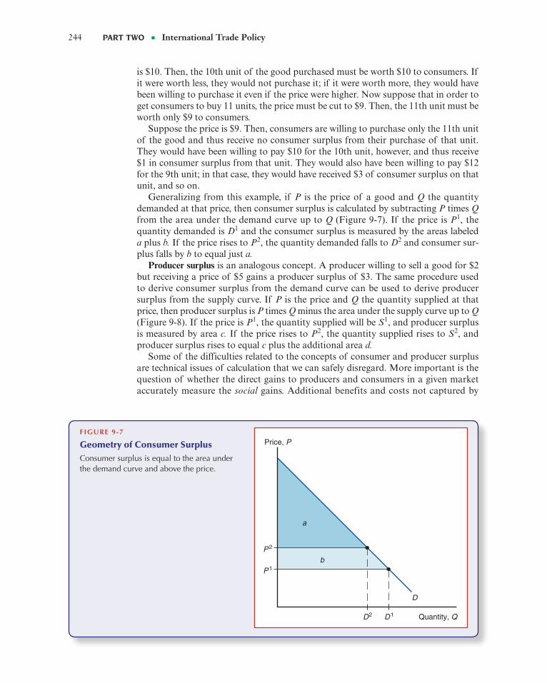
244 Part tWO   ■   International Trade Policy

is $10. Then, the 10th unit of the good purchased must be worth $10 to consumers. If it were worth less, they would not purchase it; if it were worth more, they would have been willing to purchase it even if the price were higher. Now suppose that in order to get consumers to buy 11 units, the price must be cut to $9. Then, the 11th unit must be worth only $9 to consumers.

Suppose the price is $9. Then, consumers are willing to purchase only the 11th unit of the good and thus receive no consumer surplus from their purchase of that unit. They would have been willing to pay $10 for the 10th unit, however, and thus receive $1 in consumer surplus from that unit. They would also have been willing to pay $12 for the 9th unit; in that case, they would have received $3 of consumer surplus on that unit, and so on.

Generalizing from this example, if P is the price of a good and Q the quantity demanded at that price, then consumer surplus is calculated by subtracting P times Q from the area under the demand curve up to Q (Figure 9-7). If the price is P1, the quantity demanded is D1 and the consumer surplus is measured by the areas labeled a plus b. If the price rises to P2, the quantity demanded falls to D2 and consumer sur-plus falls by b to equal just a.

Producer surplus is an analogous concept. A producer willing to sell a good for $2 but receiving a price of $5 gains a producer surplus of $3. The same procedure used to derive consumer surplus from the demand curve can be used to derive producer surplus from the supply curve. If P is the price and Q the quantity supplied at that price, then producer surplus is P times Q minus the area under the supply curve up to Q (Figure 9-8). If the price is P1, the quantity supplied will be S1, and producer surplus is measured by area c. If the price rises to P2, the quantity supplied rises to S2, and producer surplus rises to equal c plus the additional area d.

Some of the difficulties related to the concepts of consumer and producer surplus are technical issues of calculation that we can safely disregard. More important is the question of whether the direct gains to producers and consumers in a given market accurately measure the social gains. Additional benefits and costs not captured by

FIGURE 9-7

Geometry of Consumer SurplusConsumer surplus is equal to the area under the demand curve and above the price.

Price, P

Quantity, Q

D

D1

P1

P2

D2

a

b

M09_KRUG6355_11_GE_C09.indd 244 14/10/2017 08:34

CHaPtEr 9   ■   The Instruments of Trade Policy 245

consumer and producer surplus are at the core of the case for trade policy activism discussed in Chapter 10. For now, however, we will focus on costs and benefits as mea-sured by consumer and producer surplus.

Measuring the Costs and BenefitsFigure 9-9 illustrates the costs and benefits of a tariff for the importing country. The tariff raises the domestic price from PW to PT but lowers the foreign export price from PW to PT* (refer back to Figure 9-4). Domestic production rises from S1 to S2 while

FIGURE 9-8

Geometry of Producer SurplusProducer surplus is equal to the area above the supply curve and below the price.

Price, P

Quantity, Q

S

S2

P2

P1

S1

d

c

FIGURE 9-9

Costs and Benefits of a Tariff for the Importing CountryThe costs and benefits to different groups can be represented as sums of the five areas a, b, c, d, and e.

a

Price, P

Quantity, Q

D

S

D2 D1S1 S2

PW

PT

bc

d

e

PT*

QT

= consumer loss (a + b + c + d)

= government revenue gain (c + e)= producer gain (a)

M09_KRUG6355_11_GE_C09.indd 245 14/10/2017 08:34

246 Part tWO   ■   International Trade Policy

domestic consumption falls from D1 to D2. The costs and benefits to different groups can be expressed as sums of the areas of five regions, labeled a, b, c, d, e.

Consider first the gain to domestic producers. They receive a higher price and there-fore have higher producer surplus. As we saw in Figure 9-8, producer surplus is equal to the area below the price but above the supply curve. Before the tariff, producer surplus was equal to the area below PW but above the supply curve; with the price rising to PT, this surplus rises by the area labeled a. That is, producers gain from the tariff.

Domestic consumers also face a higher price, which makes them worse off. As we saw in Figure 9-7, consumer surplus is equal to the area above the price but below the demand curve. Since the price consumers face rises from PW to PT, the consumer surplus falls by the area indicated by a + b + c + d. So consumers are hurt by the tariff.

There is a third player here as well: the government. The government gains by col-lecting tariff revenue. This is equal to the tariff rate t times the volume of imports QT = D2 - S2. Since t = PT - PT*, the government’s revenue is equal to the sum of the two areas c and e.

Since these gains and losses accrue to different people, the overall cost-benefit evalu-ation of a tariff depends on how much we value a dollar’s worth of benefit to each group. If, for example, the producer gain accrues mostly to wealthy owners of resources, while consumers are poorer than average, the tariff will be viewed differently than if the good is a luxury bought by the affluent but produced by low-wage workers. Further ambiguity is introduced by the role of the government: Will it use its revenue to finance vitally needed public services or waste that revenue on $1,000 toilet seats? Despite these problems, it is common for analysts of trade policy to attempt to compute the net effect of a tariff on national welfare by assuming that at the margin, a dollar’s worth of gain or loss to each group is of the same social worth.

Let’s look, then, at the net effect of a tariff on welfare. The net cost of a tariff is

Consumer loss - producer gain - government revenue, (9-1)

or, replacing these concepts by the areas in Figure 9-9,

(a + b + c + d) - a - (c + e) = b + d - e. (9-2)

That is, there are two “triangles” whose area measures loss to the nation as a whole and a “rectangle” whose area measures an offsetting gain. A useful way to interpret these gains and losses is the following: The triangles represent the efficiency loss that arises because a tariff distorts incentives to consume and produce, while the rectangle represents the terms of trade gain that arise because a tariff lowers foreign export prices.

The gain depends on the ability of the tariff-imposing country to drive down foreign export prices. If the country cannot affect world prices (the small-country case illus-trated in Figure 9-5), region e, which represents the terms of trade gain, disappears, and it is clear that the tariff reduces welfare. A tariff distorts the incentives of both producers and consumers by inducing them to act as if imports were more expensive than they actually are. The cost of an additional unit of consumption to the economy is the price of an additional unit of imports, yet because the tariff raises the domestic price above the world price, consumers reduce their consumption to the point at which that marginal unit yields them welfare equal to the tariff-inclusive domestic price. This means that the value of an additional unit of production to the economy is the price of the unit of imports it saves, yet domestic producers expand production to the point at which the marginal cost is equal to the tariff-inclusive price. Thus, the economy pro-duces at home additional units of the good that it could purchase more cheaply abroad.

M09_KRUG6355_11_GE_C09.indd 246 14/10/2017 08:34

CHaPtEr 9   ■   The Instruments of Trade Policy 247

We saw how a tariff can be used to increase producer surplus at the expense of a loss in

consumer surplus. However, there are many other indirect costs of tariffs. In an indefinite economic environment, it is usually quite challenging to spot whether the cause of import decline is due to improved efficiency of companies in the sector or some “covered” government incentives.2 Neverthe-less, imposed tariffs by one country in most cases would be followed by retaliation from another. If country A imposes a tariff, exporting producers of country B are hurt and the country loses out by the tariff burden. Thus, country B may retaliate with a tariff of its own and form a broader violation of the free trade’s philosophies. As a result of this tariff war, both countries are likely to end up worse off by the reduced volume trade.

In June 2013, a “solar dispute” occurred between the world’s biggest econo-mies and the world’s big-gest trading partners, the European Union (EU) and China. The EU is China’s biggest interna-tional trading partner, and China is its second biggest partner, after the United States. The trade dispute between Beijing and Brussels was one of the biggest in history. The European Commission, after a nine-month investi-gation, started a formal complaint from a group of more than 20 European producers, imposed provi-sional tariffs on solar panels imported from China, and accused subsidized exporters of flooding the EU at prices below production cost. China became the largest producer of solar panels due to a rise in the world’s economy, influencing global trade by lowering prices in the manufacturing sector. Nearly 80 percent of the produced solar panels in China are exported to the EU market. However, according to EU trade commissioner Karel de Gucht, under a fair price the Chinese solar panels would be 88

tarIFFS aND rEtaLIatION

percent higher than the current price. The inflow of Chinese solar panels became a big issue for local producers and competitors. There were opposing opinions between EU member states, because there were uncertainties about the impact of the tariff on the sector and the fact that the EU solar industry supports 265,000 jobs across Europe.

However, a tariff of 11.8 percent was to be applied to Chinese solar imports to Europe from June 6, 2013, and was set to rise to an average of 47.6 percent within two months, imposing these duties for up to five years. Although the tariff was set to be applied to imports of solar panels, which value was €21 billion a year, this would have cre-ated a negative effect on the entire trading rela-

tionship worth about €480 billion and would have undermined the confidence of Chinese companies doing business in Europe.

However, a tariff of 11.8 percent was to be applied to Chinese solar imports to Europe from June 6, 2013, and was set to rise to an average of 47.6 percent within two months, impos-

ing these duties for up to five years. Although the tariff was set to be applied to imports of solar panels, which value was €21 billion a year, this would have created a negative effect on the entire trading relationship worth about €480 billion and would have undermined the confidence of Chinese companies doing business in Europe.

China, as opposed to the EU solar restraint, took steps to defend its interests and Beijing launched anti-dumping and anti-subsidy probes into imports of European wine, as of the received requests and allegations of unfair trade from domestic wine producers. At the same time, export-ers of luxury cars were also threatened as China was about to conduct another probe in the EU luxury cars industry. The wine industry is not the

2WTO, “Trade and Public Policies: A Closer Look at Non-Tariff Measures in the 21st Century,” World Trade Report 2012, https://www.wto.org/english/res_e/booksp_e/anrep_e/wtr12-2e_e.pdf.

M09_KRUG6355_11_GE_C09.indd 247 14/10/2017 08:34

248 Part tWO   ■   International Trade Policy

The net welfare effects of a tariff are summarized in Figure 9-10. The negative effects consist of the two triangles b and d. The first triangle is the production distortion loss resulting from the fact that the tariff leads domestic producers to produce too much of this good. The second triangle is the domestic consumption distortion loss resulting from the fact that a tariff leads consumers to consume too little of the good. Against these losses must be set the terms of trade gain measured by the rectangle e, which results from the decline in the foreign export price caused by a tariff. In the important case of a small country that cannot significantly affect foreign prices, this last effect drops out; thus, the costs of a tariff unambiguously exceed its benefits.

FIGURE 9-10

Net Welfare Effects of a TariffThe colored triangles represent efficiency losses, while the rectangle represents a terms of trade gain.

Price, P

Quantity, Q

D

S

PW

PT

b d

e

Imports

= efficiency loss (b + d)

= terms of trade gain (e)

PT*

these two partners is estimated at €1 billion per day. As a result of this tariff war, the volume of trade between these two countries would be reduced, hurting the economies of both countries.

In July 2013, per the settlement on the solar panel dispute both parties reached an agreement—a minimum price of €0.56 per watt peak for the solar panels until the end of 2015 and a limita-tion on the export volume. Nearly 90 percent of China’s solar manufacturers agreed to the terms of this settlement.3

EU’s core industry. However, some EU countries, such as France, Italy, and Spain, would definitely experience a negative and damaging impact. Chi-na’s total bottled wine imports from 2002 to 2012 skyrocketed to around 15,000 percent and China is the number one importer of French wine. China’s local wine suppliers are the ones who would have benefited the most out of this tariff war.

Nonetheless, China and the EU agreed to settle the dispute through negotiations rather than con-tinuing to heat up the trade war. Trade between

3Yu-Chen, “EU-China Solar Panels Trade Dispute: Settlement and challenges to the EU,” EU-Asia at a Glance, European Institute for Asian Studies, June 2015, http://www.eias.org.

M09_KRUG6355_11_GE_C09.indd 248 14/10/2017 08:34

CHaPtEr 9   ■   The Instruments of Trade Policy 249

Other Instruments of Trade PolicyTariffs are the simplest trade policies, but in the modern world, most government inter-vention in international trade takes other forms, such as export subsidies, import quotas, voluntary export restraints, and local content requirements. Fortunately, once we have understood tariffs, it is not too difficult to understand these other trade instruments.

Export Subsidies: TheoryAn export subsidy is a payment to a firm or individual that ships a good abroad. Like a tariff, an export subsidy can be either specific (a fixed sum per unit) or ad valorem (a proportion of the value exported). When the government offers an export subsidy, shippers will export the good up to the point at which the domestic price exceeds the foreign price by the amount of the subsidy.

The effects of an export subsidy on prices are exactly the reverse of those of a tariff (Figure 9-11). The price in the exporting country rises from PW to PS, but because the price in the importing country falls from PW to PS*, the price increase is less than the subsidy. In the exporting country, consumers are hurt, producers gain, and the govern-ment loses because it must expend money on the subsidy. The consumer loss is the area a + b; the producer gain is the area a + b + c; the government subsidy (the amount of exports times the amount of the subsidy) is the area b + c + d + e + f + g. The net welfare loss is therefore the sum of the areas b + d + e + f + g. Of these, b and d represent consumption and production distortion losses of the same kind that a tariff produces. In addition, and in contrast to a tariff, the export subsidy worsens the terms of trade because it lowers the price of the export in the foreign market from PW to PS*. This leads to the additional terms of trade loss e + f + g, which is equal to PW - PS* times the quantity exported with the subsidy. So an export subsidy unam-biguously leads to costs that exceed its benefits.

FIGURE 9-11

Effects of an Export SubsidyAn export subsidy raises prices in the exporting country while lowering them in the importing country.

*

a

Price, P

Quantity, Q

D

S

PW

= consumer loss (a + b)

PS

= producer gain (a + b + c)

d

= cost of government subsidy (b + c + d + e + f + g)

Exports

e f g

b c

PS

Subsidy

M09_KRUG6355_11_GE_C09.indd 249 14/10/2017 08:34

250 Part tWO   ■   International Trade Policy

Europe’s Common Agricultural PolicyIn 1957, six Western European nations—Germany, France, Italy, Belgium, the Netherlands, and Luxembourg—formed the European Economic Community, which has since grown to include most of Europe. Now called the European Union (EU), its two biggest effects are on trade policy. First, the members of the European Union have removed all tariffs with respect to each other, thus creating a customs union (discussed in Chapter 10). Second, the agricultural policy of the European Union has developed into a massive export subsidy program.

The European Union’s Common Agricultural Policy (CAP) began not as an export subsidy but as an effort to guarantee high prices to European farmers by having the European Union buy agricultural products whenever the prices fell below specified support levels. To prevent this policy from drawing in large quanti-ties of imports, it was initially backed by tariffs that offset the difference between European and world agricultural prices.

Since the 1970s, however, the support prices set by the European Union have turned out to be so high that Europe—which, under free trade, would be an importer of most agricultural products—was producing more than consumers were willing to buy. As a result, the European Union found itself obliged to buy and store huge quantities of food. At the end of 1985, for example, European nations had stored 780,000 tons of beef, 1.2 million tons of butter, and 12 million tons of wheat. To avoid unlimited growth in these stockpiles, the European Union turned to a policy of subsidizing exports to dispose of surplus production.

Figure 9-12 shows how the CAP works. It is, of course, exactly like the export subsidy shown in Figure 9-11, except that Europe would actually be an importer under free trade. The support price is set not only above the world price that would prevail in its absence but also above the price that would equate demand and sup-ply even without imports. To export the resulting surplus, an export subsidy is paid that offsets the difference between European and world prices. The subsidized exports themselves tend to depress the world price, increasing the required subsidy. A recent study estimated that the welfare cost to European consumers exceeded the benefits to farm producers by nearly $30 billion (21.5 billion euros) in 2007.4

Despite the considerable net costs of the CAP to European consumers and taxpayers, the political strength of farmers in the EU has been so strong that the program has been difficult to rein in. One source of pressure has come from the United States and other food-exporting nations, which complain that Europe’s export subsidies drive down the price of their own exports. The budgetary conse-quences of the CAP have also posed concerns: In 2013, the CAP cost European taxpayers $65 billion (59 billion euros)—and that figure doesn’t include the indi-rect costs to food consumers. Government subsidies to European farmers are equal to about 19 percent of the value of farm output, roughly twice the U.S. figure of 9.4 percent. (U.S. agriculture subsidies are more narrowly targeted on a subset of crops.)

4See Pierre Boulanger and Patrick Jomini, Of the Benefits to the EU of Removing the Common Agricultural Policy, Sciences Politique Policy Brief, 2010.

CASE STUDY

M09_KRUG6355_11_GE_C09.indd 250 14/10/2017 08:34

CHaPtEr 9   ■   The Instruments of Trade Policy 251

FIGURE 9-12

Europe’s Common Agricultural PolicyAgricultural prices are fixed not only above world market levels but also above the price that would clear the European market. An export subsidy is used to dispose of the resulting surplus.

Price, P

Quantity, Q

D

S

= cost of government subsidy

Exports

Support price

Worldprice

EU price without imports

Recent reforms in Europe’s agricultural policy rep-resent an effort to reduce the distortion of incentives caused by price support while continuing to provide aid to farmers. If politicians go through with their plans, farmers will increasingly receive direct pay-ments that aren’t tied to how much they produce; this should lower agricultural prices and reduce production.

Import Quotas: TheoryAn import quota is a direct restriction on the quantity of some good that may be imported. The restriction is usually enforced by issuing licenses to some group of indi-viduals or firms. For example, the United States has a quota on imports of foreign cheese. The only firms allowed to import cheese are certain trading companies, each of which is allocated the right to import a maximum number of pounds of cheese each year; the size of each firm’s quota is based on the amount of cheese it imported in the past. In some important cases, notably sugar and apparel, the right to sell in Another example is the European Union applying tariff quotas to imports of a specified origin.5

It is important to avoid having the misconception that import quotas somehow limit imports without raising domestic prices. The truth is that an import quota always raises the domestic price of the imported good. When imports are limited, the immediate

5European Commission.

M09_KRUG6355_11_GE_C09.indd 251 14/10/2017 08:34

252 Part tWO   ■   International Trade Policy

Tariff-Rate Quota Origin and its Application in Practice with Oilseeds

In international trade, oilseed products are one of the most highly traded agricul-tural products (others include grains and meat), making this trade one of crucial importance for many countries, either through production or utilization. Oilseeds are crops that have high oil content such as soybeans, rapeseed, sunflower, flax, and cottonseed. In 2001, about 80 percent of the world imports of oilseeds con-sisted of 11 percent soybeans, 9 percent rapeseed, and other types of oilseeds. Tariff quotas for these goods are more often applied than those for the traditionally protected products like dairy or sugar.

In practice, in 1990s world trade in oilseeds generally was characterized by “low to moderate” applied tariffs and bound tariff rates. The bound tariff rate, which is the maximum allowable rate under a country’s WTO commitments, in most cases is quite high, particularly in developing countries. For instance, the highest tariffs were imposed by Colombia (and Venezuela) with a 15 percent duty to its imports of soybeans in 2001, but it had a bound tariff rate of 97 percent under the WTO com-mitment. India had a 40 percent applied tariff, but imposed a 100 percent bound tariff rate. In general, tariff rates on oilseed products (for example, vegetable oils and oilseed meal) were much higher than those on whole oilseeds. This situation is called tariff escalation and its practice was designed mainly for two main reasons: to protect both domestic oilseed crushing industry and vegetable oil refineries, and to discourage the development of processing activities in the countries of its origin.

In Japan, for example, with limited domestic oilseed production, there was no tariff on whole oilseeds. However, a tariff of 12.9 yen/kg for soy oil/rape oil was imposed with intension to protect local crushers.4 The EU applied a tariff on soybean oil of 30 percent ad valorem, and had a bound tariff of 45 percent, for soybean meal a tariff was

4Mitchell D. A note on rising food prices, The world Banks Development prospects group, July 2008, Policy research working paper 4682; and Oils Crop Situation and Outlook Yearbook  / OCS-2006/May 2006, Economic Research Service, USDA.

CASE STUDY

result is that at the initial price, the demand for the good exceeds domestic supply plus imports. This causes the price to be bid up until the market clears. In the end, an import quota will raise domestic prices by the same amount as a tariff that limits imports to the same level (except in the case of domestic monopoly, in which the quota raises prices more than this; see the appendix to this chapter).

The difference between a quota and a tariff is that with a quota, the government receives no revenue. When a quota instead of a tariff is used to restrict imports, the sum of money that would have appeared with a tariff as government revenue is collected by whoever receives the import licenses. License holders are thus able to buy imports and resell them at a higher price in the domestic market. The profits received by the hold-ers of import licenses are known as quota rents. In assessing the costs and benefits of an import quota, it is crucial to determine who gets the rents. When the rights to sell in the domestic market are assigned to governments of exporting countries, as is often the case, the transfer of rents abroad makes the costs of a quota substantially higher than the equivalent tariff.

M09_KRUG6355_11_GE_C09.indd 252 14/10/2017 08:34

CHaPtEr 9   ■   The Instruments of Trade Policy 253

5 percent (with a bound tariff of 10 percent). Although the duty on soybeans imports was bound duty-free under WTO commitment, all other oilseeds and oilseed meals imports also had free of duty import status under the Dillon round. An alternative measure in the form of non-tariff policies, specifically domestic price support and subsidies served producers as a substitute. These policies encouraged excess produc-tion and distorted trade flows as well as reduced world imports, increased export subsidies, encouraged low-price selling on world markets. The EU oilseed production subsidies, real price supports, budgetary expenditures or oilseed crops increased dra-matically (by 1985 the budgetary expenditure on oilseeds and protein crops exceeded 10 percent of the EU’s total annual spending on agriculture) for domestic growers resulted in oilseeds production increase.5 The EU nearly tripled oilseed production between 1980 and 1990, which contributed to a 53 percent drop in the volume of U.S. soybean and soybean meals export for the same period, displacing and impair-ing U.S. exports to the EU. This led to an oilseeds dispute between the United States and the EU in the end of 1980s, which was later solved by the Blair House agreement on oilseeds.6

Uruguay’s Round Agreement on Agriculture (URAA) had greatly influenced the process of trade barriers reduction and the major achievement was cut in tariff levels on agricultural products, lowering the volume of and expenditures on subsidized export and reducing domestic programs for agriculture. Partici-pating developed countries in URAA were required to reduce existing tariffs on agricultural products on average of 36 percent. Developing countries had commit-ted to smaller average tariff reductions, 24 percent, and longer transition period compared to developed nations. Another important requirement was to convert existing non-tariff agricultural trade barriers to tariffs, establishing a tariff-rate quota (TRQ).

The idea by TRQ was to impose a lower tariff rate to imports below a certain quantitative limit and higher tariffs to imports above that initial limit. As of URAA tariffs were to be reduced from the base levels to a bound level. According to URAA the size of quota was aimed to be equal or greater than actual import levels during a recent period and required that out-of-quota bound tariff rates be reduced from the based tariff rates. In 1997 40percent of 1,366 TRQs were sup-posed to increase their quotas, indicating easier market access.7 Of these TRQs, 124 (which is 9 percent) were applied to oilseeds and products. The 21 member states of the WTO notified having at least one TRQ on oilseeds or oilseed products.

5Ames Glenn C.W., Gunter L., Davis C.D. (1996) Analysis of USA-European Community oilseeds agree-ment, Agriculture Economics 15, p.97-112 6Oilseed disputed narrowed During GATT Uruguay Round in 1992 a memorandum of Understanding on oilseeds (often referred to as the “Blair House Agreement”) was negotiated with the US, resolving a dispute over EU domestic support programs that weakened the US access to the EU oilseeds market. As of the agree-ment a number of restriction on production support of oilseeds was established. The EU oilseeds planting area of certain type was limited (specifically rapeseed, sunflower seed and soybeans), while certain support allowance of the production of some oilseeds to continue. The limitation included on area that should not have exceeded 5.482 million hectares. The agreement also allowed for modification of the supported area in regards to EU enlargement. While the original maximum base was set at 5.128 million hectares, it was modified to cover EU15 in 1995 with no amendments for subsequent EU enlargement.7Oils Crop Situation and Outlook Yearbook / OCS-2006/May 2006, Economic Research Service, USDA

M09_KRUG6355_11_GE_C09.indd 253 14/10/2017 08:34

254 Part tWO   ■   International Trade Policy

For instance, Iceland had 22 TRQs—Colombia, 20; Venezuela, 19; South Africa, 8; Guatemala, 7; and Thailand and Morocco had 6.8 The URAA fixed an upper bound on tariff levels for agricultural commodities, however these limits were often quite high, varying by country.

The establishment of TRQ aimed to bring more transparency of non-tariff bar-riers to trade and though was a major achievement, the level of trade creation resulting from these TRQs were quite modest. For TRQ quotas to be more effective and for the trade to be more liberalized reduced tariffs (or elimination) on imports above the quota or increased the quota level would be far better options for overall trade. The modest result was mostly linked to high over-quotas tariff rates, which was a barrier to trade in oilseeds and products. Overall tariff-rate quota became a more often used form of domestic market protection and in a way a gradual alternative to international trade liberalization form.

PERSPECTIvE On EU OIlSEED MARkET.

The EU is one of the top importers of oilseeds products, and oilseeds con-sumption is higher than the net production minus exports. In fact, the EU is highly dependent on imports of oilseed and its products (protein meals and vegetable oils). Oilseeds (rapeseed, sunflower seed, soybeans, linseed) are grown in the European Union for food, feed, fuel and industrial purposes. Nearly all oilseeds are crushed and processed to produce oil and meal.9 Vegetable oils are used in food industry, biodiesel and other industries. Oilseeds meals are also essential protein-rich animal fee ingredient. Some oilseeds have limited or no domestic production (such as soybeans, soybean products and palm oil). Around 54 percent of soybean meal, around 50 percent of sunflower meal and more that

8As of URRA requirement imports that meet a minimum of 5percent of domestic consumption by the end of the implementation period. Countries that already import over that amount are not required to raise their quota level.

FIGURE 9-13

World Oilseed Tariff Rates in cents per kgSource: Oil Crops And Outlook Yearbook, May 2007, Economic Reasearch Service, USDA.

9OECD (2003) Agriculture, Trade and the Environment: the Arable Crop Sector.

CountryBase Tariff

Rate

Bound Tariff Rate (Rate of Over Quota

Tariff)Applied Tariff

(TRQ)USA 0.7 0.45 0.53Mexico 25 22.5 15Columbia,

Venezuela108 97 15

Poland 10 5 3India 100 100 40Malaysia 13 10 0

M09_KRUG6355_11_GE_C09.indd 254 14/10/2017 08:34

CHaPtEr 9   ■   The Instruments of Trade Policy 255

80 percent of soybeans for crush are imported to meet the domestic demand. In the EU, cereal pro-duction represents the most important use of ara-ble land, whereas 5.4 million ha are allocated to the production of oilseeds. Currently, about 2/3 of the oilseeds consumed within the European Union each year are produced in the EU and the rest is being imported. Since 2012 there are no specific domestic support measures for the production of oilseeds in the EU and no longer any restriction on the EU’s oilseed area.

From January 2002 to June 2008, the world’s food prices saw a drastic growth due to several factors. The rapid increase in oilseed prices was mostly caused by a large increase in biofuels production from grains and oilseeds both in the US and EU. The growth in the EU poultry sector was mostly responsible for the growing demand for protein feed. With mandatory use of biofuels in the EU by 2020 (as stated by the 2009 Renewable Energy Direc-tive11) the use of vegetable oils in the EU also increased, causing prices to rise as well as pushing the domestic oilseed production to grow.

10For the olive oil market, the European Commission can provide private storage aid in case of disturbances in the olive oil market or the average price for the following products are recorded during a two weeks period: Eur 1,779/tonne for extra virgin olive oil, Eur 1,710/tonne for virgin olive oil, Eur 1,524/tonne for lampante olive oil; and the European Commission, Directorate-General for Agriculture and Rural Development, Unit C5, October, 2011.11Directive 2009/28/EC of the European Parliament and of the Council of 23 April 2009 on the promotion of the use of energy from renewable sources and amending and subsequently repealing Directives 2001/77/EC and 2003/30/EC.

voluntary Export RestraintsA variant on the import quota is the voluntary export restraint (VER), also known as a voluntary restraint agreement (VRA). (Welcome to the bureaucratic world of trade policy, where everything has a three-letter symbol!) A VER is a quota on trade imposed from the exporting country’s side instead of the importer’s. The most famous example is the limitation on auto exports to the United States enforced by Japan after 1981.

FIGURE 9-14

Tariffs on oilseeds as well as oilseed meals and set at zero, some duties vegetable oils (except olive oil) range from 0 to 12.8 Percent.Oilseeds And Protien Crops In The Eu Directorate-General For Agriculture and Rural Development, Unit C5, European Commission, 201110

Description Duty percentOilseeds 0Vegetable oils, other than olive oil 0–12.8Oilseed meals 0

M09_KRUG6355_11_GE_C09.indd 255 14/10/2017 08:34

256 Part tWO   ■   International Trade Policy

Voluntary export restraints are generally imposed at the request of the importer and are agreed to by the exporter to forestall other trade restrictions. As we will see in Chapter 10, certain political and legal advantages have made VERs preferred instru-ments of trade policy in some cases. From an economic point of view, however, a vol-untary export restraint is exactly like an import quota where the licenses are assigned to foreign governments and is therefore very costly to the importing country.

A VER is always more costly to the importing country than a tariff that limits imports by the same amount. The difference is that what would have been revenue under a tariff becomes rents earned by foreigners under the VER, so that the VER clearly produces a loss for the importing country.

Numerical examples suggest that voluntary export restraints can be beneficial for the exporting country and damaging to the importing country. A study that examines the welfare effect of VERs on the world economy suggests that a government’s preference for VERs offers a short-term expansion effect on the exporting country. The effects of VERs can only bring positive results in the case of perfect competition for the goods market or when the exporting country is larger than the importing country. Overall, a VER not only damages the domestic economy in the long-run but also has a deteriorat-ing effect on the overall welfare of the world economy.12

Some voluntary export agreements cover more than one country. The most famous multilateral agreement is the Multi-Fiber Arrangement, which limited textile exports from 22 countries until the beginning of 2005. Such multilateral voluntary restraint agreements are known by yet another three-letter abbreviation: OMA, for “orderly marketing agreement.”

12Wang F. (2011) Who bears the burden of voluntary export restraints? Prague Economic Paper Vol. 3., p. 216-231. DOI: 10.18267/j.pep.397

A voluntary Export Restraint in Practice

JAPAnESE AUTOS

For much of the 1960s and 1970s, the U.S. auto industry was largely insulated from import competition by the difference in the kinds of cars bought by U.S. and foreign consumers. U.S. buyers, living in a large country with low gasoline taxes, preferred much larger cars than Europeans and Japanese, and, by and large, for-eign firms had chosen not to challenge the United States in the large-car market.

In 1979, however, sharp oil price increases and temporary gasoline shortages caused the U.S. market to shift abruptly toward smaller cars. Japanese producers, whose costs had been falling relative to those of their U.S. competitors in any case, moved in to fill the new demand. As the Japanese market share soared and U.S. output fell, strong political forces in the United States demanded protection for the U.S. industry. Rather than act unilaterally and risk creating a trade war, the U.S. government asked the Japanese government to limit its exports. The Japanese, fearing unilateral U.S. protectionist measures if they did not do so, agreed to limit their sales. The first agreement, in 1981, limited Japanese exports to the United States to 1.68 million automobiles. A revision raised that total to 1.85 million in 1984. In 1985, the agreement was allowed to lapse.

CASE STUDY

M09_KRUG6355_11_GE_C09.indd 256 14/10/2017 08:34

CHaPtEr 9   ■   The Instruments of Trade Policy 257

local Content RequirementsA local content requirement is a regulation that requires some specified fraction of a final good to be produced domestically. In some cases, this fraction is specified in physical units, like the U.S. oil import quota in the 1960s. In other cases, the require-ment is stated in value terms by requiring that some minimum share of the price of a good represent domestic value added. Local content laws have been widely used by developing countries trying to shift their manufacturing base from assembly back into intermediate goods. In the United States, a local content bill for automobiles was pro-posed in 1982 but was never acted on.

From the point of view of the domestic producers of parts, a local content regulation provides protection in the same way an import quota does. From the point of view of the firms that must buy locally, however, the effects are somewhat different. Local content does not place a strict limit on imports. Instead, it allows firms to import more, provided that they also buy more domestically. This means that the effective price of inputs to the firm is an average of the price of imported and domestically produced inputs.

Consider, for instance, the earlier automobile example in which the cost of imported parts is $6,000. Suppose purchasing the same parts domestically would cost $10,000, but assembly firms are required to use 50 percent domestic parts. Then, they will face

The effects of this voluntary export restraint were complicated by several factors. First, Japanese and U.S. cars were clearly not perfect substitutes. Second, the Japanese industry to some extent responded to the quota by upgrading its qual-ity and selling larger autos with more features. Third, the auto industry is clearly not perfectly competitive. Nonetheless, the basic results were what the discussion of voluntary export restraints earlier would have predicted: The price of Japanese cars in the United States rose, with the rent captured by Japanese firms. The U.S. government estimates the total costs to the United States to be $3.2 billion in 1984, primarily in transfers to Japan rather than efficiency losses.

CHInESE SOlAR PAnElS

Although voluntary export restraints are no longer allowed under WTO rules, this only applies to an agreement negotiated by governments and imposed onto exporters. Recently, a European Union–China trade dispute over a surge in Chi-nese exports of solar panels was resolved by the Chinese producers “agreeing” to limit their exports to EU countries below 7 gigawatts-worth of solar panels per year—along with a minimum price floor for those units. EU solar panel makers were disappointed, as this agreement forestalled the imposition of 47 percent anti-dumping duties on all Chinese solar panel imports (the threat that generated those concessions by Chinese solar panel producers). However, the imposition of the anti-dumping duties would have triggered a significant retaliation from China, whose officials had already drawn up a list of European products— including lux-ury fashion goods and wines—that would be subjected to stiff import duties into China. Chinese producers were persuaded to agree to the export limit and price floor instead, since this would allow them to keep the higher prices charged in the European Union. The main losers are European consumers, who will pay substantially more for solar power (and the environment).

M09_KRUG6355_11_GE_C09.indd 257 14/10/2017 08:34

258 Part tWO   ■   International Trade Policy

Local content requirements (LCR) are attract-ing more and more attention as a non-tariff

form of protectionism providing domestic pro-ducers additional benefits over the foreign com-petitors. In fact, both developed and developing countries have turned their interest towards this policy. While LCR has been around for a long period of time, in recent years a substantial increase has been witnessed in the use of these restrictions, especially after the financial crisis of 2008. Using LCR, various governments have put in efforts to improve domestic employment and industrial performance.

For example, the healthcare sector in Bra-zil is divided into three groups: medical services and hospitals, medical devices, and pharma-ceuticals. While hospi-tals and other providers of medical services in Brazil cannot be owned by foreign companies, fore ign companies are actively engaged in other healthcare sector groups: imported medical devices make around 60 percent and pharmaceuticals – 24 percent of Brazilian market. In 2011, the Brazilian pharma-ceutical market was around $30 billion, whilst the medical devices sector was more than 10 times bigger and made it to roughly $4 billion. The Brazilian Ministry of Health controls the mar-ket of healthcare products and services through

HEaLtHCarE PrOtECtION WItH LOCaL CONtENt rEquIrEmENtS

a licensing system. In order to sell either phar-maceutical or healthcare products a producer (regardless the origin of the goods) must receive approval of the products registration as well as obtain a license. The idea of these requirements is to set a population’s sanitary control of pro-duction and marketing. As a result, it creates additional costs and requires additional time for foreign companies to register medical devices in the Brazilian market. Although registration requirements do not fall into the discriminative policy, it generates delays in business while wait-

ing for approvals and per-missions and additional costs. Around 70 percent of Brazilian pharmaceuti-cals are manufactured by foreign companies, thus, foreign companies tend to acquire Brazilian com-panies or construct green field production plants because of the local con-tent requirements and other aspects. In addition,

with the target to create demand for domestic products and positively influence economy and increase employment rate in 2012 the Brazil-ian government established a LCR policy—up to 25  percent preferences for Brazilian medical devices and medicine in government contracts. This local content requirement obviously has a discriminative nature for those devices and medi-cation produced abroad.13

13Hufbauer G.C., Schott J.J., Cimino C., Vieiro M, Wada E. Local content requirements: Report on a global problem, Peterson Institute for International Economics (June 28, 2013).

an average cost of parts of +8,000 (0.5 * +6,000 + 0.5 * +10,000), which will be reflected in the final price of the car.

The important point is that a local content requirement does not produce either government revenue or quota rents. Instead, the difference between the prices of imports and domestic goods in effect gets averaged in the final price and is passed on to consumers.

M09_KRUG6355_11_GE_C09.indd 258 14/10/2017 08:34

CHaPtEr 9   ■   The Instruments of Trade Policy 259

An interesting innovation in local content regulations has been to allow firms to sat-isfy their local content requirement by exporting instead of using parts domestically. This is sometimes important. For example, U.S. auto firms operating in Mexico have chosen to export some components from Mexico to the United States, even though those com-ponents could be produced in the United States more cheaply because doing so allows them to use less Mexican content in producing cars in Mexico for Mexico’s market.

Other Trade Policy InstrumentsGovernments influence trade in many other ways. We list some of them briefly.

1. Export credit subsidies. This is like an export subsidy except that it takes the form of a subsidized loan to the buyer. The United States, like most other countries, has a government institution, the Export-Import Bank, devoted to providing at least slightly subsidized loans to aid exports.

2. National procurement. Purchases by the government or strongly regulated firms can be directed toward domestically produced goods even when these goods are more expensive than imports. The classic example is the European telecommunications industry. The nations of the European Union in principle have free trade with each other. The main purchasers of telecommunications equipment, however, are phone companies—and in Europe, these companies have until recently all been government-owned. These government-owned telephone companies buy from domestic suppliers even when the suppliers charge higher prices than suppliers in other countries. The result is that there is very little trade in telecommunications equipment within Europe.

3. Red-tape barriers. Sometimes a government wants to restrict imports without doing so formally. Fortunately or unfortunately, it is easy to twist normal health, safety, and customs procedures in order to place substantial obstacles in the way of trade. The classic example is the French decree in 1982 that all Japanese videocassette recorders had to pass through the tiny customs house at Poitiers (an inland city nowhere near a major port)—effectively limiting the actual imports to a handful.

The Effects of Trade Policy: A SummaryThe effects of the major instruments of trade policy are usefully summarized by Table 9-1, which compares the effect of four major kinds of trade policy on the wel-fare of consumers.

TABLE 9-1 Effects of Alternative Trade Policies

Policy TariffExport Subsidy

Import Quota

Voluntary Export Restraint

Producer surplus Increases Increases Increases IncreasesConsumer surplus Falls Falls Falls FallsGovernment

revenueIncreases Falls (government

spending rises)No change

(rents to license holders)

No change (rents to foreigners)

Overall national welfare

Ambiguous (falls for small country)

Falls Ambiguous (falls for small country)

Falls

M09_KRUG6355_11_GE_C09.indd 259 14/10/2017 08:34

260 Part tWO   ■   International Trade Policy

KEY TERMS

This table certainly does not look like an advertisement for interventionist trade policy. All four trade policies benefit producers and hurt consumers. The effects of the policies on economic welfare are at best ambiguous; two of the policies definitely hurt the nation as a whole, while tariffs and import quotas are potentially beneficial only for large countries that can drive down world prices.

Why, then, do governments so often act to limit imports or promote exports? We turn to this question in Chapter 10.

SUMMARY

1. In contrast to our earlier analysis, which stressed the general equilibrium interac-tion of markets, for analysis of trade policy it is usually sufficient to use a partial equilibrium approach.

2. A tariff drives a wedge between foreign and domestic prices, raising the domestic price but by less than the tariff rate. An important and relevant special case, however, is that of a “small” country that cannot have any substantial influence on foreign prices. In the small-country case, a tariff is fully reflected in domestic prices.

3. The costs and benefits of a tariff or other trade policy may be measured using the concepts of consumer surplus and producer surplus. Using these concepts, we can show that the domestic producers of a good gain because a tariff raises the price they receive; the domestic consumers lose, for the same reason. There is also a gain in government revenue.

4. If we add together the gains and losses from a tariff, we find that the net effect on national welfare can be separated into two parts: On one hand is an efficiency loss, which results from the distortion in the incentives facing domestic produc-ers and consumers. On the other hand is a terms of trade gain, reflecting the tendency of a tariff to drive down foreign export prices. In the case of a small country that cannot affect foreign prices, the second effect is zero, so that there is an unambiguous loss.

5. The analysis of a tariff can be readily adapted to analyze other trade policy mea-sures, such as export subsidies, import quotas, and voluntary export restraints. An export subsidy causes efficiency losses similar to those of a tariff but compounds these losses by causing a deterioration of the terms of trade. Import quotas and voluntary export restraints differ from tariffs in that the government gets no rev-enue. Instead, what would have been government revenue accrues as rents to the recipients of import licenses (in the case of a quota) and to foreigners (in the case of a voluntary export restraint).

ad valorem tariff, p. 237consumer surplus, p. 243consumption distortion loss,

 p. 248effective rate of protection,

 p. 242efficiency loss, p. 246export restraint, p. 238export subsidy, p. 249

export supply curve, p. 238import demand curve, p. 238import quota, p. 238local content requirement,

 p. 257nontariff barriers, p. 238producer surplus, p. 244production distortion loss,

 p. 248

quota rent, p. 252specific tariff, p. 237tariff equivalent, p. 253terms of trade gain, p. 246voluntary export restraint

(VER), p. 255

M09_KRUG6355_11_GE_C09.indd 260 16/10/2017 22:05

CHaPtEr 9   ■   The Instruments of Trade Policy 261

PROBLEMS

1. Home’s demand curve for books is

D = 50 - 10P.

Its supply curve is

S = 10 + 10P.

Derive and graph Home’s import demand schedule. What would the price of books be in the absence of trade?

2. Now add Foreign, which has a demand curve

D* = 60 - 10P

and a supply curve

S* = 20 + 10P.

a. Derive and graph Foreign’s export supply curve and find the price of wheat that would prevail in Foreign in the absence of trade.

b. Now allow Foreign and Home to trade with each other, at zero transportation cost. Find and graph the equilibrium under free trade. What is the world price? What is the volume of trade?

3. Home imposes a specific tariff of 1.5 on books imports.a. Determine and graph the effects of the tariff on the following: (1) the price of

books in each country; (2) the quantity of books supplied and demanded in each country; (3) the volume of trade.

b. Determine the effect of the tariff on the welfare of each of the following groups: (1) Home import-competing producers; (2) Home consumers; (3) the Home government.

c. Show graphically and calculate the terms of trade gain, the efficiency loss, and the total effect on welfare of the tariff.

4. Suppose Foreign had been a much larger country, with domestic demand

D* = 8 - 2P, S* = 4 + 2P.

(Notice that this implies the Foreign price of wheat in the absence of trade would have been the same as in problem 2.)

Recalculate the free trade equilibrium and the effects of a 1.5 specific tariff by Home. Relate the difference in results to the discussion of the small-country case in the text.

5. What would be the effective rate of protection on bicycles in China if China places a 50 percent tariff on bicycles, which have a world price of $200, and no tariff on bike components, which together have a world price of $100?

6. For a company that produces candy canes, sugar constitutes 70 percent of its ingredi-ent costs. The United States limits the import of sugar to protect cane farmers, which has led to an increase in the price of sugar by about 25 percent relative to what it would be otherwise. Suppose your country, however, allows free trade in candy canes, which are made with sugar that accounts for approximately 65 percent of its cost. What is the effective rate of protection on the process of turning sugar into candy canes?

7. Return to the example of problem 2. Starting from free trade, assume that Foreign offers exporters a subsidy of 1.5 per unit. Calculate the effects on the price in each

Pearson MyLab Economics

M09_KRUG6355_11_GE_C09.indd 261 14/10/2017 08:34

262 Part tWO   ■   International Trade Policy

country and on welfare, both of individual groups and of the economy as a whole, in both countries.

8. Use your knowledge about trade policy to evaluate each of the following statements:a. “Tariffs on imported goods will increase domestic price, leading to high

unemployment.”b. “High tariffs and quotas can result in trade wars between nations.”c. “Smartphone manufacturing jobs are heading back to United States because

wages started to rise in China. As a result, we should implement tariffs on smartphones equal to the difference between U.S. and China’s wage rates.”

9. The nation of Cologne is “large” but unable to affect world prices. It imports chocolates at the price of $20 per box. The demand curve is

D = 700 - 10P.

The supply curve is

S = 200 + 5P.

Determine the free trade equilibrium. Then calculate and graph the following effects of an import quota that limits imports to 50 boxes.a. The increase in the domestic price.b. The quota rents.c. The consumption distortion loss.d. The production distortion loss.

10. If tariffs are already in place as a trade policy, why might a country choose to apply also nontariff barriers as another way to control the amount of trade that they conduct with other countries?

11. Suppose workers involved in manufacturing are paid less than all other workers in the economy. What would be the effect on the real income distribution within the economy if there were a substantial tariff levied on manufactured goods?

FURTHER READINGS

Jagdish Bhagwati. “On the Equivalence of Tariffs and Quotas,” in Robert E. Baldwin et al., eds. Trade, Growth, and the Balance of Payments. Chicago: Rand McNally, 1965. The classic comparison of tariffs and quotas under monopoly.

W. M. Corden. The Theory of Protection. Oxford: Clarendon Press, 1971. A general survey of the effects of tariffs, quotas, and other trade policies.

Robert W. Crandall. Regulating the Automobile. Washington, D.C.: Brookings Institution, 1986. Contains an analysis of the most famous of all voluntary export restraints.

Robert C. Feenstra. “How Costly Is Protectionism?” Journal of Economic Perspectives 6 (1992), pp. 159–178. A survey article summarizing the empirical work measuring the costs associated with protectionist policies.

Gary Clyde Hufbauer and Kimberly Ann Elliot. Measuring the Costs of Protection in the United States. Washington, D.C.: Institute for International Economics, 1994. An assessment of U.S. trade policies in 21 different sectors.

Kala Krishna. “Trade Restrictions as Facilitating Practices.” Journal of International Economics 26 (May 1989), pp. 251–270. A pioneering analysis of the effects of import quotas when both foreign and domestic producers have monopoly power, showing that the usual result is an increase in the profits of both groups—at consumers’ expense.

Patrick Messerlin. Measuring the Costs of Protection in Europe: European Commercial Policy in the 2000s. Washington, D.C.: Institute for International Economics, 2001. A survey of European trade policies and their effects, similar to Hufbauer and Elliot’s work for the United States.

M09_KRUG6355_11_GE_C09.indd 262 14/10/2017 08:34

CHaPtEr 9   ■   The Instruments of Trade Policy 263

D. Rousslang and A. Suomela. “Calculating the Consumer and Net Welfare Costs of Import Relief.” U.S. International Trade Commission Staff Research Study 15. Washington, D.C.: International Trade Commission, 1985. An exposition of the framework used in this chapter, with a description of how the framework is applied in practice to real industries.

U.S. International Trade Commission. The Economic Effects of Significant U.S. Import Restraints. Washington, D.C., 2009. A regularly updated economic analysis of the effects of protection on the U.S. economy.

Pearson MyLab Economics Can Help You Get a Better GradeIf your exam were tomorrow, would you be ready? For each chapter, Pearson

MyLab Economics Practice Tests and Study Plans pinpoint sections you have mastered and those you need to study. That way, you are more efficient with your study time, and you are better prepared for your exams.To see how it works, turn to page 31 and then go towww.myeconlab.com

Pearson MyLab Economics

M09_KRUG6355_11_GE_C09.indd 263 14/10/2017 08:34

264

Tariffs and Import Quotas in the Presence of MonopolyThe trade policy analysis in this chapter assumed that markets are perfectly competitive, so that all firms take prices as given. As we argued in Chapter 8, however, many markets for internationally traded goods are imperfectly competitive. The effects of interna-tional trade policies can be affected by the nature of the competition in a market.

When we analyze the effects of trade policy in imperfectly competitive markets, a new consideration appears: International trade limits monopoly power, and policies that limit trade may therefore increase monopoly power. Even if a firm is the only pro-ducer of a good in a country, it will have little ability to raise prices if there are many foreign suppliers and free trade. If imports are limited by a quota, however, the same firm will be free to raise prices without fear of competition.

The link between trade policy and monopoly power may be understood by examin-ing a model in which a country imports a good and its import-competing production is controlled by only one firm. The country is small on world markets, so the price of the import is unaffected by its trade policy. For this model, we examine and compare the effects of free trade, a tariff, and an import quota.

The Model with Free TradeFigure 9A-1 shows free trade in a market where a domestic monopolist faces com-petition from imports. D is the domestic demand curve: demand for the product by domestic residents. PW is the world price of the good; imports are available in unlimited quantities at that price. The domestic industry is assumed to consist of only a single firm, whose marginal cost curve is MC.

APPENDIX TO CHAPTER 9

FIGURE 9A-1

A Monopolist under Free TradeThe threat of import competition forces the monopolist to behave like a perfectly competitive industry.

Price, P

Quantity, Q

MR

MC

D

PM

PW

Qf DfQM

Imports under free trade

M09_KRUG6355_11_GE_C09.indd 264 14/10/2017 08:34

CHaPtEr 9   ■   The Instruments of Trade Policy 265

If there were no trade in this market, the domestic firm would behave as an ordinary profit-maximizing monopolist. Corresponding to D is a marginal revenue curve MR, and the firm would choose the monopoly profit-maximizing level of output QM and price PM.

With free trade, however, this monopoly behavior is not possible. If the firm tried to charge PM, or indeed any price above PW, nobody would buy its product, because cheaper imports would be available. Thus international trade puts a lid on the monopo-list’s price at PW.

Given this limit on its price, the best the monopolist can do is produce up to the point where marginal cost is equal to the world price, at Qf. At the price PW, domes-tic consumers will demand Df units of the good, so imports will be Df - Qf. This outcome, however, is exactly what would have happened if the domestic industry had been perfectly competitive. With free trade, then, the fact that the domestic industry is a monopoly does not make any difference in the outcome.

The Model with a TariffThe effect of a tariff is to raise the maximum price the domestic industry can charge. If a specific tariff t is charged on imports, the domestic industry can now charge PW + t (Figure 9A-2). The industry still is not free to raise its price all the way to the monopoly price, however, because consumers will still turn to imports if the price rises above the world price plus the tariff. Thus the best the monopolist can do is to set price equal to marginal cost, at Qt. The tariff raises the domestic price as well as the output of the domestic industry, while demand falls to Dt and thus imports fall. However, the domes-tic industry still produces the same quantity as if it were perfectly competitive.15

15There is one case in which a tariff will have different effects on a monopolistic industry than on a perfectly competitive one. This is the case where a tariff is so high that imports are completely eliminated (a prohibi-tive tariff). For a competitive industry, once imports have been eliminated, any further increase in the tariff has no effect. A monopolist, however, will be forced to limit its price by the threat of imports even if actual imports are zero. Thus, an increase in a prohibitive tariff will allow a monopolist to raise its price closer to the profit-maximizing price PM.

FIGURE 9A-2

A Monopolist Protected by a TariffThe tariff allows the monopolist to raise its price, but the price is still limited by the threat of imports.

Price, P

Quantity, Q

MR

MC

D

PM

PW

Qf DfDtQMQt

Imports under a tariff, t

PW + t

M09_KRUG6355_11_GE_C09.indd 265 14/10/2017 08:34

266 Part tWO   ■   International Trade Policy

The Model with an Import QuotaSuppose the government imposes a limit on imports, restricting their quantity to a fixed level Q. Then the monopolist knows that when it charges a price above PW, it will not lose all its sales. Instead, it will sell whatever domestic demand is at that price, minus the allowed imports Q. Thus, the demand facing the monopolist will be domestic demand less allowed imports. We define the post-quota demand curve as Dq; it is parallel to the domestic demand curve D but shifted Q units to the left (so long as the quota is binding and the domestic price is above the world price PW; see Figure 9A-3).

Corresponding to Dq is a new marginal revenue curve MRq. The firm protected by an import quota maximizes profit by setting marginal cost equal to this new marginal revenue, producing Qq and charging the price Pq. (The license to import one unit of the good will therefore yield a rent of Pq - PW.)

Comparing a Tariff and a QuotaWe now ask how the effects of a tariff and a quota compare. To do this, we compare a tariff and a quota that lead to the same level of imports (Figure 9A-4). The tariff level t leads to a level of imports Q; we therefore ask what would happen if instead of a tariff, the government simply limited imports to Q.

We see from the figure that the results are not the same. The tariff leads to domestic production of Qt and a domestic price of PW + t. The quota leads to a lower level of domestic production, Qq, and a higher price, Pq. When protected by a tariff, the monopolistic domestic industry behaves as if it were perfectly competitive; when pro-tected by a quota, it clearly does not.

The reason for this difference is that an import quota creates more monopoly power than a tariff. When monopolistic industries are protected by tariffs, domestic firms know that if they raise their prices too high, they will still be undercut by imports. An import quota, on the other hand, provides absolute protection: No matter how high the domestic price, imports cannot exceed the quota level.

FIGURE 9A-3

A Monopolist Protected by an Import QuotaThe monopolist is now free to raise prices, knowing that the domestic price of imports will rise too.

Imports = Q

Price, P

Quantity, Q

MRq

MC

D

Pq

PW

Dq

Qq Qq + Q

M09_KRUG6355_11_GE_C09.indd 266 14/10/2017 08:34

CHaPtEr 9   ■   The Instruments of Trade Policy 267

This comparison seems to say that if governments are concerned about domestic monopoly power, they should prefer tariffs to quotas as instruments of trade policy. In fact, however, protection has increasingly drifted away from tariffs toward nontariff barriers, including import quotas. To explain this, we need to look at considerations other than economic efficiency that motivate governments.

FIGURE 9A-4

Comparing a Tariff and a QuotaA quota leads to lower domestic output and a higher price than a tariff that yields the same level of imports.

Price, P

MC

Qq

Imports = Q

Qt Qt + Q Quantity, Q

D

DqMRq

Pq

PW

PW + t

M09_KRUG6355_11_GE_C09.indd 267 14/10/2017 08:34

268

The Political Economy of Trade Policy

In 2008, several developing countries were forced to reduce crop prices domestically. To increase domestic supply for food products, countries like

Thailand, Russia, and Ukraine chose to restrict food exports. Such a trade policy was not only politically improper, as it serves only one country’s interest, but also economically counter-productive. For example, farmers in Ukraine dumped around €90 million worth of grain as they harvested more than they could supply domestically, due to the export restrictions, while the world supply was insuf-ficient. Banning exports may have reduced domestic prices, but importers had to look elsewhere for sources of supply, creating a rise in global crop prices. Thus, such policies produce more costs than benefits as higher the price, the greater the incentive to hoard, which create shifts in prices. Clearly, government policies reflect intentions that go beyond simple measures of cost and benefit.

In this chapter, we examine some of the reasons governments either should not or, at any rate, do not base their trade policy on economists’ cost-benefit calcula-tions. The examination of the forces motivating trade policy in practice continues in Chapters 11 and 12, which discuss the characteristic trade policy issues facing developing and advanced countries, respectively. The first step toward under-standing actual trade policies is to ask what reasons there are for governments not to interfere with trade—that is, what is the case for free trade? With this ques-tion answered, arguments for intervention can be examined as challenges to the assumptions underlying the case for free trade.

LEARNING GOALS

After reading this chapter, you will be able to:■■ Articulate arguments for free trade that go beyond the conventional gains

from trade.■■ Evaluate national welfare arguments against free trade.■■ Relate the theory and evidence behind “political economy” views of trade policy.■■ Explain how international negotiations and agreements have promoted

world trade.■■ Discuss the special issues raised by preferential trade agreements.

C H A P T E R 10

M10_KRUG6355_11_GE_C10.indd 268 14/10/2017 08:33

CHAPTER 10   ■   The Political Economy of Trade Policy 269

The Case for Free TradeFew countries have anything approaching completely free trade. The city of Hong Kong, which is legally part of China but maintains a separate economic policy, may be the only modern economy with no tariffs or import quotas. Nonetheless, since the time of Adam Smith, economists have advocated free trade as an ideal toward which trade policy should strive. The reasons for this advocacy are not quite as simple as the idea itself. At one level, theoretical models suggest that free trade will avoid the effi-ciency losses associated with protection. Many economists believe free trade produces additional gains beyond the elimination of production and consumption distortions. Finally, even among economists who believe free trade is a less-than-perfect policy, many believe free trade is usually better than any other policy a government is likely to follow.

Free Trade and EfficiencyThe efficiency case for free trade is simply the reverse of the cost-benefit analysis of a tariff. Figure 10-1 shows the basic point once again for the case of a small country that cannot influence foreign export prices. A tariff causes a net loss to the economy mea-sured by the area of the two triangles; it does so by distorting the economic incentives of both producers and consumers. Conversely, a move to free trade eliminates these distortions and increases national welfare.

In the modern world, for reasons we will explain later in this chapter, tariff rates are generally low and import quotas relatively rare. As a result, estimates of the total costs of distortions due to tariffs and import quotas tend to be modest in size. Table 10-1 shows an estimate of the gains from a move to worldwide free trade, measured as a percentage of GDP. For the world as a whole, according to these estimates, protection costs less than 1 percent of GDP. The gains from free trade are somewhat smaller for advanced economies such as the United States and Europe and somewhat larger for poorer “developing countries.”

FIGURE 10-1

The Efficiency Case for Free TradeA trade restriction, such as a tariff, leads to production and consumption distortions.

Price, P

World priceplus tariff

World price

Quantity,Q

Productiondistortion

Consumptiondistortion

S

D

M10_KRUG6355_11_GE_C10.indd 269 14/10/2017 08:33

270 PART TWO   ■   International Trade Policy

Additional Gains from Free Trade1

There is a widespread belief among economists that such calculations, even though they report substantial gains from free trade in some cases, do not represent the whole story. In the case of small countries in general and developing countries in particular, many economists would argue that there are important gains from free trade not accounted for in conventional cost-benefit analysis.

One kind of additional gain involves economies of scale, which were the theme of Chapters 7 and 8. Protected markets limit gains from external economies of scale by inhibiting the concentration of industries; when the economies of scale are internal, they not only fragment production internationally, but by reducing competition and raising profits, they also lead too many firms to enter the protected industry. With a proliferation of firms in narrow domestic markets, the scale of production of each firm becomes inefficient. A good example of how protection leads to inefficient scale is the case of the Argentine automobile industry, which emerged because of import restrictions. An efficient scale assembly plant should make from 80,000 to 200,000 automobiles per year, yet in 1964 the Argentine industry, which produced only 166,000 cars, had no fewer than 13 firms! Some economists argue that the need to deter exces-sive entry and the resulting inefficient scale of production is a reason for free trade that goes beyond the standard cost-benefit calculations.

Another argument for free trade is that by providing entrepreneurs with an incentive to seek new ways to export or compete with imports, free trade offers more opportuni-ties for learning and innovation than are provided by a system of “managed” trade, where the government largely dictates the pattern of imports and exports. Chapter 11 discusses the experiences of less-developed countries that discovered unexpected export opportunities when they shifted from systems of import quotas and tariffs to more open trade policies.

A related form of gains from free trade involves the tendency, documented in Chapter 8, for more productive firms to engage in exports while less productive firms stay with the domestic market. This suggests that a move to free trade makes the economy as a whole more efficient by shifting the industrial mix toward firms with higher productivity.

These additional arguments for free trade are difficult to quantify, although some economists have tried to do so. In general, models that try to take economies of scale and imperfect competition into account yield bigger numbers than those reported

1The additional gains from free trade discussed here are sometimes referred to as “dynamic” gains becauseincreased competition and innovation may need more time to take effect than the elimination of productionand consumption distortions.

TABLE 10-1 Benefits of a Move to Worldwide Free Trade (percent of GDP)

United States 0.57European Union 0.61Japan 0.85Developing countries 1.4World 0.93

Source: William Cline, Trade Policy and Global Poverty (Washington, D.C.: Institute for International Economics, 2004), p. 180.

M10_KRUG6355_11_GE_C10.indd 270 14/10/2017 08:33

CHAPTER 10   ■   The Political Economy of Trade Policy 271

in Table 10-1. However, there is no consensus about just how much bigger the gains from free trade really are. If the additional gains from free trade are as large as some economists believe, the costs of distorting trade with tariffs, quotas, export subsidies, and so on are correspondingly larger than the conventional cost-benefit analysis measures.

Rent SeekingWhen imports are restricted with a quota rather than a tariff, the cost is sometimes magnified by a process known as rent seeking. Recall from Chapter 9 that to enforce an import quota, a government has to issue import licenses and economic rents accrue to whoever receives these licenses. In some cases, individuals and companies incur substantial costs—in effect, wasting some of the economy’s productive resources—in an effort to get import licenses.

A famous example involved India in the 1950s and 1960s. At that time, Indian companies were allocated the right to buy imported inputs in proportion to their installed capacity. This created an incentive to overinvest—for example, a steel company might build more blast furnaces than it expected to need simply because this would give it a larger number of import licenses. The resources used to build this idle capacity represented a cost of protection over and above the costs shown in Figure 10-1.

A more modern and unusual example of rent seeking involves U.S. imports of canned tuna. Tuna is protected by a “tariff-rate quota”: A small quantity of tuna (4.8 percent of U.S. consumption) can be imported at a low tariff rate, 6 percent, but any imports beyond that level face a 12.5 percent tariff. For some reason, there are no import licenses; each year, the right to import tuna at the low tariff rate is assigned on a first come, first served basis. The result is a costly race to get tuna into the United States as quickly as possible. Here’s how the U.S. International Trade Commission describes the process of rent seeking:

Importers attempt to qualify for the largest share of the TRQ [tariff-rate quota] as possible by stockpiling large quantities of canned tuna in Customs-bonded ware-houses in late December and releasing the warehoused product as soon as the cal-endar year begins.

The money importers spend on warehousing lots of tuna in December represents a loss to the U.S. economy over and above the standard costs of protection.

Political Argument for Free TradeA political argument for free trade reflects the fact that a political commitment to free trade may be a good idea in practice even though there may be better policies in prin-ciple. Economists often argue that trade policies in practice are dominated by special-interest politics rather than by consideration of national costs and benefits. Economists can sometimes show that in theory, a selective set of tariffs and export subsidies could increase national welfare, but that in reality, any government agency attempting to pursue a sophisticated program of intervention in trade would probably be captured by interest groups and converted into a device for redistributing income to politically influential sectors. If this argument is correct, it may be better to advocate free trade without exceptions even though on purely economic grounds, free trade may not always be the best conceivable policy.

M10_KRUG6355_11_GE_C10.indd 271 14/10/2017 08:33

272 PART TWO   ■   International Trade Policy

The three arguments outlined in the previous section probably represent the stan-dard view of most international economists, at least those in the United States:

1. The conventionally measured costs of deviating from free trade are large.2. There are other benefits from free trade that add to the costs of protectionist

policies.3. Any attempt to pursue sophisticated deviations from free trade will be subverted

by the political process.

Nonetheless, there are intellectually respectable arguments for deviating from free trade, and these arguments deserve a fair hearing.

National Welfare Arguments against Free TradeMost tariffs, import quotas, and other trade policy measures are undertaken primarily to protect the income of particular interest groups. Politicians often claim, however, that the policies are being undertaken in the interest of the nation as a whole, and sometimes they are even telling the truth. Although economists frequently argue that deviations from free trade reduce national welfare, there are some theoretical grounds for believing that activist trade policies can sometimes increase the welfare of the nation as a whole.

The Terms of Trade Argument for a TariffOne argument for deviating from free trade comes directly out of cost-benefit analysis: For a large country that is able to affect the prices of foreign exporters, a tariff lowers the price of imports and thus generates a terms of trade benefit. This benefit must be set against the costs of the tariff, which arise because the tariff distorts production and consumption incentives. It is possible, however, that in some cases the terms of trade benefits of a tariff outweigh its costs, so there is a terms of trade argument for a tariff.

The appendix to this chapter shows that for a sufficiently small tariff, the terms of trade benefits must outweigh the costs. Thus, at small tariff rates, a large country’s wel-fare is higher than with free trade (Figure 10-2). As the tariff rate is increased, however, the costs eventually begin to grow more rapidly than the benefits and the curve relating national welfare to the tariff rate turns down. A tariff rate that completely prohibits trade (tp in Figure 10-2) leaves the country worse off than with free trade; further increases in the tariff rate beyond tp have no effect, so the curve flattens out.

At point 1 on the curve in Figure 10-2, corresponding to the tariff rate to, national welfare is maximized. The tariff rate to that maximizes national welfare is the optimum tariff. (By convention, the phrase optimum tariff is usually used to refer to the tariff justified by a terms of trade argument rather than to the best tariff given all possible considerations.) The optimum tariff rate is always positive but less than the prohibitive rate (tp) that would eliminate all imports.

What policy would the terms of trade argument dictate for export sectors? Since an export subsidy worsens the terms of trade, and therefore unambiguously reduces national welfare, the optimal policy in export sectors must be a negative subsidy, that is, a tax on exports that raises the price of exports to foreigners. Like the optimum tariff, the optimum export tax is always positive but less than the prohibitive tax that would eliminate exports completely.

The policy of Saudi Arabia and other oil exporters has been to tax their exports of oil, raising the price to the rest of the world. Although oil prices have fluctuated up and down over the years, it is hard to argue that Saudi Arabia would have been better off under free trade.

M10_KRUG6355_11_GE_C10.indd 272 14/10/2017 08:33

CHAPTER 10   ■   The Political Economy of Trade Policy 273

The terms of trade argument against free trade has some important limitations, however. Most small countries have very little ability to affect the world prices of either their imports or their exports, and thus the terms of trade argument is of little practi-cal importance to them. For big countries like the United States, the problem is that the terms of trade argument amounts to an argument for using national monopoly power to extract gains at other countries’ expense. The United States could surely do this to some extent, but such a predatory policy would probably bring retaliation from other large countries. A cycle of retaliatory trade moves would, in turn, undermine the attempts at international trade policy coordination described later in this chapter.

The terms of trade argument against free trade, then, is intellectually impeccable but of doubtful usefulness. In practice, it is more often emphasized by economists as a theo-retical proposition than actually used by governments as a justification for trade policy.

The Domestic Market Failure Argument against Free TradeLeaving aside the issue of the terms of trade, the basic theoretical case for free trade rested on cost-benefit analysis using the concepts of consumer and producer surplus. Many economists have made a case against free trade based on the counterargument that these concepts, producer surplus in particular, do not properly measure costs and benefits.

Why might producer surplus not properly measure the benefits of producing a good? We consider a variety of reasons in Chapters 11 and 12: These include the possibility that the labor used in a sector would otherwise be unemployed or underemployed, the existence of defects in the capital or labor markets that prevent resources from being transferred as rapidly as they should be to sectors that yield high returns, and the pos-sibility of technological spillovers from industries that are new or particularly innovative. These can all be classified under the general heading of domestic market failures. That is, in each of these examples, some market in the country is not doing its job right—the labor market is not clearing, the capital market is not allocating resources efficiently, and so on.

Suppose, for example, that the production of some good yields experience that will improve the technology of the economy as a whole but that the firms in the sector can-not appropriate this benefit and therefore do not take it into account in deciding how

FIGURE 10-2

The Optimum TariffFor a large country, there is an optimum tariff to at which the marginal gain from improved terms of trade just equals the marginal efficiency loss from production and consumption distortion.

National welfare

Optimumtariff, to

Prohibitivetariff rate, tp

Tariff rate

1

M10_KRUG6355_11_GE_C10.indd 273 14/10/2017 08:33

274 PART TWO   ■   International Trade Policy

much to produce. Then there is a marginal social benefit to additional production that is not captured by the producer surplus measure. This marginal social benefit can serve as a justification for tariffs or other trade policies.

Figure 10-3 illustrates the domestic market failure argument against free trade. Figure 10-3a shows the conventional cost-benefit analysis of a tariff for a small country (which rules out terms of trade effects). Figure 10-3b shows the marginal benefit from produc-tion that is not taken account of by the producer surplus measure. The figure shows the effects of a tariff that raises the domestic price from PW to PW + t. Production rises from S1 to S2, with a resulting production distortion indicated by the area labeled a. Consumption falls from D1 to D2, with a resulting consumption distortion indicated by the area b. If we considered only consumer and producer surplus, we would find that the costs of the tariff exceed its benefits. Figure 10-3b shows, however, that this calculation overlooks an additional benefit that may make the tariff preferable to free trade. The increase in production yields a social benefit that may be measured by the area under the marginal social benefit curve from S1 to S2, indicated by c. In fact, by an argument similar to that in the terms of trade case, we can show that if the tariff is small enough, the area c must always exceed the area a + b and that there is some welfare-maximizing tariff that yields a level of social welfare higher than that of free trade.

The domestic market failure argument against free trade is a particular case of a more general concept known in economics as the theory of the second best. This theory states that a hands-off policy is desirable in any one market only if all other markets

FIGURE 10-3

The Domestic Market Failure Argument for a TariffIf production of a good yields extra social benefits [measured in panel (b) by area c] not captured as producer surplus, a tariff can increase welfare.

Price, P

Quantity, Q

S

D

PW + t

PW

(b)

D2 D1

S2S1

Dollars

Marginal social benefit

Quantity, Q(a)

S2S1

ba

c

M10_KRUG6355_11_GE_C10.indd 274 14/10/2017 08:33

CHAPTER 10   ■   The Political Economy of Trade Policy 275

are working properly. If they are not, a government intervention that appears to distort incentives in one market may actually increase welfare by offsetting the consequences of market failures elsewhere. For example, if the labor market is malfunctioning and fails to deliver full employment, a policy of subsidizing labor-intensive industries, which would be undesirable in a full-employment economy, might turn out to be a good idea. It would be better to fix the labor market by, for example, making wages more flex-ible, but if for some reason this cannot be done, intervening in other markets may be a “second-best” way of alleviating the problem.

When economists apply the theory of the second best to trade policy, they argue that imperfections in the internal functioning of an economy may justify interfering in its external economic relations. This argument accepts that international trade is not the source of the problem but suggests nonetheless that trade policy can provide at least a partial solution.

How Convincing Is the Market Failure Argument?When they were first proposed, market failure arguments for protection seemed to undermine much of the case for free trade. After all, who would want to argue that the real economies we live in are free from market failures? In poorer nations, in particular, market imperfections seem to be legion. For example, unemployment and massive differences between rural and urban wage rates are present in many less-developed countries (Chapter 11). The evidence that markets work badly is less glaring in advanced countries, but it is easy to develop hypotheses suggesting major market failures there as well—for example, the inability of innovative firms to reap the full rewards of their innovations. How can we defend free trade given the likelihood of interventions that could raise national welfare?

There are two lines of defense for free trade: The first argues that domestic mar-ket failures should be corrected by domestic policies aimed directly at the problems’ sources; the second argues that economists cannot diagnose market failure well enough to prescribe policy.

The point that domestic market failure calls for domestic policy changes, not inter-national trade policies, can be made by cost-benefit analysis modified to account for any unmeasured marginal social benefits. Figure 10-3 showed that a tariff might raise welfare, despite the production and consumption distortions it causes, because it leads to additional production that yields social benefits. If the same production increase were achieved via a production subsidy rather than a tariff, however, the price to con-sumers would not increase and the consumption loss b would be avoided. In other words, by targeting directly the particular activity we want to encourage, a production subsidy would avoid some of the side costs associated with a tariff.

This example illustrates a general principle when dealing with market failures: It is always preferable to deal with market failures as directly as possible because indirect policy responses lead to unintended distortions of incentives elsewhere in the economy. Thus, trade policies justified by domestic market failure are never the most efficient response; they are always “second-best” rather than “first-best” policies.

This insight has important implications for trade policy makers: Any proposed trade policy should always be compared with a purely domestic policy aimed at correcting the same problem. If the domestic policy appears too costly or has undesirable side effects, the trade policy is almost surely even less desirable—even though the costs are less apparent.

In the European Union (EU), for example, banana producers were guaranteed a rate with a specified ceiling of banana production till 2007. Around 16 percent of the total EU consumption was produced in the EU. The remaining was imported from Latin

M10_KRUG6355_11_GE_C10.indd 275 14/10/2017 08:33

276 PART TWO   ■   International Trade Policy

American, African, Caribbean, and Pacific (ACP) countries. To support economic growth for some ACP countries, a large import quota was provided to access the EU market. In 1993, the EU had imposed tariffs on banana imports from non-ACP coun-tries. However, the EU compensatory aid policy actually required large subsidy pay-ments, which influenced the central government’s budget deficit and required a tax increase. Workers in the EU are also among the highest-paid workers in the agriculture sector. Thus, the import quota provided to the ACP countries and gains received by the ACP exporters came at a high cost both to Latin American exporters and to EU consumers who had a distortion to consumer choice by paying a higher price. However, this cost came in the form of higher prices rather than direct government expenditures. Following several WTO disputes and subsequent reforms of its banana trade regime, the compensatory aid system for the EU farmers was withdrawn.

Critics of the domestic market failure justification for protection argue that this case is typical: Most deviations from free trade are adopted not because their benefits exceed their costs but because the public fails to understand their true costs. Comparing the costs of trade policy with alternative domestic policies is thus a useful way to focus attention on just how large these costs are.

The second defense of free trade is that because market failures are typically hard to identify precisely, it is difficult to be sure what the appropriate policy response should be. For example, suppose there is urban unemployment in a less-developed country; what is the appropriate policy? One hypothesis (examined more closely in Chapter 11) says that a tariff to protect urban industrial sectors will draw the unemployed into productive work and thus generate social benefits that would more than compensate for the tariff’s costs. However, another hypothesis says that this policy will encourage so much migration to urban areas that unemployment will, in fact, increase. It is difficult to say which of these hypotheses is right. While economic theory says much about the working of markets that function properly, it provides much less guidance on those that don’t; there are many ways in which markets can malfunction, and the choice of a second-best policy depends on the details of the market failure.

The difficulty of ascertaining the correct second-best trade policy to follow rein-forces the political argument for free trade mentioned earlier. If trade policy experts are highly uncertain about how policy should deviate from free trade and disagree among themselves, it is all too easy for trade policy to ignore national welfare altogether and become dominated by special-interest politics. If the market failures are not too bad to start with, a commitment to free trade might in the end be a better policy than opening a Pandora’s box of a more flexible approach.

This is, however, a judgment about politics rather than about economics. We need to realize that economic theory does not provide a dogmatic defense of free trade, even though it is often accused of doing so.

Income Distribution and Trade PolicyThe discussion so far has focused on national welfare arguments for and against tariff policy. It is appropriate to start there, both because a distinction between national welfare and the welfare of particular groups helps to clarify the issues and because the advocates of trade policies usually claim that the policies will benefit the nation as a whole. When looking at the actual politics of trade policy, however, it becomes necessary to deal with the reality that there is no such thing as national welfare; there are only the desires of individuals, which get more or less imperfectly reflected in the objectives of government.

M10_KRUG6355_11_GE_C10.indd 276 14/10/2017 08:33

CHAPTER 10   ■   The Political Economy of Trade Policy 277

How do the preferences of individuals get added up to produce the trade policy we actually see? There is no single, generally accepted answer, but there has been a growing body of economic analysis that explores models in which governments are assumed to be trying to maximize political success rather than an abstract measure of national welfare.

Electoral CompetitionPolitical scientists have long used a simple model of competition among political parties to show how the preferences of voters might be reflected in actual policies.2 The model runs as follows: Suppose two competing parties are willing to promise whatever will enable each to win the next election, and suppose policy can be described along a single dimension, say, the level of the tariff rate. And finally, suppose voters differ in the poli-cies they prefer. For example, imagine a country exports skill-intensive goods and imports labor-intensive goods. Then voters with high skill levels will favor low tariff rates, but voters with low skills will be better off if the country imposes a high tariff (because of the Stolper-Samuelson effect discussed in Chapter 5). We can therefore think of lining up all the voters in the order of the tariff rate they prefer, with the voters who favor the lowest rate on the left and those who favor the highest rate on the right.

What policies will the two parties then promise to follow? The answer is that they will try to find the middle ground—specifically, both will tend to converge on the tariff rate preferred by the median voter, the voter who is exactly halfway up the lineup. To see why, consider Figure 10-4. In the figure, voters are lined up by their preferred tariff rate, which is shown by the hypothetical upward-sloping curve; tM is the median voter’s preferred rate. Now suppose one of the parties has proposed the tariff rate tA, which is considerably above that preferred by the median voter. Then the other party could propose the slightly lower rate, tB, and its program would be preferred by almost all voters who want a lower tariff, that is, by a majority. In other words, it would always be in the political interest of a party to undercut any tariff proposal that is higher than what the median voter wants.

2See Anthony Downs, An Economic Theory of Democracy (Washington, D.C.: Brookings Institution, 1957).

FIGURE 10-4

Political CompetitionVoters are lined up in order of the tariff rate they prefer. If one party proposes a high tariff of tA, the other party can win over most of the voters by offering a somewhat lower tariff, tB. This political competition drives both parties to propose tariffs close to tM, the tariff preferred by the median voter.

Preferred tariff rate

tA

Voters

Politicalsupport

tB

tM

Medianvoter

M10_KRUG6355_11_GE_C10.indd 277 14/10/2017 08:33

278 PART TWO   ■   International Trade Policy

Similar reasoning shows that self-interested politicians will always want to promise a higher tariff if their opponents propose one that is lower than the tariff the median voter prefers. So both parties end up proposing a tariff close to the one the median voter wants.

Political scientists have modified this simple model in a number of ways. For exam-ple, some analysts stress the importance of party activists in getting out the vote; since these activists are often ideologically motivated, the need for their support may prevent parties from being quite as cynical, or adopting platforms quite as indistinguishable, as this model suggests. Nonetheless, the median voter model of electoral competition has been very helpful as a way of thinking about how political decisions get made in the real world, where the effects of policy on income distribution may be more important than their effects on efficiency.

One area in which the median voter model does not seem to work very well, however, is trade policy! In fact, it makes an almost precisely wrong prediction. According to this model, a policy should be chosen on the basis of how many voters it pleases: A policy that inflicts large losses on a few people but benefits a large number of people should be a political winner; a policy that inflicts widespread losses but helps a small group should be a loser. In fact, however, protectionist policies are more likely to fit the latter than the former description. For example, the U.S. dairy industry is protected from foreign competition by an elaborate system of tariffs and quotas. These restrictions impose losses on just about every family in America while providing much smaller benefits to a dairy industry that employs only about 0.1 percent of the nation’s work force. How can such a thing happen politically?

Collective ActionIn a now famous book, economist Mancur Olson pointed out that political activity on behalf of a group is a public good; that is, the benefits of such activity accrue to all members of the group, not just the individual who performs the activity.3 Suppose a consumer writes a letter to his congressperson demanding a lower tariff rate on his favorite imported good, and this letter helps change the congressperson’s vote so that the lower tariff is approved. Then all consumers who buy the good benefit from lower prices, even if they did not bother to write letters.

This public good character of politics means policies that impose large losses in total—but small losses on any individual—may not face any effective opposition. Again, take the example of dairy protectionism. This policy imposes a cost on a typical American family of approximately $3 per year. Should a consumer lobby his or her congressperson to remove the policy? From the point of view of individual self-interest, surely not. Since one letter has only a marginal effect on the policy, the individual payoff from such a letter is probably not worth the paper it is written on, let alone the postage stamp. (Indeed, it is surely not worth even learning of the policy’s existence unless you are interested in such things for their own sake.) And yet, if a million voters were to write demanding an end to dairy protection, it would surely be repealed, bringing benefits to consumers significantly exceeding the costs of sending the letters. In Olson’s phrase, there is a problem of collective action: While it is in the interests of the group as a whole to press for favorable policies, it is not in any individual’s interest to do so.

The problem of collective action can best be overcome when a group is small (so that each individual reaps a significant share of the benefits of favorable policies)

3Mancur Olson, The Logic of Collective Action (Cambridge: Harvard University Press, 1965).

M10_KRUG6355_11_GE_C10.indd 278 14/10/2017 08:33

CHAPTER 10   ■   The Political Economy of Trade Policy 279

A s we explain in the text, it’s hard to make sense of actual trade policy if you assume govern-

ments are genuinely trying to maximize national welfare. On the other hand, actual trade policy does make sense if you assume special-interest groups can buy influence. But is there any direct evidence that politicians really are for sale?

Votes by the U.S. Congress on some crucial trade issues in the 1990s offer useful test cases. The reason is that U.S. campaign finance laws require politicians to reveal the amounts and sources of campaign contributions; this disclosure allows economists and political scientists to look for any relationship between those contributions and actual votes.

A 1998 study by Robert Baldwin and Christo-pher Magee* focuses on two crucial votes: the 1993 vote on the North American Free Trade Agreement (generally known as NAFTA, and described at greater length below), and the 1994 vote ratifying the latest agreement under the General Agreement on Tariffs and Trade (generally known as the GATT, also described below). Both votes were bitterly fought, largely along business-versus-labor lines—that is, business groups were strongly in favor; labor unions were strongly against. In both cases, the free trade position backed by business won; in the NAFTA vote, the outcome was in doubt until the last minute, and the margin of victory—34 votes in the House of Representatives—was not very large.

Baldwin and Magee estimate an econometric model of congressional votes that controls for such factors as the economic characteristics of members’ districts as well as business and labor contributions to the congressional representative. They find a strong impact of money on the voting pattern. One way to assess this impact is to run a series of “counterfactuals”: How different would the overall vote have been if there had been no business contributions, no labor contributions, or no contributions of any type at all?

The following table summarizes the results. The first row shows how many representatives voted in favor of each bill; bear in mind that

*Robert E. Baldwin and Christopher S. Magee, “Is Trade Policy for Sale? Congressional Voting on Recent Trade Bills,” Working Paper 6376, National Bureau of Economic Research, January 1998.

POLITICIANS FOR SALE: EVIDENCE FROM THE 1990s

passage required at least 214 votes. The second row shows the number of votes predicted by Bald-win and Magee’s equations: Their model gets it right in the case of NAFTA but overpredicts by a few votes in the case of the GATT. The third row shows how many votes each bill would have received, according to the model, in the absence of labor contributions; the next row shows how many representatives would have voted in favor in the absence of business contributions. The last row shows how many would have voted in favor if both business and labor contributions had been absent.

Vote for NAFTA

Vote for GATT

Actual 229 283Predicted by model 229 290Without labor contributions 291 346Without business contributions 195 257Without any contributions 256 323

If these estimates are correct, contributions had big impacts on the vote totals. In the case of NAFTA, labor contributions induced 62 repre-sentatives who would otherwise have supported the bill to vote against; business contributions moved 34 representatives the other way. If there had been no business contributions, according to this estimate, NAFTA would have received only 195 votes—not enough for passage.

On the other hand, given that both sides were making contributions, their effects tended to can-cel out. Baldwin and Magee’s estimates suggest that in the absence of contributions from either labor or business, both NAFTA and the GATT would have passed anyway.

It’s probably wrong to emphasize the fact that in these particular cases, contributions from the two sides did not change the final outcome. The really important result is that politicians are, indeed, for sale—which means that theories of trade policy that emphasize special interests are on the right track.

M10_KRUG6355_11_GE_C10.indd 279 14/10/2017 08:33

280 PART TWO   ■   International Trade Policy

and/or well organized (so that members of the group can be mobilized to act in their collective interest). The reason that a policy like dairy protection can happen is that dairy producers form a relatively small, well-organized group that is well aware of the size of the implicit subsidy members receive, while dairy consumers are a huge population that does not even perceive itself as an interest group. The problem of collective action, then, can explain why policies that not only seem to produce more costs than benefits but that also seem to hurt far more voters than they help can nonetheless be adopted.

Modeling the Political ProcessWhile the logic of collective action has long been invoked by economists to explain seemingly irrational trade policies, the theory is somewhat vague on the ways in which organized interest groups actually go about influencing policy. A growing body of analysis tries to fill this gap with simplified models of the political process.4

The starting point of this analysis is obvious: While politicians may win elections partly because they advocate popular policies, a successful campaign also requires money for advertising, polling, and so on. It may therefore be in the interest of a politi-cian to adopt positions against the interest of the typical voter if the politician is offered a sufficiently large financial contribution to do so; the extra money may be worth more votes than those lost by taking the unpopular position.

Modern models of the political economy of trade policy therefore envision a sort of auction in which interest groups “buy” policies by offering contributions contingent on the policies followed by the government. Politicians will not ignore overall welfare, but they will be willing to trade off some reduction in the welfare of voters in return for a larger campaign fund. As a result, well-organized groups—that is, groups that are able to overcome the problem of collective action—will be able to get policies that favor their interests at the expense of the public as a whole.

Who Gets Protected?As a practical matter, which industries actually get protected from import competition? Many developing countries traditionally have protected a wide range of manufacturing, in a policy known as import-substituting industrialization. We discuss this policy and the reasons why it has become considerably less popular in recent years in Chapter 11. The range of protectionism in advanced countries is much narrower; indeed, much protectionism is concentrated in just two sectors: agriculture and clothing.

Agriculture There are not many farmers in modern economies—in the United States, agriculture employs only about 2 million workers out of a labor force of more than 130 million. Farmers are, however, usually a well-organized and politically powerful group that has been able in many cases to achieve very high rates of effective protection. We discussed Europe’s Common Agricultural Policy in Chapter 9; the export subsidies in that program mean that a number of agri-cultural products sell at two or three times world prices. In Japan, the govern-ment has traditionally banned imports of rice, thus driving up internal prices of the country’s staple food to more than five times as high as the world price.

4See, in particular, Gene Grossman and Elhanan Helpman, “Protection for Sale,” American Economic Review 89 (September 1994), pp. 833–850.

M10_KRUG6355_11_GE_C10.indd 280 14/10/2017 08:33

CHAPTER 10   ■   The Political Economy of Trade Policy 281

This ban was slightly relaxed in the face of bad harvests in the mid-1990s, but in late 1998—over the protests of other nations, including the United States—Japan imposed a 1,000  percent tariff on rice imports.

The United States is generally a food exporter, which means that tariffs or import quotas cannot raise prices. (Sugar and dairy products are exceptions.) While farmers have received considerable subsidies from the federal government, the government’s reluctance to pay money out directly (as opposed to imposing more or less hidden costs on consumers) has limited the size of these subsidies. As a result of the government’s reluctance, much of the protection in the United States is concentrated on the other major protected sector: the clothing industry.

Clothing The clothing industry consists of two parts: textiles (spinning and weav-ing of cloth) and apparel (assembly of cloth into clothing). Both industries, but especially the apparel industry, historically have been protected heavily through both tariffs and import quotas. Until 2005, they were subject to the Multi-Fiber Arrangement (MFA), which set both export and import quotas for a large number of countries.

Apparel production has two key features. It is labor-intensive: A worker needs rela-tively little capital, in some cases no more than a sewing machine, and can do the job without extensive formal education. And the technology is relatively simple: There is no great difficulty in transferring the technology even to very poor countries. As a result, the apparel industry is one in which low-wage nations have a strong compara-tive advantage and high-wage countries have a strong comparative disadvantage. It is also traditionally a well-organized sector in advanced countries; for example, many American apparel workers have long been represented by the International Ladies’ Garment Worker’s Union.

Later in this chapter, we’ll describe how trade negotiations work; one of the most important provisions of the Uruguay Round trade agreements, signed in 1994, was the phaseout of the MFA, which took place at the end of 2004. Although import quotas were reimposed on China in 2005, those quotas have since phased out. At this point, trade in clothing no longer faces many restrictions.

Table 10-2 shows just how important clothing used to be in U.S. protectionism, and how much difference the end of the restrictions on clothing makes. In 2002, with the MFA still in effect, clothing restrictions were responsible for more than 80 percent of the overall welfare costs of U.S. protectionism. Because the MFA assigned import licenses to exporting countries, most of the welfare cost to the United States came not from distortion of production and consumption but from the transfer of quota rents to foreigners.

With the expiration of the MFA, the costs of clothing protection and hence the overall costs of U.S. protection fell sharply.

TABLE 10-2 Welfare Costs of U.S. Protection ($ billion)

2002 Estimate 2015

Total 14.1 2.6Textiles and apparel 11.8 0.5

Source: U.S. International Trade Commission.

M10_KRUG6355_11_GE_C10.indd 281 14/10/2017 08:33

282 PART TWO   ■   International Trade Policy

International Negotiations and Trade PolicyOur discussion of the politics of trade policy has not been very encouraging. We have argued that it is difficult to devise trade policies that raise national welfare and that trade policy is often dominated by interest group politics. “Horror stories” of trade policies that produce costs that greatly exceed any conceivable benefits abound; it is thus easy to be highly cynical about the practical side of trade theory.

Yet, in fact, from the mid-1930s until about 1980, the United States and other advanced countries gradually removed tariffs and some other barriers to trade, and by so doing aided a rapid increase in international integration. Figure 10-5 shows the average tariff rates on imports in the United Kingdom, France, and the United States from 1900 to 2000.5 Most economists believe, especially in the case of the United States, that this progressive trade liberalization was highly beneficial. Given what we have said about the politics of trade policy, however, how was this removal of tariffs politically possible?

5Measures of changes in the average rate of protection can be problematic because the composition of imports changes—partly because of tariff rates themselves. Imagine, for example, a country that imposes a tariff on some goods that is so high that it shuts off all imports of these goods. Then the average tariff rate on goods actually imported will be zero! Figure 10-5 has been adapted from Imlah, A. (1958), Economic Elements of the Pax Britannica, New York: Russell and Russell, and the Agricultural Distortions Working Paper 79, May 2009, www.worldbank.org/agdistortions.

FIGURE 10-5

Average Tariff Rates on Total Imports (France, the U.K., and the U.S.)

Ave

rage

tarif

f rat

es %

0

60

50

40

30

20

10

Years1900 1910 1920 1930

The United States The United Kingdom

France

1940 1950 1960 1970 1980 1990 2000

M10_KRUG6355_11_GE_C10.indd 282 16/10/2017 22:46

CHAPTER 10   ■   The Political Economy of Trade Policy 283

At least part of the answer is that the great postwar liberalization of trade was achieved through international negotiation. That is, governments agreed to engage in mutual tariff reduction. These agreements linked reduced protection for each coun-try’s import-competing industries to reduced protection by other countries against that country’s export industries. Such a linkage, as we will now argue, helps to offset some of the political difficulties that would otherwise prevent countries from adopting good trade policies.

The Advantages of NegotiationThere are at least two reasons why it is easier to lower tariffs as part of a mutual agree-ment than to do so as a unilateral policy. First, a mutual agreement helps mobilize support for freer trade. Second, negotiated agreements on trade can help governments avoid getting caught in destructive trade wars.

The effect of international negotiations on support for freer trade is straightforward. We have noted that import-competing producers are usually better informed and orga-nized than consumers. International negotiations can bring in domestic exporters as a counterweight. The United States and Japan, for example, could reach an agreement in which the United States refrains from imposing import quotas to protect some of its manufacturers from Japanese competition in return for removal of Japanese bar-riers against U.S. exports of agricultural or high-technology products to Japan. U.S. consumers might not be effective politically in opposing such import quotas on foreign goods, even though these quotas may be costly to them, but exporters who want access to foreign markets may, through their lobbying for mutual elimination of import quo-tas, protect consumer interests.

International negotiation can also help to avoid a trade war. The concept of a trade war can best be illustrated with a stylized example.

Imagine there are only two countries in the world, the United States and Japan, and these countries have only two policy choices: free trade or protection. Suppose these are unusually clear-headed governments that can assign definite numerical values to their satisfaction with any particular policy outcome (Table 10-3).

The particular values of the payoffs given in the table represent two assumptions. First, we assume that each country’s government would choose protection if it could take the other country’s policy as given. That is, whichever policy Japan chooses, the U.S. government is better off with protection. This assumption is by no means necessar-ily true; many economists would argue that free trade is the best policy for the nation, regardless of what other governments do. Governments, however, must act not only

Free trade10 –10

20 –5

Free tradeU.S.

Protection

ProtectionJapan

10 20

–10 –5

TABLE 10-3 The Problem of Trade Warfare

M10_KRUG6355_11_GE_C10.indd 283 14/10/2017 08:33

284 PART TWO   ■   International Trade Policy

in the public interest but also in their own political interest. For the reasons discussed in the previous section, governments often find it politically difficult to avoid giving protection to some industries.

The second assumption built into Table 10-3 is that even though each government acting individually would be better off with protection, they would both be better off if both chose free trade. That is, the U.S. government has more to gain from an opening of Japanese markets than it has to lose from opening its own markets, and the same is true for Japan. We can justify this assumption simply by appealing to the gains from trade.

To those who have studied game theory, this situation is known as a Prisoner’s dilemma. Each government, making the best decision for itself, will choose to protect. These choices lead to the outcome in the lower right box of the table. Yet both govern-ments are better off if neither protects: The upper left box of the table yields a payoff that is higher for both countries. By acting unilaterally in what appear to be their best interests, the governments fail to achieve the best outcome possible. If the countries act unilaterally to protect, there is a trade war that leaves both worse off. Trade wars are not as serious as shooting wars, but avoiding them is similar to the problem of avoiding armed conflict or arms races.

Obviously, Japan and the United States need to establish an agreement (such as a treaty) to refrain from protection. Each government will be better off if it limits its own freedom of action, provided the other country limits its freedom of action as well. A treaty can make everyone better off.

This is a highly simplified example. In the real world there are both many coun-tries and many gradations of trade policy between free trade and complete protection against imports. Nonetheless, the example suggests both that there is a need to coor-dinate trade policies through international agreements and that such agreements can actually make a difference. Indeed, the current system of international trade is built around a series of international agreements.

International Trade Agreements: A Brief HistoryInternationally coordinated tariff reduction as a trade policy dates back to the 1930s. In 1930, the United States passed a remarkably irresponsible tariff law, the Smoot-Hawley Act. Under this act, tariff rates rose steeply and U.S. trade fell sharply; some economists argue that the Smoot-Hawley Act helped deepen the Great Depression. Within a few years after the act’s passage, the U.S. administration concluded that tariffs needed to be reduced, but this posed serious problems of political coalition building. Any tariff reduction would be opposed by those members of Congress whose districts contained firms producing competing goods, while the benefits would be so widely diffused that few in Congress could be mobilized on the other side. To reduce tariff rates, tariff reduction needed to be linked to some concrete benefits for exporters. The initial solution to this political problem was bilateral tariff negotia-tions. The United States would approach some country that was a major exporter of some good—say, a sugar exporter—and offer to lower tariffs on sugar if that country would lower its tariffs on some U.S. exports. The attractiveness of the deal to U.S. exporters would help counter the political weight of the sugar interest. In the foreign country, the attractiveness of the deal to foreign sugar exporters would balance the political influence of import-competing interests. Such bilateral negotiations helped reduce the average duty on U.S. imports from 59 percent in 1932 to 25 percent shortly after World War II.

Bilateral negotiations, however, do not take full advantage of international coordi-nation. For one thing, benefits from a bilateral negotiation may “spill over” to parties

M10_KRUG6355_11_GE_C10.indd 284 14/10/2017 08:33

CHAPTER 10   ■   The Political Economy of Trade Policy 285

that have not made any concessions. For example, if the United States reduces tariffs on coffee as a result of a deal with Brazil, Colombia will also gain from a higher world coffee price. Furthermore, some advantageous deals may inherently involve more than two partners: The United States sells more to Europe, Europe sells more to Saudi Arabia, Saudi Arabia sells more to Japan, and Japan sells more to the United States. Thus, the next step in international trade liberalization was to proceed to multilateral negotiations involving a number of countries.

Multilateral negotiations began soon after the end of World War II. Originally, dip-lomats from the victorious Allies imagined such negotiations would take place under the auspices of a proposed body called the International Trade Organization, parallel-ing the International Monetary Fund and the World Bank. In 1947, unwilling to wait until the ITO was in place, a group of 23 countries began trade negotiations under a provisional set of rules that became known as the General Agreement on Tariffs and Trade, or GATT. As it turned out, the ITO was never established because it ran into severe political opposition, especially in the United States. So the provisional agreement ended up governing world trade for the next 48 years.

Officially, the GATT was an agreement, not an organization—the countries partici-pating in the agreement were officially designated as “contracting parties,” not mem-bers. In practice, the GATT did maintain a permanent “secretariat” in Geneva, which everyone referred to as “the GATT.” In 1995, the World Trade Organization, or WTO, was established, finally creating the formal organization envisaged 50 years earlier. However, the GATT rules remain in force, and the basic logic of the system remains the same.

One way to think about the GATT-WTO approach to trade is to use a mechanical analogy: It’s like a device designed to push a heavy object, the world economy, gradu-ally up a slope—the path to free trade. To get there requires both “levers” to push the object in the right direction and “ratchets” to prevent backsliding.

The principal ratchet in the system is the process of binding. When a tariff rate is “bound,” the country imposing the tariff agrees not to raise the rate in the future. At present, almost all tariff rates in developed countries are bound, as are about three-quarters of the rates in developing countries. There is, however, some wiggle room in bound tariffs: A country can raise a tariff if it gets the agreement of other countries, which usually means providing compensation by reducing other tariffs. In practice, binding has been highly effective, with very little backsliding in tariffs over the past half-century.

In addition to binding tariffs, the GATT-WTO system generally tries to prevent nontariff interventions in trade. Export subsidies are not allowed, with one big excep-tion: Back at the GATT’s inception, the United States insisted on a loophole for agricultural exports, which has since been exploited on a large scale by the European Union.

As we pointed out earlier in this chapter, most of the actual cost of protection in the United States comes from import quotas. The GATT-WTO system in effect “grandfathers” existing import quotas, though there has been an ongoing and often successful effort to remove such quotas or convert them to tariffs. New import quotas are generally forbidden except as temporary measures to deal with “market disruption,” an undefined phrase usually interpreted to mean surges of imports that threaten to put a domestic sector suddenly out of business.

The lever used to make forward progress is the somewhat stylized process known as a trade round, in which a large group of countries get together to negotiate a set of tariff reductions and other measures to liberalize trade. Eight trade rounds have been

M10_KRUG6355_11_GE_C10.indd 285 14/10/2017 08:33

286 PART TWO   ■   International Trade Policy

completed since 1947, the last of which—the Uruguay Round, completed in 1994—established the WTO. In 2001, a meeting in the Persian Gulf city of Doha inaugurated a ninth round, but despite many years of negotiations this never led to an agreement. We’ll discuss the reasons for this failure later in this chapter.

The first five trade rounds under the GATT took the form of “parallel” bilateral negotiations, where each country negotiates pairwise with a number of countries at once. For example, if Germany were to offer a tariff reduction that would benefit both France and Italy, it could ask both of them for reciprocal concessions. The ability to make more extensive deals, together with the worldwide economic recovery from the war, helped to permit substantial tariff reductions.

The sixth multilateral trade agreement, known as the Kennedy Round, was com-pleted in 1967. This agreement involved an across-the-board 50 percent reduction in tariffs by the major industrial countries, except for specified industries whose tariffs were left unchanged. The negotiations concerned which industries to exempt rather than the size of the cut for industries not given special treatment. Overall, the Kennedy Round reduced average tariffs by about 35 percent.

The so-called Tokyo Round of trade negotiations (completed in 1979) reduced tariffs by a formula more complex than that of the Kennedy Round. In addition, new codes were established in an effort to control the proliferation of nontariff barriers, such as voluntary export restraints and orderly marketing agreements. Finally, in 1994, an eighth round of negotiations, the so-called Uruguay Round, was completed. The provi-sions of that round were approved by the U.S. Congress after acrimonious debate; we describe the results of these negotiations below.

The Uruguay RoundMajor international trade negotiations invariably open with a ceremony in one exotic locale and conclude with a ceremonial signing in another. The eighth round of global trade negotiations carried out under the GATT began in 1986, with a meeting at the coastal resort of Punta del Este, Uruguay (hence the name Uruguay Round). The participants then repaired to Geneva, where they engaged in years of offers and counter offers, threats and counterthreats, and, above all, tens of thousands of hours of meetings so boring that even the most experienced diplomat had difficulty staying awake. The round had been scheduled for completion by 1990 but ran into serious political difficulties. In late 1993, the negotiators finally produced a basic document consisting of 400 pages of agreements, together with supplementary documents detail-ing the specific commitments of member nations with regard to particular markets and products—about 22,000 pages in all. The agreement was signed in Marrakesh, Morocco, in April 1994, and ratified by the major nations—after bitter political con-troversy in some cases, including in the United States—by the end of that year.

As the length of the document suggests, the end results of the Uruguay Round are not easy to summarize. The most important results, however, may be grouped under two headings, trade liberalization and administrative reforms.

Trade LiberalizationThe Uruguay Round, like previous GATT negotiations, cut tariff rates around the world. The numbers can sound impressive: The average tariff imposed by advanced countries fell almost 40 percent as a result of the round. However, tariff rates were already quite low. In fact, the average tariff rate fell only from 6.3 to 3.9 percent, enough to produce only a small increase in world trade.

M10_KRUG6355_11_GE_C10.indd 286 14/10/2017 08:33

CHAPTER 10   ■   The Political Economy of Trade Policy 287

More important than this overall tariff reduction were the moves to liberalize trade in two important sectors: agriculture and clothing.

World trade in agricultural products has been highly distorted. Japan is notorious for import restrictions that lead to internal prices of rice, beef, and other foods that are several times as high as world market prices; Europe’s massive export subsidies under the Common Agricultural Policy were described in Chapter 9. At the beginning of the Uruguay Round, the United States had an ambitious goal: free trade in agricultural products by the year 2000. The actual achievement was far more modest but still signifi-cant. The agreement required agricultural exporters to reduce the value of subsidies by 36 percent, and the volume of subsidized exports by 21 percent, over a six-year period. Countries like Japan that protect their farmers with import quotas were required to replace quotas with tariffs, which may not be increased in the future.

World trade in textiles and clothing was also highly distorted by the Multi-Fiber Arrangement, also described in Chapter 9. The Uruguay Round phased out the MFA over a 10-year period, eliminating all quantitative restrictions on trade in textiles and clothing. (Some high tariffs remain in place.) This was a fairly dramatic liberalization—remember, most estimates suggested that protection of clothing imposed a larger cost on U.S. consumers than all other protectionist measures combined. It is worth noting, however, that the formula used in phasing out the MFA was heavily “backloaded”: Much of the liberalization was postponed until 2003 and 2004, with the final end of the quotas not taking place until January 1, 2005.

Sure enough, the end of the MFA brought a surge in clothing exports from China. For example, in January 2005, China shipped 27 million pairs of cotton trousers to the United States, up from 1.9 million a year earlier. And there was a fierce political reac-tion from clothing producers in the United States and Europe. While new restrictions were imposed on Chinese clothing exports, these restrictions were phased out over time; world trade in clothing has, in fact, been largely liberalized. A final important trade action under the Uruguay Round was a new set of rules concerning government procurement, purchases made not by private firms or consumers but by government agencies. Such procurement has long provided protected markets for many kinds of goods, from construction equipment to vehicles. (Recall the box on imported trucks in Chapter 9.) The Uruguay Round set new rules that should open up a wide range of government contracts for imported products.

Administrative Reforms: From the GATT to the WTOMuch of the publicity that surrounded the Uruguay Round, and much of the contro-versy swirling around the world trading system since then, has focused on the round’s creation of a new institution, the World Trade Organization. In 1995, this organiza-tion replaced the ad hoc secretariat that had administered the GATT. As we’ll see in Chapter 12, the WTO has become the organization that opponents of globalization love to hate; it has been accused by both the left and the right of acting as a sort of world government, undermining national sovereignty.

How different is the WTO from the GATT? From a legal point of view, the GATT was a provisional agreement, whereas the WTO is a full-fledged international organiza-tion; however, the actual bureaucracy remains small (a staff of 500). An updated ver-sion of the original GATT text has been incorporated into the WTO rules. The GATT, however, applied only to trade in goods; world trade in services—that is, intangible things like insurance, consulting, and banking—was not subject to any agreed-upon set of rules. As a result, many countries applied regulations that openly or de facto dis-criminated against foreign suppliers. The GATT’s neglect of trade in services became an

M10_KRUG6355_11_GE_C10.indd 287 14/10/2017 08:33

288 PART TWO   ■   International Trade Policy

increasingly glaring omission, because modern economies have increasingly focused on the production of services rather than physical goods. So the WTO agreement includes rules on trade in services (the General Agreement on Trade in Services, or GATS). In practice, these rules have not yet had much impact on trade in services; their main purpose is to serve as the basis for negotiating future trade rounds.

In addition to a broad shift from producing goods to producing services, advanced countries have also experienced a shift from depending on physical capital to depending on “intellectual property,” which is protected by patents and copyrights. (Thirty years ago, General Motors was the quintessential modern corporation; now it’s Apple or Google.) Thus, defining the international application of international property rights has also become a major preoccupation. The WTO tries to take on this issue with its Agreement on Trade-Related Aspects of Intellectual Property (TRIPS). The applica-tion of TRIPS in the pharmaceutical industry has become a subject of heated debate.

The most important new aspect of the WTO, however, is generally acknowledged to be its “dispute settlement” procedure. A basic problem arises when one country accuses another of violating the rules of the trading system. Suppose, for example, that Moldova accuses Ukraine in restraining importation of products originated from Moldova, and Ukraine denies the charge. What happens next?

A dispute can arise when one country adopts a trade policy or violates the WTO agreements. The WTO member countries use a multilateral system of settling disputes instead of taking actions unilaterally, meaning abiding by the agreed WTO procedures and respecting judgments. However, the WTOs priority is to settle disputes through consultations and not to pass a judgment.

Let’s assume the WTO concludes that Ukraine has, in fact, been violating the rules, but refuses to change its policy. What happens then? The WTO itself has no enforce-ment powers. What it can do is grant the complainant the right to retaliate. In our given example, the Russian government might be given the right to impose restrictions on Ukrainian exports without being considered in violation of WTO rules.

Under GATT rules there were international tribunals that would take several years to issue a ruling; and even when it did, it was easier to block it. Of course, neither country would want to get a reputation of scofflaws, so countries used to make efforts to keep the actions as of the GATT rules.6 The Uruguay round agreement, under the WTO, introduced a more formal and structured procedure with more clearly defined stages.

The hope and expectation is that few disputes will get this far. In many cases, the threat to bring a dispute before the WTO should lead to a settlement; in the great majority of other cases, countries accept the WTO ruling and change their policies.

The following box describes an example of the WTO dispute settlement procedure at work: the U.S.–Venezuela dispute over imported gasoline. As the box explains, this case has also become a prime example for those who accuse the WTO of undermining national sovereignty.

Benefits and CostsThe economic impact of the Uruguay Round is difficult to estimate. If nothing else, think about the logistics: To do an estimate, one must translate an immense document from one impenetrable jargon (legalese) into another (economese), assign numbers to the translation, then feed the whole thing into a computer model of the world economy.

The most widely cited estimates are those of the GATT itself and of the Orga-nization for Economic Cooperation and Development, another international

6World Trade Organization, www.wto.org

M10_KRUG6355_11_GE_C10.indd 288 14/10/2017 08:33

CHAPTER 10   ■   The Political Economy of Trade Policy 289

The very first application of the WTO’s new dis-pute settlement procedure has also been one

of the most controversial. To WTO supporters, it illustrates the new system’s effectiveness. To oppo-nents, it shows that the organization stands in the way of important social goals such as protecting the environment.

The case arose out of new U.S. air pollution standards. These standards set rules for the chemical composition of gasoline sold in the United States. A uniform standard would clearly have been legal under WTO rules. However, the new standards included some loopholes: Refineries in the United States, or those selling 75 percent or more of their output in the United States, were given “baselines” that depended on their 1990 pollutant levels. This provision generally set a less strict standard than was set for imported gasoline, and thus in effect intro-duced a preference for gasoline from domestic refineries.

Venezuela, which ships considerable quanti-ties of gasoline to the United States, brought a complaint against the new pollution rules early in 1995. Venezuela argued that the rules violated the principle of “national treatment,” which says that imported goods should be subject to the same regulations as domestic goods (so that regu-lations are not used as an indirect form of pro-tectionism). A year later, the panel appointed by the WTO ruled in Venezuela’s favor; the United States appealed, but the appeal was rejected. The United States and Venezuela then negotiated a revised set of rules.

SETTLING A DISPUTE—AND CREATING ONE

At one level, this outcome was a demonstration of the WTO doing exactly what it was supposed to do. The United States had introduced measures that pretty clearly violated the letter of its trade agreements; when a smaller, less influential coun-try appealed against those measures, it got fairly quick results.

On the other hand, environmentalists were understandably upset: The WTO ruling, in effect, blocked a measure that would have made the air cleaner. Furthermore, there was little question that the clean-air rules were promulgated in good faith—that is, they were really intended to reduce air pollution, not to exclude exports.

Defenders of the WTO point out that the United States clearly could have written a rule that did not discriminate against imports; the fact that it had not done so was a political concession to the refining industry, which did in effect constitute a sort of pro-tectionism. The most you can say is that the WTO’s rules made it more difficult for U.S. environmental-ists to strike a political deal with the industry.

In the mythology of the anti-globalization movement, which we discuss in Chapter 12, the WTO’s intervention against clean-air standards has taken on iconic status: The case is seen as a prime example of how the organization deprives nations of their sovereignty, preventing them from following socially and environmentally respon-sible policies. The reality of the case, however, is nowhere near that clear-cut: If the United States had imposed a “clean” clean-air rule that had not discriminated among sources, the WTO would have had no complaints.

organization (this one consisting only of rich countries and based in Paris). Both estimates suggest a gain to the world economy as a whole of more than $200 billion annually, raising world income by about 1 percent. As always, there are dissenting estimates on both sides. Some economists claim that the estimated gains are exagger-ated, particularly because the estimates assume that exports and imports responded strongly to the new liberalizing moves. A probably larger minority of critics argues that these estimates are considerably too low, for the “dynamic” reasons discussed earlier in this chapter.

In any case, it is clear that the usual logic of trade liberalization applies: The costs of the Uruguay Round were felt by concentrated, often well-organized groups, while

M10_KRUG6355_11_GE_C10.indd 289 14/10/2017 08:33

290 PART TWO   ■   International Trade Policy

the benefit accrued to broad, diffuse populations. The progress on agriculture hurt the small but influential populations of farmers in Europe, Japan, and other countries where agricultural prices are far above world levels. These losses were much more than offset by gains to consumers and taxpayers in those countries, but because these ben-efits were very widely spread, they were little noticed. Similarly, the liberalization of trade in textiles and clothing produced some concentrated pain for workers and compa-nies in those industries, offset by considerably larger but far less visible consumer gains.

Given these strong distributional impacts of the Uruguay Round, it is actually remarkable that an agreement was reached at all. Indeed, after the failure to achieve anything close to agreement by the 1990 target, many commentators began to pro-nounce the whole trade negotiation process to be dead. That in the end, agreement was achieved, if on a more modest scale than originally hoped, may be attributed to an interlocking set of political calculations. In the United States, the gains to agricul-tural exporters and the prospective gains to service exporters if the GATT opened the door to substantial liberalization helped offset the complaints of the clothing industry. Many developing countries supported the round because of the new opportunities it would offer to their own textile and clothing exports. Also, some of the “concessions” negotiated under the agreement were an excuse to make policy changes that would eventually have happened anyway. For example, the sheer expense of Europe’s Com-mon Agricultural Policy in a time of budget deficits made it ripe for cutting in any case.

An important factor in the final success of the round, however, was fear of what would happen if it failed. By 1993, protectionist currents were evidently running strong in the United States and elsewhere. Trade negotiators in countries that might otherwise have refused to go along with the agreement—such as France, Japan, or South Korea, in all of which powerful farm lobbies angrily opposed trade liberalization—therefore feared that failure to agree would be dangerous. That is, they feared a failed round would not merely mean lack of progress but substantial backsliding on the progress made toward free trade over the previous four decades.

Testing the WTO’s MetalIn March 2002, the U.S. government imposed 30 percent tariffs on a range of imported steel products. The official reason for this action was that the U.S. indus-try faced a surge in imports and needed time to restructure. But the real reason, almost everyone agreed, was politics: West Virginia, Ohio, and Pennsylvania, where the steel industry is concentrated, were widely expected to be crucial “swing states” in the 2004 election.

Europe, Japan, China, and South Korea filed suit against the U.S. steel tariff with the WTO, asserting that the U.S. action was illegal. In July 2003, a WTO panel agreed, ruling that the U.S. action was unjustified. Many observers regarded the U.S. response to this ruling as a crucial test of the WTO’s credibility: Would the government of the world’s most powerful nation really allow an international organization to tell it to remove a politically important tariff? There was even talk of a looming trade war.

In fact, the United States complied with the ruling, lifting the steel tariffs in December 2003. The official explanation for the decision was that the tariffs had served their purpose. Most observers believed, however, that the key motivation was

CASE STUDY

M10_KRUG6355_11_GE_C10.indd 290 14/10/2017 08:33

CHAPTER 10   ■   The Political Economy of Trade Policy 291

The End of Trade Agreements?The ninth major round of world trade negotiations began in 2001 with a ceremony in the Persian Gulf city of Doha. But as we’ve already noted, no agreement was ever reached.

It’s important to realize that the failure of the Doha Round does not undo the progress achieved in previous trade negotiations. Remember that the world trading system is a combination of “levers”—international trade negotiations that push trade liberalization forward—and “ratchets,” mainly the practice of binding tariffs, which prevent backsliding. The levers seem to have failed in the latest trade round, but the ratchets are still in place: The reductions in tariff rates that took place in the previous eight rounds remain in effect. As a result, world trade remains much freer than at any previous point in modern history.

In fact, Doha’s failure owes a lot to the success of previous trade negotiations. Because previous negotiations had been so successful at reducing trade barriers, the remaining barriers to trade are fairly low, so that the potential gains from further trade liberalization are modest. Indeed, barriers to trade in most manufactured goods other than apparel and textiles are now more or less trivial. Most of the potential gains from a move to freer trade would come from reducing tariffs and export subsidies in agri-culture—which has been the last sector to be liberalized because it’s the most sensitive sector politically.

Table 10-4 illustrates this point. It shows a World Bank estimate of where the wel-fare gains from “full liberalization”—that is, the elimination of all remaining barriers to trade and export subsidies—would come from, and how they would be distrib-uted across countries. In the modern world, agricultural goods account for less than 10  percent of total international trade. Nonetheless, according to the World Bank’s estimate, liberalizing agricultural trade would produce 63 percent of the total world

a threat by the European Union, which by now had received WTO clearance to take retaliatory action, and was getting ready to impose tariffs on more than $2  billion in U.S. exports. (The Europeans, who understand politics as well as we do, targeted their tariffs on goods produced in—you guessed it—political swing states.)

So the WTO passed a big test. Still, it’s one thing for the United States to defer to a complaint from the European Union, which is an economic superpower with an economy roughly the same size as that of the United States. The next question is what will happen when the WTO rules in favor of smaller economies against major economic powers like the United States or the EU.

In March 2005, in a landmark decision, the WTO agreed with Brazil’s claim that U.S. subsidies to cotton producers were illegal. The United States said it would comply and eliminate the subsidies, but by 2009 had made only partial moves toward compliance; at that point, the WTO authorized Brazil to retaliate with substantial sanctions on U.S. exports. In 2010, however, Brazil withdrew its complaint—not because the United States had ended subsidies, but because it made a side deal to pay Brazil hundreds of millions of dollars in compensation. It was a troubling example of just how powerful special interests can be.

M10_KRUG6355_11_GE_C10.indd 291 14/10/2017 08:33

292 PART TWO   ■   International Trade Policy

gains from free trade for the world as a whole. And these gains are very hard to get at. As already described, farmers in rich countries are highly effective at getting favors from the political process.

The proposals that came closest to actually getting accepted in the Doha Round in fact fell far short of full liberalization. As a result, the likely gains even from a success-ful round would have been fairly small. Table 10-5 shows World Bank estimates of the welfare gains, as a percentage of income, under two scenarios of how Doha might have played out: an “ambitious” scenario that would have been very difficult to achieve, and a “less ambitious” scenario in which “sensitive” sectors would have been spared major lib-eralization. The gains for the world as a whole even in the ambitious scenario would have been only 0.18 percent of GDP; in the more plausible scenario, the gains would have been less than a third as large. For middle- and lower-income countries, the gains would have been even smaller. (Why would China have actually lost? Because, as explained in the box above, it would have ended up paying higher prices for imported agricultural goods.)

The smallness of the numbers in Table 10-5 helps explain why the round failed. Poor countries saw little in the proposals for them; they pressed for much bigger concessions

TABLE 10-4 Percentage Distribution of Potential Gains from Free Trade

Full Liberalization of:

EconomyAgriculture and

FoodTextiles and

ClothingOther

Merchandise All GoodsDeveloped 46 6 3 55Developing 17 8 20 45All 63 14 23 100

Source: Kym Anderson and Will Martin, “Agricultural Trade Reform and the Doha Agenda,” The World Economy 28 (September 2005), pp. 1301–1327.

One of the major complaints of developing countries during the Doha negotiations

was the continuing existence of large agricultural export and production subsidies in rich countries. The U.S. cotton subsidy, which depresses world cotton prices and therefore hurts cotton growers in West Africa, is the most commonly cited example.

But we learned in Chapter 9 that an export sub-sidy normally raises the welfare of the importing country, which gets to buy goods more cheaply. So shouldn’t export subsidies by rich countries actu-ally help poorer countries?

The answer is that in many cases they do. The estimates shown in Table 10-5 indicate that a successful Doha Round would actually have hurt China. Why? Because China, which exports manufactured goods and imports food and

DO AGRICULTURAL SUBSIDIES HURT THE THIRD WORLD?

other agricultural products, would be hurt by the removal of agricultural subsidies.

And it’s not just China that may actually ben-efit from rich-country export subsidies. Some third-world farmers are hurt by low prices of sub-sidized food exports from Europe and the United States—but urban residents in the third world benefit, and so do those farmers producing goods, such as coffee, that don’t compete with the subsi-dized products.

Africa is a case in point. A survey of estimates of the likely effects of the Doha Round on low-income African nations found that, in most cases, African countries would actually be made worse off, because the negative effects of higher food prices would more than offset the gains from higher prices for crops such as cotton.

M10_KRUG6355_11_GE_C10.indd 292 14/10/2017 08:33

CHAPTER 10   ■   The Political Economy of Trade Policy 293

from rich countries. The governments of rich countries, in turn, refused to take the political risk of crossing powerful interest groups, especially farmers, without some-thing in return—and poor countries were unwilling to offer the deep cuts in their remaining tariffs that might have been sufficient.

Preferential Trading AgreementsThe international trade agreements that we have described so far all involved a “nondiscrim-inatory” reduction in tariff rates. For example, as discussed earlier, the long-lasting Banana dispute the European Commission initiated an agreement on bananas with Latin American suppliers and soured EU and U.S. external trade relations. According to the agreement, the EU gradually cuts the import tariff on bananas (as of eight stages) from the rate of 176 Eur/tonne to 114 Eur/tonne in 2017 at the earliest (or 2019 at the latest) for “most favored nation” (MFN). The MFN status was granted to most Latin American countries, which guarantees that their exporters will pay tariffs no higher than that of the nation that pays the lowest. All countries granted MFN status thus pay the same rates.7 Tariff reductions under the GATT always—with one important exception—are made on an MFN basis.

There are some important cases, however, in which nations establish preferential trading agreements under which the tariffs they apply to each other’s products are lower than the rates on the same goods coming from other countries. The GATT in general prohibits such agreements but makes a rather strange exception: It is against the rules for country A to have lower tariffs on imports from country B than on those from country C, but it is acceptable if countries B and C agree to have zero tariffs on each other’s products. That is, the GATT forbids preferential trading agreements in general, as a violation of the MFN principle, but allows them if they lead to free trade between the agreeing countries.8

In general, two or more countries agreeing to establish free trade can do so in one of two ways. They can establish a free trade area in which each country’s goods can be shipped to the other without tariffs, but in which the countries set tariffs against the outside world independently. Or they can establish a customs union in which the coun-tries must agree on tariff rates. The North American Free Trade Agreement—which

7“Bananas other than Plantains,” European Commission, Directorate-General for Agriculture and Rural Development, September 2013, https://ec.europa.eu/agriculture/sites/agriculture/files/bananas/fact-sheet_en.pdf8The logic here seems to be legal rather than economic. Nations are allowed to have free trade within their boundaries: Nobody insists that California wine pay the same tariff as French wine when it is shipped to New York. That is, the MFN principle does not apply within political units. But what is a political unit? The GATT sidesteps that potentially thorny question by allowing any group of economies to do what countries do, and establish free trade within some defined boundary.

TABLE 10-5 Percentage Gains in Income under Two Doha Scenarios

Ambitious Less AmbitiousHigh-income 0.20 0.05Middle-income 0.10 0.00China -0.02 -0.05Low-income 0.05 0.01World 0.18 0.04

Source: See Table 10-4.

M10_KRUG6355_11_GE_C10.indd 293 14/10/2017 08:33

294 PART TWO   ■   International Trade Policy

establishes free trade among Canada, the United States, and Mexico—creates a free trade area: There is no requirement in the agreement that, for example, Canada and Mexico have the same tariff rate on textiles from China. The European Union, on the other hand, is a full customs union. All of the countries must agree to charge the same tariff rate on each imported good. Each system has both advantages and disadvan-tages; these are discussed in the accompanying box.

Subject to the qualifications mentioned earlier in this chapter, tariff reduction is a good thing that raises economic efficiency. At first, it might seem that preferential tariff reductions are also good, if not as good as reducing tariffs all around. After all, isn’t half a loaf better than none?

Perhaps surprisingly, this conclusion is too optimistic. It is possible for a country to make itself worse off by joining a customs union. The reason may be illustrated by a hypothetical example using Britain, France, and the United States. The United States is a low-cost producer of wheat ($4 per bushel), France a medium-cost producer ($6 per bushel), and Britain a high-cost producer ($8 per bushel). Both Britain and France maintain tariffs against all wheat imports. If Britain forms a customs union with France, the tariff against French, but not U.S., wheat will be abolished. Is this good or bad for Britain? To answer this, consider two cases.

First, suppose Britain’s initial tariff was high enough to exclude wheat imports from either France or the United States. For example, with a tariff of $5 per bushel, it would cost $9 to import U.S. wheat and $11 to import French wheat, so British consumers would buy $8 British wheat instead. When the tariff on French wheat is eliminated, imports from France will replace British production. From Britain’s point of view, this is a gain, because it costs $8 to produce a bushel of wheat domestically, while Britain needs to produce only $6 worth of export goods to pay for a bushel of French wheat.

The difference between a free trade area and a customs union is, in brief, that the first is

politically straightforward but an administrative headache, while the second is just the opposite.

Consider first the case of a customs union. Once such a union is established, tariff adminis-tration is relatively easy: Goods must pay tariffs when they cross the border of the union, but from then on can be shipped freely between countries. A cargo that is unloaded at Marseilles or Rot-terdam must pay duties there, but will not face any additional charges if it then goes by truck to Munich. To make this simple system work, however, the countries must agree on tariff rates: The duty must be the same whether the cargo is unloaded at Marseilles, Rotterdam, or, for that matter, Hamburg, because otherwise, import-ers would choose the point of entry that mini-mizes their fees. So a customs union requires that Germany, France, the Netherlands, and all the

FREE TRADE AREA VERSUS CUSTOMS UNION

other countries agree to charge the same tariffs. This is not easily done: Countries are, in effect, ceding part of their sovereignty to a supranational entity, the European Union.

This has been possible in Europe for a variety of reasons, including the belief that economic unity would help cement the postwar political alli-ance between European democracies. (One of the founders of the European Union once joked that it should erect a statue of Joseph Stalin, without whose menace the Union might never have been created.) But elsewhere these conditions are lack-ing. The three nations that formed NAFTA would find it very difficult to cede control over tariffs to any supranational body; if nothing else, it would be hard to devise any arrangement that would give due weight to U.S. interests without effectively allowing the United States to dictate trade policy to Canada and Mexico. NAFTA, therefore, while it permits Mexican goods to enter the United

M10_KRUG6355_11_GE_C10.indd 294 14/10/2017 08:33

CHAPTER 10   ■   The Political Economy of Trade Policy 295

On the other hand, suppose the tariff was lower, for example, $3 per bushel, so that before joining the customs union, Britain bought its wheat from the United States (at a cost to consumers of $7 per bushel) rather than producing its own wheat. When the customs union is formed, consumers will buy French wheat at $6 rather than U.S. wheat at $7. So imports of wheat from the United States will cease. However, U.S. wheat is really cheaper than French wheat; the $3 tax that British consumers must pay on U.S. wheat returns to Britain in the form of gov-ernment revenue and is therefore not a net cost to the British economy. Britain will have to devote more resources to exports to pay for its wheat imports and will be worse off rather than better off.

States without tariffs and vice versa, does not require that Mexico and the United States adopt a common external tariff on goods they import from other countries.

This, however, raises a different problem. Under NAFTA, a shirt made by Mexican work-ers can be brought into the United States freely. But suppose the United States wants to maintain high tariffs on shirts imported from other coun-tries, while Mexico does not impose similar tariffs. What is to prevent someone from shipping a shirt from, say, Bangladesh to Mexico, then putting it on a truck bound for Chicago?

The answer is that even though the United States and Mexico may have free trade, goods shipped from Mexico to the United States must still pass through a customs inspection. And they can enter the United States without duty only if

they have documents proving that they are in fact Mexican goods, not transshipped imports from third countries.

But what is a Mexican shirt? If a shirt comes from Bangladesh, but Mexicans sew on the but-tons, does that make it Mexican? Probably not. But if everything except the buttons were made in Mexico, it probably should be considered Mexi-can. The point is that administering a free trade area that is not a customs union requires not only that the countries continue to check goods at the border, but that they specify an elaborate set of “rules of origin” that determine whether a good is eligible to cross the border without paying a tariff.

As a result, free trade agreements like NAFTA impose a large burden of paperwork, which may be a significant obstacle to trade even when such trade is in principle free.

The European Union began in 1957 as the Common Market, a customs union among six

nations. Ever since, it has been the world’s prime example of how a customs union can work—and for almost half a century it was an overwhelming success story. Over time the economic integration of Europe was both widened and deepened; that is, more countries joined the customs union, and the range of activities on which Europe was united expanded. But in 2016 the European Union expe-rienced a shocking reversal: Britain held a referen-dum on whether to leave the union—a proposition that came to be known as “Brexit” (for British

BREXIT

exit)—and a narrow majority of the public voted to leave.

What happened? It probably wasn’t about trade in goods and services; that is, it wasn’t about the customs union. Instead, there was a backlash against the ways Europe tried to become more than a customs union, an effort symbolized by the change in name from Common Market to Euro-pean Union.

More specifically, in 1992 the group known by then as the European Economic Community established new rules that harmonized regulations and, perhaps more important, guaranteed free

M10_KRUG6355_11_GE_C10.indd 295 14/10/2017 08:33

296 PART TWO   ■   International Trade Policy

This possibility of a loss is another example of the theory of the second best. Think of Britain as initially having two policies that distort incentives: a tariff against U.S. wheat and a tariff against French wheat. Although the tariff against French wheat may seem to distort incentives, it may actually help to offset the distortion of incen-tives resulting from the tariff against the United States by encouraging consumption of the cheaper U.S. wheat. Thus, removing the tariff on French wheat can actually reduce welfare.

Returning to our two cases, notice that Britain gains if the formation of a customs union leads to new trade—French wheat replacing domestic production—while it loses if the trade within the customs union simply replaces trade with countries outside the union. In the analysis of preferential trading arrangements, the first case is referred to as trade creation, while the second is trade diversion. Whether a customs union is desirable or undesirable depends on whether it mainly leads to trade creation or trade diversion.

Trade Diversion in South AmericaIn 1991, four South American nations, Argentina, Brazil, Paraguay, and Uruguay, formed a free trade area known as Mercosur. The pact had an immediate and dramatic effect on trade: Within four years, the value of trade among the nations tripled. Leaders in the region proudly claimed Mercosur as a major success, part of a broader package of economic reform.

But while Mercosur clearly was successful in increasing intraregional trade, the theory of preferential trading areas tells us that this need not be a good thing: If the new trade came at the expense of trade that would otherwise have taken place with the rest of the world—that is, if the pact diverted trade instead of

CASE STUDY

movement of people among member countries. At first, this seemed to cause few problems. But after 2004 the Union was also expanded substantially, adding a number of former Communist countries in Eastern Europe. These countries are relatively poor—for example, per capita income in both Romania and Bulgaria is less than half its level in Britain. As a result, significant numbers of work-ers began migrating to richer European nations.

There is a widespread perception in the coun-tries experiencing inward migration that the migrants are having an adverse effect on native-born citizens: taking jobs, putting strain on pub-lic services, and so on. Most economic analyses suggest that this perception greatly overstates the reality and fails to take account of the benefits of

additional workers, but it’s not hard to see why such claims get popular traction, especially given declining wages for many blue-collar workers. Add in fears that national identity is being under-mined, and the conditions were there for a popu-list backlash.

At the time of this writing the British gov-ernment had not yet begun the formal process of withdrawing from the European Union, so it was unclear what form future economic relations within Europe would take. What is clear from the story of Brexit is that the political economy of international economic policy remains difficult, and one should not take the historical down-ward trend in barriers to economic integration as irreversible.

M10_KRUG6355_11_GE_C10.indd 296 14/10/2017 08:33

CHAPTER 10   ■   The Political Economy of Trade Policy 297

The Trans-Pacific PartnershipIn early 2016 negotiators from twelve countries around the Pacific Rim, including the United States but not including China, agreed on a proposal for a new economic agreement called the Trans-Pacific Partnership, or TPP. In some ways TPP sounded like previous trade agreements, and negotiators seem to have expected the proposal to follow the path of efforts like the Uruguay Round or NAFTA. That is, they expected that there would be considerable controversy, but that eventually economic self-interest would lead the nations involved to ratify the agreement.

At the time of this writing, however, TPP seemed to be very nearly a dead letter, unlikely to go anywhere. In part this was because of a widespread backlash against globalization, discussed further in Chapter 12. But it was also because TPP, arguably, wasn’t really a trade agreement in the traditional sense. That is, it didn’t do much to reduce tariffs or eliminate import quotas, largely because previous agreements had done so much to eliminate conventional barriers to trade.

So what did TPP do? One important aspect was a strengthening of “intellectual property rights”—the ability to enforce patents and copyrights across borders. Another aspect was “investor-state dispute settlement”—dealing with arguments between pri-vate businesses and national governments. TPP would have set up special panels, with representatives from both sectors, to resolve such disputes.

There was a case to be made for both aspects, which would arguably provide busi-nesses with an assurance of fair treatment and foster greater trade and investment. There was also, however, a reasonable case against the agreement, which was that it might reinforce corporate interests at the expense of workers—for example, making

created it—it might actually have reduced welfare. And sure enough, in 1996 a study prepared by the World Bank’s chief trade economist concluded that despite Mercosur’s success in increasing regional trade—or rather, because that success came at the expense of other trade—the net effects on the economies involved were probably negative.

In essence, the report argued that as a result of Mercosur, consumers in the member countries were being induced to buy expensively produced manufac-tured goods from their neighbors rather than cheaper but heavily tariffed goods from other countries. In particular, because of Mercosur, Brazil’s highly protected and somewhat inefficient auto industry had in effect acquired a captive market in Argentina, thus displacing imports from elsewhere, just like our text example in which French wheat displaces American wheat in the British market. “These findings,” concluded the initial draft of the report, “appear to constitute the most convincing, and disturbing, evidence produced thus far concerning the potential adverse effects of regional trade arrangements.”

But that is not what the final, published report said. The initial draft was leaked to the press and generated a firestorm of protest from Mercosur governments, Brazil in particular. Under pressure, the World Bank first delayed publication and then eventually released a version that included a number of caveats. Still, even in its published version, the report made a fairly strong case that Mercosur, if not entirely counterproductive, nonetheless has produced a considerable amount of trade diversion.

M10_KRUG6355_11_GE_C10.indd 297 14/10/2017 08:33

298 PART TWO   ■   International Trade Policy

it easier for drug companies to charge high prices. The point is not that one side was right and the other wrong, but rather that the simple logic of free trade offered little guidance to the desirability of TPP.

This murkiness, combined with growing skepticism about trade in general, made TPP a more or less impossible sell. And the apparent failure of TPP, along with the Doha Round, added to a sense that big trade agreements are a thing of the past.

SUMMARY

1. Although few countries practice free trade, most economists continue to hold up free trade as a desirable policy. This advocacy rests on three lines of argument. First is a formal case for the efficiency gains from free trade that is simply the cost-benefit analysis of trade policy read in reverse. Second, many economists believe that free trade produces additional gains that go beyond this formal analy-sis. Finally, given the difficulty of translating complex economic analysis into real policies, even those who do not see free trade as the best imaginable policy see it as a useful rule of thumb.

2. There is an intellectually respectable case for deviating from free trade. One argu-ment that is clearly valid in principle is that countries can improve their terms of trade through optimal tariffs and export taxes. This argument is not too important in practice, however. Small countries cannot have much influence on their import or export prices, so they cannot use tariffs or other policies to raise their terms of trade. Large countries, on the other hand, can influence their terms of trade, but in imposing tariffs, they run the risk of disrupting trade agreements and provok-ing retaliation.

3. The other argument for deviating from free trade rests on domestic market failures. If some domestic market, such as the labor market, fails to function properly, deviating from free trade can sometimes help reduce the consequences of this mal-functioning. The theory of the second best states that if one market fails to work properly, it is no longer optimal for the government to abstain from intervention in other markets. A tariff may raise welfare if there is a marginal social benefit to production of a good that is not captured by producer surplus measures.

4. Although market failures are probably common, the domestic market failure argument should not be applied too freely. First, it is an argument for domestic policies rather than trade policies; tariffs are always an inferior, “second-best” way to offset domestic market failure, which is always best treated at its source. Furthermore, market failure is difficult to analyze well enough to be sure of the appropriate policy recommendation.

5. In 2004 the United States signed a free trade agreement with several Central Ameri-can nations and the Dominican Republic, known as DR-CAFTA. The agreement was expected to boost clothing exports from these nations, which had until then been suffering from growing Asian competition. Assuming the agreement worked in this respect, what would this say about its overall economic impact?

6. One important theme in the 2016 U.S. presidential election was a backlash against trade agreements in general; a significant number of voters were convinced that America’s trade deals amounted to a giveaway of sovereignty, and that the United States should stop tying its own hands and pursue whatever trade policy serves its self-interest. How would you respond to that assertion?

M10_KRUG6355_11_GE_C10.indd 298 14/10/2017 08:33

CHAPTER 10   ■   The Political Economy of Trade Policy 299

7. Although some progress was made in the 1930s toward trade liberalization via bilateral agreements, since World War II international coordination has taken place primarily via multilateral agreements under the auspices of the General Agreement on Tariffs and Trade. The GATT, which comprises both a bureau-cracy and a set of rules of conduct, is the central institution of the international trading system. The most recent worldwide GATT agreement also set up a new organization, the World Trade Organization (WTO), to monitor and enforce the agreement.

8. In addition to the overall reductions in tariffs that have taken place through multi-lateral negotiation, some groups of countries have negotiated preferential trading agreements under which they lower tariffs with respect to each other but not the rest of the world. Two kinds of preferential trading agreements are allowed under the GATT: customs unions, in which the members of the agreement set up common external tariffs, and free trade areas, in which members do not charge tariffs on each other’s products but set their own tariff rates against the outside world. Either kind of agreement has ambiguous effects on economic welfare. If joining such an agreement leads to replacement of high-cost domestic production by imports from other members of the agreement—the case of trade creation—a country gains. But if joining leads to the replacement of low-cost imports from outside the zone with higher-cost goods from member nations—the case of trade diversion—a country loses.

9. Production of high-technology products such as smartphones depends crucially on the use of “rare earths,” a small group of exotic metals. As it happens, China dominates the production of these rare earths; given possible international ten-sions, there have been calls for special policies to encourage rare-earth production in the United States. Can such calls be justified in economic terms? Where would the justification fit into the analysis of this chapter?

KEY TERMS

binding, p. 285collective action, p. 278customs union, p. 293domestic market failures, p. 273efficiency case for free

trade, p. 269free trade area, p. 293General Agreement on Tariffs

and Trade (GATT), p. 285international negotiation, p. 283

marginal social benefit,  p. 274

median voter, p. 277optimum tariff, p. 272political argument for free

trade, p. 271preferential trading agree-

ment, p. 293Prisoner’s dilemma, p. 284rent seeking, p. 271

terms of trade argument for a tariff, p. 272

theory of the second best, p. 274trade creation, p. 296trade diversion, p. 296trade round, p. 285trade war, p. 283World Trade Organization

(WTO), p. 285

PROBLEMS

1. “For a small country like the Philippines, a move to free trade would have huge advantages. It would let consumers and producers make their choices based on the real costs of goods, not artificial prices determined by government policy; it would allow escape from the confines of a narrow domestic market; it would open new hori-zons for entrepreneurship; and, most important, it would help to clean up domestic politics.” Separate and identify the arguments for free trade in this statement.

Pearson MyLab Economics

M10_KRUG6355_11_GE_C10.indd 299 14/10/2017 08:33

300 PART TWO   ■   International Trade Policy

2. Which of the following are potentially valid arguments for tariffs or export subsi-dies, and which are not? Explain your answers.a. “Earnings of Dairy producers in Wales are at their lowest peak despite an

overall rise in farm business incomes.”b. “The more ecologically certified food products the EU requires, the higher the

price of these products will be on common market.”c. “U.S. soybean exports to China and India don’t just mean increased wealth for

farmers–they mean increased wealth for everyone in the value chain.”d. “The PET industry continued to sustain US recycling programs; this shows the

strength of the PET recycling market in the face of significant global economic slowdown and a drop in virgin feedstock prices.”

e. “The price of coal has been stable, but the production dropped 10.3 percent, and workers have been forced to look for other jobs.”

3. A small country can import a good at a world price of 5 per unit. The domestic supply curve of the good is

S = 10 + 10P.

The demand curve is

D = 600 - 10P.

In addition, each unit of production yields a marginal social benefit of 5. a. Calculate the total effect on welfare of a tariff of 10 per unit levied on imports. b. Calculate the total effect of a production subsidy of 10 per unit. c. Why does the production subsidy produce a greater gain in welfare than the tariff? d. What would the optimal production subsidy be?

4. Suppose demand and supply are exactly as described in problem 3, but there is no marginal social benefit to production. However, for political reasons the gov-ernment counts a dollar’s worth of gain to producers as being worth $5 of either consumer gain or government revenue. Calculate the effects on the government’s objective of a tariff of 10 per unit.

5. Upon Poland’s entering the European Union, suppose it is discovered that the cost of automobile production in Poland is €20,000 while it is €30,000 in Germany. Sup-pose the EU, which has a customs union, has an X percent tariff on automobiles and the costs of production are equal to Y (valued in euros) in Japan. Comment on whether the addition of Poland to the European Union would result in trade creation or trade diversion under the following scenarios:

a. X = 50, and Y = :18,000 b. X = 100, and Y = :18,000 c. X = 100, and Y = :12,000

6. “China gives its aluminum industry an unfair advantage through underpriced loans and other illegal government subsidies. These kinds of policies have disadvantaged American manufacturers and contributed to the global glut in aluminum, steel, and other sectors.

7. Give an intuitive explanation for the optimal tariff argument.8. If governments make trade policies based on national economic welfare, is the

problem of trade warfare still represented by a Prisoner’s dilemma game as in Table 10-3? What is the equilibrium solution to the game if governments formulate policy in this way? Would they ever choose the strategy of protectionism?

M10_KRUG6355_11_GE_C10.indd 300 14/10/2017 08:33

CHAPTER 10   ■   The Political Economy of Trade Policy 301

9. Norway banned the imports of agricultural biotech products and developed extremely restrictive policies for crops derived from agricultural biotech, which are not related to the protection of health, food safety, or the environment. These policies are made to protect domestic agricultural interests, as Norway cares a lot about rural employment and subsidizes small farms to help them remain competi-tive with imported goods. Comment on this trade policy approach.

FURTHER READINGS

W. Max Corden. Trade Policy and Economic Welfare. Oxford: Clarendon Press, 1974. The classic survey of economic arguments for and against protection.

I. M. Destler. American Trade Politics, 4th edition. Washington, D.C.: Peterson Institute for International Economics, 2005. A comprehensive portrait of the real-world process of trade policy making, and its evolution over time.

Gene M. Grossman and Elhanan Helpman. Interest Groups and Trade Policy. Princeton: Princeton University Press, 2002. A collection of papers and case studies on modern political economy models of trade policy.

Jeffrey Schott. The Uruguay Round: An Assessment. Washington, D.C.: Institute for Interna-tional Economics, 1994. A mercifully brief and readable survey of the issues and accom-plishments of the most recent GATT round, together with a survey of much of the relevant research.

Peter Van den Bossche. The Law and Policy of the World Trade Organization. Cambridge: Cam-bridge University Press, 2008. A comprehensive survey, with texts and other materials, of the legal framework of international trade.

World Trade Organization, Understanding the WTO. Geneva: World Trade Organization, 2007. A useful self-survey of the institution’s role and history.

The Economist, “Cereal Offenders: Curbing Food Exports to Feed Hungry Mouths Is a Recipe for Trouble,” May 27, 2008, http://www.economist.com/node/10926502.

Pearson MyLab Economics Can Help You Get a Better GradeIf your exam were tomorrow, would you be ready? For each chapter, Pearson

MyLab Economics Practice Tests and Study Plans pinpoint sections you have mastered and those you need to study. That way, you are more efficient with your study time, and you are better prepared for your exams.

To see how it works, turn to page 31 and then go to www.myeconlab.com

Pearson MyLab Economics

M10_KRUG6355_11_GE_C10.indd 301 14/10/2017 08:33

302

Proving That the Optimum Tariff Is PositiveA tariff always improves the terms of trade of a large country but at the same time distorts production and consumption. This appendix shows that for a sufficiently small tariff, the terms of trade gain is always larger than the distortion loss. Thus, there is always an optimal tariff that is positive.

To make the point, we focus on the case where all demand and supply curves are linear, that is, are straight lines.

Demand and SupplyWe assume that Home, the importing country, has a demand curve whose equation is

D = a - bP∼, (10A-1)

where P∼ is the internal price of the good, and a supply curve whose equation is

Q = e + fP∼. (10A-2)

Home’s import demand is equal to the difference between domestic demand and supply,

D - Q = (a - e) - (b + f )P∼. (10A-3)

Foreign’s export supply is also a straight line,

(Q* - D*) = g + hPW, (10A-4)

where PW is the world price. The internal price in Home will exceed the world price by the tariff

P∼ = PW + t. (10A-5)

The Tariff and PricesA tariff drives a wedge between internal and world prices, driving the internal Home price up and the world price down (Figure 10A-1).

In world equilibrium, Home import demand equals Foreign export supply:

(a - e) - (b + f ) * (PW + t) = g + hPW. (10A-6)

Let PF be the world price that would prevail if there were no tariff. Then a tariff, t, will raise the internal price to

P∼ = PF + th>(b + f + h), (10A-7)

while lowering the world price to

PW = PF - t(b + f )>(b + f + h). (10A-8)

(For a small country, foreign supply is highly elastic; that is, h is very large. So for a small country, a tariff will have little effect on the world price while raising the domestic price almost one-for-one.)

APPENDIX TO CHAPTER 10

M10_KRUG6355_11_GE_C10.indd 302 14/10/2017 08:33

CHAPTER 10   ■   The Political Economy of Trade Policy 303

FIGURE 10A-1

Effects of a Tariff on PricesIn a linear model, we can calculate the exact effect of a tariff on prices.

Foreign exportsupply

Home importdemand

Quantity, Q

Price, P

PW

PF

~P

t

The Tariff and Domestic WelfareWe now use what we have learned to derive the effects of a tariff on Home’s welfare (Figure 10A-2). Q1 and D1 represent the free trade levels of consumption and produc-tion. With a tariff, the internal price rises, with the result that Q rises to Q2 and D falls to D2, where

Q2 = Q1 + tfh>(b + f + h) (10A-9)

FIGURE 10A-2

Welfare Effects of a TariffThe net benefit of a tariff is equal to the area of the colored rectangle minus the area of the two shaded triangles.

Quantity, Q

Price, P

PW

PF

Q1 Q2 D2 D1

Loss

Gain D

S

~P

M10_KRUG6355_11_GE_C10.indd 303 14/10/2017 08:33

304 PART TWO   ■   International Trade Policy

and

D2 = D1 - tbh>(b + f + h). (10A-10)

The gain from a lower world price is the area of the rectangle in Figure 10A-2, the fall in the price multiplied by the level of imports after the tariff:

Gain = (D2 - Q2) * t(b + f)>(b + f + h) (10A-11) = t * (D1 - Q1) * (b + f)>(b + f + h) - (t)2 * h(b + f)2>(b + f + h)2.

The loss from distorted consumption is the sum of the areas of the two triangles in Figure 10A-2:

Loss = (1>2) * (Q2 - Q1) * (P∼ - PF) + (1>2) * (D1 - D2) * (P∼ - PF) = (t)2 * (b + f) * (h)2>2(b + f + h)2. (10A-12)

The net effect on welfare, therefore, is

Gain - loss = t * U - (t)2 * V, (10A-13)

where U and V are complicated expressions that are, however, independent of the level of the tariff and positive. That is, the net effect is the sum of a positive number times the tariff rate and a negative number times the square of the tariff rate.

We can now see that when the tariff is small enough, the net effect must be positive. The reason is that when we make a number smaller, the square of that number gets smaller faster than the number itself. Suppose a tariff of 20 percent turns out to pro-duce a net loss. Then try a tariff of 10 percent. The positive term in that tariff ’s effect will be only half as large as with a 20 percent tariff, but the negative part will be only one-quarter as large. If the net effect is still negative, try a 5 percent tariff; this will again reduce the negative effect twice as much as the positive effect. At some sufficiently low tariff, the negative effect will have to be outweighed by the positive effect.

M10_KRUG6355_11_GE_C10.indd 304 14/10/2017 08:33

305

Trade Policy in Developing Countries

So far, we have analyzed the instruments of trade policy and its objectives without specifying the context—that is, without saying much about the coun-

try undertaking these policies. Each country has its own distinctive history and issues, but in discussing economic policy, one difference between countries becomes obvious: their income levels. As Table 11-1 suggests, nations differ greatly in their per-capita incomes. At one end of the spectrum are the developed or advanced nations, a club whose members include Western Europe, several countries largely settled by Europeans (including the United States), and Japan; these countries have per-capita incomes that in some cases exceed $40,000 per year. Most of the world’s population, however, live in nations that are substantially poorer. The income range among these developing countries1 is very wide. Some former developing countries, like South Korea, have graduated to advanced- country status. Others, such as Bangladesh, remain desperately poor. Nonetheless, for virtually all developing countries, the attempt to close the income gap with more advanced nations has been a central concern of economic policy.

Why are some countries so much poorer than others? Why have some coun-tries that were poor a generation ago succeeded in making dramatic progress, while others have not? These are deeply disputed questions, and to try to answer them—or even to describe at length the answers that economists have proposed over the years—would take us outside the scope of this book. What we can say, however, is that changing views about economic development have had a major role in determining trade policy.

For about 30 years after World War II, trade policies in many developing coun-tries were strongly influenced by the beliefs that the key to economic develop-ment was the creation of a strong manufacturing sector, and that the best way to create that manufacturing sector was to protect domestic manufacturers from international competition. The first part of this chapter describes the rationale for this strategy of import-substituting industrialization, as well as the critiques of that strategy that became increasingly common after about 1970 and the emergence

1Developing country is a term used by international organizations that has now become standard, even though some “developing” countries have gone through extended periods of declining living standards. A more descriptive but less polite term is less-developed countries (LDCs).

C H A P T E R 11

M11_KRUG6355_11_GE_C11.indd 305 14/10/2017 08:33

306 Part tWO   ■   International Trade Policy

in the late 1980s of a new conventional wisdom that stressed the virtues of free trade. The second part of the chapter describes the remarkable shift in developing-country trade policy that has taken place since the 1980s.

Finally, while economists have debated the reasons for persistent large income gaps between nations, since the mid-1960s a widening group of Asian nations has astonished the world by achieving spectacular rates of economic growth. The third part of this chapter is devoted to the interpretation of this “Asian miracle” and its (much disputed) implications for international trade policy.

LEARNING GOALS

After reading this chapter, you will be able to:■■ Recapitulate the case for protectionism as it has been historically practiced

in developing countries and discuss import-substitution-led industrialization and the “infant industry” argument.

■■ Summarize the basic ideas behind “economic dualism” and its relationship to international trade.

■■ Discuss the recent economic history of the Asian countries, such as China and India, and detail the relationship between their rapid economic growth and their participation in international trade.

Import-Substituting IndustrializationFrom World War II until the 1970s, many developing countries attempted to acceler-ate their development by limiting imports of manufactured goods, in order to foster a manufacturing sector serving the domestic market. This strategy became popular for a number of reasons, but theoretical economic arguments for import substitution played an important role in its rise. Probably the most important of these arguments was the infant industry argument, which we mentioned in Chapter 7.

The Infant Industry ArgumentAccording to the infant industry argument, developing countries have a potential comparative advantage in manufacturing, but new manufacturing industries in devel-oping countries cannot initially compete with well-established manufacturing in devel-oped countries. To allow manufacturing to get a toehold, then, governments should

TABLE 11-1 Gross Domestic Product Per Capita, 2016 (dollars, adjusted for differences in price levels)

United States 56,220Germany 48,282Japan 38,317South Korea 32,954Mexico 18,471China 13,395Bangladesh 3,087

Source: Conference Board Total Economy Database.

Real-time data

M11_KRUG6355_11_GE_C11.indd 306 14/10/2017 08:33

CHaPtEr 11    ■   Trade Policy in Developing Countries 307

temporarily support new industries until they have grown strong enough to meet inter-national competition. Thus, it makes sense, according to this argument, to use tariffs or import quotas as temporary measures to get industrialization started. It is a historical fact that some of the world’s largest market economies began their industrialization behind trade barriers: The United States had high tariff rates on manufacturing in the 19th century, while Japan had extensive import controls until the 1970s.

Problems with the Infant Industry Argument The infant industry argument seems highly plausible, and in fact it has been persuasive to many governments. Yet economists have pointed out many pitfalls in the argument, suggesting that it must be used cautiously.

First, it is not always a good idea to try to move today into the industries that will have a comparative advantage in the future. Suppose a country that is currently labor-abundant is in the process of accumulating capital. When it accumulates enough capital, it will have a comparative advantage in capital-intensive industries. However, that does not mean it should try to develop these industries immediately. In the 1980s, for example, South Korea became an exporter of automobiles; it would probably not have been a good idea for South Korea to have tried to develop its auto industry in the 1960s, when capital and skilled labor were still very scarce.

Second, protecting manufacturing does no good unless the protection itself helps make industry competitive. For example, Pakistan and India have protected their manu-facturing sectors for decades and have recently begun to develop significant exports of manufactured goods. The goods they export, however, are light manufactures like textiles, not the heavy manufactures that they protected; a good case can be made that they would have developed their manufactured exports even if they had never protected manufacturing. Some economists have warned of the case of the “pseudoinfant indus-try,” in which an industry is initially protected, then becomes competitive for reasons that have nothing to do with the protection. In this case, infant industry protection ends up looking like a success but may actually have been a net cost to the economy.

More generally, the fact that it is costly and time-consuming to build up an industry is not an argument for government intervention unless there is some domestic market failure. If an industry is supposed to be able to earn high enough returns for capital, labor, and other factors of production to be worth developing, then why don’t private investors develop the industry without government help? Sometimes, it is argued that private investors take into account only the current returns in an industry and fail to take account of the future prospects, but this argument is not consistent with market behavior. In advanced countries at least, investors often back projects whose returns are uncertain and lie far in the future. (Consider, for example, China’s electric vehicle indus-try, which attracted enormous investments since the early 2000s. Its sales skyrocketed only in the end of 2014 by almost 30 times compared to beginning of the same year, surpassing the United States as the world’s largest market for electric vehicles in 2015.)

Market Failure Justifications for Infant Industry Protection To justify the infant indus-try argument, it is necessary to go beyond the plausible but questionable view that industries always need to be sheltered when they are new. Whether infant industry protection is justified depends on an analysis of the kind we discussed in Chapter 10. That is, the argument for protecting an industry in its early growth must be related to some particular set of market failures that prevent private markets from developing the industry as rapidly as they should. Sophisticated proponents of the infant industry argument have identified two market failures as reasons why infant industry protec-tion may be a good idea: imperfect capital markets and the problem of appropriability.

M11_KRUG6355_11_GE_C11.indd 307 14/10/2017 08:33

308 Part tWO   ■   International Trade Policy

The imperfect capital markets justification for infant industry protection is as fol-lows: If a developing country does not have a set of financial institutions (such as efficient stock markets and banks) that would allow savings from traditional sectors (such as agriculture) to be used to finance investment in new sectors (such as manu-facturing), then growth of new industries will be restricted by the ability of firms in these industries to earn current profits. Thus, low initial profits will be an obstacle to investment even if the long-term returns on the investment will be high. The first-best policy is to create a better capital market, but protection of new industries, which would raise profits and thus allow more rapid growth, can be justified as a second-best policy option.

The appropriability argument for infant industry protection can take many forms, but all have in common the idea that firms in a new industry generate social benefits for which they are not compensated. For example, the firms that first enter an industry may have to incur “start-up” costs of adapting technology to local circumstances or of opening new markets. If other firms are able to follow their lead without incurring these start-up costs, the pioneers will be prevented from reaping any returns from these outlays. Thus, pioneering firms may, in addition to producing physical out-put, create intangible benefits (such as knowledge or new markets) in which they are unable to establish property rights. In some cases the social benefits from creation of a new industry will exceed its costs, yet because of the problem of appropriability, no private entrepreneurs will be willing to enter. The first best answer is to compensate firms for their intangible contributions. When this is not possible, however, there is a second-best case for encouraging entry into a new industry by using tariffs or other trade policies.

Both the imperfect capital markets argument and the appropriability case for infant industry protection are clearly special cases of the market failure justification for inter-fering with free trade. The difference is that in this case, the arguments apply specifically to new industries rather than to any industry. The general problems with the market failure approach remain, however. In practice it is difficult to evaluate which industries really warrant special treatment, and there are risks that a policy intended to promote development will end up being captured by special interests. There are many stories of infant industries that have never grown up and remain dependent on protection.

Promoting Manufacturing through ProtectionAlthough there are doubts about the infant industry argument, many developing coun-tries have seen this argument as a compelling reason to provide special support for the development of manufacturing industries. In principle, such support could be provided in a variety of ways. For example, countries could provide subsidies to manufactur-ing production in general, or they could focus their efforts on subsidies for the export of some manufactured goods in which they believe they can develop a comparative advantage. In most developing countries, however, the basic strategy for industrial-ization has been to develop industries oriented toward the domestic market by using trade restrictions such as tariffs and quotas to encourage the replacement of imported manufactures by domestic products. The strategy of encouraging domestic industry by limiting imports of manufactured goods is known as the strategy of import-substituting industrialization.

One might ask why a choice needs to be made. Why not encourage both import substitution and exports? The answer goes back to the general equilibrium analysis of tariffs in Chapter 6: A tariff that reduces imports also necessarily reduces exports. By protecting import-substituting industries, countries draw resources away from actual or

M11_KRUG6355_11_GE_C11.indd 308 14/10/2017 08:33

CHaPtEr 11    ■   Trade Policy in Developing Countries 309

potential export sectors. So a country’s choice to seek to substitute for imports is also a choice to discourage export growth.

The reasons why import substitution rather than export growth has usually been chosen as an industrialization strategy are a mixture of economics and politics. First, until the 1970s many developing countries were skeptical about the possibility of exporting manufactured goods (although this skepticism also calls into question the infant industry argument for manufacturing protection). They believed that industrial-ization was necessarily based on a substitution of domestic industry for imports rather than on a growth of manufactured exports. Second, in many cases, import-substituting industrialization policies dovetailed naturally with existing political biases. We have already noted the case of Latin American nations that were compelled to develop substitutes for imports during the 1930s because of the Great Depression and during the first half of the 1940s because of the wartime disruption of trade (Chapter 10). In these countries, import substitution directly benefited powerful, established interest groups, while export promotion had no natural constituency.

It is also worth pointing out that some advocates of a policy of import substitution believed that the world economy was rigged against new entrants—that the advantages of established industrial nations were simply too great to be overcome by newly indus-trializing economies. Extreme proponents of this view called for a general policy of delinking developing countries from advanced nations; but even among milder advo-cates of protectionist development strategies, the view that the international economic system systematically works against the interests of developing countries remained common until the 1980s.

The 1950s and 1960s saw the high tide of import-substituting industrialization. Developing countries typically began by protecting final stages of industry, such as food processing and automobile assembly. In the larger developing countries, domes-tic products almost completely replaced imported consumer goods (although the manufacturing was often carried out by foreign multinational firms). Once the pos-sibilities for replacing consumer goods imports had been exhausted, these countries turned to protection of intermediate goods, such as automobile bodies, steel, and petrochemicals.

In most developing economies, the import-substitution drive stopped short of its logical limit: Sophisticated manufactured goods such as computers, precision machine tools, and so on continued to be imported. Nonetheless, the larger countries pursuing import-substituting industrialization reduced their imports to remarkably low levels. The most extreme case was India: In the early 1970s, India’s imports of products other than oil were only about 3 percent of GDP.

As a strategy for encouraging growth of manufacturing, import-substituting indus-trialization clearly worked. Latin American economies began generating almost as large a share of their output from manufacturing as advanced nations. (India gen-erated less, but only because its poorer population continued to spend a high pro-portion of its income on food.) For these countries, however, the encouragement of manufacturing was not a goal in itself; rather, it was a means to the end goal of economic development. Did import-substituting industrialization promote economic development? Here serious doubts appeared. Although many economists approved of import-substitution measures in the 1950s and early 1960s, since the 1960s, import-substituting industrialization has come under increasingly harsh criticism. Indeed, much of the focus of economic analysts and of policy makers has shifted from trying to encourage import substitution to trying to correct the damage done by bad import-substitution policies.

M11_KRUG6355_11_GE_C11.indd 309 14/10/2017 08:33

310 Part tWO   ■   International Trade Policy

Export-Led StrategyAfter the Soviet Union collapse in 1991, various countries gained their indepen-dency, signaling the beginning of constructing market-based economies for such countries. Consequently, international trade and economic cooperation in general became of predominant importance for economic development. In 2001, Lithu-ania became a member of World Trade Organization, which, as explained in Chap-ter 10, has become the main body for international trade. Lithuania’s foreign trade liberalization to relatively free trade actually began almost as soon as it became independent, regulated largely via market economy instruments known in the West and approved by WTO. For smaller countries like Lithuania, export-led strategy is one of main forms of engaging in international markets, thus, is a key determinant to achieve economic growth and improve competition in the domestic market.

By 2000, Lithuania was involved with over 160 countries in economic rela-tions. One of the Lithuania’s transition goals was reorientation of trade away from the former Soviet Union and towards the West. Accession to the WTO helped Lithuania in further reorientation of its trade relation away from Russia and other CIS countries, helping it to increase its trade at a time of fragile economic stabil-ity. On the other hand, by becoming a WTO member Lithuania had to take steps towards market based agriculture policies. Lithuania could not avoid the European Union (EU) agriculture disciplines and therefore had to reduce domestic agricul-ture subsidies by 20 percent over five years and remove agricultural export sub-sidies. This process demonstrated that Lithuania was preparing for EU accession in 2004. The accession process was followed by the adoption of the EU common trade policy, which included all trade agreements concluded between the EU and third countries.2 A number of these policies together with trade liberalization in Lithuania and other smaller EU countries helped to boost exports. Membership in WTO and EU accession assured investors some stability to enter the market. In 1995 Lithuanian export was 53 percent of GDP – and much of that was trade with Russia, which negatively affected Lithuania during the Russian financial cri-sis in 1998. This was an expensive lesson indicating that dependency on such an unpredictable economy was risky. In 2015, exports grew up to 76 percent of GDP and their main partner became the EU. Lithuanian companies also became more oriented towards international trade and the international market, because this increases their yield, increases internationalization, provides higher return on investments, creates new jobs, and influences the growth of economy.

CASE STUDY

2Ginevičius R., Tvaronavičiene M., Korsakiene R. & Kalaūinskaite K (2007) Lithuania - Belarus economic relations: How the EU accession impacted bilateral trade, Journal of Business Economics and Management, 8:2, p. 137-144.

TABLE 11-2 Lithuanian Export (Percentage of GDP)

1995 2000 2005 2010 2015Export, % of GDP 53 43 59 68 76

M11_KRUG6355_11_GE_C11.indd 310 14/10/2017 08:33

CHaPtEr 11    ■   Trade Policy in Developing Countries 311

Results of Favoring Manufacturing: Problems of Import-Substituting Industrialization

Import-substituting industrialization began to lose favor when it became clear that countries pursuing import substitution were not catching up with advanced countries. In fact, some developing countries lagged further behind advanced countries even as they developed a domestic manufacturing base. India was poorer relative to the United States in 1980 than it had been in 1950, the first year after it achieved independence.

Why didn’t import-substituting industrialization work the way it was supposed to? The most important reason seems to be that the infant industry argument is not as universally valid as many people had assumed. A period of protection will not create a competitive manufacturing sector if there are fundamental reasons why a country lacks a comparative advantage in manufacturing. Experience has shown that the reasons for failure to develop often run deeper than a simple lack of experience with manufacturing. Poor countries lack skilled labor, entrepreneurs, and managerial competence and have problems of social organization that make it difficult for these countries to maintain reliable supplies of everything from spare parts to electricity. These problems may not be beyond the reach of economic policy, but they cannot be solved by trade policy: An import quota can allow an inefficient manufacturing sector to survive, but it cannot directly make that sector more efficient. The infant industry argument is that, given the temporary shelter of tariffs or quotas, the manufacturing

The export-led strategy is supported in underdeveloped economics with insuf-ficient capital and technology and narrow markets. The deregulation of the indus-try, international investment and trade has resulted in a greater number of new domestic and foreign competitors. It increased competition in the local market and reduced opportunities for the domestic companies to sell within the coun-try, being forced to search for other distribution methods in foreign countries.3 Consequently, today Lithuania’s international trade through export has helped people in the country obtain economic welfare to improve their life conditions. Extensions of markets also help promote income growth per capita (from $2,169 in 1995 to $14,172 in 2015). For small countries, the export-led strategy pro-vides opportunities for growth. However, one negative aspect of this strategy is it is highly dependent upon exports. Countries such as Lithuania are too small to be devoted to serving only their own small domestic market (in case of import-substitution strategy). Despite having small geographical areas, small populations, and little market, export-led strategy helps small countries obtain large-scale eco-nomic profit. However, most of the countries in the world are implementing this export-led strategy, causing enormous competition not only for high productivity in developed countries but also with other developing countries. International competition is tough and exports are certain to decline.

3Dzemydaitė G., Dzemyda I, Jurgelevičius A. (2012) Evaluation of the Implementation of National Export Development Strategy: Case Study of the Republic of Lithuania, Intellectual economics Vol. 6, no 1(13), p. 776-797

M11_KRUG6355_11_GE_C11.indd 311 14/10/2017 08:33

312 Part tWO   ■   International Trade Policy

industries of less-developed nations will learn to be efficient. In practice, this is not always, or even usually, true.

With import substitution failing to deliver the promised benefits, attention turned to the costs of the policies used to promote industry. On this issue, a growing body of evidence showed that the protectionist policies of many less-developed countries badly distorted incentives. Part of the problem was that many countries used excessively complex methods to promote their infant industries. That is, they used elaborate and often overlapping import quotas, exchange controls, and domestic content rules instead of simple tariffs. It is often difficult to determine how much protection an administra-tive regulation is actually providing, and studies show that the degree of protection is often both higher and more variable across industries than the government intended. As Table 11-3 shows, some industries in Latin America and South Asia were protected by regulations that were the equivalent of tariff rates of 200 percent or more. These high rates of effective protection allowed industries to exist even when their cost of production was three or four times the price of the imports they replaced. Even the most enthusiastic advocates of market failure arguments for protection find rates of effective protection that high difficult to defend.

A further cost that has received considerable attention is the tendency of import restrictions to promote production at an inefficiently small scale. The domestic markets of even the largest developing countries are only a small fraction of the size of that of the United States or the European Union. Often, the whole domestic market is not large enough to allow an efficient-scale production facility. Yet, when this small market is protected, say, by an import quota, if only a single firm were to enter the market, it could earn monopoly profits. The competition for these profits typically leads several firms to enter a market that does not really have enough room even for one, and produc-tion is carried out at a highly inefficient scale. The answer to the problem of scale for small countries is, as noted in Chapter 8, to specialize in the production and export of a limited range of products and to import other goods. Import-substituting industrializa-tion eliminates this option by focusing industrial production on the domestic market.

Those who criticize import-substituting industrialization also argue that it has aggra-vated other problems, such as income inequality and unemployment.

By the late 1980s, the critique of import-substituting industrialization had been widely accepted, not only by economists but also by international organizations like the World Bank—and even by policy makers in the developing countries themselves. Statistical evidence appeared to suggest that developing countries that followed rela-tively free trade policies had, on average, grown more rapidly than those that followed protectionist policies (although this statistical evidence has been challenged by some

TABLE 11-3 Effective Protection of Manufacturing in Some Developing Countries (percent)

Mexico (1960) 26Philippines (1965) 61Brazil (1966) 113Chile (1961) 182Pakistan (1963) 271

Source: Bela Balassa, The Structure of Protection in Developing Countries (Baltimore: Johns Hopkins Press, 1971), p. 82.

M11_KRUG6355_11_GE_C11.indd 312 14/10/2017 08:33

CHaPtEr 11    ■   Trade Policy in Developing Countries 313

FIGURE 11-1

Tariff Rates in Developing CountriesOne measure of the shift away from import-substituting industrialization is the sharp drop in tariff rates in developing countries, which have fallen from an average of more than 30 percent in the early 1980s to only about 10 percent today. Countries that once had especially strong import-substitution policies, like India and Brazil, have also seen the steepest declines in tariff rates.

Source: World Bank.

Percent

India

Brazil

All developing

0

20

40

60

80

100

120

1981

1982

1983

1984

1985

1986

1987

1988

1989

1990

1991

1992

1993

1994

1995

1996

1997

1998

1999

2000

2001

2002

2003

2004

2005

2006

2007

2008

2009

2010

economists).4 This intellectual sea change led to a considerable shift in actual policies, as many developing countries removed import quotas and lowered tariff rates.

Trade Liberalization since 1985Beginning in the mid-1980s, a number of developing countries moved to lower tariff rates and removed import quotas and other restrictions on trade. The shift of develop-ing countries toward freer trade is the big trade policy story of the past two and a half decades.

After 1985, many developing countries reduced tariffs, removed import quotas, and in general opened their economies to import competition. Figure 11-1 shows trends in tariff rates for an average of all developing countries and for two important develop-ing countries, India and Brazil, which once relied heavily on import substitution as a development strategy. As you can see, there has been a dramatic fall in tariff rates in those two countries. Similar if less drastic changes in trade policy took place in many other developing countries.

4See Francisco Rodriguez and Dani Rodrik, “Trade Policy and Economic Growth: A Skeptic’s Guide to the Cross-National Evidence,” in Ben Bernanke and Kenneth S. Rogoff, eds., NBER Macroeconomics Annual 2000 (Cambridge, MA: MIT Press for NBER, 2001).

M11_KRUG6355_11_GE_C11.indd 313 14/10/2017 08:33

314 Part tWO   ■   International Trade Policy

Trade liberalization in developing countries had two clear effects. One was a dra-matic increase in the volume of trade. Figure 11-2 plots exports and imports of devel-oping countries, measured as percentages of GDP, since 1970. As you can see, the share of trade in GDP has tripled over that period, with most of the growth happening after 1985.

The other effect was a change in the nature of trade. Before the change in trade policy, developing countries mainly exported agricultural and mining products. But as we saw in Figure 2-6, that changed after 1980: The share of manufactured goods in developing-country exports surged, coming to dominate the exports of the biggest developing economies.

But trade liberalization, like import substitution, was intended as a means to an end rather than a goal in itself. As we’ve seen, import substitution fell out of favor as it became clear that it was not delivering on its promise of rapid economic development. Has the switch to more open trade delivered better results?

The answer is that the picture is mixed. Growth rates in Brazil and other Latin American countries have actually been slower since the trade liberalization of the late 1980s than they were during import-substituting industrialization. India, on the other hand, has experienced an impressive acceleration of growth—but as we’ll see in the next section of this chapter, there is intense dispute about how much of that acceleration can be attributed to trade liberalization.

In addition, there is growing concern about rising inequality in developing countries. In Latin America at least, the switch away from import-substituting industrialization seems to have been associated with declining real wages for blue-collar workers, even as earnings of highly skilled workers have risen.

One thing is clear, however: The old view that import substitution is the only path to development has been proved wrong, as a number of developing countries have achieved extraordinary growth while becoming more, not less, open to trade.

FIGURE 11-2

The Growth of Developing-Country TradeBeginning in the 1980s, many developing countries began shifting away from import-substitution policies. One result has been a large rise in both exports and imports as a percentage of GDP.

Source: http://data.worldbank.org/indicator/NE.EXP.GNFS.ZS, http://data.worldbank.org/indicator/NE.IMP.GNFS.ZS

0

5

10

15

20

25

30

35

Percent of GDP

1960

1962

1964

1966

1968

1970

1972

1974

1976

1978

1980

1982

1984

1986

1988

1990

1992

1994

1996

1998

2000

2002

2004

2006

2008

2010

2012

2014

Exports

Imports

M11_KRUG6355_11_GE_C11.indd 314 14/10/2017 08:33

CHaPtEr 11    ■   Trade Policy in Developing Countries 315

FIGURE 11-3

The Asian TakeoffBeginning in the 1960s, a series of economies began converging on advanced-country levels of income. Here we show GDP per capita as a percentage of its level in the United States, using a proportional scale to highlight the changes. South Korea began its ascent in the 1960s, China at the end of the 1970s, and India about a decade later.

Source: Total Economy Database.

India

South Korea

China

GDP per capita as % of U.S. level

0

10

20

30

40

50

60

70

1950

1953

1956

1959

1962

1965

1968

1971

1974

1977

1980

1983

1986

1989

1992

1995

1998

2001

2004

2007

2010

2013

Trade and Growth: Takeoff in AsiaAs we have seen, by the 1970s there was widespread disillusionment with import-sub-stituting industrialization as a development strategy. But what could take its place?

A possible answer began to emerge as economists and policy makers took note of some surprising success stories in the developing world—cases of economies that expe-rienced a dramatic acceleration in their growth and began to converge on the incomes of advanced nations. At first, these success stories involved a group of relatively small East Asian economies: South Korea, Taiwan, Hong Kong, and Singapore. Over time, however, these successes began to spread; today, the list of countries that have experienced startling economic takeoffs includes the world’s two most populous nations, China and India.

Figure 11-3 illustrates the Asian takeoff by showing the experiences of three coun-tries: South Korea, the biggest of the original group of Asian “tigers”; China; and India. In each case, we show per-capita GDP as a percentage of the U.S. level, an indicator that highlights the extent of these nations’ economic “catchup.” As you can see, South Korea began its economic ascent in the 1960s, China at the end of the 1970s, and India circa 1990.

What caused these economic takeoffs? Each of the countries shown in Figure 11-3 experienced a major change in its economic policy around the time of its takeoff. This new policy involved reduced government regulation in a variety of areas, including a move toward freer trade. The most spectacular change was in China, where Deng

M11_KRUG6355_11_GE_C11.indd 315 14/10/2017 08:33

316 Part tWO   ■   International Trade Policy

FIGURE 11-4

Asia’s Surging Trade

Source: World Bank.

Exports as a percentage of GDP

1960

1963

1966

1969

1972

1975

1978

1981

1984

1987

1990

1993

1996

1999

2002

2005

2008

2011

India

South Korea

China

0

10

20

30

40

50

60

Real-time data

Xiaoping, who had taken power in 1978, converted a centrally planned economy into a market economy in which the profit motive had relatively free rein. But as explained in the box on page 316, policy changes in India were dramatic, too.

In each case, these policy reforms were followed by a large increase in the economy’s openness, as measured by the share of exports in GDP (see Figure 11-4). So it seems fair to say that these Asian success stories demonstrated that the proponents of import-substituting industrialization were wrong: It is possible to achieve development through export-oriented growth.

What is less clear is the extent to which trade liberalization explains these success stories. As we have just pointed out, reductions in tariffs and the lifting of other import restrictions were only part of the economic reforms these nations undertook, which makes it difficult to assess the importance of trade liberalization per se. In addition, Latin American nations like Mexico and Brazil, which also sharply liber-alized trade and shifted toward exports, did not see comparable economic takeoffs, suggesting at the very least that other factors played a crucial role in the Asian miracle.

So the implications of Asia’s economic takeoff remain somewhat controversial. One thing is clear, however: The once widely held view that the world economy is rigged against new entrants and that poor countries cannot become rich have been proved spectacularly wrong. Never before in human history have so many people experienced such a rapid rise in their living standards.

M11_KRUG6355_11_GE_C11.indd 316 14/10/2017 08:33

CHaPtEr 11    ■   Trade Policy in Developing Countries 317

India, with a population of more than 1.1 billion people, is the world’s second-most-populous

country. It’s also a growing force in world trade—especially in new forms of trade that involve infor-mation rather than physical goods. The Indian city of Bangalore has become famous for its growing role in the global information technol-ogy industry.

Yet a generation ago, India was a very minor player in world trade. In part this was because the country’s economy performed poorly in gen-eral: Until about 1980, India eked out a rate of economic growth—sometimes mocked as the “Hindu rate of growth”—that was only about 1 percentage point higher than population growth.

This slow growth was widely attributed to the stifling effect of bureaucratic restrictions. Observ-ers spoke of a “license Raj”: Virtually any kind of business initiative required hard-to-get government permits, which placed a damper on investment and innovation. And India’s sluggish economy par-ticipated little in world trade. After the country achieved independence in 1948, its leaders adopted a particularly extreme form of import-substitut-ing industrialization as the country’s development strategy: India imported almost nothing that it could produce domestically, even if the domes-tic product was far more expensive and of lower quality than what could be bought abroad. High

INDIa’S BOOM

costs, in turn, crimped exports. So India was a very “closed” economy. In the 1970s, imports and exports averaged only about 5 percent of GDP, close to the lowest levels of any major nation.

Then everything changed. India’s growth accel-erated dramatically: GDP per capita, which had risen at an annual rate of only 1.3 percent from 1960 to 1980, has grown at close to 4 percent annu-ally since 1980. And India’s participation in world trade surged as tariffs were brought down and import quotas were removed. In short, India has become a high-performance economy. It’s still a very poor country, but it is rapidly growing richer and has begun to rival China as a focus of world attention.

The big question, of course, is why India’s growth rate has increased so dramatically. That question is the subject of heated debate among economists. Some have argued that trade liber-alization, which allowed India to participate in the global economy, was crucial.* Others point out that India’s growth began accelerating around 1980, whereas the big changes in trade policy didn’t occur until the beginning of the 1990s.†

Whatever caused the change, India’s transition has been a welcome development. More than a billion people now have much greater hope for a decent standard of living.

*See Arvind Panagariya, “The Triumph of India’s Market Reforms: The Record of the 1980s and 1990s.” Policy Analysis 554, Cato Institute, November 2005.†See Dani Rodrik and Arvind Subramanian, “From ‘Hindu Growth’ to Productivity Surge: The Mystery of the Indian Growth Transition,” IMF Staff Papers 55 (2, 2005), pp. 193–228.

SUMMARY

1. Trade policy in less-developed countries can be analyzed using the same analytical tools used to discuss advanced countries. However, the particular issues charac-teristic of developing countries are different from those of advanced countries. In particular, trade policy in developing countries is concerned with two objec-tives: promoting industrialization and coping with the uneven development of the domestic economy.

M11_KRUG6355_11_GE_C11.indd 317 14/10/2017 08:33

318 Part tWO   ■   International Trade Policy

PROBLEMS

1. Which countries appear to have benefited the most from international trade during the last few decades? What policies do these countries seem to have in common? Does their experience lend support for the infant industry argument or help to argue against it?5

2. Why do you think the problems with the infant industry argument are criticized by many economists? Explain why the example of Asian countries creates controversies in this matter.

3. Country A currently imports solar panels at $30,000 each. The government is using only 10 percent of the program as domestic content, exporting clean energy to neighboring countries. Country B imports also solar panels at $25,000 each, but uses 70 percent of the program as domestic content. If both countries produced solar panels home, the costs would have reached $25,000 for country A and $20,000

5This question is intended to challenge students and extend the theory presented in this chapter.

2. Government policy to promote industrialization has often been justified by the infant industry argument, which says that new industries need a temporary period of protection against competition from established industries in other coun-tries. However, the infant industry argument is valid only if it can be cast as a market failure argument for intervention. Two usual justifications are the existence of imperfect capital markets and the problem of appropriability of knowledge gen-erated by pioneering firms.

3. Using the infant industry argument as justification, many less-developed coun-tries pursued policies of import-substituting industrialization in which domes-tic industries are created under the protection of tariffs or import quotas. Although these policies succeeded in promoting manufacturing, by and large they did not deliver the expected gains in economic growth and living standards. Many economists are now harshly critical of the results of import substitution, arguing that it fostered high-cost, inefficient production.

4. Beginning about 1985, many developing countries, dissatisfied with the results of import-substitution policies, greatly reduced rates of protection for manufacturing. As a result, developing-country trade grew rapidly, and the share of manufactured goods in exports rose. The results of this policy change in terms of economic devel-opment, however, have been, at best, mixed.

5. The view that economic development must take place via import substitution, and the pessimism about economic development that spread as import-substituting industrialization seemed to fail, have been confounded by the rapid economic growth of a number of Asian economies. These Asian economies have grown not via import substitution but via exports. They are characterized both by very high ratios of trade to national income and by extremely high growth rates. The reasons for the success of these economies are highly disputed, with much controversy over the role played by trade liberalization.

KEY TERMSappropriability, p. 307developing countries, p. 305

imperfect capital markets,  p. 307

import-substituting industrial-ization, p. 308

Pearson MyLab Economics

M11_KRUG6355_11_GE_C11.indd 318 14/10/2017 08:33

CHaPtEr 11    ■   Trade Policy in Developing Countries 319

Pearson MyLab Economics Can Help You Get a Better GradeIf your exam were tomorrow, would you be ready? For each chapter, Pearson

MyLab Economics Practice Tests and Study Plans pinpoint which sections you have mastered and those you need to study. That way, you are more efficient with your study time, and you are better prepared for your exams.To see how it works, turn to page 31 and then go towww.myeconlab.com

Pearson MyLab Economics

for country B, but there would have been an initial shakedown period during which solar panels would cost $35,000 for country A to produce and $40,000 for country B to produce.a. Suppose each country must go through a shakedown period of high costs

on its own, before accessing any financial support from abroad. Under what circumstances would the existence of the initial high costs justify infant industry protection?

b. Now suppose that both countries bring infant industry argument for protect-ing this industry. Explain which country will be successful in preserving this argument and why.

4. From Figure 11.3, we observe that South Korea, China, and India experienced major changes in their economic policies during the 1960s. What would account for the differences in their development paths?

5. What were some of the reasons for the decline in the import-substituting industri-alization strategy in favor of a strategy that promotes open trade?

FURTHER READINGS

W. Arthur Lewis. The Theory of Economic Development. Homewood, IL: Irwin, 1955. A good example of the upbeat view taken of trade policies for economic development during the import-substitution high tide of the 1950s and 1960s.

I. M. D. Little, Tibor Scitovsky, and Maurice Scott. Industry and Trade in Some Developing Countries. New York: Oxford University Press, 1970. A key work in the emergence of a more downbeat view of import substitution in the 1970s and 1980s.

Barry Naughton. The Chinese Economy: Transitions and Growth. Cambridge: MIT Press, 2007. A good overview of the radical changes in Chinese policy over time.

Dani Rodrik. One Economics, Many Recipes. Princeton: Princeton University Press, 2007. Views on trade and development from a leading skeptic of prevailing orthodoxies.

T. N. Srinivasan and Suresh D. Tendulkar. Reintegrating India with the World Economy. Wash-ington: Institute for International Economics, 2003. How India shifted away from import substitution and what happened as a result.

M11_KRUG6355_11_GE_C11.indd 319 14/10/2017 08:33

320

Controversies in Trade Policy

A s we have seen, the theory of international trade policy, like the theory of international trade itself, has a long, intellectual tradition. Experienced inter-

national economists tend to have a cynical attitude toward people who come along with “new” issues in trade—the general feeling tends to be that most sup-posedly new concerns are simply old fallacies in new bottles.

Every once in a while, however, truly new issues do emerge. This chapter describes four controversies over international trade that have arisen over the past 35 years, each raising issues that previously had not been seriously analyzed by international economists.

First, in the 1980s, a new set of sophisticated arguments for government inter-vention in trade emerged in advanced countries. These arguments focused on the “high-technology” industries that came to prominence as a result of the rise of the silicon chip. While some of the arguments were closely related to the market failure analysis in Chapter 10, the new theory of strategic trade policy was based on different ideas and created a considerable stir. The dispute over high-technology industries and trade subsided for a while in the 1990s, but it has recently made a comeback as new concerns have emerged about U.S. innovation.

Second, in the 1990s, a heated dispute arose over the effects of growing inter-national trade on workers in developing countries—and whether trade agree-ments should include standards for wage rates and labor conditions. This dispute often widened into a broader debate about the effects of globalization; it was a debate played out not just in academic journals but also, in some cases, in the streets.

More recently, there has been growing concern about the intersection between environmental issues—which increasingly transcend national boundaries—and trade policy, with a serious economic and legal dispute about whether policies such as “carbon tariffs” are appropriate.

Finally, some economists have recently argued that conventional analysis underestimates the disruption to communities caused by rapid shifts in interna-tional trade, like the surge in Chinese exports after 2000, which adversely affected a number of manufacturing regions in the United States.

C H A P T E R 12

M12_KRUG6355_11_GE_C12.indd 320 14/10/2017 08:30

CHAPTER 12    ■   Controversies in Trade Policy 321

LEARNING GOALS

After reading this chapter, you will be able to:■■ Summarize the more sophisticated arguments for interventionist trade pol-

icy, especially those related to externalities and economies of scale.■■ Evaluate the claims of the anti-globalization movement related to trade

effects on workers, labor standards, and the environment in light of the counterarguments.

■■ Discuss the role of the World Trade Organization (WTO) as a forum for resolving trade disputes and the tension between the rulings of the WTO and individual national interests.

■■ Discuss key issues in the debate over trade policy and the environment.

Sophisticated Arguments for Activist Trade PolicyNothing in the analytical framework developed in Chapters 9 and 10 rules out the desir-ability of government intervention in trade. That framework does show that activist government policy needs a specific kind of justification; namely, it must offset some preexisting domestic market failure. The problem with many arguments for activist trade policy is precisely that they do not link the case for government intervention to any particular failure of the assumptions on which the case for laissez-faire rests.

The difficulty with market failure arguments for intervention is being able to recog-nize a market failure when you see one. Economists studying industrial countries have identified two kinds of market failure that seem to be present and relevant to the trade policies of advanced countries: (1) the inability of firms in high-technology industries to capture the benefits of that part of their contribution to knowledge that spills over to other firms and (2) the presence of monopoly profits in highly concentrated oli-gopolistic industries.

Technology and ExternalitiesThe discussion of the infant industry argument in Chapter 11 noted that there is a potential market failure arising from difficulties of appropriating knowledge. If firms in an industry generate knowledge that other firms can use without paying for it, the industry is in effect producing some extra output—the marginal social benefit of the knowledge—that is not reflected in the incentives of firms. Where such externalities (benefits that accrue to parties other than the firms that produce them) can be shown to be important, there is a good case for subsidizing the industry.

At an abstract level, this argument is the same for the infant industries of less-developed countries as it is for the established industries of the advanced countries. In advanced countries, however, the argument has a special edge because in those countries, there are important high-technology industries in which the generation of knowledge is in many ways the central aspect of the enterprise. In high-technology industries, firms devote a great deal of their resources to improving technology, either by explicitly spending on research and development or by being willing to take initial losses on new products and processes to gain experience. Because such activities take place in nearly all industries, there is no sharp line between high-tech and the rest of the economy. There are clear differences in degree, however, and it makes sense to talk of a high-technology sector in which investment in knowledge is the key part of the business.

M12_KRUG6355_11_GE_C12.indd 321 14/10/2017 08:30

322 PART TWO   ■   International Trade Policy

The point for activist trade policy is that while firms can appropriate some of the benefits of their own investment in knowledge (otherwise they would not be investing!), they usually cannot appropriate them fully. Some of the benefits accrue to other firms that can imitate the ideas and techniques of the leaders. In electronics, for example, it is not uncommon for firms to “reverse engineer” their rivals’ designs, taking their products apart to figure out how they work and how they were made. Because patent laws provide only weak protection for innovators, one can reasonably presume that under laissez-faire, high-technology firms do not receive as strong an incentive to innovate as they should.

The Case for Government Support of High-Technology Industries Should the Jordan government, for example, subsidize high-technology industries like other developing economies? While there is a pretty good case for such a subsidy, we need to exercise some caution. Two questions in particular arise: (1) Can the government target the right industries or activities? and (2) How important, quantitatively, would the gains be from such targeting?

Although high-technology industries probably produce extra social benefits because of the knowledge they generate, much of what goes on even in those industries has nothing to do with generating knowledge. There is no reason to subsidize the employ-ment of capital or nontechnical workers in high-technology industries; on the other hand, innovation and technological spillovers happen to some extent even in industries that are not at all high-tech. A general principle is that trade and industrial policy should be targeted specifically on the activity in which the market failure occurs. Thus, policy should seek to subsidize the generation of knowledge that firms cannot appro-priate. The problem, however, is that it is not always easy to identify that knowledge generation; as we’ll see shortly, industry practitioners often argue that focusing only on activities specifically labeled “research” is taking far too narrow a view of the problem.

The Rise, Fall, and Rise of High-Tech Worries Arguments that the United States in particular should have a deliberate policy of promoting high-technology industries and helping them compete against foreign rivals have a curious history. Such arguments gained widespread attention and popularity in the 1980s and early 1990s, then fell from favor, only to experience a strong revival in recent years.

The high-technology discussions of the 1980s and early 1990s were driven in large part by the rise of Japanese firms in some prominent high-tech sectors that had previ-ously been dominated by U.S. producers. Most notably, between 1978 and 1986, the U.S. share of world production of dynamic random access memory chips—a key com-ponent of many electronic devices—plunged from about 70 percent to 20 percent, while Japan’s share rose from under 30 percent to 75 percent. There was widespread concern that other high-technology products might suffer the same fate. But as described in the box on page 327, the fear that Japan’s dominance of the semiconductor memory mar-ket would translate into a broader dominance of computers and related technologies proved to be unfounded. Furthermore, Japan’s overall growth sputtered in the 1990s, while the United States surged into a renewed period of technological dominance, tak-ing the lead in Internet applications and other information industries.

More recently, however, concerns about the status of U.S. high-technology industries have reemerged. A central factor in these concerns has been the decline in U.S. employ-ment in so-called advanced technology—ATP—products. As Figure 12-1 shows, the United States has moved into a large trade deficit in ATP goods, while as Figure 12-2 shows, U.S. employment in the production of computers and related goods has plunged since 2000, falling substantially faster than overall manufacturing employment.

M12_KRUG6355_11_GE_C12.indd 322 14/10/2017 08:30

CHAPTER 12    ■   Controversies in Trade Policy 323

FIGURE 12-1

U.S. Trade Balance in Information GoodsSince 2000, the United States has developed a large trade deficit in advanced technology products, which are widely seen as the cutting edge of innovation.

Source: National Science Foundation, Science and Engineering Indicators 2012.

–120

–100

–80

–60

–40

–20

0

20

U.S. trade balance in ATPgoods ($ billion)

2000 2001 2002 2003 2004 2005 2006 2007 2008 2009 2010 2011 2012

FIGURE 12-2

U.S. Manufacturing EmploymentSince 2000, the number of workers producing computers and related goods in the United States has fallen sharply, outpacing the general decline in manufacturing employment.

Source: Bureau of Labor Statistics.

0

20

40

60

80

100

Index of employment, 2000 = 100120

2000

2001

2002

2003

2004

2005

2006

2007

2008

2009

2010

2011

2012

2013

2014

2015

All manufacturing

Computers and related

Real-time data

M12_KRUG6355_11_GE_C12.indd 323 14/10/2017 08:30

324 PART TWO   ■   International Trade Policy

Does this matter? The United States could, arguably, continue to be at the cutting edge of innovation in information technology while outsourcing much of the actual production of high-technology goods to factories overseas. However, as explained in the box on page 326, some influential voices warn that innovation can’t thrive unless the innovators are close, physically and in business terms, to the people who turn those innovations into physical goods.

It’s a difficult debate to settle, in large part because it’s not at all clear how to put numbers to these concerns. It seems likely, however, that the debate over whether or not high-technology industries need special consideration will grow increasingly intense in the years ahead.

Imperfect Competition and Strategic Trade PolicyDuring the 1980s, a new argument for industrial targeting received substantial theoreti-cal attention. Originally proposed by economists Barbara Spencer and James Brander of the University of British Columbia, this argument identifies the market failure that justifies government intervention as the lack of perfect competition. In some industries, they point out, there are only a few firms in effective competition. Because of the small number of firms, the assumptions of perfect competition do not apply. In particular, there will typically be excess returns; that is, firms will make profits above what equally risky investments elsewhere in the economy can earn. There will thus be an interna-tional competition over who gets these profits.

Spencer and Brander noticed that, in this case, it is possible in principle for a govern-ment to alter the rules of the game to shift these excess returns from foreign to domestic firms. In the simplest case, a subsidy to domestic firms, by deterring investment and production by foreign competitors, can raise the profits of domestic firms by more than the amount of the subsidy. Setting aside the effects on consumers—for example, when firms are selling only in foreign markets—this capture of profits from foreign competitors would mean the subsidy raises national income at other countries’ expense.

The Brander-Spencer Analysis: An Example The Brander-Spencer analysis can be illus-trated with a simple example in which only two firms compete, each from a different country. Bearing in mind that any resemblance to actual events may be coincidental, let’s call the firms Boeing and Airbus and the countries the United States and Europe. Suppose there is a new product, a superjumbo aircraft, that both firms are capable of making. For simplicity, assume each firm can make only a yes/no decision: either to produce superjumbo aircraft or not.

Table 12-1 illustrates how the profits earned by the two firms might depend on their decisions. (The setup is similar to the one we used to examine the interaction of

Produce–5 100

0 0

ProduceBoeing

Don’t produce

Don’t produce

–5 0

100 0

Airbus

TABLE 12-1 Two-Firm Competition

M12_KRUG6355_11_GE_C12.indd 324 14/10/2017 08:30

CHAPTER 12    ■   Controversies in Trade Policy 325

different countries’ trade policies in Chapter 10.) Each row corresponds to a particular decision by Boeing; each column corresponds to a decision by Airbus. In each box are two entries: The entry on the lower left represents the profits of Boeing, while that on the upper right represents the profits of Airbus.

As set up, the table reflects the following assumption: Either firm alone could earn profits making superjumbo aircraft, but if both firms try to produce them, both will incur losses. Which firm will actually get the profits? This depends on who gets there first. Suppose Boeing is able to get a small head start and commits itself to produce superjumbo aircraft before Airbus can get going. Airbus will find that it has no incentive to enter. The outcome will be in the upper right of the table, with Boeing earning profits.

Now comes the Brander-Spencer point: The European government can reverse this situation. Suppose the European government commits itself to pay its firm a subsidy of 25 if it enters. The result will be to change the table of payoffs to that represented in Table 12-2. In this case, it will be profitable for Airbus to produce superjumbo aircraft whatever Boeing does.

Let’s work through the implications of this shift. Boeing now knows that whatever it does, it will have to compete with Airbus and will therefore lose money if it chooses to produce. So now it is Boeing that will be deterred from entering. In effect, the govern-ment subsidy has removed the advantage of a head start that we assumed was Boeing’s and has conferred it on Airbus instead.

The end result is that the equilibrium shifts from the upper right of Table 12-1 to the lower left of Table 12-2. Airbus ends up with profits of 125 instead of 0, profits that arise because of a government subsidy of only 25. That is, the subsidy raises profits by more than the amount of the subsidy itself, because of its deterrent effect on foreign competition. The subsidy has this effect because it creates an advantage for Airbus comparable with the strategic advantage Airbus would have had if it, not Boeing, had had a head start in the industry.

Problems with the Brander-Spencer Analysis This hypothetical example might seem to indicate that this strategic trade policy argument provides a compelling case for government activism. A subsidy by the European government sharply raises the prof-its of a European firm at the expense of its foreign rivals. Leaving aside the interest of consumers, this seems clearly to raise European welfare (and reduce U.S. welfare). Shouldn’t the U.S. government put this argument into practice?

In fact, this strategic justification for trade policy, while it has attracted much inter-est, has also received much criticism. Critics argue that making practical use of the theory would require more information than is likely to be available, that such policies

Produce–5 100

0 0

ProduceBoeing

Don’t produce

Don’t produce

20 0

125 0

Airbus

TABLE 12-2 Effects of a Subsidy to Airbus

M12_KRUG6355_11_GE_C12.indd 325 14/10/2017 08:30

326 PART TWO   ■   International Trade Policy

would risk foreign retaliation, and that in any case, the domestic politics of trade and industrial policy would prevent the use of such subtle analytical tools.

The problem of insufficient information has two aspects. The first is that even when looking at an industry in isolation, it may be difficult to fill in the entries in a table like Table 12-1 with any confidence. And if the government gets it wrong, a subsidy policy may turn out to be a costly misjudgment. Suppose, for example, that Boeing has some underlying advantage—maybe a better technology—so that even if Airbus enters, Boeing will still find it profitable to produce. Airbus, however, cannot produce profitably if Boeing enters.

In the absence of a subsidy, the outcome will be that Boeing produces and Airbus does not. Now suppose that, as in the previous case, the European government pro-vides a subsidy sufficient to induce Airbus to produce. In this case, however, because of Boeing’s underlying advantage, the subsidy won’t act as a deterrent to Boeing, and the profits of Airbus will fall short of the subsidy’s value—in short, the policy will turn out to have been a costly mistake.

The point is that even though the two cases might look very similar, in one case a subsidy looks like a good idea, while in the other case it looks like a terrible idea. It seems that the desirability of strategic trade policies depends on an exact reading of the situation. This leads some economists to ask whether we are ever likely to have enough information to use the theory effectively.

The information requirement is complicated because we cannot consider industries in isolation. If one industry is subsidized, it will draw resources from other industries and lead to increases in their costs. Thus, even a policy that succeeds in giving U.S. firms a strategic advantage in one industry will tend to cause strategic disadvantage elsewhere. To ask whether the policy is justified, the U.S. government would need to

When Andy Grove speaks about technology, people listen. In 1968, he co-founded Intel,

which invented the microprocessor—the chip that drives your computer—and dominated the semi-conductor business for decades.

So many people took notice in 2010 when Grove issued a stark warning about the fate of U.S. high technology: The erosion of manufac-turing employment in technology industries, he argued, undermines the conditions for future innovation.* Grove wrote:

Startups are a wonderful thing, but they can-not by themselves increase tech employment. Equally important is what comes after that mythical moment of creation in the garage, as technology goes from prototype to mass

A WARNING FROM INTEL’S FOUNDER

production. This is the phase where companies scale up. They work out design details, figure out how to make things affordably, build factories, and hire people by the thousands. Scaling is hard work but necessary to make innovation matter.

The scaling process is no longer happening in the U.S. And as long as that’s the case, plow-ing capital into young companies that build their factories elsewhere will continue to yield a bad return in terms of American jobs.

In effect, Grove was arguing that technological spillovers require more than researchers; they require the presence of large numbers of workers putting new ideas to work. If he’s right, his asser-tion constitutes a strong argument for industrial targeting.

*Andy Grove, “How to Make an American Job Before It’s Too Late,” Bloomberg.com, July 1, 2010.

M12_KRUG6355_11_GE_C12.indd 326 14/10/2017 08:30

CHAPTER 12    ■   Controversies in Trade Policy 327

weigh these offsetting effects. Even if the government has a precise understanding of one industry, this is not enough because it also needs an equally precise understanding of those industries with which that industry competes for resources.

If a proposed strategic trade policy can overcome these criticisms, it still faces the problem of foreign retaliation, essentially the same problem faced when considering the use of a tariff to improve the terms of trade (Chapter 10). Strategic policies are beggar-thy-neighbor policies that increase our welfare at other countries’ expense. These policies therefore risk a trade war that leaves everyone worse off. Few economists would advocate that the United States be the initiator of such policies. Instead, the furthest that most economists are willing to go is to argue that the United States should be pre-pared to retaliate when other countries appear to be using strategic policies aggressively.

Finally, can theories like this ever be used in a political context? We discussed this issue in Chapter 10, where the reasons for skepticism were placed in the context of a political skeptic’s case for free trade.

When the Chips Were UpDuring the years when arguments about the effectiveness of strategic trade policy were at their height, advocates of a more interventionist trade policy on the part of the United States often claimed that Japan had prospered by deliberately promot-ing key industries. By the early 1990s, one example in particular—that of semi-conductor chips—had become exhibit A in the case that promoting key industries “works.” Indeed, when author James Fallows published a series of articles in 1994 attacking free trade ideology and alleging the superiority of Japanese-style inter-ventionism, he began with a piece titled “The Parable of the Chips.” By the end of the 1990s, however, the example of semiconductors had come to seem an object lesson in the pitfalls of activist trade policy.

A semiconductor chip is a small piece of silicon on which complex circuits have been etched. As we saw on page 326, the industry began in the United States when the U.S. firm Intel introduced the first microprocessor, the brains of a com-puter on a chip. Since then, the industry has experienced rapid yet peculiarly pre-dictable technological change: Roughly every 18 months, the number of circuits that can be etched on a chip doubles, a rule known as Moore’s Law. This progress underlies much of the information technology revolution of the last three decades.

Japan broke into the semiconductor market in the late 1970s. The industry was definitely targeted by the Japanese government, which supported a research effort that helped build domestic technological capacity. The sums involved in this subsidy, however, were fairly small. The main component of Japan’s activist trade policy, according to U.S. critics, was tacit protectionism. Although Japan had few formal tariffs or other barriers to imports, U.S. firms found that once Japan was able to manufacture a given type of semiconductor chip, few U.S. products were sold in that country. Critics alleged that there was a tacit understanding by Japanese firms in such industries as consumer electronics, in which Japan was already a leading producer, that they should buy domestic semiconductors, even if the price was higher or the quality lower than that for competing U.S. products. Was this assertion true? The facts of the case are in dispute to this day.

CASE STUDY

M12_KRUG6355_11_GE_C12.indd 327 14/10/2017 08:30

328 PART TWO   ■   International Trade Policy

Observers also alleged that the protected Japanese market—if that was indeed what it was—indirectly promoted Japan’s ability to export semiconductors. The argument went like this: Semiconductor production is characterized by a steep learning curve (recall the discussion of dynamic scale economies in Chapter 7). Guaranteed a large domestic market, Japanese semiconductor producers were certain they would be able to work their way down the learning curve, which meant they were willing to invest in new plants that could also produce for export.

It remains unclear to what extent these policies led to Japan’s success in taking a large share of the semiconductor market. Some features of the Japanese industrial system may have given the country a “natural” comparative advantage in semicon-ductor production, where quality control is a crucial concern. During the 1970s and 1980s, Japanese factories developed a new approach to manufacturing based on, among other things, setting acceptable levels of defects much lower than those that had been standard in the United States.

In any case, by the mid-1980s Japan had surpassed the United States in sales of one type of semiconductor, which was widely regarded as crucial to industry suc-cess: random access memories, or RAMs. The argument that RAM production was the key to dominating the whole semiconductor industry rested on the belief that it would yield both strong technological externalities and excess returns. RAMs were the largest-volume form of semiconductors; industry experts asserted that the know-how acquired in RAM production was essential to a nation’s ability to keep up with advancing technology in other semiconductors, such as micropro-cessors. So it was widely predicted that Japan’s dominance in RAMs would soon translate into dominance in the production of semiconductors generally—and that this supremacy, in turn, would give Japan an advantage in the production of many other goods that used semiconductors.

It was also widely believed that although the manufacture of RAMs had not been a highly profitable business before 1990, it would eventually become an industry characterized by excess returns. The reason was that the number of firms producing RAMs had steadily fallen: In each successive generation of chips, some producers had exited the sector, with no new entrants. Eventually, many observers thought, there would be only two or three highly profitable RAM producers left.

During the decade of the 1990s, however, both justifications for targeting RAMs—technological externalities and excess returns—apparently failed to materialize. On one side, Japan’s lead in RAMs ultimately did not translate into an advantage in other types of semiconductors: For example, American firms retained a secure lead in microprocessors. On the other side, instead of continu-ing to shrink, the number of RAM producers began to rise again, with the main new entrants from South Korea and other newly industrializing economies. By the end of the 1990s, RAM production was regarded as a “commodity” business: Many people could make RAMs, and there was nothing especially strategic about the sector.

The important lesson seems to be how hard it is to select industries to promote. The semiconductor industry appeared, on its face, to have all the attributes of a sector suitable for activist trade policy. But in the end, it yielded neither strong externalities nor excess returns.

M12_KRUG6355_11_GE_C12.indd 328 14/10/2017 08:30

CHAPTER 12    ■   Controversies in Trade Policy 329

Globalization and Low-Wage LaborIt’s a good bet that most of the clothing you are wearing as you read this came from a country far poorer than the United States. The rise of manufactured exports from developing countries has been one of the major shifts in the world economy over the last generation; even a desperately poor nation like Bangladesh, with a per-capita GDP less than 5 percent that of the United States, now relies more on exports of manufac-tured goods than on exports of traditional agricultural or mineral products. (A govern-ment official in a developing country remarked to one of the authors, “We are not a banana republic—we are a pajama republic.”)

It should come as no surprise that the workers who produce manufactured goods for export in developing countries are paid very little by advanced-country standards—often less than $1 per hour, sometimes less than $0.50. After all, the workers have few good alternatives in such generally poor economies. Nor should it come as any surprise that the conditions of work are also very bad in many cases—sometimes lethal, as explained in the Case Study on page 334.

Should low wages and poor working conditions be a cause for concern? Many people think so. In the 1990s, the anti-globalization movement attracted many adherents in advanced countries, especially on college campuses. Outrage over low wages and poor working conditions in developing-country export industries was a large part of the movement’s appeal, although other concerns (discussed below) were also part of the story.

It’s fair to say that most economists have viewed the anti-globalization movement as, at best, misguided. The standard analysis of comparative advantage suggests that trade is mutually beneficial to the countries that engage in it; it suggests, furthermore, that when labor-abundant countries export labor-intensive manufactured goods like cloth-ing, not only should their national incomes rise but the distribution of income should also shift in favor of labor. But is the anti-globalization movement entirely off base?

The Anti-Globalization MovementBefore 1995, most complaints about international trade made by citizens of advanced countries targeted its effects on people who were also citizens of advanced countries. During the 1980s, most Europeans were concerned about globalization’s effects on their national culture, political independence, jobs and economic equality, the biggest part of these concerns are still applicable nowadays. In Europe the process of Europeaniza-tion (European integration) in the 1980s was a form of introduction to globalization in the 1990s.

In the 1990s, a growing anti-globalization movement—originally started in 1968 in Europe, especially France, as a worldwide protest against the War in Vietnam War and later developed by the U.S. students developed into the anti-globalization movement as it is known today, alleged harm international trade was doing to workers in the developing countries by producing equality in working conditions and wages, by using benefits that poorer counties could offer for Western markets. Activists/protestors of anti-globalization gained more visible presence, providing vocal opposition to proposed international trade agreements and a number of organizations, directly opposing to the development of the global activities of their arrangements. Nowadays globalization idea has evolved. The European Union, for example, created a large single market that allows its members to benefit from the process of globalization. In the 1980’s major European economies were very restricted in terms of capital and labor mobility as well as highly regulated by the governments and different trade barriers. These days some

M12_KRUG6355_11_GE_C12.indd 329 14/10/2017 08:30

330 PART TWO   ■   International Trade Policy

critics still protest against globalization for growing international interdependence that challenges the EU, national cultures, immigration and some new unprecedented threats (terrorism and human rights, for example). The anti-globalization group targets such organizations and groups as the World Bank, the Organization for Economic Coopera-tion and Development (OECD), the World Trade Organization (WTO), International Monetary Fund (IMF) and free trade agreements as General Agreement on Trade in Services (GATS), the North American Free Agreement (NAFTA) and such.

Trade and Wages RevisitedOne strand of the opposition to globalization is familiar from the analysis in Chapter 3. Activists pointed to the very low wages earned by many workers in developing-country export industries. These critics argued that the low wages (and the associated poor working conditions) showed that, contrary to the claims of free trade advocates, glo-balization was not helping workers in developing countries.

For example, Japan is the leading country in foreign direct investments in Vietnam and Indonesia. Over 70 percent of the population resides in rural areas, relying primar-ily on agricultural production. More than 50 percent of the working force in Vietnam is represented by the younger population, who are potential human resources and pro-vide a large supply of low wage workers, giving foreign investors an incentive to invest. Consequently, the Vietnamese unemployment rate especially since the end of 1990’s was roughly reduced twice. The WTO accession in 2007 and Trans-Pacific Partnership Agreement (TPP) entrance in 2008 has also influenced the investment environment favorably.1 However, minimum wages in Vietnam are still below $4 per day, and work-ing conditions in most cases are appalling by the standards of developed countries. Opponents of the globalization argue that by making it easier for employers to replace high-wage workers in Japan with lower-paid workers in Vietnam, the globalization had hurt employees from both countries.

The standard economist’s answer to this argument goes back to our analysis in Chapter 3 of the misconceptions about comparative advantage. We saw that it is a common misconception that trade must involve the exploitation of workers if they earn much lower wages than their counterparts in a richer country.

Table 12-3 repeats that analysis briefly. In this case, we assume that there are two countries, Japan and Vietnam, and two industries, high-tech and low-tech. We also assume that labor is the only factor of production, and that Japanese labor is more

TABLE 12-3 Real Wages

(A) Before TradeHigh-Tech Goods/Hour Low-Tech Goods/Hour

Japan 1 1Vietnam 1>8 1>2

(B) After TradeHigh-Tech Goods/Hour Low-Tech Goods/Hour

Japan 1 2Vietnam 1>4 1>2

1LNT & Partners. Japan Investments Profile in Vietnam. Source:http://lntpartners.com/documents/Japan_Investment%20Profile_LNTpartners.pdf

M12_KRUG6355_11_GE_C12.indd 330 14/10/2017 08:30

CHAPTER 12    ■   Controversies in Trade Policy 331

productive than Vietnamese labor in all industries. Specifically, it takes only one hour of Japanese worker to produce a unit of output in either industry; it takes two hours of Vietnamese worker to produce a unit of low-tech output and eight hours to produce a unit of high-tech output. The upper part of the table shows the real wages of workers in each country in terms of each good in the absence of trade: the real wage in each case is simply the quantity of each good that a worker could produce in one hour.

Now suppose that trade is opened. In the equilibrium after trade, the relative wage rates of Japanese and Vietnamese workers would be somewhere between the relative productivity of workers in the two industries—for example, Japan’s wages might be four times Vietnam’s wages. Thus, it would be cheaper to produce low-tech goods in Vietnam and high-tech goods in the Japan.

A critic of globalization might look at this trading equilibrium and conclude that trade works against the interest of workers. First of all, in low-tech industries, highly paid jobs in the Japan are replaced with lower-paid jobs in Vietnam. Moreover, you could make a plausible case that the Vietnam’s workers are underpaid: Although they are half as productive in low-tech manufacturing as the Japanese workers they replace, their wage rate is only 1>4 (not 1>2 ) that of Japanese workers.

But as shown in the lower half of Table 12-3, in this example the purchasing power of wages has actually increased in both countries. Japanese workers, all of whom are now employed in high-tech, can purchase more low-tech goods than before: two units per hour of work versus one. Vietnamese workers, all of whom are now employed in low-tech, find that they can purchase more high-tech goods with an hour’s labor than before: 1>4 instead of 1>8 . Because of trade, the price of each country’s imported good in terms of that country’s wage rate has fallen.

The point of this example is not to reproduce the real situation in any exact way; it is to show that the evidence usually cited as proof that globalization hurts workers in developing countries is exactly what you would expect to see even if the world were well described by a model that says that trade actually benefits workers in both advanced and developing countries.

One might argue that this model is misleading because it assumes that labor is the only factor of production. It is true that if one turns from the Ricardian model to the factor-proportions model discussed in Chapter 5, it becomes possible that trade hurts workers in the labor-scarce, high-wage country—that is, the Japan in this example. But this does not help the claim that trade hurts workers in developing countries. On the contrary, the case for believing that trade is beneficial to workers in the low-wage coun-try actually becomes stronger: Standard economic analysis says that while workers in a capital-abundant nation like the Japan might be hurt by trade with a labor-abundant country like Vietnam, the workers in the labor-abundant country should benefit from a shift in the distribution of income in their favor.

In our given case, economists argue that while wages in Vietnam are very low com-pared with wages in the Japan, that situation is inevitable because of the lack of other opportunities in Vietnam, which has far lower overall productivity. And it follows that while wages and working conditions in the Vietnam may appear terrible, they represent an improvement over the alternatives available in the country. Indeed, the rapid rise of employment in foreign factories indicated that workers preferred the jobs they could find there to the alternatives.

The standard economist’s argument, in other words, is that despite the low wages earned by workers in developing countries, those workers are better off than they would have been if globalization had not taken place. Some activists do not accept this argu-ment—they maintain that increased trade makes workers in both advanced and devel-oping countries worse off. It is hard, however, to find a clear statement of the channels

M12_KRUG6355_11_GE_C12.indd 331 14/10/2017 08:30

332 PART TWO   ■   International Trade Policy

through which this is supposed to happen. Perhaps the most popular argument is that capital is mobile internationally, while labor is not; and that this mobility gives capi-talists a bargaining advantage. As we saw in Chapter 4, however, international factor mobility is similar in its effects to international trade.

Labor Standards and Trade NegotiationsFree trade proponents and anti-globalization activists may debate the big questions such as, is globalization good for workers or not? Narrower practical policy issues are at stake, however: whether and to what extent international trade agreements should also contain provisions aimed at improving wages and working conditions in poor countries.

The most modest proposals have come from economists who argue for a system that monitors wages and working conditions and makes the results of this monitoring avail-able to consumers. Their argument is a version of the market failure analysis in Chapter 10. Suppose, they suggest, that consumers in advanced countries feel better about buying manufactured goods that they know were produced by decently paid workers. Then a system that allows these consumers to know, without expending large efforts on informa-tion gathering, whether the workers were indeed decently paid offers an opportunity for mutual gain. (Kimberly Ann Elliott, cited in the Further Readings list at the end of the chapter, quotes a teenager: “Look, I don’t have time to be some kind of major political activist every time I go to the mall. Just tell me what kinds of shoes are okay to buy, okay?”) Because consumers can choose to buy only “certified” goods, they are better off because they feel better about their purchases. Meanwhile, workers in the certified factories gain a better standard of living than they otherwise would have had.

Proponents of such a system admit that it would not have a large impact on the stan-dard of living in developing countries, mainly because it would affect only the wages of workers in export factories, who are a small minority of the work force even in highly export-oriented economies. But they argue that it would do some good and little harm.

A stronger step would be to include formal labor standards—that is, conditions that export industries are supposed to meet—as part of trade agreements. Such standards have considerable political support in advanced countries; indeed, President Bill Clinton spoke in favor of such standards at the disastrous Seattle meeting described previously.

The economic argument in favor of labor standards in trade agreements is similar to the argument in favor of a minimum wage rate for domestic workers: While economic theory suggests that the minimum wage reduces the number of low-skill jobs available, some (though by no means all!) reasonable economists argue that such effects are small and are outweighed by the effect of the minimum wage in raising the income of the workers who remain employed.

Labor standards in trade, however, are strongly opposed by most developing coun-tries, which believe that the standards would inevitably be used as a protectionist tool: Politicians in advanced countries would set standards at levels that developing coun-tries could not meet, in effect pricing their goods out of world markets. A particular concern—in fact, it was one of the concerns that led to the collapse of the talks in Seattle—is that labor standards would be used as the basis for private lawsuits against foreign companies, similar to the way antidumping legislation has been used by private companies to harass foreign competitors.

Environmental and Cultural IssuesComplaints against globalization go beyond labor issues. Many critics argue that globalization is bad for the environment. It is unmistakably true that environmental standards in developing-country export industries are much lower than in advanced-country industries. It is also true that in a number of cases, substantial environmental

M12_KRUG6355_11_GE_C12.indd 332 14/10/2017 08:30

CHAPTER 12    ■   Controversies in Trade Policy 333

damage has been and is being done in order to provide goods to advanced-country markets. A notable example is the heavy logging of Southeast Asian forests carried out to produce forest products for sale to Japanese and Western markets.

On the other hand, there are at least as many cases of environmental damage that has occurred in the name of “inward-looking” policies of countries reluctant to inte-grate with the global economy. A notable example is the destruction of many square miles of rain forest in Brazil, the consequence partly of a domestic policy that sub-sidizes development in the interior. This policy has nothing to do with exports and in fact began during the years that Brazil was attempting to pursue inward-looking development.

As in the case of labor standards, there is debate over whether trade agreements should include environmental standards. On one side, proponents argue that such agreements can lead to at least modest improvements in the environment, benefiting all concerned. On the other side, opponents insist that attaching environmental stan-dards to trade agreements will in effect shut down potential export industries in poor countries, which cannot afford to maintain anything like Western standards.

An even trickier issue involves the effect of globalization on local and national cul-tures. It is unmistakably true that the growing integration of markets has led to a homogenization of cultures around the world. People worldwide increasingly tend to wear the same clothing, eat the same food, listen to the same music, and watch the same films and TV shows.

Much but not all of this homogenization is also Americanization. For example, McDonald’s is now found almost everywhere, but so is sushi. Hollywood action films dominate the global box office, but stylized fight scenes in Hollywood blockbusters like The Matrix are based on the conventions of Hong Kong martial arts films.

It is hard to deny that something is lost as a result of this cultural homogenization. One can therefore make a market failure argument on behalf of policies that attempt to preserve national cultural differences by, for example, limiting the number of American films that can be shown in theaters, or the fraction of TV time that can be taken up with programming from overseas.

As soon as one advances this argument, however, it becomes clear that another principle is involved: the right of individuals in free societies to entertain themselves as they like. How would you feel if someone denied you the right to listen to the Rolling Stones or watch Jackie Chan movies, on the grounds that American cultural indepen-dence must be safeguarded?

The WTO and National IndependenceOne recurrent theme in the anti-globalization movement is that the drive for free trade and free flow of capital has undermined national sovereignty. In the extreme versions of this complaint, the World Trade Organization is characterized as a supranational power able to prevent national governments from pursuing policies in their own interests. How much substance is there to this charge?

The short answer is that the WTO does not look anything like a world govern-ment; its authority is basically limited to that of requiring countries to live up to their international trade agreements. However, the small grain of truth in the view of the WTO as a supranational authority is that its mandate allows it to monitor not only the traditional instruments of trade policy—tariffs, export subsidies, and quantitative restrictions—but also domestic policies that are de facto trade policies. And since the line between legitimate domestic policies and de facto protectionism is fuzzy, there have been cases in which the WTO has seemed to some observers to be interfering in domestic policy.

M12_KRUG6355_11_GE_C12.indd 333 14/10/2017 08:30

334 PART TWO   ■   International Trade Policy

A Tragedy in BangladeshBangladesh is a very poor country. According to World Bank estimates, in 2010 some 77 percent of Bangladeshis were living on the equivalent of less than $2 a day, and 43 percent were living on less than $1.25 a day. Incredibly, however, these numbers reflected a major improvement from the not-so-distant past: In 1992, 93 percent of the population lived on less than $2 a day in today’s dollars, 67 percent on less than $1.25.

This decline in poverty was the byproduct of two decades of impressive eco-nomic growth that doubled the nation’s GDP per capita. Bangladeshi growth, in turn, relied crucially on rising exports, specifically, exports of apparel. As we noted in Chapter 11, the Bangladeshi clothing industry is a classic case of com-parative advantage: It has relatively low productivity, even compared with other developing countries, but Bangladesh has even lower relative productivity in other industries, so it has become a clothing export powerhouse.

Bangladeshi competitiveness in clothing depends, however, on low wages and poor working conditions. How poor? On April 24, 2013, the world was shocked by news that an eight-story building in Bangladesh, containing a number of gar-ment factories, had collapsed, killing more than 1,200 people. Inquiries revealed that cracks had appeared in the building the day before, but garment workers had been ordered back to work anyway. It also appeared that the building was struc-turally unsuited for manufacturing work and may have had extra stories added without a permit.

And who was buying the clothing made under these unsafe conditions? We were: The factories in the building were supplying clothing to a number of popular Western clothing brands.

Clearly, Bangladesh needs to take steps to protect its workers, starting by enforcing its own building and worker-safety laws. But how should consumers in wealthy nations—that means, among other people, you—respond?

An immediate, instinctive response is that we shouldn’t buy goods produced in countries where workers are treated so badly. Yet as we’ve just seen, Ban-gladesh desperately needs to keep exporting clothing, and it can only do so if its workers receive very low wages by Western standards. Indeed, it needs to pay less even than China, whose apparel industry has higher productivity. And low wages and poor working conditions tend, whatever we might like, to go together.

Does this mean that nothing can be done to help Bangladeshi workers that won’t end up hurting them instead? No. One can imagine trying, either by law or simply through consumer pressure, some basic standards for working conditions that apply not just to Bangladesh but to its competitors. Provided that they’re not too ambitious, such standards could make life better for Bangladeshi workers without destroying the exports the country relies on.

But it won’t be easy, and one shouldn’t expect too much from such mea-sures. For the foreseeable future, two uncomfortable facts will continue to be true when it comes to trade with poor countries: Workers in those countries will suffer from worse wages and working conditions than Westerners can eas-ily imagine, yet refusing to buy what those workers produce would make them much worse off.

CASE STUDY

M12_KRUG6355_11_GE_C12.indd 334 14/10/2017 08:30

CHAPTER 12    ■   Controversies in Trade Policy 335

On page 325, we described a well-known example that illustrates the ambiguity of the issue. As we saw, the United States amended its Clean Air Act to require imported gasoline to be no more polluting than the average of gasoline supplied by domestic refineries. The WTO ruled that this requirement was a violation of existing trade agree-ments. To critics of the WTO, this ruling exemplified how the institution could frustrate an attempt by a democratically elected government to improve the environment.

As defenders of the WTO pointed out, however, the ruling was based on the fact that the United States was applying different standards to imports and to domestic production. After all, some U.S. refineries supply gasoline that is more polluting than the average, yet they are allowed to remain in operation. So the rule in effect prevented the sale of polluting gasoline from Venezuela in U.S. markets but permitted the sale of equally polluting gasoline from a domestic refinery. If the new rule had applied the same standards to domestic and foreign gasoline, it would have been acceptable to the WTO.

Globalization and the EnvironmentConcerns about human impacts on the environment are growing in much of the world. In turn, these concerns are playing a growing role in domestic politics. For example, in November 2007, the government of Australian Prime Minister John Howard was voted out of office; most political analysts believed the ruling party’s decisive defeat had a lot to do with public perceptions that Australia’s Liberal Party (which is actually conservative—Labor is on the left) was unwilling to act against environmental threats.

Inevitably, then, environmental issues are playing a growing role in disputes about international trade as well. Some anti-globalization activists claim that growing inter-national trade automatically harms the environment; some also claim that international trade agreements—and the role of the World Trade Organization in particular—have the effect of blocking environmental action. Most international economists view the first claim as simplistic and disagree with the second. That is, they deny that there is a simple relationship between globalization and environmental damage and do not believe that trade agreements prevent countries from having enlightened environmen-tal policies. Nonetheless, the intersection of trade and the environment does raise a number of important issues.

Globalization, Growth, and PollutionBoth production and consumption often lead, as a byproduct, to environmental dam-age. Factories emit pollution into the air and sometimes dump effluent into rivers; farmers use fertilizer and pesticides that end up in water; consumers drive pollution-emitting cars. As a result—other things equal—economic growth, which increases both production and consumption, leads to greater environmental damage.

However, other things are not equal. For one thing, countries change the mix of their production and consumption as they grow richer, to some extent in ways that tend to reduce the environmental impact. For example, as the U.S. economy becomes increasingly devoted to the production of services rather than goods, it tends to use less energy and raw material per dollar of GDP.

In addition, growing wealth tends to lead to growing political demands for environ-mental quality. As a result, rich countries generally impose stricter regulations to ensure clean air and water than poorer countries—a difference that is apparent to anyone who has gone back and forth between a major city in the United States or Europe and one in a developing country, and taken a deep breath in both places.

In the early 1990s, Princeton economists Gene Grossman and Alan Krueger, study-ing the relationship between national income levels and pollutants such as sulfur

M12_KRUG6355_11_GE_C12.indd 335 14/10/2017 08:30

336 PART TWO   ■   International Trade Policy

dioxide, found that these offsetting effects of economic growth lead to a distinctive “inverted U” relationship between per-capita income and environmental damage known as the environmental Kuznets curve.2 This concept, whose relevance has been confirmed by a great deal of further research, is illustrated schematically in Figure 12-3.

The idea is that as a country’s income per capita rises due to economic growth, the initial effect is growing damage to the environment. Thus, China, whose economy has surged in recent decades, is in effect moving from point A to point B: As the country burns more coal in its power plants and produces more goods in its factories, it emits more sulfur dioxide into the air and dumps more effluent into its rivers.

But when a country gets sufficiently rich, it can afford to take action to protect the environment. As the United States has grown richer in recent decades, it has also moved to limit pollution. For example, cars are required to have catalytic converters that reduce smog, and a government-licensing scheme limits emissions of sulfur diox-ide from power plants. In terms of Figure 12-3, the United States has on some fronts, such as local air pollution, moved from C to D: growing richer and doing less damage to the environment.

What does this have to do with international trade? Trade liberalization is often advocated on the grounds that it will promote economic growth. To the extent that it succeeds in accomplishing this end, it will raise per-capita income. Will this improve or worsen environmental quality? It depends which side of the environmental Kuznets curve an economy is on. In their original paper, which was in part a response to critics of the North American Free Trade Agreement who argued that the agreement would be environmentally harmful, Grossman and Krueger suggested that Mexico might be on the right side of the curve—that is, to the extent that NAFTA raises Mexican income, it might actually lead to a reduction in environmental damage.

However, the environmental Kuznets curve does not, by any means, necessarily imply that globalization is good for the environment. In fact, it’s fairly easy to make the argument that at a world level, globalization has indeed harmed the environment—at least so far.

This argument would run as follows: The biggest single beneficiary of globaliza-tion has arguably been China, whose export-led economy has experienced incredible

2Gene Grossman and Alan Krueger, “Environmental Effects of a North American Free Trade Agreement,” in Peter Garber, ed., The U.S. Mexico Free Trade Agreement. MIT Press, 1994.

FIGURE 12-3

The Environmental Kuznets CurveEmpirical evidence suggests that as economies grow, they initially do increasing environmental damage—but they become more environmentally friendly once they become sufficiently rich. China, where the environment is deteriorating as the eco-nomy expands, is in effect moving from A to B. Richer countries may be moving from C to D, using some of their growth to improve the environment.

Environmental damage

Income per capita

A

BC

D

M12_KRUG6355_11_GE_C12.indd 336 14/10/2017 08:30

CHAPTER 12    ■   Controversies in Trade Policy 337

growth since 1980. Meanwhile, the single biggest environmental issue is surely climate change: There is broad scientific consensus that emissions of carbon dioxide and other greenhouse gases are leading to a rise in the Earth’s average temperature.

China’s boom has been associated with a huge increase in its emissions of carbon dioxide. Figure 12-4 shows carbon dioxide emissions of the United States, Europe, and China from 1980 to 2011. In 1980, China was a minor factor in global warming; by 2008, it was, by a substantial margin, the world’s leading emitter of greenhouse gases.

It’s important to realize, though, that the problem here isn’t globalization per se—it’s China’s economic success, which has to some extent come as a result of globalization. And despite environmental concerns, it’s difficult to argue that China’s growth, which has raised hundreds of millions of people out of dire poverty, is a bad thing.

The Problem of “Pollution Havens”When ships get too old to continue operating, they are disassembled to recover their scrap metal and other materials. One way to look at “shipbreaking” is that it is a form of recycling: Instead of leaving a ship to rust, a shipbreaking firm extracts and reuses its components. Ultimately, this salvaging means that less iron ore needs to be mined, less oil extracted, and so on. One might expect shipbreaking to be good for the

FIGURE 12-4

Carbon Dioxide EmissionsThe rapid economic growth of China has turned it from a minor factor in climate change to the world’s largest emitter of carbon dioxide.

Source: Energy Information Agency.

0

1000

2000

3000

4000

5000

6000

7000

8000

9000

10000

1980

1982

1984

1986

1988

1990

1992

1994

1996

1998

2000

2002

2004

2006

2008

2010

Carbon dioxide emissions(million metric tons)

China

United States

Europe

M12_KRUG6355_11_GE_C12.indd 337 14/10/2017 08:30

338 PART TWO   ■   International Trade Policy

environment. The task itself, however, can be environmentally hazardous: Everything from the residual oil in a ship’s tanks to the plastic in its chairs and interior fittings, if not handled carefully, can be toxic to the local environment.

As a result, shipbreaking in advanced countries is subject to close environmental regulation. When a ship is taken apart in Baltimore or Rotterdam, great care is taken to avoid environmental harm. But these days, shipbreaking rarely takes place in advanced countries. Instead, it’s done in places like the Indian shipbreaking center of Alang, where ships are run aground on a beach and then dismantled by men with blowtorches, who leave a lot of pollution in their wake.

In effect, Alang has become a pollution haven: Thanks to international trade, an eco-nomic activity subject to strong environmental controls in some countries can take place in other countries with less strict regulation. Some activist groups are very concerned about the problem of pollution havens. Indeed, the environmental group Greenpeace made a cause celebre out of Alang, demanding that higher environmental standards be imposed. There are really two questions about pollution havens: (1) Are they really an important factor? and (2) Do they deserve to be a subject of international negotiation?

On the first question, most empirical research suggests that the pollution haven effect on international trade is relatively small. That is, there is not much evidence that “dirty” industries move to countries with lax environmental regulation.3 Even in the case of the shipbreaking industry, India’s low wages seem to have been more of a lure than its loose environmental restrictions.

Second, do nations have a legitimate interest in each other’s environmental policies? That turns out to depend on the nature of the environmental problem.

Pollution is the classic example of a negative externality—a cost that individuals impose on others but don’t pay for. That’s why pollution is a valid reason for govern-ment intervention. However, different forms of pollution have very different geographi-cal reach—and only those that extend across national boundaries obviously justify international concern.

Thus, to the extent that Indian shipbreaking pollutes the local environment at Alang, this is a problem for India; it’s less clear that it is a problem for other countries. Simi-larly, air pollution in Mexico City is a problem for Mexico; it’s not clear why it’s a valid U.S. interest. On the other hand, emissions of carbon dioxide affect the future climate for all countries: They’re an international externality and deserve to be the subject of international negotiation.

At this point, it’s hard to come up with major examples of industries in which the pollution haven phenomenon, to the extent that it occurs, leads to international nega-tive externalities. That situation may change dramatically, however, if some but not all major economies adopt strong policies to limit climate change.

The Carbon Tariff DisputeIn 2009, the U.S. House of Representatives passed a bill that would have created a cap-and-trade system for greenhouse gases—that is, a system under which a limited number of emissions licenses are issued and firms are required to buy enough licenses to cover their actual emissions, in effect putting a price on carbon dioxide and other gases. The Senate failed to pass any comparable bill, so climate-change legislation is on hold for the time being. Nonetheless, there was a key trade provision in the House bill that may represent the shape of things to come: It imposed carbon tariffs on imports from countries that fail to enact similar policies.

3See, for example, Josh Ederington, Arik Levinson, and Jenny Minier, “Trade Liberalization and Pollution Havens,” Working Paper 10585, National Bureau of Economic Research, June 2004.

M12_KRUG6355_11_GE_C12.indd 338 14/10/2017 08:30

CHAPTER 12    ■   Controversies in Trade Policy 339

What was that about? One question that has been raised about climate-change leg-islation is whether it can be effective if only some countries take action. The United States accounts for only part of the world’s emission of greenhouse gases—in fact, as we saw in Figure 12-4, it’s not even the largest emitter. So a unilateral reduction in emissions by the United States would have only a limited effect on global emissions, and hence on future climate change. Furthermore, policies that put a high price on carbon might make the pollution haven effect much larger than it has been so far, leading to “carbon leakage” as emissions-intensive industries relocate to countries without strong climate-change policies.

The obvious answer to these concerns is to make the initiative global, to have all major economies adopt similar policies. But there’s no guarantee that such an agree-ment would be forthcoming, especially when some countries like China feel that they deserve the right to have laxer environmental policies than rich countries that have already achieved a high standard of living.

So what’s the answer? The idea behind carbon tariffs is to charge importers of goods from countries without climate-change policies an amount proportional to the carbon dioxide emitted in the production of those goods. The charge per ton of emissions would be equal to the price of carbon dioxide emission licenses in the domestic market. This would give overseas producers an incentive to limit their carbon emissions and would remove the incentive to shift production to countries with lax regulation. In addition, it would, possibly, give countries with lax regulations an incentive to adopt climate-change policies of their own.

Critics of carbon tariffs argue that they would be protectionist, and also violate international trade rules, which prohibit discrimination between domestic and foreign products. Supporters argue that they would simply place producers of imported goods and domestic producers on a level playing field when selling to domestic consumers, with both required to pay for their greenhouse gas emissions. And because carbon tariffs create a level playing field, they argue, such tariffs—carefully applied—should also be legal under existing trade rules.

At this point, the issue of carbon tariffs is hypothetical, since no major economy has yet placed a significant price on greenhouse gas emissions. Correspondingly, the WTO hasn’t issued any rulings on the legality of such tariffs, and probably won’t until or unless a real case emerges. But if climate-change legislation makes a comeback—and it is a good bet that it will sooner or later—it will clearly lead to some major new issues in trade policy.

Trade Shocks and Their Impact on CommunitiesContrary to the widespread caricature, the economic analysis of international trade does not say that free trade is good for everyone. As we’ve seen, it’s well understood that increased trade can shift the distribution of income within countries and create losers as well as winners. But do standard models fully account for the losses caused by rapid shifts in trade?

In recent years a number of authors have suggested that the answer is no. One par-ticularly influential analysis by David Autor, David Dorn, and Gordon Hanson argued that the rapid growth of Chinese exports after 1990, and especially after 2001, when China joined the WTO, created much more hardship in the United States than most economists had realized.4

4David H. Autor, David Dorn, and Gordon H. Hanson, “The China Shock: Learning from Labor-Market Adjustment to Large Changes in Trade,” Annual Review of Economics, October 2016.

M12_KRUG6355_11_GE_C12.indd 339 14/10/2017 08:30

340 PART TWO   ■   International Trade Policy

The Autor et al. analysis rested on three key observations:

■■ Chinese export growth was very uneven across industries. For example, China virtually took over world production of women’s nonathletic footwear while making very modest inroads into production of furniture, also a very labor intensive sector.

■■ Many U.S. manufacturing industries are or were very highly concentrated geographi-cally—probably due to the external economies discussed in Chapter 7—so the out-sized China impact on certain industries fell heavily on some communities, while largely passing others by.

■■ Finally, U.S. workers and families are much less willing or able to move away from depressed regions than one might have expected.

For these reasons, they argue, surging Chinese exports had a bigger impact on American workers than looking at overall numbers might have suggested. Autor et al. estimated that the “China shock” displaced, in total, around a million U.S. manufacturing jobs. That is actually not that big a number in an economy that employs 145 million workers, and in which 1.5 million workers lose their jobs every month. But the China-related job losses were concentrated in a relatively small number of regions and led to further job losses in those regions as demand for local services fell. As a result, they argued, the impact on some communities was devastating.

This kind of analysis suggests that rapid changes in international trade are more painful than economists had realized. And this reality may partly explain the political backlash against globalization that was visible in 2016, when Britain voted to leave the European Union and the United States elected a candidate with a strongly protection-ist platform.

SUMMARY

1. Some new arguments for government intervention in trade have emerged over the past quarter-century: The theory of strategic trade policy offered reasons why countries might gain from promoting particular industries. In the 1990s a new cri-tique of globalization emerged that focused on the effects of globalization on work-ers in developing countries. And possible action on climate change has raised some major trade issues, including that of the desirability and legality of carbon tariffs.

2. Activist trade policy arguments rest on two ideas. One is the argument that govern-ments should promote industries that yield technological externalities. The other, which represents a greater departure from standard market failure arguments, is the Brander-Spencer analysis, which suggests that strategic intervention can enable nations to capture excess returns. These arguments are theoretically persuasive; however, many economists worry that they are too subtle and require too much information to be useful in practice.

3. With the rise of manufactured exports from developing countries, a new movement opposed to globalization has emerged. The central concern of this movement is with the low wages paid to export workers, although there are other themes as well. The response of most economists is that developing-country workers may earn low wages by Western standards, but that trade allows them to earn more than they otherwise would.

4. An examination of cases suggests how difficult the discussion of globalization really is, especially when one tries to view it as a moral issue; it is all too easy for people to do harm when they are trying to do good. The causes most favored by activists, such as labor standards, are feared by developing countries, which believe the standards will be used as protectionist devices.

M12_KRUG6355_11_GE_C12.indd 340 14/10/2017 08:30

CHAPTER 12    ■   Controversies in Trade Policy 341

5. To the extent that globalization promotes economic growth, it has ambiguous effects on the environment. The environmental Kuznets curve says that economic growth initially tends to increase environmental damage as a country grows richer but that beyond a certain point, growth is actually good for the environment. Unfortunately, some of the world’s fastest-growing economies are still relatively poor and on the “wrong” side of the curve.

6. There is growing concern that globalization may allow highly polluting industries to move to pollution havens, where regulation is looser. There is little evidence that this is a major factor in actual location decisions, at least so far. But that may change if serious climate-change policies are implemented; in that case, there is a strong case for carbon tariffs, but also strong criticism of the concept.

7. A recent concern, driven by growth in Chinese exports, is that rapid, large changes in international trade may cause severe losses to geographically concentrated groups of workers and their communities, so that the adverse effects are more serious than economists had previously realized.

KEY TERMS

beggar-thy-neighbor poli-cies, p. 327

Brander-Spencer analysis,  p. 324

carbon tariffs, p. 338environmental Kuznets

curve, p. 336excess returns, p. 324

externalities, p. 321pollution haven, p. 338strategic trade policy, p. 320

PROBLEMS

1. What are the disadvantages of engaging in strategic trade policy even in cases in which it can be shown to yield an increase in a country’s welfare?

2. It’s widely believed that space exploration will become commonplace in the fairly new future and that we will also see huge strides in satellite use. Does this mean that the United States should have policies designed to ensure that they are leaders in the space exploration sector?

3. Many European policy analysts criticize the European Union and its member states for heavily subsidizing basic research. Instead, they say that applied research should be encouraged to generate competitive advantages for European companies. Explain.

4. What are the key assumptions that allow strategic trade policy to work in the Brander-Spencer example of Airbus and Boeing?

5. Some retailers in developing countries sell products from advanced countries with high wages but assure customers that these goods are produced under high stan-dards of quality. Is demanding that kind of guarantee the same thing as applying a subsidy on exports? Is there any way it can benefit consumers overseas?

6. What is the main critique against the WTO with respect to environmental protec-tion? How does the WTO justify its position on trade disputes that involve envi-ronmental issues?

7. France, in addition to its occasional stabs at strategic trade policy, pursues an active nationalist cultural policy that promotes French art, music, fashion, cuisine, and so on. This may be primarily a matter of attempting to preserve a national identity in an increasingly homogeneous world, but some French officials also defend this policy on economic grounds. In what sense could some features of such a policy be defended as a kind of strategic trade policy?

M12_KRUG6355_11_GE_C12.indd 341 16/10/2017 22:19

342 PART TWO   ■   International Trade Policy

8. Many countries have value-added taxes—taxes that are paid by producers, but are intended to fall on consumers. (They’re basically just an indirect way of imposing sales taxes.) Such value-added taxes are always accompanied by an equal tax on imports; such import taxes are considered legal because like the value-added tax, they’re really an indirect way of taxing all consumer purchases at the same rate. Compare this situation to the argument over carbon tariffs. Why might defenders argue that such tariffs are legal? What objections can you think of?

9. Our usual models of trade assume that jobs lost in one industry will be offset by jobs gained in other industries. The Autor et al. paper argued, however, that com-munities that lose manufacturing jobs to imports end up losing other jobs as well. Is this a contradiction?

FURTHER READINGS

James A. Brander and Barbara J. Spencer. “Export Subsidies and International Market Share Rivalry.” Journal of International Economics 16 (1985), pp. 83–100. A basic reference on the potential role of subsidies as a tool of strategic trade policy.

Kimberly Ann Elliott. Can Labor Standards Improve Under Globalization? Washington, D.C.: Institute for International Economics, 2001. A survey of the issues by an economist sympa-thetic to the cause of the activists.

Edward M. Graham. Fighting the Wrong Enemy: Antiglobalization Activists and Multinational Corporations. Washington, D.C.: Institute for International Economics, 2001. A survey of the issues by an economist less sympathetic to the activists.

Elhanan Helpman and Paul Krugman. Trade Policy and Market Structure. Cambridge: MIT Press, 1989. A survey and synthesis of the literature on strategic trade policy and related topics.

William Langewiesche. “The Shipbreakers.” The Atlantic Monthly (August 2000). A fascinating description of the shipbreaking industry of Alang and the dispute it has generated.

Hearing on Trade Aspects of Climate Change Legislation, Before the Subcommittee on Trade, 112th Cong. (March 24 2009) (statement of Joost Pauwelyn). A clear, concise discussion by a trade lawyer of the issues surrounding carbon tariffs, in which he argues that if done care-fully, they would be legal under existing agreements.

Pearson MyLab Economics Can Help You Get a Better GradeIf your exam were tomorrow, would you be ready? For each chapter, Pearson

MyLab Economics Practice Tests and Study Plans pinpoint sections you have mastered and those you need to study. That way, you are more efficient with your study time, and you are better prepared for your exams.To see how it works, turn to page 31 and then go to www.myeconlab.com

Pearson MyLab Economics

M12_KRUG6355_11_GE_C12.indd 342 14/10/2017 08:30

343

The Factor-Proportions ModelIn this postscript we set out a formal mathematical treatment for the factor-proportions model of production explained in Chapter 5. The mathematical treatment is useful in deepening your understanding of the model.

Factor Prices and CostsConsider the production of some good that requires capital and labor as factors of production. Provided the good is produced with constant returns to scale, the technol-ogy of production may be summarized in terms of the unit isoquant (II in Figure 5P-1), a curve showing all the combinations of capital and labor that can be used to produce one unit of the good. Curve II shows that there is a trade-off between the quantity of capital used per unit of output, aK, and the quantity of labor per unit of output, aL. The curvature of the unit isoquant reflects the assumption that it becomes increasingly difficult to substitute capital for labor as the capital-labor ratio increases, and vice versa.

In a competitive market economy, producers will choose the capital-labor ratio in production that minimizes their cost. Such a cost-minimizing production choice is shown in Figure 5P-1 as point E, the point at which the unit isoquant II is tangent to a line whose slope is equal to minus the ratio of the price of labor, w, to the price of capital, r.

The actual cost of production is equal to the sum of the cost of capital and labor inputs,

c = aKr + aLw, (5P-1)

where the input coefficients, aK and aL, have been chosen to minimize c.Because the capital-labor ratio has been chosen to minimize costs, it follows that

a change in that ratio cannot reduce costs. Costs cannot be reduced by increasing aK while reducing aL, nor conversely. It follows that an infinitesimal change in the capital-labor ratio from the cost-minimizing choice must have no effect on cost. Let daK, daL be small changes from the optimal input choices. Then

rdaK + wdaL = 0 (5P-2)

for any movement along the unit isoquant.Consider next what happens if the factor prices r and w change. This will have two

effects: It will change the choice of aK and aL, and it will change the cost of production.First, consider the effect on the relative quantities of capital and labor used to pro-

duce one unit of output. The cost-minimizing labor-capital ratio depends on the ratio of the price of labor to that of capital:

aK

aL= Φ aw

r b . (5P-3)

Mathem

atical Postscripts

P O S T S C R I P T T O C H A P T E R 5

Z01_KRUG6355_11_GE_APP.indd 343 16/10/2017 22:26

344 Mathematical Postscripts

The cost of production will also change. For small changes in factor prices dr and dw, the change in production cost is

dc = aKdr + aLdw + rdaK + wdaL. (5P-4)

From equation (5P-2), however, we already know that the last two terms of equation (5P-4) sum to zero. Hence the effect of factor prices on cost may be written

dc = aKdr + aLdw. (5P-4′)

It turns out to be very convenient to derive a somewhat different equation from equation (5P-4′). Dividing and multiplying some of the elements of the equation leads to the following new equation:

dcc = ¢ aKr

c badrr b + ¢ aLw

c ≤adww b . (5P-5)

The term dc>c may be interpreted as the percentage change in c, and may conve-niently be designated as cn; similarly, let dr>r = rn and dw>w = wn . The term aKr>c may be interpreted as the share of capital in total production costs; it may be conveniently designated uK. Thus equation (5P-5) can be compactly written

cn = uKrn + uLwn , (5P-5′)

where

uK + uL = 1.

This is an example of “hat algebra,” an extremely useful way to express mathematical relationships in international economics.

FIGURE 5P-1

Efficient ProductionThe cost-minimizing capital-labor ratio depends on factor prices.

aK

aL

II

II

E

slope = – w/r

Z01_KRUG6355_11_GE_APP.indd 344 16/10/2017 22:26

Postscript to Chapter 5 345

The Basic Equations in the Factor-Proportions Model Suppose a country produces two goods, cloth C and food F, using two factors of pro-duction, capital and labor. Assume that food production is capital-intensive. The price of each good must equal its production cost:

PF = aKFr + aLFw, (5P-6)

PC = aKCr + aLCw, (5P-7)

where aKF, aLF, aKC, aLC are the cost-minimizing input choices given the price of capi-tal, r, and labor, w.

Also, the economy’s factors of production must be fully employed:

aKFQF + aKCQC = K, (5P-8)

aLFQF + aLCQC = L, (5P-9)

where K, L are the total supplies of capital and labor.The factor-price equations (5P-6) and (5P-7) imply equations for the rate of change

for factor prices.

PnF = uKFrn + uLFwn , (5P-10)

PnC = uKCrn + uLCwn , (5P-11)

where uKF is the share of capital in production cost of F, etc., uKF 7 uKC and uLF 6 uLC because F is more capital-intensive than C.

The quantity equations (5P-8) and (5P-9) must be treated more carefully. The unit inputs aKF, etc., can change if factor prices change. If goods prices are held constant, however, then factor prices will not change. Thus for given prices of F and C, it is also possible to write hat equations in terms of factor supplies and outputs:

aKFQnF + aKCQnC = Kn, (5P-12)

aLFQnF + aLCQnC = Ln, (5P-13)

where aKF is the share of the economy’s capital supply that is used in production of F, etc., aKF 7 aLF and aKC 6 aLC because of the greater capital intensity of F production.

Goods Prices and Factor PricesThe factor-price equations (5P-10) and (5P-11) may be solved together to express fac-tor prices as the outcome of goods prices (these solutions make use of the fact that uLF = 1 - uKF and uLC = 1 - uKC):

rn = a 1Db [(1 - uKC)PnF - uLFPnC], (5P-14)

wn = a 1Db [uKFPnC - uKCPnF], (5P-15)

Z01_KRUG6355_11_GE_APP.indd 345 16/10/2017 22:26

346 Mathematical Postscripts

where D = uKF - uKC (implying that D 7 0). These may be arranged in the form

rn = PnF + ¢ uLF

D≤(PnF - PnC), (5P-14′)

wn = PnC + ¢ uKC

D≤(PnF - PnC). (5P-15′)

Suppose that the price of F rises relative to the price of C, so that PnF 7 PnC. Then it follows that

rn 7 PnF 7 PnC 7 wn . (5P-16)

That is, the real price of capital rises in terms of both goods, while the real price of labor falls in terms of both goods. In particular, if the price of F were to rise with no change in the price of C, the wage rate would actually fall.

Factor Supplies and OutputsAs long as goods prices may be taken as given, equations (5P-12) and (5P-13) can be solved, using the fact that aKC = 1 - aKF and aLC = 1 - aLF, to express the change in output of each good as the outcome of changes in factor supplies:

QnF = a 1∆b [aLCKn - aKCLn], (5P-17)

QnC = a 1∆b [-aLFKn + aKFLn], (5P-18)

where ∆ = aKF - aLF, ∆ 7 0.These equations may be rewritten

QnF = Kn + ¢aKC

∆≤(Kn - Ln), (5P-17′)

QnC = Ln - ¢aLF

∆≤(Kn - Ln). (5P-18′)

Suppose that PF and PC remain constant, while the supply of capital rises relative to the supply of labor—Kn 7 Ln. Then it is immediately apparent that

QnF 7 Kn 7 Ln 7 QnC. (5P-19)

In particular, if K rises with L remaining constant, output of F will rise more than in proportion while output of C will actually fall.

Z01_KRUG6355_11_GE_APP.indd 346 16/10/2017 22:26

347

The Trading World EconomySupply, Demand, and Equilibrium

World Equilibrium Although for graphical purposes it is easiest to express world equilibrium as an equality between relative supply and relative demand, for a mathematical treatment, it is pref-erable to use an alternative formulation. This approach focuses on the conditions of equality between supply and demand of either one of the two goods, cloth and food. It does not matter which good is chosen because equilibrium in the cloth market implies equilibrium in the food market and vice versa.

To see this condition, let QC, Qc* be the output of cloth in Home and Foreign, respec-

tively; DC, DC* the quantity demanded in each country; and corresponding variables with

an F subscript the food market. Also, let p be the price of cloth relative to that of food.In all cases, world expenditure will be equal to world income. World income is the

sum of income earned from sales of cloth and sales of food; world expenditure is the sum of purchases of cloth and purchases of food. Thus the equality of income and expenditure may be written

p(QC + QC*) + QF + QF

* = p(DC + DC*) + DF + DF

*. (6P-1)

Now suppose that the world market for cloth is in equilibrium; that is,

QC + QC* = DC + DC

*. (6P-2)

Then from equation (6P-1), it follows that

QF + QF* = DF + DF

*. (6P-3)

That is, the market for food must be in equilibrium as well. Clearly the converse is also true: If the market for food is in equilibrium, so too is the market for cloth.

It is therefore sufficient to focus on the market for cloth to determine the equilibrium relative price.

Production and Income Each country has a production possibility frontier along which it can trade off between producing cloth and producing food. The economy chooses the point on the frontier that maximizes the value of output at the given relative price of cloth. This value may be written

V = pQC + QF. (6P-4)

As in the cost-minimization cases described in the postscript to Chapter 5 the fact that the output mix chosen maximizes value implies that a small shift in production along the production possibility frontier away from the optimal mix has no effect on the value of output:

pdQC + dQF = 0. (6P-5)

P O S T S C R I P T T O C H A P T E R 6

Z01_KRUG6355_11_GE_APP.indd 347 16/10/2017 22:26

348 Mathematical Postscripts

A change in the relative price of cloth will lead to both a change in the output mix and a change in the value of output. The change in the value of output is

dV = QCdp + pdQC + dQF. (6P-6)

However, because the last two terms are, by equation (6P-5), equal to zero, this expres-sion reduces to

dV = QC dp. (6P-6′)

Similarly, in Foreign,

dV* = QC* dp. (6P-7)

Income, Prices, and Utility Each country is treated as if it were one individual. The tastes of the country can be represented by a utility function depending on consumption of cloth and food:

U = U(DC, DF). (6P-8)

Suppose a country has an income I in terms of food. Its total expenditure must be equal to this income, so that

pDC + DF = I. (6P-9)

Consumers will maximize utility given their income and the prices they face. Let MUC, MUF be the marginal utility that consumers derive from cloth and food; then the change in utility that results from any change in consumption is

dU = MUC dDC + MUF dDF. (6P-10)

Because consumers are maximizing utility given income and prices, there cannot be any affordable change in consumption that makes them better off. This condition implies that at the optimum,

MUC

MUF= p. (6P-11)

Now consider the effect on utility of changing income and prices. Differentiating equation (6P-9) yields

p dDC + dDF = dI - DC dp. (6P-12)

But from equations (6P-10) and (6P-11),

dU = MUF [p dDC + dDF]. (6P-13)

Thus, dU = MUF [dI - DC dp]. (6P-14)

It is convenient to introduce now a new definition: The change in utility divided by the marginal utility of food, which is the commodity in which income is measured, may be defined as the change in real income, and indicated by the symbol dy:

dy =dU

MUF= dI - DC dp. (6P-15)

Z01_KRUG6355_11_GE_APP.indd 348 16/10/2017 22:26

Postscript to Chapter 6 349

FIGURE 6P-1

Consumption Effects of a Price ChangeA change in relative prices produces both income and substitution effects.

QF , DF

QC , DC

Q 2

Q0

VV 2

VV 0

D 2

D0

D1

For the economy as a whole, income equals the value of output: I = V. Thus the effect of a change in the relative price of cloth on the economy’s real income is

dy = [QC - DC]dp. (6P-16)

The quantity QC - DC is the economy’s exports of cloth. A rise in the relative price of cloth, then, will benefit an economy that exports cloth; it is thus an improvement in that economy’s terms of trade. It is instructive to restate this idea in a slightly different way:

dy = [p(QC - DC)] adpp b . (6P-17)

The term in brackets is the value of exports; the term in parentheses is the percentage change in the terms of trade. The expression therefore says that the real income gain from a given percentage in terms of trade change is equal to the percentage change in the terms of trade multiplied by the initial value of exports. If a country is initially exporting $100 billion and its terms of trade improve by 10 percent, the gain is equiva-lent to a gain in national income of $10 billion.

Supply, Demand, and the Stability of EquilibriumIn the market for cloth, a change in the relative price will induce changes in both sup-ply and demand.

On the supply side, a rise in p will lead both Home and Foreign to produce more cloth. We will denote this supply response as in Home and Foreign, respectively, so that

dQC = s dp, (6P-18)

dQC* = s*dp. (6P-19)

The demand side is more complex. A change in p will lead to both income and substitu-tion effects. These effects are illustrated in Figure 6P-1. The figure shows an economy that

Z01_KRUG6355_11_GE_APP.indd 349 16/10/2017 22:26

350 Mathematical Postscripts

initially faces a relative price indicated by the slope of the line VV0. Given this relative price, the economy produces at point Q0 and consumes at point D0. Now suppose the relative price of cloth rises to the level indicated by the slope of VV2. If there were no increase in utility, consumption would shift to D1, which would involve an unambiguous fall in consumption of cloth. There is also, however, a change in the economy’s real income; in this case, because the economy is initially a net exporter of cloth, real income rises. This change leads to consumption at D2 rather than D1, and this income effect tends to raise consumption of cloth. Analyzing the effect of change in p on demand requires taking account of both the substitution effect, which is the change in consumption that would take place if real income were held constant, and the income effect, which is the additional change in consumption that is the consequence of the fact that real income changes.

Let the substitution effect be denoted by -e dp; it is always negative. Also, let the income effect be denoted by n dy; as long as cloth is a normal good for which demand rises with real income, it is positive if the country is a net exporter of cloth, negative if it is a net importer.1 Then the total effect of a change in p on Home’s demand for cloth is

dDC = -e dp + n dy

= [-e + n(QC - DC)]dp. (6P-20)

The effect on Foreign’s demand similarly is

dDC* = [-e* + n*(QC* - DC*)]dp. (6P-21)

Because QC* - DC

* is negative, the income effect in Foreign is negative.The demand and supply effect can now be put together to get the overall effect of a

change in p on the market for cloth. The excess supply of cloth is the difference between desired world production and consumption:

ESC = QC + QC* - DC - DC

*. (6P-22)

The effect of a change in p on world excess supply is

dESC = [s + s* + e + e* - n(QC - DC) - n*(QC* - DC

*)]dp. (6P-23)

If the market is initially in equilibrium, however, Home’s exports equal Foreign’s imports, so that QC

* - DC* = -(QC - DC); the effect of p on excess supply may there-

fore be written

dESC = [s + s* + e + e* - (n - n*)(QC - DC)]dp. (6P-23′)

Suppose the relative price of cloth were initially a little higher than its equilibrium level. If the result were an excess supply of cloth, market forces would push the relative price of cloth down and thus lead to restoration of equilibrium. On the other hand, if an excessively high relative price of cloth leads to an excess demand for cloth, the price will rise further, leading the economy away from equilibrium. Thus equilibrium will be stable only if a small increase in the relative price of cloth leads to an excess supply of cloth; that is, if

dESC

dp7 0. (6P-24)

1If food is also a normal good, n must be less than 1/p. To see this effect, notice that if I were to rise by dI without any change in p, spending on cloth would rise by np dI. Unless n 6 1>p, then, more than 100 percent of the increase in income would be spent on cloth.

Z01_KRUG6355_11_GE_APP.indd 350 16/10/2017 22:26

Postscript to Chapter 6 351

Inspection of equation (6P-23′) reveals the factors determining whether or not equi-librium is stable. Both supply effects and substitution effects in demand work toward stability. The only possible source of instability lies in income effects. The net income effect is of ambiguous sign: It depends on whether n 7 n*; that is, on whether Home has a higher marginal propensity to consume cloth when its real income increases than Foreign does. If n 7 n*, the income effect works against stability, while if n 6 n*, it reinforces the other reasons for stability. The income effects can lead to equilibrium instability because they can generate a relative demand curve for the world that is upward sloping.

In what follows, it will be assumed that equation (6P-24) holds, so that the equilib-rium of the world economy is in fact stable.

Effects of Changes in Supply and Demand

The Method of Comparative Statics To evaluate the effects of changes in the world economy, a method known as compara-tive statics is applied. In each of the cases considered in the text, the world economy is subjected to some change that will lead to a change in the world relative price of cloth. The first step in the method of comparative statics is to calculate the effect of the change in the world economy on the excess supply of cloth at the original p. This change is denoted by dES ∙ p. Then the change in the relative price needed to restore equilibrium is calculated by

dp =-dES ∙ p

(dES>dp), (6P-25)

where dES/dp reflects the supply, income, and substitution effects described earlier.

The effects of a given change on national welfare can be calculated in two stages. First there is whatever direct effect the change has on real income, which we can denote by dy ∙ p; then there is the indirect effect of the resulting change in the terms of trade, which can be calculated using equation (6P-16). Thus the total effect on welfare is

dy = dy ∙ p + (QC - DC)dp. (6P-26)

Economic GrowthConsider the effect of growth in the Home economy. As pointed out in the text, by growth we mean an outward shift in the production possibility frontier. This change will lead to changes in both cloth and food output at the initial relative price p; let dQC, dQF be these changes in output. If growth is strongly biased, one or the other of these changes may be negative, but because production possibilities have expanded, the value of output at the initial p must rise:

dV = p dQC + dQF = dy ∙ p 7 0. (6P-27)

At the initial p, the supply of cloth will rise by the amount dQC. The demand for cloth will also rise, by an amount n dy ∙ p. The net effect on world excess supply of cloth will therefore be

dES ∙ p = dQC - n(p dQC + dQF). (6P-28)

Z01_KRUG6355_11_GE_APP.indd 351 16/10/2017 22:26

352 Mathematical Postscripts

This expression can have either sign. Suppose first that growth is biased toward cloth, so that while dQC 7 0, dQF … 0. Then demand for cloth will rise by

dDC = n(p dQC + dQF) … np dQC 7 dQC.

(See footnote 1.)Thus the overall effect on excess supply will be

dES ∙ p = dQC - dDC 7 0.

As a result, dp = -dES ∙ p>(dES>dp) 6 0: Home’s terms of trade worsen.On the other hand, suppose that growth is strongly biased toward food, so that

dQC … 0, dQF 7 0. Then the effect on the supply of cloth at the initial p is negative, but the effect on the demand for cloth remains positive. It follows that

dES ∙ p = dQC - dDC 6 0,

so that dp 7 0. Home’s terms of trade improve.Growth that is less strongly biased can move p either way, depending on the strength

of the bias compared with the way Home divides its income at the margin.Turning next to the welfare effects, the effect on Foreign depends only on the

terms of trade. The effect on Home, however, depends on the combination of the initial income change and the subsequent change in the terms of trade, as shown in equation (6P-26). If growth turns the terms of trade against Home, this condition will oppose the immediate favorable effect of growth.

But can growth worsen the terms of trade sufficiently to make the growing country actually worse off? To see that it can, consider first the case of a country that experiences a biased shift in its production possibilities that raises QC and lowers QF while leaving the value of its output unchanged at initial relative prices. [This change would not nec-essarily be considered growth, because it violates the assumption of equation (6P-27), but it is a useful reference point.] Then there would be no change in demand at the initial p, whereas the supply of cloth rises; hence p must fall. The change in real income is dy ∙ p - (QC - DC)dp; by construction, however, this is a case in which dy ∙ p = 0, so dy is certainly negative.

Now, this country did not grow, in the usual sense, because the value of output at initial prices did not rise. By allowing the output of either good to rise slightly more, however, we would have a case in which the definition of growth is satisfied. If the extra growth is sufficiently small, however, it will not outweigh the welfare loss from the fall in p. Therefore, sufficiently biased growth can leave the growing country worse off.

A Transfer of IncomeWe now describe how a transfer of income (say as foreign aid) affects the terms of trade.2 Suppose Home makes a transfer of some of its income to Foreign. Let the amount of the transfer, measured in terms of food, be da. What effect does this aid have on the terms of trade?

At unchanged relative prices, there is no effect on supply. The only effect is on demand. Home’s income is reduced by da, while Foreign’s is raised by the same amount. This adjustment leads to a decline in DC by -n da, while DC

* rises by n* da. Thus,

dES ∙ p = (n - n*)da (6P-29)

2In the online appendix to Chapter 6, we discuss an important historical example of a large income transfer and its implications for the terms of trade of the donor and recipient countries.

Z01_KRUG6355_11_GE_APP.indd 352 16/10/2017 22:26

Postscript to Chapter 6 353

and the change in the terms of trade is

dp = -da n - n*

dES>dp. (6P-30)

Home’s terms of trade will worsen if n 7 n*, which is widely regarded as the normal case; they will, however, improve if n* 7 n.

The effect on Home’s real income combines a direct negative effect from the transfer and an indirect terms of trade effect that can go either way. Is it possible for a favorable terms of trade effect to outweigh the income loss? In this model it is not.

To see the reason, notice that

dy = dy ∙ n + (QC - DC)dp

= -da + (QC - DC)dp

= -dab1 +(n - n*)(QC - DC)

s + s* + e + e* - (n - n*)(QC - DC)r

= -da s + s* + e + e*

s + s* + e + e* - (n - n*)(QC - DC)6 0. (6P-31)

Similar algebra will reveal correspondingly that a transfer cannot make the recipient worse off.

An intuitive explanation of this result is the following. Suppose p were to rise suf-ficiently to leave Home as well off as it would be if it made no transfer and to leave Foreign no better off as a result of the transfer. Then there would be no income effects on demand in the world economy. But the rise in price would produce both increased output of cloth and substitution in demand away from cloth, leading to an excess sup-ply that would drive down the price. This result demonstrates that a p sufficiently high to reverse the direct welfare effects of a transfer is above the equilibrium p.

A TariffSuppose Home places a tariff on imports, imposing a tax equal to the fraction t of the price. Then for a given world relative price of cloth p, Home consumers and producers will face an internal relative price p = p>(1 + t). If the tariff is sufficiently small, the internal relative price will be approximately equal to

p = p - p. (6P-32)

In addition to affecting p, a tariff will raise revenue, which will be assumed to be redistributed to the rest of the economy.

At the initial terms of trade, a tariff will influence the excess supply of cloth in two ways. First, the fall in relative price of cloth inside Home will lower production of cloth and induce consumers to substitute away from food toward cloth. Second, the tariff may affect Home’s real income, with resulting income effects on demand. If Home starts with no tariff and imposes a small tariff, however, the problem may be simplified, because the tariff will have a negligible effect on real income. To see this relation, recall that

dy = p dDC + dDF.

Z01_KRUG6355_11_GE_APP.indd 353 16/10/2017 22:26

354 Mathematical Postscripts

The value of output and the value of consumption must always be equal at world prices, so that

p dDC + dDF = p dQC + dQF

at the initial terms of trade. But because the economy was maximizing the value of output before the tariff was imposed,

p dQC + dQF = 0.

Because there is no income effect, only the substitution effect is left. The fall in the internal relative price p induces a decline in production and a rise in consumption:

dQC = -sp dt, (6P-33)

dDC = ep dt, (6P-34)

where dt is the tariff increase. Hence,

dES ∙ p = -(s + e)p dt 6 0, (6P-35)

implying

dp =-dES ∙ p

dES>dp

=p dt(s + e)

s + s* + e + e* - (n - n*)(QC - DC)7 0. (6P-36)

This expression shows that a tariff unambiguously improves the terms of trade of the country that imposes it.

Z01_KRUG6355_11_GE_APP.indd 354 16/10/2017 22:26

355

P O S T S C R I P T T O C H A P T E R 8The Monopolistic Competition Model

We want to consider the effects of changes in the size of the market on equilibrium in a monopolistically competitive industry. Each firm has the total cost relationship

C = F + cX, (8P-1)

where c is marginal cost, F a fixed cost, and X the firm’s output. This implies an aver-age cost curve of the form

AC = C>X = F>X + c. (8P-2)

Also, each firm faces a demand curve of the form

X = S[1>n - b(P - P)], (8P-3)

where S is total industry sales (taken as given), n is the number of firms, and P is the average price charged by other firms (which each firm is assumed to take as given).

Each firm chooses its price to maximize profits. Profits of a typical firm are

p = PX - C = PS [1>n - b (P - P)] - F - cS [1>n - b (P - P)]. (8P-4)

To maximize profits, a firm sets the derivative dp>dP = 0. This implies

X - SbP + Sbc = 0. (8P-5)

Since all firms are symmetric, however, in equilibrium, P = P and X = S>n. Thus (8P-5) implies

P = 1>bn + c, (8P-6)

which is the relationship derived in the text.Since X = S>n, average cost is a function of S and n,

AC = Fn>S + c. (8P-7)

In zero-profit equilibrium, however, the price charged by a typical firm must also equal its average cost. So we must have

1>bn + c = Fn>S + c, (8P-8)

which in turn implies

n = 2S>bF. (8P-9)

This shows that an increase in the size of the market, S, will lead to an increase in the number of firms, n, but not in proportion—for example, a doubling of the size of the market will increase the number of firms by a factor of approximately 1.4.

Z01_KRUG6355_11_GE_APP.indd 355 16/10/2017 22:26

356 Mathematical Postscripts

The price charged by the representative firm is

P = 1>bn + c = c + 2F>Sb, (8P-10)

which shows that an increase in the size of the market leads to lower prices.Finally, notice that the sales per firm, X, equal

X = S>n = 2SbF. (8P-11)

This shows that the scale of each individual firm also increases with the size of the market.

Z01_KRUG6355_11_GE_APP.indd 356 16/10/2017 22:26

357

Index

AAbsolute advantage, 51–52, 68

Bolt, Usain, 55Abundance of factors, 109Abundant factors, 121Activist trade policies, 321–328Ad valorem tariffs, 237Advanced technology products (ATP),

322, 323fAdvertising agencies, 187Agreement on Trade-Related Aspects

of Intellectual Property (TRIPS), 288

Agricultureemployment levels in, 42–43, 43fEuropean Common Agricultural Policy,

250–251, 251f, 280, 287, 290labor trends in, 92nprotection of U.S., 280–281subsidies, third world and, 292Uruguay Round on, 287, 290wheat imports, 294–295in world trade, 40–41, 40f

Airbus, 324–325, 324t, 325t, 326Alang, 338Aldonas, Grant D., 93nAllocation of labor, 79–83Americanization, 333Anderson, Kym, 292tAntidumping duties, 217–218Anti-globalization movement, 28, 329–330Antrás, Pol, 227nApple, 225–226Appropriability, 307–308Argentina

automobile industry in, 270Mercosur and, 296–297

Asian miracle, 306, 315–317, 315f, 316fAssociation of Southeast Asian Nations

(ASEAN)-4 countries, 207intra-industry trade and, 208–209

Australia, 335Automobile industry

equilibrium in, 204fintra-industry trade in, 208–209local content regulations and, 259market integration in, 202–206, 205tin Mexico, 259in South Korea, 307tariffs in, 247U.S. import quotas on, 275–276voluntary export restraints in,

256–257Autor, David H., 339–340Average cost of production, 179, 179f,

195–196, 196f

BBachman, Ronald, 228nBalance of payments, 28–29Balassa, Bela, 67n, 68, 312tBaldwin, Robert E., 279Bangladesh

clothing exports from, 69, 69t, 329export patterns for, 135, 135fpoverty in, 305working conditions in, 334

Barriers to trade, 36–38antidumping duties, 217–218red-tape, 259

Baseball: An Illustrated History (Ward and Burns), 55n

Beggar-thy-neighbor policies, 327Beijing Olympics, 55Belgium, U.S. trade with, 35, 36fBernanke, Ben, 313nBernard, A. B., 214t, 216nBhagwati, Jagdish, 157Biased expansion of production

possibilities, 118–119Biased growth, 154–156, 155fBinding, 285Blinder, Alan, 42Boeing, 193, 324–325, 324t, 325t, 326Bolt, Usain, 55Borders, effects of on trade, 37–38Borjas, George, 99nBorrowing and lending, international,

163–166Bound tariff rates, 252Boulanger, Pierre, 250nBowen, Harry P., 132Brander, James, 324Brander-Spencer analysis, 324–327, 324tBraun, Sebastian, 228nBrazil

cotton subsidies and, 291foreign direct investment in, 220healthcare sector, 258import-substituting industrialization

in, 312tMercosur and, 296–297rain forest destruction in, 333real valuation, 29trade liberalization in, 314wage rates in, 130t

Brexit, 295–296, 340BRICS countries, 220British Virgin Islands, 221, 221fBrownfield foreign direct investment, 219Buchanan, Patrick, 47Budget constraints, 87–88, 88fBundesbank, 29

Burnham, Forbes, 58Burns, Ken, 55Bush, George W., 73nBusiness services, 229

CCall centers, 41Cambodia, export patterns for, 135, 135fCampaign finance laws, 279Canada. See also North American Free

Trade Agreement (NAFTA)auto industry and, 208economic integration with the U.S.,

210U.S. trade with, 36–37, 36f, 37t, 38f

Canada–U.S. Free Trade Agreement, 210

Capital-intensive production, 115Capital market, international, 30Capital-skill complementarity, 128–129,

128fCarbon dioxide emissions, 337, 337f. See

also Environmental issuesCarbon tariffs, 320, 338–339Chile, import-substituting

industrialization in, 312tChina

antidumping duties on, 218in Asian takeoff, 315–316, 315fclothing exports, 69, 69t, 287clothing industry in, 334Doha Round and, 292economic growth of and U.S.

economy, 158–160, 159fexternal economies in, 176film industry in, 187foreign direct investment by, 220, 221fforeign direct investment in, 220impact of exports on the U.S.,

339–340income inequality and, 122–124in international capital market, 30iPhones from, 225–226manufactured goods trade in, 41,

339–340memorandum of understanding with

the U.S., 268patterns of exports from, 135–136,

136fpollution in, 336, 337fproductivity and wages in, 60solar panel subsidies in, 163solar panel voluntary export restraint,

257Trans-Pacific Partnership and, 297

Z02_KRUG6355_11_GE_IDX.indd 357 19/10/2017 16:19

358 Index

China (Continued)U.S. manufacturing employment and

imports from, 91–93, 93fwage rates in, 130twages and manufacturing in, 40

Clean Air Act, 335Cline, William, 270tClinton, Bill, 332Cloth

factor and goods prices, 115–116, 115f, 116f

factor substitution and, 111–112, 111n, 112f, 113f

inputs in, 115, 115fmarginal product of labor for, 76–77,

77fprices, wages, and labor allocation for,

79–83production function of, 76–77, 76frelative consumption of, 149–150,

150frelative price and relative supply of,

147–148, 148frelative price of, 82–83, 83f, 84–85, 84f

Clothing industryin developing countries, 329, 334protection of, 281, 281tUruguay Round on, 287, 290working conditions in, 334

Collective action, 278, 280Common Agricultural Policy (CAP),

250–251, 251f, 280, 287, 290Common Market, 295. See also

European Union (EU)Communities, trade shocks and,

339–340Comparative advantage, 46–72

Bolt, Usain, 55concept of, 47–48definition of, 48empirical evidence on, 67–70gains from trade and, 56–57in infant industry argument, 306–308intertemporal, 166with many goods, 62–66misconceptions about, 59–62nontraded goods and, 67one-factor economies and, 48–59pauper labor argument on, 61productivity and competitiveness in,

59–61relative wages and, 57–59transport costs and, 66–67

CompetitionBrander-Spencer analysis of, 324–327,

324teconomies of scale and, 173imperfect, 193–201monopolistic, 194–209

Consumer surplus, 243–245, 243f, 244f

Consumptiongains from trade and, 87–89international borrowing/lending and,

164–166standard model on, 147–149, 149f

Consumption distortion loss, 248

Contracting parties, 285Cost-benefit analysis, 28Cotton subsidies, 291, 292Cultural issues, 332–333Currencies

exchange rate determination and, 29international capital markets and, 30

Customs unions, 293–296

DDairy industry, U.S., 278Davis, Donald, 133Demand

consumer surplus and, 243f, 244–245, 244f

derived, 64import demand curves, 238–239, 239ffor labor, 64–66, 65flabor allocation and, 79–83market equilibrium and, 198–199market size and, 212–214optimum tariffs and, 302relative, 53–54relative prices and, 147–151

Deng Xiaoping, 315–316Derived demand, 64Desai, Mihir, 228nDeveloping countries, 41

agricultural subsidies and, 292Asian takeoff, 315–317, 315f, 316fclothing industry in, 329definition of, 305nexport patterns for, 134–136, 135f,

136fexports of, 42ffree trade gains in, 270growth of, advanced nations and,

158–160import-substituting industrialization

in, 305, 306–312income inequality and North-South

trade, 122–124labor standards in, 332low-wage labor in, 329–335tariff rates in, 313ftrade liberalization in, 313–314, 313ftrade policy in, 305–319wages in, 329–332

Differentiated products, 196Diminishing returns, 76–77, 77fDistance, as trade barrier, 36–38,

38–39Distortion loss

consumption, 248production, 248

Doha Round, 286, 291–293Domestic market failures argument

against free trade, 273–276, 274fDorn, David, 339–340Downs, Anthony, 277nDumping, 216–218Dutiable imports, 282nDynamic gains, 270n, 289Dynamic increasing returns, 185–186,

185f

EEconomic development. See also

Developing countriesmanufacturing and, 305–306

Economic geography, 186–188Economic growth, 154–156

biased, 154–156, 155fof China vs. U.S., 158–160, 159fenvironmental issues from, 335–337international effects of, 157–160standard trade model on, 154–157world relative supply and terms of

trade, 156–157, 156fEconomic integration, 202–206, 205f

winners and losers from, 212–214, 213f

Economies of scale, 67, 173–191definition of, 174external, 175–176foreign direct investment and,

223–224internal, 175–176, 192international trade and, 180–186interregional trade and, 186–188knowledge spillovers and, 176,

178–179labor market pooling and, 176,

177–178market equilibrium and, 179, 179fmarket structure and, 175–176outsourcing and, 226specialized suppliers and, 176–177

Education, immigration and, 99, 100fEdwards, Lawrence, 123nEfficiency case for free trade, 269, 269fEfficiency loss, 246, 248fElectoral competition, trade policy and,

277–278, 277f, 279U.S. steel tariffs and, 290–291

Elliott, Kimberly Ann, 332Employment

in high-tech industries, 326offshoring and, 227–229political economy of trade and, 89–94in tradable industries, 42–43, 43fU.S. autoworkers, 275–276in U.S. manufacturing, 323f

Entertainment industry exports, 188, 333Environmental issues

gasoline dispute between Venezuela and the U.S., 289

globalization and, 332–333Kuznets curve and, 336, 336ftrade policies and, 320, 335–339

carbon tariffs, 320, 338–339economic growth and, 335–337pollution havens, 337–338

Environmental Kuznets curve, 336, 336f

Equalization of factor prices, 129–130Equilibrium, market integration and,

202–206, 204fEquilibrium interest rates, 165, 165fEquilibrium number of firms, 200Equilibrium relative prices, 54, 152, 153fEuro, 30

Z02_KRUG6355_11_GE_IDX.indd 358 19/10/2017 16:19

Index 359

Europe. See also European Union (EU)U.S. trade with, 33–35, 33f, 34f, 36f

European Economic Community, 250, 295–296

European Union (EU)British exit from, 295–296, 340Chinese solar panel voluntary export

restraint to, 257Common Agricultural Policy,

250–251, 251f, 280, 287, 290as customs union, 294–296import quotas, 251national procurement in, 259oilseed production, 253–255soybean oil tariffs, 252–253U.S. steel tariffs and, 290–291U.S. trade with, 33–35, 33f, 34f, 36fwage convergence in, 96–98

Excess returns, 324Exchange rates, determination of, 29Export-biased growth, 157Export credit subsidies, 259Export-Import Bank, 259Export-led strategy, 310–311Export restraints, 238Exports

in gross domestic product, 23–24, 24f, 25f

patterns of between developed and developing countries, 134–136, 135f, 136f

productivity and, 68, 68fsubsidies, 160–163supply curves, 238–239, 239ftrade costs and firms decisions on,

214–216U.S. firms reporting, 214–215, 214tvoluntary restraints on, 256–257

Export subsidies, 160, 161–162, 249–251definition of, 249effects of, 249–250, 249f, 259tEuropean Common Agricultural

Policy, 250–251, 251fExport supply curves, 238–240, 239fExternal economies of scale, 173,

175–176. See also Economies of scale

Hollywood as, 176market equilibrium and, 179, 179ftheory of, 176

Externalities, 321–324External prices, 160–161

FFactor content of trade, 130–134Factor intensity, 109Factor-price equalization, 129–130Factor prices, 115–118Factor-proportions theory, 109,

132–134, 331Factor substitution, 111–112, 111n,

112f, 113f“Fair price” rule, 218Fajgelbaum. Pablo D., 151–152Fallick, Bruce, 75

Fallows, James, 327FDI. See Foreign direct investment

(FDI)Feenstra, Robert, 127nFirms

dumping by, 216–218foreign direct investment by,

219–227in the global economy, 192–236imperfect competition and, 193–201intra-industry trade and, 206–209monopolistic competition and,

194–209multinational corporations, 35,

219–223performance and, 209–214response of to trade, 209–214trade costs and export decisions of,

214–216Fiscal policy, 24Fixed costs, 197nFoley, C. Fritz, 228nFood

consumer spending on, 151–152factor and goods prices, 115–116,

115f, 116ffactor substitution and, 111–112,

111n, 112f, 113finputs in, 113, 114f, 115, 115fprices, wages, and labor allocation for,

79–83production function for, 77–78, 78frelative price and relative supply of,

147–148, 148frelative price of, 82–83, 83f, 84f

Foreign direct investment (FDI), 28, 219–227

horizontal, 222, 223–224patterns of flow in, 219–222, 220f,

221fvertical, 222, 224

Foreign outsourcing, 224–230Forward-falling supply curve, 179, 179fFrance, red-tape barriers in, 259Franco, Francisco, 58

Free trade, 28additional gains from, 270–271, 270fcase for, 269–272efficiency case for, 269, 269fexploitation and, 61–62income distribution and, 73–74liberalization since 1985, 313–314market failure justification and,

307–308monopolies and, 264–265national welfare arguments against,

272–276pauper labor argument on, 61political argument for, 271–272preferential trading agreements and,

293–297productivity/competitiveness and,

59–61Free trade areas, 293–296Frisch, Max, 100Function of external prices, 160–161

GGains from trade, 26–27, 56–57

income distribution and, 86–89The Gap, 61, 62Gasoline dispute between Venezuela and

the U.S., 289, 335GATT. See General Agreement on

Tariffs and Trade (GATT)General Agreement on Tariffs and Trade

(GATT), 29–30congressional votes on, 279creation of, 285preferential trading agreements and,

293–297trade rounds, 285–286Uruguay Round, 28, 281, 286–288World Trade Organization compared

with, 287–288General equilibrium analysis, 53, 238

import-substituting industrialization and, 308–309

Germanyoffshoring and, 227–229reunification of, 29wage convergence in, 97wage rates in, 130t

Gervais, Antoine, 186tGlobalization

backlash against, 28, 329environmental issues and, 320,

332–333, 335–339labor standards and, 332low-wage labor and, 329–335two waves of, 39–40

Goldin, Claudia, 124nGoldsmith, James, 61Gold standard, 29Goods prices, 115–118Gravity model of trade, 32, 33–38Great Depression, 39–40, 284

import-substituting industrialization and, 309

Greenfield foreign direct investment, 219Greenpeace, 338Gross domestic product (GDP), 32–33,

33fAsian takeoff and, 315, 315f, 316fefficiency case for free trade and, 269,

269f, 270fgains from liberalization and, 292gravity model of trade and, 33–35, 34fof India, 316–317international comparison of, 306tinternational trade and, 24, 25fproductivity and, 60–61trade liberalization and, 313–314,

313fU.S., 23, 24f

Grossman, Gene, 228n, 280n, 335Grove, Andy, 326

HHaiti, export patterns for, 135, 135fHanson, Gordon, 127n, 339–340

Z02_KRUG6355_11_GE_IDX.indd 359 19/10/2017 16:19

360 Index

Healthcare protection with LCR, 258Heckscher, Eli, 109Heckscher-Ohlin model, 109–144, 145

biased growth and, 154empirical evidence on, 130–137factor and goods prices in, 115–118on factor-price equalization, 129–130on income distribution, 121–129input mix in, 113–115on international trade between two-

factor economies, 119–130prices and production in, 110–113on relative prices and patterns of

trade, 120–121resources and output in, 118–119two-factor economy model in, 110–119

Help centers, 41Helpman, Elhanan, 280nHenderson, J. Vernon, 187nHerbert, Bob, 61nHigh-tech industries, 321–324, 326

semiconductors, 327–328wages in, 330–331, 330t

Hindu rate of growth, 317Hines, James R., 228nHollywood, 333Homogenization, cultural, 332–333Hong Kong, in Asian takeoff, 315–316Horizontal FDI, 223–224Housing markets, 30Howard, John, 335Human resources, 44Hume, David, 23, 24

IImmigration

Brexit and, 295–296international labor mobility and, 95–100in mutually beneficial trade, 26U.S. economy and, 98–100

Immiserizing growth, 157–158Imperfect capital markets, 307–308Imperfect competition, 193–201

strategic trade policy and, 324–328Import-biased growth, 157Import demand curves, 238–240, 239fImport quotas, 251–255

effects of, 259–260, 259tmonopolies and, 265–267rent seeking and, 271

Importsdemand curve, 238–239, 239fin gross domestic product, 23–24,

24f, 25fquotas on, 251–255, 259–260, 259t,

265–267sugar industry restrictions on, 89, 94tariffs on, 73, 160–163unemployment related to, 90–93

Import-substituting industrialization, 305–306

Asian takeoff and, 314–315definition of, 308infant industry argument on, 306–308problems of, 311–312

protectionism in, 308–309Import tariffs, 160Income. See also Wages

in Bangladesh, 334in developing countries, 305effects of immigration on, 98–100exports/imports in national, 23–24,

24f, 25fIncome distribution, 73–108

in developing countries, 305–306Doha Round and, 293tin the EU, 96–98gains from trade and, 86–89international trade and, 67North-South inequality in, 122–124politics of trade and, 89–94relative prices and, 83–85, 121–122skill-biased technological change and,

124–129specific factors model and, 74–86trade policies and, 276–281unequal gains from trade and, 151–152

Income effects, 149Increasing returns. See Economies

of scaleIndia

in Asian takeoff, 315–316, 315fcall/help centers in, 41economic boom in, 317foreign direct investment by, 220, 221fforeign direct investment in, 220import-substituting industrialization

in, 309manufacturing protection in, 307pollution havens in, 337–338productivity and wages in, 60rent seeking in, 271wage rates in, 130t

Indifference curves, 148–149, 149fIndonesia, intra-industry trade and,

208–209Industrial districts, 176Industrialization, economic development

and, 305–306infant industry argument on, 306–308

Infant industry argument, 186, 306–308technology and, 320–324

Information, insufficient, 325–326Information technology, 321–324Inputs

economies of scale and, 174–175, 174tin two-factor economies, 113–115, 114f

Inshoring, 229Insufficient information, 325–326Integrated markets, 202–206, 205t

winners and losers from, 212–214, 213f

Intel, 222, 326, 327Intellectual property rights, 288,

297–298Interest rates

equilibrium, 165, 165freal, 164–166

Intermediate goods, 257Internal economies of scale, 175–176.

See also Economies of scaleInternalization motive, 224

Internal prices, 160–161International borrowing and lending,

163–166International economics

trade and money in, 31what it’s about, 25–30

International Monetary Fund (IMF), 160, 285

International negotiations, 282advantages of, 283–284benefits and costs of, 289–290definition of, 283GATT and WTO, 287–291history of trade agreements and,

284–286labor standards and, 332trade liberalization and, 286–287Uruguay Round, 286–287

International tradeanalysis of, 31balance of payments and, 28–29comparative advantage and, 47–50economies of scale and, 173–191external economies and, 180–186gains from, 26–27Heckscher-Ohlin model on, 119–130how much to allow, 27–28income distribution and gains from,

86–89international policy coordination

on, 29–30patterns of, 27political economy of, 89–94relative prices and, 85–86, 86fRicardian model on, 67–70specific factors model on, 85–86statistics on, 23, 24f

International Trade Commission, 218International Trade Organization (ITO),

285Internet, distance barriers and, 38–40Interregional trade, 186–188Intertemporal budget constraint, 171Intertemporal comparative

advantage, 166Intertemporal production possibility

frontier, 164, 164fIntertemporal trade, 163–166, 170–172Intra-industry trade, 205–209

ASEAN-4 and, 208–209definition of, 205NAFTA and, 208significance of, 206–207, 207t

Investor-state dispute settlement, 297–298

IPhones, 225–226Ireland, U.S. trade with, 35Irwin, Douglas, 58Isovalue lines, 147Ito, Keito, 208n

JJapan

high-tech industries in, 322in international capital market, 30

Z02_KRUG6355_11_GE_IDX.indd 360 19/10/2017 16:19

Index 361

limited domestic oilseed production, 252rice policy, 74, 280–281semiconductor industry, 327–328voluntary export restraints, 256–257wage rates in, 130twages and manufacturing in, 40

Jefferson, Thomas, 58Jensen, J. Bradford, 43f, 186t, 214t, 216nJohnson, Robert C., 226nJomini, Patrick, 250nJones, Ronald, 74

KKambourov, Gueorgui, 75Katz, Lawrence F., 124nKennedy, Paul, 59nKennedy Round, 286Keynes, John Maynard, 39Kletzer, Lori G., 43fKnahdelwal, Amit K., 151–152Knowledge spillovers, 176, 178–179, 188

in high-tech, 326Krueger, Alan, 335Kuznets curve, 336, 336f

LLabor

allocation of, 79–83biased expansion of production

possibilities and, 118–119capital-skill complementarity and

income share of, 128–129, 128fmarginal product of, 76–77, 77fas mobile factor, 74production possibility frontier

and, 76–79in specific factors model, 75–79trade policies and low-wage, 329–335

Labor-capital ratios, 115frelative prices and, 118

Labor-intensive production, 115Labor market pooling, 176, 177–

178, 188Labor mobility

Brexit and, 295–296international, 95–100in specific factors model, 75

Labor productivity, 27comparative advantage and, 46–72competitiveness and, 59–61with many goods, 62–66offshoring and, 227–229in one-factor economies, 48–51production possibility frontier and,

49–50, 49frelative prices and supply and, 50–51relative wages and, 57–59in Ricardian model, 48–70wages and, 59–61

Labor standards, 332Laissez-faire, 321Lawrence, Robert Z., 89n, 93n, 123nLeamer, Edward E., 132

Learning curve, 185–186, 185fLeontief, Wassily, 131–132, 131tLeontief paradox, 131–132, 131tLess-developed countries (LDCs), 305n.

See also Developing countriesLicensing system, 258Lithuania, export-led strategy, 310–311Local content requirements (LCR),

257–259Location motive, 224–225

MMacDougall, G. D. A., 67nMagee, Christopher S., 279Malaysia

intra-industry trade and, 208–209

solar panel production in, 163

Manovskii, Iourii, 75Mantegna, Guido, 29Manufacturing, 27

in Canada, 210, 214in economic development, 305–306employment levels in, 42–43, 43fin the EU, 96–98in high-tech industries, 326North-South trade in, 122–124, 137offshoring and, 227–229problems of favoring, 311–312promoting through protection,

308–309U.S., and imports from China,

91–93, 93fU.S. employment in, 323fin world trade, 40–41, 40f, 41t

Marginal cost, 195–196, 196fmarkup over, 200, 216–218performance and, 210–212

Marginal product of labor, 76–77, 77f

labor allocation and, 79–81, 80fMarginal revenue, 194–195

determining, 236Marginal social benefit, 274Market disruption, 285Market equilibrium

external economies and, 179, 179fmonopolistic competition and,

198–201, 199fMarket failures, infant industry

protection and, 307–308, 321labor standards and, 332

Market integration, 202–206, 205twinners and losers from, 212–214, 213f

Market sizeintegration and, 212–214monopolistic competition and,

201–203, 202fMarkup over marginal cost, 200

dumping and, 216–218Marshall, Alfred, 176, 178Martin, Will, 292tMayer, Thierry, 216nMcDonald’s, wages at, 97f, 98

Median voter model, 277–278, 277fMelitz, Marc J., 210nMercosur, 296–297Mexico. See also North American Free

Trade Agreement (NAFTA)auto industry in, 209automobile industry in, 259income inequality and, 122–124relative wages in, 57U.S. trade with, 36–37, 36fwage rates in, 130t, 331

Miningemployment levels in, 42–43, 43fin world trade, 40–41, 40f

Mobile factors, 74, 75Monetary policy, 24

balance of payments and, 28–29Money, international, 31Monopolies, 173

free trade and, 264–265marginal revenue and, 194–195, 236pure, 194tariffs and quotas and, 264–267trade costs and exports decisions,

214–216Monopolistic competition, 194–209

assumptions on, 197–198average and marginal costs in,

195–196, 196fdifferentiated products and, 196–197market equilibrium and, 198–201,

199fmarket size and, 201–203trade and, 201–209

Moore’s Law, 327Mortgage crisis, 30Most favored nation (MFN) status, 293Multi-Fiber Arrangement, 256,

281, 287Multinational corporations, 219–223

foreign direct investment decisions, 222–224

in Ireland, 35outsourcing by, 224–230

NNAFTA. See North American Free

Trade Agreement (NAFTA)National Bureau of Economic

Research, 91fNational procurement, 259National welfare arguments against free

trade, 272collective action and, 278, 280domestic market failure, 273–276,

274felectoral competition and, 277–278,

277f, 279terms of trade argument for a tariff,

272–273Netherlands, U.S. trade with, 35, 36fNewly industrializing economies (NIEs)

economic growth of, advanced nations and, 158–160

income inequality and, 122–124

Z02_KRUG6355_11_GE_IDX.indd 361 19/10/2017 16:19

362 Index

Nontariff barriers, 238. See also Import quotas

Nontradable industries, 186–188, 186tNontraded goods, 67North American Auto Pact of 1964, 207North American Free Trade Agreement

(NAFTA), 28, 37, 127, 207congressional votes on, 279environmental issues and, 336free trade area in, 293–295intra-industry trade and, 208wages and, 330

North-South trade, income inequality and, 122–124, 137

OObama, Barack, 73nOECD. See Organization for Economic

Cooperation and Development (OECD)

Offshoring, 224–230definition of, 224

“Of the Balance of Trade” (Hume), 23Ohlin, Bertil, 109Oil prices, 160Oilseeds

meals, 254–255fproduction in EU, 253–255tariff rates, 252world trade in, 252

Oligopoly, 173, 197Olson, Mancur, 278One-factor economies, 48–50

gains from trade and, 56–57production possibilities in, 49–50relative prices and supply in, 50–56relative wages and, 57–59trade between, 51–59

Opportunity cost, 47production possibility frontier and, 50relative prices and supply and, 50–51

Optimum tariffs, 272–273, 273f, 302–304

Orderly marketing agreements (OMAs), 256

Organization for Economic Cooperation and Development (OECD), 288–289

FDI flows in, 219–220, 220fOutput

economies of scale and, 174–175, 174tmarket value of, 147resources and, 118–119

Outsourcing, 224–230consequences of, 230service, 41vertical FDI and, 226

PPakistan, 307

import-substituting industrialization in, 312t

Panagariya, Arvind, 317n

“The Parable of the Chips” (Fallows), 327

Paraguay, in Mercosur, 296–297Partial equilibrium analysis, 52–53, 238Pauper labor argument, 61Performance, firms and, 209–214Perot, Ross, 61Pew Research Center Survey, 225nPhilippines

import-substituting industrialization in, 312t

intra-industry trade and, 208–209Political argument for free trade, 271–272Political economy

case for free trade and, 269–272electoral competition and, 277–278,

277f, 279modeling the political process and,

280of trade, 89–94of trade policy, 268–304U.S. steel tariffs and, 290–291

Politics of trade, 73–74, 89–95Pollution havens, 337–338Portugal, productivity and

competitiveness of, 59–61Postel, Virginia, 210nPowell, Asafa, 55Preferential trading agreements, 293–297

Mercosur, 296–297Price discrimination, 217 Prices

equalization of factor, 129–130equal-proportional changes in, 82, 82fequilibrium world, 240, 240fexternal, 160–161factor, 115–118goods, 115–118income distribution and, 83–85internal, 160–161labor allocation and, 79–83marginal revenue and, 194–195, 236monopolistic competition and,

198–200, 199fNorth-South trade and, 122–124optimum tariffs and, 302, 303fproduction and, 113, 114frelative, 50–56

changes in, 82, 82fdemand and, 147–151

in specific factors model, 79–83Price setters, 194Price takers, 193Prisoner’s dilemma, 284Procurement, national, 259Producer surplus, 244–245, 244f, 245f,

247Production

abundance of factors of, 109average cost of, 179, 179f, 195–196, 196feconomies of scale and location of,

173–191international borrowing/lending and,

164–166intertemporal, 163–164marginal cost of, 195–196, 196fmonopolistic pricing and, 194–195, 194f

in one-factor economies, 49–50performance differences in, 210–212prices and, 113, 114fspecific factors and, 75standard model on, 147–149, 149fvertical disintegration of, 40

Production distortion loss, 248Production function, 75–76, 76fProduction possibility frontiers, 49–50,

49f, 51–52, 52fbiased expansion of, 118–119budget constraints and, 87–88, 88ffactor substitution and, 111–112,

111n, 112fintertemporal, 164–166, 164frelative supply and, 146–147in specific factors model, 76–79wages and, 59–60

Productivity, competitiveness and, 59–61Profits, 196n

economic vs. accounting, 200nProtectionism, 27–28, 73. See also Tariffs

antidumping as, 216–218effects of on world trade, 39–40, 39fin import-substituting

industrialization, 308–309rent seeking and, 271tariffs in, 241–243welfare costs of, 281twho gets protected by, 280–281

Proximity-concentration trade-off for FDI, 223–224

Pseudoinfant industries, 307Public good, 278, 280

QQuota rents, 252Quotas, 25–26

monopolies and, 264–267

RRain forest destruction, 333Random access memories (RAMs), 328Real interest rates, 164–166Redding, S. J., 214t, 216nRed-tape barriers, 259Relative demand curve, 53–54, 53fRelative prices, 50–51

budget constraints and, 87–88, 88fconvergence in, 54–55, 56f, 120–121,

120fdemand and, 147–151determination of, 84f, 151–154equilibrium, 54, 152, 153fincome distribution and, 83–85international borrowing/lending and,

163–166international trade and, 85–86, 86flabor allocation and, 79–81labor-capital ratios and, 118North-South trade and, 123–124patterns of trade and, 120–121trade and, 52–56

Z02_KRUG6355_11_GE_IDX.indd 362 19/10/2017 16:19

Index 363

Relative supply curve, 53–54, 53fproduction possibilities and, 146–147

Relative wages, 57–59determination of, 64–65, 65fwith many goods, 62–66, 63t, 65f

Rent seeking, 271Resources, 27, 109–144

gains from trade and, 26–27in interregional trade, 187output and, 118–119Ricardian model on, 67

Returns, excess, 324Reverse engineering, 178Ricardian model, 46–70, 145

biased growth and, 154definition of, 48empirical evidence on, 67–70labor in, 79with many goods, 62–66nontraded goods in, 67production possibility frontier in,

49–50, 49frelative prices and supply in, 50–51transport costs in, 66–67

Ricardo, David, 24, 27, 43on comparative advantage, 48

Rice imports policy, Japan, 74, 280–281Rodriguez, Francisco, 313nRodrik, Dani, 313n, 317nRogoff, Kenneth S., 313nRomalis, John, 134. See also Heckscher-

Ohlin modelRoses, production of, 47–48, 48tRossi-Hansberg, Esteban, 228nRothfeder, Jeffrey, 92nRussia, foreign direct investment in,

220Rybczynski, T. M., 118n

SSachs, Jeffrey D., 123nSafety nets, 89Salop, Stephen, 197nSamsung, 225Samuelson, Paul, 46, 74, 88n, 118nSchott, Peter K., 136n, 216nSchott, P. K., 214tSecond best, theory of the, 274–275,

276, 296Sector-switching costs, 74Semiconductor industry, 176–177, 327–328Service offshoring, 41–43Services

employment levels in, 42–43, 43fnontraded goods, 67in world trade, 40–41, 40f

Shatz, Howard, 123nShipbreaking, 337–338Sign test, 132–133Silicon Valley, 176–177, 178–179Singapore, in Asian takeoff, 315–316Skill-biased technological change,

124–129, 135–136, 135fSlaughter, Matthew J., 89n, 93n, 123nSmith, Adam, 23

Smoot-Hawley Act of 1930, 284Social gains, 244–245Solar panels

Chinese subsidies for, 163Chinese voluntary export restraint

on, 257South Africa, foreign direct investment

in, 220South Korea

advanced-country status of, 305in Asian takeoff, 315–316, 315fautomobile industry in, 307productivity and wages in, 60RAM production in, 328wage rates in, 130t

Sovereignty, 25–26, 333Spain

economic isolation and autarky, 58wage rates in, 130t

Special-interest politics, free trade and, 271, 279

Specialized suppliers, 176–177, 188Specific factors model, 74–86, 145

assumption in, 75–76definition of, 74–75gains from trade and, 86–89international labor mobility and,

95–100international trade in, 85–86politics of trade and, 89–95prices, wages, and labor allocation in,

79–83production possibilities in, 76–79relative prices and income distribution

in, 83–85Specific tariffs, 237Spencer, Barbara, 324Standard trade model, 145–172

economic growth in, 154–156on international borrowing and

lending, 163–166production possibilities and relative

supply in, 146–147relative price determination in,

151–154relative prices and demand in,

147–150tariffs and export subsidies in,

160–163welfare effect of terms of trade in,

150–151world relative supply and terms of

trade in, 156–157Steel tariffs, 290–291Stolper, Wolfgang, 118nStolper-Samuelson effect, 118n, 277Strategic trade policy, 320

imperfect competition and, 324–328Subramanian, Arvind, 317nSubsidies, 160–163, 249–251

cotton, 291, 292export credit, 259–260, 259tfor high-tech industries, 321–324, 323fimplications of, 162–163

Substitution effects, 149Sugar industry, 89, 94Suppliers, specialized, 176–177

Supplyin one-factor economies, 50–51optimum tariffs and, 302relative, 53–54

production possibilities and, 146–147

relative price and, 147–148, 148fworld relative, terms of trade and,

156–157, 156fSupply curves, export, 238–239, 239fSurplus

consumer, 243–245, 243f, 244fproducer, 244–245, 244f, 245f

Sveikauskas, Leo, 132

TTaiwan, in Asian takeoff, 315–316Tariff equivalent, 253–254Tariff escalation, 252Tariff-rate quotas, 271

origin and application in oilseeds, 252–255

Tariffs, 160–163ad valorem, 237amount of protection from, 241–243,

241fbasic analysis of, 237–243binding, 285carbon, 320, 338–339costs and benefits of, 243–248demand and, 302in developing countries, 313fdomestic market failures argument

for, 273–276, 274feffects of, 240–241, 241f, 259–260,

259tefficiency case for free trade and, 269,

269fimplications of, 162–163monopolies and, 264–267optimum, 272–273, 273f, 302–304political competition and, 277–278,

277fprices and, 302, 303fpunitive, 73rates of U.S., 282, 282frent seeking and, 271specific, 237supply, demand, and trade in a single

industry and, 238–240supply and, 302terms of trade argument for

272–273welfare effects of optimum, 303–304,

303fTechnology

activist trade policies and, 321–324

barriers to trade and, 38–40factor content of trade and, 132–133,

134information, service offshoring and,

41–43skill-biased technological change and,

124–129

Z02_KRUG6355_11_GE_IDX.indd 363 19/10/2017 16:19

364 Index

Technology-skill complementarity, 124–129

Terms of trade, 146implications of effects of, 162–163international effects of, 157–160tariffs/subsidies and, 160–163between U.S. and China, 158–160,

159fwelfare effect of changes in, 150–151world relative supply and, 156–157

Terms of trade argument for a tariff, 272–273

Terms of trade gain, 246, 248ffor optimum tariffs, 302–304

Textiles, 281, 281t, 287. See also ClothUruguay Round on, 290

Thailand, intra-industry trade and, 208–209

Theory of the second best, 274–275, 276, 296

Third world, 41agricultural subsidies and, 292

Thought experiments, 58Tokyo Round, 286Toyota, 223Tradable industries, 42–43, 43f,

186–188, 186tTrade. See also International trade;

World tradebarriers to, 36–38consumption possibilities expanded

by, 54–55, 56ffactor content of, 130–134gains from, 56–57, 86–89gravity model of, 32, 33–38impediments to, 36–38intertemporal, 163–166, 170–172money and, 30–31in one-factor world, 51–59politics of, 73–74, 89–94

Trade agreements, North American Free Trade Agreement, 36

Trade creation, 296Trade diversion, 163, 296–297Trade flows, equilibrium relative price

and, 152, 153fTrade policies, 237–267, 320–342

arguments for activist, 321–328collective action and, 278, 280community effects from, 339–340controversies in, 320–342in developing countries, 305–319in European countries, 238effects of, 259–260, 259tend of trade agreements and, 291–298environmental issues and, 320,

335–339export subsidies and, 249–251globalization and low-wage labor and,

329–335imperfect competition and, 324–328import quotas, 251–255income distribution and, 276–281international coordination of, 29–30international negotiations and,

282–291local content requirements, 257–259

monopolies and, 264–267national welfare arguments against

free trade and, 272–276political economy of, 268–304second-best, 274–275, 276strategic, 320tariff analysis and, 237–243tariff costs and benefits, 243–248voluntary export restraints, 256–257

Trade-Related Aspects of Intellectual Property (TRIPS), 288

Trade rounds, 285–286Doha Round, 286, 291–293

Trade shocks, 339–340Trade wars, 283–284, 283tTrans-Pacific Partnership (TPP), 297–298Transportation, barriers to trade and,

38–40Transport costs, comparative advantage

and, 66–67The Trap (Goldsmith), 61Trefler, Daniel, 132–133, 210Trump, Donald, 92nTuna, tariff-rate quota on, 271

UUmemoto, Masaru, 208nUnemployment

political economy of trade and, 89–94United Kingdom

British exit from the EU and, 295–296, 340

external economies in, 176labor productivity in, 67–69manufactured goods trade in, 41, 41t

United Statesautomobile import quotas, 275–276barriers to trade with, 36–38, 37t, 38fcampaign finance laws, 279dairy industry, 278economic growth of China and,

158–160economic integration with Canada, 210entertainment exports, 188external economies in, 176factor content of trade, 131–132, 131tfree trade to no trade in, 58gasoline dispute with Venezuela, 289,

335immigration to and economy of,

98–100income inequality in, 122labor productivity in, 67–69manufactured goods trade in, 41, 41tmemorandum of understanding with

China, 268non-production–production

employment in, 126–127, 126frelative wages in, 57semiconductor industry, 327–328service outsourcing in, 42–43steel tariff by, 290–291sugar industry, 89, 94technology industries, 321–324, 323f,

326

trade deficit with China, 225–226

trade in business services, 229trade statistics, 23, 24ftrading partners of, 32–33, 33fTrans-Pacific Partnership and,

297–298wage rates in, 130t

Unit labor requirement, 48–49, 63–64, 63t

Uruguay, in Mercosur, 296–297Uruguay Round, 28, 281, 286–288

costs and benefits of, 288–290Uruguay’s Round Agreement on

Agriculture (URAA), 253, 254U.S. Bureau of Labor Statistics, 90U.S. International Trade Commission,

271, 281tU.S. Trade Adjustment Assistance

program, 93

VVegetable oils, 252, 254–255Venezuela

bound tariff rate, 252entertainment industry, 188gasoline dispute with the U.S.,

289, 335oil exports, 160

Vertical disintegration of production, 40Vertical FDI, 223, 224

outsourcing and, 226Vertical integration, 226Voluntary export restraints (VER),

255–257effects of, 259–260, 259t

Voluntary restraint agreements (VRAs), 255

WWages

comparative international, 130tconvergence of in EU, 96–98effects of immigration on, 99exploitation and, 61–62labor allocation and, 79–83North-South inequality in, 122–124pauper labor argument on, 61productivity and competitiveness and,

59–61relative, 57–59skill-biased technological change and,

124–129in specific factors model, 79–83trade globalization and, 329–332,

330ttrade policies, globalization,

and, 329–335The Wealth of Nations (Smith), 23Weinstein, David, 133Welfare effect, 150–151

costs of U.S. protection, 281tof export subsidies, 248–249, 249f

Z02_KRUG6355_11_GE_IDX.indd 364 19/10/2017 16:19

Index 365

from full liberalization, 291–292, 292t

of intermediate goods, 258of optimum tariffs, 303–304of sugar import quota,

253–254of tariffs, 246, 248f

Wheat imports, 294–295Wolfe, Tom, 178nWood, Adrian, 123nWorking conditions, 331–332, 334World Bank, 285

on Bangladesh incomes, 334on import-substituting

industrialization, 312

on Mercosur, 297on welfare gains from liberalization,

291–292, 292tWorld trade, 32–45

anomalies in, 35changing rules in, 43–44composition of, 40–41gravity model of, 32, 33–38patterns of, 38–40service offshoring in, 41–43trading partners, 32–38

World Trade Organization (WTO), 29–30

China in, 92creation of, 287–288

dispute resolution in, 288, 289environmental issues and, 335established, 28, 285export-led strategy, 310–311national independence and, 333–335trade rounds, 285–286U.S. steel tariff and, 290–291

World War I, 39–40World War II, multilateral negotiations

after, 285

ZZero-profit number of firms, 200

Z02_KRUG6355_11_GE_IDX.indd 365 19/10/2017 16:19

366

PHOTOSChapter 3 p. 55, AP Photo; p. 58, North Wind Picture

Archives.Chapter 8 p. 217, Si Wei/Color China Photo/AP Images;

p. 225, Courtesy of IHS Markit. http://news . ihsmarkit.com/sites/ihs.newshq. businesswire .com/files/Exploded_View_Apple_iPhone_7 .jpg

Chapter 9 p. 247, Courtesy of Subaru of America, Inc.; p. 250, AP Photo/Jockel Finck; p. 255, Pearson Education, Inc.; p. 258, Tribune Content Agency LLC/Alamy Stock Photo.

TEXTChapter 2 p. 39, Keynes, John, The Economic

Consequences of the Peace. 1919. New York. Harcourt, Brace and Howe Inc.; p. 42, Blinder, Alan. Offshoring: The Next Industrial Revolution? Foreign Affairs March/April 2006.

Chapter 3 p. 68, G. D. A. MacDougall. “British and American Exports: A Study Suggested by the Theory of Comparative Costs.” Economic Journal 61 (December 1951), pp. 697–724; 62 (September 1952), pp. 487–521.

Chapter 4 p. 93, Pearson Education, Upper Saddle River; p. 97, The Conference Board International Labor Comparisons, 2015; and Orley Ashenfelter, “Comparing Real

Wage Rates.” American Economic Review 102 (2012), pp. 617–42; p. 98, U.S. Census Bureau; p. 100, U.S. Census Bureau.

Chapter 7 pp. 176–177, Annalee Saxenian. Regional Advantage. Cambridge: Harvard University Press, 1994; p. 178, Annalee Saxenian. Regional Advantage. Cambridge: Harvard University Press, 1994; p. 178, Alfred Marshall, Principles of Economics, 8th ed. (London: Macmillan and Co., 1920). From Book IV, Chapter X, Section 3. [First edition: 1890.]; p. 178, Annalee Saxenian. Regional Advantage. Cambridge: Harvard University Press, 1994.

Chapter 8 p. 218, “Wielding a Heavy Weapon Against China,” Business Week June 21, 2004.

Chapter 10 p. 271, U.S. International Trade Commission; p. 282, Compiled from official statistics of the U.S. Department of Commerce; p. 298, Michaely, Michael, Trade Preferential Agreements in Latin America: An Ex-Ante Assessment (March 1996). World Bank Policy Research Working Paper No. 1583. Available at SSRN: https://ssrn.com/abstract=620535.

Chapter 12 p. 332, Kimberly Ann Elliott. Can Labor Standards Improve Under Globalization? Washington, D.C.: Institute for International Economics, 2001. A survey of the issues by an economist sympathetic to the cause of the activists; p. 337, Energy Information Agency.

CREDITS

Z03_KRUG6355_11_GE_CRED.indd 366 16/10/2017 22:57