The migration network effect on international trade

The Migration Network Effect onInternational Trade

R. Metulini et al.

July 7, 2014

Contents

1 Outline

2 Migration and Trade Review

3 Multilateral resistance terms Review

4 Spatial Econometrics and the weight matrix

5 Empirical strategy

6 Results

7 Conclusion

R. Metulini et al. 1/22

Outline

A special (spatial) guest:I think in todays world, when everything is interconnected andeveryone is dependent on one another in this way or another, wecan of course, inflict, damage on one another but this will bemutually harmful. (V. Putin - 04/03/14 - Moscow - PressConference)

So, we cannot consider the trade-migration relationship withoutusing a more cohmprensive framework that accounts for network orspatial structure.

Outline R. Metulini et al. 2/22

Outline

I A working paper by P. Sgrignoli, R. Metulini, S.Schiavo,M.Riccaboni.

I With the aim to measure the relations between internationaltrade of different goods categories and global migration.

I We used a spatial econometric (with migration networkmatrix) model to highlight both the direct and the indirecteffect of migration on trade, using a pooled panel(1970,1980,1990,2000).

I Controlling for reverse causality and importers strength

I Obtaining results that are consistent with the literature.

Outline R. Metulini et al. 3/22

Direct/indirect migration effect on trade

I Standard Heckscher-Ohlin model suggests that the movementof goods across borders can provide a substitute for themovement of production factors but the more recent works(Gould et al.1994, Nijkamp et al. 2011) is that the twoactually complement each other.

I Two strands of research investigate on the one hand thedirect relation between trade and migration, on the otherhand the relation between migration and trade networks (i.e.the effect of the neighbors)

I Rauch et al., in a series of papers (and Felbermayr et al. -2010) looks at the role of ethnic immigrants networks infacilitating trade. In so doing he not only looks at the directeffect of migration on trade between the same pair ofcountries, but also at the indirect (or network) effect.

Migration and Trade Review R. Metulini et al. 4/22

Homogeneous versus differentiated goods

I Rauch’s 2002 classification distinguish between homogeneousand differentiated goods. The former have a reference price,whether it be a result of organized exchanges or simply ofprice quotations in a specialized journal, while the latter lacka reference price and can be thought of as brandedcommodities.

I The central result in Rauch and Trindade (2002) is that thepositive effect of migration on trade is larger for differentiatedgoods” (i.e. those items that are not homogeneous and thatare not traded in organized exchanges), therefore renderingthat knowledge about counterpart reputation particularlyvaluable.

I This is indeed the result found by Rauch and Trindade (2002)and one of the aspects we test in this paper, with a newapproach.

Migration and Trade Review R. Metulini et al. 5/22

Multilateral resistance terms review

Unconstrained Version:

Fij = β0si sjdij

(1)

I Anderson, Van Wincoop (2003) introduced and motivated theconstrained version, tht consider Multilateral resistance terms(MRTs) (role played by country specific price index). MRTsequations are not linear in the parameters.

I Different version of Fixed effects (FE) and other approachesto proxy MRT. Feenstra Fixed Effects(2004), BaierBergstrand Bonus Vetus OLS (2009), Patuelli et al.(forthcoming) Spatial Filtering approach, Behrens et al.(2012) spatial autoregressive (SAR and MA) models.

I Behrens et al. furthermore asserted that FE approach doesnot completely filters out the spatial (network) autocorrelationin the residuals.

I All in all A network matrix, the first to account as indirect, allthe countries (or ethnicities) at the same time. Somethingdifferent from rauch

Multilateral resistance terms Review R. Metulini et al. 6/22

Spatial autoregressive models

SAR y = ρWy + Xβ + ε (2)

SARAR y = ρWy + Xβ + λWε+ ε (3)

SDM y = ρWy + Xβ + WXγ + ε (4)

which becomes the SEM model in the event that included and excludedvariables are not correlated (common factor tests can be performed (LeSagePace 2008)

SEM y = Xβ + λWε+ ε. (5)

The augmented version of the SDM model (also called Manski) that fullyaccounts for all possible spatial dependency takes the form:

Manski y = ρWy + Xβ + WXγ + λWε+ ε (6)

where y is the dependent variable, X is the matrix of the explanatories and εrepresents the residuals. W is the (spatial) weight matrix, β, γ, λ and ρ are thecoefficients to be estimated.

Spatial Econometrics and the weightmatrix R. Metulini et al. 7/22

The weight matrix

I To model the spatial autoregressive component one generally usesan n × n weight matrix (W ) that defines the set of neighbors: mostfrequently W is based on spatial contiguity, so that [wij ] = 1 if iand j share geographical borders, and 0 otherwise.

I It was recently argued that the matrix can be both spatial ornon-spatial. Accordingly, several proposals have been made in theliterature, such as using the technological similarities or thetransport costs (Case 1993, Behrens et al. 2012) instead of spatialmetrics. LeSage and Pace (2011) discussed the possibility of jointlymodeling spatial and non-spatial dependence through a doubleautoregressive component

I In general, spatial matrices are assumed to be exogenous, while nonspatial is likely to be endogenous.

I The first attempt to propose a spat.econometrics estimation forendogenous matrices is proposed by Kelejian and Piras (2014).

Spatial Econometrics and the weightmatrix R. Metulini et al. 8/22

Empirical strategy

Exemplifying representation ofthe indirect migration effect(co-etnicity) as in Felbermayret al.

Exemplifying representation ofthe direct and indirectmigration channels (origin-side)

Empirical strategy R. Metulini et al. 9/22

Our W matrix

I To control for autocorrelation we use the matrix describing themigration network, so that topological distance replaces the moreusual spatial weight matrix.

I In order to identify the significant links, we use a stochasticbenchmark based on the hypergeometric distribution, as recentlydone in Riccaboni et al. 2013.

I In order to account for the effect described in the figure, we need toapply a Kroeneker transformation to our matrix:

WMK = WM ⊗ I .

I In a panel framework one needs to account for the time index sothat the matrix has to be pre-multiplied by a diagonal matrix ofdimension t:

WMK ,t = It ⊗WM

K .


Data Sources

I Migrants data come from the World Bank’s Global BilateralMigration dataset Ozden et al. (2011): it is composed ofmatrices of bilateral migrant stocks spanning from 1960 to2000 taking into account a total of 232 countries.

I For trade, we use the NBER-UN dataset described byFeenstra et al.(2005). For each country it provides the value(in thousands of US dollars) exported to all other countries.In our analysis, we focus on the decades from 1970 to 2000.

I We retain only the countries present in both of them toenhance comparability. Doing this we end up with a set of 146countries (nodes) that have active interactions in both tradeand migration.

I All the other controls used in the regressions (e.g. GDP,population, contiguity, common language, etc.) have beenretrieved from the CEPII dataset (Mayer and Zignago 2011)


Model diagnostics

I As it is nowadays customary to estimate a Fixed Effect (FE) model thatproperly accounts for MRTs, we opted for importer and exportertime-varying FE as suggested by the most recent literature (Felbermayr etal. 2012, Head and Mayer 2013).

I The causal relationship between trade and migration can hold both ways,to disentangle the effect one needs to adopt an instrumental variablestrategy. The standard method employed in the literature entails usingpast migrant stocks (Felbermayr et al. 2012, Briant and and Lafourcade2014).

I Migrants also bring knowledge, competences and business contacts thatare relevant for producing and exporting differentiated goods. As a result,migration from i to its neighbor (i.e. h) may erode i’s ability to exportspecific goods to other markets (e.g. to country j) making h a bettercompetitor. We include the total import of the destination country j netof imports from i, among the controls:

im.strength.netj =∑h 6=i

Thj − Tij (7)


The final model

I

T = ρWM

tT +

K∑k=1

Xkβk +K∑

k=1

WM

tXkγk + ε (8)

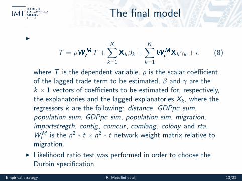
where T is the dependent variable, ρ is the scalar coefficientof the lagged trade term to be estimated, β and γ are thek × 1 vectors of coefficients to be estimated for, respectively,the explanatories and the lagged explanatories Xk , where theregressors k are the following: distance, GDPpc sum,population sum, GDPpc sim, population sim, migration,importstregth, contig , comcur , comlang , colony and rta.WM

t is the n2 ∗ t × n2 ∗ t network weight matrix relative tomigration.

I Likelihood ratio test was performed in order to choose theDurbin specification.


Elhorst flow chart

The relation netween different spatial auroregressive models


A discussant of myself

1. Why do you used Durbin Model (SDM)?

i) We want to explicitly take into account for the indirect effects.

ii) Elhorst (2010) argues that the SDM is the only model that providesunbiased parameter estimates and correct standard errors, even if the truedata-generation process is any of the other spatial regression modelsmentioned above.

2. Why you did not consider zero flows?

Zero flows are a consistent part of the dataset, however, we have tochoose between two curches: Estimation approach for the zero flows thatare accounting for indirect effects with spatial econometric approach arenot existing so far.

I spoke with T. Scherngell (AIT) that in 2009 tries (with M.Fischer) toimplement a estimation procedure to consider both indirect effect andzero flows, but the contra were more than the pro (i.e. the estimator wasbiased).

3. Why we use Migratt−1 to instrument Migratt ?

Who Know? I don’t believe this make much sense

Suggestions are very welcomed


Results

Non instrumented base total trade diff. goods homog. goodsols ols fe ols fe ols fe

migration .129***.128***.133***.140***.109***.113***R2 adj .639 .639 .752 .629 .820 .604 .716obs 29784 24105 27217 20908 23467 22256 24813

total diff. homog.trade goods goods

Correlation between Tradet and Migrationt 0.35 0.37 0.29Correlation between Tradet and Migrationt−1 0.28 0.29 0.22First stage test for the validity of the instrument >37.75>37.75>37.75Durbin-Wu-Hausman for the endogeneity in the model 14.16 4.70 12.77

Instrumented total trade diff. goods homog. goodsols fe ols fe ols fe

migration .088***.121***.109***.135***.070***.105***R2 adj .636 .746 .608 .806 .589 .707obs 17448 18551 15261 16124 16211 17039

Results R. Metulini et al. 16/22

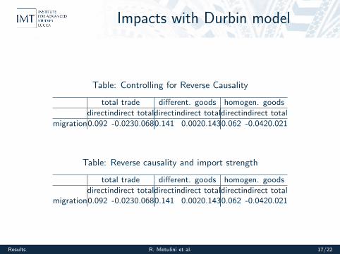
Impacts with Durbin model

Table: Controlling for Reverse Causality

total trade different. goods homogen. goods

directindirect totaldirectindirect totaldirectindirect total

migration0.092 -0.0230.0680.141 0.0020.1430.062 -0.0420.021

Table: Reverse causality and import strength

total trade different. goods homogen. goods

directindirect totaldirectindirect totaldirectindirect totalmigration0.092 -0.0230.0680.141 0.0020.1430.062 -0.0420.021


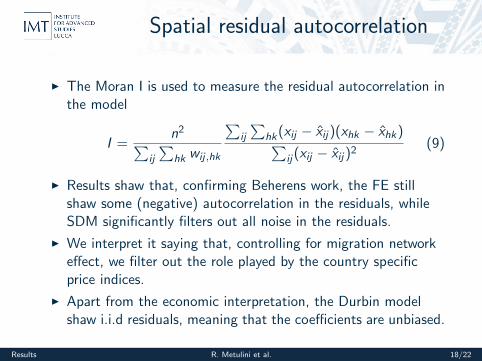
Spatial residual autocorrelation

I The Moran I is used to measure the residual autocorrelation inthe model

I =n2∑

ij

∑hk wij ,hk

∑ij

∑hk(xij − x̂ij)(xhk − x̂hk)∑

ij(xij − x̂ij)2(9)

I Results shaw that, confirming Beherens work, the FE stillshaw some (negative) autocorrelation in the residuals, whileSDM significantly filters out all noise in the residuals.

I We interpret it saying that, controlling for migration networkeffect, we filter out the role played by the country specificprice indices.

I Apart from the economic interpretation, the Durbin modelshaw i.i.d residuals, meaning that the coefficients are unbiased.


Network residual autocorrelation

Table: Moran I test for autocorrelation on the residuals of the gravitymodel estimated by OLS (colums ii. and iii.), FE (columns iv. and v.)and SDM (columns vi. and vii.)

OLS FE SDM15 near.neigh. Migration 15 near.neigh. Migration 15 near.neigh. Migration

matrix contiguity network contiguity network contiguity networktotal 0.078 0.077 -0.011 - 0.008 -0.000 0.001z-score (p-val) 29.21(0.000) 28.01 (0.000) -4.40 (0.000) -3.49 (0.000) -1.05 (0.144) 0.139 (0.444)differentiated 0.087 0.081 -0.010 -0.009 0.001 -0.012z-score (p-val) 28.14 (0.000) 25.44 (0.000) -3.83 (0.000) -3.43 (0.000) 1.152 (0.123) -2.297 (0.011)homogeneous 0.075 0.081 -0.012 -0.011 -0.001 0.001z-score (p-val) 26.07 (0.000) 27.31 (0.000) -4.87 (0.000) -4.16 (0.000)-1.209 (0.116) 0.299 (0.381)


Results

I Accounting for import strength of the destination country, theeffect of migration for the differentiated goods is signicantlyhigher than for homogeneous goods (0.143 versus 0.021)using spatial econometric approach, as already stressed in theliterature using different approaches.

I The migration indirect effect is positive for differentiatedgoods, and negative for homogeneous. Maybe thesecoefficients are the sum of two effects, one of competitionbetween neighbors (negative) and one of positive networkspillover. The negative one is stronger for homogeneousgoods, while the positive is stronger for differentiated. Infact,differentiated are more difficult to substitute for, so that theysuffer less competition from third countries.

I Using Durbin model, we filter out the residual autocorrelationI Apart from the economic interpretation, the Durbin model

shaw i.i.d residuals, meaning that the coefficients are unbiased.Conclusion R. Metulini et al. 20/22

Future developments

I To accomodate for more networks, by mean more than oneweight matrix togheter

I To disentagle the migration effect by migrant tipologies

I To find a better instruments for the reverse causality ofmigration

I To switch to Virtual Water trade (VWT) and to accomodatespat.econometric and network techniques in the analysis ofthe relation between VWT and migration.

Conclusion R. Metulini et al. 21/22

Thanks

Thank you for your attention

[email protected]

Conclusion R. Metulini et al. 22/22

The migration network effect on international trade

Documents

Transcript of The migration network effect on international trade