E

Ba

b

Gc

Rd

e

a

A

P

K

A

E

F

S

1

Et1H1U1pedpsi

0d

e c o l o g i c a l m o d e l l i n g 2 0 8 ( 2 0 0 7 ) 49–55

avai lab le at www.sc iencedi rec t .com

journa l homepage: www.e lsev ier .com/ locate /eco lmodel

cological network analysis: network construction

rian D. Fatha,∗, Ursula M. Scharlerb,c, Robert E. Ulanowiczd, Bruce Hannone

Biology Department, Towson University, Towson, MD 21252, USASchool of Biological and Conservation Sciences, University of KwaZulu-Natal, Howard College Campus,eorge Campbell Building, 4041 Durban, South AfricaDepartment of Aquatic Ecology and Water Quality Management (AEW), Wageningen University and Research Centre,itzema Bosweg 32-A, 6703 AZ Wageningen, The NetherlandsChesapeake Biological Laboratory, University of Maryland, Solomons, MD 20688, USADepartment of Geography, University of Illinois, Urbana, IL 61801, USA

r t i c l e i n f o

rticle history:

Accepted 27 April 2007

ublished on line 18 June 2007

eywords:

scendency

cological network analysis

a b s t r a c t

Ecological network analysis (ENA) is a systems-oriented methodology to analyze within

system interactions used to identify holistic properties that are otherwise not evident from

the direct observations. Like any analysis technique, the accuracy of the results is as good

as the data available, but the additional challenge is that the data need to characterize

an entire ecosystem’s flows and storages. Thus, data requirements are substantial. As a

result, there have, in fact, not been a significant number of network models constructed

and development of the network analysis methodology has progressed largely within the

ood webs

ystems analysis

purview of a few established models. In this paper, we outline the steps for one approach

to construct network models. Lastly, we also provide a brief overview of the algorithmic

methods used to construct food web typologies when empirical data are not available. It

is our aim that such an effort aids other researchers to consider the construction of such

coura

ENA, on the other hand, is capable of analyzing the structural

models as well as en

. Introduction

cological network analysis (ENA) is a methodology to holis-ically analyze environmental interactions (see e.g., Hannon,973, 1985a,b, 1986, 1991, 2001; Hannon et al., 1986, 1991;annon and Joiris, 1989; Finn, 1976; Patten, 1978, 1981,982, 1985; Higashi and Patten, 1989; Fath and Patten, 1999;lanowicz, 1980, 1983, 1986, 1997, 2004; Ulanowicz and Kemp,979). As such, it is necessary that the network model be aartition of the environment being studied, i.e., be mutuallyxclusive and exhaustive. The latter criterion in particular isifficult to realize and most models such as Lotka–Volterra

redator–prey or competition models represent only a smallubset of the interactions occurring in the ecosystem, exclud-ng both the majority of other species in the community and

∗ Corresponding author. Tel.: +1 410 704 2535; fax: +1 410 704 2405.E-mail address: bfath@towson.edu (B.D. Fath).

304-3800/$ – see front matter © 2007 Elsevier B.V. All rights reserved.oi:10.1016/j.ecolmodel.2007.04.029

ges further refinement of this procedure.

© 2007 Elsevier B.V. All rights reserved.

all abiotic processes. As a result of this limited perspective, itis impossible for such approaches to quantify the wholenessand consequent indirectness in the system, but this hasbeen the trend of reductionist science for over a century. Thereductionistic approach results in a self-fulfilling realizationin that only the few species or processes in the model haveinfluence and significance in the final interpretation, withoutconsidering the embedded nature of these activities withinthe larger ecological context. Ecosystems comprise a rich webof many interactions and it would be remiss to exclude, a pri-ori, most of them or to rely on analysis techniques that do so.

and functional properties of this web of interactions withoutreducing the model to its presumed minimal constituents.Therefore, network models aim to include all ecological com-

l i n g

50 e c o l o g i c a l m o d e l

partments and interactions and the analysis determines theoverall relationships and significance of each. The difficultyof course lies in obtaining the data necessary to quantify allthe ecological compartments and interactions. When suffi-cient data sets are not available, simple algorithms, calledcommunity assembly rules, have been employed to constructrealistic food webs to test various food web theories. Oncethe network is constructed, via data or algorithms, the ENA isquite straightforward and software is available to assist in this(Allesina and Bondavalli, 2004; Fath and Borrett, 2006). Thispaper outlines a possible scenario for developing networkmodels.

2. Data requirements and acquisition fordeveloping network models

A network flow model is essentially an ecological food web(energy–matter flow of who eats whom), which also includesnon-feeding pathways such as dissipative export out of thesystem and pathways to detritus. The first step is to iden-tify the system of interest and place a boundary (real orconceptual) around it. Energy–matter transfers within the sys-tem boundary comprise the network; transfers crossing theboundary are either input or output to the network, andall transactions starting and ending outside the boundarywithout crossing it are external to the system and are not con-sidered. Once the system boundary has been established, itis necessary to compartmentalize the system into the majorgroupings. The most aggregated model would have three com-partments: producers, decomposers/detritus, and consumers;a slightly more disaggregated model could have producers,herbivores, carnivores, omnivores, decomposers, and detri-tivores (Fath, 2004); and the most disaggregated a differentcompartment for each species. Most models use some aggre-gation based on the functional groups of the ecosystem suchthat network models in the literature typically have between6 and 60 compartments. However, this does not completelyresolve the aggregation issue. It is likely that one is interestedin greater detail for one group, but it is not entirely clear howdisaggregation of one functional group and not others affectsthe analysis results. Identifying the major species or func-tional groups should be done by those knowledgeable aboutthe system.

Once the compartments have been chosen, anenergy–matter flow currency must be selected. Typically,the currency is biomass (e.g., grams of carbon) or energy (e.g.,kilojoules) per area for terrestrial and aquatic ecosystems orvolume for aquatic ecosystems per time. The flow dimen-sions then would be ML−2T−1 or ML−3T−1 where M = mass,L = length, and T = time. There is flexibility however in thebiomass units chosen, which could also be grams of nitro-gen, phosphorus, other nutrients, or even water per spacedimension per time. Multiple currency network models usinga combination of C, N, or P, etc. can also be constructed(Ulanowicz and Baird, 1999). In addition to the input, output,

and within systems flow transfer values, it is also necessaryto measure empirically as best as possible the mass density(biomass/area) of each compartment. Storage dimensions areML−2 or ML−3, since they are not rates. Together the transfers

2 0 8 ( 2 0 0 7 ) 49–55

and storages comprise the data requirements for ecologicalnetwork analysis.

Once the currency has been chosen, we would arrangethem in the columns and rows of an adjacency matrix todetermine whether or not a resource flow of that currencyoccurs from each compartment to each other one. An adja-cency matrix, A, is a representation of the graph structuresuch that aij = 1 if there is a flow from j to i, else aij = 0,using a column to rows orientation (note that although weuse a column to row orientation here, a row to columnorientation is also used in the literature). This procedureforces one to ascertain the possible connectivity of eachpair of compartments in the network, thus reducing thechances of over-looking certain connections. This exercisemight also illuminate compartments that were excluded ini-tially, thereby providing an iterative feedback in the networkdevelopment.

The data required for ecological network analysis are asfollows: For each compartment in the network, the biomassand physiological parameters, such as consumption (C), pro-duction (P), respiration (R) and egestion (E) must be quantified.It is possible to lump respiration and egestion into one outflowif necessary. Furthermore, the diet of each compartment mustbe apportioned amongst the inputs from other compartments(consumption) in the network. This apportionment of “whoeats whom and by how much” can be depicted in a dietarymatrix, where material flows from compartment j to compart-ment i. For all compartments, inputs should balance outputs(C = P + R + E), in accordance with the conservation of matterand the laws of thermodynamics.

To quantify the network, flows of the chosen currency intoand out of each compartment should be determined. Someof the flows could also be empirically gathered from primaryfield research regarding primary production, respiration, andfeeding, but others could be assembled from various sourcessuch as literature sources and simulation model results. Fur-thermore, two recently developed methods of assigning a flowvalue between compartments can be employed to estimatetransfers (Ulanowicz and Scharler, in preparation). The firstmethod, MATBLD, assigns the transfers according to the jointproportion of predator demand and prey availability. The sec-ond method, MATLOD, begins with assigning a very small flowto all designated links and keeps on doing so until either thedemand is met or the source exhausted. The input data forboth methods are the biomasses, consumption, production,respiration, egestion, imports and exports of all compart-ments, and the topology of the networks (i.e., who eats whom).The networks originating from both methods are balancedusing the algorithm developed by Allesina and Bondavalli(2003). A comparison of the two methods to networks con-structed “by hand” revealed no statistical difference betweenthe magnitudes of the compartmental transfers.

In most cases, field data, literature sources, or results fromsimulation models do not supply all the system-specific datanecessary for the network construction. In those cases, it isrecommended to perform a sensitivity analysis to assess a

variation of the most inaccurate input data on network anal-ysis results.

Table 1 provides a step-by-step procedure for constructingecological networks.

e c o l o g i c a l m o d e l l i n g

Table 1 – Check list for constructing ecological networks

1. Identify and demarcate ecosystem of interest2. Make a list of the major species or functional groups in

ecosystem3. Select a unit of currency for the network4. Construct the adjacency matrix to determine any possible flow

interactions. Use this procedure to identify any possible holesin the initial classification

5. Empirically measure mass density of each compartment6. Empirically measure input, output, and throughflows between

compartments when possible7. Use additional literature and models to quantify network flows

not empirically determined8. Employ flow-balancing algorithm to finalize flow matrix and

3

TwcBftozridvatbl

1

2

storage, input, and outputs vectors9. Apply ecological network analysis to network10. Sensitivity analysis

. Belize example

he following example illustrates the steps involved in net-ork construction. The study ecosystem is a mangrove island

alled Twin Cays, situated in the Caribbean Sea, offshoreelize. The island features a tree height gradient from theringe (tall trees) to the interior of the island (small trees). Theree height gradient has been attributed to nutrient limitationsf Nitrogen (fringe zone), nitrogen + phosphorus (transitionone) and phosphorus (dwarf zone) (Feller et al., 2003). Theole of the network analysis was to provide system-specificnformation on the ecosystem structure and function of theifferent zones, and on the nutrient limitations of the indi-idual compartments of the zones. This project was part ofNSF Biocomplexity project, comprising 10 research groups

hat spent part of their effort on gathering information foruilding the networks. The steps of the network construction

isted here conform to those in Table 1:

. The ecosystems are the three zones on the island (fringe,transition, dwarf). The boundaries of the ecosystems aredemarcated by the tree height gradient. The boundary tothe sea is the mangrove prop roots hanging into the sea.Interior ponds marked the interior boundary of the dwarfzone.

. The three zones have a different number of compartments,since not all species occur within all zones. The patternof aggregation was the same over all three zones andflow currencies, except for the inorganic dissolved nutri-ents. The number of compartments ranges between 70and 90. Some compartments comprise a single speciesonly (e.g., mangrove trees), whereas others are taxonomicgroups (e.g., lichen, bacteria, fungi, various macrozooben-thos groups) or functional groups (e.g., bird feeding guilds).Species, for which no information on density was avail-able, were omitted from the networks. In most cases, thesewere species either living outside the ecosystem boundary

and deriving part of their diet from within the ecosystem(e.g., fish), or they live within the ecosystem boundary andderive all their diet from outside the ecosystem bound-ary as an import (e.g., some of the submerged prop rootfauna).

2 0 8 ( 2 0 0 7 ) 49–55 51

3. In all three zones, networks were constructed for threedifferent flow currencies (carbon, nitrogen, phosphorus).The biomasses were expressed as gC/N/P m−2, and allflows (consumption, production, respiration, egestion,imports, exports, and intercompartmental transfers) asgC/N/P m−2 y−1. Fluxes were reported on a yearly basis,since season-specific information was available only for arelatively small proportion of the data.

4. All possible flow interactions between all compartmentswere determined using information from field data, systemand non-system-specific literature, system-specific C andN isotope data and knowledge of people familiar with thearea.

5. System-specific biomass was empirically measured for allcompartments except for five (heterotrophic microfaunaand fungi from four different habitats). These were judgedtoo important to omit. Here, the biomass of other man-grove ecosystems or other habitats from the island wasused. The carbon networks were constructed first, since inmost cases, there is more information available on carbonthan on other nutrients. Empirically measured C/N ratiosfor all compartments were available from the island. Totalphosphorus was measured for some compartments, andinferred for others. Criteria were organism size, taxonomyand feeding guild.

6. Several of the flows in and out of the compartments weremeasured on site, e.g., for the tree species, macroalgae, andmicrobial mats.

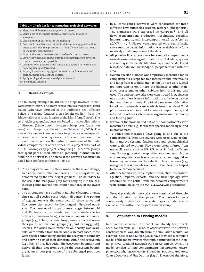
7. To derive non-measured flows going in and out of thecompartments, literature sources were used. Data of sim-ilar mangrove systems (habitat wise and geographically)were preferred to others. Flows were often inferred frommetabolic ratios, such as P/B, P/R, or assimilation efficien-cies. To assign certain respiration rates or assimilationefficiencies, criteria such as organism size, feeding guild, ortaxonomy were used in the selection. In some cases (e.g.,mangrove trees), models available in the literature helpedto derive carbon balances.

8. After the biomasses, consumption, production, respiration,egestion, imports, exports, and the flow topology weredetermined, the actual transfers between compartmentswere estimated using the MATBLD/MATLOD procedures.

Several placeholder networks were constructed through-out the duration of the project. The networks werecontinuously updated as more system-specific data becameavailable from within the project research group.

4. Application to existing models

In situations in which the model has already been devel-oped, for example, in STELLA or other software, the networkconstruction follows directly from the simulation results. Forexample, Spieles and Mitsch (2003) have provided a completemodel of the macroinvertebrate trophic structure for the Olen-

tangy River Wetland Research Park in Columbus, Ohio. Themodel consists of nine compartments: Metaphyton, Macro-phytes, Periphyton, Collectors, Shredders, Scrapers, Predators,Coarse Detritus and Fine Detritus (Fig. 1). The model, therefore,

52 e c o l o g i c a l m o d e l l i n g 2 0 8 ( 2 0 0 7 ) 49–55

STE

0 0 00 0 00 0 00 0 0.0280 0.005 00 0 00 0 0

4.94E − 6 0 00 220.00 0

⎤⎥⎥⎥⎥⎥⎥⎥⎥⎥⎥⎥⎦

,

therefore are mostly unsuitable for a full network analysiswhich is most revealing when the entire ecological networkpathways are captured.

Fig. 1 – Trophic model of Olentangy Wetland in

contains all the flow and storage connections needed for thenetwork analysis matrices. These values can be taken directlyfrom the simulation results, which in STELLA are available intabular form ready for input to Excel. This particular modelhas a seasonal forcing function, and reaches a dynamic steadystate by the end of the first year. Once the steady state isreached, one can use the average of any 1-year period as repre-sentative of the model values to create the flow, storage, inputand output network data. For this model, the following dataare obtained:

F =

⎡⎢⎢⎢⎢⎢⎢⎢⎢⎢⎢⎢⎣

0 0 0 0 0 00 0 0 0 0 00 0 0 0 0 0

0.028 0 0 0 0 00 0.010 0 0 0 00 0 0.005 0 0 00 0 0 2.34E − 7 5.54E − 7 8.97E − 100 219.99 0 0.007 0.002 0.003

34.97 0 9.995 0 0 0

x = [ 349.6751 2199.896 99.95435 0.0732 0.01718 0.0304 4.12

z = [ 34.9955 220 10 0 0 0 2.47E − 5 0 55 ]T

y = [ 0 0

LLA (recreated from Spieles and Mitsch, 2003).

In this manner, any simulation model has the necessaryinformation for network construction. The obstacle is thatmany simulation models only represent a portion of the over-all ecosystem network, such as a predator–prey relation, and

E − 5 366.6695 533.2744 ],

0 0.0490 0.0137 0.00152 2.06E − 5 0 319.9647 ]

n g

5

OfeiCrTtswtutpaimtatfasmdn(BEfpb

wIecstfatPtnifrR

6

Oern

e c o l o g i c a l m o d e l l i

. Additional methods

ther approaches have been used to construct flow networksrom ecological data. In particular, the efforts by , (1992; Paulyt al., 2000) in developing Ecopath have gained wide usagen fisheries. Activity is centered at the University of Britisholumbia’s Fishery Centre, but Ecopath has more than 2000egistered users in over 120 countries (see www.ecopath.org).he following description of Ecopath is based on informa-

ion found at their Web site. Ecopath is publicly availableoftware to construct and analyze mass-balanced flow net-orks. The ecosystem interactions in the networks represent

rophic links at the species or functional level. It allowssers to input known data regarding their ecosystem such asotal mortality estimates, consumption estimates, diet com-ositions, and fishery catchers, however, data requirementsre kept to a minimum because databases and balanc-ng procedures are used to fill in missing aspects. The

odel employs two main equations, one regarding produc-ion (production = catch + predation + net migration + biomassccumulation + other mortality) and the other consump-ion (consumption = production + respiration + unassimilatedood). In addition to examining the models using networknalysis, Ecopath highlights the benefits from the model con-truction process in bringing together scientists, governmentanagers, and public interest groups in collaborative, inter-

isciplinary team building exercise. To date, many differentetwork models have been constructed using this approach

e.g., Okey and Pauly, 1999; Pauly et al., 1998; Haggan andeattie, 1999). Recently, a dynamic time simulation module,cosim, has been added, which further benefits applicationsor environmental management. Ecopath provides a goodlatform for introducing network flow models to new usersy removing many of the technical barriers.

Another approach for constructing ecological flow net-orks has been inverse modelling (Vezina and Platt, 1988).

n this approach, a structural food web is constructed for thecosystem based on available feeding and flow patterns. Theompartmental biomasses are assumed to be at steady stateuch that the total flows entering a compartment are equal tohe total amount exiting it. The flows are then back calculatedor this particular structure using mass balance equationsnd basic biological constraints. Recent work has looked athe limitations of the steady-state assumption (Vezina andahlow, 2003) on inverse modelling as well as modificationso relax it (Richardson et al., 2003). This approach, althoughot as well known as Ecopath, has been employed in many

nstances. A recent citation index search revealed 41 citationsor the original Vezina and Platt (1988) article, including manyecent citations (e.g., Breed et al., 2004; Leguerrier et al., 2004;ichardson et al., 2004; Savenkoff et al., 2004).

. Community assembly rules

ne approach that has been used to account for the lack ofmpirically derived data is the development of simple algo-ithms to construct hypothetical, but ecologically realisticetworks. However, there have been two distinct approaches

2 0 8 ( 2 0 0 7 ) 49–55 53

marked by the initial assumptions one makes. The first group,based on population/community ecology, focuses strictly on“who eats whom”, producing structures involving primaryproducers, grazers, and predators, but explicitly lacks decom-posers and detritus. As a result, these networks do nottypically contain cycling. The two main algorithms in this cat-egory are the cascade model (Cohen and Newman, 1985) andniche model (Williams and Martinez, 2000). The second group,based on ecosystem ecology focuses on energy flow in the sys-tem and includes all functional groups including detritus anddecomposers. The algorithms here are a modified niche model(Halnes et al., 2007), a cyber-ecosystem model (Fath, 2004),and structured food webs of realistic trophic relationshipswith transfer coefficients drawn from uniform and lognor-mal distributions (Morris et al., 2005). In the cyber-ecosystemapproach, Fath (2004) used a meta-structure with six classifi-cations – (1) primary producers, (2) herbivores, (3) omnivores,(4) carnivores, (5) detrital feeders, and (6) detritus – and linkedeach class based on known ecological relationships, such thatgrazers can feed only on primary producers, omnivores canfeed on primary producers, carnivores, detrital feeders, andother omnivores, etc.; all compartments deposit into detritus;and detrital feeders feed on detritus. Resulting in the followinggeneralized adjacency matrix:

A =

⎡⎢⎢⎢⎢⎢⎣

0 0 0 0 0 01 0 0 0 0 01 1 1 1 1 00 1 1 1 1 00 0 0 0 0 11 1 1 1 1 1

⎤⎥⎥⎥⎥⎥⎦

(1)

The matrix size is expandable, since the algorithm allowsfor the selection of any number of each of the six classifi-cations while retaining the generalized connectance pattern.The number and placement of connections between individ-ual nodes in targeted classifications (such as from primaryproducers to grazers) are randomly assigned. Note also that inthe constructed matrices cannibalism (aii = 1) was not allowedalthough it is shown in the generalized structure. This classifi-cation as currently defined guarantees that cycling will occursince energy must pass out of each compartment and intodetritus, some of which is taken up by detrital feeders. Thespectral radius of Eq. (1), as given by the maximum eigenvalueof A, �max = 2.62, whereas without the diagonal �max = 1.94.This value gives an indication of the cyclic pathways inherentin the structure.

The cyber-ecosystem algorithm was used initially to cre-ate large-scale networks with 600 compartments (100 of eachclassification) to test the values of certain network properties.A structural measure of the network is connectance, the ratioof number of links (L) to total possible number of connections(n2). The average connectance for the 600 compartment net-works was around 0.18. Fath and Killian (2007) have lookedat other combinations with different number of nodes withineach classification such as at a classic ecological numberspyramid in which there are the largest amount of primary pro-

ducers and subsequently less at each higher level and inversepyramids as well as a uniform distribution.

The inclusion of six classifications although attempting torepresent known ecological categories may be more compli-

l i n g

r

54 e c o l o g i c a l m o d e l

cated than necessary. For example, another approach couldsimply have three broad classifications – (1) producers, (2)consumers, and (3) decomposers – in which they would beconnected as follows:

A =

⎡⎣

0 0 11 0 01 1 0

⎤⎦ (2)

This matrix, called within ENA the Hill-matrix after JimHill who extensively explored its properties in his thesis (Hill,1981), is the minimum model that has the requisite complex-ity to represent ecological interactions. We note that even thissimple network has structural cycling �max = 1.32. The canon-ical Hill-matrix gives insight into the complex path structureof fundamental networks. Nonetheless, the strength of ENAis to analyze indirectness; therefore, the goal is to represent afuller richness of ecological diversity with networks of largerscale.

The networks generated by Morris et al. (2005) served thepurpose of assessing (1) the effects of using different assump-tions to construct the webs, and (2) the information theoreticalindices of ascendency, development capacity, flow diversityand average mutual information to variations in web size andfunction. Results from the hypothetical webs were comparedto empirical webs. The generated networks ranged from 7 to2200 taxa and ranged from sparsely to densely connected.They are all donor-controlled food webs (i.e., flow was pro-portional to biomass of donor compartment) with a set GPPof 1000 kcal m−2 and a set import of allochthonous material of100 m−2 y−1 to facilitate the comparisons of the networks. Thecoefficients for the transfer matrix were drawn from realisticprobability sets that randomly partitioned exogenous inputsamong all primary producers.

Four kinds of networks were produced which differed inthe rules concerning the network connections. Two of these,the structured food webs were generated with taxa belong-ing to groups such as primary producers, primary, secondary,and tertiary consumers, detritivores and detritus. The num-ber of taxa in each group was determined randomly. Flowsbetween taxa were divided into mandatory (e.g., all taxa todetritus), mandatory from lower to higher trophic levels andnonobligatory flows between taxa. Respiration rates were cho-sen according to ranges reported in the literature. Transfercoefficients representing the energy flow between taxa weredrawn either from lognormal or uniform distributions.

Community assembly rules have helped provide a meansto generate realistic food web structures, when data werenot available but they should not replace empirically basedecosystem networks. The point of this paper is to provide guid-ance for constructing such empirical networks so that futurework can focus more on actual ecosystems rather than algo-rithmically assembled ones.

7. Conclusions

Ecological network analysis is an important tool to understandwhole-system interactions, and the lack of quantified networkmodels, and the difficulty in constructing them is one of the

2 0 8 ( 2 0 0 7 ) 49–55

main impediments to further application of this methodology.There is no one correct way to construct a network model, buthere we try to offer some assistance for doing so, which hope-fully will increase the number of networks that are developed.Having network construction guidelines will provide someconsistency in both the procedure and product making it eas-ier to compare and contrast various ecological networks. Thisis only a first step and we expect that the more experiencethat is gained with constructing networks the more refinedthe procedure will become.

Acknowledgements

The outline for this manuscript was developed during work-shop on Network Analysis organized by David Gattie at theUniversity of Georgia in March 2005. The STELLA model wasreconstructed by students in BDF’s Ecosystem Ecology course:Pat Brady, Melissa Cameron, Jeremiah Freeman, and ErolMiller. Special thanks to Jeremiah Freeman for providing thesteady-state network data from the model.

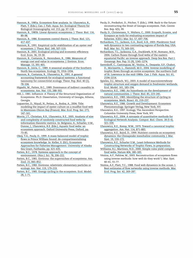
e f e r e n c e s

Allesina, S., Bondavalli, C., 2003. Steady state of ecosystem flownetworks: a comparison between balancing procedures. Ecol.Model. 165, 221–229.

Allesina, S., Bondavalli, C., 2004. WAND: an ecologicalnetwork analysis user-friendly tool. Environ. Model Soft. 19,337–340.

Breed, G.A., Jackson, G.A., Richardson, T.L., 2004. Sedimentation,carbon export and food web structure in the Mississippi Riverplume described by inverse analysis. Mar. Ecol. Prog. Ser. 278,35–51.

Christensen, V., Pauly, D., 1992. ECOPATH II – a software forbalancing steady-state ecosystem models and calculatingnetwork characteristics. Ecol. Model. 61, 169–185.

Cohen, J.E., Newman, C.M., 1985. A stochastic theory ofcommunity food webs. I. Models and aggregated data. Proc. R.Soc. Lond. Ser. B 224, 421–448.

Fath, B.D., 2004. Network analysis applied to large-scalecyber-ecosystems. Ecol. Model. 171, 329–337.

Fath, B.D., Borrett, S.R., 2006. A Matlab® Function for NetworkEnviron Analysis. Env. Model. Soft. 21, 375–405.

Fath, B.D., Killian, M., 2007. The relevance of ecological pyramidsin community assemblages. Ecol. Model.,doi:10.1016/j.ecolmodel.2007.06.001, this issue.

Fath, B.D., Patten, B.C., 1999. Review of the foundations ofnetwork environ analysis. Ecosystems 2, 167–179.

Feller, I.C., McKee, K.L., Whigham, D.F., O’Neill, J.P., 2003. Nitrogenvs. phosphorus limitation across an ecotonal gradient in amangrove forest. Biogeochemistry 62, 145–175.

Finn, J.T., 1976. Measures of ecosystem structure and functionderived from analysis of flows. J. Theor. Biol. 56,363–380.

Haggan, N., Beattie, A. (Eds.), 1999. Back to the future:reconstructing the Hecate Strait ecosystem. Fish. Centre Res.Rep. 7(3), 65.

Halnes, G., Fath, B.D., Liljenstrom, H., 2007. The modified nichemodel: including detritus in simple structural food webmodels. Ecol. Model. 208, 9–16.

Hannon, B., 1973. The structure of ecosystems. J. Theor. Biol. 41,535–546.

n g

H

H

H

H

H

H

H

H

H

H

L

M

O

P

P

P

P

using inverse methods: how well do they work? J. Mar. Syst.

e c o l o g i c a l m o d e l l i

annon, B., 1985a. Ecosystem flow analysis. In: Ulanowicz, R.,Platt, T. (Eds.), Can. J. Fish. Aqua. Sci. Ecological Theory forBiological Oceanography, vol. 213, pp. 97–118.

annon, B., 1985b. Linear dynamic ecosystems. J. Theor. Biol. 116,89–98.

annon, B., 1986. Ecosystem control theory. J. Theor. Biol. 121,417–437.

annon, B., 1991. Empirical cyclic stabilization of an oyster reefecosystem. J. Theor. Biol. 149, 507–519.

annon, B., 2001. Ecological pricing and economic efficiency.Ecol. Econ. 36, 19–30.

annon, B., Costanza, R., Herendeen, R., 1986. Measures ofenergy cost and value in ecosystems. J. Environ. Econ.Manage. 13, 391–401.

annon, B., Joiris, C., 1989. A seasonal analysis of the SouthernNorth Sea ecosystem. Ecology 70, 1916–1934.

annon, B., Costanza, R., Ulanowicz, R., 1991. A generalaccounting framework for ecological systems: a functionaltaxonomy for connectivist ecology. Theor. Pop. Biol. 40 (1),78–104.

igashi, M., Patten, B.C., 1989. Dominance of indirect causality inecosystems. Am. Nat. 133, 288–302.

ill, J., 1981. Influence: A Theory of the Structural Organization ofEcosystems. Ph.D. Dissertation, University of Georgia, Athens,Georgia.

eguerrier, D., Niquil, N., Petiau, A., Bodoy, A., 2004. Title:modeling the impact of oyster culture on a mudflat food webin Marennes-Oleron Bay (France). Mar. Ecol. Prog. Ser. 273,147–161.

orris, J.T., Christian, R.R., Ulanowicz, R.E., 2005. Analysis of sizeand complexity of randomly constructed food webs byinformation theoretic metrics. In: Belgrano, A., Scharler, U.M.,Dunne, J., Ulanowicz, R.E. (Eds.), Aquatic food webs: anecosystem approach. Oxford University Press, Oxford, pp.73–85.

key, T.A., Pauly, D., 1999. A mass-balanced model of trophicflows in Prince William Sound: de-compartmentalizingecosystem knowledge. In: Keller, S. (Ed.), EcosystemApproaches for Fisheries Management. University of AlaskaSea Grant, Fairbanks, pp. 621–635.

atten, B.C., 1978. Systems approach to the concept ofenvironment. Ohio J. Sci. 78, 206–222.

atten, B.C., 1981. Environs: the superniches of ecosystems. Am.

Zool. 21, 845–852.

atten, B.C., 1982. Environs: relativistic elementary particles orecology. Am. Nat. 119, 179–219.

atten, B.C., 1985. Energy cycling in the ecosystem. Ecol. Model.28, 1–71.

2 0 8 ( 2 0 0 7 ) 49–55 55

Pauly, D., Preikshot, D., Pitcher, T. (Eds.), 1998. Back to the future:reconstructing the Strait of Georgia ecosystem. Fish. CentreRes. Rep. 6(5), 99.

Pauly, D., Christensen, V., Walters, C., 2000. Ecopath, Ecosim, andEcospace as tools for evaluating ecosystem impact offisheries. ICES J. Mar. Sci. 57, 697–706.

Richardson, T.L., Jackson, G.A., Burd, A.B., 2003. Planktonic foodweb dynamics in two contrasting regions of florida Bay, USA.Bull. Mar. Sci. 73, 569–591.

Richardson, T.L., Jacksona, G.A., Ducklowb, H.W., Romanc, M.R.,2004. Carbon fluxes through food webs of the easternequatorial Pacific: an inverse approach. Deep Sea Res. Part I:Oceanogr. Res. Pap. 51 (9), 1245–1274.

Savenkoff, C., Castonguay, M., Vezina, A., Despatie, S.P., Chabot,D., Morissette, L., Hammill, M.O., 2004. Inverse modelling oftrophic flows through an entire ecosystem: the northern Gulfof St. Lawrence in the mid-1980s. Can. J. Fish. Aqua. Sci. 61,2194–2214.

Spieles, D.J., Mitsch, W.J., 2003. A model of macroinvertebratetrophic structure and oxygen demand in freshwater wetlands.Ecol. Model. 161, 183–194.

Ulanowicz, R.E., 1980. An hypothesis on the development ofnatural communities. J. Theor. Biol. 85, 223–245.

Ulanowicz, R.E., 1983. Identifying the structure of cycling inecosystems. Math. Biosci. 65, 219–237.

Ulanowicz, R.E., 1986. Growth and Development: EcosystemPhenomenology. Springer-Verlag, New York, NY.

Ulanowicz, R.E., 1997. Ecology, The Ascendent Perspective.Columbia University Press, New York, NY.

Ulanowicz, R.E., 2004. A synopsis of quantitative methods forEcological Network Analysis. Comput. Biol. Chem. 28 (5-6),321–339.

Ulanowicz, R.E., Kemp, W.M., 1979. Toward a canonical trophicaggregation. Am. Nat. 114, 871–883.

Ulanowicz, R.E., Baird, D., 1999. Nutrient controls on ecosystemdynamics: the Chesapeake mesohaline community. J. Mar.Syst. 19, 159–172.

Ulanowicz, R.E., Scharler U.M., Least-Inference Methods forConstructing Networks of Trophic Flows, in preparation.

Williams, R.J., Martinez, N.D., 2000. Simple rules yield complexfood webs. Nature 404, 180–183.

Vezina, A.F., Pahlow, M., 2003. Reconstruction of ecosystem flows

40–41, 55–77.Vezina, A.F., Platt, T.C., 1988. Food web dynamics in the ocean. I.

Best estimates of flow networks using inverse methods. Mar.Ecol. Prog. Ser. 42, 269–287.