Residue Network Construction and Predictions of Elastic Network Models

Running title: Construction of ENM

1

Residue Network Construction and Predictions of Elastic

Network Models

Canan Atilgan, Ibrahim Inanc, and Ali Rana Atilgan

Faculty of Engineering and Natural Sciences, Sabanci University, 34956 Istanbul, Turkey

e-mail: [email protected]

telephone: +90 (216) 4839523

telefax: +90 (216) 4839550

Keywords: elastic network models, cooperative motions, spectral dimension, fluctuations,

normal mode analysis.


2

ABSTRACT

The past decade has witnessed the development and success of coarse-grained network

models of proteins for predicting many equilibrium properties related to collective modes of

motion. Curiously, the results are usually robust towards the different methodologies used for

constructing the residue networks from knowledge of the experimental coordinates. We

present a systematical study of network construction strategies, and their effect on the

predicted properties. The analysis is based on the radial distribution function and the spectral

dimensions of a large set of proteins as well as a newly defined quantity, the angular

distribution function. By partitioning the interactions into an essential and a residual set, we

show that the robustness originates from a large number of long-distance interactions

belonging to the latter. These residuals have a vanishingly small effect on the force vectors on

each residue. The overall force balance then translates into the Hessian as small shifts in the

slow modes of motion and an invariance of the corresponding eigenvectors. Implications for

the study of biologically relevant properties of proteins are discussed.


3

INTRODUCTION

Globular proteins show diversified structures and sizes, yet, it has been claimed that they

display a nearly random packing of amino acids with strong local symmetry on the one hand

(1), and that they are regular structures that occupy specific lattice sites, on the other (2). It

was later shown that this classification depends on the property one investigates, and that

proteins display “small-world” properties, where highly ordered structures are altered with

few additional links (3). Furthermore, packing density of proteins scales uniformly with their

size (4, 5) which causes them to show similar vibrational spectral characteristics to those of

solids (6).

Dynamical studies of folded proteins draw much attention to their importance in relating the

structure of the proteins to their specific function and collective behavior. Protein dynamics is

generally both anisotropic and collective. Internal motional anisotropy is a consequence of the

general lack of symmetry in the local atomic environment, while the collectivity is mainly

caused by the dense packing of proteins (7).

Theoretical studies on fluctuations and collective motions of proteins are based on either

molecular dynamics (MD) simulations or normal mode analysis (NMA). Since, in molecular

simulations with conventional atomic models and potentials, computational effort is

demanding for larger proteins with more than a few hundreds of residues, coarse grained

protein models with simplified governing potentials have been employed, and these have

shown a great success in the description of the residue fluctuations and the collective behavior

of proteins (8).

One of these simplified models, NMA using a single parameter harmonic potential (9)

successfully predicts the large amplitude motions of proteins in the native state (10). Within

the framework of this model, proteins are modeled as elastic networks whose nodes are

residues linked by inter-residue potentials that stabilize the folded conformation. The residues

are assumed to undergo Gaussian-distributed fluctuations about their native positions. The

springs connecting each node to all other neighboring nodes are of equal strength, and only

the atom pairs within a cut-off distance are considered without making a distinction between

different types of residues. This model, with its simplicity, speed of calculation and relying

mostly on geometry and mass distribution of the protein, demonstrates that a single-parameter

model can reproduce complex vibrational properties of macromolecular systems. By

separating different components of normal modes, e.g collective (low-frequency) motions, the

nature of a conformational change, for example due to the binding of a ligand, can also be

analyzed thoroughly (11).

Following the uniform harmonic potential introduced originally by Tirion (12), residue level

application of elastic network models paved the way for the concept Gaussian Network Model

(GNM), which is based on the energy balance of the system at the energy minimum, and is a

purely thermodynamic treatment (10, 13). Elastic models based on the force balance around

each node (14) led to the development of the so called Anisotropic Network Model (ANM)

(15). In the past few years, variant methods of GNM and ANM (16, 17) have been introduced.

The applications of these models to many proteins show successful results in terms of

predicting the collective behavior of proteins. Despite numerous applications comparing the

theoretical and experimental findings on a case-by-case basis (18-22), only a few attempted a

statistical assessment of the models. A methodology that evaluates the number of modes

necessary to map a given conformational change from the degree of accuracy obtained by the

inclusion of a given number of modes, showed the results to be protein dependent (23). In

another study where 170 pairs of structures were systematically analysed, it was shown that

the success of coarse-grained elastic network models may be improved by recognizing the


4

rigidity of some residue clusters (24).

To date, the structures that form the basis of the network models have been generated from

certain rules of thumb. In GNM, which does not include directionality and is therefore a one-

dimensional model, the first correlation shell between the C or C atoms of the residues is

used as the rule for the connectedness of a given pair of residues (ca. 6.7 – 7.0 Å) (10). In the

three-dimensional ANM, values in the range of 8 – 14 Å are found in the literature based on

the argument that (i) the eigenvalue distributions obtained from the modal decomposition are

similar to those obtained from the full-atom NMA description of proteins, or (ii) these provide

atomic fluctuation profiles that display the largest correlation with the experimental B-factors.

Voronoi tessalation of the space defined by the central (usually C or C ) atom into non-

intersecting polyhedra constitute another route that frees one from defining a cut-off distance

(25). Atom-based network construction approaches have also been used [see reference (26)

for a review of the variety of network construction methods in literature.]

In this study, we use a systematic approach on a large set of globular proteins with varying

architectures and sizes to find a basis for why the network models work well to define certain

properties of the system. This enables us to assess the various residue-based approaches used

in the construction of the networks. We define a direction based radial distribution function

for this purpose, and show that the directionality of newly added links samples a spherically

symmetric collection of directions beyond a given distance of interacting residues. We show

that the network construction is free of the cut-off distance problem once a certain baseline

threshold is accessed, if one is interested in the collective motions and the fluctuation patterns

of the residues. Implications for the limitations of the ANM methodology are discussed due to

functionality-related predictions based on the most global motions.

COMPUTATIONAL DETAILS

Network construction. A protein of N residues is treated as a residue-based structure, where

the C atom of each amino acid is considered as a node, and the coordinates of the protein are

obtained from the protein data bank (PDB) (27). The network information is contained in the

N × N adjacency matrix, A, of inter-residue contacts, whose elements Aij are taken to be 1 for

contacting pairs of nodes i and j, and zero otherwise. We determine the presence of a contact

using two approaches, one involving a selected cut-off distance, and the other using Voronoi

tessellations. In the former approach, the criterion for contact is that the two nodes are within

a cut-off distance rc of each other. In the latter, Voronoi cells are formed from the PDB

coordinates of C atoms such that the three dimensional space is uniquely and completely

subdivided into polyhedra whose surfaces are defined by the intersection of contact planes

built midway between the nodes of the network. Thus, pairs of nodes sharing a common plane

are taken to be in contact. This methodology allows eliminating the choice of a cut-off

distance so that an unambiguous network construction is achieved (1, 28). We have utilized

the freely available Voro3D program for this purpose (25). Note that the nodes in these

networks have an average distance of 6.6 Å to their neighbors, and an average contact number

of 10.5.

Radial and angular distribution functions. The radial distribution function (RDF), g(r), is a

measure of the correlation between the locations of particles within a system, measured as the

probability of finding another particle at a distance, r, from a chosen particle, normalized by

the volume element. The RDF is a useful tool to describe the structure of a molecular system,

particularly those of liquids. In an ordered solid, RDF has an infinite number of sharp peaks

whose separations and heights are characteristic of the lattice structure. RDF can be deduced

experimentally from X-ray or neutron diffraction studies, thus providing a direct comparison


5

between experiment and simulation.

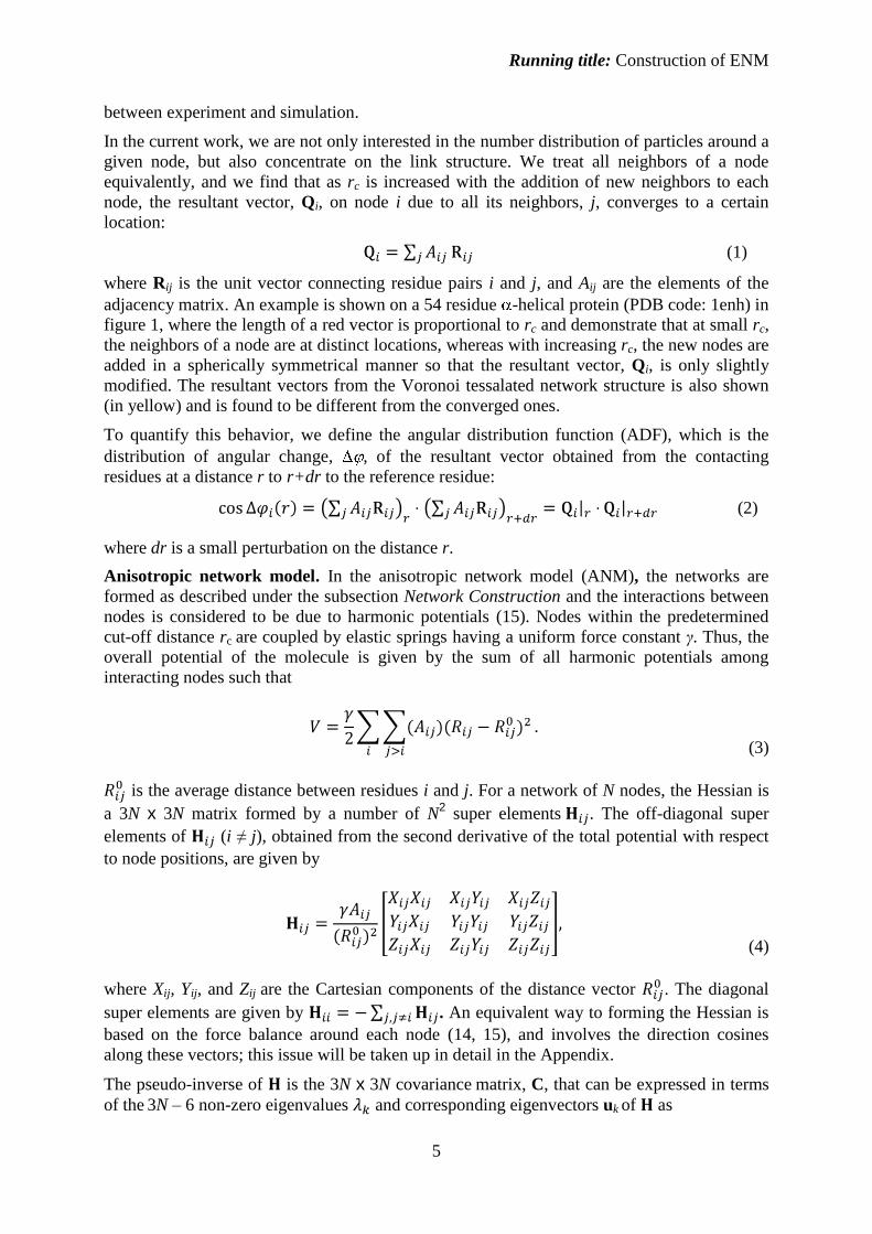
In the current work, we are not only interested in the number distribution of particles around a

given node, but also concentrate on the link structure. We treat all neighbors of a node

equivalently, and we find that as rc is increased with the addition of new neighbors to each

node, the resultant vector, Qi, on node i due to all its neighbors, j, converges to a certain

location:

(1)

where Rij is the unit vector connecting residue pairs i and j, and Aij are the elements of the

adjacency matrix. An example is shown on a 54 residue -helical protein (PDB code: 1enh) in

figure 1, where the length of a red vector is proportional to rc and demonstrate that at small rc,

the neighbors of a node are at distinct locations, whereas with increasing rc, the new nodes are

added in a spherically symmetrical manner so that the resultant vector, Qi, is only slightly

modified. The resultant vectors from the Voronoi tessalated network structure is also shown

(in yellow) and is found to be different from the converged ones.

To quantify this behavior, we define the angular distribution function (ADF), which is the

distribution of angular change, , of the resultant vector obtained from the contacting

residues at a distance r to r+dr to the reference residue:

(2)

where dr is a small perturbation on the distance r.

Anisotropic network model. In the anisotropic network model (ANM), the networks are

formed as described under the subsection Network Construction and the interactions between

nodes is considered to be due to harmonic potentials (15). Nodes within the predetermined

cut-off distance rc are coupled by elastic springs having a uniform force constant γ. Thus, the

overall potential of the molecule is given by the sum of all harmonic potentials among

interacting nodes such that

(3)

is the average distance between residues i and j. For a network of N nodes, the Hessian is

a 3N x 3N matrix formed by a number of N2 super elements . The off-diagonal super

elements of (i ≠ j), obtained from the second derivative of the total potential with respect

to node positions, are given by

(4)

where Xij, Yij, and Zij are the Cartesian components of the distance vector . The diagonal

super elements are given by . An equivalent way to forming the Hessian is

based on the force balance around each node (14, 15), and involves the direction cosines

along these vectors; this issue will be taken up in detail in the Appendix.

The pseudo-inverse of is the 3N x 3N covariance matrix, C, that can be expressed in terms

of the 3N – 6 non-zero eigenvalues and corresponding eigenvectors uk

of as


6

(5)

Here, the eigenvectors uk represent the spatial dependence (direction) of each mode . The

smallest nonzero eigenvalue λ1 corresponding to the lowest frequency is assumed to carry

information on the most collective internal modes of motion.

The residue fluctuations are predicted by the ANM for residue i from the trace of .

Theoretically, they are related to the B-factors determined from X-Ray crystallografic data

through the relation,

(6)

where kB is the Boltzmann constant and T is the absolute temperature. The value of γ is

determined a posteriori if experimental data are available, and does not affect the fluctuation

profile of residues.

Protein data sets. We base our calculations on a set of 595 proteins with sequence homology

less than 25% and sizes spanning 54–1021 residues (29). This protein set is identical to that

used in our previous statistical analyses on residue networks (3, 30). Forty-five of the proteins

in the set have fewer than 100 residues, the number of proteins in the ranges (101–200), (201–

300), (301–400), and more than 400 residues are 234, 122, 108, and 86, respectively. A list of

all the proteins used, their sizes, and distributions appear in the Supplementary Material of

reference (30).

In addition, we have studied the location dependence of certain properties. For this reason, we

calculate residue depth from the surface of the protein (31, 32). We classify residues that are

deeper than 4 Å as core, and the rest of them as surface residues. The choice of this value is

based on the fact that the size of spatial fluctuations, as calculated from MD simulations on

BPTI, of the surface and interior residues converge to the same value at the protein dynamical

transition (33). For the distinction of core/surface residues, we use a subset of the original

protein data set that has a total of 60 representatives with sizes in the range 140 – 320 amino

acids. Finally, we also study the eigenvalue spectra of proteins ( k in equation 5), which is

affected by the size of the systems. We therefore choose the subset of 26 proteins for which N

= 150 ± 10.

RESULTS AND DISCUSSION

Structural heterogeneity of amino acid distributions in proteins. The RDF, g(r), of the

residues is presented in Figure 2a for distances up 20 Å, recorded at 0.1 Å resolution. We find

that the first sharp peak in g(r) ends at ca. 6.7 Å corresponding to the first coordination shell

(i.e., the range within which residue pairs are found with the highest probability), the second

coordination shell occurs at 8.5 Å. Broader peaks ending at 10.5 and 12 Å are identified as the

third and fourth coordination shells. At larger distances, g(r) monotonically decreases,

indicating that the coarse-grained residue beads do not experience further ordering in the

liquid-like environment. In Figure 2a we also display the ADF, g( ), for the same set of

proteins in the same distance range. We find that the main peaks of ADF and RDF overlap,

the only difference in the general character of the two distribution functions being found in

the third and fourth coordination shells. In RDF, we find that a similar number of particles per

unit volume exist in these two coordination shells (same height in the distribution). The ADF

provides the additional information that, due to the asymmetry in the intensities of the third


7

and fourth coordination shells, these particles are clustered in relatively more ordered

directions in the third shell, quantified by the increase in ADF to ca. 5°. The ADF provides

the valuable information that the additional particles are taken into account as more concentric

spherical shells of 0.1 Å diameter are added (recall figure 1), have a preferred direction of

clustering at the regions of higher number density. Conversely, at larger distances, the new

neighbors carry directionality that cancel each other out, as would be expected from a random

packing of spheres, quantified by the monotonical decrease in g( ).

Since globular proteins may be considered to be made up of a core region surrounded by a

molten layer of surface residues (34), it is of interest to distinguish the topological differences

between the core and the surface (Figure 2b). We observe that core residues have larger

angular changes in the resultant vector, (equation 1) compared to the surface residues.

Note that the fraction of surface residues is ca. 0.6 for these proteins, being somewhat larger

for the smaller sized ones (3). Thus, the resultant vector on the surface residues rapidly

converges to a given directionality specific to each residue at short distances, the additional

links at higher distances arriving in directions that cancel out. The overall structural

heterogeneity is detected much clearly in the g( ) of the core residues. However, the

heterogeneity in the first coordination shell is more pronounced over that of the second for the

surface residues, possibly due to the loose packing in this region. This effect is reversed in the

core. In addition, the structural asymmetry between the third and fourth coordination shells is

found to originate from the structure of the core residues. The dissimilar behavior of the core

and surface regions is also observed in Figure 1b. As r increases, the orientation of the vectors

are more scattered in the interior, indicating its isotropic nature; conversely, the orientation of

the vectors at the surface rapidly converges.

Density of vibrational normal modes. The vibrational normal mode spectra, g( ), of

proteins was originally studied by ben-Avraham for five proteins with sizes in the range of 39

– 375 residues, the data collapsing on a single curve, especially in the slow mode region (6).

The density of states was found to increase linearly with the frequency in this region,

implying a spectral dimension of ds = 2 and deviating from the Debye model of elastic solids

where the expected value is 3 (35). The anomalous spectral dimensions of proteins was also

confirmed by inelastic neutron scattering experimental measurements, which yielded ds ≈ 1.4

for hen egg white lysozyme (36). More recently, an equation of state relating the spectral

dimension, fractal dimension and the size of a protein was developed based on the coexistence

of stability and flexibility in folded proteins (37).

In the original ANM study, the cut-off distance used in network construction was roughly

chosen to mimic this distribution of the modes (15), which was 13 Å for the retinol binding

protein studied therein; however, a wide range of cut-off distances appear in the literature

based on other criteria, as discussed in the Introduction. Nevertheless, constructing networks

with harmonic potentials whose spectra closely mimic the vibrational modes from all-atom

systems seems to be the most plausible approach, since this implies that the curvatures of the

energy functions used in the two approaches are adequately approximated, so that the

equilibrium properties would be described properly.

In figure 3a, we display the rc dependence of normal mode spectra averaged over 26 proteins

of size 150 ± 10 residues, enabling us to disregard the size effect in the calculations [the latter

was addressed in references (37) and (38).] In general, the low-frequency band of the graph is

responsible for large amplitude collective motions related to function, whereas the high-

frequency band refers to small amplitude motions of individual residues. We find that at rc = 7

Å (where neighbors are from the first coordination shell), the distribution is characterized by a

direct drop in density with increasing frequency; at this value, most proteins have additional


8

zero eigenvalues, apart from the six due to the rigid body motions. The universal behavior of

the slow vibrational modes of proteins is recovered at higher rc values. Above the cut-off

distances that include the fourth coordination shell (rc > 12 Å), a shoulder in the higher

frequency region first appears, then broadens as rc is increased. At rc > 16 Å, a two-peaked

density profile that is uncharacteristic of proteins sets in (inset to figure 3a). For the networks

obtained with Voronoi tessalations (dashed line in figure 3a), the distribution shows a flat

behavior, also uncharacteristic of proteins. Also note that, although the average distance

between adjacent nodes is 6.6 Å in these systems, their behavior is markedly different from

that of the networks with similar cut-offs (e.g. rc = 7 Å.)

Thus, an rc value in the range of 8 – 16 Å captures the general shape of protein vibrational

spectra. Yet, inasmuch as one utilizes network models to study collective motions of proteins

as a superposition of several low frequency modes, it is important to capture the distribution

in the slow mode region of the protein in more detail. This region is intimately related to

material properties, characterized by the spectral dimension, ds. In figure 3b, we plot the

spectral dimensions of these systems, obtained from power law best-fits to the cumulative

density of modes, for the first 70 modes in each set of data [with dG(ω)/dω =

g(ω)]. The dimensions approach the Debye model value of 3 as rc is increased (dotted line in

the figure). The spectral dimension of the Voronoi tessalated networks is 1.0, and is

commensurate with that of the network at rc = 9 Å. The spectral dimensions in the rc range

from the second to the fourth coordination shell, (8 – 12 Å increase from below ds = 1 to ca. ds

= 1.5. Furthermore, a crossover in the rate of change of the spectral dimension with the cut-

off distance occurs at rc = 16 Å, the slope reducing from ca. 0.13 to half this value; the

crossover is accompanied by the shift to ds > 2. Thus, it is plausible to use the cut-off value up

to 16 Å so as to capture both the general shape of the vibrational spectra of proteins, as well

as the spectral dimension that describes the density of slow modes.

Biological significance. In recent years, network models of proteins, RNA and their

complexes have opened up previously unprecedented areas of study, since the level of coarse

graining adopted has been shown to describe several important phenomena unique to these

self-assembled systems. The findings are mainly based on the observation that a simplified

harmonic potential (equation 3) is capable of describing the collective modes of motion (7),

which also are associated with the basic functioning of these molecular machines (13). First, it

was demonstrated that the Debye-Waller factors obtained from X-ray crystallography

correlate with the fluctuations predicted by the theory (10). This led to the study of the cross-

correlations between the different parts of the system with confidence, leading to information

not directly accessible by experiments; in particular, the coupled motions in the low frequency

regions were found to shed light on many experimental findings and were utilized to uncover

some mechanistic features; see, e.g. (39). It was later shown that the eigenvectors associated

with the lowest frequencies of motion also described the conformational changes

accompanying binding (40, 41). The level of success in the latter work depends on the degree

of collectivity displayed by the particular protein (24), and the number of modes that describe

the essential motions is highly specific to the protein, or even to the different ligand bound

forms of the same protein (23). Note that such analyses require knowledge of both bound and

unbound forms of the protein for proper assessment of the predictions. Nevertheless, the

eigenvectors may effectively be used to e.g. generate unique starting structures for MD

simulations to perform higher level calculations. Coupled with structural alignment tools, they

may also hint at relationships between enzymes that otherwise lack local or global structural

similarities (42).

The level of success of these studies in relation to the method of network construction has not

been addressed systematically. We find for a number of proteins that the correlation between


9

the mean-square fluctuations of Cα atoms and the theoretical predictions of equation 6

improve as the cut-off distance is increased. This curious observation is valid up to very large

rc values; i.e. for some proteins, even when all residues are interconnected, the fluctuations of

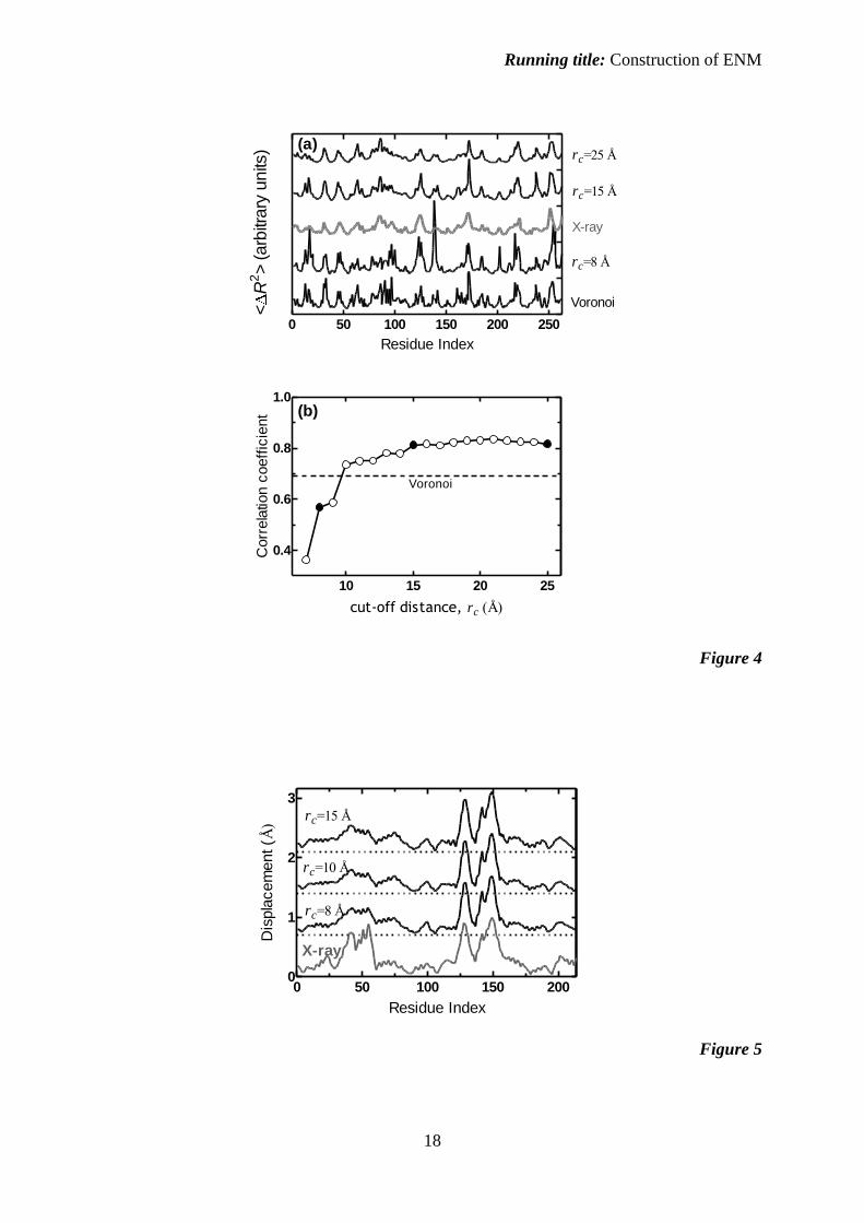
individual residues are faithfully predicted. One example is displayed in figure 4 for a 263

residue -class protein (PDB code: 1arb), where the residue-by-residue experimental B-

factors (middle curve in gray in Figure 4a) are compared with several selected theoretical

models: A relatively low correlation is obtained at rc = 8 Å; in particular, the fluctuations of

surface loop residues 15 – 20 and 135 – 145 are overestimated due to the absence of important

core-region contacts that are not taken into account at this cut-off distance. The rc = 15 Å

model captures the experimentally determined fluctuation patterns, which remains unaltered

at higher cut-offs. The fluctuations predicted by the Voronoi tessalated network model are

somewhat chaotic, lowering the correlations with experiment. The Pearson correlation

coefficients at a wide range of cut-off distances are plotted in figure 4b, along with the value

obtained from Voronoi tessalated networks (dashed line). We emphasize that the behavior

exemplified by figure 4 is not unique to this protein, but is rather a common property of all

proteins.

The increase in the correlation coefficient with rc as well as its persistence to very high rc

values implies that the main ingredients that contribute to the fluctuation predictions are

present in the Hessian obtained at a relatively low rc, and the additional contacts act as a

perturbation to this “essential” part of the matrix. We may thus partition the Hessian into two

(equation A1), where contains information due to the essential contacts of the matrix

whereas is the residual part where the interactions are added in a spherically symmetrical

manner around the nodes beyond a certain rc value (figure 2). In the Appendix we include a

proof of how the lowest eigenvalues are modified in a small window based on this

partitioning, as well as how the eigenvectors remain unchanged (equation A7). The result in

equation A8 implies that the inverse of the Hessian will be nominally modified, so that the

predicted C fluctuations will change only slightly. On the other hand, since a Voronoi

tessalated network construction of proteins is based on the minimal partitioning of space in

the neighborhood of nodes, it will not form the essential part of the Hessian, , which must

necessarily include a larger number of contacts from the first coordination shell.

Finally the findings outlined in the Appendix imply that, due to the invariance of the

eigenvectors under such a perturbation to the essential part of the Hessian, the mode based

predictions on the direction of motion between the unbound and bound conformations of the

protein will also converge. An example is shown in figure 5 for the protein adenylate kinase,

for which the eigenvector that belongs to the lowest eigenvalue is known to describe the

conformational change with high accuracy due to the highly collective behavior of the hinge

motion between the two domains (43). The Pearson correlation between the experimental and

theoretical curves is 0.9 at all cut-off distances above rc = 8 Å. The largest discrepancy

between theory and experiment is observed in the region spanning residues 30 – 67 which

belongs to the NMP binding domain closing over the ATP binding domain (called the LID)

on the opposite side, the latter spanning residues 118 – 167. The prediction does not change

with rc and may possibly be improved by the inclusion of additional modes, which is beyond

the scope of the current work.

To recapitulate, with our analysis over a large set of non-homologous proteins, the degree of

success of network models of proteins is shown to converge as the cut-off distance used in

constructing the network from the PDB coordinates of the protein is increased. A choice of

high rc in the vicinity of 16 Å covers the neighborhood structure of an arbitrary protein and its

eigenvalue spectra; however, for large proteins, this will introduce a large number of

interactions which will render the matrix inversion procedure rather cumbersome. In such


10

cases, one may resort to compute g(r), g( ) and g( ) curves and spectral dimensions for the

particular protein to choose an optimum rc; for large proteins the number of nodes will be

high enough to obtain statistics for smooth curves where the peaks may be discerned, a

problem that cannot be circumvented for small system sizes. We note that network models are

useful in describing the properties related to the fluctuations near the minimum of the

conformational energy well, and its curvature. However, they will not succeed in providing

information of the dynamical properties of the protein, unless a methodology for updating the

Hessian along the reaction coordinate is introduced.

CONCLUSIONS

Despite their different topological structures and sizes, a statistical analysis of a large number

of folded proteins leads to common features. In particular, the radial and angular distribution

functions provide the degree of (in)homogeneity in the protein as well as a quantitative

description of the location of the coordination shells. Depth dependent analysis shows that the

densely packed core region of the protein has a different local structure built around it

compared to its surface. In the core of the protein, the second neighbors have a non-random

distribution that is more pronounced than the first neighbors. In the surface residues, the

reverse is observed (figure 2).

Calculations at a variety of cut-off distances used in network construction reflect that the

dimensionality of the system approaches that of regular crystals where g(ω) scales with ω2

only at unrealistically high rc values (figure 3b). The modal spectrum resembles that obtained

from all-atom calculations with realistic atom-atom interaction potentials in the region above

the second coordination shells up to a cut-off distance of 16 Å (figure 3a). At this threshold,

the spectral dimension shifts from the region of ds = 1-2 to above 2, accompanied by a

crossover in its rate of change (figure 3b).

We have shown that the slow modes are immune to the details of network construction once

the essential contacts in the first few coordination shells are included (Appendix and figures

4-5). Therefore, the properties that depend on the most collective modes may be studied

independent of this choice. This is incontrast to the modes that affect the medium to high

frequency motions. Therefore, in studies deriving information by relying on the superposition

of a large number of modes, a cautious network construction is essential.

Network constructed by using Voronoi tessalations, on the other hand, fail to correctly define

the local interactions while they successfully incorporate the long-range pairwise interactions.

In particular, the mode distributions (figure 3a) and the spectral dimensions measured at the

slow mode region (figure 3b) do not represent the experimentally and theoretically well-

characterized shapes for proteins. Therefore, these network models will provide misleading

information on the properties that rely mostly on local interactions (e.g. residue fluctuations,

figure 4). On the other hand, they are expected to be very effective in forecasting properties

that depend on a correct incorporation of the long-range contacts, as was recently

demonstrated by their success in predicting the folding rates of two-state proteins (44).

APPENDIX. Partitioning the Hessian into its essential and residual components.

We partition the Hessian into two parts:

(A1)

We postulate that contains information due to the essential contacts of the nodes, whereas

is the residual part where the interactions are added in a spherically symmetrical manner


11

around the nodes beyond a certain rc value (figure 2). An alternative way of achieving the

Hessian is through the use of an overall force balance around each node of the network as

discussed in detail in reference (15). Therein, it is shown that the Hessian is obtained by the

product of the 3N × M direction cosine matrix, B with its transpose, for a system of N nodes

and a total of M equivalent interactions between pairs of nodes;

(A2)

Inasmuch as the overall interactions may be written as the sum of the and matrices that

contain the essential and the residual interactions, the Hessian may thus be expressed as

(A3)

We now denote the elements of the and matrices by cos ij and cos ij, respectively.

Then, the elements of the terms in equation A3 may be calculated from,

(A4)

(A5)

(A6)

The approximations in equations A5 and A6 follow from the assumption that the elements of

the residual matrix, cos ij are uncorrelated and span the entire range of values in [- , ], and

m is large. These lead to the result,

(A7)

Comparing equations A1 and A7 suggests that the modification to the essential part of the

Hessian, due to a set of randomly added interactions, is through the addition of a constant. In

the inverse operation, this leads to a modification of the eigenvalues in the range [0, ],

whereas the eigenvectors are expected to remain unchanged (45).

In reality, this is an idealization of the residual matrix, and the eigenvalues are expected to

display a distribution of values, peaking at . To determine the extent to which the

interactions above a threshold distance value approximate , we decompose the Hessian of

the protein set such that the interactions up to 17 Å are incorporated into the essential part, ,

and those in the range 17 – 25 Å are considered in the residual, . We verify that the

eigenvalue distribution of the latter matrix peaks around . Furthermore, using,

-

(A8)

we find that more than 50 % of the eigenvalues of -

is below 1 so that the main features

of the essential part of the Hessian, in particular the slow modes, remain unchanged in the

total Hessian.

ACKNOWLEDGEMENTS. We thank Tural Aksel for bringing up the observation that

large cut-off distances may improve the predictions on the residue fluctuations. İİ thanks

Deniz Turgut for his help in parts of the computations.


12

REFERENCES

1. Soyer, A., J. Chomilier, J. P. Mornon, R. Jullien, and J. F. Sadoc. 2000. Voronoi

Tessellation Reveals the Condensed Matter Character of Folded Proteins. Physical

Review Letters 85:3532-3535.

2. Raghunathan, G., and R. L. Jernigan. 1997. Ideal Architecture of Residue Packing and

Its Observation in Protein Structures. Protein Science 6:2072-2083.

3. Atilgan, A. R., P. Akan, and C. Baysal. 2004. Small-World Communication of

Residues and Significance for Protein Dynamics. Biophysical Journal 86:85-91.

4. Liang, J., and K. A. Dill. 2001. Are Proteins Well Packed? Biophys. J. 81:751-766.

5. Zhang, J. F., R. Chen, C. Tang, and J. Liang. 2003. Origin of Scaling Behavior of

Protein Packing Density: A Sequential Monte Carlo Study of Compact Long Chain

Polymers. Journal of Chemical Physics 118:6102-6109.

6. ben-Avraham, D. 1993. Vibrational Normal-Mode Spectrum of Globular-Proteins.

Physical Review B 47:14559-14560.

7. Bahar, I., A. R. Atilgan, M. C. Demirel, and B. Erman. 1998. Vibrational Dynamics of

Folded Proteins: Significance of Slow and Fast Motions in Relation to Function and

Stability. Physical Review Letters 80:2733-2736.

8. Bahar, I., and A. J. Rader. 2005. Coarse-Grained Normal Mode Analysis in Structural

Biology. Current Opinion in Structural Biology 15:586-592.

9. Cui, Q. 2006. Normal Mode Analysis: Theory and Applications to Biological and

Chemical Systems. Chapman & Hall/CRC, FL, USA.

10. Bahar, I., A. R. Atilgan, and B. Erman. 1997. Direct Evaluation of Thermal

Fluctuations in Proteins Using a Single-Parameter Harmonic Potential. Folding &

Design 2:173-181.

11. Delarue, M., and Y. H. Sanejouand. 2002. Simplified Normal Mode Analysis of

Conformational Transitions in DNA-Dependent Polymerases: The Elastic Network

Model. Journal of Molecular Biology 320:1011-1024.

12. Tirion, M. M. 1996. Large Amplitude Elastic Motions in Proteins from a Single-

Parameter, Atomic Analysis. Physical Review Letters 77:1905-1908.

13. Hinsen, K. 1998. Analysis of Domain Motions by Approximate Normal Mode

Calculations. Proteins-Structure Function and Genetics 33:417-429.

14. Yilmaz, L. S., and A. R. Atilgan. 2000. Identifying the Adaptive Mechanism in

Globular Proteins: Fluctuations in Densely Packed Regions Manipulate Flexible Parts.

Journal of Chemical Physics 113:4454-4464.

15. Atilgan, A. R., S. R. Durell, R. L. Jernigan, M. C. Demirel, O. Keskin, and I. Bahar.

2001. Anisotropy of Fluctuation Dynamics of Proteins with an Elastic Network

Model. Biophysical Journal 80:505-515.

16. Erman, B. 2006. The Gaussian Network Model: Precise Prediction of Residue

Fluctuations and Application to Binding Problems. Biophysical Journal 91:3589-3599.

17. Song, G., and R. L. Jernigan. 2007. Vgnm: A Better Model for Understanding the

Dynamics of Proteins in Crystals. Journal of Molecular Biology 369:880-893.

18. Doruker, P., A. R. Atilgan, and I. Bahar. 2000. Dynamics of Proteins Predicted by

Molecular Dynamics Simulations and Analytical Approaches: Application to Alpha-

Amylase Inhibitor. Proteins-Structure Function and Genetics 40:512-524.

19. Haliloglu, T., and I. Bahar. 1999. Structure-Based Analysis of Protein Dynamics:

Comparison of Theoretical Results for Hen Lysozyme with X-Ray Diffraction and

Nmr Relaxation Data. Proteins-Structure Function and Genetics 37:654-667.


13

20. Isin, B., E. Tajkhorshid, K. Schulten, and I. Bahar. 2007. Conformational Changes of

Rhodopsin Explored by Using Normal Modes in Steered Molecular Dynamics

Simulations. Biophysical Journal:20a-20a.

21. Rader, A. J., D. H. Vlad, Y. M. Wang, and I. Bahar. 2005. Elastic Network Models

Reveal Maturation Dynamics of Bacteriophage Hk97. Biophysical Journal 88:232a-

232a.

22. Temiz, N. A., E. Meirovitch, and I. Bahar. 2004. Escherichia Coli Adenylate Kinase

Dynamics: Comparison of Elastic Network Model Modes with Mode-Coupling N-15-

Nmr Relaxation Data. Proteins-Structure Function and Bioinformatics 57:468-480.

23. Petrone, P., and V. S. Pande. 2006. Can Conformational Change Be Described by

Only a Few Normal Modes? Biophysical Journal 90:1583-1593.

24. Yang, L., G. Song, and R. L. Jernigan. 2007. How Well Can We Understand Large-

Scale Protein Motions Using Normal Modes of Elastic Network Models? Biophysical

Journal 93:920-929.

25. Dupuis, F., J. F. Sadoc, R. Jullien, B. Angelov, and J. P. Mornon. 2005. Voro3d: 3d

Voronoi Tessellations Applied to Protein Structures. Bioinformatics 21:1715-1716.

26. Bode, C., I. A. Kovacs, M. S. Szalay, R. Palotai, T. Korcsmaros, and P. Csermely.

2007. Network Analysis of Protein Dynamics. Febs Letters 581:2776-2782.

27. Berman, H. M., J. Westbrook, Z. Feng, G. Gilliland, T. N. Bhat, H. Weissig, I. N.

Shindyalov, and P. E. Bourne. 2000. The Protein Data Bank. Nucleic Acids Research

28:235-242.

28. Poupon, A. 2004. Voronoi and Voronoi-Related Tessellations in Studies of Protein

Structure and Interaction. Current Opinion in Structural Biology 14:233-241.

29. Fariselli, P., and R. Casadio. 1999. A Neural Network Based Predictor of Residue

Contacts in Proteins. Protein Engineering 12:15-21.

30. Atilgan, A. R., D. Turgut, and C. Atilgan. 2007. Screened Nonbonded Interactions in

Native Proteins Manipulate Optimal Paths for Robust Residue Communication.

Biophysical Journal 92:3052-3062.

31. Bagci, Z., R. L. Jernigan, and I. Bahar. 2002. Residue Packing in Proteins: Uniform

Distribution on a Coarse-Grained Scale. Journal of Chemical Physics 116:2269-2276.

32. Chakravarty, S., and R. Varadarajan. 1999. Residue Depth: A Novel Parameter for the

Analysis of Protein Structure and Stability. Structure 7:723-732.

33. Baysal, C., and A. R. Atilgan. 2002. Relaxation Kinetics and the Glassiness of

Proteins: The Case of Bovine Pancreatic Trypsin Inhibitor. Biophysical Journal

83:699-705.

34. Zhou, Y. Q., D. Vitkup, and M. Karplus. 1999. Native Proteins Are Surface-Molten

Solids: Application of the Lindemann Criterion for the Solid Versus Liquid State.

Journal of Molecular Biology 285:1371-1375.

35. Kittel, C. 2004. Introduction to Solid State Physics. John Wiley & Sons.

36. Svanidze, A. V., I. L. Sashin, S. G. Lushnikov, S. N. Gvasaliya, K. K. Turoverov, I.

M. Kuznetsova, and S. Kojima. 2007. Inelastic Incoherent Neutron Scattering in Some

Proteins. Ferroelectrics 348:556-562.

37. Reuveni, S., R. Granek, and J. Klafter. 2008. Proteins: Coexistence of Stability and

Flexibility. Physical Review Letters 100:4.

38. Burioni, R., D. Cassi, F. Cecconi, and A. Vulpiani. 2004. Topological Thermal

Instability and Length of Proteins. Proteins-Structure Function and Bioinformatics

55:529-535.

39. Baysal, C., and A. R. Atilgan. 2001. Elucidating the Structural Mechanisms for

Biological Activity of the Chemokine Family. Proteins-Structure Function and

Genetics 43:150-160.


14

40. Tama, F., and Y. H. Sanejouand. 2001. Conformational Change of Proteins Arising

from Normal Mode Calculations. Protein Engineering 14:1-6.

41. Keskin, O. 2007. Binding Induced Conformational Changes of Proteins Correlate with

Their Intrinsic Fluctuations: A Case Study of Antibodies. Bmc Structural Biology

7:31.

42. Zen, A., V. Carnevale, A. M. Lesk, and C. Micheletti. 2008. Correspondences between

Low-Energy Modes in Enzymes: Dynamics-Based Alignment of Enzymatic

Functional Families. Protein Science 17:918-929.

43. Tama, F., W. Wriggers, and C. L. Brooks. 2002. Exploring Global Distortions of

Biological Macromolecules and Assemblies from Low-Resolution Structural

Information and Elastic Network Theory. Journal of Molecular Biology 321:297-305.

44. Ouyang, Z., and J. Liang. 2008. Predicting Protein Folding Rates from Geometric

Contact and Amino Acid Sequence. Protein Science 17:1256-1263.

45. Golub, G. H., and C. F. van Loan. 1996. Matrix Computations. Johns Hopkins

University Press, Baltimore.


15

FIGURE CAPTIONS

Figure 1. (a) The negative of the resultant vectors acting on the nodes, , exemplified by a

54 residue protein (PDB code: 1enh). The length of each red vector is proportional to the cut-

off distance used in network construction, rc, the shortest at 7 Å and the longest at 15 Å. The

yellow vector is the resultant obtained from the networks obtained from the Voronoi

tessalations. (b) Part of the helix marked by the square in (a) is magnified; “exterior” refers to

the solvent contacting part of the helix, and “interior” marks the side facing the core of the

protein.

Figure 2. (a) Radial and angular distribution functions (left y-axis: RDF; right y-axis: ADF)

obtained by averaging over 595 proteins. (b) ADFs computed separately for the core and

surface residues for a subset of 60 proteins.

Figure 3. (a) The change of the density of vibrational modes, g( ), with the cut-off distance,

rc, used in network construction. The main figure displays the results for rc in the first (rc = 7

Å) to above the fourth coordination shell range (up to 16 Å). Also shown, in dashed lines, is

the frequency distribution of the Voronoi tessalated networks. The inset displays the results

for very large rc values (up to 30 Å). The data is an average over a set of 26 proteins in the

size range of 150 ± 10 residues. (b) Spectral dimension, ds, of the networks, obtained from

power law best-fits to the cumulative density of modes, for the first 70 modes in

each set of data. Goodness of fit is 0.98 or better in all cases. The thin dashed lines are

included to guide the eye for the cross-over in the rate of change of ds with rc. Also indicated

on the figure are the ds of the Voronoi tessalated networks that occur at ca. 1.0, and the

theoretical limit at ds = 3 when all nodes are interconnected (rc → ∞).

Figure 4. (a) Comparison of the X-ray B-factors (gray, middle curve) with fluctuation

profiles predicted from various models (at rc = 8, 15, 25 Å and network construction with

Voronoi tessalations) for the 268 residue achromobacter lyticus protease (PDB code: 1arb).

(b) Pearson correlation coefficients at a wide range of cut-off distances for the same protein;

those that correspond to the detailed fluctuation profiles of figure 4a are shown with filled

circles and that with the cut-off free Voronoi tessalated model is marked by the dashed line.

Figure 5. The displacement profiles of adenylate kinase in unbound and bound forms (PDB

codes: 4ake and 1ake, respectively). The experimental displacements are shown in gray.

Predictions from the relative magnitudes of the eigenvector corresponding to the slowest

mode obtained at rc = 8, 10, 15 Å are shown in black. The latter curves are displaced to guide

the eye, and their zero baselines are marked by the dotted curves. The Pearson correlation

between the experimental curve and each of the predictions is 0.9.


16

Figure 1

6 10 14 182

4

6

g(r)

g( )

(a)

distance, r (Å)

g(r

) (a

rbitr

ary

units

)g

() (d

eg

ree

s)

6 10 14 18

2

4

6

8

surface residues

core residues

distance, r (Å)

g(

) (d

eg

ree

s)

(b)

Figure 2

exterior

interior

(a) (b)


17

10 20 300

20

40

60

80

100

rc=7Å

8Å

10Å

12Å14Å

16Å Voronoi

modes,

Density

of

modes,

g(

)

10 15 20 25 30

1

2

3rc

Voronoi

cut-off distance, rc (Å)

Spectr

al dim

ensio

n,ds

0 20 40 60 800

10

20

30

rc=16Å

20Å

25Å30Å

modes,

g(

)

(a)

(b)

Figure 3


18

0 50 100 150 200 250

X-ray

rc=15 Å

Voronoi

rc=25 Å

rc=8 Å

Residue Index

<R

2> (arb

itrary

units

)

10 15 20 25

0.4

0.6

0.8

1.0

Voronoi

cut-off distance, rc (Å)

Corr

ela

tion c

oeff

icie

nt

(a)

(b)

Figure 4

0 50 100 150 2000

1

2

3

rc=8 Å

rc=10 Å

rc=15 Å

X-ray

Residue Index

Dis

pla

cem

ent (Å

)

Figure 5

Residue Network Construction and Predictions of Elastic Network Models

Documents

Transcript of Residue Network Construction and Predictions of Elastic Network Models