14.581 International Trade — Lecture 2: Ricardian Theory (I)—

14.581 International Trade— Lecture 2: Ricardian Theory (I)—

14.581

Week 2

Fall 2018

14.581 (Week 2) Ricardian Theory (I) Fall 2018 1 / 34

Today’s Plan

1 Taxonomy of neoclassical trade models

2 Standard Ricardian model: DFS 1977

1 Free trade equilibrium2 Comparative statics

3 Multi-country extensions

4 The origins of cross-country technological differences


Taxonomy of Neoclassical Trade Models

In a neoclassical trade model, comparative advantage, i.e. differencesin relative autarky prices, is the rationale for trade

Differences in autarky prices may have two origins:

1 Demand (periphery of the field)2 Supply (core of the field)

1 Ricardian theory: Technological differences2 Factor proportion theory: Factor endowment differences


Taxonomy of Neoclassical Trade Models

In order to shed light on the role of technological and factorendowment differences:

Ricardian theory assumes only one aggregate factor of productionFactor proportion theory rules out technological differences acrosscountries

Neither set of assumptions is realistic, but both may be usefuldepending on the question one tries to answer:

If you want to understand the impact of the rise of China on realincomes in the US, Ricardian theory is the natural place to startIf you want to study its effects on the skill premium, more factors willbe needed

Note that:

Technological and factor endowment differences are exogenously givenNo relationship between technology and factor endowments(Skill-biased technological change?)


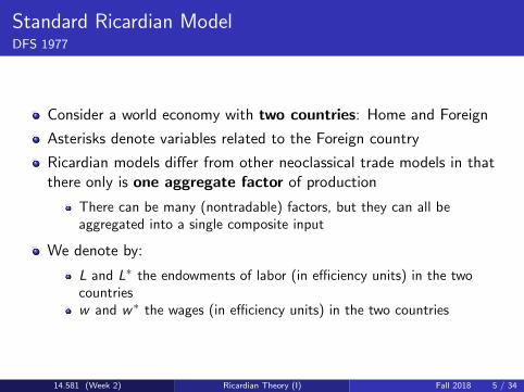
Standard Ricardian ModelDFS 1977

Consider a world economy with two countries: Home and Foreign

Asterisks denote variables related to the Foreign country

Ricardian models differ from other neoclassical trade models in thatthere only is one aggregate factor of production

There can be many (nontradable) factors, but they can all beaggregated into a single composite input

We denote by:

L and L∗ the endowments of labor (in efficiency units) in the twocountriesw and w∗ the wages (in efficiency units) in the two countries


Standard Ricardian ModelSupply-side assumptions

There is a continuum of goods indexed by z ∈ [0, 1]

Since there are CRS, we can define the (constant) unit laborrequirements in both countries: a (z) and a∗ (z)

a (z) and a∗ (z) capture all we need to know about technology in thetwo countries

W.l.o.g, we order goods such that A (z) ≡ a∗(z)a(z)

is decreasing

Hence Home has a comparative advantage in the low-z goodsFor simplicity, we’ll assume strict monotonicity


Standard Ricardian ModelFree trade equilibrium (I): Efficient international specialization

Previous supply-side assumptions are all we need to make qualitativepredictions about pattern of trade

Let p (z) denote the price of good z under free trade

Profit-maximization requires

p (z)− wa (z) ≤ 0, with equality if z produced at home (1)

p (z)− w ∗a∗ (z) ≤ 0, with equality if z produced abroad (2)

Proposition There exists z ∈ [0, 1] such that Home produces allgoods z < z and Foreign produces all goods z > z



Proof: By contradiction. Suppose that there exists z ′ < z such thatz produced at Home and z ′ is produced abroad. (1) and (2) imply

p (z)− wa (z) = 0

p(z ′)− wa

(z ′)≤ 0

p(z ′)− w ∗a∗

(z ′)

= 0

p (z)− w ∗a∗ (z) ≤ 0

This implies

wa (z)w ∗a∗(z ′)= p (z) p

(z ′)≤ wa

(z ′)w ∗a∗ (z) ,

which can be rearranged as

a∗(z ′)

/a(z ′)≤ a∗ (z) /a (z)

This contradicts A strictly decreasing.



Proposition simply states that Home should produce and specialize inthe goods in which it has a CA

Note that:

Proposition does not rely on continuum of goodsContinuum of goods + continuity of A is important to derive

A (z) =w

w∗≡ ω (3)

Equation (3) is the first of DFS’s two equilibrium conditions:

Conditional on wages, goods should be produced in the country whereit is cheaper to do so

To complete characterization of free trade equilibrium, we need tolook at the demand side to pin down the relative wage ω


Standard Ricardian ModelDemand-side assumptions

Consumers have identical Cobb-Douglas pref around the world

We denote by b (z) ∈ (0, 1) the share of expenditure on good z :

b(z) =p (z) c (z)

wL=

p (z) c∗ (z)

w ∗L∗

where c (z) and c∗ (z) are consumptions at Home and Abroad

By definition, share of expenditure satisfy:∫ 10 b (z) dz = 1


Standard Ricardian ModelFree trade equilibrium (II): trade balance

Let us denote by θ (z) ≡∫ z0 b (z) dz the fraction of income spent (in

both countries) on goods produced at Home

Trade balance requires

θ (z)w ∗L∗ = [1− θ (z)]wL

LHS≡ Home exports; RHS≡ Home imports

Previous equation can be rearranged as

ω =θ (z)

1− θ (z)

(L∗

L

)≡ B (z) (4)

Note that B ′ > 0: an increase in z leads to a trade surplus at Home,which must be compensated by an increase in Home’s relative wage ω


Standard Ricardian ModelPutting things together

!FH ~

z

ω

B(z)

z

A(z)

Efficient international specialization, Equation (3), and trade balance,(4), jointly determine (z , ω)


Standard Ricardian ModelA quick note on the gains from trade

Since Ricardian model is a neoclassical model, general results derivedin previous lecture hold

However, one can directly show the existence of gains from trade inthis environment

Argument:

Set w = 1 under autarky and free tradeIndirect utility of Home representative household only depends on p (·)For goods z produced at Home under free trade: no change comparedto autarkyFor goods z produced Abroad under free trade:p (z) = w∗a∗ (z) < a (z)Since all prices go down, indirect utility must go up


What Are the Consequences of (Relative) Country Growth?

!FH ~

z

ω

B(z)

z

A(z)

Suppose that L∗/L goes up (rise of China):

ω goes up and z goes downAt initial wages, an increase in L∗/L creates a trade deficit Abroad,which must be compensated by an increase in ω


What are the Consequences of (Relative) Country Growth?

Increase in L∗/L raises indirect utility, i.e. real wage, of representativehousehold at Home and lowers it Abroad:

Set w = 1 before and after the change in L∗/LFor goods z whose production remains at Home: no change in p (z)For goods z whose production remains Abroad:ω ↗⇒ w∗ ↘⇒ p (z) = w∗a∗ (z)↘For goods z whose production moves Abroad:w∗a∗ (z) ≤ a (z)⇒ p (z)↘So Home gains. Similar logic implies welfare loss Abroad

Comments:

In spite of CRS at the industry-level, everything is as if we had DRS atthe country-levelAs Foreign’s size increases, it specializes in sectors in which it isrelatively less productive (compared to Home), which worsens itsterms-of trade, and so, lowers real GDP per capitaThe flatter the A schedule, the smaller this effect


What are the Consequences of Technological Change?

There are many ways to model technological change:

1 Global uniform technological change: for all z , a (z) = a∗ (z) = x > 02 Foreign uniform technological change: for all z , a (z) = 0, but

a∗ (z) = x > 03 International transfer of the most efficient technology: for all z ,

a(z) = a∗ (z) (Offshoring?)

Using the same logic as in the previous comparative static exercise,one can easily check that:

1 Global uniform technological change increases welfare everywhere2 Foreign uniform technological change increases welfare everywhere (For

Foreign, this depends on Cobb-Douglas assumption)3 If Home has the most efficient technology, a(z) < a∗ (z) initially, then

it will lose from international transfer (no gains from trade)


Other Comparative Static ExercisesTransfer problem: Keynes versus Ohlin

Suppose that there is T > 0 such that:

Home’s income is equal to wL+ T ,Foreign’s income is equal to w∗L∗ − T

If preferences are identical in both countries, transfers do not affectthe trade balance condition:

[1− θ (z)] (wL+ T )− θ (z) (w ∗L∗ − T ) = T

⇔θ (z)w ∗L∗ = [1− θ (z)]wL

So there are no terms-of-trade effect

If Home consumption is biased towards Home goods, θ (z) > θ∗ (z)for all z , then transfer further improves Home’s terms-of trade

See Dekle, Eaton, and Kortum (2007) for a recent application


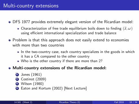
Multi-country extensions

DFS 1977 provides extremely elegant version of the Ricardian model:

Characterization of free trade equilibrium boils down to finding (z , ω)using efficient international specialization and trade balance

Problem is that this approach does not easily extend to economieswith more than two countries

In the two-country case, each country specializes in the goods in whichit has a CA compared to the other countryWho is the other country if there are more than 2?

Multi-country extensions of the Ricardian model:

1 Jones (1961)2 Costinot (2009)3 Wilson (1980)4 Eaton and Kortum (2002) [Next Lecture]


Multi-country extensionsJones (1961)

Assume N countries, G goods

Trick: restrict attention to “Class of Assigments” where

each country only produces one goodeach good is produced by the same number of countries

Characterize the properties of optimal assignment within a class

Main result:Optimal assignment of countries to goods within a class will minimizethe product of their unit labor requirements


Multi-country extensionsCostinot (2009)

Assume N countries, G goods

Trick: put enough structure on the variation of unit-laborrequirements across countries and industries to bring backtwo-country intuition

Suppose that:

countries i = 1, ...,N countries have characteristics γi ∈ Γgoods g = 1, ...,G countries have characteristics σg ∈ Γ

a (σ, γ) ≡ unit labor requirement in σ-sector and γ-country



Definition a (σ, γ) is strictly log-submodular if for any σ > σ′ andγ > γ′, a (σ, γ) a (σ′, γ′) < a (σ, γ′) a (σ′, γ)

If a is strictly positive, this can be rearranged as

a (σ, γ)/a(σ′, γ

)< a

(σ, γ′

)/a(σ′, γ′

)In other words, high-γ countries have a comparative advantage inhigh-σ sectors

Example:

In Krugman (1986), a (σs , γc ) ≡ exp (−σsγc ), where σs is an index ofgood s’s “technological intensity” and γc is a measure of country c ’scloseness to the world “technological frontier”



Proposition If a (σ, γ) is log-submodular, then high-γ countriesspecialize in high-σ sectors

Proof: By contradiction. Suppose that there exists γ > γ′ andσ > σ′ such that country γ produces good σ′ and country γ′

produces good σ. Then profit maximization implies

p(σ′)− w (γ) a

(σ′, γ

)= 0

p (σ)− w (γ) a (σ, γ) ≤ 0

p (σ)− w(γ′)a(σ, γ′

)= 0

p(σ′)− w

(γ′)a(σ′, γ′

)≤ 0

This implies

a(σ, γ′

)a(σ′, γ

)≤ a (σ, γ) a

(σ′, γ′

)which contradicts a log-submodular


Multi-country extensionsWilson (1980)

Same as in DFS 1977, but with multiple countries and more generalpreferences

Trick: Although predicting the exact pattern of trade may be difficult,one does not need to know it to make comparative static predictions

At the aggregate level, Ricardian model is similar to anexchange-economy in which countries trade their own labor for thelabor of other countries

Since labor supply is fixed, changes in wages can be derived fromchanges in (aggregate) labor demandOnce changes in wages are known, changes in all prices, and hence,changes in welfare can be derived


Multi-country extensionEaton and Kortum (2002)

Same as Wilson (1980), but with functional form restrictions on a (z)

Trick: For each country i and each good z , they assume thatproductivity, 1/a (z), is drawn from a Frechet distribution

F (1/a) = exp(−Tia

θ)

Like Wilson (and unlike Jones), no attempt at predicting which goodscountries trade:

Instead focus on bilateral trade flows and their implications for wages

Unlike Wilson, trade flows only depends on a few parameters (Ti ,θ)

Will allow for calibration and counterfactual analysis

This paper has had a profound impact on the field:

We’ll study it in detail in the next lecture


The Origins of Technological Differences Across Countries

One obvious limitation of the Ricardian model:Where do productivity differences across countries come from?

For agricultural goods:Weather conditions (Portuguese vs. English wine)

For manufacturing goods:Why don’t the most productive firms reproduce their productionprocess everywhere?

“Institutions and Trade” literature offers answer to this question


Institutions as a Source of Ricardian CA

Basic Idea:

1 Even if firms have access to same technological know-how around theworld, institutional differences across countries may affect how firmswill organize their production process, and, in turn, their productivity

2 If institutional differences affect productivity relatively more in somesectors, than institutions become source of comparative advantage

General Theme:Countries with “better institutions” tend to be relatively moreproductive, and so to specialize, in sectors that are more“institutionally dependent”


Examples of Institutional Trade Theories

1 Contract EnforcementAcemoglu, Antras, Helpman (2007), Antras (2005), Costinot* (2009),

Levchenko (2007), Nunn (2007), Vogel (2007)

2 Financial InstitutionsBeck (2000), Kletzer, Bardhan (1987), Matsuyama* (2005), Manova (2007)

3 Labor Market InstitutionsDavidson, Martin, Matusz (1999), Cunat and Melitz* (2007), Helpman,

Itskhoki (2006)

(* denote papers explicitly building on DFS 1977)


A Simple ExampleCostinot JIE (2009)

Starting point:Division of labor ≡ key determinant of productivity differences

Basic trade-off:

1 Gains from specialization⇒ vary with complexity of production process (sector-specific)

2 Transaction costs⇒ vary with quality of contract enforcement (country-specific)

Two steps:

1 Under autarky, trade-off between these 2 forces pins down the extentof the division of labor across sectors in each country

2 Under free trade, these endogenous differences in the efficientorganization of production determine the pattern of trade


A Simple ExampleTechnological know-how

2 countries, one factor of production, and a continuum of goods

Workers are endowed with 1 unit of labor in both countries

Technology (I): Complementarity. In order to produce each goodz , a continuum of tasks t ∈ [0, z ] must be performed:

q (z) = mint∈[0,z ]

[qt(z)]

Technology (II): Increasing returns. Before performing a task,workers must learn how to perform it:

lt (z) = qt (z) + ft

For simplicity, suppose that fixed training costs are s.t.∫ z0 ftdt = z

Sectors differ in terms of complexity z : the more complex a good is,the longer it takes to learn how to produce it


A Simple ExampleInstitutional constraints

Crucial, function of institutions: contract enforcement

Contracts assign tasks to workers

Better institutions—either formal or informal—increase theprobability that workers perform their contractual obligations

e−1θ and e−

1θ∗ denote this probability at Home and Abroad

Home has better institutions: θ > θ∗:


A Simple ExampleEndogenous organization

In each country and sector z , firms choose “division of labor” N ≡number of workers cooperating on each unit of good z

Conditional on the extent of the division of labor, (expected) unitlabor requirements at Home can be expressed as

a (z ,N) =ze

Nθ(

1− zN

)In a competitive equilibrium, N will be chosen optimally

a (z) = minN

a (z ,N)

Similar expressions hold for a∗ (z ,N) and a∗ (z) Abroad


A Simple ExampleThe Origins of Comparative Advantage

Proposition If θ > θ∗, then A (z) ≡ a∗ (z) /a (z) is decreasing in z

From that point on, we can use DFS 1977 to determine the patternof trade and do comparative statics

One benefit of micro-foundations is that they impose some structureon A as a function of θ and θ∗:

So we can ask what will be the welfare impact of institutionalimprovements at Home and Abroad?

The same result easily generalizes to multiple countries by setting“γi ≡ θ” and “σg ≡ z”

Key prediction is that a (σ, γ) is log-submodular


Institutional Trade TheoriesCrude summary

Institutional trade theories differ in terms of content given to notionsof institutional quality (γ) and institutional dependence (σ)

Examples:

1 Matsuyama (2005): γ ≡ “credit access”; σ ≡ “pledgeability”2 Cunat and Melitz (2007): γ ≡ “rigidity labor market”; σ ≡ “volatility”

However institutional trade theories share same fundamental objective:Providing micro-foundations for the log-submodularity of a (σ, γ)

Key theoretical question:Why are high-γ countries relatively more productive in high-σ sectors?


Other Extensions of DFS 1977

Non-homothetic preferences: Matsuyama (2000)

Goods are indexed according to priorityHome has a comparative advantage in the goods with lowest priority

External economies of scale: Grossman and Rossi-Hansberg(2009), Matsuyama (2011)

Unit labor requirements depend on total output in a givencountry-industryLike institutional models, a is endogenous, but there is a two-wayrelationship between trade on productivity


14.581 International Trade — Lecture 2: Ricardian Theory (I)—

Documents

Transcript of 14.581 International Trade — Lecture 2: Ricardian Theory (I)—