Estimating Individual Emissions in a Nonpoint Source

Pollution Problem: A Bayesian Perspective

Efthimios G. Tsionas

(Dept of Economics, Athens University of Economics and Business, Greece)

Vangelis Tzouvelekas

(Dept of Economics, University of Crete, Greece)

Anastasios Xepapadeas

(Dept of Economics, University of Crete, Greece)

(This version, March 2007)

Corresponding Author:

Vangelis Tzouvelekas Department of Economics University of Crete University Campus, 74100, Crete, Greece Tel.: +30-28310-77417; Fax: +30-28310-77406; e-mail: vangelis@econ.soc.uoc.gr This research has been partly supported by European Community’s 6th Framework Programme “A quantitative and qualitative assessment of the socio-economic and environmental impacts of decoupling of direct payments on agricultural production, markets and land use in the EU-GENEDEC”.

- 1 -

Estimating Individual Emissions in a Nonpoint Source Pollution Problem: A Bayesian Perspective

Abstract

The present paper aims to provide an alternative approach for estimating individual nitrate emission levels in a nonpoint source (NPS) pollution problem using Bayesian inference. The proposed model by taking into account the stochastic nature of nitrate improves the reliability of the estimates of individual nitrogen loadings. Simulation with artificial data reveals that the suggested model performs quite well even for small sample sizes while the posterior results are rather robust to changes in the prior distribution. The proposed framework is applied to a small catchment area in Ierapetra Valley in Crete, Greece.

Keywords: Nonpoint source pollution, nitrate leaching, bayesian analysis.

JEL codes: C11, Q15, Q20

Introduction

One of the most important pollution problems in agricultural sector concerns nitrate

leaching through the application of chemical fertilizers in crops that basically involves

nitrate removal from the soil under the influence of water (Owen et al., 1998). This

residual nitrogen is accumulated into underground water aquifers, lakes, and reservoirs

posing a serious threat to freshwater and marine ecosystems while on the other hand

reduces waters value for humans and nature (Helfand and House, 1995; Owen et al.,

1998; Classen and Horan, 2001).1 Water pollution from ground water contaminated with

leached nitrates, is an important environmental concern since approximately 30 per cent

of surface water stream flow is coming from groundwater sources (Johnson et al., 1991;

Fleming and Adams, 1997). Surface water pollution also threatens aquatic life and may

turn into an ecological disaster (Millock et al., 2002). Eutrophication of slow flowing

rivers, lakes, reservoirs and marine areas appears through the proliferation of algae

bloom, which degrades bottom fauna, fish stock and wetlands (Isik, 2004).

Given that nitrate runoff constitutes a byproduct of farm production and farmers

receive direct or indirect benefits from producing crops, nitrate emissions have a positive

shadow value to farmers, even though they do not value them directly. Hence, farmers

- 2 -

have strong private incentives to emit nitrogen although it is undesirable for the rest of

society (Chambers and Quiggin, 1996). Indeed, the intensification and specialization of

farming practices during the last decades have resulted in excess nitrate leaching which

has become crucial for the sustainability of the countryside and the balanced relationship

between farming sector and the environment. Classen and Horan (2001) analyzing the

US farming sector found that the amount of fertilizer nitrogen taken by crops is rarely

greater than 70 per cent and it is typically closer to 50 per cent, while 90 per cent of

applied nitrogen may be lost to the environment when crop yields are near optimum

levels. On the other hand, eutrophication of marine waters has caused significant political

concerns throughout EU. Nitrate leaching from agriculture is regarded as the largest

single contributor to this problem accounting for the 65-80 per cent of the total nitrogen

loading during the last decade. In order to reduce nitrate discharges from agriculture

several rules and production standards have been adopted and implemented in both EU

and US agriculture, primarily motivated by the possibilities for technological innovations

and thus, essentially ignoring the economic aspects of regulation.

The lack in designing and applying conventional instruments of environmental

regulation to mitigate environmental problems associated with nitrate leaching, is due to

the fact that nitrate leaching is a typical nonpoint (NPS) pollution problem, i.e., it is only

detectable and measurable (if at all) after it has entered the ecosystem. The control of

numerous and spatially distributed sources of nitrogen emissions from environmental

agencies constitute a very complex problem for two main reasons: first, nitrate runoff

from nonpoint sources (i.e., farmers), cannot be monitored on a continuous and

widespread basis with reasonable accuracy at an acceptable cost, and second, nonpoint

pollution problem is inherently stochastic due to the presence of uncertainty on both

production and nitrogen emissions related with weather conditions and runoff events.

These features of nonpoint pollution make the application of the emission-based policy

instruments which have been the focus of economic inquiry infeasible. Economic

literature has been focused on three basic options to mitigate nonpoint policy feasibility

problems.2

The first one is to base the associated regulation on a collective performance

variable like the ambient concentration of nitrate emissions in a specific catchment area

- 3 -

(i.e., river basin or underground aquifer). This strand of literature follows the pioneering

work of Segerson (1988) according to which monitoring is shifted from suspected

polluters to the ambient concentration of pollutants in the catchment area.3 In other

words, farmers are considered like a team whose joint product is the level of pollution

observed in the catchment area. Environmental agencies only monitor ambient pollution

concentration in a given area and individual tax payments. Ambient taxes are charged to

all the farmers within the area, when the ambient pollution concentration rises above an

exogenously determined level. In this case the ambient tax offers a clear advantage

addressing the moral hazard problems. Indeed the implementation of the ambient tax

results in the first-best outcome as a Nash equilibrium given that any essential

information is common knowledge (no informational asymmetries). However, the

appropriateness of ambient policy instruments is limited by the feasibility and the cost of

monitoring (monitoring may be costly and subject to considerable error). In addition,

there may be also political limitations (Shortle and Abler, 1997; Xepapadeas, 1999).

These and other considerations lead Weersink et al., (1998) to suggest that ambient taxes

are best suited to managing nonpoint environmental pollution in small areas in which

agriculture is the only source, farmers are relatively homogeneous in their farming

practices, water quality is readily monitored and there are short time lags between

polluting activities and their impact on the environment.4

The second option bases the regulation on individual variables related with

pollution flows, that are more or less easy and costless to monitor such as factors of

production or farming practices. In such cases, Griffin and Bromley (1982) suggest that

least cost incentive or regulatory policies can be attached to these variables rather than

the actual amount of the generated externality.5 Indeed available evidence suggests that

farmers, at least in the short-run, are quite responsive to changes in factor prices,

increasing the use of those that become relatively cheap, while conserving on those that

become relatively expensive (e.g., Shumway, 1995). In the long-run the responsiveness

of factor price changes is even greater as new farming technologies are adopted to further

conserve expensive inputs and expand those that are relatively cheaper (Hayami and

Ruttan, 1985). Several authors extended Griffin and Bromley’s (1982) work into

stochastic and imperfectly estimated emissions, demonstrated that taxing polluting inputs

- 4 -

and subsidizing inputs that reduce pollution could replicate the results of a tax on the

externality (Stevens, 1988; Dinar et al., 1989; Shortle and Abler, 1994; Shortle et al.,

1998). However, the input tax/subsidy scheme is unrealistic as it is exceptionally

informational intensive and complex from the regulatory agency’s perspective. While

purchases of polluting inputs or investments in pollution control inputs are easily tracked

in some cases, many management decisions having an important impact on the

environment can be very costly to monitor (Braden and Segerson, 1993). Also firm-

specific input-based incentives could lead to significant enforcement problems as they

would encourage input arbitrage among farms facing different rates (Helfand and House,

1995). Finally, the scheme is designed assuming that regulator knows private control

costs although asymmetric information is more likely to be the case. In general there is a

limited knowledge on the design of input based instruments taking into account both

moral hazard about one or more input choices and asymmetric information about farm

types and environmental practices.6

Finally, the last available option, which is adopted in the present study, focuses on

the development of emissions functions that estimate or predict nonpoint pollutant flows

utilizing information on farm management practices, weather conditions, soil

characteristics and other relevant factors. These models can be thought of as a type of

hydrological models that simulate or estimate pollution loads from agricultural, forest,

urban or other land uses given the characteristics of the land resources, climate and

production and pollution control practices.7 The inherent problem of asymmetric

information in nonpoint pollution is overcome as the regulator knows the relationship

between farmers’ management practices and released nitrogen runoff through the

emission function. A well designed, reliable and properly validated biophysical model of

that kind can provide the information necessary to convert a nonpoint pollution problem

to a point source one overcoming the problem of unobserved nitrogen emissions. Thus, if

the origin and the amount of nitrogen emissions are possible to assess, the first-best

solution through the imposition of an appropriate Pigouvian tax is, at least in theory,

straightforward; each farmer has to take into account the marginal cost of his nitrogen

emissions. While these models are not free of measurement error, they overcome the

informational asymmetries associated with hidden actions which induce farmers to excess

- 5 -

nitrates emissions, and adverse selection, which precludes the regulator from knowing the

individual farmers’ characteristics, impeding in this way efficient regulation.

In view of these, there is a growing interest lately in accurately determining

individual emissions functions in nonpoint pollution problems. From a statistical point of

view, nonpoint pollution is further complicated by the fact that there are more polluting

sources than observations in any given period and case study. In the case of nitrate

leaching in any particular area, there is a quite large number of farms using chemical

fertilizers, whereas we can only have data on nitrate levels in the catchment area (i.e.,

river basin, underground water aquifer). This makes the use of standard econometric

approaches infeasible and/or inappropriate. Kaplan et al., (2003) in order to overcome

this ill-posed data problem in their case study, utilized a generalized cross entropy

approach, based on the model suggested by Singh and Krstanovic (1987). However, their

approach although quite appealing, it does not account for the stochastic process

underlying individual nitrogen emissions. Specifically they assume two states of the

world for the farming practices that directly determine nitrogen outflows. Using a similar

analytical framework as Kaplan et al., (2003) we suggest an alternative cost-effective

estimation framework to transform a NPS pollution problem to a point source one using

Bayesian inference. Our model is fully stochastic taking into consideration the unknown

emission functions without any prior knowledge of farming practices inherent to the

original models suggested by Kaplan et al., (2003). Our empirical model after its

validation with artificial data simulations is applied to the case study of nitrate leaching in

the Ierapetra Valley in Crete, Greece where out-of-season vegetable cultivation in

greenhouses is extensive and serious contamination of underground water aquifers is

observed.

The rest of this paper is organised as follows: the econometric model based on

Bayesian techniques is developed in section 2. The model validation with artificial data

and the empirical application in the Ierapetra Valley are presented in the third section.

Concluding remarks follow in the last section.

Econometric Model

- 6 -

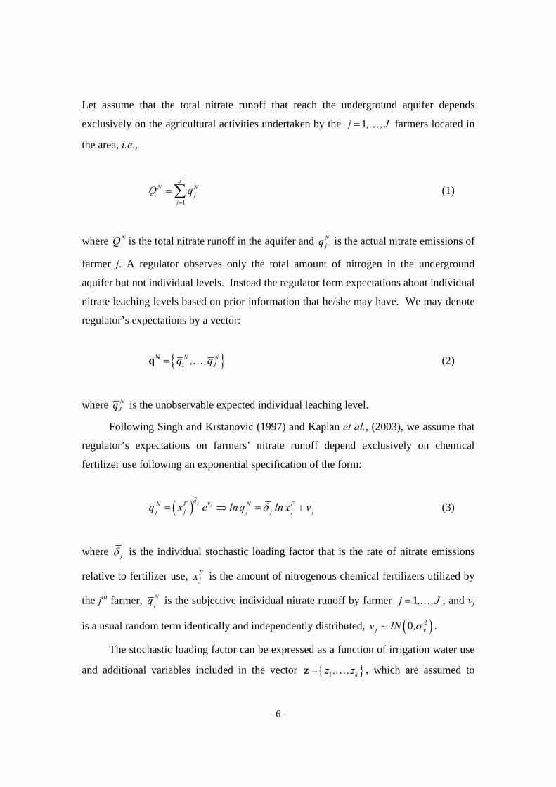
Let assume that the total nitrate runoff that reach the underground aquifer depends

exclusively on the agricultural activities undertaken by the 1j , ,J= … farmers located in

the area, i.e.,

1

JN N

jj

Q q=

=∑ (1)

where NQ is the total nitrate runoff in the aquifer and Njq is the actual nitrate emissions of

farmer j. A regulator observes only the total amount of nitrogen in the underground

aquifer but not individual levels. Instead the regulator form expectations about individual

nitrate leaching levels based on prior information that he/she may have. We may denote

regulator’s expectations by a vector:

{ }1N N

Jq , ,q=Nq … (2)

where NJq is the unobservable expected individual leaching level.

Following Singh and Krstanovic (1997) and Kaplan et al., (2003), we assume that

regulator’s expectations on farmers’ nitrate runoff depend exclusively on chemical

fertilizer use following an exponential specification of the form:

( ) j jvN F N Fj j j j j jq x e ln q ln x v

δδ= ⇒ = + (3)

where jδ is the individual stochastic loading factor that is the rate of nitrate emissions

relative to fertilizer use, Fjx is the amount of nitrogenous chemical fertilizers utilized by

the jth farmer, Njq is the subjective individual nitrate runoff by farmer 1j , ,J= … , and vj

is a usual random term identically and independently distributed, ( )20j vv ~ IN ,σ .

The stochastic loading factor can be expressed as a function of irrigation water use

and additional variables included in the vector { }1 kz , ,z=z … , which are assumed to

- 7 -

influence the managerial ability of the farmers, and thus affect individual nitrate runoff,

i.e.,

Wj j jx uδ γ′= + +jβ z (4)

where xW is the applied irrigation water and uj is the usual error term ( )20j uu ~ IN ,σ ,

which is independent of vj in relation (3). The only observables we have, are the vector z,

the chemical fertilizer application ( )Fjx , the irrigation water use ( )W

jx and the total

nitrate accumulation in the aquifer ( )NQ .

The model, as it stands, cannot be estimated as we only have one observation, NQ ,

but 1J k+ + parameters while we do not have a dependent variable in the traditional

sense. One modification is to replace the total nitrate accumulation in the underground

aquifer by:

1

JN N

jj

Q q ω=

= +∑ (5)

where ω is a standard error term, ( )20 ωω σ~ IN , . This modification gives rise to the

following hierarchical representation of the model:

2N Nj

jQ ~ N q , ωσ

⎛ ⎞⎜ ⎟⎝ ⎠∑Nq (6)

( )2N F Fj j j j j vln q ln x , ~ N ln x ,δ δ σ (7)

( )2, ~ ,W Wj j j ux N xδ γ σ′ +j jz β z (8)

From the above, it is easy to construct the following density function:

- 8 -

( )

( )

( )

2

1 2

2 2

2 2

2

2

2

N N F W N Nj

j

j N F Nv j j j v j

j j

j Wu j j u

j

p Q ,q , x ,x , , exp Q q

exp ln q ln x ln q

exp x

ω ωδ σ σ

σ δ σ

σ δ γ σ

−

−

−

⎡ ⎤⎛ ⎞⎢ ⎥= − −⎜ ⎟⎢ ⎥⎝ ⎠⎣ ⎦

⎡ ⎤− − −⎢ ⎥⎣ ⎦⎡ ⎤

′− − −⎢ ⎥⎣ ⎦

∑

∑ ∑

∑ j

z θ

β z

(9)

with { }, , ,v uγ σ σ=θ β being the parameter vector for a given value of ωσ . The marginal

density of jδ can be obtained as:

( ), , ,N F Wp Q x x =z θ ( )N N F W Np Q ,q , x ,x , , dq dδ δ∫ z θ (10)

and is the density of the dependent variable given the observed covariates. It is clear that

as ωσ approaches zero, the distribution with density ( ),N F Wp Q x x , z,θ approaches

continuously the distribution whose density corresponds to exact aggregation,

1

JN N

jj

Q q=

= ∑ .

Although jδ can be integrated out analytically from ( )N N F Wp Q ,q , x ,x , ,δ z θ ,

Njq cannot, because of the log-normality assumption. Indeed completing the square with

respect to jδ , it is not difficult to show that:

( )

2

122ωω

σσ

−

⎡ ⎤⎛ ⎞⎢ ⎥−⎜ ⎟⎢ ⎥⎝ ⎠= − −⎢ ⎥⎢ ⎥⎢ ⎥⎣ ⎦

∑∑z θ

N Nj

jN N W F Nj

j

Q lnqp Q ,q x ,x , , exp lnq

- 9 -

( )

( )( )

( )

22 2 22

22 2122 222 2 2 2

12

Nu j v j

jwu j vw

u j vwjj

v u u j v

ln q z

xx exp

x

σ σδ

σ σσ σ

σ σ σ σ

−

⎡ ⎤+⎢ ⎥−⎢ ⎥+⎡ ⎤ ⎢ ⎥+ −⎢ ⎥⎣ ⎦ ⎢ ⎥⎡ ⎤+⎢ ⎥⎢ ⎥⎣ ⎦⎢ ⎥⎣ ⎦

∑∏ (11)

which is clear that further analytical integration with respect to the Njq is not possible.

To proceed let suppose that a prior, ( )p θ , has been selected for the structural parameters,

θ. The posterior distribution, by Bayes’ theorem is given by ( )θ zN F Wp Q ,x ,x ,

( ) ( )= θ z θN F Wp Q ,x ,x , p where ( )θ zN W Fp Q ,x ,x , plays the role of likelihood. Since

( )N W Wp Q ,x ,x , =θ z ( )N N W F Np Q ,q , x ,x , dq dδ δ∫ z,θ , we also have:

( ) ( ) ( )( )

N F W N F W N N F W

F W N

p Q ,x ,x , p Q x ,x , , ,q , p q x ,x , ,

p x ,x , , dq d

δ

δ δ

= ∫θ z z θ z θ

z θ (12)

where ( )N F Wp q x ,x , ,z θ and ( )F Wp x ,x , ,δ z θ represent the prior distributions of Njq

and δ . The priors are as follows: ( )1k~ N ,γ +

⎡ ⎤≡ ⎢ ⎥⎣ ⎦

-1βΔ Δ Δ , ( )2

2v

vv

~ nε χσ

and

( )22u

uu

~ nε χσ

, where, Δ and -1Δ are, respectively, the prior mean and precision of the

regression coefficients, Δ . The prior is flexible enough to accommodate a wide range of

prior beliefs and (for scale parameters) have the interpretation that in a fictitious

experiment with vn observations the residual sum of squares is equal to vε . To

implement Bayesian inference, we use the Gibbs sampler with data augmentation.

The posterior conditional distributions in our model, are as follows. For the

regression parameters:

- 10 -

( )1N F W N

v u j kˆ, ,q , ,x ,x ,z,Q ~ N ,σ σ δ +Δ Δ V (13)

where ( ) ( )12 2u u

ˆ σ σ−

= + +Δ D'D Δ D'δ ΔΔ , ( ) 12uσ

−= +V D'D Δ , and Fx⎡ ⎤= ⎣ ⎦D z .

For the scale parameters:

( ) ( ) ( )22

N F N Fv N F N

u vv

ln q ln x ln q ln x, ,q , ,x , ,Q ~ n n

δ δ εσ δ χ

σ

′− − ++Δ z (14)

and

( ) ( ) ( )22

v N F W Nv u

u

, ,q , ,x ,x , ,Q ~ n nδ δ ε

σ δ χσ

′− − ++

DΔ DΔΔ z (15)

The posterior conditional distribution of the latent variable jδ is

( )2N F W Nj v u j j,q , , ,x ,x , ,Q ~ N ,s jδ σ σ δ ∀Δ z (16)

where ( )

( )

2 2

22 2

F N Wu j j v j

j Wu j v

x ln q x

x

σ σ γδ

σ σ

′+ +=

+

iβ z, and

( )2 2

222 2

v uj W

u j v

sx

σ σ

σ σ=

+ j∀ .

Accordingly, the posterior conditional distribution of Njq is

( ) ( ) ( )2 2

2 22 2

N N N Fj l j j jN F W N N

j j ju

q Q ln q ln xp q , ,x ,x , ,Q exp ln q

ω

δδ

σ σ

⎡ ⎤− −⎢ ⎥= − − −⎢ ⎥⎣ ⎦

Δ z (17)

- 11 -

j∀ where N N Nl j

j lQ Q q

≠

= −∑ . This distribution is non-standard and is generated using

Metropolis sampling. We generate a candidate draw ( )2~ , ωσN

ie N Q and accept the

draw with probability

( )

( )

( )

2

2

2

2

21

2

Fi j j

jv

j jF

j j jj

v

ln e ln xexp lne

P e ,e min , lne ln x

exp lne

δσ

δσ

⎧ ⎫⎡ ⎤−⎪ ⎪⎢ ⎥− −⎪ ⎪⎢ ⎥⎪ ⎪⎣ ⎦= ⎨ ⎬

⎡ ⎤⎪ ⎪−⎢ ⎥− −⎪ ⎪⎢ ⎥⎪ ⎪⎣ ⎦⎩ ⎭

(18)

where je represents the current draw. The reason behind the choice of a normal proposal

distribution, is that for most reasonable choices of the parameters the overall distribution

of Njq is approximated rather well by a bell-shaped curve centered tightly around the

value of NQ .

Model Validation and Empirical Estimation

Simulation with Artificial Data

To validate the econometric procedure suggested herein for the estimation of individual

nitrate leaching levels we run a simulation on generated artificial data sets. The number

of farms included in the simulation were assumed to be 100 (i.e., 100=J ) while the

number of exogenous variables included in the z vector were imposed to be three (k=3).

The values of the parameters in relation (4) were set [ ]1,1,1 ′=β , 1γ = while the

associated variance in relations (3) and (4) were set to 0.1v uσ σ= = . Finally, the

variance term in (5) was set to 0.01ωσ = and the difference between QN and the sum of

the simulated individual nitrate emissions, Njq , was of the order of 810− in order to ensure

exact aggregation for practical purposes. We have used Gibbs sampling with 15,000

iterations, the first 10,000 of which are discarded to mitigate the impact of start up

- 12 -

effects. The final sample was checked for convergence to the posterior using Geweke’s

(1992) diagnostic, and convergence could not be rejected.

We have used rather diffuse priors with 10Δ += k , 0 001Δ = k +1I. , 0 01ε ε= =v u . ,

and 1v un n= = . In Figure 1 we present the marginal posteriors of the structural

parameters of the model arising from a typical simulation. The correlation coefficients

between the actual and estimated values of individual loading factors and nitrate leaching

levels were about 0.90. The estimates of individual loading factors jδ were obtained as

( )11

S sj js

Sδ δ−=

= ∑ , where S is the number of Gibbs passes, and ( )sjδ is the draw for jδ

during the sth pass. A similar procedure was followed to obtain the estimate of individual

nitrate leaching levels, Njq . From the marginal posteriors presented in Figure 1, it is clear

that these are reasonable concentrated around the true values of the parameters although

they cannot be taken as normal. This emphasizes the need for data-specific small-sample

procedures, like the Bayesian approach we have proposed and implemented here.

In Figure 2, we present marginal posteriors of the same parameters obtained

through 20 different simulated data sets using the same priors used in the construction of

Figure 1. The purpose of Figure 2 is to provide an idea about the range of variation (over

alternative data sets) that should be expected. There is some definite evidence of

nonnormality and even multimodality in these posteriors, owing most likely to the small

sample size used. This makes the point for exact finite sample Bayesian inference even

more important and relevant to the problem at hand.

Data Description

The data used in this study come from a broader survey of the structural characteristics of

the agricultural sector on the Greek island of Crete, financed by the Regional Directorate

of Crete. Detailed information about production patterns, input use, average yields, gross

revenues, and structural characteristics of the surveyed farms were obtained via

questionnaire-based, field interviews. Summary statistics for these variables are reported

in Table 1. The sample consists of 265 randomly selected multi-output farms located in

the Ierapetra Valley during the 1999-00 cropping season. Farms in the sample were

spitted into four sub-samples according to their location relative to the four major

- 13 -

underground aquifers existing in the area. We have done so in order to mitigate the

biases arising from incomplete information concerning the general environmental

conditions in these areas that may affect individual nitrate emissions. As it is shown from

Table 1, nitrate levels exhibit a significant variation across aquifers which may not be

explained from the associated differences in soil quality and/or farmer’s characteristics.

Specifically, nitrates vary from a minimum of 8.8 mg/lt in Region 3 to a maximum of

19.7 mg/lt in Region 2.8

Greenhouse farms in the sample are producing four different vegetables namely,

cucumbers, tomatoes, eggplants and peppers. On the average farms are producing 20,387

kgs of vegetables, the 32.8% of which are cucumbers, the 33.4% tomatoes, the 13.7%

eggplants and the rest 20.1% peppers. A significant variation is observed concerning

crop mix across regions. Farmers in region 1 and 4 are specialized in cucumber and

peppers production, whereas farms in Regions 2 and 3 are mainly cultivating tomatoes

and eggplants. The average farm size is 5 stremmas (1 stremma equals 0.1 ha) with

significant interregional variability while on the average farms are using 1,962 kgs of

chemical fertilizers (mainly enriched in nitrogen) and 164 m3 of water for irrigation

purposes. The average age of the owner is 49 years varying from a minimum of 23 to a

maximum of 85. On the average Cretan farmers are having 8 years of formal education

while the 47.4% of the cultivated area is on sandy soils which exhibit high nitrate

leaching capacity, the 13.6% on lime stones, the 21.2% on marls and the 17.8% on

dolomites.

Empirical Application

For the empirical application in Ierapetra Valley, Bayesian inference using Gibbs

sampling with data augmentation has been implemented using 150,000 iterations, the first

50,000 of which are discarded to mitigate the impact of start up effects.9 Convergence

has been diagnosed using Geweke’s (1992) and has been found in all cases. Our

regressors included in vector z were: an aridity index defined as the average annual

temperature over the total annual precipitation (Stallings, 1960), farmer’s age and level of

formal education measured in years and four soil dummies (sandy, limestones, marly, and

dolomitic) to capture the effect of soil quality on nitrate emissions.10 As a prior we have

- 14 -

chosen a multivariate normal centered at zero with covariance matrix 1kc I +× , with

10c = . This prior is rather flat and implies essentially no special prior knowledge about

the parameters. Estimates of individual stochastic loading factors and nitrate emissions

levels have been obtained through the usual Rao-Blackwell procedure. This include the

averaging of the draws for both variables across Gibbs iterations after the burn–in phase

has been completed. This procedure yields the posterior means which were taken as the

final estimates of these parameters. Kernel densities for each one of them, across both

farms and regions, are reported in Figures 3 and 4, while the posterior results are

summarized in Table 2. Posterior standard deviations are known to be invalid since Gibbs

draws are dependent (i.e., autocorrelated). To deal with this, we have retained only one

every after the tenth draw, while the Newey and West covariance matrix with five lags

was utilized.

In Figure 5, we present the marginal posterior densities of each regression

parameter by region. Some of these densities are distinctly nonnormal and for some

parameters the assumption that they are the same across region cannot be seriously

maintained. Specifically, the marginal posterior densities for the parameters associated

with farmer’s age and education as well as with irrigation water use. are quite different

across regions (see the second and the last graph in Figure 5). Finally, we have

performed sensitivity analysis with respect to the priors. The critical parameter in our

case is the prior precision each one of the regression coefficients. The baseline prior

precision is given by 0.1 times an identity matrix so we investigated the effect when the

respective parameter varies between 0.01 and 10 and the prior mean vector (which

initially was set to zero) varies within the [ ]2 2,− range.

Next we have generated 500 different configurations of the priors by drawing

values uniformly within these intervals, i.e., [ ]0 01 10. , and [ ]2 2,− . This resulted in 500

different posteriors for the associated parameters of the model. In order to reduce the

computational burden the Sampling–Importance–Resampling (SIR) technique was

applied (Rubin, 1988; Smith and Gelfand, 1992). The SIR technique exploits the

availability of the baseline sample from the posterior (which corresponds to the baseline

prior) and transforms this sample to an approximate sample from a new posterior, which,

- 15 -

in our case, results from the new prior. Specifically, suppose that { }1 J,...,θ θ=θ is a

sample from a distribution whose kernel density is given by ( )π θ . In order to obtain a

sample with distribution whose kernel density is ( )h θ , we computed the weights

( ) ( )j j jhψ θ π θ= , and j j jj

Ψ ψ ψ= ∑ . Then we sample with replacement from the

discrete distribution whose support is { }1 J,...,θ θ=θ and the probabilities are the jΨ s. In

our case we have a sample from a posterior distribution ( ) ( ) ( )p | L ;Y p=θ Y θ θ and we

need a sample from the new posterior ( ) ( ) ( )1 1p | L ; p=θ Y θ Y θ , where ( )1p θ is the new

prior. Thus, we have to resample the posterior draws with probabilities that are

proportional to ( ) ( )1p pθ θ , that is the ratio of the priors. Since the prior is multivariate

normal, computing these ratios is straightforward. To implement SIR, we have drawn a

sample of size 1,000 for each prior. That is, the new approximate posterior sample

consists of 1,000 draws. The original posterior sample has size 10,000 since we have

retained only every tenth draw to mitigate autocorrelation induced by the nature of the

Gibbs sampling process. After each new sample the new posterior mean was computed.

The kernel densities of these posterior means minus the baseline posterior means are

reported in Figure 6. These densities are heavily concentrated around zero, which means

that the posterior results are rather robust to changes in the prior distribution.

Concerning the posterior results of the parameters estimates summarized in Table

2 and Figures 3 and 4 the following emerges. In all regions the estimated loading factors

are positively associated with irrigation water use and the general environmental

characteristics of the region as measured by the aridity index, whereas farmer’s age and

education level seem to reduce individual loading factors. Specifically, mean posterior

estimate for irrigation water ranges between 0.437 in the second region and 0.576 in the

third region exhibiting the largest influence in individual loading factors. The second

highest contribution arises from sandy soils which was rather expected. Percolation in

these soils is much easier than limestones or marls, while the corresponding estimate for

dolomite soil is statistically insignificant (in fact in the first and fourth region the mean

posterior turned to negative value). The aridity index (i.e., average temperature over

- 16 -

precipitation) has also an important contribution as the associated mean posteriors are

around 0.2 in all four regions under consideration. Finally, the two human capital

variables, farmer’s age (as a proxy of experience) and education level affect negatively

individual nitrate loading factors. The highest impact arises from formal education which

ranges between -0.162 and -0.185, while farmer’s age has a lower but significant effect, -

0.042 in the second region and -0.061 in the first. According to human capital theory,

these variables, are associated with the resource allocation skills of farm operators

(Schultz 1972; Huffman 1977). A farmer with a high level of resource allocation skills

will make more accurate predictions of fertilizer use and will thus make more efficient

decisions.

Concerning individual loading factors, mean posterior estimates increase with

chemical fertilizer use exhibiting a relative consistency with the observed data. The

variation though across regions is significant with the highest value being in the fourth

region (1.715) and the lowest in second (1.198). In the rest two regions both the mean

values and relative distribution is similar (mean values are 1.301 and 1.427 in the first

and third region, respectively). The estimated individual nitrate leaching levels computed

using individual loading factors, chemical fertilizer use and relation (3) indicate that

farms in the fourth region emit more nitrates in the underground aquifer (0.275 mg/lt),

followed by those in the first region (0.230 mg/lt), in the second (0.221 mg/lt), while in

the third region farmers pollute less (0.144 mg/lt). However, as it is indicated from

Figure 4, the variation across farms is high in regions 1, 2 and 4 and very low in the

remaining third region.

Concluding Remarks

In this paper we have argued that Bayesian inference can be well applied to transform a

NPS pollution problem into a point source one by estimating individual emission

functions. We have shown that our approach performs quite well even for small sample

sizes while the posterior results are rather robust to changes in the prior distribution.

These results suggest that our method could provide a basis for regulating agricultural

NPS pollution problems by conventional instruments such as emission taxes or emission

limits which are associated with individual farmer’s actions.

- 17 -

- 18 -

References

Braden, J.B. and K. Segerson (1993). Information Problems in the Design of Nonpoint Pollution. In Russell, C.S. and J.F. Shorgen (eds), Theory, Modeling and Experience in the Management of Nonpoint Source Pollution. Dortrecht: Kluwer Academic Press.

Cabe, R. and J. Herriges (1992). The Regulation of Nonpoint Source Pollution Under Imperfect and Asymmetric Information. J. Env. Econ. Man., 22: 134-146.

Chambers R.G. and J. Quiggin (1996). Nonpoint Source Pollution Regulation as a Multi-Task Principal Agent Problem. J. Pub. Econ., 59: 95-116.

Classen R. and R.D. Horan (2001). Uniform and Non-Uniform Second-Best Input Taxes: The Significance of Market Price Effects on Efficiency and Equity. Env. Res. Econ. 19: 1-22.

Common, M. (1977). A Note on the Use of Taxes to Control Pollution. Scand. J. Econ., 79: 345-349.

Dinar, A., Knapp, K.C. and J. Lettey (1989). Irrigation Water Pricing to Reduce and Finance Subsurface Drainage Disposal. Agr. Wat. Man., 16: 155-171.

Fleming R.A. and R.M. Adams (1997). The Importance of Site-Specific Information in the design of Policies to Control Pollution. J. Env. Econ. Manag., 33: 347-358.

Geweke J. (1992). Evaluating the Accuracy of Sampling Based Approaches to the Calculation of Posterior Moments, in Berger J.O., J.M. Bernardo, A.P. Dawid and A.F.M. Smith (Eds.), Proceedings of the Fourth Valencia International Meeting on Bayesian Statistics: 169-194, Oxford University Press.

Govindasamy, R., Herriges, J. and J. Shorgen (1994). Nonpoint Tournaments. In C. Dosi and T. Tomasi (eds), Nonpoint Source Pollution Regulation: Issues and Analysis. Dortrecht: Kluwer Academic Press.

Griffin, R.C. and D.W. Bromley (1982). Agricultural Runoff as a Nonpoint Externality: A Theoretical Development. Am. J. Agr. Econ., 64: 547-552.

Hayami, Y. and V.W. Ruttan (1985). Agricultural Development: An International Perspective. Baltimore: John Hopkins Univ. Press.

Helfand G.E. and B.W. House (1995). Regulating Nonpoint Source Pollution under Heterogeneous Conditions. Am. J. Agr. Econ., 77: 1024-1032.

Holtermann, S. (1976). Alternative Tax-Systems to Correct Externalities and the Efficiency of Paying Compensation. Economica, 46:1-16.

Horan, R.D., Shortle, J.S. and D.G. Abler (1999). Green Payments for Nonpoint Pollution Control. Am. J. Agr. Econ., 81: 1210-1215.

Huffman, W.E. (1977). Allocative Efficiency: The Role of Human Capital. Quart. J. Econ., 91: 59-79.

- 19 -

Isik M. (2004). Incentives for Technology Adoption under Environmental Policy Uncertainty: Implications for Green Payment Programs. Env. Res. Econ., 27: 247-263.

Johnson S.L., R.M. Adams and G.M. Perry (1991). The On-farm Costs of Reducing Groundwater Pollution. Am. J. Agr. Econ., 73: 1063-1073.

Kaplan, J.D., Howitt, R.E. and Y.H. Farzin (2003). An Information-Theoretical Analysis of Budget-Constrained Nonpoint Source Pollution Control. J. Env. Econ. Man., 46: 106-130.

Lichtenberg, E. (1992). Alternative Approaches to Pesticide Regulation. North. J. Agr. Res. Econ., 21: 83-92.

Meade, J.E. (1952). External Economies and Diseconomies in a Competitive Situation. Econ. J., 62: 54-67.

Miceli, T. and K. Segerson (1991). Joint Liability in Torts and Infra-Marginal Efficiency. Int. Rev. Law Econ., 11:235-249.

Millock K., D. Sunding and D. Zilberman (2002) Regulating Pollution with Endogenous Monitoring. J. Env. Econ. Manag., 44: 221-241.

Novotny, V. and H. Olem (1994). Water Quality: Prevention, Identification and Management of Diffuse Pollution. New York: Van Nostrand Reinhold.

Owen O.S., D.D. Chiras and J.P. Reganold (1998). Natural Resources Conservation, Prentice Hall: New York.

Rubin, D.B. (1988) Using the SIR algorithm to Simulate Posterior Distributions, in Bayesian Statistics 3, J.M. Bernardo, M.H. DeGroot, D.V. Lindley, and A.F.M. Smith (Eds.), Oxford: Oxford University Press, 395-402.

Schultz, T.W. (1972). The Increasing Economic Value of Human Time. Am J. Agr. Econ., 54: 843-850.

Segerson, K. (1988). Uncertainty and Incentives for Nonpoint Pollution Control. J. Env. Econ. Manag., 15: 87-98.

Shortle J.S., R.D. Horan and D.G. Abler (1998). Research Issues in Nonpoint Pollution Control. Env. Res. Econ., 11: 571-585.

Shortle, J.S. and D.G. Abler (1994). Incentives for Agricultural Nonpoint Pollution Control. In Graham-Tomasi, T. and C. Dosi (eds), The Economics of Nonpoint Pollution Control: Theory and Issues. Dortrecht: Kluwer Academic Press.

Shortle, J.S. and D.G. Abler (1997). Nonpoint Pollution. In Folmer, H. and T. Tietenberg (eds), International Yearbook of Environmental and Natural Resource Economics. Cheltenham, UK: Edward Elgar.

Shortle, J.S. and R.D. Horan (2001). The Economics of Nonpoint Pollution Control. J. Econ. Surveys, 15: 255-289.

Shumway, R. (1995). Recent Duality Contributions in Production Economics. J. Agr. Res. Econ., 20: 178-194.

- 20 -

Singh, V.P. and P.F. Krstanovic (1997). A Stochastic Model for Sediment Yield Using the Principle of Maximum Entropy. Wat. Res. Research, 23: 781-793.

Smith, A.F.M., and A.E. Gelfand (1992) Bayesian Statistics Without Tears: A Sampling-Resampling Perspective. Am. Stat., 46: 84-88.

Smith, R.B.W. and T.D. Tomasi (1995). Transaction Costs and Agricultural Nonpoint Source Water Pollution Control Policies. J. Agr. Res. Econ., 20: 277-290.

Stallings, J.L. (1960). Weather Indexes. J. Farm Econ., 42: 180-86.

Stevens, B. (1988). Fiscal Implications of Effluent Charges and Input Taxes. J. Env. Econ. Man., 15: 285-296.

Tomasi, T., Segerson, K. and J. Braden (1994). Issues in the Design of Incentives Schemes for Nonpoint Source Pollution Control. In C. Dosi and T. Tomasi (eds), Nonpoint Source Pollution Regulation: Issues and Analysis. Dortrecht: Kluwer Academic Press.

Weersink, A., Livernois, J., Shorgen, J.F. and J.S. Shortle (1998). Economic Instruments and Environmental Policy in Agriculture. Can. Pub. Policy, 24: 309-327.

Wu, J. and B. Babcock (1996). Contract Design for the Purchase of Environmental Goods from Agriculture. Am. J. Agr. Econ., 78: 935-945.

Xepapadeas A. (1991). Environmental Policy under Imperfect Information: Incentives and Moral Hazard, J. Env. Econ. Manag., 20: 113-126.

Xepapadeas A. (1992). Environmental Policy Design and dynamic Nonpoint Source Pollution. J. Env. Econ. Manag., 23: 22-39.

Xepapadeas, A. (1999). Nonpoint Source Pollution. In J. van den Bergh (ed), Handbook of Environmental and Resource Economics. Cheltenham UK: Edward Elgar.

- 21 -

Table 1. Summary Statistics of the Variables. Variable Region 1 Region 2 Region 3 Region 4

Economic Data:

Output (kgs) 21,182 20,134 18,092 23,091

Cucumbers (%) 36.9 25.9 29.8 37.1

Tomatoes (%) 27.2 37.3 36.1 25.4

Eggplants (%) 11.3 21.2 16.1 10.9

Peppers (%) 24.7 15.5 17.9 26.5

Area (stremmas) 5.5 4.3 6.2 3.9

Chemical Fertilizers (kgs) 2,012 1,892 1989 1,998

Irrigation Water (m3) 178 159 162 166

Nitrates in the Aquifer (mg/lt) 13.6 19.7 8.8 15.4

Age (years) 51 44 46 53

Education (years) 7 11 8 6

Aridity Index 1.323 1.365 1.356 1.345

Soil Type (% of Farm Land)

Sandy 46.5 47.6 42.3 51.0

Limestone 12.5 13.0 11.2 15.7

Marls 19.1 20.0 22.3 19.1

Dolomites 21.9 19.3 24.1 14.3

No of observations 59 89 61 56

- 22 -

Figure 1. Marginal Posterior Distributions in an Artificial Data Set

- 23 -

Figure 2. Marginal Posterior Distributions from Twenty Different Artificial Data Sets

- 24 -

Table 2. Posterior Results for the Four Regions. Par. Region 1 Region 2 Region 3 Region 4

βARD 0.219 (0.082) 0.191 (0.079) 0.218 (0.081) 0.212 (0.084)

βAGE -0.061 (0.009) -0.042 (0.009) -0.052 (0.008) -0.049 (0.010)

βEDU -0.162 (0.037) -0.163 (0.036) -0.185 (0.037) -0.183 (0.045)

βS1 0.454 (0.079) 0.407 (0.078) 0.432 (0.091) 0.444 (0.084)

βS2 0.246 (0.084) 0.211 (0.077) 0.218 (0.090) 0.262 (0.083)

βS3 0.227 (0.085) 0.249 (0.079) 0.240 (0.088) 0.234 (0.084)

βS4 -0.005 (0.080) 0.025 (0.079) 0.032 (0.090) -0.015 (0.089)

Γ 0.567 (0.085) 0.437 (0.091) 0.576 (0.099) 0.560 (0.096) Nq 0.230 (0.091) 0.221 (0.092) 0.144 (0.048) 0.275 (0.139)

δ 1.301 (0.600) 1.198 (0.530) 1.427 (0.739) 1.715 (0.804)

Note: The table reports posterior means. Posterior standard deviations appear in parentheses. For qN, reported is the sample average of Bayesian estimates of the individual values and the sample standard deviation appears in parentheses. The same practice is follows for δ. ARD stands for aridity index, AGE for farmer’s age, EDU for farmer’s education level and S1-S4 for the four soil dummies.

- 25 -

Figure 3. Posterior Mean Estimate of Loading Factors jδ .

Figure 4. Posterior Mean Estimate of Leaching Levels N

jq .

- 26 -

Figure 5. Marginal Posterior Densities of Parameters by Region.

- 27 -

Figure 6. Sensitivity Analysis with Respect to the Prior (500 alternative prior distributions)

- 28 -

Endnotes

1 Nitrogen flows are also associated with soil and air pollution. In particular soil is at a

high risk of eutrophication in cases where excessive nitrogen deplete oxygen in the soil,

affecting micro-organisms proper functioning and soil’s fertility. Eutrophied soils are

also a source of N2O - a powerful greenhouse gas. 2 Detailed reviews of the major issues underlying the economics of nonpoint pollution

control can be found in Tomasi et al., (1994), Shortle et al., (1998) and Shortle and

Horan (2001). 3 The seminal work by Segerson (1988) has been widely refined even since. Xepapadeas

(1991) suggested a scheme of subsidies and random fines aimed to eliminate the moral

hazard problems with budget balancing contracts, while Xepapadeas (1992), developed

dynamic ambient taxes under strategic interactions. Govindasamy et al., (1994) proposed

a nonpoint tournament while Cabe and Herriges (1992) and Horan et al., (1999) explore

the consequences of asymmetric prior information about profit and environmental types.

Finally, Miceli and Segerson (1991) suggested the introduction of liability rules among

parties that actually create incentives that are similar to the ones created by ambient

taxes. However, as noted by Lichtenberg (1992), liability rules are best suited for the

control of hazardous pollution or non-frequent occurrences of environmental degradation

like oil spills. 4 In addition, Shortle and Horan (2001) noted that ambient incentives are effective in the

case of only a single pollutant. With multiple pollutants particularly when they interact,

the decision environment is much more complex and ambient taxes are not appropriate. 5 Meade (1952) was the first who extend these output-oriented policies to inputs by

postulating that externality levels may be dependent on the amount of factors of

production employed. Several years later Holterman (1976) and Common (1977)

extended the theoretical framework suggesting a complete tax/subsidy system to correct

the generated externalities. 6 Wu and Babcock (1996) and Smith and Tomasi (1995) develop a mechanism design

approach to induce land-based nonpoint polluters to choose second-best input vectors

assuming heterogeneous farm population exploiting the same surface. However, both

- 29 -

studies are focused only on adverse selection problems assuming that input choices made

by farmers can be observed costless. 7 Novotny and Olem (1994) discuss the most widely used models of that kind that are

available for agriculture, urban and other nonpoint sources. 8 The required data of nitrate pollution in the aquifers were obtained from the local water

authorities of Ierapetra and refer to the same year that the survey was conducted. 9 We have also tried to use 500,000 passes. The posterior results remained virtually the

same. This is expected since relative numerical efficiency is rather high in this

application. For the concept of relative numerical efficiency and its place in Bayesian

computation, see Geweke (1992). 10 One may think of several other factors affecting individual stochastic nitrate loading

factor. However, our choice has been determined by data availability.