University of ConnecticutDigitalCommons@UConn

Economics Working Papers Department of Economics

1-1-2003

Nonpoint Pollution Control: Inducing First-bestOutcomes through the Use of ThreatsKathleen SegersonUniversity of Connecticut

JunJie WuOregon State University

Follow this and additional works at: http://digitalcommons.uconn.edu/econ_wpapers

This is brought to you for free and open access by the Department of Economics at DigitalCommons@UConn. It has been accepted for inclusion inEconomics Working Papers by an authorized administrator of DigitalCommons@UConn. For more information, please contactdigitalcommons@uconn.edu.

Recommended CitationSegerson, Kathleen and Wu, JunJie, "Nonpoint Pollution Control: Inducing First-best Outcomes through the Use of Threats" (2003).Economics Working Papers. Paper 200303.http://digitalcommons.uconn.edu/econ_wpapers/200303

Department of Economics Working Paper Series

Voluntary Approaches to Nonpoint Pollution Control: InducingFirst-best Outcomes through the Use of Threats

Kathleen SegersonUniversity of Connecticut

JunJie WuOregon State University

Working Paper 2003-03

January 2003

341 Mansfield Road, Unit 1063Storrs, CT 06269–1063Phone: (860) 486–3022Fax: (860) 486–4463http://www.econ.uconn.edu/

AbstractIn this paper we develop a simple economic model to analyze the use of a pol-

icy that combines a voluntary approach to controlling nonpoint-source pollutionwith a background threat of an ambient tax if the voluntary approach is unsuc-cessful in meeting a pre-specified environmental goal. We first consider the casewhere the policy is applied to a single farmer, and then extend the analysis to thecase where the policy is applied to a group of farmers. We show that in eithercase such a policy can induce cost-minimizing abatement without the need forfarm-specific information. In this sense, the combined policy approach is not onlymore effective in protecting environmental quality than a pure voluntary approach(which does not ensure that water quality goals are met) but also less costly thana pure ambient tax approach (since it entails lower information costs). However,when the policy is applied to a group of farmers, we show that there is a potentialtradeoff in the design of the policy. In this context, lowering the cutoff level of pol-lution used for determining total tax payments increases the likely effectiveness ofthe combined approach but also increases the potential for free riding. By settingthe cutoff level equal to the target level of pollution, the regulator can eliminatefree riding and ensure that cost-minimizing abatement is the unique Nash equi-librium under which the target is met voluntarily. However, this cutoff level alsoensures that zero voluntary abatement is a Nash equilibrium. In addition, withthis cutoff level the equilibrium under which the target is met voluntarily will notstrictly dominate the equilibrium under which it is not. We show that all resultsstill hold if the background threat instead takes the form of reducing governmentsubsidies if a pre-specified environmental goal is not met.

Keywords: ambient taxes, nonpoint-source pollution control, cost-minimizingabatement, voluntary approach

Voluntary Approaches to Nonpoint Pollution Control: Inducing First-best Outcomes through the Use of Threats

I. INTRODUCTION

While concerns about pollution control originally focused on point sources of pollution,

attention has now turned to the control of diffuse or nonpoint-source pollution (NPP).1 Control

of NPP is hampered by the fact that emissions of pollutants are not readily observable given their

diffuse nature, which implies that traditional policy instruments based on emissions (e.g.,

emissions taxes or regulation) cannot be used in this context. This has lead economists to

consider alternative policy instruments for the control of NPP, including input taxes, input

regulations, ambient taxes, random fines, and type-specific contracts (Griffin and Bromley 1982;

Shortle and Dunn 1986; Segerson 1988, Xepapadeas 1991, 1992, 1995; Cabe and Herriges 1992;

Herriges et al. 1994; Govindasamy et al. 1994; and Shortle and Abler 1994). Instruments that

provide flexible incentives (such as ambient taxes) can be used to induce first-best control of

NPP (Segerson 1988), but information about farm-level charactertistics is needed to design these

first-best policy instruments. They have thus been criticized as being likely to involve high

information and/or transactions costs (e.g., Cabe and Herriges 1992; Batie and Ervin 1997). This

has led some to suggest the use of second best policy instruments instead (Helfand and House

1995; Wu and Babcock 1995, 1996; Wu, et al. 1995). Use of these second best instruments

involves a tradeoff. While transaction and information costs may be lower, these instruments do

not achieve the targeted water quality level at the minimum abatement cost.

In contrast to the theoretical literature of NPP, water quality policy has historically been

based on the use of "carrot" instruments designed to entice farmers to use environmentally-

friendly practices voluntarily or to participate in voluntary programs aimed at improving water

1

quality.2 However, the varying success rates of voluntary programs have led some to question

whether reliance on voluntary measures alone will adequately control agricultural pollution

(Ribaudo and Caswell 1997), suggesting the need for mandatory controls or incentives to ensure

adequate environmental protection. Yet, as noted above, mandatory controls3 generally have

drawbacks in terms of inflexibility (in the case of second-best instruments) or high transaction or

information costs (for first-best instruments). Thus, neither purely voluntary programs nor

mandatory approaches by themselves seem to offer a desirable "solution" to agricultural NPP.

There is, however, an alternative role for voluntary and mandatory approaches to NPP,

namely, as complementary instruments to be used together rather than as substitutes to be used in

isolation. As has become apparent in the context of point source pollution, the threat of the

imposition of mandatory controls can be an effective mechanism for inducing firms to participate

in voluntary agreements (Segerson and Miceli 1998), while voluntary approaches have the

potential to provide greater flexibility in meeting environmental quality goals and hence lower

compliance and transaction costs (Commission of the European Communities 1996).

A few states have experimented with the use of mandatory approaches as threats to be

invoked if reliance on voluntary measures is insufficient to control nonpoint source pollution,

and the threat of regulation has been shown to create an incentive for farmers to alter their

production practices (Ribaudo and Caswell 1997). Yet to date the economic literature on NPP

has not considered the possible use of both voluntary and mandatory approaches as

complementary parts of a policy package. Segerson and Miceli (1998) develop a model of this

type in the context of point source pollution, where the regulator negotiates with an individual

firm (or an industry representative) over the level of abatement under the agreement. Their focus

is on the negotiated level of abatement that emerges under the agreement. They do not consider

2

an approach under which the regulator sets an environmental quality target and then seeks

participation in a program to achieve that target, as is typical in the case of NPP. Dawson and

Segerson (2002) examine the use of industry-wide threats to induce participation in voluntary

approaches, but again the context is point source pollution where the threat is an emissions tax (a

policy instrument that is not feasible in the context of NPP). Wu and Babcock (1999) compare

the relative efficiency of voluntary and mandatory approaches to NPP, but they treat the two as

alternatives and do not consider a policy package under which the two are combined.

In this paper we develop a simple economic model to analyze the use of a policy that

combines a voluntary approach to controlling nonpoint-source pollution with a background

threat of an ambient tax (or losing government subsidies) if the voluntary approach is

unsuccessful in meeting a pre-specified environmental goal. We use the model to examine

whether the regulator can use such a policy to solve free-rider problems and to induce cost-

minimizing abatement decisions without the need for farm-specific information about pollution-

related characteristics. We first consider how a single farmer would respond to such a combined

policy. We consider both a static model, in which imposition of the threat can occur

instantaneously when the target is not met, and a dynamic model, in which there is a lag between

failure to meet the goal and imposition of the threat. We then extend the analysis to the case

where the policy is applied to a group of farms. In this context, we ask whether cost-minimizing

abatement decisions are a Nash equilibrium.

We show that, in both the case where the policy is applied to a single farmer and where it

is applied to a group of farmers, such a policy can induce cost-minimizing abatement without the

need for farm-specific information. In this sense, the combined approach can be both more

effective than a purely voluntary approach and involve lower information or transaction costs

3

than a pure tax approach. However, when the policy is applied to a group of farmers, we show

that there is a potential tradeoff in the design of the policy. Lowering the cutoff level of

pollution used for determining total tax payments increases the likely effectiveness of the

combined approach but, when applied to a group of farmers, it also increases the potential for

free riding. While the cutoff level can be set to eliminate free riding and ensure that cost-

minimizing abatement is a unique Nash equilibrium under which the target is met voluntarily,

this level will also make the farmers indifferent between meeting the target voluntarily and

facing the ambient tax. While we derive the results assuming the regulator threatens imposition

of an ambient tax, all of our results still hold if the background threat instead takes the form of

reducing government subsidies if a pre-specified environmental goal is not met.

II. SINGLE POLLUTER CASE

We consider first the case of a single farmer whose agricultural activities pollute a nearby

waterbody. The farmer can engage in abatement practices, such as the use of reduced tillage,

establishment of buffer strips, construction of manure storage facilities, and land retirement, to

reduce water pollution, or, equivalently, to increase ambient water quality in the waterbody.

Expected ambient pollution in the waterbody, denoted x, is a function of the farmer’s pollution

abatement practices, denoted a a , and the physical characteristics of the farm

(e.g., the steepness of the fields and/or the proximity to the waterbody), denoted θ.

1 2( , ,..., )ma a=

Thus,

x=x(a,θ), where ∂x/∂ai≤ 0 and ∂x/∂θ ≥ 0.4 We assume that, although each farmer knows his or

her own θ, the regulator knows only the distribution of θ. The cost of abatement, denoted C,

depends on both the abatement efforts and the physical characteristics of the farm, i.e.,

C=C(a,θ), where ∂C/∂ai≥0 for all i. For example, the cost of establishing riparian buffer strips

4

depends not only on the establishment cost (e.g., fencing cost) but also on the land quality, which

determines the opportunity cost of the land taken out of production.5

We assume that there is some exogenously set target level of water quality determined by

a criterion such as "fishable and swimmable" or by the level necessary to support some desirable

activity (e.g., salmon spawning). This requires that ambient pollution not exceed an exogenous

standard, xs. The regulator takes this standard as given and tries to design a policy to ensure that

this standard is met at least cost.6 A good example is the Total Maximum Daily Loads (TMDLs),

mandated by Section 303(d) of the Clean Water Act. A TMDL is a water quality standard that

establishes the maximum amount of pollution that a watershed can assimilate without violating

state water quality standards.

The cost-minimizing abatement vector, denoted a*=a*(xs,θ), solves

(1) minimize C(a, θ)

subject to x(a, θ) ≤ xs.

a ≥ 0.

The necessary first-order conditions require that at a*(xs, θ):

(2) ∂C/∂ai +λ*(xs,θ) ∂x/∂ai ≥ 0

where λ*(xs,θ) is the optimal value of the Lagrangian multiplier. These conditions are also

sufficient, under the appropriate curvature assumptions. Then C*≡C*(xs,θ)=C(a*(xs,θ), θ) is the

minimum cost of meeting the standard, where * 0sC x <∂ ∂ .

We consider the following policy scenario. The regulator agrees to give the farmer a

chance to meet the standard voluntarily. If the standard is met, no further policy is imposed.

However, if the standard is not met, the regulator will impose an ambient tax, with the magnitude

of the tax set at the level sufficient to induce the farmer to choose an abatement vector that

5

ensures that the standard will be met. Imposition of the tax requires that the regulator spend the

resources necessary to learn θ, since the magnitude of the tax necessary to ensure that the target

is met depends on θ. However, since the farmer knows his own θ, he can anticipate the

magnitude of the tax that the regulator will impose if the voluntary approach fails. In this section

we assume that the regulator can instantaneously observe whether the standard has been met and

impose the tax if necessary. In Section III, we consider an extended dynamic model in which

imposition of a tax follows in a subsequent period.

Formally, under the above policy, the farmer faces the following policy-related costs:

(3) 0 (( ( , ) ) ( , )

v s

t v

if x a xt x a x if x a x

θθ

≤ − >

, )

sθT =

where av is the announced or intended abatement vector under the voluntary program, at is the

abatement vector that is chosen if the tax is imposed, t is the ambient tax rate, and x ≤ xs is a

“cutoff level” of pollution.7 Note that this policy is analytically similar to the pure ambient

tax/subsidy policy considered in Segerson (1988).8 Under both policies, if ambient pollution

exceeds a given target, a tax is imposed on the amount by which the ambient level exceeds a

given cutoff level. However, in Segerson (1988), the target level (xs) and the cutoff level ( x )

are the same. Under the voluntary approach proposed here, we allow the two to differ. The

importance of this is discussed in detail below. Another difference between the two policies

arises when pollution is below the target. The voluntary approach acts like a pure tax policy, in

that the farmer receives (and pays) nothing when the target is met, i.e., when ambient pollution is

at or below the target level. In contrast, under the ambient tax/subsidy policy, the farmer

receives a subsidy proportional to the amount by which pollution is below the target.9

6

We begin by establishing that, when facing the above policy, meeting the standard in the

least cost way is an optimal response for the farmer.

PROPOSITION 1: If t = λ*(xs,θ), then (i) the cost-minimizing abatement vector is an optimal

voluntary abatement vector, i.e., a*∈ argmin Cv, where Cv is the farmer’s cost under the above

policy. Furthermore, (ii) if sxx < , then a* is the unique optimal voluntary abatement vector,

while if sxx = , then 0∈ argmin Cv as well. (iii) The pollution standard will be met at minimum

cost for any x .

PROOF: The farmer’s choice of av determines whether or not the tax is imposed. Faced with the

tax, the farmer will choose at to minimize )),((),( xaxta tt −+ θθC . The first-order conditions is

then

C/∂a∂ i +t⋅ ∂x/∂ai ≥ 0.

If t = λ*(xs,θ), the solution is at*= a*(xs,θ), and the corresponding total cost is )(* xxtC s −⋅+ .

Given this, when choosing av, the farmer faces the following costs:

( , ) ( , )* ( ) ( , )

v vv

s v

C a if x a xC

C t x x if x a xθ θ

θ≤

= + − >

s

s

The results in the proposition then follow directly.

Proposition 1 implies that the combined policy can induce cost-minimizing voluntary

abatement regardless of the level of x . If sxx < , the farmer will strictly prefer to meet the

standard voluntarily (at minimum cost), while if sxx = , he will be indifferent between meeting

it voluntarily and choosing an abatement vector that triggers the tax.

7

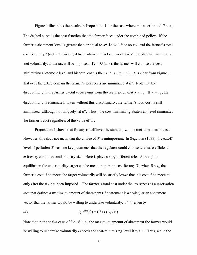
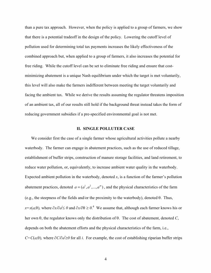
Figure 1 illustrates the results in Proposition 1 for the case where a is a scalar and .sxx <

The dashed curve is the cost function that the farmer faces under the combined policy. If the

farmer’s abatement level is greater than or equal to a*, he will face no tax, and the farmer’s total

cost is simply C(av,θ). However, if his abatement level is lower then a*, the standard will not be

met voluntarily, and a tax will be imposed. If t = λ*(xs,θ), the farmer will choose the cost-

minimizing abatement level and his total cost is then )(* xxtC s −⋅+ . It is clear from Figure 1

that over the entire domain the farmer’s total costs are minimized at a*. Note that the

discontinuity in the farmer’s total costs stems from the assumption that sxx < . If sxx = , the

discontinuity is eliminated. Even without this discontinuity, the farmer’s total cost is still

minimized (although not uniquely) at a*. Thus, the cost-minimizing abatement level minimizes

the farmer’s cost regardless of the value of x .

Proposition 1 shows that for any cutoff level the standard will be met at minimum cost.

However, this does not mean that the choice of x is unimportant. In Segerson (1988), the cutoff

level of pollution x was one key parameter that the regulator could choose to ensure efficient

exit/entry conditions and industry size. Here it plays a very different role. Although in

equilibrium the water quality target can be met at minimum cost for any x , when x <xs, the

farmer’s cost if he meets the target voluntarily will be strictly lower than his cost if he meets it

only after the tax has been imposed. The farmer’s total cost under the tax serves as a reservation

cost that defines a maximum amount of abatement (if abatement is a scalar) or an abatement

vector that the farmer would be willing to undertake voluntarily, , given by amax

(4) C( ,θ) ≡ C*+t⋅( xamaxs - x ).

Note that in the scalar case a > a*, i.e., the maximum amount of abatement the farmer would

be willing to undertake voluntarily exceeds the cost-minimizing level if x

max

s > x . Thus, while the

8

farmer’s optimal choice is still a*, when sxx < the farmer would actually be willing to undertake

more abatement to avoid payment of the tax.10

However, if the regulator sets x =xs, the farmer’s costs are not strictly lower if the

standard is met voluntarily (i.e., the discontinuity in Figure 1 is eliminated) and in the scalar case

= a*. In this case, the farmer is indifferent between meeting the standard voluntarily and

having the tax imposed, and has no incentive to undertake more abatement voluntarily than he

would undertake if he had to pay the tax. In other words, the tax is no longer a real threat to the

farmer, since it imposes no costs above and beyond what he would incur if he met the target

voluntarily.

amax

In sum, in the single farmer case, combining the voluntary approach and the ambient tax

(i.e., treating them as complements in a policy package rather than as substitute policies) can

ensure that the target is met at minimum cost without incurring the potentially high information

costs necessary for imposing an ambient tax. If sxx < , this is the unique equilibrium outcome

under the combined policy. In this case, the tax is never actually imposed because the threat of

imposition of the tax is sufficient to induce voluntary compliance. As a result, the regulator does

not need to incur the costs of learning θ. Thus, the combined policy approach is not only more

effective in protecting environmental quality than a pure voluntary approach (which does not

ensure that water quality goals are met) but also less costly than a pure ambient tax approach

(since it entails lower information costs). If sxx = , cost-minimizing voluntary abatement is still

an equilibrium outcome, but the farmer no longer strictly prefers this to the outcome under which

the tax is imposed. This suggests that in designing the policy, the regulator should set sxx < .

We show below that this conclusion continues to hold when the single farmer model is extended

to incorporate a more explicit and realistic timing of possible imposition of the tax. However,

9

we show that, when extended to apply to a group of farmers, setting sxx < can induce an

allocation inefficiency.

III. AN EXTENSION TO A DYNAMIC MODEL

The above model assumes that the regulator can observe instantaneously whether the

target has been met voluntarily and immediately impose the tax if it has not. In this section, we

present an extended model that incorporates a more explicit and realistic timing of events. We

show that, when sxx < , the result from the static model presented in the previous section

continues to hold in this context, provided the discount rate is sufficiently low relative to the

difference between xs and x .11 However, when sxx = , the farmer will strictly prefer not to

meet the standard voluntarily. This is in contrast to the result in the static model, where the

farmer was indifferent between meeting it voluntarily and facing the tax when sxx = .

We view the problem as an infinitely repeated game between the regulator and the

farmer. During each time period the farmer chooses an abatement level, which determines

whether or not the standard will be met in that period. There is no “carry over” effect of

pollution abatement. At the end of each period, the regulator observes whether the standard has

been met during that period. The regulator then plays the following trigger strategy. No tax is

imposed during the first period. If during that period the regulator observes that the water

quality standard has been met voluntarily, she does not impose any tax in the following period

and the game is repeated. However, if during that period (or any subsequent period in which a

tax has not been imposed) she observes that the standard has not been met voluntarily, then she

expends the resources necessary to learn θ and imposes a tax equal to λ*(xs,θ) for all of the

remaining periods.

10

Consider the farmer’s first-period choice. If the farmer chooses not to meet the target

voluntarily in the first period, then the present value of the stream of total costs will be

(5) [C*+t⋅(xs- x )]⋅(δ + δ2 + δ3 + …) = [C*+t⋅(xs- x )]⋅ [δ/(1-δ)],

where δ=1/(1+r) is the discount factor and r is the discount rate. Suppose instead the farmer

chooses to meet the target voluntarily in the first period, with the corresponding cost of C*.

Then the regulator will not impose the tax, and at the beginning of the second period the farmer

will face the same decision (and possible payoffs) that he faced at the beginning of the first

period. If meeting the target is optimal for the first period, then it will be optimal for the second

period and all subsequent periods as well. Let V denote the present value of the infinite stream

of costs incurred from making this choice optimally now and every time it arises in the future.

Then

(6) V = C* + δV,

which implies that

(7) V=C*/(1-δ)=C*⋅(1 + δ + δ2 + …).

Comparing the present values in (5) and (7) yields the following result.

PROPOSITION 2: Suppose the regulator employs a trigger strategy whereby he does not impose

an ambient tax initially and then imposes a (permanent) ambient tax in period T if and only if the

water quality target was not met in period T-1. Then the farmer’s optimal response is to meet

the target voluntarily in each period if and only if r<t⋅(xs- x )/C*.

Proposition 2 states that meeting the target voluntarily will be optimal for the farmer if

and only if the discount rate is sufficiently low. Rewriting this condition as C* < t(xs- x )/r

11

provides the intuition for this result: the farmer will meet the target voluntarily provided the

gain from avoiding abatement in the first period C* is less than the present value of the stream of

tax payments the farmer would incur by triggering imposition of the tax (t(xs- x )/r). Clearly, this

condition will never be met for any positive discount rate if sxx = . In this case, even if the tax

is subsequently imposed in response to failure to meet the target in the previous period, as long

as the target is subsequently met, there will be no net tax payments under the tax. Thus, even

under the trigger strategy, with sxx = the farmer is effectively given a new opportunity to meet

the standard in each period. This eliminates any opportunity to “punish” the farmer for failure to

meet the standard in a previous period. Thus, with sxx = it is optimal for the farmer to take

advantage of the first period reprieve and then meet the standard in all subsequent periods,

regardless of his discount rate. This follows provided that the tax is based on ambient pollution

in the period in which it is imposed. If the tax is based on the ambient pollution in the previous

period, i.e., if it is applied retroactively, the regulator would have the ability to punish first-

period non-compliance. Note that if the regulator had not offered the voluntary approach but had

instead simply imposed an ambient tax in all periods, farmers would faced net tax payments for

any period in which the target was not met. In this sense, if sxx = , use of a pure ambient tax

would lead to greater environmental protection than use of the voluntary approach, which allows

the farmer to postpone abatement for one period at no cost.

However, if sxx < , it is optimal for the farmer to meet the standard voluntarily in all

periods, provided his discount rate is low enough. In this case, if the farmer fails to meet the

standard voluntarily in a given period, he will face a positive tax payment in all future periods

even if he subsequently meets the standard in all future periods. Thus, with sxx < , the farmer is

not given a second chance to meet the target at no additional cost (i.e., no cost in addition to the 12

cost of abatement). As a result, by setting sxx < the regulator can induce voluntary compliance

in all periods as long as the discount rate and/or x is sufficiently low. Thus, in contrast to the

static model, in this dynamic context, cost-minimizing abatement is not an optimal voluntary

abatement vector for all x . Nonetheless, the results here confirm the result from the static

model that the policy is more likely to induce voluntary cost-minimizing abatement if the

regulator sets sxx < .

IV. MULTIPLE FARMERS

While the single-farm case provides a benchmark for the study of the combined policy

approach, in many contexts there are likely to be several farms whose activities contribute to

ambient water pollution in a neighboring lake or stream. We show in this section that a

voluntary program coupled with a background threat of an ambient tax can induce cost-

minimizing abatement decisions in this context as well. More specifically, we show that under

the appropriate design of the ambient tax cost-minimizing voluntary abatement by all farmers is

a Nash equilibrium. However, consistent with the results from the static model of a single

farmer, whether this equilibrium is unique or not depends on the relative magnitudes of xs and

x . In particular, we show that, when the policy is applied to a group of farmers, there is a

fundamental tradeoff in setting the magnitudes of xs and x between creating incentives for

voluntary abatement and inducing free-riding by some farmers.

In this extension of the model, we assume that there are n farms and each farmer knows

his own type (θj) and the other farmers’ types.12 The expected ambient water pollution is then

x=x(a1, a2, …, an; θ1, θ2 , …, θn). For simplicity, we assume that each farmer’s abatement choice

is a scalar, and that the regulator can observe instantaneously whether the target has been met

13

voluntarily and immediately impose the tax if it has not. As before, the objective of the regulator

is to meet an exogenously set water quality standard at minimum cost. The cost-minimizing

abatement choices {aj*(θ1, θ2 , …, θn, xs), j = 1, 2, …, n} solve13

(8) minimize C(a1, θ1) + C(a2, θ2) +…+C(an, θn)

(9) subject to x(a1, a2, …, an; θ1, θ2 , …, θn)≤ xs .

The necessary first order conditions are

(10) ∂C/∂aj + λ*(xs, θ1, θ2 , …, θn)⋅(∂x/∂aj)≥ 0, for all j

where λ*(xs, θ1, θ2 , …, θn) is the optimal value of the Lagrangian multiplier. Let Cj* ≡ C(aj

*(θ1,

θ2 , …, θn,xs), θj) be the corresponding abatement cost for farmer j.

As before, we assume that the regulator imposes an ambient tax if and only if the water

quality target is not met voluntarily. All farmers with potential contributions to the waterbody

would be subject to the tax. If the tax is imposed, each farmer chooses his abatement level to

minimize C(aj,θj)+t⋅[x(a1, a2, …, an; θ1, θ2 , …, θn) - x ]. If the regulator sets t= λ*(xs, θ1, θ2 ,

…, θn), then under the tax each farmer will choose the cost-minimizing abatement level aj*(θ1, θ2

, …, θn,xs), if he believes that other farmers will do the same, i.e., cost-minimizing abatement is a

Nash equilibrium under the ambient tax. 14 The corresponding cost for farmer j is then

Cj*+t⋅(xs- x ). This represents farmer j’s reservation cost. Farmer j will not voluntarily undertake

abatement that generates costs in excess of Cj*+t⋅(xs- x ); if costs under voluntary compliance

exceed Cj*+t⋅(xs- x ), the farmer would be better off if the target is not met and the ambient tax is

imposed. This reservation cost thus defines a maximum amount of abatement that farmer j

would be willing to undertake voluntarily, , given by a jmax

(11) C( ,θa jmax

j) ≡ Cj*+t⋅(xs- x ).

14

Note that > aa jmax

j*(θ1, θ2 , …, θn, xs) if xs> x , i.e., the maximum amount of abatement farmer j

would be willing to undertake voluntarily exceeds the cost-minimizing level. From (11), it

follows that

(12) max

0.j

j

a

a tx C

∂= - <

∂

This implies that an increase in the cutoff level of pollution will reduce the maximum amount of

abatement each farmer is willing to undertake. Similarly, under the assumption that and

, we can show that

0j ja aC <

j ja ax < 0

(13) *max *

*

1 1 j s

j j j j

a xj j

s a s a a a a a

xa at t

x C x C C xl

l

Ê ˆÊ ˆ∂ ∂= + = -Á ˜Á ˜∂ ∂ +Ë ¯ Ë ¯j j

>0,

where ( )* * *1 ... 0

sx nC C xl = ∂ + + ∂ <s and . This implies that reducing the water quality

standard would increase the maximum amount of abatement each farmer is willing to undertake

voluntarily. With a lower water quality standard, the cost the farmer would face under the tax is

greater. Thus, he is willing to undertake more voluntary abatement in order to avoid imposition

of the tax.

xa j< 0

We can now characterize the abatement levels that constitute Nash equilibria under a

policy where the regulator imposes an ambient tax if and only if the water quality target is not

met voluntarily.

PROPOSITION 3: The abatement levels ( are a Nash equilibrium under which the

water quality target is met voluntarily if and only if they satisfy

, ,..., )a a av v nv1 2

(i) a for all j, and ajv j£ max

15

(ii) . x a a a xv v nv n( , ,..., ; , ,..., )1 2 1 2q q q = s

PROOF: By the definition of , as long as a , farmer j would incur lower costs by

choosing this abatement level than by facing the tax if this abatement level ensured that the water

quality target is met voluntarily. Let be the voluntary abatement

choices of all farmers other than farmer j. Suppose there exists an a

a jmax ajv j£ max

,,..., 11 vjv a −

ja

'ja

max' jj a≤

),...,( 1 nvvjj aaaa +− =

ja j−

jv (denoted ' ) such that

satisfies (i) and (ii). Then ' is a best response to a . Clearly, farmer j would not

choose a level of abatement greater than this ' , since doing so would increase his cost.

Similarly, choosing an abatement level lower than would result in failure of the voluntary

approach and imposition of the tax. Because a , the cost from choosing 'can be no

higher than the cost from choosing any level of abatement that results in imposition of the tax.

Hence, the farmer can do no better (and will possibly be worse off) by choosing any abatement

level less than a . Thus, any combination of (a

ja

),'( jj aa −

ja

'j 1v, a2v,…, anv) satisfying (i) and (ii) is a Nash

equilibrium. Conversely, any Nash equilibrium under which the water quality target is met

voluntarily must satisfy (i) since otherwise some farmers would prefer the tax. It also must

satisfy (ii) because if x>xs , the water quality standard is not met; and if x<xs, then given the

abatement levels of all other farmers, some farmer could incur lower costs by reducing his

abatement to the level where x=xs . Q.E.D.

Because {aj*(θ1, θ2 , …, θn, xs), j = 1, 2, …, n} satisfies both conditions in Proposition 3,

the following proposition follows immediately:

16

PROPOSITION 4: The cost-minimizing abatement levels {aj*(θ1, θ2 , …, θn, xs), j = 1, 2, …, n} are

a Nash equilibrium under which the target is met voluntarily for any level of x .

This result implies that under the voluntary approach it is optimal for each farmer to

undertake the cost-minimizing abatement, as long as he believes other farmers are doing so.

Thus, cost-minimizing abatement is a Nash equilibrium. In this case, as in the single farmer

model, for any level of x , by providing farmers the opportunity to meet the target voluntarily,

the regulator can achieve cost-minimizing abatement without incurring the information costs that

would be associated with reliance solely on an ambient tax.

In contrast to the result in the single farmer model, with multiple farmers cost-

minimizing voluntary abatement is never a unique equilibrium. If xs> x , there are other Nash

equilibria under which the target is met voluntarily (but not at minimum cost). For example, in

the case of two farms, as long as x(0, a ;θ2max

1, θ2) = xs, (0, ) is also a Nash equilibrium but it

does not minimize the total abatement cost. In this case, farmer 2 would face a higher cost under

the tax than he would incur by achieving the water quality standard by himself. Realizing this,

farmer 1 would free ride on farmer 2’s effort. Because of the free rider problem, aggregate

abatement costs are higher than they would have been under a pure ambient tax, since the

allocation of abatement across farms is inefficient.

a2max

15

In addition, under some circumstances, zero voluntary abatement may also be a Nash

equilibrium.

17

PROPOSITION 5: Let a be implicitly defined by . Then zero

voluntary abatement ( is a Nash equilibrium if for j=1,2, …,

n.

js x a xj

sn( ,... , , ,... ; , ,... )0 0 0 0 1 2q q q =

)0= a ajs

j> ma

s

, ,...,a a av v nv1 20 0= = x

Proposition 5 states that, if all farmers would incur higher costs by meeting the target on

their own than they would incur under the ambient tax, i.e., if no farm is willing to meet the

target on its own, then an outcome under which no farmer abates voluntarily is a Nash

equilibrium. Thus, it is possible that in equilibrium the water quality target will not be met

voluntarily and the ambient tax will be imposed. Note, however, that provided sxx < , the

outcome under which each voluntarily chooses his cost-minimizing abatement aj* always strictly

dominates the zero voluntary abatement equilibrium since it yields lower total costs for all

farmers. Hence, if farmers are able to engage in "cheap talk," (see Rasmusen 1994) i.e., to

communicate about their abatement plans (as would be expected in relatively small watersheds

where farmers are neighbors), we would not expect the zero voluntary abatement outcome to

emerge as the equilibrium when sxx < .

The above results suggest that when sxx < there will be Nash equilibria under which the

target is met voluntarily but not at least cost because of free-riding. Free-riding can be avoided

by setting xs= x . However, setting sxx = also ensures that zero voluntary abatement is a Nash

equilibrium.

PROPOSITION 6. If xs= x , zero voluntary abatement by all farmers is

a Nash equilibrium.

( , ,..., )a a av v nv1 20 0= = = 0

18

Proof: Let xs= x , and suppose . If farmer j set , the tax will be imposed

and farmer j will incur a cost of C

)0,...,0(=− ja 0=vja

j*. Any other choice of avj will yield a cost at least as high as

Cj*. Thus, zero abatement by all farmers is a Nash equilibrium. QED

Note that when xs= x , the Nash equilibria include cost-minimizing abatement by all

farmers and zero abatement by all farmers. Neither equilibrium involves free-riding and both

lead to the outcome under which farmers meet the target at minimum cost. As a result, the cost

to each farmer will be the same under the two equilibria, implying that all farmers are indifferent

between them. Thus, there is no a priori reason to expect one equilibrium (for example, the

equilibrium under which the target is met voluntarily) to be more likely than the other.

Figure 2 illustrates the impact of the cut-off level of pollution on the tradeoff between

free-rider problems and the possibility that the environmental standard is not met voluntarily. As

shown in Proposition 3, all ( , combinations that satisfy a a , and

are Nash equilibria under which the water quality standard is met voluntarily.

These combinations are shown by the segment AB on the water quality constraint curve

in Figure 2a for the case where the cutoff level of pollution is set below the

pollution standard. Among these combinations, only minimizes total costs,C . All

other combinations imply an inefficient allocation of abatement across farmers.

1 2 )a a a a1 1 2 2£ £max max,

*2 )

1 2( , ) sx a a x=

1 2( , ) sx a a x=

*1( ,a a 1 C+ 2

With an increase in the cutoff level of pollution, the maximum abatement each farmer is

willing to undertake, , decreases (see (12)). As a result, the set of Nash equilibria under

which the water quality standard is met voluntarily shrinks. When the cutoff level of pollution is

set equal to the pollution standard, the maximum abatement each farmer is willing to undertake

a jmax

19

a jmax reduces to the cost-minimizing abatement level, the set of Nash equilibria under which the

water quality standard is met voluntarily shrinks to a single (unique) point (point A in figure 2b),

and the free rider problem is eliminated. Thus, in contrast to Segerson (1988) where the

regulator chooses the cutoff level of pollution x to ensure efficient exit/entry conditions and

industry size, here the regulator can choose x to eliminate or reduce the free-rider problem.

Fully eliminating the free-rider problem by setting xxs = involves a trade-off, however.

When xxs = , by Proposition 6 zero voluntary abatement is also a Nash equilibrium. As noted

above, as long as sx x< , all Nash equilibria under which the water quality standard is met

voluntarily (i.e., those located on the segment AB in figure 2a) strictly dominate those where

voluntary abatement is zero. Since the farmers pay no tax when the standard is met voluntarily,

the corresponding Nash equilibria yield lower costs for all farmers than under the equilibrium

where the tax is imposed. Thus the farmers collectively and individually strictly prefer to meet

the standard voluntarily. However, if xxs = so that the free rider problem is eliminated, the

Nash equilibrium under which the target is met voluntarily no longer strictly dominates the zero

voluntary abatement equilibrium, i.e., the strict preference for voluntary abatement is eliminated.

Farmers now become individually and collectively indifferent between meeting the standard

voluntarily and having the tax imposed, implying that success of the voluntary program is no

longer a dominating equilibrium. Thus, by setting sxx < , the regulator increases the

likelihood that the farmers will meet the target voluntarily and hence that the transaction costs

associated with imposition of the tax will be avoided (as in the single farmer case), but at the

cost of a decrease in allocative efficiency (i.e., an increase in the total abatement costs).

20

V. REDUCTION OF GOVERNMENT SUBSIDIES

The analysis above assumes that the background threat takes the form of an ambient tax.

However, agricultural water quality policy in the United States has historically been based on the

use of “carrot” approaches designed to entice farmers to use environmentally friendly practices

voluntarily through the use of government subsidies.16 Such a policy can also be used with a

background threat to achieve environmental goals at minimum costs. Instead of imposing an

ambient tax, the background threat could be a reduction in government subsidies if a pre-

specified environmental standard is not met. Specifically, under such a policy, the regulator

would agree to give the farmer a chance to meet the standard voluntarily. If the standard is met,

a pre-specified level of government subsidy would be paid. However, if the standard is not met

voluntarily, the regulator would reduce the subsidy, with the magnitude of the reduction set at

the level sufficient to induce the farmer to choose an abatement vector that ensures that the

standard would be met. Formally, under the above policy, the farmer would face the following

policy-related benefits:

0

0

( , )( ( , ) ) ( , )

v s

s v

S if x aS

S t x a x if x a xθ

θ θ≤

= − − > s

x

where is the pre-specified fixed subsidy, and is the abatement level the farmer chooses

when facing a threat of losing government subsidies. It can be shown that the results derived

above under the assumption that the regulator threatens imposition of an ambient tax would hold

as well if the regulator threatens instead to reduce government subsidies as specified above.

oS as

17

VI. CONCLUSIONS

21

Although the economic literature of NPP has focused on mandatory or stick approaches

(e.g., input use taxes or restrictions), water quality policies in the U.S. have historically been

based on the use of carrot instruments designed to entice farmers to adopt conservation practices

voluntarily. Both the mandatory and voluntary approaches have been criticized in the economic

literature. Mandatory approaches generally have drawbacks in terms of inflexibility or high

transaction or information costs, while voluntary approaches may fail to provide adequate

environmental protection. Thus, neither a purely voluntary program nor a purely mandatory

approach seems to offer a desirable solution to agricultural NPP.

In this paper we examine a policy that combines a voluntary approach to controlling

nonpoint-source pollution with a background threat of an ambient tax if the voluntary approach

is unsuccessful in meeting a pre-specified environmental goal. In particular, we use the model to

examine whether the regulator can use such a policy to induce cost-minimizing abatement

decisions without the need for farm-specific information about pollution-related characteristics.

We first consider how a single farmer would respond to such a combined policy, and then extend

the analysis to consider multiple farmers. In the context of multiple farmers, we ask whether

cost-minimizing abatement decisions are a Nash equilibrium and whether the proposed approach

leads to free-riding by some farmers. We consider both a static model, in which imposition of

the threat can occur instantaneously when the target is not met, and a dynamic model, in which

there is a one-period lag between failure to meet the goal and imposition of the threat. While we

derive the results in the context where the background threat is a tax, the results would also hold

if the background threat were instead a reduction in government subsidies.

The main results can be summarized as follows. Combining a voluntary approach with a

background threat of an ambient tax (or a reduction in government subsidies) can induce cost-

22

minimizing abatement without the need for farm-specific information about pollution-related

characteristics. This policy can therefore be both more effective than a pure voluntary approach

without a threat (which might not ensure adequate environmental protection) and involve lower

information or transaction costs than a pure ambient tax policy (since the regulator does not have

to expend the resources to learn the site characteristics of the farm).

The ability of the policy to induce voluntary cost-minimizing abatement without the need

for site-specific information holds in the context of either a single farmer or multiple farmers. In

the single farmer case with an instantaneous threat, voluntary cost-minimizing abatement is an

optimal response to the policy, regardless of the cutoff level of pollution. This will be the unique

optimal response, when the cutoff level of pollution is set below the target level. If the threat

cannot be imposed instantaneously or retroactively, then voluntary cost-minimizing abatement is

still the unique optimal response provided the cutoff level is set sufficiently low, i.e., at a level

that ensures that the present value of the stream of tax payments the farmer would face if the tax

is imposed exceeds the one-period cost savings he would enjoy by not meeting the target

voluntarily.

When the policy is applied to a group of farmers, cost-minimizing abatement is a Nash

equilibrium for any choice of the cutoff level. However, with multiple farmers the voluntary

cost-minimizing equilibrium is never unique. The nature of the other possible equilibria depends

on the relative magnitudes of the target and cutoff levels of pollution. If the cutoff level is set

less than the target level, then the combined approach will also yield Nash equilibria under

which the target is met voluntarily but some farmers free ride, i.e., abate less than they would at

the cost-minimizing allocation, implying an inefficient allocation of abatement across farmers.

In this case, to evaluate the overall efficiency of the combined approach, the loss from free-

23

riding under this approach would have to be weighed against any gain from an increase in

effectiveness relative to a purely voluntary approach or against any reduction in information

costs relative to a pure ambient tax policy.

It is possible to eliminate free-riding and ensure that cost-minimizing abatement is the

only Nash equilibrium under which the target is met voluntarily by setting the cutoff level of

pollution equal to the target level. In this case, farmers have no incentive to free ride. The

potential for free riding occurs when the farmer must pay positive tax payments if the ambient

tax is imposed but avoids these costs if the target is met voluntarily. This net gain (in the form

of avoided tax payments) from meeting the target voluntarily makes some firms willing to abate

more under voluntary compliance than they would have abated under the tax, which in turn

allows other firms to abate less, i.e., to free ride. This possibility is eliminated if in equilibrium

net tax payments are zero, as they would be if the target and cutoff levels of pollution are equal

(since in equilibrium the target is just met). However, in this case zero voluntary abatement is

also a Nash equilibrium, and the equilibrium under which the target is met voluntarily no longer

strictly dominates the equilibrium under which it is not.18 When tax payments are zero in

equilibrium, the farmer will incur the same total cost regardless of whether the target is met

voluntarily or met as a result of imposition of the ambient tax. In either case, he incurs only the

cost of abatement. Thus, while it is still possible that farmers would choose to meet the target

voluntarily, they would not have a strict preference for doing so.

The above results suggest a potential efficiency tradeoff in the choice of the policy

parameters when the combined policy is applied to a group of farmers. The regulator can

increase the likelihood that the voluntary approach will be effective (and hence that the potential

savings in information or transaction costs will be realized) by setting the cutoff level of

24

pollution below the target level. The lower the cutoff level is set, the higher are the tax payments

the farmer would have to make if the target is not met voluntarily. Thus, lowering the cutoff

level increases the severity of the threat and hence increases the incentive for the farmer(s) to

meet the target voluntarily. This holds for both the single and the multiple farmer cases.

However, when the policy is applied to a group of farmers, lowering the cutoff level has an

additional effect, namely, it also increases the potential for free-riding. Although voluntary cost-

minimizing abatement is a Nash equilibrium regardless of the cutoff level of pollution, lowering

the cutoff level expands the set of Nash equilibria and hence increases the possibility that an

equilibrium that is not cost-minimizing will emerge. When applied to a group of farmers, an

optimal policy design would need to balance these two efficiency effects.

25

REFERENCES

Babcock, Bruce, P. G. Lakshminarayan, JunJie Wu, and David Zilberman. "Public Fund For Environmental Amenities," American Journal of Agricultural Economics, Volume 78 (4) 1996: 961-971.

Batie, Sandra and David Ervin. "Flexible Incentives for Environmental Management in

Agriculture: A Typology," paper presented at conference on "Flexible Incentives for the Adoption of Environmental Technologies in Agriculture," Gainesville, FL, June 1997.

Bosch, Darrell, Zena Cook, and Keith Fuglie. "Voluntary versus Mandatory Agricultural Policies

to Protect Water Quality: Adoption of Nitrogen Testing in Nebraska," Review of Agricultural Economics, Volume 17 (1), 1995: 13-24.

Braden, John, and Stephen Lovejoy, eds. Water Quality and Agriculture: An International

Perspective on Policies, Boulder and London: Lynne Rienner Publishers, 1990. Braden, John, and Kathleen Segerson. "Information Problems in the Design of Nonpoint-Source

Pollution," in Clifford Russell and Jason Shogren, eds., Theory, Modeling, and Experience in the Management of Nonpoint-Source Pollution, Boston: Kluwer Academic Publishers, 1993, pp. 1-35.

Cabe, Richard, and Joseph A. Herriges. 1992. "The Regulation of Non-Point-Source Pollution

under Imperfect and Asymmetric Information," Journal of Environmental Economics and Management, Volume 22(2), March:134-146.

Commission of the European Communities (EC). On Environmental Agreements,

Communication from the Commission to the Council and the European Parliament, Brussels, 1996.

Cooper, Joseph C., and Russ W. Keim. "Incentive Payments to Encourage Farmer Adoption of

Water Quality Protection Practices," American Journal of Agricultural Economics, Volume 78 (1), February 1996: 54-64.

Dawson, Na Li, and Kathleen Segerson, “Voluntary Agreements with Industries: Participation

Incentives with Industry-wide Targets,” Working paper, University of Connecticut, Department of Economics, January 2002.

Govindasamy, Ramu, Joseph A. Herriges, and Jason F. Shogren. "Nonpoint Tournaments," in

Cesare Dosi and Theodore Tomasi, eds., Nonpoint Source Pollution Regulation: Issues and Analysis, Dordrecht and Boston: Kluwer Academic Publishers, 1994.

Griffin, Ronald, and Daniel W. Bromley. "Agricultural Runoff as a Nonpoint Externality,"

American Journal of Agricultural Economics, Volume 64, 1982: 547-552.

26

Hardie, Ian W., and Peter J. Parks. "Reforestation Cost-Sharing Programs," Land Economics, Volume 72, May 1996: 248-260.

Helfand, Gloria E., and Brett W. House. "Regulating Nonpoint Source Pollution Under

Heterogeneous Conditions," American Journal of Agricultural Economics, Volume 77(4), November, 1995: 1024-1032.

Herriges, Joseph A., Ramu Govindasamy, and Jason F. Shogren. "Budget-Balancing Incentive

Mechanisms," Journal of Environmental Economics and Management, Volume 27(3), November 1994: 275-285.

Lohr, Luanne, and Timothy Park. "Utility-Consistent Discrete-Continuous Choices in Soil

Conservation," Land Economics, Volume 71 (4) November 1995: 474-490. Norton, Nancy Anders, Tim T. Phipps, and Jerald J. Fletcher. "Role of Voluntary Programs in

Agricultural Nonpoint Pollution Policy," Contemporary Economic Policy, Volume 12(1), January 1994: 113-121.

Ogg, Clayton W. and Peter J. Kuch. "Cost Sharing and Incentive Payments: The Use of

Subsidies to Encourage Adoption of Environmentally Beneficial Agricultural Practices." Paper presented at conference on "Flexible Incentives for the Adoption of Environmental Technologies in Agriculture," Gainesville, FL, June 1997.

Rasmusen, Eric. 1994. Games and Information: An Introduction to Game Theory, 2nd edition.

Cambridge, MA: Blackwell Publishers. Ribaudo, Marc and Margriet Caswell. "U.S. Environmental Regulation in Agriculture and

Adoption of Environmental Technology." Paper presented at conference on "Flexible Incentives for the Adoption of Environmental Technologies in Agriculture," Gainesville, FL, June 1997.

Segerson, Kathleen. "Uncertainty and Incentives for Nonpoint Pollution Control," Journal of

Environmental Economics and Management, 15, 1988: 87-98. Segerson, Kathleen and Na Li Dawson, “Enviornmental Voluntary Agreements: Participation

and Free Riding,” in Eric Orts and Kurt Deketelaere, eds., Environmental Contracts: Comparative Approaches to Regulatory Innovation in the United States and Europe, Kluwer Law International, 2001.

Segerson, Kathleen and Thomas J. Miceli. "Voluntary Environmental Agreements: Good or

Bad News for Environmental Quality?" Journal of Environmental Economics and Management, Volume 36(2), September 1998: 109-130.

Shavell, Steven. Economic Analysis of Accident Law, Cambridge, MA: Harvard University

Press, 1987.

27

Shortle, James and David Abler. "Incentives for Nonpoint Pollution Control," in Cesare Dosi and Theodore Tomasi, eds., Nonpoint Source Pollution Regulation: Issues and Analysis, Dordrecht and Boston: Kluwer Academic Publishers, 1994.

Shortle, James and James Dunn. "The Relative Efficiency of Agricultural Source Water

Pollution Control Policies," American Journal of Agricultural Economics, 68, 1986: 668-677.

Spraggon, John. “Exogenous Targeting Instruments as a Solution to Group Moral Hazards.”

Journal of Public Economics 84, 2002: 427-456. Tomasi, Theodore, Kathleen Segerson and John Braden. "Issues in the Design of Incentive

Schemes for Nonpoint Source Pollution Control," in Cesare Dosi and Theodore Tomasi, eds., Nonpoint Source Pollution Regulation: Issues and Analysis, Dordrecht: Kluwer Academic Publishers, 1994, pp. 1-37.

Wiebe, Keith, Abebayehu Tegene, and Betsy Kuhn. Partial Interests in Land: Policy Tools for

Resource Use and Conservation. Agricultural Economic Report Number 744, U.S. Department of Agriculture, 1996.

Wu, JunJie, and Bruce A. Babcock. "Optimal Design of a Voluntary Green Payment Program

Under Asymmetric Information," Journal of Agricultural and Resource Economics, Volume 20 (2), December 1995: 316-327.

Wu, JunJie, and Bruce A. Babcock. "Purchase of Environmental Goods from Agriculture,"

American Journal of Agricultural Economics, Volume 78 (4) 1996: 935-945. Wu, JunJie, and Bruce A. Babcock. "The Relative Efficiency of Voluntary vs. Mandatory

Environmental Regulations," Journal of Environmental Economics and Management 37(September 1999): 158-175.

Wu, JunJie, M.L. Teague, H.P. Mapp, and D.J. Bernardo. "An Empirical Analysis of the

Relative Efficiency of Policy Instruments to Reduce Nitrate Water Pollution in the U.S. Southern High Plains," Canadian Journal of Agricultural Economics 43, 1995: 403-420.

Xepapadeas, A. P. "Environmental Policy under Imperfect Information: Incentives and Moral

Hazard," Journal of Environmental Economics and Management 20, 1991: 113-126. Xepapadeas, A. P. "Environmental Policy Design and Dynamic Nonpoint-Source Pollution,"

Journal of Environmental Economics and Management 23, 1992: 22-39. Xepapadeas, A. P. "Observability and Choice of Instrument Mix in the Control of Externalities,"

Journal of Public Economics 56(3), March 1995: 485-498.

28

Cost under the tax

( , )vC a θ

amax

C*

a a*

C t x xs* [ ]+ ◊ -

$

Fig. 1. Farmer’s Total Cost under the Combined Policy

29

* *1 1 2 2 1 2( , ) ( , )C a C a C Cq q+ = +

1 2( , ) sx a a x=

2a

*2a

max2a

max1a *

1a 1a

Case a: sx x<

A

B

NE where standard is met voluntarily

A

2a

ax

1 1 2( , ) ( ,C a C aq q+

* m2 2a a=

* m1 1a a= ax

1a

Case b: sx x=

* *2 1 2) C C= +

1 2( , ) sx a a x=

NE where standard is met voluntarily

Fig. 2. The Cut-off Level of Pollution and the Tradeoff Between Creating Incentives for Voluntary Abatement and Inducing Free-Rider Problems

30

31

Footnotes

1 Recent discussions of reauthorization of the Clean Water Act, for example, have focused on the control of NPP. A notable example of nonpoint source pollution (NPP) is the contamination of surface water from the runoff of agricultural chemicals. In many locations agriculture has been identified as the largest source of NPP. Hence, much of the literature on NPP is in the context of agricultural water pollution. For an overview of issues relating to nonpoint source pollution from agriculture, see Braden and Segerson (1993) and Tomasi, Segerson and Braden (1994). 2 For discussions of the use of subsidies to reduce agricultural sources of water pollution, see Braden and Lovejoy (1990), Norton et al. (1994), Lohr and Park (1995), Bosch et al. (1995), Wu and Babcock (1995), Hardie and Parks (1996), Wiebe et al. (1996), Wu and Babcock (1996), Babcock et al. (1996), Cooper and Keim (1996), Ribaudo and Caswell (1997), Ogg and Kuch (1997). 3 Henceforth, we use the term "mandatory controls" to refer both to mandatory regulations or restrictions and tax-based policies such as ambient taxes or input taxes. 4 It is well-recognized that actual water quality will depend on a and θ as well as on other random variables such as weather (e.g., Segerson, 1988). The expected level of water quality then depends on the distribution of the weather variable. However, since we state the policy goal as one of meeting a water quality standard on average over some period rather than at every instant in time, the daily variability attributable to weather is not a key part of the analysis. Thus, for simplicity of notation, we suppress the weather variable. Note, however, that when compliance with the target is determined on a continuing basis, i.e., at every point in time, rather than on average over a period of time, the existence of weather variability affects the efficiency properties of alternative policy instruments. For example, with weather variability and continual determination of compliance, a pure ambient tax would not induce first-best abatement. See Spraggon (2002) for a useful summary. 5 For some abatement practices such as installation of manure storage facilities, the abatement cost may depend on only the abatement practice. 6 This is in contrast to the model in Segerson and Miceli (1998), where the level of environmental quality under the voluntary approach is determined endogenously as a result of bargaining between the regulator and the firm. 7 We do not consider the case where sxx > , which would imply that the farmer receives net payments for meeting the standard. In this case, the farmer would never find it optimal to meet the standard voluntarily. 8 It is also similar to a negligence rule in tort law, under which an injurer is liable for damages if the level of care he undertook in conducting an activity is below the “due standard of care” but not liable if he met the standard of care. See Shavell (1987) for a discussion of the economics of negligence rules. 9 Given that the tax/subsidy policy in Segerson (1988) is based on actual pollution at each point in time, which fluctuates as a result of random factors such as weather, the use of the subsidy when pollution is below the target ensures efficient incentives. However, depending on the value of x , it

32

is possible that under the pure tax/subsidy approach, in equilibrium the farmer will choose an abatement vector such that on average the target is just met. In this case, on average no tax/subsidy payments occur in equilibrium and the equilibrium outcome under the pure tax/subsidy policy is identical to the outcome under a successful voluntary approach. 10 Segerson and Miceli (1998) derive a similar conclusion in the context of their model of point source pollution. In their context, where the regulator and polluter bargain over the level of voluntary abatement, this incentive creates the possibility of “over-compliance”, i.e., adoption of an abatement level that exceeds the level that would have been induced under the regulator’s threat. 11 This is, of course, consistent with the Folk Theorem, a well-known result from the theory of infinitely repeated games. 12 This is a reasonable assumption in a small watershed where farmers are neighbors. Our results would, however, hold even if each farmer knew only the distribution of types across the other farmers. In other words, it is not necessary for each farmer to know the types of specific farms in the watershed, but only to know the distribution of the types of farms that comprise the watershed. 13 Given the assumption of an abatement index, cost minimization simply requires that abatement be allocated efficiently across farms. With an abatement vector for each farm, cost minimization would require efficient abatement allocation both across and within farms. 14 See Segerson (1988). Note that since this is an ambient tax the tax rate would be the same for all farmers, even though farmers are not identical. 15 A similar free rider problem arises in the model of point source pollution developed by Dawson and Segerson (2002), where the regulator threatens to impose an emissions tax on an industry if it does not meet an exogenous emissions target. As in the model here, free riding generates an inefficiency because abatement is allocated inefficiently across firms. However, Segerson and Dawson (2001) show that, despite this inefficiency, the voluntary approach will still be more efficient if the regulator threatens imposition of a costly (inefficient) regulation rather than an emissions tax. Even under the threat of a tax, the voluntary approach may still be more efficient, if the welfare loss associated with the inefficient allocation of abatement across firms is less than the information or other transaction costs required for implementation of the tax. 16 See references in footnote 2. 17 Proofs are analogous and will be provided upon request. 18 Zero voluntary abatement can also be a Nash equilibrium when the cutoff level is below the target level. However, in these cases the Nash equilibria with voluntary abatement strictly dominate the zero voluntary abatement equilibria.