Estimates of Natural Selection in a Salmon Population in Captive and Natural Environments

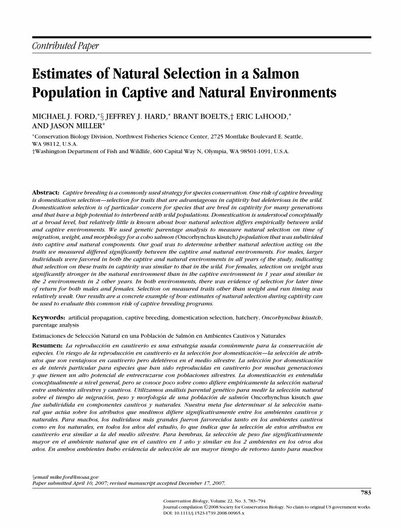
Contributed Paper

Estimates of Natural Selection in a SalmonPopulation in Captive and Natural EnvironmentsMICHAEL J. FORD,∗§ JEFFREY J. HARD,∗ BRANT BOELTS,† ERIC LAHOOD,∗

AND JASON MILLER∗∗Conservation Biology Division, Northwest Fisheries Science Center, 2725 Montlake Boulevard E. Seattle,WA 98112, U.S.A.†Washington Department of Fish and Wildlife, 600 Capital Way N, Olympia, WA 98501-1091, U.S.A.

Abstract: Captive breeding is a commonly used strategy for species conservation. One risk of captive breeding

is domestication selection—selection for traits that are advantageous in captivity but deleterious in the wild.

Domestication selection is of particular concern for species that are bred in captivity for many generations

and that have a high potential to interbreed with wild populations. Domestication is understood conceptually

at a broad level, but relatively little is known about how natural selection differs empirically between wild

and captive environments. We used genetic parentage analysis to measure natural selection on time of

migration, weight, and morphology for a coho salmon (Oncorhynchus kisutch) population that was subdivided

into captive and natural components. Our goal was to determine whether natural selection acting on the

traits we measured differed significantly between the captive and natural environments. For males, larger

individuals were favored in both the captive and natural environments in all years of the study, indicating

that selection on these traits in captivity was similar to that in the wild. For females, selection on weight was

significantly stronger in the natural environment than in the captive environment in 1 year and similar in

the 2 environments in 2 other years. In both environments, there was evidence of selection for later time

of return for both males and females. Selection on measured traits other than weight and run timing was

relatively weak. Our results are a concrete example of how estimates of natural selection during captivity can

be used to evaluate this common risk of captive breeding programs.

Keywords: artificial propagation, captive breeding, domestication selection, hatchery, Oncorhynchus kisutch,parentage analysis

Estimaciones de Seleccion Natural en una Poblacion de Salmon en Ambientes Cautivos y Naturales

Resumen: La reproduccion en cautiverio es una estrategia usada comunmente para la conservacion de

especies. Un riesgo de la reproduccion en cautiverio es la seleccion por domesticacion—la seleccion de atrib-

utos que son ventajosos en cautiverio pero deletereos en el medio silvestre. La seleccion por domesticacion

es de interes particular para especies que han sido reproducidas en cautiverio por muchas generaciones

y que tienen un alto potencial de entrecruzarse con poblaciones silvestres. La domesticacion es entendida

conceptualmente a nivel general, pero se conoce poco sobre como difiere empıricamente la seleccion natural

entre ambientes silvestres y cautivos. Utilizamos analisis parental genetico para medir la seleccion natural

sobre el tiempo de migracion, peso y morfologıa de una poblacion de salmon Oncorhynchus kisutch que

fue subdividida en componentes cautivos y naturales. Nuestra meta fue determinar si la seleccion natu-

ral que actua sobre los atributos que medimos difiere significativamente entre los ambientes cautivos y

naturales. Para machos, los individuos mas grandes fueron favorecidos tanto en los ambientes cautivos

como en los naturales, en todos los anos del estudio, lo que indica que la seleccion de estos atributos en

cautiverio era similar a la del medio silvestre. Para hembras, la seleccion de peso fue significativamente

mayor en el ambiente natural que en el cautivo en 1 ano y similar en los 2 ambientes en los otros dos

anos. En ambos ambientes hubo evidencia de seleccion de un mayor tiempo de retorno tanto para machos

§email [email protected] submitted April 10, 2007; revised manuscript accepted December 17, 2007.

783Conservation Biology, Volume 22, No. 3, 783–794Journal compilation C©2008 Society for Conservation Biology. No claim to original US government works.DOI: 10.1111/j.1523-1739.2008.00965.x

784 Selection during Captivity

como hembras. La seleccion de los atributos medidos distintos al peso y el tiempo de corrida fue relativa-

mente debil. Nuestros resultados son un ejemplo concreto de como las estimaciones de seleccion natural

durante el cautiverio pueden ser utilizadas para evaluar este riesgo comun en los programas de reproduccion

en cautiverio.

Palabras Clave: analisis parental, criadero de peces, propagacion artificial, Oncorhynchus kisutch, repro-duccion en cautiverio, seleccion por domesticacion

Introduction

Understanding how populations evolve is becomingan increasingly important part of conservation biology.There are several reasons for this. Global warming andassociated climate change have brought attention to thefact that many species live in environments that arechanging rapidly. The ability of a species to adapt to thesechanges is an important factor in the extinction risk ofthat species (e.g., Lynch & Lande 1993; Lande & Shannon1996; Etterson & Shaw 2001). In addition to global warm-ing, most species face a myriad of environmental changesthat alter the selective landscape they experience, suchas land-use changes and invasions by non-native species.Another important form of environmental change occursduring captive breeding. Many species of conservationconcern are propagated artificially in an attempt to in-crease their abundance. Most captive breeding programsare not intended to be permanent substitutions for viablenatural populations, however, and seek to minimize theamount of evolution that occurs in captivity. Whether in-tentional or not, selection for traits that are advantageousor neutral in captivity but disadvantageous in the wild(domestication selection) is expected to be a particularproblem if a species is propagated for many generationsin captivity (e.g., Frankham et al. 1986; Snyder et al. 1996;Bryant & Reed 1999).

Seven species of Pacific salmon (Oncorhynchus spp.)spawn in rivers on the west coast of North America,and all contain populations that have declined to thepoint of conservation concern (Nehlsen et al. 1991).Twenty-seven evolutionarily significant units (ESUs)of Pacific salmon have been listed as threatened orendangered under the U.S. Endangered Species Act(http://www.nwr.noaa.gov/). Salmon populations havedeclined for several reasons common to other threat-ened species, including loss and degradation of habitatand overharvest (National Research Council 1996). An-other potential factor for the decline of wild salmon pop-ulations is the genetic and ecological effects of artificialpropagation. In much of their range, salmonids are ar-tificially propagated on a very large scale. For example,over 4 billion anadromous juvenile salmon are releasedannually into the North Pacific Ocean from hatcheriesin North America and Asia (Beamish et al. 1997). Similarhatchery programs and large-scale closed-pen fish farm-

ing operations exist for Atlantic salmon (Salmo salar) inthe North Atlantic Ocean and Baltic Sea.

Artificial propagation poses both ecological and ge-netic risks to salmonids (reviewed by National ResearchCouncil 1996; Waples & Drake 2004). For example, thepotential effects of supportive breeding on effective pop-ulation size have been modeled extensively (Ryman &Laikre 1991; Ryman et al. 1995; Wang & Ryman 2001).Domestication selection may be another particularly im-portant genetic risk because salmonids are often prop-agated artificially for many generations. Several investi-gators have found evidence for domestication in salmon(e.g., Reisenbichler & McIntyre 1977; Fleming & Gross1993; Araki et al. 2007a, 2007b), and evolutionary mod-els suggest that domestication has the potential to causedeclines in the fitness of natural populations that arepartially supported by artificial propagation (e.g., Lynch& O’Hely 2001; Ford 2002). The predictions of thesemodels are quite sensitive to their underlying parame-ters, however, including the strength and form of naturalselection that occurs in the captive and wild environ-ments. Obtaining an empirical understanding of how se-lection differs between captive and natural environmentsis therefore important for predicting the outcomes oflong-term supplementation programs (Hershberger et al.1990; Ford 2002; Araki et al. 2007a).

We quantified differences in how selection operates inthe wild and in captivity for a salmon population withcomponents that experienced either a wild or a cap-tive environment. Using genetic parentage assignmentmethods, we estimated the number of progeny producedby individual fish in either of 2 distinct environments, asalmon hatchery or a natural stream. Between the 2 envi-ronments, we then compared selection gradients (regres-sions of relative progeny number upon standardized traitvalue) for several traits, including time of return to thestream, weight, and body shape. We were particularly in-terested in determining whether optimum trait values dif-fered in wild and captive environments or whether selec-tion in captivity was “relaxed” (weaker) compared withwhat we observed in the wild. The natural populationwe studied had already experienced many generationsof artificial propagation, so the situation we analyzed isprobably more typical of a captive population readaptingto the wild environment than a wild population adaptingto a captive environment.

Conservation Biology

Volume 22, No. 3, 2008

Ford et al. 785

Methods

Study Site

Minter Creek is a small stream draining into HendersonBay in Puget Sound, Washington (U.S.A.; Fig. 1). Cohosalmon in Minter Creek have a life-history pattern typi-cal for the species at this stream’s latitude (Sandercock1991), with juveniles spending about 18 months in thestream prior to smoltification and migration to salt water.The fish then typically spend another 18 months at sea,returning to freshwater as 3-year-olds. In some years a siz-able fraction of the males return as 2-year-olds (“jacks”)after approximately 6 months at sea (Salo & Bayliff 1958;Sandercock 1991), and other male and female life-historypatterns also occasionally occur.

A hatchery operated by the Washington Departmentof Fish and Wildlife (WDFW) is located near the mouthof the creek. Coho salmon have been bred and releasedfrom the hatchery since 1938, when WDFW selected thestream as a study site representative of the hundreds ofsmall Pacific Northwest streams inhabited by coho (On-

corhynchus kisutch) and chum (O. keta) salmon (Salo &

Figure 1. Map of the Minter Creek, Washington, study

area showing the location of the Minter Creek

Hatchery (including the adult sampling weir) and the

juvenile (smolt) collections weirs.

Bayliff 1958). Production-scale (>1,000,000 smolts/year)coho salmon releases were initiated in 1960 (WDFW,Olympia, Washington). There have been no sustainedattempts to keep the hatchery and natural populationsisolated from each other, and in the years leading up toour study an unquantified (probably >90%) fraction ofthe natural spawning population consisted of hatchery-produced fish. The natural population of coho salmonin Minter Creek is therefore clearly not a “pristine” wildpopulation; rather, it is representative of many of thenatural salmon populations in the Pacific Northwest thathave experienced high levels of hatchery stocking formany decades. In a previous study (Ford et al. 2006), wefound no significant differences in fitness between hatch-ery and naturally produced fish in Minter Creek. There-fore, hatchery and natural-origin fish were combined inthe analyses reported here.

In 2000 through 2004 all coho salmon were inter-cepted at a weir located at the head end of tidewater(river kilometer 0.8) as they returned from the ocean tospawn, and a fraction were detained for sampling. Eachsampled fish was sexed, weighed, and photographed,and each fish had a small piece (<1 cm2) of caudal fintissue removed for subsequent DNA analysis. Fish wereallowed to recover in fresh flowing water before eitherbeing released upstream (all years) or into the hatcheryholding pond (2001 through 2003).

In addition to our study fish, each year several thou-sand hatchery-origin fish were passed directly into thehatchery holding pond without being sampled, but nounsampled fish were allowed to pass above the weir tospawn naturally. Wild fish were identified by the pres-ence of an adipose fin (hatchery coho salmon releasedin the Puget Sound area typically have their adipose finremoved prior to release) and by scale analysis (see Fordet al. 2006 for details). In 2001 between 26 Septemberand 31 October, every third sampled fish (whether ofwild or hatchery origin) was released into the hatcheryholding pond. Prior to 26 September and after 31 Oc-tober, all but 10 fish were passed upstream so that fishmanagement spawning goals for wild fish would be met.The mean run timing (day of return to the weir measuredas days after September 1) of males put into the pond wasa few days earlier than the mean run timing of the malesput into the stream (day 45.8 [SD 15.03] vs. day 48.3[18.8], p = 0.08, t test). The mean run timing of femalesput into the pond was approximately 5 days earlier thanthe mean of the females put into the stream (day 45.1 [SD13.6] vs. 51.6 [17.7], p < 0.001, t test). All sampled fishreleased into the holding pond were tagged with num-bered metal jaw tags so that they could be identified atthe time of spawning. We followed a similar protocol fordirecting fish into the stream and hatchery pond in 2002and 2003, but these fish were not included as part ofthe parentage analyses because their progeny were notgenotyped.


Volume 22, No. 3, 2008


For the 2001 cohort spawning in the hatchery occurredon 6 days in November (5, 7, 14, 19, 20, and 27). Spawn-ing dates were determined by the hatchery staff and werethe same as for the general (nonexperimental) hatcherypopulation. We spawned the fish by randomly select-ing sexually mature, tagged males and females from thehatchery pond. Each female was spawned with one male,and >95% of the males were spawned with a single fe-male. We kept progeny from the sampled fish spawnedin the hatchery separate from the general hatchery pop-ulations until they were large enough to be sampled andtagged in summer of 2002. At that time all progeny fromsampled fish received a coded wire tag (CWT) implantedinto their snout so that they could be identified as ourstudy fish when they returned to the stream as adults in2004.

Wild juvenile progeny were sampled at the fry (firstsummer after emergence) and smolt (second spring/summer after emergence) stages between March 2001and June 2003 as described in Ford et al. (2006). Fry weresampled by electrofishing extensively throughout the wa-tershed, and smolts were sampled at weir traps through-out their outmigration period. These juvenile sampleswere a small fraction (1–5%) of the total juvenile pop-ulation. Adult progeny from the 2000 and 2001 broodswere sampled at the weir in the fall of 2003 and 2004,respectively. Progeny were assigned to parents with themaximum likelihood method implemented in the pro-gram FAMOZ (Gerber et al. 2003). See Ford et al. (2006)for a detailed description of the parentage analysis.

Morphological Analyses

We measured 6 morphological traits (Fig. 2) from the dig-ital images taken at the time of sampling. Each trait wasdigitized and measured to the nearest millimeter withthe computer program TPSDIG (Rohlf 2001). Weightswere converted to the linear scale of the other traits bycube-root transformation. To reduce allometric correla-tions among traits, we regressed each morphological traitother than weight on transformed weight with model I

Figure 2. Morphological traits that were studied for

their effects on relative fitness of coho salmon

spawning in Minter Creek. Fish image source:

National Oceanic and Atmospheric Administration

(NOAA) Photo Library.

regression and then used residuals from these regressionsas the trait values in further analyses. Some fish had miss-ing data because of occasional failures of the scale orcamera, especially for the 2000 sampling season. Timeof return was essentially independent of weight (correla-tion coefficients ranged from −0.11 to 0.14, dependingon the sex and cohort), so time of return was analyzedindependently.

Selection and Fitness Analyses

All statistical analyses were conducted with the generallinear model (GLM) function in the SYSTAT computerpackage (version 11, Systat Software, San Jose, Califor-nia). Traits were standardized within each sex and cohortby subtracting the mean and dividing by the standarddeviation. We made separate fitness estimates by count-ing progeny at fry, smolt, and adult life stages. Absolutefitness (progeny counts) within sexes, cohorts, and lo-cations (stream vs. hatchery) was converted to relativefitness by dividing by the mean fitness. In addition, weestimated the minimum number of unique mates an in-dividual had by summing the other unique parents ofthe progeny assigned to that individual regardless of lifestage. We estimated standardized linear and quadratic se-lection gradients (Lande & Arnold 1983) individually foreach trait with the following model: progeny = constant+ trait + (trait)2. We tested differences in linear selectionterms between the hatchery and natural environmentswith analysis of covariance with the model: progeny =constant + trait + location ∗ trait. No attempt was madeto correct p values for multiple tests, but results wereinterpreted with an appreciation that a large number oftests were conducted. We focused primarily on resultsthat were both highly significant at the level of individ-ual tests and that followed a consistent pattern for thedifferent life stages sampled.

As an additional measure of selection we comparedthe mean trait values of the group of parents inferred tohave produced offspring versus those inferred to haveproduced no sampled offspring. We calculated selectiondifferentials as the difference in trait means of the sam-pled population and the subset of individuals that wereinferred to produce offspring. For fish in the hatcherypond, we also estimated selection differentials indepen-dently from the parentage analysis by comparing the traitsof spawned fish as recorded in the hatchery records ver-sus all tagged fish put into the hatchery pond.

Results

All progeny assignments were the same as described inFord et al. (2006), with the exception of the adult off-spring from the parents spawned in the hatchery in 2001,which were conducted with the same methods but were


Volume 22, No. 3, 2008

Ford et al. 787

Table 1. Summary of parent and progeny sample sizes for genetic parentage analysis of Minter Creek coho salmon in stream and hatcheryenvironments.

Parents Offspring

Brood year, location females males (jacks)a fry smolts adults

2000, stream 422 473 (28) 534 801 924b

2001, stream 480 566 (8) 699 677 1683c

2001, hatchery pond 139 154 (1) 370 — 128

aMales includes all males (age 2 and 3 years). Numbers in parentheses are the total number of males that were 2 years old (jacks).bIncludes 901 3-year-old fish sampled in 2003 and 23 2-year-old fish sampled in 2002.cIncludes 1657 3-year-old fish sampled in 2004 and 26 2-year-old fish sampled in 2003.

not reported in the previous paper. Sample sizes for bothparents and progeny are in Table 1. For the 2000 brood95.4% of the potential parents sampled at the weir weregenotyped for parentage analyses. For the 2001 brood92.6% of the potential parents in the stream and 98.1% ofthe potential parents in the hatchery were genotyped forparentage analysis. The majority of the potential spawn-ers in each of the years were 3-year-old fish, with 2-year-olds making up only 6% of the males in 2000 and 1.4%of the males in 2001 (Table 1). Similarly, in 2002, 2003,and 2004, when offspring from the 2 parental years in thestudy returned to spawn, >97% of the returning adultswere 3-year-old fish. Depending on the life stage and yearsampled, 50–70% of the progeny were unambiguouslyassigned to a single pair of spawning parents.

In the stream environment significant selection onweight (size) was detected for both sexes and in bothyears (Table 2). Linear selection gradients for weightwere positive, indicating that for both males and fe-males larger individuals were more successful at produc-ing offspring (Fig. 3). For both sexes selection gradientswere generally similar among the different life stages ofprogeny that we assessed, although the smolt-stage as-sessments produced the largest selection gradients (Ta-ble 2). Selection on weight was similar between years.After taking into account the effects of size, there was nosignificant effect of male age on the number of offspringproduced (analysis of covariance, results not shown). Sig-nificant selection was also detected on run timing, aswas reported previously by Ford et al. (2006). The lin-ear terms were generally positive (indicating selectionfor later than average return time), and quadratic termswere generally negative, indicating stabilizing selectionagainst returning at the extremes of the run (Table 2).The absolute values of the selection gradients on run tim-ing differed slightly from the earlier study because in thisstudy fitness was standardized by dividing by the meanfitness (Lande & Arnold 1983), whereas the earlier es-timates were standardized by subtracting the mean anddividing by the standard deviation. For males significantlinear selection on caudal peduncle size was also detectedin the 2000 cohort but not the 2001 cohort. In 2001 sig-nificant quadratic selection was detected for males on

fin size, body depth, snout length, and caudal pedunclesize, but these results depended on a single outlying indi-vidual with high relative fitness that was unusually lightfor its size (data not shown). In general there were noclear patterns of selection on traits other than weight andrun timing after correcting for correlations with weight(Table 2).

For males selection in the hatchery pond was similar tothat observed in the stream. In particular, linear selectiongradients for weight were positive and highly significant(Table 2 & Fig. 3). Selection on weight in the hatcherypond was significantly stronger than selection on weightin the stream when progeny were counted as fry but indis-tinguishable from selection in the stream when progenywere counted at the smolt or adult life stages (Table 2).Selection on run timing was also positive and significantand not statistically distinguishable from selection on runtiming in the stream, indicating that, as in the stream envi-ronment, later-returning males produced more progenythan earlier-returning males (Table 2). In the pond, un-like the stream, significant selection was also detected ondorsal fin size, when selection was measured as numberof mates or progeny at the fry stage (Table 2).

For females in the hatchery pond, selection on weightin 2001 was weaker than was observed in the stream.In particular, linear selection gradients on weight werenot significantly greater than zero and were significantlyless than the selection gradients estimated for femalesin the stream environment for 2 of the 3 measures offitness (Table 2). Selection on run timing was similar tothat observed in the stream, with later-returning femalesproducing more progeny than earlier-returning ones, al-though the p values were generally less significant thanthey were for the stream coefficients (Table 2).

The selection differentials, which were based onlyon whether or not an individual was inferred to havespawned, were consistent with but smaller than the selec-tion gradients, which incorporated both spawning suc-cess and progeny number. Selection differentials for maleweight were significant in both environments (Table 3).For females the selection differential for weight in 2001was significant in the stream environment but not inthe pond environment, which was consistent with the


Volume 22, No. 3, 2008


Tabl

e2.

Line

ar(B

)an

dqu

adra

tic(G

)re

gres

sion

coef

ficie

nts

desc

ribi

ngth

ere

latio

nshi

pbe

twee

nre

lativ

efit

ness

(num

ber

ofin

ferr

edm

ates

and

num

ber

ofsa

mpl

edfr

y,sm

olt,

and

adul

tpro

geny

per

indi

vidu

alst

anda

rdiz

edby

the

mea

nnu

mbe

rof

prog

eny

per

indi

vidu

al)

and

the

trai

tsth

atw

ere

mea

sure

don

coho

salm

onsa

mpl

edat

the

Min

ter

Cree

kw

eir.

Loca

tion

a

stre

am

pon

d

yea

r

20

00

20

01

20

01

Inte

ract

ion

sc

Lif

e

Tra

itSex

sta

ge

bB

GB

GB

Gp

yea

rp

loca

tion

Wei

ght

mal

esm

ates

0.50

(0.0

0)0.

09(0

.09)

0.35

(0.0

0)0.

07(0

.15)

0.27

(0.0

0)−0

.03

(0.5

2)0.

490.

32fr

y0.

67(0

.00)

0.16

(0.0

6)0.

26(0

.01)

0.11

(0.1

0)0.

89(0

.00)

−0.1

0(0

.61)

0.09

0.01

smo

lts

0.75

(0.0

0)0.

18(0

.04)

0.64

(0.0

0)0.

04(0

.69)

––

0.96

–ad

ult

s0.

67(0

.00)

0.18

(0.0

6)0.

36(0

.00)

0.06

(0.4

1)0.

26(0

.03)

0.00

(0.9

9)0.

090.

43fe

mal

esm

ates

0.34

(0.0

0)0.

08(0

.17)

0.50

(0.0

0)−0

.01

(0.9

1)0.

04(0

.48)

−0.0

2(0

.58)

0.16

0.00

fry

0.27

(0.1

2)0.

27(0

.02)

0.56

(0.0

0)0.

14(0

.11)

0.30

(0.1

4)−0

.32

(0.0

4)0.

080.

06sm

olt

s0.

50(0

.00)

0.03

(0.8

0)1.

19(0

.00)

0.47

(0.0

0)–

–0.

00ad

ult

s0.

35(0

.01)

0.08

(0.3

4)0.

62(0

.00)

−0.0

1(0

.93)

0.09

(0.3

4)−0

.03

(0.6

9)0.

100.

01A

rriv

alm

ales

mat

es0.

07(0

.35)

−0.2

0(0

.00)

0.10

(0.1

3)−0

.12

(0.0

4)0.

25(0

.00)

−0.0

3(0

.64)

0.47

0.13

tim

efr

y0.

26(0

.06)

−0.1

9(0

.12)

0.20

(0.0

3)0.

03(0

.72)

0.59

(0.0

1)−0

.17

(0.4

0)0.

980.

23sm

olt

s0.

14(0

.27)

−0.3

9(0

.00)

0.29

(0.0

4)−0

.02

(0.8

8)–

–0.

13–

adu

lts

0.15

(0.2

5)−0

.15

(0.1

9)0.

15(0

.09)

−0.1

3(0

.09)

0.16

(0.1

6)−0

.16

(0.1

2)0.

860.

62fe

mal

esm

ates

0.15

(0.0

3)−0

.28

(0.0

0)0.

27(0

.00)

−0.0

8(0

.22)

0.20

(0.0

0)−0

.05

(0.3

2)0.

230.

69fr

y0.

26(0

.05)

−0.1

3(0

.27)

0.27

(0.0

1)−0

.08

(0.3

2)0.

39(0

.08)

−0.1

3(0

.54)

0.98

0.57

smo

lts

0.06

(0.6

7)−0

.40

(0.0

0)0.

18(0

.28)

−0.1

7(0

.22)

––

0.56

–ad

ult

s0.

15(0

.17)

−0.2

5(0

.01)

0.21

(0.0

5)−0

.10

(0.2

5)0.

04(0

.73)

0.07

(0.4

6)0.

700.

86Le

ngt

hm

ales

mat

es−0

.15

(0.1

1)−0

.03

(0.5

2)0.

01(0

.86)

0.00

(0.9

9)0.

02(0

.79)

0.11

(0.0

3)0.

110.

80fr

y−0

.17

(0.2

7)−0

.03

(0.6

8)0.

01(0

.91)

0.02

(0.5

5)0.

02(0

.92)

0.09

(0.6

5)0.

230.

97sm

olt

s−0

.36

(0.0

3)0.

03(0

.70)

0.05

(0.7

3)0.

01(0

.84)

––

0.08

–ad

ult

s−0

.30

(0.0

9)−0

.03

(0.7

7)0.

05(0

.61)

−0.0

2(0

.62)

−0.0

7(0

.59)

0.05

(0.6

3)0.

050.

69fe

mal

esm

ates

−0.0

8(0

.39)

−0.0

1(0

.71)

−0.0

6(0

.50)

0.01

(0.8

8)0.

03(0

.53)

−0.0

1(0

.88)

0.84

0.63

fry

− 0.1

9(0

.30)

0.03

(0.7

1)−0

.08

(0.4

4)−0

.03

(0.6

1)0.

27(0

.16)

−0.0

7(0

.53)

0.65

0.13

smo

lts

−0.1

1(0

.50)

−0.0

3(0

.62)

−0.1

2(0

.51)

−0.0

3(0

.80)

––

0.99

–ad

ult

s0.

03(0

.79)

−0.0

2(0

.64)

0.01

(0.9

0)0.

00(0

.97)

0.02

(0.8

1)0.

09(0

.13)

0.95

0.84

Bo

dy

mal

esm

ates

0.19

(0.1

8)0.

10(0

.14)

0.09

(0.1

7)0.

06(0

.03)

−0.0

6(0

.38)

0.10

(0.0

6)0.

720.

14d

epth

fry

0.15

(0.5

4)0.

17(0

.16)

0.06

(0.5

4)0.

13(0

.00)

−0.1

1(0

.63)

0.30

(0.1

2)0.

380.

10sm

olt

s0.

36(0

.13)

0.21

(0.0

7)−0

.04

(0.8

1)0.

04(0

.44)

––

0.58

–ad

ult

s0.

30(0

.24)

0.18

(0.1

6)0.

04(0

.71)

0.02

(0.5

7)0.

07(0

.53)

0.12

(0.2

3)0.

680.

95fe

mal

esm

ates

−0.0

9(0

.44)

−0.0

2(0

.66)

−0.1

1(0

.19)

0.02

(0.5

5)−0

.13

(0.0

2)0.

04(0

.25)

0.71

0.77

fry

0.26

(0.3

4)0.

04(0

.65)

−0.0

9(0

.43)

0.02

(0.6

5)−0

.37

(0.0

7)0.

16(0

.18)

0.18

0.76

smo

lts

0.02

(0.9

3)−0

.01

(0.9

2)0.

17(0

.36)

0.09

(0.2

9)–

–0.

79–

adu

lts

−0.2

0(0

.25)

−0.0

3(0

.62)

−0.1

0(0

.38)

0.03

(0.5

2)−0

.04

(0.7

3)0.

08(0

.22)

0.80

0.80

con

tin

ued


Volume 22, No. 3, 2008

Ford et al. 789

Tabl

e2.

cont

inue

d.

Loca

tion

a

stre

am

pon

d

yea

r

20

00

20

01

20

01

Inte

ract

ion

sc

Lif

e

Tra

itSex

sta

ge

bB

GB

GB

Gp

yea

rp

loca

tion

Sno

ut

mal

esm

ates

0.21

(0.1

0)−0

.05

(0.5

3)0.

00(1

.00)

0.09

(0.0

0)0.

08(0

.24)

0.09

(0.0

3)0.

240.

68le

ngt

hfr

y0.

25(0

.25)

−0.0

4(0

.75)

0.21

(0.0

2)0.

23(0

.00)

0.31

(0.2

1)0.

35(0

.15)

0.77

0.04

smo

lts

0.35

(0.1

0)−0

.09

(0.4

8)0.

06(0

.67)

0.05

(0.5

1)–

–0.

38–

adu

lts

0.39

(0.0

9)−0

.02

(0.8

7)−0

.04

(0.6

7)0.

12(0

.01)

−0.0

8(0

.55)

0.09

(0.2

2)0.

070.

84fe

mal

esm

ates

0.01

(0.9

4)−0

.01

(0.8

8)−0

.02

(0.8

1)0.

07(0

.11)

−0.0

6(0

.29)

0.01

(0.8

6)0.

770.

89fr

y−0

.25

(0.3

3)0.

41(0

.01)

−0.0

7(0

.49)

0.20

(0.0

0)−0

.33

(0.1

2)−0

.09

(0.5

9)0.

880.

31sm

olt

s0.

03(0

.89)

0.08

(0.5

7)−0

.08

(0.6

5)0.

16(0

.13)

––

0.60

–ad

ult

s−0

.05

(0.7

7)−0

.02

(0.8

3)−0

.06

(0.5

6)0.

09(0

.16)

−0.0

6(0

.59)

0.08

(0.3

3)0.

880.

74A

nal

mal

esm

ates

−0.0

2(0

.91)

0.05

(0.5

0)0.

04(0

.51)

0.03

(0.2

9)0.

02(0

.77)

0.02

(0.7

2)0.

640.

81fi

nfr

y0.

07(0

.75)

0.13

(0.3

5)0.

17(0

.06)

0.14

(0.0

0)0.

00(1

.00)

−0.0

1(0

.97)

0.65

0.68

smo

lts

−0.0

6(0

.78)

−0.0

5(0

.74)

0.02

(0.8

7)0.

04(0

.59)

––

0.83

–ad

ult

s0.

10(0

.67)

0.06

(0.7

0)0.

07(0

.45)

0.07

(0.1

0)−0

.08

(0.5

0)0.

10(0

.19)

0.86

0.36

fem

ales

mat

es0.

01(0

.94)

0.01

(0.8

9)0.

10(0

.26)

−0.0

2(0

.65)

0.04

(0.5

5)0.

02(0

.59)

0.50

0.71

fry

−0.0

2(0

.94)

0.05

(0.7

5)0.

04(0

.69)

−0.0

2(0

.80)

0.14

(0.5

3)0.

02(0

.86)

0.71

0.87

smo

lts

−0.1

9(0

.42)

0.04

(0.7

8)−0

.05

(0.7

8)−0

.03

(0.8

0)–

–0.

56–

adu

lts

−0.2

7(0

.11)

−0.0

1(0

.92)

0.15

(0.1

8)−0

.07

(0.3

4)0.

05(0

.66)

0.11

(0.0

6)0.

030.

34D

ors

alm

ales

mat

es−0

.02

(0.8

7)0.

16(0

.09)

−0.0

1(0

.89)

0.15

(0.0

0)0.

16(0

.00)

0.04

(0.2

2)0.

990.

29fi

nfr

y0.

11(0

.60)

0.56

(0.0

0)0.

14(0

.14)

0.20

(0.0

0)0.

54(0

.00)

0.00

(0.9

8)0.

740.

05sm

olt

s−0

.09

(0.6

9)0.

07(0

.65)

−0.2

0(0

.18)

0.14

(0.1

3)–

–0.

70–

adu

lts

0.00

(1.0

0)0.

00(0

.98)

0.03

(0.7

5)0.

16(0

.01)

0.13

(0.1

5)−0

.02

(0.6

9)0.

770.

76fe

mal

esm

ates

0.06

(0.6

0)−0

.14

(0.0

2)0.

09(0

.26)

−0.0

3(0

.62)

−0.0

2(0

.74)

−0.0

2(0

.53)

0.36

0.74

fry

−0.2

1(0

.46)

−0.0

6(0

.65)

0.15

(0.1

7)0.

01(0

.85)

0.01

(0.9

5)−0

.04

(0.7

5)0.

090.

40sm

olt

s−0

.02

(0.9

3)−0

.15

(0.2

1)0.

08(0

.67)

−0.0

2(0

.88)

––

0.49

–ad

ult

s0.

12(0

.51)

−0.1

6(0

.07)

0.03

(0.8

0)−0

.01

(0.8

8)0.

03(0

.79)

−0.0

1(0

.89)

0.86

0.76

Cau

dal

mal

esm

ates

0.33

(0.0

1)−0

.03

(0.6

6)0.

02(0

.73)

0.09

(0.0

0)−0

.02

(0.7

5)0.

04(0

.25)

0.06

0.58

ped

.fr

y0.

42(0

.05)

−0.0

8(0

.50)

0.05

(0.6

4)0.

23(0

.00)

−0.0

6(0

.77)

0.08

(0.5

7)0.

260.

09sm

olt

s0.

57(0

.01)

0.09

(0.4

5)0.

13(0

.42)

−0.0

1(0

.90)

––

0.13

–ad

ult

s0.

75(0

.00)

0.12

(0.3

1)0.

03(0

.78)

0.12

(0.0

0)−0

.07

(0.4

8)0.

05(0

.44)

0.00

0.44

fem

ales

mat

es0.

05(0

.69)

0.02

(0.6

7)0.

00(0

.98)

−0.0

4(0

.35)

0.08

(0.1

3)0.

03(0

.43)

0.77

0.45

fry

−0.1

7(0

.54)

0.05

(0.5

9)0.

16(0

.14)

0.01

(0.8

5)0.

23(0

.24)

−0.0

3(0

.80)

0.13

0.91

smo

lts

−0.4

4(0

.06)

−0.0

3(0

.71)

0.06

(0.7

4)−0

.06

(0.5

6)–

–0.

13–

adu

lts

−0.0

1(0

.95)

0.03

(0.6

3)−0

.10

(0.3

5)−0

.09

(0.1

5)0.

18(0

.07)

0.10

(0.1

1)0.

680.

15

aLoca

tion

refe

rsto

wh

eth

er

the

sam

ple

dfi

shw

ere

allow

ed

tosp

aw

nn

atu

rally

inth

est

rea

m(s

tea

m)

or

were

pu

tin

toth

eh

atc

hery

pon

d(p

on

d).

Th

eB

an

dG

term

sre

fer

toth

eli

nea

ra

nd

qu

adra

tic

coeff

icie

nts

of

the

regre

ssio

n,re

spect

ively

:re

lati

ve

pro

gen

y=

con

sta

nt+

B(t

rait

)+

G(t

rait

)2.Sig

nif

ica

nce

test

sfo

rth

ere

gre

ssio

nco

eff

icie

nts

(pva

lues,

un

corr

ect

ed

for

mu

ltip

le

test

s)a

rein

pa

ren

these

s.bLif

est

age

refe

rsto

the

age

at

wh

ich

pro

gen

yw

ere

sam

ple

d.P

rogen

yw

ere

sam

ple

da

nd

ass

ign

ed

topa

ren

tsa

tth

efr

y(<

1yea

rold

),sm

olt

(appro

xim

ate

ly1

.5yea

rsold

),a

nd

adu

lt

(pri

ma

rily

3yea

rsold

)li

fest

ages.

Ma

tes

refe

rsto

the

min

imu

mest

ima

teof

the

nu

mber

of

ma

tes

on

the

ba

sis

of

all

the

sam

ple

dpro

gen

y.

cSig

nif

ica

nce

of

inte

ract

ion

term

sfo

ryea

ra

nd

loca

tion

,re

spect

ively

,by

ea

chm

ea

sure

dtr

ait

,fo

rli

nea

rte

rms

on

ly.


Volume 22, No. 3, 2008


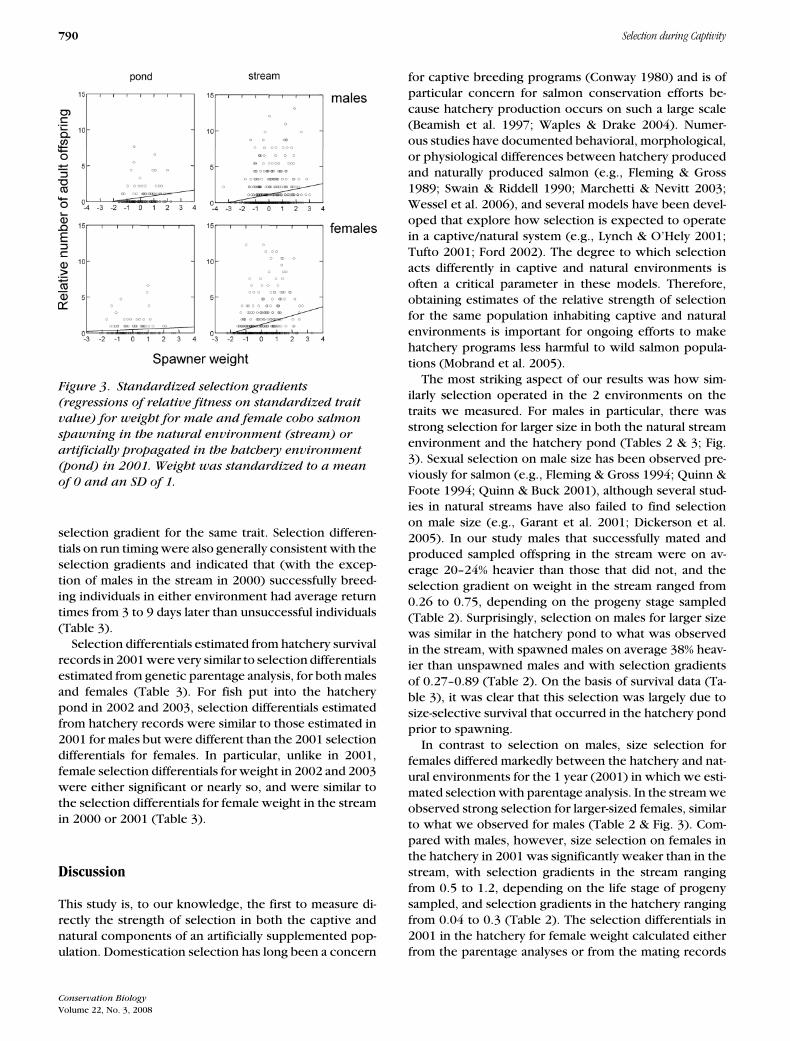
Figure 3. Standardized selection gradients

(regressions of relative fitness on standardized trait

value) for weight for male and female coho salmon

spawning in the natural environment (stream) or

artificially propagated in the hatchery environment

(pond) in 2001. Weight was standardized to a mean

of 0 and an SD of 1.

selection gradient for the same trait. Selection differen-tials on run timing were also generally consistent with theselection gradients and indicated that (with the excep-tion of males in the stream in 2000) successfully breed-ing individuals in either environment had average returntimes from 3 to 9 days later than unsuccessful individuals(Table 3).

Selection differentials estimated from hatchery survivalrecords in 2001 were very similar to selection differentialsestimated from genetic parentage analysis, for both malesand females (Table 3). For fish put into the hatcherypond in 2002 and 2003, selection differentials estimatedfrom hatchery records were similar to those estimated in2001 for males but were different than the 2001 selectiondifferentials for females. In particular, unlike in 2001,female selection differentials for weight in 2002 and 2003were either significant or nearly so, and were similar tothe selection differentials for female weight in the streamin 2000 or 2001 (Table 3).

Discussion

This study is, to our knowledge, the first to measure di-rectly the strength of selection in both the captive andnatural components of an artificially supplemented pop-ulation. Domestication selection has long been a concern

for captive breeding programs (Conway 1980) and is ofparticular concern for salmon conservation efforts be-cause hatchery production occurs on such a large scale(Beamish et al. 1997; Waples & Drake 2004). Numer-ous studies have documented behavioral, morphological,or physiological differences between hatchery producedand naturally produced salmon (e.g., Fleming & Gross1989; Swain & Riddell 1990; Marchetti & Nevitt 2003;Wessel et al. 2006), and several models have been devel-oped that explore how selection is expected to operatein a captive/natural system (e.g., Lynch & O’Hely 2001;Tufto 2001; Ford 2002). The degree to which selectionacts differently in captive and natural environments isoften a critical parameter in these models. Therefore,obtaining estimates of the relative strength of selectionfor the same population inhabiting captive and naturalenvironments is important for ongoing efforts to makehatchery programs less harmful to wild salmon popula-tions (Mobrand et al. 2005).

The most striking aspect of our results was how sim-ilarly selection operated in the 2 environments on thetraits we measured. For males in particular, there wasstrong selection for larger size in both the natural streamenvironment and the hatchery pond (Tables 2 & 3; Fig.3). Sexual selection on male size has been observed pre-viously for salmon (e.g., Fleming & Gross 1994; Quinn &Foote 1994; Quinn & Buck 2001), although several stud-ies in natural streams have also failed to find selectionon male size (e.g., Garant et al. 2001; Dickerson et al.2005). In our study males that successfully mated andproduced sampled offspring in the stream were on av-erage 20–24% heavier than those that did not, and theselection gradient on weight in the stream ranged from0.26 to 0.75, depending on the progeny stage sampled(Table 2). Surprisingly, selection on males for larger sizewas similar in the hatchery pond to what was observedin the stream, with spawned males on average 38% heav-ier than unspawned males and with selection gradientsof 0.27–0.89 (Table 2). On the basis of survival data (Ta-ble 3), it was clear that this selection was largely due tosize-selective survival that occurred in the hatchery pondprior to spawning.

In contrast to selection on males, size selection forfemales differed markedly between the hatchery and nat-ural environments for the 1 year (2001) in which we esti-mated selection with parentage analysis. In the stream weobserved strong selection for larger-sized females, similarto what we observed for males (Table 2 & Fig. 3). Com-pared with males, however, size selection on females inthe hatchery in 2001 was significantly weaker than in thestream, with selection gradients in the stream rangingfrom 0.5 to 1.2, depending on the life stage of progenysampled, and selection gradients in the hatchery rangingfrom 0.04 to 0.3 (Table 2). The selection differentials in2001 in the hatchery for female weight calculated eitherfrom the parentage analyses or from the mating records


Volume 22, No. 3, 2008

Ford et al. 791

Tabl

e3.

Infe

rred

and

estim

ated

mor

talit

yra

tes

and

sele

ctio

ndi

ffere

ntia

lsof

coho

salm

onfo

rw

eigh

tand

run

timin

gin

the

stre

aman

dha

tche

rypo

nden

viro

nmen

ts.

Mea

nru

nti

min

g,

Mea

nw

eig

ht,

g(S

D)

da

ys

aft

er

1Sep.(S

D)

Sa

mple

Mort

ali

ty

Sex

Yea

rLoca

tion

aM

eth

od

bsi

ze

(%)c

spa

wn

ed

not

spa

wn

ed

Dd

(p)

spa

wn

ed

not

spa

wn

ed

Dd

(p)

Mal

e20

00st

ream

gen

etic

449

6123

75(9

72)

1983

(929

)0.

26(0

.001

)47

.6(2

0.5)

49.2

(23.

5)−0

.04

(0.4

48)

2001

stre

amge

net

ic53

153

2593

(125

1)20

97(9

99)

0.23

(<0.

001)

50.1

(19.

4)46

.7(1

9.4)

0.10

(0.0

4)20

01p

on

dge

net

ic15

452

2778

(108

0)20

11(9

01)

0.36

(<0.

001)

50.3

(14.

6)41

.1(1

4.1)

0.25

(<0.

001)

2001

po

nd

reco

rd15

451

2817

(109

2)20

11(9

01)

0.39

(<0.

001)

46.1

(10.

6)40

.2(1

3.0)

0.20

(0.0

02)

2002

po

nd

reco

rd10

558

2543

(891

)22

23(9

57)

0.23

(0.0

9)50

.2(1

6.5)

42.7

(18.

5)0.

24(0

.033

)20

03p

on

dre

cord

244

6424

07(9

87)

1888

(965

)0.

36(<

0.00

1)39

.3(1

2.1)

32.2

(10.

4)0.

39(<

0.00

1)

Fem

ale

2000

stre

amge

net

ic40

756

2393

(692

)21

38(6

07)

0.20

(0.0

01)

55.5

(18.

0)50

.6(2

1.9)

0.13

(0.0

14)

2001

stre

amge

net

ic43

956

2518

(862

)22

15(8

53)

0.21

(<0.

001)

55.7

(16.

9)48

.5(1

7.8)

0.24

(<0.

001)

2001

po

nd

gen

etic

139

5023

18(8

09)

2244

(887

)0.

05(0

.61)

48.4

(14.

0)41

.3(1

2.1)

0.10

(0.0

01)

2001

po

nd

reco

rd13

950

2319

(810

)22

62(8

81)

0.03

(0.6

9)43

.7(8

.0)

40.4

(10.

4)0.

12(0

.036

)20

02p

on

dre

cord

8354

2587

(637

)23

13(6

92)

0.24

(0.0

7)55

.3(1

2.1)

42.6

(17.

1)0.

42(<

0.00

1)20

03p

on

dre

cord

208

6025

59(7

86)

1979

(932

)0.

45(<

0.00

1)43

.2(1

3.8)

35.1

(12.

0)0.

36(<

0.00

1)

aLoca

tion

refe

rsto

wh

eth

er

the

sam

ple

dfi

shw

ere

allow

ed

tosp

aw

nn

atu

rally

inM

inte

rC

reek

(str

ea

m)

or

were

pu

tin

toth

eh

atc

hery

pon

d(p

on

d).

bM

eth

od

refe

rsto

wh

eth

er

mem

bers

hip

of

the

spa

wn

ed

vers

us

un

spa

wn

ed

gro

ups

wa

sin

ferr

ed

on

the

ba

sis

of

resu

lts

of

the

gen

eti

cpa

ren

tage

an

aly

ses

(gen

eti

c)or

from

the

ha

tch

ery

ma

tin

g

reco

rds

(reco

rd).

cM

ort

ali

tyre

fers

toth

eest

ima

ted

pre

spa

wn

ing

mort

ali

tyra

te,ca

lcu

late

da

sth

en

um

ber

of

indiv

idu

als

kn

ow

nor

infe

rred

toh

ave

spa

wn

ed

div

ided

by

the

tota

ln

um

ber

of

indiv

idu

als

inth

e

sam

ple

gro

up

(row

).Th

epre

spa

wn

ing

mort

ali

tyra

tes

est

ima

ted

from

the

gen

eti

cpa

ren

tage

resu

lts

are

ma

xim

um

est

ima

tes

beca

use

itis

likely

tha

tso

me

indiv

idu

als

infa

ctsp

aw

ned

bu

tby

cha

nce

did

not

pro

du

cesa

mple

dpro

gen

y.

dSta

nda

rdiz

ed

sele

ctio

ndif

fere

nti

al(s

tan

da

rdiz

ed

dif

fere

nce

betw

een

the

tota

lpopu

lati

on

tra

itm

ea

na

nd

the

tra

itm

ea

nof

the

indiv

idu

als

kn

ow

nor

infe

rred

toh

ave

spa

wn

ed).

Th

ep

va

lues

were

calc

ula

ted

from

a2

-sa

mple

tte

stth

at

com

pa

red

the

dif

fere

nce

betw

een

the

spa

wn

ed

an

du

nsp

aw

ned

gro

ups.


Volume 22, No. 3, 2008


were also much smaller than the selection differentialsestimated for females in the stream (Table 3). These re-sults suggest that selection for female size was relaxedin the hatchery in 2001 compared with selection in thenatural stream setting. This result was not consistent overtime, however, and in 2002 and 2003 selection on femaleweight in the hatchery was similar to that in the streamin 2001 (Table 3).

Conceptually there could be several mechanisms lead-ing to selection for larger size in the hatchery. Large sizemight be related to good general health, for example.Interactions among fish in the hatchery pond could alsolead to size selection. For example, the fish, particularlymales, in the hatchery pond may interact and fight witheach other in a manner similar to what they do in thestream, resulting in selection for larger size in the hatch-ery even though the hatchery staff does not actively selectfor large size when choosing fish to spawn.

The similar strength of selection in the 2 environmentsin these years does not imply that the selective mecha-nisms were necessarily the same in the 2 environments,however. For example, selection for larger female size inthe wild has been related to a variety of behavioral fac-tors that would have no opportunity to be expressed inthe Minter Creek Hatchery, such as ability to dig deepernests in the gravel, defend superior spawning locations,or attract more males (e.g., van den Berghe & Gross 1989;Fleming & Gross 1994; Quinn et al. 2001). Although wehave clearly documented that selection on size occursin both environments, we have no direct data on theselective mechanism in either environment.

Natural selection for run timing was qualitatively simi-lar for both sexes in both environments, although the sta-tistical significance varied considerably among compar-isons. In both environments there was some evidence forselection for later than average time of return, with suc-cessfully breeding individuals returning anywhere fromseveral days to about a week later than unsuccessful in-dividuals (Tables 2 & 3). These results should be inter-preted in light of the long-term changes that have beenobserved in the run timing of Minter Creek coho salmon(Ford et al. 2006). Both hatchery and natural-origin fishare returning to Minter Creek more than a month ear-lier on average than they did at the time when recordswere first kept in the 1940s (Salo & Bayliff 1958). Thelikely cause of this trend toward earlier time of return isprevious selection for earlier-spawning fish in the MinterCreek Hatchery.

We previously estimated selection gradients on runtiming for those salmon that spawned in the stream (Fordet al. 2006) and hypothesized that the selection for laterrun time indicated that the current, relatively early, runtime was evidence of hatchery-induced selection. It was,therefore, initially surprising to find that selection forlater return time was just as strong in the hatchery asit was in the wild. Nevertheless, for the last decade,

hatcheries throughout Washington have been subject toreview and reform efforts designed to make them morebenign to natural salmon populations (e.g., Mobrand et al.2005). As a result, at the time we initiated our study, theMinter Creek Hatchery began to deliberately reverse itsprevious spawning protocols in favor of protocols thatwould avoid selection for early-returning spawners (D.Popochock, personal communication). The finding of se-lection for later return time therefore appears consistentwith the current spawning protocols employed by thehatchery. In addition, the high level of prespawning mor-tality that occurred in all years of the study (Table 3) likelycontributed to selection for later return time simply be-cause few early-returning fish survived long enough to bespawned.

Consistent with an earlier study on coho salmon (Flem-ing & Gross 1994), we found little evidence for strongselection on the other morphological traits we measuredafter correcting for overall size (Table 2). An importantlimitation of our study, however, was that selection couldonly be estimated on the relatively small number of traitswe measured. Other traits, including behavior and phys-iology, were likely to have been under selection in bothcaptive and natural environments, but would have goneundetected in our study. In addition, in our study all traitswere measured at the weir, often on fish that had not yetbecome fully sexually mature. Many of the morpholog-ical traits we measured vary depending on the state ofsexual maturation (Sandercock 1991), and the measure-ments made at the weir likely differ somewhat from whatthey were at the time that selection actually occurred ineither environment.

The Minter Creek coho salmon population has somecharacteristics that should be taken into account whenconsidering the patterns of selection we observed. Forexample, the low proportion of jacks during the years ofour study may explain why we found no evidence of dis-ruptive selection on male size (Fig. 3), in contrast to someprevious studies (e.g., Gross 1985). The approximately50% mortality rate of our study fish in the hatchery wasalso much higher than the 1–10% that is more typical fora coho salmon hatchery (D. Popochock, personal com-munication), and the patterns of selection we observedin the hatchery may therefore not be typical of hatcherypopulations generally. In particular, relaxation of selec-tion, at least on traits associated with breeding success,may be more typical of hatcheries with very high pre-spawning survival rates. The selection we measured inthe stream setting may also be different from what mighthave been observed had the population not already beenaffected by several decades of hatchery stocking.

Despite these caveats, our results provide an impor-tant glimpse into how natural selection operates in cap-tive and natural environments. Contrary to our initialexpectations, we found that patterns of selection weresimilar between the hatchery and stream environments,


Volume 22, No. 3, 2008

Ford et al. 793

especially for males. The observation of similar outcomesof selection in the 2 environments suggests that selectionon these traits in the hatchery would not be expected tocreate a large selective load that contributes to poor pop-ulation fitness in the natural environment. The case forfemales is somewhat different, with evidence for relaxedselection on weight in the hatchery compared with thenatural stream, at least for 1 of the 3 years studied. Differ-ences in selection regimes between captive and naturalenvironments can lead to reduced fitness in the naturalcomponent of supplemented populations (Bryant & Reed1999; Lynch & O’Hely 2001; Ford 2002). It is not clear,however, whether the degree of relaxation we observedfor selection on female weight in captivity will producea significant selective load on the natural population inMinter Creek. Addressing the fitness consequences ofthe selection we observed will require additional anal-yses that take into account factors such as the geneticbasis of the trait and the rates of gene flow between thecaptive and natural components of the population.

Acknowledgments

We particularly acknowledge the Minter Creek hatcherycrew, D. Popochock, R. Henderson, E. Kinney, S. Davis,D. Watkins, and W. Campbell, whose kind assistance, pa-tience, and unfailing good humor were essential to thesuccess of this project. R. Waples, H. Araki, I. Fleming,M. Chilcote, P. Hulett, and L. Laikre provided useful com-ments on an earlier version of this paper. This projectwas funded in large part by a grant from the HatcheryScientific Review Group, whose assistance we gratefullyacknowledge.

Literature Cited

Araki, H., W. Ardren, E. Olsen, B. Cooper, and M. Blouin. 2007a. Re-productive success of captive-bred steelhead trout in the wild: eval-uation of three hatchery programs in the Hood River. ConservationBiology 21:181–190.

Araki, H., B. Cooper, and M. S. Blouin. 2007b. Genetic effects of cap-tive breeding cause a rapid, cumulative fitness decline in the wild.Science 318:100–103.

Beamish, R. J., C. Mahnken, and C. M. Neville. 1997. Hatchery andwild production of Pacific salmon in relation to large-scale, naturalshifts in the productivity of the marine environment. ICES Journalof Marine Science 54:963–964.

Bryant, E., and D. Reed. 1999. Fitness decline under relaxed selectionin captive populations. Conservation Biology 13:665–669.

Conway, W. G. 1980. An overview of captive propagation. Pages 199–208 in M. E. Soule and B. A. Wilcox, editors. Conservation biology:an evolutionary-ecological perspective. Sinauer Associates, Sunder-land, Massachusetts.

Dickerson, B., K. Brinck, M. Willson, P. Bentzen, and T. Quinn. 2005.Relative importance of salmon body size and arrival time at breedinggrounds to reproductive success. Ecology 86:347–353.

Etterson, J., and R. Shaw. 2001. Constraint to adaptive evolution inresponse to global warming. Science 294:151–154.

Fleming, I. A., and M. R. Gross. 1989. Evolution of adult female lifehistory and morphology in a Pacific salmon (coho: Oncorhynchus

kisutch). Evolution 43:141–157.Fleming, I. A., and M. R. Gross. 1993. Breeding success of hatchery and

wild coho salmon (Oncorhynchus kisutch) in competition. Ecolog-ical Applications 3:230–245.

Fleming, I. A., and M. R. Gross. 1994. Breeding competition in a PacificSalmon (coho: Oncorhynchus kisutch): measures of natural andsexual selection. Evolution 48:637–657.

Ford, M., H. Fuss, B. Boelts, E. LaHood, J. Hard, and J. Miller. 2006.Changes in run timing and natural smolt production in a naturallyspawning coho salmon (Oncorhynchus kisutch) population after60 years of intensive hatchery supplementation. Canadian Journalof Fisheries and Aquatic Sciences 63:2343–2355.

Ford, M. J. 2002. Selection in captivity during supportive breeding mayreduce fitness in the wild. Conservation Biology 16:815–825.

Frankham, R. H., H O. Ryder, E. Cothran, M. Soule, N. Murray, and M.Snyder. 1986. Selection in captive populations. Zoo Biology 5:127–138.

Garant, D., J. J. Dodson, and L. Bernatchez. 2001. A genetic evaluation ofmating system and determinants of individual reproductive successin Atlantic salmon (Salmo salar L.). The Journal of Heredity 92:137–145.

Gerber, S., P. Chabrier, and A. Kremer. 2003. FaMoz: a software forparentage analysis using dominant, codominant and uniparentallyinherited markers. Molecular Ecology Notes 3:479–481.

Gross, M. R. 1985. Disruptive selection for alternative life histories insalmon. Nature 313:47–48.

Hershberger, W., J. Myers, R. Iwamoto, W. Mcauley, and A. Sax-ton. 1990. Genetic changes in the growth of coho salmon (On-

corhynchus kisutch) in marine net-pens, produced by 10 years ofselection. Aquaculture 85:187–197.

Lande, R., and S. J. Arnold. 1983. The measurement of selection oncorrelated characters. Evolution 37:1210–1226.

Lande, R., and S. Shannon. 1996. The role of genetic variation in adap-tation and population persistence in a changing environment. Evo-lution 50:434–437.

Lynch, M., and R. Lande. 1993. Evolution and extinction in responseto environmental change. Sinauer Associates, Sunderland, Mas-sachusetts.

Lynch, M., and H. O’Hely. 2001. Captive breeding and the genetic fitnessof natural populations. Conservation Genetics 2:363–378.

Marchetti, M., and G. Nevitt. 2003. Effects of hatchery rearing on brainstructures of rainbow trout, Oncorhynchus mykiss. EnvironmentalBiology of Fishes 66:9–14.

Mobrand, L. E., J. Barr, L. Blankenship, D. E. Campton, T. T. P. Evelyn,T. A. Flagg, C. V. W. Mahnken, L. W. Seeb, P. R. Seidel, and W. W.Smoker. 2005. Hatchery reform in Washington State: principles andemerging issues. Fisheries 30:11–33.

National Research Council. 1996. Upstream: salmon and society in thePacific Northwest. National Academy Press, Washington, D.C.

Nehlsen, W., J. E. Williams, and J. A. Lichatowich. 1991. Pacific salmonat the crossroads: stocks at risk from California, Oregon, Idaho, andWashington. Fisheries 16:4–21.

Quinn, T. P., and G. B. Buck. 2001. Size- and sex-selective mortality ofadult sockeye salmon: bears, gulls, and fish out of water. Transac-tions of the American Fisheries Society 130:995–1005.

Quinn, T. P., and C. J. Foote. 1994. The effects of body sizeand sexual dimorphism on the reproductive behavior of sock-eye salmon, Oncorhynchus nerka. Animal Behavior 48:751–761.

Quinn, T. P., A. P. Hendry, and G. B. Buck. 2001. Balancing natural andsexual selection in sockeye salmon: interactions between body size,reproductive opportunity and vulnerability to predation by bears.Evolutionary Ecology Research 3:917–937.

Reisenbichler, R. R., and J. D. McIntyre. 1977. Genetic differences ingrowth and survival of juvenile hatchery and wild steelhead trout,


Volume 22, No. 3, 2008


Salmo gairdneri. Journal of the Fisheries Research Board of Canada34:123–128.

Rohlf, F. J. 2001. TPSDIG Program for digitizing images for analysis bythin plate splines. State University of New York, Stony Brook, NewYork. Available from http://life.bio.sunysb.edu/morph/ (accessedMay, 2002).

Ryman, N., and L. Laikre. 1991. Effects of supportive breeding on thegenetically effective population size. Conservation Biology 5:325–329.

Ryman, N., P. E. Jorde, and L. Laikre. 1995. Supportive breeding andvariance effective population size. Conservation Biology 9:1619–1628.

Salo, E. O., and W. H. Bayliff. 1958. Artificial and natural production ofsilver salmon (Oncorhynchus kisutch) at Minter Creek, Washington.Washington Department of Fisheries, Olympia.

Sandercock, F. K. 1991. Life history of coho salmon (Oncorhynchus

kisutch). Pages 395–446 in C. Groot and L. Margolis, editors. Pa-cific salmon life histories. University of British Columbia Press,Vancouver.

Snyder, N., S. Derrickson, S. Beissinger, J. Wiley, T. Smith, W. Toone,and B. Miller. 1996. Limitations of captive breeding in endangeredspecies recovery. Conservation Biology 10:338–348.

Swain, D. P., and B. E. Riddell. 1990. Variation in agonistic behaviorbetween newly emerged juveniles from hatchery and wild popula-tions of coho salmon, Oncorhynchus kisutch. Canadian Journal ofFisheries and Aquatic Sciences 47:566–571.

Tufto, J. 2001. Effects of releasing maladapted individuals: ademographic-evolutionary model. The American Naturalist 158:331–340.

Van Den Berghe, E. P., and M. R. Gross. 1989. Natural selection result-ing from female breeding competition in a Pacific salmon (coho:Oncorhynchus kisutch). Evolution 43:125–140.

Wang, J., and N. Ryman. 2001. Genetic effects of multiple gen-erations of supportive breeding. Conservation Biology 16:1619–1631.

Waples, R. S., and J. Drake. 2004. Risk/benefit considerations for marinestock enhancement: a Pacific salmon perspective. Pages 260–306in L. M. Leber, S. Kitada, T. Svasand, and H. L. Blankenship, editors.Proceedings of the second international symposium on marine stockenhancement. Blackwell Publishing, Oxford, United Kingdom.

Wessel, M., W. Smoker, R. Fagen, and J. Joyce. 2006. Variation of ag-onistic behavior among juvenile Chinook salmon (Oncorhynchus

tshawytscha) of hatchery, hybrid, and wild origin. Canadian Jour-nal of Fisheries and Aquatic Sciences 63:438–447.


Volume 22, No. 3, 2008

Estimates of Natural Selection in a Salmon Population in Captive and Natural Environments

Documents

Transcript of Estimates of Natural Selection in a Salmon Population in Captive and Natural Environments