i

Essays on Regional Responses to Globalization

By

RIZKI NAULI SIREGAR

DISSERTATION

Submitted in partial satisfaction of the requirements for the degree of

DOCTOR OF PHILOSOPHY

in

Economics

in the

OFFICE OF GRADUATE STUDIES

of the

UNIVERSITY OF CALIFORNIA

DAVIS

Approved:

Robert C. Feenstra, Chair

Giovanni Peri

Deborah Swenson

Committee in Charge

2021

c© Rizki Nauli Siregar, 2021. All rights reserved.

Contents

Abstract v

Acknowledgments vii

1 Global prices and internal migration: Evidence from the

palm oil boom in Indonesia 1

1.1 Introduction 1

1.2 Indonesia in the 2000s 7

1.2.1 Overview . . . . . . . . . . . . . . . . . . . . . . . . . . . . . . . . . . . . . 7

1.2.2 The rising star of the commodity boom in the 2000s: Palm oil . . . . . . . 8

1.2.3 Three stylized facts . . . . . . . . . . . . . . . . . . . . . . . . . . . . . . . 10

1.3 Theoretical framework 12

1.3.1 Framework for measurement of exposure to price shocks: Two-sector economy 13

1.3.2 Decomposition of welfare changes: Multi-sector multi-region economy . . . 19

1.3.3 Decomposition . . . . . . . . . . . . . . . . . . . . . . . . . . . . . . . . . . 20

1.4 Data and measurement of exposure to shocks 22

1.4.1 Data . . . . . . . . . . . . . . . . . . . . . . . . . . . . . . . . . . . . . . . 23

1.4.2 Exposure to price shocks . . . . . . . . . . . . . . . . . . . . . . . . . . . . 25

1.5 Empirical results 28

1.5.1 Specification . . . . . . . . . . . . . . . . . . . . . . . . . . . . . . . . . . . 28

1.5.2 Impact of the exposure to palm oil price shocks . . . . . . . . . . . . . . . 30

1.5.3 Spillover to non-exposed districts . . . . . . . . . . . . . . . . . . . . . . . 32

1.5.4 Mechanisms . . . . . . . . . . . . . . . . . . . . . . . . . . . . . . . . . . . 34

ii

1.6 Quantitative estimation 38

1.6.1 Data and parameters . . . . . . . . . . . . . . . . . . . . . . . . . . . . . . 38

1.6.2 Results . . . . . . . . . . . . . . . . . . . . . . . . . . . . . . . . . . . . . . 39

1.7 Conclusion 40

Appendix 1 42

2 Price divergence in times of trade protection: Exploration

on the import ban on rice in Indonesia 74

2.1 Introduction 74

2.2 The import ban on rice in Indonesia 79

2.2.1 The political economy of rice in Indonesia . . . . . . . . . . . . . . . . . . . 79

2.2.2 The impact of rice price shocks . . . . . . . . . . . . . . . . . . . . . . . . 81

2.2.3 No sign of extensification or intensification . . . . . . . . . . . . . . . . . . 82

2.3 Exploration on price divergence 83

2.3.1 Data . . . . . . . . . . . . . . . . . . . . . . . . . . . . . . . . . . . . . . . 83

2.3.2 Trend of retail prices and farm-gate prices . . . . . . . . . . . . . . . . . . 84

2.3.3 Prices and crop suitability . . . . . . . . . . . . . . . . . . . . . . . . . . . 86

2.3.4 What contribute to the variation in prices . . . . . . . . . . . . . . . . . . 86

2.3.5 Price behavior after the import ban . . . . . . . . . . . . . . . . . . . . . . 87

2.3.6 Have trade costs increased over time? . . . . . . . . . . . . . . . . . . . . . 89

2.4 Discussion 90

2.5 Conclusion 94

Appendix 2 96

iii

3 New-consumer margin at work: Exposure to television ads

as driver of smoking prevalence 112

3.1 Introduction 112

3.2 The economics of smoking 116

3.2.1 Tobacco consumption . . . . . . . . . . . . . . . . . . . . . . . . . . . . . . 116

3.2.2 Tobacco industry . . . . . . . . . . . . . . . . . . . . . . . . . . . . . . . . 118

3.2.3 Tobacco-control policies . . . . . . . . . . . . . . . . . . . . . . . . . . . . . 120

3.3 Theoretical framework and empirical facts 121

3.3.1 Theory of marketing cost in international trade à la Arkolakis (2010) . . . 122

3.3.2 Productivity growth . . . . . . . . . . . . . . . . . . . . . . . . . . . . . . . 124

3.3.3 Improvement in marketing technology . . . . . . . . . . . . . . . . . . . . . 125

3.3.4 Empirical facts on smoking environment in Indonesia . . . . . . . . . . . . 125

3.4 Data and empirical strategy 128

3.4.1 Data and sample construction . . . . . . . . . . . . . . . . . . . . . . . . . 128

3.4.2 DiD estimates of the impact of TV exposure on smoking participation . . . 131

3.4.3 IV Estimates of young adults smoking participation on long-run outcomes . 133

3.5 Results 134

3.5.1 Evidence of the new-consumer margin . . . . . . . . . . . . . . . . . . . . . 134

3.5.2 Long-run impacts . . . . . . . . . . . . . . . . . . . . . . . . . . . . . . . . 137

3.5.3 Robustness analysis . . . . . . . . . . . . . . . . . . . . . . . . . . . . . . . 139

3.6 Conclusion 141

Appendix 3 142

References 165

iv

Rizki Nauli SiregarAugust 2021Economics

Abstract of the Dissertation

Essays on Regional Responses to Globalization

This dissertation explores various regional responses to globalization. The first chapter

studies how booming regions spread local windfall from a commodity boom in the world

market to other regions. The second chapter explores price divergence in the rice markets

as an impact of a binding import ban, a policy imposed to support farmers from facing im-

port competition. Lastly, the third chapter shows how the proliferation of electronic media,

an aspect of globalization, facilitates improvement in marketing technology in advertising

tobacco products. I show that such improvement in reaching consumers and potential con-

sumers increases the smoking participation of young adults.

Chapter 1 studies how regions respond to price shocks in the presence of internal mi-

gration. This paper examines Indonesia in the 2000s as it faced a commodity boom for

palm oil, which became one of its main export commodities. I exploit the variation in the

land shares and crop suitability to compute the potential contribution of main crops across

district economies as a measure of local exposure to shocks. I find that the commodity boom

increased the purchasing power of palm oil-producing districts. These districts also received

more migration, providing evidence that palm oil price shocks were no longer localized. In-

deed, internal migration spread the windfall. I also find spillover to neighboring districts.

However, these relatively higher levels of purchasing power did not last after the commodity

boom ended in 2014. I show that the palm-oil sector grew through extensification as a re-

sponse to the price shocks, with no indication of growth through intensification. I estimate

the overall welfare gains in Indonesia between 2005 and 2010 and find substantial gains from

migration.

v

Chapter 2 explores and documents the price divergence that occurs due to a large and

ongoing import ban on rice imposed by Indonesia. I find that despite the increase in the

retail price of rice, rice-producing districts do not enjoy higher purchasing power. The trade

protection did not spur growth in the rice sector either. I find that the import ban causes

price divergence in two dimensions. First, it causes regional price divergence, implying the

lack of arbitrage across rice markets. Second, I find evidence of incomplete pass-through

as the wedge between the retail prices and farm-gate prices widens. These findings provide

guidance for further research and trade policy evaluation to consider aspects such as imperfect

competition and domestic trade frictions in determining the distributional impact of the

import ban.

Chapter 3 is motivated by the fact that the tobacco epidemic kills more than 8 million

people every year. Despite a global decline in smoking rates, smoking prevalence is rising

in many developing countries. This paper exploits the temporal and regional variation in

the proliferation of television reception across Indonesia in the 2000s to examine the impact

of advertising on electronic media on smoking participation by young adults. Applying the

marketing theory drawn from international trade, I find evidence of a new-consumer margin

in tobacco consumption due to improvement in marketing technology. Living in a subdistrict

with one standard deviation higher television exposure increases male young adults smoking

participation by 4-6%. This impact is especially significant for those of 17 to 19 years old

but not older persons.

vi

Acknowledgments

Alhamdulillaahirrabil ‘alamin. Praise be to Allah, the Lord of the Universes. Allahumma

shalli ‘alaa sayyidina Muhammad wa ‘alaa ali sayyidina Muhammad. O God, send blessings

upon Muhammad and upon the Progeny of Muhammad. Only by God’s Power and Guid-

ance, I can be blessed with this journey of looking for His Knowledge, far away from home.

I am grateful for His Blessings and Knowledge that He trusted me with. I pray and hope for

His Guidance and Strength so that I can convey and uphold the Knowledge that He blessed

me with, with integrity and honesty.

I would like to thank my advisors: Prof. Robert C. Feenstra, Prof. Giovanni Peri, and

Prof. Deborah Swenson, for their support. I am thankful for their guidance, including

during the times when it felt unclear on how to make progress. I am thankful for their

encouragement in every milestone. Thank you for taking the chance on me.

I have admired Prof. Feenstra’s works since I was an undergraduate student of economics

at Universitas Indonesia. It has been a dream come true to work closely with him and to learn

so much from him directly. I will never forget when he encouraged me: “Study something

that you are passionate about, then people will get interested in it too.” when I had to ‘kill’

a project and start a new one. Indeed, such encouragement helped me find my calling in

research and I hope to continue thriving by listening to the calling. I am inspired by his

deep understanding of his expertise and how he keeps on learning advancing the frontiers,

powered by interests in fresh ideas from other fields. I am grateful for his support and how

he always considered the most optimal solution from the perspective of his advisees.

I am grateful for Prof. Peri’s extraordinary support from my first years as a student and

now as his advisee. Prof. Peri extends his care, knowing that an international student like

myself has to live a long-distance relationship with our families. It means a lot to me that

he asked how my parents were and always sent them his regards. In times of heated political

environment toward immigrants in the US, I will always remember his presence to support

vii

us. In one of our communication on the matter, he assured me that we had full commitment

and support from the department and him as the Chair of the Department of Economics at

the time. As a scholar, I am inspired by his engagement and enthusiasm in working with

policymakers and the public.

I am grateful for various opportunities to learn from and work with Prof. Swenson. I

learned a lot not only as a researcher but also as an educator from her. As a researcher, I

learned from Prof. Swenson to be able to zoom in and zoom out fluently in analyzing things.

Prof. Swenson always provides constructive inputs. These inputs have been invaluable in

helping me to not only see but also convey my ideas. I am thankful for the chance to learn

from Prof. Swenson as her teaching assistant as well. I learned how to not only engage

students but also challenge them to be their best.

Many parts of my doctoral study are prayers and support from my family. Words can

not express how grateful I am for my family’s love, trust, support, and confidence in me.

The marathon of finishing a Ph.D. is rarely done in a “controlled lab”. Challenges in life can

come at any time. I am grateful for my parents, Mara Oloan Siregar and Ade Dermawan

Nasution, who give models in building synergy, courage to try again and again, as well as

faith in and gratitude to the Mercy of The Most Kind. Both of them are first-generation and

migrated from a small town in Sumatra to the capital city, Jakarta. Breaking glass-ceiling,

both of them earned graduate degrees and meaningful careers. After retiring, they keep

thriving to create opportunities for others. They set examples that one can keep learning

and growing as well as that there is abundance in modesty. Their hard work, struggle, and

journey in making the best out of any circumstances have inspired me in every step.

I am thankful for the support from my sister, Aisyah Rahmarani, and my brother, Ibrahim

Siregar. They have been taking a lot of extra responsibility as I could not be home most of the

time. In times of ease and challenges, they give me warmth and confidence, unconditionally.

I am forever inspired by their resilience and how they thrive. Their trust and support are

one of my sources of energy to keep going. Their company -- from just eating take-outs at

viii

home to travel across the country, always energizes me. Thank you also to my new brother,

Ahmad Jamaati, for prayers and continued support.

Coming from a big family, I am grateful for the support I have received from both sides

of my extended family from Sipangko and Kayulaut as well as family and relatives in Tebet.

The prayers I have received from them make me feel less lonely and always supported. I am

also grateful for the love and support from the Pielkes. I am excited to be able to live close

to them soon.

I don’t know whether I can go this far without the support and guidance from my amazing

mentors: Prof. Gustav Papanek, Prof. Mari E. Pangestu, Bapak M. Chatib Basri, and Prof.

Katheryn E. Russ. They help me to see the gems in my work in times of doubt and challenge

me to give more in times of accomplishment. I hope to be able to pay forward their support

to many young aspiring economists.

I am also grateful for the support from the network of Indonesian economists for feedback

and encouragement along the way: Bapak Teguh Dartanto, Prof. Arief Anshory Yusuf,

Bapak Sudarno Sumarto, Bapak Elan Satriawan, Ibu Vivi Alatas, Mba Titik Anas, Mba Uti

Soejachmoen. Thank you also to Sam Bazzi for the opportunities and support. I am thankful

for the camaraderie from fellow Indonesian young scholars: Rus’an Nasrudin, Gumilang

Sahadewo, Rhita Simorangkir, Puspa Amri, Armand Sim, Daniel Halim, Masyhur Hilmy,

Roy Wirapati, Aichiro Suryo Prabowo, Zenathan Adnin, Muhammad Hanri. A special thank

you to Wisnu Harto, for always being helpful with data.

I am grateful for the support I can always rely on from my friends in and from Indonesia:

Rivana Mezaya, Referika Rahmi, Ihutan Pricely, Mas David Hutama, Mba Asrianti Mira,

Ira Febrianty, Indah Putri, Bang Ananda Siregar, Fara Elmahda, Kak Meizany Irmadhiany,

Mba Lynda Ibrahim, “NAF” family, “Kamis Romantis” Family, Arridhana Ciptadi, Mas

Fandi Nurzaman, Nia, Mas Jeje, Andra, Mba Mega, Mba Maylaffayza, and many more that

I cannot be thankful enough. I am also grateful to friends from the Indonesian art network,

including Mas Ade Darmawan, Popo, MG Pringgotono, Mba Mia Maria, Ajeng Nurul Aini,

ix

and the Ruang Rupa Collective, who always sparks my creativity, enriches my perspective,

and helps me listen to and act on what matters.

I am grateful for the hospitality, support, and resources from the Assegaf Hamzah and

Partners as well as the amazing professionals I was lucky enough to interact with. I am

thankful for the fruitful discussions with Bapak Fikri Assegaf. His questions helped shape

the direction of the first chapter of this dissertation.

I have been blessed to cross-path with many amazing people in my time in Davis. My

amazing sisters, the hijabis Ph.D. students at UC Davis, have been not only inspirations in

academic rigor but also in humility and grace as Muslimah. Thank you Nermin Dessouky,

Nadia Moukanni, Dalia Rakha, Alaa Abdelfattah, and Mba Zatil Afra for the unwavering

support. I hope our sisterhood thrives across the globe. In addition, the Temple coffee in

Davis and especially the baristas have been my second home in this town. During stay-

home order due to the long California fires to the Covid-19 pandemic, they were the only

people that I meet and connect with for many days. They cheered me in many steps of

my doctoral journey: writing a prospectus, preparing the oral exam, writing the job market

paper, preparing for the job talk, preparing for interviews, to writing the dissertation. They

not only provide, of course, caffeine boosts but also run as a pacer for me to keep going

the marathon. Thank you: Carmen, Emily, KTB, Wyatt, Alicia, Danielle, Karene, CJ,

Chloe, and many more. I have also been lucky to grow with amazing economists from

my colleagues at the Economics Department and Agricultural and Resources Economics

Department. Thank you especially, Monica Guevara, Briana Ballis, Jessica Rudder, Luis

Avalos Trujillo, Amanda Bird, Janet Horsager, John Blanchette, Matt Curtis, Ezgi Kurt,

Derek Rury, Anna Ignatenko, Akira Sasahara, Vasco Yasenov, Sarah Quincy, Mariam Yousuf

for the friendship. I look forward to learning more from your amazing works, and hopefully

collaborating with you in the future!

I am grateful for the kindness and care from the Darwents who let me stay in their cottage

for five years. I feel like I have a family who watches over me with a lot of care, support, and

x

understanding. I am really lucky to be able to spend most of my time in Davis surrounded

by a caring, warm, and accepting neighborhood at Aggie Village, just across the beautiful

and calming Arboretum. Thank you especially to Ursula Scriba for always being helpful and

cheering me with sweets and good vibes just from around the corner.

I am grateful for the holistic support provided by the UC Davis Student Health and

Counseling Services. I have benefited from the care of Dr. Moussas and Dr. Kalman,

who supported me to build a healthy body and mind. I am grateful for the thoughtful care

provided by the staff of the Student Health and Counseling Services, including in challenging

times for me. I hope for a day when everyone can have affordable access to such an excellent

universal healthcare service.

With gratitude and humility, let us continue the path to build more equitable welfare for

all. Bismillaahirrahmaanirrahiim.. In the name of Allah, the Most Gracious and the Most

Merciful.

Alhamdulillaah Alhamdulillaah Alhamdulillaah. Praise be to Allah. Praise be to Allah.

Praise be to Allah. I hope I can convey the Knowledge that Allah SWT trusts in me in

this dissertation with justice. May Allah guide and empower me to continue the journey to

contribute to others and the world.

Allahumma shalli ‘alaa sayyidina Muhammad wa ‘alaa ali sayyidina Muhammad. O God,

send blessings upon Muhammad and upon the Progeny of Muhammad. May Allah guide

me to follow the examples from Rasulullaah (Peace be Upon Him) to convey His Knowledge

with truth, honesty, and integrity. May Allah bring lots of Blessings and Meanings for many

to His Knowledge that I share with the world.

xi

Chapter 1

Global prices and internal migration:

Evidence from the palm oil boom in

Indonesia

1.1 Introduction

Many developing economies are primary-commodities producers that face trade shocks from

global price fluctuations. International macro literatures have shown that the impact of these

fluctuations is not trivial. For example, Fernández et al. (2017) show that 30% of domestic

output fluctuations are driven by world shocks that stem from commodity prices. In theory,

labor market can respond directly to these fluctuations by moving to booming sector or

regions. However, many empirical studies show that trade shocks are usually localized, i.e.,

labor does not response by moving. Meanwhile, Lucas (2015) documents that one out of

ten people in the world is an internal migrant. In developing countries, the intensity of

internal migration ranges from as low as 6% in India to as high as almost 50% in Chile.

Therefore, understanding how labor responds through mobility in the face of price shocks in

international trade is an important question for many developing countries.

The goal of this paper is to study how a multi-region economy responds to price shocks

stemming from commodity prices in the presence of internal migration. I take the context

of Indonesia as it faced a commodity boom in the 2000s. I fill the gap in the literature by

providing evidence of trade shocks that are no longer localized, especially when these trade

shocks are advantageous to local income. Many studies on the impact of trade shocks use

1

import shocks that deteriorate income.1 If there are fixed migration costs or cash-in-advance

constraints in migration, then we may not see much response through migration in the face

of trade shocks that hurt income. Specifically, I show that internal migration diffuses trade

shocks stemming from the commodity boom as people move to palm oil-producing districts.

This paper also contributes to the development policy discourse. I show that the wind-

fall from the commodity boom was short-lived. This paper is the first to document the

impact of fluctuations in global prices on welfare indicators over time. It is important to

emphasize that this temporary windfall stands in contrast to the longer-run cost imposed by

the well-documented deforestation driven by palm oil expansion.2 This evidence can inform

policymakers, including local leaders who have substantial decision-making power over land

concessions. The findings also suggest cautions about exchange rate management for the

monetary authority, given the importance of primary commodities, including palm oil, as a

source of foreign reserves.

Indonesia is an excellent context for studying the impact of price shocks in developing

economies for at least three reasons. First, Indonesia is a large country, in terms of popula-

tion, size and area, but it is mostly a price-taker in the world market. Thus, Indonesia shares

with most developing economies the feature of being a small-open economy. Second, there is

a wide heterogeneity in comparative advantage across regions in Indonesia. Hence, Indonesia

provides the opportunity to study variation in the exposure to shocks in the face of uniform

price shocks. Indeed, Indonesia’s regionally representative data makes it possible to study

the country as a multi-region economy. Third, there are no legal-restrictions on moving from

one region to another in Indonesia. Regions do vary in terms of their level of amenities

level, and people have heterogeneous preferences to live in certain regions. Nevertheless, it

1This observation is also supported by Pavcnik (2017) in her lecture in the Jackson Hole Symposiumin 2017. Some important studies using import shocks include Dix-Carneiro and Kovak (2017) for tradeliberalization in Brazil, Topalova (2010) in India and Autor et al. (2013) for the surge of imports from Chinato the US.

2Hansen et al. (2013) show that Indonesia experienced the world’s largest increase in forest loss in2000-2012. Meanwhile, Austin et al. (2019) show that palm oil plantation was the largest single driver ofdeforestation in Indonesia for the period from 2001 to 2016. Globally, commodity-driven deforestation hasbeen rampant, accounting for an estimated 27% of the world’s forest loss (Curtis et al., 2018).

2

is plausible to regard residential choices as market-driven choices.3

To answer the research question, I perform a set of empirical and quantitative analyses

guided by a theoretical framework that matches the context of Indonesia from 2000 to 2015.

In particular, I collect three stylized facts that motivate the environment of the model. First,

I choose the agriculture sector as the sector of interest, because farmers can adjust crop

choices as they face changes in crop prices.4 Districts with high shares of the agriculture

sector also tend to be poorer, which means that districts have different starts before the

exposure to price shocks. Second, I choose palm oil and rice as the main crops of interest

because they share around half of the agricultural land in Indonesia. Third, the gravity

equation on migration flows reveals that regions face upward-sloping labor supply. This

result implies that labor moves to regions with higher earnings.

Armed with the three stylized facts, I build two theoretical frameworks as the foundation

for the empirical and quantitative analysis. First, I combine a two-sector Specific Factor

Model with the multi-region economy as in Redding (2016). I show that the impact of price

shocks on regional wages depends on the share of the sector that experiences the increase in

relative price. This result guides the measurement of local shocks in the empirical analysis.

Second, I decompose the welfare changes in the multi-region economy model as in Redding

(2016) into gains from migration and gains from trade. This result guides the quantitative

analysis in estimating the overall changes in welfare in Indonesia between 2005 to 2010.

Defining districts as unit of regions, I construct a measure of exposure to price shocks for

palm oil and rice based on the result of the theoretical framework. I compute local exposure

to shocks using the potential share of palm oil and rice in district economies. In particular,

I exploit the variation in crop suitability and pre-shocks harvested area. Armed with the

computed local shocks, I employ the difference-in-difference method to estimate the impact of3According to Artuc et al. (2015), migration costs in Indonesia are close to the average migration costs in

developing countries. As a comparison, migration cost is estimated to be 3.46 of annual wage in Indonesia,5.06 in the Philippines, 3.77 in Korea, 2.75 in China, and 2.21 in the US.

4The commodity boom in the 2000s affected both the agriculture sector and the mining sector directly.To take into account the exposure of the commodity boom to the mining sector, I control for the shares ofmining sector but do not focus on it.

3

exposure to palm oil price shocks on two main outcome variables: real expenditure per capita

as the main proxy for welfare and net-inward migration rate for labor-mobility outcome. I

study the impact of the exposure to price shocks on three margins: between exposed and

non-exposed, heterogeneity in exposure and spillover to non-exposed districts. In addition,

I discuss the mechanisms that drive the results. Specifically, I analyze the responses of

factors of production, i.e., labor and land, toward the price shocks. Lastly, applying the

framework of asymmetric location and labor mobility as in Redding (2016), I estimate the

welfare changes in the Indonesian economy between 2005 and 2010. I decompose the welfare

changes into gains from migration and gains from trade.

I present three main findings. First, districts exposed to palm oil shocks had significantly

higher real expenditure per capita compared to the non-exposed ones. I find that labor

responded to the incentives from higher real expenditure per capita in districts exposed

to palm oil price shocks. Accordingly, these districts attracted more net-inward migration.

Since I follow districts’ performance over time, I find evidence that the impact of the shocks

was temporary. As the commodity boom ended, the difference between exposed and non-

exposed districts also dissipated.

In an analysis of the mechanisms that drive the result, I find that the growth in the palm

oil sector was spurred by land expansion (extensification) and not by an increase in actual

yield (intensification). Meanwhile, analyzing district premia using the two-step method

introduced by Dix-Carneiro and Kovak (2017), I find results that contrast with their results

for trade liberalization in Brazil. In this paper, I find that district premia are relatively

equalized across districts. This result implies that frictions to labor mobility may not be

significant enough to prevent any shocks from diffusing through internal migration. Indeed,

as the palm oil sector grew through land expansion, they may have increased labor demand

in palm oil-producing districts. This increase in labor demand materialized as higher real

expenditure per capita and net-inward migration.

Second, I show evidence of spillovers. The nearest non-exposed districts to districts ex-

4

posed to palm oil shocks also have significantly higher expenditure per capita and migration.

This result presents evidence that the shocks are not fully localized. They have an indirect

impact on non-exposed districts. As districts experience a boom, they demand more goods

and services as well as labor from the surrounding districts.

Lastly, I estimate that there was a welfare gain of 0.39% in Indonesia between 2005 to

2010. Gains from migration account for one-third of these gains, or 36%. Meanwhile, gains

from trade account for the other two-thirds, or 64%, of the gains.

This paper contributes to three strands of literature. First, I contribute to the broad

literature on the impact of international trade on labor markets in domestic economies.

There are two main channels through which the trade shocks materialize: the price channel

and the quantity channel. In the former, trade shocks can stem from trade liberalization

as in Topalova (2010) and Kovak (2013), world price changes as in Adão (2015), trade cost

changes as in Donaldson (2018), or a combination, such as in Sotelo (2015).5 I complement

this literature by studying trade shocks through the price channel and their relationship

with internal migration.6 I contribute to this literature by showing evidence of how local

labor markets adjust and diffuse trade shocks that are advantageous to local income through

internal migration.

Second, I contribute to the literature on trade, internal migration and regional dynamics

by showing that the impact of the commodity boom has been short-lived. I emphasize the

need for caution in taking cyclical factors such as global prices as a sustainable source of

growth for regional development. I show that districts with direct exposure to the commod-

ity boom in palm oil received more net-inward migration at the peak of the boom. This

5Meanwhile, the quantity channel can stem from implied technological changes, as studied by Autor et al.(2013) for the case of surges of imports from China by the US and by Costa et al. (2016) for the demandand supply shocks faced by Brazil due to the technological shock in China.

6Recent papers show evidence of the importance of taking into account internal migration. For example,Tombe and Zhu (2019) quantify the welfare impacts of reduction in internal trade costs, international tradecosts, and internal migration costs in China and show that most of the welfare gain stems from a reductionin internal migration costs instead of the more commonly credited reduction in international trade costs asChina joined the WTO. Meanwhile, Pellegrina and Sotelo (2020) use the case of Brazil to show that internalmigration can shape regions’ and ultimately countries’ comparative advantage.

5

mechanism allowed other districts to benefit through outmigration to the booming regions.

However, as the global palm oil prices decreased after the boom, these palm-oil producing

districts may no longer have provided such spillover to other districts. Meanwhile, using

trade liberalization in Brazil, Dix-Carneiro and Kovak (2017) show that regions facing larger

liberalization experienced increasingly lower growth in wages and employment. They show

that a lack of internal migration and slow capital adjustment amplify the local effects of trade

liberalization. Using the accession of China to the WTO, Fan (2019) shows the importance of

taking into account internal migration when estimating the impact of trade liberalization on

interregional inequality and wage inequality. Méndez-Chacón and Van Patten (2019) study

the regional dynamics in Costa Rica due to foreign direct investment flows. They show that

the ease of internal migration dampens a monopsonist’s market power to push down local

wages.

Lastly, this paper contributes to the literature on the palm-oil economy. Qaim et al.

(2020) provide the most recent survey of literature on the impact of the palm oil boom. This

present paper has much in common with Edwards’ (2018) study of the impact of palm-oil

expansion in Indonesia on local poverty and deforestation, but I am the first to show the

cyclicality of the impact of global palm oil prices on the sub-national level. In particular, I

show that districts exposed to the palm-oil boom experienced a temporary windfall.

The rest of the paper is structured as follows. I lay out the context of Indonesia during

the commodity boom in the 2000s in Section 2. In the same section, I state three facts that

motivate the choice of agriculture sector, the choice of crops and the importance of taking

into account internal migration. Guided by these facts, I describe the theoretical frameworks

that guide the empirical analysis and the quantitative simulation in Section 3. I describe

the main data and the measurement of exposures to price shocks in Section 4. Armed with

the computed exposure to shocks, I present and discuss the empirical evidence of the impact

of the exposure to the price shocks in Section 5. In Section 6, I describe the quantitative

results of welfare changes estimation. In Section 7, I present the conclusions that can be

6

drawn from the analysis.

1.2 Indonesia in the 2000s

1.2.1 Overview

Indonesia is the biggest economy in Southeast Asia. It is the largest archipelagic state in

the world, with more than 16 thousand islands7, spanning over 3000 miles from the west to

the east, i.e., approximately the distance from Seattle, Washington to Orlando, Florida. It

is an emerging economy and also home to the fourth-largest population in the world, with

more than 260 million people in 2018.

Indonesia is rich in natural resources. Such natural comparative advantages make In-

donesia an important producer of primary commodities, including agricultural and mining

commodities. The contributions of the agriculture sector and mining sector were around

10% and 7% of GDP from 2000 to 2010.8 Despite the relatively small contribution to the

size of the economy, the agriculture sector has the biggest contribution to employment in

the economy. It accounted for 45% and 38% of employment in 2000 and 2010, respectively.9

At the end of the 1990s, Indonesia experienced a deep economic crisis as part of the

Asian Financial Crisis (AFC). In the trough of the crisis in 1998, GDP growth plunged by

-13%. The crisis propelled not only economic but also political reform. The economy took

some time to benefit from the reform. It started to recover in 2000. Given the significant

differences in economic and political institutions before and after the AFC, I take the start

of the period of interest as 2000 or 2001.

In the second half of the 2000s, the Indonesian economy was characterized by high GDP

growth fueled by high export growth. This period coincides with the commodity boom, i.e.,

7BPS (2019), “Statistical Yearbook of Indonesia 2019”.8Ibid.9Calculated by the author from the tables of employment by sector and status on BPS’ website: www.

bps.go.id.

7

a period of high prices in the world commodity markets. Indonesia experienced double-digit

export growth with an average of 12.9% in this period. As shown in Table 1, nominal and

real expenditure per capita also grew by 15.8% and 7.4% between 2005 and 2010. I use the

real expenditure per capita as proxy for the standard of living in this paper.10 In general,

various economic indicators indicate higher growth in the second half of the 2000s compared

to the prior and subsequent periods.

Table 1 also shows statistics on recent migration in Indonesia. Recent migration is defined

as changes of residence between the survey year and five years prior to the survey year.11

Because I focus on internal migration, I include changes in residence at the district level and

exclude international migration. The total recent migration ratio to the nation population

may seem quite small, i.e., around 3-5%. However, as shown in Table 2, there is high variation

in the prevalence of migration across districts. I use recent migration to show the responses

of labor markets in terms of mobility.

1.2.2 The rising star of the commodity boom in the 2000s: Palm

oil

The commodity boom began around 2003-2004 and reached its peak in 2011.12 During the

Global Financial Crisis of 2008 to 2009, commodity prices also plummeted but quickly rose

again in 2010. Indonesia’s main export commodities, such as palm oil, rubber and coal,

follow this overall trend in the world commodity market.13 To illustrate the extent of the

boom for Indonesia as exporters, the world palm oil prices and rubber prices increased by

10The government also uses expenditure per capita as the indicator to measure poverty.11I extract figures of recent migration from various rich micro data that capture the location of the

respondents in the year of the survey relative to their residences five years prior. Hence, the recent migrationfigures here are flow variables.

12Fernández et al. (2020) show that the permanent component of the commodity boom peaked in 2008or 2012 for emerging economies. Meanwhile, Fernández et al. (2017) shows the highest peak occurred in2008, while the second highest peak occured in 2011. Fernández et al. (2018) estimate that the world-shockcomponent reached its peak in 2008 and 2011. In the case of Indonesia, Sienaert et al. (2015) show that thepeak for Indonesia’s commodity basket occurred in February 2011.

13See Figure 1 for the trend of main price indices constructed by the IMF and Figure 2 for the trend inIndonesia’s main commodities.

8

more than fourfold and ninefold at the peak of the boom compared to their levels in January

2000.

The extraordinary magnitude and length of the commodity boom provoked two key

changes in Indonesia’s export profile in that period. First, as shown in Table 1, exports

grew faster than the GDP. Second, Indonesia’s exports composition transformed during

this period. Indonesia’s main primary commodities for exports gained greater shares in

Indonesia’s export profile. Meanwhile, the shares of non-commodity exports, such as textiles

and electronics, shrank as shown in Figure 3.

In addition, Figure 4 shows that most of the increase in exports of Indonesia’s main

export commodities, such as palm oil, was price-driven. For example, exports of palm oil

increased fourfold in quantity but twelvefold in values between 2000 and 2010. This fact

supports the assumption used in this paper that world price fluctuations in general and

price shocks in the commodity boom period in particular are exogenous to Indonesia.

One may argue that as one of the biggest exporters of palm oil, Indonesia is not a

price taker in the world market of palm oil.14 However, various studies on the commodity

boom show that the determinants of the boom are external factors in the perspective of

Indonesian palm oil farmers. Such potential causes, as pointed out by Baffes and Haniotis

(2010), include excess liquidity, fiscal expansion and lax monetary policy in many countries.

Moreover, they argue that there is a strong link between energy commodity prices and

non-energy commodity prices. Palm oil is used widely in both categories: in biofuel as an

energy commodity as well as cooking oil and in numerous consumer goods as a non-energy

commodity. Hence, it is plausible to treat Indonesia as a small-open economy in the world

market for palm oil. In addition, exports have generally been greater than imports, making

Indonesia a net exporter of palm oil. Thus, increases of palm oil price in the world market

improve Indonesia’s terms-of-trade.14The main exporters of palm oil are Indonesia and Malaysia. Over the period of this study, Indonesia’s

market share increased from 26% in 2001 to 42% in 2011. Meanwhile, Malaysia’s market share decreasedfrom 57% in 2001 to 43% in 2011. In more recent years, Indonesia’s market shares reached more than halfof the world export market, while Malaysia’s share was around one-third of the world export market.

9

1.2.3 Three stylized facts

I document three stylized facts that guide me in building the theoretical framework and

running empirical exercises to identify the impacts of the price shocks from the commodity

boom and import restrictions on Indonesian economy. The first fact guides me to understand

the variation of the importance of the agriculture sector across districts. The second fact

profiles rice and palm oil as the two main crops over the period of study, showing changes in

their land shares and the importance of taking into account crop suitability. The third fact

motivates the non-short run framework in the labor response, i.e., spatial labor mobility as

a response to the varying degree of exposure to the commodity boom.

Fact 1: The agriculture sector had higher importance in districts that were

poorer before the commodity boom.

Figure 5 compares the shares of the agriculture sector and the mining sector in districts’

gross domestic products against their level of expenditure per capita in the period prior to

the commodity boom and the import restriction on rice. Poorer districts, having a lower

average expenditure per capita, tend to have a greater share of the agriculture sector. This

fact is not surprising given the relatively small share of the agriculture sector’s contribution

to GDP compared to its large contribution to employment. Meanwhile, there is no clear

pattern in the distribution of districts with a higher-importance mining sector among poorer

or richer districts. In addition, the mining sector depends on natural endowments that are

not as easily substituted as they are in the agriculture sector. Given the importance of the

agriculture sector to the labor force in the economy, I focus on the exposure of price shocks

in that sector. This fact also implies that there may exist some structural differences in less

developed districts. In reduced-form analysis, I include several control variables to capture

these potential structural differences.

10

Fact 2: Rice and palm oil became the two main crops.

Rice has the biggest share of agriculture land in Indonesia. It consistently takes at least

one-third of the aggregate land for crops. One million hectares of rice agricultural land were

added between 2000 to 2010, but rice’s shares of the aggregate land decreased from 37% to

33%. Meanwhile, palm oil has grown to occupy the second-largest share of agricultural land.

At the beginning of the boom, there were 2 million hectares of palm oil plantations. Over a

decade later, palm oil has increased threefold to 6 million hectares. As a result, its share of

land for crops increased from 6% to 14% from 2000 to 2010. In contrast, other main crops

have not increased as much and hence decreased in terms of shares.

The substantial increase in the land share for palm oil occurred mostly in districts with

high potential yield in producing palm oil. Comparing the ratio of palm oil plantations

relative to each district’s total area in 2001 and 2011 in Figure 7a, the increase in these

shares tends to be larger where the potential yield is higher. Meanwhile, Figure 7b shows

that land shares for rice have not increased as widely as those for palm oil. In contrast, some

districts have reduced their shares for rice. This pattern goes hand-in-hand with the fact

that there has been little increase in rice fields nationally, as shown in Table 3.15

The changes in crop mix and in particular the increase in land dedicated to palm oil

as a booming crop may imply increases in labor demand in districts suitable for this crop.

Figure 7a shows that suitability, represented by potential yield as estimated by FAO, also

needs to be taken into account and that these yields are heterogeneous across districts.16

Hence, in this study, I include changes in the prices of both palm oil and rice as price shocks.

In addition, rice also faced exogenous price shocks stemming from import restrictions that

started in 2004. McCulloch and Timmer (2008) provide a summary of the political economy

of rice in Indonesia from the 1970s to 2008. Few changes in policy occurred between 200815One may wonder why there are districts with low suitability but a high land share for rice. The

explanation is that rice is a staple food for most of the Indonesian population. People grow rice for their ownhousehold to eat. Also, because most farmers have a relatively low area of rice field per household, scalingup may not be easy.

16Another crop that could potentially be taken into account is rubber. However, FAO does not estimatethe potential yield for rubber.

11

and the period of study of this paper.

Fact 3: Districts faced upward-sloping labor supply.

The period of high palm oil and rice prices did not only present large changes in prices but

also it lasted for a relatively substantial period of time. This meant that some people had

the opportunity to maximize their welfare by changing their residency. Table 4 shows the

results of the running gravity equation on recent migration flows across districts from 2011

to 2014. This period captures internal migration during the high commodity prices period.

The result provides evidence that people move to districts that offer higher real expendi-

ture per capita, or the preferred proxy for income in this paper. Specifically, the coefficient

for real expenditure per capita in destination districts is positive and significant, implying

that districts face upward-sloping labor supply. This result remains if we control for the

estimated observed amenities level in both the destination and origin districts.

In order to see the variation of net-inward migration rates across regions, Table 5 above

tabulates the net-inward migration rates by the percentiles of potential yield in growing palm

oil and rice. Between 2000 and 2010, the median district increased its net-inward migration

rates. Districts with high suitability for growing palm oil tend to have higher net-inward

migration rates in 2010 compared to 2000. Meanwhile, districts with high suitability for

growing rice tend to have lower net-inward migration rates in 2010 compared to 2000.17

1.3 Theoretical framework

The commodities or industries of interest in this study are crops. Data on employment from

crops, unlike employment data in the manufacturing sector, is rarely available. Hence, we

cannot use an exact measurement of exposure to shocks, such as in Topalova (2010), or a more

general form as in Kovak (2013). Thus the first part of this theoretical framework provides

a guide for measuring the exposure to price shocks and predicting how the shocks affect

17Both claims are true for the 70th, 80th, and 90th percentiles, but they are reversed for the top percentile.

12

wages across regions. Guided by the stylized facts presented above, I construct a theoretical

framework that combines the classical specific factor model and the spatial economy set-up

as in Redding (2016). This framework allows for the local labor market to face an upward-

sloping labor supply. The main difference from Redding (2016) is that I assume a small-open

economy that engages in trade with no iceberg trade cost, for both for international trade

and interregional domestic trade. Meanwhile, labor can move across regions, taking into

account asymmetric for preference on amenities in these regions.18 In addition, I simplify

the model by assuming a two-sector economy with each sector having a specific factor in its

production function.

The second part of the theoretical framework uses the basic spatial model as in Redding

(2016) with a continuum of goods instead of a two-sector economy in order to match the

actual economy more realistically. In this part, I decompose the equation that shows the

welfare changes into two parts: gains from migration and gains from trade. This simple

decomposition guides the quantitative analysis in estimating the welfare changes in the

period of the trade shocks.

1.3.1 Framework for measurement of exposure to price shocks: Two-

sector economy

1.3.1.1 Environment

Consider a small-open economy consisting of N regions, indexed by n ∈ N . There are two

sectors, indexed by j = 1, 2. The first sector is the non-commodity sector, labelled as sector

1. The second sector is the commodity sector, labelled as sector 2. Both sectors use labor

as inputs and a specific factor. In this set-up, the non-commodity sector uses labor (L) and

capital (K), while the commodity sector uses labor and land (T ). The total endowment

18This setup implicitly assumes that migration frictions are more pronounced than trade frictions. Giventhat it is harder, for example, to find information on migration opportunities and there are fewer means tofinance migration compared to trade, I take this assumption to be plausible enough.

13

of labor in the economy is fixed at the amount L. Meanwhile, the goods produced by both

sectors are homogeneous and are freely traded internationally and domestically in perfect

competition markets. Let us denote the relative price of sector 2 relative to sector 1 as p2.

Consumer Preferences The preferences of each worker ω are defined over consumption

of goods produced by the non-commodity sector (C1), the consumption on goods produced

by the commodity sector (C2), and the amenities provided by the region n, bn, where she or

he chooses to live:

Un(ω) = bn(ω)

(C1

σ

)σ (C2

1− σ

)1−σ

, (1)

The elasticity of substitution between goods from sector 1 and sector 2 is α,with 0 < σ <

1. As in Redding (2016), each worker ω takes an independent and idiosyncratic draw on

amenities for each region n from the Fréchet distribution:

Gn(b) = e−Bnb−ε, (2)

where Bn, the scale parameter, determines the average amenities for region n while ε, the

shape parameter, determines the dispersion of amenities across workers for each region. In

this setup, the shape parameter is common to all regions. The higher ε, the less dispersed

the distribution is.

Price Index Given preferences and the choice of the non-commodity sector 1 as the nu-

meraire, the price index in region n is:

Pn = p1−σ2 . (3)

Note that the price index is the same in all regions due to the small-open economy assumption

and the lack of trade costs. Hence we can further define P ≡ Pn for all n ∈ N .

14

Production and Technology The production functions of both sectors are Cobb-Douglas

using labor and the specific factor of each sector. The production function of the non-

commodity sector in region n is the following:

Yn1 =

(Ln1

α

)α(Kn

1− α

)1−α

. (4)

Meanwhile, the production function of the commodity sector in region n is:

Yn2 =

(Ln2

β

)β (Tn

1− β

)1−β

. (5)

The labor demand for sector 1 in each region n is LDn1 = αYn1wn

for sector 1. Meanwhile,

the labor demand for sector 2 in region n is LDn2 = βp2Yn2wn

. Thus, the total labor demand in

region n is the sum of the labor demand for each sector in the region, i.e:

LDn =αYn1 + βp2Yn2

wn. (6)

Income Each worker is endowed with a unit of labor that he or she supplies inelastically.

Each worker receives wages for the labor services he or she provides by working in region n.

Moreover, I assume that the rent for capital and land in the whole economy is distributed

in a lump sum to all the population. I use this assumption because the focus of this study

is medium-run changes. In this regard, I do not take a stance on how non-labor inputs are

endowed. Hence, for a worker in region n, her or his income equals:

vn = wn + ϕ, (7)

where ϕ is the lump sum rental income from capital and land distributed to all of the

country’s population, or :

ϕ ≡∑N

n=1 rKnKn

L+

∑Nn=1 rTnTnL

.

15

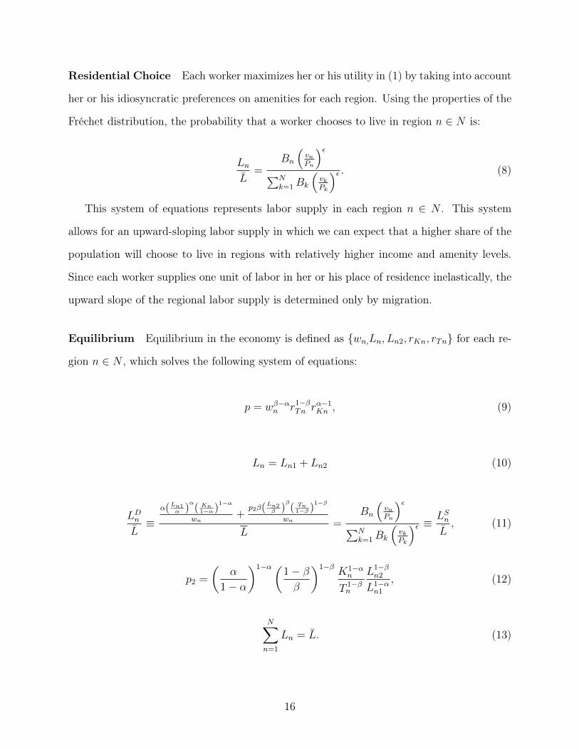
Residential Choice Each worker maximizes her or his utility in (1) by taking into account

her or his idiosyncratic preferences on amenities for each region. Using the properties of the

Fréchet distribution, the probability that a worker chooses to live in region n ∈ N is:

LnL

=Bn

(vnPn

)ε∑N

k=1 Bk

(vkPk

)ε . (8)

This system of equations represents labor supply in each region n ∈ N . This system

allows for an upward-sloping labor supply in which we can expect that a higher share of the

population will choose to live in regions with relatively higher income and amenity levels.

Since each worker supplies one unit of labor in her or his place of residence inelastically, the

upward slope of the regional labor supply is determined only by migration.

Equilibrium Equilibrium in the economy is defined as {wn,Ln, Ln2, rKn, rTn} for each re-

gion n ∈ N , which solves the following system of equations:

p = wβ−αn r1−βTn r

α−1Kn , (9)

Ln = Ln1 + Ln2 (10)

LDnL≡

α(Ln1α )α( Kn1−α)

1−α

wn+

p2β(Ln2β )β( Tn1−β )

1−β

wn

L=

Bn

(vnPn

)ε∑N

k=1Bk

(vkPk

)ε ≡ LSnL, (11)

p2 =

(α

1− α

)1−α(1− ββ

)1−βK1−αn

T 1−βn

L1−βn2

L1−αn1

, (12)

N∑n=1

Ln = L. (13)

16

1.3.1.2 Exogenous Price Shock

I will analyze the impact of exogeneous price shocks to wages in different regions. If labor

has full labor mobility and homogeneous preferences across regions, wages across regions

will equalize. Conversely, if regions as local labor markets have fixed amounts of labor, i.e.,

no labor mobility across regions, then the exogeneous price shock will be localized and the

impact will be as predicted in the classic specific-factor model. That is, the exogeneous

increase in price will be followed by an increase in wages of a lower percentage change.

Allowing for full labor mobility, but with heterogeneous preferences across regions, I

provide a framework between the two extreme cases explained above. From the labor-

supply side, each worker will consider all regions and maximize her or his expected utility.

Meanwhile, since the regions may differ in their endowments of specific-factors in each sector,

the exposure to the shock will vary across regions even though they all face uniform price

shocks. This variation in exposure to shocks leads to variation in labor demand responses

in each region. Hence, we can expect to see variation in the responses of wages in different

regions from a universal price shock.

A Simple Case: α = β

To derive the intuition above, consider a simple case in which the labor intensities in sector

1 and sector 2 are assumed to be equal, i.e., α = β. Suppose there is an exogenous change

in the relative price of sector 2. In order to see the changes in labor demand in region n,

totally differentiate (6) and use the Envelope Theorem to obtain:

LDn = γn2p2 − w, (14)

where x ≡ dx/x and γn2 ≡ αp2Yn2α(Yn1+p2Yn2)

, which is the share of sector 2 in the total output of

region n.

Meanwhile, we totally differentiate (8) to see the changes in labor supply in region n:

17

LSnLSnL

= εBn(wn + ϕ)ε−1wnwn −

[N∑k=1

wkwkεBk(wk + ϕ)ε−1

]. (15)

Let us define D ≡∑N

k=1wkwk

εBk(wk+ϕ)ε−1 . Hence,

LSnLSnL

= εBn(wn + ϕ)ε−1wnwn − D. (16)

Armed with the changes in labor demand in (14) and the changes in labor supply in (16),

we can use the population-mobility condition in (13) to solve for the changes in wages due

to changes in price. From the population mobility condition, we have:

N∑n=1

LSnLSnL

= 0. (17)

Using 16, we can get:

N∑n=1

[θnwn − D

] LSnL

= 0 (18)

⇔ D =N∑n=1

θnLSnLwn (19)

where θn ≡ εBn(wn + ϕ)ε−1wn.

Furthermore, using the labor-market clearing condition in each region n ∈ N from (11),

we have LDn = LSn, thus

⇔ wn =

(λn

λn + θn

)[γn2p+

D

λn

](20)

where λn ≡ LnL.

Proposition 1. For a given change in the relative price, p, the impact on wages between

region n and m is

18

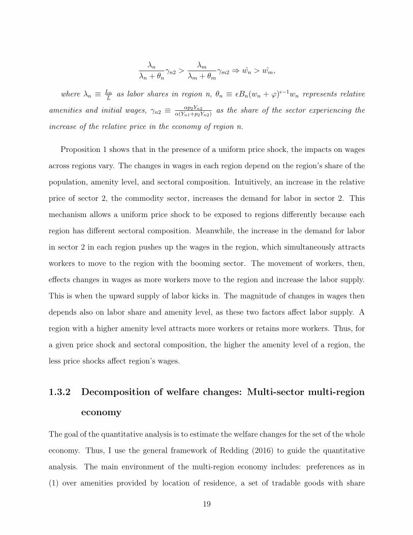
λnλn + θn

γn2 >λm

λm + θmγm2 ⇒ wn > wm,

where λn ≡ LnL

as labor shares in region n, θn ≡ εBn(wn + ϕ)ε−1wn represents relative

amenities and initial wages, γn2 ≡ αp2Yn2α(Yn1+p2Yn2)

as the share of the sector experiencing the

increase of the relative price in the economy of region n.

Proposition 1 shows that in the presence of a uniform price shock, the impacts on wages

across regions vary. The changes in wages in each region depend on the region’s share of the

population, amenity level, and sectoral composition. Intuitively, an increase in the relative

price of sector 2, the commodity sector, increases the demand for labor in sector 2. This

mechanism allows a uniform price shock to be exposed to regions differently because each

region has different sectoral composition. Meanwhile, the increase in the demand for labor

in sector 2 in each region pushes up the wages in the region, which simultaneously attracts

workers to move to the region with the booming sector. The movement of workers, then,

effects changes in wages as more workers move to the region and increase the labor supply.

This is when the upward supply of labor kicks in. The magnitude of changes in wages then

depends also on labor share and amenity level, as these two factors affect labor supply. A

region with a higher amenity level attracts more workers or retains more workers. Thus, for

a given price shock and sectoral composition, the higher the amenity level of a region, the

less price shocks affect region’s wages.

1.3.2 Decomposition of welfare changes: Multi-sector multi-region

economy

The goal of the quantitative analysis is to estimate the welfare changes for the set of the whole

economy. Thus, I use the general framework of Redding (2016) to guide the quantitative

analysis. The main environment of the multi-region economy includes: preferences as in

(1) over amenities provided by location of residence, a set of tradable goods with share

19

α and housing with share 1 − α. Agents draw idiosyncratic amenities from the Fréchet

distribution with shape parameter ε as in (2). Meanwhile, tradeable goods are produced in

monopolistic competition with many firms. Each region has productivity drawn from the

Fréchet distribution with shape parameter θ.

The welfare gains from trade in this setup are shown in Equation 21 below. The equation

shows the proportional changes in the welfare of people living in region n when the economy

changes from state 0 to state 1. The welfare gains depend on not only the changes in domestic

trade shares, πnn, but also the changes in population shares. The parameters include α as

the share of tradeable goods and services, θ as the shape parameter of the distribution of

productivity and ε as the shape parameter of the distribution of amenities across districts.

U1n

U0n

=U1

U0=

(π0nn

π1nn

)αθ(L0n

L1n

) 1ε+(1−α)

(21)

1.3.3 Decomposition

Consider the formula for the welfare gains from trade shown in Equation 21. Take the

relative changes for each region n, where x ≡ dxx.

πnn =θ

α

[(1

ε+ (1− α)

)Ln

]− θ

αU (22)

Multiply by regional weights ϕn that sum up to 1, and sum over all region n. These

regional weights are the share of expenditure by region n, i.e., ϕn = wn∑i wi

= wnE.

∑n

πnnϕn =∑n

[θ

α

(1

ε+ (1− α)

)Ln

]ϕn −

∑n

θ

αUϕn

Since the aggregate domestic trade share is the weighted sum of the regional trade

shares,19 i.e., π =∑

n πnnϕn, hence the changes in the aggregate domestic trade shares,

π:

19The total expenditure of the economy is the sum of the regional expenditures, wn.

20

π =∑n

[θ

α

(1

ε+ (1− α)

)Ln

]ϕn −

∑n

θ

αUϕn

Since∑

n ϕn = 1,

θ

αU =

∑n

[θ

α

(1

ε+ (1− α)

)Ln

]ϕn − π (23)

Meanwhile, with L as the total population of the whole economy, we also know that:

∑n

Ln = L

Take the total differentials and multiply by LnLnL:

∑n

LnLnL

=dL

L(24)

where dLL

is the aggregate growth of the population. We can set it as zero if there is no

population growth or generalize it as shown above.

To simplify, assume that there is no change in total labor endowment in the whole

economy, i.e., dLL

= 0, and subtract Equation 23 from the right-hand side of Equation 24:

∑n

wn = E

We can also express it in terms of shares of regional expenditures as below.∑n

wn

E= 1

∑n

ϕn = 1

With domestic trade shares, πnn, as how much region n buys from its own production relative to its totalexpenditures, the weighted sum of regional domestic trade shares using these regional expenditure shares isthe aggregate domestic trade shares.∑

n

πnnϕn =∑n

xnnwn

wn

E=

1

E

∑n

xnn = π

21

U =

(1

ε+ (1− α)

)∑n

Ln

(ϕn −

LnL

)︸ ︷︷ ︸

gains from migration

− αθ

∑n

πnnϕn︸ ︷︷ ︸gains from trade

(25)

Proposition 2. Assumming there is no change in total labor endowment in the whole econ-

omy, i.e., dLL

= 0 and using ϕn as the district’s share of the national expenditure and λn as

the district’s population share, the welfare change can be decomposed as the following equa-

tion. The first term represents gains from migration, while the second term represents gains

from trade.

U =

(1

ε+ (1− α)

)∑n

Ln (ϕn − λn)︸ ︷︷ ︸gains from migration

− αθ

∑n

πnnϕn︸ ︷︷ ︸gains from trade

(26)

Proposition 2 shows that the welfare gains have two components. The first is gains from

migration. The intuition is straightforward. The economy gains if people move to richer

districts, i.e., districts with higher expenditure shares, ϕn , compared to their population

shares, λn. The second component is the changes in aggregate domestic trade shares. The

economy also gains if the domestic trade share, πnn, decreases.

1.4 Data and measurement of exposure to shocks

Armed with the guidance in measuring regional exposure to price shocks as shown by Propo-

sition 1, I compute the exposure of price shocks of the two main crops: palm oil and rice.

Modeling Indonesia as a multi-region small-open economy, I use districts as the unit of ob-

servation for regions. Districts are the second-level administrative unit in Indonesia.20 The

heads of districts, like members of parliament at the district level, are elected directly by

residents of the districts every five years. Local governments have some income from local

taxes but also receive transfers from the central government. In addition, the minimum wage

20Indonesia has a central government and two levels of local government. The first level of local governmentis the province level. The second level of local government is the district level. The central government hasthe sole authority on several subjects, including trade policy.

22

is set at the district level.21 Over the course of the period studied here, there have been nu-

merous district and province proliferations. I use the administrative district definition in

2000 to maintain the same set of districts over time: 321 districts.22

1.4.1 Data

I combine several sources of data that can capture the determinants of regional welfare

and regional exposure to price shocks as guided by the theoretical framework. Indonesian

datasets allow me to do this because they contain regionally representative data. Below, I

describe the main variables and datasets I use.

Real expenditure per capita The main outcome variable is real expenditure per capita.

I use expenditure per capita because in the case of Indonesia, data on expenditure has

been better recorded than data on income. Expenditure can capture well-being better than

labor income can, because we also want to take into account any income from land rent.23

Furthermore, the households savings rate is relatively small. Vibrianti (2014) tabulates the

Indonesian Family Life Survey (IFLS) 2007 and shows that only 26% of households have

savings. Hence, household expenditure data is a good representation of income.24

I obtain data on household expenditure per capita from the Social and Economic House-

hold Survey (Susenas) directly and the from the survey published in the World Bank’s INDO

DAPOER database computed from Susenas. I use several district averages of expenditure

21There is an exception for the capital city of Jakarta, which is granted autonomy up to the province levelonly. Hence, the minimum wage is set at the province level for Jakarta province.

22The complete set has 342 districts. In most empirical exercises, I use a panel of 321 districts. A lack ofdata availability is the reason the full dataset is not used.

23Deaton (1997) discusses the advantages of using expenditures to capture lifetime well-being. As summa-rized by Goldberg and Pavcnik (2007), these advantages include (1) conditional on whether agents can shiftinter-temporal resources, current expenditure better captures lifetime well-being, (2) if there are fewer re-porting problems for consumption data than income data, and (3) changes in relative prices affect consumersnot only through income but also through the purchasing power of their current income.

24IFLS is nationally representative. Its survey sample represents 83% of the Indonesian population livingin 13 out of 26 provinces. IFLS in 2007 was the fourth wave of the survey. Given the representation,it is fair to take the estimates of the households savings rate tabulated from IFLS as an upper boundfor Indonesia. For more information on IFLS, see: RAND Corporation, https://www.rand.org/well-being/social-and-behavioral-policy/data/FLS/IFLS/study.html.

23

per capita. First, I use the total district average, which includes the whole sample for each

district. I also extract district premia from the mincerian regression on expenditure per

capita reported in Susenas as another outcome variable. Furthermore, in order to get real

expenditure per capita, I deflate expenditure per capita with Indonesia’s CPI obtained from

BPS-Statistics Indonesia (BPS ).

Recent migration I use recent migration as the outcome variable that represents labor

mobility. Recent migration is defined as a change of residential location between the survey

years and five years prior to the survey years. For the years 2011 to 2016, I extract data

on migration flows across districts from Susenas. Meanwhile, for earlier years, I obtain

migration flow data from a sample of the Population Census and Inter-Census Population

Surveys provided by IPUMS. From the constructed matrix of migration flows, I compute the

net migration rate for each district.

Crop data To estimate the potential production of each crop in each district, I use the

agro-climatically attainable yield provided in the 5-grid level raster data for palm oil and

rice from the FAO - GAEZ dataset. This estimated yield depends on climate, soil condition

and rainfall, which are exogenous factors in the production of each crop. This variable is

constructed using certain assumptions about climate, a long-term variable. Specifically, the

estimated yield is a single measure that represents the period from 1960 to 1990. The use of

a single-measure yield is reasonable beacuse farmers care more about long-run cycles than

about high-frequency variables such as daily rainfall in non-horticulture crop mix decisions

such as rice and palm oil. Furthermore, I choose assumptions about the most relevant use

of technology for each crop. I then take the district average of the yield for each crop.

I obtain data for harvested areas by district and by crop from the Ministry of Agricul-

ture’s statistics website.25 The data on harvested areas include all types of plantations, i.e.,

both large and small plantation holders. For the national aggregate crop area, I use the

25Data can be downloaded at the following link: https://aplikasi2.pertanian.go.id/bdsp/en/commodity.

24

FAO database. The total area for each district is obtained from the World Bank’s INDO

DAPOER.

Prices All data on prices are converted into rupiah. World palm oil price data is obtained

from the IMF Commodity Price Series. These price series are in US dollars.To take into

account the rupiah’s depreciation over the same period, I calculate the rupiah prices using

exchange rate data from the FRED Database. Because Indonesia’s small-open economy, the

rupiah prices are the relevant prices. Hence, the price shocks measured in this paper are

inclusive of this depreciation. Meanwhile, the retail domestic rice price data by province is

obtained from BPS. The rice price data is in Indonesian rupiah. For both crops, I deflate

the nominal prices with Indonesia’s CPI from the BPS to get real prices.

Ideally, one would use the farm-gate prices instead. For the case of palm oil, since

Indonesia is a price taker in the world market, and if we assume that the trade costs faced

by the producing districts do not vary over the period of interest, the changes in real-world

prices suffice to represent the changes in prices received by palm oil farmers, as these trade

costs cancel out. Meanwhile, for the case of rice, I assume that the pass-through margin

and the trade costs that make up the wedges between provincial retail prices and farm gate

prices do not vary over the period of interest. Hence, the changes in real provincial prices

also represent the changes in real farm-gate prices faced by rice farmers.

1.4.2 Exposure to price shocks

As we learn from Fact 1 and Fact 2, districts vary in their comparative advantage in agri-

cultural products, especially in growing palm oil and rice. Hence, districts are not uniformly

exposed to the increase in crop prices. In order to embody this exposure heterogeneity, I con-

struct a measure of exposure to price shocks for each district and crop based on Proposition

1.

First, to capture the price changes, it is useful to define the timeline that I am using.

25

I illustrate this timeline below. Figure 8 shows the trend in real palm oil prices and real

rice prices as the basis for the timeline. I define the treatment period as the onset of the

commodity boom for palm oil prices and as the import ban started to have an impact on rice

prices. For palm oil prices, I take 2010 as the end of the treatment period, because prices

started to decline in 2011 even though the average price was still quite high. Meanwhile,

as we can see from the figure below, the real prices of rices have been fairly stagnant since

2011. Hence, I also take 2010 as the end of the treatment period for rice price shocks. The

post-treatment period of interest, then, is the subsequent the three to five years after the

treatment period, i.e., from 2011 to 2014 or longer when data is available.

I define the pre-treatment period price as the average price between January 2001 and

December 2005. Meanwhile, I define the treatment period price as the average price of the

period that starts in January 2006 and ends in December 2010. To measure price changes, I

take the long difference in log between the treatment period and the pre-treatment period.

Figure 7 illustrates this timeline.

Applying Proposition 1 in the theoretical framework, which states that the impact of

exogeneous price changes on income depends on the output share of the sector whose price

changes, I construct a measure of exposure to price shocks in palm oil and rice for each

district, Sid. Equation 27 below shows the construction of this measure. The measure

allows districts to be exposed differently to uniform price shocks. The price of palm oil

is exogeneously determined in the world market. Hence, all districts in the sample face

the same prices and price changes for palm oil. Meanwhile, the prices of rice clear at the

provincial level. I assume that farmers in each district are price takers to these provincial

rice prices. This assumption is plausible given the size of each farmer relative to the province

aggregate.

Sid = piYid0

GDPd0

= pipi0 · Tid0 · ψidGDPd0

(27)

26

Crop i refers to palm oil and rice. Meanwhile, the sub-index d represents districts. The

price change of crop i, pi, is the long difference of the log price of crop i. The pre-treatment

estimated production value of crop i in district d, Ydi0, is computed using the pre-treatment

average price of crop i, pi0; the pre-treatment harvested area of crop i in district d, Tid0;

and the district-average potential yield of crop i in district d, ψid. Meanwhile, GDPd0 is the

district GDP excluding the oil and gas sector in the pre-treatment period.

Variations across districts in the estimated production of palm oil and rice are determined

by variation in harvested area in the pre-treatment period and variation in crop suitability

from the FAO GAEZ data. In the pre-treatment period, there was no indication that farmers

predicted that the commodity boom would occur. As Fact 2 suggests, even in districts that

are very suitable for palm oil, the harvested areas were relatively low, similar to those in

districts that are less suitable. Furthermore, the importance of each crop across districts is

also determined by the size of the economy of the district. I use district GDP excluding the

oil and gas sector, because I assume that this measure represents the pie of the economy

that are distributed locally in each district.

Figure 9 and 10 display the computed exposures of palm oil price shocks and rice price

shocks across districts. The districts with the highest exposure to palm oil price shocks are

concentrated in Sumatra, the main island on the west end of the country, and Borneo, the

main island east of Sumatra. Meanwhile, the districts with the highest exposure to rice

price shocks are spread out across all of the main islands of Indonesia. Table 6 exhibits the

summary statistics of the computed exposure to price shocks.

Defining exposed districts

I group districts into a set of exposed districts and a set of non-exposed districts for each

crop. As we can observe from the distribution of exposure to shocks in Figure 9, Figure

10 and Table 6, more than half of the districts are not exposed to palm oil price shocks.

Meanwhile, most districts have some degree of exposure to rice price shocks. The latter fact

27

is not surprising because rice is the staple food for most of Indonesia’s population. Many

districts produce some amount of rice even if they are not net producers.

For palm oil, I define exposed districts as districts with positive values of exposure to

shocks and non-exposed districts as those with zero exposure to palm oil price shocks. For

rice, I define exposed districts as districts with an exposure value higher than the 40th

percentile. The final set of these exposed and non-exposed districts is summarized in Table

7 and illustrated in Figures 11 and 12. Out of 321 districts, 81 districts are categorized as

exposed to palm oil price shocks and 129 districts are exposed to rice price shocks.

1.5 Empirical results

I use the constructed exposure to price shocks to study how it affects districts on two fronts:

a comparison between exposed districts and non-exposed districts and spillovers to non-

exposed districts. I also show some mechanisms that can explain the results by analysing

the responses in factors of production, especially labor and land.

1.5.1 Specification

I use the difference-in-difference method for econometrics specification to study the impact

of palm oil price shocks and rice price shocks on districts’ economies. Specifically, I perform

an event study as in Equation 28 to show the average differences between exposed and non-

exposed districts over time. Meanwhile, I use Equation 29 to show any heterogeneity in the

impact of the shocks.

ydt = α +∑i

∑r 6=2005

βir (Idi · 1 (yearr = t)) +Xd · tγ ·+δd + δt + εdt (28)

28

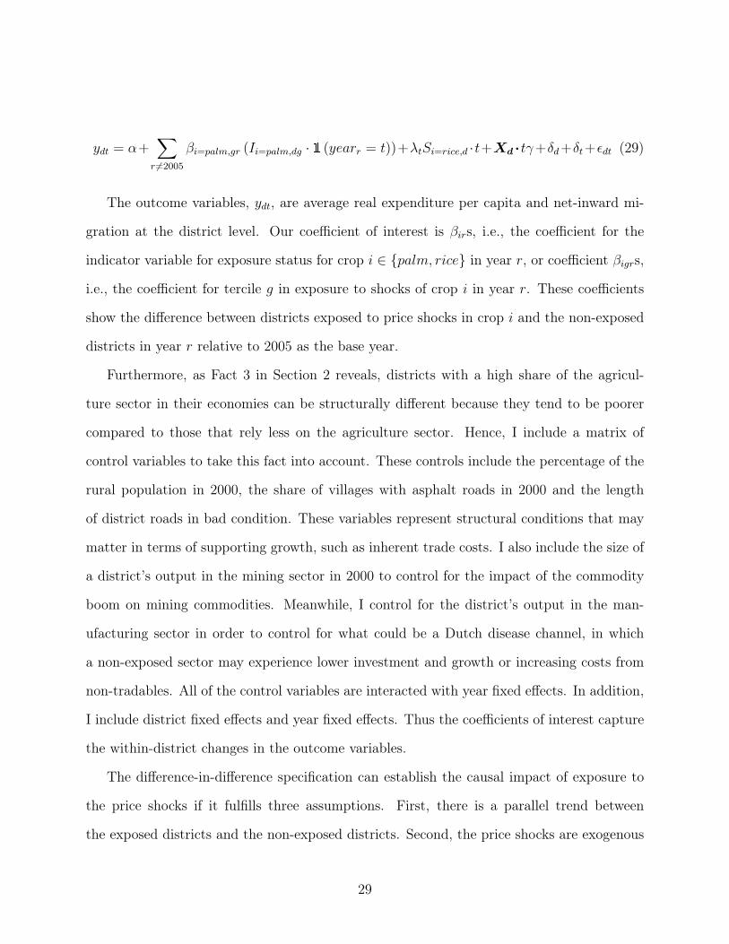
ydt = α+∑r 6=2005

βi=palm,gr (Ii=palm,dg · 1 (yearr = t))+λtSi=rice,d ·t+Xd ·tγ+δd+δt+εdt (29)

The outcome variables, ydt, are average real expenditure per capita and net-inward mi-

gration at the district level. Our coefficient of interest is βirs, i.e., the coefficient for the

indicator variable for exposure status for crop i ∈ {palm, rice} in year r, or coefficient βigrs,

i.e., the coefficient for tercile g in exposure to shocks of crop i in year r. These coefficients

show the difference between districts exposed to price shocks in crop i and the non-exposed

districts in year r relative to 2005 as the base year.

Furthermore, as Fact 3 in Section 2 reveals, districts with a high share of the agricul-

ture sector in their economies can be structurally different because they tend to be poorer

compared to those that rely less on the agriculture sector. Hence, I include a matrix of

control variables to take this fact into account. These controls include the percentage of the

rural population in 2000, the share of villages with asphalt roads in 2000 and the length

of district roads in bad condition. These variables represent structural conditions that may

matter in terms of supporting growth, such as inherent trade costs. I also include the size of

a district’s output in the mining sector in 2000 to control for the impact of the commodity

boom on mining commodities. Meanwhile, I control for the district’s output in the man-

ufacturing sector in order to control for what could be a Dutch disease channel, in which

a non-exposed sector may experience lower investment and growth or increasing costs from

non-tradables. All of the control variables are interacted with year fixed effects. In addition,

I include district fixed effects and year fixed effects. Thus the coefficients of interest capture

the within-district changes in the outcome variables.

The difference-in-difference specification can establish the causal impact of exposure to

the price shocks if it fulfills three assumptions. First, there is a parallel trend between

the exposed districts and the non-exposed districts. Second, the price shocks are exogenous

29

shocks to districts. In addition to the fact that exogenous components were used to construct

the exposure to shocks, exogeneity is fulfilled because there is no uptick in the coefficients of

interest during pre-treatment period. The plots of the coefficients of interest confirm that the

first and second assumptions are fulfilled. Third, there is no change in crop productivity. If

crop productivity increased due to the price shocks, then the coefficients are biased because

they also capture the impact of the increase in productivity. Tables 8 and 9 confirm that

there are no changes in actual yield for either palm oil or rice in the period of study. Hence,

the third assumption is also fulfilled. Thus, the coefficients of interest reflect the impact of

exposure to palm oil price shocks and exposure to rice price shocks.

1.5.2 Impact of the exposure to palm oil price shocks

Districts exposed to palm oil price shocks had higher (ln) real expenditure per capita during

the peak of the boom in 2011 and 2012. Figure 13 plots the estimated βirs for palm oil price

shocks and their respective 95% confidence obtained from running Equation 28. This result

shows that income shocks from palm oil prices were translated as an increase in purchasing

power.

Figure 13 also shows that the exposed and non-exposed districts were not significantly

different in the pre-treatment period of 2000 to 2004 relative to the base year 2005. One

exception is that districts exposed to palm oil price shocks had significantly lower (ln) real

expenditure per capita in 2002. However, the difference is negligible in other years. Hence,

the results shown by the coefficients of interest, βirs, establish the valid causal impact of the

palm oil price shocks.

The palm oil price shocks increased the real expenditure per capita in the exposed districts

by 6 log points or approximately 6% relative to the base year at its peak in 2011 and 2012.

This effect corresponds to 37% of one standard deviation in the proportional change of real

expenditure per capita in 2011 and 2012 relative to 2005. The impact of the commodity boom

decays afterward, with coefficients not different from zero. The cycle seems to directly follow

30

the global commodity prices, which started to decline in 2013 and 2014 as well. This result

fills a gap in the literature by providing the first evidence that the commodity boom affected

subnational regions differently and that these regions experienced a temporary windfall.

Among districts exposed to palm oil price shocks, I find heteregeneity in the impact of

palm oil price shocks. Figure 14 plots the estimated coefficient for three terciles of palm

oil price shocks over time. Districts in the bottom two terciles of palm oil price shocks

had a significantly higher (ln) real expenditure per capita during the post-treatment period

compared to the non-exposed districts. Following the trend in the overall impact of palm oil

price shocks, the impact of the commodity boom dissipates as the boom ended in 2013.

Because districts exposed to palm oil price shocks had higher expenditure per capita,

they might have attracted labor to move to them. To test whether districts exposed to the

shocks received more migration, I run Equation 28 on net-inward migration and share of

net-inward migration relative to district population. Figure 15 plots the estimated βirs for

net-inward migration as the outcome variable, while Figure 16 plots the coefficients for share

of net-inward migration as the outcome variable.

Before I continue with the analysis of the results, I would like to describe some of its

limitations. Because recent migration data was not collected annually before 2011, I combine

several datasets to construct recent migration flows data over time. For the years 2000 and

2010, I use the Census Population that is provided by IPUMS. For year 2005, I extract recent

migration flows from the Inter-Census Population Survey provided by IPUMS. For the years

2011 to 2014, I use the Socio-Economic Household Survey(Susenas) datasets. Hence, there

may exist some structural differences in the sampling of these datasets.26 For this reason,

in the analysis of migration as the outcome variable, I include the year 2010 as part of the

post-treatment period.

Both Figures 15 and 16 show that districts exposed to palm oil price shocks receive more

net-inward migration compared to the non-exposed ones in 2010 relative to the base year

26Table 2 tabulates the main statistics across sources of recent migration data.

31

2005, despite no significant difference in the years afterward. These results support the

previous findings that districts exposed to palm oil price shocks become more attractive to

labor to move to these regions. Because we find that labor responds to incentives to move

to booming regions, the price shocks too are no longer fully localized.

Confirming the heterogeneous findings about the impact to real expenditure per capita, I

also find that the districts exposed to palm oil price shocks in the bottom tercile are the ones

that receive significantly more net-inward migration. Figures 17 and 18, respectively, show

the impact of the commodity boom on net-inward migration and the share of net-inward

migration across terciles.

The empirical results here show that once the positive windfall has a significant effect,

we see that labor responds by moving as these booming districts became more attractive.

This finding adds to the understanding of how trade shocks affect labor mobility. Many

studies in this field find that trade shocks tend to be localized; see, for example, Autor et al.

(2013) for the case of the US, Dix-Carneiro and Kovak (2017) for the case of Brazil, and

Topalova (2010) for the case of India. However, most such studies explores trade shocks

that are disadvantegous to local incomes. Hence, if there is a cash-in-advance constraint on

migration costs, we may not see labor mobility responses to such trade shocks. The fact

that I find a contrasting result does not necessarily mean that Indonesia is a special case.

Instead, the result here provides some evidence that the labor mobility margin can be active

when trade shocks are advantegous to local income. One possible explanation is that such

trade shocks can help labor overcome the cash-in-advance constraint on migration costs.

1.5.3 Spillover to non-exposed districts

Booming districts may also demand more goods and services from nearby districts because

it is cheaper to purchase from nearer districts than from more distant districts, due to lower

transportation and transaction costs. To assess whether there is any spillover of impacts of

exposure to palm oil price shocks to non-exposed districts, I run the following specification.

32

ydt = α +∑

g∈1,2,3,4

∑r 6=2005

βgr (Igdt · 1 (yearr = t)) + ψpalm,d + δrice,d + γXd + δd + δt + νdt (30)

In Equation 30, the outcome variables are real expenditures per capita and migration

flows. As in the previous specifications, I include a set of control variables, district fixed

effects and year fixed effects. First, I control for the potential yield in growing palm oil,

ψpalm,d , to purge the effect from the impact of the districts changing status from palm-

oil non-grower to grower. I also add the status of exposure to rice price shocks, δrice,d.

I run the specification on a panel of districts that are not exposed to the palm oil price

shocks. To capture heterogeneity due to proximity to exposed districts, I create four dummy

variables. Each dummy variable indicates four of the lowest centiles of minimum distance

to exposed districts.27 Hence, the coefficients of interest are βgrs. These coefficients capture

the difference of district of centile g in year r compared to districts in the 5th to 10th centiles

(the control group) relative to the base year 2005.

First, I find that the nearest non-exposed districts to districts exposed to palm oil price

shocks also had higher real expenditure per capita. Figure 19 plots the coefficients of interest

with (ln) real expenditure per capita as the outcome variable for the distriicts in the two

lowest centiles in distance. These coefficients are positive and statistically significant from

zero for the nearest non-exposed districts. Following the trend in the impact to the exposed

districts, these coefficients also shrink over the outcome period.

In response to the spillover indicated by higher expenditure per capita in the neighboring

districts of booming regions, I find also that the same non-exposed districts that are close

to districts exposed to palm oil price shocks also receive more net-inward migration. Figure

20 plots the estimated βgrs for net-inward migration as the outcome variable. Supporting

the result above, labor seems to respond to the higher purchasing power provided by these

27The distance between two districts is computed as the distance between their centroids.

33

nearest districts. These districts receive more net-inward migration compared to the control

group, which is further away from the districts exposed to palm oil price shocks.28

1.5.4 Mechanisms

I provide several mechanisms, focusing on the response of factors of production. The idea

is that the shocks may have lasted long enough and were big enough that the factors of

production also responded to the shocks. First, I provide justification that labor responds

through internal migration by analyzing the impact of the price shocks on district premia.

Second, because I focus on agricultural commodities, I analyze two possible methods through

which the agriculture sector expands: extensification by land expansion and intensification

by increasing yield.

1.5.4.1 District premia: the role of internal migration

One may argue that, structurally, districts exposed to palm oil price shocks have a different

labor and sectoral composition that may drive their higher expenditure per capita at the peak

of the boom. Another argument is that there exist frictions in labor mobility that prevent

welfare from equalizing across districts. I follow the two-step method used by Dix-Carneiro

and Kovak (2017) to analyse the evolution of district premia over the period of study. First, to

control for labor and sectoral characteristics, I run a Mincerian-type regression on household-

level expenditure per capita by controlling household heads’ economic and demographic

variables. To avoid selection bias due to labor market biases, I follow Bryan and Morten

(2019) in imposing some selection criteria. That is, I include households with male heads

of households between the ages of 15 and 61. I also take only those who report having had

an income in the three months prior to the survey. Equation 31 below shows the Mincerian

equation.

28Due to the combination of various sources of data for migration, I also loosely take 2010 as part of theoutcome period here.

34

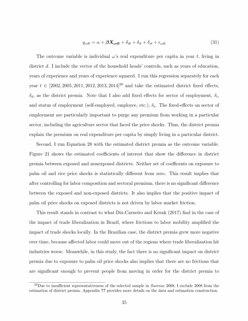
yωdt = α + βXωdt + δdt + δit + δst + εωdt (31)

The outcome variable is individual ω’s real expenditure per capita in year t, living in

district d. I include the vector of the household heads’ controls, such as years of education,

years of experience and years of experience squared. I run this regression separately for each

year t ∈ [2002, 2005, 2011, 2012, 2013, 2014]29 and take the estimated district fixed effects,

δd, as the district premia. Note that I also add fixed effects for sector of employment, δi,

and status of employment (self-employed, employee, etc.), δs. The fixed-effects on sector of

employment are particularly important to purge any premium from working in a particular

sector, including the agriculture sector that faced the price shocks. Thus, the district premia

explain the premium on real expenditure per capita by simply living in a particular district.

Second, I run Equation 28 with the estimated district premia as the outcome variable.

Figure 21 shows the estimated coefficients of interest that show the difference in district

premia between exposed and nonexposed districts. Neither set of coefficents on exposure to

palm oil and rice price shocks is statistically different from zero. This result implies that

after controlling for labor composition and sectoral premium, there is no significant difference

between the exposed and non-exposed districts. It also implies that the positive impact of

palm oil price shocks on exposed districts is not driven by labor market friction.

This result stands in contrast to what Dix-Carneiro and Kovak (2017) find in the case of

the impact of trade liberalization in Brazil, where frictions to labor mobility amplified the

impact of trade shocks locally. In the Brazilian case, the district premia grew more negative

over time, because affected labor could move out of the regions where trade liberalization hit

industries worse. Meanwhile, in this study, the fact there is no significant impact on district

premia due to exposure to palm oil price shocks also implies that there are no frictions that

are significant enough to prevent people from moving in order for the district premia to

29Due to insufficient representativeness of the selected sample in Susenas 2008, I exclude 2008 from theestimation of district premia. Appendix ?? provides more details on the data and estimation construction.

35

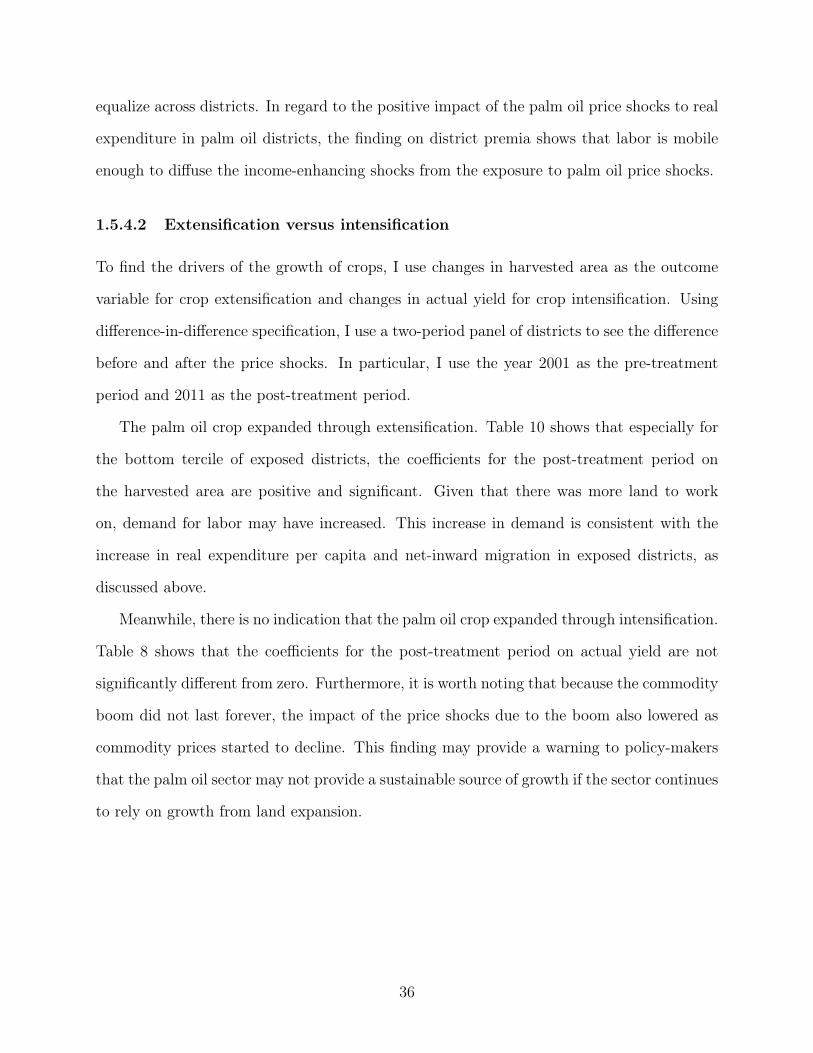
equalize across districts. In regard to the positive impact of the palm oil price shocks to real

expenditure in palm oil districts, the finding on district premia shows that labor is mobile

enough to diffuse the income-enhancing shocks from the exposure to palm oil price shocks.

1.5.4.2 Extensification versus intensification

To find the drivers of the growth of crops, I use changes in harvested area as the outcome

variable for crop extensification and changes in actual yield for crop intensification. Using

difference-in-difference specification, I use a two-period panel of districts to see the difference

before and after the price shocks. In particular, I use the year 2001 as the pre-treatment

period and 2011 as the post-treatment period.

The palm oil crop expanded through extensification. Table 10 shows that especially for

the bottom tercile of exposed districts, the coefficients for the post-treatment period on

the harvested area are positive and significant. Given that there was more land to work

on, demand for labor may have increased. This increase in demand is consistent with the

increase in real expenditure per capita and net-inward migration in exposed districts, as

discussed above.

Meanwhile, there is no indication that the palm oil crop expanded through intensification.

Table 8 shows that the coefficients for the post-treatment period on actual yield are not

significantly different from zero. Furthermore, it is worth noting that because the commodity

boom did not last forever, the impact of the price shocks due to the boom also lowered as

commodity prices started to decline. This finding may provide a warning to policy-makers

that the palm oil sector may not provide a sustainable source of growth if the sector continues

to rely on growth from land expansion.

36

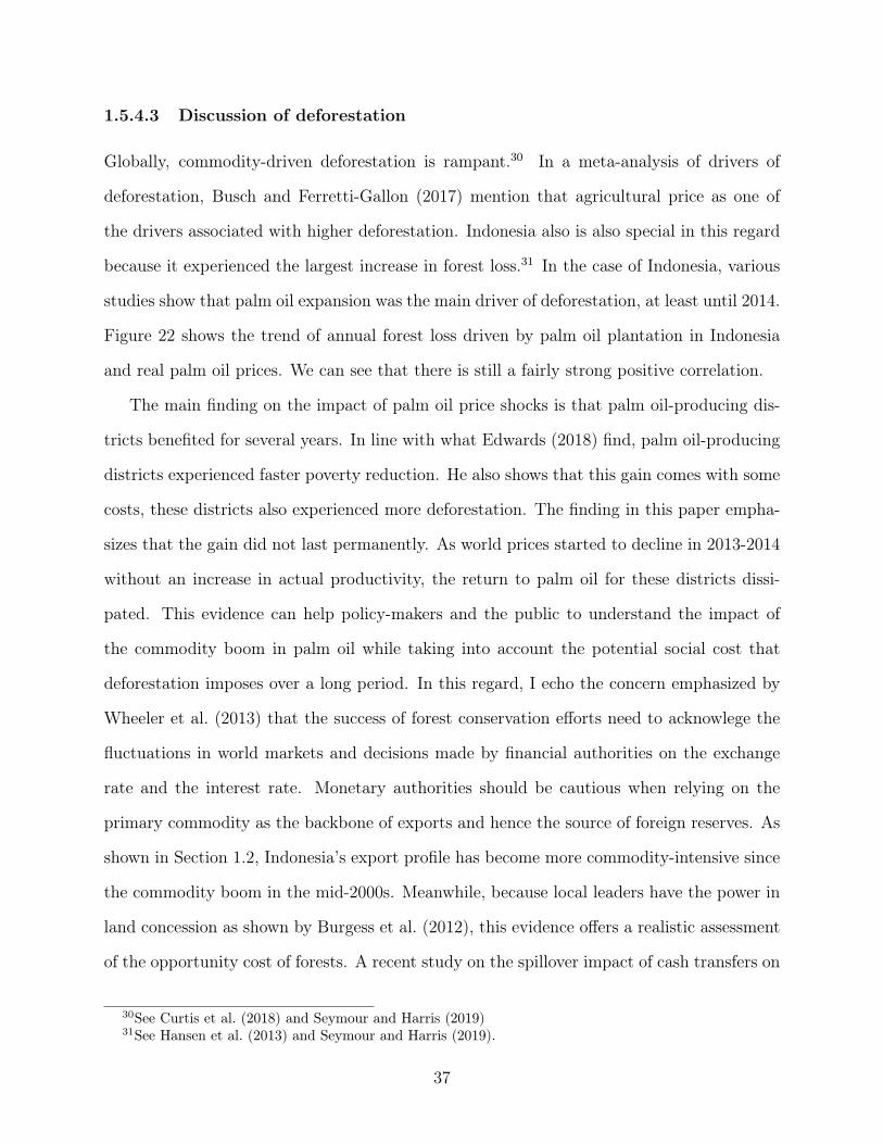
1.5.4.3 Discussion of deforestation

Globally, commodity-driven deforestation is rampant.30 In a meta-analysis of drivers of

deforestation, Busch and Ferretti-Gallon (2017) mention that agricultural price as one of

the drivers associated with higher deforestation. Indonesia also is also special in this regard

because it experienced the largest increase in forest loss.31 In the case of Indonesia, various

studies show that palm oil expansion was the main driver of deforestation, at least until 2014.

Figure 22 shows the trend of annual forest loss driven by palm oil plantation in Indonesia

and real palm oil prices. We can see that there is still a fairly strong positive correlation.

The main finding on the impact of palm oil price shocks is that palm oil-producing dis-

tricts benefited for several years. In line with what Edwards (2018) find, palm oil-producing

districts experienced faster poverty reduction. He also shows that this gain comes with some

costs, these districts also experienced more deforestation. The finding in this paper empha-

sizes that the gain did not last permanently. As world prices started to decline in 2013-2014

without an increase in actual productivity, the return to palm oil for these districts dissi-

pated. This evidence can help policy-makers and the public to understand the impact of

the commodity boom in palm oil while taking into account the potential social cost that

deforestation imposes over a long period. In this regard, I echo the concern emphasized by

Wheeler et al. (2013) that the success of forest conservation efforts need to acknowlege the

fluctuations in world markets and decisions made by financial authorities on the exchange

rate and the interest rate. Monetary authorities should be cautious when relying on the

primary commodity as the backbone of exports and hence the source of foreign reserves. As

shown in Section 1.2, Indonesia’s export profile has become more commodity-intensive since

the commodity boom in the mid-2000s. Meanwhile, because local leaders have the power in

land concession as shown by Burgess et al. (2012), this evidence offers a realistic assessment

of the opportunity cost of forests. A recent study on the spillover impact of cash transfers on

30See Curtis et al. (2018) and Seymour and Harris (2019)31See Hansen et al. (2013) and Seymour and Harris (2019).

37

deforestation by Ferraro and Simorangkir (2020) sheds lights on the importance of creating

an outside option as a source of income in regions that are prone to deforestation. Lastly,

the fact that there is no lingering benefit enjoyed by palm oil-producing districts highlights

the possibility that new palm oil concessions may not provide more benefit than costs to the

people there.

1.6 Quantitative estimation

Lastly, I quantify the welfare changes in Indonesia that occurred in the period between

2005 and 2010. I use the decomposition of welfare changes that I derived in the section on

the theoretical framework. Specifically, I decompose the source of the welfare changes into

gains from trade and gains from migration. To quantify both gains, I use internal migration

flows data and the Inter-Provincial Input Output Table. I estimate that there was a 0.39%

increase in welfare between 2005 and 2010. Gains from migrations account for one-third of

these gains. This result indicates the importance of taking into account internal migration

in welfare analysis.

1.6.1 Data and parameters

I present below the equation for welfare changes, as stated in Proposition 2. In estimating

the gains from migration and terms-of-trade gains, I use several dataset sources. First, I

compute the regional expenditure shares, ϕn , as total households expenditures by district

by multiplying the average expenditure per capita by the population of each district. I use

data from Susenas 2011. I also obtain the net-inward migration rate from the same dataset.

Extracting from its recent migration questions, I obtain data on changes in districts’ labor,

Ln, as well as the population shares, λn.

38

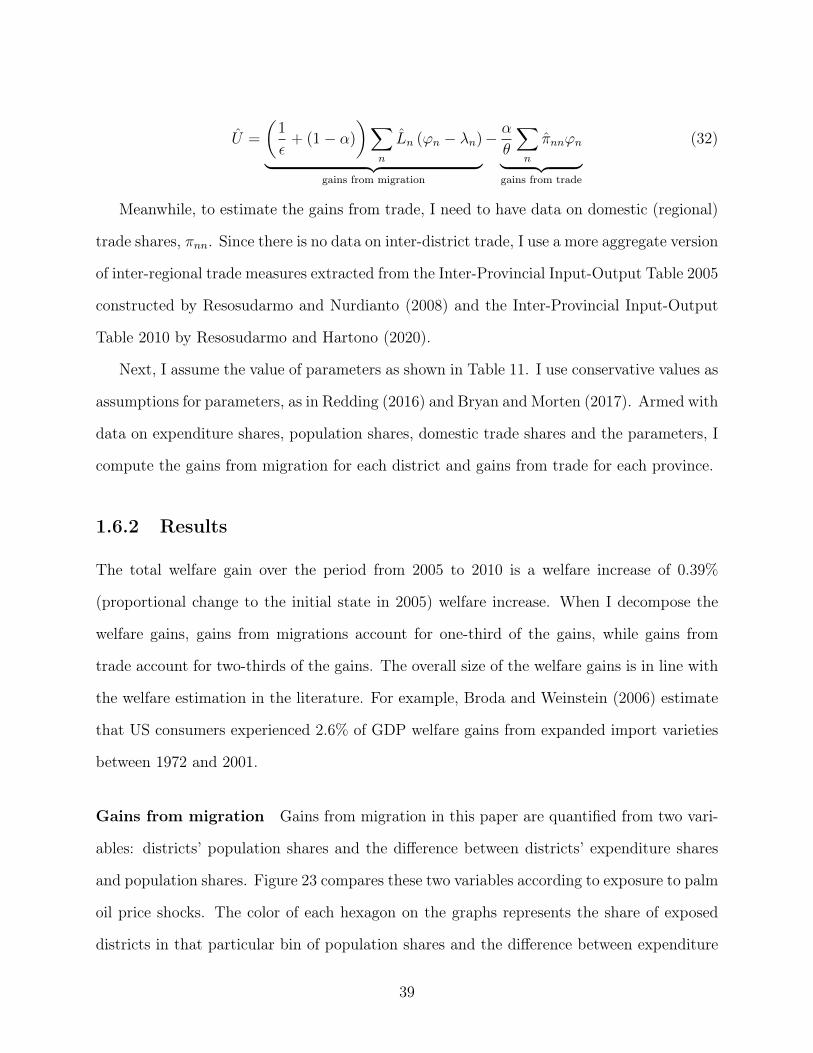
U =

(1

ε+ (1− α)

)∑n

Ln (ϕn − λn)︸ ︷︷ ︸gains from migration

− αθ

∑n

πnnϕn︸ ︷︷ ︸gains from trade

(32)

Meanwhile, to estimate the gains from trade, I need to have data on domestic (regional)

trade shares, πnn. Since there is no data on inter-district trade, I use a more aggregate version

of inter-regional trade measures extracted from the Inter-Provincial Input-Output Table 2005

constructed by Resosudarmo and Nurdianto (2008) and the Inter-Provincial Input-Output

Table 2010 by Resosudarmo and Hartono (2020).

Next, I assume the value of parameters as shown in Table 11. I use conservative values as

assumptions for parameters, as in Redding (2016) and Bryan and Morten (2017). Armed with

data on expenditure shares, population shares, domestic trade shares and the parameters, I

compute the gains from migration for each district and gains from trade for each province.

1.6.2 Results

The total welfare gain over the period from 2005 to 2010 is a welfare increase of 0.39%

(proportional change to the initial state in 2005) welfare increase. When I decompose the

welfare gains, gains from migrations account for one-third of the gains, while gains from

trade account for two-thirds of the gains. The overall size of the welfare gains is in line with

the welfare estimation in the literature. For example, Broda and Weinstein (2006) estimate

that US consumers experienced 2.6% of GDP welfare gains from expanded import varieties

between 1972 and 2001.

Gains from migration Gains from migration in this paper are quantified from two vari-

ables: districts’ population shares and the difference between districts’ expenditure shares

and population shares. Figure 23 compares these two variables according to exposure to palm

oil price shocks. The color of each hexagon on the graphs represents the share of exposed

districts in that particular bin of population shares and the difference between expenditure

39

shares and population shares.

We can see that many districts exposed to palm oil price shocks gain through migration,

because they have a positive value for the difference in expenditure shares and population

shares, i.e., the districts are richer. These districts received positive net-inward migration.

Some portion of the districts have around zero or negative net-inward migration, but their

values for the difference of expenditure shares and population shares are also negative. Such

districts gain by experiencing outmigration.

Gains from trade Meanwhile, given that there are no data for district-level domestic

trade shares, I use provincial-level (a more aggregated level than the district level) domestic

trade shares to compute gains from trade. The result for each province is presented in Table

12. Several palm oil producers are the main contributors to the gains, such as Kaliman-

tan Selatan, Kalimantan Timur, Kalimantan Barat and Sumatera Utara. Others, however,

experienced losses, such as Jambi and Riau. These results are driven by changes in (provin-

cial) domestic trade shares. Palm oil-producing provinces tend to have lower domestic trade

shares in 2010 compared to 2005 as their export shares in their economy roared due to the

commodity boom.

1.7 Conclusion

Developing economies are vulnerable to changes in the world commodity markets. This paper

studies the impact of price shocks on Indonesia in the mid-2000s. Given the magnitude and

the length of the commodity boom that exposed Indonesia as one of the main palm oil

producers, factors of production, including labor, may have responded to these shocks by

moving to districts directly exposed to the shocks. In particular, I study the impact of price

shocks on different districts in the presence of internal migration.

I present three main findings. First, palm oil price shocks benefitted producing districts

with higher real expenditure per capita. However, the impact of the palm oil price shocks

40

was temporary. I find that the palm oil sector grew through land expansion without any

significant growth in actual yield. The increase in land that needed to be cultivated was met

by more inward migration and higher real expenditure per capita.

The second main result is that there is evidence of spillover of the shocks to non-exposed

districts. In particular, the non-exposed districts nearest to districts exposed to palm oil

price shocks also experienced higher real expenditure per capita and net-inward migration.

The intuition behind this result is straightforward. Booming districts may demand more

goods and services due to the income shocks they enjoy. Hence, they demand more from

their surrounding districts, because trade and migration costs are lower if they buy from

nearby sources.

Third, I estimate that there was a 0.39% welfare increase between 2005 and 2010 in the

economy. One-third of the welfare gains during the period of interest is associated with gains

from migration. Meanwhile, gains from trade account for the remaining two-thirds of the

welfare increase. These results shed light on the importance of taking into account labor

mobility as represented by internal migration in welfare analysis.

These results provide policy-relevant lessons. First, I provide evidence of the impact of

global prices’ cyclicality at the sub-national level. The result then questions the sustain-

ability of relying on cash crops through land expansion. The concern about sustainability

is even more critical if we take into account the social costs of land expansion that causes

deforestation. This evidence can inform not only local governments who hold the author-

ity to make land concessions and who may have an interest in creating local development

strategy, but also national-level fiscal and monetary authorities who are interested in sus-

taining sources of foreign reserves and growth in general. In addition, the concern about

commodity-driven deforestation is not exclusive to Indonesia; we can see the same pattern

in other crop-exporting regions.

41

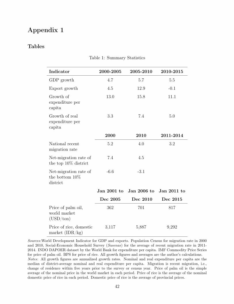
Appendix 1

Tables

Table 1: Summary Statistics

Indicator 2000-2005 2005-2010 2010-2015

GDP growth 4.7 5.7 5.5

Export growth 4.5 12.9 -0.1

Growth ofexpenditure percapita

13.0 15.8 11.1

Growth of realexpenditure percapita

3.3 7.4 5.0

2000 2010 2011-2014

National recentmigration rate

5.2 4.0 3.2

Net-migration rate ofthe top 10% district

7.4 4.5

Net-migration rate ofthe bottom 10%district

-6.6 -3.1

Jan 2001 to Jan 2006 to Jan 2011 to

Dec 2005 Dec 2010 Dec 2015

Price of palm oil,world market(USD/ton)

362 701 817

Price of rice, domesticmarket (IDR/kg)

3,117 5,887 9,292

Sources:World Development Indicator for GDP and exports. Population Census for migration rate in 2000and 2010, Social-Economic Household Survey (Susenas) for the average of recent migration rate in 2011-2014. INDO DAPOER dataset by the World Bank for expenditure per capita. IMF Commodity Price Seriesfor price of palm oil. BPS for price of rice. All growth figures and averages are the author’s calculations.Notes: All growth figures are annualized growth rates. Nominal and real expenditure per capita are themedian of district-average nominal and real expenditure per capita. Migration is recent migration, i.e.,change of residence within five years prior to the survey or census year. Price of palm oil is the simpleaverage of the nominal price in the world market in each period. Price of rice is the average of the nominaldomestic price of rice in each period. Domestic price of rice is the average of provincial prices.

42

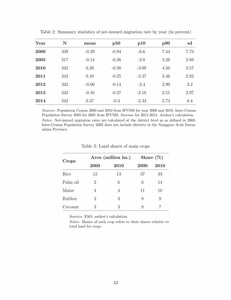
Table 2: Summary statistics of net-inward migration rate by year (in percent)

Year N mean p50 p10 p90 sd

2000 339 -0.29 -0.94 -6.6 7.44 7.73

2005 317 -0.14 -0.38 -2.8 3.26 2.89

2010 342 0.26 -0.30 -3.09 4.50 3.57

2011 342 0.10 -0.25 -2.37 3.46 2.82

2012 342 -0.06 -0.14 -2.4 2.99 3.2

2013 342 -0.16 -0.27 -2.18 2.51 2.97

2014 342 0.37 -0.3 -2.32 2.73 8.4

Sources: Population Census 2000 and 2010 from IPUMS for year 2000 and 2010, Inter-CensusPopulation Survey 2005 for 2005 from IPUMS, Susenas for 2011-2014. Author’s calculation.Notes: Net-inward migration rates are calculated at the district level as as defined in 2000.Inter-Census Population Survey 2005 does not include districts in the Nanggroe Aceh Darus-salam Province.

Table 3: Land shares of main crops

CropsArea (million ha.) Share (%)

2000 2010 2000 2010

Rice 12 13 37 33

Palm oil 2 6 6 14

Maize 4 4 11 10

Rubber 2 3 8 9

Coconut 3 3 8 7

Sources: FAO, author’s calculation.Notes: Shares of each crop refers to their shares relative tototal land for crops.

43

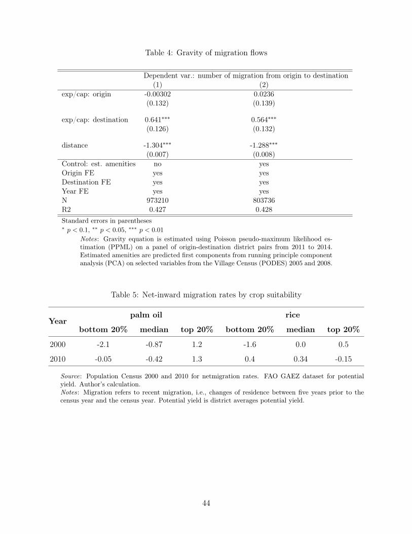
Table 4: Gravity of migration flows

Dependent var.: number of migration from origin to destination(1) (2)

exp/cap: origin -0.00302 0.0236(0.132) (0.139)

exp/cap: destination 0.641∗∗∗ 0.564∗∗∗

(0.126) (0.132)

distance -1.304∗∗∗ -1.288∗∗∗

(0.007) (0.008)Control: est. amenities no yesOrigin FE yes yesDestination FE yes yesYear FE yes yesN 973210 803736R2 0.427 0.428Standard errors in parentheses∗ p < 0.1, ∗∗ p < 0.05, ∗∗∗ p < 0.01

Notes: Gravity equation is estimated using Poisson pseudo-maximum likelihood es-timation (PPML) on a panel of origin-destination district pairs from 2011 to 2014.Estimated amenities are predicted first components from running principle componentanalysis (PCA) on selected variables from the Village Census (PODES) 2005 and 2008.

Table 5: Net-inward migration rates by crop suitability

Yearpalm oil rice

bottom 20% median top 20% bottom 20% median top 20%

2000 -2.1 -0.87 1.2 -1.6 0.0 0.5

2010 -0.05 -0.42 1.3 0.4 0.34 -0.15

Source: Population Census 2000 and 2010 for netmigration rates. FAO GAEZ dataset for potentialyield. Author’s calculation.Notes: Migration refers to recent migration, i.e., changes of residence between five years prior to thecensus year and the census year. Potential yield is district averages potential yield.

44

Table 6: Summary statistic of exposure to price shocks

Statistic rice palm oil

p10 0 0

p20 0.0001 0

p30 0.002 0

p40 0.016 0

p50 0.044 0

p60 0.068 0

p70 0.089 0

p80 0.117 0.0005

p90 0.170 0.015

p100 0.431 0.143

mean 0.094 0.016

Table 7: Number of exposed and non-exposed districts

Group palm oil rice

exposed districts 81 129

non-exposed districts 240 192

45

Table 8: Crop intensification: Actual yield for palm oil

Dep. var: actual yield(1) (2) (3)

Bottom tercile, 2011 0.513 0.512 0.556(0.546) (0.561) (0.562)

Second tercile, 2011 0.316 0.317 0.317(0.410) (0.411) (0.413)

(ln) Potential yield: palm-oil 0.00332 -0.00512(0.493) (0.467)

Price shocks: rice -1.755∗∗∗(0.605)

N 180 180 180R2 0.100 0.100 0.133Standard errors in parentheses∗ p < 0.1, ∗∗ p < 0.05, ∗∗∗ p < 0.01

Notes: The dependent variable is (ln) actual yield for palm oil.The regressions are run on a panel of districts with two periods.The two periods are the years 2001 and 2011. The coefficientsfor each tercile are relative to the top tercile in exposure to palmoil price shocks. Year FEs are included in all specifications. I userobust standard errors.

46

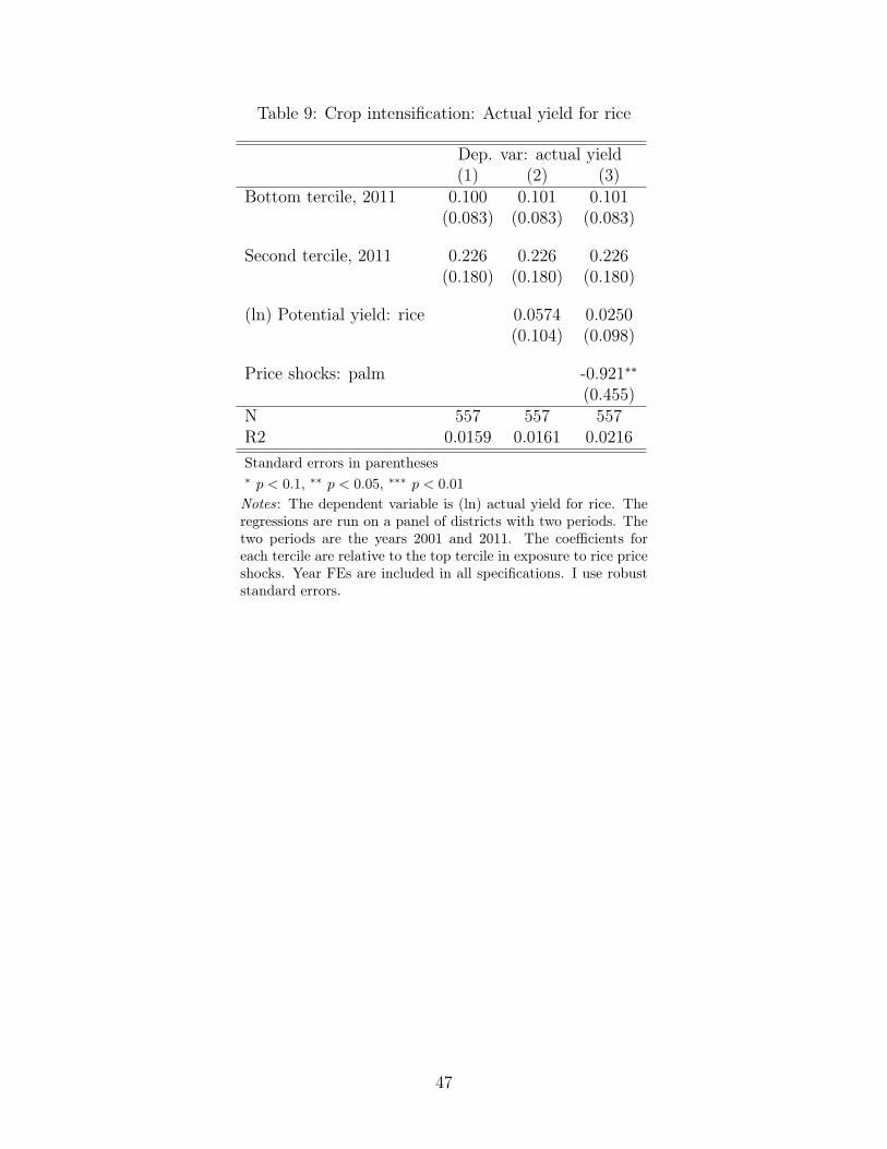
Table 9: Crop intensification: Actual yield for rice

Dep. var: actual yield(1) (2) (3)

Bottom tercile, 2011 0.100 0.101 0.101(0.083) (0.083) (0.083)

Second tercile, 2011 0.226 0.226 0.226(0.180) (0.180) (0.180)

(ln) Potential yield: rice 0.0574 0.0250(0.104) (0.098)

Price shocks: palm -0.921∗∗(0.455)

N 557 557 557R2 0.0159 0.0161 0.0216Standard errors in parentheses∗ p < 0.1, ∗∗ p < 0.05, ∗∗∗ p < 0.01

Notes: The dependent variable is (ln) actual yield for rice. Theregressions are run on a panel of districts with two periods. Thetwo periods are the years 2001 and 2011. The coefficients foreach tercile are relative to the top tercile in exposure to rice priceshocks. Year FEs are included in all specifications. I use robuststandard errors.

47

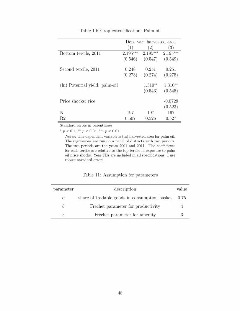
Table 10: Crop extensification: Palm oil

Dep. var: harvested area(1) (2) (3)

Bottom tercile, 2011 2.195∗∗∗ 2.195∗∗∗ 2.195∗∗∗(0.546) (0.547) (0.549)

Second tercile, 2011 0.248 0.251 0.251(0.273) (0.274) (0.275)

(ln) Potential yield: palm-oil 1.310∗∗ 1.310∗∗(0.543) (0.545)

Price shocks: rice -0.0729(0.523)

N 197 197 197R2 0.507 0.526 0.527Standard errors in parentheses∗ p < 0.1, ∗∗ p < 0.05, ∗∗∗ p < 0.01

Notes: The dependent variable is (ln) harvested area for palm oil.The regressions are run on a panel of districts with two periods.The two periods are the years 2001 and 2011. The coefficientsfor each tercile are relative to the top tercile in exposure to palmoil price shocks. Year FEs are included in all specifications. I userobust standard errors.

Table 11: Assumption for parameters

parameter description value

α share of tradable goods in consumption basket 0.75

θ Fréchet parameter for productivity 4

ε Fréchet parameter for amenity 3

48

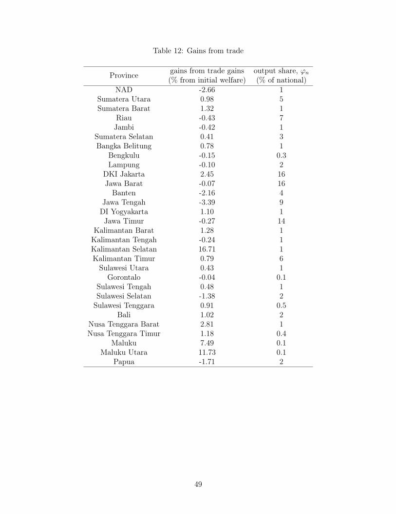
Table 12: Gains from trade

Province gains from trade gains output share, ϕn(% from initial welfare) (% of national)

NAD -2.66 1Sumatera Utara 0.98 5Sumatera Barat 1.32 1

Riau -0.43 7Jambi -0.42 1

Sumatera Selatan 0.41 3Bangka Belitung 0.78 1

Bengkulu -0.15 0.3Lampung -0.10 2

DKI Jakarta 2.45 16Jawa Barat -0.07 16Banten -2.16 4

Jawa Tengah -3.39 9DI Yogyakarta 1.10 1Jawa Timur -0.27 14

Kalimantan Barat 1.28 1Kalimantan Tengah -0.24 1Kalimantan Selatan 16.71 1Kalimantan Timur 0.79 6Sulawesi Utara 0.43 1

Gorontalo -0.04 0.1Sulawesi Tengah 0.48 1Sulawesi Selatan -1.38 2Sulawesi Tenggara 0.91 0.5

Bali 1.02 2Nusa Tenggara Barat 2.81 1Nusa Tenggara Timur 1.18 0.4

Maluku 7.49 0.1Maluku Utara 11.73 0.1

Papua -1.71 2

49

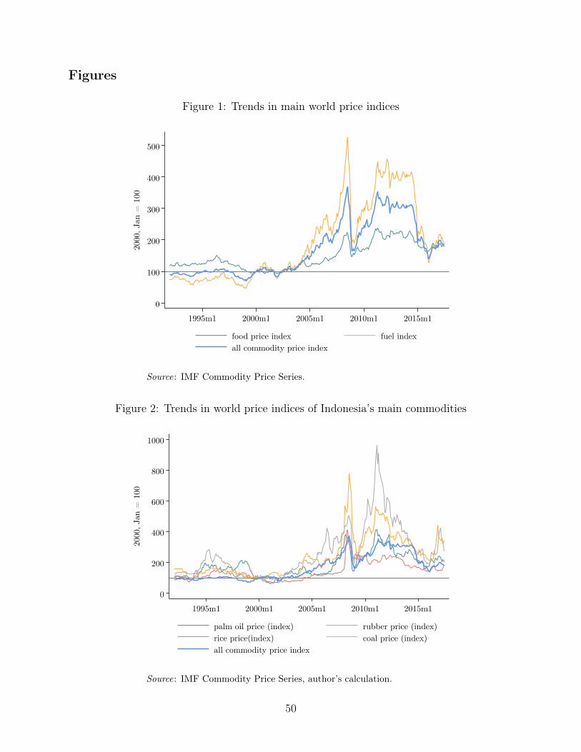
Figures

Figure 1: Trends in main world price indices

0

100

200

300

400

50020

00, J

an =

100

1995m1 2000m1 2005m1 2010m1 2015m1

food price index fuel indexall commodity price index

Source: IMF Commodity Price Series.

Figure 2: Trends in world price indices of Indonesia’s main commodities

0

200

400

600

800

1000

2000

, Jan

= 1

00

1995m1 2000m1 2005m1 2010m1 2015m1

palm oil price (index) rubber price (index)rice price(index) coal price (index)all commodity price index

Source: IMF Commodity Price Series, author’s calculation.

50

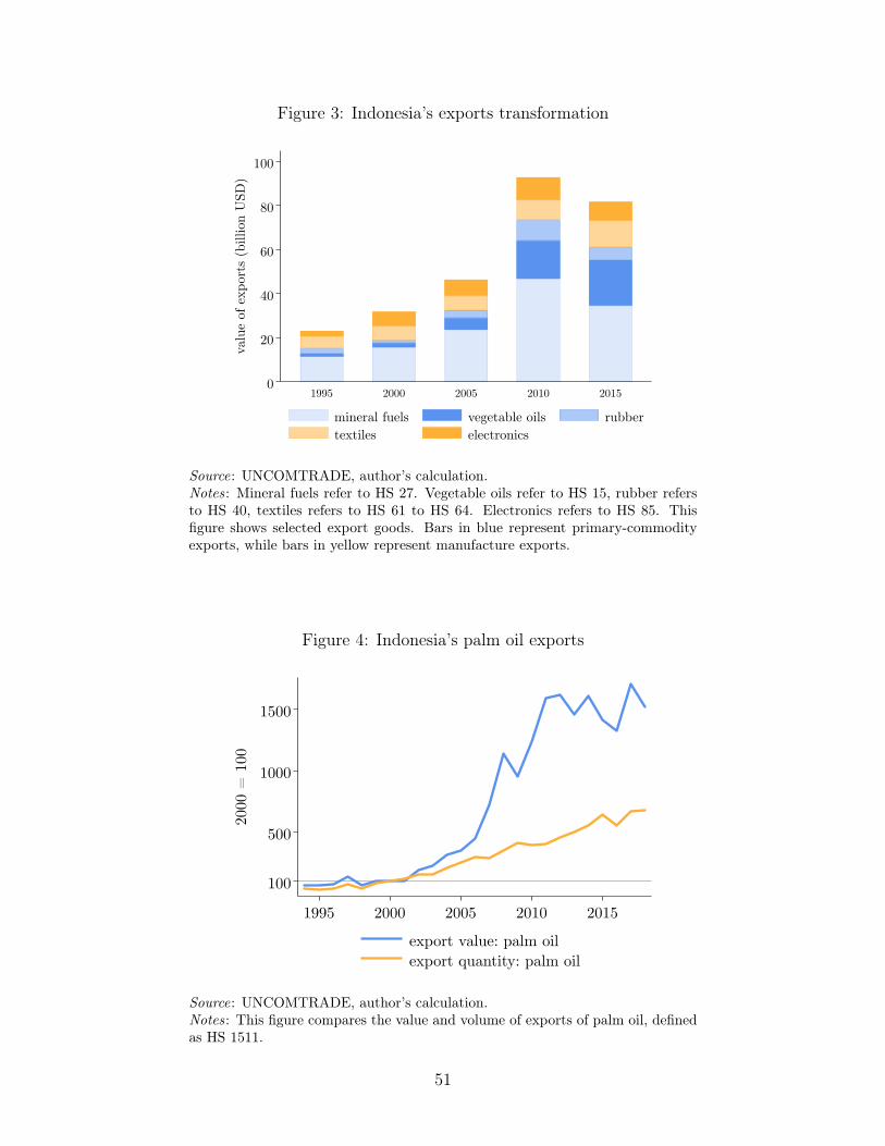
Figure 3: Indonesia’s exports transformation

0

20

40

60

80

100

valu

e of

exp

orts

(bi

llion

USD

)

1995 2000 2005 2010 2015

mineral fuels vegetable oils rubbertextiles electronics

Source: UNCOMTRADE, author’s calculation.Notes: Mineral fuels refer to HS 27. Vegetable oils refer to HS 15, rubber refersto HS 40, textiles refers to HS 61 to HS 64. Electronics refers to HS 85. Thisfigure shows selected export goods. Bars in blue represent primary-commodityexports, while bars in yellow represent manufacture exports.

Figure 4: Indonesia’s palm oil exports

100

500

1000

1500

2000

= 1

00

1995 2000 2005 2010 2015

export value: palm oilexport quantity: palm oil

Source: UNCOMTRADE, author’s calculation.Notes: This figure compares the value and volume of exports of palm oil, definedas HS 1511.

51

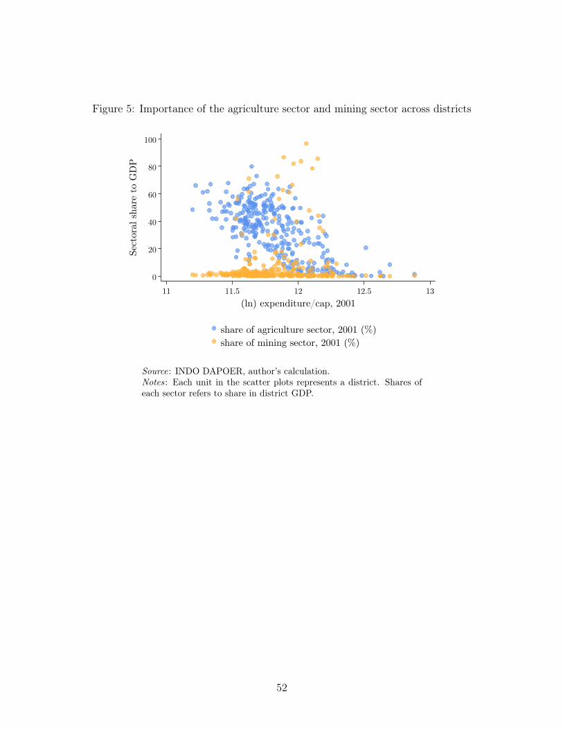
Figure 5: Importance of the agriculture sector and mining sector across districts

0

20

40

60

80

100Se

ctor

al s

hare

to

GD

P

11 11.5 12 12.5 13(ln) expenditure/cap, 2001

share of agriculture sector, 2001 (%)share of mining sector, 2001 (%)

Source: INDO DAPOER, author’s calculation.Notes: Each unit in the scatter plots represents a district. Shares ofeach sector refers to share in district GDP.

52

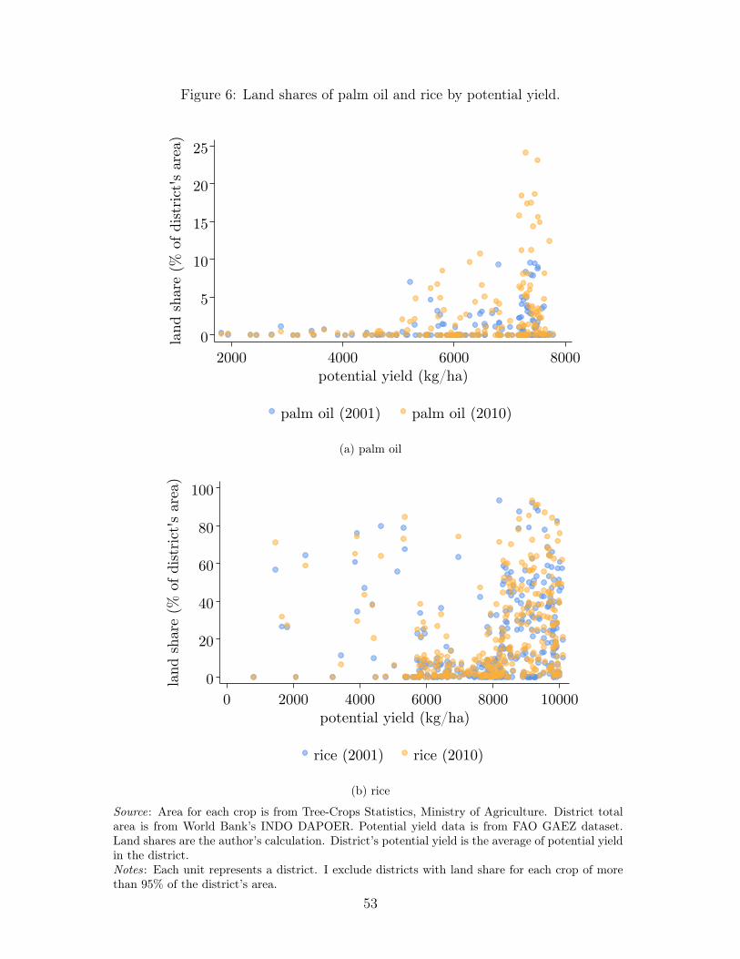
Figure 6: Land shares of palm oil and rice by potential yield.

0

5

10

15

20

25

land

sha

re (

% o

f dis

tric

t's

area

)

2000 4000 6000 8000potential yield (kg/ha)

palm oil (2001) palm oil (2010)

(a) palm oil

0

20

40

60

80

100

land

sha

re (

% o

f dis

tric

t's

area

)

0 2000 4000 6000 8000 10000potential yield (kg/ha)

rice (2001) rice (2010)

(b) rice

Source: Area for each crop is from Tree-Crops Statistics, Ministry of Agriculture. District totalarea is from World Bank’s INDO DAPOER. Potential yield data is from FAO GAEZ dataset.Land shares are the author’s calculation. District’s potential yield is the average of potential yieldin the district.Notes: Each unit represents a district. I exclude districts with land share for each crop of morethan 95% of the district’s area.

53

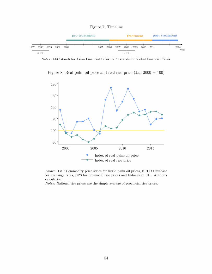
Figure 7: Timeline

year1997 1998 1999 2000 2001 2005 2006 2007 2008 2009 2010 2011 2014

pre-treatment treatment post-treatment

AFC GFC

Notes: AFC stands for Asian Financial Crisis. GFC stands for Global Financial Crisis.

Figure 8: Real palm oil price and real rice price (Jan 2000 = 100)

80

100

120

140

160

180

2000 2005 2010 2015

Index of real palm-oil priceIndex of real rice price

Source: IMF Commodity price series for world palm oil prices, FRED Databasefor exchange rates, BPS for provincial rice prices and Indonesian CPI. Author’scalculation.Notes: National rice prices are the simple average of provincial rice prices.

54

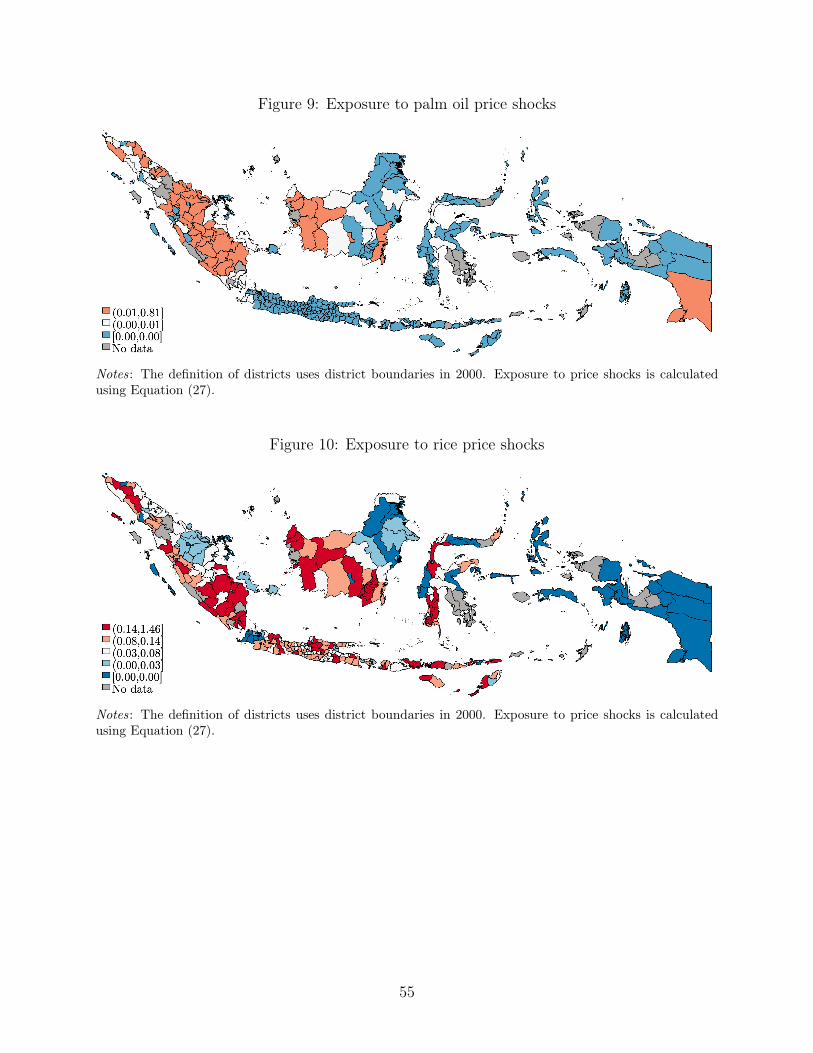
Figure 9: Exposure to palm oil price shocks

Notes: The definition of districts uses district boundaries in 2000. Exposure to price shocks is calculatedusing Equation (27).

Figure 10: Exposure to rice price shocks

Notes: The definition of districts uses district boundaries in 2000. Exposure to price shocks is calculatedusing Equation (27).

55

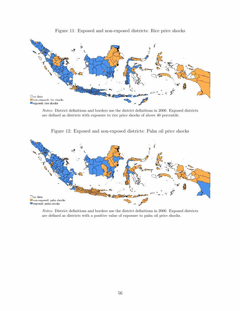
Figure 11: Exposed and non-exposed districts: Rice price shocks

Notes: District definitions and borders use the district definitions in 2000. Exposed districtsare defined as districts with exposure to rice price shocks of above 40 percentile.

Figure 12: Exposed and non-exposed districts: Palm oil price shocks

Notes: District definitions and borders use the district definitions in 2000. Exposed districtsare defined as districts with a positive value of exposure to palm oil price shocks.

56

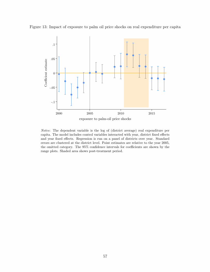
Figure 13: Impact of exposure to palm oil price shocks on real expenditure per capita

-.1

-.05

0

.05

.1C

oeffi

cien

t es

tim

ate

2000 2005 2010 2015

exposure to palm-oil price shocks

Notes: The dependent variable is the log of (district average) real expenditure percapita. The model includes control variables interacted with year, district fixed effectsand year fixed effects. Regression is run on a panel of districts over year. Standarderrors are clustered at the district level. Point estimates are relative to the year 2005,the omitted category. The 95% confidence intervals for coefficients are shown by therange plots. Shaded area shows post-treatment period.

57

Figure 14: Impact of palm oil price shocks on real expenditure per capita across terciles

-.2

-.1

0

.1

.2

Coeffi

cien

t es

tim

ate

2000 2005 2010 2015

exposure to palm-oil price shocks: top tercile

-.2

-.1

0

.1

.2

Coeffi

cien

t es

tim

ate

2000 2005 2010 2015

exposure to palm-oil price shocks: second tercile

-.2

-.1

0

.1

.2

Coeffi

cien

t es

tim

ate

2000 2005 2010 2015

exposure to palm-oil price shocks: bottom tercile

Notes: The dependent variable is (ln) real expenditure per capita. The model includescontrol variables interacted with year, district fixed effects and year fixed effects. Re-gression is run on a panel of districts over year. Standard errors are clustered at thedistrict level. Point estimates are relative to the year 2005, the omitted category. The95% confidence intervals for coefficients are shown by the range plots. Shaded areashows post-treatment period.

58

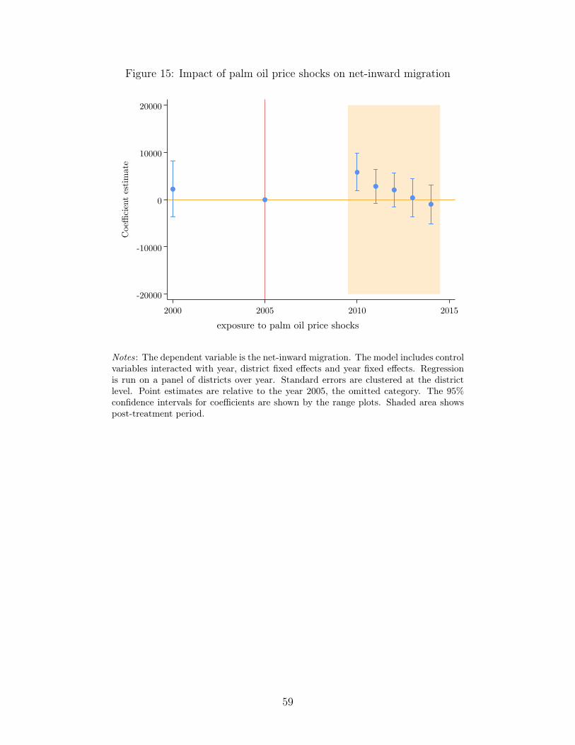
Figure 15: Impact of palm oil price shocks on net-inward migration

-20000

-10000

0

10000

20000

Coeffi

cien

t es

tim

ate

2000 2005 2010 2015

exposure to palm oil price shocks

Notes: The dependent variable is the net-inward migration. The model includes controlvariables interacted with year, district fixed effects and year fixed effects. Regressionis run on a panel of districts over year. Standard errors are clustered at the districtlevel. Point estimates are relative to the year 2005, the omitted category. The 95%confidence intervals for coefficients are shown by the range plots. Shaded area showspost-treatment period.

59

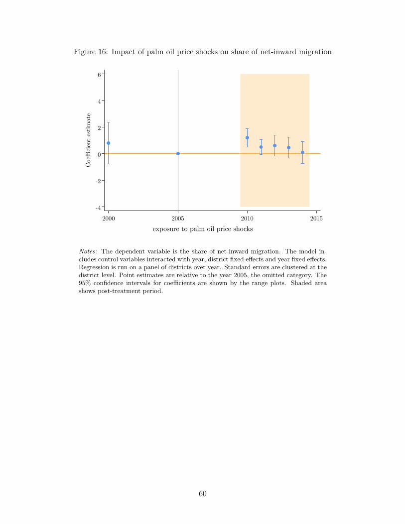
Figure 16: Impact of palm oil price shocks on share of net-inward migration

-4

-2

0

2

4

6

Coeffi

cien

t es

tim

ate

2000 2005 2010 2015

exposure to palm oil price shocks

Notes: The dependent variable is the share of net-inward migration. The model in-cludes control variables interacted with year, district fixed effects and year fixed effects.Regression is run on a panel of districts over year. Standard errors are clustered at thedistrict level. Point estimates are relative to the year 2005, the omitted category. The95% confidence intervals for coefficients are shown by the range plots. Shaded areashows post-treatment period.

60

Figure 17: Impact of palm oil price shocks on net-inward migration across terciles

-20000

-10000

0

10000

20000

Coeffi

cien

t es

tim

ate

2000 2005 2010 2015

exposure to palm-oil price shocks: top tercile

-20000

-10000

0

10000

20000

Coeffi

cien

t es

tim

ate

2000 2005 2010 2015

exposure to palm-oil price shocks: second tercile

-20000

-10000

0

10000

20000

Coeffi

cien

t es

tim

ate

2000 2005 2010 2015

exposure to palm-oil price shocks: bottom tercile

Notes: The dependent variable is net-inward migration. The model includes controlvariables interacted with year, districts fixed effects and year fixed effects. Regressionis run on a panel of districts over year. Standard errors are clustered at the districtlevel. Point estimates are relative to year the 2005, the omitted category. The 95%confidence intervals for coefficients are shown by the range plots. Shaded area showspost-treatment period.

61

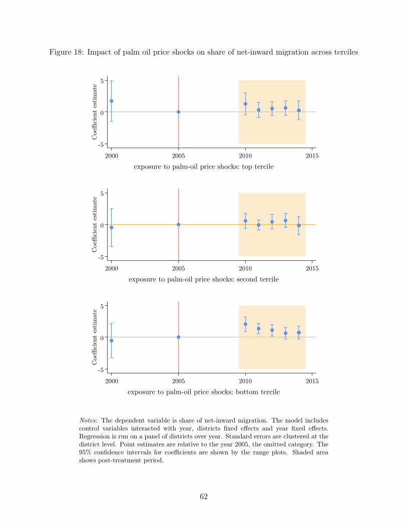
Figure 18: Impact of palm oil price shocks on share of net-inward migration across terciles

-5

0

5

Coeffi

cien

t es

tim

ate

2000 2005 2010 2015

exposure to palm-oil price shocks: top tercile

-5

0

5

Coeffi

cien

t es

tim

ate

2000 2005 2010 2015

exposure to palm-oil price shocks: second tercile

-5

0

5

Coeffi

cien

t es

tim

ate

2000 2005 2010 2015

exposure to palm-oil price shocks: bottom tercile

Notes: The dependent variable is share of net-inward migration. The model includescontrol variables interacted with year, districts fixed effects and year fixed effects.Regression is run on a panel of districts over year. Standard errors are clustered at thedistrict level. Point estimates are relative to the year 2005, the omitted category. The95% confidence intervals for coefficients are shown by the range plots. Shaded areashows post-treatment period.

62

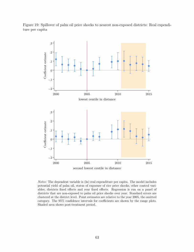
Figure 19: Spillover of palm oil price shocks to nearest non-exposed districts: Real expendi-ture per capita

-.2

-.1

0

.1

.2

.3C

oeffi

cien

t es

tim

ate

2000 2005 2010 2015

lowest centile in distance

-.2

-.1

0

.1

.2

.3

Coeffi

cien

t es

tim

ate

2000 2005 2010 2015

second lowest centile in distance

Notes: The dependent variable is (ln) real expenditure per capita. The model includespotential yield of palm oil, status of exposure of rice price shocks, other control vari-ables, districts fixed effects and year fixed effects. Regression is run on a panel ofdistricts that are non-exposed to palm oil price shocks over year. Standard errors areclustered at the district level. Point estimates are relative to the year 2005, the omittedcategory. The 95% confidence intervals for coefficients are shown by the range plots.Shaded area shows post-treatment period.

63

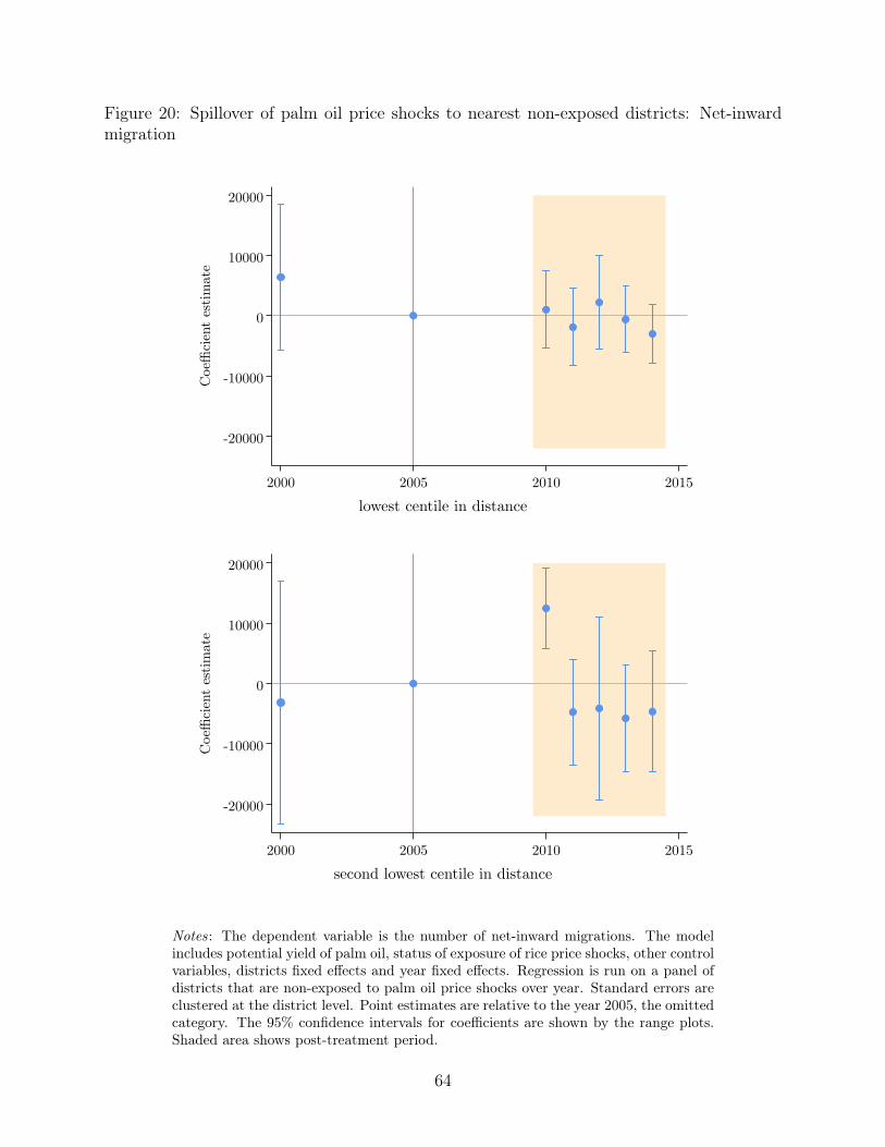
Figure 20: Spillover of palm oil price shocks to nearest non-exposed districts: Net-inwardmigration

-20000

-10000

0

10000

20000C

oeffi

cien

t es

tim

ate

2000 2005 2010 2015

lowest centile in distance

-20000

-10000

0

10000

20000

Coeffi

cien

t es

tim

ate

2000 2005 2010 2015

second lowest centile in distance

Notes: The dependent variable is the number of net-inward migrations. The modelincludes potential yield of palm oil, status of exposure of rice price shocks, other controlvariables, districts fixed effects and year fixed effects. Regression is run on a panel ofdistricts that are non-exposed to palm oil price shocks over year. Standard errors areclustered at the district level. Point estimates are relative to the year 2005, the omittedcategory. The 95% confidence intervals for coefficients are shown by the range plots.Shaded area shows post-treatment period.

64

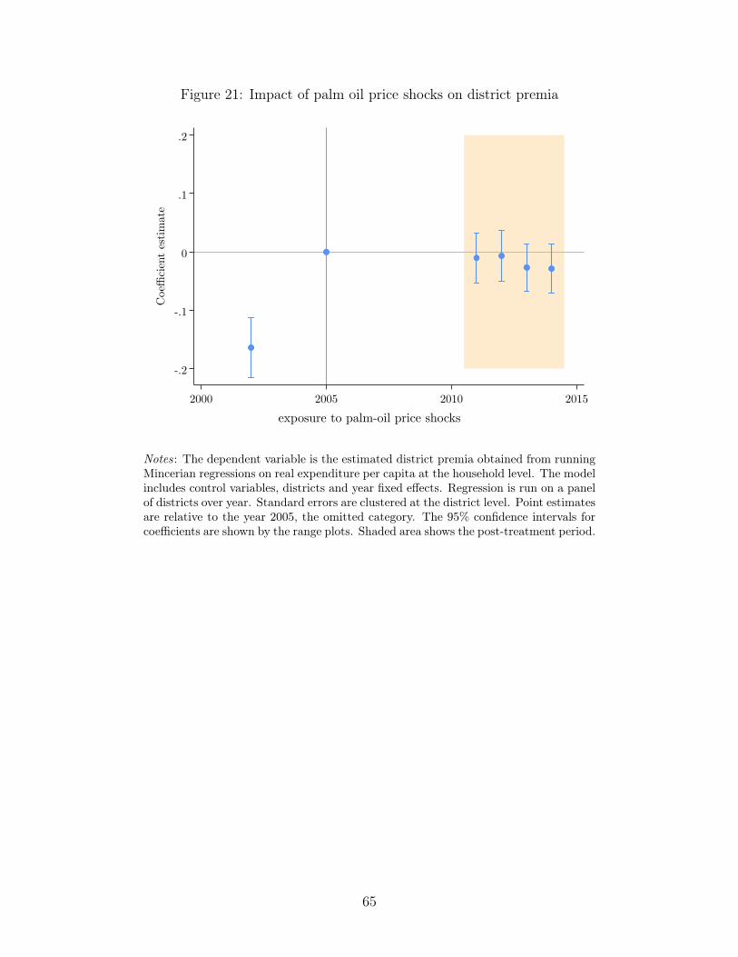
Figure 21: Impact of palm oil price shocks on district premia

-.2

-.1

0

.1

.2

Coeffi

cien

t es

tim

ate

2000 2005 2010 2015

exposure to palm-oil price shocks

Notes: The dependent variable is the estimated district premia obtained from runningMincerian regressions on real expenditure per capita at the household level. The modelincludes control variables, districts and year fixed effects. Regression is run on a panelof districts over year. Standard errors are clustered at the district level. Point estimatesare relative to the year 2005, the omitted category. The 95% confidence intervals forcoefficients are shown by the range plots. Shaded area shows the post-treatment period.

65

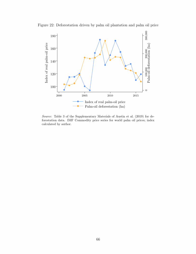
Figure 22: Deforestation driven by palm oil plantation and palm oil price

010

0,00

020

0,00

030

0,00

0Pal

m-o

il de

fore

stat

ion

(ha)

100

120

140

160

180

Inde

x of

rea

l pal

m-o

il pr

ice

2000 2005 2010 2015

Index of real palm-oil pricePalm-oil deforestation (ha)

Source: Table 3 of the Supplementary Materials of Austin et al. (2019) for de-forestation data. IMF Commodity price series for world palm oil prices; indexcalculated by author.

66

Figure 23: Distribution of drivers of gains from migration by exposure to palm oil priceshocks

-.15

-.1

-.05

0

.05

.1po

pula

tion

sha

res

-.005 0 .005 .01 .015expenditure shares - population shares

.96667

.9

.83333

.76667

.7

.63333

.56667

.5

.43333

.36667

.3

.23333

.16667

.1

.03333

exposed: palm-oil

Notes: Each bin represents a group of districts. The colors of the bins representthe share of districts exposed to palm oil price shocks at each particular bins.

67

Data Appendix

INDO-DAPOER

This dataset presents various economic indicators disaggregated to the province and district

level. The dataset is summarized from different official datasets and compiled by the World

Bank. I obtain district-average expenditure per capita as a proxy for regional welfare and

local earnings from this dataset. In addition, I also get sectoral GDP, area, and population

for each district from this dataset. For each year, I crosswalk districts to the districts defined

in 2000.

The control variables in reduced-form exercises are obtained from INDO DAPOER

dataset as well. These variables are:

• Percentage of rural population in 2000

• (ln) Regional GDP in mining and quarrying sector in 2000

• (ln) Regional GDP in manufacturing sector in 2000

• (ln) Length of district road in bad condition in 2000

• Percentage of villages with asphalt roads in 2000.

National Socio-Economic Survey (Susenas)

This household survey provides the most comprehensive household’s expenditure pattern and

other social and economic indicators annually for the Indonesian economy. The database

is sampled from around 300,000 households and is representative up to the district level.

Susenas is also the source for INDO DAPOER’s data on expenditure per capita. In general,

the survey has two sets of questionnaires: the core and the modul. The core questionnaire

poses basic economic and social indicators to members of households and households. Before

2011, the consumption modul questionaire was included every three years. In this regard,

68

the matching between the core and modul questionnaires before 2011 can be done for survey

years 2002, 2005, and 2008. Given this construction, I estimate district premia only in these

years for the pre-2011 period. Nevertheless, due to insufficient representativeness in the

invidual matched sample in 2008, I do not include 2008 in the district premia estimation.

Since 2011, Susenas has included questions on migration behaviour that were previously

only captured every five years using census and between-census population surveys. I con-

structed a migration flow matrix across districts from these migration questions. Then I

compute the recent migration rate per district destination from this dataset. Recent migra-

tion is defined as a change of residential location between the survey year and five years prior

to the survey year.

Population Census and Inter-Census Population Survey from IPUMS

I obtain past recent migration patterns from the Population Census in 2000. Inter-Census

Population Survey 2005 and Population Census 2010 are provided by IPUMS. This dataset

is a 10% sample of the complete census and is representative up to the district level.

Prices data

IMF Commodity Price Series I use commodity prices in the IMF Commodity price

series as a benchmark for world prices. The benchmark world price for palm oil is the palm

oil prices of the Malaysia Palm Oil Futures (first contract forward) 4% to 5% FFA in USD

per metric ton. The benchmark world price for rice is the 5% broken milled white rice of

the Thailand nominal price quote in USD per metric ton. Since I am using domestic retail

prices for rice, I follow Dawe (2008) in adding 20 USD per ton for rice shipping and a 10%

mark-up in order to translate the world rice price to the retail price for imported rice in

Indonesia.

69

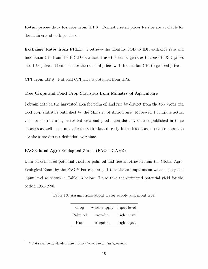
Retail prices data for rice from BPS Domestic retail prices for rice are available for

the main city of each province.

Exchange Rates from FRED I retrieve the monthly USD to IDR exchange rate and

Indonesian CPI from the FRED database. I use the exchange rates to convert USD prices

into IDR prices. Then I deflate the nominal prices with Indonesian CPI to get real prices.

CPI from BPS National CPI data is obtained from BPS.

Tree Crops and Food Crop Statistics from Ministry of Agriculture

I obtain data on the harvested area for palm oil and rice by district from the tree crops and

food crop statistics published by the Ministry of Agriculture. Moreover, I compute actual

yield by district using harvested area and production data by district published in these

datasets as well. I do not take the yield data directly from this dataset because I want to

use the same district definition over time.

FAO Global Agro-Ecological Zones (FAO - GAEZ)

Data on estimated potential yield for palm oil and rice is retrieved from the Global Agro-

Ecological Zones by the FAO.32 For each crop, I take the assumptions on water supply and

input level as shown in Table 13 below. I also take the estimated potential yield for the

period 1961-1990.

Table 13: Assumptions about water supply and input level

Crop water supply input level

Palm oil rain-fed high input

Rice irrigated high input

32Data can be dowloaded here : http://www.fao.org/nr/gaez/en/.

70

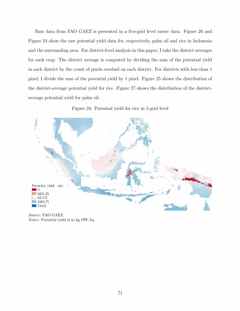
Raw data from FAO GAEZ is presented in a five-grid level raster data. Figure 26 and

Figure 24 show the raw potential yield data for, respectively, palm oil and rice in Indonesia

and the surrounding area. For district-level analysis in this paper, I take the district averages

for each crop. The district average is computed by dividing the sum of the potential yield

in each district by the count of pixels overlaid on each district. For districts with less than 1

pixel, I divide the sum of the potential yield by 1 pixel. Figure 25 shows the distribution of

the district-average potential yield for rice. Figure 27 shows the distribution of the district-

average potential yield for palm oil.

Figure 24: Potential yield for rice in 5-grid level

Source: FAO GAEZ.Notes: Potential yield is in kg DW/ha.

71

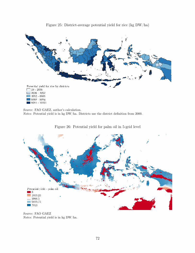
Figure 25: District-average potential yield for rice (kg DW/ha)

Source: FAO GAEZ, author’s calculation.Notes: Potential yield is in kg DW/ha. Districts use the district definition from 2000.

Figure 26: Potential yield for palm oil in 5-grid level

Source: FAO GAEZNotes: Potential yield is in kg DW/ha.

72

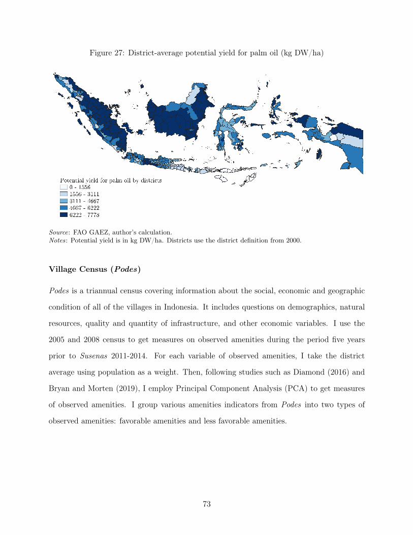
Figure 27: District-average potential yield for palm oil (kg DW/ha)

Source: FAO GAEZ, author’s calculation.Notes: Potential yield is in kg DW/ha. Districts use the district definition from 2000.

Village Census (Podes)

Podes is a triannual census covering information about the social, economic and geographic

condition of all of the villages in Indonesia. It includes questions on demographics, natural

resources, quality and quantity of infrastructure, and other economic variables. I use the

2005 and 2008 census to get measures on observed amenities during the period five years

prior to Susenas 2011-2014. For each variable of observed amenities, I take the district

average using population as a weight. Then, following studies such as Diamond (2016) and

Bryan and Morten (2019), I employ Principal Component Analysis (PCA) to get measures

of observed amenities. I group various amenities indicators from Podes into two types of

observed amenities: favorable amenities and less favorable amenities.

73

Chapter 2

Price divergence in times of trade

protection: Exploration on the import

ban on rice in Indonesia

2.1 Introduction

Despite the widespread policy reforms and reduction of trade barriers for the past four

decades, protective trade policies are still prevalent in developing countries (Atkin and Khan-

delwal, 2020). Indeed, recent surveys of literature, such as Atkin and Khandelwal (2020)

and Goldberg and Pavcnik (2016), reveal that the distributional impact of trade policies

in developing countries may not be as straightforward as predicted by the neoclassic trade

models due to various frictions. In this chapter, I study the impact of a binding non-tariff

trade policy imposed by Indonesia. Despite the relatively stable prices and parallel trend

with the world price of rice since the 1970s to early 2000s (Warr, 2005), in 2004, Indonesia

introduced a large import ban on rice, a staple food for most of its 260 million population.

As expected, domestic retail prices for rice have increased and diverted away from the world

price. I find that the rice price shocks did not increase the purchasing power of rice-producing

districts, nor did they spur growth in the rice sector. This result may indicate the ineffec-

tiveness of the trade protection to support rice farmers as well as motivate the question on

the distributional impact of the trade policy.

This paper aims to explore and document the price divergence that occurs due to the

import ban. I find that understanding this phenomenon is first-order in evaluating the

trade policy, especially in light of the insignificant impact of the trade protection to benefit

74

the rice-producing districts. I contribute to the literature as the first study that, not only

explores price divergence across regions, but also price divergence between retail prices and

farm-gate prices. The previous study has shown that there is a parallel trend of the national

retail price and national farm-gate prices.33 However, using more granular data, I am the

first to show evidence of incomplete pass-through between retail prices to farm-gate prices

of rice. In addition, I explore potential drivers of the wedges between the retail prices and

the farm-gate prices, such as search costs, transportation costs, and information costs.

To analyze the price divergence, I build upon various empirical strategies performed by

Allen (2014) and Bazzi (2017) in analyzing trade patterns and prices of agriculture com-

modities. I replicate strategies to identify incentives to arbitrage and the role of search costs

as shown by Allen (2014). Meanwhile, Bazzi (2017) explored various empirical patterns of

the retail prices of rice in Indonesia during the import-ban policy. I complement his findings

using a longer time series of regional retail prices. I also replicate his empirical methods in

understanding prices on farm-gate prices.

I document four features of the price divergence during the import-ban policy. First,

unlike the case of the Philippines, as shown by Allen (2014), the relative ranking of rice

prices persists during the trade-protection era. Indeed, weather, representing time-variant

productivity across provinces, has a small contribution in explaining the variation in log

real retail and farm-gate prices. Second, provinces with a higher relative rank of both retail

and farm-gate prices are the ones with higher (time-invariant) potential yield in growing

rice. These two facts indicate that search costs may not be substantial drivers in the lack of

arbitrage implied by the price divergence across regions.

Third, I confirm the result shown by Bazzi (2017) that provinces with higher increases

in retail prices after the ban are the ones with higher import pass-through elasticity. How-

ever, I do not find evidence of such a trend for the farm-gate prices. Lastly, I show that

transportation and communication infrastructures have been improving in Indonesia. The

33Bazzi (2017).

75

correlations between several variables representing the use of these infrastructures with retail

and farm-gate prices are mostly statistically insignificant. However, there is potential in the

role of information frictions as represented by mobile phone use in determining prices in the

upstream side of the rice value chain. Farm-gate prices have a statistically significant positive

correlation with mobile phone use. This relationship may imply the role of information in

empowering farmers to get more competitive prices. The third and fourth facts may indicate

imperfect competition in the rice markets as well as other domestic trade frictions such as

logistic costs, information frictions, and the role of middlemen. If traders perform strategic

behavior especially by charging retail prices that are higher than their competitive level and

buying with farm-gate prices that are lower than their competitive level, then the increasing

wedges between retail and farm-gate prices as well as the lack of arbitrage are the direct

outcomes.

There are at least two implications from the evidence of price divergence and why rig-

orous evaluation on the trade policy is due. First, Atkin and Khandelwal (2020) suggested

that evidence that trade affects not only the magnitude but also the dispersion of markups

indicate misallocation issues. Various studies show that domestic misallocation of resources

has a substantial contribution to aggregate income differences across countries.34 Second,

understanding what types of frictions present and acknowledging structural issues that affect

the distributional impact of trade protection can guide policymakers in evaluating the trade

policy and improve policy-making. For example, Bigsten et al. (2004) show that firms in

developing countries may not be able to seize economies of scale to be more competitive

as they face high trade costs and poverty, which create small and segmented markets for

the firm to sell to. In this case, since rice farmers are relatively small in Indonesia, simply

opening up the import ban may not directly help farmers to reap growth through economies

of scale, let alone to be internationally competitive.

I propose the collection and use of two sets of data in order to rigorously evaluate the

34See for example Banerjee and Duflo (2005) and Restuccia and Rogerson (2017).

76

trade policy. First, I propose to use and collect the data of regional farm-gate prices and

grain prices along the rice value chain. This data on prices can substantially contribute to

providing a deeper understanding of the distributional impact of the trade policy. Second, I

propose to get data on intra-national trade in rice to better understand the lack of arbitrage.

So far, such data is not available, at least for the public.

This paper contributes to three strands of literature. First, it contributes to the studies

on the impact of trade policies, in particular, in the form of a binding non-tariff barrier. Most

studies in this field focus on the impact of trade of liberalization. This paper complements

the literature with the impact of de-liberalization as Indonesia moved from a free-trade policy

to the imposition of trade protection. Goldberg and Pavcnik (2016) provide a recent survey

of literature on the impact of trade policies, while Feenstra (1995) presents the survey for

earlier studies. Several studies discuss Indonesia’s import ban on rice, such as Warr and

Yusuf (2014) and Warr (2011).35 Relative to these papers, I show that the price shocks

due to the import ban did not increase the purchasing power of rice-producing districts.

In addition, I show that the import ban creates price divergence across regions as well as

between retail prices and farm-gate prices.

Second, I contribute to the literature on the impact of trade policy on prices. As Goldberg

and Pavcnik (2016) review, there are only a few papers that focus on prices as the outcome

of interest despite their central role in trade policy evaluation. This paper focuses on one

particular crop or industry: rice. Such focus allows us to analyze how a trade policy may

affect the upstream side of the industry, i.e., as reflected by the farm-gate prices, and the

downstream side, i.e., as reflected by the retail prices, differently. Previous works that

study the impact of trade policy on prices include Topalova (2010) and De Loecker et al.

(2016). Both papers study the impact of trade liberalization in India and find that increase

competition leads to lower prices. Echoing their finding, I find that retail prices and farm-

gate prices increase due to the absence of import competition. However, the retail prices35Other studies, such as Bazzi (2017) and Sim (2020), use the price shocks due to the import ban as

sources of income shocks.

77

increase more than the farm-gate prices.

In addition, I show that the increase in retail prices is not passed on completely to farm-

gate prices. There is substantial variation across regions in terms of the wedges between retail

prices and farm-gate prices. These wedges can consist of, not only value-added for mills and

trade frictions but also markups of traders. In terms of the impact on markups, previous

studies do not show a conclusive impact of competition on markups. For example, Levinsohn

(1993), Harrison (1994), and Edmond et al. (2015) show that markups decreased with trade

liberalization policies, while De Loecker et al. (2016) find that the markups actually increased

in the trade liberalization episode in India. In this paper, I provide motivation to study the

impact of the import ban on markups, including the importance of considering frameworks

with variable markups, as part of a rigorous trade policy evaluation.

Lastly, this paper contributes to the literature on trade frictions in developing countries.

Atkin and Khandelwal (2020) provides a comprehensive survey of literature on this topic.

Exploring the increasing wedges between retail and farm-gate prices as well as the regional

price divergence due to the import ban on rice, I provide insights on the potential contribution

of imperfect competition and domestic trade frictions including the role of middlemen in

intra-national trade in a developing-country context. Studies on imperfect competition in

trade intersect with studies on the impact of trade policy on markups as mentioned above.

Meanwhile, studies on the role of intermediaries in developing countries, such as Atkin and

Donaldson (2015), show the prevalence of intermediaries and find that remote locations

hurt the most due to the interaction of high trade costs and lack of competition among

intermediaries. Dhingra and Tenreyro (2020) and Bergquist and Dinerstein (2020) show the

role of traders’ market power in explaining the degree of price pass-through.

The paper is organized as follows. I describe the trade policies related to the import ban

on rice as well as the impact of the rice price shocks due to the import ban in Section 2. I

continue in Section 3 with empirical exploration in understanding the spatial price divergence

during the import ban. I discuss the implications of the findings from the exploration in

78

Section 4. Lastly, in Section 5, I provide the conclusion.

2.2 The import ban on rice in Indonesia

2.2.1 The political economy of rice in Indonesia

Rice is an, if not the most, important agricultural commodity in Indonesia. It is the main

staple food for most Indonesians. The national household survey in 2007 shows that poor

households spends on average 22% of their total expenditure on rice, or approximately one-

third of their food expenditure (Aldaz-Carroll, 2010). Meanwhile, rice sector is also a major

employer. The agriculture census in 2003 reveals that 55% of agriculture households in

Indonesia are rice farmers. However, only 6% of those have control over more than 0.5 ha

of rice fields (McCulloch, 2008). Since rice is a necessity to most Indonesians, an increase in

its prices may reduce purchasing power to net consumers.

Given the strategic position of rice in the economy, rice policy has been closely deter-

mined by the political situation as well.36 Since the early 1970s to the late 1990s, rice price

stabilization was achieved through imports. Particularly, the national logistic agency (Bu-

log) was given a mandate to stabilize rice prices. The government also provided Bulog with

import monopoly. Then, in the short period after the Asian Financial Crisis (AFC), Bulog

lost its authority as the sole importer of rice as part of the IMF policy package that Indone-

sia took. During this time, rice price stabilization was achieved through imports by private

traders (McCulloch and Timmer, 2008). Nevertheless, throughout these periods, real rice

prices were relatively stable (Fane and Warr, 2008). Due to the trade liberalization in late

the 1990s, Indonesia became the world’s largest rice importer (Warr, 2011).

Meanwhile in the early 2000s, as Indonesia recovered from the AFC, pressure to protect

rice farmers increased as well. Some import restrictions were imposed in the form of import

36McCulloch and Timmer (2008) provide a summary of the political economy of rice in Indonesia fromthe 1970s to 2008. There is not much changes in terms of policy since 2008 up to the current period.

79

tariffs. Fane and Warr (2008) estimated that the nominal rate of protection on rice increased

from 14% in 2000 to 33% in 2003. Finally in 2004, the Indonesian government placed a ban

on imports of rice by the private sector. This ban is supposed to be a seasonal ban to avoid

flood of imports during harvest seasons. Some imports are allowed with the size of the quota

to be determined by the government. The imports can only be conducted by Bulog.37 Marks

(2017) estimates that in 2015 the nominal rate of protection and effective rate of protection

in rice sector reached consecutively 67.2% and 204.3%.

Figure 28 illustrates the trend of Indonesia’s exports, imports, and net-export for rice

over the various rice trade regimes. In most years between 1990 to 2018, Indonesia is a net-

importer of rice. In the period before 1998, Bulog conducted the imports with the objective

to stabilize domestic rice prices. In the short period of relatively free-trade of rice in 1998 to

2003, imports were conducted by private traders. Meanwhile, since the import ban in 2004,

imports are conducted by Bulog when the governnment decides to import and how much to

import. Imports can only be done during off-harvest periods.

Figure 29 shows that since the import ban took place in 2004, domestic rice prices have

surged. In addition, discrepancy between domestic prices and the price of imported rice has

increased ever since, with some period of reversal during the Food Crisis 2008. Except for

the Food Crisis period, the import ban is practically binding as there is lack of incentive to

export due to lower prices in export markets. Meanwhile, during the Food Crisis period,

the government introduced an export ban on rice to shield the country from the exorbitant

level of world prices fueled by export restrictions from main rice exporters and other trade

distortion measures.38 Despite how the import ban has continued to be binding, leading to

37These trade policies on rice are stipulated by Minister of Industry and Trade Regulation No. 9/2004,Minister of Trade Regulation No. 12/2008, and Minister of Trade Regulation No. 19/2014.

38Various studies show that the price hikes in food commodities during the Food Crisis 2008 were magnifiedby trade measures. These studies include Giordani et al. (2016), Anderson and Martin (2011) and Bouëtand Debucquet (2012). Giordani et al. (2016) in particular document that there were six countries imposingexport restrictions or import promotion measures on rice during this period. These trade measures covered35.72% of world rice trade. For the timeline of enactment of export restrictions and other trade measureson rice see Aldaz-Carroll et al. (2010) and Headey (2011).

80

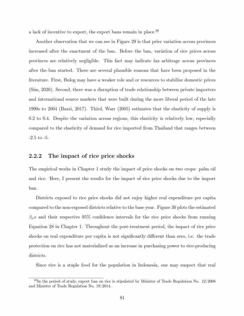
a lack of incentive to export, the export bans remain in place.39

Another observation that we can see in Figure 29 is that price variation across provinces

increased after the enactment of the ban. Before the ban, variation of rice prices across

provinces are relatively negligible. This fact may indicate lax arbitrage across provinces

after the ban started. There are several plausible reasons that have been proposed in the

literature. First, Bulog may have a weaker role and or resources to stabilize domestic prices

(Sim, 2020). Second, there was a disruption of trade relationship between private importers

and international source markets that were built during the more liberal period of the late

1990s to 2004 (Bazzi, 2017). Third, Warr (2005) estimates that the elasticity of supply is

0.2 to 0.4. Despite the variation across regions, this elasticity is relatively low, especially

compared to the elasticity of demand for rice imported from Thailand that ranges between

-2.5 to -5.

2.2.2 The impact of rice price shocks

The empirical works in Chapter 1 study the impact of price shocks on two crops: palm oil

and rice. Here, I present the results for the impact of rice price shocks due to the import

ban.

Districts exposed to rice price shocks did not enjoy higher real expenditure per capita

compared to the non-exposed districts relative to the base year. Figure 30 plots the estimated

βirs and their respective 95% confidence intervals for the rice price shocks from running

Equation 28 in Chapter 1. Throughout the post-treatment period, the impact of rice price

shocks on real expenditure per capita is not significantly different than zero, i.e. the trade

protection on rice has not materialized as an increase in purchasing power to rice-producing

districts.

Since rice is a staple food for the population in Indonesia, one may suspect that real

39In the period of study, export ban on rice is stipulated by Minister of Trade Regulation No. 12/2008and Minister of Trade Regulation No. 19/2014.

81

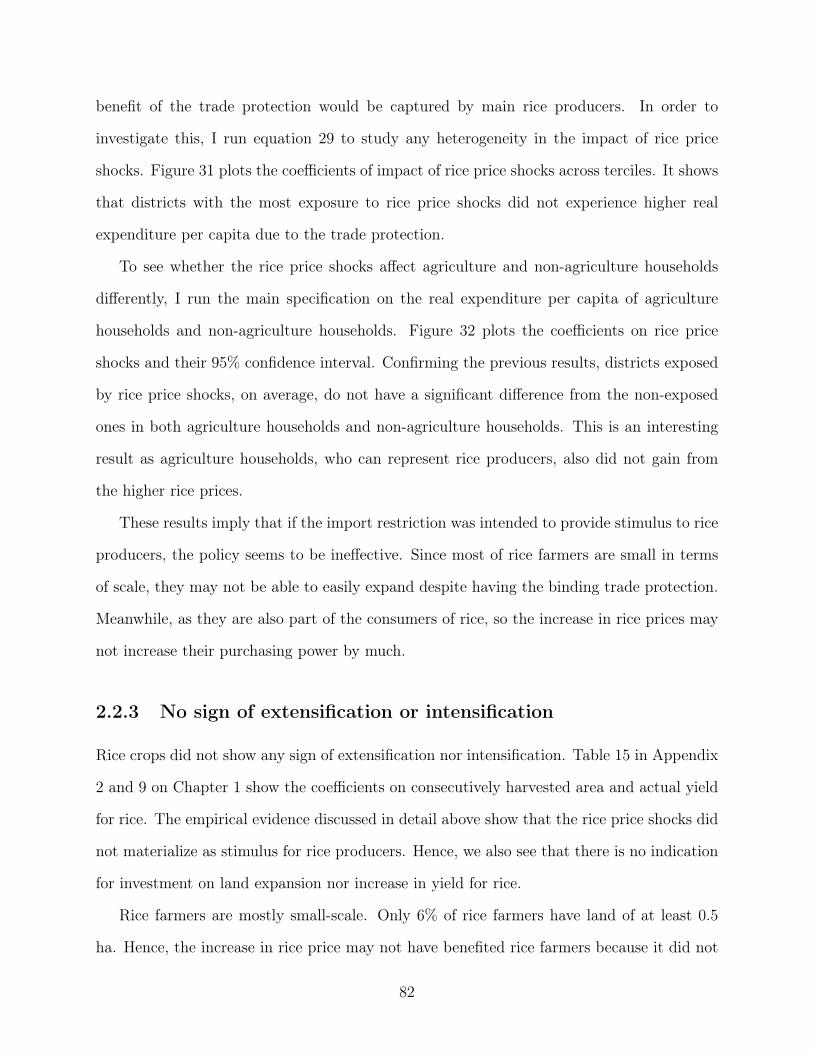
benefit of the trade protection would be captured by main rice producers. In order to

investigate this, I run equation 29 to study any heterogeneity in the impact of rice price

shocks. Figure 31 plots the coefficients of impact of rice price shocks across terciles. It shows

that districts with the most exposure to rice price shocks did not experience higher real

expenditure per capita due to the trade protection.

To see whether the rice price shocks affect agriculture and non-agriculture households

differently, I run the main specification on the real expenditure per capita of agriculture

households and non-agriculture households. Figure 32 plots the coefficients on rice price

shocks and their 95% confidence interval. Confirming the previous results, districts exposed

by rice price shocks, on average, do not have a significant difference from the non-exposed

ones in both agriculture households and non-agriculture households. This is an interesting

result as agriculture households, who can represent rice producers, also did not gain from

the higher rice prices.

These results imply that if the import restriction was intended to provide stimulus to rice

producers, the policy seems to be ineffective. Since most of rice farmers are small in terms

of scale, they may not be able to easily expand despite having the binding trade protection.

Meanwhile, as they are also part of the consumers of rice, so the increase in rice prices may

not increase their purchasing power by much.

2.2.3 No sign of extensification or intensification

Rice crops did not show any sign of extensification nor intensification. Table 15 in Appendix

2 and 9 on Chapter 1 show the coefficients on consecutively harvested area and actual yield

for rice. The empirical evidence discussed in detail above show that the rice price shocks did

not materialize as stimulus for rice producers. Hence, we also see that there is no indication

for investment on land expansion nor increase in yield for rice.

Rice farmers are mostly small-scale. Only 6% of rice farmers have land of at least 0.5

ha. Hence, the increase in rice price may not have benefited rice farmers because it did not

82

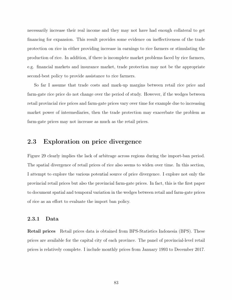
necessarily increase their real income and they may not have had enough collateral to get

financing for expansion. This result provides some evidence on ineffectiveness of the trade

protection on rice in either providing increase in earnings to rice farmers or stimulating the

production of rice. In addition, if there is incomplete market problems faced by rice farmers,

e.g. financial markets and insurance market, trade protection may not be the appropriate

second-best policy to provide assistance to rice farmers.

So far I assume that trade costs and mark-up margins between retail rice price and

farm-gate rice price do not change over the period of study. However, if the wedges between

retail provincial rice prices and farm-gate prices vary over time for example due to increasing

market power of intermediaries, then the trade protection may exacerbate the problem as

farm-gate prices may not increase as much as the retail prices.

2.3 Exploration on price divergence

Figure 29 clearly implies the lack of arbitrage across regions during the import-ban period.

The spatial divergence of retail prices of rice also seems to widen over time. In this section,

I attempt to explore the various potential source of price divergence. I explore not only the

provincial retail prices but also the provincial farm-gate prices. In fact, this is the first paper

to document spatial and temporal variation in the wedges between retail and farm-gate prices

of rice as an effort to evaluate the import ban policy.

2.3.1 Data

Retail prices Retail prices data is obtained from BPS-Statistics Indonesia (BPS). These

prices are available for the capital city of each province. The panel of provincial-level retail

prices is relatively complete. I include monthly prices from January 1993 to December 2017.

83

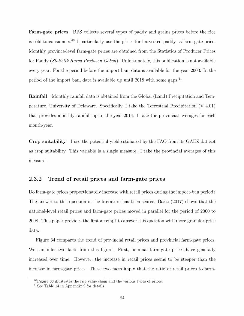
Farm-gate prices BPS collects several types of paddy and grains prices before the rice

is sold to consumers.40 I particularly use the prices for harvested paddy as farm-gate price.

Monthly province-level farm-gate prices are obtained from the Statistics of Producer Prices

for Paddy (Statistik Harga Produsen Gabah). Unfortunately, this publication is not available

every year. For the period before the import ban, data is available for the year 2003. In the

period of the import ban, data is available up until 2018 with some gaps.41

Rainfall Monthly rainfall data is obtained from the Global (Land) Precipitation and Tem-

perature, University of Delaware. Specifically, I take the Terrestrial Precipitation (V 4.01)

that provides monthly rainfall up to the year 2014. I take the provincial averages for each

month-year.

Crop suitability I use the potential yield estimated by the FAO from its GAEZ dataset

as crop suitability. This variable is a single measure. I take the provincial averages of this

measure.

2.3.2 Trend of retail prices and farm-gate prices

Do farm-gate prices proportionately increase with retail prices during the import-ban period?

The answer to this question in the literature has been scarce. Bazzi (2017) shows that the

national-level retail prices and farm-gate prices moved in parallel for the period of 2000 to

2008. This paper provides the first attempt to answer this question with more granular price

data.

Figure 34 compares the trend of provincial retail prices and provincial farm-gate prices.

We can infer two facts from this figure. First, nominal farm-gate prices have generally

increased over time. However, the increase in retail prices seems to be steeper than the

increase in farm-gate prices. These two facts imply that the ratio of retail prices to farm-

40Figure 33 illustrates the rice value chain and the various types of prices.41See Table 14 in Appendix 2 for details.

84

gate prices or I define here as “wedges” of rice prices, have increased. These wedges include

several margins such as the value-added for paddy mills, transportation costs, and other

trade costs, as well as traders’ profit margin. Figure 33 illustrates the rice value chain from

paddy grown by farmers to rice consumed by consumers. Using the ratio of the retail price

and farm-gate price as wedges, we can observe from Figure 35 the range of wedges across

provinces has widened over time.

We can also see the wider ranges of wedges of rice prices in Figure 36, which depicts the

trend of retail prices and farm gate by province. Provinces differ in terms of the evolution

of wedges over time. In general, farm-gate prices increase during the import-ban period.

However, provinces vary in the relative increase of their retail and farm-gate prices with

virtually no province have a decreasing wedge between its retail price and farm-gate price.

I follow Allen (2014) in evaluating the persistence of the ranking of relative price. In the

case of crops in the Philippines, Allen (2014) shows that the correlation of relative ranking

decreases over time. It means that provinces do not always have high or low relative prices

compared to other provinces. In his case, such a condition indicates high search costs for

farmers since it is hard to predict which provinces offer higher relative prices at any given

period.

In contrast, for the case of rice prices in Indonesia, correlations of relative ranking have

stayed relatively high especially post-2004 or as the import ban is in place. Figure 37 shows,

before 2004, the darker colors imply that relative ranking at a given period of time has a

low correlation with relative ranking in the previous five years or more. However, after 2004,

the correlations of relative ranking across periods, including between five to 10 years span,

remain high as indicated by the lighter colors. In other words, provinces with a high relative

ranking of retail prices persist to have high relative rankings. Such conditions may indicate

that search costs have a weaker role in explaining the lack of arbitrage across provinces.

85

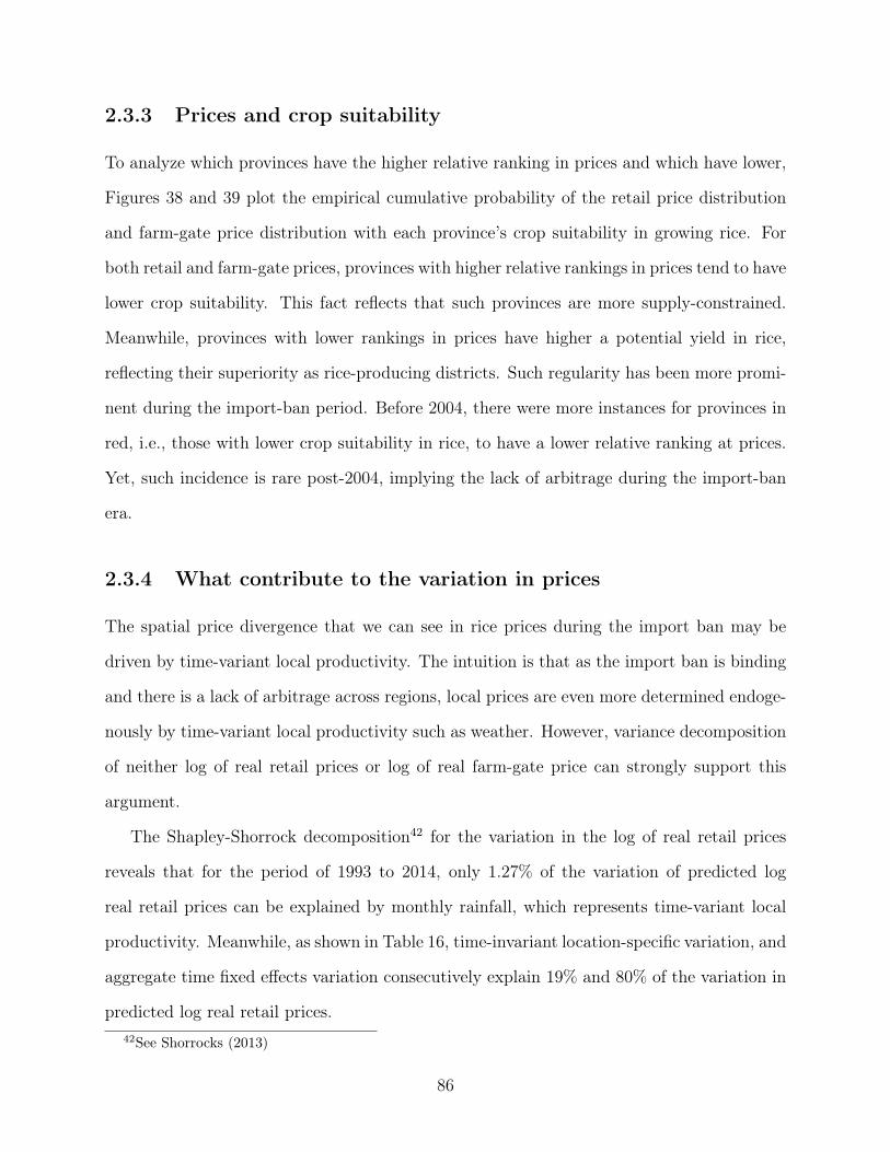
2.3.3 Prices and crop suitability

To analyze which provinces have the higher relative ranking in prices and which have lower,

Figures 38 and 39 plot the empirical cumulative probability of the retail price distribution

and farm-gate price distribution with each province’s crop suitability in growing rice. For

both retail and farm-gate prices, provinces with higher relative rankings in prices tend to have

lower crop suitability. This fact reflects that such provinces are more supply-constrained.

Meanwhile, provinces with lower rankings in prices have higher a potential yield in rice,

reflecting their superiority as rice-producing districts. Such regularity has been more promi-

nent during the import-ban period. Before 2004, there were more instances for provinces in

red, i.e., those with lower crop suitability in rice, to have a lower relative ranking at prices.

Yet, such incidence is rare post-2004, implying the lack of arbitrage during the import-ban

era.

2.3.4 What contribute to the variation in prices

The spatial price divergence that we can see in rice prices during the import ban may be

driven by time-variant local productivity. The intuition is that as the import ban is binding

and there is a lack of arbitrage across regions, local prices are even more determined endoge-

nously by time-variant local productivity such as weather. However, variance decomposition

of neither log of real retail prices or log of real farm-gate price can strongly support this

argument.

The Shapley-Shorrock decomposition42 for the variation in the log of real retail prices

reveals that for the period of 1993 to 2014, only 1.27% of the variation of predicted log

real retail prices can be explained by monthly rainfall, which represents time-variant local

productivity. Meanwhile, as shown in Table 16, time-invariant location-specific variation, and

aggregate time fixed effects variation consecutively explain 19% and 80% of the variation in

predicted log real retail prices.42See Shorrocks (2013)

86

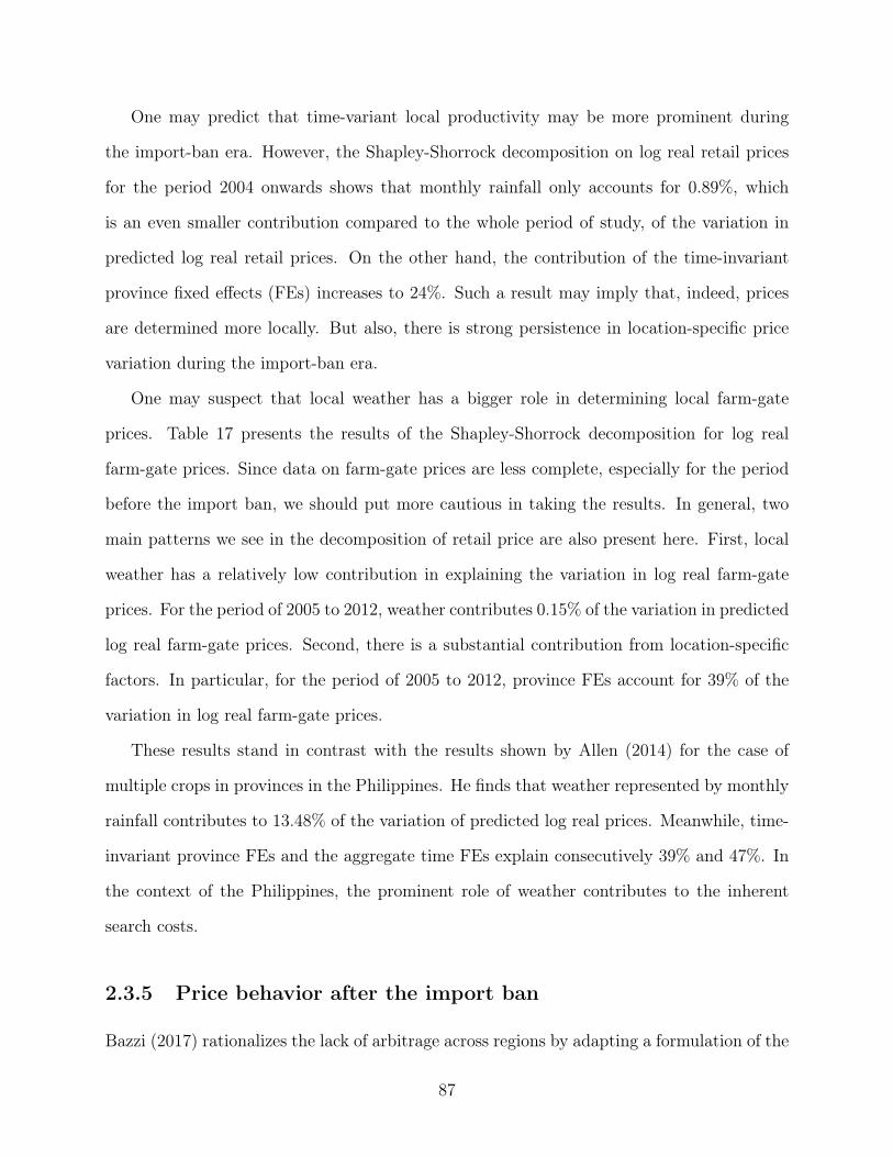
One may predict that time-variant local productivity may be more prominent during

the import-ban era. However, the Shapley-Shorrock decomposition on log real retail prices

for the period 2004 onwards shows that monthly rainfall only accounts for 0.89%, which

is an even smaller contribution compared to the whole period of study, of the variation in

predicted log real retail prices. On the other hand, the contribution of the time-invariant

province fixed effects (FEs) increases to 24%. Such a result may imply that, indeed, prices

are determined more locally. But also, there is strong persistence in location-specific price

variation during the import-ban era.

One may suspect that local weather has a bigger role in determining local farm-gate

prices. Table 17 presents the results of the Shapley-Shorrock decomposition for log real

farm-gate prices. Since data on farm-gate prices are less complete, especially for the period

before the import ban, we should put more cautious in taking the results. In general, two

main patterns we see in the decomposition of retail price are also present here. First, local

weather has a relatively low contribution in explaining the variation in log real farm-gate

prices. For the period of 2005 to 2012, weather contributes 0.15% of the variation in predicted

log real farm-gate prices. Second, there is a substantial contribution from location-specific

factors. In particular, for the period of 2005 to 2012, province FEs account for 39% of the

variation in log real farm-gate prices.

These results stand in contrast with the results shown by Allen (2014) for the case of

multiple crops in provinces in the Philippines. He finds that weather represented by monthly

rainfall contributes to 13.48% of the variation of predicted log real prices. Meanwhile, time-

invariant province FEs and the aggregate time FEs explain consecutively 39% and 47%. In

the context of the Philippines, the prominent role of weather contributes to the inherent

search costs.

2.3.5 Price behavior after the import ban

Bazzi (2017) rationalizes the lack of arbitrage across regions by adapting a formulation of the

87

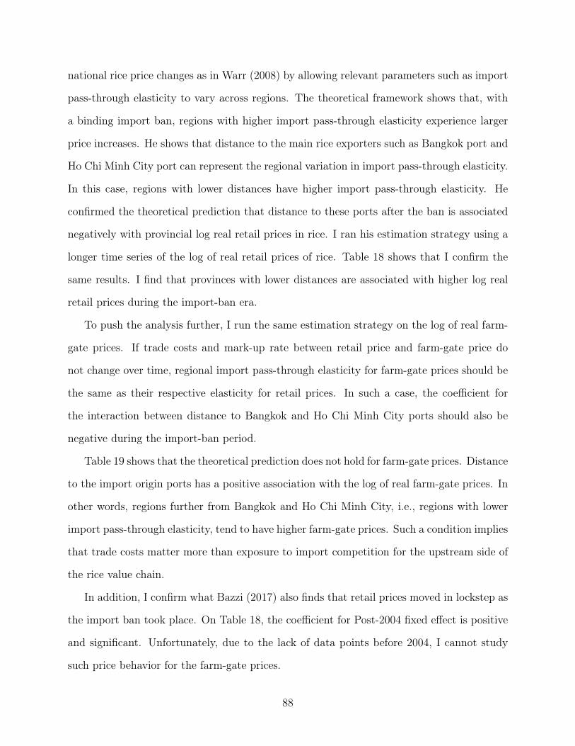
national rice price changes as in Warr (2008) by allowing relevant parameters such as import

pass-through elasticity to vary across regions. The theoretical framework shows that, with

a binding import ban, regions with higher import pass-through elasticity experience larger

price increases. He shows that distance to the main rice exporters such as Bangkok port and

Ho Chi Minh City port can represent the regional variation in import pass-through elasticity.

In this case, regions with lower distances have higher import pass-through elasticity. He

confirmed the theoretical prediction that distance to these ports after the ban is associated

negatively with provincial log real retail prices in rice. I ran his estimation strategy using a

longer time series of the log of real retail prices of rice. Table 18 shows that I confirm the

same results. I find that provinces with lower distances are associated with higher log real

retail prices during the import-ban era.

To push the analysis further, I run the same estimation strategy on the log of real farm-

gate prices. If trade costs and mark-up rate between retail price and farm-gate price do

not change over time, regional import pass-through elasticity for farm-gate prices should be

the same as their respective elasticity for retail prices. In such a case, the coefficient for

the interaction between distance to Bangkok and Ho Chi Minh City ports should also be

negative during the import-ban period.

Table 19 shows that the theoretical prediction does not hold for farm-gate prices. Distance

to the import origin ports has a positive association with the log of real farm-gate prices. In

other words, regions further from Bangkok and Ho Chi Minh City, i.e., regions with lower

import pass-through elasticity, tend to have higher farm-gate prices. Such a condition implies

that trade costs matter more than exposure to import competition for the upstream side of

the rice value chain.

In addition, I confirm what Bazzi (2017) also finds that retail prices moved in lockstep as

the import ban took place. On Table 18, the coefficient for Post-2004 fixed effect is positive

and significant. Unfortunately, due to the lack of data points before 2004, I cannot study

such price behavior for the farm-gate prices.

88

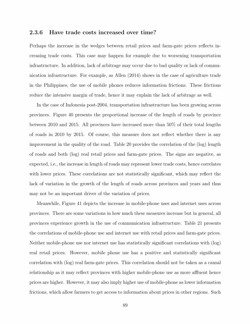
2.3.6 Have trade costs increased over time?

Perhaps the increase in the wedges between retail prices and farm-gate prices reflects in-

creasing trade costs. This case may happen for example due to worsening transportation

infrastructure. In addition, lack of arbitrage may occur due to bad quality or lack of commu-

nication infrastructure. For example, as Allen (2014) shows in the case of agriculture trade

in the Philippines, the use of mobile phones reduces information frictions. These frictions

reduce the intensive margin of trade, hence it may explain the lack of arbitrage as well.

In the case of Indonesia post-2004, transportation infrastructure has been growing across

provinces. Figure 40 presents the proportional increase of the length of roads by province

between 2010 and 2015. All provinces have increased more than 50% of their total lengths

of roads in 2010 by 2015. Of course, this measure does not reflect whether there is any

improvement in the quality of the road. Table 20 provides the correlation of the (log) length

of roads and both (log) real retail prices and farm-gate prices. The signs are negative, as

expected, i.e., the increase in length of roads may represent lower trade costs, hence correlates

with lower prices. These correlations are not statistically significant, which may reflect the

lack of variation in the growth of the length of roads across provinces and years and thus

may not be an important driver of the variation of prices.

Meanwhile, Figure 41 depicts the increase in mobile-phone uses and internet uses across

provinces. There are some variations in how much these measures increase but in general, all

provinces experience growth in the use of communication infrastructure. Table 21 presents

the correlations of mobile-phone use and internet use with retail prices and farm-gate prices.

Neither mobile-phone use nor internet use has statistically significant correlations with (log)

real retail prices. However, mobile phone use has a positive and statistically significant

correlation with (log) real farm-gate prices. This correlation should not be taken as a causal

relationship as it may reflect provinces with higher mobile-phone use as more affluent hence

prices are higher. However, it may also imply higher use of mobile-phone as lower information

frictions, which allow farmers to get access to information about prices in other regions. Such

89

information may empower farmers to get more competitive farm-gate prices.

In general, we see the growth of both transportation and communication infrastructure.

There is some indication that information frictions may have a role in the upstream of the

rice value chain. However, it seems it is hard to find evidence on increasing trade costs as a

driver of the lack of arbitrage across rice markets.

2.4 Discussion

Assuming that there is a complete pass-through of retail prices to farm-gate prices, I show

that the import-ban on rice did not increase the purchasing power of the main rice-producing

districts. I then continue the analysis with exploration on what drives the price divergence

during the import-ban era to shed light on whether the assumption of the complete pass-

through between retail prices to farm-gate prices is supported by data. Here, I discuss four

points that we can draw from exploring the price divergence.

First, there is persistence in the relative rankings of retail prices and farm-gate prices. In

other words, information on where prices are high can be learned easily as the rankings do not

vary much during the trade protection regime. In particular, provinces with high potential

yield in producing rice are the ones with lower relative rankings. Since the import ban takes

its effect, this pattern persists even stronger. This persistence in the relative rankings stands

in contrast with the case of substantial information frictions in the intra-national trade of

agriculture commodities in the Philippines as shown by Allen (2014). In that case, since

relative rankings do not persist over time, farmers and traders face substantial search costs

to find where to sell or from where to buy at any given time. In the case of rice in Indonesia,

since we see relative rankings of price do not change much over time, we can expect that

search costs to be less substantial compared to the case of the Philippines.

Second, time-invariant and location-specific attributes have large contributions to the

variation in both retail prices and farm-gate prices. In addition, time-variant local produc-

90

tivity driven by weather only accounts for small variations in prices. Hence, local production

does not vary much by weather conditions. Together with the first point above, this fact

emphasizes that there are substantial incentives to do arbitrage across regions.

Third, as shown by Bazzi (2017), retail prices increase more in provinces with a higher

elasticity of import pass-through. However, I do not find such regularity in the farm-gate

prices. The combination of the negative association of distance to ports with retail prices

with the positive association of distance to ports with a farm-gate price may be one of

the drivers of increasing and spatially diverging variation in the wedges between relative

prices and farm-gate prices. In addition, such conditions may contribute to incomplete pass-

through of increases in the retail prices to farm-gate prices as we observe from the trend of

retail and farm-gate prices by province. Any increase in retail prices is not followed by a

proportional increase in farm-gate prices during the import-ban period.

As illustrated by the rice value chain in Figure 33, there are many intermediaries between

rice farmers and consumers. They include transportation services providers, warehouse own-

ers, millers, wholesalers, to retailers. They may also benefit from trade protection. In the

world of perfect competition, any additional intermediaries add the wedge between upstream

and downstream prices. However, literature shows that if the industry is characterized by

imperfect competition, it is not as straightforward, who gains a bigger percentage of the

rents without knowing the market power of each component in the value chain. For exam-

ple, McMillan et al. (2002) show that farmers did not enjoy much of the increase in prices

as they start to export because the middlemen did not pass through the price increase.

Meanwhile, the ease of collusion between traders may matter too. Bergquist and Dinerstein

(2020) show that experimentally adding new traders does not reduce retail prices as traders

jointly maximize profits.

Fourth, Indonesia has been growing in terms of both transportation and communication

infrastructure. It is less likely that trade costs in the form of transportation costs or commu-

nication costs to worsen during the period of the import ban. However, there is potential in

91

how the variation in the improvement and use of transportation, as well as communication

infrastructure, affects the lack of arbitrage across rice markets. These factors should be

taken into consideration in explaining the cause of the price divergence. In addition, since

we observe a positive correlation between mobile-phone use and farm-gate prices, there is an

indication that information frictions and the role of information in increasing outside options

for farmers have a more substantial role in the upstream side of the rice value chain.

In addition to the four points above, the spatial price divergence may also be policy-

driven. In 2005, the government started to regulate the rice price stabilization mechanism

by allowing local governments to propose provisions of stabilization measures in the face of

regional price hikes. Once such a proposal is approved by the central government, Bulog

performs the stabilization program of open market operations in the concerned region. The

general procedure remained in place until 2018.43 Since price hikes are reported from a local

government to the central government, there may be silos in observing provincial rice prices

and thus less attention to the price variation across regions.

Another policy-related aspect that is still missing in this exploration is the role of the

state-owned logistic agency: Bulog. Bulog is given the authority to deliver the government’s

floor price regulation for farm-gate prices. As mentioned above, Bulog also conducts open

market operations to tame any price hikes in the retail markets. Future evaluation on trade

policy evaluation should take into account the variation in Bulog’s intervention across regions

and time.

For the purpose of future studies and evaluation of the trade policy, I would like to

propose several data that researchers and policymakers should collect and analyze. First,

more granular data on grain prices and value-added creation along the rice value chain can

better capture the sources of the variation of wedges between retail and farm-gate prices

across markets. For example, the Central Statistic Agency (BPS) does not survey the prices

43Rice price stabilization with local government alert mechanism is regulated by Minister of Trade Reg-ulation No. 22/2005 and then Minister of Trade Regulation No. 1/2012. The mechanism changed in 2018under Minister of Trade Regulation No. 127/2018.

92

of grained ready to be milled at mills. Rather, they estimate the transportation costs from

farmers to mills and add the costs to the price of harvested paddy to get the grain prices

at mills. Atkin and Khandelwal (2020) suggests that future studies on the impact of trade

frictions that focus on a specific industry can contribute high value to the literature. Such

studies can provide a deeper understanding of the anatomy of costs, production functions,

and markups. Policymakers with an interest to improve the effectiveness and efficiency of

the trade protection should prioritize collecting and providing such data for analysis. As we

explore here, retail prices and farm-gate prices have not moved in parallel during the trade

protection regime. Thus, if the trade protection aims to support or incentivize farmers, then

regional farm-gate prices and grain prices along the rice value chain are the statistics that

provide better information on whether the goal is achieved or not.

Second, performing pass-through tests on prices between trading provinces would be

another first-order attempt to understand the price divergence. Unfortunately, I cannot

perform such tests as intra-national trade data is not yet available. Hence, future research

on this topic as well as effort in evaluating the trade policy rigorously will benefit from the

availability of such trade data. Using intra-national rice trade data we can also study whether

there is any strategic behavior performed by traders. The theoretical framework employed by

Bazzi (2017) assumes that traders and farmers do not engage in any strategic behavior. If the

assumption does not hold, traders facing downward-sloping demand for rice would set retail

prices above their competitive level. Meanwhile, traders facing an upward-sloping supply of

rice would set farm-gate prices below their competitive level. The two forces may widen the

wedge of the retail price and farm-gate price in the form of an increase in markup. This case

can explain simultaneously the spatial price divergence and the incomplete pass-through of

retail price to farm-gate price.

93

2.5 Conclusion

Indonesia imposes a large and ongoing import ban on rice, a staple food for its 260 million

population. This binding import restriction, which started in 2004 and was followed by an

export ban since the Food Crisis 2008, has spurred not only a general increase in the retail

prices of rice across regions in Indonesia but also price divergence on two dimensions. First,

there is an increase in the variation of retail prices across regions. Second, there are widening

wedges between retail prices and farm-gate prices.

The trade protection to rice farmers is expected to provide earning supports and incen-

tivize domestic rice production. However, I find that rice-producing districts do not enjoy

higher purchasing power compared to other districts. I also find no evidence of the growth

of the rice sector, either in the form of extensification or intensification. This paper aims to

shed light on the potential reason for this result by exploring trends and potential factors

that affect retail and farm-gate prices. To the best of my knowledge, this paper is the first

in studying regional variation and trends in farm-gate prices, including how they differ with

the variation and trend of retail prices of rice during this import-ban era in Indonesia.

I draw four facts from the exploration of the price divergence. First, the relative ranking

in prices persists during the import ban. Second, relative ranking in prices is inversely

related to crop suitability, in which provinces with high relative ranking in prices have a

lower potential yield in growing rice. Third, retail prices and farm-gate prices have different

behavior in relation to the lack of import competition during the import ban. Retail prices

increase more in provinces with higher import pass-through elasticity, but not for farm-

gate prices. Fourth, there is no indication of worsening transportation and communication

infrastructure that may increase trade costs. Yet, information frictions may matter more on

the upstream side of the rice value chain.

In light of these four facts, I propose two main potential features that need to be taken

into account. First, there seems to be less role of search costs in the retail market in the

94

face of strong incentives to arbitrage. In addition, information frictions may matter more

to farmers. It is worth exploring the mechanism on how information friction affects farm-

gate price determination, for example through better outside options, or increase in market

power, or direct arbitrage. Second, since trade costs and search costs may not be the main

key determinants in the lack of arbitrage, researchers should consider analyzing whether

there is any strategic behavior present in the trading of rice as well as imperfect competition

and increasing trade frictions along the rice value chain. Such strategic behavior may emerge

especially due to the lack of import competition. In such a case, both the incomplete pass-

through of the retail price to farm-gate price and lack of arbitrage can be the expected

outcomes.

Understanding the incomplete pass-through of retail prices to farm-gate prices and the

lack of arbitrage is important in any effort to evaluate the import ban. Given the insignifi-

cance of the impact of the import ban in providing higher purchasing power nor in expanding

the rice sector, a rigorous study of the policy is necessary to avoid further misallocation that

may occur due to the trade protection. To perform the policy evaluation, I propose the

prioritization of collecting regional farm-gate prices and prices of grains along the rice value

chain and intra-national rice trade data.

95

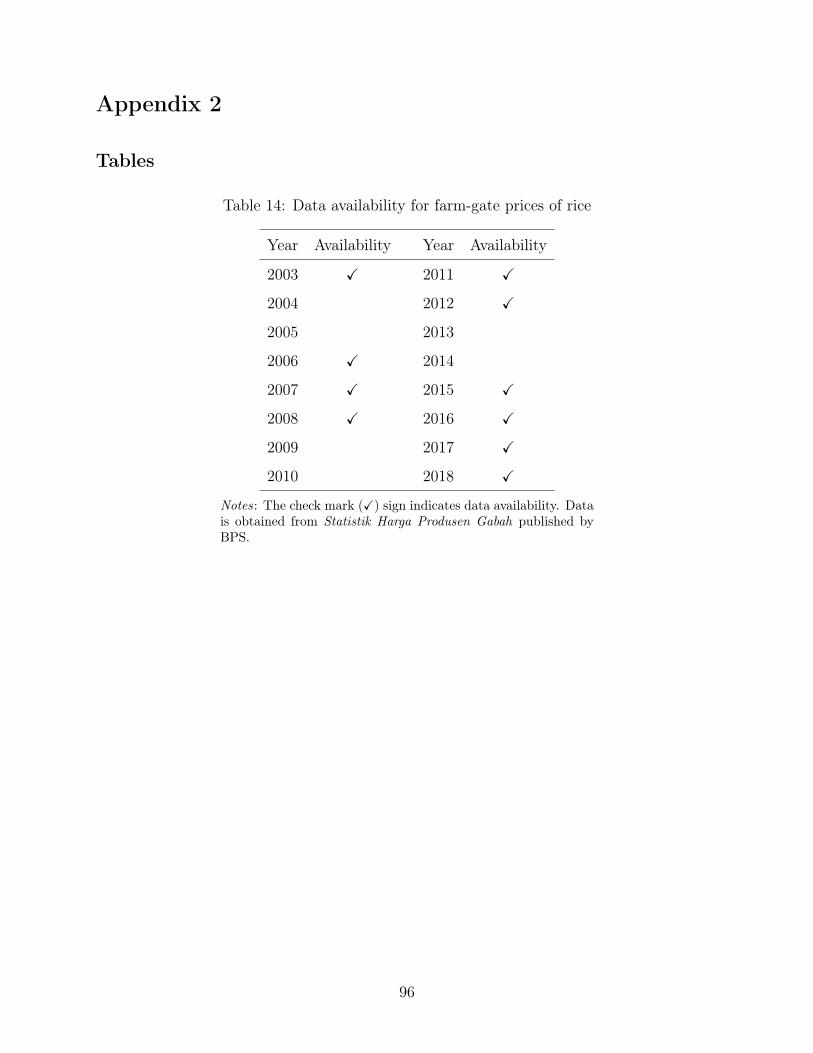
Appendix 2

Tables

Table 14: Data availability for farm-gate prices of rice

Year Availability Year Availability

2003 X 2011 X

2004 2012 X

2005 2013

2006 X 2014

2007 X 2015 X

2008 X 2016 X

2009 2017 X

2010 2018 X

Notes: The check mark (X) sign indicates data availability. Datais obtained from Statistik Harga Produsen Gabah published byBPS.

96

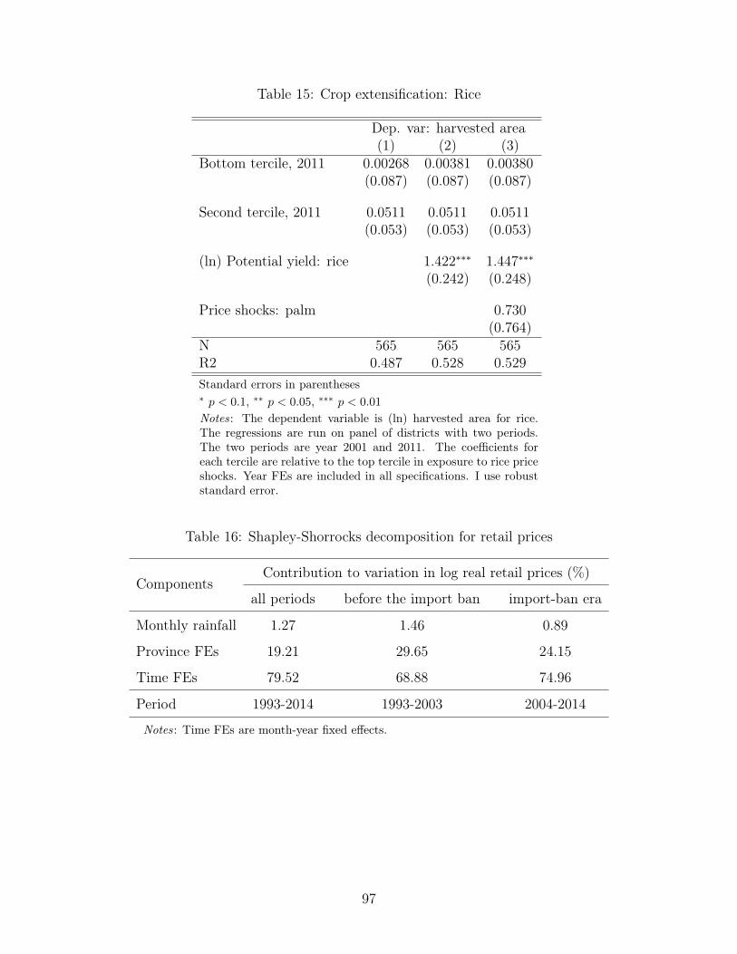
Table 15: Crop extensification: Rice

Dep. var: harvested area(1) (2) (3)

Bottom tercile, 2011 0.00268 0.00381 0.00380(0.087) (0.087) (0.087)

Second tercile, 2011 0.0511 0.0511 0.0511(0.053) (0.053) (0.053)

(ln) Potential yield: rice 1.422∗∗∗ 1.447∗∗∗(0.242) (0.248)

Price shocks: palm 0.730(0.764)

N 565 565 565R2 0.487 0.528 0.529Standard errors in parentheses∗ p < 0.1, ∗∗ p < 0.05, ∗∗∗ p < 0.01

Notes: The dependent variable is (ln) harvested area for rice.The regressions are run on panel of districts with two periods.The two periods are year 2001 and 2011. The coefficients foreach tercile are relative to the top tercile in exposure to rice priceshocks. Year FEs are included in all specifications. I use robuststandard error.

Table 16: Shapley-Shorrocks decomposition for retail prices

ComponentsContribution to variation in log real retail prices (%)

all periods before the import ban import-ban era

Monthly rainfall 1.27 1.46 0.89

Province FEs 19.21 29.65 24.15

Time FEs 79.52 68.88 74.96

Period 1993-2014 1993-2003 2004-2014

Notes: Time FEs are month-year fixed effects.

97

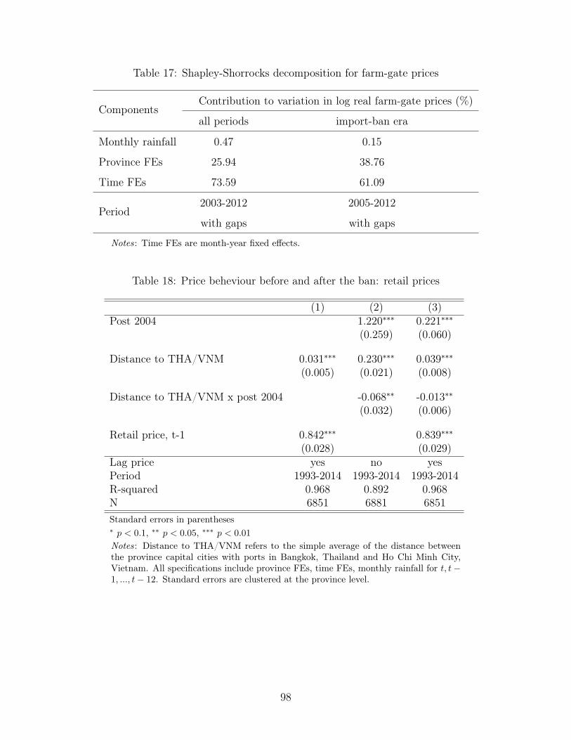
Table 17: Shapley-Shorrocks decomposition for farm-gate prices

ComponentsContribution to variation in log real farm-gate prices (%)

all periods import-ban era

Monthly rainfall 0.47 0.15

Province FEs 25.94 38.76

Time FEs 73.59 61.09

Period2003-2012 2005-2012

with gaps with gaps

Notes: Time FEs are month-year fixed effects.

Table 18: Price beheviour before and after the ban: retail prices

(1) (2) (3)Post 2004 1.220∗∗∗ 0.221∗∗∗

(0.259) (0.060)

Distance to THA/VNM 0.031∗∗∗ 0.230∗∗∗ 0.039∗∗∗(0.005) (0.021) (0.008)

Distance to THA/VNM x post 2004 -0.068∗∗ -0.013∗∗(0.032) (0.006)

Retail price, t-1 0.842∗∗∗ 0.839∗∗∗(0.028) (0.029)

Lag price yes no yesPeriod 1993-2014 1993-2014 1993-2014R-squared 0.968 0.892 0.968N 6851 6881 6851Standard errors in parentheses∗ p < 0.1, ∗∗ p < 0.05, ∗∗∗ p < 0.01

Notes: Distance to THA/VNM refers to the simple average of the distance betweenthe province capital cities with ports in Bangkok, Thailand and Ho Chi Minh City,Vietnam. All specifications include province FEs, time FEs, monthly rainfall for t, t−1, ..., t− 12. Standard errors are clustered at the province level.

98

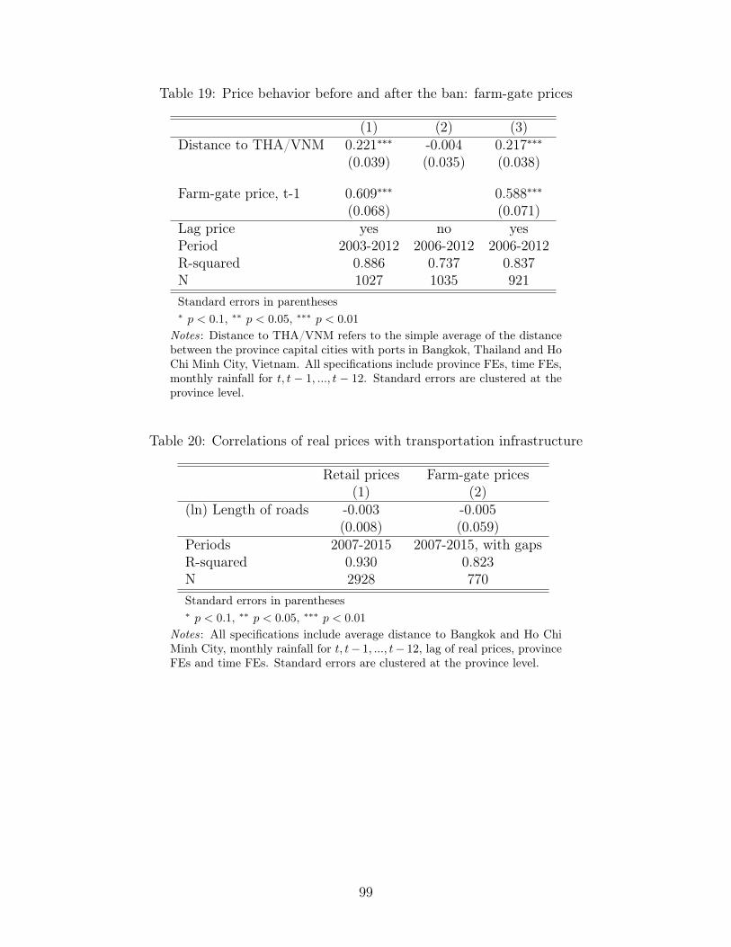
Table 19: Price behavior before and after the ban: farm-gate prices

(1) (2) (3)Distance to THA/VNM 0.221∗∗∗ -0.004 0.217∗∗∗

(0.039) (0.035) (0.038)

Farm-gate price, t-1 0.609∗∗∗ 0.588∗∗∗(0.068) (0.071)

Lag price yes no yesPeriod 2003-2012 2006-2012 2006-2012R-squared 0.886 0.737 0.837N 1027 1035 921Standard errors in parentheses∗ p < 0.1, ∗∗ p < 0.05, ∗∗∗ p < 0.01

Notes: Distance to THA/VNM refers to the simple average of the distancebetween the province capital cities with ports in Bangkok, Thailand and HoChi Minh City, Vietnam. All specifications include province FEs, time FEs,monthly rainfall for t, t − 1, ..., t − 12. Standard errors are clustered at theprovince level.

Table 20: Correlations of real prices with transportation infrastructure

Retail prices Farm-gate prices(1) (2)

(ln) Length of roads -0.003 -0.005(0.008) (0.059)

Periods 2007-2015 2007-2015, with gapsR-squared 0.930 0.823N 2928 770Standard errors in parentheses∗ p < 0.1, ∗∗ p < 0.05, ∗∗∗ p < 0.01

Notes: All specifications include average distance to Bangkok and Ho ChiMinh City, monthly rainfall for t, t− 1, ..., t− 12, lag of real prices, provinceFEs and time FEs. Standard errors are clustered at the province level.

99

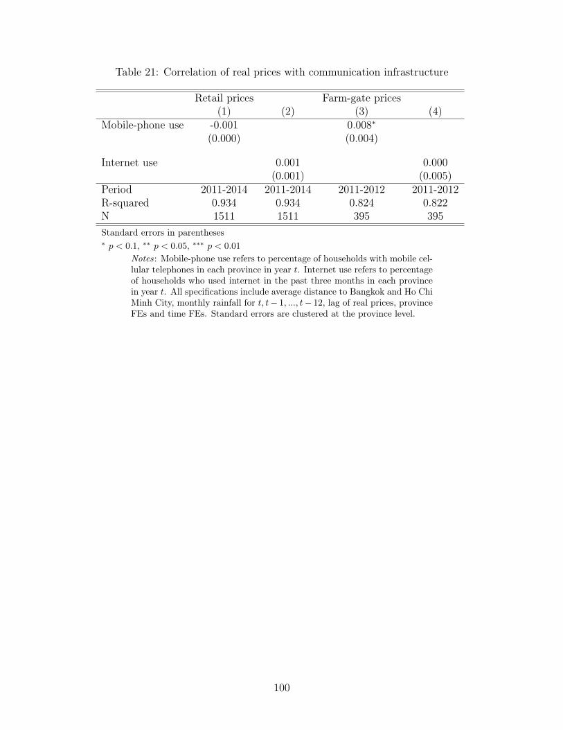
Table 21: Correlation of real prices with communication infrastructure

Retail prices Farm-gate prices(1) (2) (3) (4)

Mobile-phone use -0.001 0.008∗(0.000) (0.004)

Internet use 0.001 0.000(0.001) (0.005)

Period 2011-2014 2011-2014 2011-2012 2011-2012R-squared 0.934 0.934 0.824 0.822N 1511 1511 395 395Standard errors in parentheses∗ p < 0.1, ∗∗ p < 0.05, ∗∗∗ p < 0.01

Notes: Mobile-phone use refers to percentage of households with mobile cel-lular telephones in each province in year t. Internet use refers to percentageof households who used internet in the past three months in each provincein year t. All specifications include average distance to Bangkok and Ho ChiMinh City, monthly rainfall for t, t− 1, ..., t− 12, lag of real prices, provinceFEs and time FEs. Standard errors are clustered at the province level.

100

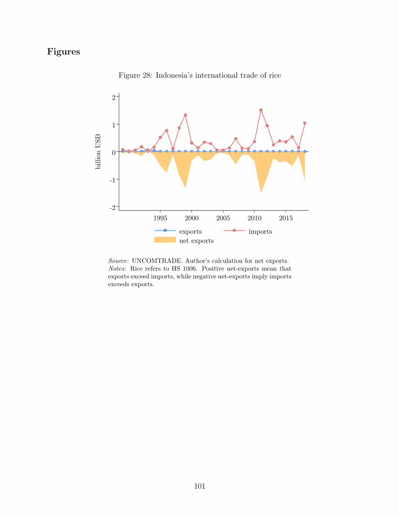
Figures

Figure 28: Indonesia’s international trade of rice

-2

-1

0

1

2bi

llion

USD

1995 2000 2005 2010 2015

exports importsnet exports

Source: UNCOMTRADE. Author’s calculation for net exports.Notes: Rice refers to HS 1006. Positive net-exports mean thatexports exceed imports, while negative net-exports imply importsexceeds exports.

101

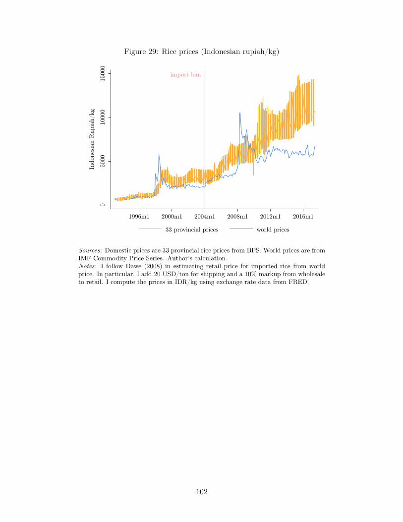
Figure 29: Rice prices (Indonesian rupiah/kg)

import ban

050

0010

000

1500

0

Indo

nesi

an R

upia

h/kg

1996m1 2000m1 2004m1 2008m1 2012m1 2016m1

33 provincial prices world prices

Sources: Domestic prices are 33 provincial rice prices from BPS. World prices are fromIMF Commodity Price Series. Author’s calculation.Notes: I follow Dawe (2008) in estimating retail price for imported rice from worldprice. In particular, I add 20 USD/ton for shipping and a 10% markup from wholesaleto retail. I compute the prices in IDR/kg using exchange rate data from FRED.

102

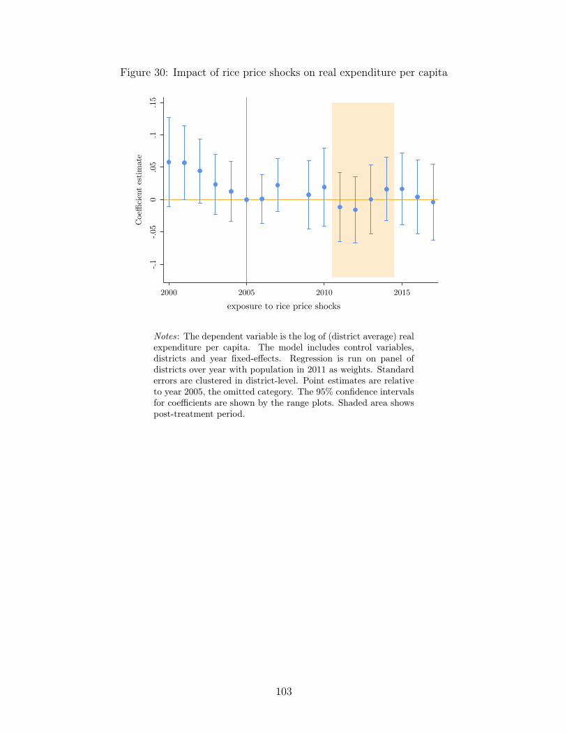
Figure 30: Impact of rice price shocks on real expenditure per capita

-.1-.0

50

.05

.1.1

5

Coeffi

cien

t es

tim

ate

2000 2005 2010 2015

exposure to rice price shocks

Notes: The dependent variable is the log of (district average) realexpenditure per capita. The model includes control variables,districts and year fixed-effects. Regression is run on panel ofdistricts over year with population in 2011 as weights. Standarderrors are clustered in district-level. Point estimates are relativeto year 2005, the omitted category. The 95% confidence intervalsfor coefficients are shown by the range plots. Shaded area showspost-treatment period.

103

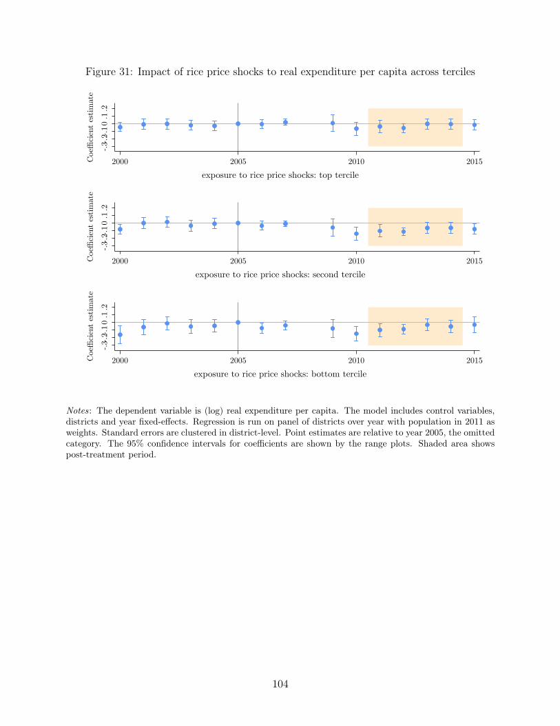
Figure 31: Impact of rice price shocks to real expenditure per capita across terciles

-.3-.2

-.10

.1.2

Coeffi

cien

t es

tim

ate

2000 2005 2010 2015

exposure to rice price shocks: top tercile

-.3-.2

-.10

.1.2

Coeffi

cien

t es

tim

ate

2000 2005 2010 2015

exposure to rice price shocks: second tercile

-.3-.2

-.10

.1.2

Coeffi

cien

t es

tim

ate

2000 2005 2010 2015

exposure to rice price shocks: bottom tercile

Notes: The dependent variable is (log) real expenditure per capita. The model includes control variables,districts and year fixed-effects. Regression is run on panel of districts over year with population in 2011 asweights. Standard errors are clustered in district-level. Point estimates are relative to year 2005, the omittedcategory. The 95% confidence intervals for coefficients are shown by the range plots. Shaded area showspost-treatment period.

104

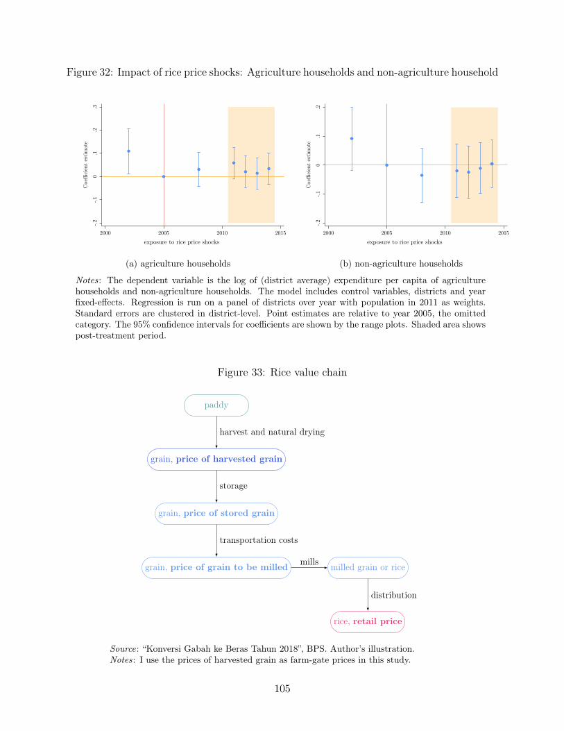
Figure 32: Impact of rice price shocks: Agriculture households and non-agriculture household

-.2-.1

0.1

.2.3

Coeffi

cien

t es

tim

ate

2000 2005 2010 2015

exposure to rice price shocks

(a) agriculture households

-.2-.1

0.1

.2

Coeffi

cien

t es

tim

ate

2000 2005 2010 2015

exposure to rice price shocks

(b) non-agriculture households

Notes: The dependent variable is the log of (district average) expenditure per capita of agriculturehouseholds and non-agriculture households. The model includes control variables, districts and yearfixed-effects. Regression is run on a panel of districts over year with population in 2011 as weights.Standard errors are clustered in district-level. Point estimates are relative to year 2005, the omittedcategory. The 95% confidence intervals for coefficients are shown by the range plots. Shaded area showspost-treatment period.

Figure 33: Rice value chain

paddy

grain, price of harvested grain

grain, price of stored grain

grain, price of grain to be milled milled grain or rice

rice, retail price

harvest and natural drying

storage

transportation costs

mills

distribution

Source: “Konversi Gabah ke Beras Tahun 2018”, BPS. Author’s illustration.Notes: I use the prices of harvested grain as farm-gate prices in this study.

105

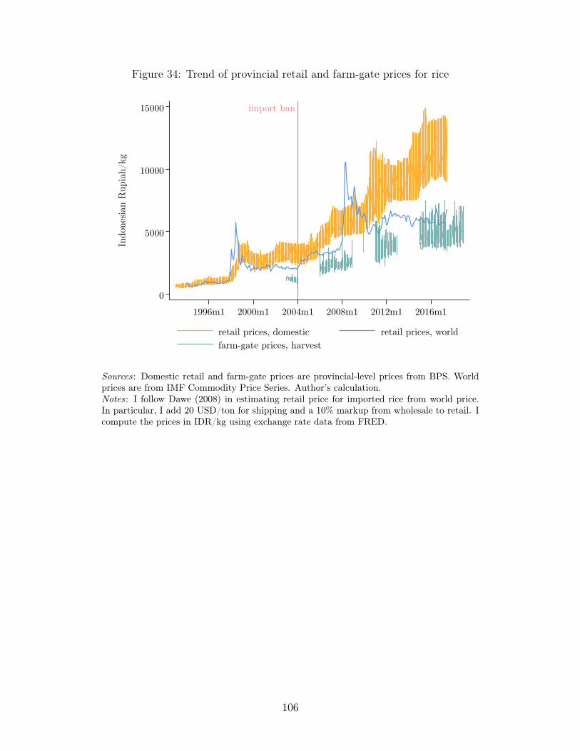
Figure 34: Trend of provincial retail and farm-gate prices for rice

import ban

0

5000

10000

15000In

done

sian

Rup

iah/

kg

1996m1 2000m1 2004m1 2008m1 2012m1 2016m1

retail prices, domestic retail prices, worldfarm-gate prices, harvest

Sources: Domestic retail and farm-gate prices are provincial-level prices from BPS. Worldprices are from IMF Commodity Price Series. Author’s calculation.Notes: I follow Dawe (2008) in estimating retail price for imported rice from world price.In particular, I add 20 USD/ton for shipping and a 10% markup from wholesale to retail. Icompute the prices in IDR/kg using exchange rate data from FRED.

106

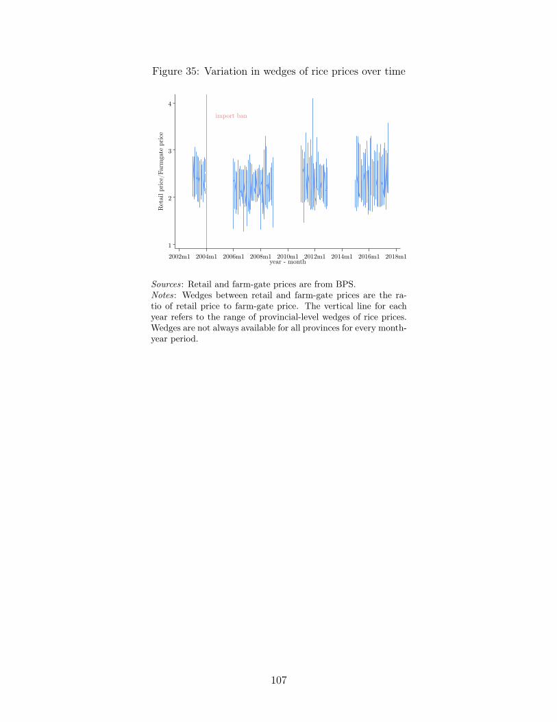
Figure 35: Variation in wedges of rice prices over time

import ban

1

2

3

4

Ret

ail p

rice

/Far

mga

te p

rice

2002m1 2004m1 2006m1 2008m1 2010m1 2012m1 2014m1 2016m1 2018m1year - month

Sources: Retail and farm-gate prices are from BPS.Notes: Wedges between retail and farm-gate prices are the ra-tio of retail price to farm-gate price. The vertical line for eachyear refers to the range of provincial-level wedges of rice prices.Wedges are not always available for all provinces for every month-year period.

107

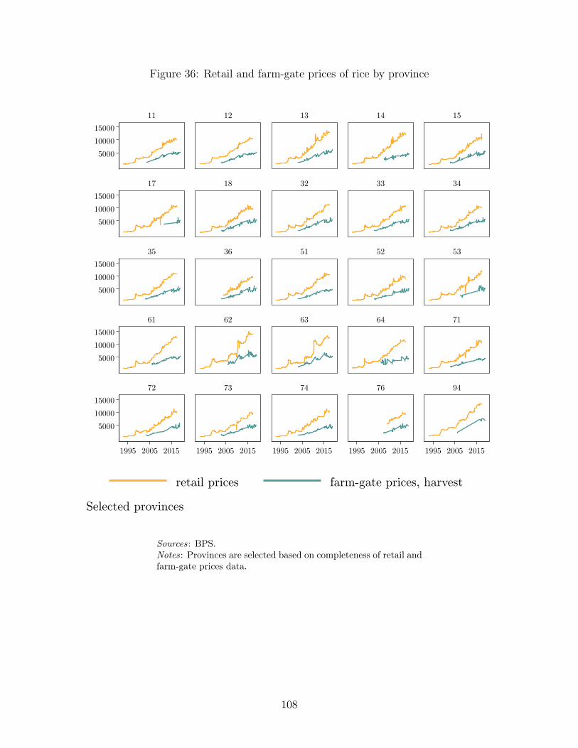
Figure 36: Retail and farm-gate prices of rice by province

50001000015000

50001000015000

50001000015000

50001000015000

50001000015000

1995 2005 2015 1995 2005 2015 1995 2005 2015 1995 2005 2015 1995 2005 2015

11 12 13 14 15

17 18 32 33 34

35 36 51 52 53

61 62 63 64 71

72 73 74 76 94

retail prices farm-gate prices, harvest

Selected provinces

Sources: BPS.Notes: Provinces are selected based on completeness of retail andfarm-gate prices data.

108

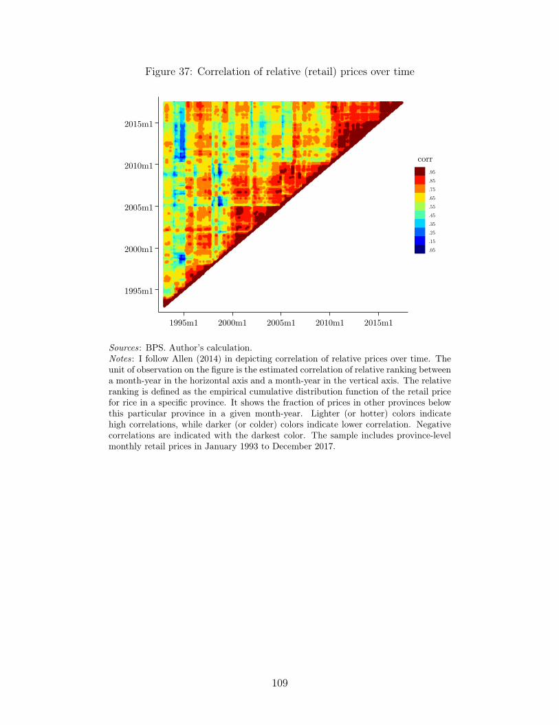
Figure 37: Correlation of relative (retail) prices over time

1995m1

2000m1

2005m1

2010m1

2015m1

1995m1 2000m1 2005m1 2010m1 2015m1

.95

.85

.75

.65

.55

.45

.35

.25

.15

.05

corr

Sources: BPS. Author’s calculation.Notes: I follow Allen (2014) in depicting correlation of relative prices over time. Theunit of observation on the figure is the estimated correlation of relative ranking betweena month-year in the horizontal axis and a month-year in the vertical axis. The relativeranking is defined as the empirical cumulative distribution function of the retail pricefor rice in a specific province. It shows the fraction of prices in other provinces belowthis particular province in a given month-year. Lighter (or hotter) colors indicatehigh correlations, while darker (or colder) colors indicate lower correlation. Negativecorrelations are indicated with the darkest color. The sample includes province-levelmonthly retail prices in January 1993 to December 2017.

109

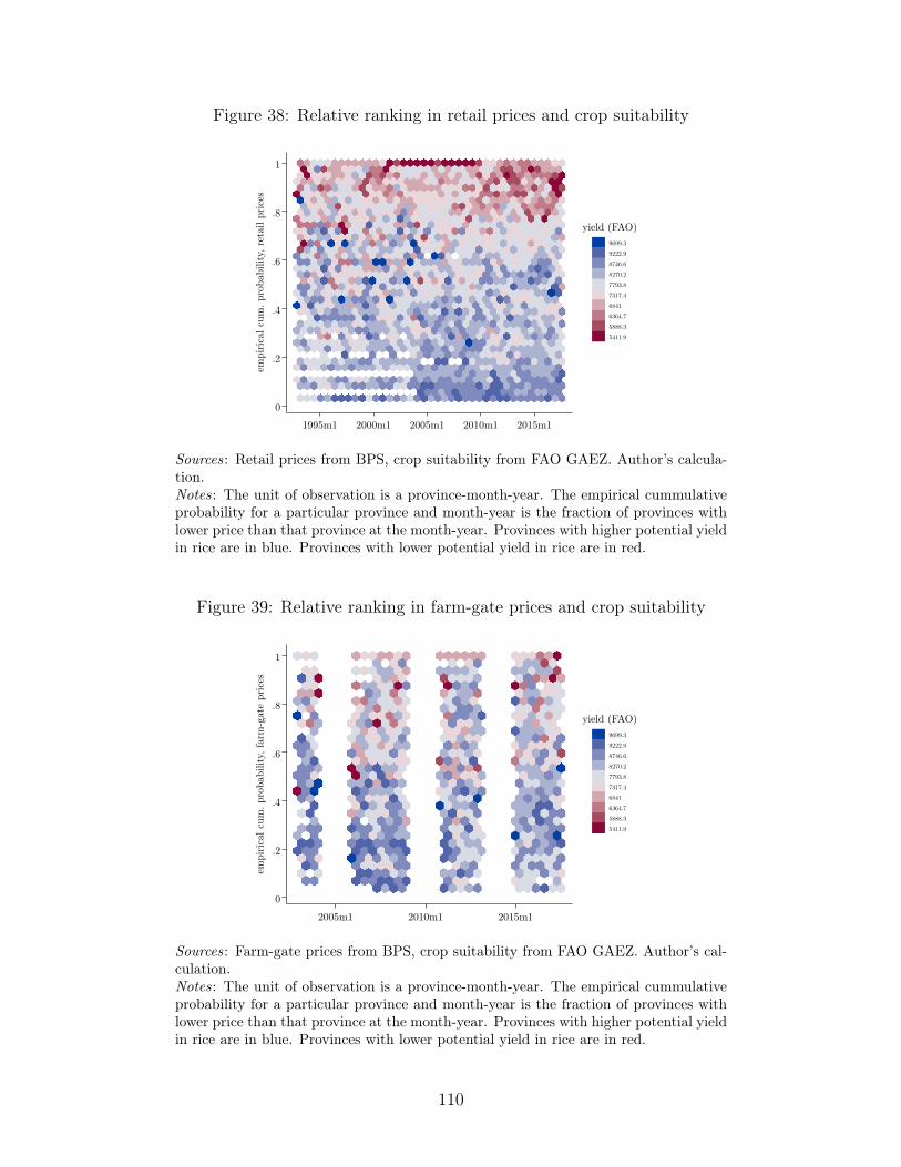
Figure 38: Relative ranking in retail prices and crop suitability

0

.2

.4

.6

.8

1

empi

rica

l cum

. pro

babi

lity,

ret

ail p

rice

s

1995m1 2000m1 2005m1 2010m1 2015m1

9699.3

9222.9

8746.6

8270.2

7793.8

7317.4

6841

6364.7

5888.3

5411.9

yield (FAO)

Sources: Retail prices from BPS, crop suitability from FAO GAEZ. Author’s calcula-tion.Notes: The unit of observation is a province-month-year. The empirical cummulativeprobability for a particular province and month-year is the fraction of provinces withlower price than that province at the month-year. Provinces with higher potential yieldin rice are in blue. Provinces with lower potential yield in rice are in red.

Figure 39: Relative ranking in farm-gate prices and crop suitability

0

.2

.4

.6

.8

1

empi

rica

l cum

. pro

babi

lity,

farm

-gat

e pr

ices

2005m1 2010m1 2015m1

9699.3

9222.9

8746.6

8270.2

7793.8

7317.4

6841

6364.7

5888.3

5411.9

yield (FAO)

Sources: Farm-gate prices from BPS, crop suitability from FAO GAEZ. Author’s cal-culation.Notes: The unit of observation is a province-month-year. The empirical cummulativeprobability for a particular province and month-year is the fraction of provinces withlower price than that province at the month-year. Provinces with higher potential yieldin rice are in blue. Provinces with lower potential yield in rice are in red.

110

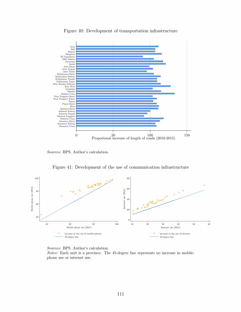
Figure 40: Development of transportation infrastructure

0 50 100 150Propotional increase of length of roads (2010-2015)

Sumatera UtaraSumatera Selatan

Sumatera BaratSulawesi Utara

Sulawesi TenggaraSulawesi TengahSulawesi Selatan

Sulawesi BaratRiau

Papua BaratPapua

Nusa Tenggara TimurNusa Tenggara Barat

Maluku UtaraMaluku

LampungKep. Riau

Kep. Bangka BelitungKalimantan Timur

Kalimantan TengahKalimantan Selatan

Kalimantan BaratJawa Timur

Jawa TengahJawa Barat

JambiGorontalo

DKI JakartaDI Yogyakarta

BengkuluBanten

BaliAceh

Sources: BPS. Author’s calculation.

Figure 41: Development of the use of communication infrastructure

40

60

80

100

Mob

ile p

hone

use

(20

14)

40 60 80 100Mobile phone use (2011)

increase in the use of mobile phones45-degree line

0

20

40

60

80

Inte

rnee

t us

e (2

014)

10 20 30 40 50 60Internet use (2011)

increase in the use of internet45-degree line

Sources: BPS. Author’s calculation.Notes: Each unit is a province. The 45-degree line represents no increase in mobile-phone use or internet use.

111

Chapter 3

New-consumer margin at work:

Exposure to television ads as driver of

smoking prevalence

3.1 Introduction

Tobacco is not just a threat to health, it is also a threat to sustainable human

development. (The Lancet, 2015)

Killing more than 8 million people every year, the World Health Organization states that

the tobacco epidemic is one of the biggest public health threats that the world ever faced

(WHO, 2020). Despite a general decline in the global smoking prevalence, the epicentrum of

the epidemic now occurs in developing countries, many of which experience rising smoking

prevalence. In fact, low- and middle-income countries account for more than 80% of 1.3

billion world’s tobacco consumers.44 Tobacco consumption is not only costly due to the

burden of diseases but also due to the impact of reverting expenditure from more productive

uses. Given the rising rate of smoking in developing countries and the cost it bears, it is

important to understand what determines the new generations of smokers.

This paper investigates how an improvement in marketing technology used to adver-

tise tobacco products affects smoking pevalence. In particular, this paper finds that higher

relative local exposure of televisions (TV), which proliferates the broadcasts of tobacco ad-

vertisements, increases smoking participation of young adults. This research contributes to

the literature and inform policy makers as it is the first study with nationally-representative

44Ibid.

112

data that focuses on the impact of marketing to smoking participation in developing countries

setting, where smoking prevalence has been on the rise.

In order to answer the research question, I derive the theoretical prediction of the impact

of improvement in marketing technology to market shares based on the theory of market-

ing in international trade as in Arkolakis (2010). The model introduces a new margin in

gains from trade, the new-consumer margin, which represents additional consumers as trade,

including marketing costs, declines. I collect three empirical facts that may affect the new-

consumer margin in the context of the Indonesian economy in 1990 to 2010. First, there is

no substantial change in the tobacco industry’s average productivity. Second, as private TV

stations started to broadcast in 1993, there has been an improvement in marketing technol-

ogy as such TV stations advertised tobacco products. Third, real prices of cigarettes, the

most common tobacco products consumed in Indonesia, have been relatively stable during

the period of study. Hence, the Indonesian economy in this period is an excellent context in

which to study the impact of an increase in advertising exposure to smoking prevalence.

Then, I empirically test the theoretical prediction that improvement in marketing technol-

ogy generates more consumers. I focus on understanding the impact of marketing technology

on young adults aged 17 to 23 years old, as preferences, including smoking habits, are formed

during this life phase (Chaloupka et al., 1997). I exploit the spatial and time variation of

relative local TV exposure in 2000 and 2007. Using this measure of TV exposure, I perform

a difference-in-difference method to study the evidence of new-consumer margin by finding

the impact of TV exposure to smoking participation of young adults. In addition, I explore

whether smoking behavior has economic consequences. Since I use the Indonesian Family

Life Survey (IFLS) data, a longitudinal household survey, I can observe the respondents’ eco-

nomic outcomes seven or fourteen years after being young adults in 2000 or 2007. In order

to overcome the endogeneity issue, I instrument current smoking participation with smok-

ing participation during young adulthood to study the impact of smoking to two economic

outcomes: college-degree attainment and working status.

113

There are two main findings. First, I empirically confirm the theoretical prediction that

improvement in marketing technology creates new consumers. This paper finds the evidence

of the new-consumer margin, in which young male adults living in subdistricts with higher

relative TV exposure have a higher chance of smoking. Furthermore, heterogeneity across

age groups matters. The impact is significant for younger male adults, especially those of

17 to 19 years of age. An increase of local TV exposure by one standard deviation increases

smoking participation by 4%, 5%, and 6%, respectively, for young male adults of 17, 18, and

19 years old. The evidence on new-consumer margin is robust using a different measure of

TV exposure, controlling for changes in price of cigarettes, as well as if we include young

adults who are also household heads in the sample.

Second, I observe evidence of the long-run economic consequences of smoking. Using

the instrument variable approach, I find that male adults who smoke have less probability

of attaining a college degree. This result may reflect the role of tobacco consumption in

diverting away resources from investment in human capital such as education. Meanwhile,

young male adults in the year 2000 also have less chance of having a job in 2014 if they

smoke. However, I do not find a significant impact for young male adults in the year 2007.

Such result may reflect the mechanism that smoking is perceived well in the society, it may

facilitate casual or informal networks. However, I do not find any significant positive impact

of smoking in the chance of getting a job.

This paper contributes to several topics in globalization and development literature.

First, it contributes to the literature on the impact of introduction and proliferation of

electronic media, an inherent aspect of globalization, to human and social capital outcomes.

The paper fills in the gap by studying how exposure to advertising through TV increases

smoking participation within a developing-country context, where smoking prevalence is

rising. It is closest to the study on the impact of the introduction of TV to smoking prevalence

in the US by Thomas (2019). However, instead of comparing smoking prevalence before and

after the introduction of television, I compare the relative intensity of TV exposure, which is

114

a relevant context in today’s society. I also follow Olken (2009), who studies the proliferation

of private TV stations in Indonesia and finds that more time spent in consuming electronic

media is associated with less social capital outcomes, such as lower participation in social

organization and lower self-reported trust. Meanwhile, Kearney and Levine (2015) find that

media may have positive influence on social outcomes by showing that the “16 and Pregnant”

TV show reduced teen births as it increased interest in contraceptive use and abortion.

Second, this paper contributes to a wide and active literature on smoking behavior.

Chaloupka and Warner (1999) provided a comprehensive survey of literature on the eco-

nomics of smoking, while Wellman et al. (2006) surveyed recent tobacco-related studies in

the public health field. From the context of Indonesia, Setyonaluri et al. (2008) presented

comprehensive descriptions and a survey of literature. Many empirical works in this stream of

literature focuses in analyzing the impact or changes in prices and taxes as tobacco-control

policies.45 Hence, they focus more on smoking cessation and intensive margin of tobacco

consumption. I contribute to this literature by studying an important margin in smoking

prevalence, i.e., smoking participation among young adults, that stem from advertising expo-

sure. As Warner et al. (1992) emphasized, despite advertisement is not the sole determinant

that young adults start smoking, it is the most policy tractable. Hence, understanding

the impact of advertising contributes directly to providing evidence-based tobacco-control

policies.

Lastly, this paper also relates to the literature on the role of advertising in international

trade and firm dynamics. In particular, I find evidence of the new-consumer margin, as

introduced by Arkolakis (2010), for a particular industry within a market. Using smok-

ing participation as indication of new consumers, I show that improvement in marketing

technology enlarges the consumer base of tobacco products in Indonesia. Recent studies in

understanding how firms grow have emphasized the substantial roles of advertising. Using

detailed consumption data and TV advertising data, Argente et al. (2021), for example,45See for example Becker et al. (1994) and Cotti et al. (2016) using US data and Ross and Chaloupka’s

(2006) survey for developing countries.

115

showed that the growth of firms in market share within a market is driven more by adver-

tising, rather than markups. Meanwhile, Cavenaile and Roldan-Blanco (2021) incorporate

advertising decision into endogeneous growth with research and development (R&D) and

show that advertising and R&D are substitutes. Importantly, they find that bigger firms

rely more on advertising than on R&D.

The rest of the paper is structured as follows. In Section 2, I describe the recent devel-

opment in tobacco consumption, the tobacco industry, as well as tobacco-control policies in

the world and in Indonesia. In Section 3, I lay out the basics of the marketing theory in

international trade based on Arkolakis (2010), and derive the theoretical predictions of the

impact of improvement in marketing technology to market shares. Based on the theoretical

framework, I document the trend of three factors that may affect the number of tobacco

consumers in Indonesia. Then, I empirically test the theoretical prediction of the existence

of the new-consumer margin. I explain the data as well as the empirical strategy in Section

4. In Section 5, I present and discuss the evidence of the new-consumer margin as well as

explore the long-run economic impacts of smoking. In Section 6, I provide the conclusions

of the paper and propose some implications from the findings.

3.2 The economics of smoking

In this section, I provide some background in terms of tobacco consumption, the tobacco

industry, and tobacco-control policies in the world in general and in Indonesia in particular.

3.2.1 Tobacco consumption

Globally, we have witnessed a general decline of smoking prevalence over time. Figure 42

shows adult male smoking prevalence by countries in the years 2000, 2005, 2010, and 2015.

Red colors depict higher smoking prevalences while yellow colors depict lower rates. We

can see that in the span of 15 years, many countries have turned from red to yellow. The

116

decreasing trend in smoking prevalence is especially starker in developed economies.

Despite such an encouraging development, there is a wide variety in the achievement of

or failure to reduce smoking prevalence. Figure 43 shows that many developing countries,

especially those in Africa and Asia, either have lower decline rates or have experienced

increases in smoking prevalence. Congo experienced the largest growth in smoking rates

with 37.2 percentage point increase between the years 2000 and 2015. Meanwhile, in the

same period, smoking prevalence increased by 14.6 percentage points in Indonesia. The

country jumped up to the second highest in smoking prevalence in 2015, with a 75.2 percent

smoking prevalence rate for adult males, from the sixteenth place in 2000.

In conjuction with the high smoking prevalence in Indonesia, tobacco products have

been documented as one of the main commodities in Indonesian households consumption

basket. Indeed, tobacco products contribute the third biggest share in households consump-

tion basket after rice and prepared foods. Table 22 also shows that in both rural and urban

households, expenditure shares on tobacco products have been around 4-6% in urban area

and 7-8% in rural areas throughout 2000 to 2015. In addition, households spend on average

more on tobacco products compared to education or health services. Spending on tobacco

products constitutes at least twice of household’s average spending on health services.

The real expenditures on tobacco products per capita have increased as well. Constructed

from the Indonesia Family Life Survey (IFLS), a longitudinal panel of households data, Figure

45 shows that the distribution of per capita consumption on tobacco products has shifted to

the right from 1993 to 2014.

There is substantial variation in smoking prevalence across regions in Indonesia. Figure

44 shows the smoking prevalence in populations of 15 years or older, retrieved from the

Indonesia’s Social and Economic Household Survey (Susenas) in 2016 across districts and

provinces. Comparing districts, the median is 30%, while the 10th percentile and 90th

percentile are 22.5% and 35%, respectively.

Table 23 compares the increases in smoking prevalence across age groups and sex in 1995,

117

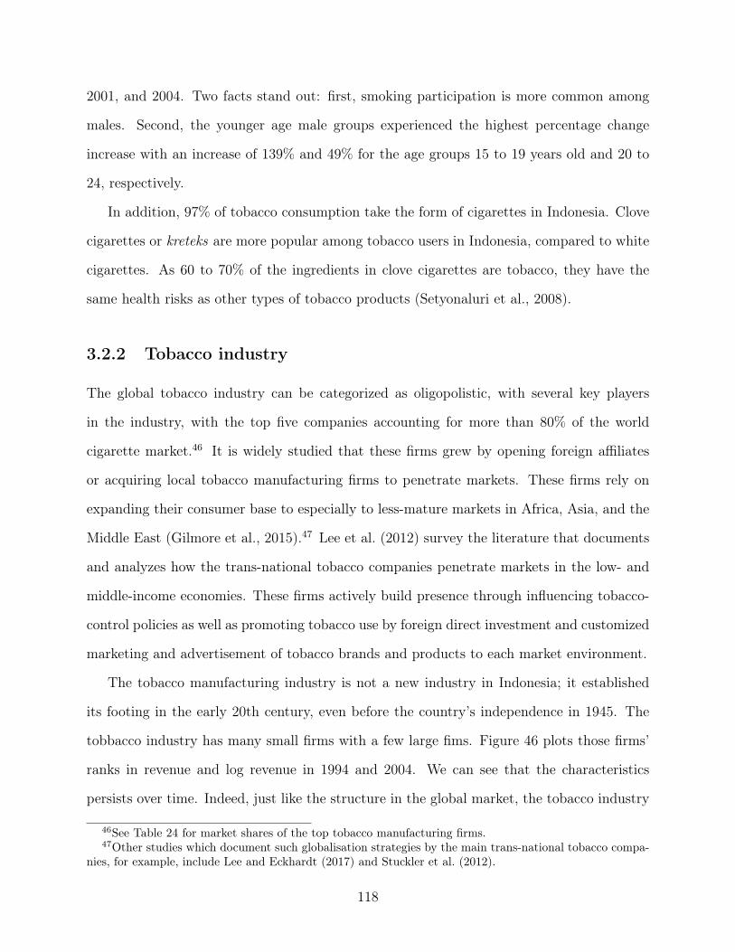
2001, and 2004. Two facts stand out: first, smoking participation is more common among

males. Second, the younger age male groups experienced the highest percentage change

increase with an increase of 139% and 49% for the age groups 15 to 19 years old and 20 to

24, respectively.

In addition, 97% of tobacco consumption take the form of cigarettes in Indonesia. Clove

cigarettes or kreteks are more popular among tobacco users in Indonesia, compared to white

cigarettes. As 60 to 70% of the ingredients in clove cigarettes are tobacco, they have the

same health risks as other types of tobacco products (Setyonaluri et al., 2008).

3.2.2 Tobacco industry

The global tobacco industry can be categorized as oligopolistic, with several key players

in the industry, with the top five companies accounting for more than 80% of the world

cigarette market.46 It is widely studied that these firms grew by opening foreign affiliates

or acquiring local tobacco manufacturing firms to penetrate markets. These firms rely on

expanding their consumer base to especially to less-mature markets in Africa, Asia, and the

Middle East (Gilmore et al., 2015).47 Lee et al. (2012) survey the literature that documents

and analyzes how the trans-national tobacco companies penetrate markets in the low- and

middle-income economies. These firms actively build presence through influencing tobacco-

control policies as well as promoting tobacco use by foreign direct investment and customized

marketing and advertisement of tobacco brands and products to each market environment.

The tobacco manufacturing industry is not a new industry in Indonesia; it established

its footing in the early 20th century, even before the country’s independence in 1945. The

tobbacco industry has many small firms with a few large fims. Figure 46 plots those firms’

ranks in revenue and log revenue in 1994 and 2004. We can see that the characteristics

persists over time. Indeed, just like the structure in the global market, the tobacco industry

46See Table 24 for market shares of the top tobacco manufacturing firms.47Other studies which document such globalisation strategies by the main trans-national tobacco compa-

nies, for example, include Lee and Eckhardt (2017) and Stuckler et al. (2012).

118

in Indonesia is also an oligopoly, with the three biggest firms accounting for more than 70%

of the market share (Setyonaluri et al., 2008).

There are a few firms with some foreign ownership. Table 25 shows the evolution of the

number of foreign and domestic firms over time, which are part of the medium and large

manufacturing survey. In our period of interest, the 1990s and 2000s, there are hundreds

of domestic firms but less than a dozen firms with any foreign ownership. Comparing firms

by status of foreign ownership, Figure 47 shows that the industry production has been

dominated by domestic firms.

The tobacco industry is also concentrated in two provinces: Central Java and East Java.

These two provinces account for 90% of all tobacco manufacturers.48 It seems that these

tobacco manufactureres cluster to get access to their main inputs as these provinces are also

the main producers of tobacco leaves. The top seven districts in tobacco farming are located

in the Central and East Java provinces. They account for 84% of national tobacco leaves

production (Sahadewo et al., 2021).

In terms of international trade, most of tobacco manufacturers, including the foreign-

owned ones, sell domestically. Only around 2 to 4% report to sell products overseas. Mean-

while, they also source their raw materials mostly from domestic suppliers. Between 1990

and 2010, on average 6% of firms reported they have imported materials, with an average of

16% of their materials are imported. Specifically for cigarettes, Indonesia’s imports fluctuate

but range between 0.5% to 6% relative to the domestic cigarette productions (Setyonaluri

et al., 2008).

Lastly, another characteristic that stands out is that the (ln) output per labor, as a raw

proxy for productivity, positively correlated with the market size of the firm as indicated by

(ln) revenue. This pattern is robust over time. For instance, Figure 48 shows this positive

correlation in 1994 and 2004.

48Calculated from Manufacturing Survey data.

119

3.2.3 Tobacco-control policies

The global decline in smoking prevalence has been driven by a stronger commitment to im-

plement tobacco control policies. In 2003, the World Health Assembly adopted the WHO

Framework Convention on Tobacco Control (WHO FCTC). The treaty is the first interna-

tional treaty under the auspices of the WHO. The WHO FCTC came into force in 2005.

There are 168 countries which signed the FCTC (WHO, 2021). Countries ratifying the

treaty commit to conduct measures to control tobacco use, including by reducing demand

for tobacco, regulating marketing activities, and providing alternatives to those growing and

producing tobacco (WHO, 2015).

Indonesia, despite being a member of the WHO, has not ratified the FCTC. Tobacco-

control policies and regulation are governed by the central government although there are

some local governments which impose stricter tobacco-control policies. The numbers of local

governments with stronger regulations unfortunately are still very limited.49

Setyonaluri et al. (2008) compiled and documented tax regimes imposed on tobacco

products and argued that the complexity of the tiered tax system based on production

volumes, that aims to protect relatively smaller tobacco manufacturers, contributes to the

industry’s characteristics of having many small firms. They also showed that the main tax

rate changes were imposed in 2008. In addition, they argued that in comparison to other low-

income countries and regional averages, Indonesia’s cigarette taxes and prices are relatively

low.

In terms of age limit, Indonesia started to have a minimum age for tobacco products

procurement in 2012. Since then, one has to be 18 years or older to be able to purchase

tobacco products. There were no age limits before 2012.

Furthermore, there are no complete smoking bans on tobacco advertisements in the

national-level regulation. Regulations for advertising on electronic media began 2000. Specif-

49The main regulations are Goverment Regulation No. 81 Year 1999, Government Regulation No. 38Year 2000, Government Regulation No. 19 Year 2003, and Government Regulation No. 109 Year 2012.

120

ically, tobacco advertising can only be aired on television between 9:30 pm to 5:00 am local

time. The regulations also impose obligations on tobacco packaging and labelling. Pictorial

health warnings have only beeen required since 2012.50

3.3 Theoretical framework and empirical facts

In order to answer the research question of how improvement in marketing technology to

advertise tobacco products affects smoking prevalence, I apply the theory of marketing cost

in international trade as developed by Arkolakis (2010). I use this framework especially in

understanding how exposure to advertising, both directly and indirectly, affects the decision

to start smoking. In this framework, such margin is called the new-consumer margin. This

margin is distinct from the other two more common margins in gains from trade, the intensive

margin and the extensive margin.

By focusing on the new-consumer margin, I acknowledge that, especially for an addictive

substance like tobacco, the utility function may need to take into account factors such as

past consumption and/or a high or varying discount rate in explaining the amount of tobacco

consumpotion. Hence, I do not aim to focus on understanding the intensive margin due to

improvement in advertising as the main focus. Chaloupka and Warner (1999) provide an

excellent summary on various utility functions which explain the addiction aspects of smoking

consumption. They categorize economic models of addiction into three groups: imperfectly

rational models of addictive behavior such as Strotz (1955) and Thaler and Shefrin (1981),

models of myopic addictive behavior such as Farrell (1952), and models of rational addictive

behavior such as Becker and Murphy (1988) and Becker et al. (1991). In addition, since I

focus on one particular market, I also do not focus on whether the improvement in marketing

technology creates new producers and importers, i.e., the extensive margin.

50For more further summarized details on tobacco-control policies, please refer to for Tobacco Free Kids.

121

3.3.1 Theory of marketing cost in international trade à la Arkolakis

(2010)

Arkolakis (2010) develops a theory of marketing cost in international trade that general-

izes the international trade model with heterogenous firms as in Melitz (2003) and Chaney

(2008).51 In this environment, heterogenous firms operate with constant-return-to-scale

(CRS) technology with productivity φ. These firms sell their products under monopolis-

tic competition.

The main difference in Arkolakis’s (2010) setup is that firms incur marketing costs to

reach individual consumers in each market. Let us define S as the number of advertisements

(ads) sent by a firm, L as the numbber of consumers, and n(S) refers to the probability that

a particular consumer sees the ad at least once after S ads have been sent.

There are three assumptions to capture the nature of the marketing technology. First,

the number of consumers who see each ad is given by L1−α, α ∈ [0, 1]. The parameter α is

the main parameter of interest in this paper. When α equals to one, each add is read by one

consumer. This case mimics the use of advertising with flyers. Meanwhile, when α is equal

to zero, then one ad can reach a given share of consumers in a market. An example of such

marketing technology is television ads. I refer to improvement in marketing technology as a

decrease in α.

The second assumption captures the decreasing return or increasing marginal cost of

marketing. In particular, Arkolakis (2010) assumes that the probability that a new ad is

seen by a consumer for the first time is [1−n(S)]β, β ∈ [0,+∞). This assumption is relevant

for the case of cigarette consumption. Brown (1978) and Thomas (1989), for example, show

evidences tha thet cigarette industry faces diminishing returns in advertising.

Lastly, the third assumption governs the production function in marketing services.

Specifically, firms employ a Cobb-Douglas techology that combines labor services in the

51I describe only the most relevant aspects of the environment of the model here.

122

source country i, li, and the labor services in the desination country j, lj as the following:

S = lγj l1−γi , with 0 ≤ γ ≤ 1.

Meanwhile, a consumer in country j consumes a composite good from combining differ-

entiated commodities using a CES aggregator with elasticity of substitution σ > 1. . The

consumer receives income, yj, from her labor income, wj, and profits earned, πj. Hence, the

demand for each variety as a function of productivity, φ, is the following:

cij(φ) =pij(φ)−σ

P 1−σj

yj, (33)

where pij is the price of that variety and Pj is the price index for all variety consumed

by the consumer in market j.

Firms operate using a constant returns to scale technology with productivity φ and

produce outputs using labor as the only factor of production. In selling to overseas markets,

firms face iceberg trade cost, τij. The optimal pricing is then a constant markup over

marginal cost, or as below:

pij(φ) =σ

σ − 1

τijwiφ

. (34)

Firms maximizes profits, which is the difference between revenue with labor cost of pro-

duction and marketing cost. Hence, provided that the firm enters the market, i.e. φ ≥ φ∗ij,

where φ∗ij is the entry threshold, the optimal consumers to be reached, nij, solves the equa-

tion below. This equation shows that the marginal revenue (after differencing out labor

cost for production) on the left-hand side equals to the marginal cost per consumer on the

right-hand side:

yjσ

[σ (τijwi/φ)]1−σ

P 1−σj

=wγjw

1−γi

ψL1−σj

1

(1− nij)β, (35)

where σ = σσ−1

, is the constant mark-up, and 1ϕ

= γγ (1− γ)1−γ, is the per-unit adver-

tisement costs. Solving equation 35 above for φ by setting nij = 0, we can derive the entry

123

threshold φ∗ij:

(φ∗ij)σ−1

= wγjw1−γi Lα−1

j /

[yjσ

(στijwi)1−σ

P 1−σj

ψ

]. (36)

Arkolakis (2010) provides three propositions. The first proposition is related to the

optimal market penetration decision, which is the focus of this paper. This proposition

states that if marketing technology is subject to diminishing returns, i.e. β > 0, then there

exists entry threshold φ∗ij, such that:

φ ≤ φ∗ij ⇒ nij(φ) = 0 and φ1 > φ2 ≥ φ∗ij ⇒ nij(φ1) > nij(φ2) ≥ 0. (37)

While, if marketing technology is not subject to diminishing returns, i.e. β = 0, then

there exists entry threshold φ∗ij, such that:

φ ≤ φ∗ij ⇒ nij(φ) = 0 and φ > φ∗ij ⇒ nij(φ) = 1. (38)

Thus, the optimal market penetration decision for a firm with productivity φ for β ≥ 0

can be expressed as below:

nij(φ) = max

{1−

(φ∗ijφ

)(σ−1)/β

, 0

}(39)

3.3.2 Productivity growth

Let us analyze the implication of an increase in a firm’s productivity, φ. Based on the

proposition of market penetration as shown by equation 37 and 38, as well as the optimal

market penetration equation that they infer as shown by equation 39, we can draw two

results. First, if the firm faces diminishing returns marketing technology, i.e. β > 0, then

the increase in productivity φ, increases the firm’s optimal market penetration nij. We can

use the first argument in equation 39 to take the derivative of nij with respect to φ and find

124

that the derivative has a positive sign. Equation 37 also shows this relationship, as it says

that conditional on entering the market, a more productive firms has higher optimal market

share.

3.3.3 Improvement in marketing technology

Conditional on passing the entry threshold, φ∗ij, we can predict the impact of the changes

in α to the optimal market penetration by taking the derivative of equation 39 and 36 with

respect to the marketing technology parameter α. The result is shown below. Since the

sign is negative, we can infer that as it gets easier to reach more consumers per ad, or as α

declines, then the optimal market share or market penetration, nij, increases. This is the

theoretical prediction that I would like to test empirically in this paper.

dnij(φ∗ij)

dφ∗ij

dφ∗ijdα

= −lnφ∗ijβφ

(φ∗ij)σ−1

β (40)

3.3.4 Empirical facts on smoking environment in Indonesia

We can collect two parameters and one variable that may affect optimal market shares. The

two parameters are productivity and marketing technology. While an outcome variable that

may affect demand is price, here, I document three empirical facts on productivity of tobacco

manufacturers, marketing technology, and prices of cigarettes from the Indonesian economy

from 1990 to 2010.

Fact 1: Exposure to marketing through television has expanded and varied spa-

tially.

In 1993, Indonesia started to have private-owned television stations. Before 1993, there

was only one state-owned television, TVRI. The state-owned television station does not

broadcast TV ads, while private-owned TV stations can. Figure 54 compares the average

number of TV stations captured in each district in 2003 and 2005.

125

There are two things we can infer from the figure. First, in both periods, there are

substantial spatial variations across subdistricts. Second, the number of private TV stations

increased between 2003 and 2005 as there were new TV stations broadcasted. Hence, districts

with a given level of exposure in 2003 may still experience some relative increase or decrease

of exposure due to the addition of these new TV stations.

Fact 2: Industry’s average TFP has been relatively stagnant.

I analyze the trend and distribution of total factor productivity (TFP) of firms in the

tobacco industry in Indonesia.52 There are two facts that we can infer from the trend of

TFP in the tobacco industry in Indonesia. First, in general, there was no substantial increase

of TFP over time in the sample period of 1990 to 2012, except for the last years in the series.

Figure 50 shows the simple and weighted average of TFP of the tobacco industry. Both

charts show a relatively stagnant level of industry-average productivity.

Second, there are a few firms that grew their TFP substantially in the last years of

the sample period. Most of these firms are domestically-owned. Figure 51 shows a panel

of estimated TFP with color indication for foreign-ownership status. Comparing domestic

firms with firms with any non-zero foreign ownership, we can infer that they have relatively

the same level of productiviy.53

Several public health studies show that foreign direct investment by trans-national to-

bacco companies has been the driver of growing market penetration especially in developing

countries.54 In the context of Indonesia from 1990 to 2010, I do not particularly analyze such

flows as the drivers in determining smoking prevalence. In addition, despite there having

been some major foreign investments, such as the acquisition of Sampoerna by Philip Morris

International55, I do not see any substantial jump or structural break in the industry-average

52Please see subsection “Data Appendix: Estimating Total Factor Productivity” in Appendix for details.53There is no guarantee that domestic firms do not get foreign loans for new investments as we cannot

observe such non-ownership foreign financial flows because the dataset only record ownership characteristics.54See for example: Bettcher et al. (2003) and WHO et al. (2012).55PMI (2005).

126

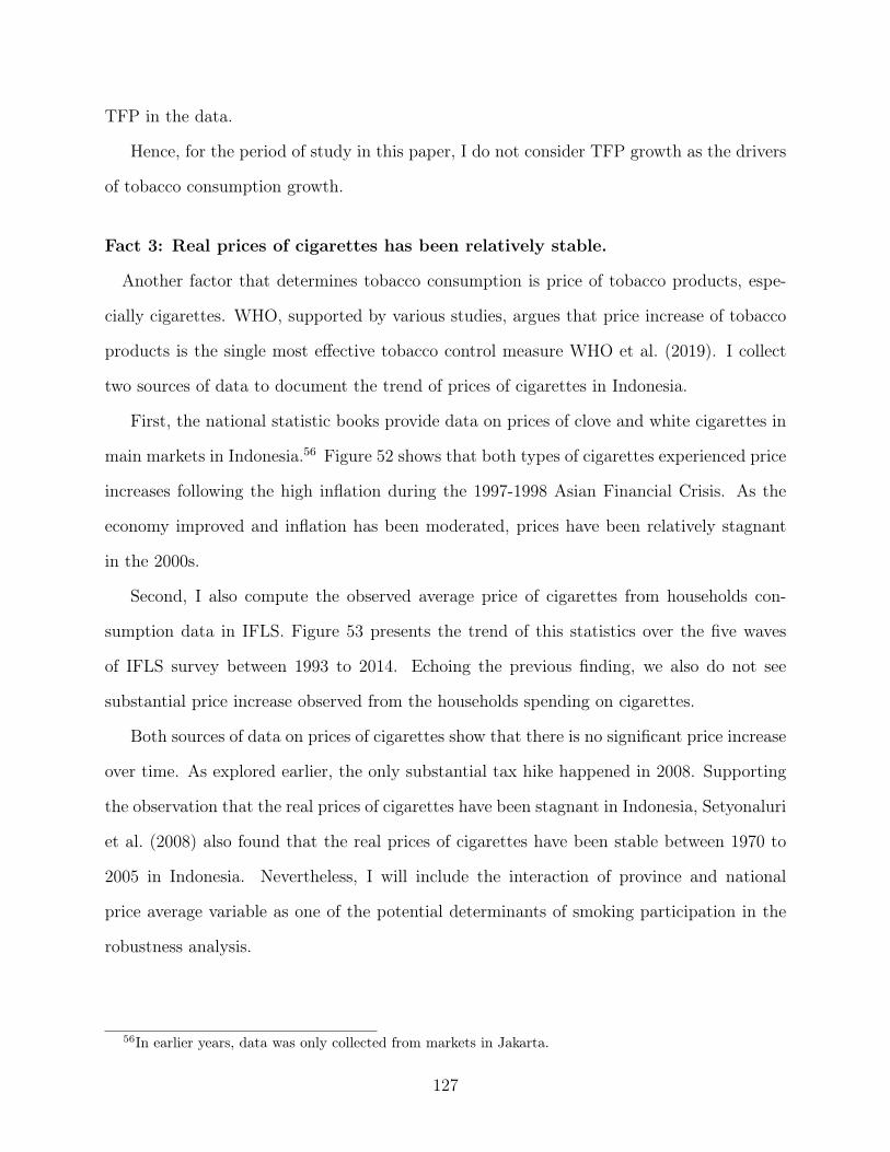
TFP in the data.

Hence, for the period of study in this paper, I do not consider TFP growth as the drivers

of tobacco consumption growth.

Fact 3: Real prices of cigarettes has been relatively stable.

Another factor that determines tobacco consumption is price of tobacco products, espe-

cially cigarettes. WHO, supported by various studies, argues that price increase of tobacco

products is the single most effective tobacco control measure WHO et al. (2019). I collect

two sources of data to document the trend of prices of cigarettes in Indonesia.

First, the national statistic books provide data on prices of clove and white cigarettes in

main markets in Indonesia.56 Figure 52 shows that both types of cigarettes experienced price

increases following the high inflation during the 1997-1998 Asian Financial Crisis. As the

economy improved and inflation has been moderated, prices have been relatively stagnant

in the 2000s.

Second, I also compute the observed average price of cigarettes from households con-

sumption data in IFLS. Figure 53 presents the trend of this statistics over the five waves

of IFLS survey between 1993 to 2014. Echoing the previous finding, we also do not see

substantial price increase observed from the households spending on cigarettes.

Both sources of data on prices of cigarettes show that there is no significant price increase

over time. As explored earlier, the only substantial tax hike happened in 2008. Supporting

the observation that the real prices of cigarettes have been stagnant in Indonesia, Setyonaluri

et al. (2008) also found that the real prices of cigarettes have been stable between 1970 to

2005 in Indonesia. Nevertheless, I will include the interaction of province and national

price average variable as one of the potential determinants of smoking participation in the

robustness analysis.

56In earlier years, data was only collected from markets in Jakarta.

127

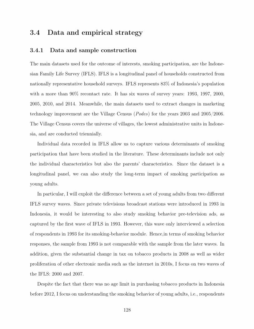
3.4 Data and empirical strategy

3.4.1 Data and sample construction

The main datasets used for the outcome of interests, smoking participation, are the Indone-

sian Family Life Survey (IFLS). IFLS is a longitudinal panel of households constructed from

nationally representative household surveys. IFLS represents 83% of Indonesia’s population

with a more than 90% recontact rate. It has six waves of survey years: 1993, 1997, 2000,

2005, 2010, and 2014. Meanwhile, the main datasets used to extract changes in marketing

technology improvement are the Village Census (Podes) for the years 2003 and 2005/2006.

The Village Census covers the universe of villages, the lowest administrative units in Indone-

sia, and are conducted triennially.

Individual data recorded in IFLS allow us to capture various determinants of smoking

participation that have been studied in the literature. These determinants include not only

the individual characteristics but also the parents’ characteristics. Since the dataset is a

longitudinal panel, we can also study the long-term impact of smoking participation as

young adults.

In particular, I will exploit the difference between a set of young adults from two different

IFLS survey waves. Since private televisions broadcast stations were introduced in 1993 in

Indonesia, it would be interesting to also study smoking behavior pre-television ads, as

captured by the first wave of IFLS in 1993. However, this wave only interviewed a selection

of respondents in 1993 for its smoking-behavior module. Hence,in terms of smoking behavior

responses, the sample from 1993 is not comparable with the sample from the later waves. In

addition, given the substantial change in tax on tobacco products in 2008 as well as wider

proliferation of other electronic media such as the internet in 2010s, I focus on two waves of

the IFLS: 2000 and 2007.

Despite the fact that there was no age limit in purchasing tobacco products in Indonesia

before 2012, I focus on understanding the smoking behavior of young adults, i.e., respondents

128

of 17 to 23 years old of age. In the analysis, I include the full sample with both male and

female respondents. However, for most of the analysis, I will focus on males as smoking

behavior is more acceptable for males in Indonesia. Ng et al. (2007), for example, found that

there was a social stigma that discourages females from smoking in Java and Bali, two of

the most populous islands in Indonesia.

In addition to using age as one of the selection criteria, I also select respondents who are

not heads of their households. The reason for this is because it is important to take into

account parents’ characteristics in understanding smoking behavior, as is shown im studies

such as Witoelar et al. (2005). Since some respondents live with extended families instead of

with their own biological parents, I find that the characteristics of the heads of households

with whom the respondents live to be the relevant parental characteristics, whether or not

the heads of households are or are not the respondents’ biological parents. In the robustness

analysis, I include all respondents between ages 17 to 23, without selecting on their household

member status.

In order to find the causality between exposure to marketing of tobacco products, I follow

Olken (2009) in using variation in local reception of television signal strength. Olken shows

that local reception is not entirely driven by the endogenous decision of placing TV towers,

but is also determined exogenously by geographical features such as terrain and topography.

These features affect the strength of reception that can be captured locally. Olken (2009)

exploits the timing of the introduction of private TV stations in 1993 as well as the spatial

variations in TV signal reception.57 Since the outcome variable of smoking participation is

not completely surveyed in the first wave of IFLS in 1993, I cannot compare the impact of

the introduction of television ads by comparing before and after such introduction. Instead,

I compare the temporal and regional variation in relative intensity of exposure to televisions.57Olken (2009) showed that, after controlling for disrict fixed effecrs, the number of television channels

received in each village was only correlated with three out of 24 geographic, and socio-economic variables.These three variables are: the presence of any social welfare group in 1990, the log number of hamlets, andwhether the subdistrict is coastal. Since I use a different dataset than the one used by Olken for the outcomevariables, I control for province fixed effects instead of district fixed effects. Olken also explored the impactof the introduction of TVs, while I explore the impact of relative TV exposure.

129

I believe, such a comparison is more relevant as it may not be feasible to eliminate all aspects

of marketing through electronic media such as TV in the contemporary world.

In order to get the measure of exposure to TV ads, I compute the number of TV channels

received by each village, as recorded in the Village Census in 2003 and 2006. Then, I take

the subdistrict average of the number of TV channels captured across each village.58 Since

there have been improvements in TV reception in general between 2003 and 2005 as well

as more private TV broadcasting stations, I compute the standardized value of the average

number of TV channels received for each subdistrict. The standardized values have a mean

of zero and standard variation of one in each survey wave. This measure is the preferred

measure to capture relative intensity of exposure to marketing through television ads. An

increase of such measure can be perceived as improvement in marketing technology. Using the

theoretical framework previously explained, we can consider an increase in relative intensity

of TV exposure as a decrease of α, i.e., one unit of TV ads can reach a bigger fraction of a

population.

The main sample includes respondents of aged 17 to 23 years of age from IFLS surveys in

2003 and 2007. Table 27 presents the summary statistics of the outcome and control variables

between the selected sample from two survey waves. For each variable, I also present the

t-test statistics. Lastly, the table also shows the joint-F test for all variables.

The two groups are comparable in several main variables such as education attainment,

working status, share of urban residence, and head of household’s real annual income. The

main outcome of interest, smoking participation, is significantly higher in 2000 compared

to 2007. But the head of households’ smoking participation status is statistically higher

in 2007. Some other individual and head of households characteristics are also statistically

different between the two survey waves. I will include all of these variables as controls in the

analysis.

58Subdistrict is the next higher administrative level above the village level.

130

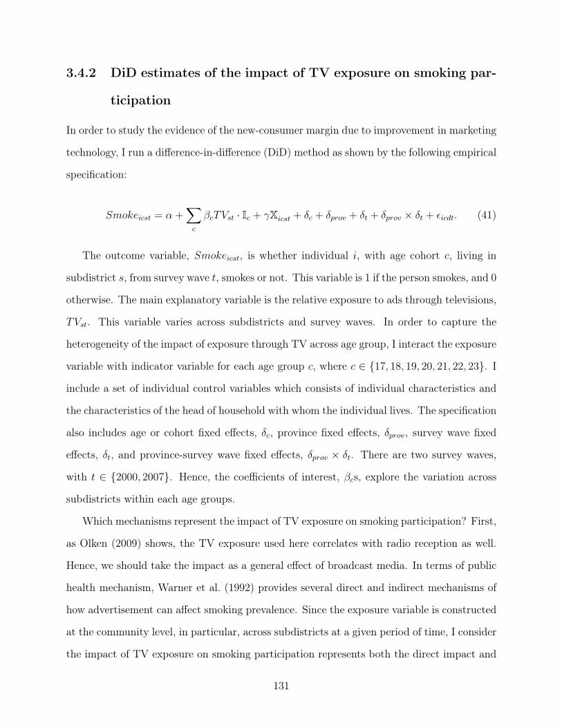
3.4.2 DiD estimates of the impact of TV exposure on smoking par-

ticipation

In order to study the evidence of the new-consumer margin due to improvement in marketing

technology, I run a difference-in-difference (DiD) method as shown by the following empirical

specification:

Smokeicst = α +∑c

βcTVst · Ic + γXicst + δc + δprov + δt + δprov × δt + εicdt. (41)

The outcome variable, Smokeicst, is whether individual i, with age cohort c, living in

subdistrict s, from survey wave t, smokes or not. This variable is 1 if the person smokes, and 0

otherwise. The main explanatory variable is the relative exposure to ads through televisions,

TVst. This variable varies across subdistricts and survey waves. In order to capture the

heterogeneity of the impact of exposure through TV across age group, I interact the exposure

variable with indicator variable for each age group c, where c ∈ {17, 18, 19, 20, 21, 22, 23}. I

include a set of individual control variables which consists of individual characteristics and

the characteristics of the head of household with whom the individual lives. The specification

also includes age or cohort fixed effects, δc, province fixed effects, δprov, survey wave fixed

effects, δt, and province-survey wave fixed effects, δprov × δt. There are two survey waves,

with t ∈ {2000, 2007}. Hence, the coefficients of interest, βcs, explore the variation across

subdistricts within each age groups.

Which mechanisms represent the impact of TV exposure on smoking participation? First,

as Olken (2009) shows, the TV exposure used here correlates with radio reception as well.

Hence, we should take the impact as a general effect of broadcast media. In terms of public

health mechanism, Warner et al. (1992) provides several direct and indirect mechanisms of

how advertisement can affect smoking prevalence. Since the exposure variable is constructed

at the community level, in particular, across subdistricts at a given period of time, I consider

the impact of TV exposure on smoking participation represents both the direct impact and

131

indirect mechanisms of how advertising affects smoking. These direct mechanisms include

reducing motivation to stop smoking, enticing smoking initiation, and encouraging relapse.

Meanwhile, the indirect mechanisms include discouraging the provision of full discussion on

the hazards of smoking in the media and increasing social acceptance to smoking behavior.

In the specification above, I allow the exposure to ads through televisions to vary across

age. Belk et al. (1982) and Moore and Stephens (1975), for example, show that there are

certain age ranges, especially during adolescence, in which preferences are formed. For

comparison, I also run a simpler specification without differentiating the impact of TV

exposure by age groups. In addition to the impact of TV exposure, the age cohort fixed

effects, δc, would capture the inclination of each age group on average towards smoking.

The set of individual controls consists of two groups of controls: the individual socio-

economic variables and the head of household’s socio-economic variables. The individual

characteristics include whether the individual is still in school, education attainment, working

status, marital status, and whether the individual lives in an urban or rural village. In the full

sample with both male and female respondents, I also include the gender of the individual.

Meanwhile, the socio-economic characteristics of the heads of households include whether

they smoke as well as their gender, education attainment, real income, working and marital

status.

Furthermore, the specification has province fixed effects, survey wave fixed effects, and

province-survey wave fixed effects. The time-invariant province fixed effects will capture all

aspects that are province-specific, including inclinations towards smoking behavior in general

across provinces. Meanwhile, survey wave fixed effects take care of all time-specific variables

that affect all respondents in each survey year, such as general macroeconomic conditions,

the growth of industry-average productivity in the tobacco industry, and overall prices of

tobacco products. In addition, province-survey year fixed effects will control confounding

factors, such as changes in tobacco-control policies imposed by local governments, local

economic conditions, and other time-varying province specific variations.

132

3.4.3 IV Estimates of young adults smoking participation on long-

run outcomes

Smoking behavior may have economic consequences. For example, since more income is

spent on tobacco consumption and less on investment in nutrition and/or education, one

may accumulate less skills. This lower level of skills may then affect one’s performance

in the labor market. However, it is challenging to investigate this due to the endogeneous

relation between current smoking behavior and current labor market performance. I propose

to use smoking status in adolescence and young adulthood as an instrument variable (IV)

to current smoking behavior to study the impact of smoking to economic outcomes.

This IV approach depends on the variation across individuals in their prolonged smoking

prevalence. The dataset that I use here allows me to investigate such prolonged tobacco

consumption, as IFLS follows each respondent over time. In particular, I study the several

economic outcomes in the most recent IFLS survey wave in 2014 for the respondents selected

in the surveys in years 2000 and 2007. For the selected sample in 2000, I explore respondents’

economic outcomes 14 years later. While for the selected sample in 2007, I study respondents’

economic outcomes after seven years later.

Specifically, the IV approach is performed using the a two-stage linear least square ap-

proach. In the first stage, smoking behavior documented in 2014 is regressed on smoking

behavior in individuals ages 17 to 23. Then, the second stage estimates the impact of smok-

ing using the instrumented smoking behavior to outcome variables, such as working status

and college-degree attainment.

133

3.5 Results

3.5.1 Evidence of the new-consumer margin

Improvement in marketing technology represented by exposure to television ads expands

smoking prevalence by inducing more new smokers. This impact is especially significant for

young male of 17 to 19 years of age. The impact of TV exposure on these age groups is

significant after controlling for age-specific inclination to smoke as captured by the age fixed

effects. Table 28 shows the results for the estimated coefficients of interests from running

equation 41, i.e., the sensitivity to smoking participation through TV exposure, in order to

investigate the evidence of new-consumer margin due to expansion of exposure to ads on

TVs.

First, the impact of TV exposure to smoking participation is not significant for the full

sample which includes both male and female respondents. The results for the full sample

are shown in columns one to three in Table 28. Such contrast between the full sample and

male-only sample is not surprising, as female smoking prevalences across age groups is a lot

less compared to the males. As previously mentioned, according to Ng et al. (2007), there

is a widespread stigma against females smoking, as smoking represents a manly behavior in

Indonesia. Such social acceptance on smoking for males is also present in India as shown by

Sen and Basu (2000) as well as in Pakistand and Bangladesh as shown by Bush et al. (2003).

Thus, from this point forward, I will focus more on studying the results for the sample set

with only male respondents.

Second, the heterogeneity across age groups turns out to be meaningful. The age fixed

effects show that the average smoking participation varies across age, even amon young adults

as the focus of this study. Figure 55 presents the coefficients and their 95% confidence interval

for the age fixed effects for male respondents. These estimated coefficients are quite high to

begin with. Among 17-year old males (the age group with the lowest coefficient), there is,

on average, a 50% chance of smoking.

134

Let us explore the results of the main coefficients of interest: the impact of TV exposure to

smoking participation. Columns four and five on Table 55 show the estimated coefficients for

male respondents. First, column four shows that without taking account the heterogeneity of

impact across age group, the impact of TV exposure is not statistically significant. However,

living in subdistricts with higher TV exposure increases the chance of smoking participation

for the younger group.

In Table 56, column one presents the main result that shows the evidence of new-consumer

margin due to improvement in marketing technology. This column shows the marginal effect

of TV exposure for each age group, i.e., how much the chance of smoking changes for an

increase of one standard deviation of TV exposure. For the age group 17, 18, and 19 years old,

an increase in TV exposure significantly increases the chance of smoking participation. In

particular, for those of 17 years of age, increasing TV exposure by one standard of deviation

increases the chance of smoking by 3.7%. The marginal effect of TV exposure is higher for

the age group 18 and 19 years of age, with an increase of 5.6% for chance of smoking due to

one standard deviation increase of TV exposure for age group 19 years of age, Meanwhile,

the marginal effect of TV exposure is not statistically significant for the older age groups

between 20 to 23 years old. Figure 56 illustrates these marginal impacts of TV exposure to

smoking participation for each age group across the distribution of TV exposure.

This result is consistent with the impact of introduction to television in the United

States to smoking participation as shown by Thomas (2019). Thomas demonstrated that

the impact is significant for the youth as well. In addition, TV exposure may not matter much

in the smoking participation decision of the older groups in this study as their preference to

smoke are formed when they are younger. Holbrook and Schindler (1989), who studied the

construction of preference to popular music for example, showed that sensitivity of preference

may peak around 24 years of age.

The findings on the evidence of the new-consumer margin here contributes to the under-

standing of the impact of the different magnitude of exposure through television ads to smok-

135

ing participation. Previous studies focus on comparing the change in smoking prevalence

with and without such marketing channels. Hence, instead of focusing on such a structural

break, I focus on how varying relative exposure presents a different impacts. Understanding

how the magnitude of exposure matters is important in informing policy makers, especially

in regulating tobacco advertisements in the current environment of high accessibility and

affordability of media.

Furthermore, I also contribute to the discussion on whether advertisements influence only

current smokers or also produce a new generation of smokers. Warner et al. (1992) mentioned

that tobacco companies usually argue that the role of advertisement is to encourage switching

to their brands or to increase loyalty to their brands. This evidence of the new-consumer

margin confirms that advertisements not only affect current smokers but also generate new

smokers.

In all specifications, I control for various individual characteristics and head of households’

characteristics. The results for these controls are consistent with the literature. Figure 57

illustrates the estimated coefficients for these controls that are factor variable. The blue

coefficients refer to the result for the full sample as part of the specification on column two

of Table 28, while the yellow coefficients are the results for the male-only sample as part of

the specification on column five of Table 28.

In both sets of samples, attending school decreases the chance of smoking for the pop-

ulation of between 17 to 23 years of age. In contrast, working status increases the chance

of smoking. Importantly, individuals who live with household heads who smoke, also have

a higher chance of smoking. This is consistent with the findings studied by Witoelar et al.

(2005) which show that having parents who smoke increases youth’s chance of smoking in

Indonesia. A study on smoking behavior in youths in Taiwan by Wen et al. (2005) also

show the important role of parental smoking behavior. In addition, living in an urban area

decreases the chance of smoking, echoing the same result presented by Adioetomo et al.

(2005).

136

Furthermore, Table 30 presents the estimated coefficients for education and income. Espe-

cially for our main specification with male-only sample, educational attainment is negatively

associated with smoking participation. Likewise, head of households’ education attainment

is also negatively associated with chances of smoking for the population in 17 to 23 years

old of age. In contrast, in the male-only sample, head of household income does not have a

statistically significant impact to chances of smoking. The negative association of education

and non-significant association of income to smoking participation is consistent with the

literature, as shown by Witoelar et al. (2005).

3.5.2 Long-run impacts

The IFLS surveys allow us to observe the dynamic of socio-economic condition over life cycles.

This feature allows us to explore the long-run impact of smoking participation when one is

young to their condition later in life. I investigate the consequences of smoking behavior

to several economic outcomes using the instrument variable (IV) approach to tackle the

endogeneity issue inherent in studying the impact of smoking to economic outcomes.

The endogeneity issue rises because individuals may smoke due to stress or lack of access

to means that can support them.59 Stress or lack of access of support may stem from weak

performance in the labor market including unemployment and job loss. In addition, the

individual may find it harder to find a job with less educational attainment such as a college

degree. On the other hand, since smoking is societally well accepted for males, individuals

who smoke may find it easier to build a social network, which is a resource in finding a

job. In addition, those who work may find it easier to retain working status due to better

social networks. Hence, it is not straightforward to which direction the impact of smoking to

economic outcome would be. Thus, instrumenting current smoking status with past smoking

status allow us to estimate the impact of smoking in the form of the cost from spending less

on productive means such as education and nutrition. However, I also include the channel

59See for example Kouvonen et al. (2005) and Westman et al. (1985).

137

in which one may actually be able to build stronger social networks.

In order to control for path dependence, such as household economic condition when

the respondents were young adults as well as other socio-economic confounding variables, I

control for a set of variables. First, I control for current socio-economic conditions such as

education attainment, marital status, urban or rural residence, and whether the individual

is a head of household or not. Second, I control for socio-economic conditions when the

respondents were young adults. In particular, I control for the head of household income,

whether the respondents were attending school as well as rural or urban residence during

young adulthood. In all specifications, I add age fixed effects and province fixed effects.

First, I find that individuals who smokes have a lower probability of possessing a college

degree. Table 31 presents the estimates for smoking status for respondents who were young

adults in 2000 in columns one and two, and for those who were young in 2007 in columns

three and four. For both sets of respondents, the OLS estimates are biased downward.

Instrumenting current smoking participation with past smoking participation results in an

estimated 11 to 13% lower chance of having a college degree when the individual smokes.

Second, the impact of smoking on working status is not as conclusive. Table 32 shows

the estimates for smoking status on working status in 2014. Using OLS, the estimates are

not significant for both groups of respondents from survey waves in 2000 and 2007. However,

instrumenting current smoking participation with past smoking participation is associated

with 9% less chance of having a job for respondents who were 17 to 23 years of age in 2000.

The estimates using IV approach are not significant for those who were young adults in 2007.

These results are consistent with the prediction that smoking behavior, despite may cause

less investment on human capital, may promote the accumulation of social capital. Thus,

the impact of smoking on working status may not be straightforward.

138

3.5.3 Robustness analysis

I perform several robustness analyses to support the evidence of the new-consumer margin

due to improvement in marketing technology represented by TV exposure. First, instead

of using the relative exposure, I also use the actual average of TV exposure as the main

variable of interest. Second, I include prices of cigarettes as controls. Lastly, I relax one of

the selection criteria in the sample construction. In particular, instead of focusing on males

who are not heads of households, I include males who are also heads of household as part of

the robustness check.

The evidence of new-consumer margin due to the improvement in marketing technology

prevails if we use the actual and not-standardized subdistrict-average number of TV channels

received. Table 33 shows the results of running equation 41 using this measure of TV

exposure on both the full sample and male-only sample. The coefficient estimate is not

significant if we do not take into account the heterogenous impacts of TV exposure across

age groups. However taking into account such heterogeneity, TV exposure significantly

increases the chance of smoking for thee younger age group. The second column of Table

29 provides the marginal effect of TV exposure on smoking participation for the male-only

sample. Increases in the number of TV broadcasting stations received is associated with

higher smoking participation for those who are 17 and 19 years old.

Controlling for prices of cigarettes also do not change the results. In order to capture

variation in prices, I interact real national prices of clove cigarettes with province fixed effects.

If there are any time invariant trade costs, the interaction with province fixed effects can

capture that. This strategy was chosen due to the unavailability of data on regional prices of

cigaretters. Prices of clove cigarettes are chosen, instead of the prices of white cigarettes, as

most Indonesian smokers consume clove cigarettes. Nevertheless, there is a high correlation

between the prices of these two types of cigarettes as illustrated in Figure 52.

Columns three and six on Table 28 present the coefficients of interest from running

the DiD estimation. We can see that there are no substantial changes in the estimated

139

coefficients. In addition, no substantial changes in estimated coefficients can be observed in

other control variables as well. Columns three and six in Table 30 provides the estimated

coefficients for education and income variables, once we control for prices.

The insignificant impact on of controlling for prices is consistent with the findings in

other studies, such as Adioetomo et al. (2005). They find that prices are not a significant

determinant in smoking participation. Yet, prices affect the amount of tobacco consumption.

In addition, Witoelar et al. (2005) also finds insignificant impact of prices to youth smoking

participation. Concerning such results, Setyonaluri et al. (2008) argue that there is not much

regional variation in prices of cigarettes, on top of relatively stable real prices of cigarettes in

Indonesia. Hence, we may not see any significant impact of prices to smoking participation.

Lastly, the evidence of new-consumer margin also persists if we relax one of the selection

criteria in the sample construction. In particular, I run equation 41 on all male-only samples

of 17 to 23 years old, including those who are household heads in their households. Given

this selection criteria, there are less variables in the set of individual controls. In particular,

I do not control the characteristics of the proxy for parents, which is the socio-economic

variables of household heads if the individu is not a household head.

Table 34 presents the marginal effect of TV exposure to smoking participation by age.

Younger age groups, especially the ones with 18 and 19 years of age, have higher chance of

smoking if they live in subdistricts with relatively higher TV exposure. In this setup, the

impact of TV exposure to smoking participation of young adults, with age 21 to 23 years

old, are not significant either. These results echo the evidence of the new-consumer margin

due to improvement in marketing technology. Such margin, across several robustness checks,

are especially active for adolescents.

140

3.6 Conclusion

Improvement in marketing technology allows firms to generate new consumers. This paper

investigates this theoretical prediction, derived from the theory of marketing cost in interna-

tional trade built by Arkolakis (2010). In particular, I test the prediction by estimating the

impact of exposure to television, representing ads through television and other broadcasted

media, on smoking prevalence among young adults in Indonesia. In general, as predicted,

higher local exposure to TV generates more smokers especially the younger adults. This

finding is robust across different measuremenst of TV exposure as well as sample construc-

tion.

This evidence on new-consumer margin in the form of smoking participation can inform

policymakers in regulating the advertisements and marketing of tobacco products. First,

the result emphasizes that the impact takes the form of new smokers. This fact stands in

contrast to the argument that the purpose of tobacco advertisement is to strengthen brand-

ing, i.e., advertisements only affect the smoking intensity or the intensive margin of tobacco

consumption. Indeed, despite the relatively limited hours of allowance for tobacco ads to

be broadcasted, I find a statistically significant impact in increasing smoking participation

in young adults. Second, I also show that smoking is associated with worse performance

in the labor market. Given that exposure to advertising entices smoking participation to

especially younger adults, the worse performance of this productive labor force in the labor

markets, in the long run, can create a bigger cost to the economy. This economic cost is

on top of the high cost of burden of disease of smoking. Third, despite the declining global

smoking prevalence, as many developing economies have a higher share of the young popu-

lation, advertising efforts of tobacco companies in such economies would have bigger macro

consequences.

141

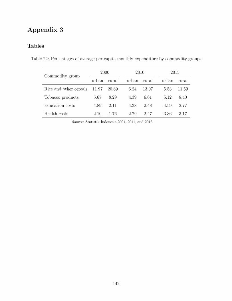
Appendix 3

Tables

Table 22: Percentages of average per capita monthly expenditure by commodity groups

Commodity group2000 2010 2015

urban rural urban rural urban rural

Rice and other cereals 11.97 20.89 6.24 13.07 5.53 11.59

Tobacco products 5.67 8.29 4.39 6.61 5.12 8.40

Education costs 4.89 2.11 4.38 2.48 4.59 2.77

Health costs 2.10 1.76 2.79 2.47 3.36 3.17

Source: Statistik Indonesia 2001, 2011, and 2016.

142

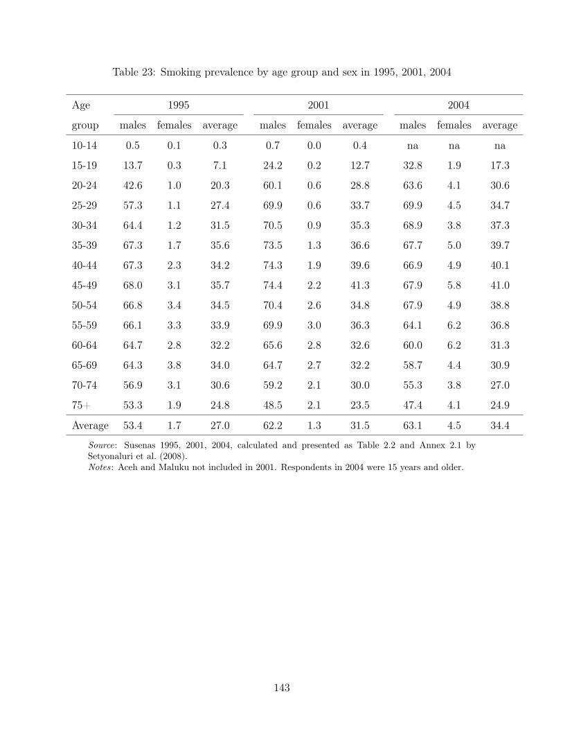
Table 23: Smoking prevalence by age group and sex in 1995, 2001, 2004

Age 1995 2001 2004

group males females average males females average males females average

10-14 0.5 0.1 0.3 0.7 0.0 0.4 na na na

15-19 13.7 0.3 7.1 24.2 0.2 12.7 32.8 1.9 17.3

20-24 42.6 1.0 20.3 60.1 0.6 28.8 63.6 4.1 30.6

25-29 57.3 1.1 27.4 69.9 0.6 33.7 69.9 4.5 34.7

30-34 64.4 1.2 31.5 70.5 0.9 35.3 68.9 3.8 37.3

35-39 67.3 1.7 35.6 73.5 1.3 36.6 67.7 5.0 39.7

40-44 67.3 2.3 34.2 74.3 1.9 39.6 66.9 4.9 40.1

45-49 68.0 3.1 35.7 74.4 2.2 41.3 67.9 5.8 41.0

50-54 66.8 3.4 34.5 70.4 2.6 34.8 67.9 4.9 38.8

55-59 66.1 3.3 33.9 69.9 3.0 36.3 64.1 6.2 36.8

60-64 64.7 2.8 32.2 65.6 2.8 32.6 60.0 6.2 31.3

65-69 64.3 3.8 34.0 64.7 2.7 32.2 58.7 4.4 30.9

70-74 56.9 3.1 30.6 59.2 2.1 30.0 55.3 3.8 27.0

75+ 53.3 1.9 24.8 48.5 2.1 23.5 47.4 4.1 24.9

Average 53.4 1.7 27.0 62.2 1.3 31.5 63.1 4.5 34.4

Source: Susenas 1995, 2001, 2004, calculated and presented as Table 2.2 and Annex 2.1 bySetyonaluri et al. (2008).Notes: Aceh and Maluku not included in 2001. Respondents in 2004 were 15 years and older.

143

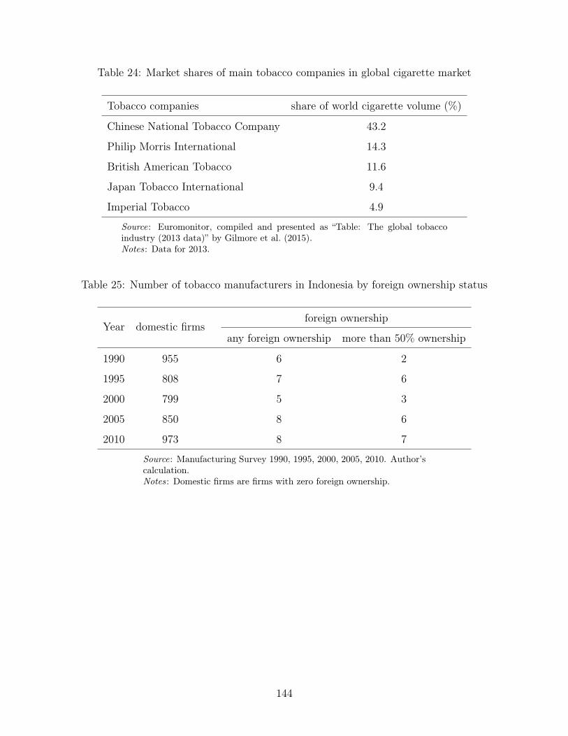
Table 24: Market shares of main tobacco companies in global cigarette market

Tobacco companies share of world cigarette volume (%)

Chinese National Tobacco Company 43.2

Philip Morris International 14.3

British American Tobacco 11.6

Japan Tobacco International 9.4

Imperial Tobacco 4.9

Source: Euromonitor, compiled and presented as “Table: The global tobaccoindustry (2013 data)” by Gilmore et al. (2015).Notes: Data for 2013.

Table 25: Number of tobacco manufacturers in Indonesia by foreign ownership status

Year domestic firmsforeign ownership

any foreign ownership more than 50% ownership

1990 955 6 2

1995 808 7 6

2000 799 5 3

2005 850 8 6

2010 973 8 7

Source: Manufacturing Survey 1990, 1995, 2000, 2005, 2010. Author’scalculation.Notes: Domestic firms are firms with zero foreign ownership.

144

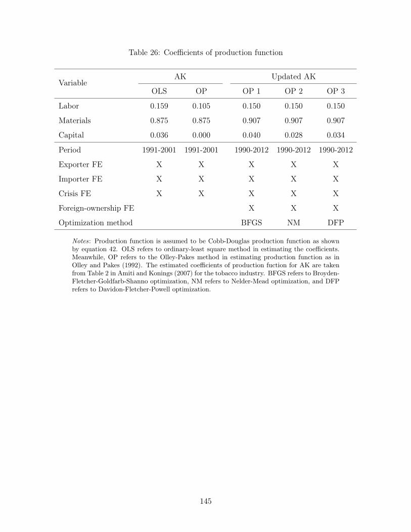
Table 26: Coefficients of production function

VariableAK Updated AK

OLS OP OP 1 OP 2 OP 3

Labor 0.159 0.105 0.150 0.150 0.150

Materials 0.875 0.875 0.907 0.907 0.907

Capital 0.036 0.000 0.040 0.028 0.034

Period 1991-2001 1991-2001 1990-2012 1990-2012 1990-2012

Exporter FE X X X X X

Importer FE X X X X X

Crisis FE X X X X X

Foreign-ownership FE X X X

Optimization method BFGS NM DFP

Notes: Production function is assumed to be Cobb-Douglas production function as shownby equation 42. OLS refers to ordinary-least square method in estimating the coefficients.Meanwhile, OP refers to the Olley-Pakes method in estimating production function as inOlley and Pakes (1992). The estimated coefficients of production fuction for AK are takenfrom Table 2 in Amiti and Konings (2007) for the tobacco industry. BFGS refers to Broyden-Fletcher-Goldfarb-Shanno optimization, NM refers to Nelder-Mead optimization, and DFPrefers to Davidon-Fletcher-Powell optimization.

145

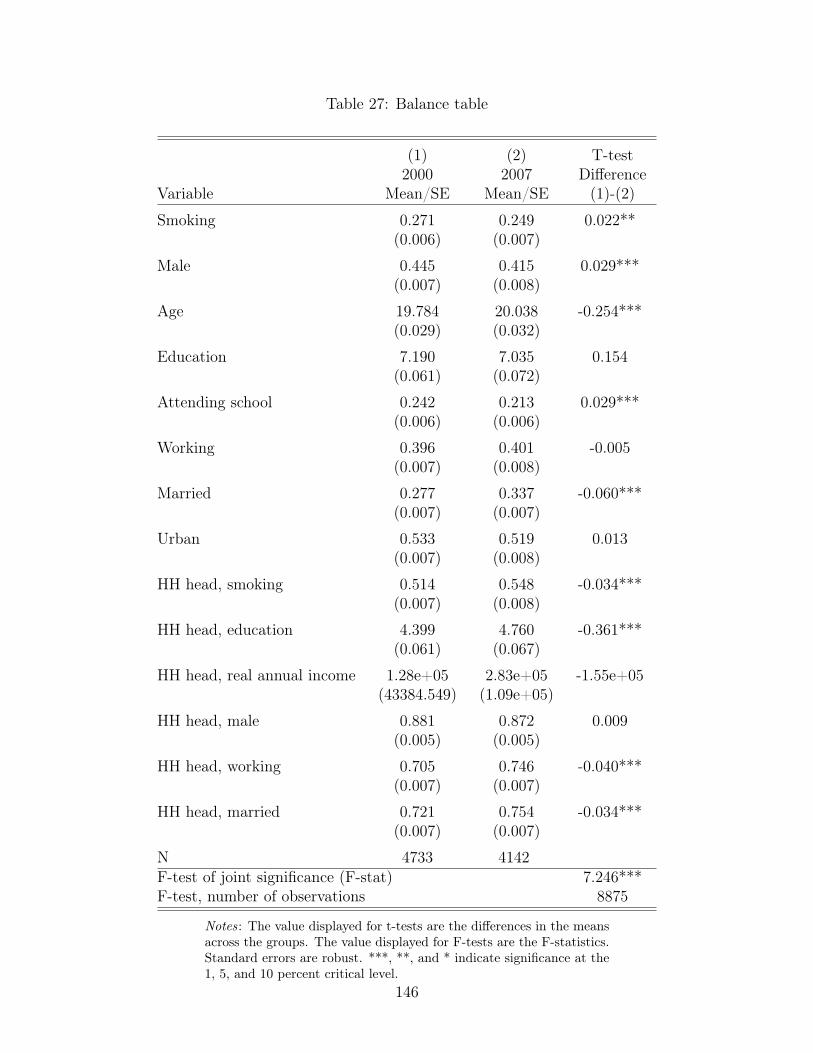
Table 27: Balance table

(1) (2) T-test2000 2007 Difference

Variable Mean/SE Mean/SE (1)-(2)

Smoking 0.271(0.006)

0.249(0.007)

0.022**

Male 0.445(0.007)

0.415(0.008)

0.029***

Age 19.784(0.029)

20.038(0.032)

-0.254***

Education 7.190(0.061)

7.035(0.072)

0.154

Attending school 0.242(0.006)

0.213(0.006)

0.029***

Working 0.396(0.007)

0.401(0.008)

-0.005

Married 0.277(0.007)

0.337(0.007)

-0.060***

Urban 0.533(0.007)

0.519(0.008)

0.013

HH head, smoking 0.514(0.007)

0.548(0.008)

-0.034***

HH head, education 4.399(0.061)

4.760(0.067)

-0.361***

HH head, real annual income 1.28e+05(43384.549)

2.83e+05(1.09e+05)

-1.55e+05

HH head, male 0.881(0.005)

0.872(0.005)

0.009

HH head, working 0.705(0.007)

0.746(0.007)

-0.040***

HH head, married 0.721(0.007)

0.754(0.007)

-0.034***

N 4733 4142F-test of joint significance (F-stat) 7.246***F-test, number of observations 8875

Notes: The value displayed for t-tests are the differences in the meansacross the groups. The value displayed for F-tests are the F-statistics.Standard errors are robust. ***, **, and * indicate significance at the1, 5, and 10 percent critical level.

146

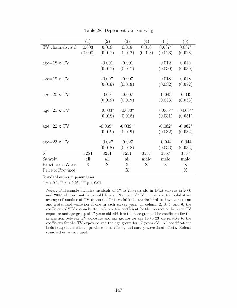
Table 28: Dependent var: smoking

(1) (2) (3) (4) (5) (6)TV channels, std 0.003 0.018 0.018 0.016 0.037∗ 0.037∗

(0.008) (0.012) (0.012) (0.013) (0.023) (0.023)

age=18 x TV -0.001 -0.001 0.012 0.012(0.017) (0.017) (0.030) (0.030)

age=19 x TV -0.007 -0.007 0.018 0.018(0.019) (0.019) (0.032) (0.032)

age=20 x TV -0.007 -0.007 -0.043 -0.043(0.019) (0.019) (0.033) (0.033)

age=21 x TV -0.033∗ -0.033∗ -0.065∗∗ -0.065∗∗(0.018) (0.018) (0.031) (0.031)

age=22 x TV -0.039∗∗ -0.039∗∗ -0.062∗ -0.062∗(0.019) (0.019) (0.032) (0.032)

age=23 x TV -0.027 -0.027 -0.044 -0.044(0.018) (0.018) (0.033) (0.033)

N 8251 8251 8251 3557 3557 3557Sample all all all male male maleProvince x Wave X X X X X XPrice x Province X XStandard errors in parentheses∗ p < 0.1, ∗∗ p < 0.05, ∗∗∗ p < 0.01

Notes: Full sample includes inviduals of 17 to 23 years old in IFLS surveys in 2000and 2007 who are not household heads. Number of TV channels is the subdistrictaverage of number of TV channels. This variable is standardized to have zero meanand a standard variation of one in each survey year. In column 2, 3, 5, and 6, thecoefficient of “TV channels, std” refers to the coefficient for the interaction between TVexposure and age group of 17 years old which is the base group. The coefficient for theinteraction between TV exposure and age groups for age 18 to 23 are relative to thecoefficient for the TV exposure and the age group for 17 years old. All specificationsinclude age fixed effects, province fixed effects, and survey wave fixed effects. Robuststandard errors are used.

147

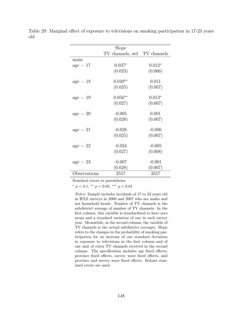
Table 29: Marginal effect of exposure to televisions on smoking participation in 17-23 yearsold

SlopeTV channels, std TV channels

mainage = 17 0.037∗ 0.012∗

(0.023) (0.006)

age = 18 0.049∗∗ 0.011(0.025) (0.007)

age = 19 0.056∗∗ 0.013∗(0.027) (0.007)

age = 20 -0.005 0.001(0.028) (0.007)

age = 21 -0.028 -0.000(0.025) (0.007)

age = 22 -0.024 -0.005(0.027) (0.008)

age = 23 -0.007 -0.001(0.028) (0.007)

Observations 3557 3557Standard errors in parentheses∗ p < 0.1, ∗∗ p < 0.05, ∗∗∗ p < 0.01

Notes: Sample includes inviduals of 17 to 23 years oldin IFLS surveys in 2000 and 2007 who are males andnot household heads. Number of TV channels is thesubdistrict average of number of TV channels. In thefirst column, this variable is standardized to have zeromean and a standard variation of one in each surveyyear. Meanwhile, in the second column, the variable ofTV channels is the actual subdistrict averages. Sloperefers to the changes in the probability of smoking par-ticipation for an increase of one standard deviationin exposure to televisions in the first column and ofone unit of extra TV channels received in the secondcolumn. The specification includes age fixed effects,province fixed effects, survey wave fixed effects, andprovince and survey wave fixed effects. Robust stan-dard errors are used.

148

Table 30: Estimates for education and income

(1) (2) (3) (4) (5) (6)Education 0.001 0.001 0.001 -0.005∗∗ -0.005∗∗ -0.005∗∗

(0.001) (0.001) (0.001) (0.002) (0.002) (0.002)

HH head, education -0.008∗∗∗ -0.008∗∗∗ -0.008∗∗∗ -0.008∗∗∗ -0.008∗∗∗ -0.008∗∗∗(0.001) (0.001) (0.001) (0.002) (0.002) (0.002)

HH head, income -0.000∗∗ -0.000∗∗ -0.000∗∗ 0.000 0.000 0.000(0.000) (0.000) (0.000) (0.000) (0.000) (0.000)

N 8251 8251 8251 3557 3557 3557Sample all all all male male allTV x Age X X X XProvince x Wave X X X X X XPrice x Province X X XStandard errors in parentheses∗ p < 0.1, ∗∗ p < 0.05, ∗∗∗ p < 0.01

Notes: Sample includes inviduals of 17 to 23 years old in IFLS surveys in 2000 and2007 who are not household heads. All specifications include age fixed effects, provincefixed effects, and survey wave fixed effects. Robust standard errors are used.

Table 31: Long-run economic impacts of smoking: college degree

(1) (2) (3) (4)Smoking -0.089∗∗∗ -0.128∗∗ -0.076∗∗∗ -0.112∗∗∗

(0.025) (0.051) (0.024) (0.040)N 1208 1208 1147 1147Wave 2000 2000 2007 2007Model OLS IV OLS IVStandard errors in parentheses∗ p < 0.1, ∗∗ p < 0.05, ∗∗∗ p < 0.01

Notes: Sample includes individuals of 17 to 23 yearsold in IFLS suveys in 2000 and 2007 who are maleand not household heads. The dependent variable iswhether the individu has a college degree as reportedin IFLS survey in 2014. Regressions are run separatelyfor each group of sample based on survey waves. OLSrefers to regression using ordinary-least squares whileIV refers to instrumenting smoking status in 2014 withsmoking status in year 2000 or 2007, i.e. when the indi-vidu was 17 to 23 years old. All specifications includeage fixed effects and province fixed effects. Robuststandard errors are used.

149

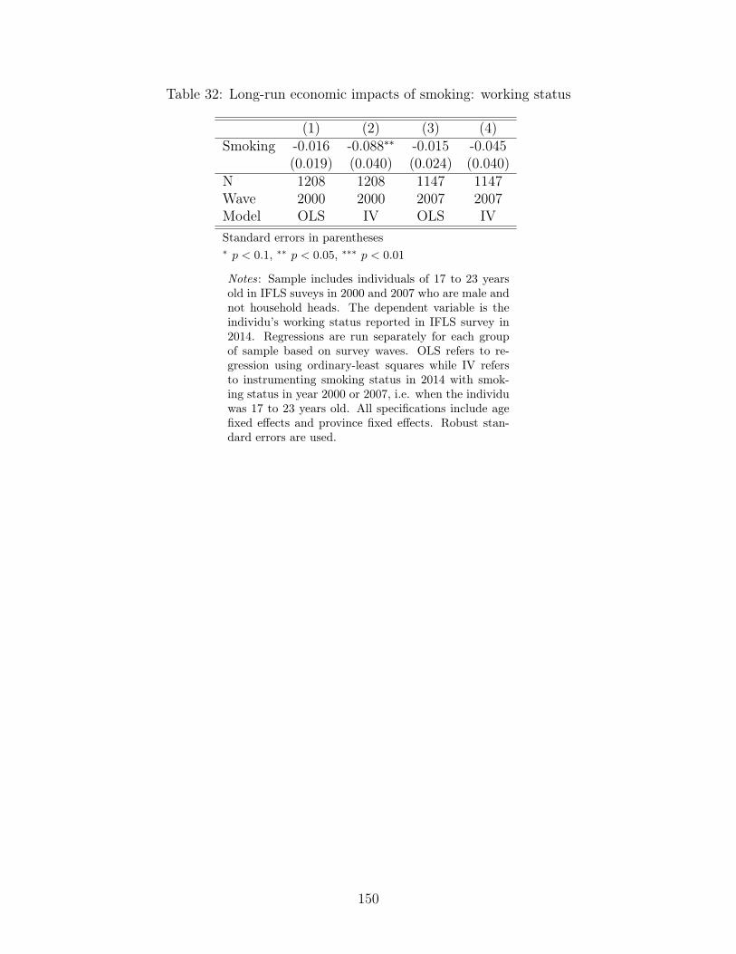
Table 32: Long-run economic impacts of smoking: working status

(1) (2) (3) (4)Smoking -0.016 -0.088∗∗ -0.015 -0.045

(0.019) (0.040) (0.024) (0.040)N 1208 1208 1147 1147Wave 2000 2000 2007 2007Model OLS IV OLS IVStandard errors in parentheses∗ p < 0.1, ∗∗ p < 0.05, ∗∗∗ p < 0.01

Notes: Sample includes individuals of 17 to 23 yearsold in IFLS suveys in 2000 and 2007 who are male andnot household heads. The dependent variable is theindividu’s working status reported in IFLS survey in2014. Regressions are run separately for each groupof sample based on survey waves. OLS refers to re-gression using ordinary-least squares while IV refersto instrumenting smoking status in 2014 with smok-ing status in year 2000 or 2007, i.e. when the individuwas 17 to 23 years old. All specifications include agefixed effects and province fixed effects. Robust stan-dard errors are used.

150

Table 33: Robustness analysis using average TV channels received, dependent variable:smoking

(1) (2) (3) (4) (5) (6)TV channels 0.002 0.006∗ 0.006∗ 0.005 0.012∗ 0.012∗

(0.002) (0.003) (0.003) (0.004) (0.006) (0.006)

age=18 x TV -0.001 -0.001 -0.001 -0.001(0.005) (0.005) (0.008) (0.008)

age=19 x TV -0.003 -0.003 0.001 0.001(0.005) (0.005) (0.008) (0.008)

age=20 x TV -0.003 -0.003 -0.011 -0.011(0.005) (0.005) (0.009) (0.009)

age=21 x TV -0.007 -0.007 -0.012 -0.012(0.005) (0.005) (0.008) (0.008)

age=22 x TV -0.013∗∗∗ -0.013∗∗∗ -0.017∗ -0.017∗(0.005) (0.005) (0.009) (0.009)

age=23 x TV -0.006 -0.006 -0.013 -0.013(0.005) (0.005) (0.009) (0.009)

N 8251 8251 8251 3557 3557 3557Sample all all all male male maleProvince x Wave X X X X X XPrice x Province X XStandard errors in parentheses∗ p < 0.1, ∗∗ p < 0.05, ∗∗∗ p < 0.01

Notes: Full sample includes inviduals of 17 to 23 years old in IFLS surveys in 2000 and2007 who are not household heads. Number of TV channels is the subdistrict average ofnumber of TV channels. In column 2, 3, 5, and 6, the coefficient of “TV channels” refersto the coefficient for the interaction between TV exposure and age group of 17 yearsold which is the base group. The coefficient for the interaction between TV exposureand age groups for age 18 to 23 are relative to the coefficient for the TV exposure andthe age group for 17 years old. All specifications include age fixed effects, provincefixed effects, and survey wave fixed effects. Robust standard errors are used.

151

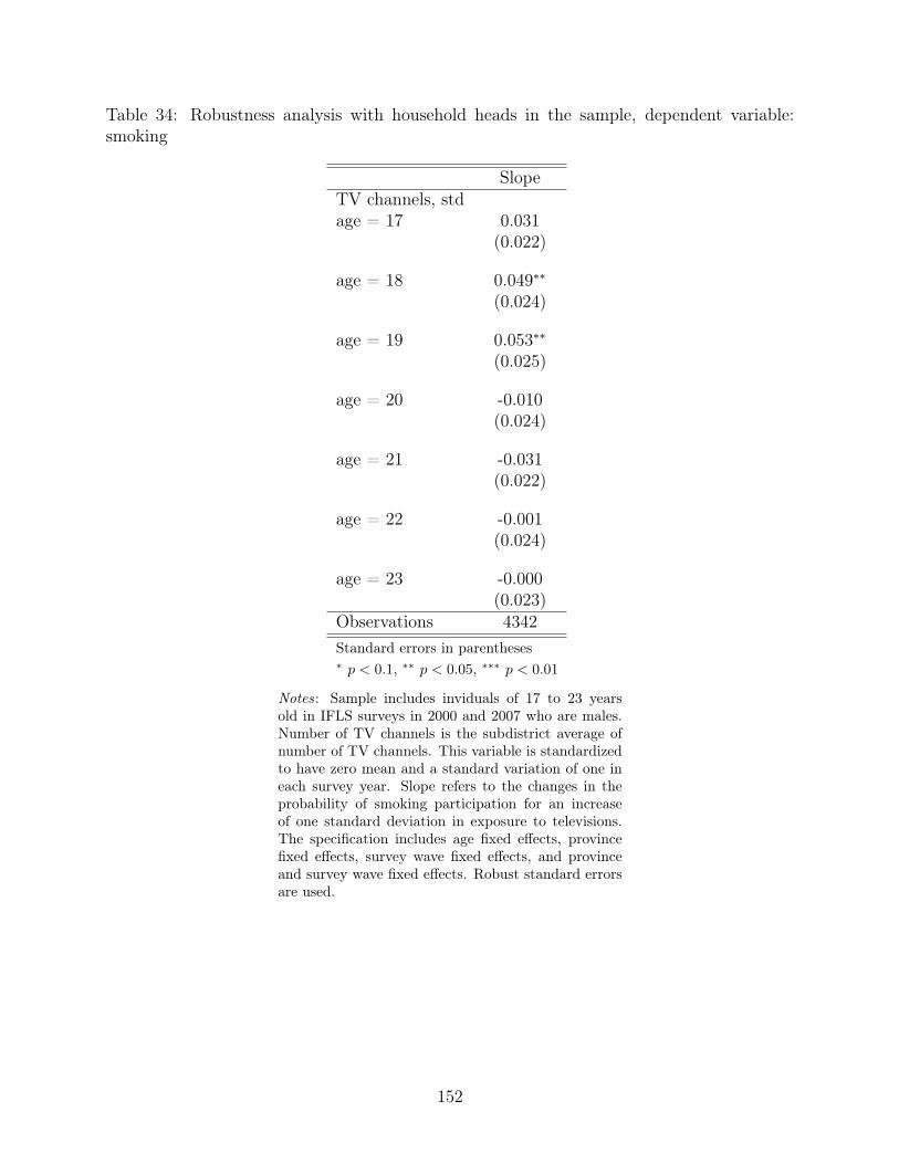
Table 34: Robustness analysis with household heads in the sample, dependent variable:smoking

SlopeTV channels, stdage = 17 0.031

(0.022)

age = 18 0.049∗∗(0.024)

age = 19 0.053∗∗(0.025)

age = 20 -0.010(0.024)

age = 21 -0.031(0.022)

age = 22 -0.001(0.024)

age = 23 -0.000(0.023)

Observations 4342Standard errors in parentheses∗ p < 0.1, ∗∗ p < 0.05, ∗∗∗ p < 0.01

Notes: Sample includes inviduals of 17 to 23 yearsold in IFLS surveys in 2000 and 2007 who are males.Number of TV channels is the subdistrict average ofnumber of TV channels. This variable is standardizedto have zero mean and a standard variation of one ineach survey year. Slope refers to the changes in theprobability of smoking participation for an increaseof one standard deviation in exposure to televisions.The specification includes age fixed effects, provincefixed effects, survey wave fixed effects, and provinceand survey wave fixed effects. Robust standard errorsare used.

152

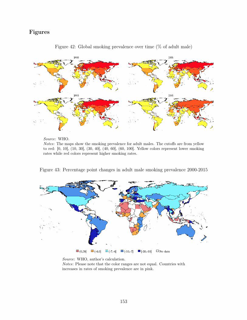
Figures

Figure 42: Global smoking prevalence over time (% of adult male)

Source: WHO.Notes: The maps show the smoking prevalence for adult males. The cutoffs are from yellowto red: [0, 10], (10, 30], (30, 40], (40, 60], (60, 100]. Yellow colors represent lower smokingrates while red colors represent higher smoking rates.

Figure 43: Percentage point changes in adult male smoking prevalence 2000-2015

Source: WHO, author’s calculation.Notes: Please note that the color ranges are not equal. Countries withincreases in rates of smoking prevalence are in pink.

153

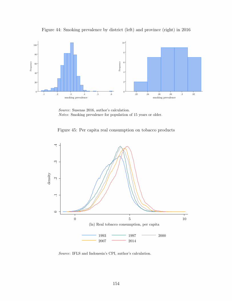
Figure 44: Smoking prevalence by district (left) and province (right) in 2016

0

20

40

60

80

100

Freq

uenc

y

.1 .2 .3 .4 .5 .6smoking prevalence

0

2

4

6

8

10

Freq

uenc

y

.22 .24 .26 .28 .3 .32smoking prevalence

Source: Susenas 2016, author’s calculation.Notes: Smoking prevalence for population of 15 years or older.

Figure 45: Per capita real consumption on tobacco products

0.1

.2.3

.4

dens

ity

0 5 10(ln) Real tobacco consumption, per capita

1993 1997 20002007 2014

Source: IFLS and Indonesia’s CPI, author’s calculation.

154

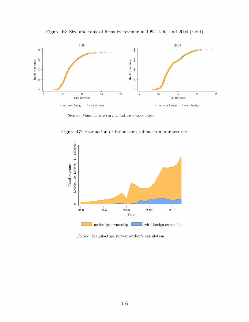
Figure 46: Size and rank of firms by revenue in 1994 (left) and 2004 (right)0

200

400

600

800

Ran

k in

rev

enue

5 10 15 20 25(ln) Revenue

not ever foreign ever foreign

1994

020

040

060

080

0

Ran

k in

rev

enue

5 10 15 20 25(ln) Revenue

not ever foreign ever foreign

2004

Source: Manufacture survey, author’s calculation.

Figure 47: Production of Indonesian tobbacco manufacturers

05.

0000

0e+

101.

0000

0e+

111.

5000

0e+

11To

tal r

even

ue

1990 1995 2000 2005 2010Year

no foreign ownership with foreign ownership

Source: Manufacture survey, author’s calculation.

155

Figure 48: Output per labor and revenue in 1994 (left) and in 2004 (right)5

1015

2025

(ln)

Rev

enue

4 6 8 10 12 14(ln) output per labor

not ever foreign ever foreign

1994

510

1520

25

(ln)

Rev

enue

5 10 15(ln) output per labor

not ever foreign ever foreign

2004

Source: Manufacture Survey, author’s calculation.

Figure 49: Comparison of estimated TFP

Notes: Each unit is estimated TFP for firm i in year t. Sample periodis 1990 to 2012. Estimated TFP labelled “TFP - Updated AK” refersto the estimated TFP using the coefficients of production functionfrom column “OP 1” on Table 26. Meanwhile, estimated TFP labeled“TFP - AK (2007)” refers to estimated TFP using the coefficients ofproduction from column “OP” on Table 26 as calculated by Amiti andKonings (2007) for the tobacco industry.

156

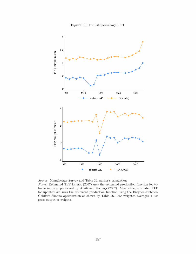
Figure 50: Industry-average TFP

Source: Manufacture Survey and Table 26, author’s calculation.Notes: Estimated TFP for AK (2007) uses the estimated production function for to-bacco industry performed by Amiti and Konings (2007). Meanwhile, estimated TFPfor updated AK uses the estimated production function using the Broyden-Fletcher-Goldfarb-Shanno optimization as shown by Table 26. For weighted averages, I usegross output as weights.

157

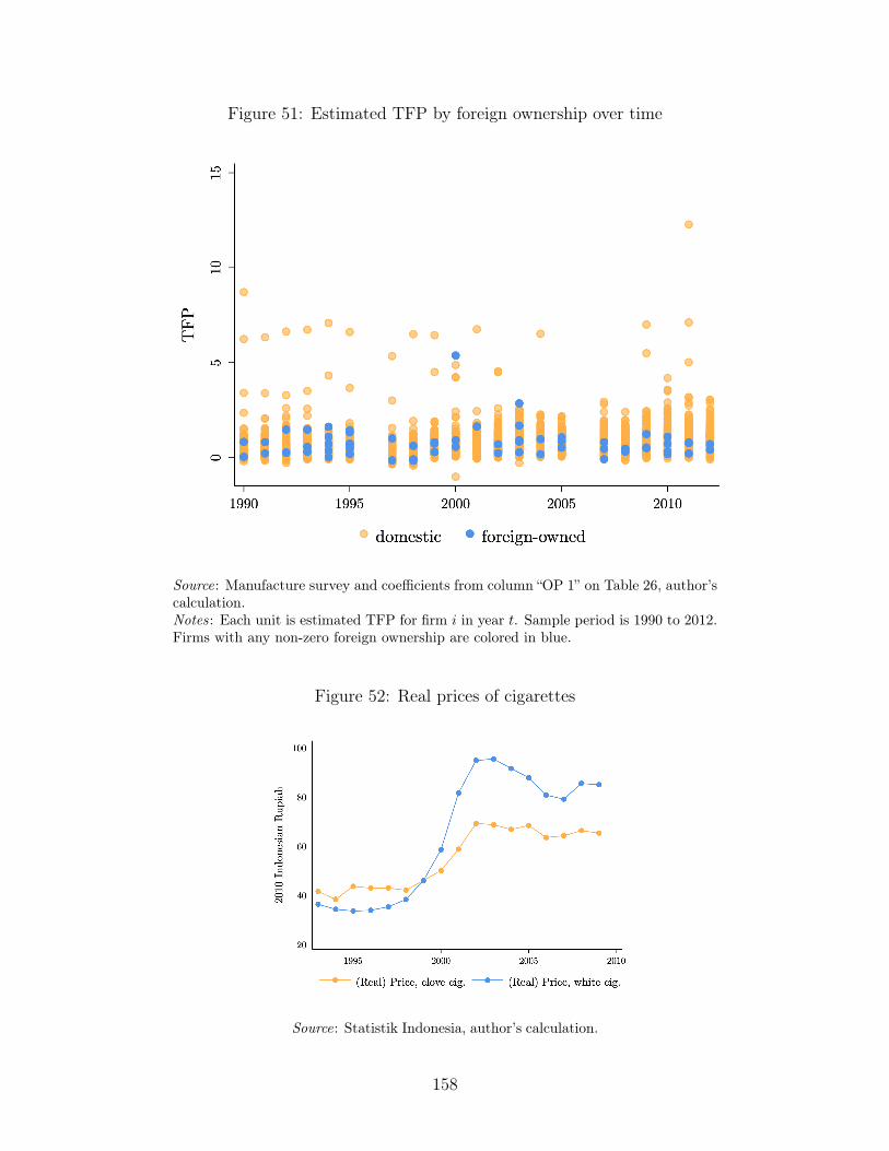
Figure 51: Estimated TFP by foreign ownership over time

Source: Manufacture survey and coefficients from column “OP 1” on Table 26, author’scalculation.Notes: Each unit is estimated TFP for firm i in year t. Sample period is 1990 to 2012.Firms with any non-zero foreign ownership are colored in blue.

Figure 52: Real prices of cigarettes

Source: Statistik Indonesia, author’s calculation.

158

Figure 53: Observed real price of cigarettes spent by households

Source: Indonesia Family Life Surveys, author’scalculation.

Figure 54: Variation in number of TV channels across districts

0

50

100

150

frequency

0 2 4 6 8 10

2003 2005

Source: Village Census 2003 and 2006, author’s calculation.Notes: Number of TV channels is the district average of number ofTV channels received in villages within a district.

159

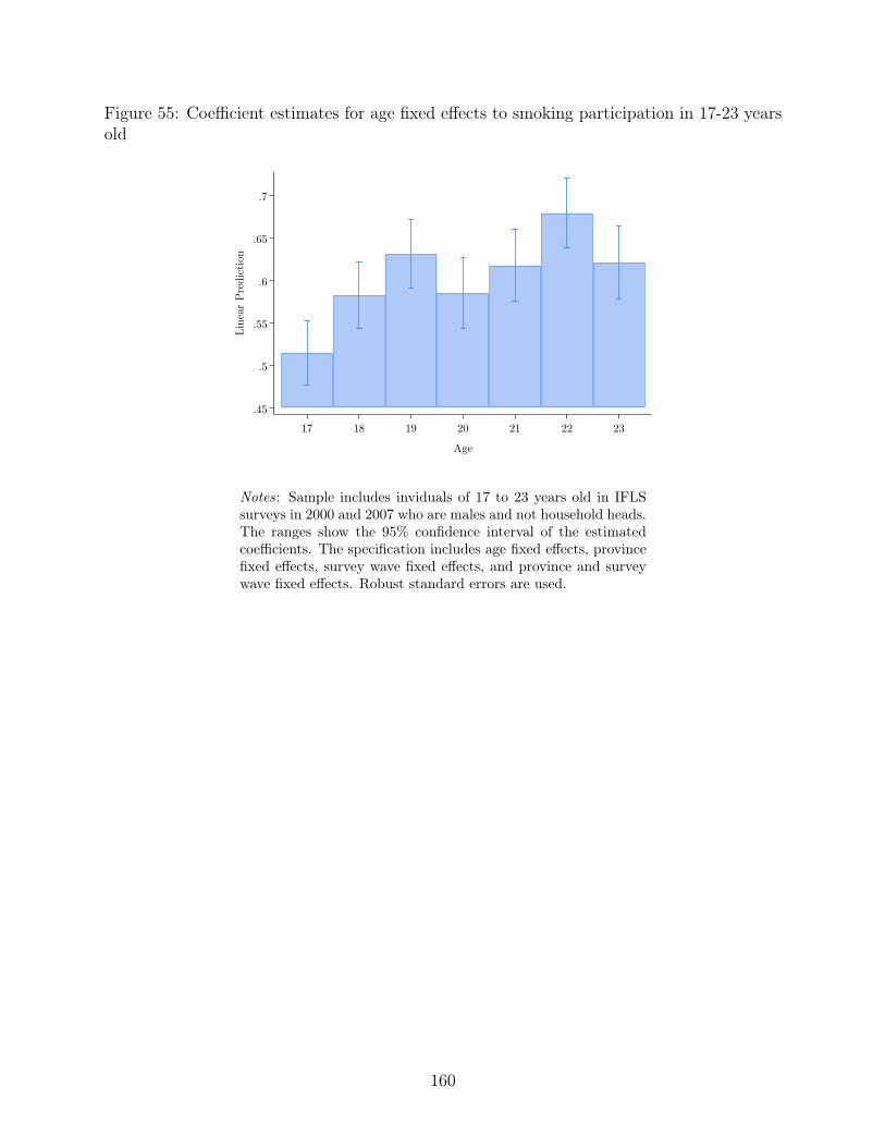
Figure 55: Coefficient estimates for age fixed effects to smoking participation in 17-23 yearsold

.45

.5

.55

.6

.65

.7

Line

ar P

redi

ctio

n

17 18 19 20 21 22 23

Age

Notes: Sample includes inviduals of 17 to 23 years old in IFLSsurveys in 2000 and 2007 who are males and not household heads.The ranges show the 95% confidence interval of the estimatedcoefficients. The specification includes age fixed effects, provincefixed effects, survey wave fixed effects, and province and surveywave fixed effects. Robust standard errors are used.

160

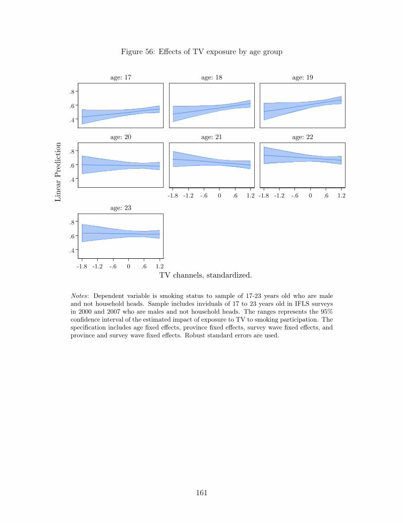
Figure 56: Effects of TV exposure by age group

.4

.6

.8

.4

.6

.8

.4

.6

.8

-1.8 -1.2 -.6 0 .6 1.2 -1.8 -1.2 -.6 0 .6 1.2

-1.8 -1.2 -.6 0 .6 1.2

age: 17 age: 18 age: 19

age: 20 age: 21 age: 22

age: 23

Line

ar P

redi

ctio

n

TV channels, standardized.

Notes: Dependent variable is smoking status to sample of 17-23 years old who are maleand not household heads. Sample includes inviduals of 17 to 23 years old in IFLS surveysin 2000 and 2007 who are males and not household heads. The ranges represents the 95%confidence interval of the estimated impact of exposure to TV to smoking participation. Thespecification includes age fixed effects, province fixed effects, survey wave fixed effects, andprovince and survey wave fixed effects. Robust standard errors are used.

161

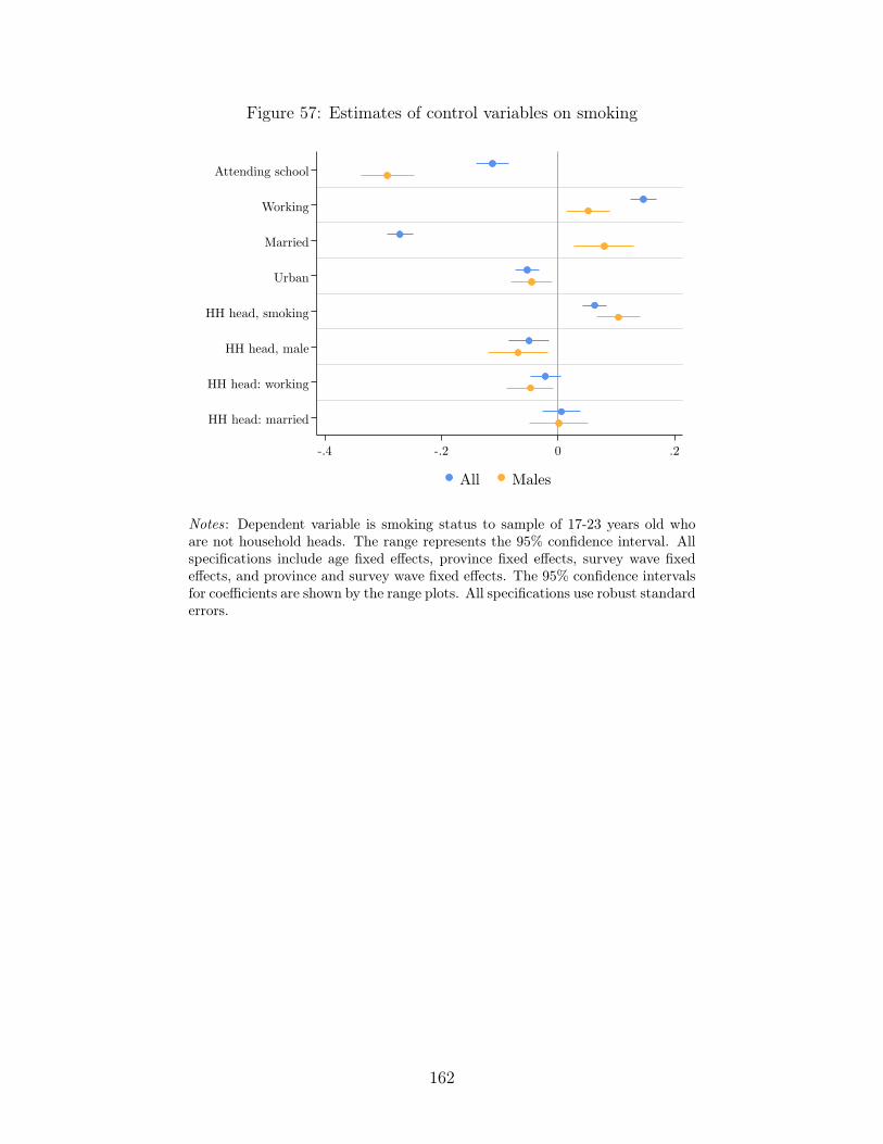
Figure 57: Estimates of control variables on smoking

Attending school

Working

Married

Urban

HH head, smoking

HH head, male

HH head: working

HH head: married

-.4 -.2 0 .2

All Males

Notes: Dependent variable is smoking status to sample of 17-23 years old whoare not household heads. The range represents the 95% confidence interval. Allspecifications include age fixed effects, province fixed effects, survey wave fixedeffects, and province and survey wave fixed effects. The 95% confidence intervalsfor coefficients are shown by the range plots. All specifications use robust standarderrors.

162

Data Appendix: Estimating Total Factor Productivity

In order to estimate firm-level total factor productivity (TFP), I replicate the estimation

strategy conducted by Amiti and Konings (2007), or henceforth AK. They estimate TFP

using the same dataset with the one that I use to analyze the tobacco industry in Indonesia,

i.e., the Indonesian Manufacturing Survey. AK analyzed thee TFP trend for the period

between 1991 to 2001 for each three-digit industry classification. AK used the Olley-Pakes

method and assumed that there are fixed costs in exporting and importing, as in Melitz

(2003). AK also took into account the effect of the Asian Financial Crisis in from 1997-1998

by including fixed effects for crisis. I follow AK’s strategy and add fixed costs of being a

foreign affiliates as in Helpman et al. (2004).

Let us assume that each firm i in year t operates with a Cobb-Douglas production function

as shown in equation 42 below. In producing output Yit, each firm combines several factors

of production: capital (K), labor (L), and materials (M). The firm’s level of productivity

is Ait.

Yit = AitLβlitK

βkit M

βmit (42)

I follow AK in performing the method introduced by Olley and Pakes (1992) in estimating

the production function. In particular, I estimate the log-linearized production function as

shown by equation 43, where x = ln(X), for each variable. TFP of firm i of industry k in

year t is then computed as the difference between its observed output, yit, and its estimated

output as shown in equation 44.

yit = β0 + βllit + βkkit + βmmit + εit (43)

tfpkit = yit − βllit − βkkit − βmmit (44)

163

Table 26 compares the estimated coefficients of each factors of production with the coeffi-

cients estimated by AK for the tobacco industry.60 These coefficients are relatively compara-

ble across different types of optimization methods. Figure 49 also confirms the comparability

between the estimated TFP using AK’s coefficients and the estimated TFP using updated

AK’s coefficients. I select the Broyden-Fletcher-Goldfarb-Shanno optimization method as

the basis of estimated TFP throughout the paper.

60I follow the suggestions from Márquez-Ramos (2020) in taking into account attrition in ManufacturingSurvey data and suggestions from Amiti and Konings (2007) in checking the consistency across the sampleperiod to improve confidence on the results.

164

References

Adão, R. (2015): “Worker heterogeneity, wage inequality, and international trade: Theory

and evidence from brazil,” Unpublished paper, MIT.

Adioetomo, S. M., T. Djutaharta, et al. (2005): “Cigarette consumption, taxation,

and household income: Indonesia case study,” .

Aldaz-Carroll, E. (2010): “A trade development report: boom, bust and up again,” Evo-

lution, Drivers and Impact of Commodity Prices: Implications for Indonesia: Executive

Summary. World Bank, Washington DC, 1.

Aldaz-Carroll, E., T. Slayton, and P. Timmer (2010): “Pricking the Price Bubble

to Avert a World Rice Crisis,” Background paper, World Bank, Washington, DC.

Allen, T. (2014): “Information frictions in trade,” Econometrica, 82, 2041–2083.

Amiti, M. and J. Konings (2007): “Trade liberalization, intermediate inputs, and pro-

ductivity: Evidence from Indonesia,” American Economic Review, 97, 1611–1638.

Anderson, K. and W. Martin (2011): “DP8494 Export Restrictions and Price Insulation

During Commodity Price Booms,” .

Argente, D., D. Fitzgerald, S. Moreira, and A. Priolo (2021): “How Do Firms

Build Market Share?” .

Arkolakis, C. (2010): “Market penetration costs and the new consumers margin in inter-

national trade,” Journal of political economy, 118, 1151–1199.

Artuc, E., D. Lederman, and G. Porto (2015): “A mapping of labor mobility costs in

the developing world,” Journal of International Economics, 95, 28–41.

Atkin, D. and D. Donaldson (2015): “Who’s getting globalized? The size and implica-

tions of intra-national trade costs,” Tech. rep., National Bureau of Economic Research.

165

Atkin, D. and A. K. Khandelwal (2020): “How Distortions Alter the Impacts of Inter-

national Trade in Developing Countries,” Annual Review of Economics.

Austin, K. G., A. Schwantes, Y. Gu, and P. S. Kasibhatla (2019): “What causes

deforestation in Indonesia?” Environmental Research Letters, 14, 024007.

Autor, D., D. Dorn, and G. H. Hanson (2013): “The China syndrome: Local labor

market effects of import competition in the United States,” American Economic Review,

103, 2121–68.

Baffes, J. and T. Haniotis (2010): “Placing the 2006/08 commodity price boom into

perspective,” World Bank Policy Research Working Paper.

Banerjee, A. V. and E. Duflo (2005): “Growth theory through the lens of development

economics,” Handbook of economic growth, 1, 473–552.

Bazzi, S. (2017): “Wealth heterogeneity and the income elasticity of migration,” American

Economic Journal: Applied Economics, 9, 219–55.

Becker, G., M. Grossman, and K. Murphy (1991): “Economics of Drugs: Rational

Addiction and the Effect of Price on Consumption,” American Economic Review, 81, 237–

241.

Becker, G. S., M. GRossMAN, and K. M. MURPHY (1994): “An Empirical Analysis

of Cigarette Addiction,” The American Economic Review, 84, 396–418.

Becker, G. S. and K. M. Murphy (1988): “A theory of rational addiction,” Journal of

political Economy, 96, 675–700.

Belk, R. W., K. D. Bahn, and R. N. Mayer (1982): “Developmental recognition of

consumption symbolism,” Journal of consumer research, 9, 4–17.

Bergquist, L. F. and M. Dinerstein (2020): “Competition and entry in agricultural

markets: Experimental evidence from Kenya,” American Economic Review, 110, 3705–47.

166

Bettcher, D. W., C. Subramaniam, E. G. Guindon, L. Soll, G. Grabman,

L. Joossens, A. L. Taylor, W. T. F. Initiative, et al. (2003): “Confronting the

tobacco epidemic in an era of trade liberalization,” Tech. rep., World Health Organization.

Bigsten, A., P. Collier, S. Dercon, M. Fafchamps, B. Gauthier, J. Willem Gun-

ning, A. Oduro, R. Oostendorp, C. Pattillo, M. Söderbom, et al. (2004): “Do

African manufacturing firms learn from exporting?” Journal of development studies, 40,

115–141.

Bouët, A. and D. L. Debucquet (2012): “Food crisis and export taxation: the cost of

non-cooperative trade policies,” Review of World Economics, 148, 209–233.

BPS (2019): Statistical Yearbook of Indonesia 2019, BPS-Statistics Indonesia.

Broda, C. and D. E. Weinstein (2006): “Globalization and the Gains from Variety,”

The Quarterly journal of economics, 121, 541–585.

Brown, R. S. (1978): “Estimating advantages to large-scale advertising,” The Review of

Economics and Statistics, 428–437.

Bryan, G. and M. Morten (2017): “The Aggregate Productivity Effects of Internal

Migration: Evidence from Indonesia,” Working Paper 23540, National Bureau of Economic

Research.

——— (2019): “The aggregate productivity effects of internal migration: Evidence from

indonesia,” Journal of Political Economy, 127, 2229–2268.

Burgess, R., M. Hansen, B. A. Olken, P. Potapov, and S. Sieber (2012): “The

political economy of deforestation in the tropics,” The Quarterly Journal of Economics,

127, 1707–1754.

Busch, J. and K. Ferretti-Gallon (2017): “What drives deforestation and what stops

it? A meta-analysis,” Review of Environmental Economics and Policy, 11, 3–23.

167

Bush, J., M. White, J. Kai, J. Rankin, and R. Bhopal (2003): “Understanding

influences on smoking in Bangladeshi and Pakistani adults: community based, qualitative

study,” Bmj, 326, 962.

Cavenaile, L. and P. Roldan-Blanco (2021): “Advertising, innovation, and economic

growth,” American Economic Journal: Macroeconomics, 13, 251–303.

Chaloupka, F. J. and K. E. Warner (1999): “The Economics of Smoking,” NBER

Working Paper.

Chaloupka, F. J., H. Wechsler, et al. (1997): “Price, tobacco control policies and

smoking among young adults,” Journal of Health Economics, 16, 359–373.

Chaney, T. (2008): “Distorted gravity: the intensive and extensive margins of international

trade,” American Economic Review, 98, 1707–21.

Costa, F., J. Garred, and J. P. Pessoa (2016): “Winners and losers from a

commodities-for-manufactures trade boom,” Journal of International Economics, 102, 50–

69.

Cotti, C., E. Nesson, and N. Tefft (2016): “The effects of tobacco control policies

on tobacco products, tar, and nicotine purchases among adults: Evidence from household

panel data,” American Economic Journal: Economic Policy, 8, 103–23.

Curtis, P. G., C. M. Slay, N. L. Harris, A. Tyukavina, and M. C. Hansen (2018):

“Classifying drivers of global forest loss,” Science, 361, 1108–1111.

Dawe, D. (2008): “Can Indonesia trust the world rice market?” Bulletin of Indonesian

Economic Studies, 44, 115–132.

De Loecker, J., P. K. Goldberg, A. K. Khandelwal, and N. Pavcnik (2016):

“Prices, markups, and trade reform,” Econometrica, 84, 445–510.

168

Deaton, A. (1997): The analysis of household surveys: a microeconometric approach to

development policy, The World Bank.

Dhingra, S. and S. Tenreyro (2020): “The rise of agribusiness and the distributional

consequences of policies on intermediated trade,” .

Diamond, R. (2016): “The Determinants and Welfare Implications of US Workers’ Diverg-

ing Location Choices by Skill: 1980-2000,” American Economic Review, 106, 479–524.

Dix-Carneiro, R. and B. K. Kovak (2017): “Trade liberalization and regional dynamics,”

American Economic Review, 107, 2908–46.

Donaldson, D. (2018): “Railroads of the Raj: Estimating the impact of transportation

infrastructure,” American Economic Review, 108, 899–934.

Edmond, C., V. Midrigan, and D. Y. Xu (2015): “Competition, markups, and the gains

from international trade,” American Economic Review, 105, 3183–3221.

Edwards, R. B. (2018): “Export agriculture and regional development: evidence from

Indonesia,” Tech. rep., mimeo.

Fan, J. (2019): “Internal geography, labor mobility, and the distributional impacts of trade,”

American Economic Journal: Macroeconomics, 11, 252–88.

Fane, G. and P. Warr (2008): “Agricultural protection in Indonesia,” Bulletin of Indone-

sian Economic Studies, 44, 133–150.

Farrell, M. J. (1952): “Irreversible demand functions,” Econometrica: Journal of the

Econometric Society, 171–186.

Feenstra, R. C. (1995): “Estimating the effects of trade policy,” Handbook of international

economics, 3, 1553–1595.

169

Fernández, A., A. González, and D. Rodriguez (2018): “Sharing a ride on the

commodities roller coaster: Common factors in business cycles of emerging economies,”

Journal of International Economics, 111, 99–121.

Fernández, A., S. Schmitt-Grohé, and M. Uribe (2017): “World shocks, world prices,

and business cycles: An empirical investigation,” Journal of International Economics, 108,

S2–S14.

——— (2020): “Does the Commodity Super Cycle Matter?” Tech. rep., National Bureau of

Economic Research.

Ferraro, P. J. and R. Simorangkir (2020): “Conditional cash transfers to alleviate

poverty also reduced deforestation in Indonesia,” Science Advances, 6, eaaz1298.

for Tobacco Free Kids, C. (2019): “Indonesia Tobacco Control Policies Fact Sheet,” .

Gilmore, A. B., G. Fooks, J. Drope, S. A. Bialous, and R. R. Jackson (2015):

“Exposing and addressing tobacco industry conduct in low-income and middle-income

countries,” The Lancet, 385, 1029–1043.

Giordani, P. E., N. Rocha, and M. Ruta (2016): “Food prices and the multiplier effect

of trade policy,” Journal of International economics, 101, 102–122.

Goldberg, P. K. and N. Pavcnik (2007): “Distributional effects of globalization in

developing countries,” Journal of economic Literature, 45, 39–82.

——— (2016): “The effects of trade policy,” in Handbook of commercial policy, Elsevier,

vol. 1, 161–206.

Hansen, M. C., P. V. Potapov, R. Moore, M. Hancher, S. A. Turubanova,

A. Tyukavina, D. Thau, S. Stehman, S. J. Goetz, T. R. Loveland, et al.

(2013): “High-resolution global maps of 21st-century forest cover change,” science, 342,

850–853.

170

Harrison, A. E. (1994): “Productivity, imperfect competition and trade reform: Theory

and evidence,” Journal of international Economics, 36, 53–73.

Headey, D. (2011): “Rethinking the global food crisis: The role of trade shocks,” Food

Policy, 36, 136–146.

Helpman, E., M. J. Melitz, and S. R. Yeaple (2004): “Export versus FDI with het-

erogeneous firms,” American economic review, 94, 300–316.

Holbrook, M. B. and R. M. Schindler (1989): “Some exploratory findings on the

development of musical tastes,” Journal of consumer research, 16, 119–124.

Kearney, M. S. and P. B. Levine (2015): “Media influences on social outcomes: The

impact of MTV’s 16 and pregnant on teen childbearing,” American Economic Review, 105,

3597–3632.

Kouvonen, A., M. Kivimäki, M. Virtanen, J. Pentti, and J. Vahtera (2005):

“Work stress, smoking status, and smoking intensity: an observational study of 46 190

employees,” Journal of Epidemiology & Community Health, 59, 63–69.

Kovak, B. K. (2013): “Regional effects of trade reform: What is the correct measure of

liberalization?” American Economic Review, 103, 1960–76.

Lee, K. and J. Eckhardt (2017): “The globalisation strategies of five Asian tobacco

companies: a comparative analysis and implications for global health governance,” Global

Public Health, 12, 367–379.

Lee, S., P. M. Ling, and S. A. Glantz (2012): “The vector of the tobacco epidemic:

tobacco industry practices in low and middle-income countries,” Cancer Causes & Control,

23, 117–129.

Levinsohn, J. (1993): “Testing the imports-as-market-discipline hypothesis,” Journal of

international Economics, 35, 1–22.

171

Lucas, R. E. (2015): “Internal migration in developing economies: An overview,” KNO-

MAD Working Paper, 6.

Marks, S. V. (2017): “Non-tariff trade regulations in Indonesia: Nominal and effective

rates of protection,” Bulletin of Indonesian Economic Studies, 53, 333–357.

Márquez-Ramos, L. (2020): “A Survey of Papers Using Indonesian Firm-Level Data: Re-

search Questions and Insights for Novel Policy-Relevant Research in Economics,” Bulletin

of Indonesian Economic Studies, 1–49.

McCulloch and Timmer (2008): “Rice policy in Indonesia: a special issue,” Bulletin of

Indonesian Economic Studies.

McCulloch, N. (2008): “Rice prices and poverty in Indonesia,” Bulletin of Indonesian

Economic Studies, 44, 45–64.

McMillan, M. S., D. Rodrik, and K. H. Welch (2002): “When economic reform goes

wrong: cashews in Mozambique,” Tech. rep.

Melitz, M. J. (2003): “The impact of trade on intra-industry reallocations and aggregate

industry productivity,” econometrica, 71, 1695–1725.

Méndez-Chacón, E. and D. Van Patten (2019): “Multinationals, Monopsony and Local

Development: Evidence from the United Fruit Company,” Tech. rep., Working Paper. 5.

Moore, R. L. and L. F. Stephens (1975): “Some communication and demographic

determinants of adolescent consumer learning,” Journal of Consumer Research, 2, 80–92.

Ng, N., L. Weinehall, and A. Öhman (2007): “’If I don’t smoke, I’m not a real man’ –

Indonesian teenage boys’ views about smoking,” Health education research, 22, 794–804.

Olken, B. A. (2009): “Do television and radio destroy social capital? Evidence from

Indonesian villages,” American Economic Journal: Applied Economics, 1, 1–33.

172

Olley, G. S. and A. Pakes (1992): “The dynamics of productivity in the telecommuni-

cations equipment industry,” Tech. rep.

Pavcnik, N. (2017): “The impact of trade on inequality in developing countries,” Tech. rep.,

National Bureau of Economic Research.

Pellegrina, H. S. and S. Sotelo (2020): “Migration, Specialization, and Trade: Evi-

dence from the Brazilian March to the West,” .

PMI, P. M. I. I. (2005): “Philip Morris International Inc. (PMI) announces agreement to

purchase 40 percent stake in PT HM Sampoerna Tbk,” https://www.pmi.com/media-

center/press-releases/details/philip-morris-international-inc.-(pmi)-announces-agreement-

to-purchase-40-stake-in-pt-hm-sampoerna-tbk-indonesia-s-third-largest-tobacco-company,

accessed: 9 July 2021.

Qaim, M., K. T. Sibhatu, H. Siregar, and I. Grass (2020): “Environmental, economic,

and social consequences of the oil palm boom,” Annual Review of Resource Economics,

12, 321–344.

Redding, S. J. (2016): “Goods trade, factor mobility and welfare,” Journal of International

Economics, 101, 148 – 167.

Resosudarmo, B. and D. Hartono (2020): “Inter-Province Input Output Table,” Tech.

rep., ANU.

Resosudarmo, BP, D. and D. Nurdianto (2008): “Inter-Island Economic Linkages and

Connections in Indonesia,” Economics and Finance Indonesia.

Restuccia, D. and R. Rogerson (2017): “The causes and costs of misallocation,” Journal

of Economic Perspectives, 31, 151–74.

Ross, H. and F. Chaloupka (2006): “Economic policies for tobacco control in developing

countries,” salud pública de méxico, 48, 113–120.

173

Sahadewo, G. A., J. Drope, Q. Li, N. Nargis, and F. Witoelar (2021): “Tobacco

or not tobacco: Predicting farming households’ income in Indonesia,” Tobacco control, 30,

320–327.

Sen, U. and A. Basu (2000): “Factors influencing smoking behavior among adolescents,”

Asian Pac J Cancer Prev, 1, 305–309.

Setyonaluri, D., S. M. Adioetomo, S. Barber, and A. Ahsan (2008): Tobacco

Economics in Indonesia, International Union Against Tuberculosis and Lung Disease.

Seymour, F. and N. L. Harris (2019): “Reducing tropical deforestation,” Science, 365,

756–757.

Shorrocks, A. F. (2013): “Decomposition procedures for distributional analysis: a unified

framework based on the Shapley value,” Journal of Economic Inequality, 11, 99.

Sienaert, A., A. Lnu, M. Adriani, M. Crystallin, F. Fitrani, A. Ihsan, E. A.

Mileva, V. Vulovic, E. T. Vashakmadze, M. M. Wihardja, et al. (2015): “In-

donesia economic quarterly: High expectations,” Tech. rep., The World Bank.

Sim, A. (2020): “Import Restriction, Price Shock, and Local Policy Responses: Evidence

from Indonesia,” Ph.D. thesis, Cornell University.

Sotelo, S. (2015): “Domestic trade frictions and agriculture,” in University of Michigan

Research Seminar in International Economics Discussion Paper, vol. 641.

Strotz, R. H. (1955): “Myopia and inconsistency in dynamic utility maximization,” The

review of economic studies, 23, 165–180.

Stuckler, D., M. McKee, S. Ebrahim, and S. Basu (2012): “Manufacturing epidemics:

the role of global producers in increased consumption of unhealthy commodities including

processed foods, alcohol, and tobacco,” PLoS Med, 9, e1001235.

174

Thaler, R. H. and H. M. Shefrin (1981): “An economic theory of self-control,” Journal

of political Economy, 89, 392–406.

The Lancet (2015): “What will it take to create a tobacco-free world?” The Lancet, 385,

915.

Thomas, L. G. (1989): “Advertising in consumer goods industries: Durability, economies

of scale, and heterogeneity,” The Journal of Law and Economics, 32, 163–193.

Thomas, M. (2019): “Was television responsible for a new generation of smokers?” Journal

of Consumer Research, 46, 689–707.

Tombe, T. and X. Zhu (2019): “Trade, migration, and productivity: A quantitative

analysis of china,” American Economic Review, 109, 1843–72.

Topalova, P. (2010): “Factor immobility and regional impacts of trade liberalization:

Evidence on poverty from India,” American Economic Journal: Applied Economics, 2,

1–41.

Vibrianti, D. (2014): “The Effect of Socio-Demographic Variables on Household Saving

in Indonesia (The Analysis of the 2007 IFLs Data),” Developing Country Studies. Vol, 4,

2225–0565.

Warner, K. E., J. Butler, K. M. Cummings, C. D’Onofrio, R. M. Davis, B. Flay,

M. McKinney, M. L. Myers, M. Pertschuk, R. G. Robinson, et al. (1992):

“Report of the tobacco policy research study group on tobacco marketing and promotion,”

Tobacco Control, 1, S19–S23.

Warr, P. (2005): “Food policy and poverty in Indonesia: a general equilibrium analysis,”

Australian Journal of Agricultural and Resource Economics, 49, 429–451.

——— (2008): “The transmission of import prices to domestic prices: an application to

Indonesia,” Applied Economics Letters, 15, 499–503.

175

Warr, P. and A. A. Yusuf (2014): “World food prices and poverty in Indonesia,” Aus-

tralian Journal of Agricultural and Resource Economics, 58, 1–21.

Warr, P. G. (2011): “Food security vs. Food self-sufficiency: the Indonesian case,” Crawford

School Research Paper.

Wellman, R. J., D. B. Sugarman, J. R. DiFranza, and J. P. Winickoff (2006):

“The extent to which tobacco marketing and tobacco use in films contribute to children’s

use of tobacco: a meta-analysis,” Archives of pediatrics & adolescent medicine, 160, 1285–

1296.

Wen, C., S. Tsai, T. Cheng, C. Hsu, T. Chen, and H. Lin (2005): “Role of parents

and peers in influencing the smoking status of high school students in Taiwan,” Tobacco

control, 14, i10–i15.

Westman, M., D. Eden, and A. Shirom (1985): “Job stress, cigarette smoking and

cessation: the conditioning effects of peer support,” Social science & medicine, 20, 637–

644.

Wheeler, D., D. Hammer, R. Kraft, S. Dasgupta, and B. Blankespoor (2013):

“Economic dynamics and forest clearing: A spatial econometric analysis for Indonesia,”

Ecological Economics, 85, 85–96.

WHO (2015): WHO global report on trends in prevalence of tobacco smoking 2015, World

Health Organization.

——— (2020): “Tobacco,” https://www.who.int/health-topics/tobacco, accessed: 14 Nov

2020.

——— (2021): “Tobacco,” https://fctc.who.int/who-fctc/overview, accessed: 8 July 2021.

WHO, W. T. F. Initiative, et al. (2012): Confronting the tobacco epidemic in a new

era of trade and investment liberalization, World Health Organization.

176

WHO et al. (2019): WHO report on the global tobacco epidemic, 2019: Offer help to quit

tobacco use, World Health Organization.

Witoelar, F., J. Strauss, and P. Rukumnuaykit (2005): “Smoking behavior among

youth in a developing country: The case of Indonesia,” Princeton University. Princeton,

NJ. Available online at http://paa2006. princeton. edu/download. aspx.

177