Error Estimation in Smoothed Particle Hydrodynamics and a New Scheme forSecond Derivatives

R. Fatehia, M.T. Manzaria,∗

aCenter of Excellence in Energy Conversion, School of Mechanical Engineering, Sharif University of Technology, Tehran, Iran.

Abstract

Several schemes for discretization of first and second derivatives are available in Smoothed Particle Hydrodynamics(SPH). Here, four schemes for approximation of the first derivative and three schemes for the second derivativeare examined using a theoretical analysis based on Taylor series expansion both for regular and irregular particledistributions. Estimation of terms in the truncation errors shows that only the renormalized (the first-order consistent)scheme has acceptable convergence properties to approximate the first derivative. None of the second derivativeschemes has the first-order consistency. Therefore, they converge only when the particle spacing decreases muchfaster than the smoothing length of the kernel function.

In addition, using a modified renormalization tensor, a new SPH scheme is presented for approximating secondderivatives that has the property of first-order consistency. To assess the computational performance of the proposedscheme, it is compared with the best available schemes when applied to a 2D heat equation. The numerical resultsshow at least one order of magnitude improvement in accuracy when the new scheme is used. In addition, the newscheme has higher-order convergence rate on regular particle arrangements even for the case of only four particles inthe neighborhood of each particle.

Key words: Smoothed Particle Hydrodynamics (SPH), Second derivative, First-order Consistency, Truncation Error,Convergence

1. Introduction

Smoothed Particle Hydrodynamics (SPH) was first introduced by Gingold and Monaghan [1] and Lucy [2] in1977 and has emerged as a viable numerical scheme in the context of mesh free methods. The method has beensuccessfully applied to numerous scientific applications. Like most other numerical schemes, however, the SPHmethod experiences continual theoretical and technical developments. In particular, various numerical schemes havebeen devised to approximate the first and second spatial derivative terms which appear in the governing equations.A typical first derivative term is the pressure gradient which plays an important role in the flow equations. Variousnumerical schemes have been proposed to deal with such terms including both symmetric [3] and non-symmetric [4]forms. On the other hand, second derivatives are manifested typically in flow problems as viscous terms. At leastthree different types of schemes have been introduced to discretize such second derivatives [5]. The computationalperformance of various methods have been investigated and reported in [4, 6, 7, 5]. Despite these valuable efforts, itseems that a sound and fairly general theoretical analysis on this issue is yet to be presented.

To have a numerical method of a desired order of accuracy, it is required that each term in the differential equationbe discretized with a certain order of accuracy. In the mesh-free methods like SPH, the spatial derivatives are ofparticular importance. Another property of numerical methods which is related to accuracy is the rate of convergence.The convergence rate of a numerical method depends on the leading error term in its modified equation. Practically,each term in the governing equation can be discretized using different methods for computation of derivatives which

∗Corresponding authorEmail addresses: mtmanzari@sharif.edu (M.T. Manzari)

Preprint submitted to Computers &Mathematics with Applications August 13, 2010

potentially lead to errors of different magnitudes. Therefore, the choice of appropriate approximations for variousderivative terms is of crucial importance especially in the SPH method.

In the context of the SPH method, Monaghan and Lattanzio [8] showed that the error of the so-called integralinterpolant of SPH is of second order in terms of smoothing length h and also demonstrated that using a higher-orderkernel function can improve the accuracy to h4. This argument is however valid only for the continuous interpolationof field functions. In the discrete summations which are used in the computation of derivatives, there are also othersources of errors. In 1987, Mas-Gallic and Raviart [9] proved that a discrete form for nth derivatives in SPH has anerror of order h2 + h−n(∆/h)2 where ∆ is the distance between the neighboring particles in one dimension. This meansthat decreasing the smoothing length h does not lead to convergence unless the particle spacing ∆ decreases muchfaster than h. The dependency of convergence of the SPH method on both particle spacing ∆ and smoothing lengthh was also confirmed in the work of Ben Moussa and Vila [10]. They also showed that to obtain a convergent firstderivative approximation in the SPH method, it is required to satisfy both h −→ 0 and ∆/h2 −→ 0 conditions.

Another property associated with the numerical schemes is the notion of consistency which is a requirement forconvergence. Unlike grid-based methods, in general, evaluation of consistency is not a straightforward matter formesh-free methods. For these types of methods, Belytschko et al. [11] have defined the order of consistency as themaximum order of a polynomial which is represented exactly by an approximation technique. Here, it is shown thatthe order of accuracy of a scheme is highly affected by its order of consistency.

An extra difficulty arises when one deals with moving particles. In such cases, the spacing between particlescan continually change and therefore the assumption of equally spaced particle distribution is no longer valid. Asa result, the error estimates based on regular arrangement of particles need to be modified. Colagrossi reported thatthe convergence rate of a method can be as much as one to three orders of magnitude lower than that for orderedparticles [12]. Quinlan et al. [13] studied convergence of two SPH schemes for the computation of the first derivativein one dimension. They calculated the derivative of a sinusoidal function using the standard and first-order consistentSPH schemes when particle arrangement is either ordered or disordered. By investigating the numerical errors, theyshowed that for a uniform distribution, the error of the standard scheme decays as a function of h2 up to a certain limitwhich is itself a function of the fraction h/∆. In the case of the first-order consistent scheme on an ordered particledistribution, however, the method retains its second-order convergence. When the particles are disordered, error of thestandard scheme can grow as h is reduced. This highlights the complex behavior of the SPH even for approximationof the first derivative of a fairly simple function.

Concerning the accuracy of second derivative approximations in SPH, there are even fewer works in the literature.Fatehi et al. [14] compared three forms of discretization of the second derivative for a heat-like equation in onedimension. Graham and Hughes [7] numerically studied a SPH scheme in 1D and 2D for random placement ofparticles and concluded that the method converges only in the case of regular particle arrangement and for specialvalues of h/∆.

In the present paper, a mathematical framework is presented to compare the truncation errors and convergenceproperties of general SPH schemes for discretization of both first and second spatial derivatives. Four schemes for thefirst derivative and three schemes for the second derivative are considered. The schemes are briefly presented in thefollowing section. Next, the truncation error associated with each scheme is found using a Taylor series expansion. Insection 4, the order of magnitude of different terms in the truncation errors are estimated both for regular and irregularparticle arrangements. Finally, a new scheme for approximation of the second derivative is introduced in section 5and its performance is assessed by solving a 2D heat equation in section 6.

2. SPH Approximation of Derivatives

SPH is a Lagrangian particle-based method in which each computational point is a part of substance and is calledparticle. The SPH method is built on the notion of interpolation. For an arbitrary field function u the interpolatedvalue ⟨u⟩ in terms of the values at neighboring particles u j is found from

⟨u (r)⟩ =∑

j

ω ju jW(r − r j, h), (1)

2

where ω j is the weight or the volume of neighboring particle j and W represents the smoothing or kernel functionwhich is a smoothed version of the Dirac delta function and is positive for

∣∣∣r − r j

∣∣∣ < h with a compact support ofradius h [1].

Several techniques have been used in SPH to discretize the first and the second spatial derivatives. In this section,a number of frequently used schemes are summarized.

2.1. First derivativeThe first derivative of field function u can be approximated using either of the following schemes.Scheme F1 Standard scheme as first introduced by Monaghan [1]:

⟨∇u⟩i =∑

j

ω ju j∇iWi j, (2)

where Wi j = W(ri − r j, h) denotes the kernel function of particle i evaluated at r j the position of particle j. Also, ∇i

denotes differentiation in space with respect to the coordinates on particle i. In the following, the subscript is droppedfor the sake of simplicity.

Scheme F2 Modified version of Scheme F1:

⟨∇u⟩i =∑

j

ω j

(u j − ui

)∇Wi j. (3)

The advantage of this form over the standard one is that here, the first derivative of a constant function is exactly zero.This property is known as zeroth-order consistency.

Scheme F3 Symmetric form⟨∇u⟩i =

∑j

ω j

(u j + ui

)∇Wi j, (4)

is not zeroth-order consistent but it is usually used for discretization of the pressure gradient in the Navier-Stokesand Euler equations. The advantage is that using symmetric forms to discretize forces leads to local momentumconservation.

Scheme F4 Renormalized scheme as introduced by Randles and Libersky [15], Bonet and Lok [16] and Vila [17]:

⟨∇u⟩i =∑

j

ω j

(u j − ui

)Bi · ∇Wi j, (5)

where

Bi = −∑

j

ω jri j∇Wi j

−1

, (6)

is the renormalization tensor in which ri j = ri − r j is the distance vector of particles i and j. Since ∇Wi j is parallelto ri j, the renormalization tensor B is symmetric. An advantage of this method is that it is first-order consistent. Thismeans by definition that the scheme can exactly calculate the gradient of a linear function. Since this form is notsymmetric, conservation is not guaranteed. In 2005, Vila [18] suggested a symmetric version of the renormalizedscheme which is conservation preserving but it is not first-order consistent any more.

2.2. Second derivativeThere are also different forms to approximate the second derivative ⟨∇ · ∇u⟩i in the context of SPH. In the follow-

ing, three forms are described.Scheme S1 Naturally, one can use each of the schemes defined in section 2.1 to obtain a numerical scheme for the

second derivative. These give⟨∇ · ∇u⟩i =

∑j

ω j ⟨∇u⟩ j · ∇Wi j, (7)

⟨∇ · ∇u⟩i =∑

j

ω j

(⟨∇u⟩ j − ⟨∇u⟩i

)· ∇Wi j, (8)

3

or⟨∇ · ∇u⟩i =

∑j

ω j

(⟨∇u⟩ j + ⟨∇u⟩i

)· ∇Wi j. (9)

These forms were used to include physical viscosity in astrophysical problems [19, 20] and to solve 2D heat conduc-tion problems [21] and to study low-Reynolds number incompressible flows [16, 22]. The above forms can be namedas double summation forms as they require two summation evaluations. Flebbe et al. [19] and Watkins et al. [20] usedthe scheme in Eq. (9) for astrophysical problems and reported some non-physical oscillations in their solution. Fatehiet al. [14] showed that using these schemes in a heat-like equation with discontinuous initial condition, essentiallyleads to oscillatory solutions. The reason can be explained by referring to the extension of the computational stencilwhich is a well-known issue in grid-based methods [23].

Scheme S2 Another way to construct second derivative is to use the second derivative of the kernel function.Using Eqs. (2), (3), and (4), one obtains

⟨∇ · ∇u⟩i =∑

j

ω ju j∇ · ∇Wi j, (10)

⟨∇ · ∇u⟩i =∑

j

ω j

(u j − ui

)∇ · ∇Wi j, (11)

and⟨∇ · ∇u⟩i =

∑j

ω j

(u j + ui

)∇ · ∇Wi j. (12)

These forms were used by Takeda et al. [24] and Chaniotis et al. [25]. Fatehi and coworkers [14] showed that tohave monotonicity preserving, when using Eq. (12), the inflection point of the kernel function must be farther than thenearest neighboring particle. Since usual smoothing functions have inflection points between 0 and h, in a complicatedflow problem, it is hard to satisfy the above condition. It should be noted that, this discussion is for ordered particles.As reported by Monaghan [3], the form of Eq. (10) is also very sensitive to particle distribution.

Scheme S3 Brookshaw [26] suggested a finite-difference-like form for the first derivation and a SPH summationfor the second derivative as

⟨∇ · ∇u⟩i =∑

j

2ω jui − u j

ri jei j · ∇Wi j, (13)

where ri j =∣∣∣ri j

∣∣∣ and ei j =ri j

ri jis a unit vector in the inter-particle direction. Basa et al. [5] showed that this technique

is best among the available SPH schemes for approximation of the second derivatives.

3. Error Analysis

In this section, truncation errors of the above mentioned schemes are assessed. Consider the multi-dimensionalTaylor series expansion of the field function u at r j about point ri as

u j =

∞∑m=0

[1

m!

((r j − ri) · ∇

)mu]

r=ri

. (14)

The first four terms are

u j = ui − ri j · ∇u∣∣∣i +

12

(ri j · ∇

) (ri j · ∇

)u∣∣∣∣i− 1

6

(ri j · ∇

) (ri j · ∇

) (ri j · ∇

)u∣∣∣∣i+ · · · ,

where subscript i denotes evaluation of the function and its derivatives at point ri. Equivalently, it can be rewritten as

u j = ui − ri j · ∇u|i +12

ri jri j : ∇∇u|i −16

ri jri jri j... ∇∇∇u|i + · · · , (15)

4

where the operator “:” denotes double dot, scalar, or inner product of second-order tensors. Similarly, triple dotproduct of two third-order tensors X and Y can be defined as

X...Y = Xαβγeαeβeγ

...Yδληeδeλeη (16)≡ XαβγYαβγ.

Substituting (15) in the schemes of section 2, one can evaluate the truncation error of each scheme. This iselaborated in the following.

3.1. First derivative

Considering scheme F1 (Eq. (2)) and using Eq. (15), one obtains

⟨∇u⟩i =∑

j

ω j

(ui − ri j · ∇u|i +

12

ri jri j : ∇∇u|i + · · ·)∇Wi j.

Since ui, ∇u|i, · · · are constant with respect to j, the above equation can be written as

⟨∇u⟩i = ui

∑j

ω j∇Wi j − ∇u|i ·∑

j

ω jri j∇Wi j +12∇∇u|i :

∑j

ω jri jri j∇Wi j + · · · .

Therefore, the truncation error Eri is obtained as

Eri ≡ ⟨∇u⟩i − ∇u|i

= ui

∑j

ω j∇Wi j − ∇u|i ·I +∑

j

ω jri j∇Wi j

+ 12∇∇u|i :

∑j

ω jri jri j∇Wi j + · · · .

Rearranging and keeping the first two terms, one obtains

Eri = ui

∑j

ω j∇Wi j + ∇u|i ·(B−1

i − I)+ · · · , (17)

in which I is the second-order unitary tensor. Eq. (17) shows that the first term in truncation error of the standardscheme is proportional to ui. Although the coefficient

∑j ω j∇Wi j can vanish in the case of ordered particle arrange-

ment, in general, it is non-zero. The order of magnitude of this term is investigated in the next section. The appearanceof ui and even ∇u|i cause a great difficulty because when a constant u0 is added to all points, the error grows pro-portionally. Also the error increases when one approximates a function with a large first derivative ∇u|i. It is notacceptable that the truncation error of a derivative approximation includes derivatives of the same order or lowerorders.

Similar behavior is observed when using scheme F3. In this case, the truncation error becomes

Eri = 2ui

∑j

ω j∇Wi j + ∇u|i ·(B−1

i − I)+ · · · , (18)

in which the multiplier of the first term has been doubled. In the case of Navier-Stokes equations, when the pressuregradient is discretized in this manner, the whole solution depends on the value of reference pressure P0 [27]. Thus,to have a reasonable result, P0 needs to be tuned for each problem. The culprit is the existence of ui in the truncationerror.

In the case of scheme F2 (Eq. (3)) the truncation error becomes independent of ui and one obtains

Eri = ∇u|i ·(B−1

i − I)+

12∇∇u|i :

∑j

ω jri jri j∇Wi j + · · · . (19)

5

The disappearance of ui is equivalent to achieving zeroth-order consistency. In addition, Eq. (19) shows that theaccuracy of this technique is one order of magnitude higher than those of both F1 and F3 schemes. However, schemeF2 still suffers from the existence of ∇u|i in the truncation error of ⟨∇u⟩i.

In a similar way, it can be shown that the truncation error of the Renormalized scheme (scheme F4) is

Eri =12∇∇u|i :

∑j

ω jri jri jBi · ∇Wi j −16∇∇∇u|i

...∑

j

ω jri jri jri jBi · ∇Wi j + · · · . (20)

Here, the lowest-order term includes the second derivative. This is why the scheme can exactly predict the firstderivative of a linear function, an important property which cannot be seen in all other known SPH schemes.

3.2. Second derivativeAs mentioned before, all techniques in the category of scheme S1 have difficulties because of the notion of

extending computational stencil. This is also visible in the truncation errors. For example, assume that the firstderivatives in Eqs. (7) to (9) are calculated using Eq. (3) (scheme F2). Thus,

⟨∇u⟩i = ∇u|i · B−1i +

12∇∇u|i :

∑j

ω jri jri j∇Wi j + · · · ,

and⟨∇u⟩ j = ∇u| j · B−1

j +12∇∇u| j :

∑k

ωkr jkr jk∇W jk + · · · .

where subscript k denotes neighbors of particle j. But from Taylor series expansion, one has

∇u| j = ∇u|i − ri j · ∇∇u|i +12

ri jri j : ∇∇∇u|i + · · · ,

and∇∇u| j = ∇∇u|i − ri j · ∇∇∇u|i +

12

ri jri j : ∇∇∇∇u|i + · · · .

Therefore,

⟨∇u⟩ j = ∇u|i · B−1j − B−1

j · ∇∇u|i · ri j +12∇∇u|i :

∑k

ωkr jkr jk∇W jk

+ · · · ,Substituting this in Eq. (7) leads to

⟨∇ · ∇u⟩i = ∇u|i ·∑

j

ω jB−1j · ∇Wi j +

∑j

ω jB−1j · ∇∇u|i · ri j · ∇Wi j (21)

+12∇∇u|i :

∑j

ω j

∑k

ωkr jkr jk∇W jk

· ∇Wi j + · · · .

Keeping in mind that B approximates I, one can conclude that the multiplier of ∇ · ∇u|i is near unity. So, the truncationerror is

Eri = ∇u|i ·∑

j

ω jB−1j · ∇Wi j +

∑j

ω jB−1j · ∇∇u|i · ri j · ∇Wi j (22)

+ ∇∇u|i :

12

∑j

ω j

∑k

ωkr jkr jk∇W jk

· ∇Wi j − I

+ · · · .

There are two problems. The first problem is the appearance of ∇u|i which is similar to the difficulties discussedpreviously. The other problem is the summation on neighbors k of each neighboring particle j. In a heat-like equation,

6

this can result in two or more decoupled sets of algebraic equations which leads to non-physical oscillations in thesolutions. Note that if schemes F1 or F3 were used for the first derivative approximation, the condition was evenworse. In those situations, the truncation error would have a leading term involving ui.

In a similar fashion, the truncation errors associated with equations (8) and (9) are obtained as

Eri = ∇u|i ·∑

j

ω j

(B−1

j − B−1i

)· ∇Wi j +

∑j

ω jB−1j · ∇∇u|i · ri j · ∇Wi j (23)

+ ∇∇u|i :

12

∑j

ω j

∑k

ωkr jkr jk∇W jk −∑

j

ω jri jri j∇Wi j

· ∇Wi j − I

+ · · · ,

and

Eri = ∇u|i ·∑

j

ω j

(B−1

j + B−1i

)· ∇Wi j +

∑j

ω jB−1j · ∇∇u|i · ri j · ∇Wi j (24)

+ ∇∇u|i :

12

∑j

ω j

∑k

ωkr jkr jk∇W jk +∑

j

ω jri jri j∇Wi j

· ∇Wi j − I

+ · · · .

Note that although the use of Eq. (8) improves the accuracy of the technique by substituting B−1j with

(B−1

j − B−1i

)in

Eq. (23), it still suffers from the same flaws. So, this scheme is not studied further in the present paper.Scheme S2 does not have the problem of extended stencil. Instead, Eqs. (10) and (12) suffer from the appearance

of ui in the truncation error of ⟨∇ · ∇u⟩i. For example, the truncation error of Eq. (10) is

Eri =ui

∑j

ω j∇ · ∇Wi j − ∇u|i ·∑

j

ω jri j∇ · ∇Wi j (25)

+ ∇∇u|i :

12

∑j

ω jri jri j∇ · ∇Wi j − I

+ · · · .The main problem here is that the term

∑j ω j∇ · ∇Wi j does not easily converge to zero. See the discussion in the next

section for more details.Using the scheme given by Eq. (11) one obtains a better condition:

Eri = − ∇u|i ·∑

j

ω jri j∇ · ∇Wi j + ∇∇u|i :

12

∑j

ω jri jri j∇ · ∇Wi j − I

+ · · · . (26)

Although the leading term in the error is now an order of magnitude lower than that of Eq. (25), the problem ofexistence of ∇u|i is yet remaining.

Scheme S3 also only uses ui and u j and thus does not have the problem of non-physical oscillations. For Eq. (13),substituting from Eq. (15) results in

⟨∇ · ∇u⟩i =∑

j

2ω j

(ei j · ∇u|i −

12

ri jei j : ∇∇u|i +16

ri jri jei j... ∇∇∇u|i + · · ·

)ei j · ∇Wi j.

Since ∇Wi j =∂Wi j

∂ri jei j and ei j · ei j = 1, the truncation error can be simplified as

Eri =2 ∇u|i ·∑

j

ω j∇Wi j + ∇∇u|i :(B−1

i − I)

(27)

+13∇∇∇u|i

...

∑j

ω jri jri j∇Wi j

+ · · · .As can be seen, the error still includes the first derivative term ∇u|i. In section 5, a new scheme will be presentedwhich resolves this difficulty.

7

4. Error Estimation

In the previous section, the truncation errors of a number of SPH schemes were obtained in terms of summationsof the gradient of the kernel function such as

∑j ω j∇Wi j,

∑j ω jri j∇Wi j, etc. Here, an order of magnitude analysis for

these terms is given.

4.1. Regular arrangementAssume that the particles are positioned orderly and weights ω j (here, chosen as the volumes of particles) are

constant and equal. By these assumptions, the computation of some terms becomes trivial. For example, it is obviousthat on such arrangements, from symmetry, one has∑

j

ω j∇Wregi j = 0, (28)

∑j

ω jrregi j rreg

i j ∇Wregi j = 0, (29)

and ∑j

ω jrregi j ∇ · ∇Wreg

i j = 0, (30)

where superscript “reg” denotes summation on a regular arrangement.On the other hand, other summations can be treated as numerical approximations of Riemann integrals. For

example,

B−1,regi = −

∑j

ω jrregi j ∇Wreg

i j (31)

=

⟨−

∫Ωi

(r − ri)∇W (r − ri, h) dΩ⟩,

where Ωi is the support of the kernel function and dΩ is the differential element of space. Using integration by partsand the divergence theorem, one obtains∫

Ωi

(r − ri)∇W (r − ri, h) dΩ =∫∂Ωi

(r − ri) W (r − ri, h) ds − I∫Ωi

W (r − ri, h) dΩ,

where ∂Ωi is the boundary of Ωi and ds is a differential element on it. By definition, W is zero on ∂Ωi and∫Ωi

W (r − ri, h) dΩ is unity. Thus, B−1,regi approximates unitary tensor I. But, Eq. (31) is a midpoint quadrature

formula and the error of∑

j ω j f (r j) over a regular particle distribution with equal spacing ∆ is CΩi∆2∇2 f (z) where z

is a point in the domain Ωi. Therefore,

B−1,regi ≈ I

(1 +CΩi∆

2∇2W(z − ri, h)).

Note that Ωi ∝ hD where D is the number of dimensions. In addition, ∇2W can be approximated as W0h2 where W0 is

the multiplier of the kernel function which is proportional to h−D.A more accurate estimation carried out by Quinlan et al. [13] using second Euler-MacLaurin formula shows that

for a sufficiently continuous function g in one dimension and ordered particles, one has

∑j

ω jg jW ′i j − g′i ≈ g′i × O

(∆h)β+2 + g′′′i ×

O (h2

)+ O

h2(∆

h

)β+2 + · · · , (32)

where prime denotes a derivation in spatial dimension and β is the boundary smoothness of the kernel function Wwhich is defined as the largest integer so that the βth derivative and all lower derivatives of kernel are zero at the edgesof the compact support [13]. It is at least 2 for common kernel functions used in SPH. Eq. (32) is obtained supposing

8

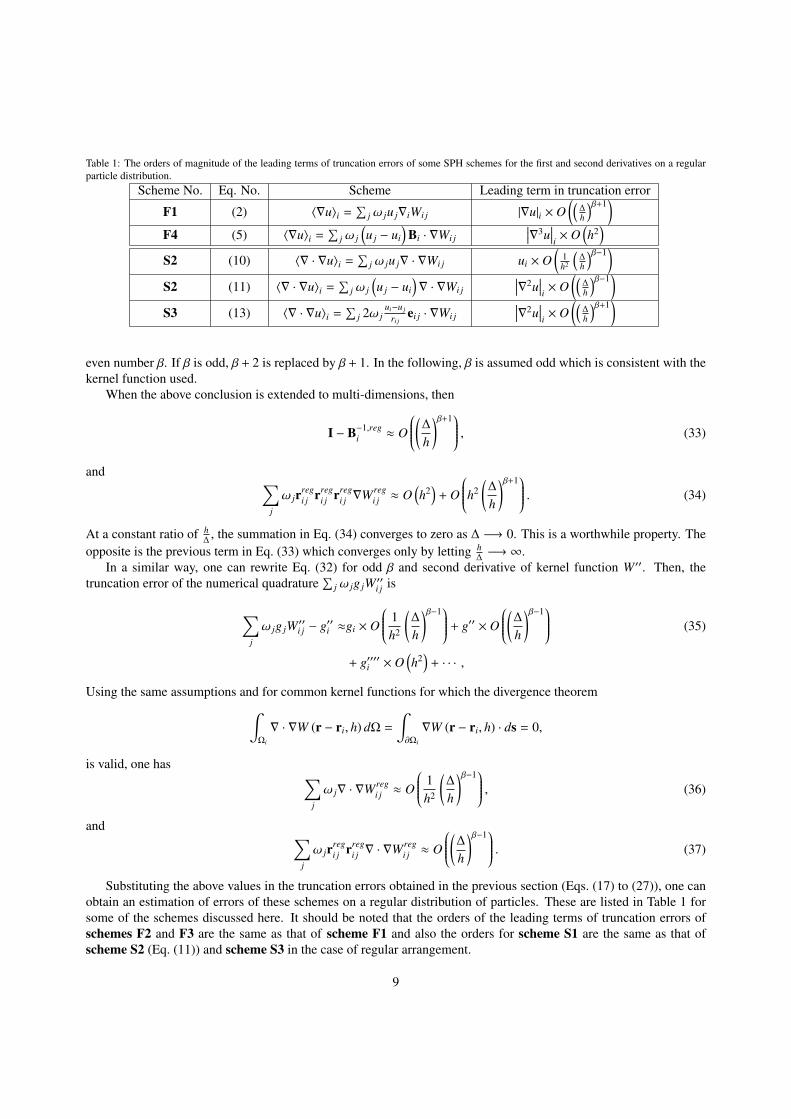
Table 1: The orders of magnitude of the leading terms of truncation errors of some SPH schemes for the first and second derivatives on a regularparticle distribution.

Scheme No. Eq. No. Scheme Leading term in truncation error

F1 (2) ⟨∇u⟩i =∑

j ω ju j∇iWi j |∇u|i × O((∆h

)β+1)

F4 (5) ⟨∇u⟩i =∑

j ω j

(u j − ui

)Bi · ∇Wi j

∣∣∣∇3u∣∣∣i × O

(h2

)S2 (10) ⟨∇ · ∇u⟩i =

∑j ω ju j∇ · ∇Wi j ui × O

(1h2

(∆h

)β−1)

S2 (11) ⟨∇ · ∇u⟩i =∑

j ω j

(u j − ui

)∇ · ∇Wi j

∣∣∣∇2u∣∣∣i × O

((∆h

)β−1)

S3 (13) ⟨∇ · ∇u⟩i =∑

j 2ω jui−u j

ri jei j · ∇Wi j

∣∣∣∇2u∣∣∣i × O

((∆h

)β+1)

even number β. If β is odd, β + 2 is replaced by β + 1. In the following, β is assumed odd which is consistent with thekernel function used.

When the above conclusion is extended to multi-dimensions, then

I − B−1,regi ≈ O

(∆h)β+1 , (33)

and ∑j

ω jrregi j rreg

i j rregi j ∇Wreg

i j ≈ O(h2

)+ O

h2(∆

h

)β+1 . (34)

At a constant ratio of h∆

, the summation in Eq. (34) converges to zero as ∆ −→ 0. This is a worthwhile property. Theopposite is the previous term in Eq. (33) which converges only by letting h

∆−→ ∞.

In a similar way, one can rewrite Eq. (32) for odd β and second derivative of kernel function W′′. Then, thetruncation error of the numerical quadrature

∑j ω jg jW ′′i j is

∑j

ω jg jW ′′i j − g′′i ≈gi × O

1h2

(∆

h

)β−1 + g′′ × O

(∆h)β−1 (35)

+ g′′′′i × O(h2

)+ · · · ,

Using the same assumptions and for common kernel functions for which the divergence theorem∫Ωi

∇ · ∇W (r − ri, h) dΩ =∫∂Ωi

∇W (r − ri, h) · ds = 0,

is valid, one has ∑j

ω j∇ · ∇Wregi j ≈ O

1h2

(∆

h

)β−1 , (36)

and ∑j

ω jrregi j rreg

i j ∇ · ∇Wregi j ≈ O

(∆h)β−1 . (37)

Substituting the above values in the truncation errors obtained in the previous section (Eqs. (17) to (27)), one canobtain an estimation of errors of these schemes on a regular distribution of particles. These are listed in Table 1 forsome of the schemes discussed here. It should be noted that the orders of the leading terms of truncation errors ofschemes F2 and F3 are the same as that of scheme F1 and also the orders for scheme S1 are the same as that ofscheme S2 (Eq. (11)) and scheme S3 in the case of regular arrangement.

9

4.2. Irregular arrangementThe above discussion was given for a regular equally spaced particle. For a general particle distribution, this is

not true especially for a multi-dimensional flow problem in which particles are moving in a complex manner. Hence,it is necessary to study the errors of the method when the particles are distributed irregularly. When the particlearrangement is not regular, the value of any typical summation S can be decomposed into two parts; S reg which wasinvestigated before and S which is the contribution due to the deviation from the regular arrangement.

Assume that each particle j is displaced by di j from its regular position rregi j . One can write

W(ri j

)=W

(rreg

i j + di j

)=W

(rreg

i j

)+ di j · ∇W

(rreg

i j

)+ · · · ,

or in short notationWi j = Wreg

i j + di j · ∇Wregi j + · · · ,

and similarly∇Wi j = ∇Wreg

i j + di j · ∇∇Wregi j + · · · ,

and∇∇Wi j = ∇∇Wreg

i j + di j · ∇∇∇Wregi j + · · · .

As a result, one can write for instance∑j

ω j∇Wi j ≈∑

j

ω j∇Wregi j +

∑j

ω jdi j · ∇∇Wregi j .

From Eq. (28), the first term on the right-hand side is zero. For the second term, one can define di as a measure ofdeviations of the neighboring particles of i. It is obvious that 0 ≤ di < ∆. Then using Eq. (36) one finds∑

j

ω j∇Wi j ≈di

∑j

ω j∇ · ∇Wregi j (38)

≈O

di

h2

(∆

h

)β−1 .Although this is a rough estimation which is different from [13], this approximation is sufficient for the presentinvestigation.

For the renormalization tensor B, the analysis is slightly more complex. One has

B−1i = −

∑j

ω jri j∇Wi j

= −∑

j

ω jrregi j ∇Wreg

i j −∑

j

ω jdi j∇Wregi j

−∑

j

ω jrregi j di j · ∇∇Wreg

i j −∑

j

ω jdi jdi j · ∇∇Wregi j .

The first term on the right-hand side was assessed in Eq. (33). The third and fourth terms are of orders higher than thesecond term, so they are omitted. As a result, one finds

I − B−1i ≈ O

(∆h)β+1 + O

di

h

(∆

h

)β+1 . (39)

By a similar analysis, the order of other terms are also obtained. The results are shown in Table 2.Now, by substituting the orders of magnitude of Table 2 into the truncation errors of the previous section, the

estimation of error for various SPH schemes is completed. (Table 3) Three schemes for the first derivative are shown.10

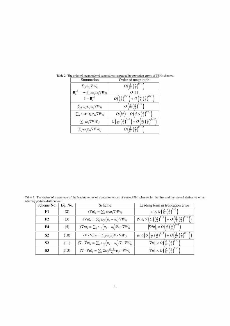
Table 2: The order of magnitude of summations appeared in truncation errors of SPH schemes.Summation Order of magnitude∑

j ω j∇Wi j O(

dih2

(∆h

)β−1)

B−1i = −

∑j ω jri j∇Wi j O (1)

I − B−1i O

((∆h

)β+1)+ O

(dih

(∆h

)β+1)

∑j ω jri jri j∇Wi j O

(di

(∆h

)β+1)

∑j ω jri jri jri j∇Wi j O

(h2

)+ O

(di∆

(∆h

)β+1)

∑j ω j∇∇Wi j O

(1h2

(∆h

)β−1)+ O

(dih3

(∆h

)β−1)

∑j ω jri j∇∇Wi j O

(dih2

(∆h

)β−1)

Table 3: The orders of magnitude of the leading terms of truncation errors of some SPH schemes for the first and the second derivative on anarbitrary particle distribution.

Scheme No. Eq. No. Scheme Leading term in truncation error

F1 (2) ⟨∇u⟩i =∑

j ω ju j∇iWi j ui × O(

dih2

(∆h

)β−1)

F2 (3) ⟨∇u⟩i =∑

j ω j

(u j − ui

)∇Wi j |∇u|i ×

(O

((∆h

)β+1)+ O

(dih

(∆h

)β+1))

F4 (5) ⟨∇u⟩i =∑

j ω j

(u j − ui

)Bi · ∇Wi j

∣∣∣∇2u∣∣∣i × O

(di

(∆h

)β+1)

S2 (10) ⟨∇ · ∇u⟩i =∑

j ω ju j∇ · ∇Wi j ui ×(O

(1h2

(∆h

)β−1)+ O

(dih3

(∆h

)β−1))

S2 (11) ⟨∇ · ∇u⟩i =∑

j ω j

(u j − ui

)∇ · ∇Wi j |∇u|i × O

(dih2

(∆h

)β−1)

S3 (13) ⟨∇ · ∇u⟩i =∑

j 2ω jui−u j

ri jei j · ∇Wi j |∇u|i × O

(dih2

(∆h

)β−1)

11

The omitted scheme F3 has the same condition as scheme F1. Table 3 demonstrates that the only acceptable SPHtechnique to discretize the first derivatives is scheme 4 because of two properties; First, its leading term in truncationerror includes a second derivative i.e. first-order consistency. The other is that the truncation error diminishes as theparticle spacing ∆ decreases. Although the scheme converges linearly, it is a valuable property because for a fixed h

∆

ratio, the other schemes converge only when the particles are ordered. As mentioned before, it is a known fact that forconvergence, other SPH methods need both ∆ −→ 0 and h

∆−→ ∞ [18]. Table 3 clearly shows this fact. For example,

scheme F1 needs ∆ to decrease faster than h1+1/β. This is tolerable in theory. But in practice, increasing h∆

meansgrowing number of neighbors and consequently higher computational costs especially in two or three dimensions.Indeed, a desirable technique is one which needs smaller neighboring particles or h

∆.

It is notable that the above two properties are not independent. For a first derivative scheme, if the truncation errorhas a term including ui, its multiplier must have dimension [L]−1 where L is a characteristic length and may be h or ∆.Accordingly, if it contains ∇u|i, its multiplier must be non-dimensional. These coefficients may not converge to zeroas ∆ −→ 0. This is the sign of trouble and means that the truncation error diminishes only by making h

∆−→ ∞.

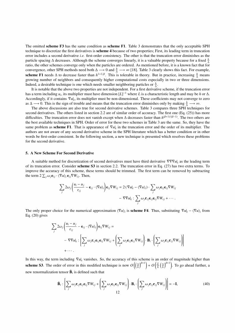
The above discussions are also true for second derivative schemes. Table 3 compares three SPH techniques forsecond derivatives. The others listed in section 2.2 are of similar order of accuracy. The first one (Eq. (25)) has moredifficulties. The truncation error does not vanish except when ∆ decreases faster than h(β+1)/(β−1). The two others arethe best available techniques in SPH. Order of error for these two schemes in Table 3 are the same. So, they have thesame problem as scheme F1. That is appearance of ∇u|i in the truncation error and the order of its multiplier. Theauthors are not aware of any second derivative scheme in the SPH literature which has a better condition or in otherwords be first-order consistent. In the following section, a new technique is presented which resolves these problemsfor the second derivative.

5. A New Scheme For Second Derivative

A suitable method for discretization of second derivatives must have third derivative ∇∇∇u|i as the leading termof its truncation error. Consider scheme S3 in section 2.2. The truncation error in Eq. (27) has two extra terms. Toimprove the accuracy of this scheme, these terms should be trimmed. The first term can be removed by subtractingthe term 2

∑j ω jei j · ⟨∇u⟩i ei j∇Wi j. Then,

∑j

2ω j

(ui − u j

ri j− ei j · ⟨∇u⟩i

)ei j∇Wi j = 2 (∇u|i − ⟨∇u⟩i) ·

∑j

ω jei jei j∇Wi j

− ∇∇u|i :∑

j

ω jri jei jei j∇Wi j + · · · .

The only proper choice for the numerical approximation ⟨∇u⟩i is scheme F4. Thus, substituting ∇u|i − ⟨∇u⟩i fromEq. (20) gives ∑

j

2ω j

(ui − u j

ri j− ei j · ⟨∇u⟩i

)ei j∇Wi j =

− ∇∇u|i :

∑j

ω jri jei jei j∇Wi j +

∑j

ω jei jei j∇Wi j

· Bi ·∑

j

ω jri jri j∇Wi j

+ · · · .

In this way, the term including ∇u|i vanishes. So, the accuracy of this scheme is an order of magnitude higher than

scheme S3. The order of error in this modified technique is now O((∆h

)β+1)+ O

(dih

(∆h

)β+1). To go ahead further, a

new renormalization tensor Bi is defined such that

Bi :

∑j

ω jri jei jei j∇Wi j +

∑j

ω jei jei j∇Wi j

· Bi ·∑

j

ω jri jri j∇Wi j

= −I, (40)

12

This tensor differs from the usual renormalization tensor Bi by incorporating a high-order term which may vanishin the case of regular arrangement. Since Bi is symmetric, calculation of this tensor in 2D leads to solving a linearsystem of simultaneous equations with three unknowns.

Therefore, the new scheme S4 takes the following form

⟨∇ · ∇u⟩i ≡ Bi :∑

j

2ω jei j∇Wi j

ui − u j

ri j− ei j ·

∑j

ω j

(u j − ui

)Bi · ∇Wi j

. (41)

Using the estimations given in Table 2, the order of the leading term in its truncation error becomes

Eri ≈∣∣∣∇3u

∣∣∣i × O

di

(∆

h

)β+1 . (42)

Equation (41) presents a new scheme for approximation of the second derivatives and can be used for examplefor discretization of the thermal conduction terms in the energy equation and viscous terms in the Navier-Stokesequations. Since the deviation distance di is smaller than the regular distance ∆, scheme S4 is first-order accurate andconverges regardless of the ratio h

∆. This means that the new scheme predicts the second derivative of either constant,

linear, or quadratic functions exactly.

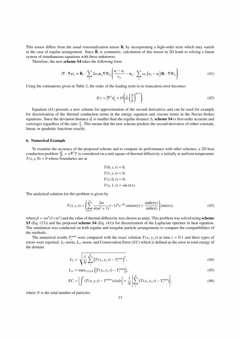
6. Numerical Example

To examine the accuracy of the proposed scheme and to compare its performance with other schemes, a 2D heatconduction problem ∂T

∂t = α∇2T is considered on a unit square of thermal diffusivity α initially at uniform temperatureT (x, y, 0) = 0 whose boundaries are at

T (0, y, t) = 0,T (1, y, t) = 0,T (x, 0, t) = 0,T (x, 1, t) = sin (πx) .

The analytical solution for this problem is given by

T (x, y, t) =

∞∑m=1

2mπ(m2 + 1)

(−1)me−βt sin(mπy) +sinh(πy)sinh(π)

sin(πx), (43)

where β = απ2(1+m2) and the value of thermal diffusivity was chosen as unity. This problem was solved using schemeS3 (Eq. (13)) and the proposed scheme S4 (Eq. (41)) for discretization of the Laplacian operator in heat equation.The simulation was conducted on both regular and irregular particle arrangements to compare the compatibilities ofthe methods.

The numerical results T numi were compared with the exact solution T (xi, yi, t) at time t = 0.1 and three types of

errors were reported: L2-norm, L∞-norm, and Conservation Error (EC) which is defined as the error in total energy ofthe domain

L2 =

√√1N

N∑i

(T (xi, yi, t) − T num

i

)2, (44)

L∞ = max1≤i≤N

(∣∣∣T (xi, yi, t) − T numi

∣∣∣) , (45)

EC =∣∣∣∣∣∫ (T (x, y, t) − T num) dxdy

∣∣∣∣∣ = 1N

∣∣∣∣∣∣∣N∑i

(T (xi, yi, t) − T num

i)∣∣∣∣∣∣∣ , (46)

where N is the total number of particles.13

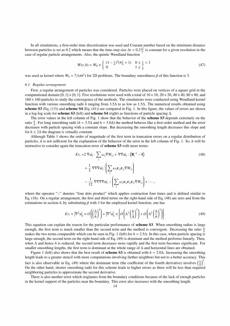
In all simulations, a first-order time discretization was used and Courant number based on the minimum distancebetween particles is set as 0.2 which means that the time-step size ∆t = 0.2∆

2

αis constant for a given resolution in the

case of regular particle arrangements. Also, the quintic Wendland function

W(r, h) = W0 ×

(1 − rh )4(4 r

h + 1) 0 ≤ rh < 1

0 1 ≤ rh

(47)

was used as kernel where W0 = 7/(πh2) for 2D problems. The boundary smoothness β of this function is 3.

6.1. Regular arrangementFirst, a regular arrangement of particles was considered. Particles were placed on vertices of a square grid in the

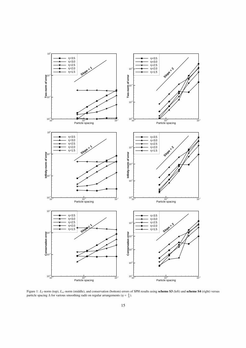
computational domain [0, 1]× [0, 1]. Five resolutions were used with a total of 10× 10, 20× 20, 40× 40, 80× 80, and160× 160 particles to study the convergence of the methods. The simulations were conducted using Wendland kernelfunction with various smoothing radii h ranging from 3.5∆ to as low as 1.5∆. The numerical results obtained usingscheme S3 (Eq. (13)) and scheme S4 (Eq. (41)) are compared in Fig. 1. In this figure, the values of errors are shownin a log-log scale for scheme S3 (left) and scheme S4 (right) as functions of particle spacing ∆.

The error values in the left column of Fig. 1 show that the behavior of the scheme S3 depends extremely on theratio h

∆. For long smoothing radii (h = 3.5∆ and h = 3.0∆) the method behaves like a first-order method and the error

decreases with particle spacing with a constant slope. But decreasing the smoothing length decreases this slope andfor h ≤ 2∆ the diagram is virtually constant.

Although Table 1 shows the order of magnitude of the first term in truncation errors on a regular distribution ofparticles, it is not sufficient for the explanation of the behavior of the error in the left column of Fig. 1. So, it will beinstructive to consider again the truncation error of scheme S3 with more terms:

Eri =2 ∇u|i ·∑

j

ω j∇Wi j + ∇∇u|i :(B−1

i − I)

(48)

+13∇∇∇u|i

...

∑j

ω jri jri j∇Wi j

− 1

12∇∇∇∇u|i ::

∑j

ω jri jri jri j∇Wi j

+ · · · ,where the operator “::” denotes “four dots product” which applies contraction four times and is defined similar toEq. (16). On a regular arrangement, the first and third terms on the right-hand side of Eq. (48) are zero and from theestimations in section 4, by substituting β with 3 for the employed kernel function, one has

Eri ≈∣∣∣∇2u

∣∣∣i × O

(∆h)4 + ∣∣∣∇4u

∣∣∣i ×

O ∆2(

h∆

)2 + O

∆2(∆

h

)2 . (49)

This equation can explain the reason for the particular performance of scheme S3. When smoothing radius is largeenough, the first term is much smaller than the second term and the method is convergent. Decreasing the ratio h

∆

makes the two terms comparable which can be seen in Fig. 1 (left) for h = 2.5∆. In this case, when particle spacing islarge enough, the second term on the right-hand side of Eq. (49) is dominant and the method performs linearly. Then,when ∆ and hence h is reduced, the second term decreases more rapidly and the first term becomes significant. Forsmaller smoothing lengths, the first term is dominant at the whole range of ∆ and horizontal lines are obtained.

Figure 1 (left) also shows that the best result of scheme S3 is obtained with h = 2.0∆. Increasing the smoothinglength leads to a greater stencil with more computations involving farther neighbors but not to a better accuracy. Thisfact is also observable in Eq. (49) where the dominant term (the coefficient of the fourth derivative) involves

(h∆

)2.

On the other hand, shorter smoothing radii for this scheme leads to higher errors as there will be less than requiredneighboring particles to approximate the second derivative.

There is also another error which originates from the boundary conditions because of the lack of enough particlesin the kernel support of the particles near the boundary. This error also increases with the smoothing length.

14

Particle spacing

Tw

o-no

rmof

erro

r

10-3 10-2 10-110-3

10-2

10-1

100

η=3.5η=3.0η=2.5η=2.0η=1.5

Slope = 1

Particle spacing

Tw

o-no

rmof

erro

r

10-3 10-2 10-110-6

10-5

10-4

10-3

η=3.5η=3.0η=2.5η=2.0η=1.5

Slope

=2

Particle spacing

Infin

ity-n

orm

ofer

ror

10-3 10-2 10-110-3

10-2

10-1

100

η=3.5η=3.0η=2.5η=2.0η=1.5

Slope = 1

Particle spacing

Infin

ity-n

orm

ofer

ror

10-3 10-2 10-110-6

10-5

10-4

10-3

η=3.5η=3.0η=2.5η=2.0η=1.5

Slope

=2

Particle spacing

Con

serv

atio

ner

ror

10-3 10-2 10-110-4

10-3

10-2

10-1

η=3.5η=3.0η=2.5η=2.0η=1.5

Slope = 1

Particle spacing

Con

serv

atio

ner

ror

10-3 10-2 10-110-7

10-6

10-5

10-4

10-3

η=3.5η=3.0η=2.5η=2.0η=1.5

Slope = 2

Figure 1: L2-norm (top), L∞-norm (middle), and conservation (bottom) errors of SPH results using scheme S3 (left) and scheme S4 (right) versusparticle spacing ∆ for various smoothing radii on regular arrangements (η = h

∆).

15

The behavior of the proposed scheme S4 is totally different as seen in the right column of Fig. 1. The order ofmagnitude of errors are 2 to 3 orders lower than those of the previous method. In addition, the method performs nearsecond order for all smoothing radii on a regular distribution of particles. This means that the scheme is an orderof magnitude more accurate than scheme S3. The most impressive advantage of scheme S4 which can be seen inFig. 1 (Right) is that it converges well even for a short smoothing radius h = 1.5∆. More precisely, this means thatcomputation is done with only 8 neighboring particles. This is important because reducing the number of neighboringparticles means less computational cost and CPU time.

The reason is that scheme S4 does not have the first term in Eq. (49). So, the truncation error on a regulardistribution is second order:

Eri ≈∣∣∣∇4u

∣∣∣i ×

O ∆2(

h∆

)2 + O

∆2(∆

h

)2 . (50)

Since both schemes S3 and S4 are not symmetric and thus are not conservative neither locally nor globally, onecould not expect the error in energy conservation (EC) to be zero. However, Fig. 1 (bottom), this error follows thesame pattern as the other error norms for both techniques. The values of the conservation error for the proposedscheme S4 are low enough to be acceptable in solving conventional problems using SPH.

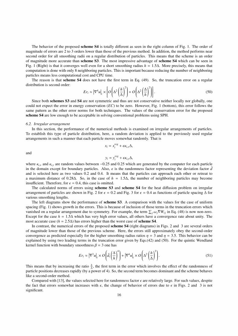
6.2. Irregular arrangementIn this section, the performance of the numerical methods is examined on irregular arrangements of particles.

To establish this type of particle distribution, here, a random deviation is applied to the previously used regulararrangements in such a manner that each particle moves somewhat randomly. That is

xi = xregi + ϵκi,x∆,

andyi = yreg

i + ϵκi,y∆,

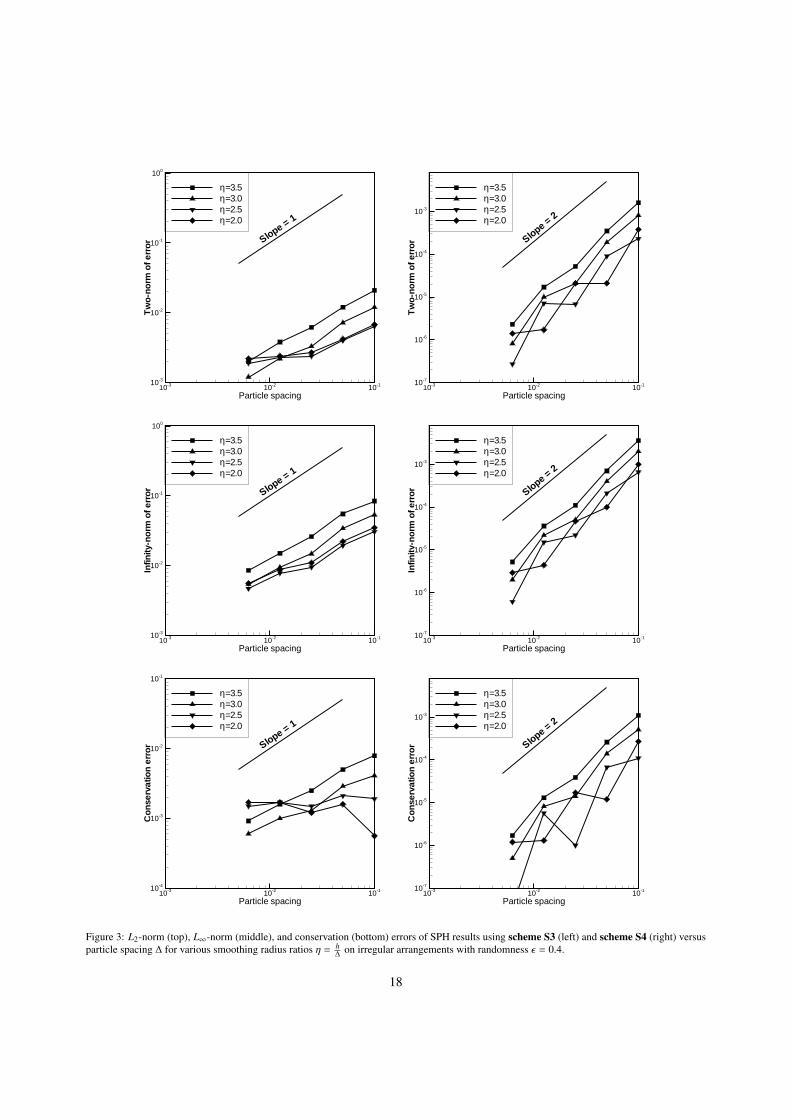
where κi,x and κi,y are random values between −0.25 and 0.25 which are generated by the computer for each particlein the domain except for boundary particles. Also, ϵ is the randomness factor representing the deviation factor dand is selected here as two values 0.2 and 0.4. It means that the particles can approach each other or retreat toa maximum distance of 0.28∆. So, in the case of h = 1.5∆, the number of neighboring particles may becomeinsufficient. Therefore, for ϵ = 0.4, this case is omitted.

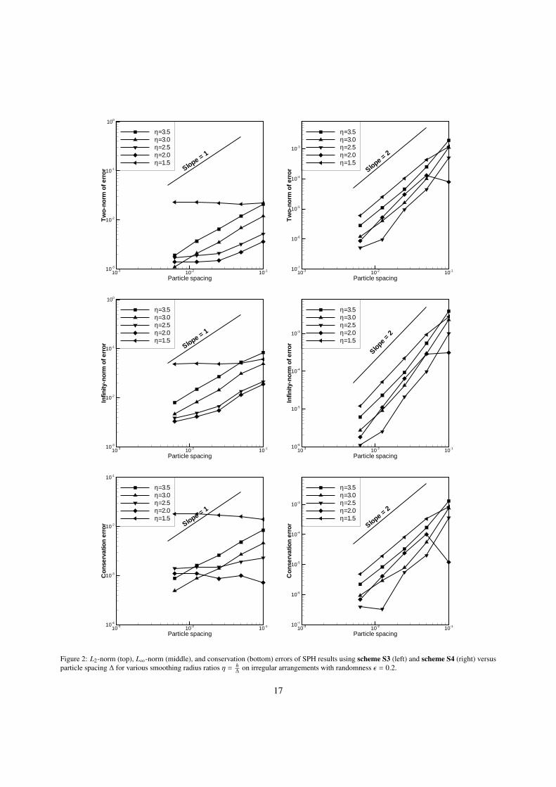
The calculated norms of errors using scheme S3 and scheme S4 for the heat diffusion problem on irregulararrangement of particles are shown in Fig. 2 for ϵ = 0.2 and Fig. 3 for ϵ = 0.4 as functions of particle spacing ∆ forvarious smoothing lengths.

The left diagrams show the performance of scheme S3. A comparison with the values for the case of uniformspacing (Fig. 1) shows growth in the errors. This is because of inclusion of those terms in the truncation errors whichvanished on a regular arrangement due to symmetry. For example, the term

∑j ω j∇Wi j in Eq. (48) is now non-zero.

Except for the case h = 1.5∆ which has very high error values, all others have a convergence rate about unity. Themost accurate case (h = 2.5∆) has errors higher than the worst case of scheme S4.

In contrast, the numerical errors of the proposed scheme S4 (right diagrams) in Figs. 2 and 3 are several ordersof magnitude lower than those of the previous scheme. Here, the errors still approximately obey the second-orderconvergence as predicted especially for the higher smoothing radius ratios η = 3 and η = 3.5. This behavior can beexplained by using two leading terms in the truncation error given by Eqs.(42) and (50). For the quintic Wendlandkernel function with boundary smoothness β = 3 one has

Eri ≈∣∣∣∇3u

∣∣∣i × O

di

(∆

h

)4 + ∣∣∣∇4u∣∣∣i × O

∆2(

h∆

)2 . (51)

This means that by increasing the ratio h∆

, the first term in the error which involves the effect of the randomness ofparticle positions decreases rapidly (by a power of 4). So, the second term becomes dominant and the scheme behaveslike a second-order method.

Compared with [13], the values selected here for randomness factor ϵ are relatively large. For such values, despitethe fact that errors somewhat increases with ϵ, the change of behavior of errors due to ϵ in Figs. 2 and 3 is notsignificant.

16

Particle spacing

Tw

o-no

rmof

erro

r

10-3 10-2 10-110-3

10-2

10-1

100

η=3.5η=3.0η=2.5η=2.0η=1.5

Slope = 1

Particle spacing

Tw

o-no

rmof

erro

r

10-3 10-2 10-110-7

10-6

10-5

10-4

10-3

η=3.5η=3.0η=2.5η=2.0η=1.5

Slope = 2

Particle spacing

Infin

ity-n

orm

ofer

ror

10-3 10-2 10-110-3

10-2

10-1

100

η=3.5η=3.0η=2.5η=2.0η=1.5

Slope = 1

Particle spacing

Infin

ity-n

orm

ofer

ror

10-3 10-2 10-110-6

10-5

10-4

10-3

η=3.5η=3.0η=2.5η=2.0η=1.5

Slope

=2

Particle spacing

Con

serv

atio

ner

ror

10-3 10-2 10-110-4

10-3

10-2

10-1

η=3.5η=3.0η=2.5η=2.0η=1.5

Slope = 1

Particle spacing

Con

serv

atio

ner

ror

10-3 10-2 10-110-7

10-6

10-5

10-4

10-3

η=3.5η=3.0η=2.5η=2.0η=1.5

Slope = 2

Figure 2: L2-norm (top), L∞-norm (middle), and conservation (bottom) errors of SPH results using scheme S3 (left) and scheme S4 (right) versusparticle spacing ∆ for various smoothing radius ratios η = h

∆on irregular arrangements with randomness ϵ = 0.2.

17

Particle spacing

Tw

o-no

rmof

erro

r

10-3 10-2 10-110-3

10-2

10-1

100

η=3.5η=3.0η=2.5η=2.0

Slope = 1

Particle spacing

Tw

o-no

rmof

erro

r

10-3 10-2 10-110-7

10-6

10-5

10-4

10-3

η=3.5η=3.0η=2.5η=2.0

Slope = 2

Particle spacing

Infin

ity-n

orm

ofer

ror

10-3 10-2 10-110-3

10-2

10-1

100

η=3.5η=3.0η=2.5η=2.0

Slope = 1

Particle spacing

Infin

ity-n

orm

ofer

ror

10-3 10-2 10-110-7

10-6

10-5

10-4

10-3

η=3.5η=3.0η=2.5η=2.0

Slope = 2

Particle spacing

Con

serv

atio

ner

ror

10-3 10-2 10-110-4

10-3

10-2

10-1

η=3.5η=3.0η=2.5η=2.0

Slope = 1

Particle spacing

Con

serv

atio

ner

ror

10-3 10-2 10-110-7

10-6

10-5

10-4

10-3

η=3.5η=3.0η=2.5η=2.0

Slope = 2

Figure 3: L2-norm (top), L∞-norm (middle), and conservation (bottom) errors of SPH results using scheme S3 (left) and scheme S4 (right) versusparticle spacing ∆ for various smoothing radius ratios η = h

∆on irregular arrangements with randomness ϵ = 0.4.

18

6.3. Computational cost

It is obvious that the proposed scheme S4 has more computational cost than scheme S3 on the same conditionsdue to three extra numerical stages. One extra calculation is approximation of the first derivative by scheme F4.Although this value may be already available in some cases. For example, in solving viscous flow equations, gradientof velocities may be calculated before approximating their Laplacian. The second extra computation is calculationof tensor B which involves solving a linear set of equations with 3 unknowns in 2D and 6 unknowns in 3D. Inheat conduction problems, since the SPH particles are fixed, this calculation is only performed once for each set ofdata. For fluid flow problems, however, the tensor must be updated at each time-step. Finally, the second derivativeis approximated by scheme S4 which has slightly more computations including multiplication of two second-ordertensors. This is the third extra work in scheme S4.

Nevertheless, the proposed scheme is still very promising because of its accuracy. For instance, solving the heatconduction problem on 160 × 160 uniformly distributed particles with smoothing radii h = 3.5∆ takes 233 secondsusing scheme S3 while it takes 856 seconds to be solved using scheme S4 on a 3 Ghz Intel Core 2 E8400 CPU.However, if one solves the same problem with h = 1.5∆ using scheme S4, the CPU time is reduced to 239 seconds.It is important to note that the error of this computation will be at least two orders of magnitude lower than that ofscheme S3 with h = 3.5∆.

7. Conclusions

In this paper, a theoretical framework was presented to assess the accuracy of different SPH schemes for dis-cretization of the first and second derivatives in multi-dimensions. Using this framework, it was shown that some ofthe frequently used SPH schemes for approximation of the first derivative ⟨∇u⟩i involve values ui and/or the derivative∇u|i in their truncation error which cause some difficulties in simulations. For example, the accuracy of a pressuregradient may be affected by the sign of pressure at each particle or even value of the reference pressure. Also, it wasobserved that all available SPH schemes for approximation of second derivative suffer from similar problems and inthe best case are zero-order consistent.

In addition, using the theory of numerical integration, the order of magnitude of the coefficients in the truncationerrors were estimated. This is done for both regular and irregular particle spacing. In this way, the order of each termand the effect of the smoothing radius ratio h

∆were clarified, so that one can predict the convergence properties of

every SPH scheme analytically.Finally, a new SPH scheme was presented for the second derivative which is consistent enough to exactly predict

the second derivative of a quadratic function. Examining the new technique for 2D unsteady heat equation on regularand irregular particle arrangements showed that it has at least one order of magnitude less errors in comparison withthe best available scheme. In addition, on uniform particle distribution, second-order convergence was observed evenfor smoothing radii as small as 1.5∆ which means a considerable decrease in computational cost without growthin errors. In addition, for irregular distribution of particles it was shown that this scheme behaves near second-orderaccurate for smoothing radii larger than 2∆. Although the proposed scheme is not symmetric and so does not conservemomentum or energy exactly, the conservation error was as low as those for other error norms and can be successfullyused in practical studies.

8. Acknowledgment

The authors would like to thank Pars Oil and Gas Company (POGC) for its partial financial support.

References

[1] R. Gingold, J. Monaghan, Smoothed Particle Hydrodynamics: Theory and application to nonspherical stars, Astrophysical Journal 181 (1977)275–389.

[2] L. Lucy, A numerical approach to the testing of fission hypothesis, Astrophysical Journal 82 (1977) 1013–1020.[3] J. Monaghan, Smoothed Particle Hydrodynamics, Reports on Progress in Physics 68 (2005) 1703–1759.[4] G. Oger, M. Doring, B. Alessandrini, P. Ferrant, An improved SPH method: Towards higher order convergence, Journal of Computational

Physics 225 (2) (2007) 1472–1492.

19

[5] M. Basa, N. Quinlan, M. Lastiwka, Robustness and accuracy of SPH formulations for viscous flow, International Journal for NumericalMethods in Fluids 60 (2009) 1127–1148.

[6] J. Ma, W. Ge, Is standard symmetric formulation always better for smoothed particle hydrodynamics?, Computers & Mathematics withApplications 55 (7) (2008) 1503–1513.

[7] D. Graham, J. Hughes, Accuracy of SPH viscous flow models, International Journal for Numerical Methods in Fluids 56 (8) (2008) 1261–1269.

[8] J. Monaghan, J. Lattanzio, A refined particle method for astrophysical problems, Astronomy and Astrophysics 149 (1) (1985) 135–143.[9] S. Mas-Gallic, P. Raviart, A particle method for first-order symmetric systems, Numerische Mathematik 51 (3) (1987) 323–352.

[10] B. Ben Moussa, J. Vila, Convergence of SPH method for scalar nonlinear conservation laws, SIAM Journal on Numerical Analysis (2000)863–887.

[11] T. Belytschko, Y. Krongauz, D. Organ, M. Fleming, P. Krysl, Meshless methods: an overview and recent developments, Computer methodsin applied mechanics and engineering 139 (1-4) (1996) 3–47.

[12] A. Colagrossi, A meshless Lagrangian method for free-surface and interface flows with fragmentation, Ph.D. thesis, Universita di Roma LaSapienza, 2005.

[13] N. Quinlan, M. Basa, M. Lastiwka, Truncation error in mesh-free particle methods, International Journal for Numerical Methods in Engi-neering 66 (13) (2006) 2064–2085.

[14] R. Fatehi, M. Fayazbakhsh, M.T. Manzari, On Discretization of Second-order Derivatives in Smoothed Particle Hydrodynamics, InternationalJournal of Natural and Applied Sciences 3 (1) (2009) 50–53.

[15] P. Randles, L. Libersky, Smoothed Particle Hydrodynamics: some recent improvements and applications, Computer Methods in AppliedMechanics and Engineering 139 (1-4) (1996) 375–408.

[16] J. Bonet, T. Lok, Variational and momentum preservation aspects of smooth particle hydrodynamic formulations, Computer Methods inApplied Mechanics and Engineering 180 (1-2) (1999) 97–115.

[17] J. Vila, On particle weighted methods and Smooth Particle Hydrodynamics, Mathematical Models and Methods in Applied Sciences 9 (2)(1999) 161–210.

[18] J. Vila, SPH renormalized hybrid methods for conservation laws: Applications to free surface flows, in: M. Griebel, M. A. Schweitzer (Eds.),Meshfree methods for partial differential equations II, Springer, 2005, p. 207.

[19] O. Flebbe, S. Munzel, H. Herold, H. Riffert, H. Ruder, Smoothed Particle Hydrodynamics-physical viscosity and the simulation of accretiondisks, The Astrophysical Journal 431 (1994) 214–226.

[20] S. Watkins, A. Bhattal, N. Francis, J. Turner, A. Whitworth, A new prescription for viscosity in smoothed particle hydrodynamics, Astronomyand Astrophysics 119 (1996) 177–187.

[21] J. Jeong, M. Jhon, J. Halow, J. van Osdol, Smoothed Particle Hydrodynamics: Applications to heat conduction, Computer Physics Commu-nications 153 (1) (2003) 71–84.

[22] S. Nugent, H. Posch, Liquid drops and surface tension with smoothed particle applied mechanics, Physical Review E 62 (4) (2000) 4968–4975.

[23] J. Ferziger, M. Peric, Computational Methods for Fluid Dynamics, Springer, 2002.[24] H. Takeda, S. Miyama, M. Sekiya, Numerical simulation of viscous flow by Smoothed Particle Hydrodynamics, Progress of Theoretical

Physics 92 (5) (1994) 939–960.[25] A. Chaniotis, D. Poulikakos, P. Koumoutsakos, Remeshed smoothed particle hydrodynamics for the simulations of viscous and heat conduct-

ing flows, Journal of Computational Physics 182 (2002) 67–90.[26] L. Brookshaw, A method of calculating radiative heat diffusion in particle simulations, in: Astronomical Society of Australia, Proceedings

(ISSN 0066-9997), Vol. 6, 1985, pp. 207–210.[27] X. Hu, N. Adams, A multi-phase SPH method for macroscopic and mesoscopic flows, Journal of Computational Physics 213 (2) (2006)

844–861.

20