1 

Refinements to the method of epicentral location based on surface waves from ambient seismic noise: Introducing Love waves Anatoli L. Levshin1, Mikhail P. Barmin1, Morgan P. Moschetti2 , Carlos Mendoza3, and Michael H. Ritzwoller1

1 - Department of Physics, University of Colorado at Boulder, Boulder, CO 80309, USA (levshin@colorado.edu) 2 - National Earthquake Information Center, U.S. Geological Survey, Golden, CO 80401, USA 3 - Centro de Geociencias, Universidad Nacional Autonoma de Mexico, Queretaro, 76230, Mexico

Summary

The purpose of this study is to develop and test a modification to a previous method of regional

seismic event location based on Empirical Green's Functions (EGF) produced from ambient

seismic noise (Barmin et al., 2011). Elastic EGFs between pairs of seismic stations are

determined by cross-correlating long ambient noise time-series recorded at the two stations. The

EGFs principally contain Rayleigh and Love wave energy on the vertical and transverse

components, respectively, and we utilize these signals between about 5 and 12 sec period. The

previous method, based exclusively on Rayleigh waves, may yield biased epicentral locations for

certain event types with hypocentral depths between 2 and 5 km. Here we present theoretical

arguments that show how Love waves can be introduced to reduce or potentially eliminate the

bias. We also present applications of Rayleigh and Love wave EGFs to locate ten reference

events in the western USA. The separate Rayleigh and Love epicentral locations and the joint

locations using a combination of the two waves agree to within 1 km distance, on average, but

confidence ellipses are smallest when both types of waves are used.

Key words: Earthquake source observations; Seismic monitoring and test-ban treaty verification; Surface waves and free oscillations; ambient noise

  2 

1. Introduction

In a previous study, Barmin et al. (2011), referred to hereafter as Paper I, presented a new

approach to the epicentral location of shallow seismic events based on use of the Empirical

Green's Functions (EGFs) obtained from ambient seismic noise. The vertical component of the

ambient noise in the period range from 7 to 15 s, which is dominated by the fundamental

Rayleigh wave, was used to compute the EGFs. It was demonstrated that this approach has

several features that make it a useful addition to existing location methods. First, the method is

based on surface waves, which are usually not applied in most location algorithms. Second, it

does not require knowledge of Earth structure and is, therefore, unbiased by uncertainties in the

knowledge of structure near the epicenter. Third, it works well for weak seismic events even if

the detection of body wave phases is problematic. Fourth, the EGFs computed during a

temporary deployment of a base network (such as the USArray Transportable Array (TA) or

PASSCAL deployments) may be applied to events that occur earlier or later using permanent

remote stations even if the temporary stations are absent. However, the method has several

evident limitations. In particular, it is based on the assumption that the event source mechanism

and depth are unknown and does not attempt to estimate them. Time shifts in the surface waves

caused by the source mechanism, therefore, can bias the epicentral location. Paper I shows that

this degradation is worst for source depths between about 2 and 5 km if the source mechanism is

different from pure strike-slip, thrust or normal faulting. In this case, the method described in

Paper I will deliver a biased estimate of the epicentral location.

This paper addresses this limitation by introducing Love waves into the location method. Love

waves possess different sensitivity to the source mechanism than Rayleigh waves and, in fact,

Love wave source phase times are quantitatively less sensitive to the source mechanism (Levshin

et al., 1999). Love waves are, however, in many cases more difficult to observe than Rayleigh

waves due to higher noise levels on horizontal components. Epicentral estimates based on Love

waves, therefore, have a larger variance than those based on Rayleigh waves, on average. Thus,

the joint application of Rayleigh and Love waves to estimate epicentral locations may be

preferable to the locations based on either wave type alone, as it strikes a balance between bias

and variance.

  3 

The outline of the paper is as follows. First, we discuss the modification of the location algorithm

to include Love waves. Second, we discuss the theoretical advantage of jointly applying

Rayleigh and Love waves in the location procedure. Finally, we describe the application of the

location algorithm to several well located events in the Western USA (California, Utah, and

Nevada).

2. Modifications to the location algorithm

The algorithm defined in Paper I is described in that paper in great detail. A general description

of that location method is presented here as well as its modifications and the extension to include

Love waves. A seismic event occurs near a set of seismic stations, called the “base stations”. It is

observed at a disjoint set of stations that lie significantly farther from the event, called the

“remote stations”. These time series are called the “event records”. In addition, cross-correlations

between long time records of ambient noise exist between the base and remote stations, which

provide what are called “Empirical Green’s functions” (EGFs). Low amplitude event records and

EGFs are discarded if their signal-to-noise ratio (SNR) is below 10, where SNR is defined by

Bensen et al. (2007). Frequency-time analysis (FTAN, e.g., Levshin et al., 1972; Levshin &

Ritzwoller, 2001; Bensen et al., 2007) is performed on the event records and the EGFs,

producing for each remote station an FTAN diagram for the event and for each inter-station pair

(base-to-remote) an FTAN diagram for the EGF. The location procedure considers a set of

hypothetical event epicentral locations and one is chosen that brings the FTAN diagrams from

the event into optimal agreement with the FTAN diagrams for the EGFs. Technically, this

comparison is performed by cross-correlation in time between the FTAN diagrams (Levshin et

al., 1989; Bensen et al., 2007).

Examples of several event records and EGFs observed in the western US are shown in Figure 1.

The event records follow one of the aftershocks of the Wells earthquake in Nevada in 2008

(Mendoza & Hartzell, 2009) that occurred on April 22, with a magnitude of 4.4, and an epicenter

located at a distance of about 23 km from TA station M12A (aftershock #6, Table 1). The map in

Figure 1a locates the epicenter and selected remote TA stations north and south of station M12A.

Rayleigh and Love waves are distinctly seen in the event record in Figure 1b at station H12A at

an epicentral distance of about 370 km. Record sections of Z-Z and T-T EGFs for the base

station M12A and selected remote stations are shown in Figure 1c,d. The symmetric component

  4 

of the EGFs is plotted and used here in every instance. Record sections of vertical and transverse

components of the observed event seismograms are similarly presented in Figures 1e,f. There is

a general similarity of SNR as well as the arrival times of the EGFs and event records, but the

frequency contents of the two types of waves differ with the EGFs being enriched at somewhat

longer periods than the event records. In addition, examples of FTAN diagrams for Rayleigh and

Love wave event records also following Wells aftershock #6 and EGFs are shown in Figure 2.

FTAN diagrams for the event records observed at remote station K16A, about 321 km northeast

of the inferred epicentral location, are in Figure 2c,d. The FTAN diagrams of the EGFs between

stations K16A and M12A (near the epicenter) are shown in Figure 2a,b. Rayleigh and Love

waves are shown to arrive at clearly different times with the Love waves arriving earlier, from

which we conclude that the waves observed on the transverse component are, in fact, Love

waves.

The algorithm of Paper I progresses by searching a grid of hypothetical event locations. For each

hypothetical event location, all of the EGFs are effectively shifted to the hypothetical location by

changing the inter-station distance under the assumption that the group velocity measured at the

remote station remains unchanged when shifting from the base station location to the epicentral

location. This spatial shift of the base station is, therefore, converted to a time shift that stretches

or compresses the time axis on the FTAN diagram for each EGF. Then, for each hypothetical

event location and all remote stations, the FTAN diagram for each EGF is cross-correlated with

the FTAN diagram of the event record observed at the appropriate remote station. This results in

a set of cross-correlations each of which can be summarized by an offset time. The mean of the

offset times over all remote stations defines the corrected origin time. The rms of the offset times

computed relative to the corrected origin time over all remote stations defines the misfit for that

hypothetical event location. The algorithm searches systematically over a spatial grid and maps

rms misfit, from which an epicentral location is determined as well as an error ellipse (Flinn,

1965; Jordan & Sverdrup, 1981).

The reliability of the procedure of Paper I, however, is degraded by a number of vagaries of

FTAN diagrams as well as the existence of several ad-hoc parameters that are set in the

algorithm. FTAN diagrams may have spectral holes as well as coda that are quite variable, which

makes them difficult to compare directly. For example, for an earthquake at a given depth the

  5 

event record may have a spectral hole between 10 and 15 sec period, say, which is not found in

the EGFs. These issues render FTAN diagrams non-ideal as a basis for operational application.

In this paper, in addition to introducing Love waves, we have modified the method to improve its

stability by removing its dependence on comparing FTAN diagrams. The modification also

simplifies and speeds up the algorithm substantially.

The modification to this algorithm that we apply here is to replace the FTAN diagrams with

group velocity curves computed from the event record and the EGFs, respectively. Thus, group

times determined from the FTAN diagrams are compared rather than comparing the offset times

from the cross-correlations of the FTAN diagrams. This simplifies the algorithm considerably

and also stabilizes it because the group times observed on an FTAN diagram are more stable than

the details of the FTAN diagram itself. The FTAN algorithm that we apply has been tuned

through extensive use to return group time measurements only in the band in which the

measurements are reliable. When comparing a particular EGF to an event record, we compute

the rms difference between the observed group times only in the period band in which both

measured curves are reliable. This band as wide is typically about 6 sec to 12 sec period.

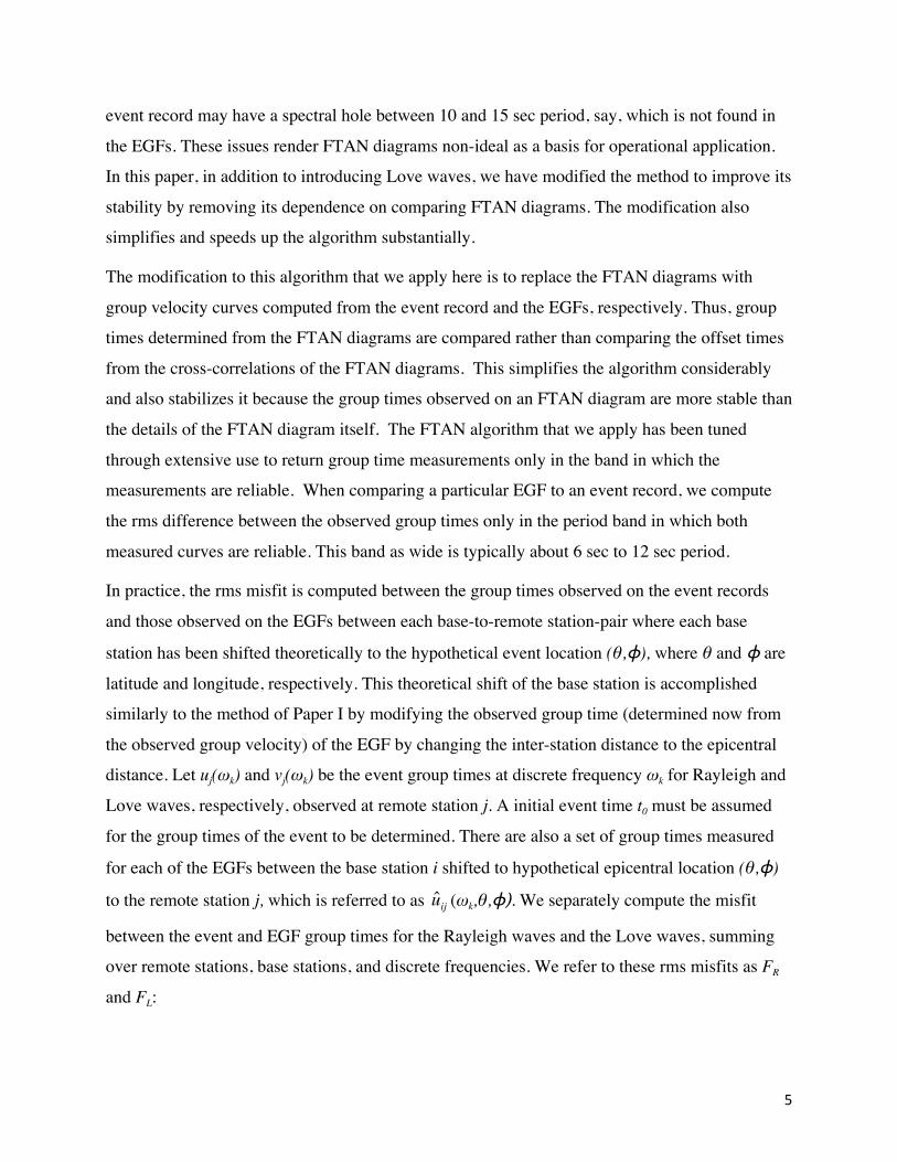
In practice, the rms misfit is computed between the group times observed on the event records

and those observed on the EGFs between each base-to-remote station-pair where each base

station has been shifted theoretically to the hypothetical event location (θ,ϕ), where θ and ϕ are

latitude and longitude, respectively. This theoretical shift of the base station is accomplished

similarly to the method of Paper I by modifying the observed group time (determined now from

the observed group velocity) of the EGF by changing the inter-station distance to the epicentral

distance. Let uj(ωk) and vj(ωk) be the event group times at discrete frequency ωk for Rayleigh and

Love waves, respectively, observed at remote station j. A initial event time t0 must be assumed

for the group times of the event to be determined. There are also a set of group times measured

for each of the EGFs between the base station i shifted to hypothetical epicentral location (θ,ϕ)

to the remote station j, which is referred to as uij (ωk,θ,ϕ). We separately compute the misfit

between the event and EGF group times for the Rayleigh waves and the Love waves, summing

over remote stations, base stations, and discrete frequencies. We refer to these rms misfits as FR

and FL:

  6 

F2R (θ,φ) = N

−1 (uj (ω k ) − uij (ω k ,θ,φ))2

i=1

I

∑j=1

J

∑k=1

K

∑

F2L (θ,φ) = M

−1 (vj (ω k ) − vij (ω k ,θ,φ))2

i=1

I

∑j=1

J

∑k=1

K

∑

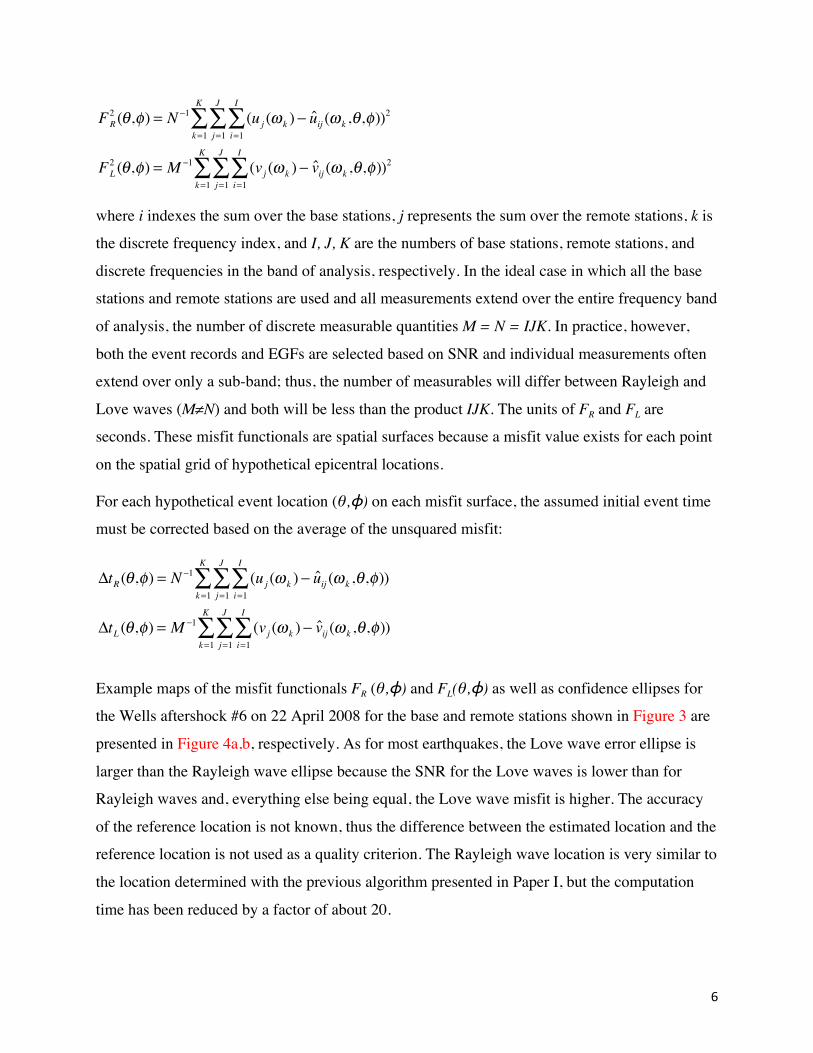
where i indexes the sum over the base stations, j represents the sum over the remote stations, k is

the discrete frequency index, and I, J, K are the numbers of base stations, remote stations, and

discrete frequencies in the band of analysis, respectively. In the ideal case in which all the base

stations and remote stations are used and all measurements extend over the entire frequency band

of analysis, the number of discrete measurable quantities M = N = IJK. In practice, however,

both the event records and EGFs are selected based on SNR and individual measurements often

extend over only a sub-band; thus, the number of measurables will differ between Rayleigh and

Love waves (M≠N) and both will be less than the product IJK. The units of FR and FL are

seconds. These misfit functionals are spatial surfaces because a misfit value exists for each point

on the spatial grid of hypothetical epicentral locations.

For each hypothetical event location (θ,ϕ) on each misfit surface, the assumed initial event time

must be corrected based on the average of the unsquared misfit:

ΔtR (θ,φ) = N−1 (uj (ω k ) − uij (ω k ,θ,φ))

i=1

I

∑j=1

J

∑k=1

K

∑

ΔtL (θ,φ) = M−1 (vj (ω k ) − vij (ω k ,θ,φ))

i=1

I

∑j=1

J

∑k=1

K

∑

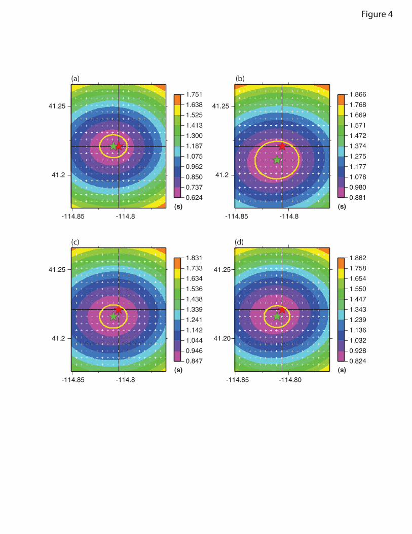
Example maps of the misfit functionals FR (θ,ϕ) and FL(θ,ϕ) as well as confidence ellipses for

the Wells aftershock #6 on 22 April 2008 for the base and remote stations shown in Figure 3 are

presented in Figure 4a,b, respectively. As for most earthquakes, the Love wave error ellipse is

larger than the Rayleigh wave ellipse because the SNR for the Love waves is lower than for

Rayleigh waves and, everything else being equal, the Love wave misfit is higher. The accuracy

of the reference location is not known, thus the difference between the estimated location and the

reference location is not used as a quality criterion. The Rayleigh wave location is very similar to

the location determined with the previous algorithm presented in Paper I, but the computation

time has been reduced by a factor of about 20.

  7 

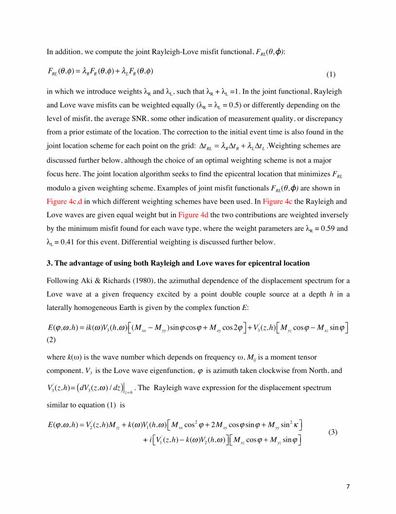
In addition, we compute the joint Rayleigh-Love misfit functional, FRL(θ,ϕ):

FRL (θ,φ) = λRFR (θ,φ) + λLFR (θ,φ) (1)

in which we introduce weights λR and λL, such that λR + λL =1. In the joint functional, Rayleigh

and Love wave misfits can be weighted equally (λR = λL = 0.5) or differently depending on the

level of misfit, the average SNR, some other indication of measurement quality, or discrepancy

from a prior estimate of the location. The correction to the initial event time is also found in the

joint location scheme for each point on the grid: ΔtRL = λRΔtR + λLΔtL .Weighting schemes are

discussed further below, although the choice of an optimal weighting scheme is not a major

focus here. The joint location algorithm seeks to find the epicentral location that minimizes FRL

modulo a given weighting scheme. Examples of joint misfit functionals FRL(θ,ϕ) are shown in

Figure 4c,d in which different weighting schemes have been used. In Figure 4c the Rayleigh and

Love waves are given equal weight but in Figure 4d the two contributions are weighted inversely

by the minimum misfit found for each wave type, where the weight parameters are λR = 0.59 and

λL = 0.41 for this event. Differential weighting is discussed further below.

3. The advantage of using both Rayleigh and Love waves for epicentral location

Following Aki & Richards (1980), the azimuthal dependence of the displacement spectrum for a

Love wave at a given frequency excited by a point double couple source at a depth h in a

laterally homogeneous Earth is given by the complex function E:

E(ϕ,ω ,h) = ik(ω )V3(h,ω ) (Mxx − Myy )sinϕ cosϕ + Mxy cos2ϕ⎡⎣ ⎤⎦ +V3' (z,h) Myz cosϕ − Mxz sinϕ⎡⎣ ⎤⎦

(2)

where k(ω) is the wave number which depends on frequency ω, Mij is a moment tensor

component, V3 is the Love wave eigenfunction, ϕ is azimuth taken clockwise from North, and

V3' (z,h)= dV3(z,ω ) / dz( )

z=h. The Rayleigh wave expression for the displacement spectrum

similar to equation (1) is

E(ϕ,ω ,h) = V2' (z,h)Mzz + k(ω )V1(h,ω ) Mxx cos2ϕ + 2Mxy cosϕ sinϕ + Myy sin2κ⎡⎣ ⎤⎦

+ i V1' (z,h) − k(ω )V2 (h,ω )⎡⎣ ⎤⎦ Mxz cosϕ + Myz sinϕ⎡⎣ ⎤⎦

(3)

  8 

where V1 and V2 are the horizontal and vertical components of the Rayleigh vectoral

eigenfunction and V1' (z,h) and V2

' (z,h) are defined similar to V3' (z,h) .

The modulus |E| of the complex function E represents the source amplitude radiation pattern and

the argument θ=arg (E) represents the source phase time delay. Both |E| and θ are real functions

of frequency ω, azimuthϕ , and source depth h. The source phase time delay produces phase

shifts in the event seismograms, but our location method is not sensitive to source phase time

delays but rather to source group time delays, δtU , which are the frequency derivative of the

source phase time delays (Levshin et al., 1999). The real part of equation (2) and the imaginary

part of equation (3) are proportional to the tangential component of stress and equal zero for a

seismic event at the surface h=0. This means that θ is independent of ω for a surface event.

Thus, source group time delays are zero for a surface source but for events below the surface will

vary depending on azimuth. The source group time delay may be expressed explicitly as

δtU =∂θ∂ω

=EE*

E 2 (4)

Substitution of E defined by equations (2) or (3) into (4) shows that the source group time delay

function for both types of waves can be rewritten as

δtU =A1 cos(ϕ +α1) + A3 cos(3ϕ +α 3)

1+ A2 cos(2ϕ +α2 ) + A4 cos(4ϕ +α 4 ) (5)

where Ai and αi (i=1,4) are frequency-dependent functions. Thus, the group time delay is an odd

function of azimuth and in most cases the numerator will dominate the azimuthal dependence.

The odd-symmetry of the azimuthal dependence implies that antipolar observations

(observations that differ in azimuth ϕ by 180°) will not cancel one another, but will actually add

constructively.

In our location procedures we assume that the source mechanism is unknown even though it may

have been estimated by other means. We do this because source depth typically is not well

known but source group time delays are strongly dependent on source depth in the period range

we use (5 – 12 sec). Source depth is typically more difficult to constrain than mechanism, except

in unusual circumstances, and corrections of observed group time delays for source mechanism

when source depth is not well known would be unreliable. Thus, source group time delays

  9 

imposed by seismic events act to bias the location procedure that we present here and in Paper I.

Locations will be minimally biased for events with small source group time delays. Paper I

shows that Rayleigh wave source group time delays are not small for particular types of

earthquakes at depths between about 2 and 5 km, for which bias may be as high as several km.

However, we show here that source group time delays for Love waves are much smaller than for

Rayleigh waves, and this is the motivation for introducing Love waves into the location

procedure.

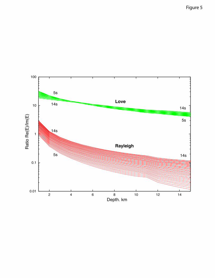
Figures 5 and 6 aim to provide some understanding of the difference in the expected magnitude

of the source group time shift for Rayleigh and Love waves. Figure 5 shows a simplified version

of the ratio between the imaginary and real parts of equations (2) and (3). The simplification

includes setting both terms in square brackets to 1, thus removing the dependence on source-

mechanism and providing a kind of average over azimuth. Clearly, the source phase shift for

Rayleigh waves is significantly smaller than for Love waves for source depths between 1 and 15

km. However, the source time shift is related to the frequency dependence of the source phase

shift (eqn. (4)). Figure 5 illustrates that the change in the source phase shift with period from 5

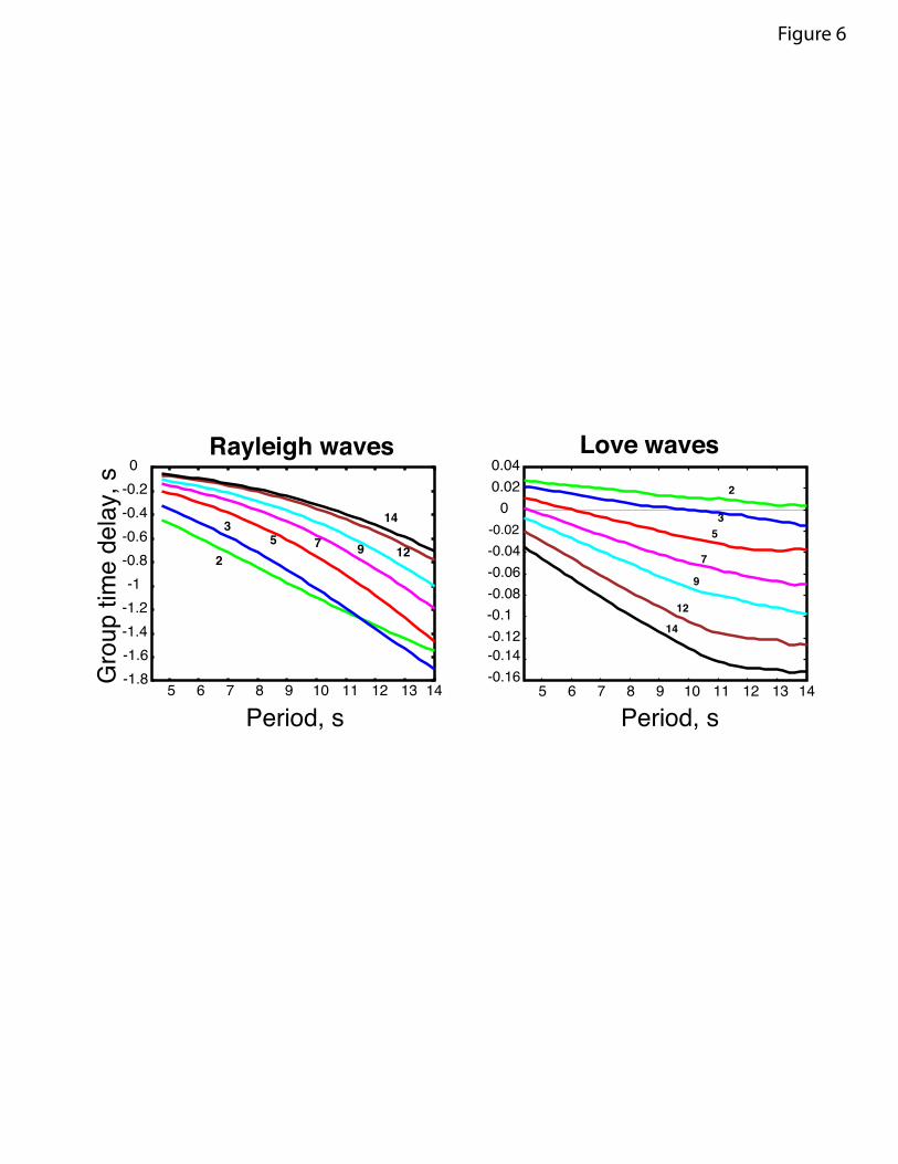
sec to 14 sec period for Love waves is much smaller than for Rayleigh waves. This is also seen

clearly in Figure 6, which shows average curves of the source group time shift δtU as a function

of period for several source depths and both types of waves. The range of δtU values for Rayleigh

waves is about 10 times greater than for Love waves.

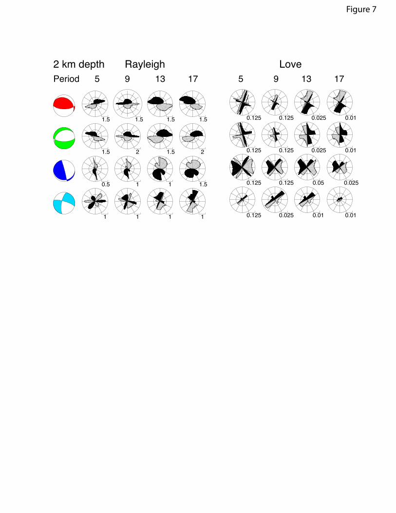
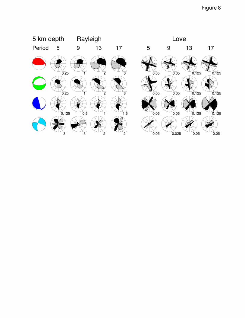
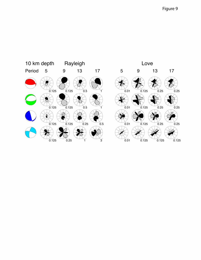
Figures 7-9 present a compendium of theoretical calculations of the source group time delay δtU

as a function of different types of source mechanism, source depth and wave period for both

Love and Rayleigh waves. These results are computed relative to a crustal model in Nevada from

the global model of Shapiro & Ritzwoller (2002). Four different source mechanisms are used

here and they are shown with different colored beachballs (e.g., Fig. 7). We refer here and later

in the paper to these four mechanisms as the red, green, dark blue, and light blue events. The

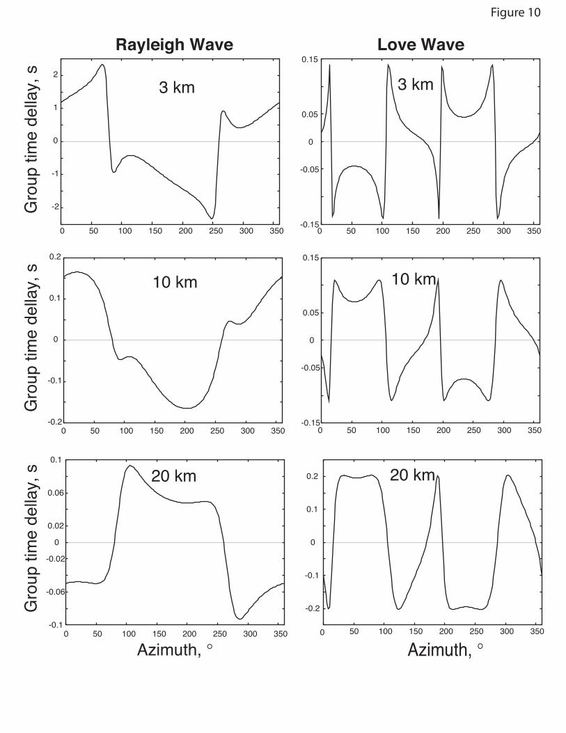
results of the calculations shown in Figures 7-9 are somewhat complicated and for the sake of

clarity Figure 10 presents a blow up at 7 sec period for one event type (red event in Fig. 7) at

several depths. Most significantly, these figures indicate that the source group time shifts δtU are

much smaller for Love waves than for Rayleigh waves, on average about an order of magnitude

smaller. This means that epicentral locations determined using Love waves will be biased less by

  10 

source mechanism. Figure 10 also demonstrates the odd-dependence of the group time delays on

azimuth.

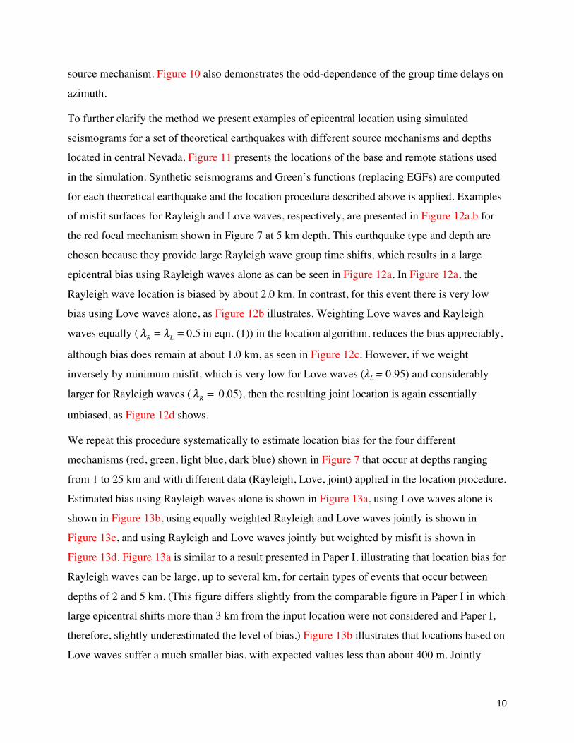
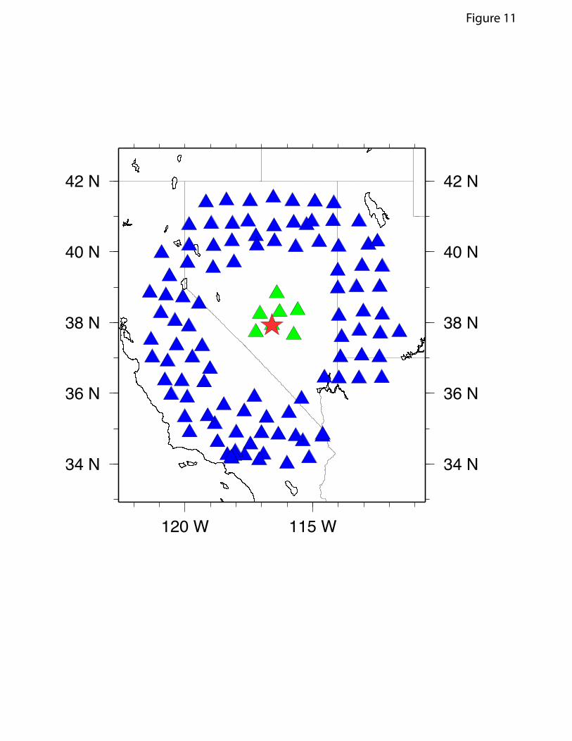
To further clarify the method we present examples of epicentral location using simulated

seismograms for a set of theoretical earthquakes with different source mechanisms and depths

located in central Nevada. Figure 11 presents the locations of the base and remote stations used

in the simulation. Synthetic seismograms and Green’s functions (replacing EGFs) are computed

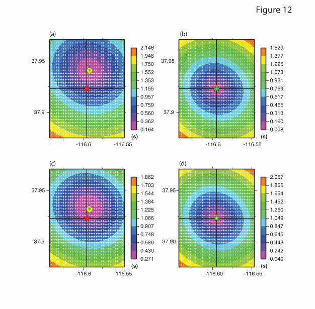
for each theoretical earthquake and the location procedure described above is applied. Examples

of misfit surfaces for Rayleigh and Love waves, respectively, are presented in Figure 12a,b for

the red focal mechanism shown in Figure 7 at 5 km depth. This earthquake type and depth are

chosen because they provide large Rayleigh wave group time shifts, which results in a large

epicentral bias using Rayleigh waves alone as can be seen in Figure 12a. In Figure 12a, the

Rayleigh wave location is biased by about 2.0 km. In contrast, for this event there is very low

bias using Love waves alone, as Figure 12b illustrates. Weighting Love waves and Rayleigh

waves equally (λR = λL = 0.5 in eqn. (1)) in the location algorithm, reduces the bias appreciably,

although bias does remain at about 1.0 km, as seen in Figure 12c. However, if we weight

inversely by minimum misfit, which is very low for Love waves (λL = 0.95) and considerably

larger for Rayleigh waves (λR = 0.05), then the resulting joint location is again essentially

unbiased, as Figure 12d shows.

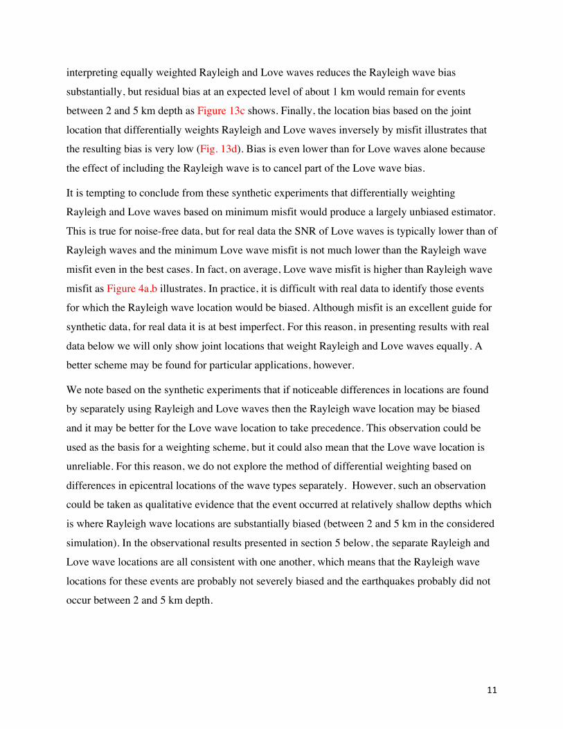
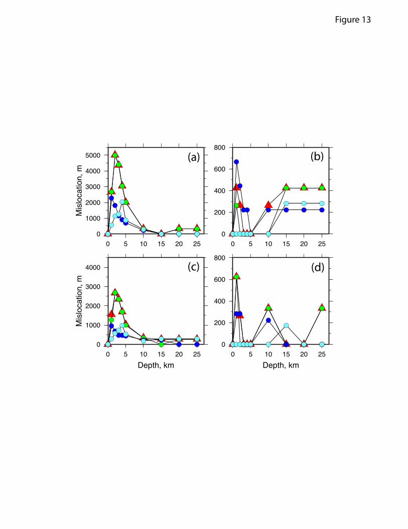
We repeat this procedure systematically to estimate location bias for the four different

mechanisms (red, green, light blue, dark blue) shown in Figure 7 that occur at depths ranging

from 1 to 25 km and with different data (Rayleigh, Love, joint) applied in the location procedure.

Estimated bias using Rayleigh waves alone is shown in Figure 13a, using Love waves alone is

shown in Figure 13b, using equally weighted Rayleigh and Love waves jointly is shown in

Figure 13c, and using Rayleigh and Love waves jointly but weighted by misfit is shown in

Figure 13d. Figure 13a is similar to a result presented in Paper I, illustrating that location bias for

Rayleigh waves can be large, up to several km, for certain types of events that occur between

depths of 2 and 5 km. (This figure differs slightly from the comparable figure in Paper I in which

large epicentral shifts more than 3 km from the input location were not considered and Paper I,

therefore, slightly underestimated the level of bias.) Figure 13b illustrates that locations based on

Love waves suffer a much smaller bias, with expected values less than about 400 m. Jointly

  11 

interpreting equally weighted Rayleigh and Love waves reduces the Rayleigh wave bias

substantially, but residual bias at an expected level of about 1 km would remain for events

between 2 and 5 km depth as Figure 13c shows. Finally, the location bias based on the joint

location that differentially weights Rayleigh and Love waves inversely by misfit illustrates that

the resulting bias is very low (Fig. 13d). Bias is even lower than for Love waves alone because

the effect of including the Rayleigh wave is to cancel part of the Love wave bias.

It is tempting to conclude from these synthetic experiments that differentially weighting

Rayleigh and Love waves based on minimum misfit would produce a largely unbiased estimator.

This is true for noise-free data, but for real data the SNR of Love waves is typically lower than of

Rayleigh waves and the minimum Love wave misfit is not much lower than the Rayleigh wave

misfit even in the best cases. In fact, on average, Love wave misfit is higher than Rayleigh wave

misfit as Figure 4a,b illustrates. In practice, it is difficult with real data to identify those events

for which the Rayleigh wave location would be biased. Although misfit is an excellent guide for

synthetic data, for real data it is at best imperfect. For this reason, in presenting results with real

data below we will only show joint locations that weight Rayleigh and Love waves equally. A

better scheme may be found for particular applications, however.

We note based on the synthetic experiments that if noticeable differences in locations are found

by separately using Rayleigh and Love waves then the Rayleigh wave location may be biased

and it may be better for the Love wave location to take precedence. This observation could be

used as the basis for a weighting scheme, but it could also mean that the Love wave location is

unreliable. For this reason, we do not explore the method of differential weighting based on

differences in epicentral locations of the wave types separately. However, such an observation

could be taken as qualitative evidence that the event occurred at relatively shallow depths which

is where Rayleigh wave locations are substantially biased (between 2 and 5 km in the considered

simulation). In the observational results presented in section 5 below, the separate Rayleigh and

Love wave locations are all consistent with one another, which means that the Rayleigh wave

locations for these events are probably not severely biased and the earthquakes probably did not

occur between 2 and 5 km depth.

  12 

4. Database of Rayleigh and Love EGFs and group velocity curves for the western USA

The database for Rayleigh and Love wave EGFs that has been used in this study was developed

at the University of Colorado for data recorded in the US between the years 2005 and 2011 using

the methodology described by Bensen et al. (2007) and Lin et al. (2008). Broadband three-

component seismograms observed at over 950 permanent and temporary stations from the

Transportable Array (TA) component of USArray were used for this purpose. This database

comprises about 350,000 Rayleigh and Love wave inter-station cross-correlation functions. For

all EGFs in this database signal/noise ratio (SNR) was estimated and individual EGFs were

retained only if SNR > 10. Data processing includes the automatic two-step frequency-time

analysis (FTAN) typically between about 5 and 12 sec period. The first step in the procedure

provides the raw FTAN diagram and the second step applies phase-match filtering (Herrin &

Goforth, 1977; Levshin & Ritzwoller, 2001) to create a cleaned FTAN diagram of the

fundamental Rayleigh and Love waves largely freed from interference with other waves, coda

and local noise. The FTAN image is used to determine the group times in the range of periods

where the power of the narrow-band output signal is not less than 95% of the maximum power.

 

5. Joint application of Rayleigh and Love waves to locate reference events in the Western

USA

We now present applications of the revised location method to ten reference events that

occurred in the Western USA between 2005 and 2008. These include the Crandall Canyon Mine

collapse in Utah on August 6, 2007 (Pechmann et al., 2007), which is a very shallow event

whose location using Rayleigh wave EGFs was described in Paper I, two well located events in

California and Utah, the large Wells earthquake in northern Nevada, and a sequence of six

aftershocks of the Wells earthquake that we refer to as aftershocks #1 - #6 (Mendoza & Hartzell,

2009). Source parameters for these events are listed in Table 1. Unfortunately, none of the

reference events are located by the authoritative source better than about 1 km and for most

events uncertainties are not well known, but 1 km is probably a reasonable 90% (2-sigma)

uncertainty estimate, on average.

  13 

The estimated epicentral locations for the ten reference events are summarized in Table 2. Each

location is compared with the reference location for Rayleigh waves alone (Ref-R), Love waves

alone (Ref-L), and jointly using Rayleigh and Love waves weighted equally (Ref-RL) such that

λR = λL = 0.5 in equation (1). In each column, the difference in kilometers between the

reference location and the estimated location is listed. In addition, the rms misfit at the estimated

epicentral location is presented for all three estimators (R, L, RL). Finally, the semi-major axis of

the error ellipse (95% confidence) is presented for each of the estimators. For the joint location,

we only present results where the Rayleigh and Love waves are weighted equally.

Other estimators could be defined that would produce somewhat different results than those we

present here. In particular, as with the synthetic experiment discussed earlier, one could weight

the Rayleigh and Love waves inversely by minimum misfit. However, inspection of Table 2

reveals that for the reference events the minimum misfit is approximately the same for Rayleigh

and Love waves so that the result of this weighting scheme would be approximately the same as

applying equal weights.

As noted earlier, the locations of the reference events are probably known to about 1 km, on

average. This may be worse for the large Wells earthquake (2008/02/21), however, which has a

rupture length of about 5 km (Mendoza and Hartzell, 2009) and our locations may be of the

centroid of this event. The difference between the estimated location and the reference location,

therefore, is probably not a reliable quality criterion for locations within 1-2 km of the reference

location. For these ten events, the Rayleigh wave locations agree quite well with the reference

locations; the discrepancy being greater than 1.0 km only for three of the events and not larger

than 1.3 km for any of the events. It is, therefore, unlikely that the Rayleigh wave location is

badly biased for any of these events. This is evidence that the depths of these events are probably

not between 2 and 5 km and/or the events do not have mechanisms that would cause a large bias.

For this reason, we do not expect the joint inversion to provide a substantial improvement over

the use of Rayleigh waves alone because the joint inversion is only expected to be appreciably

better when the Rayleigh wave location is badly biased. The choice of the ten reference events

used here is unfortunate in this regard, but identifying well located events in the western USA

that are definitely between 2 and 5 km depth is a challenging task.

  14 

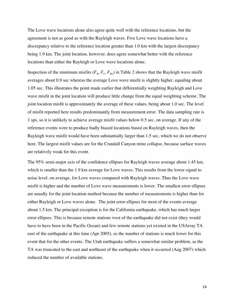
The Love wave locations alone also agree quite well with the reference locations, but the

agreement is not as good as with the Rayleigh waves. Five Love wave locations have a

discrepancy relative to the reference location greater than 1.0 km with the largest discrepancy

being 1.9 km. The joint location, however, does agree somewhat better with the reference

locations than either the Rayleigh or Love wave locations alone.

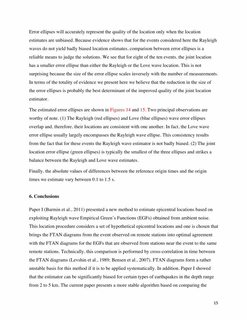
Inspection of the minimum misfits (FR, FL, FRL) in Table 2 shows that the Rayleigh wave misfit

averages about 0.9 sec whereas the average Love wave misfit is slightly higher, equaling about

1.05 sec. This illustrates the point made earlier that differentially weighting Rayleigh and Love

wave misfit in the joint location will produce little change from the equal weighting scheme. The

joint location misfit is approximately the average of these values, being about 1.0 sec. The level

of misfit reported here results predominantly from measurement error. The data sampling rate is

1 sps, so it is unlikely to achieve average misfit values below 0.5 sec, on average. If any of the

reference events were to produce badly biased locations based on Rayleigh waves, then the

Rayleigh wave misfit would have been substantially larger than 1.5 sec, which we do not observe

here. The largest misfit values are for the Crandall Canyon mine collapse, because surface waves

are relatively weak for this event.

The 95% semi-major axis of the confidence ellipses for Rayleigh waves average about 1.45 km,

which is smaller than the 1.9 km average for Love waves. This results from the lower signal to

noise level, on average, for Love waves compared with Rayleigh waves. Thus the Love wave

misfit is higher and the number of Love wave measurements is lower. The smallest error ellipses

are usually for the joint location method because the number of measurements is higher than for

either Rayleigh or Love waves alone. The joint error ellipses for most of the events average

about 1.5 km. The principal exception is for the California earthquake, which has much larger

error ellipses. This is because remote stations west of the earthquake did not exist (they would

have to have been in the Pacific Ocean) and few remote stations yet existed in the USArray TA

east of the earthquake at this time (Apr 2005), so the number of stations is much lower for this

event that for the other events. The Utah earthquake suffers a somewhat similar problem, as the

TA was truncated to the east and northeast of the earthquake when it occurred (Aug 2007) which

reduced the number of available stations.

  15 

Error ellipses will accurately represent the quality of the location only when the location

estimates are unbiased. Because evidence shows that for the events considered here the Rayleigh

waves do not yield badly biased location estimates, comparison between error ellipses is a

reliable means to judge the solutions. We see that for eight of the ten events, the joint location

has a smaller error ellipse than either the Rayleigh or the Love wave location. This is not

surprising because the size of the error ellipse scales inversely with the number of measurements.

In terms of the totality of evidence we present here we believe that the reduction in the size of

the error ellipses is probably the best determinant of the improved quality of the joint location

estimator.

The estimated error ellipses are shown in Figures 14 and 15. Two principal observations are

worthy of note. (1) The Rayleigh (red ellipses) and Love (blue ellipses) wave error ellipses

overlap and, therefore, their locations are consistent with one another. In fact, the Love wave

error ellipse usually largely encompasses the Rayleigh wave ellipse. This consistency results

from the fact that for these events the Rayleigh wave estimator is not badly biased. (2) The joint

location error ellipse (green ellipses) is typically the smallest of the three ellipses and strikes a

balance between the Rayleigh and Love wave estimates.

Finally, the absolute values of differences between the reference origin times and the origin

times we estimate vary between 0.1 to 1.5 s.

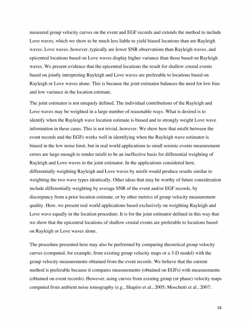
6. Conclusions

Paper I (Barmin et al., 2011) presented a new method to estimate epicentral locations based on

exploiting Rayleigh wave Empirical Green’s Functions (EGFs) obtained from ambient noise.

This location procedure considers a set of hypothetical epicentral locations and one is chosen that

brings the FTAN diagrams from the event observed on remote stations into optimal agreement

with the FTAN diagrams for the EGFs that are observed from stations near the event to the same

remote stations. Technically, this comparison is performed by cross-correlation in time between

the FTAN diagrams (Levshin et al., 1989; Bensen et al., 2007). FTAN diagrams form a rather

unstable basis for this method if it is to be applied systematically. In addition, Paper I showed

that the estimator can be significantly biased for certain types of earthquakes in the depth range

from 2 to 5 km. The current paper presents a more stable algorithm based on comparing the

  16 

measured group velocity curves on the event and EGF records and extends the method to include

Love waves, which we show to be much less liable to yield biased locations than are Rayleigh

waves. Love waves, however, typically are lower SNR observations than Rayleigh waves, and

epicentral locations based on Love waves display higher variance than those based on Rayleigh

waves. We present evidence that the epicentral locations the result for shallow crustal events

based on jointly interpreting Rayleigh and Love waves are preferable to locations based on

Rayleigh or Love waves alone. This is because the joint estimator balances the need for low bias

and low variance in the location estimate.

The joint estimator is not uniquely defined. The individual contributions of the Rayleigh and

Love waves may be weighted in a large number of reasonable ways. What is desired is to

identify when the Rayleigh wave location estimate is biased and to strongly weight Love wave

information in these cases. This is not trivial, however. We show here that misfit between the

event records and the EGFs works well in identifying when the Rayleigh wave estimator is

biased in the low noise limit, but in real world applications to small seismic events measurement

errors are large enough to render misfit to be an ineffective basis for differential weighting of

Rayleigh and Love waves in the joint estimator. In the applications considered here,

differentially weighting Rayleigh and Love waves by misfit would produce results similar to

weighting the two wave types identically. Other ideas that may be worthy of future consideration

include differentially weighting by average SNR of the event and/or EGF records, by

discrepancy from a prior location estimate, or by other metrics of group velocity measurement

quality. Here, we present real world applications based exclusively on weighting Rayleigh and

Love wave equally in the location procedure. It is for the joint estimator defined in this way that

we show that the epicentral locations of shallow crustal events are preferable to locations based

on Rayleigh or Love waves alone.

The procedure presented here may also be performed by comparing theoretical group velocity

curves (computed, for example, from existing group velocity maps or a 3-D model) with the

group velocity measurements obtained from the event records. We believe that the current

method is preferable because it compares measurements (obtained on EGFs) with measurements

(obtained on event records). However, using curves from existing group (or phase) velocity maps

computed from ambient noise tomography (e.g., Shapiro et al., 2005; Moschetti et al., 2007;

  17 

Yang et al., 2007; Lin et al., 2008; and many others) or from curves predicted from a 3-D model

that originated by inverting ambient noise dispersion maps (e.g., Yang et al., 2008; Moschetti et

al., 2010a, 2010b; Zheng et al., 2011; Yang et al., 2012; Zhou et al., 2012; and others) would

make the algorithm more flexible and would open the possibility to estimate other source

parameters such as hypocentral depth and the moment tensor.

Acknowledgements

This research was supported by DoE/NNSA contract DE-AC52-09NA29326. Support for one of

the authors (C.M.) was provided by the Direccion General de Asuntos del Personal Academico

(DGAPA) at UNAM. The facilities of the IRIS Data Management System, and specifically the

IRIS Data Management Center, were used to access the waveform and metadata required in this

study. The IRIS DMS is funded by the National Science Foundation and specifically the GEO

Directorate through the Instrumentation and Facilities Program of the National Science

Foundation under Cooperative Agreement EAR-0552316. The authors are very grateful to Drs. J.

W. Dewey, J. C. Pechman, and K. Smith for providing information about well located

earthquakes in the Western USA.

References

Aki, K., and P. G. Richards (1980), Quantitative Seismology: Theory and Methods, I, W. H.

Freeman and Co, San Francisco.

Barmin, M. P., A. L. Levshin, Y. Yang, and M. H. Ritzwoller (2011), Epicentral location based

on Rayleigh wave empirical Green's functions from ambient seismic noise, Geophys. J.

Int., 184, 869-884, doi: 10.1111/j.1365-246X.2010.04879.x.

Bensen, G. D., M. H. Ritzwoller, M. P. Barmin, A. L. Levshin, F. Lin, M. P. Moschetti, N. M.

Shapiro, and Y. Yang (2007), Processing seismic ambient noise data to obtain reliable

broad- band surface wave dispersion measurements, Geophys. J. Int., 169(3), 1239-1260,

doi:10.1111/j.1365-246X.2007.03374.x.

Flinn, E. A. (1965), Confidence regions and error determinations for seismic event locations.

Rev. Geophys, 3, 157-185.

Herrin, E. and T. Goforth (1977), Phase-matched filtering: application to the study of Rayleigh

waves, Bull. Seism. Soc. Amer., 67, 1259-1275.

Herrmann, R. B., H. Benz, and C. J. Ammon (2011), Monitoring the earthquake process in

  18 

North America, Bull. Seism. Soc. Am., 101, N6, 2609-2625, doi:10.1785/0120110095.

Jordan, T. H. and K. A. Swerdrup (1981), Teleseismic location techniques and their application

to earthquake clusters in the South-Central Pacific, Bull. Seismol. Soc. Amer., 71, 4, 1105-

1130.

Levshin, A. L., V. F. Pisarenko, and G. A. Pogrebinsky, 1972. On a frequency-time analysis of oscillations. Ann. Geophys., 28, 211-218. Levshin, A. L., T. B. Yanovskaya, A.V. Lander, B. G. Bukchin, M. P. Barmin, L. I. Ratnikova,

and E. N. Its (1989), Seismic Surface Waves in Laterally Inhomogeneous Earth, (V. I.

Keilis-Borok, Ed.), Kluwer Academic Publishers. Dordrecht/Boston/London.

Levshin, A. L., M. H. Ritzwoller, and J. S. Resovsky (1999), Source effects on surface wave

group travel times and group velocity maps, Phys. Earth Planet. Inter., 115, 293-312.

Levshin, A. L. and M. H. Ritzwoller (2001), Automatic detection, extraction, and measurement

of regional surface waves, Pure and Applied Geophysics, 158, 1531-1545.

Lin, F., M. P. Moschetti, and M. H. Ritzwoller (2008), Surface wave tomography of the western

United States from ambient seismic noise: Rayleigh and Love wave phase velocity maps,

Geophys. J. Int., 173(1), 281-298, doi:10.1111/j1365-246X.2008.03720.x.

Mendoza, C. and S. Hartzell (2009). Source analysis using regional empirical Green's functions:

The 2008 Wells, Nevada, earthquake, Geophys. Res. Lett., 36, L11302,

doi:10.1029/2009GL038073.

Moschetti, M. P., M. H. Ritzwoller, and N. M. Shapiro (2007), Surface wave tomography of the

western United States from ambient seismic noise: Rayleigh wave group velocity maps,

Geochem., Geophys., Geosys., 8, Q08010, doi:10.1029/2007GC001655.

Moschetti, M.P., M.H. Ritzwoller, and F.C. Lin (2010a), Seismic evidence for widespread crustal deformation caused by extension in the western USA, Nature, 464, Number 7290, 885-889, 8 April 2010.

Moschetti, M.P., M.H. Ritzwoller, F.C. Lin, and Y. Yang (2010b), Crustal shear velocity

structure of the western US inferred from amient noise and earthquake data, J. Geophys.

Res., 115, B10306, doi:10.1029/2010JB007448.

Pechmann, J. C., W. I. Arabasz, K. L. Pankow, R. Burlacu, and M. K. McCarter (2007),

Seismological report on the 6 Aug 2007 Crandall Canyon Mine Collapse in Utah, Seismol.

Res. Lett., 79,5, 620-636.

Shapiro, N. M., and M. Campillo (2004), Emergence of broadband Rayleigh waves from

  19 

correlations of the ambient seismic noise, Geophys. Res. Lett., 31, L07614,

doi:10.1029/2004GL019491.

Shapiro, N. M. and M. H. Ritzwoller (2002), Monte-Carlo inversion for a global shear velocity

model of the crust and upper mantle, Geophys. J. Int., 151, 88-105.

Shapiro, N. M., M. Campillo, L. Stehly, and M. H. Ritzwoller (2005), High resolution surface

wave tomography from ambient seismic noise, Science, 307(5715), 1615-1618.

Yang, Y., M.H. Ritzwoller, A.L. Levshin, and N.M. Shapiro (2007), Ambient noise Rayleigh

wave tomography across Europe, Geophys. J. Int., 168(1), page 259.

Yang, Y., M.H. Ritzwoller, F.-C. Lin, M.P. Moschetti, and N.M. Shapiro (2008), The structure

of the crust and uppermost mantle beneath the western US revealed by ambient noise and

earthquake tomography, J. Geophys. Res., 113, B12310.

Zheng, Y., W. Shen, L. Zhou, Y. Yang, Z. Xie, and M.H. Ritzwoller (2011), Crust and

uppermost mantle beneath the North China Craton, northeastern China, and the Sea of Japan

from ambient noise tomography, J. Geophys. Res., 116, B12312,

doi:10.1029/2011JB008637.

Yang, Y., M.H. Ritzwoller, Y. Zheng, A.L. Levshin, and Z. Xie (2012), A synoptic view of the distribution and connectivity of the mid-crustal low velocity zone beneath Tibet, J. Geophys. Res., in press.

Zhou, L., J. Xie, W. Shen, Y. Zheng, Y. Yang. H. Shi, and M.H. Ritzwoller (2012), The structure

of the crust and uppermost mantle beneath South China from ambient noise and earthquake

tomography, Geophys. J. Int., in press, 2012.

  20 

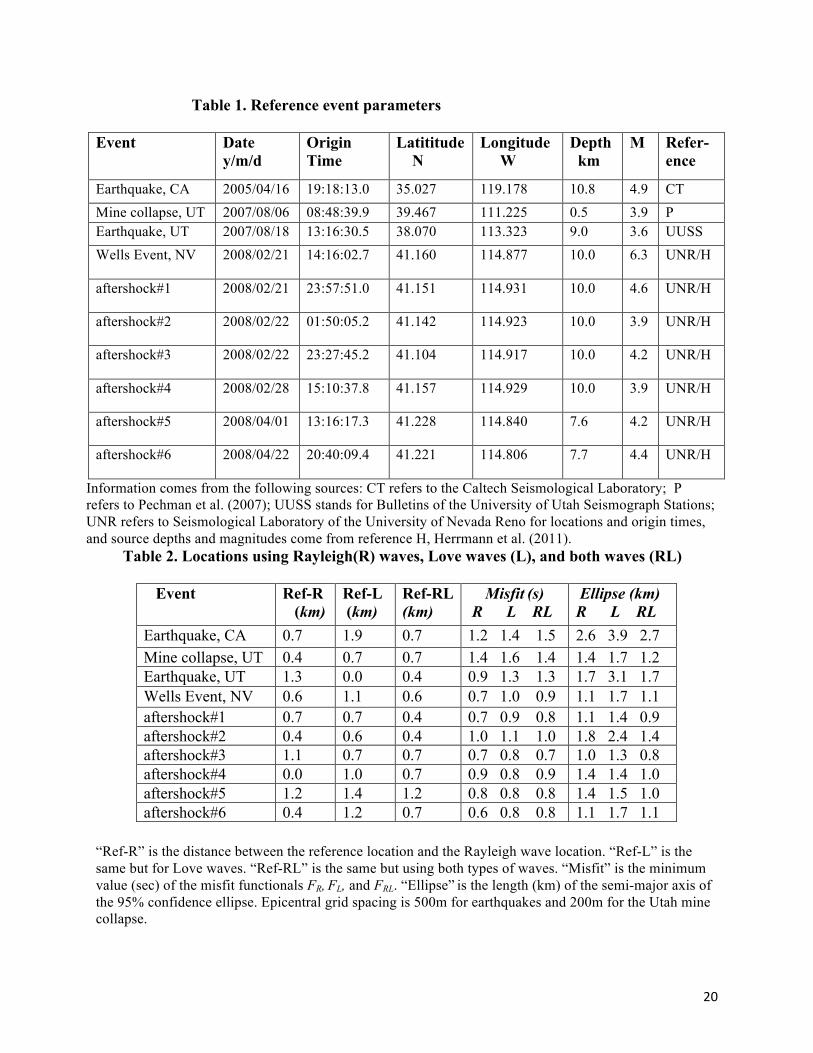
Table 1. Reference event parameters Event

Date y/m/d

Origin Time

Latititude N

Longitude W

Depth km

M Refer- ence

Earthquake, CA 2005/04/16 19:18:13.0 35.027 119.178 10.8 4.9 CT Mine collapse, UT 2007/08/06 08:48:39.9 39.467 111.225 0.5 3.9 P Earthquake, UT 2007/08/18 13:16:30.5 38.070 113.323 9.0 3.6 UUSS Wells Event, NV 2008/02/21 14:16:02.7 41.160 114.877 10.0 6.3 UNR/H

aftershock#1 2008/02/21 23:57:51.0 41.151 114.931 10.0 4.6 UNR/H

aftershock#2 2008/02/22 01:50:05.2 41.142 114.923 10.0 3.9 UNR/H

aftershock#3 2008/02/22 23:27:45.2 41.104 114.917 10.0 4.2 UNR/H

aftershock#4 2008/02/28 15:10:37.8 41.157 114.929 10.0 3.9 UNR/H

aftershock#5 2008/04/01 13:16:17.3 41.228 114.840 7.6 4.2 UNR/H

aftershock#6 2008/04/22 20:40:09.4 41.221 114.806 7.7 4.4 UNR/H

Information comes from the following sources: CT refers to the Caltech Seismological Laboratory; P refers to Pechman et al. (2007); UUSS stands for Bulletins of the University of Utah Seismograph Stations; UNR refers to Seismological Laboratory of the University of Nevada Reno for locations and origin times, and source depths and magnitudes come from reference H, Herrmann et al. (2011). Table 2. Locations using Rayleigh(R) waves, Love waves (L), and both waves (RL)

Event Ref-R

(km) Ref-L (km)

Ref-RL (km)

Misfit (s) R L RL

Ellipse (km) R L RL

Earthquake, CA 0.7 1.9 0.7 1.2 1.4 1.5 2.6 3.9 2.7 Mine collapse, UT 0.4 0.7 0.7 1.4 1.6 1.4 1.4 1.7 1.2 Earthquake, UT 1.3 0.0 0.4 0.9 1.3 1.3 1.7 3.1 1.7 Wells Event, NV 0.6 1.1 0.6 0.7 1.0 0.9 1.1 1.7 1.1 aftershock#1 0.7 0.7 0.4 0.7 0.9 0.8 1.1 1.4 0.9 aftershock#2 0.4 0.6 0.4 1.0 1.1 1.0 1.8 2.4 1.4 aftershock#3 1.1 0.7 0.7 0.7 0.8 0.7 1.0 1.3 0.8 aftershock#4 0.0 1.0 0.7 0.9 0.8 0.9 1.4 1.4 1.0 aftershock#5 1.2 1.4 1.2 0.8 0.8 0.8 1.4 1.5 1.0 aftershock#6 0.4 1.2 0.7 0.6 0.8 0.8 1.1 1.7 1.1

 “Ref-R” is the distance between the reference location and the Rayleigh wave location. “Ref-L” is the same but for Love waves. “Ref-RL” is the same but using both types of waves. “Misfit” is the minimum value (sec) of the misfit functionals FR, FL, and FRL. “Ellipse” is the length (km) of the semi-major axis of the 95% confidence ellipse. Epicentral grid spacing is 500m for earthquakes and 200m for the Utah mine collapse.

  21 

References

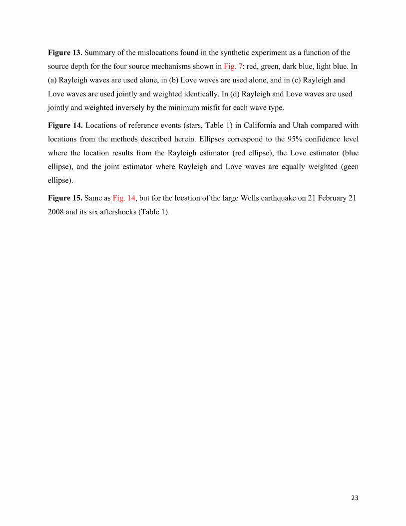
Figure 1. (a) Map of stations (triangles) selected near the meridian passing through the epicenter

(star) of aftershock #6 on 22 April 2008 of the Wells earthquake in Nevada. (b) Vertical and

transverse component seismograms following the aftershock observed at TA station H12A

located about 370 km north of the epicenter identifying Rayleigh and Love waves. (c) Symmetric

component Z-Z (Rayleigh wave) inter-station empirical Green’s functions (EGFs) for the base

station M12A and selected remote stations. (d) Same as (c) but for symmetric component T-T

(Love wave) inter-station EGFs. (e) Vertical component event records observed at the remote

stations following the aftershock. (f) The same as (e) but for transverse components. Straight

lines in (c)-(f) indicate predicted times of arrivals for Rayleigh and Love waves with group

velocities of 2.95 and 3.3 km/s, respectively.

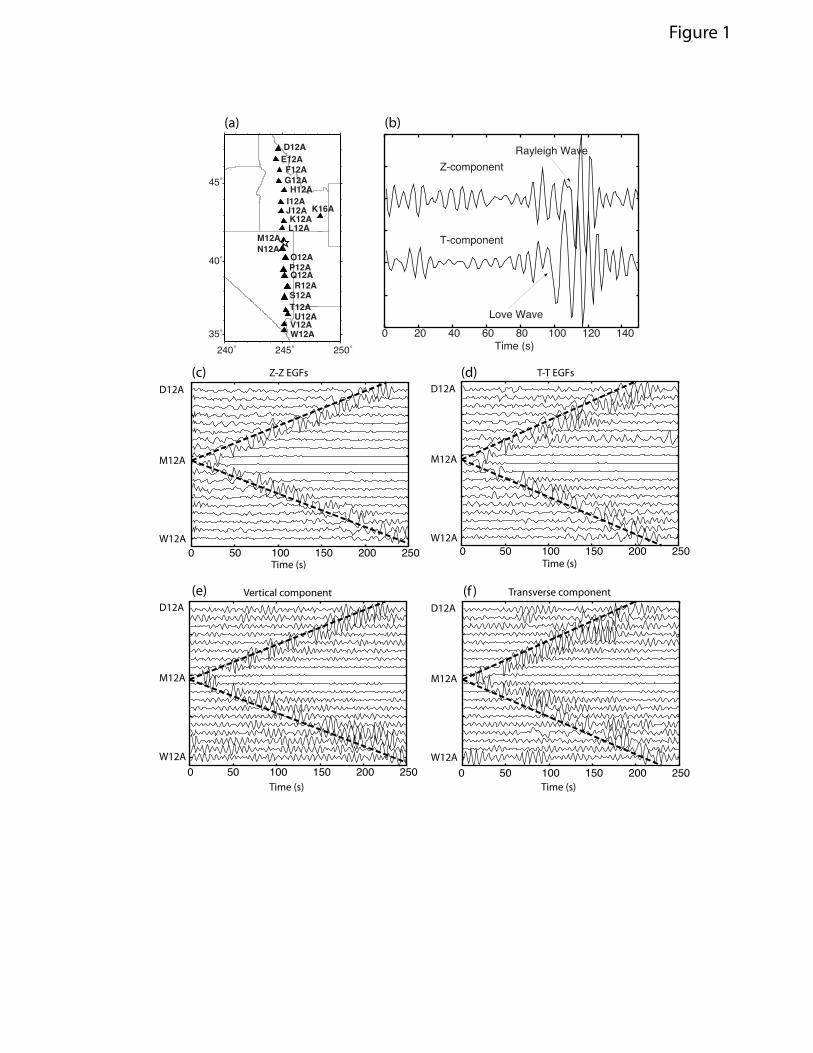
Figure 2. (a)-(b) FTAN diagrams for Rayleigh and Love wave symmetric component EGFs for a

pair of TA stations (K16A-M12A) compared with (c)-(d) the FTAN diagrams of the

corresponding event records from the earthquake in Fig. 1 observed at station K16A (location

shown Fig. 1a). Blue stars are group times determined by FTAN.

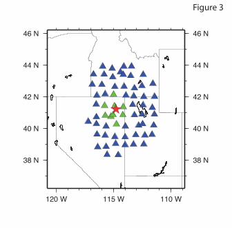
Figure 3. The network of base (green triangles) and remote (blue triangles) stations used to

locate the large Wells earthquake that occurred in northern Nevada (red star) on 21 February

2008 and for six of its aftershocks (#1 - #6) that occurred from late February to late April 2008.

Figure 4. (a) Rayleigh wave misfit surface FR (θ,φ) , in seconds, for aftershock #6 of the Wells

earthquake that occurred on 22 April 2008. (b) Love wave misfit surface FL (θ,φ) for the same

aftershock. (c) Joint misfit surface for the same aftershock where Rayleigh and Love waves have

been weighted identically (λR = λL = 0.5). (d) Joint misfit surface for the same aftershock where

Rayleigh and Love waves have been weighted inversely by minimum misfit (λR =0.59, λL =

0.41). The grid spacing is about 500 m. Error ellipses for the 95% confidence level are shown

with yellow lines. Red stars correspond to the reference location, green stars to the estimated

locations.

  22 

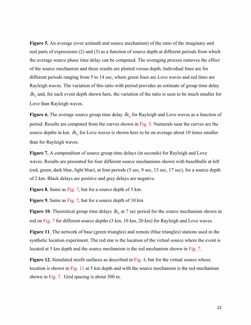
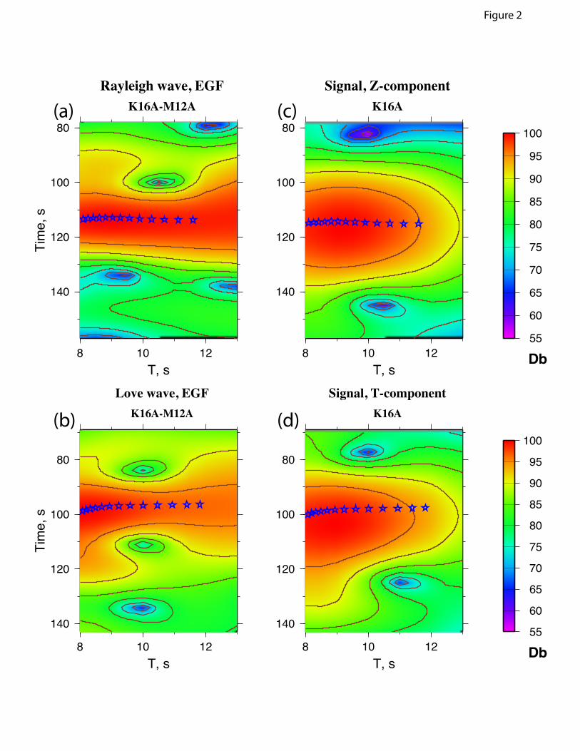
Figure 5. An average (over azimuth and source mechanism) of the ratio of the imaginary and

real parts of expressions (2) and (3) as a function of source depth at different periods from which

the average source phase time delay can be computed. The averaging process removes the effect

of the source mechanism and these results are plotted versus depth. Individual lines are for

different periods ranging from 5 to 14 sec, where green lines are Love waves and red lines are

Rayleigh waves. The variation of this ratio with period provides an estimate of group time delay

δtU and, for each event depth shown here, the variation of the ratio is seen to be much smaller for

Love than Rayleigh waves.

Figure 6. The average source group time delay δtU for Rayleigh and Love waves as a function of

period. Results are computed from the curves shown in Fig. 5. Numerals near the curves are the

source depths in km. δtU for Love waves is shown here to be on average about 10 times smaller

than for Rayleigh waves.

Figure 7. A compendium of source group time delays (in seconds) for Rayleigh and Love

waves. Results are presented for four different source mechanisms shown with beachballs at left

(red, green, dark blue, light blue), at four periods (5 sec, 9 sec, 13 sec, 17 sec), for a source depth

of 2 km. Black delays are positive and grey delays are negative.

Figure 8. Same as Fig. 7, but for a source depth of 5 km.

Figure 9. Same as Fig. 7, but for a source depth of 10 km.

Figure 10. Theoretical group time delays δtU at 7 sec period for the source mechanism shown in

red on Fig. 7 for different source depths (3 km, 10 km, 20 km) for Rayleigh and Love waves.

Figure 11. The network of base (green triangles) and remote (blue triangles) stations used in the

synthetic location experiment. The red star is the location of the virtual source where the event is

located at 5 km depth and the source mechanism is the red mechanism shown in Fig. 7.

Figure 12. Simulated misfit surfaces as described in Fig. 4, but for the virtual source whose

location is shown in Fig. 11 at 5 km depth and with the source mechanism is the red mechanism

shown in Fig. 7. Grid spacing is about 300 m.

  23 

Figure 13. Summary of the mislocations found in the synthetic experiment as a function of the

source depth for the four source mechanisms shown in Fig. 7: red, green, dark blue, light blue. In

(a) Rayleigh waves are used alone, in (b) Love waves are used alone, and in (c) Rayleigh and

Love waves are used jointly and weighted identically. In (d) Rayleigh and Love waves are used

jointly and weighted inversely by the minimum misfit for each wave type.

Figure 14. Locations of reference events (stars, Table 1) in California and Utah compared with

locations from the methods described herein. Ellipses correspond to the 95% confidence level

where the location results from the Rayleigh estimator (red ellipse), the Love estimator (blue

ellipse), and the joint estimator where Rayleigh and Love waves are equally weighted (geen

ellipse).

Figure 15. Same as Fig. 14, but for the location of the large Wells earthquake on 21 February 21

2008 and its six aftershocks (Table 1).  

Vertical component

0 50 100 150 200 250

D12A

M12A

W12A

Time (s)

0 50 100 150 200 250

D12A

M12A

W12A

Z-Z EGFs

Time (s)0 50 100 150 200 250

D12A

M12A

W12A

T-T EGFs

Time (s)

Transverse component

0 50 100 150 200 250

D12A

M12A

W12A

Time (s)

(c) (d)

(e) (f )

Time (s)0 20 40 60 80 100 120 140

Z-component

T-component

Love Wave

Rayleigh Wave

(b)

D12AE12AF12AG12A

H12AI12AJ12AK12AL12A

M12AN12A

O12AP12AQ12AR12A

S12AT12A

U12AV12AW12A

(a)

240˚ 245˚ 250˚35˚

40˚

45˚

K16A

Figure 1

80

100

120

140

Tim

e, s

8 10 12T, s

80

100

120

140

8 10 12T, s

55

60

65

70

75

80

85

90

95

100

K16ASignal, Z-component

K16A-M12ARayleigh wave, EGF

Db

80

100

120

140

Tim

e, s

8 10 12T, s

80

100

120

140

8 10 12T, s

55

60

65

70

75

80

85

90

95

100

K16A

Signal, T-componentK16A-M12A

Love wave, EGF

Db

(a)

(d)(b)

(c)

Figure 2

120 W 115 W 110 W

38 N 38 N

40 N 40 N

42 N 42 N

44 N 44 N

46 N 46 N

Figure 3

41.20

41.25

-114.85 -114.80

0.8240.9281.0321.1361.2391.3431.4471.5501.6541.7581.862

(s)

-114.85  -114.8 

41.2 

41.25 

0.8810.9801.0781.1771.2751.3741.4721.5711.6691.7681.866

(s)-114.85  -114.8 

41.2 

41.25 

0.6240.7370.8500.9621.0751.1871.3001.4131.5251.6381.751

(s)

-114.85  -114.8 

41.2 

41.25 

0.8470.9461.0441.1421.2411.3391.4381.5361.6341.7331.831

(s)

(a) (b)

(c) (d)

Figure 4

0.01

0.1

1

10

100

2 4 6 8 10 12 14

Rat

io R

e(E)

/Im(E

)

Depth. km

Love

Rayleigh

14s

5s

14s14s

5s

5s

14s

Figure 5

-0.16-0.14-0.12-0.1-0.08-0.06-0.04-0.02

00.020.04

5 6 7 8 9 10 11 12 13 14

2

35

7

9

12

14

Love waves

Period, s-1.8-1.6-1.4-1.2-1

-0.8-0.6-0.4-0.20

5 6 7 8 9 10 11 12 13 14

2

35 7 9 12

14

Rayleigh waves

Gro

up ti

me

dela

y, s

Period, s

Figure 6

1.5 1.5 1.5 1.5

1.5 2 1.5 2

0.5 1 1 1.5

1 1 1 1

0.125 0.125 0.025 0.01

0.125 0.125 0.025 0.01

0.125 0.125 0.05 0.025

0.125 0.025 0.01 0.01

Period 5 9 13 17 5 9 13 17 2 km depth Rayleigh Love

Figure 7

Period 5 9 13 17 5 9 13 17 5 km depth Rayleigh Love

0.05 0.05 0.125 0.125

0.05 0.05 0.125 0.125

0.05 0.05 0.125 0.125

0.05 0.025 0.05 0.05

0.25 1 2 3

0.25 1 2 3

0.125 0.5 1 1.5

2233

Figure 8

0.125 0.125 0.5 1

0.125 0.125 0.5 1

0.125 0.125 0.25 0.5

0.125 0.25 1 3

0.01 0.125 0.25 0.25

0.01 0.125 0.25 0.25

0.01 0.125 0.25 0.25

0.01 0.125 0.125 0.125

Period 5 9 13 17 5 9 13 17 10 km depth Rayleigh Love

Figure 9

-2

-1

0

1

2

0 50 100 150 200 250 300 350-0.15

-0.05

0

0.05

0.15

0 50 100 150 200 250 300 350

-0.2

-0.1

0

0.1

0.2

0 50 100 150 200 250 300 350-0.15

-0.05

0

0.05

0.15

0 50 100 150 200 250 300 350

-0.1

-0.06

-0.02

0

0.02

0.06

0.1

0 50 100 150 200 250 300 350

-0.2

-0.1

0

0.1

0.2

0 50 100 150 200 250 300 350

Rayleigh Wave Love Wave

Azimuth, ° Azimuth, °

Gro

up ti

me

della

y, s

Gro

up ti

me

della

y, s

Gro

up ti

me

della

y, s

3 km

10 km

20 km

3 km

10 km

20 km

Figure 10

120 W 115 W

34 N 34 N

36 N 36 N

38 N 38 N

40 N 40 N

42 N 42 N

Figure 11

-116.6 

37.9 

37.95 

0.1640.3620.5600.7590.9571.1551.3531.5521.7501.9482.146

(s)-116.55  -116.55 

0.0080.1600.3130.4650.6170.7690.9211.0731.2251.3771.529

(s)-116.6 

37.9 

37.95 

-116.6  -116.55 

37.9 

37.95 

0.2710.4300.5890.7480.9071.0661.2251.3841.5441.7031.862

(s)

37.90

37.95

-116.60 -116.55

0.0400.2420.4430.6450.8471.0491.2501.4521.6541.8552.057

(s)

)b( )a(

)d( )c(

Figure 12

0

1000

2000

3000

4000

5000

Mis

loca

tion,

m

0 5 10 15 20 250

200

400

600

800

0 5 10 15 20 25

0

1000

2000

3000

4000

Mis

loca

tion,

m

0 5 10 15 20 25Depth, km

0

200

400

600

800

0 5 10 15 20 25Depth, km

(a) (b)

(c) (d)

Figure 13

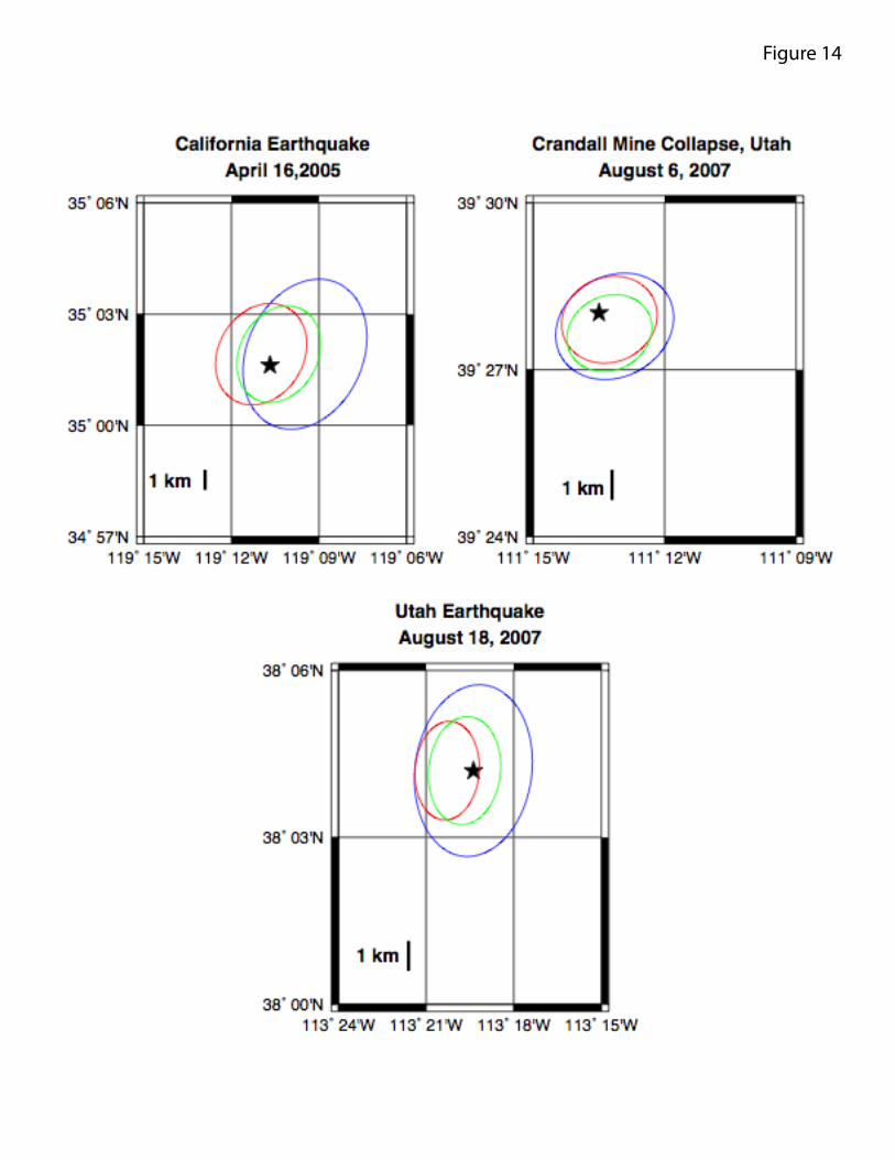
Figure 14

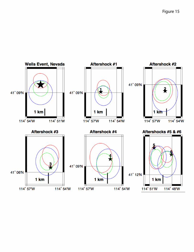
Figure 15