Journal of Applied Geophysics 73 (2011) 267–277

Contents lists available at ScienceDirect

Journal of Applied Geophysics

j ourna l homepage: www.e lsev ie r.com/ locate / jappgeo

Wave equation datuming applied to marine OBS data and to land high resolutionseismic profiling

Erika Barison a, Giuseppe Brancatelli a, Rinaldo Nicolich a,⁎, Flavio Accaino b,Michela Giustiniani b, Umberta Tinivella b

a Dipartimento di Ingegneria civile ed ambientale — DICA, University of Trieste, via Valerio 10, Italyb Istituto Nazionale di Oceanografia e di Geofisica Sperimentale — OGS, Borgo Grotta Gigante 42/C, Sgonico, Trieste, Italy

⁎ Corresponding author. Tel.: +39 0405583478; fax:E-mail address: r.nicolich@units.it (R. Nicolich).

0926-9851/$ – see front matter © 2011 Elsevier B.V. Aldoi:10.1016/j.jappgeo.2011.01.009

a b s t r a c t

a r t i c l e i n f o

Article history:Received 2 October 2009Accepted 24 January 2011Available online 31 January 2011

Keywords:Wave equation datumingOcean bottom seismographHigh resolutionStaticsCrustal investigation

One key step in seismic data processing flows is the computation of static corrections, which relocate shotsand receivers at the same datum plane and remove near surface weathering effects. We applied a standardstatic correction and a wave equation datuming and compared the obtained results in two case studies: 1) asparse ocean bottom seismometers dataset for deep crustal prospecting; 2) a high resolution land reflectiondataset for hydrogeological investigation. In both cases, a detailed velocity field, obtained by tomographicinversion of the first breaks, was adopted to relocate shots and receivers to the datum plane. The resultsemphasize the importance of wave equation datuming to properly handle complex near surface conditions. Inthe first dataset, the deployed ocean bottom seismometers were relocated to the sea level (shot positions) anda standard processing sequence was subsequently applied to the output. In the second dataset, the applicationof wave equation datuming allowed us to remove the coherent noise, such as ground roll, and to improve theimage quality with respect to the application of static correction. The comparison of the two approachesevidences that the main reflecting markers are better resolved when the wave equation datuming procedureis adopted.

+39 0405583497.

l rights reserved.

© 2011 Elsevier B.V. All rights reserved.

1. Introduction

Static correction computation is an important step in the seismicdata processing sequence. The aim is to relocate the shots and thereceivers to the samedatumlevel and to remove time shifts (weatheringeffects or near surface anomalies) caused by strong velocity changes inthe shallow layers. Static corrections are covered in many geophysicaltextbooks, such as in Cox (1999) and Yilmaz (2001). Essentially, thecorrections are based on uphole survey data merged with first breakpicking and refraction analysis.

The characterization of the velocities of the shallow layers iscrucial for static computations and a proper procedure is to define theseismic velocity field by tomographic inversion. When static correc-tions are applied, the assumption of a vertical near-surface ray path isusually accepted. This hypothesis is adequate when: (i) the static timeshifts are small, (ii) the top layer has a velocity considerably lowerthan all following layers. Nevertheless, these assumptions are notverified for high resolution data with heterogeneous near surface or

for wide-angle surveys. In these cases, more complex methods, suchas wave equation datuming (WED), are adopted.

The Kirchhoff integral solution to the scalar wave equation(using both near-field and far-field terms; (Berryhill, 1979, 1984))can provide a basis computation to deal with irregular surfaces(Wiggins, 1984) and variable velocities. In the pre-stack domain,WEDis applied in two steps: (i) common-source and (ii) common-receiverdomains.

Operating on a common-source gather has the effect of extrapo-lating the receivers from one datum to another, and, because ofreciprocity, operating on a common-receiver gather changes the datumof the source.

Recalling the main principles of the theory, it is important to dis-tinguish between migration and WED. Migration involves computingthewavefield at all depths from thewavefield at the surface, i.e. it can beintuitively explained as a succession of downward continuation steps,with theelevation zmovingever deeper into the sub-surface. In additionto downward continuation, migration requires imaging principle(Yilmaz, 2001).WEDproduces anunmigrated time section at a specifieddatum plane. In this respect, WED is an ingredient of migration, whenmigration is done as a downward-continuation process.

Basically, WED is the process of upward or downward con-tinuation of the wavefield between two arbitrarily-shaped surfaces.

Fig. 1. Position map of the seismic OBSs Profile 4–3. The frame shows the presented segment and the stars refer to the individual detector stations. The buried deformation front ofthe Gavrovo–Tripolitza western-directed thrusts with high velocity shelf carbonates is indicated. NMT=North Matapan Trough.

268 E. Barison et al. / Journal of Applied Geophysics 73 (2011) 267–277

WED was applied for the first time by Berryhill (1979) to zero-offsetpost-stack data and was based on an extrapolation scheme using theKirchhoff integral solution to the scalar wave equation (more detailsare given in Appendix A). Then, Berryhill (1984) generalized hismethod to pre-stack data by applying the same extrapolationalgorithm twice, first to common-source gathers and, finally, tocommon-receiver gathers.

Several authors have applied advanced methods to resolve seismiccomplex near-surface problems. Land seismic data, acquired in areascharacterized by rugged topography and complex overburden struc-

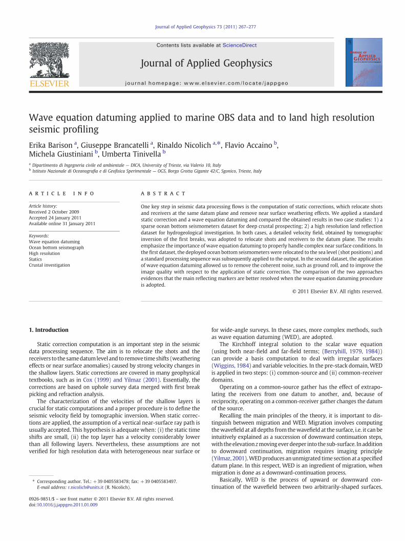
Fig. 2. Position map of the high resolution land seismic line A1. The frame points ou

tures, have been analyzed by using WED with a Kirchhoff approach(Bevc, 1997), with a finite difference scheme (Yang et al., 1999), or byusing common-focus-point technology (Al-Ali and Verschuur, 2006;Kelamis et al., 2002). Other authors have applied migration methods,such as migration weights (Gray and Marfurt, 1995) and a depthextrapolation algorithm (Reshef, 1991) to image near-surface struc-tures. Zhang and Wu (2004) proposed the common reflection surfacestack and redatuming for complex topography. In presence of high-velocity near-surface layer, Bagaini and Alkhalifah (2003) introducedthe concept of the topographic datuming operator, which fills the gap

t the presented segment. The numbers refer to the individual detector stations.

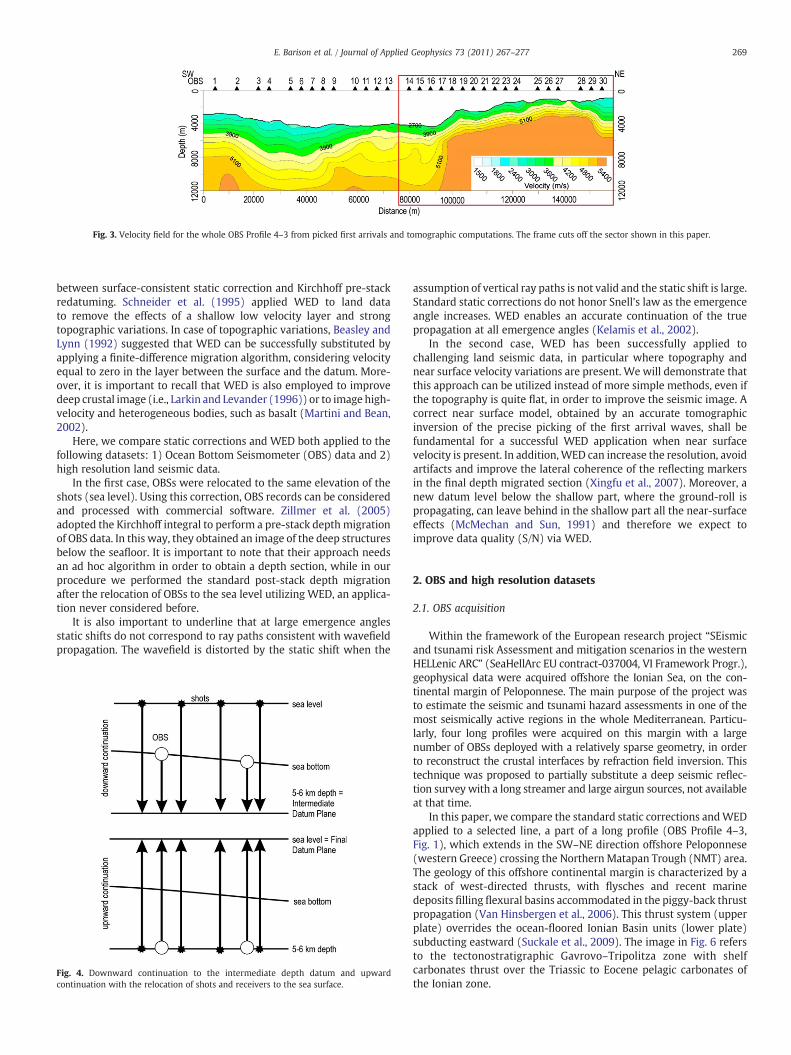
Fig. 3. Velocity field for the whole OBS Profile 4–3 from picked first arrivals and tomographic computations. The frame cuts off the sector shown in this paper.

269E. Barison et al. / Journal of Applied Geophysics 73 (2011) 267–277

between surface-consistent static correction and Kirchhoff pre-stackredatuming. Schneider et al. (1995) applied WED to land datato remove the effects of a shallow low velocity layer and strongtopographic variations. In case of topographic variations, Beasley andLynn (1992) suggested that WED can be successfully substituted byapplying a finite-difference migration algorithm, considering velocityequal to zero in the layer between the surface and the datum. More-over, it is important to recall that WED is also employed to improvedeep crustal image (i.e., Larkin and Levander (1996)) or to image high-velocity and heterogeneous bodies, such as basalt (Martini and Bean,2002).

Here, we compare static corrections and WED both applied to thefollowing datasets: 1) Ocean Bottom Seismometer (OBS) data and 2)high resolution land seismic data.

In the first case, OBSs were relocated to the same elevation of theshots (sea level). Using this correction, OBS records can be consideredand processed with commercial software. Zillmer et al. (2005)adopted the Kirchhoff integral to perform a pre-stack depth migrationof OBS data. In this way, they obtained an image of the deep structuresbelow the seafloor. It is important to note that their approach needsan ad hoc algorithm in order to obtain a depth section, while in ourprocedure we performed the standard post-stack depth migrationafter the relocation of OBSs to the sea level utilizing WED, an applica-tion never considered before.

It is also important to underline that at large emergence anglesstatic shifts do not correspond to ray paths consistent with wavefieldpropagation. The wavefield is distorted by the static shift when the

Fig. 4. Downward continuation to the intermediate depth datum and upwardcontinuation with the relocation of shots and receivers to the sea surface.

assumption of vertical ray paths is not valid and the static shift is large.Standard static corrections do not honor Snell's law as the emergenceangle increases. WED enables an accurate continuation of the truepropagation at all emergence angles (Kelamis et al., 2002).

In the second case, WED has been successfully applied tochallenging land seismic data, in particular where topography andnear surface velocity variations are present. We will demonstrate thatthis approach can be utilized instead of more simple methods, even ifthe topography is quite flat, in order to improve the seismic image. Acorrect near surface model, obtained by an accurate tomographicinversion of the precise picking of the first arrival waves, shall befundamental for a successful WED application when near surfacevelocity is present. In addition,WED can increase the resolution, avoidartifacts and improve the lateral coherence of the reflecting markersin the final depth migrated section (Xingfu et al., 2007). Moreover, anew datum level below the shallow part, where the ground-roll ispropagating, can leave behind in the shallow part all the near-surfaceeffects (McMechan and Sun, 1991) and therefore we expect toimprove data quality (S/N) via WED.

2. OBS and high resolution datasets

2.1. OBS acquisition

Within the framework of the European research project “SEismicand tsunami risk Assessment and mitigation scenarios in the westernHELLenic ARC” (SeaHellArc EU contract-037004, VI Framework Progr.),geophysical data were acquired offshore the Ionian Sea, on the con-tinental margin of Peloponnese. The main purpose of the project wasto estimate the seismic and tsunami hazard assessments in one of themost seismically active regions in the whole Mediterranean. Particu-larly, four long profiles were acquired on this margin with a largenumber of OBSs deployed with a relatively sparse geometry, in orderto reconstruct the crustal interfaces by refraction field inversion. Thistechnique was proposed to partially substitute a deep seismic reflec-tion survey with a long streamer and large airgun sources, not availableat that time.

In this paper, we compare the standard static corrections andWEDapplied to a selected line, a part of a long profile (OBS Profile 4–3,Fig. 1), which extends in the SW–NE direction offshore Peloponnese(western Greece) crossing the Northern Matapan Trough (NMT) area.The geology of this offshore continental margin is characterized by astack of west-directed thrusts, with flysches and recent marinedeposits filling flexural basins accommodated in the piggy-back thrustpropagation (Van Hinsbergen et al., 2006). This thrust system (upperplate) overrides the ocean-floored Ionian Basin units (lower plate)subducting eastward (Suckale et al., 2009). The image in Fig. 6 refersto the tectonostratigraphic Gavrovo–Tripolitza zone with shelfcarbonates thrust over the Triassic to Eocene pelagic carbonates ofthe Ionian zone.

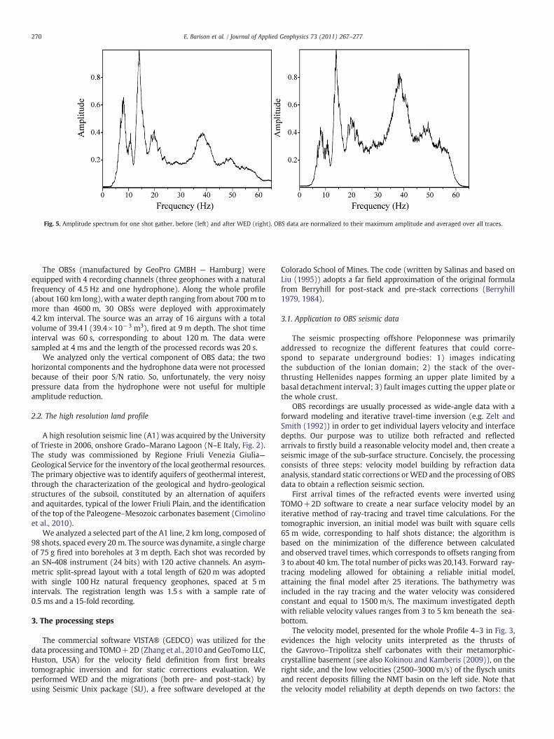
Fig. 5. Amplitude spectrum for one shot gather, before (left) and after WED (right). OBS data are normalized to their maximum amplitude and averaged over all traces.

270 E. Barison et al. / Journal of Applied Geophysics 73 (2011) 267–277

The OBSs (manufactured by GeoPro GMBH — Hamburg) wereequipped with 4 recording channels (three geophones with a naturalfrequency of 4.5 Hz and one hydrophone). Along the whole profile(about 160 km long), with a water depth ranging from about 700 m tomore than 4600 m, 30 OBSs were deployed with approximately4.2 km interval. The source was an array of 16 airguns with a totalvolume of 39.4 l (39.4×10−3 m3), fired at 9 m depth. The shot timeinterval was 60 s, corresponding to about 120 m. The data weresampled at 4 ms and the length of the processed records was 20 s.

We analyzed only the vertical component of OBS data; the twohorizontal components and the hydrophone data were not processedbecause of their poor S/N ratio. So, unfortunately, the very noisypressure data from the hydrophone were not useful for multipleamplitude reduction.

2.2. The high resolution land profile

A high resolution seismic line (A1) was acquired by the Universityof Trieste in 2006, onshore Grado–Marano Lagoon (N–E Italy, Fig. 2).The study was commissioned by Regione Friuli Venezia Giulia—Geological Service for the inventory of the local geothermal resources.The primary objective was to identify aquifers of geothermal interest,through the characterization of the geological and hydro-geologicalstructures of the subsoil, constituted by an alternation of aquifersand aquitardes, typical of the lower Friuli Plain, and the identificationof the top of the Paleogene–Mesozoic carbonates basement (Cimolinoet al., 2010).

We analyzed a selected part of the A1 line, 2 km long, composed of98 shots, spaced every 20 m. The sourcewas dynamite, a single chargeof 75 g fired into boreholes at 3 m depth. Each shot was recorded byan SN-408 instrument (24 bits) with 120 active channels. An asym-metric split-spread layout with a total length of 620 m was adoptedwith single 100 Hz natural frequency geophones, spaced at 5 mintervals. The registration length was 1.5 s with a sample rate of0.5 ms and a 15-fold recording.

3. The processing steps

The commercial software VISTA® (GEDCO) was utilized for thedata processing and TOMO+2D (Zhang et al., 2010 and GeoTomo LLC,Huston, USA) for the velocity field definition from first breakstomographic inversion and for static corrections evaluation. Weperformed WED and the migrations (both pre- and post-stack) byusing Seismic Unix package (SU), a free software developed at the

Colorado School of Mines. The code (written by Salinas and based onLiu (1995)) adopts a far field approximation of the original formulafrom Berryhill for post-stack and pre-stack corrections (Berryhill1979, 1984).

3.1. Application to OBS seismic data

The seismic prospecting offshore Peloponnese was primarilyaddressed to recognize the different features that could corre-spond to separate underground bodies: 1) images indicatingthe subduction of the Ionian domain; 2) the stack of the over-thrusting Hellenides nappes forming an upper plate limited by abasal detachment interval; 3) fault images cutting the upper plate orthe whole crust.

OBS recordings are usually processed as wide-angle data with aforward modeling and iterative travel-time inversion (e.g. Zelt andSmith (1992)) in order to get individual layers velocity and interfacedepths. Our purpose was to utilize both refracted and reflectedarrivals to firstly build a reasonable velocity model and, then create aseismic image of the sub-surface structure. Concisely, the processingconsists of three steps: velocity model building by refraction dataanalysis, standard static corrections orWED and the processing of OBSdata to obtain a reflection seismic section.

First arrival times of the refracted events were inverted usingTOMO+2D software to create a near surface velocity model by aniterative method of ray-tracing and travel time calculations. For thetomographic inversion, an initial model was built with square cells65 m wide, corresponding to half shots distance; the algorithm isbased on the minimization of the difference between calculatedand observed travel times, which corresponds to offsets ranging from3 to about 40 km. The total number of picks was 20,143. Forward ray-tracing modeling allowed for obtaining a reliable initial model,attaining the final model after 25 iterations. The bathymetry wasincluded in the ray tracing and the water velocity was consideredconstant and equal to 1500 m/s. The maximum investigated depthwith reliable velocity values ranges from 3 to 5 km beneath the sea-bottom.

The velocity model, presented for the whole Profile 4–3 in Fig. 3,evidences the high velocity units interpreted as the thrusts ofthe Gavrovo–Tripolitza shelf carbonates with their metamorphic-crystalline basement (see also Kokinou and Kamberis (2009)), on theright side, and the low velocities (2500–3000 m/s) of the flysch unitsand recent deposits filling the NMT basin on the left side. Note thatthe velocity model reliability at depth depends on two factors: the

Fig. 6. Comparison between the post-stack depth migration in the selected part of the OBS Profile 4–3, obtained after WED computation (a) and after standard static corrections (b).The sketched interpretation of the seismic data identifies the lower plate (Ionian), flexured and dipping north-eastwards, and the upper plate with the stack of the west-directedHellenic nappes. The extension of the Gavrovo thrusts over the basinal sequences of the Ionian zone is indicated. I=intra-plate interface; M=Moho at the base of the lower plate.The aspect ratio is 1.

271E. Barison et al. / Journal of Applied Geophysics 73 (2011) 267–277

velocity of the upper sediments and the maximum offset. In fact, thepresence of shallow high velocity layers requires very long offsets fordetermining the velocity field in the deep crust. Consequently, thereliability of the deep part of the velocity model is greater in the SWpart than in the NE one, due to the presence of the high velocity body,which maintains the elevated values reached at 3–4 km below sealevel (from OBS n. 18 to the end of the line) not allowing theidentification of deeper interfaces. Moreover, it is important to pointout that the shallow velocity structures are well defined only nearbythe OBS positions.

We adopted a conventional procedure (vertical static correction)to relocate the OBS from the sea bottom to the sea level consideringthe sea water velocity. After the application of static corrections,the OBS data were processed (i.e., CDP sorting and NMO corrections).

The deep velocity function was obtained by extrapolating the nearsea-bottom velocity table (Fig. 3) to a maximum depth of 30–35 km,according to the information available in literature. Vertical andhorizontal smoothing was applied to the velocity gradient toavoid artifacts as velocity pull-up or down in the depth section. Weapplied deconvolution and 2-D FK–FX filtering to enhance the lat-eral continuity of the reflections and to remove the coherent noise. Atime variant filter was finally utilized to improve the imaging. TheKirchhoff depth migration was applied to the post-stack data toavoid spatial aliasing problems.

In a second step, to enhance the seismic signals and to improvethe geological interpretation of the study area, we applied WED tothe OBS data of the selected profile by using the described velocityfield in Fig. 3. This is justified by its greater accuracy especially when

272 E. Barison et al. / Journal of Applied Geophysics 73 (2011) 267–277

OBSs are deployed in deep waters and rough sea bottom topo-graphy is present. Moreover,WED allowed us to extractmore reliableinformation of the reflection events recorded by the OBSs. AfterWED, shots and receivers are relocated at the same datum (sea level)allowing the processing by using commercial software.We underlinethat the seafloor reflection is obtained by wave propagation in thevelocity model extracted by OBS data inversion; in this way, theseafloor reflection coefficient is given by our velocity model.

We moved OBSs (receivers) and shots to an intermediate datumplane first, at about 5 km depth below the sea level (downwardcontinuation), then OBSs and shots were relocated to the sea sur-face (upward continuation). The intermediate depth datum solution(Fig. 4) was required to increase the number of traces (along theprofiles there are more shots closer to each other than OBS's), whichcontribute to the Kirchhoff summation in the migration procedureconsidering the OBS as source points and shots as receivers utilizingthe reciprocity principle. It was not possible to find a reflecting surfaceas intermediate datum because of the complex thrust tectonicinteresting the area and the poor S/N ratio. The depth we suggestedfor the new datum was settled below the near surface thrust andfolds heterogeneities and anyway at a depth where the seismic ve-locity appears to be definitely higher than 5000 m/s. This means that apartial migration was applied two times with a further reduction ofthe amplitudes of the anomalous events and noise with the pres-ervation of the velocity information for the depth converted section.Moreover, we point out that WED suffers from spatial aliasing,because it is based on a wave extrapolation process. The aliasingcontrol was performed evaluating the Fresnel zone for which a radiusequal to 1095 m was calculated assuming a root-mean-squarevelocity of 4000 m/s at 6 s two ways travel time and a dominantfrequency of 20 Hz (Yilmaz, 2001). Note that this radius is muchbigger than our traces distance (about 120 m). The amplitude

Fig. 7. Velocity field for the seismic line A1 down to 100 m (a), obtained by tomographic iobtained with CVS velocity analysis (b).

spectra in Fig. 5, before and after WED application, confirms that nospatial aliasing is present. WED enhanced higher frequencies andthe amplitude spectrum becomes roughly flat, thus increasing theresolution.

After datuming we applied a standard processing sequence tostack the data. Fig. 6 shows the comparison between the post-stackdepth migration results, obtained after WED (Fig. 6a) and the resultafter static corrections (Fig. 6b) in the selected part of the Profile 4–3.WED produces significant migrated images with increased resolu-tion, particularly in deep water, as expected. Several reflectors (bothshallow and deep) are more evident and continuous after WED pro-cedure with respect to the static correction procedure.

In the section of Fig. 6a, the overprinted white transparent linesindicate a tentative interpretative geological scheme with the IonianBasin cold and brittle crust (the lower plate) flexured and suddenlydipping north-eastwards at the collision with the Hellenic crustalroots. The Ionian Moho is proposed to reach, from 26, more than35 km depth, while a basal detachment of the Hellenic thrusts (theupper plate) is posed at about 16 km on the SW termination of thepresented section. The interpretation of the OBS data in the section ofFig. 6b is much difficult because of the poor S/N and weak reflectingmarkers obtained with the application of statics.

3.2. Application to the high resolution land data

This dataset was processed with a standard sequence. We re-constructed the geometry of the line with an in-line bin spacing of2.5 m (half of geophones inter-distance). A notch filter to remove allsignals at 50 Hz frequency, because of noise from the electric powercables, and a band-pass filter, including broad band frequencies (from25 to 180 Hz), were applied. Trace editing and a surgical muting wereperformed to remove spikes and air wave.

nversion of the first breaks, and the downward continuation for the complete section

273E. Barison et al. / Journal of Applied Geophysics 73 (2011) 267–277

The data were processed using both the standard static correctionmethod and the WED approach after reconstructing the velocity fieldby using tomographic inversion of the first breaks.

We created a 2D grid model with a square cell of 2.5 m widthfor the refraction tomography inversion; totally 1052×60 cells,in which we fixed as constraint the maximum velocity value of3000 m/s. The input data include 11,760 travel time picks,corresponding to offsets ranging from 7.5 to 450 m. The inversionallowed us to reconstruct a reliable velocity distribution with a goodresolution till about 100 m below the surface, as shown in Fig. 7a,corresponding to approximately 1/4 of the maximum source–receiver offset. The final model was obtained after 40 iterationsand the maximum root mean square misfit was equal to 7 ms.

About all the charges were shot below or near the water table at3 m depth (the elevations along the line range from+1 m to−0.5 mfrom sea level). The study area is located in a reclaimed districtseparated by embankments from the Grado–Marano Lagoon facingthe northern Adriatic Sea. The sub-surface is constituted by alter-nations of sandbanks, depressions or erosion channels filled withsilty mud. As a consequence, lateral velocity variations become sig-nificant in the shallower parts and they may generate artifacts onthe reflecting horizons with apparent tectonic distortions. In fact,the western side of the line is characterized by a slightly highervelocity and we can recognize two zones with low velocities (about1200 m/s) in the intervals between shots 510–580 and 630–782 downto about 30 m depth. Below 50 m depth, these complexities disappearand the velocity field is quite uniform, with values around 1750 m/s.For this reason, we located the datum plane at a depth of 50 m that

Fig. 8. Processing flow chart fo

still remains above our targets represented by water bearing sandyintervals within clayey strata. Information about velocities at greaterdepths was obtained by constant velocity stack (CVS) analysis(Fig. 7b). The main feature of the deep velocity model is representedby the lateral variation with lower velocities from shots 400 to 550,below 500 m depth.

The obtained velocity model was utilized to calculate thestatic corrections and to perform WED using the same input datain both cases. On the contrary, we applied two slightly differentprocessing flows after the application of the two procedures (seeFig. 8).

After static corrections, the ground roll was removed by using aFK–FX filter. The filter was defined in the FK domain with the mini-mum and the maximum slopes calculated using the minimumand the maximum apparent slowness and temporal and spatialfrequency range. This filter was then converted in the FX domain andapplied using the exact shot/receiver coordinates. Finally, the outputwas converted back to the TX domain. It is worth mentioning thattheoretically this approach cannot be applied if the geometry is notregular, i.e. in almost all land seismic data. In presence of irregularacquisition geometries, zero traces must be added to avoid numericalproblems and they must be removed after the filter application.

The two steps (static correction and ground roll removing) can bedone simultaneously by applying WED (Yilmaz, 2001). Note that thesmall shots and group spacing guarantee the absence of spatialaliasing. The WED strongly attenuates the noise such as ground-rolland improves the S/N ratio compared to the standard processingsequence, which was one of our objectives.

r the land seismic line A1.

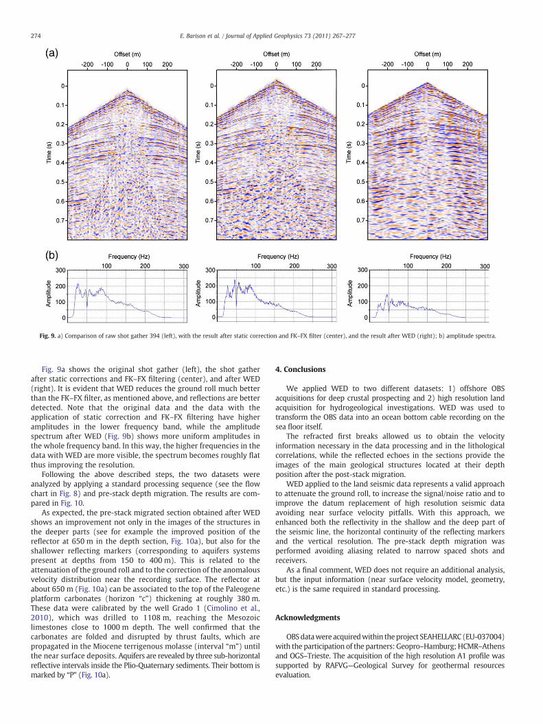
Fig. 9. a) Comparison of raw shot gather 394 (left), with the result after static correction and FK–FX filter (center), and the result after WED (right); b) amplitude spectra.

274 E. Barison et al. / Journal of Applied Geophysics 73 (2011) 267–277

Fig. 9a shows the original shot gather (left), the shot gatherafter static corrections and FK–FX filtering (center), and after WED(right). It is evident that WED reduces the ground roll much betterthan the FK–FX filter, as mentioned above, and reflections are betterdetected. Note that the original data and the data with theapplication of static correction and FK–FX filtering have higheramplitudes in the lower frequency band, while the amplitudespectrum after WED (Fig. 9b) shows more uniform amplitudes inthe whole frequency band. In this way, the higher frequencies in thedata with WED are more visible, the spectrum becomes roughly flatthus improving the resolution.

Following the above described steps, the two datasets wereanalyzed by applying a standard processing sequence (see the flowchart in Fig. 8) and pre-stack depth migration. The results are com-pared in Fig. 10.

As expected, the pre-stack migrated section obtained after WEDshows an improvement not only in the images of the structures inthe deeper parts (see for example the improved position of thereflector at 650 m in the depth section, Fig. 10a), but also for theshallower reflecting markers (corresponding to aquifers systemspresent at depths from 150 to 400 m). This is related to theattenuation of the ground roll and to the correction of the anomalousvelocity distribution near the recording surface. The reflector atabout 650 m (Fig. 10a) can be associated to the top of the Paleogeneplatform carbonates (horizon “c”) thickening at roughly 380 m.These data were calibrated by the well Grado 1 (Cimolino et al.,2010), which was drilled to 1108 m, reaching the Mesozoiclimestones close to 1000 m depth. The well confirmed that thecarbonates are folded and disrupted by thrust faults, which arepropagated in the Miocene terrigenous molasse (interval “m”) untilthe near surface deposits. Aquifers are revealed by three sub-horizontalreflective intervals inside the Plio-Quaternary sediments. Their bottom ismarked by “P” (Fig. 10a).

4. Conclusions

We applied WED to two different datasets: 1) offshore OBSacquisitions for deep crustal prospecting and 2) high resolution landacquisition for hydrogeological investigations. WED was used totransform the OBS data into an ocean bottom cable recording on thesea floor itself.

The refracted first breaks allowed us to obtain the velocityinformation necessary in the data processing and in the lithologicalcorrelations, while the reflected echoes in the sections provide theimages of the main geological structures located at their depthposition after the post-stack migration.

WED applied to the land seismic data represents a valid approachto attenuate the ground roll, to increase the signal/noise ratio and toimprove the datum replacement of high resolution seismic dataavoiding near surface velocity pitfalls. With this approach, weenhanced both the reflectivity in the shallow and the deep part ofthe seismic line, the horizontal continuity of the reflecting markersand the vertical resolution. The pre-stack depth migration wasperformed avoiding aliasing related to narrow spaced shots andreceivers.

As a final comment, WED does not require an additional analysis,but the input information (near surface velocity model, geometry,etc.) is the same required in standard processing.

Acknowledgments

OBSdatawere acquiredwithin theproject SEAHELLARC(EU-037004)with the participation of the partners: Geopro–Hamburg; HCMR–Athensand OGS–Trieste. The acquisition of the high resolution A1 profile wassupported by RAFVG—Geological Survey for geothermal resourcesevaluation.

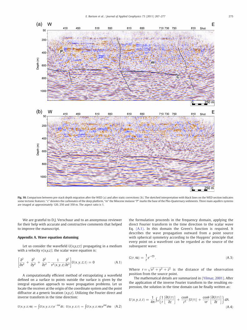
Fig. 10. Comparison between pre-stack depth migration after theWED (a) and after static corrections (b). The sketched interpretation with black lines on theWED section indicatessome tectonic features: “c” denotes the carbonates of the deep platform, “m” the Miocenemolasse “P”marks the base of the Plio-Quaternary sediments. Three main aquifers systemsare imaged at approximately 120, 250 and 350 m. The aspect ratio is 1.

275E. Barison et al. / Journal of Applied Geophysics 73 (2011) 267–277

We are grateful to D.J. Verschuur and to an anonymous reviewerfor their help with accurate and constructive comments that helpedto improve the manuscript.

Appendix A. Wave equation datuming

Let us consider the wavefield U(x,y,z;t) propagating in a mediumwith a velocity v(x,y,z); the scalar wave equation is:

∂2

∂x2+

∂2

∂y2+

∂2

∂z2− 1

v2 x; y; zð Þ∂2

∂t2

" #U x; y; z; tð Þ = 0 ðA:1Þ

A computationally efficient method of extrapolating a wavefielddefined on a surface to points outside the surface is given by theintegral equation approach to wave propagation problems. Let uslocate the receiver at the origin of the coordinate system and the pointdiffractor at a generic location (x,y,z). Utilizing the Fourier direct andinverse transform in the time direction:

Uðx; y; z;ϖÞ = ∫Uðx; y; z; tÞe−iϖtdt; Uðx; y; z; tÞ = ∫Uðx; y; z;ϖÞeiϖtdϖ ðA:2Þ

the formulation proceeds in the frequency domain, applying thedirect Fourier transform in the time direction to the scalar waveEq. (A.1). In this domain the Green's function is required. Itdescribes the wave propagation outward from a point sourcewith spherical symmetry according to the Huygens' principle thatevery point on a wavefront can be regarded as the source of thesubsequent wave:

Gðr;ϖÞ = 1re−iϖv r ; ðA:3Þ

Where r=ffiffiffiffiffiffiffiffiffiffiffiffiffiffiffiffiffiffiffiffiffiffiffiffiffiffiffiffiffix2 + y2 + z2

pis the distance of the observation

position from the source point.The mathematical details are summarized in (Yilmaz, 2001). After

the application of the inverse Fourier transform to the resulting ex-pression, the solution in the time domain can be finally written as:

U x; y; z; tð Þ = 14π

∫A1r

∂UðτÞ∂z

� �+

cosθr2

UðτÞ½ � + cosθvr

∂UðτÞ∂t

� �� �dA:

ðA:4Þ

Fig. A.1. The geometry involved in the statement of the Kirchhoff theorem Eq. (A.5). Left: θ is the angle between r and the normal to the input datum. Right: the case in which U isindependent of y. rx is the distance in the xz plane. ψ is angle between rx and r. Modified after (Berryhill, 1979).

276 E. Barison et al. / Journal of Applied Geophysics 73 (2011) 267–277

The integration over the area A is done using thewavefield U(x,y,z;t)at the retarded time τ=t−r/v; θ is the angle between r and the normalto the input datum (Fig. A.1); the first term depends on the verticalgradient of the wavefield; the second term is the near field decayingwith 1/r2; the third term is the far field term.

Let usmove thewavefield upward from the infinite planar surface A(x,y,z) to the surface A0(x0,y0,z0), for which the time distance is r/v(Fig. A.1). Assuming U(x,y,z;t) known only along a line in the plane(x) and independent of the direction (y) perpendicular to this line (U(x,y,z;t)≡U(x,z,t)) anda coordinate systemestablishedwith z=0 in theA0-plane, the Kirchhoff integral can be simplified to

U 0; z; tð Þ = 14π

∫∞

−∞dx ∫

∞

−∞dy

1r3

Uðx0; y0; z0;τÞ + r = v∂∂t Uðx0; y0; z0; τÞ

� �:

ðA:5Þ

In this equation, the output point is taken to lie above thecoordinates origin (x=0), and cosθ has been replaced with z/r.

The integration along the y direction can be changed to a time-domain convolution (see details in Berryhill, 1979 and Fig. A.2).Moreover, if we suppose that the x-integral is carried out over a finiterange of x values (real case), using data sampled at discrete loca-tions on a nonplanar surface in the presence a variable velocity, theequation to extrapolate seismic waves from one datum (indicated bythe index i) to another (indicated by the index j) is given by Berryhill(1984):

UjðtÞ =14π

∑iΔxicosθi

tiri

UiðτiÞi⁎Fih i

: ðA:6Þ

The distance between the seismic traces Ui and Uj is ri, τicorresponds to t−ri/v, θi is the angle between ri and the normal to

Fig. A.2. Schematic representation of the Kirchhoff upward and/or downwardcontinuation from an input datum to the new output, corresponding to the imple-mentation of Eq. (A.6). Modified after (Wiggins, 1984).

the input datum, and Δxi is the distance between adjacent tracelocations. F is a filter operator, function of (τi, ri, Δxi, θi), to beconvolved with the trace to prevent distortions. In conclusion, Fig. A.2is a schematic representation of the Kirchhoff upward continuationprocess corresponding to the implementation of Eq. (A.6): each inputtrace Ui is filtered, time-shifted according to τi=t−ti, scaled, andsummed into the output trace Uj.

A travel time table between the input and the output datum,obtained by using velocity information is indispensable. The velocityutilized in this extrapolation is that of the medium between the twospecified datum surfaces (Yilmaz and Lucas, 1986). Generally, theparaxial ray tracing (Beydoun and Keho, 1987) is adopted, compen-sated by solving the eikonal equation in shadow zones. Paraxialapproximation is adopted to perform ray-tracing with angles lessthan 10°; so, it is used for the first order approximation, because itconsiders a number of simplifying assumptions that makes thearithmetic of ray-tracing considerably easier. In presence of complexstructures and/or strong lateral velocity variation, the paraxial raytracing is not accurate. On the contrary, the eikonal equation is a ray-theoretical approximation to the scalar wave equation. Its solutionrepresents wavefronts of constant phase. The wave is propagatedfrom one wavefront to the next by ray paths, which are perpendicularto the wavefronts. In particular, the wavefield at a point on the outputdatum is computed using all the traces in the input gather. The outputgather should be computed beyond the lateral extent of the inputgather to prevent possible loss of steeply dipping events (Yilmaz,2001).

Eq. (A.6) describes the upward continuation of upgoing waves andthe downward continuation of downgoing waves–cases, in which thetraveling wave encounters the input locations before the outputlocation. If the traveling wave encounters the output location beforethe input location, it is necessary only to image a movie of the eventrun backwards to recover the situation previously considered. Thus,Eq. (A.6) permits the downward continuation of upgoing waves andvice versa, simply by time-reversing all input traces before processingand all output traces afterward. The essential effect is to reverse therelative signs of the times t and ti.

References

Al-Ali, M.N., Verschuur, D.J., 2006. An integrated method for resolving the seismiccomplex near-surface problem. Geophys. Prospect. 54, 739–750.

Bagaini, C., Alkhalifah, T., 2003. One step better than static corrections: the topographicdatuming operator. 65th EAGE Conference, p. C-07. Stavanger, Norway, ExtendedAbstracts.

Beasley, C., Lynn, W., 1992. The zero-velocity layer: migration from irregular surfaces.Geophysics 57, 1435–1443.

Berryhill, J.R., 1979. Wave-equation datuming. Geophysics 44, 1329–1344.Berryhill, J.R., 1984. Wave-equation datuming before stack. Geophysics 49, 2064–2066.Bevc, D., 1997. Flooding the topography: wave-equation datuming of land data with

rugged acquisition topography. Geophysics 62, 1558–1569.

277E. Barison et al. / Journal of Applied Geophysics 73 (2011) 267–277

Beydoun, W.B., Keho, T.H., 1987. The paraxial ray method. Geophysics 52, 1639–1653.Cimolino, A., Della Vedova, B.,Nicolich, R., Barison, E., Brancatelli, G., 2010. Newevidence of

the outer Dinaric deformation front in the Grado area (NE-Italy). In: Sassi, F., et al.(Eds.), Nature and geodynamics of the Northern Adriatic Lithosphere. Supplement 1to Rendiconti Lincei 21, Springer, pp. 167–179. doi:10.1007/s12210-010-0096-y.

Static Corrections for Seismic Reflection Surveys, Geophysical references. Society ofExploration Geophysicists, Tulsa. 531 pp.

Gray, S., Marfurt, K.J., 1995. Migration from topography: improving the near-surfaceimage. Can. J. Explor. Geophys. 31, 18–24.

Kelamis, P.G., Erickson, K.E., Verschuur, D.J., Berkhout, A.J., 2002. Velocity-independentredatuming: A new approach to the near-surface problem in land seismic dataprocessing. Lead. Edge 21, 730–735.

Kokinou, E., Kamberis, E., 2009. The structure of the Kythira–Antikythira strait, offshoreSW Greece (3.7–36.6 N). Geol. Soc. Lond. Spec. Publ. 311, 343–360.

Larkin, S.P., Levander, A., 1996. Wave equation datuming for improving deep crustalseismic images. Tectonophysics 264, 371–379.

Z. Liu, Migration velocity analysis, PhD thesis, CWP, 168 (1995), Center for WavePhenomena, Colorado School of Mine, Golden.

Martini, F., Bean, C.J., 2002. Interface scattering versus body scattering in subbasaltimaging and application of prestack wave equation datuming. Geophysics 67,1593–1601.

McMechan, G.A., Sun, R., 1991. Depth filtering of first breaks and ground roll. Geophysics56, 390–396.

Reshef, M., 1991. Depth migration from irregular surfaces with depth extrapolationmethods. Geophysics 56, 119–122.

Schneider, W., Phillips, L., Paal, E., 1995. Wave-equation velocity replacement of thelow-velocity layer for overthrust-belt data. Geophysics 60, 573–579.

Suckale, J., Rondenay, S., Sachpazi, M., Charalampakis, M., Hosa, A., Royden, L.H., 2009.High-resolution seismic imaging of the western Hellenic subduction zone usingteleseismic scattered waves. Geophys. J. Int. 178, 775–791.

Van Hinsbergen, D.J.J., Van der Meer, D.G., Zachariasse, W.J., Meulenkamp, J.E., 2006.Deformation of Western Greece during Neogene clockwise rotation and collisionwith Apulia. Int. J. Earth Sci. 95, 463–490.

Wiggins, J.W., 1984. Kirchhoff integral extrapolation and migration of nonplanar data.Geophysics 49, 1239–1248.

Xingfu, C., Hongbing, L., Ying, H., Hong, L., Li, Q., 2007.Wavefield continuation datumingusing a near surface model. Appl. Geophys. 4, 94–100.

Yang, K., Wang, H.Z., Ma, Z.T., 1999. Wave equation datuming from irregular surfacesusing finite difference scheme, 69th Annual International Meeting. SEG ExpandedAbstracts, pp. 1485–1488.

Yilmaz, O., 2001. Seismic Data Analysis. Investigations in Geophysics. Society ofExploration Geophysicists, Tulsa, p. 1. 1000 pp.

Yilmaz, O., Lucas, D., 1986. Prestack layer replacement. Geophysics 51, 1355–1369.Zelt, C.A., Smith, R.B., 1992. Seismic travel time inversion for 2-D crustal velocity

structure. Geophys. J. Int. 108, 16–34.Zhang, Y.H., Wu, R.S., 2004. CRS stack and redatuming for rugged surface topography: a

synthetic data example, 74th Annual International Meeting. SEG, ExpandedAbstracts, pp. 2040–2043.

Zhang, J., U.S. TenBrink, Toksöz,M.N., 2010. Non linear refraction and reflection travel timetomography. J. Goeoph. Res. 103 (B12), 29.743–29.757. doi:10.1029/98JB01981.

Zillmer, M., Flue, E.R., Petersen, J., 2005. Seismic investigation of a bottom simulatingreflector and quantification of gas hydrate in the Black Sea. Geophys. J. Int. 161,662–678.