Entry, Competitiveness and Exports: Evidence from the Indian Firm Data

Entry, Competitiveness and Exports: Evidencefrom the Indian Firm Data

Alokesh Barua & Debashis Chakraborty &

Hariprasad CG

Received: 22 July 2010 /Revised: 21 December 2010Accepted: 6 January 2011 /Published online: 24 February 2011

Abstract This paper attempts to evaluate the effects of industrial de-licensing of 1991 andWTO-induced tariff-reforms of 1995 on domestic competitiveness and export performancesof the Indian manufacturing during the post-1991. Unlike existing empirical studies notbacked by theoretical underpinnings, the paper has been founded on an open-economy-oligopoly-model framework. The paper develops an econometric method of estimating theoutput from data on sales of the firms, thereby estimating the firms’ marginal cost, which isconducive for the entire empirical analysis with a unified set of firm data. Using firm leveldata for 14 sectors for the period 1990–2008, it is observed that there has been an increasein the number of firms resulting in a fall in the concentration ratio and elasticity of demandat the point of equilibrium is generally less than unity and is declining over-time. The panelregression results of increasing exports by bigger firms also conforms the theoreticalpredictions.

Keywords competitiveness . entry . industrial liberalization . trade liberalization

JEL Classifications F12 . L50

J Ind Compet Trade (2012) 12:325–347DOI 10.1007/s10842-011-0096-3

A. BaruaInternational Trade and Development Division, School of International Studies,Jawaharlal Nehru University, New Delhi, Indiae-mail: [email protected]

D. Chakraborty (*)Indian Institute of Foreign Trade, New Delhi, Indiae-mail: [email protected]: [email protected]

H. CGEconomics Division, Competition Commission of India, New Delhi, Indiae-mail: [email protected]

# Springer Science+Business Media, LLC 2011

1 Introduction

How does entry affect competitiveness1 in an industry and hence welfare? Conventionalwisdom suggests that entry in an oligopolistic industry reduces market power of existingfirms, i.e., industrial concentration and thereby reduces price-cost margins and improvesconsumer welfare.2 The aforesaid partial equilibrium result holds also in a generalequilibrium situation as well (Barua and Pant 1995). Considering an open economyCournot model, Agarwal and Barua (2004) have shown that the limiting case of entry insuch a model confirms a competitive outcome.

The theoretical presumptions notwithstanding, there are very few studies beingpurported to empirical validation of these results in a strict sense. In view of the recenttwo major policy initiatives of the government of India,3 it becomes all the more necessaryto conduct such validation if not for anything else then at least for an attempt to judge theimpact of the policy changes. The resulting liberalization has significantly facilitated theentry of both domestic and foreign firms across all industries.

Much attention has been drawn to the debate whether firm entry has significantlyaffected the market structure in the industrial sector of the Indian economy or not. Theevidence from empirical studies in this area is found to be rather ambiguous (Athreye andKapur 2003; Barua and Chakraborty 2006; Balakrishnan and Babu 2003; Kambhampatiand Parikh 2003). In a recent analysis on the theory and evidence of market power in Indianmanufacturing, Das and Pant (2006) have argued that “the new industrial policy has notbeen able to foster competition” (p. 75), confirming the earlier findings by a number ofresearchers.

One of the central limitations of the existing studies on the effect of entry on competitionis their dependence on two or more sources of rather unrelated data for estimating theprice-cost margins in industries.4 This raises doubt as regards the reliability and alsocomparability of their estimates. The present study is an attempt to provide a unified modelof measurement of price-cost margins using only firm data of the same source. In addition,it also attempts to examine the relationship between firm size, marginal cost structure andexports.

The basic theoretical model underlying the current empirical exercise is based on theopen economy oligopoly model under segmented market hypothesis as put forward in aseries of papers by Agarwal and Barua (1993, 1994, 2004, 2007). The main arguments ofthese papers are that entry liberalization (whether internal or external) would result in (a)

1 The term ‘competitiveness’ unless defined in a specific context tends to be elusive and misleading (See, fordetails the special JICT issue on competitiveness, Vol. 6, No. 2, 2006). As Aiginger (2006) has pointed out,the term stems from the analysis of firms and is well—defined at the level of firm. It is precisely in this sensethat the term competitiveness is used in this paper. In the current framework of analysis, the benchmarkcompetitive outcome is the limiting behaviour of a Cournot model under free entry. The model converges tothe competitive outcome (marginal cost pricing) in the limit. For a formal proof of this proposition for anopen economy oligopoly model, see Agarwal and Barua (2004).2 See, Mas-Colell et al. (1995), p. 412.3 The two policies being referred here are, first, the abolition of the industrial licensing policies under theindustrial reform measures adopted in 1991, and, second, the WTO—induced trade liberalization policiesbeing initiated since 1995 onwards.4 A major source of firm data in India is PROWESS database. The PROWESS database however does notprovide any information on quantity of output produced or quantity of labor used in the production processby a firm. As a result, researchers depend largely on Annual Survey of Industries (ASI) data for some proxyestimates of labor (wage rate) or output, and match that with the corresponding PROWESS data bydeveloping a suitable concordance.

326 J Ind Compet Trade (2012) 12:325–347

increase in aggregate exports, (b) reduction in industrial concentration, (c) decrease inprice-cost margin, and (d) increase in social welfare. It is immaterial whether the firms areof domestic or foreign origin. Thus, the ongoing WTO induced reforms (externalliberalization) and the industrial reforms carried out in India since 1991 (internal industrialliberalization) are expected to significantly affect the performance of the manufacturingsector of Indian economy (Kambhapati and Parikh 2005).

The paper is organized as follows: Section 2 describes the basic theoretical model toprovide empirically testable propositions of the effects of entry liberalization on marketperformance. A review of the literature is provided in Section 3 and in Section 4 aneconometric estimation model is proposed to test the propositions described in Section 2.Analysis of the econometric estimation results as well as other findings is provided inSection 5. Section 6 draws a few policy conclusions based on the current analysis.

2 The underlying model

The basic model used here assumes that the firm behaves like a discriminating oligopolistas between domestic and foreign markets. The variables used in the analysis are defined asfollows:

V.1. xi is the output of the ith firm;V.2. N is the number of active firms;V.3. X is the industry output, i.e., X = ∑xi, i=1,......... N;V.4. qid is the domestic sales of the ith firm;V.5. Qd is the total domestic demand, i.e., Qd ¼

Pqid , i=1, .... N;

V.6. f (Qd) is the inverse demand function in the domestic market;V.7. Pf is the international price;V.8. qif is the export of the ith firm, where xi ¼ qid þ qif , i=1 ....N;V.9. Qf is the aggregate exports of the country, i.e. Qf ¼

Pqif , i=1 ....N;

V.10. Q−i isP

q jdj for j=1,.... N; i ≠ j.

The following assumptions are made in the current context:

A.1. the inverse demand function f (Qd) is twice continuously differentiable and f ′<0.A.2. the cost function of the ith firm C (xi) is twice continuously differentiable and C (0) = 0

implying that firm can freely exit from the market by producing a zero output. Further,the average cost, AC, is strictly U-shaped with minimum attained at x* where x*>0.

A.3. The profit function for the ith firm (i=1,.....N)

Π i ¼ f Qdð Þ: qid þ Pf : qf � C xi� � ð1Þ

A.4. Profit maximization under Cournot assumptions gives the first-order conditions:

@Π i

@qid¼ qid :f

0 Qdð Þ þ f Qdð Þ � C0 xi� � ¼ 0; 8i: ð2Þ

and

@Π i

@qif¼ Pf � C0 xi

� � ¼ 0; 8i: ð3Þ

J Ind Compet Trade (2012) 12:325–347 327

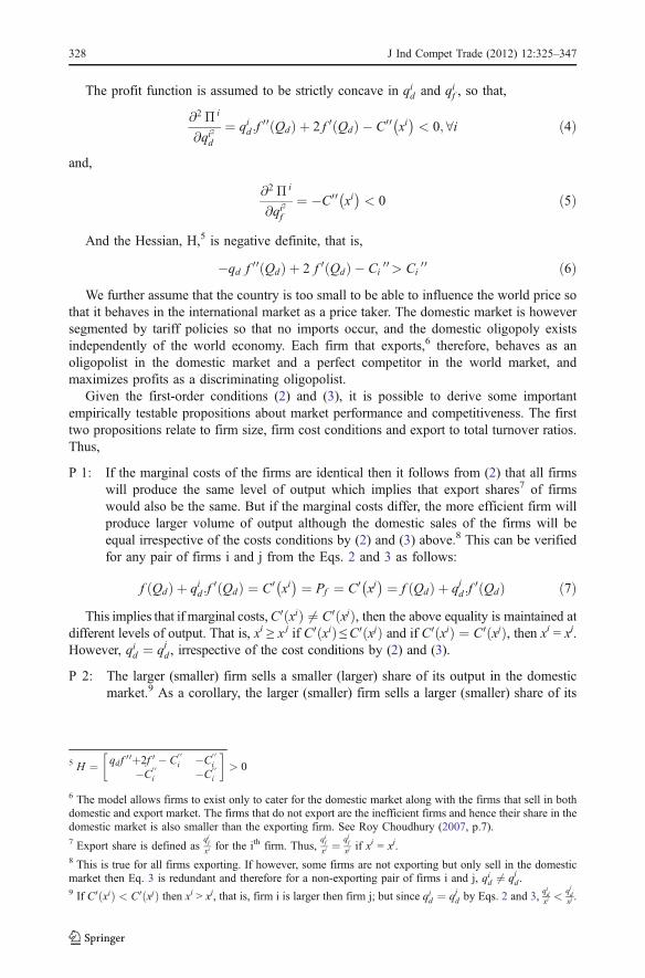
The profit function is assumed to be strictly concave in qid and qif , so that,

@2 Π i

@qi2

d

¼ qid :f00 Qdð Þ þ 2 f 0 Qdð Þ � C00 xi

� �< 0; 8i ð4Þ

and,

@2 Π i

@qi2

f

¼ �C00 xi� �

< 0 ð5Þ

And the Hessian, H,5 is negative definite, that is,

�qd f 00 Qdð Þ þ 2 f 0 Qdð Þ � Ci00> Ci

00 ð6ÞWe further assume that the country is too small to be able to influence the world price so

that it behaves in the international market as a price taker. The domestic market is howeversegmented by tariff policies so that no imports occur, and the domestic oligopoly existsindependently of the world economy. Each firm that exports,6 therefore, behaves as anoligopolist in the domestic market and a perfect competitor in the world market, andmaximizes profits as a discriminating oligopolist.

Given the first-order conditions (2) and (3), it is possible to derive some importantempirically testable propositions about market performance and competitiveness. The firsttwo propositions relate to firm size, firm cost conditions and export to total turnover ratios.Thus,

P 1: If the marginal costs of the firms are identical then it follows from (2) that all firmswill produce the same level of output which implies that export shares7 of firmswould also be the same. But if the marginal costs differ, the more efficient firm willproduce larger volume of output although the domestic sales of the firms will beequal irrespective of the costs conditions by (2) and (3) above.8 This can be verifiedfor any pair of firms i and j from the Eqs. 2 and 3 as follows:

f Qdð Þ þ qid :f0 Qdð Þ ¼ C0 xi

� � ¼ Pf ¼ C0 xj� � ¼ f Qdð Þ þ qjd :f

0 Qdð Þ ð7ÞThis implies that if marginal costs,C0 xið Þ 6¼ C0 xjð Þ, then the above equality is maintained at

different levels of output. That is, xi Q x j if C0 xið Þ eC0 xjð Þ and if C0 xið Þ ¼ C0 xjð Þ, then xi = xj.However, qid ¼ qjd , irrespective of the cost conditions by (2) and (3).

P 2: The larger (smaller) firm sells a smaller (larger) share of its output in the domesticmarket.9 As a corollary, the larger (smaller) firm sells a larger (smaller) share of its

5 H ¼ qdf 0 0þ2f 0 � C0 0i �C

0 0i

�C0 0i �C

0 0i

� �> 0

6 The model allows firms to exist only to cater for the domestic market along with the firms that sell in bothdomestic and export market. The firms that do not export are the inefficient firms and hence their share in thedomestic market is also smaller than the exporting firm. See Roy Choudhury (2007, p.7).7 Export share is defined as

qifxi for the ith firm. Thus,

qifxi ¼

qjfxj if x

i = xj.8 This is true for all firms exporting. If however, some firms are not exporting but only sell in the domesticmarket then Eq. 3 is redundant and therefore for a non-exporting pair of firms i and j, qid 6¼ qjd .9 If C0 xið Þ < C0 xjð Þ then xi > xj, that is, firm i is larger then firm j; but since qid ¼ qjd by Eqs. 2 and 3,

qidxi <

qjdxj .


output in the export market.10 Thus, firm size and export to total turnover ratios arepositively related.

Now, a few propositions relating the effects of entry on firm output, industrial concentration,price-cost margins and profitability and consumer welfare are considered below.

P 3: As entry occurs, provided the second order-conditions of profit maximization11 issatisfied, the firm output will be unaffected since the world price is given (condition (3)above).

P 4: Entry of firms implies that the firm’s share in the domestic market declines (thusindustry concentration falls) and therefore the firm’s export share rises. However,aggregate domestic sales rise with the entry of firms leading to a fall in prices andtherefore increase in consumer welfare.

P 5: As entry of firms occurs in the industry, in the limiting case price converges tomarginal cost.12 Thus, entry leads to decline in the price-cost margins.

3 Review of empirical literature

Following Sutton (1991), it can be argued that a larger market resulting from liberalizedentry conditions can accommodate more firms of efficient size and therefore concentrationlevel in the industry is expected to decline. There exist a number of studies that attempt toexamine the state of competition and competitiveness in Indian industries as a consequenceof entry liberalization policies followed in India since 1991. Several studies conductedduring the pre-liberalization period showed that concentration ratios had been quite high inIndia owing to various factors, including both economic as well as policy-driven ones(Government of India 1966; Gupta 1968; Ghosh 1974, 1975; Sandesara 1979; Sawhneyand Swahney 1973; Katrak 1980; Apte and Vaidyanathan 1982).13 On the other hand,recent studies with large and medium sized firms note decline in concentration ratios duringthe post-liberalization period (Athreye and Kapur 2003; Kambhampati and Kattuman2003a, b; Barua and Chakraborty 2006).

On the issue of price-cost margins, pre-liberalization studies have generally revealed apositive relationship between price-cost margin (PCM) and industrial concentration trends(Sawhney et al. 1973; Rao 2001). It was also observed that industries exhibit higher values ofPCM if import competition in those industries is relatively low but export orientation is highand has high levels of protection (Katrak 1980). However, while the evidence of a significantdecline in PCM for several industries was noted immediately after liberalization (Krishna andMitra 1998), more recent studies revealed an increase in the PCM for several industries

10 Suppose qid þ qif ¼ xi and qjd þ qjf ¼ xj so thatqidxi þ

qifxi ¼ 1 and

qjdxj þ

qjfxj ¼ 1. Then, if x i > x j, in that case,

given qid ¼ qjd ,qidxi <

qjdxj and hence

qifxi >

qjfxj .

11 The second—order condition of profit maximization requires that the firm equilibrium takes place on therising marginal cost curve. Any firm that enters and also exports must therefore face the same foreign price. Itis assumed that foreign price is unaffected by any such entry since the domestic industry has a marginal sharein the world trade.12 See Agarwal and Barua (2004).13 The studies broadly agreed over the fact that profitability is higher in industries with higher concentrationratios. “.. the margins are higher in industries with relatively little import competition, high export orientationand high rates of protection.” Katrak (1980), p. 75. However, Apte and Vaidyanathan (1982) concluded thatnature of licensing controls across industries does not affect performance in a significant manner.


(Srivastava et al. 2001; Balakrishnan and Babu 2003; Goldar and Agarwal 2004; Das and Pant2006). Different explanations are offered to explain this phenomenon. For instance,Kambhampati and Parikh (2003) explained rising PCM in terms of export intensity of asector, that is, higher the export to sales ratios observed in an industry, higher is also the PCMfor those industries.14 On the other hand, Goldar and Agarwal (2004) cited the declining shareof labour in the value-added as a major factor behind rising PCM.15 Das and Pant (2006)argued that entry liberalization did not lead to the expansion of the middle-sized firms butinstead it had led to expansion of firms at the lower end of the spectrum. In their leadershipmodel, such expansion of the tiny firms could not significantly affect the dominance of theleader firms in the industries.

The empirical studies discussed above however have certain limitations. First, theempirical analysis undertaken in several studies are not supported by any rigoroustheoretical framework, barring the exception of Das and Pant (2006). Second, even wheretheoretical model is present such as in Das and Pant (2006), the underlying model is set upin a purely closed economy framework and therefore the model is incapable of consideringthe impact of trade. Third, some of the above-mentioned studies often derive a concordanceand use the firm balance sheet data (PROWESS) as well as aggregate industry data (AnnualSurvey of Industries, ASI) since the balance sheet data do not provide information on outputor labour. However, the two sources of data are otherwise quite unrelated and hence thereliability of the estimates and their comparability with each other are questionable. Fourth,domestic firms may also undergo dynamic technical changes under the pressure of entry ofefficient foreign firms. As a result, a rise in PCM may be associated with a fall in prices aswell provided the reductions in costs are more that proportionate of the fall in prices. Theeffect has not been adequately addressed in the existing literature.

The present study intends to provide a unified model of estimating the level ofconcentration, price-cost margins and exports, which is an attempt to bridge the gap in existingliterature. Based on the open economy oligopoly model as discussed in Section 1, the demandand cost functions are parameterized for the econometric estimation of price-cost margin andthe elasticity of demand. The advantage of the unified model is that it can estimate allrelevant measures of market performance by using a single data source and able to show theinter-linkages between concentration, price-cost margins and exports in terms of the model.

4 Data source and methodology

4.1 Data

The PROWESS data (CMIE) provides most of the information that is required for the testing ofthe propositions as put forward in Section 2 above. For example, PROWESS provides data onfirm level total turnover (sales) and its decomposition into domestic and exports sales. These

14 This is possible if exporting leads to fall in excess capacities of firms. However, this is unlikely as itviolates the second-order condition of profit maximization. As shown by Agarwal and Barua (1994), for aprice taking firm selling in export and domestic markets, the equilibrium always takes place on the risingsegment of the cost function. Focusing on the determinants of PCMs for OECD countries between 1970–2003, Boulhol (2005) explained the rising trend by financial market development, capital mobility and theweakening of workers’ bargaining power.15 The weakness of this argument lies on the fact that a decline in the share of labour and therefore a rise inthe share of capital would result from a relative decline in the rate of return on capital and a rise in the wagerates. But by itself this does not ensure any increase in profitability.


data are classified according to the industry code. Thus, it is possible to test propositions P1and P2 relating to exports intensity and firm size and also marginal costs.

Fourteen sectors16 from 1990 to 2008 are considered for the analysis which provides thescope for a fair comparison of the current observations with pre-liberalization and pre-WTOaccession period scenario. The selection of industries has been based on two criteria, one, amoderate share in India’s export basket (approximately more than 0.8 percent) and two,relatively higher values of the Intra-Industry Trade index (signifying both-way trade). The detaildata on firm-level entry scenario across the sectors is provided in Table 1. It is observed that thenumber of firms has shown a consistent increase over the sample period in the selected sectors.

It is observed from Table 2 that the overall importance of the selected sectors in India’sexport basket has declined from 65.34 percent in 1996–97 to 57.94 percent in 2008–09.However, a closer analysis reveals that the decline is owing to the performance of textileand garments, leather and rubber sector, while all other sectors are witnessing proportionalincrease in India’s export basket. Table 3 shows the firm-level outward orientation(captured by average annual export-sales ratio) of the selected sectors, which reveals thatexport intensity has increased over the period.

The methodology adopted in the empirical estimation is discussed briefly in thefollowing section.

4.2 Methodology and the underlying model

For the purpose of estimation of price-cost margins and export intensity from the firm leveldata, it is required to parameterize the inverse demand function assumed in A1. Therefore,an iso-elastic demand function as defined by (8) below is considered here to relate domesticprice and quantity demanded at any given point in time.17 This demand function is furtherassumed to be time invariant.

QD ¼ A:P�"d ð8Þ

In Eq. 8, Pd denotes the domestic price, QD is defined as the aggregate domestic demandand ε is the elasticity of demand. It is assumed that the firms belonging to an industry producea homogenous product and all active firms play Cournot competition. Thus, in equilibrium allfirms face the same price. It is also assumed that the domestic market is segmented from theworld market and that the firms differ in their cost structures. From the first-ordermaximization condition of profit maximization subject to the demand function (8), the price-cost margin for each firm as a percentage of the price is derived in the following manner:

Pd � c0i

� �Pd

¼ si"

ð9Þ

where c’i is the marginal cost and si18 is the share of the ith firm in the domestic market

demand and ε is the elasticity of demand, which is constant.If firms are also engaged in export then the division of output between domestic market

and export is determined by the conditions (2) and (3) simultaneously. But the firm output

16 The selected sectors include: automobile, chemical, electrical, electronics, garments, gems and jewelry,leather, machinery, pharmaceuticals, plastic, rubber, steel, textile and transport equipments.17 The assumption of the iso-elastic demand function is not necessary for the analysis. It is assumed here forsimplicity.18 si ¼ qd

i

Qd, where Qd is the aggregate domestic demand.


is determined by the marginal cost conditions and the foreign price (see footnote 7), thefirm output is unaffected by entry as long as the foreign price is infinitely elastic as assumedin our model. Therefore, Proposition P1 and Proposition P2 above describe the relationshipbetween sharing of output between domestic market and export market, given the firm costconditions. For instance, if marginal costs differ across firms and the firms do not export,then the equilibrium of the industry is shown with Fig. 1, where Pd is the equilibrium price,QD is the aggregate market demand and c* is the marginal cost of the most efficient firm.

The diagram represents the standard closed economy situation. The length of thehorizontal step gives the amount that each firm sells in the market and the vertical distancebetween the steps represents the differences between the marginal costs of a firm withrespect to the most efficient firm. If the most efficient firm were to supply the entire market,then the market equilibrium would have been at D, and the price charged would have been

Table 1 Number of firms included in the analysis

Number of firms 1990 1995 2000 2005 2008

1 Automobiles 19 22 28 24 27

2 Chemicals 260 674 760 859 675

3 Electrical 101 203 218 243 207

4 Electronics 76 275 517 692 548

5 Garments 9 49 76 101 84

6 Gems & Jewelry 6 44 57 86 59

7 Iron & Steel 159 402 499 525 452

8 Leather 7 49 47 62 42

9 Non-Electrical Machinery 126 227 245 295 237

10 Pharma 79 245 283 333 271

11 Plastic 51 224 262 295 221

12 Rubber 26 65 74 106 74

13 Textiles 241 585 593 674 617

14 Transport 106 202 330 320 282

Table 2 Importance of selected sectors in India’s overall export basket (%)

Sectors 1996–97 2000–01 2002–04 2004–05 2008–09

1 Automobile / Transport 2.69 2.09 2.13 2.95 3.27

2 Chemical 3.67 4.41 4.76 5.10 4.67

3 Machinery and Equipment 5.69 6.11 6.02 6.44 9.54

4 Pharmaceuticals 2.01 2.12 2.66 2.47 2.78

5 Cotton Textiles 13.93 10.88 9.20 6.91 4.45

6 Garments 13.44 15.10 13.29 10.23 7.28

7 Gems and Jewelry 14.26 16.67 17.25 17.28 15.32

8 Iron and Steel 4.19 4.83 5.82 7.82 7.15

9 Leather 3.25 3.14 2.51 2.02 1.26

10 Plastic 1.20 1.57 1.90 2.52 1.37

11 Rubber 1.01 0.81 1.00 0.91 0.84

Total 65.34 67.73 66.54 64.64 57.94


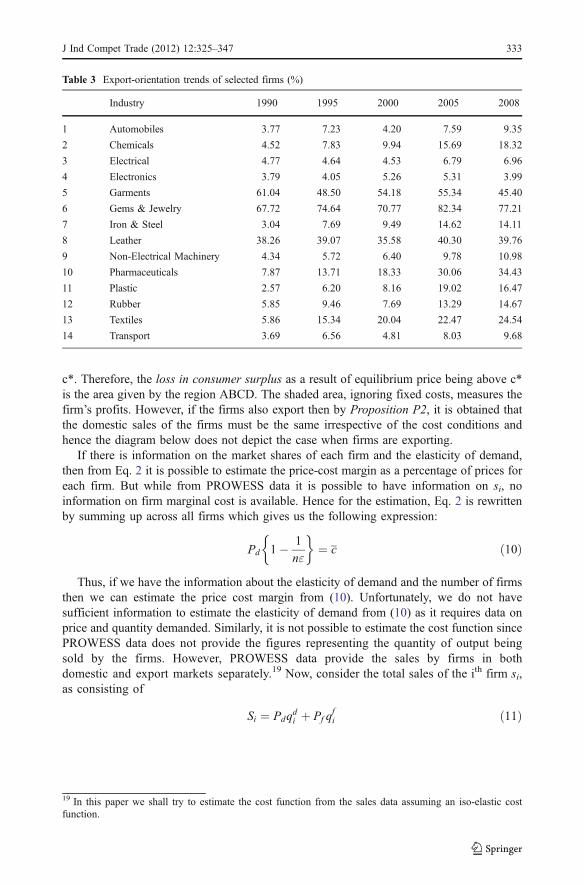
c*. Therefore, the loss in consumer surplus as a result of equilibrium price being above c*is the area given by the region ABCD. The shaded area, ignoring fixed costs, measures thefirm’s profits. However, if the firms also export then by Proposition P2, it is obtained thatthe domestic sales of the firms must be the same irrespective of the cost conditions andhence the diagram below does not depict the case when firms are exporting.

If there is information on the market shares of each firm and the elasticity of demand,then from Eq. 2 it is possible to estimate the price-cost margin as a percentage of prices foreach firm. But while from PROWESS data it is possible to have information on si, noinformation on firm marginal cost is available. Hence for the estimation, Eq. 2 is rewrittenby summing up across all firms which gives us the following expression:

Pd 1� 1

n"

� �¼ c ð10Þ

Thus, if we have the information about the elasticity of demand and the number of firmsthen we can estimate the price cost margin from (10). Unfortunately, we do not havesufficient information to estimate the elasticity of demand from (10) as it requires data onprice and quantity demanded. Similarly, it is not possible to estimate the cost function sincePROWESS data does not provide the figures representing the quantity of output beingsold by the firms. However, PROWESS data provide the sales by firms in bothdomestic and export markets separately.19 Now, consider the total sales of the ith firm si,as consisting of

Si ¼ Pdqdi þ Pf q

fi ð11Þ

Table 3 Export-orientation trends of selected firms (%)

Industry 1990 1995 2000 2005 2008

1 Automobiles 3.77 7.23 4.20 7.59 9.35

2 Chemicals 4.52 7.83 9.94 15.69 18.32

3 Electrical 4.77 4.64 4.53 6.79 6.96

4 Electronics 3.79 4.05 5.26 5.31 3.99

5 Garments 61.04 48.50 54.18 55.34 45.40

6 Gems & Jewelry 67.72 74.64 70.77 82.34 77.21

7 Iron & Steel 3.04 7.69 9.49 14.62 14.11

8 Leather 38.26 39.07 35.58 40.30 39.76

9 Non-Electrical Machinery 4.34 5.72 6.40 9.78 10.98


11 Plastic 2.57 6.20 8.16 19.02 16.47

12 Rubber 5.85 9.46 7.69 13.29 14.67

13 Textiles 5.86 15.34 20.04 22.47 24.54

14 Transport 3.69 6.56 4.81 8.03 9.68

19 In this paper we shall try to estimate the cost function from the sales data assuming an iso-elastic costfunction.


where both Pd and Pf are the same across all firms at the point of equilibrium. If thedomestic average tariff rate in the industry is t, then the following relationship is obtained,

Pd ¼ Pf : 1þ tð Þ ð12ÞIn other words, value of exports can be expressed in domestic price using Eq. 12. For

determining tariff rate, the current analysis sources the relevant data points at HS 6-digitlevel for the selected industries from the various annual volumes of customs tariff handbookand the mean tariffs constructed in this manner are used. The Si constructed in this manneris symbolized as S

»i from now on.

S»

i ¼ Pdqdi þ Pf q

fi 1þ tð Þ ð13Þ

Expressing Eq. 13 in domestic prices alone, we have:

S»

i ¼ Pd qdi þ qfi

� ð14Þ

Since all firms face the same price, therefore, S»i may be treated as output of a firm

multiplied by some constant. Summing over all firms from Eq. 14 we get:

S» ¼ PdX ð15ÞWe assume that the cost function of a firm is iso-elastic in output, i.e.,

Ci ¼ xbi ð16ÞSince we do not have firm output from the data, we replace xi by firm sales S

»i to

estimate the value of β. The assumption that all the firms face the same inverse demand

Fig. 1 Equilibrium of the Indus-try when firms do not export


P

QQd

Pd

C*

A

D

B

function (Eq. 8) facilitates the estimation of β from the sales figure.20 For regressionpurpose, Eq. 16 can be written in the following form:

lnCi ¼ a þ b ln xi þ m ð17ÞNow from Eq. 17, β can be estimated and hence the total output X can be derived by

simply inverting the function given by Eq. 16, i.e. the following:

xi ¼ C1b

i ð18ÞTherefore, the industry output is henceforth represented by:

X ¼X

xi ð19ÞGiven the industry sales as in Eq. 15, dividing Eq. 15 by Eq. 19, the estimated industry

price is obtained.Now, the firm output that is estimated can be used for estimating the average marginal

cost in the following manner:

Ci ¼ g þ dxi þ ei ð20ÞEstimating Eq. 20, the values of δ could be obtained. Having estimated the average marginal

cost from Eq. 20 and the price being already estimated from Eq. 15 and Eq. 19 as discussed above,we are now in a position to estimate industry price-cost margin (PCM). Further, with the estimatesof price and the average marginal cost, we can estimate the elasticities of demand from Eq. 10.

5 Results

With trade liberalization, the monopoly power of the firms across the industries is expectedto decline, leading to (1) reduction in industry concentration, which in turn is expected to leadto a (2) decline in the price-cost margin of the industry. Further, increase in number of firmswithin an industry due to entry liberalization is likely to result in an (3) increase in theelasticity of the domestic demand curve since more firms implies availability of greaternumber of varieties for the consumer.21 The validity of these hypotheses is tested in theIndian context. The empirical estimates of industry concentration levels, price-cost margins,elasticity of demand and importance of size variable on export behaviour are provided below.

5.1 The concentration measures

The Herfindahl index for overall sales for select years is presented in Table 4. An overalldecline is witnessed, barring certain sector specific exceptions. For instance, labour-

20 Ci ¼ S»i bem ¼ Pdxið ÞbemThus after taking log on both sides, equation (16) can be written as,lnCi ¼ b lnPd þ b ln xi þ m, which can be re-written as -lnCi ¼ a þ b ln xi þ m

21 Chamberlin (1969) argues that, “.. the larger the number of sellers in the market, the greater the elasticityof demand for each seller.” p. 282. However, we are not referring to the market demand function for eachseller, but the aggregate demand function, which can be derived from the underlying equilibrium condition.Therefore, any change in elasticity may be the result of the change in the parameter of the utility function,which essentially means a change in the utility function itself.


intensive gems and jewelry, leather, textile etc. have witnessed decline in concentration ingeneral. However, capital-intensive sectors like automobile and transport sector havewitnessed increase in concentration during 1990–1995. During 1995–2000, a similar trendhas been noticed in chemical, non-electrical machinery, rubber and textile. During 2000–2005, several sectors like automobile, electrical, electronics, garments, pharmaceuticals,plastic, rubber, transport etc. revealed rising concentration trends. This cross-sectoralvariation signifies the importance of entry, both by foreign-origin as well as domestic onessince 1991, with the foreign firms playing a key role in several sectors.22 However, whilethe concentration ratio has undergone a change, interestingly the major incumbent firms areable retain their exporting status even after entry of new firms.

The above-mentioned point can be proved with the help of Table 5, which counts thenumber of common market leaders between two periods.23 It is observed that most of thesectors have witnessed compositional change after liberalization, and newer industryleaders have emerged. The rate of the change has however varied across sectors. Forinstance, in sectors like automobile, textile and rubber several firms which dominate theindustry in 2005 were also in a dominating position back in 990. On the other hand, insectors like leather, pharmaceuticals and plastic, a completely new set of industry leadershave emerged in 2005, indicating efficiency gains by the newcomers / erstwhile marginalplayers. Interestingly, the relative stability for the export market is found to be lower ascompared to the domestic market, which signifies greater competition in the externalmarket.

22 Redington (India) Ltd., Novartis India Ltd., G E Plastics India Ltd. and Bata India Ltd. in electronics,pharmaceuticals, plastics and leather sector respectively could be cited here. But the transition has beenstrongest in transport sector, where a number of foreign firms, namely—Maruti Udyog Ltd., Hyundai MotorIndia Ltd., Motor Industries Co. Ltd., Daewoo Motors India Ltd., Ford India Ltd. etc. remain among the keyplayers.

Table 4 Harfindahl index trends in industries (overall sales)

HHI 1990 1995 2000 2005 2008

1 Automobiles 0.151 0.189 0.122 0.133 0.134

2 Chemicals 0.019 0.013 0.019 0.014 0.015

3 Electrical 0.029 0.023 0.023 0.027 0.033

4 Electronics 0.083 0.035 0.024 0.036 0.049

5 Garments 0.208 0.047 0.044 0.058 0.052

6 Gems & Jewelry 0.253 0.113 0.095 0.085 0.128

7 Iron & Steel 0.206 0.118 0.080 0.061 0.050

8 Leather 0.530 0.150 0.144 0.096 0.104


10 Pharma 0.030 0.019 0.018 0.023 0.022

11 Plastic 0.188 0.110 0.088 0.103 0.064

12 Rubber 0.100 0.089 0.109 0.115 0.134

13 Textiles 0.016 0.008 0.009 0.009 0.009

14 Transport 0.074 0.079 0.051 0.055 0.056

23 The interpretation of the number ‘5’ in first row, last column in Table 5 is that, if the exporting firms in theautomobile sector are ranked according to their value of exports in 1990 and 2005, then there are 5 commonfirms among the top ten list.


5.2 The price-cost margin (PCM)

Before going to the PCM analysis, the role of foreign presence in the Indian market needs to beunderstood with the help of Tables 6 and 7, which analyzes foreign presence in domestic andforeign market respectively.24 It is observed from Table 6 that over the years foreign presencehas increased for automobile, electrical, electronics, iron and steel, leather, non-electricalmachinery, plastic and transport equipments, but decreased for chemicals, garments,pharmaceuticals, rubber, textile etc. In case of export sales, Table 7 reveals that while foreignpresence increases for automobile, electronics, garments, iron and steel, leather, rubber,transport equipments, the same decreases in chemicals, electrical, non-electrical machinery,pharmaceuticals, plastic and textile. The overall PCM level in a sector has been significantlyinfluenced by the level of foreign penetration (i.e., entry and competition) within that sector.

Table 8 provides the estimates of PCM for various industries. A few interestingobservations can be made. First, a general rise in PCM is observed over 1990 to 1995simultaneously with the decline in concentration ratios. Second, several sectors have shownan increase in PCM over 1995 to 2000 as well (textiles, chemicals, electronics, iron andsteel, pharmaceutical etc.). Third, an increase in PCM is noticed for several categories over2000 to 2005 as well (electrical, electronics, garments, leather etc.). A declining trend in thelast reported year 2008 has been observed, which may be explained by the decline in thenumber of reported firms.25 While at the first sight this finding appears to be a bitinconsistent, a little introspection reveals that such a possibility may arise if more efficientfirms, particularly foreign firms, enter the industry after the liberalization. Alternatively,spillover of technical changes across all firms as a result of increased pressure ofcompetition due to liberalization may explain this scenario.26

24 The foreign owned firms include both private foreign firms aswell as firms coming under foreign business Groups.25 The decline is caused by incomplete updating of the firm data by PROWESS, rather than actual exit of firms.

Table 5 Relative stability in market structure: presence of top 10 firms (number)

Sectors 1990 and 1995 1990 and 2000 1990 and 2005

Domestic Export Domestic Export Domestic Export

1 Automobiles 7 6 7 6 7 5

2 Chemicals 5 4 6 4 5 2

3 Electrical 5 4 5 4 6 3

4 Electronics 7 5 7 1 4 3

5 Garments – – 4 2 1 2

6 Gems and Jewelry – – 5 5 3 4

7 Iron & Steel 7 4 5 2 2 2

8 Leather – – 5 4 4 0

9 Non-Electrical Machinery 9 6 7 5 6 4

10 Pharmaceuticals 7 2 0 0 1 0

11 Plastic 6 3 5 1 4 1

12 Rubber 10 7 7 5 5 4

13 Textiles 6 6 5 3 3 2

14 Transport 8 5 6 7 6 6

26 A higher PCM for the foreign firms can be explained by the higher average productivity growth of theforeign-affiliated firms vis-à-vis the domestic firms (Banga 2003).


5.3 Elasticity trends

The elasticity estimates for the selected industries are shown in Table 9. It is observedthat the demand curve is generally inelastic, barring the exception of automobile in1993, gems and jewelry in 1991, leather in 1992 and rubber in 1990, 1991 and 1994.The comparison between the two end years, 1990 and 2008 reveals that the value ofelasticity has declined over the period. In case of some industries (electrical, leather,non-electrical machinery), elasticity increased over 1995 to 2000, but declined in thefollowing period.

Table 6 Foreign presence in domestic sales (%)

Sectors 1990 1995 2000 2005 2008

1 Automobiles 18.61 25.05 37.09 36.29 31.81

2 Chemicals 29.68 24.57 27.96 23.81 21.87

3 Electrical 28.16 22.76 23.43 27.33 29.39

4 Electronics 11.65 15.43 20.91 25.29 17.70

5 Garments 2.09 1.92 1.85 0.40 1.92

6 Iron & Steel 0.47 1.23 1.59 1.32 0.94

7 Leather 17.46 35.11 32.09 21.90 23.85



10 Plastic 4.50 3.74 4.54 4.68 6.15

11 Rubber 5.94 5.21 8.38 5.21 4.86

12 Textiles 3.03 2.17 2.31 0.74 0.37

13 Transport 16.78 20.66 27.39 28.01 25.98

Table 7 Foreign presence in export sales (%)

Sectors 1990 1995 2000 2005 2008

1 Automobiles 15.79 26.87 35.58 53.02 35.83

2 Chemicals 47.52 30.88 32.40 25.49 18.98

3 Electrical 32.51 44.03 40.46 36.43 31.87

4 Electronics 4.90 13.36 38.71 51.67 43.05

5 Garments 0.00 0.34 2.72 0.26 2.59

6 Iron & Steel 0.56 1.36 2.53 1.53 0.99

7 Leather 3.91 4.06 2.71 6.89 4.84



10 Plastic 18.66 3.98 3.90 3.40 5.82

11 Rubber 0.67 4.15 2.19 5.29 2.22

12 Textiles 8.34 2.92 1.77 0.84 0.65

13 Transport 17.32 25.91 28.32 39.34 28.78


Tab

le8

The

pricecostmarginresults

inthemarketsegm

ents—indu

stry-w

ise

(Percentage)

Industry

Autom

obiles

Chemicals

Electrical

Electronics

Garments

Gem

s&

Jewelries

Iron

&Steel

Leather

Non

-Electrical

Machinery

Pharm

aceuticals

Plastic

Rubber

Textiles

Transport

1990

0.126

0.06

20.104

0.041

––

0.137

–0.041

0.19

70.197

0.015

0.08

70.091

1991

0.124

0.12

90.175

0.060

0.213

0.08

60.135

0.019

0.21

20.222

0.017

0.29

50.071

1992

0.337

0.05

80.177

0.147

0.138

0.22

20.010

0.043

0.054

0.03

90.228

0.039

0.10

50.177

1993

0.043

0.112

0.222

0.105

0.174

0.211

0.082

0.068

0.083

0.10

80.083

0.012

0.10

70.117

1994

0.118

0.14

30.142

0.263

0.188

0.29

30.165

0.267

0.271

0.08

40.379

−-0.007

0.16

50.134

1995

0.247

0.15

90.158

0.160

0.334

0.24

40.289

0.288

0.218

0.22

50.225

0.062

0.18

80.183

1996

0.164

0.19

10.165

0.157

0.330

0.23

30.147

0.366

0.153

0.19

80.299

0.035

0.17

40.203

1997

0.220

0.32

20.111

0.178

0.185

0.24

90.228

0.337

0.171

0.21

20.248

0.091

0.20

50.156

1998

0.225

0.31

80.017

0.245

0.224

0.18

40.266

0.602

0.113

0.30

00.339

0.021

0.18

10.226

1999

0.169

0.35

20.075

0.222

0.446

0.24

80.319

0.634

0.177

0.21

90.373

0.044

0.29

30.199

2000

0.188

0.34

30.093

0.212

0.283

0.22

90.392

0.287

0.161

0.45

10.451

0.093

0.39

70.304

2001

0.136

0.31

50.135

0.228

0.283

0.26

00.336

0.455

0.200

0.23

60.398

0.070

0.29

30.175

2002

0.101

0.34

80.085

0.254

0.306

0.24

30.298

0.373

0.238

0.30

00.428

0.077

0.34

50.232

2003

0.142

0.30

50.105

0.235

0.306

0.24

40.349

0.402

0.295

0.29

70.332

0.038

0.29

40.185

2004

0.130

0.30

00.100

0.220

0.342

0.27

10.327

0.397

0.234

0.27

80.327

0.109

0.30

00.245

2005

0.134

0.30

30.139

0.226

0.366

0.24

50.325

0.443

0.180

0.31

80.318

0.081

0.27

00.278

2006

0.134

0.29

40.254

0.253

0.326

0.24

00.272

0.444

0.224

0.21

20.360

0.052

0.29

40.212

2007

0.100

0.27

20.197

0.265

0.187

0.18

90.234

0.273

0.237

0.23

90.425

0.124

0.26

20.108

2008

0.096

0.27

80.200

0.235

0.243

0.15

10.280

0.177

0.165

0.21

60.315

0.110

0.23

70.180

Calculatedby

authors


Tab

le9

Elasticity

results

inthemarketsegm

ents—indu

stry-w

ise

(Percentage)

Indu

stry

Autom

obiles

Chemicals

Electrical

Electronics

Garments

Gem

s&

Jewlleries

Iron

&Steel

Leather

Non-Electrical

Machinery

Pharm

aceuticals

Plastic

Rubber

Textiles

Transport

1990

0.41

70.062

0.095

0.31

8–

–0.046

–0.19

20.064

0.099

2.60

90.048

0.103

1991

0.42

60.024

0.049

0.16

40.39

11.29

10.038

0.34

40.047

0.059

1.89

80.011

0.108

1992

0.15

60.048

0.045

0.06

50.45

40.40

90.406

2.312

0.10

30.216

0.052

0.71

20.027

0.039

1993

1.119

0.020

0.032

0.06

70.31

90.31

60.047

0.863

0.06

00.063

0.110

1.79

00.023

0.049

1994

0.40

40.013

0.038

0.01

80.16

60.114

0.018

0.110

0.01

80.062

0.016

−2.642

0.011

0.038

1995

0.18

40.009

0.031

0.02

30.06

10.09

30.009

0.071

0.02

00.018

0.020

0.24

70.009

0.027

1996

0.26

50.008

0.029

0.02

10.05

40.09

10.018

0.056

0.02

70.019

0.014

0.42

60.009

0.023

1997

0.19

80.005

0.047

0.01

80.09

30.09

10.012

0.064

0.02

50.020

0.017

0.16

10.008

0.030

1998

0.18

50.004

0.311

0.01

20.07

40.113

0.010

0.037

0.03

80.013

0.013

0.66

00.009

0.020

1999

0.22

80.004

0.062

0.01

00.03

40.07

30.007

0.034

0.02

30.016

0.011

0.29

80.005

0.019

2000

0.19

00.004

0.049

0.00

90.04

70.07

70.005

0.074

0.02

50.008

0.008

0.14

50.004

0.010

2001

0.28

40.004

0.034

0.00

80.04

90.06

20.006

0.049

0.02

10.015

0.010

0.19

10.005

0.018

2002

0.36

80.004

0.054

0.00

70.04

20.06

40.007

0.058

0.01

60.012

0.009

0.15

90.004

0.015

2003

0.29

30.004

0.038

0.00

60.03

30.05

40.006

0.044

0.01

20.010

0.011

0.26

70.004

0.017

2004

0.28

50.004

0.039

0.00

60.03

00.04

30.006

0.042

0.01

40.010

0.010

0.08

70.004

0.012

2005

0.29

80.004

0.030

0.00

60.02

70.04

70.006

0.036

0.01

90.009

0.011

0.116

0.005

0.011

2006

0.24

80.004

0.016

0.00

60.03

10.05

40.007

0.041

0.01

60.014

0.010

0.21

30.004

0.015

2007

0.33

30.005

0.022

0.00

60.06

40.07

40.008

0.075

0.01

60.013

0.009

0.09

20.005

0.029

2008

0.38

60.005

0.024

0.00

80.04

90.112

0.008

0.135

0.02

60.017

0.014

0.12

30.007

0.020

Calculatedby

authors


5.4 Firm size and exports

Are export intensities or export performances any way related to the size of the firms? There aremixed results on this issue at the empirical level.27 However, Agarwal and Barua (1994) hadshown that in an open economy oligopoly model under Cournot competition, firm size andexport intensities are positively related thus confirming the empirical findings of Hirsch. Inour firm level analysis of Indian industries we have observed that first, there has been aconsiderable increase in the number of exporting firms over the years, and, second, that theoverall exports of the firms have also increased confirming proposition 4 above. In order totest the hypothesis about firm size and export intensities, we have first calculated thecorrelation coefficient between these two variables. The results for the 14 industries aresummarized in Table 10. The correlation coefficients are significantly positive in all casessupporting the Proposition P2, though the extent of the size—export relationship differscross-sectionally.28 Interestingly, these results also lend indirect support to the results ofMelitz (2003) that exposure to trade induces only the more productive firms to enter theexport market. This result holds good in the Indian scenario as well (Kumar and Pradhan2007).

In our next step, we have conducted an unbalanced panel regression analysis by takinginto account not only the size variable but also some other control variables such astechnology, concentration ratio, export penetration ratio and two dummies representingindustrial liberalization and trade liberalization effects respectively.29 The purpose is toexamine the validity of the relationship between firm size and export intensity as proposedin Proposition 1 & 2.30 We expect positive signs of the regression coefficients with respectto the variables size and negative for the technology variable. As regards the concentrationvariable, the theory tells that as entry of new firms occurs, the domestic sales of firms’declines and therefore export per firm increases as the output remains constant.31 Followingthis we should expect a negative relationship between the export sales of firms and theconcentration levels. However, we do not have any a priori reason to believe any sign forthe variables representing export penetration. One possibility is that if the size of the worldmarket is given, then as more and more firms enter into the export market, the exportintensity of the existing firms should decline.

In the regression equation, the liberalization dummy is expected to capture the effects ofinternal industrial liberalization policies of a country. Following our theory we shouldexpect a negative sign for both the coefficients of the liberalization dummy and the WTOdummy. The reasons for the former is as the number of exporting firms increase, the shareof each individual exporting firm would decrease and the for the latter is that tradeliberalization implies a fall in the foreign price and a fall in the price would lead to a fall inthe firm output too (given the rising marginal cost curve). As a result, the domestic price

27 Hirsch (1971) in a pioneering study based on a sample of several hundred firms from six industries inDenmark, Holland and Israel found a positive correlation between export performance, defined as the ratio ofthe exports of a firm to its sales, and firm size, a result later confirmed in Seev Hirsch and Zvi Adar (1974).However, Glejser et al. (1980) supported Rapp’s result (1976) of a negative relationship between firm sizeand export-sales ratio.28 In an earlier study on Indian export trade (see, Barua and Chakraborty 2004), it had been shown that thesize of the industries and export intensities are positively related.29 We are very much thankful to the referee for the suggestion of confirming the results in a multipleregression framework.30 For the relationship between firm size and export, we consider output share and export share respectivelyin a particular year.31 See Agarwal and Barua (1994), P. 8.


Tab

le10

Correlatio

ncoefficientsof

marginalcost,size

andexpo

rts

Correlatio

nCoefficients

ofMC,Size&

Exp

orts

1990

1995

2000

2005

2008

MC&

Size

MC&

Exports

Exports

&Size

MC&

Size

MC&

Exports

Exports

&Size

MC&

Size

MC&

Exports

Exports

&Size

MC&

Size

MC&

Exports

Exports

&Size

MC&

Size

MC&

Exports

Exports

&Size

1Textiles

−0.35a

−0.56a

0.43

a−0

.11a

−0.15a

0.53

a−0

.03

−0.04

0.48

a−0

.07c

−0.08b

0.49

a−0

.07c

−0.05

0.71

a

2Autom

obiles

−0.24

−0.31

0.96

a−0

.19

−0.26

0.93

a−0

.14

−0.18

0.84

a−0

.14

−0.18

0.73

a−0

.36c

−0.29

0.71

a

3Chemicals

−0.33a

−0.54a

0.41

a−0

.13a

−0.19a

0.51

a−0

.03

−0.04

0.64

a−0

.06c

−0.07b

0.37

a−0

.06c

−0.05

0.49

a

4Electrical

−0.29a

−0.52a

0.67

a−0

.13

−0.27a

0.67

a−0

.16

−0.27a

0.58

a−0

.12b

−0.16b

0.77

a−0

.12c

−0.09

0.65

a

5Electronics

−0.19c

−0.39a

0.25

b−0

.12b

−0.15

0.39

a−0

.07b

−0.09b

0.26

a−0

.05

−0.06c

0.21

a−0

.06

−0.04

0.37

a

6Garments

−0.74b

−0.64c

0.25

−0.22

−0.29b

0.12

c−0

.20c

−0.28b

0.12

−0.06

−0.12

0.06

−0.10

−0.06

0.79

a

7Gem

s&

Jewelry

––

–−0

.25c

−0.24

0.08

−0.23c

−0.13

0.26

b−0

.09

−0.07

0.12

−0.31b

−0.27b

0.96

a

8Iron

&Steel

−0.15

−0.12

0.72

a−0

.04

−0.03

0.80

a−0

.02c

−0.01

0.81

a−0

.03

−0.02

0.57

a−0

.03

−0.03

0.60

a

9Leather

––

–−0

.17

−0.08

0.04

−0.28c

−0.15

0.11

−0.12

−0.06

0.02

−0.34b

−0.33b

0.41

a

10Non-ElectricalMachinery

−0.47a

−0.40a

0.29

a−0

.09

−0.09

0.55

a−0

.12b

−0.12c

0.67

a−0

.11b

−0.10c

0.80

a−0

.16a

−0.13b

0.54

a

11Pharm

a−0

.46a

−0.71a

0.52

a−0

.12b

−0.12b

0.98

a−0

.10c

−0.18a

0.57

a−0

.07

−0.13b

0.64

a−0

.16a

−0.10b

0.90

a

12Plastic

−0.23c

−0.23c

0.1

−0.11c

−0.08

0.43

a−0

.05

−0.03

0.66

a−0

.03

−0.03

0.89

a–

–0.87

a

13Rubber

−0.59a

−0.78a

0.90

a−0

.38a

−0.43a

0.88

a−0

.30a

−0.29b

0.83

a−0

.19b

−0.19c

0.68

a–

–0.66

a

14Transpo

rt−0

.11

−0.14

0.89

a−0

.11

−0.15b

0.92

a−0

.04

−0.04

0.82

a−0

.03

−0.03

0.77

a−0

.08

−0.07

0.75

a

a,band

cim

plylevelof

statistical

significance

at1percent,5percentand10

percentrespectiv

ely


would rise since the foreign price would cut the falling marginal revenue curve at a lowerpoint resulting in a decline in firm export surpluses. Therefore, we expect a negative signbetween export intensity and the WTO dummy. The regression equation therefore isdefined as follows:

Eit ¼ ao þ a1Sizeþ a2Technologyþ a3HHI þ a4Export penetrationþ a5LibDþ a6WTOD

Where,

Dependent variable Eit, Export Share (qif =Qf )Size Output Share (xi=X )Technology Average Cost (ci=xi)HHI Concentration Index (

PQ2

i , where Qi = qd + qf)Export Penetration No. of firms exporting/No. of firms operatingLib D Dummy for Industrial Liberalization effect

(1 = 1995 onwards; otherwise 0)WTO D Dummy for WTO effect (1 = 2000 onwards; otherwise 0)

The results are given in Table 11. The Hausman specification test for default random effectsmodel shows the critical value of chi-squared test statistic with six degrees of freedom is12.59. Based on these estimated chi-squared statistic, we have chosen random effects resultsfor Textliles, Chemicals, Leather, Pharma and Rubber and rest of the sectors we have chosenfixed effects results. The model is rich in terms of sample size varying from 365 observationsto 7215 observations. Goodness of fit has been good for all the models as it is evident from Fstatistic and Wald chi-square statistic for fixed and random effects results respectively.

As expected, the size variable is positive for all the sectors and is statistically significantat 1% except for the Leather for which the coefficient which is positive but not significant.The technology variable again is negative as expected for most of the sectors andsignificant as well except for the sectors Automobiles, Electricals and the Rubber. On theother hand, the coefficients for the Garments, Pharmaceuticals and the transport sectors arepositive are insignificant for the Garments and the transport sectors. The only positive andsignificant coefficient is for the Pharmaceuticals sector. In a nutshell, the size andtechnology variables indicate that bigger and more efficient firms have higher export sharesconfirming our propositions 1 & 2 above.

The coefficients for the Concentration index shows mixed results. Those which arepositive and are statistically significant at 1% are Textiles, Electronics, Leather, Non-electrical Machinery and Plastic while the coefficients for Iron & Steel is statisticallysignificant at 10%. The coefficients for the remaining sectors irrespective of their signs areall statistically insignificant.

The export penetration variable is generally insignificant in all the cases except for theElectronics and the Iron & Steel sectors for which the coefficients are positive andsignificant 1% level of significance.

The Liberalization dummy turning out to be negative and significant as expected atdifferent levels in a few cases like Textiles, Chemicals, Iron & Steel, Leather, Non—Electronic Machinery and Plastic and positive and significant only for Electronics. Thecoefficients are however insignificant for the rest of the sectors.

As expected, the WTO dummy is negative for the most of the sectors (except forElectrical, Electronics, Leather and Pharmaceuticals) and is also significant in a few cases.In general, the overall results of the regression estimates support our basic theory of firmbehaviour in an open economy oligopoly.


Tab

le11

Regressionresults

betweenfirm

size

andexports

Textiles

Autom

obiles

Chemicals

Electrical

Electronics

Garments

Gem

s&

Jewelry

Iron

&Steel

Leather

Non-Electrical

Machinery

Pharm

aPlastic

Rubber

Transport

Constant

0.003a

0.018

0.006a

0.006

−0.01

−0.0001

0.011

0.009

0.028

0.016a

−0.003

0.2b

0.02

0.001

2.97

0.25

3.32

0.78

−1.29

−0.02

0.54

1.32

0.88

2.85

−1.36

1.96

0.68

0.36

Size

0.46

a0.98

a0.54

a0.801a

0.083a

1.026a

0.77

a0.341a

0.0008

0.39

a1.08

a0.277a

0.77

a0.82

a

47.88

31.58

64.69

32.79

9.12

61.23

30.38

40.61

1.22

39.71

61.07

25.8

30.8

87.92

Technology

−0.004

a−0

.003

−0.004

a−0

.0001

−0.023

a0.005

−0.019

a−0

.02a

−0.04a

−0.021

a0.003a

−0.03a

−0.012

0.0001

−10.47

−0.2

−8.73

−0.03

−7.29

1.51

−2.69

−11.58

−6.38

−10.63

3.08

−9.04

−1.29

0.07

HHI

0.32

a−0

.003

−0.03

0.087

0.28

a−0

.021

0.052

0.46

c0.203a

0.088a

−0.02

0.11

a−0

.016

0.01

5.78

−0.02

−1.36

0.57

4.75

−0.48

0.91

1.85

5.09

2.77

−0.31

3.93

−0.09

0.27

ExportPenetratio

n−0

.2−0

.016

0.001

−0.0106

0.04

a−0

.005

0.009

0.02

a0.006

−0.0004

0.0002

−0.002

−0.006

−0.0005

−1.11

−0.26

0.01

−0.58

3.51

−0.58

0.37

2.68

0.17

−0.06

0.24

−0.15

−0.17

−0.1

Lib

Dum

my

−0.0008a

−0.002

−0.001

a−0

.0009

0.005c

0.002

−0.004

−0.007

a−0

.02b

−0.001

b0.001

−0.004

c−0

.006

−0.0004

−3.14

−0.27

−7.46

−0.87

1.70

0.55

−0.68

−3.9

1.9

−2.12

1.11

−1.77

−1.51

−0.62

WTO

Dum

my

−0.0009a

−0.001

−0.0005a

0.0002

0.004b

−0.0008

−0.0005

−0.001

0.011

−0.002

a0.0002

−0.007

a−0

.001

−0.0001

−3.76

−0.12

−3.39

0.27

2.23

−0.42

−0.15

−1.26

0.1

−3.4

0.53

−4.51

−0.24

−0.11

WaldChi2(6)

3569.04

5322.9

99.12

4436.47

1300.22

0.000

0.000

0.000

0.000

0.000

F204.25

239.28

49.1

880.56

215.61

368.71

359.47

171.58

1503.13

0.000

0.000

0.000

0.000

0.000

0.000

0.000

0.000

0.000

F(ui=0)

Hausm

an8.22

17.24

0.76

35.68

13.91

51.53

14.85

23.04

4.28

331.39

9.71

18.38

6.1

19.15

0.22

0.00

0.99

0.00

0.03

0.00

0.021

0.00

0.45

0.00

0.13

0.005

0.41

0.003

RSq

with

in0.366

0.785

0.42

0.442

0.117

0.883

0.678

0.43

0.163

0.437

0.601

0.366

0.633

0.77

between

0.382

0.939

0.46

0.685

0.028

0.784

0.543

0.293

0.038

0.473

0.649

0.661

0.684

0.813

overall

0.370

0.792

0.424

0.485

0.113

0.877

0.664

0.426

0.15

0.442

0.600

0.393

0.63

0.768

No.

ofObservatio

ns6083

365

7215

1958

2389

766

672

3165

565

2981

2957

1927

769

2908

Panel

Type

RE

FE

RE

FE

FE

FE

FE

FE

RE

FE

RE

FE

RE

FE

a,b,care1%

,5%

,10%

levelof

statistical

significance


6 Conclusion

Let us now summarize our results. First, both internal and external liberalizations have ledto a significant increase in the number of firms in almost all the industries resulting in a fallin the concentration ratio with a caveat that the relative positions of the dominant firmsthough have not changes much.32 The sectoral difference can be explained with respect tothe export behaviour of the firms. For instance, the electronics sector has been heavilydependent on exports, while the automobile sector has relied more on capturing the internalmarket. Second, the decline in the concentration ratio has been associated with a rise in theprice—cost margins across all industries. This apparently inconsistent result may seempossible in the face of entry of more efficient domestic firms or technological spillovereffects. Third, the elasticity of demand at the point of equilibrium is generally less thanunity. This is consistent under oligopoly. Further, the decline of the elasticity over timemerely confirms that unless the demand curve has shifted, the equilibrium has taken placeat still a lower point on the downward sloping time invariant demand curve implying a fallin the price. Fourth, our regression results show that that the firm size and exports arepositively related thus confirming our theoretical predictions. Similarly, the other variablessuch as technology, concentration, export penetration and liberalization dummies have alsogiven more or less the desired signs of the estimates of the regression coefficients. Fifth, amajor innovation of our study is to develop an econometric method of estimating the outputof firms from the data on sales of the firms. This has facilitated us to conduct the entireempirical analysis with a unified set of firm data alone without resorting to using differenttypes of data as usually done in comparable other studies. This innovation in estimatingmethod has made our study a class apart from the comparable existing research works.Finally, the empirical model performs very well with the theory thus providing a theoreticalfoundation to our empirical results.

Acknowledgement An earlier version of this paper has been presented at the Conference on “Growth andDevelopment: Future Directions for India”, organized by Centre for International Trade and Development,JNU, New Delhi during 23–24 April 2010. We are grateful to K.L.Krishna, B. N. Golder and PulapreBalakrishnan and other participants at the Conference for their helpful comments and suggestions. We alsosincerely thank Kisore Gawande and Kala Krishna for their comments and suggestions on a preliminaryversion of the paper. We are grateful to the anonymous referee and the editor of the journal for their helpfulsuggestions. We however are fully responsible for all remaining errors.

References

Agarwal M, Barua A (1993) Trade policy and welfare in segmented markets. Keio Econ Stud 30(2):95–108Agarwal M, Barua A (1994) Effects of entry in a model of oligopoly with international trade. J Int Trade

Econ Dev 3(1):1–13Agarwal M, Barua A (2004) Entry liberalization and export performance: a theoretical analysis in a multi-

market oligopoly model. J Int Trade Econ Dev 13(3):287–303Agarwal M, Barua A (2007) Firm and Industry Response to Liberalization in India: Theory and Evidence, In:

Huchet Jean-Francoise, Richet, Xavier and Ruet, Joel (eds) Globalization in China, India and Russia:Emergence of National Groups and Global Strategies of Firms, Academic Foundation, pp. 153–177

32 This result corroborates the revelation of ‘missing middle’ in the Indian industries. The entry has perhapstaken place at the tail of distribution of firms (Das and Pant 2006).


Aiginger K (2006) Revisiting an evasive concept: introduction to the special issue of competitiveness. J IndCompet Trade 6(2):63–66

Apte PG, Vaidyanathan R (1982) Concentration, controls and performance in twenty-nine manufacturingindustries in India. Indian Econ Rev XVII(2–4):241–262

Athreye S, Kapur S (2003) Industrial concentration in a liberalizing economy: a study of Indian manufacturing.www.econ.bbk.ac.uk/wp/ewp/concentration_dec03.pdf (last accessed on March 20, 2010)

Balakrishnan P, Babu MS (2003) Growth and distribution in Indian industry in the nineties. Economic andPolitical Weekly, September 20, 2003, pp 3997–4005

Banga R (2003) Differential impact of Japanese and US foreign direct investments on productivity growth: afirm level analysis. New Delhi: ICRIER Working Paper No. 112

Barua A, Chakraborty D (2004) Liberalization, trade and industrial performance in India: an empirical study.Presented in the Conference WTO Negotiations: India’s Post-Cancun Concerns, Organized by the ITDDivision, SIS, JNU, the Planning Commission and the ICSSR, New Delhi, 18–19 October

Barua A, Pant M (1995) Internal liberalization and entry in a general equilibrium model with oligopoly. KeioEcon Stud XXXII(2):47–58

Barua A, Chakraborty D (2006) Liberalization, trade and industrial performance: an empirical analysis forIndia. Paper for the 2nd APEA Conference, held at the Center for International Economics, University ofWashington, Seattle, July 29–30, 2006

Boulhol H (2005) Why haven't price-cost margins decreased with globalization? Available at ftp://mse.univ-paris1.fr/pub/mse/cahiers2006/Bla06007.pdf (last accessed on January 6, 2010)

Chamberlin EH (1969) The theory of monopolistic competition: a re-orientation of the theory of value, 8thedn. Oxford University Press

Das SK, Pant M (2006) Measuring market imperfection in the manufacturing sector: theory and evidencefrom India. J Int Trade Econ Dev 15(1):63–79

Ghosh A (1974) Role of large business house in Indian industries. Indian Econ J 22(2):316–45Ghosh A (1975) Concentration and growth of Indian industries: 1948–68. J Ind Econ 23(3):203–22Glejser H, Jacquemin A, Petit J (1980) Exports in an imperfect competition framework: an analysis of 1446

exporters. Q J Econ 94:507–524Goldar B, Aggarwal SC (2004) Trade liberalization and price-cost margin in Indian Industries. ICRIER

Working Paper No. 130, New DelhiGovernment of India (1966) Report of the monopolies inquiry commission. New DelhiGupta VK (1968) Cost functions, concentrations and barriers to entry in twenty-nine manufacturing

industries in India. J Ind Econ 17(1):57–72Hirsch (1971) The export performance of six manufacturing industries: a comparative study of Denmark,

Holland, and Israel. Praeger Publishers, New YorkHirsch, Adar Z (1974) Firm size and export performance. World Dev 2(7):41–46Kambhampati, US, Ashok Parikh (2003) Disciplining Firms? The Impact of Trade Reforms on Profit

Margins in Indian Industry, Applied Economics, 35(4):461–70Kambhampati, US, Ashok Parikh, (2005) Has Liberalisation Affected Profit Margins in Indian Industry?,

Bulletin of Economic Research, 57(3):273–304Kambhampati US, Kattuman P (2003) Growth response to competitive shocks: market structure dynamics

under liberalization: the case of India. Working paper number 263, ESRC Centre for Business Research,University of Cambridge

Katrak H (1980) Industry structure, foreign trade and price-cost margin in Indian manufacturing industries. JDev Stud, 62–79

Krishna P, Mitra D (1998) Trade liberalization, market discipline and productivity growth: new evidencefrom India. J Dev Econ, 447–462

Kumar N, Pradhan JP (2007) Knowledge-based exports from India: a firm level analysis of determinants. In:Kumar N, Joseph KJ (eds) International competitiveness and knowledge-based industries in India.Oxford University Press, New Delhi

Mas-Colell A, Whinston MD, Green JR (1995) Microeconomic Theory. Oxford University PressMelitz MJ (2003) The impact of trade on intra-industry reallocations and aggregate industry productivity.

Econometrica 71(6):1695–1725Rao PA (2001) A study of the determinants of firm profitability in selected industries in post-reform India.

Unpublished M.Phil. Dissertation, Delhi School of Economics, University of DelhiRapp W (1976) Firm size and Japan’s export structure. In: Patrick H (ed) Japanese industrialization and its

social consequences. The University of California Press, Berkeley, pp 201–248Roy Choudhury P (2007) Entry liberalization, export subsidy and R&D. MPRA Paper No. 1532, available at

Online at http://mpra.ub.uni-muenchen.de/1532/ (last accessed on September 7, 2010)


http://www.econ.bbk.ac.uk/wp/ewp/concentration_dec03.pdf

ftp://mse.univ-paris1.fr/pub/mse/cahiers2006/Bla06007.pdf

ftp://mse.univ-paris1.fr/pub/mse/cahiers2006/Bla06007.pdf

http://mpra.ub.uni-muenchen.de/1532/

Sandesara JC (1979) Size of the factory and concentration in the factory sector in India, 1951 to 1970. IndianEcon J 27(2):1–34

Sawhney PK, Swahney BL (1973) Capacity utilization, concentration and price-cost margins: results forIndian industries. J Ind Econ 21(2):145–153

Srivastava V, Gupta P, Datta A (2001) The impact of India’s economic reforms on industrial productivity,efficiency and competitiveness: a panel study of indian companies, 1980–97, Report, National Councilof Applied Economic Research, New Delhi

Sutton J (1991) Sunk costs and market structure: price competition, advertising, and the evolution ofconcentration. MIT Press


Entry, Competitiveness and Exports: Evidence from the Indian Firm Data

Documents

Transcript of Entry, Competitiveness and Exports: Evidence from the Indian Firm Data