Energy Management for Energy Harvesting Wireless Sensors ...

arX

iv:1

710.

0903

4v1

[cs

.IT

] 2

5 O

ct 2

017

1

Energy Management for Energy Harvesting

Wireless Sensors with Adaptive Retransmission

Animesh Yadav, Member, IEEE, Mathew Goonewardena, Student Member, IEEE, Wessam

Ajib, Senior Member, IEEE, Octavia A. Dobre, Senior Member, IEEE, and Halima

Elbiaze, Member, IEEE

Abstract

This paper analyzes the communication between two energy harvesting wireless sensor nodes. The

nodes use automatic repeat request and forward error correction mechanism for the error control. The

random nature of available energy and arrivals of harvested energy may induces interruption to the signal

sampling and decoding operations. We propose a selective sampling scheme where the length of the

transmitted packet to be sampled depends on the available energy at the receiver. The receiver performs

the decoding when complete samples of the packet are available. The selective sampling information

bits are piggybacked on the automatic repeat request messages for the transmitter use. This way, the

receiver node manages more efficiently its energy use. Besides, we present the partially observable

Markov decision process formulation, which minimizes the long-term average pairwise error probability

and optimizes the transmit power. Optimal and suboptimal power assignment strategies are introduced

for retransmissions, which are adapted to the selective sampling and channel state information. With

finite battery size and fixed power assignment policy, an analytical expression for the average packet

drop probability is derived. Numerical simulations show the performance gain of the proposed scheme

with power assignment strategy over the conventional scheme.

A part of the paper is published in the Proceeding of the IEEE International Conference on Communications (IEEE ICC

2015), London, UK, 8-12 June 2015.

A. Yadav and O. A. Dobre are with the Faculty of Engineering and Applied Science, Memorial University, St. John’s, NL,

Canada, (e-mail: animeshy, [email protected]), W. Ajib and H. Elbiaze are with the Department of Computer Science, Université

du Québec à Montréal (UQAM), Montreal, QC, Canada (e-mail: ajib.wessam, [email protected]) and M. Goonewardena

is École de Technologie Supérieure (ÉTS), Montréal, QC, Canada. (e-mail:[email protected]).

http://arxiv.org/abs/1710.09034v1

2

Index Terms

Wireless sensors networks, energy harvesting, packet drop probability, partially observable Markov

decision processes.

I. INTRODUCTION

The use of energy harvesting (EH) sources to power wireless communication systems has recently

received considerable attention [1]–[7]. The EH devices offer green communication and can operate

autonomously over long periods of time. Because of these benefits, the EH devices are also increasingly

considered in wireless sensor networks (WSNs) to power the sensor nodes [8]–[15].Sensors nodes are

low cost distributed devices which operate on minimal energy. They are very prevalent in applications

related to monitoring and controlling the environments, especially the remote and dangerous ones [16].

Usually, sensor nodes are operated by small capacity non-renewable batteries, thus, suffering from finite

lifespan of operation. Sensor nodes with EH capabilities can be an alternative to increase the lifespan

and lower the maintenance cost. Energy can be harvested from the environment using for instance solar,

vibration or thermoelectric effects. Unlike EH, another practical alternative to increase the lifespan of the

nodes is to use massive antenna arrays at the receiver nodes to mitigates severe energy constraints given

by the inexpensive transmitter nodes [17], [18].

Typically, the energy arrival amount at the EH devices is random. Thus, for such nodes, the challenging

objective is the adequate management of the collected energy to enable reliable and continuous operation.

Recently, a considerable amount of works on wireless networks solely powered by harvested energy have

emanated [4]–[11] to address this objective. Although both transmitter and receiver nodes can harvest

energy, the research is primarily focused either on the transmitter [8]–[11] or receiver [5]–[7], [19]. There

are many practicals scenarios where the transmitter and receiver nodes can harvest energy to increase their

lifespan, such as the scenario of transmitter and multiple intermediate nodes in a multi-hop WSN, and

multiple transmitter nodes communicating with a single sink node. These scenarios are more challenging

due to the presence of many random sources of energy.

3

Fewer works have considered the EH capability at both transmitter and receiver nodes simultaneously

[4], [12]–[15]. In [4], the authors considered a static additive white Gaussian noise (AWGN) channel and

used a rate-based utility as a function of both transmitter and receiver powers. They proposed directional

water-filling based power allocation policy in an offline setting. The problem of online power control for

a wireless link with automatic repeat request (ARQ) scheme is studied in [12]. The authors investigated

three fixed policies under various assumptions, such as knowledge of the receiver battery availability

at the transmitter node, finite and infinite battery storage. In [13], the authors analyzed a wireless link

which employs type-II hybrid automatic repeat request (HARQ) scheme. They derived the packet drop

probability (PDP) for predetermined transmit energy levels. In [14], the authors obtained a lower bound

on maximum achievable throughput and proposed a common threshold policy. In [15], we introduced an

energy-aware adaptive retransmission scheme, where the receiver node performs the selective sampling

(SS) and decoding operations based on the energy availability.

The receiver node spends the energy dominantly in sampling and decoding operations, if a forward error

correction (FEC) coding is employed [20]. Moreover, for small distances, the transmit energy is often

smaller than the energy needed in the decoding operation [21]. Nonetheless, because of the randomness in

the amount of energy arrivals, the receiver operations may be suspended, which leads to energy wastage.

Thus, the receiver might favor to sample a fraction of the full packet depending on the available energy

[5], which we refer to as SS. On the other hand, the transmitter with exact SS information (SSI) can

retransmit only a portion of the packet, which is not sampled by the receiver.

Furthermore, the time-varying characteristic of the wireless channel and harvested energy might con-

tribute to a higher packet error probability (PEP). Hence, the transmitter must adequately adapt the transmit

power level to the channel state information (CSI), while meeting the constraint of energy causality, to

ensure a lower PEP. The causality constraint affirms that the cumulative used energy cannot surpass the

cumulative harvested energy by nodes at any given time. Furthermore, based on the SSI knowledge, the

transmitter adapts the packet size to ensure an efficient utilization of the receiver energy. In pursuance of

providing the SSI to the transmitter, we resort to the ARQ protocol’s acknowledgement (ACK)/negative

acknowledgement (NAK) feedback messages. Consequently, the retransmission scheme, which we denote

4

by ACK/NAKx, needs to have some additional feedback messages.

In this paper, we consider a generic communication between two EH wireless nodes with the aforemen-

tioned retransmission protocol. A decision-theoretic approach is used to find the optimal transmit power

strategy. Firstly, the problem is formulated as a partially observable Markov decision process (POMDP),

which is a suitable approach for formulating problems that require sequential decision making in a

stochastic setting, when some of the system states are unknown [22]. We solve the POMDP problem

using the value iteration method by computing the value function for the belief of the unknown state.

Since the memory and computational complexity requirements are limited for sensor nodes, we propose

a suboptimal and a computationally lower greedy power assignment method.

The outline of this paper is as follows. The system model is presented in Section II. The adaptive

retransmission scheme is detailed in Section III. Section IV introduces the optimal and suboptimal methods

aiming to allocate the power over the time slots. An analytical upper bound on the PDP is derived

in Section V. Simulated numerical results and discussions are presented in Section VI, followed by

conclusions in Section VII. A list of symbols with their descriptions used in this paper is given in Table I

EhTx

ACK

EhTx

NAK

X

NAKx

EhTx

ACK

EhTx

NAKx

EhTx

ACK

TsTf

t− 5 t− 4 t− 3 t− 2 t− 1 t t+ 1

ETx ETx ETx ETx

k = 1 k = 2 k = 3 k = 1 k = 2

time index

Fig. 1: Time-slotted packet transmission time line at the transmitter node. ’99K’ and ’−→’ denote the

ARQ message and EH arrival events, respectively. Shaded areas in the slot denote the amount of energy

used for transmission.

5

II. SYSTEM MODEL

A. Transmission Model

We consider a point-to-point communication between two EH wireless sensor nodes. Sensor nodes have

limited capacity rechargeable batteries, which are charged by renewable energy sources. In the considered

model, when a transmitted packet is erroneously decoded, the receiver requests its retransmission. A

maximum of K ∈ Z retransmission requests are permitted. A packet consists of c information bits, taken

from the data buffer, encoded with an (m, c) FEC code (e.g., convolutional code), and then modulated

through an M -ary quadrature amplitude modulation, where M denotes the cardinality of the constellation.

This forms the packet of length ⌈m/ log2M⌉ symbols, where ⌈·⌉ is the ceiling operator.

The CSI and SSI are known at the transmitter through the ARQ feedback messages. Each sensor node

is aware of its own battery state information (BSI), but not of the BSI of the other node. However, the

transmitter estimates the one slot delayed BSI of the receiver via SSI.

A discrete time-slotted model is considered as depicted in Fig. 1. Each time slot is of Ts seconds

duration and indexed as t∈1, 2,. . .. The packet transmission and corresponding ARQ message reception

are completed within a slot, i.e., the round-trip time is Ts. Several slots constitute a frame of duration

Tf . A frame has variable duration depending upon the number of slots being used in packet transmission,

including retransmissions. Thus, the minimum and maximum values of frame duration are Ts and KTs,

respectively. After a maximum of K unsuccessful attempts, the transmitter drops the packet and chooses

a new one to transmit.

Without loss of generality, the system model considered here can be extended to generic short-range

communication systems involving different modulation formats, sophisticated channel coding methods,

and transmission strategies relying on multiple antennas and sub-carriers techniques.

B. Energy Consumption Model

The transmitter and receiver sensor nodes spend energy to transmit and retrieve the information bits,

respectively. For short-range commmunication, the energy consumption in a wireless link can be broken

down into two dominant factors [20]: the energy consumed at the power amplifiers PPA at the transmitter,

6

and the circuit blocks at both transmitter and receiver. The circuit blocks of the transmitter consist of

a digital-to-analog convertor, mixers, active filters, and frequency synthesizers, while mainly of a low

noise amplifier, intermediate frequency amplifier, active filters, analog-to-digital convertor, and frequency

synthesizer at the receiver. Further, for coded systems, the energy expended in the decoding operation

needs to be included [20], [21] at the receiver. Thus, for a coded system, the total energy expenditure at

time slot t, at both transmitter and receiver nodes is, respectively, given as

PTx = (1 + α)Pout︸︷︷︸

PPA

+PC,Tx, (1)

PRx = Pdec + PC,Rx + Pfb, (2)

where Pout is the transmit power, α = (ξ/η) − 1, with η as the drain efficiency and ξ as the peak-to-

average power ratio. PC,Tx and PC,Rx are the total power spent in the circuit blocks of the transmitter and

receiver, respectively. The power consumed in transmitting the ARQ messages is denoted by Pfb. Pdec

denotes the power used in the decoding operation and is ignored for the uncoded system. Typical values

of Pdec are around 70-80% of the power dissipated in the circuit blocks [21]. The index t is dropped in

(1) and (2) to simplify the presentation.

C. Energy Harvesting Model

The transmitter and receiver nodes are connected to two separate but similar renewable EH sources. In

particular, two independent and identically distributed (i.i.d.), Bernoulli random processes are considered

to model the energy arrivals, similar to [23]. The Bernoulli model is tractable and captures the intermit-

tent and irregular behavior of the energy arrival. It is worth mentioning that this work is, in essence,

independent of the energy arrival process; this will be shown later in the simulation results, where the

compound Poisson arrival model [24] is used as well. At the start of every slot, EhTx Joule (J) with

probability (w.p.) ρTx and zero J w.p. 1 − ρTx is harvested at the transmitter. The receiver node follows

a similar energy arrival process with probability ρRx and amount EhRx.

When the two nodes are in close vicinity and have the same type of harvesting source, then the two

EH processes are spatially correlated. In this case, the harvested energy pairs at time slot t are given as

7

[12]

(EtTx, E

tRx) =

(0, 0) w.p. p00,

(0, EhRx) w.p. p01,

(EhTx, 0) w.p. p10,

(EhTx, E

hRx) w.p. p11,

(3)

with the condition that p00+p01+p10+p11 = 1. For example, when p00 = p01 = p00 = p10 = p11 = 0.25

then both nodes harvest energies independent from each other. When p01 = p10 = 0 and p00 = p11 = 0.5,

the harvested energies are highly correlated.

Let BtTx and Bt

Rx denote the energy levels of the battery at the start of the tth time slot, and EtTx =

PTxTs and EtRx = PRxTs denote the energy consumed in transmitting a packet, as well as sampling

and decoding operations at the transmitter and receiver, respectively. The battery level at the transmitter

follows the Markovian evolution:

Bt+1Tx =

minBtTx + Eh

Tx − EtTx, B

maxTx , w.p. ρTx

BtTx − Et

Tx, w.p. 1− ρTx,

(4)

where BmaxTx denotes the transmitter node’s battery capacity. Replacing the subscript Tx in (4) with Rx

gives the receiver side battery evolution. For presentation simplicity, the energies are normalized by a

minimum possible energy, i.e., EminTx and Emin

Rx that are spent in transmitting and receiving a packet of

smallest size, respectively. Consequently, the transmitter energy level is an integer multiple of EminTx and

the change in the battery state whenever harvesting takes place is LTx , EhTx/E

minTx . Similarly, the battery

energy level at the receiver side is an integer multiple of EminRx and the EH amount is LRx , Eh

Rx/EminRx .

D. Channel Model

The wireless channel from the transmitter to the receiver is assumed to be Rayleigh faded and modeled

as a finite state Markov chain (FSMC) [25], [26]. This model captures the main features of fading channels,

and approximates the fading as a discrete-time Markov process. Essentially, all possible fading gains are

8

modelled as a set of finite and discrete channel states. The FSMC channel is described as follows: discrete

states of the channel G = g1,g2, . . . , g|G|, state transition probabilities Ω = p(gj |gi) : g1 < gi, gj <

g|G|, and steady state probabilities represented by ωo(gi), i = 1, 2, . . . , |G|.

Based on the FSMC channel model, the entire range of channel gains are partitioned into |G| + 1

non-overlapping intervals with boundary values denoted as γi|G|i=0, with increasing order of their values

from γ0 = 0 to γ|G| = ∞. The fading gain interval [γi−1, γi) represents the gi channel state, which is

considered fixed during the time slot t and changes to gj in time slot t + 1 with probability p(gj |gi).

The channel state is considered fixed during time slot t and changes to another in time slot t + 1 with

probability p(gj |gi) .

III. ADAPTIVE RETRANSMISSION SCHEME

In low harvesting rate, the receiver might not perform the sampling and decoding operations together

or perform only the sampling operation in one time slot. In such time slots, the receiver performs SS

and stores the samples, which can be later combined with the remaining parts of the packet for building

a full packet. Besides, the receiver sends back the SSI via ARQ messages. The transmitter then adapts

the packet length for the next transmission. In the adaptive retransmission scheme, ARQ messages carry

1 + log2 β bits, where β ∈ 1, 2, 4, 8, . . . , ⌈m/ log2M⌉, and have a total of x + 2 messages where

x ∈

0, 1, . . . , β, β > 1

∅, otherwise.

(5)

For β = 1, the scheme becomes the conventional one. The additional x messages are essentially the

SSI which are carried back to the transmitter as ARQ messages; henceforth, we refer to the adaptive

retransmission scheme by ACK/NAKx. Details of each message are as follows:

ACK: The packet decoding at the receiver is successful. In reply, the transmitter chooses a new packet

for transmission in the subsequent time slot.

NAK: The packet decoding is erroneous. In reply, the transmitter chooses the same packet for

transmission in the subsequent time slot.

9

TABLE I: List of symbolsSymbol Description Symbol Description

K and k Maximum number of retransmissions

and its index

S , |S| and St System state space, its cardinality, and

state at time slot tc and m Number of information and coded bits BTx, BRx, |BTx|, and |BRx| Transmitter and receiver battery states

space and their cardinalityM and Rc Modulation order and code rate USt , |USt |, at, BSt Action states space, its cardinality, ac-

tion, and maximum value of an action at

time slot tTs and Tf Slot duration and frame duration Z, |Z| and Zt Observation state space, its cardinality,

and observation state at time slot tEt

Tx and EtRx Transmitter and receiver energy expen-

diture at time slot t

ACK, NAK, NAKx ARQ feedback messages

Pdec and Pfb Decoding and ARQ message transmit

power expenditure at receiver

Pe(g, at) Packet error probability with energy

aEminTx via channel state g

Pout and PPA Transmit power and power amplifier out-

put power

P2(d, g, at) Modulation dependent bit error probabil-

ityPC,Tx and PC,Rx Transmitter and receiver circuit block

power

Perr Approximate packet error probability af-

ter NAK or decoding failureη and ξ Amplifier drain efficiency and PAPR Ad and dfree Weight spectral coefficient and free dis-

tance of convolution codeBmax

Tx and BmaxRx Maximum battery size of transmitter and

receiver nodes

r(s, at) Cost function of state St = s after taking

action aEh

Tx and EhRx Transmitter and receiver EH amounts ρTx and ρRx Transmitter and receiver nodes probabil-

ities of EHEmin

Tx and EminRx Minimum energy to transmit and receive

a packet of minimum size

π and Jπ(S0) Transmitter policy and total expected

cost with given start state S0

LTx and LRx EhTx/E

minTx and Eh

Rx/EminRx (Gt) Belief of channel state Gt at time slot t

G, |G|, γi, and Gt Total number of discrete channel states,

its cardinality, ith interval fading gain,

and channel state at time slot t

Pdrop and Pdrop PDP and average PDP

gi and ωo(gi) Channel state of interval [γi−1, γi) and

its steady state probability

ψ(i, j) Stationary probability distribution

with transmitter and receiver energies

(iEminTx , jE

minRx )

β and x Number of division of a packet and

number of additional ARQ messages

Ξq,r,w,y

i,j,z,k Transition probability of going from

state (i, j, z, k) to state (q, r,w, y)

NAKx: ⌈xm/(β log2M)⌉ symbols of the transmitted packet are sampled and the rest is discarded

due to the lack of energy. In reply, in the subsequent time slot, the transmitter sends a packet with the

remaining ⌈m(β − x)/(β log2M)⌉ symbols.

10

Note that the message NAK is different from NAK0, which corresponds to the case when the receiver

does not have enough energy to sample the smallest fraction of the transmitted packet. However, in

both cases, the transmitter retransmits the full packet. As for the conventional scheme, the ACK/NAKx

messages help in estimating the CSI to the transmitter node. Furthermore, it is now evident that the

SS is a function of the available energy at the receiver. Based on the chosen value of β, the receiver

selects ⌈xm/(β log2M)⌉ symbols for sampling in any given time slot, where x is related to the available

energy at the receiver. The transmitter sends the ⌈m(β − x)/(β log2M)⌉ symbols after receiving NAKx

message from the receiver. The length of the transmitted packet depends on the energy available at the

transmitter. For example, if β = 4, the variable x takes values from 0, 1, 2, 3, 4. For x = 3 and if

BRx ≥ xEC,Rx/β = 3EC,Rx/4, the receiver samples ⌈xm/(β log2M)⌉ = ⌈0.75m/ log2M⌉ symbols

and selects NAK3 to feedback to the transmitter. At the transmitter, if BTx ≥ EminTx then a part of the

packet of size ⌈m(β − x)/(β log2M⌉) = ⌈0.25m/ log2M⌉ symbols is sent out; otherwise, there is

no transmission. In another example, if BRx ≥ (EC,Rx + Edec), the receiver samples and decodes the

packet and selects the NAK or ACK message depending on the decoding outcome. In the conventional

retransmission scheme, if the receiver lacks energy to sample the full packet, it samples the packet till the

energy lasts and does not store the samples, and requests the packet retransmission, which requires full

amount of energy. In conclusion, the conventional retransmission scheme wastes energy when compared

with the proposed adaptive one.

IV. POWER ASSIGNMENT STRATEGY

Considering the adaptive retransmission scheme, we formulate in this section the power assignment

as a sequential decision problem and then discuss two methods for managing efficiently the harvested

energy at transmitter. At each time slot, the transmitter chooses the energy levels that minimize the

average PEP. The decision is based on the retransmission index, BSI, sequences of past observations and

power assignments at the transmitter. After each transmission, the transmitter receives a feedback, referred

to as observation ACK,NAK,NAKx, from the receiver. Furthermore, based on the observation, the

transmitter can also adapt the modulation and coding scheme. However, for sake of tractability, we only

consider the transmit packet size and power adaptations. The problem is considered in infinite horizon.

11

A. Problem Formulation

We formulate the problem by defining the following components: a set of time slots T = 1, 2, . . .

over which decisions are made, and a set of system states S , a set of transmitter BSI BTx, a set of

FSMC channel states G, a set of retransmission indices K = 1, 2, . . . ,K, a set of actions U , a set

of transition probabilities P, a set of observations Z, and a cost corresponding to every decision. Let

S = BTx × G × K = (b1, g1, k1), (b2, g1, k1), . . . , (b|BTx|, g|G|, k|K|) denote the complete discrete state

space of the system with a total of |BTx|×|G|×|K| states, where b, g, and k represent the transmitter battery

state, channel state, and retransmission index state, respectively. The state of the system, channel, and

observation at time slot t are represented as St ∈ S , Gt ∈ G, and Zt ∈ Z , respectively. The retransmission

index k tracks the system state within each frame and is reset to one when its maximum value K is

reached or when ACK is received, whichever comes first. Due to EH, the cardinality of the actions set

varies in every time slot. Hence, the set of actions at time slot t is denoted by Ust , 0, 1, 2, . . . , Bst,

where Bst ∈ BTx represents the current state battery level. This is a set consisting of feasible choices

of energy levels corresponding to the transmission of a full packet. An action at ∈ Ust represents the

energy level atEminTx = PoutTs in time slot t. For each action taken, the system receives an observation

belonging to the set Z . Note that a set of receiver BSI can be included in the system state space. Since

the exact receiver BSI state is unkown to the transmitter, its value can be estimated using the ARQ

messages likewise the channel state. However, including more unknown states to the system state space

increases the complexity in solving the problem.

We first define the PEP used for the proposed adaptive retransmission scheme. Note that the packet

can be transmitted in parts, as presented in Section-III, and the receiver can decode the packet only

when all the samples are available. Since the different parts of the packet have passed through different

channel states, the part which has passed through the worse channel state leads to the decoding failure. To

simplify, we assume that the full packet is transmitted through the worse channel state, and the receiver

decodes it. Thus, the approximate PEP is the one of the worse part. Consequently, we use the following

approximate PEP expression in the rest of the paper.

Definition 1: For β > 1, the PEP after the transmitter receives Zt = NAK in current time slot t and

12

retransmission index Kt = k is approximated as

Perr(Gt, at) ≈ maxl

Pe(Gt−l, at−k), 1 ≤ l ≤ k, (6)

where Pe(Gt, at) is the probability that a full packet transmitted in time slot t, with energy atEminTx via

channel state Gt = g, received in error. at−k corresponds to the energy level used by the transmitter

when sending a new packet at the retransmission k = 1. Through numerical simulations, we have verified

that the approximated PEP approaches the simulated PEP; hence, the approximation (6) is reliable.

Furthermore, for β = 1 the above expression becomes same as Pe(Gt, at).

Furthermore, PEP is a function of the modulation type and FEC coding used. With the convolution

code, for example, PEP is calculated as [27]:

Pe

(g, a

)≤ 1−

(

1−m∑

d=dfree

AdP2(d, g, a))m

, (7)

where dfree is the free distance and Ad is the weight spectra coefficients of the convolutional code.

P2(d, g, a) is the modulation dependent bit error probability. For example, the bit error probability of

binary phase-shift-keying can be approximated by P2(d, g, a) ≈ 0.5erfc(√

(dγ(g)Pout)/σ2n), where σ2n

is the noise power, erfc(·) is the complementary error function, and γ(g) is the average power gain

in channel state g, which can be found as γ(g) = (∫ γi

γi−1γp(γ)dγ)/

∫ γi

γi−1p(γ)dγ, where p(γ) is the

probability density function of γ, which is distributed exponentially. Here, we assume that the error

detection code is able to find all remaining errors.

Now, we consider a system state at time t as St = (BtTx = b,Gt = g,Kt = k). Let the ARQ message

at time t be denoted by Zt, where Zt = NAK for decoding failure, NAKx for incomplete transmission

or Zt = ACK for a decoding success. After an action at is taken at time slot t, the current system state

goes to a new state with the transition probability p(St+1 = s′|St = s, at) and is associated with a cost.

Let s = (b, g, k) be the current system state, then r(St = s, at) is the cost defined as:

r(s, at) =

Perr(g, at) at ≤ b, Zt = NAK,

0 otherwise.

(8)

The cost function is independent of the receiver available energy as it is unknown at the transmitter.

13

At time slot t, the probability of transition from state s = (b, g, k) to state s′ = (b′, g′, k′) after taking

an action at, similar to [11], is given as

p(s′|s, at) = δ(k′, k+)p(g′|g)ζ((b′, at, b, k, g), (9)

where k+ , (k mod K)1Zt+1 6=ACK+1, with the indicator function 1A equal to 1 if the event A is true,

and to zero otherwise. δ(·, ·) is the Kronecker delta function. δ(k′, k+) ensures that the transmission index

increases by one at each state transition and is reset to one when the maximum retransmission times is

reached or when Zt+1 = ACK is received, whichever occurs first. ζ(b′, at, b, k, g) is the probability that

the transmitter with current channel state and retransmission state (g, k) moves from battery state b to

another state b′ after taking an action at. For k ≥ 1,

ζ(b′, at, b, k, g) = η(b′, at, b)×

ρRxPerr(g, at) Zt+1 = NAK,Zt = NAK, NAKx

ρRx(1− Perr(g, at)) Zt+1 = ACK,Zt = NAK, NAKx

1− ρRx Zt+1 = NAKx, Zt = NAK, NAKx

0 otherwise,

(10)

where η(b′, at, b) , ρTxδ(b′, b+ LTx − at) + (1− ρTx)δ(b

′, b− at).

At time slot t, the transmitter uses the history of both observation sequence, i.e., zt , [Z1, . . . , Zt]

with Z1 = ACK, and previously selected transmit power at−1 , [a1, . . . , at−1] to choose the transmit

power at from the set UStof the admissible power level. The transmit power is selected to minimize the

total expected cost for the current and remaining packets:

a⋆t , arg minat∈USt

E

r(St, at) +

∞∑

k=t+1

r(Sk, a⋆k)

∣∣∣∣zt,at−1

for t = 1, 2, . . . , (11)

where a⋆t and a⋆k denote the optimal transmit power assignments for the current time slots t and for future

time slot k = t+ 1, respectively. E· is the expectation operator.

Let the policy π : S → U specifies the rule for the selection of an action by the transmitter in a given

time slot. Hence, a policy is basically a mapping between what happened in the past and what has to be

14

done at the current state. To find a policy π that minimizes the total expected cost, we cast (11) as an

infinite-horizon Markov decision process (MDP) as

Jπ(S0) = limT→∞

1

TE

T∑

t=1

r(St, at)

∣∣∣∣S0, zt,at−1

, (12)

where S0 is a known start state. The optimal policy π⋆ minimizes the expected long-term average cost

given by (12). The optimal policies obtained in infinite-horizon MDP problems are often stationary, and

hence, simpler to implement compared to what is obtained in a finite-horizon MDP problem that varies

in each time slot. Furthermore, since the total system state space is countable and discrete, and UStis

finite for each St ∈ S , there exists an optimal stationary deterministic policy π⋆ that minimized the total

expected cost.

B. Solution Methods

This section discusses the solution methods for solving the MDP considered in this work. The following

Bellman equation [28] is used to solve (12),

λ⋆ + h⋆(s) = minat∈Us,at≤Bs

[

r(s, at) +∑

s′∈S

p(s′|s, at)h⋆(s′)

]

, (13)

where λ⋆ is the optimal cost and h⋆(s) is an optimal differential cost or relative value function for each

state s ∈ S . The Bellman equation is a well estabilished and commonly used method for solving a

sequential decision making problem. Interested readers may refer to [22], [28] for further insights. Let

π⋆(s) denote the solution of the MDP solved via the value iteration algorithm.

In the formulation described above, the exact CSI is unknown at the transmitter while making the

decisions. Since one of the system state variable is partially known, the problem at hand is commonly

referred to as POMDP [22]. Consequently, based on the observation history, a belief channel state space

of the system is formed. It represents a sufficient statistic for the history of the previous actions and

observations, and adequate actions can be chosen depending upon the belief state. The belief channel

state (Gt) = p(Gt|zt, at−1) is defined as a probability distribution over all possible states conditioned

on the history of previous actions and observations. The belief state at time slot t can be obtained by

expanding the inferred CSI distribution via the Bayes rule

15

(Gt) =

G∑

j=1

p(Gt|Gt−1 = gj , zt, at−1)p(Gt−1 = gj |zt, at−1)

=

G∑

j=1

p(Gt|Gt−1 = gj)p(Gt−1 = gj |zt, at−1), (14)

where we use the Markov CSI variation assumption to write (14). Further, with some simple mathematical

manipulations, (14) can be written as:

p(Gt−1|zt, at−1) =p(Zt−1|at−1, Gt−1)p(Gt−1|zt−1, at−2)

∑Gl=1 p(Zt−1|at−1, Gt−1 = gl)p(Gt−1 = gl|zt−1,at−2)

, (15)

where for Gt = g

p(Zt|at, g) =

ρRxPerr(g, at) Zt = NAK, at > 0,

ρRx(1− Perr(g, at)) Zt = ACK, at > 0,

1− ρRx Zt = NAKx, at > 0,

p(Zt−1|at, g) at = 0.

(16)

Note that when at = 0, the transmitter is in energy outage; thus, no transmission takes place. Con-

sequently, the acknowledged state also remains the same as the previously received one and so is the

probability.

The POMDP can be solved using dynamic programming to find the optimal policy. However, solving

the POMDP optimally is computationally infeasible for systems with a total number of states higher than

15 [29]. In our case, the total number of system states is large, and hence, the optimal solution is not

presented. POMDPs are PSPACE-complete, i.e., they have high computational complexity and require

large memory that grows exponentially with the horizon [30]. Furthermore, PSPACE-complete problems

are even harder than NP-complete problems. However, many heuristics exist to find suboptimal policies,

e.g., maximum-likelihood policy heuristic (MLPH) [31].

16

C. Proposed Solutions

1) MLPH Power Assignment: We solve the problem in (13) using the MLPH method. In this approach,

we first determine the state that the channel is most likely in, i.e.,

gML = arg maxGt∈G

(Gt). (17)

With γML as the belief channel state at the tth time slot, the corresponding ML state is denoted as

sML = (b, g, k). Then, the transmit power policy is set as

at , π⋆(sML). (18)

Furthermore, MLPH finds the most probable state of the system from the belief state. When two or

more states are equally likely, MLPH chooses one arbitrarily.

2) Greedy Power Assignment: For low-power wireless sensors, the optimal solution should be avoided

due to the computational complexity constraint. Thus, we turn to a suboptimal greedy power assignment

scheme by modifying (11) as:

at , arg minat∈USt

Er(s, at)|zt,at−1

for t = 1, 2, . . . .

. (19)

The main idea of greedy power assignment is to avoid computation of future dependent expected

cost values. This incurs performance loss, however, at the expense of lower computational and storage

requirement. The greedy power assignment scheme can be rewritten as:

at = arg minat∈USt

G∑

i=1

r(s, at)p(Gt = gi|zt,at−1). (20)

In order to estimate the greedy power assignment, (20) has to be implemented recursively. Using (14)

and (15), we can write the following recursive implementation for the greedy power assignment.

1) Measure Zt, compute p(Zt|at−1, Gt−1) as a function of Gt−1, and calculate p(Gt|zt,at−1) using

(15).

2) Calculate p(Gt|zt,at−1) using the Markov prediction step (14).

3) Calculate at via (19).

17

For the initial packets indices t ∈ 1, 2, we use the initial steady state distribution of states ωo instead

of p(Gt−1|zt−1,at−2).

3) Implementation Issues: Here, we compare the implementation complexity issues of MLPH and

greedy heuristics. The computation required to solve MLPH is too high to cater by low power wireless

nodes. Thus, similar to [32], we use the memory resource of the sensor nodes rather than the computational

complexity. A look-up table T, which has been pre-computed and stored in the nodes memory, is used

to find the adequate transmit power. It contains the actions for different probabilities of EH, transmitter

side battery, channel, acknowledgement and retransmit index states. The node, at every time slot, updates

the channel belief state (Gt) and looks up the transmit power at, corresponding to this value.

The memory requirement for storing the look-up table T depends on the total number of the system

space states |S| and the number of actions |U|. The look-up table is stored for different values of

the probabilities of EH. If each EH probability value is divided into κ levels, then the total memory

requirement is κ × |U| × |S|2 bits. Additionally, 10|S| bits of memory are required to store the belief

vector of size |S|, and each element is quantized into 10 levels. On the other hand, the greedy algorithm

requires neither computation nor memory resource of the sensors. It only computes the immediate cost

as a function of the current state of the system including the belief state of the channel. This computation

has very low complexity when compared to computing the expected future costs.

V. PACKET DROP PROBABILITY ANALYSIS

In this section, the queuing process induced by the adaptive retransmission scheme is analyzed for

the link between two sensors nodes. In particular, PDP is derived by leveraging tools from the queuing

theory. The PDP is the probability that the transmitted packet has been dropped due to repeatedly decoding

failure or not decoded due to the lack of energy at the receiver over K retransmission attempts. In this

section, we consider that the channel state remains constant for the duration of one frame transmission

and changes to a new state with some transition probability at the start of the new frame. The EH and

consumption models are defined in Section II.

In order to make the PDP analysis tractable, we consider equal and fixed power policy, where the

energy required to transmit a full packet is fixed to βEminTx . For example, for the case when β = 4,

18

if the transmitter battery has energy sufficient to transmit only 1/2 portion of the packet, then the

transmit energy is 2EminTx . On the other hand, if the transmitter battery has less than the Emin

Tx , the

transmit energy is zero. Hence, we approximate the system by discrete-time FSMC, which has the

state space S = BTx × BRx × G × Z × K = s1, s2, . . . , s|S|. The state at time t is denoted by

St = (BtTx = i, Bt

Rx = j,Gt = g, Zt = z,Kt = k) where i, j, g, z, and k are the state values of

the battery at the transmitter and receiver nodes, channel, acknowledgement and retransmission index,

respectively.

Let Pdrop denote the average PDP. The packet drop event in a finite battery system is due to either

decoding failure or unavailability of energy at the transmitter or at the receiver during K retransmissions.

As depicted in Fig. 1, a frame consists of minimum 1 to maximum K slots. The acknowledgement

state is z = ACK and the retransmission index state is k = 1 at the start of the frame. At the end of

each slot, k is incremented by 1 if NAKx is received; otherwise, k = 1 if ACK is received. Moreover,

after K retransmission attempts, the value of k is reset to 1. If a NAK is received in the Kth attempt,

then the acknowledge state is reset to ACK to indicate the start of a next packet transmission.

The PDP as a function of K ≥ 1 can be written as

Pdrop(K) =∑

i,j

ψ(i, j)Eg

[Pdrop(K|i, j, g, z = ACK, k = 1)

], (21)

where ψ(i, j) is the stationary probability that the transmitter and receiver nodes have energy iEminTx and

jEminRx , respectively, at the start of the frame. Pdrop(K|i, j, g, z, k) is the PDP conditioned on the channel

gain being in state Gt = g, transmitter BSI iEminTx , receiver BSI jEmin

Rx , acknowledgement state z and

retransmission index k at the beginning of the frame. It is given by

Pdrop(K|i, j, g,ACK, 1) = 1− Psuc, (22)

where Psuc is the probability that the packet is successfully decoded within K attempts. Thus, Psuc

is the sum of all possible events contributing to successful packet transmission. It is given by Psuc =

∑Kk=1 Psuc,k, where Psuc,k is the probability of success at the kth retransmission index. Accounting for

19

EH events at the transmitter and receiver EHNs, Psuc,k can be upper bounded as:

Psuc,k≤

1−

[

ρTxρRxPerr(ak) + (1− ρTx)ρRxϕTxPerr(ak) + ρTx(1− ρRx)(

Perr(ak)(ϕRx + ϕdec) +

β∑

x=0

ϕRx,x

)

+(1− ρTx)(1− ρRx)(

ϕTxPerr(ak)(ϕRx + ϕdec) +

β∑

x=0

ϕRx,x

)]

× (1− Psuc,k−1), (23)

where ϕTx = 1(akEminTx ≥ETx), ϕRx = 1(jEmin

Rx ≥ERx), ϕdec = 1(jEminRx ≥Edec) and ϕRx,x = 1( x+1

βEC,Rx>jEmin

Rx ≥ x

βEC,Rx).

Perr(ak) = Perr(g, ak), where ak denotes the value of action taken at retransmission time index k.

Hereafter, the dependency of g is removed from Perr(g, ak) since the channel state is assumed fixed

during the packet transmission.

The stationary probability distribution ψ = [ψ(0, 0), · · · , ψ(i, j), · · · , ψ(BmaxTx , Bmax

Rx )] can be com-

puted by solving ψ = ψΨg, where Ψg is the transition probability matrix whose elements are given as

Eg

[Pr(Bt+1

Tx = q,Bt+1Rx = r|Bt

Tx = i, BtRx = j, g)

], under constraint

∑

(i,j) ψg(i, j) = 1. Moreover,

Eg

[Pr(Bt+1

Tx = q,Bt+1Rx = r|Bt

Tx = i, BtRx = j, g)

]=

G∑

l=1

ωo(gl)Pr(Bt+1Tx = q,Bt+1

Rx = r|BtTx = i, Bt

Rx = j), (24)

where the left hand side term is the expected probability that BSI of the transmitter and receiver is q and

r conditioned on previous BSI of i and j, respectively. Furthermore, the right hand side term of (24) can

be given as

Pr(BTxt+1 = q,BRx

t+1 = r|BTxt = i, BRx

t = j) =

|Z|∑

w

K∑

y=1

Pr(q, r, w, y|i, j, z = ACK, k = 1). (25)

We use the transition probability matrix Ξ to evaluate Pr(Bt+1Tx = q,Bt+1

Rx = r|BtTx = i, Bt

Rx = j, g).

The elements of matrix Ξ represent the transition probability of going from state (i, j, z, k) to another

state (q, r, w, y), which is denoted by Ξq,r,w,yi,j,z,k with fixed g. We have identified the following four cases

to calculate these elements:

Case i) For z ∈ ACK/NAKx, k = 1, . . . ,K, and both transmitter and receiver are harvesting

energy, then Ξq,r,w,yi,j,z,k = ρTxρRxw11, where w11 is described in Table IIa. In this case, the receiver does

not feedback NAKx messages and the transmitter resends the full packet since both nodes are harvesting.

Case ii) For z ∈ ACK/NAKx, and k = 1, . . . ,K, and the transmitter is harvesting energy, while

the receiver is not, then Ξq,r,w,yi,j,z,k = ρTx(1− ρRx)w10, where w10 is described in Table IIb. In this case,

20

the receiver can feedback NAKx messages whenever it does SS. In response, the transmitter can send

the appropriate fraction of the packet.

Case iii) For z ∈ ACK/NAKx and k = 1, . . . ,K, and the transmitter is not harvesting energy, while

the receiver is harvesting, then Ξq,r,w,yi,j,z,k = (1− ρTx)ρRxw01, where w01 is described in Table IIc. In this

case, the receiver never transmits NAKx messages as it is harvesting the entire time slot. The transmitter

node can decide to transmit or not depending upon the availability of minimum energy. However, if the

current acknowledgement state value is NAKx and the transmitter decides not to transmit, then the next

acknowledgement state remains NAKx.

Case iv) Both transmitter and receiver are not harvesting energy, and k = 1, . . . ,K, then Ξq,r,w,yi,j,z,k =

(1− ρTx)(1− ρRx)w00, where w00 is described in Table IId. In this case, assuming β = 4, if the current

system state is St = (i, j,NAK2, k) such that ϕTx = 1 and ϕRx,1 = 1, then the system moves to state

St+1 = (q, r,NAK1, k+1) with probability (1−ρTx)(1−ρRx). In another example, if the current system

state is St = (i, j,NAK, k) such that ϕTx = 1 and ϕRx,1 = 1, the system moves to the new state

St+1 = (q, r,NAK1, k + 1) with probability (1− ρTx)(1− ρRx). The energy levels at the receiver nodes

are defined as aRx = ERx/EminRx , adec =

Edec

EminRx

, and aRx,x = xEC,Rx

βEminRx

.

VI. NUMERICAL RESULTS

In this section, we evaluate the performance of the adaptive ACK/NAKx scheme and power assignment

strategy by numerical simulations. Results are compared with the conventional scheme in order to

demonstrate the benefits. The conventional retransmission scheme is denoted by ACK/NAK.

Three metrics are used to evaluate the performance: the average packet transmission time Tp(t), which

is the average time taken per packet to be successfully delivered; PDP, i.e., Pdrop(t), the probability

of dropping a packet after K retransmission attempts; the spectral efficiency, which is the ratio of the

number of successfully transmitted packets to the total number of packets selected from the data buffer

to transmit within a fixed transmission time.

The parameters summarized in Table III are used in numerical simulations unless otherwise mentioned.

The probabilities of EH for both nodes are assumed to be the same, i.e., ρTx = ρRx = ρ. Note that the

slot duration Ts = 1 second, and thus, the power and energy values can be used interchangeably. The

21

equal power assignment in each time slot is denoted by P eout. Furthermore, for low values of β such as

4, Pfb is assumed negligible in the simulations.

TABLE III: Simulation Parameters

Parameters Value

G 3c 128 bits

M and Rc 2 and 1/2K 4β 4

Ts and T 1 s and 150 sξ, η and α 3(

√M − 1)/(

√M + 1), 0.25 and 1

σ2n 5 mW

PC,Tx and PC,Rx 0.1 WρTx and ρRx [0, 1]Pout and PPA 5, 15 mW and 10, 30 mWEmin

Tx and Emin

Rx EtTx/β and Et

Rx/βBmax

Tx and Bmax

Rx 6PTx and 3PTx

Pdec 7PC,Rx

Eh

Tx and Eh

Rx 3PTxTs and 1.5PRxTs

Probability of EH (ρ)0.4 0.5 0.6 0.7 0.8 0.9 1

Ave

rage

PD

P

10-3

10-2

10-1

100

Greedy ACK/NAKx (K = 2)MLPH ACK/NAKx (K = 2)GreedyNAKx (K = 3)MLPH ACK/NAKx (K = 3)

K = 2

K = 3

Fig. 2: Average packet drop probability (PDP) Pdrop(t) for K = 2, 3.

22

We first compare the performance of the MLPH with the greedy transmit power assignments. Fig. 2

plots the average PDP versus the probability of EH. In order to reduce the overall system states, we

set the values of K to 2 and 3, and EhRx = 1.2PRxTs. The MLPH and greedy algorithms have similar

performance in lower EH rate regime, whereas the MLPH algorithm shows higher gains in higher EH

rate regime. As expected, the performances improve with higher number of retransmission attempts, i.e.,

K = 3. However, when the state size increases, the MLPH becomes impractical and the greedy power

assignment strategy becomes a natural choice. Thus, the following numerical examples only consider the

greedy approach.

Probability of EH (ρ)0.2 0.3 0.4 0.5 0.6 0.7 0.8 0.9 1

Ave

rage

pac

ket t

rans

mis

sion

tim

e (s

)

1

2

3

4

5

6

7

8

ACK/NAK, Poute = 5 mW

ACK/NAKx, Poute = 5 mW



Greedy ACK/NAKGreedy ACK/NAKx

Peout = 15 mW

Greedy

Peout = 5 mW

Fig. 3: Average packet transmission time for K = 4.

In Fig. 3, the average packet transmission time Tp(t) is shown versus the probability of EH, and

the performance of the ACK/NAKx and ACK/NAK in the greedy and equal power assignment settings,

respectively, is compared. We set P eout = 5 and 15 mW for equal power assignments. We can observe that

the ACK/NAKx scheme has the lowest average packet transmission time compared to that of ACK/NAK

23

in both greedy and equal power assignment settings. Furthermore, the performance of the ACK/NAKx

scheme, which employs the equal power assignment of 15 mW is better than the conventional scheme,

which employs the greedy power assignment in the low EH regime. As expected, for low harvesting rates,

all schemes have longer transmission time. Additionally, the ACK/NAK scheme exhibits equal average

transmission times for both greedy assignment and equal power assignment with P eout = 15 mW. This

result means that a higher transmit power helps the equal power assignment algorithm in overcoming the

channel states that are in deep fade. However, it does not help in using the receiver energy efficiently.

Moreover, the performance of ACK/NAKx over the ACK/NAK scheme is significant in lower EH rate

regime. This is because the receiver node, in the latter scheme, processes the received packet by sampling

followed by decoding it. Due to the lack of energy, the signal processing operation stops, which results

in packet drop and loss of energy. Therefore, the receiver has to wait longer to get enough energy to

sample and decode the packet in a single time slot.


Ave

rage

PD

P

10-3

10-2

10-1

100

ACK/NAK, Poute = 5mW




Greedy ACK/NAKGreedy ACK/NAKx

Greedy

Peout = 5 mW

Peout = 15 mW

Fig. 4: Average packet drop probability (PDP) Pdrop(t) for K = 4.

24

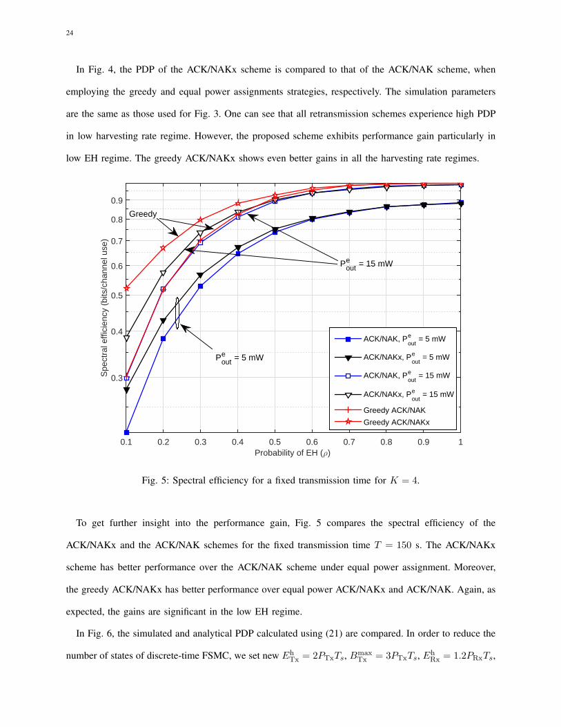
In Fig. 4, the PDP of the ACK/NAKx scheme is compared to that of the ACK/NAK scheme, when

employing the greedy and equal power assignments strategies, respectively. The simulation parameters

are the same as those used for Fig. 3. One can see that all retransmission schemes experience high PDP

in low harvesting rate regime. However, the proposed scheme exhibits performance gain particularly in

low EH regime. The greedy ACK/NAKx shows even better gains in all the harvesting rate regimes.

Probability of EH (ρ)0.1 0.2 0.3 0.4 0.5 0.6 0.7 0.8 0.9 1

Spe

ctra

l effi

cien

cy (

bits

/cha

nnel

use

)

0.3

0.4

0.5

0.6

0.7

0.8

0.9

ACK/NAK, Peout

= 5 mW

ACK/NAKx, Peout

= 5 mW

ACK/NAK, Peout

= 15 mW

ACK/NAKx, Peout

= 15 mW

Greedy ACK/NAK

Greedy ACK/NAKx

Greedy

Peout = 15 mW

Peout = 5 mW

Fig. 5: Spectral efficiency for a fixed transmission time for K = 4.

To get further insight into the performance gain, Fig. 5 compares the spectral efficiency of the

ACK/NAKx and the ACK/NAK schemes for the fixed transmission time T = 150 s. The ACK/NAKx

scheme has better performance over the ACK/NAK scheme under equal power assignment. Moreover,

the greedy ACK/NAKx has better performance over equal power ACK/NAKx and ACK/NAK. Again, as

expected, the gains are significant in the low EH regime.

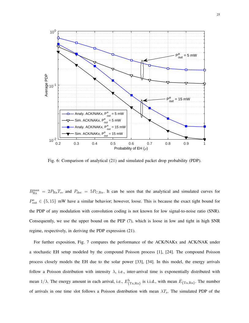
In Fig. 6, the simulated and analytical PDP calculated using (21) are compared. In order to reduce the

number of states of discrete-time FSMC, we set new EhTx = 2PTxTs, Bmax

Tx = 3PTxTs, EhRx = 1.2PRxTs,

25


Ave

rage

PD

P

10-2

10-1

100

Analy. ACK/NAKx, Peout

= 5 mW

Sim. ACK/NAKx, Peout

= 5 mW

Analy. ACK/NAKx, Peout

= 15 mW

Sim. ACK/NAKx, Peout

= 15 mW

Peout = 5 mW

Peout = 15 mW

Fig. 6: Comparison of analytical (21) and simulated packet drop probability (PDP).

BmaxRx = 2PRxTs, and Pdec = 5PC,Rx. It can be seen that the analytical and simulated curves for

P eout ∈ 5, 15 mW have a similar behavior; however, loose. This is because the exact tight bound for

the PDP of any modulation with convolution coding is not known for low signal-to-noise ratio (SNR).

Consequently, we use the upper bound on the PEP (7), which is loose in low and tight in high SNR

regime, respectively, in deriving the PDP expression (21).

For further exposition, Fig. 7 compares the performance of the ACK/NAKx and ACK/NAK under

a stochastic EH setup modeled by the compound Poisson process [1], [24]. The compound Poisson

process closely models the EH due to the solar power [33], [34]. In this model, the energy arrivals

follow a Poisson distribution with intensity λ, i.e., inter-arrival time is exponentially distributed with

mean 1/λ. The energy amount in each arrival, i.e., EhTx,Rx is i.i.d., with mean ETx,Rx. The number

of arrivals in one time slot follows a Poisson distribution with mean λTs. The simulated PDP of the

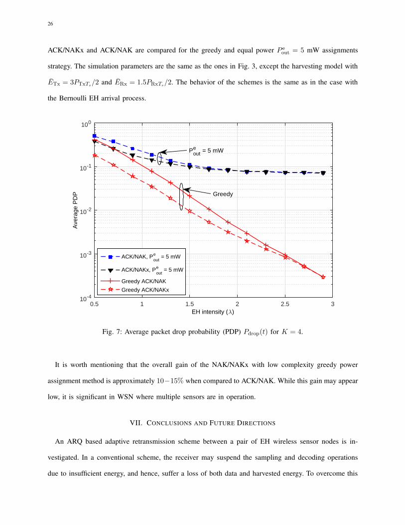
26

ACK/NAKx and ACK/NAK are compared for the greedy and equal power P eout = 5 mW assignments

strategy. The simulation parameters are the same as the ones in Fig. 3, except the harvesting model with

ETx = 3PTxTs/2 and ERx = 1.5PRxTs

/2. The behavior of the schemes is the same as in the case with

the Bernoulli EH arrival process.

EH intensity (λ)0.5 1 1.5 2 2.5 3

Ave

rage

PD

P

10-4

10-3

10-2

10-1

100



Greedy ACK/NAK

Greedy ACK/NAKx

Peout = 5 mW

Greedy

Fig. 7: Average packet drop probability (PDP) Pdrop(t) for K = 4.

It is worth mentioning that the overall gain of the NAK/NAKx with low complexity greedy power

assignment method is approximately 10−15% when compared to ACK/NAK. While this gain may appear

low, it is significant in WSN where multiple sensors are in operation.

VII. CONCLUSIONS AND FUTURE DIRECTIONS

An ARQ based adaptive retransmission scheme between a pair of EH wireless sensor nodes is in-

vestigated. In a conventional scheme, the receiver may suspend the sampling and decoding operations

due to insufficient energy, and hence, suffer a loss of both data and harvested energy. To overcome this

27

problem, a selective sampling scheme was introduced, where the receiver selectively samples the received

data and stores it. The selection depends on the amount of energy available. The receiver performs the

decoding operation when both complete samples of the packet and enough energy are available. Selective

sampling information is fed back to the transmitter by resorting to the conventional ARQ scheme. The

transmitter uses this information to re-size the packet length. A POMDP formulation was setup to further

optimize the transmit power. A suboptimal greedy power assignment method was developed, which is

well suited for low power wireless nodes from the implementation perspective. An analytical upper bound

on the PDP is derived for the proposed adaptive retransmission scheme. Simulation results agree with

the analytical solution when the fixed power assignment policy is used. Numerical results demonstrated

that the adaptive retransmission scheme and power assignment strategy provide better performance over

the conventional scheme.

The proposed adaptive retransmission framework paves the way to several other interesting research

avenues. The proposed scheme can be investigated with more sophisticated retransmission scheme, i.e.,

type-II HARQ. To conceptualize the performance of the proposed scheme in a practical scenario, one

can consider a system setup with multiple transmitters and one receiver, all with EH. Problems to be

studied under this setting are more challenging due to the involvement of an increased number of random

variables associated to each node.

REFERENCES

[1] O. Ozel , K. Tutuncuoglu, J. Yang, S. Ulukus, and A. Yener, “Transmission with energy harvesting nodes in fading wireless

channels: Optimal policies,” IEEE J. Select. Areas Commun., vol. 29, no. 8, pp. 1732–1743, Sep. 2011.

[2] M. Gorlatova, A. Wallwater, and G. Zussman, “Networking low-power energy harvesting devices: Measurements and

algorithms,” in Proc. IEEE Int. Conf. Comput. Commun., Shanghai, China, Apr. 10–15 2011, pp. 1602–1610.

[3] J. Yang and S. Ulukus, “Optimal packet scheduling in an energy harvesting communication system,” IEEE Trans. Commun.,

vol. 60, no. 1, pp. 220–230, Jan. 2012.

[4] K. Tutuncuoglu and A. Yener, “Communicating with energy harvesting transmitter and receivers,” in Proc. Inform. Theory

and Applications Workshop, San Diego, CA, USA, Feb. 05–10 2012, pp. 240–245.

[5] H. Mahdavi-Doost and R. D. Yates, “Energy-harvesting receivers: Finite battery capacity,” in Proc. IEEE Int. Symp. Inform.

Theory, Istanbul, Turkey, Mar. 19–21 2013, pp. 1799–1803.

28

[6] R. D. Yates and H. Mahdavi-Doost, “Energy-harvesting receivers:Otimal sampling and decoding policies,” in Proc. IEEE

Global Signal and Inform. Processing, Austin, TX, USA, Dec. 03–05 2013, pp. 367–370.

[7] H. Mahdavi-Doost and R. D. Yates, “Fading channels in energy-harvesting receivers,” in Proc. Conf. Inform. Sciences Syst.

(CISS), Princeton, USA, Mar. 19–21 2014, pp. 1–6.

[8] A. Kansal, J. Hsu, S. Zahedi, and M. B. Srivastava, “Power management in energy harvesting sensor netwroks,” ACM

Trans. Embedded Comput. Syst., vol. 6, no. 4, pp. 1–38, Sep. 2007.

[9] C. R. Murthy, “Power management and data rate maximization in wireless energy harvesting sensors,” Int. J. Wireless Inf.

Netw., vol. 16, no. 3, pp. 102–117, Jul. 2009.

[10] Z. Shenqiu, A. Seyedi, and B. Sikdar, “An analytical approach to the design of energy harvesting wireless sensor nodes,”

IEEE Trans. Wireless Commun., vol. 12, no. 8, pp. 4010–4024, Aug. 2013.

[11] A. Aprem, C. R. Murthy, and N. B. Mehta, “Transmit power control policies for energy harvesting sensors with

retransmissions,” IEEE J. Select. Topics Signal Processing, vol. 7, no. 5, pp. 895–906, Oct. 2013.

[12] S. Zhou, T. Chen, W. Chen, and Z. Niu, “Outage minimization for a fading wireless link with energy harvesting transmitter

and receiver,” IEEE J. Select. Areas Commun., vol. 33, no. 3, pp. 496–511, Mar. 2015.

[13] M. K. Sharma and C. R. Murthy, “Packet drop probability analysis of ARQ and HARQ-CC with energy harvesting

transmitters and receivers,” in Proc. IEEE Global Signal and Inform. Processing, Atlanta,Georgia. USA, Dec. 3–5 2014,

pp. 148–152.

[14] J. Doshi and R. Vaze, “Long term throughput and approximate capacity of transmitter-receiver energy harvesting channel

with fading,” in Proc. IEEE Int. Conf. Commun. Syst., Macau, Nov.19–21 2014, pp. 46–50.

[15] A. Yadav, M. Gonnewardhena, W. Ajib, and H. Elbiaze, “Novel retransmission scheme for energy harvesting transmitter

and receiver,” in Proc. IEEE Int. Conf. Commun., London, UK, Jun.8–12 2015, pp. 4810–4815.

[16] J. A. Stankovic, T. F. Abdelzaher, C. Lu, L. Sha, and J. C. Hou, “Real-time communication and coordination in embedded

sensor networks,” Proc. IEEE, vol. 91, no. 7, pp. 1002–1022, Jul. 2003.

[17] D. Ciuonzo, P. Salvo Rossi, and S. Dey, “Massive MIMO channel-aware decision fusion,” IEEE Trans. Signal Processing,

vol. 63, no. 3, pp. 604–619, Feb. 2015.

[18] A. Shirazinia, S. Dey, D. Ciuonzo, and P. Salvo Rossi, “Massive MIMO for decentralized estimation of a correlated source,”

IEEE Trans. Signal Processing, vol. 64, no. 10, pp. 2499–2512, May 2016.

[19] Q. Bai, A. Mezghani, and J. A. Nossek, “Throughput maximization for energy harvesting receivers,” in Proc. Int. Works.

on Smart Antennas, Stuttgart, Germany, Mar. 13–14 2013, pp. 1–8.

[20] S. Cui, A. Goldsmith, and A. Bahai, “Energy-efficiency of MIMO and cooperative MIMO techniques in sensor networks,”

IEEE J. Select. Areas Commun., vol. 22, no. 6, pp. 1089–1098, Aug. 2004.

[21] P. Grover, K. Woyach, and A. Sahai, “Towards a communication-theoretic understanding of system-level power consump-

tion,” IEEE J. Select. Areas Commun., vol. 29, no. 8, pp. 1744–1755, Sep. 2011.

[22] M. Putterman, Markov Decision Processes: Discrete Stochastic Dynamic Programming. New York, USA: Wiley-

29

Interscience, 1994.

[23] J. A. Paradiso and M. Feldmeier, A Compact, Wireless, Self-Powered Pushbutton Controller. Ubicomp 2001, Springer

Berlin Heidelberg, 2001, pp. 299–304.

[24] J. Xu and R. Zhang, “Throughput optimal policies for energy harvesting wireless transmitters with non-ideal circuit power,”

IEEE J. Select. Areas Commun., vol. 32, no. 2, pp. 322–332, Feb. 2014.

[25] H. S. Wang and N. Moayeri, “Finite-state Markov channel-A useful model for radio communication channels,” IEEE Trans.

Veh. Technol., vol. 44, no. 1, pp. 163–171, Feb. 1995.

[26] Q. Zhang and S. A. Kassam, “Finite-state Markov model for Rayleigh fading channels,” IEEE Trans. Commun., vol. 47,

no. 11, pp. 1688–1692, Nov. 1999.

[27] M. B. Pursley and D. J. Taipale, “Error probabilities for spread-spectrum packet radio with convolutional codes and Viterbi

decoding,” IEEE Trans. Commun., vol. 35, no. 1, pp. 1–12, Jan. 1987.

[28] D. P. Bertsekas, Dynamic Programming and Optimal Control, 2nd ed. Athena Scientific, 2000.

[29] M. L. Littman, A. R. Cassandra, and L. P. Kaelbling, “Learning policies for partially observable environments: Scaling

up,” in Proc. Int. Conf. Mach. Learning, Tahoe City, CA, USA, Jul.9–15 1995, pp. 362–370.

[30] C. H. Papadimitrious and J. N. Tsitsiklis, “The complexity of Markov decision processes,” Mathematics of Operations

Research, vol. 12, no. 3, pp. 441–450, Aug. 1987.

[31] I. Nourbakhsh, R. Powers, and S. Birchfield, “DERVISH: An office-navigating robot,” Artificial Intell. Magazine, vol. 16,

no. 2, pp. 53–60, Summer, 1995.

[32] R. Srivastava and C. E. Koksal, “Energy optimal transmission scheduling in wireless sensor networks,” IEEE Trans. Wireless

Commun., vol. 9, no. 5, pp. 1550–1560, May 2010.

[33] Q. Bai and J. A. Nossek, “Modulation optimization for energy harvesting transmitters with compound Poisson energy

arrivals,” in Proc. IEEE Works. on Sign. Proc. Adv. in Wirel. Comms., Darmstadt, Germany, Jun. 16–19 2013, pp. 764–768.

[34] P. Lee, Z. A. Eu, M. Han, and H. Tan, “Empirical modeling of a solar-powered energy harvesting wireless sensor node

for time-slotted operation,” in Proc. IEEE Wireless Commun. and Netw. Conf., Quintana, Mexico, Mar.28–31 2011, pp.

179–184.

30

(a) Case-I

w11 Conditions

Perr(ak)w = NAK, y = mod (k,K) + 1

q = min i+ LTx − ak, Bmax

Tx , r = min j + LRx − aRx, Bmax

Rx

1− Perr(ak)w = ACK, y = 1

q = min i+ LTx − ak, Bmax

Tx , r = min j + LRx − aRx, Bmax

Rx 0 otherwise

(b) Case-II

w10 Conditions

Perr(ak)

w = NAK, y = mod (k,K) + 1

q = mini+ LTx − ak, Bmax

Tx , r = j − aRx for z = NAK, ϕRx = 1


Tx , r = j − adec − aRx,x for z = NAKx, ϕdec = 1, ϕRx,x = 1

1− Perr(ak)

w = ACK, y = 1


Tx , r = j − aRx for z = NAK, ϕRx = 1


Tx , r = j − adec − aRx,x for z = NAKx, ϕdec = 1, ϕRx,x = 1

1w = NAKx, y = mod (k,K) + 1


Tx , r = j − aRx,x for z = NAK, NAKx, ϕRx,x = 1

0 otherwise

(c) Case-III

w01 Conditions

Perr(ak)

w = NAK, y = mod(k,K) + 1

q = i− ak, r = minj + LRx − aRx, Bmax

Rx for z = NAK, ϕTx = 1

q = i− ak, r = minj + LRx − aRx, Bmax

Rx for z = NAKx, ϕTx = 1

1− Perr(ak)

w = ACK, y = 1


Tx , r = j − aRx for z = NAK, ϕTx = 1


Tx , r = j − adec − aRx,x for z = NAKx, ϕTx = 1

1w = NAK, NAKx, y = mod (k,K) + 1

q = i, r = minj + LRx, Bmax

Rx , ϕTx = 0

0 otherwise

(d) Case-IV

w00 Conditions

Perr(ak)

w = NAK, y = mod(k,K) + 1

q = i− ak, r = j − aRx for z = NAK, ϕTx = ϕRx = 1

q = i− ak, r = j − aRx for z = NAKx, ϕTx = ϕRx = ϕdec = 1

1− Perr(ak)

w = ACK, y = 1

q = i− ak, r = j − aRx for z = NAK, ϕTx = ϕTx = 1

q = i− ak, r = j − adec for z = NAKx, ϕTx = ϕRx = ϕdec = 1

1

w = NAKx, y = mod (k,K) + 1

q = i− ak, r = j − aRx,xϕRx,x, for z = NAK, ϕTx = ϕRx,x = 1

q = i− ak, r = j − aRx,xϕRx,x, for z = NAKx, ϕTx = ϕRx,x = 1

q = i, r = j, for z = NAKx, ϕTx = 0

0 otherwise

TABLE II: Values of w11, w10, w01, and w00.

Energy Management for Energy Harvesting Wireless Sensors ...

Documents

Transcript of Energy Management for Energy Harvesting Wireless Sensors ...