Energy Investment Risk and Future Climate, Part II
16
EEC Energy Investment Risk and Future Climate, Part II May 19, 2015 © Rachael Jonassen 1 Energy Learning Journal Energy Investment Risk and Future Climate Rachael Jonassen, Department of Engineering Management and Systems Engineering, George Washington University, Washington, DC 20052, USA, [email protected]. A Compilation of Climate Risk to Energy Projects In the first segment of this sequence of articles, 1 you read lots of recent examples of how climate has affected every different type of energy project, usually in multiple ways. In this segment, you will read about using those experiences to develop a more formal picture of the specific risks that your energy project faces. We’ll begin with a simple example and explain the concepts as we go along. As we go, we’ll take a look at the relevant risk assessment input to a financial analysis. All of this is prelude to the next installment of this discussion where we will delve into how this effort is complicated by the fact that the climate of each decade seems to be different from the last and how that affects our efforts at risk assessment. The Map of Europe A few years ago, the architectural firm OMA, as part of the European Climate Foundation’s Roadmap 2050 project, presented a new vision of Europe as a set of states (Eneropa) defined by their dominant renewable energy source, connected through a mutually-supportive electric grid. 2 The map of Eneropa illustrates how climate controls the feasibility of all of the various types of renewable energy: Solaria in the southern areas that enjoy lots of sun and less cloudiness; the Isles of Wind around the North Sea and Atlantic coast where surface winds are strong and reliable; North, Central, and West Hydropea in the mountains of Scandinavia, the Alps, and the lower Danube basin respectively, where snowmelt 1 http://www.energy-learning.com/index.php/78-what-s-new/136-ener 2 Source: http://www.roadmap2050.eu/attachments/files/Roadmap%202050%20-%20Visuals.pdf, accessed: 20 November 2014. Figure 1. Eneropa, as envisioned by the Office for Metropolitan Architecture (OMA) as part of Roadmap 2050 of the European Climate Foundation.
Transcript of Energy Investment Risk and Future Climate, Part II
EEC Energy Investment Risk and Future Climate, Part II May 19, 2015
© Rachael Jonassen 1 Energy Learning Journal
Energy Investment Risk and Future Climate Rachael Jonassen, Department of Engineering Management and Systems Engineering, George Washington University, Washington, DC 20052, USA, [email protected].
A Compilation of Climate Risk to Energy Projects In the first segment of this sequence of articles,1 you read lots of recent examples of how climate has affected every different type of energy project, usually in multiple ways. In this segment, you will read about using those experiences to develop a more formal picture of the specific risks that your energy project faces. We’ll begin with a simple example and explain the concepts as we go along. As we go, we’ll take a look at the relevant risk assessment input to a financial analysis. All of this is prelude to the next installment of this discussion where we will delve into how this effort is complicated by the fact that the climate of each decade seems to be different from the last and how that affects our efforts at risk assessment.
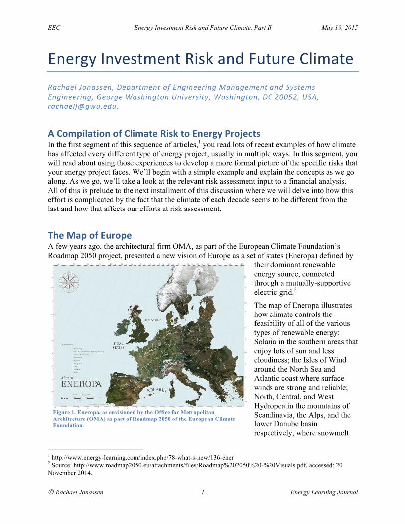
The Map of Europe A few years ago, the architectural firm OMA, as part of the European Climate Foundation’s Roadmap 2050 project, presented a new vision of Europe as a set of states (Eneropa) defined by
their dominant renewable energy source, connected through a mutually-supportive electric grid.2 The map of Eneropa illustrates how climate controls the feasibility of all of the various types of renewable energy: Solaria in the southern areas that enjoy lots of sun and less cloudiness; the Isles of Wind around the North Sea and Atlantic coast where surface winds are strong and reliable; North, Central, and West Hydropea in the mountains of Scandinavia, the Alps, and the lower Danube basin respectively, where snowmelt
1 http://www.energy-learning.com/index.php/78-what-s-new/136-ener 2 Source: http://www.roadmap2050.eu/attachments/files/Roadmap%202050%20-%20Visuals.pdf, accessed: 20 November 2014.
Figure 1. Eneropa, as envisioned by the Office for Metropolitan Architecture (OMA) as part of Roadmap 2050 of the European Climate Foundation.
EEC Energy Investment Risk and Future Climate, Part II May 19, 2015
© Rachael Jonassen 2 Energy Learning Journal
and glacier-fed rivers flow copiously; and Biomassburg, with the right mix of sun, moisture, and temperatures to support abundant plant life. These are fun names but with a serious intent, demonstrating how the current climate drives opportunity for future energy sources. And the more detailed maps underlying this analysis show an even deeper appreciation of climate’s importance. But has it always been thus? Can these climates shift positions and can the borders of Eneropa’s states change as the borders of Europe have changed so much in past?
The map of Eneropa illustrates the opportunities that climate presents in the world of renewable energy. But climate has a darker relation to energy as a risk that climate-induced events, or subtle changes in Enropa’s climate pose to energy facilities. It is that risk that we’ll investigate here.
Assessing Climate Risk to a Project Assessment of risks that climate poses to an energy project and the introduction of risk into project decision-making have traditionally considered risks as a fixed cost arising with a given and known probability and with a given and known consequence over the lifetime of the project. In such a case, the added cost of risk, R, enters into the financial analysis somewhat like a tax.
In the simplest example, we can imagine that damage is a binary event; it either occurs or it does not. Tornado damage to a transmission tower might be modeled this way. In this case, the expected cost is the likelihood of the tornado striking the tower, p, multiplied by the consequence. Here, in this simple example, we might model the consequence as total destruction of the tower so the consequence is loss of the tower and the cost is the replacement cost, C, of the tower.
! = ! × ! Equation 1
A more complicated example arises when we consider the risk of a temporary shutdown of a coal-fired power plant due to low river flow that leads to non-compliant cooling water discharge temperatures.3 In this case, there is a suite of potential river flow magnitudes, i, each with different probability, pi, and associated consequence (such as the lost value of production for the number of days in the year the plant cannot operate, Ci). To compute the expected cost over the lifetime of the plant, we must sum the product of annual probability and consequence of each possible flow and multiply that by the expected lifetime of the power plant, L.
! = ! × !! × !!
Equation 2
Values of p may be estimated from the historical record of river flow. If records are not available for that river at that location, they may be extrapolated from other locations, which increases the uncertainty. These calculations do not include uncertainty except as represented in the range of probabilities and consequences. More on uncertainty will come later.
3 In the United States, cooling water discharge temperatures for power plants are regulated by the Clean Water Act and implemented by the Environmental Protection Agency. This has led to a preference of recirculating cooling systems that release water at lower temperatures but consume more water by evaporative loss during cooling.

EEC Energy Investment Risk and Future Climate, Part II May 19, 2015
© Rachael Jonassen 3 Energy Learning Journal
What Can Happen During the Lifespan of Energy Projects When the Oyster Bay nuclear power plant, the oldest in the world, closes in 2019, it will have operated for 50 years. It is unlikely that its planners anticipated it would experience extreme weather like super storm Sandy on October 29, 2012. Sandy struck Oyster Bay with 33 m/s winds – strong enough to require shut down before the electric grid failed. An abnormal cooling water intake level (1m) was noted by 9:20am that morning. By 1:46pm, the plant entered “high winds” status (26m/s). By 6:47pm, even stronger winds pushed the tidal surge above 1.4m as measured by the control room recorders leading the operators to issue a “notice of unusual event.” Then at 7:54pm, operators issued a “loss of fuel pool cooling” alert when an outside line tripped and cut off supply of cooling water to the fuel pool. The plant just happened to be undergoing refueling (begun on 12 October) at the time. But that meant that the newly discharged hot fuel rods were in the cooling pond, making cooling water there even more important. Minutes later, at 8:08pm, the intake water level data connection to the control room failed and all signals were lost. Operators stationed at the intake structure – out in Barnegat Bay where winds were whipping up huge waves and dark had already fallen – relayed data directly from two pressure indicators on an observation platform. At this point, the level reached 1.6m. Ten minutes passed before the plant lost offsite power, and with that its shutdown cooling system and warning sirens. Another fourteen minutes passed when it became impossible to monitor the intake water level. The rising seawater threatened to short electrical lines on the platform, 1.8m above mean sea level. Water levels were already above 1.9m and rising when the operator issued an alert to State agencies. At 11:11pm, water level reached 2.1m the height of the gauge and later reached 2.3m. Fortunately, the storm center had passed and conditions began to subside.4
Given the amount of sea level rise (at least 0.17m) since the time the Oyster Bay plant was designed,5 that rise made the difference in the warning level reached and the actual danger to the plant. The U.S. Nuclear Regulatory Commission had extended the license of the 40-year-old plant by another 20 years in 2009, which means that it had judged (or assumed) that continued sea level rise during that period (at least 0.08m at historic rates) would not imperil the cooling water intake structure.
What can Oyster Bay teach us about long-term risk planning? When construction began in 1965, the operator was under no obligation to consider sea level rise in any assessment of plant safety. With a tide gauge record 50 years shorter than available today, the nearest tidal records had uncertainty of ±1.5 mm/yr. In comparison, records today have uncertainty less than ±0.3mm/yr but show an accelerating trend. Assessing risk from sea level rise today must consider information not available 50 years ago.
How Climates Affect Energy Projects In the last installment, you read lots of examples of how climate can affect energy projects. There are so many ways this can happen it’s hard to remember them all so I’ll summarize the
4 U.S. Nuclear Regulatory Commission Inspection Report, IR 05000219/2012009; 11/13/2012 – 11/27/2012; Oyster Creek Generating Station (OCGS); Inspection Procedure 93812, Special Inspection describes this event. 5 Sea level is rising at just over 4mm/yr at tide gauge stations Sandy Hook and Atlantic City, more than half of this is due to sediment compaction and other local and regional factors. Source: http://www.tidesandcurrents.noaa.gov/sltrends/northatlantictrends.htm, accessed: 18 April 2015.
EEC Energy Investment Risk and Future Climate, Part II May 19, 2015
© Rachael Jonassen 4 Energy Learning Journal
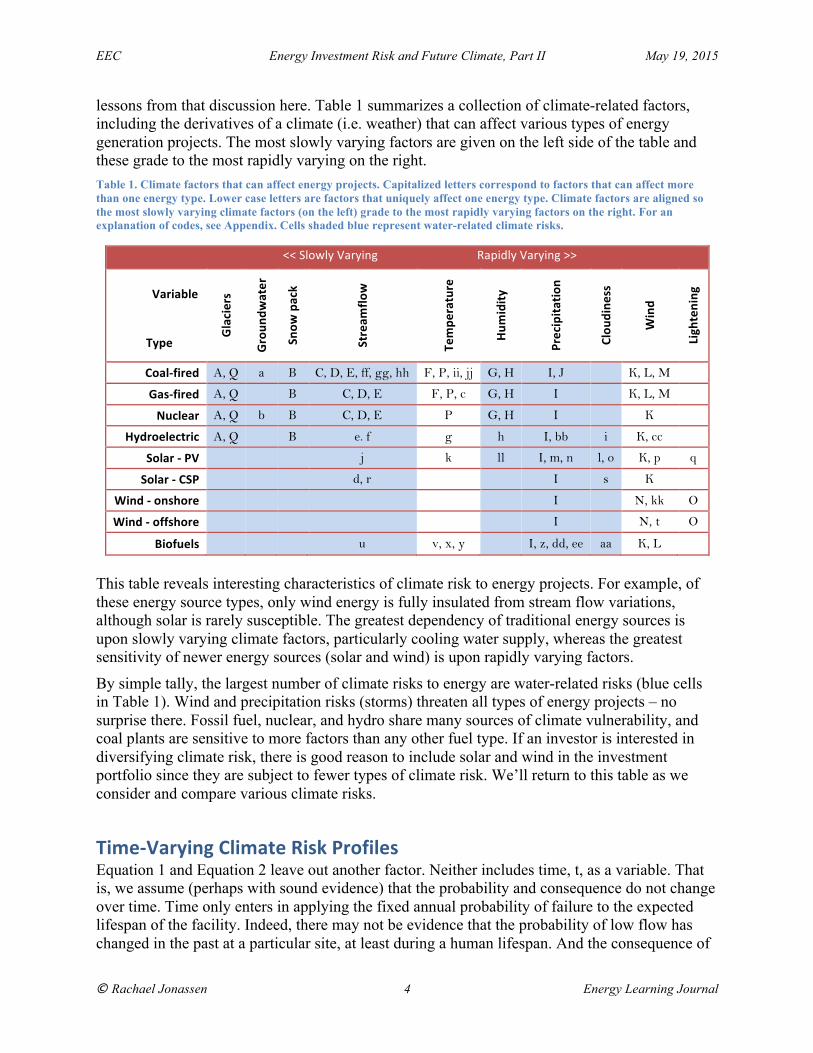
lessons from that discussion here. Table 1 summarizes a collection of climate-related factors, including the derivatives of a climate (i.e. weather) that can affect various types of energy generation projects. The most slowly varying factors are given on the left side of the table and these grade to the most rapidly varying on the right. Table 1. Climate factors that can affect energy projects. Capitalized letters correspond to factors that can affect more than one energy type. Lower case letters are factors that uniquely affect one energy type. Climate factors are aligned so the most slowly varying climate factors (on the left) grade to the most rapidly varying factors on the right. For an explanation of codes, see Appendix. Cells shaded blue represent water-related climate risks.
<< Slowly Varying Rapidly Varying >>
Variable Type
Glaciers
Groun
dwater
Snow
pack
Stream
flow
Tempe
rature
Hum
idity
Precipita
tion
Clou
dine
ss
Wind
Ligh
tening
Coal-‐fired A, Q a B C, D, E, ff, gg, hh F, P, ii, jj G, H I, J K, L, M Gas-‐fired A, Q B C, D, E F, P, c G, H I K, L, M Nuclear A, Q b B C, D, E P G, H I K
Hydroelectric A, Q B e. f g h I, bb i K, cc Solar -‐ PV j k ll I, m, n l, o K, p q
Solar -‐ CSP d, r I s K Wind -‐ onshore I N, kk O
Wind -‐ offshore I N, t O
Biofuels u v, x, y I, z, dd, ee aa K, L This table reveals interesting characteristics of climate risk to energy projects. For example, of these energy source types, only wind energy is fully insulated from stream flow variations, although solar is rarely susceptible. The greatest dependency of traditional energy sources is upon slowly varying climate factors, particularly cooling water supply, whereas the greatest sensitivity of newer energy sources (solar and wind) is upon rapidly varying factors.
By simple tally, the largest number of climate risks to energy are water-related risks (blue cells in Table 1). Wind and precipitation risks (storms) threaten all types of energy projects – no surprise there. Fossil fuel, nuclear, and hydro share many sources of climate vulnerability, and coal plants are sensitive to more factors than any other fuel type. If an investor is interested in diversifying climate risk, there is good reason to include solar and wind in the investment portfolio since they are subject to fewer types of climate risk. We’ll return to this table as we consider and compare various climate risks.
Time-‐Varying Climate Risk Profiles Equation 1 and Equation 2 leave out another factor. Neither includes time, t, as a variable. That is, we assume (perhaps with sound evidence) that the probability and consequence do not change over time. Time only enters in applying the fixed annual probability of failure to the expected lifespan of the facility. Indeed, there may not be evidence that the probability of low flow has changed in the past at a particular site, at least during a human lifespan. And the consequence of
EEC Energy Investment Risk and Future Climate, Part II May 19, 2015
© Rachael Jonassen 5 Energy Learning Journal
the low flow depends more on the character of the generating plant cooling system and inlet port design than anything else. But, as in the example of the nuclear plant above, some factors related to climate do change over time. If a climate factor changes, the picture changes. Sea level has changed over the past fifty years, in some places more than others. This means that both the probability of an event such as flooding of the inlet valve may vary with time, pit, and the consequences of that event can change (if, for example, the range of impact cost varies, perhaps as the infrastructure ages) with time Cjt. Since both p and C are changing over time, the cost of risk itself changes (for a fixed lifetime, L, being considered) depending on the year the project starts, s. In the continuous case, we must then consider the following integral:
! ! = !!" × !!"!!!!!
! !!
Equation 3
Note that this integration of the risk must occur from the start date of the project, t = s, through the expected lifespan of the project, t = s + L. So we must have a good idea of the lifespan, L, of the project. How long will energy projects last? Let’s look at some revealing statistics.
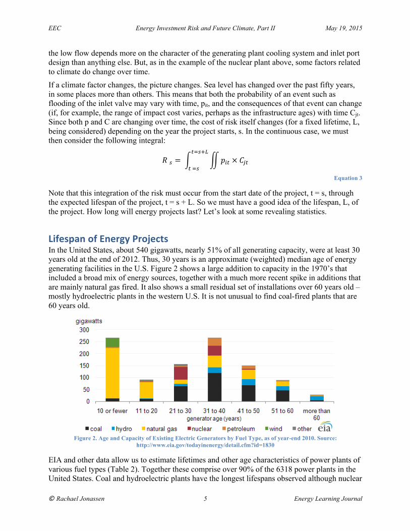
Lifespan of Energy Projects In the United States, about 540 gigawatts, nearly 51% of all generating capacity, were at least 30 years old at the end of 2012. Thus, 30 years is an approximate (weighted) median age of energy generating facilities in the U.S. Figure 2 shows a large addition to capacity in the 1970’s that included a broad mix of energy sources, together with a much more recent spike in additions that are mainly natural gas fired. It also shows a small residual set of installations over 60 years old – mostly hydroelectric plants in the western U.S. It is not unusual to find coal-fired plants that are 60 years old.
Figure 2. Age and Capacity of Existing Electric Generators by Fuel Type, as of year-end 2010. Source:
http://www.eia.gov/todayinenergy/detail.cfm?id=1830
EIA and other data allow us to estimate lifetimes and other age characteristics of power plants of various fuel types (Table 2). Together these comprise over 90% of the 6318 power plants in the United States. Coal and hydroelectric plants have the longest lifespans observed although nuclear

EEC Energy Investment Risk and Future Climate, Part II May 19, 2015
© Rachael Jonassen 6 Energy Learning Journal
energy is too recent an innovation to have yet displayed a representation of how long it may last. The natural gas fleet is much younger because a significant part (older and less efficient steam turbines) was retired in the past decade and replaced by much more efficient combined-cycle facilities. Although it is 27% of the US fleet, about 64% of retirements in the past decade were natural gas plants. And natural gas plants made up the vast majority of new plants, so the average age of the natural gas fleet declined significantly in recent years.
Table 2. Lifespans of power plants for the major electrical fuel types in the United States. Values are averages in years, rounded to the nearest decade, as of 2010. Primary information
source: U.S. Energy Information Agency.
Energy Source % Supply Expected / Max. At retirement Operating plants
Coal 39 50 / 80 60 73% > 30
Natural gas 27 < 20 / 50 50 <10 yrs
Nuclear 19 > 30 / 50 40 (license) 30
Hydroelectric 6 > 30 / 120 60 50
These data help to estimate risk for new power plants since they are one estimate of the appropriate term, L, in Equation 2 and Equation 3 given above. Table 2 implies considerable uncertainty in the appropriate value of L to apply since the actual average lifetime (age at retirement) of facilities exceeds estimates of expected lifetime when constructed. In the case of hydroelectric, the average age of existing operational plants exceeds the expected lifetime. As discussed above, the average age of natural gas fired plants is skewed by recent replacements. Actual average age at retirement may provide the best estimate of how long new natural gas plants may remain in service.6 That is the number we will use here to illustrate climate risks.
In contrast, renewable energy plants (other than hydro) are too new and too few in number to allow a retirement age-based estimate of their expected lifetimes. Table 3 presents data on the actual age and expected lifetime of existing plants in the U.S. based on data from the U.S. Energy Information Agency. In this case, we will use the expected lifetime given in Table 3 to estimate the value of L in evaluating climate risks.
Table 3. Average and expected age of operating renewable energy plants other than hydro in the U.S. Source: U.S. Energy Information Agency.
Energy Source Operating plants Expected
Biomass 25 > 30
Solar 5 10
Wind 5 20
6 Although the blades in combined cycle gas turbine require refurbishment at about 11 years, the facility may have a much longer life. Thus, the climate risk to power plant elements may be quite different from the risk profile of the whole plant, a topic we’ll explore in more depth below.

EEC Energy Investment Risk and Future Climate, Part II May 19, 2015
© Rachael Jonassen 7 Energy Learning Journal
An important lesson from this analysis is that solar and wind energy generating facilities may be less susceptible to the time-varying aspect of climate risks because they don’t remain in service as long as other energy types. Let’s see what that analysis actually says. Before we do, and to put it all in one place, Table 4 summarizes the values we will apply when examining how climate might impact energy project risk.
Table 4. Target lifetimes Used to Estimate L in Our Examples
Energy Source Target Lifefime
Coal 60
Hydroelectric 60
Natural gas 50
Nuclear 40
Biomass 30
Wind 20
Solar 10
In a situation where climate is non-stationary, it would appear on the surface that coal and hydroelectric plants are most susceptible to changes in their risk factors, while solar projects (at least PV) will be least susceptible. Let’s take a look at the climate susceptibility profiles of these different energy sources based on our analysis from the earlier post.7
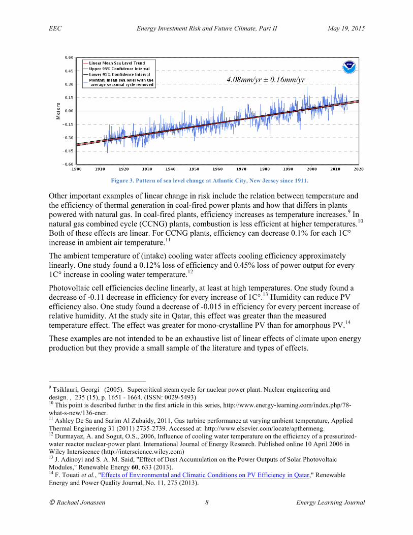
A Potpourri of Time-‐Varying Climate Risks In the case of the nuclear power plant and sea level rise (SLR), it is reasonable to model the rise as a linear function of time. Indeed, the NOAA standard is to represent all SLR using a linear trend (Figure 3).8 In this case, we have an estimate of the linear trend from the NOAA trend line (4.08mm/yr ± 0.16mm/yr) and this becomes valuable input to our calculation of changing risk profile for the facility using Equation 3. We can use the height of water level, along with the range of water level variation due to factors including storm surge, to estimate the probability of a damaging event, such as overtopping a water inlet valve.
7 http://www.energy-learning.com/index.php/78-what-s-new/136-ener 8 Source: http://www.tidesandcurrents.noaa.gov/sltrends/sltrends_station.shtml?stnid=8534720
EEC Energy Investment Risk and Future Climate, Part II May 19, 2015
© Rachael Jonassen 8 Energy Learning Journal
Other important examples of linear change in risk include the relation between temperature and the efficiency of thermal generation in coal-fired power plants and how that differs in plants powered with natural gas. In coal-fired plants, efficiency increases as temperature increases.9 In natural gas combined cycle (CCNG) plants, combustion is less efficient at higher temperatures.10 Both of these effects are linear. For CCNG plants, efficiency can decrease 0.1% for each 1C° increase in ambient air temperature.11 The ambient temperature of (intake) cooling water affects cooling efficiency approximately linearly. One study found a 0.12% loss of efficiency and 0.45% loss of power output for every 1C° increase in cooling water temperature.12
Photovoltaic cell efficiencies decline linearly, at least at high temperatures. One study found a decrease of -0.11 decrease in efficiency for every increase of 1C°.13 Humidity can reduce PV efficiency also. One study found a decrease of -0.015 in efficiency for every percent increase of relative humidity. At the study site in Qatar, this effect was greater than the measured temperature effect. The effect was greater for mono-crystalline PV than for amorphous PV.14 These examples are not intended to be an exhaustive list of linear effects of climate upon energy production but they provide a small sample of the literature and types of effects.
9 Tsiklauri, Georgi (2005). Supercritical steam cycle for nuclear power plant. Nuclear engineering and design. , 235 (15), p. 1651 - 1664. (ISSN: 0029-5493) 10 This point is described further in the first article in this series, http://www.energy-learning.com/index.php/78-what-s-new/136-ener. 11 Ashley De Sa and Sarim Al Zubaidy, 2011, Gas turbine performance at varying ambient temperature, Applied Thermal Engineering 31 (2011) 2735-2739. Accessed at: http://www.elsevier.com/locate/apthermeng. 12 Durmayaz, A. and Sogut, O.S., 2006, Influence of cooling water temperature on the efficiency of a pressurized-water reactor nuclear-power plant. International Journal of Energy Research. Published online 10 April 2006 in Wiley Intersicence (http://interscience.wiley.com) 13 J. Adinoyi and S. A. M. Said, "Effect of Dust Accumulation on the Power Outputs of Solar Photovoltaic Modules," Renewable Energy 60, 633 (2013). 14 F. Touati et al., "Effects of Environmental and Climatic Conditions on PV Efficiency in Qatar," Renewable Energy and Power Quality Journal, No. 11, 275 (2013).
Figure 3. Pattern of sea level change at Atlantic City, New Jersey since 1911.
4.08mm/yr ± 0.16mm/yr

EEC Energy Investment Risk and Future Climate, Part II May 19, 2015
© Rachael Jonassen 9 Energy Learning Journal
Non-‐Linear Changes in Climate Factors Not all changes follow this simple linear trend. Indeed, recent evidence suggests a regular increase in the rate of sea level rise.15 The sea level trend is an empirical relation. But there are some theoretical bases for non-linear relations between climate factors that can give rise to non-linear risk profiles for energy projects. For example, there is a simple and well-known relation16 showing how saturation vapor pressure p (a measure of how much moisture the air can hold) changes between two temperature states, T0 and T:
ln (! !!) = ∆!! (
1!!− 1!)
Equation 4
Put more succinctly, the amount of water vapor that the atmosphere can hold increases exponentially as the temperature rises. This places many climate factors in the area of non-linear risk since so many issues related to climate risk are water-related (refer to the blue calls in Table 1). We expect a faster hydrologic cycle in warmer climates because the air can hold so much more moisture. Evaporation rates increase, meaning reservoirs lose water more quickly, cooling towers operate more efficiently, storms carry more water (and energy as latent heat), and cloudiness changes. It is reasonable to expect that much climate risk to energy projects will have a non-linear character.
Where large bodies of water provide an ample source for evaporation, the air tends to be saturated or near saturation. This satisfies the higher capacity to hold moisture; the air actually holds more moisture. Moist air is lighter so it will rise and this can lead to the formation of cumulus clouds and local storms. The increased moisture also affects the optical properties of the atmosphere, as does the reflectivity of those clouds. Both of these changes can influence the efficiency of solar power, both PV and CSP. Thus, although moisture may have a linear effect on an energy source, moisture may increase exponentially with increasing temperature. The combined risk is non-linear.
Discontinuous Changes in Energy Risk Much more difficult to measure and model for energy risk are those discontinuous changes that may arise unexpectedly since their discontinuous nature reduces the opportunity for warning. Discontinuous phenomena we are all familiar with include storms and storm-related factors including flood onset, lightening, and attendant phenomena. Sufficient data may be available in the meteorological and hydrological literature to allow estimation of the probability and impact of these events. Most such discontinuous changes relate to water since it has a ubiquitous influence upon all types of energy sources. Phase changes of water (liquid-ice, liquid-gas, and ice-gas) are inherently discontinuous and lie at the heart of many effects upon energy projects. Short-term examples include hail damage to PV or bioenergy crops. But even rain is inherently discontinuous (gas-liquid transition) and introduces attendant uncertainty.
15 See, for example, the Sandy Hook, New Jersey record at http://www.tidesandcurrents.noaa.gov/sltrends/sltrends_update.htm?stnid=8531680 16 In the Clausius-Clapeyron relation, ∆! stands for the change in enthalpy, K is the ideal gas constant, T0 and p0 are the base temperature and saturation vapor, respectively. T and p are the final states.

EEC Energy Investment Risk and Future Climate, Part II May 19, 2015
© Rachael Jonassen 10 Energy Learning Journal
Short-term discontinuous events also include the effect of dust storms. Although dust in arid climates can accumulate in a linear and predictable pattern, dust storms break this rule. For example, a single dust storm decreased the power output by 20% for all modules at a site in Saudi Arabia.17
Migration of a mesohaline-oligohaline boundary (salt front) results from long-term increases in river flow (pushing it farther down river) or sea level rise (moving the salt front farther upriver). You may notice this first as short-term shifts related to tides and storm surges but these may preface a chronic long-term trend. Such a trend may reflect sea level changes like it has during the time of record or as stream flow changes with declining snow pack in headwaters as now happening in the western U.S. An important effect arises from cooling water salinity and the impact of cooling water discharge upon in-stream biota as a salt front passes the location of an intake structure.
Incorporating the effect of discontinuous risk factors into your risk analysis and financial planning is more complicated than the simple continuous cases described above since these risk factors usually require observational data to parameterize or the use of much more complicated models.
Interactions of Climate Risks When climate risks occur at the same time and place but are not correlated, as in random coincidental simultaneous events, determining the risk profile is easy enough. You can treat each as independent, making the risk additive. But there are climate factors, or their results, that co-vary and these must be treated differently since the correlation changes the overall probability of impact. An example of co-occurrence of unrelated events that might seem correlated can occur with floods. For example, each spring the flow of the Mississippi River increases in New Orleans as snowmelt occurs in the Rocky Mountains, a thousand miles away (and two thousand miles by river). Local storms may also affect river levels, even storms (and snow melt) that occur in the Appalachian Mountains, a few hundred miles in the other direction. The combination of these events can wreak havoc in New Orleans, but the probability of such co-occurrence is independent and risks can be considered separately.
Variations in wind (gustiness) can have two different effects upon turbine blades. On the one hand they can accelerate rotation and change generation efficiency, while on the other hand, they can lead to aging, and fatigue failure of the blade structure. Failure may be more likely during gusty times than during periods when the wind blows constantly since acceleration itself stresses the blades, which may be enough to initiate failure. Thus, the effects of varying wind velocity upon turbine performance interact. And they interact in more ways than this simple example.
You can compute risk from interacting factors as the integral of the product of the individual risks. For risks that change over time, we can modify the generic Equation 3 to account for two events, 1 and 2, with different probability and consequence.
17 J. Adinoyi and S. A. M. Said, "Effect of Dust Accumulation on the Power Outputs of Solar Photovoltaic Modules," Renewable Energy 60, 633 (2013).
EEC Energy Investment Risk and Future Climate, Part II May 19, 2015
© Rachael Jonassen 11 Energy Learning Journal
! ! = (!!!" × !!!") × (!!!!!
! !!!!!" × !!!")
Equation 5
Composite Risk Profiles This brings us to the challenge of considering the entire risk spectrum of an energy power project over its entire expected lifetime, rather than just examining the potential impact of a single risk factor on a single component of the energy project. Such a composite risk spectrum will include a wide variety of risk types and sources, even in the simplest energy projects with short expected lifetimes. For larger, longer-lived energy projects the difficulties of a comprehensive risk assessment require very large resources of data and computational power since many of the risks must be evaluated using Monte Carlo methods. This is particularly true when variability of the climate factor is an inherent and important aspect of project design. For example, in the case of a wind project, variation in wind velocity is inherent in the character of the source and in the response characteristics of the turbine. This variation shows as uncertainty in the mean of a vector quantity when estimating the proper orientation of the turbine axis. Variation also displays in the fatigue spectrum and fracture profile of the blade, both from inherent variation in wind direction and in any bias in the original estimate of the mean windfield. Bias in estimates of mean wind direction is magnified by sparse data, and changes in design heights of turbines at the same location as turbine technology improves and larger blades become practical. In this case, the well-known Eckman spiral describes how winds change with altitude in the boundary layer.
When computing composite risk profiles for a single energy project, we consider the rows of Table 1. These tell us the range of different climate factors that might affect our project. From there we decide which are actual threats to the project during its expected lifetime (Table 4), and we complete a risk analysis for those threats. For example, when considering the risk to my solar PV project, I’d want to know which of risks I, plus j-q, could be important at the candidate site, and I’d want to perform a risk analysis that includes those risks. This type of analysis provides a holistic view of the project risk profile.
On the other hand, for a given site, if you are interested in considering what project is most suitable for that site, you may want to evaluate a specific climate factor that is diagnostic of that site and consider how different energy source types might respond to that climate factor. In this case, you would consider one column of Table 1 and compare expected risk from that factor across all candidate energy source types. For example, for a site in Reno, Nevada, where mountain streams fed by spring snow melt feed the river that I want to use for cooling water for a fossil fuel power plant, I’d want to make sure I’d considered the risk to the project from snow pack, Item B in Table 1 and the Appendix.
To narrow down your potential energy projects at a particular site, you may want to compare risk profiles for more than one energy type. In this case, the analysis must compare all relevant risks from the appropriate rows of Table 1. At the screening level, some of these factors may cancel out when considering the ratio of risks. For example, considering coal and natural gas, the expected cost of risk K “High winds can damage individual sites” may be essentially identical for both types of facility since these facilities share much infrastructure in common. On the other hand, the expected cost of risk L “High winds (waves) can damage or spill cargo under
EEC Energy Investment Risk and Future Climate, Part II May 19, 2015
© Rachael Jonassen 12 Energy Learning Journal
transport” may be considerable for the coal-fired plant if it will rely upon barges to bring the daily coal supply whereas it may be low for the natural gas fired plant if that facility would only rarely rely upon barges, and then only for transporting certain heavy replacement equipment where the shipment can be postponed during high wind events. This asymmetrical risk is important in comparison.
Risk to a Project Site As Table 4 demonstrates, solar and wind projects appear to have shorter lifetimes than fossil fuel, nuclear, and hydroelectric plants. In most cases, the capital investment in individual solar and wind projects is much less than more traditional energy sources. Together, those facts suggest that the risk from climate to solar and wind projects is lower than for the other projects. Table 1 supports that assertion.
There is an important difference with wind and solar projects. Although they may have short lifetimes as the panels degrade or turbine blades fatigue, the relatively low cost of the equipment and continuing improvements in design mean that replacement is possible and likely. Sites are chosen because of their solar or wind characteristics. Those characteristics are likely to continue and when reequipped with more advanced models of panels, turbines, or other generating equipment still on the drawing board, the site becomes a long-term profit center.
Evaluating site risk for solar and wind is not just a question of lifetime risk to a specific project. The scale of investment at the site, through multiple generations of renewable energy projects, may rival that of more traditional energy sources. And the lifetime of the site as an energy resource becomes a significant consideration for the investor. For these energy types, site evaluation is more than a consideration of climate risks for the short lifetime of the initial compliment of energy equipment. Wise energy investment considers a site for solar and wind generation as a multi-decade opportunity. This is the kind of investment suitable for retirement funds and reinsurance corporations and these groups are certainly interested in risk profiles.
Whole of Energy System Risk Profile There are times when an organization, such as a regulator, may want to examine the overall risk profile of the regulated region. Climate risk is a major part of that system risk and must be included. The energy system may include every type that Table 1 lists, so the analysis could encompass all rows and columns of that table. Or the organization may be interested in climate risks that relate to water use in the energy system and could consider those cells shown in blue in Table 1. This type of analysis is far more comprehensive and complex, but the elements of that analysis remain the same.
Demand and Climate The risks discussed above all relate to the supply of energy by a climate project. Demand risk to projects also have climate-related contributions. Any full analysis of energy projects should include these demand-related climate risks. As an example, here are a few demand risks related to air-conditioning load that climate influences:
• Higher temperatures increase demand. • Demand multiplies as the duration of high temperatures increases over several days. • Air conditioning demand is higher in humid conditions. • Minimum nighttimetemperatures tend to be higher on cloudy nights.
EEC Energy Investment Risk and Future Climate, Part II May 19, 2015
© Rachael Jonassen 13 Energy Learning Journal
• Breezes help cool individuals and lessen demand for air conditioning. Demand risk has its own list of factors that must be considered as part of climate risk to projects and this list can be as complex as the supply risk list given in the Appendix.
Climate Risks to the Grid – Risk Cascades Risks from many climate factors can affect operation and stability of the grid. Let’s consider one example18 to illustrate how important these risks are. In August 2003, while Europe was experiencing the worst heat wave in 500 years, the United States had its own climate-related crisis that distracted attention from Europe’s problems, at least temporarily.
A hot summer meant that by August 14, 2003 with temperatures above 32°C, power lines had stretched and sagged, as they always do in summer heat in this continental setting. When a power station unexpectedly went offline in Eastlake, Ohio, rerouting of energy to make up for that loss added load to a 345kV transmission line that was already dealing with heavy electrical demand of air conditioners laboring in the summer heat. Under the added electrical load, the wires heated and expanded further, as transmission wires predictably do, and half an hour later sagged close enough to a tree in Walton Hills, Ohio to produce a flashover, shorting out the line and causing trips to divert power to other lines. An hour later, one of those other lines, the 345kV Chamberlin-Harding line already sagging from the summer heat and further heated by the new load, touched a tree in Parma, Ohio, flashed and was taken out of service. Half an hour passed before its replacement, a third 345kV line, the Hanna-Juniper interconnection, sagged, flashed, and went offline. Seven minutes later, another line failed from overload. In the next four minutes, 15 138kV lines dropped, another 345kV line failed and, a key interconnector quit. The whole system surged. Reduced voltage from Ohio’s draw on Michigan’s electrical system created under-voltage and overcurrent conditions, and more transmission lines tripped in both states. These losses cut supply to New York through a Buffalo interconnect. Drop in demand due to tripped lines led to automated moves offline by power stations. To make up for this, power surged in from the east coast and those overloaded plants jumped offline to avoid damage. In seconds, US Midwest grids disconnected with the East, leading to a power surge through Ontario to accommodate demand. The Ontario line overloaded and failed, and all of Ontario instantly went black. The cascade ended with 256 power plants down and fifty-five million people spread across one million square miles without power. The tally of economic damage may have reached $10B. The fall of the Ontario government in the October 2013 election was blamed on its embarrassing response.
Summary The evidence is clear that climate plays an important role in siting energy projects. Some parts of that role are obvious: hydroelectric needs reliable river flow, steam boilers need cooling water, wind needs wind and solar needs the sun. But the many ways that climate can impinge upon
18 For details, see: U.S.-Canada Power System Outage Task Force, August 14th Blackout: Causes and Recommendations, http://energy.gov/sites/prod/files/oeprod/DocumentsandMedia/BlackoutFinal-Web.pdf
EEC Energy Investment Risk and Future Climate, Part II May 19, 2015
© Rachael Jonassen 14 Energy Learning Journal
energy projects, subtly or dramatically, stretches the imagination. Table 1 and the Appendix summarize such influences.
Standard means to assess climate risks to projects require quantification of the probability and consequence of the risk as well as the project lifetime. All of these vary significantly from one form of energy to another. The time-varying nature of climate – each decade seems to have its own climate characteristics – requires a risk analysis that represents non-stationary risk over the full expected lifetime of the project. These climate risks vary over time linearly, non-linearly, and discontinuously. Climate risks also interact with one another and with other risks to create a multi-dimensional risk profile for energy projects. Composite risk profiles may consider all risks for a single project, risks to a site across energy alternatives, or comparison of all risks between energy options. Regulators consider whole of energy system risks that cross all energy types and climate risk factors. Investors in wind and solar consider risks to a site across multiple generations of equipment. Evaluation of climate risk to energy projects is a complicated endeavor that is easy to get wrong. Errors can produce devastating consequences, as illustrated by the examples cited here.
Appendix – Climate Risks to Energy Projects Here you will find a very brief synopsis of the various climate risks to energy projects that have been discussed and illustrated in the first two installments of this discussion. This list is not exhaustive and the terse terms may conceal important issues and subtle nuances. As you read the list, I hope it prompts you to think about how these factors can affect your own energy project.
The letters in this list are keyed to factors listed in Table 1. In general, capital letters in this list and in Table 1 refer to climate factors that affect more than one type of energy source while lower case letters generally refer to climate factors that affect a specific type of energy source.
Factors affecting more than one energy type (A) Changes in glacial melt alter stream flow timing, quantity, and temperature (cooling water). (B) Changes in snowpack alter stream flow timing, quantity, and temperature (cooling water). (C) Quantity of water for steam generation varies with streamflow. (D) Quantity and temperature of water for cooling vary with streamflow. (E) Low flow reduces production and cooling water supplies and reduces exhaust water dilution. (F) Temperature affects chemical reactions in combustion emissions. (G) High relative humidity decreases cooling efficiency in wet cooling towers. (H) Humidity affects chemical reactions in combustion emissions. (I) Individual sites damaged by specific isolated storms. (J) (Snow) storms / floods interrupt rail transport. (K) High winds can damage individual sites. (L) High winds (waves) can damage or spill cargo under transport. (M) Wind patterns distribute combustion products downwind. (N) Wind velocity spectrum affects turbine efficiency and integrity. (O) Lightening strikes can damage or destroy blades, bearings, and structural members. (P) Rising temperature heats the ocean whose expansion raises sea level. This can threaten coastal facilities and result in changes in the salt front location relative to cooling water intake structures.
EEC Energy Investment Risk and Future Climate, Part II May 19, 2015
© Rachael Jonassen 15 Energy Learning Journal
(Q) Changes in glacial melt (large ice sheets) add water to the ocean and raise sea level. This can threaten coastal facilities and result in changes in the salt front location relative to cooling water intake structures.
Factors unique to a single energy type (a) Increased groundwater levels can impede coal mining. (b) Changes in groundwater discharge could convey nuclide-contaminated water. (c) Higher temperature leads to lower thermal efficiency in combined cycle plants. (d) For water-cleaned CSP mirrors, quantity of water varies with streamflow. (e) Time series properties of flow affect the economics of turbine operation. (f) Floods damage dams, scour turbine blades, and deposit sediment in reservoirs. (g) Warmer temperatures raise evaporation rates in reservoirs. (h) High humidity reduces evaporation rates in reservoirs. (i) High cloudiness reduces evaporation rates in reservoirs. (j) Floods can damage or inundate solar panels. (k) High temperatures lead to lower conversion efficiencies in PV cells. (l) Rapid temperature fluctuations from passing clouds degrade solar cells. (m) Soot from fires (in drought) reduces solar input and decrease conversion efficiency. (n) Hail and frost can damage PV cells and panels. (o) High cloudiness reduces incident radiation and creates temperature fluctuations in panels. (p) Winds can transport dust and sand that obscures or scours cells. (q) Lightening strikes damage cells and panels. (r) For water-powered CSP, quantity and temperature of water for steam vary with streamflow. (s) High cloudiness reduces radiation that reaches mirrors. (t) Wind-driven waves can impede installation and O&M and (>15m) damage platforms. (u) Timing, magnitude and duration of floods affect growth. Small floods cut oxygen supply and
large floods reduce photosynthesis. (v) Extreme low temperature (early and late in the growth) and extreme high temperature
(especially during pollination) affect growth. (w) Water supply affects coal washing/sorting. (x) Cumulative temperature (growing degree days, and killing degree-days) influence yield. (y) Extended heat waves reduce crop growth. (z) Drought reduces crop growth. (aa) Cloudiness reduces photosynthesis. (bb) Chronic reduction in precipitation (drought) reduces production capacity. (cc) High wind increases evaporation rates in reservoirs. (dd) Hail size and timing (worst in tasseling) affect production. (ee) Low soil moisture decreases nutrient uptake and impede pollination. (ff) Low flows can limit transport (e.g. barge) capacity. (gg) Floods damage locks and port facilities, or can impeded movement of traffic. (hh) Frozen rivers can impede traffic. (ii) Extreme temperatures contract/expand rails and impede fuel transport. (jj) Higher temperature leads to higher thermal efficiency. (kk) Abrasion by windborne sediment damages turbine blades and other infrastructure. (ll) High humidity corrodes interconnects and enhances aging of thin-film PV panels. Rachael Jonassen

EEC Energy Investment Risk and Future Climate, Part II May 19, 2015
© Rachael Jonassen 16 Energy Learning Journal
Professorial Lecturer and Visiting Scholar The George Washington University Engineering Management and Systems Engineering Department Washington, DC 20052 USA [email protected]