Impacts of considering climate variability on investment decisions in Ethiopia

ENVIRONMENT AND PRODUCTION TECHNOLOGY DIVISION MAY 2006

EPT Discussion Paper 150

Impacts of Considering Climate Variability on Investment Decisions in Ethiopia

Paul J. Block, Kenneth Strzepek, Mark Rosegrant, and Xinshen Diao

2033 K Street, NW, Washington, DC 20006-1002 USA • Tel.: +1-202-862-5600 • Fax: +1-202-467-4439 [email protected] www.ifpri.org

IFPRI Division Discussion Papers contain preliminary material and research results. They have not been subject to formal external reviews managed by IFPRI's Publications Review Committee, but have been reviewed by at least one internal or external researcher. They are circulated in order to stimulate discussion and critical comment. Copyright 2005, International Food Policy Research Institute. All rights reserved. Sections of this material may be reproduced for personal and not-for profit use without the express written permission of but with acknowledgment to IFPRI. To reproduce the material contained herein for profit or commercial use requires express written permission. To obtain permission, contact the Communications Division at [email protected].

i

ACKNOWLEDGMENTS

The authors would like to thank Claudia Sadoff and David Grey of the World Bank for their insights and comments.

ii

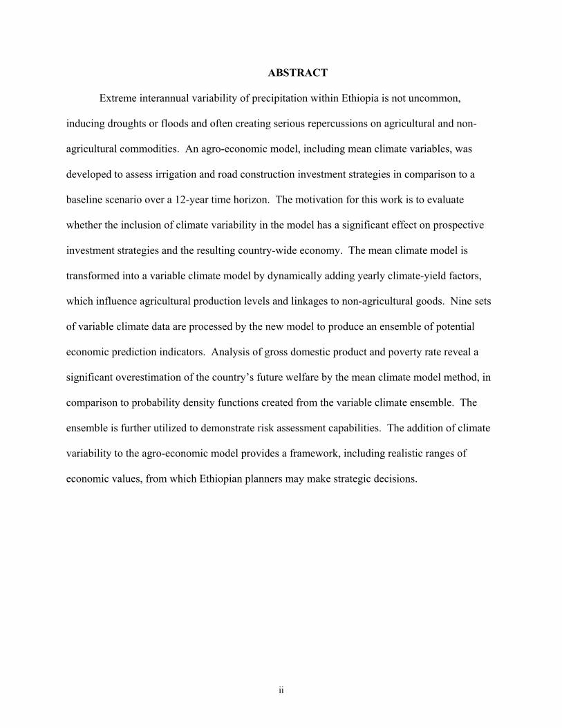
ABSTRACT

Extreme interannual variability of precipitation within Ethiopia is not uncommon,

inducing droughts or floods and often creating serious repercussions on agricultural and non-

agricultural commodities. An agro-economic model, including mean climate variables, was

developed to assess irrigation and road construction investment strategies in comparison to a

baseline scenario over a 12-year time horizon. The motivation for this work is to evaluate

whether the inclusion of climate variability in the model has a significant effect on prospective

investment strategies and the resulting country-wide economy. The mean climate model is

transformed into a variable climate model by dynamically adding yearly climate-yield factors,

which influence agricultural production levels and linkages to non-agricultural goods. Nine sets

of variable climate data are processed by the new model to produce an ensemble of potential

economic prediction indicators. Analysis of gross domestic product and poverty rate reveal a

significant overestimation of the country’s future welfare by the mean climate model method, in

comparison to probability density functions created from the variable climate ensemble. The

ensemble is further utilized to demonstrate risk assessment capabilities. The addition of climate

variability to the agro-economic model provides a framework, including realistic ranges of

economic values, from which Ethiopian planners may make strategic decisions.

iii

TABLE OF CONTENTS

1. Introduction 1

2. Background 2

3. Climatic Data 3

4. Model Framework 4

5. Methods for Climate Modifications in the Model 10

6. Results of Mean Climate (deterministic) Versus Variable Climate (stochastic) Modeling 20

7. Summary and Discussion 27

Appendix I: Equations in the Spatial, Multi-Market Model of Ethiopia Agriculture 31

References 36

1

Impacts of Considering Climate Variability on Investment Decisions in Ethiopia

Paul J. Block,1 Kenneth Strzepek,1 and 2 Mark Rosegrant,3 and Xinshen Diao3

1. INTRODUCTION

Although Ethiopia is rich in culture, history, and natural resources, it is often remembered

more for its disastrous droughts and floods, starving population, and struggling economy. Its

heavy reliance on agriculture, combined with its susceptibility to frequent climate extremes, has

left it in a precarious position, striving to not only stay on par, but to prevent vast numbers of

people from falling deeper into disparity. With 85 percent of the population living in rural areas,

agriculture plays an important role in physical and economical survival.

This work is part of an on-going study focusing on relevant and realistic potential

investment strategies within Ethiopia. The hope is that these strategies may provide insights into

how Ethiopia should best proceed in the years to come, both on regional and country levels, for

rural and urban alike. Goals set forth by the Ethiopian government are included explicitly,

including plans for development in agriculture, water resources, and roadway infrastructure. To

assist in this activity, an agro-economic model was developed by the International Food Policy

Research Institute (IFPRI) (Diao et al. 2005.) The model is designed to assess investment

strategies and afford recommendations based on forecasts of economic indicators.

1 Dept of Civil and Environmental Engineering, University of Colorado at Boulder 428 UCB, Boulder, CO 80309-0428. [email protected]. 2 Dept of Civil and Environmental Engineering, University of Colorado at Boulder 428 UCB, Boulder, CO 80309-0428. [email protected] and International Food Policy Research Institute, 2033 K Street, NW, Washington, DC 20006-1002 3 Environment and Production Technology Division (m. [email protected]) and Development Strategy and Governance Division ([email protected]), International Food Policy Research Institute, 2033 K Street, NW, Washington, DC 20006-1002.

2

The climate in Ethiopia is generally associated with tropical monsoon-type behavior,

experiencing significant June-September rainfall, yet measurably cooler due its high plateau and

central mountain range elevations. It is the occurrence of climate extremes, though, both annual

and seasonal, which can impact regional economic production, resulting in reduced or negative

growth rates. Therefore, due to the importance of climate on the economy of Ethiopia, pertinent

climatic variables are incorporated into the agro-economic model. The original version employs

average climatic variables, held constant throughout the simulation projection periods. The

motivation for this work is to assess whether the inclusion of climate variability in the model,

both annually and seasonally, has a significant effect on prospective investment strategies and

the resulting country-wide economy. If the effect is remarkable, the implications may be

significant, and aid in providing guidance and direction to strategic planners, as well as

protection of the investments through wise development decisions.

This paper begins with a brief background on the contemporary move toward modeling

with climate variability, followed by a description and validation of climate data employed in the

agro-economic model. The original model framework is presented next, after which the

methodology for modifying the climatic portion of the model is outlined. Subsequently, the

effects of modeling with and without climate variability are compared and discussed, finishing

with a summary and discussion.

2. BACKGROUND

A growing number of articles on the influence of including climate variability in models

and assessments are appearing in agricultural and economics literature. The general trend in

modeling, especially considering the increased ease and decreased processing time, is to include

3

climate variability not only for more representative and descriptive results, but to allow for risk

assessment as well (Taylor, et al. 1995; Letson, et al. 2001; Ludena, et al. 2003; Ferreyra, et al.

2001.) Numerous studies indicate that agriculture is particularly sensitive and vulnerable to

climate variability, more so than almost any other activity (Dixon, et al. 1999.) Agriculture is

often very productive in a multitude of geographic settings under the influence of mean climate

variables, but is frequently susceptible to crop failure during extreme climate events (Salinger, et

al. 1997.) Additional research has also shown that agriculture is especially vulnerable in

developing countries during extreme or semi-extreme events due in large part to the limited

infrastructure, and its inability to endure atypical climate fluctuations. Patt (1999), in a paper

concerning the treatment of low probability events, claims that extreme climate events often

dominate decision making. With this in mind, more climate-varying agriculture models are

being built for comparison to mean climate models or even actual field data if available, and are

showing that variability is of importance (Mendelsohn et al. 1999).

3. CLIMATIC DATA

The climatic data utilized for inclusion in the agro-economic model is part of the CRU

TS 2.0 dataset, obtained from the University of East Anglia, available at

http://www.cru.uea.uk/~timm/grid/CRU_TS_2_0.html. It consists of grided data in 0.5-degree

by 0.5-degree cells, containing 100 years of monthly data. Much of the data from 1901 – 1960 is

synthetic data, and is obtained based on 1961 – 1990 averages and grided anomalies (Block and

Rajagopalan 2006.)

As a result of the sparse and spotty precipitation gauges in the region, the upper Blue Nile

basin precipitation data from the CRU set (1961-2000) was validated to ensure its spatial and

4

temporal representation, by comparison with two other global precipitation datasets: University

of Delaware (UDEL) and CPC merged analysis of precipitation (CMAP). The UDEL data, also

in a 0.5-degree by 0.5-degree format, contains monthly data from 1950 – 1999, while the CMAP

data, at a resolution of 2.5-degree by 2.5-degree, is available from 1979 – 2000.

The CRU and UDEL data have strong spatial (R2 = 0.82) and temporal (R2 = 0.79)

correlations, giving positive indication that the two sets represent precipitation similarly. CMAP

data also possesses a strong correlation with CRU data, further bolstering confidence in the CRU

dataset (Block and Rajagopalan 2006.) In general, the UDEL and CMAP datasets appear to

certify the consistency of the CRU set, and it is therefore deemed acceptable.

4. MODEL FRAMEWORK

The original economy-wide, multi-sector and multi-regional model developed by Diao et

al. serves as the foundational model for this study. The model, which comprises Ethiopia’s

eleven administrative regions and 56 zones, attempts to stimulate growth through agricultural

and non-agricultural investment strategies. It is agriculturally focused, with 34 agricultural

commodities (cereals, cash crops, and livestock products), yet includes two aggregate

nonagricultural commodities as well. Both agricultural production and consumption are defined

at the zonal level; the demand side is further disaggregated into rural and urban sectors.

The model was expanded to include an agricultural water extension in order to capture

the important links between water demand-supply and economic activity in the agriculture

sector. Given its high dependency on rainfall for agricultural production and weak linkages

between domestic prices at the regional level and world markets, hydrologic variability has

potentially serious impacts on both agriculture and the whole economy. Moreover, with high

5

transportation costs and poor access conditions to distant markets, the local impact of hydrologic

variability cannot always be buffered or ameliorated through market links to other regions.

There can be significant “threshold” effects whereby prices have to rise above critical values

before inducing trade with other regions or fall below a certain level to get access to world

markets.

CRITICAL CLIMATE-RELATED EQUATIONS

General multi-market model equations, with brief description, are included in Appendix I

(Diaoet al. 2005.) The yield function, representing all agricultural commodities, is of primary

interest and re-presented in Equation 1, with further description.

iZRtiZRtiZR PY ,,

,,,ti,Z,R,,,, YA α= (1)

YR,Z,i is the yield for crop i in zone Z of region R. PR,Z,i is the producer price for the same

commodity, i, while YAR,Z,i represents a climate shift parameter. This parameter depends on a

climate-yield factor, which has been derived from 100 years of monthly climate data at the zonal

level. The climate shift parameter is defined in Equation 2.

( )iZRYtiZRtiZR gCYF

,,1YAYA ti,Z,R,1,,,1,,, +⋅= ++ (2)

CYF symbolizes the climate-yield factor, and is described in detail in the following

section of this paper. CYF is crop and zone specific, depending on the drought-tolerant ability of

the crop and the local climate condition. gY is the annual growth rate in yield productivity, based

on historical data, and also varies by zone and crop. For irrigated crops, YAR,Z,i is not climate-

yield factor dependent, and is assigned a value 50 percent higher than YAR,Z,i (producing a full

yield) for the same crop depending on rainfall only. This enhancement can be attributed to

additional fertilizers and pesticides and better seed a farmer will apply to a crop, due to their

6

confidence in knowing that sufficient water will be available for irrigation, and a good yield will

follow, barring any natural disaster.

CLIMATE YIELD FACTOR (CYF) DEVELOPMENT

The development of the climate-yield factor (CYF) is based on procedures summarized in

the United Nation’s Food and Agriculture Organization’s (FAO) Publication 33, Yield Response

to Water, and Publication 56, Crop Evapotranspiration: Guidelines for Computing Crop Water

Requirements. The CYF for each crop in each zone is a single value that attempts to encompass

crop location, soil and hydrologic characteristics, planting dates, crop duration, effective

precipitation, and evapotranspiration. It is essentially a measure, using all the aforementioned

parameters, of the yield potential of rain-fed crops, based on water constraints, for a given crop.

Values for CYF range from 0 to 1. A CYF of 1 implies no water constraint (i.e., all required

water is available) for the crop. This, of course, does not ensure a full yield, as other variables,

such as seed quality, pests, and natural disasters, to name a few, may still reduce the final yield;

it only implies that water availability will not reduce the yield. A CYF of 0.8, therefore,

indicates that the yield of a crop is reduced to 80 percent of the full potential yield by water

constraints alone.

CYF is a function of crop and actual evapotranspiration, as well as Ky, the yield response

factor, as outlined in Equation 3.

⎟⎟⎠

⎞⎜⎜⎝

⎛−⋅−=

CS

CSCSCS ETC

ETAKyCYF

,

,,, 11 (3)

S refers to either a seasonal or crop stage value; c implies the specific crop considered.

Ky values are predefined for each crop-stage and for the season as a whole, and can be found in

FAO Publication 33. In general, Ky values below 1 tend to indicate resistance to drought, or

7

drought tolerance, while values above 1 point toward drought sensitivity. It is imperative to

analyze both seasonal values as well as crop-stage values, as one detrimental crop-stage could

potentially ruin a crop. The CYF is therefore calculated for each crop-stage, including

vegetation, flowering, yield, and ripening, and for the season as a whole. Seasonal actual

evapotranspiration (ETA) and potential crop evapotranspiration (ETC) or crop-stage ETA and

ETC are correspondingly used. Once all the crop-stage and seasonal CYF values are established,

the limiting CYF value (i.e., the lowest value) for each crop in each zone is retained. Typically,

it is the seasonal CYF that produces the most restrictive value.

Table 1 lists the seven cereal crops for which the CYF is computed, the recommended

planting month, and typical harvest month for the Meher (main) cropping season.

Table 1--Cereal crop planting and harvest months Meher Season Cereal Crop Planting Month Harvest Month Barley May September Maize May October Millet June October Oats June October Sorghum May September Teff June September Wheat June October

These dates were used exclusively throughout the entire country in determining CYF values,

although variations certainly exist. The specific months listed were compiled by referencing

both the FAO’s Early Warning System website (FAO 2004) and FAO Publications 33 and 56.

Although climate-yield factors were computed annually for 100 years, only the mean

values for each crop are retained and implemented into the model. For each simulation

(described in the following section), the same mean CYFs are utilized in each year, implying that

the yield for rain-fed areas does not change from year to year based on climate effects. All

8

irrigated areas, which initially only account for just over 2 percent, are assigned a CYF of 1.

This methodology is deterministic, dampening out climate variability effects, producing a

relatively smooth growing trend, and generating one set of scenario results for each investment

strategy.

INVESTMENT STRATEGIES AND SIMULATIONS

Two major strategies, investment in irrigation for agriculture and investment in road

construction and maintenance, are simulated in the model. Irrigation investment focuses on

providing sufficient water to crops, while road investment allows good access for farmers to

transport their agricultural products to a market, both for country-wide use and as an export.

The model brings agricultural supply, demand, and market opportunity issues together to

assess the alternatives in investment strategies. The analysis gives a broad picture about

agricultural growth and poverty reduction, and reveals some important economic linkages among

agricultural sectors, between demand and supply, between exports and domestic markets, and

between production and farmer income. It is not the purpose of the model to guide a specific

investment decision for any agricultural sector in a precise region. Additionally, the analysis

reveals the complexity of economic linkages and trade-offs among different investment goals.

Model results are limited to four economic indicators for this study, including total gross

domestic product (GDP) growth rate, agricultural GDP growth rate, non-agricultural GDP

growth rate, and poverty rate.

The base simulation is considered a “business as usual” simulation, and predicts future

conditions if current practices remain unchanged, with no additional infrastructure investments

or major policy changes. Its parameters stay within the confines of historical growth rates and

9

utilize mean climate-yield factors for each year. Subsequently, a smooth growth trend occurs

over the 12-year (2003 – 2015) simulation.

The irrigation simulation is similar to the base run framework, with the addition of

implementing the Irrigation Development Program of the Water Sector Development Plan

(WSDP 2002), constructed by the Ethiopian Ministry of Water. Approximately 200,000 hectares

of crop area are currently being irrigated in Ethiopia, accounting for just over two percent of all

cropland. The new program details the addition of 274,000 hectares of irrigated cropland, more

than doubling the current investment. Just under one-half (46 percent) of the newly irrigated

crops will be devoted to small-scale projects, and the remainder to large and medium-scale

projects. One-half of the newly irrigated cropland is assumed to be cereal crops, and one-half

cash crops.

The roads simulation models transportation plans, as drawn up by the Ethiopian

government. The goal is to improve road conditions, reduce transportation costs, and increase

farmers’ accessibility to major markets. Ethiopia’s road network currently consists of

approximately 3,800 kilometers of paved road and 29,000 kilometers of unpaved, gravel or earth

roads. This density is reportedly below the all-African average, and results in 70 percent of all

farmers not being within a one-half day’s walk of a paved road. The Ethiopian Government’s

10-year Road Sector Development Program (RSDP, 1997-2007) includes creating new roads and

maintaining existing ones. The first half of the Program (1997-2002) focused on rehabilitating

the existing road network with only modest amounts of new road, and was substantially

successful. The second half of the program also has a rehabilitation component, but aims to

increase the road network by 5,000 to 8,000 kilometers of all types of road. Road construction

costs in Ethiopia are highly variable and relatively unknown, due to the extreme terrain and

10

torrential rains. For the purpose of a roads simulation, two fundamental principles are utilized as

a surrogate to reflect this infrastructure improvement. The first is to gradually lower the

marketing margins between producers and consumers and between surplus and deficit regions

over the 12 years, and the second is to increase the productivity of the service sector, also

gradually over the same time frame.

The final simulation incorporates irrigation and road investments simultaneously into the

model. Both plans, as previously described, are implemented in full, and the simulation reaps

the benefits of both. As one might expect, this produces a positive feedback between the

agriculture sector and the market/infrastructure sector, improving the potential for positive

results. This simulation, as do the previous three, utilizes mean climate-yield factors for all 12

projection years.

5. METHODS FOR CLIMATE MODIFICATIONS IN THE MODEL

The crux of this study lies in exploring the ramifications of including actual variable

climate in the agro-economic model. By solely utilizing climate means, year-to-year changes

and extreme events are not reproduced or represented explicitly in the model. Alternatively, if

the model is run stochastically, an ensemble of potential outcomes is produced. This section

outlines appropriate changes to the CYF, the manner in which climate variability is added to the

model, and a brief sensitivity analysis exposing the implications of these changes.

FLOOD FACTORS

It is evident from the historical climate record that droughts are not rare, and can be

detrimental to agriculture in Ethiopia. But climate extremes in the other direction, an excess of

water, are also apparent, and can equally devastate agricultural production and existing

11

infrastructure. Too much precipitation can flood crops, rot or suffocate roots, wash out roads,

and instigate an economic situation not entirely different than during drought conditions. The

CYFs based on FAO recommendations appropriately model drought conditions, but do not

consider conditions when excessive water is applied. Essentially, for an extreme flood event, the

respective CYF will still be 1, predicting a full yield due to water considerations. It is

imaginable, though, that for excessive water conditions, the CYF should indeed be reduced to

values less than 1, causing the model to forecast reductions in economic production.

Literature tends to support the notion of reducing yields of rain-fed crops during flood

conditions. Several factors are involved in determining the severity of crop loss, including the

timing of flooding during the crop’s life cycle, the frequency and duration of flooding, and the

air-soil temperatures during flooding (Belford et al. 1985). Lauer (2004) reports damage to

maize yields in Wisconsin due to heavy rains causing flooding and ponding in many fields; the

impacts to maize growth and development are evident even from short periods of flooding.

Lauer also points out that early flooding (a wet spring) may subject plants to greater injury later

during a dry summer due to insufficiently developed root systems which are not able to contact

available subsoil water. Precipitation/irrigation vs. crop yield curves (Linsley 1992) indicate

varying degrees of crop yield losses, dependent upon crop type and location; in all cases, though,

yields decrease when applied water is above a threshold value.

The following combined drought – flood condition occurred in Ethiopia in 1997, as

reported on the Famine Early Warning System (FAO 2004):

ETHIOPIA (1 December) 1997:

The reduction in production is primarily the result of poor Belg [spring] rains and late,

low and erratic rainfall during the Meher [summer] growing season, particularly in

lowland areas, exacerbated by unusually heavy rains at harvest time.

12

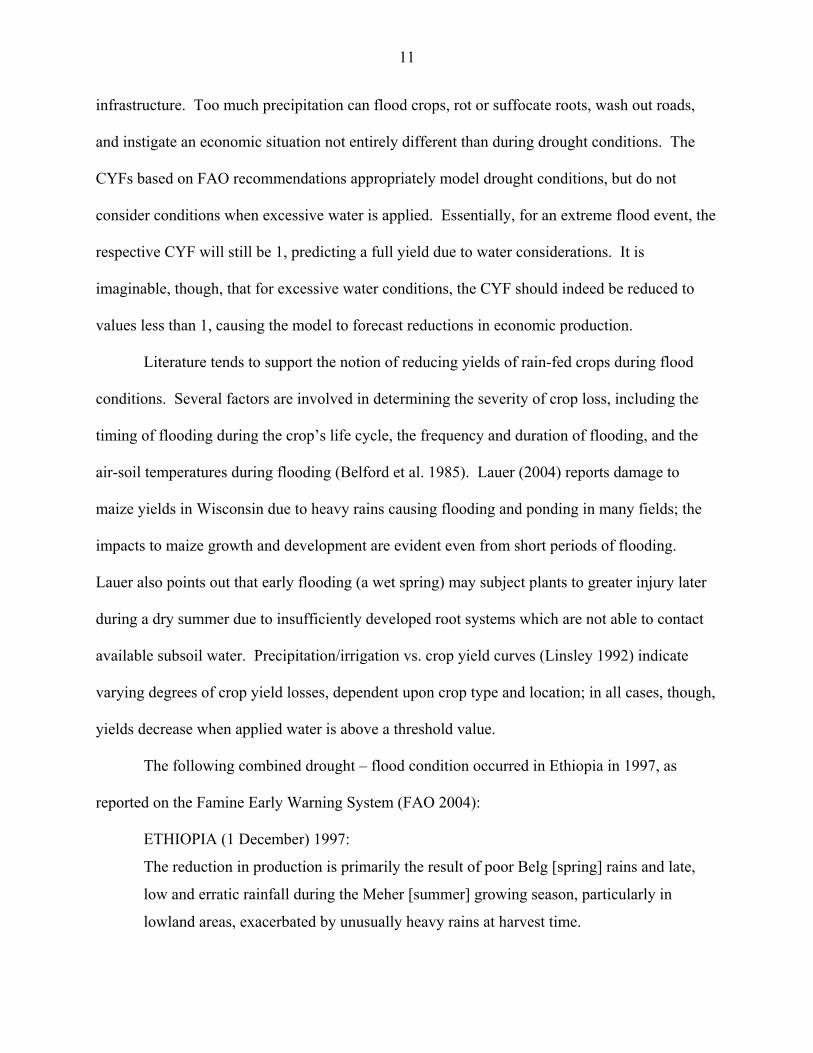
To address these issues, a flood factor was developed to appropriately reduce CYF values.

Many of the agricultural, non-agricultural and livestock production terms in the model

behave in a similar fashion in response to the quantity of precipitation received. Non-

agricultural production and livestock production, specifically for commodities produced in

Ethiopia, continue to grow as precipitation levels increase, to an extent; like agricultural

production, though, it is also easily imaginable that too much water could tend to cause a loss in

infrastructure, and a slowing or reduction in non-agricultural and livestock production. Figure 1

presents a general sketch of the relationship between the climate-yield factor (CYF) and effective

precipitation.

Figure 1--General relationship between CYF and effective precipitation

A similar pattern could also be expected for non-agricultural and livestock production.

Below point A, more effective precipitation returns a greater yield per crop area. Point A

represents a climate-yield factor of 1.0, or the maximum amount achievable. Between points A

and B, more effective precipitation produces no more yield, but neither is the yield reduced.

0

0.25

0.5

0.75

1

Effective Precipitation

CYF

A BB A

13

Finally, beyond point B, the effective precipitation has become more than the crop can sustain,

and the yield drops. It is conceivable that if the effective precipitation is too large, no yield is

possible, resulting in a CYF of 0. This sketch is for illustrative purposes only, and does not infer

that the climate-yield factor and effective precipitation form a linear relationship. Rather, this

relationship would be specific to each crop, to each climate, and to soil types and conditions,

among other factors, and may take on a variety of shapes. Similar statements could be made

concerning non-agricultural and livestock production. The figure shows a stylized relationship

with an increasing section, a flatter section, and a decreasing section which holds for agricultural

and non-agricultural commodities. It is this concept, with some variation, that is exemplified in

the flood factor, detailed in the following sections.

Flood Factor – Agricultural Commodities

The flood factor (FF) is essentially a dynamic component that forces a decrease of the

CYF if the year is deemed significantly wet, in terms of precipitation. The criterion includes

examining the standard normal distribution variable z, for precipitation data, as defined in

Equation 4,

σμ−

==xFFz (4)

where x is the observed (actual) monthly precipitation, μ is the mean monthly precipitation, and σ

is the standard deviation of the monthly precipitation data, all for a given zone. The flood factor

is calculated twice in the evaluation of flooding on agricultural commodities: once during the

vegetative/flowering stage, and once during the harvest stage. The exact months of theses two

stages are crop specific, but generally correspond with May through July for vegetative/

flowering and August through October for harvest, representing the times when the crop is most

vulnerable to flooding, and when the yield is most likely to be shocked negatively. The largest

FF value for each of these two crop stages of each year is retained for evaluation. The

magnitude of the FF, and its corresponding probabilistic chance of occurring, determines the

14

extent to which the climate-yield factors are affected through a series of CYF reduction

equations (not included.)

Flood Factor – Livestock and non-Agricultural Commodities

Livestock and non-agricultural production also exhibit a negative impact from high

precipitation and floods, due to damage to infrastructure and linkages to agricultural goods. The

same process has been adopted as for the agricultural commodities, taking advantage of the

standard normal distribution variable, Equation 4. In this case, though, only the largest FF value

from the rainy season months, June through September, of each year is retained for evaluation.

This reduction is especially crucial to the road investment scheme, as significant flooding events

may damage roads, and pose serious transportation problems.

Based on the aforementioned literature and other available guidelines (Salter, 1967), a

very conservative approach has been undertaken in determining an appropriate FF. In no case is

any commodity (agricultural or non-agricultural) reduced for a FF less than one standard

deviation above the mean. This is essentially analogous to a probabilistic occurrence of less than

once in about 6.5 years. Other rubrics are even more conservative. The reasoning for this

approach stems from the notion of limited available specific data for varying Ethiopian crops and

regions.

A water balance model of soil moisture in a region of the Ethiopian highlands was

assessed for comparison with FF occurrence, as prescribed by the rubrics. In general, the

average soil condition for a month was at or above full saturation more than twice as often as FFs

occurred. Again, this promotes a very conservative estimate, and may well be underestimating

the potentially negative effects of flooding conditions on crops.

15

NEW CLIMATE YIELD FACTORS (CYF) FOR CASH CROPS

In the original model, cash crops, which account for approximately 30 percent of all

cultivated lands, were assigned a CYF of 1, leaving them unaffected by climate. New codes

were not written to address each cash crop’s individual requirements, but rather all cash crops in

a zone were assigned a CYF value equal to the maximum cereal crop CYF in that same zone in

each year of the simulation. Although this is not a perfect estimation of cash crop CYFs, it does

more closely represent an appropriate value based on climate fluctuations, and emphasizes the

advantages of irrigated cash crops over rain-fed crops.

INCLUSION OF CLIMATE MODIFICATIONS IN THE MODEL

To include climate modifications and additions, the model was revised to dynamically

input a new set of cereal and cash crop CYFs for each year. With the 100 years of available

CYF data, nine different 12-year combinations were formed: 1900-1912, 1913-1924, 1925-1936,

1937-1948, 1949-1960, 1961-1972, 1973-1984, 1985-1996, and 1989-2000, representing actual,

chronological sets to cover the 100-year span. All 12-year combinations start from the same

base year, 2003, for ease of comparison. Each set is run through each simulation (base,

irrigation, roads, and irrigation and roads combination) to provide nine sets of results per

simulation. These ensembles do not encompass all possibilities, of course, and admittedly

correspond to a stylized stochastic process, as opposed to other approaches that generate

ensembles using a random or weighting scheme for assimilating months (Prairie et al. 2000), but

do offer good insights into the variability and its response on the economy. Additionally, the

ensemble may also be compared with historical data and trends, as available in literature.

16

MODEL SENSITIVITY TO MODIFICATIONS

The modifications and additions to the climate aspect of the model discussed in the

previous sections have varying effects on model predictions. Each aspect was evaluated

individually to determine its sensitivity on the model. The following sections outline the

sensitivity to the implementation of climate variability through dynamic CYFs, and the addition

of the flood factor.

Dynamic Climate-Yield Factors

The first portion of the sensitivity analysis involves a comparison of model predictions

incorporating mean versus dynamic climate-yield factors. Resulting economic indicators for the

base simulation are tabulated in Table 3. Due to their similarity in nature, the irrigation, roads,

and irrigation and roads combination simulations are not presented. Table 2 provides necessary

terms and abbreviations.

Table 2--Abbreviations of terms Abbreviation Actual Term Means 100-year mean GDP gross domestic product AgGDP agricultural gross domestic product NAgGDP non-agricultural gross domestic product Irri Irrigation FF flood factor

Table 3-- Base simulation: Economic indicator sensitivity of mean versus dynamic CYF Simulation - Base % Difference Means of Range of Var. Means and

Economic Indicator Means Variability* Min Max Means of Var. GDP growth rate 2.82 2.79 2.34 3.03 -0.9% Ag GDP growth rate 2.44 2.38 1.61 2.80 -2.2% NAg GDP growth rate 3.32 3.33 3.25 3.39 0.1% Poverty rate in 2003 (%) 41.55 41.55 - - - Poverty rate by 2015 (%) 42.98 44.96 40.59 52.22 2.0%

*Mean of Nine-12-year sets

17

In this comparison, only the initial and final values, from the first and twelfth year,

respectively, are utilized. The variability within the 12 years is not addressed here. The Means

column utilizes the original 100-year mean climate data, while the Means of Variability column

is the average of the nine individual 12-year runs, which incorporate the dynamic CYF. The

Range of Variability column simply provides maximum and minimum values from the nine

individual sets. Percent differences for relevant economic predictors are also included.

It is interesting to note the convergence of the Means of Variability values to the Mean

values. This is both expected and desired, and is true in all simulations. Due to the linearity of

the FAO’s model in determining CYFs, as outlined earlier, such that CYFs continue to rise

toward or remain at 1 as precipitation quantities increase, the Means of Variability should align

with the Means. Given enough 12-year sets to run through the model, the Means of Variability

will eventually converge to the Mean values. The values for the irrigation, roads, and irrigation

and roads simulations obviously differ from those in the base case, as they provide for a better

state of welfare for Ethiopia, but nonetheless converge to their respective Mean values. Each

variable CYF outcome, though, may defer substantially from the mean CYF outcome.

Flood Factors

For the second part of the sensitivity analysis, the flood factors are introduced. This

allows for a comparison of the CYFs both with and without FFs, indicating the implications of

including flooding in the model. The results for each of the four simulations are presented in

Tables 4 – 7. The Means column is representative of CYFs without FFs, due to the nature of the

flood factor equation.

18

Table 4--Base simulation: CYF with and without flood factors economic indicator comparison Simulation - Base w FF % Difference Means of Range of Var. Means and Economic Indicator Means Variability Min Max Means of Var. GDP growth rate 2.82 1.78 1.23 2.32 -36.9% Ag GDP growth rate 2.44 1.47 0.58 2.06 -39.4% NAg GDP growth rate 3.32 2.17 0.68 2.71 -34.8% Poverty rate in 2003 (%) 41.55 41.55 - - - Poverty rate by 2015 (%) 42.98 54.77 46.82 65.52 11.8%

* Mean of Nine-12-year sets

Table 5--Irrigation simulation: CYF with and without flood factors economic indicator comparison

Simulation - Irri w FF % Difference Means of Range of Var. Means and Economic Indicator Means Variability Min Max Means of Var. GDP growth rate 4.58 3.66 3.22 4.12 -20.0% Ag GDP growth rate 4.96 4.21 3.56 4.65 -15.2% NAg GDP growth rate 4.02 2.85 1.36 3.39 -29.2% Poverty rate in 2003 (%) 41.55 41.55 - - - Poverty rate by 2015 (%) 36.45 47.62 40.04 58.07 11.2%

* Mean of Nine-12-year sets Table 6--Roads simulation: CYF with and without flood factors economic indicator

comparison Simulation - Roads w FF % Difference Means of Range of Var. Means and Economic Indicator Means Variability Min Max Means of Var. GDP growth rate 4.29 3.22 2.64 3.75 -24.9% Ag GDP growth rate 2.60 1.63 0.73 2.22 -37.2% NAg GDP growth rate 6.21 5.02 3.52 5.57 -19.1% Poverty rate in 2003 (%) 41.55 41.55 - - - Poverty rate by 2015 (%) 37.04 49.27 40.95 60.84 12.2%


19

Table 7--Irri/roads simulation: CYF with and without flood factors economic indicator comparison

Simulation -Irri/Rds w FF % Difference Means of Range of Var. Means and Economic Indicator Means Variability Min Max Means of Var. GDP growth rate 5.59 4.64 4.13 5.10 -17.0% Ag GDP growth rate 5.12 4.36 3.71 4.80 -14.8% NAg GDP growth rate 6.19 4.99 3.50 5.53 -19.4% Poverty rate in 2003 (%) 41.55 41.55 - - - Poverty rate by 2015 (%) 32.24 43.58 35.39 54.88 11.3%


Not surprisingly, the Means with Variability for the new CYFs with FFs indicate a

substantial decline in the welfare of the country. Flood factors, of course, instigate only negative

shocks to the economy, and often create situations from which the country may not be able to

rebound within the 12-year simulation. The timing of these flooding events, whether early or

late in the 12-year simulation, also plays a significant role. All simulations, therefore, present

serious declines when FFs are introduced, each responding in a slightly different manner.

Agricultural reductions are more prevalent in the roads simulation, while non-agricultural

declines dominate the irrigation simulation. The base simulation is the most deeply effected,

while the irrigation/roads simulation drops the least, as expected.

These declining trends, due to the addition of the FF, are in general agreement with

historical evidence. Two examples from the recent past include flooding in 1977 and 1996.

Seasonl and/or crop stage precipitation over all of Ethiopia for both of these years is greater than

one standard deviation above the mean, implying that reductions due to the FF result. According

to the FAO’s website for agricultural yields of cereals within Ethiopia, declines are evident in the

year immediately following the flooding period. In 1977, a yield of 1,036 kg/Ha

(kilograms/hectare) was reported; in 1978, 897 kg/Ha, and in 1979, 1,124 kg/Ha, indicating a

20

rebound of yields. The percent decline from 1977 to 1978 was approximately 13 percent.

Similarly, flooding in 1996 caused a reduction in yields, dropping from 1,263 kg/Ha in 1996 to

1,140 kg/Ha in 1997, a 10 percent drop. Additional untimely flooding in the following years

even further reduced cereal yields until 2001, when they began to rebound. Non-agricultural

commodities also dropped in similar fashion during these flooding periods, adding to the overall

decline in economic welfare.

6. RESULTS OF MEAN CLIMATE (DETERMINISTIC) VERSUS VARIABLE CLIMATE (STOCHASTIC) MODELING

The sensitivity analysis brings a few key results to the forefront. The addition of climate

variability, and the ensuing transformation to a stochastic model, may produce dissimilar results

(GDP, poverty rate) compared to the deterministic model for any given run, but the average of all

climate variability runs converges to the mean climate results. However, when the flood factor is

introduced, the stochastic means no longer converge to the deterministic mean. The variability

in the climate-yield factors, in general, does not directly produce this depression, but rather the

effects of flooding. The outcomes of a deterministic approach are unaffected by flood factors, as

the “observed” precipitation value is always equal to the mean value, resulting in all flood factors

equal to zero. Contrarily, for the stochastic approach, flood factors are clearly evident, and

reduce the state of the economy, occasionally more than once within a single simulation. If a

flood occurs, then, within a simulation, it should be apparent that the economy will rarely return

to an economic state equivalent to one for which no floods are accounted.

21

BASE SIMULATION

A comparison of the deterministic and stochastic approaches in the base simulation,

including flood factors, is graphically depicted in Figures 2 and 3.

Figure 2--Base simulation: GDP variable climate sets with deterministic and stochastic means

3.85

3.90

3.95

4.00

4.05

4.10

2003 2006 2009 2012 2015

Simulation Year

GD

P (l

og m

illio

n U

S$)

Variable Climate Sets Deterministic Model Stochastic Mean

22

Figure 3--Base simulation: Poverty rate variable climate sets with deterministic and stochastic means

35

40

45

50

55

60

65

70

2003 2006 2009 2012 2015

Simulation Year

Pove

rty R

ate

(%)

Variable Climate Sets Deterministic Model Stochastic Mean

These figures portray the year-to-year fluctuations for GDP (not GDP growth rate) in

billion US dollars, and poverty rate in percent for the nine variable climate sets; the deterministic

result and stochastic mean are also illustrated. In the case of both GDP and poverty rate, the

stochastic mean quickly departs from the deterministic line, indicating a lower economic welfare,

but follows the same general trend over the 12 years. Even the vast majority of individual

variable climate set points lie to one side of the deterministic line, signifying the difficulty in

returning to a state of constant growth once a shock to the system has occurred.

INVESTMENT SIMULATIONS

The deterministic and stochastic approaches for the three investment strategies are also

analyzed in a fashion similar to the base case. Tables 8 – 10 display a comparison of the two

approaches and the nine variable climate set’s end-year values, respectively. The values in these

23

tables vary from those in Tables 5 – 7 due to additional model modifications not presented in this

report.

Table 8--Irrigation simulation: Means and means of variability comparison Simulation - Irrigation % Difference Means of Range of Var. Means and Economic Indicator Means Variability Min Max Means of Var. GDP growth rate 3.68 2.73 2.25 3.22 -25.9% Ag GDP growth rate 3.95 3.13 2.39 3.62 -20.8% NAg GDP growth rate 3.31 2.14 0.66 2.69 -35.2% Poverty rate in 2003 (%) 41.55 41.55 - - - Poverty rate by 2015 (%) 39.27 50.50 42.70 61.36 11.2%

Table 9-- Roads simulation: means and means of variability comparison Simulation - Roads % Difference Means of Range of Var. Means and Economic Indicator Means Variability Min Max Means of Var. GDP growth rate 3.58 2.53 2.00 3.08 -29.4% Ag GDP growth rate 2.60 1.64 0.75 2.22 -36.8% NAg GDP growth rate 4.78 3.61 2.11 4.16 -24.5% Poverty rate in 2003 (%) 41.55 41.55 - - - Poverty rate by 2015 (%) 39.82 51.71 43.37 62.96 11.9%

Table 10--Irrigation/roads simulation: means and means of variability comparison Simulation - Irri/Roads % Difference Means of Range of Var. Means and Economic Indicator Means Variability Min Max Means of Var. GDP growth rate 4.40 3.43 2.95 3.92 -22.2% Ag GDP growth rate 4.13 3.29 2.56 3.78 -20.2% NAg GDP growth rate 4.77 3.59 2.09 4.14 -24.9% Poverty rate in 2003 (%) 41.55 41.55 - - - Poverty rate by 2015 (%) 36.15 47.74 39.77 58.77 11.6%

In contrast to the base case, both the Means and Means of Variability for the investment

simulations have increased due to the growth of irrigated agriculture, better transportation and

easier flow of commodities to and from markets, or a combination of the two.

24

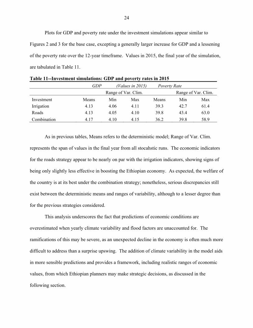
Plots for GDP and poverty rate under the investment simulations appear similar to

Figures 2 and 3 for the base case, excepting a generally larger increase for GDP and a lessening

of the poverty rate over the 12-year timeframe. Values in 2015, the final year of the simulation,

are tabulated in Table 11.

Table 11--Investment simulations: GDP and poverty rates in 2015 GDP (Values in 2015) Poverty Rate Range of Var. Clim. Range of Var. Clim. Investment Means Min Max Means Min Max Irrigation 4.13 4.06 4.11 39.3 42.7 61.4 Roads 4.13 4.05 4.10 39.8 43.4 63.0 Combination 4.17 4.10 4.15 36.2 39.8 58.9

As in previous tables, Means refers to the deterministic model; Range of Var. Clim.

represents the span of values in the final year from all stocahstic runs. The economic indicators

for the roads strategy appear to be nearly on par with the irrigation indicators, showing signs of

being only slightly less effective in boosting the Ethiopian economy. As expected, the welfare of

the country is at its best under the combination strategy; nonetheless, serious discrepancies still

exist between the deterministic means and ranges of variability, although to a lesser degree than

for the previous strategies considered.

This analysis underscores the fact that predictions of economic conditions are

overestimated when yearly climate variability and flood factors are unaccounted for. The

ramifications of this may be severe, as an unexpected decline in the economy is often much more

difficult to address than a surprise upswing. The addition of climate variability in the model aids

in more sensible predictions and provides a framework, including realistic ranges of economic

values, from which Ethiopian planners may make strategic decisions, as discussed in the

following section.

25

RISK ASSESSMENT OF INVESTMENT STRATEGIES

The inclusion of climate variability has the advantage of not only supplying more

realistic economic predictions, but also the ability to give some sense of probabilistic risk as well

through a stochastic analysis. No investment strategy can ensure economic success, so it is the

probabilistic chance of the economy falling within some acceptable range of economic values for

a given investment strategy that becomes of interest.

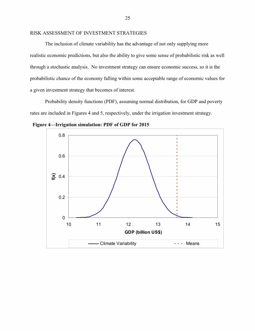
Probability density functions (PDF), assuming normal distribution, for GDP and poverty

rates are included in Figures 4 and 5, respectively, under the irrigation investment strategy.

Figure 4—Irrigation simulation: PDF of GDP for 2015

0

0.2

0.4

0.6

0.8

10 11 12 13 14 15

GDP (billion US$)

f(x)

Climate Variability Means

26

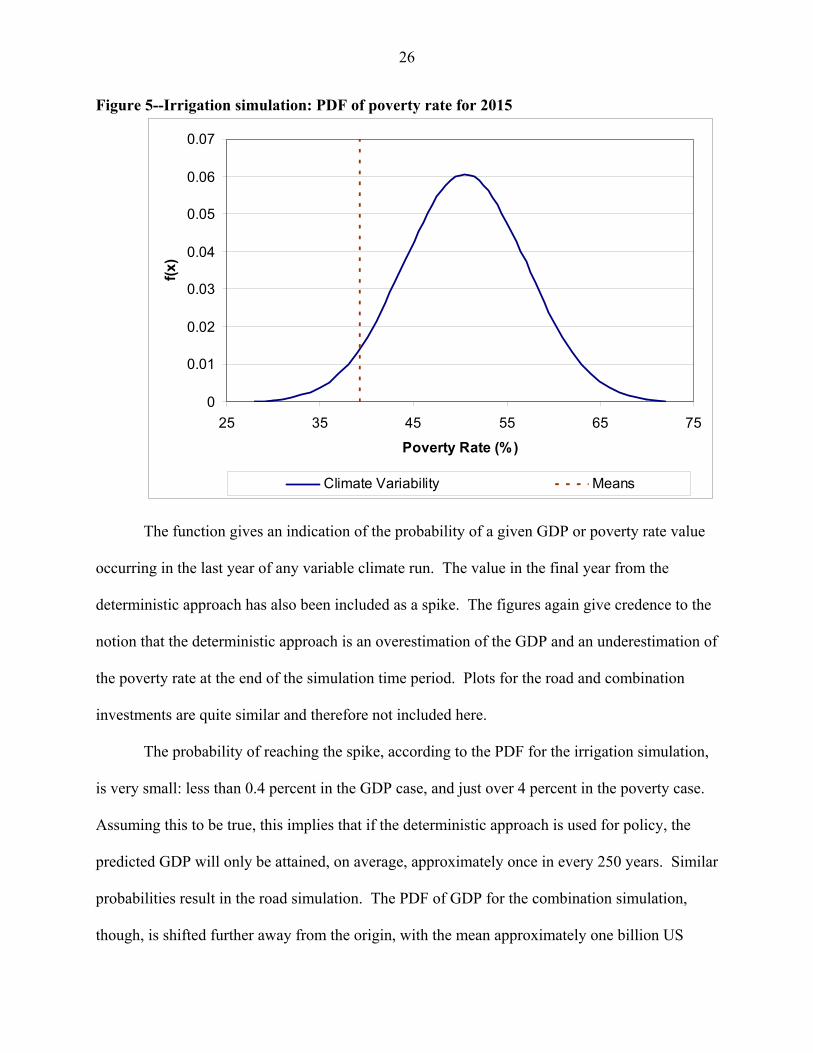
Figure 5--Irrigation simulation: PDF of poverty rate for 2015

0

0.01

0.02

0.03

0.04

0.05

0.06

0.07

25 35 45 55 65 75

Poverty Rate (%)

f(x)

Climate Variability Means

The function gives an indication of the probability of a given GDP or poverty rate value

occurring in the last year of any variable climate run. The value in the final year from the

deterministic approach has also been included as a spike. The figures again give credence to the

notion that the deterministic approach is an overestimation of the GDP and an underestimation of

the poverty rate at the end of the simulation time period. Plots for the road and combination

investments are quite similar and therefore not included here.

The probability of reaching the spike, according to the PDF for the irrigation simulation,

is very small: less than 0.4 percent in the GDP case, and just over 4 percent in the poverty case.

Assuming this to be true, this implies that if the deterministic approach is used for policy, the

predicted GDP will only be attained, on average, approximately once in every 250 years. Similar

probabilities result in the road simulation. The PDF of GDP for the combination simulation,

though, is shifted further away from the origin, with the mean approximately one billion US

27

dollars greater than for the irrigation scheme. The poverty rate PDF is shifted toward the origin,

with the difference in means between the combination strategy and the irrigation strategy at

approximately 2.75 percent, translating to almost 2 million people.

An assessment of risk levels for planning purposes naturally flows from the PDF. Table

12 demonstrates sample risk levels and associated GDP and poverty rates for the combination

approach.

Table 12--Irrigation/roads simulation: Risk levels for GDP and poverty rate Irrigation/Roads Simulation for Variable Climate

Risk Levels for GDP (billion US$) Risk Levels for Poverty Rate (%) µ=13.25 σ=0.579 µ=47.74 σ=6.711

Associated Level of Risk Associated GDP Level of Risk Poverty Rate

50% 13.25 50% 47.74 25% 12.86 25% 52.24 10% 12.51 10% 56.33 1% 11.90 1% 63.38

7. SUMMARY AND DISCUSSION

This research highlights a few important modeling aspects beyond determining which

investment strategy may provide the best outlook for Ethiopia’s future economy. Average

climate parameters, as utilized in the deterministic model, can underestimate the negative effects

of climate variability, and do not clearly represent the difficulties in recovering from extreme

climate events. Stochastic modeling, with the inclusion of climate variability, helps to alleviate

these issues, and appears to be essential and warranted when modeling investment in sectors that

are responsive to climate extremes. In the deterministic model, drought effects are modeled

appropriately (although partially negated by utilizing average climate parameters), but flood

factors, or a reduction in production due to excessive precipitation, are ignored. The inclusion of

28

flood factors in this study not only represents the expected decline in agricultural yields, but also

damage to roads and infrastructure, which further perpetuates the decline in agricultural

production, trade and other non-agricultural activities. Failure to include flood factors may well

result in misleading insights and overestimation of the welfare of the economy. Another benefit

of the stochastic approach is the ability to analyze the results from a probabilistic standpoint.

This in turn allows for policy decisions to be made and presented in a risk-based frame work.

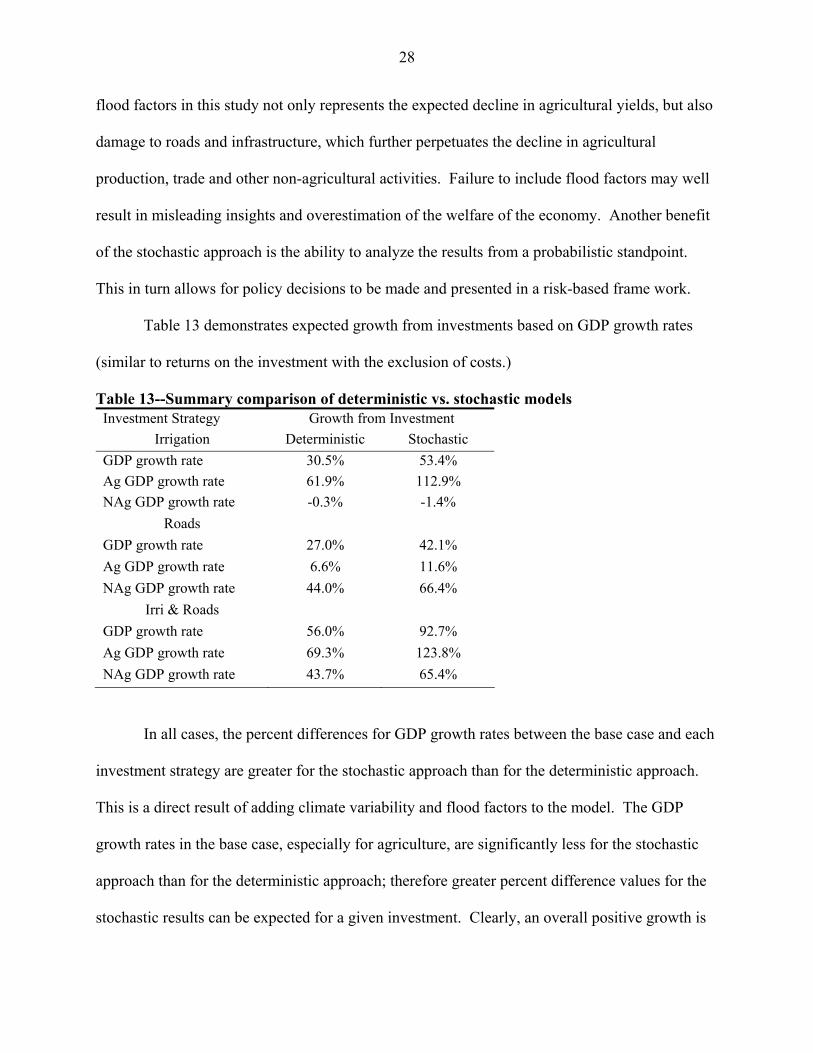
Table 13 demonstrates expected growth from investments based on GDP growth rates

(similar to returns on the investment with the exclusion of costs.)

Table 13--Summary comparison of deterministic vs. stochastic models Investment Strategy Growth from Investment

Irrigation Deterministic Stochastic GDP growth rate 30.5% 53.4% Ag GDP growth rate 61.9% 112.9% NAg GDP growth rate -0.3% -1.4%

Roads GDP growth rate 27.0% 42.1% Ag GDP growth rate 6.6% 11.6% NAg GDP growth rate 44.0% 66.4%

Irri & Roads GDP growth rate 56.0% 92.7% Ag GDP growth rate 69.3% 123.8% NAg GDP growth rate 43.7% 65.4%

In all cases, the percent differences for GDP growth rates between the base case and each

investment strategy are greater for the stochastic approach than for the deterministic approach.

This is a direct result of adding climate variability and flood factors to the model. The GDP

growth rates in the base case, especially for agriculture, are significantly less for the stochastic

approach than for the deterministic approach; therefore greater percent difference values for the

stochastic results can be expected for a given investment. Clearly, an overall positive growth is

29

expected for any investment, as costs are neglected, but the stochastic approach tends to predict

additional growth due to the more realistic prediction of the base case, which is further depressed

when climate extremes are included. The table also indicates little similarity in sector response

between irrigation and roads investments; the irrigation investment is completely manifested in

the agricultural sector, while the roads investment is predominantly driven by the non-

agricultural sector, but allows for some agricultural feedbacks.

Overall, as demonstrated in this study, the irrigation investment strategy tends to fare

slightly better than the roads investment strategy from a benefit perspective. This is due in part

to the fact that additional irrigation has particularly strong impacts on reducing the negative

effects on production and farm income of drought. Since drought has a persistent impact on

income and food security, prevention or reduction in severity of drought has long term benefits.

It is also worthwhile to note that the combination strategy of both irrigation and roads is

approximately the sum of the two individual strategies, for both the deterministic and stochastic

models, indicating a sense of linearity.

Potential future extensions of this work are numerous. One area for development

includes completing more model runs to extend the stochastic ensemble. Additional runs need

not be in chronological order, but could follow traditional K-nearest neighbor techniques to

generate plausible 12-year segments (Prairie, et al. 2000.) The broader ensemble would provide

more confidence in accurate PDF and risk assessment levels. A second avenue for future work

involves incorporating costs into the agro-economic model, and formulating a true investment

analysis considering returns. Ultimately this step will be necessary prior to development of final

investment policies in Ethiopia.

31

APPENDIX I: EQUATIONS IN THE SPATIAL, MULTI-MARKET MODEL OF ETHIOPIA AGRICULTURE

DEMAND FUNCTIONS:

(Zonal level per capita)

∑=−

∏ j jZRjZRtZRj tjZRtiZR GDPpcPCDpc ,,,,

1

,,,,,,,,

εε

Where DpcR,Z,i is per capita demand for commodity i in region R and zone Z, and PCR,Z,i is consumer price for i in region R and zone Z. j = 1,2,…,36 (including two aggregate nonagricultural goods.) GDPpcR,Z is per capita agricultural and nonagricultural income for region R and zone Z.

SUPPLY FUNCTIONS:

Yield function (for crops)

iZRtiZRtiZR PY ,,

,,,ti,Z,R,,,, YA α= Where YR,Z,i is the yield for crop i and PR,Z,i is producer price for i; YAR,Z,i is the shift parameter,

which depends on climate-yield factor coefficient derived from 100 years’ monthly climate data

at zonal level, fertilizer and other input use, and time trend growth rate (varies by zone). For

irrigated crops, YAR,Z,i does not depend on climate-yield factor and is 50 percent higher than

YAR,Z,i for the same crops depending on rainfall only.

At this moment, only climate-yield factor coefficients have been developed, and the estimation

of other coefficients (for fertilizer and other input use) are in progress. If we choose the mean

value of climate-yield factor, the shift coefficient in yield function looks like:

( )

iZRYtiZRtiZR gKc,,

1YAYA ti,Z,R,1,,,1,,, +⋅= ++ Where Kc is mean value of climate-yield factor coefficient with value between 0.5 and 1.0. 1.0

implies that on average there is no shortage in rainfall affecting the yield, and when the

32

coefficient is less than 0.5, the crop fails to grow. Kc varies by crops, depending on the drought-

tolerant ability of a specific crop and suitability of the climate condition (which varies by zone).

gY is annual growth rate in yield productivity and varies by zone and crop.

Area function (for crops)

∏=j tjZRtiZR

jZRPA ,,,,,ti,Z,R,,,, AA β

Where AR,Z,i is the yield for crop i and P1, P2, … PJ, is the vector of producer prices; AA is the

shift parameter (the trend in area).

Trends in area function:

( )iZRAtiZR g

,,1AAAA ti,Z,R,1,,, +=+

Where gA is annual growth rate in area expansion and varies by zone and crop. Total supply of crops

tiZRtiZRtiZR AYS ,,,,,,,,, ⋅= Supply function for livestock and nonagriculture

∏=j tjZR

LVtiZR

LVjZRPS ,,,,,

LVti,Z,R,,,, SA β

Trends in livestock and nonagricultural supply function

( )iZRSg

,,1SASA LV

ti,Z,R,LV

1ti,Z,R, +=+ Where gS is annual growth rate in productivity and varies by zone and commodity. gY, gA, and gS are exogenous variables in the model and are affected by the investment shocks in

the scenarios.

33

RELATIONSHIP BETWEEN PRODUCER AND CONSUMER PRICES

We assume that there are domestic market margins between import parity prices and

consumer prices, which is defined by zone; and export parity prices and producer prices, defined

also by zone. Moreover, within the country, due to difference in food deficit or surplus, and

different distances to the national major market centers, there are price gaps cross regions. To

simplify the model, we assume that Addis Ababa is the only market center and the traveling time

from Addis Ababa is used as proxy for domestic marketing costs (marking margins).

Specifically, we define import/export parity prices as the prices in Addis Ababa markets (if

tradable), such that

Import parity prices:

( ) iiAddisti PWMinWmPC ⋅+= arg1,

where Wmargin is the marketing margins between CIF prices and Addis Ababa consumer prices.

If commodity i importable, this equation holds. Consumer’s prices in the other zones with food

surplus are:

( ) Addis

tiiZRtiZR PCDgapPC ,,,,,, 1 ⋅−= and consumer’s prices in the other zones with food deficit or balanced food are:

( ) AddistiiZRtiZR PCDgapPC ,,,,,, 1 ⋅+=

Where Dgap is domestic price gap between consumer prices in Addis Ababa and in other regions

and such gap varies by zone according to the distance to Addis Ababa. In general, for food

surplus regions, producer prices are lower than that in Addis Ababa, while in food deficit or

balanced regions, consumer prices are higher than that in Addis Ababa.

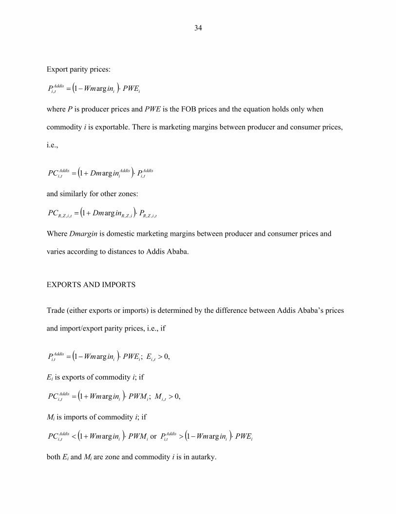
34

Export parity prices:

( ) iiAddisti PWEinWmP ⋅−= arg1,

where P is producer prices and PWE is the FOB prices and the equation holds only when

commodity i is exportable. There is marketing margins between producer and consumer prices,

i.e.,

( ) Addis

tiAddisi

Addisti PinDmPC ,, arg1 ⋅+=

and similarly for other zones:

( ) tiZRiZRtiZR PinDmPC ,,,,,,,, arg1 ⋅+= Where Dmargin is domestic marketing margins between producer and consumer prices and

varies according to distances to Addis Ababa.

EXPORTS AND IMPORTS

Trade (either exports or imports) is determined by the difference between Addis Ababa’s prices

and import/export parity prices, i.e., if

( ) ,0 ;arg1 , >⋅−= tiii

Addisi,t EPWEinWmP

Ei is exports of commodity i; if

( ) ,0 ;arg1 ,, >⋅+= tiiiAddisti MPWMinWmPC

Mi is imports of commodity i; if

( ) ( ) iiAddis

i,tiiAddisti PWEinWmPPWMinWmPC ⋅−>⋅+< arg1or arg1,

both Ei and Mi are zone and commodity i is in autarky.

35

REGIONAL CROP DEFICIT AND SURPLUS

The model can identify which zones are food crop deficit or surplus, but cannot identify

trade flows among the zones. That is, total deficit and surplus are cleared (balanced) at the

national market and there is no regional market. A regional food crop i’s deficit/surplus is

defined as

tiZRtZRtiZRtiZR SPoPDpcDEF ,,,,,,,,,,, −⋅= Positive means deficit.

BALANCE OF DEMAND AND SUPPLY AT THE NATIONAL LEVEL

∑∑ ⋅=−+ZR ZRtiZRtititiZRZR

PoPDpcEMS, ,,,,,,,,,,

GDP AND PER CAPITA ZONAL INCOME FUNCTION

ture)nonagricul including( 36,...,2,1 ,,,,,,,, =⋅=∑ jSPGDP

j tjZRtjZRtZR

Income per capita:

tZR

tZRtZR PoP

GDPGDPpc

,,

,,,, =

36

REFERENCES

Bedient, P. B., and W. C. Hubert. 2002. Hydrology and floodplain analysis. 3rd Edition. Upper

Saddle River, N.J.: Prentice Hall.

Belford, R. K., R. Q. Cannell, and R. J. Thompson. 1985. Effects of single and multiple water loggings on the growth and yield of winter wheat on clay soil. Journal of Science and Food Agriculture 36:142-156.

Benjamin, Jack R., and C. Allin Cornell. 1970. Probability, statistics, and decision for civil engineers. New York, N.Y.: McGraw-Hill Book Company.

Block, P. and B. Rajagopalan. 2006. Interannual variability and ensemble forecast of Upper Blue Nile Basin Kiremt season precipitation.” Journal of Climatology. In review.

Conway, D. Ethiopia: The warning signs of famine. BBC News, November 19, 2002.

CROPWAT, Version 4.3. Rome: Food and Agriculture Organization of the United Nations. DATE

Dalton, M.G. The welfare bias from omitting climatic variability in economic studies of global warming. Journal of Environmental Economics and Management 33: 221-239.

Diao, X. and A. Nin Pratt with M. Gautam, J. Keough, J. Chamberlin, L. You, D. Puetz, D. Resnick, and B. Yu. 2005. Growth options and poverty reduction in Ethiopia, A spatial, economywide model analysis for 2004–15. DSG Discussion Paper No. 20, Washington, D.C. International Food Policy Research Institute.

Dixon, Bruce L., and Kathleen Segerson. 1999. Impacts of Increased Climate Variability on the Profitability of Midwest Agriculture. Journal of Agricultural and Applied Economics 31: 537-549.

FAO. 1998. Crop Evapotranspiration: Guidelines for computing crop water requirements. fao irrigation and drainage. Paper No. 56. Rome: Food and Agriculture Organization of the United Nations (FAO).

FAO. 1984. Yield Response to Water. FAO Irrigation and Drainage Paper No. 33. Rome: FAO.

FAO/GIEWS. 2004. Food and Agriculture in Ethiopia. http://www.fao.org. Global Information and Early Warning System. Rome: FAO

Ferreyra, R. A., G. P. Podesta, C. D. Messina, D. Letson, J. Dardanelli, E. Guevara, and S. Meira. 2001. A linked-modeling framework to estimate maize production risk associated with ENSO-related climate variability in Argentina. Agricultural and Forest Meteorology 107: 177-192.

37

GAMS 2.0.26.8. 2004. General Algebraic Modeling System. Washington, D.C.

Hogg, R. V., and J. Ledolter. 1992. Applied statistic for engineers and scientists, 2nd Edition. New York: Macmillan Publishing Company.

Holland, W. R., S. Joussaume, and F. David. 1999. Modeling the earth’s climate and its variability. Amsterdam, the Netherlands: Elsevier Science B.V.

Kane, S., J. Reilly, and J. Tobey. 1992. Climate change on world agriculture. Climate Change 21:17-35.

Lauer, J. 2004. Flooding impacts on corn growth and yield, Wisconsin Crop Manager 11 (12): 63-64.

Letson, D., G. Podesta, C. Messina, and A. Ferreyra. 2001. ENSO forecast value, variable climate and stochastic prices. American Agricultural Economics Annual Meeting Presentation. August 5-8, Chicago, Illinois.

Linsley, R., J. Franzini, D. Freyberg, and G. Tchobanoglous. 1992. Water-resources engineering, 4th Edition. New York, N.Y.: McGraw-Hill Inc.

Ludena, C. E., K. McNamara, P. A. Hammer, and K. Foster. 2003. Development of a stochastic Model to evaluate plant growers’ enterprise budgets. American Agricultural Economics Annual Meeting Presentation. July 27-30, Montreal, Canada.

Mendelsohn, R., W.D. Nordhaus, and D. Shaw. 1994. The impact of global warming on agriculture: A Ricardian approach. American Economics Review 84: 753-771.

Mendelsohn, R., and J. Neuman. 1999. The impact of climate change of the United States economy. Cambridge, UK: Cambridge University Press.

Patt, A.G. 1999. Extreme outcomes: The strategic treatment of low probability events in scientific assessments. Risk Decision and Policy 4: 1-15.

Prairie, J., B. Rajagopalan, U. Lall and T. Fulp. A stochastic nonparametric technique for space-time disaggregation of streamflows. Water Resources Research. In review.

Rogers, C. 2004. Development of a climate yield factor to assess climate-based risk to rainfed agriculture in Ethiopia: Description of methodology and results of Ethiopian climate data analysis. Washington, D.C. International Food Policy Research Institute.

Rosegrant, M., X. Cai, and S. Cline. 2002. World, water and food to 2025: Dealing with scarcity. Washington, D.C.: International Food Policy Research Institute.

Salinger, M.J., R Desjardins, M.B. Jones, M.V.K. Sivakumar, N.D. Strommen, S. Veerasamy and Wu Lianhai. 1997. Climate variability, agriculture and forestry: An update. Technical Note No. 199. Geneva, Switzerland: World Meteorological Organization. http://www.wmo.ch/web/catalogue/New%20HTML/frame/engfil/841.html

38

Salter, P. J., and J.E. Goode. Crop responses to water at different stages of growth.

Commonwealth Agricultural Bureaux, Farnham Royal, Bucks, England, 1967.

Taylor, R.G., and R.A. Young. 1995. Rural-to-urban water transfers: measuring direct foregone benefits of irrigation water under uncertain water supplies. Journal of Agricultural and Resource Economics 20: 247-262.

Valdivia, C., and R. Quiroz. 2003. Coping and adapting to increased climate variability in the Andes. American Agricultural Economics Annual Meeting Presentation. July 27-30, Montreal, Canada.

EPT DISCUSSION PAPERS

1. Sustainable Agricultural Development Strategies in Fragile Lands, by Sara J. Scherr and Peter B.R. Hazell, June 1994.

2. Confronting the Environmental Consequences of the Green Revolution in Asia, by Prabhu L. Pingali and Mark W. Rosegrant, August 1994.

3. Infrastructure and Technology Constraints to Agricultural Development in the Humid and Subhumid Tropics of Africa, by Dunstan S.C. Spencer, August 1994.

4. Water Markets in Pakistan: Participation and Productivity, by Ruth Meinzen-Dick and Martha Sullins, September 1994.

5. The Impact of Technical Change in Agriculture on Human Fertility: District-level Evidence from India, by Stephen A. Vosti, Julie Witcover, and Michael Lipton, October 1994.

6. Reforming Water Allocation Policy through Markets in Tradable Water Rights: Lessons from Chile, Mexico, and California, by Mark W. Rosegrant and Renato Gazri S, October 1994.

7. Total Factor Productivity and Sources of Long-Term Growth in Indian Agriculture, by Mark W. Rosegrant and Robert E. Evenson, April 1995.

8. Farm-Nonfarm Growth Linkages in Zambia, by Peter B.R. Hazell and Behjat Hoijati, April 1995.

9. Livestock and Deforestation in Central America in the 1980s and 1990s: A Policy Perspective, by David Kaimowitz (Interamerican Institute for Cooperation on Agriculture. June 1995.

10. Effects of the Structural Adjustment Program on Agricultural Production and Resource Use in Egypt, by Peter B.R. Hazell, Nicostrato Perez, Gamal Siam, and Ibrahim Soliman, August 1995.

11. Local Organizations for Natural Resource Management: Lessons from Theoretical and Empirical Literature, by Lise Nordvig Rasmussen and Ruth Meinzen-Dick, August 1995.

12. Quality-Equivalent and Cost-Adjusted Measurement of International Competitiveness in Japanese Rice Markets, by Shoichi Ito, Mark W. Rosegrant, and Mercedita C. Agcaoili-Sombilla, August 1995.


13. Role of Inputs, Institutions, and Technical Innovations in Stimulating Growth in Chinese Agriculture, by Shenggen Fan and Philip G. Pardey, September 1995.

14. Investments in African Agricultural Research, by Philip G. Pardey, Johannes Roseboom, and Nienke Beintema, October 1995.

15. Role of Terms of Trade in Indian Agricultural Growth: A National and State Level Analysis, by Peter B.R. Hazell, V.N. Misra, and Behjat Hoijati, December 1995.

16. Policies and Markets for Non-Timber Tree Products, by Peter A. Dewees and Sara J. Scherr, March 1996.

17. Determinants of Farmers’ Indigenous Soil and Water Conservation Investments in India’s Semi-Arid Tropics, by John Pender and John Kerr, August 1996.

18. Summary of a Productive Partnership: The Benefits from U.S. Participation in the CGIAR, by Philip G. Pardey, Julian M. Alston, Jason E. Christian, and Shenggen Fan, October 1996.

19. Crop Genetic Resource Policy: Towards a Research Agenda, by Brian D. Wright, October 1996.

20. Sustainable Development of Rainfed Agriculture in India, by John M. Kerr, November 1996.

21. Impact of Market and Population Pressure on Production, Incomes and Natural Resources in the Dryland Savannas of West Africa: Bioeconomic Modeling at the Village Level, by Bruno Barbier, November 1996.

22. Why Do Projections on China’s Future Food Supply and Demand Differ? by Shenggen Fan and Mercedita Agcaoili-Sombilla, March 1997.

23. Agroecological Aspects of Evaluating Agricultural R&D, by Stanley Wood and Philip G. Pardey, March 1997.

24. Population Pressure, Land Tenure, and Tree Resource Management in Uganda, by Frank Place and Keijiro Otsuka, March 1997.


25. Should India Invest More in Less-favored Areas? by Shenggen Fan and Peter Hazell, April 1997.

26. Population Pressure and the Microeconomy of Land Management in Hills and Mountains of Developing Countries, by Scott R. Templeton and Sara J. Scherr, April 1997.

27. Population Land Tenure and Natural Resource Management: The Case of Customary Land Area in Malawi, by Frank Place and Keijiro Otsuka, April 1997.

28. Water Resources Development in Africa: A Review and Synthesis of Issues, Potentials, and Strategies for the Future, by Mark W. Rosegrant and Nicostrato D. Perez, September 1997.

29. Financing Agricultural R&D in Rich Countries: What’s Happening and Why? by Julian M. Alston, Philip G. Pardey, and Vincent H. Smith, September 1997.

30. How Fast Have China’s Agricultural Production and Productivity Really Been Growing? by Shenggen Fan, September 1997.

31. Does Land Tenure Insecurity Discourage Tree Planting? Evolution of Customary Land Tenure and Agroforestry Management in Sumatra, by Keijiro Otsuka, S. Suyanto, and Thomas P. Tomich, December 1997.

32. Natural Resource Management in the Hillsides of Honduras: Bioeconomic Modeling at the Micro-Watershed Level, by Bruno Barbier and Gilles Bergeron, January 1998.

33. Government Spending, Growth, and Poverty: An Analysis of Interlinkages in Rural India, by Shenggen Fan, Peter Hazell, and Sukhadeo Thorat, March 1998. Revised December 1998.

34. Coalitions and the Organization of Multiple-Stakeholder Action: A Case Study of Agricultural Research and Extension in Rajasthan, India, by Ruth Alsop, April 1998.

35. Dynamics in the Creation and Depreciation of Knowledge and the Returns to Research, by Julian Alston, Barbara Craig, and Philip Pardey, July, 1998.


36. Educating Agricultural Researchers: A Review of the Role of African Universities, by Nienke M. Beintema, Philip G. Pardey, and Johannes Roseboom, August 1998.

37. The Changing Organizational Basis of African Agricultural Research, by Johannes Roseboom, Philip G. Pardey, and Nienke M. Beintema, November 1998.

38. Research Returns Redux: A Meta-Analysis of the Returns to Agricultural R&D, by Julian M. Alston, Michele C. Marra, Philip G. Pardey, and T.J. Wyatt, November 1998.

39. Technological Change, Technical and Allocative Efficiency in Chinese Agriculture: The Case of Rice Production in Jiangsu, by Shenggen Fan, January 1999.

40. The Substance of Interaction: Design and Policy Implications of NGO-Government Projects in India, by Ruth Alsop with Ved Arya, January 1999.

41. Strategies for Sustainable Agricultural Development in the East African Highlands, by John Pender, Frank Place, and Simeon Ehui, April 1999.

42. Cost Aspects of African Agricultural Research, by Philip G. Pardey, Johannes Roseboom, Nienke M. Beintema, and Connie Chan-Kang, April 1999.

43. Are Returns to Public Investment Lower in Less-favored Rural Areas? An Empirical Analysis of India, by Shenggen Fan and Peter Hazell, May 1999.

44. Spatial Aspects of the Design and Targeting of Agricultural Development Strategies, by Stanley Wood, Kate Sebastian, Freddy Nachtergaele, Daniel Nielsen, and Aiguo Dai, May 1999.

45. Pathways of Development in the Hillsides of Honduras: Causes and Implications for Agricultural Production, Poverty, and Sustainable Resource Use, by John Pender, Sara J. Scherr, and Guadalupe Durón, May 1999.

46. Determinants of Land Use Change: Evidence from a Community Study in Honduras, by Gilles Bergeron and John Pender, July 1999.

47. Impact on Food Security and Rural Development of Reallocating Water from Agriculture, by Mark W. Rosegrant and Claudia Ringler, August 1999.


48. Rural Population Growth, Agricultural Change and Natural Resource Management in Developing Countries: A Review of Hypotheses and Some Evidence from Honduras, by John Pender, August 1999.

49. Organizational Development and Natural Resource Management: Evidence from Central Honduras, by John Pender and Sara J. Scherr, November 1999.

50. Estimating Crop-Specific Production Technologies in Chinese Agriculture: A Generalized Maximum Entropy Approach, by Xiaobo Zhang and Shenggen Fan, September 1999.

51. Dynamic Implications of Patenting for Crop Genetic Resources, by Bonwoo Koo and Brian D. Wright, October 1999.

52. Costing the Ex Situ Conservation of Genetic Resources: Maize and Wheat at CIMMYT, by Philip G. Pardey, Bonwoo Koo, Brian D. Wright, M. Eric van Dusen, Bent Skovmand, and Suketoshi Taba, October 1999.

53. Past and Future Sources of Growth for China, by Shenggen Fan, Xiaobo Zhang, and Sherman Robinson, October 1999.

54. The Timing of Evaluation of Genebank Accessions and the Effects of Biotechnology, by Bonwoo Koo and Brian D. Wright, October 1999.

55. New Approaches to Crop Yield Insurance in Developing Countries, by Jerry Skees, Peter Hazell, and Mario Miranda, November 1999.

56. Impact of Agricultural Research on Poverty Alleviation: Conceptual Framework with Illustrations from the Literature, by John Kerr and Shashi Kolavalli, December 1999.

57. Could Futures Markets Help Growers Better Manage Coffee Price Risks in Costa Rica? by Peter Hazell, January 2000.

58. Industrialization, Urbanization, and Land Use in China, by Xiaobo Zhang, Tim Mount, and Richard Boisvert, January 2000.

59. Water Rights and Multiple Water Uses: Framework and Application to Kirindi Oya Irrigation System, Sri Lanka, by Ruth Meinzen-Dick and Margaretha Bakker, March 2000.


60. Community natural Resource Management: The Case of Woodlots in Northern Ethiopia, by Berhanu Gebremedhin, John Pender and Girmay Tesfaye, April 2000.

61. What Affects Organization and Collective Action for Managing Resources? Evidence from Canal Irrigation Systems in India, by Ruth Meinzen-Dick, K.V. Raju, and Ashok Gulati, June 2000.

62. The Effects of the U.S. Plant Variety Protection Act on Wheat Genetic Improvement, by Julian M. Alston and Raymond J. Venner, May 2000.

63. Integrated Economic-Hydrologic Water Modeling at the Basin Scale: The Maipo River Basin, by M. W. Rosegrant, C. Ringler, DC McKinney, X. Cai, A. Keller, and G. Donoso, May 2000.

64. Irrigation and Water Resources in Latin America and he Caribbean: Challenges and Strategies, by Claudia Ringler, Mark W. Rosegrant, and Michael S. Paisner, June 2000.

65. The Role of Trees for Sustainable Management of Less-favored Lands: The Case of Eucalyptus in Ethiopia, by Pamela Jagger & John Pender, June 2000.

66. Growth and Poverty in Rural China: The Role of Public Investments, by Shenggen Fan, Linxiu Zhang, and Xiaobo Zhang, June 2000.

67. Small-Scale Farms in the Western Brazilian Amazon: Can They Benefit from Carbon Trade? by Chantal Carpentier, Steve Vosti, and Julie Witcover, September 2000.

68. An Evaluation of Dryland Watershed Development Projects in India, by John Kerr, Ganesh Pangare, Vasudha Lokur Pangare, and P.J. George, October 2000.

69. Consumption Effects of Genetic Modification: What If Consumers Are Right? by Konstantinos Giannakas and Murray Fulton, November 2000.

70. South-North Trade, Intellectual Property Jurisdictions, and Freedom to Operate in Agricultural Research on Staple Crops, by Eran Binenbaum, Carol Nottenburg, Philip G. Pardey, Brian D. Wright, and Patricia Zambrano, December 2000.


71. Public Investment and Regional Inequality in Rural China, by Xiaobo Zhang and Shenggen Fan, December 2000.

72. Does Efficient Water Management Matter? Physical and Economic Efficiency of Water Use in the River Basin, by Ximing Cai, Claudia Ringler, and Mark W. Rosegrant, March 2001.

73. Monitoring Systems for Managing Natural Resources: Economics, Indicators and Environmental Externalities in a Costa Rican Watershed, by Peter Hazell, Ujjayant Chakravorty, John Dixon, and Rafael Celis, March 2001.

74. Does Quanxi Matter to NonFarm Employment? by Xiaobo Zhang and Guo Li, June 2001.

75. The Effect of Environmental Variability on Livestock and Land-Use Management: The Borana Plateau, Southern Ethiopia, by Nancy McCarthy, Abdul Kamara, and Michael Kirk, June 2001.

76. Market Imperfections and Land Productivity in the Ethiopian Highlands, by Stein Holden, Bekele Shiferaw, and John Pender, August 2001.

77. Strategies for Sustainable Agricultural Development in the Ethiopian Highlands, by John Pender, Berhanu Gebremedhin, Samuel Benin, and Simeon Ehui, August 2001.

78. Managing Droughts in the Low-Rainfall Areas of the Middle East and North Africa: Policy Issues, by Peter Hazell, Peter Oram, Nabil Chaherli, September 2001.

79. Accessing Other People’s Technology: Do Non-Profit Agencies Need It? How To Obtain It, by Carol Nottenburg, Philip G. Pardey, and Brian D. Wright, September 2001.

80. The Economics of Intellectual Property Rights Under Imperfect Enforcement: Developing Countries, Biotechnology, and the TRIPS Agreement, by Konstantinos Giannakas, September 2001.

81. Land Lease Markets and Agricultural Efficiency: Theory and Evidence from Ethiopia, by John Pender and Marcel Fafchamps, October 2001.


82. The Demand for Crop Genetic Resources: International Use of the U.S. National Plant Germplasm System, by M. Smale, K. Day-Rubenstein, A. Zohrabian, and T. Hodgkin, October 2001.

83. How Agricultural Research Affects Urban Poverty in Developing Countries: The Case of China, by Shenggen Fan, Cheng Fang, and Xiaobo Zhang, October 2001.

84. How Productive is Infrastructure? New Approach and Evidence From Rural India, by Xiaobo Zhang and Shenggen Fan, October 2001.

85. Development Pathways and Land Management in Uganda: Causes and Implications, by John Pender, Pamela Jagger, Ephraim Nkonya, and Dick Sserunkuuma, December 2001.

86. Sustainability Analysis for Irrigation Water Management: Concepts, Methodology, and Application to the Aral Sea Region, by Ximing Cai, Daene C. McKinney, and Mark W. Rosegrant, December 2001.

87. The Payoffs to Agricultural Biotechnology: An Assessment of the Evidence, by Michele C. Marra, Philip G. Pardey, and Julian M. Alston, January 2002.

88. Economics of Patenting a Research Tool, by Bonwoo Koo and Brian D. Wright, January 2002.

89. Assessing the Impact of Agricultural Research On Poverty Using the Sustainable Livelihoods Framework, by Michelle Adato and Ruth Meinzen-Dick, March 2002.

90. The Role of Rainfed Agriculture in the Future of Global Food Production, by Mark Rosegrant, Ximing Cai, Sarah Cline, and Naoko Nakagawa, March 2002.

91. Why TVEs Have Contributed to Interregional Imbalances in China, by Junichi Ito, March 2002.

92. Strategies for Stimulating Poverty Alleviating Growth in the Rural Nonfarm Economy in Developing Countries, by Steven Haggblade, Peter Hazell, and Thomas Reardon, July 2002.

93. Local Governance and Public Goods Provisions in Rural China, by Xiaobo Zhang, Shenggen Fan, Linxiu Zhang, and Jikun Huang, July 2002.


94. Agricultural Research and Urban Poverty in India, by Shenggen Fan, September 2002.

95. Assessing and Attributing the Benefits from Varietal Improvement Research: Evidence from Embrapa, Brazil, by Philip G. Pardey, Julian M. Alston, Connie Chan-Kang, Eduardo C. Magalhães, and Stephen A. Vosti, August 2002.

96. India’s Plant Variety and Farmers’ Rights Legislation: Potential Impact on Stakeholders Access to Genetic Resources, by Anitha Ramanna, January 2003.

97. Maize in Eastern and Southern Africa: Seeds of Success in Retrospect, by Melinda Smale and Thom Jayne, January 2003.

98. Alternative Growth Scenarios for Ugandan Coffee to 2020, by Liangzhi You and Simon Bolwig, February 2003.

99. Public Spending in Developing Countries: Trends, Determination, and Impact, by Shenggen Fan and Neetha Rao, March 2003.

100. The Economics of Generating and Maintaining Plant Variety Rights in China, by Bonwoo Koo, Philip G. Pardey, Keming Qian, and Yi Zhang, February 2003.

101. Impacts of Programs and Organizations on the Adoption of Sustainable Land Management Technologies in Uganda, Pamela Jagger and John Pender, March 2003.

102. Productivity and Land Enhancing Technologies in Northern Ethiopia: Health, Public Investments, and Sequential Adoption, Lire Ersado, Gregory Amacher, and Jeffrey Alwang, April 2003.

103. Animal Health and the Role of Communities: An Example of Trypanasomosis Control Options in Uganda, by Nancy McCarthy, John McDermott, and Paul Coleman, May 2003.

104. Determinantes de Estrategias Comunitarias de Subsistencia y el uso de Prácticas Conservacionistas de Producción Agrícola en las Zonas de Ladera en Honduras, Hans G.P. Jansen, Angel Rodríguez, Amy Damon, y John Pender, Junio 2003.


105. Determinants of Cereal Diversity in Communities and on Household Farms of the Northern Ethiopian Highlands, by Samuel Benin, Berhanu Gebremedhin, Melinda Smale, John Pender, and Simeon Ehui, June 2003.

106. Demand for Rainfall-Based Index Insurance: A Case Study from Morocco, by Nancy McCarthy, July 2003.

107. Woodlot Devolution in Northern Ethiopia: Opportunities for Empowerment, Smallholder Income Diversification, and Sustainable Land Management, by Pamela Jagger, John Pender, and Berhanu Gebremedhin, September 2003.

108. Conservation Farming in Zambia, by Steven Haggblade, October 2003.

109. National and International Agricultural Research and Rural Poverty: The Case of Rice Research in India and China, by Shenggen Fan, Connie Chan-Kang, Keming Qian, and K. Krishnaiah, September 2003.

110. Rice Research, Technological Progress, and Impacts on the Poor: The Bangladesh Case (Summary Report), by Mahabub Hossain, David Lewis, Manik L. Bose, and Alamgir Chowdhury, October 2003.

111. Impacts of Agricultural Research on Poverty: Findings of an Integrated Economic and Social Analysis, by Ruth Meinzen-Dick, Michelle Adato, Lawrence Haddad, and Peter Hazell, October 2003.

112. An Integrated Economic and Social Analysis to Assess the Impact of Vegetable and Fishpond Technologies on Poverty in Rural Bangladesh, by Kelly Hallman, David Lewis, and Suraiya Begum, October 2003.

113. Public-Private Partnerships in Agricultural Research: An Analysis of Challenges Facing Industry and the Consultative Group on International Agricultural Research, by David J. Spielman and Klaus von Grebmer, January 2004.

114. The Emergence and Spreading of an Improved Traditional Soil and Water Conservation Practice in Burkina Faso, by Daniel Kaboré and Chris Reij, February 2004.

115. Improved Fallows in Kenya: History, Farmer Practice, and Impacts, by Frank Place, Steve Franzel, Qureish Noordin, Bashir Jama, February 2004.


116. To Reach The Poor – Results From The ISNAR-IFPRI Next Harvest Study On Genetically Modified Crops, Public Research, and Policy Implications, by Atanas Atanassov, Ahmed Bahieldin, Johan Brink, Moises Burachik, Joel I. Cohen, Vibha Dhawan, Reynaldo V. Ebora, José Falck-Zepeda, Luis Herrera-Estrella, John Komen, Fee Chon Low, Emeka Omaliko, Benjamin Odhiambo, Hector Quemada, Yufa Peng, Maria Jose Sampaio, Idah Sithole-Niang, Ana Sittenfeld, Melinda Smale, Sutrisno, Ruud Valyasevi, Yusuf Zafar, and Patricia Zambrano, March 2004

117. Agri-Environmental Policies In A Transitional Economy: The Value of Agricultural Biodiversity in Hungarian Home Gardens, by Ekin Birol, Melinda Smale, And Ágnes Gyovai, April 2004.

118. New Challenges in the Cassava Transformation in Nigeria and Ghana, by Felix Nweke, June 2004.

119. International Exchange of Genetic Resources, the Role of Information and Implications for Ownership: The Case of the U.S. National Plant Germplasm System, by Kelly Day Rubenstein and Melinda Smale, June 2004.

120. Are Horticultural Exports a Replicable Success Story? Evidence from Kenya and Côte d’Ivoire, by Nicholas Minot and Margaret Ngigi, August 2004.

121. Spatial Analysis of Sustainable Livelihood Enterprises of Uganda Cotton Production, by Liangzhi You and Jordan Chamberlin, September 2004

122. Linkages between Poverty and Land Management in Rural Uganda: Evidence from the Uganda National Household Survey, 1999/00, by John Pender, Sarah Ssewanyana, Kato Edward, and Ephraim Nkonya, September 2004.

123. Dairy Development in Ethiopia, by Mohamed A.M. Ahmed, Simeon Ehui, and Yemesrach Assefa, October 2004.

124. Spatial Patterns of Crop Yields in Latin America and the Caribbean, by Stanley Wood, Liangzhi You, and Xiaobo Zhang, October 2004.

125. Variety Demand within the Framework of an Agricultural Household Model with Attributes: The Case of Bananas in Uganda, by Svetlana Edmeades, Melinda Smale, Mitch Renkow and Dan Phaneuf, November 2004.

126. Assessing the Spatial Distribution of Crop Production Using a Cross-Entropy Method, Liangzhi You and Stanley Wood, November 2004.


127. Water Allocation Policies for the Dong Nai River Basin in Vietnam: An Integrated Perspective, by Claudia Ringler and Nguyen Vu Huy, December 2004.

128. Participation of Local People in Water Management: Evidence from the Mae Sa Watershed, Northern Thailand, by Helene Heyd and Andreas Neef, December 2004.

129. Improved Water Supply in the Ghanaian Volta Basin: Who Uses it and Who Participates in Community Decision-Making? by Stefanie Engel, Maria Iskandarani, and Maria del Pilar Useche, January 2005.

130. Improved Fallows in Eastern Zambia: History, Farmer Practice and Impacts, by Freddie Kwesiga, Steven Franzel, Paramu Mafongoya, Olu Ajayi, Donald Phiri, Roza Katanga, Elias Kuntashula, Frank Place, and Teddy Chirwa, February 2005.

131. The Case of Smallholder Dairying in Eastern Africa, by Margaret Ngigi, February 2005.

132. Incorporating Project Uncertainty in Novel Environmental Biotechnologies: Illustrated Using Phytoremediation, by Nicholas A. Linacre, Steven N. Whiting, and J. Scott Angle, May 2005.

133. Ecological Risks of Novel Environmental Crop Technologies Using Phytoremediation as an Example, by J. Scott Angle and Nicholas A. Linacre, May 2005.

134. Policy Options for Increasing Crop Productivity and Reducing Soil Nutrient Depletion and Poverty in Uganda, Ephraim Nkonya, John Pender, Crammer Kaizzi, Kato Edward, and Samuel Mugarura, March 2005.

135. Local Seed Systems and Village-Level Determinants of Millet Crop Diversity in Marginal Environments of India, by Latha Nagarajan and Melinda Smale, June 2005.

136. The Emergence of Insect Resistance in Bt-Corn: Implication of Resistance Management Information under Uncertainty, by Nicholas A. Linacre and Colin J. Thompson, June 2005.

137. Incorporating Collateral Information Using an Adaptive Management Framework for the Regulation of Transgenic Crops, by Nicholas Linacre, Mark A. Burgman, Peter K. Ades, And Allen Stewart-Oaten, August 2005.


138. Security Analysis for Agroterrorism: Applying the Threat, Vulnerability, Consequence Framework to Developing Countries, by Nicholas A. Linacre, Joanne Gaskell, Mark W. Rosegrant, Jose Falck-Zepeda, Hector Quemada, Mark Halsey, and Regina Birner, August 2005.

139. Comparing Farm and Village-Level Determinants of Millet Diversity in Marginal Environments of India: The Context of Seed Systems, Latha Nagarajan, Melinda Smale, and Paul Glewwe, August 2005.

140. Analysis for Biotechnology Innovations Using Strategic Environmental Assessment (SEA), by Nicholas A. Linacre, Joanne Gaskell, Mark W. Rosegrant, Jose Falck-Zepeda, Hector Quemada, Mark Halsey, and Regina Birner, July 2005.

141. Water Pricing and Valuation in Indonesia: Case Study of the Brantas River Basin, by Charles Rodgers and Petra J.G.J. Hellegers, August 2005.

142. Farmer Willingness to Pay for Seed-Related Information: Rice Varieties in Nigeria and Benin, by J. Daniela Horna, Melinda Smale, and Matthias von Oppen, September 2005.

143. Impact of Global Warming on Chinese Wheat Productivity, by Liangzhi You, Mark W. Rosegrant, Cheng Fang, and Stanley Wood, October 2005.

144. On Farm Conservation of Rice Biodiversity in Nepal: A Simultaneous Estimation Approach, by D. Gauchan, M. E. Van Dusen, and M. Smale, November 2005.

145. Development and Evaluation of a Regional Water Poverty Index for Benin, by Claudia Heidecke, January 2006.

146. Comparative Analysis of the National Biosafety Regulatory Systems in East Africa, by Greg Jaffe, January 2006.

147. An Analysis of Trade Related International Regulations of Genetically Modified Food and their Effects on Developing Countries, by Guillaume P. Gruère, February 2006.

148. A Hedonic Approach to Estimating the Supply of Variety Attributes of a Subsistence Crop, by Svetlana Edmeades, February 2006


149. Gap Analysis of Confined Field Trial Application Forms for Genetically Modified Crops in East Africa: Evaluating the Potential for Harmonization by Nicholas Linacre and Joel Cohen, April 2006.

Impacts of considering climate variability on investment decisions in Ethiopia

Documents

Transcript of Impacts of considering climate variability on investment decisions in Ethiopia