International Journal of Computer Applications (0975 – 8887)

Volume 43– No.5, April 2012

33

Energy Aware Routing Protocol in MANET using Power

Efficient Topology Control Method

Suchismita Rout Department of Computer Sc.

and Engineering National Institute of

Technology, Rourkela Rourkela, India

Ashok Kumar Turuk Department of Computer Sc.

and Engineering National Institute of

Technology, Rourkela Rourkela, India

Bibhudatta Sahoo Department of Computer Sc.

and Engineering National Institute of

Technology, Rourkela Rourkela, India

ABSTRACT

In MANET nodes are battery operated with dynamic network

topology due to mobility of nodes. . Therefore energy

efficiency is an important design consideration to extend the

lifetime of networks. Topology of network plays an important

role for energy conservation. This paper addresses how the

topology of the network can be adjusted by controlling the

transmission power. In this work the node in the farthest

transmission range will take part in routing and the node that

is geographically closer to the destination node is the

candidate. Energy conservation is based on sleep based

approaches. The energy is conserved by controlling a set of

neighbor to which the node communicates. We have

simulated our proposed scheme using Qualnet 4.5 simulator.

Simulation results shows that proposed approach has a good

energy conservation performance and also performs better in

context of average end-to-end delay without much affecting

the throughput.

General Terms

Mobile ad-hoc network

Keywords

Energy aware protocol, topology control, routing, farthest

node, common node, sleep based approach.

1. INTRODUCTION Mobile ad-hoc network (MANET) has an explosion of interest

from consumers in recent years for its applications in mobile

and personal communication [1]. The nodes configure

themselves dynamically to establish network connectivity [2].

Since energy is the limiting factor for lifetime and

connectivity in MANET, many research works have been

progressed in this area to conserve energy. As servicing and

replacing batteries may not be feasible for some applications,

some power aware communications and computing has

received considerable attention for extending network life

time [3].

Different energy aware techniques have been proposed from

several years. Topology control approach is one of these

techniques. Topology of network is usually temporary due to

mobility of nodes [4]. For energy efficient routing an

appropriate transmission power of data packets at each node is

decided. Fixed transmit power approach doesn't give guaranty

of finding neighbor of a node [5, 6]. Without topology control

mechanism each node transmits their packets with maximum

power.

Power-efficient topology control method is to give the

reasonable transmission power of each node so that a

moderate connectivity is maintained in networks. It also

reduces the total energy consumption for per-packet

transmission. A node selects a closest neighbor list coming in

its transmission range. The transmission range is properly

adjusted using topology control mechanism. Then the farthest

node coming in its range will take part in next hop for routing.

This node should be geographically closer to the destination

node. Each node continuously considers which neighbor it can

exclude from direct communication to conserve power. Idle

mode nodes are put into sleep mode for increasing energy

efficiency. Topology control plays an important role in

maintaining network connectivity and efficiently utilizes

node's energy for longer network lifetime [7].

In our paper, we propose a distributed protocol, named

Distance-based Sleep Scheduling (DBSS) protocol, to deal

with topology control problem at network layer and also help

to reduce total energy consumption of network to maximize

network lifetime.

Rest of the literatures has been arranged as follows. Section 2

focuses on related work. Mathematical model for MANET is

described in section 3. The mathematical model represents the

routing in MANET by considering both the distance and

residual energy of the node. Section 4 discusses the effect of

topology on energy aware routing in MANET. Our proposed

approach has been discussed in section 5 and its simulation

behavior is compared with existing LFTC protocol in section

6. It is followed by conclusions and acknowledgements in

section 7 and 8 respectively. Finally references are listed in

section 9.

2. RELATED WORK Resource limitation, mobility of hosts and changing of

wireless link make it difficult for MANET to manage for all

quality of services. In spite of all these difficulties MANET is

a good candidate for various military and civil applications. A

lot of research works have been progressed in the area for

energy conservation in MANET. For efficient operations of

network with the changing topology with the node mobility

generates higher control message overhead. Methods to

reduce energy consumption include:

International Journal of Computer Applications (0975 – 8887)

Volume 43– No.5, April 2012

34

• Considering residual battery energy while selecting the

route.

• Reducing the communication overhead of control messages.

• Efficient route reconfiguration mechanisms (effect in

topology changes).

Total energy consumption is divided into two parts. The

former is Epath-discovery and later Epacket-transmission. Epath-discovery is

directly proportional to number of control packets. A node in

packet transmission consumes energy in four states. Those are

as follows: (a) transmit, (b) receive, (c) idle and (d) sleep.

Highest power is consumed in transmit mode and least in

sleep mode. Node does not do any useful work in idle mode.

In idle mode the power consumption is as high as in receive

mode. So in this mode energy is wasted unnecessarily. The

principal sources of energy waste in MAC assume collision,

message overhearing (receiving packets addressed for other

nodes), and control packets overhead and idle listening.

packetscontrolE

EEE

erydispath

ontransmissipacketerydispathtotal

cov

cov

(1)

transientsleepactiveidleontransmissipacket EEEEE

(2)

transmitrecvactive EEE

(3)

osleepE

Traditional routing protocol find the route depending upon the

shortest path mechanism which is not appropriate for

MANET, as a very small set of nodes are overuse rapidly in

favor of others may cause network partitioning. To increase

node and network life time the route is established by taking

the lightly loaded nodes with sufficient power resources [8].

For longer network life and minimize energy consumption the

basic solution to this problem is organized is three parts.

• Power Management Approach

• Power Control Approach

• Topology Control Approach

Energy conservation is achieved not by taking any solutions

alone; it is possible by taking the combination of two or three

techniques simultaneously. There are many researches carried

out in order to reduce energy consumption in MANET. Some

of them are explained as follows.

2.1 DEAR Protocol

DEAR stands for Device and Energy Aware Routing. DEAR

protocol explains the use of device awareness to enhance

energy efficiency in the routing. A node is assumed to be

device aware if it is assumed to be powered by two states:

internal battery power and external power source [9]. It

assumes the cost of a node powered by external source is zero.

The packets can be redirected to the powered node for power

saving operations. An externally powered node has rich

resource of power. It is capable of increasing its transmission

power to a higher level so that it is easily reachable to any

desired node in network in one hop distance. DEAR provides

power saving by eliminating a number of hops which

increases system life time, also average delay in packet

receiving is minimized.

2.2 SPAN Protocol

Nodes in idle mode unnecessarily consume energy. To save

energy it is better to put those nodes in sleep state without

hampering network connectivity. For taking this decision a

master node is selected. The SPAN protocol [10] employs a

distributed approach to select a master node. The rule says

that if two of its neighbors cannot reach each other either

directly or via one or two masters, it should become a master.

This rule does not yield the minimum number of master

nodes. It provides robust connectivity with substantial energy

savings. However, the master nodes are easily overloaded. To

minimize this, the master node at any time withdraws as a

master. It gives its neighbor node a chance to become a master

if it satisfies master eligibility criteria.

2.3 XTC Protocol

The XTC topology control algorithm [11] works without

either location or directional information. The algorithm has

three phases. In first one each node broadcast at maximum

power. Then it ranks its entire neighbor depending upon its

link quality to it. The link quality could be the Euclidean

distance, signal attenuation or packet arrival rate depending

on various situations. In second steps each node transmits its

ranking results to neighboring nodes. In the final one, each

node examines the ranking results of its neighbors. Depending

upon this result it select neighbor to be linked directly. The

XTC algorithm follows both symmetry and connectivity

feature of topology control. It runs faster as compare to other

algorithms.

2.4 LFTC Protocol

The LFTC protocol [12] constructs power-efficient network

topology. It also avoids any potential collision due to hidden

terminal problem. It works in two phases: link determination

phase and interference announcement phase. In first phase

each node broadcasts hello message with vicinity table. This

table is attained by every other node in network. Each node

adjusts its transmission power Pdata to communicate with all

its direct neighbors. The set of its direct neighbors is called

direct communication set (DCS). The second phase avoids

data collision due to hidden terminal problem. This is done by

taking appropriate power for Pdata and Pcontrol. This results in

two simultaneous data transmission in networks without any

interference. The LFTC protocol has smaller hop count, low

control packet overhead and low ratio of collision as compare

to XTC.

International Journal of Computer Applications (0975 – 8887)

Volume 43– No.5, April 2012

35

In this paper we put more focus on topology control

approach for minimizing energy consumption in networks.

Before that we present the mathematical model for MANET.

This model represents the behavioral model of MANET and

show the effect of distance between two nodes and residual

energy of the node on node behavior.

3. MATHEMATICAL MODEL FOR

MANET:

In MANET, a network can be represented by a weighted

graph G=(V, E), where V is the set of nodes and E is the set of

links between two nodes. All the nodes of network are in

mobile state. The position, rate and direction of motion of

node Vi at time t can be represented as (xi(t), yi(t)), si(t), θi(t))

respectively. So the motion model is represented as follows

[13]:

))(sin()()1()(

))(cos()()1()(

ttstyty

ttstxtx

iiii

iiii

The distance between two nodes in MANET is represented as

follows:

22 ))()(())()(( tytytxtxd ijijij

The nodes are deployed in free space to establish network

connectivity. Two nodes are connected to each other if they

are in transmission range of each other. The link between two

nodes can be possible if the signals from the transmitter can

be received correctly by other node. The distance R is the

effective distance between two nodes when routing link

between two nodes sets apart. So the relation between

communication link and distance between two nodes are

summarized below:

EvvRtd jiij ),()(

If (vi,vj) distance is within the range of effective distance then

vi and vj are called as adjacent nodes. An N×N adjacency

matrix can be constituted by MANET of N nodes; the

elements should satisfy the following relations:

otherwise

Evva

ji

ij,0

),(,1

A N×N weight matrix W= (wij)N×N consists of weight matrix

of a network of N number of nodes. In routing distance

between two nodes are considered as the weight of links.

Elements of weight matrix can be rewritten as:

otherwise

Evvdw

jiij

ij,

),(,

In MANET the topology of deployment is not constant as the

nodes are mobile in nature. Both of these adjacency matrix

and weight matrix are time varying matrices. In network each

node has a unique identifier. S is the identifier of source node

and D is for destination node, all the other nodes except

source node and destination node are called intermediate

node. Then the optimization model of shortest routing can be

represented as follows:

Ejix

otherwise

Di

si

xxts

xw

ij

Eijvj

ji

Ejivj

ij

Evv

ijij

ji

),(,0

,0

,1

,1

.

min

),(,),(,

),(

We can get N×N matrix in which the link between vi and vj is

chosen as shortest routing path if xij=1.

In routing selection the length of path is considered as one

factor. But by using a single path repeatedly the energy of the

nodes of that path is gradually decreasing earlier than the

other nodes of network. That node is called as bottleneck

node. For optimization model we take both the residual

energy and distance between two nodes as two factors.

As we have mentioned earlier that a network is represented as

N= (V, E), where V is the set of nodes and E is the set of

communication links. Each node has a unique identifier, S is

the identifier of source node and D is for destination node.

Each edge is carrying a non-negative capacity function cap(e).

A network flow from source to destination is a mapping f that

maps each edge e a value f(e) such that following conditions

are satisfied.

1. Capacity constraint: 0<=f(e)<=cap(e), that is no

flow exceeds the feasible capacity. Feasible

capacity in network terminology is the minimum

residual energy of two nodes that is required to

constitute the edge. The capacity function can be

further represented as follows :

))(),(min(),( jiji vEvEvvc

2. Flow conservation: For each node except source and

destination the following holds: The sum of the f (e)

over all edges e incident to v is equal to the sum of

the f(g) over all edges g leaving v.

For all the intermediate nodes the value of flow entering is

equal to the flow leaving from the node. But for the source

node S, all the flows are leaving. Similar for the destination

node the flow are entering into the node. The traffic flow Vf

of a certain routing is exactly residual energy of the bottleneck

node in networks. It should be equal to the f(g) that outflow

for the source node and inflow f(g) for the destination node.

For intermediate node the outflow f(g) is equal to the inflow

f(e). So the residual energy model can be described as

follows:

International Journal of Computer Applications (0975 – 8887)

Volume 43– No.5, April 2012

36

Ejix

vvcvvf

otherwise

Di

si

xx

otherwise

Dief

sigf

fxfx

ts

v

ij

jiji

Eijvj

ji

Ejivj

ij

Eijvj

jiji

Ejivj

ijij

f

),(,0

),(),(0

,0

,1

,1

,0

),(

),(

.

min

),(,),(,

),(,),(,

Vf is same as the bottleneck residual energy in selected

routing. In routing by utilizing a single path its energy

decreasing rapidly, to improve the performance of network it

is combined with shortest path routing. The above equation is

rewritten as follows:

Ejix

vvcvvf

otherwise

Di

si

xx

otherwise

Dief

sigf

fxfx

ts

fwx

ij

jiji

Eijvj

ji

Ejivj

ij

Eijvj

jiji

Ejivj

ijij

N

Ejij

ijijij

),(,0

),(),(0

,0

,1

,1

,0

),(

),(

.

max

),(,),(,

),(,),(,

),(,1

In the above model we set up routing mechanism with careful

consideration of residual energy and distance between two

nodes, for energy conservation. In this paper the node in the

farthest transmission range of a node is chosen as next hop

node for transferring packet. This node is geographical closer

to the destination node. So that the resulting path has less

number of hop counts. So the total energy consumption of the

network is less, which increases network efficiency.

4. TOPOLOGY CONTROL The topology control is an effective technique for power

saving. Mobility of wireless nodes makes the topology of

network changes temporary. It is affected by many

uncontrollable factors like node mobility, weather conditions,

environmental interference and obstacles and some

controllable factors like transmission power, antenna direction

and duty-cycle scheduling. Topology of network is considered

as graph with its nodes as vertices and communication links

between node pairs as edges. The edge set is large possible

one if communication is established by node's maximum

transmission power. In dense network too many links leads to

high energy consumption. The primary target of topology

control is to replace long distance communication with small

energy efficient hops. Dense network ensures tight

connectivity and high interference. In sparse network

connectivity between nodes is being a question. So there is a

tradeoff between network connectivity and sparseness [11].

Network topology can enhance network throughput because

of two benefits. First the interference is reduced if

transmission radii of nodes are reduced to near one. Second

more data transmission is carried out simultaneously in the

neighborhood of a node. A bad network topology has many

adverse effects such as low capacity, high end-to-end delay

and weak robustness to node failure. Where as a good

network topology minimize energy consumption and end to

end delay without much affecting the throughput [14].

5. PROPOSED APPROACH The proposed method utilizes the transmission power of node

to control network the topology. It also follows sleep based

approach for nodes in idle mode. That results in energy

conservation in network with proper connectivity. The

protocol environmental assumptions are described as follows:

1. We are considering two dimensional homogeneous

networks where all the nodes have limited battery

power and similar capabilities. Each node has its

own ID and can communicate to other nodes

through Omni-directional antenna.

2. Nodes are aware of their exact co-ordinates and the

co-ordinates of the destination to which the source

node needs to send the data.

3. The signals from neighbor nodes can be received

accurately and the received signal power can be

measured with the help of radio interface at each

node.

The initial topology is G= (V, E) before power efficient

topology control is applied. Let Puv denotes the minimum

power required for node u to communicate directly to node v.

By referring the model presented in [15] for node u to

determine the power Puv where v sends a message to u, and v's

maximum transmission power Pmax is known to u. Suppose

that u receives the message with power Pr, and Pmin denotes a

node's smallest possible receiving power. Then

r

uvP

PPP minmax .

(4)

This is based on Equation (5).

rt

n

tr ggd

PP ..)4

(

(5)

Where, Pt and Pr denote the signal power at transmitting and

receiving antenna, respectively, λ denotes the carrier

wavelength, d denotes the distance between the sender and the

receiver, and gt and gr denote the antenna gains at the sender

and receiver, respectively. The energy cost for sending packet

from u to v is denoted as C(Puv) where C(Puv) = C(Pvu) as

medium is symmetric. All nodes have common maximum

International Journal of Computer Applications (0975 – 8887)

Volume 43– No.5, April 2012

37

transmission power denoted as Pmax, the nodes can change

their transmission power below Pmax.

Our protocol consists of two phases: the first phase is the link

determination phase, and the second one is sleep scheduling

phase. In link determination phase each node, say u,

independently selects the set of its neighbors according to a

power efficient topology control method. Those chosen next

hop nodes who are coming under transmission range of node

u will coming under Direct communication set of node u,

called DCS(u). The data packet transmission power of node u,

Pdata(u) is determined at the end of link determination phase

which is the minimum power by which a node can

communicate to all of its direct neighbors of DCS(u). In sleep

scheduling phase a node determines its farthest node but

geographically closer to the destination node to be chosen as

next hop neighbor for packet transferring [7], and make other

nodes to be in sleep mode instead of putting them in idle

mode so that energy can be saved.

5.1 Link Determination Phase

In the first phase a node randomly broadcast the hello

message once using the power Pmax. It is the constant

transmission power of each node. Node computes Puv and

C(Puv) after listening to hello message. Each hello message

contains the specific data structure called vicinity table as

given in Table 1. There are six fields in the vicinity table. The

first field, sender-ID records the node's ID which sends the

hello message. The second field appends the sender-location

information in the table. The field direct-comm-cost stores

C(Puv) which is required cost when a node u directly

communicates with node v. The min-comm-cost stores the

minimum cost of communication energy from node u to v.

The common-node field contains the common energy efficient

node between node u and node v. This node makes cost of

communication less than direct-comm-cost. This field can be

null or more than one node entry depending upon the

communicating path between two nodes. This field is null if it

is direct (one-hop) otherwise contain an entry if indirect

(multi-hop). The last field link-type is marked as "d" or "i".

Where "d" indicates whether the node is its direct or one-hop

neighbor otherwise it is marked as "i" if it is its indirect or

multi-hop neighbor.

The content of vicinity table of each node is empty at the

beginning. A node sends the hello message with power Pmax.

It appends its ID and location information in the field of

vicinity

Table 1: Vicinity Table

Sender-

ID

Location-

Info

Min-

comm-

cost

Common-

node

Direct-

comm-

cost

Link-

type

Figure 1: A Network structure

table. The other fields are remaining empty as given in Table

2. The receiver collects the information from the vicinity

table. Depending upon the information it updates the fields of

the vicinity table as given in Table 3.

Table 2: Vicinity Table present in hello msg of node Y

Sender-

ID

Location-

Info

Min-

comm-

cost

Common-

node

Direct-

comm-

cost

Link-

type

Y 101, 96 - - - -

The distance between two point X and Y is calculated using

Equation 6.

2

12

2

12 )()( YYXXd (6)

Where (X1, Y1) is the co-ordinate of node X and (X2, Y2) is

the co-ordinate of node Y.

Table 3: Vicinity Table of node X

Sender-

ID

Location-

Info

Min-

comm-

cost

Common-

node

Direct-

comm-

cost

Link-

type

Y 101, 96 01 - 01 D

For example in Figure 1, node X has received the hello

messages from its neighbor nodes. These nodes are coming in

its transmission power Pmax. Then it establishes the vicinity

table accordingly as given in Table 4.

Table 4: Vicinity Table of node X

Sender-

ID

Location-

Info

Min-

comm-

cost

Common-

node

Direct-

comm-

cost

Link-

type

Y 101, 96 01 - 01 D

Z 102, 98 08 - 08 D

International Journal of Computer Applications (0975 – 8887)

Volume 43– No.5, April 2012

38

M 100, 99 09 - 09 D

N 98, 94 08 - 08 D

O 99,92 17 - 17 D

Each node has initial information about its neighbor nodes.

The collected information is used by node to find any

common node. In wireless transmission the minimum energy

required to successfully transmit a data packet from source to

destination increases with the distance between them [16]. By

using the common node the cost of communication is

decreasing.

Common node finding algorithm ( ):

1. Given: the co-ordinates of 3 points X(X1, Y1), Y(X2,

Y2) and Z(X3, Y3).

2. Check for co-linearity of X, Y and Z.

If [(X2-X1)* (Y3- Y1)] == [(X3- X1)* (Y2- Y1)]

X, Y and Z are collinear and Y is in between X and

Z.

3. Y's location lies in between X and Z's location.

If [(X1 < X2 < X3) and (cost (XY) + cost (YZ) < cost

(XZ))]

Y is a common node.

4. Y is not a common node.

Node X finds common node between it and its neighbors

using common node finding algorithm. Node X gets location

information of its neighbors from Table 4. Using common-

node finding algorithm it finds the common node between two

nodes as given in Table 5.

Table 5: Modified Vicinity Table of node X showing

Common Node

Sender

-ID

Location

-Info

Min-

comm-

cost

Common

-node

Direct

-

comm

-cost

Link

-type

Y 101, 96 01 - 01 D

Z 102, 98 5+1=0

6

Y 08 I

M 100, 99 09 - 09 D

N 98, 94 08 - 08 D

O 99,92 8+5=1

3

N 17 I

This information helps to find list of direct and indirect

neighbors of node X. From this list node X will choose the

farthest direct node using farthest-direct-node finding

algorithm. Farthest direct node is the node present at

maximum distance in node X's transmission range. The direct-

comm-cost of this farthest direct node is set as Pdata(X) [12].

Pdata(x) is the new transmission power of node X. Every direct

neighbor of node X is reachable within this new transmission

range.

Farthest-direct-node finding algorithm ( ):

1. //Initialize record to 1st record of vicinity table and

direct-cost [ ] array stores the direct-comm-cost of

nodes having link-type 'd'

2. i = 0

3. while ( record != null)

{

if (record.link-type== 'd') then

{

Insert record to direct-cost [i]

i++

}

record→ record. next

}

4. Find max (direct-cost [ ], n) // n is the length of

array direct-cost [ ]

5. Find sender-ID of max (direct-cost [i] ) //sender-ID

is the farthest direct node.

Some indirect neighbor nodes are also reachable within this

new transmission range of node X. Their direct-comm-cost

lies within this range. The link-type field of these nodes are

updated from "i" to "d". Node X can directly transmit to those

nodes. It does not need to go through common node. For this

final vicinity table updating algorithm is used. It updates the

vicinity table to a final one as given in Table 6.

Final Vicinity Table updating algorithm ( ):

1. // Initialize record to 1st record of vicinity table

2. while ( record != null)

{

if (record.link-type == 'i')

{

find record.direct-comm-cost

if ( record.direct-comm-cost <Pdata(X)) // node is in

transmission range of node X

link-type= 'd' // update link-type to "d" from "i"

}

record→record. next

}

International Journal of Computer Applications (0975 – 8887)

Volume 43– No.5, April 2012

39

Table 6: Final Vicinity Table of node X

Sender

-ID

Location

-Info

Min-

comm-

cost

Common

-node

Direct

-

comm

-cost

Link

-type

Y 101, 96 01 - 01 D

Z 102, 98 5+1=0

6

Y 08 D

M 100, 99 09 - 09 D

N 98, 94 08 - 08 D

O 99, 92 8+5=1

3

N 17 I

The direct and indirect neighbors are find out from X's final

vicinity table. This is the result of our first phase. In the same

way each node only needs to broadcast the hello message

once, is attained quickly and easily. An appropriate

transmission power for each node is decided after they carry

out first phase. A node continuously checks which neighbors

it can exclude from its direct communication to conserve

power. At the end of which every node in network determines

its final vicinity table.

5.2 Sleep Scheduling Phase

At the end of link-determination phase each node is having its

final vicinity table. Every node starts to respond to sleep

scheduling phase depending upon the information from its

final vicinity table. In this phase each node utilizes its data

transmission power efficiently. The node in the farthest

transmission range is considered as next hop. This node is

geographically closer to the destination node. The other nodes

not participating in routing under goes for sleep state. The

next hop finding algorithm is stated in following algorithm.

Next hop node finding procedure ( ):

1. //Destination-location is given from vicinity table

say (X1, Y1)

2. Initialize record to 1st record of vicinity table

while ( record != null)

{

if ( record.link-type == 'd')

{

Find location-info //say(X2, Y2)

2

12

2

12 )()( YYXXd // Find distance

between (X2, Y2) and (X1, Y1)

}

record → record. next

Compare the distance and find minimum distance

}

As per the algorithm the node calculates the distance between

its direct neighbors and the destination node. Then it finds for

which direct node the distance is coming minimum. That node

is considered as next hop. The other nodes not involving in

routing are in idle mode. Energy is conserved by putting those

idle mode node into sleep state. For example in Table 6 node

X has four direct nodes Y, Z, M and N. The distance is

calculated between these direct nodes and destination node D.

The calculated distances are as given bellow:

M(100, 99)→D(400, 100)=300

Y(101, 96)→D(400, 100)=299

N(98, 94)→D(400, 100)=302

Z(102, 98)→D(400, 100)=298

Following in this way it successively follows the close

geographic hops. It traverses less number of hops in

energetically efficient manner to reach the destination. Using

above algorithm node X chooses node Z as its next hop

neighbor to forward packet to node D. So node Z is in active

mode, while the other nodes are in idle mode. In idle mode it

consumes energy unnecessarily. So it’s better to put idle mode

node in sleep mode to conserve energy.

Table 7: Inform Message Format

Source-ID Msg-type Target-node

From calculated distances node Z is considered as next hope

node. The other nodes not involving in packet transmission

are put to sleep state. Node X is using the inform message

format as given in Table 7.

Under the Msg-type header node X writes the message (Sleep,

Time) as given in Table 8. Time specifies the duration for

which the idle mode nodes are put to sleep state. Node Z is

chosen as

Table 8: Inform Message Format

Source-ID Msg-type Target-node

X Sleep, Time ~Z

next hop node of node X for packet transmission to node D.

So the sleep message is for all neighbors of node except node

Z. It is specified under Target-node field of inform message.

In the same manner node Z finds its next hop node to the

destination. It uses sleep based approaches to idle mode

nodes. Following in this way the packet successively follows

the close geographic hops to reach the destination.

6. SIMULATIONS AND RESULTS The performance of our proposed protocol (DBSS) is

compared with that of existing (LFTC) algorithm through

simulation using Qualnet 4.5 simulator. We have used three

parameters such as energy consumption, average end-to-end

delay and throughput for measuring performance. The

performance of these algorithms has been studied (i) by

varying the number of packets and (ii) by changing mobile

speed.

International Journal of Computer Applications (0975 – 8887)

Volume 43– No.5, April 2012

40

6.1 By Varying Number of Packets

Performance metrics considered for comparison are: (1)

Energy consumption vs. no. of packets (2) End to end delay

vs. no. of packets and (3) Throughput vs. no. of packets.

Parameters considered for simulation is shown in Table 9. The

number of packets to be sent through CBR traffic is varied

from 100 to 1000 in numbers.

Table 9: Simulation Parameters

Parameter Value

Terrain Co-ordinates 1000, 1000 m2

Simulation Time 30 min

Maximum nodes 8

Routing protocol AODV

Traffic CBR

Item size 512 bytes

Interval time of item sending 1 sec

The graph for energy consumption vs. no. of packets is shown

in Figure 2. It is observed from the graph that the energy

consumption in our proposed scheme is lesser that of the

existing (LFTC). This is because in proposed scheme for

Figure 2: Total energy consumption vs. no. of

packets

transmission of packet we are taking the farthest direct node

coming in transmission range of a node as next hop. Here

transmission is done through less number of hops. So the total

energy consumption is less as less number of nodes is taking

part in packet transmission as compare to existing approach.

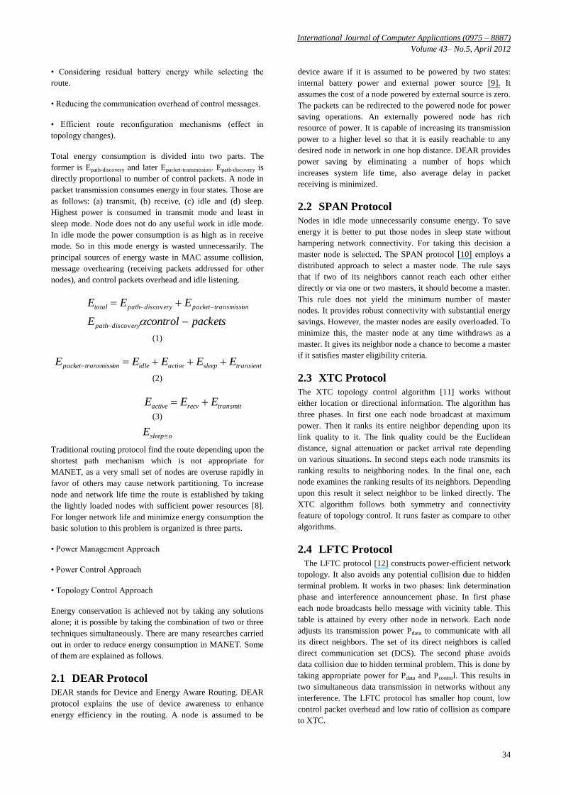
Figure 3: average end-to-end delay vs. No. of packets

The comparison for end-to-end delay in between DBSS and

LFTC protocol is shown in Figure 3. It is observed from the

figure that the end to end delay in our proposed scheme is

lesser than that of existing approach. This is because in

proposed scheme as less number of nodes are taking part in

packet transmission, so the packet needs to travel less hops,

resulting the average end-to-end delay is minimized.

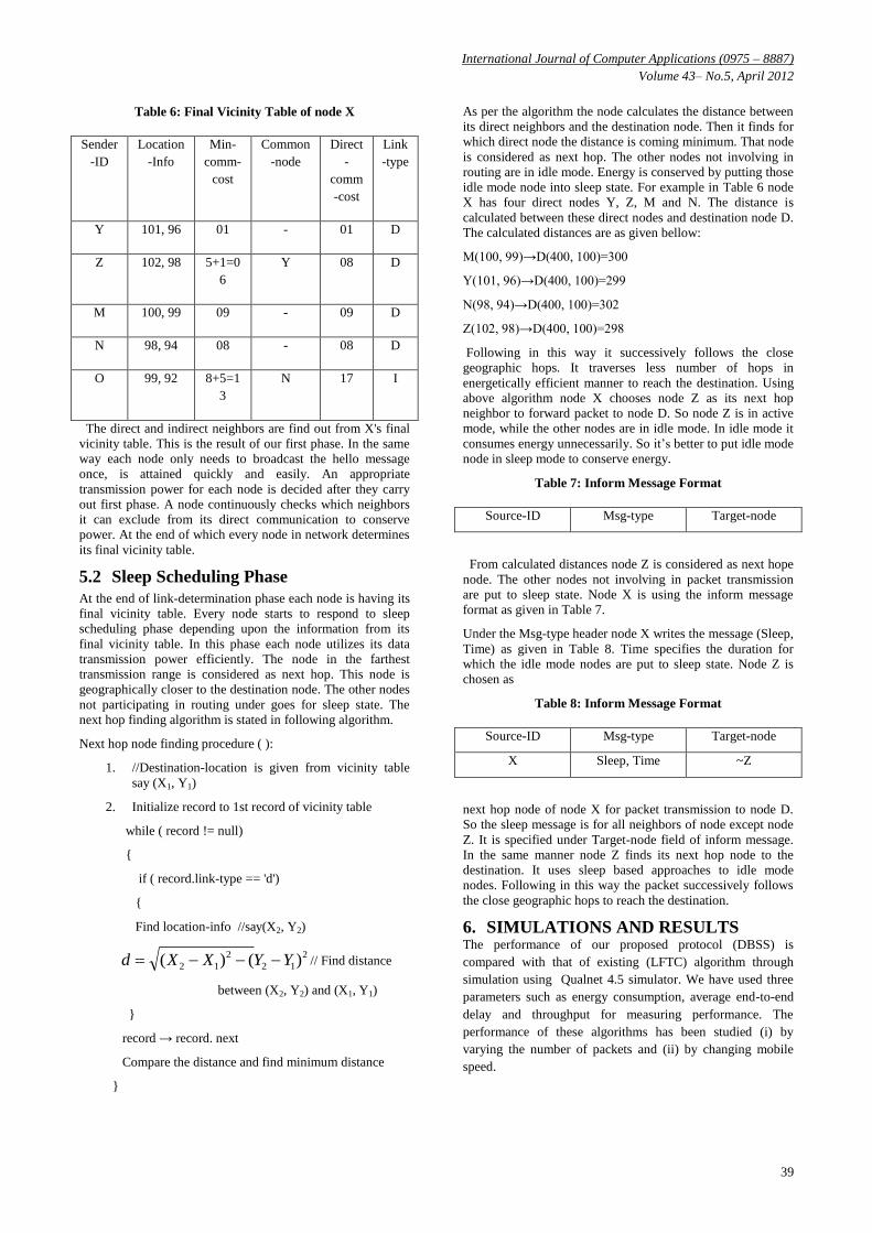
Figure 4: Throughput vs. No. of packets

The graph for throughput vs. no. of packets is plotted in

Figure 4. It is observed from the figure that the throughput in

our proposed scheme is lesser than that of the existing scheme

for packet number 100 to 900. From 1000 packets both the

proposed and existing scheme gives same throughput.

6.2 By Varying Mobile speed

In this simulation speed of node is varied by keeping number

of packets constant at 1000. Performance metrics considered

for comparison are: (1) Energy consumption vs. maximum

speed (2) End to end delay vs. maximum speed and (3)

Throughput vs. maximum speed. Parameters considered for

simulation is shown in Table 10.

100 200 300 400 500 600 700 800 900 10000

2

4

6

8

10

12

14

16

No. of Packets

Tota

l energ

y c

onsum

ption in m

joule

in (

10

-2)

DBSS

LFTC

100 200 300 400 500 600 700 800 900 10001.5

2

2.5

3

3.5

No. of Packets

End-t

o-e

nd d

ela

y in s

ec (

10

-2)

DBSS

LFTC

100 200 300 400 500 600 700 800 900 10004.09

4.1

4.11

4.12

4.13

4.14

4.15

4.16

4.17

4.18

No. of Packets

Thro

ughput

in b

its/s

ec (

10

3)

DBSS

LFTC

International Journal of Computer Applications (0975 – 8887)

Volume 43– No.5, April 2012

41

Table 10: Simulation Parameters

Parameter Value

Terrain Co-ordinates 1000, 1000 m2

Simulation Time 30 min

Maximum nodes 8

Routing protocol AODV

Traffic CBR

Item size 512 bytes

No. of Packets 1000

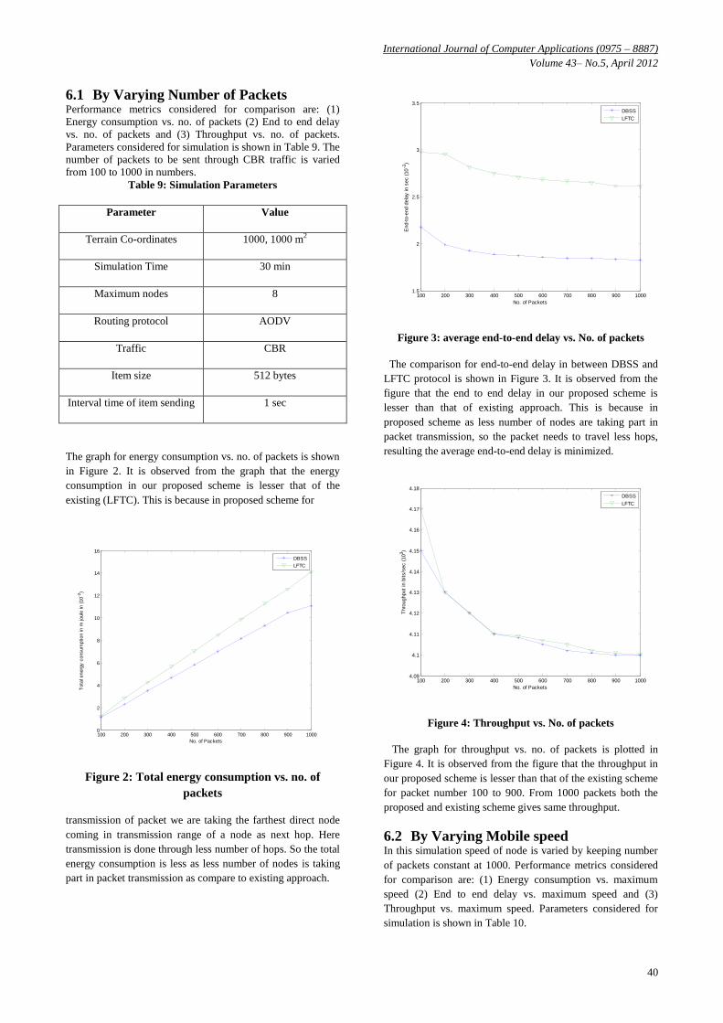
In the mobile condition of the node the comparison is studied

for the energy consumption between DBSS and LFTC

protocol.

Figure 5: Total energy consumption vs. Maximum speed

It is observed from Figure 5 that the energy consumption in

our proposed scheme is lesser that of the existing (LFTC).

This is because in proposed scheme for transmission of packet

we are taking the farthest direct node coming in transmission

range of a node as next hop, so transmission is done through

less number of hops, so the total energy consumption is less as

less number of nodes are taking part in packet transmission as

compare to existing approach.

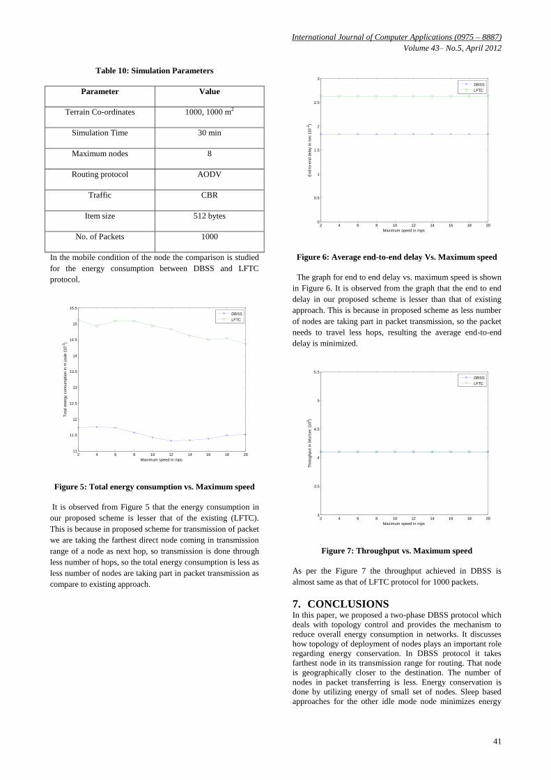
Figure 6: Average end-to-end delay Vs. Maximum speed

The graph for end to end delay vs. maximum speed is shown

in Figure 6. It is observed from the graph that the end to end

delay in our proposed scheme is lesser than that of existing

approach. This is because in proposed scheme as less number

of nodes are taking part in packet transmission, so the packet

needs to travel less hops, resulting the average end-to-end

delay is minimized.

Figure 7: Throughput vs. Maximum speed

As per the Figure 7 the throughput achieved in DBSS is

almost same as that of LFTC protocol for 1000 packets.

7. CONCLUSIONS In this paper, we proposed a two-phase DBSS protocol which

deals with topology control and provides the mechanism to

reduce overall energy consumption in networks. It discusses

how topology of deployment of nodes plays an important role

regarding energy conservation. In DBSS protocol it takes

farthest node in its transmission range for routing. That node

is geographically closer to the destination. The number of

nodes in packet transferring is less. Energy conservation is

done by utilizing energy of small set of nodes. Sleep based

approaches for the other idle mode node minimizes energy

2 4 6 8 10 12 14 16 18 2011

11.5

12

12.5

13

13.5

14

14.5

15

15.5

Maximum speed in mps

Tota

l energ

y c

onsum

ption in m

joule

(10

-2)

DBSS

LFTC

2 4 6 8 10 12 14 16 18 200

0.5

1

1.5

2

2.5

3

Maximum speed in mps

End-t

o-e

nd d

ela

y in s

ec (

10

-2)

DBSS

LFTC

2 4 6 8 10 12 14 16 18 203

3.5

4

4.5

5

5.5

Maximum speed in mps

Thro

ughput

in b

its/s

ec (

10

3)

DBSS

LFTC

International Journal of Computer Applications (0975 – 8887)

Volume 43– No.5, April 2012

42

consumption of the network. The proposed DBSS protocol is

compared with LFTC using Qualnet 4.5 simulator. Simulation

results proved that our DBSS protocol has a good energy

conservation performance. DBSS also performs better in

context of average end-to-end delay without much affecting

the throughput.

8. ACKNOWLEDGEMENTS This research was supported by project grant Vide No:

13(1)2008-CC&BT of Ministry of Communication &

Information Technology, Dept of IT, Government of India,

titled “ Energy Aware Protocol for Wireless Networks” and

being carried out at department of Computer Science and

Engineering, NIT Rourkela.

9. REFERENCES [1] S. Rout, A.K. Turuk and B. D. Sahoo, “Energy

Efficiency in Wireless Network: Through Alternate path

Routing”, in proceedings of Fourth Innovative

conference on Embedded Systems, Mobile

Communication and Computing, July 2009, pp.-3-8.

[2] S. Rout, A. K. Turuk and B. D. Sahoo, “Energy

Efficiency in Wireless Ad hoc Network using

Clustering”, in proceedings on 12th International

Conference on Information Technology, December 2009,

pp.-223-226.

[3] S. K. Sarkar, T. G. Basavaraju, and C. Puttamadappa,

“Ad Hoc Mobile Wireless Networks”, Auerbach

Publications, 2007

[4] P. Santi, “Topology Control in Wireless Ad Hoc and

Sensor Networks”, John Wiley $ Sons, Ltd., 2006.

[5] S.-L. Wu and Y.-C. Tseng. “Wireless Ad Hoc

Networking”. Auerbach Publications, 2007.

[6] M. Tarique, K. E. Tepe, and M. Naserian. “Energy

Saving Dynamic Source Routing for Ad Hoc Wireless

Networks”. Proceedings in Third International

symposium on Modeling and Optimization in Mobile Ad

Hoc, and Wireless Networks, Canada, pages 305-310,

April 2005.

[7] E. M. Royer and C. K. Toh. “A Review of Current

Routing Protocol for Ad Hoc Mobile Wireless

Networks”. Proceedings in IEEE Personal

Communication Magazine, 6(2): 46-55, April 1999.

[8] N. Gupta and S. R. Das. “Energy-Aware On-Demand

Routing for Mobile Ad Hoc Networks”. Proceedings of

the4th International Workshop on Distributed

Computing, Mobile and Wireless Computing, Lecture

notes in computer Science, 2571: 164-173, January 2002.

[9] A. Avudainayagam, W. Lou, and Y. Fang. “DEAR: A

Device and Energy Aware Routing protocol for

Heterogeneous Ad Hoc Networks”. Proceedings in

Academic press Journals of Parallel and Distributed

Computing, 63(2): 228-236, February 2003.

[10] B. Chen, K. Jamieson, H. Balakrishnan, and R. Morris.

“Span: An Energy-Efficient Coordination Algorithm for

Topology Maintenance in Ad Hoc Wireless Networks”.

Proceedings in Academic Publishers of Wireless

Networks, 8(5): 481-494, September 2002.

[11] S. Banerjee and A. Misra. “XTC: A Practical Topology

Control Algorithm for Ad-Hoc Networks”. Proceedings

in 18th International Symposium on Parallel and

Distributed Processing, Switzerland, 216-223, April

2004.

[12] J.-P. Sheu, S.-C. Tu, and C.-H. Hsu. “Location-Free

Topology Control Protocol in Wireless Ad Hoc

Networks”. Computer Communications, 31(14): 3410-

3419, 2008.

[13] X. Shen and L. Meng, “Energy-Aware Routing Protocol

in Fading Channel for Mobile Ad Hoc Networks”,

Proceedings in IEEE International conference on

Information Theory and Information Security, 871-875,

December 2010.

[14] D. Zappala. “Alternate Path Routing for Multicast”.

Proceedings in IEEE/ACM Transactions on Networking,

12(1): 30-43, February 2004.

[15] S.-L. Wu, Y.-C. Tseng, and J.-P. Sheu. “Intelligent

Medium Access for Mobile Ad Hoc Networks with Busy

Tones and Power Control”. IEEE Journal on Selected

Areas in Communications, 18(9): 1647-1657, 2000.

[16] Y. Xu, J. Heidemann, and D. Estrin. “Geography-

Informed Energy Conservation for Ad Hoc Routing”.

Proceedings of the 7th annual International Conference

on Mobile Computing and Networking, Rome, Italy, 70-

84, July 2001.