Smart identification of MANET nodes using AODV routeing ...
151
i Smart identification of MANET nodes using AODV routeing protocol By Govand Salih Kadir Department of Applied Computing University of Buckingham November 2016 A Thesis submitted in fulfilment of the requirements for the Degree of Doctor of Philosophy ( DPhil.)
-
Upload
khangminh22 -
Category
Documents
-
view
0 -
download
0
Transcript of Smart identification of MANET nodes using AODV routeing ...
i
Smart identification of MANET nodes
using AODV routeing protocol
By
Govand Salih Kadir
Department of Applied Computing
University of Buckingham
November 2016
A Thesis submitted in fulfilment of the requirements for the Degree of Doctor of Philosophy ( DPhil.)

ii
Abstract
MANET routeing protocols can be either straightforward focusing on establishing and
maintaining the path only, or too sophisticated with heavy key-based
authentication/encryption algorithms. The consequence for both cases creates issues in
the QoS implementation of MANET. This thesis focuses on providing three
enhancements to the well-known AODV routeing protocol, without altering the
functionality or impeding its performance. It proposes a scheme that improves AODV
routeing discovery process without the overhead associated with integrity/authenticity
that we called SIMAN (Smart Identification for Mobile Ad-hoc Networks).
First, SIMAN introduces a prime number based mathematical algorithm in a thin layer
between the communication links of the IP layer of the AODV routeing protocol. The
algorithm replaces existing AODV “retrieval of node addresses” from the routeing table,
with a “prime factorization of two values”. These two values are calculated during the
RREP process, and thus enhances the AODV routeing protocol to provide knowledge of
nodes in the RREP path beyond neighbouring nodes that are out of the transmission range.
The second SIMAN enhancement is to attach the node’s geographical coordinates to
the RREP message to enable the trilateration calculation of newly joined nodes. This
process enhances AODV further by providing the nodes with the knowledge of the
physical location of every node inside the path. Consequently, by combining both
enhancements, AODV can have abstract authentication to prevent from hidden nodes like
wormholes.
The final enhancement is to enable SIMAN to construct most efficient paths with
nodes that have high battery energy. This is achieved by adding each node’s battery level
to the RREP message, where the source will examine the available knowledge of the
possible routes that can work efficiently without disconnections or link breakage.
The OPNET simulation platform is used for the implementation, verification and
testing of this scheme. The results show that the AODV route discovery procedure was
not affected in function or performance by our scheme and that the overhead caused by
our three enhancements has improved the performance of AODV in certain conditions.

iii
Declaration
I hereby declare that except where specific reference is made to the work of others, the
contents of this thesis are original and have not been submitted in whole or in part for
consideration for any other degree or qualification in this, or any other University. This
thesis is the result of my own work and includes nothing which is the outcome of work
done in collaboration, except where specifically indicated in the text.
Govand Salih Kadir
2016

iv
Acknowledgements
What a journey!
I am very grateful for the challenges therein and the support that I have received.
Dr. Ihsan Lami, my research supervisor, remained a great source of inspiration for me
throughout this project. His dedication, scientific approach and scholarly advice helped
me to complete this research, for all he did for me; I have a great sense of gratitude and
will remain ever thankful to him. I would also like to express my sincere thanks to Dr
Sabah Jassim, Professor, for his exceptional guidance, ideas and continuous support
during the research work.
I would like to thank my family. I am very grateful for the continuous love and
support from my Mum, brothers, sisters and of course Aya. But most of all, I would like
to thank my dear Medya and my Hasto, for always being there for me, and cheering me
up in troublesome times during the work on this thesis.
Finally, to the memorial of my mentor, my beloved father Salih Kadir who died
last year, he was and always my number one……. I miss you, DAD.

v
Acronyms and abbreviations
AODV Ad-Hoc On-demand Distance Vector
Bridging nodes MANET nodes recently joined the network have any IP addresses
DSR Dynamic Source Routeing
Friend nodes MANET nodes known to each other have prime IP address
GCD Great Common Division
GPS Global Positioning System
MANET Mobile Ad-hoc Network
OLSR Optimum Link State Routeing
OPNET OPtimized Network Engineering Tools
OSI Open System Interconnection model
PDR Packet Delivery Ratio
PIPHN Prime-IP Host Number
PPN Prime Product Number
prime-DHCP Dynamic Host Configuration Protocol for prime IP addresses
Prime-IP IP address with prime host number
QoS Quality of Service
RBE Remaining Battery Energy
RDT Route Discovery Time
RREP Route Reply message
RREQ Route Request message
S-Flag Siman Flag
SIMAN Smart Identification for Mobile Adhoc Networks
WH Wormhole
ZRP Zone Routeing Protocol

vi
List of Figures
2.1: Mobile Ad-Hoc Network scenario. ............................................................... 8
2.2: MANET routeing protocol classification ....................................................... 9
3.1: RREQ message broadcasting in a MANET scenario. ................................. 27
3.2: Extended RREP message format to accommodate the PPN values. ............ 28
3.3: The RREP message path in MANET scenario. ........................................... 29
3.4: The RREP process for SIMAN algorithm. .................................................. 30
3.5: Data transmission for AODV routeing protocol. ......................................... 31
3.6: Data transmission for SIMAN algorithm. .................................................... 32
3.7: MANET scenario: a group of Friend nodes leaving basecamp. .................. 33
3.8: MANET scenario: Friend nodes split into clusters. ..................................... 34
3.9: RREP process executed by destination node in SIMAN algorithm. ........... 37
3.10: RREP process for Friend nodes in SIMAN algorithm. .............................. 38
3.11: RREP message passed by Bridging nodes in SIMAN scenario. ............. 39
3.12: Data transmission process for network with Bridging nodes .................... 41
4.1: SIMAN algorithm inside the OSI hierarchy for a MANET node. ............... 45
4.2: SIMAN enabled attribute for MANET nodes. ............................................. 46
4.3: Wormhole model for the OPNET Modeler. ................................................ 47
4.4: Manual configuration of the node’s initial battery energy. .......................... 48
4.5: SIMAN algorithm placement inside the node model................................... 49
4.6: The route between nodes 3 and 109 in MANET scenario. .......................... 51
4.7: MANET scenario-2 with different network layouts. ................................... 52
4.8: Scenario-3 clusters connected through Bridging nodes. .............................. 53
4.9: MANET scenario-4 with different network layouts. ................................... 54
4.10: Scenario-1, route discovery time for various data rates. ............................ 55
4.11: Scenario-1, packet retransmission attempts. .............................................. 56
4.12: Scenario-1, End to end delay. .................................................................... 57
4.13: Scenario-2, route discovery time in different layouts. ............................... 58
4.14: Scenario-2, route discovery time with different mobility speeds. ............. 58
4.15: Scenario-2, route discovery time with various node distances. ................. 59
4.16: Scenario-3, route discovery time with different data rates. ....................... 60
4.17: Scenario-3, route discovery time in different layouts. ............................... 61

vii
5.1: Three types of wormhole attacks. ................................................................ 65
5.2: The sequence of Friends and Bridging nodes during RREP process. .......... 67
5.3: Three circle intersection used to calculate Bridging node location. ............ 68
5.4: Scenario-1, the RREP message path through nodes (A-C-B-D) ................. 70
5.5: Scenario-2, the RREP message path through nodes (A-B-C-D) ................. 70
5.6: The coordiantes measurment for a Bridging node using trilateration. ......... 72
5.7: The coordinate measurment for two consecutive Bridging nodes. .............. 76
5.8: RREQ message format for SIMAN algorithm with location. ...................... 79
5.9: The RREQ process for SIMAN and coordinate measurement. ................... 80
5.10: RREP message format in SIMAN enhancement with location. ................ 81
5.11: The RREP process for SIMAN and coordinate measurement. ................. 82
5.12: MANET scenario with two WH nodes. ..................................................... 83
5.13: Scenario-1 MANET network layout. ......................................................... 87
5.14: Scenario-1, AODV route discovery without WH attack. .......................... 89
5.15: Scenario-1, AODV route discovery with open WH attack. ....................... 90
5.16: scenario-1: SIMAN route discovery with open WH attack. ...................... 91
5.17: Scenario-1, AODV route discovery with half-open WH attack. ............... 92
5.18: Scenario-1, AODV route discovery with Closed WH attack. ................... 93
5.19: Scenario-1, route discovery time with various data rates. ......................... 94
5.20: Scenario-1, End to end delay. .................................................................... 94
5.21: Scenario-2, the established path for various layout using AODV. ............ 95
5.22: Scenario-2, the established path for various layout using SIMAN. ........... 96
5.23: Scenario-2, route discovery time for different layouts. ............................. 97
5.24: Scenario-2 End to end delay for the five layouts. ...................................... 98
6.1: RREP message format with RBE enhancement in SIMAN. ..................... 104
6.2: A network scenario for SIMAN algorithm with RBE. ............................. 105
6.3: Initial RREQ process for SIMAN with RBE. ............................................ 106
6.4: Initial RREQ by SIMAN with RBE ........................................................... 107
6.5: Initial RREP for SIMAN with RBE. .......................................................... 107
6.6: Path lowest RBE measuring ....................................................................... 108
6.7: Exclude node RREQ process in SIMAN with RBE. ................................. 109
6.8: Second RREQ and RREP attempt with one excluded node. ..................... 110
6.9: Third RREQ and RREP attempt with two excluded nodes. ...................... 110
6.10: Final RREQ with excluded nodes. ........................................................... 111
6.11: Source analysis procedure to construct a new path.................................. 112

viii
6.12: Different level neighbours in paths to destination node .......................... 113
6.13: RREQ sent by source node with inclusion list ......................................... 114
6.14: The inclusion RREQ process in SIMAN. ................................................ 115
6.15: Scenario-1 network setup. ........................................................................ 116
6.16: Scenario-2, twenty node MANET with five Bridging nodes. ................. 117
6.17: Scenario-1, SIMAN route discovery. ....................................................... 118
6.18: Scenario-1 AODV route discovery. ......................................................... 118
6.19: Scenario-1, route discovery time with various data rates. ....................... 119
6.20: Scenario-1, packet delivery ratio. ............................................................ 119
6.21: Scenario-1, End to end delay. .................................................................. 120
6.22: Scenario-2, the established path for SIMAN algorithm. .......................... 121
6.23: Scenario-2, the established path for AODV. ........................................... 121
6.24: Scenario-2, packet delivery ratio. ............................................................ 122
6.25: scenario-2, End to end delay. ................................................................... 122

ix
List of Tables
2.1: Comparison of MANET routeing protocol .................................................. 15
2.2: Comparison of QoS solutions for MANET routeing ................................... 20
4.1: The characteristics of the two network scenario .......................................... 51
4.2: Scenario-2 number of hops per route ........................................................... 57
5.1: The coordinates of nodes in scenario-1 ....................................................... 87
5.2: Scenario-1 simulation parameters ................................................................ 88
5.3: Compersion for the routes established for AODV and SIMAN .................. 97
6.1: Scenario-1 simulation parameters. ............................................................. 116

x
Table of Contents
: Introduction ................................................................................................ 1
1.1 Problem statement ................................................................................................... 3
1.2 Thesis contributions ................................................................................................. 3
1.3 Thesis Organization ................................................................................................. 4
1.4 Summary .................................................................................................................. 5
: A review of QoS in MANET ..................................................................... 6
2.1. Mobile Ad-hoc Wireless Networks ......................................................................... 6
2.2. Review of MANET routeing protocols ................................................................... 9
2.2.1. Flat routeing protocols ............................................................................. 10
2.3.2. Hybrid and Hierarchical routeing protocols ............................................ 12
2.3.3. Geographically aided routeing protocols ................................................. 14
2.4. Quality of service in MANET ............................................................................... 16
2.4.1. QoS performance metrics ........................................................................ 16
2.4.2. MANET QoS routeing protocols ............................................................. 17
2.5. Summary ................................................................................................................ 21
: Smart Identification of MANET Nodes ................................................. 22
3.2. Literature review .................................................................................................... 23
3.3. Conceptual design of SIMAN ............................................................................... 26
3.4. SIMAN algorithm scheme ..................................................................................... 27
3.5. SIMAN’s non-prime IP addresses enhancement. .................................................. 33
3.5.1. Route discovery process improvement .................................................... 36
3.5.2. Data transmission update ......................................................................... 40
3.6. Summary ................................................................................................................ 42

xi
: SIMAN Implementation .......................................................................... 43
4.1. OPNET Modeler .................................................................................................... 44
4.2. SIMAN algorithm Simulation and Results ............................................................ 49
4.2.1. Network Scenarios ................................................................................... 50
4.2.2. Results and analysis ................................................................................. 54
4.3. Summary ................................................................................................................ 61
: SIMAN enhancement with location ....................................................... 62
5.1. Literature review .................................................................................................... 63
5.2. Wormhole attacks .................................................................................................. 65
5.3. Conceptual design .................................................................................................. 66
5.3.1. Distance measurement ............................................................................. 66
5.3.2. Bridging node coordinates measurement ................................................ 67
5.4. SIMAN with location implementation .................................................................. 78
5.5. Simulations and Results ......................................................................................... 86
5.5.1. Network Scenarios ................................................................................... 87
5.5.2. Results and analysis ................................................................................. 89
5.6. Summary ................................................................................................................ 98
: SIMAN with remaining battery energy ................................................. 99
6.1. Literature review .................................................................................................. 100
6.2. Conceptual design ................................................................................................ 101
6.3. SIMAN with RBE implementation ..................................................................... 104
6.4. Simulations and Results ....................................................................................... 114
6.4.1. Network Scenarios ................................................................................. 115
6.4.2. Results and analysis ............................................................................... 117
6.5. Summary .............................................................................................................. 123

xii
: Conclusion and future direction ........................................................... 124
7.1. Conclusion ........................................................................................................... 124
7.2. Future work and research area ............................................................................. 125
References .................................................................................................................. 127
: Simulation results ............................................................................... A-1
SIMAN Algorithm ............................................................................................... A-1
A.1.1 Scenario-I .............................................................................................. A-1
A.1.2 Scenario-II ............................................................................................. A-1
A.1.3 Scenario-III ............................................................................................ A-2
A.1.4 Scenario-III ............................................................................................ A-2
SIMAN algorithm with Location ........................................................................ A-2
A.2.1 Scenario-I .............................................................................................. A-2
A.2.2 Scenario-II ............................................................................................. A-3
SIMAN Algorithm (with RBE) ........................................................................... A-4
A.3.1 Scenario-I .............................................................................................. A-4
A.3.2 Scenario-II ............................................................................................. A-4

1
Introduction
In the past decade, we have witnessed a major shift toward wireless communication,
which helps people to stay connected while they are on the move. Mobile Ad-hoc
Networks MANET emerged as the promising technology that provides infrastructure-less
networks that do not require central management entities. Current wireless devices like a
smartphone can use MANET to form a network, exchange data, and later disjoin without
prior notification or permission.
At the start of this research project, my focus was to study the functionality of
MANET routeing protocols, and ways to adopt it for cooperative smartphones MANET
networking when the cellular link is lost in some areas. A further study directed me
toward Quality of Service (QoS) support for real-time MANET communication, which is
hard to achieve with best effort service provided through the routeing protocols.
QoS provisioning requires all members of the transmission path to commit to
delivering the intended service. This requires MANET nodes inside the transmission path
to share QoS metrics such as (Bandwidth and Delay) and adjust the resource accordingly.
Apparently, this does not work very well with MANET, as the routeing protocols
implement the hop-by-hop concept that has limited knowledge of other nodes beyond its
neighbours. Achieving this knowledge requires further processing that increases
overhead, and/or applies tied restriction that is against the freedom of nodes in MANET.
Accordingly, after studying various routeing algorithms by the standards and other
researchers’ contributions reviewed in section (2.3), we have identified that “reactive
routeing protocols” could perform better in comparison to proactive protocols. In term of
the on-demand nature of the route discovery process and the reduced routeing table size
that is limited to the discovered path. Therefore, we focused on formulating a method that

Chapter 1: Introduction
2
provides the knowledge beyond its neighbour and does not affect the performance or
degrade the capability of reactive routeing protocols. This concept has led us to study the
mathematical concept of prime factorization theory and design a thin layer that can be
combined with Ad-hoc On-demand Distance Vector (AODV) routeing protocol. This
layer replaces AODV addressing services provided to the IP layer, as explained in section
(4.2.1). Furthermore, we have concluded that Prime-IP Host Number (PIPHN) was the
best candidate to achieve the mentioned knowledge. This is accomplished by calculating
two variables, used to identify the sequence of nodes in an AODV path.
To prove our hypothesis, we needed a networking simulation environment to
implement scenarios and justify results. For this purpose, we selected OPNET modular;
a commercial simulation software used by engineers in the communication industry. The
implementation process and scenarios used to prove this are in section (4.3). The results
show a much-needed improvement in the AODV function with negligible overhead on
its performance.
Capitalising on this achievement, we then investigated the possibility to improve this
attainment of adding the ability for the inclusion of nodes with none-PIPHN.These nodes
act as critical Bridging nodes that connect different node-clusters inside the network. We
managed to enhance the algorithm by permitting PIPHN -nodes inside the routeing path
to generate prime IDs for the Bridging nodes.
Our further investigation has concluded that adding a geographical localisation for the
connected nodes as part of the PIPHN process, will enhance the knowledge beyond
neighbours, through sharing the physical location of the nodes inside the selected path.
Additionally, the feature helps the source node to eliminate wormhole attacks by
measuring the distance between nodes. The finding and results of this improvement are
written in a paper that will be published shortly.
This promising result has encouraged us to explore QoS-aware routeing protocols in
section 2.4 and adopt the idea of sharing performance metrics between nodes.
Accordingly, we improve SIMAN algorithm to share the remaining battery energy (RBE)
between nodes and let the source node make the necessary analysis to construct a path
with the highest RBE. The results successfully eliminated nodes with low RBE that might

Chapter 1: Introduction
3
lead to link break. The outcomes show that routeing delay has been reduced by 20% and
packet delivery ratio by 11% on average (see section 6.5).
1.1 Problem statement
QoS provisioning in MANET is a complex task, due to the challenges caused by MANET
design. This is because of the dynamic nature and mobility of devices that requires
updating routeing records frequently. Additionally, QoS implementation needs further
procedures by MANET nodes that cannot afford, due to limited battery resources.
Therefore, researchers have aimed to design protocols/algorithms, capable of sharing
the required QoS parameters without causing much overhead. However, such
contributions require nodes to have knowledge about others inside the transmission path,
which does not exist. Therefore, this challenge/issue has motivated us to develop an
algorithm that uses the existing routeing protocol procedures to obtain the mentioned
knowledge, with minimum overhead impact.
1.2 Thesis contributions
Several contributions regarding the knowledge beyond neighbours and its influence
toward achieving QoS in MANET, is reported in this thesis, which can be identified as:
i. A proven (simulated and verified) mathematical concept used to develop an
algorithm called Smart Identification of Mobile Ad-hoc Networks (SIMAN) to
calculate two values used to determine the address of nodes inside the path using
PIPHN. These two values were shared using route reply (RREP) messages of the
AODV routeing protocol. This work has been published in the international journal
of network security, with a title “SMPR: A Smartphone Based MANET Using Prime
Numbers to Enhance the network nodes Reachability and Security of Routeing
Protocols”, Dec. 2015. [1]
ii. Thereafter, this concept was upgraded to use none-PIPHN in the algorithm that
allows critical Bridging nodes to connect different clusters. The detail of the
implementation was presented and published in the 3rd World Conference on

Chapter 1: Introduction
4
Computer Applications and Information Systems, with a title “SIMAN: a Smart
Identification of MANET Nodes used by AODV routeing algorithm”, Jan. 2016 [2].
iii. SIMAN was then enhanced further to use geographical location information to share
the coordinate of the nodes inside the path. As part of this process, the source node
conducts distance measurements to detect and isolate various wormhole attacks.
This work will be published this year.
iv. Supported by the knowledge of the identity and the physical location of nodes,
SIMAN was enhanced further, to share the node RBE, so the source node analyses
different routes and builds a path consisting of nodes with the highest RBE that
prevent a link break.
1.3 Thesis Organization
The remaining chapters of this thesis are organised as follows:
Provides a background review of QoS implementation to MANET, by exploring the
MANET characteristics and its routeing protocols. Then make a comparison between
them for different performance metrics. This was followed by studying QoS solutions
designed for MANET and comparing the effect of adding performance metrics used
to enhance the routeing protocols.
Chapter 3 introduces the proposed SIMAN algorithm and provides a literature review
of the ideas used to share knowledge beyond neighbours, followed by the conceptual
design of the theoretical model used for the algorithm.
Chapter 4 describes the implementation of the algorithm using OPNET simulation
modular, then testing it with different scenarios and analysing the results.
Chapter 5 introduces an enhancement to the algorithm with node localisation
information. Starting with a review of the work done in this area, followed by the
theoretical calculation of the coordinates of the nodes and distance measurements.
The proposed improvement was executed and tested for different wormhole attacks.
Chapter 6 applies further improvement by introducing the RBE of the nodes inside
the transmission path. We review the methods employed to measure the residual
energy of the nodes. We then present the conceptual design to produce a simple model

Chapter 1: Introduction
5
to measure the RBE and implemented with SIMAN algorithm. Two scenarios are
used to test the source node’s construction of a path with the highest RBE.
Chapter 7 concludes the work presented in the thesis and sets the guidelines for future
work on this algorithm.
1.4 Summary
To summarise, this thesis proposes SIMAN algorithm that enhances the performance of
AODV routeing protocol with negligible overhead. This is achieved by using a
mathematical concept to share node’s prime IP address with others and provide
knowledge beyond neighbours inside the established path, without any alteration to the
routeing protocol functionality.
Additionally, the uniqueness of the prime factors provides abstract authentication
indirectly without applying any key-based security encryption. Then the algorithm was
boosted with the knowledge of the location and remaining battery power of the nodes
inside the path. To enable the source node to eliminate wormholes, and to examine
different paths to construct a route from nodes with the highest energy level that prevents
disconnection caused by node failure.

6
A review of QoS in MANET
During early days of MANET, most routeing protocols were designed to provide best
efforts service. However, the advancement in mobile device capabilities and growing
demand for real-time traffic (video sharing, internet gaming, and VOIP), requires more
than the best-effort service. Therefore, improving the routeing protocols to support QoS
has attracted researchers to explore different methods to improve the data transmission in
MANET, without causing extra overhead.
In this chapter, the author:
Provides an overview of MANET’s structure and characteristics, followed by an
assessment of the challenging issues that has to be considered during improvement
process.
Classify MANET routeing protocols and explain their operation and performance,
and then provides a comparison study between these routeing protocols in terms of
design, and behaviour.
Review QoS implementation issues in MANET and explain the performance metrics
that has to be considered when implemented to MANET.
Explore the solutions that attempted to provide these required metrics and make a
comparison between them.
2.1. Mobile Ad-hoc Wireless Networks
Wireless networking popularity is rising due to the freedom of movement and versatility
of technologies available. Devices in the wireless network use different radio frequency
Chapter 2: A review of QoS in MANET
7
ranges for their communication signals. These signals have limited power and lose
strength over a certain distance. Therefore, these devices have to be in transmission range
to detect each other's signal. The transmission capability and the rule that governs signal
power are managed by the Medium access control protocols for the various technologies,
which is beyond the scope of this work. Further details are found in [3].
Typically, mobile devices stay connected to their networks through fixed access points
(base stations, Wi-Fi access points) that have the duty of handling the routeing process
between the sender and the receiver. Meanwhile, the emergence of powerful devices like
smartphones, and the demand for further freedom and mobility have increased, turning
the focus to alternative technologies that do not require a fixed access point. MANET
emerges as a possible solution for facilitating this communication/connectivity [4].
Mobile Ad-hoc NETworks MANET, are wireless networks that have no infrastructure
and central management system. Moreover, it is designed from a collection of nodes
(mobile wireless devices), with a dynamic topology that changes all the time. In a typical
MANET, these nodes can join or leave the network without prior arrangement. Unlike
traditional wired networks, MANET does not have any routers (wireless devices that
conduct the routeing duties in the network). Therefore, none of the existing infrastructure
routeing protocols works for MANET.
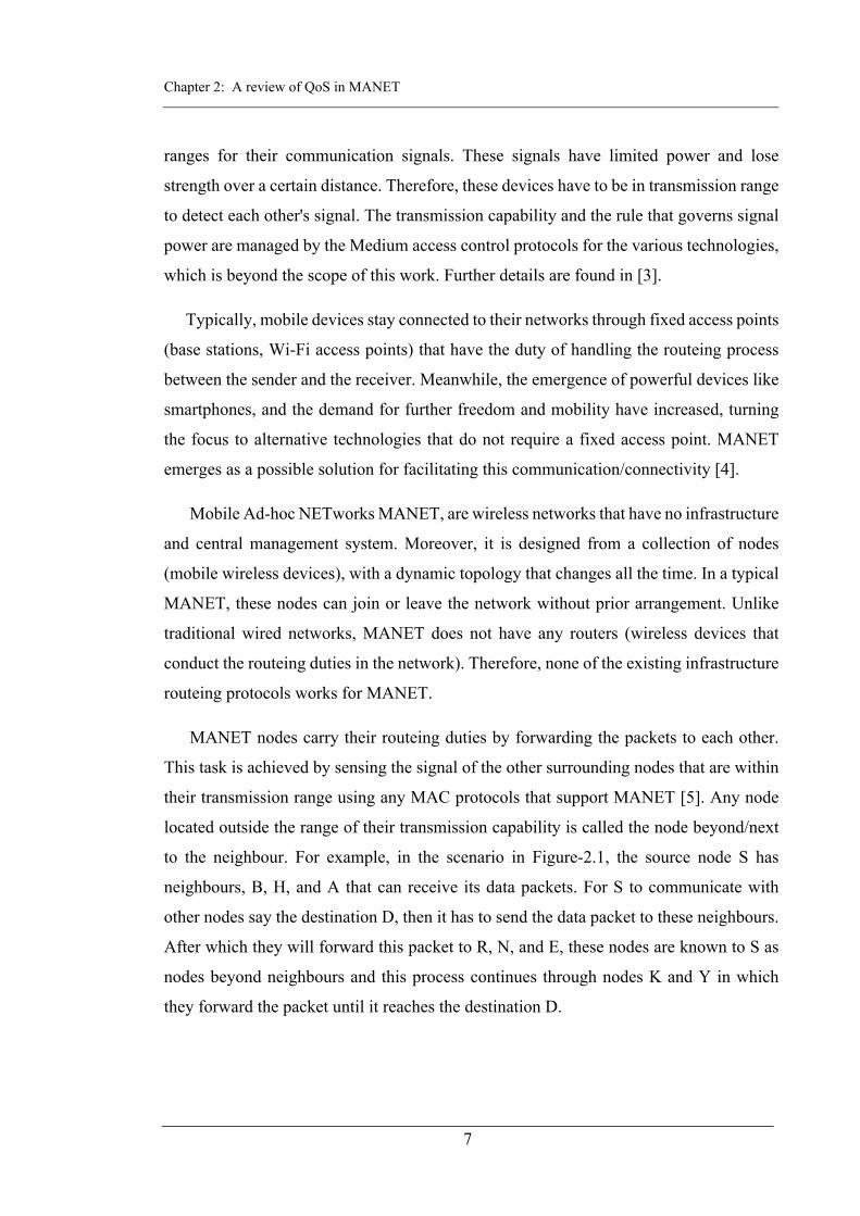
MANET nodes carry their routeing duties by forwarding the packets to each other.
This task is achieved by sensing the signal of the other surrounding nodes that are within
their transmission range using any MAC protocols that support MANET [5]. Any node
located outside the range of their transmission capability is called the node beyond/next
to the neighbour. For example, in the scenario in Figure-2.1, the source node S has
neighbours, B, H, and A that can receive its data packets. For S to communicate with
other nodes say the destination D, then it has to send the data packet to these neighbours.
After which they will forward this packet to R, N, and E, these nodes are known to S as
nodes beyond neighbours and this process continues through nodes K and Y in which
they forward the packet until it reaches the destination D.

Chapter 2: A review of QoS in MANET
8
Figure 2.1: Mobile Ad-Hoc Network scenario.
Characteristics and issues of MANET
In addition to above-described features, MANET has the following challenging issues
that influence the performance of the network [6].
Resource limitation: nodes inside the network are mobile which means they depend
on batteries as a power source with no backup system to support the node. Therefore,
the routeing processes have to avoid extra loads that drain the limited resources.
Bandwidth and link capacity: due to transmission impairments caused by the
openness nature of the wireless medium, the communication link between nodes
varies over time, which leads to the degradation of the signal quality. Additionally,
nodes joining the network adds further traffic load that leads to congestion and
requires a higher network capacity.
Scalability: MANET nodes reliance on limited resources will have serious problems
when the network size increases due to the number of routeing and maintenance
messages exchanged between nodes, which causes congestion and route failure.
Shared physical medium: Since the wireless link is an open access medium, any node
equipped with wireless capabilities can access the wireless link without restriction,
because MANET does not have any access control.

Chapter 2: A review of QoS in MANET
9
Apparently, these characteristics made the designing and improvement of MANET
routeing protocols a challenging task and researchers focused on exploring different
approaches to overcome these tasks.
2.2. Review of MANET routeing protocols
Routeing represents the process of finding a path by the source node to send data to a
destination. It can be static, which is configured to follow a specific path or dynamic
which means the route can change according to node mobility and signal characteristics.
The path setup process and routeing of the traffic are called routeing protocols.
The process of route discovery might be very complex and error prone, because of
node mobility and nodes limited knowledge of others beyond the transmission range. As
a result, it leads to problems like route breaks, which requires extra effort to repair or find
an alternative. Many of MANET routeing protocols were designed a long time ago and
improved over time since [7]. They came in many types and classified according to the
route discovery procedures, and can be grouped into three categories as in Figure-2.2.
Figure 2.2: MANET routeing protocol classification

Chapter 2: A review of QoS in MANET
10
2.2.1. Flat routeing protocols
This type of routeing does not have any predefined structure and nodes pass routeing
information among each other in an even manner without any consideration for the role
or the structure of the network. The aim is to find the best suitable path and it does not
spend any effort on the organisation of the network or the traffic. This category is divided
further into two sub-categories based on the timing of the route discovery.
Proactive protocols also called table-driven represent all protocols that activate once
the network is formed. In which, nodes establish routes with each other and store them
in tables, which is why they are called table-driven. The main advantage is that a route
is available once it is needed which in result reduces delay. Furthermore, an
alternative path is always available when there is a link failure. While the
disadvantage comes in resource consumption caused by routeing table maintenance,
especially in large networks. Additionally, the difficulty in updating routeing tables
that occurs because of node mobility.
Reactive routeing protocols known as On-Demand. It initiates route discovery when
there is data to transmit. The routeing consists of two processes, route discovery, and
route maintenance. Its advantage arises from the minimal routeing information
exchanged that causes less overhead and does not require regular updates. Moreover,
it has simpler routeing tables that require less processing time and resource
consumption. The disadvantage can be realised in the path breakage caused by the
unpredictable and dynamic nature of the network. [8]. In the next section, we review
some of the known routeing protocols in more details.
2.2.1.1. Optimum Link State Routeing Protocol
OLSR is an upgrade of the original Link-state routeing protocol of wired networks. It
relies on routeing tables to store knowledge gathered about the network, before any data
transmission. Moreover, it reduces overhead by limiting the number of neighbouring
nodes (Multipoint Relay MPR) that forward control messages. Moreover, the protocol
uses topology control messages TC to distribute the routeing information among all
nodes. The MPRs then forward the link state information to their MPR selector to

Chapter 2: A review of QoS in MANET
11
calculate the shortest path. Unlike the reactive protocols, this protocol is suitable for large
networks, as the concept of MPR’s works better with the increase in node numbers.
Additionally, the protocol does not require any reliable transfer because of regular update
of the stored information and does not require delivery order since sequence number used
to prevent out of order information [9].
2.2.1.2. Destination-Sequenced Distance Vector Protocol
DSDV is a proactive protocol focuses on destination reachability using the distance vector
concept. This protocol relies on information passed by neighbours and has no view of the
global network. All nodes periodically update the information obtained about various
destinations. Moreover, destination sequence number is used to prevent old information
and count to infinity problem. The protocol reacts rapidly to change in topology by
sending a route advertisement once a change occurs. The nodes advertise routeing
information and its destination sequence number using an even number. If a node found
out that a neighbouring node is not reachable anymore, then it increments the sequence
number on behalf of the unreachable node, using an odd number, and set the hop count
to infinity. When a node receives a route advertisement, then it compares it with the
recorded value, if the sequences are equal, then the route with less hop number is chosen.
This protocol has the advantage of simplicity and lower latency caused by route
discovery. The disadvantage comes from routeing overhead caused by routeing
information that might never be used [10].
2.2.1.3. Ad-Hoc On-demand Distance Vector Protocol
AODV is a reactive protocol based on the distance vector concept of the Bellman-Ford
[11] and the Ford-Fulkerson [12] algorithms for route discovery. The protocol uses a
packet switching mechanism for sending data. The route discovery process relies on route
request RREQ and route reply RREP messages, being exchanged using a UDP which is
passed by intermediate nodes between two end nodes. Once the source node receives the
route reply, then it starts data transmission. The protocol calculates the number of hops
rather than knowing the address of the nodes inside the path. Therefore, intermediate
nodes have no knowledge of others except the neighbours, and it has to maintain the link

Chapter 2: A review of QoS in MANET
12
constantly by sensing each other using a Hello beacon, which is sent periodically. Also,
if an error or link breakage occurred, intermediate nodes attempt to repair the link and
send a route error RERR message back to the source.
One of the important parameters in this process is the destination sequence number,
which handles the freshness of the RREQ, by comparing the received sequence number
with stored records. The RREQ message is processed if the sequence number is equal to
or larger than the current record. Otherwise, the node assumes the packet is old and drops
the message. Another important attribute is the RREQ ID, which along with the source
node IP address, prevents loop back messages and differentiate between many RREQ
attempts to find a path [13].
2.2.1.4. Dynamic Source Routeing Protocol
DSR is pure on-demand protocol based on link-state routeing protocol concept. The
protocol relies on the source node to conduct the routeing. Once the route is discovered,
then the source node inserts the full address list of the nodes inside the path to the data
packet header and then starts the transmission. Every node inside the path would process
the packet if its address were on the list.
The protocol uses the similar on-demand concept to AODV with the exception that it
does not use sequence numbering and routeing tables. Instead, it uses a list of addresses
inserted into RREQ and RREP packets, during route discovery. This feature removes the
dependency on routeing tables to obtain the next hop address. Additionally, the protocol
does not use periodic hello message, which reduces the overhead caused by regularly
sensing the neighbour. The protocol consists of two processes, route discovery and
maintenance process. [14].
2.3.2. Hybrid and Hierarchical Routeing Protocols
This category represents routeing protocols designed for large networks, as flat routeing
protocols encounter problems with an increase in the network size, due to difficulty in
retaining the route [15]. Nodes inside the network classified into two groups according to
their role inside the network:

Chapter 2: A review of QoS in MANET
13
Hybrid protocols group the nodes into zones and use a combination of proactive and
reactive routeing protocols. The topology inside these zones changes less frequently.
Therefore, proactive routeing protocols are used, while rapidly changing intergroup
connections use reactive routeing protocols. Research studies show that hybrid
protocols reduce control traffic and wasted bandwidth. Though its disadvantage
comes from a larger memory requirement caused by storing higher-level topological
information, and the significant overlap in routeing zones [16].
Hierarchical routeing protocols distribute the routeing duties into a multi-level
hierarchy. Nodes are grouped into multi-level clusters, with dynamic cluster head
selection that acts as a local coordinator. The routeing protocol selection depends on
where the node is located in the hierarchy. Nodes inside the cluster maintain local
routeing while cluster heads handle global routeing between clusters reactively. A
comparison study of different hierarchical routeing shows that they perform better
under heavy loads and over a wider coverage area [17]. The main advantage is the
reduction in the routeing table size and the number of routeing messages exchanged.
The disadvantage is in the construction of clusters that causes overhead. Besides, the
cluster head has heavy routeing duties, so it became a bottleneck in the network.
2.3.2.1. Zone Routeing Protocol
ZRP is a hybrid routeing protocol that uses table-driven routeing protocol inside the zone
and on-demand routeing between zones. Usually, in MANET, the source of the data sends
its traffic through the neighbours, which means a route to the neighbours is always
needed. Therefore, it will be ideal to have a proactive approach inside the zone that helps
the nodes to have a regularly updated routeing table. The zone represents the group of
nodes whose minimum distance in hops from a specific node is less than the zone radius.
Furthermore, peripheral nodes are those nodes that have a minimum distance to a specific
node equals to the zone radius [18].
2.3.2.2. Hierarchical State Routeing Protocol
HSR is a distributed multi-level routeing protocol based on the clusters. These clusters
are organised into levels according to the physical structure of the cluster or based on the

Chapter 2: A review of QoS in MANET
14
logical relation. Nodes inside the cluster keep track of others in terms of the connection
status and the topology and this information updated periodically. Cluster leader
broadcasts to the members of the cluster, information about the hierarchical topology of
the network. Every node in the cluster keeps the hierarchical addresses of other nodes
inside the network, in the HSR routeing table.
When a source node wants to establish a path to a destination in another cluster, it
sends the routeing packet to the cluster leader. Which in return sends the packet to the
counterpart cluster leader that has the destination address. Then the other cluster leader
passes the information to the destination node inside its cluster. The advantage of this
protocol is seen in large networks where the routeing table size and updates become a
problem. While the disadvantage comes from the inter-cluster restriction in sharing
information and selecting cluster leaders [19].
2.3.3. Geographically Aided Routeing Protocols
Currently, most wireless devices are equipped with GPS devices.This makes it possible
to reach a specific node using its location rather than relying on other identification
parameters. The source node uses the nodes location, to forward packets to other nodes
that are closer to the destination, without using network addresses or routeing tables. The
advantage of this protocol comes from the directional flooding which reduces the route
request broadcasting to those who are located in the direction of the destination thus
minimising message exchange and reducing overhead [20].
2.3.3.1. Location Aided Routeing Protocol
LAR is an on-demand routeing protocol that relies on source routeing like DSR. The
protocol benefits from the coordination information obtained from GPS-equipped nodes
that share their location with other nodes. Furthermore, it is used by the source node to
direct route requests toward the destination, rather than to flood the message to the whole
network. This minimises the message forwarding, which in result reduces the overhead,
and congestion. The directed flooding estimate conducted by the source node using
previous knowledge of the destination location, and modified according to the node
movement and speed. The expected zone where the source node assumes that the

Chapter 2: A review of QoS in MANET
15
destination is located inside consist of a circle that has a radius length that represents the
time difference before and after the movement of the destination. The source node floods
the message to the entire network if it has no prior information about destination [21].
Overall, we conclude that routeing process in MANT is similar in the general concept
and issues, and the differences can be noticed in the methods used in route discovery, as
it is illustrated in Table-2.1. Nonetheless, we noticed that reactive protocols do perform
better than proactive routeing protocols in terms of routeing updates and freshness of
information. Additionally, AODV among reactive routeing protocols is suitable for
highly dynamic networks and has less overhead. Besides, it maintains the link with
neighbouring nodes regularly using Hello messages [22].
Table 2.1: Comparison of MANET routeing protocol
Property Protocols
OLSR DSDV AODV DSR ZRP HSR LAR
Type Proactive Proactive Reactive Reactive Proactive DV & LS
Proactive LS
Reactive
Routeing metric
Shortest path
Shortest path
Shortest & fastest path
Shortest path
Local Shortest path
Via critical nodes
Shortest path
Knowledge beyond neighbours
YES YES NO NO Limited to Zone
YES No
Location NO NO NO NO NO NO YES Protection/ Encryption
NO NO NO NO NO NO NO
Routeing metric
Shortest path
Shortest path
Shortest & fastest path
Shortest path
Local Shortest path
Via critical nodes
Shortest path
Power conservation
NO NO NO NO NO NO NO
Frequency of Update
Periodic Incremental When needed
When needed
IARP: periodic IERP: when needed
Periodic When needed
Hello message
YES YES YES NO Local Local NO
QoS support NO NO NO NO NO NO NO

Chapter 2: A review of QoS in MANET
16
2.4. Quality of service in MANET
In this part, we investigate the implementation of Quality of Service provision to wireless
networks and the requirements to support routeing protocol for various types of traffic in
the MANET environment. Despite the routeing protocols success in building the path
between nodes, they come short when QoS provision required. Any improvement added
to enhance the support to QoS in these routeing protocols has to avoid the extra overhead
might affect the performance of nodes. Thus, nodes have to use the existing routeing
protocol messages to share information with others. In the next section, we explore
several performance metrics used to achieve QoS, and then investigate different QoS
solutions and compare their performance in terms of overhead caused and the QoS
guarantee obtained.
2.4.1. QoS performance metrics
QoS provision for transmission path considers a set of generic parameters that examine
the acceptable level of service. The following parameters are used to measure the network
compliance with QoS requirements [23]:
Throughput: represents the amount of data, which can be successfully delivered over
a time interval.
Throughput =Data (bits)
Time(sec) (2.1)
Packet delivery ratio (PDR): represents the proportion of the packets (bits per
second) received by the destination node, to the packets (bits per second) sent by the
source node.
PDR = Data received (packets or bits/sec)Data sent (packets or bits/sec)
(2.2)
End to end delay: The time it takes a packet to leave the source node then reach the
destination node. This value has vital importance in QoS as it provides an indication
of the state of the transmission path.
End to end delay = titstd
(2.3)

Chapter 2: A review of QoS in MANET
17
Where ts represents the initial departure of the packet from the source node, td is the
arrival time to the destination node and ti represents the time of arrival of the packet
to an intermediate node.
Delay Variation (Jitter): Random transmission of the packet between different
nodes causes variations in the delay called jitter and leads to congestion [24].
Jitteri = Ri+1-Ri - Si+1-Si (2.4)
Where Si is the packet departure time from the sender, and Ri denotes the packet
arrival time to the receiving node.
2.4.2. MANET QoS routeing protocols
MANET routeing protocol’s best effort service (BES) cannot meet the QoS demands of
current wireless devices. Therefore, applying QoS on the previously explained protocols
does not offer the desired results in terms of bandwidth and delays [25]. Accordingly,
researchers focused on designing new QoS routeing protocols or modifying the current
protocols known as QoS-aware routeing protocols. We review in the next section some
of these protocols.
2.4.2.1. Ad hoc QoS On-demand Routeing Protocol
AQOR uses resource reservation with a routeing algorithm to obtain QoS. The protocol
intends to reduce overhead, through a routeing procedure that consists of three processes:
connection establishment, connection maintenance, and connection teardown. The
destination node uses violation detection to maintain routeing adjustment overhead.
Furthermore, route discovery consists of route exploration conducted by the source node
with limited flooding of routeing messages, and the admission control process is used to
determine bandwidth and end-to-end delay requirements of each node. Once the message
reaches the destination node, another process called route registration starts that will send
a reply to the source node. A temporary reservation mechanism is used to reject routes
that cannot meet the requirements. A disadvantage might be the inaccurate measurement
of bandwidth utilisation, as the traffic estimation of the neighbouring nodes is conducted
twice [26].

Chapter 2: A review of QoS in MANET
18
2.4.2.2. Ticket-Based Probing Protocol
TBP deals with the problems of finding a low-cost path in terms of bandwidth and delay,
using imprecise state information. Search for a better route requires extra effort that
causes an overhead, therefore having a tool that controls the path discovery, helps towards
reducing these efforts.
This protocol sends probes that contain a number of tickets to candidate neighbours.
The ticket contains information about the route, bandwidth, delay, and cost in hops. The
neighbours decide to split the probe with others if there are enough tickets and forward it
to next node. The next candidate selection based on the node that has a possible, low-cost
path, which is measured using an imprecision model. Using more tickets might find better
paths but create extra overhead. Therefore, the number of paths are controlled by the
tickets. The destination node conducts the resource reservation, after receiving the data
from all paths, then selects the best as the primary path and keeps the rest as a backup.
The disadvantage is the load on the nodes that have to maintain information about all
other nodes inside the network, and better paths might not be explored because of limited
ticket numbers [27].
2.4.2.3. QoS with AODV Protocol
Several extensions were designed that modifies AODV to support QoS. The proposed
extension adds QoS metrics to improve the performance and the support to various type
of data traffics.
QAODV is an extension that incorporates several metrics like radio sensitivity, radio
antenna gain, node speed, battery power, bandwidth, and propagation delay to the hop
count during route discovery. The purpose is to add performance metrics to the path
discovery process to acquire QoS. The stated metrics represent weight factors that are
assigned values based on system requirements and forwarded using RREQ. The
receiving node examines the capability of the previous node using a formula and then
update the message and rebroadcast it toward the destination node. Upon arrival, the
destination node sends an RREP with the parameters of the selected path to the source

Chapter 2: A review of QoS in MANET
19
node. This protocol suffers from restriction applied by the number of metrics, and it
requires further resources that are not available in MANET [28].
QoS-AODV is another extension of AODV that uses resource reservation mechanism
in the MAC layer. It creates a virtual connection and uses time slot information, which
equals the maximum number of nodes in the network. The protocol works with MAC
TDMA protocols with frames that have two phases (control and data phases).
Different slotting calls are used to calculate the bandwidth during route discovery
with unique IDs saved in routeing tables. The IDs grew quickly. Therefore, it is
required to have a clean-up process to remove them from the routeing tables [29].
2.4.2.4. QoS with OLSR Protocol
QOLSR protocol enhances OLSR by including bandwidth and delay parameters to
the MPRs, to enhance the route discovery process. The protocol requires global time
synchronisation to calculate the delay that is delivered through Hello messages and
stored in a routeing table. Additionally, admission control process is applied to
incoming traffic by MPR nodes. So in result, the protocol saves up to 17.9% time in
comparison to OLSR [30].
Mob-OLSR is another extension that incorporates the available bandwidth and the
RBE collected from the lower layer and use it in route discovery. This concept
computes a value called cost-to-forward attached to the Hello message, and it is
exchanged between nodes, to select MPRs. The proposed algorithm is mostly used
for multimedia traffic [31].
2.4.2.5. Core-Extraction Distributed Ad Hoc Routeing Protocol
CEDAR is used for QoS routeing using a self-organised group of nodes selected
randomly and called core, which handles the local topology and route discovery. The
purpose is to share the bandwidth availability to stabilise the links inside a core graph.
The algorithm consist of three processes, a) core extraction, b) link state propagation and
c) route computation. The core is responsible for bandwidth estimation using the
MAC/link layer and sharing it with other cores. The route discovery is conducted by

Chapter 2: A review of QoS in MANET
20
increasing and decreasing waves to distribute state information, to find a path. The
algorithm tries to use a core concept to reduce overhead and achieve QoS [32].
2.4.2.6. Energy and Delay aware Temporally Ordered Routeing Algorithm
EDTORA is an extension to TORA routeing protocol that takes the energy and delay
parameters into consideration. The protocol aims to find a path with an adequate resource
that fulfils the QoS requirements using least effort. The source node sends a query packet
with QoS energy and delay extension transmitted by the source node requiring the
Maximum energy and minimum delay fields. Each node receives the query rejects the
query packet if it did not meet the requirements. Otherwise, it updates the packet with the
new QoS parameters. [33].
Table 2.2: Comparison of QoS solutions for MANET routeing
QoS
properties
Protocol
AQOR TBP QAODV QoS-
AODV OLSR
Mob-
OLSR CEDAR EDTORA
Guarantee
d QoS Bw & D Bw &D Several Bw Bw &D
Bw
&En Bw En &D
Sharing
knowledge
between
nodes
Flooded
via
RREQ
Extra
process,
via
selective
nodes
Flooded
via
RREQ
ID
concept
grew &
need
clean-up
Need
global
time sync
Use
hello
msg.
Limited
nodes use
flooding
Flooded
via RREQ
Routeing
overhead Small
Ticket
based
RREQ
only Large Small Small Small Small
Energy-
aware NO NO NO NO NO YES NO YES
Multipath NO YES NO NO NO NO NO YES
Cross-layer NO NO YES YES NO NO YES YES
Scheme RR RR FB RR FB FB FB RR
Bandwidth (Bw), Delay (D), Energy (En), Resource reservation (RR), Function-based (FB)
We conclude from the review of the protocols that most of these improvements are a
work in progress and according to the researchers, they require further refinement. We
notice from the comparison between QoS solutions shown in Table-2.2, that knowledge

Chapter 2: A review of QoS in MANET
21
of the metrics is shared inefficiently through broadcasting RREQ to all nodes inside the
network or through complex processes that consume resources. Additionally, most of the
protocols handle a maximum of two metrics by design, bandwidth and delay/energy.
However, many applications require more than two metrics, but through our research, we
discovered that applying more than two metrics is an NP-complete problem, which
requires resources that are not available to MANET nodes [34].
2.5. Summary
In this chapter, we observed MANET characteristics and issues that make it hard to
implement wired based QoS solutions. Moreover, from our review, we discovered that
the existing routeing protocols provide little support to QoS provisioning.
Additionally, we explored several proposed QoS solutions, and we learnt that applying
QoS require sharing the knowledge of node's capabilities with others require additional
processes that might cause overhead. Furthermore, we concluded that applying more than
two QoS metrics to routeing protocols requires resources that are not available in
MANET. In the next chapter, we present our proposed algorithm that shares knowledge
of nodes identity with others inside transmission path using AODV routeing protocol.
22
Smart Identification of MANET Nodes
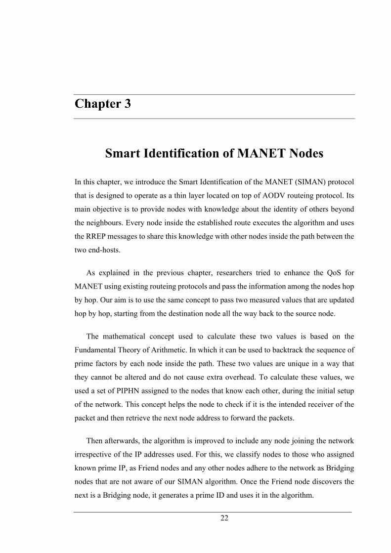
In this chapter, we introduce the Smart Identification of the MANET (SIMAN) protocol
that is designed to operate as a thin layer located on top of AODV routeing protocol. Its
main objective is to provide nodes with knowledge about the identity of others beyond
the neighbours. Every node inside the established route executes the algorithm and uses
the RREP messages to share this knowledge with other nodes inside the path between the
two end-hosts.
As explained in the previous chapter, researchers tried to enhance the QoS for
MANET using existing routeing protocols and pass the information among the nodes hop
by hop. Our aim is to use the same concept to pass two measured values that are updated
hop by hop, starting from the destination node all the way back to the source node.
The mathematical concept used to calculate these two values is based on the
Fundamental Theory of Arithmetic. In which it can be used to backtrack the sequence of
prime factors by each node inside the path. These two values are unique in a way that
they cannot be altered and do not cause extra overhead. To calculate these values, we
used a set of PIPHN assigned to the nodes that know each other, during the initial setup
of the network. This concept helps the node to check if it is the intended receiver of the
packet and then retrieve the next node address to forward the packets.
Then afterwards, the algorithm is improved to include any node joining the network
irrespective of the IP addresses used. For this, we classify nodes to those who assigned
known prime IP, as Friend nodes and any other nodes adhere to the network as Bridging
nodes that are not aware of our SIMAN algorithm. Once the Friend node discovers the
next is a Bridging node, it generates a prime ID and uses it in the algorithm.

Chapter 3: Smart Identification of MANET Nodes
23
3.2. Literature review
Due to the dynamic nature of MANET, researchers continually investigate possible
improvements to the routeing protocols to meet the QoS requirements. These
enhancements are categorised as an added extension or new routeing protocol based on
QoS in its design. The main objective is to use the available resources to satisfy the end
hosts requirements. Furthermore, the success of these efforts is decided by the capability
of the algorithm to achieve the target performance metric without causing overhead that
drains the node resources or overwhelms it with traffic that causes congestion [35].
Recently designed protocols, mainly try to provide information to nodes inside the
network transmission path to make decisions. This information can be any metric that
helps towards a better QoS. For example, priority aware QoS routeing protocol passes
user requirements for specific data rates from the higher layer, and then nodes compare
this information with a threshold and process data accordingly. The threshold value is
adjusted according to the path status and the network environment. The results show the
protocol provides accurate admission control in small networks [36]. In our opinion, the
study explains the source of the knowledge, but it does not clarify the mechanism used to
share this information and set/update the threshold value between nodes.
Another approach uses the prediction for link breakage time, in which the nodes inside
the path inform the source node, and a new route discovery starts before the breakage.
The focus is about the prediction and estimation of the remaining power of the node and
sends a repair message back to the source node if needed [37]. Usually, repair messages
are sent when transmission path breaks, therefore, sending such a message during data
transmission causes extra traffic that leads to congestion. Also, the source node has no
way of knowing the pattern of the vicinity to avoid the node that causes the breakage.
In a different study, the route selection improved by including QoS matrices. The
proposed work uses the RREQ and RREP messages to pass QoS metrics back to the
source node, which selects different paths and sorts them according to the data
requirements [38]. We have adopted a similar concept to pass nodes location that will be
explained in chapter-5.

Chapter 3: Smart Identification of MANET Nodes
24
During our research, we came across well-known algorithms used to enhance QoS
implementation into routeing protocols. For example, a genetic algorithm is used to
optimise the routeing in MANETs by generating an optimised path that avoids congestion
over the network [39]. In another study, fuzzy logic is used to design a scheduler for
MANET to determine the priority of the packet using DSR routeing protocol [40].
Furthermore, the probability is used for a distributive and systematic algorithm to address
the flooding mechanism, which reduces the control overhead [41]. Moreover, in another
research, the game theory is applied for neighbour selection during route discovery [42].
Based on the same methodology, our research led us to implement a mathematical
concept, which makes it possible to distribute the identity of nodes inside the path using
a computed value. The concept is based on a mathematical factorization theory, and it
uses prime numbers to produce two values that can be distributed between nodes and later
used to get the prime factors in the same sequence it was created [43].
Using prime number for identification is not new, researchers explored this concept
and used it to provide uniqueness to node identity and prevent malicious attacks. A prime
number based scheme proposed, that helps in restricting malicious attacks during route
discovery, using clustering mechanism with elected heads [44]. Nodes have unique prime
number IDs stored by the cluster head in a special table and used to validate any
intermediate node that wants to forward data. The cluster head helps the source node to
check the validity of the Prime Product Number (PPN) and decides the trustworthiness of
the node. We use a similar PPN concept in our algorithm, but the nodes inside the path
use the PPN value to validate previous nodes before updating it with own PIPHN.
In another approach, prime number based keys are used to secure the nodes ID in
MANETs by using a “bilinear pairing signature scheme” to reduce attacks [45]. These
prime keys act as public keys and sign the RREQ and RREP messages, with private keys
generated by each node. However, a signature-based solution implemented in higher
layers leads to extra overhead and delay. Such routeing algorithms can be further
enhanced to use the same prime IP-based keys from the route discovery stage, to reduce
attacks during the data transmission stage.

Chapter 3: Smart Identification of MANET Nodes
25
In another vein, Prime IP-addresses were used to eliminate the nodes inquiry for
duplicate IP-addresses by using a prime-DHCP [46]. To increase the performance by
reducing the overhead and latency caused by repeated duplication check. Experimenting
with this algorithm proved the concept of prime IP-addresses to be useful for our
algorithm. The result indicates that it is possible to enhance SIMAN performance by
reducing the used prime number to PIPHN.
The lack of knowledge about nodes beyond neighbours is another critical issue that
led to many different algorithms. These algorithms aim to add extra information to the
routeing process as well as restrict engagement to specific known nodes. Some of these
proposed algorithms can maintain acceptable levels of performance. However, these
security-oriented algorithms will restrict access to some necessary middle nodes, due to
geographical position, which can usually act as Bridging-nodes. Instead, valuable
node/networking resources and attempts are used by these algorithms to find alternative
paths that are not possible most of the time [47].
Moreover, prime numbers are used heavily in security-oriented algorithms for
authenticating nodes using various mechanisms, in which typically they are implemented
in traditional wired networks. Some of these algorithms work but add extra processing
overhead that degrades the performance. For example, a prime number based secure
AODV uses Sequential Aggregate Signatures (SAS) based on RSA. Every node has a
prime ID-based public key that is used to authenticate others inside transmission path and
added as a separate process to routeing discovery [48]. Authentication in our opinion is
essential especially in an open environment as in MANET. However, the process should
not add extra processing load on nodes.
Our algorithm is not a security solution, but it provides some authentication indirectly,
without covering a specific attack model. This is achieved through the checking
mechanism executed through the factorization of the PPN values by nodes during the
route discovery process. In conclusion, it is evident that solutions using unique IP-address
mechanisms can provide knowledge beyond neighbouring nodes. Furthermore, this
uniqueness can be achieved using prime numbers, an idea that we focused on
accomplishing through our algorithm, which is explained in the next section.

Chapter 3: Smart Identification of MANET Nodes
26
3.3. Conceptual design of SIMAN
AODV routeing protocol messages transported via the User Datagram Protocol UDP as
the payload data, which is added to IP header to create an IP datagram. Therefore, extra
fields can be added to AODV message format as far as it does not exceed the maximum
IP datagram size. SIMAN algorithm relies on AODV’s RREP messages to share
information between the node, and for this purpose, it adds fields to RREP message
format as required. Additionally, AODV considers a larger address field to accommodate
IPv6 in its routeing messages. Similarly, this concept can be applied to SIMAN algorithm,
which is left as future work.
The main feature in SIMAN algorithm is to calculate two values from the nodes IP
address, and then passed them node by node all the way to the source node. These two
values later used by the node to retrieve the IP addresses of nodes participated in
forwarding them in the same sequence in which they were calculated. Therefore each
node will have the knowledge of all nodes inside the established path starting from the
destination. This is achieved by using a mathematical formula that replaces the AODV
address retrieval from a routeing table stored on a physical drive. In addition, this concept
is also used during data transmission to forward packets.
The algorithm operation starts at the destination node during the RREP process, by
calculating two values named PPN1 and PPN2 (Prime Product Number) and adds them
to two new fields in the RREP message format, then forwards the message to the previous
node which received the RREQ. The mathematical concept behind the calculation is
based on a “unique factorization theorem” which states [49].
To apply this concept to our algorithm, we assume that is the PIPHN and
accordingly, the source node’s value is p1, moreover, the destination node is pd as shown
in Figure-3.1. The diagram represents nodes scattered around randomly, the arrows
between nodes represents the broadcasted RREQ message by the source to find the
destination.

Chapter 3: Smart Identification of MANET Nodes
27
Figure 3.1: RREQ message broadcasting in a MANET scenario.
(3.1)
(3.2)
(3.3)
PPN1 in (3.1) represents the multiplication product of prime numbers, and PPN2 in (3.2)
accounts for subtracting one from previous value. The great common division of
the two values PPN1 and PPN2 in (3.3) aids the receiving node to backtrack the original
factors in sequence, as they were calculated.
3.4. SIMAN algorithm scheme
SIMAN algorithm deals with PPN calculation that involves prime numbers, which gets
rapidly large. Therefore, two added extra fields added to RREP message format should
be sufficient (64 bits each) to accommodate the PPN values as shown in Figure-3.2.
Moreover, these two fields are known only by nodes aware of SIMAN algorithm and it
does not intervene with AODV operation.

Chapter 3: Smart Identification of MANET Nodes
28
Figure 3.2: Extended RREP message format to accommodate the PPN values.
Each node receives the RREP extracts the two PPN values and factor them to obtain
the sequence of addresses participated in calculating these two values, we refer to these
addresses as PPN factor list. The list will be used to check if the node is the intended
receiver of the packet. Additionally, it is used later to forward data packets.
Route discovery procedure
The network scenario in Figure-3.1 consists of ten nodes, in which they are assigned
prime-IP addresses. We assume they do not have any previous communication records,
in order to start a fresh route discovery procedure. Furthermore, “destination only flag”
is set on all nodes, so only the destination node can reply to the RREQ.
Route request process RREQ
SIMAN algorithm does not involve in the RREQ process of AODV routeing protocol.
The source node p1 creates the RREQ message and broadcasts it to all neighbouring
nodes in its transmission range. Nodes receiving the RREQ, examine the message and if
it is not the intended destination then it forwards the RREQ to other neighbouring nodes,
and this process continues until the message reaches the destination node pd.

Chapter 3: Smart Identification of MANET Nodes
29
Route reply process RREP
The RREP process conducted by AODV routeing protocol starts once the destination
receives the RREQ by creating the RREP message. SIMAN algorithm takes over the
message and calculate the PPN values and add them to the RREP message and forward it
to the previous node which forwarded the RREQ message, as shown in Figure 3.3.
Figure 3.3: The RREP message path in MANET scenario.
The following procedure explains SIMAN calculation steps conducted on each node
inside the discovered path:
1. The destination node pd starts the calculation by extracting the PIPHN denoted as
pown (the value is “11” in Figure-3.3) as well as the previous node’s value pprev (node
R with address “5”).
2. Then it calculates the two PPN values as follows:
PPN1= pown×pprev= 11×5= 55 (3.6)
PPN2= pown-1 ×pprev-1= 10×5-1= 49 (3.7)

Chapter 3: Smart Identification of MANET Nodes
30
3. pd then sends the RREP message including the two calculated PPN values to the
previous node p3.
4. p3 determines the prime factors list from PPN1 and PPN2. The latter value is used to
determine the correct sequence of the factor values, as PPN1 might have different
factor sequences, e.g. PPN1 value of “55” can be factorised as “11×5” or “5×11”.
5. Once the factorization is completed, p3 compares the last value in the calculated
factors list with its PIPHN, i.e. “5”. If they were equal, then the node calculates the
new PPN1 and PPN2 values otherwise, it drops the packet. Figure 3.4 which shows
the RREP process and the grey area represents SIMAN’s added features.
Figure 3.4: The RREP process for SIMAN algorithm.
6. The newly calculated PPN values by p3accomplished by repeating step 2 with the
exception of using the received PPNrec values instead of its own pown value, and
multiplies it with the pprev of the neighbouring node (Eq. 3.8 and 3.9).
PPN1= PPN1rec×pprev= 55×7= 385 (3.8)

Chapter 3: Smart Identification of MANET Nodes
31
PPN2= PPN2rec×pprev-1= 49×7-1= 342 (3.9)
7. Lastly, p3 updates the RREP message with the new PPN values and sends it to the
previous node, i.e. “ p2”. Then when p2 receives the RREP message, it extracts PPN
values and repeats steps 3 to 6.
8. These steps are repeated by every node inside the path until the RREP message
reaches the source node p1. Additionally, every node forwards the PPN values stores
a copy, and use it later during data transmission.
Data transmission
In AODV, once a route is established, every node receives a data packet from the source
node, checks the routeing table entry for a valid path and retrieve the next node address.
This is followed by the “expiry time” update for the path entry inside the routeing table
entry as shown in Figure-3.5.
Figure 3.5: Data transmission for AODV routeing protocol.

Chapter 3: Smart Identification of MANET Nodes
32
While in SIMAN algorithm, the source node sends a data packet to the next address
retrieved from the PPN factor list. Upon the arrival of the packet, the receiving node will
factor the stored PPN and accepts the packet only if the sender’s address is equal to the
address inside factors list. Then it forwards the packet to the next address retrieved from
the same list rather than the routeing table as it was explained in section 3.4.1. By doing
this, SIMAN prevents that data packets from following any other path, than the one
defined via the PPN factors list. This process continues until the data packet reaches the
destination node, as shown in Figure-3.6.
Figure 3.6: Data transmission for SIMAN algorithm.

Chapter 3: Smart Identification of MANET Nodes
33
3.5. SIMAN’s non-prime IP addresses enhancement.
One restriction with the above-proposed procedure is that it works for PIPHN assigned
nodes only. This means that any other node that joins the network and has a none-PIPHN
address will not be included in PPN calculations. This can be solved by excluding any
node without a prime address. However, this process might exclude nodes that can
provide better alternative paths. Therefore and in order to avoid this issue, this node has
to be assigned a prime value as an ID to use for PPN calculations. Though, this prime ID
has to be unique and generated by the node with PIPHN. Therefore, this thesis introduces
a new mechanism that enhances the previous procedure and classifies the nodes inside
the network into two categories:
a. Friend nodes: these nodes are known to each other during the initial network
setup, and they are assigned a prime IP address from a set of known addresses.
b. Bridging nodes: Any other node joins the network is assigned any IP address.
These nodes use AODV routeing protocol, and not aware of SIMAN algorithm.
For the illustration of the algorithm, we present a scenario for a group of safari expeditions
that leave the base camp as in Figure-3.7. These Friend nodes are initially assigned prime
IP addresses inside their base camp.
Figure 3.7: MANET scenario: a group of Friend nodes leaving basecamp.

Chapter 3: Smart Identification of MANET Nodes
34
Then, the group departs to the field and eventually split into three clusters with a large
distance apart from each other, and so the MANET between them is broken. After that,
due to the limited transmission range, the clusters (shaded area) lost communication as in
Figure-3.8. When relevant information has to be exchanged quickly, individual clusters
sense other nodes (Bridging nodes-dark circles) as they have unidentified IP-addresses,
and they can be good candidates to connect the different clusters.
Figure 3.8: MANET scenario: Friend nodes split into clusters.
Previously explained in the literature review, that when the identity of the nodes
passed between nodes, restrictions applied to prevent problems like impersonation and
fake identification. Therefore, some nodes that can be suitable candidates to connect
clusters (nodes L, M and G) are excluded as in the example of Figure-3.8. Our algorithm
uses these nodes without them knowing the existence of SIMAN.
Additionally, applying QoS support requires the usage of available resource that
might provide alternative paths. The mechanism of using this resource (Bridging nodes)
in SIMAN algorithm relies on the neighbouring Friend nodes to generate prime IDs to be
used to calculate the PPN values, as in the previous example (step 5), Friend nodes update
the PPN values using the prime ID as the previous node pprev.

Chapter 3: Smart Identification of MANET Nodes
35
The prime ID generation is computed using a formula known by the Friend nodes
during initial setup. Additionally, it is used again when the Friend nodes discover a
generated ID in the PPN factor list and check the validity to prevent fake IDs. Moreover,
any Friend node generates a prime value, compares it with the PPN factor list to prevent
duplication. The ID generation formula consists of the first valid (not duplicate) prime
number that is larger than the summation of the PIPHN for the previous Friend node and
Bridging nodes.
(3.10)
Where:
Gp: First valid (not duplicate) generated prime value
Fh: The PIPHN of the previous Friend node
Bh: The Bridging node PIPHN
Additionally, if two or more consecutive Bridging nodes come after each other, then
the second Bridging node will be detected by the next Friend node after the Bridging node
and eventually assigned an ID.
Finally, we can summarise the features provided by SIMAN algorithm to the Friend
nodes inside the established path as follows.
Help the Friend node to use the PPN value received through the RREP packet to
confirm the IP address of the previous node including any Bridging node.
Help the Friend nodes to check if they are the target of the RREP, they receive.
Help the Friend nodes next to Bridging nodes inside the RREP path, to detect hidden
nodes without ID. This is achieved by subtracting the PPN factor from the hop count,
which demonstrates the number of previous Bridging nodes without ID.
During Data Transmission, SIMAN shall:
o Help the Friend node to check if they are the target of the data packet.
o Help the Friend node to retrieve the next node address to forward data packets.
o Detects the direction of the flow.

Chapter 3: Smart Identification of MANET Nodes
36
3.5.1. Route discovery process improvement
SIMAN algorithm participation in the route discovery process starts at the destination
node during the RREP process as described in section 3.4. Therefore, and to explain the
process, we have to clarify the following.
1. SIMAN algorithm uses the Bridging nodes to connect clusters and it does not
consider/care about the trustworthiness of these Bridging nodes as they are not aware
of SIMAN’s existence. Therefore, we assume that the source node and destination
node are always Friend nodes. Other cases, such as Bridging node sending or
receiving data is beyond the scope of this enhancement.
2. For clarity throughout the rest of this thesis, references to previous and next nodes
used by Bridging nodes that participate in a route establishment is the same of AODV
routeing protocol. Therefore, during the RREP process references to next node
represents the node that processed the RREQ packet before, while the previous node
represents the node that forwarded the RREP.
3. On the other hand, references to the next and previous nodes in SIMAN are based on
the factors list of the PPN values, starting from the destination node toward the source
node. Moreover, during data transmission, the factors list will be used by all Friend
nodes to forward data packets, for this purpose, they reverse PPN factor list and so as
the next and previous nodes references.
During the start of PPN calculation, the destination node checks if the previous node
is a Bridging node, in which it generates a random prime ID value. Otherwise, it calculates
the "PPN” explained in section 3.4 (Eq. 2.1 and 2.2), then forwards the RREP message
as shown in Figure-3.9.

Chapter 3: Smart Identification of MANET Nodes
37
Figure 3.9: RREP process executed by destination node in SIMAN algorithm.
Each Friend node downstream shall receive the RREP checks for Bridging nodes in
which it will take into consideration the possible steps shown in Figure-3.10- (followed
by a reference to different parts in the diagram).
If the previous node was a Bridge, then the Friend node compares the hop count with
the number of nodes in the PPN factors list.
If the values were equal, then it means all Bridging nodes have prime IDs, otherwise,
one or more previous Bridging nodes are without prime IDs, which requires to:
o Calculate the number of the Bridging nodes (Figure-3.10-3).
o Generate a prime value(s) for the Bridging node(s) (Figure-3.10-4).
Then, it checks if next was a Bridging node, which requires another prime ID
generation as shown in as in (Figure-3.10-7).

Chapter 3: Smart Identification of MANET Nodes
38
Figure 3.10: RREP process for Friend nodes in SIMAN algorithm.
Example:
To implement what we explained so far with values, we assign IP addresses to the
scenario in Figure-3.11. The network consists of ten Friend nodes split into three clusters
(white circles), as follows:
Cluster-1 (from the left): Friend nodes Y, K, and S
Cluster-2: Friend nodes R, H, A, B, E, and N
Cluster-3: Friend node D

Chapter 3: Smart Identification of MANET Nodes
39
Cluster one and two are separated by one Bridging node(shaded node) L, in addition,
cluster two and three separated by two consecutive Bridging nodes G and M. These
clusters lost connectivity and are unaware of each others location. The source node S
wants to send data to the destination node D and for this, it creates a RREQ and sends it
around in an attempt to find a path to the destination node D. The RREQ propagates
through nodes until it reaches the destination node D.
Figure 3.11: RREP message passed by Bridging nodes in SIMAN scenario.
The destination node D (PIPHN value =11) creates a RREP message and notice that
the previous node G is not a Bridging node. Therefore, it generates a prime value
(explained in section 3.5), equals to 31 and associate it with the IP of the Bridging
node, and then calculates the PPN values:
PPN1=pown*Gen1=11*31=341
PPN2= pown-1 *Gen1-1=309
Apparently, the RREP message passed to the Bridging node G will be processed using
AODV, and passed to the other Bridging node M, which follows the same procedure.
The message then reaches the Friend node R (PIPHN value =5), which discovers the
previous Bridging node ID:31 from factorization of the PPNreceived values.

Chapter 3: Smart Identification of MANET Nodes
40
Friend node 5 then checks the number of prior Bridging nodes, and subtracts the
number of values in the PPN factor list from the hop count in the RREP message.
No of Bridging nodes without ID=hop count-PPN factor list values (3.11)
The hop count should be three (nodes D, G, and M) while the factor list contains only
two values (nodes 11 and 31). Friend node 5 concludes that one Bridging node is
without ID ( node M). Therefore, it generates a new ID (calculated as 37) and then
computes the new PPN values.
PPN1=PPN1received*pown=341*37=12617
PPN2=PPN2received*pown-1=309*37-1=11432
Then updates the PPN with its own PIPHN value.
PPN1=12617*5=63085
PPN2=11432*5-1=57159
Next, Friend node R senses the next node is a Bridging node L. Therefore it creates
another ID (calculated as 41) and computes the PPN values before forwarding them.
PPN1=63085*41=2586485
PPN2=57159*41-1=2343518
After that the Bridging node L processes the RREP using AODV and passed to the
source node S, which factors the PPN values and obtain the list of nodes inside the
path (41, 5, 37, 31 and 11). Therefore and based on the algorithm the source node notices that Friend node 11 generated the ID 31 and Friend node 5 generated IDs, 37
and 41 for the Bridging nodes.
3.5.2. Data transmission update
After the source node establishes the path, it starts to send the buffered packets to
the destination node D.
Any Friend node that receives the data packet and wants to forward to a Bridging
node, extracts the ID from the factor list and finds the previously stored IP address
associated with the ID and forwards the packet as it is seen in Figure-3.12.

Chapter 3: Smart Identification of MANET Nodes
41
Figure 3.12: Data transmission process for network with Bridging nodes

Chapter 3: Smart Identification of MANET Nodes
42
3.6. Summary
In this chapter, the research process and implementation of our proposed SIMAN
algorithm have been detailed and the outcome achieved through:
The literature survey conducted that has led to our Prime IP hypothesis and then
transformed into a mathematical model.
Formulated the mathematical concept of prime number factorization to be used with
prime IP addresses.
Implemented the concept to AODV routeing protocol used in MANET, to help the nodes
inside the transmission path to identify other nodes beyond neighbours using routeing
messages.
Improved the algorithm process to include nodes with any IP addresses to enrol into the
route discovery process, and the result can be used to share any performance metrics used
with other nodes so to provide better QoS.
In the next chapter, we describe the implementation of SIMAN algorithm using
OPNET Modeller to observe its operation and performance using different simulation
scenarios.

43
SIMAN Implementation
One of the main tasks during initial stages of our research was the selection of the network
simulation tools required to implement SIMAN algorithm. There are many types of
simulation software available. Some open source software is free, and others are
commercial software. Our focus was to find a simulator that implements MANET easily
with rich features and documentation that provide efficient results. In the following
section, we review five popular simulation tools we reviewed that are widely used to
implement algorithms.
1. Network Simulator 2 (NS2): an open source discrete event simulator supports most
of the routeing protocols deployed in a MANET environment. NS2 is very popular
among researchers because it is free with a huge library and online resources. The
reliability of the results is questionable due to bugs and building real systems are hard
due to its complicated structure [50].
2. Network Simulator 3 (NS3): is an update of NS2 but built from scratch, written in
C++ language that supports Python, a feature that was not available in the previous
version. The software has a questionable credibility in comparison to real results due
to the lack of reliable customer support. In addition, it has scalability problem [51].
3. GloMoSim: an open source library based parallel simulation software that can help
different types of networks with a large number of nodes, written in discrete event
language PARSEC, which is an extension to C language. The software does not have
updates because of the conversion to the commercial QUALNET [52].
4. OMNET++: an object-oriented discrete event network simulator, can be used for
various networks especially MANET. The software consists of hierarchal models that
communicate through messages passed around. They are written in C++ language and
can be modified to include any external user templates. The software is commercial

Chapter 4: SIMAN Implementation
44
and provides free licenses for academic research. The disadvantages come from the
limited protocols that are supported and compatibility problems [53].
5. OPNET: OPtimized Network Engineering Tools is a dynamic discrete event
simulator is currently known as (Riverbed), used for networks and distributed systems
simulation. It is a commercial software that provides free licenses for educational use,
with maintenance and support. It has a large set of the known libraries available for
networks. The software supports both C and C++ languages and can incorporate user-
designed models. Besides, OPNET Modeller provides a rich graphical interface, and
has a customisable network environment [54].
In conclusion, we can observe that most of the simulation software have similar
features. Therefore, the selection criteria are related to cost and usability. We selected
OPNET simulator for our research because we believe that commercial software
reliability is better, and it is equipped with features relevant to real networks, in addition
to comprehensive documentation and online support.
4.1. OPNET Modeler
OPNET is a dynamic discrete event network simulation software that supports the OSI 7-
layer model. Furthermore, it provides the platform to integrate external objects, libraries
and user-designed algorithms. It also supports most of the known network protocols and
regularly updated to include new protocols. Users can create real networks using a library
of many known devices with adjustable attributes. Furthermore, the internal
implementation and processes are also visible for users to modify according to their
requirements. The software empowers the engineers and researchers to design networks
on a computer, which reflect original network construction and behaviour [55].
SIMAN implementation in OPNET
OPNET supports most of the MANET routeing protocols including AODV, which comes
as a child of a higher level process called MANET Manager ("manet_mgr" as in Figure-
4.1), which in return is a child of the "ip_dispatch" process located inside the IP layer of
the OSI model.

Chapter 4: SIMAN Implementation
45
Figure 4.1: SIMAN algorithm inside the OSI hierarchy for a MANET node.
SIMAN algorithm is a thin layer placed between the original AODV routeing protocol
and the "manet_mgr." and accordingly the communication between manet_mgr and
AODV has to pass through SIMAN. The integration of SIMAN layer requires
modification to the implementation of AODV routeing protocol inside OPNET
environment. For example, SIMAN does not intervene in the routeing process when it
discovers the node is a Bridging node. Additionally, when manet_mgr inside Friend
nodes require the next or previous node addresses, then SIMAN take over the request and
provide the address from PPN factor list rather than AODV’s routeing table.
On the other hand, other added features like distance measurement or battery power
consumptions, are activated only when SIMAN is enabled. Moreover, SIMAN modifies
AODV routeing messages (RREQ and RREP) to carry the essential parameters as
required. The following features added to OPNET environment to support SIMAN
algorithm.
a. Prime-DHCP: during the initial network setup, Friend nodes are required to be
assigned prime-IP addresses in the base camp from an already pre-agreed set of
addresses, Prime DHCP, makes sure that the list of IP’s assigned to Friend nodes has

Chapter 4: SIMAN Implementation
46
a valid PIPHN. Moreover, SIMAN algorithm activates when it detects the IP of the
node is in the initially assigned list of addresses as shown in Figure-4.2.
b. ID generation algorithm: Friend nodes have to create unique prime ID’s for
Bridging nodes inside the network as explained in section-3.5. This feature is
activated when the Generate ID attribute is enabled through the UI of the node model
as seen in Figure 4.2.
Figure 4.2: SIMAN enabled attribute for MANET nodes.
c. Wormhole node model: A modified MANET router/station, which has two
communication link. An inbound high-speed Ethernet link with each other to forward
packets and an outbound IEEE 802.11b wireless interface used to communicate with
other nodes. The WH’s have the ability to hide its identity and copy packets from the
inbound Ethernet link with other WHs to the outbound wireless interface without
modification. The hierarchical layer design of the WH is shown in Figure-4.3.

Chapter 4: SIMAN Implementation
47
Figure 4.3: Wormhole model for the OPNET Modeler.
d. Battery level: This attribute represents the initial RBE and has a default value of 100,
but it can also be configured manually for smaller values as in Figure-4.4. It is mainly
used when the battery energy is taken into consideration in the SIMAN algorithm.
The RBE decrement according to the power consumption formula we implemented.
Once the value reaches 10%, the node then will be placed into sleeping mode and will
not participate in any routeing/communication thereafter.
e. The modification of AODV routeing message format: SIMAN algorithm and its
enhancements share information between nodes. The RREQ and RREP messages are
used to share this knowledge. Therefore, it is essential to add appropriate fields to the
messages as required, an example is explained in section 3.4. Further fields will be
added for the coming improvements of SIMAN algorithm which will be explained in
the next chapters.

Chapter 4: SIMAN Implementation
48
Figure 4.4: Manual configuration of the node’s initial battery energy.
a. SIMAN algorithm: The algorithm is part of the AODV child process activated
through the MANET manager process located inside the IP layer of node models as
seen in Figure 4.5. It consists of several function blocks precedes AODV routeing
protocol. These functions rely on several header files that execute according to the
requirement of the algorithm:
PPN factorization: This header conducts the PPN calculation carried by RREP
message and the factorisation of the PPN values as explained in section 3.4.1.
Coordinate measurement: It uses the Known Friend node coordinates to calculate the
Bridging nodes coordinates and measure distances between nodes explained in next
chapter. These coordinates are x and y attributes of the node in 2D (zero latitudes).
They represent the actual physical position of the nodes obtained from GNSS.
Power analysis: used to bypass the route discovery process of AODV conducted by
the source. It follows different route discovery procedure by examining all paths to
collect RBE and then examine and construct a path with high RBE, this will be
explained in detail in chapter 6.

Chapter 4: SIMAN Implementation
49
Figure 4.5: SIMAN algorithm placement inside the node model.
4.2. SIMAN algorithm Simulation and Results
The simulation’s goal is to evaluate SIMAN algorithm implementation through four
scenarios. The intention is to compare the operation of the routeing protocol (AODV
operation with and without SIMAN), to review its impact on the route discovery process
and the overhead caused by SIMAN algorithm. Furthermore, we observe the accuracy of
the address retrieval from the PPN factor list rather than the routeing tables during route
discovery and the data transmission processes. These behaviours measured through the
following performance metrics that are used to identify the difference:
Route Discovery Time (RDT): is measured as the average packets round trip time
required for the RREQ to reach the destination and the time required for the RREP to
arrive back at the source.
End-to-End Delay: represents the time delay that the packet encountered during
transmission from the source to the destination.

Chapter 4: SIMAN Implementation
50
Packet retransmission rate: represents the total number of retransmission attempts
by the nodes in the network until the packet transmitted successfully or discarded
because of reaching short or long retry limit (default value 7 and 4 respectively) [56].
Moreover, the following variable parameters were used in simulation to examine the
above-mentioned metrics in different scenarios:
Data Transmission Rate: Mobile nodes feature different data transmission rates that
lead to variable transmission ranges. These differences affect the performance of the
routeing protocol, as lower data rate have higher transmission range [57].
The number of nodes: The network density (i.e. the number of nodes per area unit)
has an impact on the network performance. A higher network density results in nodes
having possible alternative routes among each other. Which in result helps toward
preventing congestion and improving the overall performance of the network [58].
Node mobility: Node mobility in OPNET examined via parameters like trajectory
movement, distance between nodes, and node speeds. They impact network
performance characteristics like throughput or Packet Delivery Ratio [59].
Network layouts/topologies: represents the distribution of the nodes in different
topologies with different mobility models that impact the performance of the routeing
protocols [60].
Bridging node: Different no of Bridging nodes introduced to the network to examine
the correct prime ID generation and the overhead caused by the process.
4.2.1. Network Scenarios
Scenario-1
The scenario consists of a network of twenty MANET stations, in an area of a square
kilometre (1000m x 1000m) with a distance not exceeding 300m between any two nodes,
all nodes communicates with same data rate [61]. The simulation considers nodes 3 and
109 that send a data stream in the opposite directions (blue dash arrow line) as seen in
Figure-4.6. Each transmission will trigger a response back to the sender, with an average
volume of 500Mbytes per flow.

Chapter 4: SIMAN Implementation
51
Figure 4.6: The route between nodes 3 and 109 in MANET scenario.
The overall characteristics for the scenarios are shown in Table-4.1.
Table 4.1: The characteristics of the two network scenario
Parameter Value
Trajectory Scenario-1
Hexagonal movement, 2-types: Clockwise & Counter clockwise Movement range: 300m * 300m
Scenario-2 Manually defined mobility path with variable interval time.
Speed Scenario-1,3 & 4 5m/s Scenario-2 10, 20, 30, 40, and 50 m/s
Distance between two nodes (only Scenario-2)
50, 100, 150, 200, and 250 m
Data rate Scenario-1,3 & 4 ( 6, 12, 18, 24, & 36) Mbps
24 Mbps Scenario-2 Packet size 512 byte Packet reception power threshold -82.65 dBm Transmission power 0.0005 Watt
Traffic mix 0.977 GB, all explicit
Simulation Duration 300 sec
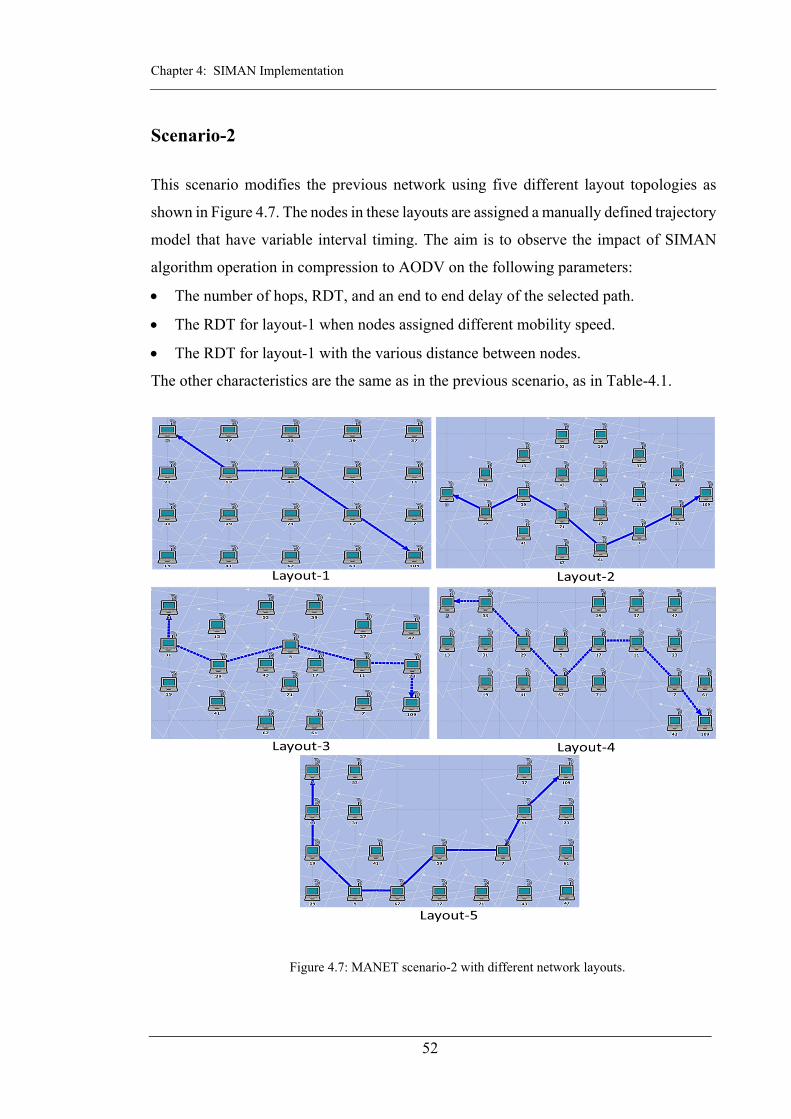
Chapter 4: SIMAN Implementation
52
Scenario-2
This scenario modifies the previous network using five different layout topologies as
shown in Figure 4.7. The nodes in these layouts are assigned a manually defined trajectory
model that have variable interval timing. The aim is to observe the impact of SIMAN
algorithm operation in compression to AODV on the following parameters:
The number of hops, RDT, and an end to end delay of the selected path.
The RDT for layout-1 when nodes assigned different mobility speed.
The RDT for layout-1 with the various distance between nodes.
The other characteristics are the same as in the previous scenario, as in Table-4.1.
Figure 4.7: MANET scenario-2 with different network layouts.

Chapter 4: SIMAN Implementation
53
Scenario-3
This scenario introduces Bridging nodes to connect different clusters. The network
consists of sixteen Friend nodes (dark nodes seen in Figure-4.8), that leaves the base and
split into three clusters (red oval) that are separated by four Bridging nodes (white nodes).
The aim is to examine the correct route discovery when Bridging nodes are
introduced, and the overhead caused by prime ID generation. Two different data streams
flow from two source nodes 3 and 5 toward the destination nodes 23 and 59 respectively.
All nodes have random mobility and the rest of the traffic characteristics are the same as
the previous scenarios in Table-4.1.
Figure 4.8: Scenario-3 clusters connected through Bridging nodes.
Scenario 4
The previous scenario was modified to have five different topology configuration, which
provides different cluster layouts that have a various number of Bridging nodes places in
a different pattern. The aim is to observe the impact of the number of Bridging nodes
involved in route discovery process as shown in Figure-4.9.

Chapter 4: SIMAN Implementation
54
Figure 4.9: MANET scenario-4 with different network layouts.
4.2.2. Results and analysis
In this section, we analyse the results of each scenario separately and discuss the impact
of simulating the scenarios for AODV routeing protocol and SIMAN algorithm on the
previously explained performance metrics in section-4.3.

Chapter 4: SIMAN Implementation
55
Scenario-1
The results of this scenario examine the route discovery success when the PPN concept
applied for addresses retrieval instead of routeing tables. We will be examining the impact
of the PPN calculation on the route discovery time. Furthermore, during data transmission
we look if the PPN address retrieval procedure causes errors which are observed through
the average packet retransmission attempts and the end to end delay.
1. Route discovery time (RDT)
The simulation results show a path of 5 hops was successfully established for both AODV
and SIMAN, as in Figure-4.10. This demonstrates the correct implementation of the PPN
concept. Moreover, from SIMAN algorithm design (see section 3.4), one can expect a
small overhead caused by the PPN calculation. This introduced overhead is around
0.01msec for data rates 6, 12 and 18 Mbps on average. However, in data rates 24 and 36
Mbps SIMAN shows an advantage of 0.04msec due to the fast retrieval of the node
addresses from the PPN factor list.
Figure 4.10: Scenario-1, route discovery time for various data rates.

Chapter 4: SIMAN Implementation
56
2. Data Transmission (DT)
As mentioned in the scenario setup (sec. 4.3.1), data transmission conducted in two
opposite directions with the destination nodes sending responses to the source node for
each received data packet. The simulation examines the capability of the nodes to forward
packets in both directions simultaneously.
Packet retransmission (PR)
The Packet retransmission happens because of loss or damage to packets. Simulation
results show that AODV has an average of 7.17 retransmission attempts compared to 4.65
using SIMAN as in Figure-4.11. This is because SIMAN algorithm improves the accuracy
of the address retrieval for packet flows in opposite directions.
Figure 4.11: Scenario-1, packet retransmission attempts.
End to end delay
Generally, the results show the increase in the data rate reduces the delay for both AODV
and SIMAN algorithm, as the packets are processed faster. Additionally, we notice that
SIMAN algorithm has 0.009msec on average less delay compared to AODV. This is
because of the larger packets retransmission attempt in AODV, which leads to further
delay to the data transmission process as seen in Figure-4.12.

Chapter 4: SIMAN Implementation
57
Figure 4.12: Scenario-1, End to end delay.
Scenario-2
In this scenario we examined the Route discovery time RDT using:
Various layouts/topologies
As explained in the scenario, we used different layouts to study the effect of various
topology on route discovery, in term of the number of hops and the RDT. We can see
from Table-4.2 that for both SIMAN algorithm and AODV routeing protocol we obtained
a path with the same number of hops for each layout as previously seen in Figure-4.7.
Table 4.2: Scenario-2 number of hops per route
Layout Number of hops per route AODV SIMAN
Layout-1 4 4 Layout-2 7 7 Layout-3 6 6 Layout-4 7 7 Layout-5 8 8
Furthermore, the RDT for SIMAN took an average 0.612sec comparing to it was
0.617sec for AODV in layout 2, 3 and 4. This result indicates that PPN factorisation
process improves the RDT for different topologies for the same number of hops, as in
Figure-4.13.

Chapter 4: SIMAN Implementation
58
Figure 4.13: Scenario-2, route discovery time in different layouts.
Variable node speed
The nodes mobility speed was another parameter used to test the impact of SIMAN
implementation on RDT, in which five different speeds of 10, 20, 30, 40, and 50 m/sec
were used for the layout-1 seen in Figure 4.7.
Figure 4.14: Scenario-2, route discovery time with different mobility speeds.
Overall, that the RDT surges with an increase in the node mobility speed, in addition,
SIMAN shows an average 1.2msec advantage over AODV. This is an indication that
obtaining the addresses from a PPN factor list works better with the increase in mobility
speed of the node.

Chapter 4: SIMAN Implementation
59
Variable distance between nodes
The third parameter used to measure the RDT was the distance between nodes. In this
scenario, various node distances incremented by 50 meters are used for each simulation.
The purpose was to examine its impact on the RDT. As we can see in Figure 4.15, the
RDT escalates with the increase in the distance between nodes. This is due to the packets
travelling distance in the air for both AODV and SIMAN. Additionally, the latter shows
an advantage of 0.2msec on average.
Figure 4.15: Scenario-2, route discovery time with various node distances.
Scenario-3
The results show that the route was established successfully for both AODV and SIMAN
using the same path and 7 hops for each flow. Additionally, we notice that both flows go
through two Bridging nodes 14, 42 and 32, 12 respectively (blue arrows in Figure-4.8),
and ignores the Friend nodes 41 and 71 which are closer to them. This is because the
Bridging nodes use the shortest path concept applied by AODV routeing protocol,
therefore, they try to establish the path with least number of hops and bypass any other
node in between. Additionally, all nodes are assigned random mobility with various start
time.

Chapter 4: SIMAN Implementation
60
Route discovery time
The RDT results show an AODV advantage of around 0.012.5sec on average for data
rates of 6, 12, and 18 Mbps respectively, while in data rates 24 and 36Mbps SIMAN
shows a 0.014sec on average advantage. As we can see from Figure-4.16, the scenario
has two separate data transmissions with two Bridging nodes involved in each
transmission path. This means SIMAN generates ID in addition to the PPN calculation
process, and as a result, it causes a small increase in RDT at lower data rates.
Figure 4.16: Scenario-3, route discovery time with different data rates.
Scenario-4
The impact of Bridging node numbers on RDT
The simulation of this scenario examines the overhead caused by the ID generation
process executed by Friend nodes neighbouring the Bridging nodes for different
topologies. This process is effected by the number of Bridging nodes and the layout of
the networks seen previously in Figure-4.8.
The RDT results for SIMAN algorithm show a small overhead of 0.02msec
introduced in layout 1 and 5. This is because four Friend nodes were involved in ID
generation that caused an increase in RDT in comparison to AODV routeing protocol. On
the other hand, in layouts 2, 3 and 4, we notice an improvement in RDT of 0.025msec on

Chapter 4: SIMAN Implementation
61
average. Which is due to lesser number of Friend nodes (2, 3 and 4 respectively) involved
in the prime ID generation process, as seen in Figure-4.17.
Figure 4.17: Scenario-3, route discovery time in different layouts.
4.3. Summary
In this chapter, we introduced OPNET simulation modular that provides a flexible and
highly organised architecture, which allows the reusability and extendability of existing
models. We used the simulator to implemented SIMAN algorithm and examine its correct
route discovery operation in comparison with the AODV routeing protocol. Furthermore,
we used performance metrics like RDT, an end to end delay, and packet retransmission
to study the algorithm’s behaviour.
Additionally, we introduced Bridging nodes that connect different Friend node
clusters and observed the overhead caused by prime ID generation and its impact on the
performance. The overall results showed that SIMAN attempts to provide knowledge
beyond neighbours come at no cost in comparison to AODV routeing protocol.

62
SIMAN enhancement with location
Thus far, we managed to use the routeing process in AODV to distribute the knowledge
of node’s identity among others inside the selected path. In this chapter, we further
enhance this knowledge with the geographical location of the nodes, to ensure that the
algorithm identifies nodes to be inside the network. The location information is obtained
through GPS localisation available on board the wireless devices and SIMAN algorithm
shares this information using the RREP message of AODV routeing protocol.
Many of MANET issues explained in chapter 2 are caused by nodes lack of
knowledge about the location of others inside the network. Thus, sharing it can help to
prevent these issues. For example, node inside the transmission path can use the distance
measurement with neighbours to adjust transmission power and save resources [62]. Or
use neighbour coordinates to predict their movement and prevent link breaks [63].
SIMAN’s shared location knowledge consist of a list created during the RREP process
to hold the location coordinates of nodes inside the established path. Friend nodes add
their coordinates to this list and forward it back to the source node. They also collaborate
to determine the coordinates of any neighbouring Bridging nodes using known
geometrical theories. Once the full coordinates list reaches the source node, it will be used
to measure the distance between the nodes and reject any route if it exceeds the threshold.
This concept has great importance when we use unknown Bridging nodes to connect
clusters, as they might be malicious nodes which cannot be detected without complex
security solutions. In the next section, we review the work accomplish on this context,
then we explain the algorithm design and implement it into different scenarios that contain
various type of Bridging node (wormholes) and observe the correct elimination process.

Chapter 5: SIMAN enhancement with location
63
5.1. Literature review
Incorporating the geographical location of nodes inside MANET is one of the methods
used to improve the routeing discovery process. Researchers used different techniques to
incorporate the physical location of nodes to improve the quality of data transmission. In
the following section, we highlight, some of these techniques toward understanding and
adopting related ideas.
Generally, the location-based algorithms are based on two old protocols. The greedy
forwarding protocol (GPSR), which uses the node location to forward packets to
neighbours, closer to the destination node, which relies on the information gathered about
the neighbour's location. However, the protocol’s weakness is based on the packet drop
policy applied to prevent loops when the neighbours cannot locate the destination node
[64]. The second protocol is Face routeing, formerly known as Compass routeing, which
is based on routeing along the boundaries of the faces, located on the line joining the
source and the destination nodes [65]. Meanwhile, the protocol’s dependency on planner
subgraph raises questions about its suitability in none planner environment.
Directed flooding is a technique used with existing routeing protocols. The
geographical information is used to reduce the flooding of route requests towards the
destination node. Geo-AODV is an improvement of Location-Aware Routeing protocol
that uses this concept, by defining the request zone as an isosceles triangle. It permits
nodes in the request zone to process the RREQ and share location information. Which in
result removes the necessity to process RREQ by others outside the zone [66].
The same concept of requested and expected zone is used in another research, to limit
the route discovery search area. This is accomplished by adding a list to the route request
message, which contains fourth Nominated Neighbour to re-broadcast. The algorithm
partitions the radio transmission range into four zones, and restricts the route discovery
area to the expected zone. Then chooses one node per zone to forward the RREQ
messages [67]. We believe that reducing the route discovery traffic helps toward saving
the resource, but we have to consider the zone restriction might lead to overhead and deny
essential nodes that provide better alternative paths for data transmission.

Chapter 5: SIMAN enhancement with location
64
In another recent approach, the distance measurement between nodes was used to
improve the route stability affected by node mobility. The node uses the RSSI method to
quantify the mobility of the neighbours, and formulate a method to find the coordinate of
the nodes when GPS device does not exist. The method is used as a mobility metric to
obtain a route that stays longer which in result leads toward better QoS [68]. The concept
in our opinion might work better if the distance list was attached to the RREP message
rather than the RREQ so to avoid extra processes for nodes that are not part of the
established path.
Quick Access Algorithm (QAA) is an alternative solution used to calculate the
distance and direction using the Average Time-of-Arrival (ATOA) and the Direction
Estimation algorithm (DES). The intention is to send data to the next maximum distance
node in the range, which in results reduces the hop numbers in the route and increases the
throughput [69]. We believe that AODV adopts the maximum distance concept between
nodes through the RREQ process. In which the destination node replies to the first
arriving RREQ message. Therefore, it's not clear how less number of hops is achieved
with this protocol. Furthermore, the frequent update of node table with the movement of
the destination node might create unnecessary traffic that consumes resources.
Additionally, the distance bounding protocol used to securely confirm the proximity
of two-hop neighbour. This is used by the node to verify the physical presence of the node
beyond neighbour. The round-trip-time for multi-cryptographic challenge-response pairs
used to obtain the upper bound of physical location between two nodes [70]. In our
opinion, sharing knowledge of nodes beyond neighbours is crucial to improving the
performance but key exchanging security solutions adds extra processing that causes
overhead and consumes nodes resources.
Moreover, location information is used in prevention and detection of attacks like a
wormhole. By measuring the distances between the node and its neighbour. In this way,
nodes inside the path will have knowledge about the distance between them [71]. The
concept of this algorithm can provide the knowledge beyond the neighbours of a node,
but there must be a mechanism to hide the implementation from the wormholes because
they can defeat the algorithm by sharing the wrong distance between them.

Chapter 5: SIMAN enhancement with location
65
5.2. Wormhole attacks
Wormhole attacks (WH) is one of the severe threats to wireless networks because of the
difficulty in the detection and prevention process. It consists of two or more malicious
nodes situated in different locations far from each other that use a special fast connection
link to forward data in attempts to win the shortest path. Once they have managed to join
the route, then they start to harm the network. WH design, techniques and the link
specification varies and it is beyond the scope of this thesis [72].
There are many different classifications for WH attacks, in and outbound attack,
physical layer attacks and visibility attacks [73]. The latter is based on one or more WH
hiding their identity and fast-forwarding packets between them to win the path. They are
classified into three different types as shown in Figure-5.1.
Figure 5.1: Three types of wormhole attacks.
1. Closed WH attack
Both WHs (dark oval) are not participating in the route discovery process. Instead, they
tunnel the routeing messages (dashed arrow) and persuade the other nodes (white ovals
D and N1) to be neighbours and they are unaware of WHs existence as in Figure-5.1-1.
2. Half open WH attack
One of the malicious nodes (WH2) acts invisibly, forwarding the received packets to the
other visible WH1, which participates in route discovery and acts like any other node as
shown in Figure-5.1-2.

Chapter 5: SIMAN enhancement with location
66
3. Open WH attack
In this type, both WHs participate in the route discovery, and they process routeing
messages but tunnel it to each other as if they are neighbours as in Figure-5.1-3.
5.3. Conceptual design
As detailed in section 3.4.1, SIMAN managed to calculate two PPN values and add them
to the RREP message then forward these accumulated values all the way back to the
source node. In this enhancement, an additional list of the node coordinates also added to
the message. Each Friend node receives the RREP, adds own (x and y) coordination to
the list known only to Friend nodes.
In order to prevent the list from alteration, it is possible to apply a solution similar to
the one used in secure AODV routeing protocol (SADOV), which uses a hash chain
function to prevent the alteration of the hop count field from malicious nodes [74]. Since
the coordinates list is a mutable field so we can protect it using a chain function known
to the Friend nodes during the initial network setup in the basecamp, the implementation
of this concept is beyond the scope of this thesis and left as future work.
In SIMAN, The operation of distance measurement consists of two parts. The first
part conducted by Friend nodes inside the RREP message path. They share their
coordinates with each other and collaborate to calculate the coordinates of Bridging
node(s) inside the path. The second part is executed by the source node to measures the
distance between any two nodes using the list of coordinates received via the RREP
message. Then reject the route, if the distance exceeds the maximum permitted threshold.
5.3.1. Distance measurement
The distance measurement conducted by the source node uses analytic geometry to
calculate the Euclidean distance between two points as in (Eq. 5.1) [75]:
d= x2-x12+ y2-y1
2 (5.1)

Chapter 5: SIMAN enhancement with location
67
5.3.2. Bridging node coordinates measurement
During the RREP process, it is possible to have one or more Bridging nodes inside the
path not aware of the SIMAN algorithm. Therefore, Friend nodes surrounding the
Bridging node calculate the coordinates and attach it to RREP message. In SIMAN
algorithm Bridging nodes can be anywhere inside the path between the source and
destination nodes which are Friends with the following possible setups.
5.3.2.1. A Bridging node between two Friend nodes:
The coordinate measurement of the Bridging node in this setup requires three Friend
nodes. This leads to two distinct sequences Fr1→Fr2→Br1→Fr3 and Fr1→Br1→Fr2→Fr3
that defines the measurement procedure as in the Figure-5.2. The sequence discovery is
decided by the Friend node after the Bridging node, using the PPN factor list.
Figure 5.2: The sequence of Friends and Bridging nodes during RREP process.
Moreover, the distance between (previous Friend node) and Br1 is required for the
calculation in both scenarios. This distance is measured using Received Signal Strength
Indicator formula (Eq. 5.2), and then attached to the RREP and forwarded to the next
Friend node.
RSSI dBm =A-10*n* log10 d (5.2)
Where RSSI represents the ratio between the transmitted to received signal, and (A)
is the received signal strength in dBm at one meter, while (n) is the transmission factor
that depends on the propagation environment (n= 2 for free space) [76].

Chapter 5: SIMAN enhancement with location
68
For any of these two sequences, the coordinate calculation process uses one of two
tracks, based on the location of the bridge node that can be inside or outside the triangle
Fr1, Fr2 and Fr3 illustrated in Figure-5.3.
First track:
We assume the Bridging node is located inside the triangle Fr1, Fr2 and Fr3 and use the
intersection of the three circles theory to calculate the coordinates (radical centre) [77].
Then we use this coordinates to calculate the area of the three triangles Ar1, Ar2 and
Ar3 and the sum of these areas should be equal to the area of the triangle Fr1, Fr2 and
Fr3 , Pythagorean Theorem -Proof 73. [78].
Figure 5.3: Three circle intersection used to calculate Bridging node location.
To formulate the equation for the three circle intersection, we make use of Mohr circle
[79], derived for the two-dimensional circle (Eq.5.3).
x-a 2+ y-b 2=r2 (5.3)
Then we consider the three circles Cr1(x1, y1), Cr2(x2, y2) and Cr3(x3, y3) with
radiuses r1, r2, and r3 to derive formulas (5.5 and 5.6) and calculate the coordinates of the
Bridging node.

Chapter 5: SIMAN enhancement with location
69
Assuming : xm=x1-x2 , xn=x2-x3 , ym=y1-y2 and yn=y2-y3
xb=ym y3
2-y22 + x3
2-x22 + r2
2-r32 -yn y2
2-y12 + x2
2-x12 + r1
2-r22
2 xm*yn-xn*ym
(5.4)
yb=xm x3
2-x22 + y3
2-y22 + r2
2-r32 -xn x2
2-x12 + y2
2-y12 + r1
2-r22
2 ym*xn-yn*xm (5.5)
Once we found the coordinates, then we calculate the area of the three inner
triangles (Fr1, Br1and Fr2), (Fr1, Br1and Fr3) and Fr2, Br1and Fr3 . The area is calculated
using shoelace formula (Eq. 5.6), using the determinant of three points [80].
Areatriangle=1
2x1y2+x2y3-x3y1-x2y1-x3y2-x2y3 (5.6)
The sum of these areas should equal the area of the main triangle Fr1, Fr2 and Fr3
(Eq.5.7) that contain them.
Area(Fr1,Fr2,Fr3)=Ar1+Ar2+Ar3 (5.7)
If (Eq.5.7) was true then the measured coordinate is correct. Otherwise, the Bridging
node located outside the triangle, and subsequently, we use the next track.
Second track:
Considering the two node sequences explained earlier, Fr1→ Fr2→Br1→Fr3 and Fr1→
Br1→Fr2→Fr3 . The distance between the two outer Friend nodes (Fr1and Fr3 to the
Bridging node Br1) represents the radius of two circles that intersect at two points. One
of these two points represents the correct coordinates of the Bridging node. We use the
following mathematical procedure to find the actual coordinates.
First, we consider the two scenarios in Figures 5.4 and 5.5. In which they represent
the possible sequence of Fr1→Fr2→Br1→Fr3 and Fr1→Br1→Fr2→Fr3 and for
simplicity, we use the upper case letters (top diagram A, C, B and D and the bottom A,
B, C, and D). The value of B represents the missing coordinate of the Bridging node.
Additionally, two lower case letters represent the distance between two points (for
example, ab represents the distance between points A and B).

Chapter 5: SIMAN enhancement with location
70
Figure 5.4: Scenario-1, the RREP message path through nodes (A-C-B-D)
Figure 5.5: Scenario-2, the RREP message path through nodes (A-B-C-D)
1. Using the rules of sine and cosine [81], we derive the appropriate formulas to find the
length of ab and bd that represents the radius of the two circles (Eq.5.8 and 5.9).

Chapter 5: SIMAN enhancement with location
71
Law of sine:
cd
sin CAD=
ad
sin ACD=
ac
sin ADC (5.8)
Law of Cosine:
cd2=ad2+ac2-2*ad*ac* cos CAD (5.9)
ac2=ad2+cd2-2*ad*cd* cos ADC
ad2=cd2+ac2-2*cd*ac* cos ACD
2. The two radiuses ab and bd then used to calculate the two intersection points B and
B` of the radical line as in (Eq. 5.10 and 5.11). These two points are measured using
the gradient of the base. The value of bg represents the perpendicular distance from
the vertex of the triangle ABD to the base ad [82].
xb=xg±bg(yd-ya)
2*ad (5.10)
yb=yg±bg(xd-xa)
2*ad (5.11)
3. Finally, we find the area of the triangle ABD, using two different methods.
The first method applies Heron’s formula explained in (Eq.5.12) [83]. Heron’s
formula:
Area= ab+ad+bd -ab+ad+bd ab-ad+bd ab+ad-bd (5.12)
Where: ab, ad, and bd represent the length of the triangle sides.
The second method applies shoelace formula previously explained in (Eq. 5.6), and
the result of one of the two points B and B` should give an equal area (Eq. 5.13).
Triangle Areausing three side length=Triangle Areausing three coordinates (5.13)
Example-1
Considering the scenario in Figure-5.6, and assuming the location of the nodes are
represented as (x and y) coordinates. The Friend node D 679,-725 receives the RREP

Chapter 5: SIMAN enhancement with location
72
message and extracts the previous two Friend nodes coordinates A (1744,-992) and
C (1510,-826), and the distance bc =259.24m. B xb, yb represents the unknown
coordinates of the Bridging node.
Figure 5.6: The coordiantes measurment for a Bridging node using trilateration.
Initially, the Friend node D assumes that the Bridging node is located inside the triangle
ACD.
It calculates ac, ad and cd using the Euclidean distance between the two points
(Eq.5.1).
ac= xa-xc2+ ya-yc
2=289.6
ad= xa-xd2+ ya-yd
2=1097.96
cd= xc-xd2+ yc-yd
2=837.12
Then using (Eq. 5.4 and 5.5) it calculates xb,yb
xb=1507.5 and yb= -885.43

Chapter 5: SIMAN enhancement with location
73
After that, it computes the area of the triangles using (Eq.5.6). ABC=6750.85m2,
CBD=160634.15m2 ACD=254700m2 respectively, and then the main triangle
ABD=26745.64m2 and finally apply (Eq.5.7) and discover that:
ABC+CBD+ACD≠ABD
Which concludes that the Bridging node is not inside the triangle ABD. Therefore it
considers the second track.
It calculates the angles DAC, ACD, and ADC (Eq. 5.9).
DAC= cos-1 ad2+ac2-cd2
2*ad*ac=21.28°
ACD= cos-1 ac2+cd2-ad2
2*ac*cd=151.58°
ADC= cos-1 cd2+ad2-cd2
2*cd*ad=7.14°
Then computes the length of ah and ch
ah=cd2+ad2-ac2-2*cd*ad* cos ACD
2*ad-2*ac* cos DAC-2*cd cos ACD=168.86
ch= ac2+ah2-2*ac*ah* cos DAC =143.31
After that finds the angle ACH and ACK.
ACH= cos-1 ch2+ac2-ah2
2*ch*ac=25.31°
ACK=180°- ACD=28.43°
Next, it calculates the length of bd and ab, which represents the radius of the two
circles with centre points A and D.
bd= bc2+cd2-2*bc*cd* cos ACK+ACH =715.01
ab= bc2+ac2-2*bc*ac* cos 180-ACH =532.9
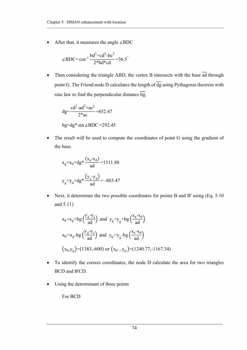
Chapter 5: SIMAN enhancement with location
74
After that, it measures the angle BDC
BDC= cos-1 bd2+cd2-bc2
2*bd*cd=36.5°
Then considering the triangle ABD, the vertex B intersects with the base ad through
point G. The Friend node D calculates the length of dg using Pythagoras theorem with
sine law to find the perpendicular distance bg.
dg=cd2-ad2+ac2
2*ac=652.47
bg=dg* sin BDC =292.45
The result will be used to compute the coordinates of point G using the gradient of
the base.
xg=xd+dg*xa-xd
ad=1311.88
yg=yd+dg*ya-yd
ad= -883.47
Next, it determines the two possible coordinates for points B and B' using (Eq. 5.10
and 5.11)
xb=xg+bgyd-ya
ad and yb=yg+bg
xa-xd
ad
xb'=xg-bgyd-ya
ad and yb'=yg-bg
xa-xd
ad
xb,yb = 1383,-600 xb' , yb' =(1240.77,-1167.34)
To identify the correct coordinates, the node D calculate the area for two triangles
BCD and B'CD.
Using the determinant of three points
For BCD

Chapter 5: SIMAN enhancement with location
75
area1=xd yc-yb +xc yb-yd +xb yd-yc
2=87490.00
For B'CD
area1=xd yc-yb' +xc yb'-yd +xb' yd-yc
2=155421.00
Then it computes the area again using (Eq. 5.12).
area2=1
4bc+cd+bd -bc+cd+bd bc-cd+bd bc+cd-bd =87490.00
By comparing the two areas, Friend node D discovers that the actual coordinate is
B 1383,-600 , as it provides an identical result.
5.3.2.2. Two consecutive Bridging nodes located between two Friends
nodes:
When a Friend node receives the RREP, it compares the hop count with the factor list
items, to check the number of Bridging nodes. If it was more than one, then it has to find
the coordinates for both Bridging nodes. This task is accomplished in two stages. First, it
computes the first Bridging node coordinates, and then uses the discovered values for the
other Bridging node.
Example 2
Considering the scenario in Figure-5.7, the sequence of the node inside the path is
extended to have another Bridging node E located after the Bridging node B, that we
calculated the coordinates in the previous example.
First, The Friend node D check if the second Bridging node E is inside the triangle
CBD using (Eq. 5.4 and 5.5) and the two calculated coordinates are:
xe=1084.43 and ye=-1993.45

Chapter 5: SIMAN enhancement with location
76
Then it calculates the area of the triangles DBC=87489.5m2, EBD=471814.3m2 and
EBC=122222.7m2 respectively and discovers that the sum of the three areas is not
equal to the area of the main triangle ECD=506547.5m2.
DBC+EBD+EBC≠ECD
Therefore, it uses the previously explained second approach to finding the coordinates
using the two circles procedure.
Figure 5.7: The coordinate measurment for two consecutive Bridging nodes.
Considering the triangle BDC, Friend node D calculates bd.
bd= xb-xd2+ -yb+yd
2=715.015
Then it finds the angles BCD and CBD.
BCD= cos-1 bc2+cd2-bd2
2*bc*cd=53.74°
CBD= cos-1 bc2+bd2-cd
2*bc*bd=109.27°

Chapter 5: SIMAN enhancement with location
77
Next, it computes the length of bh and ch.
=bd2+bc2-cd2-2*bd*cd* cos BCD
2*bd-2*bc* cos CBD-2*bc cos BCD=257.41
= bh2+bc2-2*bh*bc* cos CBD =421.31
Then it calculates the angle BHC, DHC, and EBD.
BHC= cos-1 bh2+ch2-bc2
2*bh*ch=35.51°
DHC=180°- BHC=144.49°
EBD=180°- BHC- CBD=35.22°
After that, it finds the length of eh and the angle BDE.
eh=(bd-dh)2-ch2-cd2+2*ch*cd* cos BCD-EBD
2*ch-2*cd* cos BCD-EBD -2*cd cos BHC=257.41
BDE= cos-1 de2+ bd-bh 2-eh
2*de* bd-bh=41.17°
Next, it considers the triangle CEB to calculate the length of cg and dg.
cg=de2- bh-eh 2+cd2
2*cd=144.05
eg=de* sin BCE=232.08
Then it finds the coordinates of point G.
xg=xd+cg*xc-xd
cd=822.002
yg=yd+cg*yc-yd
cd=742.38
Next determines the two possible coordinates for points E and E'
xe=xg+ eg * yd-yc
cd and ye=yg+ eg *
xc-xd
cd

Chapter 5: SIMAN enhancement with location
78
xe' =xg- eg *
yd-yc
cd and ye
' =yg- eg * xc-xd
cd
xe,ye = 850,-512 or xe' , ye
' =(794,-972.76)
Then it calculates the area of the two triangles CED and CED’.
o Using the determinant of three points
For CED area1=64287.00
For CED' the area1=94399.00
o Using the side length (Eq. 5.12).
area2=64287.00
Finally, the comparison of the two areas shows the correct coordinates is 850,-512 .
5.3.2.3. A special case for Two Bridging node
There is a special case in which two Bridging nodes are located between the source and
destination nodes. In result, there will be not enough Friend nodes to find the coordinates
of the Bridging nodes. When the source node factors PPN values and finds this case, it
creates a false RREQ to one of its neighbouring Friend nodes, and once the source node receives the RREP back, it retrieves the coordinates of the Friend node and uses it to
compute the coordinates of the Bridging nodes using the previously explained procedure.
5.4. SIMAN with location implementation
In this part, we describe the details of the modification and addition to the SIMAN
algorithm, including any changes to the routeing messages. Followed by an example
shows the route discovery procedure between nodes inside the network that contains the
two Bridging nodes (WHs), and explain the setup for different WH scenarios.

Chapter 5: SIMAN enhancement with location
79
The Route Discovery
Unlike the previous version of SIMAN, this enhancement involves RREQ messages,
which is used to prevent rejected nodes in first route discovery attempt to participate
again. The source conduct the distance measurement after the RREP arrives back. If the
distance between two nodes exceeds the threshold, then it rejects the route and starts a
fresh route discovery.
However, to prevent the RREQ from following the same path again. It has to have a
method to inform other Friend nodes inside the path to reject packets forwarded to them
from the nodes with surpassed distance. Therefore, two extra fields are added to the
RREQ message called the exclude list, which contains the list of rejected nodes (S-list).
The size of the field varies according to the number of nodes in the list. Furthermore, two-
bits SIMAN Flag (S-Flag) are added to inform the other Friend nodes about the type of
the RREQ as shown in Figure-5.8.
Figure 5.8: RREQ message format for SIMAN algorithm with location.
Once the RREQ is broadcasted, Friend nodes check the S-Flag field, and if it is set to
11, then compares the address inside the S-list with preceding node. If a match found,
then the packet is dropped. Otherwise, the RREQ is re-broadcasted as seen in Figure-5.9.
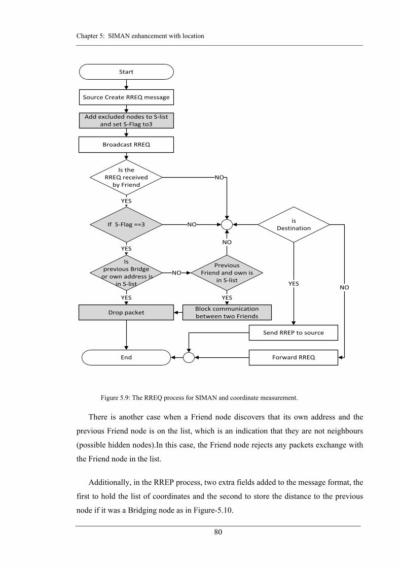
Chapter 5: SIMAN enhancement with location
80
Figure 5.9: The RREQ process for SIMAN and coordinate measurement.
There is another case when a Friend node discovers that its own address and the
previous Friend node is on the list, which is an indication that they are not neighbours
(possible hidden nodes).In this case, the Friend node rejects any packets exchange with
the Friend node in the list.
Additionally, in the RREP process, two extra fields added to the message format, the
first to hold the list of coordinates and the second to store the distance to the previous
node if it was a Bridging node as in Figure-5.10.

Chapter 5: SIMAN enhancement with location
81
Figure 5.10: RREP message format in SIMAN enhancement with location.
The process starts with the destination node, to which it adds its own coordinates, and
then forwards the RREP message to the previous node.
Every Friend node receives the RREP adds their own coordinates and forwards the
message as in Figure 5.11-1.
Bridging nodes use AODV to process the RREP message as in Figure 5.11-2.
When a Friend node receives the message from a Bridging node, it first checks the
number of Friend nodes in the PPN list, before the Bridging node.
o If there was two, then it starts the calculation using Fr1→Br1→Fr2→Fr3
otherwise, forwards this task to the next Friend node as seen in Figure 5.11-3.
o If there was no another Friend node (i.e. The Friend node was the source ), then
it sends a special RREQ to another neighbouring Friend node to get additional
coordinates, which is required for coordinates measurement using the
Fr1→Fr2→Br1→Fr3 the sequence as in Figure 5.11-4.
o Assuming there were two Friend nodes before the Bridging node. The next step is
to check for the number of Bridging nodes, by comparing the hop count with the
PPN factor list. If they were equal, then it is processed using one-step coordinate
calculation. Otherwise, it uses the two-step procedure as seen in Figure 5.11-5.
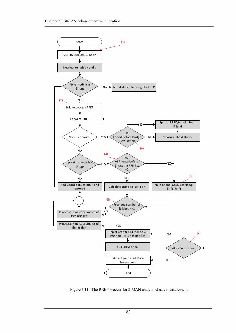
Chapter 5: SIMAN enhancement with location
82
Destination create RREP
Start
Destination adds x and y
YES
Forward RREP
Add distance to Bridge to RREP
NOprevious node is aBridge
End
YES
Process1: Find coordinates of the Bridge
NO
YES
Next node is aBridge
No. of Friends before Bridges in PPN list
=2
Node is a source
NO
YES
YES
No
Previous number of Bridges ==1
Process2: Find coordinates of two Bridges
Add Coordiante to RREP and forward
NO
Measure The distance
All distances true
Accept path start Data Transmission
Reject path & add malicious node to RREQ exclude list
Start new RREQ
YES
NO
Calculate using :Fr-Br-Fr-FrNext Friend Calculate using:
Fr-Fr-Br-Fr
Is Friend before Bridge
Destination
Special RREQ to neighbour Friend
NOYES
Bridge process RREP
(1)
(2)
(3)
(4)
(5)
(6)
(7)
Figure 5.11: The RREP process for SIMAN and coordinate measurement.

Chapter 5: SIMAN enhancement with location
83
If a Friend node received the RREP message and found that a Bridging node is without
coordinates, then it will process it using Fr1→Fr2→Br1→Fr3 as in Figure 5.11-6.
This process continues until the RREP reaches the source node, in which it starts the
distance measurement between the nodes as it can be seen in Figure 5.11-7. If the
distance between any two nodes exceeds the wireless transmission capability of
devices, then the route is rejected, and these two node addresses are added to exclude
list of the RREQ, otherwise, the route is accepted and starts data transmission.
Example-3
To explain the operation of the algorithm and the detection of an abnormal distance, we
will consider the example illustrated in Figure-5.12. The network consists of nine Friend
nodes and seven Bridging nodes in which two of them 7 and 17 are (WH nodes explained
in sec. 5.3). The source node 3 wants to send data to destination node 23, and for this
purpose, it broadcast a RREQ message. The two WH nodes make efforts to win the
shortest path by processing packets quickly using their Ethernet connection (solid red
line), and the attack comes in three different ways.
Figure 5.12: MANET scenario with two WH nodes.
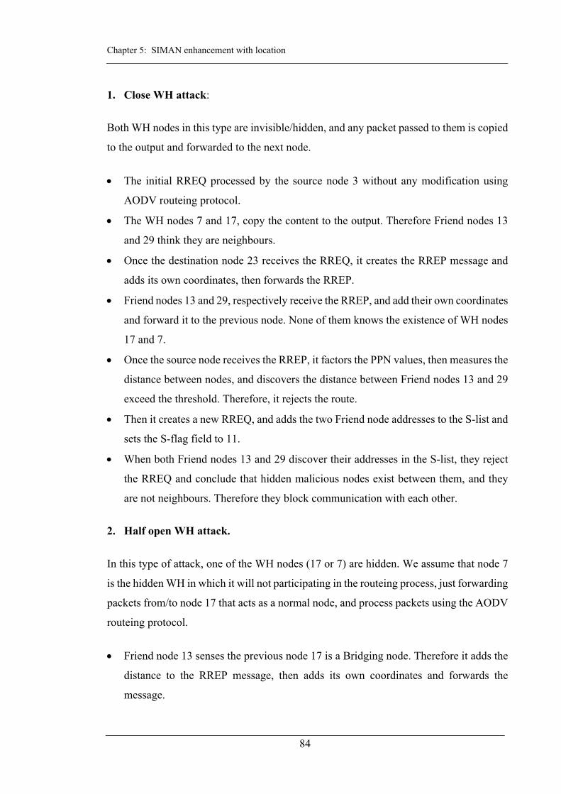
Chapter 5: SIMAN enhancement with location
84
1. Close WH attack:
Both WH nodes in this type are invisible/hidden, and any packet passed to them is copied
to the output and forwarded to the next node.
The initial RREQ processed by the source node 3 without any modification using
AODV routeing protocol.
The WH nodes 7 and 17, copy the content to the output. Therefore Friend nodes 13
and 29 think they are neighbours.
Once the destination node 23 receives the RREQ, it creates the RREP message and
adds its own coordinates, then forwards the RREP.
Friend nodes 13 and 29, respectively receive the RREP, and add their own coordinates
and forward it to the previous node. None of them knows the existence of WH nodes
17 and 7.
Once the source node receives the RREP, it factors the PPN values, then measures the
distance between nodes, and discovers the distance between Friend nodes 13 and 29
exceed the threshold. Therefore, it rejects the route.
Then it creates a new RREQ, and adds the two Friend node addresses to the S-list and
sets the S-flag field to 11.
When both Friend nodes 13 and 29 discover their addresses in the S-list, they reject
the RREQ and conclude that hidden malicious nodes exist between them, and they
are not neighbours. Therefore they block communication with each other.
2. Half open WH attack.
In this type of attack, one of the WH nodes (17 or 7) are hidden. We assume that node 7
is the hidden WH in which it will not participating in the routeing process, just forwarding
packets from/to node 17 that acts as a normal node, and process packets using the AODV
routeing protocol.
Friend node 13 senses the previous node 17 is a Bridging node. Therefore it adds the
distance to the RREP message, then adds its own coordinates and forwards the
message.

Chapter 5: SIMAN enhancement with location
85
WH node 17 receives the RREP process using AODV and forwards it to WH node 7
using the Fast Ethernet link.
WH node 7 copies the content of the RREP message to the output and forwards it to
the Friend node 29.
The Friend node 29 receives the RREP and executes the following steps:
o Factor the PPN values and realise that two Friend nodes 13 and 23 are located
before the Bridging nodes. Therefore, it uses Fr1→Br1→Fr2→Fr3 to measure the
coordinates.
o Additionally, it compares the number of nodes in Factor list (3 hops) with a hop
count (3 hops). Therefore, it proceeds with one-step Bridging node coordinates
measurement and adds the result to the list, then forwards the RREP.
o The Friend 29 is unaware of WH 7 because of the latter copies the content of the
message to the output so the hop count remains unchanged.
The Source node 3 receives the RREP and factors the PPN values, then uses the
coordinates list to measure the distance between the nodes and discovers that the
distance between the nodes 29 and 17 exceeds the threshold.
Therefore, it rejects the route, adds the two addresses to the exclude list, and
broadcasts a new RREQ.
When the Friend node 29 discovers its own address and WH node 17 in the exclude
list, inside the new RREQ. It rejects all messages from WH node 17 and drops the
RREQ message.
Additionally, when the Friend node 13 detects the address of WH node 17 in the list,
it drops the packet and rejects further messages from WH node 17. In this way, WH
17 is rejected and isolated by both neighbouring Friend node 29 and 13.
1. Open WH attack
When both WH nodes are visible, then they act like normal nodes, in term of processing
and forwarding routeing packets. The following steps show how the detection procedure
is accomplished.
As in the previous case Friend node 13, discovers that the previous node is a Bridging
node, therefore, it executes the same procedure.

Chapter 5: SIMAN enhancement with location
86
The WH nodes (17 and 7) processes the RREP message using the Fast Ethernet link,
and then WH node 7 forwards the RREP to the Friend node 29 using its wireless
interface.
When the Friend node 29 receive the RREP, it executes the following steps:
o Factors the PPN values and discovers that Friend nodes 13 and 23 are located
before the Bridging nodes, therefore, the process Fr1→Br1→Fr2→Fr3 is executed.
o Compares the number of nodes in the factor list (3 hops) with a hop count (4 hops)
and discovers that two Bridging nodes come one after another. Therefore, it uses
the two-step measurement previously explained in the previous examples 1 & 2.
o Then, it adds the distance to the neighbouring Bridging node and its own
coordinates to the list and forwards the RREP message.
Once the RREP reaches the source node, it measures the distance between the nodes
and detects the abnormal distance between WH nodes 7 and 17. Therefore it rejects
the route.
Then it starts a new RREQ process with the two Bridging node addresses added to S-
list and set the S-Flag to 11.
Therefore, Friend node 13 rejects the RREQ message from WH node 17, in result
excludes the WH nodes from the path discovery process.
5.5. Simulations and Results
In this section, we implement SIMAN’s enhancement into the MANET nodes in OPNET.
This includes the determination of the Bridging node coordinates as well as the distance
measurement conducted by the source node. For this purpose, two WH node are
introduced (sec. 4.1.2.) as Bridging nodes inside the network. This is to examine the
successful implementation and its effect on the overall performance of the network.
Several simulation scenarios are executed to compare the AODV and SIMAN
performance under three types of WH node attacks. Results are collected through the IP
route report that shows the established path in term of the number of hops and the
sequence of nodes. Furthermore, performance metrics like data rate and different
topologies with various distances between nodes are used to examine RDT and End to
end delay for both algorithms.

Chapter 5: SIMAN enhancement with location
87
5.5.1. Network Scenarios
Scenario-1
The scenario in Figure-5.13 consists of ten Friend nodes with six Bridging nodes (nodes
31, 51,15,33,12 and 49) and two WH nodes (black devices, nodes 7 and 17).
Figure 5.13: Scenario-1 MANET network layout.
The location of these nodes are shown in Table 5.1, which is extracted from the nodes
position attributes in OPNET modular as x and y components.
Table 5.1: The coordinates of nodes in scenario-1
Node Coordinates Node Coordinates X Y X X Y
31 422 617 5 1051 984.2 3 456 789 33 1098 1113 29 676 698 17 1383 600 61 645 1042 47 1258 677.8 43 793 921 12 1314 997 7 843 533 13 1514 817 15 994 656 41 1535 1159 51 1117 400 49 1702 626 37 1089 815 23 1735 977

Chapter 5: SIMAN enhancement with location
88
The scenario is designed to establish a path between the two Friends 3 and 23 that want
to exchange data in both directions. The full characteristics for the scenario are shown in
Table-5.2.
Scenario-2
The previous scenario was modified to have five different topologies/layouts, and nodes
are placed randomly at various distances. The data rate is fixed to 24Mbps for all nodes
and the other characteristics of the network stay the same as in Table-5.2.
Table 5.2: Scenario-1 simulation parameters
Parameter Value
Trajectory Random mobility waypoint Movement range: 2000m * 2000m
Distance between any two neighbouring nodes:
Nodes7 and 17
>300m
Other Nodes <300m
Data rate:
Nodes7 and 17 Outbound OB(24Mbps), inbound IB(100BaseT Ethernet link)
Other Nodes (scenario-I) Scenario-II
1,2,6,9,12,18,24 and 36 Mbps 24 Mbps
Packet size 512 Byte Packet reception power threshold
-82.65 dBm
Transmission power 0.005 Watt Active route timeout 3 sec Buffer timeout 2 sec
Traffic mix 500MB, all explicit
Simulation Duration 300 sec

Chapter 5: SIMAN enhancement with location
89
5.5.2. Results and analysis
Scenario-1:
Route discovery process
Several simulations were executed with various type of WH node attacks for both AODV
and SIMAN. The purpose was to examine the impact of each type of WH node attacks
on the route discovery and if SIMAN enhancement managed to eliminate the WH nodes.
Furthermore, observe the number of hops that are used for each route. Initially, we
simulated the scenario without wormholes using AODV, to compare it with results when
WH nodes introduced.
The route report for IP traffic flow (blue dotted arrow) shows the established path
consists of 7 hops (the nodes 3,29,43,5,12,13 and 23) as shown in Figure-5.14. and using
(eq.5.1) we realise the distance between any two consecutive nodes are (238.07, 251.8,
265.6, 273.7,225.4, and 272.8) meters respectively.
Figure 5.14: Scenario-1, AODV route discovery without WH attack.

Chapter 5: SIMAN enhancement with location
90
1. Open WH attack
The simulation then repeated for AODV with two visible WH nodes and the result shows
that they managed to divert the route discovery using 6 hops path (the nodes 3, 29, 7, 17,
13 and 23) as shown in Figure-5.15.
Figure 5.15: Scenario-1, AODV route discovery with open WH attack.
Then using the coordinates of the nodes in Table 5.1, we discover that the distance
between neighbouring nodes inside the path is (238.07, 234.7, 544.1, 253.4, and 272.8)
meters respectively. As we can see, the distance between the two nodes 7 and 17 is
544.1m, which clearly exceeds the maximum threshold distance between wireless nodes
and this provides an indication that these two nodes are WHs.
After that, the simulation was repeated for the SIMAN algorithm, and from the results,
we can see that it prevented the WH nodes from winning the path and eliminated them
by establishing the same 7 hops path, as shown in Figure-5.16.
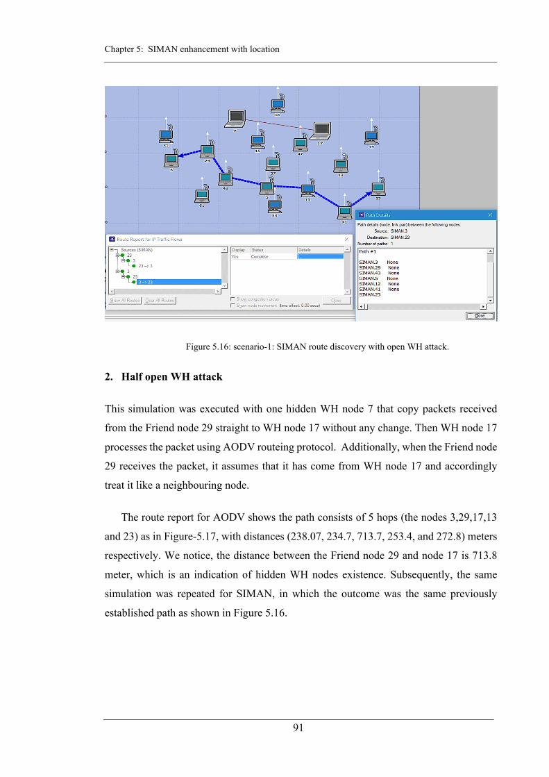
Chapter 5: SIMAN enhancement with location
91
Figure 5.16: scenario-1: SIMAN route discovery with open WH attack.
2. Half open WH attack
This simulation was executed with one hidden WH node 7 that copy packets received
from the Friend node 29 straight to WH node 17 without any change. Then WH node 17
processes the packet using AODV routeing protocol. Additionally, when the Friend node
29 receives the packet, it assumes that it has come from WH node 17 and accordingly
treat it like a neighbouring node.
The route report for AODV shows the path consists of 5 hops (the nodes 3,29,17,13
and 23) as in Figure-5.17, with distances (238.07, 234.7, 713.7, 253.4, and 272.8) meters
respectively. We notice, the distance between the Friend node 29 and node 17 is 713.8
meter, which is an indication of hidden WH nodes existence. Subsequently, the same
simulation was repeated for SIMAN, in which the outcome was the same previously
established path as shown in Figure 5.16.

Chapter 5: SIMAN enhancement with location
92
Figure 5.17: Scenario-1, AODV route discovery with half-open WH attack.
3. Closed WH attack
In the next simulation, both WH nodes were hidden so Friend nodes 29 and 13 think they
are neighbours. The result for AODV routeing protocol shows a path consists of 4 hops
(the nodes 3, 29, 13 and 23) as seen in Figure-5.18. The distances between these nodes
are (238.07, 846.4, 253.4, and 272.8) meters respectively.
We notice the distance between the Friend node 29 and 13 is 846.4 meter, which
exceeds the maximum transmission distance of two nodes. This provides an indication
that hidden WH nodes existence inside the path. After that, the simulation was repeated
for the SIMAN algorithm, and the results indicate that SIMAN eliminates the WH nodes,
and used the same path as the previous simulations.
In conclusion, the above simulated result of the IP report and the measured distances
shows that the three types of WH nodes succeeded in winning the path with AODV
routeing protocols. While in SIMAN’s case, the WH nodes were eliminated, and the same
path repeatedly was established. This demonstrates that the distance measurement
procedure was successful in preventing WH nodes from winning the path.

Chapter 5: SIMAN enhancement with location
93
Figure 5.18: Scenario-1, AODV route discovery with Closed WH attack.
Route discovery time
The next simulation was to calculate the RDT for both AODV and SIMAN using different
data rates, for all three cases of WH node attacks. The RDT results, seen in Figure-5.19,
shows that it took SIMAN 1.28sec on average more to establish the path in comparison
to AODV. This is due to the execution of the route discovery process twice, after the first
attempt with WH nodes was rejected. Furthermore, we notice the RDT in both algorithms
increases with the visibility of the WH nodes. Which is caused by the participation of the
WH nodes in processing packets instead of just forwarding them as in a closed attack
(Appx. A.2.1).
Additionally, we observe a sudden decrease in RDT in 24Mbps for both algorithms.
The reason for that as seen in Table 5.2, the WH nodes outbound data rate was 24Mbps.
Therefore, when other nodes operate at the same data rate, they process packets faster and
this reduces the RDT. Moreover, this reduction was seen sharper in AODV (0.435sec on
average) while in SIMAN (0.2sec on average). This is because SIMAN establishes the
path twice and WH nodes are involved only in first route discovery, therefore the effect
will be less in comparison to AODV.

Chapter 5: SIMAN enhancement with location
94
Figure 5.19: Scenario-1, route discovery time with various data rates.
End to end delay
The results show the impact of WH node attacks on end-to-end delay (Appx. A2.2.).
According to the type of attack, the visible WH nodes have to process packets, which in
turn causes delay. We notice that SIMAN has 0.354sec on average more delay to AODV.
This is due to the number of hops inside the path (AODV 5 hops and SIMAN 6 hops).
On the other hand, we notice the variance in SIMAN’s delay is 0.003sec compared to
0.025sec for AODV on average. This is because of the WH node setting has no effect on
the SIMAN algorithm as it is illustrated in Figure-5.20.
Figure 5.20: Scenario-1, End to end delay.

Chapter 5: SIMAN enhancement with location
95
Scenario-2:
Simulation results for five different topology/layouts show that when using AODV
routeing protocol, WH node wins the path wherever they are inside the network, as we
can see from the route report for IP traffic flow in Figure 5.21. While for the SIMAN
algorithm, the WH nodes are rejected in all layouts as in Figure 5.22.
Figure 5.21: Scenario-2, the established path for various layout using AODV.
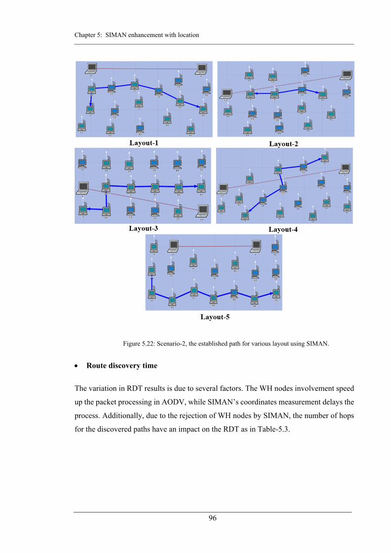
Chapter 5: SIMAN enhancement with location
96
Figure 5.22: Scenario-2, the established path for various layout using SIMAN.
Route discovery time
The variation in RDT results is due to several factors. The WH nodes involvement speed
up the packet processing in AODV, while SIMAN’s coordinates measurement delays the
process. Additionally, due to the rejection of WH nodes by SIMAN, the number of hops
for the discovered paths have an impact on the RDT as in Table-5.3.

Chapter 5: SIMAN enhancement with location
97
Table 5.3: Compersion for the routes established for AODV and SIMAN
Layout Traffic 3↔23
AODV SIMAN No of Hops Path No of Hops Path
Layout-1 6 3-43-17-7-51-23 7 3-43-33-5-31-47-23
Layout-2 5 3-17-7-51-23 4 3-5-31-23
Layout-3 4 3-7-17-23 7 3-61-29-5-47-41-23
Layout-4 5 3-43-17-7-23 6 3-12-33-31-23
Layout-5 7 3-5-17-7-12-29-23 8 3-13-43-61-47-49-29-23
In layout (1 and 5), SIMAN rejects the path with WH node and during the second route
discovery, it conducts Bridging node coordinates calculation (two for layout-1 and one
for layout-5). Therefore, we notice an increase of 2.89sec on average in RDT compared
to AODV as in Figure-5.24. Moreover, the RDT in layout-2 took on average 2.46sec more
than AODV, despite having 4 hops inside the established route.
This result represents a particular case (sec. 5.4.1.4), in which only two Bridging
nodes are in the path, thus, it requires the source node to send a false RREQ to a
neighbouring Friend node to get the extra coordinates required for coordinates
measurement. Finally, we can observe that SIMAN algorithm in layout-4 has three
Bridging nodes, and accordingly, it has a greater RDT of 2.31sec to AODV.
Figure 5.23: Scenario-2, route discovery time for different layouts.

Chapter 5: SIMAN enhancement with location
98
End to end delay
Simulation results show variable delay measurements for various topology/layouts.
Furthermore, we notice the delay difference between AODV and SIMAN is 0.248sec on
average. Which is mostly due to the hop numbers inside different routes and WH nodes
role in AODV to forward packets faster, as in Figure-55.
Figure 5.24: Scenario-2 End to end delay for the five layouts.
5.6. Summary
In conclusion, SIMAN enhancements managed to use the existing routeing protocol
processes to share node’s coordinates with others inside the path, and then use them to
prevent WH attack without using an extra key-based security solution. Additionally, we
realised that sharing the location information between nodes helps towards improving the
knowledge of the node's physical location inside the network and enables the source node
to reject routes that have unrealistic distances between nodes. Furthermore, that
coordinates measurement and location information sharing help the source node towards
building better path with specific requirements as we will see in next chapter.

99
SIMAN with remaining battery energy
MANET nodes are portable battery-powered devices that conduct routeing duties, as well
as data transmission. This can lead to consuming a lot of battery energy causing node
failure and in return, leads to disconnection and link break.
Nodes Remaining Battery Energy (RBE) plays a major role in MANET performance.
Routeing protocol does not consider RBE consumption, therefore, nodes have to process
routeing messages even if they have low RBE. Additionally, selfish nodes can dismiss
important routes by rejecting packet to save RBE. Consequently, it is important for the
source node to have a mechanism to inspect nodes RBE before conducting the routeing
process.
This chapter focuses on improving SIMAN algorithm further to include RBE of each
node inside the path. In other words, we use the existing routeing protocol messages to
carry information about the RBE gathered from each node and shared with other nodes.
Furthermore, the source node compares several received RREP messages from different
paths, to construct a route that has better RBE for data transmission.
Simulation results show that despite having a longer route discovery time, SIMAN’s
performance improved, in terms of packet delivery ratio by 19.7% and the end-to-end
delay by 7% in comparison to AODV routeing protocol. These improvements were
obtained due to fewer disconnections that occurred because of a lack of RBE. The finding
and results of this enhancement are documented in our research paper to be published
later this year.

Chapter 6: SIMAN with remaining battery energy
100
6.1. Literature review
The main concern of MANET routeing protocol is to locate the destination node using
the shortest path and to send out data immediately once a route is established. These
standard protocols have no interest in the nodes RBE. As a result, node failure occurs and
leads to link breakages. Researchers investigated the possibility of incorporating the
energy information to the routeing process, using different techniques. We review these
techniques in the following section.
A Protocol called Energy-aware and Stable Clustered based Multipath Routeing
Protocol, ES-CMR proposes the reservation of the residual energy of nodes, to increase
the networks lifetime. The protocol intends to handle the energy of nodes efficiently to
minimises the end-to-end delay of MANET and it uses a clustering structure to decrease
the routeing control overhead. The source node waits for different RREPs to arrive from
the cluster heads before sending out data, and uses two functions to assess link stability
and nodes residual energy level. Then it selects the best route based on the power
consumption and uses other paths as an alternative [84]. The concept of this protocol
relies on the source node to makes several route discoveries and choose one based on
RBE. We aim to use a similar approach, but the source node in our algorithm uses the
knowledge of location and RBE, to construct a path based on the nodes highest energy.
In another research work, energy level and link stability were used in a protocol called
Stability of the path and residual energy Based (SHUB). The proposed protocol’s concern
is the instability of the established route that occurs because of node mobility, and the
shortage of the route lifetime because of the drainage of the node battery. The two
matrices are calculated using information collected from the nodes, and the path selection
is based on total energy cost and the maximum link expiration time for the path [85]. The
route selection is conducted by a node inside the route and shared with others. However,
it is not clear how the nodes deliver this information as putting an extra load on
intermediate nodes, leads to further energy consumption (explained later).
Another solution deals with the RREQ distribution of the consumed energy called
Energy Aware Routeing Protocol. This protocol tries to reduce the RREQ flooding to
every node and prevents nodes that have critical RBE from processing the messages. This

Chapter 6: SIMAN with remaining battery energy
101
is achieved by sharing the RBE of the nodes using the RREQ. Every node forwards the
received message if the RBE value is higher than the stored record inside a routeing table.
[86]. In our opinion, the RBE record inside routeing table might be old or not available.
Therefore this comparison does not provide an accurate method to forward RREQ.
Additionally, SIMAN algorithm intends to reduce access to the routeing table on the
physical drive, because it causes further consumption of resources.
In a different method, the remaining energy level is used to construct multicast
routeing protocol, which is called Energy Aware Multicast Routeing Protocol (EAMRP).
The protocol establishes distinct paths to enhance the connectivity and reduces link
breakages that occur due to a node’s lack of energy. Using a ranking value to classify
nodes based on residual energy, it then uses this value to select the node, which can
support multicasting [87]. The protocol claimed to maximise end-to-end connectivity in
the network and minimises faults at the link node level. The concept used in route
discovery is similar to AODV and other routeing protocols, but in our opinion using three
routeing tables, requires the nodes to execute additional processes which consume further
power compared to the original routeing protocols.
In another study, the knowledge of the RBE is used to prevent congestion. The
proposed protocol is called Congestion and Energy Aware Routeing Protocol CAERP.
The research suggests that link breakages and packet retransmission causes congestion
and indirectly causes more energy consumption. For this purpose, it proposes to adjust
the data rate according to the queue state and RSSI. Therefore, if the value is high, then
it assumes that the distance from the source node to the neighbour is short, and
accordingly, reduces the data rate. Which in result leads to less energy consumption and
improves the path lifetime. [88]. However, it is not clear who conducts this data rate
reduction, because it requires sharing this information between the nodes and it has to
avoid extra overhead.
6.2. Conceptual design
The current enhancement consists of several route discovery processes conducted by the
source node to explore all possible paths to the destination node. During each RREP the

Chapter 6: SIMAN with remaining battery energy
102
nodes pass their RBE back to the source node using a list added to RREP message. The
source node then uses the RBE information from different routes to construct a new route
with the highest RBE and use it for data transmission. In the next section, we derive a
formula that is utilised by the nodes to calculate RBE.
RBE measurement
Mobile devices battery consumption has five different modes [89].
1. Transmission mode: The battery energy required by the node to transmit packets to
other nodes inside the network. We assume Plength (packet size in Bits) is fixed as the
transmission power varies with different packet sizes [90].
Pt=330* Plength
Tt*2*106 (6.1)
2. Reception mode: The battery energy consumed to receive packets from other nodes
Pr=230* Plength
Tr*2*106 (6.2)
Pt : Transmission power, Pr : Reception power, Tt: Time to transmit data packet
and Tr: Time to receive the data packet.
3. Idle mode: In this mode, the node will be listening to the channel for incoming
packets, and it consumes the same amount of battery energy used in the reception
mode. Once the node senses packet, it switches to the reception mode.
4. Overhead mode: The battery energy consumed to receive packets destined to other
nodes.
5. Sleep mode: In this mode, the node consumes nearly zero battery energy. Therefore,
the node moves to this mode to prevent the loss of battery energy.
Every Friend node in SIMAN algorithm measures its own RBE and attaches it to the
RREP message. The computation value of the RBE is obtained by subtracting the
consumed power from the initial power [91].
RBE = initial power –Consumed power (6.3)

Chapter 6: SIMAN with remaining battery energy
103
The consumed power is calculated by multiplying the number of packets to the sum of
transmission and reception powers, and then adding the idle power multiplied by time.
Consumed power= no of pkt*(Pt +Pr) +Pi* T(s) (6.4)
The main aspect of SIMAN algorithm is hiding its implementation from the Bridging
nodes. Therefore we use the neighbouring Friend nodes to measure information related
to those Bridging nodes and to share it with each other, as we saw in prime ID generation
and coordinate measurement. However, measuring the RBE is a complex process and is
left as future work. Therefore, we use a simple procedure for this measurement and
assume that Friend nodes already know the initial battery level of the Bridging nodes.
Example-1
A Bridging node B is located between source node A and destination node C with an
initial battery level of 65% and 70% respectively. The route discovery process involves a
single RREQ packet sent by source node A through Bridging nodes B to the destination
node C and an RREP packet sent in the opposite direction. During initial communication,
destination node C calculated the initial power capability of Bridging node B as 72%. The
following procedure explains the Friend nodes estimation of the RBE value.
Assuming the battery energy consumption cost:
o Transmission power per packet: 0.2watt
o Reception and idle power per packet: 0.1watt
o The no of packet processed: 2 in 1.5sec.
Friend node (the source A): sends a single RREQ and receives a single RREP packet.
Using (Eq.6.4) calculates the RBE value:
RBEA=65- 1*0.2+1*0.1+1.5*0.1 =64.55
Friend node (the destination C): receives a RREQ and sends a single RREP packet.
RBEC=70- 1*0.2+1*0.1+1.5*0.1 =69.55
Bridging node B, receive a single RREQ and forward it, then receive a single RREP
and forward it. Based on this procedure, the destination node C calculates the RBE
for the Bridging node B.
RBEB=72- 2*0.2+2*0.1+1.5*0.1 =71.25

Chapter 6: SIMAN with remaining battery energy
104
We notice from this example that the intermediate node RBE consumption during route
discovery is twice that of the source and destination nodes. Which increases the
possibility for these nodes to run out of RBE before the data transmission is complete.
6.3. SIMAN with RBE implementation
In this section, we explain the implementation of SIMAN algorithm to share information
about the RBE between nodes that participate in the route discovery process. The
following updates are required to the RREQ and RREP message format.
The RREQ message is similar to the previous version of SIMAN as explained in
Figure-5.10. The two-bit S-Flag is used to distinguish between different RREQ types.
Two extra fields are added to the RREP message format, the first is an RBE-list to
hold the nodes RBE values and the second consists of two-bit S-Flag field to
distinguish between messages as shown in Figure-6.1.
Figure 6.1: RREP message format with RBE enhancement in SIMAN.
The routeing process starts with the source node that has no previous valid path to the
destination node, by creating the RREQ and broadcasting it, in an attempt to find the
destination node. In this enhancement of the algorithm, we have three types of RREQ.

Chapter 6: SIMAN with remaining battery energy
105
Initial RREQ: Created at the beginning of the route discovery and broadcast to find
the destination node. The S-list field is left empty, and the S-Flag field is set to 00 as
an indicator for Friend nodes, that it is the initial RREQ process.
The Exclude-RREQ: starts after the first RREP arrives back to the source node,
loaded with nodes RBE. The source node analyses the RBE-list and selects the node
with lowest RBE then inserts its address into the S-list, of a new RREQ and sets the
S-Flag to 01 and broadcast it to find other paths by excluding the node in the S-list.
The Include-RREQ: is used after a route discovery trial ends, when there are no
more paths to the destination node. The source node then creates a new RREQ with a
list of preferred nodes that has a high RBE. The S-Flag field is set to 10, which
instructs to process the RREQ if the node’s address is on the S-list.
Example-2
To explain this process, we consider the scenario in Figure-6.2. The Source node 3
wants to send data to the destination node 23. The fraction under each node in the figure
represents the RBE of the node during the route discovery process. For simplicity, we
assume that the transmission and reception power costs 1% each, and neglect the idle and
overhear RBE consumption.
Figure 6.2: A network scenario for SIMAN algorithm with RBE.

Chapter 6: SIMAN with remaining battery energy
106
1. Initial Route Request
The source node creates a RREQ message and set the S-Flag=00, then broadcasts the
message. Every node receives the RREQ, checks the S-Flag field, and forwards the RREQ
if the value equals zero, as it is explained in Figure-6.3.
Figure 6.3: Initial RREQ process for SIMAN with RBE.
Eventually, the first RREQ message reaches the destination node 23 from node 5.
Other RREQs (from nodes 13 and 31) are ignored by the destination node as seen in
Figure-6.4. Then the destination node measures the Bridging node’s RBE and attaches it
to the RBE-list of the RREP message.
After that, it copies the S-Flag field value 00 from the RREQ as an indication for the
initial RREQ and forwards the message back to the Bridging node 5, which is not aware
of SIMAN. Therefore, it processes the RREP using AODV, and then node 7 add its own
RBE to the RBE-list and forwards it to the source node as in Figure-6.5.

Chapter 6: SIMAN with remaining battery energy
107
Figure 6.4: Initial RREQ by SIMAN with RBE
Figure 6.5: Initial RREP for SIMAN with RBE.

Chapter 6: SIMAN with remaining battery energy
108
2. Measuring the path with lowest RBE
The source node then starts to examine the nodes RBE for the lowest value (the node 5
has 36%) as explained in Figure-6.6.
Figure 6.6: Path lowest RBE measuring
3. Exclude-RREQ
In the next step, the source node creates a new RREQ, adds the address of the node 5 to
the RBE-list field and sets the S- Flag to 01, and broadcasts the RREQ. Every node
receives the RREQ checks the S-Flag and compares the previous node address with the
address in the list. If they match, then drops the RREQ, otherwise, it rebroadcasts the
RREQ as explained in Figure-6.7.

Chapter 6: SIMAN with remaining battery energy
109
Figure 6.7: Exclude node RREQ process in SIMAN with RBE.
The nodes 17, 7 and 43 receive the broadcast RREQ from the source node, then they
forward the RREQ because the exclude node address is 5 and the previous node is 3. This
process is repeated until the RREQ arrives at the destination node from node 5. However,
the destination node rejects the message because a match found in the S-list as seen in
Figure-6.8a. After that, it receives another copy of the RREQ from node 13. Thus it
accepts this copy and sends the RREP message through node 13 as it can be seen in
Figure-6.8b.

Chapter 6: SIMAN with remaining battery energy
110
Figure 6.8: Second RREQ and RREP attempt with one excluded node.
When the source node receives the RREP, it repeats steps 2 and 3 again, and the lowest
RBE node is 29 added to the S-list and send a new RREQ. This time, nodes, 11 rejects
the RREQ because a match found in S-list as in Figure-6.9a. After that, the destination
node rejects RREQ from node 5, while accepts the RREQ from the node 31, therefore, it
sends the RREP message back to the source node through node 31, as in Figure-6.9b.
Figure 6.9: Third RREQ and RREP attempt with two excluded nodes.

Chapter 6: SIMAN with remaining battery energy
111
Next, the source node repeats the process, and select node 7 in which it has the lowest
RBE. Then it inserts the address to the S-list and another RREQ is sent. Eventually, when
nodes 11, 23 and 47 receive the RREQ, they all drop the RREQ, and in this way, no
RREQ reaches the destination node as shown in Figure-6.10. The source node then
rebroadcasts the RREQ again with an increased lifetime, and the trial continues until it
reaches maximum RREQ limit.
Figure 6.10: Final RREQ with excluded nodes.
4. Analysis process
The analysis process is conducted by the source node, after receiving the RREP from all
possible paths. First, it calculates and updates the RBE level to a new value for all nodes
participated in forwarding RREQs for different paths. Then it executes the analysis
process, which is explained below and shown in Figure-6.11:
The source node selects the neighbour with the highest RBE, and add it to the possible
path (temp value). Then compares the second node RBE values from different paths
and chooses the node with the highest RBE.
Next, it measures the distance between the two selected nodes to make sure they are
in transmission range, and if the distance exceeds the threshold, then this node is
rejected and replaced with a node with the second highest RBE.

Chapter 6: SIMAN with remaining battery energy
112
This trial is repeated until the source node finds a combination of two nodes with a
high RBE, that are in the transmission range.The high RBE threshold is the average
of RBE of all neighbours, of the specific trial level.
If none of the neighbouring nodes meets the criteria, then the process is backtracked
and the previous level selected nodes are replaced with the second highest RBE value.
This process is repeated until the source node manages to build a path to the
destination node, through the nodes with the highest possible RBE.
Figure 6.11: Source analysis procedure to construct a new path

Chapter 6: SIMAN with remaining battery energy
113
In the example the source node 3 constructs a new route from the following stored
information for the three paths:
Path-1: 3 88% →7 (58%) →5 (31%) →23 (86%)
Path-2: 3(88%)→17(84%)→29(52%)→11(79%)→13(71%)→23(86%)
Path-3:3 88% →7 58% →47(88)→37(70%)→31(82%)→23(86%)
Figure 6.12: Different level neighbours in paths to destination node
The source starts the process by examining the first-level neighbour nodes (17 and 7)
and selecting the highest RBE, node (17) as in Figure-6.12.
Then it examines the second level (the neighbour of the neighbours) (nodes 5, 29 and
47) and selects node 47. The average RBE for those three nodes represents the
threshold (31%, 52%, and 88%) which is equal to 57%. Therefore any node below
this level is not considered for route selection unless there is no alternative.
Measuring the distance between node 17 and the newly added 47 reveals that it
exceeds 300m. Therefore it rejects 47 and selects the next high RBE node.
Node 29 and 5 RBE are below the high RBE threshold. Therefore the source node
backtracks the process and removes node 17 and selects the second highest RBE from
the previous tier (node 7), and repeats the same process again
Eventually, the constructed path was (3747373123) which it has the
highest RBE collectively.

Chapter 6: SIMAN with remaining battery energy
114
5. Inclusion RREQ process:
The source node creates a new RREQ and adds the constructed path to the S- list, and
sets the S-Flag to 10. Then it broadcasts the RREQ as in Figure-6.13.
Figure 6.13: RREQ sent by source node with inclusion list
Each Friend node receives the RREQ, compares the previous node address with the
selected path S-list addresses. Then process the RREQ if the address exists, otherwise,
it discards the message. The reason to select the previous node and not the own
address is to prevent malicious/selfish nodes self-inclusion or exclusion.
In this way, the message is propagated only through nodes on the S-list as it can be
seen in Figure-6.14. Once it reaches the destination node, an RREP message is sent
back to the source node to start data transmission.
6.4. Simulations and Results
In this section, we examine the implementation of the RBE enhancement to the SIMAN
algorithm, and its impact on the route discovery process in comparison with AODV.
Moreover, we observe the effect of node failure due to a lack of RBE on performance in
terms of RDT, packet delivery ratio PDR, and End to end delay.

Chapter 6: SIMAN with remaining battery energy
115
Figure 6.14: The inclusion RREQ process in SIMAN.
6.4.1. Network Scenarios
Scenario-1
The network in this scenario consists of twenty Friend nodes (green laptops) and eight
Bridging nodes (blue desktops), with random RBE levels as shown in Figure-6.15. The
source node 31 sends data to the destination node 109 continuously for the duration of
the simulation. The RBE consumption is calculated according to previously explained
formula, (eq. 20 and 21, sec. 6.3.1).
Several simulations were executed for both AODV and SIMAN algorithms for
different data rates. We extended the simulation duration to provide sufficient time for
nodes with low RBE to run out of RBE and fail, then observed the impact using several
metrics. The full characteristic of the scenario is shown in Table-6.1.

Chapter 6: SIMAN with remaining battery energy
116
Figure 6.15: Scenario-1 network setup.
Table 6.1: Scenario-1 simulation parameters.
Parameter Value
Trajectory Random waypoint Movement range: 2000m * 2000m
Data rate:
Scenario-I 1,2,6,9,12,18,24 and 36 Mbps
Scenario-II 24 Mbps Packet reception power threshold -82.65 dBm Transmission power 0.005 Watt Pt, Pr, and Pi 0.003,0.001 and 0.001 watts respectively Packet size 512 byte Simulation Duration 1 Hour
Scenario-2
In this scenario, we fixed the data rate to 24Mbps and measured the PDR delay every 5
minutes for one hour, to observe the effect of node failure. The scenario consisted of 15
Friend nodes and 5 Bridging nodes, distributed randomly as in Figure-6.21. The source
node 3 sends data to destination node 5.

Chapter 6: SIMAN with remaining battery energy
117
Figure 6.16: Scenario-2, twenty node MANET with five Bridging nodes.
6.4.2. Results and analysis
Scenario-1
Figure 6.17, denotes the simulation execution for SIMAN algorithm and the established
route report in OPNET. It indicates a 7 hops route that is constructed by the source node
after examining all possible paths and analysing the RBE. Then, the same simulation is
executed again for AODV, and a different route of 9 hops was established as shown in
Figure-6.18.
The reason for the difference is that AODV does not consider RBE. Therefore, we
expect that nodes 61(RBE=18%) and 71 (RBE=21%) to fail at some stage of the
simulation, due to a lack of battery energy. Which as a result causes a link breakage that
leads to the establishment of an alternative path.
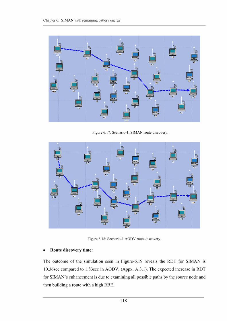
Chapter 6: SIMAN with remaining battery energy
118
Figure 6.17: Scenario-1, SIMAN route discovery.
Figure 6.18: Scenario-1 AODV route discovery.
Route discovery time: The outcome of the simulation seen in Figure-6.19 reveals the RDT for SIMAN is
10.36sec compared to 1.83sec in AODV, (Appx. A.3.1). The expected increase in RDT
for SIMAN’s enhancement is due to examining all possible paths by the source node and
then building a route with a high RBE.

Chapter 6: SIMAN with remaining battery energy
119
Figure 6.19: Scenario-1, route discovery time with various data rates.
Packet delivery ratio:
During data transmission, the PDR value gets affected by circumstances like a link break
or congestion [92]. Simulation results in Figure-6.20 show that AODV-PDR for lower
data rates is 0.785 and this increases by 0.124 for higher data rate, while SIMAN-PDR
shows an average of 0.982 and 0.935 for higher data rates. Consequently, this means an
overall PDR improvement by 11% in comparison to AODV. Therefore, we conclude that
this improvement is obtained through SIMAN’s prevention of link breakages caused by
node failure, by the avoidance of using these nodes in route discovery process.
Figure 6.20: Scenario-1, packet delivery ratio.

Chapter 6: SIMAN with remaining battery energy
120
End to end delay:
Figure-6.21 shows the End to end delay for both algorithms decline with the increase in
the data rate, due to the rise in packet delivery at higher data rates [93]. Additionally,
SIMAN maintains an average delay of 0.216sec, compared to 0.42sec for AODV. There
is an advantage for SIMAN of 0.27sec (33%) at lower data rates, which apparently shows
that the recovery from node failure takes longer at lower data rates for AODV.
Figure 6.21: Scenario-1, End to end delay.
Scenario-2
Route discovery Time
The results of the SIMAN algorithm simulation shows the discovered route consists of 8
hops and the RDT value equals 5.6sec as seen in Figure-6.22. Moreover, AODV
establishes the path in 1.297sec using 7 hops, shown in Figure-6.23. Additionally, we
notice that AODV's route went through nodes (37 and 71) which have a low RBE, while
SIMAN enhancement avoided these nodes.

Chapter 6: SIMAN with remaining battery energy
121
Figure 6.22: Scenario-2, the established path for SIMAN algorithm.
Figure 6.23: Scenario-2, the established path for AODV.
Packet delivery ratio:
Results in Figure-6.24 show that SIMAN has an average 0.986 PDR, while AODV has
0.646. This means an improvement of 20% for SIMAN. Moreover, we notice that
SIMAN’s packet delivery was stable throughout the simulation time. However, in AODV
it starts to fall after 15 minutes sharply, due to the failure of two nodes 37 and 71 that
caused the packet to drop due to a link breakage [94].

Chapter 6: SIMAN with remaining battery energy
122
Figure 6.24: Scenario-2, packet delivery ratio.
End to end delay:
Simulation results in Figure-6.25 show that the delay at the beginning is high, and it
gradually decreases with time. This is due to packets having to stay in the buffer longer
until a path is established.
Figure 6.25: scenario-2, End to end delay.
Furthermore, we notice a sudden increase in the delay for the AODV between
20-30 minutes of the simulation time, which is when the two nodes 37 and 71 failed.
The delay occurred because of the packet were buffered while the path was repaired or
an alternative route was found [95].
Chapter 6: SIMAN with remaining battery energy
123
6.5. Summary
In summary, we can conclude that sharing the RBE knowledge, helps the source node to
identify the node with low RBE inside the path. Moreover, using several RREQ’s that
excludes the nodes with low RBE, helps the source node to gather RBE knowledge of all
possible paths to a destination node.
This knowledge is used along with the identity and distance between nodes by the
source node, to build a route from nodes with a high RBE. We demonstrated through
simulation that SIMAN enhancement improves packet delivery ratio and causes less end-
to-end delay, which is caused by the examination of different routes to collect the RBE
information.

124
Conclusion and future direction
As shown in the literature review in chapter two, a lot of research work has been carried
to improve routeing protocols in MANETs. However, they have also incurred overhead
issues such as the additional processes used to improve performance, and the extra traffic
used to share information between nodes.
This thesis presented the significance of sharing the information between nodes in a
MANET, without causing extra overhead using the existing routeing protocols. In this
chapter, we present our learning experience achieved through the implementation of
several approaches to enhance the routeing protocol performance that can help to better
QoS provision and the areas in which it can be explored in the future to add more value
to the work.
7.1. Conclusion
In this thesis, we introduced an algorithm (called SIMAN) that shares knowledge about
nodes beyond neighbours, and we have demonstrated its operation using AODV routeing
protocol, albeit the algorithm will work with any of the routeing protocols.
My main challenge in developing the PPN and localisation algorithm was the
mathematical concepts involved, in which it required to understand the number theory
and factorization of prime values of the GCD product, furthermore, using circle
intersection to calculate unknown coordinates of nodes inside the path. It was a great
reward for me seeing math algorithms developed in the 19th century, implemented in a
state-of-the-art application now to solve problems in wireless communication. Moreover,

Chapter 7: Conclusion and future direction
125
these solutions indirectly help toward other enhancements that require extra processing
to implement.
The breadth of the work, from the outset, was not to divulge into authentication and
encryption type of work adopted by most preceding researchers. Which implement
sophisticated key based procedures that overwhelm the nodes with additional processes
that cause overhead. However, it was clear that the PPN concept applied to retrieve
addresses can authenticate the previous node, which sent the packets.
Moreover, the localisation concept was added to identify the physical location of the
nodes for distance measurement between nodes, but at the same time, it helped toward
eliminating wormholes. Therefore, these avenues can be explored by future research into
how to use them to prevent other types of attacks.
Additionally, regimental QoS for MANET was attempted but felt that adopting proper
QoS techniques will cause extra overhead, and it was deemed inapplicable for one-offs
of MANET’s connectivity. However, the RBE concept added to SIMAN algorithm shows
an improvement in PDR and delay because of eliminating nodes with low RBE that leads
to link break. Overall, we can conclude that SIMAN algorithm with its improvements is
implemented to improve the routeing protocols performance but it provides several other
advantages indirectly for better services in MANET.
7.2. Future work and research area
The knowledge beyond neighbours obtained through the SIMAN algorithm serves as a
platform for further research that can enhance MANET operation. The following are the
areas that can be explored in the future research work.
I. SIMAN algorithm was applied to the AODV routeing protocol, which was selected
due to its advantage in comparison to other routeing protocols. However, the
algorithm can be modified to work as a package that can work with any routeing
protocols. This is because of the algorithm operation relies on using the reply
messages sent during route discovery. A concept that is adopted by most routeing
protocols. Therefore, we can improve SIMAN to detect the routeing protocol and
adjust itself accordingly.

Chapter 7: Conclusion and future direction
126
II. We have not made any security specific claim about SIMAN algorithm because we
have not defined the threat models and so approached it that way. However, it is clear
that such low cost/overhead knowledge of nodes beyond neighbours algorithm can be
used in a proper security implementation, especially if the PPN values are used as a
replacement of the keys exchanged for authentication/encryption.
III. On the other hand, link breakage that occurs because of node mobility causes a lot of
delay and packet retransmission. Sharing the coordinate information by SIMAN
algorithm can help the intermediate nodes to repair links by tracking other node's
movement. Further development can help to predict the direction of the node's
movement, which can be a valuable addition to the highly dynamic mobile network.
IV. The nodes RBE knowledge is used by the source node to build a path that lasts longer.
This concept can be used with other performance metrics like the bandwidth or delay
of the node as part of QoS-aware routeing protocols.
V. We noticed through the implementation of RBE that it is possible to build two paths
and use the second path as an alternative that can be utilised as a backup during
congestion or link breakage. Moreover, the source node can have more than one path
designated to transmit different data type.

127
References
[1] G. Kadir, I. A. Lami and T. Kuseler, “SMPR: A Smartphone Based MANET Using
Prime Numbers to Enhance the Network nodes Reachability and Security of
Routeing Protocols,” International Journal of Network Security, vol. 18, no. 3, pp.
579-589, 2015.
[2] G. Kadir and I. A. Lami, “SIMAN: a Smart Identification of MANET Nodes used
by AODV routeing algorithm,” in The 3rd World Congress on Computer
Applications and Information Systems , 2016.
[3] H. Wu and Y. Pan, Medium access control in wireless networks, vol. 8, Nova
Publishers, 2008.
[4] J. P. Macker, Mobile Ad hoc Networking (MANET): Routeing Protocol Performance
Issues and Evaluation Considerations, RFC Editor, 2013.
[5] N. Makhlouf and P. Vajsar, “Mac Protocols in Mobile Ad Hoc Networks,”
International Journal of Advances in Telecommunications, Electrotechnics, Signals
and Systems, vol. 1, no. 1, pp. 9-12, 2012.
[6] P. K. Khemariya and J. Jain, “Overhead Reduction and Performance Enhancement
of AODV and DSR Routeing Protocols,” International Journal of Computer
Application, vol. 138, no. 6, 2016.
[7] J. Hoebeke, I. Moerman, B. Dhoedt and P. Demeester, “An overview of mobile ad
hoc networks: applications and challenges,” Journal of Communications Network,
vol. 3, no. 3, pp. 60-66, 2004.
[8] M. Abolhasan, T. Wysocki and E. Dutkiewicz, “A review of routeing protocols for
mobile ad hoc networks,” Ad Hoc Networks, vol. 2, no. 1, pp. 1-22, 2004.
[9] P. Jacquet, Optimized Link State Routeing Protocol (OLSR), RFC Editor, 2013.
[10] C. E. Perkins and P. Bhagwat, “Highly Dynamic Destination-Sequenced Distance-
Vector Routeing (DSDV) for Mobile Computers,” in Proceedings of the Conference

128
on Communications Architectures, Protocols and Applications, New York, NY,
USA, 1994.
[11] R. Bellman, On a routeing problem, Rand Corporation, 1958, pp. 87-90.
[12] L. R. Ford J. and D. R. Fulkerson, Flows in networks, Princeton university press,
2015.
[13] S. R. Das, C. E. Perkins and E. M. Belding-Royer, Ad hoc On-Demand Distance
Vector (AODV) Routeing, RFC Editor, 2003.
[14] D. A. Maltz and D. C. Johnson, The Dynamic Source Routeing Protocol (DSR) for
Mobile Ad Hoc Networks for IPv4, RFC Editor, 2013.
[15] S. Patel and K. M. Elleithy, “Hierarchically Segmented Routeing Protocol for
MANETs,” in Engineering Proceedings, 2008.
[16] K. Raheja and S. K. Maakar, “A Survey on Different Hybrid Routeing Protocols of
MANET,” International Journal of Computer Science and Information
Technologies, vol. 5, no. 4, pp. 5512-5516, 2014.
[17] I. Ouafaa, L. Jalal, K. Salah-ddine and E. Said, “The Comparison Study of
Hierarchical Routeing Protocols for Ad-Hoc and Wireless Sensor Networks: A
Literature Survey,” in Proceedings of the The International Conference on
Engineering & MIS 2015, New York, NY, USA, 2015.
[18] Z. J. Haas, M. R. Pearlman and P. Samar, The Zone Routeing Protocol (ZRP) for Ad
Hoc Networks, GI Seminar - Modeling Simulation, 2002.
[19] A. Iwata, C. Chiang, G. Pei, M. Gerla and T. Chen, “Scalable routeing strategies for
ad hoc wireless networks,” IEEE Journal on Selected Areas in Communications,
vol. 17, no. 8, pp. 1369-1379, Aug 1999.
[20] D. Torrieri, S. Talarico and M. C. Valenti, “Performance Comparisons of
Geographic Routeing Protocols in Mobile Ad Hoc Networks,” IEEE Transactions
on Communications, vol. 63, no. 11, pp. 4276-4286, Nov 2015.
[21] Y. B. Ko and N. H. Vaidya, “Location-Aided Routeing (LAR) in mobile ad hoc
networks,” Wireless Networks, vol. 6, no. 4, pp. 307-321, 2000.
[22] J. Raja and S. Santosh, “Comparative study of reactive routeing protocol (AODV,
DSR, ABR and TORA) in MANET,” International Journal of Engineering and
Computer Science, vol. 2, no. 3, 2013.

129
[23] M. Amnai, Y. Fakhri and J. Abouchabaka, “QoS Routeing and Performance
Evaluation for Mobile Ad Hoc Networks using OLSR Protocol,” International
Journal of Ad hoc, Sensor & Ubiquitou, vol. 2, no. 2, pp. 12-23, 2011.
[24] R. Pandit and V. Richariya, “Performance Evaluation of Routeing Protocols for
Manet using NS2,” International Journal of Computer Applications, vol. 66, no. 24,
pp. 12-16, 2013.
[25] L. Chen and W. B. Heinzelman, “A Survey of Routeing Protocols that Support QoS
in Mobile Ad Hoc Networks,” IEEE Network, vol. 21, no. 6, pp. 30-38, November
2007.
[26] Q. Xue and A. Ganz, “Ad hoc QoS on-demand routeing (AQOR) in mobile ad hoc
networks,”Journal of Parallel and Distributed Computing, vol. 63, no. 2, pp. 154-
165, 2003.
[27] S. Chen and K. Nahrstedt, “Distributed quality-of-service routeing in ad hoc
networks,” IEEE Journal on Selected areas in Communications, vol. 17, no. 8, pp.
1488-1505, 1999.
[28] S. Tabatabaei and K. Tabatabaei, “Routeing and quality of service support for
mobile Ad-hoc networks,” in 2nd International Conference on Computer
Engineering and Technology (ICCET), 2010.
[29] I. Gerasimov and R. Simon, “A bandwidth reservation mechanism for on-demand
ad-hoc pathfinding,” in Simulation Symposium. Proceedings. 35th Annual, 2002.
[30] H. Badis and K. A. Agha, “QOLSR multi-path routeing for mobile ad hoc network
based on multiple metrics: bandwidth and delay,” in IEEE 59th Vehicular
Technology Conference, 2004.
[31] K. Oudidi, A. Hajami and M. El Koutbi, “QoS routeing using OLSR protocol,” in
Proceedings of the IASTED International Conference, 2010.
[32] R. Sivakumar, P. Sinha and V. Bharghavan, “CEDAR: a core extraction distributed
ad-hoc routeing algorithm,” IEEE Journal on Selected Areas in Communications,
vol. 17, no. 8, pp. 1454-1465, Aug 1999.
[33] R. Asokan and A. M. Natarajan, “An approach for reducing the end-to-end delay
and increasing network lifetime in mobile ad-hoc networks,” International Journal
of Information Technology, vol. 4, no. 2, pp. 121-127, 2008.

130
[34] T. Lu and J. Zhu, “Genetic Algorithm for Energy-Efficient QoS Multicast
Routeing,” IEEE Communications Letters, vol. 17, no. 1, pp. 31-34, January 2013.
[35] A. K. S. Ali and U. V. Kulkarni, “Characteristics, Applications and Challenges in
Mobile Ad-Hoc Networks (MANET): Overview,” WIRELESS NETWORKS, vol. 3,
no. 12, 2015.
[36] J. K. Jayabarathan, A. Sivanantharaja and S. Robinson, “Quality of service
enhancement in MANET using priority aware mechanism in AOMDV protocol,” in
IEEE UP Section Conference on Electrical Computer and Electronics (UPCON),
2015.
[37] A. Yadav, Y. N. Singh and R. R. Singh, “Improving Routeing Performance in
AODV with Link Prediction in Mobile Adhoc Networks,” Wireless Personal
Communications, vol. 83, no. 1, pp. 603-618, 2015.
[38] N. Van T. and N. G. H., “Improving Multipath Routeing Protocols Performance in
Mobile Ad Hoc Networks based on QoS Cross-Layer Routeing,” Indian Journal of
Science and Technology, vol. 9, no. 19, 2016.
[39] V. Siwach, Y. Singh, S. Dheer and D. Barak, “An Approach to Optimize QOS
Routeing Protocol Using Genetic Algorithm in MANET,” in International
Conference on Emerging engineering Trends and Management, 2012.
[40] O. P. S. R. Gupta, “Analysis of QoS for DSR Protocol in Mobile Adhoc Network
using Fuzzy Scheduler,” International Journal of Advanced Research in Electrical,
Electronics and Instrumentation Engineering, vol. 3, 2014.
[41] S. Tyagi, A. V. Singh and Q. P. Rana, “A QoS-aware variant of AODV with
probabilistic broadcast of control packets in MANETs,” in 4th International
Conference on Reliability, Infocom Technologies and Optimization (ICRITO)
(Trends and Future Directions) , 2015.
[42] R. B. Dhas and Ruby.D., “A QOS Based Routeing in Mobile Ad-Hoc Networks,”
International Journal of Advanced Research in Computer and Communication
Engineering, vol. 4, no. 5, 2015.
[43] S. Jasim, I. Lami, C. Adams and A. Al-Sherbaz, “Method and process for routeing
and node addressing in wireless mesh networks”. UK Patent GB2479136 (B), 2011.

131
[44] S. Gambhir and S. Sharma, “PPN: Prime product number based malicious node
detection scheme for MANETs,” in IEEE 3rd International on Advance Computing
Conference (IACC), 2013.
[45] U. Ghosh, “Identity-Based Schemes for Securing Mobile Ad Hoc Networks,” IEEE
International Symposium on Parallel & Distributed Processing, Workshops and
Phd Forum, vol. 0, pp. 2514-2517, 2012.
[46] Y. Hsu and C. Tseng, “Prime DHCP: a prime numbering address allocation
mechanism for MANETs,” IEEE Communications Letters, vol. 9, no. 8, pp. 712-
714, 2005.
[47] W. S. Alnumay and U. Ghosh, “Secure Routeing and Data Transmission in Mobile
Ad Hoc Networks,” International Journal of Computer Networks &
Communications, vol. 6, no. 1, pp. 111-127, 2014.
[48] G. S. Kumar, M. Kaliappan and L. J. Julus, “Enhancing the performance of MANET
using EESCP,” in International Conference on Pattern Recognition, Informatics
and Medical Engineering (PRIME), 2012.
[49] F. C. Gauss, Disquisitiones Arithmeticae, Dublin University Press Series, 1801.
[50] S. Pandey and V. Tyagi, “Performance Analysis of Wired and Wireless Network
using NS2 Simulator,” International Journal of Computer Applications, vol. 72, no.
21, pp. 38-44, 2013.
[51] S. Rampfl, “Network simulation and its limitations,” in Proceeding zum Seminar
Future Internet, Innovative Internet Technologien und Mobilkommunikation und
Autonomous Communication Networks, 2013.
[52] X. Zeng, R. Bagrodia and M. Gerla, “GloMoSim: a library for parallel simulation
of large-scale wireless networks,” in Proceedings. Twelfth Workshop on Parallel
and Distributed Simulation, 1998.
[53] G. Chengetanai and G. B. O'Reilly, “Survey on simulation tools for wireless mobile
ad hoc networks,” in IEEE International Conference on Electrical, Computer and
Communication Technologies (ICECCT), 2015.
[54] G. F. Lucio, M. Paredes-Farrera, E. Jammeh, M. Fleury and M. J. Reed, “Opnet
modeller and ns-2: Comparing the accuracy of network simulators for packet-level
analysis using a network testbed,” WSEAS Transactions on Computers, vol. 2, no.
3, pp. 700-707, 2003.
132
[55] A. S. Sethi and V. Y. Hnatyshin, The Practical OPNET User Guide for Computer
Network Simulation, CRC Press, 2012.
[56] D. Sylvia, B. Jothimohan and D. S. Rao, “Study and Performance Evaluation of the
Effect of Data Rate in Wireless Ad-Hoc Networks using IEEE 802. 11b MAC
protocol,” International Journal of Computer Applications, vol. 84, no. 1, pp. 14-
19, 2013.
[57] A. Bagwari, R. Jee, P. Joshi and S. Bisht, “Performance of AODV Routeing Protocol
with Increasing the MANET Nodes and Its Effects on QoS of Mobile Ad Hoc
Networks,” in International Conference on Communication Systems and Network
Technologies (CSNT), 2012.
[58] A. Almarimi, F. Abdulaziz and A. Elashheb, “The Effect of Node Speed on Mobile
Ad Hoc Network Performance,” International Journal of Applied Mathematics,
Electronics and Computers, vol. 4, no. 1, pp. 14-16, 2016.
[59] K. P. Hrudya, P. Gupta and B. Kumar, “Impact of mobility on different routeing
approach in manets,” International Journal of Computer Applications, vol. 67, no.
23, 2013.
[60] Z. Lu and H. Yang, Unlocking the power of OPNET modeller, Cambridge
University Press, 2012.
[61] E. Gnanamanoharan and R. Bensraj, “Impact of Variable Bit Rate and Packet Size
on the Performance Evaluation of Neighbor-Aware AODV and DSDV Routeing
Protocols for MANET's,” International Journal of Computer Applications, vol. 92,
no. 8, 2014.
[62] S. Goswami, C. Agrawal and A. Jain, “Location-based Energy Efficient Scheme for
Maximizing Routeing Capability of AODV Protocol in MANET,” International
Journal of Wireless and Microwave Technologies , vol. 5, no. 3, p. 33, 2015.
[63] F. Cadger, K. Curran, J. Santos and S. Moffet, “Location and Mobility-Aware
Routeing for Improving Multimedia Streaming Performance in MANETs,” Wireless
Personal Communications, vol. 86, no. 3, pp. 1653-1672, 2016.
[64] B. Karp and H. T. Kung, “GPSR: Greedy Perimeter Stateless Routeing for Wireless
Networks,” in Proceedings of the 6th Annual International Conference on Mobile
Computing and Networking, New York, NY, USA, 2000.

133
[65] E. Kranakis, H. Singh and J. Urrutia, “Compass Routeing on Geometric Networks,”
in Proceedings of the 11th Canadian Conference on Computational Geometry,
1999.
[66] H. Asenov and V. Hnatyshin, “GPS-enhanced AODV routeing,” in Proceedings of
the International Conference on Wireless Networks (ICWN’09), 2009.
[67] J. Jacob and S. Koyakutty, “An Improved Flooding Scheme for AODV Routeing
Protocol in MANETs,” International Journal of Advanced Trends in Computer
Science and Engineering, vol. 3, no. 4, pp. 83-89, 2014.
[68] M. Saadoune, A. Hajami and H. Allali, “Distance's Quantification Algorithm in
AODV Protocol,” Computing Research Repository , vol. abs/1411.6320, 2014.
[69] S. P. Manikandan and M. Rajkumar, “QuAADD: A quick access routeing algorithm
using distance and direction of nodes in MANET,” International Journal of Applied
Engineering Research, vol. 10, no. 1, pp. 1011-1022, 2015.
[70] E. Pagnin, G. Hancke and A. Mitrokotsa, “Using Distance-Bounding Protocols to
Securely Verify the Proximity of Two-Hop Neighbours,” IEEE Communications
Letters, vol. 19, no. 7, pp. 1173-1176, 2015.
[71] E. Shakshuki, S. Galland, A. Yasar, M. Imran, F. A. Khan, T. Jamal and M. H.
Durad, “Analysis of Detection Features for Wormhole Attacks in MANETs,”
Procedia Computer Science, vol. 56, pp. 384-390, 2015.
[72] I. Woungang, S. Kumar D. and A. Gupta, Understanding Wormhole Attacks in
Pervasive Networks, Wiley Online Library, 2011, pp. 175-187.
[73] M. Enshaei and Z. B. Hanapi, “A Review on wormhole attacks in MANET,” Journal
of Theoretical and Applied Information Technology, vol. 79, no. 1, p. 7, 2015.
[74] M. G. Zapata, “Secure Ad Hoc On-demand Distance Vector Routeing,” Mobile
Computing and Communications Review, vol. 6, no. 3, pp. 106-107, 2002.
[75] G. Salmon, A treatise on the analytic geometry of three dimensions, Hodges, Smith,
and Company, 1865.
[76] J. Xu, W. Liu, F. Lang, Y. Zhang and C. Wang, “Distance measurement model based
on RSSI in WSN,” Wireless Sensor Network, vol. 2, no. 08, p. 606, 2010.
[77] M. P. Fewell, “Area of common overlap of three circles,” Defence Science and
Technology Organization, 2006.

134
[78] H. W. Eves, Great moments in mathematics (before 1650), MAA, 1983.
[79] G. E. Dieter and D. J. Bacon, Mechanical metallurgy, vol. 3, McGraw-Hill New
York, 1986.
[80] B. Braden, “The surveyor’s area formula,” The College Mathematics Journal, vol.
17, no. 4, pp. 326-337, 1986.
[81] E. F. Burkholder, “Coordinates, calculators, and intersections,” Surveying and
mapping, vol. 46, no. 1, pp. 29-39, 1986.
[82] P. Bourke, Circles and spheres, Bourke, Paul, 1992.
[83] W. Dunham, Journey Through Genius: The great theorems of mathematics, Penguin
Books, 1990.
[84] O. Smail, B. Cousin, Z. Mekkakia and R. Mekki, “Energy-aware and stable
Multipath Routeing protocol in clustered wireless ad hoc networks,” in IEEE/ACS
11th International Conference on Computer Systems and Applications (AICCSA),
2014.
[85] S. Sharma and D. Pathak, “Energy-aware path formation with link stability in
wireless ad-hoc network,” in International Conference on Advances in Computer
Engineering and Applications (ICACEA), 2015.
[86] H. Kim and S. Choi, “A New Energy-Aware Routeing Protocol for Improving Path
Stability in Ad-hoc Networks,” Contemporary Engineering Science, vol. 8, no. 19,
pp. 859-864, 2015.
[87] G. A. Walikar and R. C. Biradar, “Energy-aware multicast routeing in mobile ad-
hoc networks using NS-2,” in IEEE International Conference on Electrical,
Computer and Communication Technologies (ICECCT), 2015.
[88] A. Nedumaran and V. Jeyalakshmi, “CAERP: A Congestion and Energy Aware
Routeing Protocol for Mobile Ad Hoc Network,” Indian Journal of Science and
Technology, vol. 8, no. 35, 2015.
[89] S. Maamar and B. Abderezzak, “Predict Link Failure in AODV Protocol to provide
Quality of Service in MANET,” International Journal of Computer Network and
Information Security, vol. 8, no. 3, p. 1, 2016.

135
[90] A. Al-Nahari and M. M. Mohamad, “Receiver-Based Ad Hoc On-Demand
Multipath Routeing Protocol for Mobile Ad Hoc Networks,” PloS one, vol. 11, no.
6, p. e0156670, 2016.
[91] L. Murali and T. V. Divya, “Impact of link break on AODV and AOMDV in
MANET: A Performance Analysis,” International Journal of Electronics and
Computer Science Engineering , vol. 153, pp. 148-153, 2013.
[92] H. Sarbazi-Azad, B. Parhami, S. Miremadi and S. Hessabi, Advances in Computer
Science and Engineering, vol. 6, Springer Science & Business Media, 2008.
[93] J. Jennifer, N. Liu and I. M. R. I. C. H. Chlamtac, “Mobile ad hoc networking with
a view of 4g wireless: imperatives and challenges,” Mobile Ad Hoc Networking, vol.
1, pp. 1-45, 2004.
[94] X. Hou and D. Tipper, “Impact of failures on routeing in mobile ad hoc networks
using DSR,” in Proceeding of the Communication Networks and Distributed
Systems Modeling and Simulation Conference, 2003.
[95] D. Sharma and A. Kush, “Making Ad Hoc Network Stable, Secured and Energy
Efficient,” International Journal of Computer Science Issues, vol. 8, no. 3, pp. 276-
282, 2011.

A-1
: Simulation results
SIMAN Algorithm
A.1.1 Scenario-I
Route discovery time (sec)
Variables AODV SIMAN
Average Standard Deviation Average
Standard Deviation
Data rate (Mbps) 0.1960 0.0039 0.1976 0.0051
End to end delay and Packet retransmission
Metrics AODV SIMAN
Average Standard Deviation
Average Standard Deviation
Delay (msec) 1.2346 0.2333 1.2254 0.2303
Pkt. retransmission 7.1700 2.0789 4.5450 1.5048
A.1.2 Scenario-II
Route discovery time (sec)
Variables AODV SIMAN
Average Standard Deviation Average
Standard Deviation
layouts 0.6170 0.0902 0.6123 0.0891
Distance (m) 0.5537 0.4675 0.5511 0.4707
Speed (m/s) 0.6631 0.0038 0.6618 0.0040

Appendix-A : Simulation results
A-2
End to end delay and Packet retransmission
Metrics AODV SIMAN
Average Standard Deviation
Average Standard Deviation
Delay (msec) 1.2346 0.2333 1.2254 0.2303
Pkt. retransmission 7.1700 2.0789 4.5450 1.5048
A.1.3 Scenario-III
Variables AODV SIMAN
Average Standard Deviation Average
Standard Deviation
Data rate (Mbps) 0.5706 0.001202 0.5721 0.001569
A.1.4 Scenario-III
Variables AODV SIMAN
Average Standard Deviation Average
Standard Deviation
Data rate (Mbps) 0.6365 0.009613 0.55175 0.008
SIMAN algorithm with Location
A.2.1 Scenario-I
Route discovery time (sec)
WHs AODV SIMAN
Average Standard Deviation
Average Standard Deviation
Closed 0.7385 0.3705 2.0638 0.2594
Half Open 0.8035 0.3795 2.1014 0.2531
Open 0.8940 0.3821 2.1253 0.2437

Appendix-A : Simulation results
A-3
End to end delay(sec)
WHs
AODV SIMAN
Average Standard Deviation
Average Standard Deviation
Closed 1.2261 0.0987 1.6091 0.1167
Half Open 1.2520 0.1122 1.6040 0.1074
Open 1.2770 0.1219 1.6057 0.1022
A.2.2 Scenario-II
Route discovery time (sec)
Layouts AODV SIMAN
Layout-1 2.5213 5.4185
Layout-2 1.8134 3.1989
Layout-3 1.3811 3.8459
Layout-4 1.8696 4.1844
Layout-5 3.3398 6.2312
Average 2.1850 4.5758
Standard Deviation
0.7633 1.2280
End to end delay (sec)
Layouts AODV SIMAN
Layout-1 1.3813 1.6435
Layout-2 1.1511 0.9392
Layout-3 0.9209 1.6441
Layout-4 1.1496 1.4087
Layout-5 1.6116 1.8783
Average 1.2429 1.5028
Standard Deviation
0.2626 0.3561

Appendix-A : Simulation results
A-4
SIMAN Algorithm (with RBE)
A.3.1 Scenario-I
Metrics AODV SIMAN
Average Standard Deviation
Average Standard Deviation
RDT(sec) 1.8318 1.0450 10.3610 1.2807
PDR (%) 0.9354 0.0785 0.9907 0.0095
Delay (msec) 0.4161 0.6432 0.2767 0.5344
A.3.2 Scenario-II
Metrics AODV SIMAN
Average Standard Deviation
Average Standard Deviation
RDT 1.2969 0.0597 5.605 0.1779
PDR (%) 0.6458 0.2761 0.9861 0.0014
Delay (msec) 0.0707 0.0219 0.0619 0.0205