Stage-IV

Report of Dissertation Titled

“IMPLEMENTATION OF ENFAT –AODV USINGTOSSIM”

Submitted by

Vinod Supnekar [122190005]

M.Tech (SE)

2013-14

Under the guidance

Prof. M. M. Chandane

Department of Computer Science and InformationTechnology

1

Veermata Jijabai Technological Institute

(An Autonomous institute affiliated to University ofMumbai)

Mumbai-400019

ACKNOWLEDGEMENT

I would like to thank all those people whose support and

cooperation has been an invaluable asset during the course of this

Project. I would also like to thank our Guide Prof. M. M. Chandane

for guiding me throughout this project and giving it the present

shape. It would have been impossible to complete the project without

their support, valuable suggestions, criticism, encouragement and

guidance.

I convey my gratitude also to Dr. B. B. Meshram, Head of

Department for his motivation and providing various facilities,

which helped us greatly in the whole process of this project.

I am also grateful for all other teaching and non-teaching

staff members of the Computer Technology for directly or indirectly

helping us for the completion of this project and the resources

provided.

- Vinod Supnekar

STATEMENT OF CANDIDATE

I state that work embodied in this Project titled ― IMPLEMENTATION OF ENFAT –AODV USING TOSSIM forms my own contribution

of work under the guidance Prof. M. M. Chandane at the Department of

Computer Engg. and Information Technology, Veermata Jijabai

Technological Institute. The report reflects the work done during

the period of candidature but may include related preliminary

material provided that it has not contributed to an award of

previous degree. No part of this work has been used by me for the

requirement of another degree except where explicitly stated in the

body of the text and the attached statement.

- Vinod Supnekar

CERTIFICATE

This is to certify that Vinod Supnekar[122190005], a student

of M. Tech. II (Software Enginnering), Veermata Jijabai

Technological Institute (VJTI), Mumbai has successfully completed

the stage I of Project titled ― IMPLEMENTATION OF ENFAT –AODV USING

TOSSIM under the guidance of Prof. M. M. Chandane.

Prof. M. M. Chandane.

(Project Guide)

Dr. B. B. Meshram

Head, CS & IT Department

ABSTRACT

As use of weireless technology spreading over many

apllications, the research community of WSN realizes that several

issues need to be addressed . Issues like realibility and

availibilty are of utlmost importance in WSN, since network is

exposed to outside environment in most of the applications.

Basically def etive nature of wireless communication and

sensor network itself result in high failure rate of

communication.This can lead to interruption in data transmission.

Considering existing approaches to solve these

issues ,traditional AODV protocol for WSN have some points in

implementation which can be improved further to increase system

tolerance.In this thesis we try to implement an approach given in “

ENFAT-AODV: The Fault-Tolerant Routing Protocol for High Failure

Rate Wireless Sensor Networks” by Che-Aron, Z.; Al-Khateeb, W. F.

Anwar, F.

ContentsList of Tables 1-iv1 Introduction 21.1 Introduction...........................................2

1.2 Background.............................................4

1.3 Motivation.............................................7

1.4 Problem Statement......................................8

1.5 Conclusion.............................................9

2 Literature Survey 122.1 Introduction to wireless sensor network...............12

2.2 Wireless Sensor Network Model.........................13

2.2.1 The Sensor Node....................................142.3 Wireless Sensor Node Communication Architecture: Protocol

Stack.....................................................15

2.4 Routing Techniques in Wireless Sensor Networks........16

2.5 Security in Wireless Sensor Networks..................17

2.5.1 Security Goals for Sensor Networks.................172.5.2 Security Challenges................................172.5.3 Threat Models......................................182.5.4 Secure Routing in Wireless Sensor Networks.........202.5.5 Routing Protocol...................................20

2.6 The Frequency Hopping.................................23

2.7. IEEE 802.15.4 Standard: LR-WPAN......................24

2.7.1. Network Topologies................................242.7.2 The Physical Layer.................................252.7.3 The MAC Sub-Layer..................................272.7.4 The Superframe Structure...........................282.7.5 Carrier Sense Multiple Access – Collision Avoidance292.7.6 Data Transfer Model................................32

2.8 Simulation Tools......................................33

2.9 Performance Metrics...................................35

2.10 Awk Utility..........................................36

2.11 Applications.........................................37

3 SYSTEM DESIGN AND ANALYSIS 403.1 Use Case Diagram......................................40

3.2 Class Diagram.........................................45

3.3 Dynamic Modelling.....................................47

3.4 Collaboration Diagram.................................50

3.5 Activity Diagram......................................52

3.6 State Transition Diagram..............................54

3.7 Component Diagram.....................................56

3.8 Deployment Diagram....................................57

4 Implementation 604.1 Routing Protocol Module...............................61

4.1.1 Network Topology Design............................614.1.2 Configuring and Running Simulation.................644.1.3 Event and Post Simulation..........................66

4.2 Analysis Module.......................................67

4.3 Attack and Detection Module...........................69

4.4 Defence Mechanism Module..............................78

4.4.1 Defence against Packet Dropping Attack.............784.4.2 Defence against Flooding Attack....................794.4.3 Defence against Modification Attack................80

System Configuration......................................83

Summary of Project Modules................................84

5 Conclusion And Future Work 85References 86APPENDIX A 88Installation of NS2.......................................88

Installing an All-In-One NS2 Suite on Unix-Based Systems. .89

Installing an All-In-One NS2 Suite on Windows-Based Systems89

Directories and Convention................................90

Running Tcl Files.........................................91

List of FiguresFigure 1Components of Wireless Sensor Networks..............13Figure 2 Components of a wireless sensor node...............15Figure 3 Protocol stack.....................................15Figure 4 AODV; (a) Timing diagram, (b) Broadcasts a HELLOpacket to the neighbors.....................................21Figure 5 Structure of a RREQ packet.........................21Figure 6 Path discovery of AODV.............................23Figure 7 Network topologies: (a) Star, (b) Tree, (c) Mesh. . .25Figure 8 Layer approach of IEEE 802.15.4....................27Figure 9 A superframe structure.............................29Figure 10 Timing diagram for CSMA-CA........................30Figure 11 Un-slotted CSMA/CA flow chart.....................32Figure 12 Use Case Diagram..................................40Figure 13 Class Diagram.....................................46Figure 14 Sequence diagram..................................49Figure 15 Sequence Diagram for Log Analysis................50Figure 16 Collaboration Diagram for Simulation..............51Figure 17 Collaboration Diagram for Trace Analysis..........52Figure 18 Activity Diagram..................................53Figure 19 State Transition Diagram for Simulation...........54Figure 20 State Transition Diagram for Trace Analysis.......55Figure 21 Component Diagram.................................57Figure 22 Deployment Diagram................................58Figure 23 System Diagram....................................60Figure 24 Routing Design....................................61Figure 25 Directory Structure of NS2........................90

List of Tables Table 1 Comparison between Wireless Personal Area Networks(IEEE 802.15)...............................................26Table 2 Project Modules and Functions.......................84Table 3 Packages for Cygwin.................................90

List of ScreenshotsScreenshot 1 Topology Configuration.........................64Screenshot 2 CBR Traffic Flow...............................66Screenshot 3 Calculate Throughput...........................67Screenshot 4 Calculate Ratio................................67Screenshot 5 Calculate Routing Overhead.....................68Screenshot 6 Initial Position...............................71Screenshot 7 Packet Drop Scenario...........................72Screenshot 8 Display Node in Terminal.......................73Screenshot 9 Initial Topology...............................74Screenshot 10 Packet Dropping Scenario......................75Screenshot 11 Trace File....................................76Screenshot 12 Analysis Of Trace File........................76Screenshot 13 Alternate Route...............................79Screenshot 14 Node 0 Sending Data...........................81Screenshot 15 Encryption Scenario...........................81Screenshot 16 Decryption Scenario...........................82

Table of Figures:

Figure 1: VoIP Protocol Structure................................13Figure 2: Android Architecture...................................21Figure 3: Android Runtime........................................22Figure 4: Block Diagram..........................................33Figure 5: Use Case Diagram.......................................34Figure 6: Dataflow Diagram.......................................35Figure 7: Swim-Lane Diagram......................................35Figure 8: Activity Network.......................................42Figure 9.........................................................45Figure 10: VoIP with Wi-Fi services..............................47Figure 11: Package Diagram.......................................50Figure 12: Class Diagram.........................................52Figure 13: State Chart Diagram...................................53Figure 14: Sequence Diagram and Collaboration Diagram for Caller. 54Figure 15: Sequence Diagram and Collaboration Diagram for Callee. 55Figure 16: Sequence Diagram and Collaboration Diagram for Server. 56Figure 17: Testing Strategy......................................59

CHAPTER 1

INTRODUCTION

INTRODUCTION TO WIRELESS SENSOR NETWORK

Wireless networks consist of a number of nodes which

communicate with each other over a wireless channel. Typically

there are three kinds of wireless networks: cellular networks,

satellite networks and ad hoc mobile networks. Cellular networks

have a wired backbone with only the last hop being wireless.

Satellite networks are composed of track-predetermined mobile

satellites with the last wireless hop. As the future position of a

satellite can be predicted, it is similar to a fixed base station.

An ad hoc mobile network is a collection of mobile nodes that are

dynamically and arbitrarily located in such a manner that the

interconnections between nodes are capable of changing on a

continual basis. Due to the dynamic topology and no support of

infrastructure, the ad hoc mobile network is the most vulnerable in

wireless networks.

Wireless technologies are driving our world; it means a world

without cables where information is available from anywhere at any

time. The huge expansion of wireless technologies, and specifically

802.11 wireless data networks, in the last years have provided a

new battle field for information access. It is hard to find a place

today in the main cities and surrounding areas of most first-world

countries where there are no wireless data networks spreading

around. End users and corporations are heavily interested in taking

advantage of the flexibility, mobility and freedom offered by

wireless technologies to access and share information. These allow

connecting to data networks, like the Internet. Along with this

freedom, though, come security issues that must be thoroughly

understood and addressed.

Wireless networks are mostly used in military applications and

commercial applications. Wireless medium is available to all the

users. Wireless networks are mainly categorized into two types-

Infrastructure based and Ad hoc based. Infrastructure based

wireless networks are those networks that have a centralized

node/device. The tasks such as channel allocation, beaconing and

route maintenance are handled by the centralized node. So there are

no issues in infrastructure based networks. Ad hoc wireless

networks also known as MANETs consist of various nodes independent

of each other such that there is no centralized mechanism. The

nodes themselves handle various tasks such as routing, maintaining

routes. The main focus is on MANET wherein there are many security

issues to be concerned.

Types of wireless networks:

Wireless PAN: Wireless personal area networks (WPANs) interconnect

devices within a relatively small area that is generally within a

person's reach. For example, both Bluetooth radio and invisible

infrared light provides a WPAN for interconnecting a headset to a

laptop. ZigBee also supports WPAN applications [8]. Bluetooth is

low cost wireless connection that can link up devices Bluetooth is

primarily used as a wireless replacement for a cable to connect a

handheld, mobile phone, MP3 player, printer, or digital camera to a

PC or to each other, assuming the various devices are con gured tofi

share data [9]. These devices normally work within 10 meters, with

access speed up to 721 Kbps. This technology is widely used in a

range of devices like computer and their accessories i.e. mouse and

keyboard, PDAs, printers and mobile phones etc. [8]

Wireless LAN: A wireless local area network (WLAN) links two or

more devices over a short distance using a wireless distribution

method, usually providing a connection through an access point for

Internet access [8]. In WLAN, wireless Ethernet Protocol, IEEE

802.11 is used. WLAN is mainly used for the connection with

internet.

Wireless WAN: Wireless wide area networks are wireless networks

that typically cover large areas, such as between neighboring towns

and cities, or city and suburb [8]. These networks can be used to

connect branch offices of business or as a public internet access

system [8]. The wide area networks almost consist of one or two

local area networks. Examples of WWAN are Satellite Systems, Paging

Networks, 2G and 3G Mobile Cellular

Cellular network: A cellular network or mobile network is a radio

network distributed over land areas called cells, each served by at

least one fixed-location transceiver, known as a cell site or base

station [8]. In a cellular network, each cell characteristically

uses a different set of radio frequencies from all their immediate

neighboring cells to avoid any interference. [8]

Classification of Wireless Networks:

WPANs- IEEE 802.15, Bluetooth, IrDA

WLANs- IEEE 802.11, HiperLan

WMANs- IEEE 802.16, HiperMan

Cellular Networks- 2.5G, 3G

BACKGROUND

A wireless sensor network (WSN) is a wireless network consistingof spatially distributed autonomous devices using sensors tocooperatively monitor physical or environmental conditions, suchas temperature, sound, vibration, pressure, motion or pollutants,at different locations. In a typical WSN, there are a lot ofmicro-sensors in the detected region, and all the sensor nodesuse the wireless communication method to form a multi-hop andself-organizing network system. All the sensor nodes cooperatewith each other to feel, connect and deal with the data in thedetected field, and then send the result to the observers .

Routing in sensor networks is very challenging due to severalcharacteristics that distinguish them from contemporarycommunication and wireless ad hoc networks . First of all, incontrary to typical communication networks, almost allapplications of sensor networks require the flow of sensed datafrom multiple regions (sources) to a particular destination (sinknode). Second, sensor nodes are tightly constrained in terms oftransmission power, on-board energy, processing capacity andstorage and thus require careful resource management.

There exist several AODV based routing protocol proposalsand/or implementations which are suitable or have beenspecifically designed for the environments of WSN such asAODV[*], LOAD [*], TinyAODV [*] .To the best knowledge of theauthors, we argue that none of previously proposed AODV basedrouting protocols significantly addresses a fault tolerant issue.

AODV Overview :- AODV is the protocol chosen for this project.For the complete overview and functionality of the AODV protocolone has to refer to RFC3561 [*].

AODV General Functionality and Example Scenario

Fig . * Explaining AODV, scenario

To establish a route in a scenario like Figure * from node Ato F, node A first will broadcast a RREQ packet. This packet isreceived by its direct neighbors; they will parse and process it.The RREQ packet will include originator, destination, destinationsequence number, and lifetime.

Since node F is a neighbor of node E, and that ha path forDestination,node E will reply with a RREP to the node that sent theRREQ. The RREP packet will traverse down the network to create asymmetric unidirectional link to the originator.

The RERR is used to flag a dropped node or a broken routeand notify all other nodes which might have been used by othernodes as a precursor to a route. The RERR can be broadcasted orunicasted for all effected precursors, if broadcasting isinappropriate. When a node receives a RERR, it will check whichnode the packet is concerning. After that the local node will checkif the dropped node is part of a route, a neighbor, or adestination in its local routing table. That way the node can markthe affected routes appropriately.

Motivation:-

In ad hoc settings mobility may cause routes to break

frequently and hence alternate paths are needed. Several studies

shows that there can be 2 ways to improve routing protocols like

AODV [*] for WSN technology.

There are two general approaches to the problem.Proactive

protocols attempt to maintain routes to destinations regardless of

connection status. Reactive protocols try to find routes only when

a source needs a path to a specific destination.

The major trade-off in the two approaches is large amount of

overhead in proactive protocols versus the performance degrada-tion

in packet latency and delivery in reactive proto-cols.

Particularly, when there is high mobility, links can break

frequently and reactive protocols are forced to drop many packets

due to the lack of a valid route and delay sending packets while a

new route is be- ing discovered. In relation to this tradeo-ff,

simulation studies [*] have shown reactive protocols generally

perform better

PROBLEM STATEMENT

To improve fault tolerance mechanism of AODV there can be many

solutions. For WSN ,detection of faulty node and gaining control on

data packet sending is quite a bit long,considering delay in

delivering data.

As we have studied “ENFAT-AODV: The Fault-Tolerant Routing

Protocol for High Failure Rate Wireless Sensor Networks” work, we

have decied to implement the enhancement suggested there in AODV

fault tolerance mechanism.

So, here we try to realize the concept give in ENFAT-AODV to

improve the efficiency of AODV for WSN technology.

Chapter 2

Literature Review

Wireless Sensor Network is a heterogeneous network composed of

a large number of small low-cost devices called nodes and few

general-purpose computing devices referred to as base stations. The

definition from SmartDust program of DARPA is: “A sensor network is

a deployment of massive numbers of small, inexpensive, selfpowered

devices that can sense, compute, and communicate with other devices

for the purpose of gathering local information to make global

decisions about a physical environment” [5].

A sensor node is able to observe condition values of a certain

area like temperature, sound, vibration, pressure, motion or

pollutants. The measured values are then forwarded to a data

collection point that is in charge of their further processing.

Wireless Sensor Network (WSN) applications are suite with IEEE

802.15.4 standards [6]. IEEE 802.15.4 standard is for low rate

Wireless Personal Area Network (WPAN) [7, 8] and the standard was

defined for wireless Medium Access Control layer and the Physical

layer.

The characteristics of WSN are wireless medium, low power

consumption, low cost and low data rate. Other characteristics of

WSN are large numbers of sensors, collaborative signal processing,

easily deployed, self-configurable and self-organize, and

infrastructure-less. Whereas, the characteristics of IEEE 802.15.4

(Low Rate Wireless Personal Area Network – LR WPAN) are data rates

of 250 kb/s, 40 kb/s, and 20 kb/s, star or peer-to-peer operation,

allocated 16 bit short or 64 bit extended addresses, allocation of

guaranteed time slots (GTSs), carrier sense multiple access with

collision avoidance (CSMA-CA) [9, 10] channel access, fully

acknowledged protocol for transfer reliability, low power

consumption, energy detection (ED), link quality indication (LQI)

and 16 channels in the 2450 MHz band, 10 channels in the 915 MHz

band, and channel in the 868 MHz band.

2.1.1 Wireless Sensor Network Model

Unlike their ancestor ad-hoc networks, WSNs are resource

limited, they are deployed densely, they are prone to failures, the

number of nodes in WSNs is several orders higher than that of ad

hoc networks, WSN network topology is constantly changing, WSNs

use broadcast communication mediums and finally sensor nodes don’t

have a global identification tags [11]. The major components of a

typical sensor network are:

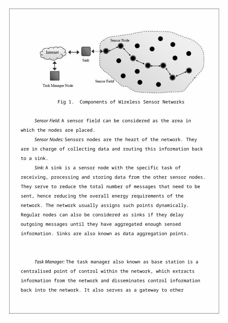
Fig 1. Components of Wireless Sensor Networks

Sensor Field: A sensor field can be considered as the area in

which the nodes are placed.

Sensor Nodes: Sensors nodes are the heart of the network. They

are in charge of collecting data and routing this information back

to a sink.

Sink: A sink is a sensor node with the specific task of

receiving, processing and storing data from the other sensor nodes.

They serve to reduce the total number of messages that need to be

sent, hence reducing the overall energy requirements of the

network. The network usually assigns such points dynamically.

Regular nodes can also be considered as sinks if they delay

outgoing messages until they have aggregated enough sensed

information. Sinks are also known as data aggregation points.

Task Manager: The task manager also known as base station is a

centralised point of control within the network, which extracts

information from the network and disseminates control information

back into the network. It also serves as a gateway to other

networks, a powerful data processing and storage centre and an

access point for a human interface. The base station is either a

laptop or a workstation. Data is streamed to these workstations

either via the internet, wireless channels, satellite etc. So

hundreds to several thousand nodes are deployed throughout a sensor

field to create a wireless multi-hop network. Nodes can use

wireless communication media such as infrared, radio, optical media

or Bluetooth for their communications. The transmission range of

the nodes varies according to the communication protocol is use.

2.1.2 . The Sensor Node

A sensor is a small device that has a micro-sensor technology,

low power signal processing, low power computation and a short-

range communications capability. Sensor nodes are conventionally

made up of four basic components as shown in Figure 2.2: a sensor,

a processor, a radio transceiver and a power supply/battery [11].

Additional components may include Analog-to-Digital Convertor

(ADC), location finding systems, mobilizers that are required to

move the node in specific applications

and power generators. The analog signals are measured by the

sensors are digitized via an ADC and in turn fed into the

processor.

The processor and its associated memory commonly RAM is used

to manage the procedures that make the sensor node carry out its

assigned sensing and collaboration tasks. The radio transceiver

connects the node with the network and serves as the communication

medium of the node. Memories like EEPROM or flash are used to store

the program code. The power supply/battery is the most important

component of the sensor node because it implicitly determines the

lifetime of the entire network. Due to size limitations of AA

batteries or quartz, cells are used as the primary sources of

power. To give an indication of the energy consumption involved,

the average sensor node will expend approximately 4.8mA receiving a

message, 12mA transmits a packet and 5μA sleeping [11]. In addition

the CPU uses on average 5.5mA when in active mode.

Fig 2.2 Components of a wireless sensor node

2.1.1.2. Wireless Sensor Node Communication Architecture:

Protocol Stack

The protocol stack used by the base station and sensor

nodes is shown in Figure. 2.3. This protocol stack combines power

and routing awareness, integrates data with networking protocols,

communicates power efficiently through the wireless medium, and

promotes cooperative efforts of sensor nodes. The protocol stack

consists of the physical layer, data link layer, network layer,

transport layer, application layer, power management plane,

mobility management plane and task management plane.

The physical layer should meet requirements like carrier

frequency generation, frequency selection, signal detection,

modulation and data encryption, transmission and receiving

mechanisms. The Data Link Layer should meet the requirements for

medium access, error control, multiplexing of data streams and data

frame detection. It also ensures reliable point to point and point

to multi-hop connections in the network. The MAC layer in the data

link layer should be capable of collision detection and use minimal

power. The network layer is responsible for routing the information

received from the transport layer i.e. finding the most efficient

path for the packet to travel on its way to a destination.

The Transport Layer is needed when the sensor network intends

to be accessed through the internet. It helps in maintaining the

flow of data whenever the application requires it. The application

layer is responsible for presenting all required information to the

application and propagating requests from the application layer

down to the lower layers.

The power management plane manages power utilization by the

nodes. Mobility management plane is responsible for the movement

pattern of the sensor nodes, if they are mobile. The task

management plane schedules the sensing and forwarding

responsibilities of the sensor nodes. Designing a network protocol

for such wireless devices should meet the limitations like limited

channel bandwidth, limited energy, electromagnetic wave

propagation, error-prone channel, time varying conditions and

mobility.

There are general ideas that can be used to overcome these

limitations. Low-energy protocols help extend the limited node

energy. Power control can be used to combat the radio wave

attenuation. A transmitter can set the power of the radio wave,

such that it will be received with an acceptable power level. Link-

layer protocols and MAC protocols can be used to combat channel

errors. Adaptive routing, MAC and link layer protocols can be used

to overcome the time-varying conditions of the wireless channel and

node mobility.

2.1.1.3. Routing Techniques in Wireless Sensor Networks

Due to WSNs differing from one network to another, many

new algorithms have been proposed for the routing problem in WSNs.

These routing mechanisms have considered the characteristics of

sensor nodes depending on the type of application and underlying

architecture requirements. Almost all of the routing protocols can

be classified according to the network structure as flat,

hierarchical or location-based.

Routing Protocols

In general, routing in WSNs can be divided into flat-based

routing, hierarchical-based routing, and location-based routing

depending on the network structure. In flat-based routing, all

nodes are typically assigned equal roles or functionality. In

hierarchical-based routing, however, nodes will play different

roles in the network. In location-based routing, sensor nodes'

positions are exploited to route data in the network.

2.4.1 Flat Based Routing Protocols

Routing protocols without any hierarchy that keeps knowledge

of the whole network or internetwork are called flat protocols.

The main advantage of flat protocols is that they are simpler to

design and implement than hierarchical protocols. Two common

paradigms can be found among flat protocols, and a third one

tries to take advantage of both paradigms, by combining them.

Proactive Protocols

Proactive protocols use the same approach as routing in the

Internet. Nodes regularly exchange routing information and use it

to build data structures. When a node has to send or forward a

packet, it only has to read its routing table to know through

which interface and to which address the packet should be sent. It

is then easy and fast to send or forward a message, but the price

to be paid is a prohibitive bandwidth overhead in order to

continuously exchange routing information. The exchanged data can

take two forms, both used in the Internet: Distance Vector and

Link State. The first one is based on having information about the

distance to the different nodes and is used for example in

Destination-Sequenced Distance-Vector (DSDV)

routing

Reactive Protocols

In order to reduce network traffic allocated to routing

information, reactive protocols compute the path to a destination

only when needed. It also relies on flooding: when a node wants to

send a packet and does not have fresh information about its

destination, it broadcasts a request for a path to this

destination. The request is flooded and keeps track of the network

path followed. The destination and nodes that have a fresh path

to this destination respond to the request. The source of the

request chooses the best response and caches it. The flooding

process operates only on demand, avoiding bandwidth overhead. It

does not take care of inactive nor unused nodes. On the other hand,

this incurs a latency that may not be acceptable in some contexts.

Ad-hoc On-demand Distance Vector (AODV), Dynamic MANET On Demand

(DYMO) and Dynamic Source Routing (DSR) protocols are well known

examples of reactive protocols.

Hierarchical Routing

Hierarchical or cluster-based routing, originally proposed in

wireline networks, are well-known techniques with special

advantages related to scalability and efficient communication. As

such, the concept of hierar- chical routing is also utilized to

perform energy-efficient routing in WSNs. In a hierarchical

architecture, higher energy nodes can be used to process and send

the information while low energy nodes can be used to perform the

sensing in the proximity of the target. This means that creation of

clusters and assigning special tasks to cluster heads can greatly

contribute to overall system scalability, lifetime, and energy

effciency. Hierarchical routing is an efficient way to lower energy

consumption within a cluster and by performing data aggregation and

fusion in order to decrease the number of transmitted messages to

the BS. Hierarchical routing is mainly two-layer routing where one

layer is used to select clusterheads and the other layer is used

for routing. However, most techniques in this category are not

about routing, rather on "who and when to send or

process/aggregate" the information, channel allocation etc., which

can be orthogonal to the multihop routing function.

The TinyOS toolchain

Applications are written in the NesC language, compiling is

needed. The whole

process starting from the NesC source and ending with an

appropriate native binary canbe divided into three parts.

First, the NesC code must be interpreted, and converted into a

normal C source code.This is done via the ncc (NesC C Compiler)

utility. Secondly, this C source must becompiled and linked with

the libraries used to get a binary code which is directly

runnableby the target architecture. This can be achieved by

executing the GNU C Compiler gccwith the appropriate parameters.

Then, using a dedicated tool like pybsl or uisp amongothers, one

could update the mote’s microcontroller’s program with the new one.

Fig. Stages in deploying TinyOs Application source code.

The make system

TinyOS’s make system is a speci c GNU make utility which isfi

able to run ncc andgcc, link the application, then deploy if

necessary. The required command-line parame-ters are user-friendly,

and clear to understand.

Example. Generating the binary code of a given NesC

application for the Iris,

TelosB and Shimmer motes is easily done with make:

$ make iris

$ make telosb

$ make shimmer

The NesC programming language []

Programming TinyOS is really challenging because it requires

using a non-traditionallanguage, NesC. On one hand, NesC appears to

be very similar to C, nevertheless where NesC differs considerably

from C is its linking model. The challenge and complexity arenot in

writing software components, but rather in combining a set of

components into a working application

Interfaces, components and wiring

The NesC language is a component-based C dialect. In some

ways, NesC components are similar to objects in the OOP paradigm or

components in VHDL. For example, they encapsulate state and couple

state with functionality. The principal distinction lies in their

naming scope. Unlike C++ and Java objects, which refer to functions

and variables in a global namespace, NesC components use a purely

local namespace.

This means that in addition to declaring the functions that it

implements, a component must also declare the functions that it

calls. The names that a component uses to call these functions are

completely local: the name it references does not have to be the

same that the one implementing the function (LEVIS [10]). This will

be clearer when interfaces,modules, components and the wiring

technique are revealed.

Interfaces

An interface is a set of services, callable functions

(commands), and event noti cation routines. An interface does notfi

represent any object or software/hardware unit, it only lays down

the mean of usage. Two simple interfaces are depicted in the next

code segment:

interface StdControl {

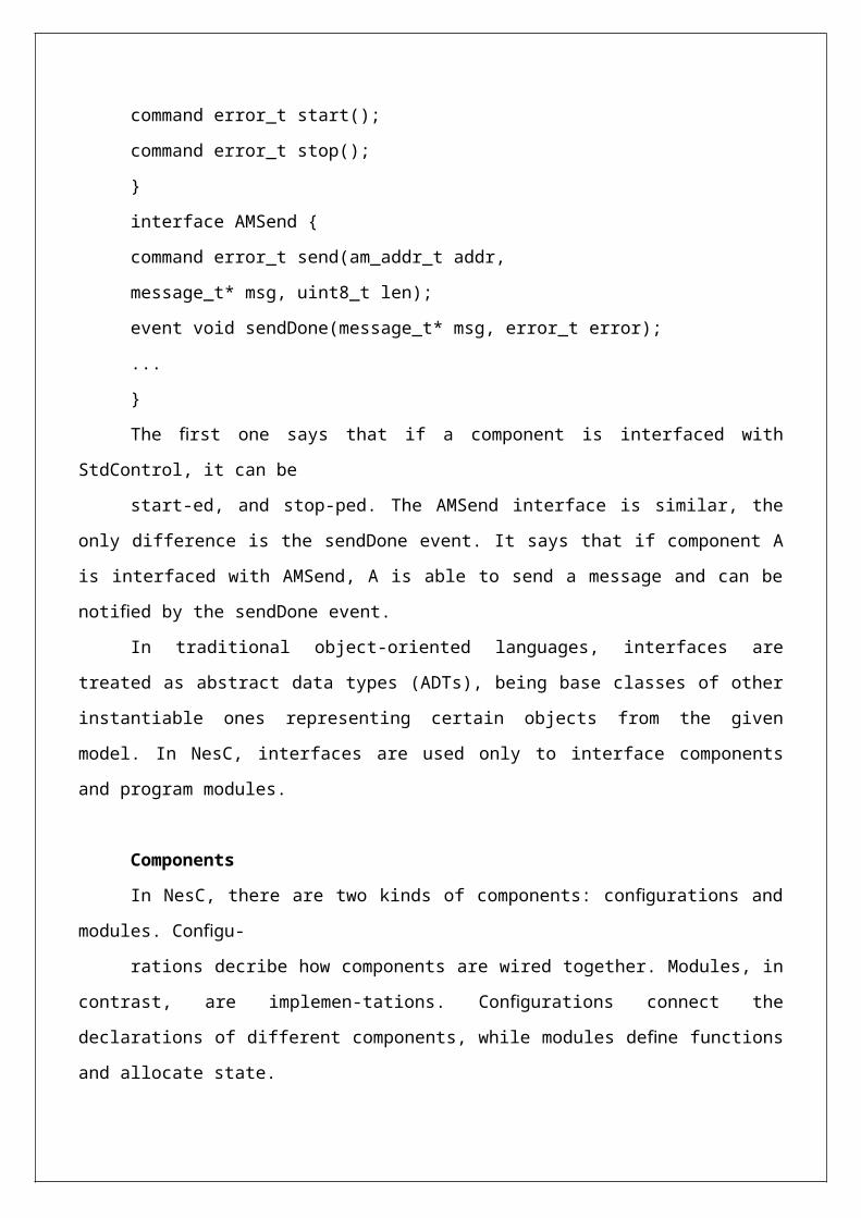
command error_t start();

command error_t stop();

}

interface AMSend {

command error_t send(am_addr_t addr,

message_t* msg, uint8_t len);

event void sendDone(message_t* msg, error_t error);

...

}

The rst one says that if a component is interfaced withfi

StdControl, it can be

start-ed, and stop-ped. The AMSend interface is similar, the

only difference is the sendDone event. It says that if component A

is interfaced with AMSend, A is able to send a message and can be

noti ed by the sendDone event.fi

In traditional object-oriented languages, interfaces are

treated as abstract data types (ADTs), being base classes of other

instantiable ones representing certain objects from the given

model. In NesC, interfaces are used only to interface components

and program modules.

Components

In NesC, there are two kinds of components: con gurations andfi

modules. Con gu-fi

rations decribe how components are wired together. Modules, in

contrast, are implemen-tations. Con gurations connect thefi

declarations of different components, while modules de ne functionsfi

and allocate state.

Each component has a speci cation, a code block declaring thefi

functions it provides (implements) and the functions that it uses

(calls). For example the following can be a speci cation of afi

ctional radio component of a mobile:fi

module MobileRadioP {

uses { interface Boot; interface Leds; }

uses interface AMSend as Sms;

}

When a component A declares that it calls a function func, it

introduces essentially the name A.func into a global namespace. Let

us consider a different component, B introducing also a func

function as B.func. Even though both A and B refer to the function

func, they might be referring to completely different

implementations.

Wiring technique

An application is built up using several components. Once a

component A uses a spe-ci c interface, it must be connected tofi

another (say B), which provides that interface. Thisis somewhat

analogous to the dynamic-binding or virtual functions used in

procedural languages, but it is hard-wired at compile-time. This

wiring technique is enormously be-ne cial to the re-usage offi

components and greatly enhances the developer’s possibilities.

To stick to our mobile phone example, let the following

components be given:

module LedsC { provides interface Leds; }

implementation { ... }

module SmsC { provides interface AMSend; }

implementation { ... }

Wiring is achieved by creating a configuration, enlisting the

components, and

creating the appropriate connections:

configuration MobilePhone {}

implementation {

components MobileRadioP, LedsC, SmsC, MainC;

MobileRadioP.Leds -> LedsC;

MobileRadioP.Boot -> MainC;

MobilePhoneP.Sms -> SmsC;

}

Using this wiring scheme, the real LEDs are controlled by

MobileRadioP, but driven by component LedsC. Our virtual mobile

phone can send messages using SmsC. The MainC component—providing a

Boot interface—is a NesC equivalent to the main()

function in C, being the main entry point of the application.

Message structure:-

TinyOs 2.1 has a common message buffer abstraction called

message_t.

 The message_t structure is defined in tos/types/message.h: [*]

typedef nx_struct message_t {

nx_uint8_t header[sizeof(message_header_t)];

nx_uint8_t data[TOSH_DATA_LENGTH];

nx_uint8_t footer[sizeof(message_footer_t)];

nx_uint8_t metadata[sizeof(message_metadata_t)];

} message_t;

Which can shown as :

Each message is divided into four main parts:

• Header. The header eld is an array of bytes whose size is thefi

size of a platform’s union of data-link headers. Because radio

stacks often prefer packets to be stored contiguously, the layout

of a packet in memory does not necessarily re ect the lay-out offl

its NesC structure. The header contains the destination and source

addresses,the user’s data length, the message’s group id, and

Active Message type.

The header size varies based on the data-link used.

For example, a CC2420 radio packet’s header is 11 bytes, while the

serial header is just 5 bytes long.

• Metadata. The metadata eld of message_t stores data that afi

single-hop stack uses or collects. This mechanism allows packet

layers to store per-packet infor-mation such as RSSI, timestamps,

link quality indicator (LQI), acknowledgement

ags, etc.fl

• Footer. The footer eld ensures that message_t has enough spacefi

to store the footers for all underlying link layers when there are

MTU-sized packets. Like hea-ders, footers are not necessarily

stored where the C structs indicate they are: instead, their

placement is implementation dependent.

• Data. The TOSH_DATA_LENGTH bytes long data eld stores thefi

single-hop packet payload. A TinyOS application can rede ne thisfi

value at compile time, but the maximum allowed value is 104 for a

128 bytes long full message. Because this

value can be recon gured, it is possible that two differentfi

versions of an application have different MTU sizes. If such

occures, every message with longer payload than expected is

automatically discarded.

When developing TinyOS applications, one should enlist all

message types that will be used, and set TOSH_DATA_LENGTH to be at

least the maximum payload length. In this way the transmission

time. can be optimized by reducing the full message length to the

optimal value

 TinyOS 2.x, a component calls AMPacket.getAddress(msg). The most

basic of these interfaces is Packet, which provides access to a

packet payload. TEP 116 describes common TinyOS packet ADT

interfaces [3].

Chapter 3

System analysis and Design.

.1. USE CASE DIAGRAM

A use case is a set of scenarios that describing an

interaction between a user and a system. A use case contains a

textual description of all of the ways that the intended users

could work with the software through its interface. The use case

diagrams describe system functionality as a set of tasks that the

system must carry out and actors who interact with the system to

complete the tasks. Use case diagram focuses on requirement

functionality or object behavior. Use case diagram illustrates

functionality of system or in other words it shows what the system

does from

user’s point of view.

Fig. Use case diagram

Use case name Run SimulationUse Case ID UC_002

Actors User, System

Brief

Description

The run simulation use case helps

in the simulation of the

environment variables initialized

in earlier use case.

TriggerThe simulation is started by

TOSSIM tool.

Use case name Configure SimulationUse Case ID UC_001

Actors User

Brief

Description

The configure simulation use case

helps in the initialization of the

parameters to be used in the steps

of simulation.Trigger The parameters are initialized.

Pre-conditionsTOSSIM simulation tool is running

and initialized.Post

Conditions

Parameters initiated for the

simulation

Priority High

Frequency Of

use

It is always used by the user to

perform the initialization of

parameters.

Pre-conditionsTOSSIM simulation tool is running

and initialized.Post

Conditions

Saving the trace file and na

m file for the simulation.

Priority High

Frequency Of

use

It is always used to perform the

simulation of parameters and

topology initialized.

Use case name Analyze trace file

Use Case ID UC_003

Actors User

Brief

Description

The analyze trace file use case

helps in the analysis of the

simulation run in earlier use case

using the make utility.

Trigger

The trace file analysis is started

by user by scripting the python

file.

Pre-conditionsTOSSIM simulation tool has saved

the trace file.Post

Conditions

Performance metrics are analyzed

using the make utility.

Priority High

Frequency Of

use

It is always used to perform the

analysis of the performance

metrics using the trace file.

Use case name Add AlgorithmUse Case ID UC_004

Actors User

Brief

Description

The add algorithm use case helps

in the user to initiate the

algorithm to explore the network

behavior .Trigger -

Pre-conditions -Post

Conditions-

Priority High

Frequency Of

use

It is always used to analyze the

trace file generated during

earlier use case using the make

utility.

DYNAMIC MODELING

Dynamic diagrams show the dynamic behavior of the objects in a

system, which can be described as a series of changes to the system

over time. Dynamic diagrams emphasize what must happen in the

system being modeled at a given time of instant. Since dynamic

diagrams illustrate the behavior of a system, they are used

extensively to describe the functionality of software systems.

UML Interaction diagram: describes the dynamic interaction of

different elements of the system.

3.3.1 Interaction DiagramThese diagrams are used to describe some type of interactions among

the different elements in the model. So this interaction is a part

of dynamic behavior of the system. This interactive behavior is

represented in UML by two diagrams known as Sequence diagram

The sequence diagram depicts the behavior of the system through

interaction between the system and the environment in time

sequence. It has two dimensions namely:

Vertical dimension – represents time.

Horizontal dimension – represents objects.

Components used for Sequence diagram:

Application:- application source which is used to start sending

data.

AODV:- Main source code to process the messages in network.

Main and Backup-route table :- Data structures for maintaining

message information at local node.

Interaces:- various interfaces that are part of RADIO STACK of

TinyOs which directly communicates with hardware layers..

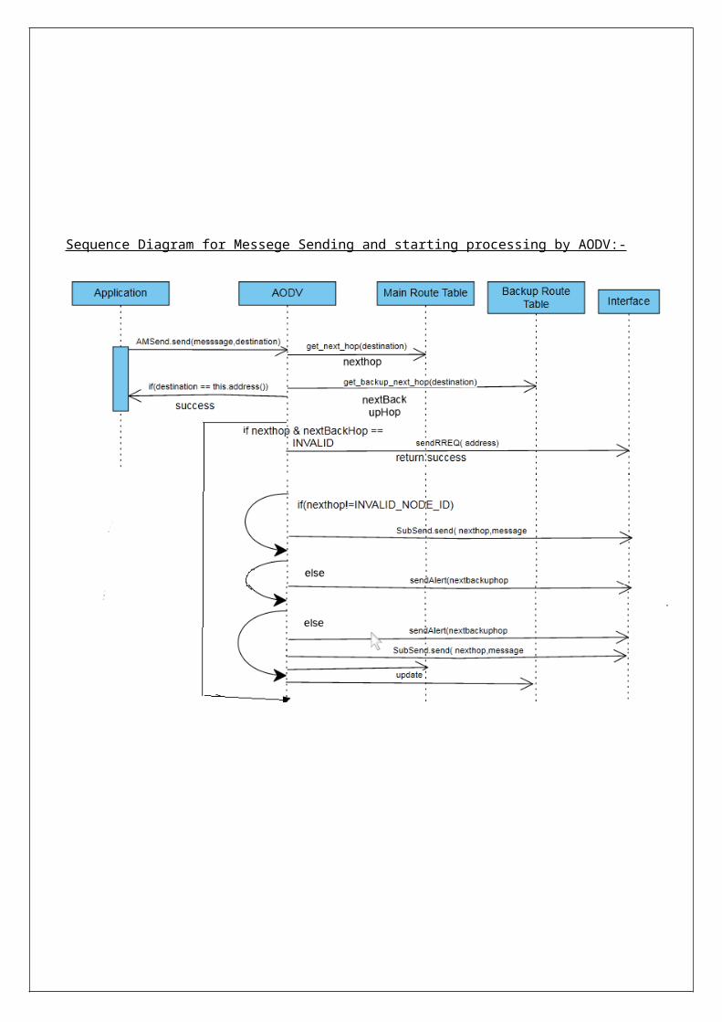
Sequence Diagram for Messege Sending and starting processing by AODV:-

Sequence Diagram for RREQ message processing:-

Sequence Diagram for RREP message processing :-

Routing Protocols (RP) Overview

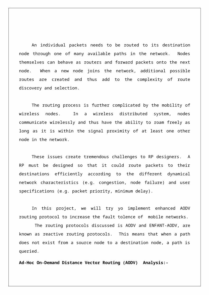
An individual packets needs to be routed to its destination

node through one of many available paths in the network. Nodes

themselves can behave as routers and forward packets onto the next

node. When a new node joins the network, additional possible

routes are created and thus add to the complexity of route

discovery and selection.

The routing process is further complicated by the mobility of

wireless nodes. In a wireless distributed system, nodes

communicate wirelessly and thus have the ability to roam freely as

long as it is within the signal proximity of at least one other

node in the network.

These issues create tremendous challenges to RP designers. A

RP must be designed so that it could route packets to their

destinations efficiently according to the different dynamical

network characteristics (e.g. congestion, node failure) and user

specifications (e.g. packet priority, minimum delay).

In this project, we will try yo implement enhanced AODV

routing protocol to increase the fault tolence of mobile networks.

The routing protocols discussed is AODV and ENFANT-AODV, are

known as reactive routing protocols. This means that when a path

does not exist from a source node to a destination node, a path is

queried.

Ad-Hoc On-Demand Distance Vector Routing (AODV) Analysis:-

The Ad-Hoc On-Demand Distance Vector Routing is a routing protocol

especially designed for ad-hoc mobile networks . The protocol uses

a routing table to determine the path that a packet will travel to

arrive at its destination. However, a route is only kept active

for a finite period of time.

A route is deemed active if there are packets travelling

along it within a set periodic time frame. If this time expires

with no packets traversing,the path is removed from the routing

table. In AODV, the routing table contains the next hop of the

path, and this next hop is the destination that the packet will

travel to.

If a source-destination path does not exist in the routing

table, a network configuration packet will be sent to request for

routes to the destination node. Figure 5, based on Universal

Modelling Language (UML), summarises the logic flow involved with

this algorithm, while Figure 6 shows how a node handles a network

configuration packet.

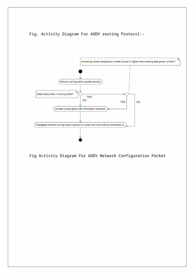
Fig. Activity Diagram For AODV routing Protocol:-

Fig Activity Diagram For AODV Network Configuration Packet

Chapter 4

Implementation

AODV Operations

This document explains the action of a node with respect to

different AODV events in terms of a pseudo code.

With this, we are also mentioning some of the modification

required in basic AODV operations to work for ENFANT-AODV.

Generating Route Requests. [ Same for ENFANT -AODV]

If (No valid entry in route table for destination) {

If (No RREQ pending){

Generate RREQ with particular sequence number ;

Broadcast RREQ;

}

Save [(RREQ_ID) and (IP address source)]; // To Avoid

rebroadcast.

}

Processing and Forwarding Route Requests:-

AODV:-

If (Node listen a RREQ) {

If (same as forwarded in near past) {

Discard;

}

Else //This is a new RREQ {

if(hop(RREQ) > AODV_MAX_HOP ){

Discard;

}

Entry for Reverse Route // (Route from node to originator

of this

RREQ message) {

// update the sequence no.

// Change the life time for route to originator.

Update the routing table entries for originator IP address;

Increase the hop count by one in RREQ packet;

}

IF (TTL > 1) {

Decrease the TTL field by one;

If [(Node is Destination for this RREQ) OR (Node has

route to destination)] {

Send RREP;

Discard RREQ;

}

Else {

Broadcast RREQ;

}

}

}

}

ENFANT- AODV:-

If (Node listen a RREQ) {

If (same as forwarded in near past) {

Discard;

}

Else //This is a new RREQ {

if(hop(RREQ) > AODV_MAX_HOP ){

Discard;

}

If(backup flag set for RREQ) {

If [(Node is Destination for this RREQ){

If (source(RREQ) found in Main Route){

// entry made for this source,hence discard RREQ

Discard;

}

}

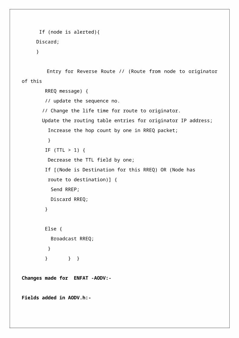
If (node is alerted){

Discard;

}

Entry for Reverse Route // (Route from node to originator

of this

RREQ message) {

// update the sequence no.

// Change the life time for route to originator.

Update the routing table entries for originator IP address;

Increase the hop count by one in RREQ packet;

}

IF (TTL > 1) {

Decrease the TTL field by one;

If [(Node is Destination for this RREQ) OR (Node has

route to destination)] {

Send RREP;

Discard RREQ;

}

Else {

Broadcast RREQ;

}

} } }

Changes made for ENFAT -AODV:-

Fields added in AODV.h:-

aodv_rreq_hdr:-

nx_uint8_t backup;

aodv_rrep_hdr:-

nx_uint8_t backup

aodv_alert_hdr:-

nx_uint8_t alert;

nx_uint8_t forward;

nx_uint8_t seq;

nx_uint8_t dest;

nx_am_addr_t src;

aodv_msg_hdr:-

x_uint8_t backup;

AODV_BACKUP_ROUTE_TABLE:-

uint8_t seq;

am_addr_t dest;

am_addr_t next;

uint8_t hop;

uint8_t ttl;

AODV_BACKUP_RREQ_CACHE:-

uint8_t seq;

am_addr_t dest;

am_addr_t src;

uint8_t hop;

uint8_t ttl;

ReceiveAlert:-

bool sendAlert( am_addr_t dest );

task void resendAlert();

uint8_t get_route_table_index( am_addr_t dest )

am_addr_t getNextAlertHopForward(am_addr_t dest);

am_addr_t getNextAlertHopBackward(uint8_t seq);

// for backup route cache.

uint8_t get_backup_rreq_cache_index( am_addr_t src, am_addr_t

dest );

bool is_backup_rreq_cached( aodv_rreq_hdr* msg );

bool add_backup_rreq_cache( uint8_t seq, am_addr_t dest,

am_addr_t src, uint8_t hop );

void del_backup_rreq_cache( uint8_t id );

task void update_backup_rreq_cache();

// for backup route table.

void del_backup_route_table( am_addr_t dest );

bool is_src_in_main_route ( aodv_rreq_hdr* rreq_hdr );

bool is_src_found_in_main_route(am_addr_t src);

uint8_t get_backup_route_table_index( am_addr_t dest );

bool add_backup_route_table( uint8_t seq, am_addr_t dest,

am_addr_t nexthop, uint8_t hop );

void del_backup_route_table( am_addr_t dest );

am_addr_t get_backup_next_hop( am_addr_t dest );

Psedu Code :-

AMSend.send(destination, message,length)

1.Initialise :-

aodv_msg_hdr* aodv_hdr;

aodv_rreq_hdr* rreq_aodv_hdr;

aodv_alert_hdr* alert_aodv_hdr ;

am_addr_t nexthop = get_next_hop(destination);

am_addr_t nextbackuphop = get_backup_next_hop(destination);

2. if(destination == this.address())

return success;

3. if( (nexthop == INVALID_NODE_ID )&& (nextbackuphop ==

INVALID_NODE_ID))

3.1 if( No_RREQ_PENDING )

sendRREQ( addr, FALSE );

return SUCCESS;

else

return FAIL;

4. // There may be Main Route or Backup Route available for

Destination.

if(nexthop!=INVALID_NODE_ID)

// there is a route to destination

4.1 Form the aodv_msg to forward to Next Hop

4.2 if( !send_pending )

4.2.1 if( call SubSend.send( nexthop,message,

length) == SUCCESS )

send_pending_ = TRUE;

return SUCCESS;

else

4.3 // There is Backup Route available for Destination.

4.3.1 Build Alert Message.

sendAlert(nextbackuphop);

4.3.2 Form the aodv_msg to forward to Next Backup Hop

4.3.3 if( !send_pending_ )

4.3.4 if( call SubSend.send(nextbackuphop,message, length

) == SUCCESS )

send_pending_ = TRUE;

return SUCCESS;

4.3.5 Copy roué from Backup Route Table to Main Route

Table

4.3.6 Update Backup Route Table (delete Destination

entry)

4.3.7 Start new Backup-RREQ from this Node.

5. return FAIL

ReceiveRREQ.receive( message , payload, length )

1.Initialise

aodv_rreq_hdr* aodv_hdr = message ->data

aodv_alert_hdr* alert_aodv_hdr = alert_message ->data

aodv_rreq_hdr* rreq_aodv_hdr = rreq_message->data)

aodv_rrep_hdr* rrep_aodv_hdr = rrep_message->data

int backup = aodv_hdr->backup

2. If aodv_hdr->hop > AODV_MAX_HOP

return message

3.

If backup==1

3.1 If alerted == TRUE

// Duplicate Backup-RREQ

return message

3.2 If is_backup_rreq_cached(aodv_hdr)

// Duplicate Backup-RREQ

return message

3.3 Add Route to Backup Route Table

3.4 Update messege cache with Backup-RREQ

3.5 If aodv_hdr->destination == me && added

sendRREP( Immediate_source, FALSE )

return message

3.6 If Not _me

3.6.1 Build Backup-RREQ Message

3.6.2 sendRREQ(destination,FALSE)

Else

3.7 If is_rreq_cached(aodv_hdr)

// Duplicate RREQ

return message

3.8 Add Route to Route Table

3.9 Update messege cache with RREQ

3.10 If aodv_hdr->destination == me && added

3.10.1 Build Alert Message.

sendAlert(nextbackuphop);

3.10.2 sendRREP(Immediate_source, FALSE )

3.11 If Not _me

3.11.1 Build RREQ Message

3.11.2 sendRREQ(destination,FALSE

3.12 return message

ReceiveAlert.receive(message , payload, length )

1. Initialse

a. me = call AMPacket.address()

b. Immediate_source = call AMPacket.source message)

c. Destination = call AMPacket.destination(message )

d. aodv_hdr = message->data

e. alert_aodv_hdr = alert_msg->data)

f. alert = aodv_hdr->alert

2. If alert ==1

2.1

If aodv_hdr->forward ==1

// Forward Direction of Alert message.

Nexthop = getNextAlertHopForward(aodv_hdr->dest);

2.1.1 If nexthop == Destination

// end of Alert receiving

return p_msg

Else

2.1.2 Nexthop = getNextAlertHopBackward(aodv_hdr->seq);

2.2 alerted =TRUE;

2.3 If (nexthop!= INVALID_NODE_ID ) && (me !=aodv_hdr-

>src)

If nexthop != destinatin

sendAlert(nexthop)

3. return message

ReceiveRREP.receive ( message , payload, length )

1.Initialise:-

aodv_hdr = message ->data

alert_aodv_hdr = alert_message ->data

rreq_aodv_hdr = rreq_message->data

rrep_aodv_hdr = rrep_message->data

backup = aodv_hdr->backup

Immediate_source = call AMPacket.source message)

Destination = call AMPacket.destination(message )

Source = aodv_hdr->src

2. If Source == me

2.1

if backup==1

2.1.1 Add Route to Backup Route Table

2.1.2 main_seq = (aodv_hdr->seq)/2;

2.1.3 main_hop = getMainHop_routed(main_seq);

2.1.4 main_dest = getMainDest_cached(main_seq);

2.1.5 main_src = getMainSRC_cached(main_seq)

2.1.6

if(aodv_hdr->src != main_src)

// Not End of Path Discovery …

2.1.6.1

if( main_src != INVALID_NODE_ID) &&(main_dest!

=INVALID_NODE_ID )

2.1.6.1.1.1 Build RREP

2.1.6.1.1.2 Add to Main Route Table

2.1.6.1.1.3 sendRREP( main_src, TRUE )

else // End of Path discovery..

rreq_aodv_hdr->backup =0

return message

Else

2.2 dest011 = get_backup_next_hop( aodv_hdr->dest )

2.3 alerted =TRUE;

2.4 rreq_aodv_hdr->backup= 1;

2.5 Add Route to Backup Route Table

2.6

If dest011 == INVALID_NODE_ID

sendRREQ( rreq_aodv_hdr->dest, FALSE );

Else

// end of path discovery!!!

Else

//Not me..

3

If backup==0

3.1 Add Route to Route Table

3.2 nexthop = getNextAlertHopBackward(aodv_hdr->seq)

3.3 Build Alert

3.4 if(nexthop!= INVALID_NODE_ID)

sendAlert(nexthop);

3.5 dest0 = get_backup_next_hop( aodv_hdr->dest );

If dest0 != INVALID_NODE_ID

// there is enrty hence continue to main route discovery

path...

// forward RREP

3.5.1 dest1 = get_next_hop( aodv_hdr->src );

3.5.2 if dest1 != INVALID_NODE_ID

3.5.2.1 Build RREP

3.5.2.2 sendRREP( dest1, TRUE );

Else

3.5.3 rreq_aodv_hdr->backup= 1;

3.5.4 Build Backup RREQ .

3.5.5 sendRREQ( rreq_aodv_hdr->dest, FALSE );

Else //backup path steps

3.6

If source ==me

3.6.1 Add Route to Backup Route Table

3.6.2 START SENDING DATA

Else

3.6.3 dest2 = get_backup_next_hop( aodv_hdr->src )

3.6.4

If get_backup_next_hop( aodv_hdr->src ) !=

INVALID_NODE_ID

sendRREP( get_backup_next_hop( aodv_hdr->src ), TRUE

)

4. return message

References :-

[1] J. Broch, D. A. Maltz, D. B. Johnson, Y.-C. Hu, and J.

Jetcheva, \A Performance Comparison of Multi-Hop Wireless Ad Hoc

Network Routing Protocols,"in Proc. of IEEE/ACM MOBICOM, 1998.

[ ]C. Perkins, E. Belding-Royer, and S. Das, “Ad hoc On Demand

Distance Vector Routing (AODV)”, RFC 3561, July 2003

[] The nesC Language: A Holistic Approach to Networked Embedded

Systems, David Gay, Phil Levis, Rob von Behren, Matt Welsh, Eric

Brewer, and David Culler. In Proceedings of Programming Language Design and

Implementation (PLDI) 2003, June 2003

[3] TEP 116:Packet Protocols.

[5] “Michael Sudkovitch, David I. Roitman,, OSPF Security project

book”. [Online]. Available:

http://webcourse.cs.technion.ac.il/236349/Spring2013/ho/WCFiles/200

9-2-ospf-report.pdf

[ ] ENFAT AODV The Fault-Tolerant Routing Protocol ,Che-Aron, Z.;

Al-Khateeb, W. F. ,Anwar, F.