proxy-AODV : Extension of AODV For Partially Connected Ad hoc Networks

proxy-AODV : Extension of AODV ForPartially Connected Ad hoc Networks

Dissertation

submitted in partial fulfillment of the requirements

for the degree of

Master of Technology

by

Anshuman Tiwari

(Roll no. 04329004)

under the guidance of

Prof. Sridhar Iyer

Kanwal Rekhi School of Information Technology

Indian Institute of Technology Bombay

2006

Dissertation Approval Sheet

This is to certify that the dissertation entitled

proxy-AODV : Extension of AODV For Partially

Connected Ad hoc Networks

by

Anshuman Tiwari

(Roll no. 04329004)

is approved for the degree of Master of Technology.

Prof. Sridhar Iyer

(Supervisor)

Prof. Om Damani

(Internal Examiner)

Prof. Ashwin Gumaste

(Additional Internal Examiner)

Prof. Girish P . Saraph

(Chairperson)

Date:

Place:

iii

INDIAN INSTITUTE OF TECHNOLOGY BOMBAY

CERTIFICATE OF COURSE WORK

This is to certify that Mr. Anshuman Tiwari was admitted to the candidacy

of the M.Tech. Degree and has successfully completed all the courses required for the

M.Tech. Programme. The details of the course work done are given below.

Sr.No. Course No. Course Name Credits

Semester 1 (Jul – Nov 2004)

1. IT601 Mobile Computing 6

2. HS699 Communication and Presentation Skills (P/NP) 4

3. IT603 Data Base Management Systems 6

4. IT619 IT Foundation Laboratory 10

5. IT623 Foundation course of IT - Part II 6

6. IT694 Seminar 4

Semester 2 (Jan – Apr 2005)

7. CS686 Object Oriented Systems 6

8. EE701 Introduction to MEMS (Institute Elective) 6

9. IT610 Quality of Service in Networks 6

10. IT628 Information Technology Project Management 6

11. IT680 Systems Lab. 6

Semester 3 (Jul – Nov 2005)

12. CS601 Algorithms and Complexity (Audit) 6

13. CS681 Performance Evaluation of Computer Systems and Networks 6

M.Tech. Project

14. IT696 M.Tech. Project Stage - I (Jul 2005) 18

15. IT697 M.Tech. Project Stage - II (Jan 2006) 30

16. IT698 M.Tech. Project Stage - III (Jul 2006) 42

I.I.T. Bombay Dy. Registrar(Academic)

Dated:

v

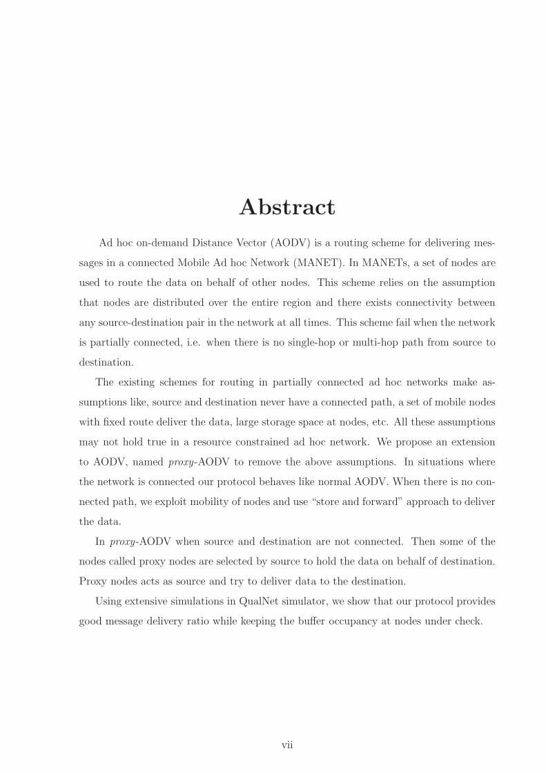
Abstract

Ad hoc on-demand Distance Vector (AODV) is a routing scheme for delivering mes-

sages in a connected Mobile Ad hoc Network (MANET). In MANETs, a set of nodes are

used to route the data on behalf of other nodes. This scheme relies on the assumption

that nodes are distributed over the entire region and there exists connectivity between

any source-destination pair in the network at all times. This scheme fail when the network

is partially connected, i.e. when there is no single-hop or multi-hop path from source to

destination.

The existing schemes for routing in partially connected ad hoc networks make as-

sumptions like, source and destination never have a connected path, a set of mobile nodes

with fixed route deliver the data, large storage space at nodes, etc. All these assumptions

may not hold true in a resource constrained ad hoc network. We propose an extension

to AODV, named proxy-AODV to remove the above assumptions. In situations where

the network is connected our protocol behaves like normal AODV. When there is no con-

nected path, we exploit mobility of nodes and use “store and forward” approach to deliver

the data.

In proxy-AODV when source and destination are not connected. Then some of the

nodes called proxy nodes are selected by source to hold the data on behalf of destination.

Proxy nodes acts as source and try to deliver data to the destination.

Using extensive simulations in QualNet simulator, we show that our protocol provides

good message delivery ratio while keeping the buffer occupancy at nodes under check.

vii

Contents

Abstract vii

List of figures xi

List of tables xiii

Abbreviations xv

1 Introduction and Motivation 1

1.1 Partially Connected Ad hoc Network . . . . . . . . . . . . . . . . . . . . . 1

1.2 AODV . . . . . . . . . . . . . . . . . . . . . . . . . . . . . . . . . . . . . . 2

1.2.1 Working of AODV . . . . . . . . . . . . . . . . . . . . . . . . . . . 2

1.2.2 AODV over Partially Connected Ad hoc Networks . . . . . . . . . . 4

1.3 Motivation and Problem Statement . . . . . . . . . . . . . . . . . . . . . . 4

1.4 Thesis Outline . . . . . . . . . . . . . . . . . . . . . . . . . . . . . . . . . . 5

2 Literature Survey 7

2.1 Epidemic Routing Scheme . . . . . . . . . . . . . . . . . . . . . . . . . . . 7

2.1.1 Example . . . . . . . . . . . . . . . . . . . . . . . . . . . . . . . . . 7

2.1.2 Pros and Cons of Epidemic Routing Scheme . . . . . . . . . . . . . 8

2.2 Message Ferrying Approach . . . . . . . . . . . . . . . . . . . . . . . . . . 9

2.2.1 Node-Initiated Message Ferrying . . . . . . . . . . . . . . . . . . . . 9

2.2.2 Ferry-Initiated Message Ferrying . . . . . . . . . . . . . . . . . . . 9

2.2.3 Pros and Cons of Message Ferrying Approach . . . . . . . . . . . . 11

2.2.4 Replace Message Ferry . . . . . . . . . . . . . . . . . . . . . . . . . 11

2.3 Designing System for Sparse Networks . . . . . . . . . . . . . . . . . . . . 11

ix

x Contents

3 proxy-AODV Protocol 13

3.1 Motivation For Selecting AODV . . . . . . . . . . . . . . . . . . . . . . . . 13

3.2 proxy-AODV . . . . . . . . . . . . . . . . . . . . . . . . . . . . . . . . . . 14

3.2.1 Overview of Protocol . . . . . . . . . . . . . . . . . . . . . . . . . . 14

3.2.2 Entities . . . . . . . . . . . . . . . . . . . . . . . . . . . . . . . . . 15

3.2.3 Issues and Parameters . . . . . . . . . . . . . . . . . . . . . . . . . 16

3.2.4 Events . . . . . . . . . . . . . . . . . . . . . . . . . . . . . . . . . . 17

3.3 p-AODV with Example . . . . . . . . . . . . . . . . . . . . . . . . . . . . . 19

4 Simulation Experiments and Results 23

4.1 p-AODV in a Simple Scenario . . . . . . . . . . . . . . . . . . . . . . . . . 23

4.2 Simulation Model and Setup . . . . . . . . . . . . . . . . . . . . . . . . . . 25

4.3 Performance Metrics . . . . . . . . . . . . . . . . . . . . . . . . . . . . . . 26

4.4 Results . . . . . . . . . . . . . . . . . . . . . . . . . . . . . . . . . . . . . . 27

4.4.1 p-AODV with single parameter . . . . . . . . . . . . . . . . . . . . 27

4.4.2 Flooding Approach . . . . . . . . . . . . . . . . . . . . . . . . . . . 28

4.4.3 Comparison of p-AODV and Flooding Approach . . . . . . . . . . . 29

5 Conclusion and Future Work 33

5.1 Conclusion . . . . . . . . . . . . . . . . . . . . . . . . . . . . . . . . . . . . 33

5.2 Future Work . . . . . . . . . . . . . . . . . . . . . . . . . . . . . . . . . . . 33

Bibliography 35

Acknowledgements 37

List of Figures

1.1 Network with partitions . . . . . . . . . . . . . . . . . . . . . . . . . . . . 2

1.2 Node S broadcasts RREQ . . . . . . . . . . . . . . . . . . . . . . . . . . . 3

1.3 Node D send RREP to Node S . . . . . . . . . . . . . . . . . . . . . . . . 3

1.4 Node S send data to node D . . . . . . . . . . . . . . . . . . . . . . . . . . 4

1.5 AODV: Connectivity Vs Number of Nodes : SimTime 300, Network Area

1.5 sq. km. . . . . . . . . . . . . . . . . . . . . . . . . . . . . . . . . . . . 5

2.1 Network instance at time T1 . . . . . . . . . . . . . . . . . . . . . . . . . . 8

2.2 Network instance at time T2 . . . . . . . . . . . . . . . . . . . . . . . . . . 8

2.3 Node-Initiated Message Ferrying . . . . . . . . . . . . . . . . . . . . . . . . 10

2.4 Ferry-Initiated Message Ferrying . . . . . . . . . . . . . . . . . . . . . . . . 10

3.1 Node has data . . . . . . . . . . . . . . . . . . . . . . . . . . . . . . . . . 18

3.2 Node listen (P)RREQ . . . . . . . . . . . . . . . . . . . . . . . . . . . . . 19

3.3 S wants to send data to D, S sends RREQ . . . . . . . . . . . . . . . . . . 20

3.4 proxy node sent proxy reply to source . . . . . . . . . . . . . . . . . . . . . 20

3.5 Source send data to proxy node . . . . . . . . . . . . . . . . . . . . . . . . 21

3.6 proxy node moves near to destination . . . . . . . . . . . . . . . . . . . . . 21

3.7 proxy node deliever data to destination . . . . . . . . . . . . . . . . . . . . 22

3.8 proxy node enters new locality . . . . . . . . . . . . . . . . . . . . . . . . . 22

4.1 p-AODV Simple Scenario : Source reaches to destination . . . . . . . . . . 24

4.2 p-AODV Simple scenario : proxy reaches the destination . . . . . . . . . . 24

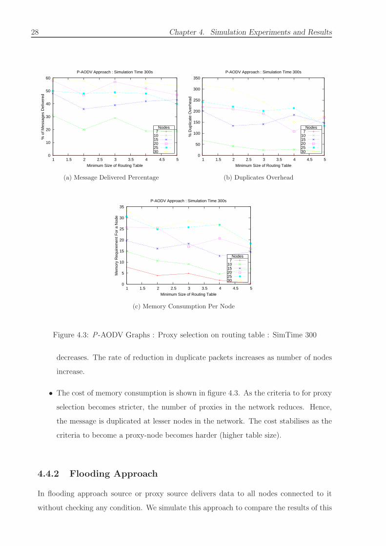
4.3 P -AODV Graphs : Proxy selection on routing table : SimTime 300 . . . . 28

(a) Message Delivered Percentage . . . . . . . . . . . . . . . . . . . . . . 28

(b) Duplicates Overhead . . . . . . . . . . . . . . . . . . . . . . . . . . . 28

xi

xii List of Figures

(c) Memory Consumption Per Node . . . . . . . . . . . . . . . . . . . . 28

4.4 P -AODV Graphs : Proxy selection on routing table : SimTime 300 . . . . 29

(a) Average Delay I . . . . . . . . . . . . . . . . . . . . . . . . . . . . . . 29

(b) Average Delay II . . . . . . . . . . . . . . . . . . . . . . . . . . . . . 29

4.5 Flooding Approach . . . . . . . . . . . . . . . . . . . . . . . . . . . . . . . 30

(a) Message Delivered Percentage . . . . . . . . . . . . . . . . . . . . . . 30

(b) Duplicates Overhead . . . . . . . . . . . . . . . . . . . . . . . . . . . 30

(c) Memory Consumption Per Node . . . . . . . . . . . . . . . . . . . . 30

4.6 Flooding Approach . . . . . . . . . . . . . . . . . . . . . . . . . . . . . . . 30

(a) Average Delay I . . . . . . . . . . . . . . . . . . . . . . . . . . . . . . 30

(b) Average Delay II . . . . . . . . . . . . . . . . . . . . . . . . . . . . . 30

4.7 Comparison Between Flooding and proxy-AODV performance . . . . . . . 31

(a) Percentage of Message Delivery . . . . . . . . . . . . . . . . . . . . . 31

(b) Average Delay For a Packet . . . . . . . . . . . . . . . . . . . . . . 31

(c) Percentage of Duplication Overhead . . . . . . . . . . . . . . . . . . 31

List of Tables

3.1 Comparison of four routing protocol . . . . . . . . . . . . . . . . . . . . . . 14

4.1 Cases for communication between nodes in p-AODV protocol operation . . 23

4.2 Number of packets delivered . . . . . . . . . . . . . . . . . . . . . . . . . . 25

4.3 Simulation Setup . . . . . . . . . . . . . . . . . . . . . . . . . . . . . . . . 25

xiii

Abbreviations and Notations

Abbreviations

AODV : Ad hoc On Demand Distance Vector

DLE : Drop-Least-Encountered

DLR : Drop-Least-Recently-Received

DOA : Drop-Oldest

DRA : Drop-Random

FIMF : Ferry-Initiated Message Ferrying

p-AODV : proxy-AODV

MANET : Mobile Ad hoc Networks

NIMF : Node-Initiated Message Ferrying

p-RRER : proxy-RRER

p-RREP : proxy-RREP

p-RREQ : proxy-RREQ

RERR : Route Error

RREP : Route Reply

RREQ : Route Request

xv

Chapter 1

Introduction and Motivation

Mobile Ad hoc networks (MANET) are considered as promising communication networks

in situations where rapid deployment and self-configuration is essential. In ad hoc net-

works, nodes are allowed to communicate with each other without any existing infrastruc-

ture. Typically every node should also play the role of a router. This kind of networking

can be applied to scenarios like conference room, disaster management, battle field com-

munication and places where deployment of infrastructure is either difficult or costly.

Many routing protocols exist to enable communication in ad hoc networks like, AODV

[1], DSR [2], DSDV [3], etc. All these protocols assume that the source and destination

nodes can reach each other using a single or multi-hop path. But, there exist situations

when connectivity between source and destination cannot be guaranteed always. In this

thesis we mainly focus on these kind of networks. We discuss more topology related details

and the applicability of one of the existing routing schemes (AODV) on these networks

in the forthcoming sections.

1.1 Partially Connected Ad hoc Network

An Ad hoc network with very less density of nodes, i.e. number of nodes per unit area,

sometimes suffer from low level of connectivity. Due to limited transmission range of

a node, and low density of nodes, a source may not be able to establish a path with

destination all the time. We term such a network as a “partially connected network”

or sparse ad hoc network. Basically, in a partially connected ad hoc network sometimes

there exists no (single or multi hop) path between a given source and destination.

Figure 1.1 shows an instance of a partially connected network. The reachability of a

node is shown using dashed lines in the figure. It can be seen that the source node S

2 Chapter 1. Introduction and Motivation

Figure 1.1: Network with partitions

cannot communicate with destination node D.

1.2 AODV

Ad hoc On Demand Distance Vector (AODV) [1] is a routing protocol designed for ad

hoc mobile networks. AODV is a reactive protocol, capable of both unicast and multicast

routing. It searches for routes between nodes only when desired by source node and

maintains these routes only as long as they are needed by the sources.

1.2.1 Working of AODV

• AODV builds routes using a route request/route reply cycle. When a source node

needs a route to a destination, it broadcasts a route request (RREQ) packet, as

shown in figure 1.2.

• Nodes that receive this packet add backward pointers in their routing tables for the

source. The nodes also keep track of source’s IP address, current sequence number,

and broadcast ID. The RREQ also contains the most recent sequence number for

the destination, of which the source node is aware.

1.2. AODV 3

Figure 1.2: Node S broadcasts RREQ

Figure 1.3: Node D send RREP to Node S

• A node receiving the RREQ may send a route reply (RREP) in the following cases:

– If it is the destination (shown in figure 1.3).

– If it has a route to the destination with sequence number greater than or equal

to that contained in the RREQ, indicating that it has recent information about

the destination.

If none of the above cases are satisfied then the RREQ is forwarded using a broad-

cast. The broadcast ID is used by nodes to detect already processed RREQs. If

they receive a RREQ which they have already processed, they discard the RREQ

and do not forward it.


• After establishing the path source sends data to destination, as shown in figure 1.4

Figure 1.4: Node S send data to node D

1.2.2 AODV over Partially Connected Ad hoc Networks

AODV [1] delivers data in a MANET with the assumption that the network is connected.

AODV, fails when the network is partially connected, source and destination are in differ-

ent partitions. Figure 1.5 shows the fraction of time for which the source and destination

nodes are connected via a single/multi-hop path using AODV routing protocol. Connec-

tivity in the network is very low for less number of nodes in the network. As the density

of nodes increases, connectivity improves.

1.3 Motivation and Problem Statement

Consider an example scenario of local communication of a village. Due to less number of

users, it would not be cost-effective for network service providers to install base-stations

to cover all areas. Assuming that an ad hoc network is used for communication, due to

less users the ad hoc network is sparsely populated. Most of the communication in these

networks is not time critical in nature and hence some delay can be tolerated.

In the above scenario the existing routing protocols for ad hoc networks can not

deliver messages because they always assume a connected path from source to destination.

And the schemes which are available to deliver messages in such kind of delay tolerant

1.4. Thesis Outline 5

0

20

40

60

80

100

5 10 15 20 25 30 35 40 45 50 55

% C

onne

ctiv

ity

Number of Nodes

Connectivity For Ad hoc Network Vs Number of Nodes

Figure 1.5: AODV: Connectivity Vs Number of Nodes : SimTime 300, Network Area 1.5

sq. km.

networks [4] are inappropriate because of the assumptions made by them. Epidemic

routing approach [5] assume unlimited capacity of buffer, source and destination are

always disconnected, and use a broadcast approach for delivery. Message ferry approach

[6] assumes a delivery node named ferry which has predetermined route. Only the ferry

nodes are responsible for delivery of data, hence the ferry becomes a single point of failure

for the scheme.

To communicate over all kind of partially connected ad hoc networks, we need a

effective protocol which makes no assumptions about the capability of the nodes or the

network. We propose a new protocol proxy-AODV, an extension of AODV, to facilitate

communication over such partially connected ad hoc networks.

1.4 Thesis Outline

proxy-AODV behaves in the same way as AODV in connected ad hoc network and uses

“store and forward” concept when source is not able to find a connected path to destina-

tion.

The major contribution of this work are :

• An insight into the problem of communication over partially connected ad hoc net-

work.


• A new approach to solve the problem in a generalised manner.

• Extensive simulation results to prove the effectiveness of the approach.

In this thesis, chapter 2 discusses the existing schemes available for communication

over partially connected network. It also discusses the reasons why they are not effective

for our scenario.

In chapter 3, we present our proposed protocol for a partially connected ad hoc net-

work. We then discuss the simulation setup and the results of simulations in chapter 4.

Finally we present conclusions and future work in chapter 5.

Chapter 2

Literature Survey

In this chapter we discuss about related work of partitioned network. The schemes “Epi-

demic Routing for Partially Connected Ad Hoc Networks” [5], “Wearable computers as

packet transport mechanisms in highly-partitioned ad-hoc networks” [7], “A message fer-

rying approach for data delivery in sparse ad hoc networks” [6] [8] and “Sending Messages

to Mobile Users in Disconnected Ad-hoc Wireless Network” [9] are able to deliver data in

partially connected networks. Here we discuss [5] and [6] in detail.

2.1 Epidemic Routing Scheme

Epidemic routing scheme [5], is an early, brute force approach to deliver a message in a

disconnected network. This approach makes use of the mobility of hosts. Hosts makes a

hash table entry for message stored in a table called vector table. Hosts use this vector

table to exchange message with neighbouring nodes. With the help of vector table, nodes

will come to know about messages stored in the other node. Only those message which are

not buffered by the other node will be transferred. In this manner each node distributes

messages which are buffered by it. This is a transitive distribution of message, and message

will reach the destination which is on other partition of network with the help of mobile

nodes. Consider an example for the above scheme.

2.1.1 Example

• Say at time T1 source S wants to send data to destination D, S will broadcast the

message which will stored by the neighbouring nodes N1 and N2. This propagation’s

of message is shown in figure 2.1.

7

8 Chapter 2. Literature Survey

Figure 2.1: Network instance at time T1

Figure 2.2: Network instance at time T2

• Suppose after a time delay, time T2, node N1 will move near to destination. Then

N1 is able to deliver the data to the destination D. This is shown in figure 2.2.

2.1.2 Pros and Cons of Epidemic Routing Scheme

Epidemic routing [5] is a very simple and effective approach, but it do not consider the

constraints on the resource limitation.

Handling Buffer

Nodes are having limited buffer to store messages. Epidemic scheme [5] is a flooding

scheme due to this sometimes nodes memory will be exhausted. To deal with this kind

of situation, authors of “Wearable computers as packet transport mechanisms in highly-

2.2. Message Ferrying Approach 9

partitioned ad-hoc networks” [7] proposed to drop the message whenever there is shortage

of memory. They talk about four different kinds of dropping strategies. They are:

• Drop-Random(DRA): The packet to be dropped is chosen at random.

• Drop-least-Recently-Received(DLR): The packet that has been in the host buffer

for longest time duration is dropped.

• Drop-oldest(DOA): The packet that has been in the network for longest duration is

dropped.

• Drop-Least-Encountered(DLE): The packet is dropped on the basis of the likelihood

of delivery.

2.2 Message Ferrying Approach

In message ferry approach [6], authors proposed two approaches to communicate. They

assume the presence of delivery node called ferry node, which have a predefined path to

move and regular nodes which follow random mobility but also remain stationary most of

the time. Approaches are Node-Initiated Message Ferrying (NIMF) and Ferry-Initiated

Message Ferrying (FIMF) approach.

2.2.1 Node-Initiated Message Ferrying

In NIMF approach, a node will move towards known route of ferry if it has data to

transmit or receive. The node comes close enough to default path of ferry so that ferry

will be in transmission range of node.

Example

Figure 2.3 explains the working of NIMF approach. In this node S wants to send data

and node R wants to receive data, so they come closer to the default route of ferry.

2.2.2 Ferry-Initiated Message Ferrying

In FIME approach, the ferry broadcast its location periodically. When a node wants to

send or receive messages via the ferry, it sends a service request message to the ferry using


Figure 2.3: Node-Initiated Message Ferrying

source of figure is [6]

its long range radio. This message contains the information of node location. According to

this information ferry will adjust their route to meet the transmission range of requested

node. After finishing the data transfer ferry will return to its default route.

Figure 2.4: Ferry-Initiated Message Ferrying

source of this figure is [6]

2.3. Designing System for Sparse Networks 11

Example

Figure 2.4 explains the working of FIMF approach. Here node S wants to send data. So

node S sends a service request to the ferry and according to the service requester ferry

adjust its moving path from default route towards node S. After collecting message ferry

returns to its default path.

2.2.3 Pros and Cons of Message Ferrying Approach

Message Ferrying Approach delivers the messages efficiently and the nodes have signifi-

cantly less overhead as compared to the ferry node. However. if the ferry node fails,then

the system as a whole fails. So this is less reliable and more susceptible to failure. Also, it

is required to fix the default route of the ferry node. This itself is challenging and involves

a number of issues.

2.2.4 Replace Message Ferry

In message ferrying approach, ferry node is a central point of failure for the system. New

approaches have been proposed which focus on the reliability of the systems. One of the

solution to this problem is replacement of ferry as proposed in [8]. They proposed two

protocols - either change the ferry node when the current ferry node fails, or change the

ferry node periodically. The first method is centralised approach where successor ferry

is always decided by the present ferry. Later is a distributed way of choosing the ferry

node. Here each node declares its willingness to become ferry and on the basis of vote,

one node will be chosen as ferry node.

2.3 Designing System for Sparse Networks

In “Messaging in Difficult Environment” [10] problems encountered in implementing com-

munication in partially connected networks are discussed. The major issues in such kind

of environments like, asynchronous message delivery, routing and fragmentation, naming

system, reliability have been discussed.

In epidemic [5] approach, authors start with assumption that source and destination

will never have connected path, which is a very restrictive assumption even for a sparse


ad hoc networks. Message Ferry [6] approach can work only for static kind of partitioned

network because of fixed route of ferry node. To eliminate these assumptions we propose

a new routing protocol proxy-AODV, which is discussed in next chapter.

Chapter 3

proxy-AODV Protocol

p-AODV is the extension proposed for AODV routing protocol, which enables AODV

to deliver data in a sparse and partitioned ad hoc network. p-AODV uses “store and

forward” and proxy concept to deliver the data.

In partially connected ad hoc networks, the destination is not always reachable. In our

protocol we need a proxy node to relay messages to the destination. Proxies are nodes

that have high probability of reaching the destination. In our scheme, when a source

sends a request for a destination and the destination is not reachable, then some of the

nodes in the network will choose to become the proxy for the destination.

3.1 Motivation For Selecting AODV

We have chosen AODV routing protocol of ad hoc network because of some simple reasons.

• It is a “popular” protocol for ad hoc networks.

• Our approach needs least modification in AODV as compare to that in other schemes

like DSR, TORA, DSDV.

Apart from above, the advantage of AODV is that it creates no extra traffic for commu-

nication along existing links. Also, distance vector routing is simple, and doesn’t require

much memory or calculation. Table 3.1 shows comparison of four protocol, [11]. perfor-

mance of AODV is good in terms of bandwidth and energy conservation. We assume that

the bandwidth and the enrgy are the scarce resources for the partially connected network.

13

14 Chapter 3. proxy-AODV Protocol

Metrics DSDV AODV DSR TORA

Scalability 4 2 3 1

Delay 1 3 2 4

Routing Overload 4 2 1 3

Packet Drop 4 1 2 3

Routing Acquisition Time 1 2 4 3

Throughput 3 1 2 4

Adaptability to Dynamic Environment 4 2 3 1

Bandwidth Conservation 4 1 3 2

Energy Conservation 4 2 1 3

Table 3.1: Comparison of four routing protocol

(1 for the best, 4 for the worst)

3.2 proxy-AODV

To get the details of the protocol we discuss the entities, events, issues, and then explain

working of protocol with a example. Before going in to details we give overview of protocol.

3.2.1 Overview of Protocol

• proxy-AODV build routes using a Route Request(RREQ)/proxy Route Request

(PRREQ)-Route Reply (RREP)/proxy route reply (PRREP) query cycle. When

a source needs a route to a destination, it broadcasts a RREQ packet across the

network.

• Nodes receiving this packet update their information for the source node and set

up backwards pointers to the source node in the routing tables. In addition to the

source node’s IP address, current sequence number, and broadcast ID, the RREQ

also contains the most recent sequence number for the destination of which the

source node is aware.

• A node receiving the RREQ may send a route reply (RREP) in the following cases:

– If it is the destination node.

3.2. proxy-AODV 15

– If it has a route to the destination with corresponding sequence number greater

than or equal to that contained in the RREQ.

– If this is the last RREQ retry, the node checks its eligibility to become a proxy

(explained in section 3.2.3) and sends a PRREP to the source if it satisfies all

the criteria.

If none of the above conditions are met, then the node re-broadcasts the RREQ.

Nodes keep track of the RREQ’s source IP address and broadcast ID. If they receive

a RREQ which they have already processed, they discard the RREQ and do not

forward it.

• If source node gets the reply from original destination then after establishing the

path, source sends data to destination. If it receives a PRREP, then it stores this

proxy reply and waits for more replies. After the expiry of timer source will select

some of the proxy replies and send data to only those proxies.

• After getting data from original source, a node stores it and periodically checks for

new locality (defined in section 3.2.2).

• When a node detects that it is in a new locality (defined in section 3.2.3) it initiates

a PRREQ i.e. proxy-RREQ, for destination on behalf of source. This is similar

to a RREQ being sent by the source to the destination. And same types of event

triggered like RREQ.

• If a proxy node gets a route reply from original destination then it deliver its data

to the destination, or it again create one or more proxy.

• A proxy node can delete the stored data in following cases:

– After delivering data to original destination.

– After end of tolerant time (defined in section 3.2.3).

3.2.2 Entities

In AODV a node can be a source, destination or can be an intermediate node for a

communication, In p-AODV a node can be one or more of below


• Node: A node is a device with routing capability. A node can also be source/Destination/proxy-

node/intermediate-node .

– Source: The node which wants to send data.

– Destination: The node which is the final destination of data.

– proxy-node: The node which can be the proxy-source/proxy-destination/ both.

∗ proxy-source: The proxy-node will become a proxy-source when sends

‘hosted data of source’ to destination/proxy-destination.

∗ proxy-Destination: A node will become proxy-destination when it is se-

lected by source/proxy-source to host data when destination is not con-

nected to source/proxy-source.

• Locality for a Node: Locality means surrounding/neighbours of a node.

3.2.3 Issues and Parameters

Proxy node as mentioned in the section 3.2.2 had the following issues related to it.

• Which node will become a proxy node ?

• How will a source choose among the several proxy replies ?

• When will a node decide that it is in a new locality ?

• When will a proxy node drop the stored data packets ?

Eligibility to Become A Proxy

A node can check its eligibility to become a proxy on the basis of the following parameters:

• “Number of entries in the Routing Table.” If a node has large number of routing

entries, it implies that the node is well connected to the network and there is a fair

chance to get the data delivered.

• “Degree of Mobility.” It is the number of neighbours seen by node per unit time. If

degree of mobility of a node is high, it implies, that the node is meeting new nodes

frequently or is having fairly good number of neighbours.

3.2. proxy-AODV 17

• “Distance from the Source.” If a node finds that it is far enough from the source

then there can be a high possibility that it is more closer to the destination.

• “If the node is already storing some data for a concerned destination.” then it can

be used to avoid creating more proxies in the network.

Out of four parameters mentioned above we consider “Number of Entries in the Rout-

ing Table” as the parameter to check the proxy eligibility. Primary reason behind this is

its simplicity, and good approximation of connectivity. Secondly the routing table entry

count is also a good indicator for the degree of mobility.

Choosing Between proxy Route Replies

This issue can be resolved by the same parameters that are used for checking the proxy

eligibility. A node which is contending for becoming proxy sends the parameter values

(used to checking proxy eligibility) to the source. The source chooses the best proxy based

on these parameters. We can also put a limit to the maximum number of proxies that

are allowed to be chosen for a given destination.

New locality

A node is said to be in a new locality if it moves to a new place or its neighbours change.

In our experiments, we periodically check for new locality and use routing table entries

to compare two instances of locality.

Dropping of Packets in Proxy Nodes

As we assume a delay tolerant network, proxies are allowed to drop the stored packets

after a particular timeout duration, which is a user defined parameter. The packets can

also be deleted once data is delivered to the destination.

3.2.4 Events

In this section, we define the working of p-AODV with respect to the different events.

• Node has data to send : This event is depicted in flowchart 3.1. A node initiates

a RREQ message if it is the original source of this message, or it initiates a PRREQ

message if it is storing data on behalf of other node.


Figure 3.1: Node has data

• Node Receives a (P)RREQ : We can see in flowchart 3.2, when a node receives

a (P)RREQ it checks whether, it is the destination for this request. If it is the

destination then the node sends a back RREP otherwise this node is not the original

destination for this request then this node makes calculation for proxy selection

parameters, if the parameter values are above some defined threshold then, the

node sends a PRREP. At the end it simply forwards the (P)RREQ.

• Node Receives a (P)RREP This situation is also shown in figure 3.1. When

a proxy/original source gets a original reply from a node. It simply sends data to

destination. If node gets a proxy reply then it will store this reply in a data structure

and wait for route retries time out and then used some functions to evaluate the

proxy route replies to choose some nodes to become proxy.

• A node receives a HELLO message : Whenever a node receives HELLO

message it updates data structure like routing table and neighbourhood list to keep

3.3. p-AODV with Example 19

Figure 3.2: Node listen (P)RREQ

track of its neighbours.

• A node receives a RERR message : Updates the routing table entry if it

exists for the node.

• A node senses a new locality : When a node realizes that it is in a new locality

then it checks for locally stored data. If it finds some data then it initiates a proxy

route request for that data. The flow for this event is depicted in flowchart 3.1

3.3 p-AODV with Example

We now explain the working of the p-AODV with the help of a simple example. This will

help in understanding the various aspects of the protocol more easily. Consider different

events in the partially connected network.

Figure 3.3 to 3.5 show the sequence of p-AODV protocol when a source S wants to

send a data to destination D and there is no connected path between them.

• Initially source S broadcasts a RREQ for node D as shown in figure 3.3


Figure 3.3: S wants to send data to D, S sends RREQ

Figure 3.4: proxy node sent proxy reply to source

• Source S gets a Proxy route reply from node N2, N5 and N8, figure 3.4. Source

stores these proxy replies.

• After waiting for original RREP uptill the timeout of last RREQ retry, source

chooses N5 and N8 to keep data on behalf of original destination, figure 3.5.

So from the above sequence we can say that source, N5 and N8 all three are the source

for the same data. As nodes are mobile, we can assume that after some time there can

be two different possibilities.

• Case 1 : source/proxy-Node moves near to the destination.

• Case 2 : source/proxy-Node moves to new part of the network area.

3.3. p-AODV with Example 21

Figure 3.5: Source send data to proxy node

Figure 3.6: proxy node moves near to destination

To show the effect of case 1 we assume that node N5 moves near to the destination.

This condition is showed in figure 3.6 and 3.7.

• N5 sends a proxy route request on behalf of source S, this is similar in function to

route request function of AODV.

• N5 gets the proxy-RREP from node A6 and RREP from destination D.

• N5 sends data only to the original destination destination D.

In case 2 let node N8 move to a new locality which is still not connected with the final

destination. This instance is depicted in figure 3.8.

• Node N8 sends a PRREQ on behalf of original source S.

• Say N8 receives PRREP message from A3.

• Node N8 sends data to node A3.


Figure 3.7: proxy node deliever data to destination

Figure 3.8: proxy node enters new locality

Chapter 4

Simulation Experiments and Results

In this chapter we simulate our protocol on simple custom made scenarios to validate

the working of our protocol. Later we show the results on more general scenarios and

then compare the performance of p-AODV with flooding approach. All simulations are

performed on QualNet Simulator1 v3.9 [12].

4.1 p-AODV in a Simple Scenario

For p-AODV, we have defined different node entities like source, destination, proxy-source,

proxy-destination in section 3.2.2. There exist different communication opportunities

between these nodes as shows in table 4.1:

Case From To Description

1 Source Destination Same like AODV

2 Source Node Destination proxy-AODV

(delayed data of its own stored locally)

3 Source Node Proxy Node proxy-AODV

4 Source/Destination Intermediate Node Same like AODV

5 Proxy Node Destination proxy-AODV

6 Proxy Node Proxy Node proxy-AODV

Table 4.1: Cases for communication between nodes in p-AODV protocol operation

All these instances are captured in two simple simulations to check the validity and

working of our protocol.

1QualNet Simulator is provided to us under the QualNet University Program

23

24 Chapter 4. Simulation Experiments and Results

• Topology 1 : Consider two nodes in a topology as depicted in figure 4.1. The Source

and Destination are far apart so that there is no direct communication possible

between them. In this scenario the source moves near to the destination and delivers

the message. This topology simulates Case 2 as mentioned in table 4.1. The number

of message packets delivered is shown in the table 4.1. The percentage of message

delivered depends on the buffer size of a node, here buffer size is limited to 50

messages.

Figure 4.1: p-AODV Simple Scenario : Source reaches to destination

• Topology 2 : Consider four nodes as depicted in figure 4.2. Source delivers data

to proxy 1, then proxy 1 delivers that data to proxy 2. Finally, proxy 2 will deliver

the data to the destination. This topology covers Cases 3, 5, and 6 from table 4.1.

In this case very less number of packets are stored by proxy because of less time

contact with original source.

Figure 4.2: p-AODV Simple scenario : proxy reaches the destination

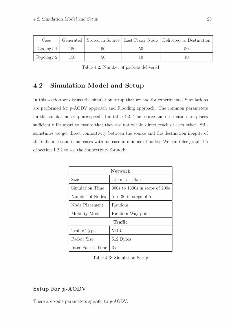
4.2. Simulation Model and Setup 25

Case Generated Stored in Source Last Proxy Node Delivered to Destination

Topology 1 150 50 50 50

Topology 2 150 50 10 10

Table 4.2: Number of packets delivered

4.2 Simulation Model and Setup

In this section we discuss the simulation setup that we had for experiments. Simulations

are performed for p-AODV approach and Flooding approach. The common parameters

for the simulation setup are specified in table 4.2. The source and destination are places

sufficiently far apart to ensure that they are not within direct reach of each other. Still

sometimes we get direct connectivity between the source and the destination in-spite of

there distance and it increases with increase in number of nodes. We can refer graph 1.5

of section 1.2.2 to see the connectivity for aodv.

Network

Size 1.5km x 1.5km

Simulation Time 300s to 1300s in steps of 200s

Number of Nodes 5 to 30 in steps of 5

Node Placement Random

Mobility Model Random Way-point

Traffic

Traffic Type VBR

Packet Size 512 Bytes

Inter Packet Time 3s

Table 4.3: Simulation Setup

Setup For p-AODV

There are some parameters specific to p-AODV.


• Every node checks its eligibility to become proxy on the basis of their “routing table

size.” We vary the routing table size from 1 to 5.

The reason for choosing these values is that average routing table size in the network

is in the range of 3 to 4.

• There is no restriction on proxy number size. Hence, a proxy-source/source can

send data to all the RREPs.

• A node will check for new locality periodically (every 5 seconds). Node will assume it

is in new environment if number of previous routing table entry and present routing

table entry having difference of two. And node will generate PRREQ.

4.3 Performance Metrics

These are the metrics we calculated to see the performance of protocol.

• Percentage of Message Delivered. This is the percentage of generated packets

that are received at the destination.

count(total packets received)

count(total packets sent)∗ 100

• Avg. Delay for a packet to reach destination. This is average delay from the

time the packet is generated tg at the source to the time the packet is delivered at

the destination td.

1

N

i=N∑

i=0

tid − tig

• Percentage of Duplicate Packets. This is a measure of the redundant packets

received at the destination.

count(total packets received) − count(unique packets received)

count(total packets received)

• Cost of memory requirement for a node over total simulation time This

is a measure of the time for which the buffer is occupied at a given node j.∑

i = 0i = NBi

N

Where Bi represents the buffer occupancy for node i and N is the number of nodes.

4.4. Results 27

4.4 Results

In graphs each point is the average of 20 simulation runs. we start with the explanation

of the performance of p-AODV then discuss about flooding approach. We conclude this

section with the comparison between them.

4.4.1 p-AODV with single parameter

In this section we show the performance of p-AODV. The delay tolerance of messages is

taken to be 300s in these simulations.

• The Message delivered percentage graph is shown in figure 4.3. It shows that most of

the time, p-AODV with proxy selection parameter as table size 1 performs better as

compared to higher table sizes. This happens because, many nodes become eligible

for becoming a proxy sooner using this relaxed criteria. This in turn leads to faster

propagation of message. Though at a cost of increased flooding in the network and

increased buffer occupancy in the node.

For more number of nodes in the network, the proxy selection criteria of table size

plays a lesser role in message delivery percentage. This is because of the increased

node density in the network. In graph we can also see that as the number of nodes

increases the percentage of message is also increasing which is expected.

• The average delay for delivery of messages is shown in figure 4.4. We can see that

in many cases increasing the number of nodes also increases the average delay for a

packet. This phenomenon is counter-intuitive, because increase in number of nodes

should have improved the chances of message delivery. The reason for this being,

overall increase in the network load because of more number of packets floating

around, leading to increase in contention at medium access layer. Also some packets

may be received very late because of a long proxy path followed, this increases the

average delay. For less number of nodes, the delay increases with increase in proxy

table size. For less number of nodes delay will increase because they were not able

to find good number of proxies as table size increases.

• The percentage of duplicate packets is shown in figure 4.3. We can see that as

the proxy selection criteria of routing table size is increased, duplication of packets


0

10

20

30

40

50

60

1 1.5 2 2.5 3 3.5 4 4.5 5

% o

f Mes

sage

s D

eliv

ered

Minimum Size of Routing Table

P-AODV Approach : Simulation Time 300s

Nodes7

1015202530

(a) Message Delivered Percentage

0

50

100

150

200

250

300

350

1 1.5 2 2.5 3 3.5 4 4.5 5

% D

uplic

ate

Ove

rhea

d



Nodes7

1015202530

(b) Duplicates Overhead

0

5

10

15

20

25

30

35

1 1.5 2 2.5 3 3.5 4 4.5 5

Mem

ory

Req

uire

men

t For

a N

ode



Nodes7

1015202530

(c) Memory Consumption Per Node

Figure 4.3: P -AODV Graphs : Proxy selection on routing table : SimTime 300

decreases. The rate of reduction in duplicate packets increases as number of nodes

increase.

• The cost of memory consumption is shown in figure 4.3. As the criteria to for proxy

selection becomes stricter, the number of proxies in the network reduces. Hence,

the message is duplicated at lesser nodes in the network. The cost stabilises as the

criteria to become a proxy-node becomes harder (higher table size).

4.4.2 Flooding Approach

In flooding approach source or proxy source delivers data to all nodes connected to it

without checking any condition. We simulate this approach to compare the results of this

4.4. Results 29

0

50

100

150

200

250

0 1 2 3 4 5 6P-A

OD

V A

ppro

ach

: Ave

rage

Del

ay in

Sec

onds

Minimum Routing Table Size

Confidence-Band Plot: Sim Time 300

Nodes7

1015

(a) Average Delay I

80

90

100

110

120

130

140

150

160

170

180

190

0 1 2 3 4 5 6P-A

OD

V A

ppro

ach

: Ave

rage

Del

ay in

Sec

onds

Minimum Routing Table Size

Confidence-Band Plot: Sim Time 300

Nodes202530

(b) Average Delay II

Figure 4.4: P -AODV Graphs : Proxy selection on routing table : SimTime 300

approach with the results of our proxy-AODV approach.

• Percentage of Message Delivered: In figure 4.5, percentage of messages delivered

increases as the number of nodes increase. Also, as the time increases, the percentage

of Message delivered increases. There is a sharp increase in the performance for from

5nodes to 10nodes. As the time increases, the message delivery percentage stabilises.

• Average delays are shown in figure 4.6. All the delay values are in the range of 100s

to 200s. This is because of increased flooding in the network.

• Percentage of Duplicate Overhead: As time increases, the duplicate overhead in-

creases with a higher rate. Also for increasing number of nodes in the network, the

duplicate overhead increases.

• Cost of Memory consumption per node of graph is shown in figure 4.5, As number

of nodes increases the cost of memory consumption increases. This is because more

flooding is observed in the network. As time increases, the buffer is occupied for

longer duration of time and hence increasing the cost.

4.4.3 Comparison of p-AODV and Flooding Approach

In figure 4.7, we present comparison between flooding and p-AODV approach. In this we

can see that

• Message Delivery Percentage in graph 4.7 shows that flooding approach has better

percentage delivery in comparison to proxy approach. The reason for this behaviour


0

10

20

30

40

50

60

70

80

90

100

5 10 15 20 25 30

% o

f Mes

sage

s D

eliv

ered

No. of Nodes

Flooding Approach : Message Delivery Vs Number of Nodes

300s500s700s900s

1100s1300s

(a) Message Delivered Percentage

0

200

400

600

800

1000

1200

1400

1600

1800

5 10 15 20 25 30

% D

uplic

ate

Ove

rhea

d

No. of Nodes

Flooding Approach : Duplicate Overhead Vs Number of Nodes

300s500s700s900s

1100s1300s

(b) Duplicates Overhead

0

20

40

60

80

100

120

140

160

180

5 10 15 20 25 30

Mem

ory

Req

uire

men

t for

a N

ode

Number of Nodes

Flooding Approach : Memory Consumption for a Node Vs SimTime

300s500s700s900s

1100s1300s

(c) Memory Consumption Per Node

Figure 4.5: Flooding Approach

0

50

100

150

200

250

300

0 5 10 15 20 25 30 35

Avg

Del

ay in

Sec

onds

Number of Nodes

Flooding Approach : Confidence-Band Plot:Title field

300s500s700s

(a) Average Delay I

0

50

100

150

200

250

300

350

400

450

0 5 10 15 20 25 30 35

Avg

Del

ay in

Sec

onds

Number of Nodes

Flooding Approach : Confidence-Band Plot:Title field

900s1100s1300s

(b) Average Delay II

Figure 4.6: Flooding Approach

4.4. Results 31

15

20

25

30

35

40

45

50

55

60

10 15 20 25 30

Per

cent

age

of M

essa

ges

Del

iver

ed

No. of Nodes

FloodingpAODV TableSize 1pAODV TableSize 2pAODV TableSize 3pAODV TableSize 4pAODV TableSize 5

(a) Percentage of Message Delivery

100

110

120

130

140

150

160

170

180

10 15 20 25 30

Ave

rage

Del

ay fo

r a

Pac

ket i

n S

econ

ds

No. of Nodes


(b) Average Delay For a Packet

0

50

100

150

200

250

300

350

400

450

500

10 15 20 25 30

% D

uplic

ate

Ove

rhea

d

No. of Nodes


(c) Percentage of Duplication Over-

head

Figure 4.7: Comparison Between Flooding and proxy-AODV performance

is that flooding makes every node a proxy. Hence, the chances of any proxy to reach

near the destination and deliver the data are very high.

• The graph for average delay in figure 4.5 shows that p-AODV consistently maintains

a lower delay time as comparison to flooding approach.

• In Duplicate Overhead graph of figure 4.5, we can see that flooding approach is

leading the graph and its very obvious because more of the nodes will reach to

destination as number of nodes will increases. The duplication of p-AODV is also

increasing but with low rate in comparison to flooding approach.

Chapter 5

Conclusion and Future Work

5.1 Conclusion

From the discussion in the previous chapters, we have seen that p-AODV performs better

in terms of overhead on networks and average consumption of memory per node. We can

also say that it is equally good as compared to flooding approach in terms of message

delivery.

There is a trade off between “Load on Network” and “Message Delivery Efficiency”.

If we impose less restrictions on proxy selection, then the probability of message delivery

increases. But, at the same time load on network and nodes increases. If we impose strict

restrictions on proxy selection criteria, then message delivery probability decreases.

To perform better in terms of message delivery percentage and at the same time

maintain low load on network and nodes, we propose some extensions in the future work

section.

5.2 Future Work

This project can be enhanced in two different directions:

• Improve the proxy selection function in terms of parameters and their values to

improve efficiency.

• Add more features to protocols, like acknowledgement for data.

A combination of both the above extensions will provide a self tuning system. For ex-

ample, an acknowledgement from destination to source can be used as carrier to distribute

value of duplication and percentage of message delivered. This will help other nodes to

33

34 Chapter 5. Conclusion and Future Work

regulate their parameters and their values while choosing the proxy, according to their

requirement of message delivery. And to stop flooding of this feedback a node is allow to

drop acknowledgement on the basis of its TTL field and last information flooding time.

On the other hand, node can free messages from buffers of respective sequence number.

We can also apply “proxy” and “store and forward” concept with other routing pro-

tocol of ad hoc network like DSDV, DSR. This will give us a opportunity to compare

two popular protocol.

Bibliography

[1] C. Perkins and E. Royer. Ad-hoc on-demand distance vector routing. pages 90–100,

1999.

[2] David B. Johnson and David A. Maltz. Dynamic source routing in ad hoc wireless

networks. In Mobile Computing, Kluwer Academic Publishers, 1996.

[3] Perkins C.E. and Praveen Bhagwat. Destination-sequenced distance vector (dsdv)

protocol. In SIGCOMM ’94, Conference on Communications Architecture, Protocol

and Application, pages 234–244, August 1994.

[4] Jain Sushant, Kevin Fall, and Patra Rabin. Routing in a delay tolerant network.

In SIGCOMM ’04: Proceedings of the 2004 conference on Applications, technologies,

architectures, and protocols for computer communications, 2004.

[5] A. Vahdat and D. Becker. Epidemic routing for partially connected ad hoc networks.

2000.

[6] Zhao W., Ammar M., and Zegura E. A message ferrying approach for data delivery

in sparse ad hoc networks. In Proceedings of 5th international symposium on mobile

ad hoc networking and computing, 2004.

[7] J. Davis, A. Fagg, and B. Levine. Wearable computers as packet transport mech-

anisms in highly-partitioned ad-hoc networks. In Wearable Computers, 2001. Pro-

ceedings. Fifth International Symposium on, pages 141–148, 2001.

[8] J. Yang, Y. Chen, M. Ammar, and C. K. Lee. Ferry replacement protocols in sparse

manet message ferrying systems. In college of Computing, Georgia Tech, 2004.

[9] Qun Li and Daniela Rus. Sending messages to mobile users in disconnected ad-hoc

wireless network. In MobiCom, 2001.

35

36 Bibliography

[10] Kevin Fall. Messaging in difficult environment. In Intel Research Berkeley, 2004.

[11] Samba S, Zongkai Y, Biao Qi, and Jianhua He. Simulation comparison of four wireless

ad hoc routing protocols. In Information Technology Journal 3 (3): 219-226, 2004.

[12] Qualnet simulator 3.9, 2004. http://www.qualnet.com.

Acknowledgements

I take this opportunity to express my sincere gratitude for Prof. Sridhar Iyer for

his constant support and encouragement. His excellent guidance has been instrumental

in making this project work a success.

I would like to thank Punit Rathod and Srinath Perur for their constant help

throughout the project. I would also like to thank my colleagues Anshu and kantu for

helpful discussions in the initial part of my project, Kaushal for being a supportive friend

and the KReSIT department for providing me world class computing infrastructure.

I would also like to thank my family and friends especially the entire MTech Batch,

who have been a source of encouragement and inspiration throughout the duration of the

project.

Last but not the least, I would like to thank the entire KReSIT family for making my

stay at IIT Bombay a memorable one.

Anshuman Tiwari

I. I. T. Bombay

July 13th, 2006

37

proxy-AODV : Extension of AODV For Partially Connected Ad hoc Networks

Documents

Transcript of proxy-AODV : Extension of AODV For Partially Connected Ad hoc Networks