EURASIP Journal on Wireless Communications and Networking 2005:5, 635–644c© 2005 Raminder P. Mann et al.

Energy-Aware Routing Protocol forAd Hoc Wireless Sensor Networks

Raminder P. MannDepartment of Electrical and Computer Engineering, Wichita State University, Wichita, KS 67260, USAEmail: rpmann@wichita.edu

Kamesh R. NamuduriDepartment of Electrical and Computer Engineering, Wichita State University, Wichita, KS 67260, USAEmail: kamesh.namuduri@wichita.edu

Ravi PendseDepartment of Electrical and Computer Engineering, Wichita State University, Wichita, KS 67260, USAEmail: ravi.pendse@wichita.edu

Received 15 June 2004; Revised 15 April 2005

Wireless ad hoc sensor networks differ from wireless ad hoc networks from the following perspectives: low energy, lightweightrouting protocols, and adaptive communication patterns. This paper proposes an energy-aware routing protocol (EARP) suitablefor ad hoc wireless sensor networks and presents an analysis for its energy consumption in various phases of route discovery andmaintenance. Based on the energy consumption associated with route request processing, EARP advocates the minimization ofroute requests by allocating dynamic route expiry times. This paper introduces a unique mechanism for estimation of route expirytime based on the probability of route validity, which is a function of time, number of hops, and mobility parameters. In contrastto AODV, EARP reduces the repeated flooding of route requests by maintaining valid routes for longer durations.

Keywords and phrases: ad hoc networks, routing protocols, mobility models.

1. INTRODUCTION

Wireless sensors are small devices with limited energy with-out energy backup; they are more of one-time-use sensors.Therefore, an energy-efficient routing mechanism wouldmean longer sensor lifetime and higher network efficiency.Active research is going on in the field of routing in adhoc sensor networks. A lot of development has been seenin ad hoc routing since the introduction of highly dynamicdestination-sequenced distance-vector routing (DSDV) [1].Ad hoc on-demand distance-vector routing (AODV) [2] anddynamic source routing (DSR) [3] have been very popu-lar and widely accepted ad hoc routing protocols. Variationsof DSR and AODV have been suggested in the literature;one such approach can be found in [4]. An enhancementto AODV is also presented in self-learning ad hoc routingprotocol (SARP) [5] which adds the route caching capabil-

This is an open access article distributed under the Creative CommonsAttribution License, which permits unrestricted use, distribution, andreproduction in any medium, provided the original work is properly cited.

ity of DSR to AODV to achieve higher efficiency. This pa-per presents an energy-aware routing protocol (EARP) basedon AODV. In particular, this paper addresses the problem offrequent route expiry and suggests a criterion to statisticallyestimate the route validity time. This criterion results in thereduction of route requests and consequently improves en-ergy efficiency.

1.1. Node communication pattern

A typical sensor network consists of two types of nodescalled sensor nodes (referred to as sensors) and data gath-ering nodes (referred to as nodes). Sensors are small wire-less devices that are capable of sensing the environment andtransmitting the data they collect. They have unidirectionalwireless links and can only receive control signals from datagathering nodes. They have two modes of operation: energysaving mode and active mode. Data gathering nodes are rela-tively more powerful wireless nodes as compared to sensors.They have larger energy backup and possess data computa-tion, aggregation, and processing abilities. They are respon-sible for collecting data from all the sensors in their vicinity

636 EURASIP Journal on Wireless Communications and Networking

N1

N2

N3

N4

N5

N6

N7

N8

N9 r

R

Figure 1: Communication pattern of nodes in an ad hoc network:smaller circles denote the sensing range and bigger circles denotethe communication range.

then aggregate and process the data before transmitting toother nodes. The links between these nodes are bidirectional;hence they have the capability to transmit and receive data.Data gathering nodes play the crucial role of removing over-lapping data collected from sensors and transmitting onlythe useful and required data to various other nodes in thenetwork. The entire routing functionality is built only in thedata gathering nodes. This mechanism is quite similar to thecluster head approach discussed in [6, 7], the major differ-ence being in the classification of nodes based on their func-tionality. In most of the cluster-head-based protocols, thecluster head is chosen based on the various parameters likeenergy backup. In this node communication pattern, the en-ergy consumption in election process is avoided by separat-ing the two types of nodes based on their hardware.

In Figure 1, each smaller circle denotes the vicinity ofeach data gathering node, that is, the region in which allthe sensors are controlled by one particular node. The ra-dius of this circle is called the sensing radius and is denotedby “r.” The bigger circle is the communication radius “R” ofthat particular node and it can directly communicate withall the nodes in this range, form neighbors, and exchangedata.

Node to sensor communication is controlled by the node;it can turn on the transmitters of all the sensors in its vicinityby sending the required control signals. On receiving thesecontrol signals, the sensors switch from energy saving modeto active mode and transmit the collected data to the cor-responding node. The transmitters of sensors would revertto energy saving mode after sending data to the node. Thecomputation is reduced at the sensors by enforcing the sleepmechanism [8] on all the sensors.

Node-to-node communication is very similar to themethod described in [9]. Every node looks for all other nodeswilling to exchange data in its communication range. Afterexchanging the start-up messages and verifying the signal-to-noise (SNR) levels, nodes establish neighbors and allocateone time division multiple access (TDMA) [10] slot within aframe to each neighbor.

t

tc

Figure 2: Channel allocation in an ad hoc wireless network: t de-notes the frame length and tc denotes the time slot assigned to eachneighboring node.

As shown in Figure 2, if the entire TDMA frame is of tseconds and the slot allocated to each neighbor is tc, then thenumber of neighbors a node can have is t/tc. The ratio t/tcwill be later used to explain the energy savings in EARP.

1.2. Energy estimation

The energy consumption estimates given in [11] are used inthis paper to calculate the total energy consumption in theroute discovery procedure using route request (RREQ) androute reply (RREP) [2]. The energy required to transmit r0

bits is given by

Pt(s1, s2

) = [α1 + α2d(s1, s2

)n]r0, (1)

where d(s1, s2) denotes the distance between nodes s1 and s2

in meters, and α1 and α2 are communication constants. Thevalue of n depends on signal propagation. The above equa-tion can be rewritten by replacing r0 with B∗t, where B is thetotal link capacity between one-hop neighbors in kbps and tis the total frame size in seconds:

P1 =[α1 + α2d

4]∗ B ∗ t. (2)

In the above expression, d represents the average distance be-tween two neighbors in the network. The path loss exponentn [12] depends on the environment and the approximatevalue of n in a shadowed urban area lying between 3 to 5.Therefore, for all the computations in this paper, the value ofn is taken as 4. Thus, P1 gives the energy consumed in trans-mitting one frame from a node to its neighbors. Similarly, theestimate for the energy consumed in receiving ri(= tc ∗ B)bits of data given in [11] is rewritten as follows:

P2 = αr ∗ tc ∗ B. (3)

In this expression, αr is the communication constant withtypical value of 135 nJ/b [11] and tc is the duration of sin-gle time slot allocated to each neighbor in seconds. Thus, P2

gives the total energy spent by one neighbor in receiving itsshare out of the total frame transmitted by the source.

Energy-Aware Routing Protocol 637

1.3. Link availability

Link availability addresses the problem of prediction of thestatus of a link between two nodes after time t based onnetwork parameters. The probability of link availability dis-cussed in [13] is used with some modifications as a base foroperation of EARP. In [13], the authors proposed a randomad hoc mobility model and computed the probability of linkavailability (Am,n(t)) between nodes m and n after time t as

Am,n(t) ≈ 1−Φ(

12

, 2,−4R2

eq

αm,n

), (4)

αm,n = 2t(σ2m + µ2

m

λm+σ2n + µ2

n

λn

), (5)

where Φ(a, b, z) is the Kummer-confluent hypergeometricfunction,1 Req is the effective communication radius, t is thetime, σ2

i and µi are the variance and mean speed of node iduring each epoch,2 and 1/λi is mean epoch length for nodei.

This equation for link availability is modified using thefollowing assumptions. (1) All nodes have equal mean speedand variance during each epoch over the time period t, repre-sented by µ and σ . Hence µ and σ are defined as network pa-rameters instead of being node parameters. (2) Mean epochlength is uniform over the network and is given by λ. There-fore, λ is also a network parameter. Based on these assump-tions, (4) can be rewritten as follows:

Am,n(t) ≈ 1−Φ(

12

, 2,−4R2

eq

α

)

α = 4tλ

(σ2 + µ2).

(6)

In the next section, the proposed energy-aware rout-ing protocol (EARP) is presented and its energy efficiencyis compared with that of the ad hoc on-demand distance-vector (AODV) routing protocol.

2. ENERGY-AWARE ROUTING PROTOCOL

In energy-efficient routing protocol (EARP), the route dis-covery process is exactly the same as in AODV; the sourceS floods an RREQ to its neighbors and the neighbors floodRREQ further to their neighbors till it reaches an interme-diate node I which knows the route to the destination or itreaches the destination D. In addition to the above proce-dure, EARP will also maintain a table of routes that have lessprobability of expiring till the next communication betweenthe same set of nodes (S and D). The criterion to select theroutes eligible to be added to the routing table is based on

1The confluent hypergeometric function has a hypergeometric seriesgiven by Φ(a, b, z) = 1 + a · z/b + a(a + 1) · z2/b(b + 1) · 2! + · · · =∑∞

k=0((a)k/(b)k)(zk/k!).2Mobility epoch is the duration in the motion of a node during which its

speed and direction remain constant.

the network parameters and the probability of route validity(Proute-valid).

In AODV, once a transmission is completed the route isdeclared invalid after a fixed route expiry time (10 seconds)and cleared from the routing table, which results in frequentinitiation of route discovery process. The EARP scheme ad-vocates saving the routes discovered in the route discoveryprocess in a route table based on the route selection crite-rion. In order to accomplish this, we define a new controlpacket called route check request (RCR) in EARP. If after acertain interval of time, some data needs to be transferredbetween the same set of source (S) and destination (D), Swill first issue an RCR control packet to verify the validity ofthat route saved in the route table. RCR is a dummy packetwhich is sent across all the nodes that appear in the route toD. If any nodes between S and D have moved out of rangein this route, a route error (RERR) is transmitted back to S.On receiving this RERR, the source S initiates a route discov-ery for the destination D and removes the expired route fromrouting table.

The success rate of RCR will typically depend on the mo-bility pattern of the nodes in the sensor network. Saving allroutes in the routing table results in higher energy consump-tion due to excessive RCR transmissions. This problem is ad-dressed in EARP with the route selection criterion which al-lows only those routes with larger probability of route valid-ity to be saved. For each route, an appropriate route validitytime is computed based on the network parameters.

2.1. Criterion for selecting routes for savingin the routing table

In this subsection, a criterion is derived for selection ofroutes. This derivation is based on the three major param-eters: probability of link validity (Plink-valid), probability ofroute validity (Proute-valid), and threshold for probability ofroute validity (Proute-valid-threshold). In addition, the derivationalso requires estimates for the energy consumption in vari-ous phases of routing.

2.1.1. Probability of link validity (Plink-valid)

This is defined as the probability of any link which is valid att = 0, will remain valid at t = T (T > 0), and is given byAm,n(t). As a convention, it is referred to as Plink-valid, so from(6) we get

Plink-valid = 1−Φ(

12

, 2,−4R2

eq

α

)

α = 4Tλ

(σ2 + µ2),

(7)

where Φ(a, b, z) is the Kummer-Confluent hypergeometricfunction [13].

2.1.2. Probability of route validity (Proute-valid)

This is the probability that the route discovered using theRREQ flooding at t = 0 and which will be valid after time

638 EURASIP Journal on Wireless Communications and Networking

T. The expression for this probability is given by

Proute-valid =[

1−Φ

(12

, 2,−4R2

eq

α

)]h

. (8)

A route with h hops will have h such links. Thus, the proba-bility of route validity is [Plink-valid]h. The parameter h acts asa decay factor since the probability of route validity reducesas the number of hops in the route increases.

2.1.3. Threshold for probability of route validity(Proute-valid-threshold)

The threshold for the probability of route validity is the valueof Proute-valid at which the energy consumption in AODVis equal to the energy consumption in EARP. Beyond thisthreshold value, EARP outperforms AODV in terms of en-ergy efficiency. Hence, any route with probability of routevalidity higher than its threshold would save energy if reusedwithin the route validity time.

2.2. Energy consumption in routing

The following subsections discuss the energy estimates re-quired to compute Proute-valid-threshold. A set-up of typicalsource S and destination D that are h hops away is assumedin the following discussion.

2.2.1. Energy estimation in route discovery

In this scenario, the source S is trying to look for the desti-nation D and an RREQ is being flooded to every neighbor toget to D. The nodes S and D are h hops away and N is thenumber of nodes in the entire sensor network.

E1 (energy consumed at S to flood an RREQ packet) =[α1 + α2d4]∗ B ∗ t = P1.

E2 (energy consumed at neighbor to receive an RREQpacket) = αr ∗ tc ∗ B = P2.

E3 (energy consumed at neighbor to flood an RREQpacket) = P1.

E4 (energy consumed at D to receive an RREQ packet)= P2.

Eq (total energy consumed in transmitting RREQ from Sto D)= E1 +(E2 +E3)∗(number of intermediate nodes)+E4.

As the RREQ packet is flooded in the entire network, thenumber of intermediate nodes will be (N − 2), that is, all thenodes in the network except S and D. Therefore,

Eq = E1 +(E2 + E3

)∗ (N − 2) + E4

= P1 +(P1 + P2

)∗ (N − 2) + P2

= (P1 + P2)∗ (N − 1).

(9)

E5 (energy consumed at D to transmit an RREP packet)= [α1 + α2d4]∗ B ∗ tc = P3.

Here, tc is being used because RREP is not flooded as thelinks between all the nodes are bidirectional and RREP has tofollow the discovered path backwards.

E6 (energy consumed at neighbor to receive RREP)= P2.E7 (energy consumed at neighbor to transmit RREP) =

P3.E8 (energy consumed at S to receive RREP) = P2.Ep (the energy consumed in transmitting RREP from D

to S)= E5 + (E6 +E7)∗ (number of intermediate nodes) +E8.As RREP follows the path discovered by RREQ, it only

travels through the route of h hops:

Ep = E5 +(E6 + E7

)∗ (h) + E8,

Ep = P3 +(P2 + P3

)∗ h + P2 =(P2 + P3

)∗ (h + 1).(10)

The total energy consumed in the route discovery process(Erd) is the sum of Eq and Ep and is given by the followingexpression:

Erd =(P1 + P2

)∗ (N − 1) +(P2 + P3

)∗ (h + 1). (11)

2.2.2. Energy estimate for route table maintenance

EARP suggests saving those routes which do not expirewithin twice the AODV route expiry time. Once the routeis discovered in EARP, each packet stores the entire route.Hence, computation overhead is only at the source node S.Route entry is made by RREQ flooding and the size of routeentry depends on the number of hops between S and D. Allestimates in this section assume h hops between S and D. Theenergy consumed by CPU in route lookup depends on thesize of routing table. As there are N nodes in the network, themaximum size of the routing table could be (N − 1). Duringroute fetch, two basic operations are performed by the sourcenode. First, it has to compare each destination in routing ta-ble to the destination D. Later, it loads the route given for Din its cache. The associated overhead for each of the abovefunctions can be estimated in terms of bi (energy consumedin a memory fetch) and bj (energy consumed in an arith-metic operation), quite similar to the approach used in [14].

E9 (energy consumed in route lookup)= (bi+bj)·(N−1).E10 (energy consumed in loading route to cache)= bi ·h.

2.2.3. Energy estimate for an RCR Request

For consistency, the size of RCR packet is assumed to be equalto that of RREQ/RREP packet, though it can be much smallerwith just an “RCR bit” set. RCR is a one-way request, and ifno route error (RERR) is received within RCR expiry time,the route is declared valid and data transmission is carriedout.

E11 (energy consumed at S to transmit RCR to the nexthop) = [α1 + α2d4]∗ B ∗ tc = P3.

E12 (energy consumed at each hop to receive and trans-mit RCR to the next hop)= αr∗tc∗B+[α1 +α2d4]∗B∗tc =P2 + P3.

E13 (energy consumed at D to receive RCR) = P2.E14 (total energy consumed in route checking) = E11 +

E12∗h+E13 = P3 +(P2 +P3)∗h+P2 = (P2 +P3)∗(h+1). Ad-ditional computational overhead due to route-table lookup

Energy-Aware Routing Protocol 639

(E9) and loading of route to cache (E10) need to be added.Thus, the total energy ERCR consumed in RCR mechanism isgiven by

ERCR = E14 + E9 + E10 =(P2 + P3

)∗ (h + 1)

+(bi + bj

) · (N − 1) + bi · h.(12)

Proposition 1. (criterion for saving a route). All routes thatsatisfy Proute-valid>Proute-valid-threshold should be saved in the routingtable as they have a high probability of staying valid after timeinterval T. An implementation of this criterion would requirean estimation of the threshold for the probability of route va-lidity. Based on the energy consumption comparison betweenEARP and AODV, this estimation is given by the followinglemma.

Lemma 1. The value of threshold for the probability of routevalidity is given by

Proute-valid-threshold

=(P2 + P3

)∗ (h + 1) +(bi + bj

) · (N − 1) + bi · h(P1 + P2

)∗ (N − 1) +(P2 + P3

)∗ (h + 1),

(13)

where P1 = [α1 + α2d4] ∗ B ∗ t, P2 = αr ∗ tc ∗ B, P3 =[α1 +α2d4]∗B∗ tc, bi = energy consumed in a single memoryfetch, bj = energy consumed in a single arithmetic operation,and N = number of nodes in the network.

The value of Proute-valid at which the energy consump-tion in EARP equals the energy consumption in AODV isdefined as the threshold value of the probability of route va-lidity Proute-valid-threshold. In order to estimate Proute-valid-threshold,the total energy associated with routing in both AODV andEARP is compared assuming that there are M repeated trans-missions between S and D. These repeated transmissionshave time interval greater than the AODV route expiry time.Proute-valid gives the ratio of the number of successful trans-missions out of M before the route from S to D becomes in-valid.

Let A denote the total energy consumed using AODV forM route discoveries. Similarly, let B denote the total energyconsumed using the RCR mechanism for M transmissions.A and B are given by the following expressions:

A = [Eq + Ep]∗M

= [(P1 + P2)∗ (N − 1) +

(P2 + P3

)∗ (h + 1)]∗M,

B = ERCR ∗M +[Eq + Ep

]∗M ∗ (1− Proute-valid).

(14)

The threshold value for Proute-valid is obtained by equatingA and B and solving for Proute-valid. By simplifying, the thresh-old value of the probability of route validity given in (13) isobtained.

Proposition 1 suggests the duration for route validity,that is, how long a route should be saved in the routing table

(troute-valid). Energy savings are possible if for all saved routesthe probability of route validity stays above the probability ofroute validity threshold. It can be interpreted that as long asProute-valid is greater than Proute-valid-threshold, the route shouldbe kept in the routing table. Using this principle in conjunc-tion with Proposition 1, an estimate for troute-valid is derivedin Proposition 2.

Proposition 2. The time for which any route is valid is givenby

troute-valid ≈[

λ

4(σ2 + µ2

)][

R2eq

(Proute-valid-threshold)1/h

]. (15)

Proof. According to Proposition 1, energy savings can beexpected, if all routes in the routing table satisfy Proute-valid >Proute-valid-threshold. As Proute-valid reduces with time, the aboveinequality fails after a certain time interval (troute-valid). Thistime interval can be estimated by equating the Proute-valid toits threshold as follows:

Proute-valid =[

1−Φ(

12

, 2,−4R2

eq

α

)]h= Proute-valid-threshold.

(16)

Expanding the Kummer confluent hypergeometric seriesto obtain expression for Proute-valid, we get

Proute-valid =[

1−(

1− R2eq

α+R4

eq

α2− 5R6

eq

6α4+ · · ·

)]h

= Proute-valid-threshold.

(17)

Taking an approximation of the series till the secondterm, we get

[1−

(1− R2

eq

α

)]h≈ Proute-valid-threshold,

R2eq

α≈ (Proute-valid-threshold

)1/h,

α ≈ R2eq(

Proute-valid-threshold)1/h .

(18)

Substituting α = 4T/λ(σ2 + µ2),

4Tλ

(σ2 + µ2) ≈ R2

eq(Proute-valid-threshold

)1/h . (19)

Replacing T by troute-valid, we get

troute-valid ≈[

λ

4(σ2 + µ2

)][

R2eq(

Proute-valid-threshold)1/h

]. (20)

640 EURASIP Journal on Wireless Communications and Networking

Table 1: Values of parameters used for quantitative analysis.

Parameter Value

N (number of data gathering nodes) 20

α1 (communication constant) 45 nJ/b

α2 (communication constant) 10 pJ/b/m4

αr (communication constant) 135 nJ/b

d (average distance between nodes) 250 m

t (frame length) 14 milliseconds

tc (size of each slot in the frame) 2 milliseconds

B (link bandwidth) 64 kbps

bi (energy consumed in a single memory fetch) 7.32 nJ

bj(energy consumed in a single arithmetic operation) 3.41 nJ

Req (effective communication radius) 500 m1λ

(mean epoch length) 30 s

µ (mean speed) 10 kph ≈ 2.5 m/s

T (minimum time for route validity) 5 min

This is the maximum value of t for which the criteriondescribed in Proposition 1 is satisfied. This time troute-valid isset in the time field of routing table for each route. As soonas troute-valid expires, the route is removed from the routingtable. Based on the two propositions, we would now presenta quantitative analysis of energy savings obtained in EARP.

3. QUANTITATIVE ANALYSIS OF EARPAND SIMULATION RESULTS

3.1. Quantitative analysis

In this section, a quantitative analysis based on a practicalscenario is presented. A network with the typical values forall the defined parameters is assumed for this analysis; thesevalues are listed in Table 1.

Using the values in Table 1 and the expressions derived inearlier sections, the following values of energy consumptionin various phases are obtained: P1 = 34.94 J, P2 = 1.728 ∗10−5 J, P3 = 4.99 J. To give a practical interpretation tothe criterion of route selection, the values of Proute-valid andProute-valid-threshold for different values of h are estimated using(8) and (13), respectively. Table 2 lists the values of Proute-valid

and Proute-valid-threshold for 1 to 8 hops. In these estimations,the time T is taken to be 5 minutes.

The values in Table 2 clearly show that the value ofProute-valid is greater than Proute-valid-threshold for routes with lessthan or equal to 6 hops. So, nodes will save all routes with lessthan or equal to 6 hops in their routing table. An estimate ofthe expiry time based on (20) for all saved routes correspond-ing to the number of hops is also shown. By substituting thevalues into the expressions derived in the previous sections,42.58% energy savings are obtained with EARP over AODV,if a route of hop count 1 is used 10 times. If the route that isused repeatedly has a hop count 6, the energy savings drop to0.006%. These results are further strengthened by the simu-lation results discussed below.

Table 2: Estimated values of probabilities and associated expirytimes.

Hops Proute-valid-threshold Proute-valid troute-valid

1 0.0148 0.4401 35.81

2 0.0220 0.2919 15.54

3 0.0292 0.1937 10.54

4 0.0362 0.1285 8.46

5 0.0431 0.0852 7.36

6 0.0500 0.0565 6.68

7 0.0561 0.03752 —

3.2. Simulation results

In order to compare the performance of EARP with AODV,a network with forty nodes uniformly positioned over anarea of 2000 ∗ 2000 meters and mobility based on randomwalk model was simulated in Glomosim network simulator[15]. Implementation of dynamic route expiry for EARP re-quired modifications in the AODV implementation of Glo-mosim. AODV is implemented in Glomosim using aodv.pcand aodv.h files. The aodv.pc file was modified to allocatethe route expiry times dynamically based on the route hopcount. The simulation code was not programmed to calcu-late the route expiry values based on network paramaters;instead the scenarios were created and route expiry timesfor each hop count were estimated manually. The simula-tion code was modified to allocate these values to each newlyadded route based on its hop count.

The changes made it possible to simulate the effect of dy-namic route expiry time on the number of route requests andcontrol packets. The evaluation and comparison of EARPwith AODV was done by simulating various scenarios. Threemajor scenarios are discussed below based on the node mo-bility characteristics as it was found that mobility had maxi-mum effect on the number of route requests.

Energy-Aware Routing Protocol 641

RREQ-EARPRREQ-AODV

1 4 7 10 13 16 19 22 25 28 31 34 37 40

Node number

0

500

1000

1500

2000

2500

3000

Nu

mbe

rof

RR

EQ

s

Figure 3: Scenario I: comparison of EARP and AODV in terms ofthe number of RREQ packets generated during high mobility.

RREP-EARPRREP-AODV

1 4 7 10 13 16 19 22 25 28 31 34 37 40

Node number

0

100

200

300

400

500

600

Nu

mbe

rof

RR

EPs

Figure 4: Scenario I: comparison of EARP and AODV in terms ofthe number of RREP packets generated during high mobility.

3.2.1. Scenario I—high mobility

The mobility parameters in config.in Glomosim file werechanged to simulate high-mobility scenarios. The mobilitymodel used was a random waypoint mobility model, themaximum node speed was set to 10 m/s, and minimum nodespeed was zero with a zero pause time. As in high mobil-ity, the links between nodes would expire quickly so EARPwould not be able to keep routes for much longer in theroute cache. The energy savings in this case would be mini-mum. The graph in Figure 3 compares the RREQs generatedby both protocols under these conditions. For most nodesEARP saved some RREQs over AODV but in aggregate forall 40 nodes, EARP generated 3.6% less RREQs than AODV.The graph in Figure 4 shows the comparison of RREPs gen-erated by each node from 0 to 39 for both EARP and AODV.In aggregate EARP generated 4.95% less RREPs than AODV.The graph in Figure 5 shows the aggregate control packetsgenerated for each node by both protocols. EARP generated3.49% less control packets than AODV. The 3.49% may looklike a small figure, but the total control packets generatedby EARP for the period of simulation were 1748 packets less

Control-EARPControl-AODV

1 5 9 13 17 21 25 29 33 37

Node number

0

500

1000

1500

2000

2500

3000

Nu

mbe

rof

con

trol

pack

ets

Figure 5: Scenario I: comparison of EARP and AODV in terms ofthe number of control packets generated during high mobility.

RREQ-EARPRREQ-AODV

1 4 7 10 13 16 19 22 25 28 31 34 37 40

Node number

0

1000

2000

3000

4000

5000

6000

7000

Nu

mbe

rof

RR

EQ

s

Figure 6: Scenario II: comparison of EARP and AODV in terms ofthe number of RREQ packets generated during medium mobility.

than AODV. If each packet is as small as 60 bytes, transmit-ting it over a 64 kbps link for a distance of 100 meters ap-proximately needs 0.1 joules of energy. Therefore, in such aworst case scenario, EARP was able to save around 175 joulesof energy over AODV.

3.2.2. Scenario II—medium mobility

As the node mobility decreases, the link availability increases.In scenarios with higher link availability, EARP is more ef-fective due to dynamic route caching. Medium mobility wassimulated by decreasing the mean speed of nodes in the ran-dom waypoint mobility model. The maximum speed was setto 3 m/s and minimum speed was set to zero with a pausetime of zero. The graph in Figure 6 compares the RREQsgenerated by both protocols under these conditions. In ag-gregate for all 40 nodes, EARP generated 22.12% less RREQsthan AODV. The graph in Figure 7 shows the comparison ofRREPs generated by each node from 0 to 39 for both EARPand AODV. In aggregate EARP generated 19.79% less RREPsthan AODV. The graph in Figure 8 shows the aggregate con-trol packets generated for each node by both protocols. EARP

642 EURASIP Journal on Wireless Communications and Networking

RREP-EARPRREP-AODV

1 4 7 10 13 16 19 22 25 28 31 34 37 40

Node number

0

100

200

300

400

500

600

700

Nu

mbe

rof

RR

EPs

Figure 7: Scenario II: comparison of EARP and AODV in terms ofthe number of RREP packets generated during medium mobility.

Control-EARPControl-AODV

1 5 9 13 17 21 25 29 33 37

Node number

0

1000

2000

3000

4000

5000

6000

7000

Nu

mbe

rof

con

trol

pack

ets

Figure 8: Scenario II: comparison of EARP and AODV in terms ofthe number of control packets generated during medium mobility.

generated 21.01% less control packets than AODV. The totalcontrol packets generated by EARP for the period of simula-tion were 12 335 packets less than AODV. Based on the sim-ilar packet size, this amounts to energy savings of approxi-mately 1233 joules.

3.2.3. Scenario III—low mobility

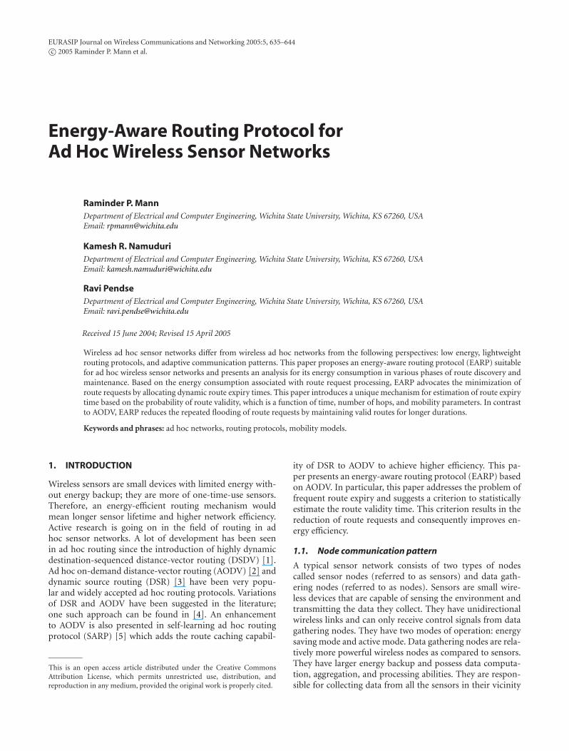
Low mobility was simulated to represent close to a best casescenario, where the nodes do not lose links very frequently.This case can be used to demonstrate an upper bound on en-ergy savings in an ad hoc wireless environment. Low mobil-ity was simulated by increasing the pause time of nodes in therandom waypoint mobility model. The maximum speed wasset to 3 m/s and minimum speed was set to zero with a pausetime of 1000 seconds. The graph in Figure 9 compares theRREQs generated by both protocols under these conditions.In aggregate for all 40 nodes, EARP generated 48.05% lessRREQs than AODV. The graph in Figure 10 shows the com-parison of RREPs generated by each node from 0 to 39 forboth EARP and AODV. In aggregate EARP generated 51.08%less RREPs than AODV. The graph in Figure 11 shows theaggregate control packets generated for each node by both

RREQ-EARPRREQ-AODV

1 4 7 10 13 16 19 22 25 28 31 34 37 40

Node number

0

1000

2000

3000

4000

5000

6000

7000

Nu

mbe

rof

RR

EQ

s

Figure 9: Scenario III: comparison of EARP and AODV in terms ofthe number of RREQ packets generated during low mobility.

RREP-EARPRREP-AODV

1 4 7 10 13 16 19 22 25 28 31 34 37 40

Node number

0

100

200

300

400

500

600

700

Nu

mbe

rof

RR

EPs

Figure 10: Scenario III: comparison of EARP and AODV in termsof the number of RREP packets generated during low mobility.

protocols. EARP generated 49.20% less control packets thanAODV. The total control packets generated by EARP for theperiod of simulation were 34 874 packets less than AODV.Based on the similar packet size, this amounts to energy sav-ings of over 3 kilojoules.

4. CONCLUSIONS

This paper provides a quantitative analysis of energy con-sumption estimates in flooding and directed broadcast meth-ods. The difference between these methods is used to provethe efficiency of EARP over AODV. EARP includes mobil-ity and number of hops as parameters in estimating the life-time of a route and suggests a unique way to accurately es-timate the validity period of a route, thus reducing the re-peated transmission of route requests. The major disadvan-tage of AODV is its overhead due to the high number of routediscoveries previously discussed in [16], and EARP definesa technique to reduce these route discoveries, which is themost critical part of ad hoc wireless sensor networks. EARPis well suited for sensor networks due to its ability to adaptto the environment and make routing decisions based on the

Energy-Aware Routing Protocol 643

Control-EARPControl-AODV

1 5 9 13 17 21 25 29 33 37

Node number

0

1000

2000

3000

4000

5000

6000

7000

Nu

mbe

rof

con

trol

pack

ets

Figure 11: Scenario III: comparison of EARP and AODV in termsof the number of control packets generated during low mobility.

communication patterns. Relative mobility between sensornodes is frequently demonstrated in the common sensor net-work applications. In our future work, relative mobility willbe included in the model to estimate the route expiry time.

ACKNOWLEDGMENT

This work was carried out under the research Grant “A Low-Energy Wireless Ad Hoc Sensor Networks Test-bed” spon-sored by Kansas NSF EPSCoR.

REFERENCES

[1] C. E. Perkins and P. Bhagwat, “Highly dynamic destination-sequenced distance-vector routing (DSDV) for mobile com-puters,” in Proc. ACM SIGCOMM ’94 Conference on Com-munications Architectures, Protocols and Applications, pp. 234–244, London, UK, August–September 1994.

[2] C. E. Perkins and E. M. Royer, “Ad-hoc on-demand distancevector routing,” in Proc. 2nd IEEE Workshop on Mobile Com-puting Systems and Applications (WMCSA ’99), pp. 90–100,New Orleans, La, USA, February 1999.

[3] D. B. Johnson and D. A. Maltz, “Dynamic source routing in adhoc wireless networks,” in Mobile Computing, vol. 353, chap-ter 5, pp. 153–181, Kluwer Academic, Boston, Mass, USA,1996.

[4] G. Kunito, K. Yamazaki, H. Morikawa, and T. Aoyama, “Anad-hoc routing control method in sensor networks,” in Proc.26th Annual Conference of the IEEE Industrial Electronics Soci-ety (IECON ’00), vol. 2, pp. 1147–1152, Nagoya, Japan, Octo-ber 2000.

[5] S. Gundeti, T. Best, R. Bhagavathula, and R. Pendse, “SARP:an Analytical Evaluation,” submitted for publication.

[6] W. B. Heinzelman, A. P. Chandrakasan, and H. Balakrishnan,“An application-specific protocol architecture for wireless mi-crosensor networks,” IEEE Transactions on Wireless Communi-cations, vol. 1, no. 4, pp. 660–670, 2002.

[7] S. Dulman, L. van Hoesel, T. Nieberg, and P. Havinga, “Col-laborative communication protocols for wireless sensor net-works,” in Proc. European Research on Middleware and Archi-tectures for Complex and Embedded Cooperative Systems Work-shop, pp. 3–7, Pisa, Italy, April 2003.

[8] N. Bansal and Z. Liu, “Capacity, delay and mobility in wirelessAd-hoc networks,” in Proc. 22nd Annual Joint Conference ofthe IEEE Computer and Communications Societies (INFOCOM’03), vol. 2, pp. 1553–1563, San Francisco, Calif, USA, March–April 2003.

[9] K. Sohrabi, J. Gao, V. Ailawadhi, and G. J. Pottie, “Protocolsfor self-organization of a wireless sensor network,” IEEE Pers.Commun., vol. 7, no. 5, pp. 16–27, 2000.

[10] D. D. Falconer, F. Adachi, and B. Gudmundson, “Time divi-sion multiple access methods for wireless personal communi-cations,” IEEE Commun. Mag., vol. 33, no. 1, pp. 50–57, 1995.

[11] Y. Thomas, Y. Shi, J. Pan, A. Efrat, and S. Midkiff, “Max-imizing lifetime of wireless video sensor networks throughoptimal flow routing,” in Proc. IEEE Military Communica-tions Conference (MILCOM ’03), Boston, Mass, USA, October2003.

[12] T. S. Rappaport, Wireless Communications, Principles andPractice, Prentice-Hall, Upper Saddle River, NJ, USA, 1996.

[13] A. B. McDonald and T. Znati, “A path availability model forwireless ad-hoc networks,” in Proc. IEEE Wireless Communi-cations and Networking Conference (WCNC ’99), vol. 1, pp.35–40, New Orleans, La, USA, September 1999.

[14] R. Szewczyk and A. Ferencz, “Energy implications of networksensor designs,” Tech. Rep., Berkeley Wireless Research Cen-ter, Santa Clara, Calif, USA, 2000.

[15] L. Bajaj, M. Takai, R. Ahuja, K. Tang, R. Bagrodia, and M.Gerla, “Glomosim: a scalable network simulation environ-ment,” Tech. Rep. 990027, Computer Science Department,University of California, Los Angeles, Calif, USA, 1999.

[16] C. E. Perkins, E. M. Royer, S. R. Das, and M. K. Marina,“Performance comparison of two on-demand routing proto-cols for ad hoc networks,” IEEE Pers. Commun., vol. 8, no. 1,pp. 16–28, 2001.

Raminder P. Mann received his B.E. degreein electrical engineering from Thapar Insti-tute of Engineering and Technology, India,in 2001. He received his M.S. degree in elec-trical engineering from Wichita State Uni-versity, USA, in 2004. During his M.S. study,he worked on various research projects, fo-cusing on energy efficiency in routing pro-tocols for wireless ad hoc sensor networks.He presented some of his work at IEEEGLOBECOM ‘04. He was awarded the Outstanding MS StudentAward by Wichita State University for his achievements. He is cur-rently working as a Senior Engineer in the consultancy division ofSouthern Kansas Telephone (SKT) Company and works on the de-sign and implementation of IP telephony projects.

Kamesh R. Namuduri received his B.E. de-gree in electronics and communication en-gineering from Osmania University, India,in 1984, M. Tech. degree in computer sci-ence from the University of Hyderabad, in1986, and Ph.D. degree in computer sci-ence and engineering from the University ofSouth Florida, in 1992. He has worked inC-DoT, a telecommunication firm in India,from 1984 to 1986. Currently, he is with theElectrical and Computer Engineering Department at Wichita StateUniversity as an Assistant Professor. His areas of research interestinclude information security, image/video processing and commu-nications, and ad hoc sensor networks. He is a Senior Member ofIEEE.

644 EURASIP Journal on Wireless Communications and Networking

Ravi Pendse is an Associate Vice Presidentfor Academic Affairs and Research, WichitaState Cisco Fellow, and Director of the Ad-vanced Networking Research Center at Wi-chita State University. He has received hisB.S. degree in electronics and communica-tion engineering from Osmania University,India, in 1982, M.S. degree in electrical en-gineering from Wichita State University, in1985, and Ph.D. degree in electrical engi-neering from Wichita State University, in 1994. He is a Senior Mem-ber of IEEE. His research interests include ad hoc networks, voiceover IP, and aviation security.

Photograph © Turisme de Barcelona / J. Trullàs

Preliminary call for papers

The 2011 European Signal Processing Conference (EUSIPCO 2011) is thenineteenth in a series of conferences promoted by the European Association forSignal Processing (EURASIP, www.eurasip.org). This year edition will take placein Barcelona, capital city of Catalonia (Spain), and will be jointly organized by theCentre Tecnològic de Telecomunicacions de Catalunya (CTTC) and theUniversitat Politècnica de Catalunya (UPC).EUSIPCO 2011 will focus on key aspects of signal processing theory and

li ti li t d b l A t f b i i ill b b d lit

Organizing Committee

Honorary ChairMiguel A. Lagunas (CTTC)

General ChairAna I. Pérez Neira (UPC)

General Vice ChairCarles Antón Haro (CTTC)

Technical Program ChairXavier Mestre (CTTC)

Technical Program Co Chairsapplications as listed below. Acceptance of submissions will be based on quality,relevance and originality. Accepted papers will be published in the EUSIPCOproceedings and presented during the conference. Paper submissions, proposalsfor tutorials and proposals for special sessions are invited in, but not limited to,the following areas of interest.

Areas of Interest

• Audio and electro acoustics.• Design, implementation, and applications of signal processing systems.

l d l d d

Technical Program Co ChairsJavier Hernando (UPC)Montserrat Pardàs (UPC)

Plenary TalksFerran Marqués (UPC)Yonina Eldar (Technion)

Special SessionsIgnacio Santamaría (Unversidadde Cantabria)Mats Bengtsson (KTH)

FinancesMontserrat Nájar (UPC)• Multimedia signal processing and coding.

• Image and multidimensional signal processing.• Signal detection and estimation.• Sensor array and multi channel signal processing.• Sensor fusion in networked systems.• Signal processing for communications.• Medical imaging and image analysis.• Non stationary, non linear and non Gaussian signal processing.

Submissions

Montserrat Nájar (UPC)

TutorialsDaniel P. Palomar(Hong Kong UST)Beatrice Pesquet Popescu (ENST)

PublicityStephan Pfletschinger (CTTC)Mònica Navarro (CTTC)

PublicationsAntonio Pascual (UPC)Carles Fernández (CTTC)

I d i l Li i & E hibiSubmissions

Procedures to submit a paper and proposals for special sessions and tutorials willbe detailed at www.eusipco2011.org. Submitted papers must be camera ready, nomore than 5 pages long, and conforming to the standard specified on theEUSIPCO 2011 web site. First authors who are registered students can participatein the best student paper competition.

Important Deadlines:

P l f i l i 15 D 2010

Industrial Liaison & ExhibitsAngeliki Alexiou(University of Piraeus)Albert Sitjà (CTTC)

International LiaisonJu Liu (Shandong University China)Jinhong Yuan (UNSW Australia)Tamas Sziranyi (SZTAKI Hungary)Rich Stern (CMU USA)Ricardo L. de Queiroz (UNB Brazil)

Webpage: www.eusipco2011.org

Proposals for special sessions 15 Dec 2010Proposals for tutorials 18 Feb 2011Electronic submission of full papers 21 Feb 2011Notification of acceptance 23 May 2011Submission of camera ready papers 6 Jun 2011