1

Improving Routing Performance in High

Mobility and High Density ad hoc Vehicular

NetworksRodolfo Oliveira(1)(2), Luis Bernardo(1)(2), Miguel Luis(1), Paulo Pinto(1)(2)

(1) FCT-UNL, Universidade Nova de Lisboa, Portugal

(2) UNINOVA, Monte da Caparica, Portugal

Abstract

In ad hoc networks the broadcast nature of the radio channel poses a unique challenge because the wireless links

have time-varying characteristics in terms of link capacity and link-error probability. In mobile networks, particularly

in vehicular ad hoc networks (VANETs), the topology is highly dynamic due to the movement of the nodes, hence

an on-going session suffers frequent path breaks.

In this paper we present a method that uses the available knowledge about the network’s topology to improve the

routing protocol’s performance through decreasing the probability of path breaks. We propose a scheme to identify

long duration links in VANETs, which are preferentially used for routing. This scheme is easily integrated in the

existent routing protocols. We describe how to integrate it in the Optimized Link-State Routing Protocol1. Finally, we

evaluate the performance of our method with the original protocol. Simulation results show that our method exhibits

better end-to-end path delay (almost one magnitude order lower) and packet delivery ratio (between 25% and 38%

higher) than the original protocol. This observation is even more evident when the node’s density increases.

Keywords: Topology Control, Routing Protocols, Vehicular ad hoc Networks.

1The source code of our proposal, entitled OLSR-FCT, was written for the network simulator ns-2.33 and is available to download at

http://tele1.dee.fct.unl.pt/people/rado/html/downloads .html, allowing the community to evaluate their own scenarios

and compare it with other protocols.

October 6, 2009 DRAFT

2

I. INTRODUCTION

Emerging vehicular networks are rapidly becoming a reality. Nowadays, several organizations are supporting

standardization activities that will enable a variety of applications such as safety, traffic efficiency, and infotainment.

Vehicular ad hoc networks (VANETS) share some common features with the traditional mobile ad hoc networks

(MANETs), namely in terms of self-organization of the nodes. But they also differ in some issues: in VANETs the

level of node’s mobility is generally higher, the mobility is constrained by the roads and in terms of energy the

nodes are not so constrained as in MANETs. Due to the fast change of the topology, VANETs demand for routing

protocols focused on decreasing the number of path breaks.

The routing protocols that have been proposed for Mobile Ad Hoc Networks can be classified into three basic

groups [1]: unicast topology-based, unicast position-based or group-based multicast and broadcast.

In topology-based protocols the nodes need to store routing tables or routes that depend on the topology. This

class of protocols include the well known Ad hoc On-Demand Distance Vector Routing (AODV) [2], Optimized

Link State Routing (OLSR) [3] and others (see [4], [5]). Traditionally these protocols were proposed for MANETs,

where the nodes are assumed to have moderate mobility. This assumption allows these protocols the establish end-

to-end paths that are valid for a reasonable amount of time and only occasionally need repairs. Therefore, these

conditions are only valid in some vehicular scenarios, where the maximum speed of the nodes is strongly restricted.

For high mobility scenarios, such as highways, the nodes exhibit unique characteristics [6] and the routing protocols

used for MANETs do not perform well on VANETs [1]. For high mobility scenarios, topology-based protocols

also pose other challenges related with the topology changes: usually they continuously maintain up-to-date routes

for valid destinations and require periodic updates to reflect network topology changes. This requirement can lead

to high bandwidth consumption, which can be alleviated by some optimization processes, such as the MultiPoint

Relay (MPR) scheme used in [3].

In unicast position-based routing protocols [7], the nodes do not need to store any route or routing table to

the destination. Instead, the nodes use the location of their neighbors and the location of the destination node to

determine the neighbor that forwards the packet. Therefore, these routing schemes require information about the

position of the nodes, which is a drawback when the positioning system fails (e.g. the GPS receivers can lose the

signal inside tunnels).

In this work we approach the topology-based routing class, which does not requires positioning systems. We

intend to use it in a high mobility scenario such as highways, to provide the deployment of comfort applications such

as onboard games and video/music file sharing. Based on the fact that this class of protocols, namely those where

the nodes store routing tables [2] [4] [3], use periodical broadcast of Hello messages to discover its neighborhood,

we present a scheme to detect long duration links between vehicles. If properly used by the routing protocol,

long-duration links are supposed to decrease the routing instability, decreasing the number of routing path breaks.

The neighbors with which a node maintains long duration links are also identified and grouped. The groups are

used to decrease the amount of broadcasts required to disseminate network topology changes.

October 6, 2009 DRAFT

3

Our approach is easily integrated in the existent routing protocols. We describe how to integrate it in the Optimized

Link-State Routing Protocol [3] and we evaluate the performance of our method. Simulation results show that our

method exhibits better end-to-end path delay (almost one magnitude order lower) and path availability for each

destination (between 25% and 38% higher) when compared to the OLSR original protocol. This observation is even

more evident when the node’s density increases.

The rest of the paper is organized as follows. Section II motivates and describes the problem approached in this

work. In Section III we describe how the long duration links are detected, and we introduce the algorithm that

groups the neighbors which maintain long duration links. This section ends with an example of how our proposals

can be incorporated in the Optimized Link-State Routing Protocol. Section IV presents the experimental results.

Finally, some concluding remarks are given in section V.

II. MOTIVATION AND PROBLEM DESCRIPTION

A. Motivation

The work presented in this paper is motivated by results obtained through simulations. We have simulated a

VANET with 120 vehicles on a segment of a straight line highway with 3 lanes and 10 kms long. The simulation

started with 30 vehicles moving on each side of the highway. During the simulation we launch more 30 vehicles

on each side of the highway to maintain a constant density of nodes in the network. Each vehicle generates 0.5

packets per second and has, on average, 6 vehicles in its radio range2. The packets are randomly destined to the

vehicles moving in the same way. The OLSR routing protocol was used.

In the first simulation, we evaluate the case when the multihop path only uses vehicles moving in the same

way. Therefore, the radios of the nodes moving in one side of the highway were turned off. The simulated results,

presented in table I, indicate that 68.8% of the packets were successfully delivered in an average time of 66.9ms. In

the second simulation we repeated the first simulation setup, except that all vehicle’s radios were turned on. Thus,

the multihop paths can use the nodes moving in the opposite way. In this case, the routing performance diminishes

almost 32% in terms of packet delivery ratio (from 68.8% in the first simulation to 47.1% in the second one).

The same behavior is observed for the average end-to-end delay. It increases approximately 48% (from 66.9 ms to

99.1ms). These results indicate that the use of the vehicles in the opposite way can severely damage the routing

performance in terms of both packet delivery ratio and end-to-end delay. These observations motivate this work,

which aims to improve the routing performance for the scenario considered in the second simulation.

B. Problem Analysis

We start to consider the mobility scenario shown in Figure 1, where the vehicles 1 to 4 are moving at velocities

~v1 to ~v4, respectively. In this analysis we adopt the following assumptions: two nodes are d length unities far away

from each other; the radio communication range of each node is expressed by r; a link is detected and subsequently

sensed if d ≤ r.

2Section IV gives more details about the simulated scenario.

October 6, 2009 DRAFT

4

TABLE I

OLSR RESULTS FOR MULTIHOP PATHS THAT ONLY USE NODES MOVING IN THE SAME WAY (SINGLE WAY) OR IN BOTH WAYS.

single way both ways

packet delivery ratio 68.8% 47.1%

average end-to-end delay 66.9 ms 99.1 ms

1 2

4

v1

v4

v2

3 v3

Fig. 1. Mobility scenario considered in the analysis.

Representing the velocity of the nodes na and nb by the vectors ~va and ~vb and being d ≤ r, we differentiate

two cases:

• ~va = ~vb - in this case the link between the nodes will remain active while this condition holds true (e.g.: ~v1

and ~v2 depicted in Figure 1);

• ~va 6= ~vb - this condition imposes that the link will be broken after some time (e.g.: ~v1 and ~v3 or ~v2 and ~v4

shown in Figure 1);

Representing ~va and ~vb in polar coordinates (va, θa) and (vb, θb), with va, vb ∈ [Vmin, Vmax] and θa, θb ∈ {0, π},

we represent the relative velocity of the nodes by

~vr = ~va − ~vb (1)

= (vacos(θa)− vbcos(θb), vasen(θa)− vbsen(θb)),

and its absolute value is defined as

|~vr| = g(va, vb, θa, θb) =√

v2a + v2

b − 2vavbcos(θa − θb). (2)

The relative velocity is a function that depends on the random variables va, vb, θa, e θb, which are mutually

independents. Considering a random variable Vr that expresses the relative velocity Vr = g(va, vb, θa, θb), the

expected relative velocity value is defined as

E(vr) =∫ +∞

−∞g(va, vb, θa, θb)f(vr) dvr. (3)

October 6, 2009 DRAFT

5

As the random variables in (3) are independent, the condition f(vr) = f(va)f(vb)f(θa)f(θb) is valid and E(vr)

yields

E(vr) =∫ Vmax

Vmin

∫ Vmax

Vmin

∫ +∞

−∞

∫ +∞

−∞f(va)f(vb)

f(θa)f(θb)√

v2a + v2

b − 2vavbcos(θa − θb) (4)

dθa dθb dva dvb.

Assuming that at instant t two nodes na and nb form a link and, considering that the node na moves with

velocity ~vr relative to node nb, the link will be considered broken if |~vr| > 0 after some time. Assuming that nodes

do not change their velocity between the interval (t, t + ∆t), which is a good approximation as ∆t → 0, the nodes

will maintain a link active if during the interval (t, t + ∆t) the distance between the nodes never exceeds 2r.

The probability of an existing link at time t remaining active in the time t + ∆t is related with the spacial

intersection of the covered areas at instants t and t + ∆t (the space covered at both instants), which is represented

by the shaded area in Figure 2.

n1n2

v1

v2→

→

n1 vr→x

y

x

y

na vr→

r

na

d

d/2

x

y

n1 vr→n1

d

d/2

n1 n2vr→ n2 n1 →

v1

A BVr

Fig. 2. Position of the node na in the time instants t + ∆t after moved d length units after the instant t.

Knowing that the radio covering circumference of the node na at instant t is given by

at = 2∫ r

−r

√r2 − x2 dx, (5)

the overlapped area in the instant t + ∆t (represented by at+∆t(d) and illustrated by the shaded area in the Figure

2) is a function of the distance d ≥ 0 travelled by the node n1 with velocity vr in the interval (t, t + ∆t), and is

given by

at+∆t(d) =

πr2 −∫ d/2

−d/2

√r2 − x2 dx 0 ≤ d ≤ 2r

0, d > 2r. (6)

Now we consider the case when Hello messages are broadcasted every TB seconds to discover and/or maintain

an active link. The distance travelled by the node na relative to the node nb during the period TB is given by

E(vr)TB . Therefore, the probability of the link remains active during k TB periods is given by

plink(k) =at+∆t

(kE(vr)TB)πr2

. (7)

October 6, 2009 DRAFT

6

When the nodes na and nb are moving in the same way, we have f(θa) = δ(θa), f(θb) = δ(θb) or f(θa) =

δ(θa − π), f(θb) = δ(θb − π). In this case, the expected relative velocity value yields

Esame way(vr) =∫ Vmax

Vmin

∫ Vmax

Vmin

f(va)f(vb) (8)√v2

a + v2b − 2vavb dva dvb.

When the nodes na and nb are moving in the opposite way, we have f(θa) = δ(θa), f(θb) = δ(θb − π) or

f(θa) = δ(θa − π), f(θb) = δ(θb). In this case, the expected relative velocity value yields

Eopposite way(vr) =∫ Vmax

Vmin

∫ Vmax

Vmin

f(va)f(vb) (9)√v2

a + v2b + 2vavb dva dvb.

Because Eopposite way(vr) > Esame way(vr) and at+∆(t)(d) is a decreasing function in 0 ≤ d ≤ 2r, the link between

the nodes na and nb has an higher probability (plink) of remaining active when the nodes are moving in the same

way. This conclusion should be adopted by the routing protocol: the multihop path created by the routing protocol

should preferentially use links between nodes moving in the same way, because the lower probability of link breaks

between these nodes will decrease the probability of path breaks.

III. ROUTING IMPROVEMENTS

A. Long Links Detection

Based on the description previously presented, this subsection introduces a solution to detect the links formed

by two nodes moving in the same direction.

In topology-based routing algorithms the links between the nodes are discovered and maintained through periodical

Hello packets exchange. The duration of the link is characterized by the number of Hello packets uninterruptedly

received. We start to define the notion of node’s logical neighborhood: the set of logical neighbors Na is the set

of 1-hop nodes from which the node na receives Hello packets.

In the time instant ti(ny), when the node na firstly receives an Hello packet from it’s neighbor node ny , an

unidirectional logical link is created between the nodes. The duration of the logical link can be quantified by its

stability value: the stability η(ny) measures the duration of the logical link between the nodes na and ny . η(ny)

is computed by the node na at instant t by applying the following expression3

η(ny) = 1 + (t− ti(ny))divTB . (10)

Each node maintains its own table of logical neighbors to detect the links created in the same moving direction.

Each line of the table represents one logical neighbor and contains information about na’s neighbors address

(ny ∈ Na), their stability value (η(ny)), the time instant when the first Hello packet was received by na (ti(ny))

and a time interval (TO(ny)) during while the information described in the line is valid. Table II represents an

hypothetic table of logical neighbors of node n3 represented in the MANET of Figure 3.

October 6, 2009 DRAFT

7

TABLE II

TABLE OF LOGICAL NEIGHBORS OF NODE n3 (ILUSTRATED IN FIGURE 3) AT THE INSTANT t = 102.5s AND CONSIDERING TB = 1s.

N3 = {n1, n2, n4} η(ny), ∀ny ∈ N3 ti(ny) TO(ny)

n1 65 37.2 k1

n2 30 72.3 k2

n4 2 100.1 k4

n6

6

n2

3

n4

n5

n1

n3

Fig. 3. MANET formed by 6 nodes.

The logical links between the nodes moving at the same direction are identified by each node through the

observation of each link stability. A logical link is said to be stable if it lasts longer than a given kest value:

η(ny) ≥ kest. (11)

By (6) and (7), a link created by two nodes moving in opposite directions presents a null probability of remaining

active when d > 2r. Thus, for a link created by two nodes moving in opposite directions, the condition plink(k) = 0

only holds when k > 2r/(Eopposite way(vr)TB). Therefore, when the condition

kest >2r

Eopposite way(vr)TB(12)

holds, the stable links identified by the condition (11) represent the links maintained by the nodes moving in the

same direction, because the links between vehicles moving in opposite directions never reach a stability η(ny)

greater than the number k of TB periods given by 2r/(Eopposite way(vr)TB). In the section IV we exemplify how

to achieve Eopposite way(vr) and TB for a real scenario.

B. Broadcast Leader Selection

The neighbors with which a node maintains stable links (stable neighbors) are more suitable to advertise network

topology changes, because these nodes sense less link breaks. To decrease the amount of broadcasts needed to flood

the network with the topology changes, we propose an algorithm that groups stable neighbors into 1-hop radius

3The symbol div is used for integer division.

October 6, 2009 DRAFT

8

groups. Each node selects a single Broadcast Group Leader (BGL). BGLs are preferentially used to broadcast the

network topology changes. We denote ξ(na) as the BGL node selected by the node na.

In the network depicted in Figure 3, the node n4 selects n5 has its own BGL, while node n2 selects the node

n6. The remaining nodes n1, n3, n5 and n6 select the node n1 as their BGL. Thus 3 different broadcast groups

(BGs) are formed, represented by the sets {n4, n5}, {n2, n6} and {n1, n3, n5n6}. Now only the BGL nodes n1,

n5 and n6 are requested to broadcast in order to flood the entire network.

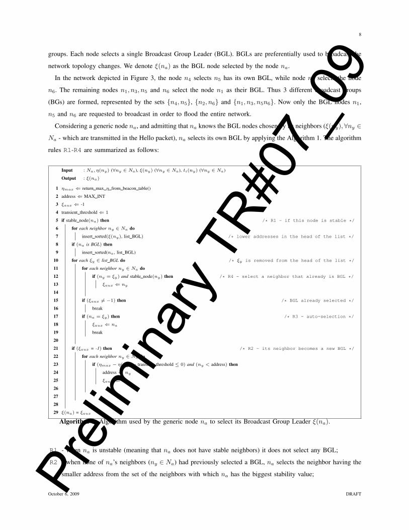
Considering a generic node na, and admitting that na knows the BGL nodes chosen by its neighbors (ξ(ny),∀ny ∈

Na - which are transmitted in the Hello packet), na selects its own BGL by applying the Algorithm 1. The algorithm

rules R1-R4 are summarized as follows:

Input : Na, η(ny) (∀ny ∈ Na), ξ(ny) (∀ny ∈ Na), ti(ny) (∀ny ∈ Na)

Output : ξ(na)

ηmax ⇐ return max η from beacon table()1

address ⇐ MAX INT2

ξaux ⇐ -13

transient threshold ⇐ 14

if stable node(na) then /* R1 - if this node is stable */5

for each neighbor ny ∈ Na do6

insert sorted(ξ(ny), list BGL) /* lower addresses in the head of the list */7

if (na is BGL) then8

insert sorted(na, list BGL)9

for each ξy ∈ list BGL do /* ξy is removed from the head of the list */10

for each neighbor ny ∈ Na do11

if (ny = ξy) and stable node(ny) then /* R4 - select a neighbor that already is BGL */12

ξaux ⇐ ny13

14

if (ξaux 6= −1) then /* BGL already selected */15

break16

if (na = ξy) then /* R3 - auto-selection */17

ξaux ⇐ na18

break19

20

if (ξaux = -1) then /* R2 - its neighbor becomes a new BGL */21

for each neighbor ny ∈ Na do22

if (ηmax − η(ny)− transient threshold ≤ 0) and (ny < address) then23

address ⇐ ny24

ξaux ⇐ ny25

26

27

28

ξ(na) = ξaux29

Algorithm 1: Algorithm used by the generic node na to select its Broadcast Group Leader ξ(na).

R1 - when na is unstable (meaning that na does not have stable neighbors) it does not select any BGL;

R2 - when none of na’s neighbors (ny ∈ Na) had previously selected a BGL, na selects the neighbor having the

smaller address from the set of the neighbors with which na has the biggest stability value;

October 6, 2009 DRAFT

9

R3 - na selects itself as a BGL when na is already a BGL node (previously selected by a neighbor) and the

neighbors’s BGL have higher addresses than na;

R4 - when na is not selected BGL by its neighbors and there exists at least one neighbor ny that is already a

BGL, na selects the node ny as its own BGL; ties are broken by choosing the smaller address neighbor;

The first BGL node selected in the network is justified by the application of the rule R2. The rule R4 is defined

to merge several BGs. The rule R3 is also used to merge several BGs in the special case when na must selects

itself as a BGL.

C. Integrating the topology information in OLSR Routing Protocol

This subsection exemplifies how the stable links and the Broadcast Groups are integrated in the Optimized

Link-State Routing Protocol [3]. The OLSR routing protocol uses Multipoint relaying. Multipoint relaying is a

technique to reduce the number of redundant re-transmissions while diffusing a broadcast message in the network

[8]. Basically, a node na chooses a set of Multipoint Relay nodes (MPRs). MPRs are chosen as the minimum set of

na’s 1-hop neighbors that cover all its neighbors 2-hops away. Thus MPR nodes guarantees 2-hops full coverage.

We use the BGL nodes in the MPR’s selection algorithm, proposing a new algorithm to compute the MPRs

(Algorithm 2). For a given node (na), the algorithm needs to know about its neighbors (ny ∈ Na), their stability

(η(ny)), their BGLs (ξ(ny)) and the required coverage. OLSR uses the smallest set of MPRs that guarantees the full

coverage 2-hops away. Because our algorithm does not guarantees the smallest set of MPRs to cover the neighbors

2-hops away, it may introduce undesired control traffic overhead. This is the main reason to design our algorithm

with an input parameter named required_coverage, that allows us to characterize our algorithm’s behavior

for different amounts of coverage.

Input : Na, {η(ny), ξ(ny), ti(ny)}∀ny ∈ Na, required coverage

Output : MPR(na)

MPR(na) ⇐ φ1

coverage ⇐ 02

for each neighbor ny ∈ Na do3

if η(ny) ≥ kest and ny is BGL then /* R1 - if ny is stable and BGL */4

MPR(na) ⇐ MPR(na) ∪ ny5

update(coverage)6

remove from list(ny , Na)7

8

Nord = sort by descendent η(Na)9

while coverage < required coverage do10

remove from list(ny , Nord)11

MPR(na) ⇐ MPR(na) ∪ ny12

update(coverage)13

14

Algorithm 2: New algorithm to select OLSR’s MPR nodes used by the OLSR.

The algorithm is summarized as follows. 1-hop neighbors of na that have been selected BGLs and have stable links

October 6, 2009 DRAFT

10

with na are selected MPRs (lines 3 to 8). If the number of MPRs are not guaranteing the required coverage 2-hops

away (line 10), the algorithm selects the MPR nodes with which na has the highest stability values.

Regarding the routing table’s computation, the OLSR uses a field named Willingness that specifies the willingness

of a node to carry and forward traffic for other nodes. Only 1-hop neighbors with Willingness different of

WILL_NEVER are used to forward packets. In our proposal, we use the OLSR’s Willingness mechanism to prohibit

na’s unstable neighbors from forwarding packets. We assign the willingness of na’s 1-hop neighbors that do not

meet the condition stated in (12) to WILL_NEVER.

IV. PERFORMANCE EVALUATION

A. Mobility Model

The VANETs simulated in our evaluation scenario were obtained using the Trans tool [9], which integrates the

SUMO traffic simulator [10]. We have simulated a segment of a straight line highway with 3 lanes in each direction.

The simulations start with the vehicles moving in both sides of the highway. During the simulation we launch more

vehicles to maintain a constant density of nodes in the network. The highway segment is 10 kms long, which limits

the minimum number of the network hops to 10. We defined three different classes of vehicles, which are described

in the table III. 60% of the vehicles belong to the class1, which represents medium size cars. The vehicles of class2

represents 25% of the highway traffic. Finally we define 15% of vehicles of class3, which represents long sized

vehicles such as trucks. Regarding the vehicle’s density, we defined 3 different scenarios, described in the table III.

All vehicles are assumed to have a radio range of 1000 meters. The scenario Scen6 was the same used to obtain

the motivation results presented in the table I.

TABLE III

CLASSES OF TRAFFIC CONSIDERED IN THE SIMULATIONS.

vehicle’s VMAX acceleration deceleration %

length (m) (m/s) (m/s2) (m/s2)

class1 4 27.8 3.6 3.6 60

class2 5 26.0 2.5 3.0 25

class3 8 20 1.5 2.0 15

B. Simulation Description

The simulations compare the performance of our improvements with the OLSR routing protocol. We used the

simulator ns-2 [11] configured with the standard IEEE 802.114 and the OLSR protocol implementation available

411 Mbps and 2 Mbps were used to transmit unicast and broadcast traffic, respectively.

October 6, 2009 DRAFT

11

TABLE IV

VEHICLE’S DENSITIES CONSIDERED IN THE SIMULATIONS.

number of average number simulation

vehicles of neighbors time (s)

Scen6 120 6.0 830

Scen8 160 8.0 915

Scen10 200 10.0 886

from [12]. Our proposals were integrated in the OLSR implementation, being the modified protocol designated

OLSR-FCT.

Vehicles moving in the same left-to-right direction generate 0.5 packets per second, which are randomly destined

to the nodes in the same direction. The vehicles moving from right-to-left do not generate packets but are able

to forward them. The number of packets generated on each density scenario were 7388, 10102 and 132205 (from

Scen6 to Scen10, respectively). We simulated 6 different situations: 3 density scenarios previously described using

the OLSR protocol and the same scenarios using our OLSR-FCT protocol.

To parameterize kest we assumed a rough approximation for the three classes of traffic, as being normally

distributed with and average VMAX and 0.5m/s of standard deviation. For this case the relative velocity between

two vehicles moving in opposite directions yields Eopposite way(vr) = 52.36 m/s, and the relative velocity between

two vehicles moving in same direction (Esame way(vr)) yields approximately 2m/s. Choosing the Hello transmission

frequency (TB) to 1Hz, the minimum kest value that guarantees unstable links formed by opposite moving vehicles

is 38.19 (given by (12) and considering r = 1000m). Therefore, we chosen kest = 50 to have a security margin of

approximately 12 TB periods. This margin avoids the vehicles moving at lower speeds to be erroneously declared as

moving in the same direction. This parameterizations indicates that the links of the vehicles moving in the opposite

direction never last longer than 50s. Moreover, when the links of the vehicles moving in the same direction last for

50s, their probability of still being active is 96.8% (plink(50) = at+∆t(50× 2× 1)/(π × 10002)).

C. Experimental Results

The OLSR protocol was firstly simulated for the 3 scenarios described in table IV. The path delivery ratio and

the average end-to-end delay were obtained within 95% of confidence interval and are shown in table V. The results

indicate that the packet delivery ratio is approximately 50% in the 3 scenarios and the end-to-end increases with

the vehicle’s density.

The results obtained with our OLSR-FCT proposal are shown in the Figures 4 and 5. The OLSR-FCT was tested

for different values of coverage (45%, 60%, 85% and 100%, and the coverage means the same as defined in

5Note that a vehicle only generates packets when it is moving.

October 6, 2009 DRAFT

12

TABLE V

OLSR EXPERIMENTAL RESULTS.

packet delivery ratio (%) end-to-end delay (ms)

Scen6 47.13% 99.10

Scen8 53.94% 221.37

Scen10 52.75% 301.59

the Algorithm2). The results obtained with the OLSR-FCT protocol present a better performance when full coverage

is used (100%). For full coverage the number of MPRs increase and, consequently, more topology traffic overhead

is generated. This fact increases the end-to-end delay (Figure 5 shows higher average end-to-end delays when the

coverage is 100%). The results plotted in Figure 4 show that the OLSR-FCT protocol exhibits better packet delivery

ratio for higher node densities.

0.4 0.5 0.6 0.7 0.8 0.9 150

55

60

65

70

75

Coverage

suce

ss [%

]

Scen6

Scen8

Scen10

Fig. 4. Average packet delivery ratio (95% confidence intervals represented by vertical bars).

Comparing the results presented in the motivation (obtained with the original OLSR protocol) we conclude that

the OLSR-FCT protocol improves the packet delivery ratio (from 47.1% to 66.9%) and almost achieves the same

ratio as in the case when the radios of the vehicles in one direction were turned off (68.8%). In terms of end-to-end

delay, the OLSR-FCT decreases the delay from 99.1ms to 42.2ms, being even shorter than the delay measured for

the case when the radios of the vehicles in one direction were turned off (66.9ms). This fact is due to the use of

long-duration links and control traffic decrease implemented by the OLSR-FCT protocol.

Finally, we present the gains obtained with OLSR-FCT in the table VI.

October 6, 2009 DRAFT

13

0.4 0.5 0.6 0.7 0.8 0.9 10

0.05

0.1

0.15

0.2

0.25

0.3

0.35

Coverage

end−

to−

end

dela

y [s

]

Scen6

Scen8

Scen10

Fig. 5. Average end-to-end delay (95% confidence intervals represented by vertical bars).

TABLE VI

OLSR-FCT EXPERIMENTAL GAINS WHEN 100% OF COVERAGE IS CONSIDERED.

packet delivery ratio gain (%) end-to-end delay gain (%)

Scen6 33.2% 52.94

Scen8 26.19% 31.76

Scen10 37.72% 30.48

V. CONCLUSIONS

In this paper we present a method that uses the available knowledge about the network’s topology to improve

the routing protocol’s performance through decreasing the probability of path breaks.

We integrate our improvements in the OLSR routing protocol. The performance results explicitly confirms that

our proposal outperforms the original protocol, recommending its use for high mobility and high density scenarios.

REFERENCES

[1] Jasmine Chennikara-Varghese, Wai Chen, Onur Altintas, and Shengwei Cai. Survey of routing protocols for inter-vehicle communications.

In Mobile and Ubiquitous Systems: Networking and Services, 2006 Third Annual International Conference on, pages 1–5, July 2006.

[2] C.E. Perkins and E.M. Royer. Ad-hoc on-demand distance vector routing. Mobile Computing Systems and Applications, 1999. Proceedings.

WMCSA ’99. Second IEEE Workshop on, pages 90–100, 25-26 Feb 1999.

[3] T. Clausen and P. Jacquet. Optimized Link State Routing Protocol. IETF Internet Draft, http://www.ietf.org/internet-drafts/draft-ietf-manet-

olsr-10.txt, 2003.

[4] Charles Perkins and Pravin Bhagwat. Highly dynamic destination-sequenced distance-vector routing (DSDV) for mobile computers. In

ACM SIGCOMM’94 Conference on Communications Architectures, Protocols and Applications, pages 234–244, 1994.

[5] David B Johnson and David A Maltz. Dynamic source routing in ad hoc wireless networks. In Imielinski and Korth, editors, Mobile

Computing, volume 353. Kluwer Academic Publishers, 1996.

October 6, 2009 DRAFT

14

[6] J.J. Blum, A. Eskandarian, and L.J. Hoffman. Challenges of intervehicle ad hoc networks. Intelligent Transportation Systems, IEEE

Transactions on, 5(4):347–351, Dec. 2004.

[7] M. Mauve, A. Widmer, and H. Hartenstein. A survey on position-based routing in mobile ad hoc networks. Network, IEEE, 15(6):30–39,

Nov/Dec 2001.

[8] A. Qayyum, L. Viennot, and A. Laouiti. Multipoint relaying for flooding broadcast messages in mobile wireless networks. Hawaii

International Conference on System Sciences, 9:298, 2002.

[9] TraNS. - open source tool for realistic simulations of VANET applications . Software Package retrieved from http://trans.epfl.ch/, 2009.

[10] Centre for Applied Informatics (ZAIK) and Institute of Transport Research at the German Aerospace Centre. SUMO - Simulation of

Urban Mobility. Software Package retrieved from http://sumo.sourceforge.net, 2009.

[11] Information Sciences Institute. NS-2 network simulator (version 2.31). Software Package retrieved from http://www.isi.edu/nsnam/ns/,

2007.

[12] Francisco J. Ros. UM-OLSR. Software Package retrieved from http://masimum.inf.um.es/um-olsr/html/, 2009.

October 6, 2009 DRAFT