
Mac Layer And Routing Protocols For Wireless Ad Hoc ...
234
University of Central Florida University of Central Florida STARS STARS Electronic Theses and Dissertations, 2004-2019 2007 Mac Layer And Routing Protocols For Wireless Ad Hoc Networks Mac Layer And Routing Protocols For Wireless Ad Hoc Networks With Asymmetric Links And Performance Evaluation Studies With Asymmetric Links And Performance Evaluation Studies Guoqiang Wang University of Central Florida Part of the Computer Sciences Commons, and the Engineering Commons Find similar works at: https://stars.library.ucf.edu/etd University of Central Florida Libraries http://library.ucf.edu This Doctoral Dissertation (Open Access) is brought to you for free and open access by STARS. It has been accepted for inclusion in Electronic Theses and Dissertations, 2004-2019 by an authorized administrator of STARS. For more information, please contact [email protected]. STARS Citation STARS Citation Wang, Guoqiang, "Mac Layer And Routing Protocols For Wireless Ad Hoc Networks With Asymmetric Links And Performance Evaluation Studies" (2007). Electronic Theses and Dissertations, 2004-2019. 3401. https://stars.library.ucf.edu/etd/3401
-
Upload
khangminh22 -
Category
Documents
-
view
2 -
download
0
Transcript of Mac Layer And Routing Protocols For Wireless Ad Hoc ...

University of Central Florida University of Central Florida
STARS STARS
Electronic Theses and Dissertations, 2004-2019
2007
Mac Layer And Routing Protocols For Wireless Ad Hoc Networks Mac Layer And Routing Protocols For Wireless Ad Hoc Networks
With Asymmetric Links And Performance Evaluation Studies With Asymmetric Links And Performance Evaluation Studies
Guoqiang Wang University of Central Florida
Part of the Computer Sciences Commons, and the Engineering Commons
Find similar works at: https://stars.library.ucf.edu/etd
University of Central Florida Libraries http://library.ucf.edu
This Doctoral Dissertation (Open Access) is brought to you for free and open access by STARS. It has been accepted
for inclusion in Electronic Theses and Dissertations, 2004-2019 by an authorized administrator of STARS. For more
information, please contact [email protected].
STARS Citation STARS Citation Wang, Guoqiang, "Mac Layer And Routing Protocols For Wireless Ad Hoc Networks With Asymmetric Links And Performance Evaluation Studies" (2007). Electronic Theses and Dissertations, 2004-2019. 3401. https://stars.library.ucf.edu/etd/3401

MAC LAYER AND ROUTING PROTOCOLS FOR WIRELESS AD HOCNETWORKS WITH ASYMMETRIC LINKS AND PERFORMANCE
EVALUATION STUDIES
by
GUOQIANG WANGB.S. Southeast University, 2001
M.S. University of Central Florida, 2007
A dissertation submitted in partial fulfillment of the requirementsfor the degree of Doctor of Philosophy
in the School of Electrical Engineering and Computer Sciencein the College of Engineering and Computer Science
at the University of Central FloridaOrlando, Florida
Summer Term2007
Major Professors:Dan C. Marinescu
Damla Turgut

c© 2007 Guoqiang Wang
ii

ABSTRACT
In a heterogeneous mobile ad hoc network (MANET), assorted devices with different computa-
tion and communication capabilities co-exist. In this thesis, we consider the case when the nodes
of a MANET have various degrees of mobility and range, and the communication links are asym-
metric. Many routing protocols for ad hoc networks routinely assume that all communication links
are symmetric, if node A can hear node B and node B can also hear node A. Most current MAC
layer protocols are unable to exploit the asymmetric links present in a network, thus leading to an
inefficient overall bandwidth utilization, or, in the worst case, to lack of connectivity. To exploit
the asymmetric links, the protocols must deal with the asymmetry of the path from a source node
to a destination node which affects either the delivery of the original packets, or the paths taken
by acknowledgments, or both. Furthermore, the problem of hidden nodes requires a more careful
analysis in the case of asymmetric links.
MAC layer and routing protocols for ad hoc networks with asymmetric links require a rigorous
performance analysis. Analytical models are usually unable to provide even approximate solutions
to questions such as end-to-end delay, packet loss ratio, throughput, etc. Traditional simulation
techniques for large-scale wireless networks require vast amounts of storage and computing cycles
iii

rarely available on single computing systems. In our search for an effective solution to study the
performance of wireless networks we investigate the time-parallel simulation.
Time-parallel simulation has received significant attention in the past. The advantages, as
well as, the theoretical and practical limitations of time-parallel simulation have been extensively
researched for many applications when the complexity of the models involved severely limits the
applicability of analytical studies and is unfeasible with traditional simulation techniques. Our goal
is to study the behavior of large systems consisting of possibly thousands of nodes over extended
periods of time and obtain results efficiently, and time-parallel simulation enables us to achieve
this objective.
We conclude that MAC layer and routing protocols capable of using asymmetric links are more
complex than traditional ones, but can improve the connectivity, and provide better performance.
We are confident that approximate results for various performance metrics of wireless networks
obtained using time-parallel simulation are sufficiently accurate and able to provide the necessary
insight into the inner workings of the protocols.
iv

To my parents.
v

ACKNOWLEDGMENTS
I would like to thank my advisors Dr. Marinescu and Dr. Turgut, as well as the committee members
Dr. Boloni and Dr. Bassiouni. In particular, I would like to thank my advisor, Dr. Dan C.
Marinescu who gave me the freedom to explore, exceptional thoughts, and sound advices when
most needed, through every step of my Ph.D study. I also greatly appreciate my co-advisor, Dr.
Damla Turgut for the constant encouragement, invaluable directions, and comments throughout. I
would like to single out Dr. Ladislau Boloni who always gave me timely help and novel advices. I
am also indebted to Dr. Bassiouni for his critical feedback and comments. Last but not least, thanks
to all my lab mates and friends in University of Central Florida, who accompanied me along this
path. Finally, I am forever grateful to my Mom and Dad who provide constant support in a faraway
country.
vi

TABLE OF CONTENTS
LIST OF FIGURES . . . . . . . . . . . . . . . . . . . . . . . . . . . . . . . . . . . . xii
LIST OF TABLES . . . . . . . . . . . . . . . . . . . . . . . . . . . . . . . . . . . . . xxv
LIST OF ACRONYMS/NOTATIONS . . . . . . . . . . . . . . . . . . . . . . . . . . xxvii
CHAPTER 1 INTRODUCTION . . . . . . . . . . . . . . . . . . . . . . . . . . . . . 1
1.1 Routing in Heterogeneous MANETs . . . . . . . . . . . . . . . . . . . . . . . . . 1
1.2 The Time-Parallel Simulation . . . . . . . . . . . . . . . . . . . . . . . . . . . . . 7
1.3 Contributions . . . . . . . . . . . . . . . . . . . . . . . . . . . . . . . . . . . . . 10
1.4 Organization . . . . . . . . . . . . . . . . . . . . . . . . . . . . . . . . . . . . . . 12
CHAPTER 2 RELATED WORK . . . . . . . . . . . . . . . . . . . . . . . . . . . . 14
2.1 Routing Protocols . . . . . . . . . . . . . . . . . . . . . . . . . . . . . . . . . . . 14
2.2 MAC Layer Protocols . . . . . . . . . . . . . . . . . . . . . . . . . . . . . . . . . 19
2.3 Analytical Models of Wireless Networks . . . . . . . . . . . . . . . . . . . . . . . 24
vii

2.4 The Time-Parallel Simulation . . . . . . . . . . . . . . . . . . . . . . . . . . . . . 28
CHAPTER 3 IMPROVING ROUTING PERFORMANCE THROUGH M-LIMITED
FORWARDING IN POWER-CONSTRAINED WIRELESS AD HOC NETWORKS . 33
3.1 m-limited Forwarding . . . . . . . . . . . . . . . . . . . . . . . . . . . . . . . . . 34
3.1.1 Alternative Forwarding Fitness Functions . . . . . . . . . . . . . . . . . . 36
3.1.2 Ad hoc On-Demand Distance Vector Routing with m-Limited Forwarding
(m-AODV) . . . . . . . . . . . . . . . . . . . . . . . . . . . . . . . . . . 42
3.2 Simulation Study . . . . . . . . . . . . . . . . . . . . . . . . . . . . . . . . . . . 43
3.2.1 Performance Metrics . . . . . . . . . . . . . . . . . . . . . . . . . . . . . 46
3.2.2 Determining the Optimal Value of m . . . . . . . . . . . . . . . . . . . . . 46
3.2.3 Performance Improvement of m-limited Forwarding in MANETs with Bidi-
rectional Links . . . . . . . . . . . . . . . . . . . . . . . . . . . . . . . . 54
3.2.4 m-limited Forwarding in MANETs with Asymmetric Links . . . . . . . . 61
3.3 Summary . . . . . . . . . . . . . . . . . . . . . . . . . . . . . . . . . . . . . . . 63
CHAPTER 4 MAC LAYER AND ROUTING PROTOCOLS FOR WIRELESS NET-
WORKS WITH ASYMMETRIC LINKS . . . . . . . . . . . . . . . . . . . . . . . . . 66
4.1 The Model of the System . . . . . . . . . . . . . . . . . . . . . . . . . . . . . . . 68
4.1.1 The System Model for Heterogeneous MANETs . . . . . . . . . . . . . . 68
viii

4.1.2 Topological Considerations for AsyMAC . . . . . . . . . . . . . . . . . . 76
4.1.3 Determination of the Sets in AsyMAC . . . . . . . . . . . . . . . . . . . . 80
4.1.4 Accuracy Metrics for Node Classification . . . . . . . . . . . . . . . . . . 83
4.2 The A4LP Routing Protocol . . . . . . . . . . . . . . . . . . . . . . . . . . . . . 84
4.2.1 Information maintained by a node and packet types . . . . . . . . . . . . . 84
4.2.2 Neighbor Discovery Process . . . . . . . . . . . . . . . . . . . . . . . . . 86
4.2.3 Location and Power Update . . . . . . . . . . . . . . . . . . . . . . . . . 88
4.2.4 m-limited Forwarding . . . . . . . . . . . . . . . . . . . . . . . . . . . . 88
4.2.5 Path Discovery . . . . . . . . . . . . . . . . . . . . . . . . . . . . . . . . 89
4.2.6 Path Maintenance . . . . . . . . . . . . . . . . . . . . . . . . . . . . . . . 93
4.3 The AsyMAC Protocol . . . . . . . . . . . . . . . . . . . . . . . . . . . . . . . . 93
4.3.1 A Solution to the Hidden Node Problem . . . . . . . . . . . . . . . . . . . 93
4.3.2 Node Status . . . . . . . . . . . . . . . . . . . . . . . . . . . . . . . . . . 94
4.3.3 Medium Access Control Model . . . . . . . . . . . . . . . . . . . . . . . 95
4.4 Simulation and Case Study . . . . . . . . . . . . . . . . . . . . . . . . . . . . . . 99
4.4.1 A Connectivity Scenario . . . . . . . . . . . . . . . . . . . . . . . . . . . 100
4.4.2 A Study of Alternative Protocol Stacks in Mobile Ad Hoc Networks . . . . 102
4.4.3 The Accuracy of Hidden Node Classification . . . . . . . . . . . . . . . . 110
ix

4.5 Summary . . . . . . . . . . . . . . . . . . . . . . . . . . . . . . . . . . . . . . . 113
CHAPTER 5 THE TIME-PARALLEL SIMULATION OF WIRELESS AD HOC NET-
WORKS . . . . . . . . . . . . . . . . . . . . . . . . . . . . . . . . . . . . . . . . . . . 115
5.1 The One-step Time-parallel Simulation Model . . . . . . . . . . . . . . . . . . . . 117
5.2 Perturbation Analysis and Improving Accuracy of Time-Parallel Simulation . . . . 119
5.2.1 Measurements on the Simulation Trace . . . . . . . . . . . . . . . . . . . 119
5.2.2 Perturbations on a Measurement . . . . . . . . . . . . . . . . . . . . . . . 120
5.2.3 Propagation of Perturbations in Wireless Ad Hoc Networks . . . . . . . . . 123
5.2.4 Techniques for Improving the Accuracy of Time-Parallel Simulation . . . . 130
5.3 Implementation of Time-parallel Simulation for Ad Hoc Networks . . . . . . . . . 134
5.3.1 Time-parallel Simulation with Iteratively Extended Warmup Interval . . . . 135
5.3.2 Time-parallel Algorithm with Initial State Approximation . . . . . . . . . 141
5.4 Simulation Study . . . . . . . . . . . . . . . . . . . . . . . . . . . . . . . . . . . 144
5.4.1 Simulation Setup . . . . . . . . . . . . . . . . . . . . . . . . . . . . . . . 145
5.4.2 Simulation Results . . . . . . . . . . . . . . . . . . . . . . . . . . . . . . 147
5.5 Summary . . . . . . . . . . . . . . . . . . . . . . . . . . . . . . . . . . . . . . . 155
CHAPTER 6 THE TIME-PARALLEL SIMULATION OF WIRELESS AD HOC NET-
WORKS WITH COMPRESSED HISTORY . . . . . . . . . . . . . . . . . . . . . . . 156
x
6.1 Compressed History . . . . . . . . . . . . . . . . . . . . . . . . . . . . . . . . . . 158
6.2 Implementation of Compressed History . . . . . . . . . . . . . . . . . . . . . . . 164
6.2.1 Load Balancing TPS with Compressed History . . . . . . . . . . . . . . . 168
6.2.2 Accuracy-speedup Tradeoffs . . . . . . . . . . . . . . . . . . . . . . . . . 169
6.3 Simulation Study . . . . . . . . . . . . . . . . . . . . . . . . . . . . . . . . . . . 171
6.3.1 Tuning the Parameters of the Compressed History for Optimal Speedup . . 174
6.3.2 The Performance Improvement Provided by Compressed History: Com-
paring TPS-CU with TPS-U . . . . . . . . . . . . . . . . . . . . . . . . . 179
6.3.3 The Performance Improvement Provided by the Uncompressed Interval:
Comparing TPS-CU with TPS-C . . . . . . . . . . . . . . . . . . . . . . . 180
6.4 Summary . . . . . . . . . . . . . . . . . . . . . . . . . . . . . . . . . . . . . . . 182
CHAPTER 7 CONCLUSIONS . . . . . . . . . . . . . . . . . . . . . . . . . . . . . 184
APPENDIX PUBLICATIONS . . . . . . . . . . . . . . . . . . . . . . . . . . . . . 188
LIST OF REFERENCES . . . . . . . . . . . . . . . . . . . . . . . . . . . . . . . . . 191
xi

LIST OF FIGURES
Figure 2.1 (a) Hidden node problem in a “classical” wireless network with mobile
nodes. All links are assumed to be bidirectional. A hidden node is a node out of
the range of the sender and in the range of the receiver. Node k is a hidden node for
a transmission from node s to node r. (b) Hidden node problem in a heterogeneous
wireless network with mobile nodes. A hidden node is a node out of the range of
the sender and whose range covers the receiver. Node k is a hidden node as for a
transmission from node s to node r. . . . . . . . . . . . . . . . . . . . . . . . . . 21
Figure 3.1 A configuration including the sender j, the destination i, and two candidate
nodes k1 and k2 as the next hop on the path from j to i. The circles centered at
the current location with the radius equal to the range of these nodes, Πj, Πk1 , and
Πk2 are also shown. The circle centered at the current position of node i and with
a radius equal to dij − Rj is called the “complementary range of j to reach i” and
denoted by Γi,j . Call Λk(i, j) the area of the intersection of Γi,j and Πk. We see
that Λk1(i, j) < Λk2(i, j). . . . . . . . . . . . . . . . . . . . . . . . . . . . . . . . 37
xii

Figure 3.2 The area of the overlapping region is the sum of area(ANBO) and area(AMBO).
The area(ANBO) is the difference of sector(KANB) and triangle(KAB). The area(AMBO)
is the difference of sector(IANB) and triangle(IAB). . . . . . . . . . . . . . . . . . 39
Figure 3.3 The plot of the area-based forwarding fitness function Fak (i, j) in function
of the location of the candidate node. The current node is at (0,0) while the des-
tination node is at (110,110). The function is plotted for a candidate node k with
transmission range of 150 meters and locations spanning the transmission range of
the current node. . . . . . . . . . . . . . . . . . . . . . . . . . . . . . . . . . . . 40
Figure 3.4 The plot of the area-based forwarding fitness function Fak (i, j), for candi-
date node k with different location and different transmission range. The scenario
is the same as above except the transmission range is variable in the range of [50,
250]. . . . . . . . . . . . . . . . . . . . . . . . . . . . . . . . . . . . . . . . . . . 41
Figure 3.5 The illustration of relationship among simulation time, setup duration, end
duration, time slice and CBR duration. Four nodes and two CBR sources are
included in this example. . . . . . . . . . . . . . . . . . . . . . . . . . . . . . . . 45
Figure 3.6 Packet loss ratio versus network load. Number of nodes = 80, Speed = 1
m/s, m = 1,2,3,4. (a) m-AODV with distance-based fitness function Fd; (b) m-
AODV with area-based fitness function Fa. m-AODV with both fitness functions
outperforms AODV, for all m >= 2. m = 2 and m = 3 are better options for both
fitness functions. . . . . . . . . . . . . . . . . . . . . . . . . . . . . . . . . . . . 49
xiii

Figure 3.7 Average power consumption versus network load. Number of nodes = 80,
Speed = 1 m/s, m=1,2,3,4. (a) m-AODV with distance-based fitness function Fd;
(b) m-AODV with area-based fitness function Fa. The average power consump-
tion increases linearly as the network load increases. m-AODV with area-based
fitness function Fa consumes less power than m-AODV with distance-based fit-
ness function Fd for the same network load. . . . . . . . . . . . . . . . . . . . . . 49
Figure 3.8 Packet loss ratio versus node mobility. Number of nodes = 80, Offered load
= 25 Kbps, m=1,2,3,4. (a) m-AODV with distance-based fitness function Fd; (b)
m-AODV with area-based fitness function Fa. The packet loss ratio of 1-limited
forwarding is noticeably the greatest. m = 3 and m = 4 are better options when
the node mobility is relatively high. . . . . . . . . . . . . . . . . . . . . . . . . . 51
Figure 3.9 Average power consumption versus node mobility. Number of nodes =
80, Offered load = 25 Kbps, m=1,2,3,4. (a) m-AODV with distance-based fitness
function Fd; (b) m-AODV with area-based fitness function Fa. AODV consumes
the most power. Among the m-limited schemes, 1-limited forwarding consumes
the least power, followed by 2-, 3-, 4-limited forwarding. . . . . . . . . . . . . . . 51
xiv

Figure 3.10 Average power consumption versus node density. Offered load = 25 Kbps,
Speed = 1 m/s, m=1,2,3,4. (a) m-AODV with distance-based fitness function Fd;
(b) m-AODV with area-based fitness function Fa. For low network density, 1-
limited forwarding performs the worst. For higher network densities, all m-limited
forwarding based schemes have a lower packet loss ratio than plain AODV. m = 2
and 3 are better options when network density is relatively high. . . . . . . . . . . 53
Figure 3.11 Average power consumption versus node density. Offered load = 25 Kbps,
Speed = 1 m/s, m=1,2,3,4. (a) m-AODV with distance-based fitness function Fd;
(b) m-AODV with area-based fitness function Fa. The power consumption for all
schemes increases as network density increases. AODV consumes the most power,
followed by 4-, 3-, 2-, and 1-limited forwarding. . . . . . . . . . . . . . . . . . . . 53
Figure 3.12 Packet loss ratio versus network load. Number of nodes = 80, Speed = 1
m/s. We compare AODV, LAR, and m-AODV with fitness functions Fd and Fa.
AODV performs the worst. m-AODV outperforms LAR when the network load is
relatively high. . . . . . . . . . . . . . . . . . . . . . . . . . . . . . . . . . . . . 56
Figure 3.13 Average power consumption versus network load. Number of nodes = 80,
Speed = 1 m/s. We compare AODV, LAR, and m-AODV with fitness functions Fd
and Fa. AODV consumes the most power, and m-AODV consumes less power
than LAR, for the same network load. . . . . . . . . . . . . . . . . . . . . . . . . 56
xv
Figure 3.14 Packet loss ratio versus node mobility. Number of nodes = 80, Offered
network load = 25 Kbps. We compare AODV, LAR, and m-AODV with fitness
functions Fd and Fa. AODV performs the worst. m-AODV with distance-based
fitness function Fd achieves a similar performance with LAR, which performs
slightly better than m-AODV with area-based fitness function Fa. . . . . . . . . . 57
Figure 3.15 Average power consumption versus node mobility. Number of nodes = 80,
Offered network load = 25 Kbps. We compare AODV, LAR, and m-AODV with
fitness functions Fd and Fa. AODV consumes the most power, and m-AODV
consumes less power than LAR, for the same node mobility. . . . . . . . . . . . . 58
Figure 3.16 Packet loss ratio versus network density. Speed = 1 m/s, Offered network
load = 25 Kbps. We compare AODV, LAR, and m-AODV with fitness functions
Fd and Fa. AODV performs the worst. m-AODV outperforms LAR when the
network density is relatively high. . . . . . . . . . . . . . . . . . . . . . . . . . . 59
Figure 3.17 Average power consumption versus network density. Speed = 1 m/s, Of-
fered network load = 25 Kbps. We compare AODV, LAR, and m-AODV with
fitness functions Fd and Fa. AODV consumes the most power, and m-AODV
consumes less power than LAR, for the same network density. . . . . . . . . . . . 59
xvi
Figure 3.18 Packet loss ratio versus network load. Speed = 1 m/s, Number of nodes
= 80. Nodes fall into four categories with transmission range of 200 (C1), 150
(C2), 100 (C3), and 50 (C4) meters. |C1|:|C2|:|C3|:|C4| =1:2:3:4. AODV/802.11,
A4LP/AsyMAC based on 3-limited forwarding withFd, and A4LP/AsyMAC based
on 3-limited forwarding with Fa are compared. . . . . . . . . . . . . . . . . . . . 63
Figure 4.1 The neighbor relationship between two nodes. (a) j is an Out-bound neigh-
bor of i. (b) j is an In-bound neighbor of of i. (c) j is an In/Out-bound neighbor
of i. (d) i and j are not neighbors. . . . . . . . . . . . . . . . . . . . . . . . . . . 71
Figure 4.2 Three-party and four-party proxy sets. (a) An infeasible scenario for a
three-party proxy set involving three unidirectional links. (b) A second infeasible
scenario for a three-party proxy set involving three unidirectional links. (c) A
feasible scenario for a three-party proxy set with only one bidirectional link. (d) A
feasible scenario for a four-party proxy set with only one bidirectional link. . . . . 74
Figure 4.3 An illustration for topology concepts. The transmission ranges of the sender
s and the receiver r are reflected by the circles centered at them. The partial reach-
ability information of the other nodes is shown by directed lines. . . . . . . . . . . 77
Figure 4.4 The algorithm for calculation of {mXHR3sr}. . . . . . . . . . . . . . . . 81
Figure 4.5 The algorithm for calculation of {MXHR3sr}. . . . . . . . . . . . . . . . 82
xvii

Figure 4.6 The path discovery in A4LP involves the following phases: Forward Path
Request, Backward Path Request, Forward Path Reply, Backward Path Reply, For-
ward Path Request Acknowledgement, and Forward Path Reply Acknowledgement. 90
Figure 4.7 Routing over asymmetric links in a heterogeneous MANET. Node s is the
sender, node r is the receiver, the link from node s to r is asymmetric, and node j
is the proxy node that can relay traffic to s for r. Nodes k1 and k2 are hidden nodes
for transmissions Trs and Tsr, respectively. Nodes j1 and j2 are the proxy nodes
that can relay traffic from s to k1 and from r to k2, respectively. . . . . . . . . . . . 96
Figure 4.8 The medium access model of AsyMAC for the scenario in Figure 4.7. (a)
The medium access model of AsyMAC for short data frames over a symmetric
link. (b) The medium access model of AsyMAC for short data frames over an
asymmetric link. (c) The medium access model of AsyMAC for long data frames
over a symmetric link. (d) The medium access model of AsyMAC for long data
frames over an asymmetric link. . . . . . . . . . . . . . . . . . . . . . . . . . . . 98
Figure 4.9 (a) The physical topology of the network, where node 0 and 4 are exchang-
ing packets. The numbers next to the nodes indicate the position in the (x,y) format
and the transmission range (underlined). The numbers on the links represent the
distance between the nodes. (b) The logical topology of the network. . . . . . . . . 101
xviii

Figure 4.10 Packet loss ratio versus network load. The ratio of packets lost by AODV/802.11
is roughly twice the ratio of packets lost by the other protocols. Among the other
protocols, A4LP-M3-F2/AsyMAC performs the best, followed by OLSR/802.11,
which delivers more packets than A4LP-M3-F1/AsyMAC for similar scenarios and
traffic patterns. . . . . . . . . . . . . . . . . . . . . . . . . . . . . . . . . . . . . 105
Figure 4.11 Average latency versus network load. The average latency of AODV/802.11
is much higher than the other protocols. Among the other protocols, OLSR/802.11
has the shortest latency. . . . . . . . . . . . . . . . . . . . . . . . . . . . . . . . . 105
Figure 4.12 Packet loss ratio versus node mobility. With the node mobility increas-
ing, the performances of A4LP-M3-F2 and OLSR/802.11 are degraded while the
performance of AODV/802.11 fluctuates between 35% and 45%. AODV/802.11
performs the worst in case of ad hoc networks with low mobility, but it outperforms
the other protocols for highly mobile ad hoc networks. . . . . . . . . . . . . . . . 107
Figure 4.13 Average latency versus node mobility. The average latency of AODV/802.11
is much higher than the other protocols that perform similarly. . . . . . . . . . . . 107
Figure 4.14 Packet loss ratio versus number of nodes. A4LP-M3-F2/AsyMAC delivers
most packets, followed by OLSR/802.11, A4LP-M3-F1/AsyMAC and AODV/802.11
for similar scenarios and traffic patterns. The packet loss ratio decreases when the
number of nodes increases. . . . . . . . . . . . . . . . . . . . . . . . . . . . . . . 109
xix

Figure 4.15 Average latency versus number of nodes. The average latency of AODV/802.11
is much higher than the other protocols. The packet delivery latency tends to de-
crease as the number of nodes increases for A4LP/AsyMAC and OLSR/802.11. . . 109
Figure 4.16 (a) The average misclassified nodes per transmission as a function of the
number of nodes. AsyMAC does not misclassify nodes in a static network. (b)
The average missed nodes per transmission for protocols A, B, and our approach,
as a function of the number of nodes. (c) The average number of incorrect silencing
decisions per transmission for protocols A, B, and for our approach. . . . . . . . . 111
Figure 5.1 An illustration of techniques for improving the accuracy of time-parallel
simulation. (a) Equal length batches without improvement. (b) Time interval shift.
(c) Warmup intervals. (d) Warm up with compressed history. . . . . . . . . . . . . 131
Figure 5.2 The time-parallel simulation with iteratively extended warmup interval (TPS-
I). The duration of the simulation S is 180 sec. It is segmented into 9 equal-
duration simulation intervals. The shaded simulation segments are used to com-
pose the final simulation trace after 3 iterations. . . . . . . . . . . . . . . . . . . . 138
Figure 5.3 An alternative approach to the time-parallel simulation in Figure 5.2. m =
9, k = 2. Shaded blocks correspond to partial results used to construct the final
simulation results. . . . . . . . . . . . . . . . . . . . . . . . . . . . . . . . . . . . 138
xx

Figure 5.4 The relative error for the packet loss ratio and the throughput, function
of the segment duration in a logarithmic scale; DSDV (left) and AODV (right).
(a) and (b) show the relative error for the packet loss ratio; (c) and (d) show the
relative error for the throughput. Plain time-parallel simulation is applied in this
set of experiments. . . . . . . . . . . . . . . . . . . . . . . . . . . . . . . . . . . 148
Figure 5.5 The relative error for the packet loss ratio and the throughput for DSDV,
function of the segment duration in a logarithmic scale. (a) shows the relative
error for the packet loss ratio; (b) shows the relative error for the throughput. ISA
time-parallel simulation is applied in this set of experiments. . . . . . . . . . . . . 149
Figure 5.6 The relative error for the packet loss ratio and the throughput, function of
the network load in a logarithmic scale; DSDV (left) and AODV (right). (a) and
(b) show the relative error for the packet loss ratio; (c) and (d) show the relative
error for the throughput. Plain time-parallel simulation is applied in this set of
experiments. . . . . . . . . . . . . . . . . . . . . . . . . . . . . . . . . . . . . . . 151
Figure 5.7 The relative error for the packet loss ratio and the throughput for DSDV,
function of the network load in a logarithmic scale. (a) shows the relative error
for the packet loss ratio; (b) show the relative error for the throughput. ISA time-
parallel simulation is applied in this set of experiments. . . . . . . . . . . . . . . . 152
xxi

Figure 5.8 The relative error for the packet loss ratio and the throughput, function of
the node mobility in a logarithmic scale; DSDV (left) and AODV (right). (a) and
(b) show the relative error for the packet loss ratio; (c) and (d) show the relative
error for the throughput. Plain time-parallel simulation is applied in this set of
experiments. . . . . . . . . . . . . . . . . . . . . . . . . . . . . . . . . . . . . . . 153
Figure 5.9 The relative error for the packet loss ratio and the throughput for DSDV,
function of the node mobility in a logarithmic scale. (a) shows the relative error
for the packet loss ratio; (b) show the relative error for the throughput. ISA time-
parallel simulation is applied in this set of experiments. . . . . . . . . . . . . . . . 154
Figure 6.1 The TPS and TPS-C (TPS with compressed history) algorithms. The |τ | =
180 sec. simulation interval is segmented into 9 simulation intervals of 20 sec.
each. The shaded simulation segments are used to compose the final simulation
trace. {Si} is the set of simulation without initial state approximation, while {S ′i}
is the set of simulation batches with their initial states approximated by the com-
pressed history of their prior simulations. . . . . . . . . . . . . . . . . . . . . . . 161
xxii

Figure 6.2 The TPS-CU (TPS with compressed history and uncompressed interval) al-
gorithm. The |τ | = 180 sec. simulation interval is segmented into 9 intervals of
20 sec. each. The uncompressed interval duration is 10 sec. for each simulation
segment. The prior simulation of Si is composed of an uncompressed interval SUi
and the compressed history of its prior simulation SUi. The shaded simulation seg-
ments are used to compose the final simulation trace. {S ′i} is the set of simulation
batches with their initial states approximated by the compressed history of their
prior simulations and uncompressed intervals. . . . . . . . . . . . . . . . . . . . . 164
Figure 6.3 Strategies to adjust the routing table update frequency when composing the
compressed history. . . . . . . . . . . . . . . . . . . . . . . . . . . . . . . . . . . 167
Figure 6.4 Strategies to adjust the routing table update frequency when composing the
compressed history, with the application of uncompressed interval. . . . . . . . . . 167
Figure 6.5 The TPS-CU algorithm: the relative error for the packet loss ratio function
of uncompressed interval duration. The error decreases when we increase either the
uncompressed interval duration, or the normalized history duration, or the segment
duration. . . . . . . . . . . . . . . . . . . . . . . . . . . . . . . . . . . . . . . . . 175
Figure 6.6 The TPS-CU algorithm: the relative error for the throughput function of
the duration of the uncompressed interval. The error decreases when we increase
either the uncompressed interval duration, the normalized history duration, or the
segment duration. . . . . . . . . . . . . . . . . . . . . . . . . . . . . . . . . . . . 176
xxiii
Figure 6.7 The TPS-U and TPS-CU algorithms: the relative error function of the dura-
tion of the uncompressed interval for (a) the packet loss ratio and (b) the through-
put, when the segment duration is 30 sec., and the normalized compressed history
duration for TPS-CU is 15 sec. . . . . . . . . . . . . . . . . . . . . . . . . . . . . 179
Figure 6.8 The TPS-C and TPS-CU algorithms: the relative error function of the dura-
tion of the uncompressed interval for (a) the packet loss ratio and (b) the through-
put, when the segment duration is 30 sec., and the uncompressed interval duration
for TPS-CU is 20 sec. . . . . . . . . . . . . . . . . . . . . . . . . . . . . . . . . . 181
xxiv

LIST OF TABLES
Table 2.1 A comparison of PDNS, SWiMNet, WiPPET and the time-parallel simula-
tion approach (TPS) proposed in this work . . . . . . . . . . . . . . . . . . . . . . 30
Table 3.1 The default values and the range of the parameters for our simulation studies 45
Table 4.1 The fields of a routing table used in the A4LP protocol . . . . . . . . . . . . 85
Table 4.2 The fields of packet types used in the A4LP protocol . . . . . . . . . . . . . 85
Table 4.3 The abbreviations used in A4LP . . . . . . . . . . . . . . . . . . . . . . . . 86
Table 4.4 The default values and the range of the parameters for our simulation studies 103
Table 5.1 The default values and the range of the parameters for our simulation studies 146
Table 5.2 The number of iterations needed (k95), the accuracy (1− ε) and the speedup
(κ), function of segment duration, for plain time-parallel simulation with both
DSDV and AODV . . . . . . . . . . . . . . . . . . . . . . . . . . . . . . . . . . . 147
Table 5.3 The number of iterations needed (k95), the accuracy (1− ε) and the speedup
(κ), function of segment duration, for ISA time-parallel simulation with DSDV . . . 149
xxv

Table 6.1 The abbreviation and notations used in our simulation studies . . . . . . . . 171
Table 6.2 The default values of the parameters used in our simulation studies . . . . . . 172
Table 6.3 Tuning the parameters of the TPS-CU algorithm based on the results of the
experimental runs. The rows corresponding to the best choice of the uncompressed
interval Tu for a given segment duration are shown in bold. The maximum achiev-
able speedup for a given segment duration is bold and underlined. . . . . . . . . . 177
Table 6.4 The combination of uncompressed interval duration and normalized com-
pressed history duration that achieve the maximum speedup for different segment
durations . . . . . . . . . . . . . . . . . . . . . . . . . . . . . . . . . . . . . . . 178
Table 6.5 The effect of the compressed history upon the relative error for the packet
loss ratio and the throughput . . . . . . . . . . . . . . . . . . . . . . . . . . . . . 180
Table 6.6 The effect of the uncompressed interval upon the relative error for the packet
loss ratio and the throughput . . . . . . . . . . . . . . . . . . . . . . . . . . . . . 182
xxvi

LIST OF ACRONYMS/NOTATIONS
ACK ACKnowledgment
A4LP Location-Aware Power-Aware routing protocol for MANETs with Asymmetric links
AODV Ad hoc On-Demand Distance Vector routing protocol
AsyMAC a MAC layer protocol for MANETs with Asymmetric links
CBR Constant Bit Rate
CSMA/CA Carrier Sense Multiple Access with Collision Avoidance
CSMA/CD Carrier Sense Multiple Access with Collision Detection
CTS Clear To Send
CW Contention Window
DIFS Distributed Inter-Frame Spacing
DSDV Destination-Sequenced Distance Vector routing protocol
GPS Global Positioning Systems
ISA Initial State Approximation
LAR Location-Aided Routing protocol
m-AODV AODV with m-limited forwarding
m-A4LP A4LP with m-limited forwarding
xxvii
MAC Medium Access Control
MANET Mobile Ad hoc NETwork
NAV Network Allocation Vector
NS-2 Network Simulation version 2
OLSR Optimized Link State Routing protocol
PDES Parallel Discrete Event Simulation
RTS Ready To Send
SIFS Short Inter-Frame Spacing
TACK Tunneled ACKnowledgment
TCTS Tunneled Clear To Send
TCP Transport Control Protocol
TPS Time-Parallel Simulation
TPS-C Time-Parallel Simulation with Compressed history
TPS-I Time-Parallel Simulation with an Iterative approach
TPS-CU Time-Parallel Simulation with Compressed history and Uncompressed interval
TPS-U Time-Parallel Simulation with Uncompressed interval
UDP User Datagram Protocol
XCTS eXtended Clear To Send
XRTS eXtended Ready To Send
xxviii

Γi,j the complementary range of node j to reach node i
δM the absolute error of measurement M
εmax the error threshold
εM the relative error for a metric M
εPLR the relative error for the packet loss ratio
εPDR the relative error for the packet delivery ratio
εTPT the relative error for the throughput
η(S, S) the compression ratio of the compressed history S
κ the speedup of an algorithm
κ(i, j) a forwarding cutoff attached to a transmitted packet sending from node j to node i
λc the regular routing table update frequency
λi the routing table update frequency of the compressed history Si
Λk(i, j) the area of the intersection of Γi,j and Πk
πi,j the j-th (starts from 0) time interval of πi
Πk the circle centered at the current location of node k
τ the time interval of a simulation
|τ | the duration of the time interval of a simulation
A the geographic area of a simulation
Ci one of the hierarchical levels of systems in a heterogeneous MANET
xxix

C(M) the complementary measure of M
dij the distance between node i and node j
E the set of events of a simulation
E the set of events that produce significant perturbations
F a MAC protocol that silences nodes during a transmission
F the final state of a simulation
Fa area-based forwarding fitness function
Fd distance-based forwarding fitness function
Hsr the set of hidden nodes of a transmission Tsr
H3sr the hidden nodes of a transmission Tsr in P3r
H-node the high-range node of an asymmetric link
I an ideal algorithm that correctly silences all nodes during a transmission
I the initial state of a simulation
Idi the unique id of node i
Ini(t) the set of In-bound neighbors of i at time t
InOuti(t) the set of In/Out-bound neighbors of i at time t
k95 the number of iterations to reach 95% accuracy, in the TPS-I algorithm
L(k) the time-parallel simulation set after k-th iteration, in the TPS-I algorithm
L-node the low-range node of an asymmetric link
xxx

Li(t) the geographical position of node i at time t
Misc(F ) the average misclassification of an algorithm F
Miscsr(F ) the misclassification ratio of an algorithm F for a transmission Tsr
Miss(F ) the average miss ratio of an algorithm F
Misssr(F ) the miss ratio of an algorithm F for a transmission Tsr
mXHR3sr the minimal extended hidden nodes relay set of a transmission Tsr in P3r
MXHR3sr the minimum extended hidden nodes relay set of a transmission Tsr in P3r
N the set of nodes in a heterogeneous MANET
P resi (t) the residual power of node i at time t
Ri(t) the transmission range of node i at time t
Rij(t) the reachability function that describes the connection between node i and j
Outi(t) the set of Out-bound neighbors of i at time t
Pi the i-th simulation segment of a time-parallel simulation set
Pi,j the j-th sub-interval of the simulation segment Pi
P3i the three-party proxy set coverage of node i
RTi the routing table of node i
S the six-tuple that describes the simulation of a MANET, S = (A, τ, E , I,F , T )
S the compressed history of a simulation S
Si the complete sequential simulation prior to Si
xxxi

Si the compressed history of the prior simulation of Si
Ssr(F ) the set of nodes that silenced by algorithm F during a transmission Tsr
Ssr(I) the ideal set of nodes that should be silenced during a transmission Tsr
SUi the uncompressed interval before the simulation Si
SWi the warmup interval before the simulation Si
SUi the compressed history of the prior simulation simulation of SUi
te the extinction time
Tc the normalized compressed history duration
Ti the segment duration
Tu the uncompressed interval duration
t(e) the firing time of an event e
T (S) a function that calculates the execution time of a simulation S
T the trace of a simulation
Vi the vicinity of node i
XH3sr the extended hidden nodes of a transmission Tsr in P3r
XHR3sr the extended hidden nodes relay set of a transmission Tsr in P3r
xxxii

CHAPTER 1INTRODUCTION
Routing protocols for ad hoc networks routinely assume that all communication links are bidirec-
tional, however, in a heterogeneous mobile ad hoc network (MANET), most communication links
are asymmetric. In this dissertation, we mainly concern ourselves with developing a MAC layer
and routing protocol suite for heterogeneous MANETs with asymmetric links.
Performance studies for new communication protocols are necessary to justify various design
decisions and to tune the parameters of the protocols. To simulate the behavior of large wireless
networks over extended periods of time is not feasible with existing techniques. Parallel simulation
offers a glimpse of hope.
1.1 Routing in Heterogeneous MANETs
Mobile ad hoc networks allow nodes with different hardware capabilities and power limitations to
communicate with one another. Most communication channels in such networks are unidirectional
due to heterogeneity of the nodes and to power constraints. Yet, routing protocols for MANETs
routinely assume that all communication links are bidirectional. In this dissertation, we consider
the case when the nodes of a MANET have various degrees of mobility and range and the com-
1

munication links are asymmetric; node i may be able to reach node j, but j may not be able to
reach i. Power consumption is a major concern for a MANET as nodes become inoperative once
they have depleted their power. Power-aware routing algorithms minimize the power consumption
and, whenever possible, avoid the nodes with a low level of residual power. The task of minimizing
power consumption can be facilitated when the location of individual nodes are known. Global Po-
sitioning Systems (GPS) [DJ96] are routinely embedded into mobile systems and location-aware
routing algorithms have the potential to extend the life of individual nodes of a MANET.
In a wireless environment, at any given time, an asymmetric link supports unidirectional com-
munication between a pair of mobile stations and requires a set of relay stations for the transmission
of packets in the other direction. Throughout this dissertation the term “asymmetric” is related to
the transmission range of a node at time t and a communication channel linking two nodes. Two
nodes linked by an asymmetric link at time t may find themselves in close proximity, or may be
able to increase their transmission range and to reach each other at time t+τ and thus be connected
by a bi-directional link. Thus, we feel compelled to make a distinction between unidirectional and
asymmetric links in wireless networks. We shall drop this distinction whenever the context allows
us to.
Asymmetric links are present in wireless networks for a variety of physical, logical, opera-
tional, and legal reasons:
(a) The transmission range is limited by the node hardware. The hardware properties of the
node (for instance, the antenna or the RF circuits) determine the maximum transmission range. The
2

different transmission ranges of the nodes lead to asymmetric links, which cannot be avoided ex-
cept by physically changing the nodes’ hardware components, for instance by installing a different
antenna.
(b) Power limitation. Different nodes may have different power constraints. For instance,
node A may have sufficient power reserves and a transmission range enabling it to reach node
B; however, node B has limited power, and either (i) cannot reach node A, or (ii) may choose
not to reach node A to save power. The two scenarios influence the design of the protocols in
different ways. In the second scenario, node B is capable to reach node A and we could exploit
this capability for short transmissions when necessary, e.g., during a network setup phase.
(c) Interference. Node A can reach node B and node B can reach node A, but if node B would
transmit at a power level sufficient to reach node A, it would interfere with node C who might be a
licensed user of the spectrum. This scenario is critical for transmitters which attempt to opportunis-
tically exploit unused parts of the licensed spectrum (such as unused television channels). Even if
operating in the unlicensed bands, dynamic spectrum management arrangements might have given
the priority to node C, thus node B needs to refrain from sending at a power level above a given
threshold.
(d) Stealth considerations. Node A and node B attempt to communicate and they wish to hide
the existence or the exact location of node B from node O. One way to achieve this is to restrict the
transmission power of node B to the minimum and/or transmit on frequencies which make location
3
detection more difficult. This is especially important in military/battlefield applications where low
probability of detection (LPD) is an important consideration [FCS, JTR].
(e) Dynamic spectrum management. In the emerging field of software defined radios, the nodes
can transmit virtually in any band across the spectrum, but they need to share the spectrum with
devices belonging to licensed operators as well as devices with limited flexibility. Once any of the
reasons discussed previously force a link to be unidirectional additional constraints, e.g., the need
for a reverse path between some pairs of nodes may cause other links to change their status and
operate in a unidirectional mode, even when there is no other reason for the unidirectionality.
Inability of some MAC layer protocols to exploit the asymmetry of some of the communication
channels could lead to an inefficient bandwidth utilization, or, in the worst case, to inability to
connect some of the nodes. To exploit the asymmetric links, the protocols must be able to deliver
the acknowledgements back to the sender in a direction opposite to the direction of the asymmetric
link. Furthermore, the problem of hidden nodes appears more often and in more complex forms
than in the case of symmetric links. Depending whether the routing protocol of a MANET is able to
handle asymmetric links, the MAC layer protocol might need to hide the existence of asymmetric
links with a symmetric overlay. The challenge for a MAC layer protocol able to exploit asymmetric
links is to solve the hard problems mentioned above, while keeping the cost incurred lower than the
benefits obtained from the utilization of the asymmetric links. MAC layer protocols for asymmetric
links were previously proposed by Poojary et al. [PKD01], Fujii et al. [FTB02] and others.
4

We discuss briefly two potential applications of the network and MAC layer protocols for
location- and power-aware networks with asymmetric links: software radios and ad hoc grids.
Recent advances in the performance of major components of wireless systems (microprocessors,
A/D converters, RF components, batteries) allow the development of a family wireless networking
technologies which replace the traditional digital circuits by software modules and limit analog
processing to a bare minimum. A software radio has distinctive advantages over a traditional
one: (a) it covers a wide operational frequency spanning multiple bands of the spectrum, (b) can
support multiple networking protocols, (c) a single hardware unit can be programmed to work with
multiple waveforms and (d) a software radio can be updated to work with new protocols, designed
after the radio hardware. Through their flexibility, software radios can enable many innovative
applications, and, at the same time, provide a significant boost to networking research.
An ad hoc grid is a heterogeneous system without a fixed infrastructure, all its components
are mobile [MMJ03]; it consists of a hierarchy of systems with different hardware, software, and
communication capabilities. Informally, we identify four classes of systems: C1, C2, C3, and C4.
Powerful laptops or regular desktop computers with significant amounts of secondary storage, a
variety of I/O devices, high speed network access, and long life batteries, mounted on all-terrain
vehicles, airplanes, ships are called C1 systems. Robots (terrestrial or airborne) and laptops with
infrared, wireless, and/or satellite communication, are examples of C2 systems. Wearable com-
puters, PDAs with little or no secondary storage and crossover devices (e.g., portable phones with
PDA) are included in the C3 systems category. A C4 system is a low-cost smart sensor, e.g., a
5

video camera, an infrared detector, a source of light, a generator of acoustic signals, or another
type of sensor or actuator. Most systems are expected to have GPS capabilities, or, as in the case of
sensors, to record their approximate position at the time when they were installed. The hierarchy
presented here serves only an illustrative purpose as the number of programmable mobile devices
increases every day (see for example http://www.fawcette.com/wireless/sherman/).
There are many potential applications of ad hoc grids for wild fire prevention and control,
disaster management, peace keeping operations in a remote part of the world, sporting events, dis-
covery expeditions, natural resource exploration, and battlefield management. Olympic Games,
Tour de France, the Trans-Africa car rally, the dog sled race in Alaska, archeological excavations,
an expedition to K9, and underwater oil exploration, are just a few practical cases when a grid-like
environment is necessary to reliably support the coordinated effort of a group of individuals work-
ing under extreme conditions. Communication and computing facets of an ad hoc grid are deeply
intertwined. One node may request computations distributed over a set of nodes (e.g., running
models to determine the humidity and combustion in an area affected by a wild fire, population
evacuation models, and so on).
In this dissertation, we are concerned with the communication aspect of ad hoc grids and we
introduce a routing protocol A4LP (a Location-Aware and Power-Aware routing protocol designed
primarily for heterogeneous MANETs with Asymmetric links), and a MAC layer protocol Asy-
MAC (A MAC layer protocol for wireless networks with Asymmetric links). Most of the existing
routing protocols focus on a single aspect such as either location- or power-awareness and do not
6

generally consider the existence of asymmetric links even though a heterogeneous MANET is
mostly composed of asymmetric links. Therefore, the novelty of our routing protocol comes from
the combined effects of not only location and power-awareness but also the usage of asymmetric
links throughout. The MAC layer protocol uses a geometric analysis of the hidden node problem
in the presence of asymmetric links for a more precise determination of the nodes which need to
be silenced during a transmission. We introduced a set of metrics characterizing the ability of a
MAC layer protocol to silence nodes which can cause collisions.
1.2 The Time-Parallel Simulation
New communication protocols require rigorous performance studies; analytical modeling, and
simulation, prior to the implementation and measurements once a system becomes available allow
us to assess the benefits and the shortcomings of new protocols. Many analytical results obtained
throughout the years for Random Multiple Access (RMA) methods cannot be readily extended to
the MAC layer of wireless networks. Analytical model of the physical layer of ad hoc networks
must consider factors such as: (1) the nodes are mobile and the network topology may change
rapidly; (2) the transmission range of a node may change over time due to the power consumption;
(3) the transmissions from different nodes interfere with each other when the network density
is high and/or when the network load is relatively high; (4) a link may be unidirectional due to
power constraints or interference; (5) the geographical locations of the nodes affects the patterns
of collisions; (6) the hidden node problem complicates the decision when a node transmits a packet.
7

The network layer models are also very intricate; they require a large number of parameters,
and the state is very complex. All these considerations make one wonder whether it is possible to
draw significant practical conclusions about the behavior of MANETs solely based on analytical
performance modeling. Thus, simulation seems to be the only alternative to evaluate the perfor-
mance of routing protocols for MANETs.
For traditional simulation approaches, the state space needed to save various simulation pa-
rameters as well as the execution time increase rapidly as the number of nodes in the network
increases. With traditional simulation approaches, the simulation of large-scale wireless networks
suffers greatly from insufficiency of data storage and computational resources. As we resort to
techniques that might be helpful to enhance the scalability of the simulation approach, we recog-
nize parallel simulation as a good candidate.
Time-parallel simulation, the simulation of large systems by partitioning the time domain,
rather than the space domain, has received significant attention in the past. The advantages, as
well as, the theoretical and practical limitations of time-parallel simulation have been extensively
researched for many applications. As a general rule time-parallel simulation requires the simulated
process to be regenerative, a situation rarely encountered in practice. Yet, oftentimes we are satis-
fied with approximate results which could give us some qualitative rather than quantitative results
important for the design of a system.
In this dissertation, we discuss time-parallel simulation of large wireless networks over ex-
tended periods of time. Such systems are rarely amenable to analytical modeling or subject to
8

traditional simulation techniques due to the complexity of the models involved, the large number
of nodes, and the very large number of events.
Systems consisting of a few thousand nodes are rather common. Indeed, let us consider a
simple scenario. In a university classroom, 120 students attend a class; each student has a cell
phone (GSM source), a PDA and laptop (two 802.11b WiFi sources). There are five Bluetooth
sources: PDA, laptop, cell phone, headset, and mouse. Some of the students might have WiFi
enabled cameras, Bluetooth enabled audio players, and matching head phones. All in all, it does
not seem out of the ordinary to have 3 WiFi and 7 Bluetooth sources per person. Thus, even
without considering that many of the WiFi nodes have a transmission range long enough to cover
neighboring classrooms as well, in order to study the networking environment of one classroom
we have to simulate a system with 1200 wireless sources operating in the same frequency band.
A wireless network with 1200 nodes pushes the limits of serial simulators such as NS-2. Even
when feasible, such simulation requires a significant computation power and can take a very long
time. An alternative is a parallel implementation of the simulation. Spatial-parallel simulation
based upon a partitioning of the geographic area into either overlapping or non-overlapping do-
mains is rather impractical.
The question we pose is if an approximate time-parallel simulation of wireless ad hoc networks
is feasible and if the quality of the results produced by such a simulation is acceptable. To analyze
and predict the performance of time-parallel simulation of wireless ad hoc networks, we introduce
the notion of perturbation of measurements and present a layer-by-layer analysis of the impact
9
of perturbations on the functioning of a wireless network. This model allows us to predict the
accuracy of the simulation relative to various measurements through an analysis of the protocols
involved at each layer.
1.3 Contributions
We decided to study wireless networks with asymmetric links because the asymmetry is an inherent
consequence of power limitations of mobile devices. It turns out that there are other practical and
technical reasons why asymmetry, the fact that node A can reach node B in one hop while node B
needs more than one hop to reach node A, is ubiquitous in wireless ad hoc networks.
Routing and medium access control under these circumstances are challenging and have been
addressed by relatively few research groups. Power constraints make broadcasting of topological
information, routes, or data packets, impractical. Like other groups, in our work we attempt to
restrict the set of nodes retransmitting a packet and we define a fitness function that can be com-
puted independently by every node and allow it to decide whether it should retransmit a packet.
This fitness function could reflect geographic information, security constraints, power limitations,
and possibly other considerations. The hidden node problem is a major issue and complicates even
further the logic of MAC layer and network protocols. The solution we propose in this dissertation
aims to silence a set of nodes that match as closely as possible the ones that would interfere with
the transmission of a node.
10

Once we have developed the logic of MAC layer and routing protocols that exploit asymmetric
links we had to provide convincing arguments that these new protocols are functional, and, even
though more complex than the ones that ignore the asymmetry, can lead to an acceptable level
of performance. We turned to analytical modeling and realized shortly that it would be rather
difficult, if possible at all, to develop analytical models. We also realized the limitations of existing
simulation tools such as NS-2. Thus, we turned our attention to time-parallel simulation that could
allow us to use existing tools, but study networks with a larger number of nodes and for extended
periods of time. The critical issue for time-parallel simulation is the estimation of the initial state
for each group of events processed concurrently and the realization that there are inherent accuracy-
speedup trade-offs. We developed several techniques to partition the set of successive events and
to estimate the initial state for each partition. Critical to our thinking is the concept of perturbation
caused by an event. Our latest approach, is to create a compressed history that identifies significant
events. The compressed history methodology is based upon the conjectured principle of temporal
locality of perturbations. One could consider a more general approach to define significant events,
or an application-specific approach as in the case of wireless ad hoc networks discussed in this
dissertation. In the former case we define several classes of events and choose to include in the
compressed history only events from one or several classes deemed to perturb the initial state of
the measurement phase the most. In the later case we carry out a careful analysis of the process
and select events from several classes and include them in the compressed history.
11

1.4 Organization
The reminder of this dissertation is organized as follows.
Chapter 2 gives an introduction and provides a survey of the literature on routing protocols,
MAC layer protocols, and the time-parallel simulation. Through Chapter 3-6 we first proposed an
algorithm, followed by a performance study of the algorithm.
Chapter 3 introduces m-limited forwarding along with two forwarding fitness functions. We
also present a variant of the Ad-hoc On-demand Distance Vector (AODV) routing algorithm [PR99]
that supports m-limited forwarding, which we call m-AODV. Then, we present the results of the
simulation study with a discussion of the effect of network load, node mobility and node den-
sity. The optimal values of m are discussed, followed by a comparison of AODV, Location-Aided
Routing (LAR) [KV98], and m-AODV with two forwarding fitness functions.
Chapter 4 describes the routing protocol (A4LP) and the MAC layer protocol (AsyMAC) for
heterogeneous MANETs. We introduce the system model for heterogeneous mobile ad hoc net-
works and discuss some topology-related concepts. Then, we present the A4LP protocol and the
AsyMAC protocol in every aspects. In the end, we illustrate the A4LP/AsyMAC protocol combi-
nation in a simulation and case study section.
Chapter 5 describes a time-parallel algorithm for simulation of wireless ad hoc networks. First,
we present our model of the propagation of perturbations in wireless networks, the impact of
the protocols at the various layers of the networking stack and the application for time-parallel
12

simulation. Several warmup strategies are also introduced. Then, we describe the details of a time-
parallel simulation algorithm with iteratively extended warmup interval, for simulation of wireless
ad hoc networks. Finally, we present a series of simulation studies investigating the speedup and
precision of the proposed methods for typical wireless networking scenarios.
Chapter 6 present a time-parallel algorithm for simulation of wireless ad hoc networks, with
the initial state approximated by the compressed history strategy. We propose the application of
compressed history and uncompressed interval in the time-parallel simulation of wireless ad hoc
networks. Then, we discussed several strategies to generate the compressed history and methods
to balance the execution time of different segments. We also discussed the compromise of speedup
and accuracy of the time-parallel simulation with compressed history strategy. In the end, a series
of simulation studies that investigate the speedup and precision of the proposed methods for typical
wireless networking scenarios are presented.
Chapter 7 concludes the work in this dissertation.
13

CHAPTER 2RELATED WORK
This chapter surveys published research covering MAC layer and routing protocols, as well as
the time-parallel simulation as a method to assess the performance of such protocols. We discuss
routing protocols and MAC layer protocols in Sections 2.1 and 2.2 respectively. Analytical models
of wireless networks are surveyed in Section 2.3 and time-parallel simulation in Section 2.4.
2.1 Routing Protocols
In a heterogeneous MANET, assorted devices with different computation and communication ca-
pabilities co-exist. As opposed to static networks, where symmetric links are the standard, routing
in a heterogeneous MANET is dominated by asymmetric links. There are several reasons. (i)
Due to the varying transmission ranges of the devices, only the devices with stronger communi-
cation capability may reach the devices with weaker communication capability. (ii) In order to
achieve power-awareness, it is assumed that devices adjust their transmitting power according to
their residual power such that their lifetime are extended. In the process, some of the symmetric
links may become asymmetric when the communication capability of a node degrades due to de-
crease in the residual power. (iii) The transmission ranges of devices with same communication
capabilities may vary due to fading and random transient phenomena.
14

Ad hoc routing protocols are generally classified into two categories:
• table-driven, or proactive, such as DSDV [PB94], CGSR [CWL97], DREAM [BCS98],
OLSR [CJL01], and WRP [MG96];
• on-demand, reactive, or source-initiated, such as DSR [JM96], AODV [PR99], LAR [KV98],
TORA [PC97], ORB [TCC06], and ABR [Toh97].
In case of proactive routing protocols, nodes periodically propagate routing update advertise-
ments to their neighbors in order to maintain up-to-date routing information. Routes are immedi-
ately available upon the request of a node. No periodical route information propagation is required.
Proactive protocols are energy inefficient for several reasons: (i) the control message overhead
grows quadratically with the number of nodes. The routing advertisement is introduced into the
network by frequent system-wide broadcasting; (ii) nodes maintain routes for each destination in
the network, which is nearly impossible for most of the nodes in a heterogeneous system [MMJ03];
(iii) a considerable fraction of the routes are never used and maintaining them causes unnecessary
power consumption.
In reactive routing protocols, a route is discovered on demand when the source needs to send a
packet to a destination. Routes are valid only for a limited period, after which are considered to be
obsolete. Reactive protocols require less bandwidth and power than proactive ones, but discovering
routes on demand leads to higher latency.
15
Hybrid protocols, such as Zone Routing Protocol (ZRP) [HP98] and Landmark Routing Pro-
tocol (LANMAR) [PGH00], combine the features of both proactive and reactive protocols. In a
hybrid protocol, routes for a subset of nodes are maintained in a routing table proactively while
routes for the remaining nodes are discovered when needed.
Location-aware protocols, such as Location-Aided Routing (LAR) [KV98] and Distance Rout-
ing Effect Algorithm for Mobility (DREAM) [BCS98] use information provided by an attached
GPS unit. LAR is a reactive protocol that makes use of location information during the discov-
ery process to reduce the overhead caused by flooding. LAR allows nodes to forward a packet
only if they are located on the path towards the destination. As the location information might be
approximate or outdated, instead of point locations LAR defines two zones: the expected zone of
destination and the request zone of the sender. A route request is rebroadcasted only by nodes in the
request zone. LAR can be applied in conjunction with existing reactive protocols such as DSR and
AODV. Distance Routing Effect Algorithm for Mobility (DREAM) [BCS98] uses two techniques
to reduce the amount of exchanged routing information. The first technique relies on the distance
effect: the observation that the greater the distance between two nodes, the slower they appear to
be moving with respect to each other. Accordingly, the location information in the routing tables
can be updated less often for the nodes farther apart from each other, while preserving the routing
accuracy. The second technique requires the nodes to determine their own mobility rate and send
location updates more or less often depending on their mobility. Instead of maintaining a routing
table of unique next hops for each destination, DREAM forwards packets to a set of recipients it
16

believes to be located in the general direction that guarantees that the destination can be found with
a given probability p. The data delivery in DREAM requires a considerable amount of duplicate
copies, which consumes a lot of bandwidth and is energy inefficient for networks with high load
and/or high node density.
Congestion control schemes [BDF01a, Pre05, HZ01] aim to avoid or resolve congestions at a
node and divert the traffic to other routes. Boukerche et. al. [BDF01a] proposed a probabilistic
congestion control scheme based on local tuning of protocol parameters for a randomized version
of DSDV (R-DSDV). Different nodes can independently determine the routing table advertise-
ment frequency according to probabilities. By reducing the routing table advertisement frequency,
the congestion at a node can be resolved as the node reduces the traffic load routed through the
node itself probabilistically. In [Pre05], the congestion control problem is addressed as a convex
optimization problem with routing and link access constraints, which are described in a network
traffic model and a link contention model. The solution is provided via a dual decomposition and
sub-gradient algorithm. The scheme proposed in [HZ01] aims to route data packets circumventing
congested path so that the traffic load over the network is balanced and the end-to-end delay is
lowered. During the route setup stage, the destination selects the path with the minimum nodal
activity; congested paths can be avoided as packets are transmitted along the least-active path. In
our proposed approach, m-limited forwarding, we aim to reduce the contention and congestion
at the locality of a node by limiting the number of nodes to rebroadcast a packet. With the ad-
17

vanced broadcast technique, supported by the m-limited forwarding, the packet delivery fraction
and overall power consumption of all nodes are improved.
Low power consumption is critical for wireless communication protocols [JSA01, MDP02].
Mobile devices are generally operated by battery power, and in some situations the power source
may not be rechargeable due to inaccessible terrains. Most of the current protocols calculate paths
by minimizing either the hop count or the transmission delay. Nodes along the critical paths are
chosen more often causing the depletion of their energy sooner than the other nodes. Power-aware
protocols [SWR98, XHE01, SHM02] take into account power consumption when determining a
route. In [ALF03], the authors propose to add a device-type aware into the routing protocol to force
the externally-powered nodes to forward more traffic and perform additional routing functions than
a battery-powered nodes, so that the system lifetime is prolonged.
Our proposed protocol, A4LP, is both location- and power-aware routing protocol supporting
asymmetric links that may be suitable for heterogeneous MANETs. We classify A4LP as a hybrid
protocol due to the following aspects. The routes to In-, Out-, and In/Out-bound are maintained
by periodical neighbor updates and immediately available upon request, while the routes to other
nodes in the network are obtained by a path discovery protocol. A4LP introduces an advanced
flooding technique - m-limited forwarding. Receivers can re-broadcast a packet only if it qualifies
a certain fitness value specified by the sender. The flooding cost is reduced and shortest high
quality path is likely to be selected as a result of m-limited forwarding. Moreover, the metrics
18

used to choose from multiple paths are based on the power consumed per packet and transmission
latency.
2.2 MAC Layer Protocols
MAC layer protocols allow a group of users to share a communication medium in a fair, stable,
and efficient way. A MAC layer protocol for MANETs must address several specific problems:
1. Mobility - the connection between nodes can become unstable because of the independent
movement of the nodes;
2. Higher error rates - a wireless channel has a higher Bit Error Rate (BER) than a wired
network;
3. Inability to detect collisions during some periods of time - wireless transceivers work in a
half-duplex mode; nodes do not “listen” when “talk” and do not “talk” when “listen”. The
sender is unable to detect the collision and the receiver is unable to notify the sender of the
collision during the transmission of a packet. Collision avoidance is almost mandatory.
Carrier Sensing Multiple Access (CSMA) [KT75], requires every node to sense the channel
before transmitting, and if the channel is busy, refrain from transmitting a packet. CSMA reduces
the possibility of collisions in the vicinity of the sender. Multiple Access Collision Avoidance
(MACA) [Kar90] and its variant MACAW [BDS94] are alternative medium access control schemes
19

for wireless ad hoc networks that aim to solve the hidden node problem by reducing the possibility
of collisions in the vicinity of the receiver.
The Floor Acquisition Multiple Access (FAMA) [FG95] protocol consists of both carrier sens-
ing and a collision avoidance handshake between the sender and receiver of a packet. Once the
control of the channel is assigned to one node, all other nodes in the network should become
silent. Carrier Sensing Multiple Access based on Collision Avoidance (CSMA/CA), the com-
bination of CSMA and MACA, is considered a variant of FAMA protocols. The IEEE 802.11
standard [MAC99] is the best-known instance of CSMA/CA.
The IEEE 802.11 standard specifies distributed coordinated function (DCF) and point coor-
dination function (PCF) as two modes to access the medium. The DCF mode is mandatory and
based on CSMA/CA protocol while the PCF mode is optional. Nodes working with DCF contend
for the medium access and attempt to send frames when no other nodes are transmitting. If a node
senses the medium is busy, it starts a random back off timer that generates a random period of time
in its contention window, and wait for the next attempt until the timer expires. The random back
off timer increases the chance of different nodes to re-attempt to transmit their data at a different
time so that collisions are significantly reduced. Acknowledgements are required to be sent at the
receiver since the sender cannot detect whether a collision has occurred. IEEE 802.11 employs
a RTS/CTS handshake before the transmission of a long frame to notify hidden nodes to reserve
the medium for that transmission. All nodes other than the sender and the receiver that receive the
RTS/CTS packets will set their network allocation vector (NAV) periods according to the reserva-
20

tion time specified in the RTS/CTS packets. A node cannot attempt to send a frame when its NAV
is not zero. The PCF is defined in the IEEE 802.11 standard to achieve quality of service (QoS) de-
livery and priority access for real-time traffic for infrastructure based ad hoc networks. The access
point polls nodes according to a polling list during a contention-free period, only the polled station
is allowed to transmitting data during a specific duration of time. PCF allows synchronous data
frames since it is a contention-free protocol. However, there are few access point in the market
that actually implement PCF. Other optional functions of the IEEE 802.11 standard include Wired
Equivalent Privacy (WEP) protocol, Power Save Mode (PSM), Fragmentation, and so on.
s r k
RTS DATA
CTS ACK
CTS s r k
j
CTS XCTS
RTS DATA
CTS ACK
(a) (b)
Figure 2.1: (a) Hidden node problem in a “classical” wireless network with mobile nodes. Alllinks are assumed to be bidirectional. A hidden node is a node out of the range of the sender andin the range of the receiver. Node k is a hidden node for a transmission from node s to node r. (b)Hidden node problem in a heterogeneous wireless network with mobile nodes. A hidden node is anode out of the range of the sender and whose range covers the receiver. Node k is a hidden nodeas for a transmission from node s to node r.
Several potential problems and issues of wireless ad hoc networks with unidirectional links
have been addressed in [Pra99] and [Aga00]. One of the important issues is the hidden node
21

problem, which becomes more complicated with the existence of unidirectional links. In a wireless
network with symmetric links only, a hidden node is generally defined as a node out of the range
of the sender and in the range of the receiver [Bha97]. According to this definition such a node
is hidden from the sender but exposed from the receiver (See Figure 2.1(a)). The hidden node
problem can be solved by a RTS/CTS handshake mechanism proposed by MACA [Kar90] (RTS
stands for Request to Send and CTS for Clear to Send). [XHG03] analyzes the effectiveness of
RTS/CTS handshake mechanism, and indicates that some of the hidden nodes may not be covered
by the receiver due to the fact that it requires much lower power to interrupt a packet reception
than to successfully deliver a packet.
We can define a hidden node in wireless ad hoc networks with asymmetric links as a node out
of the range of the sender and whose range covers the receiver (See Figure 2.1(b)). Thus, a hidden
node is hidden from the sender and possibly from the receiver as well. The RTS/CTS handshake
mechanism is not a solution for such networks since a CTS packet may not be able to reach the
hidden nodes.
Several solutions to the hidden node problem in wireless ad hoc networks with asymmetric
links are discussed in the literature. Poojary et al. [PKD01] propose that a node rebroadcasts a CTS
packet if it is received from a low-power node. To decrease the probability of collisions, each node
waits a random number (1 . . . 6) of SIFS (Short Inter-Frame Spacing) periods before transmitting
a CTS packet. Fujii et al. [FTB02] made several improvements relative to [PKD01]: (i) not only
CTS but also RTS packets are rebroadcasted; (ii) nodes with a CTS packet to rebroadcast, first
22
sense the channel and transmit only if the channel is not busy; and (iii) only high-power nodes
rebroadcast RTS or CTS packets. The solutions proposed by [PKD01] and [FTB02] can lead to
inefficient use of the channel if nodes are misclassified as hidden nodes. In such situations, nodes
that could have been active are silenced due to misclassification, severely degrading the channel
utilization. [PKD01] and [FTB02] routinely assume routing over symmetric links so that the sender
is able to receive both CTS and ACK packets. In the presence of asymmetric links, however, the
sender might not receive the CTS or ACK packets, thus the sender cannot trigger the transmission
of DATA packets, and does not know whether a transmission was successful or not. The MAC
layer protocol to be presented in Section 4.3 is designed to handle these situations as well.
Bao et al. [BG01] propose a collision-free dynamic channel access scheduling algorithm –
PANAMA. Two scheduling algorithms are proposed for wireless networks with unidirectional
links, NAMA-UN that is node activation oriented and supports broadcast traffic efficiently, and
PAMA-UN that is link activation oriented and is more suitable for relaying unicast traffic. The
channel access is allocated for NAMA-UN and PAMA-UN alternatively, with each scheduling al-
gorithm lasting for a fixed amount of time. In PANAMA, the sender node is able to detect the
hidden node that also attempts to relay traffic to the receiver. The winner of a contention is the
node with higher priority. When the link from the hidden node to the receiver is unidirectional,
the hidden node may not be aware of the sender. In these cases, the hidden node is automatically
considered as having a higher priority.
23

The protocols considered previously are based on the modification of the MAC layer protocol.
In contrast, the Sub Routing Layer (SRL) project [RM02, RCM02] handles asymmetric links by
adding an intermediary layer between the MAC and network layers. This layer partially isolates
the routing protocol from the MAC layer, although it still allows the routing protocol to directly
contact the MAC layer. For unidirectional links, reverse paths are computed using the Reverse
Distributed Bellman-Ford algorithm. The SRL implementation also signals the detection of new
neighbors and the loss of (unidirectional) links.
In this dissertation, we are going to introduce a new MAC layer protocol for MANETs with
Asymmetric links (AsyMAC). AsyMAC currently works with A4LP, since they share the process
of neighbor discovery and neighbor maintenance.
2.3 Analytical Models of Wireless Networks
As protocols for the communication networks are designed and developed, it is important to have
their performance evaluated and justified before applying them into the industry. There are two
general approaches to obtain such performance statistics, analytical modeling and simulation.
The research for analytical modeling of communication networks was started almost one cen-
tury ago, with the works of A. K. Erlang [Erl09, Erl17]. Erlang’s initiative is to develop a mathe-
matical model for telephone traffic to predict the load on telephone stations and estimate the neces-
sary equipment and personnel according to the number of subscribers. It might be out of Erlang’s
expectation that his work eventually becomes the foundation of the whole domain of applied prob-
24

ability, and is now called queueing theory. The queueing theory is extensively applied in the design
and analysis of new networking protocols. Later, C. Shannon presented the mathematical theory of
communications, which demonstrated the theoretical limits on the speed of information transmis-
sion over a noisy channel [Sha48, Sha49]. Shannon’s work is considered as another cornerstone
work since his mathematical theory gave a formal definition of communication systems for the
first time, and it also introduced message coding as well as the entropy for information. Shannon’s
theory is particularly useful for wireless medium with lots of contenders, where a noisy channel
can be abstracted and introduced to model the interfering signals from other devices nearby.
Analytical modeling of wireless networks is proposed in recent years as a way to analyze the
performance of protocols and networking behaviors of wireless networks. However, the analytical
modeling is not a universal technique to analyze the networking behaviors of wireless networks
due to its limitations. For the physical layer, the connectivity between two nodes, or say link
availability, is modeled. The unit disk model [SKM95] is a simple model in which two nodes are
connected as long as they are within a distance r, and the distribution of the nodes is described by
a uniform distribution in a compact region. The transmission regions of a node is represented by a
disk of random radius or a random convex figure, which corresponds to the different transmitting
powers of the nodes. Based on the unit disk model, the connectivity of the multi-hop networks
is studied in [CR89, Pen97, GK98, XK04], and the throughput capacity is discussed in [GK00,
Jac03]. The unit disk model ignores the interference effect at the receiving node imposed by the
noise signals from its neighboring nodes, thus it is not applicable when the load of the network is
25
relatively high. A more realistic signal reception model done by P. Jacquet [Jac98] and F. Baccelli,
B. Blaszczyszyn and P. Muhlethaler [BBM03] is based on the Signal-to-Interference-Ratio (SIR)
inequality that takes the noise signal into account. In the SIR based model, the connectivity of
two nodes with distance R is defined as a coverage probability (pR) that a node is located inside
the coverage of the other node. The distribution of the nodes is generated by the Poisson point
process χ = {Xi} with certain intensity λ, and the emitting power of the nodes Pi is another
random variable. The coverage function of two nodes at distance R depends on the distribution
of {Pi}. The solutions are given for the cases that {Pi} has an exponential distribution and Pi is
a constant [Jac98]. With the SIR based model, the connectivity of multi-hop networks is studied
in [DBT03, DBT05], and the throughput capacity is discussed in [GT02]. The SIR based model
is limited by the fact that pR is difficult to be found for general distribution of {Pi} [BBM03],
which is the case for heterogeneous MANETs where all nodes have quite different communication
capabilities. The geometric-free model is a solution for a special case of wireless networks in
which the connectivity of two nodes is not dependent on their geographical locations due to random
obstacles that partially block signals. Some characteristics of such model is studied in [CL03,
GHH06]. As we can see, there are limitations on all the listed models for the physical layer: the
unit disk model is not applicable when the network traffic becomes high; the SIR based model is
limited for homogeneous MANETs or when the distribution of the emitting powers is known; the
geometric-free model is only for a special case of wireless networks.
26

Analytical models for the MAC layer are studied in [Bia00, SKM03]. The backoff mecha-
nism of IEEE 802.11 is studied under heavy traffic assumption with a Markov chain model that
approximates the evolution of the delay timer. Two important behaviors for MAC protocols are
discussed: (1) the probability that a transmission occurring at a channel is successful; and (2) the
maximal achievable throughput. One of the main assumptions of most models of MAC layer is
that the probability of a collision pc for a node that is trying to transmit is constant. Although the
underlying physical model is not explicitly mentioned, according to the above assumption, we can
conclude that the analytical model is limited to wireless networks that (1) the nodes in the networks
are uniformly distributed; (2) all the nodes should transmit with a constant emitting power; (3) the
network traffic is fully loaded at each node. The MAC layer model is limited if any of the above
conditions is not met, since any of the violation may lead to a non-constant collision probability
pc. The models proposed in [Bia00, SKM03] only models a simplified version of IEEE 802.11, in
which the RTS/CTS handshake is not taken into account and hidden node problem is not analyzed
as well.
For the network layer, several analytical models are proposed to solve the problem on which
the model is concerned. In the work [CJV02], T. Clausen, P. Jacquet and L. Viennot analyzed
the average path length for the routing protocols that use flooding during their path discovery
phase, such as AODV [PR99] and DSR [JM96]. The network performance of OLSR [CJL01] is
investigated in [JV00,CJV04,ABJ03]. A study of AODV and the performance compared to OLSR
is introduced in [Leb05, Leb06], in which the analytical model relies on the SIR based physical
27
model [Jac98, BBM03] and the MAC layer model proposed in [Bia00, SKM03]. Since there are
too many state variables in the network layer, the analytical model for the network layer fails or
becomes inaccurate as long as some of the state variables are unavailable, guessed, approximated,
or impractical to be modeled.
As discussed above, the current analytic models of wireless networks for the physical, MAC
and network layers have many unsolved issues and problems, which could keep researchers from
conducting performance measurements for wireless networks solely based on such models. Thus,
after a review of the literature on the analytical modeling of wireless networks, we are more con-
fident to claim that simulation is the only practical alternative to investigate the performance of
protocols for wireless networks.
2.4 The Time-Parallel Simulation
Simulation of wireless networks is important for protocol design and wireless system research. As
the research progresses from relatively simple systems composed of several nodes connected to
a wireless access point to large systems which might be composed of thousands of nodes (such
as wireless sensor networks), the size of the simulation problem becomes so large that it clearly
exceeds the capabilities of a single machine. Therefore, it is important to look into parallel sim-
ulation approaches. Parallel discrete event simulation (PDES) reduces the overall execution time
by parallel execution of the simulation on multiple processors. There are two main avenues for
parallel simulation: space-parallel simulation (distributed simulation), and time-parallel simula-
28

tion. In the space-parallel simulation approach [Fuj90, MWM91], the simulation model is de-
composed into a number of components on a spatial basis. Each component is modeled by a
logical processor. Logical processors establish a communication mechanism among each other
to avoid or fix possible causality errors. There are two general mechanisms to avoid/correct
causality errors: optimistic mechanisms and conservative mechanisms. With optimistic mech-
anisms [Jef85], a processor can execute an event e without the knowledge of its prior events,
and state recovery methods [SE98, Qua01, QS03b, QS03a] are required to restore the state of the
simulation once causality errors are detected. Instances of optimistic space-parallel simulations
include [CFE94, CFL95, Fuj89, Bri91, Wie01, QS03b, QS03a]. In conservative simulations, a pro-
cessor does not execute an event e until all events that may affect event e are executed. Instances
of conservative space-parallel simulations include [LL90, Nic92, HN93, PDN].
Load balancing in PDES refers to distributing the workload over different processors evenly.
An efficient load balancing scheme can greatly improve the speedup of PDES, due to the fact that
the overall progress of the simulation is decided by the progress of the slowest processor. Various
load balancing approaches for space-parallel simulations can be found in [DHB00, RJ90, GT93,
BT94, AT96, WN96, BD97, DS98, CT99, SS00].
The Parallel/Distributed Network Simulator (PDNS) [PDN] project uses a space-parallel simu-
lation approach based on the NS-2 network simulator [VIN]. However, the applicability of PDNS
is limited to wired networks, and the traffic simulated at different spatial partitions cannot affect
each other. The SWiMNet parallel simulator [BDF99, BF00, BDF01b], is used for the simulation
29

of personal communication services (PCS) networks with fixed channel assignment by specifying
fine grained mobility, variable call process, and arbitrary coverage area. It is based on a combina-
tion of optimistic and conservative paradigms and makes use of the event pre-computation by the
model independence within the PCS model. WiPPET [PKL98], an optimistic parallel simulator for
evaluating the performance of wireless protocols, exploits the parallelism of multi-channel radio
networks either by geographic locations of the resources or by different radio channels. Table 2.1
presents a comparison of PDNS, SWiMNet, WiPPET and the time-parallel simulation approach
proposed in this work.
Table 2.1: A comparison of PDNS, SWiMNet, WiPPET and the time-parallel simulation approach(TPS) proposed in this work
PDNS SWiMNet WiPPET TPSApplicationdomain
wired networks PCS networks multi-channelradio networks
wireless ad hoc net-works
Parallelism space-parallel space-parallel space-parallel time-parallelError ControlScheme
conservative conservative /optimistic
optimistic state matching
Main IssuesThe interference between different logic proces-sors must be limited. The optimistic approach re-quires a large amount of memory.
Efficient estimation ofthe initial state of thesimulation segments.
In the time-parallel simulation approach [AO95, HA96, HA98, LL91, WA92, WA93], the long
period of simulation time is partitioned into smaller adjacent simulation intervals, and each sim-
ulation interval is assigned to a processor with a guessed initial state. The simulation terminates
when the final state of each interval matches the initial state of its successive interval. Thus, state
matching is one of the key problems of time-parallel simulation. In [LL91], the authors propose a
30

time-parallel simulation algorithm based on state matching. A simulation is defined as partial re-
generative if there exists a subset of the system state variables such that the subsystem represented
by the subset can repeat its state infinitely. The system is then partitioned at the regeneration points
which starts a regenerative substate. [NFC93,NFC94] indicate that in some cases the regeneration
points of a regenerative simulation can be found without performing a detailed simulation; the state
matching problem can be solved by performing a pre-computation. Wang and Abrams propose a
pre-simulation to identify regenerative points by using Markovian modeling [WA93].
Kiesling [Kie05] mentioned that the widespread use of time-parallel simulation is restricted
by the state-match problem, due to the difficulty in identifying regeneration points, especially
for models with complex states. Unfortunately, time-parallel simulation of wireless networks be-
longs to this category. Kiesling pointed out that the use of approximate solutions can facilitate
the temporal decomposition of simulation models. Since errors are introduced, an error con-
trol method must be provided for approximate time-parallel simulation. The simulation starts
with guessed incorrect initial states, and fix-up computations are re-executed to reduce the er-
ror. Although time-parallel simulation rarely allows us to obtain accurate results, approximate
results [HA98, WA92, Kie04, Kie05] can be produced efficiently.
The major difficulty in the parallel simulation approaches is to solve the dependencies among
the partitions. A careful study of the temporal dependencies for wireless networks with various
traffic patterns shows that there are few strong dependencies which span a large temporal inter-
val. By ignoring the weak dependencies we can achieve fast simulation results which are a good
31

approximation of the exact results. Furthermore, we can assemble a system where coarse approx-
imations are obtained very quickly, while the continuation of the simulation process yields results
with increasingly higher precision. In the knowledge of the approximate results, the researcher
might decide whether the expensive continuation of the simulation is justified or not.
32
CHAPTER 3IMPROVING ROUTING PERFORMANCE THROUGH M-LIMITEDFORWARDING IN POWER-CONSTRAINED WIRELESS AD HOC
NETWORKS
Ad hoc routing protocols use nodes with limited power reserves for forwarding packets in wireless
ad hoc networks. Most routing protocols disseminate routing information by flooding, a technique
which requires a significant consumption of energy and bandwidth.
m-limited forwarding [WJM04, WTB07a] is a technique to reduce the cost of disseminating
information in a power-constrained environment by limiting the cardinality of the subset of nodes
which retransmit a packet. In case of flooding, the number of messages increases geometrically
with the distance from the source while for m-limited forwarding the increase is only linear. In
this chapter, we analyze m-limited forwarding and perform a simulation study in networks with
symmetric and asymmetric links. Our performance studies report on power savings and packet
loss for a location-aware mobile ad hoc network.
The chapter is organized as follows. Section 3.1 introduces m-limited forwarding along with
two forwarding fitness functions: distance-based and area-based fitness functions. We also present
a variant of the Ad-hoc On-demand Distance Vector (AODV) routing protocol [PR99], m-AODV,
which is modified from the AODV source code in NS-2 to support m-limited forwarding. Sec-
tion 3.2 describes the simulation environment and presents the results of the simulation study with
33

a discussion of the effect of network load, node mobility, and node density. The optimal values
of m are discussed followed by a comparison of AODV, Location-Aided Routing (LAR), and m-
AODV with two forwarding fitness functions. We also compare m-A4LP using the two forwarding
fitness functions with AODV in heterogeneous network scenarios. We summarize our findings in
Section 3.3.
3.1 m-limited Forwarding
Maintaining the routing tables of the nodes of an ad hoc network up-to-date can consume a large
fraction of the network bandwidth and requires a significant power consumption, especially when
high node mobility demands frequent updates and when routing information is disseminated by
flooding. Thus, techniques which improve on the dissemination of routing information can signif-
icantly improve the performance of the routing protocols.
m-limited forwarding [WJM04, WTB07a] is a technique to reduce the cost of disseminating
information in a power-constrained environment by limiting the cardinality of the subset of nodes
which will retransmit a packet. In case of flooding, when node j transmits a route update packet,
all neighbors within the transmission range of the node retransmit the packet. We wish to limit the
size of the subset of nodes which forward the packet to at most m. The nodes in this subset, called
m-forwarding subset should be the ones optimally positioned vis-a-vis the packet destination node
and with the most favorable balance of power. The parameter m must satisfy a subset of sometimes
contradictory requirements, e.g., minimize the power consumption, ensure some stability of the
34

routes when the nodes move within a certain area, minimize error rates, and minimize the number
of retransmissions.
Whenever a packet is sent from node j to node i the sender of a packet provides a “hint” in the
form of a forwarding cutoff, κ(i, j) which is attached to the transmitted packet. Each node k deter-
mines if it belongs to the selected subset by evaluating its own forwarding fitness function Fk(i, j)
related to the current transmission and compares the value of this function with the forwarding
cutoff. The node k forwards the packet if and only if its fitness is higher than the forwarding cut-
off. If the location of the destination is not known, the sender sets κ(i, j) = −1 and all nodes will
retransmit the packet.
The forwarding cutoff is set such that in average m nodes forward the packet at every hop. Note
that information regarding the position and the residual power of each node in the set may not be
very accurate, due to node mobility and to node activity which affects the residual power. As a
result, the forwarding cutoff may allow fewer than m nodes to forward, if some have moved away
from their location known to node j, or have further depleted their power reserves. The actual
number of nodes forwarding the packet may be larger than m if new nodes have moved into the
optimal forwarding area, or recharged their batteries.
We assume that none of the nodes attempts to save power by refusing to replay packets. Non-
cooperative nodes may affect the proper functionality of the protocol in many ways, as discussed
in Section 3.3.
35

3.1.1 Alternative Forwarding Fitness Functions
The forwarding fitness function Fk(i, j) measures the fitness of a node k as the next hop, where j
is the sender and i is the destination. Depending on the definition of “fitness” we can define several
alternative fitness functions.
The distance-based forwarding fitness function Fd is defined by the following expression:
Fdk (i, j) =
1
dik + 1(3.1)
where j is the sender, i is the destination, k is the next hop candidate, dik is the distance between
node i and node k. Note that the function has a value of 1 when the distance to the destination is
0, and is gradually decreasing to 0 as the distance of destination increases.
This function favors the nodes closest to the destination node i and still reachable from node j.
This is the optimal choice in a network where all nodes have the same transmission range.
However, in networks which include nodes with different transmission ranges, this greedy
approach can be suboptimal. To illustrate this, let us consider the scenario in Figure 3.1. The
scenario contains the sender j, the destination i, and two candidate nodes k1 and k2 as the next
hop on the path from j to i. The transmission range of a node is a circle centered at the current
location of the node: Πj, Πk1 , and Πk2 . Intuitively, node k2 is a better choice than node k1 when
routing from j to i, although it is actually in the opposite direction from j. However, the larger
transmission range of k2 compensates for its less advantageous geographic location.
36

Transmission Range of nod e k 2
j
k 1
i
k 2
Transmission Range of node j
Transmission Range of nod e k 1
Y ji - the yet to cover range for i from j
Figure 3.1: A configuration including the sender j, the destination i, and two candidate nodes k1
and k2 as the next hop on the path from j to i. The circles centered at the current location withthe radius equal to the range of these nodes, Πj, Πk1 , and Πk2 are also shown. The circle centeredat the current position of node i and with a radius equal to dij − Rj is called the “complementaryrange of j to reach i” and denoted by Γi,j . Call Λk(i, j) the area of the intersection of Γi,j and Πk.We see that Λk1(i, j) < Λk2(i, j).
Based on this observation, we develop a somewhat more complex area-based forwarding fit-
ness function in an attempt to optimize the number of “favorable” nodes towards the destination
reachable from the new node, but not from the current one. We define “favorable” as the nodes
closer to the destination than the maximum range of the current node. We assume that the nodes of
the network are uniformly distributed, i.e. that the number of nodes in a given area is proportional
with the size of the area. This simplified assumption will be relaxed in the future as discussed in
Section 3.3.
37

The circle centered at the destination i and with a radius rij equal to dij − Rj is called the
“complementary range of j to reach i” and denoted by Γi,j . Call Λk(i, j) the area of the intersection
of Γi,j and Πk. In our example in Figure 3.1, Λk1(i, j) < Λk2(i, j). We will use the Λk(i, j) as the
new forwarding fitness function:
Fak (i, j) = Λk(i, j) (3.2)
In the following, we derive an analytic expression for Λk(i, j). The relationship between Λk(i, j)
and Πk can be exterior, exterior tangent, secant, interior tangent or interior. We notice that interior
tangent and interior cannot happen when Γi,j covers Πk since the center of Πk is outside of Γi,j . In
case dik ≥ Rk + rij , the two circles Γi,j and Πk are exterior or exterior tangent, thus Λk(i, j) = 0.
In the case when dik ≤ Rk − rij , the two circles Γi,j and Πk are either interior or interior tangent,
thus Λk(i, j) = area(Γ(i, j)) = πr2ij .
In case Rk − rij < dik < Rk + rij , two circles Γi,j and Πk are secant. In Figure 3.2, the
area of the overlapping region is the sum of two areas: (1) the area enclosed by arc ANB and
line segment AOB, called area(ANBO); (2) the area enclosed by arc AMB and line segment
AOB, called area(AMBO). area(ANBO) is the difference between area of the sector enclosed
by line segment KA, arc ANB and line segment BK and the area of the triangle KAB. Denote
the θ = ∠AKB, ϕ = ∠AIB. By the “law of cosines”, θ = 2 arccos(R2
k+d2ik−r2
ij
2·Rk·dik), and
area(ANBO) = area(KANB)− area(KAB)
=1
2θ|KA|2 − 2 · 1
2(|KA|sinθ
2)(|KA|cosθ
2)
=1
2R2
k(θ − sinθ).
(3.3)
38

A
B
O
M
N
I
K
Figure 3.2: The area of the overlapping region is the sum of area(ANBO) and area(AMBO). Thearea(ANBO) is the difference of sector(KANB) and triangle(KAB). The area(AMBO) is the dif-ference of sector(IANB) and triangle(IAB).
Similarly, ϕ = 2 arccos(r2ij+d2
ik−R2k
2·rij ·dik), and area(AMBO) = 1
2r2ij(ϕ− sinϕ). Thus,
Λk(i, j) =1
2(R2
k(θ − sinθ) + r2ij(ϕ− sinϕ)) (3.4)
To summarize the above discussed cases in a single expression:
Fak (i, j) =
0 if Rk ≤ dik − rij;
R2k(θ − sinθ) + r2
ij(ϕ− sinϕ)
2if dki − rij < Rk < dki + rij
π · r2ij if Rk ≥ dki + rij .
(3.5)
where Rk is the range of node k, rij = dij − Rj , θ = 2 arccosR2
k+d2ik−r2
ij
2·Rk·dki, and ϕ =
2 arccosr2ij+d2
ik−R2k
2·rij ·dik.
39
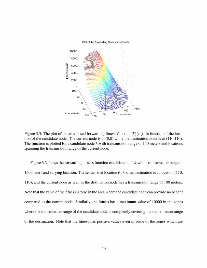
−100
−50
0
50
100
−100−50
050
100
0
2000
4000
6000
8000
10000
Y coordinate
Plot of the forwarding fitness function Fa
X coordinate
Fitn
ess
Val
ue
Figure 3.3: The plot of the area-based forwarding fitness function Fak (i, j) in function of the loca-
tion of the candidate node. The current node is at (0,0) while the destination node is at (110,110).The function is plotted for a candidate node k with transmission range of 150 meters and locationsspanning the transmission range of the current node.
Figure 3.3 shows the forwarding fitness function candidate node k with a transmission range of
150 meters and varying location. The sender is at location (0, 0), the destination is at location (110,
110), and the current node as well as the destination node has a transmission range of 100 meters.
Note that the value of the fitness is zero in the area where the candidate node can provide no benefit
compared to the current node. Similarly, the fitness has a maximum value of 10000 in the zones
where the transmission range of the candidate node is completely covering the transmission range
of the destination. Note that the fitness has positive values even in some of the zones which are
40

opposite to the destination, due to the fact that the candidate node has a larger transmission range
than the current node, which compensates for its unfavorable location.
100200
300100
200
0
2000
4000
6000
8000
Distance to destination
Plot of the forwarding fitness function Fa
Transmission range
Fitn
ess
valu
e
Figure 3.4: The plot of the area-based forwarding fitness function Fak (i, j), for candidate node k
with different location and different transmission range. The scenario is the same as above exceptthe transmission range is variable in the range of [50, 250].
Figure 3.4 plots the forwarding fitness function Fa for the case circle Γi,j and Πk are secant,
for candidate node k with different location and different transmission range. The scenario is the
same as above except the transmission range is variable in the range of [50, 250]. We combine
the location of candidate node k to a single parameter - distance to the destination. The distance
between node k and the destination is in the range [110√
2 − 100, 110√
2 + 100]. The figure
indicates the fitness value increases as the transmission range of candidate node increases, or the
41

distance to the destination decreases, or both. The fitness value achieves maximum when candidate
node is nearest to the destination and with largest transmission range.
3.1.2 Ad hoc On-Demand Distance Vector Routing with m-Limited Forwarding (m-AODV)
Ad hoc On-Demand Distance Vector Routing (AODV) [PR99] is a reactive algorithm where routes
are discovered and established only on demand and are maintained only if they are used by some
sources. Nodes that do not lie on active paths do not maintain routing information or exchange
routing tables. Only symmetric links participate in routing which is ensured by periodical hello
packets. The freshness of routes are ensured by sequence numbers as well as route maintenance.
We introduce a modified algorithm m-AODV which replaces flooding with m-limited forward-
ing in the route discovery process, and it is based upon the following modifications to AODV:
1. We added the transmission range of the node to the hello packet of AODV. When a node re-
ceives a hello packet from its neighbor, the node adds the neighbor as well as its transmission
range into the neighbor table.
2. We introduced the location-update packet, which is an infrequent system-wide broadcast
packet. A location-update packet contains the id of a node and its location. When a node
receives a location-update packet from any other node in the system, it adds the sender as
well as its location information into a location table.
42

3. Route discovery is done through the m-limited forwarding algorithm. The forwarding fit-
ness function is evaluated based on the information in the neighbor and location tables. We
support the distance-based Fd as well as the area-based Fa fitness functions.
3.2 Simulation Study
In this section, we report the results of a simulation study. The objectives of our simulation study
are twofold. First, we aim to determine the optimal values of m for m-limited forwarding. Al-
though theoretical considerations allow us to determine that the optimal range is in the low single
digits, the problem is too complex for an analytical solution. Therefore, we will determine the
optimal value by studying the performance in a simulation environment. The second objective is
to study the impact of m-limited forwarding on the performance of the routing algorithm. For this
study, we have implemented the m-AODV routing protocol as presented in Section 3.1.2 in the
NS-2 simulator [BEF00, VIN]. We implemented m-AODV using both proposed fitness functions,
Fd and Fa. We compared our implementation of the m-AODV algorithm with the default AODV
implementation from the CMU wireless extension package [CMU]. We compared the routing
algorithms in terms of average power consumption and packet loss ratio.
To perform a meaningful comparison of the algorithms, we created a scenario of a wireless
system with mobile nodes and realistic traffic patterns. To describe the movement of nodes in
the system we used the “random waypoint” model [BMJ98, JM96]. Each node randomly picks a
43

destination on the map, moves to the destination at a constant speed, and then pauses for the pause
time. After the pause time, it continues the movement following the same pattern.
In our simulations, we use traffic patterns generated by Constant Bit Rate (CBR) sources send-
ing UDP packets to another node. A node cannot be simultaneously source and destination. Each
CBR source is active for a time interval called CBR duration. Our simulation allows a setup dura-
tion before generating any traffic, during which the sender may transmit hello and location-update
packets. We also set an end duration, during which CBR sources are not allowed to send data
packets, so that data packets will not be lost due to the lack of simulation time. The remaining
simulation time, the time after the setup duration and before the end duration, is divided into equal
time slices. During each time slice, we regenerate CBR sources for different pairs of senders and
destinations. The start time of the CBR source is randomly picked in the first half of the time slice,
and the CBR duration is set to half of the time slice so that it will not cross two time slices. Fig-
ure 3.5 illustrates the relationship among simulation time, setup duration, end duration, time slice
and CBR duration. The CBR sources generate 128-byte packets (in general small data packets
favor AODV [DPR01]).
In our simulation, we choose a 500 × 500 m2 square area and the default number of nodes is
80. Every node has a transmission range of 100 meters. We run several simulation experiments
and vary the number of nodes, the speed in the “random waypoint” model, and the number of CBR
sources. The number of nodes ranges from 50 to 140, the node speed ranges from 1 to 10 m/s, and
44

Node 1
Setup Duration Time Slice
CBR Duration
End Duration
Setup Duration Time Slice
End Duration
Time Slice Time Slice
Time Slice Time Slice
Setup Duration Time Slice
End Duration Time Slice Time Slice
Setup Duration Time Slice
End Duration Time Slice Time Slice
Simulation Time
Node 2
Node 3
Node 4
CBR Duration
CBR Duration
CBR Duration
CBR Duration
CBR Duration
Figure 3.5: The illustration of relationship among simulation time, setup duration, end duration,time slice and CBR duration. Four nodes and two CBR sources are included in this example.
the number of CBR sources ranges from 4 to half of number of the nodes. Table 3.1 illustrates the
default settings and the range of the parameters for our simulation experiments.
Table 3.1: The default values and the range of the parameters for our simulation studies
Field Value Rangesimulation area 500 × 500 (m2)number of nodes 80 50 - 140transmission range 100 (m)speed 1 (m/s) 1 - 10 (m/s)pause time 15 (s)total simulation time 900 (s)setup duration 50 (s)end duration 50 (s)duration of time slices 10 (s)number of CBR sources 25 4 - 40offered network load 25 (Kbps) 4 - 40 (Kbps)CBR packet size 128 (bytes)CBR sending rate 1 (Kbps)CBR duration 5 (s)
45

3.2.1 Performance Metrics
We consider two performance metrics:
• Packet Loss Ratio – The ratio of all data packets received to the number of data packets sent
during the simulation.
• Average Power Consumption Per Node – The ratio of total power dissipated by all nodes to
the number of nodes in the network, during the simulation. Nodes dissipate power in the
following actions: transmitting packets, receiving (overhearing) packets, and idle listening.
For each setting (fixed number of CBR sources, fixed speed, fixed number of nodes), we repeat
the simulation 20 times with different randomization seeds. These two performance metrics are
studied for varying network load, node mobility, and node density.
3.2.2 Determining the Optimal Value of m
Intuitively, the optimal value of m is a small, single digit number. A large value would not provide
any benefit compared to flooding, while a too small value would adversely affect the routing per-
formance through the lack of redundancy. The problem is too complex for an analytical solution,
but we can determine the optimal value through simulation (as well as experimentally in a real
setting).
46

In a series of experiments, we have investigated 1-, 2-, 3-, and 4-limited forwarding using both
fitness functions Fd and Fa. A rough estimation of the average number of neighbors of a node in
our scenario follows: the simulation area is 250000 m2 (500m× 500m). The average node density
is 80250000 = 1
3125 . The transmission range of a node is a disk of 100m radius, thus the transmission
area covers 10000π ≈ 31400 m2. In average we will have about 10 nodes in that area, one being
the node considered and the other 9 being its neighbors (in fact, considering the nodes close to the
edge of the simulated area, the average number of neighbors is somewhat lower). Thus, values of
m larger than 4 are very close to the flooding technique.
The metrics considered in the determination of the optimal m are the packet loss ratio and
average power consumption. We are not considering the average latency, due to its dependency on
the packet loss ratio.
Routing performance function of network load. The packet loss for AODV or m-AODV
protocols can be due to the following reasons: (i) the forwarding set calculated by the fitness
function excludes nodes on the critical path from the source node to the destination node; (ii) nodes
move out a region and cause route failure; (iii) due to frequent changes of the network topology
the cached routing tables become outdated; and (iv) packets are lost at the MAC layer. There are
several reasons for a packet to be dropped at the MAC layer. In a static network, a packet is dropped
after its transmission was retried 16 times with a limited binary exponential backoff algorithm. In
a mobile ad hoc network, however, a failure at the MAC layer occurs when the nodes move out
from transmission range while waiting for a right to transmit or waiting for their retransmission
47

time. A packet may be lost after the first collision, because by the time it retransmits, the node is no
longer in the transmission range. Similarly, a packet can be lost even before the first transmission
if the destination node moves out of the transmission range while the source node is waiting for an
available transmission slot.
Figures 3.6(a) and 3.6(b) illustrate the packet loss ratio versus network load, with fitness func-
tions Fd and Fa respectively. The major reasons for 1-limited forwarding to drop packets are (i)
and (ii); while the major reason for 4-limited forwarding and flooding to drop packets is (iv) in
this scenario. When the traffic load is light, (i) and (ii) are the major reasons, 1-limited forwarding
performs the worst, while the performance of 2-, 3-, 4-limited forwarding are comparable and their
curves almost merge. When the traffic load is high, (iv) becomes the major reason of packet loss,
thus the performance of 4-limited is degraded compared to 2-, 3-limited forwarding and tends to
increase with the increase of network load. For the flooding based scheme, (iv) is always the major
issue, thus it performs much worse than m-limited forwarding based scheme in most cases. For
flooding based protocols the (i) reason is not relevant, as there is no fitness function based decision
whether to forward a packet or not.
With AODV, the power consumption is caused by (i) transmission, reception, or overhearing of
data packets and route discovery packets; (ii) idle listening; and (iii) MAC layer overhead includ-
ing RTS/CTS, retransmission, and so on. With m-AODV, additional power is consumed by (iv)
transmission and reception of hello packets and location-update packets.
48
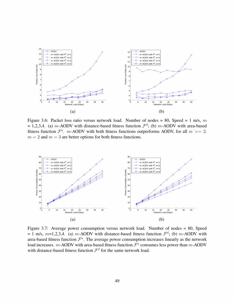
0 5 10 15 20 25 30 35 403
4
5
6
7
8
9
10
11
12
13
Network Load (Kbps)
Pac
ket L
oss
Rat
io (
%)
AODV
m−AODV with Fd, m=1
m−AODV with Fd, m=2
m−AODV with Fd, m=3
m−AODV with Fd, m=4
0 5 10 15 20 25 30 35 403
4
5
6
7
8
9
10
11
12
13
Network Load (Kbps)
Pac
ket L
oss
Rat
io (
%)
AODV
m−AODV with Fa, m=1
m−AODV with Fa, m=2
m−AODV with Fa, m=3
m−AODV with Fa, m=4
(a) (b)
Figure 3.6: Packet loss ratio versus network load. Number of nodes = 80, Speed = 1 m/s, m= 1,2,3,4. (a) m-AODV with distance-based fitness function Fd; (b) m-AODV with area-basedfitness function Fa. m-AODV with both fitness functions outperforms AODV, for all m >= 2.m = 2 and m = 3 are better options for both fitness functions.
0 5 10 15 20 25 30 35 400
10
20
30
40
50
60
70
80
90
Network Load (Kbps)
Pow
er C
onsu
mpt
ion
(J/n
ode)
AODV
m−AODV with Fd, m=1
m−AODV with Fd, m=2
m−AODV with Fd, m=3
m−AODV with Fd, m=4
0 5 10 15 20 25 30 35 400
10
20
30
40
50
60
70
80
90
Network Load (Kbps)
Pow
er C
onsu
mpt
ion
(J/n
ode)
AODV
m−AODV with Fa, m=1
m−AODV with Fa, m=2
m−AODV with Fa, m=3
m−AODV with Fa, m=4
(a) (b)
Figure 3.7: Average power consumption versus network load. Number of nodes = 80, Speed= 1 m/s, m=1,2,3,4. (a) m-AODV with distance-based fitness function Fd; (b) m-AODV witharea-based fitness function Fa. The average power consumption increases linearly as the networkload increases. m-AODV with area-based fitness function Fa consumes less power than m-AODVwith distance-based fitness function Fd for the same network load.
49

Figures 3.7(a) and 3.7(b) illustrate the average power consumption function of the network
load, for both fitness functions Fd and Fa. The average power consumption increases linearly as
the network load increases. When the network load is light, AODV consumes the least power since
it does not need to send hello packets or location-update packets. As the network load increases,
as expected, AODV needs more power than m-AODV. m1-AODV consumes less power than m2-
AODV for 1 ≤ m1 < m2 ≤ 4, for both fitness functions. m-AODV with fitness function Fa
consumes less power than m-AODV with fitness function Fd for the same network load.
Routing performance function of node mobility. Figures 3.8(a) and 3.8(b) illustrate the
packet loss ratio versus node mobility, for both fitness functions Fd and Fa. Node mobility is
measured by the speed of the node movement. The packet loss ratio of 1-limited forwarding is
noticeably greater than all other schemes as the node mobility increases. When the node mobility
is relatively high, 4-limited forwarding performs the best, followed by 3-limited forwarding and
flooding. As the node mobility increases, the performance of 2-limited forwarding becomes a little
worse than AODV. Thus, m = 1 is an unacceptable value as it is not suitable for networks with a
relatively high node mobility. m = 3 and m = 4 are better options when node mobility is relatively
high.
Figures 3.9(a) and 3.9(b) illustrate the average power consumption versus node mobility, for
both fitness functions Fd and Fa. We find that AODV consumes the most power, while among
the m-limited schemes, 1-limited forwarding consumes the least power, followed by 2-, 3-, 4-
limited forwarding. When node mobility increases, the routing table becomes outdated quickly
50

1 2 3 4 5 6 7 8 9 100
5
10
15
20
25
30
Node Mobility (m/s)
Pac
ket L
oss
Rat
io (
%)
AODV
m−AODV with Fd, m=1
m−AODV with Fd, m=2
m−AODV with Fd, m=3
m−AODV with Fd, m=4
1 2 3 4 5 6 7 8 9 100
5
10
15
20
25
30
35
Node Mobility (m/s)
Pac
ket L
oss
Rat
io (
%)
AODV
m−AODV with Fa, m=1
m−AODV with Fa, m=2
m−AODV with Fa, m=3
m−AODV with Fa, m=4
(a) (b)
Figure 3.8: Packet loss ratio versus node mobility. Number of nodes = 80, Offered load = 25 Kbps,m=1,2,3,4. (a) m-AODV with distance-based fitness function Fd; (b) m-AODV with area-basedfitness function Fa. The packet loss ratio of 1-limited forwarding is noticeably the greatest. m = 3and m = 4 are better options when the node mobility is relatively high.
1 2 3 4 5 6 7 8 9 1030
35
40
45
50
55
60
65
70
Node Mobility (m/s)
Pow
er C
onsu
mpt
ion
(J/n
ode)
AODV
m−AODV with Fd, m=1
m−AODV with Fd, m=2
m−AODV with Fd, m=3
m−AODV with Fd, m=4
1 2 3 4 5 6 7 8 9 1020
30
40
50
60
70
Node Mobility (m/s)
Pow
er C
onsu
mpt
ion
(J/n
ode)
AODV
m−AODV with Fa, m=1
m−AODV with Fa, m=2
m−AODV with Fa, m=3
m−AODV with Fa, m=4
(a) (b)
Figure 3.9: Average power consumption versus node mobility. Number of nodes = 80, Offeredload = 25 Kbps, m=1,2,3,4. (a) m-AODV with distance-based fitness function Fd; (b) m-AODVwith area-based fitness function Fa. AODV consumes the most power. Among the m-limitedschemes, 1-limited forwarding consumes the least power, followed by 2-, 3-, 4-limited forwarding.
51

and additional power is dissipated to find new routes, thus the average power consumption of all
routing schemes increases. However, as node mobility is further increased, the packet loss ratio
increases thus the power consumed for transmitting and receiving data packets is reduced as more
data packets are dropped. For all schemes based on m-limited forwarding, the portion of power
consumption reduced by dropping data packets exceeds the additional power used to find new
routes, thus the overall power consumption is reduced. The power used to find new routes by
the AODV protocol is still the dominating factor of power consumption, thus the average power
consumption still increases. Overall, the average power consumption increases steadily with the
mobility for the AODV protocol. The average power consumption increases to a maximum value,
then decreases with the further increase of the node mobility for the m-AODV protocol.
Routing performance function of network density. Figures 3.10(a) and 3.10(b) show the
packet loss ratio function of the network density, for both fitness functions Fd and Fa. We notice
that for low network density, the packet loss ratio of all schemes is high - a consequence of the
low connectivity. The 1-limited forwarding performs the worst at these values. For higher network
densities, the m-limited forwarding based schemes have a lower packet loss ratio than plain AODV.
We note that 2- and 3-limited forwarding have a lower packet loss ratio than 1- and 4-limited
forwarding. For 1-limited forwarding, only one hop is chosen to forward a route discovery packet,
thus the whole path will fail if one of the hops fails. For m-limited forwarding with (m ≥ 4), the
packets are lost due to the higher number of collisions in the forwarding of the route discovery
packet.
52

50 60 70 80 90 100 110 120 130 1400
5
10
15
20
25
Number of Nodes
Pac
ket L
oss
Rat
io (
%)
AODV
m−AODV with Fd, m=1
m−AODV with Fd, m=2
m−AODV with Fd, m=3
m−AODV with Fd, m=4
50 60 70 80 90 100 110 120 130 1400
5
10
15
20
25
Number of Nodes
Pac
ket L
oss
Rat
io (
%)
AODV
m−AODV with Fa, m=1
m−AODV with Fa, m=2
m−AODV with Fa, m=3
m−AODV with Fa, m=4
(a) (b)
Figure 3.10: Average power consumption versus node density. Offered load = 25 Kbps, Speed= 1 m/s, m=1,2,3,4. (a) m-AODV with distance-based fitness function Fd; (b) m-AODV witharea-based fitness function Fa. For low network density, 1-limited forwarding performs the worst.For higher network densities, all m-limited forwarding based schemes have a lower packet lossratio than plain AODV. m = 2 and 3 are better options when network density is relatively high.
50 60 70 80 90 100 110 120 130 1400
20
40
60
80
100
120
140
160
Number of Nodes
Pow
er C
onsu
mpt
ion
(J/n
ode)
AODV
m−AODV with Fd, m=1
m−AODV with Fd, m=2
m−AODV with Fd, m=3
m−AODV with Fd, m=4
50 60 70 80 90 100 110 120 130 1400
20
40
60
80
100
120
140
160
Number of Nodes
Pow
er C
onsu
mpt
ion
(J/n
ode)
AODV
m−AODV with Fa, m=1
m−AODV with Fa, m=2
m−AODV with Fa, m=3
m−AODV with Fa, m=4
(a) (b)
Figure 3.11: Average power consumption versus node density. Offered load = 25 Kbps, Speed= 1 m/s, m=1,2,3,4. (a) m-AODV with distance-based fitness function Fd; (b) m-AODV witharea-based fitness function Fa. The power consumption for all schemes increases as network den-sity increases. AODV consumes the most power, followed by 4-, 3-, 2-, and 1-limited forwarding.
53

From Figures 3.11(a) and 3.11(b), we observe that the average power consumption per node
for all schemes increases as network density increases. This is explained by the fact that at a
higher network density, more nodes overhear every transmission and the route discovery packet is
also retransmitted by more nodes. AODV consumes the most power, followed by 4-, 3-, 2-, and
1-limited forwarding.
Summary. The experiments performed show that there is no single choice of m which per-
forms the best in every situation. 1-limited forwarding performs poorly for low network load and/or
high mobility. 2-limited forwarding performs poorly for high node mobility. On the other hand,
4-limited forwarding does not perform well for high network load. We find that 3-limited forward-
ing shows the most consistent performance across a wide range of parameters. Therefore, unless
we have the possibility to hand optimize the algorithm for a specific network and transmission
scenario, m = 3 is the safest choice. We will use this value in the remainder of our simulations.
3.2.3 Performance Improvement of m-limited Forwarding in MANETs with Bidirectional Links
In the following, we study the performance improvement of m-limited forwarding for ad hoc
networks with symmetric links. We note that this is the most frequently encountered situation
in practice, because most of the current MAC protocols cannot handle unidirectional links. The
unidirectional links are therefore ignored at the level of the MAC protocol, and the routing protocol
sees a network composed entirely of symmetric links.
54
In the following simulation experiments, we are comparing plain AODV with m-AODV with
3-limited forwarding for the two proposed fitness functions Fd and Fa, as well as the Location-
Aided Routing (LAR) protocol. We use the same scenario and traffic patterns as in the previous
simulations.
Routing performance function of network load. The packet loss ratio versus network load
is presented in Figure 3.12. The packet loss ratio increases with the network load increasing for
all schemes, while for plain AODV it is increasing at a higher rate than LAR and both of the 3-
limited forwarding based schemes. Fd strictly requires nodes to forward the traffic on the positive
direction to the destination, as a reason, some of the nodes on the critical path but on a negative
direction may be excluded. Thus, m-AODV with Fd performs a little better than m-AODV with
Fa. LAR and both of the 3-limited forwarding based schemes have a comparable packet loss ratio
when the traffic load is light. When the traffic load is heavy, as the number of next hops restricted
by LAR is larger than that restricted by 3-limited forwarding based schemes, more packets are
dropped by LAR due to collisions or excessive retransmission failures at the MAC layer.
Figure 3.13 illustrates the average power consumption versus network load. For lightly loaded
networks, 3-limited forwarding consumes more power due to the dissemination of hello packets
and location-update packets. When the network load increases, the power dissipation of plain
AODV increases much faster than that of m-limited forwarding schemes. The next hops to forward
traffic established by Fa is more restricted, compared to Fd. Oftentimes, less than 3 nodes are
included in the forwarding set calculated by Fa, as a result, m-AODV with Fa consumes less
55

0 5 10 15 20 25 30 35 403
4
5
6
7
8
9
10
11
12
13
Network Load (Kbps)
Pac
ket L
oss
Rat
io (
%)
AODVLAR
m−AODV with Fd, m=3
m−AODV with Fa, m=3
Figure 3.12: Packet loss ratio versus network load. Number of nodes = 80, Speed = 1 m/s. Wecompare AODV, LAR, and m-AODV with fitness functions Fd and Fa. AODV performs theworst. m-AODV outperforms LAR when the network load is relatively high.
0 5 10 15 20 25 30 35 400
10
20
30
40
50
60
70
80
90
Network Load (Kbps)
Pow
er C
onsu
mpt
ion
(J/n
ode)
AODVLAR
m−AODV with Fd, m=3
m−AODV with Fa, m=3
Figure 3.13: Average power consumption versus network load. Number of nodes = 80, Speed = 1m/s. We compare AODV, LAR, and m-AODV with fitness functions Fd andFa. AODV consumesthe most power, and m-AODV consumes less power than LAR, for the same network load.
56
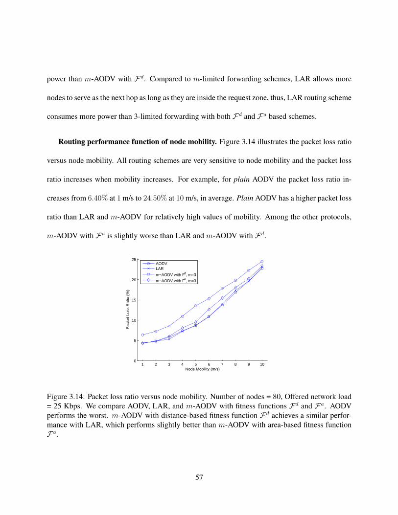
power than m-AODV with Fd. Compared to m-limited forwarding schemes, LAR allows more
nodes to serve as the next hop as long as they are inside the request zone, thus, LAR routing scheme
consumes more power than 3-limited forwarding with both Fd and Fa based schemes.
Routing performance function of node mobility. Figure 3.14 illustrates the packet loss ratio
versus node mobility. All routing schemes are very sensitive to node mobility and the packet loss
ratio increases when mobility increases. For example, for plain AODV the packet loss ratio in-
creases from 6.40% at 1 m/s to 24.50% at 10 m/s, in average. Plain AODV has a higher packet loss
ratio than LAR and m-AODV for relatively high values of mobility. Among the other protocols,
m-AODV with Fa is slightly worse than LAR and m-AODV with Fd.
1 2 3 4 5 6 7 8 9 100
5
10
15
20
25
Node Mobility (m/s)
Pac
ket L
oss
Rat
io (
%)
AODVLAR
m−AODV with Fd, m=3
m−AODV with Fa, m=3
Figure 3.14: Packet loss ratio versus node mobility. Number of nodes = 80, Offered network load= 25 Kbps. We compare AODV, LAR, and m-AODV with fitness functions Fd and Fa. AODVperforms the worst. m-AODV with distance-based fitness function Fd achieves a similar perfor-mance with LAR, which performs slightly better than m-AODV with area-based fitness functionFa.
57

1 2 3 4 5 6 7 8 9 1030
35
40
45
50
55
60
65
Node Mobility (m/s)
Pow
er C
onsu
mpt
ion
(J/n
ode)
AODVLAR
m−AODV with Fd, m=3
m−AODV with Fa, m=3
Figure 3.15: Average power consumption versus node mobility. Number of nodes = 80, Offerednetwork load = 25 Kbps. We compare AODV, LAR, and m-AODV with fitness functions Fd andFa. AODV consumes the most power, and m-AODV consumes less power than LAR, for the samenode mobility.
Figure 3.15 illustrates the average power consumption versus node mobility. We find the plain
AODV and LAR are more sensitive to node mobility than m-AODV. With the mobility increasing,
the power dissipated by AODV and LAR increases accordingly, while the power consumption of
both 3-limited forwarding based schemes remain at a certain level. For the two 3-limited forward-
ing based schemes, the Fd based scheme consumes less power than the Fa based scheme.
Routing performance function of network density. Figure 3.16 illustrates the packet loss
ratio versus node density. The packet loss ratio decreases when the number of nodes increases
from 50 to 80, and then starts to increase when the number of nodes further increases. When the
network density is relatively low, a percentage of packets are dropped due to unavailable routes;
when the network density is relatively high, excessive collisions become the major reason that
58

50 60 70 80 90 100 110 120 130 1400
5
10
15
20
25
Number of Nodes
Pac
ket L
oss
Rat
io (
%)
AODVLAR
m−AODV with Fd, m=3
m−AODV with Fa, m=3
Figure 3.16: Packet loss ratio versus network density. Speed = 1 m/s, Offered network load =25 Kbps. We compare AODV, LAR, and m-AODV with fitness functions Fd and Fa. AODVperforms the worst. m-AODV outperforms LAR when the network density is relatively high.
50 60 70 80 90 100 110 120 130 1400
20
40
60
80
100
120
140
160
Number of Nodes
Pow
er C
onsu
mpt
ion
(J/n
ode)
AODVLAR
m−AODV with Fd, m=3
m−AODV with Fa, m=3
Figure 3.17: Average power consumption versus network density. Speed = 1 m/s, Offered networkload = 25 Kbps. We compare AODV, LAR, and m-AODV with fitness functions Fd and Fa.AODV consumes the most power, and m-AODV consumes less power than LAR, for the samenetwork density.
59

packets are lost during the transmission. The packet loss ratio for AODV and LAR at high node
density increases faster than m-AODV due to excessive number of collisions. m-AODV with Fa
outperforms m-AODV with Fd at higher node density.
Figure 3.17 illustrates the average power consumption versus network density. With the in-
crease in the network density, the power dissipated by every routing scheme increases accordingly.
The increase in the power dissipation by plain AODV is slightly larger than LAR, followed by
m-AODV with Fd, and m-AODV with Fa. The Fa based scheme consumes less power than the
Fd based scheme.
Summary. We find that m-AODV exhibits a consistently lower power consumption for al-
most all operating scenarios, except when the network load is light. In that case, the overhead of
m-limited forwarding due to the dissemination of hello and location-update packets exceeds the
benefits gained by reducing the retransmissions.
In general, the more “difficult” a scenario (high network load and/or high node mobility), the
greater the benefits of m-limited forwarding in terms of power consumption. The distance-based
fitness function Fd leads to lower power consumption with an approximately constant difference
versus the area-based fitness function Fa.
We also find that the m-limited forwarding lowers the packet loss ratio in all scenarios. Al-
though the packet loss ratio is naturally increasing for all algorithms when the scenario becomes
more “difficult” (high network load and/or high node mobility), the benefits of m-limited forward-
ing become greater with the increase in the difficulty of the scenario. The two fitness functions Fd
60

and Fa have a similar evolution, with the distance-based function Fd having a lower packet loss
ratio with an approximately constant difference.
The general conclusion is m-AODV outperforms plain AODV and LAR for everything but
the easiest scenarios (with light network load and low node mobility). The distance based fitness
function Fd is a better choice in these cases, as the benefits of the area-based function Fa cannot
be observed in a network formed exclusively of symmetric links.
3.2.4 m-limited Forwarding in MANETs with Asymmetric Links
We find that for homogeneous MANETs the simpler, distance-based Fd forwarding fitness func-
tion actually performs slightly better than the more complex, area-based Fa function, in terms of
packet loss ratio. The reason for this is that, as shown in Section 3.1, the benefits of the area-
based function appear only in the case of asymmetric links. Most wireless networks are composed
of heterogeneous nodes due to the differences in the physical possibilities of the nodes, such as
power, size and shape of antennas and so on. However, most MAC layer and routing protocols re-
quire the existence of bidirectional links. These protocols ignore the large number of asymmetric
links present in heterogeneous networks. For instance the IEEE 802.11 MAC protocol works only
on bidirectional links, and most ad hoc routing protocols (including AODV) require bidirectional
links. This property is also inherited by the m-AODV variant.
In order to study the improvement provided by the area-based fitness function Fa, we need to
test it with a pair of MAC and routing protocols which both support asymmetric links. One such
61

pair is the AsyMAC (Asymmetric MAC) protocols [WTB06a, WTB07b] and the m-A4LP routing
protocol [WJM04, WJM06].
To show the benefits of the approach, we created a scenario with a set of heterogeneous nodes.
In our simulation, we have four categories of nodes – C1, C2, C3, and C4. The transmission ranges
of nodes in category C1, C2, C3, and C4 are 200, 150, 100, and 50 meters, respectively. The ratio
of the number of nodes of each category is |C1|:|C2|:|C3|:|C4| =1:2:3:4. Thus, for default 80
nodes, the number of nodes in category C1, C2, C3, and C4 are 8, 16, 24, 32, respectively. We
run a simulation comparing three protocol stacks: m-A4LP with the underlying AsyMAC protocol
in the variants with the distance-based Fd and the area-based Fa fitness function and a more
traditional ad hoc networking stack with plain AODV on top of the 802.11 MAC protocol.
Note that this is a relatively “difficult” scenario for the AODV/802.11 protocol set, due to
the large number of nodes with small transmission range and the relatively low density of nodes.
Therefore, we expect a high packet loss ratio for the AODV/802.11 stack.
The results of the experiments are presented in Figure 3.18. We find that the m-A4LP/AsyMAC
based protocol stacks have a much lower packet loss ratio than AODV/802.11. This is due to their
ability to exploit the asymmetric links which exist in the environment. Furthermore, in this scenario
we find that the area-based fitness function Fa yields a lower packet loss ratio than the distance
based function Fd. This is due to the fact that Fa can make a better choice of the set of forwarding
nodes in the presence of asymmetric links.
62
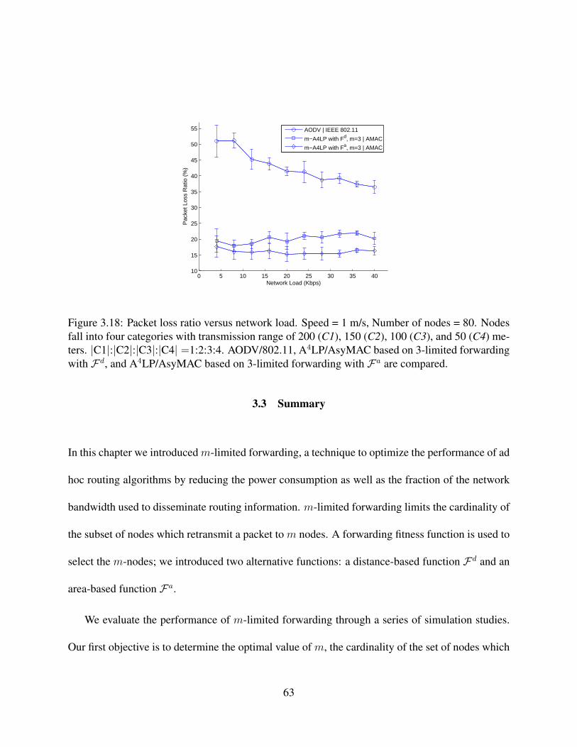
0 5 10 15 20 25 30 35 4010
15
20
25
30
35
40
45
50
55
Network Load (Kbps)
Pac
ket L
oss
Rat
io (
%)
AODV | IEEE 802.11
m−A4LP with Fd, m=3 | AMAC
m−A4LP with Fa, m=3 | AMAC
Figure 3.18: Packet loss ratio versus network load. Speed = 1 m/s, Number of nodes = 80. Nodesfall into four categories with transmission range of 200 (C1), 150 (C2), 100 (C3), and 50 (C4) me-ters. |C1|:|C2|:|C3|:|C4| =1:2:3:4. AODV/802.11, A4LP/AsyMAC based on 3-limited forwardingwith Fd, and A4LP/AsyMAC based on 3-limited forwarding with Fa are compared.
3.3 Summary
In this chapter we introduced m-limited forwarding, a technique to optimize the performance of ad
hoc routing algorithms by reducing the power consumption as well as the fraction of the network
bandwidth used to disseminate routing information. m-limited forwarding limits the cardinality of
the subset of nodes which retransmit a packet to m nodes. A forwarding fitness function is used to
select the m-nodes; we introduced two alternative functions: a distance-based function Fd and an
area-based function Fa.
We evaluate the performance of m-limited forwarding through a series of simulation studies.
Our first objective is to determine the optimal value of m, the cardinality of the set of nodes which
63

retransmit a packet containing routing information. We have found that m = 3 yields reasonable
output.
A second set of experiments study MANETs with bidirectional links and investigate two rout-
ing algorithms, AODV and LAR enhanced with m-limited forwarding. For most simulation sce-
narios, m-AODV has a lower power consumption and a lower packet loss ratio than either plain
AODV or LAR. Our simulation studies indicate that the distance-based fitness function Fd per-
forms better than the area-based function Fa.
Finally, we compared the performance of the two fitness functions in a network with asym-
metric links. Since AODV and the most commonly used MAC protocols cannot take advantage of
asymmetric links, we used the m-A4LP routing protocol and the AsyMAC (asymmetric MAC) pro-
tocol on the MAC and network layer. Our simulation studies indicate that the m-A4LP/AsyMAC
protocol stack yields a lower packet loss ratio than the AODV/802.11 stack, and the area-based
fitness function Fa outperforms the distance-based function Fd for this scenario.
A natural extension of the current research is the ability to improve the performance of the
routing algorithms by improving the accuracy of the forwarding fitness function. For instance, the
area-based fitness function assumes that the number of nodes in the area is proportional with the
size of the area, which is true only if the density of the nodes is uniform and static. If we have
information about a non-uniform node density we can introduce a density weighted area-based
fitness function where the fitness is expressed as the size of the area times the node density in the
given part of the network. If, in addition, we have information about asymmetric and/or dynami-
64

cally changing transmission ranges, this information can also be integrated in the fitness function.
Naturally, there is a delicate balance between the cost of obtaining the necessary information, and
the performance improvement which can be obtained through a fitness function with improved ac-
curacy. We conjecture that the cost of obtaining additional information is justified only in “difficult
scenarios”, such as nodes with highly heterogeneous transmission ranges or scenarios with abrupt
changes in node density. The in-depth evaluation of this conjecture and the design of low-overhead
information gathering and distribution algorithms is a subject of future work.
Another topic for future research is the study of the security and fairness aspects of the pro-
tocol. In the current protocol, a node can become a parasite on the system if either (a) refuses to
participate in the forwarding by quietly dropping packets or (b) misreports its own position such
that the node is avoided by the routes established in the network. While these misbehaviors can be
in principle detected externally, the network needs a service which monitors the participants and
takes appropriate actions against misbehaving nodes. Note that our protocol is not dependent on
the power resources of the nodes. It is very difficult to detect nodes which misrepresent their power
resources, because external observers do not normally have access to the internal power monitors
of a node.
65
CHAPTER 4MAC LAYER AND ROUTING PROTOCOLS FOR WIRELESS
NETWORKS WITH ASYMMETRIC LINKS
Mobile ad hoc networks allow nodes with different hardware capabilities and power limitations to
communicate with one another. Most communication channels in such networks are unidirectional
due to heterogeneity of the nodes and to power constraints. Yet, routing protocols for MANETs
routinely assume that all communication links are bidirectional. In this dissertation, we consider
the case when the nodes of a MANET have various degrees of mobility and range and the com-
munication links are asymmetric. Power consumption is a major concern for a MANET as nodes
become inoperative once they have depleted their power. Power-aware routing algorithms mini-
mize the power consumption and, whenever possible, avoid the nodes with a low level of residual
power. Location-aware routing algorithms have the potential to extend the life of individual nodes
of a MANET, when the location of the nodes are known by the embedded GPS systems.
In a wireless environment, at any given time, an asymmetric link supports unidirectional com-
munication between a pair of mobile stations and requires a set of relay stations for the transmission
of packets in the other direction. Asymmetric links are common in wireless networks for a variety
of physical, logical, operational, and legal considerations. The transmission range of a node might
be limited by the capabilities of the hardware or by power limitations. A node might need to limit
66

its transmission power to avoid interference with a licensed user of the spectrum, or because of
dynamic spectrum management considerations. In military applications, considerations of stealth
might require some nodes to reduce their transmission power. In addition to these, [KRD06] men-
tions some schemes have been proposed recently to maintain optimum network topology by tuning
the transmission range of individual nodes [RH00, WLB01, GTS04], which leads to possible uni-
directional links.
Inability of some MAC layer protocols to exploit the asymmetry of some of the communication
channels could lead to an inefficient bandwidth utilization, or, in the worst case, to inability to
connect some of the nodes. To exploit the asymmetric links, the protocols must be able to deliver
the acknowledgements back to the sender in a direction opposite to the direction of the asymmetric
link. Furthermore, the problem of hidden nodes appears more often and in more complex forms
than in the case of symmetric links. Depending whether the routing protocol of a MANET is able to
handle asymmetric links, the MAC layer protocol might need to hide the existence of asymmetric
links with a symmetric overlay. The challenge for a MAC layer protocol able to exploit asymmetric
links is to solve the hard problems mentioned above, while keeping the cost incurred lower than
the benefits obtained from the utilization of the asymmetric links.
In this chapter, we introduce a MAC layer and routing protocol for heterogeneous MANETs
with asymmetric links. The routing protocol A4LP, which is both location-aware and power-
aware, is designed to support routing over asymmetric links. A4LP introduces an advanced flood-
ing technique - m-limited forwarding, which significantly reduces average power consumption as
67
well as packet loss ratio. The MAC layer protocol (AsyMAC) supports reliable transmission over
asymmetric links. AsyMAC requires fewer nodes to maintain silence during a transmission than
the protocols proposed in [PKD01,FTB02], as a result, the bandwidth utilization of the network is
extended.
This chapter is organized as follows. We begin with an introduction of the system model for
heterogeneous MANETs and discuss several topology-related concepts in Section 4.1. We present
a detailed description of our proposed A4LP routing protocol for MANETs with asymmetric links
in Section 4.2. Section 4.3 describes the AsyMAC protocol in details which serves as the un-
derlying MAC layer protocol for A4LP routing protocol. The simulation and case study for the
A4LP/AsyMAC protocol combination is illustrated in Section 4.4. Finally, we summarize the find-
ings of the A4LP/AsyMAC protocol combination in Section 4.5.
4.1 The Model of the System
4.1.1 The System Model for Heterogeneous MANETs
Let N be the set of nodes in a heterogeneous MANET. We make several assumptions:
a. The number of nodes is relatively small, say | N |≤ 104.
b. All nodes use the same frequency to communicate with one another. Once a node sends a
message all the nodes in its transmission range hear the broadcast.
c. The mobility of individual nodes is limited and differs from one node to the other.
68

d. Nodes are able to adjust their transmitting power according to their residual power so that
their lifetime are extended.
Every node i ∈ N is characterized by a minimal set of attributes, two time-invariants and two
time-dependents:
1. Id, Idi; a unique string used for node identification.
2. Class, Ci; the nodes of a heterogeneous MANET are classified into several classes based
on the hardware and software resources. Throughout this thesis we assume a four level
hierarchy.
3. Location at time t, Li(t); the geographical coordinates of the position of the node at time t.
4. Residual power at time t, P resi (t); the amount of power available at time t. Let Pmax
i be the
maximum level of power that can be stored at node i. There are two water marks (e.g., high
water mark HWMi = 0.7Pmaxi and low water mark LWMi = 0.2Pmax
i ), and say that at
time t the node operates at
- full-power level if P resi (t) ≥ HWMi,
- normal-power level if P resi (t) > LWMi and P res
i (t) < HWMi, or
- low-power level if P resi (t) ≤ LWMi.
Other attributes can be derived from the ones in the minimal set.
69

The transmission range of node i at time t, Ri(t), is a function of the residual power and
possibly other factors including the configuration of the terrain, atmospheric conditions, and so on.
For simplicity we assume that
Ri(t) = constant× P resi (t) (4.1)
The distance between two nodes, i, j ∈ N , dij(t) is a function of the position of the two nodes
dij(t) = dji(t) = f(Li(t), Lj(t)) (4.2)
The average velocity of a node i over a time interval ∆t = t2 − t1, t2 > t1 is
v∆ti = f(Li(t2), Li(t1))/∆t (4.3)
The mobility region of node i over a time interval ∆t = t2 − t1, t2 > t1 is a circle of radius
M∆ti = v∆t
i ×∆t (4.4)
centered at Li(t1).
The connection between two nodes is described by the Boolean reachability function Rij(t)
which can be interpreted as follows: a node i can send a packet to node j at time t if and only
if Rij(t) = true. A link between two nodes is symmetric if Rij(t) = Rji(t) = true. Note,
that the reachability is a time varying function; the connection can be affected by various channel
conditions, fading, the mobility of the node or the mobility of the obstacles in the field.
We assume that every node is aware of the current values of the reachability function between
itself and the neighboring nodes (in both direction). In the A4LP/AsyMAC protocol stack, it is the
70

role of the neighbor discovery protocol of A4LP to find these values and keep them up-to-date.
Although neighbor discovery is a common feature of ad hoc routing protocols, most protocols
will not detect outbound neighbors, because the confirmation message will not reach back to the
originating node. Asymmetric routing protocols, such as A4LP have a provision to route back
the confirmation messages even in the absence of a direct link, thus allowing the discovery of the
full asymmetric reachability matrix. In the following definitions we omit the time parameter even
though all the sets are variable in time, a fact which needs to be considered by the protocols relying
on them.
i
i i
i
j
j
j
j
(c) I n/Out-bound : i j (d) Not neighbors : i j
(b) I n-bound: i j (a) O ut-bound: i j
Figure 4.1: The neighbor relationship between two nodes. (a) j is an Out-bound neighbor of i.(b) j is an In-bound neighbor of of i. (c) j is an In/Out-bound neighbor of i. (d) i and j are notneighbors.
71

Definition 1: Two nodes i, j ∈ N are in neighbor relationship at time t if there is a direct
communication link between them. We recognize several types of neighbors:
(i) Out-bound neighbor: j is the out-bound neighbor of i, if i can reach j but j cannot reach i,
as seen in Figure 4.1(a). In this case the link Lij between the two nodes is unidirectional
Rij(t) = true and Rji(t) = false
Call Outi(t) ⊂ N the set of Out-bound neighbors of i at time t.
(ii) In-bound neighbor: j is the In-bound neighbor of i, if j can reach i but i cannot reach j, as
seen in Figure 4.1(b). In this case the link Lji between the two nodes is unidirectional
Rij(t) = false and Rji(t) = true
Call Ini(t) ⊂ N the set of In-bound neighbors of i at time t.
(iii) In/Out-bound neighbor: j is the In/Out-bound neighbor of i, if i and j can reach each other,
as seen in Figure 4.1(c). In this case the link Lij between the two nodes is bidirectional
Rij(t) = true and Rji(t) = true
Call InOuti(t) ⊂ N the set of In/Out-bound neighbors of i at time t.
The scenario that two nodes are not neighbors is illustrated in Figure 4.1(d).
Definition 2: If node i is an Out-bound neighbor of node j, we call i the high-range node
(H-node) and j the low-range node (L-node) of the asymmetric link Lij .
72

Definition 3: A set of m nodes i1, i2, . . . im ∈ N are in an m-party proxy set if each node can
reach the other m− 1 nodes either directly or through a subset of the other m− 2 members of the
set.
Proposition 1: At least one of the links of an m-party proxy set must be bidirectional.
Proof: Suppose Proposition 1 is false, that is, there exists an m-party proxy set with no
bidirectional links. Let the m nodes in the m-party proxy relationship be i1, i2, · · · , im ∈ N and
arbitrarily pick up an asymmetric link (iu, iv) where 1 ≤ u, v ≤ m,u 6= v. Thus, node iu can reach
node iv directly, but the reciprocal is not true, Riuiv(t) = true and Riviu(t) = false:
Riu(t) ≥ diuiv(t) > Riv(t) (4.5)
By the definition of m-party proxy set, there exists at least a path for node iv to reach node
iu. Let us choose the shortest path from node iv to node iu. There are no duplicate nodes
on this path, otherwise a shorter path can be obtained by removing the sub-path consisting of
all the nodes connecting the two duplicate nodes. Call the set of nodes on the shortest path
(iv, iN1 , iN2 , · · · , iNp · · · , iNk, iu), where Np 6= Nq, Np 6= u,Np 6= v, 1 ≤ p, q ≤ k ≤ m−2, p 6= q.
Similar to (4.5), we have
Riv(t) ≥ diviN1(t) > RiN1
(t)
≥ diN1iN2
(t) > RiN2(t)
≥ · · · > RiNp(t) ≥ diNp iNp+1
(t) > RiNp+1(t)
≥ · · · > RiNk(t) ≥ diNk
iu(t) > Riu(t)
(4.6)
Equations (4.5) and (4.6) are contradictory, thus, Proposition 1 must be true.
73
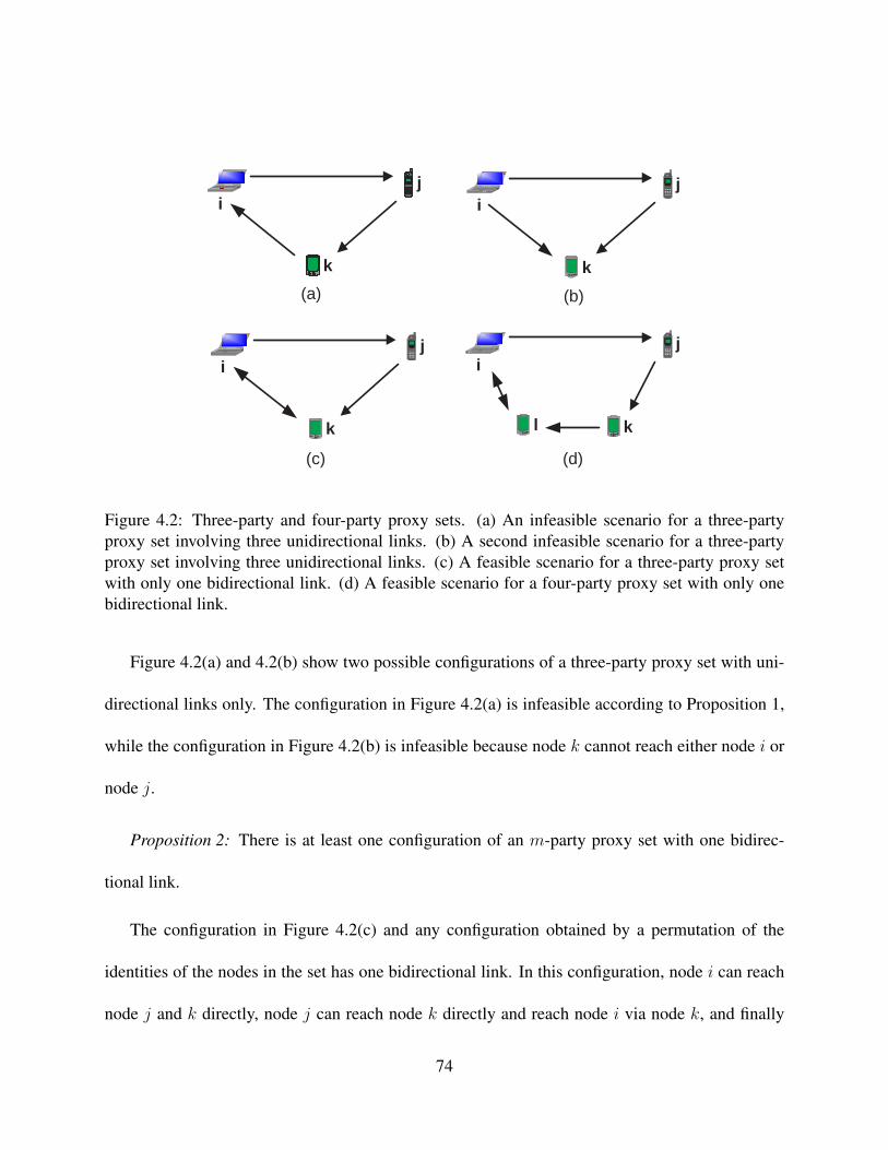
(a) (b)
(c) (d)
j
k
i j
k
i
j
k
i j
k l
i
Figure 4.2: Three-party and four-party proxy sets. (a) An infeasible scenario for a three-partyproxy set involving three unidirectional links. (b) A second infeasible scenario for a three-partyproxy set involving three unidirectional links. (c) A feasible scenario for a three-party proxy setwith only one bidirectional link. (d) A feasible scenario for a four-party proxy set with only onebidirectional link.
Figure 4.2(a) and 4.2(b) show two possible configurations of a three-party proxy set with uni-
directional links only. The configuration in Figure 4.2(a) is infeasible according to Proposition 1,
while the configuration in Figure 4.2(b) is infeasible because node k cannot reach either node i or
node j.
Proposition 2: There is at least one configuration of an m-party proxy set with one bidirec-
tional link.
The configuration in Figure 4.2(c) and any configuration obtained by a permutation of the
identities of the nodes in the set has one bidirectional link. In this configuration, node i can reach
node j and k directly, node j can reach node k directly and reach node i via node k, and finally
74
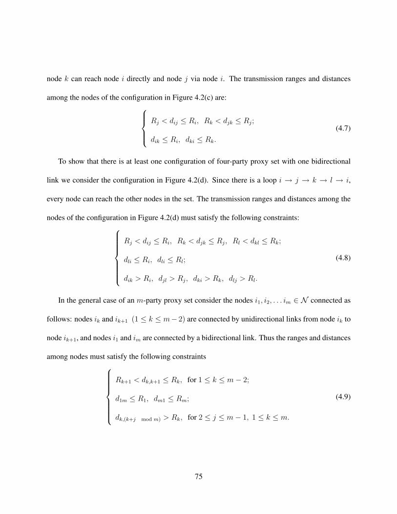
node k can reach node i directly and node j via node i. The transmission ranges and distances
among the nodes of the configuration in Figure 4.2(c) are:
Rj < dij ≤ Ri, Rk < djk ≤ Rj;
dik ≤ Ri, dki ≤ Rk.
(4.7)
To show that there is at least one configuration of four-party proxy set with one bidirectional
link we consider the configuration in Figure 4.2(d). Since there is a loop i → j → k → l → i,
every node can reach the other nodes in the set. The transmission ranges and distances among the
nodes of the configuration in Figure 4.2(d) must satisfy the following constraints:
Rj < dij ≤ Ri, Rk < djk ≤ Rj, Rl < dkl ≤ Rk;
dli ≤ Ri, dli ≤ Rl;
dik > Ri, djl > Rj, dki > Rk, dlj > Rl.
(4.8)
In the general case of an m-party proxy set consider the nodes i1, i2, . . . im ∈ N connected as
follows: nodes ik and ik+1 (1 ≤ k ≤ m− 2) are connected by unidirectional links from node ik to
node ik+1, and nodes i1 and im are connected by a bidirectional link. Thus the ranges and distances
among nodes must satisfy the following constraints
Rk+1 < dk,k+1 ≤ Rk, for 1 ≤ k ≤ m− 2;
d1m ≤ R1, dm1 ≤ Rm;
dk,(k+j mod m) > Rk, for 2 ≤ j ≤ m− 1, 1 ≤ k ≤ m.
(4.9)
75

4.1.2 Topological Considerations for AsyMAC
The handling of the hidden nodes is an essential problem for wireless MAC layer protocols oper-
ating in the presence of asymmetric links. We introduce topological concepts necessary to define
a hidden node of a network with asymmetric links.
We define a series of topological concepts related to communication in the presence of asym-
metric links and illustrate for the simple scenario in Figure 4.3; the sender node s sends a packet
to the receiver node r in the vicinity of nodes i, 1 ≤ i ≤ 9. The circles centered at s and r show
the transmission ranges of the sender and the receiver, respectively. The reachability information
of the other nodes is shown by directed lines; to avoid cluttering the figure we do not include the
links not relevant to the scenario. In this simple scenario we assume that the asymmetric links are
caused by the nodes having different transmission ranges and the transmission range is a disk; this
is not necessarily true in real life scenarios, and our definitions do not assume a unit disk model.
We have defined m-party proxy set in Section 4.1.1. In the scenario specified by Figure 4.3, the
three party proxy sets are {r, 1, 6}, {r, 2, 6}, {r, 2, 7}, {r, 3, 7}, {r, 3, 8}, {r, 4, 8}, and {r, 4, 9}.
Definition 4: Call the vicinity of node i, Vi the set of nodes that could be reached from node i.
Vi = {j |R(i, j)} (4.10)
In our scenario, the vicinity of the receiver node r is Vr = {1, 2, 3, 4, 5}.
76

s r
1 2
3
4
6
7
8
9
5
Figure 4.3: An illustration for topology concepts. The transmission ranges of the sender s and thereceiver r are reflected by the circles centered at them. The partial reachability information of theother nodes is shown by directed lines.
Definition 5: Call Hsr the set of hidden nodes of a transmission Tsr. Hsr includes nodes that
are not reachable from the sender, but from which the receiver is reachable:
Hsr = {k | ¬R(s, k) ∧R(k, r)} (4.11)
Note that Hsr are the hidden nodes for the transmission of the DATA packets, while Hrs are
the hidden nodes for the transmission of ACK packets. In our scenario, the hidden nodes of the
transmission from the source node s to the receiver node r are Hsr = {2, 3, 4, 6, 7, 8, 9}.
Definition 6: Call P3i the three-party proxy set coverage of node i. P3i is the set of nodes
which are either reachable by node i directly or participate in a three-party proxy set with node i
and a third node.
P3i = {k | R(i, k) ∨ ∃j (R(i, j) ∧R(j, k) ∧R(k, i))} (4.12)
77

In our scenario, the three-party proxy set coverage of node r is P3r = {1, 2, 3, 4, 5, 6, 7, 8, 9}.
Definition 7: Call H3sr the hidden nodes of a transmission Tsr in the three-party proxy set
coverage of node r. The set H3sr includes hidden nodes covered by P3r.
H3sr = Hsr ∩ P3r (4.13)
In our scenario, the hidden nodes in the three-party proxy set coverage of r are H3sr =
{2, 3, 4, 6, 7, 8, 9}.
Definition 8: Call XH3sr the extended hidden nodes of a transmission Tsr in three-party proxy
set coverage of node r. The set XH3sr includes nodes in H3sr not covered by Vr.
XH3sr = H3sr − Vr (4.14)
In the scenario of Figure 4.3, the extended hidden nodes of the transmission from the source
node s to the receiver node r are XH3sr = {6, 7, 8, 9}.
Definition 9: Call XHR3sr the extended hidden nodes relay set of a transmission Tsr in three-
party proxy set coverage of node r. XHR3sr includes all nodes in P3r that could relay traffic
from node r to nodes belonging to XH3sr.
XHR3sr = {j | j ∈ Vr ∧ ∃k∈XH3sr(R(j, k))} (4.15)
The extended hidden nodes relay set of the transmission from s to r on the example scenario is
XHR3sr = {1, 2, 3, 4}.
Definition 10: Call mXHR3sr a minimal extended hidden nodes relay set of a transmission
Tsr in three-party proxy set coverage of node r. mXHR3sr includes a subset of nodes from
78

XHR3r (mXHR3r ⊆ XHR3r) such that (i) the node r can relay traffic to any node in XH3sr
through some nodes from mXHR3sr and (ii) the removal of any node from mXHR3sr makes
some nodes in XH3sr unreacheable from r.
∀k∈XH3sr∃j∈mXHR3sr(R(j, k)) (4.16)
and
∀j′∈mXHR3sr∃k∈XH3sr@j∈mXHR3sr−{j′}(R(j, k)) (4.17)
Note that mXHR3sr may not be unique, and different minimal extended hidden nodes relay
sets could contain a different number of nodes. Call {mXHR3sr} the set that contains all possible
sets of mXHR3sr. For instance, in our scenario there are two possible minimal extended hidden
nodes relay sets: mXHR3sr = {2, 4} and mXHR3sr = {1, 3, 4}. Also note that the two sets
have a different number of nodes.
Definition 11: Call MXHR3sr the minimum extended hidden nodes relay set of a transmission
Tsr in three-party proxy set coverage of node r. MXHR3sr is the instance of mXHR3sr with the
smallest number of nodes. Call {MXHR3sr} the set that contains all possible sets of MXHR3sr.
In our scenario, we need to simply pick the smallest of the possible mXHR3sr sets, which in
our case will be MXHR3sr = {2, 4}.
We note that all the definitions provided above are constructive, providing their own imple-
mentation methodology. Every set is defined based on the cascade of definitions preceding it, and
all of them can be reduced to the reachability matrix R(i, j).
79

4.1.3 Determination of the Sets in AsyMAC
The sets Vr and P3r of node r are the direct results of the neighbor discovery protocol of A4LP,
based on which we can determine the sets in AsyMAC.
(1) Hsr includes all the hidden nodes of a transmission Tsr, which might be outside of the
three-party proxy coverage of node r (P3r), thus the complete set of nodes of Hsr may not be
found and is not maintained.
(2) The members of H3sr can be found by removing from the set P3r the nodes that can
be reached by the other peer of the transmission. Note that in A4LP/AsyMAC, the reachability
information of two neighbors of a node can be calculated based on their locations and transmission
ranges.
(3) XH3sr is obtained by XH3sr = H3sr − Vr.
(4) XHR3sr includes all nodes in Vr that can reach a node in set XH3sr.
(5) The calculation of {mXHR3sr} is described in Figure 4.4.
(6) {MXHR3sr} includes the set(s) in {mXHR3sr} with the smallest cardinality. During
the process of constructing {MXHR3sr}, we can ignore the minimal extended hidden nodes set
whose cardinality already exceeds the achieved minimum value, which becomes our incentive to
improve the algorithm. The calculation of {MXHR3sr} is described in Figure 4.5.
80

Input: (1) The complete permutation of nodes in XHR3sr, call it P .(2) The super set {mXHR3sr} = ∅.
Output: A superset that contains all minimal extended hidden nodes relay sets, {mXHR3sr}.
1: /* Find mXHR3sr for each permutation node set Pi ∈ P .*/2: for all permutations Pi ∈ P do3: mXHR3sr = ∅;4: T = XH3sr;5: while Pi 6= ∅∧
T 6= ∅ do6: remove the next node p from Pi, Pi = Pi − {p};7: mXHR3sr = mXHR3sr
⋃{p};8: for all nodes t ∈ T do9: if R(p, t) then
10: T = T − {t};11: end if12: end for13: end while14: add mXHR3sr to {mXHR3sr};15: end for16:17: /* Remove the set M from {mXHR3sr} if there exists a set M ′ ∈ {mXHR3sr} such that
M ′ ⊂ M . */18: for all M ∈ {mXHR3sr} do19: for all M ′ ∈ {mXHR3sr} do20: if M ′ ⊂ M then21: remove M from {mXHR3sr};22: break;23: end if24: end for25: end for26:27: return {mXHR3sr};
Figure 4.4: The algorithm for calculation of {mXHR3sr}.
81

Input: (1) The complete permutation of nodes in XHR3sr, call it P .(2) The super set {MXHR3sr} = ∅.
Output: A superset that contains all minimum extended hidden nodes relay set, {MXHR3sr}.
1: min cardinality = MAX;2:3: /* Find mXHR3sr for each permutation node set Pi ∈ P . */4: for all permutations Pi ∈ P do5: mXHR3sr = ∅;6: T = XH3sr;7: while Pi 6= ∅∧
T 6= ∅∧ |mXHR3sr| < min cardinality do8: remove the next node p from Pi, Pi = Pi − {p};9: mXHR3sr = mXHR3sr
⋃{p};10: for all nodes t ∈ T do11: if R(p, t) then12: T = T − {t};13: end if14: end for15: end while16:17: /* If the number of nodes in mXHR3sr is less than the currently achieved minimum
cardinality, update min cardinality, reset {MXHR3sr} to ∅, and add mXHR3sr into{MXHR3sr}. */
18: if T = ∅ then19: if |mXHR3sr| < min cardinality then20: {MXHR3sr} = ∅;21: min cardinality = |mXHR3sr|;22: end if23: add mXHR3sr to {MXHR3sr};24: end if25: end for26:27: return {MXHR3sr};
Figure 4.5: The algorithm for calculation of {MXHR3sr}.
82

4.1.4 Accuracy Metrics for Node Classification
We introduce a set of metrics characterizing the ability of a MAC layer protocol to silence nodes
which could cause collisions. Ideally, an algorithm should silence all nodes that have the potential
to be hidden nodes, as well as nodes that could potentially be affected by the transmission Tsr.
Assume there exists an algorithm I which constructs the set of all the nodes that should be silenced
during a transmission Tsr:
Ssr(I) = Hsr ∪Hrs ∪ Vs ∪ Vr (4.18)
In practice, the set of nodes silenced by an algorithm F , Ssr(F ), might contain nodes that
are silenced unnecessarily (misclassified) and might lack nodes which should have been silenced
(missed nodes).
Definition 12: Call the misclassification ratio of an algorithm F for a transmission Tsr as
Miscsr(F ), which measures the ratio of nodes that are incorrectly silenced by F .
Miscsr(F ) =|Ssr(F )− Ssr(I)|
|Ssr(I)| (4.19)
Definition 13: Call the miss ratio of an algorithm F for a transmission Tsr as Misssr(F ),
which measures the ratio of nodes which are not silenced by the algorithm F , although they should
have been.
Misssr(F ) =|Ssr(I)− Ssr(F )|
|Ssr(I)| (4.20)
83

Let Misc(F ) and Miss(F ) be the average misclassification ratio and average miss ratio of an
algorithm F , respectively. The averages are computed over a network N .
Misc(F ) =
∑∀s,r∈NR(s,r) |Ssr(F )− Ssr(I)|∑
∀s,r∈NR(s,r) |Ssr(I)| (4.21)
and
Miss(F ) =
∑∀s,r∈NR(s,r) |Ssr(I)− Ssr(F )|∑
∀s,r∈NR(s,r) |Ssr(I)| (4.22)
4.2 The A4LP Routing Protocol
The A4LP protocol consists of a neighbor discovery protocol that each node discovers its In-,
In/Out-, and Out-bound neighbors, a path discovery protocol with m-limited forwarding, and a
path maintenance protocol.
4.2.1 Information maintained by a node and packet types
A node i ∈ N maintains several data structures, a routing table (see Table 4.1), a path request
sequence number and a node sequence number. The information in different packet types used by
the A4LP protocol is summarized in Table 4.2, and abbreviations can be found in Table 4.3.
1. Routing Table (RTi): caches information for all neighbors and for most recently used desti-
nation nodes (Table 4.1). The field dstNBType takes one of the following values: In-bound,
84

Table 4.1: The fields of a routing table used in the A4LP protocol
Field DescriptiondstId the node id of the destination nodedstLoc the location of the destination nodedstClass the class of the destination nodedstPow the residual power of the destination nodedstRange the transmission range of the destination nodedstSeq the node sequence number of the destination nodedstNBType the neighbor type of the destination nodenextHop the next hop to forward a packetexpTime the expiration time
Table 4.2: The fields of packet types used in the A4LP protocol
Packet Type FieldsHello srcId srcLoc srcPow srcClass srcRange srcSeqConvey srcId dstId lowId lowLoc lowClass lowPow
lowRange lowSeqUpdate srcId srcLoc srcPow srcClass srcRange srcSeqPErr srcId dstId srcSeqFwdReq srcId srcLoc srcSeq dstId dstLoc dstSeq
reqSeq cutoff fwdPath weakHops powConsBackReq srcId srcLoc srcSeq dstId dstLoc dstSeq
reqSeq cutoff fwdPath backPath weakHops powConsFwdReply srcId dstId fwdPath backPathBackReply srcId dstId backPathFwdReqAck srcId dstId fwdPathFwdReplyAck srcId dstId
Out-bound, In/Out-bound, or Not-neighbor. expTime records the expiration time for an entry
after which it is no longer valid.
2. Request Sequence Number (reqSeq): a counter, uniquely identifies a path request packet sent
by the node i. reqSeq is incremented every time a route request is sent.
85

Table 4.3: The abbreviations used in A4LP
Field DescriptionsrcId/dstId/lowId the node id of the source/destination/L-nodesrcLoc/dstLoc/lowLoc the location of the source/destination/L-nodesrcClass/lowClass the class of the source/L-nodesrcPow/lowPow the residual power of the source/L-nodesrcRange/lowRange the transmission range of the source/L-nodesrcSeq/dstSeq/lowSeq the node sequence number of the source/destination/L-nodereqSeq the path request sequence numbercutoff the forward cutofffwdPath/backPath the forward/backward pathpowCons the power consumption per packetweakHops the number of weak hops
3. Node Sequence Number (seq): a counter revealing the freshness of a node, incremented when
the node detects the change of location, residual power, transmission range, and so on.
4.2.2 Neighbor Discovery Process
In-bound Neighbor Discovery Process
The In-bound neighbor discovery (which, incidentally, leads also to the discovery of neighbors
which will later turn out to be In/Out-bound) is initiated when a node joins the network. Each
node periodically broadcasts a Hello packet to inform all the neighbors in its range of its current
location, residual power, and transmission range. The time between two such transmissions is
called a hello interval.
86

Upon receiving a Hello packet a node either updates an existing entry in its routing table or
creates a new one. Acknowledgements are not required (actually not possible for In-bound neigh-
bors). A node deletes the entries of Out- and In/Out-bound neighbors if it does not receive their
Hello packets for several hello intervals. A Hello packet is a broadcast packet with a life time of
one hop. The Hello packet provides the location, the class, the residual power, and the transmission
range of the sender, see Table 4.2.
Out-bound Neighbor Discovery Process
Due to the nature of asymmetric links, Out-bound neighbors are not detected directly as their
signals cannot be heard. For example, in the three-party proxy set in Figure 4.2(c), the Hello packet
from node j cannot reach node i, thus node i cannot know that node j is an Out-bound neighbor.
However, node k, which is an In/Out-bound neighbor of node i and an Out-bound neighbor of
node j, is aware that link Lij is asymmetric with i as the H-node and j as the L-node. Thus, node
k sends a Convey packet to node i with the information of node j, and, at the same time, records
node i as the next hop to reach node j.
In the Out-bound neighbor discovery, a node periodically checks the link relationship between
its neighbors, sets up the route to its In-bound neighbor if a three-party proxy set is detected, and
informs the H-node of an asymmetric link, when it detects one. The time between two Out-bound
neighbor discovery is called a convey interval. The Convey packet contains the Id of the sender and
of the destination (the H-node of an asymmetric link), the Id, the location, the class, the residual
power, the range, and the sequence number of the L-node of the asymmetric link, see Table 4.2.
87

4.2.3 Location and Power Update
Dissemination of the approximate location of a node as well as its residual power is critical for any
location- and power-aware routing scheme, yet it is not the focus of this thesis. It can be achieved
by (i) gossiping algorithms, (ii) a broadcast scheme, in which updates are sent infrequently and
locally. (iii) a hierarchical scheme - nodes form clusters around head of a cluster, who covers a
relative large area and is able to exchange information collected from members of the cluster, or
some other scheme.
In A4LP a node sends location and power updates only when (i) it joins the network, (ii) has
moved significantly since the last reported location, (iii) its residual power goes below low water
mark.
4.2.4 m-limited Forwarding
We use m-limited forwarding as the technique to disseminate information in the power-constrained
ad hoc networks. The area-based function Fa is used for the selection of the candidate nodes to
forward the packets. The details of the m-limited forwarding technique can be found in Chapter 3
thus are not discussed here.
88
4.2.5 Path Discovery
When the sender does not have a route to the destination, it initiates path discovery. Traditional
reactive ad hoc protocols consider only symmetric links, thus, the forward/backward path from
the source/destination node to the destination/source node consists of the same set of nodes, but in
reverse order. Once a path is found as a result of a path discovery, an acknowledgment is sent to
the node originating the request.
In A4LP, the forward and backward paths are not necessary to be the same, thus we need four
phases to find and confirm both paths: forward path request, backward path request, forward path
reply, and backward path reply. Moreover, we need two additional phases, namely, forward path
request acknowledgement and forward path reply acknowledgement, if the destination node has a
current route to the source node, as can be seen in Figure 4.6. The fields of each packet type and
their abbreviations can be found in Tables 4.2 and 4.3.
Forward Path Request. The source node initiates a forward path request (FwdReq) packet,
and uses m-limited forwarding to send this packet to its Out- and In/Out-bound neighbors. fwdPath
accumulates the sequence of hops taken by the FwdReq packet as it travels through the network.
Each intermediate node appends its node id onto forward path before forwarding the FwdReq
packet. cutoff is the forwarding cutoff as described in Section 3.1. powCons accumulates the
power consumption rate of hops taken by the FwdReq packet. Both transmitting and receiving
power rate are counted. weakHops accumulates the number of nodes that operate at low-power
89

Wish to send to a node for which the path is unknown
Route to source exists?
Start sending data to the destination
No
No
Source Destination Intermediate
nodes Intermediate
nodes
Backward Path Request
Forward Path Request Acknowledgment
Receive FwdReqs, select optimal forward path
Forward Path Reply
Backward Path Reply
Forward Path Reply Acknowledgment
Forward Path Request
Receive FwdReply, a forward path is
confirmed
Receive BackReply, a backward path is
confirmed
backPath is empty?
Receive FwdReqAck
Receive BackReqs, select optimal backward path
Receive FwdRepAck
Yes
Yes
Figure 4.6: The path discovery in A4LP involves the following phases: Forward Path Request,Backward Path Request, Forward Path Reply, Backward Path Reply, Forward Path Request Ac-knowledgement, and Forward Path Reply Acknowledgement.
level, which is an indicator of the path quality. Upon receiving a FwdReq packet, an intermediate
node synchronizes information of the source and destination node according to their sequence
numbers, such that both the packet and the intermediate node contain up-to-date information about
the source and destination node. If the intermediate node is allowed to forward the packet, fwdPath,
powCons, weakHops may need to be modified. The destination node continues to accept FwdReq
packets for a given time interval, after which it chooses a forward path from the set of received
90
FwdReq packets based on the power consumption per packet, arrival time, and quality of path. The
destination node initiates either the forward path request acknowledgement phase if it has a valid
route to the source node, or the backward path request phase otherwise.
Forward Path Request Acknowledgement. The destination node initiates a forward path
request acknowledgement phase when it receives a FwdReq packet and has a route to the source.
The forward path is piggybacked into a forward path request acknowledgement (FwdReqAck)
packet. When the sender receives this packet, the forward path reply phase is triggered.
Backward Path Request. The destination initiates a backward path request (BackReq) packet,
and uses m-limited forwarding to send the packet to its Out-, In/Out-bound neighbors, with the
forward path piggybacked. Intermediate nodes handle a BackReq packet similar to a FwdReq
packet. The source node chooses the best backward path based on the BackReqs received in a
given interval, and initiates the forward path reply phase to confirm the forward path.
Forward Path Reply. The source node initiates a forward path reply phase by unicasting a
forward path reply (FwdReply) packet along the forward path to the destination node. If the for-
ward path reply phase is triggered by a BackReq packet, the source node piggybacks the backward
path. backPath is set to be empty if the forward path reply phase is initiated by a FwdReqAck
packet. A route to the destination node is established during the traversal of a FwdReply packet.
Each node on the forward path updates its next hop neighbor towards the destination node in the
fwdPath field of the FwdReply packet. To get the maximum benefit from the forward path, sub-
paths can be established between intermediate nodes. For instance, suppose an intermediate node
91

Ni receives a FwdReply packet with the forward path as [N0, N1, · · · , Ni, Ni+1, · · · , Nk] where
node N0 is the source node and node Nk is the destination node. Node Ni could establish route to
Ni+1, Ni+2, · · · , Nk with next hop as Ni+1. The destination node initiates either the backward path
reply phase if backPath is not empty, or initiates the forward path reply acknowledgement phase
otherwise.
Backward Path Reply. The destination node initiates a backward path reply phase by uni-
casting a backward path reply (BackReply) packet along the backward path to the source node. A
route to the source node is established during the traversal of a BackReply packet. All intermediate
nodes handle a BackReply packet similar to a FwdReply packet. When the source node receives a
BackReply packet, the path discovery process is completed successfully. Thus, the source node is
capable of exchanging data packets with the destination node.
Forward Path Reply Acknowledgement. The destination node initiates a forward path reply
acknowledgement phase when it receives a FwdReply packet in which backPath field is empty, and
unicasts a forward path reply acknowledgement (FwdReplyAck) packet to the source node. The
source node is informed the end of the path discovery phase by the FwdReplyAck packet and the
transmission of data packets are triggered.
92

4.2.6 Path Maintenance
Movement of nodes lying along an active path may cause a route to become invalid. In case a
route becomes invalid, at least one of the links on the route fails. A link (Li,j) failure could be
detected, if all attempts to forward a packet from node i to the next hop j fails. All packets at a
failed link will be discarded. The link failure has to be reported to the source node to avoid massive
retransmissions.
If the source node detects the link from it to the next hop becoming unreachable, it disables the
routing entry to the destination node, and initiates a path discovery process to recover the route to
the destination node. If the link failure happens at an intermediate node, it reports to the source
node by sending a path error (PErr) packet. The source node recovers the route to the destination
node by initiating a path discovery process.
4.3 The AsyMAC Protocol
4.3.1 A Solution to the Hidden Node Problem
In a wireless ad hoc network with asymmetric links, the sender may not be able to receive the CTS
or ACK packets from the receiver. In such a case a DATA packet, or the next frame cannot be sent.
The IEEE 802.11 protocol assumes that all the connections are symmetric. Our protocol relaxes
this assumption, asymmetric links can be used provided that they are part of a three-party proxy
set [WJM04].
93
Our protocol retains the use of RTS, CTS, DATA and ACK frames defined in the IEEE 802.11
standard. In addition, we introduce four new frames: XRTS (Extended RTS), XCTS (Extended
CTS), TCTS (Tunneled CTS), and TACK (Tunneled ACK).
An ideal MAC layer protocol should be based upon a scheme that delivers the RTS and CTS
packets to all hidden nodes in Hrs and Hsr, respectively. However, such a scheme can be imprac-
tical because (i) a node may not have the knowledge of all its In-bound neighbors; (ii) the number
of hops needed to reach an In-bound neighbor might be large, thus the time penalty and the power
consumption required for the RTS/CTS diffusion might outweigh the benefits of a reduced proba-
bility of collision.
Our solution is to send RTS and CTS packets to the nodes in H3rs and H3sr respectively. In
this way, a considerable number of nodes that are misclassified as “hidden” nodes by [PKD01],
referred to as protocol A, and [FTB02], referred to as protocol B, are allowed to transmit. Note that
our approach does not identify all hidden nodes, but neither methods A or B are able to identify all
hidden nodes.
4.3.2 Node Status
In IEEE 802.11, when a node overhears a RTS or a CTS packet, it becomes silent and cannot send
any packet until its NAV expires. This way, nodes in the relay set cannot send XRTS/XCTS as
they should be in a silent state after overhearing the RTS/CTS packet. To resolve this dilemma, we
94

replace the silent state with a quasi silent state, in which a node is allowed to send control packets,
except RTS and CTS.
The medium access control model proposed in this dissertation classifies a node as either idle,
active, quasi silent, or silent. When a node is idle, it is able to send or receive any type of packets.
When a node is active, it is either sending or receiving a packet. When a node is in the quasi silent
state, it can either receive packets or send any packet type except RTS, CTS, or DATA. When a
node is in the silent state, the node can receive packets but cannot send any packet.
4.3.3 Medium Access Control Model
The medium access control (MAC) model of our protocol is based upon an extended four-way
handshake (Figure 4.7). For short data frames, there is no need to initiate a RTS/CTS hand-
shake (see Figures 4.8(a) and 4.8(b)). For long data frames, we recognize several phases (see
Figures 4.8(c) and 4.8(d)):
1. Sensing. The sender s senses the medium. If it does not detect any traffic for a DIFS period,
the sender starts the contention phase; otherwise, it backs off for a random time before it
senses again.
2. Contention. The sender s generates a random γ ∈ [0, contention window] slot time. The
sender s starts a transmission if it does not detect any traffic for γ slot time.
95

s r
j 2
CTS XCTS DATA
j
CTS ACK
UCTS UACK
j 1
RTS
k 1
k 2
XRTS
RTS
Figure 4.7: Routing over asymmetric links in a heterogeneous MANET. Node s is the sender, noder is the receiver, the link from node s to r is asymmetric, and node j is the proxy node that can relaytraffic to s for r. Nodes k1 and k2 are hidden nodes for transmissions Trs and Tsr, respectively.Nodes j1 and j2 are the proxy nodes that can relay traffic from s to k1 and from r to k2, respectively.
3. RTS transmission. The sender s sends a RTS packet to the receiver r. The RTS packet
specifies the NAV(RTS), link type of Lsr and MXHR3rs. The link type field is used to
determine whether symmetric or asymmetric medium access control model is used.
4. CTS transmission. The receiver r checks whether the link is symmetric or not. If link
Lsr is symmetric, node r sends a CTS packet back to node s; otherwise, node r sends a
TCTS packet to node s. A TCTS packet specifies both the proxy node and the receiver r.
The proxy node forwards the TCTS packet to the original sender s after receiving it. A
CTS/TCTS packet can be sent only after sensing a free SIFS period. Instead of MXHR3sr,
96

MXHR3rs −MXHR3sr is specified in the CTS/TCTS packet so that every extended hid-
den node relay is included only once. Thus, the duration of XCTS/XRTS diffusion phase
can be reduced.
5. XRTS/XCTS diffusion. All nodes that overhear a RTS/CTS/TCTS packet enters a quasi
silent state. After the CTS transmission phase, all extended hidden node relays that are
either specified in RTS or CTS/TCTS starts contention for broadcasting XRTS/XCTS to its
neighbors. When a node captures the medium, all other nodes back-off for a random number
of (1. . .4) SIFS periods, and continue the contention until the XRTS/XCTS diffusion phase
finishes. An XRTS/XCTS diffusion phase lasts for 6 SIFS periods, after which all nodes
except the proxy node become silent.
6. Data transmission. When the XRTS/XCTS diffusion phase finishes, the sender s starts send-
ing DATA packets to the receiver r after sensing a free SIFS period.
7. Acknowledgement. Once the receiver r successfully received the DATA packet from the
sender s, it replies with an ACK if link Lsr is symmetric, or a TACK packet if link Lsr is
asymmetric. An ACK/TACK packet can be sent only after sensing a free SIFS period. When
the sender s receives an ACK/TACK packet, it starts contending the medium for the next
frame. Meanwhile, the NAVs that are reserved for this transmission should expire.
At any moment, if a node overhears a packet containing new NAV information, it compares it
with the currently stored NAV, and retains the NAV which expires later.
97

Node s
Node r
DATA
ACK
DIFS
SIFS t
t
CW
Node s
Node r
Node j
DATA
ACK
TACK
DIFS
SIFS
SIFS
t
t
t
CW
(a) (b)
Node s
Node r
Node j
Node j2
RTS
XCTS
CTS
XCTS
CW
Node j1 XRTS
DATA
ACK
DIFS
SIFS SIFS
SIFS
random SIFSs
random SIFSs
random SIFSs
t
t
t
t
t
(c)
Node s
Node r
Node j
Node j2
RTS
XCTS
CTS
XCTS
CW
Node j1 XRTS
DATA
ACK
TACK
DIFS
SIFS SIFS
SIFS
SIFS
random SIFSs
random SIFSs
random SIFSs
t
t
t
t
t
TCTS
SIFS
(d)
Figure 4.8: The medium access model of AsyMAC for the scenario in Figure 4.7. (a) The mediumaccess model of AsyMAC for short data frames over a symmetric link. (b) The medium accessmodel of AsyMAC for short data frames over an asymmetric link. (c) The medium access model ofAsyMAC for long data frames over a symmetric link. (d) The medium access model of AsyMACfor long data frames over an asymmetric link.
98
4.4 Simulation and Case Study
We have implemented the AsyMAC protocol in NS-2 [BEF00, VIN], an object-oriented event-
driven simulator developed at the Lawrence Berkeley National Laboratory, with the CMU wireless
extensions [CMU]. As AsyMAC requires a routing protocol able to handle asymmetric links,
we paired it with the A4LP routing protocol to form a complete ad hoc networking stack. In
our experiments, we compare the A4LP/AsyMAC pair against the standard IEEE 802.11 protocol
coupled with AODV [PR99], a widely used on-demand ad hoc routing protocol and the more recent
OLSR [CJL01] protocol.
The simulation results reflect the performance of the pair of the corresponding MAC layer
and routing protocols rather than the performance of the MAC layer or routing protocol alone.
We had chosen this experimental setup because it provides the most informative comparison of
real scenarios. We cannot run a routing protocol which does not support asymmetric links on
top of AsyMAC. On the other hand, A4LP can be run on top of MAC layer protocols which
do not support asymmetric links. However, A4LP has a higher overhead than routing protocols
which assume symmetric connections, thus an A4LP/802.11 combination would always perform
somewhat worse than combinations such as OLSR/802.11, because we can take advantage of the
existence of asymmetric links only if they are supported throughout the stack. Thus, the only
reasonable choices are to use either all symmetric protocols or all asymmetric-link aware ones in
the full stack.
99

A possible study would involve the comparison between asymmetric stacks, by substituting
for AsyMAC the protocols described by [FTB02] and [PKD01]. In Section 4.4.3, we have im-
plemented the core decision algorithms of these protocols for a comparison of the classification
accuracy. However, there is no publicly available NS-2 implementation of these protocols, and a
fully functional implementation of these protocols is beyond the scope of this thesis.
First, we analyze the benefits of algorithms able to take advantage of asymmetric links in the
maintaining the connectivity of a network. Through the study of a specific scenario, we show that
a protocol stack composed by the A4LP/AsyMAC protocol is able to maintain connectivity where
the standard IEEE 802.11 MAC layer protocol coupled with AODV or OLSR loses connectivity.
Second, we carry out a simulation study in which we evaluate the performance of the A4LP/
AsyMAC stack against the AODV/802.11 and OLSR/802.11 stacks in a series of randomized net-
working scenarios with realistic traffic patterns.
Finally, we compare the AsyMAC protocol against two previously proposed asymmetric MAC
layer protocols in terms of the accuracy of the hidden node classification.
4.4.1 A Connectivity Scenario
In this section, we briefly discuss an example when A4LP/AsyMAC uses asymmetric links to route
packets from each pair of nodes while both AODV/802.11 and OLSR/802.11 fail to route packets.
The connectivity scenario is given in Figure 4.9. The initial position of nodes is depicted in the
graph (a), which shows also the transmission range and the distance between the nodes. The graph
100

0 4 1
5
90
40
150
55
80
80
50
(0,0) 2
3
72 95
110
100 120
95
72
80
(200,60)
(140,20)
(110,60)
(40,120)
(40,0)
(0,60)
72
(a) Physical topology of the network
0 4 1
5
2
3
(b) Logical topology of the network
Figure 4.9: (a) The physical topology of the network, where node 0 and 4 are exchanging packets.The numbers next to the nodes indicate the position in the (x,y) format and the transmission range(underlined). The numbers on the links represent the distance between the nodes. (b) The logicaltopology of the network.
(b) is a logical view of the above scenario. The nodes do not move during the simulation. The
forward and reverse routes are found and established by A4LP, and MAC layer acknowledgements
are assured by AsyMAC. For instance, node 5 is a proxy node that forwards CTS and ACK packets
for a unidirectional transmission from node 1 to node 4 at the MAC layer. In this scenario, the
two far-most nodes 0 and 4 are exchanging packets. The packets are successfully delivered and
101

acknowledged by A4LP/AsyMAC, while all packets are lost by AODV/802.11 or OLSR/802.11
during the transmission.
4.4.2 A Study of Alternative Protocol Stacks in Mobile Ad Hoc Networks
The previous scenario provided an example when the A4LP/AsyMAC protocol maintained con-
nectivity, while the AODV/802.11 and OLSR/802.11 stacks did not. However, these extreme cases
might be relatively rare. In the following, we compare these protocol stacks in a series of simula-
tions involving a heterogeneous MANET in a more realistic setup. To describe the movement of
nodes in the system, we use the “random waypoint” model [BMJ98], which has been described in
Section 3.2. The nodes are classified into four classes C1, C2, C3 and C4 with different transmis-
sion ranges.
The traffic patterns are generated by CBR sources sending UDP packets. Each CBR source
resides at one node and generates packets for another node. Each CBR source is active for a
time interval called CBR duration. Our simulation allows a setup time to allow nodes gather
certain routing information before generating any traffic. After the setup time, the simulation time
is divided into equal time slices, called switching intervals. During each switching interval, we
generate CBR sources for different pairs of senders and receivers. Table 4.4 illustrates the default
settings and the range of the parameters for our simulation experiments.
To construct 95% confidence intervals, each experiment was repeated 20 times for a pair of
scenario and traffic pattern, the two elements affecting the results of a performance study. This
102
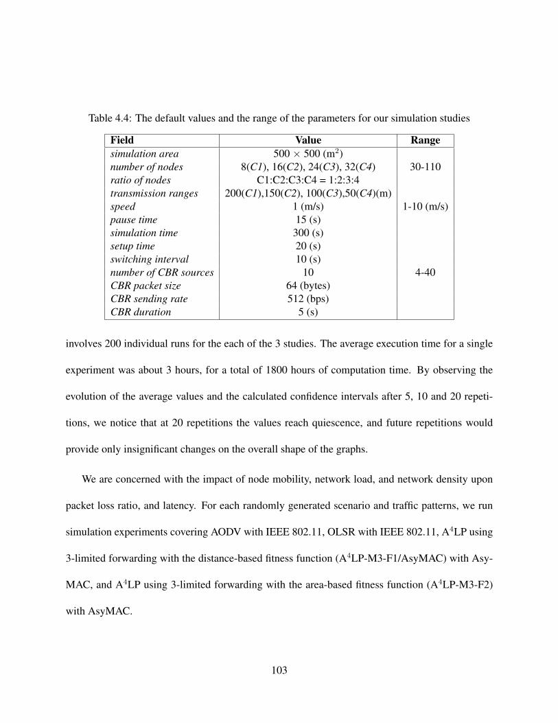
Table 4.4: The default values and the range of the parameters for our simulation studies
Field Value Rangesimulation area 500 × 500 (m2)number of nodes 8(C1), 16(C2), 24(C3), 32(C4) 30-110ratio of nodes C1:C2:C3:C4 = 1:2:3:4transmission ranges 200(C1),150(C2), 100(C3),50(C4)(m)speed 1 (m/s) 1-10 (m/s)pause time 15 (s)simulation time 300 (s)setup time 20 (s)switching interval 10 (s)number of CBR sources 10 4-40CBR packet size 64 (bytes)CBR sending rate 512 (bps)CBR duration 5 (s)
involves 200 individual runs for the each of the 3 studies. The average execution time for a single
experiment was about 3 hours, for a total of 1800 hours of computation time. By observing the
evolution of the average values and the calculated confidence intervals after 5, 10 and 20 repeti-
tions, we notice that at 20 repetitions the values reach quiescence, and future repetitions would
provide only insignificant changes on the overall shape of the graphs.
We are concerned with the impact of node mobility, network load, and network density upon
packet loss ratio, and latency. For each randomly generated scenario and traffic patterns, we run
simulation experiments covering AODV with IEEE 802.11, OLSR with IEEE 802.11, A4LP using
3-limited forwarding with the distance-based fitness function (A4LP-M3-F1/AsyMAC) with Asy-
MAC, and A4LP using 3-limited forwarding with the area-based fitness function (A4LP-M3-F2)
with AsyMAC.
103

The influence of network load
The effect of the network load upon the packet loss ratio for two standard protocol stacks
AODV/802.11, OLSR/802.11 and for A4LP-M3-F1/AsyMAC and A4LP-M3-F2/AsyMAC is sum-
marized by Figure 4.10. The ratio of the packets lost by AODV/802.11 is roughly twice the rate
of the packets lost by the other protocols. The major reason is that flooding, an inefficient broad-
cast solution, is used in AODV/802.11 for finding a route. Among the other protocols, A4LP-
M3-F2/AsyMAC performs the best, followed by OLSR/802.11, which delivers more packets than
A4LP-M3-F1/AsyMAC for similar scenarios and traffic patterns. OLSR/802.11 is able to deliver
packets only via symmetric links, thus packets are dropped if at least one asymmetric link is on the
critical path; however, A4LP/AsyMAC is able to deliver those packets. Our experiments also show
the metric we proposed in [WJM04] (A4LP-M3-F2), a combined metric with distance, power level
and class information, provides better performance than the distance only metric (A4LP-M3-F1)
in heterogeneous MANETs.
In our study, the measured values have relatively large confidence intervals, and most of these
confidence intervals overlap. This means that we do not have 95% confidence that for any particular
experimental instance the given protocol will perform better than the other protocol. Indeed, if
there are no (or very few) asymmetric links, the symmetric protocols will likely outperform the
asymmetric ones, due to the higher overhead of the asymmetric protocol. Unfortunately, the range
of the measurable values for metrics such as packet loss is very wide – in some scenarios there
might be no packet loss, in other ones, many of packets are lost. This variability is reflected in
104

1 2 3 4 5 6 7 8 9 1010
15
20
25
30
35
40
45
50
55
60
Network Load (Kbps)
Pac
ket L
oss
Rat
io (
%)
AODV / IEEE 802.11OLSR / IEEE 802.11A4LP−M3−F1 / AsyMACA4LP−M3−F2 / AsyMAC
Figure 4.10: Packet loss ratio versus network load. The ratio of packets lost by AODV/802.11is roughly twice the ratio of packets lost by the other protocols. Among the other protocols,A4LP-M3-F2/AsyMAC performs the best, followed by OLSR/802.11, which delivers more pack-ets than A4LP-M3-F1/AsyMAC for similar scenarios and traffic patterns.
1 2 3 4 5 6 7 8 9 100
500
1000
1500
2000
Network Load (Kbps)
Ave
rage
Lat
ency
(m
s)
AODV / IEEE 802.11OLSR / IEEE 802.11A4LP−M3−F1 / AsyMACA4LP−M3−F2 / AsyMAC
Figure 4.11: Average latency versus network load. The average latency of AODV/802.11 is muchhigher than the other protocols. Among the other protocols, OLSR/802.11 has the shortest latency.
105

relatively large confidence intervals. We believe that often when the average value of packet loss
is lower for one of the protocols, the protocol will perform in average better than the other ones.
The effect of the network load upon the average latency for two standard protocol stacks
AODV/802.11, OLSR/802.11 and for A4LP-M3-F1/AsyMAC and A4LP-M3-F2/AsyMAC is sum-
marized by Figure 4.11. The average latency of AODV/802.11 is much higher than that of the
other protocols. AODV is a reactive protocol which finds routes only when needed. A4LP is a
hybrid protocol, routes to non-neighbors are still discovered when needed, however, routes to cer-
tain In-, Out-, and In/Out-bound neighbors are maintained proactively in a routing table; this fact
contributes to the reduction of the average packet delivery latency.
The OLSR/802.11 stack has the lowest average packet delivery latency, followed by A4LP-M3-
F2/AsyMAC, and A4LP-M3-F1/AsyMAC. Note, however, that the average packet delivery latency
is based only on the delivered packets. The OLSR/802.11 stack drops more packets than A4LP-
M3-F2/AsyMAC; these are the packets which require a protocol able to deal with asymmetric
links. The packets that could be delivered by A4LP-M3-F2/AsyMAC but not by OLSR/802.11
generally have higher latency, and this could explain why the average packet delivery latency of
A4LP-M3-F2/AsyMAC is higher than that of OLSR/802.11.
The influence of node mobility
The average packet loss ratio versus node mobility is summarized in Figure 4.12. With the node
mobility increasing, the performances of A4LP-M3-F2/AsyMAC and OLSR/802.11 are degraded,
while the performance of AODV/802.11 fluctuates between 35% to 45%. AODV/802.11 performs
106

1 2 3 4 5 6 7 8 9 1010
20
30
40
50
60
70
Node Mobility (m/s)
Pac
ket L
oss
Rat
io (
%)
AODV / IEEE 802.11OLSR / IEEE 802.11A4LP−M3−F1 / AsyMACA4LP−M3−F2 / AsyMAC
Figure 4.12: Packet loss ratio versus node mobility. With the node mobility increasing, the perfor-mances of A4LP-M3-F2 and OLSR/802.11 are degraded while the performance of AODV/802.11fluctuates between 35% and 45%. AODV/802.11 performs the worst in case of ad hoc networkswith low mobility, but it outperforms the other protocols for highly mobile ad hoc networks.
1 2 3 4 5 6 7 8 9 100
500
1000
1500
2000
2500
Node Mobility (m/s)
Ave
rage
Lat
ency
(m
s)
AODV / IEEE 802.11OLSR / IEEE 802.11A4LP−M3−F1 / AsyMACA4LP−M3−F2 / AsyMAC
Figure 4.13: Average latency versus node mobility. The average latency of AODV/802.11 is muchhigher than the other protocols that perform similarly.
107

the worst in case of ad hoc networks with low mobility, but it outperforms the other protocols for
highly mobile ad hoc networks. The reason for this is that for ad hoc networks with relatively
high mobility, cached routes and neighbor information becomes stale rapidly, which degrades the
performance of proactive (OLSR) or hybrid (A4LP) protocols but not reactive (AODV) protocols.
However, A4LP-M3-F2/AsyMAC always outperforms OLSR/802.11 and A4LP-M3-F1/AsyMAC
at any node mobility in terms of packet loss ratio.
Figure 4.13 presents the average packet delivery latency versus node mobility. AODV, which
is an on-demand protocol, shows about the same relatively long latency irrespective of the mo-
bility of the nodes. For A4LP/AsyMAC and OLSR/802.11, the average latency increases with
the mobility since the protocols require additional overhead to keep the topology of the network
up-to-date. At the mobility of about 10 m/s, AODV/802.11, A4LP-M3-F1/AsyMAC and A4LP-
M3-F2/AsyMAC delivers packets with about the same latency. In these tests, OLSR/802.11 out-
performs A4LP/AsyMAC because the amount of topology data it needs to maintain is lower, being
restricted to the symmetric links only. This latency advantage comes at the cost of ignoring asym-
metric links, therefore, potentially disconnecting nodes which would maintain connectivity with
the A4LP/AsyMAC solution.
The influence of the number of nodes
In the following set of experiments, we vary the number of nodes moving in the measurement
area. As the nodes have a limited range, when the number of nodes is too low, some nodes might
lose connectivity.
108

30 40 50 60 70 80 90 100 11010
20
30
40
50
60
70
80
90
Number of Nodes
Pac
ket L
oss
Rat
io (
%)
AODV / IEEE 802.11OLSR / IEEE 802.11A4LP−M3−F1 / AsyMACA4LP−M3−F2 / AsyMAC
Figure 4.14: Packet loss ratio versus number of nodes. A4LP-M3-F2/AsyMAC delivers most pack-ets, followed by OLSR/802.11, A4LP-M3-F1/AsyMAC and AODV/802.11 for similar scenariosand traffic patterns. The packet loss ratio decreases when the number of nodes increases.
30 40 50 60 70 80 90 100 1100
500
1000
1500
2000
2500
Number of Nodes
Ave
rage
Lat
ency
(m
s)
AODV / IEEE 802.11OLSR / IEEE 802.11A4LP−M3−F1 / AsyMACA4LP−M3−F2 / AsyMAC
Figure 4.15: Average latency versus number of nodes. The average latency of AODV/802.11 ismuch higher than the other protocols. The packet delivery latency tends to decrease as the numberof nodes increases for A4LP/AsyMAC and OLSR/802.11.
109
Figure 4.14 illustrates the packet loss ratio versus the number of nodes. For similar scenar-
ios and traffic patterns, A4LP-M3-F2/AsyMAC delivers most packets, followed by OLSR/802.11,
A4LP-M3-F1/AsyMAC, and AODV/802.11. As the number of nodes in the network increases, the
network connectivity increases as well, thus the packet loss ratio decreases. Figure 4.14 shows that
the packet loss ratio decreases from roughly 60% to about 20% as the number of nodes increases
from 30 to 110.
Figure 4.15 shows the average packet delivery latency versus the number of nodes. The av-
erage latency of AODV/802.11 is much higher than the other protocols. For A4LP/AsyMAC and
OLSR/802.11 the packet delivery latency tends to decrease as the number of nodes increases. As
the number of nodes in the network increases, more neighbors and routes are found during the
neighbor information exchange process, thus the packet delivery latency decreases.
4.4.3 The Accuracy of Hidden Node Classification
A node is misclassified as a hidden node if it is silenced by the algorithm while it should not be
silenced. Misclassification reduces bandwidth utilization because it leads to unnecessary silencing
of nodes which could have been transmitting. A node is missed by the algorithm if it was not
silenced although it should have been. Missed nodes lead to collisions. The more accurate is a
protocol in classifying the nodes, the better the bandwidth utilization. A useful measure of the
global performance of an algorithm is the number of incorrect silencing decisions per transmission
- defined as the sum of misclassified and missed nodes.
110

40 50 60 70 80 90 100 110 1200
2
4
6
8
10
12
14
16
Number of nodes
Mis
clas
sifie
d no
des
/ tra
nsm
issi
on
Protocol AProtocol BAsyMAC
40 50 60 70 80 90 100 110 1200
0.5
1
1.5
2
2.5
Number of nodes
Mis
sed
node
s / t
rans
mis
sion
Protocol AProtocol BAsyMAC
(a) Misclassified nodes (b) Missed nodes
40 50 60 70 80 90 100 110 1200
1
2
3
4
5
6
7
8
9
Number of nodes
Inco
rrec
t sile
ncin
g ch
oice
s / t
rans
mis
sion
Protocol AProtocol BAsyMAC
(c) Incorrectly classified nodes
Figure 4.16: (a) The average misclassified nodes per transmission as a function of the number ofnodes. AsyMAC does not misclassify nodes in a static network. (b) The average missed nodes pertransmission for protocols A, B, and our approach, as a function of the number of nodes. (c) Theaverage number of incorrect silencing decisions per transmission for protocols A, B, and for ourapproach.
We compare the accuracy of the classification of our proposed AsyMAC protocol with the
accuracy of two known protocols which are performing the same classification [FTB02, PKD01].
The simulation environment is an area of 500 × 500 meters. We populate our environment with
a heterogeneous collection of nodes belonging to the four main classes of wireless nodes C1, C2,
111

C3, and C4 (see [MMJ03, WJM04]). The transmission ranges are normally distributed random
variables with the mean 100, 75, 50, and 25 meters, respectively and the standard deviations for
each class is 5 meters. The simulation scenarios are created using a set of 40 to 120 nodes including
an equal number of nodes for each class, uniformly distributed in the area. For each generated
scenario, we repeat the experiment 1000 times. The displacement of nodes are distributed around
an initial position and the standard deviation is 20% of its transmission range.
The results of the simulation are shown in Figure 4.16. The graph (a) shows the number of
misclassified nodes per transmission. The AsyMAC algorithm does not misclassify nodes in a
static network, because in the process of three-party proxy set formation, the nodes whose trans-
mission ranges do not reach the current node are filtered out. However, misclassified nodes can
appear with the AsyMAC protocol if the nodes are highly mobile and the current configuration
does not reflect the one detected when the three-party proxy set was established. The graph (b)
shows the missed nodes per transmission. Here the AsyMAC protocol performs worse than the
other two protocols considered, as it is considering only the three-party proxy sets, and ignores
possible higher order proxy sets. However, the number of missed nodes is very small for all the
three protocols. Graph (c) shows the number of incorrect silencing decisions per transmission.
Here, the AsyMAC protocol emerges with the lowest number of incorrect decisions, as its bet-
ter performance at misclassification compensates for the lower performance in regards to missed
nodes.
112

4.5 Summary
In this chapter, we argue that asymmetry of the transmission ranges in wireless networks is a reality
and should be treated as such. This asymmetry makes reliable communication more difficult and
requires special medium access control and routing protocols to handle it.
The models of traditional multiple access networks assumes that all nodes share a single com-
munication channel and have access to the feedback (success, idle slot, collision) from any trans-
mission. In this case, splitting algorithms allow sharing of the communication channel in a coop-
erative environment with reasonable efficiency and fairness. This is no longer the case for wireless
networks with asymmetric or unidirectional links, where the sender and the receiver do not share
the feedback channel and hidden nodes may interfere with ongoing transmissions.
In case of networks with asymmetric links, hidden nodes may be out of the reach for the
sender and the receiver, but their transmissions may interfere with the reception of a packet by
the intended destination. The hidden node problem is further complicated due to the fact that the
feedback from the receiver in a RTS/CTS exchange may have to pass through several relay stations
before reaching all the nodes which are expected to be silent.
Some of the solutions proposed in the literature reduce the probability of a collision by re-
quiring a larger set of nodes to be silent unnecessarily. In turn, this has negative effects upon the
communication latency and the overall throughput. We propose a MAC layer protocol, AsyMAC,
113

which reduces the number of nodes to be silenced and at the same time, it may miss some of the
nodes which should have been classified as “hidden”.
IEEE 802.11 assumes symmetric links between each pair of nodes while AsyMAC does not.
For traffic over asymmetric links, AsyMAC relies on a proxy node in the three-party proxy set to
relay acknowledgements back to the sender so that the reliability is assured. Our MAC protocol
reduces average packet loss ratio and average latency as asymmetric links are comprehensively
utilized which dominate the routing in heterogeneous MANETs.
We conducted a simulation experiment using the NS-2 simulator and compared the perfor-
mance of AODV/802.11, OLSR/802.11, A4LP using 3-limited forwarding with distance metric
(A4LP-M3-F1) with AsyMAC, and A4LP using 3-limited forwarding with the metric proposed
in [WJM04] (A4LP-M3-F2) with AsyMAC. It is reported that A4LP/AsyMAC performs much
better than AODV/802.11 in the aspects of average packet loss ratio and average latency. A4LP-
M3-F2 with AsyMAC incurs much less average packet loss ratio compared to OLSR/802.11. Our
simulation results also indicate that the fitness function proposed in [WJM04] is more proper than
the traditional distance function used in heterogeneous MANETs.
114

CHAPTER 5THE TIME-PARALLEL SIMULATION OF WIRELESS AD HOC
NETWORKS
The development of communication systems requires rigorous performance studies. Analytical
performance studies can only be carried for simple models of complex systems; such studies tend
to provide a basic understanding of system behaviors and qualitative results. Simulation, on the
other hand, is often used for quantitative performance study of more realistic models of complex
systems.
Wireless ad hoc networks are rarely amenable to analytical performance analysis due to the
complexity of the models involved. Simulation has emerged as an important tool for the study of
wireless ad hoc networks, but it is commonly used to study networks with a few hundred nodes for
a relatively short period of time.
There are many high quality simulators either developed in academic environments such as
NS-2 [VIN], GloMoSim [ZBG98] or commercial offerings such as OpNet [OPN] and QualNet
[QN]. However, we find that the recent evolution of wireless systems are creating environments
with thousands of nodes and/or very high density of wireless resources, and these scenarios are
pushing the limits of serial simulators such as NS-2. Even when feasible, such simulations require
a significant computing power and can take a very long time. Although there is a clearly perceived
115

need to develop simulators which can take advantage of parallel or cluster computers, the problem
of parallelizing simulations through spatial partitioning turned out to be very difficult, due to the
heavy interaction between the spatial partitions.
In this dissertation, we present an approach for time-parallel simulation of wireless ad hoc
networks. Time-parallel simulation has been used for some time; its applicability is strongly de-
pendent on the simulated phenomena and can yield exact results only for systems whose behavior
is modeled by regenerative stochastic processes. However, as we will show, good approximations
can be obtained quickly, and the quality of the approximation can be improved through iteration.
Our time-parallel simulation of wireless ad hoc networks uses a traditional simulation package
coupled with new techniques for the practical implementation of the simulation. We develop a
methodology to analyze the accuracy of the simulation and introduce the notion of perturbation
of measurements; then we present a layer-by-layer analysis of the impact of the perturbations on
the performance of the network. This approach allows us to predict the accuracy of the simulation
results through an analysis of the protocols involved at each layer.
This chapter is organized as follows. We present a one-step time-parallel simulation model
in Section 5.1, then in Section 5.2 we presents our model of the propagation of perturbations
in wireless networks, the impact of the protocols at the various layers of the networking stack,
and the application for time-parallel simulation. We apply these considerations to propose several
methods for improving the speed and accuracy of time-parallel simulation. Section 5.3 presents the
implementation of the theoretical models developed in the previous section with the widely used
116
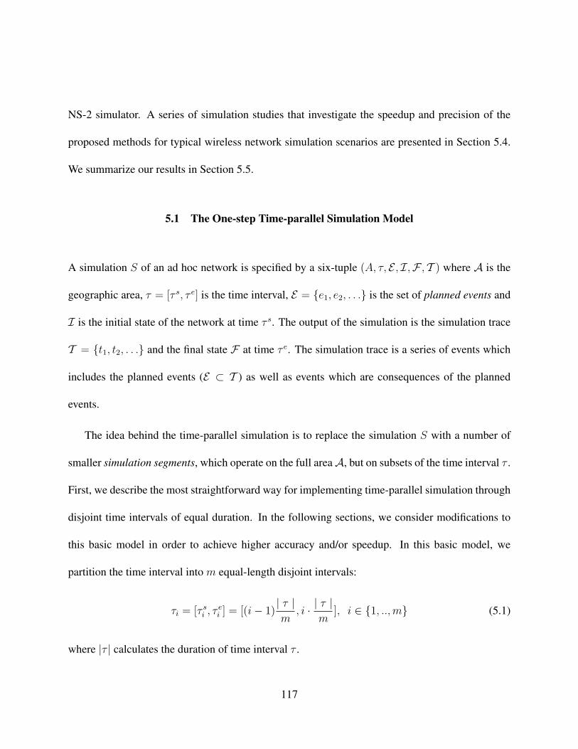
NS-2 simulator. A series of simulation studies that investigate the speedup and precision of the
proposed methods for typical wireless network simulation scenarios are presented in Section 5.4.
We summarize our results in Section 5.5.
5.1 The One-step Time-parallel Simulation Model
A simulation S of an ad hoc network is specified by a six-tuple (A, τ, E , I,F , T ) where A is the
geographic area, τ = [τ s, τ e] is the time interval, E = {e1, e2, . . .} is the set of planned events and
I is the initial state of the network at time τ s. The output of the simulation is the simulation trace
T = {t1, t2, . . .} and the final state F at time τ e. The simulation trace is a series of events which
includes the planned events (E ⊂ T ) as well as events which are consequences of the planned
events.
The idea behind the time-parallel simulation is to replace the simulation S with a number of
smaller simulation segments, which operate on the full areaA, but on subsets of the time interval τ .
First, we describe the most straightforward way for implementing time-parallel simulation through
disjoint time intervals of equal duration. In the following sections, we consider modifications to
this basic model in order to achieve higher accuracy and/or speedup. In this basic model, we
partition the time interval into m equal-length disjoint intervals:
τi = [τ si , τ e
i ] = [(i− 1)| τ |m
, i · | τ |m
], i ∈ {1, .., m} (5.1)
where |τ | calculates the duration of time interval τ .
117

Let t(e) be the firing time of an event e, this also implies the partitioning of the planned event
set:
Ei = {ei | ei ∈ E , τ si ≤ t(ei) < τ e
i } (5.2)
The segments of the time-parallel simulation are specified by the six-tuple (A, τi, Ei, Ii,Fi, Ti). As
the segments are m times shorter than in the original simulation, their execution will take roughly
m times shorter time, and they can be executed in parallel on m independent processors. The
simulation trace of the full simulation will be the union of the simulation traces T = T1
⋃. . .
⋃ Tm,
while the final state of the network will be F = Fm.
The main difficulty pertains the calculation of the initial state Ii. For the first segment, we have
I1 = I. For the other segments, the correct initial state is the final state of the previous segment
Ii = Fi−1. However, using the final state of the previous simulation segment would require the
in-order simulation of the segments, preventing any parallelism.
One crude approximation would be to assume that every simulation segment starts with the
original state of the network (I). In this one-step time-parallel simulation model, the simulation
segments are specified by (A, τi, Ei, I,Fi, Ti).
Experiments show that the accuracy of the one-step time-parallel simulation is not sufficient
for the practical purposes of wireless ad hoc network simulation. In the following, we analyze the
source of errors in the time-parallel simulation of wireless ad hoc networks, estimate the magnitude
of these errors, and propose methods to improve the accuracy of the simulation.
118

5.2 Perturbation Analysis and Improving Accuracy of Time-Parallel Simulation
A simulation trace includes planned events, (E ⊂ T ), as well as new events triggered by the
planned events and calculated by the simulation process. For example the event corresponding to
sending a packet may trigger a new event indicating a collision with with another transmission.
Every event ei has a set of properties, e.g, the firing time of the event t(ei), the type of the event,
the packet size, etc. Such information allows us to determine important measures of performance
such as packet delay, packet loss ratio, throughput, and so on.
The purpose of running a simulation is to collect the information associated to the events in the
trace. However, we are rarely interested in individual events, we are concerned with observations,
or measurements, spanning longer time intervals, or the entire trace.
5.2.1 Measurements on the Simulation Trace
Measurements can be:
(a) instantaneous M i(tc), reflecting the situation at the current time tc.
(b) cumulative M c(tc), reflecting the evolution of the measurement from the beginning of the
simulation to the current time tc. For every instantaneous measurement M i, there is an associated
cumulative measurement M c:
M c(tc) =
∫ tc
0
M i(t)dt (5.3)
119

(c) average Ma(tc). For every instantaneous measurement M i, there is an associated average
measurement Ma defined by:
Ma(tc) =
∫ tc0
M i(t)dt
tc(5.4)
An example is of instantaneous measurement is the current transmission rate, with the asso-
ciated cumulative measurement total transmitted data, and the associated average measurement
average transmission rate.
Many average measurements are expressed as ratios of measured quantities. For some of these
measurements, we find it useful to define the complementary measure C(Ma) = 1 − Ma. For
instance the ratio measure average packet loss ratio has its complement average packet delivery
ratio.
5.2.2 Perturbations on a Measurement
In the following, we investigate how an event perturbs the measurements of a simulation of wire-
less ad hoc networks. Our model accurately captures the underlying phenomena and provides a
framework in which observations can be analyzed and predictions can be made.
We call an approximate simulation for the measurement M , related to simulation S, a simula-
tion S ′ which generates a trace T ′ such that M(T ′) ≈ M(T ).
The absolute error of simulation for measurement M is
δM = |M(T )−M(T ′)| (5.5)
120
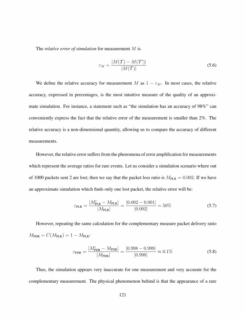
The relative error of simulation for measurement M is
εM =|M(T )−M(T ′)|
|M(T )| (5.6)
We define the relative accuracy for measurement M as 1 − εM . In most cases, the relative
accuracy, expressed in percentages, is the most intuitive measure of the quality of an approxi-
mate simulation. For instance, a statement such as “the simulation has an accuracy of 98%” can
conveniently express the fact that the relative error of the measurement is smaller than 2%. The
relative accuracy is a non-dimensional quantity, allowing us to compare the accuracy of different
measurements.
However, the relative error suffers from the phenomena of error amplification for measurements
which represent the average ratios for rare events. Let us consider a simulation scenario where out
of 1000 packets sent 2 are lost; then we say that the packet loss ratio is MPLR = 0.002. If we have
an approximate simulation which finds only one lost packet, the relative error will be:
εPLR =|M ′
PLR −MPLR||MPLR| =
|0.002− 0.001||0.002| = 50% (5.7)
However, repeating the same calculation for the complementary measure packet delivery ratio
MPDR = C(MPLR) = 1−MPLR:
εPDR =|M ′
PDR −MPDR||MPDR| =
|0.998− 0.999||0.998| ≈ 0.1% (5.8)
Thus, the simulation appears very inaccurate for one measurement and very accurate for the
complementary measurement. The physical phenomenon behind is that the appearance of a rare
121

event, e.g. a packet loss in a lightly loaded network, is dependent on the coincidence of a number of
factors. An approximate simulation might approximate well the probability of occurrence of those
factors, but not the exact location and time where the event will take place. Therefore, the absolute
error might be a better indicator of the accuracy of simulation for the measurements on rare events.
The absolute error has the additional advantage that the absolute error of the measurement and the
complementary measurement is identical:
δM = |M(T )−M(T ′)| = |(1−M(T ))− (1−M(T ′))| = δC(M) (5.9)
Now we introduce the notion of a perturbing event ep. We consider a simulation with the
planned events E = {e1, e2, . . .} and a perturbed set E ′ = E ⋃ep. The perturbed set of planned
events will lead to a simulation trace T ′ and, obviously, to perturbed measurements M ′(t). We are
interested in the size and the temporal extent of the perturbations ∆M(t) = M ′(t) − M(t). We
say that:
• The perturbation has no effect on measurement M if ∆M(t) = 0, ∀t.
• The event ep creates a time limited perturbation in the measurement M which lasts until the
extinction time te if ∆M(t) = 0, ∀t > te.
• The event ep has a shift effect perturbation on the measurement M if limt→∞(∆M(t)) = c,
with c being the shift constant. If there exists a time point ts with the property that ∆M(t) =
c, ∀t > ts, we call ts the stabilization point.
122

Property 1: If an event ep causes a time-limited perturbation on the instantaneous measurement
M i with the extinction time te, it creates a shift effect perturbation on the corresponding cumulative
measurement M c, with the stabilization point ts = te. The shift constant can be expressed as:
c =
∫ te
t(ep)
∆M i(t)dt (5.10)
• We say that an event causes a destabilizing perturbation of measurement M if @ ts > t(ep)
such that ∆M = c, ∀t > ts.
5.2.3 Propagation of Perturbations in Wireless Ad Hoc Networks
As a first approximation, the events in a wireless ad hoc network are caused by individual trans-
missions of packets. We consider the perturbing event to be the insertion of a new packet in the
network. The removal of the packet is not considered separately, because it is equivalent to simply
reversing the perturbed and the original system. As we are concerned about the absolute values
of the difference on the measurements of these systems, the reversed system will yield the same
conclusions. An additional type of perturbation we consider is the perturbation of the initial state,
that is, the simulation starts with a different initial state than expected. We discuss this type of
perturbation separately.
For events representing the addition or removal of a single packet, the immediate affect of the
perturbations is usually minimal. However, the networking protocols deployed at various levels
of the networking stack can amplify or (in some cases) reduce the impact of the perturbations.
123

In the following, we investigate the impact of the protocols deployed at the various layers of the
networking stack on the perturbation produced by the insertion of a single packet.
Physical layer. An inserted packet will perturb the physical layer measurements only for the
duration of the packet transmission. The time it takes to transmit a packet can be calculated as
follows. Assume that we send a packet of 1536 bit, the maximum length supported by the 802.11b
protocol. The transmission rate of 802.11b is 1.375 Mbps. The time required to send this packet is
composed of:
• Distributed Inter-Frame Space (DIFS), set to 50µs
• Data packet transmission: 192µs for the preamble + 1536/ 1.375Mbps = 192µs + 1118µs
• Short Inter-Frame Space (SIFS), set to 10µs
• 802.11 ACK packet: 192µs + 14/1.375Mbps = 203µs
Thus, the total transmission time becomes 2084µs, or approximately, 2 ms. This might change
slightly for different protocols, but the order of magnitude remains the same. We conclude that
the perturbation at the physical layer due to a new packet is time-limited, with a very short (2 ms)
extinction time.
MAC layer. The perturbation caused by an inserted packet at the MAC layer depends on the
load of the network, and the type of the inserted packet. If the packet is a control packet such as
RTS, CTS, or ACK, its influence extends beyond the time frame covered. For instance, receiving
124

an RTS packet in a CSMA/CA network forces the node to refrain from transmitting for the duration
specified in the packet. The size of this interval can be as long as the maximum packet transmission
time, on the order of magnitude of 2µs.
Delaying the sending of a packet can in its turn delay the sending of the response or follow-up
packets, creating a ripple effect. Normally, this will appear as a time-limited perturbation. For a
TDMA (Time Division Multiple Access) type protocol, for a channel with the capacity of n bps,
with a load of ν ≤ 1, and a packet size of l, the extinction time can be estimated as:
te =l
n · (1− ν)(5.11)
Note that for a full channel, ν = 1, the perturbation becomes a shift effect perturbation.
For CSMA/CD (Carrier Sense Multiple Access with Collision Detection) protocols, the per-
turbation will extend to the length of the contention window. IEEE 802.11b uses an exponential
back-off algorithm where the contention window (CW) can vary between CWMIN and CWMAX. Typ-
ical values of CWMIN are between 7-15 and of CWMAX are between 7-255 with the numbers being
multiples of a slot time which is 20µs in IEEE 802.11b. Thus, the influence of the initial collision
can extend to 5000µs. However, if the channel is very busy, the initial collision can lead to fur-
ther collisions down the line. Furthermore, every collision extends the collision window through
exponential back-off, which will be only gradually reduced.
In conclusion, for highly loaded networks, the insertion of a packet that creates a collision can
cause perturbations for up to several seconds in the worst case.
125

Network layer. Perturbations triggered by packet insertion at the network layer are heavily
dependent on the nature of the protocol and the inserted packet. The critical question is whether
the packet will change the routing of future packets or not. If the packet is part of an established
flow of application layer data, it will most likely not affect the routing of the other packets. If
the packet is the first packet of a new flow, and the routing protocol is a reactive one, the packet
will establish a new route. This frequently requires broadcast of routing information, which in its
turn triggers the transmission of additional packets. Although this appears to be a destabilizing
perturbation, the extent of this flooding is carefully constrained by the routing protocol and it will
last at most several seconds.
Proactive routing algorithms deploy a routing table periodically updated by routing packets.
The insertion of a routing packet triggers a perturbation in the network by changing the routing
table of a node, and this will affect the routing of future packets. This is a major perturbation,
affecting a large number of packets and a time interval on the order of minutes. A routing table
perturbation is extinct when the routing tables of the original and the perturbed system re-converge.
This situation occurs when:
• The modified routes are superseded by new, independently discovered routes, in both the
original and the perturbed system (for instance, as a result of node mobility).
• The original system acquires the same routes as the perturbed one.
• The modified routes expire through a timeout and the routing table returns to the unperturbed
version.
126

• An external command or a predetermined timeout flushes partially or completely the routing
tables, forcing the recomputing of all routes.
Although it is technically possible to imagine a routing protocol where the loss or addition of a
single routing packet would change the routes indefinitely, virtually all protocol designers, in their
quest to make the protocols more reliable, have adapted features which make the routing tables
converge; this has the indirect effect of limiting the perturbations and improve the accuracy of
time-parallel simulations.
Transport layer and application layer. Finally, we investigate how a perturbing event af-
fects the transport layer and the application layer protocols. The major difference here is between
reliable or non-reliable protocols. Let us consider the case of the most frequently used reliable
transport protocol, TCP. The loss of a single TCP packet can significantly perturb the subsequent
TCP flow: the packet will be retransmitted, the transmission window reset to its minimal value,
which will then extend through the slow start algorithm. Thus, the loss of a single packet can exert
an influence over the network for several tens of seconds.
In the case of the UDP protocol, which does not implement reliable transmission, the pertur-
bation is minimal or nonexistent at the transport layer. However, applications which deploy UDP
at the transport layer frequently use application layer protocols to control the flow of data. For in-
stance, the multimedia streaming application RealPlayer is using an application level byte stream
protocol RTP (Real-time Transport Protocol, specified in RFC 1889) for the transfer of multime-
dia information, with UDP being the transport protocol. Packet losses are handled by a complex
127

logic and actions involving the RTSP (Real Time Streaming Protocol), RTCP (Real Time Control
Protocol), SDP (Session Description Protocol) and, of course RTP.
We conclude that perturbations have effects up to the application layer. However, at the appli-
cation layer, the behavior of the system becomes very complex, and in some cases, small perturba-
tions can have major effects on the state of the system. This problem is not specific to time-parallel
simulation. Most simulation studies of wireless ad hoc networks consider scenarios with constant
or variable bit rate generic UDP sources, without application level protocols deployed in the simu-
lator. When application level flow is simulated, it is done by an artificially generated stream which
replicates the properties of a packet stream generated by the application level protocol, without
actually deploying the application in the simulator [WAH06]. In these types of models pertur-
bations propagate only over very short time frames, thus creating an environment favorable for
time-parallel simulation.
Up to this moment we have considered only perturbations caused by a single perturbing event.
In the following, we discuss the possible inter-event perturbations, that is, the perturbations which
arise from the interaction between two or more independent perturbing events. There can be several
ways in which the perturbations caused by several events can be are composed:
Dual events. Dual events cancel each other; their successive occurrence does not change the
state of the system. For instance, a reboot sequence is represented by two events: a node failure,
followed after a short time by the node recovery. Individually, each event causes a perturbation,
128

however, their effects cancel each other. The state of the system will be the same as if none of the
events occurred. This favorable case rarely occurs in practice.
Idempotent events. Idempotent events lead to the same state regardless if only one, a subset,
or all of them occur. For instance, two subsequent missed routing table updates create the same
effect – an incorrect routing table entry, which requires the need to run a path discovery process.
Idempotent events appear whenever some component of the system has a special “correct” state,
while the other, “incorrect” states are functionally identical. Such system components are relatively
frequent; examples are routing table entries or established end-to-end connections.
Independent events. Independent events lead to the same state of the system regardless of the
order in which they occur; the overall perturbation of state caused by the events is additive. Their
compound effect can be studied considering the perturbations caused by the individual events
independently.
Mutually amplifying events. Such events lead to drastic alteration of state; the perturbation
caused by the a sequence of such events is significantly larger than the perturbations caused by the
individual events occurring independently. For example, an event that causes a routing table to be
overwritten with incorrect values and the second event that propagates the incorrect routing table
to all the nodes in the network, will cause the network failure.
Naturally, mutually amplifying events are the worst scenario from the point of view of the ac-
curacy of the time-parallel simulation. We need to carefully consider whether they can occur in
the considered scenarios. Note that in our hypothetical example, the mutually amplifying events
129

caused a total interruption of the communication in the simulation. Practically deployed network-
ing stacks contain build-in guards against such types of unstable behavior. Mutually amplifying
events are clearly possible during the experimental testing of new routing or MAC protocols. The
observation of such an unstable behavior is an important feedback to the developers; at the same
time, they need to be aware that the errors in the time-parallel simulation of such unstable systems
are significantly higher.
We conclude that inter-event interactions yield perturbations which are identical or smaller than
the perturbations considered individually, for most practically deployed, stable protocols. Mutually
amplifying events, however, are possible if the deployed protocol stack shows unstable behavior
(most frequently, as a result of experimental code). In these cases the accuracy of the simulation
will be much lower.
5.2.4 Techniques for Improving the Accuracy of Time-Parallel Simulation
Let us now return to the one-step time-parallel simulation described in Section 5.1, and consider
the sources of errors in the approximation. For instance, in Figure 5.1(a) we see a partitioning of
the simulation interval [0, t] into three equal time intervals: [0, t1 = t/3], [t1 = t/3, t2 = 2t/3] and
[t2 = 2t/3, t]. The event e1, in the first segment is creating a perturbation which is not extinguished
until the middle of the second segment. As the two segments are simulated independently, the
processor simulating the second segment does not know about the perturbation which leads to an
130

t e 1 e 2 t 2 t 1
t e 1 e 2 t 2 t 1
t e 1 e 2 t 2 t 1
t e 2 t 2
(a)
warmup interval
measured interval
compressed history
(b)
(c) (d)
measured interval
measured interval
measured interval
e 1
Figure 5.1: An illustration of techniques for improving the accuracy of time-parallel simulation.(a) Equal length batches without improvement. (b) Time interval shift. (c) Warmup intervals. (d)Warm up with compressed history.
inaccurate simulation. Let us now review several techniques through which this inaccuracy can be
reduced or eliminated.
Time interval shift. One way to increase the accuracy of the simulation is to select the bound-
aries of the simulation intervals such that the perturbations are completely contained in the seg-
ments, as shown in Figure 5.1(b). These points are the equivalent of the regenerative states of
stochastic processes. If we cannot find states where all the perturbations are extinguished, we can
131

search for points where there are a comparatively smaller number of ongoing perturbations (partial
regenerative states).
There are several problems with this approach. First, there might not be any regenerative
states in the simulation, or their distribution might not lead to segments of size appropriate for
parallelization. The most difficult problem, however, is to find regenerative or partially regenerative
states in a simulation without first running the simulation itself. There are certain circumstances
that the identification of such points is possible. If a routing protocol periodically flushes the
complete set of routing information, that instance corresponds to a regenerative state. Similarly,
long periods of silence can be used as regenerative states, and they can be identified with an initial
analysis of the scenario.
Warmup interval. This technique relies on separating the time span of the simulation segment
into a warmup interval followed by the measurement interval. During the warmup interval, we
perform the simulation but do not perform any measurements. Thus, the simulation performed
during the measurement interval will be more accurate, since it considers not only the events
occurring during the measurement interval, but also the perturbations caused by events generated
during the warmup interval.
The ideal size of the warmup interval is the shortest period which contains all the perturbing
events that generate perturbations extending to the measurement interval (see Figure 5.1(c)). The
size of the required warmup interval can vary between various segments, the first segment does not
132

require a warmup interval. Unfortunately, for practical cases we cannot accurately compute the
ideal duration of the warmup interval without first running the simulation.
Warmup with compressed history. In a practical run of time-parallel simulation with warmup
interval, the size of the warmup interval can be significantly longer than the measurement interval;
thus most of the computation time is spent into the simulation of the warmup interval, which does
not contribute to the measurements. Traditionally, the warmup interval is the exact copy of the
simulation scenario for a period before the measurement interval. We can replace the warmup
interval with a shorter and/or simpler simulation interval which, however, would yield the same
results. For instance, we can remove all the events from the warmup interval which do not produce
perturbations at the measured point. For the events which produce perturbations, we might be able
to replace them with events that are easier and faster to simulate. We call this modified warmup
interval a compressed history (see Figure 5.1(d)).
Initial state approximation (ISA). In this technique, we are computing an approximation of
the initial state of the simulation segments without previous execution of the simulation. We had
seen that for a typical simulation of a wireless ad hoc network the perturbation with the largest
impact on the measurements relates to the changes in the routing tables. As most simulations
start with an empty routing table which will be filled in during the initial phase of the simulation,
which becomes a major source of errors. Approximating the routing table at the beginning of each
simulated segment can thus significantly increase the accuracy of the simulation.
133

Composite methods. The methods of improving the precision of the time-parallel simulation
can be used in conjunction with one another. The warmup interval can be composed of two phases:
one compressed history (for instance, covering the complete time frame from the beginning of
the simulation), followed by a warmup interval operating on the original planned event list. The
initial state approximation method can be used to approximate the state at the beginning of the
warmup interval. The time interval shift method can also be deployed in conjunction with any of
the methods.
5.3 Implementation of Time-parallel Simulation for Ad Hoc Networks
In the following, we present our implementation of the time-parallel simulation using the NS-2
simulator [VIN]. The first method, based on the iteratively extended warmup of the simulation
segments, can be deployed without changes to the NS-2 implementation of the protocols. An alter-
native method that combines iteratively extended warmup and initial state approximation produces
better results; this method requires some knowledge of the implementation of the routing protocol
and additional code to allow the initialization of the routing tables.
Let us now highlight the relevant features of the NS-2 simulator. We defined a simulation as
the transformation of the six-tuple (A, τ, E , I,F , T ) into the output consisting of the final state F
and the simulation trace T . While NS-2 is compatible to this definition, there are differences in
our ability to extract, interpret and modify the different components.
134

The NS-2 script and trace files, E and T , are very easy to create, parse and filter; they consist
of lines of text, one event per line. Once the simulation passes a given time line, the output at that
time point immediately becomes available, thus the data can be extracted while the simulation is
still in progress.
In contrast, it is relatively difficult to generate and extract the initial and final state of the
simulation. The data associated with the state is distributed across the protocol implementations;
there is no standard format and API through which this information can be accessed. While there
is no obstacle in principle to access this information, this task needs to be handled case by case,
and it requires extensive knowledge of the implementation details of the protocols involved. We
proposed an alternative method that relaxes the need for state saving and restoration such that we
can use the stock unpatched simulator for simulation of arbitrary protocols.
5.3.1 Time-parallel Simulation with Iteratively Extended Warmup Interval
Our first method for implementing time-parallel simulation relies on iterative extension of the
warmup interval. The approach allows us to obtain simulation results with increasingly higher
accuracy during the runtime of the simulation. The simulation can be stopped when the desired
accuracy is reached. This approach does not require the manipulation of the initial or the final
state of the simulation, thus it is independent of the simulated protocols. Nevertheless, different
protocols might converge at a different speed to the correct solution.
135

We partition the temporal dimension of a simulation S = (A, τ, E , I,F , T ) into m time in-
tervals {τi|τi = [(i − 1) |τ |m
, i |τ |m
], 1 ≤ i ≤ m}. Then, we obtain a time-parallel simulation set
L(0) = {S(0)i |S(0)
i = (A, τi, E (0)i , I,F (0)
i , T (0)i ), 1 ≤ i ≤ m}, in which all simulation segments
start with the initial state of the network (I). Thus the time-parallel simulation set will operate on
the full spatial component A, but a subset of the temporal span τi. We call this raw time-parallel
simulation method as the TPS algorithm. In case of an exact simulation, the final state of S(0)i
needs to match the initial state of S(0)i+1, 1 ≤ i ≤ m−1. However, since there is no prior knowledge
for the initial states of S(0)2 , . . . , S
(0)m , when they are parallelized, the combined simulation trace
T (0) = T (0)1 ∪ T (0)
2 ∪ . . . ∪ T (0)m is far from being approximate.
We notice that the simulation trace of S(0)1 becomes an accurate trace after the execution of
L(0). As we discussed in Section 5.2.4, a solution to refine the other simulation traces is to apply
a warmup interval before the measurement interval, or say, to apply the final state of a simulation
interval to the initial state of its successive simulation interval. The new simulation set becomes
L(1) = {S(1)i |S(1)
i = (A, τi, E (1)i ,F (0)
i−1,F (1)i , T (1)
i ), 2 ≤ i ≤ m}}. The causality dependencies of
events of two consecutive time intervals are now removed, meanwhile the dependencies for events
in a time interval to affect later time intervals are weakened, since the strongest causality depen-
dencies (dependencies of two consecutive time intervals) are already removed. The combined
simulation trace after the first iteration, T (1) = T (0)1 ∪ T (1)
2 ∪ T (1)3 ∪ . . . ∪ T (1)
m , should become
more accurate, compared to T (0).
136

As we repeat this process, all strong dependencies between consecutive simulation intervals
are further removed and the simulation trace becomes more accurate. The parallel simulation
continues until the error of simulation results in all relevant metrics is lower than a pre-defined
threshold. The k-thiteration contains m− k simulation segments
L(k) = {S(k)i |S(k)
i = (A, τi, E (k)i ,F (k−1)
i−1 ,F (k)i , T (k)
i ), i ∈ {k + 1, . . . , m}} (5.12)
After the k-th iteration, the traces of simulation intervals S(0)1 , S
(1)2 , . . . , S
(k)k+1 become accurate.
The combined simulation trace of L(k) can be obtained by
T (k) = T (0)1 ∪ T (1)
2 ∪ T (2)3 ∪ . . . ∪ T (k−1)
k ∪ T (k)k+1 ∪ T (k)
k+2 ∪ . . . ∪ T (k)m (5.13)
We illustrate the approximate simulation in the following example, see Figure 5.2. Assume a
simulation S = (500× 500, [0, 180], E , I,F , T ) is segmented into 9 equal-duration time intervals,
with τi = [20(i− 1), 20i], i ∈ {1, . . . , 9}. The simulation sets of iteration 0, 1, 2 are as follows
L(0) = S(0)1 ∪ S
(0)2 ∪ S
(0)3 ∪ S
(0)4 ∪ S
(0)5 ∪ S
(0)6 ∪ S
(0)7 ∪ S
(0)8 ∪ S
(0)9 ∪ S
(0)9 ;
L(1) = S(1)2 ∪ S
(1)3 ∪ S
(1)4 ∪ S
(1)5 ∪ S
(1)6 ∪ S
(1)7 ∪ S
(1)8 ∪ S
(1)9 ∪ S
(1)9 ;
L(2) = S(2)3 ∪ S
(2)4 ∪ S
(2)5 ∪ S
(2)6 ∪ S
(2)7 ∪ S
(2)8 ∪ S
(2)9 ∪ S
(2)9 .
(5.14)
The simulation traces after iterations 0, 1, 2 are as follows
T (0) = T (0)1 ∪ T (0)
2 ∪ T (0)3 ∪ T (0)
4 ∪ T (0)5 ∪ T (0)
6 ∪ T (0)7 ∪ T (0)
8 ∪ T (0)9 ;
T (1) = T (0)1 ∪ T (1)
2 ∪ T (1)3 ∪ T (1)
4 ∪ T (1)5 ∪ T (1)
6 ∪ T (1)7 ∪ T (1)
8 ∪ T (1)9 ;
T (2) = T (0)1 ∪ T (1)
2 ∪ T (2)3 ∪ T (2)
4 ∪ T (2)5 ∪ T (2)
6 ∪ T (2)7 ∪ T (2)
8 ∪ T (2)9 .
(5.15)
137
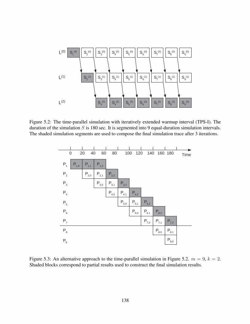
S 1 (0) S 2
(0) S 3 (0) S 4
(0) S 5 (0) S 6
(0) S 7 (0) S 8
(0) S 9 (0)
S 2 (1) S 3
(1) S 4 (1) S 5
(1) S 6 (1) S 7
(1) S 8 (1) S 9
(1)
S 3 (2) S 4
(2) S 5 (2) S 6
(2) S 7 (2) S 8
(2) S 9 (2)
L (0)
L (1)
L (2)
Figure 5.2: The time-parallel simulation with iteratively extended warmup interval (TPS-I). Theduration of the simulation S is 180 sec. It is segmented into 9 equal-duration simulation intervals.The shaded simulation segments are used to compose the final simulation trace after 3 iterations.
P 1,0 P 1,1 P 1,2 P 1
P 2,0 P 2,1 P 2,2
P 3,0 P 3,1 P 3,2
P 4,0 P 4,1 P 4,2
P 5,0 P 5,1 P 5,2
P 6,0 P 6,1 P 6,2
P 7,0 P 7,1 P 7,2
P 8,0 P 8,1
P 9,0
P 2
P 3
P 4
P 5
P 6
P 7
P 8
P 9
20 40 60 80 0 100 120 140 160 180 Time
Figure 5.3: An alternative approach to the time-parallel simulation in Figure 5.2. m = 9, k = 2.Shaded blocks correspond to partial results used to construct the final simulation results.
138
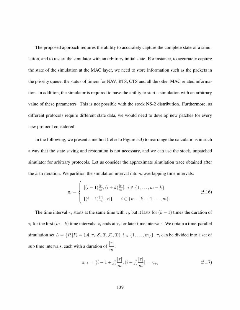
The proposed approach requires the ability to accurately capture the complete state of a simu-
lation, and to restart the simulator with an arbitrary initial state. For instance, to accurately capture
the state of the simulation at the MAC layer, we need to store information such as the packets in
the priority queue, the status of timers for NAV, RTS, CTS and all the other MAC related informa-
tion. In addition, the simulator is required to have the ability to start a simulation with an arbitrary
value of these parameters. This is not possible with the stock NS-2 distribution. Furthermore, as
different protocols require different state data, we would need to develop new patches for every
new protocol considered.
In the following, we present a method (refer to Figure 5.3) to rearrange the calculations in such
a way that the state saving and restoration is not necessary, and we can use the stock, unpatched
simulator for arbitrary protocols. Let us consider the approximate simulation trace obtained after
the k-th iteration. We partition the simulation interval into m overlapping time intervals:
πi =
[(i− 1) |τ |m
, (i + k) |τ |m
], i ∈ {1, . . . , m− k};
[(i− 1) |τ |m
, |τ |], i ∈ {m− k + 1, . . . , m}.(5.16)
The time interval πi starts at the same time with τi, but it lasts for (k + 1) times the duration of
τi for the first (m−k) time intervals; πi ends at τe for later time intervals. We obtain a time-parallel
simulation set L = {Pi|Pi = (A, πi, Ei, I,Fi, Ti), i ∈ {1, . . . , m}}. πi can be divided into a set of
sub time intervals, each with a duration of|τ |m
:
πi,j = [(i− 1 + j)|τ |m
, (i + j)|τ |m
] = τi+j (5.17)
139

Call Pi,j the j-th sub-interval of Pi (enumeration starts at 0):
Pi,j = (A, πi,j, Ei,j, Ii,j,Fi,j, Ti,j), 1 ≤ i ≤ m, 0 ≤ j ≤ min{k,m− i} (5.18)
where
Ii,j =
I, for j = 0;
Fi,j−1, for j > 1.
(5.19)
Then,
Pi =
Pi,0 + Pi,1 + . . . + Pi,k, i ∈ {1, . . . , m− k};
Pi,0 + Pi,1 + . . . + Pi,m−i, i ∈ {m− k + 1, . . . , m}.(5.20)
Pi,j simulates the same simulation interval as Si+j (πi,j = τi+j). For instance, in Figures 5.2
and 5.3, P3,2, P4,1 and S5 all simulate the simulation interval [80, 100].
We assume the same simulation S in Figure 5.2 as our example, m = 9, k = 2. The new
simulation set L = {P1, P2, . . . , P9} is shown in Figure 5.3. We observe that Pi,0 and Si are
essentially equivalent since they simulate the same time interval as well as the same set of events,
without prior knowledge of the initial states (see Figures 5.2 and 5.3). Thus, L(0) can be rewritten
as
L(0) = {S(0)i |i ∈ {1, . . . , m}} = {Pi,0|i ∈ {1, . . . , m}} (5.21)
The final state of simulation Pi,0 is naturally transferred as the initial state of simulation Pi,1, thus
Pi,1 and S(1)i+1 are essentially equivalent since they simulate the same time interval and the same set
of events with the same initial states. Thus, I(1) can be rewritten as
L(1) = {S(1)i |i ∈ {2, . . . , m}} = {Pi,1|i ∈ {1, . . . , m− 1}} (5.22)
140

Similarly,
L(k) = {S(k)i |i ∈ {k + 1, . . . , m}} = {Pi,k|i ∈ {1, . . . , m− k}} (5.23)
The alternative simulation algorithm has several desirable properties: (i) the final state cor-
responding to time interval τi is naturally and accurately accepted as the initial state of its suc-
cessive time interval, τi+1, and the obstacle to save the state information is removed; (ii) if the
number of iterations (k + 1) to obtain the approximate simulation trace is known, the subset
{Pi|i ∈ {m−k+1, . . . , m}} is not needed in the computation of T (k), thus the required number of
computational nodes can be reduced from m to m−k. In our example, the simulation set {P8, P9}
is not needed, and the required number of cluster nodes can be reduced from 9 to 7.
5.3.2 Time-parallel Algorithm with Initial State Approximation
In the previous section, we have seen how our implementation of iteratively extended warmup
involves the threads of simulation specified by the six-tuple Si = (A, τi, Ei, Ii,Fi, Ti), that is, the
simulation threads start with the same initial state I, which is accurate only for S1 and is one of the
major source of errors for other simulation threads. To obtain an accurate simulation, we would
need to start the simulation with an initial state Ii which describes the state of the simulation as
would appear at the corresponding moment in a linear simulation run.
The initial state approximation method relies on running the simulation threads specified by
(A, τi, Ei, I ′i,F ′i , T ′
i ) where I ′i is an approximation of the initial state. The whole point of the
141

method is that I ′i is computable without the need to run a serial simulation to the corresponding
time point.
The analysis of Section 5.2.3 shows that the perturbations with the largest effect on the behavior
of the network are the changes in the routing tables. Therefore, in our implementation of the
initial state approximation, we will concentrate on the estimation of the state of the routing table
at the simulated time point. Naturally, this method can be applied only to the routing protocols
which use a routing table. The method cannot be applied to purely reactive routing protocols
such as AODV. On the other hand, reactive routing protocols maintain less state information, and
approximating their initial state with an empty state yields less error. This conjecture is supported
by our experiments in Section 5.4.
The approximation of the routing table needs to be implemented separately for every routing
protocol, as both the routing table and its representation in the simulation code can vary among
different protocols. In the following, we describe our implementation for the DSDV routing pro-
tocol.
The implementation requires the understanding of the procedure used by the protocol to build
its routing table. In DSDV, every node maintains a routing table which contains all available des-
tinations, the next node to reach a given destination and the number of nodes necessary to reach
that destination. In essence, this is a shortest path problem, complicated by the fact that (a) no
global view of the network is available and (b) the mobility of the nodes can change the network
connectivity and make the routing tables obsolete. DSDV solves the first problem by deploying
142

a distributed version of the Bellman-Ford algorithm. This algorithm relies on the iterative im-
provement of the routing tables through periodic or event-triggered broadcast of the routes to the
immediate neighbors of the node. Even in a static network, it needs several send/receive cycles
until the correct distance information is distributed all over the network. In a mobile network, the
routing tables contain only an approximation of the correct shortest path information.
Let us now consider how we approximate the initial state of the routing table at time t. When
running a simulation, the researcher is in the position of an omniscient external observer. Knowing
the mobility models deployed in the simulation, one can obtain the correct location information of
the nodes at any time point. Using this information, an “ideal” routing table can be obtained by
simply running Dijkstra’s shortest path algorithm for each node. Note that having a global view of
the network, there is no point in running a distributed algorithm. The resulting routing table is the
one that the DSDV algorithm would converge to if the nodes would be immobile for a sufficiently
long time; this table will be used as the approximate initial state Ii in the time-parallel simulation.
In practice, the actual routing tables will be somewhat out of date due to node mobility.
This approach can be readily adapted to routing protocols which use a distance vector based
routing table; routing protocols which use tables constructed based on different principles (e.g. ge-
ographic routing algorithms, directed diffusion, and so on) need different approximation methods.
143

5.4 Simulation Study
We present the results of an investigation of the performance, accuracy, and benefits of our method-
ology for the time-parallel simulation. We first performed the simulation using the serial NS-2 sim-
ulator, obtaining a baseline result. Next, we repeated the simulation using the iteratively extended
warmup model of time-parallel simulation as described in Section 5.3.1, with data concerning the
packet loss ratio and the throughput collected after every iteration. We repeated the simulations
for the widely used Ad-hoc On-demand Distance Vector (AODV) routing protocol and Destination
Sequenced Distance Vector (DSDV) routing protocol; for the table-driven protocol DSDV, we run
the simulation both with and without initial state approximation.
We are only concerned with the relative error of the simulation results; the absolute values
of the measured metrics are not relevant for our study, since they are dependent on the scenario
and the deployed protocols, rather than the parallelization model. However, the considerations in
Section 5.2.3 show that certain parameters of the scenario, such as the mobility of the nodes and
the network load, affect the number and nature of perturbations. To quantify this influence, we
investigate the accuracy of the time-parallel simulation function of these scenario parameters.
In all our experiments, we found that the first several iterations lead to a major decrease in the
relative errors of metrics, followed by a smaller improvement in subsequent iterations. Thus, we
find it useful to use a logarithmic scale for the presentation of the results.
144

5.4.1 Simulation Setup
To run our simulations in a realistic setting, we chose a setting representative for practical scenar-
ios. We consider a set of mobile nodes moving in a rectangular area, with a set of pre-determined
communication patterns. The transmission range of the nodes is significantly smaller than the sim-
ulation area. The node-to-node communication is facilitated by an ad hoc routing protocol. One of
the challenges of the scenario is that the mobility of the nodes changes the network topology and
the routing of the packets.
Our scenarios use two well-known protocols, representative of the major classes of wireless ad
hoc routing protocols. DSDV [PB94] is a pro-active routing protocol in which the nodes maintain
routing tables and perform actions to keep them up-to-date. AODV [PR99] is a reactive, on-
demand routing protocol where the routes are established only as a result of explicit demand. These
two classes of protocols exhibit different behaviors in relation to the time-parallel simulation.
We use the “random waypoint” model [BMJ98] to simulate the node movement. Traffic pat-
terns are generated by CBR sources sending 512-byte UDP packets at a rate of 1 packet per second.
The simulation area is 500 × 500 m2 square area and the default number of nodes is 80. All the
nodes have a transmission range of 100 meters. The scenario extends over a time interval of 600
seconds. Table 5.1 shows the default settings and the range of the parameters for our experiments.
We investigate the relative error for the packet loss ratio and the throughput of the given algo-
rithm. Notice that both of these are average measurements.
145

Table 5.1: The default values and the range of the parameters for our simulation studies
Field Value Rangesimulation area 500 × 500 (m2)number of nodes 80transmission range 100 (m)speed 1 (m/s) 1 - 21 (m/s)pause time 15 (s)simulation time 600 (s)segment duration 30 (s) 10 - 60number of CBR sources 20 4 - 40CBR packet size 512 (bytes)CBR sending rate 4 (kbps)
For each experiment, we randomize the source-destination pairs of CBR sources, and execute
10 times to obtain the average, as well as, 95% confidence interval for each quantity. The iterations
will stop when the desired accuracy is reached. We assume that the desired accuracy is 95% and the
simulation requires k95 iterations to reach this level of accuracy. The speedup of the time-parallel
simulation will be κ = m/k95. The value of k95 depends on many factors: the choice of m, the
length of the simulation, the deployed protocols and the simulation scenario. The use of initial
state approximation can reduce the required number of iterations.
As we discussed in Section 5.2.4, we are interested in investigating the techniques that could
potentially improve the accuracy of the time-parallel simulation. We implemented the initial state
approximation techniques for both DSDV and AODV routing protocols. In the follow context, the
time-parallel simulation algorithm without ISA is referred as plain time-parallel simulation, while
the one with ISA is called ISA time-parallel simulation.
146

5.4.2 Simulation Results
Segment Duration. This set of experiments (Figures 5.4 and 5.5) allows us to determine the
number of iterations required and the level of accuracy that could be achieved by the time-parallel
simulation, for different segment durations. Figure 5.4 and Figure 5.5 are the simulation results
obtained by plain time-parallel simulation and ISA time-parallel simulation, respectively. We ex-
periment with segment durations of 10, 20, 30, 40, 50, and 60 sec. As the simulation time is fixed
at 600 sec., the number of segments are 60, 30, 20, 15, 12, and 10, respectively.
The curves labeled PROTOCOL.ITERATION.i in Figure 5.4 show the relative error after it-
eration i for the two protocols. Table 5.2 summarizes the number of iterations needed (k95), the
accuracy (1 − ε), as well as the speedup (κ) compared to sequential execution, for plain time-
parallel simulation with both DSDV and AODV. Table 5.3 reflects the same parameters for ISA
time-parallel simulation with DSDV.
Table 5.2: The number of iterations needed (k95), the accuracy (1−ε) and the speedup (κ), functionof segment duration, for plain time-parallel simulation with both DSDV and AODV
Segment DSDV AODVDuration (s) k95 1− ε κ k95 1− ε κ
10 14 97.3% 4.28 3 95.6% 20.020 8 96.9% 3.75 2 95.4% 15.030 5 96.7% 4 2 95.4% 10.040 4 96.5% 3.75 2 95.8% 7.550 4 97.7% 3 2 95.8% 6.060 3 97.3% 3.3 2 95.7% 5.0
147

0 10 20 30 40 50 60 7010
0
101
102
103
Segment Duration (s)
Rel
ativ
e E
rror
for
Pac
ket L
oss
Rat
io (
%)
in L
ogar
ithm
Sca
le
DSDV.ITERATION.0DSDV.ITERATION.1DSDV.ITERATION.2DSDV.ITERATION.3DSDV.ITERATION.4
0 10 20 30 40 50 60 7010
0
101
102
103
Segment Duration (s)
Rel
ativ
e E
rror
for
Pac
ket L
oss
Rat
io (
%)
in L
ogar
ithm
Sca
le
AODV.ITERATION.0AODV.ITERATION.1AODV.ITERATION.2
(a) (b)
0 10 20 30 40 50 60 7010
−1
100
101
102
Segment Duration (s)
Rel
ativ
e E
rror
for
Thr
ough
put (
%)
in L
ogar
ithm
Sca
le
DSDV.ITERATION.0DSDV.ITERATION.1DSDV.ITERATION.2DSDV.ITERATION.3DSDV.ITERATION.4
0 10 20 30 40 50 60 7010
−1
100
101
102
103
Segment Duration (s)
Rel
ativ
e E
rror
for
Thr
ough
put (
%)
in L
ogar
ithm
Sca
le AODV.ITERATION.0AODV.ITERATION.1AODV.ITERATION.2
(c) (d)
Figure 5.4: The relative error for the packet loss ratio and the throughput, function of the segmentduration in a logarithmic scale; DSDV (left) and AODV (right). (a) and (b) show the relative errorfor the packet loss ratio; (c) and (d) show the relative error for the throughput. Plain time-parallelsimulation is applied in this set of experiments.
For plain time-parallel simulation with DSDV (Table 5.2), the accumulated warmup intervals
of the time-parallel simulation with segment duration of 10, 20, 30, 40, 50, and 60 sec. are 130,
140, 120, 120, 150, and 120 sec., respectively; the same figures for ISA time-parallel simulation
with DSDV (Table 5.3) are 60, 60, 60, 80, 50, and 60 sec., respectively. We observed that with the
148

0 10 20 30 40 50 60 7010
−1
100
101
102
103
Segment Duration (s)
Rel
ativ
e E
rror
for
Pac
ket L
oss
Rat
io (
%)
in L
ogar
ithm
Sca
le
DSDV.ITERATION.0DSDV.ITERATION.1DSDV.ITERATION.2DSDV.ITERATION.3
0 10 20 30 40 50 60 7010
−1
100
101
102
Segment Duration (s)
Rel
ativ
e E
rror
for
Thr
ough
put (
%)
in L
ogar
ithm
Sca
le
DSDV.ITERATION.0DSDV.ITERATION.1DSDV.ITERATION.2DSDV.ITERATION.3
(a) (b)
Figure 5.5: The relative error for the packet loss ratio and the throughput for DSDV, function ofthe segment duration in a logarithmic scale. (a) shows the relative error for the packet loss ratio;(b) shows the relative error for the throughput. ISA time-parallel simulation is applied in this set ofexperiments.
Table 5.3: The number of iterations needed (k95), the accuracy (1−ε) and the speedup (κ), functionof segment duration, for ISA time-parallel simulation with DSDV
Segment DSDVDuration (s) k95 1− ε κ
10 7 98.4% 8.620 4 97.6% 7.530 4 98.4% 5.040 3 98.1% 5.050 2 96.3% 6.060 2 97.2% 5.0
similar duration of warmup intervals, the accuracy achieved by the time-parallel simulation with
different segment durations are approximately the same.
For AODV, the performance increases when the warmup interval increases from 0 to 20 sec.,
however, it does not further increase when the warmup interval exceeds 20 sec. AODV is a reac-
149

tive routing protocol which does not require the maintenance of routing tables (largest victim of
perturbations), so the perturbation effect is relatively small. This indicates that in our time-parallel
simulation with AODV, the extinction time for events is less than 20 sec., which explains that no
further performance can be enhanced when the warmup interval is greater than 20 sec.
We also notice that the speedup is significantly improved when the initial state approximation
technique is applied in the time-parallel simulation. ISA time-parallel simulation greatly improves
the speedup/accuracy compared to plain time-parallel simulation.
We note that the speedup for a single iteration is equal with the number of simulation segments
(provided that there are a sufficient number of computational nodes); however, smaller segments
require a larger number of iterations to achieve equivalent precision. Overall, however, the speedup
tends to increase with the decrease of segment size. Thus, a proper segment duration need to be
chosen according to the simulation time and the number of available computational nodes.
Network Load. This set of experiments (Figure 5.6, 5.7) investigate the effect of the network
load upon the number of iterations and the accuracy. The number of CBR sources ranges from 4
to 40. The size of a CBR packet is 512-bytes, and the rate for each source is 1 packet per second.
The simulation results presented by Figure 5.6 and Figure 5.7 are obtained by plain time-
parallel simulation and ISA time-parallel simulation, respectively. We notice that for both plain
and ISA time-parallel simulation, the relative error fluctuates around a stable value regardless of
workload after a certain number of iterations. For plain time-parallel simulation, the number of
iterations, the approximate accuracy and speedup for DSDV are: 5, 95.3% − 98.4%, and 4.0
150

0 5 10 15 20 25 30 35 40 4510
0
101
102
103
Number of CBR Sources (Size = 512, Rate = 1 packet/s)
Rel
ativ
e E
rror
for
Pac
ket L
oss
Rat
io (
%)
in L
ogar
ithm
Sca
le
DSDV.ITERATION.0DSDV.ITERATION.1DSDV.ITERATION.2DSDV.ITERATION.3DSDV.ITERATION.4
0 5 10 15 20 25 30 35 40 4510
0
101
102
103
Number of CBR Sources (Size = 512, Rate = 1 packet/s)
Rel
ativ
e E
rror
for
Pac
ket L
oss
Rat
io (
%)
in L
ogar
ithm
Sca
le
AODV.ITERATION.0AODV.ITERATION.1AODV.ITERATION.2
(a) (b)
0 5 10 15 20 25 30 35 40 4510
−1
100
101
102
103
Number of CBR Sources (Size = 512, Rate = 1 packet/s)
Rel
ativ
e E
rror
for
Thr
ough
put (
%)
in L
ogar
ithm
Sca
le
DSDV.ITERATION.0DSDV.ITERATION.1DSDV.ITERATION.2DSDV.ITERATION.3DSDV.ITERATION.4
0 5 10 15 20 25 30 35 40 4510
−1
100
101
102
Number of CBR Sources (Size = 512, Rate = 1 packet/s)
Rel
ativ
e E
rror
for
Thr
ough
put (
%)
in L
ogar
ithm
Sca
le AODV.ITERATION.0AODV.ITERATION.1AODV.ITERATION.2
(c) (d)
Figure 5.6: The relative error for the packet loss ratio and the throughput, function of the networkload in a logarithmic scale; DSDV (left) and AODV (right). (a) and (b) show the relative errorfor the packet loss ratio; (c) and (d) show the relative error for the throughput. Plain time-parallelsimulation is applied in this set of experiments.
respectively; the same figures for AODV are 2, 93.8%−96.6%, and 10.0 respectively. For ISA time-
parallel simulation with DSDV, the number of iterations, the approximate accuracy and speedup
are: 4, 97.5% − 98.5%. and 5.0 respectively. The number of iterations required to obtain the
simulation results is about the same regardless of the number of CBR sources.
151

0 5 10 15 20 25 30 35 40 4510
−1
100
101
102
103
Number of CBR Sources (Size = 64, Rate = 1 packet/s)
Rel
ativ
e E
rror
for
Pac
ket L
oss
Rat
io (
%)
in L
ogar
ithm
Sca
le
DSDV.ITERATION.0DSDV.ITERATION.1DSDV.ITERATION.2DSDV.ITERATION.3
0 5 10 15 20 25 30 35 40 4510
−1
100
101
102
103
Number of CBR Sources (Size = 64, Rate = 1 packet/s)
Thr
ough
put (
Kbp
s)
DSDV.ITERATION.0DSDV.ITERATION.1DSDV.ITERATION.2DSDV.ITERATION.3
(a) (b)
Figure 5.7: The relative error for the packet loss ratio and the throughput for DSDV, function ofthe network load in a logarithmic scale. (a) shows the relative error for the packet loss ratio; (b)show the relative error for the throughput. ISA time-parallel simulation is applied in this set ofexperiments.
Node Mobility. We conducted this set of experiments (Figures 5.8 and 5.9) to reveal whether
the node mobility will affect the number of iterations required to achieve a relative error threshold.
The node mobility ranges from 1 to 21 m/sec.
The simulation results presented by Figure 5.8 and Figure 5.9 are obtained by plain time-
parallel simulation and ISA time-parallel simulation, respectively. From Figure 5.8 and Figure 5.9,
we can see that for both protocols the relative error for the metrics we investigate fluctuates around
a relatively stable value regardless of the node mobility. The results are increasingly more accurate
as the number of iterations increases. The number of iterations and the speedup for both protocols
are identical with those presented earlier, when we allowed node mobility to vary.
152

0 5 10 15 20 2510
0
101
102
103
Node Mobility (m/s)
Rel
ativ
e E
rror
for
Pac
ket L
oss
Rat
io (
%)
in L
ogar
ithm
Sca
le
DSDV.ITERATION.0DSDV.ITERATION.1DSDV.ITERATION.2DSDV.ITERATION.3DSDV.ITERATION.4
0 5 10 15 20 2510
−1
100
101
102
Node Mobility (m/s)
Rel
ativ
e E
rror
for
Pac
ket L
oss
Rat
io (
%)
in L
ogar
ithm
Sca
le
AODV.ITERATION.0AODV.ITERATION.1AODV.ITERATION.2
(a) (b)
0 5 10 15 20 2510
−2
10−1
100
101
102
103
Node Mobility (m/s)
Rel
ativ
e E
rror
for
Thr
ough
put (
%)
in L
ogar
ithm
Sca
le DSDV.ITERATION.0DSDV.ITERATION.1DSDV.ITERATION.2DSDV.ITERATION.3DSDV.ITERATION.4
0 5 10 15 20 2510
−1
100
101
102
Node Mobility (m/s)
Rel
ativ
e E
rror
for
Thr
ough
put (
%)
in L
ogar
ithm
Sca
le AODV.ITERATION.0AODV.ITERATION.1AODV.ITERATION.2
(c) (d)
Figure 5.8: The relative error for the packet loss ratio and the throughput, function of the nodemobility in a logarithmic scale; DSDV (left) and AODV (right). (a) and (b) show the relative errorfor the packet loss ratio; (c) and (d) show the relative error for the throughput. Plain time-parallelsimulation is applied in this set of experiments.
We conclude that the performance of the time-parallel simulation is not sensitive to the network
load, or to the node mobility.
153
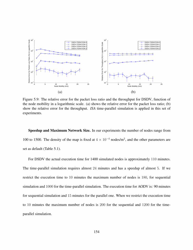
0 5 10 15 20 2510
−1
100
101
102
103
Node Mobility (m/s)
Rel
ativ
e E
rror
for
Pac
ket L
oss
Rat
io (
%)
in L
ogar
ithm
Sca
le
DSDV.ITERATION.0DSDV.ITERATION.1DSDV.ITERATION.2DSDV.ITERATION.3
0 5 10 15 20 2510
−1
100
101
102
103
Node Mobility (m/s)
Rel
ativ
e E
rror
for
Thr
ough
put (
%)
in L
ogar
ithm
Sca
le DSDV.ITERATION.0DSDV.ITERATION.1DSDV.ITERATION.2DSDV.ITERATION.3
(a) (b)
Figure 5.9: The relative error for the packet loss ratio and the throughput for DSDV, function ofthe node mobility in a logarithmic scale. (a) shows the relative error for the packet loss ratio; (b)show the relative error for the throughput. ISA time-parallel simulation is applied in this set ofexperiments.
Speedup and Maximum Network Size. In our experiments the number of nodes range from
100 to 1500. The density of the map is fixed at 4 × 10⁻⁴ nodes/m2, and the other parameters are
set as default (Table 5.1).
For DSDV the actual execution time for 1400 simulated nodes is approximately 110 minutes.
The time-parallel simulation requires almost 24 minutes and has a speedup of almost 5. If we
restrict the execution time to 10 minutes the maximum number of nodes is 180, for sequential
simulation and 1000 for the time-parallel simulation. The execution time for AODV is: 90 minutes
for sequential simulation and 15 minutes for the parallel one. When we restrict the execution time
to 10 minutes the maximum number of nodes is 200 for the sequential and 1200 for the time-
parallel simulation.
154

5.5 Summary
In this chapter, we described a methodology for time-parallel simulation of wireless ad hoc net-
works. We presented an analysis of perturbations, which gives us some understanding of the
source of errors in one-shot time-parallel simulation results. Based on a layer-by-layer analysis of
the propagation of perturbations in the wireless networking stack, we proposed several avenues for
improving the accuracy of the simulation results. Building on these considerations, we described
an implementation of time-parallel simulation based on the NS-2 simulator. The techniques de-
ployed are the iterative extension of the warmup interval and initial state approximation for the
table-driven routing protocols. A series of experiments showed that 5-20 times speedup can be ob-
tained for an accuracy of 95%, depending on the choice of the routing protocol and whether initial
state approximation was deployed or not. In general, the simulations of reactive routing protocols
show a higher accuracy and/or speedup than the one for proactive protocols. We demonstrate,
however, that the accuracy is relatively independent of other parameters of the scenario, such as
network load or node mobility. We conclude that time-parallel simulation allows us to study rela-
tively large wireless ad hoc networks consisting of a few thousand nodes over extended periods of
time.
155
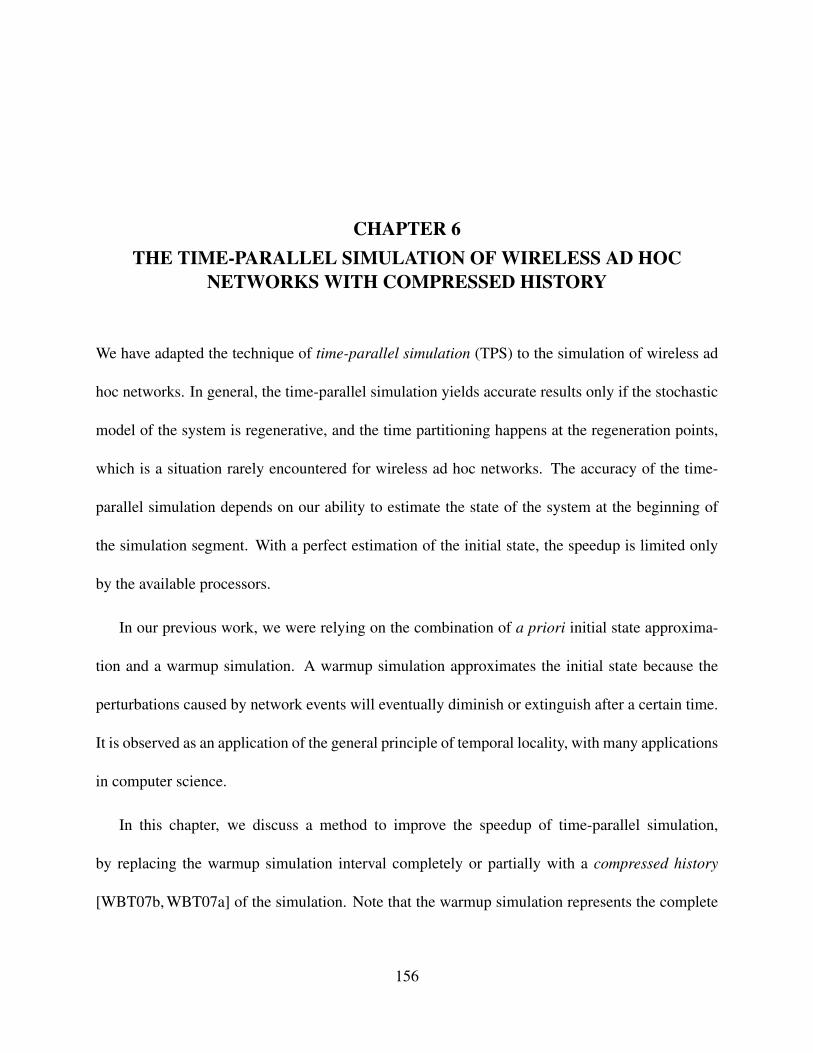
CHAPTER 6THE TIME-PARALLEL SIMULATION OF WIRELESS AD HOC
NETWORKS WITH COMPRESSED HISTORY
We have adapted the technique of time-parallel simulation (TPS) to the simulation of wireless ad
hoc networks. In general, the time-parallel simulation yields accurate results only if the stochastic
model of the system is regenerative, and the time partitioning happens at the regeneration points,
which is a situation rarely encountered for wireless ad hoc networks. The accuracy of the time-
parallel simulation depends on our ability to estimate the state of the system at the beginning of
the simulation segment. With a perfect estimation of the initial state, the speedup is limited only
by the available processors.
In our previous work, we were relying on the combination of a priori initial state approxima-
tion and a warmup simulation. A warmup simulation approximates the initial state because the
perturbations caused by network events will eventually diminish or extinguish after a certain time.
It is observed as an application of the general principle of temporal locality, with many applications
in computer science.
In this chapter, we discuss a method to improve the speedup of time-parallel simulation,
by replacing the warmup simulation interval completely or partially with a compressed history
[WBT07b, WBT07a] of the simulation. Note that the warmup simulation represents the complete
156

simulation of a time period (a history) before the measured part of the simulation. From this simu-
lation, we only retain the final state, which will serve as the initial state for the measured simulation
segment. The idea behind the compressed history is that we can replace the warmup interval with
a simplified simulation scenario, which might not yield the same simulation trace, but will leave
the network in the same (or very similar) final state. Thus, we replace the computation of a long
complex warmup interval with a computationally much cheaper compressed history.
Though the technique of compressed history is quite general and can be applied for time-
parallel simulation in any domain, the way in which the compressed history calculates a good
approximation of the final state at a cheaper cost is dependent on the domain. We need to apply
domain specific knowledge about what type of events have an impact on the final state of the
simulation and which are the events which can be removed or substituted with simpler events. It is
also critical to focus removing the events whose simulation is computationally the most expensive.
The domain on which we focus in this chapter is the simulation of wireless ad hoc networks
with proactive routing protocols (such as DSDV). We have seen that these protocols require a
comparatively long warmup interval to achieve the required accuracy, which limits the speedup to
4-5 times. We have identified the periodic routing table updates as the most expensive component
of the warmup interval, and generate the compressed history by reducing the frequency of the
routing table updates in the warmup interval. Naturally, this is just one of the possible techniques
which can be deployed: other techniques would be the elimination of events whose effects are
157

shadowed by later events, or replacing long trains of identical packet transmission with a smaller
set of transmissions between the same sources.
This chapter is organized as follows. We provide a formal model of the compressed history
technique in Section 6.1, while our implementation is detailed in Section 6.2. A simulation study
analyzing the benefits of compressed history is described in Section 6.3. We conclude in Sec-
tion 6.4.
6.1 Compressed History
A simulation S of an ad hoc network calculates the simulation trace T of an event set E which
occurs in a geographic area A, within a time interval τ , when the initial state is I, and the final
state is F . Formally, we denote a simulation as a six-tuple S = (A, τ, E , I,F , T ). We partition the
temporal dimension of the simulation S into m time intervals {τi|τi = [(i−1) |τ |m
, i |τ |m
], 1 ≤ i ≤ m},
where |τ | is the duration of time interval τ .
A time-parallel simulation is a set of simulation segments
L = {Si|Si = (A, τi, Ei, Ii,Fi, Ti), 1 ≤ i ≤ m} (6.1)
For any simulation Si, the event set Ei ⊂ E is the events from E which fall in the time interval of
Si. Thus the segments of the time-parallel simulation simulate the full spatial component A, but
only a subset of the temporal span τi. In order to have an exact simulation, the initial state of Si+1
158

needs to match the final state of Si, 1 ≤ i ≤ m − 1. This final state, however, cannot be obtained
without actually running all the previous simulation segments.
A crude approximation can be obtained by assuming that every segment starts with initial
network state, Ii = I, and combining the simulation traces T = T1 ∪ T2 ∪ . . . ∪ Tm of the
simulation segments. We call this raw time-parallel simulation method as the TPS algorithm.
A better approximation can be obtained through a warmup interval. For every simulation
segment Si, define a warmup simulation SWi = (A, [τ si − Tw, τ s
i ], EWi, I,FWi, TWi). We will use
the final state of the warmup interval as the initial state of the measured part of the simulation
FWi = Ii. We will call this simulation approach as the TPS-U algorithm (with the U denoting that
the warmup interval is uncompressed). Naturally, the longer the warmup interval Tw, the better the
approximation of the initial state. In the extreme case, Tw = τ si , and the warmup simulation SWi
produces an exact initial state for the simulation segment Si. However, this would not provide any
speedup over a linear simulation of the entire interval.
Let us now introduce the notion of the compressed history. Note that from the warmup sim-
ulation we are only interested in the final state FWi. The computational effort to perform this
simulation is monotonically dependent on the set of events in the warmup simulation. Our goal is
to find a simplified set of events EWi, which, when replaces in the warmup simulation, will provide
a final state which is either equal to the one of the full warmup (FWi = FWi) or a close approxi-
mation (FWi ≈ FWi). Naturally, we are interested only in the cases where the simulation of EWi
is significantly cheaper than that of EWi.
159

Let us now discuss the ways in which the compressed history EWi can be determined. Intu-
itively, we need to retain the events that produce significant perturbations of the final state. Some of
these considerations can be expressed in a generic way. For instance, if some events have a limited
effect in time and their effect extinguishes before the start of the measured part of the simulation,
they can be removed from the warmup simulation when composing the compressed history. An-
other approach is to replace a set of events with an event which summarizes them. For example,
when we wish to simulate the behavior of a lightly or moderately loaded system we can define
recursively past windows and summarize the effect of each one on the next. We can calculate an
average request arrival rate λavg and an average service time µavg for a window of duration δ, ig-
nore all other events (e.g., events signaling completion of a request, preemptive actions, etc.), and
replace all events in this interval with a single request with the service time λavg · µavg arrived at a
random time in the interval (0, δ).
In general, the knowledge of the application domain, the perturbations caused by the specific
classes of events, their interrelationships, as well as their impact on the simulation interval can help
us design compressed histories with high compression ratio and high accuracy.
Let Si be the complete sequential simulation prior to Si,
Si = (A, [0, τ si ], Ei, I,Fi, Ti), 2 ≤ i ≤ m (6.2)
The initial state of a simulation batch Si can be approximated by the final state of the com-
pressed history of its prior simulation Si,
Si = (A, [0, τ si ], Ei, I, Fi, Ti), 2 ≤ i ≤ m (6.3)
160

Thus, we obtain a new time-parallel simulation set
L′ = {S ′i|S ′i = (A, τi, E ′, I ′i,F ′i , T ′
i ), 1 ≤ i ≤ m} (6.4)
where
I ′i =
I, for i = 1;
Fi, for 2 ≤ i ≤ m.
(6.5)
We call the time-parallel simulation algorithm with compressed history as the TPS-C algorithm.
Figure 6.1 illustrates an example of the TPS-C algorithm.
S 1
S 2
S 3
S 4
S 5
S 6
S 7
S 8
S 9
S 1 '
S 2 '
S 3 '
S 4 '
S 5 '
S 6 '
S 7 '
S 8 '
S 9 '
S 2
^
S 3
^
S 4
^
S 5
^
S 6
^
S 7
^
S 8
^
S 9
^
Figure 6.1: The TPS and TPS-C (TPS with compressed history) algorithms. The |τ | = 180 sec.simulation interval is segmented into 9 simulation intervals of 20 sec. each. The shaded simulationsegments are used to compose the final simulation trace. {Si} is the set of simulation withoutinitial state approximation, while {S ′i} is the set of simulation batches with their initial statesapproximated by the compressed history of their prior simulations.
161

We define the compression ratio of the compressed history S by
η(Si, Si) =|E||E | (6.6)
Assume S = (500 × 500, [0, 180], E , I,F , T ) is segmented into 9 equal intervals, with τi =
[20(i − 1), 20i], 1 ≤ i ≤ 9. The compressed history of the prior simulation for each simulation
batch Si is
Si = (500× 500, [0, 20(i− 1)], Ei, I, Fi, Ti), 2 ≤ i ≤ 9 (6.7)
The set of simulation batches improved by the application of compressed history are
S ′i = (500× 500, [20(i− 1), 20], E ′i , I ′i,F ′i , T ′
i ), 1 ≤ i ≤ 9 (6.8)
where
I ′i =
I, for i = 1;
Fi, for 2 ≤ i ≤ 9.
(6.9)
Experimental results show that an aggressive compression of the warmup interval can produce
high approximation errors. It turns out, however, that the events at the very end of the compressed
interval (that is, immediately before the start of the measurement interval) are responsible for a
large part of the approximation errors. One way to improve the accuracy is to introduce a short
uncompressed interval between the compressed history and the beginning of the measurement in-
terval. The introduction of uncompressed simulation interval reduces the influence of perturbations
at the measured point.
162
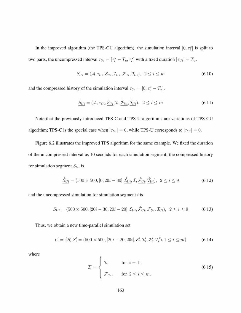
In the improved algorithm (the TPS-CU algorithm), the simulation interval [0, τ si ] is split to
two parts, the uncompressed interval τUi = [τ si − Tu, τ
si ] with a fixed duration |τUi| = Tu,
SUi = (A, τUi, EUi, IUi,FUi, TUi), 2 ≤ i ≤ m (6.10)
and the compressed history of the simulation interval τCi = [0, τ si − Tu],
SUi = (A, τCi, EUi, I, FUi, TUi), 2 ≤ i ≤ m (6.11)
Note that the previously introduced TPS-C and TPS-U algorithms are variations of TPS-CU
algorithm; TPS-C is the special case when |τUi| = 0, while TPS-U corresponds to |τCi| = 0.
Figure 6.2 illustrates the improved TPS algorithm for the same example. We fixed the duration
of the uncompressed interval as 10 seconds for each simulation segment; the compressed history
for simulation segment SUi is
SUi = (500× 500, [0, 20i− 30], EUi, I, FUi, TUi), 2 ≤ i ≤ 9 (6.12)
and the uncompressed simulation for simulation segment i is
SUi = (500× 500, [20i− 30, 20i− 20], EUi, FUi,FUi, TUi), 2 ≤ i ≤ 9 (6.13)
Thus, we obtain a new time-parallel simulation set
L′ = {S ′i|S ′i = (500× 500, [20i− 20, 20i], E ′i , I ′i,F ′i , T ′
i ), 1 ≤ i ≤ m} (6.14)
where
I ′i =
I, for i = 1;
FUi, for 2 ≤ i ≤ m.
(6.15)
163
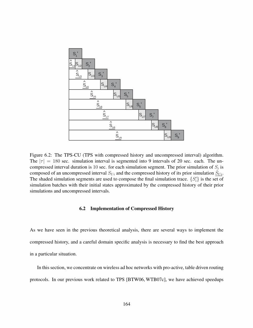
S 1 '
S 2 '
S 3 '
S 4 '
S 5 '
S 6 '
S 7 '
S 8 '
S 9 '
S U2
^ S U2
S U3
S U4
S U5
S U6
S U7
S U8
S U9
S U3
^
S U4
^
S U5
^
S U6
^
S U7
^
S U8
^
S U9
^
Figure 6.2: The TPS-CU (TPS with compressed history and uncompressed interval) algorithm.The |τ | = 180 sec. simulation interval is segmented into 9 intervals of 20 sec. each. The un-compressed interval duration is 10 sec. for each simulation segment. The prior simulation of Si iscomposed of an uncompressed interval SUi and the compressed history of its prior simulation SUi.The shaded simulation segments are used to compose the final simulation trace. {S ′i} is the set ofsimulation batches with their initial states approximated by the compressed history of their priorsimulations and uncompressed intervals.
6.2 Implementation of Compressed History
As we have seen in the previous theoretical analysis, there are several ways to implement the
compressed history, and a careful domain specific analysis is necessary to find the best approach
in a particular situation.
In this section, we concentrate on wireless ad hoc networks with pro-active, table driven routing
protocols. In our previous work related to TPS [BTW06, WTB07c], we have achieved speedups
164

of 16-20 times for scenarios involving reactive routing protocols, but only 4-5 times for pro-active
routing protocols. The reason behind the lower speedup is that pro-active protocols maintain more
state information (in the form of the routing tables), and thus require longer and more expensive
warmup for equivalent accuracy. Our goal is to replace part of the warmup interval with com-
pressed history, such that the overall speedup will be brought closer to the reactive protocols.
In order to find an efficient compression mechanism, we will use our domain specific knowl-
edge. The specific protocol we will consider is Destination Sequenced Distance Vector (DSDV)
[PB94], although the same considerations apply to most other pro-active routing protocols. In
DSDV, the nodes periodically update their routing tables even in the absence of any data flow
(hence the pro-active nature of the protocol). The justification for the frequent routing table up-
dates is the mobility of the nodes. The routing table updates involve a significant number of packet
exchanges, which are computationally expensive to simulate. However, note that for the measure-
ment interval, we are interested only in the final configuration of the routing tables, and the history
of the routing table entries does not affect the current state of the network.
Thus, one possible strategy to generate the compressed history is based on the selective removal
of the routing table update packets. The event that updates a routing table entry which will be
overwritten before the start of the measurement interval is called a shadowed event, and can be
removed from the compressed history without a loss of accuracy. Similarly, we could remove
the events concerning routing table entries which are not used during the measurement interval
165
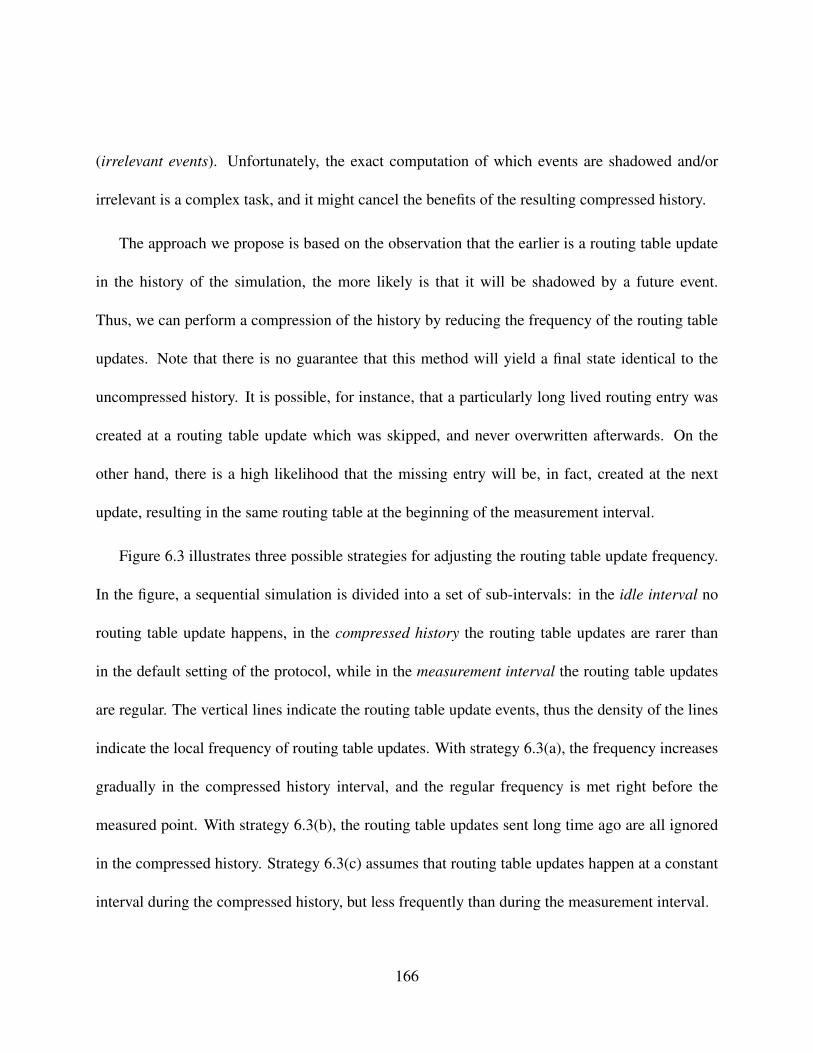
(irrelevant events). Unfortunately, the exact computation of which events are shadowed and/or
irrelevant is a complex task, and it might cancel the benefits of the resulting compressed history.
The approach we propose is based on the observation that the earlier is a routing table update
in the history of the simulation, the more likely is that it will be shadowed by a future event.
Thus, we can perform a compression of the history by reducing the frequency of the routing table
updates. Note that there is no guarantee that this method will yield a final state identical to the
uncompressed history. It is possible, for instance, that a particularly long lived routing entry was
created at a routing table update which was skipped, and never overwritten afterwards. On the
other hand, there is a high likelihood that the missing entry will be, in fact, created at the next
update, resulting in the same routing table at the beginning of the measurement interval.
Figure 6.3 illustrates three possible strategies for adjusting the routing table update frequency.
In the figure, a sequential simulation is divided into a set of sub-intervals: in the idle interval no
routing table update happens, in the compressed history the routing table updates are rarer than
in the default setting of the protocol, while in the measurement interval the routing table updates
are regular. The vertical lines indicate the routing table update events, thus the density of the lines
indicate the local frequency of routing table updates. With strategy 6.3(a), the frequency increases
gradually in the compressed history interval, and the regular frequency is met right before the
measured point. With strategy 6.3(b), the routing table updates sent long time ago are all ignored
in the compressed history. Strategy 6.3(c) assumes that routing table updates happen at a constant
interval during the compressed history, but less frequently than during the measurement interval.
166

Measured Interval
Compressed History
(a)
Measured Interval
Compressed History Idle Interval
(b)
Measured Interval
Compressed History
(c)
Figure 6.3: Strategies to adjust the routing table update frequency when composing the compressedhistory.
Measured Interval
Uncompressed Interval
Compressed History
(a)
Measured Interval
Uncompressed Interval
Compressed History Idle Interval
(b)
Measured Interval
Compressed History Uncompressed Interval
(c)
Figure 6.4: Strategies to adjust the routing table update frequency when composing the compressedhistory, with the application of uncompressed interval.
167

Figure 6.4 illustrates the corresponding strategies with an uncompressed warmup interval in-
serted between the compressed history and the measurement interval. The routing table updates
are sent at a regular level within the uncompressed interval. In our simulation, we implemented
and investigated strategies 6.3(c) and 6.4(c). As the experimental results will show, even a small
uncompressed interval can provide a significant improvement in the accuracy of the simulation.
6.2.1 Load Balancing TPS with Compressed History
The overall execution time of a parallel simulation is determined by the simulation segment with
the longest execution time. As the measurement interval of the individual time-parallel simulation
threads starts at different time points, the length of the compressed history will be different. This
leads to an imbalance in the execution time: with a constant compression ratio, the execution
time of a simulation segment increases when its compressed history duration increases. Our goal
is to balance the execution time of the compressed histories, by adjusting the compression ratio
according to the compressed history duration.
Assume the routing table update frequency of a sequential simulation Si is a constant λc, and
the routing table update frequency of the compressed history SUi is λi. The compression ratio
η ≥ 1 is the ratio of the original size of the history to the size of the compressed history. Thus a
value of η = 1 represents no compression. The compression ratio of SUi can be approximated by
η(SUi, SUi) ≈ λc
λi
(6.16)
168

Define the normalized compressed history duration as the compressed history duration divided
by the compression ratio, which reflects the approximate duration of a compressed history if it was
not compressed. The normalized compressed history duration of SUi is |τCi| / η(SUi, SUi).
The balancing of the execution time of different simulation segments can be achieved by equal-
izing the normalized compressed history duration. If all simulation segments have a constant nor-
malized compressed history duration Tc, that is
Tc =|τCi|
η(SUi, SUi)≈ |τCi| · λi
λc
(6.17)
Thus, the required routing table update frequency for each simulation segment can be obtained by
λi = λc · Tc
|τCi| (6.18)
6.2.2 Accuracy-speedup Tradeoffs
In the TPS-CU algorithm, the initial state of the measurement interval S ′i is obtained as the final
state of the uncompressed interval SUi, whose initial state is approximated by the final state of the
compressed history SUi.
Thus, we have two ways to increase the accuracy of the initial state in the TPS-CU algorithm:
either we increase the normalized compressed history duration of SUi (that is, decrease the com-
pression ratio), or we increase the length of the uncompressed history duration. Unfortunately, this
way we also reduce the speedup of the simulation.
169

Let us consider a simulation S over a duration τ , segmented into m equal measurement in-
tervals. The duration of each measured simulation interval (S ′i) is Ti = |τ |/m, the normalized
compressed history (SUi) duration is Tc, and the uncompressed interval (SUi) duration is Tu. Let
T (S) be the function that calculates the execution of a simulation S. The speedup of our algorithm
is
κ =T (S)
maxi{T (SUi) + T (SUi) + T (S ′i)}(6.19)
If we assume that the events are evenly distributed over the simulation interval and the execu-
tion of each event takes about the same time ∆t,
T (S) ≈ |E| ·∆t (6.20)
If we ignore the execution time for data packets, the speedup can be approximated by
κ =T (S)
maxi{T (SUi) + T (SUi) + T (S ′i)}≈ |E| ·∆t
maxi{(|EUi|+ |EUi|+ |E ′i|) ·∆t}=
λc · |τ |maxi{λi · |τCi|+ λc · |τUi|+ λc · |τi|}
=λc · |τ |
λc · Tc + λc · Tu + λc · Ti
=|τ |
Tc + Tu + Ti
(6.21)
According to this formula, there are three possible means to increase the speedup: (1) decrease
the normalized compressed history duration Tc; (2) decrease the uncompressed interval duration
Tu; or (3) decrease the duration of the individual measurement intervals Ti, which is equivalent to
increasing the number of measurement intervals m. Each of these choices also affects the accuracy
170

of the simulation. Our goal is to determine the optimal values of: (i) the normalized compressed
history duration, (ii) the uncompressed interval duration, and (iii) the measurement interval dura-
tion such that we achieve the largest possible speedup while meeting accuracy constraints.
6.3 Simulation Study
In this section, we describe the results of a simulation study which studies the accuracy of time-
parallel simulation with compressed history. We compare the approximate results produced by
TPS-U, TPS-C and TPS-CU with those produced by exact sequential simulation over several fre-
quently used metrics. Table 6.1 lists the abbreviations and notations used throughout this section.
Table 6.1: The abbreviation and notations used in our simulation studies
Notation DescriptionTPS-C the TPS algorithm with compressed historyTPS-U the TPS algorithm with uncompressed interval
TPS-CU the TPS algorithm with compressed history and uncompressed intervalTc the duration of the normalized compressed historyTi the duration of segment iTu the duration of the uncompressed interval
εPLR the relative error for the packet loss ratioεTPT the relative error for the throughputεmax the relative error threshold
κ the speedup of the algorithm
The simulation scenarios on which we test our implementations are representative for the sce-
narios used in the study of wireless ad hoc networks. A set of mobile nodes are moving in a
rectangular area, while communicating using wireless connections. The transmission range of the
171

nodes is smaller than the size of the area, and there are no fixed wireless access points available.
Thus, in order to communicate, the nodes need to use hop-by-hop transmissions relying on ad hoc
routing algorithms. Due to the mobility of the nodes, the routes need to be frequently updated,
even during the course of the transmissions.
In our experimental study, 80 nodes move in a simulation area of size 500 × 500 m2 square
area; all nodes have a transmission range of 100 meters. The duration of the scenario is 600 sec-
onds. The node movement is modeled by the random waypoint model [BMJ98, JM96]. The traffic
patterns are generated by CBR sources sending 512-byte UDP packets at a rate of 1 packet/second.
The nodes use the Destination-Sequenced Distance Vector (DSDV) routing algorithm. Table 6.2
shows the default settings of the parameters for our experiments.
Table 6.2: The default values of the parameters used in our simulation studies
Field Valuesimulation area 500 × 500 (m2)number of nodes 80transmission range 100 (m)speed 1 (m/s)pause time 15 (s)simulation time 600 (s)number of CBR sources 20CBR packet size 512 (bytes)CBR sending rate 4 (kbps)
Let us now describe the specific approaches we compare.
• TPS-U is the time-parallel simulation with uncompressed warmup interval. This is the base-
line algorithm described in [BTW06, WTB07c].
172

• TPS-C is the time-parallel simulation with the warmup interval being composed exclusively
of the compressed history. The strategy used for this approach is the one described in Fig-
ure 6.3(c), that is, the warmup interval extends to the complete simulation scenario, and the
routing table update frequency is equidistant. To balance the load of the simulation threads,
we maintained a constant normalized compressed history duration.
• TPS-CU is the time-parallel simulation with a warmup interval composed of the compressed
history followed by an uncompressed interval. The particular strategy used in this simulation
study is the one described in Figure 6.4(c), that is, the compressed interval starts at the begin-
ning of the simulation scenario and the routing table update frequency is constant for a given
simulation. To balance the load of the simulation threads, we maintained an uncompressed
component of constant duration and a compressed component of constant normalized com-
pressed history duration.
Our approach for comparing the accuracy of different simulation runs is based on the calcu-
lation of the relative error of specific measurement types. The methodology is implemented as
follows. First, we run a serial, accurate simulation and extract an exact measurement M0 on its
trace. Then, we perform a time-parallel simulation with one of the proposed algorithms (TPS-U,
TPS-C and TPS-CU), assemble the simulation trace from the segments, and perform the same
measurement, obtaining an approximate value M . The relative error of the specific algorithm for
this scenario will be εM = M−M0
M0× 100%. As the relative error fluctuates from scenario to sce-
nario, we repeat the experiment 20 times, each time with a different random configuration of the
173

source destination pairs of the CBR sources. We calculate the mean, as well as the 95% confidence
interval of the relative error. The two measurements considered in this study are the relative error
for the packet loss ratio εPLR and the relative error for the throughput εTPT.
As we described in the [BTW06], the relative error of simulation tends to be larger for metrics
which measure rare phenomena (such as packet loss), compared to metrics which measure fre-
quently occurring phenomena (such as throughput). As a result, εTPT is always smaller than εPLR.
The error threshold εmax used in this study was 5%. In practice, this means that the measurement
of the packet loss ratio will be roughly 95% accurate, while the accuracy of the measured through-
put will be much higher, around 99.5% for most simulation runs. The speedup of the algorithm
was determined by the method discussed in Section 6.2.2.
The time-parallel simulation was run on a cluster of 128 64-bit Opteron processors with Gigabit
Ethernet interconnection. Each simulation segment was run on its own dedicated processor.
6.3.1 Tuning the Parameters of the Compressed History for Optimal Speedup
The TPS-C and TPS-CU algorithms have several parameters which can determine the speedup and
accuracy of the algorithm. Before we perform a comparison between the accuracy and speedup of
the TPS-U, TPS-C and TPS-CU algorithms, we need to determine the parameters under which the
compressed history approach works best. These tuned parameters will be then used in the actual
comparisons.
174
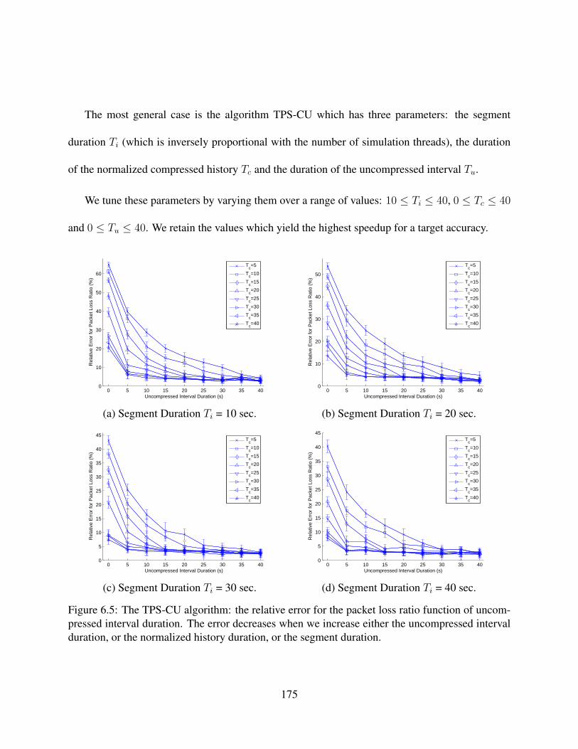
The most general case is the algorithm TPS-CU which has three parameters: the segment
duration Ti (which is inversely proportional with the number of simulation threads), the duration
of the normalized compressed history Tc and the duration of the uncompressed interval Tu.
We tune these parameters by varying them over a range of values: 10 ≤ Ti ≤ 40, 0 ≤ Tc ≤ 40
and 0 ≤ Tu ≤ 40. We retain the values which yield the highest speedup for a target accuracy.
0 5 10 15 20 25 30 35 400
10
20
30
40
50
60
Uncompressed Interval Duration (s)
Rel
ativ
e E
rror
for
Pac
ket L
oss
Rat
io (
%)
Tc=5
Tc=10
Tc=15
Tc=20
Tc=25
Tc=30
Tc=35
Tc=40
0 5 10 15 20 25 30 35 400
10
20
30
40
50
Uncompressed Interval Duration (s)
Rel
ativ
e E
rror
for
Pac
ket L
oss
Rat
io (
%)
Tc=5
Tc=10
Tc=15
Tc=20
Tc=25
Tc=30
Tc=35
Tc=40
(a) Segment Duration Ti = 10 sec. (b) Segment Duration Ti = 20 sec.
0 5 10 15 20 25 30 35 400
5
10
15
20
25
30
35
40
45
Uncompressed Interval Duration (s)
Rel
ativ
e E
rror
for
Pac
ket L
oss
Rat
io (
%)
Tc=5
Tc=10
Tc=15
Tc=20
Tc=25
Tc=30
Tc=35
Tc=40
0 5 10 15 20 25 30 35 400
5
10
15
20
25
30
35
40
45
Uncompressed Interval Duration (s)
Rel
ativ
e E
rror
for
Pac
ket L
oss
Rat
io (
%)
Tc=5
Tc=10
Tc=15
Tc=20
Tc=25
Tc=30
Tc=35
Tc=40
(c) Segment Duration Ti = 30 sec. (d) Segment Duration Ti = 40 sec.
Figure 6.5: The TPS-CU algorithm: the relative error for the packet loss ratio function of uncom-pressed interval duration. The error decreases when we increase either the uncompressed intervalduration, or the normalized history duration, or the segment duration.
175

0 5 10 15 20 25 30 35 400
5
10
15
20
25
30
Uncompressed Interval Duration (s)
Rel
ativ
e E
rror
for
Thr
ough
put (
%)
Tc=5
Tc=10
Tc=15
Tc=20
Tc=25
Tc=30
Tc=35
Tc=40
0 5 10 15 20 25 30 35 400
2
4
6
8
10
12
14
16
Uncompressed Interval Duration (s)
Rel
ativ
e E
rror
for
Thr
ough
put (
%)
Tc=5
Tc=10
Tc=15
Tc=20
Tc=25
Tc=30
Tc=35
Tc=40
(a) Segment Duration Ti = 10 sec. (b) Segment Duration Ti = 20 sec.
0 5 10 15 20 25 30 35 400
2
4
6
8
10
12
Uncompressed Interval Duration (s)
Rel
ativ
e E
rror
for
Thr
ough
put (
%)
Tc=5
Tc=10
Tc=15
Tc=20
Tc=25
Tc=30
Tc=35
Tc=40
0 5 10 15 20 25 30 35 400
1
2
3
4
5
6
7
8
9
Uncompressed Interval Duration (s)
Rel
ativ
e E
rror
for
Thr
ough
put (
%)
Tc=5
Tc=10
Tc=15
Tc=20
Tc=25
Tc=30
Tc=35
Tc=40
(c) Segment Duration Ti = 30 sec. (d) Segment Duration Ti = 40 sec.
Figure 6.6: The TPS-CU algorithm: the relative error for the throughput function of the duration ofthe uncompressed interval. The error decreases when we increase either the uncompressed intervalduration, the normalized history duration, or the segment duration.
Figures 6.5 and 6.6 show the relative error for the packet loss ratio and the throughput function
of the duration of the uncompressed interval, for several segment lengths. Given a segment and a
normalized compressed history of fixed length, the relative error for both metrics tend to decrease
when the uncompressed interval duration increases. Also, the relative error for the two metrics
tend to decrease when the normalized compressed history duration increases, given the duration
176

of the segment and of the uncompressed interval. The relative errors for the two metrics decrease
when the segment duration increases. For instance, with (Tu, Tc) = (5, 5) sec., the relative error
for the packet loss ratio is reduced from 39.76% when Ti = 10 sec., to 24.09% when Ti = 40 sec.;
the relative error for the throughput is reduced from 8.82% when Ti = 10 sec., to 3.90% when
Ti = 40 sec.
Table 6.3: Tuning the parameters of the TPS-CU algorithm based on the results of the experimentalruns. The rows corresponding to the best choice of the uncompressed interval Tu for a given seg-ment duration are shown in bold. The maximum achievable speedup for a given segment durationis bold and underlined.
Tu min{Tc} εPLR εTPT κ10 40 4.42% 0.59% 4.0115 30 4.15% 0.57% 5.2920 25 4.70% 0.67% 5.3025 25 3.15% 0.41% 5.2030 15 3.32% 0.45% 6.3235 10 4.63% 0.63% 6.5140 5 4.31% 0.58% 5.67
Tu min{Tc} εPLR εTPT κ10 35 4.32% 0.53% 6.6215 30 4.13% 0.49% 6.3320 20 3.94% 0.48% 7.3425 20 4.21% 0.51% 6.4330 10 4.80% 0.59% 7.3035 10 4.29% 0.51% 6.3940 5 4.73% 0.58% 6.39
(a) Segment Duration Ti = 10 sec. (b) Segment Duration Ti = 20 sec.
Tu min{Tc} εPLR εTPT κ5 35 3.76% 0.51% 4.88
10 25 4.77% 0.65% 7.4415 15 4.01% 0.54% 7.4620 15 3.70% 0.49% 7.5425 10 4.12% 0.55% 6.9930 5 4.64% 0.63% 6.84
Tu min{Tc} εPLR εTPT κ5 30 3.70% 0.66% 5.51
10 25 4.59% 0.56% 6.1715 15 4.07% 0.50% 6.7920 15 4.61% 0.58% 6.0425 15 3.33% 0.32% 6.4330 5 3.86% 0.46% 6.14
(c) Segment Duration Ti = 30 sec. (d) Segment Duration Ti = 40 sec.
177

To maximize the speedup for a given Tu, we choose the minimal Tc such that the relative errors
for the corresponding metrics are below εmax. We conducted a series of simulations with different
segment durations. The simulation results are summarized in Tables 6.3. Each table, shows the
minimal value of Tc, the normalized compressed history duration as well as εPLR, the relative error
for the packet loss ratio, εTPT, the relative error for the throughput, and κ, the speedup, function
of Tu, the uncompressed interval duration. The normalized compressed history duration required
to achieve the accuracy threshold tends to decrease when the uncompressed interval duration in-
creases. When Ti = 10 sec., the largest speedup is κ = 6.51 with (Tu, Tc) = (35, 10) sec. and the
relative errors are (εPLR, εTPT) = (4.63%, 0.63%); when Ti = 40 sec., the largest speedup is 6.79
with (Tu, Tc) = (15, 15) sec. and the relative errors are (εPLR, εTPT) = (4.07%, 0.50%).
Table 6.4: The combination of uncompressed interval duration and normalized compressed historyduration that achieve the maximum speedup for different segment durations
Ti Tu Tc κ10 35 10 6.5120 20 20 7.3430 20 15 7.5440 15 15 6.79
Table 6.4 lists the combination of the uncompressed interval duration and the normalized com-
pressed history duration that led to the largest speedup, under all segment durations simulated. The
largest speedup increases when Ti increases from 10 to 30 sec., and starts to decrease when Ti in-
creases beyond 30 sec. The largest speedup, κ = 7.54, is achieved when (Ti, Tu, Tc) = (30, 20, 15)
sec. These values will be chosen for the simulation results presented later.
178

6.3.2 The Performance Improvement Provided by Compressed History: Comparing TPS-CUwith TPS-U
We investigate the effect of the compressed history, for a range of durations of the uncompressed
interval when the segment duration is 30 sec., the normalized compressed history duration for the
TPS-CU algorithm is 15 sec., and the uncompressed interval duration is 10 ≤ Tu ≤ 40 sec.
Figure 6.7 shows the relative errors produced by the TPS-U and TPS-CU algorithms. For both
algorithms the relative error for the packet loss ratio and the throughput tend to decrease when
the uncompressed interval duration increases. For the same duration of the uncompressed interval
the relative errors produced by the TPS-CU are smaller than the ones produced by the TPS-C
algorithm; the TPS-U algorithm produces errors below εmax for considerably smaller values of the
uncompressed interval.
0 10 20 30 40 50 60 70 80 900
10
20
30
40
50
60
70
80
Uncompressed Interval Duration (s)
Rel
ativ
e E
rror
for
Pac
ket L
oss
Rat
io (
%)
TPS−UTPS−CU
0 10 20 30 40 50 60 70 80 900
10
20
30
40
50
60
70
80
90
100
Uncompressed Interval Duration (s)
Rel
ativ
e E
rror
for
Thr
ough
put (
%)
TPS−UTPS−CU
(a) (b)
Figure 6.7: The TPS-U and TPS-CU algorithms: the relative error function of the duration ofthe uncompressed interval for (a) the packet loss ratio and (b) the throughput, when the segmentduration is 30 sec., and the normalized compressed history duration for TPS-CU is 15 sec.
179

Table 6.5: The effect of the compressed history upon the relative error for the packet loss ratio andthe throughput
TuεPLR εTPT
Tc = 0 Tc = 15 Tc = 0 Tc = 15
0 79.38% 32.48% 90.10% 6.70%10 69.42% 8.26% 38.84% 1.39%20 55.71% 3.70% 18.32% 0.59%30 43.20% 2.58% 10.38% 0.50%40 28.49% 2.31% 5.21% 0.34%50 19.77 % 2.24% 3.15% 0.40%60 10.49% 2.64% 1.47% 0.34%70 5.72% 2.28% 0.75% 0.31%80 3.93% 2.09% 0.50% 0.25%
Table 6.5 summarizes the effect of the compressed interval upon the relative errors. A 15-sec.
normalized compressed history, leads to the reduction of the relative error for the packet loss ratio
from 69.42% to 8.26% when Tu = 10 sec. and from 43.20% to 2.58% when Tu = 30 sec. the
relative error for the throughput is reduced from 38.84% to 1.39% when Tu = 10 sec., and from
10.38% to 0.50% when Tu = 30 sec.
We conclude that the compressed history allows us to obtain a better approximation for both
the packet loss ratio and the throughput.
6.3.3 The Performance Improvement Provided by the Uncompressed Interval: ComparingTPS-CU with TPS-C
The next question we investigate is whether we can dispense the uncompressed interval entirely
and just rely on the compressed history to provide the warmup simulation, which is the case of the
180
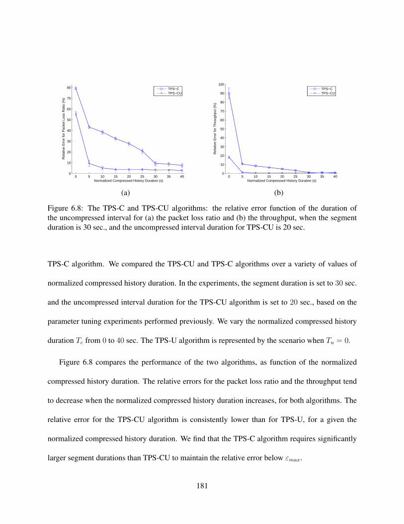
0 5 10 15 20 25 30 35 400
10
20
30
40
50
60
70
80
Normalized Compressed History Duration (s)
Rel
ativ
e E
rror
for
Pac
ket L
oss
Rat
io (
%)
TPS−CTPS−CU
0 5 10 15 20 25 30 35 400
10
20
30
40
50
60
70
80
90
100
Normalized Compressed History Duration (s)
Rel
ativ
e E
rror
for
Thr
ough
put (
%)
TPS−CTPS−CU
(a) (b)
Figure 6.8: The TPS-C and TPS-CU algorithms: the relative error function of the duration ofthe uncompressed interval for (a) the packet loss ratio and (b) the throughput, when the segmentduration is 30 sec., and the uncompressed interval duration for TPS-CU is 20 sec.
TPS-C algorithm. We compared the TPS-CU and TPS-C algorithms over a variety of values of
normalized compressed history duration. In the experiments, the segment duration is set to 30 sec.
and the uncompressed interval duration for the TPS-CU algorithm is set to 20 sec., based on the
parameter tuning experiments performed previously. We vary the normalized compressed history
duration Tc from 0 to 40 sec. The TPS-U algorithm is represented by the scenario when Tu = 0.
Figure 6.8 compares the performance of the two algorithms, as function of the normalized
compressed history duration. The relative errors for the packet loss ratio and the throughput tend
to decrease when the normalized compressed history duration increases, for both algorithms. The
relative error for the TPS-CU algorithm is consistently lower than for TPS-U, for a given the
normalized compressed history duration. We find that the TPS-C algorithm requires significantly
larger segment durations than TPS-CU to maintain the relative error below εmax.
181
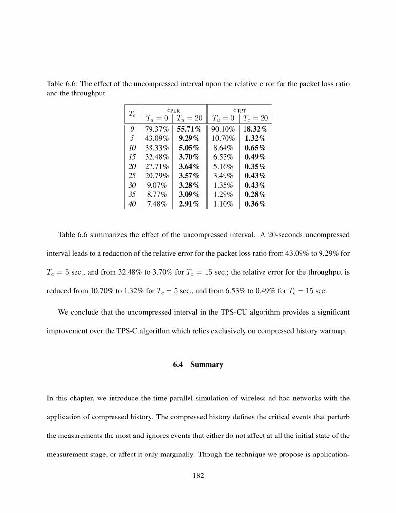
Table 6.6: The effect of the uncompressed interval upon the relative error for the packet loss ratioand the throughput
TcεPLR εTPT
Tu = 0 Tu = 20 Tu = 0 Tc = 20
0 79.37% 55.71% 90.10% 18.32%5 43.09% 9.29% 10.70% 1.32%
10 38.33% 5.05% 8.64% 0.65%15 32.48% 3.70% 6.53% 0.49%20 27.71% 3.64% 5.16% 0.35%25 20.79% 3.57% 3.49% 0.43%30 9.07% 3.28% 1.35% 0.43%35 8.77% 3.09% 1.29% 0.28%40 7.48% 2.91% 1.10% 0.36%
Table 6.6 summarizes the effect of the uncompressed interval. A 20-seconds uncompressed
interval leads to a reduction of the relative error for the packet loss ratio from 43.09% to 9.29% for
Tc = 5 sec., and from 32.48% to 3.70% for Tc = 15 sec.; the relative error for the throughput is
reduced from 10.70% to 1.32% for Tc = 5 sec., and from 6.53% to 0.49% for Tc = 15 sec.
We conclude that the uncompressed interval in the TPS-CU algorithm provides a significant
improvement over the TPS-C algorithm which relies exclusively on compressed history warmup.
6.4 Summary
In this chapter, we introduce the time-parallel simulation of wireless ad hoc networks with the
application of compressed history. The compressed history defines the critical events that perturb
the measurements the most and ignores events that either do not affect at all the initial state of the
measurement stage, or affect it only marginally. Though the technique we propose is application-
182

specific, it is based upon the temporal locality of perturbations rooted on the assumption that
causality has a limited scope, the effect of perturbations caused by distant events in the past will
eventually diminish or extinguish after a certain time. Time-parallel simulation with compressed
history allows us to speed up the simulation and produces good approximations to the exact simu-
lation results; there is a tradeoff between the accuracy of the results and the speedup.
We propose several strategies for generating the compressed history for wireless ah hoc net-
works; we also introduce an uncompressed interval method that further improves the quality of
the solution. Finally, we present a simulation study and discuss the accuracy of the algorithms as
well as the speedup. We study the accuracy of simulated results for the packet loss ratio and the
throughput for a table-driven routing protocol – DSDV. The results of the simulations are better
in terms of speedup and accuracy than the results without the application of compressed history,
reported in [BTW06, TWB06, WTB06b, WTB07c]. We compare the performance of TPS-CU,
TPS-U, and TPS-C algorithms and conclude that the introduction of compressed history and un-
compressed interval improves the accuracy of the solution; the new algorithms allow us to study
wireless ad hoc networks with several thousand nodes for extended periods of time.
We plan to further investigate the strategies illustrated in Figure 6.4 and determine the best way
to generate the compressed history, and then to implement compressed history for simulation of
on-demand routing protocols, such as AODV [PR99].
183
CHAPTER 7CONCLUSIONS
In this dissertation, we developed MAC layer and routing protocols suitable for heterogeneous
MANETs with asymmetric links, and evaluated their performance. We also designed a time-
parallel simulation (TPS) of ad hoc networks and evaluated its performance using the NS-2 simu-
lation tool.
We first introduced m-limited forwarding, a technique to optimize the performance of ad hoc
routing algorithms by reducing the power consumption as well as the fraction of the network
bandwidth used to disseminate routing information. We introduced two alternative functions: a
distance-based function Fd and an area-based function Fa. We evaluate the performance of m-
limited forwarding through a series of simulation studies. Our first objective is to determine the
optimal value of m, the cardinality of the set of nodes which retransmit a packet containing routing
information. We have found that m = 3 yields reasonable output. We implemented a version of
AODV with m-limited forwarding (m-AODV), and simulation results show that for most simu-
lation scenarios, m-AODV has a lower power consumption and packet loss ratio than both plain
AODV and LAR.
We applied the m-limited forwarding concept in our location-aware and power-aware routing
protocol (A4LP) for heterogeneous ad hoc networks with asymmetric links. A4LP has three types
184

of neighbors: In-, Out- and In/Out-bound. We introduced the concept of an m-party proxy set
as a subset of nodes that can reach each other either directly or through a subset of members.
Simulation results show that both packet loss ratio and latency are reduced as a result of the A4LP
routing protocol.
Although we have proposed a routing protocol to utilize the asymmetric links in heterogeneous
MANETs, when we survey the literature of MAC layer protocols, we found that most MAC layer
protocols simply assume symmetric links and ignore all asymmetric links. We proposed a MAC
layer protocol (AsyMAC) which serves as the underlying MAC layer protocol for A4LP in het-
erogeneous MANETs. Most current MAC protocols are unable to exploit the asymmetric links
present in a network, thus leading to an inefficient overall bandwidth utilization, or, in the worst
case, to loss of connectivity. The AsyMAC protocol is able to exploit the asymmetric links in such
networks, and solves the problem of delivering the acknowledgements back to the sender against
the direction of the asymmetric link. Some of the current solutions proposed in the literature re-
duce the probability of a collision, however, they silence more nodes than required. This is because
hidden nodes appear more often and in more complex forms in heterogeneous MANETs, thus the
traditional definition becomes invalid. We redefine the meaning of hidden nodes in our context
as nodes out of the range of the sender and whose ranges cover the receiver. Simulation results
demonstrate that the AsyMAC protocol utilizes asymmetric links efficiently and the benefits of our
protocol outweighs its cost.
185
Once we have developed the logic of MAC layer and routing protocols that exploit asymmetric
links we had to provide convincing arguments that these new protocols are functional, and, even
though more complex than the ones that ignore the asymmetry, can lead to an acceptable level of
performance. We turned to analytical modeling and realized shortly that it would be rather diffi-
cult, if possible at all, to develop analytical models. We also realized the limitations of existing
simulation tools such as NS-2. Thus, we turned our attention to time-parallel simulation that could
allow us to use existing tools, but study networks with a larger number of nodes and for extended
periods of time. In Chapter 5, we explored the challenges and the benefits of time-parallel simula-
tion of wireless ad hoc networks. We introduced the notion of perturbation of measurements and
present a layer-by-layer analysis of the impact of perturbations on the functioning of the wireless
network. We have found ways to predict the accuracy of a time-parallel simulation and proposed
the following methods: time interval shift, warmup interval, warmup with compressed history, and
warmup with initial state approximation (ISA). We have presented an iterative approach for the
time-parallel simulation with equal intervals and variable lengths of warmup intervals. We study
the speedup and the accuracy of simulation results for packet loss ratio and throughput for two pop-
ular ad hoc routing algorithms: AODV and DSDV. The simulation results are in good concordance
with the predictions made through the model.
The compressed history methodology is based upon the conjectured principle of temporal lo-
cality of perturbations. One could consider a more general approach to define significant events,
or an application-specific approach as in the case of wireless ad hoc networks discussed in this
186

dissertation. There are many ways to implement compressed history, e.g. reducing the route dis-
covery events that do not contribute to routing during the measured simulation interval. In this
dissertation, we notice the fact that table-driven routing protocols require a considerable amount
of computations on the frequent routing table updates, thus, the compressed history of such sim-
ulation can be implemented by reducing the frequency of insignificant routing table updates. We
use DSDV routing protocol to investigate the performance of the time-parallel simulation with the
application of the compressed history strategy. We propose several strategies for generating the
compressed history of a simulation. We study the accuracy of simulated results for packet loss
ratio and throughput. The results of the simulations are better than our previous results without
the application of compressed history, in both aspects of speedup and accuracy. We compared the
performance of the TPS-CU, TPS-U, and TPS-C algorithms, and conclude that the introduction of
uncompressed interval and compressed history can greatly improve the accuracy of time-parallel
simulation. We conclude that time-parallel simulation with compressed history allows us to study
relatively large wireless ad hoc networks consisting of a few thousand nodes over extended periods
of time.
187

APPENDIXPUBLICATIONS
188

Book Chapters
• G. Wang, Y. Ji, D. C. Marinescu, D. Turgut, and L. Boloni. “Location- and power-aware
protocols for wireless networks with asymmetric links.” In E. Gelenbe, editors, Computer
System Performance Modeling in Perspective: A Tribute to the Work of Prof. Kenneth C.
Sevcik (Advances in Computer Science and Engineering: Texts), pp. 101-136, Imperial
College Press, 2006.
• X. Bai, H. Yu, G. Wang, Y. Ji, G. M. Marinescu, D. C. Marinescu and L. Boloni. “Intelligent
grids.” Grid Computing: Software Environments and Tools, pp. 45-74, Springer, 2005.
• L. Boloni, M. A. Khan, X. Bai, G. Wang, Y. Ji, and D. C. Marinescu. “Software engineering
challenges for mutable agent systems.” Software Engineering for Multi-Agent Systems II,
Lecture Notes in Computer Science Vol 2940, pp. 149-167, Springer, 2004.
Journals
• G. Wang, L. Boloni, D. Turgut, and D. C. Marinescu. “Time-Parallel simulation of wire-
less ad hoc networks with compressed history.” Submitted to Transactions on Parallel and
Distributed Systems, 2007.
• G. Wang, D. Turgut, L. Boloni, Y. Ji, and D. C. Marinescu. “Improving routing performance
through m-limited forwarding in power-constrained wireless ad hoc networks.” Accepted for
publication in Journal of Parallel and Distributed Computing (JPDC), 2007.
• G. Wang, D. Turgut, L. Boloni, Y. Ji, and D. C. Marinescu. “A MAC layer protocol for
wireless networks with asymmetric links.” Ad hoc Networks Journal (in print), 2007.
• G. Wang, D. Turgut, L. Boloni, and D. C. Marinescu. “Time-parallel simulation of wireless
ad hoc networks.” Accepted for publication in ACM/Springer Journal of Wireless Networks
(WINET), 2006.
• X. Bai, H. Yu, G. Wang, Y. Ji, G. M. Marinescu, D. C. Marinescu, and L. Boloni. “Co-
ordination in intelligent grid environments.” Proceedings of the IEEE, 93(3), pp. 613-630,
2005.
189

Conferences
• G. Wang, L. Boloni, D. Turgut, and D. C. Marinescu. “Time-parallel simulation with com-
pressed history.” In The 3rd International Conference on Wireless and Mobile Communica-
tions (ICWMC), pp. 48-56, 2007.
• G. Wang, D. Turgut, L. Boloni, and D. C. Marinescu. “Accuracy-speedup tradeoffs for a
time-parallel simulation of wireless ad hoc networks.” In 2nd IEEE International Workshop
on Performance and Management of Wireless and Mobile Networks (IEEE P2M-Net 2006),
pp. 730-737, 2006.
• G. Wang, Y. Ji, D. Turgut, L. Boloni, and D. C. Marinescu. “A simulation study of a
MAC layer protocol for wireless networks with asymmetric links.” In International Wireless
Communications and Mobile Computing Conference (IWCMC), pp. 929-936, 2006.
• G. Wang, Y. Ji, D. C. Marinescu, and D. Turgut. “A routing protocol for power constrained
networks with asymmetric links.” In Proceedings of ACM Workshop on Performance Evalu-
ation of Wireless Ad Hoc, Sensor, and Ubiquitous Networks (PE-WASUN 2004), pp. 69-76,
IEEE Press, 2004.
• D. Turgut, G. Wang, L. Boloni, and D. C. Marinescu. “Speedup-precision tradeoffs in time-
parallel simulation of wireless ad hoc networks.” In 10th IEEE International Symposium on
Distributed Simulation and Real Time Applications (DS-RT), pp. 265-268, 2006.
• L. Boloni, D. Turgut, G. Wang, and D. C. Marinescu. “Challenges and benefits of time-
parallel simulation of wireless ad hoc networks.” In 1st International Conference on Perfor-
mance Evaluation Methodologies and Tools (Valuetools-2006), 2006.
• H. Yu, X. Bai, G. Wang, Y. Ji, and D. C. Marinescu. “Metainformation and workflow
management for solving complex problems in grid environments.” In Proceedings of 18th
International Parallel and Distributed Processing Symposium, pp. 107-120, 2004.
• L. Boloni, M. A. Khan, X. Bai, G. Wang, Y. Ji, and D. C. Marinescu. “Software engineering
challenges for mutable agent systems.” In 2nd International Workshop on Software Engi-
neering for Multi-Agent Systems II, Research Issues and Practical Applications (SELMAS
2003), 2003.
190
LIST OF REFERENCES
[ABJ03] C. Adjih, E. Bacelli, and P. Jacquet. “Link state routing in wireless ad-hoc networks.”Technical Report 4874, INRIA, 2003.
[Aga00] S. Agarwal. “Handling unidirectional links in ad-hoc wireless networks.” Technicalreport, University of California, Berkeley, 2000.
[ALF03] Arun Avudainayagam, Wenjing Lou, and Yuguang Fang. “DEAR: A Device and En-ergy Aware Routing protocol for heterogeneous ad hoc networks.” Journal of Paralleland Distributed Computing, 63(2):228–236, 2003.
[AO95] S. Andradottir and T. J. Ott. “Time segmentation parallel simulation of networks ofqueues with loss or communication blocking.” ACM Transactions on Modeling andComputer Simulations, 5(4):269–305, 1995.
[AT96] H. Avril and C. Tropper. “The dynamic load balancing of clustered time warp forlogic simulation.” In PADS ’96: Proceedings of the 10th Workshop on Parallel andDistributed Simulation, pp. 20–27, 1996.
[BBM03] F. Baccelli, B. Blaszczyszyn, and P. Muhlethaler. “A spatial reuse aloha MAC protocolfor multihop wireless mobile networks.” Technical Report 4955, INRIA, 2003.
[BCS98] S. Basagni, I. Chlamtac, V. R. Syrotiuk, and B. A. Woodward. “A Distance RoutingEffect Algorithm for Mobility (DREAM).” In Proceedings of 4th Annual ACM/IEEEInternational Conference on Mobile Computing and Networking (MOBICOM ’98),pp. 76–84, 1998.
[BD97] A. Boukerche and S. K. Das. “Dynamic load balancing strategies for conservativeparallel simulations.” In PADS ’97: Proceedings of the 11th Workshop on Paralleland Distributed Simulation, pp. 20–28, 1997.
[BDF99] A. Boukerche, S. K. Das, A. Fabbri, and O. Yildiz. “Exploiting model independencefor PCS parallel simulation.” In Proceedings of the 13th ACM/IEEE workshop onParallel and Distributed Simulation, pp. 166–173, 1999.
[BDF01a] Azzedine Boukerche, Sajal K. Das, and Alessandro Fabbri. “Analysis of a randomizedcongestion control scheme with DSDV routing in ad hoc wireless networks.” Journalof Parallel and Distributed Computing, 61(7):967–995, 2001.
191

[BDF01b] Azzedine Boukerche, Sajal K. Das, and Alessandro Fabbri. “SWiMNet: A scalableparallel simulation testbed for wireless and mobile networks.” ACM/Kluwer WirelessNetworks, 7(5):467–486, 2001.
[BDS94] V. Bharghavan, A. Demers, S. Shenker, and L. Zhang. “MACAW: A media accessprotocol for wireless LAN’s.” In ACM Special Interest Group on Data Communica-tions (ACM SIGCOMM), pp. 221–225, 1994.
[BEF00] L. Breslau, D. Estrin, K. Fall, S. Floyd, J. Heidemann, A. Helmy, P. Huang, S. Mc-Canne, K. Varadhan, Y. Xu, and H. Yu. “Advances in network simulation.” IEEEComputer, 33(5):59–67, 2000.
[BF00] A. Boukerche and A. Fabbri. “Partitioning parallel simulation of wireless networks.”In Proceedings of the 2000 Winter Simulation Conference, pp. 1449–1457, 2000.
[BG01] L. Bao and J.J. Garcia-Luna-Aceves. “Channel access scheduling in ad hoc networkswith unidirectional links.” In Proceedings of Workshop on Discrete Algorithms andMethods for Mobile Computing and Communications (DIALM), pp. 9–18, 2001.
[Bha97] V. Bharghavan. “A new protocol for medium access in wireless packet networks.”Technical report, Urbana, IL: Timely Group, 1997.
[Bia00] G. Bianchi. “Performance analysis of the IEEE 802.11 Distributed Coordination Func-tion.” IEEE Journal on Selected Areas in Communications, 18(3):535–547, 2000.
[BMJ98] J. Broch, D. A. Maltz, D. B. Johnson, Y.-C. Hu, and J. Jetcheva. “A performance com-parison of multi-hop wireless ad hoc network routing protocols.” In Proceedings of 4thAnnual ACM/IEEE International Conference on Mobile Computing and Networking(MOBICOM ’98), pp. 85–97, 1998.
[Bri91] J. Briner. “Fast parallel simulation of digital systems.” In Proceedings of Multiconfer-ence on Advances in Parallel and Distributed Simulation, pp. 71–77, 1991.
[BT94] A. Boukerche and C. Tropper. “A static partitioning and mapping algorithm forconservative parallel simulations.” ACM SIGSIM Simulation Digest, 24(1):164–172,1994.
[BTW06] L. Boloni, D. Turgut, G. Wang, and D. C. Marinescu. “Challenges and benefits oftime-parallel simulation of wireless ad hoc networks.” In Proceedings of 1st Interna-tional Conference on Performance Evaluation Methodologies and Tools (Valuetools),2006.
[CFE94] C. D. Carothers, R. M. Fujimoto, P. England, and Y. B. Lin. “Distributed simulation oflarge-scale PCS networks.” In Proceedings of the 2nd IEEE International Workshop
192

on Modeling, Analysis, and Simulation of Computer and Telecommunication Systems,pp. 2–6. IEEE Computer Society, 1994.
[CFL95] C. D. Carothers, R. M. Fujimoto, and Y. B. Lin. “A case study in simulating PCSnetworks using time warp.” In Proc. of the 9th Workshop on Parallel and DistributedSimulation, pp. 87–94. ACM/SCS, 1995.
[CJL01] T. Clausen, P. Jacquet, A. Laouiti, P. Muhlethaler, A. Qayyum, and L. Viennot. “Opti-mized link state routing protocol for ad hoc networks.” In Proceedings of the 5th IEEEMulti Topic Conference (INMIC 2001), pp. 62–68, 2001.
[CJV02] T. Clausen, P. Jacquet, and L. Viennot. “Optimizing route length in reactive protocolsfor ad hoc networks.” In The 1st Annual Mediterranean Ad Hoc Networking Workshop(Med-hoc-Net), 2002.
[CJV04] T. Clausen, P. Jacquet, and L. Viennot. “Analyzing control traffic overhead versusmobility and data traffic activity in mobile ad-hoc network protocols.” ACM WirelessNetworks Journal (WINET), 10(4):447–455, 2004.
[CL03] F. Chung and L. Lu. “The average distance in a random graph with given expecteddegrees.” Internet Mathematics, 1(1):91–114, 2003.
[CMU] “CMU Monarch Extensions to ns.” URL http://www.monarch.cs.cmu.edu/.
[CR89] Y.-C. Cheng and T. G. Robertazzi. “Critical connectivity phenomena in multi-hopradio models.” IEEE Transactions on Communications, 37(7):770–777, 1989.
[CT99] M. Choe and C. Tropper. “On learning algorithms and balancing loads in time warp.”In PADS ’99: Proceedings of the 13th Workshop on Parallel and Distributed Simula-tion, pp. 101–108, 1999.
[CWL97] C. Chiang, H. Wu, W. Liu, and M. Gerla. “Routing in clustered multihop, mobilewireless networks.” In Proceedings of IEEE Singapore International Conference onNetworks (SICON ’97), pp. 197–211, 1997.
[DBT03] O. Dousse, F. Baccelli, and P. Thiran. “Impact of interferences on the connectivity ofad hoc networks.” In The 22nd Conference of the IEEE Computer and Communica-tions Societies (INFOCOM), volume 3, pp. 1724–1733, 2003.
[DBT05] O. Dousse, F. Baccelli, and P. Thiran. “Impact of interferences on the connectivity ofad hoc networks.” IEEE Transactions on Networking, 13(2):425–436, 2005.
[DHB00] K. Devine, B. Hendrickson, E. Boman, M. St. John, and C. Vaughan. “Design ofdynamic load-balancing tools for parallel applications.” In ICS ’00: Proceedings ofthe 14th international conference on Supercomputing, pp. 110–118, 2000.
193

[DJ96] G. Dommety and R. Jain. “Potential networking applications of Global PositioningSystems (GPS).” Technical Report TR-24, Ohio State University, 1996.
[DPR01] S. R. Das, C. E. Perkins, and E. E. Royer. “Performance comparison of two on-demandrouting protocols for ad hoc networks.” In IEEE Personal Communications Magazinespeccial issue on Ad hoc Networking, pp. 16–28, 2001.
[DS98] E. Deelman and B. K. Szymanski. “Dynamic load balancing in parallel discrete eventsimulation for spatially explicit problems.” In PADS ’98: Proceedings of the 12thWorkshop on Parallel and Distributed Simulation, pp. 46–53, 1998.
[Erl09] A. K. Erlang. “The theory of probabilities and telephone conversations.” Nyt Tidsskriftfor Matematik, B(20), 1909.
[Erl17] A. K. Erlang. “Solution of some problems in the theory of probabilities of significancein automatic telephone exchanges.” Elektroteknikeren, 13:5–13, 1917.
[FCS] “DARPA Advanced Technology Office - FCS Communications program.” URL http://www.darpa.mil/ato/programs/fcs comm.htm.
[FG95] C. Fullmer and J. J. Garcia-Luna-Aceves. “Floor Acquisition Multiple Access(FAMA) for packet-radio networks.” In Proceedings of ACM SIGCOMM ’95, pp.262–273, 1995.
[FTB02] T. Fujii, M. Takahashi, M. Bandai, T. Udagawa, and I. Sasase. “An efficient MACprotocol in wireless ad-hoc networks with heterogeneous power nodes.” In The 5thInternational Symposium on Wireless Personal Multimedia Communications (WPMC’2002), pp. 776–780, 2002.
[Fuj89] R. M. Fujimoto. “Time warp on a shared memory multiprocessor.” Transactions ofthe Society for Computer Simulation, 6(3):211–239, 1989.
[Fuj90] R. M. Fujimoto. “Parallel discrete event simulation.” Communications of ACM,33(10):30–53, 1990.
[GHH06] R. Gowaikar, B. Hochwald, and B. Hassibi. “Communication over a wireless networkwith random connections.” IEEE Transactions on Information Theory, 52(7):2857–2871, 2006.
[GK98] P. Gupta and P. Kumar. “Critical power for asymptotic connectivity in wireless net-works.” In Stochastic Analysis, Control, Optimization and Applications, pp. 547–566,1998.
[GK00] P. Gupta and P. R. Kumar. “The capacity of wireless networks.” IEEE Transactionson Information Theory, 46(2):388–404, 2000.
194

[GT93] D. W. Glazer and C. Tropper. “On process migration and load balancing in time warp.”IEEE Transactions on Parallel and Distributed Systems, 4(3):318–327, 1993.
[GT02] M. Grossglauser and D. Tse. “Mobility increases the capacity of ad hoc networks.”IEEE Transactions on Networking, 10(4):477–486, 2002.
[GTS04] P. C. Gurumohan, T. J. Taylor, and V. R. Syrotiuk. “Topology control for MANETs.”In Proceedings of the IEEE Wireless Communications and Networking Conference(WCNC’04), pp. 600–604, 2004.
[HA96] M. Hoseyni-Nasab and S. Andradottir. “Parallel simulation by time segmentation:Methodology and applications.” In Proceeding of the 1996 Winter Simulation Confer-ence, pp. 376–381, 1996.
[HA98] M. Hoseyni-Nasab and Sigrun Andradottir. “Time segmentation parallel simulationof tandem queues with manufacturing blocking.” In Proceeding of the 1998 WinterSimulation Conference, 1998.
[HN93] P. Heidelberger and D.M. Nicol. “Conservative parallel simulation of continuous timeMarkov chains using uniformization.” IEEE Transactions on Parallel and DistributedSystems, 4(8):906–921, 1993.
[HP98] Z. J. Haas and M. R. Pearlman. “The Zone Routing Protocol (ZRP) for ad hoc net-works.” In Internet Draft, 1998.
[HZ01] Hossam Hassanein and Audrey Zhou. “Routing with load balancing in wireless ad hocnetworks.” In MSWIM ’01: Proceedings of the 4th ACM international workshop onModeling, analysis and simulation of wireless and mobile systems, pp. 89–96, 2001.
[Jac98] P. Jacquet. “Elements of analytical information theory, models and performance eval-uation.” Technical Report 3505, INRIA, 1998.
[Jac03] P. Jacquet. “Geometry of information propagation in massively dense ad hoc net-works.” Technical Report 4992, INRIA, 2003.
[Jef85] D. R. Jefferson. “Virtual time.” ACM Transactions on Programming Languages andSystem, 7(3):404–325, 1985.
[JM96] D. B. Johnson and D. A. Maltz. “Dynamic source routing in ad hoc wireless net-works.” In Imielinski and Korth, editors, Mobile Computing, volume 353. KluwerAcademic Publishers, 1996.
[JSA01] C. E. Jones, K.M. Sivalingam, P. Agrawal, and J. C. Chen. “A survey of energy ef-ficient network protocols for wireless networks.” Wireless Networks, 7(4):343–358,2001.
195

[JTR] “Joint Tactical Radio System (JTRS).” URL http://jtrs.army.mil/.
[JV00] P. Jacquet and L. Viennot. “Overhead in mobile ad-hoc network protocols.” TechnicalReport 3965, INRIA, 2000.
[Kar90] P. Karn. “MACA - a new channel access method for packet radio.” In Proceedings ofthe 9th ARRL Computer Networking Conference, pp. 134–140, 1990.
[Kie04] T. Kiesling. “Approximate time-parallel cache simulation.” In Procedings of 2004Winter Simulation Conference, pp. 345–354, 2004.
[Kie05] T. Kiesling. “Using approximation with time-parallel simulation.” Simulation,81(4):255–266, 2005.
[KRD06] Sunil Kumar, Vineet S. Raghavan, and Jing Deng. “Medium access control protocolsfor ad hoc wireless networks: A survey.” Ad Hoc Networks Journal, Elsevier, 4:326–358, 2006.
[KT75] L. Kleinrock and F.A. Tobagi. “Packet switching in radio channels: Part I - car-rier sense multiple-access modes and their throughput-delay characeteristics.” IEEETransactions on Communications, COM-23(12):1400–1416, 1975.
[KV98] Y. Ko and N.H. Vaidya. “Location-Aided Routing (LAR) in mobile ad hoc networks.”In Proceedings of the 4th Annual ACM International Conference on Mobile Computingand Networking (MobiCom 1998), pp. 66–75, 1998.
[Leb05] D. Lebedev. “A framework for the comparison of AODV and OLSR protocols.” In 1stAsian Internet Engineering Conference (AINTEC), 2005.
[Leb06] D. Lebedev. Ad hoc networks: Study of protocol behavior. PhD thesis, Ecole Poly-technique, 2006.
[LL90] Y. B. Lin and E. D. Lazowska. “Exploiting lookahead in parallel simulation.” IEEETransactions on Parallel and Distributed Systems, 1(4):457–469, 1990.
[LL91] Y. Lin and E. D. Lazowska. “A time-division algorithm for parallel simulation.” ACMTransactions on Modeling and Computer Simulations, 1(1):73–83, 1991.
[MAC99] IEEE Std 802.11b 1999. Part 11. “Wireless LAN medium access control (MAC) andphysical layer (PHY) specifications.” IEEE Standard 802.11, August 1999.
[MDP02] M. Maleki, K. Dantu, and M. Pedram. “Power-aware source routing protocol formobile ad hoc networks.” In Proceedings of the 2002 International Symposium onLow Power Electronics and Design, pp. 72–75, 2002.
196
[MG96] S. Murthy and J. J. Garcia-Luna-Aceves. “An efficient routing protocol for wirelessnetworks.” MONET, 1(2):183–197, 1996.
[MMJ03] D. C. Marinescu, G. M. Marinescu, Y. Ji, L. Boloni, and H. J. Siegel. “Ad hoc grids:Communication and computing in a power constrained environment.” In Proceed-ings of the Workshop on Energy-Efficient Wireless Communications and Networks(EWCN), pp. 113–122, 2003.
[MWM91] V. K. Madisetti, J. C. Walrand, and D. G. Messerschmitt. “Asynchronous algorithmsfor the parallel simulation of event-driven dynamical systems.” ACM Transactions onModeling and Computer Simulations, 1(3):244–274, 1991.
[NFC93] I. Nikolaidis, R. Fujimoto, and C. A. Cooper. “Parallel simulation of high-speednetwork multiplexers.” IEEE Conference on Decision and Control, 3(1):2224–2229,1993.
[NFC94] I. Nikolaidis, R. Fujimoto, and C. A. Cooper. “Time-parallel simulation of cascadedstatistical multiplexers.” In Proceedings of the 1994 ACM SIGMETRICS conferenceon Measurement and modeling of computer systems, pp. 231–240, 1994.
[Nic92] D. Nicol. “Conservative parallel simulation of priority class queuing networks.” IEEETransactions on Parallel and Distributed Systems, 3(3):294–303, 1992.
[OPN] “OPNET Network Simulator.” URL http://www.opnet.com/.
[PB94] C. E. Perkins and P. Bhagwat. “Highly dynamic Destination-Sequenced Distance-Vector routing (DSDV) for mobile computers.” In ACM Special Interest Group onData Communications (ACM SIGCOMM), pp. 234–244, 1994.
[PC97] V. D. Park and M. S. Corson. “A highly adaptive distributed routing algorithm formobile wireless networks.” In The 16th Conference of the IEEE Computer and Com-munications Societies (INFOCOM), pp. 1405–1413, 1997.
[PDN] “PDNS – Parallel/Distributed NS.” URL http://www.cc.gatech.edu/computing/compass/pdns/.
[Pen97] M. D. Penrose. “The longest edge of the random minimal spanning tree.” Annals ofApplied Probability, 7(2):340–361, 1997.
[PGH00] G. Pei, M. Gerla, and X. Hong. “LANMAR: Landmark routing for large scale wirelessad hoc networks with group mobility.” In Proceedings of the 1st ACM InterationalSymposium on Mobile Ad Hoc Networking and Computing (MobiHoc), pp. 11–18,2000.
197

[PKD01] N. Poojary, S. V. Krishnamurthy, and S. Dao. “Medium access control in a network ofad hoc mobile nodes with heterogeneous power capabilities.” In Proceedings of IEEEICC 2001, volume 3, pp. 872–877, 2001.
[PKL98] Jignesh Panchal, Owen Kelly, Jie Lai, Narayan Mandayam, Andrew T. Ogielski, andRoy Yates. “WiPPET, a virtual testbed for parallel simulations of wireless networks.”In PADS ’98: Proceedings of the 12th Workshop on Parallel and Distributed Simula-tion, pp. 162–169. IEEE Computer Society, 1998.
[PR99] C. E. Perkins and E. M. Royer. “Ad hoc On-demand Distance Vector routing.” In Pro-ceedings of the 2nd IEEE Workshop on Mobile Computing Systems and Applications,pp. 99–100, 1999.
[Pra99] R. Prakash. “Unidirectional links prove costly in wireless ad-hoc networks.” In Pro-ceedings of DIMACS Workshop on Mobile Networks and Computers, pp. 15–22, 1999.
[Pre05] Francesco Lo Presti. “Joint congestion control: Routing and media access controloptimization via dual decomposition for ad hoc wireless networks.” In MSWiM ’05:Proceedings of the 8th ACM international symposium on Modeling, analysis and sim-ulation of wireless and mobile systems, pp. 298–306, 2005.
[QN] “QualNet Network Simulator.” URL http://www.scalable-networks.com/.
[QS03a] F. Quaglia and A. Santoro. “Modeling and optimization of non-blocking checkpoint-ing for optimistic simulation on myrinet clusters.” In ICS ’03: Proceedings of the 17thannual international conference on Supercomputing, pp. 130–139. ACM Press, 2003.
[QS03b] F. Quaglia and A. Santoro. “Nonblocking checkpointing for optimistic parallel simu-lation: description and an implementation.” IEEE Transactions on Parallel and Dis-tributed Systems, 14(6):593–610, 2003.
[Qua01] F. Quaglia. “A cost model for selecting checkpoint positions in time warp parallelsimulation.” IEEE Transactions on Parallel and Distributed Systems, 12(4):346–362,2001.
[RCM02] V. Ramasubramanian, R. Chandra, and D. Mosse. “Providing a bidirectional abstrac-tion for unidirectional ad-hoc networks.” In Proceedings of INFOCOM 2002, pp.1258–1267, 2002.
[RH00] Ram Ramanathan and Regina Hain. “Topology control of multihop wireless networksusing transmit power adjustment.” In Proceedings of INFOCOM, pp. 404–413, 2000.
[RJ90] P. L. Reiher and D. Jefferson. “Dynamic load management in the time warp operatingsystem.” Transactions of the Society for Computer Simulation, 7(2):91–120, 1990.
198

[RM02] V. Ramasubramanian and D. Mosse. “Statistical analysis of connectivity in unidirec-tional ad hoc networks.” In Proceedings of the International Workshop on Ad HocNetworking 2002, Vancouver, pp. 109–115, 2002.
[SE98] H. M. Soliman and A. S. Elmaghraby. “An analytical model for hybrid checkpointingin time warp distributed simulation.” IEEE Transactions on Parallel and DistributedSystems, 9(10):947–951, 1998.
[Sha48] C. E. Shannon. “A mathematical theory of communication.” The Bell System technicaljournal, 27:379–423, 1948.
[Sha49] C. E. Shannon. “Communications in the presence of noise.” Proceedings of the Insti-tute of Radio Engineers (IRE), 37:10–21, 1949.
[SHM02] Ahmed Safwat, Hossam Hassanein, and Hussein Mouftah. “Energy-aware routing inMANETs: analysis and enhancements.” In MSWiM ’02: Proceedings of the 5th ACMinternational workshop on Modeling analysis and simulation of wireless and mobilesystems, pp. 46–53, 2002.
[SKM95] D. Stoyan, W. S. Kendall, and J. Mecke. Stochastic geometry and its applications.John Wiley and Sons, 2 edition, 1995.
[SKM03] N.-O. Song, B.-J. Kwak, and L. El Miller. “On the stability of exponential back-off.” Journal of Research of the National Institute of Standards and Technology,108(4):289–297, 2003.
[SS00] T. K. Som and R. G. Sargent. “Model structure and load balancing in optimistic par-allel discrete event simulation.” In PADS ’00: Proceedings of the 14th Workshop onParallel and Distributed Simulation, pp. 147–154, 2000.
[SWR98] S. Singh, M. Woo, and C.S. Raghavendra. “Power-aware routing in mobile ad hocnetworks.” In Proceedings of 4th Annual ACM/IEEE International Conference onMobile Computing and Networking (MOBICOM ’98), pp. 181–190, 1998.
[TCC06] H.-W. Tsai, T.-S. Chen, and C.-P. Chu. “An on-demand routing protocol with back-tracking for mobile ad hoc networks.” Wireless Personal Communications, 38(3):279–300, 2006.
[Toh97] C.-K. Toh. “Associativity-based routing for ad-hoc mobile networks.” In Wireless Per-sonal Communications Journal, Special Issue on Mobile Networking and ComputingSystems., volume 4, pp. 103–139. Kluwer Academic Publishers, 1997.
[TWB06] D. Turgut, G. Wang, L. Boloni, and D. C. Marinescu. “Speedup-precision tradeoffs intime-parallel simulation of wireless ad hoc networks.” In Proceedings of 10th IEEE
199

International Symposium on Distributed Simulation and Real Time Applications (DS-RT), pp. 265–268, 2006.
[VIN] “The UCB/LBNL/VINT Network Simulator - NS (Version 2).” URL http://www.isi.edu/nsnam/ns.
[WA92] J. J. Wang and M. Abrams. “Approximate time-parallel simulation of queueing sys-tems with losses.” In Proceedings of the 24th conference on Winter simulation (WSC’92), pp. 700–708. ACM Press, 1992.
[WA93] J. J. Wang and M. Abrams. “Determining initial states for time-parallel simulations.”In Proceedings of the 7th Workshop on Parallel and Distributed Simulation (PADS’93), pp. 19–26. ACM Press, 1993.
[WAH06] Michele C. Weigle, Prashanth Adurthi, Felix Hernandez-Campos, Kevin Jeffay, andF. Donelson Smith. “Tmix: a tool for generating realistic TCP application workloadsin ns-2.” SIGCOMM Computer Communication Review, 36(3):65–76, 2006.
[WBT07a] G. Wang, L. Boloni, D. Turgut, and D. C. Marinescu. “Time-parallel simulation ofwireless ad hoc networks with compressed history.” Submitted to Transactions onParallel and Distributed Systems (TPDS), 2007.
[WBT07b] G. Wang, L. Boloni, D. Turgut, and D. C. Marinescu. “Time-parallel simulation withcompressed history.” In Proceedings of the 3rd International Conference on Wirelessand Mobile Communications (ICWMC), pp. 48–56, 2007.
[Wie01] F. Wieland. “Practical parallel simulation applied to aviation control.” In Proceed-ings of the 15th Workshop on Parallel and Distributed Simulation, pp. 109–116.ACM/IEEE Computer Society, 2001.
[WJM04] G. Wang, Y. Ji, D. C. Marinescu, and D. Turgut. “A routing protocol for power con-strained networks with asymmetric links.” In Proceedings of the ACM Workshop onPerformance Evaluation of Wireless Ad Hoc, Sensor, and Ubiquitous Networks (PE-WASUN), pp. 69–76, 2004.
[WJM06] G. Wang, Y. Ji, D. C. Marinescu, D. Turgut, and L. Boloni. “Location- and power-aware protocols for wireless networks with asymmetric links.” In E. Gelenbe, editor,Computer System Performance Modeling in Perspective: A Tribute to the Work of Prof.Kenneth C. Sevcik (Advances in Computer Science and Engineering: Texts - Vol. 1),pp. 101–136. Imperial College Press, 2006.
[WLB01] Roger Wattenhofer, Li Li, Paramvir Bahl, and Yi-Min Wang. “Distributed topologycontrol for wireless multihop ad-hoc networks.” In Proceedings of INFOCOM, pp.1388–1397, 2001.
200

[WN96] L. F. Wilson and D. M. Nicol. “Experiments in automated load balancing.” In PADS’96: Proceedings of the 10th Workshop on Parallel and Distributed Simulation, pp.4–11, 1996.
[WTB06a] G. Wang, D. Turgut, L. Boloni, Y. Ji, and D. C. Marinescu. “A simulation study ofa MAC layer protocol for wireless networks with asymmetric links.” In InternationalWireless Communications and Mobile Computing Conference (IWCMC), pp. 929–936,2006.
[WTB06b] G. Wang, D. Turgut, L. Boloni, and D. C. Marinescu. “Accuracy-speedup tradeoffsfor a time-parallel simulation of wireless ad hoc networks.” In 2nd IEEE InternationalWorkshop on Performance and Management of Wireless and Mobile Networks (P2M-Net), pp. 730–737, 2006.
[WTB07a] G. Wang, D. Turgut, L. Boloni, Y. Ji, and D. C. Marinescu. “Improving routing perfor-mance through m-limited forwarding in power-constrained wireless ad hoc networks.”Accepted for publication in Journal of Parallel and Distributed Computing (JPDC),2007.
[WTB07b] G. Wang, D. Turgut, L. Boloni, Y. Ji, and D. C. Marinescu. “A MAC layer protocol forwireless networks with asymmetric links.” Ad hoc Networks Journal (in print), 2007.
[WTB07c] G. Wang, D. Turgut, L. Boloni, and D. C. Marinescu. “Time-parallel simulation ofwireless ad hoc networks.” Accepted for publication in ACM/Springer Journal ofWireless Networks (WINET), 2007.
[XHE01] Y. Xu, J. S. Heidemann, and D. Estrin. “Geography-informed energy conservation forAd Hoc routing.” In Proceedings of 7th Annual International conference on MobileComputing and Networking (MOBICOM ’01), pp. 70–84, 2001.
[XHG03] K. Xu, X. Hong, and M. Gerla. “Landmark routing in ad hoc networks with mobilebackbones.” Journal of Parallel and Distributed Computing, 63(2):110–122, 2003.
[XK04] F. Xue and P. R. Kumar. “The number of neighbors needed for connectivity of wirelessnetworks.” Wireless Networks, 10(2):169–181, 2004.
[ZBG98] X. Zeng, R. Bagrodia, and Mario Gerla. “Simulation of large-scale wireless network.”In Proceedings of the 12th Workshop on Parallel and Distributed Simulation, pp. 154–161, 1998.
201