Determining recycled content with the 'mass balance approach'
Upload
khangminh22Category
view
4download
0
“Energy and mass balance modelling for glaciers on the Tibetan Plateau
- Extension, validation and application of a coupled snow and
energy balance model“
Von der Fakultät für Georessourcen und Materialtechnik
der Rheinisch-Westfälischen Technischen Hochschule Aachen
zur Erlangung des akademischen Grades eines
Doktors der Naturwissenschaften
genehmigte Dissertation
vorgelegt von M.A.
Eva Huintjes
aus Aachen
Berichter: Univ.-Prof. Dr. rer. nat. Christoph Schneider Univ.-Prof. Dr. phil. Dieter Scherer
Tag der mündlichen Prüfung: 16. Oktober 2014
Diese Dissertation ist auf den Internetseiten der Hochschulbibliothek online verfügbar.
Tashi Dor Monastery at Nam Co, April 2009.
„Die Berge, die es zu versetzen gilt,
sind in unserem Bewusstsein.“ (R. Messner)
Abstract
The Tibetan Plateau is the source region of five of the largest Asian rivers. The large amount of ice,
snow and permafrost on the plateau and its surrounding mountain ranges and the stored water
therein is important in sustaining seasonal water availability. According to the overall trend of in-
creasing air temperatures on the Tibetan Plateau and its adjacent areas since several decades, most
glaciers are retreating. The regional patterns of glacier change are contrasting, influenced by local
factors and the spatial and temporal heterogeneity of climate and climate variability. The individual
feedback mechanisms between atmosphere and glacier, and the role of the various components of
the glacier surface energy and mass balance in the melt process for different climate regions on the
Tibetan Plateau have not yet been analysed in detail.
This thesis deals with the modelling of glacier surface energy and mass balances on the Tibetan Pla-
teau. Four glaciers and one ice cap on the plateau and its surrounding mountain ranges form the re-
gional study sites: Zhadang glacier (south eastern Tibetan Plateau), Purogangri ice cap (central pla-
teau), Naimona’nyi glacier (western Himalayas), Halji glacier (western Himalayas) and Muztag Ata
glacier (eastern Pamirs). The study sites have a maximum distance of ≈1700 km from each other and
are located in different climate regions. As it is the case for most remote regions of the world, data
availability from in-situ observations is insufficient for more complex, physically-based glacier energy
and mass balance models. Hence, we use the in-situ measurement data from the intensive observa-
tion period at Zhadang glacier to evaluate the surface energy and mass balance model performance
in detail. For decadal model simulations high resolution atmospheric model data from the High Asia
Reanalysis is applied. The model scheme couples the atmospheric energy balance to a subsurface
multi-layer snow module in order to analyse the atmosphere-cryosphere interactions.
For Zhadang glacier the different model components are thoroughly validated using different meth-
ods and data sources. The installed complex monitoring system including a time-lapse camera system
at Zhadang glacier is the first of its kind on the Tibetan Plateau. It provides an excellent data base for
model evaluation and provides new opportunities for further analysis. The developed surface energy
and mass balance model is applied to the five study sites. From every regional study we obtain a 10-
year time series of glacier-wide surface energy and mass balance components. At each study site
model results are compared to either in-situ meteorological or glaciological data or remote sensing
analyses which provide evidence for further constraints regarding the tuning parameters of the mo-
delling chain. This is the largest and most detailed homogeneous glaciological data set from the Tibe-
tan Plateau so far regarding the modelling of surface energy and mass balance. The thesis contri-
butes to a further and detailed understanding of the role of the various energy and mass balance
components for glacier change in the different climate regions of the Tibetan Plateau. It serves to in-
crease knowledge on the various driving mechanisms for the energy and mass balance components.
The findings are crucial for estimating future glacier evolution. It forms the basis for further analysis
and research on glacier related water availability on the Tibetan Plateau.
Zusammenfassung
Das Tibetische Plateau ist Quellgebiet von fünf der größten Flüsse Asiens. Das in den großen Eis-,
Schnee- und Permafrostgebieten auf dem Plateau und den angrenzenden Gebirgszügen gespeicherte
Wasser ist wichtig, um die saisonale Wasserverfügbarkeit zu gewährleisten. Aufgrund der in den letz-
ten Jahrzehnten steigenden Temperaturen verlieren viele der Gletscher an Masse. Die regionalen
Muster der Gletscherveränderungen sind gegensätzlich, beeinflusst von lokalen Faktoren, sowie der
räumlichen und zeitlichen Heterogenität des Klimas und seiner Variabilität. Die verschiedenen Rück-
kopplungen zwischen Atmosphäre und Gletschern, sowie die Rolle der einzelnen Komponenten der
Energie- und Massenbilanz der Gletscher im Schmelzprozess innerhalb der verschiedenen Klimare-
gionen auf dem Tibetischen Plateau wurden bislang noch nicht detailliert betrachtet.
Die vorliegende Arbeit beschäftigt sich mit der Modellierung von Oberflächenenergie- und -massen-
bilanzen von Gletschern auf dem Tibetplateau. Vier Gletscher und eine Eiskappe in verschiedenen
Regionen des Plateaus und der umliegenden Gebirgszüge dienen als regionale Beispiele: Zhadang
Gletscher (südöstliches Tibetplateau), Purogangri Eiskappe (zentrales Tibetplateau), Naimona’nyi
Gletscher (westlicher Himalaya), Halji Gletscher (westlicher Himalaya) und Muztagh Ata Gletscher
(östlicher Pamir). Die Untersuchungsgebiete liegen in einer maximalen Entfernung von ≈1700 km zu-
einander und befinden sich in unterschiedlichen Klimaregionen. Wie in den meisten abgelegenen Re-
gionen der Erde ist die Datenverfügbarkeit aus lokalen Messungen für die Verwendung in komplexen,
physikalisch basierten Gletscherenergie- und –massenbilanzmodellen unzureichend. Wir verwenden
Daten aus lokalen Messungen einer Intensivmesskampagne am Zhadang Gletscher um das Ergebnis
des entwickelten Energie- und Massenbilanzmodells im Detail zu validieren. Für 10-jährige Modell-
läufe werden hoch aufgelöste atmosphärische Modelldaten der High Asia Reanalysis verwendet. Das
Modellschema koppelt die atmosphärische Energiebilanz mit einem mehrschichtigen Schneemodul,
um die Wechselbeziehungen zwischen Atmosphäre und Kryosphäre zu analysieren.
Am Beispiel des Zhadang Gletschers werden die verschiedenen Modellkomponenten anhand unter-
schiedlichster Methoden und Datengrundlagen validiert. Die am Zhadang Gletscher installierte kom-
plexe Messapparatur beinhaltet ein Zeitraffer-Kamerasystem, welches das erste dieser Art auf dem
Tibetischen Plateau ist. Es bietet eine exzellente Datengrundlage für die Modellevaluierung und er-
öffnet neue Möglichkeiten für weitergehende Analysen. Das entwickelte Gletscherenergie- und
-massenbilanzmodell wird auf alle fünf Untersuchungsgebiete angewendet, um eine 10-jährige Zeit-
reihe aller Energie- und Massenbilanzkomponenten zu erzeugen. Für jedes Untersuchungsgebiet
werden die Modellergebnisse mit meteorologischen oder glaziologischen Messungen oder Ergeb-
nissen aus Fernerkundungsstudien verglichen und so das mögliche Parameterset zur Modellabstimm-
ung eingeschränkt. Dies ist der bislang größte und detaillierteste homogene glaziologische Datensatz
auf dem Tibetischen Plateau bezüglich der Komponenten der Energie- und Massenbilanz von Glet-
schern. Somit trägt diese Arbeit zu einem besseren Verständnis der Rolle der einzelnen Energie- und
Massenbilanzkomponenten für die Gletscherveränderung in verschiedenen Klimaregionen auf dem
Tibetplateau bei. Sie dient weiterhin dazu, das Wissen über die verschiedenen Antriebsmechanismen
der Gletscherenergie- und -massenbilanzkomponenten zu erweitern. Dieser Aspekt ist entscheidend,
um Angaben über die zukünftige Gletscherentwicklung zu treffen. Sie bildet die Basis für weiterge-
hende Analysen, die die Einflüsse von Gletschern auf die Wasserverfügbarkeit in Tibet untersuchen.

Acknowledgements
During the last years lots of people supported me in their very own way.
First of all I thank Christoph Schneider for being a great supervisor. Thank you for your trust, your
good ideas, the endless support and last but not least for the opportunity to work at such an over-
whelming place like Tibet.
I am especially thankful to Tobias Sauter from whom I learned so much over the past years. He is lar-
gely responsible for the development and the programming of the MB model applied in this thesis.
Many thanks to Thomas Mölg and to Peter Kuipers Munneke for supporting me in the model deve-
lopment and for being available for my questions.
Thanks to Thomas Foken, Wolfgang Babel and Tobias Biermann from Bayreuth for their support with
the EC data and for having a great time not only in Bayreuth.
I thank my present and former colleagues in Aachen for the pleasant atmosphere, the enriching dis-
cussions and the great support throughout the years: Gunnar, Elke, Tobias, Marco, Lars, Stephanie,
Marinka, Georg, Oliver, Katja, Isabell, Timo, Mareike, Bastian, Achim, Hendrik, Miriam. A special
thank you goes to you, Gunnar, for being always around for any kind of questions, good advice, mo-
tivation or just a nice chat. Thank you Gernot for the perfect IT support!
Thanks to my colleagues in the WET and DynRG-TiP projects and my fellow travellers during various
field campaigns to Tibet for the great support: Fabien, Dieter, Niklas, Nicolai, Sophie, Benny, Tobias,
Christoph, Manfred B., Tino, Jan K., Marinka, Julia, Frank, Manfred F., Volker, Holm, Jochen.
Many thanks to my Chinese colleagues for the scientific collaboration and for the successful organiza-
tion of various field campaigns: Yang Wei, Liu Xiaobo, Zhang Guoshuai.
Unschätzbarer Dank gilt meiner Familie und meinen Freunden, die mich in den letzten Jahren immer
begleitet und unterstützt haben.
Thanks to IT for arranging everything so perfectly.

Content
i
Content
Content i
List of figures iv
List of tables xi
List of acronyms, symbols and abbreviations xiii
1 Introduction 1
1.1 Motivation and intention 1
1.2 Thesis outline and published research papers 2
1.3 Current state of research 5
1.3.1 Present atmospheric circulation patterns over the Tibetan Plateau and its
surroundings 5
1.3.2 Climate and glacier change on the Tibetan Plateau and adjacent areas since the
Little Ice Age 7
1.3.3 Comprehensive physical geography of the Tibetan Plateau 10
1.3.4 Methodological background 15
1.3.4.1 Glacier surface energy balance 15
1.3.4.2 Glacier mass balance 17
1.3.5 Characteristics of glaciers on the Tibetan Plateau 21
1.4 Study sites 22
1.4.1 Regional climate setting and glacier characteristics of the study sites 22
1.4.2 In-situ measurements 30
1.4.2.1 Zhadang glacier 30
1.4.2.2 Naimona’nyi glacier 35
2 Evaluation of a coupled snow and energy balance model for Zhadang glacier, southern
central Tibetan Plateau, using glaciological measurements and time-lapse photography 41
2.1 Introduction and regional climate conditions 41
2.2 Data basis 44
2.2.1 In-situ measurements relevant for the SEB/MB model 44
2.2.2 Time-lapse photography 45
2.2.3 High Asia Reanalysis 45
2.3 Methods 47
2.3.1 SEB/MB modelling 48
2.3.2 Image processing 53
2.4 Results and Discussion 54
2.4.1 MB model calibration and uncertainty assessment 55
2.4.2 MB model performance 55
2.4.2.1 AWS driven point MB model 55
2.4.2.2 HAR driven point MB model 56
Content
ii
2.4.2.3 Density profiles from the point MB model 58
2.4.2.4 Evaluation of the distributed MB model with ablation stakes 59
2.4.2.5 Evaluation of the distributed MB model using time-lapse photography 61
2.4.3 SEB/MB from the AWS driven distributed model 2009-2012 63
2.4.4 Snow line characteristics from the AWS driven distributed model 2010-2012 67
2.4.5 Strong ablation event in winter 83
2.4.6 SEB/MB characteristics for the WRF driven model 2001-2011 92
2.5 Discussion of uncertainties 98
2.6 Conclusion regarding model results for Zhadang glacier 99
3 Energy and mass balance for Purogangri ice cap, central Tibetan Plateau, 2000-2011 103
3.1 Introduction and regional climate conditions 103
3.2 Data basis 104
3.3 Initialisation of the SEB/MB model for application at Purogangri ice cap 106
3.4 Results and discussion 106
3.4.1 SEB/MB characteristics 2000-2011 107
3.4.2 Snow line and ELA characteristics 2000-2011 114
3.5 Conclusion regarding model results for Purogangri ice cap 118
4 Energy and mass balance for Naimona’nyi glacier, south western Tibetan Plateau, 2000–
2012 121
4.1 Introduction and regional climate conditions 121
4.2 Data basis 122
4.3 Initialisation of the SEB/MB model for application at Naimona’nyi glacier 124
4.4 Results and discussion 124
4.4.1 SEB/MB characteristics 2000-2012 125
4.4.2 Snow line and ELA characteristics 2000-2012 132
4.5 Discussion of uncertainties 134
4.6 Conclusion regarding model results for Naimona’nyi glacier 138
5 Energy and mass balance for Halji glacier, north western Nepal, 2000-2011, as derived
from a coupled snow and energy balance model 141
5.1 Introduction and regional climate conditions 141
5.2 Data basis 142
5.3 Initialisation of the SEB/MB model for application at Halji glacier 144
5.4 Results and discussion 144
5.4.1 SEB/MB characteristics 2000-2011 145
5.4.2 Snow line and ELA characteristics 2000-2011 151
5.5 Discussion of uncertainties and comparison to measured elevation changes 154
5.6 Conclusion regarding model results at Halji glacier 159
Content
iii
6 Energy and mass balance for a glacier in the Muztagh Ata region, north western Tibetan
Plateau, 2000-2012 161
6.1 Introduction and regional climate conditions 161
6.2 Data basis 162
6.3 Initialisation of the SEB/MB model for the application at Muztagh Ata glacier 163
6.4 Results and discussion 164
6.4.1 SEB/MB characteristics 2000-2012 164
6.4.2 Snow line and ELA characteristics 2000-2012 171
6.5 Discussion of uncertainties 173
6.6 Conclusion regarding model results for Muztagh Ata region 174
7 Comparison and interpretation of the glacier characteristics at the five study sites on the
Tibetan Plateau, 2001-2012 175
7.1 Comparison and interpretation of the SEB and MB components at the five study sites,
2001-2012 175
7.2 Air temperature, precipitation and MB at the five study sites and their link to atmos-
pheric teleconnection patterns, 2001-2012 184
7.2.1 Description of the chosen teleconnection patterns 184
7.2.2 Seasonal influences of the teleconnection patterns at the study sites 186
7.2.3 Summary regarding the influences of teleconnection patterns on glacier mass
balance at the study sites 192
8 Overall conclusion 193
References 199
Appendix 215
A Monthly glacier-wide SEB/MB components for the model runs with precipitation scaling
factors 0.31 and 0.81 for the four glaciers and ice caps, 2000-2012 216
B Comparison of monthly glacier-wide SEB and MB components for the five glaciers and
ice caps, 2000-2012 220
C Monthly indices for selected teleconnection patterns, 2000-2012 222
List of figures
iv
List of figures
Chapter 1
Fig. 1.1: Map of the Tibetan Plateau with main mountain ridges, natural regions, climate zones,
important ice core sites and location of the study areas of this thesis 5
Fig. 1.2: Examples of the schematic representation of the wind systems influencing the climate
of the TP 6
Fig. 1.3: Schematic representation of main wind directions in Central Asia and adjacent areas 7
Fig. 1.4: Elevation history of the Tibetan Plateau. Solid lines show the development of the
4000 m contour as derived from oxygen-isotope data from sedimentary basins 11
Fig. 1.5: Schematic picture of the major energy fluxes at the glacier surface 17
Fig. 1.6: Components of the mass balance of a glacier 18
Fig. 1.7: Glacial mass balance components considered in the MB model applied in this thesis 18
Fig. 1.8: Stake measurements of seasonal MB in a year of positive and a year of negative surface
MB, with no superimposed ice 20
Fig. 1.9: Classification of glacier accumulation regimes according to precipitation seasonality 23
Fig. 1.10: Glacier hypsometry and climate chart for Zhadang glacier 24
Fig. 1.11: Wind direction and intensity from hourly HAR data at Zhadang glacier for summer
and winter season between October 2001 and September 2011 24
Fig. 1.12: Glacier hypsometry and climate chart for Halji glacier 26
Fig. 1.13: Wind direction and intensity from hourly HAR data at Halji glacier for summer and
winter season between October 2000 and September 2011 26
Fig. 1.14: Glacier hypsometry and climate chart for Naimona’nyi glacier 27
Fig. 1.15: Wind direction and intensity from hourly HAR data at Naimona’nyi glacier for summer
and winter season between October 2000 and September 2012 27
Fig. 1.16: Glacier hypsometry and climate chart for Purogangri ice cap 29
Fig. 1.17: Wind direction and intensity from hourly HAR data at PIC for summer and winter
season between October 2000 and September 2011 29
Fig. 1.18: Glacier hypsometry and climate chart for Muztagh Ata glacier 30
Fig. 1.19: Wind direction and intensity from hourly HAR data at Muztagh Ata glacier for summer
and winter season between October 2000 and September 2012 30
Fig. 1.20: Daily mean air and ice temperatures at AWS1 on Zhadang glacier, 2009-2011 32
Fig. 1.21: Wind direction and intensity from hourly observations at AWS1 (Zhadang glacier) for
summer and winter season between 27 April 2009 and 10 June 2012 33
Fig. 1.22: Comparison of different published glacier outlines for Zhadang glacier 33
Fig. 1.23: Ranges of electrical conductivity for aqueous solutions at 25°C 34
Fig. 1.24: Measurements of electrical conductivity in melt water channels in the forefield of
Zhadang glacier, May / October 2010 and May 2011 35
List of figures
v
Fig. 1.25: Daily mean values of air temperature, relative humidity, shortwave incoming radiation,
wind speed and longwave incoming radiation at the AWS at Naimona’nyi glacier 37
Fig. 1.26: Differences in hourly mean air temperature between the AWS at Naimona’nyi glacier
and the respective HAR grid cell 38
Fig. 1.27: Wind direction and intensity from daily AWS data (2.2 m, Naimona’nyi glacier) for
summer and winter season between September 2011 and August 2012 38
Fig. 1.28: Qualitative comparison of the retreat of the dead ice body at Naimona'nyi glacier bet-
ween September 2011 and August 2012 39
Fig. 1.29: Qualitative comparison of the glacier surface elevation change at the tongue of Nai-
mona’nyi glacier between September 2011 and August 2012 39
Fig. 1.30: Daily mean ice temperatures in three depths and AWS air temperature at an ice cored
moraine west of Naimona’nyi glacier, 10 September 2011 – 20 August 2012 39
Chapter 2
Fig. 2.1: Zhadang glacier with glacier outline from 2009 and locations of available measure-
ments and fields of view of the cameras 42
Fig. 2.2: Daily means of incoming shortwave radiation, air temperature, relative humidity, cloud
cover fraction, wind speed, air pressure, and daily sums of solid precipitation at AWS1 bet-
ween 27 April 2009 and 10 June 2012 43
Fig. 2.3: Monthly means or sums (precipitation) of meteorological variables from the HAR dataset
at the atmospheric grid cell containing Zhadang glacier (5611 m a.s.l.), October 2001-Sep-
tember 2011 46
Fig. 2.4: Effect of altitude difference between AWS1 and HAR grid cell and its correction for daily
mean values 48
Fig. 2.5: Altitude dependency of the HAR variables that serve as input for the MB model at
Zhadang glacier 49
Fig. 2.6: Left: Illustration of an SEB model including a multi-layer snow model. Right: Flow chart
of the MB model 50
Fig. 2.7: Measured and modelled daily means of incoming longwave radiation and surface
albedo at AWS1 between 24 April 2009 and 10 June 2012. 56
Fig. 2.8: Measurements and AWS forced MB model results at AWS1. (a) accumulated surface
height change; (b) glacier surface temperature and temperature deviations; (c) subsur-
face temperature and temperature deviations 57
Fig. 2.9: Measurements and HAR forced MB model results at the location of AWS1. (a) accumu-
lated surface height change; (b) glacier surface temperature and temperature deviations;
(c) subsurface temperature and temperature deviations 58
Fig. 2.10: Observed and modelled snow density profiles for 17 May 2010 and 22 May 2011 at
Zhadang glacier 59
Fig. 2.11: Observed and modelled surface height change and MB over the available ablation
stakes at Zhadang glacier. The MB model is forced with AWS data 60
Fig. 2.12: Observed and modelled surface height change and MB over the available ablation
stakes at Zhadang glacier. The MB model is forced with HAR data 60
List of figures
vi
Fig. 2.13: Mapped and modelled temporal evolution of the mean transient snow line altitude
at 16:00 BT for the three ablation seasons at Zhadang glacier 61
Fig. 2.14: Mapped and modelled mean transient snow line altitude in the ablation season in
2010, 2011 and 2012 at 16:00 BT at Zhadang glacier 62
Fig. 2.15: Examples of the direct spatial evaluation of the transient snow line for two days in
2010 and 2011 at Zhadang glacier 63
Fig. 2.16: Modelled vertical profiles of the annual specific mass balance and its components
and mean SEB components on Zhadang glacier for the MB years 2009/10 and 2010/11 65
Fig. 2.17: Glacier-wide monthly (a) SEB components and (b) MB components from May 2009
to May 2012 at Zhadang glacier 67
Fig. 2.18: Transient snow line on 4 June 2012 68
Fig. 2.19: Spatial and temporal evolution of the transient snow line at Zhadang glacier 2010 83
Fig. 2.20: Time series of ortho-images of the ablation event in winter 2012 at Zhadang glacier 90
Fig. 2.21: Period of strong ablation in winter 2012 at Zhadang glacier; (a) hourly and daily means
of Tair and Ts, hourly means of u at AWS2; (b) selected MB components at the lowermost
pixel of the glacier tongue 91
Fig. 2.22: Two-hourly means for (a) Ts, Tair, u and RH, (b) SEB components and (c) MB compo-
nents during 5-15 March 2012 at the lowermost pixel of the glacier tongue 92
Fig. 2.23: Modelled vertical profiles of the specific mass balance and its components and mean
SEB components on Zhadang glacier averaged over the simulation period October 2001 –
September 2011 94
Fig. 2.24: Relation between annual MB and AAR at Zhadang glacier, 2001-2011 95
Fig. 2.25: Glacier-wide monthly (a) SEB components and (b) MB components from October 2001
to September 2011 at Zhadang glacier. 95
Fig. 2.26: Glacier-wide annual MB for MB years 2001-2011 estimated by the HAR forced MB
model and compared to values from other studies 98
Fig. 2.27: Glacier-wide annual mean differences in SEB components between the results of Mölg
et al. (2014) and this study 99
Fig. 2.28: Glacier-wide annual differences in MB components between the results of Mölg et al.
(2014) and this study 99
Chapter 3
Fig. 3.1: Purogangri Ice Cap with glacier outlines from 2000 104
Fig. 3.2: Monthly means or sums (precipitation) of meteorological variables at the highest and low-
est atmospheric grid cell containing Purogangri ice cap, October 2000-September 2011 105
Fig. 3.3: Altitude dependency of the HAR variables that serve as input for the MB model at PIC 106
Fig. 3.4: Modelled vertical profiles of the specific mass balance and its components and mean
SEB components at PIC averaged over the simulation period October 2000 – September
2011 108
Fig. 3.5: Glacier-wide monthly (a) SEB components and (b) MB components from October 2000
to September 2011 at PIC (reference run) 110
List of figures
vii
Fig. 3.6: Glacier-wide annual MB for MB years 2000-2011 estimated by the HAR forced MB
model for PIC 113
Fig. 3.7: Mean total surface height change and mean annual MB for the single glaciers of PIC,
2001-2011 113
Fig. 3.8: Spatial comparison of modelled surface height change of PIC for the reference run,
2001-2011, with the results of Neckel et al. (2013) 114
Fig. 3.9: Comparison of modelled mean intra-annual snow line pattern at PIC, 2001-2011, with
the results of Spieß et al. (2014) 116
Fig. 3.10: Comparison of modelled annual ELA at PIC, 2000-2011, with the results of Spieß et al.
(2014) 117
Fig. 3.11: Relation between annual MB and AAR at PIC, 2001-2011, for the MB model run with
a precipitation scaling factor of 0.56 118
Chapter 4
Fig. 4.1: Naimona’nyi glacier with glacier outlines from 2005 122
Fig. 4.2: Monthly means or sums (precipitation) of meteorological variables at the atmospheric
grid cell containing Naimona’nyi glacier, October 2000-September 2012 123
Fig. 4.3: Altitude dependency of the HAR variables that serve as input for the MB model at Nai-
mona’nyi glacier 124
Fig. 4.4: Modelled vertical profiles of the specific mass balance and its components and mean
SEB components at Naimona’nyi glacier averaged over the simulation period October
2000 – September 2012 126
Fig. 4.5 Glacier-wide monthly (a) SEB components and (b) MB components from October 2000
to September 2012 at Naimona’nyi glacier (reference run) 128
Fig. 4.6: Glacier-wide annual MB for MB years 2000-2012 estimated by the HAR forced MB mo-
del for Naimona’nyi glacier and compared to the results published in Yao et al. (2012) 130
Fig. 4.7: Spatial comparison of modelled surface height change of Naimona’nyi glacier for the
0.31-model run, 2001-2012, with the results of Holzer et al. (2014) 131
Fig. 4.8: Modelled mean intra-annual snow line altitude at Naimona’nyi glacier, 2001-2012 133
Fig. 4.9: Glacier-wide annual ELA at Naimona’nyi glacier, 2000-2012, calculated by the HAR
forced MB model and compared to the results published in Yao et al. (2012) 133
Fig. 4.10: Relation between annual MB and AAR at Naimona’nyi glacier, 2001-2012, for the MB
model run with a precipitation scaling factor of 0.31 134
Fig. 4.11: MB and surface height change for 2001-2012 along a north-south profile at Naimo-
na’nyi glacier for HAR precipitation and temperature offsets 136
Fig. 4.12: Glacier-wide monthly (a) SEB components and (b) MB components from October 2000
to September 2012 at Naimona’nyi glacier (precipitation scaling factor 0.31 / Tair +3 K) 137
Fig. 4.13: Glacier-wide annual MB for MB years 2000-2012 estimated by the HAR forced MB mo-
del for Naimona’nyi glacier glacier (precipitation scaling factor 0.31 / Tair +3 K) and com-
pared to the results published in Yao et al. (2012) 137
List of figures
viii
Chapter 5
Fig. 5.1: Halji glacier with glacier outlines from 2001 142
Fig. 5.2: Monthly means or sums (precipitation) of meteorological variables at the atmospheric
grid cell containing Halji glacier, October 2000-September 2011 143
Fig. 5.3: Altitude dependency of the HAR variables that serve as input for the MB model at
Halji glacier 144
Fig. 5.4: Modelled vertical profiles of the specific mass balance and its components and mean
SEB components on Halji glacier averaged over the simulation period October 2000 – Sep-
tember 2011 147
Fig. 5.5: Glacier-wide monthly (a) SEB components and (b) MB components from October 2000
to September 2011 at Halji glacier (reference run) 148
Fig. 5.6: Glacier-wide annual MB and runoff for MB years 2000-2011 estimated by the HAR
forced MB model for Halji glacier 151
Fig. 5.7: Modelled mean intra-annual snow line pattern at Halji glacier, 2001-2011 153
Fig. 5.8: Glacier-wide annual ELA at Halji glacier, 2000-2011 153
Fig. 5.9: Relation between annual MB and AAR at Halji glacier, 2001-2011, for the MB model run
with a precipitation scaling factor of 0.56 153
Fig. 5.10: Surface elevation differences at Halji glacier and its surroundings from ICESat, 2004-
2009 154
Fig. 5.11: Spatial comparison of modelled surface height change of Halji glacier (precipitation sca-
ling factor 0.56 / Tair +1 K), 2001-2011, with the results provided by N. Holzer 156
Fig. 5.12: MB and surface height change for 2001-2011 along a northeast-south profile at Halji
glacier for HAR precipitation and temperature offsets 157
Fig. 5.13: Glacier-wide monthly (a) SEB components and (b) MB components from October 2000
to September 2011 at Halji glacier (precipitation scaling factor 0.56 / Tair +1 K) 158
Fig. 5.14: Glacier-wide annual MB and runoff for MB years 2000-2011 estimated by the HAR
forced MB model for Halji glacier (precipitation scaling factor 0.56 / Tair +1 K) 158
Chapter 6
Fig. 6.1: Selected glacier at Muztagh Ata with glacier outlines from 2001 162
Fig. 6.2: Monthly means or sums (precipitation) of meteorological variables at the atmospheric
grid cell containing the analyzed glacier at Muztagh Ata, October 2000-September 2012 163
Fig. 6.3: Altitude dependency of the HAR variables that serve as input for the MB model at
Muztagh Ata 164
Fig. 6.4: Modelled vertical profiles of the specific mass balance and its components and mean
SEB components at Muztagh Ata glacier averaged over the simulation period October
2000 – September 2012 166
Fig. 6.5: Glacier-wide monthly (a) SEB components and (b) MB components at Muztag Ata
glacier from October 2001 to September 2011 (reference run) 167
Fig. 6.6: Glacier-wide annual MB for MB years 2000-2012 estimated by the HAR forced MB mo-
del for Muztagh Ata glacier and compared to the results published in Yao et al. (2012) 170
List of figures
ix
Fig. 6.7: Spatial comparison of modelled surface height change of Muztagh Ata glacier for the
0.31-model run, 2001-2012, with the results provided by N. Holzer 171
Fig. 6.8: Modelled mean intra-annual cycle of the snow line at Muztagh Ata glacier, 2001-2012 172
Fig. 6.9: Glacier-wide annual ELA at Muztagh Ata glacier, 2000-2012, calculated by the HAR
forced MB model and compared to the results published in Yao et al. (2012) 172
Fig. 6.10: Relation between annual MB and AAR at Muztagh Ata glacier, 2001-2012, for the
MB model run with a precipitation scaling factor of 0.31 173
Chapter 7
Fig. 7.1: Glacier-wide mean annual cycles of the SEB components for the studied glaciers on
the TP as derived from the HAR driven MB model, 2001-2011/12 179
Fig. 7.2: Glacier-wide mean annual cycles of the MB components including liquid precipitation,
runoff and Tair for the studied glaciers on the TP as derived from the HAR driven MB
model, 2001-2011/12 180
Fig. 7.3: Glacier-wide inter-annual variation of the SEB components for the five studied
glaciers and ice caps, 2001-2012 181
Fig. 7.4: Glacier-wide inter-annual variation of the MB components and Tair for the five studied
glaciers and ice caps, 2001-2012 182
Fig. 7.5: Monthly glacier-wide anomalies of Tair, precipitation, snowfall and MB at Zhadang
glacier, PIC, Halji glacier, Naimona’nyi glacier and Muztagh Ata glacier, 2000-2012, as
derived from the HAR driven MB model 183
Fig. 7.6: Location of the air pressure anomaly centres of the chosen teleconnection patterns 187
Appendix
Fig. A.1: Glacier-wide monthly (a) SEB components and (b) MB components from October
2000 to September 2011 at PIC (precipitation scaling factor 0.31) 216
Fig. A.2: Glacier-wide monthly (a) SEB components and (b) MB components from October
2000 to September 2011 at PIC (precipitation scaling factor 0.81) 216
Fig. A.3: Glacier-wide monthly (a) SEB components and (b) MB components from October
2000 to September 2011 at Naimona’nyi glacier (precipitation scaling factor 0.31) 217
Fig. A.4: Glacier-wide monthly (a) SEB components and (b) MB components from October
2000 to September 2011 at Naimona’nyi glacier (precipitation scaling factor 0.81) 217
Fig. A.5: Glacier-wide monthly (a) SEB components and (b) MB components from October
2000 to September 2012 at Halji glacier (precipitation scaling factor 0.31) 218
Fig. A.6: Glacier-wide monthly (a) SEB components and (b) MB components from October
2000 to September 2012 at Halji glacier (precipitation scaling factor 0.81) 218
Fig. A.7: Glacier-wide monthly (a) SEB components and (b) MB components from October
2000 to September 2012 at Muztagh Ata glacier (precipitation scaling factor 0.31) 219
Fig. A.8: Glacier-wide monthly (a) SEB components and (b) MB components from October
2000 to September 2012 at Muztagh Ata glacier (precipitation scaling factor 0.81) 219

List of figures
x
Fig. B.1: Glacier-wide monthly SEB components for the five study sites, 2000-2012, derived
from the HAR driven MB model 220
Fig. B.2: Glacier-wide monthly MB components and Tair for the five study sites, 2000-2012,
derived from the HAR driven MB model 221
Fig. C.1: Monthly indices for selected teleconnection patterns that influence the TP, 2000-2012 222
List of tables
xi
List of tables
Chapter 1
Table 1.1: Sensor specifications at Zhadang glacier AWS1 31
Table 1.2: Sensor specifications at Zhadang glacier AWS2 32
Table 1.3: Sensor specifications at Naimona’nyi glacier AWS 38
Chapter 2
Table 2.1: Measurement specifications for AWS1 located at 5665 m a.s.l. 45
Table 2.2: Energy fluxes at the glacier surface and their physical links as treated in the MB model 50
Table 2.3: Free parameters in the MB model 54
Table 2.4: Mean absolute values of energy flux components as modelled for 27 April 2009 – 10
June 2012 and for the two MB years at Zhadang glacier with proportional contribution to
total energy flux 66
Table 2.5: Calculated glacier-wide mass balance components for the total period 27 April 2009 –
10 June 2012 and for the two MB years at Zhadang glacier 66
Table 2.6: Mean absolute values of energy flux components as modelled for October 2001 – Sep-
tember 2011 and for the respective MB years at Zhadang glacier with proportional contri-
bution to total energy flux 97
Table 2.7: Calculated glacier-wide mass balance components for the total period October 2001 –
September 2011 and for the respective MB years at Zhadang glacier 97
Table 2.8: Comparison of the main parameterizations within the coupled snow and SEB model
developed and applied in this study and applied in Mölg et al. (2014) 101
Chapter 3
Table 3.1: Mean absolute values of energy flux components as modelled for October 2000 –
September 2011 and for the respective MB years with proportional contribution to total
energy flux at PIC 112
Table 3.2: Calculated glacier-wide mass balance components for the total period October 2000 –
September 2011 and for the respective MB years at PIC 112
Chapter 4
Table 4.1: Mean absolute values of energy flux components as modelled for October 2000 –
September 2012 and for the respective MB years with proportional contribution to total
energy flux at Naimona’nyi glacier 129
Table 4.2: Calculated glacier-wide mass balance components for the total period October 2001 –
September 2012 and for the respective MB years at Naimona’nyi glacier 130
List of tables
xii
Chapter 5
Table 5.1: Mean absolute values of energy flux components as modelled for October 2000 –
September 2011 and for the respective MB years with proportional contribution to total
energy flux at Halji glacier 149
Table 5.2: Calculated glacier-wide mass balance components for the total period October 2000 –
September 2011 and for the respective MB years at Halji glacier 149
Table 5.3: Surface height change for the period 1 October 2003 – 30 September 2007 for the
ICESat profile at Halji glacier for several precipitation scaling factors and Tair offsets 155
Chapter 6
Table 6.1: Mean absolute values of energy flux components as modelled for October 2000 – Sep-
tember 2012 and for the respective MB years with proportional contribution to total
energy flux at Muztag Ata glacier 169
Table 6.2: Calculated glacier-wide mass balance components for the total period October 2000 –
September 2012 and for the respective MB years at Muztagh Ata glacier 169
Chapter 7
Table 7.1: SEB and MB components at the five studied glaciers for the total simulation periods
2001-2011/12 178
Table 7.2: Pearson’s R and R2 for monthly anomalies of Tair, precipitation and MB at the five
study sites within the simulation period 2001-2011/12 183
Table 7.3: Seasonal Pearson’s R for selected northern Hemisphere teleconnection patterns and
SO for glacier-wide Tair, total precipitation and MB at Zhadang glacier, 2001-2011 189
Table 7.4: Seasonal Pearson’s R for selected northern Hemisphere teleconnection patterns and
SO for glacier-wide Tair, total precipitation and MB at PIC, 2001-2011 190
Table 7.5: Seasonal Pearson’s R for selected northern Hemisphere teleconnection patterns and
SO for glacier-wide Tair, total precipitation and MB at Naimona’nyi glacier, 2001-2012 190
Table 7.6: Seasonal Pearson’s R for selected northern Hemisphere teleconnection patterns and
SO for glacier-wide Tair, total precipitation and MB at Halji glacier, 2001-2011 191
Table 7.7: Seasonal Pearson’s R for selected northern Hemisphere teleconnection patterns and
SO for glacier-wide Tair, total precipitation and MB at Muztagh Ata glacier, 2001-2012 191

List of acronyms, symbols and abbreviations
xiii
List of acronyms, symbols and abbreviations
A glacier area
AC accumulation area of a glacier
AAR accumulation area ratio
AAR0 accumulation area ratio at glacier equilibrium
AO Arctic Oscillation
AWS automatic weather station
BMBF Bundesministerium für Bildung und Forschung (Federal Ministry of Education and
Research)
CAME Central Asia – Monsoon dynamics and Geo-ecosystems (BMBF programme)
CAS Chinese Academy of Sciences
Clat bulk-transfer coefficient for latent heat
Cse bulk-transfer coefficient for sensible heat
CRN cosmogenic radionuclides
DEM digital elevation model
DFG Deutsche Forschungsgemeinschaft (German Research Foundation)
DInSAR differential synthetic aperture radar interferometry
DynRG-TiP Dynamic Response of Glaciers on the Tibetan Plateau to Climate Change (DFG
project)
E activation energy for snow pack densification
EAWR East Atlantic/Western Russia teleconnection pattern
ELA equilibrium line altitude
ENSO El Nino Southern Oscillation
F refreezing rate
GCP ground control point
GIS geographic information system
GLOF glacier lake outburst flood
GPS global positioning system
GRACE gravity recovery and climate experiment
HAR High Asia reanalysis
ICESat ice, cloud and land elevation satellite
ITP Institute for Tibetan Plateau Research (CAS)
K rate factor for snow pack densification
LE latent heat for evaporation
LGM Last Glacial Maximum
LIA Little Ice Age
LM latent heat for melt
LWin longwave incoming radiation (atmospheric radiation)
LWnet net longwave radiation
LWout longwave outgoing (emitted) radiation)
LS latent heat for sublimation
M melt rate
MB mass balance
MODIS moderate resolution imaging spectroradiometer
N cloud cover factor

List of acronyms, symbols and abbreviations
xiv
NAO North Atlantic Oscillation
NOAA National Oceanic and Atmospheric Administration
PDH positive degree hours
PIC Purogangri Ice Cap
PNA Pacific/North America teleconnection pattern
POL Polar/Eurasia teleconnection pattern
PT Pacific transition teleconnection pattern
QC conductive heat flux
QG ground heat flux
Qlat latent heat flux
Qmelt melt energy
QPS energy flux from penetrating shortwave radiation
Qsens sensible heat flux
R correlation coefficient
RH relative humidity
Ri bulk Richardson number
RMSE root mean squared error
RMSEh root mean squared error explicitly for snow depth
Rnet net radiation
RSG remote sensing software Graz
S electrical conductance
SEB surface energy balance
SO Southern Oscillation teleconnection pattern
SRTM shuttle radar topography mission
SWin shortwave incoming radiation (global radiation)
SWin,pot potential shortwave incoming radiation (without the influence of clouds)
SWnet net shortwave radiation
SWout shortwave outgoing (reflected) radiation
SWTOA top of atmosphere solar irradiance
T subsurface temperature
Tair air temperature
Tair(C) air temperature explicitly in °C
Tb base temperature
Ts surface temperature
TerraSAR-X radar earth observation satellite
TP Tibetan Plateau and surrounding mountain ranges
U uncertainty
UTM universal transverse Mercator (coordinate system)
WET Variability and Trends in Water Balance Components of Benchmark Drainage Basins
on the Tibetan Plateau (BMBF project)
WGS world geodetic system
WP West Pacific teleconnection pattern
WRF weather research and forecasting
a constant for the calculation of atmospheric emissivity
b constant for the calculation of atmospheric emissivity
cp specific heat capacity of air
cpi specific heat capacity of ice

List of acronyms, symbols and abbreviations
xv
cref accumulation by refreezing of percolating water
csolid accumulation by solid precipitation
d* constant for the effect of snow depth an albedo
e water vapour pressure
f constant for snow pack densification
g acceleration of gravity
h snow depth
mm w.e. millimetre water equivalent
np number of SRTM pixels along the glacier flow line
p air pressure
qair specific humidity in 2 m
qs specific humidity at the surface
r gas constant
ri ratio of SWin,pot at any location of the glacier to SWin,pot at a specific point
tsnow time since the last snowfall
t* constant for the effect of ageing on snow albedo
u wind speed
w liquid water content
wi irreducible water content
z distance to the ice surface / instrument height
z0 surface roughness length
ΔH altitude difference
ΔHp altitude difference per SRTM pixel
Δh snow depth difference
Δhp snow depth difference per SRTM pixel
Ω electrical resistance
α surface albedo
αd index to define the difference of AAR and AAR0
β extinction coefficient
γ cold content
ε atmospheric emissivity
εcl cloud emissivity
εcs clear-sky emissivity
ζ absorbed fraction of SWnet
κ thermal diffusivity
λ thermal conductivity
ρ subsurface density (snow/firn and ice)
ρair air density
ρice density of ice
ρsnow density of snow/firn

1 Introduction
1
1 Introduction
1.1 Motivation and intention
Due to the unique topography, climate characteristics, geological history, natural environment and
cultural heritage, the Tibetan Plateau and its surrounding mountain ranges (TP) are of considerable
interest for scientists of various fields. More than 1.4 billion people depend on the water from five of
the largest Asian rivers originating on the TP (Immerzeel et al. 2010). The large amount of ice, snow
and permafrost and the stored water therein is important in sustaining seasonal water availability.
Therefore, the TP is also called the “Asian Water Tower” (Immerzeel et al. 2010) or the “Third Pole”
(Qiu 2008). According to the overall trend of increasing air temperatures on the TP and its adjacent
areas since several decades, most glaciers on the TP (Kang et al. 2010, Yao et al. 2012) and in the Hi-
malayas (Bolch et al. 2012, Kargel et al. 2011) are retreating. Generally, the rates of area loss have
been increasing in recent years (e.g. Bolch et al. 2012, Yao et al. 2012). The regional patterns are con-
trasting (Kääb et al. 2012), influenced by local factors (e.g. topography, debris cover, glacier type) and
the spatial and temporal heterogeneity of climate and climate variability (Kang et al. 2010). Remote
sensing technologies incredibly increased the knowledge on spatially heterogeneous glacier respon-
ses especially in regions where in-situ measurements are lacking (e.g. Bolch et al. 2012, Gardelle et
al. 2012, 2013a, Kääb et al. 2012, Neckel et al. 2014). However, the individual feedback mechanisms
between atmosphere and glacier, and the role of the various components of the glacier surface ener-
gy (SEB) and mass balance (MB) in the melt process for different climate regions on the TP have not
yet been analyzed.
In 2008, the German Research Foundation (DFG) initiated a Sino-German Priority Programme (Tibet-
an Plateau: Formation – Climate – Ecosystem) to focus on the interactions of the major forcing me-
chanisms on the TP: plateau formation, climate evolution, human impact, and their effects on eco-
systems. The DynRG-TiP project (Dynamic Response of Glaciers on the Tibetan Plateau to Climate
Change) is part of this priority programme and focuses on the atmosphere-cryosphere interactions
on the TP. The project is a cooperation between RWTH Aachen University, TU Berlin and TU Dresden.
It is funded for 2008-2014. Since 2011, the DFG project is complemented by a R&D collaborative
project of the Federal Ministry of Education and Research (BMBF) (Central Asia – Monsoon dynamics
and Geo-ecosystems (CAME)). Within this framework, the WET project (Variability and Trends in Wa-
ter Balance Components of Benchmark Drainage Basins on the Tibetan Plateau) deals with the rela-
tion of the relevant atmospheric, hydrological and glaciological variables within drainage basins on
1 Introduction
2
the TP. The project is a cooperation between RWTH Aachen University, TU Berlin, TU Dresden, Uni
Marburg, Uni Tübingen and Uni Jena and is funded for 2011-2014. The subproject of RWTH Aachen
University focuses on the glacier SEB and MB in the different benchmark drainage basins on the TP.
This includes the development of a model scheme that couples the atmospheric energy balance to a
subsurface module in order to analyze the atmosphere-cryosphere interactions. Within the two pro-
jects, seven Sino-German field campaigns on the TP have been carried out since 2009. All of these
were supported by the Institute of Tibetan Plateau Research (ITP) of the Chinese Academy of Scien-
ces (CAS). The work presented in this thesis is the result of these projects and cooperation.
The following key questions are in the focus of this thesis:
1. How precise can glacier surface elevation change and MB be modelled for individual glaciers and
validated through in-situ measurements and remote sensing methods?
2. How much of the generated melt water at the glacier surface effectively runs off and how does
this proportion vary regionally and seasonally?
3. How do climate variables modify the glacier SEB and MB? How do these influences vary region-
ally and seasonally?
4. Which components dominate the glacier SEB and MB and how does their influence vary region-
ally and seasonally?
1.2 Thesis outline and published research papers
This thesis is organized into four main parts. It starts with an overview on the regional description of
the broader study area, the TP, with a focus on atmospheric circulation patterns (section 1.3.1), cli-
mate and glacier change since the Little Ice Age (section 1.3.2) and a comprehensive view on the phy-
sical geography (section 1.3.3). A second overview is given on the theoretical background of the sci-
entific methods related to the modelling of glacier SEB and MB (section 1.3.4). An introduction into
the basic principles of both, surface energy and mass balance, various feedback mechanisms and ob-
servation methods provide the framework for this thesis. A section on the glacier characteristics on
the TP attempts to integrate both natural boundary conditions and related glaciological couplings to
identify the distinct regional patterns (section 1.3.5). After presenting a plateau-wide overview in
terms of different aspects of the physical geography, the following section focuses on the five study
sites selected for this thesis (section 1.4). Each study area (glacier or ice cap) is presented based on
the previous summaries. Additionally, the in-situ measurements carried out on two of the selected
glaciers (Zhadang glacier and Naimona’nyi glacier, Fig. 1.1) are described.
Following the introductory overviews the five studies forming the main part of this thesis are presen-
ted. These five studies can be grouped into two main parts (chapter 2 and chapters 3-6).
Chapter 2 presents a detailed description of the developed and applied coupled SEB/MB model. The
different steps of model calibration and validation for the reference glacier (Zhadang glacier) using
different methods and data sources are explained. The installed complex monitoring system inclu-
ding a time-lapse camera system at Zhadang glacier is the first of its kind on the TP so far. It provides
an excellent data base for the model evaluation and opens up new opportunities for further analysis.
Finally, the study derives a 10-year SEB and MB time series for Zhadang glacier that is integrated in
previously published findings of other authors.
Chapters 3-6 present regional studies on the characteristics of four glaciers and ice caps on the TP.
The developed and verified SEB/MB model is directly transferred and applied to the Purogangri ice
1 Introduction
3
cap (central TP, chapter 3), Naimona’nyi glacier (western Himalayas, chapter 4), Halji glacier (south
western TP, chapter 5) and Muztag Ata glacier (north western TP, chapter 6) (Fig. 1.1). The model
structure, the applied parameterizations, constants, and assumptions made for Zhadang glacier
(chapter 2) remain unchanged to ensure the required transferability of the model to other regions
without in-situ measurements. Every regional study derives a 10-year time series of the different SEB
and MB components. This is the largest and most detailed homogeneous glaciological data set on the
TP so far regarding modelling of SEB/MB.
Chapter 7 integrates the derived model results to an overall picture and understanding of the glaciers
on the TP. Knowledge on the various driving mechanisms for the SEB and MB components is crucial
for estimations of future glacier evolution and forms the basis for further analysis and research.
The author was responsible for or contributed to the following publications and conference contribu-
tions which are of relevance for this thesis:
Publications:
Bolch, T., Yao, T., Kang, S., Buchroithner, M., Scherer, D., Maussion, F., Huintjes, E. and Schneider, C. (2010): A glacier inventory for the western Nyainqentanglha Range and Nam Co Basin, Tibet, and glacier changes 1976-2009. The Cryosphere, 4, 419-43. (Contribution to the literature review, minor contribution to the analysis and writing) Referred to in sec-tion 1.4
Maussion, F., Yang, W., Huintjes, E., Pieczonka, T., Scherer, D., Yao, T., Kang, S., Bolch, T., Buchroithner, M. and Schneider, C. (2011a): Glaciological field studies at Zhadang Glacier (5500 - 6095 m), Tibetan Plateau. Workshop on the use of automatic measuring systems on glaciers, IASC Workshop, Pontresina (Switzer-land). (Contribution to the field work, data acquisition, structure, figures, data analysis and writing) Referred to in section 1.4
Zhang, G., Kang, S., Fujita, K., Wei, Y., Huintjes, E., Xu, J., Yamazaki, T., Haginoya, S., Scherer, D., Schneider, C. and Yao, T. (2013): Energy and mass balance of the Zhadang Glacier surface, central Tibetan Plateau. Journal of Glaciology, 59, 213, 137-148. (Contribution to the field work, data acquisition, minor contribution to analysis and writing) Referred to in chapter 2
Conference contributions:
Huintjes, E., Neckel, N., Maussion, F., Spieß, M., Scherer, D., Hochschild, V., Sauter, T. and Schneider, C. (2013a): Evolution of Purogangri Ice Cap, central Tibetan Plateau, 2000-2012 - a comparison of two glacio-logical methods. Himalayan Karakorum Tibet Workshop & International Symposium on Tibetan Plateau 2013, Tübingen. (Responsible for the study design, numerical simulations, model data preparation and analysis, contri-bution to figures and writing) Referred to in chapter 3
Huintjes, E., Sauter, T., Schröter, B., Maussion, F., Kropacek, J., Yang, W., Kang, K., Zhang, G., Scherer, D., Buchroithner, M. and Schneider, C. (2013b): Evaluation of a distributed energy balance model for a high-altitude glacier on the Tibetan Plateau using glaciological measurements and a time-lapse camera system. Himalayan Karakorum Tibet Workshop & International Symposium on Tibetan Plateau 2013, Tübingen. (Responsible for the study design, numerical simulations, data preparation and analysis, figures and wri-ting; contribution to the field work and data acquisition) Referred to in chapter 2
Huintjes, E., Sauter, T., Krenscher, T., Maussion, F., Kropacek J., Yang, W., Zhang, G., Kang, S., Scherer, D., Buchroithner, M. and Schneider, C. (2013c): Evaluation of a distributed energy balance model for a high-altitude glacier on the Tibetan Plateau using a time lapse camera system. EGU General Assembly 2013, Vienna. (Responsible for the study design, numerical simulations, data preparation and analysis, figures and wri-ting; contribution to the field work and data acquisition) Referred to in chapter 2

1 Introduction
4
Kropacek, J., Neckel, N., Tyrna, B., Huintjes, E., Schneider, C., Maussion, F. and Scherer, D. (2013): Explo-ration of a periodic GLOF in Halji, West Nepal using modeling and remote sensing. Himalayan Karakorum Tibet Workshop & International Symposium on Tibetan Plateau 2013, Tübingen. (Responsible for the numerical simulations, model data preparation and analysis; contribution to figures and writing) Referred to in chapter 5
Schneider, C., Yao, T., Scherer, D., Kang, S., Buchroithner, M., Fink, M., Hochschild, V., Bendix, J., Kropacek, J., Maussion, F., Yang, W., Huintjes, E., Biskop, S., Curio, J., Zhang, G., Ruethrich, F., Thies, B., Spiess, M., Neckel, N, Holzer, N. and Schroeter, B. (2013): Advances in the process-related understanding of atmos-phere-cryosphere-hydrosphere couplings on the Tibetan Plateau. Himalayan Karakorum Tibet Workshop & International Symposium on Tibetan Plateau 2013, Tübingen. (Responsible for the glaciological data preparation; contribution to the field work, data acquisition and figures) Referred to in chapters 2, 3, 4
Huintjes, E., Spieß, M., Sauter, T., Scherer, D. and Schneider, C. (2012): Gletscher als „Messinstrumente“ großräumiger Klimavariabilität auf dem Tibetischen Plateau – Ansätze basierend auf Massenbilanzmodell-ierung und Schneefernerkundung. Arbeitskreis Klima, Berlin. (Responsible for the study design and numerical simulations; contribution to the field work, data acqui-sition and data preparation, analysis, figures and writing) Referred to in chapter 3
Huintjes, E., Yang, W., Kang, S. and Schneider, C. (2011a): Mass balance modelling of Zhadang Glacier, Tibetan Plateau. 7th Sino-German Workshop on Tibetan Plateau Research, Hamburg. (Responsible for the study design, numerical simulations, data preparation and analysis, figures and wri-ting; contribution to the field work and data acquisition) Referred to in chapter 1
Huintjes, E., Yang, W., Pieczonka, T., Maussion, F., Sauter, T., Kang, S., Yao, T., Bolch, T., Buchroithner, M., Scherer, D. and Schneider, C. (2011b): Glaciological field studies at Zhadang Glacier, Tibetan Plateau. 7th Sino-German Workshop on Tibetan Plateau Research, Hamburg. (Responsible for the study design; contribution to the field work, data acquisition, data preparation, analy-sis, figures and writing) Referred to in section 1.4
Maussion, F., Huintjes, E., Yang, W., Scherer, D. and Schneider, C. (2011b): Atmospheric data retrieval at Zhadang Glacier, Tibetan Plateau. 7th Sino-German Workshop on Tibetan Plateau Research, Hamburg. (Responsible for the analysis of the turbulence data; contribution to the field work, data acquisition, fi-gures and writing) Referred to in section 1.4
Schneider, C., Huintjes, E., Bhattacharya, A., Sauter, T., Yang, W., Bolch, T., Pieczonka, T., Maussion, F., Kang, S., Buchroithner, M., Scherer, D. and Yao, T. (2011): Calibration of a distributed ablation model for Zhadang Glacier, Tibetan Plateau, using a time lapse camera system. AGU Fall Meeting 2011, San Francisco. (Contribution to the field work, data acquisition, numerical simulations, data preparation, analysis and fi-gures) Referred to in chapter 2
Maussion, F., Huintjes, E., Schneider, C. and Scherer, D. (2010): Exceptional ablation season 2009 on the Zhadang Glacier, Central Tibet - An approach combining field measurements and numerical modelling. EGU General Assembly 2010, Vienna. (Contribution to the study design, field work, data acquisition and analysis) Referred to in section 1.4
1 Introduction
5
1.3 Current state of research
In the following section a short overview on the physical geography of the TP with a focus on atmos-
pheric circulation patterns, climate change and glacier change is given. The methodological back-
ground (section 1.3.4) and derived glacier characteristics (section 1.3.5) provide the framework and
basis for the SEB and MB studies within this thesis. The locations and geographical features referred
to in this thesis are summarized in Fig. 1.1.
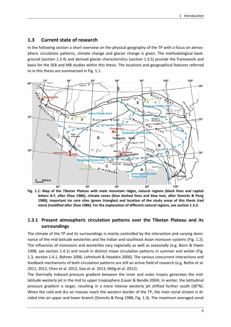
Fig. 1.1: Map of the Tibetan Plateau with main mountain ridges, natural regions (black lines and capital
letters A-F, after Zhao 1986), climate zones (blue dashed lines and blue text, after Domrös & Peng 1988), important ice core sites (green triangles) and location of the study areas of this thesis (red stars) (modified after Zhao 1986). For the explanation of different natural regions, see section 1.3.3.
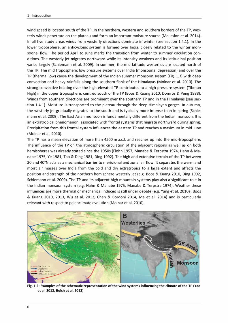
1.3.1 Present atmospheric circulation patterns over the Tibetan Plateau and its surroundings
The climate of the TP and its surroundings is mainly controlled by the interaction and varying domi-
nance of the mid-latitude westerlies and the Indian and southeast Asian monsoon systems (Fig. 1.2).
The influences of monsoons and westerlies vary regionally as well as seasonally (e.g. Benn & Owen
1998, see section 1.4.1) and result in distinct mean circulation patterns in summer and winter (Fig.
1.3, section 1.4.1, Böhner 2006, Lehmkuhl & Haselein 2000). The various concurrent interactions and
feedback mechanisms of both circulation patterns are still an active field of research (e.g. Bothe et al.
2011, 2012, Chen et al. 2012, Gao et al. 2013, Mölg et al. 2012).
The thermally induced pressure gradient between the inner and outer tropics generates the mid-
latitude westerly jet in the mid to upper troposphere (Lauer & Bendix 2004). In winter, the latitudinal
pressure gradient is larger, resulting in a more intense westerly jet shifted further south (30°N).
When the cold and dry air masses reach the western border of the TP, the main zonal stream is di-
vided into an upper and lower branch (Domrös & Peng 1988, Fig. 1.3). The maximum averaged zonal
1 Introduction
6
wind speed is located south of the TP. In the northern, western and southern borders of the TP, wes-
terly winds penetrate on the plateau and form an important moisture source (Maussion et al. 2014).
In all five study areas winds from westerly directions dominate in winter (see section 1.4.1). In the
lower troposphere, an anticyclonic system is formed over India, closely related to the winter mon-
soonal flow. The period April to June marks the transition from winter to summer circulation con-
ditions. The westerly jet migrates northward while its intensity weakens and its latitudinal position
varies largely (Schiemann et al. 2009). In summer, the mid-latitude westerlies are located north of
the TP. The mid tropospheric low pressure systems over India (monsoonal depression) and over the
TP (thermal low) cause the development of the Indian summer monsoon system (Fig. 1.3) with deep
convection and heavy rainfalls along the southern flank of the Himalayas (Molnar et al. 2010). The
strong convective heating over the high elevated TP contributes to a high pressure system (Tibetan
High) in the upper troposphere, centred south of the TP (Boos & Kuang 2010, Domrös & Peng 1988).
Winds from southern directions are prominent over the southern TP and in the Himalayas (see sec-
tion 1.4.1). Moisture is transported to the plateau through the deep Himalayan gorges. In autumn,
the westerly jet gradually migrates to the south and is typically more intense than in spring (Schie-
mann et al. 2009). The East Asian monsoon is fundamentally different from the Indian monsoon. It is
an extratropical phenomenon, associated with frontal systems that migrate northward during spring.
Precipitation from this frontal system influences the eastern TP and reaches a maximum in mid June
(Molnar et al. 2010).
The TP has a mean elevation of more than 4500 m a.s.l. and reaches up into the mid-troposphere.
The influence of the TP on the atmospheric circulation of the adjacent regions as well as on both
hemispheres was already stated since the 1950s (Flohn 1957, Manabe & Terpstra 1974, Hahn & Ma-
nabe 1975, Ye 1981, Tao & Ding 1981, Ding 1992). The high and extensive terrain of the TP between
30 and 40°N acts as a mechanical barrier to meridional and zonal air flow. It separates the warm and
moist air masses over India from the cold and dry extratropics to a large extent and affects the
position and strength of the northern hemisphere westerly jet (e.g. Boos & Kuang 2010, Ding 1992,
Schiemann et al. 2009). The TP and its adjacent high mountain systems play also a significant role in
the Indian monsoon system (e.g. Hahn & Manabe 1975, Manabe & Terpstra 1974). Weather these
influences are more thermal or mechanical induced is still under debate (e.g. Yang et al. 2010a, Boos
& Kuang 2010, 2013, Wu et al. 2012, Chen & Bordoni 2014, Ma et al. 2014) and is particularly
relevant with respect to paleoclimate evolution (Molnar et al. 2010).
Fig. 1.2: Examples of the schematic representation of the wind systems influencing the climate of the TP (Yao
et al. 2012, Bolch et al. 2012)
1 Introduction
7
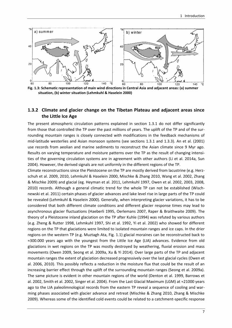
Fig. 1.3: Schematic representation of main wind directions in Central Asia and adjacent areas: (a) summer
situation, (b) winter situation (Lehmkuhl & Haselein 2000)
1.3.2 Climate and glacier change on the Tibetan Plateau and adjacent areas since the Little Ice Age
The present atmospheric circulation patterns explained in section 1.3.1 do not differ significantly
from those that controlled the TP over the past millions of years. The uplift of the TP and of the sur-
rounding mountain ranges is closely connected with modifications in the feedback mechanisms of
mid-latitude westerlies and Asian monsoon systems (see sections 1.3.1 and 1.3.3). An et al. (2001)
use records from aeolian and marine sediments to reconstruct the Asian climate since 9 Myr ago.
Results on varying temperature and moisture patterns over the TP as the result of changing intensi-
ties of the governing circulation systems are in agreement with other authors (Li et al. 2014a, Sun
2004). However, the derived signals are not uniformly in the different regions of the TP.
Climate reconstructions since the Pleistocene on the TP are mostly derived from lacustrine (e.g. Herz-
schuh et al. 2009, 2010, Lehmkuhl & Haselein 2000, Mischke & Zhang 2010, Wang et al. 2002, Zhang
& Mischke 2009) and glacial (eg. Heyman et al. 2011, Lehmkuhl 1997, Owen et al. 2002, 2003, 2008,
2010) records. Although a general climatic trend for the whole TP can not be established (Wisch-
newski et al. 2011) certain phases of glacier advances and lake level rise in large parts of the TP could
be revealed (Lehmkuhl & Haselein 2000). Generally, when interpreting glacier variations, it has to be
considered that both different climate conditions and different glacier response times may lead to
asynchronous glacier fluctuations (Haeberli 1995, Oerlemans 2007, Raper & Braithwaite 2009). The
theory of a Pleistocene inland glaciation on the TP after Kuhle (1994) was refuted by various authors
(e.g. Zheng & Rutter 1998, Lehmkuhl 1997, Shi et al. 1992, Yi et al. 2002) who showed for different
regions on the TP that glaciations were limited to isolated mountain ranges and ice caps. In the drier
regions on the western TP (e.g. Muztagh Ata, Fig. 1.1) glacial moraines can be reconstructed back to
≈300.000 years ago with the youngest from the Little Ice Age (LIA) advances. Evidence from old
glaciations in wet regions on the TP was mostly destroyed by weathering, fluvial erosion and mass
movements (Owen 2009, Seong et al. 2009a, Xu & Yi 2014). Over large parts of the TP and adjacent
mountain ranges the extent of glaciation decreased progressively over the last glacial cycles (Owen et
al. 2006, 2010). This possibly reflects a reduction in the moisture flux that could be the result of an
increasing barrier effect through the uplift of the surrounding mountain ranges (Seong et al. 2009a).
The same picture is evident in other mountain regions of the world (Denton et al. 1999, Barrows et
al. 2002, Smith et al. 2002, Singer et al. 2004). From the Last Glacial Maximum (LGM) at ≈21000 years
ago to the LIA paleolimnological records from the eastern TP reveal a sequence of cooling and war-
ming phases associated with glacier advance and retreat (Mischke & Zhang 2010, Zhang & Mischke
2009). Whereas some of the identified cold events could be related to a catchment-specific response
1 Introduction
8
to climate variations, the majority corresponds to cold events also identified at sites on the central
and western TP within the same periods or slightly shifted in time (Mischke & Zhang 2010).
The LIA is considered to be a global cooling period although its timing and nature are highly variable
for different regions (Bradley & Jones 1993, Jones et al. 1998, 1999, Mann et al. 1999). In Europe, the
LIA began in the 16th century and lasted until the end of the 19th century (Grove & Switsur 1994)
associated with significant glacier advances (Holzhauser et al. 2005, Ivy-Ochs et al. 2009, Nussbaumer
et al. 2007). For the reconstruction of LIA climate fluctuations on the TP the majority of authors draw
their conclusions based on the extents and chronologies of glacial moraines (e.g. Owen 2009, Xu & Yi
2014). During the LIA three well pronounced terminal moraine systems have been formed in many
regions that are associated with three colder periods. The second period can be related to the Maun-
der Minimum (1645-1715) (Shi & Liu 2000). Dating methods are mainly based on radiocarbon 14C,
lichenometry and cosmogenic radionuclides (CRN, 10Be). The latter is a comparatively new method
and could provide new insights into the timing of the LIA in recent years (Xu & Yi 2014). The maritime
(temperate) glaciers on the wetter eastern and south eastern TP are highly sensitive to climate varia-
tions (see section 1.3.5). Therefore, research on late Holocene changes of the monsoonal climate and
glacier fluctuations especially focuses on this area (e.g. Loibl et al. 2014, Su & Shi 2002, Yang et al.
2008, Zhou et al. 2010). The climate and the lower altitude favour the growth of trees on the glacial
moraines. Bräuning (2006) reconstructed multiple glacier advances between 1580 and 1987 in eas-
tern and south eastern TP from dendrochronological moraine dating. In general, subsequent moraine
formations beyond the contemporary glaciers indicate multiple periods of glacier advance and re-
treat during the LIA on the TP. However, the uncertainties within the different applied dating meth-
ods recommend the comparison of the timing of the LIA maximum glacier extents only, especially the
retreating time (Xu & Yi 2014). The majority of glaciers on the southern TP (Himalayas, Nyainqen-
tanglha Shan, Hengduan Shan, Fig. 1.1) reached their LIA maximum extent in the late 14th century
and retreated from that extent during the 16th to the early 18th century. At some glaciers a re-ad-
vance in the late 18th to the early 19th century can be identified (e.g. Barnard 2004a,b, Owen et al.
2005, 2010, Xu & Yi 2014). On the north western TP (Karakorum, Pamir, Fig. 1.1) glaciers advanced to
their LIA maximum extents in the early 14th century and retreated between the late 14th and the
early 15th century. Some glacial moraines again show re-advances between late 18th and early 19th
century (e.g. Seong et al. 2007, 2009a,b, Xu & Yi 2014). For the glaciers on the north eastern TP (Qili-
an Shan, Fig. 1.1) the periods of glacier advance can not be inferred. They retreated quite synchron-
ously from the LIA maximum extents in the early 16th, the late 18th and the late 19th century, res-
pectively (e.g. Chen 1989, Xu & Yi 2014). On the central TP LIA moraine datings are scarce. Few li-
chenometry samples on LIA moraines in the Tanggula Shan (Fig. 1.1) are dated to the 19th century
(Xu & Yi 2014). From these results it can be concluded that the glaciers on the TP reacted quite syn-
chronously between the late 18th to the late 19th century. However, the glacier retreat from the LIA
maximum extents (outermost LIA moraines) was not synchronous in the different regions of the TP.
To compare the moraine dated LIA glacier fluctuations to climate variations, ice core records from
Dasuopu, Purogangri, Dunde and Guliya ice cores from the Himalayas, the Tanggula Shan, the Qilian
Shan and the Kunlun Shan (Fig. 1.1), respectively, need to be evaluated (Yang et al. 2009, Yao et al.
2007, 2008). The dating of the Dasuopu ice core indicates a long period of generally low tempera-
tures before the 17th century and between the late 18th and the early 19th century. These periods
agree with phases of glacier advances on the southern TP. During the late 19th century precipitation
increased. However, no signals for glacier advances during this time could be revealed on the south-
ern TP. The ice core from the Purogangri ice cap revealed several cold periods from the 15th century
to the early 19th century that correspond to LIA glacier advance of glaciers on the eastern and south-
ern TP (Yang et al. 2009). An abrupt warming occurred between 1910 and 1920 suggesting a transi-
1 Introduction
9
tion to a warmer, wetter climate (Thompson et al. 2006). The Guliya ice core record shows cold peri-
ods around 1230-1360, 1480-1520 and 1670-1880 (Xu & Yi 2014). During the latter period precipita-
tion decreased and therefore can not have contributed to the glacier advances between late 18th
and early 19th century on the north western TP. Generally, the periods of lower temperatures cor-
respond well with the phases of glacier advances in this region. The temperature record of the Dunde
ice core is closely related to glacier fluctuations on the north eastern TP with phases of higher tem-
peratures during inferred glacier retreat. The relationship between TP ice core records and LIA mo-
raines implies that temperature variations on the TP during the LIA had a stronger influence on gla-
cier fluctuations than precipitation changes.
The climate and glacier change on the TP since the 20th century can be revealed from meteorological
and glaciological field observations as well as from satellite data. Numerous studies agree, that air
temperatures on the TP and its adjacent areas increased since the late 19th century with an accelera-
ting trend in the 1950s and since the 1980s and 1990s (e.g. Yang et al. 2009, Liu & Chen 2000, Sheng
& Yao 2009, Takeuchi et al. 2009, Xue et al. 2009, You et al. 2010). Highest significant temperature in-
creases could be observed in winter and autumn, whereas warming in spring and summer is less pro-
nounced (Liu & Chen 2000, Wei & Fang 2013, Xie et al. 2010, You et al. 2010). Spatially, the regions of
highest elevations (and lowest temperatures) and the warmer temperature zones in low altitudes on
the TP experienced less temperature increase. These areas only account for a small proportion of the
total area of the TP (≈20%). Therefore, the largest warming trends can be identified in the central,
north western and north eastern plateau regions (Wei & Fang 2013). You et al. (2010) also found the
north eastern TP to experience the most significant warming trends especially in winter and autumn.
Furthermore, the authors find large scale atmospheric circulation patterns (e.g. sea level pressure
anomalies, El Nino) to be contributing factors to the observed decadal and seasonal TP temperature
trends. Further air temperature evaluations show that the warming rates both in summer and winter
increase with altitude from 3000 to 4000 m a.s.l. Above 4000 m a.s.l. they are stable with altitude or
show a slight decline (Liu & Chen 2000, Qin et al. 2009). Wei & Fang (2013) showed that this pattern
was predominating on the TP during 1961-2010. However, this trend has been weakened due to
more rapid warming at lower altitudes. This is an important finding because most glaciers on the TP
are located at higher altitudes above 4500 m a.s.l. Precipitation variations on the TP are less pro-
nounced and regionally contrasting. For the south western TP Li et al. (2010, 2011) show a weak
overall decreasing trend 1961-2008, with increasing precipitation only in winter and spring. This is in
agreement with Yao et al. (2012) who give decreasing precipitation in the Himalayas and increasing
amounts in the eastern Pamir mountains. Palazzi et al. (2013) indicate a statistically significant de-
creasing trend in summer in the Hindukush-Karakorum-Himalaya region. Reasons for this spatial vari-
ability might be the weakening of the Indian monsoon and the strengthening of the westerlies as
found in recent studies (Wu 2005, Zhao et al. 2012).
According to the overall trend of increasing air temperatures on the TP and its adjacent areas since
several decades, most glaciers on the TP (Kang et al. 2010, Yao et al. 2012) and in the Himalayas
(Bolch et al. 2012, Kargel et al. 2011) are retreating. Generally, the rates of area loss have been in-
creasing in recent years. The regional patterns are contrasting (Kääb et al. 2012), influenced by local
factors (e.g. topography, debris cover, glacier type) and the spatial and temporal heterogeneity of
climate and climate variability mentioned above in this section and in section 1.3.1. Yao et al. (2012)
summarize the systematic differences in glacier behaviour in the different regions of the TP over the
past 30 years based on satellite imagery and in-situ observations. The Himalayan glaciers and the
glaciers of the Hengduan Shan experienced the greatest reduction in mass, length and area, whereas
the observed shrinkage decreases to the central and northern TP (Neckel et al. 2014, Wei et al.
2014). The region of the eastern Pamir and Karakorum mountains showed even positive MB and
1 Introduction
10
smallest retreat rates. Bolch et al. (2012) and Scherler et al. (2011) draw a similar picture for the Hi-
malaya-Karakorum region but stress the high variability both in time between the decades and in
space between individual glaciers. Between 1920 and 1940 half of the recorded Himalayan glaciers
were stable or advanced. During 1976 to 2007 some glaciers in the Hindukush and the Kunlun Shan
(1970-1990) showed a similar pattern (Bolch et al. 2012, Shangguan et al. 2007). The heterogeneous
and oscillatory response of individual glaciers in the Himalayas to climate variability is also shown by
Fujita & Nuimura (2011) based on in-situ measurements. The so called ‘Karakorum anomaly’ or
‘Pamir-Karakorum anomaly’ was subject to a number of publications with the attempt to explain the
observed glacier expansions through surging, winter temperature decrease and increased solid preci-
pitation (Hewitt 2005, Gardelle et al. 2012, 2013a, Mukhopadhyay & Khan 2014). Bhambri et al.
(2013) found that the observed glaciers in the northeast Karakorum show an irregular behaviour
since 1973 with phases of retreat and advance. Evaluations of glacier changes based on GRACE reveal
an overall negative trend in this area since 2002 with a strong five-year cycle (Yi & Sun 2014). The
authors conclude from their analyses that this five-year signal of glacier change in the Pamir-Karako-
rum region is controlled by both the ENSO and AO. The former plays a greater role because its
correlation with precipitation is much stronger (-0.62, AO: -0.20).
Yao et al. (2012) give an overview on the distribution of the ELA on the TP and its adjacent mountain
ranges. Generally, the ELA is lower where accumulation is greater (Bolch et al. 2012). Thus, a low ELA
concentrates on the south eastern and the north western TP, influenced by high precipitation
amounts from Indian monsoon and mid-latitude westerlies, respectively (see section 1.4.1). These
regions coincide with the two centres of recent glaciation on the TP (see section 1.3.3). The smaller
number of glaciers and the higher ELA on the interior plateau are the result of decreased moisture
supply through the barrier-effect of the surrounding mountain ridges (see section 1.3.1). However,
the local ELA for single glaciers can be highly variable both in time and space (see section 1.4.1).
1.3.3 Comprehensive physical geography of the Tibetan Plateau
Due to its unique topography, climate and geological history, the Tibetan Plateau (TP, also Qinghai-
Xizang Plateau) forms a single natural unit within China (Zhao 1986). Its mean elevation is around
4700 m a.s.l. With an area of around 2.5 million km2 it contains 25% of the total land area of China
(Meyerhoff et al. 1991, Zhao 1986). It is surrounded by a series of high mountain ranges. The Kunlun
Shan, the Altun Shan and the Qilian Shan in the north, the Hengduan Shan in the southeast, the
Himalayas in the south and the Karakoram and the Pamir moutains in the west (Fig. 1.1).
The present physical environment both of the TP and of the whole country is the product of its geo-
logical history. The Indo-China tectonic movement during the early and the Yanshan tectonic move-
ment during the late Mesozoic era determined the broad geological structures of China. Since the Eo-
cene the Himalayan tectonic movement, caused by the collision of the Indo-Australian Plate and the
Eurasian Plate, shaped the Chinese physical environment. Crustal thickening by subduction during
the early Cretaceous perhaps caused the raising of the southern TP to an elevation of 3000-
4000 m a.s.l. prior to the actual collision (Murphy et al. 1997). After collision, intracontinental defor-
mation and uplift continued and stepwise migrated northward to involve the whole TP (Fig. 1.4, Li et
al. 2014a, Mulch & Chamberlain 2006). The uplift of the eastern plateau occurred much later through
crustal shortening in the western and central TP and an eastward flow within the deep crust (Royden
et al. 2008). The phase of the Himalayan tectonic movement can be subdivided into several stages (Li
1987, Wang & Li 1985). The first occurred in the middle Eocene when the Himalayas were folded and
the Tethys Sea was closed through the emergence of the TP. From the end of the Oligocene to the
middle Miocene intensive folding, metamorphism and magmatic activities characterized the Hima-
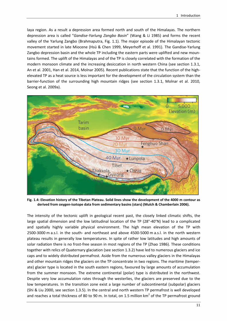
1 Introduction
11
laya region. As a result a depression area formed north and south of the Himalayas. The northern
depression area is called “Gandise-Yarlung Zangbo Basin” (Wang & Li 1985) and forms the recent
valley of the Yarlung Zangbo (Brahmaputra, Fig. 1.1). The major episode of the Himalayan tectonic
movement started in late Miocene (Hsü & Chen 1999, Meyerhoff et al. 1991). The Gandise-Yarlung
Zangbo depression basin and the whole TP including the eastern parts were uplifted and new moun-
tains formed. The uplift of the Himalayas and of the TP is closely correlated with the formation of the
modern monsoon climate and the increasing desiccation in north western China (see section 1.3.1,
An et al. 2001, Han et al. 2014, Molnar 2005). Recent publications state that the function of the high-
elevated TP as a heat source is less important for the development of the circulation system than the
barrier-function of the surrounding high mountain ridges (see section 1.3.1, Molnar et al. 2010,
Seong et al. 2009a).
Fig. 1.4: Elevation history of the Tibetan Plateau. Solid lines show the development of the 4000 m contour as derived from oxygen-isotope data from sedimentary basins (stars) (Mulch & Chamberlain 2006).
The intensity of the tectonic uplift in geological recent past, the closely linked climatic shifts, the
large spatial dimension and the low latitudinal location of the TP (28°-40°N) lead to a complicated
and spatially highly variable physical environment. The high mean elevation of the TP with
2500-3000 m a.s.l. in the south- and northeast and above 4500-5000 m a.s.l. in the north western
plateau results in generally low temperatures. In spite of rather low latitudes and high amounts of
solar radiation there is no frost-free season in most regions of the TP (Zhao 1986). These conditions
together with relics of Quaternary glaciation (see section 1.3.2) have led to numerous glaciers and ice
caps and to widely distributed permafrost. Aside from the numerous valley glaciers in the Himalayas
and other mountain ridges the glaciers on the TP concentrate in two regions. The maritime (temper-
ate) glacier type is located in the south eastern regions, favoured by large amounts of accumulation
from the summer monsoon. The extreme continental (polar) type is distributed in the northwest.
Despite very low accumulation rates through the westerlies, the glaciers are preserved due to the
low temperatures. In the transition zone exist a large number of subcontinental (subpolar) glaciers
(Shi & Liu 2000, see section 1.3.5). In the central and north western TP permafrost is well developed
and reaches a total thickness of 80 to 90 m. In total, on 1.5 million km2 of the TP permafrost ground
1 Introduction
12
occurs, corresponding to 60% of the plateau area (Cui & Graf 2009). It is the highest and most exten-
sive high-altitude permafrost area on Earth (Liu & Chen 2000) and influences the alpine ecosystem
(Wang et al. 2006). From the 1970s to the 1990s, permafrost temperatures rose by up to 0.5°C over
most of the TP along with an increasing thickness of the active layer (Wu & Zhang 2010). The
reduction of the permafrost area over the same period is estimated to be 100 000 km2 (Kang et al.
2010). The mean lower elevation of permafrost occurrence rose by 25 m on the northern TP and up
to 80 m in the southern regions of the TP during the past decades (Cheng & Wu 2007). The wide-
spread degradation of permafrost and seasonally frozen ground caused desertification processes in
the eastern and western TP through surface drying and decrease in vegetation cover (Xue et al. 2009,
Yang et al. 2010b).
The tectonic uplift of the ancient erosional surface forced the rejuvenation of geomorphic processes
and landforms. In the humid south eastern parts of the TP the valley-within-a-valley structure is
commonly seen in the middle and lower reaches of large rivers. The domination of fluvial erosion
leads to a deeply dissected landscape. The relatively warm and humid climate favours strong bio-
chemical weathering. In the more arid central and north western parts desiccation and nivation pro-
cesses dominate. Physical weathering through freeze-thaw cycles plays a major role for denudation.
In these areas an undulating and almost undissected high plateau surface with periglacial landforms
prevails. Due to the recent geological development, the strong glaciation and weak chemical wea-
thering, soils are generally young and slightly developed in most regions of the TP. The hydrological
drainage system changes from exorheic in the southeast to endorheic in the interior regions (Neckel
et al. 2014, Zhao 1986). In recent years, lake level changes of the endorheic basin lakes on the TP
have been subject to extensive research because they are considered to be sensitive indicators of
climate variability (Song et al. 2014). Water level fluctuations may reflect regional-scale variations in
evaporation, precipitation amounts and glacier melt water supply (Wu et al. 2014). The regional pat-
terns of lake area changes on the TP are diverse (Song et al. 2014a). In general, inland lakes were
stable or shrinking before 2000 and expanded in the 2000s. These results were confirmed in various
studies using different methods (e.g. Huang et al. 2011, Kropacek et al. 2012, Liu et al. 2009, Wu & Zu
2008, Ye et al. 2007, Zhu et al. 2010). Phan et al. (2011), Song et al. (2014b), Zhang et al. (2011a) and
Zhang et al. (2013) report a rapid increase in water levels between 2003 and 2009/10 for the major-
ity of closed basin lakes on the TP. Although some authors emphasize the contribution of glacier melt
water to lake level rise (Chen et al. 2007, Wu & Zhu 2008), recent studies agree that lake expansions
on the TP in the 2000s were driven primarily by changes in precipitation and evaporation (Song et al.
2014b, Wu et al. 2014, Ye et al. 2007, Zhu et al. 2010).
Both flora and fauna on the TP follow the temperature and moisture induced southeast-northwest
gradient. The continental central and north-western regions belong to the paleoarctic realm with
dwarf shrubs and montane desert steppe. The warmer and more humid south eastern parts pertain
to the oriental realm. Vegetation becomes more diverse with large areas of needle-leaved forests.
The east-west oriented high elevated Himalayas south of the TP serve as an effective barrier for tro-
pical and subtropical fauna and flora from the Indian subcontinent. The Kunlun-Altun-Qilian moun-
tain system in the north has a lower relative altitude and numerous mountain passes. The less effect-
tive barrier leads to many species of flora and fauna appearing both on the TP and in the Northwest
of China. The favourable orientation of the Hengduan Shan in the southeast and the Karakoram in
the west enable the migrating and mixing of different species. Furthermore, the noticeable vertical
zonation on the TP due to the large relief energy favoured the survival of many pre-Tertiary species
(Zhao 1986).
1 Introduction
13
The horizontal zonation on the TP is mainly characterized by the moisture gradient, caused by the
atmospheric circulation and the barrier-effect of the surrounding mountain ranges. A latitudinal tem-
perature change exists as well but is usually disguised by the much stronger vertical zonation. The
integration of horizontal and vertical zonation leads to the definition of six natural regions on the TP
(Fig. 1.1). The regions basically correspond to the climate zones on the TP described by Domrös &
Peng (1988). The transition zones between the different regions are continuous. The region of the
southern Himalayan slopes (A in Fig. 1.1) comprises the East Himalayas at the southern border of the
TP. The crest line is remarkably lower than in the Central and West Himalayas and there are a num-
ber of maritime (temperate) type glaciers. The glaciers exist even at low altitudes and characteristi-
cally run through the montane needle-leaved forest belt and end in the evergreen broad-leaved
forest belt. The region experiences no dry period. It is the most humid section of the Himalayas. The
Indian summer monsoon lasts from May to October. The humid air masses are directed to the south-
ern slopes of the Himalayas and through the river gorges onto the TP. The elevation of maximum
precipitation depends on the location, exposition and topography of the mountain ranges. In the East
Himalayas it is generally located around 2500 m a.s.l. (Zhao 1986). At the lowest altitudes tropical
rainforests appear, followed by the lower montane belt of evergreen broad-leaved forest. The latter
covers the largest area within the vertical zonation and corresponds with the altitude of maximum
precipitation. Above this vegetation belt the montane needle and broad-leaved mixed forest belt and
the montane coniferous forest belt occur. The upper forest limit is located in an altitude between
3700 and 4100 m a.s.l. Miehe et al. (2007) found the highest tree stands of Juniperus indica at an ele-
vation of 4750 m a.s.l. in northern Bhutan. Above the forest belt, there are alpine scrubs and mea-
dows followed by the subnival and nival belts.
The south-eastern part of the TP comprises mainly the middle-northern parts of the Hengduan Shan
and the eastern parts of the Nyainqentanglha Shan (B in Fig. 1.1). Between June and September the
region is under the influence of monsoons, both from the southeast and the southwest. Precipitation
amounts decrease to the northwest. Generally, the region inclines from north to south. The upper
reaches of the rivers in the north are located in a slightly dissected plateau with broad valleys and
gentle slopes. The landscape is shaped by periglacial structures and freezing-thawing processes. A
large number of maritime (temperate) type glaciers are located in the eastern Nyainqentanglha
Shan. The predominant vegetation consists of alpine scrubs and meadow. The south of the defined
region (Zhao 1986) is characterized by a series of north-south directed high mountain ridges and
deep river gorges. The foehn and rainshadow effects result in a number of warm, dry valleys in the
gorge area. Vegetation consists of thorny and succulent shrubs. With the exception of the dry valleys,
a number of montane evergreen broadleaf forests exist. Most areas are covered by mixed leaf and
needle-leaved forests (Zhao 1986). Forest areas decrease to the northwest. The upper forest limit is
around 4500 m a.s.l. Miehe et al. (2007) even located the highest forest stand of Juniperus tibetica at
4900 m a.s.l. This is the highest treeline in the northern hemisphere (Miehe et al. 2007). Above the
tree line occur alpine shrubs and meadows.
The southern TP is defined as the region between the Gangdise-Nyainqentanglha ranges in the north
and the highest section of the Himalayas in the south (C in Fig. 1.1). A large number of maritime
(temperate) and subcontinental (subpolar) type glaciers are located in the mountain ranges. The
southern side of the Himalayan range is steep-sloped whereas the northern slopes descend gradually
to the TP. The latter are characterized by large glaciofluvial fans, morainic platforms and fault basins
(Zhao 1986). The Yarlung Zangbo (Brahmaputra) flows from west to east in the graben structure at
the southern foot of the Gangdise-Nyainqentanglha ranges. Broad valleys with alluvial plains, bar-
chan sand dunes and braided channels alternate with narrow gorges. As a result of the barrier func-
tion of the Himalayas, precipitation amounts generally decrease from east to west. Total precipita-
1 Introduction
14
tion reaches its minimum in the areas of rainshadow to the north of the Himalayas. The predominant
vegetation is montane shrubby-steppe and alpine steppe. The broad valleys and lower lower slopes
are mainly covered by montane steppe. Above altitudes of around 4500 m a.s.l. the alpine steppe
occurs, followed by alpine meadow from around 5000 m a.s.l. upwards. In the valley of the Yarlung
Zangbo and adjacent areas, the alpine meadow consists mainly of Kobresia pygmaea. The Kobresia
pygmaea pastures of the southern, south-eastern and central TP are the world’s largest ecosystem
(Miehe et al. 2008). The extremely firm turf protects large surfaces against erosion. Recent dynamics
show a degradation of the pastures under the grazing impact of increasing livestock numbers (Miehe
et al. 2008). In recent years, the forest areas of southern and south-eastern TP decreased signifycant-
ly and were replaced by cropland (Cui & Graf 2009).
The central TP stretches from southwest to northeast in the central part of the plateau and includes
the eastern Qiangtang Plateau, southern Qinghai Province and the eastern Qinghai-Qilian Shan (D in
Fig. 1.1). The lofty Qiangtang Plateau is an intramontane basin at around 4700 m a.s.l. between the
Kunlun Shan in the north and the Gangdise-Nyainqentanglha Shan in the south (Fig. 1.1). The area
belongs to the interior/endorheic drainage system and contains a large number of lakes (e.g. Nam
Co). The numerous glaciers in the mountain ranges belong to the subcontinental (subpolar) and the
extreme continental (polar) type. The Qiangtang Plateau is characterized by strong cryo-weathering
and significant alternation of freezing and thawing. The Qilian Shan in the northeast is separated
from the TP by the Hexi Corridor and Lake Qinghai (Qinghai Hu, Fig. 1.1). The latter is the largest lake
in China (Zhao 1986). The eastern region of Qinghai is covered by loess. Intense fluvial activity leads
to the occurrence of erosional terraces. The climate is subhumid to semi-arid because the lofty, near
parallel mountain ranges in the south are an effective precipitation barrier. Generally, precipitation
amounts decrease from east to west. The main type of vegetation on Qiangtang Plateau is the alpine
steppe, followed by the alpine meadow that consists of Kobresia pygmaea. Valleys and basins are
covered by marshy meadows. Vegetation in the valleys of the Qilian Shan is dominated by montane
forest steppe with needle-leaved forest. Above, alpine scrubs and meadows occur.
The region which includes the Qaidam Basin, the western Qilian Shan, the Altun Shan and the nor-
thern slopes of the Kunlun Shan, almost extends in east-west direction on the northern TP (E in Fig.
1.1). It is the transition from the TP to the desert regions of northwest China. The region, especially
the Qaidam Basin, is characterized by a temperate desert. On the basis of its thermal conditions and
its geological formation it is still considered to be part of the TP. The Qaidam basin is a graben struc-
ture between 2600 and 3000 m a.s.l. with a series of concentric belts from the outer mountain barri-
ers to the piedmont plain with lakes in the centre. Land types are composed from sandy deserts with
dunes and yardangs, and gravel desert. The central part is covered by clay, silt and salty marshlands
(Zhao 1986). The western Qilian Shan consists of a series of mountain ranges with a crest line altitude
of about 4000 to 5000 m a.s.l., trending nearly northwest-southeast. The Altun Shan with an altitude
of 3600 to 4000 m a.s.l. runs from northeast to southwest. The Kunlun Shan is nearly west-east direc-
ted and high ridges reach over 6000 m a.s.l. in the middle section. In the high mountain ranges a
number of extreme continental (polar) type glaciers occur (Shi & Liu 2000). The region is influenced
by mid-latitude westerlies year round. The numerous mountain ranges in the south cut off the mois-
ture transport from the monsoonal air masses. The Qaidam basin is the driest area on the TP. The de-
sert vegetation mainly consists of xerophilous shrubs. The montane desert occurs at altitudes up to
3800 m a.s.l. followed by the montane steppe.
The Ngari-Kunlun Shan region is located in the north-western part of the TP (F in Fig. 1.1). It includes
the western Ngari prefecture and the southern side of the middle and western Kunlun Shan. The
Ngari prefecture is surrounded by the western Himalayas, the Gangdise Shan and the Karakorum
with crest lines of more than 6000 m a.s.l. Due to the dry climate, only few glaciers appear. The Kun-
1 Introduction
15
lun Shan trends towards the northern rim of the TP. Because of its higher elevation and continental
location, the climate in the Kunlun Shan is arid and cold. Permafrost occurs everywhere and the wes-
tern part of the Kunlun Shan is one centre of glaciation with glaciers of the extreme continental (po-
lar) type. The Ngari area is rather temperate. The montane desert steppe and the alpine shrubby-
steppe are limited to the Ngari area. In the region of the Kunlun Shan, alpine desert vegetation, cha-
racterized by sparse cover and dwarf plants, dominates. The vegetation mainly consists of the shrub
Ajania tibetica which is a species endemic to the TP (Zhao 1986).
During the Holocene the natural environment of the TP changed due to varying forcing of the mid-
latitude westerlies and the monsoonal circulation. Analyses of pollen records show strong regional
differrences in vegetation changes over the TP (Herzschuh et al. 2010). In the central, northern and
eastern regions of the TP, vegetation types were relatively stable. Environmental changes were
primarily characterized by the evolution from steppe to desert steppe in the north (Li et al. 1985) and
by a gradual variation from temperate steppe to alpine meadows in the central and eastern regions.
In the Qaidam Basin, temperate desert was the dominating land cover throughout the Holocene
(Herzschuh et al. 2010). The greatest environmental changes are found in the north- and south-
eastern regions of the TP. Pollen records from Lake Qinghai indicate that forest areas were replaced
by forest steppe since the mid Holocene. In the south and southeast TP, forest and savanne
vegetation gradually changed to shrubby steppe and steppe (Herzschuh et al. 2010, Li et al. 1985).
1.3.4 Methodological background
The methods used in this thesis are centred in the field of numerical glacier mass balance modelling.
A conceptual, physically based model has been developed that directly couples the glacier SEB to a
subsurface multi-layer snow model in order to derive glacier MB and runoff (see section 2.3.1). The
major physical processes are represented by mathematical relationships. A first outline of such a mo-
del was given by Anderson (1976). These formulations are in contrast to index models that use one
or more variables in an empirical expression to estimate glacier melt (Singh & Singh 2001). Air tem-
perature is the most commonly used index because it strongly influences the most important energy
sources for melt on most glaciers (longwave incoming radiation and sensible heat flux) (Ohmura
2001). This section gives an overview of the basic assumptions and concepts in glacier SEB (section
1.3.4.1) and MB modelling (section 1.3.4.2).
1.3.4.1 Glacier surface energy balance
The glacier SEB describes the balance in the amount of energy of the glacier near-surface layer due to
flows of energy to or away from this layer (Cogley et al. 2011). The near-surface layer links atmos-
pheric processes and the glacier body and is assumed to be an interface, the thickness of which
approaches zero and therefore cannot store energy. The energy fluxes that govern the energy ex-
change between glacier surface and atmosphere or subsurface are presented in Fig. 1.5. If the sum of
these fluxes, the energy balance, is positive and surface temperature is at the melting point, melt
occurs. Phase changes, such as melting and sublimation, couple the surface energy balance to the
mass balance. Hence, it is crucial to determine the energy balance to model glacier ablation and, in
general, to understand the influence of meteorological conditions to the energy budget of a glacier
surface.
On most glaciers, shortwave and longwave radiation and the turbulent fluxes play a major role in the
surface energy balance (Fig. 1.5). Incoming shortwave radiation (SWin) shows both a daily and seaso-
nal cycle and is additionally modified through the structure of the atmosphere, cloud cover and local
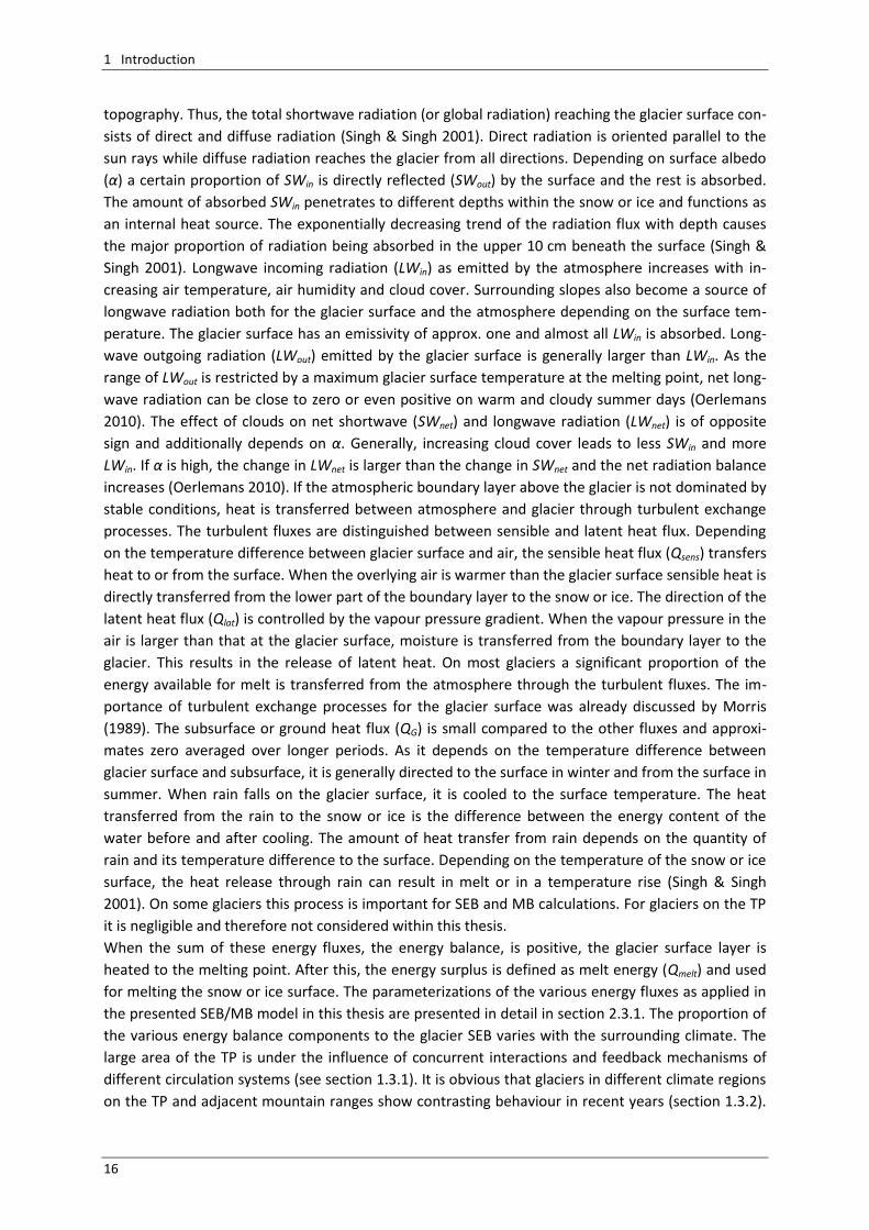
1 Introduction
16
topography. Thus, the total shortwave radiation (or global radiation) reaching the glacier surface con-
sists of direct and diffuse radiation (Singh & Singh 2001). Direct radiation is oriented parallel to the
sun rays while diffuse radiation reaches the glacier from all directions. Depending on surface albedo
(α) a certain proportion of SWin is directly reflected (SWout) by the surface and the rest is absorbed.
The amount of absorbed SWin penetrates to different depths within the snow or ice and functions as
an internal heat source. The exponentially decreasing trend of the radiation flux with depth causes
the major proportion of radiation being absorbed in the upper 10 cm beneath the surface (Singh &
Singh 2001). Longwave incoming radiation (LWin) as emitted by the atmosphere increases with in-
creasing air temperature, air humidity and cloud cover. Surrounding slopes also become a source of
longwave radiation both for the glacier surface and the atmosphere depending on the surface tem-
perature. The glacier surface has an emissivity of approx. one and almost all LWin is absorbed. Long-
wave outgoing radiation (LWout) emitted by the glacier surface is generally larger than LWin. As the
range of LWout is restricted by a maximum glacier surface temperature at the melting point, net long-
wave radiation can be close to zero or even positive on warm and cloudy summer days (Oerlemans
2010). The effect of clouds on net shortwave (SWnet) and longwave radiation (LWnet) is of opposite
sign and additionally depends on α. Generally, increasing cloud cover leads to less SWin and more
LWin. If α is high, the change in LWnet is larger than the change in SWnet and the net radiation balance
increases (Oerlemans 2010). If the atmospheric boundary layer above the glacier is not dominated by
stable conditions, heat is transferred between atmosphere and glacier through turbulent exchange
processes. The turbulent fluxes are distinguished between sensible and latent heat flux. Depending
on the temperature difference between glacier surface and air, the sensible heat flux (Qsens) transfers
heat to or from the surface. When the overlying air is warmer than the glacier surface sensible heat is
directly transferred from the lower part of the boundary layer to the snow or ice. The direction of the
latent heat flux (Qlat) is controlled by the vapour pressure gradient. When the vapour pressure in the
air is larger than that at the glacier surface, moisture is transferred from the boundary layer to the
glacier. This results in the release of latent heat. On most glaciers a significant proportion of the
energy available for melt is transferred from the atmosphere through the turbulent fluxes. The im-
portance of turbulent exchange processes for the glacier surface was already discussed by Morris
(1989). The subsurface or ground heat flux (QG) is small compared to the other fluxes and approxi-
mates zero averaged over longer periods. As it depends on the temperature difference between
glacier surface and subsurface, it is generally directed to the surface in winter and from the surface in
summer. When rain falls on the glacier surface, it is cooled to the surface temperature. The heat
transferred from the rain to the snow or ice is the difference between the energy content of the
water before and after cooling. The amount of heat transfer from rain depends on the quantity of
rain and its temperature difference to the surface. Depending on the temperature of the snow or ice
surface, the heat release through rain can result in melt or in a temperature rise (Singh & Singh
2001). On some glaciers this process is important for SEB and MB calculations. For glaciers on the TP
it is negligible and therefore not considered within this thesis.
When the sum of these energy fluxes, the energy balance, is positive, the glacier surface layer is
heated to the melting point. After this, the energy surplus is defined as melt energy (Qmelt) and used
for melting the snow or ice surface. The parameterizations of the various energy fluxes as applied in
the presented SEB/MB model in this thesis are presented in detail in section 2.3.1. The proportion of
the various energy balance components to the glacier SEB varies with the surrounding climate. The
large area of the TP is under the influence of concurrent interactions and feedback mechanisms of
different circulation systems (see section 1.3.1). It is obvious that glaciers in different climate regions
on the TP and adjacent mountain ranges show contrasting behaviour in recent years (section 1.3.2).
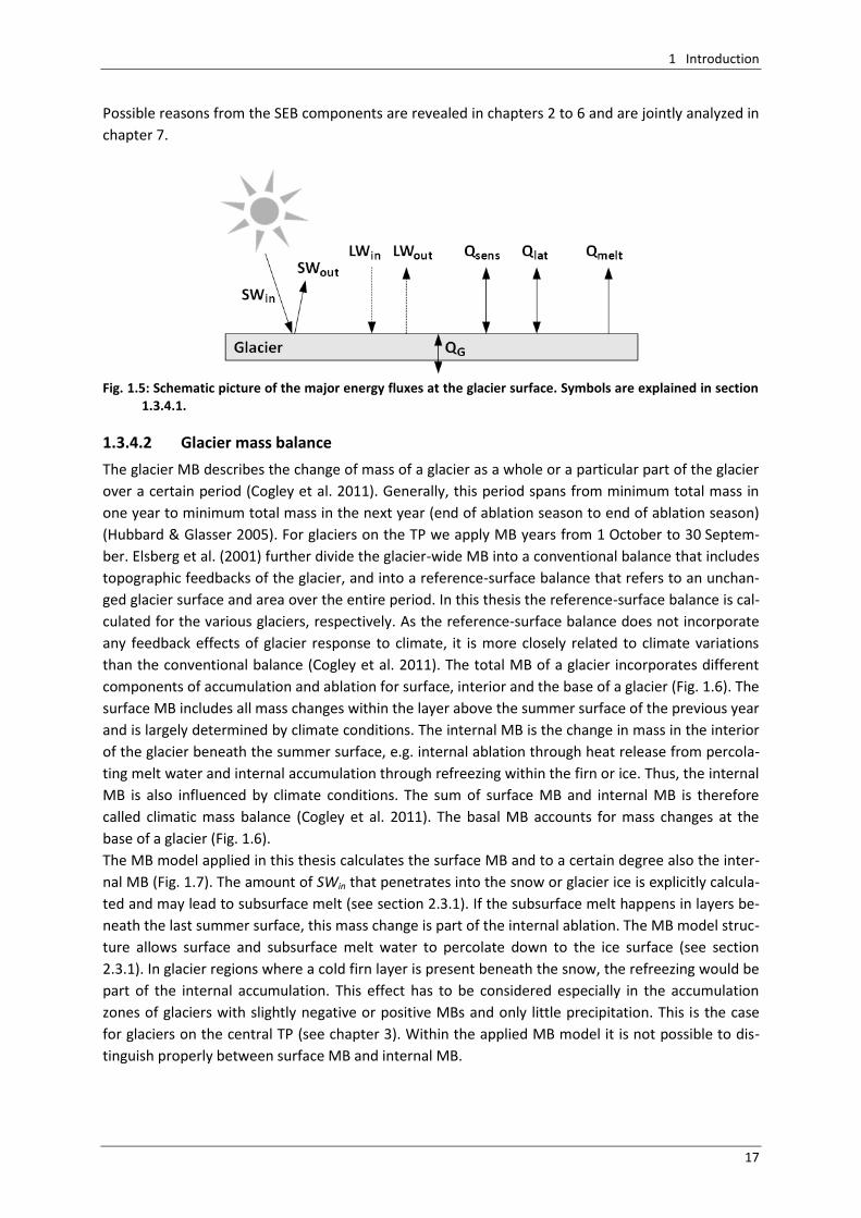
1 Introduction
17
Possible reasons from the SEB components are revealed in chapters 2 to 6 and are jointly analyzed in
chapter 7.
Fig. 1.5: Schematic picture of the major energy fluxes at the glacier surface. Symbols are explained in section
1.3.4.1.
1.3.4.2 Glacier mass balance
The glacier MB describes the change of mass of a glacier as a whole or a particular part of the glacier
over a certain period (Cogley et al. 2011). Generally, this period spans from minimum total mass in
one year to minimum total mass in the next year (end of ablation season to end of ablation season)
(Hubbard & Glasser 2005). For glaciers on the TP we apply MB years from 1 October to 30 Septem-
ber. Elsberg et al. (2001) further divide the glacier-wide MB into a conventional balance that includes
topographic feedbacks of the glacier, and into a reference-surface balance that refers to an unchan-
ged glacier surface and area over the entire period. In this thesis the reference-surface balance is cal-
culated for the various glaciers, respectively. As the reference-surface balance does not incorporate
any feedback effects of glacier response to climate, it is more closely related to climate variations
than the conventional balance (Cogley et al. 2011). The total MB of a glacier incorporates different
components of accumulation and ablation for surface, interior and the base of a glacier (Fig. 1.6). The
surface MB includes all mass changes within the layer above the summer surface of the previous year
and is largely determined by climate conditions. The internal MB is the change in mass in the interior
of the glacier beneath the summer surface, e.g. internal ablation through heat release from percola-
ting melt water and internal accumulation through refreezing within the firn or ice. Thus, the internal
MB is also influenced by climate conditions. The sum of surface MB and internal MB is therefore
called climatic mass balance (Cogley et al. 2011). The basal MB accounts for mass changes at the
base of a glacier (Fig. 1.6).
The MB model applied in this thesis calculates the surface MB and to a certain degree also the inter-
nal MB (Fig. 1.7). The amount of SWin that penetrates into the snow or glacier ice is explicitly calcula-
ted and may lead to subsurface melt (see section 2.3.1). If the subsurface melt happens in layers be-
neath the last summer surface, this mass change is part of the internal ablation. The MB model struc-
ture allows surface and subsurface melt water to percolate down to the ice surface (see section
2.3.1). In glacier regions where a cold firn layer is present beneath the snow, the refreezing would be
part of the internal accumulation. This effect has to be considered especially in the accumulation
zones of glaciers with slightly negative or positive MBs and only little precipitation. This is the case
for glaciers on the central TP (see chapter 3). Within the applied MB model it is not possible to dis-
tinguish properly between surface MB and internal MB.
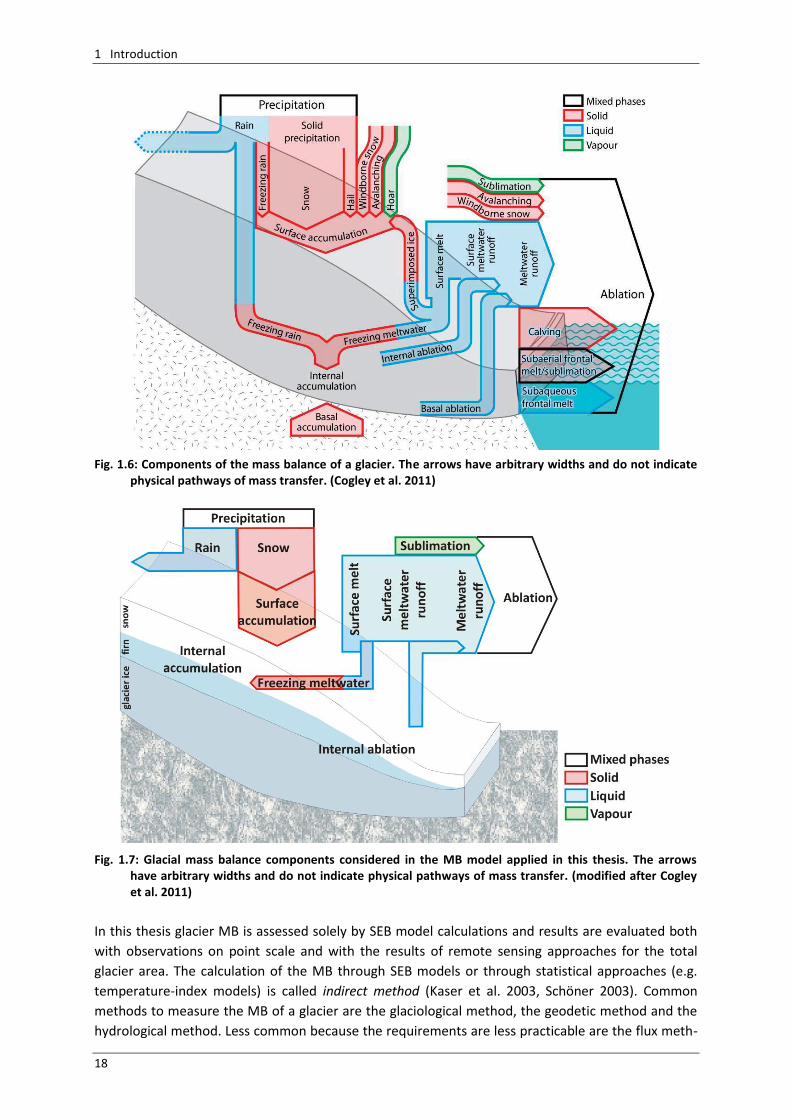
1 Introduction
18
Fig. 1.6: Components of the mass balance of a glacier. The arrows have arbitrary widths and do not indicate
physical pathways of mass transfer. (Cogley et al. 2011)
Fig. 1.7: Glacial mass balance components considered in the MB model applied in this thesis. The arrows have arbitrary widths and do not indicate physical pathways of mass transfer. (modified after Cogley et al. 2011)
In this thesis glacier MB is assessed solely by SEB model calculations and results are evaluated both
with observations on point scale and with the results of remote sensing approaches for the total
glacier area. The calculation of the MB through SEB models or through statistical approaches (e.g.
temperature-index models) is called indirect method (Kaser et al. 2003, Schöner 2003). Common
methods to measure the MB of a glacier are the glaciological method, the geodetic method and the
hydrological method. Less common because the requirements are less practicable are the flux meth-
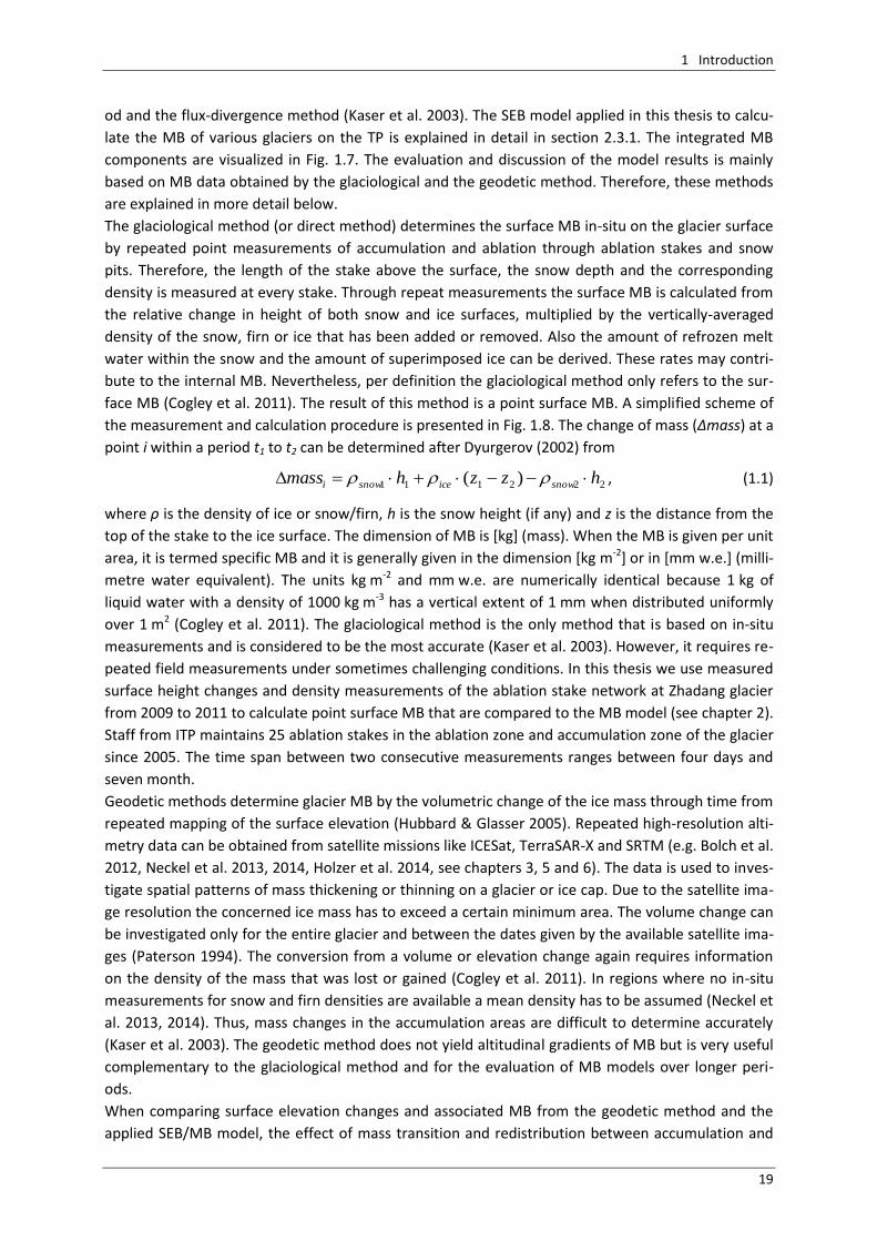
1 Introduction
19
od and the flux-divergence method (Kaser et al. 2003). The SEB model applied in this thesis to calcu-
late the MB of various glaciers on the TP is explained in detail in section 2.3.1. The integrated MB
components are visualized in Fig. 1.7. The evaluation and discussion of the model results is mainly
based on MB data obtained by the glaciological and the geodetic method. Therefore, these methods
are explained in more detail below.
The glaciological method (or direct method) determines the surface MB in-situ on the glacier surface
by repeated point measurements of accumulation and ablation through ablation stakes and snow
pits. Therefore, the length of the stake above the surface, the snow depth and the corresponding
density is measured at every stake. Through repeat measurements the surface MB is calculated from
the relative change in height of both snow and ice surfaces, multiplied by the vertically-averaged
density of the snow, firn or ice that has been added or removed. Also the amount of refrozen melt
water within the snow and the amount of superimposed ice can be derived. These rates may contri-
bute to the internal MB. Nevertheless, per definition the glaciological method only refers to the sur-
face MB (Cogley et al. 2011). The result of this method is a point surface MB. A simplified scheme of
the measurement and calculation procedure is presented in Fig. 1.8. The change of mass (Δmass) at a
point i within a period t1 to t2 can be determined after Dyurgerov (2002) from
222111 )( hzzhmass snowicesnowi , (1.1)
where ρ is the density of ice or snow/firn, h is the snow height (if any) and z is the distance from the
top of the stake to the ice surface. The dimension of MB is [kg] (mass). When the MB is given per unit
area, it is termed specific MB and it is generally given in the dimension [kg m-2] or in [mm w.e.] (milli-
metre water equivalent). The units kg m-2 and mm w.e. are numerically identical because 1 kg of
liquid water with a density of 1000 kg m-3 has a vertical extent of 1 mm when distributed uniformly
over 1 m2 (Cogley et al. 2011). The glaciological method is the only method that is based on in-situ
measurements and is considered to be the most accurate (Kaser et al. 2003). However, it requires re-
peated field measurements under sometimes challenging conditions. In this thesis we use measured
surface height changes and density measurements of the ablation stake network at Zhadang glacier
from 2009 to 2011 to calculate point surface MB that are compared to the MB model (see chapter 2).
Staff from ITP maintains 25 ablation stakes in the ablation zone and accumulation zone of the glacier
since 2005. The time span between two consecutive measurements ranges between four days and
seven month.
Geodetic methods determine glacier MB by the volumetric change of the ice mass through time from
repeated mapping of the surface elevation (Hubbard & Glasser 2005). Repeated high-resolution alti-
metry data can be obtained from satellite missions like ICESat, TerraSAR-X and SRTM (e.g. Bolch et al.
2012, Neckel et al. 2013, 2014, Holzer et al. 2014, see chapters 3, 5 and 6). The data is used to inves-
tigate spatial patterns of mass thickening or thinning on a glacier or ice cap. Due to the satellite ima-
ge resolution the concerned ice mass has to exceed a certain minimum area. The volume change can
be investigated only for the entire glacier and between the dates given by the available satellite ima-
ges (Paterson 1994). The conversion from a volume or elevation change again requires information
on the density of the mass that was lost or gained (Cogley et al. 2011). In regions where no in-situ
measurements for snow and firn densities are available a mean density has to be assumed (Neckel et
al. 2013, 2014). Thus, mass changes in the accumulation areas are difficult to determine accurately
(Kaser et al. 2003). The geodetic method does not yield altitudinal gradients of MB but is very useful
complementary to the glaciological method and for the evaluation of MB models over longer peri-
ods.
When comparing surface elevation changes and associated MB from the geodetic method and the
applied SEB/MB model, the effect of mass transition and redistribution between accumulation and
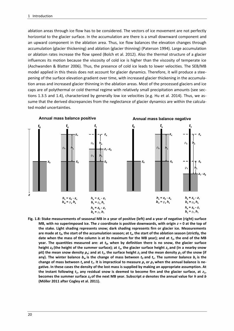
1 Introduction
20
ablation areas through ice flow has to be considered. The vectors of ice movement are not perfectly
horizontal to the glacier surface. In the accumulation are there is a small downward component and
an upward component in the ablation area. Thus, ice flow balances the elevation changes through
accumulation (glacier thickening) and ablation (glacier thinning) (Paterson 1994). Large accumulation
or ablation rates increase the flow speed (Bolch et al. 2012). Also the thermal structure of a glacier
influences its motion because the viscosity of cold ice is higher than the viscosity of temperate ice
(Aschwanden & Blatter 2006). Thus, the presence of cold ice leads to lower velocities. The SEB/MB
model applied in this thesis does not account for glacier dynamics. Therefore, it will produce a stee-
pening of the surface elevation gradient over time, with increased glacier thickening in the accumula-
tion areas and increased glacier thinning in the ablation areas. Most of the processed glaciers and ice
caps are of polythermal or cold thermal regime with relatively small precipitation amounts (see sec-
tions 1.3.5 and 1.4), characterized by generally low ice velocities (e.g. Hu et al. 2014). Thus, we as-
sume that the derived discrepancies from the neglectance of glacier dynamics are within the calcula-
ted model uncertainties.
Fig. 1.8: Stake measurements of seasonal MB in a year of positive (left) and a year of negative (right) surface
MB, with no superimposed ice. The z coordinate is positive downwards, with origin z = 0 at the top of the stake. Light shading represents snow; dark shading represents firn or glacier ice. Measurements are made at t0, the start of the accumulation season; at tx, the start of the ablation season (strictly, the date when the mass of the column is at its maximum for the MB year); and at t1, the end of the MB year. The quantities measured are: at t0, when by definition there is no snow, the glacier surface height z0 (the height of the summer surface); at tx, the glacier surface height zx and (in a nearby snow pit) the mean snow density ρx; and at t1, the surface height z1 and the mean density ρ1 of the snow (if any). The winter balance bw is the change of mass between t0 and tx. The summer balance bs is the change of mass between tx and t1. It is impractical to measure ρs or ρ1 when the annual balance is ne-gative. In these cases the density of the lost mass is supplied by making an appropriate assumption. At the instant following t1, any residual snow is deemed to become firn and the glacier surface, at z1, becomes the summer surface z0 of the next MB year. Subscript a denotes the annual value for h and b (Möller 2011 after Cogley et al. 2011).
1 Introduction
21
1.3.5 Characteristics of glaciers on the Tibetan Plateau
When working on glaciers on the TP the different climate influences in the different regions have to
be considered. It is obvious that the varying atmospheric circulation patterns in the past (section
1.3.1) led to spatially and temporal heterogeneous climate and glacier changes in the past (section
1.3.2) with an on-going influence on the present physical environment of the TP (section 1.3.3). Ta-
king into account the numerous feedback mechanisms within the glacier SEB and MB (section 1.3.4)
it is practical to classify the glaciers on the TP according to their thermal regime and their accumula-
tion regime.
The timing and amount of snowfall is revealed to be a key process for the SEB and MB of glaciers on
the TP (Fujita 2008a,b, Fujita & Ageta 2000, Kang et al. 2009, Mölg et al. 2012, Yang et al. 2011,
2013). According to the governing circulation patterns, the glaciers on the TP receive their major ac-
cumulation in different seasons. Most glaciers on the eastern, southern and southern central TP and
in the eastern and central Himalayas belong to the so called “summer-accumulation type” that was
defined by Ageta & Higuchi (1984). They are gaining mass mainly from the summer monsoon snow-
fall. Maximum annual ablation and accumulation occur simultaneously in summer. The annual vari-
ation in MB is generally small (Ageta & Fujita 1996, Cogley et al. 2011). “Summer-accumulation type”
glaciers are very sensitive to changes in air temperature because they highly depend on summer
snowfall associated with the positive albedo feedback that restrains the heat supply from SWin (see
section 1.3.4.1). A temperature rise will not only increase melt directly, but also cause a decrease in
the solid proportion of total precipitation and additionally decrease α (Fujita 2008a,b, Fujita et al.
2007). In a humid environment, more liquid precipitation also increases the glacier sensitivity. “Win-
ter-accumulation type” glaciers as known in Europe and North America are concentrated on the
western TP including the western Himalayas. They are characterized by distinct accumulation and ab-
lation seasons and are less sensitive to changes in air temperature (Fujita 2008). Based on atmos-
pheric model data Maussion et al. (2014) modified the classification of TP glaciers depending on their
precipitation seasonality. Using an objective clustering approach with the percentage of precipitation
falling in December-January-February (DJF), March-April-May (MAM) and June-July-August (JJA) as
input variables, the authors define five distinct output classes (Fig. 1.9). The classes are named after
their cluster centres’ characteristics. The dominant classes are the winter- (DJF) and summer- (JJA)
accumulation types with the largest occurrence at glaciers on the TP. The spring-accumulation type
(MAM) has fewer elements (Fig. 1.9). Two intermediate classes are defined for glaciers that experi-
ence maximum precipitation in summer (MAM/JJA) or the winter (MAM/DJF) but with less defined
centres (Maussion et al. 2014). The mean seasonal cycle of each class shows that the JJA, MAM and
DJF classes each have a distinct precipitation peak (Fig. 1.9) whereas the two mixed classes have a
less pronounced seasonal cycle. The MAM/DJF class experiences precipitation all year with two peaks
in February and August. Except for the DJF class, all precipitation classes show their minimum in No-
vember/December. It is obvious from Fig. 1.9 that the glaciers on the western TP and the adjacent
mountain ranges are dominated by the DJF and the southern central and north eastern regions are
dominated by the JJA precipitation class. The MAM class is distributed on the northern and north
western TP. On the southeast, northeast, northwest and western central TP as well as along the Hi-
malayas, large regions of the mixed precipitation classes occur and classes change over short distan-
ces. The high variability in the precipitation regimes has been observed by many authors at least for
the Himalayas (e.g. Fujita & Nuimura 2011, Kansakar 2004). Local factors such as the glacier expo-
sition and the topographic surroundings with respect to the wind direction play a significant role. The
data basis for the study of Maussion et al. (2014) is total precipitation. As mentioned in section 1.3.3
air temperatures on the TP are generally low and decrease with altitude. Therefore, large propor-
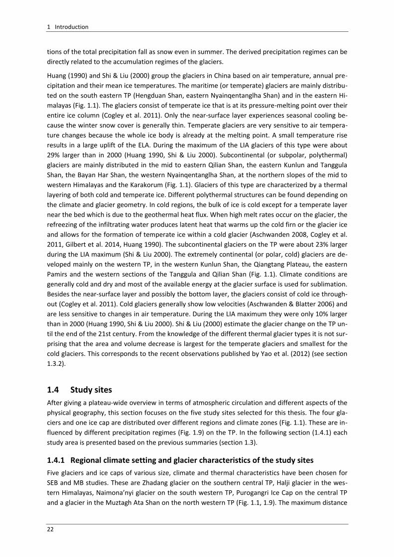
1 Introduction
22
tions of the total precipitation fall as snow even in summer. The derived precipitation regimes can be
directly related to the accumulation regimes of the glaciers.
Huang (1990) and Shi & Liu (2000) group the glaciers in China based on air temperature, annual pre-
cipitation and their mean ice temperatures. The maritime (or temperate) glaciers are mainly distribu-
ted on the south eastern TP (Hengduan Shan, eastern Nyainqentanglha Shan) and in the eastern Hi-
malayas (Fig. 1.1). The glaciers consist of temperate ice that is at its pressure-melting point over their
entire ice column (Cogley et al. 2011). Only the near-surface layer experiences seasonal cooling be-
cause the winter snow cover is generally thin. Temperate glaciers are very sensitive to air tempera-
ture changes because the whole ice body is already at the melting point. A small temperature rise
results in a large uplift of the ELA. During the maximum of the LIA glaciers of this type were about
29% larger than in 2000 (Huang 1990, Shi & Liu 2000). Subcontinental (or subpolar, polythermal)
glaciers are mainly distributed in the mid to eastern Qilian Shan, the eastern Kunlun and Tanggula
Shan, the Bayan Har Shan, the western Nyainqentanglha Shan, at the northern slopes of the mid to
western Himalayas and the Karakorum (Fig. 1.1). Glaciers of this type are characterized by a thermal
layering of both cold and temperate ice. Different polythermal structures can be found depending on
the climate and glacier geometry. In cold regions, the bulk of ice is cold except for a temperate layer
near the bed which is due to the geothermal heat flux. When high melt rates occur on the glacier, the
refreezing of the infiltrating water produces latent heat that warms up the cold firn or the glacier ice
and allows for the formation of temperate ice within a cold glacier (Aschwanden 2008, Cogley et al.
2011, Gilbert et al. 2014, Huang 1990). The subcontinental glaciers on the TP were about 23% larger
during the LIA maximum (Shi & Liu 2000). The extremely continental (or polar, cold) glaciers are de-
veloped mainly on the western TP, in the western Kunlun Shan, the Qiangtang Plateau, the eastern
Pamirs and the western sections of the Tanggula and Qilian Shan (Fig. 1.1). Climate conditions are
generally cold and dry and most of the available energy at the glacier surface is used for sublimation.
Besides the near-surface layer and possibly the bottom layer, the glaciers consist of cold ice through-
out (Cogley et al. 2011). Cold glaciers generally show low velocities (Aschwanden & Blatter 2006) and
are less sensitive to changes in air temperature. During the LIA maximum they were only 10% larger
than in 2000 (Huang 1990, Shi & Liu 2000). Shi & Liu (2000) estimate the glacier change on the TP un-
til the end of the 21st century. From the knowledge of the different thermal glacier types it is not sur-
prising that the area and volume decrease is largest for the temperate glaciers and smallest for the
cold glaciers. This corresponds to the recent observations published by Yao et al. (2012) (see section
1.3.2).
1.4 Study sites
After giving a plateau-wide overview in terms of atmospheric circulation and different aspects of the
physical geography, this section focuses on the five study sites selected for this thesis. The four gla-
ciers and one ice cap are distributed over different regions and climate zones (Fig. 1.1). These are in-
fluenced by different precipitation regimes (Fig. 1.9) on the TP. In the following section (1.4.1) each
study area is presented based on the previous summaries (section 1.3).
1.4.1 Regional climate setting and glacier characteristics of the study sites
Five glaciers and ice caps of various size, climate and thermal characteristics have been chosen for
SEB and MB studies. These are Zhadang glacier on the southern central TP, Halji glacier in the wes-
tern Himalayas, Naimona’nyi glacier on the south western TP, Purogangri Ice Cap on the central TP
and a glacier in the Muztagh Ata Shan on the north western TP (Fig. 1.1, 1.9). The maximum distance
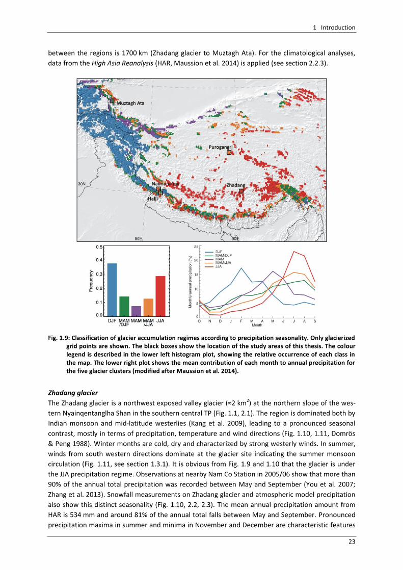
1 Introduction
23
between the regions is 1700 km (Zhadang glacier to Muztagh Ata). For the climatological analyses,
data from the High Asia Reanalysis (HAR, Maussion et al. 2014) is applied (see section 2.2.3).
Fig. 1.9: Classification of glacier accumulation regimes according to precipitation seasonality. Only glacierized
grid points are shown. The black boxes show the location of the study areas of this thesis. The colour legend is described in the lower left histogram plot, showing the relative occurrence of each class in the map. The lower right plot shows the mean contribution of each month to annual precipitation for the five glacier clusters (modified after Maussion et al. 2014).
Zhadang glacier
The Zhadang glacier is a northwest exposed valley glacier (≈2 km2) at the northern slope of the wes-
tern Nyainqentanglha Shan in the southern central TP (Fig. 1.1, 2.1). The region is dominated both by
Indian monsoon and mid-latitude westerlies (Kang et al. 2009), leading to a pronounced seasonal
contrast, mostly in terms of precipitation, temperature and wind directions (Fig. 1.10, 1.11, Domrös
& Peng 1988). Winter months are cold, dry and characterized by strong westerly winds. In summer,
winds from south western directions dominate at the glacier site indicating the summer monsoon
circulation (Fig. 1.11, see section 1.3.1). It is obvious from Fig. 1.9 and 1.10 that the glacier is under
the JJA precipitation regime. Observations at nearby Nam Co Station in 2005/06 show that more than
90% of the annual total precipitation was recorded between May and September (You et al. 2007;
Zhang et al. 2013). Snowfall measurements on Zhadang glacier and atmospheric model precipitation
also show this distinct seasonality (Fig. 1.10, 2.2, 2.3). The mean annual precipitation amount from
HAR is 534 mm and around 81% of the annual total falls between May and September. Pronounced
precipitation maxima in summer and minima in November and December are characteristic features
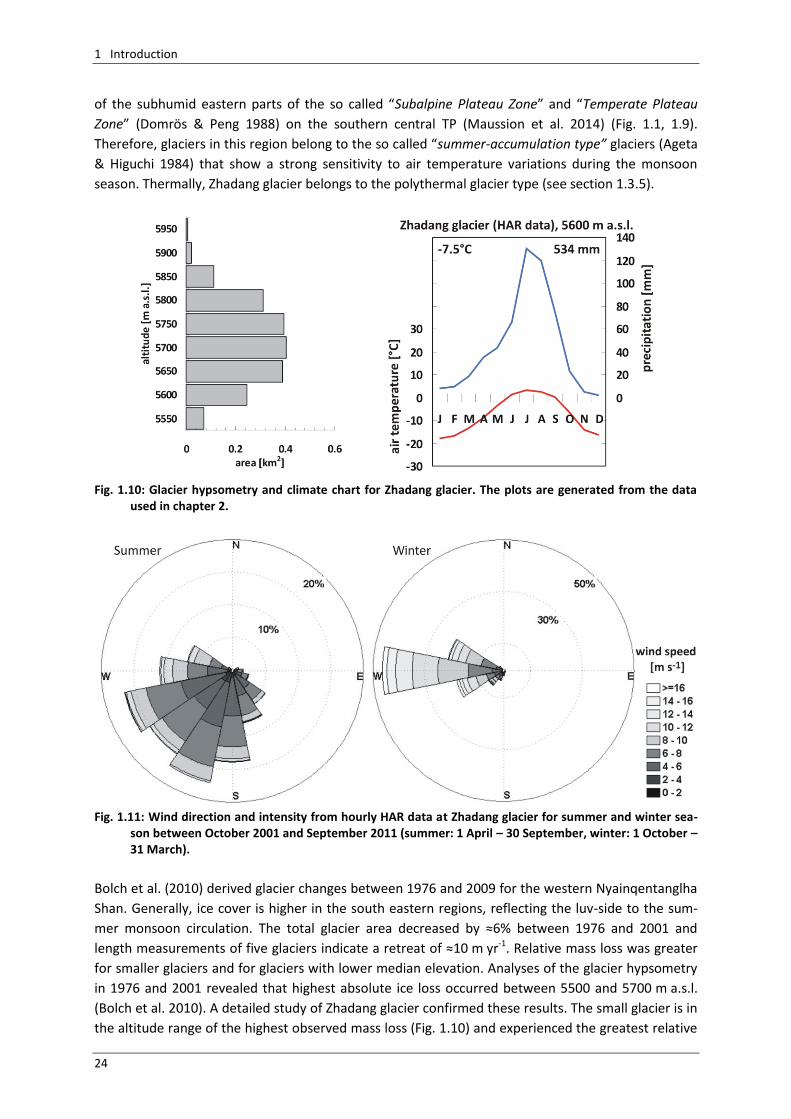
1 Introduction
24
of the subhumid eastern parts of the so called “Subalpine Plateau Zone” and “Temperate Plateau
Zone” (Domrös & Peng 1988) on the southern central TP (Maussion et al. 2014) (Fig. 1.1, 1.9).
Therefore, glaciers in this region belong to the so called “summer-accumulation type” glaciers (Ageta
& Higuchi 1984) that show a strong sensitivity to air temperature variations during the monsoon
season. Thermally, Zhadang glacier belongs to the polythermal glacier type (see section 1.3.5).
Fig. 1.10: Glacier hypsometry and climate chart for Zhadang glacier. The plots are generated from the data
used in chapter 2.
Fig. 1.11: Wind direction and intensity from hourly HAR data at Zhadang glacier for summer and winter sea-
son between October 2001 and September 2011 (summer: 1 April – 30 September, winter: 1 October – 31 March).
Bolch et al. (2010) derived glacier changes between 1976 and 2009 for the western Nyainqentanglha
Shan. Generally, ice cover is higher in the south eastern regions, reflecting the luv-side to the sum-
mer monsoon circulation. The total glacier area decreased by ≈6% between 1976 and 2001 and
length measurements of five glaciers indicate a retreat of ≈10 m yr-1. Relative mass loss was greater
for smaller glaciers and for glaciers with lower median elevation. Analyses of the glacier hypsometry
in 1976 and 2001 revealed that highest absolute ice loss occurred between 5500 and 5700 m a.s.l.
(Bolch et al. 2010). A detailed study of Zhadang glacier confirmed these results. The small glacier is in
the altitude range of the highest observed mass loss (Fig. 1.10) and experienced the greatest relative
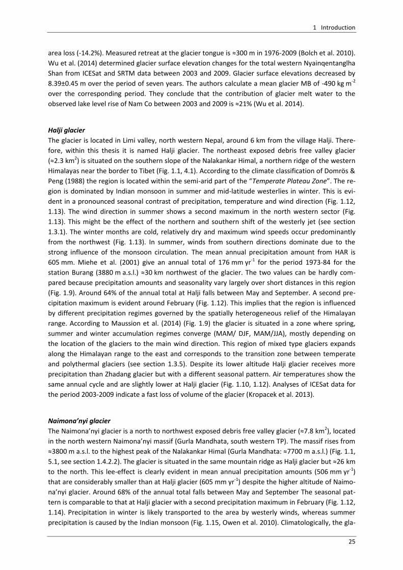
1 Introduction
25
area loss (-14.2%). Measured retreat at the glacier tongue is ≈300 m in 1976-2009 (Bolch et al. 2010).
Wu et al. (2014) determined glacier surface elevation changes for the total western Nyainqentanglha
Shan from ICESat and SRTM data between 2003 and 2009. Glacier surface elevations decreased by
8.39±0.45 m over the period of seven years. The authors calculate a mean glacier MB of -490 kg m-2
over the corresponding period. They conclude that the contribution of glacier melt water to the
observed lake level rise of Nam Co between 2003 and 2009 is ≈21% (Wu et al. 2014).
Halji glacier
The glacier is located in Limi valley, north western Nepal, around 6 km from the village Halji. There-
fore, within this thesis it is named Halji glacier. The northeast exposed debris free valley glacier
(≈2.3 km2) is situated on the southern slope of the Nalakankar Himal, a northern ridge of the western
Himalayas near the border to Tibet (Fig. 1.1, 4.1). According to the climate classification of Domrös &
Peng (1988) the region is located within the semi-arid part of the “Temperate Plateau Zone”. The re-
gion is dominated by Indian monsoon in summer and mid-latitude westerlies in winter. This is evi-
dent in a pronounced seasonal contrast of precipitation, temperature and wind direction (Fig. 1.12,
1.13). The wind direction in summer shows a second maximum in the north western sector (Fig.
1.13). This might be the effect of the northern and southern shift of the westerly jet (see section
1.3.1). The winter months are cold, relatively dry and maximum wind speeds occur predominantly
from the northwest (Fig. 1.13). In summer, winds from southern directions dominate due to the
strong influence of the monsoon circulation. The mean annual precipitation amount from HAR is
605 mm. Miehe et al. (2001) give an annual total of 176 mm yr-1 for the period 1973-84 for the
station Burang (3880 m a.s.l.) ≈30 km northwest of the glacier. The two values can be hardly com-
pared because precipitation amounts and seasonality vary largely over short distances in this region
(Fig. 1.9). Around 64% of the annual total at Halji falls between May and September. A second pre-
cipitation maximum is evident around February (Fig. 1.12). This implies that the region is influenced
by different precipitation regimes governed by the spatially heterogeneous relief of the Himalayan
range. According to Maussion et al. (2014) (Fig. 1.9) the glacier is situated in a zone where spring,
summer and winter accumulation regimes converge (MAM/ DJF, MAM/JJA), mostly depending on
the location of the glaciers to the main wind direction. This region of mixed type glaciers expands
along the Himalayan range to the east and corresponds to the transition zone between temperate
and polythermal glaciers (see section 1.3.5). Despite its lower altitude Halji glacier receives more
precipitation than Zhadang glacier but with a different seasonal pattern. Air temperatures show the
same annual cycle and are slightly lower at Halji glacier (Fig. 1.10, 1.12). Analyses of ICESat data for
the period 2003-2009 indicate a fast loss of volume of the glacier (Kropacek et al. 2013).
Naimona’nyi glacier
The Naimona’nyi glacier is a north to northwest exposed debris free valley glacier (≈7.8 km2), located
in the north western Naimona’nyi massif (Gurla Mandhata, south western TP). The massif rises from
≈3800 m a.s.l. to the highest peak of the Nalakankar Himal (Gurla Mandhata: ≈7700 m a.s.l.) (Fig. 1.1,
5.1, see section 1.4.2.2). The glacier is situated in the same mountain ridge as Halji glacier but ≈26 km
to the north. This lee-effect is clearly evident in mean annual precipitation amounts (506 mm yr-1)
that are considerably smaller than at Halji glacier (605 mm yr-1) despite the higher altitude of Naimo-
na’nyi glacier. Around 68% of the annual total falls between May and September The seasonal pat-
tern is comparable to that at Halji glacier with a second precipitation maximum in February (Fig. 1.12,
1.14). Precipitation in winter is likely transported to the area by westerly winds, whereas summer
precipitation is caused by the Indian monsoon (Fig. 1.15, Owen et al. 2010). Climatologically, the gla-
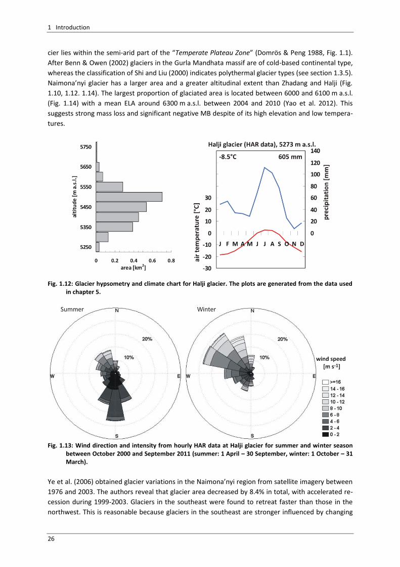
1 Introduction
26
cier lies within the semi-arid part of the “Temperate Plateau Zone” (Domrös & Peng 1988, Fig. 1.1).
After Benn & Owen (2002) glaciers in the Gurla Mandhata massif are of cold-based continental type,
whereas the classification of Shi and Liu (2000) indicates polythermal glacier types (see section 1.3.5).
Naimona’nyi glacier has a larger area and a greater altitudinal extent than Zhadang and Halji (Fig.
1.10, 1.12. 1.14). The largest proportion of glaciated area is located between 6000 and 6100 m a.s.l.
(Fig. 1.14) with a mean ELA around 6300 m a.s.l. between 2004 and 2010 (Yao et al. 2012). This
suggests strong mass loss and significant negative MB despite of its high elevation and low tempera-
tures.
Fig. 1.12: Glacier hypsometry and climate chart for Halji glacier. The plots are generated from the data used
in chapter 5.
Fig. 1.13: Wind direction and intensity from hourly HAR data at Halji glacier for summer and winter season
between October 2000 and September 2011 (summer: 1 April – 30 September, winter: 1 October – 31 March).
Ye et al. (2006) obtained glacier variations in the Naimona’nyi region from satellite imagery between
1976 and 2003. The authors reveal that glacier area decreased by 8.4% in total, with accelerated re-
cession during 1999-2003. Glaciers in the southeast were found to retreat faster than those in the
northwest. This is reasonable because glaciers in the southeast are stronger influenced by changing
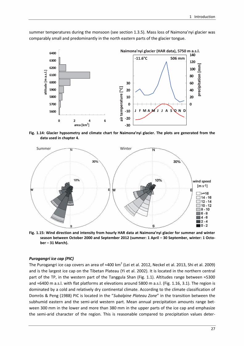
1 Introduction
27
summer temperatures during the monsoon (see section 1.3.5). Mass loss of Naimona’nyi glacier was
comparably small and predominantly in the north eastern parts of the glacier tongue.
Fig. 1.14: Glacier hypsometry and climate chart for Naimona’nyi glacier. The plots are generated from the
data used in chapter 4.
Fig. 1.15: Wind direction and intensity from hourly HAR data at Naimona’nyi glacier for summer and winter
season between October 2000 and September 2012 (summer: 1 April – 30 September, winter: 1 Octo-ber – 31 March).
Purogangri ice cap (PIC)
The Purogangri ice cap covers an area of ≈400 km2 (Lei et al. 2012, Neckel et al. 2013, Shi et al. 2009)
and is the largest ice cap on the Tibetan Plateau (Yi et al. 2002). It is located in the northern central
part of the TP, in the western part of the Tanggula Shan (Fig. 1.1). Altitudes range between ≈5300
and ≈6400 m a.s.l. with flat platforms at elevations around 5800 m a.s.l. (Fig. 1.16, 3.1). The region is
dominated by a cold and relatively dry continental climate. According to the climate classification of
Domrös & Peng (1988) PIC is located in the “Subalpine Plateau Zone” in the transition between the
subhumid eastern and the semi-arid western part. Mean annual precipitation amounts range bet-
ween 300 mm in the lower and more than 380 mm in the upper parts of the ice cap and emphasize
the semi-arid character of the region. This is reasonable compared to precipitation values deter-
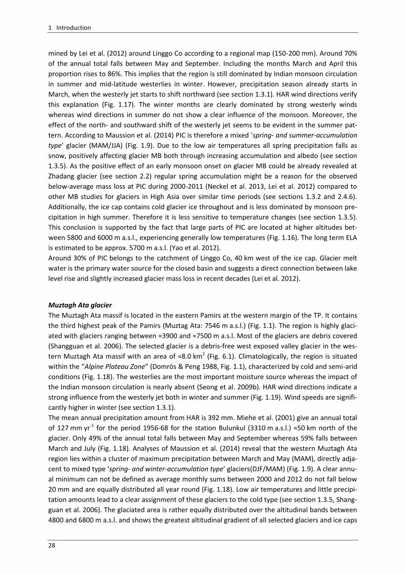
1 Introduction
28
mined by Lei et al. (2012) around Linggo Co according to a regional map (150-200 mm). Around 70%
of the annual total falls between May and September. Including the months March and April this
proportion rises to 86%. This implies that the region is still dominated by Indian monsoon circulation
in summer and mid-latitude westerlies in winter. However, precipitation season already starts in
March, when the westerly jet starts to shift northward (see section 1.3.1). HAR wind directions verify
this explanation (Fig. 1.17). The winter months are clearly dominated by strong westerly winds
whereas wind directions in summer do not show a clear influence of the monsoon. Moreover, the
effect of the north- and southward shift of the westerly jet seems to be evident in the summer pat-
tern. According to Maussion et al. (2014) PIC is therefore a mixed ‘spring- and summer-accumulation
type’ glacier (MAM/JJA) (Fig. 1.9). Due to the low air temperatures all spring precipitation falls as
snow, positively affecting glacier MB both through increasing accumulation and albedo (see section
1.3.5). As the positive effect of an early monsoon onset on glacier MB could be already revealed at
Zhadang glacier (see section 2.2) regular spring accumulation might be a reason for the observed
below-average mass loss at PIC during 2000-2011 (Neckel et al. 2013, Lei et al. 2012) compared to
other MB studies for glaciers in High Asia over similar time periods (see sections 1.3.2 and 2.4.6).
Additionally, the ice cap contains cold glacier ice throughout and is less dominated by monsoon pre-
cipitation in high summer. Therefore it is less sensitive to temperature changes (see section 1.3.5).
This conclusion is supported by the fact that large parts of PIC are located at higher altitudes bet-
ween 5800 and 6000 m a.s.l., experiencing generally low temperatures (Fig. 1.16). The long term ELA
is estimated to be approx. 5700 m a.s.l. (Yao et al. 2012).
Around 30% of PIC belongs to the catchment of Linggo Co, 40 km west of the ice cap. Glacier melt
water is the primary water source for the closed basin and suggests a direct connection between lake
level rise and slightly increased glacier mass loss in recent decades (Lei et al. 2012).
Muztagh Ata glacier
The Muztagh Ata massif is located in the eastern Pamirs at the western margin of the TP. It contains
the third highest peak of the Pamirs (Muztag Ata: 7546 m a.s.l.) (Fig. 1.1). The region is highly glaci-
ated with glaciers ranging between ≈3900 and ≈7500 m a.s.l. Most of the glaciers are debris covered
(Shangguan et al. 2006). The selected glacier is a debris-free west exposed valley glacier in the wes-
tern Muztagh Ata massif with an area of ≈8.0 km2 (Fig. 6.1). Climatologically, the region is situated
within the “Alpine Plateau Zone” (Domrös & Peng 1988, Fig. 1.1), characterized by cold and semi-arid
conditions (Fig. 1.18). The westerlies are the most important moisture source whereas the impact of
the Indian monsoon circulation is nearly absent (Seong et al. 2009b). HAR wind directions indicate a
strong influence from the westerly jet both in winter and summer (Fig. 1.19). Wind speeds are signifi-
cantly higher in winter (see section 1.3.1).
The mean annual precipitation amount from HAR is 392 mm. Miehe et al. (2001) give an annual total
of 127 mm yr-1 for the period 1956-68 for the station Bulunkul (3310 m a.s.l.) ≈50 km north of the
glacier. Only 49% of the annual total falls between May and September whereas 59% falls between
March and July (Fig. 1.18). Analyses of Maussion et al. (2014) reveal that the western Muztagh Ata
region lies within a cluster of maximum precipitation between March and May (MAM), directly adja-
cent to mixed type ‘spring- and winter-accumulation type’ glaciers(DJF/MAM) (Fig. 1.9). A clear annu-
al minimum can not be defined as average monthly sums between 2000 and 2012 do not fall below
20 mm and are equally distributed all year round (Fig. 1.18). Low air temperatures and little precipi-
tation amounts lead to a clear assignment of these glaciers to the cold type (see section 1.3.5, Shang-
guan et al. 2006). The glaciated area is rather equally distributed over the altitudinal bands between
4800 and 6800 m a.s.l. and shows the greatest altitudinal gradient of all selected glaciers and ice caps
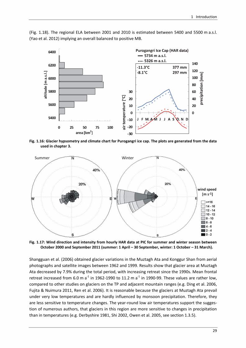
1 Introduction
29
(Fig. 1.18). The regional ELA between 2001 and 2010 is estimated between 5400 and 5500 m a.s.l.
(Yao et al. 2012) implying an overall balanced to positive MB.
Fig. 1.16: Glacier hypsometry and climate chart for Purogangri ice cap. The plots are generated from the data
used in chapter 3.
Fig. 1.17: Wind direction and intensity from hourly HAR data at PIC for summer and winter season between
October 2000 and September 2011 (summer: 1 April – 30 September, winter: 1 October – 31 March).
Shangguan et al. (2006) obtained glacier variations in the Muztagh Ata and Konggur Shan from aerial
photographs and satellite images between 1962 and 1999. Results show that glacier area at Muztagh
Ata decreased by 7.9% during the total period, with increasing retreat since the 1990s. Mean frontal
retreat increased from 6.0 m a-1 in 1962-1990 to 11.2 m a-1 in 1990-99. These values are rather low,
compared to other studies on glaciers on the TP and adjacent mountain ranges (e.g. Ding et al. 2006,
Fujita & Nuimura 2011, Ren et al. 2006). It is reasonable because the glaciers at Muztagh Ata prevail
under very low temperatures and are hardly influenced by monsoon precipitation. Therefore, they
are less sensitive to temperature changes. The year-round low air temperatures support the sugges-
tion of numerous authors, that glaciers in this region are more sensitive to changes in precipitation
than in temperatures (e.g. Derbyshire 1981, Shi 2002, Owen et al. 2005, see section 1.3.5).
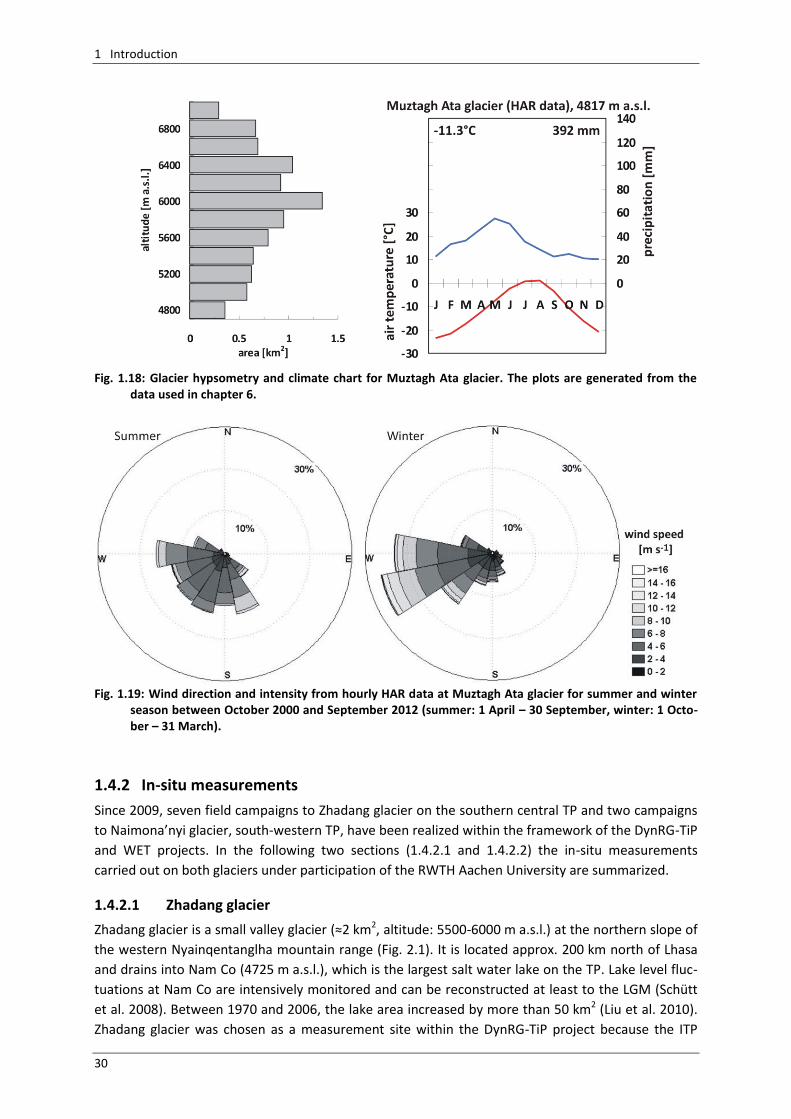
1 Introduction
30
Fig. 1.18: Glacier hypsometry and climate chart for Muztagh Ata glacier. The plots are generated from the
data used in chapter 6.
Fig. 1.19: Wind direction and intensity from hourly HAR data at Muztagh Ata glacier for summer and winter
season between October 2000 and September 2012 (summer: 1 April – 30 September, winter: 1 Octo-ber – 31 March).
1.4.2 In-situ measurements
Since 2009, seven field campaigns to Zhadang glacier on the southern central TP and two campaigns
to Naimona’nyi glacier, south-western TP, have been realized within the framework of the DynRG-TiP
and WET projects. In the following two sections (1.4.2.1 and 1.4.2.2) the in-situ measurements
carried out on both glaciers under participation of the RWTH Aachen University are summarized.
1.4.2.1 Zhadang glacier
Zhadang glacier is a small valley glacier (≈2 km2, altitude: 5500-6000 m a.s.l.) at the northern slope of
the western Nyainqentanglha mountain range (Fig. 2.1). It is located approx. 200 km north of Lhasa
and drains into Nam Co (4725 m a.s.l.), which is the largest salt water lake on the TP. Lake level fluc-
tuations at Nam Co are intensively monitored and can be reconstructed at least to the LGM (Schütt
et al. 2008). Between 1970 and 2006, the lake area increased by more than 50 km2 (Liu et al. 2010).
Zhadang glacier was chosen as a measurement site within the DynRG-TiP project because the ITP
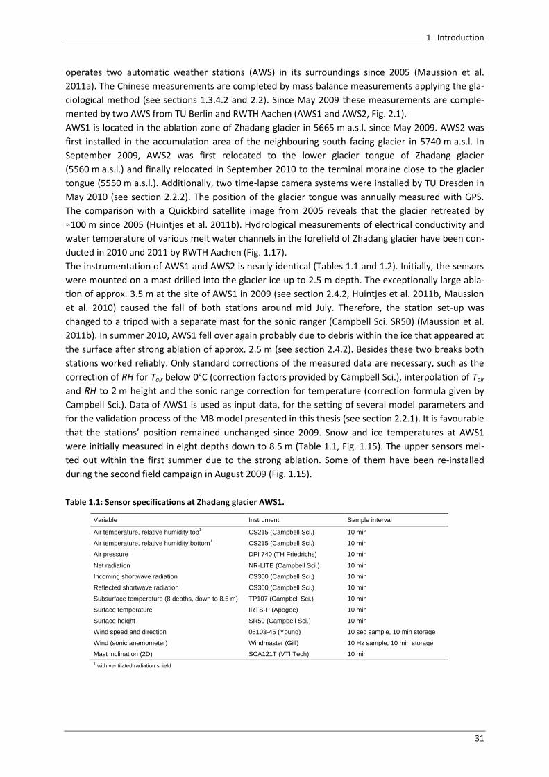
1 Introduction
31
operates two automatic weather stations (AWS) in its surroundings since 2005 (Maussion et al.
2011a). The Chinese measurements are completed by mass balance measurements applying the gla-
ciological method (see sections 1.3.4.2 and 2.2). Since May 2009 these measurements are comple-
mented by two AWS from TU Berlin and RWTH Aachen (AWS1 and AWS2, Fig. 2.1).
AWS1 is located in the ablation zone of Zhadang glacier in 5665 m a.s.l. since May 2009. AWS2 was
first installed in the accumulation area of the neighbouring south facing glacier in 5740 m a.s.l. In
September 2009, AWS2 was first relocated to the lower glacier tongue of Zhadang glacier
(5560 m a.s.l.) and finally relocated in September 2010 to the terminal moraine close to the glacier
tongue (5550 m a.s.l.). Additionally, two time-lapse camera systems were installed by TU Dresden in
May 2010 (see section 2.2.2). The position of the glacier tongue was annually measured with GPS.
The comparison with a Quickbird satellite image from 2005 reveals that the glacier retreated by
≈100 m since 2005 (Huintjes et al. 2011b). Hydrological measurements of electrical conductivity and
water temperature of various melt water channels in the forefield of Zhadang glacier have been con-
ducted in 2010 and 2011 by RWTH Aachen (Fig. 1.17).
The instrumentation of AWS1 and AWS2 is nearly identical (Tables 1.1 and 1.2). Initially, the sensors
were mounted on a mast drilled into the glacier ice up to 2.5 m depth. The exceptionally large abla-
tion of approx. 3.5 m at the site of AWS1 in 2009 (see section 2.4.2, Huintjes et al. 2011b, Maussion
et al. 2010) caused the fall of both stations around mid July. Therefore, the station set-up was
changed to a tripod with a separate mast for the sonic ranger (Campbell Sci. SR50) (Maussion et al.
2011b). In summer 2010, AWS1 fell over again probably due to debris within the ice that appeared at
the surface after strong ablation of approx. 2.5 m (see section 2.4.2). Besides these two breaks both
stations worked reliably. Only standard corrections of the measured data are necessary, such as the
correction of RH for Tair below 0°C (correction factors provided by Campbell Sci.), interpolation of Tair
and RH to 2 m height and the sonic range correction for temperature (correction formula given by
Campbell Sci.). Data of AWS1 is used as input data, for the setting of several model parameters and
for the validation process of the MB model presented in this thesis (see section 2.2.1). It is favourable
that the stations’ position remained unchanged since 2009. Snow and ice temperatures at AWS1
were initially measured in eight depths down to 8.5 m (Table 1.1, Fig. 1.15). The upper sensors mel-
ted out within the first summer due to the strong ablation. Some of them have been re-installed
during the second field campaign in August 2009 (Fig. 1.15).
Table 1.1: Sensor specifications at Zhadang glacier AWS1.
Variable Instrument Sample interval
Air temperature, relative humidity top1 CS215 (Campbell Sci.) 10 min
Air temperature, relative humidity bottom1 CS215 (Campbell Sci.) 10 min
Air pressure DPI 740 (TH Friedrichs) 10 min
Net radiation NR-LITE (Campbell Sci.) 10 min
Incoming shortwave radiation CS300 (Campbell Sci.) 10 min
Reflected shortwave radiation CS300 (Campbell Sci.) 10 min
Subsurface temperature (8 depths, down to 8.5 m) TP107 (Campbell Sci.) 10 min
Surface temperature IRTS-P (Apogee) 10 min
Surface height SR50 (Campbell Sci.) 10 min
Wind speed and direction 05103-45 (Young) 10 sec sample, 10 min storage
Wind (sonic anemometer) Windmaster (Gill) 10 Hz sample, 10 min storage
Mast inclination (2D) SCA121T (VTI Tech) 10 min
1 with ventilated radiation shield
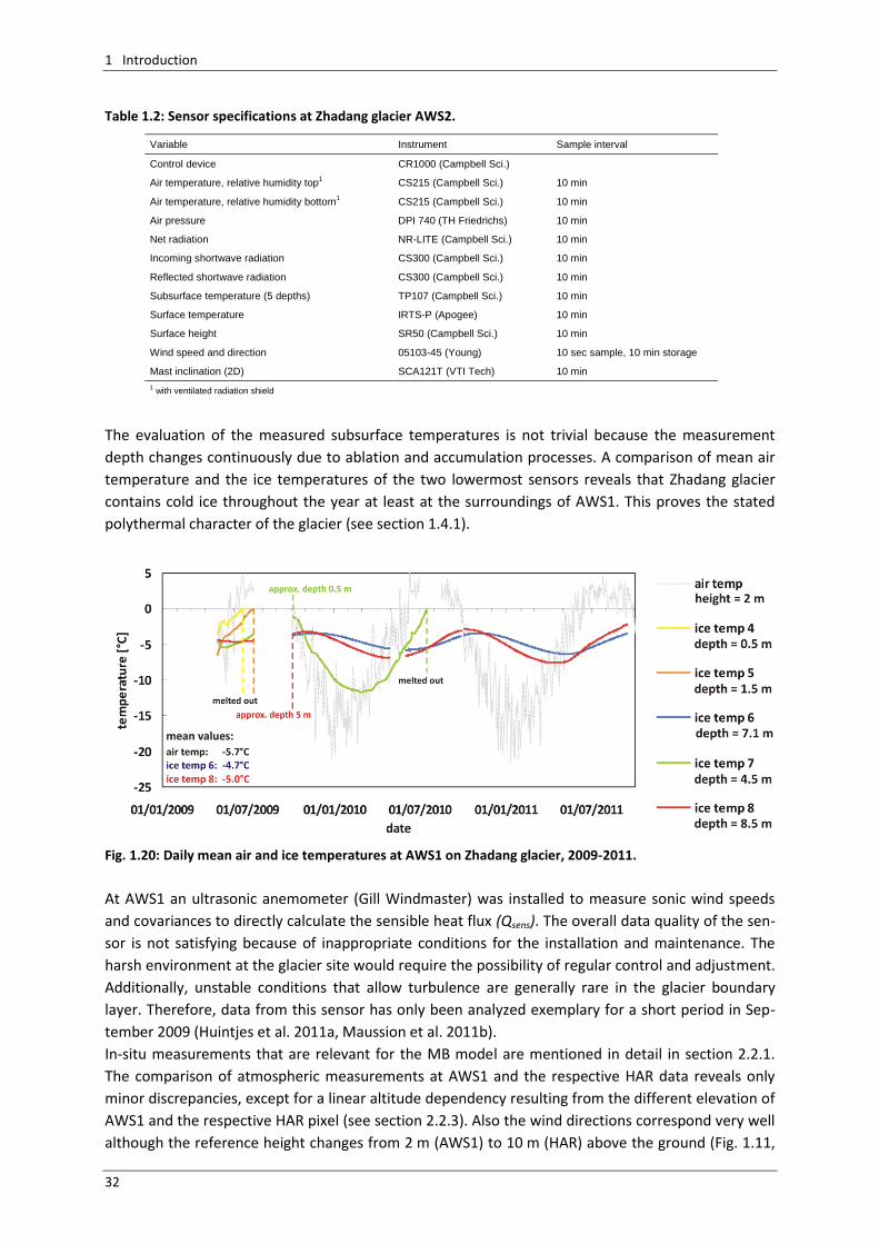
1 Introduction
32
Table 1.2: Sensor specifications at Zhadang glacier AWS2.
Variable Instrument Sample interval
Control device CR1000 (Campbell Sci.)
Air temperature, relative humidity top1 CS215 (Campbell Sci.) 10 min
Air temperature, relative humidity bottom1 CS215 (Campbell Sci.) 10 min
Air pressure DPI 740 (TH Friedrichs) 10 min
Net radiation NR-LITE (Campbell Sci.) 10 min
Incoming shortwave radiation CS300 (Campbell Sci.) 10 min
Reflected shortwave radiation CS300 (Campbell Sci.) 10 min
Subsurface temperature (5 depths) TP107 (Campbell Sci.) 10 min
Surface temperature IRTS-P (Apogee) 10 min
Surface height SR50 (Campbell Sci.) 10 min
Wind speed and direction 05103-45 (Young) 10 sec sample, 10 min storage
Mast inclination (2D) SCA121T (VTI Tech) 10 min
1 with ventilated radiation shield
The evaluation of the measured subsurface temperatures is not trivial because the measurement
depth changes continuously due to ablation and accumulation processes. A comparison of mean air
temperature and the ice temperatures of the two lowermost sensors reveals that Zhadang glacier
contains cold ice throughout the year at least at the surroundings of AWS1. This proves the stated
polythermal character of the glacier (see section 1.4.1).
Fig. 1.20: Daily mean air and ice temperatures at AWS1 on Zhadang glacier, 2009-2011.
At AWS1 an ultrasonic anemometer (Gill Windmaster) was installed to measure sonic wind speeds
and covariances to directly calculate the sensible heat flux (Qsens). The overall data quality of the sen-
sor is not satisfying because of inappropriate conditions for the installation and maintenance. The
harsh environment at the glacier site would require the possibility of regular control and adjustment.
Additionally, unstable conditions that allow turbulence are generally rare in the glacier boundary
layer. Therefore, data from this sensor has only been analyzed exemplary for a short period in Sep-
tember 2009 (Huintjes et al. 2011a, Maussion et al. 2011b).
In-situ measurements that are relevant for the MB model are mentioned in detail in section 2.2.1.
The comparison of atmospheric measurements at AWS1 and the respective HAR data reveals only
minor discrepancies, except for a linear altitude dependency resulting from the different elevation of
AWS1 and the respective HAR pixel (see section 2.2.3). Also the wind directions correspond very well
although the reference height changes from 2 m (AWS1) to 10 m (HAR) above the ground (Fig. 1.11,
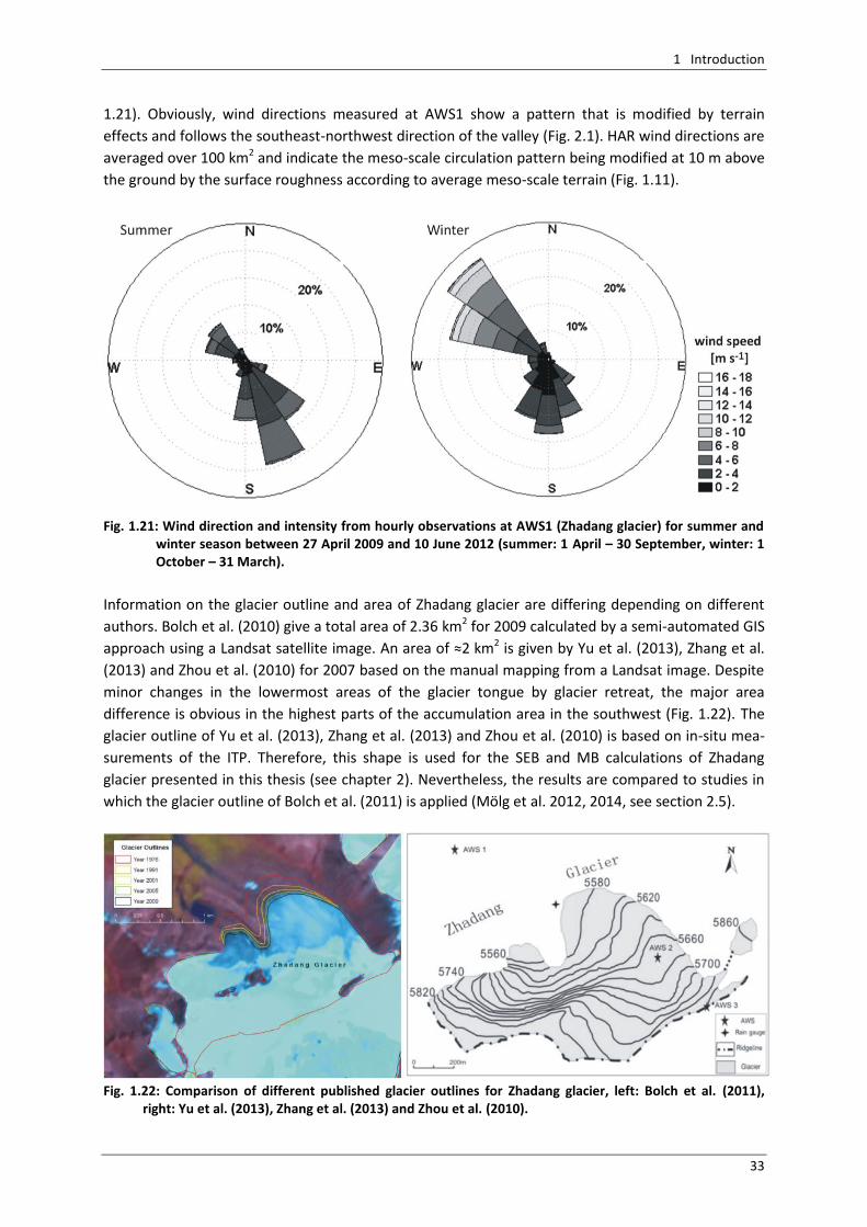
1 Introduction
33
1.21). Obviously, wind directions measured at AWS1 show a pattern that is modified by terrain
effects and follows the southeast-northwest direction of the valley (Fig. 2.1). HAR wind directions are
averaged over 100 km2 and indicate the meso-scale circulation pattern being modified at 10 m above
the ground by the surface roughness according to average meso-scale terrain (Fig. 1.11).
Fig. 1.21: Wind direction and intensity from hourly observations at AWS1 (Zhadang glacier) for summer and
winter season between 27 April 2009 and 10 June 2012 (summer: 1 April – 30 September, winter: 1 October – 31 March).
Information on the glacier outline and area of Zhadang glacier are differing depending on different
authors. Bolch et al. (2010) give a total area of 2.36 km2 for 2009 calculated by a semi-automated GIS
approach using a Landsat satellite image. An area of ≈2 km2 is given by Yu et al. (2013), Zhang et al.
(2013) and Zhou et al. (2010) for 2007 based on the manual mapping from a Landsat image. Despite
minor changes in the lowermost areas of the glacier tongue by glacier retreat, the major area
difference is obvious in the highest parts of the accumulation area in the southwest (Fig. 1.22). The
glacier outline of Yu et al. (2013), Zhang et al. (2013) and Zhou et al. (2010) is based on in-situ mea-
surements of the ITP. Therefore, this shape is used for the SEB and MB calculations of Zhadang
glacier presented in this thesis (see chapter 2). Nevertheless, the results are compared to studies in
which the glacier outline of Bolch et al. (2011) is applied (Mölg et al. 2012, 2014, see section 2.5).
Fig. 1.22: Comparison of different published glacier outlines for Zhadang glacier, left: Bolch et al. (2011),
right: Yu et al. (2013), Zhang et al. (2013) and Zhou et al. (2010).
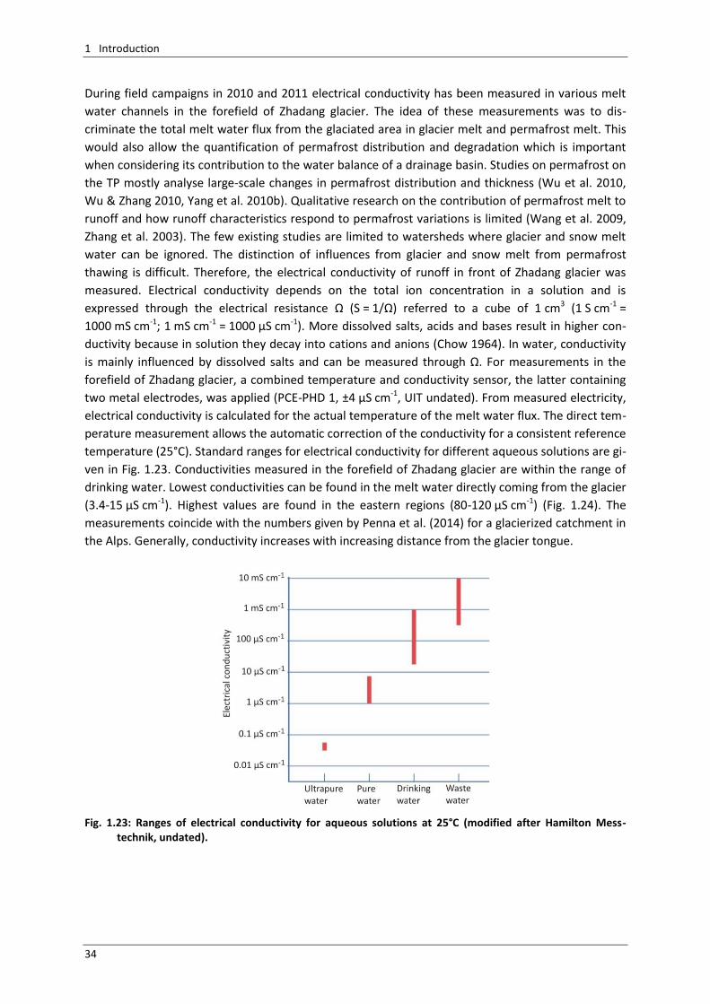
1 Introduction
34
During field campaigns in 2010 and 2011 electrical conductivity has been measured in various melt
water channels in the forefield of Zhadang glacier. The idea of these measurements was to dis-
criminate the total melt water flux from the glaciated area in glacier melt and permafrost melt. This
would also allow the quantification of permafrost distribution and degradation which is important
when considering its contribution to the water balance of a drainage basin. Studies on permafrost on
the TP mostly analyse large-scale changes in permafrost distribution and thickness (Wu et al. 2010,
Wu & Zhang 2010, Yang et al. 2010b). Qualitative research on the contribution of permafrost melt to
runoff and how runoff characteristics respond to permafrost variations is limited (Wang et al. 2009,
Zhang et al. 2003). The few existing studies are limited to watersheds where glacier and snow melt
water can be ignored. The distinction of influences from glacier and snow melt from permafrost
thawing is difficult. Therefore, the electrical conductivity of runoff in front of Zhadang glacier was
measured. Electrical conductivity depends on the total ion concentration in a solution and is
expressed through the electrical resistance Ω (S = 1/Ω) referred to a cube of 1 cm3 (1 S cm-1 =
1000 mS cm-1; 1 mS cm-1 = 1000 μS cm-1). More dissolved salts, acids and bases result in higher con-
ductivity because in solution they decay into cations and anions (Chow 1964). In water, conductivity
is mainly influenced by dissolved salts and can be measured through Ω. For measurements in the
forefield of Zhadang glacier, a combined temperature and conductivity sensor, the latter containing
two metal electrodes, was applied (PCE-PHD 1, ±4 μS cm-1, UIT undated). From measured electricity,
electrical conductivity is calculated for the actual temperature of the melt water flux. The direct tem-
perature measurement allows the automatic correction of the conductivity for a consistent reference
temperature (25°C). Standard ranges for electrical conductivity for different aqueous solutions are gi-
ven in Fig. 1.23. Conductivities measured in the forefield of Zhadang glacier are within the range of
drinking water. Lowest conductivities can be found in the melt water directly coming from the glacier
(3.4-15 μS cm-1). Highest values are found in the eastern regions (80-120 μS cm-1) (Fig. 1.24). The
measurements coincide with the numbers given by Penna et al. (2014) for a glacierized catchment in
the Alps. Generally, conductivity increases with increasing distance from the glacier tongue.
Fig. 1.23: Ranges of electrical conductivity for aqueous solutions at 25°C (modified after Hamilton Mess-technik, undated).
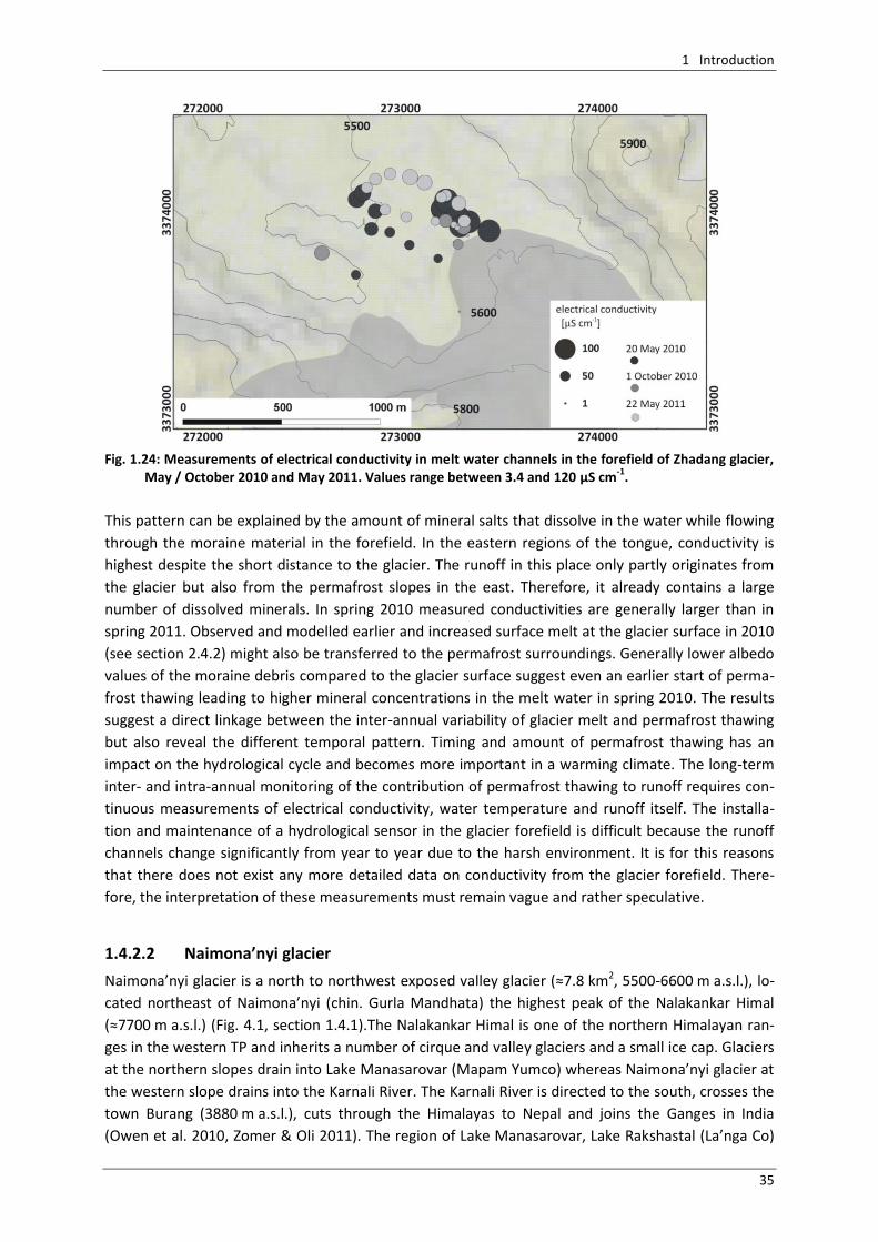
1 Introduction
35
Fig. 1.24: Measurements of electrical conductivity in melt water channels in the forefield of Zhadang glacier,
May / October 2010 and May 2011. Values range between 3.4 and 120 μS cm-1
.
This pattern can be explained by the amount of mineral salts that dissolve in the water while flowing
through the moraine material in the forefield. In the eastern regions of the tongue, conductivity is
highest despite the short distance to the glacier. The runoff in this place only partly originates from
the glacier but also from the permafrost slopes in the east. Therefore, it already contains a large
number of dissolved minerals. In spring 2010 measured conductivities are generally larger than in
spring 2011. Observed and modelled earlier and increased surface melt at the glacier surface in 2010
(see section 2.4.2) might also be transferred to the permafrost surroundings. Generally lower albedo
values of the moraine debris compared to the glacier surface suggest even an earlier start of perma-
frost thawing leading to higher mineral concentrations in the melt water in spring 2010. The results
suggest a direct linkage between the inter-annual variability of glacier melt and permafrost thawing
but also reveal the different temporal pattern. Timing and amount of permafrost thawing has an
impact on the hydrological cycle and becomes more important in a warming climate. The long-term
inter- and intra-annual monitoring of the contribution of permafrost thawing to runoff requires con-
tinuous measurements of electrical conductivity, water temperature and runoff itself. The installa-
tion and maintenance of a hydrological sensor in the glacier forefield is difficult because the runoff
channels change significantly from year to year due to the harsh environment. It is for this reasons
that there does not exist any more detailed data on conductivity from the glacier forefield. There-
fore, the interpretation of these measurements must remain vague and rather speculative.
1.4.2.2 Naimona’nyi glacier
Naimona’nyi glacier is a north to northwest exposed valley glacier (≈7.8 km2, 5500-6600 m a.s.l.), lo-
cated northeast of Naimona’nyi (chin. Gurla Mandhata) the highest peak of the Nalakankar Himal
(≈7700 m a.s.l.) (Fig. 4.1, section 1.4.1).The Nalakankar Himal is one of the northern Himalayan ran-
ges in the western TP and inherits a number of cirque and valley glaciers and a small ice cap. Glaciers
at the northern slopes drain into Lake Manasarovar (Mapam Yumco) whereas Naimona’nyi glacier at
the western slope drains into the Karnali River. The Karnali River is directed to the south, crosses the
town Burang (3880 m a.s.l.), cuts through the Himalayas to Nepal and joins the Ganges in India
(Owen et al. 2010, Zomer & Oli 2011). The region of Lake Manasarovar, Lake Rakshastal (La’nga Co)
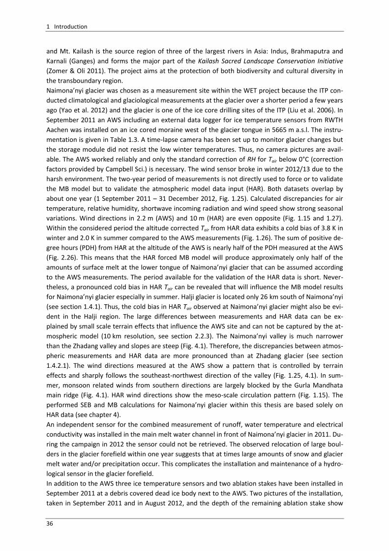
1 Introduction
36
and Mt. Kailash is the source region of three of the largest rivers in Asia: Indus, Brahmaputra and
Karnali (Ganges) and forms the major part of the Kailash Sacred Landscape Conservation Initiative
(Zomer & Oli 2011). The project aims at the protection of both biodiversity and cultural diversity in
the transboundary region.
Naimona’nyi glacier was chosen as a measurement site within the WET project because the ITP con-
ducted climatological and glaciological measurements at the glacier over a shorter period a few years
ago (Yao et al. 2012) and the glacier is one of the ice core drilling sites of the ITP (Liu et al. 2006). In
September 2011 an AWS including an external data logger for ice temperature sensors from RWTH
Aachen was installed on an ice cored moraine west of the glacier tongue in 5665 m a.s.l. The instru-
mentation is given in Table 1.3. A time-lapse camera has been set up to monitor glacier changes but
the storage module did not resist the low winter temperatures. Thus, no camera pictures are avail-
able. The AWS worked reliably and only the standard correction of RH for Tair below 0°C (correction
factors provided by Campbell Sci.) is necessary. The wind sensor broke in winter 2012/13 due to the
harsh environment. The two-year period of measurements is not directly used to force or to validate
the MB model but to validate the atmospheric model data input (HAR). Both datasets overlap by
about one year (1 September 2011 – 31 December 2012, Fig. 1.25). Calculated discrepancies for air
temperature, relative humidity, shortwave incoming radiation and wind speed show strong seasonal
variations. Wind directions in 2.2 m (AWS) and 10 m (HAR) are even opposite (Fig. 1.15 and 1.27).
Within the considered period the altitude corrected Tair from HAR data exhibits a cold bias of 3.8 K in
winter and 2.0 K in summer compared to the AWS measurements (Fig. 1.26). The sum of positive de-
gree hours (PDH) from HAR at the altitude of the AWS is nearly half of the PDH measured at the AWS
(Fig. 2.26). This means that the HAR forced MB model will produce approximately only half of the
amounts of surface melt at the lower tongue of Naimona’nyi glacier that can be assumed according
to the AWS measurements. The period available for the validation of the HAR data is short. Never-
theless, a pronounced cold bias in HAR Tair can be revealed that will influence the MB model results
for Naimona’nyi glacier especially in summer. Halji glacier is located only 26 km south of Naimona’nyi
(see section 1.4.1). Thus, the cold bias in HAR Tair observed at Naimona’nyi glacier might also be evi-
dent in the Halji region. The large differences between measurements and HAR data can be ex-
plained by small scale terrain effects that influence the AWS site and can not be captured by the at-
mospheric model (10 km resolution, see section 2.2.3). The Naimona’nyi valley is much narrower
than the Zhadang valley and slopes are steep (Fig. 4.1). Therefore, the discrepancies between atmos-
pheric measurements and HAR data are more pronounced than at Zhadang glacier (see section
1.4.2.1). The wind directions measured at the AWS show a pattern that is controlled by terrain
effects and sharply follows the southeast-northwest direction of the valley (Fig. 1.25, 4.1). In sum-
mer, monsoon related winds from southern directions are largely blocked by the Gurla Mandhata
main ridge (Fig. 4.1). HAR wind directions show the meso-scale circulation pattern (Fig. 1.15). The
performed SEB and MB calculations for Naimona’nyi glacier within this thesis are based solely on
HAR data (see chapter 4).
An independent sensor for the combined measurement of runoff, water temperature and electrical
conductivity was installed in the main melt water channel in front of Naimona’nyi glacier in 2011. Du-
ring the campaign in 2012 the sensor could not be retrieved. The observed relocation of large boul-
ders in the glacier forefield within one year suggests that at times large amounts of snow and glacier
melt water and/or precipitation occur. This complicates the installation and maintenance of a hydro-
logical sensor in the glacier forefield.
In addition to the AWS three ice temperature sensors and two ablation stakes have been installed in
September 2011 at a debris covered dead ice body next to the AWS. Two pictures of the installation,
taken in September 2011 and in August 2012, and the depth of the remaining ablation stake show
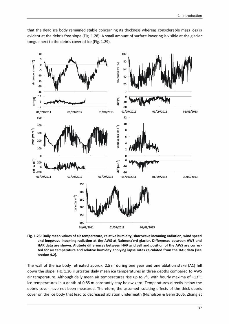
1 Introduction
37
that the dead ice body remained stable concerning its thickness whereas considerable mass loss is
evident at the debris free slope (Fig. 1.28). A small amount of surface lowering is visible at the glacier
tongue next to the debris covered ice (Fig. 1.29).
Fig. 1.25: Daily mean values of air temperature, relative humidity, shortwave incoming radiation, wind speed
and longwave incoming radiation at the AWS at Naimona’nyi glacier. Differences between AWS and HAR data are shown. Altitude differences between HAR grid cell and position of the AWS are correc-ted for air temperature and relative humidity applying lapse rates calculated from the HAR data (see section 4.2).
The wall of the ice body retreated approx. 2.5 m during one year and one ablation stake (A1) fell
down the slope. Fig. 1.30 illustrates daily mean ice temperatures in three depths compared to AWS
air temperature. Although daily mean air temperatures rise up to 7°C with hourly maxima of +13°C
ice temperatures in a depth of 0.85 m constantly stay below zero. Temperatures directly below the
debris cover have not been measured. Therefore, the assumed isolating effects of the thick debris
cover on the ice body that lead to decreased ablation underneath (Nicholson & Benn 2006, Zhang et
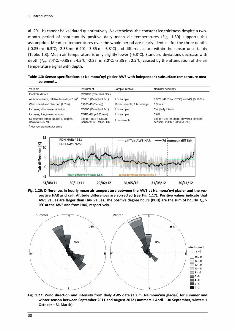
1 Introduction
38
al. 2011b) cannot be validated quantitatively. Nevertheless, the constant ice thickness despite a two-
month period of continuously positive daily mean air temperatures (Fig. 1.30) supports this
assumption. Mean ice temperatures over the whole period are nearly identical for the three depths
(-0.85 m: -6.3°C; -2.35 m: -6.2°C; -3.35 m: -6.3°C) and differences are within the sensor uncertainty
(Table. 1.3). Mean air temperature is only slightly lower (-6.8°C). Standard deviations decrease with
depth (Tair: 7.4°C; -0.85 m: 4.5°C; -2.35 m: 3.0°C; -3.35 m: 2.5°C) caused by the attenuation of the air
temperature signal with depth. Table 1.3: Sensor specifications at Naimona’nyi glacier AWS with independent subsurface temperature mea-
surements.
Variable Instrument Sample interval Nominal accuracy
Controle device CR1000 (Campbell Sci.)
Air temperature, relative humidity (2 m)1 CS215 (Campbell Sci.) 1 hr sample 0.9°C (-40°C to +70°C) and 4% (0-100%)
Wind speed and direction (2.2 m) 05103-45 (Young) 10 sec sample, 1 hr storage 0.3 m s-1
Incoming shortwave radiation CS300 (Campbell Sci.) 1 hr sample 5% (daily totals)
Incoming longwave radiation CGR3 (Kipp & Zonen) 1 hr sample 5.6%
Subsurface temperatures (3 depths, down to 3.35 m)
Logger: U12 (HOBO); Sensors: 3x TMC20-HD
3 hrs sample Logger: 1% for logger-powered sensors; sensors: 0.3°C (-20°C to 0°C)
1 with ventilated radiation shield
Fig. 1.26: Differences in hourly mean air temperature between the AWS at Naimona’nyi glacier and the res-
pective HAR grid cell. Altitude differences are corrected (see Fig. 1.17). Positive values indicate that AWS values are larger than HAR values. The positive degree hours (PDH) are the sum of hourly Tair > 0°C at the AWS and from HAR, respectively.
Fig. 1.27: Wind direction and intensity from daily AWS data (2.2 m, Naimona’nyi glacier) for summer and
winter season between September 2011 and August 2012 (summer: 1 April – 30 September, winter: 1 October – 31 March).
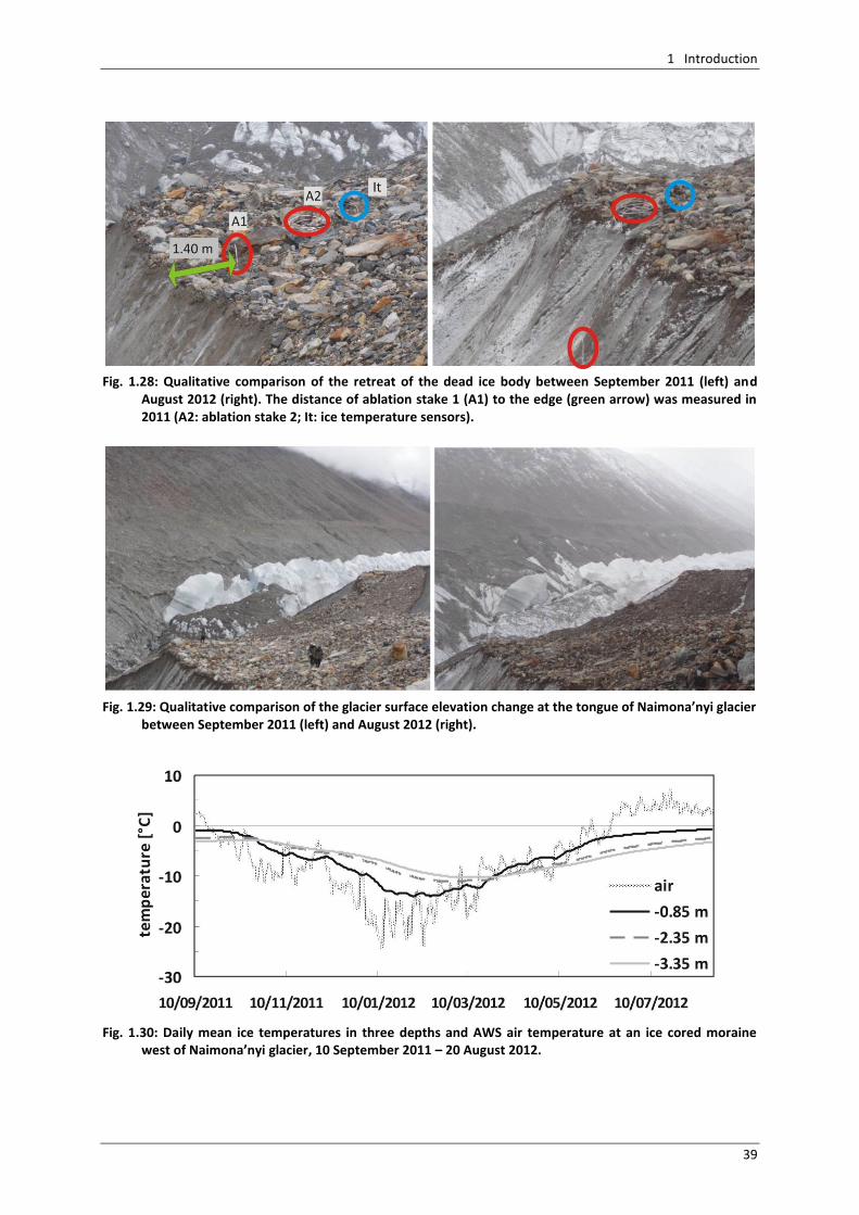
1 Introduction
39
Fig. 1.28: Qualitative comparison of the retreat of the dead ice body between September 2011 (left) and
August 2012 (right). The distance of ablation stake 1 (A1) to the edge (green arrow) was measured in 2011 (A2: ablation stake 2; It: ice temperature sensors).
Fig. 1.29: Qualitative comparison of the glacier surface elevation change at the tongue of Naimona’nyi glacier
between September 2011 (left) and August 2012 (right).
Fig. 1.30: Daily mean ice temperatures in three depths and AWS air temperature at an ice cored moraine
west of Naimona’nyi glacier, 10 September 2011 – 20 August 2012.

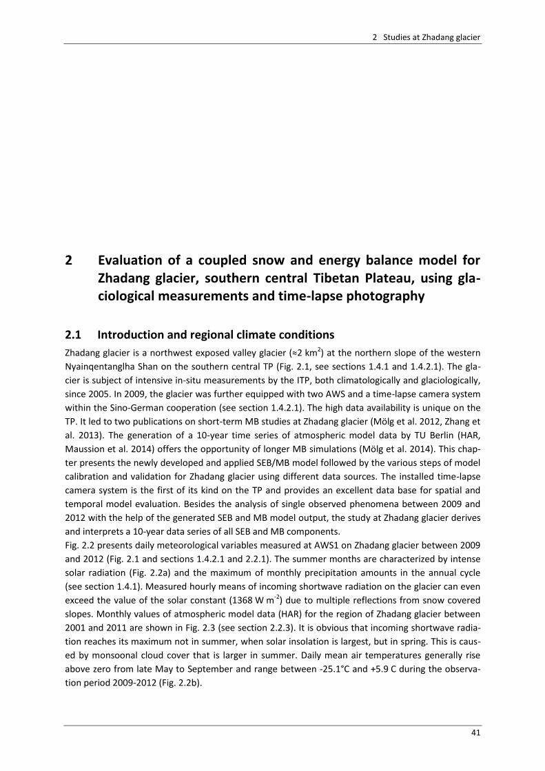
2 Studies at Zhadang glacier
41
2 Evaluation of a coupled snow and energy balance model for Zhadang glacier, southern central Tibetan Plateau, using gla-ciological measurements and time-lapse photography
2.1 Introduction and regional climate conditions
Zhadang glacier is a northwest exposed valley glacier (≈2 km2) at the northern slope of the western
Nyainqentanglha Shan on the southern central TP (Fig. 2.1, see sections 1.4.1 and 1.4.2.1). The gla-
cier is subject of intensive in-situ measurements by the ITP, both climatologically and glaciologically,
since 2005. In 2009, the glacier was further equipped with two AWS and a time-lapse camera system
within the Sino-German cooperation (see section 1.4.2.1). The high data availability is unique on the
TP. It led to two publications on short-term MB studies at Zhadang glacier (Mölg et al. 2012, Zhang et
al. 2013). The generation of a 10-year time series of atmospheric model data by TU Berlin (HAR,
Maussion et al. 2014) offers the opportunity of longer MB simulations (Mölg et al. 2014). This chap-
ter presents the newly developed and applied SEB/MB model followed by the various steps of model
calibration and validation for Zhadang glacier using different data sources. The installed time-lapse
camera system is the first of its kind on the TP and provides an excellent data base for spatial and
temporal model evaluation. Besides the analysis of single observed phenomena between 2009 and
2012 with the help of the generated SEB and MB model output, the study at Zhadang glacier derives
and interprets a 10-year data series of all SEB and MB components.
Fig. 2.2 presents daily meteorological variables measured at AWS1 on Zhadang glacier between 2009
and 2012 (Fig. 2.1 and sections 1.4.2.1 and 2.2.1). The summer months are characterized by intense
solar radiation (Fig. 2.2a) and the maximum of monthly precipitation amounts in the annual cycle
(see section 1.4.1). Measured hourly means of incoming shortwave radiation on the glacier can even
exceed the value of the solar constant (1368 W m-2) due to multiple reflections from snow covered
slopes. Monthly values of atmospheric model data (HAR) for the region of Zhadang glacier between
2001 and 2011 are shown in Fig. 2.3 (see section 2.2.3). It is obvious that incoming shortwave radia-
tion reaches its maximum not in summer, when solar insolation is largest, but in spring. This is caus-
ed by monsoonal cloud cover that is larger in summer. Daily mean air temperatures generally rise
above zero from late May to September and range between -25.1°C and +5.9 C during the observa-
tion period 2009-2012 (Fig. 2.2b).
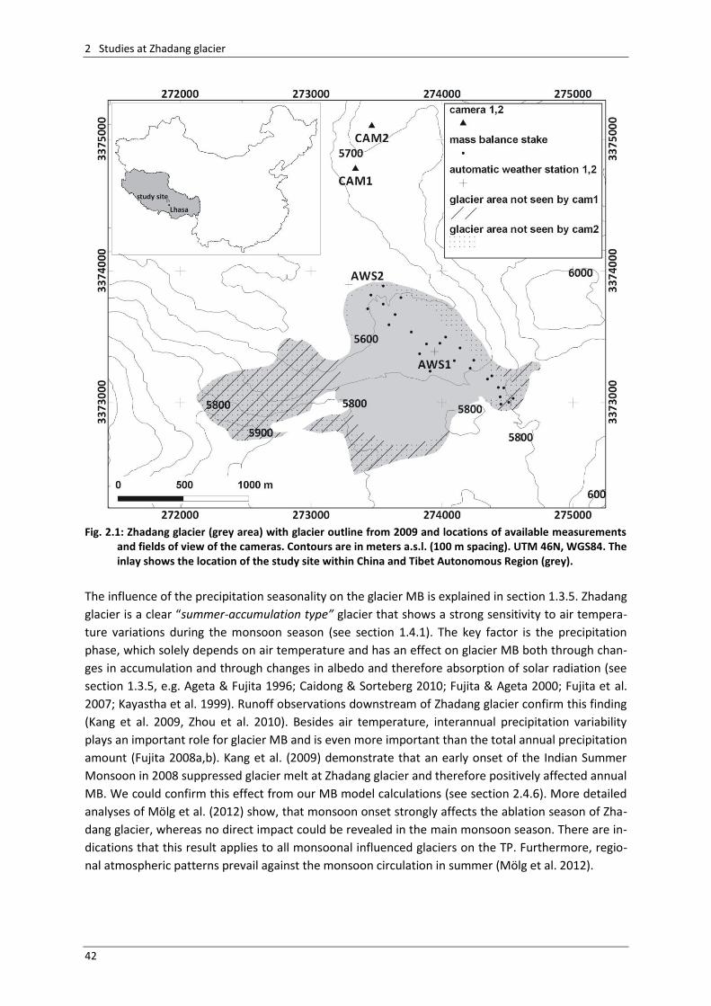
2 Studies at Zhadang glacier
42
Fig. 2.1: Zhadang glacier (grey area) with glacier outline from 2009 and locations of available measurements
and fields of view of the cameras. Contours are in meters a.s.l. (100 m spacing). UTM 46N, WGS84. The inlay shows the location of the study site within China and Tibet Autonomous Region (grey).
The influence of the precipitation seasonality on the glacier MB is explained in section 1.3.5. Zhadang
glacier is a clear “summer-accumulation type” glacier that shows a strong sensitivity to air tempera-
ture variations during the monsoon season (see section 1.4.1). The key factor is the precipitation
phase, which solely depends on air temperature and has an effect on glacier MB both through chan-
ges in accumulation and through changes in albedo and therefore absorption of solar radiation (see
section 1.3.5, e.g. Ageta & Fujita 1996; Caidong & Sorteberg 2010; Fujita & Ageta 2000; Fujita et al.
2007; Kayastha et al. 1999). Runoff observations downstream of Zhadang glacier confirm this finding
(Kang et al. 2009, Zhou et al. 2010). Besides air temperature, interannual precipitation variability
plays an important role for glacier MB and is even more important than the total annual precipitation
amount (Fujita 2008a,b). Kang et al. (2009) demonstrate that an early onset of the Indian Summer
Monsoon in 2008 suppressed glacier melt at Zhadang glacier and therefore positively affected annual
MB. We could confirm this effect from our MB model calculations (see section 2.4.6). More detailed
analyses of Mölg et al. (2012) show, that monsoon onset strongly affects the ablation season of Zha-
dang glacier, whereas no direct impact could be revealed in the main monsoon season. There are in-
dications that this result applies to all monsoonal influenced glaciers on the TP. Furthermore, regio-
nal atmospheric patterns prevail against the monsoon circulation in summer (Mölg et al. 2012).
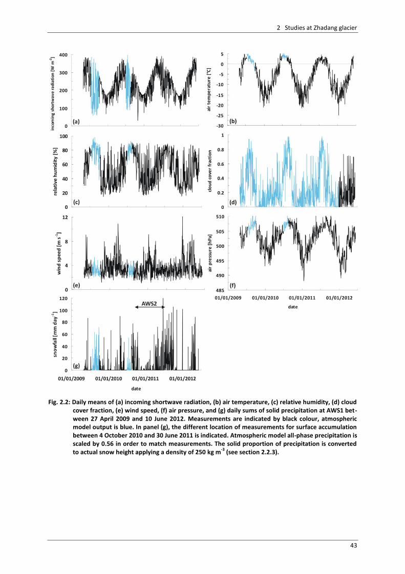
2 Studies at Zhadang glacier
43
Fig. 2.2: Daily means of (a) incoming shortwave radiation, (b) air temperature, (c) relative humidity, (d) cloud
cover fraction, (e) wind speed, (f) air pressure, and (g) daily sums of solid precipitation at AWS1 bet-ween 27 April 2009 and 10 June 2012. Measurements are indicated by black colour, atmospheric model output is blue. In panel (g), the different location of measurements for surface accumulation between 4 October 2010 and 30 June 2011 is indicated. Atmospheric model all-phase precipitation is scaled by 0.56 in order to match measurements. The solid proportion of precipitation is converted to actual snow height applying a density of 250 kg m
-3 (see section 2.2.3).
2 Studies at Zhadang glacier
44
2.2 Data basis
In this study we use various data from in-situ measurements at the glacier site to force (see sections
2.2.1 and 2.3.1), calibrate (see section 2.4.1) and evaluate the SEB/MB model between 2009 and
2012 (see section 2.4.2). Measurements not used for forcing and calibration are applied to evaluate
the model performance. Additionally, we calibrated (see section 2.4.1) and evaluated (see section
2.4.2) the model forced by atmospheric model output from the High Asia Reanalysis (HAR) and ran it
for the period 2001 to 2011 (see section 2.4.6). The distributed model runs on a SRTM digital ele-
vation model (DEM) (Rabus et al. 2003) resampled to 45 m resolution. The glacier size is kept const-
ant throughout the modelling period and is based on the 2009 glacier extent (glacier outlines at the
tongue based on Bolch et al. 2010, see section 1.4.2.1).
2.2.1 In-situ measurements relevant for the SEB/MB model
In a first step, we use observational data from an automatic weather station (AWS1) to force the
SEB/MB model (Table 2.1). AWS1 is operated in the ablation zone of Zhadang Glacier at 5665 m a.s.l.
since 2009 (Fig. 2.1, 2.2). Due to the extreme environment, two data gaps are evident in late summer
2009 and 2010 respectively (see section 1.4.2.1). Therefore, three periods are sufficiently covered by
AWS data: (P1) 27 April 2009 – 14 July 2009, (P2) 1 October 2009 – 1 July 2010, (P3) 16 August 2010 –
10 June 2012. To obtain a continuous data series from 2009 to 2012 these gaps were filled with data
from HAR (see section 2.2.3). Except for the period 4 October 2010 – 30 June 2011 within P3, snow
accumulation recorded by the sonic ranger (SR50) is directly used as model input. The heat flux from
liquid precipitation is neglected (see section 2.3.1). The missing period was characterized by weak
ablation (Fig. 2.8a) and the sensor at AWS1 was buried by snow. We used SR50 data from nearby
AWS2 (Fig. 2.1) that is operated since 2010 at 5550 m a.s.l. in front of the glacier instead. Subsurface
temperatures have been measured at AWS1 until a maximum initial depth of ≈ 8.5 m (7.1 m), where
ice temperature is almost constant (-4.7°C, see section 1.4.2.1). This value is used to define the lower
boundary condition (Tb) of the MB model. Further, temperature measurements at the surface and in
≈ 1.5 m, ≈ 4.5 m and ≈ 5 m depth initially served for initialization of the temperature profile and the
latter also for model evaluation. In the final model run, the temperature profile is initialized with air
temperature (Tair) and Tb only (see section 2.3.1). According to Mölg et al. 2012, the actual height of
the Tair/ relative humidity (RH) sensor, as well as the depth of the subsurface sensors, has been esti-
mated from the SR50 record. From sensors in two heights, Tair and RH have been linearly interpolated
to the 2 m standard height (see section 1.4.2.1). Tair at AWS1 and AWS2 was used to calculate a linear
vertical gradient (-0.007 K m-1) that is applied in the distributed model version (see section 2.4).
The AWS data was processed according to the instruments’ manuals and screened in order to detect
and correct measurement errors. No further corrections for radiative sensor heating and/or riming
were conducted as Mölg et al. (2012) identified only 0.9% of wind data and between 0 and 0.7% of
the other variables to be erroneous.
A total of 25 ablation stakes in the eastern part of the glacier serve for MB model calibration and
evaluation (see section 1.3.4.2). Measurements are available for 16 intervals within the ablation
seasons between May 2009 and October 2011. The intervals range between four days and seven
months (see Fig. 2.8a and section 2.4.2.4). Snow pits were dug at AWS1 in 2009, 2010 and 2011 in
order to measure vertical density profiles that serve for density assumptions within the model (see
section 2.3.1) and for model evaluation (see section 2.4.2.3).
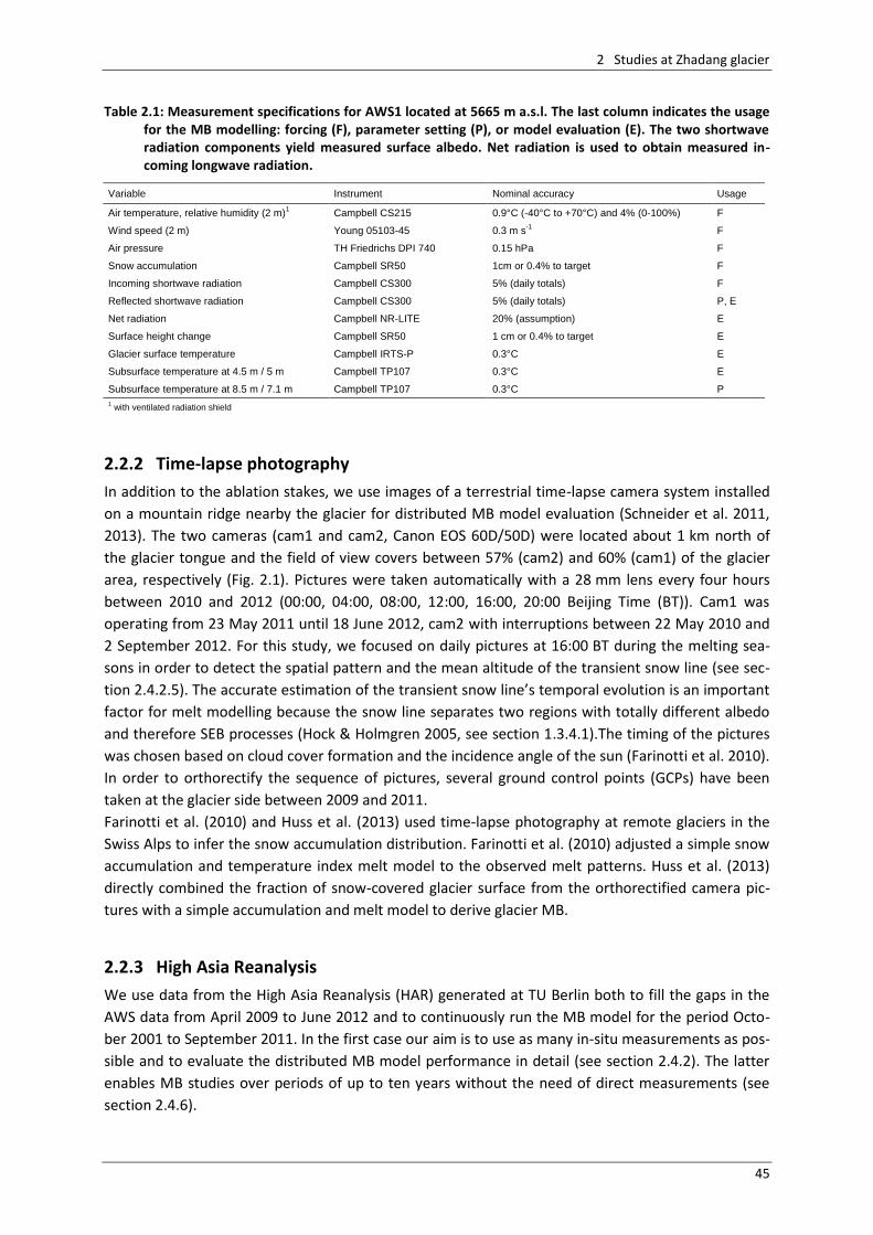
2 Studies at Zhadang glacier
45
Table 2.1: Measurement specifications for AWS1 located at 5665 m a.s.l. The last column indicates the usage for the MB modelling: forcing (F), parameter setting (P), or model evaluation (E). The two shortwave radiation components yield measured surface albedo. Net radiation is used to obtain measured in-coming longwave radiation.
Variable Instrument Nominal accuracy Usage
Air temperature, relative humidity (2 m)1 Campbell CS215 0.9°C (-40°C to +70°C) and 4% (0-100%) F
Wind speed (2 m) Young 05103-45 0.3 m s-1
F
Air pressure TH Friedrichs DPI 740 0.15 hPa F
Snow accumulation Campbell SR50 1cm or 0.4% to target F
Incoming shortwave radiation Campbell CS300 5% (daily totals) F
Reflected shortwave radiation Campbell CS300 5% (daily totals) P, E
Net radiation Campbell NR-LITE 20% (assumption) E
Surface height change Campbell SR50 1 cm or 0.4% to target E
Glacier surface temperature Campbell IRTS-P 0.3°C E
Subsurface temperature at 4.5 m / 5 m Campbell TP107 0.3°C E
Subsurface temperature at 8.5 m / 7.1 m Campbell TP107 0.3°C P
1 with ventilated radiation shield
2.2.2 Time-lapse photography
In addition to the ablation stakes, we use images of a terrestrial time-lapse camera system installed
on a mountain ridge nearby the glacier for distributed MB model evaluation (Schneider et al. 2011,
2013). The two cameras (cam1 and cam2, Canon EOS 60D/50D) were located about 1 km north of
the glacier tongue and the field of view covers between 57% (cam2) and 60% (cam1) of the glacier
area, respectively (Fig. 2.1). Pictures were taken automatically with a 28 mm lens every four hours
between 2010 and 2012 (00:00, 04:00, 08:00, 12:00, 16:00, 20:00 Beijing Time (BT)). Cam1 was
operating from 23 May 2011 until 18 June 2012, cam2 with interruptions between 22 May 2010 and
2 September 2012. For this study, we focused on daily pictures at 16:00 BT during the melting sea-
sons in order to detect the spatial pattern and the mean altitude of the transient snow line (see sec-
tion 2.4.2.5). The accurate estimation of the transient snow line’s temporal evolution is an important
factor for melt modelling because the snow line separates two regions with totally different albedo
and therefore SEB processes (Hock & Holmgren 2005, see section 1.3.4.1).The timing of the pictures
was chosen based on cloud cover formation and the incidence angle of the sun (Farinotti et al. 2010).
In order to orthorectify the sequence of pictures, several ground control points (GCPs) have been
taken at the glacier side between 2009 and 2011.
Farinotti et al. (2010) and Huss et al. (2013) used time-lapse photography at remote glaciers in the
Swiss Alps to infer the snow accumulation distribution. Farinotti et al. (2010) adjusted a simple snow
accumulation and temperature index melt model to the observed melt patterns. Huss et al. (2013)
directly combined the fraction of snow-covered glacier surface from the orthorectified camera pic-
tures with a simple accumulation and melt model to derive glacier MB.
2.2.3 High Asia Reanalysis
We use data from the High Asia Reanalysis (HAR) generated at TU Berlin both to fill the gaps in the
AWS data from April 2009 to June 2012 and to continuously run the MB model for the period Octo-
ber 2001 to September 2011. In the first case our aim is to use as many in-situ measurements as pos-
sible and to evaluate the distributed MB model performance in detail (see section 2.4.2). The latter
enables MB studies over periods of up to ten years without the need of direct measurements (see
section 2.4.6).
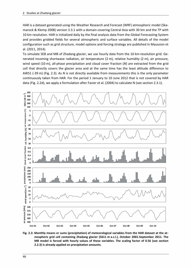
2 Studies at Zhadang glacier
46
HAR is a dataset generated using the Weather Research and Forecast (WRF) atmospheric model (Ska-
marock & Klemp 2008) version 3.3.1 with a domain covering Central Asia with 30 km and the TP with
10 km resolution. HAR is initialized daily by the final analysis data from the Global Forecasting System
and provides gridded fields for several atmospheric and surface variables. All details of the model
configuration such as grid structure, model options and forcing strategy are published in Maussion et
al. (2011, 2014).
To simulate SEB and MB of Zhadang glacier, we use hourly data from the 10 km-resolution grid. Ge-
nerated incoming shortwave radiation, air temperature (2 m), relative humidity (2 m), air pressure,
wind speed (10 m), all-phase precipitation and cloud cover fraction (N) are extracted from the grid
cell that directly covers the glacier area and at the same time has the least altitude difference to
AWS1 (-39 m) (Fig. 2.3). As N is not directly available from measurements this is the only parameter
continuously taken from HAR. For the period 1 January to 10 June 2012 that is not covered by HAR
data (Fig. 2.2d), we apply a formulation after Favier et al. (2004) to calculate N (see section 2.3.1).
Fig. 2.3: Monthly means or sums (precipitation) of meteorological variables from the HAR dataset at the at-
mospheric grid cell containing Zhadang glacier (5611 m a.s.l.), October 2001-September 2011. The MB model is forced with hourly values of these variables. The scaling factor of 0.56 (see section 2.2.3) is already applied on precipitation amounts.
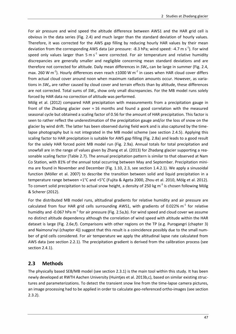
2 Studies at Zhadang glacier
47
For air pressure and wind speed the altitude difference between AWS1 and the HAR grid cell is
obvious in the data series (Fig. 2.4) and much larger than the standard deviation of hourly values.
Therefore, it was corrected for the AWS gap filling by reducing hourly HAR values by their mean
deviation from the corresponding AWS data (air pressure: -8.3 hPa; wind speed: -4.7 m s-1). For wind
speed only values larger than 5 m s-1 were corrected. For air temperature and relative humidity
discrepancies are generally smaller and negligible concerning mean standard deviations and are
therefore not corrected for altitude. Daily mean differences in SWin can be large in summer (Fig. 2.4,
max. 260 W m-2). Hourly differences even reach ±1000 W m-2 in cases when HAR cloud cover differs
from actual cloud cover around noon when maximum radiation amounts occur. However, as varia-
tions in SWin are rather caused by cloud cover and terrain effects than by altitude, these differences
are not corrected. Total sums of SWin show only small discrepancies. For the MB model runs solely
forced by HAR data no correction of altitude was performed.
Mölg et al. (2012) compared HAR precipitation with measurements from a precipitation gauge in
front of the Zhadang glacier over ≈ 16 months and found a good correlation with the measured
seasonal cycle but obtained a scaling factor of 0.56 for the amount of HAR precipitation. This factor is
seen to rather reflect the underestimation of the precipitation gauge and/or the loss of snow on the
glacier by wind drift. The latter has been observed during field work and is also captured by the time-
lapse photography but is not integrated in the MB model scheme (see section 2.4.5). Applying this
scaling factor to HAR precipitation is suitable for AWS gap filling (Fig. 2.8a) and leads to a good result
for the solely HAR forced point MB model run (Fig. 2.9a). Annual totals for total precipitation and
snowfall are in the range of values given by Zhang et al. (2013) for Zhadang glacier supporting a rea-
sonable scaling factor (Table 2.7). The annual precipitation pattern is similar to that observed at Nam
Co Station, with 81% of the annual total occurring between May and September. Precipitation mini-
ma are found in November and December (Fig. 1.10, 2.3, see section 1.4.2.1). We apply a sinusoidal
function (Möller et al. 2007) to describe the transition between solid and liquid precipitation in a
temperature range between +1°C and +5°C (Fujita & Ageta 2000, Zhou et al. 2010, Mölg et al. 2012).
To convert solid precipitation to actual snow height, a density of 250 kg m-3 is chosen following Mölg
& Scherer (2012).
For the distributed MB model runs, altitudinal gradients for relative humidity and air pressure are
calculated from four HAR grid cells surrounding AWS1, with gradients of 0.022% m-1 for relative
humidity and -0.067 hPa m-1 for air pressure (Fig. 2.5a,b). For wind speed and cloud cover we assume
no distinct altitude dependency although the correlation of wind speed with altitude within the HAR
dataset is large (Fig. 2.6e,f). Comparisons with other regions on the TP (e.g. Purogangri (chapter 3)
and Naimona’nyi (chapter 4)) suggest that this result is a coincidence possibly due to the small num-
ber of grid cells considered. For air temperature we apply the altitudinal lapse rate calculated from
AWS data (see section 2.2.1). The precipitation gradient is derived from the calibration process (see
section 2.4.1).
2.3 Methods
The physically based SEB/MB model (see section 2.3.1) is the main tool within this study. It has been
newly developed at RWTH Aachen University (Huintjes et al. 2013b,c), based on similar existing struc-
tures and parameterizations. To detect the transient snow line from the time-lapse camera pictures,
an image processing had to be applied in order to calculate geo-referenced ortho-images (see section
2.3.2).
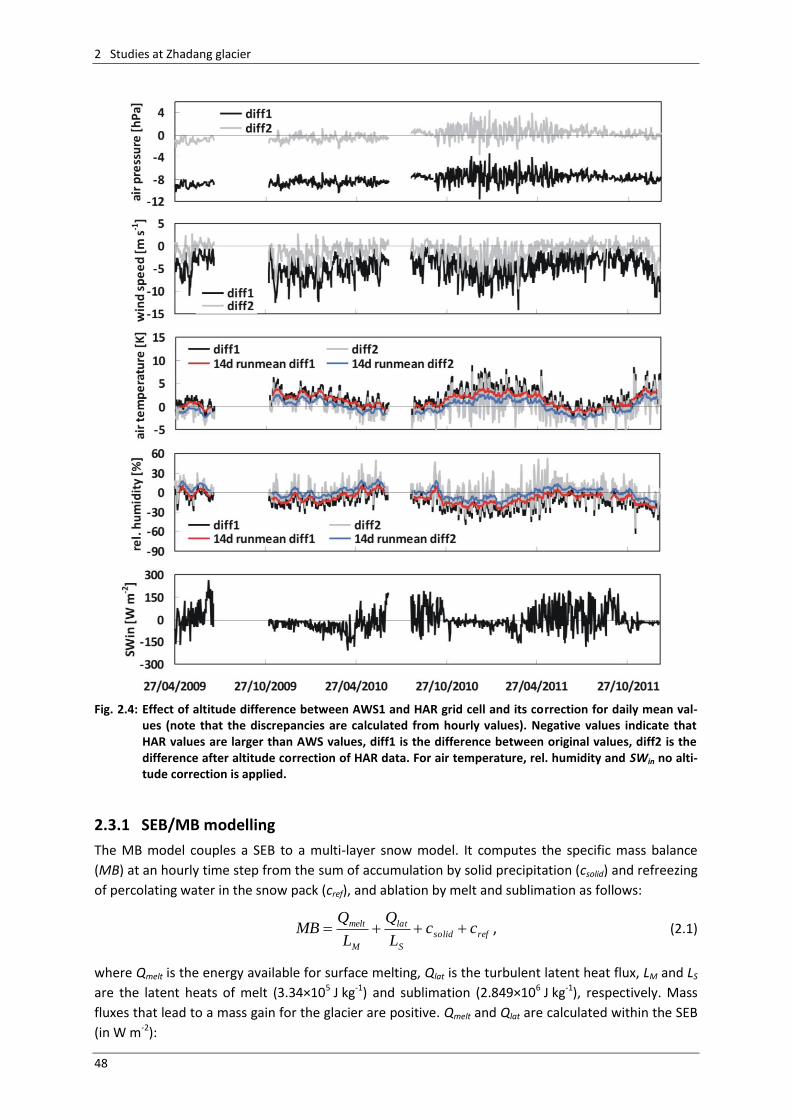
2 Studies at Zhadang glacier
48
Fig. 2.4: Effect of altitude difference between AWS1 and HAR grid cell and its correction for daily mean val-
ues (note that the discrepancies are calculated from hourly values). Negative values indicate that HAR values are larger than AWS values, diff1 is the difference between original values, diff2 is the difference after altitude correction of HAR data. For air temperature, rel. humidity and SWin no alti-tude correction is applied.
2.3.1 SEB/MB modelling
The MB model couples a SEB to a multi-layer snow model. It computes the specific mass balance
(MB) at an hourly time step from the sum of accumulation by solid precipitation (csolid) and refreezing
of percolating water in the snow pack (cref), and ablation by melt and sublimation as follows:
refsolid
S
lat
M
melt ccL
Q
L
QMB , (2.1)
where Qmelt is the energy available for surface melting, Qlat is the turbulent latent heat flux, LM and LS
are the latent heats of melt (3.34×10⁵ J kg-1) and sublimation (2.849×10⁶ J kg-1), respectively. Mass
fluxes that lead to a mass gain for the glacier are positive. Qmelt and Qlat are calculated within the SEB
(in W m-2):
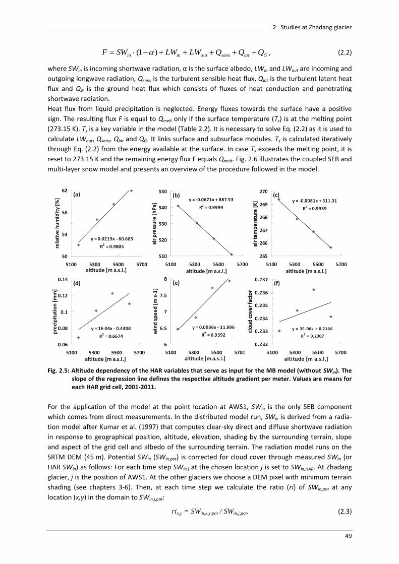
2 Studies at Zhadang glacier
49
Glatsensoutinin QQQLWLWSWF )1( , (2.2)
where SWin is incoming shortwave radiation, α is the surface albedo, LWin and LWout are incoming and
outgoing longwave radiation, Qsens is the turbulent sensible heat flux, Qlat is the turbulent latent heat
flux and QG is the ground heat flux which consists of fluxes of heat conduction and penetrating
shortwave radiation.
Heat flux from liquid precipitation is neglected. Energy fluxes towards the surface have a positive
sign. The resulting flux F is equal to Qmelt only if the surface temperature (Ts) is at the melting point
(273.15 K). Ts is a key variable in the model (Table 2.2). It is necessary to solve Eq. (2.2) as it is used to
calculate LWout, Qsens, Qlat and QG. It links surface and subsurface modules. Ts is calculated iteratively
through Eq. (2.2) from the energy available at the surface. In case Ts exceeds the melting point, it is
reset to 273.15 K and the remaining energy flux F equals Qmelt. Fig. 2.6 illustrates the coupled SEB and
multi-layer snow model and presents an overview of the procedure followed in the model.
Fig. 2.5: Altitude dependency of the HAR variables that serve as input for the MB model (without SWin). The
slope of the regression line defines the respective altitude gradient per meter. Values are means for each HAR grid cell, 2001-2011.
For the application of the model at the point location at AWS1, SWin is the only SEB component
which comes from direct measurements. In the distributed model run, SWin is derived from a radia-
tion model after Kumar et al. (1997) that computes clear-sky direct and diffuse shortwave radiation
in response to geographical position, altitude, elevation, shading by the surrounding terrain, slope
and aspect of the grid cell and albedo of the surrounding terrain. The radiation model runs on the
SRTM DEM (45 m). Potential SWin (SWin,pot) is corrected for cloud cover through measured SWin (or
HAR SWin) as follows: For each time step SWin,j at the chosen location j is set to SWin,HAR. At Zhadang
glacier, j is the position of AWS1. At the other glaciers we choose a DEM pixel with minimum terrain
shading (see chapters 3-6). Then, at each time step we calculate the ratio (ri) of SWin,pot at any
location (x,y) in the domain to SWin,j,pot:
rix,y = SWin,x,y,pot / SWin,j,pot. (2.3)
2 Studies at Zhadang glacier
50
SWin,j,pot is potential SWin according to Kumar et al. (1997) at the chosen location j. The spatial matrix
of cloud-corrected shortwave irradiance SWin at any location (x,y) in the domain calculated by
SWin,x,y = SWin,j * rix,y (2.4)
for each time step finally provides a spatial mask of SWin including effects from terrain shading and
from cloud cover.
Table 2.2: Energy fluxes at the glacier surface and their physical links as treated in the MB model.
SEB component Determined froma
SWin (incoming shortwave radiation) Direct measurement of solar radiation / radiation model
α (surface albedo) Snowfall amount and frequency, snow depth
LWin (incoming longwave radiation) Water vapour pressure, air temperature, cloud cover factor
LWout (outgoing longwave radiation) Glacier surface temperature (Ts)
Qsens (turbulent sensible heat flux) Air temperature, Ts, wind speed, air pressure
Qlat (turbulent latent heat flux) Air humidity, Ts, wind speed, air pressure
QG (ground heat flux) Thermodynamic heat equation (forced by Ts)
a for details see section 2.3.1
Fig. 2.6: Left: Illustration of an SEB model including a multi-layer snow model. Symbols are as in the text, sub-script i denotes the ith model level. Parameters obtained from measurements or atmospheric model output are outlined. Arrows indicate the direction of the energy flux. Fluxes directed towards the surface are defined positive. Right: Flow chart of the MB model.
The parameterization of surface albedo follows the scheme of Oerlemans & Knap (1998) where α is
determined as a function of snowfall frequency and snow depth:
*)/exp()( ttsnowfirnfrsnowfirnsnow and (2.5)
*)/exp( dhsnowicesnow . (2.6)
tsnow is the time since the last snowfall, t* is a constant for the effect of ageing on snow albedo, h is
the snow depth and d* is a constant for the effect of snow depth on albedo. The free parameters in
the albedo scheme are determined from measurements of SWin and SWout at AWS1 between 2009
and 2011 (see section 2.2.1) and according to Mölg et al. (2012). Final values are: albedo fresh snow
2 Studies at Zhadang glacier
51
(αfrsnow) = 0.9, albedo firn (αfirn) = 0.55, albedo ice (αice) = 0.3, t* = 6 days and d* = 8 cm. A comparison
of measured daily mean α with the respective modelled α is given in Fig. 2.7.
LWin and LWout are obtained by the Stefan-Boltzmann law. For LWin, the atmospheric emissivity ε is
calculated after Klok & Oerlemans (2002):
a
cl
a
cs NN )1( , (2.7)
where εcs is clear-sky emissivity and εcl is cloud emissivity, N is cloud cover factor. εcs is calculated as
follows:
8/1)/(23.0 aircs Teb , (2.8)
where e is water vapour pressure and Tair is air temperature. For a, b and εcl we take the values of 2,
0.433 and 0.984, respectively, as determined by Klok & Oerlemans (2002). N is directly taken from
HAR except during the period 1 January to 10 June 2012 that is not covered by HAR data (Fig. 2.2d).
During the latter period we determine N by comparing SWin to the theoretical values of the top of
atmosphere solar irradiance (SWTOA) using the expression after Favier et al. (2004):
)/(4.13.1 TOAin SWSWN . (2.9)
SWTOA is calculated through the radiation model after Kumar et al. (1997) considering solar constant
and geographical position.
Turbulent heat fluxes Qsens and Qlat are calculated through the bulk aerodynamic method after Oerle-
mans (2001) between the surface and 2 m, using Tair, RH and wind speed (u) data from AWS1:
)( sairsepairsens TTuCcQ (2.10)
)(/ sairlatSEairlat qquCLQ . (2.11)
ρair is air density, calculated from air pressure, Tair and specific humidity in 2 m, cp is specific heat
capacity of air (1004.67 J kg-1 K-1), LE is latent heat of evaporation (2.514×10⁶ J kg-1), LS for sublimation
(2.849×10⁶ J kg-1), qair and qs are specific humidity at 2 m and at the surface, calculated from RH, p (air
pressure) and saturation water vapour pressure. RH is assumed to be 100% at the surface. Cse and Clat
are bulk-transfer coefficients for sensible and latent heat. Oerlemans (2001) found Cse and Clat to
differ by less than 5%, therefore we assume Cse = Clat. Cse is calculated after Braithwaite (1995):
2
0
2 )]//[ln( zzkCse , (2.12)
with k the von Karman constant (0.41), z the instrument height (2 m) and z0 the surface roughness
length that changes time dependent (z0m = z0h) (Mölg et al. 2009a). Similar to Mölg et al. 2012, z0
increases linearly from 0.24 mm for fresh snow (Gromke et al. 2011) to 4 mm for aged snow (Brock et
al. 2006). If the surface is snow free, we assume z0 to be 1.7 mm (Cullen et al. 2007). A correction of
turbulent fluxes for stable conditions is carried out after Braithwaite (1995):
2.00
01.02.0)51(
/
2
//
RiQ
RiRiQQ
latsens
latsenslatsens , (2.13)
were Ri is the bulk Richardson number, calculated from Tair and u:
2
)( /)( uTzTgRi airCair . (2.14)
In formula 2.12 after Braithwaite (1995) g is the acceleration of gravity (9.81 m s-1) and Tair(C) is the air
temperature in °C.
QG is the sum of the conductive heat flux (QC) and the energy flux from penetrating shortwave radia-
tion (QPS). QPS is calculated following Bintanja & van den Broeke (1995). By
2 Studies at Zhadang glacier
52
z
neti eSWzS )1()( (2.15)
the extinction of SWnet in the snow or ice layers is parameterized. In the top model layer, a fraction ζ
is absorbed and an exponentially decreasing flux with constant extinction coefficient β reaches the
layers at depth –z and increases subsurface temperatures. Thus, QPS is equal to SWnet(1-ζ). For ζ and β
we take the values of 0.8 and 2.5 for ice, and 0.9 and 17.1 for snow, respectively, as determined by
Bintanja & van den Broeke (1995).
QC is determined from the temperature difference between the surface and the two uppermost
subsurface layers and depends on the thermal conductivity (λ) of the medium (ice or snow). λ is cal-
culated from the subsurface density (ρ, in kg m-3) after Anderson (1976):
2)1000/(5.2021.0 . (2.16)
Thus, in order to calculate QG vertical profiles of subsurface temperature (T) and density (ρ) need to
be known which are calculated within the subsurface snow model. The snow model uses a vertical
grid that consists of layers with an equal thickness (dz) of 0.1 m in the point model version and 0.2 m
in the distributed model runs. Each layer is characterized by a temperature, density, liquid water
content (w) and depth (z). On this grid, T is solved from the thermodynamic heat equation:
2
2
z
T
t
T
. (2.17)
κ is the thermal diffusivity and is calculated using the expression after Sturm et al. (1997) (ρ in kg m-3):
)/( pic , (2.18)
where cpi is the specific heat of ice, that is a function of T: Tcpi 122.72.152 (Paterson, 1994).
The initial temperature profile is defined from the available subsurface measurements (see section
2.2.1) by linear interpolation. Tests showed that model results are the same for an initial tempera-
ture profile linearly interpolated between Tair (= Ts) and Tb as for an initial temperature profile linearly
interpolated between the subsurface measurements. The density profile of the initial snow pack is
calculated by a linear interpolation between 250 and 550 kg m-3 as estimated from the snow pits (see
section 2.2.1).
First, the temperature profile is calculated without considering the effects of refreezing or subsurface
melt but considering temperature increase by QPS only. In case a snow/firn pack is present, the model
then calculates the densification of the dry snow pack through an empirical relation after Herron &
Langway (1980):
iceice
f
solidcTrEKdt
d
/)())/(exp( , (2.19)
where K is a rate factor, E is activation energy (J mol-1), r is the gas constant (8.3144 J K-1 mol-1), csolid is
the accumulation rate (in mm w.e.) and f is a factor that is approximately equal to 1 (Reijmer & Hock
2008). For K and E we take the values as determined by Herron & Langway (1980) for two stages of
densification: for ρ<550 kg m-3 we take K = 11 and E = 10160, for 550 kg m-3<ρ<800 kg m-3 we take
K = 575 and E = 21400.
After the densification process, the available amount of surface and subsurface melt water perco-
lates downwards and a small amount is held in each layer. We choose constant percolation velocities
of 0.06 cm s-1 for unsaturated layers and 0.042 cm s-1 (70%) for saturated layers where the liquid
water content (w) exceeds the irreducible water content (wi). These values are within the boundaries
2 Studies at Zhadang glacier
53
for water film flow and tubular flow through homogenous snow layers (Baumgartner et al. 1990). wi
is assumed to be 5% of the total mass of the layer (Fujita & Ageta 2000). Then w is calculated and
depending on the cold content (γ) of the layer, the available water can refreeze. γ is defined as the
amount of energy that is required to raise the temperature of the respective layer to the melting
point and is calculated as follows (Cogley et al. 2011):
)15.273( Tcp . (2.20)
Therefore, the amount of refreezing is limited by T, which cannot be raised above the melting point,
and by w. Refreezing is largest in early summer, when percolating melt water reaches cold winter
snow layers, and in autumn, when capillary water freezes (van Pelt et al. 2012). When a wet snow
layer is present in summer, internal water can refreeze at night. This leads to an increase in T and ρ in
the respective layer. When T exceeds the melting point in the model, T is reset to 273.15 K and the
remaining energy is used for subsurface melt. This melt water is added to the water content of the
respective layer. If w exceeds wi, the remaining water percolates downwards into the next layer until
it reaches the glacier ice and runs off.
Including the described processes, the subsurface temperature evolution can be expressed as:
z
LM
z
LF
z
zS
z
Q
z
T
t
T MMiC
)(2
2
, (2.21)
where F and M are refreezing and melt rate, respectively.
Table 2.3 summarizes the free parameters within the MB model and the chosen values.
The application of the presented model to a number of glaciers on the TP shows that a spin-up time
of about one year is needed for the subsurface module to adapt to the surrounding conditions (see
sections 2.4.6, 3.4.1, 4.4.1, 5.4.1). In the first months of simulation, w is zero and no refreezing can
happen. This influences both the temperature and the density profiles and leads to a number of
feedback processes that generally result in above average melt rates. Therefore, calculated values for
the first year of simulation should be treated with caution.
2.3.2 Image processing
In order to obtain quantitative information, e.g. the transient snow line from the sequence of pic-
tures taken by the two fixed time-lapse cameras, the landscape images had to be geo-referenced and
orthorectified (Huss et al. 2013). This procedure including the manual snow line mapping was carried
out at TU Dresden applying the software RSG (Remote Sensing Software Graz) for the image ortho-
rectification. In a first step, one image per week and camera had to be manually orthorectified be-
cause of shifts in the camera position due to ground deformation. The orthorectification requires the
definition of a transfer function relating the two-dimensional pixels of the picture to the three-
dimensional orography as represented by the DEM (SRTM bicubically resampled to 1 m resolution).
The correct scaling functions were defined by adjusting the position of five to six selected GCP (see
section 2.2.2) to the corresponding locations in the pictures. The image coordinates of the GCP and
therefore the scaling functions changed due to the movement of cameras over time. Applying a
spline function the weekly detected GCP positions have been interpolated to all available camera
pictures for automatic orthorectification. The transformation results in geo-referenced ortho-images
that were further evaluated with regard to the spatial and temporal evolution of the transient snow
line (see section 2.4.2.5). All pictures have been thoroughly checked and transient snow lines were
manually digitized for daily images at 16:00 BT. The intersection of the digital snow lines with the re-
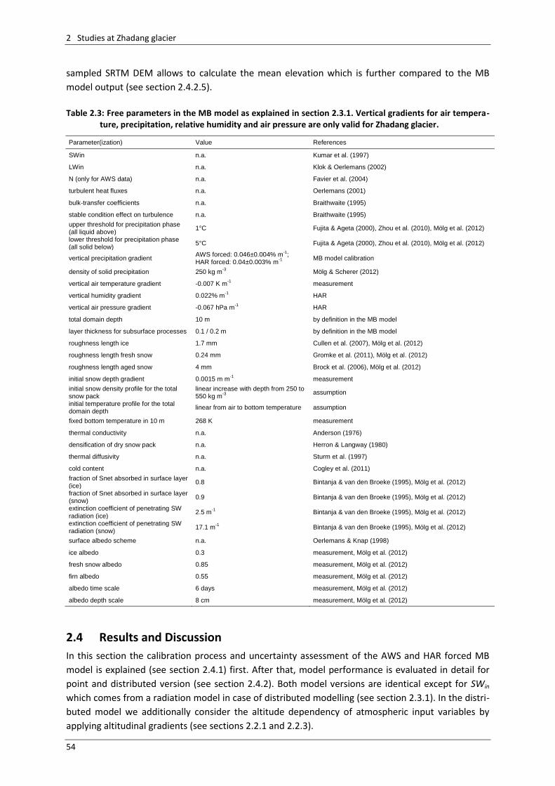
2 Studies at Zhadang glacier
54
sampled SRTM DEM allows to calculate the mean elevation which is further compared to the MB
model output (see section 2.4.2.5).
Table 2.3: Free parameters in the MB model as explained in section 2.3.1. Vertical gradients for air tempera-
ture, precipitation, relative humidity and air pressure are only valid for Zhadang glacier.
Parameter(ization) Value References
SWin n.a. Kumar et al. (1997)
LWin n.a. Klok & Oerlemans (2002)
N (only for AWS data) n.a. Favier et al. (2004)
turbulent heat fluxes n.a. Oerlemans (2001)
bulk-transfer coefficients n.a. Braithwaite (1995)
stable condition effect on turbulence n.a. Braithwaite (1995)
upper threshold for precipitation phase (all liquid above)
1°C Fujita & Ageta (2000), Zhou et al. (2010), Mölg et al. (2012)
lower threshold for precipitation phase (all solid below)
5°C Fujita & Ageta (2000), Zhou et al. (2010), Mölg et al. (2012)
vertical precipitation gradient AWS forced: 0.046±0.004% m
-1;
HAR forced: 0.04±0.003% m-1
MB model calibration
density of solid precipitation 250 kg m-3
Mölg & Scherer (2012)
vertical air temperature gradient -0.007 K m-1
measurement
vertical humidity gradient 0.022% m-1
HAR
vertical air pressure gradient -0.067 hPa m-1
HAR
total domain depth 10 m by definition in the MB model
layer thickness for subsurface processes 0.1 / 0.2 m by definition in the MB model
roughness length ice 1.7 mm Cullen et al. (2007), Mölg et al. (2012)
roughness length fresh snow 0.24 mm Gromke et al. (2011), Mölg et al. (2012)
roughness length aged snow 4 mm Brock et al. (2006), Mölg et al. (2012)
initial snow depth gradient 0.0015 m m-1
measurement
initial snow density profile for the total snow pack
linear increase with depth from 250 to 550 kg m
-3
assumption
initial temperature profile for the total domain depth
linear from air to bottom temperature assumption
fixed bottom temperature in 10 m 268 K measurement
thermal conductivity n.a. Anderson (1976)
densification of dry snow pack n.a. Herron & Langway (1980)
thermal diffusivity n.a. Sturm et al. (1997)
cold content n.a. Cogley et al. (2011)
fraction of Snet absorbed in surface layer (ice)
0.8 Bintanja & van den Broeke (1995), Mölg et al. (2012)
fraction of Snet absorbed in surface layer (snow)
0.9 Bintanja & van den Broeke (1995), Mölg et al. (2012)
extinction coefficient of penetrating SW radiation (ice)
2.5 m-1
Bintanja & van den Broeke (1995), Mölg et al. (2012)
extinction coefficient of penetrating SW radiation (snow)
17.1 m-1
Bintanja & van den Broeke (1995), Mölg et al. (2012)
surface albedo scheme n.a. Oerlemans & Knap (1998)
ice albedo 0.3 measurement, Mölg et al. (2012)
fresh snow albedo 0.85 measurement, Mölg et al. (2012)
firn albedo 0.55 measurement, Mölg et al. (2012)
albedo time scale 6 days measurement, Mölg et al. (2012)
albedo depth scale 8 cm measurement, Mölg et al. (2012)
2.4 Results and Discussion
In this section the calibration process and uncertainty assessment of the AWS and HAR forced MB
model is explained (see section 2.4.1) first. After that, model performance is evaluated in detail for
point and distributed version (see section 2.4.2). Both model versions are identical except for SWin
which comes from a radiation model in case of distributed modelling (see section 2.3.1). In the distri-
buted model we additionally consider the altitude dependency of atmospheric input variables by
applying altitudinal gradients (see sections 2.2.1 and 2.2.3).
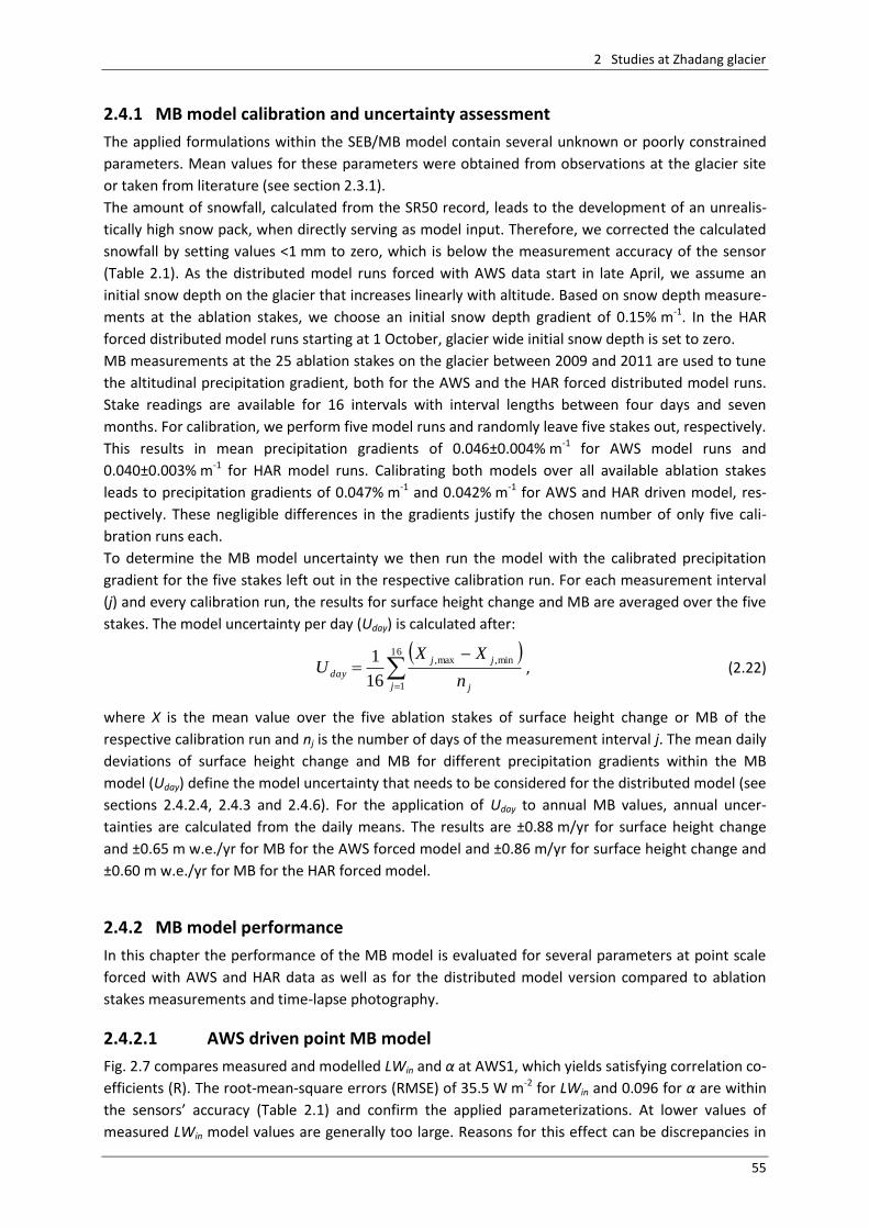
2 Studies at Zhadang glacier
55
2.4.1 MB model calibration and uncertainty assessment
The applied formulations within the SEB/MB model contain several unknown or poorly constrained
parameters. Mean values for these parameters were obtained from observations at the glacier site
or taken from literature (see section 2.3.1).
The amount of snowfall, calculated from the SR50 record, leads to the development of an unrealis-
tically high snow pack, when directly serving as model input. Therefore, we corrected the calculated
snowfall by setting values <1 mm to zero, which is below the measurement accuracy of the sensor
(Table 2.1). As the distributed model runs forced with AWS data start in late April, we assume an
initial snow depth on the glacier that increases linearly with altitude. Based on snow depth measure-
ments at the ablation stakes, we choose an initial snow depth gradient of 0.15% m-1. In the HAR
forced distributed model runs starting at 1 October, glacier wide initial snow depth is set to zero.
MB measurements at the 25 ablation stakes on the glacier between 2009 and 2011 are used to tune
the altitudinal precipitation gradient, both for the AWS and the HAR forced distributed model runs.
Stake readings are available for 16 intervals with interval lengths between four days and seven
months. For calibration, we perform five model runs and randomly leave five stakes out, respectively.
This results in mean precipitation gradients of 0.046±0.004% m-1 for AWS model runs and
0.040±0.003% m-1 for HAR model runs. Calibrating both models over all available ablation stakes
leads to precipitation gradients of 0.047% m-1 and 0.042% m-1 for AWS and HAR driven model, res-
pectively. These negligible differences in the gradients justify the chosen number of only five cali-
bration runs each.
To determine the MB model uncertainty we then run the model with the calibrated precipitation
gradient for the five stakes left out in the respective calibration run. For each measurement interval
(j) and every calibration run, the results for surface height change and MB are averaged over the five
stakes. The model uncertainty per day (Uday) is calculated after:
16
1
min,max,
16
1
j j
jj
dayn
XXU , (2.22)
where X is the mean value over the five ablation stakes of surface height change or MB of the
respective calibration run and nj is the number of days of the measurement interval j. The mean daily
deviations of surface height change and MB for different precipitation gradients within the MB
model (Uday) define the model uncertainty that needs to be considered for the distributed model (see
sections 2.4.2.4, 2.4.3 and 2.4.6). For the application of Uday to annual MB values, annual uncer-
tainties are calculated from the daily means. The results are ±0.88 m/yr for surface height change
and ±0.65 m w.e./yr for MB for the AWS forced model and ±0.86 m/yr for surface height change and
±0.60 m w.e./yr for MB for the HAR forced model.
2.4.2 MB model performance
In this chapter the performance of the MB model is evaluated for several parameters at point scale
forced with AWS and HAR data as well as for the distributed model version compared to ablation
stakes measurements and time-lapse photography.
2.4.2.1 AWS driven point MB model
Fig. 2.7 compares measured and modelled LWin and α at AWS1, which yields satisfying correlation co-
efficients (R). The root-mean-square errors (RMSE) of 35.5 W m-2 for LWin and 0.096 for α are within
the sensors’ accuracy (Table 2.1) and confirm the applied parameterizations. At lower values of
measured LWin model values are generally too large. Reasons for this effect can be discrepancies in
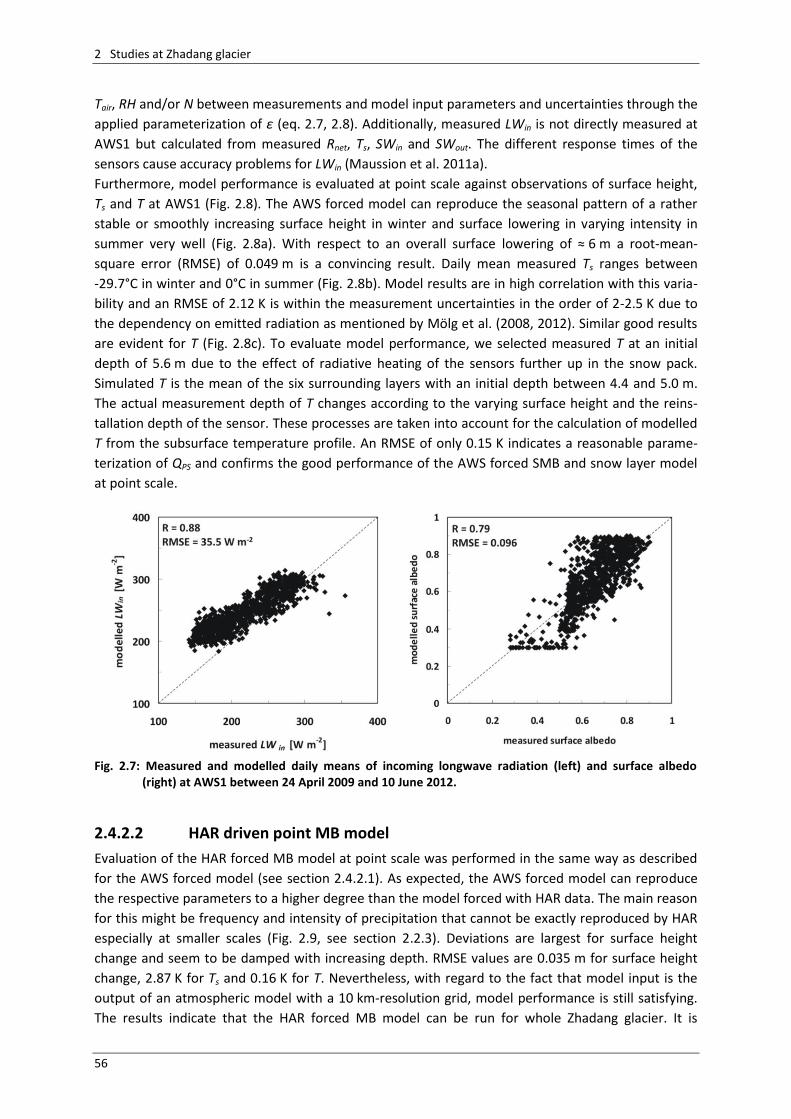
2 Studies at Zhadang glacier
56
Tair, RH and/or N between measurements and model input parameters and uncertainties through the
applied parameterization of ε (eq. 2.7, 2.8). Additionally, measured LWin is not directly measured at
AWS1 but calculated from measured Rnet, Ts, SWin and SWout. The different response times of the
sensors cause accuracy problems for LWin (Maussion et al. 2011a).
Furthermore, model performance is evaluated at point scale against observations of surface height,
Ts and T at AWS1 (Fig. 2.8). The AWS forced model can reproduce the seasonal pattern of a rather
stable or smoothly increasing surface height in winter and surface lowering in varying intensity in
summer very well (Fig. 2.8a). With respect to an overall surface lowering of ≈ 6 m a root-mean-
square error (RMSE) of 0.049 m is a convincing result. Daily mean measured Ts ranges between
-29.7°C in winter and 0°C in summer (Fig. 2.8b). Model results are in high correlation with this varia-
bility and an RMSE of 2.12 K is within the measurement uncertainties in the order of 2-2.5 K due to
the dependency on emitted radiation as mentioned by Mölg et al. (2008, 2012). Similar good results
are evident for T (Fig. 2.8c). To evaluate model performance, we selected measured T at an initial
depth of 5.6 m due to the effect of radiative heating of the sensors further up in the snow pack.
Simulated T is the mean of the six surrounding layers with an initial depth between 4.4 and 5.0 m.
The actual measurement depth of T changes according to the varying surface height and the reins-
tallation depth of the sensor. These processes are taken into account for the calculation of modelled
T from the subsurface temperature profile. An RMSE of only 0.15 K indicates a reasonable parame-
terization of QPS and confirms the good performance of the AWS forced SMB and snow layer model
at point scale.
Fig. 2.7: Measured and modelled daily means of incoming longwave radiation (left) and surface albedo
(right) at AWS1 between 24 April 2009 and 10 June 2012.
2.4.2.2 HAR driven point MB model
Evaluation of the HAR forced MB model at point scale was performed in the same way as described
for the AWS forced model (see section 2.4.2.1). As expected, the AWS forced model can reproduce
the respective parameters to a higher degree than the model forced with HAR data. The main reason
for this might be frequency and intensity of precipitation that cannot be exactly reproduced by HAR
especially at smaller scales (Fig. 2.9, see section 2.2.3). Deviations are largest for surface height
change and seem to be damped with increasing depth. RMSE values are 0.035 m for surface height
change, 2.87 K for Ts and 0.16 K for T. Nevertheless, with regard to the fact that model input is the
output of an atmospheric model with a 10 km-resolution grid, model performance is still satisfying.
The results indicate that the HAR forced MB model can be run for whole Zhadang glacier. It is
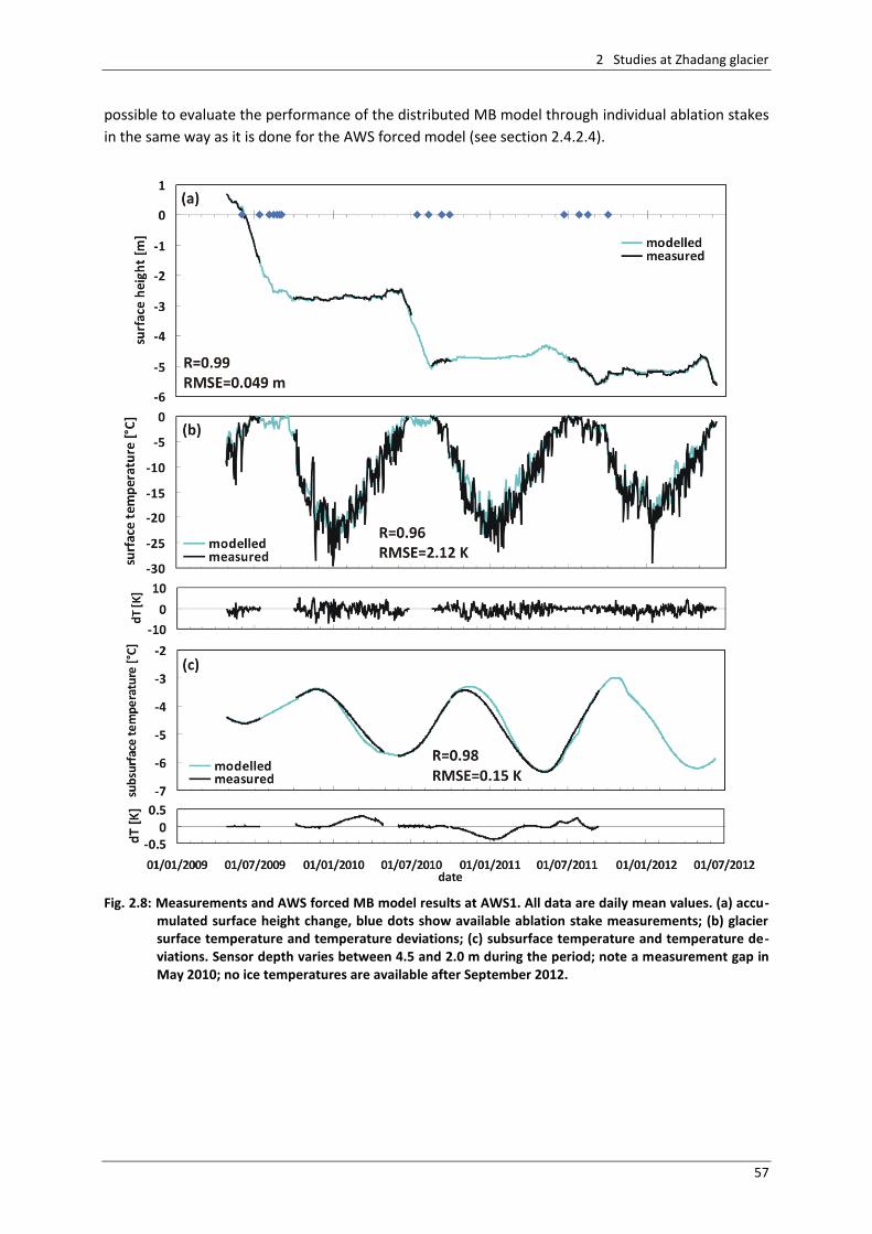
2 Studies at Zhadang glacier
57
possible to evaluate the performance of the distributed MB model through individual ablation stakes
in the same way as it is done for the AWS forced model (see section 2.4.2.4).
Fig. 2.8: Measurements and AWS forced MB model results at AWS1. All data are daily mean values. (a) accu-
mulated surface height change, blue dots show available ablation stake measurements; (b) glacier surface temperature and temperature deviations; (c) subsurface temperature and temperature de-viations. Sensor depth varies between 4.5 and 2.0 m during the period; note a measurement gap in May 2010; no ice temperatures are available after September 2012.
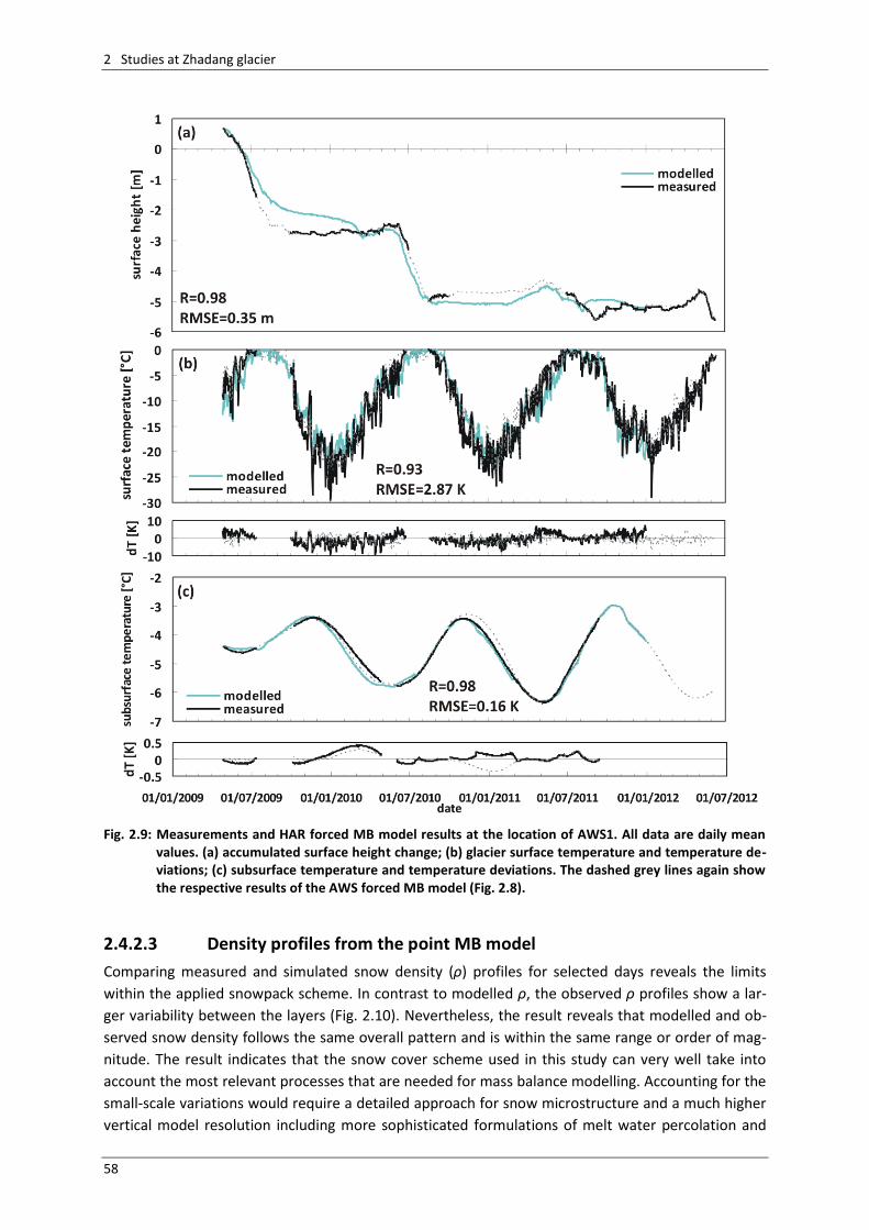
2 Studies at Zhadang glacier
58
Fig. 2.9: Measurements and HAR forced MB model results at the location of AWS1. All data are daily mean
values. (a) accumulated surface height change; (b) glacier surface temperature and temperature de-viations; (c) subsurface temperature and temperature deviations. The dashed grey lines again show the respective results of the AWS forced MB model (Fig. 2.8).
2.4.2.3 Density profiles from the point MB model
Comparing measured and simulated snow density (ρ) profiles for selected days reveals the limits
within the applied snowpack scheme. In contrast to modelled ρ, the observed ρ profiles show a lar-
ger variability between the layers (Fig. 2.10). Nevertheless, the result reveals that modelled and ob-
served snow density follows the same overall pattern and is within the same range or order of mag-
nitude. The result indicates that the snow cover scheme used in this study can very well take into
account the most relevant processes that are needed for mass balance modelling. Accounting for the
small-scale variations would require a detailed approach for snow microstructure and a much higher
vertical model resolution including more sophisticated formulations of melt water percolation and
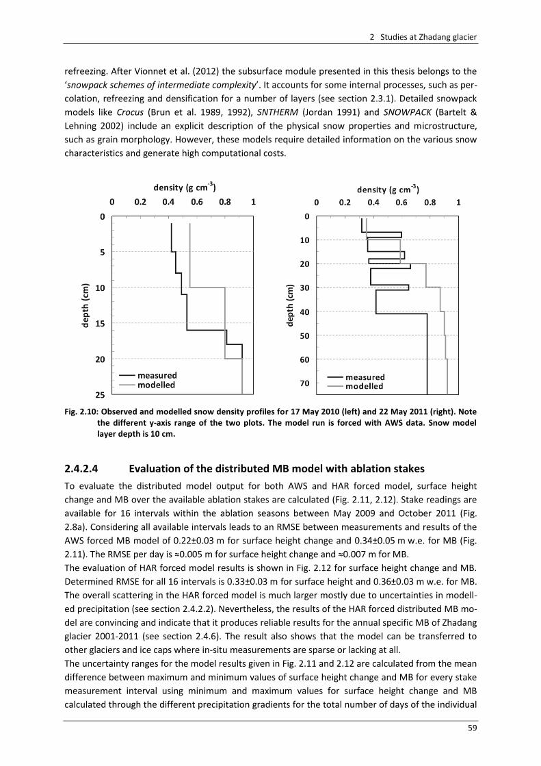
2 Studies at Zhadang glacier
59
refreezing. After Vionnet et al. (2012) the subsurface module presented in this thesis belongs to the
‘snowpack schemes of intermediate complexity’. It accounts for some internal processes, such as per-
colation, refreezing and densification for a number of layers (see section 2.3.1). Detailed snowpack
models like Crocus (Brun et al. 1989, 1992), SNTHERM (Jordan 1991) and SNOWPACK (Bartelt &
Lehning 2002) include an explicit description of the physical snow properties and microstructure,
such as grain morphology. However, these models require detailed information on the various snow
characteristics and generate high computational costs.
Fig. 2.10: Observed and modelled snow density profiles for 17 May 2010 (left) and 22 May 2011 (right). Note
the different y-axis range of the two plots. The model run is forced with AWS data. Snow model layer depth is 10 cm.
2.4.2.4 Evaluation of the distributed MB model with ablation stakes
To evaluate the distributed model output for both AWS and HAR forced model, surface height
change and MB over the available ablation stakes are calculated (Fig. 2.11, 2.12). Stake readings are
available for 16 intervals within the ablation seasons between May 2009 and October 2011 (Fig.
2.8a). Considering all available intervals leads to an RMSE between measurements and results of the
AWS forced MB model of 0.22±0.03 m for surface height change and 0.34±0.05 m w.e. for MB (Fig.
2.11). The RMSE per day is ≈0.005 m for surface height change and ≈0.007 m for MB.
The evaluation of HAR forced model results is shown in Fig. 2.12 for surface height change and MB.
Determined RMSE for all 16 intervals is 0.33±0.03 m for surface height and 0.36±0.03 m w.e. for MB.
The overall scattering in the HAR forced model is much larger mostly due to uncertainties in modell-
ed precipitation (see section 2.4.2.2). Nevertheless, the results of the HAR forced distributed MB mo-
del are convincing and indicate that it produces reliable results for the annual specific MB of Zhadang
glacier 2001-2011 (see section 2.4.6). The result also shows that the model can be transferred to
other glaciers and ice caps where in-situ measurements are sparse or lacking at all.
The uncertainty ranges for the model results given in Fig. 2.11 and 2.12 are calculated from the mean
difference between maximum and minimum values of surface height change and MB for every stake
measurement interval using minimum and maximum values for surface height change and MB
calculated through the different precipitation gradients for the total number of days of the individual
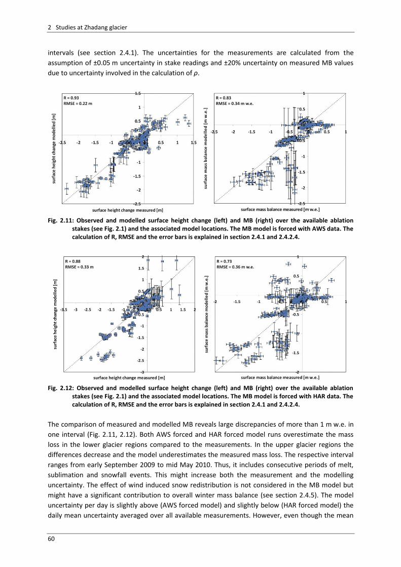
2 Studies at Zhadang glacier
60
intervals (see section 2.4.1). The uncertainties for the measurements are calculated from the
assumption of ±0.05 m uncertainty in stake readings and ±20% uncertainty on measured MB values
due to uncertainty involved in the calculation of ρ.
Fig. 2.11: Observed and modelled surface height change (left) and MB (right) over the available ablation
stakes (see Fig. 2.1) and the associated model locations. The MB model is forced with AWS data. The calculation of R, RMSE and the error bars is explained in section 2.4.1 and 2.4.2.4.
Fig. 2.12: Observed and modelled surface height change (left) and MB (right) over the available ablation
stakes (see Fig. 2.1) and the associated model locations. The MB model is forced with HAR data. The calculation of R, RMSE and the error bars is explained in section 2.4.1 and 2.4.2.4.
The comparison of measured and modelled MB reveals large discrepancies of more than 1 m w.e. in
one interval (Fig. 2.11, 2.12). Both AWS forced and HAR forced model runs overestimate the mass
loss in the lower glacier regions compared to the measurements. In the upper glacier regions the
differences decrease and the model underestimates the measured mass loss. The respective interval
ranges from early September 2009 to mid May 2010. Thus, it includes consecutive periods of melt,
sublimation and snowfall events. This might increase both the measurement and the modelling
uncertainty. The effect of wind induced snow redistribution is not considered in the MB model but
might have a significant contribution to overall winter mass balance (see section 2.4.5). The model
uncertainty per day is slightly above (AWS forced model) and slightly below (HAR forced model) the
daily mean uncertainty averaged over all available measurements. However, even though the mean
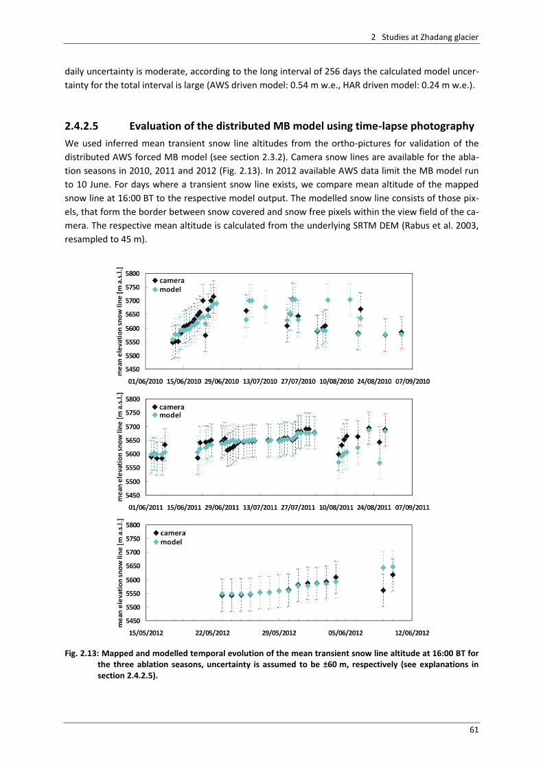
2 Studies at Zhadang glacier
61
daily uncertainty is moderate, according to the long interval of 256 days the calculated model uncer-
tainty for the total interval is large (AWS driven model: 0.54 m w.e., HAR driven model: 0.24 m w.e.).
2.4.2.5 Evaluation of the distributed MB model using time-lapse photography
We used inferred mean transient snow line altitudes from the ortho-pictures for validation of the
distributed AWS forced MB model (see section 2.3.2). Camera snow lines are available for the abla-
tion seasons in 2010, 2011 and 2012 (Fig. 2.13). In 2012 available AWS data limit the MB model run
to 10 June. For days where a transient snow line exists, we compare mean altitude of the mapped
snow line at 16:00 BT to the respective model output. The modelled snow line consists of those pix-
els, that form the border between snow covered and snow free pixels within the view field of the ca-
mera. The respective mean altitude is calculated from the underlying SRTM DEM (Rabus et al. 2003,
resampled to 45 m).
Fig. 2.13: Mapped and modelled temporal evolution of the mean transient snow line altitude at 16:00 BT for
the three ablation seasons, uncertainty is assumed to be ±60 m, respectively (see explanations in section 2.4.2.5).
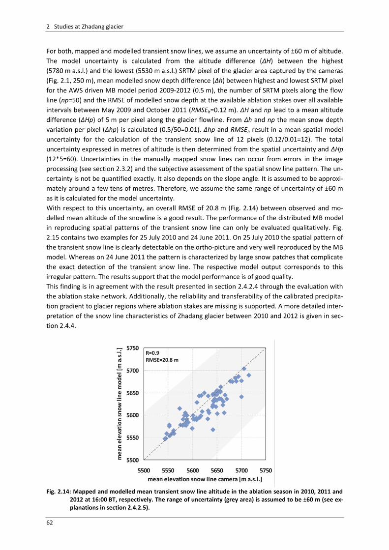
2 Studies at Zhadang glacier
62
For both, mapped and modelled transient snow lines, we assume an uncertainty of ±60 m of altitude.
The model uncertainty is calculated from the altitude difference (ΔH) between the highest
(5780 m a.s.l.) and the lowest (5530 m a.s.l.) SRTM pixel of the glacier area captured by the cameras
(Fig. 2.1, 250 m), mean modelled snow depth difference (Δh) between highest and lowest SRTM pixel
for the AWS driven MB model period 2009-2012 (0.5 m), the number of SRTM pixels along the flow
line (np=50) and the RMSE of modelled snow depth at the available ablation stakes over all available
intervals between May 2009 and October 2011 (RMSEh=0.12 m). ΔH and np lead to a mean altitude
difference (ΔHp) of 5 m per pixel along the glacier flowline. From Δh and np the mean snow depth
variation per pixel (Δhp) is calculated (0.5/50=0.01). Δhp and RMSEh result in a mean spatial model
uncertainty for the calculation of the transient snow line of 12 pixels (0.12/0.01=12). The total
uncertainty expressed in metres of altitude is then determined from the spatial uncertainty and ΔHp
(12*5=60). Uncertainties in the manually mapped snow lines can occur from errors in the image
processing (see section 2.3.2) and the subjective assessment of the spatial snow line pattern. The un-
certainty is not be quantified exactly. It also depends on the slope angle. It is assumed to be approxi-
mately around a few tens of metres. Therefore, we assume the same range of uncertainty of ±60 m
as it is calculated for the model uncertainty.
With respect to this uncertainty, an overall RMSE of 20.8 m (Fig. 2.14) between observed and mo-
delled mean altitude of the snowline is a good result. The performance of the distributed MB model
in reproducing spatial patterns of the transient snow line can only be evaluated qualitatively. Fig.
2.15 contains two examples for 25 July 2010 and 24 June 2011. On 25 July 2010 the spatial pattern of
the transient snow line is clearly detectable on the ortho-picture and very well reproduced by the MB
model. Whereas on 24 June 2011 the pattern is characterized by large snow patches that complicate
the exact detection of the transient snow line. The respective model output corresponds to this
irregular pattern. The results support that the model performance is of good quality.
This finding is in agreement with the result presented in section 2.4.2.4 through the evaluation with
the ablation stake network. Additionally, the reliability and transferability of the calibrated precipita-
tion gradient to glacier regions where ablation stakes are missing is supported. A more detailed inter-
pretation of the snow line characteristics of Zhadang glacier between 2010 and 2012 is given in sec-
tion 2.4.4.
Fig. 2.14: Mapped and modelled mean transient snow line altitude in the ablation season in 2010, 2011 and
2012 at 16:00 BT, respectively. The range of uncertainty (grey area) is assumed to be ±60 m (see ex-planations in section 2.4.2.5).
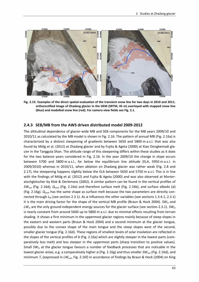
2 Studies at Zhadang glacier
63
Fig. 2.15: Examples of the direct spatial evaluation of the transient snow line for two days in 2010 and 2011; orthorectified image of Zhadang glacier in the DEM (SRTM, 45 m) overlayed with mapped snow line (blue) and modelled snow line (red). For camera view fields see Fig. 2.1.
2.4.3 SEB/MB from the AWS driven distributed model 2009-2012
The altitudinal dependence of glacier-wide MB and SEB components for the MB years 2009/10 and
2010/11 as calculated by the MB model is shown in Fig. 2.16. The pattern of annual MB (Fig. 2.16a) is
characterized by a distinct steepening of gradients between 5650 and 5800 m a.s.l. that was also
found by Mölg et al. (2012) at Zhadang glacier and by Fujita & Ageta (2000) at Xiao Dongkemadi gla-
cier in the Tanggula Shan. The altitude range of this steepening differs within these studies as it does
for the two balance years considered in Fig. 2.16. In the year 2009/10 the change in slope occurs
between 5700 and 5800 m a.s.l., far below the equilibrium line altitude (ELA, 5950 m a.s.l. in
2009/2010) whereas in 2010/11, when ablation on Zhadang glacier was rather weak (Fig. 2.8 and
2.17), the steepening happens slightly below the ELA between 5650 and 5750 m a.s.l. This is in line
with the findings of Mölg et al. (2012) and Fujita & Ageta (2000) and was also observed at Morter-
atschgletscher by Klok & Oerlemans (2002). A similar pattern can be found in the vertical profiles of
SWnet (Fig. 2.16d), Qmelt (Fig. 2.16e) and therefore surface melt (Fig. 2.16b), and surface albedo (α)
(Fig. 2.16g). Qmelt has the same shape as surface melt because the two parameters are directly con-
nected through LM (see section 2.3.1). As α influences the other variables (see sections 1.3.4.1, 2.3.1)
it is the main driving factor for the shape of the vertical MB profile (Braun & Hock 2004). SWin and
LWin are the only ground-independent energy sources for the glacier surface (see section 2.3.1). SWin
is nearly constant from around 5600 up to 5800 m a.s.l. due to minimal effects resulting from terrain
shading. It shows a first minimum in the uppermost glacier regions mainly because of steep slopes in
the eastern and western parts (Braun & Hock 2004) and a second minimum at the glacier tongue,
possibly due to the convex shape of the main tongue and the steep slopes west of the second,
smaller glacier tongue (Fig. 2.16d). These regions of smallest levels of solar insolation are reflected in
the slopes of the vertical profiles of b (Fig. 2.16a) which are slightly steeper in the lowest parts (com-
paratively less melt) and less steeper in the uppermost parts (sharp transition to positive values).
Small SWin at the glacier tongue favours a number of feedback processes that are noticable in the
lowest glacier areas, e.g. a comparatively higher α (Fig. 2.16g) and thus smaller SWnet (Fig. 2.16d), and
minimum Ts (expressed in LWout, Fig. 2.16f) in accordance of findings by Braun & Hock (2004) on King
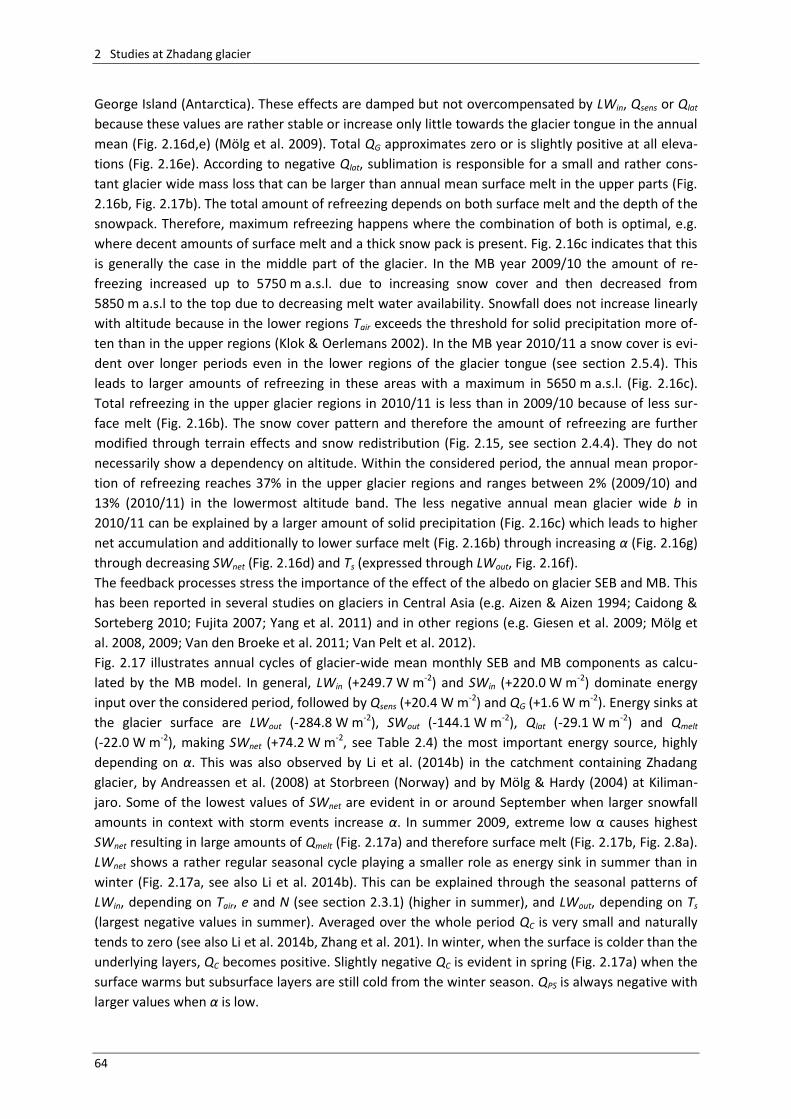
2 Studies at Zhadang glacier
64
George Island (Antarctica). These effects are damped but not overcompensated by LWin, Qsens or Qlat
because these values are rather stable or increase only little towards the glacier tongue in the annual
mean (Fig. 2.16d,e) (Mölg et al. 2009). Total QG approximates zero or is slightly positive at all eleva-
tions (Fig. 2.16e). According to negative Qlat, sublimation is responsible for a small and rather cons-
tant glacier wide mass loss that can be larger than annual mean surface melt in the upper parts (Fig.
2.16b, Fig. 2.17b). The total amount of refreezing depends on both surface melt and the depth of the
snowpack. Therefore, maximum refreezing happens where the combination of both is optimal, e.g.
where decent amounts of surface melt and a thick snow pack is present. Fig. 2.16c indicates that this
is generally the case in the middle part of the glacier. In the MB year 2009/10 the amount of re-
freezing increased up to 5750 m a.s.l. due to increasing snow cover and then decreased from
5850 m a.s.l to the top due to decreasing melt water availability. Snowfall does not increase linearly
with altitude because in the lower regions Tair exceeds the threshold for solid precipitation more of-
ten than in the upper regions (Klok & Oerlemans 2002). In the MB year 2010/11 a snow cover is evi-
dent over longer periods even in the lower regions of the glacier tongue (see section 2.5.4). This
leads to larger amounts of refreezing in these areas with a maximum in 5650 m a.s.l. (Fig. 2.16c).
Total refreezing in the upper glacier regions in 2010/11 is less than in 2009/10 because of less sur-
face melt (Fig. 2.16b). The snow cover pattern and therefore the amount of refreezing are further
modified through terrain effects and snow redistribution (Fig. 2.15, see section 2.4.4). They do not
necessarily show a dependency on altitude. Within the considered period, the annual mean propor-
tion of refreezing reaches 37% in the upper glacier regions and ranges between 2% (2009/10) and
13% (2010/11) in the lowermost altitude band. The less negative annual mean glacier wide b in
2010/11 can be explained by a larger amount of solid precipitation (Fig. 2.16c) which leads to higher
net accumulation and additionally to lower surface melt (Fig. 2.16b) through increasing α (Fig. 2.16g)
through decreasing SWnet (Fig. 2.16d) and Ts (expressed through LWout, Fig. 2.16f).
The feedback processes stress the importance of the effect of the albedo on glacier SEB and MB. This
has been reported in several studies on glaciers in Central Asia (e.g. Aizen & Aizen 1994; Caidong &
Sorteberg 2010; Fujita 2007; Yang et al. 2011) and in other regions (e.g. Giesen et al. 2009; Mölg et
al. 2008, 2009; Van den Broeke et al. 2011; Van Pelt et al. 2012).
Fig. 2.17 illustrates annual cycles of glacier-wide mean monthly SEB and MB components as calcu-
lated by the MB model. In general, LWin (+249.7 W m-2) and SWin (+220.0 W m-2) dominate energy
input over the considered period, followed by Qsens (+20.4 W m-2) and QG (+1.6 W m-2). Energy sinks at
the glacier surface are LWout (-284.8 W m-2), SWout (-144.1 W m-2), Qlat (-29.1 W m-2) and Qmelt
(-22.0 W m-2), making SWnet (+74.2 W m-2, see Table 2.4) the most important energy source, highly
depending on α. This was also observed by Li et al. (2014b) in the catchment containing Zhadang
glacier, by Andreassen et al. (2008) at Storbreen (Norway) and by Mölg & Hardy (2004) at Kiliman-
jaro. Some of the lowest values of SWnet are evident in or around September when larger snowfall
amounts in context with storm events increase α. In summer 2009, extreme low α causes highest
SWnet resulting in large amounts of Qmelt (Fig. 2.17a) and therefore surface melt (Fig. 2.17b, Fig. 2.8a).
LWnet shows a rather regular seasonal cycle playing a smaller role as energy sink in summer than in
winter (Fig. 2.17a, see also Li et al. 2014b). This can be explained through the seasonal patterns of
LWin, depending on Tair, e and N (see section 2.3.1) (higher in summer), and LWout, depending on Ts
(largest negative values in summer). Averaged over the whole period QC is very small and naturally
tends to zero (see also Li et al. 2014b, Zhang et al. 201). In winter, when the surface is colder than the
underlying layers, QC becomes positive. Slightly negative QC is evident in spring (Fig. 2.17a) when the
surface warms but subsurface layers are still cold from the winter season. QPS is always negative with
larger values when α is low.
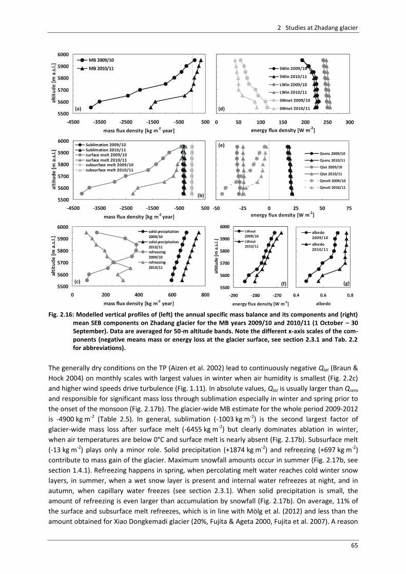
2 Studies at Zhadang glacier
65
Fig. 2.16: Modelled vertical profiles of (left) the annual specific mass balance and its components and (right)
mean SEB components on Zhadang glacier for the MB years 2009/10 and 2010/11 (1 October – 30 September). Data are averaged for 50-m altitude bands. Note the different x-axis scales of the com-ponents (negative means mass or energy loss at the glacier surface, see section 2.3.1 and Tab. 2.2 for abbreviations).
The generally dry conditions on the TP (Aizen et al. 2002) lead to continuously negative Qlat (Braun &
Hock 2004) on monthly scales with largest values in winter when air humidity is smallest (Fig. 2.2c)
and higher wind speeds drive turbulence (Fig. 1.11). In absolute values, Qlat is usually larger than Qsens
and responsible for significant mass loss through sublimation especially in winter and spring prior to
the onset of the monsoon (Fig. 2.17b). The glacier-wide MB estimate for the whole period 2009-2012
is -4900 kg m-2 (Table 2.5). In general, sublimation (-1003 kg m-2) is the second largest factor of
glacier-wide mass loss after surface melt (-6455 kg m-2) but clearly dominates ablation in winter,
when air temperatures are below 0°C and surface melt is nearly absent (Fig. 2.17b). Subsurface melt
(-13 kg m-2) plays only a minor role. Solid precipitation (+1874 kg m-2) and refreezing (+697 kg m-2)
contribute to mass gain of the glacier. Maximum snowfall amounts occur in summer (Fig. 2.17b, see
section 1.4.1). Refreezing happens in spring, when percolating melt water reaches cold winter snow
layers, in summer, when a wet snow layer is present and internal water refreezes at night, and in
autumn, when capillary water freezes (see section 2.3.1). When solid precipitation is small, the
amount of refreezing is even larger than accumulation by snowfall (Fig. 2.17b). On average, 11% of
the surface and subsurface melt refreezes, which is in line with Mölg et al. (2012) and less than the
amount obtained for Xiao Dongkemadi glacier (20%, Fujita & Ageta 2000, Fujita et al. 2007). A reason
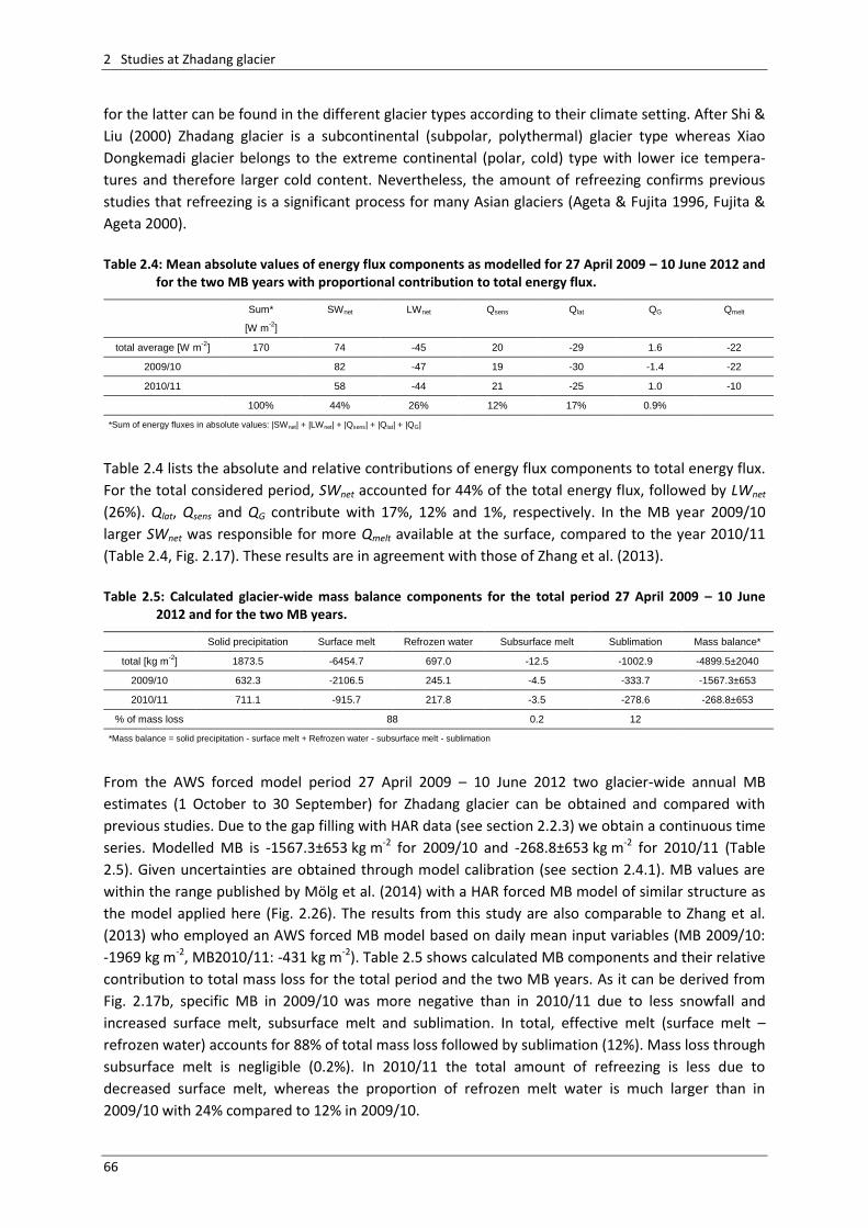
2 Studies at Zhadang glacier
66
for the latter can be found in the different glacier types according to their climate setting. After Shi &
Liu (2000) Zhadang glacier is a subcontinental (subpolar, polythermal) glacier type whereas Xiao
Dongkemadi glacier belongs to the extreme continental (polar, cold) type with lower ice tempera-
tures and therefore larger cold content. Nevertheless, the amount of refreezing confirms previous
studies that refreezing is a significant process for many Asian glaciers (Ageta & Fujita 1996, Fujita &
Ageta 2000).
Table 2.4: Mean absolute values of energy flux components as modelled for 27 April 2009 – 10 June 2012 and
for the two MB years with proportional contribution to total energy flux.
Sum* SWnet LWnet Qsens Qlat QG Qmelt
[W m-2
]
total average [W m-2
] 170 74 -45 20 -29 1.6 -22
2009/10 82 -47 19 -30 -1.4 -22
2010/11 58 -44 21 -25 1.0 -10
100% 44% 26% 12% 17% 0.9%
*Sum of energy fluxes in absolute values: |SWnet| + |LWnet| + |Qsens| + |Qlat| + |QG|
Table 2.4 lists the absolute and relative contributions of energy flux components to total energy flux.
For the total considered period, SWnet accounted for 44% of the total energy flux, followed by LWnet
(26%). Qlat, Qsens and QG contribute with 17%, 12% and 1%, respectively. In the MB year 2009/10
larger SWnet was responsible for more Qmelt available at the surface, compared to the year 2010/11
(Table 2.4, Fig. 2.17). These results are in agreement with those of Zhang et al. (2013).
Table 2.5: Calculated glacier-wide mass balance components for the total period 27 April 2009 – 10 June
2012 and for the two MB years.
Solid precipitation Surface melt Refrozen water Subsurface melt Sublimation Mass balance*
total [kg m-2
] 1873.5 -6454.7 697.0 -12.5 -1002.9 -4899.5±2040
2009/10 632.3 -2106.5 245.1 -4.5 -333.7 -1567.3±653
2010/11 711.1 -915.7 217.8 -3.5 -278.6 -268.8±653
% of mass loss 88 0.2 12
*Mass balance = solid precipitation - surface melt + Refrozen water - subsurface melt - sublimation
From the AWS forced model period 27 April 2009 – 10 June 2012 two glacier-wide annual MB
estimates (1 October to 30 September) for Zhadang glacier can be obtained and compared with
previous studies. Due to the gap filling with HAR data (see section 2.2.3) we obtain a continuous time
series. Modelled MB is -1567.3±653 kg m-2 for 2009/10 and -268.8±653 kg m-2 for 2010/11 (Table
2.5). Given uncertainties are obtained through model calibration (see section 2.4.1). MB values are
within the range published by Mölg et al. (2014) with a HAR forced MB model of similar structure as
the model applied here (Fig. 2.26). The results from this study are also comparable to Zhang et al.
(2013) who employed an AWS forced MB model based on daily mean input variables (MB 2009/10:
-1969 kg m-2, MB2010/11: -431 kg m-2). Table 2.5 shows calculated MB components and their relative
contribution to total mass loss for the total period and the two MB years. As it can be derived from
Fig. 2.17b, specific MB in 2009/10 was more negative than in 2010/11 due to less snowfall and
increased surface melt, subsurface melt and sublimation. In total, effective melt (surface melt –
refrozen water) accounts for 88% of total mass loss followed by sublimation (12%). Mass loss through
subsurface melt is negligible (0.2%). In 2010/11 the total amount of refreezing is less due to
decreased surface melt, whereas the proportion of refrozen melt water is much larger than in
2009/10 with 24% compared to 12% in 2009/10.
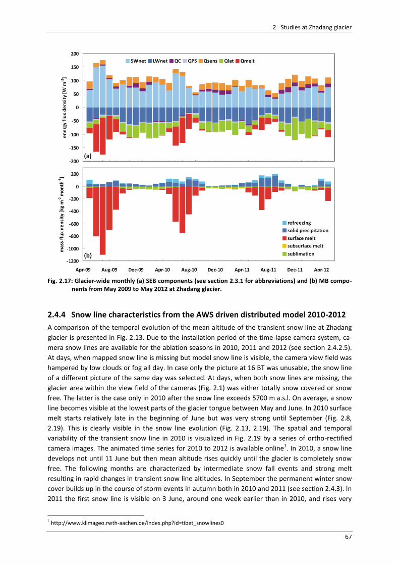
2 Studies at Zhadang glacier
67
Fig. 2.17: Glacier-wide monthly (a) SEB components (see section 2.3.1 for abbreviations) and (b) MB compo-
nents from May 2009 to May 2012 at Zhadang glacier.
2.4.4 Snow line characteristics from the AWS driven distributed model 2010-2012
A comparison of the temporal evolution of the mean altitude of the transient snow line at Zhadang
glacier is presented in Fig. 2.13. Due to the installation period of the time-lapse camera system, ca-
mera snow lines are available for the ablation seasons in 2010, 2011 and 2012 (see section 2.4.2.5).
At days, when mapped snow line is missing but model snow line is visible, the camera view field was
hampered by low clouds or fog all day. In case only the picture at 16 BT was unusable, the snow line
of a different picture of the same day was selected. At days, when both snow lines are missing, the
glacier area within the view field of the cameras (Fig. 2.1) was either totally snow covered or snow
free. The latter is the case only in 2010 after the snow line exceeds 5700 m a.s.l. On average, a snow
line becomes visible at the lowest parts of the glacier tongue between May and June. In 2010 surface
melt starts relatively late in the beginning of June but was very strong until September (Fig. 2.8,
2.19). This is clearly visible in the snow line evolution (Fig. 2.13, 2.19). The spatial and temporal
variability of the transient snow line in 2010 is visualized in Fig. 2.19 by a series of ortho-rectified
camera images. The animated time series for 2010 to 2012 is available online1. In 2010, a snow line
develops not until 11 June but then mean altitude rises quickly until the glacier is completely snow
free. The following months are characterized by intermediate snow fall events and strong melt
resulting in rapid changes in transient snow line altitudes. In September the permanent winter snow
cover builds up in the course of storm events in autumn both in 2010 and 2011 (see section 2.4.3). In
2011 the first snow line is visible on 3 June, around one week earlier than in 2010, and rises very
1 http://www.klimageo.rwth-aachen.de/index.php?id=tibet_snowlines0
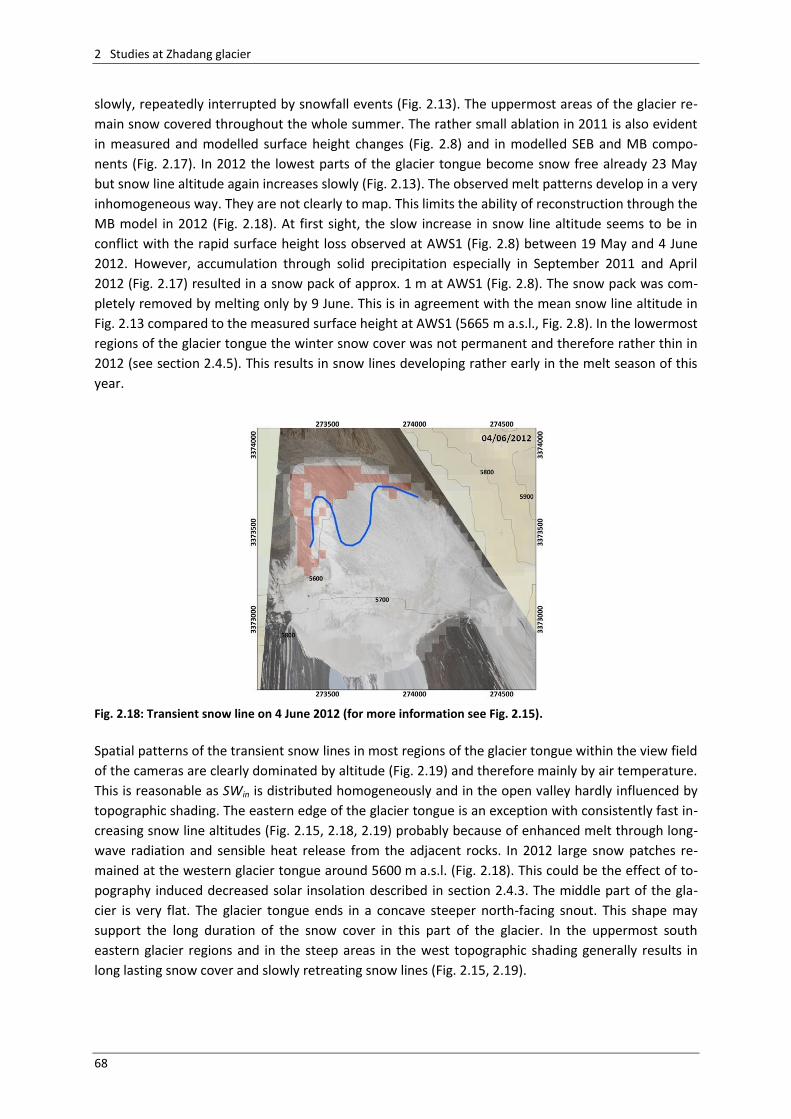
2 Studies at Zhadang glacier
68
slowly, repeatedly interrupted by snowfall events (Fig. 2.13). The uppermost areas of the glacier re-
main snow covered throughout the whole summer. The rather small ablation in 2011 is also evident
in measured and modelled surface height changes (Fig. 2.8) and in modelled SEB and MB compo-
nents (Fig. 2.17). In 2012 the lowest parts of the glacier tongue become snow free already 23 May
but snow line altitude again increases slowly (Fig. 2.13). The observed melt patterns develop in a very
inhomogeneous way. They are not clearly to map. This limits the ability of reconstruction through the
MB model in 2012 (Fig. 2.18). At first sight, the slow increase in snow line altitude seems to be in
conflict with the rapid surface height loss observed at AWS1 (Fig. 2.8) between 19 May and 4 June
2012. However, accumulation through solid precipitation especially in September 2011 and April
2012 (Fig. 2.17) resulted in a snow pack of approx. 1 m at AWS1 (Fig. 2.8). The snow pack was com-
pletely removed by melting only by 9 June. This is in agreement with the mean snow line altitude in
Fig. 2.13 compared to the measured surface height at AWS1 (5665 m a.s.l., Fig. 2.8). In the lowermost
regions of the glacier tongue the winter snow cover was not permanent and therefore rather thin in
2012 (see section 2.4.5). This results in snow lines developing rather early in the melt season of this
year.
Fig. 2.18: Transient snow line on 4 June 2012 (for more information see Fig. 2.15).
Spatial patterns of the transient snow lines in most regions of the glacier tongue within the view field
of the cameras are clearly dominated by altitude (Fig. 2.19) and therefore mainly by air temperature.
This is reasonable as SWin is distributed homogeneously and in the open valley hardly influenced by
topographic shading. The eastern edge of the glacier tongue is an exception with consistently fast in-
creasing snow line altitudes (Fig. 2.15, 2.18, 2.19) probably because of enhanced melt through long-
wave radiation and sensible heat release from the adjacent rocks. In 2012 large snow patches re-
mained at the western glacier tongue around 5600 m a.s.l. (Fig. 2.18). This could be the effect of to-
pography induced decreased solar insolation described in section 2.4.3. The middle part of the gla-
cier is very flat. The glacier tongue ends in a concave steeper north-facing snout. This shape may
support the long duration of the snow cover in this part of the glacier. In the uppermost south
eastern glacier regions and in the steep areas in the west topographic shading generally results in
long lasting snow cover and slowly retreating snow lines (Fig. 2.15, 2.19).
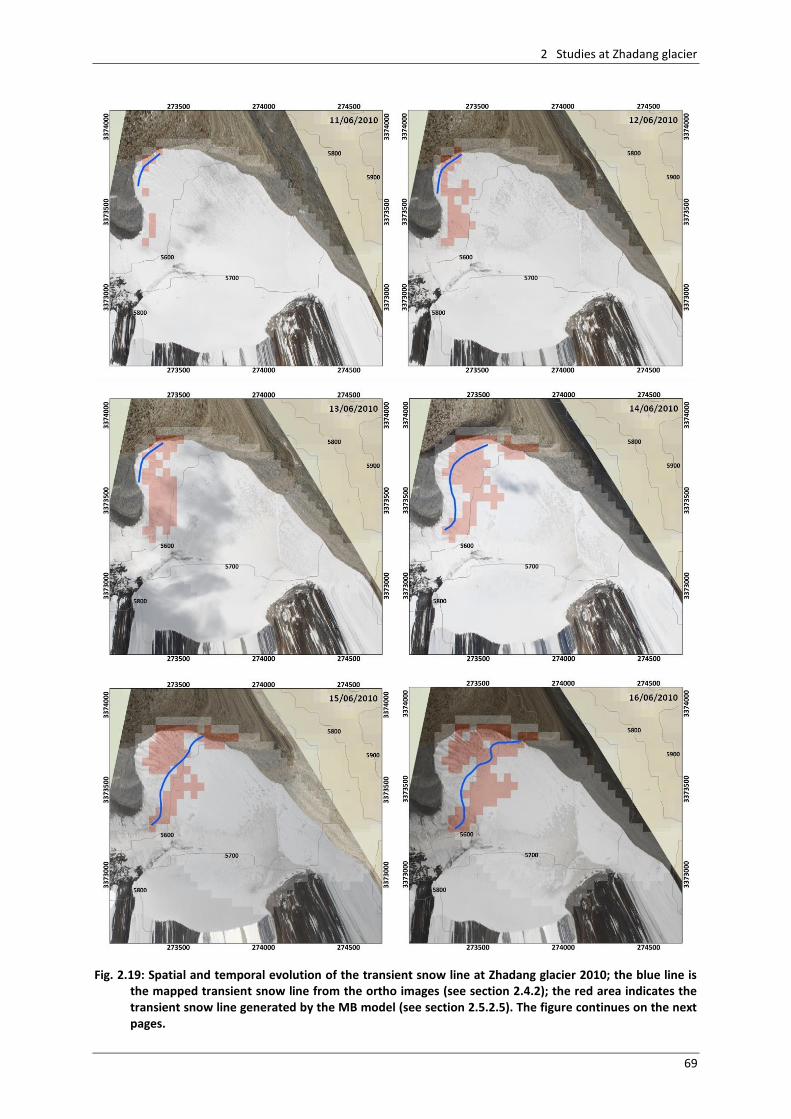
2 Studies at Zhadang glacier
69
Fig. 2.19: Spatial and temporal evolution of the transient snow line at Zhadang glacier 2010; the blue line is the mapped transient snow line from the ortho images (see section 2.4.2); the red area indicates the transient snow line generated by the MB model (see section 2.5.2.5). The figure continues on the next pages.
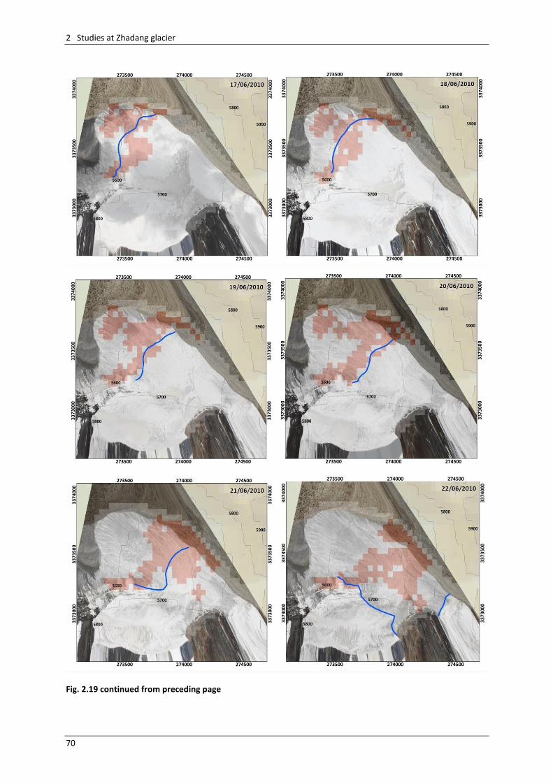
2 Studies at Zhadang glacier
70
Fig. 2.19 continued from preceding page
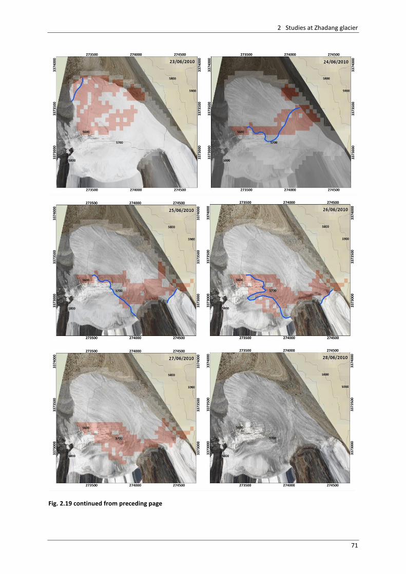
2 Studies at Zhadang glacier
71
Fig. 2.19 continued from preceding page
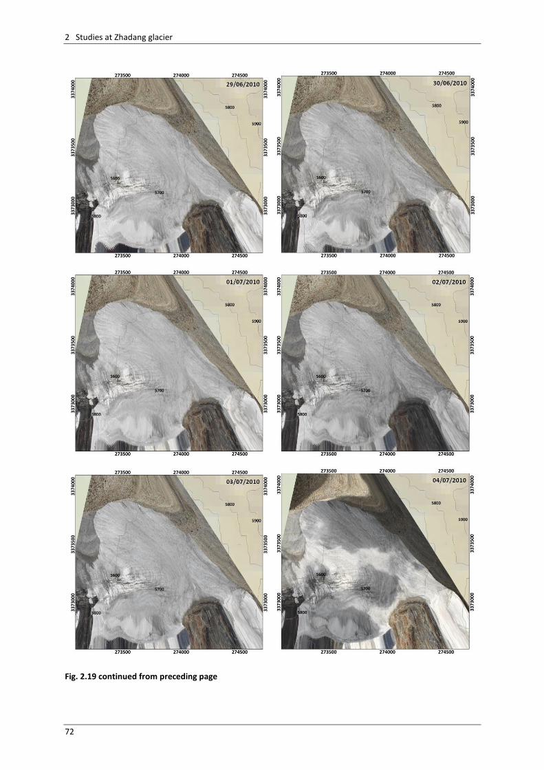
2 Studies at Zhadang glacier
72
Fig. 2.19 continued from preceding page
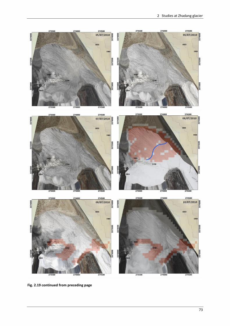
2 Studies at Zhadang glacier
73
Fig. 2.19 continued from preceding page
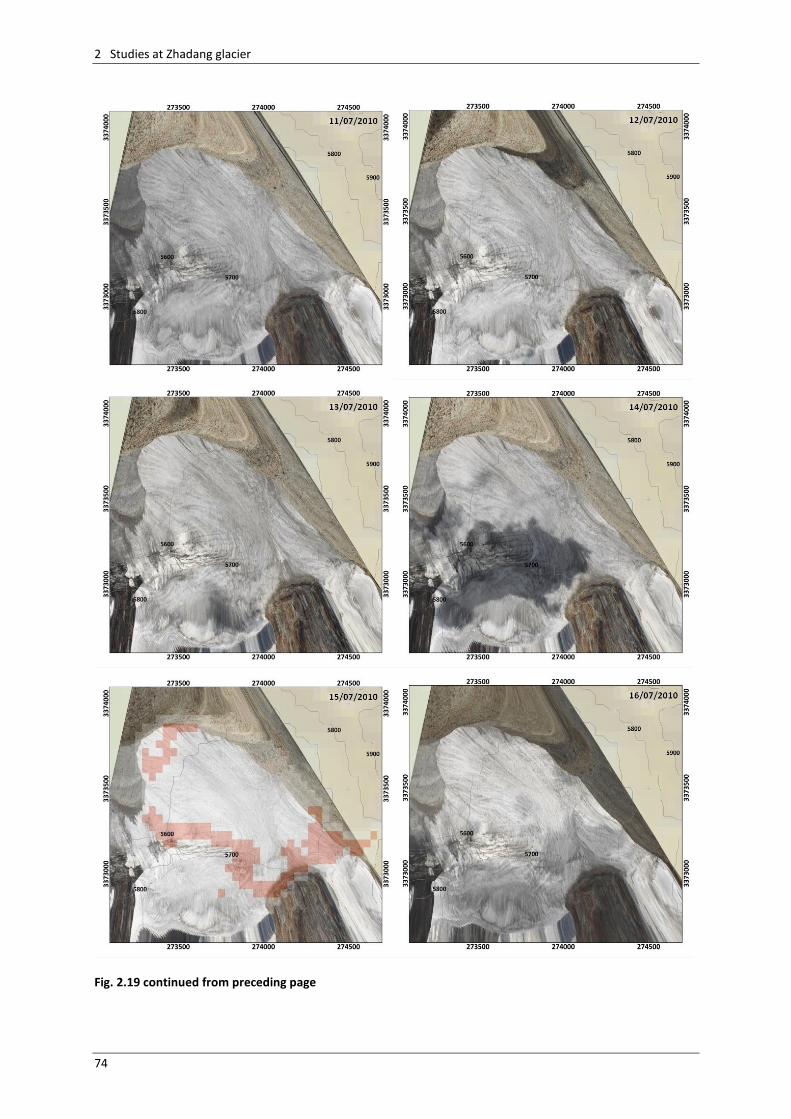
2 Studies at Zhadang glacier
74
Fig. 2.19 continued from preceding page
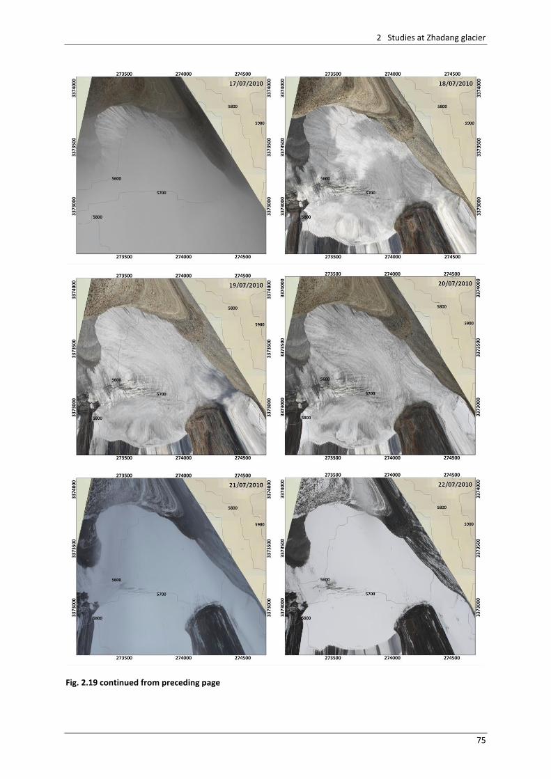
2 Studies at Zhadang glacier
75
Fig. 2.19 continued from preceding page
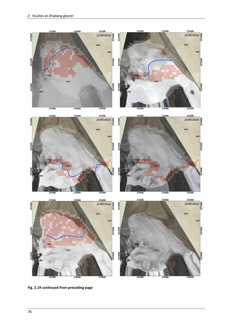
2 Studies at Zhadang glacier
76
Fig. 2.19 continued from preceding page
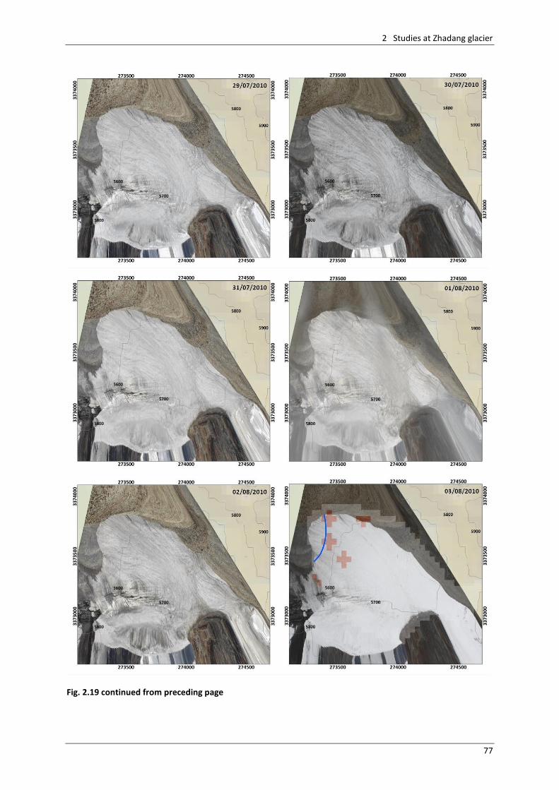
2 Studies at Zhadang glacier
77
Fig. 2.19 continued from preceding page
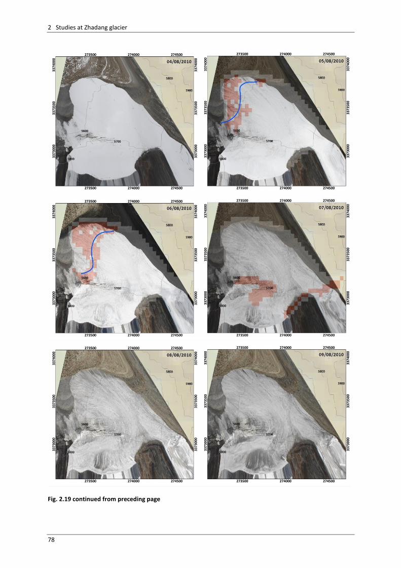
2 Studies at Zhadang glacier
78
Fig. 2.19 continued from preceding page
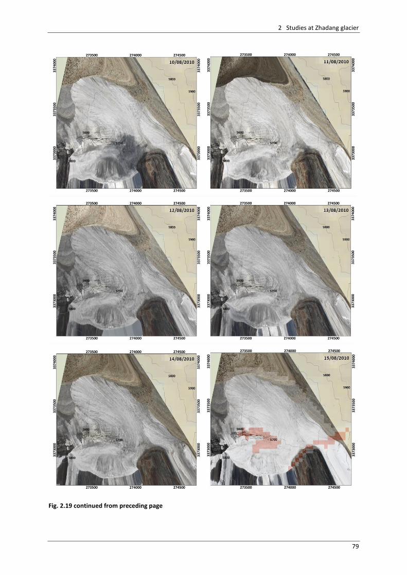
2 Studies at Zhadang glacier
79
Fig. 2.19 continued from preceding page
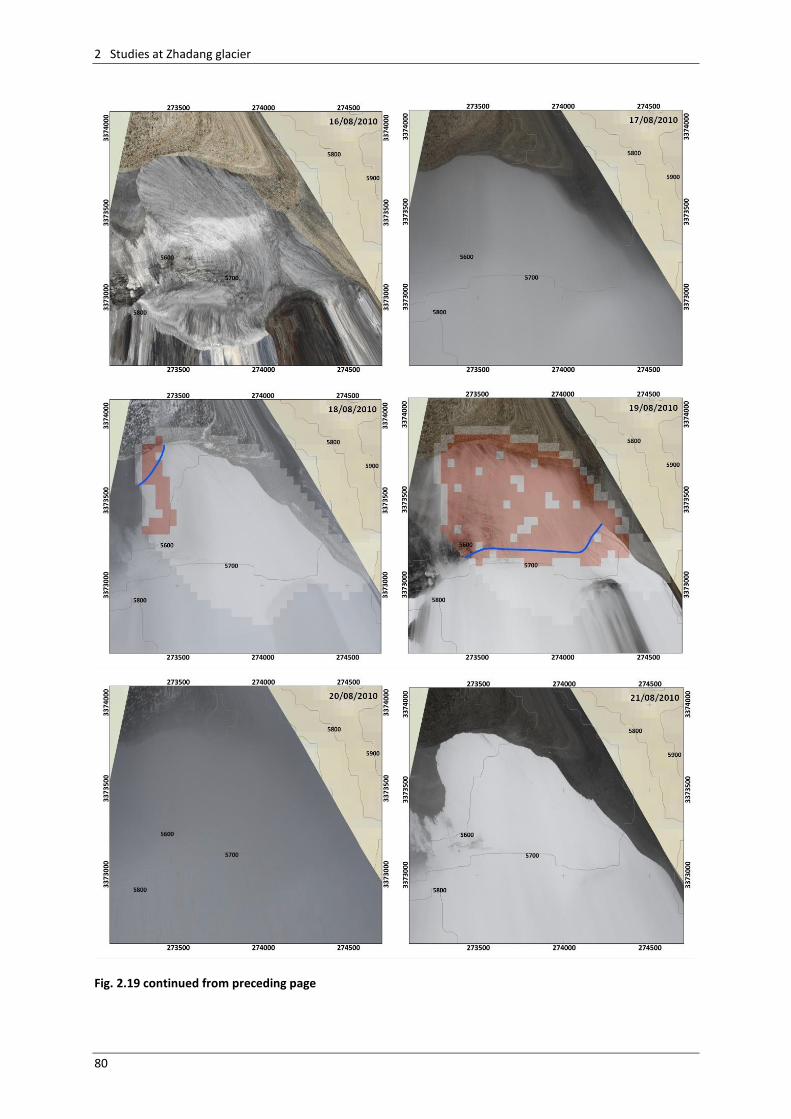
2 Studies at Zhadang glacier
80
Fig. 2.19 continued from preceding page
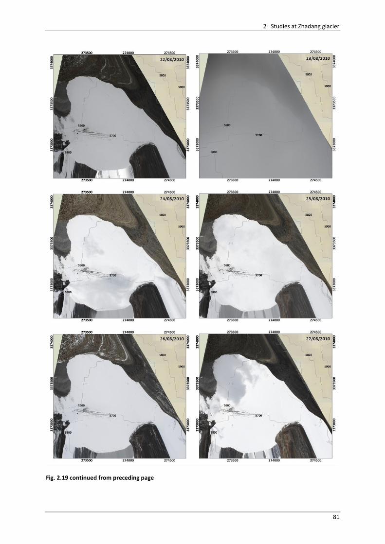
2 Studies at Zhadang glacier
81
Fig. 2.19 continued from preceding page
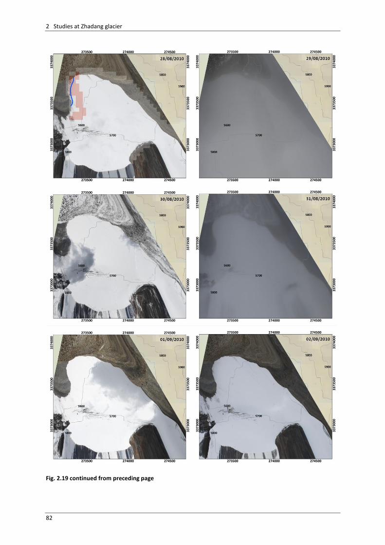
2 Studies at Zhadang glacier
82
Fig. 2.19 continued from preceding page
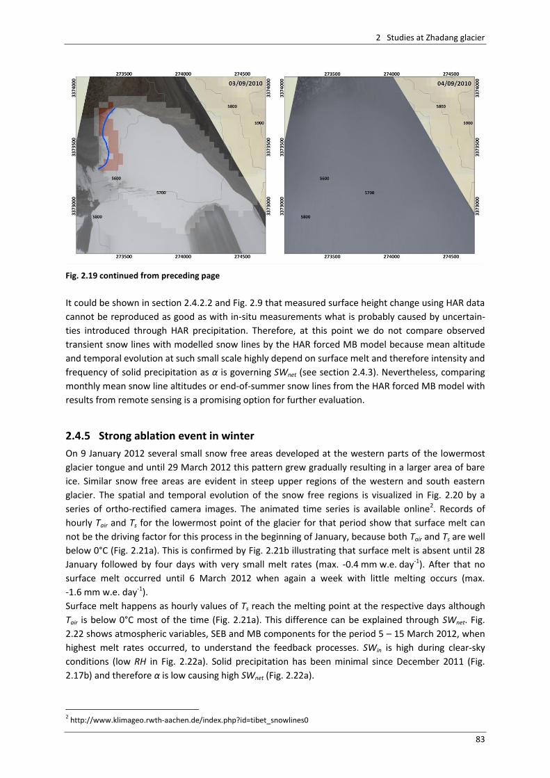
2 Studies at Zhadang glacier
83
Fig. 2.19 continued from preceding page
It could be shown in section 2.4.2.2 and Fig. 2.9 that measured surface height change using HAR data
cannot be reproduced as good as with in-situ measurements what is probably caused by uncertain-
ties introduced through HAR precipitation. Therefore, at this point we do not compare observed
transient snow lines with modelled snow lines by the HAR forced MB model because mean altitude
and temporal evolution at such small scale highly depend on surface melt and therefore intensity and
frequency of solid precipitation as α is governing SWnet (see section 2.4.3). Nevertheless, comparing
monthly mean snow line altitudes or end-of-summer snow lines from the HAR forced MB model with
results from remote sensing is a promising option for further evaluation.
2.4.5 Strong ablation event in winter
On 9 January 2012 several small snow free areas developed at the western parts of the lowermost
glacier tongue and until 29 March 2012 this pattern grew gradually resulting in a larger area of bare
ice. Similar snow free areas are evident in steep upper regions of the western and south eastern
glacier. The spatial and temporal evolution of the snow free regions is visualized in Fig. 2.20 by a
series of ortho-rectified camera images. The animated time series is available online2. Records of
hourly Tair and Ts for the lowermost point of the glacier for that period show that surface melt can
not be the driving factor for this process in the beginning of January, because both Tair and Ts are well
below 0°C (Fig. 2.21a). This is confirmed by Fig. 2.21b illustrating that surface melt is absent until 28
January followed by four days with very small melt rates (max. -0.4 mm w.e. day-1). After that no
surface melt occurred until 6 March 2012 when again a week with little melting occurs (max.
-1.6 mm w.e. day-1).
Surface melt happens as hourly values of Ts reach the melting point at the respective days although
Tair is below 0°C most of the time (Fig. 2.21a). This difference can be explained through SWnet. Fig.
2.22 shows atmospheric variables, SEB and MB components for the period 5 – 15 March 2012, when
highest melt rates occurred, to understand the feedback processes. SWin is high during clear-sky
conditions (low RH in Fig. 2.22a). Solid precipitation has been minimal since December 2011 (Fig.
2.17b) and therefore α is low causing high SWnet (Fig. 2.22a).
2 http://www.klimageo.rwth-aachen.de/index.php?id=tibet_snowlines0
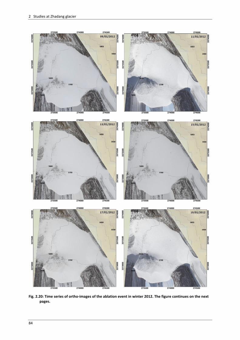
2 Studies at Zhadang glacier
84
Fig. 2.20: Time series of ortho-images of the ablation event in winter 2012. The figure continues on the next pages.
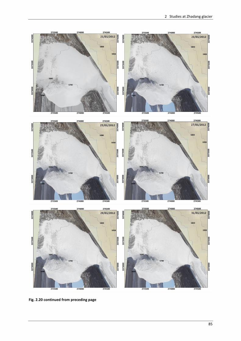
2 Studies at Zhadang glacier
85
Fig. 2.20 continued from preceding page
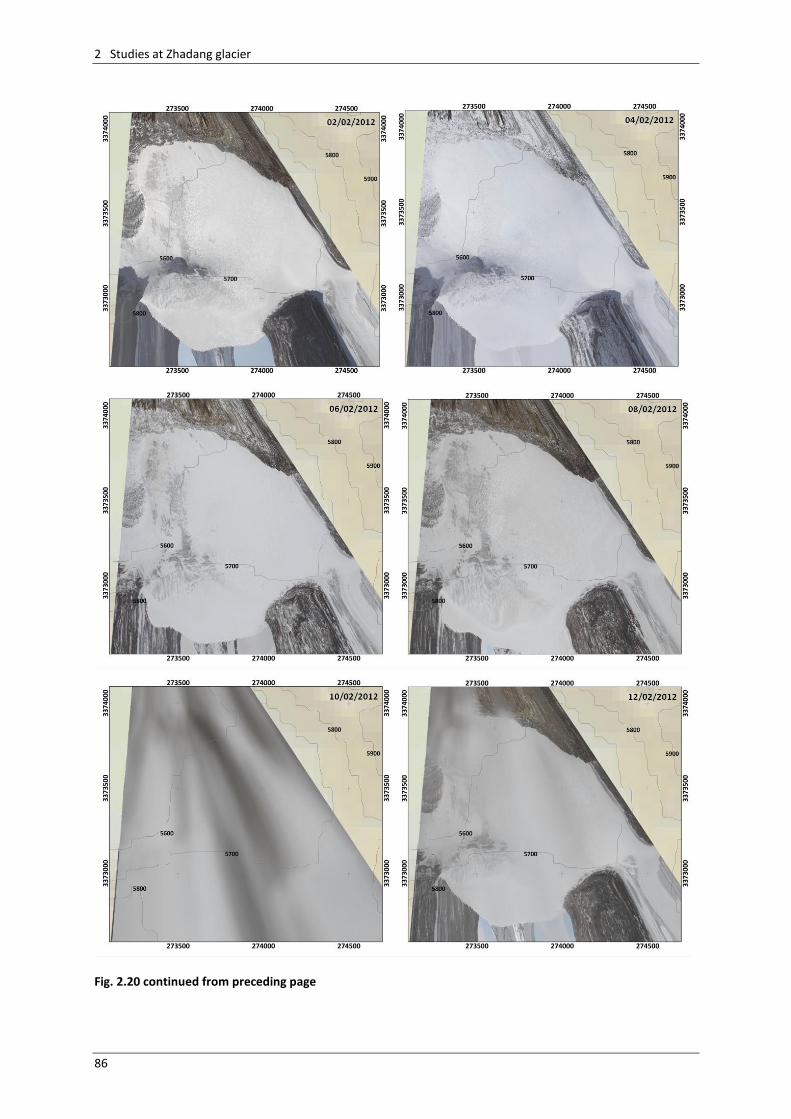
2 Studies at Zhadang glacier
86
Fig. 2.20 continued from preceding page
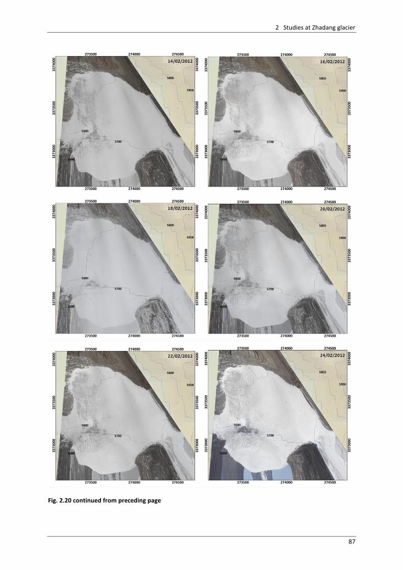
2 Studies at Zhadang glacier
87
Fig. 2.20 continued from preceding page
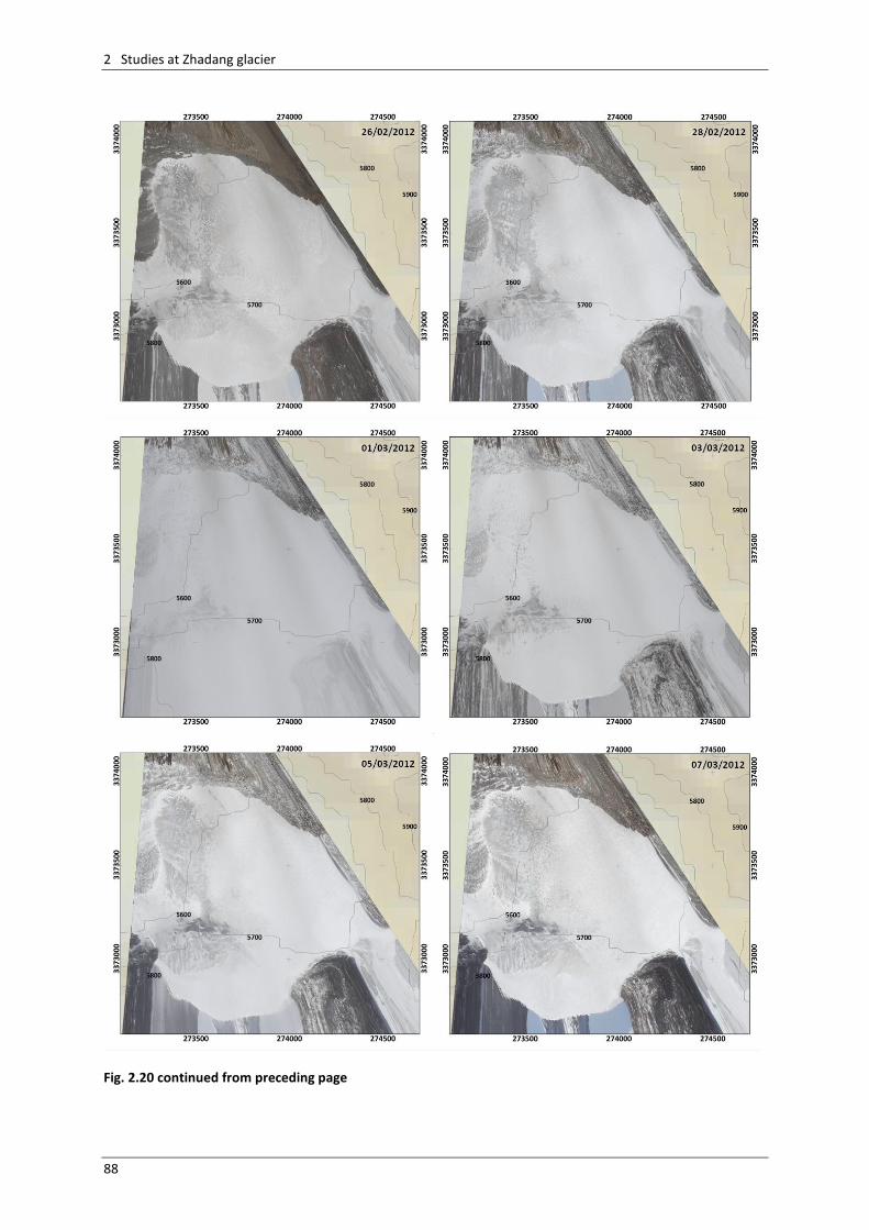
2 Studies at Zhadang glacier
88
Fig. 2.20 continued from preceding page
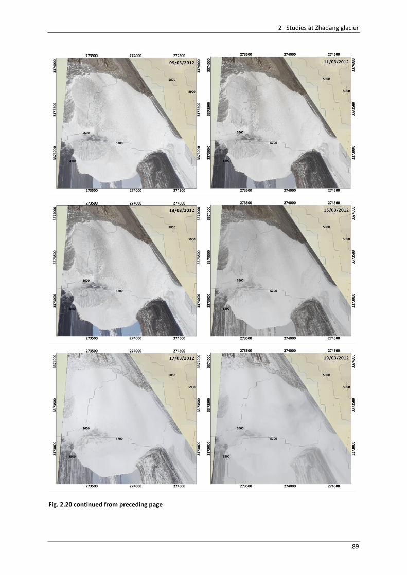
2 Studies at Zhadang glacier
89
Fig. 2.20 continued from preceding page
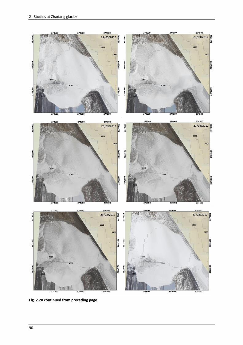
2 Studies at Zhadang glacier
90
Fig. 2.20 continued from preceding page
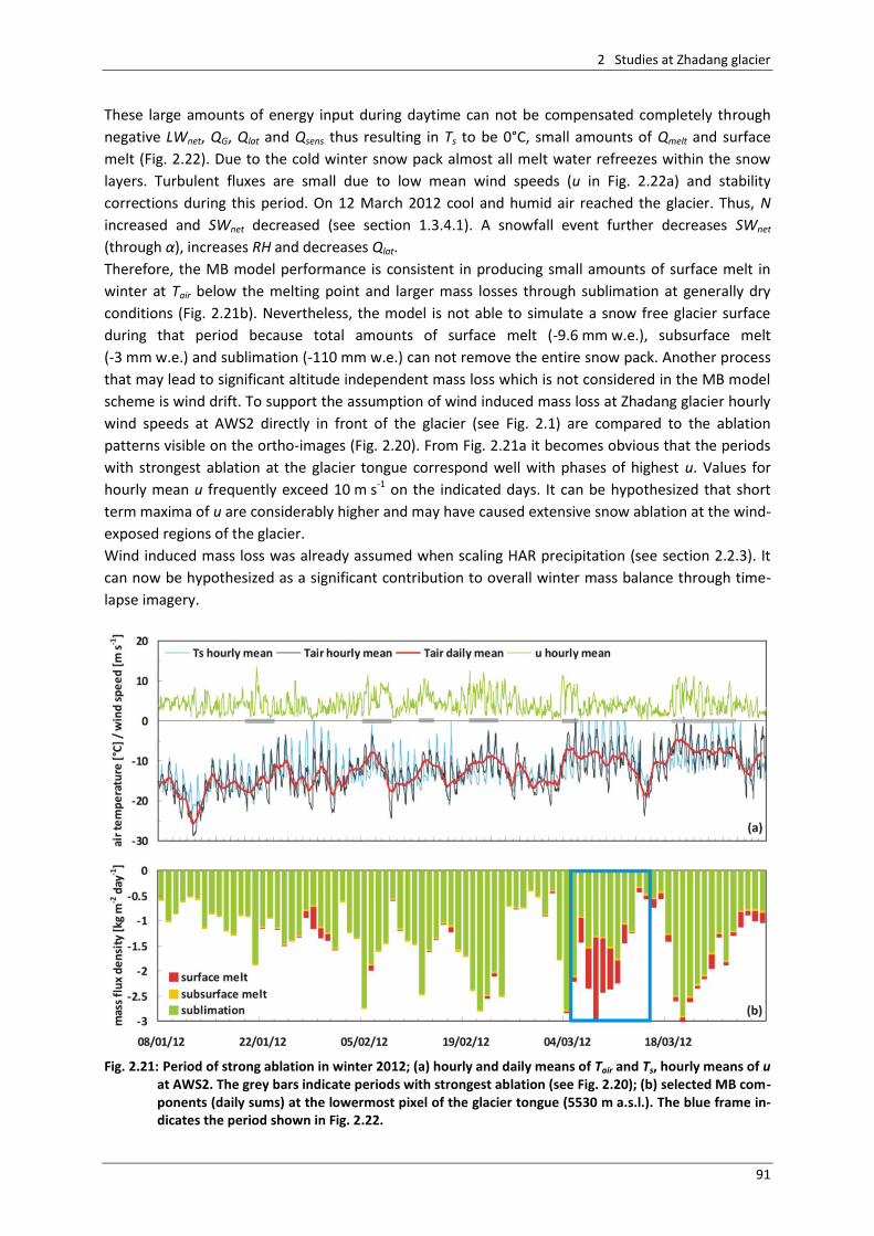
2 Studies at Zhadang glacier
91
These large amounts of energy input during daytime can not be compensated completely through
negative LWnet, QG, Qlat and Qsens thus resulting in Ts to be 0°C, small amounts of Qmelt and surface
melt (Fig. 2.22). Due to the cold winter snow pack almost all melt water refreezes within the snow
layers. Turbulent fluxes are small due to low mean wind speeds (u in Fig. 2.22a) and stability
corrections during this period. On 12 March 2012 cool and humid air reached the glacier. Thus, N
increased and SWnet decreased (see section 1.3.4.1). A snowfall event further decreases SWnet
(through α), increases RH and decreases Qlat.
Therefore, the MB model performance is consistent in producing small amounts of surface melt in
winter at Tair below the melting point and larger mass losses through sublimation at generally dry
conditions (Fig. 2.21b). Nevertheless, the model is not able to simulate a snow free glacier surface
during that period because total amounts of surface melt (-9.6 mm w.e.), subsurface melt
(-3 mm w.e.) and sublimation (-110 mm w.e.) can not remove the entire snow pack. Another process
that may lead to significant altitude independent mass loss which is not considered in the MB model
scheme is wind drift. To support the assumption of wind induced mass loss at Zhadang glacier hourly
wind speeds at AWS2 directly in front of the glacier (see Fig. 2.1) are compared to the ablation
patterns visible on the ortho-images (Fig. 2.20). From Fig. 2.21a it becomes obvious that the periods
with strongest ablation at the glacier tongue correspond well with phases of highest u. Values for
hourly mean u frequently exceed 10 m s-1 on the indicated days. It can be hypothesized that short
term maxima of u are considerably higher and may have caused extensive snow ablation at the wind-
exposed regions of the glacier.
Wind induced mass loss was already assumed when scaling HAR precipitation (see section 2.2.3). It
can now be hypothesized as a significant contribution to overall winter mass balance through time-
lapse imagery.
Fig. 2.21: Period of strong ablation in winter 2012; (a) hourly and daily means of Tair and Ts, hourly means of u
at AWS2. The grey bars indicate periods with strongest ablation (see Fig. 2.20); (b) selected MB com-ponents (daily sums) at the lowermost pixel of the glacier tongue (5530 m a.s.l.). The blue frame in-dicates the period shown in Fig. 2.22.
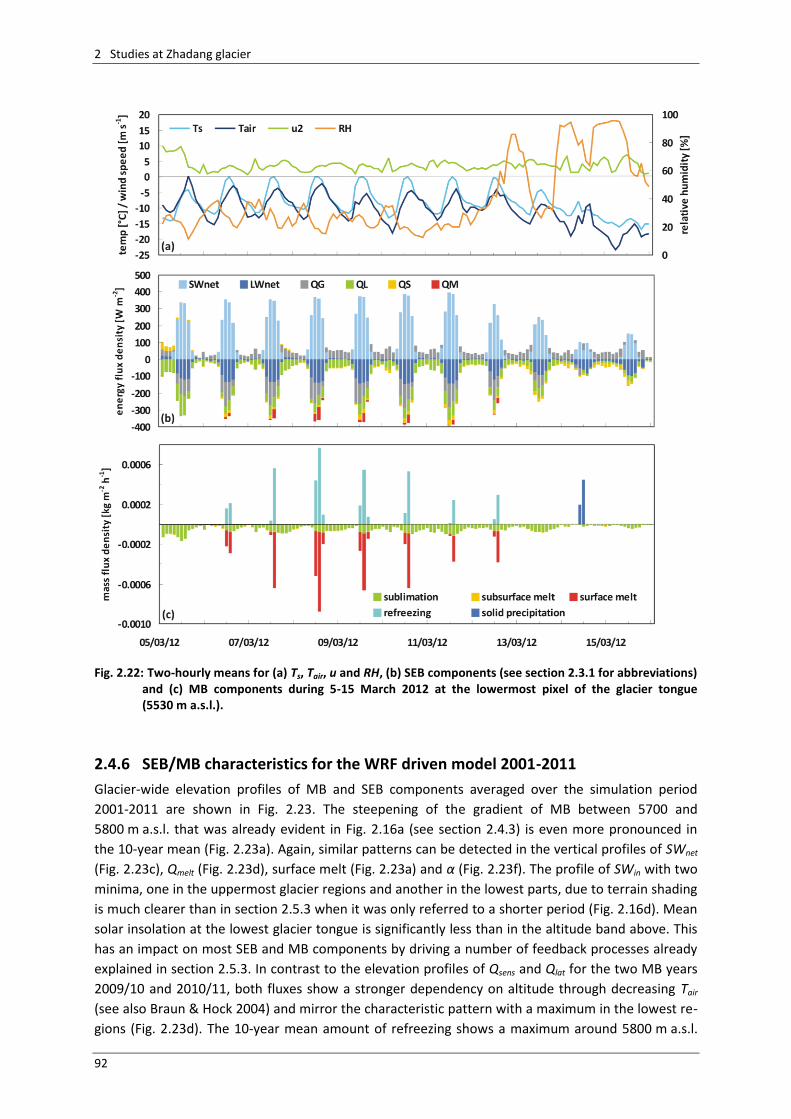
2 Studies at Zhadang glacier
92
Fig. 2.22: Two-hourly means for (a) Ts, Tair, u and RH, (b) SEB components (see section 2.3.1 for abbreviations)
and (c) MB components during 5-15 March 2012 at the lowermost pixel of the glacier tongue (5530 m a.s.l.).
2.4.6 SEB/MB characteristics for the WRF driven model 2001-2011
Glacier-wide elevation profiles of MB and SEB components averaged over the simulation period
2001-2011 are shown in Fig. 2.23. The steepening of the gradient of MB between 5700 and
5800 m a.s.l. that was already evident in Fig. 2.16a (see section 2.4.3) is even more pronounced in
the 10-year mean (Fig. 2.23a). Again, similar patterns can be detected in the vertical profiles of SWnet
(Fig. 2.23c), Qmelt (Fig. 2.23d), surface melt (Fig. 2.23a) and α (Fig. 2.23f). The profile of SWin with two
minima, one in the uppermost glacier regions and another in the lowest parts, due to terrain shading
is much clearer than in section 2.5.3 when it was only referred to a shorter period (Fig. 2.16d). Mean
solar insolation at the lowest glacier tongue is significantly less than in the altitude band above. This
has an impact on most SEB and MB components by driving a number of feedback processes already
explained in section 2.5.3. In contrast to the elevation profiles of Qsens and Qlat for the two MB years
2009/10 and 2010/11, both fluxes show a stronger dependency on altitude through decreasing Tair
(see also Braun & Hock 2004) and mirror the characteristic pattern with a maximum in the lowest re-
gions (Fig. 2.23d). The 10-year mean amount of refreezing shows a maximum around 5800 m a.s.l.
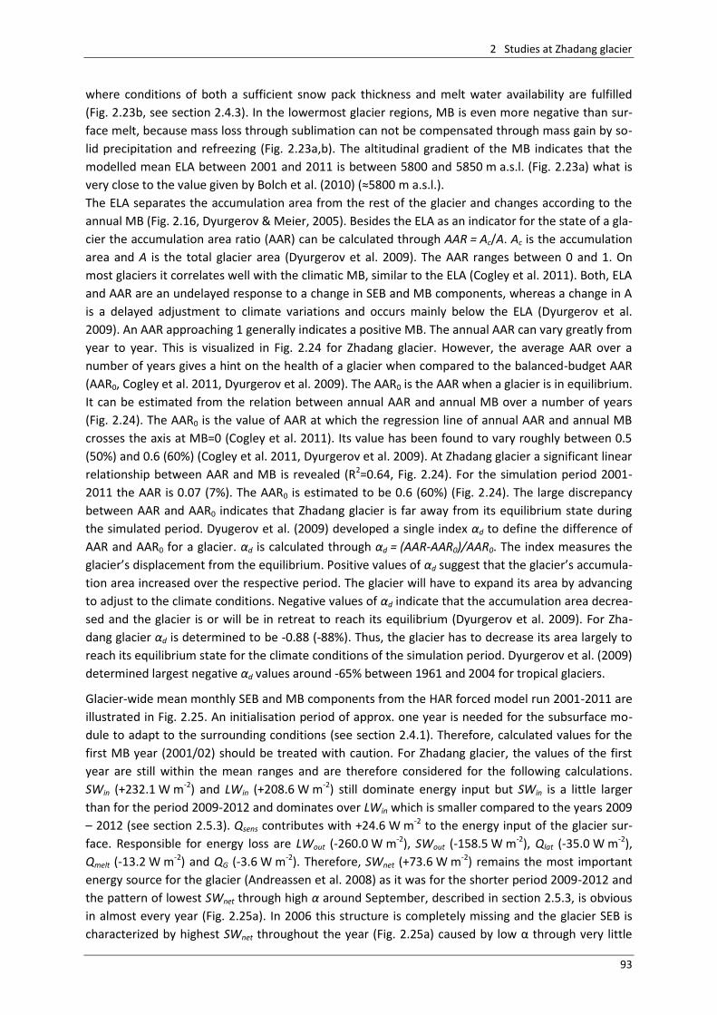
2 Studies at Zhadang glacier
93
where conditions of both a sufficient snow pack thickness and melt water availability are fulfilled
(Fig. 2.23b, see section 2.4.3). In the lowermost glacier regions, MB is even more negative than sur-
face melt, because mass loss through sublimation can not be compensated through mass gain by so-
lid precipitation and refreezing (Fig. 2.23a,b). The altitudinal gradient of the MB indicates that the
modelled mean ELA between 2001 and 2011 is between 5800 and 5850 m a.s.l. (Fig. 2.23a) what is
very close to the value given by Bolch et al. (2010) (≈5800 m a.s.l.).
The ELA separates the accumulation area from the rest of the glacier and changes according to the
annual MB (Fig. 2.16, Dyurgerov & Meier, 2005). Besides the ELA as an indicator for the state of a gla-
cier the accumulation area ratio (AAR) can be calculated through AAR = Ac/A. Ac is the accumulation
area and A is the total glacier area (Dyurgerov et al. 2009). The AAR ranges between 0 and 1. On
most glaciers it correlates well with the climatic MB, similar to the ELA (Cogley et al. 2011). Both, ELA
and AAR are an undelayed response to a change in SEB and MB components, whereas a change in A
is a delayed adjustment to climate variations and occurs mainly below the ELA (Dyurgerov et al.
2009). An AAR approaching 1 generally indicates a positive MB. The annual AAR can vary greatly from
year to year. This is visualized in Fig. 2.24 for Zhadang glacier. However, the average AAR over a
number of years gives a hint on the health of a glacier when compared to the balanced-budget AAR
(AAR0, Cogley et al. 2011, Dyurgerov et al. 2009). The AAR0 is the AAR when a glacier is in equilibrium.
It can be estimated from the relation between annual AAR and annual MB over a number of years
(Fig. 2.24). The AAR0 is the value of AAR at which the regression line of annual AAR and annual MB
crosses the axis at MB=0 (Cogley et al. 2011). Its value has been found to vary roughly between 0.5
(50%) and 0.6 (60%) (Cogley et al. 2011, Dyurgerov et al. 2009). At Zhadang glacier a significant linear
relationship between AAR and MB is revealed (R2=0.64, Fig. 2.24). For the simulation period 2001-
2011 the AAR is 0.07 (7%). The AAR0 is estimated to be 0.6 (60%) (Fig. 2.24). The large discrepancy
between AAR and AAR0 indicates that Zhadang glacier is far away from its equilibrium state during
the simulated period. Dyugerov et al. (2009) developed a single index αd to define the difference of
AAR and AAR0 for a glacier. αd is calculated through αd = (AAR-AAR0)/AAR0. The index measures the
glacier’s displacement from the equilibrium. Positive values of αd suggest that the glacier’s accumula-
tion area increased over the respective period. The glacier will have to expand its area by advancing
to adjust to the climate conditions. Negative values of αd indicate that the accumulation area decrea-
sed and the glacier is or will be in retreat to reach its equilibrium (Dyurgerov et al. 2009). For Zha-
dang glacier αd is determined to be -0.88 (-88%). Thus, the glacier has to decrease its area largely to
reach its equilibrium state for the climate conditions of the simulation period. Dyurgerov et al. (2009)
determined largest negative αd values around -65% between 1961 and 2004 for tropical glaciers.
Glacier-wide mean monthly SEB and MB components from the HAR forced model run 2001-2011 are
illustrated in Fig. 2.25. An initialisation period of approx. one year is needed for the subsurface mo-
dule to adapt to the surrounding conditions (see section 2.4.1). Therefore, calculated values for the
first MB year (2001/02) should be treated with caution. For Zhadang glacier, the values of the first
year are still within the mean ranges and are therefore considered for the following calculations.
SWin (+232.1 W m-2) and LWin (+208.6 W m-2) still dominate energy input but SWin is a little larger
than for the period 2009-2012 and dominates over LWin which is smaller compared to the years 2009
– 2012 (see section 2.5.3). Qsens contributes with +24.6 W m-2 to the energy input of the glacier sur-
face. Responsible for energy loss are LWout (-260.0 W m-2), SWout (-158.5 W m-2), Qlat (-35.0 W m-2),
Qmelt (-13.2 W m-2) and QG (-3.6 W m-2). Therefore, SWnet (+73.6 W m-2) remains the most important
energy source for the glacier (Andreassen et al. 2008) as it was for the shorter period 2009-2012 and
the pattern of lowest SWnet through high α around September, described in section 2.5.3, is obvious
in almost every year (Fig. 2.25a). In 2006 this structure is completely missing and the glacier SEB is
characterized by highest SWnet throughout the year (Fig. 2.25a) caused by low α through very little
2 Studies at Zhadang glacier
94
snowfall in November and December 2005, January to March and again June to August 2006 (Fig.
2.25b). The result is that the model returns largest amounts of Qmelt and therefore surface melt from
March to September (Fig. 2.25). This stresses the impact of the monsoon onset as reported by Mölg
et al. (2012) and Kang et al. (2009) (see section 2.1) but also the importance of winter snowfall
events that keep α high. Generally, α decreases at the end of each year (increasing SWnet, Fig. 2.25a)
because solid precipitation is minimal in that period (see section 1.4.2.1, Fig. 2.25b). Then α gradually
increases in late winter and spring (decreasing SWnet). LWnet and QG show a rather regular seasonal
cycle (Fig. 2.25a) as explained in section 2.4.3. Generally, monthly means of Qsens and Qlat are of oppo-
site sign and sometimes cancel each other out (see also Braun & Hock 2004). Qsens can reach negative
values during winter through cold air advection over the glacier or high SWnet (through low α) and
increasing Ts (see section 2.4.5). As described in section 2.4.3 the dry conditions on the TP cause
absolute values of Qlat to be usually larger than Qsens and being responsible for significant mass loss
through sublimation in every month (Fig. 2.25).
Fig. 2.23: Modelled vertical profiles of (left) the specific mass balance and its components and (right) mean
SEB components on Zhadang glacier averaged over the simulation period October 2001 – September 2011. Data are averaged for 50-m altitude bands. Note the different x-axis scales of the components (negative means mass or energy loss at the glacier surface, see section 2.3.1 and Table 2.2 for abbre-viations).
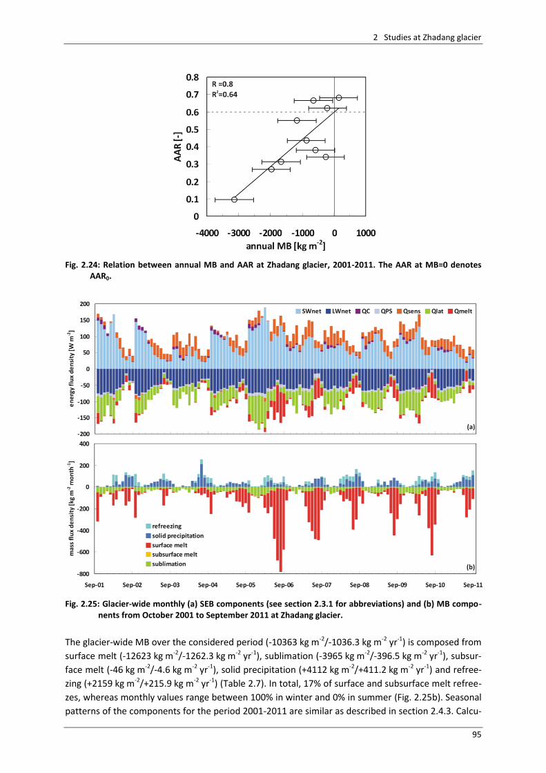
2 Studies at Zhadang glacier
95
Fig. 2.24: Relation between annual MB and AAR at Zhadang glacier, 2001-2011. The AAR at MB=0 denotes
AAR0.
Fig. 2.25: Glacier-wide monthly (a) SEB components (see section 2.3.1 for abbreviations) and (b) MB compo-
nents from October 2001 to September 2011 at Zhadang glacier.
The glacier-wide MB over the considered period (-10363 kg m-2/-1036.3 kg m-2 yr-1) is composed from
surface melt (-12623 kg m-2/-1262.3 kg m-2 yr-1), sublimation (-3965 kg m-2/-396.5 kg m-2 yr-1), subsur-
face melt (-46 kg m-2/-4.6 kg m-2 yr-1), solid precipitation (+4112 kg m-2/+411.2 kg m-2 yr-1) and refree-
zing (+2159 kg m-2/+215.9 kg m-2 yr-1) (Table 2.7). In total, 17% of surface and subsurface melt refree-
zes, whereas monthly values range between 100% in winter and 0% in summer (Fig. 2.25b). Seasonal
patterns of the components for the period 2001-2011 are similar as described in section 2.4.3. Calcu-
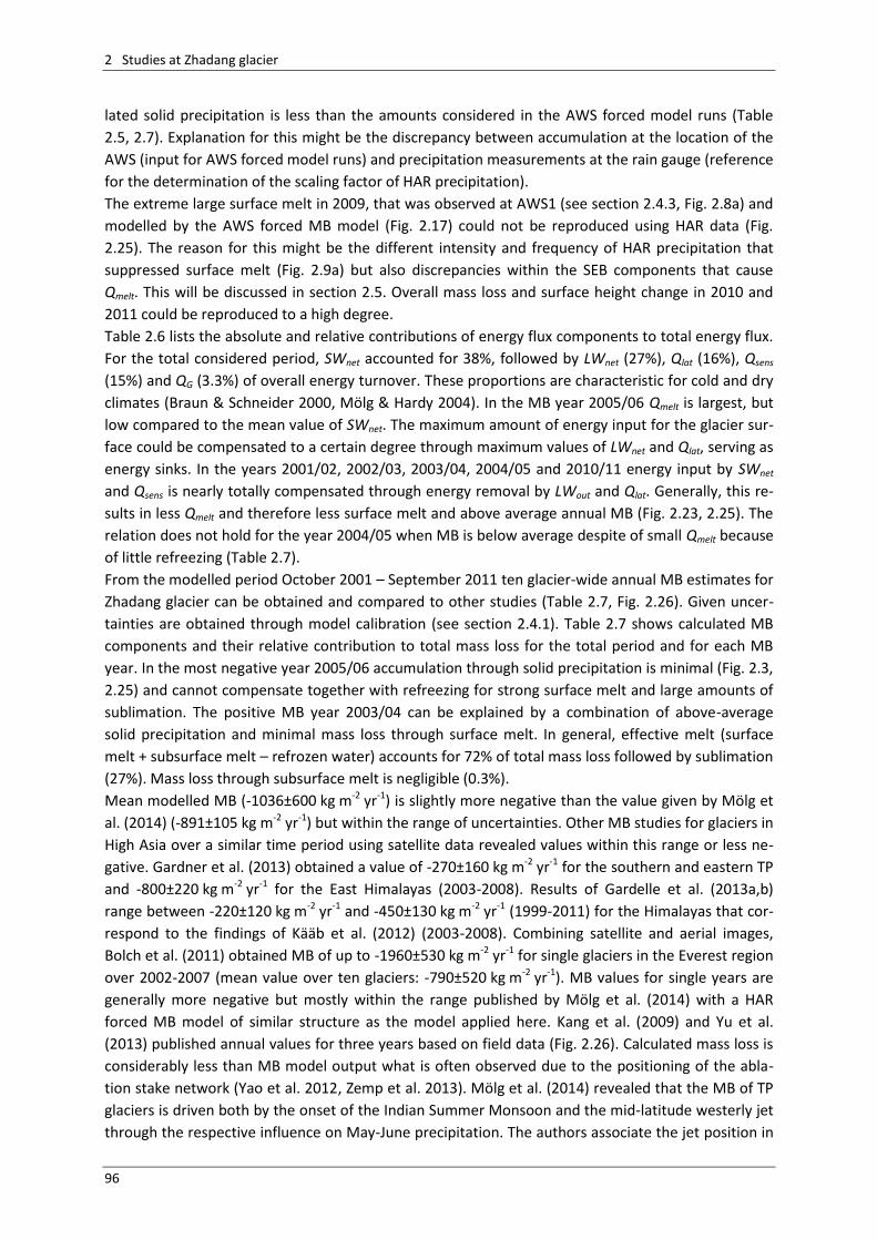
2 Studies at Zhadang glacier
96
lated solid precipitation is less than the amounts considered in the AWS forced model runs (Table
2.5, 2.7). Explanation for this might be the discrepancy between accumulation at the location of the
AWS (input for AWS forced model runs) and precipitation measurements at the rain gauge (reference
for the determination of the scaling factor of HAR precipitation).
The extreme large surface melt in 2009, that was observed at AWS1 (see section 2.4.3, Fig. 2.8a) and
modelled by the AWS forced MB model (Fig. 2.17) could not be reproduced using HAR data (Fig.
2.25). The reason for this might be the different intensity and frequency of HAR precipitation that
suppressed surface melt (Fig. 2.9a) but also discrepancies within the SEB components that cause
Qmelt. This will be discussed in section 2.5. Overall mass loss and surface height change in 2010 and
2011 could be reproduced to a high degree.
Table 2.6 lists the absolute and relative contributions of energy flux components to total energy flux.
For the total considered period, SWnet accounted for 38%, followed by LWnet (27%), Qlat (16%), Qsens
(15%) and QG (3.3%) of overall energy turnover. These proportions are characteristic for cold and dry
climates (Braun & Schneider 2000, Mölg & Hardy 2004). In the MB year 2005/06 Qmelt is largest, but
low compared to the mean value of SWnet. The maximum amount of energy input for the glacier sur-
face could be compensated to a certain degree through maximum values of LWnet and Qlat, serving as
energy sinks. In the years 2001/02, 2002/03, 2003/04, 2004/05 and 2010/11 energy input by SWnet
and Qsens is nearly totally compensated through energy removal by LWout and Qlat. Generally, this re-
sults in less Qmelt and therefore less surface melt and above average annual MB (Fig. 2.23, 2.25). The
relation does not hold for the year 2004/05 when MB is below average despite of small Qmelt because
of little refreezing (Table 2.7).
From the modelled period October 2001 – September 2011 ten glacier-wide annual MB estimates for
Zhadang glacier can be obtained and compared to other studies (Table 2.7, Fig. 2.26). Given uncer-
tainties are obtained through model calibration (see section 2.4.1). Table 2.7 shows calculated MB
components and their relative contribution to total mass loss for the total period and for each MB
year. In the most negative year 2005/06 accumulation through solid precipitation is minimal (Fig. 2.3,
2.25) and cannot compensate together with refreezing for strong surface melt and large amounts of
sublimation. The positive MB year 2003/04 can be explained by a combination of above-average
solid precipitation and minimal mass loss through surface melt. In general, effective melt (surface
melt + subsurface melt – refrozen water) accounts for 72% of total mass loss followed by sublimation
(27%). Mass loss through subsurface melt is negligible (0.3%).
Mean modelled MB (-1036±600 kg m-2 yr-1) is slightly more negative than the value given by Mölg et
al. (2014) (-891±105 kg m-2 yr-1) but within the range of uncertainties. Other MB studies for glaciers in
High Asia over a similar time period using satellite data revealed values within this range or less ne-
gative. Gardner et al. (2013) obtained a value of -270±160 kg m-2 yr-1 for the southern and eastern TP
and -800±220 kg m-2 yr-1 for the East Himalayas (2003-2008). Results of Gardelle et al. (2013a,b)
range between -220±120 kg m-2 yr-1 and -450±130 kg m-2 yr-1 (1999-2011) for the Himalayas that cor-
respond to the findings of Kääb et al. (2012) (2003-2008). Combining satellite and aerial images,
Bolch et al. (2011) obtained MB of up to -1960±530 kg m-2 yr-1 for single glaciers in the Everest region
over 2002-2007 (mean value over ten glaciers: -790±520 kg m-2 yr-1). MB values for single years are
generally more negative but mostly within the range published by Mölg et al. (2014) with a HAR
forced MB model of similar structure as the model applied here. Kang et al. (2009) and Yu et al.
(2013) published annual values for three years based on field data (Fig. 2.26). Calculated mass loss is
considerably less than MB model output what is often observed due to the positioning of the abla-
tion stake network (Yao et al. 2012, Zemp et al. 2013). Mölg et al. (2014) revealed that the MB of TP
glaciers is driven both by the onset of the Indian Summer Monsoon and the mid-latitude westerly jet
through the respective influence on May-June precipitation. The authors associate the jet position in
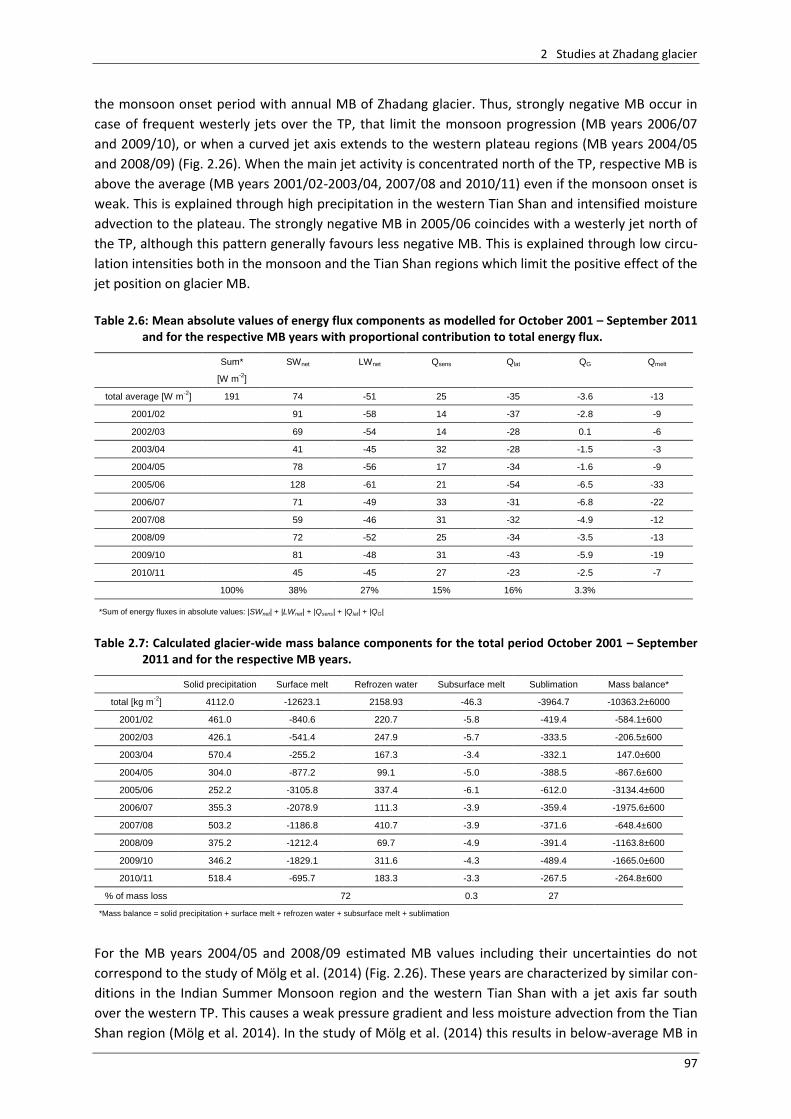
2 Studies at Zhadang glacier
97
the monsoon onset period with annual MB of Zhadang glacier. Thus, strongly negative MB occur in
case of frequent westerly jets over the TP, that limit the monsoon progression (MB years 2006/07
and 2009/10), or when a curved jet axis extends to the western plateau regions (MB years 2004/05
and 2008/09) (Fig. 2.26). When the main jet activity is concentrated north of the TP, respective MB is
above the average (MB years 2001/02-2003/04, 2007/08 and 2010/11) even if the monsoon onset is
weak. This is explained through high precipitation in the western Tian Shan and intensified moisture
advection to the plateau. The strongly negative MB in 2005/06 coincides with a westerly jet north of
the TP, although this pattern generally favours less negative MB. This is explained through low circu-
lation intensities both in the monsoon and the Tian Shan regions which limit the positive effect of the
jet position on glacier MB.
Table 2.6: Mean absolute values of energy flux components as modelled for October 2001 – September 2011
and for the respective MB years with proportional contribution to total energy flux.
Sum* SWnet LWnet Qsens Qlat QG Qmelt
[W m-2
]
total average [W m-2
] 191 74 -51 25 -35 -3.6 -13
2001/02 91 -58 14 -37 -2.8 -9
2002/03 69 -54 14 -28 0.1 -6
2003/04 41 -45 32 -28 -1.5 -3
2004/05 78 -56 17 -34 -1.6 -9
2005/06 128 -61 21 -54 -6.5 -33
2006/07 71 -49 33 -31 -6.8 -22
2007/08 59 -46 31 -32 -4.9 -12
2008/09 72 -52 25 -34 -3.5 -13
2009/10 81 -48 31 -43 -5.9 -19
2010/11 45 -45 27 -23 -2.5 -7
100% 38% 27% 15% 16% 3.3%
*Sum of energy fluxes in absolute values: |SWnet| + |LWnet| + |Qsens| + |Qlat| + |QG|
Table 2.7: Calculated glacier-wide mass balance components for the total period October 2001 – September
2011 and for the respective MB years.
Solid precipitation Surface melt Refrozen water Subsurface melt Sublimation Mass balance*
total [kg m-2
] 4112.0 -12623.1 2158.93 -46.3 -3964.7 -10363.2±6000
2001/02 461.0 -840.6 220.7 -5.8 -419.4 -584.1±600
2002/03 426.1 -541.4 247.9 -5.7 -333.5 -206.5±600
2003/04 570.4 -255.2 167.3 -3.4 -332.1 147.0±600
2004/05 304.0 -877.2 99.1 -5.0 -388.5 -867.6±600
2005/06 252.2 -3105.8 337.4 -6.1 -612.0 -3134.4±600
2006/07 355.3 -2078.9 111.3 -3.9 -359.4 -1975.6±600
2007/08 503.2 -1186.8 410.7 -3.9 -371.6 -648.4±600
2008/09 375.2 -1212.4 69.7 -4.9 -391.4 -1163.8±600
2009/10 346.2 -1829.1 311.6 -4.3 -489.4 -1665.0±600
2010/11 518.4 -695.7 183.3 -3.3 -267.5 -264.8±600
% of mass loss 72 0.3 27
*Mass balance = solid precipitation + surface melt + refrozen water + subsurface melt + sublimation
For the MB years 2004/05 and 2008/09 estimated MB values including their uncertainties do not
correspond to the study of Mölg et al. (2014) (Fig. 2.26). These years are characterized by similar con-
ditions in the Indian Summer Monsoon region and the western Tian Shan with a jet axis far south
over the western TP. This causes a weak pressure gradient and less moisture advection from the Tian
Shan region (Mölg et al. 2014). In the study of Mölg et al. (2014) this results in below-average MB in
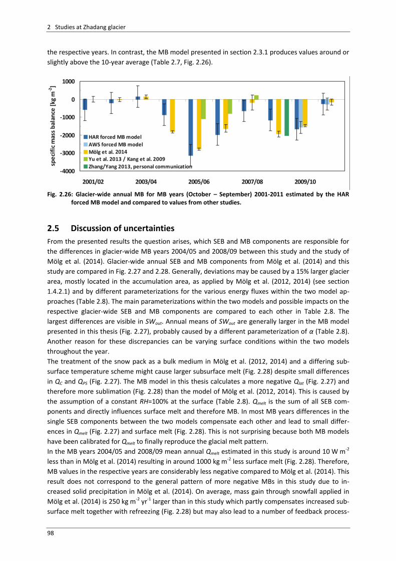
2 Studies at Zhadang glacier
98
the respective years. In contrast, the MB model presented in section 2.3.1 produces values around or
slightly above the 10-year average (Table 2.7, Fig. 2.26).
Fig. 2.26: Glacier-wide annual MB for MB years (October – September) 2001-2011 estimated by the HAR
forced MB model and compared to values from other studies.
2.5 Discussion of uncertainties
From the presented results the question arises, which SEB and MB components are responsible for
the differences in glacier-wide MB years 2004/05 and 2008/09 between this study and the study of
Mölg et al. (2014). Glacier-wide annual SEB and MB components from Mölg et al. (2014) and this
study are compared in Fig. 2.27 and 2.28. Generally, deviations may be caused by a 15% larger glacier
area, mostly located in the accumulation area, as applied by Mölg et al. (2012, 2014) (see section
1.4.2.1) and by different parameterizations for the various energy fluxes within the two model ap-
proaches (Table 2.8). The main parameterizations within the two models and possible impacts on the
respective glacier-wide SEB and MB components are compared to each other in Table 2.8. The
largest differences are visible in SWout. Annual means of SWout are generally larger in the MB model
presented in this thesis (Fig. 2.27), probably caused by a different parameterization of α (Table 2.8).
Another reason for these discrepancies can be varying surface conditions within the two models
throughout the year.
The treatment of the snow pack as a bulk medium in Mölg et al. (2012, 2014) and a differing sub-
surface temperature scheme might cause larger subsurface melt (Fig. 2.28) despite small differences
in QC and QPS (Fig. 2.27). The MB model in this thesis calculates a more negative Qlat (Fig. 2.27) and
therefore more sublimation (Fig. 2.28) than the model of Mölg et al. (2012, 2014). This is caused by
the assumption of a constant RH=100% at the surface (Table 2.8). Qmelt is the sum of all SEB com-
ponents and directly influences surface melt and therefore MB. In most MB years differences in the
single SEB components between the two models compensate each other and lead to small differ-
ences in Qmelt (Fig. 2.27) and surface melt (Fig. 2.28). This is not surprising because both MB models
have been calibrated for Qmelt to finally reproduce the glacial melt pattern.
In the MB years 2004/05 and 2008/09 mean annual Qmelt estimated in this study is around 10 W m-2
less than in Mölg et al. (2014) resulting in around 1000 kg m-2 less surface melt (Fig. 2.28). Therefore,
MB values in the respective years are considerably less negative compared to Mölg et al. (2014). This
result does not correspond to the general pattern of more negative MBs in this study due to in-
creased solid precipitation in Mölg et al. (2014). On average, mass gain through snowfall applied in
Mölg et al. (2014) is 250 kg m-2 yr-1 larger than in this study which partly compensates increased sub-
surface melt together with refreezing (Fig. 2.28) but may also lead to a number of feedback process-
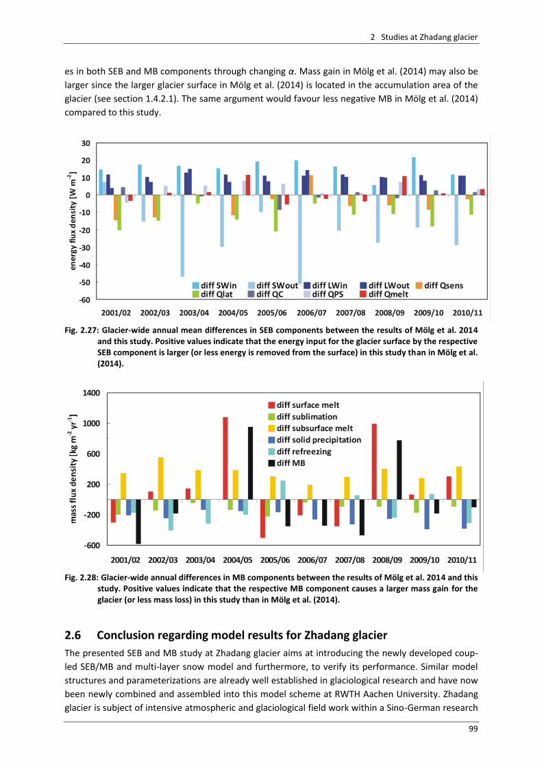
2 Studies at Zhadang glacier
99
es in both SEB and MB components through changing α. Mass gain in Mölg et al. (2014) may also be
larger since the larger glacier surface in Mölg et al. (2014) is located in the accumulation area of the
glacier (see section 1.4.2.1). The same argument would favour less negative MB in Mölg et al. (2014)
compared to this study.
Fig. 2.27: Glacier-wide annual mean differences in SEB components between the results of Mölg et al. 2014
and this study. Positive values indicate that the energy input for the glacier surface by the respective SEB component is larger (or less energy is removed from the surface) in this study than in Mölg et al. (2014).
Fig. 2.28: Glacier-wide annual differences in MB components between the results of Mölg et al. 2014 and this
study. Positive values indicate that the respective MB component causes a larger mass gain for the glacier (or less mass loss) in this study than in Mölg et al. (2014).
2.6 Conclusion regarding model results for Zhadang glacier
The presented SEB and MB study at Zhadang glacier aims at introducing the newly developed coup-
led SEB/MB and multi-layer snow model and furthermore, to verify its performance. Similar model
structures and parameterizations are already well established in glaciological research and have now
been newly combined and assembled into this model scheme at RWTH Aachen University. Zhadang
glacier is subject of intensive atmospheric and glaciological field work within a Sino-German research
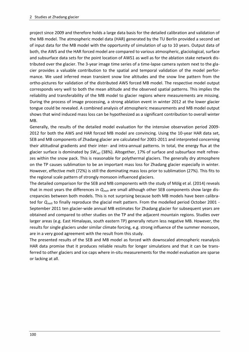
2 Studies at Zhadang glacier
100
project since 2009 and therefore holds a large data basis for the detailed calibration and validation of
the MB model. The atmospheric model data (HAR) generated by the TU Berlin provided a second set
of input data for the MB model with the opportunity of simulation of up to 10 years. Output data of
both, the AWS and the HAR forced model are compared to various atmospheric, glaciological, surface
and subsurface data sets for the point location of AWS1 as well as for the ablation stake network dis-
tributed over the glacier. The 3-year image time series of a time-lapse camera system next to the gla-
cier provides a valuable contribution to the spatial and temporal validation of the model perfor-
mance. We used inferred mean transient snow line altitudes and the snow line pattern from the
ortho-pictures for validation of the distributed AWS forced MB model. The respective model output
corresponds very well to both the mean altitude and the observed spatial patterns. This implies the
reliability and transferability of the MB model to glacier regions where measurements are missing.
During the process of image processing, a strong ablation event in winter 2012 at the lower glacier
tongue could be revealed. A combined analysis of atmospheric measurements and MB model output
shows that wind induced mass loss can be hypothesized as a significant contribution to overall winter
MB.
Generally, the results of the detailed model evaluation for the intensive observation period 2009-
2012 for both the AWS and HAR forced MB model are convincing. Using the 10-year HAR data set,
SEB and MB components of Zhadang glacier are calculated for 2001-2011 and interpreted concerning
their altitudinal gradients and their inter- and intra-annual patterns. In total, the energy flux at the
glacier surface is dominated by SWnet (38%). Altogether, 17% of surface and subsurface melt refree-
zes within the snow pack. This is reasonable for polythermal glaciers. The generally dry atmosphere
on the TP causes sublimation to be an important mass loss for Zhadang glacier especially in winter.
However, effective melt (72%) is still the dominating mass loss prior to sublimation (27%). This fits to
the regional scale pattern of strongly monsoon influenced glaciers.
The detailed comparison for the SEB and MB components with the study of Mölg et al. (2014) reveals
that in most years the differences in Qmelt are small although other SEB components show large dis-
crepancies between both models. This is not surprising because both MB models have been calibra-
ted for Qmelt to finally reproduce the glacial melt pattern. From the modelled period October 2001 -
September 2011 ten glacier-wide annual MB estimates for Zhadang glacier for subsequent years are
obtained and compared to other studies on the TP and the adjacent mountain regions. Studies over
larger areas (e.g. East Himalayas, south eastern TP) generally return less negative MB. However, the
results for single glaciers under similar climate forcing, e.g. strong influence of the summer monsoon,
are in a very good agreement with the result from this study.
The presented results of the SEB and MB model as forced with downscaled atmospheric reanalysis
HAR data promise that it produces reliable results for longer simulations and that it can be trans-
ferred to other glaciers and ice caps where in-situ measurements for the model evaluation are sparse
or lacking at all.

2 Studies at Zhadang glacier
101
Table 2.8: Comparison of the main parameterizations within the coupled snow and SEB model developed and applied in this study and applied in Mölg et al. (2014) and impact on glacier-wide SEB and MB results.
Parameter(ization) this study Mölg et al. (2014) Impact on glacier-wide results
altitudinal lapse rates
air temperature (Tair) -0.007 K m-1
night: -0.0035 K m
-1
day: -0.0095 K m-1
?
precipitation +0.042% m-1
+0.038% m-1
negligible
relative humidity (RH) +0.022% m-1
- ?
air pressure (ρair) -0.067 hPa m-1
- ?
threshold for precipiation phase 1-5°C 1-6.5°C >20% difference in solid precipitation / accumulation → less negative MB in Mölg et al. (2014) precipitation scaling factor 0.56 0.79654
radiation
SWin radiation model after Kumar et al. (1997) corrected for clouds through HAR SW in
radiation model after Mölg et al. (2009b) optimized after SWin from the AWS
Comparison of SWin sums between HAR and AWS showed slightly more SW in from HAR; but maximum hourly summertime SWin at noon can differ by up to 1000 W m
-2→ ?
α
function of snowfall frequen-cy and depth after Oerle-mans & Knap (1998); control parameters (α for fresh snow, firn and ice, effects of ageing and snow depth) are the same as in Mölg et al. (2014)
function of snowfall frequency and depth after Oerlemans & Knap (1998); αice is variable as a function of dew point temperature
slightly lower αice causes larger SWnet and therefore increasing Qmelt and QPS → temporarily more surface and subsurface melt in Mölg et al. (2014)
LWin after Klok & Oerlemans (2002)
after Mölg et al. (2009b) or Klok & Oerlemans (2002)
less LW in in Mölg et al.
LWout Stefan-Boltzmann law through Ts (ε=0.97)
Stefan-Boltzmann law through Ts
larger LWout in Mölg et al. (2014) (due to differences in Ts)
turbulent fluxes
Qsens simplified bulk aero-dynamic method after Oerlemans (2001)
analytical expressions of the bulk aerodynamik method following the Monin-Obukhov similarity theory (Mölg & Hardy 2004)
generally larger Qsens in Mölg et al. (2014)
Qlat
simplified bulk aerodynamic method after Oerlemans (2001); surface RH is set to 100%
analytical expressions of the bulk aerodynamik method following the Monin-Obukhov similarity theory (Mölg & Hardy 2004)
larger Qlat in this study → increased mass loss through sublimation compared to Mölg et al. (2014)
subsurface
penetrating SW / subsurface melt
after Bintanja & van den Broeke (1995); depending on SWnet
after Bintanja & van den Broeke (1995); depending on SWnet
more subsurface melt in Mölg et al. (2014) → more negative MB
refreezing in snow refreezing process is resolved vertically; layer thickness: 0.2 m
snow pack treated as a bulk medium; refreezing process is not resolved vertically
more refreezing in Mölg et al. (2014) → less negative MB
superimposed ice not calculated explicitely calculated increased internal accumulation in Mölg et al. (2014) → less negative MB
densification of dry snow pack simulated due to T and overburden pressure after Herron & Langway (1980)
simulated from the viscous fluid assumption after Sturm & Holmgren (1998)
?
T solved from the thermo-dynamic heat equation; layer thickness: 0.2 m
solved from the thermo-dynamic heat equation; layer thickness: 0.5 m
?
QC
temperature difference between surface and the two uppermost subsurface layers; variable thermal conductivity
temperature difference between surface and first subsurface layer; constant values for thermal conduc-tivity
?

3 Studies at Purogangri Ice Cap
103
3 Energy and mass balance for Purogangri ice cap, central Tibet-an Plateau, 2000-2011
3.1 Introduction and regional climate conditions
Purogangri ice cap (PIC) is the largest ice cap on the Tibetan Plateau (Yi et al. 2002), located in the
northern central part of the TiP (Fig. 3.1). Its large area favours the application of various remote
sensing techniques to determine the state of the ice cap. In this study, we use the geodetic MB from
a TerraSAR-X analysis (Neckel et al. 2013, see section 3.4.1) and the snow line and ELA estimation
based on MODIS data (Spieß et al. 2014, see section 3.4.2) to evaluate the MB model performance.
The region is characterized by a cold and relatively dry continental climate (see section 1.4.1). The
climate chart based on HAR data (Fig. 1.16) implies that the region is still dominated by Indian mon-
soon circulation in summer and mid-latitude westerlies in winter. However, precipitation season al-
ready starts in March, when the westerly jet starts to shift northward (see sections 1.3.1, 1.4.1). Daily
mean air temperature generated by HAR generally rise above zero from June to September in the
lower regions of PIC whereas positive daily mean temperatures in the middle parts are limited to July
and August. Daily mean air temperatures 2000-2011 range between -29.6°C and 10.8 C (average
-8.1°C) in the lowest regions and between -32.7 and 6.4°C (average -11.3°C) at the uppermost HAR
grid cell (Fig. 1.16). Lei et al. (2012) give a mean annual air temperature of -6°C around Linggo Co
(40 km east of PIC, 5060 m a.s.l.). Monthly means of those HAR variables that serve as input for the
applied MB model are shown in Fig. 3.2. SWin reaches its maximum around May and decreases in
summer, when monsoonal cloud cover increases. The monsoon season is associated with annual ma-
xima in precipitation and air pressure associated with the Tibetan High (see section 1.3.1) whereas
wind speeds are generally low (Fig. 3.2). The mean annual precipitation amount at PIC (380 mm) is
lower compared to Zhadang glacier (534 mm). Significant amounts of precipitation already occur in
spring (Fig. 1.16, see section 1.4.1). Due to the low air temperatures all spring precipitation falls as
snow, positively affecting glacier MB both through increasing accumulation and albedo (see sections
1.3.5, 1.4.1). MB model results reveal that ≈86% of total HAR precipitation fall as snow between 2000
and 2011. This supports the observed below-average mass loss at PIC 2000-2011 (Neckel et al. 2013,
Lei et al. 2012) compared to other MB studies for glaciers in High Asia over a similar period (see sec-
tions 1.3.2 and 2.4.6).
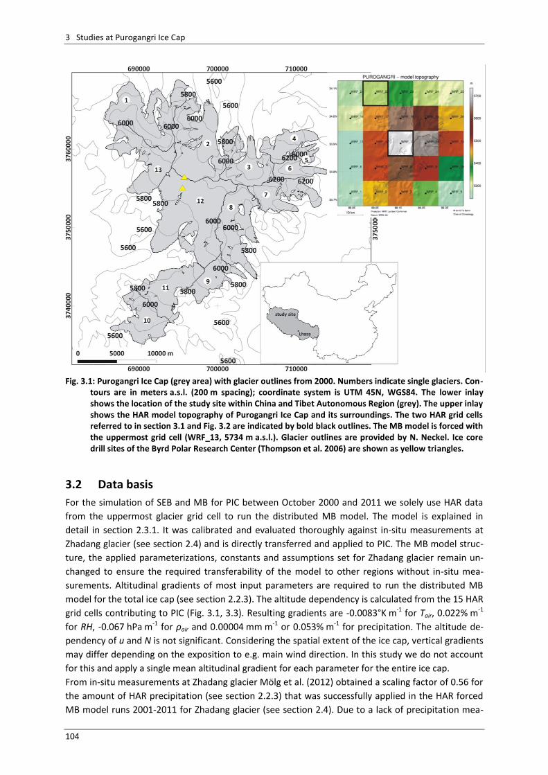
3 Studies at Purogangri Ice Cap
104
Fig. 3.1: Purogangri Ice Cap (grey area) with glacier outlines from 2000. Numbers indicate single glaciers. Con-
tours are in meters a.s.l. (200 m spacing); coordinate system is UTM 45N, WGS84. The lower inlay shows the location of the study site within China and Tibet Autonomous Region (grey). The upper inlay shows the HAR model topography of Purogangri Ice Cap and its surroundings. The two HAR grid cells referred to in section 3.1 and Fig. 3.2 are indicated by bold black outlines. The MB model is forced with the uppermost grid cell (WRF_13, 5734 m a.s.l.). Glacier outlines are provided by N. Neckel. Ice core drill sites of the Byrd Polar Research Center (Thompson et al. 2006) are shown as yellow triangles.
3.2 Data basis
For the simulation of SEB and MB for PIC between October 2000 and 2011 we solely use HAR data
from the uppermost glacier grid cell to run the distributed MB model. The model is explained in
detail in section 2.3.1. It was calibrated and evaluated thoroughly against in-situ measurements at
Zhadang glacier (see section 2.4) and is directly transferred and applied to PIC. The MB model struc-
ture, the applied parameterizations, constants and assumptions set for Zhadang glacier remain un-
changed to ensure the required transferability of the model to other regions without in-situ mea-
surements. Altitudinal gradients of most input parameters are required to run the distributed MB
model for the total ice cap (see section 2.2.3). The altitude dependency is calculated from the 15 HAR
grid cells contributing to PIC (Fig. 3.1, 3.3). Resulting gradients are -0.0083°K m-1 for Tair, 0.022% m-1
for RH, -0.067 hPa m-1 for ρair and 0.00004 mm m-1 or 0.053% m-1 for precipitation. The altitude de-
pendency of u and N is not significant. Considering the spatial extent of the ice cap, vertical gradients
may differ depending on the exposition to e.g. main wind direction. In this study we do not account
for this and apply a single mean altitudinal gradient for each parameter for the entire ice cap.
From in-situ measurements at Zhadang glacier Mölg et al. (2012) obtained a scaling factor of 0.56 for
the amount of HAR precipitation (see section 2.2.3) that was successfully applied in the HAR forced
MB model runs 2001-2011 for Zhadang glacier (see section 2.4). Due to a lack of precipitation mea-
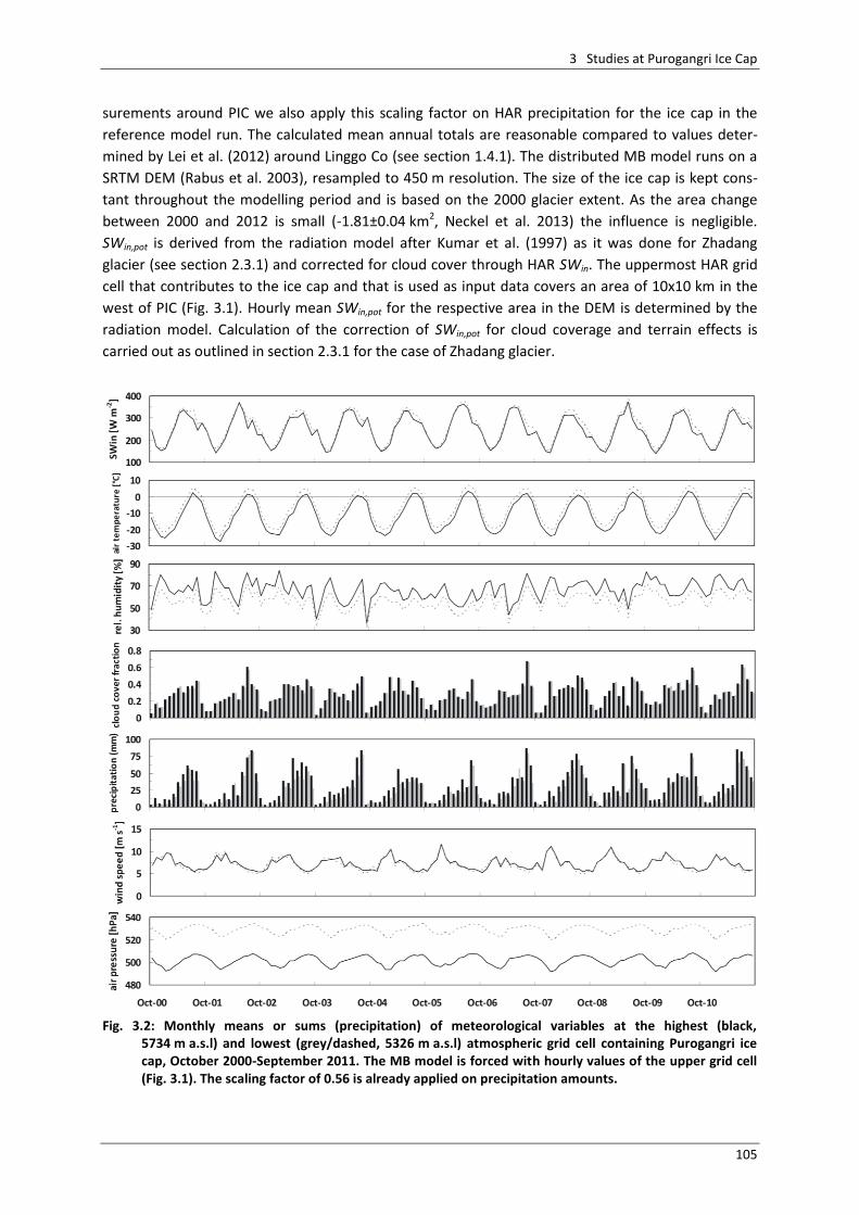
3 Studies at Purogangri Ice Cap
105
surements around PIC we also apply this scaling factor on HAR precipitation for the ice cap in the
reference model run. The calculated mean annual totals are reasonable compared to values deter-
mined by Lei et al. (2012) around Linggo Co (see section 1.4.1). The distributed MB model runs on a
SRTM DEM (Rabus et al. 2003), resampled to 450 m resolution. The size of the ice cap is kept cons-
tant throughout the modelling period and is based on the 2000 glacier extent. As the area change
between 2000 and 2012 is small (-1.81±0.04 km2, Neckel et al. 2013) the influence is negligible.
SWin,pot is derived from the radiation model after Kumar et al. (1997) as it was done for Zhadang
glacier (see section 2.3.1) and corrected for cloud cover through HAR SWin. The uppermost HAR grid
cell that contributes to the ice cap and that is used as input data covers an area of 10x10 km in the
west of PIC (Fig. 3.1). Hourly mean SWin,pot for the respective area in the DEM is determined by the
radiation model. Calculation of the correction of SWin,pot for cloud coverage and terrain effects is
carried out as outlined in section 2.3.1 for the case of Zhadang glacier.
Fig. 3.2: Monthly means or sums (precipitation) of meteorological variables at the highest (black,
5734 m a.s.l) and lowest (grey/dashed, 5326 m a.s.l) atmospheric grid cell containing Purogangri ice cap, October 2000-September 2011. The MB model is forced with hourly values of the upper grid cell (Fig. 3.1). The scaling factor of 0.56 is already applied on precipitation amounts.
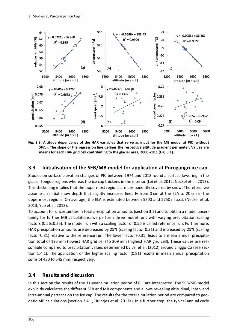
3 Studies at Purogangri Ice Cap
106
Fig. 3.3: Altitude dependency of the HAR variables that serve as input for the MB model at PIC (without
SWin). The slope of the regression line defines the respective altitude gradient per meter. Values are means for each HAR grid cell contributing to the glacier area, 2000-2011 (Fig. 3.1).
3.3 Initialisation of the SEB/MB model for application at Purogangri ice cap
Studies on surface elevation changes of PIC between 1974 and 2012 found a surface lowering in the
glacier tongue regions whereas the ice cap thickens in the interior (Lei et al. 2012, Neckel et al. 2013).
This thickening implies that the uppermost regions are permanently covered by snow. Therefore, we
assume an initial snow depth that slightly increases linearly from 0 cm at the ELA to 20 cm in the
uppermost regions. On average, the ELA is estimated between 5700 and 5750 m a.s.l. (Neckel et al.
2013, Yao et al. 2012).
To account for uncertainties in total precipitation amounts (section 3.2) and to obtain a model uncer-
tainty for further MB calculations, we perform three model runs with varying precipitation scaling
factors (0.56±0.25). The model run with a scaling factor of 0.56 is called reference run. Furthermore,
HAR precipitation amounts are decreased by 25% (scaling factor 0.31) and increased by 25% (scaling
factor 0.81) relative to the reference run. The lower factor (0.31) leads to a mean annual precipita-
tion total of 195 mm (lowest HAR grid cell) to 209 mm (highest HAR grid cell). These values are rea-
sonable compared to precipitation values determined by Lei et al. (2012) around Linggo Co (see sec-
tion 1.4.1). The application of the higher scaling factor (0.81) results in mean annual precipitation
sums of 430 to 545 mm, respectively.
3.4 Results and discussion
In this section the results of the 11-year simulation period of PIC are interpreted. The SEB/MB model
explicitly calculates the different SEB and MB components and allows revealing altitudinal, inter- and
intra-annual patterns on the ice cap. The results for the total simulation period are compared to geo-
detic MB calculations (section 3.4.1, Huintjes et al. 2013a). In a further step, the typical annual cycle
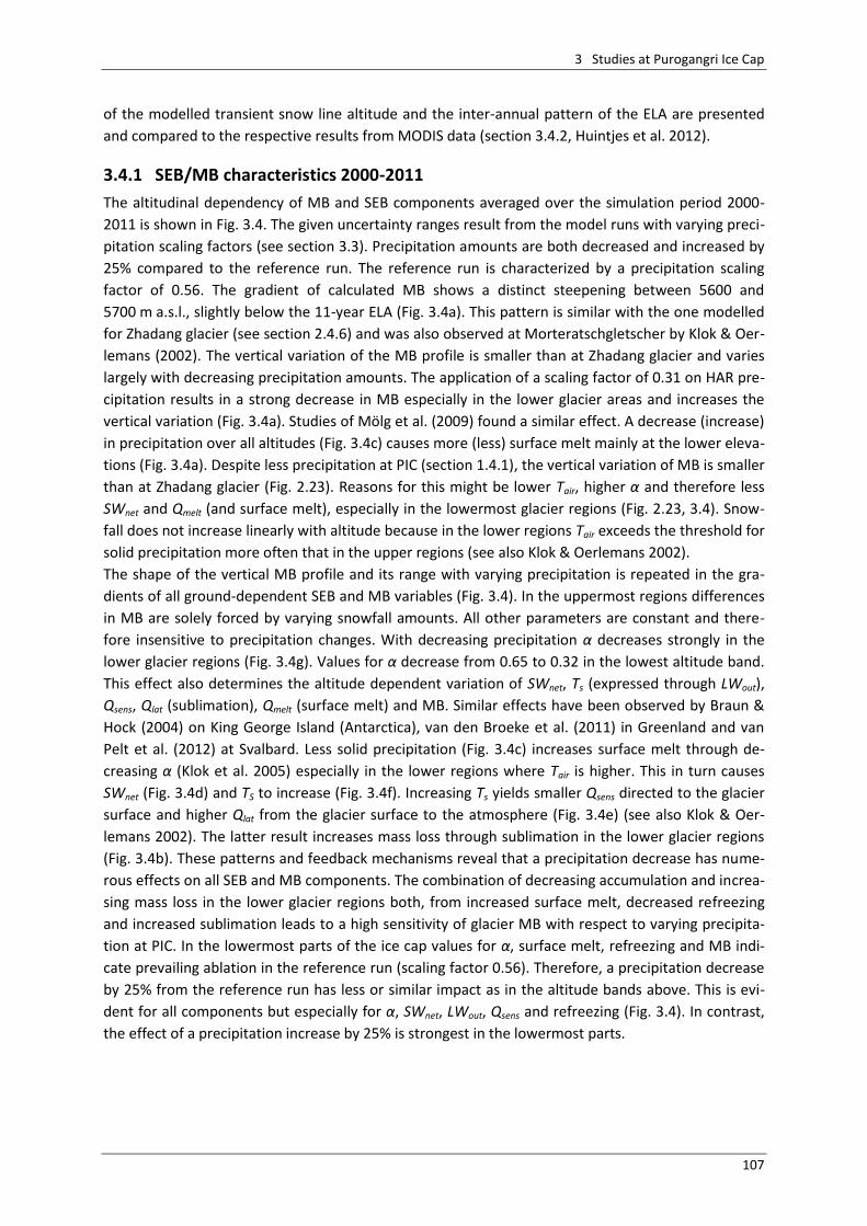
3 Studies at Purogangri Ice Cap
107
of the modelled transient snow line altitude and the inter-annual pattern of the ELA are presented
and compared to the respective results from MODIS data (section 3.4.2, Huintjes et al. 2012).
3.4.1 SEB/MB characteristics 2000-2011
The altitudinal dependency of MB and SEB components averaged over the simulation period 2000-
2011 is shown in Fig. 3.4. The given uncertainty ranges result from the model runs with varying preci-
pitation scaling factors (see section 3.3). Precipitation amounts are both decreased and increased by
25% compared to the reference run. The reference run is characterized by a precipitation scaling
factor of 0.56. The gradient of calculated MB shows a distinct steepening between 5600 and
5700 m a.s.l., slightly below the 11-year ELA (Fig. 3.4a). This pattern is similar with the one modelled
for Zhadang glacier (see section 2.4.6) and was also observed at Morteratschgletscher by Klok & Oer-
lemans (2002). The vertical variation of the MB profile is smaller than at Zhadang glacier and varies
largely with decreasing precipitation amounts. The application of a scaling factor of 0.31 on HAR pre-
cipitation results in a strong decrease in MB especially in the lower glacier areas and increases the
vertical variation (Fig. 3.4a). Studies of Mölg et al. (2009) found a similar effect. A decrease (increase)
in precipitation over all altitudes (Fig. 3.4c) causes more (less) surface melt mainly at the lower eleva-
tions (Fig. 3.4a). Despite less precipitation at PIC (section 1.4.1), the vertical variation of MB is smaller
than at Zhadang glacier (Fig. 2.23). Reasons for this might be lower Tair, higher α and therefore less
SWnet and Qmelt (and surface melt), especially in the lowermost glacier regions (Fig. 2.23, 3.4). Snow-
fall does not increase linearly with altitude because in the lower regions Tair exceeds the threshold for
solid precipitation more often that in the upper regions (see also Klok & Oerlemans 2002).
The shape of the vertical MB profile and its range with varying precipitation is repeated in the gra-
dients of all ground-dependent SEB and MB variables (Fig. 3.4). In the uppermost regions differences
in MB are solely forced by varying snowfall amounts. All other parameters are constant and there-
fore insensitive to precipitation changes. With decreasing precipitation α decreases strongly in the
lower glacier regions (Fig. 3.4g). Values for α decrease from 0.65 to 0.32 in the lowest altitude band.
This effect also determines the altitude dependent variation of SWnet, Ts (expressed through LWout),
Qsens, Qlat (sublimation), Qmelt (surface melt) and MB. Similar effects have been observed by Braun &
Hock (2004) on King George Island (Antarctica), van den Broeke et al. (2011) in Greenland and van
Pelt et al. (2012) at Svalbard. Less solid precipitation (Fig. 3.4c) increases surface melt through de-
creasing α (Klok et al. 2005) especially in the lower regions where Tair is higher. This in turn causes
SWnet (Fig. 3.4d) and TS to increase (Fig. 3.4f). Increasing Ts yields smaller Qsens directed to the glacier
surface and higher Qlat from the glacier surface to the atmosphere (Fig. 3.4e) (see also Klok & Oer-
lemans 2002). The latter result increases mass loss through sublimation in the lower glacier regions
(Fig. 3.4b). These patterns and feedback mechanisms reveal that a precipitation decrease has nume-
rous effects on all SEB and MB components. The combination of decreasing accumulation and increa-
sing mass loss in the lower glacier regions both, from increased surface melt, decreased refreezing
and increased sublimation leads to a high sensitivity of glacier MB with respect to varying precipita-
tion at PIC. In the lowermost parts of the ice cap values for α, surface melt, refreezing and MB indi-
cate prevailing ablation in the reference run (scaling factor 0.56). Therefore, a precipitation decrease
by 25% from the reference run has less or similar impact as in the altitude bands above. This is evi-
dent for all components but especially for α, SWnet, LWout, Qsens and refreezing (Fig. 3.4). In contrast,
the effect of a precipitation increase by 25% is strongest in the lowermost parts.
3 Studies at Purogangri Ice Cap
108
Fig. 3.4: Modelled vertical profiles of (left) the specific mass balance and its components and (right) mean
SEB components at PIC averaged over the simulation period October 2000 – September 2011. Data are averaged for 50-m altitude bands. The uncertainty ranges are calculated assuming different precipita-tion amounts (see section 3.3). Note the different x-axis scales of the components (negative means mass or energy loss at the glacier surface, see section 2.3.1 and Tab. 2.2 for abbreviations).
SWin and LWin are the only ground-independent energy sources for the glacier surface (see section
2.3.1) and do not change with varying precipitation amounts (Fig. 3.4d) because energy fluxes from
the surrounding terrain are not considered. SWin increases with altitude because the optical air mass
decreases (see Klok & Oerlemans 2002) and the glacier surface is hardly affected by terrain obstruc-
tions. In the reference run refreezing is largest in ≈5600 m a.s.l. (Fig. 3.4c) where decent amounts of
surface melt and a thick snow pack are present. The annual mean proportion of refreezing reached
45% in the upper glacier regions and 1% in the lowermost altitude band. A precipitation decrease by
25% from the reference run raises the altitude of maximum refreezing to 5900 m a.s.l., whereas a
precipitation increase by 25% yields to a larger snow pack in the lower glacier regions and therefore
significantly larger amounts of refreezing. For all other SEB and MB components, increasing precipita-
tion by 25% compared to the reference run has a much smaller effect than a precipitation decrease
by 25%. This is also evident for ELA variations. From the vertical MB profile the ELA of the reference
run is estimated between 5800 and 5900 m a.s.l. (Fig. 3.4a). The ELA coincides with the results from
Yao et al. (2012) and Neckel et al. (2013) (see section 3.3). A decrease (increase) of the precipitation
amount by 25% rises (lowers) the ELA by ≈400 m (≈300 m). Concerning the glacier hypsometry (Fig.
1.16) an ELA increase will have important consequences for the glacier MB because the largest area
proportion is located in these altitude bands.
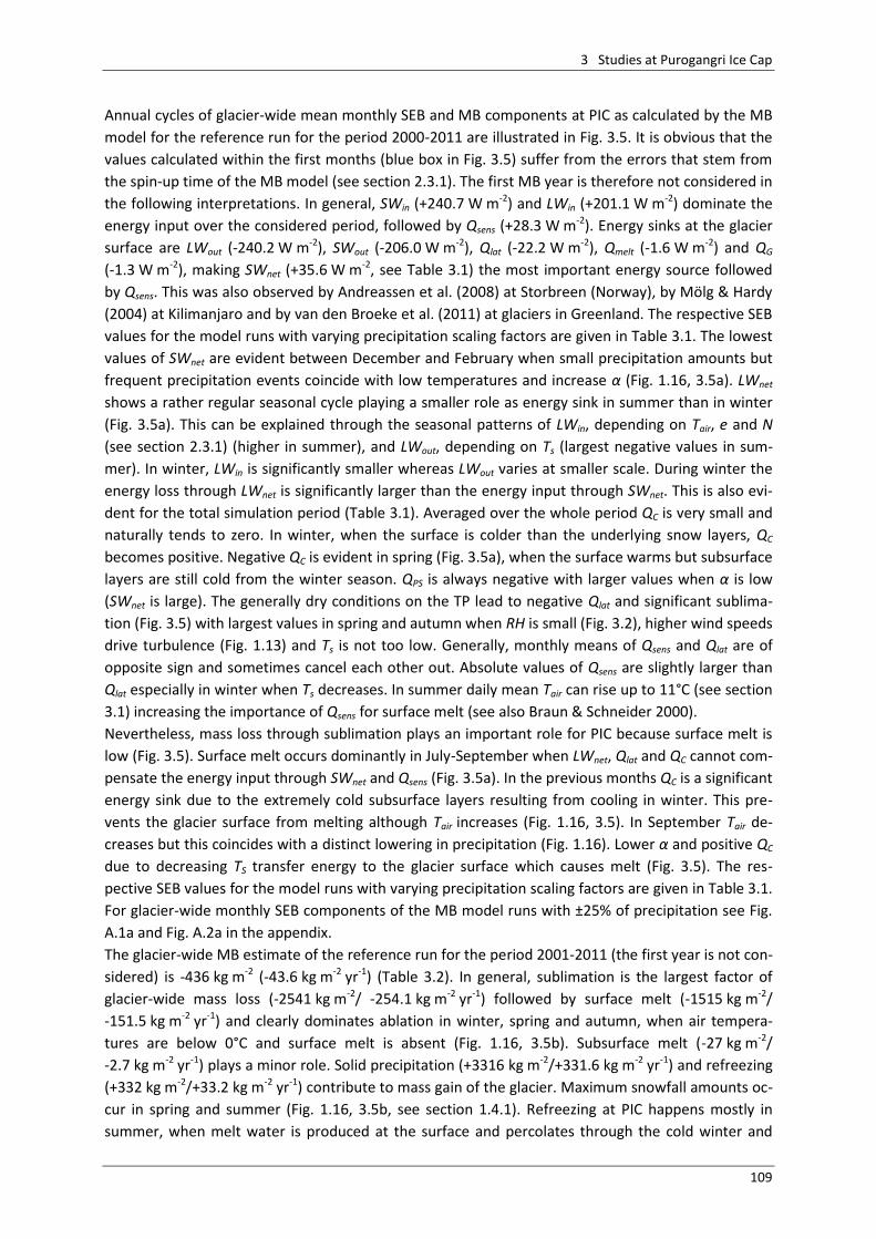
3 Studies at Purogangri Ice Cap
109
Annual cycles of glacier-wide mean monthly SEB and MB components at PIC as calculated by the MB
model for the reference run for the period 2000-2011 are illustrated in Fig. 3.5. It is obvious that the
values calculated within the first months (blue box in Fig. 3.5) suffer from the errors that stem from
the spin-up time of the MB model (see section 2.3.1). The first MB year is therefore not considered in
the following interpretations. In general, SWin (+240.7 W m-2) and LWin (+201.1 W m-2) dominate the
energy input over the considered period, followed by Qsens (+28.3 W m-2). Energy sinks at the glacier
surface are LWout (-240.2 W m-2), SWout (-206.0 W m-2), Qlat (-22.2 W m-2), Qmelt (-1.6 W m-2) and QG
(-1.3 W m-2), making SWnet (+35.6 W m-2, see Table 3.1) the most important energy source followed
by Qsens. This was also observed by Andreassen et al. (2008) at Storbreen (Norway), by Mölg & Hardy
(2004) at Kilimanjaro and by van den Broeke et al. (2011) at glaciers in Greenland. The respective SEB
values for the model runs with varying precipitation scaling factors are given in Table 3.1. The lowest
values of SWnet are evident between December and February when small precipitation amounts but
frequent precipitation events coincide with low temperatures and increase α (Fig. 1.16, 3.5a). LWnet
shows a rather regular seasonal cycle playing a smaller role as energy sink in summer than in winter
(Fig. 3.5a). This can be explained through the seasonal patterns of LWin, depending on Tair, e and N
(see section 2.3.1) (higher in summer), and LWout, depending on Ts (largest negative values in sum-
mer). In winter, LWin is significantly smaller whereas LWout varies at smaller scale. During winter the
energy loss through LWnet is significantly larger than the energy input through SWnet. This is also evi-
dent for the total simulation period (Table 3.1). Averaged over the whole period QC is very small and
naturally tends to zero. In winter, when the surface is colder than the underlying snow layers, QC
becomes positive. Negative QC is evident in spring (Fig. 3.5a), when the surface warms but subsurface
layers are still cold from the winter season. QPS is always negative with larger values when α is low
(SWnet is large). The generally dry conditions on the TP lead to negative Qlat and significant sublima-
tion (Fig. 3.5) with largest values in spring and autumn when RH is small (Fig. 3.2), higher wind speeds
drive turbulence (Fig. 1.13) and Ts is not too low. Generally, monthly means of Qsens and Qlat are of
opposite sign and sometimes cancel each other out. Absolute values of Qsens are slightly larger than
Qlat especially in winter when Ts decreases. In summer daily mean Tair can rise up to 11°C (see section
3.1) increasing the importance of Qsens for surface melt (see also Braun & Schneider 2000).
Nevertheless, mass loss through sublimation plays an important role for PIC because surface melt is
low (Fig. 3.5). Surface melt occurs dominantly in July-September when LWnet, Qlat and QC cannot com-
pensate the energy input through SWnet and Qsens (Fig. 3.5a). In the previous months QC is a significant
energy sink due to the extremely cold subsurface layers resulting from cooling in winter. This pre-
vents the glacier surface from melting although Tair increases (Fig. 1.16, 3.5). In September Tair de-
creases but this coincides with a distinct lowering in precipitation (Fig. 1.16). Lower α and positive QC
due to decreasing TS transfer energy to the glacier surface which causes melt (Fig. 3.5). The res-
pective SEB values for the model runs with varying precipitation scaling factors are given in Table 3.1.
For glacier-wide monthly SEB components of the MB model runs with ±25% of precipitation see Fig.
A.1a and Fig. A.2a in the appendix.
The glacier-wide MB estimate of the reference run for the period 2001-2011 (the first year is not con-
sidered) is -436 kg m-2 (-43.6 kg m-2 yr-1) (Table 3.2). In general, sublimation is the largest factor of
glacier-wide mass loss (-2541 kg m-2/ -254.1 kg m-2 yr-1) followed by surface melt (-1515 kg m-2/
-151.5 kg m-2 yr-1) and clearly dominates ablation in winter, spring and autumn, when air tempera-
tures are below 0°C and surface melt is absent (Fig. 1.16, 3.5b). Subsurface melt (-27 kg m-2/
-2.7 kg m-2 yr-1) plays a minor role. Solid precipitation (+3316 kg m-2/+331.6 kg m-2 yr-1) and refreezing
(+332 kg m-2/+33.2 kg m-2 yr-1) contribute to mass gain of the glacier. Maximum snowfall amounts oc-
cur in spring and summer (Fig. 1.16, 3.5b, see section 1.4.1). Refreezing at PIC happens mostly in
summer, when melt water is produced at the surface and percolates through the cold winter and
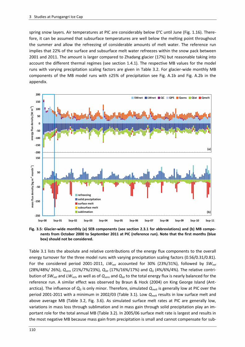
3 Studies at Purogangri Ice Cap
110
spring snow layers. Air temperatures at PIC are considerably below 0°C until June (Fig. 1.16). There-
fore, it can be assumed that subsurface temperatures are well below the melting point throughout
the summer and allow the refreezing of considerable amounts of melt water. The reference run
implies that 22% of the surface and subsurface melt water refreezes within the snow pack between
2001 and 2011. The amount is larger compared to Zhadang glacier (17%) but reasonable taking into
account the different thermal regimes (see section 1.4.1). The respective MB values for the model
runs with varying precipitation scaling factors are given in Table 3.2. For glacier-wide monthly MB
components of the MB model runs with ±25% of precipitation see Fig. A.1b and Fig. A.2b in the
appendix.
Fig. 3.5: Glacier-wide monthly (a) SEB components (see section 2.3.1 for abbreviations) and (b) MB compo-
nents from October 2000 to September 2011 at PIC (reference run). Note that the first months (blue box) should not be considered.
Table 3.1 lists the absolute and relative contributions of the energy flux components to the overall
energy turnover for the three model runs with varying precipitation scaling factors (0.56/0.31/0.81).
For the considered period 2001-2011, LWnet accounted for 30% (23%/31%), followed by SWnet
(28%/48%/ 26%), Qsens (21%/7%/23%), Qlat (17%/16%/17%) and QG (4%/6%/4%). The relative contri-
bution of SWnet and LWnet, as well as of Qsens and Qlat to the total energy flux is nearly balanced for the
reference run. A similar effect was observed by Braun & Hock (2004) on King George Island (Ant-
arctica). The influence of QG is only minor. Therefore, simulated Qmelt is generally low at PIC over the
period 2001-2011 with a minimum in 2002/03 (Table 3.1). Low Qmelt results in low surface melt and
above average MB (Table 3.2, Fig. 3.6). As simulated surface melt rates at PIC are generally low,
variations in mass loss through sublimation and in mass gain through solid precipitation play an im-
portant role for the total annual MB (Table 3.2). In 2005/06 surface melt rate is largest and results in
the most negative MB because mass gain from precipitation is small and cannot compensate for sub-
3 Studies at Purogangri Ice Cap
111
limation. However, in 2010/11 surface melt is only slightly lower but MB is positive due to large pre-
cipitation amounts, increased refreezing and less sublimation. Over the total simulation period,
effective melt (surface melt + subsurface melt - refreezing) accounts only for 32% (84%/21%) and
sublimation for 68% (16%/79%) of the total mass loss (Table 3.2).
The importance of the various SEB and MB components to surface melt and MB differs largely within
the three model runs. Firstly, with decreasing precipitation compared to the reference run (scaling
factor 0.31) the relative contribution of SWnet to the total energy flux increases through decreasing α.
The differences in SWnet between the two model runs (0.56/0.31) are largest in 2001/02, 2002/03
and 2005/06. Qsens is significantly smaller in the respective years indicating an increase in Ts. This is
supported by the large negative increase in QG meaning that more energy from the surface is trans-
ferred into the snow or ice and warms the subsurface. However, this energy transfer cannot com-
pensate for the large SWnet that causes a strong negative increase of Qmelt, surface melt and an above
average decrease of MB in the respective years (Table 3.1, 3.2, Fig. 3.6). In the model run with de-
creased precipitation relative to the reference run (scaling factor 0.31) MB is closer linked to surface
melt, because the contribution of effective melt to total mass loss increased to 84% (Table. 3.2).
Annual and total averages of LWnet and Qlat do not experience large variations through varying preci-
pitation amounts by ±25%. However, they follow the pattern of SWnet with larger variations in the
respective years (Table 3.1) because the decrease in α and increasing Ts affect all SEB components
(see sections 1.3.4.1 and 2.3.1). The year 2005/06 is characterized by higher Qmelt and low annual pre-
cipitation even in the reference run (Table 3.1, 3.2). Thus, the tipping point to further increased mass
loss is closer than in the other MB years. A precipitation increase relative to the reference run (sca-
ling factor 0.81) causes overall positive MB at PIC (Fig. 3.6) but the differences in the SEB and MB
components to the reference run are less distinct (Tab. 3.1, 3.2, Fig. 3.6). It could be revealed in Fig.
3.4 that only the lowest regions of PIC are sensitive to an increase in precipitation by 25% whereas a
decrease by 25% affects almost all regions except for the uppermost parts. Therefore, based on the
reference run the overall mass balance response for a 25%-increase in precipitation is smaller than
for 25% decreasing precipitation.
Model results for PIC can be evaluated against surface height changes and geodetic MB estimations
from TerraSAR-X data (Neckel et al. 2013). In this study total modelled MB for the total ice cap
between 2001 and 2011 with varying precipitation scaling factors (0.56/0.31/0.81) is -436 kg m-2
(-22979 kg m-2/+1618 kg m-2) with annual means of -44 kg m-2 yr-1 (-2298 kg m-2 yr-1/+161 kg m-2 yr-1).
Neckel et al. (2013) employed Differential Synthetic Aperture Radar Interferometry (DInSAR) to derive
surface elevation changes for PIC between February 2000 and January 2012. An average ice density
of 900±17 kg m-3 was applied for the conversion into mass changes. Neckel et al. (2013) estimated an
annual MB of -44±15 kg m-2 yr-1 for the period 2000-2012. Respective surface height change over the
total ice cap is -0.58 m (-26 m / +2.1 m) within this study and -0.59±2.4 m in Neckel et al. (2013). Both
results are totally within the assumed uncertainty ranges and confirm the reasonable performance of
the MB model. Additionally, Neckel et al. (2013) give surface height changes and MB for the single
glaciers of PIC (see Fig. 3.1). The given values are again compared to the MB model calculations. The
results are visualized in Fig. 3.7. For all glaciers the results for surface height change and MB from
both studies are within the given uncertainties. The results for glacier 11 can not be compared be-
cause large parts of the accumulation area are not covered by the interferometric data set (Fig. 3.8).
Possible reasons for the discrepancies in surface height change and MB can be revealed from the
spatial comparison of the results of both studies. It is evident in Fig. 3.8 that a glacier thinning
occurred in the lower parts of the ice cap while a slightly thickening appears in the upper regions
around 6000 m a.s.l. where a large proportion of the glacier area is located (Fig. 1.16). This spatial
pattern agrees well within the two data sets. The result of Neckel et al. (2013) indicates a stronger
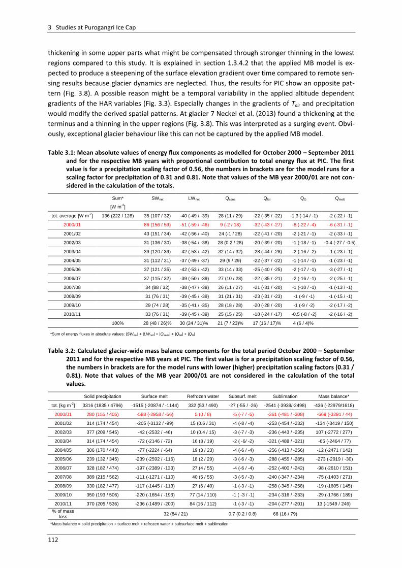
3 Studies at Purogangri Ice Cap
112
thickening in some upper parts what might be compensated through stronger thinning in the lowest
regions compared to this study. It is explained in section 1.3.4.2 that the applied MB model is ex-
pected to produce a steepening of the surface elevation gradient over time compared to remote sen-
sing results because glacier dynamics are neglected. Thus, the results for PIC show an opposite pat-
tern (Fig. 3.8). A possible reason might be a temporal variability in the applied altitude dependent
gradients of the HAR variables (Fig. 3.3). Especially changes in the gradients of Tair and precipitation
would modify the derived spatial patterns. At glacier 7 Neckel et al. (2013) found a thickening at the
terminus and a thinning in the upper regions (Fig. 3.8). This was interpreted as a surging event. Obvi-
ously, exceptional glacier behaviour like this can not be captured by the applied MB model.
Table 3.1: Mean absolute values of energy flux components as modelled for October 2000 – September 2011
and for the respective MB years with proportional contribution to total energy flux at PIC. The first value is for a precipitation scaling factor of 0.56, the numbers in brackets are for the model runs for a scaling factor for precipitation of 0.31 and 0.81. Note that values of the MB year 2000/01 are not con-sidered in the calculation of the totals.
Sum* SWnet LWnet Qsens Qlat QG Qmelt
[W m-2
]
tot. average [W m-2
] 136 (222 / 128) 35 (107 / 32) -40 (-49 / -39) 28 (11 / 29) -22 (-35 / -22) -1.3 (-14 / -1) -2 (-22 / -1)
2000/01 86 (156 / 59) -51 (-59 / -46) 9 (-2 / 18) -32 (-43 / -27) -8 (-22 / -4) -6 (-31 / -1)
2001/02 43 (151 / 34) -42 (-56 / -40) 24 (-1 / 28) -22 (-41 / -20) -2 (-21 / -1) -2 (-33 / -1)
2002/03 31 (136 / 30) -38 (-54 / -38) 28 (0.2 / 28) -20 (-39 / -20) -1 (-18 / -1) -0.4 (-27 / -0.5)
2003/04 39 (120 / 39) -42 (-53 / -42) 32 (14 / 32) -28 (-44 / -28) -2 (-16 / -2) -1 (-23 / -1)
2004/05 31 (112 / 31) -37 (-49 / -37) 29 (9 / 29) -22 (-37 / -22) -1 (-14 / -1) -1 (-23 / -1)
2005/06 37 (121 / 35) -42 (-53 / -42) 33 (14 / 33) -25 (-40 / -25) -2 (-17 / -1) -3 (-27 / -1)
2006/07 37 (115 / 32) -39 (-50 / -39) 27 (10 / 28) -22 (-35 / -21) -2 (-16 / -1) -2 (-25 / -1)
2007/08 34 (88 / 32) -38 (-47 / -38) 26 (11 / 27) -21 (-31 / -20) -1 (-10 / -1) -1 (-13 / -1)
2008/09 31 (76 / 31) -39 (-45 / -39) 31 (21 / 31) -23 (-31 / -23) -1 (-9 / -1) -1 (-15 / -1)
2009/10 29 (74 / 28) -35 (-41 / -35) 28 (18 / 28) -20 (-28 / -20) -1 (-9 / -2) -2 (-17 / -2)
2010/11 33 (76 / 31) -39 (-45 / -39) 25 (15 / 25) -18 (-24 / -17) -0.5 (-8 / -2) -2 (-16 / -2)
100% 28 (48 / 26)% 30 (24 / 31)% 21 (7 / 23)% 17 (16 / 17)% 4 (6 / 4)%
*Sum of energy fluxes in absolute values: |SWnet| + |LWnet| + |Qsens| + |Qlat| + |QG|
Table 3.2: Calculated glacier-wide mass balance components for the total period October 2000 – September
2011 and for the respective MB years at PIC. The first value is for a precipitation scaling factor of 0.56, the numbers in brackets are for the model runs with lower (higher) precipitation scaling factors (0.31 / 0.81). Note that values of the MB year 2000/01 are not considered in the calculation of the total values.
Solid precipitation Surface melt Refrozen water Subsurf. melt Sublimation Mass balance*
tot. [kg m-2
] 3316 (1835 / 4796) -1515 (-20874 / -1144) 332 (53 / 490) -27 (-55 / -26) -2541 (-3939/-2498) -436 (-22979/1618)
2000/01 280 (155 / 405) -588 (-2958 / -56) 5 (0 / 8) -5 (-7 / -5) -361 (-481 / -308) -669 (-3291 / 44)
2001/02 314 (174 / 454) -205 (-3132 / -99) 15 (0.6 / 31) -4 (-8 / -4) -253 (-454 / -232) -134 (-3419 / 150)
2002/03 377 (209 / 545) -42 (-2532 / -46) 10 (0.4 / 15) -3 (-7 / -3) -236 (-443 / -235) 107 (-2772 / 277)
2003/04 314 (174 / 454) -72 (-2146 / -72) 16 (3 / 19) -2 ( -6/ -2) -321 (-488 / -321) -65 (-2464 / 77)
2004/05 306 (170 / 443) -77 (-2224 / -64) 19 (3 / 23) -4 (-6 / -4) -256 (-413 / -256) -12 (-2471 / 142)
2005/06 239 (132 / 345) -239 (-2592 / -116) 18 (2 / 29) -3 (-6 / -3) -288 (-455 / -285) -273 (-2919 / -30)
2006/07 328 (182 / 474) -197 (-2389 / -133) 27 (4 / 55) -4 (-6 / -4) -252 (-400 / -242) -98 (-2610 / 151)
2007/08 389 (215 / 562) -111 (-1271 / -110) 40 (5 / 55) -3 (-5 / -3) -240 (-347 / -234) -75 (-1403 / 271)
2008/09 330 (182 / 477) -117 (-1445 / -113) 27 (6 / 40) -1 (-3 / -1) -258 (-345 / -258) -19 (-1605 / 145)
2009/10 350 (193 / 506) -220 (-1654 / -193) 77 (14 / 110) -1 ( -3 / -1) -234 (-316 / -233) -29 (-1766 / 189)
2010/11 370 (205 / 536) -236 (-1489 / -200) 84 (16 / 112) -1 (-3 / -1) -204 (-277 / -201) 13 (-1549 / 246)
% of mass loss
32 (84 / 21) 0.7 (0.2 / 0.8) 68 (16 / 79)
*Mass balance = solid precipitation + surface melt + refrozen water + subsurface melt + sublimation
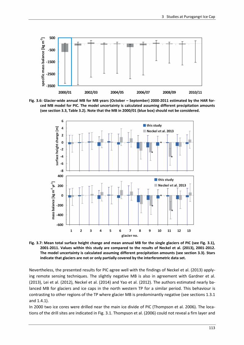
3 Studies at Purogangri Ice Cap
113
Fig. 3.6: Glacier-wide annual MB for MB years (October – September) 2000-2011 estimated by the HAR for-
ced MB model for PIC. The model uncertainty is calculated assuming different precipitation amounts (see section 3.3, Table 3.2). Note that the MB in 2000/01 (blue box) should not be considered.
Fig. 3.7: Mean total surface height change and mean annual MB for the single glaciers of PIC (see Fig. 3.1),
2001-2011. Values within this study are compared to the results of Neckel et al. (2013), 2001-2012. The model uncertainty is calculated assuming different precipitation amounts (see section 3.3). Stars indicate that glaciers are not or only partially covered by the interferometric data set.
Nevertheless, the presented results for PIC agree well with the findings of Neckel et al. (2013) apply-
ing remote sensing techniques. The slightly negative MB is also in agreement with Gardner et al.
(2013), Lei et al. (2012), Neckel et al. (2014) and Yao et al. (2012). The authors estimated nearly ba-
lanced MB for glaciers and ice caps in the north western TP for a similar period. This behaviour is
contrasting to other regions of the TP where glacier MB is predominantly negative (see sections 1.3.1
and 1.4.1).
In 2000 two ice cores were drilled near the main ice divide of PIC (Thompson et al. 2006). The loca-
tions of the drill sites are indicated in Fig. 3.1. Thompson et al. (2006) could not reveal a firn layer and
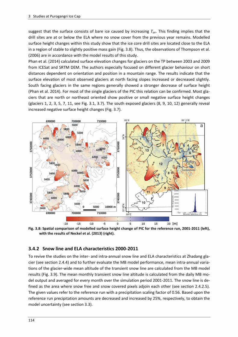
3 Studies at Purogangri Ice Cap
114
suggest that the surface consists of bare ice caused by increasing Tair. This finding implies that the
drill sites are at or below the ELA where no snow cover from the previous year remains. Modelled
surface height changes within this study show that the ice core drill sites are located close to the ELA
in a region of stable to slightly positive mass gain (Fig. 3.8). Thus, the observations of Thompson et al.
(2006) are in accordance with the model results of this study.
Phan et al. (2014) calculated surface elevation changes for glaciers on the TP between 2003 and 2009
from ICESat and SRTM DEM. The authors especially focused on different glacier behaviour on short
distances dependent on orientation and position in a mountain range. The results indicate that the
surface elevation of most observed glaciers at north facing slopes increased or decreased slightly.
South facing glaciers in the same regions generally showed a stronger decrease of surface height
(Phan et al. 2014). For most of the single glaciers of the PIC this relation can be confirmed. Most gla-
ciers that are north or northeast oriented show positive or small negative surface height changes
(glaciers 1, 2, 3, 5, 7, 11, see Fig. 3.1, 3.7). The south exposed glaciers (8, 9, 10, 12) generally reveal
increased negative surface height changes (Fig. 3.7).
Fig. 3.8: Spatial comparison of modelled surface height change of PIC for the reference run, 2001-2011 (left),
with the results of Neckel et al. (2013) (right).
3.4.2 Snow line and ELA characteristics 2000-2011
To revive the studies on the inter- and intra-annual snow line and ELA characteristics at Zhadang gla-
cier (see section 2.4.4) and to further evaluate the MB model performance, mean intra-annual varia-
tions of the glacier-wide mean altitude of the transient snow line are calculated from the MB model
results (Fig. 3.9). The mean monthly transient snow line altitude is calculated from the daily MB mo-
del output and averaged for every month over the simulation period 2001-2011. The snow line is de-
fined as the area where snow free and snow covered pixels adjoin each other (see section 2.4.2.5).
The given values refer to the reference run with a precipitation scaling factor of 0.56. Based upon the
reference run precipitation amounts are decreased and increased by 25%, respectively, to obtain the
model uncertainty (see section 3.3).
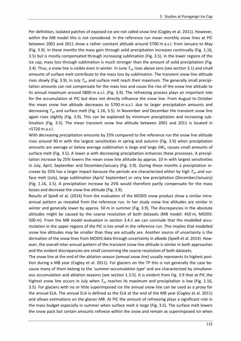
3 Studies at Purogangri Ice Cap
115
Per definition, isolated patches of exposed ice are not called snow line (Cogley et al. 2011). However,
within the MB model this is not considered. In the reference run mean monthly snow lines at PIC
between 2001 and 2011 show a rather constant altitude around 5700 m a.s.l. from January to May
(Fig. 3.9). In these months the mass gain through solid precipitation increases continually (Fig. 1.16,
3.5) but is mostly compensated through increasing sublimation (Fig. 3.5). In the lower regions of the
ice cap, mass loss through sublimation is much stronger than the amount of solid precipitation (Fig.
3.4). Thus, a snow line is visible even in winter. In June Tair rises above zero (see section 3.1) and small
amounts of surface melt contribute to the mass loss by sublimation. The transient snow line altitude
rises slowly (Fig. 3.9). In July Tair and surface melt reach their maximum. The generally small precipi-
tation amounts can not compensate for the mass loss and cause the rise of the snow line altitude to
its annual maximum around 5800 m a.s.l. (Fig. 3.9). The refreezing process plays an important role
for the accumulation at PIC but does not directly influence the snow line. From August to October
the mean snow line altitude decreases to 5700 m a.s.l. due to larger precipitation amounts and
decreasing Tair and surface melt (Fig. 1.16, 3.5). In November and December the transient snow line
again rises slightly (Fig. 3.9). This can be explained by minimum precipitation and increasing sub-
limation (Fig. 3.5). The mean transient snow line altitude between 2001 and 2011 is located in
≈5720 m a.s.l.
With decreasing precipitation amounts by 25% compared to the reference run the snow line altitude
rises around 90 m with the largest sensitivities in spring and autumn (Fig. 3.9) when precipitation
amounts are average or below average sublimation is large and large SWin causes small amounts of
surface melt (Fig. 3.5). A lower α with decreasing precipitation enhances these processes. A precipi-
tation increase by 25% lowers the mean snow line altitude by approx. 10 m with largest sensitivities
in July, April, September and December/January (Fig. 3.9). During these months a precipitation in-
crease by 25% has a larger impact because the periods are characterized either by high Tair and sur-
face melt (July), large sublimation (April/ September) or very low precipitation (December/January)
(Fig. 1.16, 3.5). A precipitation increase by 25% would therefore partly compensate for the mass
losses and decrease the snow line altitude (Fig. 3.9).
Results of Spieß et al. (2014) from the evaluation of the MODIS snow product show a similar intra-
annual pattern as revealed from the reference run. In her study snow line altitudes are similar in
winter and generally lower by approx. 50 m in summer (Fig. 3.9). The discrepancies in the absolute
altitudes might be caused by the coarse resolution of both datasets (MB model: 450 m, MODIS:
500 m). From the MB model evaluation in section 3.4.1 we can conclude that the modelled accu-
mulation in the upper regions of the PIC is too small in the reference run. This implies that modelled
snow line altitudes may be smaller than they are actually are. Another source of uncertainty is the
derivation of the snow lines from MODIS data through uncertainty in albedo (Spieß et al. 2014). How-
ever, the overall inter-annual pattern of the transient snow line altitude is similar in both approaches
and the evident discrepancies are small concerning the coarse resolution of both datasets.
The snow line at the end of the ablation season (annual snow line) usually represents its highest posi-
tion during a MB year (Cogley et al. 2011). For glaciers on the TP this is not generally the case be-
cause many of them belong to the ‘summer-accumulation type’ and are characterized by simultane-
ous accumulation and ablation seasons (see section 1.3.5). It is evident from Fig. 3.9 that at PIC the
highest snow line occurs in July when Tair reaches its maximum and precipitation is low (Fig. 1.16,
3.5). For glaciers with no or little superimposed ice the annual snow line can be used as a proxy for
the annual ELA. The annual ELA is defined as the ELA at the end of the MB year (Cogley et al. 2011)
and allows estimations on the glacier MB. At PIC the amount of refreezing plays a significant role in
the mass budget especially in summer when surface melt is large (Fig. 3.5). The surface melt lowers
the snow pack but certain amounts refreeze within the snow and remain as superimposed ice when
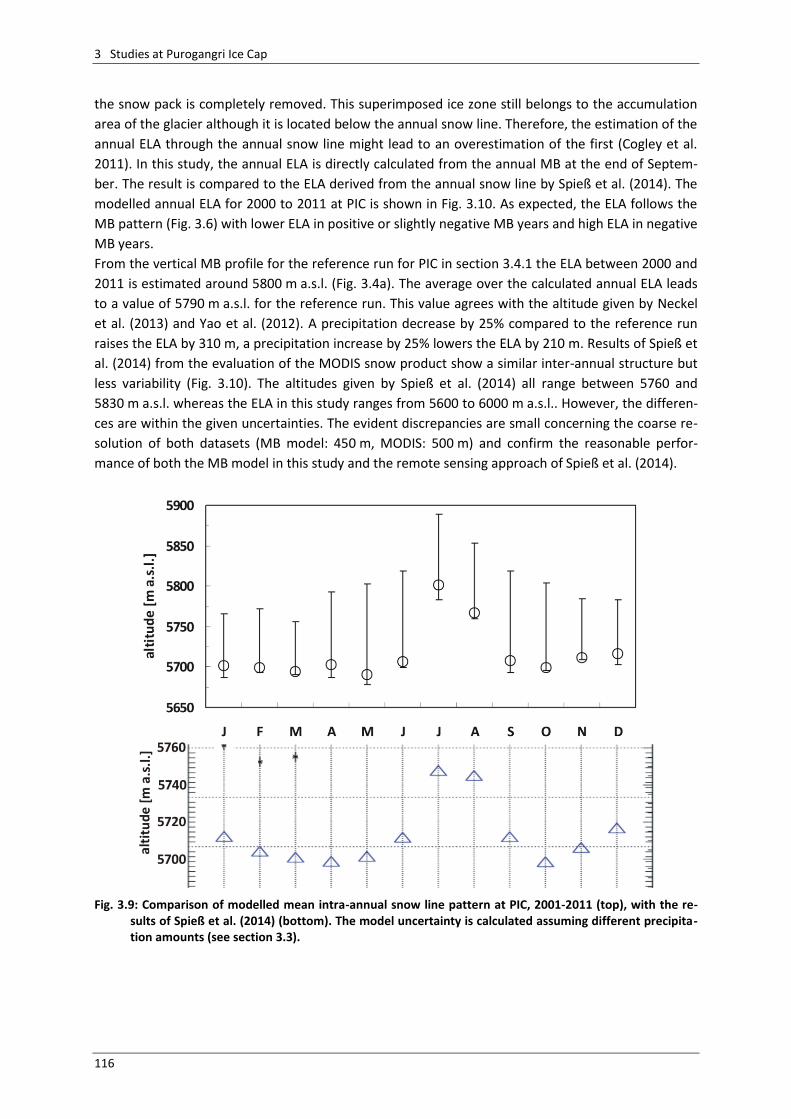
3 Studies at Purogangri Ice Cap
116
the snow pack is completely removed. This superimposed ice zone still belongs to the accumulation
area of the glacier although it is located below the annual snow line. Therefore, the estimation of the
annual ELA through the annual snow line might lead to an overestimation of the first (Cogley et al.
2011). In this study, the annual ELA is directly calculated from the annual MB at the end of Septem-
ber. The result is compared to the ELA derived from the annual snow line by Spieß et al. (2014). The
modelled annual ELA for 2000 to 2011 at PIC is shown in Fig. 3.10. As expected, the ELA follows the
MB pattern (Fig. 3.6) with lower ELA in positive or slightly negative MB years and high ELA in negative
MB years.
From the vertical MB profile for the reference run for PIC in section 3.4.1 the ELA between 2000 and
2011 is estimated around 5800 m a.s.l. (Fig. 3.4a). The average over the calculated annual ELA leads
to a value of 5790 m a.s.l. for the reference run. This value agrees with the altitude given by Neckel
et al. (2013) and Yao et al. (2012). A precipitation decrease by 25% compared to the reference run
raises the ELA by 310 m, a precipitation increase by 25% lowers the ELA by 210 m. Results of Spieß et
al. (2014) from the evaluation of the MODIS snow product show a similar inter-annual structure but
less variability (Fig. 3.10). The altitudes given by Spieß et al. (2014) all range between 5760 and
5830 m a.s.l. whereas the ELA in this study ranges from 5600 to 6000 m a.s.l.. However, the differen-
ces are within the given uncertainties. The evident discrepancies are small concerning the coarse re-
solution of both datasets (MB model: 450 m, MODIS: 500 m) and confirm the reasonable perfor-
mance of both the MB model in this study and the remote sensing approach of Spieß et al. (2014).
Fig. 3.9: Comparison of modelled mean intra-annual snow line pattern at PIC, 2001-2011 (top), with the re-sults of Spieß et al. (2014) (bottom). The model uncertainty is calculated assuming different precipita-tion amounts (see section 3.3).
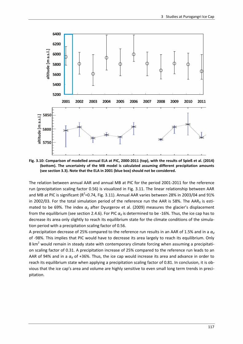
3 Studies at Purogangri Ice Cap
117
Fig. 3.10: Comparison of modelled annual ELA at PIC, 2000-2011 (top), with the results of Spieß et al. (2014) (bottom). The uncertainty of the MB model is calculated assuming different precipitation amounts (see section 3.3). Note that the ELA in 2001 (blue box) should not be considered.
The relation between annual AAR and annual MB at PIC for the period 2001-2011 for the reference
run (precipitation scaling factor 0.56) is visualized in Fig. 3.11. The linear relationship between AAR
and MB at PIC is significant (R2=0.74, Fig. 3.11). Annual AAR varies between 28% in 2003/04 and 91%
in 2002/03. For the total simulation period of the reference run the AAR is 58%. The AAR0 is esti-
mated to be 69%. The index αd after Dyurgerov et al. (2009) measures the glacier’s displacement
from the equilibrium (see section 2.4.6). For PIC αd is determined to be -16%. Thus, the ice cap has to
decrease its area only slightly to reach its equilibrium state for the climate conditions of the simula-
tion period with a precipitation scaling factor of 0.56.
A precipitation decrease of 25% compared to the reference run results in an AAR of 1.5% and in a αd
of -98%. This implies that PIC would have to decrease its area largely to reach its equilibrium. Only
8 km2 would remain in steady state with contemporary climate forcing when assuming a precipitati-
on scaling factor of 0.31. A precipitation increase of 25% compared to the reference run leads to an
AAR of 94% and in a αd of +36%. Thus, the ice cap would increase its area and advance in order to
reach its equilibrium state when applying a precipitation scaling factor of 0.81. In conclusion, it is ob-
vious that the ice cap’s area and volume are highly sensitive to even small long term trends in preci-
pitation.
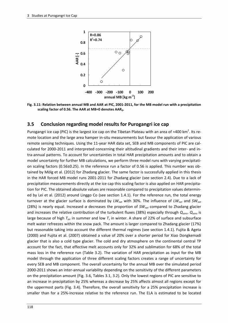
3 Studies at Purogangri Ice Cap
118
Fig. 3.11: Relation between annual MB and AAR at PIC, 2001-2011, for the MB model run with a precipitation
scaling factor of 0.56. The AAR at MB=0 denotes AAR0.
3.5 Conclusion regarding model results for Purogangri ice cap
Purogangri ice cap (PIC) is the largest ice cap on the Tibetan Plateau with an area of ≈400 km2. Its re-
mote location and the large area hamper in-situ measurements but favour the application of various
remote sensing techniques. Using the 11-year HAR data set, SEB and MB components of PIC are cal-
culated for 2000-2011 and interpreted concerning their altitudinal gradients and their inter- and in-
tra-annual patterns. To account for uncertainties in total HAR precipitation amounts and to obtain a
model uncertainty for further MB calculations, we perform three model runs with varying precipitati-
on scaling factors (0.56±0.25). In the reference run a factor of 0.56 is applied. This number was ob-
tained by Mölg et al. (2012) for Zhadang glacier. The same factor is successfully applied in this thesis
in the HAR forced MB model runs 2001-2011 for Zhadang glacier (see section 2.4). Due to a lack of
precipitation measurements directly at the ice cap this scaling factor is also applied on HAR precipita-
tion for PIC. The obtained absolute values are reasonable compared to precipitation values determin-
ed by Lei et al. (2012) around Linggo Co (see section 1.4.1). For the reference run, the total energy
turnover at the glacier surface is dominated by LWnet with 30%. The influence of LWnet and SWnet
(28%) is nearly equal. Increased α decreases the proportion of SWnet compared to Zhadang glacier
and increases the relative contribution of the turbulent fluxes (38%) especially through Qsens. Qsens is
large because of high Tair in summer and low Ts in winter. A share of 22% of surface and subsurface
melt water refreezes within the snow pack. The amount is larger compared to Zhadang glacier (17%)
but reasonable taking into account the different thermal regimes (see section 1.4.1). Fujita & Ageta
(2000) and Fujita et al. (2007) obtained a value of 20% over a shorter period for Xiao Dongkemadi
glacier that is also a cold type glacier. The cold and dry atmosphere on the continental central TP
account for the fact, that effective melt accounts only for 32% and sublimation for 68% of the total
mass loss in the reference run (Table 3.2). The variation of HAR precipitation as input for the MB
model through the application of three different scaling factors creates a range of uncertainty for
every SEB and MB component. The overall uncertainty for the annual MB over the simulated period
2000-2011 shows an inter-annual variability depending on the sensitivity of the different parameters
on the precipitation amount (Fig. 3.6, Tables 3.1, 3.2). Only the lowest regions of PIC are sensitive to
an increase in precipitation by 25% whereas a decrease by 25% affects almost all regions except for
the uppermost parts (Fig. 3.4). Therefore, the overall sensitivity for a 25% precipitation increase is
smaller than for a 25%-increase relative to the reference run. The ELA is estimated to be located
3 Studies at Purogangri Ice Cap
119
around 5790 m a.s.l. in the reference run. A precipitation decrease by 25% raises the ELA by ≈300 m,
a precipitation increase by 25% lowers the ELA by ≈200 m. These values are within the range given by
Neckel et al. (2013) and Yao et al. (2012).
The large area of the PIC favours the application of remote sensing approaches for the analysis of
surface elevation changes, MB and snow line altitudes. These data sets are a good opportunity to
evaluate the MB model performance because the remote location and the large size of the ice cap
hamper in-situ measurements. The comparison of the MB model with glacier-wide surface height
changes and geodetic MB estimations from TerraSAR-X data for a similar period (Neckel et al. 2013)
show only minor discrepancies for the reference run. Concerning the single glaciers of the ice cap the
results for surface height change and MB from both studies are within the given ranges of uncertain-
ties despite the coarse resolution of 450 m of the MB model domain. The spatial evaluation (Fig. 3.7,
3.8) shows no regional errors. This justifies the application of only one mean altitudinal gradient for
each HAR input parameter for the entire ice cap (see section 3.2). In general, the MB model simu-
lates less glacier thickening in some higher regions for the reference run what is compensated by less
thinning in the lowest parts compared to Neckel et al. (2013). This suggests general discrepancies or
a temporal variability in the applied altitude dependent gradients of the HAR variables. Due to a lack
of in-situ measurements at the PIC uncertainties in the obtained gradients can not be quantified in
more detail.
The model evaluation against MODIS derived snow line altitude and annual ELA (Spieß et al. 2014)
confirms the overall satisfying model performance for PIC considering the reference run. The intra-
and inter-annual patterns of both studies agree very well whereby modelled snow line altitude is
higher in summer and the annual ELA varies stronger between the respective years. The calculated
slightly negative overall MB in the reference run is in agreement with Gardner et al. (2013), Lei et al.
(2012), Neckel et al. (2014) and Yao et al. (2012). These authors estimated nearly balanced MB for
glaciers and ice caps in the north western TP for a similar period. These results support the applicabi-
lity of the precipitation scaling factor of 0.56 revealed for Zhadang glacier (see section 2.2.3) also for
PIC.
It can be concluded from the application of the MB model to PIC that the derived intra- and inter-
annual cycles of SEB and MB components are within reasonable limits. The model result largely de-
pends on the respective patterns of the input parameters from HAR. The obtained SEB and MB com-
ponents are consistent with each other because they interact through physical relationships (see sec-
tions 1.3.4 and 2.3.1). The application of a precipitation scaling factor of 0.56 as determined for Zha-
dang glacier yields satisfying results that could be confirmed based on different remote sensing
approaches.

4 Studies at Naimona’nyi glacier
121
4 Energy and mass balance for Naimona’nyi glacier, south wes-tern Tibetan Plateau, 2000–2012
4.1 Introduction and regional climate conditions
Naimona’nyi glacier is a north to northwest exposed valley glacier (≈7.8 km2), located northeast of
Naimona’nyi (chin. Gurla Mandhata) the highest peak of the Nalakankar Himal (≈7700 m a.s.l., Fig.
4.1). The glacier was chosen as a measurement site within the WET project because the staff from
ITP conducted climatological and glaciological measurements at the glacier over a shorter period a
few years ago (Yao et al. 2012) and the glacier is one of the ice core drilling sites of the ITP (Liu et al.
2006). In September 2011 an AWS was installed on an ice cored moraine west of the glacier tongue
(see section 1.4.2.2). The comparison of HAR data with AWS measurements (see section 1.4.2.2)
reveals that daily mean Tair from HAR is up to 10°K lower than the respective AWS measurement.
Hourly Tair even differs by up to 12°K. The discrepancies partly might be explained by the influence of
terrain effects in the very narrow valley of the glacier tongue (Fig. 4.1). These small scale patterns can
not be captured by the atmospheric model (10 km resolution, see section 2.2.3). Thus, the estimates
of the MB model forced with HAR data can be expected to differ from in-situ measurements or re-
mote sensing analyses. We use surface height changes and the geodetic MB derived from the analy-
sis of Pleiades data (Holzer et al. 2014) to evaluate the model performance.
The region is clearly dominated by Indian monsoon in summer and mid-latitude westerlies in winter
(see section 1.4.1) and most atmospheric variables, generated by HAR show a pronounced seasonal
contrast (Fig. 1.14, 1.15, 4.2). Daily mean air temperatures generated by HAR generally rise above
zero from mid July to August. Daily means range between -31.8°C and +3.8 C (average -11.6°C) within
the period 2000-2012. Monthly means of those HAR variables that serve as input for the applied MB
model are shown in Fig. 4.2. SWin reaches its maximum around May and decreases in summer, when
monsoonal cloud cover is large. The monsoon season is associated with annual maxima in
precipitation, RH and air pressure associated with the Tibetan High (see section 1.3.1) whereas wind
speeds are generally low (Fig. 4.2). The glacier is situated in the same mountain chain as Halji glacier
but ≈26 km to the north (see sections 1.4.1, 1.4.2.2). The lee-effect of the more northern location is
clearly evident in mean annual precipitation amounts (506 mm) that are considerably smaller than at
Halji glacier (605 mm) despite the higher altitude of the considered HAR pixel (see section 1.4.1).
However, Naimona’nyi glacier has a much larger area and a greater altitudinal extent than Halji
glacier (Fig. 1.12, 1.14). Precipitation amounts increase with altitude and Tair from HAR is already low
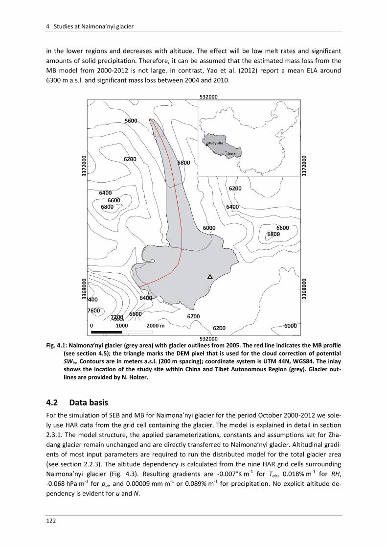
4 Studies at Naimona’nyi glacier
122
in the lower regions and decreases with altitude. The effect will be low melt rates and significant
amounts of solid precipitation. Therefore, it can be assumed that the estimated mass loss from the
MB model from 2000-2012 is not large. In contrast, Yao et al. (2012) report a mean ELA around
6300 m a.s.l. and significant mass loss between 2004 and 2010.
Fig. 4.1: Naimona’nyi glacier (grey area) with glacier outlines from 2005. The red line indicates the MB profile
(see section 4.5); the triangle marks the DEM pixel that is used for the cloud correction of potential SWin. Contours are in meters a.s.l. (200 m spacing); coordinate system is UTM 44N, WGS84. The inlay shows the location of the study site within China and Tibet Autonomous Region (grey). Glacier out-lines are provided by N. Holzer.
4.2 Data basis
For the simulation of SEB and MB for Naimona’nyi glacier for the period October 2000-2012 we sole-
ly use HAR data from the grid cell containing the glacier. The model is explained in detail in section
2.3.1. The model structure, the applied parameterizations, constants and assumptions set for Zha-
dang glacier remain unchanged and are directly transferred to Naimona’nyi glacier. Altitudinal gradi-
ents of most input parameters are required to run the distributed model for the total glacier area
(see section 2.2.3). The altitude dependency is calculated from the nine HAR grid cells surrounding
Naimona’nyi glacier (Fig. 4.3). Resulting gradients are -0.007°K m-1 for Tair, 0.018% m-1 for RH,
-0.068 hPa m-1 for ρair and 0.00009 mm m-1 or 0.089% m-1 for precipitation. No explicit altitude de-
pendency is evident for u and N.
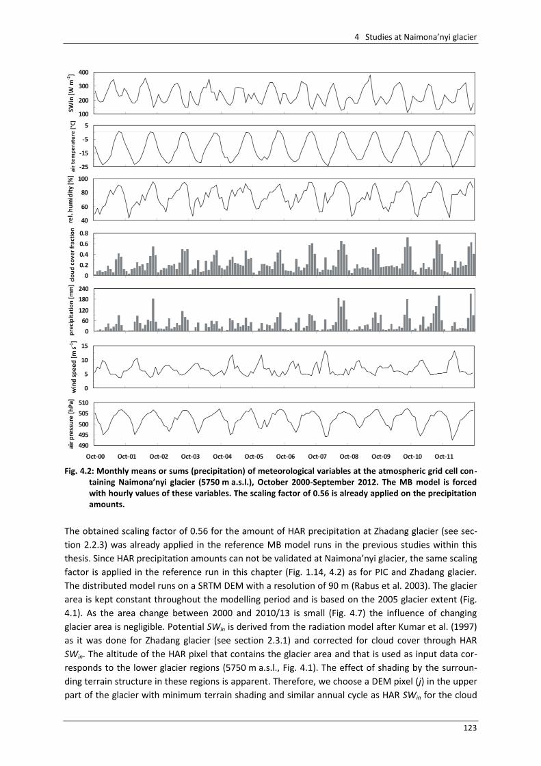
4 Studies at Naimona’nyi glacier
123
Fig. 4.2: Monthly means or sums (precipitation) of meteorological variables at the atmospheric grid cell con-
taining Naimona’nyi glacier (5750 m a.s.l.), October 2000-September 2012. The MB model is forced with hourly values of these variables. The scaling factor of 0.56 is already applied on the precipitation amounts.
The obtained scaling factor of 0.56 for the amount of HAR precipitation at Zhadang glacier (see sec-
tion 2.2.3) was already applied in the reference MB model runs in the previous studies within this
thesis. Since HAR precipitation amounts can not be validated at Naimona’nyi glacier, the same scaling
factor is applied in the reference run in this chapter (Fig. 1.14, 4.2) as for PIC and Zhadang glacier.
The distributed model runs on a SRTM DEM with a resolution of 90 m (Rabus et al. 2003). The glacier
area is kept constant throughout the modelling period and is based on the 2005 glacier extent (Fig.
4.1). As the area change between 2000 and 2010/13 is small (Fig. 4.7) the influence of changing
glacier area is negligible. Potential SWin is derived from the radiation model after Kumar et al. (1997)
as it was done for Zhadang glacier (see section 2.3.1) and corrected for cloud cover through HAR
SWin. The altitude of the HAR pixel that contains the glacier area and that is used as input data cor-
responds to the lower glacier regions (5750 m a.s.l., Fig. 4.1). The effect of shading by the surroun-
ding terrain structure in these regions is apparent. Therefore, we choose a DEM pixel (j) in the upper
part of the glacier with minimum terrain shading and similar annual cycle as HAR SWin for the cloud
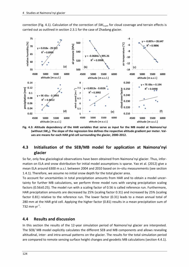
4 Studies at Naimona’nyi glacier
124
correction (Fig. 4.1). Calculation of the correction of SWin,pot for cloud coverage and terrain effects is
carried out as outlined in section 2.3.1 for the case of Zhadang glacier.
Fig. 4.3: Altitude dependency of the HAR variables that serve as input for the MB model at Naimona’nyi
(without SWin). The slope of the regression line defines the respective altitude gradient per meter. Val-ues are means for each HAR grid cell surrounding the glacier, 2000-2012.
4.3 Initialisation of the SEB/MB model for application at Naimona’nyi glacier
So far, only few glaciological observations have been obtained from Naimona’nyi glacier. Thus, infor-
mation on ELA and snow distribution for initial model assumptions is sparse. Yao et al. (2012) give a
mean ELA around 6300 m a.s.l. between 2004 and 2010 based on in–situ measurements (see section
1.4.1). Therefore, we assume no initial snow depth for the total glacier area.
To account for uncertainties in total precipitation amounts from HAR and to obtain a model uncer-
tainty for further MB calculations, we perform three model runs with varying precipitation scaling
factors (0.56±0.25). The model run with a scaling factor of 0.56 is called reference run. Furthermore,
HAR precipitation amounts are decreased by 25% (scaling factor 0.31) and increased by 25% (scaling
factor 0.81) relative to the reference run. The lower factor (0.31) leads to a mean annual total of
280 mm at the HAR grid cell. Applying the higher factor (0.81) results in a mean precipitation sum of
732 mm yr-1.
4.4 Results and discussion
In this section the results of the 12-year simulation period of Naimona’nyi glacier are interpreted.
The SEB/ MB model explicitly calculates the different SEB and MB components and allows revealing
altitudinal, inter- and intra-annual patterns on the glacier. The results for the total simulation period
are compared to remote sensing surface height changes and geodetic MB calculations (section 4.4.1).
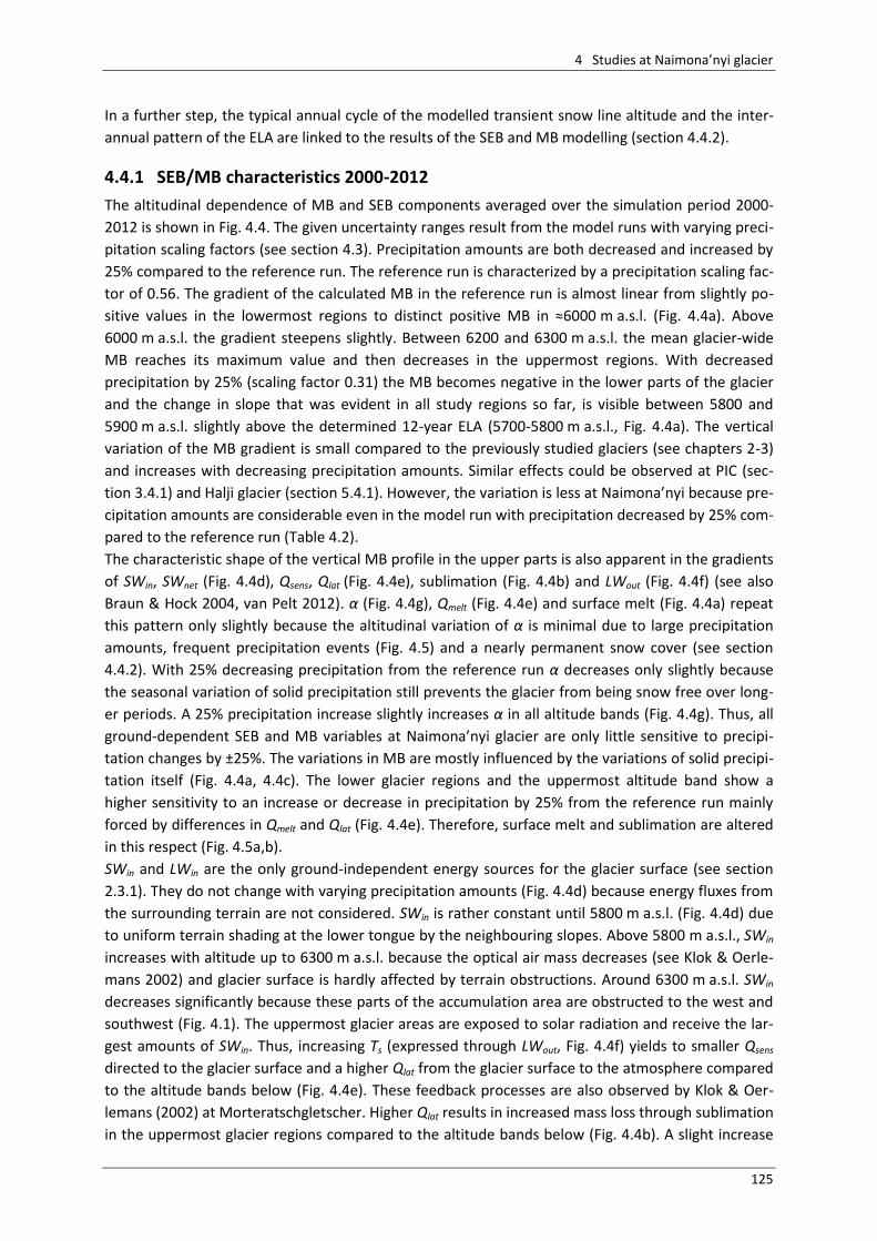
4 Studies at Naimona’nyi glacier
125
In a further step, the typical annual cycle of the modelled transient snow line altitude and the inter-
annual pattern of the ELA are linked to the results of the SEB and MB modelling (section 4.4.2).
4.4.1 SEB/MB characteristics 2000-2012
The altitudinal dependence of MB and SEB components averaged over the simulation period 2000-
2012 is shown in Fig. 4.4. The given uncertainty ranges result from the model runs with varying preci-
pitation scaling factors (see section 4.3). Precipitation amounts are both decreased and increased by
25% compared to the reference run. The reference run is characterized by a precipitation scaling fac-
tor of 0.56. The gradient of the calculated MB in the reference run is almost linear from slightly po-
sitive values in the lowermost regions to distinct positive MB in ≈6000 m a.s.l. (Fig. 4.4a). Above
6000 m a.s.l. the gradient steepens slightly. Between 6200 and 6300 m a.s.l. the mean glacier-wide
MB reaches its maximum value and then decreases in the uppermost regions. With decreased
precipitation by 25% (scaling factor 0.31) the MB becomes negative in the lower parts of the glacier
and the change in slope that was evident in all study regions so far, is visible between 5800 and
5900 m a.s.l. slightly above the determined 12-year ELA (5700-5800 m a.s.l., Fig. 4.4a). The vertical
variation of the MB gradient is small compared to the previously studied glaciers (see chapters 2-3)
and increases with decreasing precipitation amounts. Similar effects could be observed at PIC (sec-
tion 3.4.1) and Halji glacier (section 5.4.1). However, the variation is less at Naimona’nyi because pre-
cipitation amounts are considerable even in the model run with precipitation decreased by 25% com-
pared to the reference run (Table 4.2).
The characteristic shape of the vertical MB profile in the upper parts is also apparent in the gradients
of SWin, SWnet (Fig. 4.4d), Qsens, Qlat (Fig. 4.4e), sublimation (Fig. 4.4b) and LWout (Fig. 4.4f) (see also
Braun & Hock 2004, van Pelt 2012). α (Fig. 4.4g), Qmelt (Fig. 4.4e) and surface melt (Fig. 4.4a) repeat
this pattern only slightly because the altitudinal variation of α is minimal due to large precipitation
amounts, frequent precipitation events (Fig. 4.5) and a nearly permanent snow cover (see section
4.4.2). With 25% decreasing precipitation from the reference run α decreases only slightly because
the seasonal variation of solid precipitation still prevents the glacier from being snow free over long-
er periods. A 25% precipitation increase slightly increases α in all altitude bands (Fig. 4.4g). Thus, all
ground-dependent SEB and MB variables at Naimona’nyi glacier are only little sensitive to precipi-
tation changes by ±25%. The variations in MB are mostly influenced by the variations of solid precipi-
tation itself (Fig. 4.4a, 4.4c). The lower glacier regions and the uppermost altitude band show a
higher sensitivity to an increase or decrease in precipitation by 25% from the reference run mainly
forced by differences in Qmelt and Qlat (Fig. 4.4e). Therefore, surface melt and sublimation are altered
in this respect (Fig. 4.5a,b).
SWin and LWin are the only ground-independent energy sources for the glacier surface (see section
2.3.1). They do not change with varying precipitation amounts (Fig. 4.4d) because energy fluxes from
the surrounding terrain are not considered. SWin is rather constant until 5800 m a.s.l. (Fig. 4.4d) due
to uniform terrain shading at the lower tongue by the neighbouring slopes. Above 5800 m a.s.l., SWin
increases with altitude up to 6300 m a.s.l. because the optical air mass decreases (see Klok & Oerle-
mans 2002) and glacier surface is hardly affected by terrain obstructions. Around 6300 m a.s.l. SWin
decreases significantly because these parts of the accumulation area are obstructed to the west and
southwest (Fig. 4.1). The uppermost glacier areas are exposed to solar radiation and receive the lar-
gest amounts of SWin. Thus, increasing Ts (expressed through LWout, Fig. 4.4f) yields to smaller Qsens
directed to the glacier surface and a higher Qlat from the glacier surface to the atmosphere compared
to the altitude bands below (Fig. 4.4e). These feedback processes are also observed by Klok & Oer-
lemans (2002) at Morteratschgletscher. Higher Qlat results in increased mass loss through sublimation
in the uppermost glacier regions compared to the altitude bands below (Fig. 4.4b). A slight increase
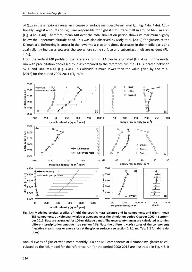
4 Studies at Naimona’nyi glacier
126
of Qmelt in these regions causes an increase of surface melt despite minimal Tair (Fig. 4.4a, 4.4e). Addi-
tionally, largest amounts of SWnet are responsible for highest subsurface melt in around 6400 m a.s.l.
(Fig. 4.4b, 4.4d). Therefore, mean MB over the total simulation period shows its maximum slightly
below the uppermost altitude band. This was also observed by Mölg et al. (2009) for glaciers at the
Kilimanjaro. Refreezing is largest in the lowermost glacier regions, decreases in the middle parts and
again slightly increases towards the top where some surface and subsurface melt are evident (Fig.
4.4c).
From the vertical MB profile of the reference run no ELA can be estimated (Fig. 4.4a). In the model
run with precipitation decreased by 25% compared to the reference run the ELA is located between
5700 and 5800 m a.s.l. (Fig. 4.4a). This altitude is much lower than the value given by Yao et al.
(2012) for the period 2005-2011 (Fig. 4.9).
Fig. 4.4: Modelled vertical profiles of (left) the specific mass balance and its components and (right) mean
SEB components at Naimona’nyi glacier averaged over the simulation period October 2000 – Septem-ber 2012. Data are averaged for 100-m altitude bands. The uncertainty ranges are calculated assuming different precipitation amounts (see section 4.3). Note the different x-axis scales of the components (negative means mass or energy loss at the glacier surface, see section 2.3.1 and Tab. 2.2 for abbrevia-tions).
Annual cycles of glacier-wide mean monthly SEB and MB components at Naimona’nyi glacier as cal-
culated by the MB model for the reference run for the period 2000-2012 are illustrated in Fig. 4.5. It
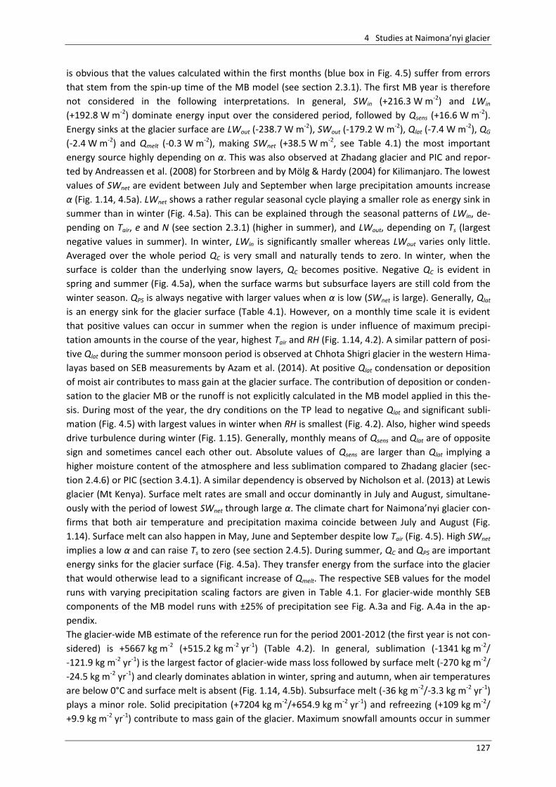
4 Studies at Naimona’nyi glacier
127
is obvious that the values calculated within the first months (blue box in Fig. 4.5) suffer from errors
that stem from the spin-up time of the MB model (see section 2.3.1). The first MB year is therefore
not considered in the following interpretations. In general, SWin (+216.3 W m-2) and LWin
(+192.8 W m-2) dominate energy input over the considered period, followed by Qsens (+16.6 W m-2).
Energy sinks at the glacier surface are LWout (-238.7 W m-2), SWout (-179.2 W m-2), Qlat (-7.4 W m-2), QG
(-2.4 W m-2) and Qmelt (-0.3 W m-2), making SWnet (+38.5 W m-2, see Table 4.1) the most important
energy source highly depending on α. This was also observed at Zhadang glacier and PIC and repor-
ted by Andreassen et al. (2008) for Storbreen and by Mölg & Hardy (2004) for Kilimanjaro. The lowest
values of SWnet are evident between July and September when large precipitation amounts increase
α (Fig. 1.14, 4.5a). LWnet shows a rather regular seasonal cycle playing a smaller role as energy sink in
summer than in winter (Fig. 4.5a). This can be explained through the seasonal patterns of LWin, de-
pending on Tair, e and N (see section 2.3.1) (higher in summer), and LWout, depending on Ts (largest
negative values in summer). In winter, LWin is significantly smaller whereas LWout varies only little.
Averaged over the whole period QC is very small and naturally tends to zero. In winter, when the
surface is colder than the underlying snow layers, QC becomes positive. Negative QC is evident in
spring and summer (Fig. 4.5a), when the surface warms but subsurface layers are still cold from the
winter season. QPS is always negative with larger values when α is low (SWnet is large). Generally, Qlat
is an energy sink for the glacier surface (Table 4.1). However, on a monthly time scale it is evident
that positive values can occur in summer when the region is under influence of maximum precipi-
tation amounts in the course of the year, highest Tair and RH (Fig. 1.14, 4.2). A similar pattern of posi-
tive Qlat during the summer monsoon period is observed at Chhota Shigri glacier in the western Hima-
layas based on SEB measurements by Azam et al. (2014). At positive Qlat condensation or deposition
of moist air contributes to mass gain at the glacier surface. The contribution of deposition or conden-
sation to the glacier MB or the runoff is not explicitly calculated in the MB model applied in this the-
sis. During most of the year, the dry conditions on the TP lead to negative Qlat and significant subli-
mation (Fig. 4.5) with largest values in winter when RH is smallest (Fig. 4.2). Also, higher wind speeds
drive turbulence during winter (Fig. 1.15). Generally, monthly means of Qsens and Qlat are of opposite
sign and sometimes cancel each other out. Absolute values of Qsens are larger than Qlat implying a
higher moisture content of the atmosphere and less sublimation compared to Zhadang glacier (sec-
tion 2.4.6) or PIC (section 3.4.1). A similar dependency is observed by Nicholson et al. (2013) at Lewis
glacier (Mt Kenya). Surface melt rates are small and occur dominantly in July and August, simultane-
ously with the period of lowest SWnet through large α. The climate chart for Naimona’nyi glacier con-
firms that both air temperature and precipitation maxima coincide between July and August (Fig.
1.14). Surface melt can also happen in May, June and September despite low Tair (Fig. 4.5). High SWnet
implies a low α and can raise Ts to zero (see section 2.4.5). During summer, QC and QPS are important
energy sinks for the glacier surface (Fig. 4.5a). They transfer energy from the surface into the glacier
that would otherwise lead to a significant increase of Qmelt. The respective SEB values for the model
runs with varying precipitation scaling factors are given in Table 4.1. For glacier-wide monthly SEB
components of the MB model runs with ±25% of precipitation see Fig. A.3a and Fig. A.4a in the ap-
pendix.
The glacier-wide MB estimate of the reference run for the period 2001-2012 (the first year is not con-
sidered) is +5667 kg m-2 (+515.2 kg m-2 yr-1) (Table 4.2). In general, sublimation (-1341 kg m-2/
-121.9 kg m-2 yr-1) is the largest factor of glacier-wide mass loss followed by surface melt (-270 kg m-2/
-24.5 kg m-2 yr-1) and clearly dominates ablation in winter, spring and autumn, when air temperatures
are below 0°C and surface melt is absent (Fig. 1.14, 4.5b). Subsurface melt (-36 kg m-2/-3.3 kg m-2 yr-1)
plays a minor role. Solid precipitation (+7204 kg m-2/+654.9 kg m-2 yr-1) and refreezing (+109 kg m-2/
+9.9 kg m-2 yr-1) contribute to mass gain of the glacier. Maximum snowfall amounts occur in summer
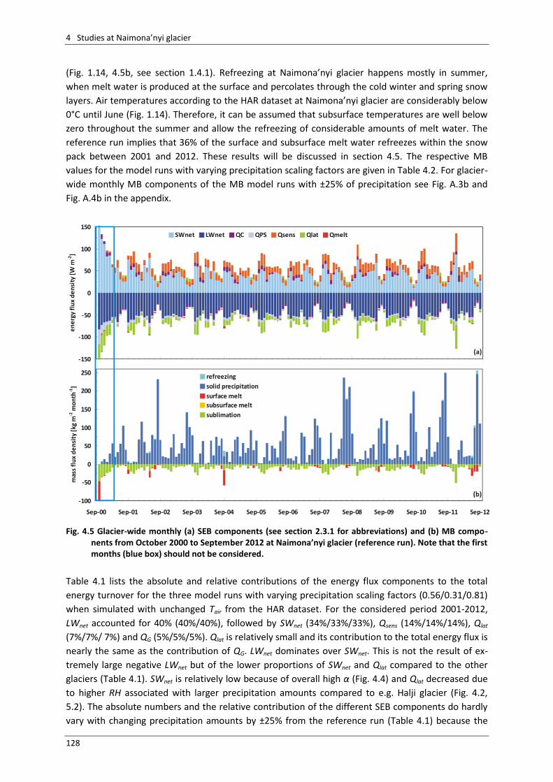
4 Studies at Naimona’nyi glacier
128
(Fig. 1.14, 4.5b, see section 1.4.1). Refreezing at Naimona’nyi glacier happens mostly in summer,
when melt water is produced at the surface and percolates through the cold winter and spring snow
layers. Air temperatures according to the HAR dataset at Naimona’nyi glacier are considerably below
0°C until June (Fig. 1.14). Therefore, it can be assumed that subsurface temperatures are well below
zero throughout the summer and allow the refreezing of considerable amounts of melt water. The
reference run implies that 36% of the surface and subsurface melt water refreezes within the snow
pack between 2001 and 2012. These results will be discussed in section 4.5. The respective MB
values for the model runs with varying precipitation scaling factors are given in Table 4.2. For glacier-
wide monthly MB components of the MB model runs with ±25% of precipitation see Fig. A.3b and
Fig. A.4b in the appendix.
Fig. 4.5 Glacier-wide monthly (a) SEB components (see section 2.3.1 for abbreviations) and (b) MB compo-
nents from October 2000 to September 2012 at Naimona’nyi glacier (reference run). Note that the first months (blue box) should not be considered.
Table 4.1 lists the absolute and relative contributions of the energy flux components to the total
energy turnover for the three model runs with varying precipitation scaling factors (0.56/0.31/0.81)
when simulated with unchanged Tair from the HAR dataset. For the considered period 2001-2012,
LWnet accounted for 40% (40%/40%), followed by SWnet (34%/33%/33%), Qsens (14%/14%/14%), Qlat
(7%/7%/ 7%) and QG (5%/5%/5%). Qlat is relatively small and its contribution to the total energy flux is
nearly the same as the contribution of QG. LWnet dominates over SWnet. This is not the result of ex-
tremely large negative LWnet but of the lower proportions of SWnet and Qlat compared to the other
glaciers (Table 4.1). SWnet is relatively low because of overall high α (Fig. 4.4) and Qlat decreased due
to higher RH associated with larger precipitation amounts compared to e.g. Halji glacier (Fig. 4.2,
5.2). The absolute numbers and the relative contribution of the different SEB components do hardly
vary with changing precipitation amounts by ±25% from the reference run (Table 4.1) because the
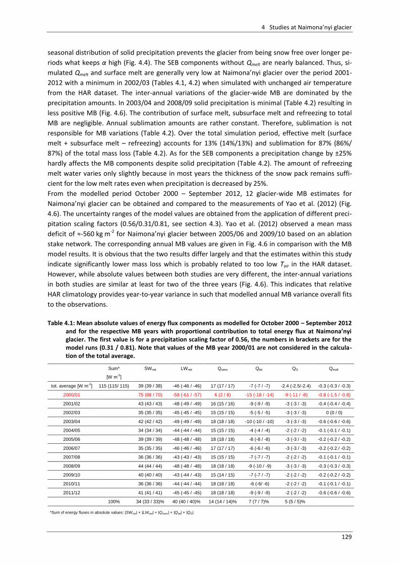
4 Studies at Naimona’nyi glacier
129
seasonal distribution of solid precipitation prevents the glacier from being snow free over longer pe-
riods what keeps α high (Fig. 4.4). The SEB components without Qmelt are nearly balanced. Thus, si-
mulated Qmelt and surface melt are generally very low at Naimona’nyi glacier over the period 2001-
2012 with a minimum in 2002/03 (Tables 4.1, 4.2) when simulated with unchanged air temperature
from the HAR dataset. The inter-annual variations of the glacier-wide MB are dominated by the
precipitation amounts. In 2003/04 and 2008/09 solid precipitation is minimal (Table 4.2) resulting in
less positive MB (Fig. 4.6). The contribution of surface melt, subsurface melt and refreezing to total
MB are negligible. Annual sublimation amounts are rather constant. Therefore, sublimation is not
responsible for MB variations (Table 4.2). Over the total simulation period, effective melt (surface
melt + subsurface melt – refreezing) accounts for 13% (14%/13%) and sublimation for 87% (86%/
87%) of the total mass loss (Table 4.2). As for the SEB components a precipitation change by ±25%
hardly affects the MB components despite solid precipitation (Table 4.2). The amount of refreezing
melt water varies only slightly because in most years the thickness of the snow pack remains suffi-
cient for the low melt rates even when precipitation is decreased by 25%.
From the modelled period October 2000 – September 2012, 12 glacier-wide MB estimates for
Naimona’nyi glacier can be obtained and compared to the measurements of Yao et al. (2012) (Fig.
4.6). The uncertainty ranges of the model values are obtained from the application of different preci-
pitation scaling factors (0.56/0.31/0.81, see section 4.3). Yao et al. (2012) observed a mean mass
deficit of ≈-560 kg m-2 for Naimona’nyi glacier between 2005/06 and 2009/10 based on an ablation
stake network. The corresponding annual MB values are given in Fig. 4.6 in comparison with the MB
model results. It is obvious that the two results differ largely and that the estimates within this study
indicate significantly lower mass loss which is probably related to too low Tair in the HAR dataset.
However, while absolute values between both studies are very different, the inter-annual variations
in both studies are similar at least for two of the three years (Fig. 4.6). This indicates that relative
HAR climatology provides year-to-year variance in such that modelled annual MB variance overall fits
to the observations.
Table 4.1: Mean absolute values of energy flux components as modelled for October 2000 – September 2012
and for the respective MB years with proportional contribution to total energy flux at Naimona’nyi glacier. The first value is for a precipitation scaling factor of 0.56, the numbers in brackets are for the model runs (0.31 / 0.81). Note that values of the MB year 2000/01 are not considered in the calcula-tion of the total average.
Sum* SWnet LWnet Qsens Qlat QG Qmelt
[W m-2
]
tot. average [W m-2
] 115 (115/ 115) 39 (39 / 38) -46 (-46 / -46) 17 (17 / 17) -7 (-7 / -7) -2.4 (-2.5/-2.4) -0.3 (-0.3 / -0.3)
2000/01 75 (88 / 70) -58 (-61 / -57) 6 (2 / 8) -15 (-18 / -14) -9 (-11 / -8) -0.8 (-1.5 / -0.8)
2001/02 43 (43 / 43) -48 (-49 / -49) 16 (15 / 16) -9 (-9 / -9) -3 (-3 / -3) -0.4 (-0.4 / -0.4)
2002/03 35 (35 / 35) -45 (-45 / -45) 15 (15 / 15) -5 (-5 / -5) -3 (-3 / -3) 0 (0 / 0)
2003/04 42 (42 / 42) -49 (-49 / -49) 18 (18 / 18) -10 (-10 / -10) -3 (-3 / -3) -0.6 (-0.6 / -0.6)
2004/05 34 (34 / 34) -44 (-44 / -44) 15 (15 / 15) -4 (-4 / -4) -2 (-2 / -2) -0.1 (-0.1 / -0.1)
2005/06 39 (39 / 39) -48 (-48 / -48) 18 (18 / 18) -8 (-8 / -8) -3 (-3 / -3) -0.2 (-0.2 / -0.2)
2006/07 35 (35 / 35) -46 (-46 / -46) 17 (17 / 17) -6 (-6 / -6) -3 (-3 / -3) -0.2 (-0.2 / -0.2)
2007/08 36 (36 / 36) -43 (-43 / -43) 15 (15 / 15) -7 (-7 / -7) -2 (-2 / -2) -0.1 (-0.1 / -0.1)
2008/09 44 (44 / 44) -48 (-48 / -48) 18 (18 / 18) -9 (-10 / -9) -3 (-3 / -3) -0.3 (-0.3 / -0.3)
2009/10 40 (40 / 40) -43 (-44 / -43) 15 (14 / 15) -7 (-7 / -7) -2 (-2 / -2) -0.2 (-0.2 / -0.2)
2010/11 36 (36 / 36) -44 (-44 / -44) 18 (18 / 18) -6 (-6/ -6) -2 (-2 / -2) -0.1 (-0.1 / -0.1)
2011/12 41 (41 / 41) -45 (-45 / -45) 18 (18 / 18) -9 (-9 / -9) -2 (-2 / -2) -0.6 (-0.6 / -0.6)
100% 34 (33 / 33)% 40 (40 / 40)% 14 (14 / 14)% 7 (7 / 7)% 5 (5 / 5)%
*Sum of energy fluxes in absolute values: |SWnet| + |LWnet| + |Qsens| + |Qlat| + |QG|
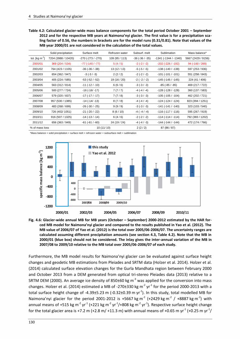
4 Studies at Naimona’nyi glacier
130
Table 4.2: Calculated glacier-wide mass balance components for the total period October 2001 – September 2012 and for the respective MB years at Naimona’nyi glacier. The first value is for a precipitation sca-ling factor of 0.56, the numbers in brackets are for the model runs (0.31/0.81). Note that values of the MB year 2000/01 are not considered in the calculation of the total values.
Solid precipitation Surface melt Refrozen water Subsurf. melt Sublimation Mass balance*
tot. [kg m-2
] 7204 (3988 / 10420) -270 (-273 / -270) 109 (95 / 113) -36 (-36 / -35) -1341 (-1344 / -1340) 5667 (2429 / 9156)
2000/01 369 (204 / 534) -77 (-140 / -77) 5 (4 / 5) -2 (-2 / -2) -202 (-226 / -192) 94 (-160 / 269)
2001/02 764 (423 / 1105) -36 (-36 / -38) 13 (12 / 13) -5 (-5 / -5) -138 (-140 / -138) 597 (253 / 936)
2002/03 654 (362 / 947) -3 (-3 / -3) 2 (2 / 2) -2 (-2 / -2) -101 (-101 / -101) 551 (258 / 843)
2003/04 405 (224 / 585) -53 (-52 / -52) 19 (16 / 20) -2 ( -2 / -2) -145 (-145 / -145) 224 (41 / 406)
2004/05 563 (312 / 814) -11 (-12 / -10) 6 (6 / 6) -3 (-3 / -3) -85 (-85 / -85) 469 (217 / 722)
2005/06 500 (277 / 724) -16 (-16/ -17) 7 (7 / 7) -4 (-4 / -4) -128 (-128 / -128) 360 (137 / 583)
2006/07 579 (320 / 837) -17 (-17 / -17) 7 (7 / 8) -3 (-3 / -3) -105 (-105 / -104) 462 (202 / 721)
2007/08 957 (530 / 1385) -14 (-14/ -13) 8 (7 / 8) -4 (-4 / -4) -124 (-124 / -124) 823 (394 / 1251)
2008/09 483 (268 / 699) -26 (-30 / -25) 9 (9 / 9) -3 (-3 / -3) -141 (-141 / -140) 323 (103 / 540)
2009/10 726 (402/ 1051) -21 (-20 / -22) 8 (6 / 10) -4 ( -4 / -4) -116 (-117 / -116) 595 (267 / 919)
2010/11 916 (507 / 1325) -14 (-13 / -14) 6 (4 / 6) -2 (-2 / -2) -114 (-114 / -114) 792 (383 / 1202)
2011/12 656 (363 / 949) -61 (-61 / -60) 24 (19 / 24) -4 (-4 / -3) -144 (-144 / -144) 472 (174 / 766)
% of mass loss 10 (11/ 10) 2 (2 / 2) 87 (86 / 87)
*Mass balance = solid precipitation + surface melt + refrozen water + subsurface melt + sublimation
Fig. 4.6: Glacier-wide annual MB for MB years (October – September) 2000-2012 estimated by the HAR for-
ced MB model for Naimona’nyi glacier and compared to the results published in Yao et al. (2012). The MB value of 2006/07 of Yao et al. (2012) is the total over 2005/06-2006/07. The uncertainty ranges are calculated assuming different precipitation amounts (see section 4.3, Table 4.2). Note that the MB in 2000/01 (blue box) should not be considered. The inlay gives the inter-annual variation of the MB in 2007/08 to 2009/10 relative to the MB total over 2005/06-2006/07 of each study.
Furthermore, the MB model results for Naimona’nyi glacier can be evaluated against surface height
changes and geodetic MB estimations from Pleiades and SRTM data (Holzer et al. 2014). Holzer et al.
(2014) calculated surface elevation changes for the Gurla Mandhata region between February 2000
and October 2013 from a DEM generated from optical tri-stereo Pleiades data (2013) relative to a
SRTM DEM (2000). An average ice density of 850±60 kg m-3 was applied for the conversion into mass
changes. Holzer et al. (2014) estimated a MB of -270±330 kg m-2 yr-1 for the period 2000-2013 with a
total surface height change of -4.39±5.23 m (-0.32±0.39 m yr-1). In this study, total modelled MB for
Naimona’nyi glacier for the period 2001-2012 is +5667 kg m-2 (+2429 kg m-2 / +8887 kg m-2) with
annual means of +515 kg m-2 yr-1 (+221 kg m-2 yr-1/+808 kg m-2 yr-1). Respective surface height change
for the total glacier area is +7.2 m (+2.8 m/ +11.3 m) with annual means of +0.65 m yr-1 (+0.25 m yr-1/
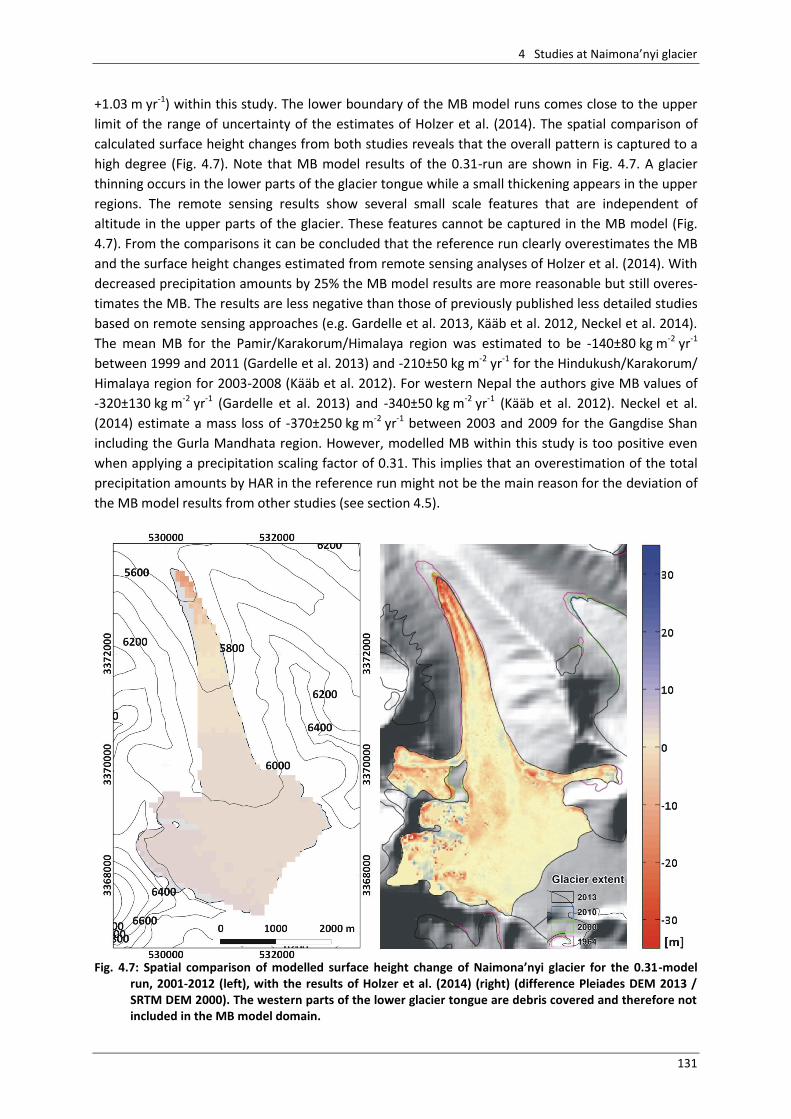
4 Studies at Naimona’nyi glacier
131
+1.03 m yr-1) within this study. The lower boundary of the MB model runs comes close to the upper
limit of the range of uncertainty of the estimates of Holzer et al. (2014). The spatial comparison of
calculated surface height changes from both studies reveals that the overall pattern is captured to a
high degree (Fig. 4.7). Note that MB model results of the 0.31-run are shown in Fig. 4.7. A glacier
thinning occurs in the lower parts of the glacier tongue while a small thickening appears in the upper
regions. The remote sensing results show several small scale features that are independent of
altitude in the upper parts of the glacier. These features cannot be captured in the MB model (Fig.
4.7). From the comparisons it can be concluded that the reference run clearly overestimates the MB
and the surface height changes estimated from remote sensing analyses of Holzer et al. (2014). With
decreased precipitation amounts by 25% the MB model results are more reasonable but still overes-
timates the MB. The results are less negative than those of previously published less detailed studies
based on remote sensing approaches (e.g. Gardelle et al. 2013, Kääb et al. 2012, Neckel et al. 2014).
The mean MB for the Pamir/Karakorum/Himalaya region was estimated to be -140±80 kg m-2 yr-1
between 1999 and 2011 (Gardelle et al. 2013) and -210±50 kg m-2 yr-1 for the Hindukush/Karakorum/
Himalaya region for 2003-2008 (Kääb et al. 2012). For western Nepal the authors give MB values of
-320±130 kg m-2 yr-1 (Gardelle et al. 2013) and -340±50 kg m-2 yr-1 (Kääb et al. 2012). Neckel et al.
(2014) estimate a mass loss of -370±250 kg m-2 yr-1 between 2003 and 2009 for the Gangdise Shan
including the Gurla Mandhata region. However, modelled MB within this study is too positive even
when applying a precipitation scaling factor of 0.31. This implies that an overestimation of the total
precipitation amounts by HAR in the reference run might not be the main reason for the deviation of
the MB model results from other studies (see section 4.5).
Fig. 4.7: Spatial comparison of modelled surface height change of Naimona’nyi glacier for the 0.31-model
run, 2001-2012 (left), with the results of Holzer et al. (2014) (right) (difference Pleiades DEM 2013 / SRTM DEM 2000). The western parts of the lower glacier tongue are debris covered and therefore not included in the MB model domain.
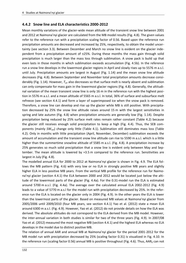
4 Studies at Naimona’nyi glacier
132
4.4.2 Snow line and ELA characteristics 2000-2012
Mean monthly variations of the glacier-wide mean altitude of the transient snow line between 2001
and 2012 at Naimona’nyi glacier are calculated from the MB model results (Fig. 4.8). The given values
refer to the reference run with a precipitation scaling factor of 0.56. Based upon the reference run
precipitation amounts are decreased and increased by 25%, respectively, to obtain the model uncer-
tainty (see section 3.3). Between December and March no snow line is evident on the glacier inde-
pendent from a precipitation amount of ±25%. During these months the mass gain through solid
precipitation is much larger than the mass loss through sublimation. A snow pack is build up that
even lasts in those months in which sublimation exceeds accumulation (Fig. 4.5b). In the reference
run a snow line develops in the lowermost glacier regions in April and slowly rises up to 5576 m a.s.l.
until July. Precipitation amounts are largest in August (Fig. 1.14) and the mean snow line altitude
decreases (Fig. 4.8). Between September and November total precipitation amounts decrease consi-
derably (Fig. 1.14). However, Tair also decreases so that surface melt is nearly absent and sublimation
can only compensate for mass gain in the lowermost glacier regions (Fig. 4.8). Generally, the altitudi-
nal variation of the mean transient snow line is only 16 m in the reference run with the highest posi-
tion in 5576 m a.s.l. and a mean altitude of 5565 m a.s.l. In total, 36% of surface and subsurface melt
refreeze (see section 4.4.1) and form a layer of superimposed ice when the snow pack is removed.
Therefore, a snow line can develop and rise up the glacier while MB is still positive. With precipita-
tion decreased by 25% the snow line altitude raises around 15 m with the largest sensitivities in
spring and late autumn (Fig. 4.8) when precipitation amounts are generally low (Fig. 1.14). Despite
precipitation being reduced by 25% surface melt rates remain rather constant (Table 4.2) because
the glacier still receives enough solid precipitation to keep α high (Fig. 4.4). Thus, the SEB com-
ponents (mainly SWnet) change only little (Table 4.1). Sublimation still dominates mass loss (Table
4.2). Only in months with little precipitation (April, November, December) sublimation exceeds the
amount of accumulation and the transient snow line altitude can rise to 5590 m a.s.l. which is a little
higher than the summertime snowline altitude of 5585 m a.s.l. (Fig. 4.8). A precipitation increase by
25% generates so much solid precipitation that a snow line is evident only between May and Sep-
tember. The mean altitude is lowered by ≈3.5 m compared to the reference run. Sensitivities are
largest in July (Fig. 4.8).
The modelled annual ELA for 2000 to 2012 at Naimona’nyi glacier is shown in Fig. 4.9. The ELA fol-
lows the MB pattern (Fig. 4.6) with very low or no ELA in strongly positive MB years and slightly
higher ELA in less positive MB years. From the vertical MB profile for the reference run for Naimo-
na’nyi glacier (section 4.4.1) the ELA between 2000 and 2012 would be located just below the alti-
tude of the lowermost parts of the glacier (Fig. 4.4a). For the 0.31-model run the ELA is estimated
around 5700 m a.s.l. (Fig. 4.4a). The average over the calculated annual ELA 2002-2012 (Fig. 4.9)
leads to a value of 5770 m a.s.l for the model run with precipitation decreased by 25%. In the refer-
ence run the ELA is located on the glacier only in 2004 (Fig. 4.9). In the other years the ELA is lower
than the lowermost parts of the glacier. Based on measured MB values at Naimona’nyi glacier from
2005/2006 until 2009/2010 (four MB years, see section 4.4.1) Yao et al. (2012) state a mean ELA
around 6300 m a.s.l. (Fig. 4.9). However, Yao et al. (2012) do not provide details on how the ELA was
derived. The absolute altitudes do not correspond to the ELA derived from the MB model. However,
the inter-annual variation in both studies is similar for two of the three years (Fig. 4.9). In 2007/08
Yao et al. (2012) measured the most negative MB (section 4.4.1) and the highest ELA whereas no ELA
develops in the model due to distinct positive MB.
The relation of annual AAR and annual MB at Naimona’nyi glacier for the period 2001-2012 for the
MB model run with precipitation decreased by 25% (scaling factor 0.31) is visualized in Fig. 4.10. In
the reference run (scaling factor 0.56) annual MB is positive throughout (Fig. 4.6). Thus, AAR0 can not
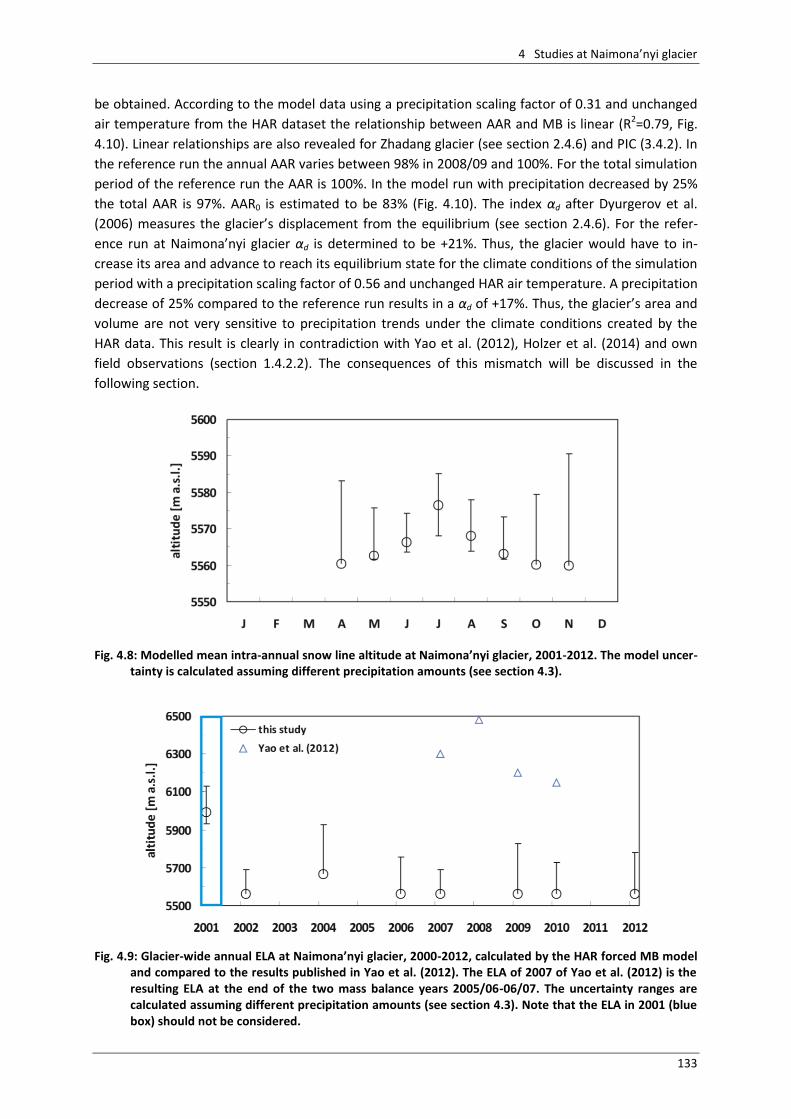
4 Studies at Naimona’nyi glacier
133
be obtained. According to the model data using a precipitation scaling factor of 0.31 and unchanged
air temperature from the HAR dataset the relationship between AAR and MB is linear (R2=0.79, Fig.
4.10). Linear relationships are also revealed for Zhadang glacier (see section 2.4.6) and PIC (3.4.2). In
the reference run the annual AAR varies between 98% in 2008/09 and 100%. For the total simulation
period of the reference run the AAR is 100%. In the model run with precipitation decreased by 25%
the total AAR is 97%. AAR0 is estimated to be 83% (Fig. 4.10). The index αd after Dyurgerov et al.
(2006) measures the glacier’s displacement from the equilibrium (see section 2.4.6). For the refer-
ence run at Naimona’nyi glacier αd is determined to be +21%. Thus, the glacier would have to in-
crease its area and advance to reach its equilibrium state for the climate conditions of the simulation
period with a precipitation scaling factor of 0.56 and unchanged HAR air temperature. A precipitation
decrease of 25% compared to the reference run results in a αd of +17%. Thus, the glacier’s area and
volume are not very sensitive to precipitation trends under the climate conditions created by the
HAR data. This result is clearly in contradiction with Yao et al. (2012), Holzer et al. (2014) and own
field observations (section 1.4.2.2). The consequences of this mismatch will be discussed in the
following section.
Fig. 4.8: Modelled mean intra-annual snow line altitude at Naimona’nyi glacier, 2001-2012. The model uncer-
tainty is calculated assuming different precipitation amounts (see section 4.3).
Fig. 4.9: Glacier-wide annual ELA at Naimona’nyi glacier, 2000-2012, calculated by the HAR forced MB model
and compared to the results published in Yao et al. (2012). The ELA of 2007 of Yao et al. (2012) is the resulting ELA at the end of the two mass balance years 2005/06-06/07. The uncertainty ranges are calculated assuming different precipitation amounts (see section 4.3). Note that the ELA in 2001 (blue box) should not be considered.
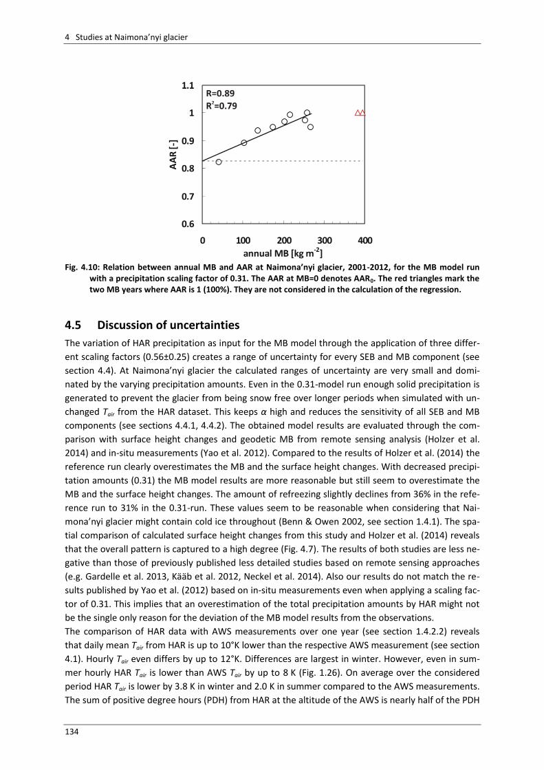
4 Studies at Naimona’nyi glacier
134
Fig. 4.10: Relation between annual MB and AAR at Naimona’nyi glacier, 2001-2012, for the MB model run
with a precipitation scaling factor of 0.31. The AAR at MB=0 denotes AAR0. The red triangles mark the two MB years where AAR is 1 (100%). They are not considered in the calculation of the regression.
4.5 Discussion of uncertainties
The variation of HAR precipitation as input for the MB model through the application of three differ-
ent scaling factors (0.56±0.25) creates a range of uncertainty for every SEB and MB component (see
section 4.4). At Naimona’nyi glacier the calculated ranges of uncertainty are very small and domi-
nated by the varying precipitation amounts. Even in the 0.31-model run enough solid precipitation is
generated to prevent the glacier from being snow free over longer periods when simulated with un-
changed Tair from the HAR dataset. This keeps α high and reduces the sensitivity of all SEB and MB
components (see sections 4.4.1, 4.4.2). The obtained model results are evaluated through the com-
parison with surface height changes and geodetic MB from remote sensing analysis (Holzer et al.
2014) and in-situ measurements (Yao et al. 2012). Compared to the results of Holzer et al. (2014) the
reference run clearly overestimates the MB and the surface height changes. With decreased precipi-
tation amounts (0.31) the MB model results are more reasonable but still seem to overestimate the
MB and the surface height changes. The amount of refreezing slightly declines from 36% in the refe-
rence run to 31% in the 0.31-run. These values seem to be reasonable when considering that Nai-
mona’nyi glacier might contain cold ice throughout (Benn & Owen 2002, see section 1.4.1). The spa-
tial comparison of calculated surface height changes from this study and Holzer et al. (2014) reveals
that the overall pattern is captured to a high degree (Fig. 4.7). The results of both studies are less ne-
gative than those of previously published less detailed studies based on remote sensing approaches
(e.g. Gardelle et al. 2013, Kääb et al. 2012, Neckel et al. 2014). Also our results do not match the re-
sults published by Yao et al. (2012) based on in-situ measurements even when applying a scaling fac-
tor of 0.31. This implies that an overestimation of the total precipitation amounts by HAR might not
be the single only reason for the deviation of the MB model results from the observations.
The comparison of HAR data with AWS measurements over one year (see section 1.4.2.2) reveals
that daily mean Tair from HAR is up to 10°K lower than the respective AWS measurement (see section
4.1). Hourly Tair even differs by up to 12°K. Differences are largest in winter. However, even in sum-
mer hourly HAR Tair is lower than AWS Tair by up to 8 K (Fig. 1.26). On average over the considered
period HAR Tair is lower by 3.8 K in winter and 2.0 K in summer compared to the AWS measurements.
The sum of positive degree hours (PDH) from HAR at the altitude of the AWS is nearly half of the PDH
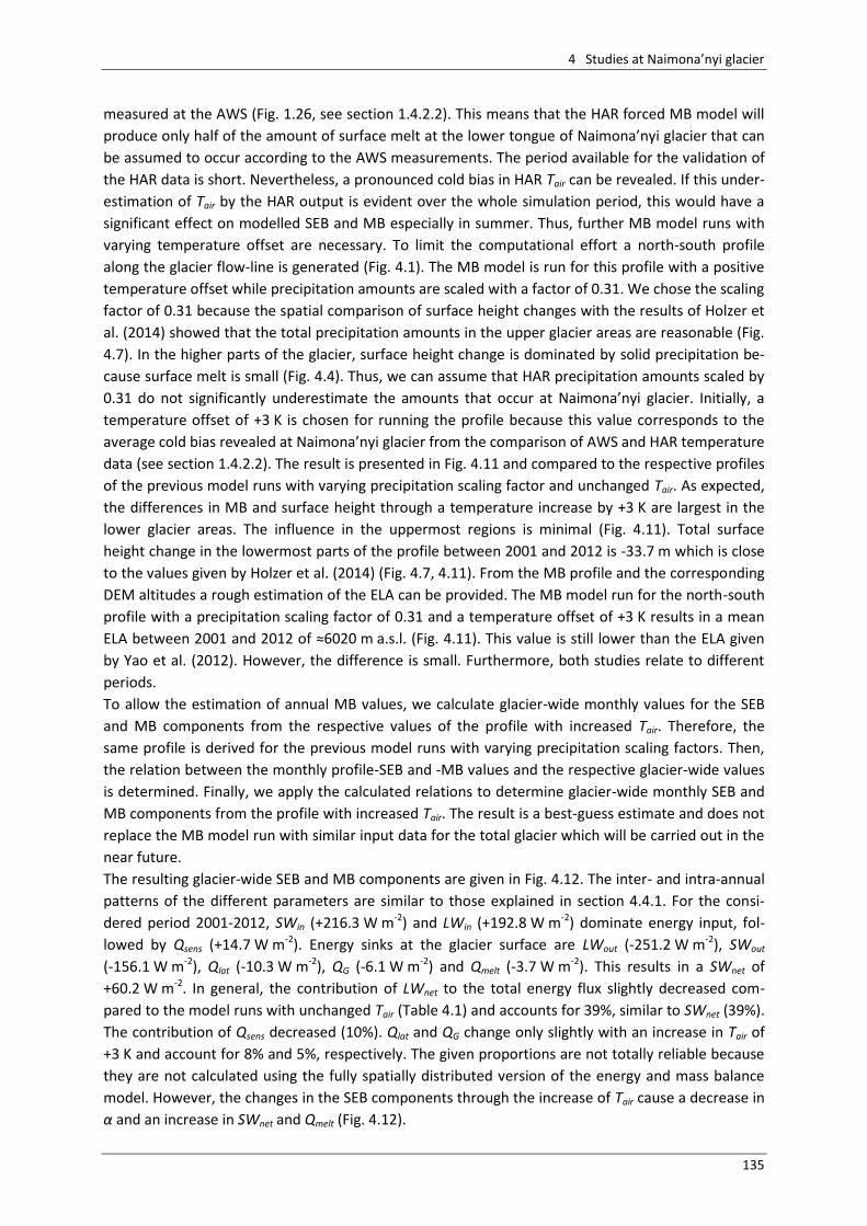
4 Studies at Naimona’nyi glacier
135
measured at the AWS (Fig. 1.26, see section 1.4.2.2). This means that the HAR forced MB model will
produce only half of the amount of surface melt at the lower tongue of Naimona’nyi glacier that can
be assumed to occur according to the AWS measurements. The period available for the validation of
the HAR data is short. Nevertheless, a pronounced cold bias in HAR Tair can be revealed. If this under-
estimation of Tair by the HAR output is evident over the whole simulation period, this would have a
significant effect on modelled SEB and MB especially in summer. Thus, further MB model runs with
varying temperature offset are necessary. To limit the computational effort a north-south profile
along the glacier flow-line is generated (Fig. 4.1). The MB model is run for this profile with a positive
temperature offset while precipitation amounts are scaled with a factor of 0.31. We chose the scaling
factor of 0.31 because the spatial comparison of surface height changes with the results of Holzer et
al. (2014) showed that the total precipitation amounts in the upper glacier areas are reasonable (Fig.
4.7). In the higher parts of the glacier, surface height change is dominated by solid precipitation be-
cause surface melt is small (Fig. 4.4). Thus, we can assume that HAR precipitation amounts scaled by
0.31 do not significantly underestimate the amounts that occur at Naimona’nyi glacier. Initially, a
temperature offset of +3 K is chosen for running the profile because this value corresponds to the
average cold bias revealed at Naimona’nyi glacier from the comparison of AWS and HAR temperature
data (see section 1.4.2.2). The result is presented in Fig. 4.11 and compared to the respective profiles
of the previous model runs with varying precipitation scaling factor and unchanged Tair. As expected,
the differences in MB and surface height through a temperature increase by +3 K are largest in the
lower glacier areas. The influence in the uppermost regions is minimal (Fig. 4.11). Total surface
height change in the lowermost parts of the profile between 2001 and 2012 is -33.7 m which is close
to the values given by Holzer et al. (2014) (Fig. 4.7, 4.11). From the MB profile and the corresponding
DEM altitudes a rough estimation of the ELA can be provided. The MB model run for the north-south
profile with a precipitation scaling factor of 0.31 and a temperature offset of +3 K results in a mean
ELA between 2001 and 2012 of ≈6020 m a.s.l. (Fig. 4.11). This value is still lower than the ELA given
by Yao et al. (2012). However, the difference is small. Furthermore, both studies relate to different
periods.
To allow the estimation of annual MB values, we calculate glacier-wide monthly values for the SEB
and MB components from the respective values of the profile with increased Tair. Therefore, the
same profile is derived for the previous model runs with varying precipitation scaling factors. Then,
the relation between the monthly profile-SEB and -MB values and the respective glacier-wide values
is determined. Finally, we apply the calculated relations to determine glacier-wide monthly SEB and
MB components from the profile with increased Tair. The result is a best-guess estimate and does not
replace the MB model run with similar input data for the total glacier which will be carried out in the
near future.
The resulting glacier-wide SEB and MB components are given in Fig. 4.12. The inter- and intra-annual
patterns of the different parameters are similar to those explained in section 4.4.1. For the consi-
dered period 2001-2012, SWin (+216.3 W m-2) and LWin (+192.8 W m-2) dominate energy input, fol-
lowed by Qsens (+14.7 W m-2). Energy sinks at the glacier surface are LWout (-251.2 W m-2), SWout
(-156.1 W m-2), Qlat (-10.3 W m-2), QG (-6.1 W m-2) and Qmelt (-3.7 W m-2). This results in a SWnet of
+60.2 W m-2. In general, the contribution of LWnet to the total energy flux slightly decreased com-
pared to the model runs with unchanged Tair (Table 4.1) and accounts for 39%, similar to SWnet (39%).
The contribution of Qsens decreased (10%). Qlat and QG change only slightly with an increase in Tair of
+3 K and account for 8% and 5%, respectively. The given proportions are not totally reliable because
they are not calculated using the fully spatially distributed version of the energy and mass balance
model. However, the changes in the SEB components through the increase of Tair cause a decrease in
α and an increase in SWnet and Qmelt (Fig. 4.12).
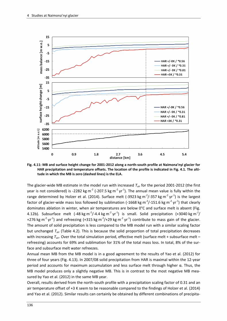
4 Studies at Naimona’nyi glacier
136
Fig. 4.11: MB and surface height change for 2001-2012 along a north-south profile at Naimona’nyi glacier for
HAR precipitation and temperature offsets. The location of the profile is indicated in Fig. 4.1. The alti-tude in which the MB is zero (dashed lines) is the ELA.
The glacier-wide MB estimate in the model run with increased Tair for the period 2001-2012 (the first
year is not considered) is -2282 kg m-2 (-207.5 kg m-2 yr-1). The annual mean value is fully within the
range determined by Holzer et al. (2014). Surface melt (-3923 kg m-2/-357 kg m-2 yr-1) is the largest
factor of glacier-wide mass loss followed by sublimation (-1668 kg m-2/-151.6 kg m-2 yr-1) that clearly
dominates ablation in winter, when air temperatures are below 0°C and surface melt is absent (Fig.
4.12b). Subsurface melt (-48 kg m-2/-4.4 kg m-2 yr-1) is small. Solid precipitation (+3040 kg m-2/
+276 kg m-2 yr-1) and refreezing (+315 kg m-2/+29 kg m-2 yr-1) contribute to mass gain of the glacier.
The amount of solid precipitation is less compared to the MB model run with a similar scaling factor
but unchanged Tair (Table 4.2). This is because the solid proportion of total precipitation decreases
with increasing Tair. Over the total simulation period, effective melt (surface melt + subsurface melt –
refreezing) accounts for 69% and sublimation for 31% of the total mass loss. In total, 8% of the sur-
face and subsurface melt water refreezes.
Annual mean MB from the MB model is in a good agreement to the results of Yao et al. (2012) for
three of four years (Fig. 4.13). In 2007/08 solid precipitation from HAR is maximal within the 12-year
period and accounts for maximum accumulation and less surface melt through higher α. Thus, the
MB model produces only a slightly negative MB. This is in contrast to the most negative MB mea-
sured by Yao et al. (2012) in the same MB year.
Overall, results derived from the north-south profile with a precipitation scaling factor of 0.31 and an
air temperature offset of +3 K seem to be reasonable compared to the findings of Holzer et al. (2014)
and Yao et al. (2012). Similar results can certainly be obtained by different combinations of precipita-
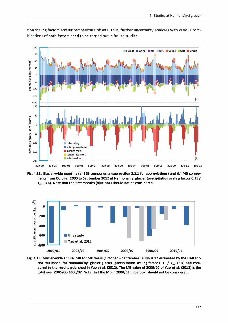
4 Studies at Naimona’nyi glacier
137
tion scaling factors and air temperature offsets. Thus, further uncertainty analyses with various com-
binations of both factors need to be carried out in future studies.
Fig. 4.12: Glacier-wide monthly (a) SEB components (see section 2.3.1 for abbreviations) and (b) MB compo-
nents from October 2000 to September 2012 at Naimona’nyi glacier (precipitation scaling factor 0.31 / Tair +3 K). Note that the first months (blue box) should not be considered.
Fig. 4.13: Glacier-wide annual MB for MB years (October – September) 2000-2012 estimated by the HAR for-
ced MB model for Naimona’nyi glacier glacier (precipitation scaling factor 0.31 / Tair +3 K) and com-pared to the results published in Yao et al. (2012). The MB value of 2006/07 of Yao et al. (2012) is the total over 2005/06-2006/07. Note that the MB in 2000/01 (blue box) should not be considered.
4 Studies at Naimona’nyi glacier
138
4.6 Conclusion regarding model results for Naimona’nyi glacier
The Naimona’nyi glacier is one of the measurement sites within the WET project. The comparison of
atmospheric AWS data at the glacier tongue with HAR data revealed that Tair from HAR data exhibits
a significant cold bias of 3.8 K in winter and 2.0 K in summer compared to the AWS measurements
(see section 1.4.2.2). In this chapter, SEB and MB components of Naimona’nyi glacier are calculated
for 2000-2012 and interpreted concerning their altitudinal gradients and their inter- and intra-annual
patterns. To account for uncertainties in total HAR precipitation amounts and to obtain a model un-
certainty for further MB calculations, we perform three model runs with varying precipitation scaling
factors (0.56±0.25) while keeping Tair from HAR unchanged. In the reference run a factor of 0.56 is
applied. This number was obtained by Mölg et al. (2012) for Zhadang glacier and successfully applied
in this thesis in the HAR forced MB model runs 2001-2011 for Zhadang glacier (see section 2.4) and
for PIC (see chapter 3). In total, the energy input to the glacier surface of Naimona’nyi is dominated
by LWnet with 40% both in the reference run and in the model run with 25% decreased precipitation
(0.31) when simulated with unchanged Tair from the HAR dataset. The increase of Tair by +3 K increa-
ses surface melt and α because larger glacier areas are snow free. Thus, both the absolute value and
the relative importance of SWnet increase by 21.7 W m-2 or by 6%. When applying Tair directly from
the HAR output very low air temperatures and frequent amounts of snowfall suppress surface melt
and favour refreezing in the reference model run. Thus, effective melt accounts only for 13% and
sublimation for 87% of the total mass loss in the reference run (Table 4.2). The increase of Tair by +3 K
increases the proportion of effective melt to 69%. The variation of HAR precipitation as input for the
MB model through the application of three different scaling factors creates only a small range of
uncertainty for every SEB and MB component. A pronounced cold bias in HAR Tair leads to a high
proportion of total precipitation falling as snow even in summer. Thus, glacier-wide α is generally
high and reduces the sensitivity of all SEB and MB components (see sections 4.4.1, 4.4.2). Only the
lower glacier regions are sensitive to a precipitation decrease by 25% (Fig. 4.4). The ELA at Naimo-
na’nyi for 2002-2012 is estimated around 5770 m a.s.l. (scaling factor 0.31) what is significantly lower
than the value given by Yao et al. (2012) (≈6300 m a.s.l.) but within the large scale ELA for the region
of the western Himalayas (Fig. 1 in Yao et al. 2002). An ELA of ≈6020 m a.s.l. is estimated from the
north-south profile with an air temperature offset of +3 K.
Compared to the results of Holzer et al. (2014) the reference run clearly overestimates the MB and
the surface height changes when simulated with unchanged Tair from the HAR dataset. With pre-
cipitation decreased by 25% (0.31) the MB model results are more reasonable but still seem to over-
estimate the MB and the surface height changes especially in the lower glacier regions. A pro-
nounced cold bias in HAR Tair is evident from the comparison with AWS measurements. To reveal the
effects of a positive temperature offset on the glacier behaviour without high computational efforts,
the MB model was not run for the total glacier area but for a north-south profile along the glacier
flow-line. The profile is calculated with a precipitation scaling factor of 0.31 and a temperature offset
of +3 K. The derived surface height changes agree well with the results of Holzer et al. (2014). We
imply that the SEB and MB components determined for the profile allow concluding for the whole
glacier. Thus, the calculated glacier-wide annual MB need to be treated with caution. However, the
results are close to the findings of Holzer et al. (2014) and Yao et al. (2012) and are within the range
of several remote sensing studies.
It can be concluded from the application of the MB model to Naimona’nyi glacier that the derived
intra- and inter-annual cycles of SEB and MB components are within reasonable limits depending on
the respective patterns of the input parameters from HAR. The obtained SEB and MB components
are consistent with each other because they interact through physical relationships (see sections
1.3.4 and 2.3.1). The HAR output overestimates the precipitation amounts in the reference run. A

4 Studies at Naimona’nyi glacier
139
scaling factor of 0.31 is more reasonable (see section 4.4.1). However, at Naimona’nyi glacier the cal-
culated MB and surface height changes still seem to be overestimated. This could be revealed from
the comparison with available remote sensing results and few in-situ measurements. In regions with
limited availability of in-situ measurements remote sensing data is important for the evaluation of
MB models. The overestimation of the calculated MB most probably is caused by a significant under-
estimation of Tair by the HAR output resulting in significantly too small MB estimates especially in the
lower regions of the glacier tongue. This effect can be revealed from the comparison with AWS data
over one year. The modelled MB and the in-situ and remote sensing based observations indicate that
this cold bias of Tair by HAR is evident over the whole simulation period. The consequence is a signi-
ficant effect on modelled SEB and MB. Therefore, a major conclusion from chapter 4 is that glacier
SEB and MB modelling based on modelled atmospheric data always requires some kind of meteoro-
logical, glaciological or remote sensing based field observation. In consequence, the continuation and
extension of at least basic in-situ measurements is a crucial requirement in order to obtain reliable
SEB and MB estimates for different benchmark glaciers on the TP.

5 Studies at Halji glacier
141
5 Energy and mass balance for Halji glacier, north western Nepal, 2000-2011, as derived from a coupled snow and energy balance model
5.1 Introduction and regional climate conditions
Halji glacier is a northeast exposed valley glacier (≈2.3 km2) at the southern slope of the Nalakankar
Himal, a northern ridge of the western Himalayas in north western Nepal (Fig. 5.1, see section 1.4.1).
Since 2006, a periodic GLOF occurs in Limi valley and threatens the village Halji. The analysis of sa-
tellite imagery revealed that the flood is probably released from a supra-glacial lake at ≈5350 m a.s.l.
on Halji glacier (≈6 km away) (Kropacek et al. 2013). In the central and eastern Himalayas the growth
of glacial lakes, both on (supra-glacial) and in front (pro-glacial) of the glacier, has been observed in
recent decades (Ageta et al. 2000, Bayracharya & Mool 2009, Bolch et al. 2012, Fujita et al. 2009, Sa-
kai 2012). Supra-glacial lakes evolve in regions of small surface slopes when the glacier tongue stag-
nates (Sakai et al. 2000). The release of thermal energy from the water to the glacier ice accelerates
the melting process (Sakai et al. 2009). Generally, the risk related to a GLOF in the Himalayas is main-
ly due to large lake volumes and associated wide reach of the flood (Richardson & Reynolds 2000).
As the GLOF in Limi valley does not happen annually and the reason for the pattern is not yet under-
stood, the developed SEB/MB model (see section 2.3.1) is applied to Halji glacier to estimate glacier
MB and melt water runoff. The physically based model is especially valuable in remote areas like Limi
valley because it does not directly depend on in-situ measurements. The model allows linking the
atmospheric conditions from HAR data to glacier runoff in order to find possible causes for ‘GLOF
years’ and ‘non-GLOF years’.
The region is clearly dominated by Indian monsoon in summer and mid-latitude westerlies in winter
(see section 1.4.1). Most atmospheric variables, generated by HAR show a pronounced seasonal con-
trast (Fig. 1.13, 5.2). Daily mean air temperatures generated by HAR generally rise above zero from
mid June to September and daily means range between -26.9°C and 6.1 C (average -8.5°C) within the
period 2000-2011. Monthly means of those HAR variables that serve as input for the applied MB
model are shown in Fig. 5.2. SWin reaches its maximum around May and decreases in summer, when
monsoonal cloud cover is large. The monsoon season is associated with annual maxima in precipita-
tion, RH and air pressure associated with the Tibetan High (see section 1.3.1) whereas wind speeds
are generally low (Fig. 5.2). The mean annual precipitation amount at Halji glacier (605 mm) is larger
compared to Zhadang glacier (534 mm) and PIC (380 mm) when applying the same scaling factor of
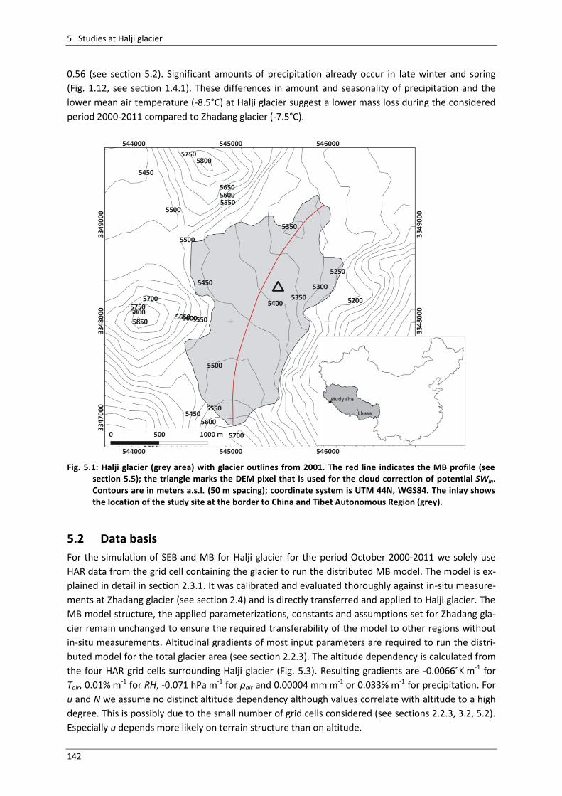
5 Studies at Halji glacier
142
0.56 (see section 5.2). Significant amounts of precipitation already occur in late winter and spring
(Fig. 1.12, see section 1.4.1). These differences in amount and seasonality of precipitation and the
lower mean air temperature (-8.5°C) at Halji glacier suggest a lower mass loss during the considered
period 2000-2011 compared to Zhadang glacier (-7.5°C).
Fig. 5.1: Halji glacier (grey area) with glacier outlines from 2001. The red line indicates the MB profile (see
section 5.5); the triangle marks the DEM pixel that is used for the cloud correction of potential SWin. Contours are in meters a.s.l. (50 m spacing); coordinate system is UTM 44N, WGS84. The inlay shows the location of the study site at the border to China and Tibet Autonomous Region (grey).
5.2 Data basis
For the simulation of SEB and MB for Halji glacier for the period October 2000-2011 we solely use
HAR data from the grid cell containing the glacier to run the distributed MB model. The model is ex-
plained in detail in section 2.3.1. It was calibrated and evaluated thoroughly against in-situ measure-
ments at Zhadang glacier (see section 2.4) and is directly transferred and applied to Halji glacier. The
MB model structure, the applied parameterizations, constants and assumptions set for Zhadang gla-
cier remain unchanged to ensure the required transferability of the model to other regions without
in-situ measurements. Altitudinal gradients of most input parameters are required to run the distri-
buted model for the total glacier area (see section 2.2.3). The altitude dependency is calculated from
the four HAR grid cells surrounding Halji glacier (Fig. 5.3). Resulting gradients are -0.0066°K m-1 for
Tair, 0.01% m-1 for RH, -0.071 hPa m-1 for ρair and 0.00004 mm m-1 or 0.033% m-1 for precipitation. For
u and N we assume no distinct altitude dependency although values correlate with altitude to a high
degree. This is possibly due to the small number of grid cells considered (see sections 2.2.3, 3.2, 5.2).
Especially u depends more likely on terrain structure than on altitude.
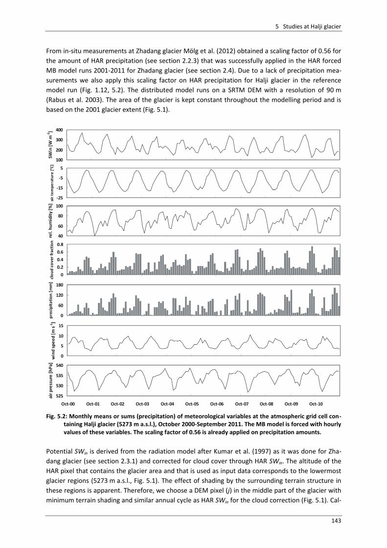
5 Studies at Halji glacier
143
From in-situ measurements at Zhadang glacier Mölg et al. (2012) obtained a scaling factor of 0.56 for
the amount of HAR precipitation (see section 2.2.3) that was successfully applied in the HAR forced
MB model runs 2001-2011 for Zhadang glacier (see section 2.4). Due to a lack of precipitation mea-
surements we also apply this scaling factor on HAR precipitation for Halji glacier in the reference
model run (Fig. 1.12, 5.2). The distributed model runs on a SRTM DEM with a resolution of 90 m
(Rabus et al. 2003). The area of the glacier is kept constant throughout the modelling period and is
based on the 2001 glacier extent (Fig. 5.1).
Fig. 5.2: Monthly means or sums (precipitation) of meteorological variables at the atmospheric grid cell con-
taining Halji glacier (5273 m a.s.l.), October 2000-September 2011. The MB model is forced with hourly values of these variables. The scaling factor of 0.56 is already applied on precipitation amounts.
Potential SWin is derived from the radiation model after Kumar et al. (1997) as it was done for Zha-
dang glacier (see section 2.3.1) and corrected for cloud cover through HAR SWin. The altitude of the
HAR pixel that contains the glacier area and that is used as input data corresponds to the lowermost
glacier regions (5273 m a.s.l., Fig. 5.1). The effect of shading by the surrounding terrain structure in
these regions is apparent. Therefore, we choose a DEM pixel (j) in the middle part of the glacier with
minimum terrain shading and similar annual cycle as HAR SWin for the cloud correction (Fig. 5.1). Cal-
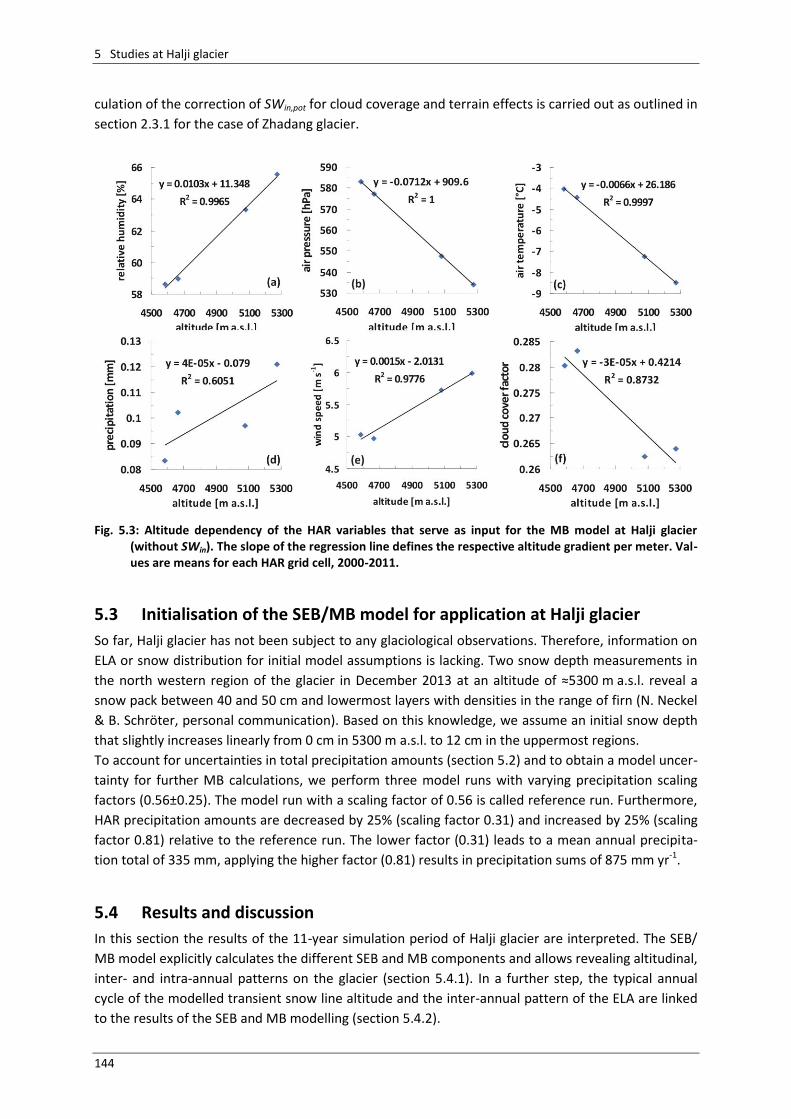
5 Studies at Halji glacier
144
culation of the correction of SWin,pot for cloud coverage and terrain effects is carried out as outlined in
section 2.3.1 for the case of Zhadang glacier.
Fig. 5.3: Altitude dependency of the HAR variables that serve as input for the MB model at Halji glacier
(without SWin). The slope of the regression line defines the respective altitude gradient per meter. Val-ues are means for each HAR grid cell, 2000-2011.
5.3 Initialisation of the SEB/MB model for application at Halji glacier
So far, Halji glacier has not been subject to any glaciological observations. Therefore, information on
ELA or snow distribution for initial model assumptions is lacking. Two snow depth measurements in
the north western region of the glacier in December 2013 at an altitude of ≈5300 m a.s.l. reveal a
snow pack between 40 and 50 cm and lowermost layers with densities in the range of firn (N. Neckel
& B. Schröter, personal communication). Based on this knowledge, we assume an initial snow depth
that slightly increases linearly from 0 cm in 5300 m a.s.l. to 12 cm in the uppermost regions.
To account for uncertainties in total precipitation amounts (section 5.2) and to obtain a model uncer-
tainty for further MB calculations, we perform three model runs with varying precipitation scaling
factors (0.56±0.25). The model run with a scaling factor of 0.56 is called reference run. Furthermore,
HAR precipitation amounts are decreased by 25% (scaling factor 0.31) and increased by 25% (scaling
factor 0.81) relative to the reference run. The lower factor (0.31) leads to a mean annual precipita-
tion total of 335 mm, applying the higher factor (0.81) results in precipitation sums of 875 mm yr-1.
5.4 Results and discussion
In this section the results of the 11-year simulation period of Halji glacier are interpreted. The SEB/
MB model explicitly calculates the different SEB and MB components and allows revealing altitudinal,
inter- and intra-annual patterns on the glacier (section 5.4.1). In a further step, the typical annual
cycle of the modelled transient snow line altitude and the inter-annual pattern of the ELA are linked
to the results of the SEB and MB modelling (section 5.4.2).
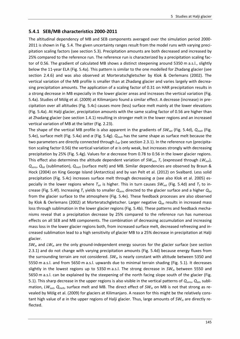
5 Studies at Halji glacier
145
5.4.1 SEB/MB characteristics 2000-2011
The altitudinal dependency of MB and SEB components averaged over the simulation period 2000-
2011 is shown in Fig. 5.4. The given uncertainty ranges result from the model runs with varying preci-
pitation scaling factors (see section 5.3). Precipitation amounts are both decreased and increased by
25% compared to the reference run. The reference run is characterized by a precipitation scaling fac-
tor of 0.56. The gradient of calculated MB shows a distinct steepening around 5350 m a.s.l., slightly
below the 11-year ELA (Fig. 5.4a). This pattern is similar to the one modelled for Zhadang glacier (see
section 2.4.6) and was also observed at Morteratschgletscher by Klok & Oerlemans (2002). The
vertical variation of the MB profile is smaller than at Zhadang glacier and varies largely with decrea-
sing precipitation amounts. The application of a scaling factor of 0.31 on HAR precipitation results in
a strong decrease in MB especially in the lower glacier areas and increases the vertical variation (Fig.
5.4a). Studies of Mölg et al. (2009) at Kilimanjaro found a similar effect. A decrease (increase) in pre-
cipitation over all altitudes (Fig. 5.4c) causes more (less) surface melt mainly at the lower elevations
(Fig. 5.4a). At Halji glacier, precipitation amounts with the same scaling factor of 0.56 are higher than
at Zhadang glacier (see section 1.4.1) resulting in stronger melt in the lower regions and an increased
vertical variation of MB at the latter (Fig. 2.23).
The shape of the vertical MB profile is also apparent in the gradients of SWnet (Fig. 5.4d), Qmelt (Fig.
5.4e), surface melt (Fig. 5.4a) and α (Fig. 5.4g). Qmelt has the same shape as surface melt because the
two parameters are directly connected through LM (see section 2.3.1). In the reference run (precipita-
tion scaling factor 0.56) the vertical variation of α is only weak, but increases strongly with decreasing
precipitation by 25% (Fig. 5.4g). Values for α decrease from 0.78 to 0.56 in the lower glacier regions.
This effect also determines the altitude dependent variation of SWnet, Ts (expressed through LWout),
Qsens, Qlat (sublimation), Qmelt (surface melt) and MB. Similar dependencies are observed by Braun &
Hock (2004) on King George Island (Antarctica) and by van Pelt et al. (2012) on Svalbard. Less solid
precipitation (Fig. 5.4c) increases surface melt through decreasing α (see also Klok et al. 2005) es-
pecially in the lower regions where Tair is higher. This in turn causes SWnet (Fig. 5.4d) and TS to in-
crease (Fig. 5.4f). Increasing Ts yields to smaller Qsens directed to the glacier surface and a higher Qlat
from the glacier surface to the atmosphere (Fig. 5.4e). These feedback processes are also observed
by Klok & Oerlemans (2002) at Morteratschgletscher. Larger negative Qlat results in increased mass
loss through sublimation in the lower glacier regions (Fig. 5.4b). These patterns and feedback mecha-
nisms reveal that a precipitation decrease by 25% compared to the reference run has numerous
effects on all SEB and MB components. The combination of decreasing accumulation and increasing
mass loss in the lower glacier regions both, from increased surface melt, decreased refreezing and in-
creased sublimation lead to a high sensitivity of glacier MB to a 25% decrease in precipitation at Halji
glacier.
SWin and LWin are the only ground-independent energy sources for the glacier surface (see section
2.3.1) and do not change with varying precipitation amounts (Fig. 5.4d) because energy fluxes from
the surrounding terrain are not considered. SWin is nearly constant with altitude between 5350 and
5550 m a.s.l. and from 5650 m a.s.l. upwards due to minimal terrain shading (Fig. 5.1). It decreases
slightly in the lowest regions up to 5350 m a.s.l. The strong decrease in SWin between 5550 and
5650 m a.s.l. can be explained by the steepening of the north facing slope south of the glacier (Fig.
5.1). This sharp decrease in the upper regions is also visible in the vertical patterns of Qsens, Qlat, subli-
mation, LWout, Qmelt, surface melt and MB. The direct effect of SWin on MB is not that strong as re-
vealed by Mölg et al. (2009) for glaciers at Kilimanjaro. A reason for this might be the relatively cons-
tant high value of α in the upper regions of Halji glacier. Thus, large amounts of SWin are directly re-
flected.
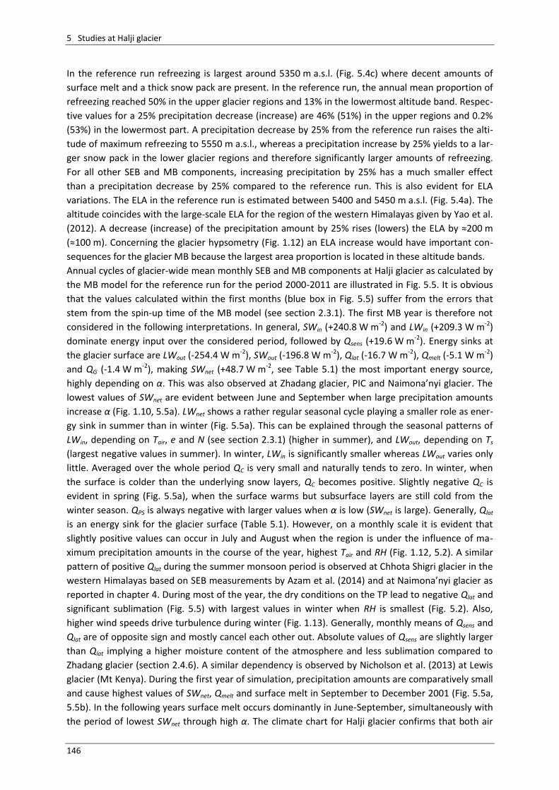
5 Studies at Halji glacier
146
In the reference run refreezing is largest around 5350 m a.s.l. (Fig. 5.4c) where decent amounts of
surface melt and a thick snow pack are present. In the reference run, the annual mean proportion of
refreezing reached 50% in the upper glacier regions and 13% in the lowermost altitude band. Respec-
tive values for a 25% precipitation decrease (increase) are 46% (51%) in the upper regions and 0.2%
(53%) in the lowermost part. A precipitation decrease by 25% from the reference run raises the alti-
tude of maximum refreezing to 5550 m a.s.l., whereas a precipitation increase by 25% yields to a lar-
ger snow pack in the lower glacier regions and therefore significantly larger amounts of refreezing.
For all other SEB and MB components, increasing precipitation by 25% has a much smaller effect
than a precipitation decrease by 25% compared to the reference run. This is also evident for ELA
variations. The ELA in the reference run is estimated between 5400 and 5450 m a.s.l. (Fig. 5.4a). The
altitude coincides with the large-scale ELA for the region of the western Himalayas given by Yao et al.
(2012). A decrease (increase) of the precipitation amount by 25% rises (lowers) the ELA by ≈200 m
(≈100 m). Concerning the glacier hypsometry (Fig. 1.12) an ELA increase would have important con-
sequences for the glacier MB because the largest area proportion is located in these altitude bands.
Annual cycles of glacier-wide mean monthly SEB and MB components at Halji glacier as calculated by
the MB model for the reference run for the period 2000-2011 are illustrated in Fig. 5.5. It is obvious
that the values calculated within the first months (blue box in Fig. 5.5) suffer from the errors that
stem from the spin-up time of the MB model (see section 2.3.1). The first MB year is therefore not
considered in the following interpretations. In general, SWin (+240.8 W m-2) and LWin (+209.3 W m-2)
dominate energy input over the considered period, followed by Qsens (+19.6 W m-2). Energy sinks at
the glacier surface are LWout (-254.4 W m-2), SWout (-196.8 W m-2), Qlat (-16.7 W m-2), Qmelt (-5.1 W m-2)
and QG (-1.4 W m-2), making SWnet (+48.7 W m-2, see Table 5.1) the most important energy source,
highly depending on α. This was also observed at Zhadang glacier, PIC and Naimona’nyi glacier. The
lowest values of SWnet are evident between June and September when large precipitation amounts
increase α (Fig. 1.10, 5.5a). LWnet shows a rather regular seasonal cycle playing a smaller role as ener-
gy sink in summer than in winter (Fig. 5.5a). This can be explained through the seasonal patterns of
LWin, depending on Tair, e and N (see section 2.3.1) (higher in summer), and LWout, depending on Ts
(largest negative values in summer). In winter, LWin is significantly smaller whereas LWout varies only
little. Averaged over the whole period QC is very small and naturally tends to zero. In winter, when
the surface is colder than the underlying snow layers, QC becomes positive. Slightly negative QC is
evident in spring (Fig. 5.5a), when the surface warms but subsurface layers are still cold from the
winter season. QPS is always negative with larger values when α is low (SWnet is large). Generally, Qlat
is an energy sink for the glacier surface (Table 5.1). However, on a monthly scale it is evident that
slightly positive values can occur in July and August when the region is under the influence of ma-
ximum precipitation amounts in the course of the year, highest Tair and RH (Fig. 1.12, 5.2). A similar
pattern of positive Qlat during the summer monsoon period is observed at Chhota Shigri glacier in the
western Himalayas based on SEB measurements by Azam et al. (2014) and at Naimona’nyi glacier as
reported in chapter 4. During most of the year, the dry conditions on the TP lead to negative Qlat and
significant sublimation (Fig. 5.5) with largest values in winter when RH is smallest (Fig. 5.2). Also,
higher wind speeds drive turbulence during winter (Fig. 1.13). Generally, monthly means of Qsens and
Qlat are of opposite sign and mostly cancel each other out. Absolute values of Qsens are slightly larger
than Qlat implying a higher moisture content of the atmosphere and less sublimation compared to
Zhadang glacier (section 2.4.6). A similar dependency is observed by Nicholson et al. (2013) at Lewis
glacier (Mt Kenya). During the first year of simulation, precipitation amounts are comparatively small
and cause highest values of SWnet, Qmelt and surface melt in September to December 2001 (Fig. 5.5a,
5.5b). In the following years surface melt occurs dominantly in June-September, simultaneously with
the period of lowest SWnet through high α. The climate chart for Halji glacier confirms that both air
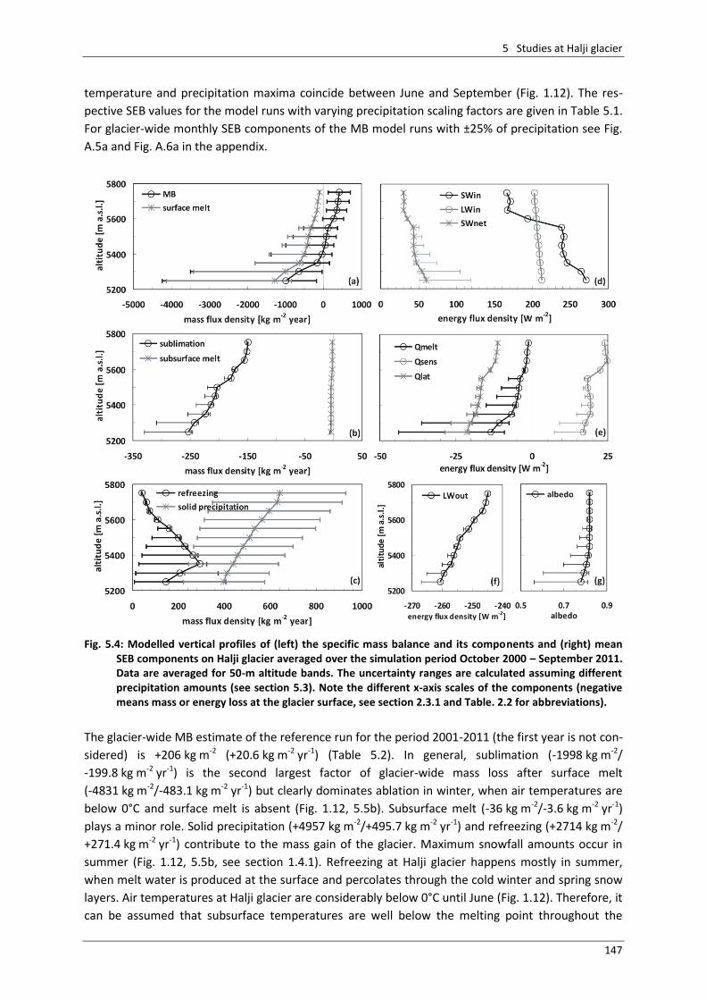
5 Studies at Halji glacier
147
temperature and precipitation maxima coincide between June and September (Fig. 1.12). The res-
pective SEB values for the model runs with varying precipitation scaling factors are given in Table 5.1.
For glacier-wide monthly SEB components of the MB model runs with ±25% of precipitation see Fig.
A.5a and Fig. A.6a in the appendix.
Fig. 5.4: Modelled vertical profiles of (left) the specific mass balance and its components and (right) mean
SEB components on Halji glacier averaged over the simulation period October 2000 – September 2011. Data are averaged for 50-m altitude bands. The uncertainty ranges are calculated assuming different precipitation amounts (see section 5.3). Note the different x-axis scales of the components (negative means mass or energy loss at the glacier surface, see section 2.3.1 and Table. 2.2 for abbreviations).
The glacier-wide MB estimate of the reference run for the period 2001-2011 (the first year is not con-
sidered) is +206 kg m-2 (+20.6 kg m-2 yr-1) (Table 5.2). In general, sublimation (-1998 kg m-2/
-199.8 kg m-2 yr-1) is the second largest factor of glacier-wide mass loss after surface melt
(-4831 kg m-2/-483.1 kg m-2 yr-1) but clearly dominates ablation in winter, when air temperatures are
below 0°C and surface melt is absent (Fig. 1.12, 5.5b). Subsurface melt (-36 kg m-2/-3.6 kg m-2 yr-1)
plays a minor role. Solid precipitation (+4957 kg m-2/+495.7 kg m-2 yr-1) and refreezing (+2714 kg m-2/
+271.4 kg m-2 yr-1) contribute to the mass gain of the glacier. Maximum snowfall amounts occur in
summer (Fig. 1.12, 5.5b, see section 1.4.1). Refreezing at Halji glacier happens mostly in summer,
when melt water is produced at the surface and percolates through the cold winter and spring snow
layers. Air temperatures at Halji glacier are considerably below 0°C until June (Fig. 1.12). Therefore, it
can be assumed that subsurface temperatures are well below the melting point throughout the
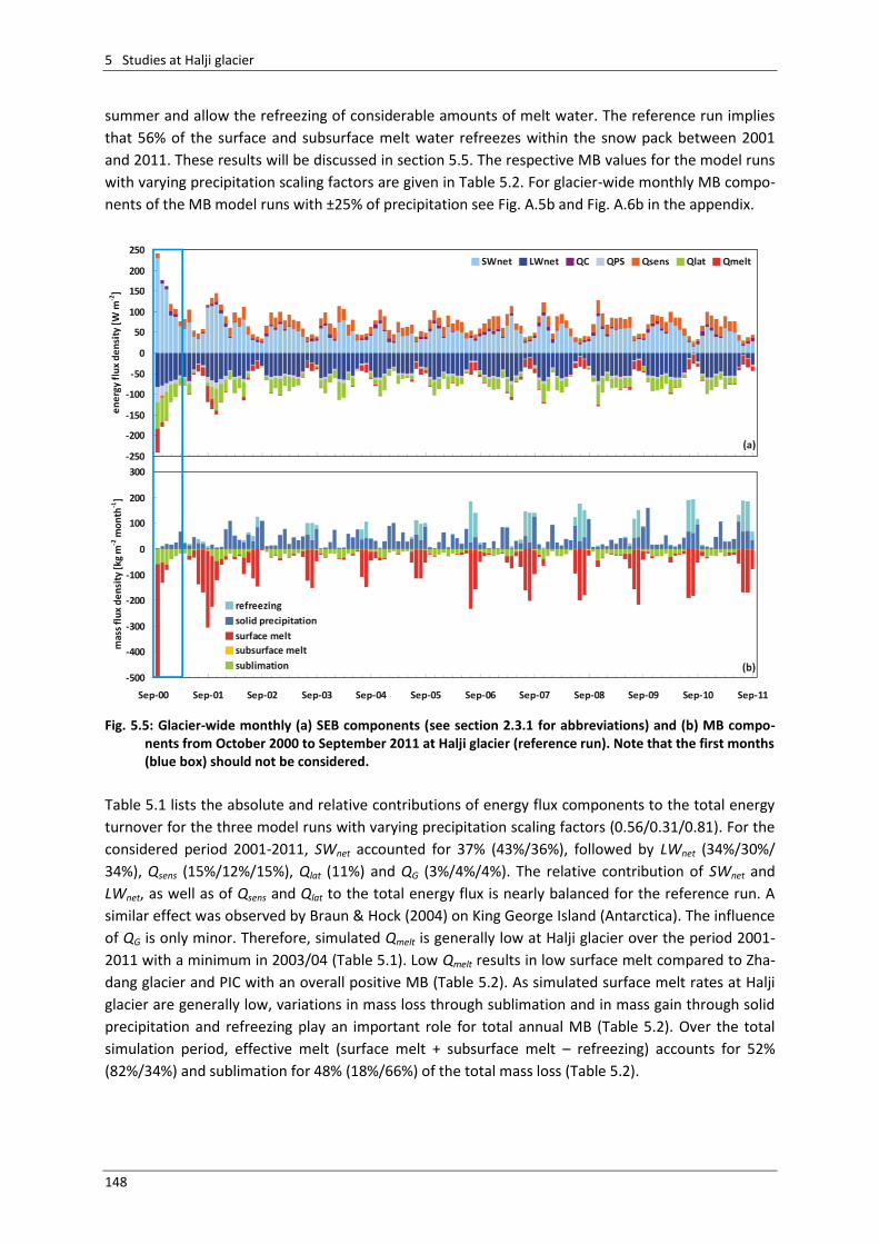
5 Studies at Halji glacier
148
summer and allow the refreezing of considerable amounts of melt water. The reference run implies
that 56% of the surface and subsurface melt water refreezes within the snow pack between 2001
and 2011. These results will be discussed in section 5.5. The respective MB values for the model runs
with varying precipitation scaling factors are given in Table 5.2. For glacier-wide monthly MB compo-
nents of the MB model runs with ±25% of precipitation see Fig. A.5b and Fig. A.6b in the appendix.
Fig. 5.5: Glacier-wide monthly (a) SEB components (see section 2.3.1 for abbreviations) and (b) MB compo-
nents from October 2000 to September 2011 at Halji glacier (reference run). Note that the first months (blue box) should not be considered.
Table 5.1 lists the absolute and relative contributions of energy flux components to the total energy
turnover for the three model runs with varying precipitation scaling factors (0.56/0.31/0.81). For the
considered period 2001-2011, SWnet accounted for 37% (43%/36%), followed by LWnet (34%/30%/
34%), Qsens (15%/12%/15%), Qlat (11%) and QG (3%/4%/4%). The relative contribution of SWnet and
LWnet, as well as of Qsens and Qlat to the total energy flux is nearly balanced for the reference run. A
similar effect was observed by Braun & Hock (2004) on King George Island (Antarctica). The influence
of QG is only minor. Therefore, simulated Qmelt is generally low at Halji glacier over the period 2001-
2011 with a minimum in 2003/04 (Table 5.1). Low Qmelt results in low surface melt compared to Zha-
dang glacier and PIC with an overall positive MB (Table 5.2). As simulated surface melt rates at Halji
glacier are generally low, variations in mass loss through sublimation and in mass gain through solid
precipitation and refreezing play an important role for total annual MB (Table 5.2). Over the total
simulation period, effective melt (surface melt + subsurface melt – refreezing) accounts for 52%
(82%/34%) and sublimation for 48% (18%/66%) of the total mass loss (Table 5.2).
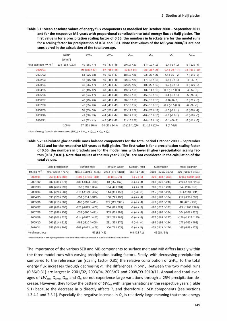
5 Studies at Halji glacier
149
Table 5.1: Mean absolute values of energy flux components as modelled for October 2000 – September 2011 and for the respective MB years with proportional contribution to total energy flux at Halji glacier. The first value is for a precipitation scaling factor of 0.56, the numbers in brackets are for the model runs for a scaling factor for precipitation of 0.31 and 0.81. Note that values of the MB year 2000/01 are not considered in the calculation of the total average.
Sum* SWnet LWnet Qsens Qlat QG Qmelt
[W m-2
]
total average [W m-2
] 134 (154 / 133) 49 (65 / 47) -45 (-47 / -45) 20 (17 / 20) -17 (-19 / -16) -1.4 (-5 / -1) -5 (-12 / -4)
2000/01 96 (187 / 87) -57 (-65 / -56) 12 (1 / 14) -28 (-36 / -26) -9.4 (-26 / -7) -13 (-61 / -10)
2001/02 64 (92 / 53) -49 (-53 / -47) 18 (12 / 21) -23 (-28 / -21) -4.4 (-10 / -2) -7 (-14 / -5)
2002/03 48 (50 / 48) -45 (-46 / -46) 20 (19 / 20) -17 (-18 / -18) -1.5 (-3 / -1) -4 (-4 / -4)
2003/04 48 (66 / 47) -47 (-48 / -47) 22 (20 / 22) -18 (-20 / -18) -1.7 (-6 / -1) -3 (-12 / -3)
2004/05 42 (49 / 42) -43 (-44 / -43) 19 (17 / 19) -13 (-14 / -13) -0.6 (-3 / -0.1) -4 (-5 / -3)
2005/06 48 (54 / 47) -46 (-46 / -46) 19 (19 / 19) -15 (-15 / -15) -1.1 (-3 / -1) -5 (-9 / -4)
2006/07 48 (79 / 46) -45 (-48 / -45) 20 (15 / 19) -15 (-18 / -15) -0.8 (-8 / 0) -7 (-21 / -5)
2007/08 47 (55 / 46) -44 (-43 / -43) 17 (16 / 17) -15 (-16 / -15) -0.7 (-3 / -0.1) -6 (-9 / -5)
2008/09 51 (83 / 50) -47 (-50 / -47) 22 (17 / 22) -19 (-23 / -19) -1.5 (-9 / -1) -5 (-20 / -4)
2009/10 49 (58 / 49) -44 (-44 / -44) 18 (17 / 17) -16 (-16 / -16) -1.3 (-4 / -1) -5 (-10 / -5)
2010/11 41 (62 / 41) -42 (-45 / -42) 21 (16 / 21) -14 (-18 / -14) -0.1 (-5 / 1) -5 (-11 / -5)
100% 37 (43 / 36)% 34 (30 / 34)% 15 (12 / 15)% 11 (11 / 11)% 3 (4 / 4)%
*Sum of energy fluxes in absolute values: |SWnet| + |LWnet| + |Qsens| + |Qlat| + |QG|
Table 5.2: Calculated glacier-wide mass balance components for the total period October 2000 – September
2011 and for the respective MB years at Halji glacier. The first value is for a precipitation scaling factor of 0.56, the numbers in brackets are for the model runs with lower (higher) precipitation scaling fac-tors (0.31 / 0.81). Note that values of the MB year 2000/01 are not considered in the calculation of the total values.
Solid precipitation Surface melt Refrozen water Subsurf. melt Sublimation Mass balance*
tot. [kg m-2
] 4957 (2744 / 7170) -4831 (-10875 / -4175) 2714 (775 / 3181) -36 (-41 / -36) -1998 (-2211/-1970) 206 (-9830 / 3491)
2000/01 268 (149 / 388) -1200 (-5734 / -981) 41 (0.1 / 79) -6 (-7 / -6) -320 (-403 / -303) -1216 (-5994/-830)
2001/02 602 (334 / 871) -686 (-1324 / -489) 84 (25 / 167) -5 (-6 / -4) -268 (-321 / -244) -273 (-1293 / 284)
2002/03 484 (268 / 699) -352 (-391 / -354) 134 (40 / 204) -4 (-4 / -3) -208 (-211 / -208) 54 (-298 / 318)
2003/04 407 (226 / 589) -316 (-1129 / -267) 114 (35 / 152) -3 ( -4 / -3) -215 (-238 / -215) -13 (-1110 / 241)
2004/05 593 (328 / 857) -357 (-514 / -319) 150 (72 / 180) -4 (-4 / -4) -165 (-178 / -164) 217 (-296 / 532)
2005/06 389 (215 / 562) -460 (-832 / -411) 271 (122 / 321) -4 (-4 / -4) -178 (-182 / -178) 18 (-681 / 258)
2006/07 481 (266 / 695) -623 (-2015 / -478) 254 (61 / 324) -3 (-4 / -3) -182 (-217 / -181) -73 (-1908 / 326)
2007/08 520 (288 / 752) -532 (-860 / -491) 303 (60 / 392) -4 (-4 / -4) -184 (-190 / -184) 104 (-707 / 426)
2008/09 363 (201 / 525) -514 (-1877 / -420) 212 (28 / 289) -3 (-4 / -4) -227 (-263 / -227) -170 (-1915 / 135)
2009/10 566 (314 / 819) -483 (-910 / -468) 291 (33 / 376) -4 ( -4 / -4) -194 (-198 / -194) 177 (-765 / 493)
2010/11 553 (306 / 799) -509 (-1022 / -478) 300 (76 / 374) -3 (-4 / -4) -176 (-213 / -176) 165 (-858 / 478)
% of mass loss 57 (82 / 45) 0.8 (0.3 / 1) 42 (18 / 54)
*Mass balance = solid precipitation + surface melt + refrozen water + subsurface melt + sublimation
The importance of the various SEB and MB components to surface melt and MB differs largely within
the three model runs with varying precipitation scaling factors. Firstly, with decreasing precipitation
compared to the reference run (scaling factor 0.31) the relative contribution of SWnet to the total
energy flux increases through decreasing α. The differences in SWnet between the two model runs
(0.56/0.31) are largest in 2001/02, 2003/04, 2006/07 and 2008/09-2010/11. Annual and total aver-
ages of LWnet, Qsens, Qlat and QG do not experience large variations through a 25% precipitation de-
crease. However, they follow the pattern of SWnet with larger variations in the respective years (Table
5.1) because the decrease in α directly affects Ts and therefore all SEB components (see sections
1.3.4.1 and 2.3.1). Especially the negative increase in QG is relatively large meaning that more energy
5 Studies at Halji glacier
150
from the surface is transferred into the snow or ice and warms the subsurface. Altogether, this re-
sults in a strong negative increase of Qmelt and surface melt and an above average decrease of MB in
the respective years compared to the 10-year mean (Table 5.1, 5.2, Fig. 5.6). In the model run with
decreased precipitation relative to the reference run (scaling factor 0.31) MB is closer linked to sur-
face melt, because the contribution of effective melt to total mass loss increased to 82% (Table. 5.2).
The six years in which the MB is most sensitive to a 25% precipitation decrease are characterized by
higher Qmelt already in the reference run and/or low annual precipitation (Table 5.1, 5.2). Thus, the
tipping point to further increased mass loss is closer than in the other MB years. A precipitation in-
crease relative to the reference run (scaling factor 0.81) causes overall positive MB at Halji glacier
(Fig. 5.6) but the differences in the SEB and MB components to the reference run are less distinct
(Table 5.1, 5.2). A possible reason might be that the reference run already simulates an overall po-
sitive MB and relatively high α in the lower glacier regions (Fig. 5.4g) through periodical strong snow
fall events. Thus, any further precipitation increase can not have large impacts on these variables.
Simulated annual mean MB at Halji glacier can hardly be evaluated because no in-situ measurements
are available so far and the glacier area is too small for intensive remote sensing analyses (see sec-
tion 5.5). Kropacek et al. (2013) report a periodic GLOF event since 2006 (see section 5.1). The water
is released from a supra-glacial lake on Halji glacier. To reveal possible consistencies between glacial
runoff generated by the MB model and the occurrence of ‘GLOF years’ and ‘non-GLOF years’, the
annual amount of water supply from the glacier is calculated (Fig. 5.6). Runoff (in kg m-2) is deter-
mined from surface and subsurface melt, refreezing and liquid precipitation for the total glacier area.
The effect of routing, the time delay of the melt water movement vertically through the snowpack
and horizontally along the glacier surface (Singh & Singh 2001), is not considered. The actual
drainage basin of the supra-glacial lake might be smaller than the total glacier area. This can be
neglected because it does not affect the quantitative comparison. Between 2001 and 2011 four ‘non-
GLOF years’ were observed (Fig. 5.6). In 2002/03 and 2004/05 simulated runoff is small when
including the ranges of uncertainties. In these years no GLOF occurred. This might be an indication
that the amount of runoff is possibly linked to a GLOF event. However, simulated runoff in the years
2005/06, 2007/08, 2009/10 and 2010/11 is similar but 2009/10 is the only ‘non-GLOF year’ of those.
In 2001/02 no GLOF event is evident despite high runoff (Fig. 5.6). Thus, the link between simulated
runoff and GLOF events at Halji glacier is limited. Kropacek et al. (2013) assume external factors, e.g.
sediment damming of the lake, to override the meteorological forcing. Furthermore, the lake
geometry and the temporal melt pattern may influence the lake outburst.
Mean modelled MB between 2001 and 2011 for Halji glacier with varying precipitation scaling factors
(0.56/0.31/0.81) is +21 kg m-2 yr-1 (-983 kg m-2 yr-1/+349 kg m-2 yr-1). Considering the published results
of less detailed studies for glaciers in the Himalayas (e.g. Gardelle et al. 2013a,b, Kääb et al. 2012,
Bolch et al. 2011), the obtained MB for the reference run appears to be too positive. The mean MB
for the Pamir/Karakorum/Himalaya region was estimated to be -140±80 kg m-2 yr-1 for 1999-2011
(Gardelle et al. 2013) and -210±50 kg m-2 yr-1 for the Hindukush/Karakorum/Himalaya region for
2003-2008 (Kääb et al. 2012). For western Nepal the authors give MB values of -320±130 kg m-2 yr-1
(Gardelle et al. 2013) and -340±50 kg m-2 yr-1 (Kääb et al. 2012). Neckel et al. (2014) estimate a mass
loss of -370±250 kg m-2 yr-1 between 2003 and 2009 for the Gangdise Shan including the Halji region.
The few existing MB measurements over several years reveal the most negative mass balances in the
Himalayas, ranging from -1100 kg m-2 yr-1 to -760 kg m-2 yr-1 (average -930 kg m-2 yr-1) between 2002
and 2010 (Yao et al. 2012).
Thus, the MB model result for a precipitation scaling factor of 0.31 (-983 kg m-2 yr-1) is within the
range of the results of Yao et al. (2012). However, the detection of a cold bias in HAR air temperature
at Naimona’nyi glacier (see section 4) implies that a similar effect probably has to be considered also
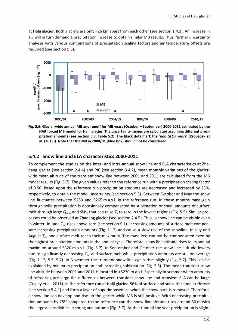
5 Studies at Halji glacier
151
at Halji glacier. Both glaciers are only ≈26 km apart from each other (see section 1.4.1). An increase in
Tair will in turn demand a precipitation increase to obtain similar MB results. Thus, further uncertainty
analyses with various combinations of precipitation scaling factors and air temperature offsets are
required (see section 5.5).
Fig. 5.6: Glacier-wide annual MB and runoff for MB years (October – September) 2000-2011 estimated by the
HAR forced MB model for Halji glacier. The uncertainty ranges are calculated assuming different preci-pitation amounts (see section 5.3, Table 5.2). The black dots mark the ‘non GLOF years’ (Kropacek et al. (2013)). Note that the MB in 2000/01 (blue box) should not be considered.
5.4.2 Snow line and ELA characteristics 2000-2011
To complement the studies on the inter- and intra-annual snow line and ELA characteristics at Zha-
dang glacier (see section 2.4.4) and PIC (see section 3.4.2), mean monthly variations of the glacier-
wide mean altitude of the transient snow line between 2001 and 2011 are calculated from the MB
model results (Fig. 5.7). The given values refer to the reference run with a precipitation scaling factor
of 0.56. Based upon the reference run precipitation amounts are decreased and increased by 25%,
respectively, to obtain the model uncertainty (see section 5.3). Between October and May the snow
line fluctuates between 5250 and 5265 m a.s.l. in the reference run. In these months mass gain
through solid precipitation is occasionally compensated by sublimation or small amounts of surface
melt through large Qsens and SWin that can raise Ts to zero in the lowest regions (Fig. 5.5). Similar pro-
cesses could be observed at Zhadang glacier (see section 2.4.5). Thus, a snow line can be visible even
in winter. In June Tair rises above zero (see section 5.1). Increasing amounts of surface melt compen-
sate increasing precipitation amounts (Fig. 1.12) and cause a slow rise of the snowline. In July and
August Tair and surface melt reach their maximum. The mass loss can not be compensated even by
the highest precipitation amounts in the annual cycle. Therefore, snow line altitude rises to its annual
maximum around 5320 m a.s.l. (Fig. 5.7). In September and October the snow line altitude lowers
due to significantly decreasing Tair and surface melt while precipitation amounts are still on average
(Fig. 1.12, 5.5, 5.7). In November the transient snow line again rises slightly (Fig. 5.7). This can be
explained by minimum precipitation and increasing sublimation (Fig. 5.5). The mean transient snow
line altitude between 2001 and 2011 is located in ≈5270 m a.s.l. Especially in summer when amounts
of refreezing are large the differences between transient snow line and transient ELA can be large
(Cogley et al. 2011). In the reference run at Halji glacier, 56% of surface and subsurface melt refreeze
(see section 5.4.1) and form a layer of superimposed ice when the snow pack is removed. Therefore,
a snow line can develop and rise up the glacier while MB is still positive. With decreasing precipita-
tion amounts by 25% compared to the reference run the snow line altitude rises around 30 m with
the largest sensitivities in spring and autumn (Fig. 5.7). At that time of the year precipitation is slight-
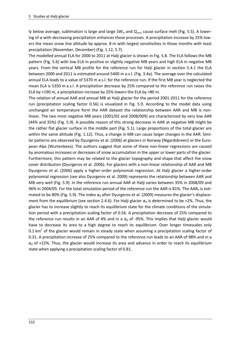
5 Studies at Halji glacier
152
ly below average, sublimation is large and large SWin and Qsens cause surface melt (Fig. 5.5). A lower-
ing of α with decreasing precipitation enhances these processes. A precipitation increase by 25% low-
ers the mean snow line altitude by approx. 8 m with largest sensitivities in those months with least
precipitation (November, December) (Fig. 1.12, 5.7).
The modelled annual ELA for 2000 to 2011 at Halji glacier is shown in Fig. 5.8. The ELA follows the MB
pattern (Fig. 5.6) with low ELA in positive or slightly negative MB years and high ELA in negative MB
years. From the vertical MB profile for the reference run for Halji glacier in section 5.4.1 the ELA
between 2000 and 2011 is estimated around 5400 m a.s.l. (Fig. 3.4a). The average over the calculated
annual ELA leads to a value of 5370 m a.s.l. for the reference run. If the first MB year is neglected the
mean ELA is 5350 m a.s.l. A precipitation decrease by 25% compared to the reference run raises the
ELA by ≈190 m, a precipitation increase by 25% lowers the ELA by ≈80 m.
The relation of annual AAR and annual MB at Halji glacier for the period 2001-2011 for the reference
run (precipitation scaling factor 0.56) is visualized in Fig. 5.9. According to the model data using
unchanged air temperature form the HAR dataset the relationship between AAR and MB is non-
linear. The two most negative MB years (2001/02 and 2008/009) are characterized by very low AAR
(44% and 35%) (Fig. 5.9). A possible reason of this strong decrease in AAR at negative MB might be
the rather flat glacier surface in the middle part (Fig. 5.1). Large proportions of the total glacier are
within the same altitude (Fig. 1.12). Thus, a change in MB can cause larger changes in the AAR. Simi-
lar patterns are observed by Dyurgerov et al. (2006) at glaciers in Norway (Nigardsbreen) or the Euro-
pean Alps (Wurtenkees). The authors suggest that some of these non-linear regressions are caused
by anomalous increases or decreases of snow accumulation in the upper or lower parts of the glacier.
Furthermore, this pattern may be related to the glacier topography and shape that affect the snow
cover distribution (Dyurgerov et al. 2006). For glaciers with a non-linear relationship of AAR and MB
Dyurgerov et al. (2006) apply a higher-order polynomial regression. At Halji glacier a higher-order
polynomial regression (see also Dyurgerov et al. 2009) represents the relationship between AAR and
MB very well (Fig. 5.9). In the reference run annual AAR at Halji varies between 35% in 2008/09 and
96% in 2004/05. For the total simulation period of the reference run the AAR is 81%. The AAR0 is esti-
mated to be 80% (Fig. 5.9). The index αd after Dyurgerov et al. (2009) measures the glacier’s displace-
ment from the equilibrium (see section 2.4.6). For Halji glacier αd is determined to be +2%. Thus, the
glacier has to increase slightly to reach its equilibrium state for the climate conditions of the simula-
tion period with a precipitation scaling factor of 0.56. A precipitation decrease of 25% compared to
the reference run results in an AAR of 4% and in a αd of -95%. This implies that Halji glacier would
have to decrease its area to a high degree to reach its equilibrium. Over longer timescales only
0.1 km2 of the glacier would remain in steady state when assuming a precipitation scaling factor of
0.31. A precipitation increase of 25% compared to the reference run leads to an AAR of 98% and in a
αd of +22%. Thus, the glacier would increase its area and advance in order to reach its equilibrium
state when applying a precipitation scaling factor of 0.81.
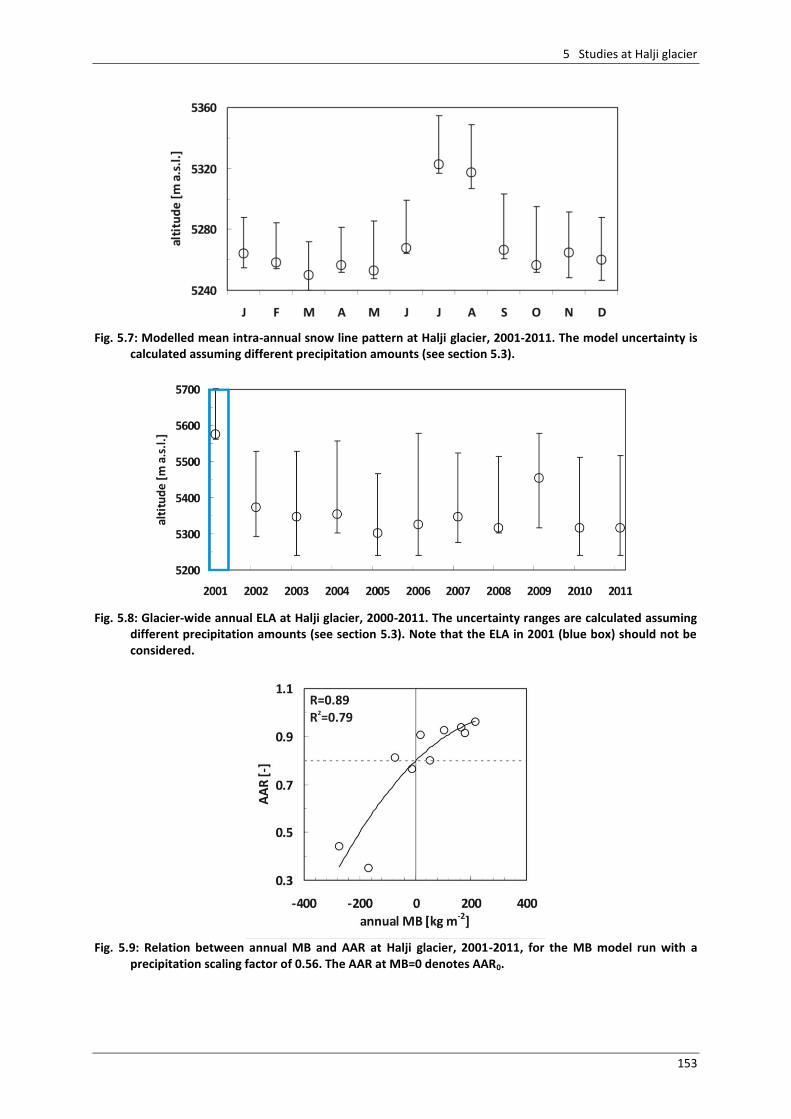
5 Studies at Halji glacier
153
Fig. 5.7: Modelled mean intra-annual snow line pattern at Halji glacier, 2001-2011. The model uncertainty is
calculated assuming different precipitation amounts (see section 5.3).
Fig. 5.8: Glacier-wide annual ELA at Halji glacier, 2000-2011. The uncertainty ranges are calculated assuming
different precipitation amounts (see section 5.3). Note that the ELA in 2001 (blue box) should not be considered.
Fig. 5.9: Relation between annual MB and AAR at Halji glacier, 2001-2011, for the MB model run with a
precipitation scaling factor of 0.56. The AAR at MB=0 denotes AAR0.
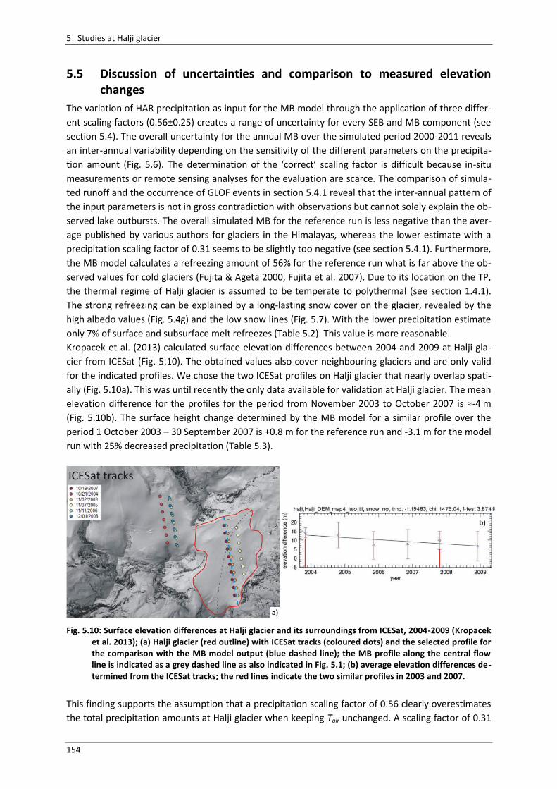
5 Studies at Halji glacier
154
5.5 Discussion of uncertainties and comparison to measured elevation changes
The variation of HAR precipitation as input for the MB model through the application of three differ-
ent scaling factors (0.56±0.25) creates a range of uncertainty for every SEB and MB component (see
section 5.4). The overall uncertainty for the annual MB over the simulated period 2000-2011 reveals
an inter-annual variability depending on the sensitivity of the different parameters on the precipita-
tion amount (Fig. 5.6). The determination of the ‘correct’ scaling factor is difficult because in-situ
measurements or remote sensing analyses for the evaluation are scarce. The comparison of simula-
ted runoff and the occurrence of GLOF events in section 5.4.1 reveal that the inter-annual pattern of
the input parameters is not in gross contradiction with observations but cannot solely explain the ob-
served lake outbursts. The overall simulated MB for the reference run is less negative than the aver-
age published by various authors for glaciers in the Himalayas, whereas the lower estimate with a
precipitation scaling factor of 0.31 seems to be slightly too negative (see section 5.4.1). Furthermore,
the MB model calculates a refreezing amount of 56% for the reference run what is far above the ob-
served values for cold glaciers (Fujita & Ageta 2000, Fujita et al. 2007). Due to its location on the TP,
the thermal regime of Halji glacier is assumed to be temperate to polythermal (see section 1.4.1).
The strong refreezing can be explained by a long-lasting snow cover on the glacier, revealed by the
high albedo values (Fig. 5.4g) and the low snow lines (Fig. 5.7). With the lower precipitation estimate
only 7% of surface and subsurface melt refreezes (Table 5.2). This value is more reasonable.
Kropacek et al. (2013) calculated surface elevation differences between 2004 and 2009 at Halji gla-
cier from ICESat (Fig. 5.10). The obtained values also cover neighbouring glaciers and are only valid
for the indicated profiles. We chose the two ICESat profiles on Halji glacier that nearly overlap spati-
ally (Fig. 5.10a). This was until recently the only data available for validation at Halji glacier. The mean
elevation difference for the profiles for the period from November 2003 to October 2007 is ≈-4 m
(Fig. 5.10b). The surface height change determined by the MB model for a similar profile over the
period 1 October 2003 – 30 September 2007 is +0.8 m for the reference run and -3.1 m for the model
run with 25% decreased precipitation (Table 5.3).
Fig. 5.10: Surface elevation differences at Halji glacier and its surroundings from ICESat, 2004-2009 (Kropacek et al. 2013); (a) Halji glacier (red outline) with ICESat tracks (coloured dots) and the selected profile for the comparison with the MB model output (blue dashed line); the MB profile along the central flow line is indicated as a grey dashed line as also indicated in Fig. 5.1; (b) average elevation differences de-termined from the ICESat tracks; the red lines indicate the two similar profiles in 2003 and 2007.
This finding supports the assumption that a precipitation scaling factor of 0.56 clearly overestimates
the total precipitation amounts at Halji glacier when keeping Tair unchanged. A scaling factor of 0.31
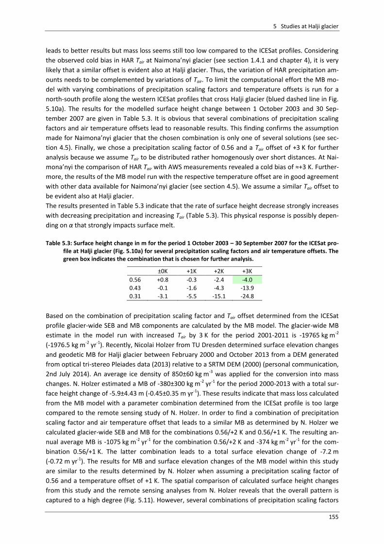
5 Studies at Halji glacier
155
leads to better results but mass loss seems still too low compared to the ICESat profiles. Considering
the observed cold bias in HAR Tair at Naimona’nyi glacier (see section 1.4.1 and chapter 4), it is very
likely that a similar offset is evident also at Halji glacier. Thus, the variation of HAR precipitation am-
ounts needs to be complemented by variations of Tair. To limit the computational effort the MB mo-
del with varying combinations of precipitation scaling factors and temperature offsets is run for a
north-south profile along the western ICESat profiles that cross Halji glacier (blued dashed line in Fig.
5.10a). The results for the modelled surface height change between 1 October 2003 and 30 Sep-
tember 2007 are given in Table 5.3. It is obvious that several combinations of precipitation scaling
factors and air temperature offsets lead to reasonable results. This finding confirms the assumption
made for Naimona’nyi glacier that the chosen combination is only one of several solutions (see sec-
tion 4.5). Finally, we chose a precipitation scaling factor of 0.56 and a Tair offset of +3 K for further
analysis because we assume Tair to be distributed rather homogenously over short distances. At Nai-
mona’nyi the comparison of HAR Tair with AWS measurements revealed a cold bias of ≈+3 K. Further-
more, the results of the MB model run with the respective temperature offset are in good agreement
with other data available for Naimona’nyi glacier (see section 4.5). We assume a similar Tair offset to
be evident also at Halji glacier.
The results presented in Table 5.3 indicate that the rate of surface height decrease strongly increases
with decreasing precipitation and increasing Tair (Table 5.3). This physical response is possibly depen-
ding on α that strongly impacts surface melt.
Table 5.3: Surface height change in m for the period 1 October 2003 – 30 September 2007 for the ICESat pro-
file at Halji glacier (Fig. 5.10a) for several precipitation scaling factors and air temperature offsets. The green box indicates the combination that is chosen for further analysis.
±0K +1K +2K +3K
0.56 +0.8 -0.3 -2.4 -4.0
0.43 -0.1 -1.6 -4.3 -13.9
0.31 -3.1 -5.5 -15.1 -24.8
Based on the combination of precipitation scaling factor and Tair offset determined from the ICESat
profile glacier-wide SEB and MB components are calculated by the MB model. The glacier-wide MB
estimate in the model run with increased Tair by 3 K for the period 2001-2011 is -19765 kg m-2
(-1976.5 kg m-2 yr-1). Recently, Nicolai Holzer from TU Dresden determined surface elevation changes
and geodetic MB for Halji glacier between February 2000 and October 2013 from a DEM generated
from optical tri-stereo Pleiades data (2013) relative to a SRTM DEM (2000) (personal communication,
2nd July 2014). An average ice density of 850±60 kg m-3 was applied for the conversion into mass
changes. N. Holzer estimated a MB of -380±300 kg m-2 yr-1 for the period 2000-2013 with a total sur-
face height change of -5.9±4.43 m (-0.45±0.35 m yr-1). These results indicate that mass loss calculated
from the MB model with a parameter combination determined from the ICESat profile is too large
compared to the remote sensing study of N. Holzer. In order to find a combination of precipitation
scaling factor and air temperature offset that leads to a similar MB as determined by N. Holzer we
calculated glacier-wide SEB and MB for the combinations 0.56/+2 K and 0.56/+1 K. The resulting an-
nual average MB is -1075 kg m-2 yr-1 for the combination 0.56/+2 K and -374 kg m-2 yr-1 for the com-
bination 0.56/+1 K. The latter combination leads to a total surface elevation change of -7.2 m
(-0.72 m yr-1). The results for MB and surface elevation changes of the MB model within this study
are similar to the results determined by N. Holzer when assuming a precipitation scaling factor of
0.56 and a temperature offset of +1 K. The spatial comparison of calculated surface height changes
from this study and the remote sensing analyses from N. Holzer reveals that the overall pattern is
captured to a high degree (Fig. 5.11). However, several combinations of precipitation scaling factors
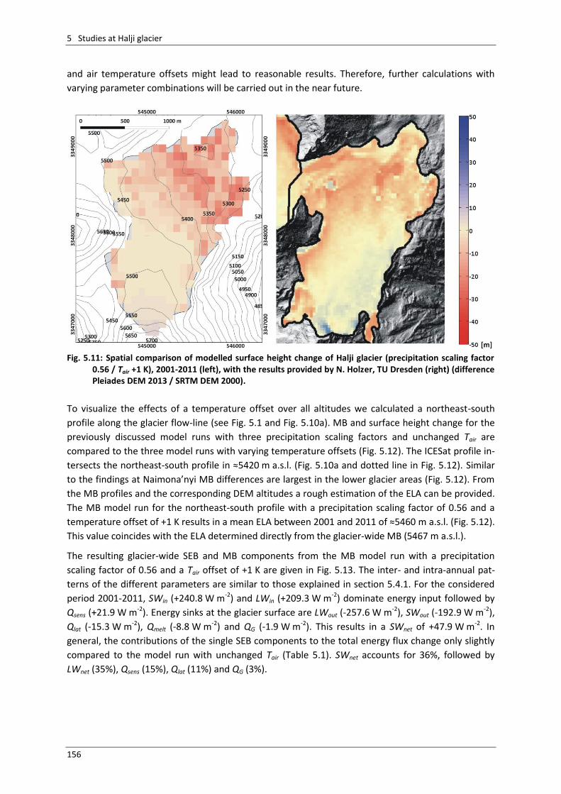
5 Studies at Halji glacier
156
and air temperature offsets might lead to reasonable results. Therefore, further calculations with
varying parameter combinations will be carried out in the near future.
Fig. 5.11: Spatial comparison of modelled surface height change of Halji glacier (precipitation scaling factor
0.56 / Tair +1 K), 2001-2011 (left), with the results provided by N. Holzer, TU Dresden (right) (difference Pleiades DEM 2013 / SRTM DEM 2000).
To visualize the effects of a temperature offset over all altitudes we calculated a northeast-south
profile along the glacier flow-line (see Fig. 5.1 and Fig. 5.10a). MB and surface height change for the
previously discussed model runs with three precipitation scaling factors and unchanged Tair are
compared to the three model runs with varying temperature offsets (Fig. 5.12). The ICESat profile in-
tersects the northeast-south profile in ≈5420 m a.s.l. (Fig. 5.10a and dotted line in Fig. 5.12). Similar
to the findings at Naimona’nyi MB differences are largest in the lower glacier areas (Fig. 5.12). From
the MB profiles and the corresponding DEM altitudes a rough estimation of the ELA can be provided.
The MB model run for the northeast-south profile with a precipitation scaling factor of 0.56 and a
temperature offset of +1 K results in a mean ELA between 2001 and 2011 of ≈5460 m a.s.l. (Fig. 5.12).
This value coincides with the ELA determined directly from the glacier-wide MB (5467 m a.s.l.).
The resulting glacier-wide SEB and MB components from the MB model run with a precipitation
scaling factor of 0.56 and a Tair offset of +1 K are given in Fig. 5.13. The inter- and intra-annual pat-
terns of the different parameters are similar to those explained in section 5.4.1. For the considered
period 2001-2011, SWin (+240.8 W m-2) and LWin (+209.3 W m-2) dominate energy input followed by
Qsens (+21.9 W m-2). Energy sinks at the glacier surface are LWout (-257.6 W m-2), SWout (-192.9 W m-2),
Qlat (-15.3 W m-2), Qmelt (-8.8 W m-2) and QG (-1.9 W m-2). This results in a SWnet of +47.9 W m-2. In
general, the contributions of the single SEB components to the total energy flux change only slightly
compared to the model run with unchanged Tair (Table 5.1). SWnet accounts for 36%, followed by
LWnet (35%), Qsens (15%), Qlat (11%) and QG (3%).
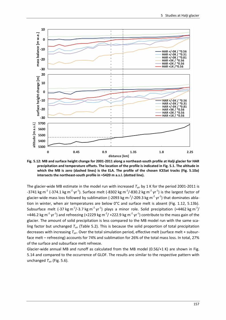
5 Studies at Halji glacier
157
Fig. 5.12: MB and surface height change for 2001-2011 along a northeast-south profile at Halji glacier for HAR
precipitation and temperature offsets. The location of the profile is indicated in Fig. 5.1. The altitude in which the MB is zero (dashed lines) is the ELA. The profile of the chosen ICESat tracks (Fig. 5.10a) intersects the northeast-south profile in ≈5420 m a.s.l. (dotted line).
The glacier-wide MB estimate in the model run with increased Tair by 1 K for the period 2001-2011 is
-3741 kg m-2 (-374.1 kg m-2 yr-1). Surface melt (-8302 kg m-2/-830.2 kg m-2 yr-1) is the largest factor of
glacier-wide mass loss followed by sublimation (-2093 kg m-2/-209.3 kg m-2 yr-1) that dominates abla-
tion in winter, when air temperatures are below 0°C and surface melt is absent (Fig. 1.12, 5.13b).
Subsurface melt (-37 kg m-2/-3.7 kg m-2 yr-1) plays a minor role. Solid precipitation (+4462 kg m-2/
+446.2 kg m-2 yr-1) and refreezing (+2229 kg m-2/ +222.9 kg m-2 yr-1) contribute to the mass gain of the
glacier. The amount of solid precipitation is less compared to the MB model run with the same sca-
ling factor but unchanged Tair (Table 5.2). This is because the solid proportion of total precipitation
decreases with increasing Tair. Over the total simulation period, effective melt (surface melt + subsur-
face melt – refreezing) accounts for 74% and sublimation for 26% of the total mass loss. In total, 27%
of the surface and subsurface melt refreeze.
Glacier-wide annual MB and runoff as calculated from the MB model (0.56/+1 K) are shown in Fig.
5.14 and compared to the occurrence of GLOF. The results are similar to the respective pattern with
unchanged Tair (Fig. 5.6).
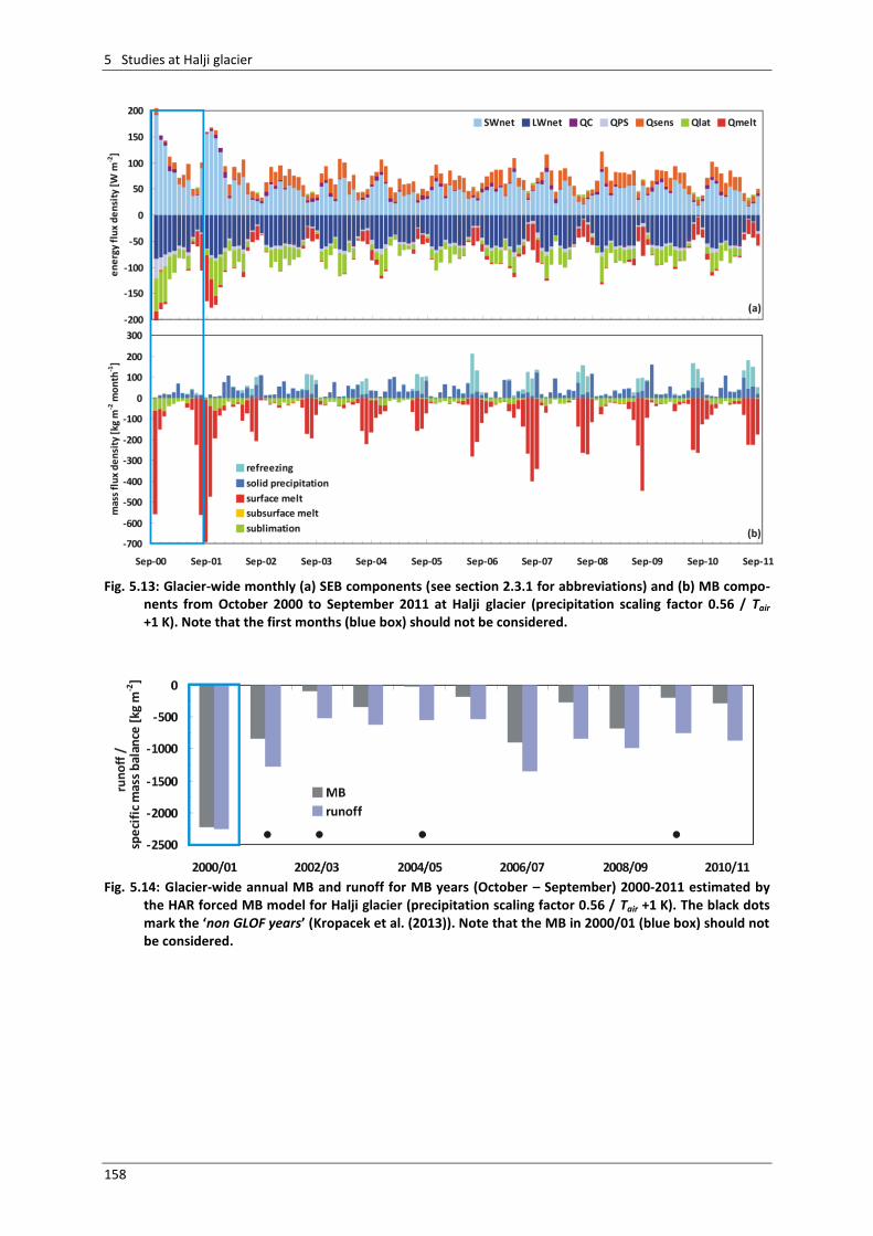
5 Studies at Halji glacier
158
Fig. 5.13: Glacier-wide monthly (a) SEB components (see section 2.3.1 for abbreviations) and (b) MB compo-
nents from October 2000 to September 2011 at Halji glacier (precipitation scaling factor 0.56 / Tair +1 K). Note that the first months (blue box) should not be considered.
Fig. 5.14: Glacier-wide annual MB and runoff for MB years (October – September) 2000-2011 estimated by
the HAR forced MB model for Halji glacier (precipitation scaling factor 0.56 / Tair +1 K). The black dots mark the ‘non GLOF years’ (Kropacek et al. (2013)). Note that the MB in 2000/01 (blue box) should not be considered.
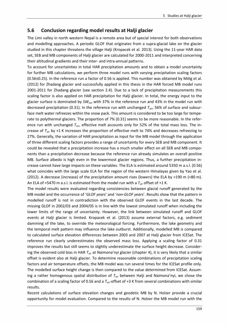
5 Studies at Halji glacier
159
5.6 Conclusion regarding model results at Halji glacier
The Limi valley in north western Nepal is a remote area but of special interest for both observations
and modelling approaches. A periodic GLOF that originates from a supra-glacial lake on the glacier
studied in this chapter threatens the village Halji (Kropacek et al. 2013). Using the 11-year HAR data
set, SEB and MB components of Halji glacier are calculated for 2000-2011 and interpreted concerning
their altitudinal gradients and their inter- and intra-annual patterns.
To account for uncertainties in total HAR precipitation amounts and to obtain a model uncertainty
for further MB calculations, we perform three model runs with varying precipitation scaling factors
(0.56±0.25). In the reference run a factor of 0.56 is applied. This number was obtained by Mölg et al.
(2012) for Zhadang glacier and successfully applied in this thesis in the HAR forced MB model runs
2001-2011 for Zhadang glacier (see section 2.4). Due to a lack of precipitation measurements this
scaling factor is also applied on HAR precipitation for Halji glacier. In total, the energy input to the
glacier surface is dominated by SWnet with 37% in the reference run and 43% in the model run with
decreased precipitation (0.31). In the reference run with unchanged Tair, 56% of surface and subsur-
face melt water refreezes within the snow pack. This amount is considered to be too large for tempe-
rate to polythermal glaciers. The proportion of 7% (0.31) seems to be more reasonable. In the refer-
ence run with unchanged Tair, effective melt accounts only for 52% of the total mass loss. The in-
crease of Tair by +1 K increases the proportion of effective melt to 74% and decreases refreezing to
27%. Generally, the variation of HAR precipitation as input for the MB model through the application
of three different scaling factors provides a range of uncertainty for every SEB and MB component. It
could be revealed that a precipitation increase has a much smaller effect on all SEB and MB compo-
nents than a precipitation decrease because the reference run already simulates an overall positive
MB. Surface albedo is high even in the lowermost glacier regions. Thus, a further precipitation in-
crease cannot have large impacts on these variables. The ELA is estimated around 5350 m a.s.l. (0.56)
what coincides with the large scale ELA for the region of the western Himalayas given by Yao et al.
(2012). A decrease (increase) of the precipitation amount rises (lowers) the ELA by ≈190 m (≈80 m).
An ELA of ≈5470 m a.s.l. is estimated from the model run with a Tair offset of +1 K.
The model results were evaluated regarding consistencies between glacial runoff generated by the
MB model and the occurrence of ‘GLOF years’ and ‘non-GLOF years’. Results show that the pattern in
modelled runoff is not in contradiction with the observed GLOF events in the last decade. The
missing GLOF in 2002/03 and 2004/05 is in line with the lowest simulated runoff when including the
lower limits of the range of uncertainty. However, the link between simulated runoff and GLOF
events at Halji glacier is limited. Kropacek et al. (2013) assume external factors, e.g. sediment
damming of the lake, to override the meteorological forcing. Furthermore, the lake geometry and
the temporal melt pattern may influence the lake outburst. Additionally, modelled MB is compared
to calculated surface elevation differences between 2003 and 2007 at Halji glacier from ICESat. The
reference run clearly underestimates the observed mass loss. Applying a scaling factor of 0.31
improves the results but still seems to slightly underestimate the surface height decrease. Consider-
ing the observed cold bias in HAR Tair at Naimona’nyi glacier (chapter 4), it is very likely that a similar
offset is evident also at Halji glacier. To determine reasonable combinations of precipitation scaling
factors and air temperature offsets, the MB model was run several times for the ICESat profile only.
The modelled surface height change is then compared to the value determined from ICESat. Assum-
ing a rather homogenous spatial distribution of Tair between Halji and Naimona’nyi, we chose the
combination of a scaling factor of 0.56 and a Tair-offset of +3 K from several combinations with similar
results.
Recent calculations of surface elevation changes and geodetic MB by N. Holzer provide a crucial
opportunity for model evaluation. Compared to the results of N. Holzer the MB model run with the
5 Studies at Halji glacier
160
combination of precipitation scaling factor and temperature offset determined from the ICESat
profile clearly overestimates mass loss. With the combination 0.56/+1 K the MB model results are
more reasonable.
From the application of the MB model to Halji glacier it can be concluded that the derived intra- and
inter-annual cycles of SEB and MB components are within reasonable limits. The results depend on
the respective patterns of the input parameters from HAR. The obtained SEB and MB components
are consistent with each other because they interact through physical relationships (see sections
1.3.4 and 2.3.1). HAR output overestimates the amount of solid precipitation in the reference run. A
scaling factor of 0.31 is more reasonable when no correction to HAR air temperature data is included
(see sections 5.4 and 5.5). Recent remote sensing analyses provided by N. Holzer largely improve the
opportunities for model evaluation. However, the results from N. Holzer lead to a different ‘best-fit’
combination of precipitation scaling factor and Tair-offset than the remote sensing analyses by Kro-
pacek et al. (2013). The lack of meteorological field observations hampers the ability to verify HAR
precipitation amounts and possible Tair offsets.
A cold bias in HAR Tair, even though possibly smaller that at Naimona’nyi, seems to be nevertheless
plausible since both remote sensing studies provide evidence that the results of the MB model re-
produce observed glacier change best when Tair is increased by at least 1 K. The result from chapter 5
points to the fact that it is difficult to obtain absolute values for glacier-wide MB or runoff in regions
where precipitation and/or temperature measurements are not available or MB model results can-
not be validated in detail by other means as for example by glaciological MB observations.
6 Studies at Muztagh Ata
161
6 Energy and mass balance for a glacier in the Muztagh Ata re-gion, north western Tibetan Plateau, 2000-2012
6.1 Introduction and regional climate conditions
The selected glacier is part of the glaciation of Muztagh Ata, the third highest peak of the Pamir
Mountains (≈7500 m a.s.l.), the western margin of the Tibetan Plateau (Fig. 6.1, see section 1.4.1).
The region is highly glaciated and therefore favours the application of remote sensing techniques to
determine the state of the glaciers. Annual MB between 2005 and 2010 is available for one small
glacier (Yao et al. 2012). Most glaciers in this region are characterized by a large amount of debris co-
ver (Shangguan et al. 2006, see section 1.4.1). Since the debris cover modifies the glacier SEB and MB
depending on its thickness (see section 1.4.2.2) a debris free glacier was chosen for the MB model
application. It is a west exposed valley glacier with an area of ≈8.0 km2 at the western slope of Muz-
tagh Ata (Fig. 6.1).
The region is strongly influenced by the westerlies that are the most important source of moisture
(see section 1.4.1). The impact of the monsoon precipitation is absent. Daily mean air temperatures
generated by HAR generally rise above zero only in July and August and daily means range between
-36.7°C and +6.1 C (average -11.3°C) within the period 2000-2012. Fig. 6.2 shows monthly means of
those HAR variables that serve as input for the applied MB model. The atmospheric variables that are
influenced by SWin and/or Tair show the typical annual cycle (RH, p, Fig. 6.2). N is relatively high
throughout the year and reveals a maximum in winter when the humid air masses of the westerly
winds are forced to ascent at the Pamirs. Precipitation amounts are generally small but equally distri-
buted over the year with a maximum in spring (Fig. 6.2, see section 1.4.1). The large altitudinal range
of the glacier (≈2000 m) causes a significant impact of both temperature and precipitation gradients.
Precipitation amounts increase with altitude and Tair from HAR is already low in the lower glacier re-
gions (4817 m a.s.l., Fig. 1.18, 6.1) and decreases with altitude. Therefore, it can be assumed that the
estimated mass loss from the MB model from 2000-2012 is not large. This assumption is supported
by the observations published by Yao et al. (2012). For a neighbouring glacier in the same region the
authors give a regional ELA of 5460 m a.s.l. for the years 2001-2010. They find an overall positive MB
between 2005 and 2010 (Yao et al. 2012).
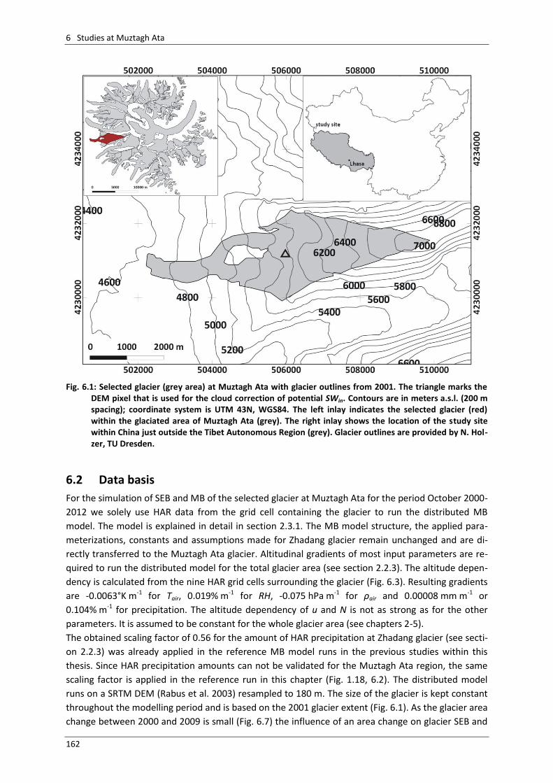
6 Studies at Muztagh Ata
162
Fig. 6.1: Selected glacier (grey area) at Muztagh Ata with glacier outlines from 2001. The triangle marks the DEM pixel that is used for the cloud correction of potential SWin. Contours are in meters a.s.l. (200 m spacing); coordinate system is UTM 43N, WGS84. The left inlay indicates the selected glacier (red) within the glaciated area of Muztagh Ata (grey). The right inlay shows the location of the study site within China just outside the Tibet Autonomous Region (grey). Glacier outlines are provided by N. Hol-zer, TU Dresden.
6.2 Data basis
For the simulation of SEB and MB of the selected glacier at Muztagh Ata for the period October 2000-
2012 we solely use HAR data from the grid cell containing the glacier to run the distributed MB
model. The model is explained in detail in section 2.3.1. The MB model structure, the applied para-
meterizations, constants and assumptions made for Zhadang glacier remain unchanged and are di-
rectly transferred to the Muztagh Ata glacier. Altitudinal gradients of most input parameters are re-
quired to run the distributed model for the total glacier area (see section 2.2.3). The altitude depen-
dency is calculated from the nine HAR grid cells surrounding the glacier (Fig. 6.3). Resulting gradients
are -0.0063°K m-1 for Tair, 0.019% m-1 for RH, -0.075 hPa m-1 for ρair and 0.00008 mm m-1 or
0.104% m-1 for precipitation. The altitude dependency of u and N is not as strong as for the other
parameters. It is assumed to be constant for the whole glacier area (see chapters 2-5).
The obtained scaling factor of 0.56 for the amount of HAR precipitation at Zhadang glacier (see secti-
on 2.2.3) was already applied in the reference MB model runs in the previous studies within this
thesis. Since HAR precipitation amounts can not be validated for the Muztagh Ata region, the same
scaling factor is applied in the reference run in this chapter (Fig. 1.18, 6.2). The distributed model
runs on a SRTM DEM (Rabus et al. 2003) resampled to 180 m. The size of the glacier is kept constant
throughout the modelling period and is based on the 2001 glacier extent (Fig. 6.1). As the glacier area
change between 2000 and 2009 is small (Fig. 6.7) the influence of an area change on glacier SEB and
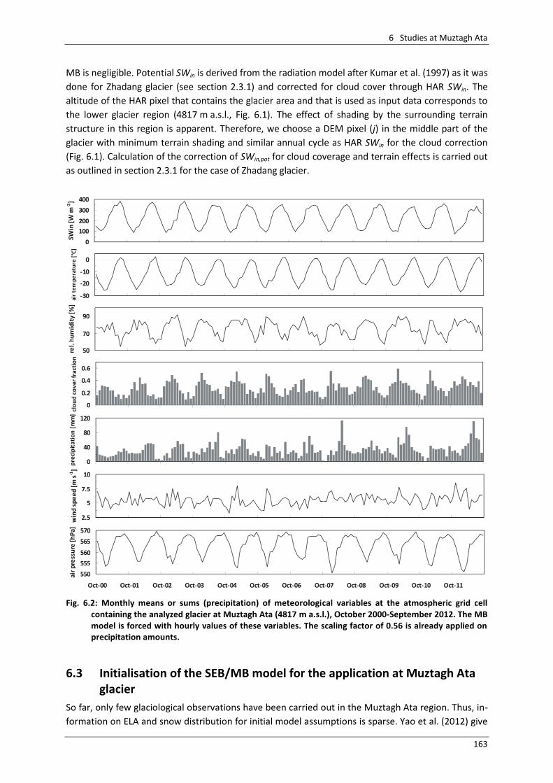
6 Studies at Muztagh Ata
163
MB is negligible. Potential SWin is derived from the radiation model after Kumar et al. (1997) as it was
done for Zhadang glacier (see section 2.3.1) and corrected for cloud cover through HAR SWin. The
altitude of the HAR pixel that contains the glacier area and that is used as input data corresponds to
the lower glacier region (4817 m a.s.l., Fig. 6.1). The effect of shading by the surrounding terrain
structure in this region is apparent. Therefore, we choose a DEM pixel (j) in the middle part of the
glacier with minimum terrain shading and similar annual cycle as HAR SWin for the cloud correction
(Fig. 6.1). Calculation of the correction of SWin,pot for cloud coverage and terrain effects is carried out
as outlined in section 2.3.1 for the case of Zhadang glacier.
Fig. 6.2: Monthly means or sums (precipitation) of meteorological variables at the atmospheric grid cell
containing the analyzed glacier at Muztagh Ata (4817 m a.s.l.), October 2000-September 2012. The MB model is forced with hourly values of these variables. The scaling factor of 0.56 is already applied on precipitation amounts.
6.3 Initialisation of the SEB/MB model for the application at Muztagh Ata glacier
So far, only few glaciological observations have been carried out in the Muztagh Ata region. Thus, in-
formation on ELA and snow distribution for initial model assumptions is sparse. Yao et al. (2012) give
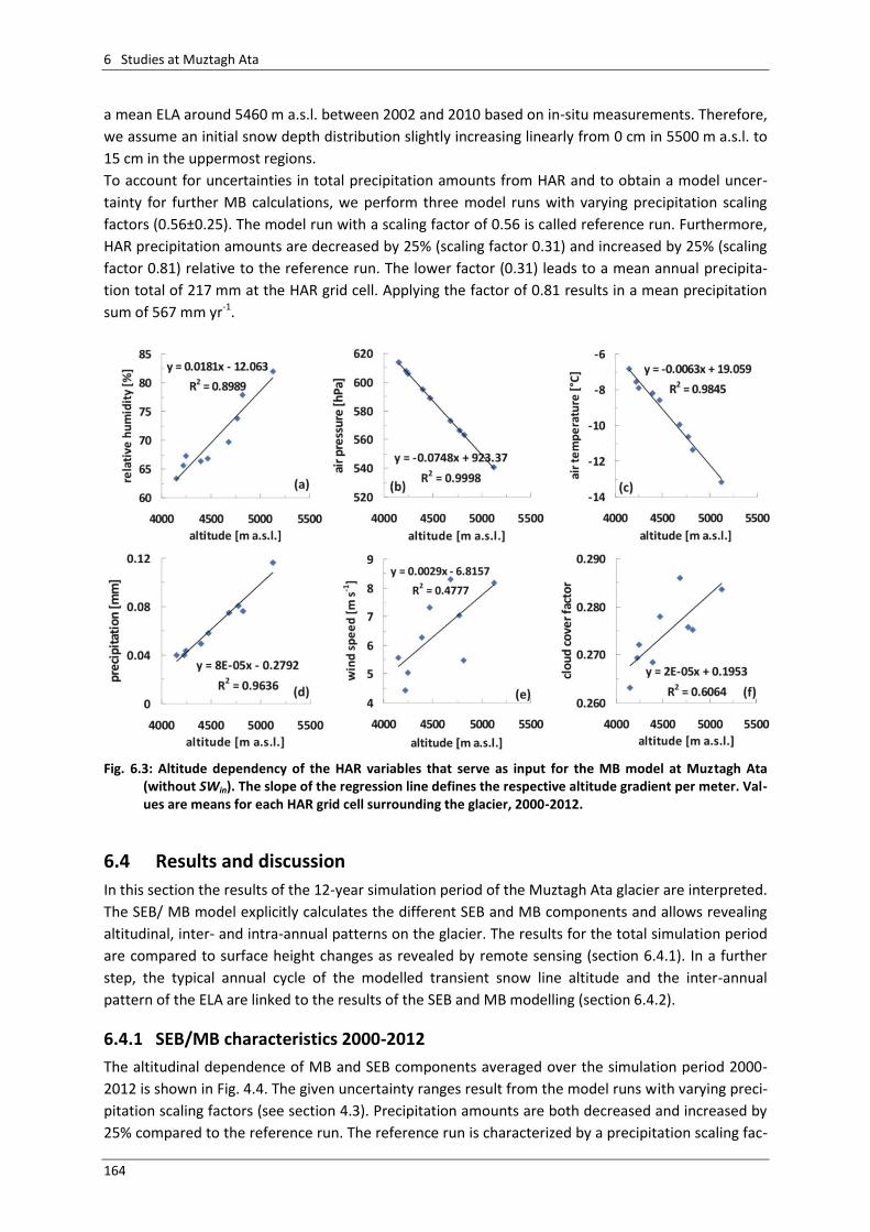
6 Studies at Muztagh Ata
164
a mean ELA around 5460 m a.s.l. between 2002 and 2010 based on in-situ measurements. Therefore,
we assume an initial snow depth distribution slightly increasing linearly from 0 cm in 5500 m a.s.l. to
15 cm in the uppermost regions.
To account for uncertainties in total precipitation amounts from HAR and to obtain a model uncer-
tainty for further MB calculations, we perform three model runs with varying precipitation scaling
factors (0.56±0.25). The model run with a scaling factor of 0.56 is called reference run. Furthermore,
HAR precipitation amounts are decreased by 25% (scaling factor 0.31) and increased by 25% (scaling
factor 0.81) relative to the reference run. The lower factor (0.31) leads to a mean annual precipita-
tion total of 217 mm at the HAR grid cell. Applying the factor of 0.81 results in a mean precipitation
sum of 567 mm yr-1.
Fig. 6.3: Altitude dependency of the HAR variables that serve as input for the MB model at Muztagh Ata
(without SWin). The slope of the regression line defines the respective altitude gradient per meter. Val-ues are means for each HAR grid cell surrounding the glacier, 2000-2012.
6.4 Results and discussion
In this section the results of the 12-year simulation period of the Muztagh Ata glacier are interpreted.
The SEB/ MB model explicitly calculates the different SEB and MB components and allows revealing
altitudinal, inter- and intra-annual patterns on the glacier. The results for the total simulation period
are compared to surface height changes as revealed by remote sensing (section 6.4.1). In a further
step, the typical annual cycle of the modelled transient snow line altitude and the inter-annual
pattern of the ELA are linked to the results of the SEB and MB modelling (section 6.4.2).
6.4.1 SEB/MB characteristics 2000-2012
The altitudinal dependence of MB and SEB components averaged over the simulation period 2000-
2012 is shown in Fig. 4.4. The given uncertainty ranges result from the model runs with varying preci-
pitation scaling factors (see section 4.3). Precipitation amounts are both decreased and increased by
25% compared to the reference run. The reference run is characterized by a precipitation scaling fac-
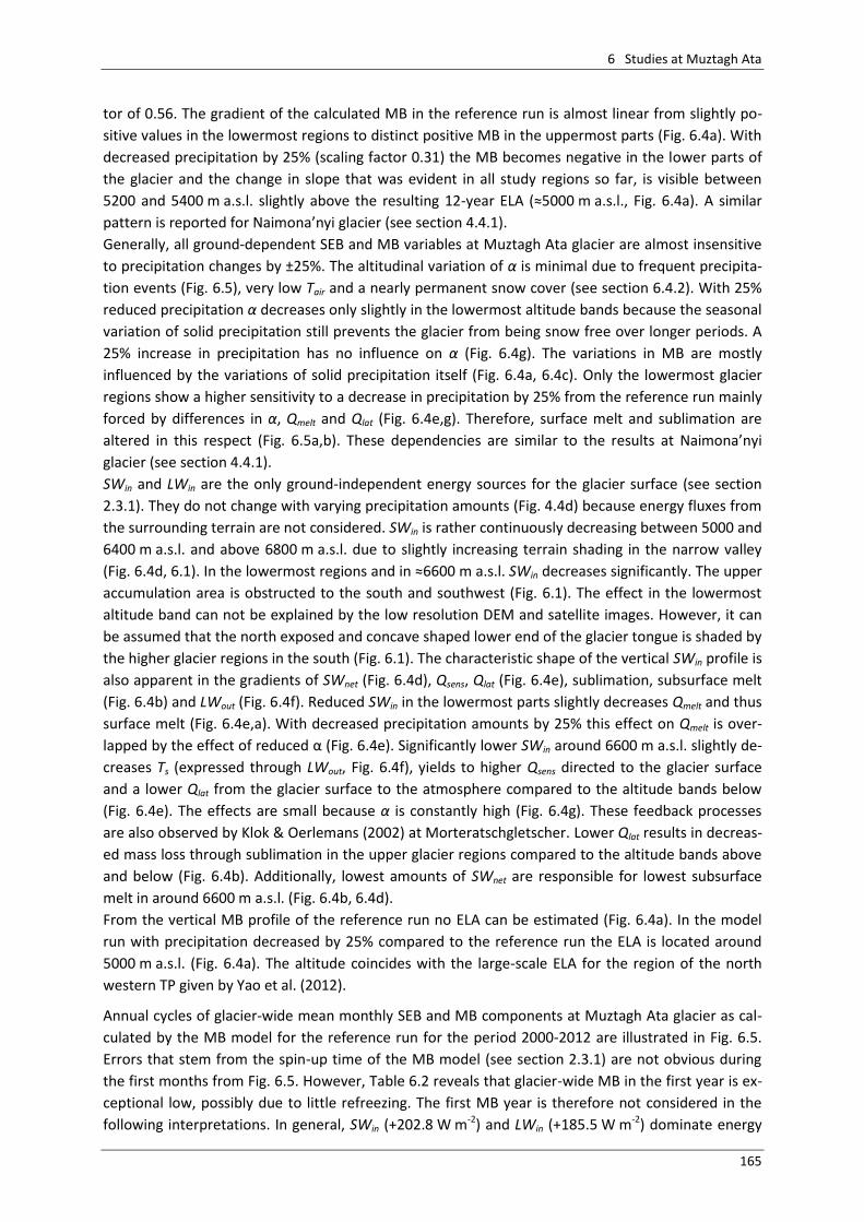
6 Studies at Muztagh Ata
165
tor of 0.56. The gradient of the calculated MB in the reference run is almost linear from slightly po-
sitive values in the lowermost regions to distinct positive MB in the uppermost parts (Fig. 6.4a). With
decreased precipitation by 25% (scaling factor 0.31) the MB becomes negative in the lower parts of
the glacier and the change in slope that was evident in all study regions so far, is visible between
5200 and 5400 m a.s.l. slightly above the resulting 12-year ELA (≈5000 m a.s.l., Fig. 6.4a). A similar
pattern is reported for Naimona’nyi glacier (see section 4.4.1).
Generally, all ground-dependent SEB and MB variables at Muztagh Ata glacier are almost insensitive
to precipitation changes by ±25%. The altitudinal variation of α is minimal due to frequent precipita-
tion events (Fig. 6.5), very low Tair and a nearly permanent snow cover (see section 6.4.2). With 25%
reduced precipitation α decreases only slightly in the lowermost altitude bands because the seasonal
variation of solid precipitation still prevents the glacier from being snow free over longer periods. A
25% increase in precipitation has no influence on α (Fig. 6.4g). The variations in MB are mostly
influenced by the variations of solid precipitation itself (Fig. 6.4a, 6.4c). Only the lowermost glacier
regions show a higher sensitivity to a decrease in precipitation by 25% from the reference run mainly
forced by differences in α, Qmelt and Qlat (Fig. 6.4e,g). Therefore, surface melt and sublimation are
altered in this respect (Fig. 6.5a,b). These dependencies are similar to the results at Naimona’nyi
glacier (see section 4.4.1).
SWin and LWin are the only ground-independent energy sources for the glacier surface (see section
2.3.1). They do not change with varying precipitation amounts (Fig. 4.4d) because energy fluxes from
the surrounding terrain are not considered. SWin is rather continuously decreasing between 5000 and
6400 m a.s.l. and above 6800 m a.s.l. due to slightly increasing terrain shading in the narrow valley
(Fig. 6.4d, 6.1). In the lowermost regions and in ≈6600 m a.s.l. SWin decreases significantly. The upper
accumulation area is obstructed to the south and southwest (Fig. 6.1). The effect in the lowermost
altitude band can not be explained by the low resolution DEM and satellite images. However, it can
be assumed that the north exposed and concave shaped lower end of the glacier tongue is shaded by
the higher glacier regions in the south (Fig. 6.1). The characteristic shape of the vertical SWin profile is
also apparent in the gradients of SWnet (Fig. 6.4d), Qsens, Qlat (Fig. 6.4e), sublimation, subsurface melt
(Fig. 6.4b) and LWout (Fig. 6.4f). Reduced SWin in the lowermost parts slightly decreases Qmelt and thus
surface melt (Fig. 6.4e,a). With decreased precipitation amounts by 25% this effect on Qmelt is over-
lapped by the effect of reduced α (Fig. 6.4e). Significantly lower SWin around 6600 m a.s.l. slightly de-
creases Ts (expressed through LWout, Fig. 6.4f), yields to higher Qsens directed to the glacier surface
and a lower Qlat from the glacier surface to the atmosphere compared to the altitude bands below
(Fig. 6.4e). The effects are small because α is constantly high (Fig. 6.4g). These feedback processes
are also observed by Klok & Oerlemans (2002) at Morteratschgletscher. Lower Qlat results in decreas-
ed mass loss through sublimation in the upper glacier regions compared to the altitude bands above
and below (Fig. 6.4b). Additionally, lowest amounts of SWnet are responsible for lowest subsurface
melt in around 6600 m a.s.l. (Fig. 6.4b, 6.4d).
From the vertical MB profile of the reference run no ELA can be estimated (Fig. 6.4a). In the model
run with precipitation decreased by 25% compared to the reference run the ELA is located around
5000 m a.s.l. (Fig. 6.4a). The altitude coincides with the large-scale ELA for the region of the north
western TP given by Yao et al. (2012).
Annual cycles of glacier-wide mean monthly SEB and MB components at Muztagh Ata glacier as cal-
culated by the MB model for the reference run for the period 2000-2012 are illustrated in Fig. 6.5.
Errors that stem from the spin-up time of the MB model (see section 2.3.1) are not obvious during
the first months from Fig. 6.5. However, Table 6.2 reveals that glacier-wide MB in the first year is ex-
ceptional low, possibly due to little refreezing. The first MB year is therefore not considered in the
following interpretations. In general, SWin (+202.8 W m-2) and LWin (+185.5 W m-2) dominate energy
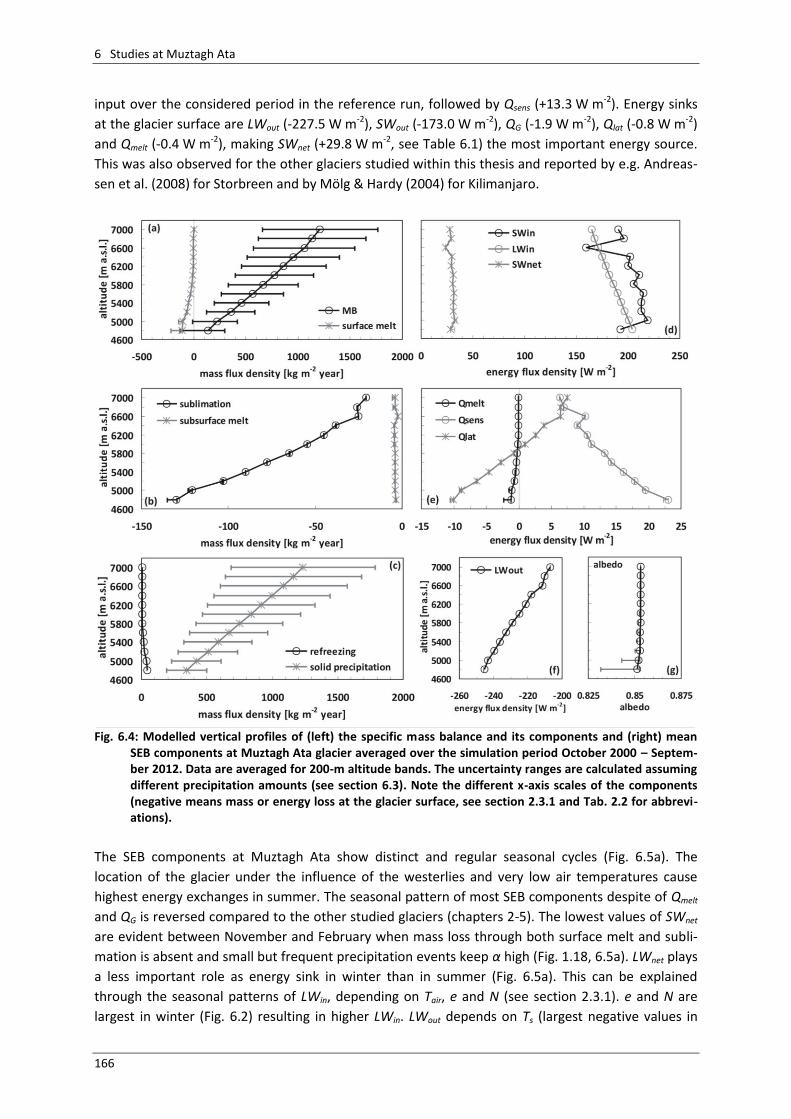
6 Studies at Muztagh Ata
166
input over the considered period in the reference run, followed by Qsens (+13.3 W m-2). Energy sinks
at the glacier surface are LWout (-227.5 W m-2), SWout (-173.0 W m-2), QG (-1.9 W m-2), Qlat (-0.8 W m-2)
and Qmelt (-0.4 W m-2), making SWnet (+29.8 W m-2, see Table 6.1) the most important energy source.
This was also observed for the other glaciers studied within this thesis and reported by e.g. Andreas-
sen et al. (2008) for Storbreen and by Mölg & Hardy (2004) for Kilimanjaro.
Fig. 6.4: Modelled vertical profiles of (left) the specific mass balance and its components and (right) mean
SEB components at Muztagh Ata glacier averaged over the simulation period October 2000 – Septem-ber 2012. Data are averaged for 200-m altitude bands. The uncertainty ranges are calculated assuming different precipitation amounts (see section 6.3). Note the different x-axis scales of the components (negative means mass or energy loss at the glacier surface, see section 2.3.1 and Tab. 2.2 for abbrevi-ations).
The SEB components at Muztagh Ata show distinct and regular seasonal cycles (Fig. 6.5a). The
location of the glacier under the influence of the westerlies and very low air temperatures cause
highest energy exchanges in summer. The seasonal pattern of most SEB components despite of Qmelt
and QG is reversed compared to the other studied glaciers (chapters 2-5). The lowest values of SWnet
are evident between November and February when mass loss through both surface melt and subli-
mation is absent and small but frequent precipitation events keep α high (Fig. 1.18, 6.5a). LWnet plays
a less important role as energy sink in winter than in summer (Fig. 6.5a). This can be explained
through the seasonal patterns of LWin, depending on Tair, e and N (see section 2.3.1). e and N are
largest in winter (Fig. 6.2) resulting in higher LWin. LWout depends on Ts (largest negative values in
6 Studies at Muztagh Ata
167
summer). QC follows the expected pattern with positive values in winter and negative values in
summer (see chapters 2-5). QPS is always negative with larger values when α is low (and SWnet is
large) (Fig. 6.5a). Generally, Qlat is a small energy sink for the glacier surface (Table 6.1). However, on
a monthly time scale it is evident that positive values regularly occur in winter (Fig. 6.5a) when the
region is under the influence of maximum precipitation amounts and highest RH in the course of the
year (Fig. 1.18, 6.2). At positive Qlat in winter deposition of moist air contributes to mass gain at the
glacier surface. The contribution of deposition to the glacier MB is not yet explicitly calculated in the
MB model applied in this thesis (see section 4.4.1). In summer, the dry conditions on the western TP
lead to negative Qlat and sublimation (Fig. 6.5). Qsens is always positive. Absolute values of Qsens are
generally larger than Qlat implying a higher moisture content of the atmosphere and less sublimation
compared to the other study sites (chapters 2-5). A similar dependency is observed by Nicholson et
al. (2013) at Lewis glacier (Mt Kenya). Furthermore, the very low Tair might limit the turbulent energy
exchange. Surface melt rates are very small and occur dominantly in July and August when the
energy supply by Qsens is largest (Fig. 6.5a). The SEB values for the model runs with varying precipita-
tion scaling factors are given in Table 6.1. For glacier-wide monthly SEB components of the MB model
runs with ±25% of precipitation see Fig. A.7a and Fig. A.8a in the appendix.
Fig. 6.5: Glacier-wide monthly (a) SEB components (see section 2.3.1 for abbreviations) and (b) MB com-
ponents at Muztag Ata glacier from October 2001 to September 2011 (reference run). Note that the first months (blue box) should not be considered.
The glacier-wide MB estimate of the reference run at Muztagh Ata glacier for the period 2001-2012
(the first year is not considered) is +7765 kg m-2 (+705.9 kg m-2 yr-1) (Table 6.2). In general, sublima-
tion (-753 kg m-2/ -68.5 kg m-2 yr-1) is the largest factor of glacier-wide mass loss followed by surface
melt (-405 kg m-2/ -36.8 kg m-2 yr-1) and clearly dominates ablation in spring and autumn (Fig. 6.5b).
Subsurface melt (-44 kg m-2/-4.0 kg m-2 yr-1) plays a minor role. Solid precipitation (+8793 kg m-2/
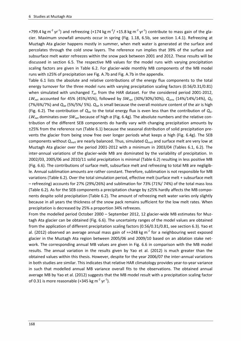
6 Studies at Muztagh Ata
168
+799.4 kg m-2 yr-1) and refreezing (+174 kg m-2/ +15.8 kg m-2 yr-1) contribute to mass gain of the gla-
cier. Maximum snowfall amounts occur in spring (Fig. 1.18, 6.5b, see section 1.4.1). Refreezing at
Muztagh Ata glacier happens mostly in summer, when melt water is generated at the surface and
percolates through the cold snow layers. The reference run implies that 39% of the surface and
subsurface melt water refreezes within the snow pack between 2001 and 2012. These results will be
discussed in section 6.5. The respective MB values for the model runs with varying precipitation
scaling factors are given in Table 6.2. For glacier-wide monthly MB components of the MB model
runs with ±25% of precipitation see Fig. A.7b and Fig. A.7b in the appendix.
Table 6.1 lists the absolute and relative contributions of the energy flux components to the total
energy turnover for the three model runs with varying precipitation scaling factors (0.56/0.31/0.81)
when simulated with unchanged Tair from the HAR dataset. For the considered period 2001-2012,
LWnet accounted for 45% (45%/45%), followed by SWnet (30%/30%/30%), Qsens (14%/14%/14%), QG
(7%/6%/7%) and Qlat (5%/5%/ 5%). Qlat is small because the overall moisture content of the air is high
(Fig. 6.2). The contribution of Qlat to the total energy flux is even less than the contribution of QG.
LWnet dominates over SWnet because of high α (Fig. 6.4g). The absolute numbers and the relative con-
tribution of the different SEB components do hardly vary with changing precipitation amounts by
±25% from the reference run (Table 6.1) because the seasonal distribution of solid precipitation pre-
vents the glacier from being snow free over longer periods what keeps α high (Fig. 6.4g). The SEB
components without Qmelt are nearly balanced. Thus, simulated Qmelt and surface melt are very low at
Muztagh Ata glacier over the period 2001-2012 with a minimum in 2003/04 (Tables 6.1, 6.2). The
inter-annual variations of the glacier-wide MB are dominated by the variability of precipitation. In
2002/03, 2005/06 and 2010/11 solid precipitation is minimal (Table 6.2) resulting in less positive MB
(Fig. 6.6). The contributions of surface melt, subsurface melt and refreezing to total MB are negligib-
le. Annual sublimation amounts are rather constant. Therefore, sublimation is not responsible for MB
variations (Table 6.2). Over the total simulation period, effective melt (surface melt + subsurface melt
– refreezing) accounts for 27% (29%/26%) and sublimation for 73% (71%/ 74%) of the total mass loss
(Table 6.2). As for the SEB components a precipitation change by ±25% hardly affects the MB compo-
nents despite solid precipitation (Table 6.2). The amount of refreezing melt water varies only slightly
because in all years the thickness of the snow pack remains sufficient for the low melt rates. When
precipitation is decreased by 25% a proportion 34% refreezes.
From the modelled period October 2000 – September 2012, 12 glacier-wide MB estimates for Muz-
tagh Ata glacier can be obtained (Fig. 6.6). The uncertainty ranges of the model values are obtained
from the application of different precipitation scaling factors (0.56/0.31/0.81, see section 6.3). Yao et
al. (2012) observed an average annual mass gain of ≈+248 kg m-2 for a neighbouring west exposed
glacier in the Muztagh Ata region between 2005/06 and 2009/10 based on an ablation stake net-
work. The corresponding annual MB values are given in Fig. 6.6 in comparison with the MB model
results. The annual variation in the results given by Yao et al. (2012) is much greater than the
obtained values within this thesis. However, despite for the year 2006/07 the inter-annual variations
in both studies are similar. This indicates that relative HAR climatology provides year-to-year variance
in such that modelled annual MB variance overall fits to the observations. The obtained annual
average MB by Yao et al. (2012) suggests that the MB model result with a precipitation scaling factor
of 0.31 is more reasonable (+345 kg m-2 yr-1).
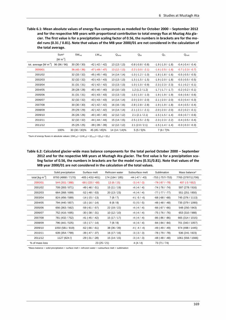
6 Studies at Muztagh Ata
169
Table 6.1: Mean absolute values of energy flux components as modelled for October 2000 – September 2012 and for the respective MB years with proportional contribution to total energy flux at Muztag Ata gla-cier. The first value is for a precipitation scaling factor of 0.56, the numbers in brackets are for the mo-del runs (0.31 / 0.81). Note that values of the MB year 2000/01 are not considered in the calculation of the total average.
Sum* SWnet LWnet Qsens Qlat QG Qmelt
[W m-2
]
tot. average [W m-2
] 96 (96 / 96) 30 (30 / 30) -42 (-42 / -42) 13 (13 / 13) -0.8 (-0.8 / -0.8) -1.9 (-1.9 / -1.8) -0.4 (-0.4 / -0.4)
2000/01 36 (43 / 36) -47 (-49 / -47) 13 (12 / 13) -2.2 (-3.0 / -2.1) -1.6 (-2.5 / -1.6) -0.7 (-2.3 / -0.7)
2001/02 32 (33 / 32) -45 (-45 / -45) 14 (14 / 14) -1.0 (-1.2 / -1.0) -1.8 (-1.8 / -1.6) -0.5 (-0.5 / -0.5)
2002/03 32 (32 / 32) -43 (-43 / -43) 13 (13 / 13) -1.5 (-1.5 / -1.5) -1.9 (-2.0 / -1.8) -0.5 (-0.5 / -0.5)
2003/04 31 (31 / 31) -42 (-42 / -42) 13 (13 / 13) -1.0 (-1.0 / -0.9) -2.3 (-2.3 / -2.3) -0.1 (-0.2 / -0.1)
2004/05 28 (28 / 28) -40 (-40 / -40) 10 (10 / 10) 1.2 (1.2 / 1.2) -1.7 (-1.7 / -1.7) -0.2 (-0.2 / -0.1)
2005/06 31 (31 / 31) -43 (-43 / -43) 13 (13 / 13) -1.0 (-1.0 / -1.0) -1.9 (-1.9 / -1.9) -0.6 (-0.6 / -0.6)
2006/07 32 (32 / 32) -43 (-43 / -43) 14 (14 / 14) -2.0 (-2.0 / -2.0) -2.1 (-2.0 / -2.0) -0.3 (-0.4 / -0.3)
2007/08 30 (30 / 30) -42 (-42 / -42) 16 (16 / 16) -2.8 (-2.8 / -2.8) -1.9 (-1.9 / -1.8) -0.4 (-0.5 / -0.4)
2008/09 29 (29 / 29) -42 (-42 / -42) 14 (14 / 14) -2.1 (-2.1 / -2.1) -2.0 (-2.0 / -2.0) -0.2 (-0.2 / -0.1)
2009/10 26 (26 / 26) -40 (-40 / -40) 12 (12 / 12) 2.1 (2.1 / 2.1) -1.5 (-1.5 / -1.4) -0.6 (-0.7 / -0.6)
2010/11 32 (32 / 32) -44 (-44 / -44) 15 (14 / 15) -2.5 (-2.5 / -2.5) -2.3 (-2.3 / -2.2) -0.4 (-0.5 / -0.4)
2011/12 25 (25 / 25) -39 (-39 / -39) 12 (12 / 12) 2.1 (2.0 / 2.1) -1.5 (-1.4 / -1.4) -0.3 (-0.3 / -0.3)
100% 30 (30 / 30)% 45 (45 / 45)% 14 (14 / 14)% 5 (5 / 5)% 7 (6 / 7)%
*Sum of energy fluxes in absolute values: |SWnet| + |LWnet| + |Qsens| + |Qlat| + |QG|
Table 6.2: Calculated glacier-wide mass balance components for the total period October 2000 – September
2012 and for the respective MB years at Muztagh Ata glacier. The first value is for a precipitation sca-ling factor of 0.56, the numbers in brackets are for the model runs (0.31/0.81). Note that values of the MB year 2000/01 are not considered in the calculation of the total values.
Solid precipitation Surface melt Refrozen water Subsurface melt Sublimation Mass balance*
total [kg m-2
] 8793 (4868 / 7170) -405 (-431/-401) 174 (164 / 185) -44 (-47 / -43) -753 (-757/-753) 7765 (3797/11706)
2000/01 544 (301 / 388) -68 (-220 / -68) 13 (6 / 15) -3 (-4 / -3) -79 (-87 / -79) 407 (-3 / 652)
2001/02 709 (393 / 871) -49 (-46 / -51) 15 (11 / 19) -4 (-4 / -4) -74 (-76 / -74) 597 (278 / 916)
2002/03 664 (368 / 699) -52 (-48 / -53) 20 (13 / 23) -4 (-4 / -4) -77 (-77 / -77) 551 (251 / 850)
2003/04 824 (456 / 589) -14 (-15 / -13) 7 (8 / 7) -4 ( -5 / -4) -68 (-68 / -68) 745 (376 / 1113)
2004/05 794 (440 / 857) -15 (-16 / -14) 8 (8 / 8) -5 (-5 / -5) -48 (-48 / -48) 735 (379 / 1090)
2005/06 656 (363 / 562) -59 (-61 / -57) 22 (19 / 22) -4 (-4 / -4) -66 (-67 / -66) 548 (250 / 843)
2006/07 752 (416 / 695) -30 (-38 / -31) 10 (12 / 10) -4 (-4 / -4) -75 (-76 / -76) 653 (310 / 988)
2007/08 781 (432 / 752) -41 (-45 / -42) 15 (17 / 17) -4 (-4 / -4) -86 (-86 / -86) 665 (314 / 1015)
2008/09 796 (441 / 525) -15 (-17 / -14) 7 (8 / 8) -4 (-4 / -4) -84 (-84 / -84) 701 (343 / 1057)
2009/10 1050 (581 / 819) -62 (-66 / -61) 38 (36 / 39) -4 ( -4 / -4) -49 (-49 / -49) 974 (498 / 1445)
2010/11 639 (354 / 799) -39 (-47 / -37) 16 (17 / 16) -3 (-3 / -3) -78 (-79 / -78) 536 (241 / 823)
2011/12 1127 (624 /) -29 (-31 / -28) 15 (14 / 15) -3 (-4 / -3) -48 (-48 / -48) 1061 (556 / 1566)
% of mass loss 23 (25 / 21) 4 (4 / 4) 73 (71 / 74)
*Mass balance = solid precipitation + surface melt + refrozen water + subsurface melt + sublimation
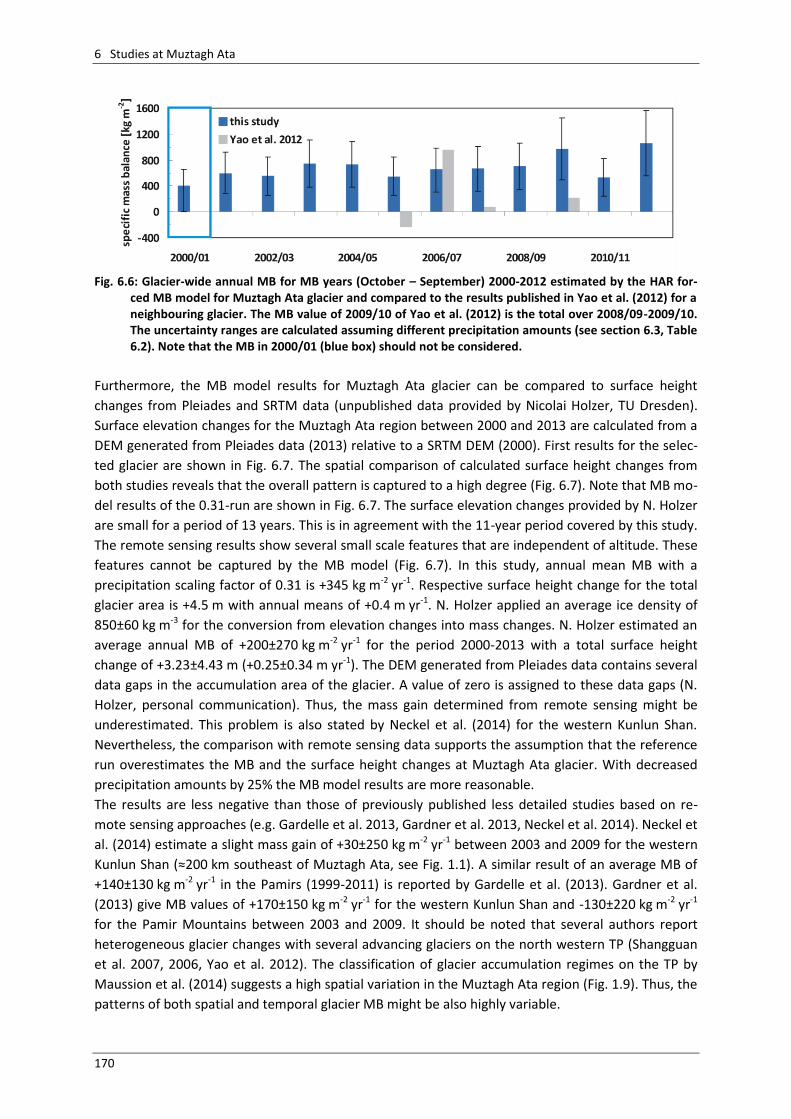
6 Studies at Muztagh Ata
170
Fig. 6.6: Glacier-wide annual MB for MB years (October – September) 2000-2012 estimated by the HAR for-
ced MB model for Muztagh Ata glacier and compared to the results published in Yao et al. (2012) for a neighbouring glacier. The MB value of 2009/10 of Yao et al. (2012) is the total over 2008/09-2009/10. The uncertainty ranges are calculated assuming different precipitation amounts (see section 6.3, Table 6.2). Note that the MB in 2000/01 (blue box) should not be considered.
Furthermore, the MB model results for Muztagh Ata glacier can be compared to surface height
changes from Pleiades and SRTM data (unpublished data provided by Nicolai Holzer, TU Dresden).
Surface elevation changes for the Muztagh Ata region between 2000 and 2013 are calculated from a
DEM generated from Pleiades data (2013) relative to a SRTM DEM (2000). First results for the selec-
ted glacier are shown in Fig. 6.7. The spatial comparison of calculated surface height changes from
both studies reveals that the overall pattern is captured to a high degree (Fig. 6.7). Note that MB mo-
del results of the 0.31-run are shown in Fig. 6.7. The surface elevation changes provided by N. Holzer
are small for a period of 13 years. This is in agreement with the 11-year period covered by this study.
The remote sensing results show several small scale features that are independent of altitude. These
features cannot be captured by the MB model (Fig. 6.7). In this study, annual mean MB with a
precipitation scaling factor of 0.31 is +345 kg m-2 yr-1. Respective surface height change for the total
glacier area is +4.5 m with annual means of +0.4 m yr-1. N. Holzer applied an average ice density of
850±60 kg m-3 for the conversion from elevation changes into mass changes. N. Holzer estimated an
average annual MB of +200±270 kg m-2 yr-1 for the period 2000-2013 with a total surface height
change of +3.23±4.43 m (+0.25±0.34 m yr-1). The DEM generated from Pleiades data contains several
data gaps in the accumulation area of the glacier. A value of zero is assigned to these data gaps (N.
Holzer, personal communication). Thus, the mass gain determined from remote sensing might be
underestimated. This problem is also stated by Neckel et al. (2014) for the western Kunlun Shan.
Nevertheless, the comparison with remote sensing data supports the assumption that the reference
run overestimates the MB and the surface height changes at Muztagh Ata glacier. With decreased
precipitation amounts by 25% the MB model results are more reasonable.
The results are less negative than those of previously published less detailed studies based on re-
mote sensing approaches (e.g. Gardelle et al. 2013, Gardner et al. 2013, Neckel et al. 2014). Neckel et
al. (2014) estimate a slight mass gain of +30±250 kg m-2 yr-1 between 2003 and 2009 for the western
Kunlun Shan (≈200 km southeast of Muztagh Ata, see Fig. 1.1). A similar result of an average MB of
+140±130 kg m-2 yr-1 in the Pamirs (1999-2011) is reported by Gardelle et al. (2013). Gardner et al.
(2013) give MB values of +170±150 kg m-2 yr-1 for the western Kunlun Shan and -130±220 kg m-2 yr-1
for the Pamir Mountains between 2003 and 2009. It should be noted that several authors report
heterogeneous glacier changes with several advancing glaciers on the north western TP (Shangguan
et al. 2007, 2006, Yao et al. 2012). The classification of glacier accumulation regimes on the TP by
Maussion et al. (2014) suggests a high spatial variation in the Muztagh Ata region (Fig. 1.9). Thus, the
patterns of both spatial and temporal glacier MB might be also highly variable.
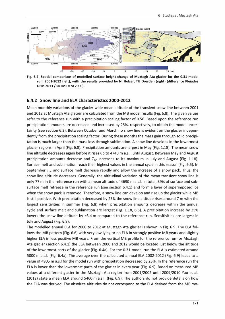
6 Studies at Muztagh Ata
171
Fig. 6.7: Spatial comparison of modelled surface height change of Muztagh Ata glacier for the 0.31-model
run, 2001-2012 (left), with the results provided by N. Holzer, TU Dresden (right) (difference Pleiades DEM 2013 / SRTM DEM 2000).
6.4.2 Snow line and ELA characteristics 2000-2012
Mean monthly variations of the glacier-wide mean altitude of the transient snow line between 2001
and 2012 at Muztagh Ata glacier are calculated from the MB model results (Fig. 6.8). The given values
refer to the reference run with a precipitation scaling factor of 0.56. Based upon the reference run
precipitation amounts are decreased and increased by 25%, respectively, to obtain the model uncer-
tainty (see section 6.3). Between October and March no snow line is evident on the glacier indepen-
dently from the precipitation scaling factor. During these months the mass gain through solid precipi-
tation is much larger than the mass loss through sublimation. A snow line develops in the lowermost
glacier regions in April (Fig. 6.8). Precipitation amounts are largest in May (Fig. 1.18). The mean snow
line altitude decreases again before it rises up to 4740 m a.s.l. until August. Between May and August
precipitation amounts decrease and Tair increases to its maximum in July and August (Fig. 1.18).
Surface melt and sublimation reach their highest values in the annual cycle in this season (Fig. 6.5). In
September Tair and surface melt decrease rapidly and allow the increase of a snow pack. Thus, the
snow line altitude decreases. Generally, the altitudinal variation of the mean transient snow line is
only 77 m in the reference run with a mean altitude of 4690 m a.s.l. In total, 39% of surface and sub-
surface melt refreeze in the reference run (see section 6.4.1) and form a layer of superimposed ice
when the snow pack is removed. Therefore, a snow line can develop and rise up the glacier while MB
is still positive. With precipitation decreased by 25% the snow line altitude rises around 7 m with the
largest sensitivities in summer (Fig. 6.8) when precipitation amounts decrease within the annual
cycle and surface melt and sublimation are largest (Fig. 1.18, 6.5). A precipitation increase by 25%
lowers the snow line altitude by ≈3.4 m compared to the reference run. Sensitivities are largest in
July and August (Fig. 6.8).
The modelled annual ELA for 2000 to 2012 at Muztagh Ata glacier is shown in Fig. 6.9. The ELA fol-
lows the MB pattern (Fig. 6.6) with very low lying or no ELA in strongly positive MB years and slightly
higher ELA in less positive MB years. From the vertical MB profile for the reference run for Muztagh
Ata glacier (section 6.4.1) the ELA between 2000 and 2012 would be located just below the altitude
of the lowermost parts of the glacier (Fig. 6.4a). For the 0.31-model run the ELA is estimated around
5000 m a.s.l. (Fig. 6.4a). The average over the calculated annual ELA 2002-2012 (Fig. 6.9) leads to a
value of 4905 m a.s.l for the model run with precipitation decreased by 25%. In the reference run the
ELA is lower than the lowermost parts of the glacier in every year (Fig. 6.9). Based on measured MB
values at a different glacier in the Muztagh Ata region from 2001/2002 until 2009/2010 Yao et al.
(2012) state a mean ELA around 5460 m a.s.l. (Fig. 6.9). The authors do not provide details on how
the ELA was derived. The absolute altitudes do not correspond to the ELA derived from the MB mo-
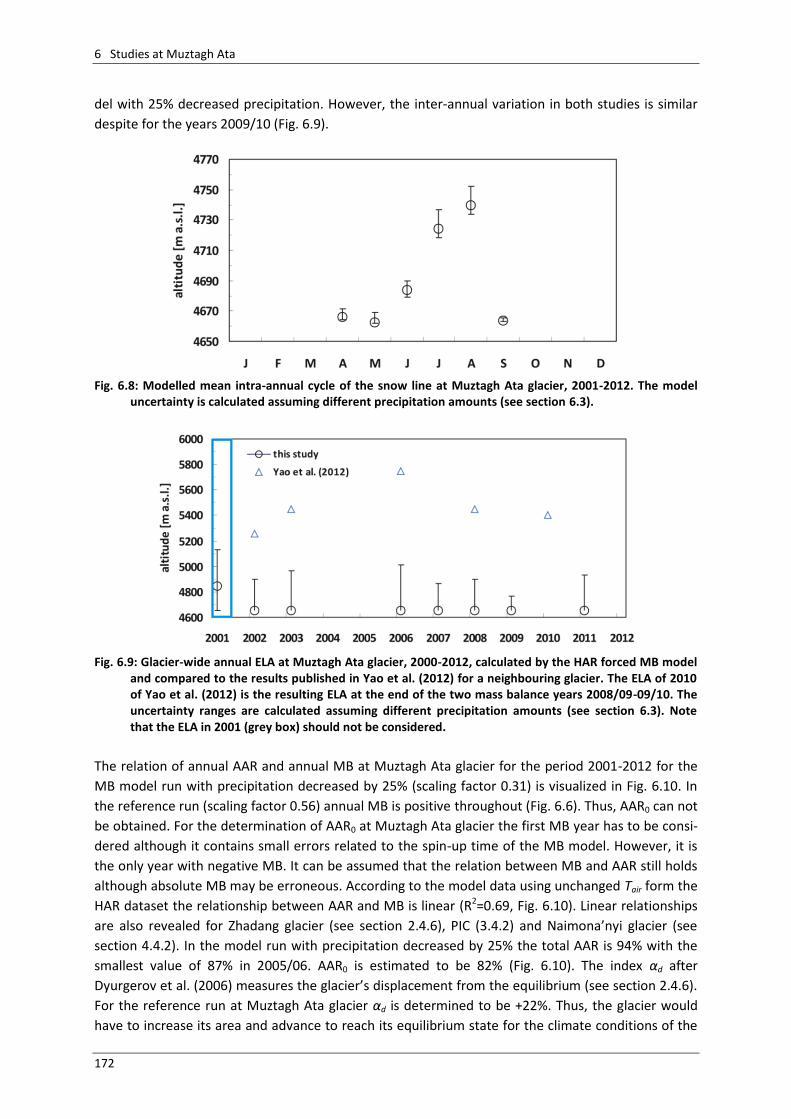
6 Studies at Muztagh Ata
172
del with 25% decreased precipitation. However, the inter-annual variation in both studies is similar
despite for the years 2009/10 (Fig. 6.9).
Fig. 6.8: Modelled mean intra-annual cycle of the snow line at Muztagh Ata glacier, 2001-2012. The model
uncertainty is calculated assuming different precipitation amounts (see section 6.3).
Fig. 6.9: Glacier-wide annual ELA at Muztagh Ata glacier, 2000-2012, calculated by the HAR forced MB model
and compared to the results published in Yao et al. (2012) for a neighbouring glacier. The ELA of 2010 of Yao et al. (2012) is the resulting ELA at the end of the two mass balance years 2008/09-09/10. The uncertainty ranges are calculated assuming different precipitation amounts (see section 6.3). Note that the ELA in 2001 (grey box) should not be considered.
The relation of annual AAR and annual MB at Muztagh Ata glacier for the period 2001-2012 for the
MB model run with precipitation decreased by 25% (scaling factor 0.31) is visualized in Fig. 6.10. In
the reference run (scaling factor 0.56) annual MB is positive throughout (Fig. 6.6). Thus, AAR0 can not
be obtained. For the determination of AAR0 at Muztagh Ata glacier the first MB year has to be consi-
dered although it contains small errors related to the spin-up time of the MB model. However, it is
the only year with negative MB. It can be assumed that the relation between MB and AAR still holds
although absolute MB may be erroneous. According to the model data using unchanged Tair form the
HAR dataset the relationship between AAR and MB is linear (R2=0.69, Fig. 6.10). Linear relationships
are also revealed for Zhadang glacier (see section 2.4.6), PIC (3.4.2) and Naimona’nyi glacier (see
section 4.4.2). In the model run with precipitation decreased by 25% the total AAR is 94% with the
smallest value of 87% in 2005/06. AAR0 is estimated to be 82% (Fig. 6.10). The index αd after
Dyurgerov et al. (2006) measures the glacier’s displacement from the equilibrium (see section 2.4.6).
For the reference run at Muztagh Ata glacier αd is determined to be +22%. Thus, the glacier would
have to increase its area and advance to reach its equilibrium state for the climate conditions of the
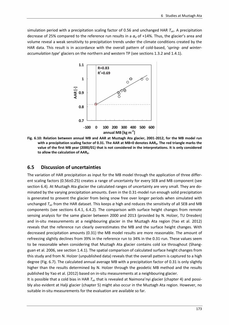
6 Studies at Muztagh Ata
173
simulation period with a precipitation scaling factor of 0.56 and unchanged HAR Tair. A precipitation
decrease of 25% compared to the reference run results in a αd of +14%. Thus, the glacier’s area and
volume reveal a weak sensitivity to precipitation trends under the climate conditions created by the
HAR data. This result is in accordance with the overall pattern of cold-based, ‘spring- and winter-
accumulation type’ glaciers on the northern and western TP (see sections 1.3.2 and 1.4.1).
Fig. 6.10: Relation between annual MB and AAR at Muztagh Ata glacier, 2001-2012, for the MB model run
with a precipitation scaling factor of 0.31. The AAR at MB=0 denotes AAR0. The red triangle marks the value of the first MB year (2000/01) that is not considered in the interpretations. It is only considered to allow the calculation of AAR0.
6.5 Discussion of uncertainties
The variation of HAR precipitation as input for the MB model through the application of three differ-
ent scaling factors (0.56±0.25) creates a range of uncertainty for every SEB and MB component (see
section 6.4). At Muztagh Ata glacier the calculated ranges of uncertainty are very small. They are do-
minated by the varying precipitation amounts. Even in the 0.31-model run enough solid precipitation
is generated to prevent the glacier from being snow free over longer periods when simulated with
unchanged Tair from the HAR dataset. This keeps α high and reduces the sensitivity of all SEB and MB
components (see sections 6.4.1, 6.4.2). The comparison with surface height changes from remote
sensing analysis for the same glacier between 2000 and 2013 (provided by N. Holzer, TU Dresden)
and in-situ measurements at a neighbouring glacier in the Muztagh Ata region (Yao et al. 2012)
reveals that the reference run clearly overestimates the MB and the surface height changes. With
decreased precipitation amounts (0.31) the MB model results are more reasonable. The amount of
refreezing slightly declines from 39% in the reference run to 34% in the 0.31-run. These values seem
to be reasonable when considering that Muztagh Ata glacier contains cold ice throughout (Shang-
guan et al. 2006, see section 1.4.1). The spatial comparison of calculated surface height changes from
this study and from N. Holzer (unpublished data) reveals that the overall pattern is captured to a high
degree (Fig. 6.7). The calculated annual average MB with a precipitation factor of 0.31 is only slightly
higher than the results determined by N. Holzer through the geodetic MB method and the results
published by Yao et al. (2012) based on in-situ measurements at a neighbouring glacier.
It is possible that a cold bias in HAR Tair that is revealed at Naimona’nyi glacier (chapter 4) and possi-
bly also evident at Halji glacier (chapter 5) might also occur in the Muztagh Ata region. However, no
suitable in-situ measurements for the evaluation are available so far.
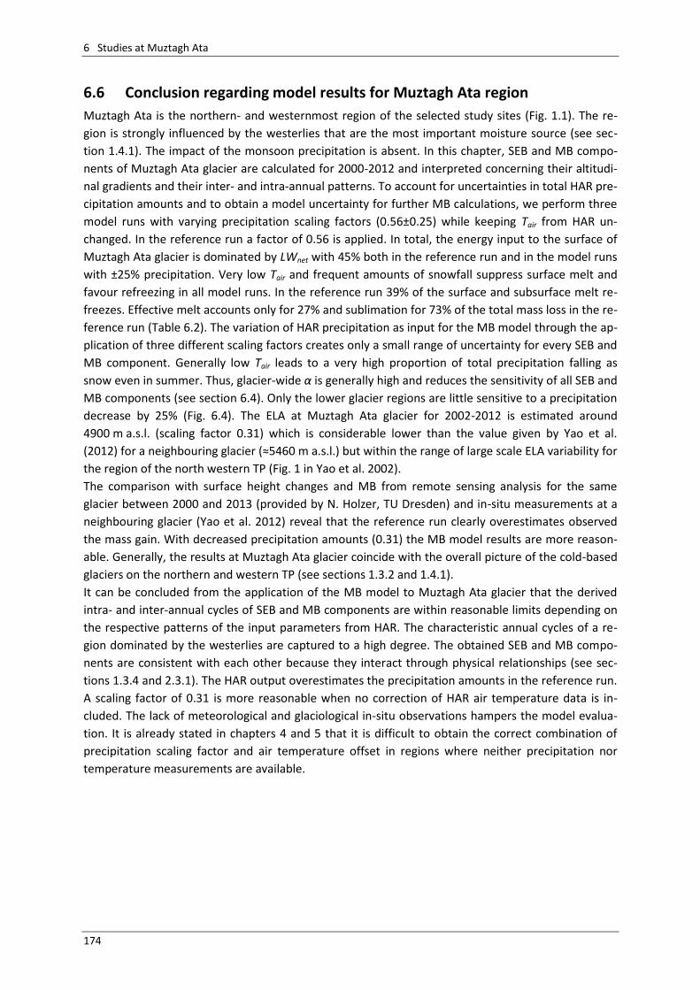
6 Studies at Muztagh Ata
174
6.6 Conclusion regarding model results for Muztagh Ata region
Muztagh Ata is the northern- and westernmost region of the selected study sites (Fig. 1.1). The re-
gion is strongly influenced by the westerlies that are the most important moisture source (see sec-
tion 1.4.1). The impact of the monsoon precipitation is absent. In this chapter, SEB and MB compo-
nents of Muztagh Ata glacier are calculated for 2000-2012 and interpreted concerning their altitudi-
nal gradients and their inter- and intra-annual patterns. To account for uncertainties in total HAR pre-
cipitation amounts and to obtain a model uncertainty for further MB calculations, we perform three
model runs with varying precipitation scaling factors (0.56±0.25) while keeping Tair from HAR un-
changed. In the reference run a factor of 0.56 is applied. In total, the energy input to the surface of
Muztagh Ata glacier is dominated by LWnet with 45% both in the reference run and in the model runs
with ±25% precipitation. Very low Tair and frequent amounts of snowfall suppress surface melt and
favour refreezing in all model runs. In the reference run 39% of the surface and subsurface melt re-
freezes. Effective melt accounts only for 27% and sublimation for 73% of the total mass loss in the re-
ference run (Table 6.2). The variation of HAR precipitation as input for the MB model through the ap-
plication of three different scaling factors creates only a small range of uncertainty for every SEB and
MB component. Generally low Tair leads to a very high proportion of total precipitation falling as
snow even in summer. Thus, glacier-wide α is generally high and reduces the sensitivity of all SEB and
MB components (see section 6.4). Only the lower glacier regions are little sensitive to a precipitation
decrease by 25% (Fig. 6.4). The ELA at Muztagh Ata glacier for 2002-2012 is estimated around
4900 m a.s.l. (scaling factor 0.31) which is considerable lower than the value given by Yao et al.
(2012) for a neighbouring glacier (≈5460 m a.s.l.) but within the range of large scale ELA variability for
the region of the north western TP (Fig. 1 in Yao et al. 2002).
The comparison with surface height changes and MB from remote sensing analysis for the same
glacier between 2000 and 2013 (provided by N. Holzer, TU Dresden) and in-situ measurements at a
neighbouring glacier (Yao et al. 2012) reveal that the reference run clearly overestimates observed
the mass gain. With decreased precipitation amounts (0.31) the MB model results are more reason-
able. Generally, the results at Muztagh Ata glacier coincide with the overall picture of the cold-based
glaciers on the northern and western TP (see sections 1.3.2 and 1.4.1).
It can be concluded from the application of the MB model to Muztagh Ata glacier that the derived
intra- and inter-annual cycles of SEB and MB components are within reasonable limits depending on
the respective patterns of the input parameters from HAR. The characteristic annual cycles of a re-
gion dominated by the westerlies are captured to a high degree. The obtained SEB and MB compo-
nents are consistent with each other because they interact through physical relationships (see sec-
tions 1.3.4 and 2.3.1). The HAR output overestimates the precipitation amounts in the reference run.
A scaling factor of 0.31 is more reasonable when no correction of HAR air temperature data is in-
cluded. The lack of meteorological and glaciological in-situ observations hampers the model evalua-
tion. It is already stated in chapters 4 and 5 that it is difficult to obtain the correct combination of
precipitation scaling factor and air temperature offset in regions where neither precipitation nor
temperature measurements are available.
7 Comparison and interpretation of results
175
7 Comparison and interpretation of the glacier characteristics at the five study sites on the Tibetan Plateau, 2001-2012
Within this chapter the different SEB and MB components of all five glaciers and ice caps presented
in this thesis are compared and interpreted concerning their inter- and intra-annual patterns (section
7.1). Furthermore, seven atmospheric circulation and teleconnection patterns that influence the TP
are chosen to explain the variability in air temperature, precipitation and MB at the five study sites
(section 7.2).
7.1 Comparison and interpretation of the SEB and MB components at the five study sites, 2001-2012
The inter-annual patterns of the different SEB and MB components for the individual glaciers and ice
caps as derived from the MB model are discussed in the respective chapters 2-6. The comparison of
the inter- and intra-annual patterns reveals commonalities and differences between the studied gla-
ciers and their driving mechanisms. For the comparison within this section we chose the results of
the model run with the precipitation scaling factor and air temperature offset that fits best to the
available observations at each glacier (see chapters 3-6). The obtained best fit combinations are
0.56/±0 K for Zhadang glacier and PIC, 0.31/+3 K for Naimona’nyi glacier, 0.56/+1 K for Halji and
0.31/±0 K for Muztagh Ata glacier. Note that the glacier-wide results for Naimona’nyi are calculated
from the respective profile (see chapter 4). The closure of the SEB is not necessarily fulfilled. Thus,
absolute values and relative proportions are a best guess. Additional glacier-wide model runs for Nai-
mona’nyi glacier will be carried out in subsequent studies that are not part of this thesis in the near
future.
Mean annual cycles of all SEB and MB components for each glacier are summarized in Fig. 7.1 and
7.2. The glacier-wide monthly SEB components as a time series for the five study sites are shown in
Fig. B.1 in appendix B. The respective MB components including Tair are given in Fig. B.2. Mean
monthly glacier-wide Tair show a regular cycle in all study regions with distinct negative values in win-
ter and less negative to positive values in summer (Fig. 7.2, B.2f).
All study regions besides Muztagh Ata experience highest Tair in summer 2006 (B.2f). At Zhadang
glacier this coincides with below-average precipitation amounts resulting in below-average MB (Fig.
B.2d, B.2e). This is evident also in Fig. 7.5 that visualizes monthly anomalies for Tair, precipitation and
MB for all five glaciers. Over the total simulation period Tair is highest at Zhadang glacier (-8.1°C) and
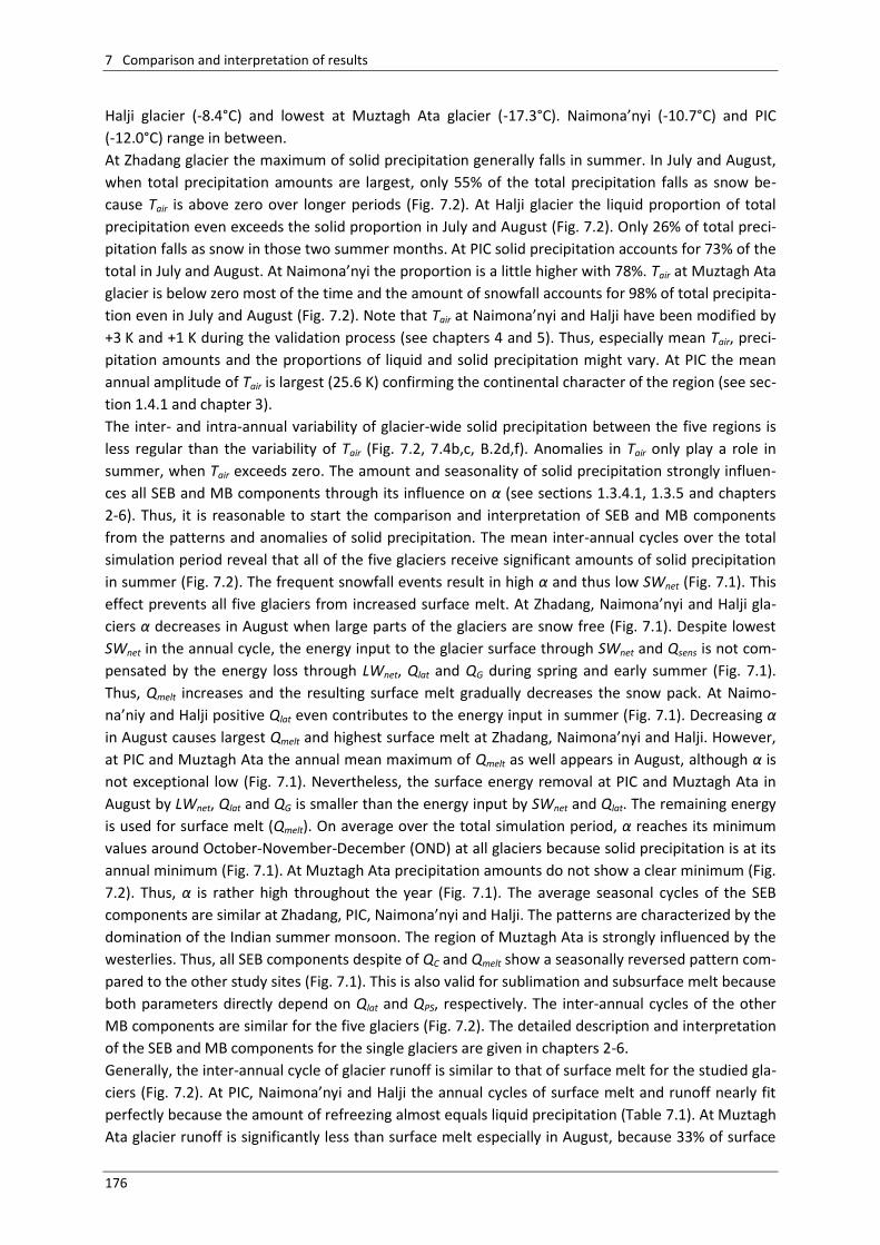
7 Comparison and interpretation of results
176
Halji glacier (-8.4°C) and lowest at Muztagh Ata glacier (-17.3°C). Naimona’nyi (-10.7°C) and PIC
(-12.0°C) range in between.
At Zhadang glacier the maximum of solid precipitation generally falls in summer. In July and August,
when total precipitation amounts are largest, only 55% of the total precipitation falls as snow be-
cause Tair is above zero over longer periods (Fig. 7.2). At Halji glacier the liquid proportion of total
precipitation even exceeds the solid proportion in July and August (Fig. 7.2). Only 26% of total preci-
pitation falls as snow in those two summer months. At PIC solid precipitation accounts for 73% of the
total in July and August. At Naimona’nyi the proportion is a little higher with 78%. Tair at Muztagh Ata
glacier is below zero most of the time and the amount of snowfall accounts for 98% of total precipita-
tion even in July and August (Fig. 7.2). Note that Tair at Naimona’nyi and Halji have been modified by
+3 K and +1 K during the validation process (see chapters 4 and 5). Thus, especially mean Tair, preci-
pitation amounts and the proportions of liquid and solid precipitation might vary. At PIC the mean
annual amplitude of Tair is largest (25.6 K) confirming the continental character of the region (see sec-
tion 1.4.1 and chapter 3).
The inter- and intra-annual variability of glacier-wide solid precipitation between the five regions is
less regular than the variability of Tair (Fig. 7.2, 7.4b,c, B.2d,f). Anomalies in Tair only play a role in
summer, when Tair exceeds zero. The amount and seasonality of solid precipitation strongly influen-
ces all SEB and MB components through its influence on α (see sections 1.3.4.1, 1.3.5 and chapters
2-6). Thus, it is reasonable to start the comparison and interpretation of SEB and MB components
from the patterns and anomalies of solid precipitation. The mean inter-annual cycles over the total
simulation period reveal that all of the five glaciers receive significant amounts of solid precipitation
in summer (Fig. 7.2). The frequent snowfall events result in high α and thus low SWnet (Fig. 7.1). This
effect prevents all five glaciers from increased surface melt. At Zhadang, Naimona’nyi and Halji gla-
ciers α decreases in August when large parts of the glaciers are snow free (Fig. 7.1). Despite lowest
SWnet in the annual cycle, the energy input to the glacier surface through SWnet and Qsens is not com-
pensated by the energy loss through LWnet, Qlat and QG during spring and early summer (Fig. 7.1).
Thus, Qmelt increases and the resulting surface melt gradually decreases the snow pack. At Naimo-
na’niy and Halji positive Qlat even contributes to the energy input in summer (Fig. 7.1). Decreasing α
in August causes largest Qmelt and highest surface melt at Zhadang, Naimona’nyi and Halji. However,
at PIC and Muztagh Ata the annual mean maximum of Qmelt as well appears in August, although α is
not exceptional low (Fig. 7.1). Nevertheless, the surface energy removal at PIC and Muztagh Ata in
August by LWnet, Qlat and QG is smaller than the energy input by SWnet and Qlat. The remaining energy
is used for surface melt (Qmelt). On average over the total simulation period, α reaches its minimum
values around October-November-December (OND) at all glaciers because solid precipitation is at its
annual minimum (Fig. 7.1). At Muztagh Ata precipitation amounts do not show a clear minimum (Fig.
7.2). Thus, α is rather high throughout the year (Fig. 7.1). The average seasonal cycles of the SEB
components are similar at Zhadang, PIC, Naimona’nyi and Halji. The patterns are characterized by the
domination of the Indian summer monsoon. The region of Muztagh Ata is strongly influenced by the
westerlies. Thus, all SEB components despite of QC and Qmelt show a seasonally reversed pattern com-
pared to the other study sites (Fig. 7.1). This is also valid for sublimation and subsurface melt because
both parameters directly depend on Qlat and QPS, respectively. The inter-annual cycles of the other
MB components are similar for the five glaciers (Fig. 7.2). The detailed description and interpretation
of the SEB and MB components for the single glaciers are given in chapters 2-6.
Generally, the inter-annual cycle of glacier runoff is similar to that of surface melt for the studied gla-
ciers (Fig. 7.2). At PIC, Naimona’nyi and Halji the annual cycles of surface melt and runoff nearly fit
perfectly because the amount of refreezing almost equals liquid precipitation (Table 7.1). At Muztagh
Ata glacier runoff is significantly less than surface melt especially in August, because 33% of surface
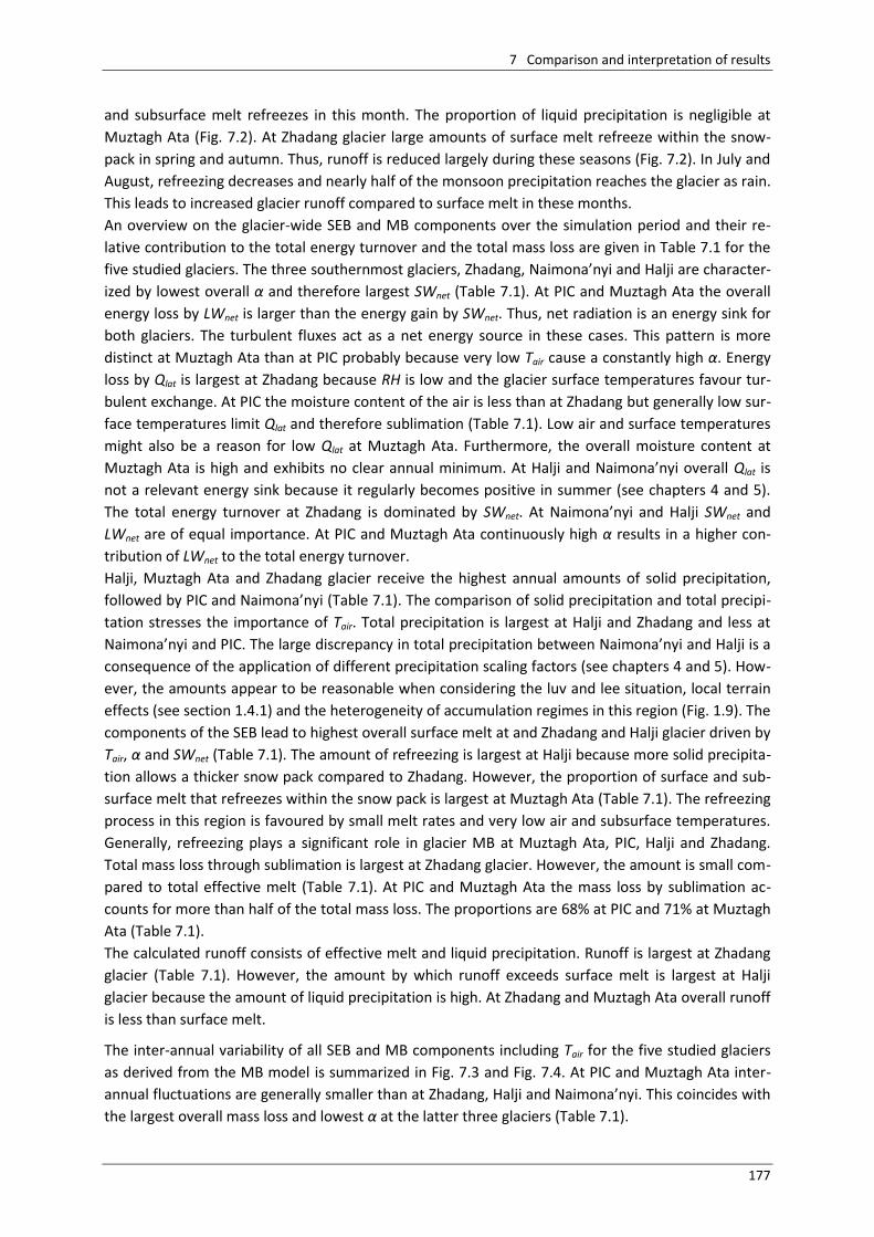
7 Comparison and interpretation of results
177
and subsurface melt refreezes in this month. The proportion of liquid precipitation is negligible at
Muztagh Ata (Fig. 7.2). At Zhadang glacier large amounts of surface melt refreeze within the snow-
pack in spring and autumn. Thus, runoff is reduced largely during these seasons (Fig. 7.2). In July and
August, refreezing decreases and nearly half of the monsoon precipitation reaches the glacier as rain.
This leads to increased glacier runoff compared to surface melt in these months.
An overview on the glacier-wide SEB and MB components over the simulation period and their re-
lative contribution to the total energy turnover and the total mass loss are given in Table 7.1 for the
five studied glaciers. The three southernmost glaciers, Zhadang, Naimona’nyi and Halji are character-
ized by lowest overall α and therefore largest SWnet (Table 7.1). At PIC and Muztagh Ata the overall
energy loss by LWnet is larger than the energy gain by SWnet. Thus, net radiation is an energy sink for
both glaciers. The turbulent fluxes act as a net energy source in these cases. This pattern is more
distinct at Muztagh Ata than at PIC probably because very low Tair cause a constantly high α. Energy
loss by Qlat is largest at Zhadang because RH is low and the glacier surface temperatures favour tur-
bulent exchange. At PIC the moisture content of the air is less than at Zhadang but generally low sur-
face temperatures limit Qlat and therefore sublimation (Table 7.1). Low air and surface temperatures
might also be a reason for low Qlat at Muztagh Ata. Furthermore, the overall moisture content at
Muztagh Ata is high and exhibits no clear annual minimum. At Halji and Naimona’nyi overall Qlat is
not a relevant energy sink because it regularly becomes positive in summer (see chapters 4 and 5).
The total energy turnover at Zhadang is dominated by SWnet. At Naimona’nyi and Halji SWnet and
LWnet are of equal importance. At PIC and Muztagh Ata continuously high α results in a higher con-
tribution of LWnet to the total energy turnover.
Halji, Muztagh Ata and Zhadang glacier receive the highest annual amounts of solid precipitation,
followed by PIC and Naimona’nyi (Table 7.1). The comparison of solid precipitation and total precipi-
tation stresses the importance of Tair. Total precipitation is largest at Halji and Zhadang and less at
Naimona’nyi and PIC. The large discrepancy in total precipitation between Naimona’nyi and Halji is a
consequence of the application of different precipitation scaling factors (see chapters 4 and 5). How-
ever, the amounts appear to be reasonable when considering the luv and lee situation, local terrain
effects (see section 1.4.1) and the heterogeneity of accumulation regimes in this region (Fig. 1.9). The
components of the SEB lead to highest overall surface melt at and Zhadang and Halji glacier driven by
Tair, α and SWnet (Table 7.1). The amount of refreezing is largest at Halji because more solid precipita-
tion allows a thicker snow pack compared to Zhadang. However, the proportion of surface and sub-
surface melt that refreezes within the snow pack is largest at Muztagh Ata (Table 7.1). The refreezing
process in this region is favoured by small melt rates and very low air and subsurface temperatures.
Generally, refreezing plays a significant role in glacier MB at Muztagh Ata, PIC, Halji and Zhadang.
Total mass loss through sublimation is largest at Zhadang glacier. However, the amount is small com-
pared to total effective melt (Table 7.1). At PIC and Muztagh Ata the mass loss by sublimation ac-
counts for more than half of the total mass loss. The proportions are 68% at PIC and 71% at Muztagh
Ata (Table 7.1).
The calculated runoff consists of effective melt and liquid precipitation. Runoff is largest at Zhadang
glacier (Table 7.1). However, the amount by which runoff exceeds surface melt is largest at Halji
glacier because the amount of liquid precipitation is high. At Zhadang and Muztagh Ata overall runoff
is less than surface melt.
The inter-annual variability of all SEB and MB components including Tair for the five studied glaciers
as derived from the MB model is summarized in Fig. 7.3 and Fig. 7.4. At PIC and Muztagh Ata inter-
annual fluctuations are generally smaller than at Zhadang, Halji and Naimona’nyi. This coincides with
the largest overall mass loss and lowest α at the latter three glaciers (Table 7.1).
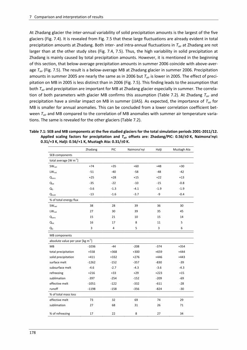
7 Comparison and interpretation of results
178
At Zhadang glacier the inter-annual variability of solid precipitation amounts is the largest of the five
glaciers (Fig. 7.4). It is revealed from Fig. 7.5 that these large fluctuations are already evident in total
precipitation amounts at Zhadang. Both inter- and intra-annual fluctuations in Tair at Zhadang are not
larger than at the other study sites (Fig. 7.4, 7.5). Thus, the high variability in solid precipitation at
Zhadang is mainly caused by total precipitation amounts. However, it is mentioned in the beginning
of this section, that below-average precipitation amounts in summer 2006 coincide with above-aver-
age Tair (Fig. 7.5). The result is a below-average MB at Zhadang glacier in summer 2006. Precipitation
amounts in summer 2005 are nearly the same as in 2006 but Tair is lower in 2005. The effect of preci-
pitation on MB in 2005 is less distinct than in 2006 (Fig. 7.5). This finding leads to the assumption that
both Tair and precipitation are important for MB at Zhadang glacier especially in summer. The correla-
tion of both parameters with glacier MB confirms this assumption (Table 7.2). At Zhadang Tair and
precipitation have a similar impact on MB in summer (JJAS). As expected, the importance of Tair for
MB is smaller for annual anomalies. This can be concluded from a lower correlation coefficient bet-
ween Tair and MB compared to the correlation of MB anomalies with summer air temperature varia-
tions. The same is revealed for the other glaciers (Table 7.2).
Table 7.1: SEB and MB components at the five studied glaciers for the total simulation periods 2001-2011/12.
Applied scaling factors for precipitation and Tair offsets are: Zhadang/PIC: 0.56/±0 K, Naimona’nyi: 0.31/+3 K, Halji: 0.56/+1 K, Muztagh Ata: 0.31/±0 K.
Zhadang PIC Naimona’nyi Halji Muztagh Ata
SEB components
total average [W m-2]
SWnet +74 +35 +60 +48 +30
LWnet -51 -40 -58 -48 -42
Qsens +25 +28 +15 +22 +13
Qlat -35 -22 -10 -15 -0.8
QG -3.6 -1.3 -4.1 -1.9 -1.9
Qmelt -13 -1.6 -3.7 -9 -0.4
% of total energy flux
SWnet 38 28 39 36 30
LWnet 27 30 39 35 45
Qsens 15 21 10 15 14
Qlat 16 17 8 11 5
QG 3 4 5 3 6
MB components
absolute value per year [kg m-2]
MB -1036 -44 -208 -374 +354
total precipitation +558 +368 +300 +659 +444
solid precipitation +411 +332 +276 +446 +443
surface melt -1262 -152 -357 -830 -39
subsurface melt -4.6 -2.7 -4.3 -3.6 -4.3
refreezing +216 +33 +29 +223 +15
sublimation -397 -254 -152 -209 -69
effective melt -1051 -122 -332 -611 -28
runoff -1198 -158 -356 -824 -30
% of total mass loss
effective melt 73 32 69 74 29
sublimation 27 68 31 26 71
% of refreezing 17 22 8 27 34
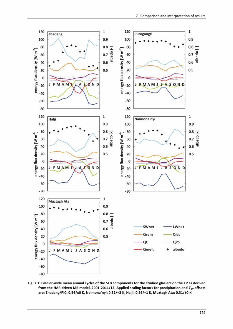
7 Comparison and interpretation of results
179
Fig. 7.1: Glacier-wide mean annual cycles of the SEB components for the studied glaciers on the TP as derived
from the HAR driven MB model, 2001-2011/12. Applied scaling factors for precipitation and Tair offsets are: Zhadang/PIC: 0.56/±0 K, Naimona’nyi: 0.31/+3 K, Halji: 0.56/+1 K, Muztagh Ata: 0.31/±0 K.
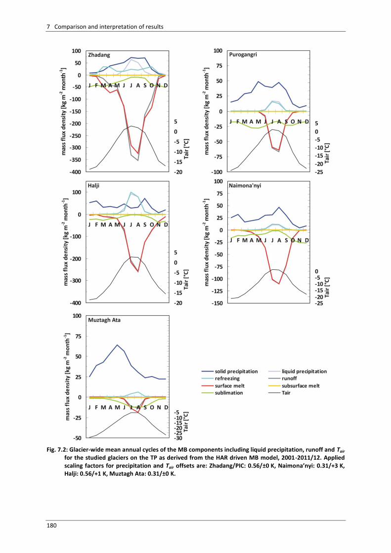
7 Comparison and interpretation of results
180
Fig. 7.2: Glacier-wide mean annual cycles of the MB components including liquid precipitation, runoff and Tair
for the studied glaciers on the TP as derived from the HAR driven MB model, 2001-2011/12. Applied scaling factors for precipitation and Tair offsets are: Zhadang/PIC: 0.56/±0 K, Naimona’nyi: 0.31/+3 K, Halji: 0.56/+1 K, Muztagh Ata: 0.31/±0 K.
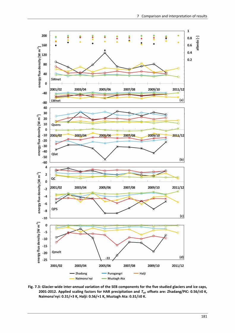
7 Comparison and interpretation of results
181
Fig. 7.3: Glacier-wide inter-annual variation of the SEB components for the five studied glaciers and ice caps,
2001-2012. Applied scaling factors for HAR precipitation and Tair offsets are: Zhadang/PIC: 0.56/±0 K, Naimona’nyi: 0.31/+3 K, Halji: 0.56/+1 K, Muztagh Ata: 0.31/±0 K.
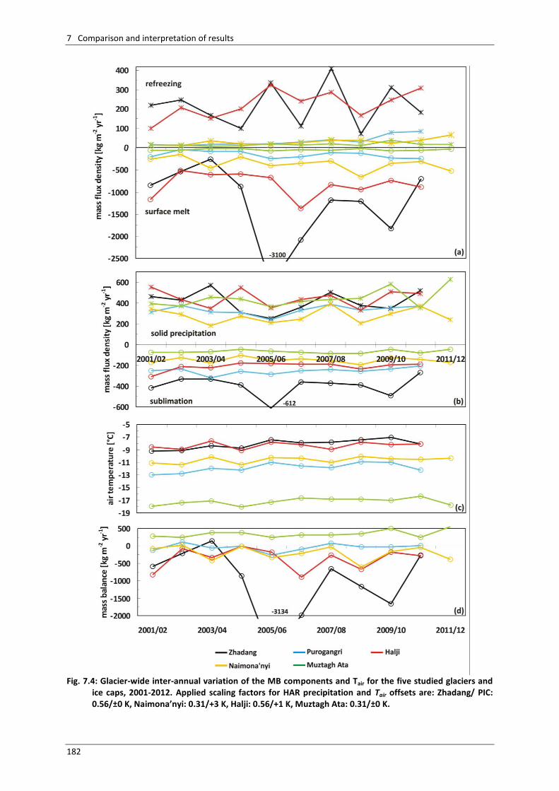
7 Comparison and interpretation of results
182
Fig. 7.4: Glacier-wide inter-annual variation of the MB components and Tair for the five studied glaciers and
ice caps, 2001-2012. Applied scaling factors for HAR precipitation and Tair offsets are: Zhadang/ PIC: 0.56/±0 K, Naimona’nyi: 0.31/+3 K, Halji: 0.56/+1 K, Muztagh Ata: 0.31/±0 K.
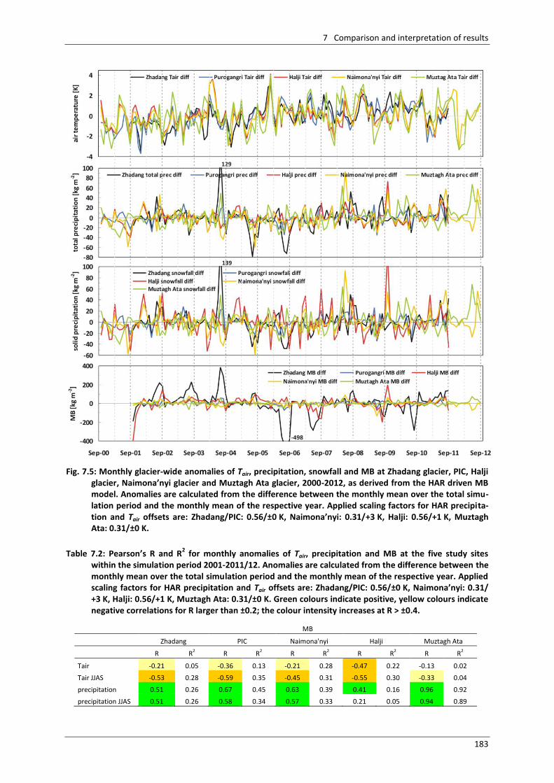
7 Comparison and interpretation of results
183
Fig. 7.5: Monthly glacier-wide anomalies of Tair, precipitation, snowfall and MB at Zhadang glacier, PIC, Halji
glacier, Naimona’nyi glacier and Muztagh Ata glacier, 2000-2012, as derived from the HAR driven MB model. Anomalies are calculated from the difference between the monthly mean over the total simu-lation period and the monthly mean of the respective year. Applied scaling factors for HAR precipita-tion and Tair offsets are: Zhadang/PIC: 0.56/±0 K, Naimona’nyi: 0.31/+3 K, Halji: 0.56/+1 K, Muztagh Ata: 0.31/±0 K.
Table 7.2: Pearson’s R and R
2 for monthly anomalies of Tair, precipitation and MB at the five study sites
within the simulation period 2001-2011/12. Anomalies are calculated from the difference between the monthly mean over the total simulation period and the monthly mean of the respective year. Applied scaling factors for HAR precipitation and Tair offsets are: Zhadang/PIC: 0.56/±0 K, Naimona’nyi: 0.31/ +3 K, Halji: 0.56/+1 K, Muztagh Ata: 0.31/±0 K. Green colours indicate positive, yellow colours indicate negative correlations for R larger than ±0.2; the colour intensity increases at R > ±0.4.
MB
Zhadang PIC Naimona'nyi Halji Muztagh Ata
R R2 R R2 R R2 R R2 R R2
Tair -0.21 0.05 -0.36 0.13 -0.21 0.28 -0.47 0.22 -0.13 0.02
Tair JJAS -0.53 0.28 -0.59 0.35 -0.45 0.31 -0.55 0.30 -0.33 0.04
precipitation 0.51 0.26 0.67 0.45 0.63 0.39 0.41 0.16 0.96 0.92
precipitation JJAS 0.51 0.26 0.58 0.34 0.57 0.33 0.21 0.05 0.94 0.89
7 Comparison and interpretation of results
184
MB at Muztagh Ata is clearly dominated by precipitation also in summer (Table 7.2). The correlation
of Tair and MB is weak possibly because Tair is generally low. MB at Halji glacier reveals generally low
dependencies for precipitation. The importance of precipitation for MB decreases in summer possi-
bly because large amounts fall as rain and do not contribute to the MB.
The below-average MB at Zhadang in summer 2006 impacts the MB of the total year 2005/06 sup-
ported by a high annual mean Tair (Fig. 7.4). The below-average precipitation amounts are mirrored in
the low annual α and highest SWnet over the simulation period at Zhadang glacier (Fig. 7.3). Both
values are exceptional compared to the other glaciers. The same is evident for Qlat (sublimation) and
Qmelt (surface melt). In summer 2004 above-average precipitation amounts cause above-average MB
and an overall positive MB in the year 2003/04 at Zhadang (Fig. 7.4, 7.5).
All glaciers are heavily influenced by anomalies in Tair and precipitation (Fig. 7.5). As expected, fluc-
tuations in Tair are spatially and temporally more homogenous than the precipitation anomalies. In
order to obtain insight into the driving mechanisms for these fluctuations, the influence of various te-
leconnection patterns on Tair, precipitation and MB at the five study sites is investigated in the follow-
ing section 7.2.
7.2 Air temperature, precipitation and MB at the five study sites and their link to atmospheric teleconnection patterns, 2001-2012
The circulation on the TP is mainly controlled by the mid-latitude westerlies and the Indian and
southeast Asian monsoon systems (Bothe et al. 2010, see section 1.3.1). The strength and intensity of
the three circulation patterns and therefore the characteristics of the atmospheric variables on inter-
and intra-annual scale are related either to local climate anomalies or to large-scale dynamical pro-
cesses (Bothe et al. 2012). Several authors revealed the interaction of the monsoon systems with the
North Atlantic, the tropical Pacific (Feliks et al. 2013, Wu et al. 2009) and the western North Pacific
(Takaya & Nakamura 2013) by analyzing the monsoon activity over India and eastern Asia, the North
Atlantic Oscillation (NAO) index, the Southern Oscillation (SO) index and the West Pacific (WP) index.
Bothe et al. (2010, 2011) focused on the response of standardized precipitation on the TP to changes
in the North Atlantic Oscillation (NAO) index, Pacific/North America (PNA) index, East Atlantic/ Wes-
tern Russia (EAWR) index, Polar/Eurasia (POL) index and indices for the Southern Oscillation. Yi & Sun
(2014) carried out a correlation analysis for distinct regions in High Asia. They found that precipita-
tion in the Pamir and Karakorum Mountains between January and March is strongly influenced by
the SO index (Yi & Sun 2014).
It is outlined in chapter 1 that the five glaciers and ice caps studied in this thesis are located in differ-
ent climate regions on the TP. The detailed analyses in chapters 2-6 and section 7.1 reveal similar as
well as contrasting intra- and inter-annual patterns of the SEB and MB components for the single gla-
ciers. Thus, the question arises, which teleconnection patterns impact the study regions and whether
their influence varies seasonally.
7.2.1 Description of the chosen teleconnection patterns
In total, we chose six northern Hemisphere teleconnection patterns that very likely influence the TP:
NAO, EAWR, POL, WP, PNA and the Pacific Transition (PT) index (Fig. 7.6). Additionally, we use the SO
index because it has strong impacts on both hemispheres (e.g. Dai & Wigley 2000). All climate pat-
tern indices are obtained from the Climate Prediction Center (NOAA)3 as monthly values.
3 http://www.cpc.ncep.noaa.gov/
7 Comparison and interpretation of results
185
The NAO consists of two centres of air pressure anomaly in the North Atlantic, with one centre loca-
ted over Greenland (polar low) and the other centre in the North Atlantic between 35°N and 40°N
(subtropical high) (e.g. Barnston & Livezey 1987, Wallace & Gutzler 1981, Wu et al. 2009, Climate
Prediction Center 2012) (Fig. 7.6). The NAO+ phase is characterized by below-average air pressure
over Greenland and above-average air pressure over the subtropical Atlantic. Thus, the pressure gra-
dient between the two centres increases, which in turn results in intensified mid-latitude westerlies
(Lauer & Bendix 2004). Additionally, the jet stream is shifted northward. The NAO- phase is associa-
ted with an opposite pattern of air pressure anomalies and a decreased pressure gradient between
the two regions. The mid-latitude westerlies are weaker. Both phases of the NAO and the associated
changes in the intensity of the westerly jet stream cause large-scale variations of the temperature
and precipitation patterns (e.g. Hurrell 1995). The effects are largest across Europe and the eastern
United States (Climate Prediction Center 2012). However, several studies revealed that the NAO also
affects the Asian climate associated with the North Atlantic storm track (e.g. Feliks et al. 2013, Wata-
nabe 2004, Wu et al. 2009). Chang et al. (2001) suggest that the NAO+ phase relates to a weakening
of the relationship between the Indian summer monsoon and the SO.
The EAWR pattern consists of four main centres of air pressure anomalies: one centre over Europe,
one over northern China, one over the central North Atlantic and one north of the Caspian Sea (Barn-
ston & Livezey 1987, Climate Prediction Center 2012) (Fig. 7.6). It affects Europe and Asia throughout
the year. The EAWR+ phase is characterized by above-average air pressure over Europe and northern
China and below-average air pressure over the North Atlantic and north of the Caspian Sea. General-
ly, mean surface temperatures and precipitation departures over eastern China are correlated posi-
tively to the EAWR index in winter and spring and negatively in summer and autumn (Climate Predic-
tion Center 2012).
The POL pattern appears in all seasons and consists of air pressure anomalies over the northern polar
region and over northern China and Mongolia (Climate Prediction Center 2012) (Fig. 7.6). The POL+
phase is characterized by below-average air pressure over the polar region and above-average air
pressure over northern China associated with an enhanced circumpolar vortex (Climate Prediction
Center 2012). Between spring and autumn long-term surface temperatures correlate negatively over
eastern China and positively over eastern Siberia to the POL index (Climate Prediction Center 2012).
The WP pattern consists of a north-south dipole of air pressure anomalies in the North Pacific. In win-
ter and spring one centre is located over the Kamchatka Peninsula and the other centre over South-
east Asia and the western subtropical Pacific (Barnston & Livezey 1987, Wallace & Gutzler 1981) (Fig.
7.6). In summer the pattern is shifted northward. Thus, the influence of the WP pattern on the TP is
strongest in winter and spring. The WP+ phase is characterized by an increased pressure gradient
between the two centres and an intensified Pacific (East Asian) jet stream (Climate Prediction Center
2012). Surface temperatures over China and the TP correlate strongly positive to the WP index in
winter and also positively in spring but with overall weaker correlation. Precipitation departures cor-
relate negatively over southern China and positively over eastern China in spring (Climate Prediction
Center 2012).
The PNA pattern consists of four air pressure anomaly centres: one over Hawaii, one over northern
North America, one south of the Aleutian Islands and one over the south eastern United States (Cli-
mate Prediction Center 2012) (Fig. 7.6). The PNA+ phase is associated with above-average air pres-
sure over Hawaii and over North America and below-average air pressure south of the Aleutians and
the south eastern United States. The result is an enhanced East Asian jet stream with an eastward
shift of the jet entrance and exit region. The PNA- phase is characterized by a westward shift of the
jet stream towards eastern Asia (Climate Prediction Center 2012). Surface temperatures in southern
7 Comparison and interpretation of results
186
China correlate negatively with the PNA index in winter and spring, and positively in summer (Cli-
mate Prediction Center 2012).
The PT pattern is reported only for August and September. It consists of four centres of air pressure
anomaly: west of Hawaii, over western North America, at the Gulf of Alaska and over the south eas-
tern United States (Climate Prediction Center 2012) (Fig. 7.6). The PT+ phase is characterized by
above-average air pressure west of Hawaii and over North America and below-average pressure in
the Gulf of Alaska and over the south eastern United States. This is associated with increased wave-
train activity in the 500 hPa level between the central subtropical North Pacific and the eastern
United States (Climate Prediction Center 2012). Generally, surface temperature departures in south-
ern China correlate positively with the PT index. Precipitation departures on the TP correlate posi-
tively in the eastern, middle and western part and negatively in the north and southwest (Climate
Prediction Center 2012).
The SO index is calculated based on air pressure anomalies over the eastern tropical Pacific and Indo-
nesia and the western tropical Pacific (Fig. 7.6). The SO- phase is characterized by below-average air
pressure over the eastern tropical Pacific and above-average air pressure over Indonesia. Thus, the
pressure gradient between the two centres decreases. This in turn results in a reduced strength of
the equatorial Walker circulation with e.g. reduced easterly winds across the eastern tropical Pacific
in the lower atmosphere (Climate Prediction Center 2005, Lauer & Bendix 2004). Long and intensive
periods of SO- are related to above-average sea surface temperatures and above-average rainfall
across the eastern tropical Pacific, the so called El Niño episodes (Climate Prediction Center 2005).
During intensive SO+ phases, the strength of the Walker circulation increases (La Niña). Thus, easterly
winds in the lower atmosphere over the eastern tropical Pacific increase and result in below-average
sea surface temperatures in this region (Climate Prediction Center 2005). Long and intensive SO+ and
SO- phases have strong impacts on both hemispheres. Generally, the southern TP and India experi-
ence above-average air temperatures during SO- episodes in winter. During summer precipitation
over India is below-average (Climate Prediction Center 2005). SO+ phases generally result in below-
average air temperatures and above-average precipitation over the southern and central TP and In-
dia (Bothe et al. 2010, Climate Prediction Center 2005).
7.2.2 Seasonal influences of the teleconnection patterns at the study sites
Glacier MB as calculated by the model applied in this thesis is the result of the balance of all different
energy and mass flux components (see section 2.3.1). The use of Tair as index for empirical glacier
melt models is reasonable because it strongly influences almost all energy sources for melt on most
glaciers (see sections 1.3.4, 2.3.1). The second obvious variable that significantly alters glacier melt is
precipitation through its influence on α (see chapters 2-6). Thus, the three parameters Tair, precipita-
tion and MB are chosen to reveal the seasonal influence of the teleconnection patterns on each gla-
cier. The Pearson product-moment correlation coefficient (Pearson’s R) is calculated for the glacier-
wide values of Tair, precipitation and MB for three consecutive months and the respective index of
each climate pattern. We chose the periods DJF, MAM and JJA according to the classification of
Maussion et al. (2014) (see section 1.3.5). Additionally, we chose three months periods starting from
January (JFM, AMJ, JAS, OND). In OND precipitation and surface albedo reach their minimum in the
annual cycle at the five glaciers (see section 7.1). No standardization or time delay to the climate in-
dices is applied to the three variables. The revealed correlation coefficients are generally low (see
Tables 7.3-7.7). At this stage neither a detailed analysis of the significance of correlations has been
carried out nor has the reduction of significance due to autocorrelation within the time series been
considered. This study only aims at providing an overview on possible mechanisms and not their
detailed analysis. The latter may be subject of subsequent studies.
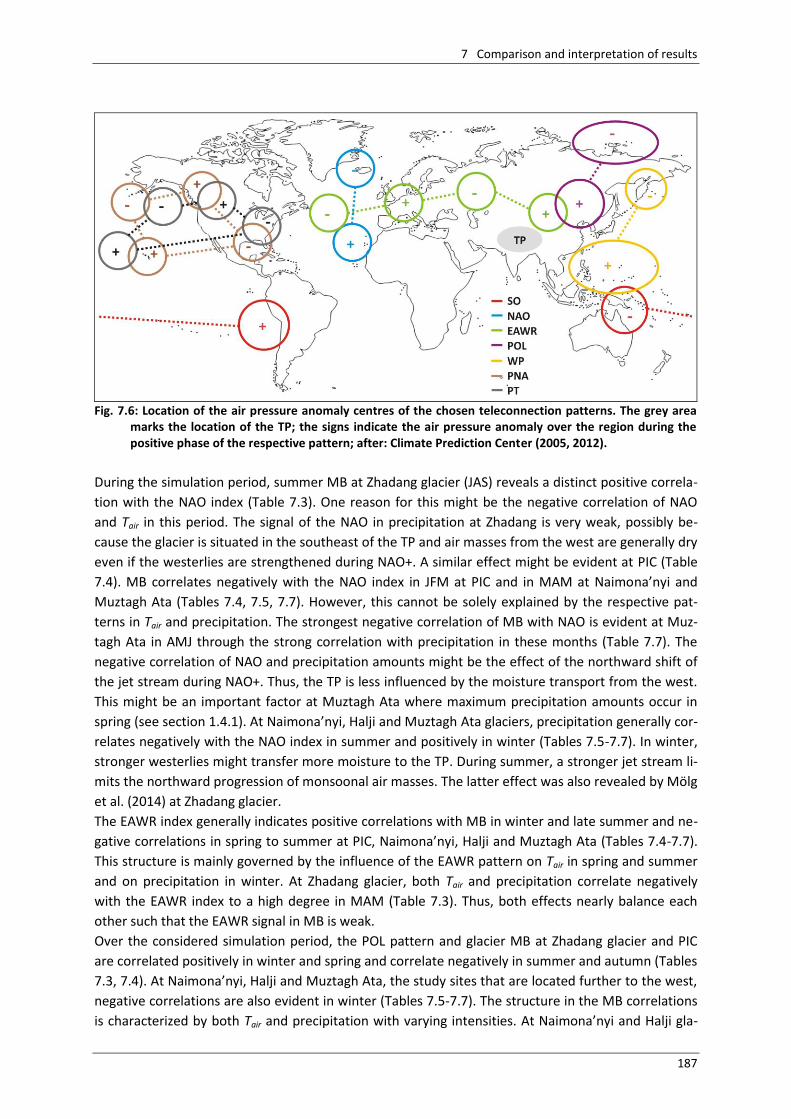
7 Comparison and interpretation of results
187
Fig. 7.6: Location of the air pressure anomaly centres of the chosen teleconnection patterns. The grey area
marks the location of the TP; the signs indicate the air pressure anomaly over the region during the positive phase of the respective pattern; after: Climate Prediction Center (2005, 2012).
During the simulation period, summer MB at Zhadang glacier (JAS) reveals a distinct positive correla-
tion with the NAO index (Table 7.3). One reason for this might be the negative correlation of NAO
and Tair in this period. The signal of the NAO in precipitation at Zhadang is very weak, possibly be-
cause the glacier is situated in the southeast of the TP and air masses from the west are generally dry
even if the westerlies are strengthened during NAO+. A similar effect might be evident at PIC (Table
7.4). MB correlates negatively with the NAO index in JFM at PIC and in MAM at Naimona’nyi and
Muztagh Ata (Tables 7.4, 7.5, 7.7). However, this cannot be solely explained by the respective pat-
terns in Tair and precipitation. The strongest negative correlation of MB with NAO is evident at Muz-
tagh Ata in AMJ through the strong correlation with precipitation in these months (Table 7.7). The
negative correlation of NAO and precipitation amounts might be the effect of the northward shift of
the jet stream during NAO+. Thus, the TP is less influenced by the moisture transport from the west.
This might be an important factor at Muztagh Ata where maximum precipitation amounts occur in
spring (see section 1.4.1). At Naimona’nyi, Halji and Muztagh Ata glaciers, precipitation generally cor-
relates negatively with the NAO index in summer and positively in winter (Tables 7.5-7.7). In winter,
stronger westerlies might transfer more moisture to the TP. During summer, a stronger jet stream li-
mits the northward progression of monsoonal air masses. The latter effect was also revealed by Mölg
et al. (2014) at Zhadang glacier.
The EAWR index generally indicates positive correlations with MB in winter and late summer and ne-
gative correlations in spring to summer at PIC, Naimona’nyi, Halji and Muztagh Ata (Tables 7.4-7.7).
This structure is mainly governed by the influence of the EAWR pattern on Tair in spring and summer
and on precipitation in winter. At Zhadang glacier, both Tair and precipitation correlate negatively
with the EAWR index to a high degree in MAM (Table 7.3). Thus, both effects nearly balance each
other such that the EAWR signal in MB is weak.
Over the considered simulation period, the POL pattern and glacier MB at Zhadang glacier and PIC
are correlated positively in winter and spring and correlate negatively in summer and autumn (Tables
7.3, 7.4). At Naimona’nyi, Halji and Muztagh Ata, the study sites that are located further to the west,
negative correlations are also evident in winter (Tables 7.5-7.7). The structure in the MB correlations
is characterized by both Tair and precipitation with varying intensities. At Naimona’nyi and Halji gla-
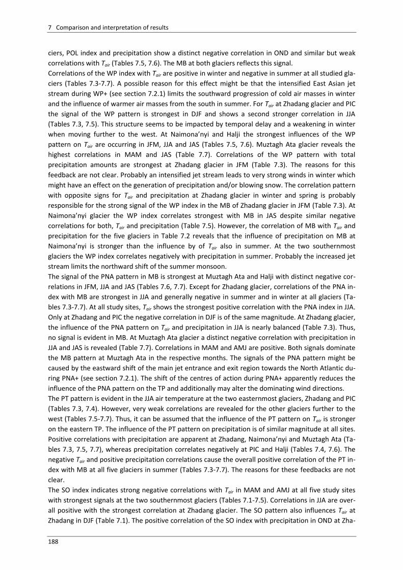
7 Comparison and interpretation of results
188
ciers, POL index and precipitation show a distinct negative correlation in OND and similar but weak
correlations with Tair (Tables 7.5, 7.6). The MB at both glaciers reflects this signal.
Correlations of the WP index with Tair are positive in winter and negative in summer at all studied gla-
ciers (Tables 7.3-7.7). A possible reason for this effect might be that the intensified East Asian jet
stream during WP+ (see section 7.2.1) limits the southward progression of cold air masses in winter
and the influence of warmer air masses from the south in summer. For Tair at Zhadang glacier and PIC
the signal of the WP pattern is strongest in DJF and shows a second stronger correlation in JJA
(Tables 7.3, 7.5). This structure seems to be impacted by temporal delay and a weakening in winter
when moving further to the west. At Naimona’nyi and Halji the strongest influences of the WP
pattern on Tair are occurring in JFM, JJA and JAS (Tables 7.5, 7.6). Muztagh Ata glacier reveals the
highest correlations in MAM and JAS (Table 7.7). Correlations of the WP pattern with total
precipitation amounts are strongest at Zhadang glacier in JFM (Table 7.3). The reasons for this
feedback are not clear. Probably an intensified jet stream leads to very strong winds in winter which
might have an effect on the generation of precipitation and/or blowing snow. The correlation pattern
with opposite signs for Tair and precipitation at Zhadang glacier in winter and spring is probably
responsible for the strong signal of the WP index in the MB of Zhadang glacier in JFM (Table 7.3). At
Naimona’nyi glacier the WP index correlates strongest with MB in JAS despite similar negative
correlations for both, Tair and precipitation (Table 7.5). However, the correlation of MB with Tair and
precipitation for the five glaciers in Table 7.2 reveals that the influence of precipitation on MB at
Naimona’nyi is stronger than the influence by of Tair also in summer. At the two southernmost
glaciers the WP index correlates negatively with precipitation in summer. Probably the increased jet
stream limits the northward shift of the summer monsoon.
The signal of the PNA pattern in MB is strongest at Muztagh Ata and Halji with distinct negative cor-
relations in JFM, JJA and JAS (Tables 7.6, 7.7). Except for Zhadang glacier, correlations of the PNA in-
dex with MB are strongest in JJA and generally negative in summer and in winter at all glaciers (Ta-
bles 7.3-7.7). At all study sites, Tair shows the strongest positive correlation with the PNA index in JJA.
Only at Zhadang and PIC the negative correlation in DJF is of the same magnitude. At Zhadang glacier,
the influence of the PNA pattern on Tair and precipitation in JJA is nearly balanced (Table 7.3). Thus,
no signal is evident in MB. At Muztagh Ata glacier a distinct negative correlation with precipitation in
JJA and JAS is revealed (Table 7.7). Correlations in MAM and AMJ are positive. Both signals dominate
the MB pattern at Muztagh Ata in the respective months. The signals of the PNA pattern might be
caused by the eastward shift of the main jet entrance and exit region towards the North Atlantic du-
ring PNA+ (see section 7.2.1). The shift of the centres of action during PNA+ apparently reduces the
influence of the PNA pattern on the TP and additionally may alter the dominating wind directions.
The PT pattern is evident in the JJA air temperature at the two easternmost glaciers, Zhadang and PIC
(Tables 7.3, 7.4). However, very weak correlations are revealed for the other glaciers further to the
west (Tables 7.5-7.7). Thus, it can be assumed that the influence of the PT pattern on Tair is stronger
on the eastern TP. The influence of the PT pattern on precipitation is of similar magnitude at all sites.
Positive correlations with precipitation are apparent at Zhadang, Naimona’nyi and Muztagh Ata (Ta-
bles 7.3, 7.5, 7.7), whereas precipitation correlates negatively at PIC and Halji (Tables 7.4, 7.6). The
negative Tair and positive precipitation correlations cause the overall positive correlation of the PT in-
dex with MB at all five glaciers in summer (Tables 7.3-7.7). The reasons for these feedbacks are not
clear.
The SO index indicates strong negative correlations with Tair in MAM and AMJ at all five study sites
with strongest signals at the two southernmost glaciers (Tables 7.1-7.5). Correlations in JJA are over-
all positive with the strongest correlation at Zhadang glacier. The SO pattern also influences Tair at
Zhadang in DJF (Table 7.1). The positive correlation of the SO index with precipitation in OND at Zha-
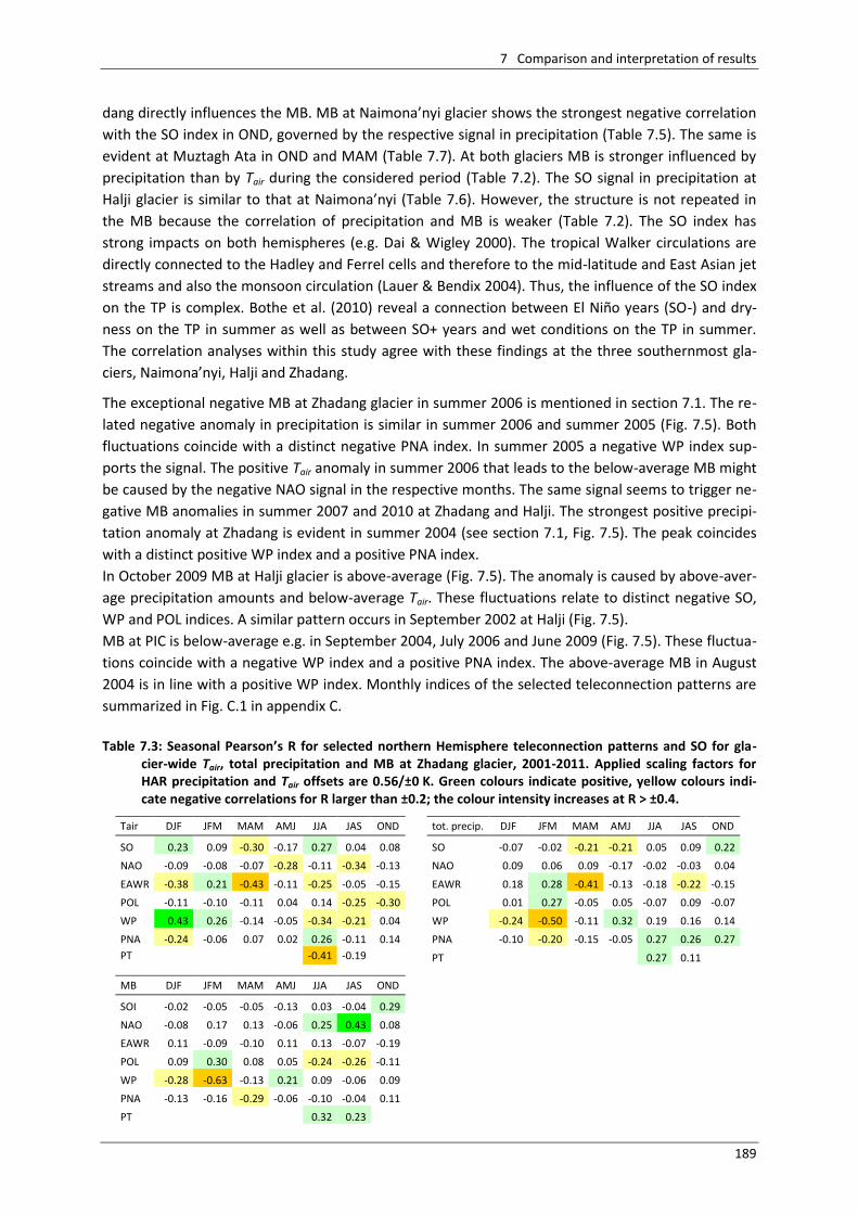
7 Comparison and interpretation of results
189
dang directly influences the MB. MB at Naimona’nyi glacier shows the strongest negative correlation
with the SO index in OND, governed by the respective signal in precipitation (Table 7.5). The same is
evident at Muztagh Ata in OND and MAM (Table 7.7). At both glaciers MB is stronger influenced by
precipitation than by Tair during the considered period (Table 7.2). The SO signal in precipitation at
Halji glacier is similar to that at Naimona’nyi (Table 7.6). However, the structure is not repeated in
the MB because the correlation of precipitation and MB is weaker (Table 7.2). The SO index has
strong impacts on both hemispheres (e.g. Dai & Wigley 2000). The tropical Walker circulations are
directly connected to the Hadley and Ferrel cells and therefore to the mid-latitude and East Asian jet
streams and also the monsoon circulation (Lauer & Bendix 2004). Thus, the influence of the SO index
on the TP is complex. Bothe et al. (2010) reveal a connection between El Niño years (SO-) and dry-
ness on the TP in summer as well as between SO+ years and wet conditions on the TP in summer.
The correlation analyses within this study agree with these findings at the three southernmost gla-
ciers, Naimona’nyi, Halji and Zhadang.
The exceptional negative MB at Zhadang glacier in summer 2006 is mentioned in section 7.1. The re-
lated negative anomaly in precipitation is similar in summer 2006 and summer 2005 (Fig. 7.5). Both
fluctuations coincide with a distinct negative PNA index. In summer 2005 a negative WP index sup-
ports the signal. The positive Tair anomaly in summer 2006 that leads to the below-average MB might
be caused by the negative NAO signal in the respective months. The same signal seems to trigger ne-
gative MB anomalies in summer 2007 and 2010 at Zhadang and Halji. The strongest positive precipi-
tation anomaly at Zhadang is evident in summer 2004 (see section 7.1, Fig. 7.5). The peak coincides
with a distinct positive WP index and a positive PNA index.
In October 2009 MB at Halji glacier is above-average (Fig. 7.5). The anomaly is caused by above-aver-
age precipitation amounts and below-average Tair. These fluctuations relate to distinct negative SO,
WP and POL indices. A similar pattern occurs in September 2002 at Halji (Fig. 7.5).
MB at PIC is below-average e.g. in September 2004, July 2006 and June 2009 (Fig. 7.5). These fluctua-
tions coincide with a negative WP index and a positive PNA index. The above-average MB in August
2004 is in line with a positive WP index. Monthly indices of the selected teleconnection patterns are
summarized in Fig. C.1 in appendix C.
Table 7.3: Seasonal Pearson’s R for selected northern Hemisphere teleconnection patterns and SO for gla-
cier-wide Tair, total precipitation and MB at Zhadang glacier, 2001-2011. Applied scaling factors for HAR precipitation and Tair offsets are 0.56/±0 K. Green colours indicate positive, yellow colours indi-cate negative correlations for R larger than ±0.2; the colour intensity increases at R > ±0.4.
Tair DJF JFM MAM AMJ JJA JAS OND tot. precip. DJF JFM MAM AMJ JJA JAS OND
SO 0.23 0.09 -0.30 -0.17 0.27 0.04 0.08 SO -0.07 -0.02 -0.21 -0.21 0.05 0.09 0.22
NAO -0.09 -0.08 -0.07 -0.28 -0.11 -0.34 -0.13 NAO 0.09 0.06 0.09 -0.17 -0.02 -0.03 0.04
EAWR -0.38 0.21 -0.43 -0.11 -0.25 -0.05 -0.15 EAWR 0.18 0.28 -0.41 -0.13 -0.18 -0.22 -0.15
POL -0.11 -0.10 -0.11 0.04 0.14 -0.25 -0.30 POL 0.01 0.27 -0.05 0.05 -0.07 0.09 -0.07
WP 0.43 0.26 -0.14 -0.05 -0.34 -0.21 0.04 WP -0.24 -0.50 -0.11 0.32 0.19 0.16 0.14
PNA -0.24 -0.06 0.07 0.02 0.26 -0.11 0.14 PNA -0.10 -0.20 -0.15 -0.05 0.27 0.26 0.27
PT -0.41 -0.19 PT 0.27 0.11
MB DJF JFM MAM AMJ JJA JAS OND
SOI -0.02 -0.05 -0.05 -0.13 0.03 -0.04 0.29
NAO -0.08 0.17 0.13 -0.06 0.25 0.43 0.08
EAWR 0.11 -0.09 -0.10 0.11 0.13 -0.07 -0.19
POL 0.09 0.30 0.08 0.05 -0.24 -0.26 -0.11
WP -0.28 -0.63 -0.13 0.21 0.09 -0.06 0.09
PNA -0.13 -0.16 -0.29 -0.06 -0.10 -0.04 0.11
PT 0.32 0.23
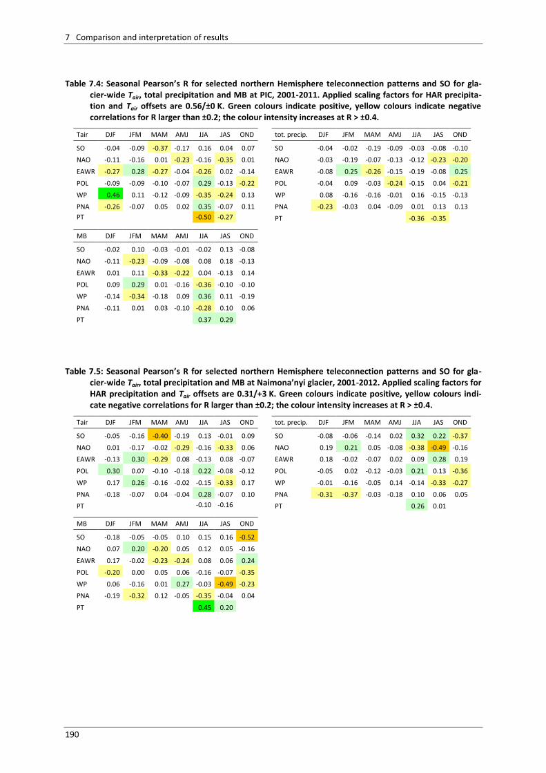
7 Comparison and interpretation of results
190
Table 7.4: Seasonal Pearson’s R for selected northern Hemisphere teleconnection patterns and SO for gla-
cier-wide Tair, total precipitation and MB at PIC, 2001-2011. Applied scaling factors for HAR precipita-tion and Tair offsets are 0.56/±0 K. Green colours indicate positive, yellow colours indicate negative correlations for R larger than ±0.2; the colour intensity increases at R > ±0.4.
Tair DJF JFM MAM AMJ JJA JAS OND tot. precip. DJF JFM MAM AMJ JJA JAS OND
SO -0.04 -0.09 -0.37 -0.17 0.16 0.04 0.07 SO -0.04 -0.02 -0.19 -0.09 -0.03 -0.08 -0.10
NAO -0.11 -0.16 0.01 -0.23 -0.16 -0.35 0.01 NAO -0.03 -0.19 -0.07 -0.13 -0.12 -0.23 -0.20
EAWR -0.27 0.28 -0.27 -0.04 -0.26 0.02 -0.14 EAWR -0.08 0.25 -0.26 -0.15 -0.19 -0.08 0.25
POL -0.09 -0.09 -0.10 -0.07 0.29 -0.13 -0.22 POL -0.04 0.09 -0.03 -0.24 -0.15 0.04 -0.21
WP 0.46 0.11 -0.12 -0.09 -0.35 -0.24 0.13 WP 0.08 -0.16 -0.16 -0.01 0.16 -0.15 -0.13
PNA -0.26 -0.07 0.05 0.02 0.35 -0.07 0.11 PNA -0.23 -0.03 0.04 -0.09 0.01 0.13 0.13
PT -0.50 -0.27 PT -0.36 -0.35
MB DJF JFM MAM AMJ JJA JAS OND
SO -0.02 0.10 -0.03 -0.01 -0.02 0.13 -0.08
NAO -0.11 -0.23 -0.09 -0.08 0.08 0.18 -0.13
EAWR 0.01 0.11 -0.33 -0.22 0.04 -0.13 0.14
POL 0.09 0.29 0.01 -0.16 -0.36 -0.10 -0.10
WP -0.14 -0.34 -0.18 0.09 0.36 0.11 -0.19
PNA -0.11 0.01 0.03 -0.10 -0.28 0.10 0.06
PT 0.37 0.29
Table 7.5: Seasonal Pearson’s R for selected northern Hemisphere teleconnection patterns and SO for gla-
cier-wide Tair, total precipitation and MB at Naimona’nyi glacier, 2001-2012. Applied scaling factors for HAR precipitation and Tair offsets are 0.31/+3 K. Green colours indicate positive, yellow colours indi-cate negative correlations for R larger than ±0.2; the colour intensity increases at R > ±0.4.
Tair DJF JFM MAM AMJ JJA JAS OND tot. precip. DJF JFM MAM AMJ JJA JAS OND
SO -0.05 -0.16 -0.40 -0.19 0.13 -0.01 0.09 SO -0.08 -0.06 -0.14 0.02 0.32 0.22 -0.37
NAO 0.01 -0.17 -0.02 -0.29 -0.16 -0.33 0.06 NAO 0.19 0.21 0.05 -0.08 -0.38 -0.49 -0.16
EAWR -0.13 0.30 -0.29 0.08 -0.13 0.08 -0.07 EAWR 0.18 -0.02 -0.07 0.02 0.09 0.28 0.19
POL 0.30 0.07 -0.10 -0.18 0.22 -0.08 -0.12 POL -0.05 0.02 -0.12 -0.03 0.21 0.13 -0.36
WP 0.17 0.26 -0.16 -0.02 -0.15 -0.33 0.17 WP -0.01 -0.16 -0.05 0.14 -0.14 -0.33 -0.27
PNA -0.18 -0.07 0.04 -0.04 0.28 -0.07 0.10 PNA -0.31 -0.37 -0.03 -0.18 0.10 0.06 0.05
PT -0.10 -0.16 PT 0.26 0.01
MB DJF JFM MAM AMJ JJA JAS OND
SO -0.18 -0.05 -0.05 0.10 0.15 0.16 -0.52
NAO 0.07 0.20 -0.20 0.05 0.12 0.05 -0.16
EAWR 0.17 -0.02 -0.23 -0.24 0.08 0.06 0.24
POL -0.20 0.00 0.05 0.06 -0.16 -0.07 -0.35
WP 0.06 -0.16 0.01 0.27 -0.03 -0.49 -0.23
PNA -0.19 -0.32 0.12 -0.05 -0.35 -0.04 0.04
PT 0.45 0.20
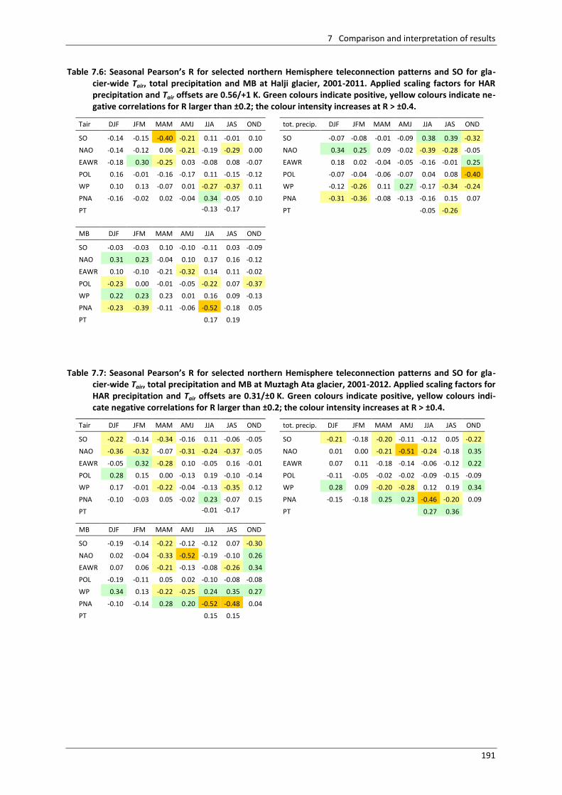
7 Comparison and interpretation of results
191
Table 7.6: Seasonal Pearson’s R for selected northern Hemisphere teleconnection patterns and SO for gla-cier-wide Tair, total precipitation and MB at Halji glacier, 2001-2011. Applied scaling factors for HAR precipitation and Tair offsets are 0.56/+1 K. Green colours indicate positive, yellow colours indicate ne-gative correlations for R larger than ±0.2; the colour intensity increases at R > ±0.4.
Tair DJF JFM MAM AMJ JJA JAS OND tot. precip. DJF JFM MAM AMJ JJA JAS OND
SO -0.14 -0.15 -0.40 -0.21 0.11 -0.01 0.10 SO -0.07 -0.08 -0.01 -0.09 0.38 0.39 -0.32
NAO -0.14 -0.12 0.06 -0.21 -0.19 -0.29 0.00 NAO 0.34 0.25 0.09 -0.02 -0.39 -0.28 -0.05
EAWR -0.18 0.30 -0.25 0.03 -0.08 0.08 -0.07 EAWR 0.18 0.02 -0.04 -0.05 -0.16 -0.01 0.25
POL 0.16 -0.01 -0.16 -0.17 0.11 -0.15 -0.12 POL -0.07 -0.04 -0.06 -0.07 0.04 0.08 -0.40
WP 0.10 0.13 -0.07 0.01 -0.27 -0.37 0.11 WP -0.12 -0.26 0.11 0.27 -0.17 -0.34 -0.24
PNA -0.16 -0.02 0.02 -0.04 0.34 -0.05 0.10 PNA -0.31 -0.36 -0.08 -0.13 -0.16 0.15 0.07
PT -0.13 -0.17 PT -0.05 -0.26
MB DJF JFM MAM AMJ JJA JAS OND
SO -0.03 -0.03 0.10 -0.10 -0.11 0.03 -0.09
NAO 0.31 0.23 -0.04 0.10 0.17 0.16 -0.12
EAWR 0.10 -0.10 -0.21 -0.32 0.14 0.11 -0.02
POL -0.23 0.00 -0.01 -0.05 -0.22 0.07 -0.37
WP 0.22 0.23 0.23 0.01 0.16 0.09 -0.13
PNA -0.23 -0.39 -0.11 -0.06 -0.52 -0.18 0.05
PT 0.17 0.19
Table 7.7: Seasonal Pearson’s R for selected northern Hemisphere teleconnection patterns and SO for gla-
cier-wide Tair, total precipitation and MB at Muztagh Ata glacier, 2001-2012. Applied scaling factors for HAR precipitation and Tair offsets are 0.31/±0 K. Green colours indicate positive, yellow colours indi-cate negative correlations for R larger than ±0.2; the colour intensity increases at R > ±0.4.
Tair DJF JFM MAM AMJ JJA JAS OND tot. precip. DJF JFM MAM AMJ JJA JAS OND
SO -0.22 -0.14 -0.34 -0.16 0.11 -0.06 -0.05 SO -0.21 -0.18 -0.20 -0.11 -0.12 0.05 -0.22
NAO -0.36 -0.32 -0.07 -0.31 -0.24 -0.37 -0.05 NAO 0.01 0.00 -0.21 -0.51 -0.24 -0.18 0.35
EAWR -0.05 0.32 -0.28 0.10 -0.05 0.16 -0.01 EAWR 0.07 0.11 -0.18 -0.14 -0.06 -0.12 0.22
POL 0.28 0.15 0.00 -0.13 0.19 -0.10 -0.14 POL -0.11 -0.05 -0.02 -0.02 -0.09 -0.15 -0.09
WP 0.17 -0.01 -0.22 -0.04 -0.13 -0.35 0.12 WP 0.28 0.09 -0.20 -0.28 0.12 0.19 0.34
PNA -0.10 -0.03 0.05 -0.02 0.23 -0.07 0.15 PNA -0.15 -0.18 0.25 0.23 -0.46 -0.20 0.09
PT -0.01 -0.17 PT 0.27 0.36
MB DJF JFM MAM AMJ JJA JAS OND
SO -0.19 -0.14 -0.22 -0.12 -0.12 0.07 -0.30
NAO 0.02 -0.04 -0.33 -0.52 -0.19 -0.10 0.26
EAWR 0.07 0.06 -0.21 -0.13 -0.08 -0.26 0.34
POL -0.19 -0.11 0.05 0.02 -0.10 -0.08 -0.08
WP 0.34 0.13 -0.22 -0.25 0.24 0.35 0.27
PNA -0.10 -0.14 0.28 0.20 -0.52 -0.48 0.04
PT 0.15 0.15
7 Comparison and interpretation of results
192
7.2.3 Summary regarding the influences of teleconnection patterns on glacier mass balance at the study sites
Generally, the influence of the seven selected teleconnection patterns on Tair from HAR at the five
study sites within the simulation period 2001-2011/12 is homogeneous. The signs of the respective
correlation coefficients usually reveal similar seasonal patterns at the five glaciers (Tables 7.3-7.7).
However, the strength of the different signals varies regionally. Concerning the correlations with Tair,
the influences of the selected teleconnection patterns coincide at Zhadang glacier and PIC, as well as
at Naimona’nyi and Halji glaciers to a high degree. Partly, Tair at Muztagh Ata shows similar depen-
dencies as Tair at Naimona’nyi and Halji. The respective signals in HAR precipitation do not reveal re-
gional patterns similar for all teleconnection indices (Tables 7.3-7.7). However, precipitation correla-
tions at Naimona’nyi and Halji glaciers coincide to a higher degree because the two glaciers are only
≈26 km apart. Similar signals in precipitation in two or more regions are rather evident for individual
teleconnection patterns. Thus, the correlations of the different indices with MB for the five study re-
gions are even more disperse (Tables 7.3-7.7). The superposition of teleconnection signals in Tair and
precipitation are further altered by the varying importance of Tair and precipitation for glacier MB at
the different glaciers (Table 7.2).
Many of the anomalies in MB, Tair and precipitation at the five glaciers can be related to telecon-
nection pattern indices. Some fluctuations seem to follow none of the selected signals. To reveal the
atmospheric drivers in detail would require the consideration of further teleconnection indices, the
extensive pre-processing of the data series and an extended statistical analysis. Such an approach
would require a thorough analysis of the levels of significance of the relations and an investigation of
possible non-linear or combined effects between two or more variables. However, this further elabo-
ration cannot be achieved as part of this thesis. It will be worthwhile to address these issues in detail
within future research.
8 Overall conclusion
193
8 Overall conclusion
SEB/MB modelling and validation
The newly developed coupled SEB/MB and multi-layer snow model is calibrated and validated for
Zhadang glacier. The glacier is subject of intensive Sino-German atmospheric and glaciological field
work since 2009 and therefore holds a large data basis. Output data of both, the AWS and the HAR
forced model are compared to various atmospheric, glaciological, surface and subsurface data sets
for the point location of AWS1 as well as for the ablation stake network distributed over the glacier.
The 3-year image time series of a time-lapse camera system next to the glacier provides an important
contribution to the spatial and temporal validation of the model performance. The respective model
output corresponds very well to both the mean altitude of the transient snowline and the observed
spatial MB patterns. Furthermore, the results of the detailed model evaluation for the intensive ob-
servational period 2009-2012 for both the AWS and HAR forced MB model are convincing. The de-
tailed comparison for the SEB and MB components of the HAR model run 2001-2011 with the study
of Mölg et al. (2014) with a similar model reveals that in most years the differences in Qmelt are small
although other SEB components show large discrepancies between both models. The parameteriza-
tions for the various energy fluxes are different within both models. However, both models have
been calibrated for Qmelt to finally reproduce the glacial melt pattern derived from the glaciological
MB method. Thus, in most MB years differences in the single SEB components between the two mo-
dels compensate each other and lead to small differences in Qmelt and surface melt.
At all five study sites the derived intra- and inter-annual cycles of SEB and MB components are within
reasonable limits. The results of glaciological in-situ MB observations over several years are available
at Zhadang and Naimona’nyi glacier for comparison. In the Muztagh Ata region field data is available
from a neighbouring glacier. The comparison with the in-situ MB measurements reveals that overall
inter-annual variations in this study and the respective observations are similar. Discrepancies are
apparent for single years only. The results depend on the respective patterns of the input parameters
from HAR. This indicates that relative HAR climatology provides year-to-year variance in such that
modelled annual MB variance in general terms fits to the observations at the study sites.
At PIC, Naimona’nyi, Halji and Muztagh Ata glacier surface height changes and geodetic MB estima-
tions from high resolution remote sensing analyses are available for similar periods as covered by this
study. These data allow the spatial evaluation of the MB model results. Furthermore, the average
annual MB estimations from the remote sensing studies can be compared to the results of this study.
8 Overall conclusion
194
At the four glaciers the spatial comparison of calculated surface height changes from modelling and
remote sensing reveals that the overall pattern is captured to a high degree.
The results of the evaluation of absolute values for MB and surface elevation changes through in-situ
measurements and remote sensing methods in the five study areas are very heterogeneous. A preci-
pitation scaling factor of 0.56 with respect to HAR precipitation was obtained from the comparison
with rain gauge measurements at Zhadang glacier (chapter 2). Applying this factor leads to satisfying
results in the HAR forced MB model runs 2001-2011 for Zhadang glacier. HAR Tair and Tair measure-
ments at the AWS at Zhadang glacier are in good agreement. Due to a lack of precipitation measure-
ments at the glacier sites HAR precipitation amounts can not be validated at the other four study
areas. Thus, the same scaling factor of 0.56 is applied in the reference run for each glacier. To ac-
count for uncertainties in total HAR precipitation amounts, three model runs with varying precipita-
tion scaling factors (0.56±0.25) are performed.
At PIC (chapter 3) the reference run with unchanged HAR Tair leads to reasonable results. The compa-
rison of the MB model with glacier-wide surface height changes and geodetic MB estimations shows
only minor discrepancies. The model evaluation against MODIS derived snow line altitude and annual
ELA confirms the overall satisfying model performance for PIC considering the reference run.
At Naimona’nyi glacier (chapter 4) the application of a scaling factor of 0.56 with unchanged Tair
clearly overestimates MB and surface height changes that are available from in-situ MB measure-
ments and remote sensing analysis. With precipitation decreased by 25% (0.31) the MB model results
are more reasonable but still seem to overestimate the MB and the surface height changes especially
in the lower glacier regions. The comparison of atmospheric AWS data at the glacier tongue with HAR
data revealed that Tair from HAR data exhibits a significant cold bias of 3.8 K in winter and 2.0 K in
summer compared to AWS measurements. Thus, a north-south profile of Naimona’nyi glacier is cal-
culated with a precipitation scaling factor of 0.31 and a temperature offset of +3 K. The derived sur-
face height changes agree well with the results derived by remote sensing. Using these settings mo-
delled glacier-wide annual MB is close to the in-situ MB observations.
At Halji glacier (chapter 5) the application of a scaling factor of 0.56 with unchanged Tair overesti-
mates MB and surface height changes that are available from two different remote sensing analyses.
A cold bias in HAR Tair as revealed at Naimona’nyi glacier is assumed to be evident also at Halji.
Therefore, the MB model was run several times for the total glacier area to determine reasonable
combinations of precipitation scaling factors and Tair offsets. The two different results derived by re-
mote sensing lead to a different ‘best-fit’ combination of precipitation scaling factor and Tair-offset at
Halji. The lack of meteorological field observations hampers the ability to verify HAR precipitation
amounts and possible Tair offsets. A cold bias in HAR Tair, even though possibly smaller that at Naimo-
na’nyi, seems to be nevertheless plausible since both remote sensing studies provide evidence that
the results of the MB model reproduce observed glacier change best when Tair is increased by at least
1 K. Comparing this study to the more detailed remote sensing study covering the total simulation
period suggests a combination of a scaling factor of 0.56 and a Tair-offset of +1 K to be reasonable.
At Muztagh Ata glacier (chapter 6) the application of a scaling factor of 0.56 with unchanged Tair
clearly overestimates MB and surface height changes that are available from in-situ MB measure-
ments and remote sensing analysis. With decreased precipitation amounts (0.31) the MB model re-
sults are more reasonable.
The different analyses show that the atmospheric data provided by the HAR dataset can not be ap-
plied directly for glacier SEB and MB modelling. The ranges of uncertainty that are created through
different combinations of precipitation scaling factors and Tair offsets are large. Furthermore, the re-
quired factors and offsets for the HAR data seem to vary regionally. The applied parameterizations
8 Overall conclusion
195
for the various energy fluxes within the MB model contain several unknown or poorly constrained
parameters. Mean values for these parameters were obtained from observations at Zhadang glacier
or taken from literature. Through the lack of detailed measurements at the other four remote glacier
sites it is impossible to verify the applicability of the chosen parameters to these glaciers in more
detail. Furthermore, some physical processes within the glacier SEB and MB are simplified or not
considered at all. This makes it difficult to obtain absolute values for glacier-wide MB or surface ele-
vation changes in regions where precipitation and/or temperature measurements are not available
and MB model results can not be validated in detail by other means as for example by remote sen-
sing analysis or in situ MB measurements.
A major conclusion from the findings within this thesis is that glacier SEB and MB modelling based on
modelled atmospheric data always requires some kind of meteorological, glaciological or remote
sensing based field observation. In consequence, the continuation and extension of at least basic in-
situ measurements at glaciers on the TP is a crucial requirement in order to obtain reliable and de-
tailed SEB and MB estimates based on complex modelling chains for those glaciers.
Surface melt, refreezing and runoff
The obtained SEB and MB components at the single glaciers are consistent with each other because
they interact through physical relationships within the MB model (see sections 1.3.4 and 2.3.1).
Generally, the inter-annual cycle of glacier runoff is similar to that of surface melt for the studied gla-
ciers (Fig. 7.2). At Zhadang glacier large amounts of surface melt refreeze within the snowpack in
spring and autumn. A maximum proportion of 70% occurs in March. Thus, runoff is reduced largely in
these seasons. In July and August, refreezing decreases to ≈7%. Almost half of the monsoon precipi-
tation reaches the glacier as rain. This leads to increased glacier runoff compared to surface melt in
these months. In total, 17% of the melt water refreezes at Zhadang glacier. Glacier melt water ac-
counts for 95% of the total runoff with a minimum of 81% in July.
At Naimona’nyi the surface melt and runoff are almost equivalent because the amount of refreezing
approximately equals liquid precipitation. In total, only 8% of the generated melt water refreezes.
The proportion is largest in mid-winter (30%) and smallest in October (1%). Total amounts of liquid
precipitation are not large at Naimona’nyi even in summer. Thus, glacier melt water accounts for
98% of the total runoff with a minimum of 89% in July.
At Halji glacier the surface melt and runoff are almost equivalent because the amount of refreezing
approximately equals liquid precipitation. This is the case despite the fact that large amounts of total
precipitation in July and August fall as rain. In total, 27% of surface and subsurface melt refreezes at
Halji. Proportions are largest in February, July and August with up to 47% and smallest between Oc-
tober and December (4%). Glacier melt water accounts for 90% of the total runoff with minima of
65% in June and 55% in July.
At PIC runoff is slightly exceeding surface melt only in August. In this month the amount of liquid pre-
cipitation exceeds the amount of refreezing. In total, 22% of the generated melt water refreezes at
PIC. The proportion exceeds 70% from November until April. In September, only 7% refreezes. Gla-
cier melt water accounts for 91% of the total runoff with a minimum of 70% in June.
At Muztagh Ata glacier runoff is significantly smaller than surface melt especially in August. In total,
34% of the generated melt water refreezes. The proportion is highest in winter with nearly 100% and
lowest in September (27%). The proportion of liquid precipitation at Muztagh Ata is negligible
because of very low Tair. Glacier melt water accounts for 98% of the total runoff with a minimum of
87% in June.
8 Overall conclusion
196
Generally, the proportion of glacier melt water that actually runs off is largest at Naimona’nyi, one of
the two southernmost glaciers. At Muztagh Ata on the north western TP the proportion is smallest.
At all studied glaciers surface melt is largest in late summer and significantly contributes to the total
runoff.
SEB and MB components
The three southernmost glaciers, Zhadang, Naimona’nyi and Halji are characterized by lowest overall
α and therefore largest SWnet. At PIC and Muztagh Ata the overall energy loss by LWnet is larger than
the energy gain by SWnet. Thus, net radiation is an energy sink for both glaciers. The turbulent fluxes
act as a net energy source. This pattern is more distinct at Muztagh Ata than at PIC probably because
very low Tair and frequent precipitation events cause persistent high α. Overall energy loss by Qlat is
largest at Zhadang because RH is low and the glacier surface temperatures favour turbulent ex-
change. Low air and surface temperatures might also be a reason for low Qlat at Muztagh Ata. Fur-
thermore, the overall RH Muztagh Ata is high and exhibits no clear annual minimum. At Halji and Nai-
mona’nyi overall Qlat is not a large energy sink because it regularly becomes positive in summer. The
high moisture content of the monsoonal air masses favour condensation and deposition. The total
energy turnover at Zhadang is dominated by SWnet. At Naimona’nyi and Halji overall SWnet and LWnet
are of equal importance while SWnet dominates in summer and LWnet dominates in winter. At PIC and
Muztagh Ata the continuously high α results in a high contribution of LWnet to total energy turnover.
At Muztagh Ata the absolute proportion of LWnet is larger than that of SWnet year-round.
At PIC and Muztagh Ata the energy gain by SWnet is minimal in winter and nearly equal to the energy
gain by Qsens. At PIC the energy gain through Qsens and thus its contribution to the total energy flux
even exceeds that of SWnet.
Halji, Muztagh Ata and Zhadang glaciers receive the highest annual amounts of solid precipitation,
followed by PIC and Naimona’nyi. At Zhadang and Naimona’nyi the maximum of solid precipitation
generally falls in summer. Snowfall amounts at PIC reveal two peaks in spring and summer. Muztagh
Ata receives maximum solid precipitation amounts in spring. At Halji glacier high proportions of liquid
precipitation in summer result in snowfall maxima in late winter and late summer. Overall surface
melt is largest at Zhadang and Halji glaciers driven by Tair, α and SWnet. The highest amounts of refree-
zing are generated at Halji glacier because more solid precipitation allows a thicker snow pack com-
pared to Zhadang glacier. At Muztagh Ata the proportion of surface and subsurface melt that refree-
zes within the snow pack is largest. Total mass loss through sublimation is highest at Zhadang glacier.
However, the amount is small compared to total effective melt. At PIC and Muztagh Ata the mass
loss by sublimation accounts for more than half of the total mass loss. The proportions are 68% at PIC
and 71% at Muztagh Ata.
At all five studied glaciers mass loss through sublimation dominates over surface melt in winter. Sub-
limation accounts for more than 50% of the total mass loss at least between November and April. At
the two northernmost study regions, PIC and Muztagh Ata, effective melt only dominates in July and
August.
The overall results for the different regions on the TP coincide with the glacier characteristics out-
lined in sections 1.3 and 1.4. PIC and Muztagh Ata glacier belong to the extremely continental or cold
glacier types with a balanced or slightly positive mass budget. The influence of the Indian summer
monsoon is weak or completely absent. Zhadang, Naimona’nyi and Halji are glaciers of the subconti-
nental or polythermal type and are strongly influenced by the summer monsoon. These glaciers ex-
perienced significant mass loss in recent decades. The studies at Naimona’nyi and Halji glaciers con-
8 Overall conclusion
197
firm the high variability in single SEB and MB components between individual glaciers over short dis-
tances.
Influences of teleconnection patterns
The MB at all five studied glaciers is crucially influenced by anomalies in Tair and precipitation. As
expected, fluctuations in Tair are distributed more homogeneously over the TP at least with respect to
the five study sites than the precipitation anomalies. The correlation of seven selected teleconnec-
tion patterns with Tair, precipitation and MB of each glacier reveals that the influences of the respec-
tive patterns on Tair coincide at Zhadang glacier and PIC, as well as at Naimona’nyi and Halji glaciers
to a high degree. The respective signals in HAR precipitation do not reveal regional patterns similar
for all teleconnection indices. However, precipitation correlations at Naimona’nyi and Halji glaciers
coincide to a higher degree because the two glaciers are only ≈26 km apart. The correlations of the
different indices with MB for the five study regions are mostly the result of the overlapping tele-
connection signals in Tair and precipitation. These influences are altered by the varying importance of
Tair and precipitation for glacier MB at the selected glaciers.
Outlook
The SEB and MB studies on selected glaciers in different regions on the TP allow the comparison and
understanding of the various driving mechanisms for the SEB and MB components. However, several
HAR output parameters require further adjustment. The ranges of uncertainty that are created
through different combinations of precipitation scaling factors and Tair offsets are large. Furthermore,
the required parameterizations seem to vary regionally. The availability of in-situ observations and
remote sensing data for the selected glaciers varies largely. For those glaciers where meteorological
or detailed glaciological in-situ observations are lacking further uncertainty analyses with various
combinations of precipitation scaling factors and air temperature offsets need to be carried out in
future studies. The analysis at Halji glacier revealed that several combinations of precipitation scaling
factors and air temperature offsets lead to similar results for MB and surface elevation changes. This
also applies to the other glacier sites. Thus, further uncertainty analyses and the detailed evaluation
of the SEB and MB components as well as field observations or remote sensing studies are crucial for
further process understanding.

References
199
References
Ageta, Y. and Higuchi, K. (1984): Estimation of mass balance components of a summer-accumulation type gla-
cier in the Nepal Himalaya, Geogr. Ann. A., 66, 3, 249-255.
Ageta, Y. and Fujita, K. (1996): Characteristics of mass balance of summer-accumulation type glaciers in the Hi-
malayas and Tibetan Plateau, Z. Gletscherk. Glazialgeol., 32, 61-65.
Ageta, Y., Iwata, S., Yabuki, H., Naito, N., Sakai, A., Narama, C. And Karma, T. (2000): Expansion of glacier lakes
in recent decades in the Bhutan Himalayas, IAHS publication, 165-176.
Aizen, V.B. and Aizen, E.M. (1994): Features of regime and mass exchange of some glaciers on central Asia peri-
phery, Bull. Glac. Res., 12, 9-24.
Aizen, V.B., Aizen, E.M. and Nikitin, S.A. (2002): Glacier regime on the northern slope of the Himalaya (Xixibang-
ma glaciers), Quatern. Int., 97-98, 27-39.
An, Z., Kutzbach, J.E., Prell, W.L. and Porter, S.C. (2001): Evolution of Asian monsoons and phased uplift of the
Himalaya-Tibetan plateau since Late Miocene times, Nature, 411, 62-66.
Anderson, E.A. (1976): A point energy and mass balance model of a snow cover, Techn. Rep. NWS19, NOAA.
Andreassen, L.M., van den Broeke, M.R., Giesen, R.H. and Oerlemans, J. (2008): A 5 year record of surface ener-
gy and mass balance from the ablation zone of Storbreen, Norway, J. Glaciol., 54, 185, 245-258.
Aschwanden, A. and Blatter, H. (2006): Numerical modelling of glacier flow, Excerpt from the Proceedings of
the COMSOL users conference, Frankfurt, 3 pp.
Aschwanden, A. (2008): Mechanics and thermodynamics of polythermal glaciers, Dissertation, ETH Zürich, 93
pp.
Azam, M.F., Wagnon, P., Vincent, C., Ramanathan, A.L., Mandal, A. and Pottakkal, J.G. (2014): Processes
governing the mass balance of Chhota Shingri Glacier (Western Himalaya, India) assessed by point-scale
surface energy balance measurements, TCD, 8, 2867-2922.
Barnard, P.L., Owen, L.A. and Finkel, R.C. (2004a): Style and timing of glacial and paraglacial sedimentation in a
monsoonal influenced high Himalayan environment, the upper Bhagirathi Valley, Garhwal Himalaya, Se-
diment. Geol., 165, 199-221.
Barnard, P.L., Owen, L.A., Sharma, M.C. and Finkel, R.C. (2004b): Late Quaternary landscape evolution of a
monsoon-influenced high Himalayan valley, Gori Ganga, Nanda Devi, NE Garhwal, Geomorphology, 61,
91-110.
Barnston, A.G. and Livezey, R.E. (1987): Classification, seasonality and persistence of low-frequency
atmospheric circulation patterns, Monthly Weather Review, 115, 1083-1126.
References
200
Barrows, T.T., Stone, J.O., Fifield, L.K. and Cresswell, R.G. (2002): The timing of the Last Glacial Maximum in
Australia, Quaternary Science Reviews, 21, 159–173.
Bartelt, P. and Lehning, M. (2002): A physical SNOWPACK model for the Swiss avalanche warning: Part I: nume-
rical model, Cold Regions Science and Technology, 35, 123-145.
Baumgartner, A., Liebscher, H.-J. and Benecke, P. (1990): Lehrbuch der Hydrologie, Bd 1: Allgemeine Hydrolo-
gie, Gebrüder Borntraeger.
Bajracharya, S.R. and Mool, P. (2009): Glaciers, glacial lakes and glacial lake outburst floods in the Mount
Everest region, Nepal, Ann. Glaciol., 50, 53, 81-86.
Benn, D.I. and Owen, L.A. (1998): The role of the Indian summer monsoon and the mid-latitude westerlies in
Himalayan glaciation: review and speculative discussion, J. Geol. Soc., 155, 353-363.
Benn, D.I. and Owen,L.A. (2002): Himalayan glacial sedimentary environments: a framework for reconstructing
and dating former glacial extents in high mountain regions, Quaternary International, 97/98,3-26.
Bhambri, R., Bolch, T., Kawishwar, P., Dobhal, D.P., Srivastava, D. and Pratap, B. (2013): Heterogeneity in glacier
response in the upper Shyok valley, northeast Karakoram, TC, 7, 1385-1398.
Bintanja, R. and van den Broeke, M. (1995): The surface energy balance of Antarctic snow and blue ice, J. Appl.
Meteorol., 34, 902-926.
Böhner, J. (2006): General climatic controls and topoclimatic variations in Central and High Asia, Boreas, 35,
279-295.
Bolch, T., Yao, T., Kang, S., Buchroithner, M., Scherer, D., Maussion, F., Huintjes, E. and Schneider, C. (2010): A
glacier inventory for the western Nyainqentanglha Range and the Nam Co Basin, Tibet, and glacier chan-
ges 1976-2009, TC, 4, 419-433.
Bolch, T., Pieczonka, T. and Benn D.I. (2011): Multi-decadal mass loss of glaciers in the Everest area (Nepal Hi-
malaya) derived from stereo imagery, TC, 5, 349-358.
Bolch, T., Kulkarni, A., Kääb, A., Huggel, C., Paul, F., Cogley, J.G., Frey, H., Kargel, J.S., Fujita, K., Scheel, M., Baj-
racharya, S. and Stoffel, M. (2012): The state and fate of Himalayan glaciers, Science, 336, 310-314, doi:
10.1126/science.1215828.
Boos, W.R. and Kuang, Z. (2010): Dominant control of the South Asian monsoon by orographic insulation versus
plateau heating, Nature, 463, 218-U102.
Boos, W.R. and Kuang, Z. (2013): Sensitivity of the South Asian monsoon to elevated and non-elevated heating,
Scientific Reports, 3, 1192, doi: 10.1038/srep01192.
Bothe, O., Fraedrich, K. and Zhu, X. (2011): Large-scale circulations and Tibetan Plateau summer drought and
wetness in a high-resolution climate model, Int. J. Climatol., 31, 832-846.
Bothe, O., Fraedrich, K. and Zhu, X. (2012): Tibetan Plateau summer precipitation: covariability with circulation
indices, Theor. Appl. Climatol., 108, 293-300.
Bradley, R.S. and Jones, P.D. (1993): ‘Little Ice Age’ summer temperature variations: their nature and relevance
to recent global warming trends, The Holocene, 3, 367-376.
Bräuning, A. (2006): Tree-ring evidence of ‘Little Ice Age’ glacier advances in southern Tibet, The Holocene, 16,
3, 369-380.
Braithwaite, R.J. (1995): Aerodynamic stability and turbulent sensible heat flux over a melting ice surface, the
Greenland ice sheet, J. Glaciol., 41, 562-571.
References
201
Braun, M. and Schneider, C. (2000): Characteristics of summer energy balance on the west coast of the
Antarctic Peninsula, Ann. Glaciol., 31, 179-183.
Braun, M. and Hock, R. (2004): Spatially distributed surface energy balance and ablation modelling on the ice
cap of King George Island (Antarctica), Global and Planetary Change, 42, 45-58.
Brock, B.W., Willis, I.C. and Martin, M.J. (2006): Measurement and parameterization of aerodynamic roughness
length variations at Haut Glacier d’Arolla, Switzerland, J. Glaciol., 52, 281-297.
Brun, E., Martin, E., Simon, V., Gendre, C. and Coleou, C. (1989): An energy and mass model of snow cover suit-
able for operational avalanche forecasting, J. Glaciol., 35, 333-342.
Brun, E., David, P., Sudul, M. and Brunot, G. (1992): A numerical model to simulate snow-cover stratigraphy for
operational avalanche forecasting, J. Glaciol., 38, 13-22.
Caidong, C. and Sorteberg, A. (2010): Modelled mass balance of Xibu glacier, Tibetan Plateau: sensitivity to cli-
mate change, J. Glaciol., 56, 235-248.
Chen, J. (1989): Preliminary researches on lichenometric chronology of Holocene glacial fluctuations and on
other topics in the headwater of Urumqi River, Tianshan Mountains, Sci. China B 32, 1487-1500.
Chen, X., Cui, P., Li, Y., Yang, Z. and Qi, Y. (2007): Changes in glacial lakes and glaciers of post-1986 in the Poiqu
River basin, Nyalam, Xizang (Tibet), Geomorphology, 88, 298-311.
Chen, B., Xu, X., Yang, S. and Zhang, W. (2012): On the origin and destination of atmospheric moisture and air
mass over the Tibetan Plateau, Theor. Appl. Climatol., 110, 423-435.
Chen, J. and Bordoni, S. (2014): Orographic effects of the Tibetan Plateau on the East Asian summer monsoon:
An energetic perspective, J. Climate, doi:10.1175/JCLI-D-13-00479.1.
Cheng, G. and Wu, T. (2007): Responses of permafrost to climate change and their environmental significance,
Qinghai-Tibet Plateau, J. Geophys. Res., 112, F02S03, doi:10.1029/2006JF000631.
Chow, V.T. (Eds.)(1964): Handbook of applied hydrology, McGraw-Hill.
Climate Prediction Center (2012): Northern Hemisphere Teleconnection Patterns. Available at:
http://www.cpc.ncep.noaa.gov/data/teledoc/telecontents.shtml (11.06.2014)
Climate Prediction Center (2005): The ENSO cycle. Available at: http://www.cpc.ncep.noaa.gov/products/
analysis_monitoring/ensocycle/enso_cycle.shtml (11.06.2014)
Cogley, J.G., Hock, R., Rasmussen, L.A., Arendt, A.A., Bauder, A. Braithwaite, R.J., Jansson, P., Kaser, G., Möller,
M., Nicholson, L. and Zemp. M. (2011): Glossary of Glacier Mass Balance and Related Terms, IHP-VII
Technical Documents in Hydrology No. 86, IACS Contribution No. 2, UNESCO-IHP, Paris.
Cui, X. and Graf, H.F. (2009): Recent land cover changes on the Tibetan Plateau: a review, Climatic Change, 94,
47-61.
Cullen, N.J., Mölg, T., Kaser, G., Steffen, K. and Hardy, D.R. (2007): Energy-balance model validation on the top
of Kilimanjaro, Tanzania, using eddy covariance data, Ann. Glaciol., 46, 227-233.
Dai A. and Wigley, T.M.L. (2000): Global patterns of ENSO–induced precipitation, Geophys. Res. Lett., 27, 1283–
1286.
Denton, G.H., Heusser, C.J., Lowell, T.V., Moreno, P.I., Anderson, B.G., Heusser, L.E., Schlüchter, C. and Mar-
chant, D.R. (1999): Interhemispheric linkage of paleoclimate during the last glaciation, Geografiska
Annaler, 81A, 107–154.
References
202
Derbyshire, E. (1981): Glacier regime and glacial sediment facies: a hypothetical framework for the Qinghai–Xi-
zang Plateau. Proceedings of Symposium on Qinghai–Xizang (Tibet) Plateau, Beijing, China, Geological
and Ecological studies of Qinghai–Xizang Plateau, 2, 1649-1656.
Ding, Y. (1992): Effects of the Qinghai-Xizang (Tibetan) Plateau on the circulation features over the plateau and
its surrounding areas, Advances in Atmospheric Sciences, 9, 1, 112-130.
Ding, Y., Liu, S., Li, J. and Shangguan, D. (2006): The retreat of glaciers in response to recent climate warming in
western China, Ann. Glaciol., 43, 97-105.
Domrös, M. and Peng. G. (1988): The Climate of China, Springer, 361 pp.
Dyurgerov, M. (2002): Glacier mass balance and regime: Data of measurements and analysis, Institute of Arctic
and Alpine Research, University of Colorado, INSTAAR Occasional Paper No. 55, 88 pp.
Dyurgerov, M. and Meier, M.F. (2005): Glaciers and the changing earth system: a 2004 snapshot, Institute of
Arctic and Alpine Research, University of Colorado, INSTAAR Occasional Paper No. 58.
Dyurgerov, M., Meier, M.F. and Bahr, D.B. (2009): A new index of glacier area change: a tool for glacier moni-
toring, J. Glaciol., 55, 192, 710-716.
Elsberg, D.H., Harrison, W.D., Echelmeyer, K.A. and Krimmel, R.M. (2001): Quantifying the effects of climate
and surface change on glacier mass balance, J. Glaciol., 47, 159, 649-658.
Farinotti, D., Magnusson, J., Huss, M. and Bauder, M. (2010): Snow accumulation distribution inferred from
time-lapse photography and simple modelling, Hydrol. Process., 24, 2087-2097.
Favier, V., Wagnon, P., Chazarin, J.-P., Maisincho, L. and Coudrain, A. (2004): One-year measurements of sur-
face heat budget on the ablation zone of Antizana Glacier 15, Ecuadorian Andes, J. of Geophys. Res.,
109, D18105.
Feliks, Y., Groth, A., Robertson, A.W. and Ghil, M. (2013): Oscillatory climate models in the Indian monsoon,
North Atlantic, and tropical Pacific, J. Climate, 26, 9528-9544.
Flohn H. (1957): Large-scale aspects of “summer monsoon” in South and East Asia, J. Meteor. Soc. Japan, 75,
180-186.
Fujita, K. and Ageta, Y. (2000): Effect of summer accumulation on glacier mass balance on the Tibetan Plateau
revealed by mass-balance model. J. Glaciol., 46, 244-252.
Fujita, K. (2007): Effect of dust event timing on glacier runoff: sensitivity analysis for a Tibetan glacier, Hydrol.
Process., 21, 2892-2896.
Fujita, K., Ohta, T. and Ageta, Y. (2007): Characteristics and climate sensitivities of runoff from a cold-type gla-
cier on the Tibetan Plateau, Hydrol. Process., 21, 21, 2882-2891.
Fujita, K. (2008a): Effect of precipitation seasonality on climatic sensitivity of glacier mass balance, Earth Planet.
Sci. Lett., 276, 1-2, 14-19.
Fujita, K. (2008b): Influence of precipitation seasonality on glacier mass balance and its sensitivity to climate
change, Ann. Glaciol., 48, 88-92.
Fujita, K., Sakai, A., Nuimura, T., Yamaguchi, S. and Sharma, R.R. (2009): Recent changes in Imja glacial lake and
its damming moraine in the Nepal Himalaya revealed by in situ surveys and multi-temporal ASTER ima-
gery, Environ. Res. Lett., 4, doi:10.1088/1748-9326/4/4/045205.
Fujita, K. and Nuimura, T. (2011): Spatially heterogeneous wastage of Himalayan glaciers, PNAS, 108, 34,
14011-14014.
References
203
Gao, Y., Cuo, L. and Zhang, Y. (2013): Changes in moisture flux over the Tibetan Plateau during 1979-2011 and
possible mechanisms, J. Climate, 27, 1876-1893.
Gardelle, J., Berthier, E. and Arnaud, Y. (2012): Slight mass gain of Karakoram glaciers in the early twenty-first
century, Nature Geoscience, DOI: 10.1038/NGEO1450.
Gardelle, J., Berthier, E., Arnaud, Y. and Kääb, A. (2013a): Region-wide glacier mass balances over the Pamir-Ka-
rakoram-Himalaya during 1999-2011, TC, 7, 1263-1286.
Gardelle, J., Berthier, E., Arnaud, Y. and Kääb, A. (2013b): Corrigendum to “Region-wide glacier mass balances
over the Pamir-Karakoram-Himalaya during 1999-2011”, TC, 7, 1885-1886.
Gardner, A.S., Moholdt, G., Cogley, J.G., Wouters, B., Arendt, A.A., Wahr, J., Berthier, E., Hock, R., Pfeffer, W.T.,
Kaser, G., Ligtenberg, S.R.M., Bolch, T., Sharp, M.J., Hagen, J.O., van den Broeke, M.R. and Paul, F. (2013):
A reconciled estimate of glacier contributions to sea level rise: 2003 to 2009, Science, 340, 6134, 852-
857.
Giesen, R.H., Andreassen, L.M., van den Broeke, M.R. and Oerlemans, J. (2009): Comparison of the meteorolo-
gy and surface energy balance at Storbreen and Midtdalsbreen, two glaciers in southern Norway, TC, 3,
57-74.
Gilbert, A., Vincent, C., Six, D., Wagnon, P., Piard, L. and Ginot, P. (2014): Modeling near-surface firn tempera-
ture in a cold accumulation zone (Col du Dome, French Alps): from a physical to a semi-parameterized
approach, TC, 8, 689-703.
Gromke, C., Manes, C., Walter, B., Lehning, M. and Guala, M. (2011): Aerodynamic roughness length of fresh
snow, Bound. Lay. Meteorol., 141, 21-34.
Grove, J.M. and Switsur, R. (1994): Glacial geological evidence for the Medieval Warm Period, Clim. Change, 30,
143-171.
Haeberli, W. (1995): Glacier fluctuations and climate change detection - operational elements of a worldwide
monitoring strategy, World Meteorological Organisation, Bulletin 44, 23-31.
Hahn, D.G. and Manabe, S. (1975): The role of mountains in the South Asian monsoon circulation, Journal of
the Atmospheric Sciences, 32, 1515-1541.
Hamilton Messtechnik (undated): Grundlagen der Leitfähigkeitsmessung. Available at: http://www.hamilton-
messtechnik.de/joomla/index.php/allgemeines/159-grundlagen-der-leitfaehigkeitsmessung (24.01.2014)
Han, W., Fang, X., Ye, C., Teng, X. and Zhang, T. (2014): Tibet forcing Quaternary stepwise enhancement of wes-
terly jet and central Asian aridification: Carbonate isotope records from deep drilling in the Qaidam salt
playa, NE Tibet, Global and Planetary Change, 116, 68-75.
Herron, M.H. and Langway, C.C. (1980): Firn Densification: An Empirical Model. J. Glaciol., 25, 93, 373-385.
Herzschuh, U., Kramer, A., Mischke, S. and Zhang, C. (2009): Quantitative climate and vegetation trends since
the late glacial on the northeastern Tibetan Plateau deduced from Koucha Lake pollen spectra, Quarter-
nary Research, 71, 162-171.
Herzschuh, U., Birks, H.J.B., Ni, J., Zhao, Y., Liu, H., Liu, X. and Grosse, G. (2010): Holocene land-cover changes
on the Tibetan Plateau, The Holocene, 20, 91-104.
Hewitt, K. (2005): The Karakoram Anomaly? Glacier expansion and the ‘elevation effect’, Karakoram Himalaya,
Mountain Research and Development, 25, 4, 332-340.
References
204
Heyman, J., Stroeven, A.P., Caffee, M.W., Hättestrand, C., Harbor, J.M., Li, Y., Alexanderson, H., Zhou, L. and
Hubbard, A. (2011): Palaeoglaciology of Bayan Har Shan, NE Tibetan Plateau: exposure ages reveal a
missing LGM expansion, Quaternary Science Reviews, 30, 15-16, 1988-2001.
Hock, R. and Holmgren, B. (2005): A distributed surface energy-balance model for complex topography and its
application to Storglaciären, Sweden, J. Glaciol., 51, 172, 25-36.
Holzer, N., Neckel, N., Buchroithner, M., Gourmelen, N., Colin, J. and Bolch, T. (2014): Glacier variations at Gurla
Mandhata (Naimona’nyi), Tibet: a multi-sensoral approach including TanDem-X, Pleiades and KH-7 Gam-
bit-1, Remote Sensing of Environment, in preparation.
Holzhauser, H., Magny, M. and Zumbühl, H.J. (2005): Glacier and lake-level variations in west-central Europe
over the last 3500 years. The Holocene, 15, 789-801.
Hsü, K.J. and Chen, H. (1999): Geologic Atlas of China, Elsevier, 262 pp.
Hu, J., Li, Z., Li, J., Zhang, L., Ding, X., Zhu, J. and Sun, Q. (2014): 3-D movements mapping of the alpine glacier in
Qinghai-Tibetan Plateau by integrating D-InSAR, MAI and Offset-Tracking: Case study of the Dongkemadi
Glacier, Global and Planetary Change, doi: 10.1016/j.gloplacha.2014.04.002.
Huang, M. (1990): On the temperature distribution of glaciers in China, J. Glaciol., 36, 123, 210-216.
Huang, L., Liu, J., Shao, Q. and Liu, R. (2011): Changing inland lakes responding to climate warming in Northeas-
tern Tibetan Plateau, Climatic Change, 109, 479-502.
Hubbard, B. and Glasser, N. (2005): Field techniques in glaciology and glacial geomorphology, Wiley, 400 pp.
Huintjes, E., Yang, W., Kang, S. and Schneider, C. (2011a): Mass balance modelling of Zhadang Glacier, Tibetan
Plateau, 7th Sino-German Workshop on Tibetan Plateau Research, Hamburg.
Huintjes, E., Yang, W., Pieczonka, T., Maussion, F., Sauter, T., Kang, S., Yao, T., Bolch, T., Buchroithner, M.,
Scherer, D. and Schneider, C. (2011b): Glaciological field studies at Zhadang Glacier, Tibetan Plateau, 7th
Sino-German Workshop on Tibetan Plateau Research, Hamburg.
Huintjes, E., Spieß, M., Sauter, T., Scherer, D. and Schneider, C. (2012): Gletscher als „Messinstrumente“ groß-
räumiger Klimavariabilität auf dem Tibetischen Plateau – Ansätze basierend auf Massenbilanzmodell-
ierung und Schneefernerkundung. Arbeitskreis Klima, Berlin.
Huintjes, E., Neckel, N., Maussion, F., Spieß, M., Scherer, D., Hochschild, V., Sauter, T. and Schneider, C.
(2013a): Evolution of Purogangri Ice Cap, central Tibetan Plateau, 2000-2012 - a comparison of two gla-
ciological methods. Himalayan Karakorum Tibet Workshop & International Symposium on Tibetan Pla-
teau 2013, Tübingen.
Huintjes, E., Sauter, T., Schröter, B., Maussion, F., Kropacek, J., Yang, W., Kang, K., Zhang, G., Scherer, D., Buch-
roithner, M. and Schneider, C. (2013b): Evaluation of a distributed energy balance model for a high-alti-
tude glacier on the Tibetan Plateau using glaciological measurements and a time-lapse camera system.
Himalayan Karakorum Tibet Workshop & International Symposium on Tibetan Plateau 2013, Tübingen.
Huintjes, E., Sauter, T., Krenscher, T., Maussion, F., Kropacek J., Yang, W., Zhang, G., Kang, S., Scherer, D., Buch-
roithner, M. and Schneider, C. (2013c): Evaluation of a distributed energy balance model for a high-alti-
tude glacier on the Tibetan Plateau using a time lapse camera system. EGU General Assembly 2013,
Wien.
Hurrell, J. W. (1995): Decadal trends in the North Atlantic Oscillation: Regional temperatures and precipitation,
Science, 269, 676-679.
References
205
Huss, M., Sold, L., Hoelzle, M., Stokvis, M., Salzmann, N., Farinotti, D. and Zemp, M. (2013): Towards remote
monitoring of sub-seasonal glacier mass balance, Ann. Glaciol., 54, 63, 85-93.
Immerzeel, W.W., van Beek, L.P.H. and Bierkens, M.F.P. (2010): Climate change will affect the Asian water
towers, Science, 328, 1382-1385.
Ivy-Ochs, H., Kerschner, H., Maisch, M., Christl, M., Kubik, P. and Schlüchter, C. (2009): Latest Pleistocene and
Holocene glacier variations in the European Alps, Quat. Sci. Rev., 28, 2137-2149.
Jones, P.D., Briffa, K.R., Barnett, T.P. and Tett, S.F.B. (1998): High-resolution palaeoclimatic records for the last
millennium: interpretation, integration and comparison with General Circulation Model Control run tem-
peratures, The Holocene, 8, 477-483.
Jones, P.D., New, M., Parker, D.E., Martin, S. and Rigor, I.C. (1999): Surface air temperature and its changes
over the past 150 years, Rev. Geophys., 37, 173-199.
Jordan, R. (1991): A one-dimensional temperature model for snow cover: Technical documentation for
SNTHERM, 89. Technical Report, Cold Regions Research and Engineering Lab, Hanover NH.
Kääb, A., Berthier, E., Nuth, C., Gardelle, J. and Arnaud, Y. (2012): Contrasting patterns of early 21st century gla-
cier mass change in the Himalayas, Nature, 488, 495-498.
Kang, S., Chen, F., Gao, T., Zhang, Y., Yang, W., Yu, W. and Yao, T. (2009): Correspondence: Early onset of rainy
season suppresses glacier melt: a case study on Zhadang glacier, Tibetan Plateau, J. Glaciol., 55, 192,
755-758.
Kang, S., Xu, Y., You, Q., Flügel, W.-A., Pepin, N. and Yao, T. (2010): Review of climate and cryospheric change in
the Tibetan Plateau, Environ. Res. Let., 5, doi:10.1088/1748-9326/5/1/015101.
Kansakar, S., Hannah, D., Gerrard, J. and Rees, G. (2004): Spatial pattern in the precipitation regime of Nepal,
Int. J. Climatol., 24, 13, 1645-1659.
Kargel, J.S., Cogley, J.G., Leonard, G.J., Haritashya, U. and Byers, A. (2011): Himalayan glaciers: The big picture is
a montage, PNAS, 108, 36, 14709-14710.
Kaser, G., Fountain, A. and Jansson, P. (2003): A manual for monitoring the mass balance of mountain glaciers,
Technical Documents in Hydrology, 59, 137 pp.
Kayastha, R.B., Ohta, T. and Ageta, Y. (1999): Application of a mass balance model to a Himalayan glacier, J.
Glaciol., 45, 559-567.
Klok, E.J. and Oerlemans, J. (2002): Model study of the spatial distribution of the energy and mass balance of
Morteratschgletscher, Switzerland. J. Glaciol., 48, 505-518.
Klok, E.J., Nolan, M. and van den Broeke, M.R. (2005): Analysis of meteorological data and the surface energy
balance of McCall Glacier, Alaska, USA, J. Glaciol., 51, 174, 451-461.
Kropacek, J., Braun, A., Kang, S., Feng, C., Ye, Q. and Hochschild, V. (2012): Analysis of lake level changes in Nam
Co in central Tibet utilizing synergistic satellite altimetry and optical imagery, Int. J. Appl. Earth Observ.
Geoinf., 17, 3-11.
Kropacek, J., Neckel, N., Tyrna, B., Huintjes, E., Schneider, C., Maussion, F. and Scherer, D. (2013): Exploration
of a periodic GLOF in Halji, West Nepal using modeling and remote sensing, Himalayan Karakorum Tibet
Workshop & International Symposium on Tibetan Plateau 2013, Tübingen.
References
206
Kuhle, M. (1994): Present and Pleistocene glaciation on the north-western margin of Tibet between the Karako-
rum main ridge and the Tarim Basin, supporting the evidence of a Pleistocene inland glaciation in Tibet,
GeoJournal, 33.2/3, 133-272.
Kumar, L., Skidmore, A.K., Knowles, E. (1997): Modelling topographic variation in solar radiation in a GIS envir-
onment. Int. J. Geographical Information Science, 11, 5, 475-497.
Lauer, W. and Bendix, J. (2004): Klimatologie, Westermann, 352 pp.
Lehmkuhl, F. (1997): Extent and spatial distribution of Pleistocene glaciations in eastern Tibet, Quaternary
International, 45/46, 123-134.
Lehmkuhl, F. and Haselein, F. (2000): Quaternary paleoenvironmental change on the Tibetan Plateau and ad-
jacent areas (Western China and Western Mongolia), Quaternary International, 65/66, 121-145.
Lei, Y., Yao, T., Yi, C., Wang, W., Sheng, Y., Li, J. and Joswiak, D. (2012): Glacier mass loss induced the rapid growth of Linggo Co on the central Tibetan Plateau, J. Glaciol., 58, 207, 177-184.
Li, B., Yang, Y., Zhang, Q. and Wang, F. (1985): On the environmental evolution of Xizang (Tibet) in Holocene. In:
Liu, T. (Edt.) (1985): Quaternary geology and environment of China, Springer, 234-240.
Li, Q. (Edt.) (1987): Geotectonic evolution of China, Springer, 203 pp.
Li, Z., He, Y., Pu, T., Jia, W., He, X., Pang, H., Zhang, N., Liu, Q., Wang, S., Zhu, G., Wang, S., Chang, L., Du, J. and
Xin, H. (2010): Changes of climate, glaciers and runoff in China’s monsoonal temperate glacier region
during the last several decades, Quaternary International, 218, 13-28.
Li, Z., He, Y., An, W., Song, L, Zhang, W., Catto, N., Wang, Y., Wang, S., Liu, H., Cao, W., Theakstone, W.H., Wang
S. and Du, J. (2011): Climate and glacier change in southwestern China during the past several decades,
Environ. Res. Lett., 6, doi:10.1088/1748-9326/6/4/045404.
Li, J., Fang, X., Song, C., Pan, B., Ma, Y. and Yan, M. (2014a): Late Miocene-Quaternary rapid stepwise uplift of
the NE Tibetan Plateau and its effects on climatic and environmental changes, Quaternary Research,
http://dx.doi.org/10.1016/j.yqres.2014.01.002.
Li, B., Yu, Z., Liang, Z. and Acharya, K. (2014b): Hydrologic response of a high altitude glacierized basin in the
central Tibetan Plateau, Global and Planetary Change, doi: 10.1016/j.gloplacha.2014.04.006.
Liu, X. and Chen, B. (2000): Climatic warming in the Tibetan Plateau during recent decades, Int. J. Climatol., 20,
1729-1742.
Liu, Y., Yao, T., Tian, L., Xu, B. and Wu, G. (2006): Glaciochemical records from Naimona’Nyi ice core in the Hi-
malayas, J. Geographical Sciences, 16, 4, 465-471.
Liu, J., Wang, S., Yu, S., Yang, D. and Zhang, L. (2009): Climate warming and growth of high-elevation inland
lakes on the Tibetan Plateau, Global and Planetary Change, 67, 209-217.
Liu, J., Kang, S., Gong, T. and Lu, A. (2010): Growth of a high-elevation inland lake, associated with climate
change and permafrost degradation in Tibet, Hydrol. Earth Syst. Sci., 14, 3, 481-489.
Loibl, D., Lehmkuhl, F. and Grießinger, J. (2014): Reconstructing glacier retreat since the Little Ice Age in SE Ti-
bet by glacier mapping and equilibrium line altitude calculation, Geomorphology, doi: 10.1016/j.geo-
morph.2014.03.018
Ma, D., Boos, W. and Kuang, Z. (2014): Effects of orography and surface heat fluxes on the south Asian summer
monsoon, J. Climate, doi:10.1175/JCLI-D-14-00138.1, in press.
References
207
Manabe, S. and Terpstra, T.B. (1974): The effects of mountains on the general circulation of the atmosphere as
identified by numerical experiments, Journal of the Atmospheric Sciences, 31, 1, 3-42.
Mann, M.E., Bradley, R.S. and Hughes, M.K. (1999): Northern Hemisphere temperatures during the past mil-
lennium: inferences, uncertainties, and limitations. Geophys. Res. Lett., 26, 759-762.
Maussion, F., Huintjes, E., Schneider, C. and Scherer, D. (2010): Exceptional ablation season 2009 on the Zha-
dang Glacier, Central Tibet - An approach combining field measurements and numerical modelling, EGU
General Assembly 2010, Wien.
Maussion, F., Yang, W., Huintjes, E., Pieczonka, T., Scherer, D., Yao, T., Kang, S., Bolch, T., Buchroithner, M. and
Schneider, C. (2011a): Glaciological field studies at Zhadang Glacier (5500 – 6095 m), Tibetan Plateau.
Workshop on the use of automatic measuring systems on glaciers, IASC Workshop, Pontresina (Switzer-
land).
Maussion, F., Scherer, D., Finkelnburg, R., Richters, J., Yang, W. and Yao, T. (2011b): WRF simulation of a preci-
pitation event over the Tibetan Plateau, China – an assessment using remote sensing and ground obser-
vations, Hydrol. Earth Syst. Sci., 15, 1795-1817.
Maussion, F., Scherer, D., Mölg, T., Collier, E., Curio, J. and Finkelnburg, R. (2014): Precipitation seasonality and
variability over the Tibetan Plateau as resolved by the High Asia Reanalysis. J. Climate,27, 1910-1927.
Meyerhoff, A.A., Kamen-Kaye, M., Chen, C. and Taner, I. (1991): China – Stratigraphy, Palaeogeography and
Tectonics, Kluwer Academic Publishers, 188 pp.
Miehe, G., Winiger, M., Böhner, J. and Zhang, Y. (2001): The climatic diagram map of High Asia, Erdkunde, 55,
94-98.
Miehe, G., Miehe, S., Vogel, J., Co, S. and Duo, L. (2007): Highest treeline in the northern hemisphere found in
southern Tibet, Mountain Research and Development, 27, 2, 169-173.
Miehe, G., Miehe, S., Kaiser, K., Liu, J. and Zhao, X. (2008): Status and dynamics of the Kobresia pygmaea eco-
system on the Tibetan Plateau, Ambio, 37, 4, 272-279.
Mischke, S. and Zhang, C. (2010): Holocene cold events on the Tibetan Plateau, Global and Planetary Change,
72, 155-163.
Mölg, T. and Hardy, D.R. (2004): Ablation and associated energy balance of a horizontal glacier surface on Kili-
manjaro. J. Geophys. Res., 109, D16104.
Mölg, T., Cullen, N.J., Hardy, D.R., Kaser, G. and Klok, E.J. (2008): Mass balance of a slope glacier on Kilimanjaro
and its sensitivity to climate, Int. J. Climatol., 28, 881-892.
Mölg, T., Cullen, N.J., Hardy, D.R., Winkler, M. and Kaser, G. (2009a): Quantifying climate change in the tropical
midtroposphere over East Africa from glacier shrinkage on Kilimanjaro, J. Climate, 22, 4162-4181.
Mölg, T., Cullen, N.J. and Kaser, G. (2009b): Solar radiation, cloudiness and longwave radiation over low-lati-
tude glaciers: Implications for mass balance modelling. J. Glaciol., 55, 292-302.
Mölg, T., Maussion, F., Yang, W., Scherer, D. (2012): The footprint of Asian monsoon dynamics in the mass and
energy balance of a Tibetan glacier. TC, 6, 1445-1461.
Mölg, T. and Scherer, D. (2012): Retrieving important mass-balance model parameters from AWS measure-
ments and high-resolution mesoscale atmospheric modelling. J. Glaciol., 58, 209, 625-628.
Mölg, T., Maussion, F. and Scherer, D. (2014): Mid-latitude westerlies as a driver of glacier variability in mon-
soonal High Asia. Nature Climate Change, 4, 68-73.
References
208
Möller, M., Schneider, C. and Kilian, R. (2007): Glacier change and climate forcing in recent decades at Gran
Campo Nevado, southernmost Patagonia, Ann. Glaciol., 46, 136-144.
Möller, M. (2011): Observation and modelling of glacier mass balances in Patagonia and Svalbard – Application
and enhancement of temperature-index based modelling approaches, Dissertation, RWTH Aachen Uni-
versity, 145 pp.
Molnar, P. (2005): Mio-Pliocene growth of the Tibetan Plateau and evolution of East Asian climate, Paleontolo-
gica Electronica, 8.1.2, 23 pp.
Molnar, P., Boos, W.R. and Battisti, D.S. (2010): Orographic controls on climate and paleoclimate of Asia: Ther-
mal and mechanical roles of the Tibetan Plateau, Annu. Rev. Earth Planet. Sci., 38, 77-102.
Morris, E.M. (1989): Turbulent transfer over snow and ice. J. Hydrol., 105, 205-223.
Mukhopadhyay, B. and Khan, A. (2014): Rising river flows and glacial mass balance in central Karakoram, J.
Hydrol., 513, 192-203.
Mulch, A. and Chamberlain, C.P. (2006): The rise and growth of Tibet, Nature, 439, 670-671.
Murphy, M.A., An, Y., Harrison, T.M., Dürr, S.B., Chen, Z., Ryerson, F.J., Kidd, W.S.F., Wang, X. and Zhou, X.
(1997): Did the Indo-Asian collision alone create the Tibetan plateau?, Geology, 25, 8, 719-722.
Neckel, N., Braun, A., Kropacek, J. and Hochschild, V. (2013): Recent mass balance of the Purogangri Ice Cap,
central Tibetan Plateau, by means of differential X-band SAR interferometry, TC, 7, 1623-1633.
Neckel, N., Kropacek, J., Bolch, T. and Hochschild, V. (2014): Glacier mass changes on the Tibetan Plateau 2003-
2009 derived from ICESat laser altimetry measurements, Environ. Res. Let., 9, doi:10.1088/1748-9326/
9/1/014009.
Nicholson, L.I. and Benn, D.I. (2006): Calculating ice melt beneath a debris layer using meteorological data, J.
Glaciol., 52, 178, 463-470.
Nicholson, L.I., Prinz, R., Mölg, T. and Kaser, G. (2013): Micrometeorological conditions and surface mass and
energy fluxes on Lewis Glacier, Mt Kenya, in relation to other tropical glacier, TC, 7, 1205-1225.
Nussbaumer, S.U., Zumbühl, H. and Steiner, D. (2007): Fluctuations of the Mer de Glace (Mont Blanc area,
France) AD 1500-2050. An interdisciplinary approach using new historical data and neural network simu-
lations, Z. Gletscherk. Glazialgeol., 40, 1-183.
Oerlemans, J. and Knap, W.H. (1998): A 1 year record of global radiation and albedo in the ablation zone of
Morteratschgletscher, Switzerland. J. Glaciol., 44, 147, 231-238.
Oerlemans, J. (2001): Glaciers and Climate Change, Swets & Zeitlinger, 148 pp.
Oerlemans, J. (2007): Estimating response times of Vadret da Morteratsch, Vadret da Palü, Briksdalsbreen and
Nigardsbreen from their length record, J. Glaciol., 53, 357-362.
Oerlemans, J. (2010): The microclimate of valley glaciers, Igitur, 138 pp.
Ohmura, A. (2001): Physical basis for the temperature-based melt-index method, J. Appl. Meteorol., 40, 4, 753-
761.
Owen, L.A., Finkel, R.C. and Caffee, M.W. (2002): A note on the extent of glaciation throughout the Himalaya
during the global Last Glacial Maximum, Quaternary Science Reviews, 21, 147-157.
Owen, L.A., Finkel, R.C., Ma, H., Spencer, J.Q., Derbyshire, E., Barnard, P.L. and Caffee, M.W. (2003): Timing and
style of Late Quaternary glaciation in northeastern Tibet, GSA Bulletin, 115, 11, 1356-1364.
References
209
Owen, L.A., Finkel, R.C., Barnard, P.L., Haizhou, M., Asahi, K., Caffee, M.W. and Derbyshire, E. (2005): Climatic
and topographic controls on the style and timing of Late Quaternary glaciation throughout Tibet and the
Himalaya defined by 10Be cosmogenic radionuclide surface exposure dating, Quat. Sci. Rev., 24, 1391-
1411.
Owen, L.A., Finkel, R.C., Ma, H. and Barnard, P.L. (2006): Late Quaternary landscape evolution in the Kunlun
Mountains and Qaidam Basin, Northern Tibet: A framework for examining the links between glaciation,
lake level changes and alluvial fan formation, Quaternary International, 154-155, 73-86.
Owen, L.A., Caffee, M.W., Finkel, R.C. and Seong, Y. (2008): Quaternary glaciation of the Himalayan-Tibetan
orogen, J. Quaternary Sci., 23, 6-7, 513-531.
Owen, L.A. (2009): Latest Pleistocene and Holocene glacier fluctuations in the Himalaya and Tibet, Quaternary
Science Reviews, 28, 2150-2164.
Owen, L.A., Yi, C., Finkel, R.C. and Davis, N.K. (2010): Quaternary glaciation of Gurla Mandhata (Naimon’anyi),
Quaternary Science Reviews, 29, 1817-1830.
Palazzi, E., von Hardenberg, J. and Provenzale, A. (2013): Precipitation in the Hindu-Kush Karakoram Himalaya:
Observations and future scenarios, J. Geophys. Res.: Atmospheres, 118, 85-100.
Paterson, W.S.B. (1994): The Physics of Glaciers, Pergamon, 480 pp.
Penna, D., Engel, M., Mao, L., Dell’Agnese, A., Bertoldi, G. and Comiti, F. (2014): Tracer-based analysis of spatial
and temporal variation of water sources in a glacierized catchment, Hydrol. Earth Syst. Sci. Discuss., 11,
4879-4924.
Phan, V.H., Lindenbergh, R. and Menenti, M. (2011): ICESat derived elevation changes of Tibetan lakes between
2003 and 2009, Int. J. Appl. Earth Observ. Geoinf., 17, 12-22.
Phan, V.H., Lindenbergh, R. and Menenti, M. (2014): Orientation dependent glacial changes at the Tibetan Pla-
teau derived from 2003-2009 ICESat laser altimetry, TCD, 8, 2425-2463.
Qin, J., Yang, K., Liang, S. and Guo, X. (2009): The altitudinal dependence of recent rapid warming over the Tibe-
tan Plateau, Climatic Change, 97, 321-327.
Qiu, J. (2008): The third pole, Nature News, 454, 393-396.
Rabus, B., Eineder, M., Roth, A. and Bamler, R. (2003): The shuttle radar topography mission – a new class of
digital elevation models acquired by spaceborne radar, J. Photogramm. Remote Sens., 57, 241-262.
Raper, S.C.B. and Braithwaite, R.J. (2009): Glacier volume response time and its links to climate and topography
based on a conceptual model of glacier hypsometry, TC, 3, 183-194.
Reijmer, C.H. and Hock, R. (2008): Internal accumulation on Storglaciären, Sweden, in a multi-layer snow model
coupled to a distributed energy and mass balance model, J. Glaciol., 54, 184, 61-72.
Ren, J., Jing, Z., Pu, J. and Qin, X. (2006): Glacier variations and climate change in the central Himalaya over the
past few decades, Ann. Glaciol., 43, 218-222.
Richardson, S.D. and Reynolds, J.M. (2000): An overview of glacial hazards in the Himalayas, Quaternary Inter-
national, 65/66, 31-47.
Royden, L.H., Burchfiel, B.C. and Van der Hilst, R.D. (2008): The geological evolution of the Tibetan Plateau,
Science, 22, 321, 1054-1058.
Sakai, A., Chikita, K. and Yamada, T. (2000): Expansion of a moraine-dammed glacial lake, Tsho Rolpa, in Rolwa-
ling Himal, Nepal Himalaya, Limnol. Oceanogr., 45, 6, 1401-1408.
References
210
Sakai, A., Nishmura, K., Kadota, T. and Takeuchi, N. (2009): Onset of calving at supraglacial lakes on debris-
covered glaciers of the Nepal Himalaya, J. Glaciol., 55, 193, 909-917.
Sakai, A. (2012): Glacial lakes in the Himalayas: A review on formation and expansion processes, Glob. Environ.
Res., 16, 23-30.
Scherler, D., Bookhagen, B. and Strecker, M.R. (2011): Spatially variable response of Himalayan glaciers to cli-
mate change affected by debris cover, Nature Geoscience, DOI: 10.1038/NGEO1068.
Schiemann, R., Lüthi, D. and Schär, C. (2009): Seasonality and interannual variability of the westerly jet in the
Tibetan Plateau region, J. Climate, 22, 2940-2957.
Schneider, C., Huintjes, E., Bhattacharya, A., Sauter, T., Yang, W., Bolch, T., Pieczonka, T., Maussion, F., Kang, S.,
Buchroithner, M., Scherer, D. and Yao, T. (2011): Calibration of a distributed ablation model for Zhadang
Glacier, Tibetan Plateau, using a time lapse camera system. AGU Fall Meeting 2011, San Francisco.
Schneider, C., Yao, T., Scherer, D., Kang, S., Buchroithner, M., Fink, M., Hochschild, V., Bendix, J., Kropacek, J.,
Maussion, F., Yang, W., Huintjes, E., Biskop, S., Curio, J., Zhang, G., Ruethrich, F., Thies, B., Spiess, M.,
Neckel, N, Holzer, N. and Schroeter, B. (2013): Advances in the process-related understanding of atmos-
phere-cryosphere-hydrosphere couplings on the Tibetan Plateau. Himalayan Karakorum Tibet Workshop
& International Symposium on Tibetan Plateau 2013, Tübingen.
Schöner, W. (2003): Massenhaushaltsbestimmung alpiner Gletscher, Arbeitsunterlagen für die Lehrveranstal-
tung “Gletscherhaushaltsuntersuchungen” am Institut für Meteorologie und Physik der Universität für
Bodenkultur Wien und am Institut für Meteorologie und Geophysik der Universität Wien, 36 pp.
Schütt, B., Berking, J., Frechen, M. and Yi, C. (2008): Late pleistocene lake level fluctuations of the Nam Co, Ti-
betan Plateau, China. Z. Geomorph., Supplementary Issues, 52, 2, 57-75.
Seong, Y.B., Owen, L.A., Bishop, M.P., Bush, A., Clendon, Pl, Copland, P., Finkel, R., Kamp, U. and Shroder, J.F.
(2007): Quaternary glacial history of the Central Karakoram, Quat. Sci. Rev., 26, 3384-3405.
Seong, Y.B., Owen, L.A., Yi, C. and Finkel, R.C. (2009a): Quaternary glaciation of Muztag Ata and Kongur Shan:
Evidence for glacier response to rapid climate changes throughout the Late Glacial and Holocene in
westernmost Tibet, GSA Bulletin, 121, 3/4, 348-365.
Seong, Y.B., Owen, L.A., Yi, C., Finkel, R.C. and Schoenbohm, L. (2009b): Geomorphology of anomalously high
glaciated mountains at the northwestern end of Tibet: Muztag Ata and Kongur Shan, Geomorphology,
103, 227-250.
Shangguan, D., Liu, S., Ding, Y., Ding, L, Xiong, L., Cai, D., Li, G., Lu, A., Zhang, S. and Zhang, Y. (2006): Monitoring
the glacier changes in the Muztag Ata and Konggur mountains, east Pamirs, based on Chinese Glacier In-
ventory and recent satellite imagery, Ann. Glaciol., 43, 79-85.
Shangguan, D., Liu, S., Ding, Y., Li, J., Zhang, Y., Ding, L., Wang, X., Xie, C. and Li, G. (2007): Glacier changes in the
west Kunlun Shan from 1970 to 2001 derived from Landsat TM/ETM+ and Chinese glacier inventory
data, Ann. Glaciol., 46, 204-208.
Sheng, Y. and Yao, T. (2009): Integrated assessments of environmental change on the Tibetan Plateau, Envi-
ronm. Res. Lett., 4, doi:10.1088/1748-9326/4/4/045201.
Shi, Y., Zheng, B. and Li, S. (1992): Last glaciation and maximum glaciation in the Qinghai-Xizang (Tibet) plateau:
a controversy to M. Kuhle’s ice sheet hypothesis, Chinese Geographical Science, 2, 4, 293-311.
Shi, Y. and Liu, S. (2000): Estimation on the response of glaciers in China to the global warming in the 21st cen-
tury, Chinese Sci. Bull., 45, 7, 668-672.
References
211
Shi, Y., Liu, C. and Kang, E. (2009): The glacier inventory of China, Ann. Glaciol., 50, 53, 1-4, doi:10.3189/685
172756410790595831.
Shi, Y. (2002): Characteristics of late Quaternary monsoonal glaciation on the Tibetan Plateau and in East Asia,
Quaternary International, 97/98, 79-91.
Singer, B.S., Ackert, R.P. and Guillou, H. (2004): 40Ar/39Ar and K-Ar chronology of Pleistocene glaciations in Pa-
tagonia, Geological Society of America Bulletin, 116, 434–450.
Singh, P. and Singh, V.P. (2001): Snow and glacier hydrology, Kluwer, 742 pp.
Skamarock, W.C. and Klemp, J.B. (2008): A time-split nonhydrostatic atmospheric model for weather research
and forecasting applications, J. Comput. Phys., 227, 3465-3485.
Smith, J.A., Farber, D.L., Seltzer, G.O., Finkel, R.C. and Rodbell, D.T. (2002): Chronology of tropical glaciation
from cosmogenic dating, Eos (Transactions, American Geophysical Union), 83, 47, F922.
Song, C., Huang, B., Ke, L. and Richards, K.S. (2014a): Seasonal and abrupt changes in the water level of closed
lakes on the Tibetan Plateau and implications for climate impacts, Journal of Hydrology, 514, 131-144.
Song, C., Huang, B., Richards, K., Ke, L. and Phan, V.H. (2014b): Accelerated lake expansion on the Tibetan Pla-
teau in the 2000s: induced by glacial melting or other processes?, Water Resour. Res., doi: 10.1002/
2013WR014724.
Spieß, M., Maussion, F., Möller, M., Scherer, D. and Schneider, C. (2014): An approach to analyse snow lines
from MODIS data for glaciers on the Tibetan Plateau., 7th EARSeL workshop on Land Ice and Snow, Bern.
Sturm, M., Holmgren, J., König, M. and Morris, K. (1997): The thermal conductivity of seasonal snow, J. Glaciol.,
43, 143, 26-41.
Sturm, M. and Holmgren, J. (1998): Differences in compaction behaviour of three climate classes of snow, Ann.
Glaciol., 26, 125-130.
Su, Z. and Shi, Y. (2002): Response of monsoonal temperate glaciers to global warming since the Little Ice Age,
Quaternary International, 97-98, 123-131.
Sun, D. (2004): Monsoon and westerly circulation changes recorded in the late Cenozoic sequences of Northern
China, Global and Planetary Change, 41, 63-80.
Takaya, K. and Nakamura, H. (2013): Interannual variability of the East Asian winter monsoon and related
modulations of the planetary waves, J. Climate, 26, 9445-9461.
Takeuchi, N., Miyake, T., Nakazawa, F., Narita, H., Fujita, K., Sakai, A., Nakawo, M., Fujii, Y., Duan, K. and Yao, T.
(2009): A shallow ice core re-drilled on the Dunde Ice Cap, western China: recent changes in the Asian
high mountains, Environ. Res. Lett., 4, doi:10.1088/1748-9326/4/4/045207.
Tao, S. and Ding, Y. (1981): Observational evidence of the influence of the Qinghai-Xizang (Tibet) Plateau on the
occurrence of heavy rain and severe convective storms in China, Bulletin American Meteorological So-
ciety, 62, 1, 23-30.
Thompson, L.G., Yao, T., Davis, M.E., Mosley-Thompson, E., Mashiotta, T.A., Lin, P., Mikhalenko, V.N. and Zago-
rodnov, V.S. (2006): Holocene climate variability archived in the Puruogangri ice cap on the central Tibet-
an Plateau, Ann. Glaciol., 43, 61-69.
UIT (Umwelt- und Ingenieurleistungen) (undated): Bedienhandbuch CTD-GPRS, Version 3.0, Dresden, 34pp.
References
212
Van den Broeke, M.R., Smeets, C.J.P.P. and Van de Wal, R.S.W. (2011): The seasonal cycle and interannual vari-
ability of surface energy balance and melt in the alblation zone of the west Greenland ice sheet, TC, 5,
377-390.
Van Pelt, W.J.J., Oerlemans, J., Reijmer, C.H., Pohjola, V.A., Pettersson, R. and van Angelen, J.H. (2012): Simu-
lating melt, runoff and refreezing on Nordenskiöldbreen, Svalbard, using a coupled snow and energy
balance model. TC, 6, 641-659.
Vionnet, V., Brun, E., Morin, S., Boone, A., Faroux, S., Le Moigne, P., Martin, E. And Willemet, J.M. (2012): The
detailed snowpack scheme Crocus and its implementation in SURFEX v7.2, Geoscientific Model Develop-
ment, 5, 773-791.
Wallace, J.M. and Gutzler, D.S. (1981): Teleconnections in the geopotential height field during the Northern
Hemisphere winter, Monthly Weather Review, 109, 784-812.
Wang, F. and Li, B. (1985): The lower boundary of the Quaternary in the Himalayan region in China. In: Liu, T.
(Edt.) (1985): Quaternary geology and environment of China, Springer, 18-22.
Wang, R.L., Scarpitta, S.C., Zhang, S.C. and Zheng, M.P. (2002): Later Pleistocene/Holocene climate conditions
of Qinghai-Xizhang Plateau (Tibet) based on carbon and oxygen stable isotopes of Zabuye Lake sedi-
ments, Earth and Planetary Science Letters, 203, 461-477.
Wang, G., Li, Y., Wu, Q. and Wang, Y. (2006): Impacts of permafrost changes on alpine ecosystem in Qinghai-
Tibet Plateau, Science in China Series D: Earth Sciences, 49, 11, 1156-1169.
Wang, G., Hu, H. and Li, T. (2009): The influence of freeze-thaw cycles of active soil layer on surface runoff in a
permafrost watershed, J. Hydrol., 375, 3-4, 438-449.
Wei, Y. and Fang, Y. (2013): Spatio-temporal characteristics of global warming in the Tibetan Plateau during the
last 50 years based on a generalised temperature zone – elevation model, PLOS ONE, 8, 4, e60044.
Wei, J., Liu, S., Guo, W., Yao, X., Xu, J., Bao, W. and Jiang, Z. (2014): Surface-area changes of glaciers in the Ti-
betan Plateau interior area since the 1970s using recent Landsat images and historical maps, Ann. Gla-
ciol., 55, 66, 213-222.
Wischnewski, J., Mischke, S., Wang, Y. and Herzschuh, U. (2011): Reconstructing climate variability on the
northeastern Tibetan Plateau since the late Lateglacial – a multi-proxy, dual site approach comparing
terrestrial and aquatic signals, Quaternary Science Reviews, 30, 82-97.
Wu, B. (2005): Weakening of Indian summer monsoon in recent decades, Adv. Atmos. Sci., 22, 21-29.
Wu, Y. and Zhu, L. (2008): The response of lake-glacier variations to climate change in the Nam Co Catchment,
central Tibetan Plateau, during 1970-2000, J. Geogr. Sci., 18, 177-189.
Wu, Z., Wang, B., Li, J. and Jin, F. (2009): An empirical seasonal prediction model of the east Asian summer
monsoon using ENSO and NAO, J. Geophys. Res., 114, D18120, doi:10.1029/2009JD011733.
Wu, Q. and Zhang, T. (2010): Changes in active layer thickness over the Qinghai-Tibetan Plateau from 1995 to
2007, J. Geophys. Res., 115, D09107, doi:10.1029/2009JD012974.
Wu, Q., Zhang, T. and Liu, Y. (2010): Permafrost temperatures and thickness on the Qinghai-Tibet Plateau, Glo-
bal and Planetary Change, 72, 32-38.
Wu, G., Liu, Y., He, B., Bao, Q., Duan, A. and Jin, F. (2012): Thermal controls on the Asian summer monsoon,
Scientific Reports, 2, 404, doi: 10.1038/srep00404.
References
213
Wu, H., Wang, N., Jiang, X. and Guo, Z. (2014): Variations in water level and glacier mass balance in Nam Co
lake, Nyainqentanglha range, Tibetan Plateau, based on ICESat data for 2003-09, Ann. Glaciol., 55, 66,
239-247.
Xie, H., Ye, J., Liu, X. and E, C. (2010): Warming and drying trends on the Tibetan Plateau (1971-2005), Theor.
Appl. Climatol., 101, 241-253.
Xu, X. and Yi, C. (2014): Little Ice Age on the Tibetan Plateau and its bordering mountains: Evidence from mo-
raine chronologies, Global and Planetary Change, 116, 41-53.
Xue, X., Guo, J., Han, B., Sun, Q. and Liu, L. (2009): The effect of climate warming and permafrost thaw on de-
sertification in the Qinghai-Tibetan Plateau, Geomorphology, 108, 182-190.
Yang, B., Bräuning, A., Dong, Z., Zhang, Z. and Keqing, J. (2008): Late Holocene monsoonal temperate glacier
fluctuations on the Tibetan Plateau, Global and Planetary Change, 60, 126-140.
Yang, B., Bräuning, A., Liu, J., Davis, M.E. and Yajun, S. (2009): Temperature changes on the Tibetan Plateau
during the past 600 years inferred from ice cores and tree rings, Global and Planetary Change, 69, 71-78.
Yang, K., Guo, X., He, J., Qin, J. and Koike, T. (2010a): On the climatology and trend of the atmospheric heat
source over the Tibetan Plateau: An experiments-supported revisit, J. Climate, 24, 5, 1525-1541.
Yang, M., Nelson, F.E., Shiklomanov, N.I., Guo, D. and Wan, G. (2010b): Permafrost degradation and its envi-
ronmental effects on the Tibetan Plateau: A review of recent research, Earth-Science Reviews, 103, 31-
44.
Yang, W., Guo, X., Yao, T., Yang, K., Zhao, L., Li, S. and Zhu, M. (2011): Summertime surface energy budget and
ablation modelling in the ablation zone of a maritime Tibetan glacier, J. Geophys. Res., 116, D14116.
Yang, W., Yao, T., Guo, X., Zhu, M., Li, S. and Kattel, D.B. (2013): Mass balance of a maritime glacier on the
southeast Tibetan plateau and its climatic sensitivity, J. Geophys. Res.: Atmospheres, 118, 17, 9579-
9594.
Yao, T., Duan, K., Thompson, L.G., Wang, N., Tian, L., Xu, B., Wang, Y. and Yu, W. (2007): Temperature variations
over the past millennium on the Tibetan Plateau revealed by four ice cores, Ann. Glaciol., 46, 362-366.
Yao, T., Duan, K., Wang, N., Guo, X. and Yang, X. (2008): Precipitation record since AD 1600 from ice cores on
the central Tibetan Plateau, Clim. Past, 4, 175-180.
Yao, T., Thompson, L., Yang, W., Yu, W., Gao, Y., Guo, X., Yang, X., Duan, K., Zhao, H., Xu, B., Pu, J., Lu, A., Xiang,
Y., Kattel, D. and Joswiak, D. (2012): Different glacier status with atmospheric circulations in Tibetan Pla-
teau and surroundings, Nature Clim. Change, 2, 663-667.
Ye, D. (1981): Some characteristics of the summer circulation over the Qinghai-Xizang (Tibet) Plateau and its
neighborhood, Bulletin American Meteorological Society, 62, 1, 14-19.
Ye, Q., Tandong, Y., Kang, S., Chen, F. and Wang, J. (2006): Glacier variations in the Naimona’nyi region, wes-tern Himalaya, in the last three decades, Ann. Glaciol., 43, 385-389.
Ye, Q., Zhu, L., Zheng, H., Naruse, R., Zhang, X. and Kang, S. (2007): Glacier and lake variations in the Yamzhog
Yumco basin, southern Tibetan Plateau, from 1980 to 2000 using remote-sensing and GIS technologies, J.
Glaciol., 53, 183, 673-676.
Yi, C., Li, X. and Qu, J. (2002): Quaternary glaciation of Puruogangri – the last modern ice field in Tibet, Quarter-
nary International, 97-98, 111-121.
Yi, S. and Sun, W. (2014): Evaluation of glacier changes in High Mountain Asia based on 10-year GRACE-RL05
models, J. Geophys. Res. Solid Earth, 119, 2504-2517.
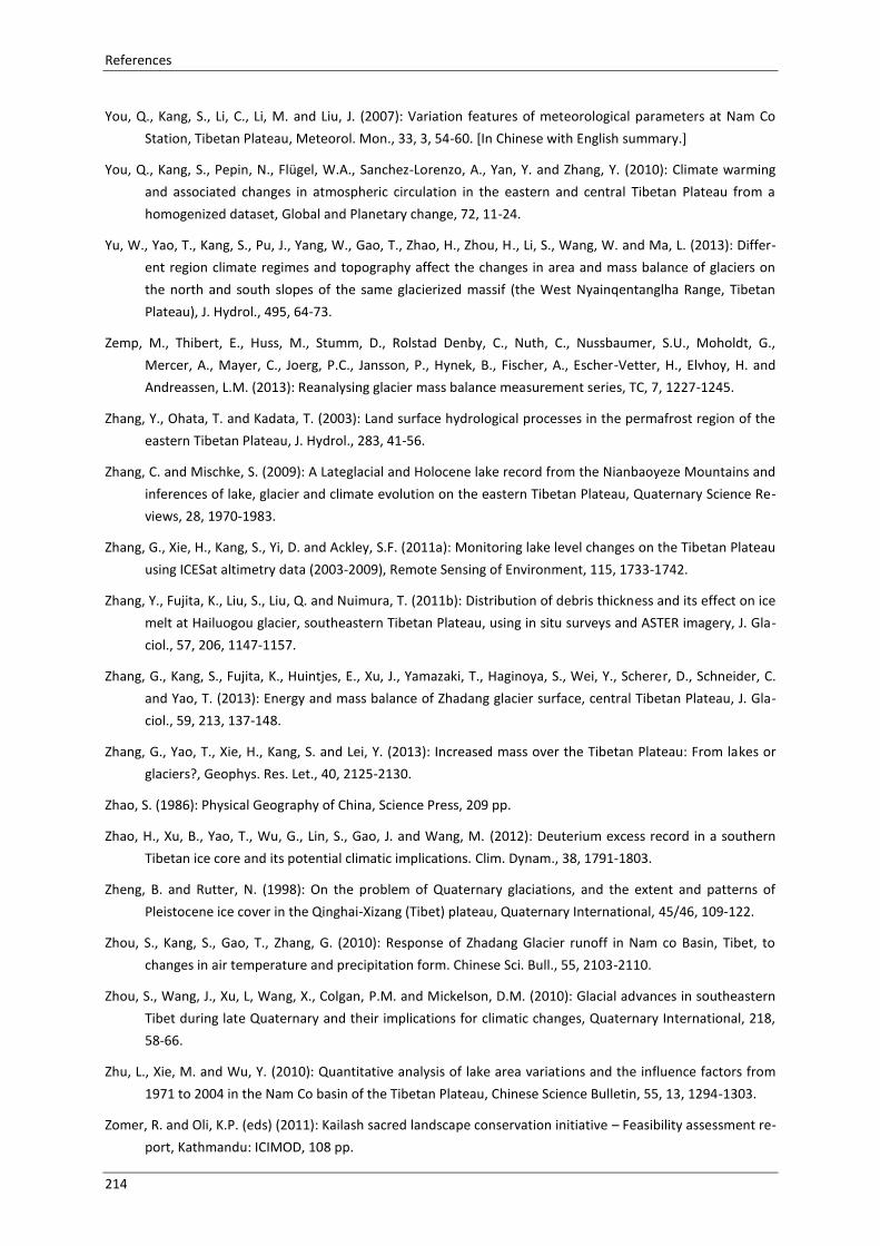
References
214
You, Q., Kang, S., Li, C., Li, M. and Liu, J. (2007): Variation features of meteorological parameters at Nam Co
Station, Tibetan Plateau, Meteorol. Mon., 33, 3, 54-60. [In Chinese with English summary.]
You, Q., Kang, S., Pepin, N., Flügel, W.A., Sanchez-Lorenzo, A., Yan, Y. and Zhang, Y. (2010): Climate warming
and associated changes in atmospheric circulation in the eastern and central Tibetan Plateau from a
homogenized dataset, Global and Planetary change, 72, 11-24.
Yu, W., Yao, T., Kang, S., Pu, J., Yang, W., Gao, T., Zhao, H., Zhou, H., Li, S., Wang, W. and Ma, L. (2013): Differ-
ent region climate regimes and topography affect the changes in area and mass balance of glaciers on
the north and south slopes of the same glacierized massif (the West Nyainqentanglha Range, Tibetan
Plateau), J. Hydrol., 495, 64-73.
Zemp, M., Thibert, E., Huss, M., Stumm, D., Rolstad Denby, C., Nuth, C., Nussbaumer, S.U., Moholdt, G.,
Mercer, A., Mayer, C., Joerg, P.C., Jansson, P., Hynek, B., Fischer, A., Escher-Vetter, H., Elvhoy, H. and
Andreassen, L.M. (2013): Reanalysing glacier mass balance measurement series, TC, 7, 1227-1245.
Zhang, Y., Ohata, T. and Kadata, T. (2003): Land surface hydrological processes in the permafrost region of the
eastern Tibetan Plateau, J. Hydrol., 283, 41-56.
Zhang, C. and Mischke, S. (2009): A Lateglacial and Holocene lake record from the Nianbaoyeze Mountains and
inferences of lake, glacier and climate evolution on the eastern Tibetan Plateau, Quaternary Science Re-
views, 28, 1970-1983.
Zhang, G., Xie, H., Kang, S., Yi, D. and Ackley, S.F. (2011a): Monitoring lake level changes on the Tibetan Plateau
using ICESat altimetry data (2003-2009), Remote Sensing of Environment, 115, 1733-1742.
Zhang, Y., Fujita, K., Liu, S., Liu, Q. and Nuimura, T. (2011b): Distribution of debris thickness and its effect on ice
melt at Hailuogou glacier, southeastern Tibetan Plateau, using in situ surveys and ASTER imagery, J. Gla-
ciol., 57, 206, 1147-1157.
Zhang, G., Kang, S., Fujita, K., Huintjes, E., Xu, J., Yamazaki, T., Haginoya, S., Wei, Y., Scherer, D., Schneider, C.
and Yao, T. (2013): Energy and mass balance of Zhadang glacier surface, central Tibetan Plateau, J. Gla-
ciol., 59, 213, 137-148.
Zhang, G., Yao, T., Xie, H., Kang, S. and Lei, Y. (2013): Increased mass over the Tibetan Plateau: From lakes or
glaciers?, Geophys. Res. Let., 40, 2125-2130.
Zhao, S. (1986): Physical Geography of China, Science Press, 209 pp.
Zhao, H., Xu, B., Yao, T., Wu, G., Lin, S., Gao, J. and Wang, M. (2012): Deuterium excess record in a southern
Tibetan ice core and its potential climatic implications. Clim. Dynam., 38, 1791-1803.
Zheng, B. and Rutter, N. (1998): On the problem of Quaternary glaciations, and the extent and patterns of
Pleistocene ice cover in the Qinghai-Xizang (Tibet) plateau, Quaternary International, 45/46, 109-122.
Zhou, S., Kang, S., Gao, T., Zhang, G. (2010): Response of Zhadang Glacier runoff in Nam co Basin, Tibet, to
changes in air temperature and precipitation form. Chinese Sci. Bull., 55, 2103-2110.
Zhou, S., Wang, J., Xu, L, Wang, X., Colgan, P.M. and Mickelson, D.M. (2010): Glacial advances in southeastern
Tibet during late Quaternary and their implications for climatic changes, Quaternary International, 218,
58-66.
Zhu, L., Xie, M. and Wu, Y. (2010): Quantitative analysis of lake area variations and the influence factors from
1971 to 2004 in the Nam Co basin of the Tibetan Plateau, Chinese Science Bulletin, 55, 13, 1294-1303.
Zomer, R. and Oli, K.P. (eds) (2011): Kailash sacred landscape conservation initiative – Feasibility assessment re-
port, Kathmandu: ICIMOD, 108 pp.

Appendix
215
Appendix
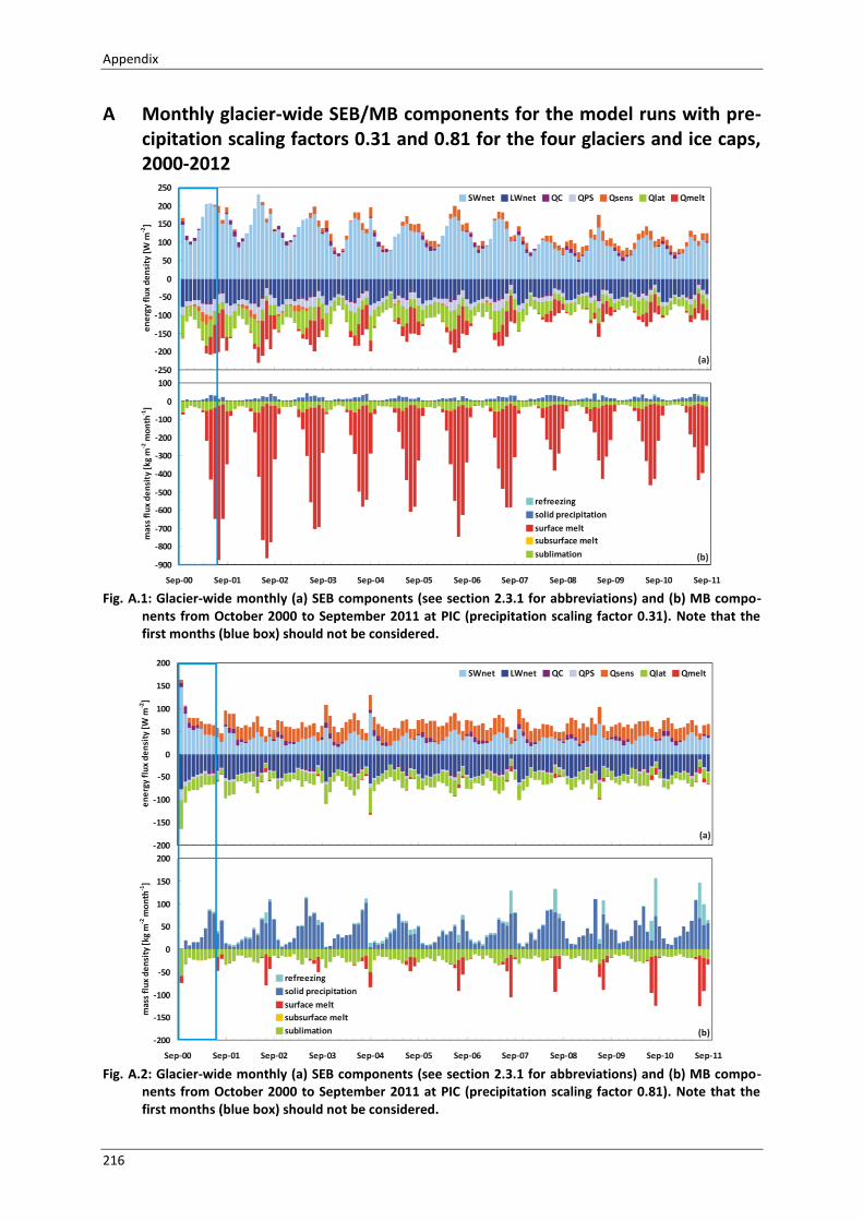
Appendix
216
A Monthly glacier-wide SEB/MB components for the model runs with pre-cipitation scaling factors 0.31 and 0.81 for the four glaciers and ice caps, 2000-2012
Fig. A.1: Glacier-wide monthly (a) SEB components (see section 2.3.1 for abbreviations) and (b) MB compo-
nents from October 2000 to September 2011 at PIC (precipitation scaling factor 0.31). Note that the first months (blue box) should not be considered.
Fig. A.2: Glacier-wide monthly (a) SEB components (see section 2.3.1 for abbreviations) and (b) MB compo-
nents from October 2000 to September 2011 at PIC (precipitation scaling factor 0.81). Note that the first months (blue box) should not be considered.
Appendix
217
Fig. A.3: Glacier-wide monthly (a) SEB components (see section 2.3.1 for abbreviations) and (b) MB compo-
nents from October 2000 to September 2011 at Naimona’nyi glacier (precipitation scaling factor 0.31). Note that the first months (blue box) should not be considered.
Fig. A.4: Glacier-wide monthly (a) SEB components (see section 2.3.1 for abbreviations) and (b) MB compo-
nents from October 2000 to September 2011 at Naimona’nyi glacier (precipitation scaling factor 0.81). Note that the first months (blue box) should not be considered.
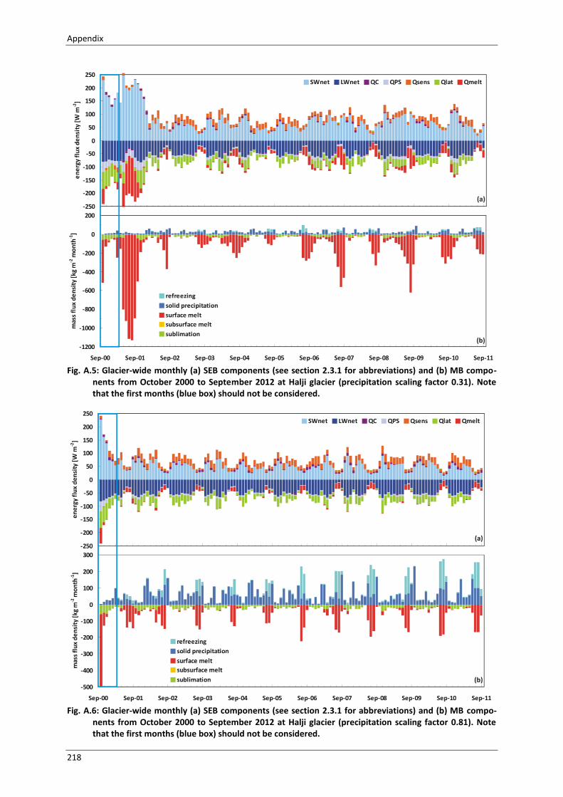
Appendix
218
Fig. A.5: Glacier-wide monthly (a) SEB components (see section 2.3.1 for abbreviations) and (b) MB compo-
nents from October 2000 to September 2012 at Halji glacier (precipitation scaling factor 0.31). Note that the first months (blue box) should not be considered.
Fig. A.6: Glacier-wide monthly (a) SEB components (see section 2.3.1 for abbreviations) and (b) MB compo-
nents from October 2000 to September 2012 at Halji glacier (precipitation scaling factor 0.81). Note that the first months (blue box) should not be considered.
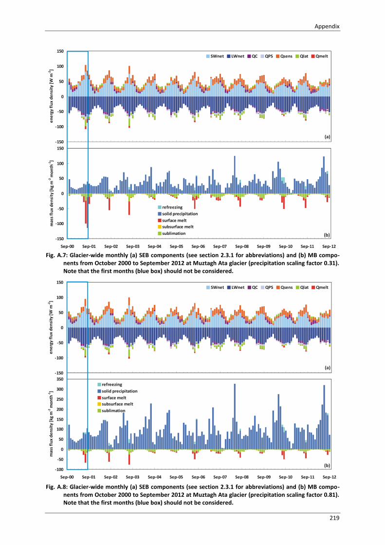
Appendix
219
Fig. A.7: Glacier-wide monthly (a) SEB components (see section 2.3.1 for abbreviations) and (b) MB compo-
nents from October 2000 to September 2012 at Muztagh Ata glacier (precipitation scaling factor 0.31). Note that the first months (blue box) should not be considered.
Fig. A.8: Glacier-wide monthly (a) SEB components (see section 2.3.1 for abbreviations) and (b) MB compo-
nents from October 2000 to September 2012 at Muztagh Ata glacier (precipitation scaling factor 0.81). Note that the first months (blue box) should not be considered.
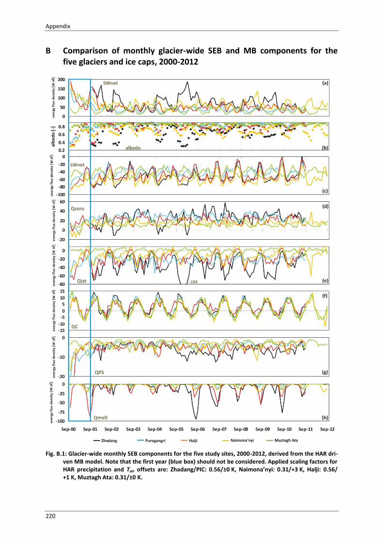
Appendix
220
B Comparison of monthly glacier-wide SEB and MB components for the five glaciers and ice caps, 2000-2012
Fig. B.1: Glacier-wide monthly SEB components for the five study sites, 2000-2012, derived from the HAR dri-
ven MB model. Note that the first year (blue box) should not be considered. Applied scaling factors for HAR precipitation and Tair offsets are: Zhadang/PIC: 0.56/±0 K, Naimona’nyi: 0.31/+3 K, Halji: 0.56/ +1 K, Muztagh Ata: 0.31/±0 K.
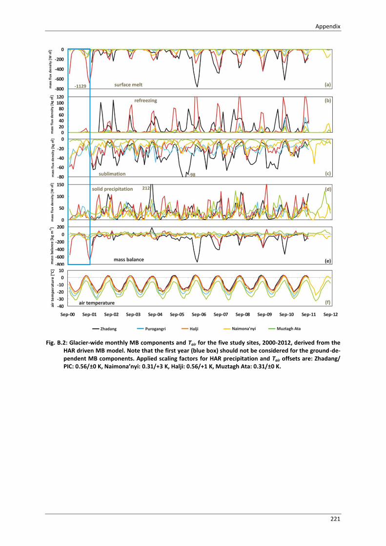
Appendix
221
Fig. B.2: Glacier-wide monthly MB components and Tair for the five study sites, 2000-2012, derived from the
HAR driven MB model. Note that the first year (blue box) should not be considered for the ground-de-pendent MB components. Applied scaling factors for HAR precipitation and Tair offsets are: Zhadang/ PIC: 0.56/±0 K, Naimona’nyi: 0.31/+3 K, Halji: 0.56/+1 K, Muztagh Ata: 0.31/±0 K.
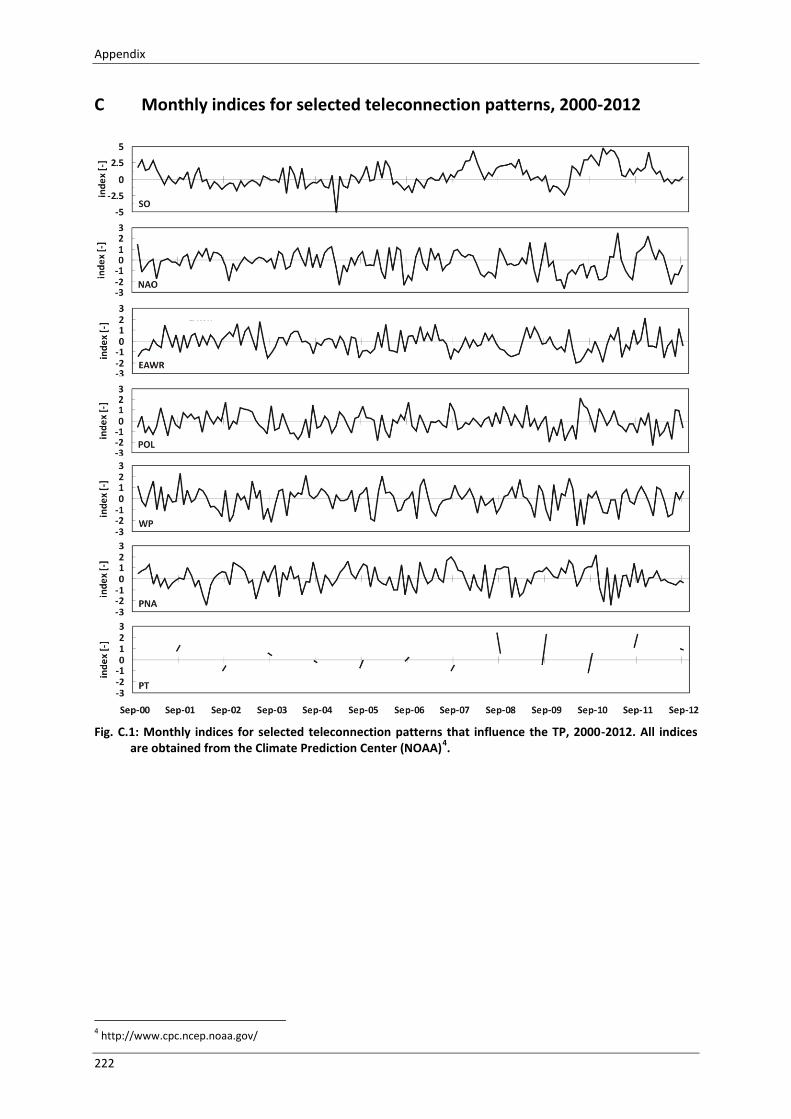
Appendix
222
C Monthly indices for selected teleconnection patterns, 2000-2012
Fig. C.1: Monthly indices for selected teleconnection patterns that influence the TP, 2000-2012. All indices
are obtained from the Climate Prediction Center (NOAA)4.
4 http://www.cpc.ncep.noaa.gov/
Copyright © 2022 FDOKUMEN