Emd of Gaussian White Noise: Effects of Signal Length and Sifting Number on the Statistical...

October 30, 2009 9:9 WSPC/244-AADA 00021

Advances in Adaptive Data AnalysisVol. 1, No. 4 (2009) 517–527c! World Scientific Publishing Company

EMD OF GAUSSIAN WHITE NOISE: EFFECTS OF SIGNALLENGTH AND SIFTING NUMBER ON THE STATISTICAL

PROPERTIES OF INTRINSIC MODE FUNCTIONS

GASTON SCHLOTTHAUER!,§, MARIA EUGENIA TORRES!,¶,HUGO L. RUFINER†," and PATRICK FLANDRIN‡,!!

!Lab. Signals and Nonlinear Dynamics, Applied Research groupon Signal Processing and Pattern Recognition (ARSiPRe)

Facultad de Ingenierıa, Universidad Nacional de Entre RıosRuta 11 Km 10 Oro Verde, Entre Rıos 3100, Argentina†Lab.de Senales e INteligencia Computacional (SINC)

Fac. de Ingenierıa y Cs Hıdricas, Univ. Nac. del LitoralCC 217, Ciudad Universitaria,

Paraje El Pozo, S3000 Santa Fe, Argentina‡Laboratoire de Physique (UMR 5672 CNRS)

Ecole normale superieure de Lyon46 allee d’Italie, 69364 Lyon Cedex 07, France

§[email protected]¶[email protected]

"[email protected][email protected]

This work presents a discussion on the probability density function of Intrinsic ModeFunctions (IMFs) provided by the Empirical Mode Decomposition of Gaussian whitenoise, based on experimental simulations. The influence on the probability density func-tions of the data length and of the maximum allowed number of iterations is analyzedby means of kernel smoothing density estimations. The obtained results are confirmedby statistical normality tests indicating that the IMFs have non-Gaussian distributions.Our study also indicates that large data length and high number of iterations producemultimodal distributions in all modes.

Keywords: Empirical Mode Decomposition (EMD); Intrinsic Mode Function (IMF);Gaussian white noise; sifting.

1. Introduction

The Empirical Mode Decomposition (EMD), first proposed by Huang et al., aroseas a new completely data-driven method for signal analysis with many potentialapplications.1 However, some aspects concerning its theoretical properties are stillobscure and the results of its application on a given signal cannot be predicted. Stud-ies have been carried out by Flandrin et al. which allow us to assert that, when

517


518 G. Schlotthauer et al.

applied to Gaussian white noise, EMD acts in a similar way as a wavelet filterbank.2,3 A research on the EMD e!ects on uniformly distributed white noise wasperformed by Wu and Huang, and normal distributions of the Intrinsic Mode Func-tions (IMFs) were reported.4 On the basis of these results, Wu and Huang suggesteda chi-square distribution for the energy density distribution of the IMFs. In the men-tioned article, the authors used one million length white noise time series and thesifting process was limited to 10 iterations. A similar study was carried out by thesame authors on Gaussian white noise, with 7–10 sifting iterations deriving similarconclusions.5 However, in none of this works a normality test was applied and theconclusions were based on a Gaussian-like histogram estimation, using 50,000 datapoints in Refs. 4 and 5. An extension of these experiments to fractional Gaussiannoise was conducted by Flandrin et al., and a similar conclusion was reached aboutthe normality of the IMFs.

In this work, we study the statistical properties of EMD on Gaussian distributedwhite noise. We show and discuss the dependence of the IMFs distribution on thesignal lengths and the number of allowed iterations that involves the sifting process.Additionally, normality tests are carried out on the IMFs in order to test the nullhypothesis of normality.

2. Experimental Design

In order to study the Probability Density Functions (PDFs) of the IMFs obtainedby EMD of Gaussian white noise, a random signal with Gaussian distribution x(n)was generated with zero mean and unitary variance, with 220 data points. Then,the signal x(n) was split into W non-overlapping windows xw(n) of lengths L =210, 212, . . . , 220. For each window xw(n), the EMD algorithm was applied using agiven maximum number Ni of iterations in the sifting process (Ni = 5, 10, 15, 25, 50and unlimited), yielding the IMFw

k (n) for modes k = 1, . . . , K. In this way, we obtaina number of realizations to be used for the PDFs estimation purpose. Therefore,the here considered IMFs are built by concatenation:

IMFk(n) = [IMF1k(n) | IMF2

k(n) | · · · | IMFWk (n)], (1)

for k = 1, 2, . . . , K.We used the Matlab implementation of EMD available at Ref. 8. The sifting

is ended when the number of zero-crossings and the number of extrema di!er atmost by one, and when the local mean between the upper and lower envelopes areclose to zero. The criteria for deciding if such local mean is close to zero enough,are adopted as in Ref. 7, using the typical values suggested in this paper. If thesecriteria are not achieved, but an a priori established maximum number of siftingiterations is reached, the process is terminated.

In this way, using (1) for each IMFk, the PDF was estimated (at the di!erentwindow lengths L and number of iterations Ni) using N = 220 data points. Theprobability density estimation was performed by Gaussian kernel method,9 using


EMD of Gaussian White Noise 519

11

12

1K

21

22

2K

W1

W2

WK

1 W2

PDF(IMFK(n))

PDF(IMF1(n))

PDF(IMF2(n))

Fig. 1. The signal x(n) was split into nonoverlapping windows, (x1(n), x2(n), . . . , xW (n)). EMDwas applied and the K modes IMFw

k (n), k = 1, . . . , K, were obtained for each xw(n), w = 1, . . . , W .Next, the PDF was estimated for each IMFk(n), k = 1, . . . , K.

Ns = 500 equally spaced points ys covering the range of data in the correspondingIMFk:

PDF(ys) =1N

N!

n=1

!(ys ! IMFk(n);h), (2)

where ! is the kernel function, whose variance is controlled by the parameter h. Inour case, !(z; h) denotes the normal density function in z with mean 0 and standarddeviation h. For each mode k, the bandwidth h of the Gaussian kernel was chosenas the optimal for normal densities9:

h ="

43N

#1/5

", (3)

where " is its standard deviation.The above described procedure is depicted in Fig. 1.

3. Results and Discussion

First we analyze and compare the PDFs corresponding to each of the IMFwk for

modes k = 1, 2, . . . , 6 for windows xw(n) of fixed length and unlimited sifting iter-ations (Sec. 3.1).



In order to discuss the incidence of the signal length and the maximum numberof sifting iterations, we perform the analysis of the above described data PDFsusing di!erent approaches: (i) density estimation for a fixed value of window length(L) and di!erent number of maximum iterations (Ni), (ii) density estimation for afixed maximum number of sifting iterations (Ni) varying the data length (L). SeeSecs. 3.2 and 3.3, respectively.

The first case is equivalent to study the influence of data length on the statisticalproperties of the IMFs.

We also study the number of sifting iterations demanded by the method toaccomplished the stopping criteria (Ni is unlimited) in relation to the data lengthL (Sec. 3.4).

In Sec. 3.5 a normality test is applied to the IMFs.

3.1. IMF density estimation

In Fig. 2, we compare the kernel smoothing density estimations of IMFwk , with w =

1, 2, . . . , 1024 and k = 1, 2, . . . , 6 for a Gaussian noise realization xw(n) of lengthL = 210 and Ni set to unlimited, plotted in gray lines. It must be noticed that inthis way we are estimating the PDFs corresponding to 210 = 1024 realizations. Thecorresponding averages are displayed in black lines. The PDFs have been estimatingusing 50 Gaussian kernels.

It can be appreciated that the individual PDFs do not seems to be normal.However, the average of these estimated distributions tends to a normal curve. Anexception is observed in the first mode, where a bimodal behavior can be appreci-ated. An explanation of this situation can be read in Ref. 3.

3.2. Fixed data length

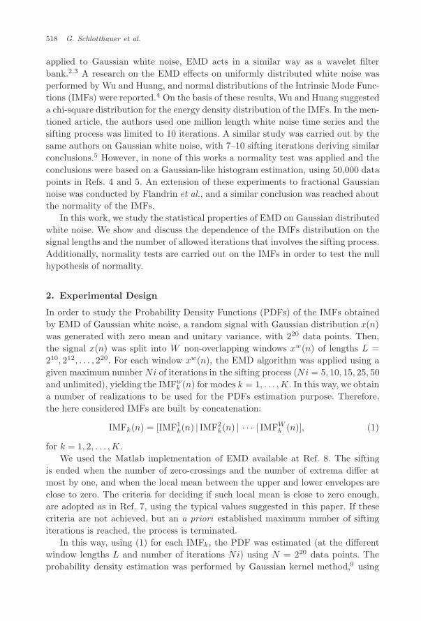
By means of EMD we obtain the IMFk for k = 1, 2, . . . , 10 with L = 210, usingdi!erent Ni values, (Ni = 5, 10, 15, 20, 25, 50, . . . ,"). The corresponding PDFs areestimated with a Gaussian kernel smoothing method using 500 equally spaced pointsthat cover the range of each IMFk. The obtained results for modes k = 1, . . . , 6 areshown in Fig. 3. We can observe that for Ni larger than 5, the distributions lookvery similar within each mode. In every case, except the first mode, we can appre-ciate slightly spiky shape around the maximum that corresponds to the statisticalmode.

A similar experiment is carried out with L = 220. In Fig. 4 are displayed thePDFs estimations of IMFs 1–6. In this case the PDFs exhibit a greater dependenceon the Ni. It can be observed that, in all the cases, increasing Ni the PDF evolvesfrom a “spiky” shape (alike those obtained with L = 210) towards a flattened one.In occasions bimodal (k = 5 and 6) and tri-modal (k = 2, 3 and 4) PDFs areobserved when Ni is unlimited.

These observations confirm to the need of performing a normality test.



!2 !1 0 1 2

x 10-3

0

200

400

600

IMF 1!2 !1.5 !1 !0.5 0 0.5 1 1.5 2

x 10!3

0

200

400

600

800

1000

1200

IMF 2

(a) (b)

!1 !0.5 0 0.5 1

x 10-3

0

500

1000

1500

2000

IMF 3

!1 !0.5 0 0.5 1

x 10!3

0

1000

2000

3000

IMF 4

(c) (d)

!6 !4 !2 0 2 4 6

x 10-4

0

1000

2000

3000

4000

5000

IMF 5!5 0 5

x 10!4

0

5000

10000

15000

IMF 6

(e) (f)

Fig. 2. Kernel smoothing density estimation of IMFs 1–6 for L = 210 and unlimited sifting iter-ations. The PDF estimations for each xw(n), w = 1, 2, . . . , 1024 are plotted in gray. The averagedPDFs are displayed in black. The averaged PDFs for IMFs 2–6 are approximately Gaussian.

3.3. Fixed maximum number of iterations

Setting Ni = 5, we obtain the PDFs shown in Fig. 5, depending on the data lengthL = 210, 212, . . . , 220. Once more, the PDFs are very close within each mode, andseem not to depend on L. Their shapes look to be closer to a Laplacian distributionthan to a Gaussian.

On the other hand, allowing an unlimited number of sifting iterations Ni, weobserve in Fig. 6 that increasing the signal length L, the densities maxima go lowerand the shape of the PDFs changes from unimodal to multimodal.

3.4. Maximum number of iterations

From a practical point of view, an interesting question about the previous experi-ments should be which is the number of iterations demanded by EMD to accomplish



!2 !1 0 1 2

x 10!3

0

200

400

600

IMF 1!1.5 !1 !0.5 0 0.5 1 1.5

x 10!3

0

500

1000

IMF 2

(a) (b)

!1 !0.5 0 0.5 1

x 10!3

0

500

1000

1500

IMF 3-1 !0.5 0 0.5 1

x 10!3

0

500

1000

1500

2000

IMF 4

(c) (d)

!6 !4 !2 0 2 4 6

x 10!4

0

1000

2000

3000

IMF 5!5 0 5

x 10!4

010002000300040005000

IMF 6

(e) (f)

Ni = 5; Ni = 10; Ni = 15; Ni = 20; Ni = 25; Ni = 50; Ni = ".

Fig. 3. Kernel smoothing density estimation of IMFs. The PDF estimations of IMFs 1–6 areshown in (a)–(f). The IMFs are constructed by concatenation of the obtained IMFs of xw(n) withlength L = 210. The maximum number of iterations varies: Ni = 5, 10, 15, 20, 25, 50 and unlimited.

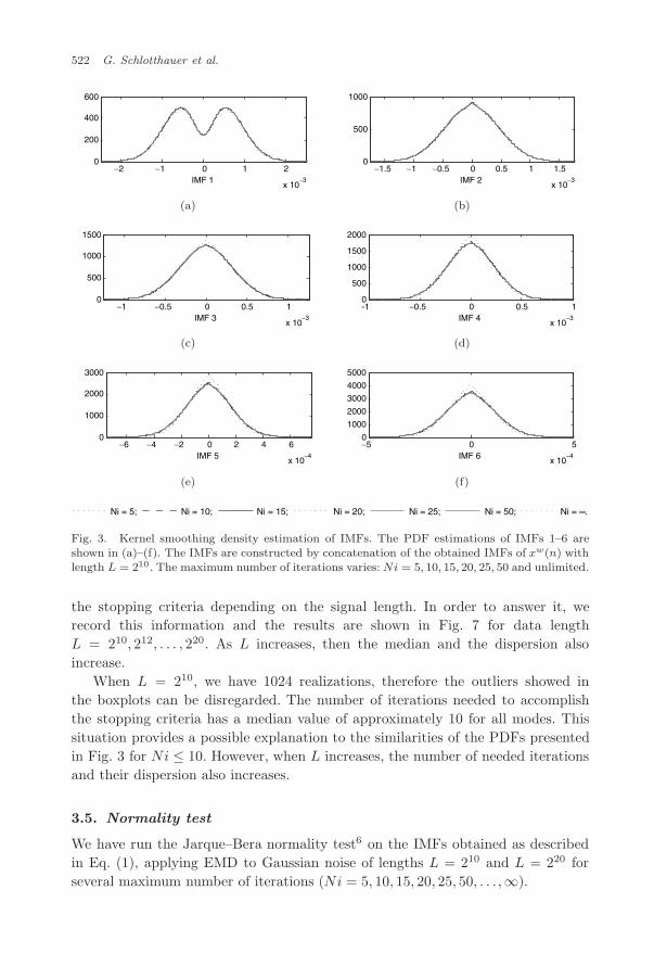
the stopping criteria depending on the signal length. In order to answer it, werecord this information and the results are shown in Fig. 7 for data lengthL = 210, 212, . . . , 220. As L increases, then the median and the dispersion alsoincrease.

When L = 210, we have 1024 realizations, therefore the outliers showed inthe boxplots can be disregarded. The number of iterations needed to accomplishthe stopping criteria has a median value of approximately 10 for all modes. Thissituation provides a possible explanation to the similarities of the PDFs presentedin Fig. 3 for Ni # 10. However, when L increases, the number of needed iterationsand their dispersion also increases.

3.5. Normality test

We have run the Jarque–Bera normality test6 on the IMFs obtained as describedin Eq. (1), applying EMD to Gaussian noise of lengths L = 210 and L = 220 forseveral maximum number of iterations (Ni = 5, 10, 15, 20, 25, 50, . . . ,").



!2 !1 0 1 2

x 10!3

0

200

400

600

800

IMF 1!1.5 !1 !0.5 0 0.5 1 1.5

x 10!3

0

500

1000

IMF 2

(a) (b)

!1 !0.5 0 0.5 1

x 10!3

0

500

1000

1500

IMF 3!1 !0.5 0 0.5 1

x 10!3

0

500

1000

1500

2000

IMF 4

(c) (d)

!6 !4 !2 0 2 4 6

x 10!4

0

1000

2000

3000

IMF 5!4 !2 0 2 4 6

x 10!4

0

1000

2000

3000

4000

5000

IMF 6

(e) (f)

Ni = 5; Ni = 10; Ni = 15; Ni = 20; Ni = 25; Ni = 50; Ni = ".

Fig. 4. Kernel smoothing density estimation of IMFs. The PDF estimations of IMFs 1–6 areshown in (a)–(f). The IMFs are obtained by EMD of x(n) with length L = 220. The maximumnumber of iterations varies: Ni = 5, 10, 15, 20, 25, 50, . . . ,".

In the case of L = 210 the null hypothesis of normality has been always rejectedwith # = 0.05 and p < 0.001. On the other hand, for L = 220 the null hypothesishas not been rejected only for IMF 6 when Ni = 10 (p = 0.496), IMFs 3, 4 and 5when Ni = 15 (p = 0.448, p = 0.500, and p = 0.378, respectively), and IMF 6 whenNi = 25 (p = 0.500). The null hypothesis has been rejected with a larger value ofp (p = 0.002) for IMF 4, corresponding to Ni = 10. Similar results were obtainedby applying Lilliefors test of normality.

Looking at Fig. 3, the curves corresponding to those cases when the null hypoth-esis was not rejected seemed to be Gaussians. The occurrence of these Gaussian-like



!2 !1 0 1 2

x 10!3

0100200300400500

IMF 1!2 !1.5 !1 !0.5 0 0.5 1 1.5 2

x 10!3

0

500

1000

IMF 2

(a) (b)

!1 !0.5 0 0.5 1

x 10!3

0

500

1000

1500

IMF 3!1 !0.5 0 0.5 1

x 10!3

0

500

1000

1500

2000

IMF 4

(c) (d)

!6 !4 !2 0 2 4 6

x 10!4

0

1000

2000

3000

IMF 5!5 0 5

x 10!4

010002000300040005000

IMF 6

(e) (f)

L = 210 L = 212 L = 214 L = 216 L = 218 L = 220

Fig. 5. Kernel smoothing density estimation of IMFs. The PDF estimations of IMFs 1–6 areshown in (a)–(f). The IMFs are constructed by concatenation of the obtained IMFs of xw(n) withlengths L = 210, 212, . . . , 220. The maximum number of iterations was fixed to : Ni = 5.

distributions, become evident while increasing Ni the curves change from “spiky”to multimodal alike shapes.

3.6. Further remarks

As discussed in the previous sections, a finding of this paper is that the shape of thePDFs of the IMFs have a tendency to become bimodal, or even multimodal, as thesifting number or the data length becomes large. Also, the first IMF always shows abimodal structure. In order to explore this situation further and try to understandthe mechanism behind this tendency, one could think in running similar experimentsusing, instead of the EMD, the ensemble empirical mode decomposition (EEMD)proposed by Wu and Huang, which overcomes some of the EMD modes mixing



!2 !1 0 1 2

x 10!3

0

200

400

600

800

IMF 1!2 !1.5 !1 !0.5 0 0.5 1 1.5 2

x 10!3

0

500

1000

IMF 2

(a) (b)

!1 !0.5 0 0.5 1

x 10!3

0

500

1000

1500

IMF 3!1 !0.5 0 0.5 1

x 10!3

0

500

1000

1500

2000

IMF 4

(c) (d)

!6 !4 !2 0 2 4 6

x 10!4

0500

1000150020002500

IMF 5!4 !2 0 2 4 6

x 10!4

0

1000

2000

3000

4000

IMF 6

(e) (f)

L = 210 L = 212 L = 214 L = 216 L = 218 L = 220

Fig. 6. Kernel smoothing density estimation of IMFs. The PDF estimations of IMFs 1–6 areshown in (a)–(f). The IMFs are constructed by concatenation of the obtained IMFs of xw(n) withlengths L = 210, 212, . . . , 220. The maximum number of iterations was unlimited.

problems.10 It defines the true IMF components as the mean of certain ensembleof trials of size Ne, each obtained by adding white noise of finite variance to theoriginal signal.

In preliminary experiments using EEMD with only five sifting iterations andNe = 500, the Gaussian null hypothesis could not be rejected in any mode exceptthe first one, where a bimodal PDF was still present. In fact, this could be anexpected result, because of the central limit theorem, given that at each mode thefinal IMF component is obtained by the addition of the mode corresponding to eachnew noisy realization of the original signal.

It must be noticed that these preliminary EEMD results could only be com-pared with those shown in Fig. 5. Usually, in the EEMD approach the number ofrealizations is high (200 # Ne # 1000) while the sifting number is fixed as low as



1 2 3 4 5 6 7 8 9 10

0

20

40

60

80

100

120

Itera

tions

IMF

L=210

1 2 3 4 5 6 7 8 9 10

0

50

100

150

Itera

tions

IMF

L=212

1 2 3 4 5 6 7 8 9 100

50

100

150

Itera

tions

IMF

L=214

1 2 3 4 5 6 7 8 9 100

50

100

150

200

250

300

350

Itera

tions

IMF

L=216

1 2 3 4 5 6 7 8 9 100

200

400

600

800

Itera

tions

IMF

L=218

1 2 3 4 5 6 7 8 9 100

500

1000

1500

2000L=220

Itera

tions

IMF

Fig. 7. Boxplots of the number of sifting iterations for data of lengths L = 210, 212, . . . , 210

and number of sifting iterations for L = 220 datapoints. The maximum number of iterations wasunlimited.

possible. Therefore, taking into account its extensive computational cost, it wouldnot be a realistic situation to perform experiments in the EEMD framework withunlimited number of iterations. Therefore, the new experiments with EEMD shouldbe carefully designed. These ideas will be explored and developed in future works.

4. Conclusions

A study of the statistical properties of the IMFs obtained by EMD of Gaussiannoise, and its dependence on data lengths and number of allowed sifting iterationswas presented. It indicates that the PDFs is strongly relied on the data length, andon the maximum allowed number of iterations. Depending on these parameters,the PDF can have a Laplacian alike or a multimodal shape. Only in a few settings,a Gaussian distribution is obtained. These results were confirmed by two di!erentnormality tests. Similar conclusions were derived from uniformly distributed whitenoise data.



Acknowledgments

This work was supported by Universidad Nacional de Entre Rıos under ProjectsPID 6107-2 and PID 6111-2, Universidad Nacional del Litoral, National Agencyof Scientific and Technological Promotion (ANPCyT), and National Council ofScientific and Technical Research (CONICET) under Projects PAE 37122 and PAE-PICT 2007-00052.

References

1. N. E. Huang, Z. Shen, S. R. Long, M. L. Wu, H. H. Shih, Q. Zheng, N. C. Yen, C.C. Tung and H. H. Liu, The empirical mode decomposition and Hilbert spectrumfor nonlinear and non-stationary time series analysis, Proc. Roy. Soc. London A 454(1998) 903–995.

2. P. Flandrin, G. Rilling and P. Goncalves, Empirical mode decomposition as a filterbank, IEEE Signal Process. Lett. 11 (2004) 112–114.

3. P. Flandrin and P. Goncalves, Empirical mode decomposition as data-driven wavelet-like expansions, Int. J. Wavelets Multiresolution Inform. Process. 2 (2004) 477–496.

4. Z. Wu and N. E. Huang, A study of the characteristics of white noise using the empir-ical mode decomposition method, Proc. Roy. Soc. London A 460 (2004) 1597–1611.

5. Z. Wu and N. E. Huang, Statistical significance test of intrinsic mode functions,in Hilbert–Huang Transform and its Applications, in Interdisciplinary MathematicalScience, Vol. 5 (World Scientific, Singapore, 2005), pp. 107–127.

6. C. M. Jarque and A. L. Bera, A test for normality of observations and regressionresiduals, Int. Stat. Rev. 55 (1987) 163–172.

7. G. Rilling, P. Flandrin and P. Goncalves, On Empirical Mode Decomposition and itsalgorithms, in IEEE-EURASIP Workshop on Nonlinear Signal and Image Processing,NSIP-03, Grado (I), June 2003.

8. http://perso.ens-lyon.fr/patrick.flandrin/emd.html9. A. W. Bowman and A. Azzalini, Applied smoothing techniques for data analysis, in

The Kernel Approach with S-plus Illustrations (Oxford University Press, New York,1997).

10. Z. Wu and N. E. Huang, Ensemble empirical mode decomposition: A noise-assisteddata analysis method, Adv. Adapt. Data Anal. 1(1) (2009) 1–41.

Emd of Gaussian White Noise: Effects of Signal Length and Sifting Number on the Statistical...

Documents

Transcript of Emd of Gaussian White Noise: Effects of Signal Length and Sifting Number on the Statistical...