The Intrinsic Properties of Reconstituted Soils - ScholarWorks ...
240
University of Arkansas, Fayetteville University of Arkansas, Fayetteville ScholarWorks@UARK ScholarWorks@UARK Graduate Theses and Dissertations 5-2018 The Intrinsic Properties of Reconstituted Soils The Intrinsic Properties of Reconstituted Soils Nabeel Shaker Mahmood University of Arkansas, Fayetteville Follow this and additional works at: https://scholarworks.uark.edu/etd Part of the Geotechnical Engineering Commons Citation Citation Mahmood, N. S. (2018). The Intrinsic Properties of Reconstituted Soils. Graduate Theses and Dissertations Retrieved from https://scholarworks.uark.edu/etd/2670 This Dissertation is brought to you for free and open access by ScholarWorks@UARK. It has been accepted for inclusion in Graduate Theses and Dissertations by an authorized administrator of ScholarWorks@UARK. For more information, please contact [email protected].
-
Upload
khangminh22 -
Category
Documents
-
view
0 -
download
0
Transcript of The Intrinsic Properties of Reconstituted Soils - ScholarWorks ...

University of Arkansas, Fayetteville University of Arkansas, Fayetteville
ScholarWorks@UARK ScholarWorks@UARK
Graduate Theses and Dissertations
5-2018
The Intrinsic Properties of Reconstituted Soils The Intrinsic Properties of Reconstituted Soils
Nabeel Shaker Mahmood University of Arkansas, Fayetteville
Follow this and additional works at: https://scholarworks.uark.edu/etd
Part of the Geotechnical Engineering Commons
Citation Citation Mahmood, N. S. (2018). The Intrinsic Properties of Reconstituted Soils. Graduate Theses and Dissertations Retrieved from https://scholarworks.uark.edu/etd/2670
This Dissertation is brought to you for free and open access by ScholarWorks@UARK. It has been accepted for inclusion in Graduate Theses and Dissertations by an authorized administrator of ScholarWorks@UARK. For more information, please contact [email protected].

The Intrinsic Properties of Reconstituted Soils
A dissertation submitted in partial fulfillment of the
requirements for the degree of
Doctor of Philosophy in Engineering
by
Nabeel S. Mahmood
University of Anbar Bachelor of Science in Civil Engineering, 2001
University of Baghdad Master of Science in Civil Engineering, 2004
May 2018
University of Arkansas
This dissertation is approved for recommendation to the Graduate Council.
____________________________________
Richard A. Coffman, Ph.D., P.E., P.L.S.
Dissertation Director
____________________________________ ____________________________________
Michelle Bernhardt-Barry, Ph.D., P.E. Paul Millett, Ph.D.
Committee Member Committee Member
____________________________________
Clinton Wood, Ph.D., P.E.
Committee Member

ABSTRACT
Reconstituted specimens are often utilized to characterize engineering properties of
cohesive soils. A series of undrained triaxial tests were conducted on reconstituted soil
specimens to evaluate 1) the influence of stress path, 2) the intrinsic shear strength behavior, and
3) the small-strain characteristics. The stress path tests were conducted on kaolinite specimens
reconstituted from slurries with water content values of one and one-half times the liquid limit of
the soil (1.5LL). To evaluate the intrinsic undrained shear strength and the intrinsic small-strain
properties, the triaxial tests were performed on kaolinite and illite specimens that were
reconstituted at two levels of slurry water content of 1.5LL and three times the corresponding
liquid limit of the soil. Bender elements were employed with the triaxial device to measure shear
wave velocity during the triaxial tests that were performed to evaluate the small-strain
characteristics.
The stress-strain behavior of the normally consolidated kaolinite specimens was similar
to the typical behavior of the overconsolidated specimens. Identical stress-strain behavior was
observed from the stress paths tests at the same orientation of the principal stresses. A new
interpretation method was proposed to normalize the undrained shear strength values of the
overconsolidated specimens based on the concept of void index. By utilizing this method, better
correlation was obtained between the undrained shear strength values and the intrinsic shear
strength line. The values of the shear wave velocity and shear modulus were also normalized to
the void index to evaluate the intrinsic small-strain characteristics. The values of both the shear
wave velocity and the shear modulus did not normalize with respect to the void index values.
As discussed herein, the triaxial compression test and the reduced triaxial extension test
are adequate to represent the different loading and unloading conditions in the field. Unlike
previous recommendations of preparing soil slurries at water contents of 1.25 times the liquid
limit, soil slurries should be prepared at water content values of at least 3LL. By preparing soil
slurries with a water content of 3LL, undrained shear strength and small-strain characteristics
that are in better agreement with those for natural soils will be obtained.

ACKNOWLEDGEMENTS
I would like to express my deep appreciation and sincere gratitude to my academic
advisor and committee chair, Dr. Richard Coffman for his continuous guidance, assistance, and
motivation throughout my years at the University of Arkansas. Similarly, I would like to thank
my committee members, Dr. Michelle Bernhardt-Barry, Dr. Paul Millett, and Dr. Clinton Wood
for generously offering their time, support, guidance and advice along this project.
I want to also thank the Higher Committee for Education Development in Iraq (HCED)
who granted me the financial support and to the University of Anbar who granted me a six-year
study leave.
I would like to acknowledge my colleagues, including but not limited to: Yi Zhao, Elvis
Ishimwe, Sean Salazar, and Cyrus Garner for their valuable assistance and friendship throughout
the years.
Finally, I am very grateful to my mother, who passed away during my study. She was
always there with unconditional love and encouragement. I am thankful to my father, parents-in-
law, brothers and sisters for their encouragement and inspiration. Special thanks to my wife
Noor, who provided me with love and strength to face the difficulties. Many thanks to my
children, Zaid, Yousif, and Adam, who provided me hope to finish my degree.

TABLE OF CONTENTS
Chapter Overview .............................................................................................................. 1
Project Description and Objectives .................................................................................... 1 Benefits to Geotechnical Engineering ............................................................................... 4 Dissertation Organization .................................................................................................. 5 References .......................................................................................................................... 6
Chapter Overview .............................................................................................................. 7 Stress Path in Triaxial Testing ........................................................................................... 7
Reconstituted Soils........................................................................................................... 21
Small-Strain Moduli of Reconstituted Soils .................................................................... 31
References ........................................................................................................................ 39
Chapter Overview ............................................................................................................ 47
Soil Properties .................................................................................................................. 47 Specimens Preparation ..................................................................................................... 48 Triaxial Equipment .......................................................................................................... 50 Triaxial Testing Procedures ............................................................................................. 53 Bender Element Tests ...................................................................................................... 54
References ........................................................................................................................ 56
Chapter Overview ............................................................................................................ 58 The Effects of Stress Path on the Characterization of Reconstituted Low Plasticity
Kaolinite .................................................................................................................................. 59 Abstract ............................................................................................................................ 59

Introduction ...................................................................................................................... 60 Testing Program ............................................................................................................... 65
Test Results and Discussion............................................................................................. 71
Implementations for Practice ........................................................................................... 84 Conclusions ...................................................................................................................... 84 References ........................................................................................................................ 86
Chapter Overview ............................................................................................................ 90
Intrinsic Shear Strength Behavior of Reconstituted Kaolinite and Illite Soils ................ 91 Abstract ............................................................................................................................ 91
Background ...................................................................................................................... 92 Materials and Methods ..................................................................................................... 94
Results and Discussion .................................................................................................... 98
Conclusions .................................................................................................................... 115 References ...................................................................................................................... 116
Chapter Overview .......................................................................................................... 119 Additional Results not Included in the Aforementioned Manuscript ............................ 120 Small-strain Characteristics of Reconstituted Soils: The Effect of Slurry Water Content
122
Abstract .......................................................................................................................... 122
Introduction .................................................................................................................... 123 Test Specimens .............................................................................................................. 126 Testing Apparatus and Methods .................................................................................... 127 Test Results and Discussion........................................................................................... 130
Conclusions .................................................................................................................... 138
References .................................................................................................................... 139
Chapter Overview .......................................................................................................... 143 Selected Contributions from this Research Project ....................................................... 143
Conclusions of Intrinsic Properties of Reconstituted Soils............................................ 144
Recommendations for Future Work............................................................................... 148
References ...................................................................................................................... 149
A.1. Chapter Overview ......................................................................................................... 161 A.2. Specimen Properties ...................................................................................................... 161 A.3. Triaxial Tests Data ........................................................................................................ 165
A.4. Shear Wave Velocity and Shear Modulus Results ........................................................ 217

LIST OF FIGURES
Figure 1.1. The flow chart of the research plan. ............................................................................. 3
Figure 2.1. Orientation of the principal stresses and typical in situ modes of failure (modified
from Ladd and Foott 1974). ................................................................................................ 9
Figure 2.2. Undrained shear strength from three shear tests with different modes of shearing
(data from Lefebrve et al. 1983, reproduced from Ladd 1991). ....................................... 11
Figure 2.3. Pore water pressure parameter for compression and extension tests (reproduced from
Simons and Som 1970). .................................................................................................... 15
Figure 2.4. Total and effective stress paths from CTC and TC tests (reproduced from Wroth
1984). ................................................................................................................................ 16
Figure 2.5. Definition of Ei, Et, and Es from triaxial testing (from Lambe and Whitman 1969,
Atkinson 2000).................................................................................................................. 18
Figure 2.6. Degradation of vertical Young’s modulus for specimens tested in triaxial
compression and extension (from Clayton 2011). ............................................................ 18
Figure 2.7. The effect of end restraint the radial deformation a specimen in triaxial testing a)
Extension and b) Compression (reproduced from Bishop and Henkel 1962). ................. 21
Figure 2.8. Typical particle arrangement of cohesive soils: a) flocculated fabric, and b) dispersed
fabric (from Mitchell and Soga 2005). ............................................................................. 23
Figure 2.9. Compression curves of reconstituted Baimahu Clay at different initial water contents
of the slurry (from Hong et al. 2010). ............................................................................... 24
Figure 2.10. Intrinsic compression lines for three clays obtained by normalizing the compression
curves to the void index (reproduced from Burland 1990). .............................................. 26
Figure 2.11. Normalized compression curves for natural clays (from Cerato and Lutenegger
2004). ................................................................................................................................ 27
Figure 2.12. Undrained shear strength values as a function of initial water content (from Hong et
al. 2013). ........................................................................................................................... 29
Figure 2.13. Normalized undrained shear strength and intrinsic strength line (from Chandler
2000). ................................................................................................................................ 30
Figure 2.14. Normalized values of undrained shear strength obtained from isotropically
consolidated undrained triaxial testes (from Hong et al. 2013). ....................................... 30
Figure 2.15. Bender elements installed in the vertical and horizontal directions within an
oedometer device (after Kang et al. 2014). ....................................................................... 32
Figure 2.16. Photograph and schematic of bender elements within BP-CRS-BE device in the a)
horizontal orientation, and b) vertical orientation (after Zhao et al 2017). ....................... 33
Figure 2.17. Schematic of a triaxial specimen instrumented with bender elements in the a)
horizontal orientation, and b) vertical orientation (after Finno and Kim 2012). .............. 34
Figure 2.18. Secant shear modus degradation of constant mean normal stress compression
(CMS), reduced constant mean normal stress (CMSE), and anisotropic unloading (AU)
stress paths (from Finno and Cho 2011). .......................................................................... 36
Figure 2.19. Different positions of bender elements within triaxial specimens and the
corresponding shear wave velocity measurements (from Yamashita et al., 2000). .......... 38
Figure 3.1. Photograph of a slurry consolidometer....................................................................... 50
Figure 3.2. The main parts of the triaxial equipment. ................................................................... 51
Figure 3.3. Photograph of the triaxial chamber (after Salazar and Coffman 2014). ..................... 52
Figure 3.4. Photograph and schematics of the (b) piezoelectric-integrated top platen with vacuum
and (b) piezoelectric-integrated bottom platen (from Salazar and Coffman 2014). ......... 55
Figure 4.1. Flow chart of the testing program. ............................................................................. 66
Figure 4.2. Total stress paths that were followed to shear the samples. ....................................... 66
Figure 4.3. Cambridge effective stress paths of the triaxial compression and triaxial extension
tests on reconstituted kaolinite: a) OCR= 1, b) OCR= 2, c) OCR= 4, d) OCR= 8. .......... 72
Figure 4.4. Variation of the effective cohesion, as a function of OCR, for the different stress
paths. ................................................................................................................................. 74
Figure 4.5. Variation of the effective internal friction angle, as a function of OCR, for the
different stress paths. ........................................................................................................ 74
Figure 4.6. Normalized deviatoric stress, as a function of axial strain, for the TC tests at OCR=1.
........................................................................................................................................... 75
Figure 4.7. Normalized undrained shear strength values from the SHANSEP procedure. .......... 76
Figure 4.8. Variation of deviatoric stress as a function of axial strain for different stress paths: a)
OCR= 1, b) OCR= 2, c) OCR= 4, d) OCR= 8. ................................................................. 77
Figure 4.9. Photographs of the kaolinite samples after triaxial testing showing the failure planes
associated with the: a) TC, b) RTC, c) TE, d) RTE stress paths for an OCR=1............... 78
Figure 4.10. Average values of axial strain at failure for different stress paths, as a function of
OCR. ................................................................................................................................. 79

Figure 4.11. Normalized secant Young’s modulus relations for: a) OCR= 1, b) OCR= 2, c)
OCR= 4, and d) OCR= 8. ................................................................................................. 81
Figure 4.12. Normalized excess pore water pressure relations for: a) OCR= 1, b) OCR= 2, c)
OCR= 4, and d) OCR= 8. ................................................................................................. 83
Figure 5.1. A schematic illustration of the determination of Iv values, corresponded to the σ’vc
value, from the ICL and from the ISL. ............................................................................. 97
Figure 5.2. Scanning electron microscope images of the reconstituted soils: a) kaolinite,
ws=1.5LL, b) kaolinite, ws=3LL, c) illite, ws=1.5LL, d) illite, ws= 3LL. ........................ 101
Figure 5.3. Typical compression and swelling curves for: a) kaolinite, and b) illite soil
specimens. ....................................................................................................................... 102
Figure 5.4. Variation void index, as a function of vertical effective stress, for the laboratory
prepared: a) kaolinite, and b) illite soil specimens. ........................................................ 104
Figure 5.5. Cambridge effective stress paths for the triaxial compression tests: a) kaolinite-NC,
b) illite-NC, c) kaolinite-OC, d) illite-OC. ..................................................................... 105
Figure 5.6. Variation of deviatoric stress, as a function of axial strain, for: a) kaolinite-NC, b)
illite-NC, c) kaolinite-OC, d) illite-OC. .......................................................................... 107
Figure 5.7. Normalized excess pore water pressure relationships for: a) kaolinite-NC, b) illite-
NC, c) kaolinite-OC, d) illite-OC. .................................................................................. 109
Figure 5.8. Variation of a) effective cohesion, c', and b) effective internal friction angle, ', as a
function of the normalized slurry water content. ............................................................ 110
Figure 5.9. Undrained shear strength values for: a) kaolinite, b) illite. ...................................... 111
Figure 5.10. The relationship between void index, as obtained from ICL, and undrained shear
strength values. ............................................................................................................... 112
Figure 5.11. The relationship between void index, as obtained from intrinsic swelling lines for
the OC specimens, and undrained shear strength values. ............................................... 113
Figure 5.12. The relation between void index, as obtained from intrinsic swelling lines for the
OC specimens, and undrained shear strength ratio. ........................................................ 114
Figure 6.1. The results of small-strain values during the shearing stage: (a) shear wave velocity-
vertical effective stress relationships for kaolinite, (b) shear modulus- axial strain
relationships for kaolinite, (c) shear wave velocity- vertical effective stress relationships
for illite, and (d) shear modulus- axial strain relationships for illite. ............................. 121
Figure 6.2. Photograph of inverted top platen with the details of the drainage tube attachment.
......................................................................................................................................... 129

Figure 6.3. Compression relationships for the reconstituted soils: (a) typical compression and
swelling curves, (b) void index as a function of vertical effective stress. ...................... 131
Figure 6.4. Small strain results obtained from bender elements during reconsolidation and
overconsolidation: (a) shear wave velocity-vertical effective stress relationships, (b) shear
wave velocity-axial strain relationships. ......................................................................... 134
Figure 6.5. Normalized small-strain results: (a) shear wave velocity as a function of void index,
(b) shear modulus as a function of void index. ............................................................... 135
Figure 6.6. Comparison of the values of shear wave velocity values obtained from bender
elements in the triaxial apparatus and BP-CRS-BE device, during Ko-reconsolidation,
for: (a) kaolinite, and (b) illite. ........................................................................................ 137
Figure A.1. Time-consolidation curves for the kaolinite specimens that were used for the stress
path tests.......................................................................................................................... 162
Figure A.2. Time-consolidation curves for the a) kaolinite and b) illite specimens that were
utilized for the triaxial tests with bender element measurements. .................................. 164
Figure A.3. a) Deviatoric stress as a function of axial strain, b) excess pore water pressure as a
function of axial strain, c) Mohr circle, and d) Cambridge p-q stress path for the TC test
at OCR=1 and ’v,max=310 kPa. ...................................................................................... 169
Figure A.4. a) Deviatoric stress as a function of axial strain, b) excess pore water pressure as a
function of axial strain, c) Mohr circle, and d) Cambridge p-q stress path for the TC test
at OCR=1 and ’v,max=414 kPa. ...................................................................................... 170
Figure A.5. a) Deviatoric stress as a function of axial strain, b) excess pore water pressure as a
function of axial strain, c) Mohr circle, and d) Cambridge p-q stress path for the TC test
at OCR=1 and ’v,max=828 kPa. ...................................................................................... 171
Figure A.6. a) Deviatoric stress as a function of axial strain, b) excess pore water pressure as a
function of axial strain, c) Mohr circle, and d) Cambridge p-q stress path for the TC test
at OCR=2 and ’v,max=310 kPa. ...................................................................................... 172
Figure A.7. a) Deviatoric stress as a function of axial strain, b) excess pore water pressure as a
function of axial strain, c) Mohr circle, and d) Cambridge p-q stress path for the TC test
at OCR=2 and ’v,max=414 kPa. ...................................................................................... 173
Figure A.8. a) Deviatoric stress as a function of axial strain, b) excess pore water pressure as a
function of axial strain, c) Mohr circle, and d) Cambridge p-q stress path for the TC test
at OCR=2 and ’v,max=828 kPa. ...................................................................................... 174
Figure A.9. a) Deviatoric stress as a function of axial strain, b) excess pore water pressure as a
function of axial strain, c) Mohr circle, and d) Cambridge p-q stress path for the TC test
at OCR=4 and ’v,max=310 kPa. ...................................................................................... 175
Figure A.10. a) Deviatoric stress as a function of axial strain, b) excess pore water pressure as a
function of axial strain, c) Mohr circle, and d) Cambridge p-q stress path for the TC test
at OCR=4 and ’v,max=414 kPa. ...................................................................................... 176
Figure A.11. a) Deviatoric stress as a function of axial strain, b) excess pore water pressure as a
function of axial strain, c) Mohr circle, and d) Cambridge p-q stress path for the TC test
at OCR=4 and ’v,max=828 kPa. ...................................................................................... 177
Figure A.12. a) Deviatoric stress as a function of axial strain, b) excess pore water pressure as a
function of axial strain, c) Mohr circle, and d) Cambridge p-q stress path for the TC test
at OCR=8 and ’v,max=310 kPa. ...................................................................................... 178
Figure A.13. a) Deviatoric stress as a function of axial strain, b) excess pore water pressure as a
function of axial strain, c) Mohr circle, and d) Cambridge p-q stress path for the TC test
at OCR=8 and ’v,max=414 kPa. ...................................................................................... 179
Figure A.14. a) Deviatoric stress as a function of axial strain, b) excess pore water pressure as a
function of axial strain, c) Mohr circle, and d) Cambridge p-q stress path for the TC test
at OCR=8 and ’v,max=828 kPa. ...................................................................................... 180
Figure A.15. a) Deviatoric stress as a function of axial strain, b) excess pore water pressure as a
function of axial strain, c) Mohr circle, and d) Cambridge p-q stress path for the RTC test
at OCR=1 and ’v,max=310 kPa. ...................................................................................... 181
Figure A.16. a) Deviatoric stress as a function of axial strain, b) excess pore water pressure as a
function of axial strain, c) Mohr circle, and d) Cambridge p-q stress path for the RTC test
at OCR=1 and ’v,max=414 kPa. ...................................................................................... 182
Figure A.17. a) Deviatoric stress as a function of axial strain, b) excess pore water pressure as a
function of axial strain, c) Mohr circle, and d) Cambridge p-q stress path for the RTC test
at OCR=1 and ’v,max=828 kPa. ...................................................................................... 183
Figure A.18. a) Deviatoric stress as a function of axial strain, b) excess pore water pressure as a
function of axial strain, c) Mohr circle, and d) Cambridge p-q stress path for the RTC test
at OCR=2 and ’v,max=310 kPa. ...................................................................................... 184
Figure A.19. a) Deviatoric stress as a function of axial strain, b) excess pore water pressure as a
function of axial strain, c) Mohr circle, and d) Cambridge p-q stress path for the RTC test
at OCR=2 and ’v,max=414 kPa. ...................................................................................... 185
Figure A.20. a) Deviatoric stress as a function of axial strain, b) excess pore water pressure as a
function of axial strain, c) Mohr circle, and d) Cambridge p-q stress path for the RTC test
at OCR=2 and ’v,max=828 kPa. ...................................................................................... 186
Figure A.21. a) Deviatoric stress as a function of axial strain, b) excess pore water pressure as a
function of axial strain, c) Mohr circle, and d) Cambridge p-q stress path for the RTC test
at OCR=4 and ’v,max=310 kPa. ...................................................................................... 187

Figure A.22. a) Deviatoric stress as a function of axial strain, b) excess pore water pressure as a
function of axial strain, c) Mohr circle, and d) Cambridge p-q stress path for the RTC test
at OCR=4 and ’v,max=414 kPa. ...................................................................................... 188
Figure A.23. a) Deviatoric stress as a function of axial strain, b) excess pore water pressure as a
function of axial strain, c) Mohr circle, and d) Cambridge p-q stress path for the RTC test
at OCR=4 and ’v,max=828 kPa. ...................................................................................... 189
Figure A.24. a) Deviatoric stress as a function of axial strain, b) excess pore water pressure as a
function of axial strain, c) Mohr circle, and d) Cambridge p-q stress path for the RTC test
at OCR=8 and ’v,max=310 kPa. ...................................................................................... 190
Figure A.25. a) Deviatoric stress as a function of axial strain, b) excess pore water pressure as a
function of axial strain, c) Mohr circle, and d) Cambridge p-q stress path for the RTC test
at OCR=8 and ’v,max=414 kPa. ...................................................................................... 191
Figure A.26. a) Deviatoric stress as a function of axial strain, b) excess pore water pressure as a
function of axial strain, c) Mohr circle, and d) Cambridge p-q stress path for the RTC test
at OCR=8 and ’v,max=828 kPa. ...................................................................................... 192
Figure A.27. a) Deviatoric stress as a function of axial strain, b) excess pore water pressure as a
function of axial strain, c) Mohr circle, and d) Cambridge p-q stress path for the TE test
at OCR=1 and ’v,max =310 kPa. ..................................................................................... 193
Figure A.28. a) Deviatoric stress as a function of axial strain, b) excess pore water pressure as a
function of axial strain, c) Mohr circle, and d) Cambridge p-q stress path for the TE test
at OCR=1 and ’v,max =414 kPa. ..................................................................................... 194
Figure A.29. a) Deviatoric stress as a function of axial strain, b) excess pore water pressure as a
function of axial strain, c) Mohr circle, and d) Cambridge p-q stress path for the TE test
at OCR=1 and ’v,max=828 kPa. ...................................................................................... 195
Figure A.30. a) Deviatoric stress as a function of axial strain, b) excess pore water pressure as a
function of axial strain, c) Mohr circle, and d) Cambridge p-q stress path for the TE test
at OCR=2 and ’v,max=310 kPa. ...................................................................................... 196
Figure A.31. a) Deviatoric stress as a function of axial strain, b) excess pore water pressure as a
function of axial strain, c) Mohr circle, and d) Cambridge p-q stress path for the TE test
at OCR=2 and ’v,max=414 kPa. ...................................................................................... 197
Figure A.32. a) Deviatoric stress as a function of axial strain, b) excess pore water pressure as a
function of axial strain, c) Mohr circle, and d) Cambridge p-q stress path for the TE test
at OCR=2 and ’v,max=828 kPa. ...................................................................................... 198
Figure A.33. a) Deviatoric stress as a function of axial strain, b) excess pore water pressure as a
function of axial strain, c) Mohr circle, and d) Cambridge p-q stress path for the TE test
at OCR=4 and ’v,max=310 kPa. ...................................................................................... 199

Figure A.34. a) Deviatoric stress as a function of axial strain, b) excess pore water pressure as a
function of axial strain, c) Mohr circle, and d) Cambridge p-q stress path for the TE test
at OCR=4 and ’v,max=414 kPa. ...................................................................................... 200
Figure A.35. a) Deviatoric stress as a function of axial strain, b) excess pore water pressure as a
function of axial strain, c) Mohr circle, and d) Cambridge p-q stress path for the TE test
at OCR=4 and ’v,max=828 kPa. ...................................................................................... 201
Figure A.36. a) Deviatoric stress as a function of axial strain, b) excess pore water pressure as a
function of axial strain, c) Mohr circle, and d) Cambridge p-q stress path for the TE test
at OCR=8 and ’v,max=310 kPa. ...................................................................................... 202
Figure A.37. a) Deviatoric stress as a function of axial strain, b) excess pore water pressure as a
function of axial strain, c) Mohr circle, and d) Cambridge p-q stress path for the TE test
at OCR=8 and ’v,max=414 kPa. ...................................................................................... 203
Figure A.38. a) Deviatoric stress as a function of axial strain, b) excess pore water pressure as a
function of axial strain, c) Mohr circle, and d) Cambridge p-q stress path for the TE test
at OCR=8 and ’v,max=828 kPa. ...................................................................................... 204
Figure A.39. a) Deviatoric stress as a function of axial strain, b) excess pore water pressure as a
function of axial strain, c) Mohr circle, and d) Cambridge p-q stress path for the RTE test
at OCR=1 and ’v,max =310 kPa. ..................................................................................... 205
Figure A.40. a) Deviatoric stress as a function of axial strain, b) excess pore water pressure as a
function of axial strain, c) Mohr circle, and d) Cambridge p-q stress path for the RTE test
at OCR=1 and ’v,max =414 kPa. ..................................................................................... 206
Figure A.41. a) Deviatoric stress as a function of axial strain, b) excess pore water pressure as a
function of axial strain, c) Mohr circle, and d) Cambridge p-q stress path for the RTE test
at OCR=1 and ’v,max=828 kPa. ...................................................................................... 207
Figure A.42. a) Deviatoric stress as a function of axial strain, b) excess pore water pressure as a
function of axial strain, c) Mohr circle, and d) Cambridge p-q stress path for the RTE test
at OCR=2 and ’v,max=310 kPa. ...................................................................................... 208
Figure A.43. a) Deviatoric stress as a function of axial strain, b) excess pore water pressure as a
function of axial strain, c) Mohr circle, and d) Cambridge p-q stress path for the RTE test
at OCR=2 and ’v,max=414 kPa. ...................................................................................... 209
Figure A.44. a) Deviatoric stress as a function of axial strain, b) excess pore water pressure as a
function of axial strain, c) Mohr circle, and d) Cambridge p-q stress path for the RTE test
at OCR=2 and ’v,max=828 kPa. ...................................................................................... 210
Figure A.45. a) Deviatoric stress as a function of axial strain, b) excess pore water pressure as a
function of axial strain, c) Mohr circle, and d) Cambridge p-q stress path for the RTE test
at OCR=4 and ’v,max=310 kPa. ...................................................................................... 211

Figure A.46. a) Deviatoric stress as a function of axial strain, b) excess pore water pressure as a
function of axial strain, c) Mohr circle, and d) Cambridge p-q stress path for the RTE test
at OCR=4 and ’v,max=414 kPa. ...................................................................................... 212
Figure A.47. a) Deviatoric stress as a function of axial strain, b) excess pore water pressure as a
function of axial strain, c) Mohr circle, and d) Cambridge p-q stress path for the RTE test
at OCR=4 and ’v,max=828 kPa. ...................................................................................... 213
Figure A.48. a) Deviatoric stress as a function of axial strain, b) excess pore water pressure as a
function of axial strain, c) Mohr circle, and d) Cambridge p-q stress path for the RTE test
at OCR=8 and ’v,max=310 kPa. ...................................................................................... 214
Figure A.49. a) Deviatoric stress as a function of axial strain, b) excess pore water pressure as a
function of axial strain, c) Mohr circle, and d) Cambridge p-q stress path for the RTE test
at OCR=8 and ’v,max=414 kPa. ...................................................................................... 215
Figure A.50. a) Deviatoric stress as a function of axial strain, b) excess pore water pressure as a
function of axial strain, c) Mohr circle, and d) Cambridge p-q stress path for the RTE test
at OCR=8 and ’v,max=828 kPa. ...................................................................................... 216
Figure A.51. The small-strain values for reconstituted illite (I1.5LL): a) shear wave velocity-
vertical effective stress relationship, b) shear modulus-axial strain relationship, c) shear
wave velocity as a function of void index, and d) shear modulus as a function of void
index. ............................................................................................................................... 218
Figure A.52. The small-strain values for reconstituted kaolinite (K1.5LL): a) shear wave
velocity-vertical effective stress relationship, b) shear modulus-axial strain relationship,
c) shear wave velocity as a function of void index, and d) shear modulus as a function of
void index........................................................................................................................ 219
Figure A.53. The small-strain values for reconstituted illite (I3LL): a) shear wave velocity-
vertical effective stress relationship, b) shear modulus-axial strain relationship, c) shear
wave velocity as a function of void index, and d) shear modulus as a function of void
index. ............................................................................................................................... 220
Figure A.54. The small-strain values for reconstituted kaolinite (K3LL): a) shear wave velocity-
vertical effective stress relationship, b) shear modulus-axial strain relationship, c) shear
wave velocity as a function of void index, and d) shear modulus as a function of void
index. ............................................................................................................................... 221
Figure A.55. Shear modulus-excess pore water pressure relationships, during shearing stage, for
the kaolinite specimens. .................................................................................................. 222
Figure A.56. Shear modulus-excess pore water pressure relationships, during shearing stage, for
the illite specimens. ......................................................................................................... 222

LIST OF TABLES
Table 2.1. Shearing methods during triaxial compression and extension tests (modified from
Salazar and Coffman 2014). ............................................................................................. 12
Table 2.2. Undrained shear strength from compression and extension tests. ............................... 14
Table 3.1. Properties of kaolinite and illite soils. ......................................................................... 48
Table 3.2. Stresses associated with the triaxial testing consolidation and overconsolidation
processes. .......................................................................................................................... 54
Table 4.1. Stresses associated with the triaxial testing consolidation and overconsolidation
processes. .......................................................................................................................... 69
Table 5.1. Properties of kaolinite and illite soils. ......................................................................... 95
Table 5.2. Summary of initial physical soil properties and triaxial tests values. ........................ 100
Table 6.1. Properties of kaolinite and illite soils (from Mahmood and Coffman, 2018a). ......... 127
Table 6.2. Summary of initial physical soil properties. .............................................................. 130
Table 7.1. Effective shear strength parameters for the different stress paths. ............................ 145
Table A.1. The initial properties of the specimen used for the stress path triaxial tests. ............ 163
Table A.2. The initial properties of the specimen used for the triaxial tests with bender elements.
......................................................................................................................................... 164
Table A.3. Summary of triaxial test values as obtained from the stress path testing program. .. 166
Table A.4. The effective shear strength parameters as obtained from the controlled stress path
triaxial tests. .................................................................................................................... 167
Table A.5. Summary of the triaxial test values as obtained from the triaxial tests with bender
element measurements. ................................................................................................... 167
Table A.6. Shear strength parameters for kaolinite and illite soils as obtained from the triaxial
tests with bender element measurements. ....................................................................... 168

LIST OF PUBLISHED OR SUBMITTED PAPERS
Chapter 4: Mahmood, N. S. and Coffman, R. A., (2017). “The Effects of Stress Path on the
Characterization of Reconstituted Low Plasticity Kaolinite.” Soils and Foundations,
(Under Review, Manuscript Number: SANDF-D-17-00352-R1).
Chapter 5: Mahmood, N. S., and Coffman, R. A., (2018a). “Intrinsic Shear Strength Behavior of
Reconstituted Kaolinite and Illite Soils.” Quarterly Journal of Engineering Geology and
Hydrogeology, (In Review, Manuscript Number: qjegh2018-056-R1).
Chapter 6: Mahmood, N. S., and Coffman, R. A., (2018b). “Small-strain of Reconstituted Soils:
The Effect of Slurry Water Content.” Geotechnical Testing Journal, (Under Review,
Manuscript Number: GTJ-2018-0098-R1).
1
Introduction
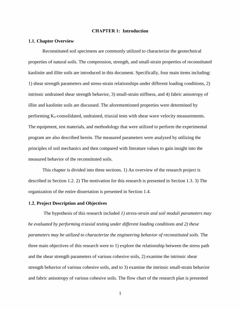
Chapter Overview
Reconstituted soil specimens are commonly utilized to characterize the geotechnical
properties of natural soils. The compression, strength, and small-strain properties of reconstituted
kaolinite and illite soils are introduced in this document. Specifically, four main items including:
1) shear strength parameters and stress-strain relationships under different loading conditions, 2)
intrinsic undrained shear strength behavior, 3) small-strain stiffness, and 4) fabric anisotropy of
illite and kaolinite soils are discussed. The aforementioned properties were determined by
performing Ko-consolidated, undrained, triaxial tests with shear wave velocity measurements.
The equipment, test materials, and methodology that were utilized to perform the experimental
program are also described herein. The measured parameters were analyzed by utilizing the
principles of soil mechanics and then compared with literature values to gain insight into the
measured behavior of the reconstituted soils.
This chapter is divided into three sections. 1) An overview of the research project is
described in Section 1.2. 2) The motivation for this research is presented in Section 1.3. 3) The
organization of the entire dissertation is presented in Section 1.4.
Project Description and Objectives
The hypothesis of this research included 1) stress-strain and soil moduli parameters may
be evaluated by performing triaxial testing under different loading conditions and 2) these
parameters may be utilized to characterize the engineering behavior of reconstituted soils. The
three main objectives of this research were to 1) explore the relationship between the stress path
and the shear strength parameters of various cohesive soils, 2) examine the intrinsic shear
strength behavior of various cohesive soils, and to 3) examine the intrinsic small-strain behavior
and fabric anisotropy of various cohesive soils. The flow chart of the research plan is presented

2
in Figure 1.1. Several tasks were completed to evaluate the hypothesis of this research, as
described below.
A series of Ko-reconsolidated, undrained, triaxial compression and extension tests were
performed under different loading conditions on kaolinite specimens that were
reconstituted at initial water content of the slurry (ws) of one and one-half times the liquid
limit (1.5LL) of the soil.
A series of Ko-reconsolidated, undrained, triaxial compression tests were conducted on
kaolinite and illite specimens that were reconstituted at sw levels of 1.5LL and three
times the liquid limit (3LL) to explore the intrinsic shear strength characteristics.
Small-strain shear modulus values were determined for kaolinite and illite specimens
during the reconsolidation and shearing stages of the triaxial compression tests. These
values were computed based on the shear wave velocity values that were measured by
utilizing bender elements. The specimens for this scope of work were reconstituted at sw
values of 1.5LL and 3LL.
The values of shear wave velocity were compared with the shear wave velocity values
that were obtained by utilizing bender elements within a constant rate of strain
consolidation device.
Problems associated with the test methods were discussed and new test procedures were
proposed.

3
Figure 1.1. The flow chart of the research plan.
Symbol Definitions
OCR= Overconsolidation Ratio
TC= Triaxial Compression Test
RTC= Reduced Triaxial Compression
TE= Triaxial Extension Test
RTE= Reduced Triaxial Extension Test
σc = Cell Pressure
σa = Axial Stress
c′ = Effective Cohesion
′= Effective Angle of Internal Friction
Gray outlines indicating tests performed on
specimens with ws of 1.5LL and 3LL
Triaxial Extension Test
Ko-consolidation
Consolidation Strain Rate=0.2%/hr
Shearing Strain Rate=0.5%/hr
RTE
σc constant
Decreasing σa
TC
σc constant
Increasing σa
OCR= 8
OCR= 1
OCR= 4
OCR= 2
Kaolinite Specimens Consolidated under a
Vertical Effective Stress of 207 kPa
in a Slurry Consolidometer, ws of 1.5LL
Triaxial Compression Test
Ko-consolidation
Consolidation Strain Rate=0.2%/hr
Shearing Strain Rate=0.5%/hr
Maximum Vertical Consolation
Stress (σ′ v,max)= 310 kPa
Maximum Vertical Consolation
Stress (σ′ v,max)= 410 kPa
Maximum Vertical Consolation
Stress (σ′ v,max)= 828 kPa
RTC
σa constant
Decreasing σc
TE
σa constant
Increasing σc
Determine the intrinsic
Small-strain behavior
Determine the effect of
Stress Path
Determine the intrinsic
Shear strength behavior
Small-Strain Measurements
(Vs,VH , GBE)
Stress-strain and Shear
Strength Parameters
(c′, ′, su, a, ue, Eu)
Stress-strain and Shear
Strength Parameters
(c′, ′, su, a, ue, Eu)
Vs,HV values (Zhao et al. 2017b)
Determine the effect of ws
Evaluate the fabric
anisotropy
Normalize su values to Iv Normalize Vs,VH and GBE
values to Iv
su= Undrained Shear Strength
a= Axial Strain
ue= Excess Pore Water Pressure
Eu= Undrained Young’s Modulus
Iv= Void Index
GBE= Small-strain Shear Modulus
Vs,VH= Vertically-propagated, Horizontally-polarized Shear Wave Velocity
Vs,HV= Horizontally -propagated, Vertically -polarized Shear Wave Velocity
ws= Initial Water Content of the Slurry
Kaolinite and Illite Specimens Consolidated
under a Vertical Effective Stress of 207 kPa
in a Slurry Consolidometer, ws of 1.5LL and 3LL
Compare the values
ws

4
Benefits to Geotechnical Engineering
Characterization of the shear strength of soil for engineering practice requires applying
various stress paths to soil to represent loading field conditions. Based on the concept of stress
path, different site characterization and design methods have been developed to account for
different orientations of the major, minor, and intermediate principal stress states. These methods
have been developed because the use of conventional triaxial testing has often led to either
unsafe or over-conservative designs. The shear strength parameters, as obtained from controlled
stress path triaxial testing, will aid in the solution of many instu stress path related problems.
Furthermore, limited amounts of triaxial compression testing data are currently available to
evaluate the parameters for advanced constitutive models. The data obtained from this research
will be analyzed and compared to develop an understanding of the testing techniques required to
represent certain field conditions. Moreover, these data will be useful to develop or validate
advanced constitutive models.
A better understanding of the engineering behavior of the reconstituted soils will aid in
the quantification and characterization of the engineering behavior of the natural soils. Few
studies have investigated the correlations between the initial water content of a given slurry and
the engineering characteristics of the reconstituted soils that were developed from the slurry.
Specifically, the intrinsic shear strength of reconstituted specimens that were overconsolidated
during the triaxial testing has not been previously evaluated. Furthermore, the influence of the
initial water content of the slurry and fabric anisotropy on the small-strain behavior of
reconstituted soil specimens has been studied by a limited number of researchers. Recommended
sw levels, that should be considered when reconstituting specimens of cohesive soils for shear
strength small-strain measurements, will be provided. More representative values of shear

5
strength and small-strain characteristics of corresponding natural soils will be obtained as the
result of this study by using the recommended slurry reconstitution procedures.
Dissertation Organization
The results from this research are described in seven chapters of this dissertation. The
organization of the dissertation is described in this chapter (Chapter 1). A review the related
literature, describing fundamental aspects of stress path, reconstituted soils, and small-strain
measurements, is presented in Chapter 2. The contents of Chapters 4 through 6 have been
submitted for publication. Information about the submissions is described below. The main
conclusions drawn from the research are presented in Chapter 7.
A technical paper about the effect of the stress path on 1) the stress-strain behavior and 2)
the shear strength characteristics of reconstituted low plasticity kaolinite soil, as obtained from a
comprehensive triaxial testing program, is presented in Chapter 4. The paper was submitted to
Soils and Foundations. The full reference is: Mahmood, N. S. and Coffman, R. A., (2017). “The
Effects of Stress Path on the Characterization of Reconstituted Low Plasticity Kaolinite.” Soils
and Foundations, Under Review, Manuscript Number: SANDF-D-17-00352-R1.
The observed relationships between the initial water content of the slurry and the
corresponding shear strength characteristics of reconstituted kaolinite and illite soils, is presented
in Chapter 5. The paper was submitted to Quarterly Journal of Engineering Geology and
Hydrogeology. The full reference is: Mahmood, N. S. and Coffman, R. A., (2018a). “Intrinsic
shear strength behavior of reconstituted kaolinite and illite soils.” Quarterly Journal of
Engineering Geology and Hydrogeology, Under Review, Manuscript Number: qjegh2018-056-
R1.

6
The shear wave velocity and small-strain shear stiffness of reconstituted kaolinite and
illite specimens were investigated by utilizing triaxial apparatus instrumented with bender
elements. The results obtained from this investigation were documented in a technical paper
which is presented in Chapter 6. The paper was submitted to the Geotechnical Testing Journal.
The full reference is: Mahmood, N. S. and Coffman, R. A., (2018b). “Small-strain of
Reconstituted Soils: The Effect of Slurry Water Content.” Geotechnical Testing Journal, Under
Review, Manuscript Number: GTJ-2018-0098-R1.
References
Mahmood, N. S. and Coffman, R. A., (2017). “The Effects of Stress Path on the Characterization
of Reconstituted Low Plasticity Kaolinite.” Soils and Foundations, (Under Review,
Manuscript Number: SANDF-D-17-00352-R1).
Mahmood, N. S., and Coffman, R. A., (2018a). “Intrinsic Shear Strength Behavior of
Reconstituted Kaolinite and Illite Soils.” Quarterly Journal of Engineering Geology and
Hydrogeology, (In Review, Manuscript Number: qjegh2018-056-R1).
Mahmood, N. S., and Coffman, R. A., (2018b). “Small-strain of Reconstituted Soils: The Effect
of Slurry Water Content.” Geotechnical Testing Journal, (Under Review, Manuscript
Number: GTJ-2018-0098-R1).

7
Literature Review
Chapter Overview
A review of literature on the key areas of the research is presented in this chapter.
Specifically, consideration is given to the stress-strain behavior and small-strain properties of
cohesive soils under different loading conditions in undrained triaxial testing. An overview of
the concept and the importance of stress path in triaxial testing, as well as the effects of stress
path on the measurements engineering parameters is presented in Section 2.2. The engineering
behavior of reconstituted soils, is discussed in Section 2.3. A description of the small-strain soil
measurements and a discussion of the influences of stress history and fabric anisotropy on these
measurements are presented in Section 2.4.
Stress Path in Triaxial Testing
Historically, triaxial testing has been the most utilized test method for reliable
measurements of stress-strain relationships for soil. One of the factors that influences the stress-
strain relationships, as obtained from triaxial testing, is the applied stress path. The concept and
importance of stress path are presented in Section 2.2.1. The methods for applying stress paths
during triaxial tests are discussed in Section 2.2.2. The effects of stress path on shear strength
parameters are discussed in Section 2.2.3. The influences of stress path on 1) developed
constitutive models and on 2) soil moduli are discussed in Sections 2.2.4 and Section 2.2.5,
respectively.
The Concept and Importance of Stress Path
By definition, the stress path is the line that is developed by recording the direction and
magnitude of the three principal stresses as a function of time during the consolidation and
shearing stages of a triaxial test (Lambe 1967). Soil deformation during loading is mainly due to
sliding between soil particles. Therefore, this deformation is highly irrecoverable and is

8
significantly dependent on the stress path (Lade and Duncan 1976). The amount of shear strength
anisotropy, for a given soil, is influenced by the stress path that the soil experiences. Shear
strength anisotropy is an important factor that may have significant effects on shear strength
properties. In nature, anisotropic consolidation occurs during sedimentation of soil; this process
is known as the inherent anisotropy. Examinations of the structure of clay samples following
one-dimensional consolidation have led to the realization that clay particles tend to be oriented
perpendicularly with respect to the direction of the major principal stress. Therefore, any change
in the directions of the principal stress will affect the compressibility and shear strength of the
clay (Hanse and Gibson 1949, Duncan and Seed 1966).
In addition to the inherent anisotropy, another form of anisotropy occurs as a result of the
rotation of the three principal stresses during consolidation and shear. This rotation of the
principal stresses is known as stress induced anisotropy (Hanse and Gibson 1949, Atkinson et al.
1987, Prashant and Penumadu 2005). It has been recognized by many researchers that different
loading conditions encountered in the field result in a rotation of the principal stresses during
shear (Figure 2.1). Therefore, the selected stress paths utilized during laboratory testing must be
selected to represent the insitu loading conditions. Heave of soil at the bottom of an excavation,
for instance, has been shown to be reproduced using triaxial extension tests while the bearing
capacity of an embankment has been modeled by using a combination of plan strain active
(PSA), plan strain passive (PSP), and direct simple shear (DSS) tests. For instance, the Earth
Retaining Structures Manual (2007) distributed by the Federal Highway Administration (FHWA)
states that triaxial extension tests should be conducted to evaluate the shear strength parameters
in cases such as 1) deep excavations in soft clays or 2) soils in the passive zone. The manual also

9
states that the value of shear strength for soil in the passive zone is typically lower than the value
of shear strength for soil in the active zone.
Figure 2.1. Orientation of the principal stresses and typical in situ modes of failure
(modified from Ladd and Foott 1974).
Many different design methods have been employed to evaluate the stress-strain behavior
of a given soil element soil when the soil is subjected to loading or unloading (e.g., Davis and
Poulos 1968, Simons and Som 1970, Davis and Poulos 1972, Coffman et al. 2010). These
methods have been developed to account for stress changes, in the field, that require
representative laboratory obtained soil parameters, as obtained from laboratory stress path tests.
Simons and Som (1970) stated that the modulus of elasticity value should be determined from an
appropriate stress path to take in account the field stress conditions for settlement analyses.
In most design cases, the triaxial compression test (conventional triaxial) has been used
to evaluate the undrained shear behavior of clay because of the simplicity and expediency of this
test compared with other controlled stress path tests (Bishop and Henkel 1962, Kulhawy and

10
Mayne 1990, Bayoumi 2006). In the conventional triaxial compression test, the axial stress
increased while the confining stress remains constant. However, the directions of the stresses
induced by this test are not always representative of the directions of the principal stresses in the
field.
Ladd and Foott (1974) stated that the undrained shear strength values obtained from PSA
were greater than those obtained from DSS and the values obtained from the DSS were greater
than those obtained from PSP. As described in Ladd and Foott (1974), the methods that have
been commonly used in design to evaluate shear strength of soil have tended to self-compensate.
Specifically, high values of undrained strength (su) that resulted from high levels of strain rate
during the tests were compensated by the low su values that resulted from sample disturbance.
This compensating error cannot to be controlled, so conservative or unsafe values of su may be
mistakenly utilized for the design.
The SHANSEP (Stress History and Normalized Soil Engineering Properties) method, as
based on the concept of normalization of the undrained shear strength (𝑠𝑢) with respect to the in
situ vertical effective stress (𝜎′𝑣𝑐), has been utilized to ensure the use of representative values of
undrained shear strength. As shown in Figure 2.2, the undrained shear strength is observed to
increase with an increase in the over consolidation ratio (OCR). This relationship between the
OCR and the undrained shear strength was formulated by the SHANSEP equation (Equation
2.1). This method was established by conducting a series of triaxial compression, triaxial
extension, or direct simple shear tests, in addition to consolidation tests. Historically, the
undrained shear strength has been characterized by using this procedure.
𝑠𝑢
𝜎′𝑣𝑐= 𝑆(𝑂𝐶𝑅)𝑚 (after Ladd and Foott 1974) Equation 2.1

11
Within Equation 2.1, S is the normalized undrained strength ratio for the respective stress
paths at OCR=1 and m is the slope of the regression line for the respective stress paths.
Figure 2.2. Undrained shear strength from three shear tests with different modes of shearing
(data from Lefebrve et al. 1983, reproduced from Ladd 1991).
Stress Path Methods in Triaxial Testing
Triaxial testing is widely used, within the laboratory, to evaluate the strain-strain and
strength properties of various soil types. One of the factors that influences the stress-strain and
strength relationships obtained from triaxial testing is the applied stress path during the
consolidation and shearing stages. Recent advances in the triaxial testing apparatus have led to
stress path dependent triaxial tests being easier to conduct (Parry 2004, Holtz et al. 2011). The
consolidation stage may consist of either isotropic or anisotropic consolidation (Bishop and
Henkel 1962). Isotropic consolidation is achieved by applying equal vertical and horizontal
effective stresses while anisotropic consolidation is achieved when the vertical effective stress is
12
greater than the horizontal effective stress. The purpose of the consolidation stage is to restore
the original stress conditions before the sample is sheared.
Based on the assumption that the lateral stresses that are produced in the laboratory are
the same as that in the field, the original field conditions, during the deposition process of natural
soils, may be better represented using Ko-consolidation, (Hansen and Gibson 1949).
Consolidation and reconsolidation may also be required to achieve certain overconsolidation
values. Ladd and Foott (1974) recommended that soil specimens be reconsolidated to
consolidation pressures that exceed the in situ preconsolidation pressures (σ′c) by one and one-
half to four times to eliminate the effects of sampling disturbance. Baldi et al. (1988) mentioned
that 1) a suitable stress path must be selected to reconsolidate soil samples and that 2) the
selected stress path should depend on the in situ effective stress, the overconsolidation ratio, and
the clay type.
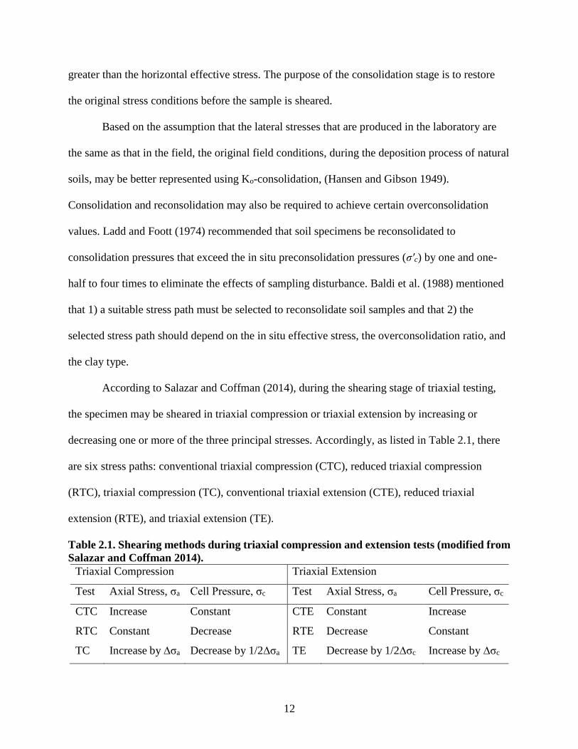
According to Salazar and Coffman (2014), during the shearing stage of triaxial testing,
the specimen may be sheared in triaxial compression or triaxial extension by increasing or
decreasing one or more of the three principal stresses. Accordingly, as listed in Table 2.1, there
are six stress paths: conventional triaxial compression (CTC), reduced triaxial compression
(RTC), triaxial compression (TC), conventional triaxial extension (CTE), reduced triaxial
extension (RTE), and triaxial extension (TE).
Table 2.1. Shearing methods during triaxial compression and extension tests (modified from
Salazar and Coffman 2014).
Triaxial Compression Triaxial Extension
Test Axial Stress, σa Cell Pressure, σc Test Axial Stress, σa Cell Pressure, σc
CTC Increase Constant CTE Constant Increase
RTC Constant Decrease RTE Decrease Constant
TC Increase by ∆σa Decrease by 1/2∆σa TE Decrease by 1/2∆σc Increase by ∆σc

13
Except for the Ko-consolidated specimens with Ko values greater than one, the major
principal stress acts in the vertical direction and the minor principal stress acts in the horizontal
direction at the end of consolidation stage. During the triaxial compression tests, the orientation
of the principal stresses does not change during the shearing stage. The term “reorientation” of
principal stresses was introduced by Duncan and Seed (1966) to describe the change in the state
of stress when the orientation of the principal stresses, at the end of shearing stage, did not
coincide with the orientation of the principal stresses prior to shearing. During triaxial extension
testing, increasing the horizontal stress during the shearing or decreasing the vertical stress may
cause the major principal stress to act in the horizontal direction and the minor principal stress to
act in the vertical direction. Therefore, the principal stresses will be reoriented by 90 degrees at
the end of shearing stage (Duncan and Seed 1966).
Effect of Stress Path on Shear Strength Parameters
The stress path that a sample is subjected to is one of the major factors that has a
significant influence on both drained and undrained shear strength parameters. Based on the
results from one of the earliest series of triaxial extension tests on clay, which were performed by
Hirschfield (1958), the values of undrained strength (su) of extension tests were 20 to 25 percent
less than those obtained from compression tests. More recently, Ladd and Foott (1974) reported
that the shear strength values from the triaxial extension test (TE) were 10 to 25 percent less than
those from (PSP) tests. Some examples of previous work concerning the effect of stress path on
undrained shear strength values are presented in Table 2.2. Furthermore, the reported values of
undrained shear strength were observed to decrease with an increase in the vertical stress level.
Bishop (1966) attributed the lower values of undrained strength, that were obtained from triaxial
extension tests, to differences in the amount of excess pore water pressure that developed during
shearing.

14
Table 2.2. Undrained shear strength from compression and extension tests.
su(compression) /su(Extension) Reference Clay Type
1.25 Duncan and Seed (1966) San Francisco Bay Mud
2.13 Ladd et al. (1971) Resedimented Boston Blue Clay
2.5 Bjerrum et al. (1972) Normally Consolidated Clay
1.75 to 3.78 Bjerrum (1973) Bangkok Clay
1.2 Parry and Nadarajah (1974) Fulford Clay
1.74 to 1.90 Moniz (2009) Resedimented Boston Blue Clay
According to Bishop and Henkel (1962), Bishop (1966), and Lambe (1967), the drained
shear strength parameters c′ and ′ can be calculated from the undrained triaxial tests with pore
water pressure measurements. Parry (2004) stated that there has been conflicting evidence
presented in the available data regarding the effect of stress path on ′ values. A few researchers
have indicated that the effect of the stress path on the drained shear strength is insignificant.
Duncan and Seed (1966) and Gens (1983) reported that the effective angle of internal friction in
compression (′c) and the effective angle of internal friction in extension (′e) are approximately
equal. Many other researchers (e.g. Parry 1960, Saada and Bianchanini 1977) reported that ′c is
less than ′e by a few degrees. Atkinson et al. (1990) investigated the effect of stress history and
stress path on kaolinite samples. Based on the Atkinson et al. (1990) results, the critical state
lines for compression and extension test were symmetrical about p′ axis and the ′c values were
significantly less than ′e values. Parry (2004) attributed the difference in the results to the
instability of the sample during shearing in extension tests.
As discussed by Skempton (1954), the orientation of the principal stresses influences the
amount of pore water pressure developed during shearing. The pore pressure parameter Af,
which represents the relationship between the change in pore pressure (u) and the change in
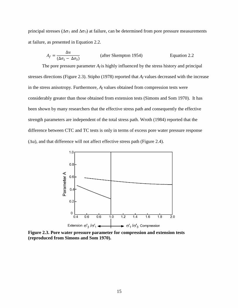
15
principal stresses (1 and 3) at failure, can be determined from pore pressure measurements
at failure, as presented in Equation 2.2.
𝐴𝑓 =∆𝑢
(∆𝜎1 − ∆𝜎3) (after Skempton 1954) Equation 2.2
The pore pressure parameter Af is highly influenced by the stress history and principal
stresses directions (Figure 2.3). Stipho (1978) reported that Af values decreased with the increase
in the stress anisotropy. Furthermore, Af values obtained from compression tests were
considerably greater than those obtained from extension tests (Simons and Som 1970). It has
been shown by many researchers that the effective stress path and consequently the effective
strength parameters are independent of the total stress path. Wroth (1984) reported that the
difference between CTC and TC tests is only in terms of excess pore water pressure response
(u), and that difference will not affect effective stress path (Figure 2.4).
Figure 2.3. Pore water pressure parameter for compression and extension tests
(reproduced from Simons and Som 1970).

16
Figure 2.4. Total and effective stress paths from CTC and TC tests (reproduced from
Wroth 1984).
Stress Path Influences on Developed Constitutive Models
Constitutive models are essential for numerical simulations of geotechnical problems
such as ground deformation, slope and tunnels stability, and excavations. As mentioned in
Hashash et al. (2002), over the last few decades, many constitutive models have been formulated
based on elasto-plasticity theory to predict stress-strain behavior of soils during shearing (from
the initial stress condition to the critical state condition). The loading conditions play a
significant role in obtaining a realistic prediction of soil behavior using these models. Utilizing
the classic elastoplastic theory and the critical state concept for soil, as defined by Roscoe et al.
(1958) and later referred by Roscoe and Burland (1968), the Modified Cam Clay model (MCC)
was developed to represent clay behavior. More recently, advanced soil models, such as MIT-E3
(Whittle and Kavvadas 1994) and S-CLAY1 (Wheeler et al. 2003), were developed to account
for soil anisotropy and structure destruction. Lade (2005) mentioned that most of the current
research related to constitutive modeling has focused on the effect of anisotropy and stress path.
Only a few of the aforementioned constitutive models were established based on
comprehensive laboratory data (Wheeler et al. 2003). If laboratory data are available,
constitutive parameters are typically obtained from triaxial tests. Therefore, these acquired
parameters include shear strength parameters and soil moduli values. Most of the constitutive

17
models that were developed based on triaxial data were derived from conventional triaxial
compression tests. The parameters from these tests are simple and provide only limited
information. Therefore, there is still a lack of knowledge about the performance of the developed
constitutive models when the soil is subjected to different loading conditions (Bayoumi 2006).
Bryson and Salehian (2011) evaluated the performance of four constitutive models in predicting
the behavior of medium plasticity remolded clay. As described by Bryson and Salehian (2011),
the 3-SKH and Cam Clay models were the most suitable for predicting the stress-strain behavior
of the remolded clay under different stress paths.
Effect of Stress path on Soil Moduli
Soil moduli including: shear modulus (G), Young’s modulus (E), bulk modulus (K), and
constrained modulus (M), are essential in the evaluation of soil deformation and stress
distribution in a soil mass by using elastic solutions. These values can be determined from either
field or laboratory tests. As shown in Figure 2.5, there are three types of the modulus of the
elasticity which may be determined from triaxial testing: the initial tangent modulus (Ei), the
tangent modulus (Et), and the secant modulus (Es). Simons and Som (1970) reported that
modulus of elasticity for isotropically consolidated samples are significantly less than those for
Ko-consolidated samples due to the effect of disturbance. Skempton and Hankel (1957) reported
that large strain modulus of elasticity for extension is higher than that for compression. Clayton
and Heymann (2001) also indicated that the stiffness at large strain for extension tests performed
on London clay are higher than those for compression tests (Figure 2.6).

18
Figure 2.5. Definition of Ei, Et, and Es from triaxial testing (from Lambe and Whitman
1969, Atkinson 2000).
Figure 2.6. Degradation of vertical Young’s modulus for specimens tested in triaxial
compression and extension (from Clayton 2011).

19
The decrease in soil stiffness with increasing strain, is well known as stiffness
degradation. Soil moduli as obtained from small shear strain (<10-3%), including modulus of
elasticity (Eo), constrained modulus (M) and shear modulus (Go), are of great importance for
estimating response of structures to dynamic loads, soil improvement, and liquefaction
assessment (Hardin and Drnevich 1972, Woods and Partos 1981, Clayton 2011). However,
measurements of small-stain stiffness utilizing triaxial tests with conventional external strain
measurements may not be accurate because there are many sources of error in the measurement
of small strain including seating, bedding, and alignment errors (Baldi et al. 1988).
Problems Associated with the Triaxial Extension Test
Recent advances in triaxial testing equipment, including load system control and stress
strain measurements, have led to ease in conducting stress path dependent triaxial tests.
However, there are some problems associated with the triaxial extension test that may prevent
utilizing results obtained from the triaxial extension test in practice (Wu and Kolymbas 1991,
Parry 2004). Specifically, the development of necking during shearing in extension test, may
cause significant errors in the test results. Many researchers have argued that the greatest
shortcoming of the triaxial test is the stress-strain nonuniformity that exists along the
longitudinal direction of the sample due to the restriction of the sample ends. Necking during the
test causes the shear stress levels to peak, which invalidates the data because of the inaccurate
calculation of the cylindrical area. Sheahan (1991) reported that as the strain rate increased, the
cross-sectional area decreased due to the effect of added dilation at high strain rates. Liu (2004)
also reported that the necking associated with triaxial extension tests increased with an increase
in the specimen height to the diameter ratio. Therefore, polished and lubricated end platens have
been used to reduce the effect of ends restriction (Stipho 1978, Sheahan 1991, Liu 2004).

20
The deviatoric stress during shearing stage is calculated from the axial load and the
average cross-sectional area. The conventional method to determine the corrected cross-sectional
area (Ac) for a given value of axial strain, ε, and an initial average cross-sectional area of the
specimen (Ao) is presented in Equation 2.3. This equation, as suggested in ASTM D4767 (2011),
is limited because it only relies upon the axial strain measurements.
𝐴𝑐 =𝐴𝑜
(1 − 𝜀) ASTM D4767 Equation 2.3
This conventional procedure relies on the assumption of uniform radial deformation
throughout the sample. However, as illustrated in Figure 2.7, the radial deformation at the ends
of the specimen is resisted by the end restraint. Therefore, this procedure provides imprecise
determination of the sample cross-sectional area, specifically when failure occurs at large levels
of strain (Bishop and Henkel 1962). As discussed in Scholey (1996), many localized
measurements have been used to measure the radial deformation (such as local strain probes and
digital imaging techniques). One of the digital imaging techniques consists of using small board
cameras, within the triaxial cell, to measure the change in volume of the specimen (Salazar and
Coffman 2015).
Another source of errors in triaxial extension tests is caused by the friction between the
loading piston and the bearings within the top cap of the triaxial cell. Many methods have been
attempted to eliminate the effect of piston friction. According to Bishop and Henkel (1962) the
amount of this friction is between one to five percent of the applied axial load. Therefore, this
friction may be a significant contribution of the load for soft samples. Race and Coffman (2011)
utilized an internal load cell placed between the top platten and the loading piston to measure the
applied axial force inside the triaxial cell to avoid the effect of piston friction.
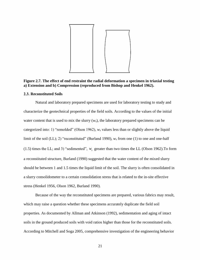
21
Figure 2.7. The effect of end restraint the radial deformation a specimen in triaxial testing
a) Extension and b) Compression (reproduced from Bishop and Henkel 1962).
Reconstituted Soils
Natural and laboratory prepared specimens are used for laboratory testing to study and
characterize the geotechnical properties of the field soils. According to the values of the initial
water content that is used to mix the slurry (ws), the laboratory prepared specimens can be
categorized into: 1) “remolded” (Olson 1962), ws values less than or slightly above the liquid
limit of the soil (LL); 2) “reconstituted” (Burland 1990), ws from one (1) to one and one-half
(1.5) times the LL; and 3) “sedimented”, sw greater than two times the LL (Olson 1962).To form
a reconstituted structure, Burland (1990) suggested that the water content of the mixed slurry
should be between 1 and 1.5 times the liquid limit of the soil. The slurry is often consolidated in
a slurry consolidometer to a certain consolidation stress that is related to the in-site effective
stress (Henkel 1956, Olson 1962, Burland 1990).
Because of the way the reconstituted specimens are prepared, various fabrics may result,
which may raise a question whether these specimens accurately duplicate the field soil
properties. As documented by Allman and Atkinson (1992), sedimentation and aging of intact
soils in the ground produced soils with void ratios higher than those for the reconstituted soils.
According to Mitchell and Soga 2005, comprehensive investigation of the engineering behavior

22
of laboratory prepared specimens will result in better characterization of the properties of natural
soils. The values of the initial water content of the slurry that are utilized to reconstitute cohesive
soils may have significant effects on the compression and shear strength behavior of the soils due
to the influence of sw on the soil fabric. The term “intrinsic” was introduced by Burland (1990)
to describe the properties for specimens that were reconstituted within the aforementioned water
content values. Burland (1990) further reported that the shear strength and compressibility of
reconstituted soils may be utilized to develop a reference framework to correlate the laboratory
obtained properties from reconstituted soils with those from the intact soils.
Fabric of Reconstituted Soils
Previous studies (e.g., Olson 1962, Martin and Ladd 1978, Carrier and Beckman 1984)
have shown that using different levels of initial water content )( sw to remold or reconstitute soil
specimens will affect the mechanical behavior of the specimens due to the significant changes in
the soils structure. As describe by Mitchell and Soga (2005), soil structure is composed of fabric
and bonding (interparticle force system). The term fabric refers to the arrangement of particles
and the arrangement of pore space within a given soil. The term fabric, however, has been used
interchangeably with the term structure. As presented in Figure 2.8, clay particles may have a
flocculated (random arrangement) fabric or dispersed (parallel arrangement) fabric (Mitchell and
Soga 2005).

23
(a) (b)
Figure 2.8. Typical particle arrangement of cohesive soils: a) flocculated fabric, and b)
dispersed fabric (from Mitchell and Soga 2005).
According to Olson (1962), Burland (1990), and Prashant and Penumadu (2007), soil
fabric has been shown to play an essential role in the engineering behavior of clayey soils. Soil
fabric can vary considerably as a result of using different water content values to reconstitute
clay soils. Olson (1962) indicated that laboratory prepared specimens, at water content less than
or slightly above liquid limit, may not represent the natural deposition process. Moreover, Olson
(1962) mentioned that specimens at these low levels of water content will have dispersed
microfabric and exhibit intrinsic properties of overconsolidated clayey soil regardless of the level
of overconsolidation within the specimen. Olson (1962) also indicated that sedimentation of
specimens from slurries with sw values higher than two times the respective liquid limit will
produce specimens with flocculated fabric. To obtain more representative specimens, Olson
(1962) reported that the water content of the mixed slurry should be at least two times the liquid
limit. However, sedimentation of specimens at such high water content requires an extended
period of time. Moreover, it has been shown that these specimens are often difficult to extrude
and trim. Therefore, the following researchers: Henkel (1956), Parry (1960), Bryson and
Salehian (2011), Tiwari and Ajmera (2011), Zhao and Coffman (2016), Zhao et al. (2017), and
Zhao et al. (2018) have instead prepared reconstituted clay specimens at lower water content
values.

24
Intrinsic Compression Behavior
The results from many studies (e.g. Carrier and Beckman 1984, Cerato and Lutenegger
2004, Hong et al. 2010) indicated that both initial void ratio and compression behavior of
reconstructed soils were affected by the initial water content. As shown in Figure 2.9, the
compression curves of specimens prepared at a higher initial water content lied above the
compression curves of the specimens prepared at a lower initial water content. Based on the
results from these studies, increasing the initial water content of the slurry tended to increase the
initial void ratio and to increase the compressibility of the reconstituted clays for a given vertical
effective stress.
Figure 2.9. Compression curves of reconstituted Baimahu Clay at different initial water
contents of the slurry (from Hong et al. 2010).
Many previous studies (e.g., Burland 1990, Hong et al. 2010, Tiwari and Ajmera 2011,
Al Haj and Standing 2015) have indicated that the shape of the compression curve that was
obtained from odometer tests conducted on reconstituted soils was different than the typical
shape of the compression curve for natural soils. The shapes of the compression curve (as

25
presented previously in Figure 2.9), that were observed by these studies, tended to slightly
concave upwards in a pattern similar to that for soft clays. Burland (1990) reported that intrinsic
properties of the reconstituted soils were inherent and independent of the soil structure.
Furthermore, the compression curves of different reconstituted clays with sw values of 1.25 LL
can be normalized by using the void index )( vI , as presented in Equations 2.4 and 2.5.
*
*
100
c
vC
eeI
Burland (1990) Equation 2.4
*
1000
*
100
* eeCc Burland (1990) Equation 2.5
Within Equations 2.4 and 2.5,*
100e and *
1000e are the void ratio of the reconstituted clay
corresponded to vertical stress levels of 100 and 1000 kPa respectively;*
cC is the intrinsic
compression index.
When laboratory measurements are not available, Equations 2.6 and 2.7 can be used to
estimate the *
100e and *
cC respectively, based on the values of the initial void ration at the liquid
limit ( Le ), as suggested by Burland (1990).
32*
100 016.0089.0679.0109.0 LLL eeee Burland (1990) Equation 2.6
04.0256.0* Lc eC Burland (1990) Equation 2.7
As shown in Figure 2.10, the normalized compression lines for three clays exhibited identical
relationships. The normalized curves were represented by a unique line which was descried by
Burland (1990) as the intrinsic compression line (ICL), as presented in Equation 2.8. In Equation
2.8, v is the vertical effective stress in kPa.
3)(log015.0log285.145.2 vvvI Burland (1990) Equation 2.8
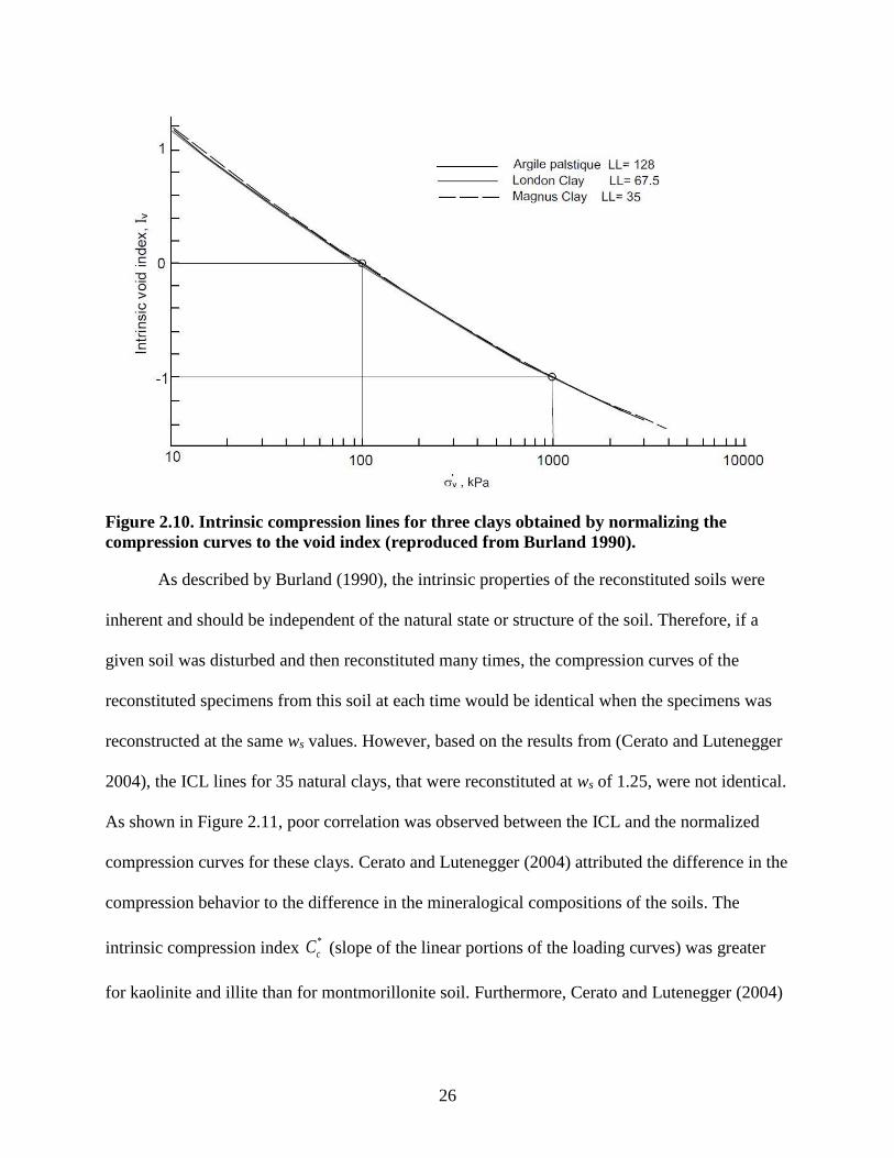
26
Figure 2.10. Intrinsic compression lines for three clays obtained by normalizing the
compression curves to the void index (reproduced from Burland 1990).
As described by Burland (1990), the intrinsic properties of the reconstituted soils were
inherent and should be independent of the natural state or structure of the soil. Therefore, if a
given soil was disturbed and then reconstituted many times, the compression curves of the
reconstituted specimens from this soil at each time would be identical when the specimens was
reconstructed at the same ws values. However, based on the results from (Cerato and Lutenegger
2004), the ICL lines for 35 natural clays, that were reconstituted at ws of 1.25, were not identical.
As shown in Figure 2.11, poor correlation was observed between the ICL and the normalized
compression curves for these clays. Cerato and Lutenegger (2004) attributed the difference in the
compression behavior to the difference in the mineralogical compositions of the soils. The
intrinsic compression index *
cC (slope of the linear portions of the loading curves) was greater
for kaolinite and illite than for montmorillonite soil. Furthermore, Cerato and Lutenegger (2004)

27
indicated that the degree to which the ws affected the compression behavior was also dependent
on the soil mineralogy.
Figure 2.11. Normalized compression curves for natural clays (from Cerato and
Lutenegger 2004).
Intrinsic Undrained Shear Strength Behavior
Based on previous research on reconstituted soils, the stress-strain behavior of these soils
was significantly affected by the sw levels (Henkel 1962, Burland 1990, Allman and Atkinson
1992, Chandler 2000, Hong et al. 2013). As documented by Allman and Atkinson (1992), at the
same specific volume and water content, the undrained shear strength values of the intact
samples were from 10 to 15 times greater than those for reconstituted soils. Allman and Atkinson
(1992), attributed the higher values of the undrained shear strength for the intact soils to the
aging of the naturally sedimented specimens. The pattern of behavior, during shearing of the
normally consolidated reconstituted specimens, was different from the typical behavior that has
been observed for normally consolidated soils. As described by Olson (1962), slurried specimens

28
that were prepared at sw values less than or slightly above the liquid limit exhibited shear
strength characteristics similar to the typical characteristics of the overconsolidated clay soils.
Therefore, Olson (1962), suggested that a water content values of at least two times the liquid
limit should be utilized to prepare the slurry.
Furthermore, as reported by Burland (1990) and Atkinson et al. (1987), postpeak shear
planes were observed to develop in one-dimensional consolidated kaolinite specimens regardless
of whether the soil was normally consolidated or overconsolidated. The difference in the
magnitude of the shear induced pore water pressure during shear may explain the unusual
behavior of normally consolidated specimens during shear. As discussed by Cerato and
Lutenegger (2004), the double layer may have not completely been developed around the
particles of the flocculated soils that were reconstituted at low values initial water content.
Therefore, the particles may absorb additional water during shear, depending on the initial water
content of the specimens )( ow .
Previous researchers have reported that the undrained shear strength values of the
reconstituted soils decreased with increasing levels of the sw (Chandler 2000, Hong et al. 2013,
Al Haj and Standing 2015). As observed by Hong et al. (2013), the undrained shear strength
values, obtained from isotropic consolidation undrained triaxial compression tests, decreased
with the increasing values of the initial water content (Figure 2.12).

29
Figure 2.12. Undrained shear strength values as a function of initial water content (from
Hong et al. 2013).
Following a normalization procedure that was similar to Burland (1990), the values of the
undrained shear strength were normalized to the values of the vI that corresponded to the
vertical effective stress values prior to shear. The intrinsic shear strength behavior was
introduced by Chandler (2000) to describe the relation between the sw and the undrained shear
strength of the reconstituted soils. As shown in Figure 2.13, the normalized line was defined by
Chandler (2000) as the intrinsic strength line )( LISu . However, this line was not unique for a
given soil type, but it was developed based on a single value of 0.33 of the undrained shear
strength ratio )( *
suR , which is defined as the ratio of the undrained shear strength of the
reconstituted soil )( *
us to the preshear vertical effective stress )( vc . As presented in Figure 2.14,
similar procedure was successfully utilized by Hong et al. (2013) to normalize the values of the
undrained shear strength, obtained from isotropically consolidated undrained triaxial tests that
were conducted on of an illitic soil. However, Hong et al. (2013) utilized the values of effective
isotropic consolidation stress instead of the values of vertical effective stress to determine the vI
values.

30
Figure 2.13. Normalized undrained shear strength and intrinsic strength line (from
Chandler 2000).
Figure 2.14. Normalized values of undrained shear strength obtained from isotropically
consolidated undrained triaxial testes (from Hong et al. 2013).

31
Small-Strain Moduli of Reconstituted Soils
As previously mentioned, measurements of soil moduli by utilizing triaxial tests, with
conventional external strain measurements, may not be accurate because of the errors that have
been associated with these measurements. Alternately, bender elements and piezoelectric disks
have been previously utilized to determine soil moduli based on the seismic wave velocity
measurements. A brief description of the shear wave velocity measurements by utilizing bender
elements technique is presented in Section 2.4.1. The effect of stress history and fabric
anisotropy are discussed in Section 2.4.2 and Section 2.4.3, respectively.
Bender Elements Technique
During the last few decades, bender elements (BE) have been utilized to measure shear
wave velocities for different types of soils. The BE technique has provided an inexpensive and
reliable alternative to study small-strain soil properties (Clayton 2011). The velocity of a shear
wave that travels through a soil specimen is computed by measuring the travel time of the wave
from the transmitter BE to the receiver BE. As described in Equations 2.9, soil moduli Go may be
related to shear wave velocity ( sV ) by utilizing the total mass density of the soil (ρ).
2
so VG Richart et al. 1970 Equation 2.9
Bender elements have been employed within open odometer, floating wall
consolidometer, and constant-rate-of-strain consolidometer devices to examine small-strain soil
properties during consolidation. Some researchers (e.g., Fam and Santamarina 1995, Jovicic and
Coop 1998, Kang et al. 2014) have incorporated bender elements within the top and bottom
plates of an oedometer to measure shear waves in the vertical direction. As presented in Figure
2.15, bender elements have also been installed in the horizontal direction (Jamiolkowski et al.
1995, Kang et al. 2014, Zhao and Coffman 2016, Zhao et al. 2017) to acquire horizontally

32
propagated shear waves. Recently, a back-pressure saturated, constant rate-of-strain,
consolidation device, with bender elements (BP-CRS-BE) was developed at the University of
Arkansas by Zhao and Coffman (2016), as shown in Figure 2.16. Velocities of two types of shear
waves were measured by utilizing the BP-CRS-BE device: 1) horizontally propagated-vertically
polarized shear waves (HVsV ,
), and 2) horizontally propagated-horizontally polarized shear waves
(HHsV ,
).
Figure 2.15. Bender elements installed in the vertical and horizontal directions within an
oedometer device (after Kang et al. 2014).

33
Figure 2.16. Photograph and schematic of bender elements within BP-CRS-BE device in
the a) horizontal orientation, and b) vertical orientation (after Zhao et al 2017).
The bender elements technique has also been utilized within the triaxial apparatus (e.g.,
Viggiani and Atkinson 1995, Jovicic and Coop 1998, Gasparre and Coop 2006, Finno and Kim
2012, Choo 2013, Salazar and Coffman 2014) in different orientations, as presented in Figure
2.17. As discussed by Viggiani and Atkinson (1995) and Jovicic and Coop (1998), valuable
measurements of small-strain stiffness were obtained by utilizing bender elements within the
triaxial apparatus because of the different loading conditions that can be applied by the triaxial
apparatus during the consolidation and shearing stages.
(a)
(b)
A. Alumimum loading cap. B. Porous stone. C. Soil sample. D. Horizontal bender element.
E. Polyoxymethylene slide bar. F. Vertical bender element.
FIG. 1. Photograph and schematic of BE within the fabricated Polyoxymethylene slide bars in the
(a) horizontal orientation, and (b) vertical orientation.
A
F
D
E
B
C

34
Figure 2.17. Schematic of a triaxial specimen instrumented with bender elements in the a)
horizontal orientation, and b) vertical orientation (after Finno and Kim 2012).
Effect of Stress History on Small-Strain Behavior
The term “recent stress history” was first introduced by Atkinson et al. (1990) to describe
the current applied stress path that has a direction different than the direction of the previous
stress path. Atkinson et al. (1990) showed that the recent stress history has an impact on small-
strain stiffness during consolidation and shearing stages of the triaxial tests. Simons and Som
(1970) reported that the modulus of elasticity for isotropically consolidated samples are less than
those obtained from Ko consolidated samples, due to the effect of disturbance. The relationship
between shear modulus, specific volume (v), current effective stress (p′), and overconsolidation
ratio (Ro) is provided in Equation 2.10 (Atkinson 2000).
𝐺𝑜
𝑝𝑎= 𝐴 (
𝑝′
𝑝𝑎)
𝑛
𝑅𝑜𝑚 Atkinson (2000) Equation 2.10

35
Within Equation 2.10, pa is the atmospheric pressure; A, n, and m are material
parameters. Amorosi et al. (1999) and Choo et al. (2013) showed that stress history during
consolidation stage in triaxial testing has a significant effect on stiffness degradation during
shear.
Although there have been many studies to investigate the effect of recent stress history on
small-strain stiffness and the degradation of small-strain stiffness during shear, conflicting data
has been presented in these studies (Finno and Cho 2011). Based on the experimental work
performed by Atkinson et al. (1990), Zdravkovic (1996), and Lings et al. (2000), recent stress
path has a strong impact on small-strain stiffness during shear. Similar observations were
obtained from bender element tests on completely decomposed granite performed by Wang and
Ng (2004). The shear modulus values measured in triaxial extension tests were about sixty
percent higher than those measured in triaxial compression tests. Furthermore, Wang and Ng
(2004) showed that the Go value increased as the void ratio decreased and the mean effective
stress increased. Likewise, Santagata (2008) reported that the small-strain stiffness, for
sedimented Boston Blue Clay from undrained triaxial tests, was highly influenced by the recent
stress history. In contrast to aforementioned results, Clayton and Heymann (2001) showed that
the recent stress history in undrained triaxial tests has insignificant influences on the small-strain
stiffness. Based on the small-strain results obtained from triaxial tests with bender elements, as
conducted by Finno and Cho (2011) on lightly over consolidated samples, the stress path
direction had no effect on small-strain stiffness at very small levels of shear strain (less than
0.001 percent). However, the direction of the stress path had a strong effect on the small-strain
stiffness when the small-strains were measured by utilizing local small-strain measurements
which detected shear strain greater than 0.002 percent. Finno and Cho (2011) also showed that

36
effect of stress path on the small-strain stiffness decreased as the shear strain increased, as shown
in Figure 2.18.
Figure 2.18. Secant shear modus degradation of constant mean normal stress compression
(CMS), reduced constant mean normal stress (CMSE), and anisotropic unloading (AU)
stress paths (from Finno and Cho 2011).
Fabric Anisotropy
As previously presented, using different levels of initial water content )( sw to
reconstitute specimens from cohesive soils will affect the initial void ratio, fabric, and initial
water content )( ow of the prepared specimens. The effect of void ratio and fabric of cohesive
soils on the small-strain stiffness has been well documented in the previous studies. As reported
by Atkinson et al. (1990), Lings et al. (2000), Clayton (2011), Finno and Cho (2011), small-
strain stiffness increased with decreasing values of void ratio. Furthermore, Equation 2.11 was
proposed by Hardin and Blandford (1989) to correlate shear modulus of a given soil to the
inherent properties and state of stress of the soil.
nn
a
k
pPeF
OCRSG )(
)(
1
max
(after Hardin and Blandford 1989) Equation 2.11

37
Within Equation 2.11, Gmax is the small-strain shear modulus of soil; S is a non-
dimensional material constant representing the fabric anisotropy; OCR is overconsolidation ratio;
k is an empirical constant depends on the soil plasticity index; Pa is the atmospheric pressure; n
=0.5 is non-dimensional material constant; p is the effective stress; and F (e) is the void ratio
function, 27.03.0)( eeF .
Previous studies on soil anisotropy (e.g., Duncan 1966, Mitchell 1972, Martin and Ladd
1978, Jovicic and Coop 1998) have indicated that anisotropy of soil fabric occurred during
deposition of soil particles (inherent anisotropy) or as a result of change in the stress conditions
(stress-induced anisotropy). The importance of soil fabric as a factor influencing the small-strain
stiffness has been discussed and illustrated by previous researchers (e.g, Hardin and Brandford
1989, Jovicic and Coop 1998, Zhao et al. 2017). The inherent anisotropy was determined to have
a significant effect on the small-strain behavior, while the stress induced anisotropy was found to
slightly affect this behavior (Jovicic and Coop 1998). The inherent fabric anisotropy for
cohesive soils was essentially caused by the large strain levels during one-dimensional
deposition (Jovicic and Coop 1998).
Bender elements can be installed in different positions within the specimen. As shown in
Figure 2.19, velocities of three types of shear waves were measured from these positions: 1)
vertically propagated-horizontally polarized shear waves )( ,VHsV , 2) horizontally propagated-
horizontally polarized shear waves )( ,HHsV , and 3) horizontally propagated-vertically polarized
shear waves )( ,HVsV . For a given soil specimen, at the same stress state, different values of the
three aforementioned types of shear wave velocities may be measured as a result of fabric
anisotropy. Accordingly, different values of the shear modulus may be calculated for the
specimens from these three types of shear wave velocities (Jovicic and Coop 1998, Yamashita et

38
al. 2005, Kang et al. 2014, Zhao et al. 2017). Kang et al. (2014) reported that the HVsHHs VV ,, / ratio
was around 1.20, for reconstituted kaolinite soil. As also reported by Yamashita et al. (2000), the
HVsHHs VV ,, / ratio was between 1.05 and 1.13 for Toyoura sand and Kussharo sand, respectively.
Figure 2.19. Different positions of bender elements within triaxial specimens and the
corresponding shear wave velocity measurements (from Yamashita et al., 2000).
Previous research (e.g., Jovicic and Coop 1998, Lings et al. 2000, Yimsiri and Soga
2000, Cho and Finno 2010) has demonstrated that one-dimensionally deposited soils will
essentially experience cross anisotropy ( ),, VHsHVs VV . As also documented by Yamashita et al.
(2000), insignificant difference between the Vs,HV and Vs,VH values was observed for sandy soils.
In contrast to the aforementioned observations, the amount of fabric anisotropy of natural clays
that have been observed by Pennington et al. (1997) and Lee et al. (2008) indicated that the HVsV ,
values were greater than the VHsV ,
values. Pennington et al. (1997) reported that for natural Gault
clay, the VHsHVs VV ,, / ratio was around 1.17, while the
HVsHHs VV ,, / ratio was around 1.2. Similarly,

39
for reconstituted kaolinite soil, Kang et al. (2014) observed that the VHsHVs VV ,, / ratio was around
1.14.
As a result of fabric anisotropy, the shear modulus has been found to be inherently
anisotropic (Pennington et al. 1997). The values of stiffness anisotropy (also known as modulus
ratio), refers to the ratio of shear modulus in the horizontal direction (GHH) to the shear modulus
in the vertical direction (GVH), ranged from 1.2 to 1.7 for normally and lightly overconsolidated
soils, as obtained from laboratory bender elements tests. For the overconsolidated soils, the
stiffness anisotropy was greater than two (Roesler 1979, Jamiolkowski et al. 1995, Lings et al.
2000, Kang et al. 2014, Zhao et al. 2017). The modulus ratio )/( VHHH GG that was measured by
Pennington et al. (1997) for reconstituted Gault clay was around 1.5.
As reported by Jovicic and Coop (1998), the VHHH GG / of natural clays was greater than
the VHHH GG / of reconstituted soils. The values of VHHH GG / for natural London clay ranged from
1.5 to 1.7, while the values of VHHH GG / for the reconstituted London clay ranged from 1.24 to
1.33 (Jovicic and Coop 1998). Nash et al. (1999) reported that the values of the VHHH GG / for
anisotropically consolidated specimens were between 1.5 and 1.9. For isotropically consolidated
specimens, the values of VHHH GG / that were measured by Nash et al. (1999) were between 1.45
and 1.52.
References
Al Haj, K. M. A., Standing, J. R., (2015). “Mechanical Properties of Two Expansive Clay Soils
from Sudan.” Geotechnique, Vol. 65, No. 4, pp. 258-273.
Allman, M. and A., Atkinson, J. H., (1992). “Mechanical Properties of Reconstituted Bothkennar
Soil.” Geotechnique, Vol 42, No 2, pp. 289-301.
American Society for Testing and Materials (2011). “Standard Test Method for Unconsolidated-
Undrained Triaxial Compression Test on Cohesive Soils.” Annual Book of ASTM
Standards, Designation D4767, Vol. 4.08, ASTM, West Conshohocken, PA.
40
Amorosi, A., Callisto, L., and Rampello, S., (1999). “Observed Behavior of Reconstituted Clay
Along Stress Paths Typical of Excavations.” Proceedings of the Second International
Symposium on Pre-Failure Deformation Characteristics of Geomaterials, Torino, Italy,
pp. 28-30. CRC Press.
Atkinson, J. H., (2000). “Non-linear Soil Stiffness in Routine Design.” Geotechnique, Vol.50,
No. 5, pp 487-508.
Atkinson, J. H., Richardson, D., and Robinson, P. J., (1987). “Compression and Extension of K0
Normally Consolidated Kaolin Clay.” Journal of Geotechnical Engineering, Vol.113. No.
12, pp. 1468-1482.
Atkinson, J.H., Richardson, D. and Stallebrass, S.E., (1990). “Effect of Recent Stress History on
the Stiffness of Overconsolidated Soil.” Geotechnique, Vol.40, No. 4, pp.531-540.
Baldi, G., Hight, D. W., and Thomas, G. E. (1988). “A Reevaluation of Conventional Triaxial
Test Methods.” Advanced Triaxial Testing of Soil and Rock.” ASTM STP, 977, 219-263.
Bayoumi, A., (2006). “New Laboratory Test Procedure for the Enhanced Calibration of
Constitutive Models.” Doctoral Dissertation, Georgia Institute of Technology, GA.
Bishop, A.W., and Henkel, D.J. (1962). “The Measurement of Soil Properties in the Triaxial
Test.” Edward Arnold LTD, London.
Bishop, A. W., (1966). “The Strength of Soils as Engineering Materials.” Geotechnique, Vol. 16,
pp. 91-130.
Bjerrum, L., (1973). “Problems of Soil Mechanics and Construction on Soft Clays and
Structurally Unstable Soils (Collapsible, Expansive and others).” In Proceeding of 8th
International Conference on SMFE, Vol. 3, pp. 111-159.
Bjerrum, L., Frimann, L.J., Has, M. and Duncan, J.M., (1972). “Earth Pressures on Flexible
Structures.” A State-of-the-Art-Report; Procedding of the 5th European Conference on
Soil Mechanics and Foundations Engineering, Madrid, Vol 2, pp.169 - 196.
Bryson, L. S., and Salehian, A. (2011). “Performance of Constitutive Models in Predicting
Behavior of Remolded Clay.” Acta Geotechnica, Vol. 6, No. 3, pp.143-154.
Burland, J. B., (1990). “On the Compressibility and Shear Strength of Natural Clays.”
Geotechnique 40 (3), 329-378.
Carrier, W. D., and Beckman, J. F., (1984). “Correlations Between Index Tests and the
Properties of Remolded Clays.” Geotechnique, Vol. 34, No. 2, pp. 211-228.
Cerato, A. B., and Lutenegger, A. J., (2004). “Determining Intrinsic Compressibility of Fine
Grained Soils.” Journal of Geotechnical and Geoenvironmental Engineering, Vol. 130,
No. 8, pp. 872–877.
41
Chandler, R.J., (2000). “The Third Glossop Lecture Clay Sediments in Depositional Basins: the
Geotechnical Cycle.” Quarterly Journal of Eng. Geology and Hydrogeology, Vol. 33, No.
1, pp.7-39.
Cho,W., and Finno, R. J. (2010). “Stress-strain Responses of Block Samples of Compressible
Chicago Glacial Clays.” Journal of Geotechnical and Geoenvironmental Engineering,
Vol. 136, No.1, pp 178–188.
Choo, J., Jung, Y.H., Cho, W. and Chung, C.K., (2013). “Effect of Pre-Shear Stress Path on
Nonlinear Shear Stiffness Degradation of Cohesive Soils.” Geotechnical Testing Journal,
Vol. 36, No. 2.
Clayton, C.R.I., (2011). “Stiffness at Small Strain: Research and Practice.” Geotechnique, Vol.
61, No. 1, pp. 5-37.
Clayton, C.R.I., and Heymann, G., (2001). “Stiffness of Geomaterials at Very Small Strains.”
Geotechnique, Vol. 51, No. 3, pp 245–255.
Coffman, R. A., Bowders, J. J., and Burton, P. M., (2010). “Use of SHANSEP Design
Parameters in Landfill Design: A Cost/Benefit Case Study.” ASCE Geotechnical Special
Publication No. 199, Proceedings GeoFlorida 2010, Advances in Analysis, Modeling and
Design, West Palm Beach, FL, Feb 20–24, pp. 2859–2866.
Davis, E. H., and Poulos, H. G., (1972). “Rate of Settlement Under Two-and Three-dimensional
Conditions.” Geotechnique, Vol. 22, No. 1.
Davis, E.H. and Poulos, H.G., (1968). “The Use of Elastic Theory for Settlement Prediction
under Three-dimensional Conditions.” Geotechnique, Vol.18, No. 1, pp.67-91.
Duncan, J. M., and Seed, H. B., (1966). “Anisotropy and Stress Reorientation in Clay.” Journal
of the Soil Mechanics and Foundations Division, Vol. 92, No. 5, pp. 21-50.
Fam, M., and Santamarina, J. C., (1995). “Study of Geoprocesses with Complementary
Mechanical and Electromagnetic Wave Measurements in an Oedometer.” Journal of
Geotechnical Engineering, Vol. 18, No. 3, pp. 307-314.
FHWA (2007). “Earth Retaining Structures, Reference Manual.” Publication No. FHWA NHI-
07-071. USDOT FHWA, National Highway Institute, December, pp. 2-41.
Finno, R. J., and Kim, T., (2011). “Effects of Stress Path Rotation Angle on Small Strain
Responses.” Journal of Geotechnical and Geoenvironmental Engineering, Vol. 138, No.
4, pp. 526-534.
Finno, R.J. and Cho, W., (2011). “Recent Stress-History Effects on Compressible Chicago
Glacial Clays.” Journal of Geotechnical and Geoenvironmental Engineering, Vol. 137,
No. 3, pp.197-207.

42
Gasparre, A. and Coop, M., (2006). “Techniques for Performing Small-Strain Probes in the
Triaxial Apparatus.” Geotechnique, Vol. 56, No. 7, pp. 491-495.
Gens, A., (1983). “Stress-strain and Strength Characteristics of a Low Plasticity Clay.” Doctoral
Dissertation, University of London, London, England.
Hansen, J. B., and Gibson, R. E., (1949). “Undrained Shear Strengths of Anisotropically
Consolidated Clays.” Geotechnique, Vol.1, No. 3, pp.189-200.
Hardin, B.O. and Blandford, G.E., (1989). “Elasticity of Particulate Material.” Journal of
Geotechnical Engineering, Vol. 115, No. 6, pp.788-805.
Hardin, B.O. and Drnevich, V.P. (1972). “Shear Modulus and Damping in Soils: Measurement
and Parameter Effects.” Journal of Soil Mechanics and Foundations Division, ASCE.
Vol. 98, No. 6, pp. 603-624.
Hashash, Y., Wotring, D., Yao, J., Lee, J. and Fu, Q. (2002). “Visual Framework for
Development and Use of Constitutive Models.” International Journal for Numerical and
Analytical Methods in Geomechanics, Vol. 26. No. 15, pp. 1493-1513.
Henkel, D.J. (1956). “The Effect of Overconsolidation on the Behavior of Clays During Shear.”
Geotechnique, Vol. 6, No. 4, pp.139-150.
Hirschfield, R. C. (1958). “Factors Influencing the Constant Volume of Clays.” Doctoral
dissertation, Howard University, Washington, DC.
Hong, Z. S., Bian, X., Cui, Y. J., Gao, Y. F., Zeng, L. L., (2013). “Effect of Initial Water Content
on Undrained Shear Behaviour of Reconstituted Clays.” Geotechnique, Vol. 63, No. 6,
pp. 441-450.
Hong, Z. S., Yin, J., Cui, Y. J., (2010). “Compression Behaviour of Reconstituted Soils at High
Initial Water Contents.” Geotechnique, Vol. 60, No. 9, pp. 691-700.
Jamiolkowski, M., Lancellotta, R., and Lo Presti, D. C. F., (1995). “Remarks on the Stiffness at
Small Strains of Six Italian Clays.” Proceedings of the International Symposium, In Pre-
Failure Deformation of Geomaterials, Sapporo, Japan, pp. 817-845.
Jovicic, V., and Coop, M. R., (1998). “The Measurement of Stiffness Anisotropy in Clays with
Bender Element Tests in the Triaxial Apparatus.” Geotechnical Testing Journal, ASTM,
Vol. 21, No.1, pp. 3-10.
Kang, X., Kang, G.-C., and Bate, B., (2014). “Measurement of Stiffness Anisotropy of Kaolinite
Using Bender Element Tests in a Floating Wall Consolidometer”. Geotechnical Testing
Journal. ASTM. Vol. 37, No.5, pp. 1-16.
Kulhawy, F. H., and Mayne, P. W., (1990). “Manual on Estimating Soil Properties for
Foundation Design.” Electric Power Res. Inst. EL-6800; Prof. 1493-6, Electric Power
Research Inst., Palo Alto, CA, pp. 4-5.

43
Ladd, C.C, and Foott, R., (1974). “New Design Procedure for Stability of Soft Clays.” Journal of
Geotechnical Engineering Division.” Vol. 100, No. 7, pp. 763-768.
Ladd, C.C. (1991). “Stability Evaluation During Staged Construction (22nd Terzaghi Lecture).”
Journal of Geotechnical Engineering. Vol. 117 No. 4, pp. 540-615.
Ladd, C.C., Bovee, R.B., Edgers, L. and Rixner, J.J., (1971). “Consolidated-undrained Plane
Strain Shear Tests on Boston Blue Clay.” Research Report R71-13, No. 273, No. 284,
Massachusetts Institute of Technology, Cambridge, pp. 243.
Lade, P. V. (2005). “Overview of Constitutive Models for Soils.” Soil constitutive models:
Evaluation, selection and calibration, J. A. Yamamuro and V. N. Kaliakin, eds., ASCE,
Reston, VA. pp 1-34.
Lade, P. V., and Duncan, J. M., (1999). “Stress-path Independent Behavior of Cohesionless
Soil.” Journal of the Geotechnical Engineering Division, Vol.102. No. 1, pp. 51-68.
Lambe, T. W. (1967). “Stress Path Method.” Journal of Soil Mechanics and Foundations
Division,
Lee, C., Lee, J. S., Lee, W., and Cho, H., (2007). “Experiment Setup for Shear Wave and
Electrical Resistance Measurements in an Oedometer.” Geotechnical Testing Journal,
Vol. 31, No. 2, pp. 149-156.
Lings, M. L., Pennington, D. S., and Nash, D. F. T. (2000). “Anisotropic Stiffness Parameters
and their Measurement in a Stiff Natural Clay.” Geotechnique, Vol. 50, No. 2, pp. 109-
125.
Liu, Y. (2004). “The Stress-Strain Behavior of Kaolin Clay in Triaxial.” Ph.D. Thesis. University
of Delaware. Newark, DE.
Martin, R. T., and Ladd, C. C., (1978). “Fabric of Consolidated Kaolinite.” Clays and Clay
Minerals, Vol. 23, 17-25.
Mitchell, J.K., and Soga, K., (2005). “Fundamental of Soil Behavior, 3rd Edition.” John Wiley
and Sons.
Mitchell, R. J., (1972). “Some Deviations from Isotropy in Lightly Overconsolidated Clay.”
Geotechnique, Vol. 22, No. 3, pp. 459-467.
Moniz, Safia R., (2009). “The Influence of Effective Consolidation Stress on the Normalized
Extension Strength Properties of Resedimented Boston Blue Clay.” MEng Thesis, MIT,
Cambridge, MA.
Nash, D.F.T., Lings, M.L., and Pennington, D.S., (1999). “The Dependence of Anisotropy G0
Shear Moduli on Void Ratio and Stress State for Reconstituted Gault Clay.” Proc., 2nd
Int. Symp. on Pre-Failure Deformation Characteristics of Geomaterials, Torino, pp. 229-
238.

44
Olson, R.E., (1962). “The Shear Properties of Calcium Illite.” Geotechnique, Vol.12, No. 1,
pp.23-43.
Parry, R. H. G., (2004). “Mohr Circles, Stress Paths and Geotechnics.” Spon Press, London.
Parry, R.H.G. (1960). “Triaxial Compression and Extension Tests on Remolded Clay.”
Geotechnique, Vol. 10, No. 4, pp. 160-188.
Parry, R.H.G. and Nadarajah, V., (1974). “Observations on Laboratory Prepared, Lightly
Overconsolidated Specimens of Kaolin.” Geotechnique, Vol. 24, No. 4, pp.345-357.
Pennington, D. S., Nash, D. F. T., and Lings, M. L., (1997). “Anisotropy of G0 Shear Stiffness in
Gault Clay.” Geotechnique, Vol. 47, No. 3, pp. 391-398.
Prashant, A. and Penumadu, D., (2005). “A Laboratory Study of Normally Consolidated Kaolin
Clay.” Canadian Geotechnical Journal, Vol. 42, No. 1, pp.27-37.
Race, M.L., Coffman, R.A., (2011). “Effects of Piston Uplift, Piston Friction, and Machine
Deflection in Reduced Triaxial Extension Testing.” ASCE Geotechnical Special
Publication No. 211, Proc. GeoFrontiers 2011: Advances in Geotechnical Engineering,
Dallas, Texas, March, pp. 2649-2658.
Richart, F. E., Hall, J. R., and Woods, R. D., (1970). “Vibrations of Soils and Foundations.”
Prentice-Hall, Inc., NJ.
Roesler, S. K., (1979). “Anisotropic Shear Modulus due to Stress Anisotropy.” J. Geotech. Eng.
Div., Vol. 105, No. 7, pp. 871-880.
Roscoe, K. H., and Burland, J. B. (1968). “On the Generalized Stress-strain Behaviour of “Wet”
Clay.” Engineering plasticity, J. Hayman and F. A. A. Leckie, eds., Cambridge Univ.
Press, Cambridge, U.K. pp. 535-609.
Roscoe, K. H., Schofield, A., and Wroth, C., P., (1958). “On the Yielding of Soils.”
Geotechnique, Vol. 8, No.1, pp. 22-53.
Saada, A.S. and Bianchini, G.F., (1977). “Strength of One Dimensionally Consolidated Clays.”
Journal of Geotechnical and Geoenvironmental Engineering, Vol. 103, (HGT-6), pp. 655-
660.
Salazar, S. E. and Coffman, R. A., (2014). “Design and Fabrication of End Platens for
Acquisition of Small-Strain Piezoelectric Measurements During Large-Strain Triaxial
Extension and Triaxial Compression Testing.” Geotechnical Testing Journal, Vol. 37,
No. 6, pp. 1-12.
Salazar, Sean E. and Coffman, Richard A. (2015). “Consideration of Internal Board Camera
Optics for Triaxial Testing Applications.” Geotechnical Testing Journal, Vol. 38, No. 1,
pp. 1–10.

45
Santagata, M. C. (2008). “Effects of Stress History on the Stiffness of a Soft Clay.” Proceeding
Deformational Characteristics of Geomaterials, Keynote Lecture, IOS Press/Millpress.
Scholey, G. K., Frost, J. D., Lo Presti, D. C. E, and Jamiolkowski, M. (1996). “A Review of
Instrumentation for Measuring Small Strains During Triaxial Testing of Soil Specimens.”
Geotechnical Testing Journal, GTJODJ, Vol. 18, No. 2, pp. 137-156.
Sheahan, T. C. (1991). “An Experimental Study of the Time-dependent Undrained Shear
Behavior of Resedimented Clay Using Automated Stress Path Triaxial Equipment.”
Doctoral dissertation, Massachusetts Institute of Technology, MA.
Simons, N. E. and Som, N. N. (1970). “Settlement of Structures on Clay: with Particular
Emphasis on London Clay.” Construction industry research and information Association,
London. Report 22.
Skempton, A. W. (1954) “The Pore-pressure Coefficients A and B.” Geotechnique, Vol. 4, No.
4, pp.143-147.
Skempton, A. W. and Henkel, D. J. (1957). “Test on London Clay from Deep Boarding at
Paddington, Victoria and South Bank.” Proceeding of the 4th International Conference on
Soil Mechanics and Foundation Engineering, Vol.1, No.100, London, U.K.
Stipho, A. S. A. (1978). “Experimental and Theoretical Investigation of the Behavior of
Anisotropically Consolidated Kaolin.” Doctoral Dissertation, University College,
Cardiff, U.K.
Tiwari, B., and Ajmera, B., (2011). “New Correlation Equations for Compression Index of
Remolded Clays.” Geotechnical and Geoenvironmental Engineering, Vol. 138, No. 6, pp.
757-762.
Viggiani, G. and Atkinson, J. H., (1995). “Stiffness of Fine-grained Soil at Very Small Strains.
Geotechnique, Vol. 45, No. 2, pp. 249-265.
Wang, Y. and Ng, C.W., (2005). “Effects of Stress Paths on the Small-strain Stiffness of
Completely Decomposed Granite.” Canadian Geotechnical Journal, Vol. 42, No. 4,
pp.1200-1211.
Wheeler, S. J., Näätänen, A., Karstunen, M., and Lojander, M., (2003). “An Anisotropic
Elastoplastic Model for Soft Clays.” Canadian Geotechnical Journal, Vol. 40. No. 2, pp.
403-418.
Whittle, A.J. and Kavvadas, M.J., (1994). “Formulation of MIT-E3 Constitutive Model for
Overconsolidated Clays.” Journal of Geotechnical Engineering, Vol. 120, No.1, pp.173-
198.
Woods, R.D. and Partos, A., (1981). “Control of Soil Improvement by Crosshole Testing.” Jn
Proceeding to the 10th International Conference on Soil Mechanics and Foundation
Engineering, Stockholm, pp. 793-796.

46
Wroth, C. P., (1984). “The Interpretation of in Situ Soil Tests.” Geotechnique, Vol. 34, No. 4,
pp. 449-489.
Wu, W., and Kolymbas, D., (1991). “On Some Issues in Triaxial Extension Tests.” Geotechnical
Testing Journal, Vol. 14, No. 3, pp. 276-287.
Yamashita, S., Hori, T., and Suzuki, T., (2005). “Effects of Initial and Induced Anisotropy on
Initial Stiffness of Sand by Triaxial and Bender Elements Tests.” Geomechanics, pp. 350-
369. doi: 10.1061/40797(172)20.
Yamashita, S., Jamiolkowski, M., and Presti, D.C.F., (2000). “Stiffness Nonlinearity of Three
Sands.” Journal of Geotechnical and Geoenvironmental Engineering, Vol. 126, No.10,
pp. 929-938.
Yimsiri, S., Soga, K., (2002). “Application of Micromechanics Model to Study Anisotropy of
Soils at Small Strain.” Soil and Foundations, Vol. 42, pp. 15-26.
Zdravkovic, L. (1996). “The Stress-strain-strength Anisotropy of a Granular Medium under
General Stress Conditions.” Doctoral Dissertation, Imperial College, London, UK.
Zhao, Y., and Coffman, R.A., (2016). “Back-Pressure Saturated Constant-Rate-of-Strain
Consolidation Device with Bender Elements: Verification of System Compliance.”
Journal of Testing and Evaluation, Vol. 44, No. 6, pp. 1-12.
Zhao, Y., Mahmood, N., and Coffman, R. A., (2017). “Soil Fabric and Anisotropy as Observed
Using Bender Elements during Consolidation.” Clays and Clay Minerals, Under Review,
Manuscript Number: CCM-1143.
Zhao, Y., Mahmood, N. S., and Coffman, R.A., (2018). “Small-Strain and Large-Strain Modulus
Measurements with a Consolidation Device.” Journal of Testing and Evaluation, In Press,
Manuscript Number: JTE-2016-0331.

47
Materials and Testing Procedures
Chapter Overview
A description of the material properties, equipment, and procedures that were utilized to
perform the experimental program are contained within this chapter. Specifically, the properties
of the soils that were utilized to prepare the specimens for the experimental program are
described in Section 3.2. The methods that were followed to form fully-saturated, reconstituted,
specimens are presented in Section 3.3. The advanced triaxial equipment that were used to
investigate the stress-strain and strength properties of the reconstituted soils is discussed in
Section 3.4. The methods and procedures to perform the triaxial compression and triaxial
extension test are described in Section 3.5. Additionally, a description of the bender elements
tests along with the procedures to perform the tests are presented in Section 3.6.
Soil Properties
Kaolinite and illite soils were selected and used for sample preparation throughout the
study. Kaolinite was selected 1) due to the high permeability when compared with other cohesive
soils and 2) to compare with other available data in the literature (Jafroudi 1983). The high
permeability reduced the time required to obtain primary consolidation and also provided a more
homogenous distribution of pore water pressure through the specimen. Specifically, KaoWhite-
S, a commercially available product that is produced by Thiele Kaolin Company in Sandersville,
Georgia, was used. The Kaowhite-S product had G.E. The kaolinite soil had a brightness values
between 88 and 90 percent and a pH value from 6.5 to 8.0 (Theile 2016). Illite soil was obtained
from the Knight Hawk Coal Company of Percy, Illinois. The illite soil was ground by utilizing a
commercially available mechanical grinder. The soil was then sieved using the Number 200
sieve (nominal opening size of 0.075 mm). The portion of the illite soil that passed the sieve was
used for the specimens preparation.

48
Shear strength, consolidation, small-strain modulus, and unsaturated soil information of
these two types of the kaolinite and illite soils have been studied at the University of Arkansas to
determine the parameters of these soils and to provide the input data for the numerical modeling
(Zhao and Coffman 2016, Zhao et al. 2017, Zhao et al. 2018). The index properties of the
kaolinite and illite soils are summarized in Table 3.1. The kaolinite and illite soils were
classified, according to the Unified Soil Classification System (ASTM D2487, 2011), as Low
Plasticity Silt (ML) and Low Plasticity Clay (CL), respectively.
Table 3.1. Properties of kaolinite and illite soils.
Property Kaolinite Illite
Liquid limit 31.5 46.7
Plastic limit 28.1 23.6
Clay size fraction (<0.002 mm) 47.2 46.5
Specific gravity, Gs 2.67 2.69
Specimens Preparation
Laboratory prepared specimens were used throughout the study, instead of naturally
deposit soils, to obtain high-quality, fully-saturated soil specimens. The specimens were prepared
from slurries in accordance with the procedure that was reported in Zhao and Coffman (2016),
Zhao et al. (2017), and Zhao et al. (2018). The kaolinite and illite soils were formed by mixing
the powdered soils with de-ionized, de-aired, water. The slurries were prepared at two different
water content values. For the slurries that were used to form kaolinite specimens, for the stress
path triaxial tests, the slurries were initially mixed at water content of 1.5LL. The slurries that
were utilized to form kaolinite and illite specimens to investigate the intrinsic shear strength and
intrinsic small-strain behavior were initially mixed at two water content values of 1.5LL and
3LL.
For the kaolinite soil, each slurry was manually mixed with a spatula for three minutes.
The slurry was then allowed to settle for one minute, and was then remixed for one additional

49
minute. For illite soil, the slurry was first mixed with a spatula for two minutes. The slurry was
then mixed by utilizing a mechanical dispersion device for five minutes.
Following mixing, the slurry was consolidated in a double drained, 1.5 inch (3.81
centimeter) inside diameter, acrylic, static weight, slurry consolidometer (Figure 3.1). The
consolidometer was designed to simulate the Ko-consolidation of natural soils. Before the
consolidometer was assembled, a piece of filter paper was placed on the top of the porous stone
that was located in the bottom plate. The slurry consolidometer was then assembled by securing
the acrylic tube in position between the top and bottom plates. The slurry was poured into the
consolidometer through a 0.5-inch aperture plastic funnel. For the illite soil, it was necessary to
continuously tap the funnel against the top of the consolidometer to aid in the flow of the slurry
into the consolidometer. A piece of filter paper was placed onto the porous stone that was located
in the piston. This piece of filter paper was initially moisturized to help keep the filter paper in
place after inverting the piston and while pushing the piston into the consolidometer tube. The
slurry was allowed to consolidate, in a double drained condition, under a constant overburden
pressure of 30 psi (207 kPa). The overburden pressure was achieved by placing sufficient static
weight onto the loading piston. The axial deformation of the sample during consolidation was
measured by utilizing an electronic dial gauge that was attached to a laboratory stand.
The amount of time required for completion of primary consolidation was calculated
using the square root of time procedure, as described by Taylor (1948). After primary
consolidation was completed, one specimen was extruded at a time (two total specimens) from
each consolidometer. The consolidated specimens were cut using a wire saw to develop a length
to diameter ratio of two for each specimen. After extrusion of a given specimen from the
consolidometer, the specimen properties: length, diameter, and weight were measured, and

50
trimmings were collected to obtain the initial water content and the corresponding phase diagram
measurements for each of the soil specimens.
Figure 3.1. Photograph of a slurry consolidometer.
Triaxial Equipment
Using advanced, automated, triaxial equipment, a series of Ko-consolidated, undrained,
triaxial compression ( UTCCKo ) and Ko-consolidated, undrained, triaxial extension ( UTECKo )
tests with pore water pressure measurements were conducted on the laboratory prepared kaolinite
and illite specimens. GEOTAC (Geotechnical Test Acquisition Control) equipment and software
were utilized to perform these tests and to record the collected data. The equipment, as illustrated
in Figure 3.2, was comprised of 1) a triaxial chamber, 2) an automated load frame with a direct
current displacement transducer (DCDT) and a 100 pound (444 N) external load cell, 3) a
DigiFlow automated pump (155 ml), filled with silicon oil, to control and measure the cell
Dial Gauge
Static Weight
Soil Sample
Porous Stone
1.5 in (ID) Tube
O-ring
Laboratory Stand
Loading Piston
Extruded Fluid
Bottom Plate
Drainage Port
Piston

51
pressure, and 4) a DigiFlow automated pump (75 ml), filled with deionized water, to control and
measure the backpressure as well as to control the pore water pressure.
Figure 3.2. The main parts of the triaxial equipment.
The details of the triaxial chamber are illustrated in Figure 3.3. The axial stress was
measured inside the triaxial cell with an internal load cell to eliminate the effect of piston friction
and piston uplift. By utilizing a vacuum top cap connection (as described in Race and Coffman
2011 and in Salazar and Coffman 2014), the loading piston was connected to the top platten to
allow for the application of a downward or upward axial force. To prevent damage to the internal
electronics, silicon oil (5cSt) was utilized, instead of water, as the confining fluid. The GEOTAC
software named TruePath-SI, Version 1.0.1 was utilized to control the aforementioned
equipment and to collect the data from all of the tests. The measured data were recorded and
Triaxial Chamber
Personal Computer
DCDT
Automated Load Frame
75 ml Automated Water
Pump (Pore Pump)
155 ml Automated Silicon
Oil Pump (Cell Pump)

52
stored by the associated data acquisition system. The data were then analyzed using spreadsheet
tools.
Figure 3.3. Photograph of the triaxial chamber (after Salazar and Coffman 2014).

53
Triaxial Testing Procedures
The triaxial compression tests were conducted in accordance with ASTM D4767 (2011).
Because there is no standard for triaxial extension tests, these tests were conducted following the
procedures described by Parry (1960) and Bishop and Henkel (1962). The specimens were
mounted into the triaxial chamber using the wet method described in ASTM D4767 (2011).
Saturated porous stones were located between the top and the bottom of the specimen and the top
and bottom platens. Likewise, pieces of filter paper were placed between the top and bottom
surfaces of the specimens and the porous stones. To ensure no fluid connectivity between the cell
fluid and the pore fluid, the specimen was encompassed by two latex, non-lubricated membranes
(condoms) and two rubber o-rings were used at each end of the specimen to connect the
membranes to the top and bottom platens.
A back pressure of at least 40 psi (276 kPa) was used to saturate each specimens and to
achieve a pore pressure parameter (B) value greater than 0.95. After the back pressure saturation
stage was completed, Ko-strain controlled consolidation, with a strain rate of 0.2 percent per
hour, was utilized to consolidate each specimen. To maintain zero lateral strain during the
consolidation stage, the GEOTAC software continually adjusted the axial force and cell pressure
based on the feedback from the change in volume as measured by the pore water pump. The
specimens were initially reconsolidated within the triaxial cell under the Ko conditions to
maximum vertical stress levels of 45, 60, and 120 psi (310, 414, and 828 kPa, respectively). As
recommended by SHANSEP procedure, the maximum vertical effective stress levels represent
1.5, 2 and 4 times the vertical effective stress that was used to pre-consolidate the soil slurry
within the slurry consolidometer. The overconsolidated specimens were then allowed to swell
under the Ko conditions to the vertical effective consolidation stresses that was required to
achieve the prescribed OCR values, as listed in Table 3.2.

54
Table 3.2. Stresses associated with the triaxial testing consolidation and overconsolidation
processes.
Maximum Vertical Consolidation Stress
within the Triaxial Cell ('v,max)*
Pre-shear Vertical Effective Stress ('vc)
OCR=1 OCR=2 OCR=4 OCR=8
[kPa] [kPa] [kPa] [kPa] [kPa]
310 310 155 78 39
414 414 207 103 52
828 828 414 207 103
* Pre-consolidated to 276 kPa in the slurry consolidometer
To investigate the effect of stress path on the shear strength characteristics, the kaolinite
specimens were overconsolidated to four OCR values of 1, 2, 4, and 8. These specimens were
then sheared by following one of four stress paths: triaxial compression (TC), reduced triaxial
compression (RTC), triaxial extension (TE), or reduced triaxial extension (RTE), as previously
presented in Figure 2.1. For the kaolinite and illite specimens that were used to investigate the
intrinsic shear strength and intrinsic small-strain behavior, the specimens were overconsolidated
to achieve two OCR values of one and eight. These specimens were then sheared by following
the prescribed standard procedure of the triaxial compression test.
Bender Element Tests
To investigate the small-strain properties of the reconstituted soils during triaxial testing,
the triaxial apparatus was instrumented with bender elements to measure the shear wave velocity
in the specimens. Specifically, vertically-propagated, horizontally-polarized shear waves were
passed through the specimens during consolidation and shearing stages of the triaxial tests. The
top and bottom platens of the triaxial device, that included bender elements, were developed at
the University of Arkansas by Salazar and Coffman (2014). As shown in Figure 3.4, the top and
bottom platens were integrated with two types of transducers 1) bender elements to measure
shear waves, and 2) bender disks to measure compression waves (the bender disks were not used
in this test program). The piezoelectric platens were used by Salazar and Coffman (2014) to

55
measure shear wave and compression wave velocities in dry Ottawa sand. To measure shear
wave velocity in saturated cohesive soils, however, some modifications were made to the top
platen to prevent leakage through the platen. These modifications will be discussed in Chapter 6.
Figure 3.4. Photograph and schematics of the (b) piezoelectric-integrated top platen with
vacuum and (b) piezoelectric-integrated bottom platen (from Salazar and Coffman 2014).
For each kaolinite and illite soil type, four triaxial tests, with bender elements, were
performed on the respective specimens (initially prepared at two ws values of 1.5LL and 3LL).

56
Following the same prescribed reconsolidation procedure, the specimens were Ko-reconsolidated
to a maximum vertical effective stress of 60 psi (414 kPa). The overconsolidated specimens were
then allowed to swell to achieve an OCR value of eight prior to shear. The specimens were then
sheared following the standard triaxial compression test stress path.
The velocity of the shear waves that traveled through the specimen was determined
following a procedure presented by Brignoli et al. (1996). The transducer at the bottom end was
excited, and the developed shear waves were received by the transducer at the top end; the travel
time was also recorded. The distance of propagation was calculated by subtracting the embedded
length of the bender elements from the total length of the sample at the time of excitation. Axial
deformation measurements were used to determine the length of the specimen at any time during
the test. Assuming that the specimens represented an infinite, isotropic, and elastic medium, the
measured shear wave velocity )( sV , along with the total mass density of the soil )( , were then
used to calculate the small-strain shear modulus, as previously presented Equation 2.9.
There have been several different interpretation methods to determine the travel time
obtained from piezoelectric measurements, as described in Viggiani and Atkinson (1995),
Alvarado and Coop (2012), and Salazar and Coffman (2014). The use of time domain or frequency
domain have been employed by previous studies to determine the travel time. In this testing
program, several excitation frequencies were generated to determine the optimum frequency of the
input signal that provided a clear output signal. A frequency of 10 kHz was utilized.
References
Alvarado, G., and Coop, M. R., (2012). “On the Performance of Bender Elements in Triaxial
Tests.” Geotechnique, Vol. 62, No. 1, pp 1-17.
American Society for Testing and Materials (2011). “Standard Test Method for Unconsolidated-
Undrained Triaxial Compression Test on Cohesive Soils.” Annual Book of ASTM
Standards, Designation D4767, Vol. 4.08, ASTM, West Conshohocken, PA.

57
American Society for Testing and Materials (2017). “Standard Practice for Classification of Soils
for Engineering Purposes (Unified Soil Classification System).” Annual Book of ASTM
Standards, Designation D2487, Vol. 4.08, ASTM, West Conshohocken, PA.
Bishop, A.W., and Henkel, D.J. (1962). “The Measurement of Soil Properties in the Triaxial
Test.” Edward Arnold LTD, London.
Brignoli, E. G. M., Gotti, M., and Stokoe, K. H., II, (1996). “Measurement of Shear Waves in
Laboratory Specimens by Means of Piezoelectric Transducers.” Geotechnical Test. J.,
Vol. 19, No. 4, pp. 384–397.
Jafroudi, S., (1983). “Experimental Verification of Bounding Surface Plasticity Theory for
Cohesive Soils.” Doctoral dissertation, University of California, Davis, CA.
Parry, R.H.G. (1960). “Triaxial Compression and Extension Tests on Remolded Clay”
Geotechnique, Vol. 10, NO. 4, pp. 160-188.
Race, M.L., Coffman, R.A., (2011). “Effects of Piston Uplift, Piston Friction, and Machine
Deflection in Reduced Triaxial Extension Testing.” ASCE Geotechnical Special
Publication No. 211, Proc. GeoFrontiers 2011: Advances in Geotechnical Engineering,
Dallas, Texas, March, pp. 2649-2658.
Salazar, S.E., Coffman, R.A., (2014). “Design and Fabrication of End Platens for Acquisition of
Small-Strain Piezoelectric Measurements during Large-Strain Triaxial Extension and
Triaxial Compression Testing.” Geotechnical Testing Journal, Vol. 37, No. 6, pp. 1-12.
doi:10.1520/GTJ20140057.
Taylor, D. W. (1948). “Fundamentals of Soil Mechanics.” John Wiley and Sons, New York,
NY.
Theile (2016). “Product Information for Clay Products.” Theile Kaolin Company.
https://www.thielekaolin.com/sites/default/files/inline-files/KAOWHITE%20S_0.pdf.
Accessed April 2016.
Viggiani, G. and Atkinson, J. H. (1995). “Interpretation of Bender Element Tests.” Geotechnique
Vol. 45, No. 1, pp.149-154.
Zhao, Y., Mahmood, N., and Coffman, R. A., (2017). “Soil Fabric and Anisotropy as Observed
Using Bender Elements during Consolidation.” Clays and Clay Minerals, Under Review,
Manuscript Number: CCM-1143.
Zhao, Y., Mahmood, N. S., and Coffman, R.A., (2018). “Small-Strain and Large-Strain Modulus
Measurements with a Consolidation Device.” Journal of Testing and Evaluation, In Press,
Manuscript Number: JTE-2016-0331.

58
The Effects of Stress Path on the Characterization of Reconstituted Low
Plasticity Kaolinite
Chapter Overview
Stress-strain and shear strength characteristics of reconstituted kaolinite specimens were
evaluated by conducting undrained triaxial compression and undrained triaxial extension tests
with pore pressure measurements. The triaxial tests were conducted on kaolinite specimens that
were Ko-reconsolidated to four levels of over-consolidation ratios. The specimens were sheared
in the undrained condition by following four different stress paths. The effect of stress path on
soil characterizations was thoroughly demonstrated and evaluated. For practical purposes, this
evaluation is essential to select adequate soil parameters to characterize the shear strength
parameters and to validate constitutive models for a clay soil deposit subjected to different
loading conditions.
This chapter contains a research description and a summary (Section 4.1 through Section
4.3), an introduction on the concept and applications of stress path (Section 4.4), a description of
the test specimens and procedures (Section 4.5), the findings of this project (Section 4.6), and a
description of the implementations and conclusions (Section 4.7 and Section 4.8, respectively).
The paper enclosed in this chapter has been submitted to Soils and Foundations Journal. The full
reference is: Mahmood, N. S., and Coffman, R. A., (2017). “The Effects of Stress Path on the
Characterization of Reconstituted Low Plasticity Kaolinite.” Soils and Foundations, (Under
Review, Manuscript Number: SANDF-D-17-00352-R1).
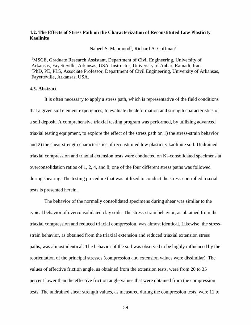
59
The Effects of Stress Path on the Characterization of Reconstituted Low Plasticity
Kaolinite
Nabeel S. Mahmood1, Richard A. Coffman2
1MSCE, Graduate Research Assistant, Department of Civil Engineering, University of
Arkansas, Fayetteville, Arkansas, USA. Instructor, University of Anbar, Ramadi, Iraq. 2PhD, PE, PLS, Associate Professor, Department of Civil Engineering, University of Arkansas,
Fayetteville, Arkansas, USA.
Abstract
It is often necessary to apply a stress path, which is representative of the field conditions
that a given soil element experiences, to evaluate the deformation and strength characteristics of
a soil deposit. A comprehensive triaxial testing program was performed, by utilizing advanced
triaxial testing equipment, to explore the effect of the stress path on 1) the stress-strain behavior
and 2) the shear strength characteristics of reconstituted low plasticity kaolinite soil. Undrained
triaxial compression and triaxial extension tests were conducted on Ko-consolidated specimens at
overconsolidation ratios of 1, 2, 4, and 8; one of the four different stress paths was followed
during shearing. The testing procedure that was utilized to conduct the stress-controlled triaxial
tests is presented herein.
The behavior of the normally consolidated specimens during shear was similar to the
typical behavior of overconsolidated clay soils. The stress-strain behavior, as obtained from the
triaxial compression and reduced triaxial compression, was almost identical. Likewise, the stress-
strain behavior, as obtained from the triaxial extension and reduced triaxial extension stress
paths, was almost identical. The behavior of the soil was observed to be highly influenced by the
reorientation of the principal stresses (compression and extension values were dissimilar). The
values of effective friction angle, as obtained from the extension tests, were from 20 to 35
percent lower than the effective friction angle values that were obtained from the compression
tests. The undrained shear strength values, as measured during the compression tests, were 11 to

60
38 percent greater than the those measured in the extension tests. The axial strain values, at
failure, from the extension tests were determined to be 0.3 to 5.0 percent greater than those
obtained from the compression tests. As discussed herein, for practical purposes, a testing
program that includes triaxial compression tests along with reduced triaxial extension tests is
adequate to represent loading or unloading in the field, respectively.
Keywords: Triaxial testing methods; Reconstituted soils; Stress path; Stress-strain behavior; Pore
pressure; Site characterization
Introduction
Triaxial testing is widely used, within the laboratory, to evaluate the strength and strain
properties of various soil types. The method of increasing or decreasing the principal stresses on
a given sample, commonly referred to as a stress path, has been shown to play a significant role
when evaluating the strength and strain properties of clay soils (Lambe 1967). For many
geotechnical problems, such as those related to: passive earth pressure, excavation support, and
slope stability, the major and minor principal stress states are switched due the field loading
conditions. Based on the concept of stress path, many site characterization and design methods
have been developed to account for the various orientations of the major, minor, and
intermediate principal stress states. For instance, one procedure, identified by the acronym
SHANSEP (Stress History and Normalized Soil Engineering Properties), was developed by Ladd
and Foott (1974) and later modified by Ladd and DeGroot (2003) to evaluate the undrained shear
strength of clay. The SHANSEP procedure was developed because data from triaxial
compression test often led to either unsafe or over-conservative designs.
Many other methods have also been used to predict the stress-strain response of a given
soil deposit when the soil deposit is subjected to foundation loading or to loading induced by
61
excavations (e.g., Davis and Poulos 1968, Simons and Som 1970, Davis and Poulos 1972,
Coffman et al. 2010). These other methods were developed to account for changes in the stress
state within the soil deposit. For these methods, representative soil parameters, as obtained from
laboratory stress path tests, were required to determine the field loading conditions. Furthermore,
the utilization of stress path tests has received additional attention in recent years. This increased
level of attention has been associated with only limited amounts of triaxial compression testing
data being available to evaluate the parameters for advanced constitutive models. As discussed in
Lade (2005) and Bryson and Salehian (2011), most of the current research related to advanced
constitutive modeling has focused on the effect of anisotropy and stress path.
During the shearing stage of triaxial tests, the soil specimen may be sheared in triaxial
compression or triaxial extension by increasing or decreasing one or more of the three principal
stresses. As described by Lambe (1967) and Ladd and Varallyay (1965), there are four stress
paths that represent most of the common field loading conditions: triaxial compression (TC),
reduced triaxial compression (RTC), triaxial extension (TE), and reduced triaxial extension
(RTE). During the shearing stage of the TC and RTE tests, the cell pressure is maintained while
the axial stress is increased for the TC tests or decreased for the RTE tests. For the other two
types of tests (RTC and TE), the specimens are sheared by maintaining the axial stress and
decreasing the cell pressure for the RTC tests or increasing the cell pressure for the TE tests. The
term “R”, as used in the prescribed acronyms, has previously been used to describe the tests that
were performed by reducing the cell pressure (RTC tests) or reducing the axial stress (RTE tests)
during the shearing stage (Salazar and Coffman 2014, Salazar et al. 2017, Zhao et al. 2018). The
term “reorientation” of principal stresses was introduced by Duncan and Seed (1966) to describe
the change in the state of stress when the orientation of the principal stresses, at the end of

62
shearing stage, did not coincide with the orientation of the initial principal stresses. During
triaxial compression, the orientation of the principal stresses at the end of shearing stage is the
same as the orientation of the principal stresses at the beginning of the shearing stage. However,
during triaxial extension testing, decreasing the vertical stress or increasing the horizontal stress
during the shearing may cause the major principal stress to act in the horizontal direction and the
minor principal stress to act in the vertical direction. Therefore, the principal stresses will be
reoriented by 90 degrees at the end of shearing stage (Duncan and Seed 1966).
The stress path that a specimen undergoes is one of the major factors that influences both
the drained and undrained shear strength parameters for a given soil. Over the past few decades,
the relationship between the effective friction angle ( ' ), as measured from undrained triaxial
tests with pore water pressure measurements, and the stress path has been controversial. A few
researchers have indicated that the effect of the stress path on the effective shear strength is
insignificant. For example, Duncan and Seed (1966) and Gens (1983) reported that the effective
angle of internal friction in compression (comp' ) and the effective angle of internal friction in
extension ( ext' ) are approximately equal. Other researchers (e.g., Parry 1960, Saada and
Bianchanini 1977, Rossato et al. 1992) reported that comp' is less than ext' by several degrees.
Based on the results presented in Atkinson et al. (1990), the critical state lines for the
compression and extension tests were symmetrical about the mean effective stress (p′) axis; the
comp' values were significantly less than ext' values. Parry (2004) attributed the difference in the
comp' and ext' results to the instability of the specimen in extension tests due to the rapid
development of necking near failure. Based on the results from other studies (e.g., Ladd and
Foott 1974, Parry and Nadarajah 1974, Moniz 2009), the values of undrained strength (su) of
extension tests were 10 to 25 percent less than those obtained from compression tests. As

63
discussed by Skempton (1954), the reorientation of the principal stresses influenced the amount
of pore water pressure developed during the shearing stage of the triaxial test, thereby affecting
the measured strength.
According to Olson (1962), Burland (1990), and Prashant and Penumadu (2007), the
arrangement of particles and arrangement of pore space within a given soil, commonly referred
to as the microfabric, has also been shown to play an essential role in the engineering behavior of
clayey soils. Soil microfabric can vary considerably as a result of using different water content
values to “reconstitute” (Burland 1990) clay soils. To form a reconstituted structure, Burland
(1990) suggested that the water content of the mixed slurry should be between 1 to 1.5 times the
liquid limit of the soil. The term “intrinsic” was introduced by Burland (1990) to describe the
properties for specimens that were reconstituted within the aforementioned water content values.
Burland (1990) further reported that shear strength and compressibility of reconstituted soils may
be utilized to develop a reference framework to correlate obtained properties with those from
intact soils.
Olson (1962) indicated that laboratory prepared specimens, at water content less than or
slightly above liquid limit, may not represent the natural deposition process. Moreover, Olson
(1962) mentioned that these specimens will have dispersed microfabric and exhibit intrinsic
properties of overconsolidated clayey soil regardless of the level of overconsolidation within the
specimen. To obtain more representative specimens, Olson (1962) reported that the water content
of the mixed slurry should be at least two times the liquid limit. However, sedimentation of
specimens at such high water content requires an extended period of time. Moreover, it has been
shown that these specimens are often difficult to extrude and trim. Therefore, the following
researchers: Henkel (1956), Parry (1960), Bryson and Salehian (2011), Tiwari and Ajmera

64
(2011), Zhao and Coffman (2016), Zhao et al. (2017), and Zhao et al. (2018) have instead
prepared reconstituted clay specimens at lower water content values.
To date, data obtained from historic TC tests have been 1) utilized to determine the
stress-strain behavior, and then 2) used as inputs for constitutive models. TC tests have
specifically been used because of the simplicity and expediency of the TC test as compared with
other tests (Bishop and Henkel 1962, Kulhawy and Mayne 1990, Prashant and Penumadu 2004).
Relatively few studies (e.g., Ladd and Varallyay 1965, Simons and Som 1970, Wroth 1984) have
reported the results from undrained RTC or TE tests. Furthermore, problems associated with
previous triaxial extension test results have prevented the use of the results (Wu and Kolymbas
1991, VandenBerge et al. 2015). Specifically, development of necking during shearing in
extension tests (Sheahan 1991, Liu 2004), inaccurate determination of the cross-sectional area
during shearing (Scholey et al. 1996, Salazar and Coffman 2015), and friction between the
loading piston and the bearings within the top cap of the triaxial cell (Bishop and Henkel 1962,
Race and Coffman 2011) have all resulted in testing errors within previously obtained triaxial
extension test results.
Recent advances in the triaxial testing apparatus, including servo-controlled loading
systems to control the stress-strain measurements, have led to a reduction in the amount of
testing errors associated with the triaxial extension test. These advances have also led to stress
path dependent triaxial tests being easier to conduct. The results from an experimental study on
the effects of the change in the magnitudes and/or orientations of the principal stresses on
parameters including: shear strength, stress-strain behavior, and excess pore water pressure
development in reconstituted low plasticity kaolinite, under undrained triaxial testing conditions,
are presented herein. A procedure to perform stress-controlled triaxial testes is also presented. A

65
total of four series of triaxial compression and triaxial extension tests were conducted on
kaolinite specimens that were reconstituted in the laboratory at water content values of 1.5 times
the liquid limit of the kaolinite soil. The data obtained from these tests were analyzed and
compared to develop an understanding of the testing techniques required to represent certain
field conditions. Moreover, these data will be useful to develop or validate kaolinite-based
constitutive models.
Testing Program
The main objective of the testing program, that is presented herein, was to determine the
effect of stress path on the shear strength characteristics of saturated, reconstituted, low plasticity
kaolinite. A flow chart of the testing program is shown in Figure 4.1. As shown in the flow chart
of the testing program, the specimens were Ko- consolidated to various levels of OCR and then
sheared by following one of four stress paths: TC, RTC, TE, or RTE. The angle of reorientation
of the principal stress between the compression tests and the extension tests was 90 degrees.
During the shearing stage, either the axial stress ( a ) or the cell pressure ( c ) was changed to
produce the required total stress paths (Figure 4.2).
Test Material and Specimens Preparation
To obtain high-quality, fully-saturated, reconstituted, soil specimens, laboratory prepared
specimens were created and utilized. Kaolinite soil was selected 1) due to the high value of
permeability and 2) to compare with other available data in the literature (Jafroudi, 1983, Zhao
and Coffman, 2016, Zhao et al., 2018). The high value of permeability of the kaolinite reduced

66
Figure 4.1. Flow chart of the testing program.
Figure 4.2. Total stress paths that were followed to shear the samples.
the amount of time required to obtain primary consolidation and also provided a more
homogenous distribution of pore water pressure through the specimen. Specifically, KaoWhite-
S, a commercially available product that is produced by The Thiele Kaolin Company in
Sandersville, Georgia, was utilized. This type of kaolinite has been extensively used at the
University of Arkansas to study the strength, consolidation, and small-strain stiffness of

67
laboratory prepared soils (Coffman et al. 2014, Zhao and Coffman 2016, Zhao et al. 2017, Zhao
et al. 2018). The kaolinite soil had a liquid limit of 32 percent, a plastic limit of 28 percent, and a
clay size fraction (<0.002 mm) of 47 percent.
The specimens were prepared in accordance with the procedure that was reported in Zhao
and Coffman (2016), Zhao et al. (2018), and Zhao et al. (2018). Specifically, the kaolinite slurry
was prepared at a water content of 1.5 times the liquid limit of the kaolinite by manually mixing
dry powdered kaolinite with deaired, deionized, water. The slurry was mixed together with a
spatula for three minutes. The slurry was then allowed to settle for one minute, and was then
remixed again for one additional minute. Following mixing, the slurry was poured into a 3.81
centimeter inside diameter slurry consolidometer, and was allowed to consolidate, in a double
drained condition, under a constant vertical stress of 207 kPa that was applied to the soil by static
weight.
The time for primary consolidation was calculated according to the square root of time
procedure, as described by Taylor (1948). After primary consolidation was completed, one
specimen was extruded at a time (two total specimens) from each consolidometer. The
consolidated specimens were cut using a wire saw to develop a length to diameter ratio of two
for each specimen. After extrusion of a given specimen from the consolidometer, the specimen:
length, diameter, and weight were measured, and trimmings were collected for initial water
content and phase diagram measurements for each of the soil specimens.
Triaxial Testing
Using advanced, automated, triaxial equipment, a series of Ko-consolidated, undrained,
triaxial compression ( UTCCKo ) and Ko-consolidated, undrained, triaxial extension ( UTECKo )
tests, with pore water pressure measurements, were conducted on the laboratory prepared

68
kaolinite specimens. GEOTAC (Geotechnical Test Acquisition Control) equipment and software
were utilized to perform these tests and to record the data. The equipment was comprised of a
triaxial chamber, an automated load frame, and two pumps that were used to control and
measure: stresses, strains, cell pressure, and pore pressure within the soil specimen during the
tests. The axial stress was measured inside the triaxial cell with an internal load cell to eliminate
the effect of piston friction. The triaxial compression tests were conducted in accordance with
ASTM D4767 (2011). Because there is no standard for triaxial extension tests, these tests were
conducted following the procedures described by Parry (1960) and Bishop and Henkel (1962).
The data from all of the tests were recorded and stored by the associated data acquisition system.
The individual specimens were mounted within the triaxial chamber using the wet
preparation method as described in ASTM D4767 (2011). Two saturated porous stones were
placed at the top and the bottom of the specimen. Filter paper was placed between the top and
bottom surfaces of the specimen and the porous stones. To ensure no fluid connectivity between
the cell fluid and the pore fluid, the specimen was encompassed by two latex, non-lubricated
membranes (condoms) and two rubber o-rings were used at each end of the specimen to clamp
the membranes to the top and bottom platens located above and below the specimen,
respectively. By utilizing a vacuum top cap connection (as previously described by Race and
Coffman, 2011 and in Salazar and Coffman, 2014), the loading piston was connected to the top
platten to allow application of a downward or upward axial force. To prevent damage to the
internal electronics, silicon oil (5cSt) was utilized, instead of water, as the confining fluid. A
back pressure of at least 276 kPa was used to saturate each specimen and to achieve a pore
pressure parameter (B) value greater than 0.95.

69
After the back pressure saturation stage was completed, strain-controlled consolidation,
with a strain rate of 0.2 percent per hour, was utilized to consolidate each specimen. The
GEOTAC software controlled the axial force and the cell pressure, to maintain zero lateral strain,
based on the feedback from the change in the pore water volume. As listed in Table 4.1, for each
overconsolidation ratio (1, 2, 4, and 8), the specimens were initially re-consolidated within the
triaxial cell under the Ko-conditions to maximum vertical effective stress values of 310, 414, and
828 kPa and then overconsolidated to the respective OCR levels. As recommended by the
SHANSEP procedure, the stress levels represented 1.5, 2, and 4 times the vertical effective stress
that was used to pre-consolidate the kaolinite slurry within the slurry consolidometer. The Ko
values were measured for the specimens during the consolidation and the overconsolidation
processes. After consolidating each of the specimens to the required level of vertical effective
stress, each specimen was then sheared, under undrained conditions, at an axial strain rate of 0.5
percent per hour. A total of 48 specimens (12 specimens per stress path) were required to
develop the four stress paths at the various levels of OCR (as previously presented in Figure 4.1).
Table 4.1. Stresses associated with the triaxial testing consolidation and overconsolidation
processes.
Maximum Vertical Consolidation
Stress ('v,max), kPa
Pre-shear Vertical Effective Stress ('vc), kPa
OCR=1 OCR=2 OCR=4 OCR=8
310 310 155 78 39
414 414 207 103 52
828 828 414 207 103
Although, the GEOTAC software controlled all stages of the test: seating, back pressure
saturation, consolidation, and shear, inherent shearing procedures were only available within the
GEOTAC software for the TC and RTE tests. Following these two stress paths, the cell pressure
was maintained and the axial stress was altered by moving the loading piston downward for TC
or upward for RTE (strain-controlled) with a constant strain rate of 0.5 percent per hour. To

70
measure the plastic failure, these tests were continued until 15 percent axial strain was reached.
The other two types of tests (RTC and TE) were stress-controlled tests. For these tests, the
principal stresses were changed by manually controlling the loading piston and the cell pressure
by utilizing the “manual mode” within the GEOTAC software program. For the RTC and TE
tests, when the cell pressure was changed by c for each step, the deviatoric stress was also
simultaneously changed by d to maintain a constant axial stress (Equation 4.1). The initial
change in the cell pressure, for the first step in each of the stress-controlled tests, was estimated
based on the maximum deviatoric stress and shearing duration of the corresponding, previously
completed, strain-controlled compression and extension tests (i.e. TC and RTE). The rate of
strain was monitored every hour and c was adjusted to maintain an axial strain rate of 0.5
percent per hour. However, once the failure was approached and due to the stress softening,
excessive levels of strain rate (2.5 to 6 percent per hour) were imposed by the system to maintain
the target stresses over the period of the stress increment. Therefore, the stress-controlled tests
were stopped at that point and stress-strain data were not considered for these large levels of
strain rate. Also, for this reason maximum deviatoric stress was considered as a failure criterion
for all the tests. Similar failure criterion for stress-controlled tests was also considered by Parry
and Nadarajah (1974).
A
AA pc
cd
)( Equation 4.1
where Ac was the area of the specimen top cap; Ap was the area of the piston; A was the
corrected area of the specimen at the test step; and c was positive when cell pressure increased
and negative when the cell pressure decreased.

71
Test Results and Discussion
The behavior of the undrained kaolinite, as obtained from the triaxial tests using the four
stress paths, is discussed herein. Specifically, for completeness, four main parts including: 1)
shear strength parameters, 2) stress-strain relationships, 3) Young’s Modulus, and 4) pore water
pressure response are discussed. These parameters are also compared with literature values to
gain insight into the measured behavior of the kaolinite soil.
Shear Strength Parameters
Effective stress paths, for each series of the tests, in terms of mean effective stress
)3
'2''( cap
and deviatoric stress )''( caq , are shown in Figure 4.3. To determine the
effective cohesion ( 'c ) and the effective friction angle ( ' ) values, failure envelopes were
developed based on the peak principal stress difference (PPSD) that were observed for each
stress path. The specimens that were sheared along compression stress paths (TC and RTC)
followed identical effective stress paths, however the specimens reached different maximum
deviatoric stress values. Similar behavior was also noticed for the specimens sheared along
extension stress paths (TE and RTE).
The effective stress paths for the OCR=1 tests initially decreased in 'p during shearing
(indicating contractive behavior), but before reaching the peak principal stress difference, the
stress paths changed direction and began to move to the right (indicating dilative behavior) until
the failure envelope was reached. This pattern of behavior, during shearing stage, has typically
not been observed for naturally occurring, normally consolidated, clay soil types. However, this
behavior was in agreement with prior studies conducted on reconstituted clays (Parry 1960 and
Olson 1962). On the other hand, the effective stress paths for the overconsolidated specimens
followed the typical behavior of overconsolidated clays. The stress path moved to the right

72
during shear (dilative behavior) then bent downward or upward for compression and extension,
respectively, after reaching the failure envelope.
Figure 4.3. Cambridge effective stress paths of the triaxial compression and triaxial
extension tests on reconstituted kaolinite: a) OCR= 1, b) OCR= 2, c) OCR= 4, d) OCR= 8.
The variations of the 'c and ' values, as a function of the overconsolidation ratio, are
shown in Figures 4.4 and 4.5, respectively. It is unusual to have effective cohesion intercept
-400
-300
-200
-100
0
100
200
300
400
500
0 100 200 300 400 500 600 700
Devia
tori
c S
tress, q
, [k
Pa]
Mean Effective Stress, p', [kPa]
Compression
Extension
OCR=4
-400
-300
-200
-100
0
100
200
300
400
500
0 100 200 300 400 500 600 700
Devia
tori
c S
tress
, q,
[kP
a]
Mean Effective Stress, p', [kPa]
TC PPSD-TC
RTC PPSD-RTC
TE PPSD-TE
RTE PPSD-RTE
OCR=8
Compression
Extension
-400
-300
-200
-100
0
100
200
300
400
500
0 100 200 300 400 500 600 700
Devia
tori
c S
tress
, q,
[kP
a]
Mean Effective Stress, p', [kPa]
Compression
Extension
OCR=2
-400
-300
-200
-100
0
100
200
300
400
500
0 100 200 300 400 500 600 700
Devia
tori
c S
tress, q
, [k
Pa]
Mean Effective Stress, p', [kPa]
Compression
Extension
OCR=1
(a) (b)
(c) (d)

73
values for normally consolidated soils (Holtz et al. 2011), however those values may also
indicate that the behavior of the normally consolidated reconstituted kaolinite is similar to the
behavior of the overconsolidated specimens. It was clear that 'c values and ' values obtained
from the compression tests (TC and RTC) were similar. Comparable values were also obtained
from the extension (TE and RTE) tests; albeit, there was a difference in the cohesion values for
the extension tests at low levels of OCR and in the friction angle values for the compression tests
at high levels of OCR. Based on these observations, for the specimens that were consolidated to
the same vertical effective stress and sheared following the same mode (compression or
extension), the effective stress path was independent of the change in the magnitude of the
principal stresses. Similar results were reported by Simons and Som (1970) and Wroth (1984).
The change in the stress path, as associated with reorientation of the principal stresses
(from compression to extension), had a significant effect on the effective shear strength
parameters. As shown in Figure 4.4, the c' values obtained from the extension tests were greater
than those obtained from the compression tests by 8 to 34 kPa (almost four times as great for all
levels of OCR). However, as indicted by Ladd and Varallyay (1965), the cohesion intercept has
been shown to be difficult measure accurately. The relationships between the effective internal
friction angle and the OCR, for the different stress paths are shown in Figure 4.5. The values of
' for extension tests were 20 to 35 percent less than those for corresponding compression tests.
Similar results and findings regarding the values from extension tests being less than the values
obtained from compression tests were reported by Parry (1960) and Saada and Bianchanini
(1977).
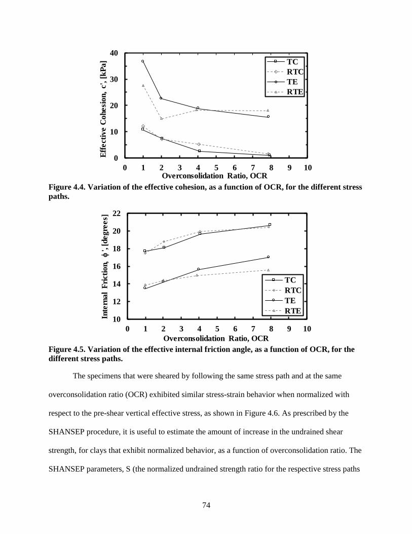
74
Figure 4.4. Variation of the effective cohesion, as a function of OCR, for the different stress
paths.
Figure 4.5. Variation of the effective internal friction angle, as a function of OCR, for the
different stress paths.
The specimens that were sheared by following the same stress path and at the same
overconsolidation ratio (OCR) exhibited similar stress-strain behavior when normalized with
respect to the pre-shear vertical effective stress, as shown in Figure 4.6. As prescribed by the
SHANSEP procedure, it is useful to estimate the amount of increase in the undrained shear
strength, for clays that exhibit normalized behavior, as a function of overconsolidation ratio. The
SHANSEP parameters, S (the normalized undrained strength ratio for the respective stress paths
0
10
20
30
40
0 1 2 3 4 5 6 7 8 9 10
Eff
ect
ive
Co
he
sio
n,
c',
[kP
a]
Overconsolidation Ratio, OCR
TC
RTC
TE
RTE
10
12
14
16
18
20
22
0 1 2 3 4 5 6 7 8 9 10
Inte
rna
l F
rict
ion,
',
[de
gre
es]
Overconsolidation Ratio, OCR
TC
RTC
TE
RTE

75
at OCR=1) and m (the slope of the regression line for the respective stress paths), are presented
in Figure 4. 7 for the various stress paths. The four stress paths exhibited similar normalized
behavior; increased levels of overconsolidation produced increased levels of normalized
undrained shear strength. Although the values of m parameter are, typically, larger for extension
tests than for compression tests (Ladd and DeGroot 2003), the values of m obtained from the
four stress paths were similar. The measured values for the m parameter (0.54 to 0.56) were
smaller than the typical value of 0.8 (Ladd 1991, Jamiolkowski et al. 1985) for silt soils.
Likewise, with one exception for RTE tests, the measured values for the S parameter (0.26 to
0.28) were larger than the typical value of 0.25 (Ladd 1991) for most silt soils. These findings
were in agreement with Ladd (1991), which organic clays and silts had more scattered
normalized shear strength than inorganic clays.
Figure 4.6. Normalized deviatoric stress, as a function of axial strain, for the TC tests at
OCR=1.
0
0.1
0.2
0.3
0.4
0.5
0.6
0.7
0.8
0.9
1
0 2 4 6 8 10 12 14 16
No
rma
lize
d
De
via
tori
c S
tre
ss, q
/σ' v
c
Axial Strain, A, [%]
OCR = 1
σ’ = 310 kPa
σ’ = 414 kPa
σ’ = 828 kPa
PPSD
v,max
v,max
v,max

76
Figure 4.7. Normalized undrained shear strength values from the SHANSEP procedure.
The measured undrained shear strength values obtained from the compression tests were
11 to 38 percent greater than the undrained shear strength values obtained from the extension
tests. As described by Bishop (1966), the lower values of the undrained strength that were
obtained from the triaxial extension tests may be attributed to the difference in the amount of
excess pore water pressure that developed during shearing. Overall, the normalized undrained
shear strength values that were measured during the stress-controlled tests (i.e RTC and TE)
were higher than those measured in strain-controlled tests (i.e TC and RTE). These higher values
that were obtained from the stress-controlled tests may be attributed to the high rate of strain that
developed during the shearing stage when the specimens yielded.
Stress-Strain Relationships
The deviatoric stress-axial strain curves for all of the tests are shown in Figure 4.8. The
points of PPSD are also indicated for completeness. The same general shape of the stress-strain
curves was observed for both the normally consolidated and overconsolidated specimens that
were tested following the TC and RTE stress paths. The behavior was characterized by a peak
deviatoric stress followed by postpeak strain softening. The pattern of failure for the RTC and
0.1
1.0
1 10
Norm
ali
zed
S
hear
Str
en
gth
, s u
/σ' v
c
Overconsolidation Ratio, OCR
TC
RTC
TE
RTE
S m
0.28
0.28
0.26
0.25
0.54
0.55
0.54
0.56

77
TE was similar to the TC and RTE stress paths, respectively, with higher magnitudes of
deviatoric stress )(q and higher values of axial strain at failure )( , fA being observed for the RTC
Figure 4.8. Variation of deviatoric stress as a function of axial strain for different stress
paths: a) OCR= 1, b) OCR= 2, c) OCR= 4, d) OCR= 8.
tests. Because the RTC and TE tests were stress controlled, no postpeak stress-strain data were
observed and no softening was observed. Generally, for each overconsolidation ratio, and each
-450
-350
-250
-150
-50
50
150
250
350
450
-16 -12 -8 -4 0 4 8 12 16
De
via
tori
c S
tre
ss, q
, [k
Pa
]
Axial Strain, A, [%]
σ’ = 310 kPa
σ’ = 414 kPa
σ’ = 828 kPa
PPSD-TC
PPSD-RTC
PPSD-TE
PPSD-RTE
v,max
Compression
Extension
OCR=1
v,max
v,max
-450
-350
-250
-150
-50
50
150
250
350
450
-16 -12 -8 -4 0 4 8 12 16
De
via
tori
c S
tre
ss, q
, [k
Pa
]
Axial Strain, A, [%]
Compression
Extension
OCR=2
-450
-350
-250
-150
-50
50
150
250
350
450
-16 -12 -8 -4 0 4 8 12 16
Devia
tori
c S
tress
, q,
[kP
a]
Axial Strain, A, [%]
Compression
Extension
OCR=4
-450
-350
-250
-150
-50
50
150
250
350
450
-16 -12 -8 -4 0 4 8 12 16
Dev
iato
ric
Str
ess
, q,
[kP
a]
Axial Strain, A, [%]
Compression
Extension
OCR=8
(a) (b)
(c) (d)

78
stress path that was tested, the strain at failure tended to decrease as a function of increasing the
amount of maximum consolidation stress. The overconsolidation ratio had an insignificant effect
on the amount of axial strain at failure. As shown in the photographs presented in Figure 4. 9,
postpeak shear planes were observed for all of the tests regardless of whether the soil was
normally consolidated or overconsolidated. As reported by Burland (1990) and Atkinson et al.
(1987), shear planes were observed to develop in one-dimensional consolidated kaolinite
specimens.
Figure 4.9. Photographs of the kaolinite samples after triaxial testing showing the failure
planes associated with the: a) TC, b) RTC, c) TE, d) RTE stress paths for an OCR=1.
As presented in Figure 4.10, larger axial strain values were required for the extension
tests to mobilize the peak resistance and the postpeak strain softening than were required for the
mobilization to occur in the compression tests. The average values of the axial strain at failure
)( , fA , for the extension tests, were between 0.3 and 5 percent greater than those for the
compression tests. For the compression tests, the fA, values for the RTC tests were between 0.5
and 3.6 percent greater than the axial strain values at failure for the TC tests. For the extension
tests, the fA, values for the RTE tests were between 0.1 and 2.4 percent greater than those for the
TE tests. As described in the previous section, higher deviatoric stresses and axial strains, which
(a) (b) (c) (d)

79
were obtained from the stress-controlled tests, may be attributed to the high rate of strain of the
stress-controlled tests when the specimens yielded. This attribution was also documented in the
results from the previous studies on stress rate effects (e.g., Bjerrum 1969, Sheahan 1991,
Sheahan et al. 1996). From the aforementioned studies, the deviatoric stress at failure has been
shown to decrease with the increasing strain rate.
Figure 4.10. Average values of axial strain at failure for different stress paths, as a function
of OCR.
Young’s Modulus
The variations of undrained secant Young’s modulus, as normalized to the vertical
consolidation stress ( vcuE '/ ), for the different stress paths, are presented in Figure 4.11. In this
figure, the modulus relations for the extension tests were also plotted on the positive side of the
axial strain axis to facilitate a comparison between the extension and compression test results.
Because the axial strain was measured by employing conventional external measurements, the
undrained Young’s modulus values were only determined for axial strain levels above 0.1
percent. Based on the observed variations of the undrained Young’s modulus, as a function of
axial strain, 1) the soil exhibited non-linear behavior and 2) the stiffness significantly decreased
near failure. Normalizable behavior of the Young’s modulus relations was observed for the
0
2
4
6
8
10
12
14
16
0 1 2 3 4 5 6 7 8 9 10
Axia
l S
train
at
Failure
,
A,f
, [%
]
Overconsolidatio Ratio, OCR
TC
RTC
TE
RTE

80
normally consolidated specimens. For these specimens, at an axial strain level of 0.1 percent, the
values of the normalized undrained Young’s modulus for the extension tests were 2 to 2.5 times
larger than the values of the normalized undrained Young’s modulus for the compression tests.
These values were in agreement with Atkinson et al. (1990), where the small strain stiffness was
observed to increase as a result of the change in the direction of the stress path (from
compression, during consolidation stage, to extension). Furthermore, the Young’s modulus
values that were obtained from tests conducted on the normally consolidated specimens, as
determined from the compression tests, were consistently smaller than the Young’s modulus
values of the overconsolidated specimens.
For the overconsolidated specimens, the normalized modulus curves did not exhibit a
normalized behavior. In addition, there was no clear trend of the modulus variations with the
increase in the overconsolidation ratio. As described by Hardin and Blandford (1989) and
Jamiolokwski et al. (1994), the initial undrained Young’s modulus values were dependent on
both the pre-shear effective consolidation stress and the overconsolidation ratio. For the
overconsolidated specimens, as the overconsolidation ratio increased, the pre-shear effective
consolidation stress decreased. Therefore, it was not a simple task to isolate the effect of the
overconsolidation ratio from the effect of the pre-shear effective stress levels.

81
Figure 4.11. Normalized secant Young’s modulus relations for: a) OCR= 1, b) OCR= 2, c)
OCR= 4, and d) OCR= 8.
Excess Pore Water Pressure Response
The variations of excess pore water pressure )( eu , that were developed during shearing,
as normalized to the vertical consolidation stress, for the different stress paths, are shown in
Figure 4.12. Because the excess pore water pressure was generated by a combination of the
0
20
40
60
80
100
120
140
0.1 1 10 100
Norm
alize
d Y
oung's
M
odulu
s, E
u/
' vc
Axial Strain, A, [%]
OCR=4
0
20
40
60
80
100
120
140
0.1 1 10 100
No
rma
lize
d Y
oung
's M
odulu
s, E
u/
' vc
Axial Strain, A, [%]
OCR=8
0
20
40
60
80
100
120
140
0.1 1 10 100
Norm
alize
d Y
ou
ng's
M
od
ulu
s, E
u/
' vc
Axial Strain, A, [%]
TC
RTC
TE
RTE
OCR=1
0
20
40
60
80
100
120
140
0.1 1 10 100
Norm
alize
d Y
oung's
M
odulu
s, E
u/
' vc
Axial Strain, A, [%]
OCR=2
(a) (b)
(c) (d)

82
changes in the shearing stress and the changes in the mean total stress, the changes in excess pore
water pressure that were developed during shear may not be considered as a unique behavior of
the soil, under the applied stress path. The initial portion of the pore pressure response, for all of
the stress paths, changed rapidly over small levels of axial strain. This rapid change in the excess
pore pressure may also explain the shape of the effective stress paths for the normally
consolidated (OCR=1) specimens that were previously presented in Figure 4.3.
For the TC tests that were performed on the normally consolidated specimens, the excess
pore water pressure increased during the shearing stage (indicating contractive behavior) until
the PPSD was reached and then the values dropped slightly. The excess pore water pressure
values, for the TC tests that were conducted on the overconsolidated specimens, showed an
initial contractive response and then the pore pressure response changed from a slightly
contractive behavior to a slightly dilative behavior. For the stress-controlled RTC tests, where
the shearing was associated with a decrease in the cell pressure, a sharp decrease in the amount
of excess pore water pressure was observed without an initial contractive response.
An excess pore pressure response that was larger in magnitude than the response obtained
from the TC tests was generated during the RTC tests. This difference in pore pressure response
was because the shearing during RTC tests was associated with decreasing cell pressure. The
general shapes of the variation of the shear induced pore water pressure, that were developed
during the triaxial extension tests, were similar regardless of the induced amount of the
overconsolidation. As observed by previous researcher, the shear stress-strain and strength
characteristics were highly influenced by the shear induced pore water pressure (Skempton,1954,
Ladd and DeGroot, 2003). Therefore, difference in the magnitude of the measured excess pore

83
water pressure during shear may have caused the slight variation of the stress-strain relationships
that were obtained from the different stress paths (as shown previously in Figure 4.8).
Figure 4.12. Normalized excess pore water pressure relations for: a) OCR= 1, b) OCR= 2,
c) OCR= 4, and d) OCR= 8.
-3.0
-2.5
-2.0
-1.5
-1.0
-0.5
0.0
0.5
1.0
-16 -12 -8 -4 0 4 8 12 16
Norm
lize
d E
xce
ss P
ore
Pre
ssure
, u
e /
' vc
Axial Strain, A, [%]
TC
RTCRTE
TE OCR= 4
-3.0
-2.5
-2.0
-1.5
-1.0
-0.5
0.0
0.5
1.0
-16 -12 -8 -4 0 4 8 12 16
No
rmlize
d E
xce
ss P
ore
Pre
ssure
, u
e /
' vc
Axial Strain, A, [%]
TC
RTC
TE
RTE
OCR= 8
-3.0
-2.5
-2.0
-1.5
-1.0
-0.5
0.0
0.5
1.0
-16 -12 -8 -4 0 4 8 12 16
Norm
lize
d E
xce
ss P
ore
Pre
ssure
, u
e /
' vc
Axial Strain, A, [%]
RTC
TC
RTE
TE OCR= 2
-3.0
-2.5
-2.0
-1.5
-1.0
-0.5
0.0
0.5
1.0
-16 -12 -8 -4 0 4 8 12 16
No
rmlize
d E
xce
ss P
ore
Pre
ssure
, u
e /
' vc
Axial Strain, A, [%]
σ’ = 310 kPa
σ’ = 414 kPa
σ’ = 828 kPa
PPSD-CTC
PPSD-RTC
PPSD-CTE
PPSD-RTE
TE TC
RTE RTC
v,max
OCR= 1
v,max
v,max
(a) (b)
(c) (d)

84
Implementations for Practice
As presented in the previous test results section, for the same orientation of the principal
stress, the shear strength properties and failure conditions did not differ greatly regardless of
which of the stress paths were utilized to shear the specimens. However, when the orientation of
the principal stresses was altered, the corresponding stress paths were different. Even though the
observed normalized excess pore pressure profiles were different between TC and RTC tests,
geotechnical analyses conducted with shear strength values obtained from TC tests will not differ
greatly from analyses based on the values obtained from RTC tests. Likewise, even though the
observed normalized excess pore pressure profiles were different between TE and RTE tests,
geotechnical analyses conducted with shear strength values obtained from TE tests will not differ
greatly from analyses based on the values obtained from RTE tests. Both the effective and the
undrained shear strength parameters were affected by the reorientation of the principal stresses.
When comparing the results from the compression and extension tests, lower values of shear
strain at failure and lower initial stiffness values were measured by the compression tests. Based
on these results, if the TC or RTC tests were utilized to obtain shear strength values for a design
where the TE or RTE were more representative of the field conditions, then the compression data
overestimate the shear strength and lead to an unconservative design. Moreover, TE or RTE tests
data will be essential to develop new constitutive models or to validate existing constitutive
models that have previously been developed based on only TC or RTC data.
Conclusions
Undrained triaxial compression and triaxial extension tests were performed on kaolinite
specimens to study the influence of the stress path on the corresponding shear strength
properties. The specimens were reconstituted at values of water content that were slightly greater
than the liquid limit. Based on the findings, similar stress-strain behavior was observed for the

85
stress paths that had the same orientation of the principal stresses. The stress-strain behavior,
however, was found to be different when the orientation of the principal stresses was changed. In
general, strength and deformation properties generated from the TC tests corresponded closely to
those generated from the RTC tests. The same correspondence was also observed between TE
test data and RTE test data. For simplicity and practicality, TC test results may be utilized when
compression tests are required, and RTE test results may be utilized when extension tests are
required. TC tests data should not be used when extension data are required for design. Likewise,
RTE test results should not be used when compression data are required for design. These test
types are recommended because strain-controlled testing is much easier to perform than the
stress-controlled testing. Regardless of which test is utilized, an internal load cell should be used
to measure the axial load to remove the effects of piston uplift and piston friction.
The reorientation of the principal stresses (from compression to extension) had
significant effects on the effective and undrained shear strength properties. The measured values
of ' were lower for the extension tests than for the compression tests by approximately 20 to 35
percent. The obtained undrained shear strengths values that were collected from the compression
tests were greater than those obtained from the extension tests by 11 to 38 percent. The amounts
of axial strain at failure, as measured from the extension tests, were 0.3 to 5.0 percent greater
than those as measured from the compression tests. The amount of the initial stiffness for
normally consolidated specimens, as evaluated from the undrained secant Young’s modulus
values, were 2 to 2.5 times larger for extension tests than for compression tests. The variation in
the undrained Young’s modulus values for the overconsolidated specimens showed no obvious
trend with the changes in stress path. Moreover, the initial portion of the excess pore water
pressure response for all of the stress paths changed rapidly as a function of axial strain until the

86
yield point was reached. Therefore, any parameters that are utilized to characterize the shear
strength of soil or to validate constitutive models should account for the dependence of the
reorientation of the principal stress state.
References
American Society for Testing and Materials (2011). “Standard Test Method for Unconsolidated-
Undrained Triaxial Compression Test on Cohesive Soils.” Annual Book of ASTM
Standards, Designation D4767, Vol. 4.08, ASTM, West Conshohocken, PA.
Atkinson, J. H., Richardson, D., and Robinson, P. J., (1987). “Compression and Extension of K0
Normally Consolidated Kaolin Clay.” Journal of Geotechnical Engineering, Vol.113. No.
12, pp. 1468-1482.
Atkinson, J.H., Richardson, D. and Stallebrass, S.E., (1990). “Effect of Recent Stress History on
the Stiffness of Overconsolidated Soil.” Geotechnique, Vol.40, No. 4, pp.531-540.
Bishop, A.W., and Henkel, D.J. (1962). “The Measurement of Soil Properties in the Triaxial
Test.” Edward Arnold LTD, London.
Bishop, A. W., (1966). “The strength of soils as engineering materials.” Geotechnique, Vol. 16,
pp. 91-130.
Bjerrum, L., Simons, N., and Toblaa, I., (1958). “The Effect of Time on the Shear Strength of a
Soft Marine Clay.” Proceedings of Conference on Earth Pressure Problems, I, pp.148-
158.
Bryson, L. S., and Salehian, A. (2011). “Performance of Constitutive Models in Predicting
Behavior of Remolded Clay.” Acta Geotechnica, Vol. 6, No. 3, pp.143-154.
Burland, J. B., (1990). “On the Compressibility and Shear Strength of Natural Clays.”
Geotechnique 40 (3), 329-378.
Coffman, R. A., Bowders, J. J., and Burton, P. M., (2010). “Use of SHANSEP Design
Parameters in Landfill Design: A Cost/Benefit Case Study.” ASCE Geotechnical Special
Publication No. 199, Proceedings GeoFlorida 2010, Advances in Analysis, Modeling and
Design, West Palm Beach, FL, Feb 20–24, pp. 2859–2866.
Coffman, R.A., Salazar, S.E., Zhao, Y., (2014). “Discussion of Measurement of Stiffness
Anisotropy in Kaolinite Using Bender Element Tests in a Floating Wall Consolidometer
by X. Kang, G.-C. Kang, B. Bate.” Geotech. Test. J. Vo. 37, No. 6, pp. 1-5.
Davis, E. H., and Poulos, H. G., (1972). “Rate of Settlement Under Two-and Three-dimensional
Conditions.” Geotechnique, Vol. 22, No. 1.
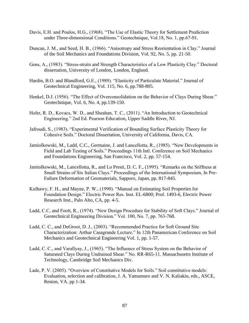
87
Davis, E.H. and Poulos, H.G., (1968). “The Use of Elastic Theory for Settlement Prediction
under Three-dimensional Conditions.” Geotechnique, Vol.18, No. 1, pp.67-91.
Duncan, J. M., and Seed, H. B., (1966). “Anisotropy and Stress Reorientation in Clay.” Journal
of the Soil Mechanics and Foundations Division, Vol. 92, No. 5, pp. 21-50.
Gens, A., (1983). “Stress-strain and Strength Characteristics of a Low Plasticity Clay.” Doctoral
dissertation, University of London, London, England.
Hardin, B.O. and Blandford, G.E., (1989). “Elasticity of Particulate Material.” Journal of
Geotechnical Engineering, Vol. 115, No. 6, pp.788-805.
Henkel, D.J. (1956). “The Effect of Overconsolidation on the Behavior of Clays During Shear.”
Geotechnique, Vol. 6, No. 4, pp.139-150.
Holtz, R. D., Kovacs, W. D., and Sheahan, T. C., (2011). “An Introduction to Geotechnical
Engineering.” 2nd Ed. Pearson Education, Upper Saddle River, NJ.
Jafroudi, S., (1983). “Experimental Verification of Bounding Surface Plasticity Theory for
Cohesive Soils.” Doctoral Dissertation, University of California, Davis, CA.
Jamiolkowski, M., Ladd, C.C., Germaine, J. and Lancellotta, R., (1985). “New Developments in
Field and Lab Testing of Soils.” Proceedings 11th Intl. Conference on Soil Mechanics
and Foundations Engineering, San Francisco, Vol. 2, pp. 57-154.
Jamiolkowski, M., Lancellotta, R., and Lo Presti, D. C. F., (1995). “Remarks on the Stiffness at
Small Strains of Six Italian Clays.” Proceedings of the International Symposium, In Pre-
Failure Deformation of Geomaterials, Sapporo, Japan, pp. 817-845.
Kulhawy, F. H., and Mayne, P. W., (1990). “Manual on Estimating Soil Properties for
Foundation Design.” Electric Power Res. Inst. EL-6800; Prof. 1493-6, Electric Power
Research Inst., Palo Alto, CA, pp. 4-5.
Ladd, C.C, and Foott, R., (1974). “New Design Procedure for Stability of Soft Clays.” Journal of
Geotechnical Engineering Division.” Vol. 100, No. 7, pp. 763-768.
Ladd, C. C., and DeGroot, D. J., (2003). “Recommended Practice for Soft Ground Site
Characterization: Arthur Casagrande Lecture.” In 12th Panamerican Conference on Soil
Mechanics and Geotechnical Engineering Vol. 1, pp. 1-57.
Ladd, C. C., and Varallyay, J., (1965). “The Influence of Stress System on the Behavior of
Saturated Clays During Undrained Shear.” No. RR-R65-11. Massachusetts Institute of
Technology, Cambridge Soil Mechanics Div.
Lade, P. V. (2005). “Overview of Constitutive Models for Soils.” Soil constitutive models:
Evaluation, selection and calibration, J. A. Yamamuro and V. N. Kaliakin, eds., ASCE,
Reston, VA. pp 1-34.

88
Lambe, T. W. (1967). “Stress Path Method.” Journal of Soil Mechanics and Foundations
Division,
Liu, Y. (2004). “The Stress-Strain Behavior of Kaolin Clay in Triaxial.” Ph.D. Thesis. University
of Delaware. Newark, DE.
Moniz, Safia R., (2009). “The Influence of Effective Consolidation Stress on the Normalized
Extension Strength Properties of Resedimented Boston Blue Clay.” MEng Thesis, MIT,
Cambridge, MA.
Olson, R.E., (1962). “The ShearS properties of Calcium Illite.” Geotechnique, Vol.12, No. 1,
pp.23-43.
Parry, R. H. G., (2004). “Mohr Circles, Stress Paths and Geotechnics.” Spon Press, London.
Parry, R.H.G. (1960). “Triaxial Compression and Extension Tests on Remolded Clay.”
Geotechnique, Vol. 10, No. 4, pp. 160-188.
Parry, R.H.G. and Nadarajah, V., (1974). “Observations on Laboratory Prepared, Lightly
Overconsolidated Specimens of Kaolin.” Geotechnique, Vol. 24, No. 4, pp.345-357.
Prashant, A. and Penumadu, D., (2005). “A Laboratory Study of Normally Consolidated Kaolin
Clay.” Canadian Geotechnical Journal, Vol. 42, No. 1, pp.27-37.
Prashant, A., and Penumadu, D., (2007). “Effect of Microfabric on Mechanical Behavior of
Kaolin Clay Using Cubical True Triaxial Testing.” J. Geotech. Geoenviron. Eng. Vol.
133, No. 4, pp. 433-444.
Race, M.L., Coffman, R.A., (2011). “Effects of Piston Uplift, Piston Friction, and Machine
Deflection in Reduced Triaxial Extension Testing.” ASCE Geotechnical Special
Publication No. 211, Proc. GeoFrontiers 2011: Advances in Geotechnical Engineering,
Dallas, Texas, March, pp. 2649-2658.
Rossato, G., Ninis, N. L., and Jardine, R. J., (1992). “Properties of Some Kaolin-based Model
Clay Soils.” Geotech. Test. J., Vol. 15, No. 2, pp.166-179.
Saada, A.S. and Bianchini, G.F., (1977). “Strength of One Dimensionally Consolidated Clays.”
Journal of Geotechnical and Geoenvironmental Engineering, Vol. 103, (HGT-6), pp. 655-
660.
Salazar, S. E. and Coffman, R. A., (2014). “Design and Fabrication of End Platens for
Acquisition of Small-Strain Piezoelectric Measurements During Large-Strain Triaxial
Extension and Triaxial Compression Testing.” Geotechnical Testing Journal, Vol. 37,
No. 6, pp. 1-12.
Salazar, Sean E. and Coffman, Richard A., (2015). “Consideration of Internal Board Camera
Optics for Triaxial Testing Applications.” Geotechnical Testing Journal, Vol. 38, No. 1,
pp. 1–10.

89
Salazar, S.E., Miramontes, L.D., Barnes, A.R., Bernhardt, M.L., Coffman, R.A., (2017).
“Verification of an Internal Close-range Photogrammetry Approach for Volume
Determination During Undrained Triaxial Testing.” Geotech. Test. J. (Under Second
Review, Manuscript Number: GTJ-2017-0125-R1).
Scholey, G. K., Frost, J. D., Lo Presti, D. C. E, and Jamiolkowski, M. (1996). “A Review of
Instrumentation for Measuring Small Strains During Triaxial Testing of Soil Specimens.”
Geotechnical Testing Journal, GTJODJ, Vol. 18, No. 2, pp. 137-156.
Sheahan, T. C. (1991). “An Experimental Study of the Time-dependent Undrained Shear
Behavior of Resedimented Clay Using Automated Stress Path Triaxial Equipment.”
Doctoral dissertation, Massachusetts Institute of Technology, MA.
Sheahan, T.C., Ladd, C.C., and Germaine, J.T., (1996). “Rate-dependent Undrained Shear
Behavior of Saturated Clay.” Journal of Geotechnical Engineering, Vol. 122, No. 2, pp.
99-108.
Simons, N. E. and Som, N. N. (1970). “Settlement of Structures on Clay: with Particular
Emphasis on London Clay.” Construction industry research and information Association,
London. Report 22.
Skempton, A. W. (1954) “The Pore-pressure Coefficients A and B.” Geotechnique, Vol. 4, No.
4, pp.143-147.
Taylor, D. W., (1948). “Fundamentals of Soil Mechanics.” John Wiley and Sons, New York,
NY.
Tiwari, B., and Ajmera, B., (2011). “New Correlation Equations for Compression Index of
Remolded Clays.” Geotechnical and Geoenvironmental Engineering, Vol. 138, No. 6, pp.
757-762.
Wroth, C. P., (1984). “The Interpretation of in Situ Soil Tests.” Geotechnique, Vol. 34, No. 4,
pp. 449-489.
Wu, W., and Kolymbas, D., (1991). “On Some Issues in Triaxial Extension Tests.” Geotechnical
Testing Journal, Vol. 14, No. 3, pp. 276-287.
Zhao, Y., and Coffman, R.A., (2016). “Back-Pressure Saturated Constant-Rate-of-Strain
Consolidation Device with Bender Elements: Verification of System Compliance.”
Journal of Testing and Evaluation, Vol. 44, No. 6, pp. 1-12.
Zhao, Y., Mahmood, N., and Coffman, R. A., (2017). “Soil Fabric and Anisotropy as Observed
Using Bender Elements during Consolidation.” Clays and Clay Minerals, Under Review,
Manuscript Number: CCM-1143.
Zhao, Y., Mahmood, N. S., and Coffman, R.A., (2018). “Small-Strain and Large-Strain Modulus
Measurements with a Consolidation Device.” Journal of Testing and Evaluation, In Press,
Manuscript Number: JTE-2016-0331.

90
Intrinsic Shear Strength Behavior of Reconstituted Kaolinite and Illite Soils
Chapter Overview
The effect of slurry water content on the shear strength behavior of reconstituted soils
was introduced and discussed. Specifically, undrained triaxial compression tests were performed
on kaolinite and illite soil specimens to evaluate the relationship between the slurry water content
values and the corresponding shear strength parameters. The influence of the slurry water content
on the soil fabric and the compression behavior of the reconstituted soils was also introduced and
discussed. A new method was proposed to normalize the undrained shear strength values of
overconsolidated soils based on the concept of the intrinsic shear strength line. Using this
proposed method, void index values were determined from the intrinsic swelling line rather than
from the intrinsic compression line. Better correlation between the undrained shear strength
values, for the overconsolidated specimens, and the intrinsic shear strength line was obtained by
using the proposed normalization method. It was recommended to prepare soil slurries at water
content of three times the corresponding liquid limit of the soil.
An introduction including the research description and summary is included as Section
5.1 through Section 5.3. A literature review of the intrinsic shear strength characteristics is
included in Section 5.4. The materials and the experimental program are presented in Section
5.5. The results obtained from the triaxial tests are documented in Section 5.6. The paper
enclosed in this chapter has been submitted within Quarterly Journal of Engineering Geology
and Hydrogeology. The full reference is: Mahmood, N. S., and Coffman, R. A., (2018a).
“Intrinsic Shear Strength Behavior of Reconstituted Kaolinite and Illite Soils.” Quarterly
Journal of Engineering Geology and Hydrogeology, (In Review, Manuscript Number:
qjegh2018-056-R1).

91
Intrinsic Shear Strength Behavior of Reconstituted Kaolinite and Illite Soils
Nabeel S. Mahmood1, Richard A. Coffman2
1MSCE, Graduate Research Assistant, Department of Civil Engineering, University of
Arkansas, Fayetteville, Arkansas, USA. Instructor, University of Anbar, Ramadi, Iraq. 2PhD, PE, PLS, Associate Professor, Department of Civil Engineering, University of Arkansas,
Fayetteville, Arkansas, USA.
Abstract
The initial water content that is utilized to reconstitute cohesive soils, into a slurry (ws),
may have significant effects on the compression and shear strength behavior of any given soil.
The effects are due to the influence of the ws on the soil fabric. A series of Ko-reconsolidated,
undrained, triaxial compression tests were conducted on reconstituted kaolinite and reconstituted
illite specimens to explore the relationship between ws values and the corresponding shear
strength characteristics. The soil specimens were created from a slurry mixture at two levels of
ws; ws values of one and one-half (1.5) and three (3.0) times the corresponding liquid limit of
each soil type were investigated. The intrinsic compression, swelling, and shear strength lines
were established from the test results. When sheared from the same level of post consolidation
vertical stress, the undrained shear strength values of the specimens with ws values of 3.0 times
the liquid limit were from five to 16 percent lower than those of the specimens with ws of 1.5
times the liquid limit. The effective cohesion tended to increase by increasing the value of ws.
The values of the effective friction angle () were found to be independent of the ws values.
A new method is proposed herein to provide a better correlation between the normalized
values of the undrained shear strength for overconsolidated specimens and the “intrinsic shear
strength line.” Using this proposed method, void index values were determined from the intrinsic
swelling line rather than from the intrinsic compression line. As discussed herein, reconstituting
a low plasticity kaolinite soil at ws values of 1.5 times the liquid limit may not be appropriate for

92
evaluating of the intrinsic shear strength characteristics. However, the illite soil appeared to be
less affected than kaolinite soil by an increase in the ws values. These finding were based on the
observed soil fabric and the undrained shear strength behavior.
Keywords: Reconstituted soils; Slurry water content; Intrinsic behavior; Triaxial testing; Stress
path; Undrained shear strength
Background
Laboratory prepared specimens are often utilized to characterize the engineering behavior
of natural soils. These prepared specimens basically prepared by mixing natural soil with water
to form a slurry of the given soil. The slurry is often consolidated, in a slurry consolidometer, to
a certain consolidation stress that is related to the in-site effective stress (Henkel 1956, Olson
1962, Burland 1990, Chandler 2000, Hong et al. 2013, Zhao et al. 2018, Mahmood and Coffman
2017). Previous studies (e.g., Olson 1962, Martin and Ladd 1978, Carrier and Beckman 1984)
have shown that using different levels of slurry water content (ws) to “remold” (Olson 1962) or
“reconstitute” (Burland 1990) soil specimens will affect the mechanical behavior of these
specimens due to the significant changes in the structure of the soil. This aforementioned soil
structure is composed of “fabric”, the pattern that is produced from particles shape and
arrangement, and “bonding”, the interparticle forces in the system. As per Lambe and Whitman
(1969), clay partials may have a flocculated (random arrangement) structure or dispersed
(parallel arrangement) structure.
The term “intrinsic” was introduced by Burland (1990) to describe specimens that were
reconstituted at ws values between one to one and one-half times the liquid limit (LL) of the
given soil. Burland (1990) reported that the intrinsic properties of the reconstituted soils were
inherent and independent of the soil structure. Furthermore, the compression curves for different

93
reconstituted clays prepared with ws values of one and one-quarter (1.25) times the LL can be
normalized by using the void index ( vI ), as presented in Equation 5.1.
*
1000
*
100
*
100
ee
eeIv
Burland (1990) Equation 5.1
where *
100e and *
1000e are the void ratio of the reconstituted clay that corresponded to
vertical effective stress (σv) levels of 100 and 1000 kPa, respectively. As described in Burland
(1990), the normalized curves (in the σv -Iv space) were expressed by using one unique curve
called the intrinsic compression line (ICL). By using the Iv values and the ICL, Burland (1990)
reported that shear strength and compressibility of reconstituted soils may be utilized as a
reference framework for the corresponding intact natural soils.
It has been well documented that the stress-strain behavior of reconstituted soils was
significantly affected by ws values (e.g., Henkel 1962, Burland 1990 Allman and Atkinson 1992,
Chandler 2000, Hong et al. 2013). As described by Olson (1962), slurried specimens that were
prepared at ws values less than or slightly above the LL exhibited shear strength characteristics
that were similar to the typical characteristics of overconsolidated soils. Therefore, Olson (1962),
suggested that slurry water content values of at least two times the LL should be utilized to
prepare slurry samples. It has also been reported that the undrained shear strength of
reconstituted soils decreased with increased levels of ws (Chandler 2000, Hong et al. 2013, Al
Haj and Standing 2015). Like the ICL that was introduced by Burland (1990), Chandler (2000)
introduced the concept of intrinsic shear strength behavior to describe the relation between sw and
the undrained shear strength of the reconstituted soils (𝑠𝑢∗). Specifically, Chandler (2000)
followed a normalization procedure that was similar to that of Burland (1990). By using this
procedure, the 𝑠𝑢∗ values were normalized to Iv values that corresponded to vertical effective

94
stress values after consolidation and prior to shear (σvc). The normalized line (in the 𝑠𝑢∗-Iv space)
was defined by Chandler (2000) as the intrinsic strength line ( LISu ). The LISu was not unique
for a given soil type, but the line was developed based on a single value of the undrained shear
strength ratio )( *
suR of 0.33. *
suR was defined by Chandler (2000) as the ratio of the obtained 𝑠𝑢∗
value to the corresponding σvc value. A similar procedure was successfully utilized by Hong et
al. (2013) to normalize the undrained shear strength values, as obtained from isotropically
consolidated, undrained, triaxial tests that were conducted on an illitic soil.
Emphasis has been placed on the relationship between the compression properties and the
slurry water content of the reconstituted soils (on the ICL). A relatively limited number of studies
(e.g., Chandler 2000, Hong et al. 2013, Al Haj and Standing 2015) have investigated the
correlations between the ws and 𝑠𝑢∗ values (on the LISu ). Furthermore, based on the literature
that was examined, a relationship between Iv and 𝑠𝑢∗ values, as obtained from specimens that
were overconsolidated during the triaxial test procedure, has not been previously evaluated.
Materials and Methods
Consolidated-undrained triaxial compression tests were performed on reconstituted
kaolinite and illite specimens that were each reconstituted at two different levels of slurry water
content (1.5 or 3.0 times the LL). The purpose of this experimental program was to evaluate and
compare the intrinsic shear strength properties of the reconstituted kaolinite and illite specimens.
Specifically, the triaxial tests were conducted at overconsolidation ratio (OCR) values of one and
eight to evaluate the effect of the OCR on the intrinsic compression and intrinsic shear strength
behavior of the reconstituted specimens. The materials and the experimental program are
presented herein. Furthermore, the procedures that were followed to normalize the compression,
swell, and undrained shear strength values are presented.

95
Materials and Specimen Preparation
A commercially available kaolinite soil (KaoWhite-S) from the Thiele Kaolin
Company in Sandersville, Georgia was utilized in this study. Likewise, an illite soil, as obtained
from the Knight Hawk Coal Company of Percy, Illinois, was also utilized in this study. The
index properties of the kaolinite and illite soils are summarized in Table 5.1. Shear strength,
consolidation, and small-strain modulus properties of these two types of soils have been
previously studied at the University of Arkansas 1) to determine the parameters of these soils and
2) to provide the input data for numerical modeling purpose (Zhao and Coffman 2016, Zhao et
al. 2017, Mahmood and Coffman 2017, Zhao et al. 2018). The kaolinite and illite soils were
classified, according to the Unified Soil Classification System (ASTM D2487, 2011), as Low
Plasticity Silt (ML) and Low Plasticity Clay (CL), respectively.
Table 5.1. Properties of kaolinite and illite soils.
Property Kaolinite Illite
Liquid limit 31.5 46.7
Plastic limit 28.1 23.6
Clay size fraction (<0.002 mm) 47.2 46.5
Specific gravity, Gs 2.67 2.69
The kaolinite and illite slurries were formed by mixing the dry powdered soils with de-
ionized, de-aired, water. The slurry preparation procedure followed the laboratory preparation
method that was reported in Zhao and Coffman (2016), Zhao et al. (2017), and Zhao et al.
(2018). Each soil type was prepared at water content values of one and one-half times the liquid
limit ( sw = 1.5LL) and three times the liquid limit ( sw = 3LL) of the corresponding soil type.
Each slurry was then preconsolidated in a double drained, 3.81 cm inside diameter slurry
consolidometer. The soil slurry inside the consolidometer was subjected to a constant vertical
stress of 207 kPa that was applied to the slurry specimens by means of static weight. After
primary consolidation was completed in the slurry consolidometer, two specimens, each with a

96
length to diameter ratio of two, were extruded from each consolidometer and then mounted into
the triaxial cells. The length, diameter, and mass of each of the specimens were measured and
reported prior to mounting the specimens into the triaxial cell. To examine the influence of the ws
level on the fabric of the prepared specimens, scanning electron microscope images were
measured on each type of the specimens extruded from the slurry consolidometer.
Normalization Procedures
To evaluate the intrinsic compression behavior of the prepared specimens, the
compression curves were normalized by the void index, by using Equation 5.1, as previously
presented. The values of *
1000e were estimated by extrapolating the virgin compression line of the
compression curves to vertical effective stress values of 1000 kPa. The intrinsic compression
lines of the two soils were then compared with the ICL proposed by Burland (1990), as presented
in Equation 5.2.
3)(log015.0log285.145.2 vvvI Burland (1990) Equation 5.2
Similar procedure was used to normalize the swell curves. Values of void ratio during
swelling were used in Equation 1, as previously presented, to determine the Iv values. The
normalized swell curve for each soil (in the σv -Iv space) was referred as the intrinsic swelling
line (ISL). The propose of the developed ISL was to explore a more representative procedure to
normalize the undrained shear strength values for specimens that were overconsolidated during
the triaxial tests.
To represent the undrained shear strength values of the overconsolidated specimens as a
function of Iv, two procedures were followed to determine the Iv values that corresponded to the
σvc values. In the first procedure, the Iv values were determined by following the same steps that
were suggested by Chandler (2000) to develop the LISu of normally consolidated specimens. As

97
presented in Figure 5.1, Chandler (2000) used the void index from the ICL (IICL) at the
corresponding level of σvc. In the second procedure, the relationship between the undrained
shear strength values, for the overconsolidated specimens, and the Iv values were determined by
utilizing the ISL for each specimen. Specifically, for each specimen, the void index was
determined from the ISL (IISL) at the corresponding level of σvc.
Figure 5.1. A schematic illustration of the determination of Iv values, corresponded to the
σ’vc value, from the ICL and from the ISL.
Testing Methods
A series of Ko-consolidated, undrained, triaxial compression tests, with pore water pressure
measurements ( UTCCKo ), were performed on the aforementioned slurry consolidometer prepared
specimens by utilizing advanced triaxial equipment. The triaxial tests were conducted in
accordance with ASTM D4767 (2011). The individual specimens were mounted within the triaxial
chamber using the wet preparation method, as described in ASTM D4767 (2011). The top and
bottom platens of the triaxial device were instrumented with piezoelectric transducers that were
-1
0
1
100 σv,maxσvc
log σv, kPa
IICL = Void index from the isotropic compression
line (Chandler, 2000)IISL = Void index from the isotropic swell line
Void
Index,
I v
IICL
IISL
10 1000

98
developed at the University of Arkansas (Salazar and Coffman 2014) to investigate the small-strain
properties of the specimens (small-strain data are not included within this paper). After the back
pressure saturation stage of the test was completed, each specimen was reconsolidated, under the
Ko-condition, to the required maximum vertical effective stress.
To investigate the influence of the vertical effective stress on the undrained shear
strength, the specimens were reconsolidated and then overconsolidated according to the
reconsolidation procedure that was similar to the procedure recommended by Ladd and Foott
(1974). Three different levels of maximum vertical effective stress ( max,v ), equal to 310, 414, or
828 kPa, were utilized to reconsolidate each of the previously prepared specimens. The
aforementioned max,v levels represented one and one-half, two, and four times the vertical
effective stress value that was used to preconsolidate the slurries within the slurry
consolidometer. After the required max,v level was reached, the overconsolidated specimens were
allowed to swell under Ko-conditions to achieve an OCR value of eight prior to shear. The Ko
values were measured for the specimens during the consolidation and the over-consolidation
processes. After consolidation for the normally consolidated specimens and overconsolidation
for the overconsolidated specimens, the specimens were sheared at axial strain rate of 0.5 percent
per hour under undrained conditions. A total of 24 triaxial tests were performed (12 tests were
performed for each soil type).
Results and Discussion
The effect of the ws values on 1) the fabric of laboratory prepared kaolinite and illite soil
types and 2) on the engineering behavior of these soils during the performed undrained triaxial
compression tests, are discussed herein. Specifically, four main findings are presented and
discussed: 1) soil fabric, 2) the characteristics of the compression and swell behavior, 3) the

99
effective shear strength parameters, and 4) the undrained shear strength behavior. The findings
are also compared with information from the literature. For simplicity, the specimens that were
prepared from slurries at ws =1.5LL and ws =3LL, are hereinafter referred to as K1.5LL and
K3LL for kaolinite, respectively, and as I1.5LL and I3LL for illite, respectively. Likewise, the
NC and OC terms were added to indicate if the triaxial test was performed on normally
consolidated or overconsolidated soil, respectively. A summary of the measured initial soil
properties and the triaxial test results is presented in Table 5.2. As is common, and as was
previously presented in this manuscript, the asterisk was used, throughout the paper, to identify
the intrinsic parameters for the reconstituted soils.
Soil Fabric
The typical soil fabric of the reconstituted kaolinite and illite soils, as observed using the
scanning electron microscope images, is presented in Figure 5.2. Visual examination of these
images indicated that the fabric of the kaolinite specimens was affected by an increased level of
ws. The fabric of the kaolinite specimens at ws = 3LL was more homogenous than the fabric of
the kaolinite specimens at ws =1.5LL. The fabric of the kaolinite specimens with lower ws was
characterized by more open and randomly aggregated areas. For the kaolinite specimens at
ws=3LL and for the illite specimens at both values of ws (1.5LL and 3LL), the observed fabrics
were well-oriented; these fabrics were similar to the typical fabric observed for one-dimensional,
normally consolidated, flocculated, clays that were reported in Cotecchia and Chandler (1997)
and Fearon and Coop (2000).

100
Table 5.2. Summary of initial physical soil properties and triaxial tests values.
Soil Specimen LL
ws OCR
’v,max
[KPa]
wo
[%] T
[kN/m3] eo *
suR
*
us
[kPa]
310 31.4 18.0 0.89 0.299 92.7
Kaolinite K1.5LL-NC 1.5 1 414 31.4 18.0 0.90 0.286 118.3
828 30.6 18.1 0.88 0.256 212.1
310 38.7 17.4 1.07 0.277 85.8
Kaolinite K3LL-NC 3 1 414 38.3 17.4 1.06 0.238 98.6
828 39.0 18.0 1.00 0.241 199.7
310 31.3 17.6 0.93 0.871 31.7
Kaolinite K1.5LL-OC 1.5 8 414 31.2 18.0 0.89 0.782 39.1
828 31.7 18.0 0.90 0.756 75.8
310 37.5 17.6 1.01 0.782 30.4
Kaolinite K3LL-OC 3 8 414 38.4 17.9 1.00 0.671 37.3
828 39.0 18.1 0.99 0.763 73.7
310 37.7 17.9 1.00 0.253 78.5
Illite I1.5LL-NC 1.5 1 414 35.2 17.6 0.99 0.312 128.9
828 35.8 17.4 1.03 0.285 235.4
310 42.6 17.0 1.17 0.225 69.9
Illite I3LL-NC 3 1 414 42.1 17.0 1.16 0.286 118.5
828 42.6 17.0 1.18 0.270 223.3
310 37.0 16.9 1.11 1.663 64.2
Illite I1.5LL-OC 1.5 8 414 36.6 17.5 1.02 1.752 90.6
828 35.9 17.7 0.99 1.570 131.9
310 40.1 17.0 1.13 1.592 61.5
Illite I3LL-OC 3 8 414 39.8 17.1 1.12 1.654 85.5
828 42.6 17.0 1.18 1.580 133.1
oTo ew ,, are initial water content, total unit weight, and initial void ratio of the specimens after being removed
from the slurry consolidometer following preconsolidation, respectively.

101
Figure 5.2. Scanning electron microscope images of the reconstituted soils: a) kaolinite,
ws=1.5LL, b) kaolinite, ws=3LL, c) illite, ws=1.5LL, d) illite, ws= 3LL.
Characteristics of the Compression and Swell Behavior
The typical compression and swelling curves for the kaolinite and illite specimens are
shown in Figure 5.3. The two soils followed similar patterns during the compression and
swelling stages. The shape of the compression curves was similar to the typical shape of other
compression curves for medium to stiff natural clays (Cotecchia and Chandler, 1997). However,
the shape of the observed curves was in disagreement with the generally observed shape from
oedometer obtained curves from reconstituted soils (Burland 1990, Hong et al. 2010, Tiwari and
Ajmera 2011, Yin and Miao 2013, Al Haj and Standing 2015). The shape of the compression
curves that was observed by these aforementioned previous studies on reconstituted soils tended
a b
c d
10 mm

102
to be slightly concave upward, in a pattern similar to that for soft clay soils. There were marked
differences in the size of the specimens, the loading rate, and the lateral confinement between the
triaxial tests in this study and the oedometer tests from the previous studies. The measured
curves from the triaxial tests in this study matched those obtained from the constant rate-of-strain
consolidation test performed by Zhao and Coffman (2016). Similar to the observations that were
documented by Zhao and Coffman (2016), both the initial void ratio and the compression
behavior were highly affected by the water content of the slurry. The compression curves of the
specimens with a higher slurry water content ( sw =3LL) lied above the compression curves of the
specimens with a lower slurry water content ( sw =1.5LL). This observation also matched the
observations from other previous studies (e.g. Carrier and Beckman 1984, Cerato and
Lutenegger 2004, Hong et al. 2010) in which it was determined that increasing the water content
of the slurry tended to increase the initial void ratio and to increase the compressibility of the
reconstituted clays for a given change in the vertical effective stress values.
Figure 5.3. Typical compression and swelling curves for: a) kaolinite, and b) illite soil
specimens.
0.6
0.7
0.8
0.9
1
1.1
1.2
1 10 100 1000
Void
Rati
o,
e
Vertical Effective Stress, 'v , [kPa]
I1.5LL,σ’ = 310 kPa
I1.5LL,σ’ = 414 kPa
I1.5LL,σ’ = 828 kPa
I3LL,σ’ = 310 kPa
I3LL,σ’ = 414 kPa
I3LL,σ’ = 828 kPa
v,max
v,max
v,max
v,max
v,max
v,max
Illite
0.6
0.7
0.8
0.9
1
1.1
1.2
1 10 100 1000
Vo
id R
ati
o,
e
Vertical Effective Stress, 'v , [kPa]
K1.5LL,σ’ = 310 kPa
K1.5LL,σ’ = 414 kPa
K1.5LL,σ’ = 828 kPa
K3LL,σ’ = 310 kPa
K3LL,σ’ = 414 kPa
K3LL,σ’ = 828 kPa
v,max
v,max
v,max
v,max
v,max
v,max
Kaolinite
(a) (b)
103
In general, the illite specimens were more compressible than the kaolinite specimens, as
shown by higher measured values of intrinsic compression index, *
cC (the slope of the linear
portion of the loading curves). The average measured value of the *
cC parameter was 0.15 for
kaolinite and 0.40 for illite. The average measured value of the intrinsic swelling index, *
sC (the
slope of the linear portions of the unloading curves) was higher for kaolinite (0.032) than for
illite (0.011). This observation, of the *
sC value being greater for kaolinite than for illite, may
imply that the illite specimens were more structured than the kaolinite specimens and, therefore,
the bonding reduced the amount of swelling (Gasparre and Coop 2008). Furthermore, the
difference between the void ratio of the compression curves for the illite soil tended to decrease
with increased levels of the applied vertical effective stress. As described by Cerato and
Lutenegger (2004) and Hong et al. (2013), the difference in the compression behavior between
kaolinite and illite may be attributed to the difference in the mineralogical compositions.
As shown in Figure 5.4, the intrinsic compression lines that were obtained for the two
soils exhibited similar behavior as the ICL that was obtained by using Equation 5.2, as
previously presented. Based on a comparison of the results that are shown in Figure 5.4, the ICL
that was proposed by Burland (1990) may be applicable for specimens that are reconstituted at ws
values of up to three times the liquid limit of the soil. Moreover, based on a comparison of the
intrinsic compression lines of the kaolinite soil to the Burland (1990) ICL, the Burland (1990)
ICL equation may be applicable for low plasticity silts. The swell curves that were normalized by
using the parameter vI are also presented in Figure 5.4. The swell curves seem to be more of a
function of soil type; the slope of the normalized swelling curves was steeper for kaolinite soil
type than for illite soil type.

104
Figure 5.4. Variation void index, as a function of vertical effective stress, for the laboratory
prepared: a) kaolinite, and b) illite soil specimens.
Effective Shear Strength Parameters
Effective stress paths, for the normally consolidated and for the overconsolidated
specimens, are shown in Figure 5.5. The effective stress paths were represented in terms of
Cambridge mean effective stress (p) and deviatoric stress (q), as presented in Equations 5.3 and
5.4, respectively.
3
'2'' cap
Equation 5.3
caq '' Equation 5.4
Within Equations 5.3 and 5.4, a and c were the effective axial stress and the effective
confining pressure, respectively. For the same types of specimens that were sheared at different
levels of vertical effective stress, the effective cohesion ( 'c ) and the effective friction angle ( ' )
values were determined from the failure envelopes that were plotted through the peak principal
stress difference (PPSD) value that was observed for each stress path.
-1
-0.8
-0.6
-0.4
-0.2
0
0.2
0.4
1 10 100 1000
Void
Index
, I v
Vertical Effective Stress, 'v , [kPa]
I1.5LL,σ’ = 310 kPa
I1.5LL,σ’ = 414 kPa
I1.5LL,σ’ = 828 kPa
I3LL,σ’ = 310 kPa
I3LL,σ’ = 414 kPa
I3LL,σ’ = 828 kPa
ICL-Burland (1990)
v,max
v,max
v,max
v,max
v,max
v,max
Illite
-1
-0.8
-0.6
-0.4
-0.2
0
0.2
0.4
1 10 100 1000
Void
Index,
I v
Vertical Effective Stress, 'v , [kPa]
K1.5LL,σ’ = 310 kPa
K1.5LL,σ’ = 414 kPa
K1.5LL,σ’ = 828 kPa
K3LL,σ’ = 310 kPa
K3LL,σ’ = 414 kPa
K3LL,σ’ = 828 kPa
ICL-Burland (1990)
v,max
v,max
v,max
v,max
v,max
v,max
Kaolinite
(a) (b)

105
Figure 5.5. Cambridge effective stress paths for the triaxial compression tests performed on
the reconstituted kaolinite and illite specimens: a) kaolinite-NC, b) illite-NC, c) kaolinite-
OC, d) illite-OC.
For the normally consolidated K1.5LL specimens, the effective stress paths initially
decreased in 'p (indicating contractive behavior), but before reaching the failure envelope, the
'p values began to increase and the stress paths changed directions (dilative behavior) until the
PPSD was reached. All of the other normally consolidated specimens (K3LL, I1.5LL, and I3LL)
0
50
100
150
200
250
300
350
400
450
500
0 100 200 300 400 500 600 700
Dev
iato
ric
Str
ess
, q,
[kP
a]
Mean Effective Stress, p', [kPa]
I.5LL
I3LL
PPSD-I1.5LL
PPSD-I3LL
Illite-OC
0
50
100
150
200
250
300
350
400
450
500
0 100 200 300 400 500 600 700
De
via
tori
c S
tre
ss, q
, [k
Pa
]
Mean Effective Stress, p', [kPa]
K1.5LLK3LLPPSD-K1.5LLPPSD-K3LL
Kaolinite-OC
0
50
100
150
0 100 200
0
50
100
150
200
250
300
350
400
450
500
0 100 200 300 400 500 600 700
De
via
tori
c S
tress
, q,
[kP
a]
Mean Effective Stress, p', [kPa]
I1.5LL
I3LL
PPSD-I1.5LL
PPSD-I3LL
Illite-NC
0
50
100
150
200
250
300
350
400
450
500
0 100 200 300 400 500 600 700
De
via
tori
c S
tre
ss, q
, [k
Pa]
Mean Effective Stress, p', [kPa]
K1.5LL
K3LL
PPSD-K1.5LL
PPSD-K3LL
Kaolinite-NC
(a) (b)
(c) (d)
106
followed stress paths that were characterized by contractive behavior from the beginning of the
shearing stage. The contractive behavior was observed to be greater for the illite specimens.
The effective stress paths for the kaolinite and illite overconsolidated specimens followed
the typical behavior of overconsolidated soils during the shearing stage. The stress paths
increased in 'p (indicating dilative behavior) then bent downward after reaching the PPSD. The
pattern of behavior, during shearing of the normally consolidated K1.5LL, was different from the
typical behavior that has been observed for normally consolidated soils (Mitchell and Soga
2005). However, similar behavior has been previously reported for the reconstituted soils (e.g.,
Parry 1960, Olson 1962, Mahmood and Coffman 2017).
The deviatoric stress-axial strain curves for all the triaxial tests are presented in Figure
5.6. Except for the overconsolidated K3LL, the same general shape of deviatoric stress-axial
strain curves was observed for all the specimens during the shearing stage. The behavior was
characterized by an increase in the deviatoric stress until a peak, followed by strain softening
behavior. This behavior was similar to the typical behavior of overconsolidated clays, as
described by Mitchell and Soga (2005). Furthermore, at high levels of axial strain, the stress-
strain curves of the specimens with lower values of sw tended to converge with the curves for the
specimens with higher values of ws. Postpeak shear planes were observed to develop during
shearing within both the normal consolidated specimens and the overconsolidated specimens,
regardless of the ws values. These planes may explain the peak deviatoric stress values that were
observed for the normally consolidated specimens, which might not otherwise be expected for
the normally consolidated specimens. Similar findings regarding the stress-strain behavior of
one-dimensionally, normally consolidated, reconstituted clays were reported by Atkinson et al.
(1987) and Burland (1990).

107
Figure 5.6. Variation of deviatoric stress, as a function of axial strain, for the reconstituted
kaolinite and illite specimens: a) kaolinite-NC, b) illite-NC, c) kaolinite-OC, d) illite-OC.
The illite specimens reached failure at lower levels of the axial strain when compared to
the levels of the axial strain at which the kaolinite specimens reached failure. For specimens
prepared at sw =1.5LL, the values axial strain at failure )( , fa were from 0.2 to 4.7 percent for the
illite specimens and from 7.1 to 8.7 percent for the kaolinite specimens. Likewise, for the
0
50
100
150
200
250
300
350
400
450
500
0 3 6 9 12 15
Devia
tori
c S
tress
, q,
[kP
a]
Axial Strain, a, [%]
PPSD-I1.5LL
PPSD-I3LL
Illite-OC
0
50
100
150
200
250
300
350
400
450
500
0 3 6 9 12 15
Dev
iato
ric
Str
ess
, q,
[kP
a]
Axial Strain, a, [%]
PPSD-K1.5LL
PPSD-K3 LL
Kaolinite-OC
0
50
100
150
200
250
300
350
400
450
500
0 3 6 9 12 15
Devia
tori
c S
tress
, q,
[kP
a]
Axial Strain, a, [%]
PPSD-I1.5LL
PPSD- I3LL
Illite-NC
0
50
100
150
200
250
300
350
400
450
500
0 3 6 9 12 15
Dev
iato
ric
Str
ess
, q,
[kP
a]
Axial Strain, a, [%]
σ’ = 310 kPa OCR = 1
σ’ = 414 kPa PPSD-K1.5LL
σ’ = 828 kPa PPSD-K3LLv,max
Kaolinite-NC
Soild-ws=1.5LLDashed-ws=3LL
v,max
v,max
(a) (b)
(c) (d)

108
specimens with sw =1.5LL, the fa, values were from 0.9 to 4.8 percent for the illite specimens
and from 4.9 to 13.0 percent for the kaolinite specimens. The low levels of the axial strain at
failure for the illite specimens may support the claim that the illite specimens were more
“structured” than the kaolinite specimens. This was in agreement with a description of the typical
behavior of structured soils that has been presented in the literature (e.g., Coop et al. 1995,
Kavvadas and Amorosi 2000). Larger values of fa, were observed for the overconsolidated
specimens, which may be attributed to the lower level of vertical effective stress that was applied
to these specimens as compared to the level of the vertical effective stress that was maintained on
the normally consolidated specimens.
Variations within the measured excess pore water pressure (eu ), as normalized by the
vertical consolidation stress for the different stress paths, are presented in Figure 5.7. For the
triaxial tests that were conducted on the NC specimens, the shear induced excess pore water
pressure values of the K1.5LL and I1.5LL specimens were consistently smaller than the shear
induced excess pore water pressure values of the K3LL and I3LL specimens, respectively. For
the NC specimens, the excess pore water pressure continued to increase (contractive behavior)
during the shearing stage, with the exception of the K1.5LL specimens. For the K1.5LL
specimens, the excess pore water pressure values initially increased, in the same manner as the
other NC specimens, and then the values decreased slightly before the PPSD was reached. The
observed “strong” contractive behavior for the NC I3LL specimens, as observed from the pore
water pressure response that was also observed from the shape of the stress path, may be
attributed to the “rigid body sliding” following the formation of the shear planes (Burland 1990).
An initial contractive behavior was observed, from the excess pore water pressure response, for
all of the overconsolidated specimens then the excess pore pressure response changed to that of a

109
dilative behavior. The differences in the magnitude of the shear induced excess pore water
pressure values that were observed during shearing may explain the variation in the shape of the
effective stress paths that were previously described and presented in Figure 5.5.
Figure 5.7. Normalized excess pore water pressure relationships for: a) kaolinite-NC, b)
illite-NC, c) kaolinite-OC, d) illite-OC.
The variations of the 'c and ' values, as a function of the slurry water content, are
shown in Figure 5.8. The measured values of 'c ranged from 1.5 to 18.3 kPa; the values tended to
-1.0
-0.8
-0.6
-0.4
-0.2
0.0
0.2
0.4
0.6
0 3 6 9 12 15
Norm
lize
d E
xce
ss P
ore
Pre
ssure
, u
e /
' vc
Axial Strain, a, [%]
PPSD- I1.5LL
PPSD- I3LL
Illite-OC
-1.0
-0.8
-0.6
-0.4
-0.2
0.0
0.2
0.4
0.6
0 3 6 9 12 15
Norm
lize
d E
xce
ss P
ore
Pre
ssure
, u
e /
' vc
Axial Strain, a, [%]
PPSD-K1.5LL
PPSD-K3LL
Kaolinite-OC
-1.0
-0.8
-0.6
-0.4
-0.2
0.0
0.2
0.4
0.6
0 3 6 9 12 15
Norm
lize
d E
xce
ss P
ore
Pre
ssu
re, u
e /
' vc
Axial Strain, a, [%]
PPSD-I1.5LL
PPSD-I3LL
Illite-NC
-1.0
-0.8
-0.6
-0.4
-0.2
0.0
0.2
0.4
0.6
0 3 6 9 12 15
Norm
lize
d E
xce
ss P
ore
Pre
ssure
, u
e /
' vc
Axial Strain, a, [%]
σ’ = 310 kPa zero
σ’ = 414 kPa PPSD-K1.5LL
σ’ = 828 kPa PPSD-K3LL
v,max
v,max
v,max
Kaolinite-NC
Soild-ws=1.5LL
Dashed-ws=3LL
(a) (b)
(c) (d)

110
increase as a function of an increase in the amount of the ws. Effective cohesion intercept values
are typically not measured for naturally occurring, normally consolidated, soils (Holtz et al.
2011). Moreover, values for cohesion intercept have been shown to be difficult measure
accurately from undrained triaxial testing (Ladd and Varallyay 1965). Cohesion intercept values
were measured and reported in this study because the behavior of the reconstituted normally
consolidated kaolinite specimens were similar to the typical behavior of overconsolidated
specimens. In addition to the observed values of cohesion intercept, the observed change in the
values of ' , due to an increase in the values of ws, was from -6 to +11 percent. Unlike the
cohesion intercept being dependent upon ws, the ' values were independent of ws (Figure 5.8b).
Figure 5.8. Variation of a) effective cohesion, c', and b) effective internal friction angle, ',
as a function of the normalized slurry water content.
Undrained Shear Strength Behavior
The values of the undrained shear strength that were measured at different levels of vc
and ws, are presented in Figure 5.9. The undrained shear strength values increased
proportionately with the values of applied post consolidation/preshear vertical effective stress.
For the normally consolidated specimens, the *
us values of the specimens, with higher values of
0
5
10
15
20
25
30
1 1.5 2 2.5 3 3.5
Inte
rnal
Fri
ctio
n,
',
[de
gre
es]
ws/LL
Kaolinite-NC
Kaolinite-OC
Illite-NC
Illite-OC0
2
4
6
8
10
12
14
16
18
20
1 1.5 2 2.5 3 3.5
Eff
ect
ive
Coh
esi
on
, c'
, [k
Pa]
ws/LL
Kaolinite-NCKaolinite-OCIllite-NCIllite-OC
(a) (b)

111
ws (K3LL-NC and I3LL-NC), were from 5.0 to 16.0 percent lower than those of the specimens
with lower values of sw (K1.5LL-NC and I1.5LL-NC). For the overconsolidated specimens, the
*
us values of the K3LL-OC and I3LL-OC specimens were from 0.5 to 5.5 percent less than the *
us
values for the K1.5LL-OC and I1.5LL-OC. Following the preconsolidation process in the slurry
consolidometer, the increased levels of ws produced specimens with higher void ratio values and
higher initial water content (wo), which led to the decrease in the *
us values.
Figure 5.9. Undrained shear strength values for: a) kaolinite, b) illite.
As shown in Figure 5.10, the undrained shear strength values were represented as a
function of the vI values that were determined from the ICL at the corresponding levels of vc .
The LISu that was proposed by Chandler (2000) is also shown in Figure 5.10. The prescribed
method of normalization of the *
us values, based on the values of vI from the ICL, was unable to
accurately represent the overconsolidated specimens (Figure 5.10). The value of the coefficient
of determination (R2) for the regression line of the *
us -Iv values was 0.62. The new normalization
procedure, that was described in the Materials and Methods section, was utilized to determine the
Iv values for the overconsolidated specimens, as presented in Figure 5.11. The aforementioned
0
50
100
150
200
250
0 200 400 600 800 1000
Un
dra
ine
d
Sh
ea
r S
tre
ng
th,
s u, [
kP
a]
Post Consolidation (Preshear) Vertical Stress, σ'vc, [kPa]
K1.5LL-NC
K3LL-NC
K1.5LL-OC
K3LL-OC
*
(a) (b)
0
50
100
150
200
250
0 200 400 600 800 1000
Undra
ined
Shea
r S
treng
th,
su, [
kP
a]
Post Consolidation (Preshear) Vertical Stress, σ'vc, [kPa]
I1.5LL-NC
I3LL-NC
I1.5LL-OC
I3LL-OC
*

112
normalization procedure was also applied to *
us values that were obtained from Ko-consolidated
undrained triaxial tests that were conducted on K1.5LL specimens (Figure 5.11), at two other
OCR levels (OCR= 2 and OCR= 4); the data from these OCR levels were obtained from
Mahmood and Coffman (2017). The new normalized data, for the overconsolidated specimens,
were in a better agreement with the ISuL. Furthermore, by utilizing this procedure the R2 value
for the all of the normalized data increased to 0.90.
Figure 5.10. The relationship between void index, as obtained from ICL, and undrained
shear strength values.
Iv = -0.537ln(su) + 2.127R² = 0.62
Iv = -0.442ln(su) + 1.4948R² = 0.91
-1
-0.8
-0.6
-0.4
-0.2
0
0.2
0.4
1 10 100 1000 10000
Vo
id I
nd
ex
, I v
Undrained Shear Strength, su, [kPa]
Kaolinite- NC
Kaolinite- OCR= 8
Illite- NC
Illite- OCR= 8
ISuL- Chandler (2000)
Regression line- NC and OC
Regression line- NC only
*
*
Regression line- NC and OC
Regression line- NC only
*

113
Figure 5.11. The relationship between void index, as obtained from intrinsic swelling lines
for the OC specimens, and undrained shear strength values.
The relationship between the values of vI and the undrained shear strength ratio )( *
suR is
presented in Figure 5.12. The deviation of the *
us values for the OC specimens from the ISuL may
be attributed to the higher values of the *
suR of these specimens as compared to the *
suR of 0.33
that was used by Chandler (2000) to develop the LISu . This observation indicated that different
LISu could be found for the different values of *
suR rather than a single LISu . More data are
required to confirm this finding.
Based on the aforementioned results, the influence of the slurry water content on the 1)
stress-strain and 2) strength characteristics of the kaolinite soil was much more than the influence
on the same characteristics of the illite soil. The increased level of slurry water content of the
kaolin slurry led to a more homogenous fabric that produced the stress-strain behavior and
excess pore water pressure response that were like the typical behavior of the naturally
occurring, normally consolidated, soils. Based on these observations, the slurry water content of
Iv = -0.377ln(su) + 1.1314R² = 0.90
-1
-0.8
-0.6
-0.4
-0.2
0
0.2
0.4
1 10 100 1000 10000
Vo
id I
nd
ex
, I v
Undrained Shear Strength, su, [kPa]
Kaolinite-NC
Kaolinite-OCR= 8
Illite-NC
Illite-OCR= 8
Kaolinite-OCR=2,4
ISuL- Chandler (2000)
Regression line- NC and OC
*
*
a
Data from Mahmood and
Coffman (2017)
a
Regression line- NC and OC

114
1 to 1.5LL, that was recommended by Burland (1990) may not be appropriate to reconstitute low
plasticity kaolinite soils. The difference in the magnitude of the shear induced excess pore water
pressure between the kaolinite specimens that were prepared at different ws values may have
caused the observed variations of the stress-strain and strength characteristics behavior of these
different specimens. As discussed by Cerato and Lutenegger (2004), the diffuse double layer
may have not completely been developed around the particles of the flocculated soils that were
reconstituted at low slurry water content values. Therefore, the particles may have absorbed
additional water during shear, depending on the initial water content of the specimens. The low
values of the wo for the K1.5LL specimens, as compared to those for the other specimens, as
previously listed in Table 2, confirms this assumption.
Figure 5.12. The relation between void index, as obtained from intrinsic swelling lines for
the OC specimens, and undrained shear strength ratio.
-1.3
-1.1
-0.9
-0.7
-0.5
-0.3
-0.1
0.1
0.3
0.0 0.5 1.0 1.5 2.0
Void
Index,
I v
Undrained Shear Strength Ratio, Rsu
Kaolinite-NC
Kaolinite-OC
Illite-NC
Illite-OC
*

115
Conclusions
Undrained triaxial compression tests were performed on reconstituted kaolinite and illite
specimens to study the influence of the slurry water content on the corresponding intrinsic shear
strength properties. The slurry water content was observed to affect the compression behavior,
effective shear strength parameters, and undrained shear strength for the reconstituted soils. The
intrinsic compression lines of both reconstituted soil type were established and found to be the
same as the ICL that was proposed by Burland (1990). Following the same procedure used to
establish the ICL, ISL was successfully established for each soil. The ISL was identical for each
soil that was reconstituted at different sw and unloaded from the same level of the maximum
effective stress.
The kaolinite soil that was reconstituted at ws of 1.5LL may not represent the intrinsic
behavior because the fabric of the soil and the shear strength characteristics were different than
those observed for kaolinite soil that was reconstituted at a ws value of 3LL. Based on these
observations, a low plasticity soil that was reconstructed at ws value from 1 to 1.5LL, as
recommended by Burland (1990), may not exhibit the intrinsic properties that were described by
Burland (1990). While the effective cohesion tended to increase with increasing values of the ws,
the values of ' were determined to be independent of the levels of ws. The *
us values for the
specimens with ws of 3LL were from 5 to 16 percent lower than the *
us values for the specimens
with sw of 1.5LL. A better correlation between the normalized values of *
us and the LISu for the
overconsolidated specimens was obtained by using the values of the vI from the ISL instead of
the values of the vI from ICL. The differences in the shear strength behavior was determined to
be caused by the differences in the shear induced excess pore water pressure response.

116
References
Al Haj, K. M. A., and Standing, J. R., (2015). “Mechanical Properties of Two Expansive Clay
Soils from Sudan.” Geotechnique, Vol. 65, No.4, pp. 258-273.
Allman, M. A., and Atkinson, J. H., (1992). “Mechanical Properties of Reconstituted Bothkennar
Soil.” Geotechnique, Vol. 42, No.2, pp. 289-301.
ASTM D2487, (2011). “Standard Practice for Classification of Soils for Engineering Purposes
(Unified Soil Classification System).” ASTM International, West Conshohocken, PA,
USA.
ASTM D4767, (2011). “Standard Test Method for Consolidated Undrained Triaxial
Compression Test for Cohesive Soils.” ASTM International, West Conshohocken, PA,
USA.
Atkinson, J.H., Richardson, D., and Robinson, P.J., (1987). “Compression and Extension of Ko
Normally Consolidated Kaolin Clay.” Journal of Geotechnical Engineering, Vol. 113,
No.12, pp.1468-1482.
Burland, J.B., (1990). “On the Compressibility and Shear Strength of Natural Clays.”
Geotechnique, Vol.40, No. 3, pp. 329-378.
Carrier, W. D., and Beckman, J. F., (1984). “Correlations Between Index Tests and the
Properties of Remolded Clays.” Geotechnique, Vol. 34, No. 2, pp. 211-228.
Cerato, A.B., and Lutenegger, A.J., (2004). Determining Intrinsic Compressibility of Fine
Grained Soils.” Journal of Geotechnical and Geoenvironmental Engineering, Vol. 130,
No. 8, pp. 872-877.
Chandler, R.J., (2000). “Clay Sediments in Depositional Basins: The Geotechnical Cycle.”
Quarterly J. of Eng. Geology and Hydrogeology, Vol. 33, No. 1, pp.7-39.
Coop, M. R., Atkinson, J. H., and Taylor. R. N., (1995). “Strength, yielding and Stiffness of
Structured and Unstructured Soils.” Proceedings of the 11th European Conference on
Soil Mechanics and Foundation Engineering, Copenhagen, Denmark, Vol. 28.
Cotecchia, F., and Chandler, R.J., (1997). “The Influence of Structure on the Pre-Failure
Behaviour of a Natural Clay.” Geotechnique, Vol. 47, No. 3, pp. 523-544.
Fearon, R.E., and Coop, M.R., (2000). “Reconstitution: What Makes an Appropriate Reference
Material?.” Geotechnique, Vol. 50, No. 4, pp. 471-477.
Gasparre, A., and Coop, M.R., (2008). “Quantification of the Effects of Structure on the
Compression of a Stiff Clay.” Canadian Geotechnical Journal, Vol 45, No. 9, pp. 1324-
1334.

117
Henkel, D.J., (1956). “The Effect of Overconsolidation on the Behavior of Clays During Shear.”
Geotechnique, Vol. 6, No. 4, pp. 139-150.
Holtz, R. D., Kovacs, W. D., and Sheahan, T. C., (2011). “An Introduction to Geotechnical
Engineering, 2nd Edition.” Pearson Education, Upper Saddle River, New Jersey.
Hong, Z. S., Yin, J., and Cui, Y. J, (2010). “Compression Behaviour of Reconstituted Soils at
High Initial Water Contents.” Geotechnique, Vol. 60, No. 9, pp. 691-700.
Hong, Z.S., Bian, X., Cui, Y.J., Gao, Y.F., and Zeng, L.L., (2013). “Effect of Initial Water
Content on Undrained Shear Behaviour of Reconstituted Clays.” Geotechnique, Vol. 63,
No. 6, pp. 441-450.
Kavvadas, M., and Amorosi, A., (2000). “A constitutive Model for Structured Soils.”
Geotechnique, Vol. 50, No. 3, pp. 263-273.
Ladd, C. C., and Foott, R., (1974). “New Design Procedure for Stability of Soft Clays.” Journal
of Geotechnical Engineering Division, Vol. 100, No. 7, pp. 763-768.
Ladd, C. C., and Varallyay, J., (1965). “The Influence of Stress System on the Behavior of
Saturated Clays during Undrained Shear.” No. RR-R65-11. Massachusetts Institute of
Technology, Cambridge Soil Mechanics Div.
Lambe, T. W., and Whitman, R. V., (1969). “Soil Mechanics.” John Wiley and Sons, New York.
Mahmood, N. S., and Coffman, R.A., 2017. The Effects of Stress Path on the Characterization of
Reconstituted Low Plasticity Kaolinite.” Soils and Foundations, (Under Review,
Manuscript Number: SANDF-D-17-00352-R1).
Martin, R. T., and Ladd, C. C., (1978). “Fabric of consolidated kaolinite.” Clays and Clay
Minerals, Vol. (23), pp. 17-25.
Mitchell, J.K., and Soga, K., (2005). “Fundamental of Soil Behavior, 3rd Edition.” John Wiley
and Sons, New York.
Olson, R. E., (1962). “The Shear Strength Properties of Calcium Illite.” Geotechnique, Vol. 12,
No. 1, pp. 23-43.
Parry, R. H. G., (1960). “Triaxial Compression and Extension Tests on Remolded Clay.”
Geotechnique, Vol. 10, No. 4, pp. 160-188.
Salazar, S. E., and Coffman, R. A., (2014). “Design and Fabrication of End Platens for
Acquisition of Small-Strain Piezoelectric Measurements During Large-Strain Triaxial
Extension and Triaxial Compression Testing.” Geotech. Test. J., Vol. 37, No. 6, pp. 1-12.
Tiwari, B., and Ajmera, B., (2011). “New Correlation Equations for Compression Index of
Remolded Clays.” J. Geotech. Geoenviron. Eng., Vol. 138, No. 6, pp. 757-762.
118
Yin, J., and Miao, Y., (2013). “Intrinsic Compression Behavior of Remolded and Reconstituted
Clays-Reappraisal.” Open Journal of Civil Engineering, Vol.3, No. 3, pp. 8-12.
Zhao, Y., and Coffman, R.A., (2016). “Back-Pressure Saturated Constant-Rate-of-Strain
Consolidation Device with Bender Elements: Verification of System Compliance.”
Journal of Testing and Evaluation, Vol. 44, No. 6, pp.1-12.
Zhao, Y., Mahmood, N. S., and Coffman, R.A., (2017). “Soil Fabric and Anisotropy as Observed
Using Bender Elements during Consolidation.” Clays and Clay Minerals, (Under Review,
Manuscript Number: CCM-1143-R1).
Zhao, Y., Mahmood, N. S., and Coffman, R.A., (2018). “Small-Strain and Large-Strain Modulus
Measurements with a Consolidation Device.” Journal of Testing and Evaluation, (In
Press).

119
Small-strain of Reconstituted Soils: The Effect of Slurry Water Content
Chapter Overview
The influence of the slurry water content on the small-strain properties of reconstituted
kaolinite and illite soils were investigated by performing shear wave velocity measurements.
Vertically-propagated, horizontally-polarized shear wave velocity measurements were obtained
by utilizing bender elements within triaxial testing equipment. To quantify the amount of fabric
anisotropy, the triaxial shear wave velocity measurements were compared to horizontally-
propagated, vertically-polarized, shear wave velocity measurements that were obtained by
utilizing bender elements within a consolidation device. The values of the shear wave velocity
and shear modulus were normalized to the void index to examine the intrinsic small-strain
properties. The values of both shear wave velocity and shear modulus did not normalize with
respect to the void index procedure. It was recommended to utilize a water content of the slurry
of at least three times the liquid limit of the soil to obtain small-strain characteristics for
reconstituted soils that are in better agreement with those for natural soils.
This chapter contains a research description, additional results, and a summary (Section
6.1 through Section 6.4), an introduction on small-strain characteristics (Section 6.5), a
description of the test specimens and procedures (Section 6.6 and Section 6.7, respectively), the
findings of this project (Section 6.8), and a description of the conclusions and recommendations
(Section 6.9). The paper enclosed in this chapter has been submitted within the Geotechnical
Testing Journal. The full citation of this document is: Mahmood, N. S. and Coffman, R. A.,
(2018b). “Small-strain of reconstituted soils: The effect of slurry water content.” Geotechnical
Testing Journal, (Under Review, Manuscript Number: GTJ-2018-0098-R1).

120
Additional Results not Included in the Aforementioned Manuscript
The measured values of shear wave velocity and shear modulus, for the two soils during
the shearing stage, are presented in Figure 6.1. Because external axial strain measurements were
utilized to measure the axial strain values, modulus degradation at small axial strain levels could
not be measured. There was no clear trend of the variation of shear wave velocity with the vertical
effective stress. The increase and decrease in the vertical effective stress levels during shear may
have caused the variable trend of the measured shear wave velocity values. However, the values
of the shear modulus tended to decrease, during shearing, before failure was reached. As
previously observed during the reconsolidation stage, the values of the shear modulus for the
specimens with sw of 3LL were less than those for the specimens with sw of 1.5LL. The decrease
in shear modulus with the increasing sw values may be attributed to the same factors (grater eo
and wo values for the specimens with sw of 3LL) that were believed to have affected the shear
wave velocity as a result of increasing sw during reconsolidation, as previously presented.
The shear modulus values that were obtained from tests conducted on the normally
consolidated specimens, as determined from the bender element measurements, were 1.4 to 2.5
times the values of the shear modulus for the overconsolidated specimens. However, the difference
in the shear modulus values between the normally and overconsolidated specimens cannot be
solely explained by the change in the OCR values because it was not possible to isolate the effect
of the overconsolidation ratio from the effect of the vertical effective stress prior to shear. As the
overconsolidation ratio increased from 1 to 8, the pre-shear effective vertical stress decreased from
414 to 51.75 kPa.

121
Figure 6.1. The results of small-strain values during the shearing stage: (a) shear wave
velocity- vertical effective stress relationships for kaolinite, (b) shear modulus- axial strain
relationships for kaolinite, (c) shear wave velocity- vertical effective stress relationships for
illite, and (d) shear modulus- axial strain relationships for illite.
Two main phenomena that may have led to the inconsistent and, therefore, not reliable
shear modulus-axial strain relationships. First, as observed by Mahmood and Coffman (2018a)
postpeak shear planes were developed in all of the normally and overconsolidated specimens.
0
20
40
60
80
100
120
140
160
180
200
0 100 200 300 400 500 600
Shear
wave v
elo
city
, V
s,V
H, [
m/s
]
Vertical Effective Stress, 'v, [kPa]
I1.5LL, NC
I1.5LL, OC
I3LL, NC
I3LL, OC
σ’
σ’ at Failurev
vc
0
10
20
30
40
50
60
70
0 5 10 15 20
Shear
Modulu
s, G
BE,
[MP
a]
Axial Strain, a, [%]
I1.5LL, NC
I1.5LL, OC
I3LL, NC
I3LL, OC
Axial Strain at Failure
0
10
20
30
40
50
60
70
0 5 10 15 20
Sh
ear
Mod
ulu
s, G
BE,
[MP
a]
Axial Strain, a, [%]
K1.5LL, NC
K1.5LL, OC
K3LL, NC
K3LL, OC
Axial Strain at Failure
0
20
40
60
80
100
120
140
160
180
200
0 100 200 300 400 500 600
Shear
Wave V
elo
city
, V
s,V
H, [
m/s
]
Vertical Effective Stress, 'v, [kPa]
K1.5LL, NC
K1.5LL, OC
K3LL, NC
K3LL, OC
σ’
σ’ at Failurev
vc
(a) (b)
(c) (d)

122
These planes caused non-uniformity of the specimens and discontinuity in the travel paths of the
shear wave, thereby affecting the shear modulus. Second, alignment errors may have resulted from
tilting of both the specimen and the top platen during shear.
Small-strain Characteristics of Reconstituted Soils: The Effect of Slurry Water
Content
Nabeel S. Mahmood1, Sean E. Salazar2, Richard A. Coffman3
1MSCE, Graduate Research Assistant, Department of Civil Engineering, University of
Arkansas, Fayetteville, Arkansas, USA. Instructor, University of Anbar, Ramadi, Iraq. 2MSCE, Graduate Research Assistant, Department of Civil Engineering, University of
Arkansas, Fayetteville, Arkansas, USA. 3PhD, PE, PLS, Associate Professor, Department of Civil Engineering, University of Arkansas,
Fayetteville, Arkansas, USA.
Abstract
The influences of slurry water content (ws) and fabric anisotropy, on the small-strain
behavior of reconstituted kaolinite and illite specimens were investigated. Bender elements were
employed, within triaxial testing equipment, to obtain vertically-propagated, horizontally-
polarized, shear wave velocity measurements, and corresponding shear modulus, during the
consolidation of eight triaxial tests. The soils were initially prepared at water content values of
one and one-half (1.5x) and three (3x) times the respective liquid limit for each soil type. At the
same level of overconsolidation ratio and vertical effective stress, the specimens with lower ws
values were from 1.1 to 2.1 times stiffer than those with higher ws values. The shear wave
velocity and shear modulus data were normalized to the void index by following a procedure that
was similar to procedures that have previously been used to normalize compression and
undrained shear strength data. Unique “intrinsic” relationships for shear wave velocity or shear
modulus, independent of soil fabric, were not observed during this study.
Inherent fabric anisotropy was also assessed by comparing the aforementioned triaxial
shear wave velocity data to measurements of horizontally-propagated, vertically-polarized, shear
123
wave velocity that were obtained by utilizing bender elements within a consolidation device. The
amount of fabric anisotropy was dissimilar and the characteristics of the cross-anisotropic fabric
was not observed for the specimens. The amount of inherent fabric anisotropy ranged from 0.63
to 0.97 for the kaolinite and illite specimens with ws values of 1.5x the liquid limit, and ranged
from 1.13 to 1.21 for kaolinite specimens with ws values of 3x the liquid limit. During the
shearing stage, inconsistent and unreliable relationships were obtained for the shear wave
velocity-vertical effective stress behavior and shear modulus-axial strain behavior. As discussed
herein, the ws level should be considered when reconstituting specimens of cohesive soils for
small-strain determination.
Keywords: Shear Wave Velocity, Shear Modulus, Bender Elements, Reconstituted Soils, Slurry
Water Content, Intrinsic Behavior, Fabric Anisotropy
Introduction
Accurate measurements of soil moduli are essential for geotechnical analyses when
computing deformations and stress distributions in a soil mass by utilizing numerical methods
and advanced constitutive models. Various field and laboratory testing methods have been
employed to determine elastic shear modulus, at small strains, based on the measurements of
shear wave velocity through the soil. During the last few decades, bender elements have been
used extensively within odometer (e.g., Jamiolkowski et al. 1995; Fam and Santamarina 1995;
Kang et al. 2014; Zhao and Coffman 2016) and triaxial devices (e.g., Viggiani and Atkinson
1995; Jovicic and Coop 1998; Gasparre and Coop 2006; Choo et al. 2013; Salazar and Coffman
2014) to measure shear wave velocities. This technique has proven to be an inexpensive and
reliable means of studying dynamic soil properties (Clayton 2011).

124
The effect of 1) void ratio and 2) fabric of cohesive soils on the small-strain stiffness has
been well documented in previous studies. As reported by Atkinson et al. (1990), Lings et al.
(2000), Clayton (2011), and Finno and Cho (2011), small-strain stiffness was observed to
increase with decreasing values of void ratio. The importance of soil fabric, as a factor
influencing the small-strain stiffness, has also been discussed and illustrated (e.g., Hardin and
Brandford 1989; Jovicic and Coop 1998; Kang et al. 2014; Zhao et al. 2017). Based on the
results from many studies (e.g., Olson 1962; Martin and Ladd 1978; Carrier and Beckman 1984;
Burland 1990; Cerato and Lutenegger 2004; Mahmood and Coffman 2018a), the use of different
levels of slurry water content )( sw to “reconstitute” (Burland 1990) cohesive soils will affect the
initial void ratio, soil fabric, and initial water content )( ow of the prepared specimens. As
described by Olson (1962), specimens reconstituted at sw values less than or slightly above the
liquid limit (LL), will have dispersed fabric and the particles will be well-orientated in directions
perpendicular to the direction of deposition. Olson (1962) also indicated that sedimentation of
specimens from slurries with sw values higher than two times (2x) the liquid limit will produce
specimens with a flocculated fabric.
The “void index (Iv)” concept was introduced by Burland (1990) to normalize
compression curves of reconstituted soils that have been prepared from soil slurries at sw values
between 1x and 1.5x the liquid limit of the soil. Burland (1990) also introduced the intrinsic
compression line (ICL) to describe the “intrinsic” compression behavior that was independent of
the initial structure of the reconstituted soils. Based on the described concept, several studies
have attempted to correlate the Iv concept to different engineering related soil properties to obtain
properties of intact soils. In particular, normalized relationships have been successfully
established between void index and undrained shear strength (Chandler 2000; Hong et al. 2013;

125
Mahmood and Coffman 2018a), between void index and swelling curves (Mahmood and
Coffman 2018a), and unsuccessfully established between void index and hydraulic conductivity
(Zeng et al. 2011).
Previously, reconstituted specimens have been used to characterize the small-strain
behavior of cohesive soils (e.g., Viggiani and Atkinson 1995; Jung et al. 2012; Trhlikova 2012;
Choo 2013; Zhao and Coffman 2016). The values of sw that have been used in the
aforementioned studies ranged from 0.7x to 2x the corresponding liquid limit of the soil. The
majority of these studies focused on the effects of overconsolidation ratio, stress path, void ratio,
and fabric anisotropy on the small-strain behavior of the reconstituted soils. The previous studies
also focused on the difference in the small-strain stiffness behavior between reconstituted and
intact soils. Except for the research that was performed by Zhao et al. (2017), the effect of sw
levels on small-strain stiffness and stiffness anisotropy of reconstituted soils was not previously
addressed in the literature.
Based on past studies related to soil anisotropy (Duncan and Seed 1966; Mitchell 1972;
Martin and Ladd 1978; Jovicic and Coop 1998), anisotropy of the soil fabric occurs during
deposition of soil particles (inherent anisotropy) or as a result of changes in the stress conditions
(stress-induced anisotropy). Different shear wave velocity values have been measured from
different waves propagation directions depending on the installation position of the bender
elements within the specimen, and as a result of fabric anisotropy (Jovicic and Coop 1998;
Yamashita et al. 2005; Kang et al. 2014; Zhao et al. 2017). Moreover, different shear modulus
values have been calculated from the corresponding shear wave velocity measurements.
According to Roesler (1979), Jamiolkowski et al. (1995), Lings et al. (2000), Kang et al. (2014),
and Zhao et al. (2017), the values of bender elements acquired stiffness anisotropy, as referred to

126
as the ratio of shear modulus in the horizontal direction to the shear modulus in the vertical
direction, ranged from 1.2 to 1.7 for normally and lightly overconsolidated soils. For
overconsolidated soils, the stiffness anisotropy was greater than 2.0. Furthermore, as reported by
Jovicic and Coop (1998) and Zhao et al. (2017), during the Ko-reconsolidation process, the effect
of stress-induced fabric anisotropy on small-strain stiffness was insignificant when compared
with the effect of inherent fabric anisotropy.
A comprehensive understanding of the influence of 1) the slurry water content and 2) the
fabric anisotropy of reconstituted soils on the small-strain characteristics has not been
demonstrated in the reviewed literature. Furthermore, the relationships between the shear wave
velocity and the corresponding shear modulus of reconstituted soils and the void index concept
has not been evaluated. To evaluate these concepts, a series of undrained triaxial compression
tests, with measurements of vertically-propagated, horizontally-polarized shear wave velocity,
were performed on reconstituted kaolinite and illite specimens. The soils were initially mixed at
respective water content values of 1.5x and 3x the liquid limit of the respective soil type. The
values of shear wave velocity and shear modulus of these specimens were measured during the
Ko-reconsolidation and shearing stages. The relationships between the void index and 1) the
shear wave velocity measurements and 2) the shear modulus measurements are discussed. The
values of the vertically-propagated shear wave velocity are also compared with the horizontally-
propagated shear wave velocities that were previously measured by Zhao et al. (2017) to
evaluate the fabric anisotropy of the reconstituted soils.
Test Specimens
Kaolinite and illite soil types were used to determine the effect of the slurry water content
on the small-strain properties of these soils. KaoWhite-S, a commercially available kaolinite soil,
127
and illite soil obtained from the Knight Hawk Coal Company of Percy, Illinois were utilized in
this experimental program. These types of kaolinite and illite soils have been used previously at
the University of Arkansas to evaluate shear strength, compression, and small-strain stiffness of
reconstituted soils (Coffman et al. 2014; Zhao and Coffman 2016; Mahmood and Coffman 2017;
Zhao et al. 2017, Zhao et al. 2018; Mahmood and Coffman 2018a). The index properties of the
utilized soils are presented in Table 6.1. The kaolinite and illite soils were classified as Low
Plasticity Silt (ML) and Low Plasticity Clay (CL), respectively, according to the Unified Soil
Classification System (ASTM D2487-2017).
Table 6.1. Properties of kaolinite and illite soils (from Mahmood and Coffman, 2018a).
Property Kaolinite Illite
Liquid limit 31.5 46.7
Plastic limit 28.1 23.6
Clay size fraction (<0.002 mm) 47.2 46.5
Specific gravity, Gs 2.67 2.69
The specimens were prepared according to the method that was described by Zhao and
Coffman (2016). Each powdered form of the kaolinite and illite soil was mixed with de-ionized,
de-aired water to form a slurry at two different levels of water content (1.5x and 3x the
corresponding liquid limit of the soil). The slurries were then pre-consolidated in a double drained,
3.81 cm, inside diameter, acrylic, static weight, slurry consolidometer under a constant vertical
stress of 207kPa. After primary consolidation was completed for the pre-consolidation process,
two specimens were extruded from each consolidometer. Each extruded specimen was trimmed to
develop a specimen with a length to diameter ratio of two and then placed into the triaxial device.
Testing Apparatus and Methods
Advanced, automated, triaxial equipment, with pore water pressure measurements, were
utilized to perform Ko-consolidated, undrained, triaxial compression tests )( UTCCKo on the
prepared specimens, in accordance with ASTM D4767-2011. Each specimen was reconsolidated,

128
under the Ko-condition, to a maximum vertical effective stress )( max,v of 414 kPa, which
represented two times the pre-consolidation stress of the slurry within the slurry consolidometer.
The overconsolidated specimens were allowed to swell, under the Ko-conditions, to achieve an
overconsolidation ratio (OCR) of eight (8) prior to shear. After reconsolidating the specimens to
the required levels of vertical effective stress and OCR, the specimens were sheared in an
undrained condition at an axial strain rate of 0.5 percent per hour. A total number of eight triaxial
tests were performed on the prepared specimens (four tests were performed for each soil type).
The top and bottom platens of the triaxial device were instrumented with piezoelectric
transducers that were developed at the University of Arkansas (Salazar and Coffman 2014). As
shown in Figure 6.2, the top and bottom platens were integrated with two types of transducers: 1)
bender elements to measure shear waves, and 2) bender disks to measure compression waves
(bender disks were not used in this testing program). Similar piezoelectric platens were previously
used by Salazar and Coffman (2014) to measure shear wave and compression wave velocities in
dry Ottawa sand. Modifications were made to the Salazar and Coffman (2014) top platen to prevent
leaking through the top platen that was observed during earlier triaxial tests. It was determined that
the leak occurred due to the drainage ports and the wire feed port. The leak from the drainage ports
was eliminated by utilizing a pair of O-rings, a metal tube, and a union to connect each drainage
port to the corresponding drainage tube (Figure 6.2). To eliminate the leak through the wire feed
port, high vacuum grease was injected into the cavity between the stainless steel insert and the
acrylic platen.

129
Figure 6.2. Photograph of inverted top platen with the details of the drainage tube
attachment.
The velocity of the shear waves that traveled through the specimen was determined
following the procedure presented by Brignoli et al. (1996). The bender element located in the
bottom platen was excited, and the developed shear waves were received by the bender element
located in the top platen. The travel time during sending and receiving was recorded. The distance
of propagation was calculated by subtracting the embedded length of the bender elements from the
total length of the specimen at the time of excitation. Axial deformation measurements were used
to determine the length of the specimen at any time during the test. Assuming that the specimens
represented an infinite, isotropic, and elastic medium, the measured shear wave velocity )( sV , along
with the total mass density of the soil )( , were then used to calculate the small-strain shear
modulus )( BEG , as presented in Equation 6.1 (Richart et al. 1970).
2
sBE VG Richart et al. (1970) (Equation 6.1)
A. Bender element
B. Porous ring
C. Stainless steel insert
D. Wire feed port
E. Bender disk
B
A
C
D
E
F
H
I
J
F. Drainage port
G. Steel tube (1/8 inch) placed into (F)
H. O-ring
I. Union (1/8 inch pipe taper threads to
1/8 inch single ferrule threads)
J. Drainage tube
G

130
Because there have been several different interpretation methods to determine the travel
time, as obtained from piezoelectric measurements (for example, by using the time or frequency
domains of the signals, as described in Atkinson 1995, Alvarado and Coop 2012, and Salazar and
Coffman 2014), several excitation frequencies were used to determine the optimum frequency of
the input signal (10kHz) that provided a clear output signal.
Test Results and Discussion
The small-strain stiffness values that were determined for the laboratory prepared kaolinite
and illite specimens, as obtained from shear wave velocity measurements are discussed herein.
Specifically, three main items: 1) intrinsic compression and swelling behavior; 2) shear wave
velocity measurements and shear modulus determination during reconsolidation; and 3) fabric
anisotropy are discussed and compared with literature values. For simplicity, the specimens that
were prepared from slurries at sw values of 1.5x and 3x the corresponding liquid limit of the soil,
are hereinafter referred to as K1.5LL and K3LL for kaolinite, respectively, and as I1.5LL and I3LL
for illite, respectively. A summary of the initial values for the specimens is presented in Table 6.2.
Table 6.2. Summary of initial physical soil properties.
Soil Specimen LL
ws OCR
’v,max
[kPa]
wo
[%] T
[kN/m3] eo cC
Kaolinite K1.5LL-NC 1.5 1 414 31.4 18.0 0.90 0.124
Kaolinite K3LL-NC 3 1 414 38.3 17.4 1.06 0.132
Kaolinite K1.5LL-OC 1.5 8 414 31.2 18.0 0.89 0.122
Kaolinite K3LL-OC 3 8 414 38.4 17.9 1.00 0.135
Illite I1.5LL-NC 1.5 1 414 35.2 17.6 0.99 0.402
Illite I3LL-NC 3 1 414 42.1 17.0 1.16 0.433
Illite I1.5LL-OC 1.5 8 414 36.6 17.5 1.02 0.400
Illite I3LL-OC 3 8 414 39.8 17.1 1.12 0.432
oTo ew ,, are initial water content, total unit weight, and initial void ratio of the specimens after being removed
from the slurry consolidometer following pre-consolidation, respectively.
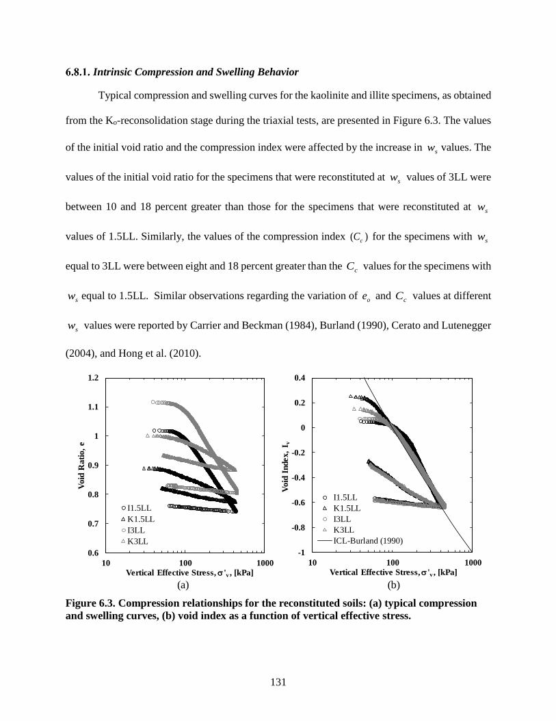
131
Intrinsic Compression and Swelling Behavior
Typical compression and swelling curves for the kaolinite and illite specimens, as obtained
from the Ko-reconsolidation stage during the triaxial tests, are presented in Figure 6.3. The values
of the initial void ratio and the compression index were affected by the increase in sw values. The
values of the initial void ratio for the specimens that were reconstituted at sw values of 3LL were
between 10 and 18 percent greater than those for the specimens that were reconstituted at sw
values of 1.5LL. Similarly, the values of the compression index )( cC for the specimens with sw
equal to 3LL were between eight and 18 percent greater than the cC values for the specimens with
sw equal to 1.5LL. Similar observations regarding the variation of oe and cC values at different
sw values were reported by Carrier and Beckman (1984), Burland (1990), Cerato and Lutenegger
(2004), and Hong et al. (2010).
Figure 6.3. Compression relationships for the reconstituted soils: (a) typical compression
and swelling curves, (b) void index as a function of vertical effective stress.
-1
-0.8
-0.6
-0.4
-0.2
0
0.2
0.4
10 100 1000
Void
Index,
I v
Vertical Effective Stress, 'v , [kPa]
I1.5LL
K1.5LL
I3LL
K3LL
ICL-Burland (1990)
0.6
0.7
0.8
0.9
1
1.1
1.2
10 100 1000
Vo
id R
ati
o,
e
Vertical Effective Stress, 'v , [kPa]
I1.5LL
K1.5LL
I3LL
K3LL
(a) (b)
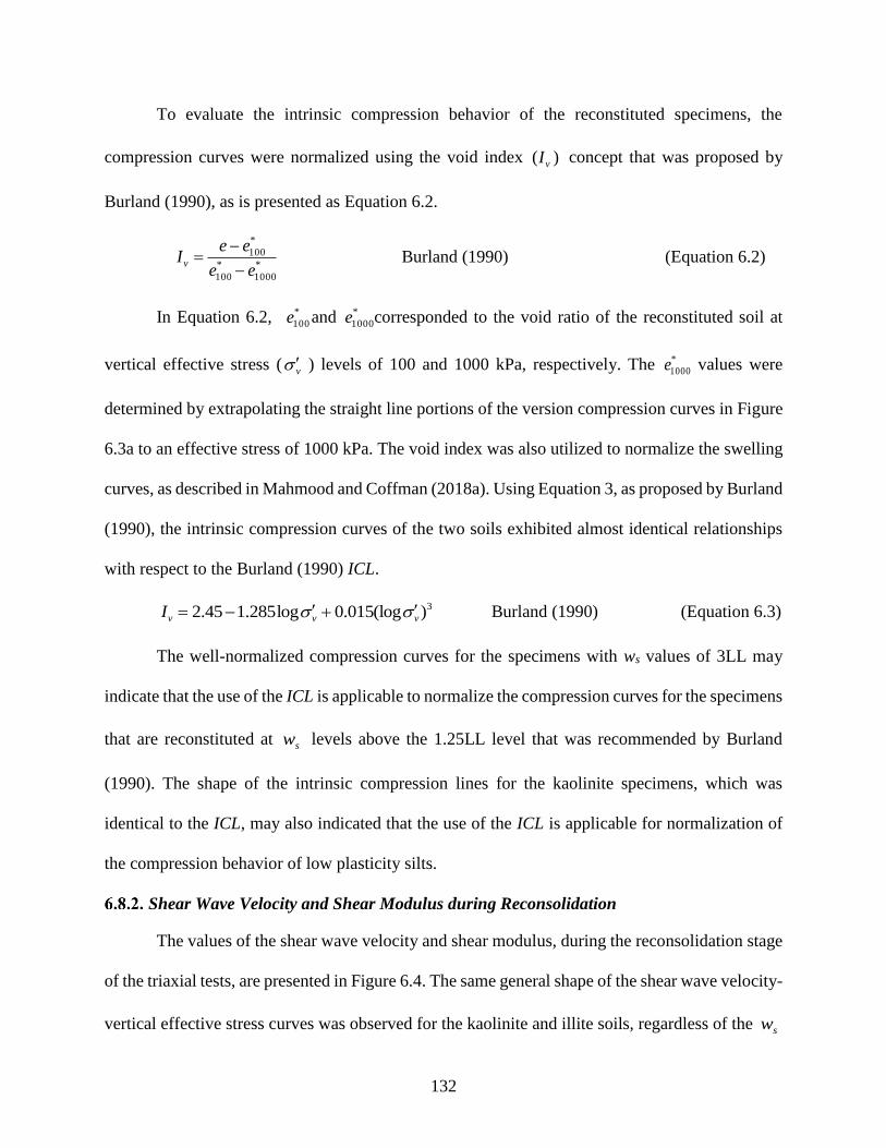
132
To evaluate the intrinsic compression behavior of the reconstituted specimens, the
compression curves were normalized using the void index )( vI concept that was proposed by
Burland (1990), as is presented as Equation 6.2.
*
1000
*
100
*
100
ee
eeIv
Burland (1990) (Equation 6.2)
In Equation 6.2, *
100e and *
1000e corresponded to the void ratio of the reconstituted soil at
vertical effective stress ( v ) levels of 100 and 1000 kPa, respectively. The *
1000e values were
determined by extrapolating the straight line portions of the version compression curves in Figure
6.3a to an effective stress of 1000 kPa. The void index was also utilized to normalize the swelling
curves, as described in Mahmood and Coffman (2018a). Using Equation 3, as proposed by Burland
(1990), the intrinsic compression curves of the two soils exhibited almost identical relationships
with respect to the Burland (1990) ICL.
3)(log015.0log285.145.2 vvvI Burland (1990) (Equation 6.3)
The well-normalized compression curves for the specimens with ws values of 3LL may
indicate that the use of the ICL is applicable to normalize the compression curves for the specimens
that are reconstituted at sw levels above the 1.25LL level that was recommended by Burland
(1990). The shape of the intrinsic compression lines for the kaolinite specimens, which was
identical to the ICL, may also indicated that the use of the ICL is applicable for normalization of
the compression behavior of low plasticity silts.
Shear Wave Velocity and Shear Modulus during Reconsolidation
The values of the shear wave velocity and shear modulus, during the reconsolidation stage
of the triaxial tests, are presented in Figure 6.4. The same general shape of the shear wave velocity-
vertical effective stress curves was observed for the kaolinite and illite soils, regardless of the sw

133
values. The behavior was characterized by increasing shear wave velocity with increasing vertical
effective stress during loading, followed by decreasing shear wave velocity with decreasing
vertical effective stress during unloading. The change of the shear wave velocity during loading
and unloading was associated with the change in the void ratio values from consolidation of the
soil.
At similar levels of effective stress, during reconsolidation, the specimens that were
reconstituted from ws values of 1.5LL had higher values of shear wave velocity than the specimens
that were reconstituted from ws values of 3LL. The shear wave velocity values for the K1.5LL
specimens were between 20 and 41 percent higher than those for the K3LL specimens. Similarly,
the shear wave velocity values for the I1.5LL specimens were between seven and 14 percent higher
than those for the I3LL specimens. The slower shear wave velocities that were measured for the
specimens that were reconstituted at higher ws were attributed to the 1) higher initial void ratio and
2) higher initial water content (wo) of these specimens prior to reconsolidation in the triaxial testing
device. Increasing level of ws led to slower measured values of shear wave velocity because shear
waves do not propagate through water. The additional water that was present occupied the void
space and separated the particles, thereby slowing the measured shear wave velocity. Moreover,
the influence of ws on the shear wave velocity was greater for kaolinite soil than for illite soil. As
reported by Mahmood and Coffman (2018a), more changes in the fabric were observed for
kaolinite soil than for illite soil as a result of increased ws values. As also indicated by Zhao et al.
(2017) and Mahmood and Coffman (2018a), the influence of the ws on the shear wave velocity,
stress-strain behavior, and strength characteristics of the kaolinite soil was more significant than
the influence of ws on the same characteristics of the illite soil.

134
Figure 6.4. Small strain results obtained from bender elements during reconsolidation and
overconsolidation: (a) shear wave velocity-vertical effective stress relationships, (b) shear
wave velocity-axial strain relationships.
The shear modulus-axial strain relations followed the same trend of the shear wave
velocity-effective stress relations during loading and unloading. The shear modulus within the
shear modulus-axial strain curves was observed to increase with increasing axial strain during
loading, then a sharp decrease was observed in the shear modulus during unloading. The BEG
values for K1.5LL specimens were from 1.7 to 2.1 higher than the BEG values for the K3LL
specimens. Likewise, the I1.5LL specimens were from 1.1 to 1.4 higher than the I3LL specimens.
The observation that the specimens with lower sw values were stiffer than those with higher sw
values was in agreement with the results of the observed undrained shear strength that were
obtained by Mahmood and Coffman (2018a).
As shown in Figure 6.5, the values of shear wave velocity and shear modulus were
normalized as a function of Iv. The values of Iv that were used to normalize these curves were
determined from the ICL of each specimen, as previously presented in Figure 6.3, at the
0
10
20
30
40
50
60
0.1 1 10 100
Shear
Modulu
s, G
BE,
[MP
a]
Axial Strain, a, [%]
I1.5LL
K1.5LL
I3LL
K3LL
Unl
oad
ing
60
80
100
120
140
160
180
10 100 1000
Sh
ear
Wave
Velo
city
, V
s, [
m/s
]
Vertical Effective Stress, 'v, [kPa]
I1.5LL
K1.5LL
I3LL
K3LL
(a) (b)

135
corresponding vertical effective stress. The same general shape of the Vs-Iv curves and BEG -Iv
curves was observed for the two soils during the re-consolidation and swelling stages. However,
unlike the historic ability of the void index normalization procedure to produce a unique
relationship between Iv and compression or undrained shear strength, the void index normalization
procedure was unable to produce a unique relationship between the sV and vI values. Likewise,
the shear modulus data did not appear to normalize within the shear modulus-void index space. As
previously described, there were other factors affecting shear wave velocity and small-strain
stiffness beside the void ratio that was accounted for in the void index value in Equation 6.2. The
difference in the initial water content of the specimens, as well as the difference in the fabric
between the specimens, that were initially prepared at different levels of slurry water content,
appeared to dominate the values of shear wave velocity. This difference in fabric was not
completely captured in the void ratio values that were used to calculate the void index values.
Figure 6.5. Normalized small-strain results: (a) shear wave velocity as a function of void
index, (b) shear modulus as a function of void index.
-0.7
-0.6
-0.5
-0.4
-0.3
-0.2
-0.1
0
0.1
0.2
10 100
Vo
id I
ndex
, I v
Shear Modulus, GBE , [MPa]
I1.5LL
K1.5LL
I3LL
K3LL-0.7
-0.6
-0.5
-0.4
-0.3
-0.2
-0.1
0
0.1
0.2
10 100 1000
Void
Index,
I v
Shear Wave Velocity, Vs, [m/s]
I1.5LL
K1.5LL
I3LL
K3LL
(a) (b)

136
Fabric Anisotropy
The values of the shear wave velocity during the reconsolidation stage were compared with
the values of shear wave velocity that were obtained from a back-pressure saturated, constant rate-
of-strain, consolidation device, with bender elements (BP-CRS-BE) that were measured by Zhao
and Coffman (2016). As shown in Figure 6.6, the values of horizontally propagated-vertically
polarized shear wave velocity )( ,HVsV , as obtained by utilizing the BP-CRS-BE device, were
compared with the values of vertically propagated-horizontally polarized shear wave velocity
)( ,VHsV that were measured in this study.
The difference in the velocity between the vertically-propagated shear waves and the
horizontally-propagated shear waves indicated that the reconstituted specimens from both soils
had inherent fabric anisotropy. However, the amount of the inherent anisotropy was dissimilar.
For the K1.5LL specimens, the amount of fabric anisotropy (HVsV ,
/VHsV ,
) ranged from 0.89 to 0.97
at the corresponding levels of applied vertical effective stress. Likewise, for the I1.5LL specimens,
the (HVsV ,
/VHsV ,
) ratio ranged from 0.63 to 0.74. The observation that the K1.5LL and I1.5LL
specimens had higher values of vertically-propagated shear wave velocity than horizontally-
propagated shear wave velocity was in direct contrast with that of Yamashita et al. (2005), Choo
et al. (2013), and Kang et al. (2014). The higher values of VHsV ,
may be attributed to the dispersed
fabric of the 1.5LL specimens that was created within the slurry consolidometer. Within the
dispersed fabric, the contact areas between the faces of the particles along the vertical direction
were much greater than the contact areas between the edges of the particles along the direction of
prefered orientation. Therefore, the shear waves propagated faster in the vertical direction.

137
Figure 6.6. Comparison of the values of shear wave velocity values obtained from bender
elements in the triaxial apparatus and BP-CRS-BE device, during Ko-reconsolidation, for:
(a) kaolinite, and (b) illite.
When comparing the values of HVsV ,
to the values of VHsV ,
for the K3LL specimens, the
amount of fabric anisotropy (HVsV ,
/VHsV ,
) ranged from 1.13 to 1.21. Although previous studies (e.g.,
Jovicic and Coop 1998; Lings et al. 2000; Yimsiri and Soga 2000; Cho and Finno 2010) have
indicated that one-dimensionally deposited soils will essentially experience cross anisotropy
)( ,, VHsHVs VV , perfect cross anisotropic fabric was not observed for the specimens that were
reconstituted from a slurry, at high slurry water content values. The fabric anisotropy of natural
clays that have been observed by Pennington et al. (1997) and Lee et al. (2008) have led to the
indication that the values of HVsV ,
were greater than the values VHsV ,
. Similar observations being
obtained for the K3LL samples )( ,, VHsHVs VV implies that reconstitution of soils at water content
levels of at least 3LL may produce a soil fabric that is similar to the fabric of naturally sedimented
soils.
0
40
80
120
160
200
240
10 100 1000
Shea
r W
av
e V
elo
city
, V
s, [
m/s
]
Vertical Effective Stress, 'v, [kPa]
I1.5LL V , Triaxial
I1.5LL V , BP-CRS-BE
s,VH
s,HV
0
40
80
120
160
200
240
10 100 1000
Shear
Wave V
elo
city
, V
s, [
m/s
]
Vertical Effective Stress, 'v, [kPa]
K1.5LL V , Triaxial
K1.5LL V , BP-CRS-BE
K3LL V , Triaxial
K3LL V , BP-CRS-BE
s,VH
s,HV
s,VH
s,HV
(a) (b)

138
Conclusions
Based on the results of triaxial compression tests, with shear wave velocity measurements,
the ws was determined to be a significant parameter that influenced the compression behavior,
shear wave velocity, shear modulus, and fabric anisotropy of the reconstituted soils. During Ko-
reconsolidation, the values of the shear wave velocity of the specimens, that were initially
reconstituted with lower slurry water content, were from 7 to 41 percent higher than those that
were reconstituted at higher slurry water content. The decrease in shear wave velocity, as a
function of increasing ws, was believed to be caused by the higher initial void ratio and higher
initial water content of the specimens. Furthermore, the specimens with lower ws values were from
1.1 to 2.1 stiffer than those with higher ws values. Following the same procedures that were used
by Mahmood and Coffman (2018a) to normalize the compression and undrained shear strength
values, the values of shear wave velocity and shear modulus were normalized by utilizing the
corresponding values of the void index. The normalized curves did not appear to normalize with
respect to the Iv procedure.
The amount of inherent fabric anisotropy for specimens prepared at ws of 1.5LL ranged
from 0.89 to 0.97 for the kaolinite and from 0.63 to 0.74 for illite. However, the amount of inherent
fabric anisotropy was between 1.13 and 1.21 for kaolinite specimens prepared at ws of 3LL. These
observations indicated that the fabric anisotropy characteristics of the natural soils could not be
reproduced by reconsidering kaolinite and illite soils prepared at sw of 1.5 LL. As documented
herein, the ws levels should be considered when reconstituting specimens of cohesive soils for
small-strain measurements. Furthermore, the small-strain behavior of reconstituted kaolinite and
illite soils cannot be simply quantified by reconstituting the soils at slurry water content values
that range from 1 to 1.5 times the liquid limit of the soil, as suggested by Burland (1990).

139
Therefore, a water content of the slurry of at least 3LL is recommended to obtain small-strain
characteristics of reconstituted soils that are more representative of the small-strain characteristics
of natural soils.
References
Alvarado, G., and Coop, M. R., (2012). “On The Performance of Bender Elements in Triaxial
Tests.” Geotechnique, Vol. 62, No. 3, pp. 1–17.
ASTM Standard D2487 (2011). Unified Soil Classification System. ASTM International, West
Conshohocken, PA, www.astm.org
ASTM Standard D4767 (2011). Standard Test Method for Consolidated Undrained Triaxial
Compression Test for Cohesive Soils. ASTM International, West Conshohocken, PA,
www.astm.org
Atkinson, J. H., Richardson, D. and Stallebrass, S.E., (1990). “Effect of Recent Stress History on
the Stiffness of Overconsolidated Soil.” Geotechnique, Vol. 40, No. 4, pp. 531-540.
Brignoli, E. G. M., Gotti, M., and Stokoe, K. H., II, (1996). “Measurement of Shear Waves in
Laboratory Specimens by Means of Piezoelectric Transducers.” Geotech. Test. J., Vol.
19, No. 4, pp. 384-397.
Burland, J. B., (1990). “On the Compressibility and Shear Strength of Natural Clays.”
Geotechnique, Vol. 40, No. 3, pp. 329-378.
Carrier, W. D., and Beckman, J. F., (1984). “Correlations Between Index Tests and the
Properties of Remolded Clays.” Geotechnique, Vol. 34, No. 2, pp. 211–228.
Cerato, A. B., and Lutenegger, A.J., (2004). “Determining Intrinsic Compressibility of Fine
Grained Soils.” Journal of Geotechnical and Geoenvironmental Engineering, Vol. 130,
No. 8, pp. 872–877.
Chandler, R. J., (2000). “Clay Sediments in Depositional Basins: The Geotechnical Cycle.”
Quarterly J. of Eng. Geology and Hydrogeology, Vol. 33, No. 1, pp.7–39.
Cho, W., and Finno, R.J., (2010). “Stress-strain Responses of Block Samples of Compressible
Chicago Glacial Clays.” Journal of Geotechnical and Geoenvironmental Engineering,
Vol. 136, No. 1, pp.178-188.
Choo, J., Jung, Y.H., Cho, W. and Chung, C.K., (2013). “Effect of Pre-Shear Stress Path on
Nonlinear Shear Stiffness Degradation of Cohesive Soils.” Geotech. Test. J., Vol. 36, No.
2. pp. 198-205.
Clayton, C. R. I., (2011). “Stiffness at Small Strain: Research and Practice.” Geotechnique, Vol.
61, No1, pp. 5-37.

140
Coffman, R.A., Salazar, S.E., and Zhao, Y., (2014). “Discussion of measurement of stiffness
anisotropy in kaolinite using bender element tests in a floating wall consolidometer by X.
Kang, G.-C. Kang, B. Bate.” Geotech. Test. J., Vol. 37, No. 6, pp. 1-5.
Duncan, J. M., and Seed, H. B., (1966). “Anisotropy and Stress Reorientation in Clay.” Journal
of the Soil Mechanics and Foundations Division, Vol. 92, No. 5, pp. 21-50.
Fam, M. and Santamarina, J. C., (1995). “Study of Geoprocesses with Complementary
Mechanical and Electromagnetic Wave Measurements in an Oedometer.” Geotech. Test.
J., Vol. 18, No. 3, pp. 307–314.
Finno, R. J. and Cho, W., (2011). “Recent Stress-History Effects on Compressible Chicago
Glacial Clays.” Journal of Geotechnical and Geoenvironmental Engineering, Vol.137,
No. 3, pp. 197-207.
Gasparre, A. and Coop, M., (2006). “Techniques for Performing Small-Strain Probes in the
Triaxial Apparatus.” Geotechnique, Vol. 56, No. 7, pp. 491–495.
Hardin, B. O. and Blandford, G. E., (1989). “Elasticity of Particulate Materials.” Journal of
Geotechnical Engineering, Vol. 115, No. 6, pp. 788-805.
Hong, Z. S., Bian, X., Cui, Y. J., Gao, Y. F., and Zeng, L. L., (2013). “Effect of Initial Water
Content on Undrained Shear Behaviour of Reconstituted Clays.” Geotechnique, Vol. 63,
No. 6, pp. 441–450.
Jamiolkowski, M., Lancellotta, R., and Lo Presti, D. C. F., (1995). “Remarks on the Stiffness at
Small Strains of Six Italian Clays.” Proceedings of the International Symposium, In Pre-
Failure Deformation of Geomaterials, Sapporo, Japan, pp. 817-845.
Jovicic, V. and Coop, M. R., (1998). “The Measurement of Stiffness Anisotropy in Clays with
Bender Element Tests in the Triaxial Apparatus.” Geotech. Test. J., Vol. 21, No. 1, pp. 3-
10.
Kang, X., Kang, G.-C., and Bate, B., (2014). “Measurement of Stiffness Anisotropy in Kaolinite
Using Bender Element Tests in A Floating Wall Consolidometer.” Geotech. Test. J., Vol.
37, No. 5, pp. 869–883.
Ladd, C. C., and Foott, R., (1974). “New Design Procedure for Stability of Soft Clays.” Journal
of Geotechnical Engineering Division, Vol.100, No.7, pp. 763-768.
Lee, C., Lee, J. S., Lee, W., and Cho, H., (2007). “Experiment Setup for Shear wave and
Electrical Resistance Measurements in an Oedometer.” Geotech. Test. J., Vol. 31, No. 2,
pp. 149-156.
Lings, M. L., Pennington, D. S., and Nash, D. F. T., (2000). “Anisotropic Stiffness Parameters
and Their Measurement in a Stiff Natural Clay.” Geotechnique, Vol. 50, No. 2, pp. 109–
125.

141
Mahmood, N. S. and Coffman, R. A., (2017). “The Effects of Stress Path on the Characterization
of Reconstituted Low Plasticity Kaolinite.” Soils and Foundations (In Review,
Manuscript Number: SANDF-D-17-00352-R1).
Mahmood, N. S. and Coffman, R. A., (2018a). “Intrinsic Shear Strength Behavior of
Reconstituted Kaolinite and Illite Soils.” Quarterly Journal of Engineering Geology and
Hydrogeology, (In Review, Manuscript Number: qjegh2018-056-R1).
Martin, R. T. and Ladd, C. C. (1978). “Fabric of Consolidated Kaolinite.” Clays and Clay
Minerals J., Vol. 23, pp. 17-25
Mitchell, R. J., (1972). “Some Deviations from Isotropy in Lightly Overconsolidated Clay.”
Geotechnique, Vol. 22, No. 3, pp. 459-467.
Olson, R. E., (1962). “The Shear Strength Properties of Calcium Illite.” Geotechnique, Vol.12,
No. 1, pp. 23-43.
Richart, F. E., Hall, J. R., and Woods, R. D., (1970). “Vibrations of Soils and Foundations.”
Prentice-Hall, Inc., NJ.
Roesler, S. K., (1979). “Anisotropic Shear Modulus Due to Stress Anisotropy.” Journal of the
Geotechnical Engineering Division, Vol. 105, pp. 871-880.
Salazar, S. E. and Coffman, R. A., (2014). “Design and Fabrication of End Platens for
Acquisition of Small-Strain Piezoelectric Measurements During Large-Strain Triaxial
Extension and Triaxial Compression Testing.” Geotech. Test. J., Vol. 37, No. 6, pp. 1-12.
Trhlikova, J., Masin, D., and Bohac, J., (2012). “Small-strain Behaviour of Cemented Soils.”
Geotechnique, Vo. 62, No. 10, pp. 943-947.
Viggiani, G. and Atkinson, J. H., (1995). “Stiffness of Fine-grained Soil at Very Small Strains.
Geotechnique, Vol. 45, No. 2, pp. 249-265.
Yamashita, S., Hori, T., and Suzuki, T., (2003). “Effects of Initial and Induced Anisotropy on
Initial Stiffness of Sand by Triaxial and Bender Elements Tests.” Geomechanics: Testing,
modeling, and simulation (GSP 143), A. J.Yamamuro and J.Koseki, eds., ASCE, Reston,
Va., pp. 350–369.
Yimsiri, S. and Soga, K., (2000). “Micromechanics-based Stress- Strain Behaviour of Soils at
Small Strains.” Geotechnique, Vol. 50, No. 5, pp. 559–571.
Zeng, L. L., Hong, Z. S., Cai, Y. Q., and Han, J., (2011). “Change of Hydraulic Conductivity
During Compression of Undisturbed and Remolded Clays.” Applied Clay Science, Vol.
51, No. 1, pp. 86-93.
Zhao, Y. and Coffman, R.A., (2016). “Back-Pressure Saturated Constant-Rate-of-Strain
Consolidation Device with Bender Elements: Verification of System Compliance.”
Journal of Testing and Evaluation, Vol.44, No.6, pp. 1-12.

142
Zhao, Y., Mahmood, N. S., Coffman, R.A., (2017). “Soil Fabric and Anisotropy as Observed
Using Bender Elements During Consolidation.” Clays and Clay Minerals, (In Review,
Manuscript Number: CCM-1143-R1).
Zhao, Y., Mahmood, N. S., Coffman, R.A., (2018). “Small-Strain and Large-Strain Modulus
Measurements with a Consolidation Device.” Journal of Testing and Evaluation, (In
Press).

143
Conclusions and Recommendations
Chapter Overview
A description of the conclusions drawn from the findings of the research project, and
recommendations for further research on reconstituted soils are contained in this chapter.
Specifically, the contributions from the research project, as discussed in this document, are
presented in Section 7.2. The conclusions drawn from the results obtained from this testing
program, as described previously in Chapters 4 through 6, are provided in Section 7.3.
Recommendations for additional work are presented in Section 7.4.
Selected Contributions from this Research Project
The purpose of this research project was to evaluate the compression, shear strength, and
small-strain properties of reconstituted kaolinite and illite. The primary contributions of the
research project are described briefly in this section. The stress path testing program consisted of
utilizing advanced triaxial testing equipment to evaluate stress-strain and strength characteristics
of reconstituted soils subject to different loading conditions. The need for advanced testing was
associated with data from conventional triaxial testing being used for site characterization. The
use of conventional triaxial data has often led to either unsafe or over-conservative designs. The
primary contribution of this scope of the research was the development of an understanding of
the testing techniques that are required to represent certain loading conditions in the field.
Furthermore, the collected stress path testing data will be useful in the development or validation
of advanced constitutive models. Using the new data, models that account for the various
orientations of the principal stresses can be developed.
Historically, reconstituted specimens have been conveniently utilized to evaluate shear
strength and small-strain behavior of cohesive soils. However, few studies have investigated the
relationship between the slurry water content and 1) the intrinsic shear strength and 2) the

144
intrinsic small-strain behavior of the created soil specimens. Through the work described herein,
a new method to normalize the intrinsic undrained shear strength values, using the void index
concept, was introduced for overconsolidated specimens. Recommended values of slurry water
content that should be used to prepare slurries of cohesive soils for triaxial testing and bender
element measurements were also developed. These recommended levels of water content will
produce reconstituted specimens with shear strength and small-strain soil properties that are in
better agreement with shear strength and small-strain properties for natural soil specimens.
Conclusions of Intrinsic Properties of Reconstituted Soils
The conclusions drawn from the observations of the reconstituted soil properties are
contained in this section. Conclusions related to the effect of stress path on 1) the stress-strain
behavior and 2) the shear strength characteristics of reconstituted low plasticity kaolinite soil are
documented in Section 7.3.1. The conclusions drawn from the triaxial testing program that was
performed to evaluate the intrinsic shear strength behavior of reconstituted illite and kaolinite
soils, are discussed in Section 7.3.2. Conclusions related to the 1) small-strain stiffness, and 2)
fabric anisotropy of reconstituted illite and kaolinite soils are described in Section 7.3.
Conclusions Regarding the Effects of Stress Path
A triaxial testing program was performed on reconstituted low plasticity kaolinite soil to
determine the effects of the magnitudes and orientations of the principal stresses on parameters
including: shear strength, stress-strain behavior, and excess pore water pressure development.
The stress-strain behavior, as obtained from the TC and RTC stress paths, was found to be
almost identical as shown previously in Figure 4.8 on page 77. Likewise, the stress-strain
behavior, as obtained from the TE and RTE stress paths, was found to be almost identical. As
presented in Table 7.1, the effective friction angle ( ' ) values, as obtained from the extension

145
tests, were from 20 to 35 percent lower than the ' values that were obtained from the
compression tests. Likewise, the measured undrained shear strength values (su), as obtained from
the extension tests, were from 11 to 38 percent lower than the su values that were obtained from
the compression tests.
Table 7.1. Effective shear strength parameters for the different stress paths.
TC RTC TE RTE
OCR
c
[kPa]
[degree]
c
[kPa]
[degree]
c
[kPa]
[degree]
c
[kPa]
[degree]
1 10.6 17.7 12.1 17.5 36.8 13.5 27.6 13.9
2 7.2 18.1 7.1 18.8 22.7 14.2 14.9 14.4
4 2.4 19.6 5.0 19.9 18.8 15.6 18.1 14.9
8 0.8 20.7 1.4 20.4 15.5 17.0 18.1 15.6
The axial strain values, at failure, that were obtained from the extension tests were
determined to be 0.3 to 5.0 percent greater than the axial strain values, at failure, that were
obtained from the compression tests. For normally consolidated specimens, the values of
undrained secant Young’s modulus obtained from the compression tests were from two to two
and one-half times greater than the values obtained from the extension tests. For
overconsolidated specimens, there was no clear relationship between the undrained secant
Young’s modulus and the axial strain. Additionally, for all of the stress paths, the excess pore
water pressure changed rapidly, as a function of axial stress, until the peak principle stress level
was reached. For practical purposes, a series of TC tests along with a series of RTE tests are
adequate to characterize the strength properties for cohesive soils when only the magnitude of
the principal stresses is changed without a change in the orientation of the principal stresses.
Furthermore, shear strength parameters, as obtained from these stress path tests, should be
utilized to develop or validate soil constitutive models.

146
Conclusions Regarding Intrinsic Shear Strength
The intrinsic shear strength properties of reconstituted soils were evaluated by
performing a series of triaxial compression tests on reconstituted kaolinite and illite specimens
that were each reconstituted at two different levels of slurry water content (1.5 or 3.0 times the
LL). A new method was proposed to normalize the undrained shear strength values for the
overconsolidated specimens based on the void index concept. It was observed that compression
behavior and undrained shear strength behavior for the reconstituted specimens were highly
dependent on the level of the slurry water content. The ICL for each soil type was identical to the
ICL that was proposed by Burland (1990). For each soil type, the intrinsic swell lines for all of
the specimens were similar when the specimens were unloaded from the same level of the
maximum stress, regardless of the slurry water content value that was used.
The undrained shear strength values of the specimens with ws= 1.5LL were from 5 to 16
percent lower than the undrained shear strength values of the specimens with ws = 3LL. The
effective cohesion tended to increase as a function of increasing amount of ws while the values of
the effective friction angle values were independent of the ws values. By utilizing the proposed
normalization method, the normalized undrained shear strength values for the overconsolidated
specimens were in a better agreement with the ISuL. The kaolinite soil was more affected than
the illite soil by an increase in the ws values. Based on the observed soil fabric and the undrained
shear strength values, reconstituting a low plasticity kaolinite soil at ws =1.5 LL is not
appropriate to evaluate the intrinsic shear strength behavior of this soil. Soil slurries should be
prepared at water content values of at least three times the corresponding liquid limit of the soil
to obtain undrained shear strength characteristics that are in better agreement with undrained
shear strength characteristics for natural soils.

147
Conclusions Regarding Small-Strain Measurements of Reconstituted Soils
The effects of the slurry water content and the soil fabric on the small-strain properties of
reconstituted kaolinite and illite soils were investigated by performing triaxial tests with bender
element measurements. Values of shear wave velocity and shear modulus were normalized by
utilizing the concept of void index. The major observations are summarized below.
1) At the same level of overconsolidation ratio and vertical effective stress, the Vs values for
the kaolinite and illite specimens with ws=1.5LL were from 7 to 41 percent greater than the
Vs values for the specimens with ws=3LL. Accordingly, the shear modulus values for the
kaolinite and illite specimens prepared at ws=1.5LL were from 1.1 to 2.1 times greater than
the shear modulus values for the kaolinite and illite specimens prepared at ws=3LL.
2) Unique intrinsic relationships for Vs-Iv or GBE-Iv were not observed for the normalized
values because the small-strain properties were highly dependent on the soil fabric.
3) Cross anisotropic characteristics of the fabric ( ),, VHsHVs VV were not observed for the
kaolinite specimens that were prepared at ws values of 3LL. When comparing the values
of HVsV ,
, as obtained by utilizing the BP-CRS-BE device, to the values of VHsV ,
, the amount
of fabric anisotropy (HVsV ,
/VHsV ,
) ranged from 1.13 to 1.21.
4) The inherent fabric anisotropy ranged from 0.63 to 0.97 for the kaolinite and illite
specimens with ws=1.5 LL, and ranged from 1.13 to 1.21 for the kaolinite specimens with
ws=3LL.
5) The ws level should be considered when reconstituting cohesive soil specimens for small-
strain measurements. Soil slurries should be prepared at water content values of at least
three times the corresponding liquid limit of the soil to obtain small-strain characteristics
that are in better agreement with small-strain characteristics for natural soils.

148
Recommendations for Future Work
Recommendations for further research, related to the intrinsic properties of the
reconstituted soils, are summarized below.
1. Preparation and testing of reconstituted soils with various values of slurry water content
is recommended for further examination of the findings of this research. The
recommended slurry water content levels are one, two, and four times the liquid limit of
the soil. By utilizing these levels of slurry water content, compression and shear strength
characteristics different than those obtained from this research project are expected.
2. Preparation and testing of other soil types should be performed to examine the effect of
mineralogy and plasticity index on the intrinsic soil properties that were investigated in
this research project. The recommended soil types including, but not limited to,
montmorillonite and high plasticity kaolinite.
3. The obtained experimental data should be utilized to review and assess previous empirical
equations to calculate the coefficient of lateral earth pressure at rest (Ko). Specifically, the
effect of 1) slurry water content, 2) OCR, and 3) shear strength parameters should be
investigated when evaluating the ability of these empirical equations to predict the Ko
values of reconstituted soils.
4. A comprehensive image analysis of the scanning electron microscope images should be
performed to quantify the influence of the ws level on the fabric of the reconstituted soils.
Examples of image analyses to quantify soil fabric are described in Frost and Wright
(1993).
5. Local strain measurements, such as LDVT, should be incorporated within the triaxial
device to measure axial strain and radial strain at small-strain range (from 0.001 to 0.1
percent) during the consolidation and shearing stages of the triaxial tests.

149
6. Two additional sets of bender elements should be incorporated within the triaxial device.
The first set should include two horizontally oriented bender elements to measure
horizontally-propagated, vertically polarized shear wave velocity. The second set should
include two vertically oriented bender elements to measure horizontally-propagated,
horizontally polarized shear wave velocity. The propose of these sets is to evaluate fabric
anisotropy within the same soil specimen.
7. The obtained experimental data may be utilized to developed new constitutive models to
predict the behavior of reconstituted soils when subjected to different loading conditions.
The developed models should account for the dependence of the compression and shear
strength parameters on the soil structure and on the applied stress path.
8. The parameters that were obtained from this research project may be utilized to
investigate the validity of selected constitutive models. The selected constitutive models
to be validated may include, but are not limited to, 1) Modified Cam Clay (MCC) that
was developed by Roscoe and Burland (1968), 2) MIT-E3 (Whittle and Kavvadas 1994),
and 3) S-CLAY1 (Wheeler et al. 2003). The MCC model has been widely used with
numerical and analytical methods in geotechnical engineering (Lade 2005). The MIT-E3
model and S-CLAY1 model were developed to account for soil anisotropy and soil
structure (Whittle and Kavvadas 1994; Wheeler et al. 2003).
References
Burland, J.B., (1990). “On the Compressibility and Shear Strength of Natural Clays.”
Geotechnique, Vol.40, No. 3, pp. 329-378.
Frost, J. D., and Wright, J. R. (1993). “Digital Image Processing; Techniques and Applications in
Civil Engineering.” Proceedings, ASCE, New York.
Lade, P. V. (2005). “Overview of Constitutive Models for Soils.” Soil Constitutive Models:
Evaluation, selection and calibration, J. A. Yamamuro and V. N. Kaliakin, eds., ASCE,
Reston, VA. pp 1-34.

150
Roscoe, K. H., and Burland, J. B. (1968). “On the Generalized Stress-strain Behaviour of “Wet”
Clay.” Engineering Plasticity, J. Hayman and F. A. A. Leckie, eds., Cambridge Univ.
Press, Cambridge, U.K. pp. 535-609.
Wheeler, S. J., Näätänen, A., Karstunen, M., and Lojander, M., (2003). “An Anisotropic
Elastoplastic Model for Soft Clays.” Canadian Geotechnical Journal, Vol. 40, No. 2, pp.
403-418.
Whittle, A. J., and Kavvadas, M. J., (1994). “Formulation of MIT-E3 Constitutive Model for
Overconsolidated Clays.” Journal of Geotechnical Engineering, Vol. 120, No. 1, pp. 173-
198.

151
References
Al Haj, K. M. A., and Standing, J. R., (2015). “Mechanical Properties of Two Expansive Clay
Soils from Sudan.” Geotechnique, Vol. 65, No.4, pp. 258-273.
Allman, M. A., and Atkinson, J. H., (1992). “Mechanical Properties of Reconstituted Bothkennar
Soil.” Geotechnique, Vol. 42, No.2, pp. 289-301.
Alvarado, G., and Coop, M. R., (2012). “On The Performance of Bender Elements in Triaxial
Tests.” Geotechnique, Vol. 62, No. 3, pp. 1–17.
American Society for Testing and Materials (2011). “Standard Practice for Classification of Soils
for Engineering Purposes (Unified Soil Classification System).” Annual Book of ASTM
Standards, Designation D2487, Vol. 4.08, ASTM, West Conshohocken, PA.
American Society for Testing and Materials (2011). “Standard Test Method for Unconsolidated-
Undrained Triaxial Compression Test on Cohesive Soils.” Annual Book of ASTM
Standards, Designation D4767, Vol. 4.08, ASTM, West Conshohocken, PA.
Amorosi, A., Callisto, L., and Rampello, S., (1999). “Observed Behavior of Reconstituted Clay
Along Stress Paths Typical of Excavations.” Proceedings of the Second International
Symposium on Pre-Failure Deformation Characteristics of Geomaterials, Torino, Italy,
pp. 28-30. CRC Press.
Atkinson, J. H., (2000). “Non-linear Soil Stiffness in Routine Design.” Geotechnique, Vol.50,
No. 5, pp 487-508.
Atkinson, J. H., Richardson, D. and Stallebrass, S.E., (1990). “Effect of Recent Stress History on
the Stiffness of Overconsolidated Soil.” Geotechnique, Vol. 40, No. 4, pp. 531-540.
Atkinson, J. H., Richardson, D., and Robinson, P. J., (1987). “Compression and Extension of K0
Normally Consolidated Kaolin Clay.” Journal of Geotechnical Engineering, Vol.113. No.
12, pp. 1468-1482.
Atkinson, J.H., Richardson, D. and Stallebrass, S.E., (1990). “Effect of Recent Stress History on
the Stiffness of Overconsolidated Soil.” Geotechnique, Vol.40, No. 4, pp.531-540.
Atkinson, J.H., Richardson, D., and Robinson, P.J., (1987). “Compression and Extension of Ko
Normally Consolidated Kaolin Clay.” Journal of Geotechnical Engineering, Vol. 113,
No.12, pp.1468-1482.
Baldi, G., Hight, D. W., and Thomas, G. E. (1988). “A Reevaluation of Conventional Triaxial
Test Methods.” Advanced triaxial testing of soil and rock.” ASTM STP, 977, 219-263.
Bayoumi, A., (2006). “New Laboratory Test Procedure for the Enhanced Calibration of
Constitutive Models.” Doctoral dissertation, Georgia Institute of Technology, GA.

152
Bishop, A. W., (1966). “The strength of soils as engineering materials.” Geotechnique, Vol. 16,
pp. 91-130.
Bishop, A.W., and Henkel, D.J. (1962). “The Measurement of Soil Properties in the Triaxial
Test.” Edward Arnold LTD, London.
Bjerrum, L., (1973). “Problems of Soil Mechanics and Construction on Soft Clays and
Structurally Unstable Soils (Collapsible, Expansive and others).” In Proceeding of 8th
International Conference on SMFE ,Vol. 3, pp. 111-159.
Bjerrum, L., Frimann, L.J., Has, M. and Duncan, J.M., (1972). “Earth Pressures on Flexible
Structures.” A State-of-the-Art-Report; Procedding of the 5th European Conference on
Soil Mechanics and Foundations Engineering, Madrid, Vol 2, pp. pp.169 - 196.
Bjerrum, L., Simons, N., and Toblaa, I., (1958). “The Effect of Time on the Shear Strength of a
Soft Marine Clay.” Proceedings of Conference on Earth Pressure Problems, I, pp.148-
158.
Brignoli, E. G. M., Gotti, M., and Stokoe, K. H., II, (1996). “Measurement of Shear Waves in
Laboratory Specimens by Means of Piezoelectric Transducers.” Geotech. Test. J., Vol.
19, No. 4, pp. 384-397.
Bryson, L. S., and Salehian, A. (2011). “Performance of Constitutive Models in Predicting
Behavior of Remolded Clay.” Acta Geotechnica, Vol. 6, No. 3, pp.143-154.
Burland, J. B., (1990). “On the Compressibility and Shear Strength of Natural Clays.”
Geotechnique, Vol. 40, No. 3, pp. 329-378.
Carrier, W. D., and Beckman, J. F., (1984). “Correlations Between Index Tests and the
Properties of Remolded Clays.” Geotechnique, Vol. 34, No. 2, pp. 211–228.
Cerato, A. B., and Lutenegger, A. J., (2004). “Determining Intrinsic Compressibility of Fine
Grained Soils.” Journal of Geotechnical and Geoenvironmental Engineering, Vol. 130,
No. 8, pp. 872–877.
Chandler, R. J., (2000). “Clay Sediments in Depositional Basins: The Geotechnical Cycle.”
Quarterly J. of Eng. Geology and Hydrogeology, Vol. 33, No. 1, pp.7–39.
Cho, W., and Finno, R.J., (2010). “Stress-strain Responses of Block Samples of Compressible
Chicago Glacial Clays.” Journal of Geotechnical and Geoenvironmental Engineering,
Vol. 136, No. 1, pp.178-188.
Choo, J., Jung, Y.H., Cho, W. and Chung, C.K., (2013). “Effect of Pre-Shear Stress Path on
Nonlinear Shear Stiffness Degradation of Cohesive Soils.” Geotech. Test. J., Vol. 36, No.
2. pp. 198-205.
Clayton, C. R. I., (2011). “Stiffness at Small Strain: Research and Practice.” Geotechnique, Vol.
61, No1, pp. 5-37.

153
Clayton, C.R.I., and Heymann, G., (2001). “Stiffness of Geomaterials at Very Small Strains.”
Geotechnique, Vol. 51, No. 3, pp 245–255.
Coffman, R. A., Bowders, J. J., and Burton, P. M., (2010). “Use of SHANSEP Design
Parameters in Landfill Design: A Cost/Benefit Case Study.” ASCE Geotechnical Special
Publication No. 199, Proceedings GeoFlorida 2010, Advances in Analysis, Modeling and
Design, West Palm Beach, FL, Feb 20–24, pp. 2859–2866.
Coffman, R.A., Salazar, S.E., and Zhao, Y., (2014). “Discussion of measurement of stiffness
anisotropy in kaolinite using bender element tests in a floating wall consolidometer by X.
Kang, G.-C. Kang, B. Bate.” Geotech. Test. J., Vol. 37, No. 6, pp. 1-5.
Coop, M. R., Atkinson, J. H., and Taylor. R. N., (1995). “Strength, yielding and Stiffness of
Structured and Unstructured Soils.” Proceedings of the 11th European Conference on
Soil Mechanics and Foundation Engineering, Copenhagen, Denmark, Vol. 28.
Cotecchia, F., and Chandler, R.J., (1997). “The Influence of Structure on the Pre-Failure
Behaviour of a Natural Clay.” Geotechnique, Vol. 47, No. 3, pp. 523-544.
Davis, E. H., and Poulos, H. G., (1972). “Rate of Settlement Under Two-and Three-dimensional
Conditions.” Geotechnique, Vol. 22, No. 1.
Davis, E.H. and Poulos, H.G., (1968). “The Use of Elastic Theory for Settlement Prediction
under Three-dimensional Conditions.” Geotechnique, Vol.18, No. 1, pp.67-91.
Duncan, J. M., and Seed, H. B., (1966). “Anisotropy and Stress Reorientation in Clay.” Journal
of the Soil Mechanics and Foundations Division, Vol. 92, No. 5, pp. 21-50.
Fam, M. and Santamarina, J. C., (1995). “Study of Geoprocesses with Complementary
Mechanical and Electromagnetic Wave Measurements in an Oedometer.” Geotech. Test.
J., Vol. 18, No. 3, pp. 307–314.
Fearon, R.E., and Coop, M.R., (2000). “Reconstitution: What Makes an Appropriate Reference
Material?.” Geotechnique, Vol. 50, No. 4, pp. 471-477.
FHWA (2007). “Earth Retaining Structures, Reference Manual.” Publication No. FHWA NHI-
07-071. USDOT FHWA, National Highway Institute, December, pp. 2-41.
Finno, R. J. and Cho, W., (2011). “Recent Stress-History Effects on Compressible Chicago
Glacial Clays.” Journal of Geotechnical and Geoenvironmental Engineering, Vol.137,
No. 3, pp. 197-207.

154
Frost, J. D., and Wright, J. R. (1993). “Digital Image Processing; Techniques and Applications in
Civil Engineering.” Proceedings, ASCE, New York.
Gasparre, A. and Coop, M., (2006). “Techniques for Performing Small-Strain Probes in the
Triaxial Apparatus.” Geotechnique, Vol. 56, No. 7, pp. 491–495.
Gens, A., (1983). “Stress-strain and Strength Characteristics of a Low Plasticity Clay.” Doctoral
dissertation, University of London, London, England.
Hansen, J. B., and Gibson, R. E., (1949). “Undrained Shear Strengths of Anisotropically
Consolidated Clays.” Geotechnique, Vol.1, No. 3, pp.189-200.
Hardin, B. O. and Blandford, G. E., (1989). “Elasticity of Particulate Materials.” Journal of
Geotechnical Engineering, Vol. 115, No. 6, pp. 788-805.
Hardin, B.O. and Blandford, G.E., (1989). “Elasticity of Particulate Material.” Journal of
Geotechnical Engineering, Vol. 115, No. 6, pp.788-805.
Hardin, B.O. and Drnevich, V.P. (1972). “Shear Modulus and Damping in Soils: Measurement
and Parameter Effects.” Journal of Soil Mechanics and Foundations Division, ASCE.
Vol. 98, No. 6, pp. 603-624.
Hashash, Y., Wotring, D., Yao, J., Lee, J. and Fu, Q. (2002). “Visual Framework for
Development and Use of Constitutive Models.” International Journal for Numerical and
Analytical Methods in Geomechanics, Vol. 26. No. 15, pp. 1493-1513.
Henkel, D.J. (1956). “The Effect of Overconsolidation on the Behavior of Clays During Shear.”
Geotechnique, Vol. 6, No. 4, pp.139-150.
Hirschfield, R. C. (1958). “Factors Influencing the Constant Volume of Clays.” Doctoral
dissertation, Howard University, Washington, DC.
Holtz, R. D., Kovacs, W. D., and Sheahan, T. C., (2011). “An Introduction to Geotechnical
Engineering.” 2nd Ed. Pearson Education, Upper Saddle River, NJ.
Hong, Z. S., Bian, X., Cui, Y. J., Gao, Y. F., and Zeng, L. L., (2013). “Effect of Initial Water
Content on Undrained Shear Behaviour of Reconstituted Clays.” Geotechnique, Vol. 63,
No. 6, pp. 441–450.
Hong, Z. S., Yin, J., Cui, Y. J., (2010). “Compression Behaviour of Reconstituted Soils at High
Initial Water Contents.” Geotechnique, Vol. 60, No. 9, pp. 691-700.
Hong, Z.S., Bian, X., Cui, Y.J., Gao, Y.F., and Zeng, L.L., (2013). “Effect of Initial Water
Content on Undrained Shear Behaviour of Reconstituted Clays.” Geotechnique, Vol. 63,
No. 6, pp. 441-450.
Jafroudi, S., (1983). “Experimental Verification of Bounding Surface Plasticity Theory for
Cohesive Soils.” Doctoral dissertation, University of California, Davis, CA.

155
Jamiolkowski, M., Ladd, C.C., Germaine, J. and Lancellotta, R., (1985). “New Developments in
Field and Lab Testing of Soils.” Proceedings 11th Intl. Conference on Soil Mechanics
and Foundations Engineering, San Francisco, Vol. 2, pp. 57-154.
Jamiolkowski, M., Lancellotta, R., and Lo Presti, D. C. F., (1995). “Remarks on the Stiffness at
Small Strains of Six Italian Clays.” Proceedings of the International Symposium, In Pre-
Failure Deformation of Geomaterials, Sapporo, Japan, pp. 817-845.
Jovicic, V. and Coop, M. R., (1998). “The Measurement of Stiffness Anisotropy in Clays with
Bender Element Tests in the Triaxial Apparatus.” Geotech. Test. J., Vol. 21, No. 1, pp. 3-
10.
Kang, X., Kang, G.-C., and Bate, B., (2014). “Measurement of Stiffness Anisotropy in Kaolinite
Using Bender Element Tests in A Floating Wall Consolidometer.” Geotech. Test. J., Vol.
37, No. 5, pp. 869–883.
Kavvadas, M., and Amorosi, A., (2000). “A constitutive Model for Structured Soils.”
Geotechnique, Vol. 50, No. 3, pp. 263-273.
Kulhawy, F. H., and Mayne, P. W., (1990). “Manual on Estimating Soil Properties for
Foundation Design.” Electric Power Res. Inst. EL-6800; Prof. 1493-6, Electric Power
Research Inst., Palo Alto, CA, pp. 4-5.
Ladd, C. C., and DeGroot, D. J., (2003). “Recommended Practice for Soft Ground Site
Characterization: Arthur Casagrande Lecture.” In 12th Panamerican Conference on Soil
Mechanics and Geotechnical Engineering Vol. 1, pp. 1-57.
Ladd, C. C., and Foott, R., (1974). “New Design Procedure for Stability of Soft Clays.” Journal
of Geotechnical Engineering Division, Vol.100, No.7, pp. 763-768.
Ladd, C. C., and Varallyay, J., (1965). “The Influence of Stress System on the Behavior of
Saturated Clays During Undrained Shear.” No. RR-R65-11. Massachusetts Institute of
Technology, Cambridge Soil Mechanics Div.
Ladd, C.C. (1991). “Stability Evaluation During Staged Construction (22nd Terzaghi Lecture).”
Journal of Geotechnical Engineering. Vol. 117 No. 4, pp. 540-615.
Ladd, C.C., Bovee, R.B., Edgers, L. and Rixner, J.J., (1971). “Consolidated-undrained Plane
Strain Shear Tests on Boston Blue Clay.” Research Report R71-13, No. 273, No. 284,
Massachusetts Institute of Technology, Cambridge, pp. 243.
Lade, P. V. (2005). “Overview of Constitutive Models for Soils.” Soil constitutive models:
Evaluation, selection and calibration, J. A. Yamamuro and V. N. Kaliakin, eds., ASCE,
Reston, VA. pp 1-34.
Lade, P. V., and Duncan, J. M., (1999). “Stress-path Independent Behavior of Cohesionless
Soil.” Journal of the Geotechnical Engineering Division, Vol.102. No. 1, pp. 51-68.

156
Lambe, T. W. (1967). “Stress Path Method.” Journal of Soil Mechanics and Foundations
Division,
Lambe, T. W., and Whitman, R. V., (1969). “Soil Mechanics.” John Wiley and Sons, New York.
Lee, C., Lee, J. S., Lee, W., and Cho, H., (2007). “Experiment Setup for Shear wave and
Electrical Resistance Measurements in an Oedometer.” Geotech. Test. J., Vol. 31, No. 2,
pp. 149-156.
Lings, M. L., Pennington, D. S., and Nash, D. F. T. (2000). “Anisotropic Stiffness Parameters
and their Measurement in a Stiff Natural Clay.” Geotechnique, Vol. 50, No. 2, pp. 109-
125.
Liu, Y. (2004). “The Stress-Strain Behavior of Kaolin Clay in Triaxial.” Ph.D. Thesis. University
of Delaware. Newark, DE.
Mahmood, N. S. and Coffman, R. A., (2017). “The Effects of Stress Path on the Characterization
of Reconstituted Low Plasticity Kaolinite.” Soils and Foundations (In Review,
Manuscript Number: SANDF-D-17-00352-R1).
Mahmood, N. S. and Coffman, R. A., (2018a). “Intrinsic Shear Strength Behavior of
Reconstituted Kaolinite and Illite Soils.” Quarterly Journal of Engineering Geology and
Hydrogeology, (In Review, Manuscript Number: qjegh2018-056-R1).
Mahmood, N. S., and Coffman, R. A., (2018b). “Small-strain of Reconstituted Soils: The Effect
of Slurry Water Content.” Geotechnical Testing Journal, (Under Review, Manuscript
Number: GTJ-2018-0098-R1).
Martin, R. T. and Ladd, C. C. (1978). “Fabric of Consolidated Kaolinite.” Clays and Clay
Minerals J., Vol. 23, pp. 17-25
Mitchell, J.K., and Soga, K., (2005). “Fundamental of Soil Behavior, 3rd Edition.” John Wiley
and Sons, New York.
Mitchell, R. J., (1972). “Some Deviations from Isotropy in Lightly Overconsolidated Clay.”
Geotechnique, Vol. 22, No. 3, pp. 459-467.
Moniz, Safia R., (2009). “The Influence of Effective Consolidation Stress on the Normalized
Extension Strength Properties of Resedimented Boston Blue Clay.” MEng Thesis, MIT,
Cambridge, MA.
Nash, D.F.T., Lings, M.L., and Pennington, D.S., (1999). “The Dependence of Anisotropy G0
Shear Moduli on Void Ratio and Stress State for Reconstituted Gault Clay.” Proc., 2nd
Int. Symp. on Pre-Failure Deformation Characteristics of Geomaterials, Torino, pp. 229-
238.
Olson, R. E., (1962). “The Shear Strength Properties of Calcium Illite.” Geotechnique, Vol.12,
No. 1, pp. 23-43.

157
Parry, R. H. G., (1960). “Triaxial Compression and Extension Tests on Remolded Clay.”
Geotechnique, Vol. 10, No. 4, pp. 160-188.
Parry, R. H. G., (2004). “Mohr Circles, Stress Paths and Geotechnics.” Spon Press, London.
Parry, R.H.G. and Nadarajah, V., (1974). “Observations on Laboratory Prepared, Lightly
Overconsolidated Specimens of Kaolin.” Geotechnique, Vol. 24, No. 4, pp.345-357.
Pennington, D. S., Nash, D. F. T., and Lings, M. L., (1997). “Anisotropy of G0 Shear Stiffness in
Gault Clay.” Geotechnique, Vol. 47, No. 3, pp. 391-398.
Prashant, A. and Penumadu, D., (2005). “A Laboratory Study of Normally Consolidated Kaolin
Clay.” Canadian Geotechnical Journal, Vol. 42, No. 1, pp.27-37.
Prashant, A., and Penumadu, D., (2007). “Effect of Microfabric on Mechanical Behavior of
Kaolin Clay Using Cubical True Triaxial Testing.” J. Geotech. Geoenviron. Eng. Vol.
133, No. 4, pp. 433-444.
Race, M.L., Coffman, R.A., (2011). “Effects of Piston Uplift, Piston Friction, and Machine
Deflection in Reduced Triaxial Extension Testing.” ASCE Geotechnical Special
Publication No. 211, Proc. GeoFrontiers 2011: Advances in Geotechnical Engineering,
Dallas, Texas, March, pp. 2649-2658.
Richart, F. E., Hall, J. R., and Woods, R. D., (1970). “Vibrations of Soils and Foundations.”
Prentice-Hall, Inc., NJ.
Roesler, S. K., (1979). “Anisotropic Shear Modulus Due to Stress Anisotropy.” Journal of the
Geotechnical Engineering Division, Vol. 105, pp. 871-880.
Roesler, S. K., (1979). “Anisotropic Shear Modulus due to Stress Anisotropy.” J. Geotech. Eng.
Div., Vol. 105, No. 7, pp. 871-880.
Roscoe, K. H., and Burland, J. B. (1968). “On the Generalized Stress-strain Behaviour of “Wet”
Clay.” Engineering plasticity, J. Hayman and F. A. A. Leckie, eds., Cambridge Univ.
Press, Cambridge, U.K. pp. 535-609.
Roscoe, K. H., Schofield, A., and Wroth, C., P., (1958). “On the Yielding of Soils.”
Geotechnique, Vol. 8, No.1, pp. 22-53.
Rossato, G., Ninis, N. L., and Jardine, R. J., (1992). “Properties of Some Kaolin-based Model
Clay Soils.” Geotech. Test. J., Vol. 15, No. 2, pp.166-179.
Saada, A.S. and Bianchini, G.F., (1977). “Strength of One Dimensionally Consolidated Clays.”
Journal of Geotechnical and Geoenvironmental Engineering, Vol. 103, (HGT-6), pp. 655-
660.
Salazar, S. E. and Coffman, R. A., (2014). “Design and Fabrication of End Platens for
Acquisition of Small-Strain Piezoelectric Measurements During Large-Strain Triaxial

158
Extension and Triaxial Compression Testing.” Geotechnical Testing Journal, Vol. 37,
No. 6, pp. 1-12.
Salazar, S. E., Miramontes, L. D., Barnes, A.R., Bernhardt, M.L., Coffman, R.A., (2017).
“Verification of an Internal Close-range Photogrammetry Approach for Volume
Determination During Undrained Triaxial Testing.” Geotech. Test. J. (Under Second
Review, Manuscript Number: GTJ-2017-0125-R1).
Salazar, Sean E. and Coffman, Richard A. (2015). “Consideration of Internal Board Camera
Optics for Triaxial Testing Applications.” Geotechnical Testing Journal, Vol. 38, No. 1,
pp. 1–10.
Santagata, M. C. (2008). “Effects of Stress History on the Stiffness of a Soft Clay.” Proceeding
Deformational Characteristics of Geomaterials, Keynote Lecture, IOS Press/Millpress.
Scholey, G. K., Frost, J. D., Lo Presti, D. C. E, and Jamiolkowski, M. (1996). “A Review of
Instrumentation for Measuring Small Strains During Triaxial Testing of Soil Specimens.”
Geotechnical Testing Journal, GTJODJ, Vol. 18, No. 2, pp. 137-156.
Sheahan, T. C. (1991). “An Experimental Study of the Time-dependent Undrained Shear
Behavior of Resedimented Clay Using Automated Stress Path Triaxial Equipment.”
Doctoral dissertation, Massachusetts Institute of Technology, MA.
Sheahan, T.C., Ladd, C.C., and Germaine, J.T., (1996). “Rate-dependent Undrained Shear
Behavior of Saturated Clay.” Journal of Geotechnical Engineering, Vol. 122, No. 2, pp.
99-108.
Simons, N. E. and Som, N. N. (1970). “Settlement of Structures on Clay: with Particular
Emphasis on London Clay.” Construction industry research and information Association,
London. Report 22.
Skempton, A. W. (1954) “The Pore-pressure Coefficients A and B.” Geotechnique, Vol. 4, No.
4, pp.143-147.
Skempton, A. W. and Henkel, D. J. (1957). “Test on London Clay from Deep Boarding at
Paddington, Victoria and South Bank.” Proceeding of the 4th International Conference on
Soil Mechanics and Foundation Engineering, Vol.1, No.100, London, U.K.
Stipho, A. S. A. (1978). “Experimental and Theoretical Investigation of the Behavior of
Anisotropically Consolidated Kaolin.” Doctoral Dissertation, University College,
Cardiff, U.K.
Taylor, D. W. (1948). “Fundamentals of Soil Mechanics.” John Wiley and Sons, New York,
NY.
Theile (2016). “Product Information for Clay Products.” Theile Kaolin Company.
https://www.thielekaolin.com/sites/default/files/inline-files/KAOWHITE%20S_0.pdf.
Accessed April 2016.

159
Tiwari, B., and Ajmera, B., (2011). “New Correlation Equations for Compression Index of
Remolded Clays.” Geotechnical and Geoenvironmental Engineering, Vol. 138, No. 6, pp.
757-762.
Trhlikova, J., Masin, D., and Bohac, J., (2012). “Small-strain Behaviour of Cemented Soils.”
Geotechnique, Vo. 62, No. 10, pp. 943-947.
VandenBerge, D. R., Duncan, J. M., and Brandon, T. L., (2015). “Undrained Strength of
Compacted Clay Under Principal Stress Reorientation.” J. Geotech. Geoenviron. Eng.,
Vol. 141, No. 8, pp.1-11.
Viggiani, G. and Atkinson, J. H. (1995). “Interpretation of Bender Element Tests.” Geotechnique
Vol. 45, No. 1, pp.149-154.
Wang, Y. and Ng, C.W., (2005). “Effects of Stress Paths on the Small-strain Stiffness of
Completely Decomposed Granite.” Canadian geotechnical journal, Vol. 42, No. 4,
pp.1200-1211.
Wheeler, S. J., Näätänen, A., Karstunen, M., and Lojander, M., (2003). “An Anisotropic
Elastoplastic Model for Soft Clays.” Canadian Geotechnical Journal, Vol. 40. No. 2, pp.
403-418.
Whittle, A. J., and Kavvadas, M. J., (1994). “Formulation of MIT-E3 Constitutive Model for
Overconsolidated Clays.” Journal of Geotechnical Engineering, Vol. 120, No. 1, pp. 173-
198.
Woods, R.D. and Partos, A., (1981). “Control of Soil Improvement by Crosshole Testing.” Jn
Proceeding to the 10th International Conference on Soil Mechanics and Foundation
Engineering, Stockholm, pp. 793-796.
Wroth, C. P., (1984). “The Interpretation of in Situ Soil Tests.” Geotechnique, Vol. 34, No. 4,
pp. 449-489.
Wroth, C. P., (1984). “The Interpretation of in Situ Soil Tests.” Geotechnique, Vol. 34, No. 4,
pp. 449-489.
Wu, W., and Kolymbas, D., (1991). “On Some Issues in Triaxial Extension Tests.” Geotechnical
Testing Journal, Vol. 14, No. 3, pp. 276-287.
Yamashita, S., Hori, T., and Suzuki, T., (2003). “Effects of Initial and Induced Anisotropy on
Initial Stiffness of Sand by Triaxial and Bender Elements Tests.” Geomechanics: Testing,
modeling, and simulation (GSP 143), A. J.Yamamuro and J.Koseki, eds., ASCE, Reston,
Va., pp. 350–369.
Yamashita, S., Jamiolkowski, M., and Presti, D.C.F., (2000). “Stiffness Nonlinearity of Three
Sands.” Journal of Geotechnical and Geoenvironmental Engineering, Vol. 126, No.10,
pp. 929-938.

160
Yimsiri, S. and Soga, K., (2000). “Micromechanics-based Stress- Strain Behaviour of Soils at
Small Strains.” Geotechnique, Vol. 50, No. 5, pp. 559–571.
Yimsiri, S., Soga, K., (2002). “Application of Micromechanics Model to Study Anisotropy of
Soils at Small Strain.” Soil and Foundations, Vol. 42, pp. 15-26.
Yin, J., and Miao, Y., (2013). “Intrinsic Compression Behavior of Remolded and Reconstituted
Clays-Reappraisal.” Open Journal of Civil Engineering, Vol.3, No. 3, pp. 8-12.
Zdravkovic, L. (1996). “The Stress-strain-strength Anisotropy of a Granular Medium under
General Stress Conditions.” Doctoral Dissertation, Imperial College, London, UK.
Zeng, L. L., Hong, Z. S., Cai, Y. Q., and Han, J., (2011). “Change of Hydraulic Conductivity
During Compression of Undisturbed and Remolded Clays.” Applied Clay Science, Vol.
51, No. 1, pp. 86-93.
Zhao, Y. and Coffman, R.A., (2016). “Back-Pressure Saturated Constant-Rate-of-Strain
Consolidation Device with Bender Elements: Verification of System Compliance.”
Journal of Testing and Evaluation, Vol.44, No.6, pp. 1-12.
Zhao, Y., and Coffman, R.A., (2016). “Back-Pressure Saturated Constant-Rate-of-Strain
Consolidation Device with Bender Elements: Verification of System Compliance.”
Journal of Testing and Evaluation, Vol. 44, No. 6, pp. 1-12.
Zhao, Y., Mahmood, N. S., and Coffman, R. A., (2017). “Soil Fabric and Anisotropy as
Observed Using Bender Elements during Consolidation.” Clays and Clay Minerals,
(Under Review, Manuscript Number: CCM-1143-R1).
Zhao, Y., Mahmood, N. S., and Coffman, R.A., (2018). “Small-Strain and Large-Strain Modulus
Measurements with a Consolidation Device.” Journal of Testing and Evaluation, In Press,
Manuscript Number: JTE-2016-0331.

161
Triaxial Testing Data
A.1. Chapter Overview
Continued in this appendix are 1) the initial values and the physical properties of the
specimens and 2) the triaxial tests values, and 3) the bender elements measurements, as obtained
from the laboratory testing program.
A.2. Specimen Properties
Contained in this section are 1) data collected during specimen preparation within the
slurry consolidometer, and 2) initial physical properties of the specimens. The specimens were
pre-consolidated by utilizing a slurry consolidometer. The time-consolidation curves for the
prepared slurries were developed from the data collected during the pre-consolidation process.
The time-consolidation curves for the kaolinite specimens that were used for the controlled stress
path triaxial tests are presented in Figure A.1. The time-consolidation curves for the kaolinite and
illite specimens that were used for the triaxial tests with bender element measurements are
presented in Figure A.2.
The initial properties of the specimens were measured after the specimens were removed
from the slurry consolidometer following the pre-consolidation process. A summary of the initial
properties of the specimen, that were used for the controlled stress path triaxial tests, is presented
in Table A.1. The initial properties of the specimens that were used for the triaxial tests with
bender element measurements are presented in Table A.2.

162
Figure A.1. Time-consolidation curves for the kaolinite specimens that were used for the
stress path tests.
0
1
2
3
4
5
6
1 10 100 1000 10000 100000
Vert
ica
l D
ispla
cem
ent,
[cm
]Time, t, [minut]
25 34
43 45
46 48
53 60
Consolidometer No.
0
1
2
3
4
5
6
1 10 100 1000 10000 100000
Ve
rtic
al
Dis
pla
cem
en
t, [
cm]
Time, t, [minut]
3 7
8 9
10 18
23 24
Consolidometer No.

163
Table A.1. The initial properties of the specimen used for the stress path triaxial tests. Consolidometer Specimen
Test OCR
’v,max
[kPa] No.
Slurry
Height, [cm]
Length
[cm]
w
[%] T
[kN/m3]
S
[%] e
310 3 26.9 7.67 31.4 18.0 94.20 0.89
TC 1 414 3 26.9 7.87 31.4 18.0 93.15 0.90
828 7 27.1 7.84 30.6 18.0 92.84 0.88
310 7 27.1 7.65 31.5 18.0 93.45 0.90
TC 2 414 8 27.4 7.85 31.8 18.2 91.30 0.93
828 8 27.4 7.90 31.2 18.0 92.56 0.90
310 9 22.5 7.59 31.6 18.1 90.72 0.93
TC 4 414 9 22.5 7.62 31.3 18.2 94.97 0.88
828 13 22.1 7.82 31.5 18.1 94.50 0.89
310 10 22.8 7.86 31.3 18.1 89.86 0.93
TC 8 414 13 22.1 7.65 31.2 18.0 93.60 0.89
828 10 22.8 7.98 31.7 18.0 94.04 0.90
310 34 22.5 7.52 31.6 18.2 95.88 0.88
RTC 1 414 39 22.1 7.92 31.3 17.9 91.84 0.91
828 39 22.1 7.59 30.5 18.0 92.54 0.88
310 34 22.5 7.65 31.5 17.9 92.42 0.91
RTC 2 414 43 22.9 7.80 31.4 18.1 94.20 0.89
828 41 22.2 7.98 32.0 18.0 94.93 0.90
310 43 22.9 7.92 31.2 18.1 94.66 0.88
RTC 4 414 44 22.8 7.34 32.2 18.0 94.48 0.91
828 45 22.1 7.75 31.7 18.1 95.10 0.89
310 45 22.1 7.87 31.7 17.9 93.01 0.91
RTC 8 414 60 22.6 7.89 31.7 18.2 96.18 0.88
828 60 22.6 7.82 30.5 18.3 95.81 0.85
310 46 23.4 7.98 30.6 18.1 93.91 0.87
TE 1 414 48 21.9 7.98 31.8 18.0 94.34 0.90
828 48 21.9 7.80 31.3 18.1 94.97 0.88
310 54 22.5 7.62 31.5 18.0 94.50 0.89
TE 2 414 49 23.1 7.90 30.1 18.2 93.45 0.86
828 55 22.1 7.80 31.7 18.2 96.18 0.88
310 54 22.5 7.54 30.1 18.2 94.55 0.85
TE 4 414 53 21.2 7.82 31.4 18.0 94.20 0.89
828 53 21.2 7.82 30.1 18.2 94.55 0.85
310 55 22.1 8.03 31.2 18.0 93.60 0.89
TE 8 414 46 23.4 7.72 31.9 18.2 95.70 0.89
828 47 22.7 7.98 30.6 18.0 92.84 0.88
310 21 22.5 7.72 30.6 18.0 92.84 0.88
RTE 1 414 23 22.5 7.98 31.1 18.1 94.36 0.88
828 18 22.8 7.62 31.3 18.0 93.90 0.89
310 18 22.8 7.85 30.7 18.1 94.22 0.87
RTE 2 414 23 22.5 7.73 31.4 18.2 95.27 0.88
828 19 22.2 7.80 30.4 17.8 90.19 0.90
310 21 22.5 7.65 30.9 18.1 93.75 0.88
RTE 4 414 24 20.8 7.80 31.5 17.8 91.42 0.92
828 22 22.7 7.44 31.5 17.9 92.42 0.91
310 24 20.8 7.76 31.5 18.0 93.45 0.90
RTE 8 414 25 22.4 7.67 31.3 18.0 88.91 0.94
828 25 22.4 7.98 31.3 17.9 92.86 0.90
eSw T ,,, are water content, total unit weight, degree of saturation, and void ratio of the specimens respectively.

164
Figure A.2. Time-consolidation curves for the a) kaolinite and b) illite specimens that were
utilized for the triaxial tests with bender element measurements.
Table A.2. The initial properties of the specimen used for the triaxial tests with bender
elements. Consolidometer Specimen
Test OCR
’v,max
[kPa] No.
Slurry
Height, [cm]
Length
[cm]
w
[%] T
[kN/m3]
S
[%] e
310 3 26.9 7.67 31.4 18.0 94.20 0.89
K1.5LL-NC 1 414 3 26.9 7.87 31.4 18.0 93.15 0.90
828 7 27.1 7.84 30.6 18.0 92.84 0.88
310 59 32.1 7.98 38.7 17.4 96.6 1.07
K3LL-NC 1 414 63 33.4 8.01 38.3 17.4 96.5 1.06
828 59 32.1 7.72 37.7 18.0 100.0 1.00
310 10 22.8 7.86 31.3 18.1 89.86 0.93
K1.5LL-OC 8 414 13 22.1 7.65 31.2 18.0 93.60 0.89
828 10 22.8 7.98 31.7 18.0 94.04 0.90
310 63 33.4 7.62 37.5 17.6 99.1 1.01
K3LL-OC 8 414 67 31.7 7.80 37.4 17.9 99.9 1.00
828 67 31.7 7.90 37.4 18.1 100.0 0.99
310 I1 34.5 7.80 37.7 17.9 100.0 1.00
I1.5LL-NC 1 414 I1 34.5 7.59 35.2 17.6 95.6 0.99
828 I2 33.4 7.66 37.8 17.4 98.7 1.03
310 I5 41.5 7.87 42.6 17.0 97.9 1.17
I3LL-NC 1 414 I5 41.5 7.62 42.1 17.0 97.6 1.16
828 I7 38.4 7.84 42.6 17.0 97.1 1.18
310 I2 33.4 7.55 38.9 16.9 94.3 1.11
I1.5LL-OC 8 414 I3 34.3 7.61 36.6 17.5 96.5 1.02
828 I4 32.6 7.92 35.9 17.7 97.5 0.99
310 I7 38.4 8.10 40.1 17.0 95.5 1.13
I3LL-OC 8 414 I8 43.2 7.62 39.8 17.1 95.6 1.12
828 I9 42.8 7.72 42.6 17.0 97.1 1.18
eSw T ,,, are water content, total unit weight, degree of saturation, and void ratio of the specimens respectively.
0
2
4
6
8
10
12
14
16
18
20
1 10 100 1000 10000 100000
Ve
rtic
al
Dis
pla
cem
en
t, [
cm]
Time, t, [minut]
I1
I3
I4
I5
Consolidometer No.
0
2
4
6
8
10
12
14
16
18
1 10 100 1000 10000 100000
Ve
rtic
al
Dis
pla
cem
en
t, [
cm]
Time, t, [minut]
3 7
10 63
13 67
Consolidometer No.

165
A.3. Triaxial Tests Data
Included in this section are the results obtained from the triaxial tests that were performed
on the kaolinite and illite specimens. The triaxial tests data, for the specimens that were used for
the controlled stress path triaxial tests are summarized in Table A.3 and Table A.4. The results of
the triaxial tests with bender element measurements that were conducted on kaolinite and illite
specimens are summarized in Tables A.5 and Table A.6. The triaxial test data are also presented
as 1) deviatoric stress as a function of axial strain, 2) excess pore water pressure as a function of
axial strain, 3) Mohr circle, and 4) Cambridge p-q stress path, as recommended by ASTM D4767
(2011).
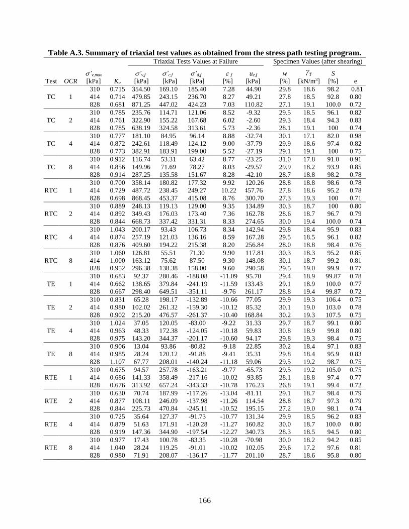
166
Table A.3. Summary of triaxial test values as obtained from the stress path testing program. Triaxial Tests Values at Failure
Specimen Values (after shearing)
Test OCR
’v,max
[kPa] Ko
’v,f
[kPa]
’c,f
[kPa]
’d,f
[kPa]
,f
[%]
ue,f
[kPa]
w
[%] T
[kN/m3]
S
[%] e
310 0.715 354.50 169.10 185.40 7.28 44.90
29.8 18.6 98.2 0.81
TC 1 414 0.714 479.85 243.15 236.70 8.27 49.21
27.8 18.5 92.8 0.80
828 0.681 871.25 447.02 424.23 7.03 110.82
27.1 19.1 100.0 0.72
310 0.785 235.76 114.71 121.06 8.52 -9.32
29.5 18.5 96.1 0.82
TC 2 414 0.761 322.90 155.22 167.68 6.02 -2.60
29.3 18.4 94.3 0.83
828 0.785 638.19 324.58 313.61 5.73 -2.36
28.1 19.1 100 0.74
310 0.777 181.10 84.95 96.14 8.88 -32.74
30.1 17.1 82.0 0.98
TC 4 414 0.872 242.61 118.49 124.12 9.00 -37.79
29.9 18.6 97.4 0.82
828 0.773 382.91 183.91 199.00 5.52 -27.19
29.1 19.1 100 0.75
310 0.912 116.74 53.31 63.42 8.77 -23.25
31.0 17.8 91.0 0.91
TC 8 414 0.856 149.96 71.69 78.27 8.03 -29.57
29.9 18.2 93.9 0.85
828 0.914 287.25 135.58 151.67 8.28 -42.10
28.7 18.8 98.2 0.78
310 0.700 358.14 180.82 177.32 9.92 -120.26
28.8 18.8 98.6 0.78
RTC 1 414 0.729 487.72 238.45 249.27 10.22 457.76
27.8 18.6 95.2 0.78
828 0.698 868.45 453.37 415.08 8.76 -300.70
27.3 19.3 100 0.71
310 0.889 248.13 119.13 129.00 9.35 -134.89
30.3 18.7 100 0.80
RTC 2 414 0.892 349.43 176.03 173.40 7.36 -162.78
28.6 18.7 96.7 0.79
828 0.844 668.73 337.42 331.31 8.33 -274.65
30.0 19.4 100.0 0.74
310 1.043 200.17 93.43 106.73 8.34 -142.94
29.8 18.4 95.9 0.83
RTC 4 414 0.874 257.19 121.03 136.16 8.59 -167.28
29.5 18.5 96.1 0.82
828 0.876 409.60 194.22 215.38 8.20 -256.84
28.0 18.8 98.4 0.76
310 1.060 126.81 55.51 71.30 9.90 -117.81
30.3 18.3 95.2 0.85
RTC 8 414 1.000 163.12 75.62 87.50 9.30 -148.08
30.1 18.7 99.2 0.81
828 0.952 296.38 138.38 158.00 9.60 -290.58
29.5 19.0 99.9 0.77
310 0.683 92.37 280.46 -188.08 -11.09 95.70
29.4 18.9 99.87 0.78
TE 1 414 0.662 138.65 379.84 -241.19 -11.59 133.43
29.1 18.9 100.0 0.77
828 0.667 298.40 649.51 -351.11 -9.76 261.17
28.8 19.4 99.87 0.72
310 0.831 65.28 198.17 -132.89 -10.66 77.05
29.9 19.3 106.4 0.75
TE 2 414 0.980 102.02 261.32 -159.30 -10.12 85.32
30.1 19.0 103.0 0.78
828 0.902 215.20 476.57 -261.37 -10.40 168.84
30.2 19.3 107.5 0.75
310 1.024 37.05 120.05 -83.00 -9.22 31.33
29.7 18.7 99.1 0.80
TE 4 414 0.963 48.33 172.38 -124.05 -10.18 59.83
30.8 18.9 99.8 0.80
828 0.975 143.20 344.37 -201.17 -10.60 94.17
29.8 19.3 98.4 0.75
310 0.906 13.04 93.86 -80.82 -9.18 22.85
30.2 18.4 97.1 0.83
TE 8 414 0.985 28.24 120.12 -91.88 -9.41 35.31
29.8 18.4 95.9 0.83
828 1.107 67.77 208.01 -140.24 -11.18 59.06
29.5 19.2 98.7 0.75
310 0.675 94.57 257.78 -163.21 -9.77 -65.73
29.5 19.2 105.0 0.75
RTE 1 414 0.686 141.33 358.49 -217.16 -10.02 -93.85
28.1 18.8 97.4 0.77
828 0.676 313.92 657.24 -343.33 -10.78 -176.23
26.8 19.1 99.4 0.72
310 0.630 70.74 187.99 -117.26 -13.04 -81.11
29.1 18.7 98.4 0.79
RTE 2 414 0.877 108.11 246.09 -137.98 -11.26 -114.54
28.8 18.7 97.3 0.79
828 0.844 225.73 470.84 -245.11 -10.52 -195.15
27.2 19.0 98.1 0.74
310 0.725 35.64 127.37 -91.73 -10.77 -131.34
29.9 18.5 96.2 0.83
RTE 4 414 0.879 51.63 171.91 -120.28 -11.27 -160.82
30.0 18.7 100.0 0.80
828 0.919 147.36 344.90 -197.54 -12.27 -340.73
28.3 18.5 94.5 0.80
310 0.977 17.43 100.78 -83.35 -10.28 -70.98
30.0 18.2 94.2 0.85
RTE 8 414 1.040 28.24 119.25 -91.01 -10.02 -102.05
29.6 17.2 97.6 0.81
828 0.980 71.91 208.07 -136.17 -11.77 -201.10
28.7 18.6 95.8 0.80

167
Table A.4. The effective shear strength parameters as obtained from the controlled stress
path triaxial tests.
TC RTC TE RTE
OCR
c
[kPa]
[degree]
c
[kPa]
[degree]
c
[kPa]
[degree]
c
[kPa]
[degree]
1 10.6 17.7 12.1 17.5 36.8 13.5 27.6 13.9
2 7.2 18.1 7.1 18.8 22.7 14.2 14.9 14.4
4 2.4 19.6 5.0 19.9 18.8 15.6 18.1 14.9
8 0.8 20.7 1.4 20.4 15.5 17.0 18.1 15.6
Table A.5. Summary of the triaxial test values as obtained from the triaxial tests with bender
element measurements. Triaxial Tests Values at Failure
Specimen Values (after shearing)
Test OCR
’v,max
[kPa]
’v,f
[kPa]
’c,f
[kPa]
’d,f
[kPa]
,f
[%]
ue,f
[kPa]
w
[%] T
[kN/m3]
S
[%] e
310 354.50 169.10 185.40 7.28 44.90
29.8 18.6 98.2 0.81
K1.5LL-NC 1 414 479.85 243.15 236.70 8.27 49.21
27.8 18.5 92.8 0.80
828 871.25 447.02 424.23 7.03 110.82
27.1 19.1 100.0 0.72
310 169.63 41.19 128.44 4.73 2.66
28.1 16.9 77.9 0.96
K3LL-NC 1 414 258.87 77.67 181.20 2.23 -8.51
29.5 18.2 89.3 0.88
828 384.70 120.93 263.78 3.93 -26.98
27.4 17.9 86.8 0.84
310 116.74 53.31 63.42 8.77 -23.25
31.0 17.8 91.0 0.91
K1.5LL-OC 8 414 149.96 71.69 78.27 8.03 -29.57
29.9 18.2 93.9 0.85
828 287.25 135.58 151.67 8.28 -42.10
28.7 18.8 98.2 0.78
310 154.73 31.83 122.90 3.18 4.98
35.5 18.0 99.8 0.95
K3LL-OC 8 414 254.81 83.75 171.06 4.83 -18.46
34.8 18.5 99.8 0.93
828 389.50 123.27 266.23 4.93 -29.99
28.9 17.5 85.1 0.91
310 265.99 108.91 157.08 1.32 67.63
31.0 18.5 99.1 0.84
I1.5LL-NC 1 414 450.66 192.89 257.77 0.15 23.16
29.0 19.9 99.5 0.78
828 841.87 371.07 470.80 0.68 103.41
25.1 20.5 99.4 0.68
310 169.63 41.19 128.44 4.73 2.66
28.7 18.2 98.7 0.78
I3LL-NC 1 414 258.87 77.67 181.20 2.23 -8.51
29.3 18.5 97.1 0.81
828 384.70 120.93 263.78 3.93 -26.98
25.0 18.9 93.7 0.72
310 226.40 86.60 139.80 1.71 100.51
31.3 18.5 100.0 0.84
I1.5LL-OC 8 414 383.00 146.00 237.00 0.95 74.95
29.5 19.1 99.7 0.80
828 762.73 316.14 446.59 2.13 274.66
26.1 19.4 98.0 0.72
310 154.73 31.83 122.90 3.18 4.98
31.9 18.1 97.4 0.88
I3LL-OC 8 414 254.81 83.75 171.06 4.83 -18.46
30.3 18.7 99.3 0.82
828 389.50 123.27 266.23 4.93 -29.99
25.0 18.9 93.7 0.72

168
Table A.6. Shear strength parameters for kaolinite and illite soils as obtained from the
triaxial tests with bender element measurements.
Test OCR
’v,max
[kPa]
c
[kPa]
[degree] *
suR
*
us
[kPa]
310 0.299 92.7
K1.5LL-NC 1 414 10.62 17.69 0.286 118.3
828 0.256 212.1
310 0.277 85.8
K3LL-NC 1 414 18.31 17.55 0.238 98.6
828 0.241 199.7
310 0.871 31.7
K1.5LL-OC 8 414 0.85 20.70 0.782 39.1
828 0.756 75.8
310 0.782 30.4
K3LL-OC 8 414 4.26 18.47 0.671 37.3
828 0.763 73.7
310 0.253 78.5
I1.5LL-NC 1 414 7.79 21.98 0.312 128.9
828 0.285 235.4
310 0.225 69.9
I3LL-NC 1 414 9.40 23.38 0.286 118.5
828 0.270 223.3
310 1.663 64.2
I1.5LL-OC 8 414 13.07 27.43 1.752 90.6
828 1.570 131.9
310 1.592 61.5
I3LL-OC 8 414 13.34 26.09 1.654 85.5
828 1.580 133.1

169
Figure A.3. a) Deviatoric stress as a function of axial strain, b) excess pore water pressure
as a function of axial strain, c) Mohr circle, and d) Cambridge p-q stress path for the TC
test at OCR=1 and ’v,max=310 kPa.
0
50
100
150
200
250
300
350
400
0 50 100 150 200 250 300 350 400
Sh
ea
r S
tress
, t
, [k
Pa
]
Normal Stress, ', [kPa]
'1'3
0
10
20
30
40
50
60
0 2 4 6 8 10 12 14 16
Exce
ss P
ore
Wate
r P
ress
ure
, u
e ,
[kP
a]
Axial Strain, A, [%]
0
50
100
150
200
250
300
0 2 4 6 8 10 12 14 16
De
via
tori
c S
tre
ss,
d ,
[kP
a]
Axial Strain, A, [%]
σ’ = 310 kPa
PPSD-TC
OCR=1
v,max
0
50
100
150
200
250
300
0 50 100 150 200 250 300
Devia
tori
c S
tress
, q,
[kP
a]
Mean Effective Stress, p', [kPa]
(a) (b)
(c) (d)

170
Figure A.4. a) Deviatoric stress as a function of axial strain, b) excess pore water pressure
as a function of axial strain, c) Mohr circle, and d) Cambridge p-q stress path for the TC
test at OCR=1 and ’v,max=414 kPa.
0
50
100
150
200
250
300
350
400
450
500
0 50 100 150 200 250 300 350 400 450 500
Shea
r S
tress
, t
, [k
Pa
]
Normal Stress, ', [kPa]
'1'3
0
10
20
30
40
50
60
70
0 2 4 6 8 10 12 14 16
Exce
ss P
ore
Wate
r P
ress
ure
, u
e ,
[kP
a]
Axial Strain, A, [%]
0
50
100
150
200
250
300
0 2 4 6 8 10 12 14 16
De
via
tori
c S
tre
ss,
d ,
[kP
a]
Axial Strain, A, [%]
PPSD-TC
σ’ = 414 kPa
OCR=1
v,max
0
50
100
150
200
250
300
350
400
0 50 100 150 200 250 300 350 400
De
via
tori
c S
tre
ss, q
, [k
Pa
]
Mean Effective Stress, p', [kPa]
(a) (b)
(c) (d)

171
Figure A.5. a) Deviatoric stress as a function of axial strain, b) excess pore water pressure
as a function of axial strain, c) Mohr circle, and d) Cambridge p-q stress path for the TC
test at OCR=1 and ’v,max=828 kPa.
0
100
200
300
400
500
600
700
800
900
0 100 200 300 400 500 600 700 800 900
Shear
Str
ess
, t
, [k
Pa]
Normal Stress, ', kPa
'1'3
0
20
40
60
80
100
120
140
0 2 4 6 8 10 12 14 16
Exce
ss P
ore
Pre
ssure
, u
e ,
[kP
a]
Axial Strain, A, [%]
0
50
100
150
200
250
300
350
400
450
500
0 2 4 6 8 10 12 14 16
Devia
tori
c S
tress
,
' d ,
[kP
a]
Axial Strain, A, [%]
PPSD-TC
σ’ = 828 kPa
OCR=1
v,max
0
100
200
300
400
500
600
700
0 100 200 300 400 500 600 700
Devia
tori
c S
tress
, q,
[kP
a]
Mean Effective Stress, p', [kPa]
(a) (b)
(c) (d)

172
Figure A.6. a) Deviatoric stress as a function of axial strain, b) excess pore water pressure
as a function of axial strain, c) Mohr circle, and d) Cambridge p-q stress path for the TC
test at OCR=2 and ’v,max=310 kPa.
0
50
100
150
200
250
300
0 50 100 150 200 250 300
Shear
Str
ess
, t
, [k
Pa]
Normal Stress, ', [kPa]
'1'3
-25
-20
-15
-10
-5
0
5
10
15
20
0 2 4 6 8 10 12 14 16
Exce
ss P
ore
Wate
r P
ress
ure
, u
e ,
[kP
a]
Axial Strain, A, [%]
0
50
100
150
200
250
300
0 2 4 6 8 10 12 14 16
Devia
tori
c S
tress
,
d ,
[kP
a]
Axial Strain, A, [%]
σ’ = 310 kPa
PPSD-TC
OCR=2
v,max
0
50
100
150
200
250
300
350
400
0 100 200 300 400
Devia
tori
c S
tress
, q,
[kP
a]
Mean Effective Stress, p', [kPa]
(a) (b)
(c) (d)

173
Figure A.7. a) Deviatoric stress as a function of axial strain, b) excess pore water pressure
as a function of axial strain, c) Mohr circle, and d) Cambridge p-q stress path for the TC
test at OCR=2 and ’v,max=414 kPa.
0
50
100
150
200
250
300
350
400
0 50 100 150 200 250 300 350 400
Sh
ea
r S
tre
ss, t
, [k
Pa
]
Normal Stress, ', [kPa]
'1'3
-15
-10
-5
0
5
10
15
20
0 2 4 6 8 10 12 14 16
Exce
ss P
ore
Wate
r P
ress
ure
, u
e ,
[kP
a]
Axial Strain, A, [%]
0
50
100
150
200
250
300
0 2 4 6 8 10 12 14 16
Devia
tori
c S
tress
,
d ,
[kP
a]
Axial Strain, A, [%]
σ’ = 414 kPa
PPSD-TC
OCR=2
v,max
0
50
100
150
200
250
300
350
400
0 100 200 300 400
Dev
iato
ric
Str
ess
, q,
[kP
a]
Mean Effective Stress, p', [kPa]
(a) (b)
(c) (d)

174
Figure A.8. a) Deviatoric stress as a function of axial strain, b) excess pore water pressure
as a function of axial strain, c) Mohr circle, and d) Cambridge p-q stress path for the TC
test at OCR=2 and ’v,max=828 kPa.
0
100
200
300
400
500
600
700
0 100 200 300 400 500 600 700
Sh
ea
r S
tre
ss, t
, [k
Pa
]
Normal Stress, ', [kPa]
'1'3
-40
-30
-20
-10
0
10
20
30
40
0 2 4 6 8 10 12 14 16
Ex
cess
Po
re P
ress
ure
, u
e ,
[kP
a]
Axial Strain, A, [%]
0
50
100
150
200
250
300
350
400
0 2 4 6 8 10 12 14 16
Dev
iato
ric
Str
ess
,
d ,
[kP
a]
Axial Strain, A, [%]
σ’ = 828 kPa
PPSD-TC
OCR=2
v,max
0
100
200
300
400
500
0 100 200 300 400 500
Dev
iato
ric
Str
ess
, q,
[kP
a]
Mean Effective Stress, p', [kPa]
(a) (b)
(c) (d)

175
Figure A.9. a) Deviatoric stress as a function of axial strain, b) excess pore water pressure
as a function of axial strain, c) Mohr circle, and d) Cambridge p-q stress path for the TC
test at OCR=4 and ’v,max=310 kPa.
0
50
100
150
200
0 50 100 150 200
Sh
ea
r S
tre
ss, t
, [k
Pa
]
Normal Stress, ', kPa
'1'3
-50
-40
-30
-20
-10
0
10
0 2 4 6 8 10 12 14 16
Ex
cess
Po
re P
ress
ure
, u
e ,
[kP
a]
Axial Strain, A, [%]
0
20
40
60
80
100
120
140
160
180
200
0 2 4 6 8 10 12 14 16
De
via
tori
c S
tre
ss,
d ,
[kP
a]
Axial Strain, A, [%]
σ’ = 310 kPa
PPSD-TC
OCR=4
v,max
0
25
50
75
100
125
150
175
200
0 50 100 150 200
Dev
iato
ric
Str
ess
, q,
[kP
a]
Mean Effective Stress, p', [kPa]
(a) (b)
(c) (d)

176
Figure A.10. a) Deviatoric stress as a function of axial strain, b) excess pore water pressure
as a function of axial strain, c) Mohr circle, and d) Cambridge p-q stress path for the TC
test at OCR=4 and ’v,max=414 kPa.
0
50
100
150
200
250
300
0 50 100 150 200 250 300
Sh
ea
r S
tress
, t
, [k
Pa
]
Normal Stress, ', kPa
'1'3
(c) (d)
-50
-40
-30
-20
-10
0
10
0 2 4 6 8 10 12 14 16
Ex
cess
Po
re P
ress
ure
, u
e ,
[kP
a]
Axial Strain, A, [%]
0
20
40
60
80
100
120
140
160
180
200
0 2 4 6 8 10 12 14 16
Dev
iato
ric
Str
ess
,
d ,
[kP
a]
Axial Strain, A, [%]
σ’ = 414 kPa
PPSD-TC
OCR=4
v,max
0
25
50
75
100
125
150
175
200
0 50 100 150 200
Dev
iato
ric
Str
ess
, q,
[kP
a]
Mean Effective Stress, p', [kPa]
(a) (b)

177
Figure A.11. a) Deviatoric stress as a function of axial strain, b) excess pore water pressure
as a function of axial strain, c) Mohr circle, and d) Cambridge p-q stress path for the TC
test at OCR=4 and ’v,max=828 kPa.
0
50
100
150
200
250
300
350
400
0 50 100 150 200 250 300 350 400
Sh
ea
r S
tress
, t
, [k
Pa
]
Normal Stress, ', kPa
'1'3
(c) (d)
-60
-50
-40
-30
-20
-10
0
10
20
0 2 4 6 8 10 12 14 16
Ex
cess
Po
re P
ress
ure
, u
e ,
[kP
a]
Axial Strain, A, [%]
0
25
50
75
100
125
150
175
200
225
250
0 2 4 6 8 10 12 14 16
De
via
tori
c S
tre
ss,
d ,
[kP
a]
Axial Strain, A, [%]
σ’ = 828 kPa
PPSD-TC
OCR=4
v,max
0
50
100
150
200
250
300
0 50 100 150 200 250 300
De
via
tori
c S
tre
ss, q
, [k
Pa
]
Mean Effective Stress, p', [kPa]
(a) (b)

178
Figure A.12. a) Deviatoric stress as a function of axial strain, b) excess pore water pressure
as a function of axial strain, c) Mohr circle, and d) Cambridge p-q stress path for the TC
test at OCR=8 and ’v,max=310 kPa.
0
20
40
60
80
100
120
140
160
0 20 40 60 80 100 120 140 160
Sh
ea
r S
tre
ss, t
, [k
Pa
]
Normal Stress, ', kPa
'1'3
-50
-40
-30
-20
-10
0
10
0 2 4 6 8 10 12 14 16
Ex
cess
Po
re P
ress
ure
, u
e ,
[kP
a]
Axial Strain, A, [%]
0
10
20
30
40
50
60
70
80
90
100
0 2 4 6 8 10 12 14 16
De
via
tori
c S
tre
ss,
d ,
[kP
a]
Axial Strain, A, [%]
σ’ = 310 kPa
PPSD-CTC
OCR=8
v,max
0
10
20
30
40
50
60
70
80
90
100
0 10 20 30 40 50 60 70 80 90 100
Dev
iato
ric
Str
ess
, q,
[kP
a]
Mean Effective Stress, p', [kPa]
(a) (b)
(c) (d)

179
Figure A.13. a) Deviatoric stress as a function of axial strain, b) excess pore water pressure
as a function of axial strain, c) Mohr circle, and d) Cambridge p-q stress path for the TC
test at OCR=8 and ’v,max=414 kPa.
0
20
40
60
80
100
120
140
160
0 20 40 60 80 100 120 140 160
Shea
r S
tress
, t, [
kP
a]
Normal Stress, ', kPa
'1'3
-50
-40
-30
-20
-10
0
10
0 2 4 6 8 10 12 14 16
Ex
cess
Po
re P
ress
ure
, u
e ,
[kP
a]
Axial Strain, A, [%]
0
10
20
30
40
50
60
70
80
90
100
0 2 4 6 8 10 12 14 16
Dev
iato
ric
Str
ess
,
' d ,
[kP
a]
Axial Strain, A, [%]
σ’ = 414 kPa
PPSD-CTC
OCR=8
v,max
0
10
20
30
40
50
60
70
80
90
100
110
120
0 20 40 60 80 100 120
Dev
iato
ric
Str
ess
, q,
[kP
a]
Mean Effective Stress, p', [kPa]
(a) (b)
(c) (d)

180
Figure A.14. a) Deviatoric stress as a function of axial strain, b) excess pore water pressure
as a function of axial strain, c) Mohr circle, and d) Cambridge p-q stress path for the TC
test at OCR=8 and ’v,max=828 kPa.
0
50
100
150
200
250
300
350
400
0 50 100 150 200 250 300 350 400
Shea
r S
tress
, t, [
kP
a]
Normal Stress, ', kPa
'1'3
-70
-60
-50
-40
-30
-20
-10
0
10
20
0 2 4 6 8 10 12 14 16
Ex
cess
Po
re P
ress
ure
, u
e ,
[kP
a]
Axial Strain, A, [%]
0
20
40
60
80
100
120
140
160
180
0 2 4 6 8 10 12 14 16
De
via
tori
c S
tre
ss,
d ,
[kP
a]
Axial Strain, A, [%]
σ’ = 828 kPa
PPSD-CTC
OCR=8
v,max
0
50
100
150
200
250
300
350
0 50 100 150 200 250
Dev
iato
ric
Str
ess
, q,
[kP
a]
Mean Effective Stress, p', [kPa]
(a) (b)
(c) (d)
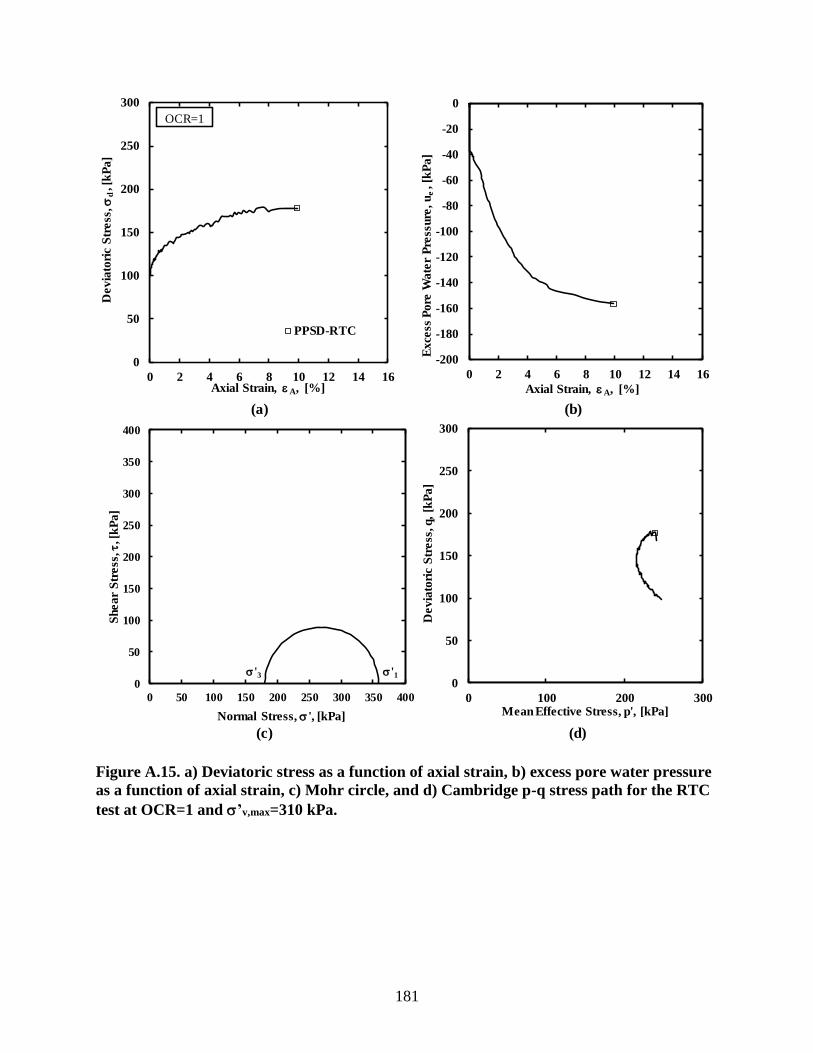
181
Figure A.15. a) Deviatoric stress as a function of axial strain, b) excess pore water pressure
as a function of axial strain, c) Mohr circle, and d) Cambridge p-q stress path for the RTC
test at OCR=1 and ’v,max=310 kPa.
0
50
100
150
200
250
300
350
400
0 50 100 150 200 250 300 350 400
Sh
ear
Str
ess
, t, [
kP
a]
Normal Stress, ', [kPa]
'1'3
-200
-180
-160
-140
-120
-100
-80
-60
-40
-20
0
0 2 4 6 8 10 12 14 16
Exce
ss P
ore
Wate
r P
ress
ure
, u
e ,
[kP
a]
Axial Strain, A, [%]
0
50
100
150
200
250
300
0 2 4 6 8 10 12 14 16
Devia
tori
c S
tress
,
d ,
[kP
a]
Axial Strain, A, [%]
PPSD-RTC
OCR=1
0
50
100
150
200
250
300
0 100 200 300
Devia
tori
c S
tress
, q,
[kP
a]
Mean Effective Stress, p', [kPa]
(a) (b)
(c) (d)

182
Figure A.16. a) Deviatoric stress as a function of axial strain, b) excess pore water pressure
as a function of axial strain, c) Mohr circle, and d) Cambridge p-q stress path for the RTC
test at OCR=1 and ’v,max=414 kPa.
0
100
200
300
400
500
600
0 100 200 300 400 500 600
Sh
ea
r S
tress
, t
, [k
Pa
]
Normal Stress, ', kPa
'1'3
-200
-180
-160
-140
-120
-100
-80
-60
-40
-20
0
0 2 4 6 8 10 12 14 16
Exce
ss P
ore
Pre
ssu
re,
ue
, [k
Pa]
Axial Strain, A, [%]
0
50
100
150
200
250
300
0 2 4 6 8 10 12 14 16
Devia
tori
c S
tress
,
d ,
[kP
a]
Axial Strain, A, [%]
PPSD-RTC
OCR=1
0
100
200
300
400
0 100 200 300 400
Dev
iato
ric
Str
ess
, q,
[kP
a]
Mean Effective Stress, p', [kPa]
(a) (b)
(c) (d)

183
Figure A.17. a) Deviatoric stress as a function of axial strain, b) excess pore water pressure
as a function of axial strain, c) Mohr circle, and d) Cambridge p-q stress path for the RTC
test at OCR=1 and ’v,max=828 kPa.
0
100
200
300
400
500
600
700
800
900
1000
0 100 200 300 400 500 600 700 800 900 1000
Sh
ea
r S
tress
, t
, [k
Pa
]
Normal Stress, ', kPa
'1'3
-350
-300
-250
-200
-150
-100
-50
0
0 2 4 6 8 10 12 14 16
Exce
ss P
ore
Pre
ssu
re,
ue
, [k
Pa]
Axial Strain, A, [%]
0
50
100
150
200
250
300
350
400
450
0 2 4 6 8 10 12 14 16
Devia
tori
c S
tress
,
d ,
[kP
a]
Axial Strain, A, [%]
PPSD-RTC
OCR=1
0
100
200
300
400
500
600
700
800
0 100 200 300 400 500 600 700 800
Dev
iato
ric
Str
ess
, q,
[kP
a]
Mean Effective Stress, p', [kPa]
(a) (b)
(c) (d)

184
Figure A.18. a) Deviatoric stress as a function of axial strain, b) excess pore water pressure
as a function of axial strain, c) Mohr circle, and d) Cambridge p-q stress path for the RTC
test at OCR=2 and ’v,max=310 kPa.
0
50
100
150
200
250
300
0 50 100 150 200 250 300
Shea
r S
tress
, t
, [k
Pa
]
Normal Stress, ', kPa
'1'3
-120
-100
-80
-60
-40
-20
0
0 2 4 6 8 10 12 14 16
Ex
cess
Po
re P
ress
ure
, u
e ,
[kP
a]
Axial Strain, A, [%]
0
50
100
150
200
250
300
0 2 4 6 8 10 12 14 16
Dev
iato
ric
Str
ess
,
d ,
[kP
a]
Axial Strain, A, [%]
σ’ = 310 kPa
PPSD-RTC
OCR=2
v,max
0
50
100
150
200
250
300
0 50 100 150 200 250 300
Dev
iato
ric
Str
ess
, q,
[kP
a]
Mean Effective Stress, p', [kPa]
(a) (b)
(c) (d)

185
Figure A.19. a) Deviatoric stress as a function of axial strain, b) excess pore water pressure
as a function of axial strain, c) Mohr circle, and d) Cambridge p-q stress path for the RTC
test at OCR=2 and ’v,max=414 kPa.
0
50
100
150
200
250
300
350
400
0 50 100 150 200 250 300 350 400
Shear
Str
ess
, t, [
kP
a]
Normal Stress, ', kPa
'1'3
-140
-120
-100
-80
-60
-40
-20
0
0 2 4 6 8 10 12 14 16
Exce
ss P
ore
Pre
ssu
re, u
e ,
[kP
a]
Axial Strain, A, [%]
0
50
100
150
200
250
300
0 2 4 6 8 10 12 14 16
Devia
tori
c S
tress
,
d ,
[kP
a]
Axial Strain, A, [%]
σ’ = 414 kPa
PPSD-RTC
OCR=2
v,max
0
50
100
150
200
250
300
0 50 100 150 200 250 300
Devia
tori
c S
tress
, q,
[kP
a]
Mean Effective Stress, p', [kPa]
(a) (b)
(c) (d)

186
Figure A.20. a) Deviatoric stress as a function of axial strain, b) excess pore water pressure
as a function of axial strain, c) Mohr circle, and d) Cambridge p-q stress path for the RTC
test at OCR=2 and ’v,max=828 kPa.
0
100
200
300
400
500
600
700
0 100 200 300 400 500 600 700
Shear
Str
ess
, t, [
kP
a]
Normal Stress, ', kPa
'1'3
-250
-225
-200
-175
-150
-125
-100
-75
-50
-25
0
0 2 4 6 8 10 12 14 16
Exce
ss P
ore
Pre
ssure
, u
e ,
[kP
a]
Axial Strain, A, [%]
0
50
100
150
200
250
300
350
400
0 2 4 6 8 10 12 14 16
Devia
tori
c S
tress
,
d ,
[kP
a]
Axial Strain, A, [%]
σ’ = 828 kPa
PPSD-RTC
OCR=2
v,max
0
100
200
300
400
500
0 100 200 300 400 500
Devia
tori
c S
tress
, q,
[kP
a]
Mean Effective Stress, p', [kPa]
(a) (b)
(c) (d)

187
Figure A.21. a) Deviatoric stress as a function of axial strain, b) excess pore water pressure
as a function of axial strain, c) Mohr circle, and d) Cambridge p-q stress path for the RTC
test at OCR=4 and ’v,max=310 kPa.
0
50
100
150
200
250
300
0 50 100 150 200 250 300
Shear
Str
ess
, t
, [k
Pa]
Normal Stress, ', kPa
'1'3
-25
-20
-15
-10
-5
0
0 2 4 6 8 10 12 14 16
Exce
ss P
ore
Pre
ssure
, u
e ,
[kP
a]
Axial Strain, A, [%]
0
20
40
60
80
100
120
140
160
180
200
0 2 4 6 8 10 12 14 16
Devia
tori
c S
tress
,
d ,
[kP
a]
Axial Strain, A, [%]
σ’ = 310 kPa
PPSD-RTC
OCR=4
v,max
0
25
50
75
100
125
150
175
200
0 50 100 150 200
Devia
tori
c S
tress
, q,
[kP
a]
Mean Effective Stress, p', [kPa]
(a) (b)
(c) (d)

188
Figure A.22. a) Deviatoric stress as a function of axial strain, b) excess pore water pressure
as a function of axial strain, c) Mohr circle, and d) Cambridge p-q stress path for the RTC
test at OCR=4 and ’v,max=414 kPa.
0
50
100
150
200
250
300
0 50 100 150 200 250 300
Shea
r S
tress
, t, [
kP
a]
Normal Stress, ', kPa
'1'3
-30
-25
-20
-15
-10
-5
0
0 2 4 6 8 10 12 14 16
Ex
cess
Po
re P
ress
ure
, u
e ,
[kP
a]
Axial Strain, A, [%]
0
20
40
60
80
100
120
140
160
180
200
0 2 4 6 8 10 12 14 16
De
via
tori
c S
tre
ss,
d ,
[kP
a]
Axial Strain, A, [%]
σ’ = 414 kPa
PPSD-RTC
OCR=4
v,max
0
25
50
75
100
125
150
175
200
0 50 100 150 200
Dev
iato
ric
Str
ess
, q,
[kP
a]
Mean Effective Stress, p', [kPa]
(a) (b)
(c) (d)

189
Figure A.23. a) Deviatoric stress as a function of axial strain, b) excess pore water pressure
as a function of axial strain, c) Mohr circle, and d) Cambridge p-q stress path for the RTC
test at OCR=4 and ’v,max=828 kPa.
0
50
100
150
200
250
300
350
400
450
0 50 100 150 200 250 300 350 400 450
Shear
Str
ess
, t, [
kP
a]
Normal Stress, ', kPa
'1'3
-300
-250
-200
-150
-100
-50
0
0 2 4 6 8 10 12 14 16
Exce
ss P
ore
Pre
ssu
re,
ue
, [k
Pa]
Axial Strain, A, [%]
0
25
50
75
100
125
150
175
200
225
250
0 2 4 6 8 10 12 14 16
Devia
tori
c S
tress
,
d ,
[kP
a]
Axial Strain, A, [%]
σ’ = 828 kPa
OCR=4
v,max
0
25
50
75
100
125
150
175
200
225
250
275
300
0 50 100 150 200 250 300
De
via
tori
c S
tre
ss, q
, [k
Pa]
Mean Effective Stress, p', [kPa]
(a) (b)
(c) (d)

190
Figure A.24. a) Deviatoric stress as a function of axial strain, b) excess pore water pressure
as a function of axial strain, c) Mohr circle, and d) Cambridge p-q stress path for the RTC
test at OCR=8 and ’v,max=310 kPa.
0
25
50
75
100
125
150
0 25 50 75 100 125 150
Shear
Str
ess
, t, [
kP
a]
Normal Stress, ', kPa
'1'3
-120
-100
-80
-60
-40
-20
0
0 2 4 6 8 10 12 14 16
Exce
ss P
ore
Pre
ssure
, u
e ,
[kP
a]
Axial Strain, A, [%]
0
10
20
30
40
50
60
70
80
90
100
0 2 4 6 8 10 12 14 16
Devia
tori
c S
tress
,
d ,
[kP
a]
Axial Strain, A, [%]
σ’ = 310 kPa
PPSD-RTC
OCR=8
v,max
0
10
20
30
40
50
60
70
80
90
100
0 50 100 150 200
Devia
tori
c S
tress
, q,
[kP
a]
Mean Effective Stress, p', [kPa]
(a) (b)
(c) (d)

191
Figure A.25. a) Deviatoric stress as a function of axial strain, b) excess pore water pressure
as a function of axial strain, c) Mohr circle, and d) Cambridge p-q stress path for the RTC
test at OCR=8 and ’v,max=414 kPa.
0
50
100
150
200
0 50 100 150 200
Shea
r S
tress
, t, [
kP
a]
Normal Stress, ', kPa
'1'3
0
10
20
30
40
50
60
70
80
90
100
0 2 4 6 8 10 12 14 16
De
via
tori
c S
tre
ss,
d ,
[kP
a]
Axial Strain, A, [%]
σ’ = 414 kPa
PPSD-RTC
OCR=8
v,max
-160
-140
-120
-100
-80
-60
-40
-20
0
0 2 4 6 8 10 12 14 16
Exce
ss P
ore
Pre
ssure
, u
e ,
[kP
a]
Axial Strain, A, [%]
0
20
40
60
80
100
120
0 20 40 60 80 100 120
Dev
iato
ric
Str
ess
, q,
[kP
a]
Mean Effective Stress, p', [kPa]
(a) (b)
(c) (d)

192
Figure A.26. a) Deviatoric stress as a function of axial strain, b) excess pore water pressure
as a function of axial strain, c) Mohr circle, and d) Cambridge p-q stress path for the RTC
test at OCR=8 and ’v,max=828 kPa.
0
50
100
150
200
250
300
0 50 100 150 200 250 300
Shea
r S
tress
, t, [
kP
a]
Normal Stress, ', kPa
'1'3
0
20
40
60
80
100
120
140
160
180
200
0 2 4 6 8 10 12 14 16
De
via
tori
c S
tre
ss,
d ,
[kP
a]
Axial Strain, A, [%]
σ’ = 828 kPa
PPSD-RTC
OCR=8
v,max
-300
-250
-200
-150
-100
-50
0
0 2 4 6 8 10 12 14 16
Exce
ss P
ore
Pre
ssure
, u
e ,
[kP
a]
Axial Strain, A, [%]
0
20
40
60
80
100
120
140
160
180
200
0 50 100 150 200
De
via
tori
c S
tre
ss, q
, [k
Pa
]
Mean Effective Stress, p', [kPa]
(a) (b)
(c) (d)

193
Figure A.27. a) Deviatoric stress as a function of axial strain, b) excess pore water pressure
as a function of axial strain, c) Mohr circle, and d) Cambridge p-q stress path for the TE
test at OCR=1 and ’v,max =310 kPa.
0
50
100
150
200
250
300
0 50 100 150 200 250 300
Shear
Str
ess
, t, [
kP
a]
Normal Stress, ', [kPa]
'1'3
-400
-350
-300
-250
-200
-150
-100
-50
0
50
100
150
-16 -14 -12 -10 -8 -6 -4 -2 0
De
via
tori
c S
tre
ss,
d ,
[kP
a]
Axial Strain, A, [%]
σ’ =310 kPa
PPSD-TE
v,max
OCR=1
-400
-300
-200
-100
0
100
200
300
0 100 200 300 400 500 600 700
De
via
tori
c S
tre
ss, q
, [k
Pa]
Mean Effective Stress, p', [kPa]
0
5
10
15
20
25
30
35
40
45
50
-16 -14 -12 -10 -8 -6 -4 -2 0
Exce
ss P
ore
Wate
r P
ress
ure
, u
e ,
[kP
a]
Axial Strain, A, [%]
(a) (b)
(c) (d)
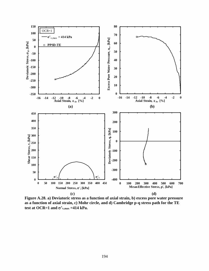
194
Figure A.28. a) Deviatoric stress as a function of axial strain, b) excess pore water pressure
as a function of axial strain, c) Mohr circle, and d) Cambridge p-q stress path for the TE
test at OCR=1 and ’v,max =414 kPa.
0
50
100
150
200
250
300
350
400
450
0 50 100 150 200 250 300 350 400 450
Sh
ea
r S
tre
ss, t
, [k
Pa
]
Normal Stress, ', [kPa]
'1'3
-350
-300
-250
-200
-150
-100
-50
0
50
100
150
-16 -14 -12 -10 -8 -6 -4 -2 0
De
via
tori
c S
tre
ss,
d ,
[kP
a]
Axial Strain, A, [%]
σ’ = 414 kPa
PPSD-TE
v,max
OCR=1
-400
-300
-200
-100
0
100
200
300
0 100 200 300 400 500 600 700
Dev
iato
ric
Str
ess
, q,
[kP
a]
Mean Effective Stress, p', [kPa]
0
10
20
30
40
50
60
70
80
-16 -14 -12 -10 -8 -6 -4 -2 0
Ex
cess
Po
re W
ate
r P
ress
ure
, u
e ,
[kP
a]
Axial Strain, A, [%]
(a) (b)
(c) (d)
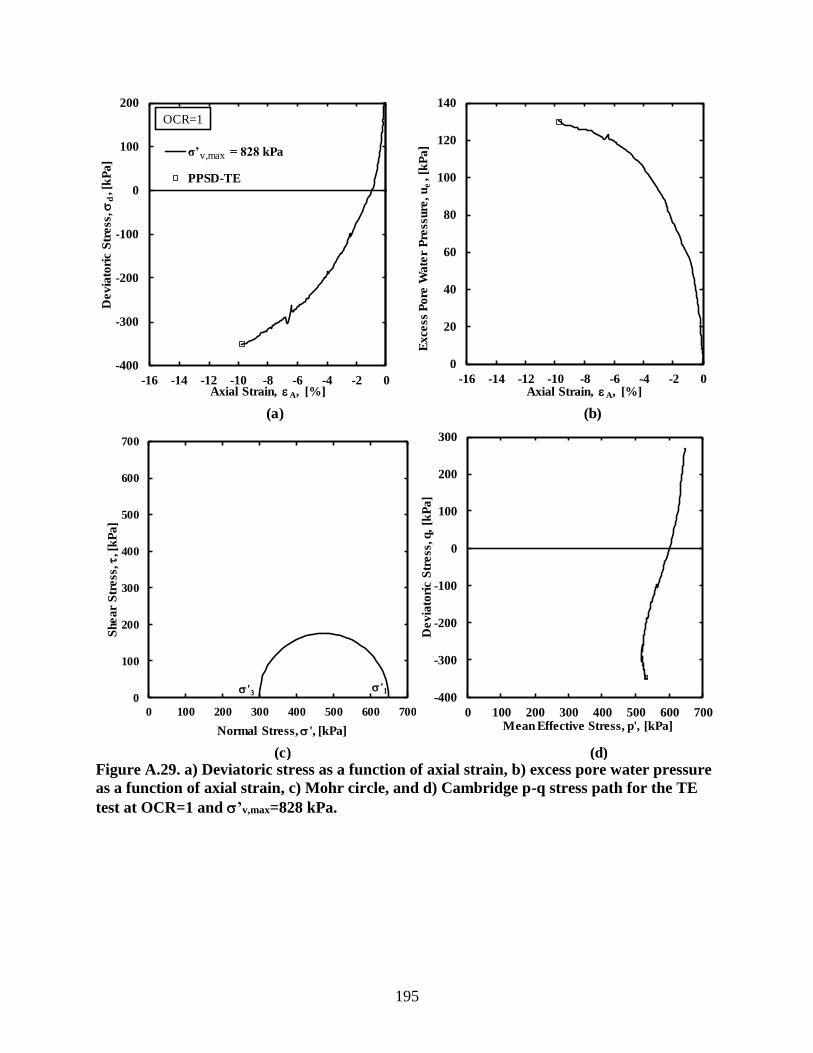
195
Figure A.29. a) Deviatoric stress as a function of axial strain, b) excess pore water pressure
as a function of axial strain, c) Mohr circle, and d) Cambridge p-q stress path for the TE
test at OCR=1 and ’v,max=828 kPa.
0
100
200
300
400
500
600
700
0 100 200 300 400 500 600 700
Shea
r S
tress
, t
, [k
Pa
]
Normal Stress, ', [kPa]
'1'3-400
-300
-200
-100
0
100
200
300
0 100 200 300 400 500 600 700
De
via
tori
c S
tre
ss, q
, [k
Pa
]
Mean Effective Stress, p', [kPa]
0
20
40
60
80
100
120
140
-16 -14 -12 -10 -8 -6 -4 -2 0
Ex
cess
Po
re W
ate
r P
ress
ure
, u
e ,
[kP
a]
Axial Strain, A, [%]
-400
-300
-200
-100
0
100
200
-16 -14 -12 -10 -8 -6 -4 -2 0
Dev
iato
ric
Str
ess
,
d ,
[kP
a]
Axial Strain, A, [%]
σ’ = 828 kPa
PPSD-TE
v,max
OCR=1
(a) (b)
(c) (d)

196
Figure A.30. a) Deviatoric stress as a function of axial strain, b) excess pore water pressure
as a function of axial strain, c) Mohr circle, and d) Cambridge p-q stress path for the TE
test at OCR=2 and ’v,max=310 kPa.
0
50
100
150
200
250
300
0 50 100 150 200 250 300
Shear
Str
ess
, t
, [k
Pa]
Normal Stress, ', [kPa]
'1'3-300
-250
-200
-150
-100
-50
0
50
100
0 100 200 300
Devia
tori
c S
tress
, q,
[kP
a]
Mean Effective Stress, p', [kPa]
0
20
40
60
80
100
120
140
160
180
-16 -14 -12 -10 -8 -6 -4 -2 0
Ex
cess
Po
re W
ate
r P
ress
ure
, u
e ,
[kP
a]
Axial Strain, A, [%]
-300
-250
-200
-150
-100
-50
0
50
-16 -14 -12 -10 -8 -6 -4 -2 0
Devia
tori
c S
tress
,
d ,
[kP
a]
Axial Strain, A, [%]
σ’ = 310 kPa
PPSD-TE
OCR=2
v,max
(a) (b)
(c) (d)

197
Figure A.31. a) Deviatoric stress as a function of axial strain, b) excess pore water pressure
as a function of axial strain, c) Mohr circle, and d) Cambridge p-q stress path for the TE
test at OCR=2 and ’v,max=414 kPa.
0
50
100
150
200
250
300
0 50 100 150 200 250 300
Shear
Str
ess
, t, [
kP
a]
Normal Stress, ', [kPa]
'1'3-300
-250
-200
-150
-100
-50
0
50
100
0 100 200 300
Devia
tori
c S
tress
, q,
[kP
a]
Mean Effective Stress, p', [kPa]
0
20
40
60
80
100
120
140
160
180
-16 -14 -12 -10 -8 -6 -4 -2 0
Ex
cess
Po
re W
ate
r P
ress
ure
, u
e ,
[kP
a]
Axial Strain, A, [%]
-300
-250
-200
-150
-100
-50
0
50
-16 -14 -12 -10 -8 -6 -4 -2 0
Devia
tori
c S
tress
,
d ,
[kP
a]
Axial Strain, A, [%]
σ’ = 414 kPa
PPSD-TE
OCR=2
v,max
(a) (b)
(c) (d)

198
Figure A.32. a) Deviatoric stress as a function of axial strain, b) excess pore water pressure
as a function of axial strain, c) Mohr circle, and d) Cambridge p-q stress path for the TE
test at OCR=2 and ’v,max=828 kPa.
0
100
200
300
400
500
600
0 100 200 300 400 500 600
Shear
Str
ess
, t, [
kP
a]
Normal Stress, ', [kPa]
'1'3-400
-300
-200
-100
0
100
200
0 100 200 300 400
Devia
tori
c S
tress
, q,
[kP
a]
Mean Effective Stress, p', [kPa]
0
20
40
60
80
100
120
140
160
180
-16 -14 -12 -10 -8 -6 -4 -2 0
Ex
cess
Po
re W
ate
r P
ress
ure
, u
e ,
[kP
a]
Axial Strain, A, [%]
-300
-250
-200
-150
-100
-50
0
50
-16 -14 -12 -10 -8 -6 -4 -2 0
Devia
tori
c S
tress
,
d ,
[kP
a]
Axial Strain, A, [%]
σ’ = 828 kPa
PPSD-TE
OCR=2
v,max
(a) (b)
(c) (d)

199
Figure A.33. a) Deviatoric stress as a function of axial strain, b) excess pore water pressure
as a function of axial strain, c) Mohr circle, and d) Cambridge p-q stress path for the TE
test at OCR=4 and ’v,max=310 kPa.
0
50
100
150
200
0 50 100 150 200
Sh
ea
r S
tre
ss, t
, [k
Pa
]
Normal Stress, ', [kPa]
'1'3 -150
-125
-100
-75
-50
-25
0
25
50
0 25 50 75 100 125 150 175 200
Dev
iato
ric
Str
ess
, q,
[kP
a]
Mean Effective Stress, p', [kPa]
0
20
40
60
80
100
120
140
160
180
-16 -14 -12 -10 -8 -6 -4 -2 0
Ex
cess
Po
re W
ate
r P
ress
ure
, u
e ,
[kP
a]
Axial Strain, A, [%]
(a) (b)
(c) (d)
-150
-130
-110
-90
-70
-50
-30
-10
10
30
50
-16 -14 -12 -10 -8 -6 -4 -2 0
Devia
tori
c S
tress
,
d ,
[kP
a]
Axial Strain, A, [%]
σ’ = 310 kPa
PPSD-TE
OCR=4
v,max

200
Figure A.34. a) Deviatoric stress as a function of axial strain, b) excess pore water pressure
as a function of axial strain, c) Mohr circle, and d) Cambridge p-q stress path for the TE
test at OCR=4 and ’v,max=414 kPa.
0
50
100
150
200
0 50 100 150 200
Sh
ea
r S
tre
ss, t
, [k
Pa
]
Normal Stress, ', [kPa]
'1'3
0
20
40
60
80
100
120
140
160
180
-16 -14 -12 -10 -8 -6 -4 -2 0
Ex
cess
Po
re W
ate
r P
ress
ure
, u
e ,
[kP
a]
Axial Strain, A, [%]
-150
-125
-100
-75
-50
-25
0
25
50
0 25 50 75 100 125 150 175 200
Dev
iato
ric
Str
ess
, q,
[kP
a]
Mean Effective Stress, p', [kPa]
-150
-130
-110
-90
-70
-50
-30
-10
10
30
50
-16 -14 -12 -10 -8 -6 -4 -2 0
De
via
tori
c S
tre
ss,
d ,
[kP
a]
Axial Strain, A, [%]
σ’ = 414 kPa
PPSD-TE
OCR=4
v,max
(a) (b)
(a) (b)

201
Figure A.35. a) Deviatoric stress as a function of axial strain, b) excess pore water pressure
as a function of axial strain, c) Mohr circle, and d) Cambridge p-q stress path for the TE
test at OCR=4 and ’v,max=828 kPa.
0
50
100
150
200
250
300
350
400
0 50 100 150 200 250 300 350 400
Shear
Str
ess
, t, [
kP
a]
Normal Stress, ', [kPa]
'1'3
0
20
40
60
80
100
120
140
160
180
-16 -14 -12 -10 -8 -6 -4 -2 0
Ex
cess
Po
re W
ate
r P
ress
ure
, u
e ,
[kP
a]
Axial Strain, A, [%]
-300
-250
-200
-150
-100
-50
0
50
0 50 100 150 200 250 300
Dev
iato
ric
Str
ess
, q,
[kP
a]
Mean Effective Stress, p', [kPa]
-150
-130
-110
-90
-70
-50
-30
-10
10
30
50
-16 -14 -12 -10 -8 -6 -4 -2 0
Devia
tori
c S
tress
,
d ,
[kP
a]
Axial Strain, A, [%]
σ’ = 414 kPa
PPSD-TE
OCR=4
v,max
(c) (d)
(a) (b)

202
Figure A.36. a) Deviatoric stress as a function of axial strain, b) excess pore water pressure
as a function of axial strain, c) Mohr circle, and d) Cambridge p-q stress path for the TE
test at OCR=8 and ’v,max=310 kPa.
0
25
50
75
100
125
150
175
200
0 25 50 75 100 125 150 175 200
Shea
r S
tress
, t, [
kP
a]
Normal Stress, ', [kPa]
'1'3 -100
-80
-60
-40
-20
0
20
0 20 40 60 80 100 120
Devia
tori
c S
tress
, q,
[kP
a]
Mean Effective Stress, p', [kPa]
0
5
10
15
20
25
30
-16 -14 -12 -10 -8 -6 -4 -2 0
Exce
ss P
ore
Wate
r P
ress
ure
, u
e ,
[kP
a]
Axial Strain, A, [%]
-120
-90
-60
-30
0
30
-16 -14 -12 -10 -8 -6 -4 -2 0
Dev
iato
ric
Str
ess
,
d ,
[kP
a]
Axial Strain, A, [%]
σ’ = 310 kPa
PPSD-TE
OCR=8 v,max
(a) (b)
(c) (d)

203
Figure A.37. a) Deviatoric stress as a function of axial strain, b) excess pore water pressure
as a function of axial strain, c) Mohr circle, and d) Cambridge p-q stress path for the TE
test at OCR=8 and ’v,max=414 kPa.
0
50
100
150
200
0 50 100 150 200
Sh
ea
r S
tre
ss, t
, [k
Pa
]
Normal Stress, ', [kPa]
'1'3-100
-80
-60
-40
-20
0
20
0 20 40 60 80 100 120
De
via
tori
c S
tre
ss, q
, [k
Pa
]
Mean Effective Stress, p', [kPa]
0
5
10
15
20
25
30
-16 -14 -12 -10 -8 -6 -4 -2 0
Exce
ss P
ore
Wate
r P
ress
ure
, u
e ,
[kP
a]
Axial Strain, A, [%]
-120
-90
-60
-30
0
30
-16 -14 -12 -10 -8 -6 -4 -2 0
De
via
tori
c S
tre
ss,
d ,
[kP
a]
Axial Strain, A, [%]
σ’ = 414 kPa
PPSD-TE
OCR=8 v,max
(a) (b)
(c) (d)

204
Figure A.38. a) Deviatoric stress as a function of axial strain, b) excess pore water pressure
as a function of axial strain, c) Mohr circle, and d) Cambridge p-q stress path for the TE
test at OCR=8 and ’v,max=828 kPa.
0
50
100
150
200
250
300
0 50 100 150 200 250 300
Shear
Str
ess
, t
, [k
Pa]
Normal Stress, ', [kPa]
'1'3
-150
-125
-100
-75
-50
-25
0
25
50
0 50 100 150 200
Devia
tori
c S
tress
, q,
[kP
a]
Mean Effective Stress, p', [kPa]
0
5
10
15
20
25
30
35
40
45
50
-16 -14 -12 -10 -8 -6 -4 -2 0
Ex
cess
Po
re W
ate
r P
ress
ure
, u
e ,
[kP
a]
Axial Strain, A, [%]
-150
-120
-90
-60
-30
0
-16 -14 -12 -10 -8 -6 -4 -2 0
Devia
tori
c S
tress
,
d ,
[kP
a]
Axial Strain, A, [%]
σ’ = 828 kPa
PPSD-TE
OCR=8 v,max
(a) (b)
(c) (d)

205
Figure A.39. a) Deviatoric stress as a function of axial strain, b) excess pore water pressure
as a function of axial strain, c) Mohr circle, and d) Cambridge p-q stress path for the RTE
test at OCR=1 and ’v,max =310 kPa.
0
50
100
150
200
250
300
0 50 100 150 200 250 300
Shea
r S
tress
, t
, [k
Pa
]
Normal Stress, ', [kPa]
'1'3
-80
-70
-60
-50
-40
-30
-20
-10
0
-16 -14 -12 -10 -8 -6 -4 -2 0
Ex
cess
Po
re W
ate
r P
ress
ure
, u
e ,
[kP
a]
Axial Strain, A, [%]
-200
-150
-100
-50
0
50
100
150
200
0 50 100 150 200 250 300
De
via
tori
c S
tre
ss, q
, [k
Pa
]
Mean Effective Stress, p', [kPa]
-400
-300
-200
-100
0
100
200
-16 -14 -12 -10 -8 -6 -4 -2 0
De
via
tori
c S
tre
ss,
d ,
[kP
a]
Axial Strain, A, [%]
σ’ = 310 kPa
PPSD-RTE
v,max
OCR=1
(a) (b)
(c) (d)

206
Figure A.40. a) Deviatoric stress as a function of axial strain, b) excess pore water pressure
as a function of axial strain, c) Mohr circle, and d) Cambridge p-q stress path for the RTE
test at OCR=1 and ’v,max =414 kPa.
0
50
100
150
200
250
300
350
400
0 50 100 150 200 250 300 350 400
Shear
Str
ess
, t, [
kP
a]
Normal Stress, ', [kPa]
'1'3
-100
-90
-80
-70
-60
-50
-40
-30
-20
-10
0
-16 -14 -12 -10 -8 -6 -4 -2 0
Exce
ss P
ore
Wate
r P
ress
ure
, u
e ,
[kP
a]
Axial Strain, A, [%]
-400
-300
-200
-100
0
100
200
300
0 100 200 300 400 500 600 700
Devia
tori
c S
tress
, q,
[kP
a]
Mean Effective Stress, p', [kPa]
-400
-300
-200
-100
0
100
200
-16 -14 -12 -10 -8 -6 -4 -2 0
Devia
tori
c S
tress
, d
, [k
Pa]
Axial Strain, A, [%]
σ’ = 414 kPa
PPSD-RTE
v,max
OCR=1
(a) (b)
(c) (d)

207
Figure A.41. a) Deviatoric stress as a function of axial strain, b) excess pore water pressure
as a function of axial strain, c) Mohr circle, and d) Cambridge p-q stress path for the RTE
test at OCR=1 and ’v,max=828 kPa.
0
100
200
300
400
500
600
700
800
0 100 200 300 400 500 600 700 800
Sh
ea
r S
tress
, t
, [k
Pa
]
Normal Stress, ', [kPa]
'1'3
-225
-200
-175
-150
-125
-100
-75
-50
-25
0
-16 -14 -12 -10 -8 -6 -4 -2 0
Ex
cess
Po
re W
ate
r P
ress
ure
, u
e ,
[kP
a]
Axial Strain, A, [%]
-400
-300
-200
-100
0
100
200
300
0 100 200 300 400 500 600 700
Dev
iato
ric
Str
ess
, q,
[kP
a]
Mean Effective Stress, p', [kPa]
-400
-300
-200
-100
0
100
200
-16 -14 -12 -10 -8 -6 -4 -2 0
De
via
tori
c S
tre
ss,
d ,
[kP
a]
Axial Strain, A, [%]
σ’ = 828 kPa
PPSD-RTE
v,max
OCR=1
(a) (b)
(c) (d)

208
Figure A.42. a) Deviatoric stress as a function of axial strain, b) excess pore water pressure
as a function of axial strain, c) Mohr circle, and d) Cambridge p-q stress path for the RTE
test at OCR=2 and ’v,max=310 kPa.
0
20
40
60
80
100
120
140
160
180
200
0 20 40 60 80 100 120 140 160 180 200
Sh
ea
r S
tress
, t
, [k
Pa
]
Normal Stress, ', [kPa]
'1'3-200
-150
-100
-50
0
50
100
0 100 200 300
De
via
tori
c S
tre
ss, q
, [k
Pa
]
Mean Effective Stress, p', [kPa]
-160
-140
-120
-100
-80
-60
-40
-20
0
-16 -14 -12 -10 -8 -6 -4 -2 0
Exce
ss P
ore
Wate
r P
ress
ure
, u
e ,
[kP
a]
Axial Strain, A, [%]
-300
-250
-200
-150
-100
-50
0
50
-16 -14 -12 -10 -8 -6 -4 -2 0
Devia
tori
c S
tress
, d
, [k
Pa]
Axial Strain, A, [%]
σ’ = 310 kPa
PPSD-RTE
OCR=2
v,max
(a) (b)
(c) (d)

209
Figure A.43. a) Deviatoric stress as a function of axial strain, b) excess pore water pressure
as a function of axial strain, c) Mohr circle, and d) Cambridge p-q stress path for the RTE
test at OCR=2 and ’v,max=414 kPa.
0
50
100
150
200
250
300
0 50 100 150 200 250 300
Sh
ea
r S
tre
ss, t
, [k
Pa
]
Normal Stress, ', [kPa]
'1'3-300
-250
-200
-150
-100
-50
0
50
100
0 100 200 300
Devia
tori
c S
tress
, q,
[kP
a]
Mean Effective Stress, p', [kPa]
-160
-140
-120
-100
-80
-60
-40
-20
0
-16 -14 -12 -10 -8 -6 -4 -2 0
Ex
cess
Po
re W
ate
r P
ress
ure
, u
e ,
[kP
a]
Axial Strain, A, [%]
-300
-250
-200
-150
-100
-50
0
50
-16 -14 -12 -10 -8 -6 -4 -2 0
Dev
iato
ric
Str
ess
,
d ,
[kP
a]
Axial Strain, A, [%]
σ’ = 414 kPa
PPSD-RTE
OCR=2
v,max
(a) (b)
(c) (d)
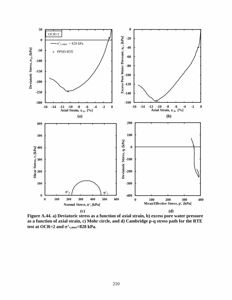
210
Figure A.44. a) Deviatoric stress as a function of axial strain, b) excess pore water pressure
as a function of axial strain, c) Mohr circle, and d) Cambridge p-q stress path for the RTE
test at OCR=2 and ’v,max=828 kPa.
0
100
200
300
400
500
600
0 100 200 300 400 500 600
Sh
ea
r S
tress
, t
, [k
Pa
]
Normal Stress, ', [kPa]
'1'3-400
-300
-200
-100
0
100
200
0 100 200 300 400
Dev
iato
ric
Str
ess
, q,
[kP
a]
Mean Effective Stress, p', [kPa]
-160
-140
-120
-100
-80
-60
-40
-20
0
-16 -14 -12 -10 -8 -6 -4 -2 0
Exce
ss P
ore
Wate
r P
ress
ure
, u
e ,
[kP
a]
Axial Strain, A, [%]
-300
-250
-200
-150
-100
-50
0
50
-16 -14 -12 -10 -8 -6 -4 -2 0
Dev
iato
ric
Str
ess
,
d ,
[kP
a]
Axial Strain, A, [%]
σ’ = 828 kPa
PPSD-RTE
OCR=2
v,max
(a) (b)
(c) (d)
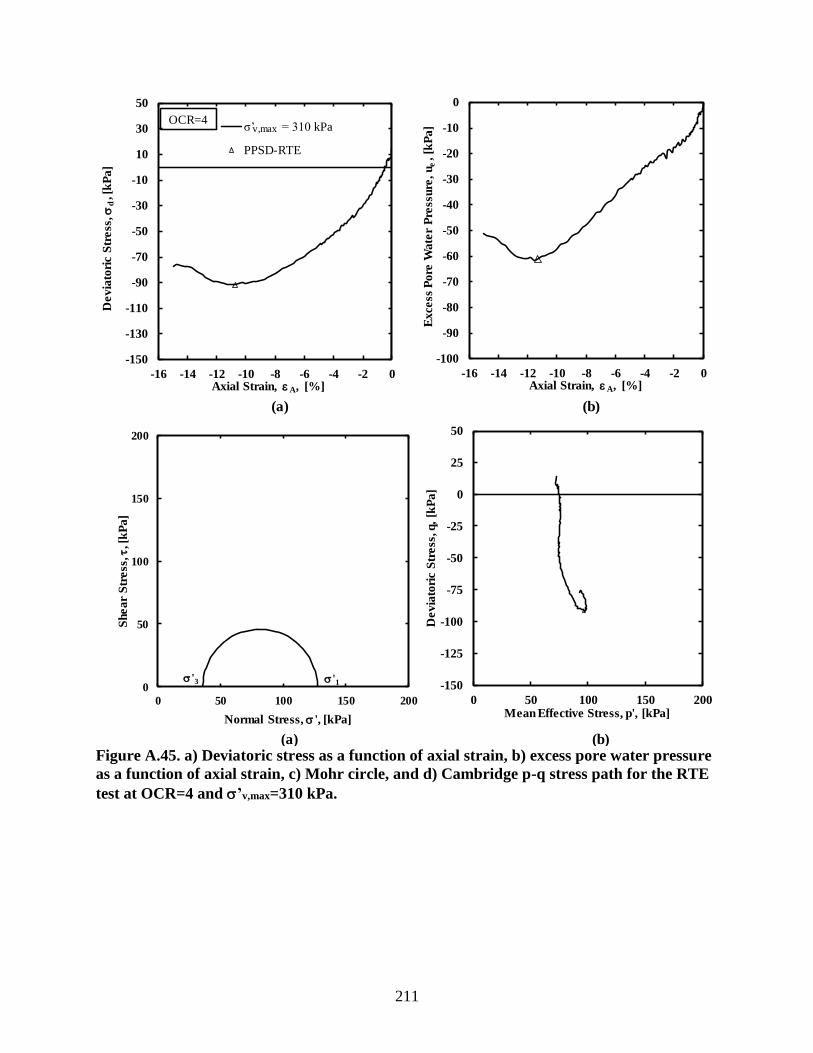
211
Figure A.45. a) Deviatoric stress as a function of axial strain, b) excess pore water pressure
as a function of axial strain, c) Mohr circle, and d) Cambridge p-q stress path for the RTE
test at OCR=4 and ’v,max=310 kPa.
0
50
100
150
200
0 50 100 150 200
Sh
ear
Str
ess
, t, [
kP
a]
Normal Stress, ', [kPa]
'1'3 -150
-125
-100
-75
-50
-25
0
25
50
0 50 100 150 200
Devia
tori
c S
tress
, q,
[kP
a]
Mean Effective Stress, p', [kPa]
-100
-90
-80
-70
-60
-50
-40
-30
-20
-10
0
-16 -14 -12 -10 -8 -6 -4 -2 0
Exce
ss P
ore
Wate
r P
ress
ure
, u
e ,
[kP
a]
Axial Strain, A, [%]
-150
-130
-110
-90
-70
-50
-30
-10
10
30
50
-16 -14 -12 -10 -8 -6 -4 -2 0
Dev
iato
ric
Str
ess
,
d ,
[kP
a]
Axial Strain, A, [%]
σ’ = 310 kPa
PPSD-RTE
OCR=4v,max
(a) (b)
(a) (b)

212
Figure A.46. a) Deviatoric stress as a function of axial strain, b) excess pore water pressure
as a function of axial strain, c) Mohr circle, and d) Cambridge p-q stress path for the RTE
test at OCR=4 and ’v,max=414 kPa.
0
50
100
150
200
0 50 100 150 200
Shear
Str
ess
, t, [
kP
a]
Normal Stress, ', [kPa]
'1'3-150
-125
-100
-75
-50
-25
0
25
50
0 50 100 150 200
Devia
tori
c S
tress
, q,
[kP
a]
Mean Effective Stress, p', [kPa]
-100
-90
-80
-70
-60
-50
-40
-30
-20
-10
0
-16 -14 -12 -10 -8 -6 -4 -2 0
Exce
ss P
ore
Wate
r P
ress
ure
, u
e ,
[kP
a]
Axial Strain, A, [%]
-150
-130
-110
-90
-70
-50
-30
-10
10
30
50
-16 -14 -12 -10 -8 -6 -4 -2 0
De
via
tori
c S
tre
ss,
d ,
[kP
a]
Axial Strain, A, [%]
σ’ = 414 kPa
PPSD-RTE
OCR=4v,max
(a) (b)
(c) (d)

213
Figure A.47. a) Deviatoric stress as a function of axial strain, b) excess pore water pressure
as a function of axial strain, c) Mohr circle, and d) Cambridge p-q stress path for the RTE
test at OCR=4 and ’v,max=828 kPa.
0
50
100
150
200
250
300
350
400
0 50 100 150 200 250 300 350 400
Shea
r S
tress
, t
, [k
Pa
]
Normal Stress, ', [kPa]
'1'3-250
-200
-150
-100
-50
0
50
0 100 200 300
Dev
iato
ric
Str
ess
, q,
[kP
a]
Mean Effective Stress, p', [kPa]
-250
-200
-150
-100
-50
0
-16 -14 -12 -10 -8 -6 -4 -2 0
Ex
cess
Po
re W
ate
r P
ress
ure
, u
e ,
[kP
a]
Axial Strain, A, [%]
-250
-200
-150
-100
-50
0
50
-16 -14 -12 -10 -8 -6 -4 -2 0
Dev
iato
ric
Str
ess
,
d ,
[kP
a]
Axial Strain, A, [%]
σ’ = 828 kPa
PPSD-RTE
OCR=4
v,max
(a) (b)
(c) (d)

214
Figure A.48. a) Deviatoric stress as a function of axial strain, b) excess pore water pressure
as a function of axial strain, c) Mohr circle, and d) Cambridge p-q stress path for the RTE
test at OCR=8 and ’v,max=310 kPa.
0
50
100
150
200
0 50 100 150 200
Sh
ear
Str
ess
, t, [
kP
a]
Normal Stress, ', [kPa]
'1'3 -150
-125
-100
-75
-50
-25
0
25
50
0 50 100 150 200
Devia
tori
c S
tress
, q,
[kP
a]
Mean Effective Stress, p', [kPa]
-100
-90
-80
-70
-60
-50
-40
-30
-20
-10
0
-16 -14 -12 -10 -8 -6 -4 -2 0
Ex
cess
Po
re W
ate
r P
ress
ure
, u
e ,
[kP
a]
Axial Strain, A, [%]
-150
-130
-110
-90
-70
-50
-30
-10
10
30
50
-16 -14 -12 -10 -8 -6 -4 -2 0
Dev
iato
ric
Str
ess
,
d ,
[kP
a]
Axial Strain, A, [%]
σ’ = 310 kPa
PPSD-RTE
OCR=8v,max
(a) (b)
(d) (c)

215
Figure A.49. a) Deviatoric stress as a function of axial strain, b) excess pore water pressure
as a function of axial strain, c) Mohr circle, and d) Cambridge p-q stress path for the RTE
test at OCR=8 and ’v,max=414 kPa.
0
50
100
150
200
0 50 100 150 200
Shea
r S
tress
, t
, [k
Pa
]
Normal Stress, ', [kPa]
'1'3-150
-125
-100
-75
-50
-25
0
25
50
0 50 100 150 200
De
via
tori
c S
tre
ss, q
, [k
Pa
]
Mean Effective Stress, p', [kPa]
-100
-90
-80
-70
-60
-50
-40
-30
-20
-10
0
-16 -14 -12 -10 -8 -6 -4 -2 0
Ex
cess
Po
re W
ate
r P
ress
ure
, u
e ,
[kP
a]
Axial Strain, A, [%]
-150
-130
-110
-90
-70
-50
-30
-10
10
30
50
-16 -14 -12 -10 -8 -6 -4 -2 0
Dev
iato
ric
Str
ess
,
d ,
[kP
a]
Axial Strain, A, [%]
σ’ = 414 kPa
PPSD-RTE
OCR=8v,max
(a) (b)
(c) (d)

216
Figure A.50. a) Deviatoric stress as a function of axial strain, b) excess pore water pressure
as a function of axial strain, c) Mohr circle, and d) Cambridge p-q stress path for the RTE
test at OCR=8 and ’v,max=828 kPa.
0
50
100
150
200
250
300
0 50 100 150 200 250 300
Sh
ea
r S
tress
, t
, [k
Pa
]
Normal Stress, ', [kPa]
'1'3
-150
-125
-100
-75
-50
-25
0
25
50
0 50 100 150 200
Dev
iato
ric
Str
ess
, q,
[kP
a]
Mean Effective Stress, p', [kPa]
-150
-125
-100
-75
-50
-25
0
-16 -14 -12 -10 -8 -6 -4 -2 0
Ex
cess
Po
re W
ate
r P
ress
ure
, u
e ,
[kP
a]
Axial Strain, A, [%]
-150
-130
-110
-90
-70
-50
-30
-10
10
30
50
-16 -14 -12 -10 -8 -6 -4 -2 0
Dev
iato
ric
Str
ess
,
d ,
[kP
a]
Axial Strain, A, [%]
σ’ = 828 kPa
PPSD-RTE
OCR=8v,max
(a) (b)
(c) (d)

217
A.4. Shear Wave Velocity and Shear Modulus Results
Included in this section are the results obtained from the triaxial tests, with bender
element measurements, that were performed on kaolinite and illite soil specimens. These results
include: 1) measured shear wave velocity as a function of axial stress, 2) shear modulus as a
function of axial strain, 3) measured shear wave velocity as a function of void index, 4) shear
modulus as a function of void index, and 5) shear modulus as a function of excess pore water
pressure.

218
Figure A.51. The small-strain values for reconstituted illite (I1.5LL): a) shear wave
velocity-vertical effective stress relationship, b) shear modulus-axial strain relationship, c)
shear wave velocity as a function of void index, and d) shear modulus as a function of void
index.
60
80
100
120
140
160
180
10 100 1000
Sh
ea
r W
av
e V
elo
city
, V
s, [
m/s
]
Vertical Effective Stress, 'v, [kPa]
Illite, I1.5LL
0
10
20
30
40
50
60
0.1 1 10 100
Sh
ea
r M
od
ulu
s, G
BE,
[MP
a]
Axial Strain, a, [%]
Unl
oad
ing
-0.7
-0.6
-0.5
-0.4
-0.3
-0.2
-0.1
0
0.1
0.2
10 100 1000
Void
Index,
I v
Shear Wave Velocity, Vs, [m/s]
-0.7
-0.6
-0.5
-0.4
-0.3
-0.2
-0.1
0
0.1
0.2
10 100
Void
Index,
I v
Shear Modulus, GBE , [MPa]
(a) (b)
(c) (d)

219
Figure A.52. The small-strain values for reconstituted kaolinite (K1.5LL): a) shear wave
velocity-vertical effective stress relationship, b) shear modulus-axial strain relationship, c)
shear wave velocity as a function of void index, and d) shear modulus as a function of void
index.
60
80
100
120
140
160
180
10 100 1000
Shear
Wave V
elo
city
, V
s, [
m/s
]
Vertical Effective Stress, 'v, [kPa]
Kaolinite, K1.5LL
0
10
20
30
40
50
60
0.1 1 10S
hear
Mod
ulu
s, G
BE,
[MP
a]
Axial Strain, a, [%]
Unl
oad
ing
-0.7
-0.6
-0.5
-0.4
-0.3
-0.2
-0.1
0
0.1
0.2
10 100 1000
Void
In
dex,
I v
Shear Wave Velocity, Vs, [m/s]
-0.7
-0.6
-0.5
-0.4
-0.3
-0.2
-0.1
0
0.1
0.2
10 100
Void
In
de
x,
I v
Shear Modulus, GBE , [MPa]
(a) (b)
(c) (d)

220
Figure A.53. The small-strain values for reconstituted illite (I3LL): a) shear wave velocity-
vertical effective stress relationship, b) shear modulus-axial strain relationship, c) shear
wave velocity as a function of void index, and d) shear modulus as a function of void index.
60
80
100
120
140
160
180
10 100 1000
Sh
ea
r W
av
e V
elo
city
, V
s, [
m/s
]
Vertical Effective Stress, 'v, [kPa]
Illite, I3LL
0
10
20
30
40
50
60
0.1 1 10 100
Sh
ea
r M
od
ulu
s, G
BE,
[MP
a]
Axial Strain, a, [%]
Unl
oad
ing
-0.7
-0.6
-0.5
-0.4
-0.3
-0.2
-0.1
0
0.1
0.2
10 100 1000
Vo
id I
nd
ex
, I v
Shear Wave Velocity, Vs, [m/s]
-0.7
-0.6
-0.5
-0.4
-0.3
-0.2
-0.1
0
0.1
0.2
10 100
Vo
id I
nd
ex
, I v
Shear Modulus, GBE , [MPa]
(a) (b)
(c) (d)

221
Figure A.54. The small-strain values for reconstituted kaolinite (K3LL): a) shear wave
velocity-vertical effective stress relationship, b) shear modulus-axial strain relationship, c)
shear wave velocity as a function of void index, and d) shear modulus as a function of void
index.
60
80
100
120
140
160
180
10 100 1000
Sh
ea
r W
av
e V
elo
city
, V
s, [
m/s
]
Vertical Effective Stress, 'v, [kPa]
Kaolinite, K3LL
0
10
20
30
40
50
60
0.1 1 10
Sh
ea
r M
od
ulu
s, G
BE,
[MP
a]
Axial Strain, a, [%]
-0.7
-0.6
-0.5
-0.4
-0.3
-0.2
-0.1
0
0.1
0.2
10 100 1000
Vo
id I
nd
ex
, I v
Shear Wave Velocity, Vs, [m/s]
-0.7
-0.6
-0.5
-0.4
-0.3
-0.2
-0.1
0
0.1
0.2
10 100
Vo
id I
nd
ex
, I v
Shear Modulus, GBE , [MPa]
(a) (b)
(c) (d)

222
Figure A.55. Shear modulus-excess pore water pressure relationships, during shearing
stage, for the kaolinite specimens.
Figure A.56. Shear modulus-excess pore water pressure relationships, during shearing
stage, for the illite specimens.
-60
-20
20
60
100
140
180
220
0 20 40 60 80
Exce
ss P
ore
Wate
r P
ress
ure
, u
e, [k
Pa]
Shear Modulus, GBE, [MPa]
K1.5LL, NC
K1.5LL, OC
K3LL, NC
K3LL, OC
at PPSDue
-60
-20
20
60
100
140
180
220
0 20 40 60 80
Exce
ss P
ore
Wate
r P
ress
ure
, u
e, [k
Pa]
Shear Modulus, GBE, [MPa]
I1.5LL, NC
I1.5LL, OC
I3LL, NC
I3LL, OC
at PPSDue