Electrically Driven Membrane Processes - in English

Søren Prip Beier

Electrically Driven MembraneProcesses

Download free books at

Download free eBooks at bookboon.com

2

Søren Prip Beier

Electrically Driven Membrane Processes

http://bookboon.com/


3

Electrically Driven Membrane Processes1st edition© 2014 Søren Prip Beier & bookboon.comISBN 87-7681-215-4

http://bookboon.com



Click on the ad to read more


4

Contents

Contents

Electrically Driven Membrane Processes 5

Nomenclature 6

1 Introduction 8

2 Electrodialysis 182.1 Basic concept 192.2 Critical current and critical current density 212.3 Desalination degree 392.4 Current efficiency 412.5 Energy requirement 422.6 Anti-fouling mechanism 48

3 Summary 49

Notes 51

Stand out from the crowdDesigned for graduates with less than one year of full-time postgraduate work experience, London Business School’s Masters in Management will expand your thinking and provide you with the foundations for a successful career in business.

The programme is developed in consultation with recruiters to provide you with the key skills that top employers demand. Through 11 months of full-time study, you will gain the business knowledge and capabilities to increase your career choices and stand out from the crowd.

Applications are now open for entry in September 2011.

For more information visit www.london.edu/mim/ email [email protected] or call +44 (0)20 7000 7573

Masters in Management

London Business SchoolRegent’s ParkLondon NW1 4SAUnited KingdomTel +44 (0)20 7000 7573Email [email protected]/mim/

Fast-track your career


http://bookboon.com/count/advert/eba1fd82-96d7-e011-adca-22a08ed629e5



5


Electrically Driven Membrane ProcessesThis text is written to all chemical engineering students who are participating in courses about membrane processes and membrane technology. Membrane processes find applications in almost all kinds of industries as one or more down stream purification/separation processes:

- Chemical industries - Pharmaceutical industries - Food industries - Dairy industries - Wastewater treatment - Etc…

Because of the wide spectrum of applications, knowledge about membrane processes is of great importance and each engineering student who chooses membranes as the main path of interests has a world of opportunities in coming career.

For reading and understanding this text you are supposed to have the basic skills in mathematics and chemistry in general. Thus this text is for students who have completed the basic engineering introduction courses or for industry staff who wants to get a quick introduction to this field. This text gives an introduction to principles behind electrically driven membrane processes in general and electrodialysis in particular. Relevant theory will be presented together with terms widely used in the world of membrane technology.

After the presentation of certain equations the SI-units will be given in order to give the reader an easy overview of the different terms and parameters in that particular equation and why these terms are included in the equation. Relevant examples will be included in order to show how the described theory can be applied in practice.

I alone am responsible for any misprints or errors and I will be grateful to receive any critics and suggestions for improvement.

November 2006

Søren Prip Beier




6

Nomenclature

Nomenclaturea Activity A Anion exchange membrane

membraneA Area of membrane

BC Boundary condition

C Cation exchange membrane c Concentration

321 ,, CCC Constants

cc Concentrate bulk concentration

cc' Concentrate concentration at membrane surface

dc Diluate bulk concentration

dc' Diluate concentration at membrane surface

D Diffusion coefficient

hd Hydraulic diameter

E Voltage

donE Donnan potential �

E Energy consumption

.eq EquivalentF Faraday number (96485 C/eq.) i Current density I Current J Flux

k Mass transfer coefficient

L Length of flow channel m Mobilityn Number of cell pairs Q Volume flow rate

cQ Concentrate volume flow rate

dQ Diluate volume flow rate

eQ Electrode solution volume flow rate

R Electrical resistance Re Reynolds number

gasR Gas constant

S Desalination degree

Sc Schmidt number

Sh Sherwood number




7

Nomenclature

�t Transport number of cation in solution

�t Transport number of anion in solution

�t Transport number of cation in membrane

�t Transport number of anion in membrane

T Absolute temperature u Flow velocity x Direction z Valence of ion

�z Valence of cation

�z Valence of anion

Greek letters � Boundary layer thickness

p� Pressure drop � Current efficiency

pumpedcxx ,,,, �� Pump efficiency

� Chemical potential � Kinematic viscosity � Electrical conductance � Electrical potential � Current utilization




8

Introduction

1 IntroductionA membrane process is capable of performing a certain separation by use of a membrane. The core in every membrane process is thus the membrane that allows certain components to pass through and retain other components. Initially some of the most important terms used in membrane technology are shown in Figure 1.

Figure 1: Membrane process Sketch of a membrane process. The core is the membrane it self through which a driving force induces a flux from the bulk to the permeate side.

The feed side is often referred to as the bulk solution. The components in the bulk solution that are retained can also be referred to at the retentate. When a driving force is established across the membrane a flux will go through the membrane from the bulk solution to the permeate side. The flux is referred to with the letter “J”. On the other side of the membrane the permeate is located.





9

Introduction

A particular separation is accomplished by use of a membrane with the ability of transporting one component more readily than another. In other words, the membrane is more permeable to certain components than other components because of differences in physical or chemical properties between the membrane and the components that are transported through the membrane. As seen in Figure 1, a driving force across the membrane induces a flux from the bulk solution to the permeate side. Different driving forces are used in different membrane processes (listed in Table 1).

Different driving forces, different membrane processes.

Driving force Membrane process

Pressure difference Micro-, ultra-, nanofiltration and reverse osmosis

Concentration difference Gas separation, pervaporation, dialysis

Temperature difference Membrane distillation, thermo osmosis

Electrical voltage difference Electrodialysis, membrane electrolysis

Table 1: Different membrane processes

Who are we?We are the world’s largest oilfield services company. Working globally—often in remote and challenging locations—we invent, design, engineer, and apply technology to help our customers find and produce oil and gas safely.

Who are we looking for?We’re looking for high-energy, self-motivated graduates with vision to work in our engineering, research and operations domain.

What will you be?

careers.slb.com

>120,000 employees

>140 nationalities

~ 85 countries of operation

years of

innovation85

Copyright © 2013 Schlumberger. All rights reserved.

ENGINEERING, RESEARCH AND OPERATIONS


http://bookboon.com/count/advert/ce678aff-77f9-484e-ac5e-a23100ef2ded



10

Introduction

In this text we will focus on membrane processes in which the driving force consists of an electrical voltage difference. Electrically driven membrane processes are widely used to remove charged components from a given feed solution or suspension. Thus the applied driving force is a voltage difference and the components that are removed are ions. In contrast to pressure driven membrane processes where you have a volume flux through the membrane, you have a flux of ions through the membrane in electrically driven membrane processes. In order to establish an electrical driving force you need an electrical field. Therefore two electrodes are required; a cathode and an anode. The positive ions (cations) in a solution will migrate to the negative electrode (cathode), the negative ions (anions) will migrate to the positive electrode (anode) and the uncharged molecules will not be affected by the electrical field. One of the greatest applications of electrically driven membrane processes is the desalination of saline water in the production of potable water. The membranes used for this purpose are ion exchange membranes which only allow transport of certain ions.

- Cation exchange membranes: Cation exchange membranes are incorporated with negatively charged groups (for example sulfonic or carboxylic acid groups) which will repel anions and only allow transport of cations.

- Anion exchange membranes: Anion exchange membranes are incorporated with positively charged groups (for example those derived from quartenary ammonium salts) which will repel cations and only allow transport of anions.

Various types of ion exchange membranes can be distinguished. You can either have heterogeneous or homogeneous ion exchange membranes:

- Heterogeneous ion exchange membranes: Heterogeneous ion exchange membranes are prepared from ion exchange resins and a film-forming polymer. These materials are combined and made into a film by dry-molding for example. The mechanical strength is relatively poor especially at high swelling degrees and the electrical resistance is relatively high which of course is unwanted.

- Homogeneous ion exchange membranes: In homogeneous ion exchange membranes the charged groups are attached directly to the polymer chains. The charge is thus distributed uniformly within the whole membrane structure. The swelling of these membranes can be reduced by crosslinking the polymers.

In order to have a good ion exchange membrane, the membrane has to fulfill certain criteria:

- High selectivity - High electrical conductivity - High mechanical strength - High chemical strength - High ion permeability - Low electrical resistance




11

Introduction

The separation principle when ion exchange membranes are used is based on Donnan exclusion which is sketched in Figure 2. The figure shows the case with anions being excluded by cations at the surface of a cation exchange membrane.

Figure 2: Donnan exclusion at membrane surface

The separation principle associated with ion exchange membranes is based on Donnan exclusion. The cation exchange membrane is incorporated with negative charges and thus a “layer” of oppositely charges cations occupy the region close the membrane surface which is the boundary layer (1). Outside the boundary layer the concentration of cations and anions is equal (2).

Donnan exclusion is named after the British chemist Frederick George Donnan, and as sketched in Figure 2 ions which the same charge as the membrane are excluded because a layer of oppositely charged ions are located closest to the membrane surface in the boundary layer. The chemical potential of the cations in the membrane (phase 1, Figure 2) and outside the boundary layer (phase 2, Figure 2) can be expressed as follows:

� � � �� bulkin thepotentialchemical,ln

membranein thepotentialchemical,ln22022

11011

��

��

��

��

FzaTR

FzaTR

gas

gas

��

�� (1)

At equilibrium the chemical potential in the membrane and in the bulk solution must equal according to thermodynamic considerations. The Donnan potential Edon is defined at the difference between the potential in the membrane y1 and in the bulk solution y2. If the chemical potential at reference state is assumed to be equal the following expression for the Donnan potential can be derived from equation (1):

��

��

��

�

��

�

�

�2

121 ln

aa

FzTR

E gasdon �� (2)





12

Introduction

The Donnan potential here is defined from the activities of the cations. A similar expression can be written for the anions. It is seen from equation (2) that the Donnan potential is proportional to the natural logarithmic ratio between the activity of the ions in the membrane (phase 1) and the activity of the ions in the bulk solution (phase 2). Thus it is the much higher concentration of one of the ions inside the membrane that induces the Donnan potential. The Donnan potential results in the potential build-up in the boundary layer (Figure 2) which gives a certain distribution of ions in the membrane, boundary layer and in the bulk and it is this distribution that determines the transport of ions. The Donnan exclusion can also be depicted in another way that might explain the situation better. In Figure 3 a cross sectional cut of a cation exchange membrane is sketched. You can see a pore through the membrane and the walls are incorporated with negatively charges just as the membrane surface sketched in Figure 2.

www.liu.se/master

Study at Linköping Universityand get the competitive edge!Interested in Engineering and its various branches? Kick-start your career with a master’s degree from Linköping University, Sweden – one of top 150 universities in the world in the field of Engineering.


http://bookboon.com/count/advert/755581d9-3607-4736-b12a-a30200b37613



13

Introduction

Figure 3: Donnan exclusion inside membrane pore The “walls” of a cation exchange membrane pore are covered with negative charges. Thus cations will cover the walls because of electrostatic interactions. In the rest of the pore volume both cations and anions can in principle be found. When a voltage difference is applied the anions will migrate towards the anode and the cation toward the cathode.

In Figure 3 it is seen that because of the negatively charges incorporated in the cation exchange membrane there are many more cations present inside the membrane than anions. When an electrical voltage then is applied over the membrane the cations will migrate towards the cathode and the anions towards the anode. Because there are many more cations present inside the membrane than anions, many more cations will be transported through the membrane than anions. The same is the case in anion exchange membranes where many more anions are transported through because many more anions are present inside anion exchange membranes. This is the principle behind the separation of differently charged ions in ion exchange membranes. Some anions are able to pass through a cation exchange membrane but compared to the number of cations that pass through the cation exchange membrane this amount of transported anions is very low. Ions are transported through ion exchange membranes as sketched in Figure 3 but also water molecules can convectively be dragged in the same direction as the ions. This is called electroosmotic water transport. In the situation sketched in Figure 3 we will thus have an electroosmotic transport of water molecules toward the cathode (water molecules are convectively dragged along with cations) that is very much larger that the small electroosmotic water transport towards the anode (water molecules are convectively dragged along with the anions). Thus the overall electroosmotic water transport will be in the direction of the cathode in the situation sketched in Figure 3 with the cation exchange membrane. In anion exchange membranes the overall electroosmotic water transport will of course be in the direction of the anode.




14

Introduction

If the concentration of negatively incorporated charges in the cation exchange membrane is known (or concentration of positively incorporated charges in the anion exchange membrane) the concentration of co-ions inside the membrane can be calculated. We are looking at the case with a cation exchange membrane as sketched in Figure 2 and Figure 3. When the so-called Donnan equilibrium is established there is a connection between the concentrations of negative charges in the bulk solution, in the membrane pores and the negative charges incorporated into the membrane. If we are looking at an example with sodium chloride in solution in equilibrium with sodium chloride in a cation exchange membrane an expression for the Donnan equilibrium can be derived since there has to be electrical neutrality overall:

1��

�

�

�

Cl

R

Cl

Cl

cc

cc

(3)

Here the concentration of chloride in the bulk solution is denoted �Clc and the concentration of chloride in the cation exchange membrane is denoted �Clc . The concentration of fixed negative charges inside the cation exchange membrane is denoted �RcR–. This expression can be used to determine the concentration of anions inside a cation exchange membrane. This can be useful in the calculation of so-called transport numbers which we will se later.

Since we are dealing with an electrical field and the flow of current we first have to introduce the difference between two important terms:

- I, Current (flow of charges) ��

��

sCIIunitsSI :

- i, Current density (flux of charges) ��

��

��

smCiiunitsSI 2:

As one can see the current is the total flow of charges in a given cross sectional area (wire, membrane area etc.) and can be obtained by multiplying the current density with the cross sectional area of the flow of charges. We denote the current with a capital “I” and the current density with a small “i”.

If we are looking at cations, the transport through a bulk solution and through a cation exchange membrane can be written based on a phenomenological equation:

� �

� � ��

�

�

��

�

�

��

�

��

��

��

��

�

��

��

2

2

..

:membraneinflux

solutionbulkinflux

msmole

eqC

moleeq

msC

JunitsSI

FzitJ

FzitJ

(4)





15

Introduction

As seen from the SI-units in equation (4) we are dealing with a flux of charges (coulombs pr. time pr. area). The flux is proportional to the current density i and z+ is the valence of the cations (eq. pr. mole) and F is the Faraday constant (96485 C/eq.). As mentioned earlier, the flux is a flux of charges pr. time pr. area (moles of charges). This is in contrast to pressure driven membrane processes where we have a volume flux (volume pr. time pr. area). The proportionally constants in equation (4) are transport numbers.

� �

� �membraneincationsofnumbertransport

solutionincationsofnumbertransport

�

�

t

t

(5)

Transport numbers can be defined for specific ions in specific phases based on their concentrations and mobility in that respective phase. Here the transport numbers of cations are defined in solutions and in the membrane phase:

membraneincationsofnumbertransport,

solutionincationsofnumbertransport,

��

��

��

��

��

�

��

�

cmcmcmt

cmcmcmt

(6)

��

��

� ��


http://bookboon.com/count/advert/870f8991-0aa1-45cc-a7e3-a33f00e81194



16

Introduction

Here m is the mobility of the ions. The mobility of cations and anions respectively is almost the same in the membrane and in the solutions which is also visualized in Figure 3 where anions and cations are equally mobile. Thus it is the concentrations that roughly determine the size of the transport number. Sodium chloride (NaCl) can be used as an example. In a solution sodium ions and chloride ions are transported almost equally since they are equal in concentration and in mobility. Thus t+ and t- are almost the same according to equation (6), but in a cation exchange membrane almost only sodium ions are present (see again Figure 3). Thus the cation concentration in the membrane is much larger than the anion concentration which according to equation (6) gives a transport number of almost 1. The sum of transport numbers of the cations and anions in solutions and in membrane respectively equals 1 (can be derived from equation (6)), and thus the following can be stated for solutions containing sodium chloride:

� �

� �� membraneexchangeanioninnumbers transport,11

membraneexchangecationinnumbers transport,11

solutionsinnumberstransport½1

��

��

��

��

��

��

ttttt

ttttt

tttt

(7)

Thus in a solution both sodium and chloride ions have transport numbers of ~½. In cation exchange membranes the transport number of anions almost equals zero and thus the transport number of cations in a cation exchange membrane almost equal 1. In anion exchange membrane on the other hand the transport number of cations almost equals zero leading to a transport number of anions close to 1. As seen in equation (5), (6) and (7) a “bar” is placed on top of the “t” in order to show that the corresponding transport number refers to the transport number in the membrane.

We have now seen in equation (7) that for sodium chloride the transport numbers almost equal ½ and 1 in solution and in the membrane respectively. This is also true when we are dealing with dilute solutions when the concentration of co-ions inside the membrane is very low. Of course this co-ion concentration will increase if the bulk concentration increases and thus according to equation (6) the co-ion concentration can no longer be neglected when the transport numbers inside the membrane is to be calculated. We will look more at that in the following example:




17

Introduction

Example A: Transport numbers

The transport number of sodium ions inside a cation exchange membrane is to be calculated when the membrane is in equilibrium with a solution of 0.1 M and 1.0 M respectively. The producer of the membrane informs that the fixed negative charge concentration inside the cation exchange membrane is CR– = 1.54 M. The transport number of cations inside the cation exchange membrane can be calculated according to equation (6) on page 13. We assume that the mobility of cations and anions respectively are equal:

�

��

��

��

��

��

Na

ClClClNaNa

NaNa

cccmcm

cmt1

1

The concentration of sodium ions inside the membrane must equal the sum of chloride ions and fixed negative charges because of electrical neutrality. This means the transport number can be calculated as follows:

��

�

�

�

��

��

��

RCl

Cl

Na

Cl

ccc

cc

t1

1

1

1

The concentration of chloride inside the membrane can be calculated from the Donnan equilibrium expression given in equation (3) on page 13. For the two bulk concentrations of 0.1 M and 1.0 M this give the following chloride concentrations inside the membrane:

CNaCl = 0.1 M: ��

�

�

�

1Cl

R

Cl

Cl

cc

cc

Mcc

Mc

MCl

ClCl0065.0154.11.0

��

��

CNaCl = 1.0 M: ��

�

�

�

1Cl

R

Cl

Cl

cc

cc

Mcc

Mc

MCl

ClCl492.0154.10.1

��

��

These two concentration of chloride inside the membrane are inserted into the expression for the transport numbers which are then calculated:

CNaCl = 0.1 M: 996.0

54.10065.00065.01

1

1

1�

��

�

��

�

��

��

MMM

ccc

t

RCl

Cl

CNaCl = 1.0 M: 805.0

54.1492.0492.01

1

1

1�

��

�

��

�

��

��

MMM

ccc

t

RCl

Cl

It is thus seen that the transport numbers inside the ion exchange membranes are relatively dependent on the bulk concentrations. At low concentrations the transport number of cations is close to 1 which is also stated in equation (7) on page 16 but when the bulk concentration is increased the transport number decreases.

The concepts mentioned and explained in this introduction section are all important terms concerning electrically driven membrane processes. In following section the heavyweight of all electrically driven membrane processes will be introduced and explained in details; we are going into the world of electrodialysis.





18

Electrodialysis

2 ElectrodialysisElectrodialysis is an electrically driven membrane process in which electrically charged membranes (ion exchange membranes) are used to remove ions from aqueous solutions by use of an electrical field. Electrodialysis finds many applications such as:

- Production of potable water by desalination - Production of salt from seawater - Removal of salts and acids from pharmaceutical solutions - Removal of salts and acids in food processing - Recovery of water and valuable metal ions from industrial effluents

In this chapter the basic concepts of electrodialysis will be presented together with equation describing different parameters and important terms concerning the operation of electrodialysis systems. Relevant examples from experiments done on a smaller electrodialysis system will be included in order to show how the described theory can be utilized in practice. The energy consumption will also be described by using different equations and considerations.

sara afshar as a PhD stuDent in MDh i

feel as a Part of the research coMMunity anD i aM MotivateD to

continue My carrier as a researcher.

she’ll tell you all about it anD answer your questions at

mdustudent.com

www.mdh.se

taKe therIGht tracKGIve your career a headstart at mälardalen unIversIty

part of the scIence wIthout borders InItIatIvelearn More about how to aPPly for the scholarshiP at www.MDh.se/csf

study In sweden - close collaboratIon wIth future employersMälarDalen university collaborates with Many eMPloyers such as abb, volvo anD ericsson


http://bookboon.com/count/advert/09623944-d141-47a5-9f53-a18600985bda



19

Electrodialysis

2.1 Basic concept

The basic principle in electrodialysis is that two electrodes are separated by cation exchange membranes and anion exchange membrane placed in an alternating way. A sketch of an electrodialysis system is shown in Figure 4.

Figure 4: Electrodialysis system Schematic representation of the principle behind electrodialysis. A: Anion exchange membrane, C: Cation exchange membrane. Two electrodes (anode and cathode) are separated between cation exchange membranes and anion exchange membranes placed in an alternating way. In the electrical field, anions will migrate towards the anode and cations towards the cathode.

The feed solution (saline water for example) is pumped into the chambers between the ion exchange membranes. When a voltage difference is established between the anode and the cathode the anions will start to migrate towards the anode and the cations will start to migrate towards the cathode. The anions are only able to pass anion exchange membranes and cations are only able to pass cation exchange membranes. Thus an anion is only able to pass one anion exchange membrane whereas it is rejected by cation exchange membranes. On the other hand cations are only able to pass cation exchange membranes and are rejected by anion exchange membranes. This means that when you are looking at Figure 4 every second chamber will increase in concentration (concentrate) and every second chamber will decrease in concentration (diluate). The two chambers closest to the electrodes are called electrode chambers. In these electrode chambers the following electrode reactions take place when sodium chloride solutions are used as feed solution:

2½

22

22

2�

��

��

��

��

��

HOOHeClCl

Anode reaction

�222 22�� OHHeOH Cathode reaction




20

Electrodialysis

It is thus seen that when electrodialysis is done on sodium chloride solutions, chlorine and oxygen gas is produced at the anode and hydrogen gas is produced at the cathode. This is not wanted and this is the reason (among other aspects) that electrodialysis systems often consists of up to several hundreds of cell pair placed in parallel in order to minimize the irreversible energy consumption associated with producing gasses at the electrodes. By definition one cell pair consists of the following:

chamberdilutionOne-chamberionconcentratOne-

membraneexchangeanionOne-membraneexchangecationOne-

��

��

�

One cell pair

In commercial electrodialysis systems up to 500 cell pairs (n = 500) are placed in parallel in a so-called membrane stack. The maximum number of cell pairs is determined by practical considerations such as maximum allowed voltage over the whole stack, stability of the stack and the ability of the system to supply the individual chamber equally with feed solution. By using such a membrane stack the applied driving force is utilized very efficiently. The net result of the electrodialysis process is that at the outlet from the membrane stack diluted and concentrated solutions can be collected from the alternating chambers. The ion exchange membranes are separated by spacers. The flow channels in these spacers can have different geometries that can be optimized in order to minimize the concentration polarization in the boundary layer and thus increase the mass transfer coefficient. We will go more into details about that later. Normally two types of spacers can be distinguished: Sheet-flow spacers and tortuous-path spacers. In the sheet flow spacers the velocity is relative low and the residence time is low as well, whereas the residence time in tortuous-path spacers is much larger. The velocity in the tortuous-path spacers is also much larger (which decreases the concentration polarization problems) since the flow channel constitutes a long flow path with many turns. On the other hand the pressure drop is generally larger in a tortuous-path spacer than in a sheet-flow spacer. This gives a larger pump energy consumption (this will be explained in section 2.5.1 Pump energy). In electrodialysis systems three pumps are normally required:

- Pump for electrode solution - Pump for concentrate solution - Pump for diluate solution

Thus in energy calculation those three pumps normally have to be taken into consideration when the total energy consumption is to be calculated and evaluated. This will be described in more details in section 2.5 Energy requirement.





21

Electrodialysis

2.2 Critical current and critical current density

When a voltage different is applied between the two electrodes, current flows between the two electrodes in the form of ions. Below a certain critical current the voltage difference is proportional to the current according to Ohm’s law which can be written as follows:

� �

� ��

�

�

��

�

�

��

��

��

��

��

��

��

�

�

��

�

�

��

��

��

2

2

2

2

:,densityCurrent

1:,Current1

msC

mCJ

msJC

msCiunitsSI

dxdEi

sC

CJ

CsJs

CIunitsSIER

I

�

(8)

In the general form of Ohm’s law we see proportionality between the current (C/s) and the voltage (J/C). The term “R” is the electrical resistance (J.s/C2 = W, Ohm). Ohm’s law can also be written in a “flux form” by dividing the current with the area (of the membrane). By doing this you get the current density (Coulomb/sec/area = C/(s.m2)) i and then the term “σ” is the electrical conductance (C2/(J.s.m)). The current density is then proportional to the voltage gradient (J/(C.m)) The “flux form” of Ohm’s law is a general way of describing different kinds of transport from phenomenological equations. Similar kinds of transport can be mentioned1:

Realizar o que realmente importa – com uma carreira na Siemens.

siemens.com/careers


http://bookboon.com/count/advert/3557ebb7-4994-4f8e-be63-a46c00aeb804



22

Electrodialysis

- Transport of mass by diffusion (Fick’s law) - Transport of energy by heat conduction (Fourier’s law) - Transport of momentum by shear (Newton’s law of viscosity) - Transport of volume by pressure (Darcy’s law)

If an ion exchange membrane is completely selective, one equivalent of ions will be transported through the ion exchange membrane pr. Faraday used electrical current. The Faraday number is 96485 Coulomb pr. equivalent. This means that one mole of salt (NaCl) is removed pr. Faraday electrical current because sodium and chloride ions both have valences z of 1 eq./mole. If the electrodialysis membrane stack then consists of n cell pairs, n moles of NaCl will be removed pr. Faraday electrical current. In general, n equivalents of salt are removed pr. Faraday electrical current.

Ohm’s law is only valid below a certain critical current. A critical current exists because of concentration polarization phenomena in the laminar boundary layer at the membrane surfaces2. The polarization phenomenon is explained in Figure 5. The description here concerns the polarization phenomenon at cation exchange membranes.

Figure 5: Concentration polarization Concentration polarization of cations in electrodialysis in the boundary layers at both sides of a cation exchange membrane at steady state. This phenomenon results in the existence of a critical current.




23

Electrodialysis

In Figure 5 a cation exchange membrane is sketched and the concentration levels shown concerns the concentration of cations. The flow of anions is also sketched in Figure 5 in order to show the full picture. It is seen that the flow of anions inside the cation exchange membrane is almost zero which is explained by the fact that the transport number of anions inside the cation exchange membrane is almost zero according to equation (7) on page 16. The cations will migrate through the cation exchange membrane toward the cathode. On the right side of the membrane we have a concentration chamber and on the left side we have a dilution chamber. In the solutions both cations and anions (Na+ and Cl-) have almost equal transport numbers (value ~ ½) according to equation (7) on page 16. This means that they are transported in almost the same amount at constant applied voltage. Cations and anions are thus transported in the bulk solution and in the boundary layer with a transport number of ~½. In the membrane cations are transported in a much larger amount than anions (see also Figure 3 on page 13) because of the negative incorporated charges which means that they are transported with transport number of almost 1. The ions are transported by diffusion and by the applied electrical driving force. This means that in the laminar boundary layer at both sides of the membrane at steady state there will be a linear concentration gradient as sketched in Figure 5. This is because the cations are transported in a much larger amount than anion inside the membrane than in the boundary layer. If we look at the left side of the membrane the ions are removed away from the left surface through the membrane faster than they are supplied by diffusion in the boundary layer. Thus a decreasing cation concentration is established in the left side boundary layer. At the right side of the membrane an accumulation of cations will initially take place because the cations are transported in a much less amount in solution that in the membrane and thus they will be a concentration increase when leaving the membrane. When steady state is reached the cation concentration profile sketched in Figure 5 will exists.

Why is the concentration polarization a problem? In order the run an economically rentable electrodialysis process the overall electrical resistance of the membrane stack must not be too high. The electrical resistance of a single cell pair can be divided into four sub resistances which are all sketched in Figure 6.




24

Electrodialysis

Figure 6: Electrical sub resistances in a cell pair The overall electrical resistance of a cell pair can be divided into four sub resistances. A: Anion exchange membrane, C: Cation exchange membrane, Ram: Resistance of anion exchange membrane, Rcm: Resistance of cation exchange membrane, Rd: Resistance of diluate solution, Rc: Resistance of concentrate solution, Rcell: Total resistance of cell pair.

From Figure 6 it is seen that the electrical resistance of a single cell pair can be divided into the four following sub resistances:

- Resistance of anion exchange membrane, Ram

- Resistance of diluate chamber, Rd

- Resistance of cation exchange membrane, Rcm

- Resistance of concentrate chamber, Rc

The overall resist of a single cell pair (Rcell) is the sum of the four sub-resistances. The resistance of the whole membrane stack consisting of n cell pair is thus given in equation (9)

� � ��

��

�� 2:,C

sJRunitsSIRRRRnRnR ccmdamcellstackmembrane (9)





25

Electrodialysis

The electrical resistance is very dependent on the ease of which the ions are transported and on the presence of ions since the ions constitute the electrical current. The electrical resistance of the ion exchange membranes are relatively low whereas the resistance in the diluate can become quite high because of low ion concentration. A large polarization on the left side of the membrane (Figure 5 on page 22) gives a very low ion concentration resulting in large electrical resistance. The polarization on right side of the membrane (Figure 5 on page 22) is not of great importance since it results in higher ion concentration which will not result in an enhanced electrical resistance3. Thus it is often the resistance in the diluate chambers that determines the overall resistance of the membrane stack because of low ion concentration at the membrane surface (low c´d) due to concentration polarization. Therefore the concentration polarization is a problem that has to be minimized in order to keep the overall electrical resistance and the energy requirement low.

When the current reaches a certain level the concentration polarization on the diluate side of the membrane (see Figure 5 on page 22) reaches a level where the cation concentration at the membrane surface c´d reaches zero4. At that point the critical current is reached and Ohm’s law (equation (8) on page 21) can no longer describe the association between current and voltage). When the concentration of cations is zero, water splitting at the membrane surface is observed:

Water splitting : �� HOHOH 2

© Agilent Technologies, Inc. 2012 u.s. 1-800-829-4444 canada: 1-877-894-4414

Budget-Friendly. Knowledge-Rich.The Agilent InfiniiVision X-Series and 1000 Series offer affordable oscilloscopes for your labs. Plus resources such as lab guides, experiments, and more, to help enrich your curriculum and make your job easier.

See what Agilent can do for you.www.agilent.com/find/EducationKit

Scan for free Agilent iPhone Apps or visit qrs.ly/po2Opli


http://bookboon.com/count/advert/d8341782-d27b-4407-8185-a09900f1de0d



26

Electrodialysis

The water splitting takes place in order to generate ions that can constitute the electrical current. When water starts to split, the OH- ions can pass through the anion exchange membranes and the H+ ions can pass through the cation exchange membranes. This will affect the pH in the different chambers. When the current through a membrane stack is measured at increasing values of the voltage, the Current-Voltage plot will typically look as sketched in Figure 7.

Voltage

Cur

rent

Ohmic region

Region of limiting current

Region of overlimiting current

(water splitting)

Figure 7: Typically Current-Voltage plot The current at increasing values of the voltage. Three regions can normally be observed. I) Ohmic region, II) Region of limiting current and III) Region of overlimiting current (water splitting).

The initial region is described by Ohm’s law and is thus called the Ohmic region. At a certain voltage there are not enough ions to transfer the charges which mean that the critical current is reached and the cation concentration at the cation exchange membrane surface on the diluate side is close to zero. Thus the current can not increase anymore even though the voltage is increased. This is the region of limiting current. When the voltage is further increased water molecules start to split at the membrane surface and thus “new” ions are generated that are able to increase the current. Thus at this point the current increases again at increasing voltage. This is the region of overlimiting current.

By setting up mathematical models for the cation transport through the cation exchange membrane sketched in Figure 5 on page 22, an expression for calculation of the critical current can be derived. First we look at Figure 8 in which the cation concentration profile between the dilute stream and the cation exchange membrane is sketched. It is in this area the concentration decrease towards zero leads to the existence of a critical current.




27

Electrodialysis

Figure 8: Cation concentration profile The concentration profile of cations in the laminar boundary layer between the diluate stream and the cation exchange membrane. Two types of cation transport is sketched: Electrical transport due to electrical field (E-field) and diffusive transport due to concentration gradient.

In Figure 8, electrical and diffusive transport of salt ions (only cations in this case) is shown5. We are looking at the situation in steady state where a linear concentration decrease in the laminar boundary layer exists. When the current density (flux of charges) through the system is denoted i, the flux of cations in the membrane and in the boundary layer can be expressed as follows:

� �

� �

� ��

�

�

��

�

�

��

��

�

�

��

�

�

��

��

�

�

��

�

�

��

�

��

��

��

��

��

�

��

��

smmole

mm

mole

smJunitsSI

dxdcDJ

smmole

eqC

moleeq

smC

JunitsSI

FzitJ

FzitJ

2

32

3

2

2

2

1

:layerboundaryinfluxDiffusive

..

:field-E toduelayerboundaryinFlux,

field-E toduemembraneinFlux,

The fluxes J1 and J2 are caused by the electrical field (E-field) according to equation (4) on page 14. The flux J3 is caused by the concentration gradient of cations in the boundary layer according to Darcy’s law. At steady state a mole balance for the cations can be set up at the membrane surface which gives the following first order differential equation with the following boundary conditions (BC). The direction of x is defined to go from the left to the right according to Figure 8 on page 27.





28

Electrodialysis

� �

d

d

ccx

ccx

dxdcDtt

Fzi

dxdcD

Fzit

FzitJJJ

'0:BC2

:BC1

321

��

��

��

��

��

��

��

�

��

�

�

�

(10)

Equation (10) can be integrated by use of the boundary conditions to yield an expression for the dependency between the current density and the bulk concentration (of the dilute stream) and the boundary layer thickness:

� � � �

� � � � � ��

��

�

��

��

�

��

��

��

��

ttFzccDiccDtt

Fzi

dcDdxttFzi

dxdcDtt

Fzi

dddd

c

c

d

d

��

�

''

'0


http://bookboon.com/count/advert/62a3fd82-96d7-e011-adca-22a08ed629e5



29

Electrodialysis

As mentioned earlier the critical current density is reached when the concentration of cations at the membrane surface (c´d) at the diluate side reaches zero. At this point water molecules start to split in order to generate “new” ions to conduct the current. An expression for the calculation the critical current density (icrit) can thus be derived by letting c´d go to zero:

� ��

� � � �

��

��

��

��

��

��

��

��

��

�

��

�

��

�

��

�

��

�

��

�

sC

eqC

moleeq

mmole

smmIunitsSI

ttFzck

AI

ttFzck

ttFzcD

ttFzccD

i

crit

dmembranecrit

ddddcrit

..:

currentCritical

densitycurrentCritical'

lim

32

0cm ��

(11)

Again it is seen that the current is just the current density multiplied by the cross sectional area, which in this case is the area of one of the ion exchange membranes. The ratio between the diffusion coefficient and the boundary layer thickness can be replaced by k which is the mass transfer coefficient (k = D/δ). It is thus seen that the critical current density is a function of the concentration of cations in the bulk (diluate stream) and the boundary layer thickness (mass transfer coefficient). Therefore the critical current density is highly dependent of the hydrodynamic conditions and can be increased by decreasing the boundary layer thickness (increasing the mass transfer coefficient) for example by increasing the flow rate along the membrane surface in the diluate chambers. The critical current density will also increase with increased ion concentration in the diluate since more ions will then be present to constitute the flow of charges (the current)6. Equation (11) can be used to calculate the critical current for a given electrodialysis system but often you don’t know the mass transfer coefficient. Therefore you can do two things to determine the critical current for a given electrodialysis system:

- Experimental determination of critical current - Determination of critical current from literature correlations

In the experimental determination you don’t need to know the mass transfer coefficient. On the other hand, by estimation of the critical current from literature correlation you actually calculate the mass transfer coefficient (diffusion coefficient divided with the boundary layer thickness) and insert it into equation (11). It can often be a good idea to do both things in order to get a more accurate picture of the level of the critical current and to check whether your flow and mass transfer in the system can be described by the well known correlation from the literature. In the following two sections we shall see how the critical current can be determined from experiments and from literature correlations.





30

Electrodialysis

2.2.1 Experimental determination of critical current

In a given electrodialysis system the critical current can be determined by measuring the current (with an ampere meter) through the membrane stack as a function to the voltage. Then you can plot the current vs. the voltage and determine the critical current as the point where the curve flattens as in Figure 7 on page 26. This can however often be quite uncertain because the curve often does not flatten so much. Another approach can sometimes be more accurate. The resistance can be plotted vs. the reciprocal value of the current. By doing this, the level of the current (reciprocal value of the current) where the resistance is constant (the Ohm’s law region) and the level of the current where the resistance starts to increase (the region of limiting current) can be determined more accurate. The resistance is calculated as E/I according to Ohm’s law (equation (8) on page 21). In the following example the critical current will be determined from actual electrodialysis experiments according to these two approaches.

your chance to change the worldHere at Ericsson we have a deep rooted belief that the innovations we make on a daily basis can have a profound effect on making the world a better place for people, business and society. Join us.

In Germany we are especially looking for graduates as Integration Engineers for • Radio Access and IP Networks• IMS and IPTV

We are looking forward to getting your application!To apply and for all current job openings please visit our web page: www.ericsson.com/careers





31

Electrodialysis

Example B: Experimental determination of critical current

For an electrodialysis system consisting of 20 cell pairs the current is measured at different values of the voltage between 0 and 50 volts. The data are plotted in an “I vs. E plot” and an “E/I vs. 1/I plot” which is shown in Figure 9. Sodium chloride solutions are used as feed solutions.

(a)

0

0,4

0,8

1,2

1,6

2

0 10 20 30 40 50 60

E [V]

I [A] (b)

15

20

25

30

35

40

0,8 1 1,2 1,4 1,6 1,8 2

1/I [1/A]

R=E/I [ohm]

Figure 9: Experimental determination of critical current (a)The current through the membrane stack as a function of the voltage. (b) The resistance (E/I) as a function of 1/I. The critical current in this case is most easily identified on the right plot indicated by the blue arrow. Constant flow rate.

It is seen that the curve (Figure 9a) has the same sequence as the initial sequence of the typical current-voltage plot shown in Figure 7 page 24. Up to around 15 volt linear relationship between the current and voltage exists according to Ohm’s law. Above ~ 15 volt the curve is flattened but identification of an actual critical current is from this plot difficult. By plotting the resistance of the membrane stack (voltage divided by the current) as a function of the reciprocal value of the current, the critical current can be identified as the point where the resistance starts to increase when going from the right to the left on the curve in Figure 9b. Ohm’s law assumes a constant resistance which is seen on the right part of the curve. At high values of the current (low values of 1/I) the resistance starts to increase indicating that the Ohmic region is exceeded and the region of limiting current is entered. The point where the curve breaks is identified as the critical current, which in this case can be estimated to:

AA

Icrit 78.028.1

11 ��

This value of 0.78 A would have be more uncertain determined if only Figure 9a have been used.

The critical current density can then be calculated by dividing the critical current with the area of one of the ion exchange membranes in the membrane stack.

2.2.2 Determination of critical current from literature correlations

As mentioned earlier the critical current can experimentally be determined by plotting data of the current as a function of the voltage. On the other hand in order to calculate the critical current by use of equation (11) on page 29 you need to have a value for the mass transfer coefficient.




32

Electrodialysis

One way to get a value for the mass transfer coefficient is to use different flow correlations from the literature that combines different dimensionless numbers concerning flow and mass transfer. These dimensionless numbers are:

� �

� �

� ��

��

�

�

��

�

�

��

��

�

��

��

��

�

��

��

�

�

��

�

�

��

��

�

��

��

�

��

��

��

�

�

��

�

�

��

��

�

��

��

��

�

sm

msm

unitsSIDdk

smsm

unitsSID

smsmm

unitsSIud

h

h

2

2

2

2

Sh:,Sh:numberSherwood

Sc:,Sc:numberSchmidt

Re:,Re:numberReynolds

�

�

(12)

The hydraulic diameter of the flow channel is denoted dh. The Reynolds number includes the flow velocity u and thus tells whether the flow is in the laminar or turbulent region. The Schmidt number is the ratio between the kinematic viscosity ν and the diffusion coefficient D and thus the Schmidt number tells how fast velocity is propagated through the fluid compared to how fast mass propagates (diffuses) through the fluid. The Sherwood number includes the mass transfer coefficient k and by using correlations combining these three dimensionless number given in equation (12) you can estimate the mass transfer coefficient. Such correlations are shown in Table 2.

Laminar flow Turbulent flow

Tube geometry � � 33.0h L/dScRe62.1Sh ��

0.3375.0 ScRe04.0Sh ��Channel geometry � � 33.0

h L/dScRe85.1Sh ��

Table 2: Flow correlations7

Different flow correlations for different flow regimes and flow geometries.

How can these correlations be used to find the mass transfer coefficient and how can we then afterward calculate the critical current? These questions are most easily answered by looking at an example.





33

Electrodialysis

Example C: Determination of critical current from literature correlations

We are looking at a lab scale electrodialysis system at which an experiment with NaCl solution is conducted. From current and voltage data a critical current of 5.55 A has been determined by the method sketched in Example B on page 31. Relevant experimental parameters are given in Table 3.

Spacer flow channel Cellpairs, n

Area of one membrane,Amembrane

Mean log. diluate conc., cd

Totaldiluateflow, Qd

height Width Length, L

20 218 cm2 7.44×10-5

mole/cm311.72 g/s 0.10 cm 0.61 cm ~ 18 cm

Table 3: Experimental parameters Relevant experimental parameters for an electrodialysis experiment done with a lab scale electrodialysis system.

First of all we have to know whether we are in the turbulent or laminar region. For this purpose we have to calculate the Reynolds number according to equation (12) on page 32. We have to know the kinematic viscosity, the diluate flow velocity and the hydraulic diameter of the diluate flow spacer channel. The kinematic viscosity of water at 20oC is used (0.01 cm2/s) since the solution is very dilute. The total flow in the 20 diluate channels Qd (we have 20 diluate channels since there are a total of 20 cell pairs) is 11.72 g/s. Since the solution is quite diluted we use the density of water. The flow qd in each of the 20 channels is therefore:

scm

smls

mlsg

nQq d

d

3

59.059.020

72.11

20

72.11��

Sweden www.teknat.umu.se/english

Think Umeå. Get a Master’s degree!• modern campus • world class research • 31 000 students • top class teachers • ranked nr 1 by international students

Master’s programmes:• Architecture • Industrial Design • Science • Engineering


http://bookboon.com/count/advert/67428f56-c209-46df-ba7c-a45100e3a2c8



34

Electrodialysis

The flow velocity u can be calculated by dividing the flow qd with the cross sectional area of the flow channel. The cross sectional area is product of the channel height and width in the spacer (0.10 cm × 0.61 cm = 0.061 cm2):

scm

cms

cm

Aq

uchannel

d 61.9061.0

59.02

3

��

The hydraulic diameter of the spacer channel is also calculated:

cmcmcm

cmL

Adperipherywet

channelh 17.0

)10.061.0(2061.044

2

��

��

Now we can calculate the Reynolds number according to equation (12) on page 31:

16501.0

61.917.0Re 2 �

��

��

scm

scmcmudh

�

Since the Reynolds number is relatively low we assume that we are in the laminar region. In order to calculate the Sherwood number according to the laminar “channel flow” correlation in Table 2 (page 32), we first have to calculate the Schmidt number according to equation (12). The diffusion coefficient of NaCl in water is roughly 1.5×10-5 cm2/s:

7.666105.1

01.0Sc 2

5

2

��

��

scms

cm

D�

The correlation from Table 2 on page 32 is used to calculate the Sherwood number. The spacer channel length is approximately 18 cm.

� � 31.181817.07.66616585.1L/dScRe85.1Sh

33.033.0

h ��

��

��

cmcm

The mass transfer coefficient can be calculated from the Sherwood number according to equation (12) on page 31:

scm

cms

cm

dDShk

Ddk

h

h 3

25

106.117.0

105.131.18Sh �

�

��

��

��

�

With this value of the mass transfer coefficient the critical current can be calculated according to equation (11) on page 29 with a mean logarithmic diluate concentration of 7.44×10-5 mole/cm3. We use a mean logarithmic concentration in the diluate chambers since the concentration changes from the inlet to the outlet.

� � � � AeqC

moleeq

cmmole

scm

cmtt

FzckAI bmembranecrit 0.5

½1.

96485.11044.7106.1218

353

2 ��

��

��

��

��

��

�

It is seen that this value is close to the experimentally determined critical current of 5.55 ampere, and thus the flow correlations apparently gives a good approximation for the mass transfer coefficient and thus for the calculation of the critical current. Of course there are uncertainties. For example the diffusion coefficient is concentration dependent and the linear length of the flow channel is also not so easy to define since the channels are equipped with insert and it is a question if you can talk about a linear flow channel length at all. But anyway the use of literature correlations can lead you to get an idea of level of the mass transfer coefficient and thus the critical current.




35

Electrodialysis

2.2.3 Influence of hydrodynamic conditions on the critical current

As mentioned earlier and according to equation (11) on page 29 the critical current is proportional to the mass transfer coefficient. Since the mass transfer coefficient is very dependent on the hydrodynamic conditions in the membrane stack the critical current can be varied by changing for example the flow velocity in the diluate chambers. Experimental values of the critical current at different flow velocities in the diluate chambers can be compared with the literature flow correlations. This can be useful if you want to see whether your flow and mass transfer in your electrodialysis system follow the well known literature correlaitons. The mass transfer coefficient can be expressed by the flow correlation for channel geometry given in Table 2 on page 32:

� �

� � flowlaminarforncorrelatio

constant85.1C

C85.1

L/dScRe85.1Sh

33.02

1

133.0

33.0

33.0h

��

�

��

�

�

��

��

�

��

��

��

��

��

LDd

dD

uLd

Ddu

dDk

h

h

hh

h

��

(13)

� � flowentfor turbulncorrelatio

constant04.0C

C04.0

ScRe04.0Sh

33.075.0

2

275.0

33.075.0

0.3375.0

��

�

��

�

�

��

��

��

��

��

��

��

��

��

Dd

dD

uD

dudDk

h

h

h

h

��

��

These expressions for the mass transfer coefficient can be inserted into the expression for the critical current (equation (11) on page 29):

� ��

� � � �

� ��

�

��

�

��

��

��

��

��

��

��

�

��

��

��

�

��

��

��

��

ttFzAC

Dd

dDC

LDd

dDC

CucI

CucI

Cktt

FzAkcI

membraneh

h

h

h

d

crit

d

crit

membrane

d

crit

3

33.075.0

2

33.02

1

3275.0

3133.0

3

,04.0,85.1

flowentfor turbulncorrelatioC

flowlaminarforncorrelatioC

��

(14)





36

Electrodialysis

The expressions in equation (14) give the dependency between critical current and hydrodynamic conditions (flow velocity). These expressions can be compared with experimental values of the critical current and diluate concentrations at different flow velocities. We are going to do such a comparison in the following example:

Maersk.com/Mitas

�e Graduate Programme for Engineers and Geoscientists

Month 16I was a construction

supervisor in the North Sea

advising and helping foremen

solve problems

I was a

hes

Real work International opportunities

�ree work placementsal Internationaor�ree wo

I wanted real responsibili� I joined MITAS because

Maersk.com/Mitas





solve problems

I was a

hes




Maersk.com/Mitas





solve problems

I was a

hes




Maersk.com/Mitas





solve problems

I was a

hes




www.discovermitas.com


http://bookboon.com/count/advert/9da50518-808b-41b3-9e08-9fe200fbad87



37

Electrodialysis

Example D: Influence of hydrodynamic conditions on the critical current

We are going to investigate the influence of the flow velocity on the critical current. Data from an electrodialysis experiment with NaCl solutions at three different flow velocities in the diluate chamber are given in Table 4. Again an electrodialysis system consisting of 20 cell pairs is used.

Experimental values for electrodialysis experiments with NaCl solutions at different flow velocities.

Flow velocity in diluate chamber, u [m/s]

Mean log. Conc. in diluate chamber, cd [mole/m3]

Critical current*,Icrit [A=C/s]

6.50×10-2 77.58 4,357.37×10-2 74.83 4,65 9.61×10-2 74.45 5,55

* Experimentally determined as sketched in Example B on page 31 Table 4: Critical current at different flow velocities

* Experimentally determined as sketched in Example B on page 31

A mean logarithmic value for the diluate concentration is used since the concentration changes from the inlet to the outlet of the membrane stack. The data in Table 4 can be plotted together with the expressions given in (14) on page 37, but first the constants C1, C2 and C3 are to be calculated (SI-Units are used as in Table 4):

� �

� � � � molCmCeq

Cmoleeqm

ttFzAC

smC

sm

sm

sm

mms

m

Dd

dDC

smC

ms

mm

ms

m

LDd

dDC

membrane

h

h

h

h

��

�

��

��

�

��

��

��

�

�

��

�

�

��

��

�

�

��

�

��

��

��

��

��

��

��

��

��

��

�

�

��

�

�

��

��

�

��

��

��

�

��

��

�

�

�

�

�

�

�

�

�

�

�

�

�

2

3

2

3

25.05

2

33.0

29

26

75.0

26

2

2

29

33.075.0

2

67.05

1

33.0

29

22

2

29

33.02

1

8.4206½1

.96485.10218.0

1099.7105.1

10

10

1017.01017.0

105.104.0

04.0

1049.318.0105.1

1017.01017.0

105.185.1

85.1

��




38

Electrodialysis

These constants can now be inserted into the expressions in equation (14):

� � � �

� � � �ncorrelatioturbulent34.0C

ncorrelatiolaminar15.0C

225.075.0

3275.0

267.033.0

3133.0

molCm

smuCu

cI

moleCm

smuCu

cI

b

crit

b

crit

��

��

��

��

��

��

The natural logarithm of these expressions is plotted together with the data from Table 4 in Figure 10 in order to give straight lines.

-4

-3

-2

-4 -3 -2 -1

ln(u)

ln(Icr/cd)

ExperimentalTurbulent correlationLaminar correlation

Figure 10: Hydrodynamic influence on the critical current Influence of hydrodynamic conditions (flow velocity) on the critical current visualized by plotting ln(Icr/cd) vs. ln(u). Icr: Critical current, cd: diluate concentration (mean logarithmic value), u: flow velocity. Experimental data are plotted together with expressions from literature correlations for mass transfer at turbulent or laminar flow.

In the plot one sees that the slope of the experimental values is close to the slope predicted by the turbulent correlation. This can be explained by the presence of turbulence promoters in the flow channels even though the Reynolds number is low. Overall the hydrodynamic influence (flow velocity) on the critical current seems to be well predicted by the literature correlations. One has to remember that many uncertainties are associated with using the flow correlations. The length of the flow channel for example is difficult to measure / estimate since many spacers have flow channels with many turns (tortuous-path spacers). Whether the flow is to be considered laminar or turbulent is also a question since many spacers are equipped with different insert in order to reduce the laminar boundary layer thickness and thus enhance the mass transfer coefficient. As mentioned earlier the diffusion coefficient is also concentration dependent and not totally constant. Finally the used flow equation from Table 2 on page 32 are just a few of many different flow equations for many different flow geometries so there might be correlation in the literature that fits this particular electrodialysis system more accurate.

But overall the experimental values of critical current, diluate concentrations and flow velocities seem to fit the literature correlations concerning flow and mass transfer very well in our case.





39

Electrodialysis

2.3 Desalination degree

An import factor concerning the performance of an electrodialysis system is the desalination degree. The desalination degree indicates how large an amount of the salt in the diluate stream that is removed during one passage through the membrane stack. The desalination degree S can be calculated from the following equation:

� ��

��

�

�

��

�

�

��

��

��

��

��

�

3

3

,

,, :,

mmolem

mole

SunitsSIc

ccS

ind

outdind (15)

The concentration in the diluate is denoted cd and from equation (15) is can be seen that the desalination degree can be determined from the diluate concentration that enters the dilution chambers and the diluate concentration that exits the dilution chambers. From the equation it is seen that a total desalination corresponds to a desalination degree of 1 (100%). The desalination degree is (among different factors) influenced by the flow rate of the feed stream. This will be shown in the following example:

© Agilent Technologies, Inc. 2012 u.s. 1-800-829-4444 canada: 1-877-894-4414

Teach with the Best. Learn with the Best.Agilent offers a wide variety of affordable, industry-leading electronic test equipment as well as knowledge-rich, on-line resources —for professors and students.We have 100’s of comprehensive web-based teaching tools, lab experiments, application notes, brochures, DVDs/ CDs, posters, and more. See what Agilent can do for you.

www.agilent.com/find/EDUstudentswww.agilent.com/find/EDUeducators


http://bookboon.com/count/advert/350593b6-ce94-4c54-b83f-a09900f1d859



40

Electrodialysis

Example E: Desalination degree

In an electrodialysis system consisting of 20 cell pairs the outlet concentrations from the diluate chambers are measured for experiments conducted at different flow rates at constant inlet concentration of 0.2 M. The concentrations are measured at a voltage difference over the membrane stack of 10 volts and the feed consists of sodium chloride solutions. Data from the experiments are shown in Table 5.

Feed concentration = 0.2 M, outlet concentration and desalination degree for experiments conducted at 10 volts at different flow velocities. Feed solutions consist of diluted sodium chloride.

Flow rate [g/s]

Outlet concentration, cd,out [mole/l]

Desalination degree, S

5.74 0.150 0.25 7.52 0.160 0.20 9.22 0.165 0.18 11.29 0.175 0.13

Table 5: Desalination degree

It is seen that when the feed flow rate is increased the desalination degree decreases. The desalination degree vs. the total feed flow rate is plotted in Figure 11.

0,1

0,14

0,18

0,22

0,26

5 6 7 8 9 10 11 12

Total f low rate [g/s]

S

Figure 11: Desalination degree vs. feed flow rate Desalination degree (S) at different feed flow rates at a constant feed concentration (0.2 M). Voltage = 10 V.

The decreasing effect on the desalination degree at increasing feed flow rate is clearly seen in Figure 11. An increased feed flow rate decreases the time the salt spend in the diluate chamber in one passage and thus the possibility of desalination decreases.




41

Electrodialysis

2.4 Current efficiency

The current efficiency is also a relevant term to consider in the evaluation of an electrodialysis system operated at different conditions. The current efficiency tells how many equivalents of salt that has been removed from the diluate to the concentrate pr. transferred current equivalents. In the ideal case the current efficiency equals 1 which corresponds to the case where one current equivalent is able to remove one salt equivalent. The following equation can be used to calculate the current efficiency η:

��sequivalentcurrentused

removedsequivalentsaltefficiencycurrent

� � � ��

��

�

�

��

�

�

��

��

��

��

�

��

�

�

��

�

�

��

��

�

��

��

��

��

��

��

��

seqs

eq

eqCsC

moleeq

mmole

sm

unitsSI

FIn

zccQ outdindd

.

.

.

.

:,3

3

,, �� (16)

The total flow rate in the dilution chambers is denoted Qd, the number of cell pairs n, I is the current, z is the valence of the salt ions (eq./mole, z = 1 if we are dealing with NaCl solutions) and F is the Faraday number (96485 C/eq.). The number of salt equivalents removed from the diluate to the concentrate can thus be calculated as the difference between “in-” and “out-concentration” multiplied by the flow rate and the valence of the ions. The number of used current equivalents is calculated as the current divided by the Faraday number. The number of cell pairs also has to be multiplied since every cell pair each transfers the same amount of current equivalents. From the SI-Units in equation (16) one sees that the current efficiency is dimensionless just as the desalination degree described in section 2.3 Desalination degree on page 39. In the following example we will see an application of equation (16) for calculating the current efficiency from real electrodialysis data.




42

Electrodialysis

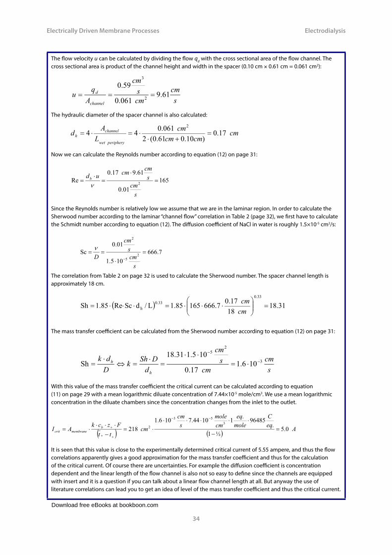
Example F: Current efficiency

An electrodialysis experiment is conducted at a small scale plant consisting of 20 cell pairs. A sodium chloride solution is used as feed stream and the in- and outlet concentration and the current is measured for an experiment conducted with a total diluate flow rate of 11.72 g/s and a voltage difference of 50 volts. Relevant parameters and experimental data are shown in Table 6.

Parameters and experimental data for an electrodialysis experiment conducted with a sodium chloride feed solution.

Diluate flow rate, Qd [m3/s] 11.72×10-6

Diluate inlet concentration, cd,in [mole/m3] 160Diluate outlet concentration, cd.out [mole/m3] 30Number of cell pairs, n 20Current, I [A = C/s] 8.09Valence of salt ions, z [eq./mole] 1Faraday number, F [C/eq.] 96485

Table 6: Experimental parameters

The numbers given in Table 6 are directly inserted into equation (16) on page 41 in order to calculate the current efficiency:

� � � �91.0

.96485

09.820

.11003.01016.01072.11 333

36

,, �

��

�

�

��

�

�

�

��

��

��

��

�

eqCsC

moleeq

mmole

sm

FIn

zccQ outdindd�

It is thus seen that the number of transferred salt equivalents are calculated from diluate inlet and outlet concentrations and the total diluate volume flow rate whereas the total number of current equivalents are determined from the current and the number of cell pairs. In this case it is thus seen that 0.91 equivalents of salt is removed pr. transferred equivalent of current.

2.5 Energy requirement

Evaluation of the energy consumption when running an electrodialysis system is of very great importance. Generally the energy consumption in electrodialysis can be divided into two parts:

- Pump energy: Energy to pump the solutions through the electrodialysis system - Electrical energy: Electrical energy to transfer ions through the ion exchange membranes

The overall energy requirement is often dominated by one of these two terms depending on different process parameters and operation conditions.





43

Electrodialysis

2.5.1 Pump energy

In chemical engineering it is well know that the energy consumption associated with pumping liquids through a given system is dependent on the volume flow rate Q, the pressure drop in the system ∆p and the efficiency of the pump ηpump. The pump energy can thus be calculated by use of the following equation:

��

��

��

��

��

�

�

sJ

sNm

mN

smPa

smEunitsSI

pQEenergyPumppump

2

33

:

:� (17)

Normally in an electrodialysis system three pumps are required as mentioned earlier:

- One pump to pump the solutions through the dilution chambers - One pump to pump the solutions through the concentration chambers - One pump to pump electrode solutions through the two electrode chambers

www.liu.se/master

Study at Linköping Universityand get the competitive edge!Interested in Engineering and its various branches? Kick-start your career with a master’s degree from Linköping University, Sweden – one of top 150 universities in the world in the field of Engineering.


http://bookboon.com/count/advert/755581d9-3607-4736-b12a-a30200b37613



44

Electrodialysis

Thus the energy consumption to pump the solutions through an electrodialysis system can be calculated from knowledge of the pressure drops in the dilution-, concentration and electrode chambers, efficiencies of dilution-, concentration and electrode pumps and the volume flow rates in the three different types of chambers:

e

ee

c

cc

d

ddtotalpump

pQpQpQE

��

��

��

��

, (18)

The sup-scripts d, c and e refer to the diluate, concentrate and electrode solutions respectively. The volume flow rates are normally easy to measure but determining the actual pressure drop in the three circuits can be more uncertain and difficult to measure.

2.5.2 Electrical energy

The energy consumption associated with removing ions from the diluate to the concentrate through the ion exchange membranes is proportional to the current I flowing through the membrane stack and the total voltage drop E between the two electrodes over the whole membrane stack. This energy consumption can be expressed as follows:

��

��

��

sJ

CJ

sCEunitsSIEIEenergyElectrical electrical :,: (19)

As for the pump energy in equation (17) on page 43 the unit of the electrical energy in equation( 19) is given in “energy pr. time” (Joules pr. second). If one knows the resistance of one single cell pair Rcell

the total resistance of the membrane stack consisting of n cell pairs can be calculated by multiplying the number of cell pairs with the resistance of one single cell pair (according to equation (9) on page 24). Thus equation (19) can be rewritten when the voltage drop over the whole membrane stack E is replaced by product of the total resistance of the membrane stack and the current flowing through the membrane stack according to Ohm’s law:

nRIE cellelectrical ��

2 (20)

The amount of salt that is removed from the diluate to the concentrate is directly proportional to the amount of current flowing through the membrane stack. The amount of current flowing through the membrane stack, the diluate volume flow rate Qd and the current utilization ξ determines the difference between the inlet and outlet concentrations of the diluate ∆cd (the level of desalination). The current utilization is the product of the current efficiency η (from equation (16) on page 41) and the number of cell pairs n (ξ = η×n). This can be gathered in the following equation:

��

��

��

��

sC

eqC

moleeq

sm

mmoleIunitsSI

FzQcI dd

..:,

3

3� (21)




45

Electrodialysis

Again the term z is the valence of the ions and F is the Faraday number. The expression for the current in equation (21) can inserted into the equation (20) in order to get another expression for the electrical energy requirement to transfer ions through the ion exchange membranes:

��

��

��

��

��

�

�

sJ

eqC

moleeq

sm

mmole

CsJ

sCEunitsSI

FzQcnRIE

electrical

ddcellelectrical

..:

,

3

32

� (22)

It is often the cell resistance that is difficult to determine since is consists of different sub resistances (according to equation (9) on page 24) that can be very difficult to measure.

The different equations presented in this sub section can be used to calculate the energy requirement needed to remove a certain amount of ions from the diluate to concentration. Thus the electrical energy together with the energy required to pump the solutions through the system determines the overall energy consumption.

2.5.3 Thermodynamic least amount of energy

The energy consumption given in the previous section (2.5.2 Electrical energy) gives the actual energy consumption associated with ion transfer for a given electrodialysis system and this amount of energy is often much larger that the least amount of energy required just by looking at the thermodynamic least amount of energy required. The thermodynamic least amount of energy can be considered as the numerical value of the amount of energy that is released when a given amount of diluate and concentrate are mixed together. The thermodynamic least amount of energy required can be calculated by use of the following equation:

� �

��

��

��

��

��

�

�

��

�

�

��

��

��

��

��

�

�

��

��

��

��

��

�

��

�

�

sJ

mmoleK

sm

KmoleJEunitsSI

cc

cc

cc

cc

ccTQRE

outc

ind

outc

ind

outd

ind

outd

ind

outdinddgas

3

3

amountleastmicthermodyna

,

,

,

,

,

,

,

,

,,amountleastmicthermodyna

:

ln1

ln

ln1

ln2

(23)

In this equation it should be mentioned that “Rgas” is the gas constant, Qd is the total volume flow rate of the diluate and T is the absolute temperature. As mentioned above, this thermodynamic least amount of energy is often much less that the actual electrical energy requirement for transferring ion through the membranes (equation (19) on page 44 for example). This is due to the influence of different factors such as:

- The current efficiency η (equation (16) on page 41) is less than 1. - The Ohmic resistance in the concentrate, diluate and electrode solutions and in the anion

and cation exchange membranes causes generation of heat and thus “loss” of energy.





46

Electrodialysis

The thermodynamic efficiency can be evaluated by comparing the thermodynamic least amount of energy to remove ions from the diluate to the concentrate with the actual amount of energy used to remove ions from the diluate to the concentrate.

Thermodynamic efficiency ��

��

��

�

1923amountleastmicthermodyna

equationequation

E

E

electrical

� ��

��

�

�

��

�

�

��

��

��

��

�

sJsJ

SI-units efficiencymicThermodyna:

(24)

The thermodynamic efficiency is often very low (often below 5–10%) which for an electrodialysis experiment will be sketched in the following example.

By 2020, wind could provide one-tenth of our planet’s electricity needs. Already today, SKF’s innovative know-how is crucial to running a large proportion of the world’s wind turbines.

Up to 25 % of the generating costs relate to mainte-nance. These can be reduced dramatically thanks to our systems for on-line condition monitoring and automatic lubrication. We help make it more economical to create cleaner, cheaper energy out of thin air.

By sharing our experience, expertise, and creativity, industries can boost performance beyond expectations.

Therefore we need the best employees who can meet this challenge!

The Power of Knowledge Engineering

Brain power

Plug into The Power of Knowledge Engineering.

Visit us at www.skf.com/knowledge


http://bookboon.com/count/advert/0d9efd82-96d7-e011-adca-22a08ed629e5



47

Electrodialysis

Example G: Thermodynamic efficiency

For an electrodialysis system consisting of 20 cell pairs the in- and outlet concentrations from the concentration and diluate chambers and the current were measured at each step of the voltage between 10 and 50 volts. The diluate flow rate was kept constant (6.6 g/s) and the feed solution consisted of sodium chloride. The temperature was also kept constant. At each voltage-step the electrical energy consumption was calculated by using equation (19):

Ėelectrical = I . E

The thermodynamic least amount of energy was also calculated at each voltage-step from the volume flow rate of the diluate and the different concentrations by use of equation (23):


48

� �

��

�

�

��

�

�

��

��

��

��

��

�

�

��

��

��

��

��

�

��

outc

ind

outc

ind

outd

ind

outd

ind

outdinddgas

cc

cc

cc

cc

ccTQRE

,

,

,

,

,

,

,

,


ln1

ln

ln1

ln2

The thermodynamic efficiency is the defined as the ratio between the thermodynamic least amount of energy and the actual electrical energy requirement according to equation ( 24) on page 47:


��

��

�


equationequation

E

E

electrical

The thermodynamic efficiency is plotted as a function of the voltage for the experiment in Figure 12.

0

1

2

3

4

0 10 20 30 40 50

E [V]

Thermodyn. efficiency [%]

Figure 12: Thermodynamic efficiency vs. voltage The thermodynamic efficiency vs. the voltage for an electrodialysis experiments conducted at a constant diluate flow rate of 6.6 g/s and a sodium chloride feed solution of 0.16 mole/l.

It is seen in Figure 12 that the thermodynamic efficiency throughout the whole experiment is very low and in all cases below 4 %. It is also seen that at low voltage the thermodynamic is higher than at large voltage. An explanation could be that at these conditions the irreversible processes at the electrodes do not play as large a role at when the voltage is increased. Therefore the efficiency at low voltage is “closer” the thermodynamic least amount of required energy than at larger voltage.

Electrodialysis

The thermodynamic efficiency is the defined as the ratio between the thermodynamic least amount of energy and the actual electrical energy requirement according to equation (24) on page 46:


48

� �

��

�

�

��

�

�

��

��

��

��

��

�

�

��

��

��

��

��

�

��

outc

ind

outc

ind

outd

ind

outd

ind

outdinddgas

cc

cc

cc

cc

ccTQRE

,

,

,

,

,

,

,

,


ln1

ln

ln1

ln2



��

��

�


equationequation

E

E

electrical


0

1

2

3

4

0 10 20 30 40 50

E [V]




Electrodialysis



48

� �

��

�

�

��

�

�

��

��

��

��

��

�

�

��

��

��

��

��

�

��

outc

ind

outc

ind

outd

ind

outd

ind

outdinddgas

cc

cc

cc

cc

ccTQRE

,

,

,

,

,

,

,

,


ln1

ln

ln1

ln2



��

��

�


equationequation

E

E

electrical


0

1

2

3

4

0 10 20 30 40 50

E [V]




Electrodialysis


It is seen in Figure 12 that the thermodynamic efficiency throughout the whole experiment is very low and in all cases below 4%. It is also seen that at low voltage the thermodynamic is higher than at large voltage. An explanation could be that at these conditions the irreversible processes at the electrodes do not play as large a role at when the voltage is increased. Therefore the efficiency at low voltage is “closer” the thermodynamic least amount of required energy than at larger voltage.




48

Electrodialysis

2.6 Anti-fouling mechanism

When electrodialysis is applied commercially to desalt seawater, fouling of the ion exchange membranes can be a severe problem as in every other membrane separation process. Particle material, colloids, macromolecules and other charged or uncharged components can block the membrane pores or membrane surface and thus increase the resistance of the membrane. This will increase the operation costs. In electrodialysis in which a current flows in one direction, especially larger charged components can be transferred to the membrane surface but because of their size they are not able to pass through the membrane. Scaling on the membrane surface at high concentrations can also create problems. Because most of the colloids and macromolecules that appear in the water are negatively charged, it is mostly the anion exchange membranes that are affected by the fouling problems. In some commercial electrodialysis system this is avoided by changing the direction of the current every 30 minutes for example. Of course this leads to changes of the chambers every 30 minutes:

- Diluate chambers → Concentrate chambers - Concentrate chambers → Diluate chambers

This means that the outlet from the chambers in the first short period after changing the direction of the current can not be used as concentrate and diluate. But after this period the concentrate and diluate can again be collected from the outlet of the membrane stack. By doing this changing of current direction the charged larger particles and components that eventually will stick to the membrane surfaces will every 30 minutes be removed and moved to the other side the chamber and thus a build up of a large fouling layer over a longer period is avoided. Thus the overall resistance of the membrane stack will by average be kept constant and the running costs will be kept constant.





49

Summary

3 SummaryIn this text we have learned about basic terms used in the world of electrically driven membrane processes. The core in electrically driven membrane processes are membranes incorporated with fixed charges:

- The anion exchange membranes and - The cation exchange membranes.

We have been looking at the fluxes of ions through these membranes and we have seen that these fluxes depend on the transport numbers of the ions. The membranes achieve their selectivity because these transport numbers for the oppositely charged ions are very different inside the membrane whereas the transport numbers in the solution for the oppositely charged ions are almost equal for equal valences. It is also explained that the separation principle in electrical driven membrane processes is based on Donnan exclusion.

www.simcorp.com

MITIGATE RISK REDUCE COST ENABLE GROWTH

The financial industry needs a strong software platformThat’s why we need you

SimCorp is a leading provider of software solutions for the financial industry. We work together to reach a common goal: to help our clients

succeed by providing a strong, scalable IT platform that enables growth, while mitigating risk and reducing cost. At SimCorp, we value

commitment and enable you to make the most of your ambitions and potential.

Are you among the best qualified in finance, economics, IT or mathematics?

Find your next challenge at www.simcorp.com/careers





50

Summary

One major part of the electrical driven membrane processes is electrodialysis. Electrodialysis has many applications and one of the greatest is the desalination of saline water into potable water. The basic concepts of electrodialysis are explained as well as the existence of a critical current. Examples are included in order to show ways to determine this critical current experimentally and from literature correlations based on dimensionless numbers concerning flow and mass transfer. The influence of the hydrodynamic conditions on the critical current is also explained and discussed. Other relevant terms used in the evaluation of electrodialysis systems such as the desalination degree and the current efficiency are also described and discussed through relevant examples. The energy required to run electrodialysis systems can be divided into the energy required to pump the solutions through the system and the energy required to transfer ions through the ion exchange membranes. Relevant equations are given in order to calculate these energy requirements and the thermodynamic efficiency is also defined. Finally some fouling problems are briefly mentioned together with an approach for avoiding these fouling problems.

Other electrically driven membrane processes such at the REED process patented by the Danish company Jurag Separation A/S, Donnan dialysis, Membrane electrolysis, the use of bipolar membranes and finally fuel cells can also be mentioned. Some of these processes certainly have the potential to grow in the future.

Since electrically driven membrane processes and membrane processes and membrane technology in general have such a broad spectrum of applications and opportunities, knowledge and practical experience of this field is of very great importance. Every engineering student choosing this path will have the potential of a great and exciting career…

… so keep on using your memBRAIN! … or something, huh, heh.

Søren Prip Beier



51

Notes

Notes1. For further explanation of different kinds of transport please see ”Transport phenomena”, S.P. Beier, Ventus

Publishing (2006), ISBN: 87-7681-123-9. 2. For explanations of concentration polarization phenomena in general please see “Pressure driven

membrane processes”, S.P. Beier, Ventus Publishing (2006), ISBN: 87-7681-152-2.3. It shall however be mentioned that the enhanced concentration in the boundary layer on the concentrate

side can lead to scaling of ionic solids at the membrane surface on the concentrate side for example if the concentrate contains calcium ions.

4. This happens at the cation exchange membrane before it happens at the anion exchange membrane. This is due to fact that the electrical mobility of the cations is generally a bit lower than for the anions. In the case of sodium chloride the transport number of sodium ions is approximately 0.4 and the transport number for chloride ions is approximately 0.6 (and actually not equal which is stated in equation (7) on page 13). This is because the friction between the water molecules and the ions is largest for cations. This means that at a given current the concentration at the membrane surface on the diluate side (c´d) will reach zero at the cation exchange membrane before is reaches zero at the anion exchange membrane. Thus the limiting current will be attained faster at the cation exchange membrane than at the anion exchange membrane.

5. Other kinds of transport concerning the transport of water molecules through the ion exchange membranes are also observed in electrodialysis. Osmotic transport of water from the diluate to the concentrate can be observed because of the concentration difference. Electroosmotic water transport can also be observed as sketched in Figure 3 on page 10 where water molecules are dragged along with the electrically transported ions.

6. When, however, the feed solution ion concentration is increased and reaches a level of concentration as the fixed charges in the ion exchange membrane, some co-ions may also enter the membrane which of course is unwanted since the membrane then looses it selectivity. That way the current efficiency becomes very low and the electrical energy consumption increases.

7. From M. Mulder, “Basic principles of membrane technology”, 2nd edition, Kluwer Academic Publishers, 1996.

Electrically Driven Membrane Processes - in English

Documents

Transcript of Electrically Driven Membrane Processes - in English