OPTIMIZING THE COMPACT-FDTD ALGORITHM FOR ELECTRICALLY LARGE WAVEGUIDING STRUCTURES

Progress In Electromagnetics Research, PIER 75, 253–269, 2007

OPTIMIZING THE COMPACT-FDTD ALGORITHMFOR ELECTRICALLY LARGE WAVEGUIDINGSTRUCTURES

M. F. Hadi and S. F. Mahmoud

Electrical EngineeringKuwait UniversityP.O. Box 5969, Safat 13060, Kuwait

Abstract—This work investigates the unique numerical dispersionbehavior of the Compact-FDTD method for waveguide analysis,especially when the waveguide dimensions are much larger than theoperating wavelength as in high-frequency EMC analysis or radio-wavepropagation in tunnels. The divergence of this dispersion behaviorfrom the standard FDTD algorithm is quantified and a major sourceof dispersion error is isolated and effectively eliminated. Optimizedmodeling parameters in terms of appropriate spatial and temporalresolutions are generated for computationally efficient and error-freenumerical simulations of electrically large waveguiding structures.

1. INTRODUCTION

The Compact-FDTD algorithm which was first proposed by Xiao,Vahldieck and Jin [1] as a borrowed technique from their work onthe Transmission-Line-Method [2] allows full wave analysis of generalwaveguiding structures using a two-dimensional FDTD grid. Inthis algorithm the spatial derivative along the propagation direction(assumed along the z-axis in the present work) is evaluated analyticallyafter restricting the entire EM fields’ z-dependence to an exp[−βzz]term, where =

√−1. A careful substitution of this z-derivative

will result in real-valued FDTD update equations—the format thealgorithm settled with in its final incarnation [3, 4] for modeling losslessor weakly lossy waveguides. This idea of benefiting from analyticallypredictable modal field variations to compact the FDTD cell has beenrecently extended by Luo and Chen [5] to design one-dimensionalFDTD modal absorbing boundary conditions for waveguide analysiswhere numerical simulation is executed along the waveguide axis and

254 Hadi and Mahmoud

the field variations across the transverse plane are analytically imposed.Frequency domain versions of the Compact-FDTD algorithm havealso appeared in the literature. Of special mention among them isthe efficient, though mathematically intensive, multiresolution-basedMRFD algorithm by Gokten, Elsherbeni and Arvas [6].

The advantages of the Compact-FDTD algorithm in terms ofcomputing resources savings—though quite obvious—still fall shortwhen the cross-sectional area of the waveguiding structure becomeslarge compared to the shortest wavelength of interest. Examplesof such situations are high-frequency EMC analysis of microwavecircuits and radiowave propagation in mine-shafts and railway tunnels[7, 8]. To illustrate the motivation of this work consider wavepropagation through a lossless hollow metallic rectangular waveguideat a frequency high enough such that its cross-sectional dimensionsare 4λo × 2λo. Fig. 1 shows this waveguide’s dispersion curves forthe first 8 TEm0-only modes for simplicity. If the Compact-FDTDalgorithm is used with the choice βz = 0.2βo, corresponding resultswill only correctly produce the group of modes just under the TE80

mode. To properly highlight the dominant TE10 mode behavior aroundthe fo operating frequency, the propagation constant must be chosenaround βz = 0.99βo. Another class of waveguide applications wherethe propagation constant βz approaches the unbounded wavenumber βincludes metamaterial-inspired open dielectric waveguides which couldsupport modes with βz = β as demonstrated by Lu, Wu and Kong [9].As will be shown later in this work, such high βz values present seriouschallenges to the Compact-FDTD algorithm in terms of excessivenumerical dispersion errors.

In this work a condensed review of the Compact-FDTD algorithmwill be presented, including the necessary modifications required tomodel lossy waveguides and anisotropic fill materials. Rigorousdispersion analysis will follow which will highlight the increasing modalsolutions errors introduced as βz → βo. The source of these increasingerrors will be highlighted and a simple solution will be discussed andvalidated numerically through solutions of the dispersion relation andlater through practical Compact-FDTD simulations.

2. REVIEW OF THE COMPACT-FDTD ALGORITHM

Replacing the z-derivative in Maxwell’s equations with the −βz termwill render the complex-valued time-domain equations

ε∂Ex

∂t=

∂Hz

∂y+ βzHy (1)

Progress In Electromagnetics Research, PIER 75, 2007 255

Normalized Frequency, f / fo

Nor

mal

ized

Wav

enum

ber

z/

o

0 0.2 0.4 0.6 0.8 10

0.2

0.4

0.6

0.8

1

ββ

Figure 1. Effect of βz choices on modal frequencies: Dispersion curvesfor a rectangular waveguide with dimensions 4λ×2λ at fo. Only TEm0

modes are shown. The normalizing wavenumber is βo = 2πfo/c.

ε∂Ey

∂t= −∂Hz

∂x− βzHx (2)

ε∂Ez

∂t=

∂Hy

∂x− ∂Hx

∂y(3)

µ∂Hx

∂t= −∂Ez

∂y− βzEy (4)

µ∂Hy

∂t=

∂Ez

∂x+ βzEx (5)

µ∂Hz

∂t=

∂Ex

∂y− ∂Ey

∂x(6)

These equations when adapted directly by the FDTD method willproduce complex-valued update equations. We should note howeverthat the two field groups {Ex, Ey, Hz} and {Ez, Hx, Hy} will always bephase-shifted off each other by π/2. When the waveguide is composedof lossless or weakly lossy materials and when the fill dielectrics areisotropic, this phase shift could be prevented from producing complexupdate equations by replacing one of the two groups, say the first one,


with {Ex, Ey, Hz} [4] to produce†

ε∂Ex

∂t=

∂Hz

∂y+ βzHy (7)

ε∂Ey

∂t= −∂Hz

∂x− βzHx (8)

ε∂Ez

∂t=

∂Hy

∂x− ∂Hx

∂y(9)

µ∂Hx

∂t= −∂Ez

∂y+ βzEy (10)

µ∂Hy

∂t=

∂Ez

∂x− βzEx (11)

µ∂Hz

∂t=

∂Ex

∂y− ∂Ey

∂x(12)

Zhao, Juntunen and Raisanen [12] have demonstrated mathemat-ically that expanding the complex-valued equations (1)–(6) will pro-duce two decoupled and redundant sets of real-valued equations, oneof which is represented by equations (7)–(12). They also verified thatif the fill-dielectric is anisotropic, decoupling is still maintained as longas anisotropy is limited to one axis only. If dielectric anisotropy ex-tends to more than one axis then decoupling is unattainable and thecomplex-valued equations need to be used for numerical simulations.

To accurately model loss-induced fast-attenuating waveguidemodes, the z-derivative in Maxwell’s equations must accommodatethe attenuation factor as in exp[−(αz + βz)z]. This modification willresult in a similar set of equations to (1)–(6), except that every βz

occurrence is replaced with αz + βz, and σE terms are injected intheir usual places

ε∂Ex

∂t=

∂Hz

∂y+ (αz + βz)Hy − σEx (13)

ε∂Ey

∂t= −∂Hz

∂x− (αz + βz)Hx − σEy (14)

ε∂Ez

∂t=

∂Hy

∂x− ∂Hx

∂y− σEz (15)

µ∂Hx

∂t= −∂Ez

∂y− (αz + βz)Ey (16)

† There seems to be some confusion in the literature regarding the re-mapped Maxwell’sequations. The signs of the βz terms are reversed in [4] for (8) and (10), and in [10] for (8)and (11). References [11] and [12] on the other hand contain the correct equations.


µ∂Hy

∂t=

∂Ez

∂x+ (αz + βz)Ex (17)

µ∂Hz

∂t=

∂Ex

∂y− ∂Ey

∂x(18)

Wang, Shao and Wang [13] used these equations in an iterativetechnique that based input αz choices on the decay (or growth)behavior of the simulated solutions with time. An overestimated αz

choice will cause solutions to decay while an underestimated choice willcause them to grow over time. Steady solutions over time on the otherhand will signify an accurate αz estimate.

For weakly lossy waveguides, αz in (13)–(18) can be neglectedand the resulting equations can be decoupled back to (7)–(12), withthe added σE terms as in (13)–(15). The advantage being a reductionof simulation complexity and time at the expense of minimal errors asdemonstrated later in the numerical experiments.

Fundamental to all Compact-FDTD variants is the z-compactedFDTD grid shown in Fig. 2 [3]. When second-order finite-differencesare introduced, say, in equations (7)–(12) the Compact-FDTD updateequations are produced, of which the following is an example

Ex|n+ 1

2i,j = Ex|

n− 12

i,j +βz∆tεHy|ni,j

+∆tε∆y

(Hz|ni,j+ 1

2−Hz|ni,j− 1

2

)(19)

where ∆t is the time step and ∆y is the Compact-FDTD cell sizealong y. (In the remainder of this work ∆x = ∆y = h willbe assumed). A typical Compact-FDTD simulation would start byspecifying a propagation constant βz (and αz when present) as aninput with an appropriate initial field distribution that mimics theexpected waveguide mode of interest.‡ The frequency response ofthe collected time series from the simulation will exhibit the guidedmodes pertaining to the chosen propagation constant. If βz = 0 ischosen instead, the algorithm will produce the cutoff frequencies ofthe waveguide modes [2].

The dispersion relation and stability criterion for the Compact-FDTD algorithm were derived early in the literature by Cangellaris[14] (

h√µε

∆t

)2

sin2 ω∆t2

= sin2 βxh

2+ sin2 βyh

2+

(βzh

2

)2

(20)

‡ Introducing a time function excitation here will simulate a line source extendingalong the axis of the waveguide which would complicate deriving the modal attenuationcharacteristics from the collected data.


Hz

Ez

Ex

Ey

Hx

Hy

Figure 2. The Compact-FDTD grid. Bold and thin icons representthe E and H field nodes, respectively. Like-field components areequispaced by ∆x = ∆y = h.

∆t ≤ h√µε√

2 +(

βzh2

)2(21)

where√β2

x + β2y = βT is the numerically rendered transverse

wavenumber by the Compact-FDTD algorithm.

3. NUMERICAL DISPERSION ANALYSIS

In his numerical dispersion analysis [14], Cangellaris used a rectangularhollow waveguide as an example and replaced βx and βy in thedispersion relation (20) with the theoretical βx = mπ/a and βy = nπ/bvalues, respectively, in an effort to predict the resonance frequenciesand consequently the numerically rendered modal guide wavelengths.In reality, however, the main value of the FDTD dispersion relationsin general is their accurate prediction of the errors in the numericallyrendered wavenumbers. In the case of the Compact-FDTD algorithmfor example, it is the βT deviation from βT =

√β2

o − β2z that can be

predicted by (20). The resonance frequencies on the other hand canonly be produced from actual Compact-FDTD simulations.


In the following analysis the figure of merit of choice for numericaldispersion will be the Global Phase Error

Φ =12π

∫ 2π

0

∣∣∣βT − βT

∣∣∣2 dφ (22)

which is a square-error function averaged over all propagation angles φwithin the Compact-FDTD grid. This error function will be evaluatedand compared at several resolution factors among other variables.The resolution factor in the present context, however, requires someclarification. In normal, non-compact FDTD algorithms the resolutionfactor is conventionally defined as the number of FDTD cells perwavelength. Adopting such a definition for the Compact-FDTDalgorithm is acceptable so long as the frequency range of interest is atthe vicinity of the cutoff frequencies. When attempting to investigatemodal solutions at higher frequencies with this resolution definition,the unbounded wavelength shrinks and the h = λ/R values will becomeunnecessarily small and numerically costly.

The fact is, in modal analysis, the waveguide’s transversewavelength for any given mode is a function of the waveguide’sdimensions and constituent parameters of its fill-materials and isindependent of the frequency’s proximity to the cutoff frequency; Theentire Hz variation for the TE10 mode of a rectangular waveguide forexample constitute a single half-cycle along the x-axis and no variationat all along the y-axis. Indeed, a single cell along the y-axis is all thatis needed if only TEm0 modes are of interest. Given this fact, theCompact-FDTD grid discretization level should be referenced not tothe unbounded wavelength λ but rather to the transverse wavelengthλT = 2π/βT and βT in turn is independent of frequency. Moreimportantly, if one discretization level is good enough for one frequencyto accurately analyze the mode’s behavior then it is good enough forall higher operating frequencies for the same mode. This feature ofthe Compact-FDTD algorithm could allow simple and computationallyefficient frequency dispersion analysis of elaborate waveguides in theTera-Hertz [15] and optical [16] frequency ranges.

To generalize the discussion away from any specific waveguideexample as befitting the general dispersion relation let us define βz =κβ where β is the unbounded wavelength and κ→ 1 as the frequencyincreases or equivalently, as the waveguide becomes electrically large.Using β2 = β2

T + β2z we can write

λT =2πβT

=2π√

1 − κ2β=

λ√1 − κ2

(23)

and henceforth define the Compact-FDTD resolution factor as R cells


per λT or h = λT /R.Fig. 3 demonstrates the Global phase error deterioration as the

normalized propagation constant κ approaches unity and the time stepis kept at the maximum limit allowed by the stability criterion (21) foreach κ value. This figure clearly shows that excessively high resolutionfactors are needed near the limiting value of κ = 1. The data inthis figure and those in the following section were calculated assuminga 1 GHz operating frequency in an air-filled general waveguide (β =20.96 rad/m).

4. ALGORITHM OPTIMIZATION

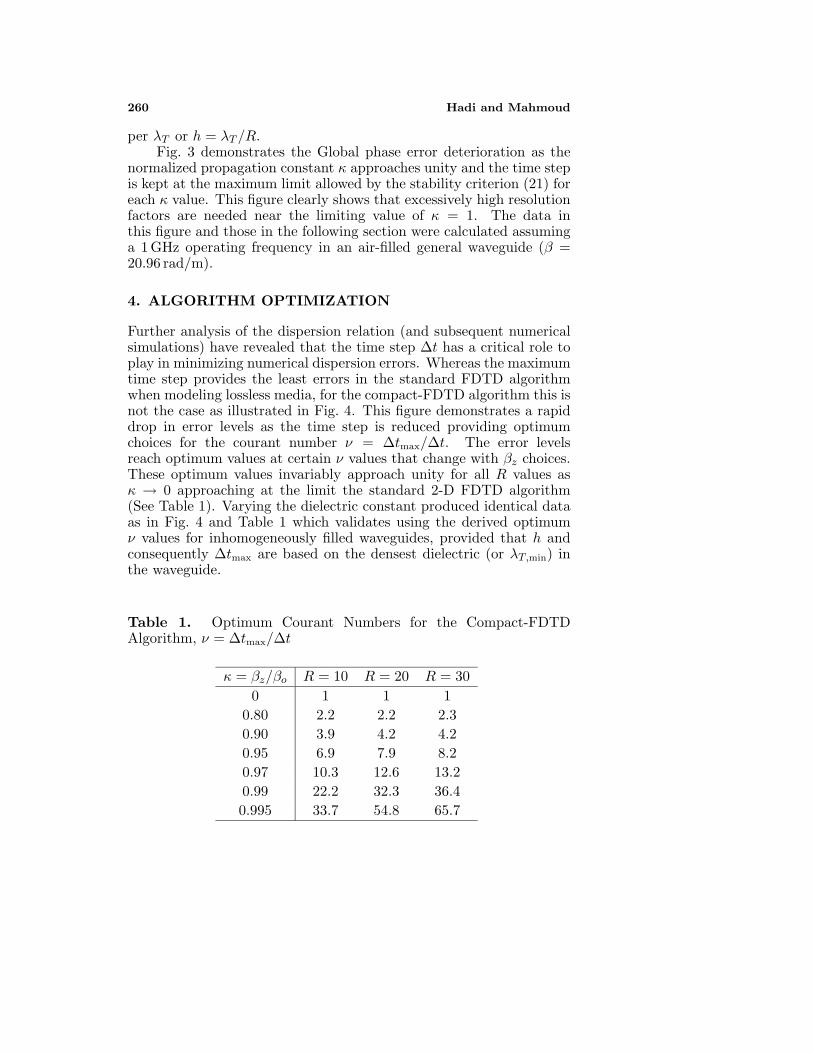
Further analysis of the dispersion relation (and subsequent numericalsimulations) have revealed that the time step ∆t has a critical role toplay in minimizing numerical dispersion errors. Whereas the maximumtime step provides the least errors in the standard FDTD algorithmwhen modeling lossless media, for the compact-FDTD algorithm this isnot the case as illustrated in Fig. 4. This figure demonstrates a rapiddrop in error levels as the time step is reduced providing optimumchoices for the courant number ν = ∆tmax/∆t. The error levelsreach optimum values at certain ν values that change with βz choices.These optimum values invariably approach unity for all R values asκ → 0 approaching at the limit the standard 2-D FDTD algorithm(See Table 1). Varying the dielectric constant produced identical dataas in Fig. 4 and Table 1 which validates using the derived optimumν values for inhomogeneously filled waveguides, provided that h andconsequently ∆tmax are based on the densest dielectric (or λT,min) inthe waveguide.

Table 1. Optimum Courant Numbers for the Compact-FDTDAlgorithm, ν = ∆tmax/∆t

κ = βz/βo R = 10 R = 20 R = 300 1 1 1

0.80 2.2 2.2 2.30.90 3.9 4.2 4.20.95 6.9 7.9 8.20.97 10.3 12.6 13.20.99 22.2 32.3 36.40.995 33.7 54.8 65.7


Normalized Propagation Constant, = z / o

Glo

balP

hase

Err

or,

0 0.1 0.2 0.3 0.4 0.5 0.6 0.7 0.8 0.9 110 5

10 4

10 3

10 2

10 1

100

101

102

β β

Φ

κ

−

−

−

−

−

Figure 3. Effect of βz choice on the Global Phase Error at theresolution factors (from top to bottom) R = 10, 15, 20, 25, 30, 35cells per transverse wavelength at corresponding maximum allowabletime steps. Operating frequency is 1 GHz or βo = 20.96 rad/m.

Courant Number, = tmax/ t

Glo

balP

hase

Err

or,

0 5 10 15 20 25 30 35 40 45 5010 5

10 4

10 3

10 2

10 1

100

101

102

Φ

∆ν ∆

−

−

−

−

−

Figure 4. Sensitivity of the Global Phase Error to ∆t choices. Thesix curves (from top to bottom at ν = 40) correspond to βz/βo =0.8, 0.9, 0.95, 0.97, 0.99, 0.995 with R = 10 at 1 GHz.


Normalized Propagation Constant, = z / o

Glo

balP

hase

Err

or,

0.5 0.55 0.6 0.65 0.7 0.75 0.8 0.85 0.9 0.95 110 7

10 6

10 5

10 4

10 3

10 2

10 1

100

101

β β

Φ

κ

−

−

−

−

−

−

−

Figure 5. Sensitivity of the (βz,Φ) dispersion curves to the time stepchoice (compare to Fig. 3). The three sets of curves were optimizedfor κ = 0.8 (dotted), 0.9 (dashed), and 0.99 (solid), and in each set thecurves correspond (from top to bottom) to R = 10, 20, 30 cells pertransverse wavelength λT .

To verify the time step optimization the numerical dispersioncurves of Fig. 3 are recalculated using the optimum time steps andpresented in Fig. 5, clearly demonstrating the advantage of time stepoptimization, especially as κ→ 1. For example, at κ = 0.99, the GlobalPhase Error has been reduced from near infinite value at R = 10 toroughly 10−4.

An optimization that is based on reducing the time stepindependently from the spatial step has added advantages comparedto reducing both in lock step as is usually done. If h is halved forexample as a means of reducing numerical dispersion then the totalsimulation time steps required must be increased by at least 23 = 8times for the same total simulated time, N∆t, to accommodate theincreased resolutions in all three pertinent axes, x, y and t. On theother hand halving ∆t alone would only require doubling the numberof time steps for the same total simulated time.


Time Steps

= 1

= 2

= 4

0 20 40 60 80 100 120 140 160 180 200

0 10 20 30 40 50 60 70 80 90 100

0 5 10 15 20 25 30 35 40 45 50

-200

0

200

-200

0

200

-200

0

200

ν

ν

ν

Figure 6. Effective temporal resolutions at different time step choices,demonstrating the Compact-FDTD’s need for lower time steps (asκ→ 1) compared to the standard FDTD method. Plots are for the Ey

field component.

5. NUMERICAL VALIDATION

A simple waveguide example is used here to validate the need for theproposed time step optimization. The waveguide has a rectangularcross section of 4λ × 2λ at 1 GHz where it is assumed to operate;namely, a = 1.199 m and b = 0.5995 m. The walls are assumed perfectconductors and the dielectric fill is homogeneous with εr = 1 and σis assumed finite to observe the effect of dielectric losses on solutionsconvergence. The waveguide cross-section is divided into a coarse 10×5FDTD cells and βz is chosen as 0.99βo to closely observe the TE10

mode at the 1 GHz operating frequency. Initial field distribution isintroduced for the Hz component with Hz = −1 for x < a/2 and +1for x > a/2 which will excite the odd TEm0 modes.

Fig. 6 is presented to demonstrate first hand the need for movingaway from the maximum time step as the condition κ ≈ 1 generatesan effective temporal resolution of under 4 steps per wave period at∆tmax even though spatial resolution is effectively 17.7 cells per λT

(defined earlier) at 1 GHz. Fig. 7 tracks the convergence of TE10

resonance as the time step decreases for two dielectric loss choices


Courant Number

TE

10

Res

onan

ceFr

eque

ncy

(GH

z)

Courant Number

= 0.001 S/m = 0.002 S/m

0 10 20 300 10 20 300.98

1

1.02

1.04

1.06

1.08

1.1

0.98

1

1.02

1.04

1.06

1.08

1.1

ν

σ

ν

σ

Figure 7. Homogeneously filled rectangular waveguide: Convergenceof the TE10 mode resonance with time step reduction at two dielectricloss values. Good convergence is achieved at Courant numbers as smallas ν = 10.

(σ = 0.001, 0.002 S/m). It is clear that resonance frequencies convergeto their steady solutions with only a relatively moderate time stepreduction, ν ≈ 10 or a time step that is one-tenth of the maximumallowable time step by the stability criterion.

Fig. 8 on the other hand which tracks the quality factorconvergence, confirms the need for larger time step reductions (ν > 22)to reach steady solutions. The attained quality factor values differ fromthe analytical values (Q = ωε/σ for homogeneously filled waveguides[17]) by 1.8% and 2.4% at σ = 0.001, 0.002 S/m, respectively. Thisis due to the coupling effect of the dielectric losses on the closelyspaced resonance modes at the high 1 GHz operating frequency asdemonstrated in the spectral power density plots of Fig. 9.

To investigate the effect of both waveguide inhomogeneity andlosses the previous rectangular waveguide was allowed to be onlypartially filled as in (εr = 2, σ = 0.0005) for 0 < x < a/2 and (εo, σ = 0)for a/2 < x < a. This is a well-known test problem of numericaltechniques for waveguide structures [18, 19] and its theoretical analysiscan be found in Harrington’s classic EM book (Section 4.6) for thelossless case [20]. Again, it took a time step reduction of ν > 10 to


Courant Number

Qua

lity

Fact

or

Courant Number

= 0.001 S/m = 0.002 S/m

0 10 20 300 10 20 3028

28.5

29

29.5

30

30.5

31

31.5

55

56

57

58

59

60

61

ν

σ

ν

σ

Figure 8. Homogeneously filled Rectangular Waveguide: Qualityfactor convergence requires twice as much time step reductioncompared to resonance frequency convergence; ν > 22.

Frequency (Hz)

= 0.001 S/m

= 0.002 S/m

0.9 0.95 1 1.05 1.1 1.15 1.2 1.25 1.3 1.35 1.4109

0.9 0.95 1 1.05 1.1 1.15 1.2 1.25 1.3 1.35 1.4109

0

500

1000

1500

2000

2500

0

2000

4000

6000

8000

×

σ

×

σ

Figure 9. Power spectral density plots of the Ey field componentin the homogeneously filled rectangular waveguide. Mode couplingincreases with dielectric losses causing a slight deviation whengraphically determining the quality factors.


Courant Number

TE

10

Res

onan

ceFr

eque

ncy

(GH

z)

Courant Number

Qua

lity

Fact

or

0 10 20 300 10 20 30200

210

220

230

240

250

260

0.99

1

1.01

1.02

1.03

1.04

1.05

1.06

1.07

1.08

1.09

νν

Figure 10. Convergence of the partially filled waveguide’s TE10 moderesonance frequency and quality factor with time step reduction. Toobtain the 1 GHz resonance frequency, βz was chosen as 0.985

√εrβo.

obtain resonance frequency convergence for the TE10 mode and ν > 20to obtain quality factor convergence as summarized in Fig. 10. Theconverged quality factor value deviated from the analytical value byonly 0.7% due to the reduced dielectric loss compared to the previousexample, and consequently, reduced cross-modal coupling.

To appreciate the level of accuracy obtained in both examples ofthis section as well as the efficiency of the proposed optimization, itshould be reiterated here that the spatial resolution used was only 10×5FDTD cells for the entire cross-section of the electrically large 4λo×2λo

waveguide (at 1 GHz). Simulations were allowed to run for as high as221 time steps to achieve frequency resolutions high enough to collectdata directly from the FFT plots. Even then run times were no longerthan a couple of minutes each on an old portable PC. From the authors’previous experiences with Pade rational function approximation [21],post-FFT processing could have been used to drastically reduce FDTDrun times while maintaining excellent articulation of closely spacedresonance frequencies. Conducted experiments, however, have shownthat the quality factors in the above examples were unpredictablysensitive to the chosen Pade approximation model order.


6. CONCLUSION

When the frequency of interest is much higher than the modalcutoff frequencies of the investigated waveguide, the Compact-FDTDalgorithm requires an input βz value that is very close to the unboundedwavenumebr, β. This close proximity in turn causes a serious deviationof the numerical dispersion behavior of the Compact-FDTD algorithmfrom the well known behavior of the standard FDTD algorithm.This paper investigated in depth this unique dispersion behavior anddemonstrated, in particular, the impossibility of getting any validsimulation results if the chosen time step is kept at or near themaximum value allowed by the stability criterion as favored by thestandard FDTD algorithm.

Specific optimum ∆t values were derived which allowed effectivenumerical dispersion reduction while keeping the spatial resolutioncoarse enough to track the modal distribution at the wavequide’scross-section. These optimum values are functions of the ratio βz/βwhich approaches unity as the electrical size of the waveguide becomeslarge. They are however relatively insensitive to the spatial resolutionexcept for extremely large waveguides which allows their general use invarious cross-sectional geometries without the need for problem-specificoptimization.

Numerical simulations were carried out that validated the positiveeffect of reducing the time step away from the maximum limitsthat include both inhomogeneities and dielectric losses within thewaveguide’s structure. Typical problems that could benefit from thisalgorithm optimization include EMC analysis of high-frequency signalscoupling to waveguides and high frequency wave propagation in mineshafts and road and rail-way tunnels.

REFERENCES

1. Xiao, S., R. Vahldieck, and H. Jin, “Full-wave analysis of guidedwave structures using a novel 2-D FDTD,” IEEE MicrowaveGuided Wave Lett., Vol. 2, No. 5, 165–167, May 1992.

2. Jin, H., R. Vahkdieck, and S. Xiao, “An improved TLM full-wave analysis using a two dimensional mesh,” IEEE MTT-S Int.Microwave Symp., 675–677, Boston, MA, June 1991.

3. Asi, A. and L. Shafai, “Dispersion analysis of anisotropicinhomogeneous waveguides using compact 2D-FDTD,” Electron.Lett., Vol. 28, No. 15, 1451–1452, July 1992.


4. Xiao, S. and R. Vahldieck, “An efficient 2-D FDTD algorithmusing real variables,” IEEE Microwave Guided Wave Lett., Vol. 3,No. 5, 127–129, May 1993.

5. Luo, S. and Z. Chen, “An efficient modal FDTD for absorbingboundary conditions and incident wave generator in waveguidestructures,” Progress In Electromagnetics Research, PIER 68,229–246, 2007.

6. Gokten, M., A. Z. Elsherbeni, and E. Arvas, “The multiresolutionfrequency domain method for general guided wave structures,”Progress In Electromagnetics Research, PIER 69, 55–66, 2007.

7. Mahmoud, S. F., “Modal propagation of high frequencyelectromagnetic waves in straight and curved tunnels withinthe earth,” Journal of Electromagnetic Waves and Applications,Vol. 19, No. 12, 1611–1627, 2005.

8. Pingenot, J., R. N. Rieben, D. A. White, and D. G. Dudley,“Full wave analysis of RF signal attenuation in a lossy roughsurface cave using a high order time domain vector finite elementmethod,” Journal of Electromagnetic Waves and Applications,Vol. 20, No. 12, 1695–1705, 2006.

9. Lu, J., B.-I. Wu, and J. A. Kong, “Guided Modes with a linearlyvarying transverse field inside a left-handed dielectric slab,”Journal of Electromagnetic Waves and Applications, Vol. 20, No.5, 689–697, 2006.

10. Liu, F., J. E. Schutt-Aine, and J. Chen, “Full-wave analysis andmodelling of multiconductor transmission lines via 2-D-FDTD andsignal-processing techniques,” IEEE Trans. Microwave TheoryTech., Vol. 50, No. 2, 570–577, Feb. 2002.

11. Pile, D. F. P., “Compact-2d fdtd for waveguides including ma-terials with negative dielectric permittivity, magnetic permeabil-ity and refractive index,” Applied Physics B: Lasers and Optics,Vol. 81, No. 5, 607–613, Sept. 2005.

12. Zhao, A. P., J. Juntunen, and A. V. Raisanen, “Relationshipbetween the compact complex and real variable 2-D FDTDmethods in arbitrary anisotropic dielectric waveguides,” IEEEMTT-S Int. Microwave Symp., Vol. 1, 83–87, Denver, CO, June1997.

13. Wang, B.-Z., W. Shao, and Y. Wang, “2-d FDTD method forexact attenuation constant extraction of lossy transmission lines,”IEEE Microwave Wireless Compon. Lett., Vol. 14, No. 6, 289–291,June 2004.

14. Cangellaris, A. C., “Numerical stability and numerical dispersionof a compact 2D-FDTD method used for the dispersion analysis of


waveguides,” IEEE Microwave Guided Wave Lett., Vol. 3, No. 1,3–5, Jan. 1993.

15. Zhang, J. and T. Y. Hsiang, “Dispersion characteristics ofcoplanar waveguides at subterahertz frequencies,” Journal ofElectromagnetic Waves and Applications, Vol. 20, No. 10, 1411–1417, 2006.

16. Maurya, S. N., V. Singh, B. Prasad, and S. P. Ojha, “Modalanalysis and waveguide dispersion of an optical waveguidehaving a cross-section of the shape of a cardioid,” Journal ofElectromagnetic Waves and Applications, Vol. 20, No. 8, 1021–1035, 2006.

17. Johnk, C. T., Engineering Electromagnetic Fields and Waves, 2ndedition, John Wiley, New York, NY, 1988.

18. Zhou, X. and G. Pan, “Application of Physical Spline FiniteElement Method (PSFEM) to fullwave analysis of waveguides,”Progress In Electromagnetics Research, PIER 60, 19–41, 2006.

19. Xiao, J.-K. and Y. Li, “Analysis for transmission characteristicsof similar rectangular guide filled with arbitrary-shaped inhomo-geneous dielectric,” Journal of Electromagnetic Waves and Appli-cations, Vol. 20, No. 3, 331–340, 2006.

20. Harrington, R. F., Time-Harmonic Electromagnetic Fields, IEEEPress/Wiley-Interscience, New York, NY, 2001.

21. Hadi, M. F. and R. K. Dib, “Phase-matching the hybridFV24/S22 FDTD algorithm,” Progress In ElectromagneticsResearch, PIER 72, 307–323, 2007.

OPTIMIZING THE COMPACT-FDTD ALGORITHM FOR ELECTRICALLY LARGE WAVEGUIDING STRUCTURES

Documents

Transcript of OPTIMIZING THE COMPACT-FDTD ALGORITHM FOR ELECTRICALLY LARGE WAVEGUIDING STRUCTURES