Modeling of femtosecond pulse interaction with inhomogeneously broadened media using an iterative...

Modeling of femtosecond pulseinteraction with inhomogeneously

broadened media using an iterativepredictor corrector FDTD method

Friso Schlottau, Melinda Piket-May and Kelvin WagnerDepartment of Electrical and Computer Engineering,

University of Colorado, Boulder, CO 80309-0425

[email protected]

Abstract: We present a one-dimensional iterative predictor-correctorfinite-difference time-domain method for modeling of broadband opticalpulse propagation and interaction with inhomogeneously broadened ma-terials. The simulator is used to demonstrate two- and three-pulse photonechoes resulting from bandwidth limited pulse and matched chirp interac-tions with a material modeled with hundreds of equally spaced, discretespectral lines of detuning. The results are illustrated as Bloch-sphereevolution movies.

© 2005 Optical Society of America

OCIS codes: (020.1670) Coherent optical effects, (020.3690) Line shapes and shifts,(070.4340) Nonlinear optical signal processing, (160.5690) Rare earth doped materials,(320.7150) Ultrafast spectroscopy

References and links1. T. Chang, M. Tian, Z. W. Barber, and W. R. Babbitt, “Numerical modeling of optical coherent transient processes

with complex configurations - II. Angled beams with arbitrary phase modulations,” J. Luminescence 107, 138–145 (2004).

2. R. Ziolkowski, J. Arnold, and D. Gogny, “Ultrafast pulse interaction with two-level atoms,” Phys. Rev. 52, 3082–3094 (1995).

3. M. Mitsunaga and R. G. Brewer, “Generalized perturbation theory of coherent optical emission,” Phys. Rev. A32, 1605–1613 (1985).

4. K. Merkel, R. K. Mohan, Z. Cole, T. Chang, A. Olson, and W. Babbitt, “Multi-Gigahertz radar range processingof baseband and RF carrier modulated signals in Tm:YAG,” J. Luminescence 107, 62–74 (2004).

5. V. Lavielle, F. D. Seze, I. Lorgere, and J.-L. L. Gouet, “Wideband radio frequency spectrum analyzer: Improveddesign and experimental results,” J. of Luminescence 107, 75–89 (2004).

6. Y. S. Bai, W. R. Babbitt, N. W. Carlson, and T. W. Mossberg, “Real-Time Optical Waveform Convolver CrossCorrelator,” Appl. Phys. Lett. 45, 714–716 (1984).

7. T. W. Mossberg, “Time-Domain frequency selective optical data storage,” Opt. Lett. 7, 77–79 (1982).8. S. Nakamura, Applied Numerical Methods in C, 1st ed., Prentice-Hall Inc, Englewood Cliffs, New Jersey (1993).9. L. Allen and J. Eberly, Optical Resonance and Two-Level Atoms, 2nd ed., General Publishing Ltd., Don Mills,

Toronto (1987).10. K. D. Merkel and W. R. Babbitt, “Coherent transient optical signal processing without brief pulses,” Appl. Opt.

35, 278–285 (1996).11. F. Schlottau and K. H. Wagner, “Demonstration of a continuous scanner and time-integrating correlator using

spatial-spectral holography,” J. Luminescence 107, 90–102 (2004).

(C) 2005 OSA 10 January 2005 / Vol. 13, No. 1 / OPTICS EXPRESS 182#5676 - $15.00 US Received 16 November 2004; revised 22 December 2004; accepted 27 December 2004

mailto:[email protected]

1. Introduction

Nonlinear optical processes have potential applications in lasers, optical memory, fiber optics,and optical signal processing (OSP). Optical coherent transients (OCT) nonlinear processes in-volve pulses interacting with two-level systems (TLS), that is, media whose atomic state can bevaried between two distinct energy levels by the application of an optical field at the appropriateresonance frequency. In solid or crystalline hosts, due to fluctuations of the local environmentsurrounding each TLS, the homogeneous resonance line of each individual two-level systemcan shift, with the effect that the absorbtion lineshape is said to be inhomogeneously broadened,since different subsets of atoms will have different resonance frequencies. Another mechanismthat can cause inhomogeneous broadening is the Doppler shift due to atomic motion in gasses.

In order to understand the behaviour of inhomogeneously broadened absorbers (IBA) bet-ter, several simulation schemes of varying complexity have been developed, with the newestgeneration of simulations allowing for phase modulated signals interacting at multiple differ-ent angles of propagation [1]. One possible shortcoming of most simulation methods is theuse of the rotating wave approximation (RWA), in which terms oscillating at twice the opticalfrequency are omitted. We have developed a simulator for IBA materials which avoids usingthe RWA and could thus be used to compare high bandwidth simulations based on other tech-niques to verify their validity. The simulator is based on an extension of Ziolkowski’s iterativepredictor-corrector finite difference time-domain (IPC-FDTD) scheme for simulating a singleTLS interaction with a short pulse optical field [2], but has been extended to calculate theMaxwell-Bloch system for hundreds of lines of detuning simultaneously in order to approxi-mate an inhomogeneously broadened lineshape continuum. This approach does not make theRWA, and thus incorporates the physical effects of the higher frequency terms. Of particularinterest is the interaction of a three-pulse sequence with the IBAs, since this results in a threepulse photon echo, whose behaviour is governed (for small pulses) by a causal correlation-convolution integral, but can be evaluated with the techniques presented here for arbitrarilylarge pulses [3]. The three-pulse echo can be used to directly correlate high bandwidth opticalsignals, or can be used to perform a number of OSP tasks [4, 5, 6, 7, 11]. In this paper we willoutline the Bloch system for an inhomogeneously broadened absorber, the iterative predictorcorrector FDTD simulation and visualization techniques, and present simulation results for astandard two- and three-pulse photon echo, as well as chirped two- and three-pulse echos.

2. Maxwell-Bloch system

The Maxwell-Bloch system for IBAs consists of Maxwell’s equations for the magnetic andelectric field propagation, with the appropriate terms for coupling to the Bloch equations, whichgovern the two-level system. The analytic form of the 1-D Maxwell’s equations is given below,where we have assumed a z-propagating electric field polarized along the x-dimension (Ex),along with a y-polarized magnetic field (Hy).

∂tHy = − 1µ0

∂zEx (1)

∂tEx = − 1ε0

∂zHy − 1ε0

∂tPx

= − 1ε0

∂zHy −∑j

Njγε0T2

ρ j1(z)+

Njγωj

ε0ρ j

2(z) (2)

In these equations, ∂ represents a partial derivative with respect to the subscripted variable, µ0

and ε0 are the permeability and permittivity of the host material, repectively, and the Px termindicates that a polarization in the material is coupling back into the electric field. Nj is the


density of TLS at the jth line center (so that Natoms = ∑ j Nj), γ is the dipole matrix elementcoupling coefficient, ωj is the resonance frequency of the jth transition and T2 is the coherencelifetime. The polarization term is due to the TLS that is provided by the IBA, and is governedby the Bloch equations for each resonance frequency ωj:

∂tρ1, j = − 1T2

ρ1, j +ωjρ2, j (3)

∂tρ2, j = −ωjρ1, j − 1T2

ρ2, j +2γh

Exρ3, j (4)

∂tρ3, j = −2γh

Exρ2, j − 1T1

(ρ3, j −ρ30) (5)

The Bloch equations consist of three coupled evolution equations for ρ1, j,ρ2, j, and ρ3, j, whichare also functions of space. ρ1, j and ρ2, j represent the in-phase (dispersion) and quadrature(absorbtion) components of the coherence between the E-field and the TLS wave function,while ρ3, j represents the TLS inversion of a subset of atoms at a particular resonance frequency.In other words, ρ1, j and ρ2, j provide a measure of the phase relationship between the upper andlower atomic state coherence of the jth detuned absorbtion line and the driving optical field.Also, ρ1, j and ρ2, j are the terms which couples energy back and forth between the two-levelsystem and the electric field. ρ3, j provides a measure of what fraction of the atomic ensemble isin the upper / lower level. Without decoherence and the limited excited state lifetime, ρ2

1 +ρ22 +

ρ23 = 1 for each j, resulting in the famous Bloch sphere, in which the atomic TLS dynamics

are governed by the evolution of the Bloch vector on the surface of a unit sphere. The northpole (ρ3 = 1) represents full inversion, while the south pole (ρ3 = −1) represents the groundstate. The rotating dynamics in the equitorial plane represent the relative phase of the groundand excited state, and causes the Bloch vectors to spin around the polar axis at an angular rateof ωj. Decoherence of the atomic system can be envisioned in the Bloch sphere picture as anexponential shrinking of the ρ1,2 plane with a time constant of T2 (coherence time), while theexcited state lifetime manifests itself as an exponential term which drives ρ3 towards −1 (theground state, or −ρ30 for a non-zero equillibrium inversion) with a time constant of T1, theexcited state lifetime.

In previous work, Ziolkowski thoroughly outlined a derivation of a numerical Maxwell-Bloch solver for a 1D, single homogeneous resonance line using an IPC-FDTD code, whichcan be duplicated with our simulation by letting ωj = ω0 [2]. We will start with Ziolkowski’snumerical equations, and outline how the system can be modified to incorporate multiple in-homogeneous lines, as indicated in the analytic equations above. It should be noted that a fewtypographical errors in the original numerical equations were corrected in the equations below.The discretized numerical equations for the typical FDTD leap-frog algorithm, in which thez-propagating magnetic field (Hy) and electric field (Ex) are spatially separated by ∆z/2 andtemporally separated by ∆t/2, are shown in Eq. (6 - 7), in which m and n denote the spatial andtemporal discretization steps, respectively. The Bloch-vector values describing the in-phase andquadrature components of the polarization, as well as the population of a particular resonanceline, are given by Eq. (8 - 10) as u1, u2, and u3, respectively. These values are numerically con-strained to u2

1 + u22 + u2

3 = 1, and will later be multiplied by the corresponding exponentials totransform them to ρ1,ρ2, and ρ3, thus simulating decoherence and excited state lifetime decay.

Maxwell equations

Hy∣∣n+ 1

2

m+ 12

= Hy∣∣n− 1

2

m+ 12− ∆t

µ0∆z

[Ex

∣∣nm+1 −Ex

∣∣nm

](6)

Ex∣∣n+1m = Ex

∣∣nm −∆t

[1

ε0∆z

[Hy

∣∣n+ 12

m+ 12−Hy

∣∣n+ 12

m− 12

]−A

12

[u1

∣∣n+1m +u1

∣∣nm

]+B

12

[u2

∣∣n+1m +u2

∣∣nm

]](7)


Bloch equations

u1∣∣n+1m = u1

∣∣nm +∆t

[ω0

12

[u2

∣∣n+1m +u2

∣∣nm

]](8)

u2∣∣n+1m = u2

∣∣nm +∆t

[ω0

12

[u1

∣∣n+1m +u1

∣∣nm

]+

12

[Ex

∣∣n+1m +Ex

∣∣nm

]×

{12

C+

[u3

∣∣n+1m +u3

∣∣nm

]+D

}](9)

u3∣∣n+1m = u3

∣∣nm −∆t

[C−

{12

[Ex

∣∣n+1m +Ex

∣∣nm

]× 1

2

[u2

∣∣n+1m +u2

∣∣nm

]}](10)

In these equations, ∆z is the spatial increment, and should typically not exceed λ100 for stable,

dispersion-free numerics of a nonlinear problem, thus also locking the value of ∆t, since theCourant condition requires that ∆t < ∆z/c. For more robust FDTD simulations, ∆t is commonlymade smaller, and in our case ∆t = ∆z/2c was chosen. Other constants are the permeability andpermittivity of the material host, µ0 and ε0, while coefficients used in the equations above aregiven by

A =Njγε0T2

exp

[− t

T2

], (11)

B =Njγω0

ε0exp

[− t

T2

], (12)

C+ = 2γh

exp

[−t

(1T1

− 1T2

)], (13)

C− = 2γh

exp

[−t

(1T2

− 1T1

)], (14)

D =2γρ30

hexp

[t

T2

]. (15)

In our simulation, we chose some illustrative values for the parameters which simplify andmitigate the enormous computational burden, and help illustrate the physics as efficiently as wecould, even though the chosen values do not precisely model any particular physical system.In particular, Natom = 1024m−3 is the number of two-level atoms involved in the interaction ata particular frequency bin, γ = 10−29Cm is the dipole coupling coefficient, ω0 = 2π f0, f0 =2.0× 1014s−1 is the resonance frequency of a two-level system, h is Planck’s constant, andT1 = 10−10s and T2 = 3×10−12s are the excited state lifetime and coherence times, respectively.Finally, ρ30 gives the initial ground state population, and is usually set to -1, indicating that thesystem is in the ground state before the pulse interaction occurs. It should be noted that then + 1

2 superscript indicating a time dependence of the variables A, B, C+,C−, and D has beenomitted for brevity. Values used in the simulations are identical to those in Ziolkowski’s paper,unless stated otherwise, and are appropriate for low coherence time systems such as organicsor semiconductors. Since the electric field equations (Eq. (7)) and the Bloch equations (Eq.(8-10)) are coupled, they can not be integrated in the typical FDTD leap-frog scheme. Theseequations do, however, lend themselves to be integrated via a predictor-corrector (PC) scheme[8]. In this method of numerical integration, the unknown future value of a certain variable onthe RHS of the equation is predicted, and the LHS is calculated. The calculated value is thencompared to the predicted value, and if the two differ by a more than a maximum allowableerror, the process is repeated using the calculated value from the previous PC iteration as thepredicted value on the RHS. This is represented in Eq. (16),

Xnew = Xold +∆t f (Xold ,Xpredicted) (16)


where X represents the variables of interest (Ex, u1,u2 and u3), and f is the final bracketedterm in Eq. (8 - 10) and Eq. (7) or (17) (depending on whether the simulated system is homo-geneously or inhomogeneously broadened). This process is repeated for all four variables ateach spatial and temporal step until the coupled equations yield acceptable results. It was foundthat 3-4 PC steps result in differences of predicted and calculated values that were on the orderof 0.001%. Once a predictor-corrector step is complete, the dephasing effect due to the lim-ited coherence time is implemented by multiplying u1 and u2 by a decaying exponential so thatρ1,2 = u1,2e−n∆t/T2 . Similarly, a slowly decaying inversion of the form ρ3 = (u3 +1)e−n∆t/T1 −1is generated, which exhibits the effect of slow decay into the ground state. In the simulationsshown later, ρ1,2,3 are plotted for each j, and the coherence-decay is easily visible. The life-time effect is less pronounced, since the lifetime of the material is hundereds of times longerthan the simulation time. The code was tested with only one material resonance, and pulses ofareas π and 2π verified proper operation for an inversting pulse and self-induced transparency,reproducing Ziolkowski’s results and the well-known analytic solutions [9].

3. Inhomogeneous media

After verifying the model’s response with a single homogeneous absorbtion line, and comparingthe results with Ziolkowski’s, the model was expanded to handle an inhomogeneously broad-ened absorber. Typically, inhomogeneous broadening is a result of Doppler shift in gaseousmedia (0.1 - 1 GHz), or the result of variations in the local crystal environment in rare-earthion-doped crystal lattices (10 - 100 GHz), or the result of amorphous environment fluctuationsin glasses, polymers, or liquids (1 - 10 THz). The result is that the homogeneous absorptionlines are detuned from some central wavelength, as shown in Fig. 1. Since the simulation willbe used with either Fourier-limited pulses with only a few optical cycles (corresponding to apulse duration of as little as 35 fsec) or chirped pulses spanning the same spectral range (butlasting up to 450 fsec), the spectral bandwidth (or inhomogeneous linewidth) of the materialshould be at least ΓIN = 30 THz. This is the absolute lowest limit of the spectral bandwidth ofthe material, and we found that extending the spectral domain by a factor of 3-4 gives superiorresults, since the tailing ends of the pulse’s spectra are thus also adequately sampled. For thisreason, we chose a material bandwidth of 120 THz. This choice is not physically realistic, butis used to better illustrate the dynamics on the Bloch sphere and shorten the simulation time,since higher bandwidth can accomodate shorter pulses.

At the optical carrier frequency of 200 THz, the 120 THz bandwidth corresponds to a frac-tional bandwidth of 0.6, and in both the short- and chirped-pulse case, 301 equally spacedspectral lines were used to cover the inhomogeneous bandwidth, corresponding to about onemodeled line per homogeneous linewidth (1/T2 = 0.3 THz). The modeled material has a rect-angular inhomogeneous absorption profile, which was achieved numerically by giving all theNj terms in Eq. (11 & 12) the same value, even though a different lineshape (such as a Gaus-sian) could easily be created by using the appropriate Nj weighting terms. The modified rateequation for the electric field is given below, while the rate equations for u1,u2 and u3 are prac-tically unchanged, except for the resonance frequency ωj (previously ω0), which now variesfor different values of detuning.

Ex∣∣n+1m = Ex

∣∣nm −∆t

[1

ε0∆z

[Hy

∣∣n+ 12

m+ 12−Hy

∣∣n+ 12

m− 12

]+

Nlines

∑j=0

{−A j

12

[u1, j

∣∣n+1m +u1, j

∣∣nm

]

+B j12

[u2, j

∣∣n+1m +u2, j

∣∣nm

]}](17)

Different inhomogeneous absorbtion profiles could easily be implemented by applying the


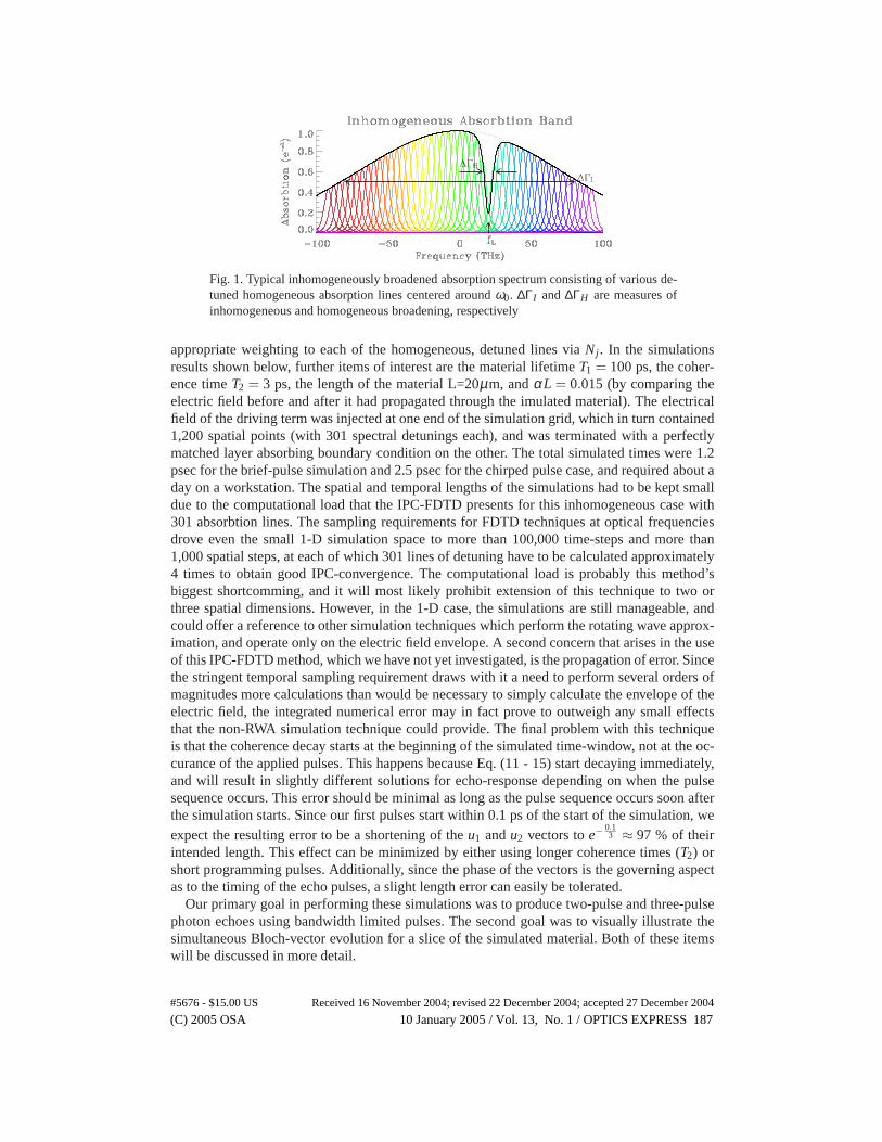
Fig. 1. Typical inhomogeneously broadened absorption spectrum consisting of various de-tuned homogeneous absorption lines centered around ω0. ∆ΓI and ∆ΓH are measures ofinhomogeneous and homogeneous broadening, respectively

appropriate weighting to each of the homogeneous, detuned lines via Nj. In the simulationsresults shown below, further items of interest are the material lifetime T1 = 100 ps, the coher-ence time T2 = 3 ps, the length of the material L=20µm, and α L = 0.015 (by comparing theelectric field before and after it had propagated through the imulated material). The electricalfield of the driving term was injected at one end of the simulation grid, which in turn contained1,200 spatial points (with 301 spectral detunings each), and was terminated with a perfectlymatched layer absorbing boundary condition on the other. The total simulated times were 1.2psec for the brief-pulse simulation and 2.5 psec for the chirped pulse case, and required about aday on a workstation. The spatial and temporal lengths of the simulations had to be kept smalldue to the computational load that the IPC-FDTD presents for this inhomogeneous case with301 absorbtion lines. The sampling requirements for FDTD techniques at optical frequenciesdrove even the small 1-D simulation space to more than 100,000 time-steps and more than1,000 spatial steps, at each of which 301 lines of detuning have to be calculated approximately4 times to obtain good IPC-convergence. The computational load is probably this method’sbiggest shortcomming, and it will most likely prohibit extension of this technique to two orthree spatial dimensions. However, in the 1-D case, the simulations are still manageable, andcould offer a reference to other simulation techniques which perform the rotating wave approx-imation, and operate only on the electric field envelope. A second concern that arises in the useof this IPC-FDTD method, which we have not yet investigated, is the propagation of error. Sincethe stringent temporal sampling requirement draws with it a need to perform several orders ofmagnitudes more calculations than would be necessary to simply calculate the envelope of theelectric field, the integrated numerical error may in fact prove to outweigh any small effectsthat the non-RWA simulation technique could provide. The final problem with this techniqueis that the coherence decay starts at the beginning of the simulated time-window, not at the oc-curance of the applied pulses. This happens because Eq. (11 - 15) start decaying immediately,and will result in slightly different solutions for echo-response depending on when the pulsesequence occurs. This error should be minimal as long as the pulse sequence occurs soon afterthe simulation starts. Since our first pulses start within 0.1 ps of the start of the simulation, weexpect the resulting error to be a shortening of the u1 and u2 vectors to e−

0.13 ≈ 97 % of their

intended length. This effect can be minimized by either using longer coherence times (T2) orshort programming pulses. Additionally, since the phase of the vectors is the governing aspectas to the timing of the echo pulses, a slight length error can easily be tolerated.

Our primary goal in performing these simulations was to produce two-pulse and three-pulsephoton echoes using bandwidth limited pulses. The second goal was to visually illustrate thesimultaneous Bloch-vector evolution for a slice of the simulated material. Both of these itemswill be discussed in more detail.


4. Photon echo using brief pulses

In this section we present the results for both the two-pulse (2P) and three-pulse (3P) photonecho simulations using 35 fs bandwidth-limited hyperbolic-secant pulses. The interaction oftwo optical pulses which are seperated by a time τ12 will write a spectral grating in an inhomo-geneously broadened material [7], assuming τ12 is less than the coherence time of the material.These two pulses also result in the emission of an optical pulse by the material, delayed after thesecond pulse by τ12, known as the 2-pulse photon echo. This process is commonly explainedby two different methods.

The first method evolves all of the inhomogeneously detuned lines on the same Bloch sphereat their particular phase evolution rates. After the first pulse hits the material, the Bloch vectorsof all the detunings are excited, and thus rotate around the ρ2 axis by an amount that dependsboth on the spectral content of the pulse, and the area or the pulse. For the hyperbolic secantpulse with a hyperbolic secant spectrum, the spectral excitation follows the spectral hyperbolicsecant, and thus the Bloch vectors are somewhat distributed in the ρ1,3 plane. Since the differentdetunings have linearly varying phase evolution rates, the corresponding Bloch vectors quicklyfan out and spread apart as they rotate around the ρ3 axis at a rate proportional to their resonancefrequency, undergoing what is called inhomogeneous dephasing. The effect of this dephasing isthat the vector sum of all the Bloch vectors, which is responsible for the polarization induced inthe material, sums to approximately zero once the Bloch vectors have evenly spread throughoutthe ρ1,2 plane. However, since this inhomogeneous dephasing process is deterministic and notirreversible like homogeneous dephasing, and the ensemble of Bloch vectors is controllable bysubsequent applications of optical pulses, one can rephase the dephasing Bloch vectors withthe following approach. By applying a second pulse to the material, (easiest to visualize is aπ pulse, although other pulse areas have a similar though less efficient result), all the Blochvectors with rotate around the ρ2 axis by 180o and then continue to process around the ρ3 axisin the same direction at their individual rates. This has the effect of setting up the individualinhomogeneous lines to fan back together so that they all re-phase at a time τ12 after the secondpulse on the opposite side of the Bloch sphere than they were initially excited to. This rephasingof the Bloch vectors will then induce a polarization in the material, and cause the two-pulsephoton echo to be emitted coherently [9]. The second method is based on Fourier analysis.Because the two pulses act upon the material within its coherence time, a spectral grating withperiod 1

τ12is recorded. The second half of pulse two can read out this grating, causing the

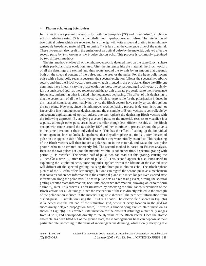
2P echo at a time τ12 after the second pulse [7]. This second approach also lends itself toexplaining the 3P photon echo, since any pulse applied within the lifetime of the excited statewill diffract off the spectral grating, causing the three pulse photon echo. The Bloch spherepicture of the 3P echo offers less insight, but one can regard the second pulse as a mechanismthat converts coherence information in the equitorial plane into much longer-lived excited stateinformation along the polar axis. The third pulse acts as a rephasing event, turning the spectralgrating (excited state information) back into coherence information, allowing an echo to forma time τ12 later. This process is best illustrated by observing the simultaneous evolution of theBloch vectors for all detunings, since the vector sum of these is directly related to the strengthof the polarization induced in the material. Figure 2 shows all the pertinent information froma short-pulse PE simulation using the IPC-FDTD code. The electric field shown in Fig. 2(a)is launched into the left end of the simulation grid, where at every location in the grid (atsuccessively delayed propagation times) it creates a time-varying excited state inversion asshown in Fig. 2(b). This excited state inversion for the different detunings numerically rangesfrom -1 to 1, and corresponds directly to the ρ3 value of the Bloch vector. Once the atomicensemble has been lifted out of the ground state, the inhomogeneous lines can dephase at theirparticular rate, according to the value of inhomogeneous detuning, while slowly decaying due


(a)

(b)

(c)

(d)

Fig. 2. Short-pulse photon echo simulation: The electric field due to a femtosecond pulsetrain (a) excites the inhomogeneously broadened absorber. The delay between pulse 1 and 2cause the sinusoidal modulation of the inversion (b), whose periodicity is inversely propor-tional to the pulse seperation time. The detuned lines of the IBA dephase at their particularrate, as shown by the rotating coordinate frame, in-phase component of the Bloch-vector(c). Two and three-pulse echoes are visible as re-phasings of the different detuned lines,seen as hyperbolic Moire patterns in (c). Finally, (d) shows the electric field detected at theoutput of the material. The programming pulses are visible, as well as the 2P and 3P photonechoes. The vertical scale in (d) is amplified by ten to make the echoes more apparent.


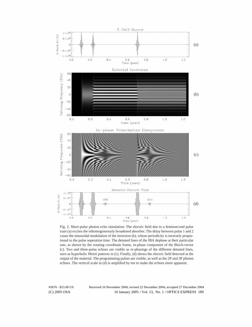
Fig. 3. A single frame from the rotating coordinate frame Bloch-vector evolution movie. Onthe left is a perspective view of the Bloch-sphere, in which the color-coding of the vectorsindicates the amount of detuning (blue and red colors indicate frequency up and downshifts, respectively) for a particular homogeneous line. The right view shows a projectionof the coherence, or ρ1,ρ2 plane. The plot at the bottom indicates the rotating coordinateframe electric-field as well as an artificial decoherence function, which is applied in orderto shorten the simulation time (as described in the text). [Small movie file 1.7MB] [Largemovie file 6.3MB]

to the decoherence goverened by T2. This is illustrated in Fig. 2(c), in which the data hasbeen down-converted into a rotating coordinate frame corresponding to the central detuningto remove the confusion which a 200 THz temporal carrier would cause. In essence, this down-conversion puts the viewer into a rotating coordinate frame, so that only the relative motionbetween the Bloch vectors is visible, but the overall continuous spinning around the Bloch-sphere at 200 THz has been eliminated. Finally, Fig. 2(d) shows the electric field detected atthe output of the material, which demonstrates that the inhomogeneous lines have collectivelygenerated a polarization that is momentum matched to efficiently radiate into the propagatingelectric field. This process is the underlying mechanism for both the 2PE and 3PE. The causeof the echos is easiest to see in Fig. 2(c) - the reversal of the dephasing of the different linescauses them to undo the initial dephasing, so that they come back into coincidence when theecho occurs, which is seen as a Moire-pattern at the time of the echo. An artificial decoherencewas implemented to shorten the simulation time. In an experiment, one would normally waitseveral T2’s before applying the third pulse, since this assures that the third pulse does notinteract coherently with the first two. Since this idle waiting makes the simulations unbearablylong, we multiplied the values for u1,2 by a smoothly varying decay term 0.6 ps before applyingthe third pulse.

Another way of viewing the same information is with an animated Bloch sphere evolution,such as that depicted in the movie referenced by Fig. 3. The data displayed in this movie isthe same as that which is displayed in Fig. 2, with the exception that the electric field has alsobeen placed in a rotating coordinate frame (mixed to DC with the central frequency carrier) foreasier visualization of the data. The left part of the movie shows a perspective view of the Blochvectors evolving, where each of the different homogeneously broadened lines is represented by


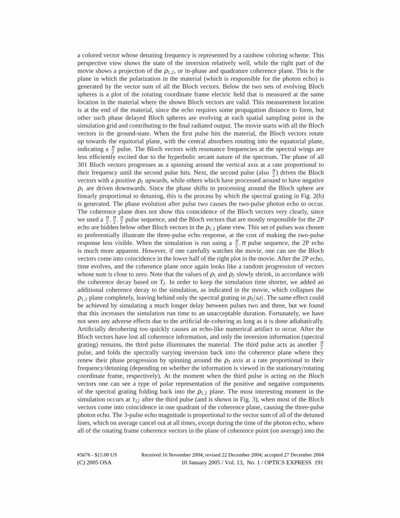
a colored vector whose detuning frequency is represented by a rainbow coloring scheme. Thisperspective view shows the state of the inversion relatively well, while the right part of themovie shows a projection of the ρ1,2, or in-phase and quadrature coherence plane. This is theplane in which the polarization in the material (which is responsible for the photon echo) isgenerated by the vector sum of all the Bloch vectors. Below the two sets of evolving Blochspheres is a plot of the rotating coordinate frame electric field that is measured at the samelocation in the material where the shown Bloch vectors are valid. This measurement locationis at the end of the material, since the echo requires some propagation distance to form, butother such phase delayed Bloch spheres are evolving at each spatial sampling point in thesimulation grid and contributing to the final radiated output. The movie starts with all the Blochvectors in the ground-state. When the first pulse hits the material, the Bloch vectors rotateup towards the equitorial plane, with the central absorbers rotating into the equatorial plane,indicating a π

2 pulse. The Bloch vectors with resonance frequencies at the spectral wings areless efficiently excited due to the hyperbolic secant nature of the spectrum. The phase of all301 Bloch vectors progresses as a spinning around the vertical axis at a rate proportional totheir frequency until the second pulse hits. Next, the second pulse (also π

2 ) drives the Blochvectors with a positive ρ1 upwards, while others which have processed around to have negativeρ1 are driven downwards. Since the phase shifts in processing around the Bloch sphere arelinearly proportional to detuning, this is the process by which the spectral grating in Fig. 2(b)is generated. The phase evolution after pulse two causes the two-pulse photon echo to occur.The coherence plane does not show this coincidence of the Bloch vectors very clearly, sincewe used a π

2 , π2 , π

2 pulse sequence, and the Bloch vectors that are mostly responsible for the 2Pecho are hidden below other Bloch vectors in the ρ1,2 plane view. This set of pulses was chosento preferentially illustrate the three-pulse echo response, at the cost of making the two-pulseresponse less visible. When the simulation is run using a π

2 ,π pulse sequence, the 2P echois much more apparent. However, if one carefully watches the movie, one can see the Blochvectors come into coincidence in the lower half of the right plot in the movie. After the 2P echo,time evolves, and the coherence plane once again looks like a random progression of vectorswhose sum is close to zero. Note that the values of ρ1 and ρ2 slowly shrink, in accordance withthe coherence decay based on T2. In order to keep the simulation time shorter, we added anadditional coherence decay to the simulation, as indicated in the movie, which collapses theρ1,2 plane completely, leaving behind only the spectral grating in ρ3(ω). The same effect couldbe achieved by simulating a much longer delay between pulses two and three, but we foundthat this increases the simulation run time to an unacceptable duration. Fortunately, we havenot seen any adverse effects due to the artificial de-cohering as long as it is done adiabatically.Artificially decohering too quickly causes an echo-like numerical artifact to occur. After theBloch vectors have lost all coherence information, and only the inversion information (spectralgrating) remains, the third pulse illuminates the material. The third pulse acts as another π

2pulse, and folds the spectrally varying inversion back into the coherence plane where theyrenew their phase progression by spinning around the ρ3 axis at a rate proportional to theirfrequency/detuning (depending on whether the information is viewed in the stationary/rotatingcoordinate frame, respectively). At the moment when the third pulse is acting on the Blochvectors one can see a type of polar representation of the positive and negative componentsof the spectral grating folding back into the ρ1,2 plane. The most interesting moment in thesimulation occurs at τ12 after the third pulse (and is shown in Fig. 3), when most of the Blochvectors come into coincidence in one quadrant of the coherence plane, causing the three-pulsephoton echo. The 3-pulse echo magnitude is proportional to the vector sum of all of the detunedlines, which on average cancel out at all times, except during the time of the photon echo, whereall of the rotating frame coherence vectors in the plane of coherence point (on average) into the


same quadrant.

5. Photon echo using chirped pulses

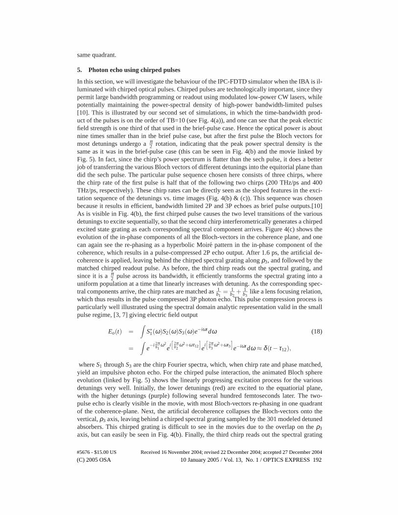
In this section, we will investigate the behaviour of the IPC-FDTD simulator when the IBA is il-luminated with chirped optical pulses. Chirped pulses are technologically important, since theypermit large bandwidth programming or readout using modulated low-power CW lasers, whilepotentially maintaining the power-spectral density of high-power bandwidth-limited pulses[10]. This is illustrated by our second set of simulations, in which the time-bandwidth prod-uct of the pulses is on the order of TB=10 (see Fig. 4(a)), and one can see that the peak electricfield strength is one third of that used in the brief-pulse case. Hence the optical power is aboutnine times smaller than in the brief pulse case, but after the first pulse the Bloch vectors formost detunings undergo a π

2 rotation, indicating that the peak power spectral density is thesame as it was in the brief-pulse case (this can be seen in Fig. 4(b) and the movie linked byFig. 5). In fact, since the chirp’s power spectrum is flatter than the sech pulse, it does a betterjob of transferring the various Bloch vectors of different detunings into the equitorial plane thandid the sech pulse. The particular pulse sequence chosen here consists of three chirps, wherethe chirp rate of the first pulse is half that of the following two chirps (200 THz/ps and 400THz/ps, respectively). These chirp rates can be directly seen as the sloped features in the exci-tation sequence of the detunings vs. time images (Fig. 4(b) & (c)). This sequence was chosenbecause it results in efficient, bandwidth limited 2P and 3P echoes as brief pulse outputs.[10]As is visible in Fig. 4(b), the first chirped pulse causes the two level transitions of the variousdetunings to excite sequentially, so that the second chirp interferometrically generates a chirpedexcited state grating as each corresponding spectral component arrives. Figure 4(c) shows theevolution of the in-phase components of all the Bloch-vectors in the coherence plane, and onecan again see the re-phasing as a hyperbolic Moire pattern in the in-phase component of thecoherence, which results in a pulse-compressed 2P echo output. After 1.6 ps, the artificial de-coherence is applied, leaving behind the chirped spectral grating along ρ3, and followed by thematched chirped readout pulse. As before, the third chirp reads out the spectral grating, andsince it is a π

2 pulse across its bandwidth, it efficiently transforms the spectral grating into auniform population at a time that linearly increases with detuning. As the corresponding spec-tral components arrive, the chirp rates are matched as 1

b1= 1

b2+ 1

b3like a lens focusing relation,

which thus results in the pulse compressed 3P photon echo. This pulse compression process isparticularly well illustrated using the spectral domain analytic representation valid in the smallpulse regime, [3, 7] giving electric field output

Eo(t) =∫

S∗1(ω)S2(ω)S3(ω)e−iωtdω (18)

=∫

e−i 2π

b1ω2

ei[

2πb2

ω2+ωτ12

]e

i[

2πb3

ω2+ωt3]e−iωtdω ≈ δ(t − τ12),

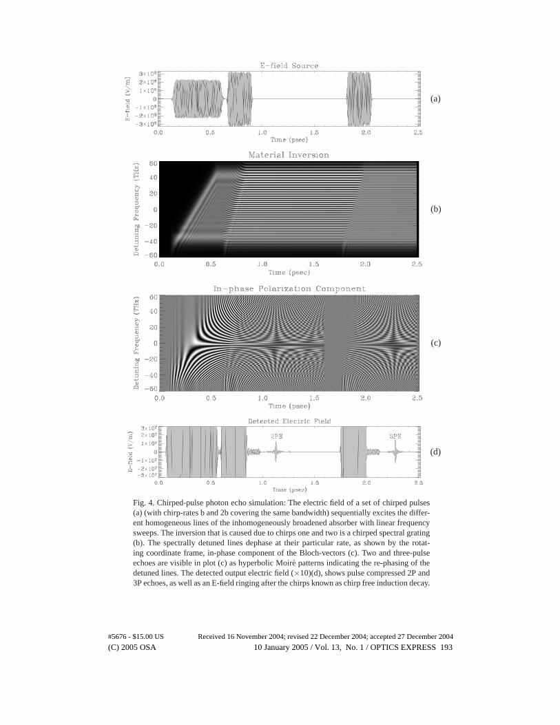
where S1 through S3 are the chirp Fourier spectra, which, when chirp rate and phase matched,yield an impulsive photon echo. For the chirped pulse interaction, the animated Bloch sphereevolution (linked by Fig. 5) shows the linearly progressing excitation process for the variousdetunings very well. Initially, the lower detunings (red) are excited to the equatiorial plane,with the higher detunings (purple) following several hundred femtoseconds later. The two-pulse echo is clearly visible in the movie, with most Bloch-vectors re-phasing in one quadrantof the coherence-plane. Next, the artificial decoherence collapses the Bloch-vectors onto thevertical, ρ3 axis, leaving behind a chirped spectral grating sampled by the 301 modeled detunedabsorbers. This chirped grating is difficult to see in the movies due to the overlap on the ρ3

axis, but can easily be seen in Fig. 4(b). Finally, the third chirp reads out the spectral grating


(a)

(b)

(c)

(d)

Fig. 4. Chirped-pulse photon echo simulation: The electric field of a set of chirped pulses(a) (with chirp-rates b and 2b covering the same bandwidth) sequentially excites the differ-ent homogeneous lines of the inhomogeneously broadened absorber with linear frequencysweeps. The inversion that is caused due to chirps one and two is a chirped spectral grating(b). The spectrally detuned lines dephase at their particular rate, as shown by the rotat-ing coordinate frame, in-phase component of the Bloch-vectors (c). Two and three-pulseechoes are visible in plot (c) as hyperbolic Moire patterns indicating the re-phasing of thedetuned lines. The detected output electric field (×10)(d), shows pulse compressed 2P and3P echoes, as well as an E-field ringing after the chirps known as chirp free induction decay.


Fig. 5. A single frame from the rotating coordinate frame Bloch-vector evolution movie.Again, the color-coding of the vectors indicates the amount of detuning (blue and red col-ors indicate frequency up and down shifts, respectively). The plot at the bottom indicatesthe rotating coordinate frame electric-field consisting of three chirps with the same powerspectral density, aswell as an artificial decoherence function. The moment of re-coherencefor the three-pulse echo is shown. [Small movie file 2.3MB] [Large movie file 14MB]

sequentially, transfers the spectral components to the equitorial plane, and the three-pulse echooccurs when most of the Bloch-vectors re-phase in one quadrant of the sphere. This modelingand illustration technique could be used for a variety of other processing techniques, but thecomputational inefficiency of the FDTD technique precludes modeling of multidimensionalspatial-spectral holography or the precise modeling of GHz bandwidth operations currently ofgreat experimental interest for RF signal processing applications [4, 5, 6, 7, 11].

6. Conclusion

We have successfully implemented an IPC-FDTD simulator designed to predict the interactionof short optical pulses with inhomogeneously broadened media. Two- and three-pulse photonechoe simulations were demonstrated from brief- and chirped-pulse sequences inside a mate-rial with 301 lines of inhomogeneous detuning. The complicated dynamics of these 301 spectralcomponents were illustrated with plots as well as color-coded movies of multiple simultaneousBloch vectors on the Bloch sphere as a powerful visualization technique. The formation of 2Pand 3P echoes was illustrated on the Bloch-sphere, and the detailed rephasing of all the inho-mogeneous lines that leads to the formation of the photon echoes was graphically illustrated.

Acknowledgments

We wish to acknowledge support from W. Schneider of DARPA (MSU subcontract MDA972-03-1-0002), as well as valuable discussions with W.R. Babbitt, K. Anderson and M. Mohamed.


Modeling of femtosecond pulse interaction with inhomogeneously broadened media using an iterative...

Documents

Transcript of Modeling of femtosecond pulse interaction with inhomogeneously broadened media using an iterative...