Signal Processing 83 (2003) 695–712

www.elsevier.com/locate/sigpro

E!cient selection of feature sets possessing high coe!cients ofdetermination based on incremental determinationsRonaldo F. Hashimotoa;b, Edward. R. Doughertya;c;∗ , Marcel Bruna;b,

Zheng-Zheng Zhoud, Michael L. Bittnere, Je3rey M. Trente

aDepartment of Electrical Engineering, Texas A&M University, 3128 TAMU, College Station, TX 77843-3128, USAbDepartamento de Ciencia de Computac'ao, Instituto de Matem*atica e Estat*+stica, Universidade de Sao Paulo, Sao Paulo, Brazil

cDepartment of Pathology, University of Texas M.D. Anderson Cancer Center, Houston, TX 77030, USAdNuTec Sciences, Inc., USA

eNational Human Genome Research Institute of the National Institutes of Health, Bethesda, MD 20892, USA

Received 7 March 2002; received in revised form 27 August 2002

Abstract

Feature selection is problematic when the number of potential features is very large. Absent distribution knowledge, toselect a best feature set of a certain size requires that all feature sets of that size be examined. This paper considers thequestion in the context of variable selection for prediction based on the coe!cient of determination (CoD). The CoD variesbetween 0 and 1, and measures the degree to which prediction is improved by using the features relative to prediction in theabsence of the features. It examines the following heuristic: if we wish to >nd feature sets of size m with CoD exceeding �,what is the e3ect of only considering a feature set if it contains a subset with CoD exceeding �¡�? This means that if thesubsets do not possess su!ciently high CoD, then it is assumed that the feature set itself cannot possess the required CoD.As it stands, the heuristic cannot be applied since one would have to know the CoDs beforehand. It is meaningfully posedby assuming a prior distribution on the CoDs. Then one can pose the question in a Bayesian framework by consideringthe probability P(�¿� |max{�1; �2; : : : ; �v}¡�), where � is the CoD of the feature set and �1; �2; : : : ; �v are the CoDs ofthe subsets. Such probabilities allow a rigorous analysis of the following decision procedure: the feature set is examined ifmax{�1; �2; : : : ; �v}¿ �. Computational saving increases as � increases, but the probability of missing desirable feature setsincreases as the increment �− � decreases; conversely, computational saving goes down as � decreases, but the probabilityof missing desirable feature sets decreases as � − � increases. The paper considers various loss measures pertaining toomitting feature sets based on the criteria. After specializing the matter to binary features, it considers a simulation model,and then applies the theory in the context of microarray-based genomic CoD analysis. It also provides optimal computationalalgorithms.? 2002 Elsevier Science B.V. All rights reserved.

Keywords: Coe!cient of determination; Feature selection; Gene microarray; Optimal classi>er

∗ Corresponding author. Department of Electrical Engineer-ing, Texas A&M University, 3128 TAMU, College Station, TX77843-3128, USA. Tel.: +1-409-845-7441; fax: +1-409-845-6259.

E-mail address: edward@ee.tamu.edu (E.R. Dougherty).

1. Introduction

The feature-selection problem in pattern recog-nition is to select a subset of k random variablesfrom a set on n random variables that provides an

0165-1684/03/$ - see front matter ? 2002 Elsevier Science B.V. All rights reserved.doi:10.1016/S0165-1684(02)00468-1

696 R.F. Hashimoto et al. / Signal Processing 83 (2003) 695–712

optimal classi>er with minimum error among all op-timal classi>ers for subsets of size k. The inherentcombinatorial nature of the problem is readily seenfrom a classic theorem of Cover and Van Campenhout[2]: if {X1;X2; : : : ;Xr} is the set of possible featuresets formed from the set {X1; X2; : : : ; Xn} of randomvariables under the assumption that i¡ j if Xi ⊂ Xj,and if Y is a binary target random variable, then thereexists a multivariate distribution of X1; X2; : : : ; Xn; Ysuch that �[X1]¿�[X2]¿ · · ·¿�[Xr], where �[Xj]is the Bayes error for Xj, given by �[Xj] = P(Y �= 0(Xj)), where 0 is the optimal classi>er basedon Xj. The requirement that i¡ j if Xi ⊂ Xj isnecessary because the subset condition implies that�[Xi]¿ �[Xj]. A consequence of the theorem is thatall k-element subsets must be checked unless thereis distributional knowledge that mitigates the searchrequirement. Various heuristic suboptimal algorithmshave been developed to circumvent the full combina-torial search that requires estimating the Bayes errorof C(n; k) subsets [3,12,15], and a branch and boundalgorithm has been used for e!cient selection of thebest feature set [10].We will take an approach that is well-suited to the

context in which we are confronting feature selection.There is a very large number n of variables, and wedesire very small feature sets (k = 1; 2; 3; 4). More-over, we are not necessarily interested in the best fea-ture set of size k, but rather >nding good feature setsof size k; indeed, our speci>c concern is >nding col-lections of good feature sets for a family of target ran-dom variables. To be precise, we have a set X of nbinary random variables X1; X2; : : : ; Xn and we wantto >nd small subsets of the variables to predict othervariables in X. The number of variables n often ex-ceeds 500, perhaps signi>cantly so. To check all fea-ture sets would require computing optimal estimatorsand errors for all subsets up to maximum sizem, whichwould require computing C(n; 1) + C(n; 2) + · · · +C(n; m) errors if we wish to consider feature sets up tosize m.Instead of stating the feature-selection problem in

terms of error, we can equivalently state it in termsof the coe!cient of determination (CoD), which pro-vides a normalized measure of the degree to whichY can be better predicted using the observations in afeature set than it can be in the presence of no obser-vations. Speci>cally, for any feature set X, the CoD

relative to the target variable Y is de>ned to be

�X =�• − �X

�•;

where �• is the error of the best estimate for Y in theabsence of other observations and �X is the Bayes er-ror for X. The coe!cient has historically been used tomeasure the e3ect of linear regression [16], and hasbeen recently employed in nonlinear signal processing[5] and for measuring multivariate interaction amonggenes based on gene expression [5,8], and for con-structing probabilistic Boolean networks [13]. It is thislast application that has motivated the current analy-sis. It is evident from the de>nition that 06 �X6 1and X ⊆ Z implies �X6 �Z. In terms of the coe!-cient, the feature-selection problem is to >nd a subsetof k random variables possessing the highest coe!-cient among all subsets of size k.The particular application we have in mind, and

will discuss in detail following the development ofthe methodology, involves the prediction whethera gene is up- or down-regulated based on the up-or down-regulation of other genes using data fromgene-expression microarrays [8,9]. The full searchfor this problem is currently done using massivelyparallel hardware, practically halts at m= 3 for aboutn = 600 genes, and takes 2 weeks using over 100CPU’s if all 600 targets are to be considered [14].Since gene-expression data is severely limited withcurrent genomic technology, for statistical reasonsthere is usually little to be gained by going beyondthree predictors; nonetheless, it is of great practicalbene>t to reduce the computation so that two-geneprediction can be accomplished easily on a work-station, three-gene prediction can be accomplishedfor a small subset of targets on a workstation, andprediction for full target sets can be accomplishedsigni>cantly faster on a parallel system. Moreover,with the rapid evolution of microarray technology,sample sizes are increasing and four-predictor setsmay soon exhibit statistically signi>cant gains overthree-predictor sets su!ciently often to be of seriousinterest.

2. Distributional selection of variables

A simple approach to avoiding the full combinato-rial search for the optimal two-feature set is to skip

R.F. Hashimoto et al. / Signal Processing 83 (2003) 695–712 697

the computation of the CoD for two variables relativeto a target variable if the individual CoDs of the vari-ables relative to the target are both small. For a >xedtarget Y , if �i, �i; j and �i; j; k denote the CoD for {Xi},{Xi; Xj} and {Xi; Xj; Xk}, respectively, then a subopti-mal algorithm is de>ned by saying that if both �i and �j

are very small, then we ignore �i; j, thereby saving itscomputation. The problem is it may be that �i=�j=0,while �i; j = 1. This extreme case is not just a mathe-matical possibility but actually happens in real-worldapplications, including genomics. Indeed, it could bethat �i = �j = �k = 0, while �i; j; k = 1, and so on. It isjust this kind of behavior that has motivated the de-velopment of software for high-performance parallelprocessing. But this extreme behavior is rare. Moretypically, if both �i and �j are very small, then �i; j issmall.To take advantage of this behavior, rather than

consider each CoD as a deterministic quantity as-sociated with a >xed multivariate distribution of{Y; X1; X2; : : : ; Xn}, we will consider the multivariatedistribution to be random, thereby making the CoDsrandom, and allowing us to discuss the probabilitythat �i; j is small given that �i and �j are small. Specif-ically, we can consider the probability that �i; j ¿�given that �i ¡� and �j ¡�. If we are only concernedwith feature sets for which the CoDs exceed a givenvalue �, then (on average) little is lost by not comput-ing the joint CoD if both marginal CoDs are beneath�, and � is su!ciently smaller than �. We skip thecomputation of �i; j if and only if max{�i; �j}¡�.More generally, given a function g : [0; 1]×[0; 1] →

R and a number �∈R, we can use the following cri-terion: �i; j will not be computed if g(�i; �j)¡�. Forinstance, instead of g(�i; �j)=max{�i; �j}, one mightuse g(�i; �j) = �i + �j. In this paper, we con>ne our-selves to the maximum and, in this case, we can as-sume �∈ [0; 1].The requirement that max{�i; �j} exceed � for the

calculation of �i; j under the supposition that �i; j mustexceed � to be signi>cant can be viewed as a con-dition on the incremental determinations for the set{Xi; Xj} relative to the sets {Xi} and {Xj}, where theincremental determination for feature set Z relative toa subset X ⊆ Z is de>ned to be �Z − �X [5]. Thecondition can be interpreted as the assumption thatincrements cannot exceed � − �. Under this assump-tion, max{�i; �j}¡� implies �i; j6 � and therefore

there is no point to computing �i; j. A number of issuesare relevant to the condition that max{�i; �j}¿ � forcomputing �i; j.One issue is computational savings. For the criterion

max{�i; �j}¡� not to compute �i; j, the probability

�ij(�) = P(max{�i; �j}¡�)

provides a measure of computational saving: the prob-ability of not computing �i; j. Assuming continuousdistributions, �ij(�) → 0 as � → 0 and �ij(�) → 1 as� → 1.Typically, we are interested in CoDs above some

threshold level. Accordingly, we say that �i; j is signif-icant at level � if �i; j ¿�. If we skip the computationof �i; j when max{�i; �j}¡�, then the probability

�ij(�; �) = P(�i; j ¿� |max{�i; �j}¡�)

provides a measure of risk of losing signiBcant CoDs.It gives the probability of a pairwise CoD being signif-icant at level �, given that it is not computed (at level�). A tolerance for such risk can be expressed by for-mulating a requirement that �ij(�; �)¡�. In this case,� quanti>es our tolerance level by providing an upperbound on the probability with which we are willing tomiss a signi>cant relationship on account of omittingthe computation. We would like � to be as high aspossible to save as much computation as possible, andwe would like to have � ≈ 0; however, the problemis that as � increases, the probability of �i; j exceeding� also tends to increase.Expanding the conditional probability de>ning

�ij(�; �) and dividing both sides of the equation byP(�i; j ¿�) yields

�ij(�; �)P(�i; j ¿�)

=P(�i; j ¿�;max{�i; �j}¡�)

P(�i; j ¿�)P(max{�i; �j}¡�)

=P(max{�i; �j}¡� | �i; j ¿�)

P(max{�i; �j}¡�)

=�ij(�; �)

P(max{�i; �j}¡�);

where

�ij(�; �) = P(max{�i; �j}¡� | �i; j ¿�)

provides a measure of loss for signiBcant CoDs.�ij(�; �) gives the probability of not computing a sig-ni>cant CoD. As in the case of �ij(�; �), we would like

698 R.F. Hashimoto et al. / Signal Processing 83 (2003) 695–712

�ij(�; �) to be small. Also, as with �ij(�; �), pushingup � to increase computational savings, also pushesup �ij(�; �).The e3ect on �ij(�; �) of increasing � for >xed �

is easily seen by expanding �ij(�; �). If �1 ¡�2, then�ij(�1; �)6 �ij(�2; �). �ij(�; �) is important, because itquanti>es the noncomputation of signi>cant pairwiseCoDs; however, if we take the view that we only wishto discover whether or not �i; j is signi>cant, withoutnecessarily >nding its value, then the problem can belooked at slightly di3erently. According to the de>-nition of the CoD, if max{�i; �j}¿�, then �i; j ¿�.Hence, if max{�i; �j}¿�, there is no need to com-pute �i; j. Omitting such computations means that thecomputational savings are enhanced, with �ij(�) beingreplaced by

�ij(�; �)

=P(max{�i; �j}¡�) + P(max{�i; �j}¿�):

We will say that �i; j is nonredundantly signiBcant atlevel � if max{�i; �j}6 � and �i; j ¿�. Having com-puted the single-variable CoDs, we need only >ndthose that are nonredundantly signi>cant.Continuing to take the view that we only want to

discover signi>cant CoDs, not their values, we canadjust our notion of loss, replacing �ij(�; �) by

�ij(�; �)

=P(max{�i; �j}¡� | �i; j ¿�;max{�i; �j}6 �)

which is the probability of not computing nonredun-dantly signi>cant CoDs. Assuming �¡�, we showthat �ij(�; �)¿ �ij(�; �):

�ij(�; �)

=P(�i;j ¿ �;max{�i; �j}¡�)

P(�i;j ¿ �)

=P(�i;j ¿ �;max{�i; �j}¡�)

P(�i;j ¿ �;max{�i; �j}6 �) + P(�i;j ¿ �;max{�i; �j}¿�)

6P(�i;j ¿ �;max{�i; �j}¡�)P(�i;j ¿ �;max{�i; �j}6 �)

=P(�i;j ¿ �;max{�i; �j}¡�;max{�i; �j}6 �)

P(�i;j ¿ �;max{�i; �j}6 �)

=�ij(�; �):

3. Increasing the predictor variables

In the preceding section, we paid particular atten-tion to the case of two-predictor variables. In this sec-tion, we extend those considerations to estimation us-ing three or more variables. The criterion for not com-puting the CoD can be just an extension of the crite-rion for two variables:

h(�i; �j; �k)¡�;

where h : [0; 1] × [0; 1] × [0; 1] → R. Another possi-bility is to use a function that depends on the CoDsfor two variables:

h(�i; j ; �j;k ; �i; k)¡�;

where, �i; j is de>ned to be 0 if it has been omitted atthe previous stage. Criteria depending on other com-binations of CoDs of lower order are possible. In thispaper we will consider the condition

max{�i; �j; �k}¡�:

The following proposition is straightforward andshows that the condition max{�i; j ; �j;k ; �i; k}¡� ismore restrictive than the conditionmax{�i; �j; �k}¡�.This means that, for a >xed �, the computational sav-ing is bigger using the condition max{�i; �j; �k}¡�.

Proposition 1. If max{�i; j ; �j;k ; �i; k}¡�, thenmax{�i; �j; �k}¡�.

Under the condition max{�i; �j; �k}¡�, �ij(�; �)becomes �ijk(�; �). The form of �ij(�; �) remainsthe same except that max{�i; �j} is replaced bymax{�i; �j; �k}. Analogous comments apply to�ij(�; �), �ij(�; �), �ij(�; �), and �ij(�; �).Similar considerations apply to using more than

three variables.

4. Error of the optimal binary predictor

The theory of feature selection based on the distri-bution of the CoDs applies to binary-decision patternrecognition by considering only binary target vari-ables. A special case occurs when all variables arebinary. This is the situation that occurs in binarysignal processing and, of importance to functional

R.F. Hashimoto et al. / Signal Processing 83 (2003) 695–712 699

genomics, in probabilistic Boolean networks [13]. Thevariable-selection theory possesses an intuitive ana-lytic form for binary variables.Consider a set of n binary random variables

X1; X2; : : : ; Xn to predict (estimate) another binary ran-dom variable Y . Let Xi denote the conBguration ofthe random vector X = (X1; X2; : : : ; Xn) whose binaryexpression equals the integer i. For instance, for n=3,X0 = 000, X1 = 001; : : : ;X7 = 111. For n variables,there are m = 2n possible con>gurations. Assumingthe binary random variables X1; X2; : : : ; Xn; Y possessa joint probability distribution, for each con>gurationXi, we have the probabilities ri = P(X = Xi) andpi = P(Y = 1|Xi). The best predictor for Y in termsof the mean absolute error (MAE) and in the absenceof observations is its mean E[Y ] = � =

∑m−1i=0 piri

followed by the binary threshold function T : [0; 1] →{0; 1} de>ned as T (x) = 0 if and only if x6 0:5. Theerror of the thresholded mean predictor is given by

�• =

{� if �6 0:5

1− � if �¿ 0:5= min{�; 1− �}:

If we consider observations, then we can designanother predictor for Y and decrease the error.Let {Xj1 ; Xj2 ; : : : ; Xj‘} be a subset of the variables{X1; X2; : : : ; Xn} such that 16 j1 ¡j2 ¡ · · ·¡j‘6 n.To develop an analytical formula for the error ofthe best predictor of Y in terms of the MAE basedon the observations of the variables Xj1 ; Xj2 ; : : : ; Xj‘ ,let Xk denote the con>guration of the random vec-tor X = (Xj1 ; Xj2 ; : : : ; Xj‘) whose binary expressionequals the integer k. For a >xed con>guration Xk

of X, there will be some con>gurations Xi of thevector X that match Xk . For instance, supposeX = (X1; X2; X3; X4; X5) and we wish to predict Y us-ing only the variables X2 and X4. Thus, X = (X2; X4)and, for k = 1, we have X1 = 01. The con>gurationsof Xi that match X1 are given in the following table:

i Xi i Xi i Xi i Xi

2 00010 3 00011 6 00110 7 0011118 10010 19 10011 22 10110 23 10111

If we consider the con>gurations for Xi and Xk as

Xi = (X i1 ; : : : ; X

ij1 ; : : : ; X

ij2 ; : : : ; X

ij‘ ; : : : ; X

in)

and

Xk = (X kj1 ; X

kj2 ; : : : ; X

kj‘);

then, for a >xed k, we can de>ne the set {i: Xi ∼ Xk}as

{i: Xi ∼ Xk}={i: X i

j1 = X kj1 ; X

ij2 = X k

j2 ; : : : ; Xij‘ = X k

j‘}:For instance, if k = 1, the set {i: Xi ∼ X1} for thepreceding table is {2; 3; 6; 7; 18; 19; 22; 23}.Now, let us introduce two probabilities:

Ak(X) = P(X =Xk) =∑

{i: Xi∼Xk}ri;

Bk(X) = P(Y = 1 and X =Xk) =∑

{i: Xi∼Xk}piri:

In terms of these probabilities, the error for predictingY using the variables in the vector X is

�X =2‘−1∑k=0

min{Bk(X); Ak(X)− Bk(X)}:

If we use all variables, X = X, then

Ak(X) = P(X = Xk) =∑

{i: Xi∼Xk}ri = rk ;

Bk(X) = P(Y = 1 and X = Xk)

=∑

{i:Xi∼Xk}piri = pkrk

and the error of the best predictor is

�X =2n−1∑k=0

min{pkrk ; rk − pkrk}

=2n−1∑k=0

min{pk; 1− pk}rk :

5. Simulations

In this section, we study variable selection in thecontext of a binary model for the joint probabilitydistribution P(X1; : : : ; Xn; Y ). We employ a modelwith three parameters, �; �, and %�, used previouslyin the analysis of estimation error [1]. A realization

700 R.F. Hashimoto et al. / Signal Processing 83 (2003) 695–712

of the joint probability P(Y; X1; : : : ; Xn) is de>ned bythe probabilities ri and the conditional probabilitiespi. The probabilities ri are generated randomly fromthe Gamma distribution with parameters �= 1=m and% = �=m, where m = 2n is the number of possiblecon>gurations. A normalization is used to satisfy theprobability requirement

∑m−1i=0 ri = 1:

ri =r′i∑m−1

i=0 r′i;

where r′i comes from the Gamma distribution with�=1=m and %=�=m. The conditional probabilities pi

are de>ned by pi = 1 − � for i = 0; 1; : : : ; ' − 1 andpi=� for i='; : : : ; m−1, where the integer ' de>neshow many con>gurations produce the output Y = 1and ' is taken from the uniform distribution between0 and m. In practical situations it is unlikely to haveconstant error contribution �=min{pi; 1−pi} for allcon>gurations. Hence, Gaussian noise with �=0 and% = %� is added to the conditional probabilities pi.Given a realization ri and pi taken from the model

(�; �; %�), we can directly compute the CoDs �i and�i; j. The >rst simulation results presented in this sec-tion are based on n = 5 variables, 10; 000 generatedreplications, and the model parameters �=1:5, �=0:2,and %� = 0:2.Fig. 1(a) displays the computational saving �ij(�)

obtained from the model. The graphic can be used toselect a value for � to obtain a desired computationalsaving. For example, for at least 90% of computationalsaving, we must select �¿ 0:4.The risk �ij(�; �) of losing signi>cant CoDs ob-

tained from the model is shown in Fig. 1(b). Once �is selected, this graphic can be used to check if therisk of losing CoDs �i; j ¿� is smaller than a desiredtolerance. For example, if the tolerance for the riskpertaining to coe!cients �i; j ¿ 0:6 is 10%, then for�=0:4 this tolerance is satis>ed, since the risk is lessthan 1%.Fig. 1(c) shows the probability �ij(�; �) of not

computing signi>cant CoDs. Once � is selected, thegraphic can be used to check if the risk of losingCoDs �i; j ¿� is smaller than a desired tolerance.For example, if the tolerance for losing coe!cients�i; j ¿ 0:7 is 20%, then for � = 0:4 this condition issatis>ed, since the risk is less than 10%.Fig. 1(d) shows the probability �ij(�; �) of not com-

puting nonredundantly signi>cant coe!cients. Again

considering tolerance, if the tolerance for noncompu-tation of coe!cients �i; j ¿ 0:7 is 20%, then for �=0:4this condition is satis>ed, since the risk is less than10%.Fig. 1(e) shows the loss for signi>cant CoDs versus

computational saving. This graphic shows that whencomputational saving is high, the respective loss ofsigni>cant CoDs is not so high. For example, for a90% computational saving, the loss of signi>cant co-e!cients is less than 10%.The curves in Fig. 1 are model dependent,

for model (n; �; �; %�) = (5; 1:5; 0:2; 0:2). Fig. 2shows a set of curves for a di3erent model with(n; �; �; %�) = (5; 2:8; 0:3; 0:1). Notice in Fig. 2(b) thesmaller risk, with the risk being essentially 0 for all �when �= 0:7 or 0.8. Notice in Fig. 2(c) the basicallyvertical curvers for � = 0:7 and 0.8. This means thateven for an extremely small increment �− �, the lossis essentially 0 for �= 0:7 and 0.8, so long as �¡�.A very di3erent situation is depicted for the model(n; �; �; %�) = (5; 1:5; 0:1; 0:2) in Fig. 3. Not only arethe risks in Fig. 3(b) much greater, but the curves insucceeding parts of the >gure rise more slowly.The model not only depends on �, � and %�, but also

on n. In Figs. 4 and 5, n= 10. Although similar fam-ilies of curves occur as with n = 5, these result fromdi3erent choices of �, � and %� than for n=5. Note thesimilarities between the curves in Fig. 4, correspond-ing to the model (n; �; �; %�) = (10; 9:0; 0:12; 0:01),with the curves in Fig. 1. Also note the similarities be-tween the curves in Fig. 5 corresponding to the model,(n; �; �; %�) = (10; 1:5; 0:2; 0:2), with the curves inFig. 2.

6. Glioma application

In this section, we apply the variable-selection the-ory to real gene-expression data from glioma patients.We will see that there are similarities between the be-havior of the simulation-based coe!cients and thosefrom actual cancer patients. More importantly, theloss of high coe!cients will be seen to be relativelysmall even when signi>cant computational savings areachieved.The study of expression-level prediction has re-

cently been made possible by the development ofcDNA microarrays, in which transcript levels can be

R.F. Hashimoto et al. / Signal Processing 83 (2003) 695–712 701

0.7

0.8

0.9

1

0.2 0.3 0.4 0.5 0.6 0.7 0.8 0.9 1

Com

puta

tiona

l Sav

ing

�

� = 1.5 - � = 0.2 - �� = 0.2 � = 1.5 - � = 0.2 - �� = 0.2

� = 1.5 - � = 0.2 - �� = 0.2

� = 1.5 - � = 0.2 - �� = 0.2 � = 1.5 - � = 0.2 - �� = 0.2

(a) Computational saving.

� = 0 . 7� = 0 . 8

� = 0 . 6� = 0 . 5

0

0.005

0.01

0.015

0.02

0.025

0.03

0.035

0.04

0.045

0.05

0.2 0.3 0.4 0.5 0.6 0.7 0.8 0.9 1�

Ris

k

� = 0 . 5� = 0 . 6� = 0 . 7� = 0 . 8

0

0.2

0.4

0.6

0.8

1

0.2 0.3 0.4 0.5 0.6 0.7 0.8 0.9 1

Los

s

�

(b) Risk of losing significant CoDs. (c) Loss for significant CoDs.

� = 0 . 5� = 0 . 6� = 0 . 7� = 0 . 8

0

0.2

0.4

0.6

1

0.2 0.3 0.4 0.5 0.6 0.7 0.8 0.9 1

Los

s

�

0.8

� = 0 . 5� = 0 . 6� = 0 . 7� = 0 . 8

0

0.1

0.2

0.3

0.4

0.5

0.6

0.7

0.8

0.9

1

0.2 0.3 0.4 0.5 0.6 0.7 0.8 0.9 1

Los

s

Computational Saving

(d) Loss for nonredundant significant CoDs.(e)

Loss for significant CoDs ×

Computational saving.

Fig. 1. Simulations for model (n; �; �; %�) = (5; 1:5; 0:2; 0:2): (a) computational saving, (b) risk of losing signi>cant CoDs, (c) loss forsigni>cant CoDs, (d) loss for nonredundant signi>cant CoDs, and (e) loss for signi>cant CoDs × computational saving.

702 R.F. Hashimoto et al. / Signal Processing 83 (2003) 695–712

0.7

0.8

0.9

1

0.2 0.3 0.4 0.5 0.6 0.7 0.8 0.9 1

Com

puta

tiona

l Sav

ing

�

(a) Computational saving.

0

0.0005

0.001

0.0015

0.002

0.0025

0.003

0.0035

0.2 0.3 0.4 0.5 0.6 0.7 0.8 0.9 1�

Ris

k

0

0.2

0.4

0.6

0.8

1

0.2 0.3 0.4 0.5 0.6 0.7 0.8 0.9 1

Los

s

�

0

0.2

0.4

0.6

0.8

1

0.2 0.3 0.4 0.5 0.6 0.7 0.8 0.9 1

Los

s

0

0.1

0.2

0.3

0.4

0.5

0.6

0.7

0.8

0.9

1

0.2 0.3 0.4 0.5 0.6 0.7 0.8 0.9 1

Los

s

� = 2.8 - � = 0.3 - �� = 0.1

� = 2.8 - � = 0.3 - �� = 0.1 � = 2.8 - � = 0.3 - �� = 0.1

� = 2.8 - � = 0.3 - �� = 0.1 � = 2.8 - � = 0.3 - �� = 0.1

� = 0 . 7� = 0 . 8

� = 0 . 6� = 0 . 5

� = 0 . 7� = 0 . 8

� = 0 . 6� = 0 . 5

� = 0 . 7� = 0 . 8

� = 0 . 6� = 0 . 5

� = 0 . 7� = 0 . 8

� = 0 . 6� = 0 . 5

(b) Risk of losing significant CoDs. (c) Loss for significant CoDs.

� Computational Saving

(d) Loss for nonredundant significant CoDs.(e)

Loss for significant CoDs ×

Computational saving.

Fig. 2. Simulations for model (n; �; �; %�) = (5; 2:8; 0:3; 0:1): (a) computational saving, (b) risk of losing signi>cant CoDs, (c) loss forsigni>cant CoDs, (d) loss for nonredundant signi>cant CoDs, and (e) loss for signi>cant CoDs × computational saving.

R.F. Hashimoto et al. / Signal Processing 83 (2003) 695–712 703

0.7

0.8

0.9

1

0.2 0.3 0.4 0.5 0.6 0.7 0.8 0.9 1

Com

puta

tiona

l Sav

ing

�

(a) Computational saving.

0

0.02

0.04

0.06

0.08

0.1

0.12

0.14

0.2 0.3 0.4 0.5 0.6 0.7 0.8 0.9 1�

Ris

k

0

0.1

0.2

0.3

0.4

0.5

0.6

0.7

0.8

0.9

1

0.2 0.3 0.4 0.5 0.6 0.7 0.8 0.9 1

Los

s

�

0

0.1

0.2

0.3

0.4

0.5

0.6

0.7

0.8

0.9

1

0.2 0.3 0.4 0.5 0.6 0.7 0.8 0.9 1

Los

s

0

0.1

0.2

0.3

0.4

0.5

0.6

0.7

0.8

0.9

1

0.2 0.3 0.4 0.5 0.6 0.7 0.8 0.9 1

Los

s

� Computational Saving

(d) Loss for nonredundant significant CoDs.(e)

Loss for significant CoDs ×

Computational saving.

� = 1.5 - � = 0.1 - �� = 0.2

� = 1.5 - � = 0.1 - �� = 0.2 � = 1.5 - � = 0.1 - �� = 0.2

� = 1.5 - � = 0.1 - �� = 0.2 � = 1.5 - � = 0.1 - �� = 0.2

� = 0 . 7� = 0 . 8

� = 0 . 6� = 0 . 5

� = 0 . 7� = 0 . 8

� = 0 . 6� = 0 . 5

� = 0 . 7� = 0 . 8

� = 0 . 6� = 0 . 5

� = 0 . 7� = 0 . 8

� = 0 . 6� = 0 . 5

(b) Risk of losing significant CoDs. (c) Loss for significant CoDs.fi

Fig. 3. Simulations for model (n; �; �; %�) = (5; 1:5; 0:1; 0:2): (a) computational saving, (b) risk of losing signi>cant CoDs, (c) loss forsigni>cant CoDs, (d) loss for nonredundant signi>cant CoDs, and (e) loss for signi>cant CoDs × computational saving.

704 R.F. Hashimoto et al. / Signal Processing 83 (2003) 695–712

0.7

0.8

0.9

1

0.2 0.3 0.4 0.5 0.6 0.7 0.8 0.9 1

Com

puta

tiona

l Sav

ing

�

0

0.01

0.02

0.03

0.04

0.05

0.06

0.07

0.2 0.3 0.4 0.5 0.6 0.7 0.8 0.9 1 �

Ris

k

0

0.2

0.4

0.6

0.8

1

0.2 0.3 0.4 0.5 0.6 0.7 0.8 0.9 1

Los

s

�

0

0.2

0.4

0.6

0.8

1

0.2 0.3 0.4 0.5 0.6 0.7 0.8 0.9 1

Los

s

0

0.1

0.2

0.3

0.4

0.5

0.6

0.7

0.8

0.9

1

0.2 0.3 0.4 0.5 0.6 0.7 0.8 0.9 1

Los

s

(a) Computational saving.

� = 9.0 - � = 0.12 - �� = 0.01

� = 9.0 - � = 0.12 - �� = 0.01 � = 9.0 - � = 0.12 - �� = 0.01

� = 9.0 - � = 0.12 - �� = 0.01 � = 9.0 - � = 0.12 - �� = 0.01

� = 0 . 7� = 0 . 8

� = 0 . 6� = 0 . 5

� = 0 . 7� = 0 . 8

� = 0 . 6� = 0 . 5

� = 0 . 7� = 0 . 8

� = 0 . 6� = 0 . 5

� = 0 . 7� = 0 . 8

� = 0 . 6� = 0 . 5

(b) Risk of losing significant CoDs. (c) Loss for significant CoDs.

� Computational Saving

(d) Loss for nonredundant significant CoDs.(e)

Loss for significant CoDs ×

Computational saving.

Fig. 4. Simulations for model (n; �; �; %�) = (10; 9:0; 0:12; 0:01): (a) computational saving, (b) risk of losing signi>cant CoDs, (c) loss forsigni>cant CoDs, (d) loss for nonredundant signi>cant CoDs, and (e) loss for signi>cant CoDs × computational saving.

R.F. Hashimoto et al. / Signal Processing 83 (2003) 695–712 705

0.7

0.8

0.9

1

0.2 0.3 0.4 0.5 0.6 0.7 0.8 0.9 1

Com

puta

tiona

l Sav

ing

�

(a) Computational saving.

0

0.002

0.004

0.006

0.008

0.01

0.012

0.014

0.016

0.018

0.02

0.2 0.3 0.4 0.5 0.6 0.7 0.8 0.9 1�

Ris

k

0

0.2

0.4

0.6

0.8

1

0.2 0.3 0.4 0.5 0.6 0.7 0.8 0.9 1

Los

s

�

0

0.2

0.4

0.6

0.8

1

0.2 0.3 0.4 0.5 0.6 0.7 0.8 0.9 1

Los

s

0

0.1

0.2

0.3

0.4

0.5

0.6

0.7

0.8

0.9

1

0.2 0.3 0.4 0.5 0.6 0.7 0.8 0.9 1

Los

s

� = 1.5 - � = 0.2 - �� = 0.2

� = 1.5 - � = 0.2 - �� = 0.2 � = 1.5 - � = 0.2 - �� = 0.2

� = 1.5 - � = 0.2 - �� = 0.2 � = 1.5 - � = 0.2 - �� = 0.2

� = 0 . 7� = 0 . 8

� = 0 . 6� = 0 . 5

� = 0 . 7� = 0 . 8

� = 0 . 6� = 0 . 5

� = 0 . 7� = 0 . 8

� = 0 . 6� = 0 . 5

� = 0 . 7� = 0 . 8

� = 0 . 6� = 0 . 5

(b) Risk of losing significant CoDs. (c) Loss for significant CoDs.

� Computational Saving

(d) Loss for nonredundant significant CoDs.(e)

Loss for significant CoDs ×

Computational saving.

Fig. 5. Simulations for model (n; �; �; %�) = (10; 1:5; 0:2; 0:2): (a) computational saving, (b) risk of losing signi>cant CoDs, (c) loss forsigni>cant CoDs, (d) loss for nonredundant signi>cant CoDs, and (e) loss for signi>cant CoDs × computational saving.

706 R.F. Hashimoto et al. / Signal Processing 83 (2003) 695–712

determined for thousands of genes simultaneously[4,6,11]. Microarray data has been used to designdiscrete nonlinear predictors and >nd signi>cantCoDs among the genes, the variables being gene ex-pression levels [8,9]. The data are discrete becausethe analog expression levels are quantized. Here weconsider binary quantization: [0 (down-regulated),1 (up-regulated)]. Ternary quantization can be usedwhen a test of signi>cance is applied to determinedown or up regulation: [−1 (down-regulated), 1(up-regulated), or 0 (invariant)]. External stimuli arequanti>ed as 1 [present] and 0 [not present]. Becausethere are many genes and a very small number ofmicroarrays, it is not practical to precisely designclassi>ers, but it is possible to estimate CoDs. Herewe consider binarized expression data for 597 genesderived from 26 human glioma surgical tissue sam-ples [7].We have chosen 47 target genes from the 597 genes.

To compute the computational savings and risks, foreach target gene, we have estimated the CoDs for allcombinations of one, two and three predictors fromthe other 596 genes. This has been done by using amassively parallel computer. CoD estimation involvesestimating the optimal classi>er from the data, usingcross-validation to estimate the Bayes error, and thenforming an estimate � of � according to the de>ni-tion of the CoD. In the estimation setting it may notbe true that the data directly yields max{�i; �j}6 �i; j;however, given that max{�i; �j}6 �i; j, if this relationis not directly given by the data, then the estimate of�i; j is taken to be max{�i; �j} [8]. Figs. 6–8 presentthe computational savings �ij(�), the risk �ij(�; �) oflosing signi>cant CoDs, and the probability �ij(�; �)of not computing signi>cant coe!cients, respectively,for the glioma data across all 47 target genes whenusing two and three predictors (the “hat” notation in-dicating that these values have been computed fromsample data, not a theoretical probability distribution).Table 1 shows the number of computed and not

computed signi>cant coe!cients for various pairs of �and �. It also shows the computational savings, whichare substantial. The loss of signi>cant CoDs (not com-puted column) is quite small when � − � = 0:2, andvery small when �− �= 0:3.Fig. 9 shows the probability �ij(�; �) of not comput-

ing nonredundantly signi>cant coe!cients. As in themodel-based simulations, the results are not as striking

0.7

0.8

0.9

1

0.2 0.3 0.4 0.5 0.6 0.7 0.8 0.9 1

Com

puta

tiona

l Sav

ing

Com

puta

tiona

l Sav

ing

�

2 Predictors

0.7

0.8

0.9

1

0.2 0.3 0.4 0.5 0.6 0.7 0.8 0.9 1�

3 Predictors

Fig. 6. Computational saving for glioma data.

as for the probability �ij(�; �) of not computing sig-ni>cant coe!cients, shown in Fig. 8. Nonetheless, forhigh � values the probabilities are modest for �=0:3,�ij(0:3; 0:7) ≈ �ij(0:3; 0:8) ≈ 0:2 for both two andthree predictors, and �ij(0:3; 0:8)¡ 0:3 for three pre-dictors. Referring to Fig. 6, we see that, for both twoand three predictors, there is signi>cant computationalsavings, with �ij(0:3)¿ 0:9. Moreover, when compar-ing �ij(�; �) to �ij(�; �), it must be remembered thatthe loss is mitigated because the redundantly signi>-cant coe!cients are not computed, and therefore, al-though we know they are signi>cant, we do not knowtheir actual values, which we would know in the caseof �ij(�; �) and which often must be known—for in-stance, in the case of probabilistic Boolean networks.Finally, the loss of signi>cant coe!cients versus

computational saving for � = 0:3 for the glioma datafor two and three predictors is presented in Fig. 10.In practice, one would like to be able to use the

various sets of curves to make computational deci-sions based on increments of interest. One potential

R.F. Hashimoto et al. / Signal Processing 83 (2003) 695–712 707

0

0.001

0.002

0.003

0.004

0.005

0.006

0.007

0.008

0.009

0.2 0.3 0.4 0.5 0.6 0.7 0.8 0.9 1�

2 Predictors

Ris

k

0

0.002

0.004

0.006

0.008

0.01

0.012

0.014

0.016

0.018

0.2 0.3 0.4 0.5 0.6 0.7 0.8 0.9 1 �

3 Predictors

Ris

k

� = 0 . 5� = 0 . 6� = 0 . 7� = 0 . 8

� = 0 . 5� = 0 . 6� = 0 . 7� = 0 . 8

Fig. 7. Risk of losing signi>cant CoDs for glioma data.

0

0.1

0.2

0.3

0.4

0.5

0.6

0.7

0.8

0.9

1

0.2 0.3 0.4 0.5 0.6 0.7 0.8 0.9 1

Los

s

�

2 Predictors

0

0.1

0.2

0.3

0.4

0.5

0.6

0.7

0.8

0.9

1

0.2 0.3 0.4 0.5 0.6 0.7 0.8 0.9 1

Los

s

�

3 Predictors

� = 0 . 5� = 0 . 6� = 0 . 7� = 0 . 8

� = 0 . 5� = 0 . 6� = 0 . 7� = 0 . 8

Fig. 8. Loss for signi>cant CoDs for glioma data.

approach to this problem is to have a model whoseparameters can be estimated from the data, and thengenerate the curves for the model. A key obstacle tothis approach is >nding a model that is su!cientlycomplex to produce curves that su!ciently approxi-mate the curves for the population of interest. If thiscan be accomplished, then a second issue would beto >nd satisfactory estimators of the model parame-ters. Leaving this problem to future research, we hereconsider a di3erent approach.If one has a large number of genes, say 500 or

1000, the CoD computations for three-predictor vari-ables are prohibitive and require extensive time on asupercomputer. One way to use the theory presentedin this paper is to choose a manageable subset of thetotal and compute the relevant curves for that subset.If these curves su!ciently approximate the curves forthe full set, then computational decisions can be based

on the curves from the subset. To test the feasibilityof this approach, we have randomly chosen 50 sub-sets of 25 genes from the set of 47 genes, computedthe relevant curves for each of the 50 subsets, andfound the mean curves for �ij(�), �ij(�; �), �ij(�; �),and �ij(�; �). These mean curves are shown in Fig. 11for three predictors. Note how close they are to thefull-glioma-set curves. This indicates that, on aver-age, choosing a subset of 25 genes provides accuratecurves.A salient issue remains: if we randomly select a sin-

gle subset of 25 genes from a set of 1000 genes and usethe curves for the subset of 25 genes to make decisions,what kind of deviation from the mean of all possible25-gene subsets can we expect for the four types ofcurves? To address this question, we have computedthe variance curves for 0:26 �6 0:6 (below whichcomputational savings are too low and above which

708 R.F. Hashimoto et al. / Signal Processing 83 (2003) 695–712

Table 1Computed and not computed signi>cant CoDs

Number of predictors � � Computational Signi>cant coe!cients Signi>cant coe!cientssaving of determination of determination

that are computed that are not computed

02 0.40 0.60 97.74% 14016 (90.11%) 1538 (9.89%)03 0.40 0.60 96.64% 5104453 (80.16%) 1263560 (19.84%)

02 0.40 0.70 97.74% 3970 (95.64%) 181 (4.36%)03 0.40 0.70 96.64% 1345615 (89.39%) 159741 (10.61%)

02 0.40 0.80 97.74% 1245 (98.50%) 19 (1.50%)03 0.40 0.80 96.64% 394852 (95.94%) 16722 (4.06%)

02 0.50 0.70 99.40% 3838 (92.46%) 313 (7.54%)03 0.50 0.70 99.10% 1246813 (82.83%) 258543 (17.17%)

02 0.50 0.80 99.40% 1234 (97.63%) 30 (2.37%)03 0.50 0.80 99.10% 385966 (93.78%) 25608 (6.22%)

02 0.60 0.80 99.86% 1226 (96.99%) 38 (3.01%)03 0.60 0.80 99.80% 379110 (92.11%) 32464 (7.89%)

0.1

0.2

0.3

0.4

0.5

0.6

0.7

0.8

0.9

1

0.2 0.3 0.4 0.5 0.6 0.7 0.8 0.9 1

Los

s

�

2 Predictors

0.1

0.2

0.3

0.4

0.5

0.6

0.7

0.8

0.9

1

0.2 0.3 0.4 0.5 0.6 0.7 0.8 0.9 1

Los

s

�

3 Predictors

� = 0 . 5� = 0 . 6� = 0 . 7� = 0 . 8

� = 0 . 5� = 0 . 6� = 0 . 7� = 0 . 8

Fig. 9. Loss for nonredundant signi>cant CoDs for glioma data.

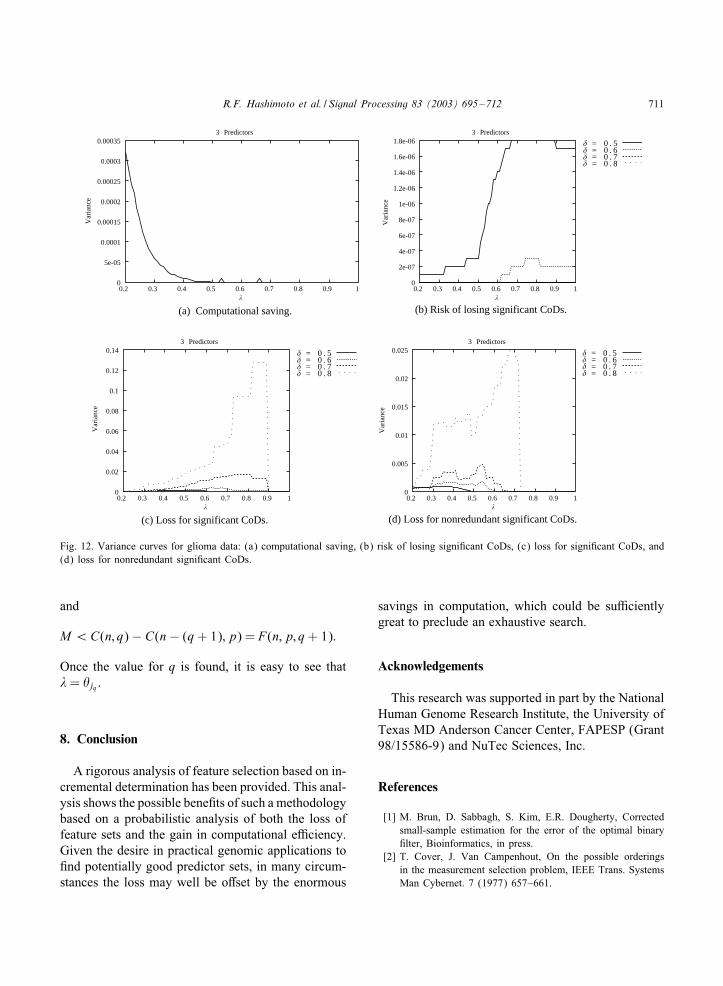
computational savings exceed 99%) corresponding to�ij(�), �ij(�; �), �ij(�; �), and �ij(�; �) for three pre-dictors using the same 50 randomly selected subsets.These are shown in Fig. 12. For the cases of �ij(�; �),�ij(�; �), and �ij(�; �), the variance is very small forthe lower values of �, which is when the probabilitiesare higher. The variance is higher for higher values of�, but in this case the probabilities are much smaller,so that a larger variance does not portend as muchchance of having a large risk or loss when using themean curves. Indeed, one can adjust the mean curves

by adding a standard deviation at each value of � tolessen the possibility of an optimistic assessment.

7. Algorithm

In this section, we present an algorithm for selectingsubsets (with a >xed cardinality p, 1¡p6 n) fromthe set {X1; X2; : : : ; Xn} to compute CoDs under themaximum requirement, max{�j1 ; �j2 ; : : : ; �jp}¡�. Tomotivate the section, let us consider the simple case

R.F. Hashimoto et al. / Signal Processing 83 (2003) 695–712 709

0.1

0.2

0.3

0.4

0.5

0.6

0.7

0.8

0.9

1

0.2 0.3 0.4 0.5 0.6 0.7 0.8 0.9 1

Los

s

Computational Saving

2 Predictors

0

0.1

0.2

0.3

0.4

0.5

0.6

0.7

0.8

0.9

1

0.2 0.3 0.4 0.5 0.6 0.7 0.8 0.9 1

Los

s

Computational Saving

3 Predictors

� = 0 . 5� = 0 . 6� = 0 . 7� = 0 . 8

� = 0 . 5� = 0 . 6� = 0 . 7� = 0 . 8

Fig. 10. Loss for signi>cant CoDs × computational saving for glioma data.

0.7

0.8

0.9

1

0.2 0.3 0.4 0.5 0.6 0.7 0.8 0.9 1

Com

puta

tiona

l Sav

ing

�

3 Predictors

0

0.002

0.004

0.006

0.008

0.01

0.012

0.014

0.016

0.018

0.2 0.3 0.4 0.5 0.6 0.7 0.8 0.9 1 �

3 Predictors

Ris

k

0

0.1

0.2

0.3

0.4

0.5

0.6

0.7

0.8

0.9

1

0.2 0.3 0.4 0.5 0.6 0.7 0.8 0.9 1

Los

s

�

3 Predictors

0

0.1

0.2

0.3

0.4

0.5

0.6

0.7

0.8

0.9

1

0.2 0.3 0.4 0.5 0.6 0.7 0.8 0.9 1

Los

s

�

3 Predictors

� = 0 . 5� = 0 . 6� = 0 . 7� = 0 . 8

� = 0 . 5� = 0 . 6� = 0 . 7� = 0 . 8

� = 0 . 5� = 0 . 6� = 0 . 7� = 0 . 8

(a) Computational saving. (b) Risk of losing significant CoDs.

(c) Loss for significant CoDs. (d) Loss for nonredundant significant CoDs.

Fig. 11. Mean curves for glioma data: (a) computational saving, (b) risk of losing signi>cant CoDs, (c) loss for signi>cant CoDs, and(d) loss for nonredundant signi>cant CoDs.

710 R.F. Hashimoto et al. / Signal Processing 83 (2003) 695–712

where p=2. In this case, a trivial selection procedureis given by the following algorithm:

for each i1 in {1; 2; : : : ; n− 1} dofor each i2 in {i1 + 1; : : : ; n} do

if max{�i1 ; �i2}¿ � thencompute �i1 ;i2 .

Although this algorithm selects exactly the CoDsaccording to the criterion max{�i1 ; �i2}¿ �, there isno di3erence (in terms of time complexity) betweenit and the algorithm that computes all CoDs for twovariables. In fact, the former performsC(n; 2) compar-isons and the latter C(n; 2) computations. We presentan e!cient algorithm for selecting subsets to computeCoDs.If one of the coe!cients in {�i1 ; �i2 ; : : : ; �ip} is

greater than or equal to �, then max{�i1 ; �i2 ; : : : ; �ip}¿�. Thus, we can proceed in the following way.Sort the coe!cients in {�1; �2; : : : ; �n} to obtain{�j1 ; �j2 ; : : : ; �jn} such that �j1 ¿ �j2 ¿ · · ·¿ �jn , andthen apply the following algorithm:

Algorithm Select:Input: {�j1 ; �j2 ; : : : ; �jn},

such that �j1 ¿ �j2 ¿ · · ·¿ �jn ,�∈ [0; 1] and 1¡p6 n.

Output: �ji1 ;ji2 ;:::;jipsuch that

max{�ji1; �ji2

; : : : ; �jip }¿ �.

Let q=min{|{i: �i¿ �}|, n− p+ 1}.for each i1 in {1; 2; : : : ; q} do

for each i2 in {i1 + 1; : : : ; n− p+ 2} dofor each i3 in {i2 + 1; : : : ; n− p+ 3} do

. . .for each ip−1 in {ip−2 + 1; : : : ; n− 1} dofor each ip in {ip−1 + 1; : : : ; n} docompute �ji1 ;ji2 ;:::;jip

.

We state two propositions without proof. The>rst assures correctness. The second gives the timecomplexity.

Proposition 2. Let 1¡p6 n and 16 i1 ¡i2 ¡ · · ·¡ip6 n. The CoD �ji1 ;ji2 ;:::;jip

is computed by Selectif and only if max{�ji1

; �ji2; : : : ; �jip }¿ �.

Proposition 3. Let 1¡p6 n and q = min{|{i: �i

¿ �}|; n−p+1}. The time complexity of the algo-rithm Select is F(n; p; q), where

F(n; p; q) =

C(n; p) if q= n− p+ 1;

C(n; p)

−C(n− q; p) if q¡n− p+ 1

and where n, p and q are integers such that n¿ 0,1¡p6 n and 06 q6 n− p+ 1.

To prove that the algorithm Select is the best one interms of time complexity, we have to show that, given1¡p6 n and �∈ [0; 1], the cardinality of the setsS(p; �) = {{ji1 ; ji2 ; : : : ; jip}: �ji1 ;ji2 ;:::;jip

is computed by Select}and

A(p; �) = {{ji1 ; ji2 ; : : : ; jip}: 16 i1 ¡i2 ¡ · · ·¡ip

6 n and max{�ji1; �ji2

; : : : ; �jip }¿ �}areboth equal toF(n; p; q),whereq=min{|{i: �i¿�}|;n − p + 1}. In fact, by Proposition 2, we have thatS(p; �)=A(p; �) and, by Proposition 3, |S(p; �)|=F(n; p; q).Now, by the results obtained from this section, we

can easily compute the computational saving of thealgorithm Select. In fact, given �, we can compute q=min{|{i: �i¿ �}|; n−p+1}, and the computationalsaving for Select is given by

1− F(n; p; q)C(n; p)

:

Note that this value must agree the computational sav-ing P(max{�i1 ; �i2 ; : : : ; �ip}¡�).To conclude, we comment on how to >nd the value

for � given the sorted set {�j1 ; �j2 ; : : : ; �jn} and a de-sired number M ¡C(n; p) of CoDs we wish to com-pute. This situation arises when M imposes a limiton the number of computations allowed, which wouldconstitute a real-time requirement. Since F(n; p; q) isthe number coe!cients computed by Select, then wemust >nd q¡n− p+ 1 such that

F(n; p; q) = C(n; p)− C(n− q; p)6M

R.F. Hashimoto et al. / Signal Processing 83 (2003) 695–712 711

0

5e-05

0.0001

0.00015

0.0002

0.00025

0.0003

0.00035

0.2 0.3 0.4 0.5 0.6 0.7 0.8 0.9 1�

3 Predictors

Var

ianc

e

Var

ianc

e

Var

ianc

e

Var

ianc

e

0

2e-07

4e-07

6e-07

8e-07

1e-06

1.2e-06

1.4e-06

1.6e-06

1.8e-06

0.2 0.3 0.4 0.5 0.6 0.7 0.8 0.9 1�

3 Predictors

0

0.02

0.04

0.06

0.08

0.1

0.12

0.14

0.2 0.3 0.4 0.5 0.6 0.7 0.8 0.9 1�

3 Predictors

0

0.005

0.01

0.015

0.02

0.025

0.2 0.3 0.4 0.5 0.6 0.7 0.8 0.9 1�

3 Predictors

� = 0 . 5� = 0 . 6� = 0 . 7� = 0 . 8

� = 0 . 5� = 0 . 6� = 0 . 7� = 0 . 8

� = 0 . 5� = 0 . 6� = 0 . 7� = 0 . 8

(a) Computational saving. (b) Risk of losing significant CoDs.

(c) Loss for significant CoDs. (d) Loss for nonredundant significant CoDs.

Fig. 12. Variance curves for glioma data: (a) computational saving, (b) risk of losing signi>cant CoDs, (c) loss for signi>cant CoDs, and(d) loss for nonredundant signi>cant CoDs.

and

M ¡C(n; q)− C(n− (q+ 1); p) = F(n; p; q+ 1):

Once the value for q is found, it is easy to see that�= �jq .

8. Conclusion

A rigorous analysis of feature selection based on in-cremental determination has been provided. This anal-ysis shows the possible bene>ts of such a methodologybased on a probabilistic analysis of both the loss offeature sets and the gain in computational e!ciency.Given the desire in practical genomic applications to>nd potentially good predictor sets, in many circum-stances the loss may well be o3set by the enormous

savings in computation, which could be su!cientlygreat to preclude an exhaustive search.

Acknowledgements

This research was supported in part by the NationalHuman Genome Research Institute, the University ofTexas MD Anderson Cancer Center, FAPESP (Grant98/15586-9) and NuTec Sciences, Inc.

References

[1] M. Brun, D. Sabbagh, S. Kim, E.R. Dougherty, Correctedsmall-sample estimation for the error of the optimal binary>lter, Bioinformatics, in press.

[2] T. Cover, J. Van Campenhout, On the possible orderingsin the measurement selection problem, IEEE Trans. SystemsMan Cybernet. 7 (1977) 657–661.

712 R.F. Hashimoto et al. / Signal Processing 83 (2003) 695–712

[3] P. Devijver, J. Kittler, Pattern Recognition: A StatisticalApproach, Prentice-Hall, Englewood Cli3s, NJ, 1982.

[4] J.L. De Risi, V.R. Ilyer, P.O. Brown, Exploring the metabolicand genetic control of gene expression on a genomic scale,Science 278 (1997) 680–686.

[5] E.R. Dougherty, S. Kim, Y. Chen, Coe!cient ofdetermination in nonlinear signal processing, Signal Process.80 (10) (2000) 2219–2235.

[6] D.J. Duggan, M.L. Bittner, Y. Chen, J.M. Trent, Expressionusing cDNA microarrays, Natur. Genet. 21 (1999) 10–14.

[7] G.N. Fuller, C.H. Rhee, K.R. Hess, L.S. Caskey, R.Wang, J.M. Bruner, W.K. Yung, W. Zhang, Reactivationof insulin-like growth factor binding protein 2 expressionduring glioblastoma transformation revealed by parallel geneexpression pro>ling, Cancer Res. 59 (1999) 4228–4232.

[8] S. Kim, E.R. Dougherty, M.L. Bittner, Y. Chen, K.Sivakumar, P. Meltzer, J.M. Trent, General nonlinearframework for the analysis of gene interaction via multivariateexpression arrays, J. Biomed. Opt. 5 (4) (October 2000)411–424.

[9] S. Kim, E.R. Dougherty, Y. Chen, K. Sivakumar, P. Meltzer,J.M. Trent, M.L. Bittner, Multivariate measurement of geneexpression relationships, Genomics 67 (2000) 201–209.

[10] P. Narenda, K. Fukunaga, A branch and bound algorithmfor feature subset selection, IEEE Trans. Comput. 26 (1977)917–922.

[11] M. Schena, D. Shalon, R.W. Davis, P.O. Brown, Quantitativemonitoring of gene expression patterns with a complementaryDNA microarray, Science 270 (1995) 467–470.

[12] G. Sebestyen, Decision-Making Processes in PatternRecognition, Macmillan, New York, 1962.

[13] I. Shmulevich, E.R. Dougherty, W. Zhang, ProbabilisticBoolean networks: a rule-based uncertainty model for generegulatory networks, J. Bioinform. 18 (2002) 261–274.

[14] E.B. Suh, E.R. Dougherty, S. Kim, D.E. Russ, R.R. Martino,Parallel computing methods for analyzing gene expressionrelationships, in: Proceedings of the SPIE Microarrays:Optical Technologies and Informatics, San Jose, January,2001.

[15] T. Vilmansen, Feature evaluation with measures ofprobabilistic independence, IEEE Trans. Comput. 22 (1973)381–388.

[16] R.E. Walpole, R.H. Meyers, Probability and Statistics forEngineers and Scientists, 3rd Edition, Macmillan, New York,1985.