arX

iv:0

801.

1990

v1 [

cond

-mat

.sup

r-co

n] 1

3 Ja

n 20

08

Effects of inhomogeneities and thermal fluctuations on the

spectral function of a model d-wave superconductor

Daniel Valdez-Balderas∗

Department of Physics and Astronomy,

University of Rochester, Rochester, New York, 14621

David Stroud†

Department of Physics, The Ohio State University, Columbus, Ohio 43210

(Dated: February 22, 2013)

Abstract

We compute the spectral function A(k, ω) of a model two-dimensional high-temperature super-

conductor, at both zero and finite temperatures T . The model consists of a two-dimensional BCS

Hamiltonian with d-wave symmetry, which has a spatially varying, thermally fluctuating, complex

gap ∆. Thermal fluctuations are governed by a Ginzburg-Landau free energy functional. We as-

sume that an areal fraction cβ of the superconductor has a large ∆ (β regions), while the rest has

a smaller ∆ (α regions), both of which are randomly distributed in space. We find that A(k, ω)

is most strongly affected by inhomogeneity near the point k = (π, 0) (and the symmetry-related

points). For cβ ≃ 0.5, A(k, ω) exhibits two double peaks (at positive and negative energy) near

this k-point if the difference between ∆α and ∆β is sufficiently large in comparison to the hopping

integral; otherwise, it has only two broadened single peaks. The strength of the inhomogeneity

required to produce a split spectral function peak suggests that inhomogeneity is unlikely to be

the cause of a second branch in the dispersion relation, such as has been reported in underdoped

LSCO. Thermal fluctuations also affect A(k, ω) most strongly near k = (π, 0). Typically, peaks

that are sharp at T = 0 become reduced in height, broadened, and shifted toward lower energies

with increasing T ; the spectral weight near k = (π, 0) becomes substantial at zero energy for T

greater than the phase-ordering temperature.

∗Electronic address: valdez@pas.rochester.edu†Electronic address: stroud@mps.ohio-state.edu

1

I. INTRODUCTION

In the last several years, the measured electronic properties of cuprate superconductors

have shown considerable evidence of inhomogeneities. For example, spatial variations of the

superconducting energy gap and of the local density of states spectrum have been observed

in scanning tunneling microscopy (STM) experiments [1, 2, 3, 4, 5, 6, 7, 8]. There have also

been a number of reports of magnetic and charge ordering in these materials, which also

indicate inhomogeneities [9, 10, 11, 12, 13, 14, 15, 16, 17]. Other studies of cuprates have

shown that electronic states within certain energy ranges show checkerboard-like spatial

modulations [18].

A number of theoretical approaches have been developed to model these inhomogeneities

[19, 20, 21, 22, 23, 24, 25, 26, 27, 28, 29, 30, 31, 32, 33]. These works are reviewed and

extended in a recent article [34]. In the present article, we use the approach of Ref. 34 to

explore how the spectral function of a d-wave superconductor is affected by gap inhomo-

geneities and thermal fluctuations.

The spectral function of cuprate superconductors has been studied theoretically by a

number of groups, though most have omitted the effects of quenched inhomogeneities. For

example, Wakabayashi et al.[35] used a weak-coupling BCS theory combined with a Green’s

function approach to explain the narrow quasiparticle peak at the gap edge, which has been

observed by ARPES experiments in overdoped cuprates along the antinodal direction. Pieri

et al.[36], using a Nambu formalism, have studied a model which includes pairing fluctuation

effects, and which accounts for some features of the single-particle spectral function as

observed in certain cuprates. Zacher et al.[37] have used a cluster perturbation technique

to compute the single-particle spectral function of the t-J and Hubbard models, and to

study stripe phases in the cuprates. Paramekanti et al.[38] have studied a Hubbard model

for (uniform) projected d-wave states. They used a variational Monte Carlo technique in

which one of the variational parameters is the magnitude ∆ of the pairing field, and find

that ∆, as a function of doping, scales with the (π, 0) hump and T ∗ as observed in ARPES

experiments.

In another recent work, using a generalization of BCS theory, Chen et al. [39] found a

sharpening of the peaks in the spectral function as T is reduced below Tc, similar to what

we find as discussed below. (Their model involves a homogeneous superconductor.) Hotta

2

et al.[40] have used a self-consistent t-matrix approximation to study a model for s and d

wave superconductivity at finite T . They found a gap in both the single-particle density of

states and the spectral function even above the superconducting transition temperature Tc;

the energy scale for the pseudogap is found to be the Cooper-pair binding energy.

More recently, Mayr et al.[41] have introduced an extended Hubbard model, which in-

cludes both superconductivity and antiferromagnetism; they found that quenched disorder

is a necessary ingredient for that model to reproduce the double branch, or split band, ob-

served in angle-resolved photoemission (ARPES) experiments on La2−xSrxCuO4. Finally, a

model to study how A(k, ω) is affected by thermal fluctuations of the phase, but not the

amplitude, of the superconducting order parameter has been treated by Eckl et al. [42] for

homogenous systems.

In the present work, we propose a simple model for A(k, ω). This model can exhibit a split

peak near k = (π, 0), but only for certain parameter choices which are unlikely to be realized

experimentally. Our model consists of a BCS superconductor with d-wave symmetry, where

the pairing field (given by the superconducting order parameter) is inhomogeneous, and

is also subject to thermal amplitude and phase fluctuations at finite T . We assume that

those thermal fluctuations are governed by a discretized Ginzburg-Landau (GL) free energy

functional. To compute the spectral function, we use exact numerical diagonalization of the

BCS Hamiltonian on a finite lattice and average over many different configurations of the

thermally fluctuating superconducting order parameter as obtained using the Monte Carlo

technique. Thermal averages are obtained by averaging over these configurations.

Inhomogeneities are introduced in our model phenomenologically. The atomic lattice is

subdivided into cells, which we call XY cells, of size 2×2 atomic sites; within each such cell,

we assume ∆ to be constant. Then we choose the coefficients of the GL free energy functional

so as to give, at T = 0, a binary distribution of the superconducting order parameter |∆| at

each atomic lattice site. XY cells with small and large |∆| values are called α and β cells,

respectively. We take the distribution of α and β cells on the atomic lattice to be random,

as suggested by STM experiments. The two parameters which we vary in our calculations

are (i) the area fraction cβ of β cells, and (ii) the magnitude |∆β | of the gap in those cells.

The value of |∆α| is kept the same through our calculation, and is inferred from the STM

experiments.

At T = 0, we find that the main consequence of this binary, random distribution of ∆

3

is to broaden the peaks in the spectral function A(k, ω) near the points k = (π, 0) [and the

symmetry-related points at k = (−π, 0) and (0,±π)]. This broadening is most pronounced

at cβ = 0.5. For a sufficiently large ratio ∆β/∆α of the large to the small gap, we find that

A(k, ω) near k = (π, 0) shows two peaks rather than one (“split band regime”). Otherwise,

we find a single peak which is broadened by disorder. Although the experimental ARPES

results of Yoshida et al. [43] also show a double peak, there are several reasons to believe

that this split peak is not caused by the kind of inhomogeneities we consider here. This

point is discussed further below.

At finite T , we find that, near k = (π, 0), the originally sharp coherence peaks of A(k, ω)

as a function of ω broaden and shift to lower energies with increasing T . This broadening is

similar to that found in the calculations of Eckl et al. [42], which omits quenched disorder

and also include thermal fluctuations only in the phase but not the amplitude of the gap.

These calculations focused on T near that of the phase ordering transition. By contrast, we

present calculations showing how A(k, ω) evolves near k = (π, 0) as a function of ω over a

broad range of temperature, including both amplitude fluctuations and quenched disorder.

The remainder of this paper is organized as follows. In Section II, we briefly describe our

model, which is already presented in Ref. 34. In Section III, we give our numerical results,

followed by a discussion and conclusions in Section IV.

II. MODEL

A. Microscopic Hamiltonian

We consider the following Hamiltonian:

H = 2∑

〈i,j〉,σ

tijc†iσcjσ + 2

∑

〈i,j〉

(∆ijci↓cj↑ + c.c.) − µ∑

i,σ

c†iσciσ (1)

Here,∑

〈i,j〉 denotes a sum over distinct pairs of nearest neighbors on a square lattice with

N sites, c†jσ creates an electron with spin σ (↑ or ↓) at site j, µ is the chemical potential, ∆ij

denotes the strength of the pairing interaction between sites i and j, and tij is the hopping

energy, which we write as

tij = −thop. (2)

where thop > 0.

4

Following a similar approach to that of Ref. [34] and Ref. [44] we take ∆ij to be given by

∆ij =1

4

|∆i| + |∆j |2

eiθij , (3)

where

θij =

(θi + θj)/2, if bond 〈i, j〉 is in x-direction,

(θi + θj)/2 + π, if bond 〈i, j〉 is in y-direction,(4)

and

∆j = |∆j|eiθj , (5)

is the value of the complex superconducting order parameter at site j. The sums in (1) are

carried out over a lattice we will refer to as the atomic lattice (as distinguished from the

XY lattice, described below). The first term in eq. (1) corresponds to the kinetic energy,

the second term is a BCS type of pairing interaction with d-wave symmetry, and the third

term is the energy associated with the chemical potential.

B. Numerical Calculation of Spectral Function

We wish to compute the spectral function A(k, ω) for the system described by the Hamil-

tonian (1). Given the ∆i’s, tij, and µ, A(k, ω) is computed through

A(ω,k, {∆i}) =∑

n,En≥0

[|un(k)|2δ(ω −En) + |vn(k)|2δ(ω + En)], (6)

where

un(k) =1

N1/2

N∑

i=1

exp(ik · ri)un(ri), (7)

vn(k) =1

N1/2

N∑

i=1

exp(ik · ri)vn(ri), (8)

En is the nth eigenenergy of Hamiltonian (1), and

ψn(ri) =

un(ri)

vn(ri)

, i = 1, N. (9)

is its nth eigenvector, as described in detail in [34]. Here,

ri = a0(nix+miy), (10)

5

and ni and mi are integers in the range [0, Nx − 1] and [0, Ny − 1]. In our numerical

calculations, we take the size of the atomic lattice to be N = NxNy, where x and y are unit

vectors in the x and y directions, and a0 is the lattice constant. We use periodic boundary

conditions, ψn(r) = ψn(r +Nxa0x) and ψn(r) = ψn(r +Nya0y), which leads to k-vectors of

the form

k =2π

a0

(

mx

Nxx+

my

Nyy

)

(11)

The detailed procedure to obtain ∆i is described in Ref. 34. Basically, we subdivide

the atomic lattice into cells, which we call XY cells, of size ξ0 × ξ0. Here ξ0 is the T = 0

Ginzburg-Landau (GL) coherence length, which we take to be an integer multiple of a0. The

value of ∆i is assumed to be the same for each atomic site within a given XY cell, and is

governed by the following discretized GL free energy functional:

F

K1

=M

∑

i=1

(

T

Tc0i− 1

)

1

λ2

i (0)

∣

∣

∣

∣

∆i

kBTc0i

∣

∣

∣

∣

2

+M

∑

i=1

1

18.76

1

λ2

i (0)

∣

∣

∣

∣

∆i

kBTc0i

∣

∣

∣

∣

4

+∑

〈ij〉

∣

∣

∣

∣

∆i

λi(0)kBTc0i− ∆j

λj(0)kBTc0j

∣

∣

∣

∣

2

.

(12)

Here K1 = h4d/[32(9.38)πm∗,2µ2

B], where m∗ = 2me is twice the electron mass, µB is the

Bohr magneton, and d is the thickness of the superconducting layer. If d = 10A, K1 = 2866

eV A2. ∆i is the complex gap parameter in the ith XY cell. In eq. (12), the sums run over

the lattice of XY cells, each of which contains (ξ/a0)2 atomic sites.

We choose the coefficients of this GL free energy functional Tc0i and λi(0) to have binary

distribution on the XY lattice, corresponding to either a small or a large value of |∆i|. We

call an XY cell with a small (large) value of |∆i| an α (β) cell, while the area fraction of β

cells is called cβ . The corresponding values of Tc0i and λi(0) are denoted Tc0α and Tc0β . At

T = 0, in a homogeneous system made up entirely of α (β) cells, the magnitude of |∆i| will

be the same in each XY cell and given by the minimum of the corresponding free energy

functional F , i. e. |∆i| =√

9.38kBTc0α (√

9.38kBTc0β). In the binary case (0 < cβ < 1), at

T = 0, we will still generally have |∆i| =√

9.38kBTc0i, although this value may be modified

slightly by the proximity effect term in F/K1 [the last term in eq. (12)].

We compute A(k, ω) at T = 0 by diagonalizing the model hamiltonian (1) using ∆i

determined by minimizing the Ginzburg-Landau free energy F . This minimum value will

always correspond to gaps ∆i = |∆i|eiθi such that all the phases θi are equal. At finite T , we

compute A(k, ω) as an average over different configurations {∆i}. These are obtained, as

in Ref. [34], by assuming that the thermal fluctations of the ∆i are governed by the GL free

6

energy functional F described above. Thus, F is treated as an effective classical Hamiltonian

and thermal averages such as 〈A(k, ω)〉 are computed as

〈A(k, ω)〉 =

∫

ΠNi=1d2∆ie

−F/kBTA(k, ω, {∆i})∫

ΠNi=1d2∆ie−F/kBT

. (13)

We will be using the GL free energy functional at both T = 0 and finite T in spite of the

fact that it was originally intended for T near the mean-field transition temperature. Strictly

speaking, the correct free energy functional near T = 0 should not have the GL form but

would be expected to contain additional terms, such as higher powers of |ψ|2. We use the

GL form for convenience, and because we expect that it will exhibit the qualitative behavior

that would be seen in a more accurate functional - that is, the effects of inhomogeneities

would be qualititatively the same in the GL model as in a more accurate model containing

additional powers of |ψ|2.To obtain A(k, ω) for a given distribution of the ∆i’s, we diagonalize the Hamiltonian (1)

for that configuration, then obtain A(k, ω) using eq. (6). The canonical averages are then

evaluated using a Metropolis Monte Carlo technique to determine the canonical distribution

of the ∆i’s at the temperature of interest. The detailed description of this Monte Carlo

approach are given in Section IV.A of Ref. [34]. As noted there, we first choose the values

of Tc0i and λi(0) in each XY cell, taking these to be quenched variables. In contrast to our

calculations of Ref. [34], we do not include a smoothing magnetic field to reduce finite-size

effects; as a result, our results have more numerical noise than do our earlier results for the

density of states.

For the present model calculation, we arbitrarily set the chemical potential µ = 0, for sim-

plicity, and use thop as the unit of energy. This corresponds to half filling in the band model.

Exactly half filling would correspond to x = 0 in LaxSr1−xCuO4 (LSCO), for example[45].

It should be noted that some of the most interesting experimental results for the spectral

function[43] are carried out in the underdoped superconducting regime of the phase diagram,

where µ is slightly negative. If we set µ 6= 0 in our model, this leads to unequal integrated

weights of the spectral function peaks at positive and negative energy, but we have found

that otherwise our numerical results are not very different from those at µ = 0, for our

model Hamiltonian. However, the present results and model, for reasons which we discuss

below, are probably not directly relevant to those experiments.

In order to show that our results are not strongly affected by setting µ = 0, we have also

7

done simulations using µ 6= 0. For example, in Figure 8 we present results using µ = −0.05.

For this value of µ, the average number of electrons per site, defined as,

〈n〉 =1

N

N∑

i=0

〈ni〉 (14)

with

ni =∑

σ

c†i,σci,σ (15)

is found to be 〈n〉 ∼ 0.94. This corresponds to a strongly underdoped cuprate x ∼ 0.06.

C. Homogeneous systems

For a homogeneous system at T = 0, ∆i = ∆ and we can rewrite Hamiltonian (1) as

H =∑

k,σ

ǫkc†kσckσ +

∑

k

(∆kck↓c−k↑ + c.c.) − µ∑

k

c†kσckσ, (16)

where ǫk = −2t[cos(kxa0) + cos(kya0)] and ∆k = 1

2∆[cos(kxa0) − cos(kya0)]. In obtaining

(16) we have used c†j = 1

N1/2

∑

kexp(−ik · rj) c

†k

and its hermitian conjugate. In this case,

the excitation energies of the system are given by [47]

Ek =√

(ǫk − µ)2 + ∆2

k(17)

The corresponding spectral function will be a sum of two delta functions, as indicated by

eq. (6).

III. NUMERICAL RESULTS: INHOMOGENEITIES AND THERMAL FLUCTU-

ATIONS

In this section we present our numerical results for A(k, ω) for inhomogeneous systems

both at zero and finite temperatures; for reference, we also show the corresponding results

for homogeneous systems in some cases. For T = 0, we use 48 × 48 atomic lattices used,

while at finite T we used lattices of 32×32. In al cases, we use 2×2 XY cells. Through the

rest of this article, we show energy measured in units of thop, distance in units of a0, and k

in units of 1/a0.

8

A. Zero temperature

Before describing our results at zero temperature, we first comment on our choice of

gap parameters used in the calculations. Our primary goal is to ascertain what kinds of

qualitative spectral functions could result from the type of inhomogeneity described by our

models, not to compare directly to experiment. For this reason, we will examine gaps which

are, in general, substantially larger (in units of thop) than those which would describe realistic

cuprate superconductors. This point is examined further in the discussion section.

With this preamble, we now present our results at T = 0. Fig. 1 shows the spectral

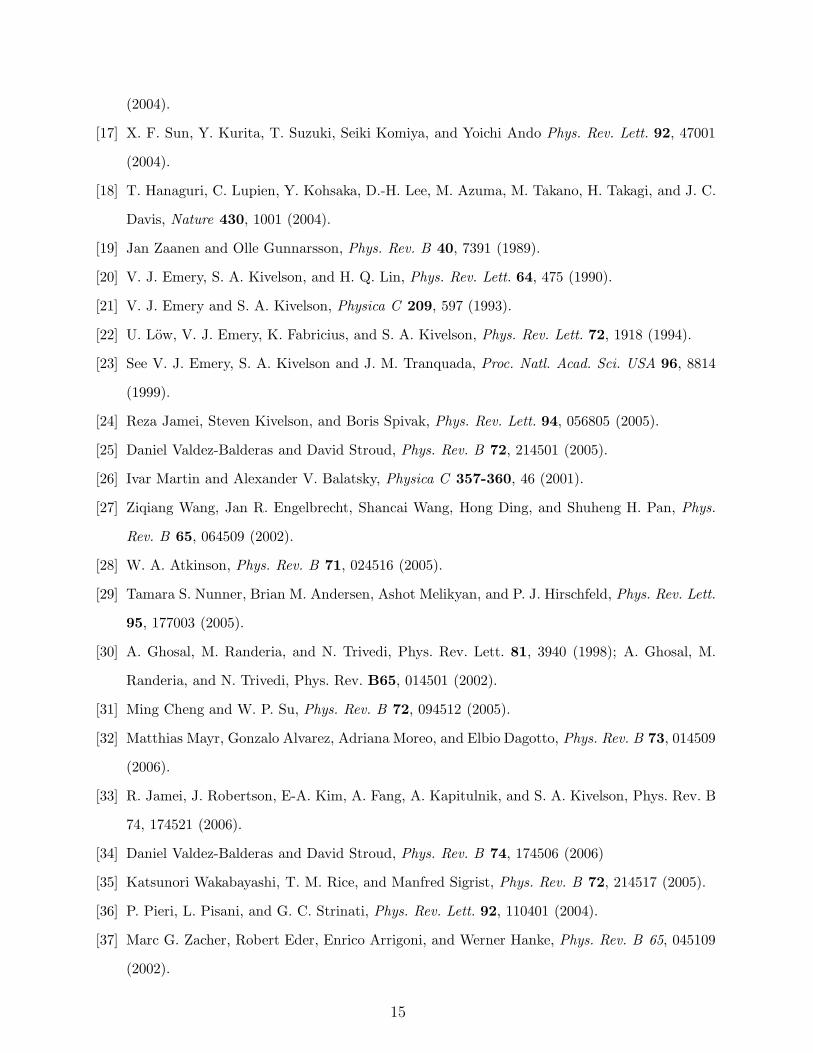
function A(k, ω) (represented as a contour plot) as well as plots of the dispersion relation

Ek as a function of k, for two homogeneous systems: one with ∆ = 0, and another with

∆ = 0.42. For such homogeneous systems, A(k, ω) is simply proportional to the sum of two

delta functions: A(k, ω) ∝ δ(ω−Ek)+δ(ω+Ek). In parts (a) and (b), the dark (light) regions

correspond to regions where Ek, as calculated from Eq. (17), is large (small); these are shown

for all k vectors in the first Brillouin zone (BZ). For a system with ∆ = 0 [Fig. 1(a)] there

are four lines (white) in k-space for which Ek = 0: ky = ±kx ± π. When ∆ > 0 [Fig. 1(b)],

the lines are reduced to four points: (kx = π/2, ky = ±π/2) and (kx = −π/2, ky = ±π/2),

located at the center of the white blobs in Fig. 1(b). In Fig. 1(c) and (d), density plots of

A(k, ω) as a function of ω are presented for those homogeneous systems at selected k values.

These values lie along three standard lines in the first BZ: from k = (0, 0) to k = (π, 0),

from k = (π, 0) to k = (π, π), and from k = (π, π) to k = (0, 0). Dark (light) regions

correspond to large (small) values of the spectral function. For each k in these homogeneous

systems, there is a sharp peak in A(k, ω), whose energy and width are indicated as the very

short dashed lines in the plot. Also, the spectral function is clearly most strongly affected

by a finite value of ∆ near k = (π, 0), where an energy gap of magnitude ∆ opens around

ω − µ = 0.

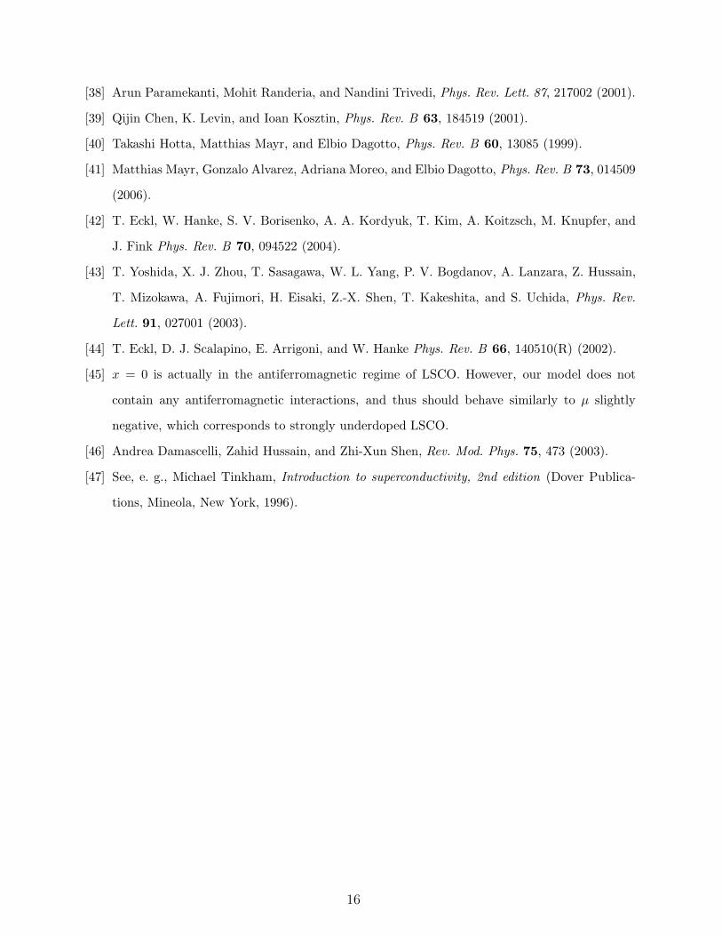
Figures 2 and 3 show the spectral function of several inhomogeneous systems with differ-

ent concentrations cβ of β cells, at T = 0. In these systems, the atomic cells within the β

cells have ∆ = 1.26, and are randomly distributed in the atomic lattice, while α cells, which

occupy the rest of the lattice, have ∆0.42. Fig. 4 shows a representative arrangements of α

and β cells for an 16 × 16 XY lattice with cβ = 0.1. We can observe in Fig. 2 that the dis-

order introduced by this binary distribution of the superconducting order parameter affects

9

mostly the region k = (π, 0). This disorder effect is almost unobservable for cβ = 0.9: the

results are almost the same as those for cβ = 1.0, a homogeneous system with only β cells.

On the other hand, a small but noticeable disorder effect is observed cβ = 0.1, in the form

of a slight broadening of the spectral function at k ≃ (0.8π, 0). However, it is the system

with cβ = 0.5 the one that shows a most dramatic blurring of the energy in the region of

k = (π, 0), as we now discuss.

Since the effects of the binary distribution of ∆ are more pronounced near k = (π, 0), we

have also plotted A(k, ω) versus ω for fixed k = (π, 0), at different values of cβ in Fig. 3. For

the pure α system, cβ = 0.0, two sharp peaks appear at |ω| = ∆α = 0.42. When a fraction

0.1 of the α XY cells are replaced by β cells, cβ = 0.1, the height of the peaks decreases from

about 45 (arbitrary units) to about 15, with a corresponding broadening of the peak and a

shifting of the weight toward a higher energy. At cβ = 0.5, the peak height is only about 1.5,

and the width is very large; the peak fills the entire frequency range from ω = ∆α = 0.42

to ∆β = 1.26. At cβ = 0.9, most of the weight of A(k, ω) shifts to ω = ∆β = 1.26, with

a slight broadening near the bottom of the peaks, which is, however, less pronounced than

the corresponding broadening of the cβ = 0.1 peaks. At cβ = 1.0 the peaks become sharp

at ω = ±∆β = ±1.26.

We now discuss the calculated effects of a binary gap distribution on systems similar

to those of Fig. 2, but with ∆β = 2.52 instead of ∆β = 1.26. These systems, like the one

previously discussed, have ∆α = 0.42. For concentrations cβ = 0.1 and cβ = 0.9, the effect of

inhomogeneities qualitatively resembles that seen for ∆β = 1.26: they produce broadening

of the spectral function near k = (π, 0). The main difference is that the broadening is

slightly greater for ∆β = 2.52. However, the case cβ = 0.5 shows a real qualitative change:

the spectral function now splits into two well-defined peaks for k vectors near (π, 0). We

can better visualize this effect by looking at Fig. 6, where we plot A(k, ω) versus ω for fixed

k = (π, 0) and several values of cβ. Clearly, A(k, ω) for cβ = 0.1 and cβ = 0.9 behaves

similarly to the case ∆β = 1.26: slightly broadened peaks at an energy near the ∆ of the

majority of the XY cells, i. e., at ω = 0.42 for cβ = 0.1 and at ω = 2.52 for cβ = 0.9. But for

cβ = 0.5, A(k, ω) shows several peaks, two of which are particularly clear: one at ω ≃ 0.42

and the other at ω ≃ 2.52. This is the “split band” regime one expects for large contrast

between ∆α and ∆β.

In order to better visualize how the spectral function depends on disorder, we have

10

calculated A(k, ω) as function of |∆α| for a fixed ratio |∆β/∆α| = 6, at cβ = 0.5. The

results are shown in Figs. 7 and 8. This series of plots clearly shows the evolution of A(k, ω)

from a split-band regime at |∆β| = 2.52 (in units of thop) to a broadened single band for

|∆β| = 0.22|thop) or smaller. In general, we find that the split band regime occurs only if

the difference |∆β |− |∆α| is of order thop or larger; otherwise, A(k, ω) at k = (π, 0) is simply

the sum of two broadened peaks at positive and negative energies.

B. Finite temperatures

Fig. 9 shows the T -dependence of A(k, ω) for a system with cβ = 0.1. The α and β cells

are now characterized by values of tc0 such that at low T , ∆ = 0.42 in the α cells, and

1.26 in the β cells. The value of ∆ itself at finite T will, of course, thermally fluctuate, as

governed by the GL free energy functional discussed at the end of Section II. The spectral

function presented here is therefore an average of A(ω,k, {∆i}) over different configurations

{∆i} obtained by a Monte Carlo sampling procedure, as described above and in Ref. [34].

Hereafter, we denote this ensemble average simply as A(k, ω).

Fig. 9 shows that, as in the case of quenched disorder, A(k, ω) is most strongly affected

by thermal fluctuations near k = (π, 0), where it broadens more and more with increasing T .

In addition to this broadening, the peaks can be seen to shift towards smaller energies. This

behavior can be seen more clearly in Fig. 10, which shows A(k, ω) at k = (π, 0) as a function

of ω−µ. We observe that at T = 0, A(k, ω) shows relatively sharp peaks at ω−µ = ±0.42,

with some disorder-induced broadening only in the wings of the peak. At t = 0.01, the peak

height of A(k, ω) decreases from ∼ 17 to about ∼ 7, with a correspondingly increased width.

As the temperature is increased, the system eventually undergoes a phase-disordering

transition, above which the superconductor loses phase coherence. For the parameters used

in Fig. 10, this transition occurs at tc ≃ 0.035. tc is the phase ordering transition temperature

in units of thop/kB. We use a dimensionless temperature t = kBT/thop in these plots. At

t = 0.03, near but slightly below the phase ordering temperature tc ≃ 0.035, the height of

the peak is further decreased, its width further increased, and its energy shifted to a still

lower energy. At t = 0.05 > tc, the peak shifts still further toward lower energy, but the

maximum remains at finite energy.

11

IV. DISCUSSION

We have presented a simple model to study how the spectral function of a model d-wave

superconductor is affected by quenched inhomogeneities and by thermal fluctuations of the

superconducting order parameter. The model consists of a BCS Hamiltonian for an order

parameter with dx2−y2-wave symmetry, which has a position-dependent pairing field, and

which also undergoes finite-temperature thermal fluctuations. The spatial dependence we

assume for the pairing field is motivated by recent STM experiments on Bi2212: we assume

two types of regions: and α region with a small gap, and a β region with a large gap.

To treat thermal fluctuations (of both amplitude and phase of the superconducting order

parameter), we assume that they are governed by a suitable Ginzburg-Landau free energy

functions, which we treat by classical Monte Carlo simulations.

At T = 0, we find that A(k, ω) is most strongly affected by disorder near k = (π, 0). In

general, this effect consists of a broadening of the peaks of A(k, ω) (plotted as a function

of ω for fixed k). However, at area fraction cβ = 0.5, we find that quenched disorder can

have two qualitatively different effects, depending on the relative magnitudes of ∆α and ∆β.

If the difference between ∆α and ∆β is small, A(k, ω) has a single, broad peak for k near

(π, 0), extending from ∼ ∆α to ∼ ∆β . But for a large enough difference between ∆α and

∆β, the A(k, ω) show a characteristic “split-band” behavior: instead of a wide, single peak,

there are two prominent peaks, at ω = ∆α and ω = ∆β.

Thermal fluctuations of the pairing field also have their strongest effect on A(k, ω) near

k = (π, 0). The effect consists of a gradual broadening of the T = 0 peaks with increasing

temperature, and also a shifting of those peaks towards lower energies. However, no dramatic

change is noticeable near the phase-ordering transition.

Finally, we comment on the possible connection, if any, between our results and exper-

iment. In recent angle-resolved photoemission studies by Yoshida et al[43], for LSCO, it

was observed that for doping level x = 0.03, a second branch developed in the dispersion

relation near k = (π, 0). An explanation for the presence of these two branches has recently

been suggested by Mayr et al. [41]. These authors showed that the extra branch could be

explained by a model with quenched disorder, in which the material breaks up into spatially

separated superconducting and antiferromagnetic patches.

In the present work, we find that a similar effect, with two spectral peaks, can be produced

12

if there are spatially distinct superconducting regions with sufficiently different supercon-

ducting gaps. However, we also find that a split spectral peak can be produced only if the

magnitudes of the gaps |∆α| and |∆β|, and of their difference, is much larger than seems

physically reasonable. Specifically, unless one of the gaps in the bimodal distribution is

around 2.5thop, we do not obtain a split peak in A(k, ω) at the point k = (π, 0). For typical

values (thop ∼ 200 meV), this would represent a |∆| of around 0.5eV. Since the average

value of |∆| in most of the cuprate superconductors is ∼ 0.05eV, it seems most unlikely that

random spatial fluctuations in |∆|, due to quenched disorder, could produce such a large

gap locally. Furthermore, even with such large quenched fluctuations in the gap, we need a

bimodal gap distribution to obtain a split spectral function - equally large quenched fluctua-

tions, but with a continuous distribution due to quenched disorder, would probably not give

rise to a split spectral function. Therefore, it seems very improbable that our model could

account for the second branch in the dispersion relation reported in Ref. [43]. However, our

results should give a reasonable picture of how quenched gap inhomogeneities affect A(k, ω)

in a d-wave superconductor over a range of parameters.

V. ACKNOWLEDGMENTS

We are grateful for support through the National Science Foundation grant DMR04-

13395. We also thank Rajdeep Sensarma for useful conversations. The computations de-

scribed here were carried out using the facilities of the Ohio Supercomputing Center, with

the help of a grant of time.

13

[1] T. Cren, D. Roditchev, W. Sacks, J. Klein, J.-B. Moussy, C. Deville-Cavellin, and M. Lagues,

Phys. Rev. Lett 84, 147 (2000).

[2] C. Howald, P. Fournier, and A. Kapitulnik, Phys. Rev. B 64, 100504(R) (2001).

[3] S. H. Pan, J. P. O’Neal, R. L. Badzey, C. Chamon, H. Ding, J. R. Engelbrecht, Z. Wang,

H. Eisaki, S. Uchida, A. K. Gupta, K.-W. Ng, E. W. Hudson, K. M. Lang, and J. C. Davis,

Nature 413, 282 (2001).

[4] K. M. Lang, V. Madhavan, J. E. Hoffman, E. W. Hudson, H. Eisaki, S. Uchida, and J. C.

Davis, Nature 415, 412 (2002).

[5] C. Howald, H. Eisaki, N. Kaneko, M. Greven, and A. Kapitulnik, Phys. Rev. B 67, 014533

(2003).

[6] T. Kato, S. Okitsu, and H. Sakata, Phys. Rev. B 72, 144518 (2005).

[7] A. C. Fang, L. Capriotti, D. J. Scalapino, S. A. Kivelson, N. Kaneko, M. Greven, and A.

Kapitulnik, Phys. Rev. Lett. 96, 017007 (2006).

[8] H. Mashima, N. Fukuo, Y. Matsumoto, G. Kinoda, T. Kondo, H. Ikuta, T. Hitosugi and T.

Hasegawa, Phys. Rev. B 73, 060502(R) (2006).

[9] S.-W. Cheong, G. Aeppli, T. E. Mason, H. Mook, S. M. Hayden, P. C. Canfield, Z. Fisk, K.

N. Clausen, and J. L. Martinez, Phys. Rev. Lett. 67, 1791 (1991).

[10] K. Yamada, C. H. Lee, K. Kurahashi, J. Wada, S. Wakimoto, S. Ueki, H. Kimura, Y. Endoh.,

S. Hosoya, G. Shirane, R. J. Birgeneau, M. Greven, M. A. Kastner, and Y. J. Kim Phys. Rev.

B. 57, 6165 (1998).

[11] J. M. Tranquada, B. J. Sternlieb, J. D. Axe, Y. Nakamura, S. Uchida, Nature 375, 561 (1995).

[12] T. Niemoller, N. Ichikawa, T. Frello, H. Hunnefeld, N.H. Andersen, S. Uchida, J. R. Schneider,

and J. M. Tranquada, Eur. Phys. J. B 12, 509 (1999).

[13] H. A. Mook, Pengcheng Dai, S. M. Hayden, G. Aeppli, T. G. Perring, and F. Dogan, Nature

395, 580 (1998).

[14] M. Arai, T. Nishijima, Y. Endoh, T. Egami, S. Tajima, K. Tomimoto, Y. Shiohara, M.

Takahashi, A. Garrett, and S. M. Bennington, Phys. Rev. Lett. 83, 608 (1999).

[15] Pengcheng Dai, H. A. Mook, R. D. Hunt, F. Dogan, Phys. Rev. B 63, 54525 (2001).

[16] S. M. Hayden, H. A. Mook, Pengcheng Dai, T. G. Perring, and F. Dogan, Nature 429, 531

14

(2004).

[17] X. F. Sun, Y. Kurita, T. Suzuki, Seiki Komiya, and Yoichi Ando Phys. Rev. Lett. 92, 47001

(2004).

[18] T. Hanaguri, C. Lupien, Y. Kohsaka, D.-H. Lee, M. Azuma, M. Takano, H. Takagi, and J. C.

Davis, Nature 430, 1001 (2004).

[19] Jan Zaanen and Olle Gunnarsson, Phys. Rev. B 40, 7391 (1989).

[20] V. J. Emery, S. A. Kivelson, and H. Q. Lin, Phys. Rev. Lett. 64, 475 (1990).

[21] V. J. Emery and S. A. Kivelson, Physica C 209, 597 (1993).

[22] U. Low, V. J. Emery, K. Fabricius, and S. A. Kivelson, Phys. Rev. Lett. 72, 1918 (1994).

[23] See V. J. Emery, S. A. Kivelson and J. M. Tranquada, Proc. Natl. Acad. Sci. USA 96, 8814

(1999).

[24] Reza Jamei, Steven Kivelson, and Boris Spivak, Phys. Rev. Lett. 94, 056805 (2005).

[25] Daniel Valdez-Balderas and David Stroud, Phys. Rev. B 72, 214501 (2005).

[26] Ivar Martin and Alexander V. Balatsky, Physica C 357-360, 46 (2001).

[27] Ziqiang Wang, Jan R. Engelbrecht, Shancai Wang, Hong Ding, and Shuheng H. Pan, Phys.

Rev. B 65, 064509 (2002).

[28] W. A. Atkinson, Phys. Rev. B 71, 024516 (2005).

[29] Tamara S. Nunner, Brian M. Andersen, Ashot Melikyan, and P. J. Hirschfeld, Phys. Rev. Lett.

95, 177003 (2005).

[30] A. Ghosal, M. Randeria, and N. Trivedi, Phys. Rev. Lett. 81, 3940 (1998); A. Ghosal, M.

Randeria, and N. Trivedi, Phys. Rev. B65, 014501 (2002).

[31] Ming Cheng and W. P. Su, Phys. Rev. B 72, 094512 (2005).

[32] Matthias Mayr, Gonzalo Alvarez, Adriana Moreo, and Elbio Dagotto, Phys. Rev. B 73, 014509

(2006).

[33] R. Jamei, J. Robertson, E-A. Kim, A. Fang, A. Kapitulnik, and S. A. Kivelson, Phys. Rev. B

74, 174521 (2006).

[34] Daniel Valdez-Balderas and David Stroud, Phys. Rev. B 74, 174506 (2006)

[35] Katsunori Wakabayashi, T. M. Rice, and Manfred Sigrist, Phys. Rev. B 72, 214517 (2005).

[36] P. Pieri, L. Pisani, and G. C. Strinati, Phys. Rev. Lett. 92, 110401 (2004).

[37] Marc G. Zacher, Robert Eder, Enrico Arrigoni, and Werner Hanke, Phys. Rev. B 65, 045109

(2002).

15

[38] Arun Paramekanti, Mohit Randeria, and Nandini Trivedi, Phys. Rev. Lett. 87, 217002 (2001).

[39] Qijin Chen, K. Levin, and Ioan Kosztin, Phys. Rev. B 63, 184519 (2001).

[40] Takashi Hotta, Matthias Mayr, and Elbio Dagotto, Phys. Rev. B 60, 13085 (1999).

[41] Matthias Mayr, Gonzalo Alvarez, Adriana Moreo, and Elbio Dagotto, Phys. Rev. B 73, 014509

(2006).

[42] T. Eckl, W. Hanke, S. V. Borisenko, A. A. Kordyuk, T. Kim, A. Koitzsch, M. Knupfer, and

J. Fink Phys. Rev. B 70, 094522 (2004).

[43] T. Yoshida, X. J. Zhou, T. Sasagawa, W. L. Yang, P. V. Bogdanov, A. Lanzara, Z. Hussain,

T. Mizokawa, A. Fujimori, H. Eisaki, Z.-X. Shen, T. Kakeshita, and S. Uchida, Phys. Rev.

Lett. 91, 027001 (2003).

[44] T. Eckl, D. J. Scalapino, E. Arrigoni, and W. Hanke Phys. Rev. B 66, 140510(R) (2002).

[45] x = 0 is actually in the antiferromagnetic regime of LSCO. However, our model does not

contain any antiferromagnetic interactions, and thus should behave similarly to µ slightly

negative, which corresponds to strongly underdoped LSCO.

[46] Andrea Damascelli, Zahid Hussain, and Zhi-Xun Shen, Rev. Mod. Phys. 75, 473 (2003).

[47] See, e. g., Michael Tinkham, Introduction to superconductivity, 2nd edition (Dover Publica-

tions, Mineola, New York, 1996).

16

FIG. 1: Contour plots of the energy Ek of single-particle excitations, and the corresponding spectral

function spectral function A(k, ω), for two homogeneous systems at zero temperature: one with

∆ = 0, and another with ∆ = 0.42. In parts (a) and (b), the dark (light) regions correspond to

large (small) values of the excitation energies, as calculated from Eq. (17). In parts (c) and (d),

we plot the positions of the peaks of A(k, ω) for these two homogeneous systems.

17

FIG. 2: Same as Fig. 1(c) and 1(d), but for several inhomogeneous systems, with different concen-

trations of β (large-gap) cells, at T = 0. In all four plots, atomic sites within the α and β cells have

∆ = 0.42 and ∆ = 1.26, respectively; the cells are randomly distributed over the atomic lattice,

as illustrated in Fig. 4 for the case cβ = 0.1. The dark (light) regions correspond to large (small)

values of A(k, ω). A more quantitative view of A(k, ω) is shown in Fig. 3 for k = (π, 0).

18

0 10 20 30 40 50

-4 -3 -2 -1 0 1 2 3 4ω-µ

cβ=1.0 0

5

10

15

20 cβ=0.9 0

0.5

1

1.5

2

A(k

,ω)

cβ=0.5 0

4

8

12

16 cβ=0.1

0

10

20

30

40

50k=(π,0), ∆β=3∆α, t=0.0

cβ=0.0

FIG. 3: Spectral function A[k = (π, 0), ω] as a function of ω of systems with different concentrations

cβ of β cells at zero temperature. We have taken ∆α = 0.42thop, ∆β = 1.26thop

19

FIG. 4: A typical realization of disorder in a system with a concentration cβ = 0.1 of β cells

(white) immersed in a background of α cells (grey). Each cell contains four atomic sites.

20

FIG. 5: Same as Fig. 2, except that β cells have a ∆β = 2.52 instead of ∆β = 1.26.

21

0 10 20 30 40 50

-4 -3 -2 -1 0 1 2 3 4ω-µ

cβ=1.0 0

5

10

15

20 cβ=0.9 0

0.5

1

1.5

2

A(k

,ω)

cβ=0.5 0

4

8

12

16 cβ=0.1

0

10

20

30

40

50k=(π,0), ∆β=6∆α, t=0.0

cβ=0.0

FIG. 6: Same as Fig. 3 but for β cells which have ∆ = 2.52 instead of ∆ = 1.26.

22

0

2

4

6

8

-3 -2 -1 0 1 2 3ω-µ

∆α=0.06

0

1

2

3∆α=0.12

0

1

A(k

,ω)

∆α=0.18 0

1

2

∆α=0.24

0

1

2k=(π,0), ∆β=6∆α, t=0.0, cβ=0.5

∆α=0.42

FIG. 7: Spectral function A[k = (π, 0), ω] as a function of ω for a system with concentration

cβ = 0.5 of β cells at T = 0, plotted as a function of the magnitude |∆α| of the component with

the smaller gap. In all cases, |∆β/∆α| = 6.

23

0 2 4 6 8

10 12

-3 -2 -1 0 1 2 3ω-µ

∆α=0.06

0

1

2

3

4

∆α=0.12

0

1

2

3

A(k

,ω)

∆α=0.18

0

1

2

∆α=0.24

0

1

2

k=(π,0), ∆β=6∆α, t=0.0, cβ=0.5

∆α=0.42

FIG. 8: Same as Fig. 7, but with chemical potential µ = −0.05 instead of µ = 0. With our model,

setting µ = −0.05 results in having an average occupation number 〈n〉 ∼ 0.94, which corresponds

to an strongly underdoped cuprate x ∼ 0.06.

24

FIG. 9: Plots of the spectral functionA(k, ω) for a system at zero and finite temperatures. The

system has a concentration cβ = 0.1 of β cells with ∆β = 1.26 randomly distributed in a background

of α cells having ∆α = 0.42. The phase-ordering temperature is tc ≈ 0.035. The detailed evolution

of the curve A[k = (π, 0), ω] versus ω can be seen in Fig. 10.

25

0

1

2

3

4

-2 -1 0 1 2ω-µ

t=0.05

0

1

2

3

4

A(k

,ω)

t=0.03

0 1 2 3 4 5 6 7 t=0.01 0 2 4 6 8

10 12 14 16 18

cβ=0.1, k=(π,0)

t=0.00

FIG. 10: Spectral function A[k = (π, 0), ω] as a function of ω for a system with cβ = 0.1 at

different temperatures. The phase-ordering temperature of the system is tc ≃ 0.035.

26