© Science China Press and Springer-Verlag Berlin Heidelberg 2010 csb.scichina.com www.springerlink.com

Article

SPECIAL TOPICS:

Acoustics July 2010 Vol.55 No.21: 2243–2251

doi: 10.1007/s11434-010-3186-4

Effects of anisotropy on time-depth relation in transversely isotropic medium with a vertical axis of symmetry

FA Lin1*, CASTAGNA John P2, ZENG ZhengWen3, BROWN Ray L4 & ZHAO MeiShan5

1 School of Electronic Engineering, Xi’an University of Posts and Telecommunications, Xi’an 710061, China;

2 Department of Earth and Atmospheric Sciences, University of Houston, Houston, TX 77204, USA;

3 Department of Geology and Geological Engineering, University of North Dakota, Grand Forks, ND 58202, USA;

4 Ray Brown Creative Interpretation Processing, Norman, OK 73071, USA;

5 The James Franck Institute and Department of Chemistry, The University of Chicago, Chicago, IL 60637, USA

Received October 20, 2009; accepted January 22, 2010

It is known that rock anisotropy can significantly influence the phase and energy velocities of an elastic wave, as well as its re-flection/transmission (R/T) coefficients. As a result, it can distort the velocity analysis of seismic-reflection data. In this work we present a velocity analysis for seismic-reflection data based on the available anisotropic rock parameters. We analyzed the created errors on time-depth relation of the seismic-reflection data in neglecting rock anisotropy and/or neglecting the difference between energy velocity and phase velocity, including the case of wide-angle reflection. The calculated results show that the effect of rock anisotropy on time-depth relation of seismic-reflection data is dependent not only on the values of anisotropic parameters, but also on the space arrangement of both source and receiver-array. For all studied cases (weak, moderate or strong anisotropy), we found that the effect of rock anisotropy on time-depth relation could not be neglected. Nevertheless, for the case of weak anisotropy, the energy velocity may be replaceable by the phase velocity to obtain a very good approximation on time-depth relation. Conse-quently, the seismic-reflection data processing algorithm for numerical computations can be simplified.

rock anisotropy, phase velocity, energy velocity, time-depth relation

Citation: Fa L, Castagna J P, Zeng Z W, et al. Effects of anisotropy on time-depth relation in transversely isotropic medium with a vertical axis of symmetry. Chinese Sci Bull, 2010, 55: 2243−2251, doi: 10.1007/s11434-010-3186-4

Arguably, elastic anisotropy is one of the most important phenomena in the Earth’s interior [1,2]. One form of rock anisotropy is the so-called transverse isotropy. It has been reported that the rock anisotropy can significantly influence the phase and energy velocities, as well as the R/T coeffi-cients of elastic wave [3–8]. As a result, it distorts the ve-locity analysis of seismic-reflection data [9] and the ampli-tude variation with an offset (AVO) analysis which is one of the few existing methods capable of direct-detection of hy-drocarbons [10–13]. Banik [14], Sams et al. [15], Vladimir and George [16], and Tsvankin [10] have provided various discussions on the effect of the rock anisotropy on seismic exploration. Banik [17] showed that rock anisotropy could *Corresponding author (email: fa_yy@yahoo.com.cn)

cause discrepancies between the well-log depth and the seismically determined depth. Some considerable efforts have been done for accurate reconstruction and the imaging of geological structures of the Earth’s interior by employing available seismic-reflection data [18–22]. Numerical calcu-lations of anisotropic effect on travel-time of seismic-ref- lection signals have been reported by Alkhalifah et al. [23], as well as by Alkhalifah and Tsvankin [24].

The accuracy of time-depth relation is critically impor-tant to the velocity analysis of seismic-reflection signals, the depth estimation of reflector, the reconstruction of geological structure of the Earth’s interior and the synthesis of seismo-gram. A fundamental assumption in conventional velocity analysis of seismic-reflection waves is to treat formation- media as isotropic. Nevertheless, for a seismic-reflection

2244 FA Lin, et al. Chinese Sci Bull July (2010) Vol.55 No.21

wave propagating in anisotropic elastic media, its magni-tude and direction of phase velocity are different from those of the energy velocity. Obviously, the conventional velocity analysis is insufficient for processing, interpreting, and im-aging of seismic-reflection data due to its simplified as-sumption. This is especially true for the case of strong ani-sotropy [9,14,16,25].

In this work, we study the effect of rock anisotropy on phase and energy velocities and present an analysis of time- depth relation on the created error arising from neglecting the anisotropy and/or neglecting the difference between energy and phase velocities.

1 Theory and method

Most geological systems can be modeled as fine layering, which refers to the case where the dominant wavelength of a pulse is much larger than the thickness of the individual layers [1,26,27]. Therefore, sedimentary rocks such as shale are commonly treated as being transversely isotropic [2,26,28]. Generally, a transversely isotropic medium with a vertical axis of symmetry is called a VTI medium and its stiffness matrix can be expressed as [29]

11 12 13

12 11 13

13 13 33VTI

44

44

66

0 0 00 0 00 0 0

,0 0 0 0 00 0 0 0 00 0 0 0 0

c c cc c cc c c

cc

c

⎡ ⎤⎢ ⎥⎢ ⎥⎢ ⎥

= ⎢ ⎥⎢ ⎥⎢ ⎥⎢ ⎥⎢ ⎥⎣ ⎦

C

where c12=c11−2c66 and cjl (j, l = 1, 2, 3, 4, 5, 6) is a modulus with respect to stress and strain in the medium.

Due to the transversely isotropic feature, we need to fo-cus our discussions on the two-dimensional seismic-refle- ction waves propagating in xz-plane (Figure 1). Based on Christoffel equation, the phase velocities of P-wave and SV-wave in an elastic VTI medium are obtained as [7]

24 5( sin ) / 2,p p pv A A Qθ= ± + + (1)

24 5( sin ) / 2,sv sv svv A A Qθ= ± + − (2)

where 2 2 21 2 3sin cos sin 2i i i iQ A A Aθ θ θ= + + and i = {p,

sv}. θi is the phase angle, i.e. the angle between the direc-tion of phase velocity and the normal to horizontal plane (Figure 1). A1=A11−A44, A2=A44−A33, A3=A13+A44, A4= A11+A33, A5=A33+A44, and Ajl=cjl/ρ with mass density ρ. Be-cause we do not consider the case of inhomogeneous wave propagating in the following calculation and analysis, the signs of eqs. (1) and (2) are taken as “+”.

The normalized particle displacement vectors of P- and

SV-waves can be written as [7]

exp[ ( )],px pp

pz p

u lj t

u mω

±⎛ ⎞ ⎛ ⎞= = − ⋅⎜ ⎟ ⎜ ⎟⎜ ⎟ ⎜ ⎟±⎝ ⎠ ⎝ ⎠

pu k r (3)

exp[ ( )],svx sv

svz sv

u mj t

u lω

±⎛ ⎞ ⎛ ⎞= = − ⋅⎜ ⎟ ⎜ ⎟±⎝ ⎠ ⎝ ⎠

sv svu k r (4)

where li and mi are the polarization coefficients. The signs of these coefficients are dependent on the anisotropic pa-rameters and the corresponding phase angle, which are ex-pressed as

2 2 213 33 11( ) ,i il Γ / Γ Γ v= + −

2 2 213 13 33/ ( ) ,i im Γ Γ Γ v= + −

2 211 11 44sin cos ,i iΓ A Aθ θ= +

13 31 13 44( )sin 2 / 2,iΓ Γ A A θ= = +

2 222 44 66cos sin ,i iΓ A Aθ θ= +

2 233 33 44cos sin ,i iΓ A Aθ θ= +

sin / and cos / .i ix i i iz ik k k kθ θ= =

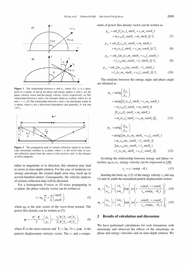
For an elastic wave, the phase velocity is perpendicular to its wave-front. The energy velocity is in the ray direction, i.e. the direction of the power flux density vector. In an elastic isotropic medium, the wave-front is spherical. The direction and magnitude of the phase velocity are the same as those of the energy velocity (Figure 1(a)). However, for the elastic anisotropic medium, the wave-front is no longer spherical. Both direction and magnitude of the phase veloc-ity are generally different from those of the energy velocity (Figure 1(b)). The seismic-reflection wave should propagate at the magnitude of the energy velocity in the ray direction in an elastically anisotropic medium.

Let us consider the propagation and reflection of a wave as shown in Figure 2, with an observation position R. A wave leaves a source S, propagates to a point O on the re-flector, and then is reflected back to a surface position R. The energy incident angle (φi) on the reflection point O is different from the corresponding phase incident angle (θi). The energy angle is determined by the offset and the reflec-tor depth and the phase angle is dependent on the energy angle and the rock anisotropy. Because both energy and phase velocities are functions of phase angle and the rock anisotropy, the travel-time of a reflection signal varies with respect to several factors, including the reflector depth, the rock anisotropy, the vertical phase velocity of the wave and the offset.

If the rock anisotropy is neglected and/or the distinctions between energy velocity and phase velocity are ignored,

FA Lin, et al. Chinese Sci Bull July (2010) Vol.55 No.21 2245

Figure 1 The relationship between vi and vei, where P(x, z) is a space point in xz-plane, θi and φi are phase and energy angles; vi and vei are the phase velocity vector and the energy velocity vector, respectively. (a) The relationship between vi and vei for isotropic media in xz-plane, where θi = φi and vi = vei; (b) The relationship between vi and vei for anisotropic media in xz-plane, where vi has a directional dependence and generally, θi ≠φi and vi≠vei.

Figure 2 The propagation path of seismic-reflection signal in an elasti-cally anisotropic medium in xz-plane, where ti is the travel time of seis-mic-reflection signal from the source to the receiver; and l is the distance of offset midpoint.

either in magnitude or in direction, this situation may lead to errors in time-depth relation. For the case of moderate (or strong) anisotropy the created depth error may reach up to several-hundred meters. Consequently, the velocity analysis of seismic-reflection data will be distorted.

For a homogenous P-wave or SV-wave propagating in xz-plane, the phase velocity vector can be written as

sin=

cosi

iii i

vk k

θω ωθ

⎛ ⎞= ⎜ ⎟

⎝ ⎠kie , (5)

where eki is the unit vector of the wave-front normal. The power flux density can be written as [7]

* **1 5

* *5 3

12 2

ix ix i iz ii i

iz ix i iz i

p T Tp T T

⎛ ⎞+⎛ ⎞⋅= − = = − ⎜ ⎟⎜ ⎟ +⎝ ⎠ ⎝ ⎠

i

V VV Tp

V V, (6)

where Ti is the stress tensors and /i i it jω= ∂ ∂ =V u u is the

particle displacement velocity vector. The x- and z-compo-

nents of power flux density vector can be written as

11 13

44

[ ( sin cos )

( cos sin )] / 2, (7)px p p p p p p

p p p p p

p k l c l c m

m c l m

ω θ θ

θ θ

= +

+ +

44

13 33

[ ( cos sin )

( sin cos )] / 2, (8)pz p p p p p p

p p p p p

p k l c l m

m c l c m

ω θ θ

θ θ

= +

+ +

11 13

44

[ ( sin cos ) ( cos sin )] / 2, (9)

svx sv sv sv sv sv sv

sv sv sv sv sv

p k m c m c ll c m l

ω θ θθ θ

= +

+ +

44

13 33

[ ( cos sin ) ( sin cos )] / 2. (10)

svz sv sv sv sv sv sv

sv sv sv sv sv

p k m c m ll c m c l

ω θ θθ θ

= +

+ +

The relations between the energy angle and phase angle are obtained as

{

}

11 13

44

44

13 33

acrtg

arctg [ ( sin cos )

( cos sin )]

[ ( cos sin )

( sin cos )] , (11)

pxp

pz

p p p p p

p p p p p

p p p p p

p p p p p

pp

l c l c m

m c l m

l c l m

m c l c m

ϕ

θ θ

θ θ

θ θ

θ θ

⎛ ⎞= ⎜ ⎟⎜ ⎟

⎝ ⎠

= +

+ +

+

+ +

{

}

11 13

44

44

13 33

acrtg

arctg [ ( sin cos )

( cos sin )] [ ( cos sin ) ( sin cos )] . (12)

svxsv

svz

sv sv sv sv sv

sv sv sv sv sv

sv sv sv sv sv

sv sv sv sv sv

pp

m c m c l

m c m lm c m ll c m c l

ϕ

θ θ

θ θθ θ

θ θ

⎛ ⎞= ⎜ ⎟

⎝ ⎠= +

+ +

+

+ +

Invoking the relationship between energy and phase ve-locities, eki·vei=vi, energy velocity can be expressed as [30]

/ cos( ).ei i i iv v φ θ= − (13)

Inserting the form, eq. (13), of the energy velocity vei into eqs. (3) and (4) yields the normalized particle displacement vectors:

sin cosexp ,

cos( )px p p p

ppz p ep p p

u l x zj t

u m vθ θ

ωϕ θ

⎡ ⎤± ⎛ ⎞⎛ ⎞ ⎛ ⎞ += = −⎢ ⎥⎜ ⎟⎜ ⎟ ⎜ ⎟⎜ ⎟ ⎜ ⎟ ⎜ ⎟± −⎢ ⎥⎝ ⎠ ⎝ ⎠ ⎝ ⎠⎣ ⎦

u (14)

sin cosexp .

cos( )svx sv sv sv

svsvz sv esv sv sv

u m x zj t

u l vθ θ

ωϕ θ

⎡ ⎤± ⎛ ⎞⎛ ⎞ ⎛ ⎞ += = −⎢ ⎥⎜ ⎟⎜ ⎟ ⎜ ⎟± −⎢ ⎥⎝ ⎠ ⎝ ⎠ ⎝ ⎠⎣ ⎦

u (15)

2 Results of calculation and discussion

We have performed calculations for rock formations with anisotropy and observed the effects of the anisotropy on phase and energy velocities and on time-depth relation. We

2246 FA Lin, et al. Chinese Sci Bull July (2010) Vol.55 No.21

selected three typical rock samples with anisotropic pa-rameters as reported by Thomsen [5]. These parameters are listed in Table 1. Specifically, Sample 1 is an M-sandstone with very small anisotropic parameters, Sample 2 is a C-sandstone with weak to moderate anisotropy, and Sample 3 is an M-shale with moderate anisotropy. For convenience in discussion, we listed the notations in Table 2.

For the transversely isotropic rocks, the relationships between elastic moduli and anisotropy parameters were reported by Thomsen [5],

211 (2 1) ,c ε ρα= + (16)

233 ,c ρα= (17)

* 4 2 2 2 2 213 ( )[( 1) ] ,c ρ δ α α β ε α β ρβ= + − + − − (18)

244 ,c αβ= (19)

266 (2 1) ,c γ ρβ= + (20)

where α and β are the vertical phase velocities of P- and SV-waves. These phase velocities have no relation with anisotropic parameters and they can be considered as the phase velocities of P- and SV-waves in isotropic rock sam-ples. We also noted that for a fixed coordinate system, the HTI model can be obtained by a 90° rotation from the VTI model [27], and we only need to discuss the VTI model.

2.1 Effect of anisotropy on phase velocity and energy velocity

We have calculated the effects of anisotropy on the phase and energy velocities for the three samples, listed in Table 1, and presented the results in Figures 3–5, respectively.

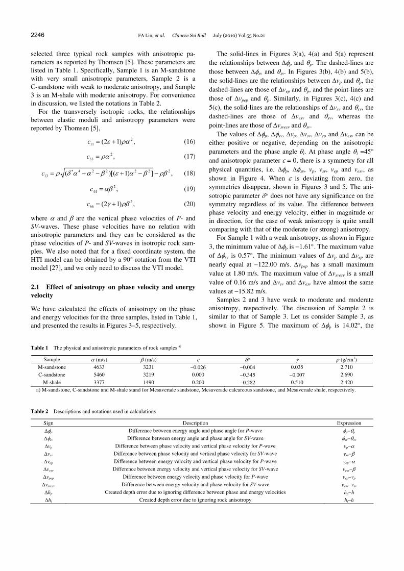
The solid-lines in Figures 3(a), 4(a) and 5(a) represent the relationships between Δφp and θp. The dashed-lines are those between Δφsv and θsv. In Figures 3(b), 4(b) and 5(b), the solid-lines are the relationships between Δvp and θp, the dashed-lines are those of Δvep and θp, and the point-lines are those of Δvpep and θp. Similarly, in Figures 3(c), 4(c) and 5(c), the solid-lines are the relationships of Δvsv and θsv, the dashed-lines are those of Δvesv and θsv, whereas the point-lines are those of Δvsvesv and θsv.

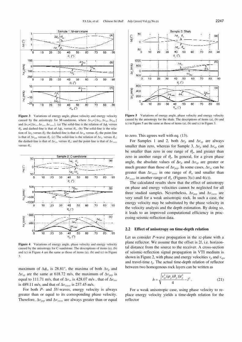
The values of Δφp, Δφsv, Δvp, Δvsv, Δvep and Δvesv can be either positive or negative, depending on the anisotropic parameters and the phase angle θi. At phase angle θi =45° and anisotropic parameter ε = 0, there is a symmetry for all physical quantities, i.e. Δφp, Δφsv, vp, vsv, vep and vesv, as shown in Figure 4. When ε is deviating from zero, the symmetries disappear, shown in Figures 3 and 5. The ani-sotropic parameter δ* does not have any significance on the symmetry regardless of its value. The difference between phase velocity and energy velocity, either in magnitude or in direction, for the case of weak anisotropy is quite small comparing with that of the moderate (or strong) anisotropy.

For Sample 1 with a weak anisotropy, as shown in Figure 3, the minimum value of Δφp is −1.61°. The maximum value of Δφsv is 0.57°. The minimum values of Δvp and Δvep are nearly equal at −122.00 m/s. Δvpep has a small maximum value at 1.80 m/s. The maximum value of Δvsvesv is a small value of 0.16 m/s and Δvsv and Δvesv have almost the same values at −15.82 m/s.

Samples 2 and 3 have weak to moderate and moderate anisotropy, respectively. The discussion of Sample 2 is similar to that of Sample 3. Let us consider Sample 3, as shown in Figure 5. The maximum of Δφp is 14.02°, the

Table 1 The physical and anisotropic parameters of rock samples a)

Sample α (m/s) β (m/s) ε δ* γ ρ (g/cm3) M-sandstone 4633 3231 −0.026 −0.004 0.035 2.710 C-sandstone 5460 3219 0.000 −0.345 −0.007 2.690

M-shale 3377 1490 0.200 −0.282 0.510 2.420 a) M-sandstone, C-sandstone and M-shale stand for Mesaverade sandstone, Mesaverade calcareous sandstone, and Mesaverade shale, respectively.

Table 2 Descriptions and notations used in calculations

Sign Description Expression

Δφp Difference between energy angle and phase angle for P-wave φp−θp

Δφsv Difference between energy angle and phase angle for SV-wave φsv−θsv

Δvp Difference between phase velocity and vertical phase velocity for P-wave vp−α

Δvsv Difference between phase velocity and vertical phase velocity for SV-wave vsv−β

Δvep Difference between energy velocity and vertical phase velocity for P-wave vep−α

Δvesv Difference between energy velocity and vertical phase velocity for SV-wave vesv−β

Δvpep Difference between energy velocity and phase velocity for P-wave vep−vp

Δvsvesv Difference between energy velocity and phase velocity for SV-wave vesv−vsv

Δhp Created depth error due to ignoring difference between phase and energy velocities hp−h

Δhi Created depth error due to ignoring rock anisotropy hi−h

FA Lin, et al. Chinese Sci Bull July (2010) Vol.55 No.21 2247

Figure 3 Variations of energy angle, phase velocity and energy velocity caused by the anisotropy for M-sandstone, where Δvm={Δvp, Δvep, Δvpep} and Δvn={Δvsv, Δvesv, Δvsvesv}. (a) The solid-line is the relation of Δφp versus θp, and dashed-line is that of Δφsv versus θsv. (b) The solid-line is the rela-tion of Δvp versus θp; the dashed-line is that of Δvep versus θp; the point-line is that of Δvpep versus θp. (c) The solid-line is the relation of Δvsv versus θsv; the dashed-line is that of Δvesv versus θsv; and the point-line is that of Δvsvesv versus θsv.

Figure 4 Variations of energy angle, phase velocity and energy velocity caused by the anisotropy for C-sandstone. The descriptions of items (a), (b) and (c) in Figure 4 are the same as those of items (a), (b) and (c) in Figure 3.

maximum of Δφsv is 28.81°, the maxima of both Δvp and Δvep are the same at 618.72 m/s, the maximum of Δvpep is equal to 111.71 m/s, that of Δvsv is 428.07 m/s , that of Δvesv is 489.11 m/s, and that of Δvsvesv is 237.45 m/s.

For both P- and SV-waves, energy velocity is always greater than or equal to its corresponding phase velocity. Therefore, Δvpep and Δvsvesv are always greater than or equal

Figure 5 Variations of energy angle, phase velocity and energy velocity caused by the anisotropy for the shale. The descriptions of items (a), (b) and (c) in Figure 5 are the same as those of items (a), (b) and (c) in Figure 3.

to zero. This agrees well with eq. (13). For Samples 1 and 2, both Δvp and Δvep are always

smaller than zero, whereas for Sample 3, Δvp and Δvep can be smaller than zero in one range of θp, and greater than zero in another range of θp. In general, for a given phase angle, the absolute values of Δvp and Δvep are greater or much greater than those of Δvpep. In some cases, Δvsv can be greater than Δvsvesv in one range of θsv and smaller than Δvsvesv in another range of θsv (Figures 3(c) and 4(c)).

The calculated results show that the effect of anisotropy on phase and energy velocities cannot be neglected for all three studied samples. Nevertheless, Δvpep and Δvsvesv are very small for a weak anisotropic rock. In such a case, the energy velocity may be substituted by the phase velocity in the velocity analysis and the depth estimation. By doing so, it leads to an improved computational efficiency in proc-essing seismic-reflection data.

2.2 Effect of anisotropy on time-depth relation

Let us consider P-wave propagation in the xz-plane with a plane reflector. We assume that the offset is 2l, i.e. horizon-tal distance from the source to the receiver. A cross-section of seismic-reflection signal propagation in VTI medium is shown in Figure 2, with phase and energy velocities vp and vep, and travel-time tp. The actual time-depth relation of reflector between two homogenous rock layers can be written as

2 22( ( )).

4ep p p pv t

h lϕ θ

= − (21)

For a weak anisotropic case, using phase velocity to re-place energy velocity yields a time-depth relation for the reflector

2248 FA Lin, et al. Chinese Sci Bull July (2010) Vol.55 No.21

2 22( ( )).

4p p p p

p

v th l

ϕ θ= − (22)

Furthermore, if neglecting the effect of the anisotropy and using vertical phase velocity α to replace the energy velocity vep[φp(θp)], the time-depth relation yields

2 22 .

4p

i

th l

α= − (23)

Now, we can show that this expression would lead to a significant created error for the above three rock samples studied: weak anisotropy, weak to moderate anisotropy and moderate anisotropy.

We use the following two cases to discuss the created errors for the time-depth relation, by ignoring the difference between energy velocity and phase velocity and/or neglect-ing the rock anisotropy. In the first case, we consider a con-stant offset with a variable depth. As an example, we set off-set (2l) to be 2000 m and let the reflector depth (h) vary from 500 m to 3000 m. In the second case, we keep a constant depth and a variable offset. Specifically, we set the depth at 2000 m and the offset varying from 200 m to 4000 m.

For the first case, the energy angle (φp) decreases from 63.43° to 18.43° with the reflector depth (h) ranging from 500 m to 3000 m. According to the parameters of the above three samples in Table 1, we have calculated the relation-ship between energy angle (φp) and reflection travel time (tp), as well as that of phase angle (θp) and reflection travel time (tp), as shown in Figure 6. These results of calculations are summarized in Table 3. The entries in Table 3 show that the weak-moderate anisotropy or moderate anisotropy leads to a significant difference between energy angle (φp) and phase angle (θp).

Figure 6 Relations of both φp and θp versus tp, where the offset (2l) is equal to 2000 m and the variation range of reflector depth is from 500 m to 3000 m; the solid-line is for M-sandstone, the dashed-line is for C-sandstone and the point-line is for the shale. (a) The relation of φp versus tp; (b) the relation of θp versus tp.

Table 3 Variations of phase angle (θp) with respect to reflection travel- time in the studied rock samples

Sample tp (ms) θp (°) M-sandstone 492.37–1367.69 64.90–19.10 C-sandstone 440.26–1211.14 53.60–30.20

M-shale 608.90–1883.70 49.80–19.20

In terms of eqs. (13), (21), (22) and (23), we have also

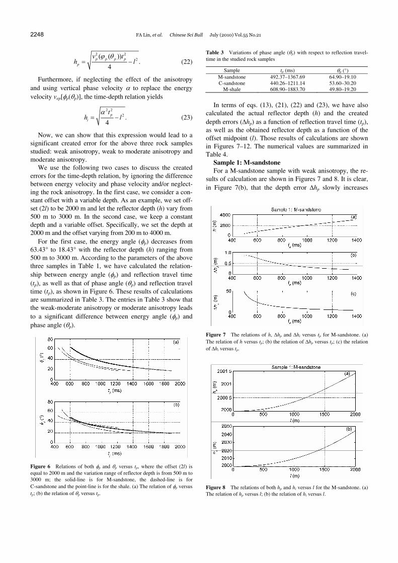
calculated the actual reflector depth (h) and the created depth errors (Δhp) as a function of reflection travel time (tp), as well as the obtained reflector depth as a function of the offset midpoint (l). Those results of calculations are shown in Figures 7–12. The numerical values are summarized in Table 4.

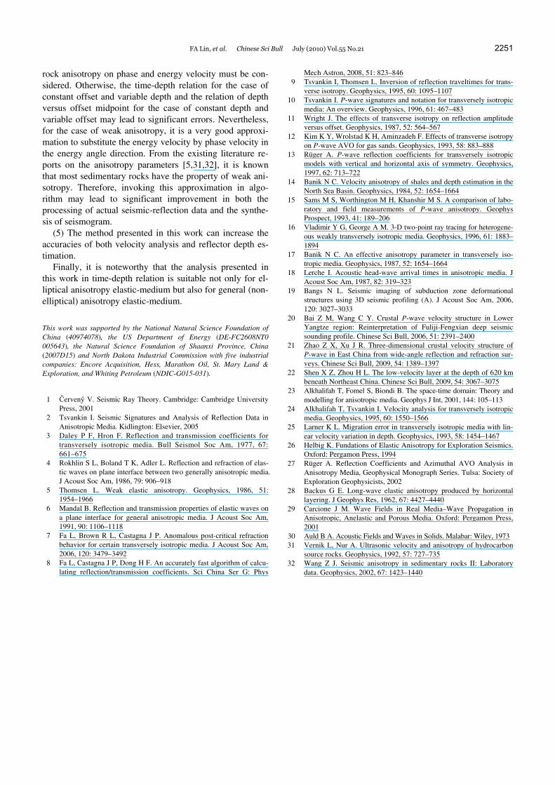
Sample 1: M-sandstone For a M-sandstone sample with weak anisotropy, the re-

sults of calculation are shown in Figures 7 and 8. It is clear, in Figure 7(b), that the depth error Δhp slowly increases

Figure 7 The relations of h, Δhp and Δhi versus tp for M-sandstone. (a) The relation of h versus tp; (b) the relation of Δhp versus tp; (c) the relation of Δhi versus tp.

Figure 8 The relations of both hp and hi versus l for the M-sandstone. (a) The relation of hp versus l; (b) the relation of hi versus l.

FA Lin, et al. Chinese Sci Bull July (2010) Vol.55 No.21 2249

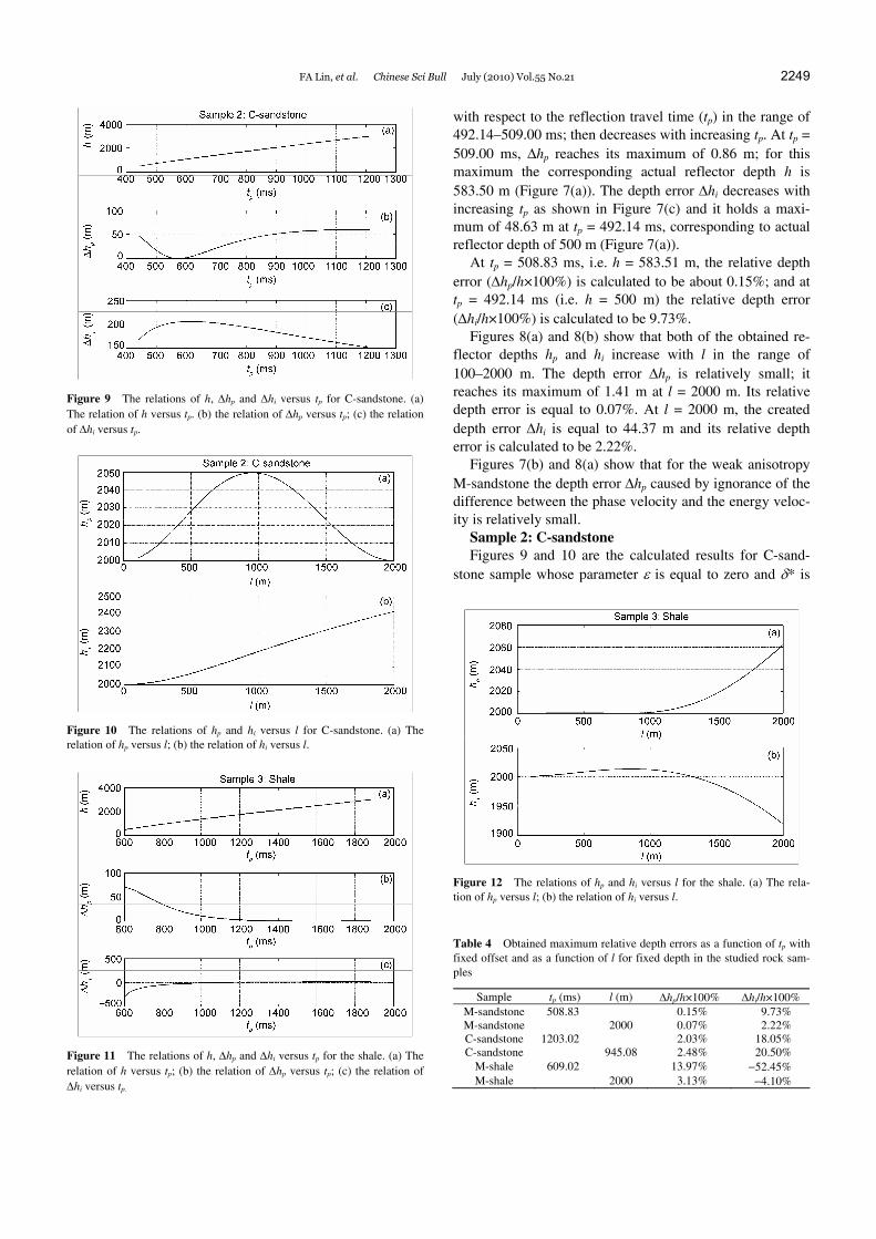
Figure 9 The relations of h, Δhp and Δhi versus tp for C-sandstone. (a) The relation of h versus tp. (b) the relation of Δhp versus tp; (c) the relation of Δhi versus tp.

Figure 10 The relations of hp and hi versus l for C-sandstone. (a) The relation of hp versus l; (b) the relation of hi versus l.

Figure 11 The relations of h, Δhp and Δhi versus tp for the shale. (a) The relation of h versus tp; (b) the relation of Δhp versus tp; (c) the relation of Δhi versus tp.

with respect to the reflection travel time (tp) in the range of 492.14–509.00 ms; then decreases with increasing tp. At tp = 509.00 ms, Δhp reaches its maximum of 0.86 m; for this maximum the corresponding actual reflector depth h is 583.50 m (Figure 7(a)). The depth error Δhi decreases with increasing tp as shown in Figure 7(c) and it holds a maxi-mum of 48.63 m at tp = 492.14 ms, corresponding to actual reflector depth of 500 m (Figure 7(a)).

At tp = 508.83 ms, i.e. h = 583.51 m, the relative depth error (Δhp/h×100%) is calculated to be about 0.15%; and at tp = 492.14 ms (i.e. h = 500 m) the relative depth error (Δhi/h×100%) is calculated to be 9.73%.

Figures 8(a) and 8(b) show that both of the obtained re-flector depths hp and hi increase with l in the range of 100–2000 m. The depth error Δhp is relatively small; it reaches its maximum of 1.41 m at l = 2000 m. Its relative depth error is equal to 0.07%. At l = 2000 m, the created depth error Δhi is equal to 44.37 m and its relative depth error is calculated to be 2.22%.

Figures 7(b) and 8(a) show that for the weak anisotropy M-sandstone the depth error Δhp caused by ignorance of the difference between the phase velocity and the energy veloc-ity is relatively small.

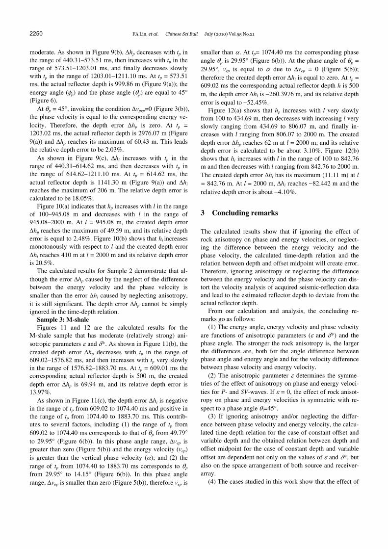
Sample 2: C-sandstone Figures 9 and 10 are the calculated results for C-sand-

stone sample whose parameter ε is equal to zero and δ* is

Figure 12 The relations of hp and hi versus l for the shale. (a) The rela-tion of hp versus l; (b) the relation of hi versus l.

Table 4 Obtained maximum relative depth errors as a function of tp with fixed offset and as a function of l for fixed depth in the studied rock sam- ples

Sample tp (ms) l (m) Δhp/h×100% Δhi/h×100% M-sandstone 508.83 0.15% 9.73% M-sandstone 2000 0.07% 2.22% C-sandstone 1203.02 2.03% 18.05% C-sandstone 945.08 2.48% 20.50%

M-shale 609.02 13.97% −52.45% M-shale 2000 3.13% −4.10%

2250 FA Lin, et al. Chinese Sci Bull July (2010) Vol.55 No.21

moderate. As shown in Figure 9(b), Δhp decreases with tp in the range of 440.31–573.51 ms, then increases with tp in the range of 573.51–1203.01 ms, and finally decreases slowly with tp in the range of 1203.01–1211.10 ms. At tp = 573.51 ms, the actual reflector depth is 999.86 m (Figure 9(a)); the energy angle (φp) and the phase angle (θp) are equal to 45° (Figure 6).

At θp = 45°, invoking the condition Δvpep=0 (Figure 3(b)), the phase velocity is equal to the corresponding energy ve-locity. Therefore, the depth error Δhp is zero. At tp = 1203.02 ms, the actual reflector depth is 2976.07 m (Figure 9(a)) and Δhp reaches its maximum of 60.43 m. This leads the relative depth error to be 2.03%.

As shown in Figure 9(c), Δhi increases with tp in the range of 440.31–614.62 ms, and then decreases with tp in the range of 614.62–1211.10 ms. At tp = 614.62 ms, the actual reflector depth is 1141.30 m (Figure 9(a)) and Δhi reaches the maximum of 206 m. The relative depth error is calculated to be 18.05%.

Figure 10(a) indicates that hp increases with l in the range of 100–945.08 m and decreases with l in the range of 945.08–2000 m. At l = 945.08 m, the created depth error Δhp reaches the maximum of 49.59 m, and its relative depth error is equal to 2.48%. Figure 10(b) shows that hi increases monotonously with respect to l and the created depth error Δhi reaches 410 m at l = 2000 m and its relative depth error is 20.5%.

The calculated results for Sample 2 demonstrate that al-though the error Δhp caused by the neglect of the difference between the energy velocity and the phase velocity is smaller than the error Δhi caused by neglecting anisotropy, it is still significant. The depth error Δhp cannot be simply ignored in the time-depth relation.

Sample 3: M-shale Figures 11 and 12 are the calculated results for the

M-shale sample that has moderate (relatively strong) ani-sotropic parameters ε and δ*. As shown in Figure 11(b), the created depth error Δhp decreases with tp in the range of 609.02–1576.82 ms, and then increases with tp very slowly in the range of 1576.82–1883.70 ms. At tp = 609.01 ms the corresponding actual reflector depth is 500 m, the created depth error Δhp is 69.94 m, and its relative depth error is 13.97%.

As shown in Figure 11(c), the depth error Δhi is negative in the range of tp from 609.02 to 1074.40 ms and positive in the range of tp from 1074.40 to 1883.70 ms. This contrib-utes to several factors, including (1) the range of tp from 609.02 to 1074.40 ms corresponds to that of θp from 49.79° to 29.95° (Figure 6(b)). In this phase angle range, Δvep is greater than zero (Figure 5(b)) and the energy velocity (vep) is greater than the vertical phase velocity (α); and (2) the range of tp from 1074.40 to 1883.70 ms corresponds to θp from 29.95° to 14.15° (Figure 6(b)). In this phase angle range, Δvep is smaller than zero (Figure 5(b)), therefore vep is

smaller than α. At tp= 1074.40 ms the corresponding phase angle θp is 29.95° (Figure 6(b)). At the phase angle of θp = 29.95°, vep is equal to α due to Δvep = 0 (Figure 5(b)); therefore the created depth error Δhi is equal to zero. At tp = 609.02 ms the corresponding actual reflector depth h is 500 m, the depth error Δhi is −260.3976 m, and its relative depth error is equal to −52.45%.

Figure 12(a) shows that hp increases with l very slowly from 100 to 434.69 m, then decreases with increasing l very slowly ranging from 434.69 to 806.07 m, and finally in-creases with l ranging from 806.07 to 2000 m. The created depth error Δhp reaches 62 m at l = 2000 m; and its relative depth error is calculated to be about 3.10%. Figure 12(b) shows that hi increases with l in the range of 100 to 842.76 m and then decreases with l ranging from 842.76 to 2000 m. The created depth error Δhi has its maximum (11.11 m) at l = 842.76 m. At l = 2000 m, Δhi reaches −82.442 m and the relative depth error is about −4.10%.

3 Concluding remarks

The calculated results show that if ignoring the effect of rock anisotropy on phase and energy velocities, or neglect-ing the difference between the energy velocity and the phase velocity, the calculated time-depth relation and the relation between depth and offset midpoint will create error. Therefore, ignoring anisotropy or neglecting the difference between the energy velocity and the phase velocity can dis-tort the velocity analysis of acquired seismic-reflection data and lead to the estimated reflector depth to deviate from the actual reflector depth.

From our calculation and analysis, the concluding re-marks go as follows:

(1) The energy angle, energy velocity and phase velocity are functions of anisotropic parameters (ε and δ*) and the phase angle. The stronger the rock anisotropy is, the larger the differences are, both for the angle difference between phase angle and energy angle and for the velocity difference between phase velocity and energy velocity.

(2) The anisotropic parameter ε determines the symme-tries of the effect of anisotropy on phase and energy veloci-ties for P- and SV-waves. If ε = 0, the effect of rock anisot-ropy on phase and energy velocities is symmetric with re-spect to a phase angle θi=45°.

(3) If ignoring anisotropy and/or neglecting the differ-ence between phase velocity and energy velocity, the calcu-lated time-depth relation for the case of constant offset and variable depth and the obtained relation between depth and offset midpoint for the case of constant depth and variable offset are dependent not only on the values of ε and δ*, but also on the space arrangement of both source and receiver- array.

(4) The cases studied in this work show that the effect of

FA Lin, et al. Chinese Sci Bull July (2010) Vol.55 No.21 2251

rock anisotropy on phase and energy velocity must be con-sidered. Otherwise, the time-depth relation for the case of constant offset and variable depth and the relation of depth versus offset midpoint for the case of constant depth and variable offset may lead to significant errors. Nevertheless, for the case of weak anisotropy, it is a very good approxi-mation to substitute the energy velocity by phase velocity in the energy angle direction. From the existing literature re-ports on the anisotropy parameters [5,31,32], it is known that most sedimentary rocks have the property of weak ani-sotropy. Therefore, invoking this approximation in algo-rithm may lead to significant improvement in both the processing of actual seismic-reflection data and the synthe-sis of seismogram.

(5) The method presented in this work can increase the accuracies of both velocity analysis and reflector depth es-timation.

Finally, it is noteworthy that the analysis presented in this work in time-depth relation is suitable not only for el-liptical anisotropy elastic-medium but also for general (non- elliptical) anisotropy elastic-medium.

This work was supported by the National Natural Science Foundation of China (40974078), the US Department of Energy (DE-FC2608NT0 005643), the Natural Science Foundation of Shaanxi Province, China (2007D15) and North Dakota Industrial Commission with five industrial companies: Encore Acquisition, Hess, Marathon Oil, St. Mary Land & Exploration, and Whiting Petroleum (NDIC-G015-031).

1 Ĉervenŷ V. Seismic Ray Theory. Cambridge: Cambridge University Press, 2001

2 Tsvankin I. Seismic Signatures and Analysis of Reflection Data in Anisotropic Media. Kidlington: Elsevier, 2005

3 Daley P F, Hron F. Reflection and transmission coefficients for transversely isotropic media. Bull Seismol Soc Am, 1977, 67: 661–675

4 Rokhlin S L, Boland T K, Adler L. Reflection and refraction of elas-tic waves on plane interface between two generally anisotropic media. J Acoust Soc Am, 1986, 79: 906–918

5 Thomsen L. Weak elastic anisotropy. Geophysics, 1986, 51: 1954–1966

6 Mandal B. Reflection and transmission properties of elastic waves on a plane interface for general anisotropic media. J Acoust Soc Am, 1991, 90: 1106–1118

7 Fa L, Brown R L, Castagna J P. Anomalous post-critical refraction behavior for certain transversely isotropic media. J Acoust Soc Am, 2006, 120: 3479–3492

8 Fa L, Castagna J P, Dong H F. An accurately fast algorithm of calcu-lating reflection/transmission coefficients. Sci China Ser G: Phys

Mech Astron, 2008, 51: 823–846 9 Tsvankin I, Thomsen L. Inversion of reflection traveltimes for trans-

verse isotropy. Geophysics, 1995, 60: 1095–1107 10 Tsvankin I. P-wave signatures and notation for transversely isotropic

media: An overview. Geophysics, 1996, 61: 467–483 11 Wright J. The effects of transverse isotropy on reflection amplitude

versus offset. Geophysics, 1987, 52: 564–567 12 Kim K Y, Wrolstad K H, Aminzadeh F. Effects of transverse isotropy

on P-wave AVO for gas sands. Geophysics, 1993, 58: 883–888 13 Rüger A. P-wave reflection coefficients for transversely isotropic

models with vertical and horizontal axis of symmetry. Geophysics, 1997, 62: 713–722

14 Banik N C. Velocity anisotropy of shales and depth estimation in the North Sea Basin. Geophysics, 1984, 52: 1654–1664

15 Sams M S, Worthington M H, Khanshir M S. A comparison of labo-ratory and field measurements of P-wave anisotropy. Geophys Prospect, 1993, 41: 189–206

16 Vladimir Y G, George A M. 3-D two-point ray tracing for heterogene- ous weakly transversely isotropic media. Geophysics, 1996, 61: 1883– 1894

17 Banik N C. An effective anisotropy parameter in transversely iso-tropic media. Geophysics, 1987, 52: 1654–1664

18 Lerche I. Acoustic head-wave arrival times in anisotropic media. J Acoust Soc Am, 1987, 82: 319–323

19 Bangs N L. Seismic imaging of subduction zone deformational structures using 3D seismic profiling (A). J Acoust Soc Am, 2006, 120: 3027–3033

20 Bai Z M, Wang C Y. Crustal P-wave velocity structure in Lower Yangtze region: Reinterpretation of Fuliji-Fengxian deep seismic sounding profile. Chinese Sci Bull, 2006, 51: 2391–2400

21 Zhao Z X, Xu J R. Three-dimensional crustal velocity structure of P-wave in East China from wide-angle reflection and refraction sur-veys. Chinese Sci Bull, 2009, 54: 1389–1397

22 Shen X Z, Zhou H L. The low-velocity layer at the depth of 620 km beneath Northeast China. Chinese Sci Bull, 2009, 54: 3067–3075

23 Alkhalifah T, Fomel S, Biondi B. The space-time domain: Theory and modelling for anisotropic media. Geophys J Int, 2001, 144: 105–113

24 Alkhalifah T, Tsvankin I. Velocity analysis for transversely isotropic media. Geophysics, 1995, 60: 1550–1566

25 Larner K L. Migration error in transversely isotropic media with lin-ear velocity variation in depth. Geophysics, 1993, 58: 1454–1467

26 Helbig K. Fundations of Elastic Anisotropy for Exploration Seismics. Oxford: Pergamon Press, 1994

27 Rüger A. Reflection Coefficients and Azimuthal AVO Analysis in Anisotropy Media, Geophysical Monograph Series. Tulsa: Society of Exploration Geophysicists, 2002

28 Backus G E. Long-wave elastic anisotropy produced by horizontal layering. J Geophys Res, 1962, 67: 4427–4440

29 Carcione J M. Wave Fields in Real Media–Wave Propagation in Anisotropic, Anelastic and Porous Media. Oxford: Pergamon Press, 2001

30 Auld B A. Acoustic Fields and Waves in Solids. Malabar: Wiley, 1973 31 Vernik L, Nur A. Ultrasonic velocity and anisotropy of hydrocarbon

source rocks. Geophysics, 1992, 57: 727–735 32 Wang Z J. Seismic anisotropy in sedimentary rocks II: Laboratory

data. Geophysics, 2002, 67: 1423–1440