AZIMUTHAL SHEAR WAVE ANISOTROPY ANALYSIS, GUIDED IN TIME DOMAIN

SPWLA 55th Annual Logging Symposium, May 18-22, 2014

1

AZIMUTHAL SHEAR WAVE ANISOTROPY ANALYSIS,GUIDED IN TIME DOMAIN

Marek Kozak, Mirka Kozak, Jefferson Williams, Supersonic Geophysical LLC

Copyright 2014, held jointly by the Society of Petrophysicists and Well LogAnalysts (SPWLA) and the submitting authors.This paper was prepared for presentation at the SPWLA 55th AnnualLogging Symposium held in Abu Dhabi, United Arab Emirates, May 18-22,2014.

ABSTRACT

Ideally, waveform data excited by an acoustic dipolesource should only generate Flexural waves.Unfortunately, other acoustic modes are also oftencreated; including Stoneley or Compressional waves.Whether these undesired modes appear or not dependson tool position, well deviation, and boreholeconditions. Classic shear wave anisotropy analysis candeliver erroneous values due to the presence of mixedacoustic modes within the processing window in timedomain. Therefore, we propose to augment shear waveanisotropy analysis with waveform guiding in timedomain. Flexural wave arrival time is tracked at eachreceiver station independently. This travel timesearching procedure is repeated twice: first utilizingdipole XX (on axis) data, and then dipole YY (also onaxis) data. During each of the passes, the faster arrivalis selected, thus yielding the vector of depth domaincurves that define zero phase arrival time at eachreceiver level independently. Under isotropicconditions with collocated transmitters, dipole XX anddipole YY zero phase arrival times will be the same.However, when the formation is anisotropic, thesearrival times will differ according to the strength of theanisotropy field. Angular energy distributions can becalculated using the time domain tracking curvesdescribed above. These distributions are computed ateach receiver station separately, yielding on axis Exx

and off axis Exy angular energy fields. Since energydistribution computations are guided and performedwithin a relatively narrow time window, the possibilitythat non-flexural mode wave forms (e.g. Stoneleymode) contaminate the outcome is significantlyreduced. We illustrate how to identify a mixed acousticmode condition, and how to control the quality ofmaximum stress direction computations. We also showhow to qualify cross dipole data using theinstantaneous frequency/slowness analysis method.Various field examples are also presented.

INTRODUCTION

Cross-dipole logging tools are commonly used tomeasure formation anisotropic properties in a boreholeenvironment. Shear wave anisotropy analysis is basedon four-component waveform data, generated by twoorthogonal dipole sources X and Y, and an array oforthogonal receivers. Since the sources and receiversare mounted orthogonally, the cross-dipole tool willexcite two in-line (XX and YY), and two cross-line(XY and YX) sets of waveforms. In an isotropicformation at the low frequency limit, flexural wavepropagation velocity will approach that of formationshear. In the case of an anisotropic formation, theflexural wave will split into slow and fast modes thattravel with different velocities. Since polarizations ofslow and fast flexural waves are aligned with these offormation shear waves (Ellefsen et al., 1991), dipolelogging data may be used to estimate:

directions of fast and slow flexural wavepropagation, using wave form rotationtechnique (for example Alford, 1986).

fast and slow flexural wave velocities, usingwave form inversion and decompositionmethods discussed in various articles (forexample Thomsen, 1988 or Cheng andCheng, 1995).

In this article we assume that the formations are ofhexagonal symmetry and therefore the split waves arepolarized orthogonally (as, for example, occurs whenshear wave anisotropy is caused only by the fractures).In a more general case however, when thin layers andfractures are present simultaneously, it is possible thatfast and slow waves will travel at a relative angle thatis different than 90 degrees (Nolte and Cheng, 1995).

In the case of orthogonal propagation, four componentwaveform data matrix V(t) can be diagonalized asfollows (Alford, 1986) :

(ݐ) = (ߠ)(ݐ)(ߠ)ଵି (1)

Where ߠ is the angle between the direction of the fastshear wave propagation and the dipole X source planeof excitation.


2

Also:

(ݐ) = (ݐ)ݔݔܸ (ݐ)ݔݕܸ(ݐ)ݕݔܸ (ݐ)ݕݕܸ

൨ (2)

and the rotation matrix R that has diagonal form as:

(ߠ) = (ߠ)ݏܥ ܵ݅ (ߠ݊)−ܵ݅ (ߠ݊) (ߠ)ݏܥ

൨ (3)

(ߠ)ଵି = (ߠ)ݏܥ −ܵ݅ (ߠ݊)ܵ݅ (ߠ݊) (ߠ)ݏܥ

൨ (4)

Formula (1) after evaluation will yield fourcomponents:

(ߠ,ݐ)ݔݔ =−(ߠ)ݏܥ(ݐ)ݔݔܸ(ߠ)ݏܥ ݅ܵ(ݐ)ݕݔܸ(ߠ)ݏܥ ((ߠ݊) −ܵ݅ (ߠ)ݏܥ(ݐ)ݔݕܸ(ߠ݊) + ܵ݅ ݅ܵ(ݐ)ݕݕܸ(ߠ)݊ (ߠ݊) (5)

(ߠ,ݐ)ݕݔ =ܵ݅ (ߠ)ݏܥ(ݐ)ݔݔܸ(ߠ݊) + ((ߠ)ݏܥ(ݐ)ݕݔܸ(ߠ)ݏܥ −ܵ݅ ݅ܵ(ݐ)ݔݕܸ(ߠ݊) (ߠ݊) − ݅ܵ(ݐ)ݕݕܸ(ߠ)ݏܥ (ߠ݊) (6)

(ߠ,ݐ)ݔݕ =ܵ݅ −(ߠ)ݏܥ(ݐ)ݔݔܸ(ߠ݊) ܵ݅ ݅ܵ(ݐ)ݕݔܸ(ߠ)݊ ((ߠ݊) +(ߠ)ݏܥ(ݐ)ݔݕܸ(ߠ)ݏܥ − ݅ܵ(ݐ)ݕݕܸ(ߠ)ݏܥ (ߠ݊) (7)

(ߠ,ݐ)ݕݕ =ܵ݅ ݅ܵ(ݐ)ݔݔܸ(ߠ݊) (ߠ݊) + ܵ݅ ((ߠ)ݏܥ(ݐ)ݕݔܸ(ߠ)݊ +݅ܵ(ݐ)ݔݕܸ(ߠ)ݏܥ (ߠ݊) + (ߠ)ݏܥ(ݐ)ݕݕܸ(ߠ)ݏܥ (8)

All four components shown above represent the usualAlford rotation equations. Typically, in order to getfast shear direction, off axis components ݕݔ) or (ݔݕare minimized (with respect to (ߠ - most frequently theleast-squares method is used. If wave form data is ofgood quality, the least-squares technique will deliverrobust results. However, when the signal to noise ratiois poor, or if mixed acoustic modes are present withinrecording window, then the least-squares method willencounter convergence problems. Simply stated - theregression and least-squares techniques might not beadequate.

PROCESSING METHOD

Time domain guided shear wave anisotropy analysis isdescribed below as a series of separate processingsteps. Each step is explained and results are presentedand discussed.

#1. Transmitter Data Collocation. This step is requiredonly if the X and Y dipole transmitters are notphysically co-located. If the logging step is equal to thereceiver interspacing, then some of the waveforms willhave to be reduced. For example, assuming thattransmitters X and Y are mis-collocated by 12 inches,and that receiver interspacing is equal to 6 inches, thentwo receiver wave forms created by each of dipoleexcitations will have to be discarded. This process,although quite simple conceptually, might introduceerrors due to tool spinning between two consecutiveshots. In other words, after “enforced” collocation,transmitters X and Y azimuthal positions might not beorthogonal.

#2. Flexural Wave Time Domain Tracking. Flexuralwave arrival time is tracked at each receiver stationindependently. The travel time searching routine isrepeated twice: first utilizing dipole XX (on axis) data,and then dipole YY (also on axis) data. During each ofthe passes, the faster arrival is selected, thus yieldingthe vector of depth domain curves that define zerophase arrival time independently at each receiver level.Under isotropic conditions, since the transmitter dataare collocated, dipole XX and dipole YY zero phasearrival times will be the same. However, when theformation is anisotropic, they will differ by thestrength of the anisotropy field. This procedure isessential. It assures that the fast flexural wave willalways be located within processing window positionin time domain. Figures 1 and 2 show an example ofdipole XX and YY flexural wave forms, together withimposed arrival times obtained in slow formation. Astrong compressional wave is evident in the front offlexural arrivals. Flexural data is generally of goodquality – there are only a few narrow depth intervalswhere the signal to noise ratio drops to lower values.Figure 3 presents flexural wave travel time trackingresults obtained with dipole XX (brown), and dipoleYY (blue). At the top of the log, dipole XX travel timeis substantially faster than the one obtained with dipoleYY. A reversed effect is observed over the bottomdepth zone, thus indicating that shear wave azimuthalanisotropy might be present. This is confirmed inFigure 4, illustrating minimum of XX vs. YY traveltimes (brown), and tool azimuth log (black). Toolangular position shows rapid spin from approximately90 degrees at the top zone, down to an average of 20degrees at the bottom part of the log. Figures 5 and 6show the first receiver XX and YY waveforms withimposed minimum travel time curve.


3

Figure 1. Near receiver dipole XX wave forms shownwith imposed arrival time.

Figure 2. Near receiver dipole YY wave forms shownwith imposed arrival time.

Figure 3. Flexural wave travel time tracking resultsobtained with dipole XX (brown), and dipole YY(blue). At the top of the log dipole XX travel time issubstantially faster than the one obtained with dipoleYY. Reversed effect is observed over the bottom depthzone.

Figure 4. Minimum (brown) and maximum (blue) ofXX and YY travel time curves obtained from the logspresented in Figure 3. Tool azimuth (black) showsrapid spin from ~90 degrees at the top zone, down to~20 degrees at the bottom part of the log.

Figure 5. The first receiver dipole XX wave formswith imposed minimum arrival time.

Figure 6. The first receiver dipole YY wave formswith imposed minimum arrival time.


4

#3. Angular Energy Distribution. Using time domaintracking profiles (computed in step #2), and wave formrotation formulas (5, 6, 7, and 8), angular energydistributions are calculated as follows:

(ߠ) = [(ߠ)(ݐ)(ߠ)ଵି]ୀ

ୀ

(9)

Where (ߠ) is four component angular energy matrix.

Figure 7. Angular energy matrix components Exx andExy obtained under perfect anisotropic conditions (e.g=ݔݔܸ ,ݕݕܸ ݕݔܸ = ,(ݔݕܸ computed from equation(9).

Thus if the formation is anisotropic, the on axisangular energy distributions will contain two clearlydefined maxima and minima, separated by 180degrees. The off axis angular energy distributions willcontain four local maxima and minima, separated by90 degrees. Local maxima of the on axis energycomponent are in phase with the local minima of offaxis component. Also, on axis and off axis Eyy and Eyx

components will be shifted by 90 degrees with respectto Exx and Exy respectively.

Since the signals are discrete the tstart and tstop limitsin equation (9) represent the first and last time domainsamples of the desired range of summation. Fourenergy components are computed at each receiver levelseparately for on axis Exx, Eyy, and off axis Exy, Eyx

fields. A unique feature of this algorithm is that theenergy distribution computations are guided (i.e. starttime is varying as a function of depth) and performedwithin a relatively narrow time band; thus reducing thepossibility that non-flexural mode waveforms (e.g.Stoneley or compressional mode) can contaminate theoutcome. The width of the time window is usuallyfixed and covers one to three wave cycles;dependingon the formation properties. Also, since the rotationmatrix components are periodic, the azimuth angle ߠvaries from 0 up to 2π only. Figures 8 and 9 present onaxis Exx and off axis Exy energy distributions (receiver#1 and #8 for image clarity) obtained over anisotropicinterval. Note that the angular position of themaximum of on axis energy Exx fits very well into theminimum of off axis energy Exy as was predicted fromformula (9). Finally, on axis Eyy and off axis Exy

components are the same as Exx and Exy respectively -the only difference being a 90 degree shift betweenthem (compare Figures 8, 9, 10, and 11).

The observations above yield the followingconclusion: in order to get azimuthal maximum stressdirection, either the minimum of off axis energy Exy, orthe maximum of on axis energy Exx can be tracked. Inother words, if off axis energies are noisy then on axisenergies can be used, and vice versa. Dipole Y energycomponents might also be used.

The results of anisotropy analysis obtained with datarecorded under difficult borehole conditions (washedout zone up to 14 inches in diameter) are shown on theFigures 12 (predicted from formula (9)) and Figures13, 14, 15, and 16 (well data). The pattern of 2 on axisExx energy picks accompanied by 4 off axis Exy energypicks is getting less visible. Also, the ratio between themaximum and minimum of on axis energies is gettinglower, especially over bottom part of the interval.


5

Figure 8. Near and far receiver Exx angular energydistributions, obtained over anisotropic intervals.

Figure 9. Near and far receiver Exy angular energydistributions, obtained over anisotropic intervals.

Figure 10. Near and far receiver Eyy angular energydistributions, obtained over anisotropic intervals.

Figure 11. Near and far receiver Eyx angular energydistributions, obtained over anisotropic intervals.

Figure 12. Angular energy matrix components Exx andExy, obtained under difficult borehole conditions (e.g≠ݔݔܸ ,ݕݕܸ ≠ݕݔܸ ,(ݔݕܸ computed from equation(9).


6

Figure 13. Near receiver dipole XX wave formsrecorded over washed out zone, with imposed flexuralwave arrival time.

Figure 14. Near receiver dipole YY wave formsrecorded over washed out zone, with imposed flexuralwave arrival time.

Figure 15. Near and far receiver Exx angular energydistributions, obtained over washed out zone.

Figure 16. Near and far receiver Exy angular energydistributions, obtained over washed out zone.

The conclusion is that even under washed outconditions a pattern of 0 degrees shift between themaximum of on axis energy Exx and the minimum ofoff axis energy Exy is still indicated, although thiseffect is much less obvious. Also, the pattern of 2 onaxis energy peaks by 4 off axis energy peaks vanishes,especially over washed out interval. This effect can beused to identify Stoneley mode contamination (due tothe possibility of tool decentralization due to the washout).

Figures 17 and 18 below show results obtained whileguiding anisotropy analysis using various arrivalprofiles. In each case, the time window position wasshifted evenly by 250 uSec towards the end of thewave train. A constant window width of 500 uSec wasapplied. The depth domain arrival profile was the samefor each test.. It is clearly noticeable that the pattern of2 by 4 maxima and minima gradually shifts to a 4 by 4pattern as one samples later into the wave train. Thiseffect is also confirmed by theoretical predictionsshown on Figure 19, and can be used to identifyerroneous window position in time domain.

Figures 20 and 21 present results obtained when aproper time window position is selected but its width istoo broad (1500 uSec in this case). The conclusionhere is that as long as the time window position iscorrect, a time band that is too broad will contaminateangular energy components, making it significantlymore difficult (although still possible) to track thepeaks of the energies.


7

Figure 17. Near receiver dipole XX wave forms withimposed processing time window. For each case timewindow position was shifted by 250 uSec toward theend of recorded wave train.

Figure 18. Near receiver dipole X (on axis Exx - lefttrack), and dipole XY (off axis Exy - right track),angular energy distributions obtained over anisotropicintervals. Corresponding processing time windowposition and its width are shown on Figure 17.


8

Figure 19. Angular energy matrix components Exx andExy, obtained with time window position allocated toodeeply into the wave train, computed from equation(9).

Figure 20. Near receiver dipole XX wave forms withimposed processing time window, and its width (broadband).

Figure 21. Near receiver dipole XX (on axis left track)and dipole XY (off axis - right track) angular energydistributions obtained over anisotropic intervals.Corresponding processing time window position andits width are shown on Figure 20.

#4. Angular Energy Distribution Stack. In order toimprove the signal to noise ratio, the angular energydistribution data computed in previous steps arestacked together across the receiver array. Thisoperation does not significantly degrade verticalresolution because shear wave anisotropy, if present,manifests itself along considerable depth intervalsrather than within thin bed boundaries.

Figure 22. Near receiver dipole XX (on axis lefttrack), and dipole XY (off axis right track) angularenergy distributions, obtained after stacking individualresponses across the receiver array.

#5. Wave Form Rotation Angle. If the formation isanisotropic, the on axis angular energy distribution willcontain two clearly defined maxima and minimaseparated by 180 degrees. The off axis angular energydistribution will contain four local maxima and minima


9

separated by 90 degrees (see theoretical predictionspresented in Figure 7). The waveform rotation angle istracked through one of the troughs of off axis energyExy component that is in phase with an Exx energypeak. A key quality control indicator will be how wellthe waveform rotation angle correlates with themagnetically derived logging tool azimuth curve. If theformation is isotropic, on/off axis energies either don’tshow peaks, or their appearance will be fuzzy and theresulting waveform rotation angle curve will notcorrelate well with the tool azimuth data.

Figure 23. Dipole X angular energy distributions Exx

and Exy, shown with imposed tool azimuth (pad - blackcurve), and the minimum of off axis energy (blue).

Figure 24. Magnetically derived tool azimuth (pad -black curve) and minimum of off axis energy Exy (bluecurve) are presented. Note excellent agreementbetween directional package and dipole tool derivedrotation azimuth. Fast shear azimuth can be computedfrom modulo 360 degrees arithmetic on the toolazimuth and rotation curves.

#6. Rotation, Fast and Slow flexural DTS. Using the

waveform rotation angle, original data (all cross dipolecomponents), and the rotation formulas, the fast andslow flexural mode waveforms are generated.Depending on the signal to noise ratio of the rotatedflexural modes, IFS (Instantaneous FrequencySlowness) Analysis or phase method (Kozak, Boonen,and Seifert, 2001), Guided Semblance Analysis, or acombination of both methods may be used to computefast and slow flexural wave slowness logs. Fast shearwave azimuth can also be calculated.

Figure 25. Near receiver post rotated fast flexuralwave forms, shown together with fast wave arrivaltime.

Figure 26. Near receiver post rotated slow flexuralwave forms, shown together with slow wave arrivaltime.

Whether semblance and IFS methods areused tocompute fast and slow flexural slowness curves,waveforms should be guided in time domain. Applyinga relatively narrow time window width in the pickingprocess assures that potentially competing acousticmodes arrive outside of the processing window.


10

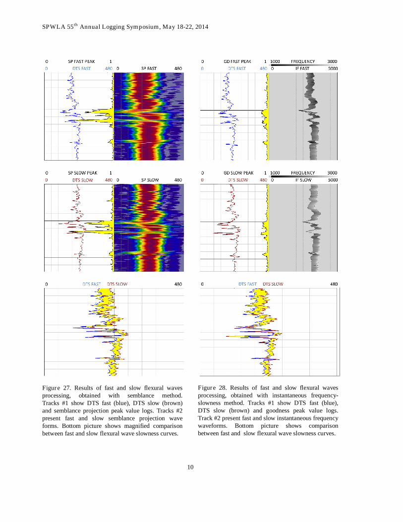
Figure 27. Results of fast and slow flexural wavesprocessing, obtained with semblance method.Tracks #1 show DTS fast (blue), DTS slow (brown)and semblance projection peak value logs. Tracks #2present fast and slow semblance projection waveforms. Bottom picture shows magnified comparisonbetween fast and slow flexural wave slowness curves.

Figure 28. Results of fast and slow flexural wavesprocessing, obtained with instantaneous frequency-slowness method. Tracks #1 show DTS fast (blue),DTS slow (brown) and goodness peak value logs.Track #2 present fast and slow instantaneous frequencywaveforms. Bottom picture shows comparisonbetween fast and slow flexural wave slowness curves.


11

#7. Quality Control Measures. Angular energydistribution wave forms are computed at each receiverlevel separately (e.g. on axis Exx and Eyy, and off axisExy and Eyx fields). Each energy component consists ofan array of 8 vectors derived from dipole X and Yexcitations. Standard deviation and coherencecomputations are performed (in azimuth domain).Since angular response at each receiver station shouldbe similar, then under good well conditions standarddeviation of each energy component ought to be closeto 0 degrees. Also, the coherence should be close to 1 –characteristic similar to semblance projection peakvalue.

Figure 29. Example of Exx azimuthal signature ofdipole X energy obtained over anisotropic intervals.

Figure 30. Example of Exy azimuthal signature ofdipole X energy obtained over anisotropic intervals.

Finally, cross dipole elements created during thewaveform rotation can be used to get post rotatedenergy distribution components. If the anisotropyanalysis was performed correctly, the resulting energyExx should peak at 0 or 180 degrees relative to the tool;

meaning no further rotation is needed. Also the 2 by 4peaks pattern ought to be present. Furthermore, all fourenergy components Exx, Exy, Eyx, and Eyy should haveaflat depth invariant appearance (see Figure 32 below).

Figure 31. Track #1 shows coherence (black) andstandard deviation (brown) curves of on axis Exx

energies. Track #2 shows coherence (black) andstandard deviation (brown) of off axis Exy energies.Long term average standard deviation approaches 2degrees while the coherence is at the level of 0.85 orhigher.

Figure 32. Near receiver dipole XX (on axis Exx - lefttrack) and dipole XY (off axis Exy - right track) angularenergy distributions obtained after waveform rotation.

CONCLUSIONS

A modified technique for processing cross dipoleacoustic data that is based on guiding in time domainhas been presented and discussed. This method worksvery well in vertical to moderately inclined wells. Thistechnique is weakly sensitive to the position and width


12

of the processing window in time domain. The methodproduces information that may be used to identifymixed acoustic mode contamination present within theprocessing window -for example due to Stoneleymode. The technique also generates various qualitymeasures, including coherence and standard deviationof energy components across receiver array.Theoretical predictions were compared against realdata.

REFERENCES

Alford, R.M., 1986. Shear data in presence ofazimuthal anisotropy, 56th Annual International

Ellefsen, K. J., Cheng, C.H., and Toksoz, M.N., 1991,Effects of anisotropy upon the normal modes in aborehole, J. Acoustic Society, Am., 89, 2597-2616

Kozak, M., Boonen, P., Seifert D., 2001, Phasevelocity processing for acoustic logging-while-drillingfull wave form data, SPWLA proceedings.

Kurkjian, A.L., Chang, S.K., 1986, Acoustic multipolesources in fluid-filled boreholes, Geophysics, v. 51, p.148-163.

Nolte, B., Cheng, C.H., 1995. Observation of flexuralwave anisotropy from cross-dipole logs in the PowderRiver Basin, Wyoming, Earth Resources Laboratory,MIT.

Tanner, M. T., Koehler, F., Sheriff, R.E., 1979,Complex trace analysis, Geophysics, v. 44, p. 1041-1063.

Thomsen, L., 1988. Reflection seismology overazimuthally anisotropic media, Geophysics, 53, 304-313.

ABOUT THE AUTHORS

Marek Kozak is a cofounder of SupersonicGeophysical LLC located in Newark, California. Heholds a Ph.D. in EE/ Measurement Systems from theWarsaw University of Technology in Poland. He hasbeen instrumental in the development of pulsed powerwire line induction and acoustic logging tools, and dataprocessing software. Prior to arriving to USA in 1990he was with the Warsaw University of Technology,

conducting research in theoretical and appliedmagnetics sponsored by Polish Academy of Sciences,teaching classes in measurement of non-electricalquantities, and working as the industry consultant inDSP systems. He is a member of IEEE, SEG andPlanetary Society.

Mirka Kozak holds Master’s Degrees in ComputerScience and Electrical Engineering from the WarsawUniversity of Technology in Poland. Prior to arrivingto USA she was working at the Institute of ComputerScience in Warsaw, Poland, as a researcher in the widearea networking systems. In 1992 she joined MagneticPulse Inc. and in 2004 Supersonic Geophysical LLC,as a Software Development Engineer instrumental inthe development of induction and acoustic dataprocessing software. She is a member of IEEE.

Jefferson Williams is a co-founder of SupersonicGeophysical LLC. He possesses Bachelor’s degrees inGeology and Mechanical Engineering as well asMaster’s Degrees in Electrical and Civil Engineering.He started his career as a seismologist for GeophysicalServices Inc. and later became a Field Engineer forGearhart Industries. Later, he joined MPI where hewas a Field and Maintenance Engineer as well as aLog Analyst specializing in acoustic logs. Afterconsulting in borehole acoustics for a number of years,he co-founded Supersonic Geophysical in 2001. He isa member of SEG and SPWLA.


13

AZIMUTHAL SHEAR WAVE ANISOTROPY ANALYSIS, GUIDED IN TIME DOMAIN

Documents

Transcript of AZIMUTHAL SHEAR WAVE ANISOTROPY ANALYSIS, GUIDED IN TIME DOMAIN