arX

iv:c

ond-

mat

/990

5148

v2 [

cond

-mat

.str

-el]

1 S

ep 1

999

Effects of dimensionality and anisotropy on the Holstein polaron

Aldo H. Romero0,1,2, David W. Brown3, and Katja Lindenberg4

1 Department of Chemistry and Biochemistry,

University of California, San Diego, La Jolla, CA 92093-03402 Department of Physics,

University of California, San Diego, La Jolla, CA 92093-03543 Institute for Nonlinear Science,

University of California, San Diego, La Jolla, CA 92093-0402

(June 21, 2011)

We apply weak-coupling perturbation theory and strong-coupling perturbation theory to the Holstein molecular crys-tal model in order to elucidate the effects of anisotropy onpolaron properties in D dimensions. The ground state en-ergy is considered as a primary criterion through which tostudy the effects of anisotropy on the self-trapping transi-tion, the self-trapping line associated with this transition,and the adiabatic critical point. The effects of dimension-ality and anisotropy on electron-phonon correlations and po-laronic mass enhancement are studied, with particular atten-tion given to the polaron radius and the characteristics ofquasi-1D and quasi-2D structures. Perturbative results areconfirmed by selected comparisons with variational calcula-tions and quantum Monte Carlo data.

PACS numbers: 71.38.+i, 71.15.-m, 71.35.Aa, 72.90.+y

I. INTRODUCTION

Polarons are ubiquitous quasiparticles in deformablematerials embodying the renormalizing effects of defor-mation quanta (phonons) on free carriers. The effectsthat can appear depend on the strength of the electron-phonon coupling and on the relative time scales of the freeelectron motion and the relevant host vibrations, this lat-ter relationship being subsumed in the common notionof adiabaticity. Loosely speaking, at fixed adiabatic-ity weakly-coupled polarons may be spread over manylattice sites (“large” or “free”) while strongly-coupledpolarons may be highly localized, even essentially com-pletely collapsed (“small” or “self-trapped”). Similarly,at fixed electron-phonon coupling strength very adiabaticpolarons may be quite broad, while non-adiabatic po-larons may be quite compact. Part of the looseness inthis characterization has to do with the nature of theself-trapping transition, and with dependences on the ef-fective dimensionality of the host system.

0Present address: Max-Planck Institut fur Festkorper-forschung, Heisenbergstr. 1, 70569 Stuttgart, Germany

Well-known and widely-invoked results tied to the adi-abatic approximation [1–16] suggest that polarons in 1Dshould be qualitatively distinct from those found in 2Dand 3D, and that even the notion of self-trapping shouldtake on different meaning in low and high dimensions[1–16]. The root of this lies in stability arguments sug-gesting that in 1D all polaron states should be character-ized by finite widths, while in 2D and 3D polaron statesmay have either infinite radii (“free” states at weak cou-pling) or finite radii (“self-trapped” states at strong cou-pling). The self-trapping transition is thus taken to meanthe abrupt transition from delocalized “free” states char-acterized by the free electron mass to highly-localized“self-trapped” states characterized by strongly-enhancedeffective masses.

The overall conclusion of this paper, on the other hand,consistent with a growing body of independent work[17–22], is that the properties of higher-dimensional po-larons are more qualitatively similar in most respects tothose of 1D polarons than they are different, and thatthose distinctions that can meaningfully be drawn areonly distantly related to the more familiar expectationsoutlined above.

Central in this subject is the notion of anisotropy,which figures particularly strongly in quasi-1D systemssuch as conducting polymers or in quasi-2D systems suchas high-Tc materials. The nature of self-trapping ina quasi-1D system poses particularly potent challenges,since depending on one’s stance one may reach divergentconclusions: the polaron may self-trap, or it may not; itmay be sharply localized, soliton-like, or free; its massmay be the free electron mass, may be weakly renor-malized, or may be enhanced by orders of magnitude.The resolution of such ambiguities lies not uniquely atthe interface between 1D and 2D systems, but in a gen-eral understanding of the role of anisotropy in polaronstructure, within which the clarification of the nature ofself-trapping in quasi-1D systems is a byproduct.

An essential preliminary observation is that the self-trapping transition is not, in fact, an abrupt phenomenonin any dimension except in the adiabatic limit; at finiteparameter values the physically-meaningful transition ismore in keeping with a smooth, if rapid, “crossover” frompolaron structures characteristic of the weak-couplingregime to structures characteristic of the strong-couplingregime. The “self-trapping line” describing this transi-

1

tion can be located by criteria sensitive to changes in po-laron structure; these may involve physical observablessuch as the polaron ground state energy and effectivemass, or may rely upon more formal properties less ac-cessible to direct physical measurement. Here, we con-sider several physical observables at finite parameters aswell as in asymptotic regimes. Through these, we areable to characterize self-trapping in one, two, and threedimensions for any degree of anisotropy.

For the explicit calculations to follow, we use the Hol-stein Hamiltonian [3,23] on a D-dimensional Euclideanlattice

H = Hkin + Hph + Hint , (1)

Hkin = −∑

~n

D∑

i=1

Jia†~n(a~n+~ǫi

+ a~n−~ǫi) , (2)

Hph = hω∑

~n

b†~nb~n , (3)

Hint = −ghω∑

~n

a†~na~n(b†~n + b~n) , (4)

in which a†~n creates a single electronic excitation in the

rigid-lattice Wannier state at site ~n, and b†~n creates aquantum of vibrational energy in the Einstein oscillatorat site ~n. All sums are understood to run over the entireinfinite, periodic, D-dimensional lattice. Because thereis no phonon dispersion in this model, and because theelectron-phonon coupling is strictly local, it is in Hkin

where lattice dimensionality and structure have theirgreatest influence; the Ji are the nearest-neighbor elec-tronic transfer integrals along the primitive crystal axes,and the ǫi are unit vectors associated with the primitivetranslations. The above model encompasses all Bravaislattices, with the different lattice structures appearingonly in the relative values of the hopping integrals Ji.For simplicity in the following, we use terms appropriateto orthorhombic lattices in which conventionally i = x, y,or z; however, all results hold for lattices of lower sym-metry with appropriate transcription of these labels tothose of the primitive axes.

For some purposes in this paper, we qualify and quan-tify anisotropy through a vector

~J = Jxǫx + Jy ǫy + Jz ǫz (5)

whose orientation in a Cartesian system can be usedto objectively quantify anisotropy. In these terms, anisotropic property is one depending only on the modulus

| ~J | = ( ~J · ~J)1/2.For other purposes, however, it is convenient to think

of dimensions being turned “on” or “off” according towhether particular Ji are finite or vanishing. Anisotropycan then be tuned by varying selected Ji in the inter-val (0, J ]. In several illustrations to follow, we do thissequentially, so that dimensions are “turned on” one byone, arriving ultimately at the isotropic D-dimensional

case in which Ji = J along all axes. In the following,we reserve the unsubscripted scalar symbol J to repre-sent common magnitude of all Ji in an isotropic case

(J = Ji = | ~J |/√

D). This manner of tuning dimensional-ity does not isolate anisotropy, however, since changingone Ji keeping others fixed changes both the orientation

and modulus of ~J .From either perspective, it is such tuning between di-

mensions by continuously varying the anisotropy thatis the physically-meaningful concept in most situationscharacterized as quasi-1D (Jx >> Jy, Jz) or quasi-2D(Jx, Jy >> Jz).

Quite apart from such very direct quantifications ofanisotropy, another quantity that arises naturally in thefollowing is the sum of the transfer integrals along eachaxis

J ≡D

∑

i=1

Ji ∝ Tr M−1

0, (6)

in which M−1

0is the reciprocal effective mass tensor of

the free electron (see Eq. 35 ff.); in the isotropic case,J = DJ .

Using weak-coupling perturbation theory (WCPT)

identifying the unperturbed Hamiltonian as H0 = Hkin+Hph and the perturbation as H ′ = Hint [24–27], one canshow that the form of the polaron energy band at weakcoupling in D dimensions is given by

E(~κ) = E(0)WC(~κ) + E

(2)WC(~κ) + Og4 , (7)

where

E(0)WC(~κ) = −

D∑

i=1

2Ji cosκi , (8)

E(2)WC(~κ) =

−g2h2ω2

∫ ∞

0

dt e−hωtD∏

i=1

e−2Jit cos κiI0(2Jit), (9)

in which In(z) is the modified Bessel function of order n.Using strong-coupling perturbation theory (SCPT) fol-

lowing the Lang-Firsov transformation, identifying theunperturbed Hamiltonian as H0 = Hph + Hint and the

perturbation as H ′ = Hkin) [24,27–29], one finds

E(~κ) = E(0)SC(~κ) + E

(1)SC(~κ) + E

(2)SC(~κ) + O

J3

h3ω3

,

(10)

where J is an effective, dressed tunneling parameter thatmay be either comparable to or much smaller than thebare J depending on regime, and

E(0)SC(~κ) = −g2 (11)

2

E(1)SC(~κ) = −e−g2

D∑

i=1

2Ji cosκi (12)

E(2)SC(~κ) = −e−2g2

f(2g2)

D∑

i=1

2J2i

−e−2g2

f(g2)

D∑

i=1

2J2i cos 2κi

−e−2g2

f(g2)

D∑

i6=j

JiJj cosκi cosκj (13)

f(y) = Ei(y) − γ − ln(y) (14)

where γ is the Euler’s constant and Ei(y) is the exponen-tial integral.

0.0 0.5 1.0 1.5 2.0 2.5 3.0 3.5−6

−5

−4

−3

−2

−7

−6

−5

−4

−9

−8

−7

−6

−5

1 D

2 D

3 D

Gro

un

d S

tate

En

erg

y

g

1 D

2 D

3 D

g

Free Electron Band

Free Electron Band

Free Electron Band

FIG. 1. Ground state energies (in units of hω) in 1D,2D, and 3D for J/hω = 1. Solid line: Strong-couplingperturbation theory through second order. Dashed line:Weak-coupling perturbation theory through second order.Circles: Quantum Monte Carl data kindly provided by P.E. Kornilovitch [21,22] . Triangles: Estimated self-trappingpoints gST as discussed in Section IV.

In Figure 1, we show results for the ground state en-ergy in 1D, 2D, and 3D for weak-coupling perturbationtheory through second order and strong-coupling per-turbation theory through second order, together withcorresponding results of quantum Monte Carlo simula-tion [21,22]. This comparison shows that in any di-mension weak-coupling and strong-coupling perturbationtheory are both quite good up to a relatively small in-terval around the “knee” that is associated with theself-trapping transition. The real knee as discernible inthe quantum Monte Carlo data characteristically fallsto the strong-coupling side of the intersection (or near-intersection) of the WCPT and SCPT curves, but tothe weak-coupling side of gST as discussed in Section IV[30]. (These systematic offsets are symptomatic of the

smooth nature of the physically-meaningful transition,as discussed in the next section.)

Beyond validating both weak and strong-coupling per-turbation theory as used in this paper, Figure 1 alsoholds a message regarding the qualitative character ofself-trapping in different dimensions. That message isthat the occurrence of self-trapping is qualitatively simi-lar in one, two, and three dimensions, with the primaryqualitative changes being that the transition systemati-cally increases in abruptness and shifts to stronger cou-pling as dimensionality is increased.

II. SELF-TRAPPING PRELIMINARIES

A central result upon which the following sections buildis the concept of a self-trapping line as contained in theempirical curve

gST [1] = 1 +√

J/hω (15)

that has been found to accurately characterize the tran-sition between the small and large polaron regimes in onedimension. This curve was inferred through the applica-tion of objective criteria to physical properties such as thepolaron effective mass [31], ground state energy, kineticenergy, phonon energy, electron-phonon interaction en-ergy [30], and electron-phonon correlation function [32].Although this simple construct consistently describes awealth of data drawn from multiple polaron propertiesobtained by our own and independent methods, it is wellto stress what the above relation is not, since the samelimitations apply to other constructs we are led to in thebalance of this paper.

The self-trapping curves we address do not describea phase transition, nor even the exact location of theobjectively-determined point of crossover implicit in anyone physical property. Different physical properties gen-erally signal the occurrence of self-trapping at distinct,though systematically and tightly clustered points on thepolaron phase diagram. The empirical self-trapping lineis not intended to describe any one property exactly, butto accurately describe the central trend of clusters oftransition properties over a large range of the polaronparameter space. Self-trapping loci drawn from observa-tions of different physical properties thus track the em-pirical trend line with their own systematic deviationsthat narrow as the adiabatic limit is approached.

Clearly, the form of gST [1] has not been derived fromfirst principles. Indeed, one can easily be persuaded fromapproximate descriptions of the problem that the initialdependence of gST [1] upon J/hω is most likely not sin-gular, but regular, if perhaps steep [33]. Our retention ofthe square root in gST [1] and its higher-dimensional gen-eralizations developed below thus reflects not an assertionof singular physical behavior, but merely an economy ofphenomenology.

3

III. SELF-TRAPPING TRANSITION IN THE

SCALING REGIME

The location of the self-trapping line can be estimatedunder the practical assumption that the self-trappingtransition should lie near the crossover from the weak-coupling regime to the strong-coupling regime; here,specifically, by the intersection of the ground state energycurves as given by the leading orders of each perturbationtheory

This is an imperfect assumption, since the errorsin both weak-coupling perturbation theory and strong-coupling perturbation theory increase in absolute termsas the transition is approached. Absolute precision in theperturbative energy is not required, however, in order toaccurately locate the transition in parameter space. Han-dled carefully, we can expect a WCPT/SCPT crossingcondition to capture dependences that are asymptoticallycorrect in the adiabatic strong-coupling limit, providedthat relative errors in the appropriate quantities remaincontrolled. Since we are limited to the low orders of per-turbation theory, we necessarily depend upon there beingno unexpected surprises lurking in the higher orders ofeither weak or strong-coupling perturbation theory thatupset the scaling relationships evident in the leading or-ders; that such might, in principle, occur is a caveat,however unlikely, that must attach to our arguments.

To this end, we consider the adiabatic strong-couplinglimit where the self-trapping line coincides with the adia-batic critical point; i.e., where the smooth physical tran-sition steepens critically. The composite parameter

λ =E0

SC(0)

E0WC(0)

=g2hω

2J (16)

appears frequently in discussions of this regime becauseit embodies the essential scaling relationship character-izing the adiabatic strong-coupling limit. This dominantscaling relationship, g2 ∼ J /hω, guides our applicationof perturbation theory to the estimation of the locationof the self-trapping transition. We note that λ depends

not on the modulus of ~J but on J , the sum of the com-ponents Ji, and thus by its very definition λ includes adependence on anisotropy.

The perturbative results (7) - (14) can be used to inferthe expected value of the adiabatic critical point by re-taining only those terms that dominate in the adiabaticstrong-coupling regime; these are terms of comparable,leading magnitude when both g and J /hω are large such

that g2 ∼ J /hω. The weak-coupling correction E(2)WC is

O−λ at large J and is thus negligible relative to E(0)WC ,

which is −2J . The strong-coupling correction E(1)SC is

exponentially small (in g2) relative to E(0)SC and is thus

negligible in the adiabatic strong-coupling regime. Of

the several contributions to E(2)SC appearing in (13), only

the term containing f(2g2) is not exponentially small,and of the terms contributing to this non-exponential

contribution, only a single, dominant term remains non-vanishing in the adiabatic strong-coupling regime. Thus,combining all non-vanishing terms through second orderof both weak- and strong-coupling perturbation theory,the crossing condition that obtains is

− 2J = −g2hω − | ~J |2g2hω

. (17)

The graphical solution of (17) is indicated in Figure 2.

0.0 0.5 1.0 1.5 2.0 2.5 3.0g / J

1/2

−4.0

−3.5

−3.0

−2.5

−2.0

−1.5

−1.0

−0.5

0.0

Ene

rgy

/ 2J

1D

2D

3D

FIG. 2. Ground state energies in the adiabatic strong-coupling limit for the isotropic case. Horizontal lines indicatethe l.h.s. of (17) and curved lines indicate the r.h.s. of (17).Solid: 1D. Short-dashed: 2D. Long-dashed: 3D. Symbols in-dicate λc. The chain-dotted curve (−g2) can be viewed ascorresponding to the D = 0 case.

In obtaining (17), we are using perturbative resultsin extreme limits that may not obviously lie within thescope of the retained orders of either perturbation the-ory, or in principle may even lie beyond the scope of oneor the other perturbation theory taken to all orders. Al-though the legitimacy of our arguments in this regard isbeyond the scope of any available proof, it is not unsup-ported; that the trends in the true ground state energyare consistent with the scaling properties used to obtain(17) is evident in the results of multiple independent non-perturbative methods on both sides of the self-trappingtransition [34]. Such studies are necessarily at finite pa-rameter values, however, and though confirmatory can-not in themselves prove that these trends continue un-abated into the adiabatic limit. In Appendix A, we pro-vide a discussion of WCPT in particular, showing how itis feasible that WCPT may continue to be valid in thescaling regime despite what may appear to be essentiallystrong coupling.

We note that it is the second-order SCPT contributionon the r.h.s. of (17) that is the crucial element in muchof the discussion that follows. If one fails to capture thiscontribution to the crossing condition, the self-trapping

4

criterion that results is simply λ = 1. This is, in fact, awidely-asserted self-trapping condition and is not grosslyincorrect in many cases; however, considerable structureis lost to the casualness with which this estimate is oftenused, and the potential exists for significant quantitativeerrors if applied to the inappropriate regimes.

In terms of the composite parameter λ and accordingto the full condition (17), the adiabatic critical point inany dimension is given by

λc =1

2

[

1 ±√

1 − | ~J |2/J 2

]

. (18)

Of the two roots, it is the larger, (+) root that is thephysically meaningful one, yielding the isotropic (super-scripts “i”) critical values

λic[D] =

1

2

[

1 +√

1 − D−1]

, (19)

λc[1] = 0.5 , λic[2] = 0.8536... , λi

c[3] = 0.9082... , (20)

λc[0] = 0 , λic[∞] = 1.0 . (21)

The (−) root, besides implying an unmeaningful depen-dence of the ground state energy on parameters, wouldimply a λc that decreases with increasing dimensionality,contrary to considerable evidence, including the quantumMonte Carlo data shown in Figures 1 and 7.

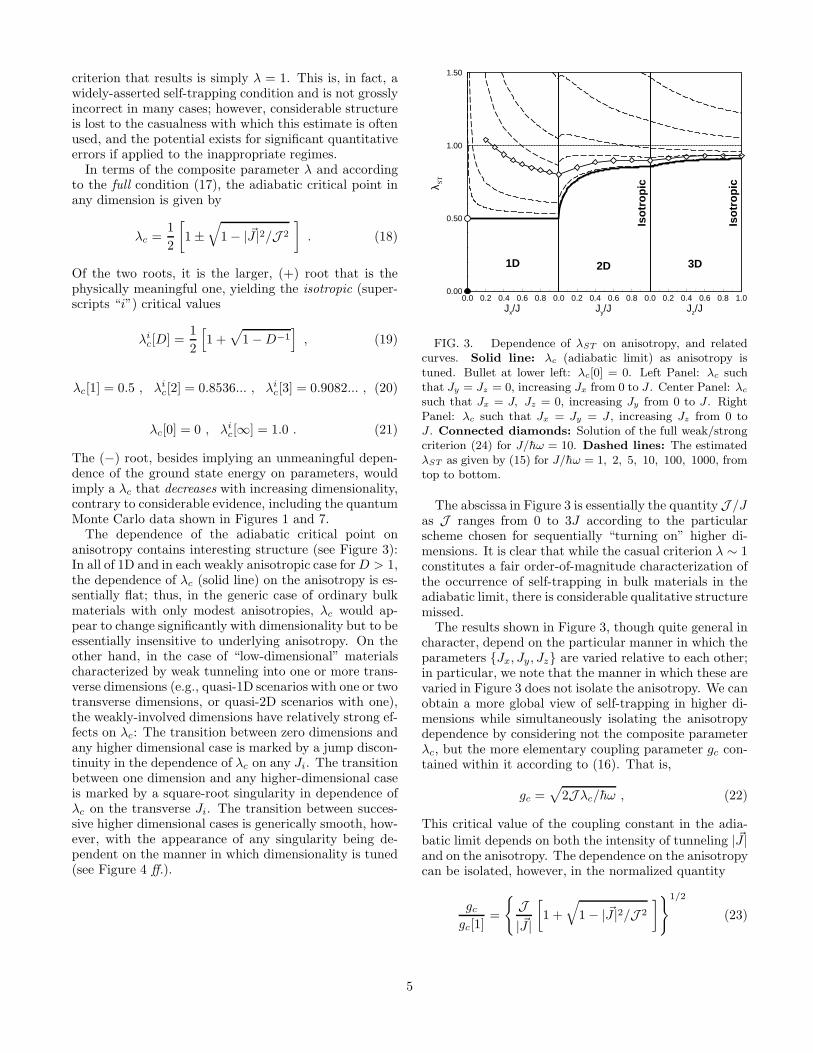
The dependence of the adiabatic critical point onanisotropy contains interesting structure (see Figure 3):In all of 1D and in each weakly anisotropic case for D > 1,the dependence of λc (solid line) on the anisotropy is es-sentially flat; thus, in the generic case of ordinary bulkmaterials with only modest anisotropies, λc would ap-pear to change significantly with dimensionality but to beessentially insensitive to underlying anisotropy. On theother hand, in the case of “low-dimensional” materialscharacterized by weak tunneling into one or more trans-verse dimensions (e.g., quasi-1D scenarios with one or twotransverse dimensions, or quasi-2D scenarios with one),the weakly-involved dimensions have relatively strong ef-fects on λc: The transition between zero dimensions andany higher dimensional case is marked by a jump discon-tinuity in the dependence of λc on any Ji. The transitionbetween one dimension and any higher-dimensional caseis marked by a square-root singularity in dependence ofλc on the transverse Ji. The transition between succes-sive higher dimensional cases is generically smooth, how-ever, with the appearance of any singularity being de-pendent on the manner in which dimensionality is tuned(see Figure 4 ff.).

0.0 0.2 0.4 0.6 0.8Jx/J

0.00

0.50

1.00

1.50

λ ST

0.0 0.2 0.4 0.6 0.8Jy/J

0.0 0.2 0.4 0.6 0.8 1.0Jz/J

Iso

tro

pic

Iso

tro

pic

1D 2D 3D

FIG. 3. Dependence of λST on anisotropy, and relatedcurves. Solid line: λc (adiabatic limit) as anisotropy istuned. Bullet at lower left: λc[0] = 0. Left Panel: λc suchthat Jy = Jz = 0, increasing Jx from 0 to J . Center Panel: λc

such that Jx = J, Jz = 0, increasing Jy from 0 to J . RightPanel: λc such that Jx = Jy = J , increasing Jz from 0 toJ . Connected diamonds: Solution of the full weak/strongcriterion (24) for J/hω = 10. Dashed lines: The estimatedλST as given by (15) for J/hω = 1, 2, 5, 10, 100, 1000, fromtop to bottom.

The abscissa in Figure 3 is essentially the quantity J /Jas J ranges from 0 to 3J according to the particularscheme chosen for sequentially “turning on” higher di-mensions. It is clear that while the casual criterion λ ∼ 1constitutes a fair order-of-magnitude characterization ofthe occurrence of self-trapping in bulk materials in theadiabatic limit, there is considerable qualitative structuremissed.

The results shown in Figure 3, though quite general incharacter, depend on the particular manner in which theparameters Jx, Jy, Jz are varied relative to each other;in particular, we note that the manner in which these arevaried in Figure 3 does not isolate the anisotropy. We canobtain a more global view of self-trapping in higher di-mensions while simultaneously isolating the anisotropydependence by considering not the composite parameterλc, but the more elementary coupling parameter gc con-tained within it according to (16). That is,

gc =√

2J λc/hω , (22)

This critical value of the coupling constant in the adia-

batic limit depends on both the intensity of tunneling | ~J |and on the anisotropy. The dependence on the anisotropycan be isolated, however, in the normalized quantity

gc

gc[1]=

J| ~J |

[

1 +

√

1 − | ~J |2/J 2

]

1/2

(23)

5

in which gc[1] =

√

| ~J/hω| represents the critical cou-

pling parameter in the one-dimensional case subject tothe condition that the 1D tunneling parameter is fixed

at the value | ~J | appropriate to the D-dimensional case.While dependent on each of Jx, Jy, and Jz, the ratio

(23) is independent of | ~J | and depends only on the angu-lar variables in a spherical polar coordinate representa-tion of the Jx, Jy, Jz system. Eq. 23 thus describes asurface having the interpretation that the radial distancefrom the origin is the factor by which the critical couplingconstant gc in D dimensions exceeds the critical value inone-dimension (gc[1]) having the same intensity of tun-neling. This surface is plotted in Figure 4, together withan isotropic (spherical) reference surface, and a surfacecorresponding to the condition λc = const. This lattersurface shows that the oft cited condition λc ∼ 1 containsimplicit anisotropy; however, it is evident that the realanisotropy of self-trapping is even greater than might beinferred from this common rule of thumb.

0

0.5

1

1.5

0 0.5 1 1.5

0

0.5

1

1.5

0

0.5

1

0 0.5 1

FIG. 4. Dependence of self-trapping on anisotropy. TheCartesian axes are the positive half-axes of the Jx, Jy , Jzsystem. The innermost surface is an octant of the unit sphereexhibited as a reference surface reflecting isotropic depen-dence on | ~J | only. The outermost surface is defined such thatthe radial distance from the origin represents the ratio gc/gc[1]as in (23). The interleaved surface is defined such that theradial distance from the origin reflects the anisotropy implicitin the condition λc = const. at fixed | ~J |.

The presentation of λc shown in Figure 3 correspondsto a particular transit of the gc surface seen in Figure 4:The 0D case can be considered to occupy the origin, andthe 1D cases correspond to the three corners of the dis-played surface. The “turning on” of the second dimen-sion according to the scheme of Figure 3 corresponds tomovement along the edge of the displayed surface to themidpoint of that edge corresponding to the 2D isotropic

case. The subsequent “turning on” of the third dimen-sion corresponds to movement perpendicular from thisedge along a straight line (geodesic) to the center of thesurface corresponding to the 3D isotropic case. This com-parison shows in particular (as may be proven analyti-cally): 1) that both the jump discontinuity between 0Dand higher dimensions and the square-root singularitybetween 1D and higher dimensions are generic features,not dependent on the manner or sequence with whichtransverse dimensions are “turned on”, and 2) that theless-singular feature seen in Figure 3 at the transitionfrom 2D to 3D is not generic, but appears only becausedimensions in Figure 3 were turned on sequentially.

Thus, for a given | ~J |, we can distinguish three regimesbased on sensitivity to anisotropy:

g > gic; there are no large polaron states at any degree

of anisotropy.g < gc[1]; there are no small polaron states for any

degree of anisotropy.gc[1] < g < gi

c; large polaron states exist for suf-ficiently isotropic tunneling, small polaron states existfor sufficiently anisotropic tunneling, and these regimesare separated by a self-trapping transition as a function

of anisotropy at fixed | ~J | and g. This effect of self-trapping as a function of anisotropy alone can be un-derstood in terms of the size, shape, and content of thephonon cloud. As discussed in Appendix A, the moreisotropic and higher-dimensional polaron scenarios arecharacterized by phonon clouds that are spread over thelargest volumes of space and contain the fewest num-bers of phonons. With increasing anisotropy, the po-laron cloud grows more compressed, occupying smallervolumes of space, but being occupied by larger numbersof phonons. If this anisotropy-driven compression canproceed sufficiently far, the number of phonons in thephonon cloud can be driven sufficiently high that self-trapping can occur.

IV. SELF-TRAPPING AWAY FROM THE

ADIABATIC STRONG-COUPLING LIMIT

At general parameter values away from extreme limits,accurate estimations of the location of the polaron self-trapping line are scarce. Until rather recently, estimateseven in one dimension were largely casual rules of thumb.As noted above, a frequently-encountered characteriza-tion holds that self-trapping occurs when λ ∼ 1; this con-dition is often supplemented by the condition g > 1 ac-knowledging that the strong-coupling theory from whichthe λ condition arises is not expected to hold to arbitrar-ily weak coupling.

We can improve on the common rule of thumb by iden-tifying the self-trapping transition not with a single fixedvalue of λ (e.g., unity) but with the critical value ob-taining in the adiabatic limit for the particular dimen-

sion and ~J appropriate to each unique circumstance (i.e.,

6

λ ∼ λc). In so doing, we capture all the structure evi-dent in λc (Figures 3 and 4) and make the preliminaryassumption that the scaling relationships that character-ize the adiabatic limit hold to a meaningful degree atmoderate parameter values; i.e, we may consider extrap-olation of critical scaling relationships to finite parametervalues. The implications of such an assumption for theelementary coupling parameter gc are shown in Figure 5.The shifting of these estimated self-trapping lines withanisotropy is a direct reflection of the anisotropy of λc.

0.0 2.0 4.0 6.0 8.0 10.0J/hω

0.0

1.0

2.0

3.0

4.0

5.0

6.0

7.0

8.0

g c

1D

2D

3D

FIG. 5. Dependence of the self-trapping line on anisotropyunder the assumption λST = λc. The bold solid lines corre-spond to the isotropic cases in (from bottom to top) 1D, 2D,and 3D. The textured lines between the 1D and 2D isotropiccases correspond to (from bottom to top) Jx = J , Jz = 0,with Jy = 0.2J, 0.4J, 0.6J , and 0.8J . The textured linesbetween the 2D and 3D isotropic cases correspond to (frombottom to top) Jx = Jy = J , with Jz = 0.2J, 0.4J, 0.6J , and0.8J .

The shifting of these estimated self-trapping lines withanisotropy is a direct reflection of the anisotropy of λc; itis this qualitative character of the mutual relationshipsamong self-trapping curves of differing anisotropies thatwe expect to be largely preserved as necessary correc-tions are made. The need for further correction is ev-ident, for example, in that the 1D example in Figure 5differs substantially in absolute terms from the 1D empir-ical curve (15) although the two are qualitatively quitesimilar. Moreover, all of the curves displayed in Fig-ure 5 violate the ancillary condition g > 1 at small J /hω,reflecting the expected eventual failure of extrapolationfrom the adiabatic strong-coupling regime.

We should be able to improve on this estimate by us-ing a more complete weak/strong condition (24) employ-ing the complete results of both perturbation theoriesthrough second order as given in (7) - (14), thus ob-jectively capturing non-adiabatic corrections implicit inthose terms that do not contribute in the adiabatic limit.Thus we consider the condition

E(0)WC(0) + E

(2)WC(0) = E

(0)SC(0) + E

(1)SC(0) + E

(2)SC(0) .

(24)

This refinement yields estimated self-trapping lines asillustrated by the truncated curves in Figure 6; thesecurves are truncated (arbitrarily at J/hω = 2) becauseintersections of WCPT and SCPT begin to disappear atlower values of J/hω, as can be seen in the 1D panel ofFigure 1.

0.0 1.0 2.0 3.0 4.0 5.0 6.0 7.0 8.0 9.0 10.0J/hω

0.0

1.0

2.0

3.0

4.0

5.0

6.0

7.0

8.0

g

WCPT / SCPT CriteriongST

1D

2D

3D

FIG. 6. Truncated curves show the dependence ofthe self-trapping line on anisotropy using the completeweak/strong condition (24) as a self-trapping criterion; thesecurves are clipped below J/hω = 2 because crossings of weak-and strong-coupling results begin to disappear (see the 1Dcase of Figure 1). The untruncated solid curves are the em-pirical gST of (25) in the isotropic cases of each dimension-ality. The bold solid lines correspond to the isotropic casesin (from bottom to top) 1D, 2D, and 3D. The textured linesbetween the 1D and 2D isotropic cases correspond to (frombottom to top) Jx = J , Jy = 0.2J, 0.4J, 0.6J , and 0.8J , andJz = 0. The textured lines between the 2D and 3D isotropiccases correspond to (from bottom to top) Jx = Jy = J , andJz = 0.2J, 0.4J, 0.6J , and 0.8J .

The effects of including non-adiabatic corrections de-pend on dimensionality, anisotropy, and “distance” fromthe adiabatic limit: 1) The self-trapping curves describ-ing 1D and quasi-1D cases shift strongly to stronger cou-pling values, suggesting a corrective shift of order unity

at essentially all ~J . 2) The self-trapping curves describing2D and 3D cases shift only weakly at moderate adiabatic-ity and more weakly with increasing adiabaticity. 3) Ex-cept for strong corrections in the quasi-1D regime, thequalitative character of the dependence of self-trappingon anisotropy is little affected by non-adiabatic correc-tions. 4) At low adiabaticity, all self-trapping curves shiftto stronger coupling values in a manner and to a degree

consistent with a condition g > 1 at ~J = 0 rather thanthe condition g > 0 suggested by adiabatic scaling.

7

Gathering all the implications of the above together,we are led to extend our 1D empirical curve (15) describ-ing the one-dimensional self-trapping to the general casedescribing any dimension and any degree of anisotropy.To do this we combine: a) the empirical curve gST [1] thateffectually characterizes the one-dimensional case, b) theadiabatic critical curve gc that effectually characterizesthe higher-dimensional, higher-adiabaticity regime, andc) the adiabatic critical parameter λc that compactly de-scribes the qualitatively distinct characteristics of the lowand high dimensionalities.

From such considerations we are led to a family of em-pirical curves

gST ∼ (1 + J /hω)(λc[1]−λc)·(J /| ~J|) + gc (25)

in which all quantities have been previously defined. Thisfamily of curves is not derived from any theory, and,apart from the 1D case, is not backed by a large bodyof independent high-quality data since such data is quitesparse at the present time. What high-quality data doesexist at the present time is quantitatively consistent withthis family of curves in the same fashion that an abun-dance of high-quality 1D data has been found consistentwith gST [1] (see Figures 1 and 7). In keeping with thediscussion of Section II, we have not attempted to regu-larize square root dependences that arise naturally in theadiabatic limit, but which are most likely softened withdecreasing adiabaticity. The utility of (25) lies in com-pactly and simply describing the apparent and mutuallyconsistent trends in a large volume of results of inde-pendent methods and arguments, providing meaningfulestimates for the location of the self-trapping transitionin any dimension for any degree of anisotropy or adia-baticity. This estimated gST is compared with quantumMonte Carlo data for the ground state energy in Figure 1and effective mass in Figure 7.

In Figure 3, we have included several curves (dashedlines) corresponding to λST ≡ g2

ST /2J , using (25) forJ/hω = 1, 2, 5, 10, 100, 1000. These curves indicatehow we expect the physically meaningful self-trappingline at finite parameters as estimated by (25) to be re-lated to the results of the adiabatic limit. Figure 3 showsthat the higher-dimensional, more isotropic cases con-verge toward their adiabatic limits more rapidly than dolower-dimensional, more anisotropic cases. This conver-gence in one dimension is particularly poor, with signif-icant deviations from the adiabatic limit persisting forJ/hω > 1000, by which point the higher-dimensionalcases have converged beyond plotting precision.

Viewed collectively, the dashed curves of Figure 3 alsoshow that the composite parameter λ does not provide avery natural or even qualitatively self-consistent charac-terization of the self-trapping transition over the whole ofthe adiabatic regime (J/hω > 1/4). In the far adiabaticregime, where we may take λc to fairly characterize thelocation of the self-trapping transition (solid curve in Fig-ure 3), one may be led to conclude that large polarons

are relatively more stable in higher dimensions and atweaker anisotropies since the occurrence of self-trappingis found to shift to larger values of λ in these regimes.On the other hand, at more moderate degrees of adia-baticity (e.g., J/hω = 1, 2, 5 in Figure 3) one is led bythe same reasoning to conclude that large polarons arerelatively less stable in higher dimensions and at weakeranisotropies since the occurrence of self-trapping is foundto shift to lower values of λ in these regimes. In partic-ular, one of the most actively-investigated cases in con-temporary studies is the “typical” scenario with J/hω oforder unity; Figure 3 shows that in terms of λ, the self-trapping trends in this case are quite distinct from thosefound in the adiabatic limit, certainly complicating theinterpretation of results.

From Figure 6, on the other hand, based on the moreelementary coupling parameter g appearing directly inthe Hamiltonian, one is led to conclude that large po-larons are everywhere relatively more stable in higherdimensions and at weaker anisotropies since the self-trapping line shifts to larger values of g as these trends arefollowed regardless of the degree of adiabaticity. Thesetrends in g are qualitatively similar and uniform for alldegrees of anisotropy and adiabaticity, whereas the sametrends in λ vary strongly with regime. For the same rea-sons that λ is a convenient parameter with which to char-acterize polarons in the far adiabatic regime, it proves tobe an inconvenient parameter in the broader context ofthe problem away from the adiabatic limit.

V. CORRELATION FUNCTION AND POLARON

RADIUS

In view of the local nature of the electron-phonon cou-pling in the Holstein model, the spatial extent of thepolaron can be characterized quite directly through ananalysis of electron-phonon correlations. This can bedone using a correlation function that has been long andwidely used to characterize polaron size in D dimensions[27,35,32]:

C[D]~r = 〈C [D]

~r 〉 =1

2g

∑

~n

〈a†~na~n(b†~n+~r + b~n+~r)〉 , (26)

normalized such that∑

~r C[D]~r = 1. This function can

be viewed as measuring the shape of the polaron latticedistortion around the instantaneous position of the elec-tron.

Using Rayleigh-Schrodinger perturbation theory in theweak-coupling regime as in the preceeding sections onefinds that [27,35]

C[D]~r = hω

∫ ∞

0

dt e−hωtD∏

i=1

e−2JitIri(2Jit) . (27)

Note that setting any one Ji to zero or summing C[D]~r over

one ri recovers C[D−1]~r . This property implies that the

8

effect of “turning on” transverse dimensions is simply tospread electron-phonon correlation strength transversely.

Characterizing this multi-dimensional correlation func-tion in terms of a width measure involves a variance ten-sor,

σ2

ij=

∑

~r

rirjC[D]~r = δijσ

2ii , (28)

where

σ2ii = hω

∫ ∞

0

dt e−hωt∑

ri

r2i e−2JitIri

(2Jit) (29)

=2Ji

hω=

h

2m0iiω

1

l2i. (30)

in which m0ii is the free electron effective mass and li is

the lattice constant in the i direction. Thus, along eachof the primitive crystallographic axes, the real-space vari-ance is simply proportional to the electron transfer inte-gral along that axis, and in a general direction is justthe appropriate mixture determined by rotation. In ab-solute units (unrationalized by the lattice constants) thereal-space variance is the same as that of the zero-pointmotion of a harmonic oscillator characterized by the lat-tice frequency ω, but with the lattice mass replaced bythe free electron mass measured along the appropriatedirection.

Utilizing the notion of a polaron half-width defined interms of the correlation variance

Ri =li2

√

σ2ii , (31)

we can associate with the polaron characteristic ellip-soidal volumes V [D]

V [1] ∼ 2Rx ∼ lx

(

2Jx

hω

)1/2

∼(

h

2ω

)1/2 (

1

m0ii

)1/2

(32)

V [2] ∼ πRxRy ∼ lxlyπ

4

(

2Jx

hω

2Jy

hω

)1/2

∼ π

4

(

h

2ω

)

(

det M−1

0

)1/2. (33)

V [3] ∼ 4π

3RxRyRz ∼ lxlylz

π

6

(

2Jx

hω

2Jy

hω

2Jz

hω

)1/2

∼ π

6

(

h

2ω

)3/2(

det M−1

0

)1/2. (34)

This characteristic volume thus increases with the inten-sity of tunneling (V [D] ∝ | ~J/hω|D/2), and is largestin the isotropic case and decreases with increasinganisotropy. In the isotropic case we may regard R = Ri

as the polaron radius.

Contrary to much prevailing opinion, these resultsshow that in the weak-coupling regime: i) there are nosignificant qualitative or quantitative differences between1D, 2D, and 3D polaron radii, ii) the polaron radius in2D and 3D is not infinite, and iii) the polaron radiusdoes not scale as J/g2hω in any dimension as commonly

expected, but as√

J/hω in every dimension [27,35,32].

VI. EFFECTIVE MASS

For the circumstances we address in this paper, thereciprocal effective mass tensor is diagonal, with elementsgiven by

M−1

ij= h−2 ∂2E(~κ)

∂κi∂κj

∣

∣

∣

∣

~κ=0

= δij1

mii. (35)

From this, it is easily shown that the reciprocal effec-tive mass in any direction through second order of weak-coupling perturbation theory is given by

m0ii

m∗ii

= 1 − g2h2ω2

∫ ∞

0

dt t e−hωtD∏

i=1

e−2JitI0(2Jit), (36)

where m∗ii and m0

ii are respectively the polaron and freeelectron effective masses in the i direction..

Figure 7 shows the dependence of the isotropic polaronmass on dimensionality according to WCPT and quan-tum Monte Carlo simulation. Although this is a compar-ison between isotropic cases of J/hω = 1 only, the ex-cellent agreement between WCPT and quantum MonteCarlo out to g ∼

√D suggests that the WCPT mass may

be similarly accurate for λ < 1/2 as defined in (16) at

general ~J .

0.0 1.0 2.0 3.0g

0.0

0.2

0.4

0.6

0.8

1.0

m0/

m*

WCPT Global−Local QMCSTT

1D 2D3D

FIG. 7. The reciprocal effective mass ratio m0

ii/m∗

ii forthe isotropic case. Solid curve: Global-Local mass for D = 1.Chain-dashed curves: WCPT masses for D = 1, 2, and 3.Scatter-plot: Quantum Monte Carlo data for D = 1, 2, and 3;data kindly provided by P. E. Kornilovitch [21,22] . Triangles:Estimated self-trapping points gST as discussed in Section IV.

9

The weak-coupling result (36) shows that althoughanisotropy has definite effects on the value of the effectivemass, the effect of anisotropy appears only in the valueof a scalar multipler of the free electron mass; that is,although anisotropy of the free electron mass (inequal-ities among Jx, Jy, and Jz) is manifested in real-spaceanisotropies in electron-phonon correlation (i.e., in dis-tortions of the shape of the polaron as discussed in theprevious section), the mass renormalization associatedwith such distortions of polaron shape is isotropic. In-terestingly, this implies that increasing Jy or Jz at fixedJx (for example) results in a decrease in m∗

xx, translatinginto an associated increase in mobility in the x direc-tion. This influence of transverse directions on m∗

xx isillustrated in Figure 8. In the center and right panels ofFigure 8, Jx/hω is held fixed at unity, yet the effectivemass in the x direction continues to decrease as tunnelinginto transverse dimensions is turned on.

These effects can be understood in terms of the trans-verse spreading of electron-phonon correlation strengthas discussed in the last section. As a fixed correlationstrength is spread over an increasing number of sites(characteristic volume of the polaron increases as dis-cussed in the previous section), the average lattice defor-mation per participating site decreases. Consequently,mean square measures of lattice deformation decreaseand exhibit changes that suggest a diminishing effective-ness of electron-phonon interactions in producing typicalpolaronic effects. The polaronic mass enhancement bearssuch a mean square dependence on the lattice deforma-tion and like other such measures (e.g., the number ofphonons in the phonon cloud as discussed in AppendixA), decreases with increasing dimensionality and decreas-ing anisotropy.

0.0 0.2 0.4 0.6 0.8Jx/J

1.0

1.2

1.4

1.6

1.8

2.0

m* xx

/m0 xx

0.0 0.2 0.4 0.6 0.8Jy/J

0.0 0.2 0.4 0.6 0.8 1.0Jz/J

g=0.5

g=1.0

g=1.5

FIG. 8. The effective mass ratio m∗

xx/m0

xx according to(36), showing the effects of changing anisotropy and dimen-sionality. Left Panel: 1D mass (Jy = Jz = 0) at fixedg, increasing Jx/hω from 0 to 1. Center Panel: 2D mass(Jx/hω, Jz/hω = 0) at fixed g, increasing Jy/hω from 0 to1. Right Panel: 3D mass (Jx/hω = Jy/hω = 1) at fixed g,increasing Jz/hω from 0 to 1.

The corresponding polaron effective mass resultingfrom strong-coupling perturbation theory through sec-ond order is given by

m0ii

m∗ii

= e−g2

+ e−2g2

f(g2)(3Ji + J )/hω . (37)

This result is isotropic at first order simply by virtue ofbeing independent of all Ji at that order, but the second-order correction is anisotropic because the r.h.s. of (37)bears an explicit, unbalanced sensitivity to the directionalong which the effective mass component is being mea-sured.

Unfortunately, this strong-coupling result is not veryhelpful; it disagrees substantially with more reliable re-sults [20–22,31] except at small J/hω. We take this asan indication that dominating (perhaps non-exponential)contributions have yet to be extracted from higher ordersof SCPT. For such reasons we cannot estimate the loca-tion of the self-trapping transition from any crossing of(36) and (37). Instead, we have included in Figure 7 sev-eral symbols to indicate the values of gST as given by(25); these several values are mutually consistent in lo-cating essentially the same feature of the effective massin every dimension, and coincides very well with the ef-fective mass feature we have previously identified withthe self-trapping transition (see Ref. [31]).

VII. ON DIMENSIONALITY AND

ADIABATICITY

As noted in the introduction, the results that havelong characterized commonly-held expectations for thedimensionality dependence of polaron structure are dueto behavior ascertainable in the adiabatic approximation[1–16].

In 2D and 3D, the minimum energy states in theadiabatic approximation are found to be “free” statesthroughout the weak-coupling regime up to a discretecoupling threshold beyond which “self-trapped” stateshave the minimum energy. This abrupt transition phe-nomenon is what is meant by the term “self-trappingtransition” in the adiabatic approximation. Accordingly,there is no occasion to distinguish large polarons fromsmall polarons in 2D and 3D since the “free” states belowthe transition are of infinite radius and distinct from largepolarons, and the “self-trapped” states above the transi-tion are always interpretable as small polarons. This setof circumstances in 2D and 3D is reflected in the catch

10

phrase “all polarons are small”, since in this view largepolarons in the adiabatic sense are never characteristicof the polaron ground state in bulk materials.

In 1D, on the other hand, “free” states are unsta-ble in the adiabatic approximation; instead, finite-radius(i.e. “self-trapped”) states are found at all finite cou-pling strengths, leading to the commonly encounteredview that there is no self-trapping transition in 1D. Thatpolaron states in 1D might be distinguishable as large orsmall is inconsequential in this view, as is the notion ofa resolvable transition between distinct large and smallpolaron structures.

The results of this paper differ strongly from the con-ventional adiabatic picture in multiple respects:

i) The quasiparticles implicit in the weak-couplingstates of every dimension are not weakly-scattered “free”electrons, but dressed electrons having finite radii gener-ally greater than a lattice constant.

ii) Although these weak-coupling quasiparticles can besensibly characterized as large polarons, in no dimensiondo these weak-coupling states coincide with the large po-laron states familiar from the adiabatic approximation in1D.

iii) The finite radii characterizing the weak-couplingquasiparticles in every dimension saturate to finite valueswith vanishing electron-phonon coupling, unlike the largepolaron radii in the adiabatic approximation that in 1Ddiverge with vanishing coupling and in 2D and 3D areinfinite already at finite coupling.

iv) The self-trapping transition exists in every dimen-sion, including 1D.

v) The self-trapping transition is associated with thechange from large polaron structure to small polaronstructure in every dimension, including 2D and 3D, andnot with a change from infinite to finite radii.

vi) Dependences of polaron properties on parametersare smooth through the self-trapping transition in every

dimension, unlike the abrupt changes often found in theadiabatic approximation in 2D and 3D.

Our results are quantitatively supported by indepen-dent high-quality methods (including variational meth-ods [27,30,31,34,36,37], cluster diagonalization [38–41],density matrix renormalization group [20], and quantumMonte Carlo [17–19,21,22,42]). Moreover, elaborationsof adiabatic theory incorporating non-adiabatic correc-tions [11,41,43] support our overall conclusion that theadiabatic approximation as it is widely regarded fails toembrace non-adiabatic characteristics that are essentialto the proper description of polaron states in the weakcoupling regime, and therefore fails as well to properlydescribe the self-trapping transition itself [44].

With so many results at variance with the adiabaticapproximation, it is well to ask in what respects, if any,are our results consistent with the adiabatic approxima-tion and whether some sense can be made of the pervasivediscrepancies. Indeed, several consistencies can be foundthat are illuminating.

We first note that the dependence of λc on dimen-sionality and anisotropy exhibits a generic square-rootsingularity at the boundary between 1D and any higherdimensional case, while at the boundary between higher-dimensional cases this dependence is generically smooth.For essentially the same underlying reasons, λc is con-stant throughout 1D, but varies with detail of tunnel-ing in higher dimensions. These distinctions are at leastsuggestive of the sharp contrasts between 1D and higherdimensional cases in the adiabatic approximation.

Secondly, we note that the weak-coupling polaron ra-dius R as here derived diverges in any dimension in theadiabatic limit. Further considering the WCPT validitytest in Appendix A, there is reason to speculate that thisweak-coupling radius might continue to be a reasonablyvalid construct in 2D and 3D up to the vicinity of theself-trapping transition. Such a possibility might be con-sistent with the finding of strictly infinite-radius stateson the weak-coupling side of the transition in 2D and3D in the adiabatic approximation, while the possiblebreakdown of the weak-coupling radius construct belowthe transition in 1D might be consistent with existenceof finite-width states in the 1D adiabatic approximation.

VIII. CONCLUSION

In this paper we have analyzed the dependence of nu-merous polaron properties on the effective real-space di-mensionality and anisotropy as determined by the elec-tronic tunnelling matrix elements; these properties in-clude the polaron ground state energy, polaron shape,size, and volume, the number of phonons in the phononcloud and the polaron effective mass. In pursuingthese analyses we have made extensive use of weak-and strong-coupling perturbation theories supported byselected comparisons with non-perturbative methods.Through the use of a scaling argument combining weak-and strong-coupling perturbation theory in the adiabaticstrong-coupling regime, we have been able to infer theprobable location of the self-trapping critical point in theadiabatic limit in any dimension and for any degree ofanisotropy, and by combining information from multiplesources we have been able to extend this estimate fromthe adiabatic limit to finite adiabaticity.

Central among our findings is the over-arching qualita-tive conclusion that polarons in any dimension and anydegree of anisotropy are similar in most respects. In par-ticular, polarons on the weak-coupling side of the self-trapping transition share a structure that is essentiallyidentical in every dimension. This weak-coupling struc-ture is consistent with the notion of the weak-couplingpolaron as a finite-radius quasiparticle, but is incon-

sistent both with the notion of a weakly-scattered freeelectron (adiabatic approximation in 2D and 3D) andwith the historical notion of the large polaron (adiabaticapproximation in 1D). The strong-coupling structure is

11

consistent with traditional notions of small polarons, in-cluding strong-coupling perturbation theory and the adi-abatic approximation.

Since the essential character of the weak-couplingstates and strong-coupling states is only inessentially af-fected by dimensionality and anisotropy, the notion of theself-trapping transition separating the weak- and strong-coupling states is similarly not altered in any essentialway by changes in dimensionality or anisotropy. Neces-sarily, one is led to view self-trapping as the more-or-lessrapid transition, occurring in every dimension, betweencharacteristic weak- and strong-coupling states, both ofwhich are characterized by finite radii.

If we may transcend the jargon that historically hashad a tendency to polarize the conventional wisdom, itis fairly concluded that not all polarons are small, evenin bulk materials, and that in every dimension and forevery degree of anisotropy the self-trapping transition isa smooth, albeit rapid crossover between large and smallpolaron character.

ACKNOWLEDGEMENT

The authors gratefully acknowledge P. Kornilovitch forproviding the quantum Monte Carlo data used in Fig-ures 1 and 7. This work was supported in part by theU.S. Department of Energy under Grant No. DE-FG03-86ER13606.

APPENDIX A: BREAKDOWN OF

WEAK-COUPLING PERTURBATION THEORY

The weak-coupling perturbation theory considered inthis paper is based on an expansion in states contain-ing limited numbers of phonon quanta. The zeroth or-der properties are based upon states containing zerophonons, and second order properties upon states con-taining one phonon. The first neglected order of WCPTis the fourth order, built upon states containing no morethan two phonons. A test of internal consistency ofWCPT at particular parameters, therefore, is to com-pute the expected number of phonons to the retainedorder of perturbation theory, and compare this numberto the maximum number of phonons present at that or-der. For second order WCPT as used in this paper, thisnumber of phonons should be less than unity.

The required computation is contained in

nph =1

N

∑

~q

g2hω

E(0)WC(0) − [E

(0)WC(−~q) + hω]2

, (A1)

where E(0)WC(~κ) is defined in (9). When each Ji is large

relative to hω, one finds that

nph ∼ 1

4g2

(

Jx

hω

)−1/2

in 1D , (A2)

∼ 1

πg2

(

JxJy

h2ω2

)−1/2

in 2D , (A3)

∼ 1

πg2

(

JxJyJz

h3ω3

)−1/2

in 3D . (A4)

These expressions can be consolidated into the single ap-proximate relation

nph ∝ g2 Ω[D]

V [D], (A5)

where Ω[D] is the primitive cell volume and V [D] thecharacteristic volume of the polaron in D dimensions.The dimension-dependent constant of proportionality isnear 1/2 in all cases. This simple relation, here provenonly for the adiabatic weak-coupling regime (broad po-larons), demonstrates the very direct but inverse relationbetween the number of phonons in the phonon cloud andthe volume occupied by it.

In the isotropic case and in terms of the compositeparameter λ, the condition that expected phonon num-bers should be less than unity results in the conditions(J ≫ hω)

λ < 2

(

J

hω

)−1/2

in 1D , (A6)

<π

4in 2D , (A7)

<π

6

(

J

hω

)1/2

in 3D . (A8)

Recalling that the self-trapping transition is expectedto occur at λ of order unity, it would appear that WCPTthrough second order is consistent with the conditionnph < 1 up to the transition in 2D and beyond the tran-sition in 3D. It is the 1D case that appears to be on theweakest footing in the adiabatic strong-coupling regime;however, it is the 1D case that has been most exhaus-tively studied by non-perturbative means and found tobe widely consistent with second-order WCPT.

[1] E. I. Rashba, Opt. Spektrosk. 2, 75 (1957).[2] E. I. Rashba, Opt. Spektrosk. 2, 88 (1957).[3] T. Holstein, Ann. Phys. (N.Y.) 8, 325 (1959).[4] G. H. Derrick, J. Math. Phys. 5, 1252 (1962).[5] D. Emin, Adv. Phys. 22, 57 (1973).[6] A. Sumi and Y. Toyozawa, J. Phys. Soc. Japan 35, 137

(1973).[7] D. Emin and T. Holstein, Phys. Rev. Lett. 36, 323

(1976).

12

[8] Y. Toyozawa and Y. Shinozuka, J. Phys. Soc. Jap. 48,472 (1980).

[9] H. B. Schuttler and T. Holstein, Ann. Phys. (N.Y.) 166,93 (1986).

[10] M. Ueta, H. Kanzaki, K. Kobayashi, Y. Toyozawa, andE. Hanamura, Excitonic Processes in Solids (Springer-Verlag, Berlin, 1986).

[11] V. V. Kabanov and O. Y. Mashtakov, Phys. Rev. B 47,6060 (1993).

[12] E. A. Silinsh and V. Capek, Organic Molecular Crys-

tals: Interaction, Localization and Transport Phenomena

(AIP-Press, New York, 1994).[13] K. S. Song and R. T. Williams, Self-Trapped Excitons

(Springer Verlag, Berlin, 1996).[14] T. Holstein, Mol. Cryst. Liq. Cryst. 77, 235 (1981).[15] T. Holstein and L. Turkevich, Phys. Rev. B 38, 1901

(1988).[16] T. Holstein and L. Turkevich, Phys. Rev. B 38, 1923

(1988).[17] H. D. Raedt and A. Lagendijk, Phys. Rev. B 27, 6097

(1983).[18] H. D. Raedt and A. Lagendijk, Phys. Rev. B 30, 1671

(1984).[19] A. Lagendijk and H. D. Raedt, Phys. Lett. A 108A, 91

(1985).[20] E. Jeckelmann and S. R. White, Phys. Rev. B 57, 6376

(1998).[21] P. E. Kornilovitch, Phys. Rev. Lett. 81, 5382 (1998).[22] P. E. Kornilovitch, private communication (1999).[23] T. Holstein, Ann. Phys. (N.Y.) 8, 343 (1959).[24] A. S. Alexandrov and S. N. Mott, Polarons & Bipolarons

(World Scientific, London, 1995).[25] S. Nakajima, Y. Toyozawa, and R. Abe, The Physics of

Elementary Excitations (Springer-Verlag, Berlin, 1980).[26] G. D. Mahan, Many-Particle Physics (Plenum Press,

New York, 1993).[27] A. H. Romero, Ph.D. thesis, University of California, San

Diego, 1998.[28] F. Marsiglio, Physica C 244, 21 (1995).[29] W. Stephan, Phys. Rev. B 54, 8981 (1996).[30] A. H. Romero, D. W. Brown, and K. Lindenberg, Phys.

Rev. B 60, 4609 (1999).[31] A. H. Romero, D. W. Brown, and K. Lindenberg, Phys.

Rev. B 59, 13728 (1999).[32] A. H. Romero, D. W. Brown, and K. Lindenberg, cond-

mat 9905174 (1999).[33] A. H. R. David W. Brown and K. Lindenberg, submitted

to J. Phys. Chem. cond (1999).[34] A. H. Romero, D. W. Brown, and K. Lindenberg, J.

Chem. Phys. 109, 6540 (1998).[35] A. H. Romero, D. W. Brown, and K. Lindenberg, Phys.

Lett. A 254, 287 (1999).[36] D. W. Brown, K. Lindenberg, and Y. Zhao, J. Chem.

Phys. 107, 3179 (1997).[37] S. A. Trugman and J. Bonca, J. Supercon. 12, 221 (1999).[38] M. Capone, W. Stephan, and M. Grilli, Phys. Rev. B 56,

4484 (1997-II).[39] G. Wellein and H. Fehske, Phys. Rev. B 56, 4513 (1997).[40] E. V. L. de Mello and J. Ranninger, Phys. Rev. B 55,

14872 (1997).

[41] A. S. Alexandrov, V. V. Kabanov, and D. E. Ray, Phys.Rev. B 49, 9915 (1994).

[42] A. S. Alexandrov and P. E. Kornilovitch, Phys. Rev. Lett.82, 807 (1998).

[43] V. V. Kabanov and D. K. Ray, Phys. Lett. A 186, 438(1994).

[44] A. H. Romero, D. W. Brown, and K. Lindenberg, MRSSymp. Proc. XX, to appear (1998).

13