VARCLUST: clustering variables using dimensionality reduction

Piotr Sobczyk∗ Stanisªaw Wilczy«ski† Maªgorzata Bogdan‡� Piotr Graczyk¶

Julie Josse ‖ Fabien Panloup¶∗∗ Valérie Seegers †† Mateusz Staniak ‡‡‡

December 17, 2020

Abstract

VARCLUST algorithm is proposed for clustering variables under the assumption that vari-ables in a given cluster are linear combinations of a small number of hidden latent variables,corrupted by the random noise. The entire clustering task is viewed as the problem of selectionof the statistical model, which is de�ned by the number of clusters, the partition of variablesinto these clusters and the 'cluster dimensions', i.e. the vector of dimensions of linear subspacesspanning each of the clusters. The �optimal� model is selected using the approximate Bayesiancriterion based on the Laplace approximations and using a non-informative uniform prior onthe number of clusters. To solve the problem of the search over a huge space of possible mod-els we propose an extension of the ClustOfVar algorithm of [36, 7], which was dedicated tosubspaces of dimension only 1, and which is similar in structure to the K-centroids algorithm.We provide a complete methodology with theoretical guarantees, extensive numerical experi-mentations, complete data analyses and implementation. Our algorithm assigns variables toappropriate clusterse based on the consistent Bayesian Information Criterion (BIC), and esti-mates the dimensionality of each cluster by the PEnalized SEmi-integrated Likelihood Criterion(PESEL) of [29], whose consistency we prove. Additionally, we prove that each iteration of ouralgorithm leads to an increase of the Laplace approximation to the model posterior probabilityand provide the criterion for the estimation of the number of clusters. Numerical comparisonswith other algorithms show that VARCLUST may outperform some popular machine learningtools for sparse subspace clustering. We also report the results of real data analysis includingTCGA breast cancer data and meteorological data, which show that the algorithm can lead tomeaningful clustering. The proposed method is implemented in the publicly available R packagevarclust.

Keywords� subspace clustering, dimensionality reduction, principal components analysis,Bayesian Information Criterion, k-centroids

∗OLX group in Poland†Microsoft Development Center, Oslo, Norway‡Institute of Mathematics, University of Wrocªaw, Poland�Department of Statistics, Lund University, Sweden¶Laboratoire Angevin de Recherche en Mathématiques (LAREMA), Université d'Angers, France‖INRIA Montpellier and Ecole Polytechnique in Paris, France∗∗SIRIC ILIAD, Nantes, Angers, France††ICO Angers, France‡‡Department of Computer Science, Northeastern University, USA

1

1 Introduction

Due to the rapid development of measurement and computer technologies, large data bases are nowa-days stored and explored in many �elds of industry and science. This in turn triggered developmentof new statistical methodology for acquiring information from such large data.

In large data matrices it usually occurs that many of the variables are strongly correlated and infact convey a similar message. Principal Components Analysis (PCA) [25, 16, 17, 19] is one of themost popular and powerful methods for data compression. This dimensionality reduction methodrecovers the low dimensional structures spanning the data. The mathematical hypothesis which isassumed for this procedure is based upon the belief that the denoised data matrix is of a low rank,i.e. that the data matrix Xn×p can be represented as

X = M + µ+ E, (1.1)

where M is deterministic, rank(M)� min(n, p), the mean matrix µ is rank one and the matrix Erepresents a centered normal noise.

Thus, PCA model assumes that all data points come from the same low dimensional space, whichis often unrealistic. Fortunately, in many unsupervised learning applications it can be assumed thatthe data can be well approximated by a union of lower dimensional manifolds. One way to analyzesuch data is to apply the nonlinear data projection techniques (see [22]). Another approach is tocombine local linear models, which can often e�ectively approximate the low dimensional manifolds(see e.g., [15]). Therefore, in recent years we have witnessed a rapid development of machinelearning and statistical technoques for subspace clustering (see [34], [31] and references therein),i.e. for clustering the data into multiple low dimensional subspaces. As discussed in [31] thesetechniques have been successfully used in �elds as diverse as computer vision (see e.g, [11, 12]),identi�cation and classi�cation of diseases [23] or music analysis [20], to name just a few.

The most prominent statistical method for subspace clustering is the mixture of probabilisticprincipal component analyzers (MPPCA) [33]. The statistical model of MPPCA assumes that therows of the data matrix are independent identically distributed random vectors from the mixture ofmultivariate gaussian distributions with the low rank covariance matrices. The mixture parametersare usually estimated using the Expectation Maximization algorithm, which is expected to workwell when n >> p.

In this paper we propose a more direct approach for subspace clustering, where the �xed e�ectsmodel (1.1) is applied separately for each cluster. The statistical model for the whole data base isdetermined by the partition of variables into di�erent clusters and the vector of dimensions (ranksof the correspondingM matrices) for each of the clusters. Our approach allows for creating clusterswith the number of variables substantially larger than n.

The optimal subspace clustering model is identi�ed through the modi�ed Bayesian InformationCriterion, based on the Laplace approximations to the model posterior probability. To solve theproblem of the search over a huge space of possible models we propose in Section 2 a VARCLUSTalgorithm, which is based on a novel K-centroids algorithm, made of two steps based on twodi�erent Laplace approximations. In the �rst step, given a partition of the variables, we use PESEL[29], a BIC-type estimator, to estimate the dimensions of each cluster. Cluster centroids are thenrepresented by the respective number of principal components. In the second step we perform thepartition where the similarity between a given variable and cluster centroid is measured by theBayesian Information Criterion in the corresponding multiple regression model. From a theoreticalpoint of view, we prove in Section 4 the consistency of PESEL, i.e. the convergence of the estimatorof the cluster dimension towards its true dimension (see Theorem 1). For the VARCLUST itself, weshow that our algorithm leads to an increase of the Laplace approximation to the model posterior

2

probability(see Corollary 2). From a numerical point of view, our paper investigates numerous issuesin Section 5. The convergence of VARCLUST is empirically checked and some comparisons withother algorithms are provided showing that the VARCLUST algorithm seems to have the ability toretrieve the true model with an higher probability than other popular sparse subspace clusteringprocedures. Finally, in Section 6, we consider two important applications to breast cancer andmeteorological data. Once again, in this part, the aim is twofold: reduction of dimension but alsoidenti�cation of groups of genes/indicators which seem to take action together. In Section 7, the Rpackage varclust which uses parallel computing for computational e�ciency is presented and itsmain functionalities are detailed.

2 VARCLUST model

2.1 A low rank model in each cluster

Let Xn×p be the data matrix with p columns x•j ∈ Rn, j ∈ {1, . . . , p}. The clustering of p variablesx•j ∈ Rn into K clusters consists in considering a column-permuted matrix X ′ and decomposing

X ′ =[X1|X2| . . . |XK

](2.1)

such that each bloc Xi has dimension n × pi, with∑K

i=1 pi = p. In this paper we apply to eachcluster Xi the model (1.1):

Xi = M i + µi + Ei, (2.2)

where M i is deterministic, rank(M i) = ki � min(n, pi), the mean matrix µi is rank one and thematrix Ei represents the centered normal noise N(0, σ2

i Id).As explained in [29], the form of the rank one matrix µi depends on the relation between n and

pi. When n > pi, the n rows of the matrix µi are identical, i.e. µi =

ri

...

ri

where ri = (µi1, . . . , µipi).

If n ≤ pi, the pi columns of the matrix µi are identical, i.e. µi =

(ci . . . ci

)with ci = (µi1, . . . , µ

in)>.

We point out that our modeling allows some clusters to have pi ≥ n, whereas in other clusters pimaybe smaller than n. This �exibility is one of important advantages of the VARCLUST model.

Next we decompose each matrix M i, for i = 1, . . . ,K, as a product

M i = F in×kiCiki×pi (2.3)

The columns of Fn×ki are linearly independent and will be called factors (by analogy to PCA).

This model extends the classical model (1.1) for PCA, which assumes that all variables in thedata set can be well approximated by a linear combination of just a few hidden �factors�, or, inother words, the data belong to a low dimensional linear space. Here we assume that the datacomes from a union of such low dimensional subspaces. This means that the variables (columns ofthe data matrix X) can be divided into clusters Xi, each of which corresponds to variables fromone of the subspaces. Thus, we assume that every variable in a single cluster can be expressed as alinear combination of small number of factors (common for every variable in this cluster) plus some

3

noise. This leads to formulas (2.2) and (2.3). Such a representation is clearly not unique. Thegoal of our analysis is clustering columns in X and in M , such that all coe�cients in the matricesC1, . . . , CK are di�erent from zero and

∑Ki=1 ki is minimized.

Let us summarize the model that we study. An element of M is de�ned by four parameters(K,Π,~k,Pθ) where:

• K is the number of clusters and K ≤ Kmax for a �xed Kmax � p,

• Π is a K-partition of {1, . . . , p} encoding a segmentation of variables (columns of the datamatrix Xn×p) into clusters Xi

n×pi =: XΠi ,

• ~k = (k1, . . . , kK) ∈ {1, . . . , d}⊗K , where d is the maximal dimension of (number of factors in)a cluster. We choose d� n and d� p.

• Pθ is the probability law of the data speci�ed by the vectors of parameters θ = (θ1, . . . , θK),with θi containing the factor matrix F i, the coe�cient matrix Ci, the rank one mean matrixµi and the error variance σ2

i ,

Pθ(X) =K∏i=1

P (XΠi |θi)

and P (XΠi |θi) is de�ned as follows: let xi•j be the j-th variable in the i-th cluster and let

µi•j be the j-th column of the matrix µi. The vectors xi•j , j = 1, . . . , pi, are independentconditionally on θi and it holds

xi•j |θi = xi•j |(F i, Ci, µi, σ2i ) ∼ N(F ici•j + µi•j , σ

2i In) . (2.4)

Note that according to the model (2.4), the vectors xi•j |θi, j = 1, . . . , ki, in the same cluster Xi

have the same covariance matrices σ2i In.

2.2 Bayesian approach to subspace clustering

To select a model (number of clusters, variables in a cluster and dimensionality of each cluster), weconsider a Bayesian framework. We assume that for any modelM the prior π(θ) is given by

π(θ) =

K∏i=1

π(θi) .

Thus, the log-likelihood of the data X given the modelM is given by

ln (P(X|M)) = ln

(∫ΘP(X|θ)π(θ)dθ

)= ln

K∏i=1

(∫Θi

P(Xi|θi)π(θi)dθi

)

=

K∑i=1

ln

(∫Θi

P(Xi|θi)π(θi)dθi

)

=

K∑i=1

ln(P(Xi|Mi)

), (2.5)

4

whereMi is the model for the i-th cluster Xi speci�ed by (2.3) and (2.4).In our approach we propose an informative prior distribution onM. The reason is that in our

case we have, for given K, roughly Kp di�erent segmentations, where p is the number of variables.Moreover, given a maximal cluster dimension d = dmax, there are d

K di�erent selections of clusterdimensions. Thus, given K, there are approximately KpdK di�erent models to compare. Thisnumber quickly increases with K and assuming that all models are equally likely we would in factuse a prior on the number of clusters K, which would strongly prefer large values of K. Similarproblems were already observed when using BIC to select the multiple regression model based ona data base with many potential predictors. In [5] this problem was solved by using the modi�edversion of the Bayes Information Criterion (mBIC) with the informative sparsity inducing prioron M. Here we apply the same idea and use an approximately uniform prior on K from the setK ∈ {1, . . . ,Kmax}, which, for every modelM with the number of clusters K, takes the form:

π(M) =C

KpdK

ln(π(M)) = −p ln(K)−K ln(d) + C , (2.6)

where C is a proportionality constant, that does not depend on the model under consideration.Using the above formulas and the Bayes formula, we obtain the following Bayesian criterion for themodel selection: pick the model (partition Π and cluster dimensions ~k) such that

ln(P(M|X)) = ln(P(X|M)) + ln(π(M))− ln(P(X))

=K∑i=1

lnP(Xi|Mi)− p ln(K) (2.7)

−K ln(d) + C − lnP(X) .

obtains a maximal value. Since P(X) is the same for all considered models this amounts to selectingthe model, which optimizes the following criterion

C(M|X) =

K∑i=1

lnP(Xi|Mi)− p ln(K)−K ln(d) . (2.8)

The only quantity left to calculate in the above equation is P(Xi|Mi).

3 VARCLUST method

3.1 Selecting the rank in each cluster with the PESEL method

Before presenting the VARCLUST method, let us present shortly the PESEL method, introducedin [29] designed to estimate the number of principal components in PCA. It will be used in the �rststep of the VARCLUST.

As explained in Section 2 (cf. (2.4)), our model for one cluster can be described by its setof parameters (for simplicity we omit the index of the cluster) θ : F ∈ Rn×k, c1, . . . , cp, whereci ∈ Rk×1 (vectors of coe�cients), σ2 and µ. In order to choose the best model we have to considermodels with di�erent dimensions, i.e. di�erent values of k. The penalized semi-integrated likelihood(PESEL, [29]) criterion is based on the Laplace approximation to the semi-integrated likelihood andin this way it shares some similarities with BIC. The general formulation of PESEL allows for usingdi�erent prior distributions on F (when n > p) or C (when p > n). The basic version of PESEL

5

uses the standard gaussian prior for the elements of F or C and has the following formulation,depending on the relation between n and p.

We denote by (λj)j=1,...,p the non-increasing sequence of eigenvalues of the sample covariancematrix Sn. When n ≤ p we use the following form of the PESEL

ln(P(Xi|Mi)) ≈ PESEL(p, k, n) =

− p

2

k∑j=1

ln(λj) + (n− k) ln

1

n− k

n∑j=k+1

λj

+ n ln(2π) + n

− ln(p)

nk − k(k+1)2 + k + n+ 1

2(3.1)

and when n > p we use the form

ln(P(Xi|Mi)) ≈ PESEL(n, k, p) =

− n

2

k∑j=1

ln(λj) + (p− k) ln

1

p− k

p∑j=k+1

λj

+ p ln(2π) + p

− ln(n)

pk − k(k+1)2 + k + p+ 1

2. (3.2)

The function of the eigenvalues λj of Sn appearing in (3.1),(3.2) and approximating the log-likelihood P(Xi|Mi) is called a PESEL function. The criterion consists in choosing the value of kmaximizing the PESEL function.

When n > p, the above form of PESEL coincides with BIC in Probabilistic PCA (see [24]) orthe spiked covariance structure model. These models assume that the rows of the X matrix arei.i.d. random vectors. Consistency results for PESEL under these probabilistic assumptions can befound in [2].

In Section 4.1 we will prove consistency of PESEL under a much more general �xed e�ects model(4.1), which does not assume the equality of laws of rows in X.

3.2 Membership of a variable in a cluster with the BIC criterion

To measure the similarity between lth variable and a subspace corresponding to ith cluster we usethe Bayesian Information Criterion. Since the model (2.4) assumes that all elements of the errormatrix Ei have the same variance, we can estimate σ2

i by MLE

σ2i =

∑`∈Πi‖x•` − Pi(x•`)‖2

npi,

where Pi(x•`) denotes the orthogonal projection of the column x•` on the linear space correspondingto the ith cluster and next use BIC of the form

BIC(l, i) =1

2

(−‖x•` − Pi(x•`)‖

2

σ2i

− lnnki

). (3.3)

As an alternative, one can consider a standard multiple regression BIC, which allows for di�erentvariances in di�erent columns of Ei:

BIC(l, i) = −n ln

(RSSlin

)− ki ln(n), (3.4)

where RSSli is the residual sum of squares from regression of x•` on the basis vectors spanning ith

cluster.

6

3.3 VARCLUST algorithm

Initialization and the �rst step of VARCLUST Choose randomly a K-partition of p =p0

1 + . . .+ p0K and group randomly p0

1, . . . , p0K columns of X to form Π0.

Then, VARCLUST proceeds as follows:

Π0 → (Π0, k0) → (Π1, k0) , (3.5)

where k0 is computed by using PESEL K times, separately to each matrix Xi0, i = 1, . . . ,K. Next,

for each matrix Xi0, PCA is applied to estimate k0

i principal factors F 1i , which represent the basis

spanning the subspace supporting ith cluster and the center of the clusters. The next partition Π1

is obtained by using BIC(l, i) as a measure of similarity between lth variable and ith cluster toallocate each variable to its closest cluster. After the �rst step of VARCLUST, we get the couple:the partition and the vector of cluster dimensions (Π1, k0).

Other schemes of initialization can be consider such as a one-dimensional initialization. Chooserandomly K variables which will play the role of one dimensional centers of K clusters . Distribute,by minimizing BIC, the p columns of X to form the �rst partition Π1. In this way, after the �rststep of VARCLUST we again get (Π1, k0), where k0 is the K dimensional all ones vector.

Step m+ 1 of VARCLUST In the sequel we continue by �rst using PESEL to calculate a newvector of dimensions and next PCA and BIC to obtain the next partition:

(Πm, km−1) → (Πm, km) → (Πm+1, km).

4 Theoritical guarentees

In this Section we prove the consistency of PESEL and show that each iteration of VARCLUSTasymptotically leads to an increase of the objective function (2.8).

4.1 Consistency of PESEL

In this section we prove that PESEL consistently estimates the rank of the denoised data matrix.The consistency holds when n or p diverges to in�nity, while the other dimension remains constant.This result can be applied separately to each cluster Xi, i ∈ {1, . . . ,K}, of the full data matrix.

First, we prove the consistency of PESEL (Section 3.1) when p is �xed as n→∞.

Assumption 1. Assume that the data matrix X is generated according to the following proba-bilistic model :

Xn×p = Mn×p + µn×p + En×p, (4.1)

where

• for each n ∈ N, matrices Mn×p and µn×p are deterministic

• µn×p is a rank-one matrix in which all rows are identical, i.e. it represents average variablee�ect.

• the matrix Mn×p is centered:∑n

i=1Mij = 0 and rank(Mn×p) = k0 for all n ≥ k0

7

• the elements of matrix Mn×p are bounded: supn,i∈(1,...,n),j∈(1,...,p) |Mij | <∞

• there exists the limit: limn→∞1nM

Tn×pMn×p = L and, for all n∣∣∣∣∣ 1nMT

n×pMn×p − L

∣∣∣∣∣ < C

√2 ln lnn√

n, (4.2)

where C is some positive constant and L = UDp×pUT with

Dp×p =

diag[γi]k0i=1 0

0 diag[0]

with non-increasing γi > 0 and UTU = Idp×p.

• the noise matrix En×p consists of i.i.d. terms eij ∼ N (0, σ2).

Theorem 1 (Consistency of PESEL). Assume that the data matrix Xn×p satis�es the Assumption

1. Let k0(n) be the PESEL(p, k, n) estimator of the rank of M .Then, for p �xed, it holds

P(∃n0 ∀n > n0 k0(n) = k0) = 1.

Scheme of the Proof.Let us consider the sample covariance matrix

Sn =(X − X)T (X − X)

n.

and the population covariance matrix Σn = E (Sn). The idea of the proof is the following.Let us denote by F (n, k) the PESEL function in the case when n > p. By (3.2), we have

F (n, k) =

− n

2

[ k∑j=1

ln(λj) + (p− k) ln

1

p− k

p∑j=k+1

λj

+ p ln(2π) + p

]− ln(n)

pk − k(k+1)2 + k + p+ 1

2

The proof comprises two steps. First, we quantify the di�erence between eigenvalues of matricesSn, Σn and L. We prove it to be bounded by the matrix norm of their di�erence, which goes to 0

at the pace√

ln lnn√n

as n grows to in�nity, because of the law of iterated logarith (LIL). We use the

most general form of LIL from [26]. Secondly, we use the results from the �rst step to prove that forsu�ciently large n the PESEL function F (n, k) is increasing for k < k0 and decreasing for k > k0.To do this, the crucial Lemma 1 is proven and used. The detailed proof is given in Appendix 9.

Since the version of PESEL for p >> n, PESEL(n, k, p), is obtained simply by applying PE-SEL(p,k,n) to the transposition of X, Theorem 1 implies the consistency of PESEL also in thesituation when n is �xed, p→∞ and the transposition of X satis�es the Assumption 1.

8

Corollary 1. Assume that the transposition of the data matrix Xn×p satis�es the Assumption 1.

Let k0(n) be the PESEL(n, k, p) estimator of the rank of M .Then, for n �xed, it holds

P(∃p0 ∀p > p0 k0(p) = k0) = 1.

Remark 1. The above results assume that p or n is �xed. We believe that they hold also in thesituation when n

p → ∞ or vice versa. The mathematical proof of this conjecture is an interestingtopic for a further research. These theoretical results justify the application of PESEL when n >> por p >> n. Moreover, simulation results reported in [29] illustrate good properties of PESEL alsowhen p ∼ n. The theoretical analysis of the properties of PESEL when p/n → C 6= 0 remains aninteresting topic for further research.

4.2 Convergence of VARCLUST

As noted above in (2.8), the main goal of VARCLUST is identifying the modelM which maximizes,for a given dataset X,

ln(P(M|X)) =

K∑i=1

lnP(Xi|ki) + ln(π(M)) ,

where ln(π(M)) depends only on the number of clusters K and the maximal allowable dimensionof each cluster d.

Since, given the number of clustersK, the VARCLUST model is speci�ed by the vector of clusterdimensions k = (k1, . . . , kK) and a partition Π = (Π1, . . . ,ΠK) of p variables into these K clusters,our task reduces to identifying the model for which the following objective function

ϕ(Π, k) :=

K∑i=1

lnP(Xi|ki) , (4.3)

obtains a maximum.Below we will discuss consecutive steps of the VARCLUST Algorithm with respect to the opti-

mization of (4.3). Recall that the m+ 1 step of VARCLUST is

(Πm, km−1) → (Πm, km) → (Πm+1, km),

where we �rst use PESEL to estimate the dimension and next PCA to compute the factors andBIC to allocate variables to a cluster.

1. PESEL step: choice of cluster dimensions, for a �xed partition of X.

First, observe that the dimension of ith cluster in the next (m + 1)th step of VARCLUST isobtained as

kmi = arg maxki∈{1,...,d}

PESEL(Xi|ki) .

Thus, denoting by PESEL the PESEL function from (3.1) and (3.2),

K∑i=1

PESEL(Xim|kmi ) ≥

K∑i=1

PESEL(Xim|km−1

i ) .

9

Now, observe that under the standard regularity conditions for the Laplace approximation(see e.g. [4])

lnP(Xi|ki) = PESEL(Xi|ki) +On(1)

when n→∞ and pi is �xed and

lnP(Xi|ki) = PESEL(Xi|ki) +Opi(1)

when pi →∞ and n is �xed (see [29]). Thus,

ϕ(Π, k) =K∑i=1

PESEL(Xi|ki) +R ,

where the ratio of R over∑K

i=1 PESEL(Xi|ki) converges to zero in probability, under ourasymptotic assumptions.

Therefore, the �rst step of VARCLUST leads to an increase of ϕ(Π, k) up to Laplace approx-imation, i.e. with a large probability when for all i ∈ {1, . . . ,K}, n >> pi or pi >> n.

2. PCA and Partition step: choice of a partition, with cluster dimensions kmi �xed.

In the second step of the m + 1-st iteration of VARCLUST, the cluster dimensions kmi are�xed, PCA is used to compute the cluster centers F i and the columns of X are partitioned todi�erent clusters by minimizing the BIC distance from F i.

Below we assume that the priors πC(dC) and π(dσ) satisfy classical regularity conditions forLaplace approximation ([4]). Now, let us de�ne the kmi �dimensional linear space through theset of respective directions F i = (F i1, . . . , F

iki

) with, as a natural prior, the uniform distributionπF on the compact Grassman manifold F of free ki-systems of Rn. Moreover, we assumethat the respective columns of coe�cients Ci = (Ci1, . . . , C

iki

) are independent with a priordistribution πC on Rp.It holds

logP(Xi|ki) = log

∫F×σ

∫CP(Xi|F i, Ci, σi)

π(dCi)π(dσi)πF (dF i)

= log

∫F×σ

∏`∈Πi

∫P(X•`|F i, C•`)

πC(dC•`)π(dσi)πF (dF i).

When n� ki, a Laplace-approximation argument leads to∫P(X•`|F i, C•`)πC(dC•`) ≈ eBIC`|Fi,σi

where

BIC`|Fi, σi =1

2

(−‖x•` − Pi(x•`)‖

2

σ2i

− kilnn).

Thus, thanks to the Laplace approximation above,

logP(Xi|ki)

≈ log

∫F i×σi

e∑

`∈Πi BIC`|Fi,σiπ(dσi)πF (dF i) (4.4)

10

and

K∑i=1

logP(Xi|ki)

≈ log

∫F×σ

e∑K

i=1

∑`∈Πi BIC`|Fi,σiπ(dσ)πF (dF ) . (4.5)

Now, by Laplace approximation, when pi >> ki, the right-hand side of (4.5) can be approxi-mated by

ψ(Π|k)−K∑i=1

dimFi + 1

2lnn, (4.6)

where we denote

ψ(Π|k) = max(F,σ)ξ(Π, F, σ|k), (4.7)

ξ(Π, F, σ|k) =

K∑i=1

∑`∈Πi

(−‖x•` − Pi(x•`)‖

2

σ2i

− lnnki

). (4.8)

Now, the term lnn∑K

i=1dimFi+1

2 in (4.6) is the same for each Π, so increasing (4.5) is equiv-alent to increasing ψ(Π|k).

Now, due to the well known Eckhart-Young theorem, for each i ∈ {1, . . . ,K}, the �rst kiprincipal components of Xi form the basis for the linear space �closest� to Xi, i.e. the PCApart of VARCLUST allows to obtain Fm and σm, such that

(Fm, σm|Πm, km) = argmaxF,σξ(Πm, F, σ|km) .

Thus ψ(Πm|km) = ξ(Πm, Fm, σm|km).

Finally, in the Partition (BIC) step of the algorithm the partition Πm+1 is selected such that

Πm+1|Em, σm, km = argmaxΠξ(Π, Em, σm|km) .

In the result it holds thatψ(Πm+1|km) ≥ ψ(Πm|km)

and consequently,ϕ(Πm+1, km) ≥ ϕ(Πm, km) ,

with a large probability if only ki << min(n, pi) for all i ∈ {1, . . . ,K}.

The combination of results for both steps of the algorithm implies

Corollary 2. In the VARCLUST algorithm, the objective function ϕ(Πm+1, km) increases with mwith a large probability if for all i ∈ {1, . . . ,K}, ki << min(n, pi) and one of the following twoconditions holds: n >> pi or pi >> n .

11

Remark 2. The above reasoning illustrates that both steps of VARCLUST asymptotically lead toan increase of the same objective function. The formula (4.8) suggests that this function is bounded,which implies that VARCLUST converges with a large probability. In Figure 7 we illustrate theconvergence of VARCLUST based on the more general version of BIC (3.4) and a rather systematicincrease of the mBIC approximation to the model posterior probability

mBIC(K,Π, k)

=K∑i=1

PESEL(Xim|kmi )− p lnK −K ln d

in consecutive iterations of the algorithm.

5 Simulation study

In this section, we present the results of simulation study, in which we compare VARCLUST withother methods of variable clustering. To assess the performance of the procedures we measure theire�ectiveness and execution time. We also use VARCLUST to estimate the number of clusters inthe data set. In all simulations we use VARCLUST based on the more general version of BIC (3.4).

5.1 Clustering methods

In our simulation study we compare the following methods:

1. Sparse Subspace Clustering (SSC, [11, 31])

2. Low Rank Subspace Clustering (LRSC, [35])

3. VARCLUST with multiple random initializations. In the �nal step, the initialization with thehighest mBIC is chosen.

4. VARCLUST with initialization by the result of SSC (VARCLUSTaSSC)

5. ClustOfVar (COV, [36], [8])

The �rst two methods are based on spectral clustering and detailed description can be foundin the given references. Speci�cally, Sparse Subspace Clustering comes with strong theoreticalguarantees, proved in [31]. For the third considered procedure we use the one-dimensional randominitialization. This means that we sample without replacement K variables which are used asone dimensional centers of K clusters. The fourth method takes advantage of the possibility toprovide the initial segmentation before the start of the VARCLUST procedure. It acceleratesthe method, because then there is no need to run it many times with di�erent initializations.We build the centers by using the second step of VARCLUST (PESEL and PCA) for a givensegmentation. In this case we use the assignment of the variables returned by SSC. Finally, wecompare mentioned procedures with COV, which VARCLUST is an extended version of. COValso exploits k-means method. Initial clusters' centers are chosen uniformly at random from thedata. Unlike in VARCLUST the center of a cluster is always one variable. The similarity measureis squared Pearson correlation coe�cient. After assignment of variables, for every cluster PCA isperformed to �nd the �rst principal component and make it a new cluster center. VARCLUST aimsat overcoming the weaknesses of COV. Rarely in applications the subspace is generated by only onefactor and by estimating the dimensionality of each cluster VARCLUST can better re�ect the trueunderlying structure.

12

5.2 Synthetic data generation

To generate synthetic data to compare the methods from the previous section we use two generationprocedures detailed in algorithms 1 and 2. Later we refer to them as modes. Factors spanning thesubspaces in the �rst mode are shared between clusters, whereas in the second mode subspaces areindependent. As an input to both procedures we use: n - number of individuals, SNR - signal tonoise ratio, K - number of clusters, p - number of variables, d - maximal dimension of a subspace.SNR is the ratio of the power of signal to the power of noise, i.e., SNR = σ2

σ2ethe ratio of variance

of the signal to the variance of noise.

Algorithm 1 Data generation with shared factors

Require: n, SNR, K, p, dNumber of factors m← K d

2Factors F = (f1, . . . , fm) are generated independently from the multivariate standard normaldistribution and then F is scaled to have columns with mean 0 and standard deviation 1Draw subspaces dimension d1, . . . dK uniformly from {1, . . . , d}for i = 1, . . . ,K do

Draw i-th subspace basis as sample of size di uniformly from columns of F as F i

Draw matrix of coe�cients Ci from U(0.1, 1) · sgn(U(−1, 1))Variables in the i-th subspace are Xi ← F iCi

end for

Scale matrix X = (X1, . . . , XK) to have columns with unit variancereturn X + Z where Z ∼ N (0, 1

SNRIn)

Algorithm 2 Data generation with independent subspaces

Require: n, SNR, K, p, dDraw subspaces' dimension d1, . . . dK uniformly from {1, . . . , d}for i = 1, . . . ,K do

Draw i-th subspace basis F i as sample of size di from multivariate standard normal distribution

Draw matrix of coe�cients Ci from U(0.1, 1) · sgn(U(−1, 1))Variables in i-th subspace are Xi ← F iCi

end for

Scale matrix X = (X1, . . . , XK) to have columns with unit variancereturn X + Z where Z ∼ N (0, 1

SNRIn)

5.3 Measures of e�ectiveness

To compare clustering produced by our methods we use three measures of e�ectiveness.

1. Adjusted Rand Index - one of the most popular measures. Let A,B be the partitions that wecompare (one of them should be true partition). Let a, b, c, d denote respectively the numberof pairs of points from data set that are in the same cluster both in A and B, that are inthe same cluster in A but in di�erent clusters in B, that are in the same cluster in B but indi�erent clusters in A and that are in the di�erent clusters both in A and B. Note that the

13

total number of pairs is(p2

). Then

ARI =(p2

)(a+ d)− [(a+ b)(a+ c) + (b+ d)(c+ d)](p2

)2 − [(a+ b)(a+ c) + (b+ d)(c+ d)]

The maximum value of ARI is 1 and when we assume that every clustering is equally probableits expected value is 0. For details check [18].

The next two measures are taken from [32]. Let X = (x1, . . . xp) be the data set, A be apartition into clusters A1, . . . An (true partition) and B be a partition into clusters B1, . . . , Bm.

2. Integration - for the cluster Aj it is given by formula

Int(Aj) =

maxk=1,...,m#{i ∈ {1, . . . p} : Xi ∈ Aj ∧Xi ∈ Bk}#Aj

Cluster Bk for which the maximum is reached is called integrating cluster of Aj . Integrationcan be interpreted as the percentage of data points from given cluster of true partition thatare in the same cluster in partition B. For the whole clustering

Int(A,B) =1

n

n∑j=1

Int(Aj)

3. Acontamination - for cluster Aj it is given by formula

Acont(Aj) =#{i ∈ {1, . . . p} : Xi ∈ Aj ∧Xi ∈ Bk}

#Bk

where Bk is integrating cluster for Aj . Idea of acontamination is complementary to integration.It can be interpreted as the percentage of the data in the integrating cluster Bk are from Aj .For the whole clustering

Acont(A,B) =1

n

n∑j=1

Acont(Aj)

Note that the bigger ARI, integration and acontamination are, the better is the clustering. Forall three indices the maximal value is 1.

5.4 Simulation study results

In this section we present the outcome of the simulation study. We generate the synthetic data100 times. We plot multiple boxplots to compare clusterings of di�erent methods. By default thenumber of runs (random initializations) is set to ninit = 30 and the maximal number of iterationswithin the k-means loop is set to niter = 30. Other parameters used in given simulation are writtenabove the plots. They include parameters from data generation algorithms (1, 2) as well as modeindicating which of them was used.

14

Figure 1: Comparison with respect to the data generation method. Simulation parameters: n = 100, p = 800, K = 5, d =3, SNR = 1.

(a) factors not shared (b) shared factors

5.4.1 Generation method

In this section we compare the methods with respect to the parameter mode, which takes the valueshared (data generated using 1), if the subspaces may share the factors, and the value not_shared(data generated using 2) otherwise (Figure 1). When the factors are not shared, SSC and VAR-CLUST provide almost perfect clustering. We can see that in case of shared factors the taskis more complex. All the methods give worse results in that case. However, VARCLUST andVARCLUSTaSSC outperform all the other procedures and supply acceptable clustering in contrastto SSC, LRSC and COV. The reason for that is the mathematical formulation of SSC and LRSC -they assume that the subspaces are independent and do not have common factors in their bases.

5.4.2 Number of variables

In this section we compare the methods with respect to the number of variables (Figure 2). Whenthe number of features increases, VARCLUST tends to produce better clustering. For our methodthis is an expected e�ect because when the number of clusters and subspace dimension stay thesame we provide more information about the cluster's structure with every additional predictor.Moreover, PESEL from (3.1) gives a better approximation of the cluster's dimensionality and thetask of �nding the real model becomes easier. However, for COV, LRSC, SSC this does not hold asthe results are nearly identical.

5.4.3 Maximal dimension of subspace

We also check what happens when the number of parameters in the model of VARCLUST increases.In Figure 3, in the �rst column, we compare the methods with respect to the maximal dimension of asubspace (d = 3, 5, 7). However, in real-world clustering problems it is common that it is not known.

15

Figure 2: Comparison with respect to the number of variables. Simulation parameters: n = 100, K = 5, d = 3, SNR =1, mode : shared.

(a) p = 300 (b) p = 600

(c) p = 800 (d) p = 1500

16

Figure 3: Comparison with respect to the number of variables. Simulation parameters: n = 100, p = 600, K = 5, SNR =1, mode : shared. In the left column the maximal dimension passed to VARCLUST was equal to d, in the right we passed 2d.

(a) d = 3 (b) d = 3

(c) d = 5 (d) d = 5

(e) d = 7 (f) d = 7

17

Therefore, in the second column, we check the performance of VARCLUST and VARCLUSTaSSCwhen the given maximal dimension as a parameter is twice as large as maximal dimension used togenerate the data.

Looking at the �rst column, we can see that the e�ectiveness of VARCLUST grows slightlywhen the maximal dimension increases. However, this e�ect is not as noticeable as for SSC. It mayseem unexpected for VARCLUST but variables from subspaces of higher dimensions are easier todistinguish because their bases have more independent factors. In the second column, the e�ective-ness of the methods is very similar to the �rst column except for d = 3, where the di�erence is notnegligible. Nonetheless, these results indicate that thanks to PESEL, VARCLUST performs well interms of estimating the dimensions of the subspaces.

5.4.4 Number of clusters

The number of the parameters in the model for VARCLUST grows signi�cantly with the numberof clusters in the data set. In Figure 4 we can see that for VARCLUST the e�ectiveness of theclustering diminishes when the number of clusters increases. The reason is the larger number ofparameters in our model to estimate. The opposite e�ect holds for LRSC, SSC and COV, althoughit is not very apparent.

5.4.5 Signal to noise ratio

One of the most important characteristics of the data set is signal to noise ratio (SNR). Of course,the problem of clustering is much more di�cult when SNR is small because the corruption causedby noise dominates the data. However, it is not uncommon in practice to �nd data for whichSNR < 1.

In Figure 5 we compare our methods with respect to SNR. For SNR = 0.5, VARCLUST suppliesa decent clustering. In contrary, SSC and LRSC perform poorly. All methods give better resultswhen SNR increases, however for SSC this e�ect is the most noticeable. For SNR ≥ 1, SSCproduces perfect or almost perfect clustering while VARCLUST performs slightly worse.

5.4.6 Estimation of the number of clusters

Thanks to mBIC, VARCLUST can be used for automatic setection of the number of clusters. Wegenerate the data set with given parameters 100 times and check how often each number of clustersfrom range

[K − K

2 ,K + K2

]is chosen (Figure 6). We see that for K = 5 the correct number of

clusters was chosen most times. However, when the number of clusters increases, the clusteringtask becomes more di�cult, the number of parameters in the model grows and VARCLUST tendsto underestimate the number of clusters.

5.4.7 Number of iterations

In this section we investigate convergence of mBIC within k-means loop for four di�erent initializa-tions (Figure 7). We can see that it is quite fast: in most cases it needed no more than 20 iterationsof the k-means loop. We can also notice that the size of the data set (in this case the number ofvariables) has only small impact on the number of iterations needed till convergence. However, theresults in Figure 7 show that multiple random initializations in our algorithm are required to getsatisfying results - the value of mBIC criterion varies a lot between di�erent initializations.

18

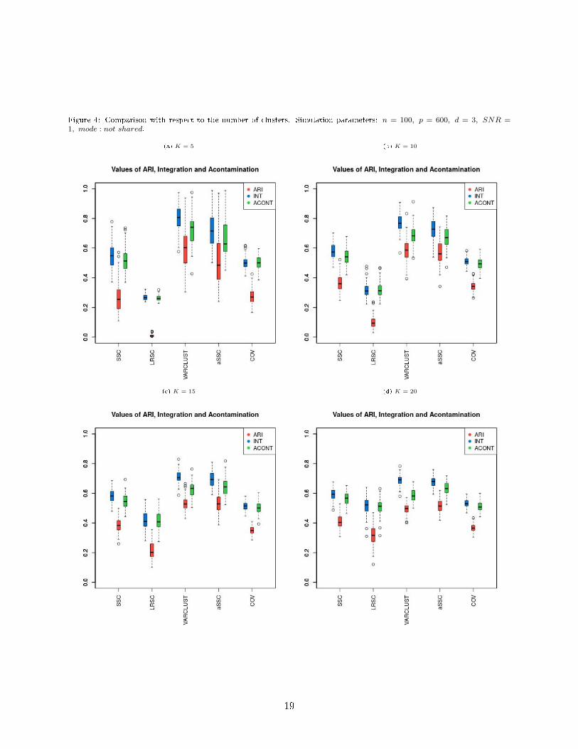
Figure 4: Comparison with respect to the number of clusters. Simulation parameters: n = 100, p = 600, d = 3, SNR =1, mode : not shared.

(a) K = 5 (b) K = 10

(c) K = 15 (d) K = 20

19

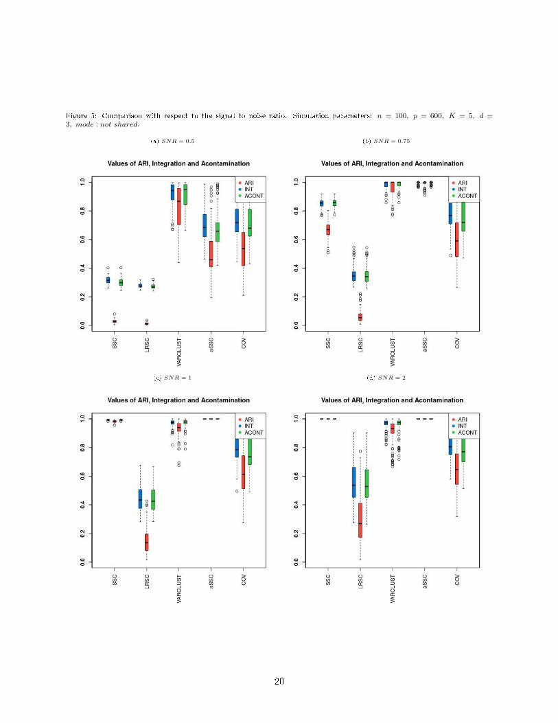
Figure 5: Comparison with respect to the signal to noise ratio. Simulation parameters: n = 100, p = 600, K = 5, d =3, mode : not shared.

(a) SNR = 0.5 (b) SNR = 0.75

(c) SNR = 1 (d) SNR = 2

20

Figure 6: Estimation of the number of clusters. Simulation parameters: n = 100, p = 600, d = 3, SNR = 1 mode : not shared.

(a) K = 5 (b) K = 10

(c) K = 15 (d) K = 20

21

Figure 7: mBIC with respect to the number of iterations for 4 di�erent initializations. Simulation parameters: n = 100, K =5, d = 3, SNR = 1 mode : shared.

(a) p = 750 (b) p = 1500

(c) p = 3000

22

Figure 8: Comparison of the execution time of the methods with respect to p and K. Simulation parameters:n = 100, d =3, SNR = 1 mode : shared.

(a) With respect to the number of variables (b) With respect to the number of clusters

5.4.8 Execution time

In this section we compare the execution times of compared methods. They were obtained on themachine with Intel(R) Core(TM) i7-4790 CPU 3.60GHz, 8 GB RAM. The results are in Figure 8.For the left plot K = 5 and for the right one p = 600. On the plots for both VARCLUST and COVwe used only one random initialization. Therefore, we note that for ninit = 30 the execution time ofVARCLUST will be larger. However, not by exact factor of ninit thanks to parallel implementationin [30]. Nonetheless, VARCLUST is the most computationally complex of these methods. We cansee that COV and SSC do not take longer for bigger number of clusters when the opposite holds forVARCLUST and LRSC. What is more, when the number of variables increases, the execution timeof SSC grows much more rapidly than time of one run of VARCLUST. Therefore, for bigger data setsit is possible to test more random initializations of VARCLUST in the same time as computationof SSC. Furthermore, running VARCLUST with segmentation returned by SSC (enhancing theclustering) is not much more time consuming than SSC itself.

5.4.9 Discussion of the results

The simulation results prove that VARCLUST is an appropriate method for variable clustering.As one of the very few approaches, it is adapted to the data dominated by noise. One of itsbiggest advantages is a possibility to recognize subspaces which share factors. It is also quite robustto increase in the maximal dimension of a subspace. Furthermore, it can be used to detect thenumber of clusters in the data set. Last but not least, in every setting of the parameters usedin our simulation, VARCLUST outperformed LRSC and COV and did better or as well as SSC.The main disadvantage of VARCLUST is its computational complexity. Therefore, to reduce theexecution time one can provide custom initialization as in VARCLUSTaSSC . This method in allcases provided better results than SSC, so our algorithm can also be used to enhance the clusteringresults of the other methods. The other disadvantage of VARCLUST is a problem with the choice

23

of the parameters ninit or niter. Unfortunately, when data size increases, in order to get acceptableclustering we have to increase at least one of these two values. However, it is worth mentioning thatin case of parameters used in out tests ninit = 30 and the maximal number of iterations equal to 30on a machine with 8 cores the execution time of VARCLUST is comparable with execution time ofSSC.

6 Applications to real data analysis

In this section we apply VARCLUST to two di�erent data sets and show that our algorithm canproduce meaningful, interpretable clustering and dimensionality reduction.

6.1 Meteorological data

First, we will analyze air pollution data from Kraków, Poland [1]. This example will also serve asa short introduction to the varclust R package.

6.1.1 About the data

Krakow is one of the most polluted cities in Poland and even in the world. This issue has gainedenough recognition to inspire several grass-root initiatives that aim to monitor air quality and informcitizens about health risks. Airly project created a huge network of air quality sensors which weredeployed across the city. Information gathered by the network is accessible via the map.airly.eu

website. Each of 56 sensors measures temperature, pressure, humidity and levels of particulatematters PM1, PM2.5 and PM10 (number corresponds to the mean diameter). This way, air qualityis described by 336 variables. Measurements are done on an hourly basis.

Here, we used data from one month. We chose March, because in this month the number of miss-ing values is the smallest. First, we removed non-numerical variables from the data set. We removecolumns with a high percentage (over 50%) of missing values and impute the other by the mean.We used two versions of the data set: march_less data frame containing hourly measurements (inthis case number of observations is greater than number of variables) and march_daily containingaveraged daily measurements (which satis�es the p� n assumption). Results for both versions areconsistent. The dimensions of the data are 577×263 and 25×263, respectively. Both data sets alongwith R code and results are available on https://github.com/mstaniak/varclust_example

6.1.2 Clustering based on random initialization

When the number of clusters is not known, we can use the mlcc.bic function which �nds a clusteringof variables with an estimated number of clusters and also returns factors that span each cluster.A minimal call to mlcc.bic function requires just the name of a data frame in which the data arestored.

varclust_minimal <−mlcc . b i c ( march_less , greedy = F)

The returned object is a list containing the resulting segmentation of variables (segmentationelement), a list with matrices of factors for each cluster, mBIC for the chosen model, list describingdimensionality of each cluster and models �tted in other iterations of the algorithm (non-optimalmodels). By default, at most 30 iterations of the greedy algorithm are used to pick a model. Also bydefault it is assumed that the number of clusters is between 1 and 10, and the maximum dimension

24

of a single cluster is 4. These parameters can be tweaked. Based on comparison of mBIC values forclustering results with di�erent maximum dimensions, we selected 6 as the maximum dimension.

v a r c l u s t_c l u s t e r s =mlcc . b i c ( march_less , greedy = TRUE,f l a t . p r i o r = TRUE, max . dim = 6)

To minimize the impact of random initialization, we can run the algorithm many times andselect best clustering based on the value of mBIC criterion. We present results for one of clusteringsobtained this way.

We can see that variables describing temperature, humidity and pressure were grouped in fourclusters (with pressure divided into two clusters and homogenous clusters for humidity and temper-ature related variables), while variables that describe levels of particulate matters are spread amongdi�erent clusters that do not describe simply one size of particulate matter (1, 2.5 or 10), which mayimply that measurements are in a sense non-homogenous. In Figure 9 we show how these clustersare related to geographical locations.

6.1.3 Clustering based on SSC algorithm

The mlcc.bic function performs clustering based on a random initial segmentation. When thenumber of clusters is known or can be safely assumed, we can use the mlcc.reps function, whichcan start from given initial segmentations or a random segmentation. We will show how to initial-ize the clustering algorithm with a �xed grouping. For illustration, we will use results of SparseSubspace Clustering (SSC) algorithm. SSC is implemented in a Matlab package maintained byEhsan Elhamifar [11]. As of now, no R implementation of SSC is available. We store resultingsegmentations for numbers of clusters from 1 to 20 in vectors called clx, where x is the number ofclusters. Now the calls to mlcc.reps function should look like the following example.

vc lu s t10 <− mlcc . reps ( march_less ,numb . c l u s t e r s =10,max . i t e r =50,i n i t i a l . segmentat ions=l i s t ( c l 10 ) )

The result is a list with a number of clusters (segmentation), calculated mBIC and a listof factors spanning each of the clusters. For both initialization methods, variability of resultsregarding the number of clusters diminished by increasing the numb.runs argument to mlcc.bic

and mlcc.reps functions which control the number of runs of the k-means algorithm.

6.1.4 Conclusions

We applied VARCLUST algorithm to data describing air quality in Kraków. We were able to reducethe dimensionality of the data signi�cantly. It turns out that for each characteristics: temperature,humidity and the pressure, measurements made in 56 locations can be well represented by a lowdimensional projection found by Varclust. Additionally, variables describing di�erent particulatematter levels can be clustered into geographically meaningful groups, clearly separating the centerand a few bordering regions. If we were to use these measurements as explanatory variables in amodel describing for example e�ects of air pollution on health, factors that span clusters could beused instead as predictors, allowing for a signi�cant dimension reduction.

The results of the clustering are random by default. Increasing the number of runs of k-meansalgorithm and maximum number of iterations of the algorithm stabilize the results. Increasing theseparameters also increases the computation time. Another way to remove randomness is to select an

25

Figure 9: Clusters of variables describing particulate matter levels on a map of Krakow. Without any prior knowledge on spatialstructure, VARCLUST groups variables corresponding to sensors located near each other.

26

initial clustering using another method. In the examples, clustering based on SSC algorithm wasused.

The mlcc.bic function performs greedy search by default, meaning that the search stops after�rst decrease in mBIC score occurs. On the one hand, this might lead to suboptimal choice ofnumber of clusters, so setting greedy argument to FALSE might be helpful, but on the other hand,the criterion may become unstable for some larger numbers of clusters.

6.2 TCGA Breast Cancer Data

In the next subsection, the VARCLUST clustering method is applied on large open-sourcedata generated by The Cancer Genome Atlas (TCGA) Research Network, available on http:

//cancergenome.nih.gov/. TCGA has pro�led and analyzed large numbers of human tumoursto discover molecular aberrations at the DNA, RNA, protein, and epigenetic levels. In this analysis,we focus on the Breast Cancer cohort, made up of all patients reviewed by the TCGA Research Net-work, including all stages and all anatomopathological characteristics of the primary breast cancerdisease, as in [6].

The genetic informations in tumoral tissues DNA that are involved in gene expression are mea-sured from messenger RNA (mRNA) sequencing. The analysed data set is composed of p = 60488mRNA transcripts for n = 1208 patients.

For this data set, our objective is twofold. First, from a machine learning point of view, wehope that this clustering procedure will provide a su�ciently e�cient dimension reduction in orderto improve the forecasting issues related to the cancer, for instance the prediction of the reaction ofpatients to a given treatment or the life expectancy in terms of the transcriptomic diagnostic.Second, from a biological point of view, the clusters of gene expression might be interpreted asdistinct biological processes. Then, a way of measuring the quality of the VARCLUST method isto compare the composition of the selected clusters with some biological pathways classi�cation(see Figure 10). More precisely, the goal is to check if the clusters constructed by VARCLUSTcorrespond to already known biological pathways (Gene Ontology, [13]).

6.2.1 Data extraction and gene annotations

This ontological classi�cation aims at doing a census of all described biological pathways. To graspthe subtleties inherent to biology, it is important to keep in mind that one gene may be involvedin several biological pathways and that most of biological pathways are slot or associated with eachother. The number of terms on per Biological process ontology was 29687 in January 2019 whilethe number of protein coding genes is around 20000. Therefore, one cannot consider each identi�edbiological process as independent characteristic.

The RNASeq raw counts were extracted from the TCGA data portal. The scaling normalizationand log transformation ([28]) were computed using voom function ([21]) from limma package version3.38.3 ([27]). The gene annotation was realised with biomaRt package version 2.38.0 ([9], [10]).

The enrichment process aims to retrieve a functional pro�le of a given set of genes in orderto better understand the underlying biological processes. Therefore, we compare the input geneset (i.e, the genes in each cluster) to each of the terms in the gene ontology. A statistical testcan be performed for each bin to see if it is enriched for the input genes. It should be mentionedthat all genes in the input genes may not be retrieved in the Gene Ontology Biological Processand conversely, all genes in the Biological Process may not be present in the input gene set. Toperform the GO enrichment analysis, we used GoFuncR package [14] version 1.2.0. Only Biological

27

Processes identi�ed with Family-wise Error Rate p-value < 0.05 were reviewed. Data processingand annotation enrichment were performed using R software version 3.5.2.

Figure 10: Bioinformatic annotation process for each cluster identi�ed by VARCLUST

6.2.2 Evolution of the mBIC and clusters strucure

The number of clusters to test was �xed to 50, 100, 150, 175, 200, 225, 250. The maximal subspacedimension was �xed to 8, the number of runs was 40, and the maximal number of iterations of thealgorithm was 30.

As illustrated in the Figure 12, the mBICs remain stable from the 35th iteration. The mBIC isnot a.s. increasing between 50 and 250 clusters sets. The mBIC for K = 175 and K = 250 clusterssets were close. The proportion of clusters with only one principal component is also higher forK = 175 and K = 250 clusters sets.

6.2.3 Biological speci�city of clusters

In this subsection, we focus on some biological interpretations in the case: K = 175 clusters.In order to illustrate the correspondance between the genes clustering and the biological annotationsin Gene Ontology, we have selected one cluster with only one Gene Ontology Biological Process(Cluster number 3) and one cluster with two Gene Ontology Biological processes (Cluster number88). We keep this numbering notation in the sequel.Among the 98 genes in Cluster 3, 70 (71.4%, called �Speci�c Genes�) were reported in the GOBiological process named calcium-independent cell-cell adhesion via plasma membrane, cell-adhesionmolecules (GO : 0016338). The number of principal components in this cluster was 8 (which mayindicate that one Biological process has to be modeled using many components). Among the 441genes in Cluster 88, 288 (65.3%) were reported in the GO Biological processes named small moleculemetabolic process ( GO : 0044281) and cell-substrate adhesion (GO : 0031589). The number ofprincipal components in this cluster was also 8.

Figure 11: Left: evolution of the mBIC with the number of clusters; middle: evolution of the mBIC with the number ofiterations; right: number of principal components in clusters in terms of K.

28

To investigate whether the speci�c genes, i.e. involved in the GO biological process are well separatedfrom unspeci�c genes (not involved in the GO biological process), we computed two standard PCAsin Clusters 3 and 88 separetely. As shown in Figure 12, the separation is well done.

Figure 12: Repartition of speci�c (red color) and unspeci�c genes (black color) according to a standard PCA.

7 VARCLUST package

The package [30] is an R package that implements VARCLUST algorithm. To install it, runinstall.packages("varclust") in R console. The main function is called mlcc.bic and it pro-vides estimation of:

• Number of clusters K

• Clusters dimensions ~k

• Variables segmentation Π

These estimators minimize modi�ed BIC described in Section 2.For the whole documentation use ?mlcc.bic. Apart from running VARCLUST algorithm usingrandom initializations, the package allows for a hot start speci�ed by the user.

Information about all parameters can be found in the package documentation. Let us just pointout few most important from practical point of view.

• If possible one should use multiple cores computation to speed up the algorithm. By defaultall but one cores are used. User can override this with numb.cores parameter

• To avoid algorithm getting stuck in the local minimum one should run it with random initial-ization multiple times (see parameter numb.runs). Default value is 20. We advice to use asmany runs as possible (100 or even more).

29

• We recommend doing a hot-start initialization with some non-random segmentation. Sucha segmentation could be result of some expert knowledge or di�erent clustering method e.g.SSC. We explore this option in simulation studies.

• Parameter max.dim should re�ect how large dimensions of clusters are expected to be. Defaultvalue is 4.

8 Acknowledgements

M. Bogdan, P. Graczyk, F. Panloup and S. Wilczy«ski thank the AAP MIR 2018-2020 (University ofAngers) for its support. P. Graczyk and F. Panloup are grateful to SIRIC ILIAD program (supportedby the French National Cancer Institute national (INCa), the Ministry of Health and the Institutefor Health and Medical Research) and to PANORisk program of the Région Pays de la Loire fortheir support. F. Panloup is also supported by the Institut de Cancérologie de l'Ouest. M. Bogdanwas also supported by the Polish National Center of Science via grant 2016/23/B/ST1/00454. M.Staniak was supported by the Polish National Center of Science grant 2020/37/N/ST6/04070.

9 Appendix. Proof of the PESEL Consistency Theorem

In the following we shall denote the sample covariance matrix

Sn =(X − X)T (X − X)

n,

the covariance matrix

Σn = E (Sn) =MTn×pMn×p

n+n− 1

nσ2Id

and the heterogeneous PESEL function F (n, k)

F (n, k) =

− n

2

k∑j=1

ln(λj) + (p− k) ln

1

p− k

p∑j=k+1

λj

+ p ln(2π) + p

︸ ︷︷ ︸

G(k)

− ln(n)pk − k(k+1)

2 + k + p+ 1

2︸ ︷︷ ︸P (n,k)

(9.1)

Proposition 1. Let E have i.i.d. entries with a normal distribution N (0, σ2). There exists aconstant C > 1 such that almost surely,

∃n0∀n≥n0 ‖ 1

n(E − E)T (E − E)− σ2Id‖ ≤

C

√2 ln lnn√

n

Proof. It is a simple corollary of LLN and LIL. The term jk of 1n(E − E)T (E − E) equals

1

n(E•j − E•j1)T (E•k − E•k1) =

1

n

n∑i=1

EijEik − E•jE•k.

30

An upper bound of convergence of 1n

∑ni=1EijEik to σ2δjk is

√2 ln lnn√

n. It is easy to show that an

upper bound of convergence of E•jE•k to 0 is (√

2 ln lnn√n

)2 ≤√

2 ln lnn√n

.

Proposition 2. Let E have i.i.d. entries with a normal law N (0, σ2). There exists a constantC > 1 such that almost surely,

∃n0 ∀n≥n0 ‖ 1

n(X − X)T (X − X)− (L+ σ2Id)‖ ≤

C

√2 ln lnn√

n(9.2)

Proof. It is easy to check that X − X = M + E − E. We write

1

n(X − X)T (X − X) =

1

nMTM +

1

n(E − E)T (E − E)

+1

n(MTE + ETM)− 1

n(MT E + ETM)

To the �rst two terms we apply, respectively, the hypothesis (4.2) and the Proposition 1.To prove the right pace of convergence of the third term 1

n(MTE + ETM) we consider everyterm (MTE)ij = 〈M•i, E•j〉 for which we use a generalized version of Law of Iterated Logarithmfrom [26]. Its assumptions are trivially met for random variables

MliElj ∼ N (0,M2liσ

2)

as they are Gaussian and Bn+1

Bn= n+1

n → 1, where Bn is de�ned as Bn =∑

lM2liσ

2. Then, by [26],the following holds

lim supn→∞

∑lMliElj√

2Bn log logBn= 1 a.s.

The fourth term 1n(MT E + ETM) is treated using Cauchy-Schwarz inequality:

|( 1

nMT E)ij | =

1

n|〈M•i, E•j〉|

≤ 1

n‖M•i‖‖E•j‖ =

1

n‖M•i‖

√n E•j

2

=1√n‖M•i‖|E•j |.

By LIL, |E•j | ≤ C√

2 ln lnn√n

. The square of the �rst term ( 1√n‖M•i‖)2 converges to a �nite limit

by the assumption (4.2).

Lemma 1. There exists C ′ > 0 such that almost surely,

∃n0 ∀n ≥ n0 ‖λ(S)− λ(Σ)‖∞ ≤ C ′√

2 ln lnn√n

, (9.3)

where S is sample covariance matrix for data drawn according to model (4.1), Σ is its expected valueand function λ(·) returns sequence of eigenvalues.

31

Proof.Observe that ∥∥∥∥∥(X −X)T (X − X)

n− Σ

∥∥∥∥∥∞

≤ ‖ 1

n(X − X)T (X − X)− (L+ σ2Id)‖

+ ‖(L+ σ2Id)− Σ‖

We apply Proposition 2 to the �rst term and the assumption (4.2) to the second one.Inequality (9.3) holds because (9.2) holds and, by Theorem A.46(A.7.3) from [3], when A,B aresymmetric, it holds

maxk|λk(A)− λk(B)| ≤ ‖A−B‖,

where function λk(·) denotes the kth eigenvalue in the non-increasing order.

Proof of Theorem 1.

Let εn = maxi |λi(Sn) − λi(L)|. From Lemma 1 we have limn εn = 0 almost surely, so fork ≤ k0 − 1, for almost all samplings, there exists n0 such that if n ≥ n0,

εn < σ2 and εn <1

4min

k≤k0−1ck(γ),

where ck(γ) = γk+1 −∑p

k+2 γip−k−1 > 0.

We study the sequence of non-penalty terms G(k) (see (9.1)). For simplicity, from now on, we usenotation λj = λj(Sn). We consider G(k)−G(k + 1) thus getting rid of the minus sign.

G(k)−G(k + 1) =

= lnλk+1 + (p− k − 1) ln

∑pk+2 λj

p− k − 1

− (p− k) ln

∑pk+1 λj

p− k

= lnλk+1 − ln

∑pk+2 λj

p− k − 1

+ (p− k)

[ln

∑pk+2 λj

p− k − 1− ln

∑pk+1 λj

p− k

]

Let us now denote a = λk+1 and b =∑p

k+2 λjp−k−1 . Then the above becomes:

ln a− ln b+ (p− k)

[ln b− ln

b(p− k − 1) + a

p− k

]Case k ≤ k0 − 1.

We will use notation as above and exploit concavity of ln function by taking Taylor expansion atpoint x0

f(x) = f(x0) + f ′(x0)(x− x0) +f ′′(x?)

2(x− x0)2,

32

where x? ∈ (x, x0).Let x0 = θx1 + (1− θ)x2 and x = x1. Then

f(x1) = f(x0) + f ′(x0)(1− θ)(x1 − x2)

+f ′′(x?1)

2(1− θ)2(x1 − x2)2.

Similarly, we take x = x2, multiply both equations by θ and 1 − θ respectively and sum them up.We end up with the formula

θf(x1) + (1− θ)f(x2) =

f(x0) + θ(1− θ)(x2 − x1)2

[f ′′(x?1)

2(1− θ) +

f ′′(x?2)

2θ

].

In our case f ′′(x) = − 1x2 , which means that

f ′′(x?i )2 < f ′′(x2)

2 because x?1 ∈ (x1, x0) < x2 andx?2 ∈ (x0, x2) < x2. This yields

θf(x1) + (1− θ)f(x2)− f(x0) =

θ(1− θ)(x2 − x1)2

[f ′′(x?1)

2(1− θ) +

f ′′(x?2)

2θ

](9.4)

< θ(1− θ)(x2 − x1)2 f′′(x2)

2

Now, going back to G(k), we set

x1 = b =

∑pk+2 λj

p− k − 1, x2 = a = λk+1, θ = 1− 1

p− k. (9.5)

By multiplying both sides of (9.4) by p− k we get

(p− k − 1) ln

(∑pk+2 λj

p− k − 1

)+ ln(λk+1)

− (p− k) ln

((1− 1

p− k)

∑pk+2 λj

p− k − 1+

1

p− kλk+1

)

< −(

1− 1

p− k

)(λk+1 −

∑pk+2 λj

p− k − 1

)21

2λ2k+1

So, using k + 1 ≤ k0 in the last inequality, we get

G(k + 1)−G(k) >(1− 1

p− k

)(λk+1 −

∑pk+2 λj

p− k − 1

)21

2λ2k+1

=p− k − 1

p− k

(λk+1 −

∑pk+2 λj

p− k − 1

)21

2λ2k+1

>p− k0 − 1

p− k0

(λk+1 −

∑pk+2 λj

p− k − 1

)21

2λ21

33

From Lemma 1, λi ∈ [γi + σ2 − εn, γi + σ2 + εn], where εn goes to 0 and

(λk+1 −

∑pk+2 λj

p− k − 1

)≥

≥ γk+1 + σ2 − εn −∑p

k+2(γi + σ2 + εn)

p− k − 1

= ck(γ)− 2εn ≥ mink≤k0−1

ck(γ)− 2εn > 0

for some constants ck(γ). Thus

G(k + 1)−G(k)

>p− k0 − 1

p− k0( mink≤k0−1

ck(γ)− 2εn)2 1

2(γ1 + σ2 + εn)2

>C ′

2min

k≤k0−1ck(γ) > C > 0

where C,C ′ are constants independent of k and n. It follows that for n large enough

n

2[G(k + 1)−G(k)]

≥ n

2C

� lnn

2(p− k)

= P (n, k + 1)− P (n, k).

This implies that the PESEL function F (n, k) = n2G(k)−P (n, k) is strictly increasing for k ≤ k0.

Case k ≥ k0. By Lemma 1 we have that, for almost all samplings, there exists n0 such that ifn ≥ n0,

εn ≤ C√

2 ln lnn√n

and εn <1

2σ2.

We apply the formula (9.4) and as before, we use the notations (9.5). It yields

G(k + 1)−G(k) ≤(

1− 1

p− k

)(λk+1 −

∑pk+2 λj

p− k − 1

)21

2b2

≤ (λk+1 − b)2 1

2b2

≤ (|λk+1 − σ2|+ |σ2 − b|)2 1

2b2

≤ (|λk+1 − σ2|+∑p

k+2 |σ2 − λj |

p− k − 1)2 1

2b2

≤ 4ε2n1

2(σ2 − εn)2≤ C2 2 ln lnn

n

4

2σ4

= C ′ln lnn

n

34

and consequentlyn

2[G(k + 1)−G(k)] ≤ C ′′ ln lnn

Recall that the PESEL function equals F (n, k) = n2G(k)−P (n, k). The increase of n2G(k) is smaller

than the rate ln lnn, while the increase of penalty P (n, k+ 1)−P (n, k) = lnn2 (p− k) is of rate lnn.

Consequently, there exists n1 such that for n > n1, the PESEL function is strictly decreasing fork ≥ k0 with probability 1.We saw in the �rst part of the proof that the PESEL function F (n, k) is strictly increasing fork ≤ k0, for n big enough. It implies that with probability 1, there exists n2 such that for n > n2

we have k0(n) = k0.

References

[1] Airly. Airly sp. z.o.o., Air quality data from extensive network of sensors (ver-sion 2), 2017. Retrieved from https://www.kaggle.com/datascienceairly/

air-quality-data-from-extensive-network-of-sensors.

[2] Z. Bai, K.P. Choi, and Y. Fujikoshi. Consistency of AIC and BIC in estimating the numberof signi�cant components in high-dimensional principal component analysis. Ann. Statist.,46(3):1050�1076, 2018.

[3] Z. Bai and J. W. Silverstein. Spectral Analysis of Large Dimensional Random Matrices.Springer, 2010.

[4] H. S. Bhat and N. Kumar. On the derivation of the bayesian information criterion. School ofNatural Sciences, University of California, 2010.

[5] M. Bogdan, J. K. Ghosh, and R. W. Doerge. Modifying the schwarz bayesian informationcriterion to locate multipleinteracting quantitative trait loci. Genetics, 167:989�999, 2004.

[6] Cancer Genome Atlas Network. Comprehensive molecular portraits of human breast tumours.Nature, 490(7418):61�70, 2012.

[7] M. Chavent, V. Kuentz, B. Liquet, and L. Saracco. ClustOfVar: An R Package for the Clus-tering of Variables. ArXiv e-prints, December 2011.

[8] M. Chavent, V. Kuentz, B. Liquet, and L. Saracco. Clustofvar: An r package for the clusteringof variables. J. Stat. Softw, 50, 12 2011.

[9] S. Durinck, Y. Moreau, A. Kasprzyk, S. Davis, B. De Moor, A. Brazma, and W. Huber.BioMart and Bioconductor: a powerful link between biological databases and microarray dataanalysis. Bioinformatics, 21(16):3439�3440, 2005.

[10] S. Durinck, P. T. Spellman, E. Birney, and W. Huber. Mapping identi�ers for the integrationof genomic datasets with the R/Bioconductor package biomaRt. Nat Protoc, 4(8):1184�1191,2009.

[11] E. Elhamifar and R. Vidal. Sparse subspace clustering. In In CVPR, 2009.

[12] E. Elhamifar and R. Vidal. Sparse subspace clustering: algorithm, theory, and applications.IEEE Transactions on Pattern Analysis and Machine Intelligence, 35(11):2765�81, 2013.

35

[13] Gene Ontology Consortium. The Gene Ontology (GO) database and informatics resource.Nucleic Acids Res., 32(Database issue):D258�261, 2004.

[14] S. Grote. GOfuncR: Gene ontology enrichment using FUNC, 2018. R package version 1.2.0.

[15] T. Hastie and P. Y. Simard. Metrics and models for handwritten character recognition.Statistical Science, 13:54�65, 1998.

[16] H. Hotelling. Analysis of a complex of statistical variables into principal components. Journalof Educational Psychology, 24:417�441, 498�520, 1933.

[17] H. Hotelling. Relations between two sets of variates. Biometrika, 28:321�377, 1936.

[18] L. Hubert and P. Arabie. Comparing partitions. Journal of classi�cation, 2(1):193�218, 1985.

[19] I.T. Jolli�e. Principal Component Analysis. Springer Series in Statistics. Springer, 2002.

[20] Y.P.C. Kotropoulos and G.R. Arce. l1-graph based music structure analysis. In In InternationalSociety for Music Information Retrieval Conference, ISMIR 2011, 2011.

[21] C. W. Law, Y. Chen, W. Shi, and G. K. Smyth. voom: Precision weights unlock linear modelanalysis tools for RNA-seq read counts. Genome Biol., 15(2):R29, 2014.

[22] J.A. Lee and M. Verleysen. Nonlinear Dimensionality Reduction. Springer, 2007.

[23] B. McWilliams and G. Montana. Subspace clustering of high-dimensional data: a predictiveapproach. Data Mining and Knowledge Discovery, 28:736�772, 2014.

[24] T. P. Minka. Automatic choice of dimensionality for pca. NIPS, 13:514, 2000.

[25] K. Pearson. On Lines and Planes of Closest Fit to Systems of Points in Space. PhilosophicalMagazine, 2(11):559�572, 1901.

[26] P.V.V. Petrov and V.V. Petrov. Limit Theorems of Probability Theory: Sequences ofIndependent Random Variables. Oxford science publications. Clarendon Press, 1995.

[27] M. E. Ritchie, B. Phipson, D. Wu, Y. Hu, C. W. Law, W. Shi, and G. K. Smyth. limmapowers di�erential expression analyses for RNA-sequencing and microarray studies. NucleicAcids Res., 43(7):e47, 2015.

[28] M. D. Robinson and A. Oshlack. A scaling normalization method for di�erential expressionanalysis of RNA-seq data. Genome Biol., 11(3):R25, 2010.

[29] P. Sobczyk, M. Bogdan, and J. Josse. Bayesian dimensionality reduction with pca using penal-ized semi-integrated likelihood. Journal of Computational and Graphical Statistics, 26(4):826�839, 2017.

[30] P. Sobczyk, S. Wilczy«ski, J. Josse, and M. Bogdan. varclust: Variables Clustering, 2017. Rpackage version 0.9.4.

[31] M. Soltanolkotabi and E. J. Candès. A geometric analysis of subspace clustering with outliers.Ann. Statist., 40(4):2195�2238, 08 2012.

[32] M. Soªtys. Metody analizy skupie«. Master's thesis, Wrocªaw University of Technology, 2010.

36

[33] M. E. Tipping and C. M. Bishop. Mixtures of probabilistic principal component analyzers.Neural Computation, 11(2):443�482, February 1999.

[34] R. Vidal. Subspace clustering. Signal Processing Magazine, 28:52�68, 2011.

[35] R. Vidal and P. Favaro. Low rank subspace clustering (lrsc). Pattern Recognition Letters,43(0):47 � 61, 2014. {ICPR2012} Awarded Papers.

[36] E. Vigneau and E. M. Qannari. Clustering of variables around latent components.Communications in Statistics-Simulation and Computation, 32(4):1131�1150, 2003.

37