Fröhlich polaron and bipolaron: recent developments - arXiv

arX

iv:0

904.

3682

v2 [

cond

-mat

.sup

r-co

n] 2

7 A

pr 2

009

Frohlich polaron and bipolaron: recent developments

Jozef T. Devreese∗

Universiteit Antwerpen, Groenenborgerlaan 171, B-2020 Antwerpen, Belgium

Alexandre S. Alexandrov†

Department of Physics, Loughborough University, Loughborough LE11 3TU,

United Kingdom

Abstract

It is remarkable how the Frohlich polaron, one of the simplest examples of a Quan-

tum Field Theoretical problem, as it basically consists of a single fermion interacting

with a scalar Bose field of ion displacements, has resisted full analytical or numerical

solution at all coupling since ∼ 1950, when its Hamiltonian was first written. The

field has been a testing ground for analytical, semi-analytical, and numerical tech-

niques, such as path integrals, strong-coupling perturbation expansion, advanced

variational, exact diagonalisation (ED), and quantum Monte Carlo (QMC) tech-

niques. This article reviews recent developments in the field of continuum and

discrete (lattice) Frohlich (bi)polarons starting with the basics and covering a num-

ber of active directions of research.

∗Electronic address: [email protected]†Electronic address: [email protected]

1

http://arxiv.org/abs/0904.3682v2

mailto:[email protected]

mailto:[email protected]

Contents

I. INTRODUCTION 3

II. Continuum polaron 8

A. Pekar’s polaron 9

1. Ground state 10

2. Effective mass of Pekar’s polaron 11

B. Weak-coupling Frohlich polaron 13

C. Lee-Low-Pines transformation 15

D. All-coupling continuum polaron 16

1. Feynman theory 16

2. Diagrammatic Monte-Carlo algorithm 19

III. Response of continuum polarons 25

A. Mobility 25

B. Optical absorption at weak coupling 30

C. Optical absorption at strong coupling 32

D. Optical absorption at arbitrary coupling 36

E. Main-peak line and strong-coupling expansion 39

F. Comparison between optical conductivity spectra obtained by different methods 43

G. Sum rules for the optical conductivity spectra of Frohlich polarons 44

H. Optical absorption spectra of continuum-polaron gas 47

I. Ripplopolarons 48

J. Polaron scaling relations 50

IV. Discrete Holstein and Frohlich polaron 52

A. Holstein model 52

1. Non-adiabatic Holstein polaron 54

2. Adiabatic Holstein polaron 55

B. Lang-Firsov canonical transformation 57

1. “1/λ” expansion and polaron band 59

2. Temperature effect on the polaron band 60

2

C. Discrete Frohlich polaron at strong coupling 63

D. Effect of dispersive phonons 65

E. All-coupling discrete polaron 66

1. Holstein model at any coupling 66

2. Holstein polaron in infinite lattices 69

3. Discrete Frohlich polaron at any coupling 73

F. Isotope effect on the polaron mass and the polaron band-structure 74

G. Jahn-Teller polaron 77

V. Response of discrete polarons 79

A. Hopping mobility 79

B. Optical conductivity 82

C. Spectral function of discrete strong-coupling polarons 85

D. Spectral function of discrete all-coupling polarons 88

VI. Bipolaron 90

A. Polaron-polaron interaction 90

B. Holstein bipolaron 92

C. Continuum Frohlich bipolaron 97

D. Discrete strong-coupling Frohlich bipolaron 100

E. Discrete all-coupling Frohlich bipolaron 105

F. Polaronic exciton 107

VII. Current status of polarons and open problems 108

Acknowledgments 114

References 114

I. INTRODUCTION

Charge carriers in inorganic and organic matter interact with ion vibrations. The cor-

responding electron-phonon interaction (EPI) causes phase transformations, including su-

perconductivity, and dominates the transport properties of many metals and semiconduc-

3

tors. EPIs have been shown to be relevant in cuprate and other high-temperature su-

perconductors through, for example, isotope substitution experiments (Khasanov et al. ,

2004; Zhao and Morris , 1995; Zhao et al. , 1997), high resolution angle resolved photoe-

mission (ARPES) (Gweon et al. , 2004; Lanzara et al. , 2001; Meevasana et al. , 2006), a

number of earlier optical (Calvani et al. , 1994; Mihailovic et al. , 1990; Zamboni et al. ,

1989), neutron-scattering (Sendyka et al. , 1995) and more recent inelastic scattering

(Reznik et al. , 2006), pump-probe (Gadermaier et al., 2009; Radovic et al. , 2008) and

tunnelling (Shim et al. , 2008) measurements. In colossal magnetoresistance (CMR) man-

ganites, isotope substitutions (Zhao et al. , 1996), X-ray and neutron scattering spectro-

scopies (Campbell et al., 2001, 2003) and a number of other experiments also show a sig-

nificant effect of EPI on the physical properties (for review see (Tokura, 2000)). There-

fore it has been suggested that the long-range (Frohlich , 1954) and/or the molecular-

type (e.g. (Jahn and Teller , 1937)) EPIs play significant role in high-temperature su-

perconductors (see (Alexandrov , 1996; Alexandrov, 1998; Bednorz and Muller , 1988;

Devreese, 1996, 2005; Muller , 2000), and references therein), and in CMR manganites (see

(Alexandrov and Bratkovsky , 1999a; Edwards , 2002; Millis et al. , 1995) and references

therein). Very recent experimental observations of the optical conductivity in the Nb-doped

SrTiO3 (van Mechelen et al., 2008) reveal the evidence of the mid-infrared optical conduc-

tivity band provided by the polaron mechanism like in many other oxides. The effective

mass of the charge carriers is obtained by analyzing the Drude spectral weight. Defining

the mass renormalization of the charge carriers as the ratio of the total electronic spectral

weight and the Drude spectral weight, a twofold mass enhancement is obtained, which is

attributed in Ref. (van Mechelen et al., 2008) to the electron-phonon coupling. The missing

spectral weight is recovered according the sum rule (Devreese et al. , 1977) in a mid-infrared

optical conductivity band. This band results from the electron-phonon coupling interaction,

traditionally associated with the polaronic nature of the charge carriers. The effective mass

obtained from the optical spectral weights yields an intermediate electron-phonon coupling

strength, 3 < α < 4. Therefore it has been suggested in Ref. (van Mechelen et al., 2008)

that the charge transport in the Nb-doped SrTiO3 is carried by large polarons.

When EPI is sufficiently strong, electron Bloch states are affected even in the nor-

mal phase. Phonons are also affected by conduction electrons. In doped insulators bare

phonons are well defined in insulating parent compounds, but microscopic separation of

4

electrons and phonons is not so straightforward in metals and heavily doped insulators

(Maximov et al. , 1997), where the Born and Oppenheimer (1927) and density functional

(Hohenberg and Kohn , 1964; Kohn and Sham , 1965) methods are used. Here we have to

start with the first principle Hamiltonian describing conduction electrons and ions coupled

by the Coulomb forces.

One cannot solve the corresponding Schrodinger equation perturbatively because the

Coulomb interaction is strong. The ratio of the characteristic Coulomb energy to the kinetic

energy is rs = mee2/(4πne/3)1/3 ≈ 1 for the electron density ne = ZN = 1023cm−3 (here

and further we take the volume of the system as V = 1, unless specified otherwise, and

~ = c = kB = 1). However, one can take advantage of the small value of the electron

to ion mass ratio, me/M < 10−3. Ions are heavy and the amplitudes of their vibrations,

〈|u|〉 ≃√

1/MωD, near equilibrium positions are much smaller than the lattice constant

(a = N−1/3), 〈|u|〉/a ≈ (me/Mrs)1/4 ≪ 1. In this estimate we take the characteristic

vibration frequency ωD of the order of the ion plasma frequency ω0 =√

4πNZ2e2/M .

Hence one can expand the Hamiltonian in powers of |u|.Any further progress requires a simplifying physical idea, which commonly is to approach

the ground state of the many-electron system via a one-electron picture. In the framework

of the local density approximation (LDA), where the Coulomb electron-electron interaction

is replaced by an effective one-body potential, the Hamiltonian is written as

H = He +Hph +He−ph +He−e, (1)

where

He =∑

k,n,s

ξnksc†nkscnks, (2)

Hph =∑

q,ν

ωqν(d†qνdqν + 1/2) (3)

describe independent Bloch electrons and phonons, created (annihilated) by c†nks (cnks) and

by d†qν (dqν), respectively, ξnks = Enks − µ is the band energy spectrum with respect to the

chemical potential µ, (k,q) are quasi-momenta of electrons and phonons, respectively, n is

the electron band index, ν is the phonon mode index, and s is the electron spin. The part

of the electron-phonon interaction, which is linear in the phonon operators, is written as

He−ph =1√2N

∑

k,q,n,n′,ν,s

γnn′(q,k, ν)ωqνc†n′kscnk−qsdqν +H.c., (4)

5

where γnn′(q,k, ν) is the dimensionless matrix element. If we restrict the summations over q

and k to the first Brillouin zone of the crystal, then He−ph should also include the summation

over reciprocal lattice vectors G of umklapp scattering contributions where q is replaced

by q + G. The terms of He−ph which are quadratic and of higher orders in the phonon

operators, dqν , are usually small. They play a role only for those phonons which are not

coupled with electrons by the linear interaction, Eq.(4).

The electron-electron correlation energy of a homogeneous electron system is often written

as

He−e =1

2

∑

q

Vc(q)ρ†qρq, (5)

where Vc(q) is a matrix element, which is zero for q = 0 because of electroneutrality and

ρ†q =∑

k,s c†ksck+qs is the density fluctuation operator. H should also include a random

potential in doped semiconductors and amorphous metals, which could affect the EPI matrix

element (Belitz and Kirkpatrick , 1994).

For the purpose of this review we mostly confine our discussions to a single band approx-

imation with the EPI matrix element γnn(q,k, ν) = γ(q) depending only on the momentum

transfer q. The approximation allows for qualitative and in many cases quantitative descrip-

tions of essential polaronic effects in advanced materials. Nevertheless there are might be

degenerate atomic orbitals in solids coupled to local molecular-type Jahn-Teller distortions,

where one has to consider multi-band electron energy structures.

Quantitative calculations of the matrix element in the whole region of momenta can be

performed from pseudopotentials (Baryakhtar et al. , 1999; Maximov et al. , 1997). On the

other hand one can parameterize EPI rather than to compute it from first principles in many

physically important cases (Mahan , 1990). There are three most important interactions in

doped semiconductors, which are polar coupling to optical phonons (the Frohlich EPI),

deformation potential coupling to acoustical phonons, and the local (Holstein) EPI with

molecular type vibrations in complex lattices. While the matrix element is ill defined in

metals, the bare phonons ωqν and the electron band structure Enks are well defined in

doped semiconductors, which have their parent dielectric compounds. Here the effect of

carriers on the crystal field and on the dynamic matrix is small while the carrier density

is much less than the atomic one. Hence one can use the band structure and the crystal

field of parent insulators to calculate the matrix element in doped semiconductors. The

6

interaction constant γ(q) has different q-dependence for different phonon branches. In the

long wavelength limit (q ≪ π/a), γ(q) ∝ qn, where n = −1, 0 and n = −1/2 for polar optical,

molecular (ωq = ω0)) and acoustic (ωq ∝ q) phonons, respectively. Not only q dependence

is known but also the absolute values of γ(q) are well parameterized in this limit. For

example in polar semiconductors |γ(q)|2 = 4πe2/κω0q2, where κ = (ε−1 − ε−1

0 )−1, and ε and

ε0 are high-frequency and static dielectric constants, respectively. If the crystal lacks an

inversion center to be piezoelectric, there is EPI with piezoelectric (acoustic) phonons with

an anysotropic matrix element, which also contribute to a polaron effect and a Coulomb-like

attraction of two polarons (Mahan , 1972).

To get a better insight into physical constraints of the above approximation let us trans-

form the Bloch states to the real space or Wannier states using the canonical linear transfor-

mation of the electron operators, ci = N−1∑

k eik·mcks, where i = (m, s) includes both site

m and spin quantum numbers. In this site (Wannier) representation the electron kinetic

energy takes the following form

He =∑

i,j

t(m − n)δss′c†icj, (6)

where t(m) = N−1∑

kEkeik·m is the “bare” hopping integral, j = (n, s′), and Ek is the

Bloch band dispersion in the rigid lattice.

The electron-phonon interaction and the Coulomb correlations acquire simple forms in the

Wannier representation, if their matrix elements in the momentum representation depend

only on the momentum transfer q (here we follow (Alexandrov and Mott , 1995)),

He−ph =∑

q,i

ωqni [ui(q,)dq +H.c.] , (7)

He−e =1

2

∑

i6=j

Vc(m− n)ninj , (8)

where

ui(q) =1√2N

γ(q)eiq·m (9)

and

Vc(m) =1

N

∑

q

Vc(q)eiq·m, (10)

are the matrix elements of the electron-phonon and Coulomb interactions, respectively, in

the Wannier representation for electrons, and ni = c†ici is the density operator.

7

We see that taking the interaction matrix element depending only on the momentum

transfer one neglects the terms in the electron-phonon and Coulomb interactions, which are

proportional to the overlap integrals of the Wannier orbitals on different sites. This approx-

imation is justified for narrow band materials, where the electron bandwidth is less than the

characteristic magnitude of the crystal field potential. In the Wannier representation the

Hamiltonian is

H =∑

i,j

t(m − n)δss′c†icj +

∑

q,i

ωqni [ui(q)dq +H.c.]

+1

2

∑

i6=j

Vc(m− n)ninj +∑

q

ωq(d†qdq + 1/2). (11)

One can transform it further using the site-representation also for phonons. The site repre-

sentation of He−ph is particularly convenient for the interaction with dispersionless modes,

when ωq = ω0 and the phonon polarization vector eq = e are roughly q-independent. Intro-

ducing the phonon site-operators dn = N−1∑

q eiq·ndq one obtains in this case,

He−ph = ω0

∑

n,m,s

g(m− n)(e · em−n)nms(d†n + dn), (12)

where g(m) is the dimensionless force acting between the electron on site m and the displace-

ment of ion n, proportional to the Fourier transform of γ(q), and em−n ≡ (m− n)/|m− n|is the unit vector in the direction from the electron on site m to the ion n. The real space

representation is particularly convenient in parameterizing EPI in complex lattices. Atomic

orbitals of an ion adiabatically follow its motion. Therefore the electron does not interact

with the displacement of the ion, whose orbitals it occupies, that is g(0) = 0.

II. CONTINUUM POLARON

If characteristic phonon frequencies are sufficiently low, the local deformation of ions,

caused by electron itself, creates a potential well, which traps the electron even in a perfect

crystal lattice. This self-trapping phenomenon was predicted by Landau (Landau , 1933)

more than 70 years ago. It was studied in greater detail (Devreese, 1996; Feynman, 1955;

Frohlich , 1954; Pekar , 1946; Rashba , 1957) in the effective mass approximation for the

electron placed in a continuum polarizible (or deformable) medium, which leads to a so-

called large or continuum polaron. Large polaron wave functions and corresponding lattice

8

distortions spread over many lattice sites. The self-trapping is never complete in the perfect

lattice. Due to finite phonon frequencies ion polarisations can follow polaron motion if

the motion is sufficiently slow. Hence, large polarons with a low kinetic energy propagate

through the lattice as free electrons but with an enhanced effective mass.

When the polaron binding energy Ep is larger than the halfbandwidth D of the elec-

tron band, all states in the Bloch bands are “dressed” by phonons. In this strong-coupling

regime, λ = Ep/D > 1, the finite bandwidth becomes important, so the continuum ap-

proximation cannot be applied. In this case the carriers are described as small or dis-

crete (lattice) polarons. The main features of small polarons were understood a long time

ago (Eagles , 1963; Holstein , 1959a,b; Lang and Firsov , 1962; Sewell , 1958; Tyablikov ,

1952; Yamashita and Kurosawa , 1958). The first identification of small polarons in solids

was made for non-stoichiometric uranium dioxide in Refs. (Devreese, 1963; Nagels et al. ,

1963). Large and small polarons were discussed in a number of review papers and textbooks,

for example (Alexandrov and Mott , 1994, 1995; Appel , 1968; Bottger and Bryksin , 1985;

Devreese, 1996; Firsov , 1975; Itoh and Stoneham , 2001; Mahan , 1990; Mitra et al., 1987;

Rashba , 2005; Salje et al. , 1995).

In many models of EPI the ground-state polaron energy is an analytical function

of the coupling constant for any dimensionality of space (Fehske and Trugman , 2007;

Gerlach and Lowen , 1991; Hague et al. , 2006a; Lowen , 1988; Peeters and Devreese ,

1982). There is no abrupt (nonanalytical) phase transition of the ground state as the

electron-phonon coupling increases. It is instead a crossover from Bloch states of band

electrons or large polarons propagating with almost bare mass in a rigid lattice to heavily

dressed Bloch states of small polarons propagating at low temperatures with an exponen-

tially enhanced effective mass. The ground-state wave function of any polaron is delocalized

for any coupling strength. This result holds for both finite-site models and infinite-site

models (Lowen , 1988).

A. Pekar’s polaron

First let us briefly discuss a single electron interacting with the lattice deformation in

the continuum approximation, as studied by Pekar (1946). In his model a free electron

interacts with the dielectric polarisable continuum, described by the static ε0 and the optical

9

(high frequency) ε dielectric constants. This is the case for carriers interacting with optical

phonons in ionic crystals under the condition that the size of the self-trapped state is large

compared with the lattice constant so that the lattice discreteness is irrelevant.

1. Ground state

Describing the ionic crystal as a polarisable dielectric continuum one should keep in

mind that only the ionic part of the total polarisation contributes to the polaron state.

The interaction of a carrier with valence electrons responsible for the optical properties is

taken into account via the Hartree-Fock periodic potential and included in the band mass

m. Therefore only ion displacements contribute to the self-trapping. Following Pekar we

minimise the sum E(ψ) of the electron kinetic energy and the potential energy due to the

self-induced polarisation field (here we follow (Alexandrov and Mott , 1995)),

E(ψ) =

∫

dr

[

ψ∗(r)

(

−∇2

2m

)

ψ(r) −P(r) ·D(r)

]

(13)

where

D(r) = e∇∫

dr′|ψ(r′)|2|r − r′| (14)

is the electric field of the electron in the state with the wave function ψ(r) and P is the

ionic part of the lattice polarisation. Minimising E(ψ) with respect to ψ∗(r) at fixed P and∫

dr|ψ(r)|2 = 1 one arrives at the equation of motion,

(

−∇2

2m− e

∫

dr′P(r′) · ∇′ 1

|r′ − r|

)

ψ(r) = E0ψ(r), (15)

where E0 is the polaron ground state energy. The ionic part of the total polarisation is

obtained using the definition of the susceptibilities χ0 and χ, P = (χ0 −χ)D. The dielectric

susceptibilities χ0 and χ are related to the static and high frequency dielectric constants,

respectively, (χ0 = (ε0−1)/4πε0, and χ = (ε−1)/4πε), so that P = D4πκ

. Then the equation

of motion becomes

(

−∇2

2m− e2

4πκ

∫

dr′∫

dr′′|ψ(r′′)|2∇′ 1

|r′ − r′′| · ∇′ 1

|r′ − r|

)

ψ(r) = E0ψ(r). (16)

Differentiating by parts with the use of ∇2r−1 = −4πδ(r) one obtains

(

−∇2

2m− e2

κ

∫

dr′|ψ(r′)|2|r′ − r|

)

ψ(r) = E0ψ(r). (17)

10

The solution of this nonlinear integro-differential equation can be found using a variational

minimisation of the functional

J(ψ) =1

2m

∫

dr|∇ψ(r)|2 − 1

2maB

∫

drdr′|ψ(r)|2|ψ(r′)|2

|r′ − r| , (18)

where aB = κ/me2 is the effective Bohr radius. The simplest choice of the normalised trial

function is ψ(r) = Ae−r/rp with A = (πr3p)

−1/2. Substituting the trial function into the

functional yields J(ψ) = T + 12U , where the kinetic energy is T = 1/2mr2

p, and the potential

energy U = −5/8maBrp. Minimising the functional with respect to rp yields the polaron

radius, rp = 16aB/5, and the ground state energy E0 = T + U as E0 = −0.146/ma2B. This

can be compared with the ground state energy of the hydrogen atom −0.5mee4, where me

is the free electron mass. Their ratio is 0.3m/(meκ2). In typical polar solids κ & 4, so that

the continuum polaron binding energy is about 0.25eV or less, if m ≃ me. The potential

energy in the ground state is U = −4T = 4E0/3.

The lowest photon energy ωmin to excite the polaron into the bare electron band is

ωmin = |E0|. The ion configuration does not change in the photoexcitation process of

the polaron. However, a lower activation energy WT is necessary, if the self-trapped state

disappears together with the polarisation well due to thermal fluctuations, WT = |E0| −Ud,

where Ud is the deformation energy. In ionic crystals

Ud =1

2

∫

drP(r) · D(r), (19)

which for the ground state is Ud = 2|E0|/3. Therefore the thermal activation energy is

WT = |E0|/3. The ratio of four characteristic energies for the continuum Pekar’s polaron is

WT : Ud : ωmin : |U | = 1 : 2 : 3 : 4 (Pekar , 1951).

Using Pekar’s choice,

ψ(r) = A(1 + r/rp + βr2)e−r/rp (20)

one obtains A = 0.12/r3/2p , β = 0.45/r2

p, the polaron radius rp = 1.51aB and a better

estimate for the ground state energy, E0 = −0.164/ma2B as compared to the result of the

simplest exponential choice.

2. Effective mass of Pekar’s polaron

The lattice polarization is responsible for the polaron mass enhancement

(Landau and Pekar, 1948). Within the continuum approximation the evolution of

11

the lattice polarisation P(r, t) is described by a harmonic oscillator subjected to an external

force ∼ D/κ:

ω−20

∂2P(r, t)

∂t2+ P(r, t) =

D(r, t)

4πκ, (21)

where ω0 is the optical phonon frequency. If during the characteristic time of the lattice

relaxation ≃ ω−10 the polaron moves a distance much less than the polaron radius, the

polarisation practically follows the polaron motion. Hence for a slow motion with the velocity

v ≪ ω0aB the first term in Eq.(21) is a small perturbation, so that

P(r, t) ≈ 1

4πκ

(

D(r, t) − ω−20

∂2D(r, t)

∂t2

)

. (22)

The total energy of the crystal with an extra electron,

E = E(ψ) + 2πκ

∫

dr

[

P(r, t)2 + ω−20

(

∂P(r, t)

∂t

)2]

, (23)

is determined in such a way that it gives Eq.(21) when it is minimised with respect to P.

We note that the first term of the lattice contribution to E is the deformation energy Ud,

discussed in the previous section. The lattice part of the total energy depends on the polaron

velocity and contributes to the effective mass. Replacing the static wave function ψ(r) in all

expressions for ψ(r − vt) and neglecting a contribution to the total energy of higher orders

than v2 one obtains

E = E0 + Ud +m∗v2

2, (24)

where

m∗ = − 1

12πω20κ

∫

drD(r) · ∇2D(r) (25)

is the polaron mass. Using the equation ∇ · D = −4πe|ψ(r)|2 yields

m∗ =4πe2

3ω20κ

∫

dr|ψ(r)|4. (26)

Calculating the integral with the trial function Eq.(20) one obtains

m∗≈ 0.02α4m, (27)

where α is the dimensionless constant, defined as α = (e2/κ)√

m/2ω0.

Concluding the discussion of the Pekar’s polarons let us specify conditions of its existence.

The polaron radius should be large compared with the lattice constant, rp ≫ a to justify the

effective mass approximation for the electron. Hence the value of the coupling constant α

12

should not be very large, α ≪ (D/zω0)1/2, where D ≃ z/2ma2 is the bare half-bandwidth,

and z is the lattice coordination number. On the other hand the classical approximation for

the lattice polarisation is justified if the number of phonons taking part in the polaron cloud

is large. This number is of the order of Ud/ω0. The total energy of the immobile polaron

and the deformed lattice is E = −0.109α2ω0 and Ud = 0.218α2ω0, respectively. Then α

is bounded from below by the condition Ud/ω0 ≫ 1 as α2 ≫ 5. The typical adiabatic

ratio D/ω0 is of the order of 10 to 100. In fact in many transition metal oxides with

narrow bands and high optical phonon frequencies this ratio is about 10 or even less, which

makes the continuum strong-coupling polaron hard to be realised in oxides and related ionic

compounds with light ions (Alexandrov and Mott , 1995).

B. Weak-coupling Frohlich polaron

Frohlich (1954) applied the second quantisation form of the electron-lattice interaction

(Frohlich et al. , 1950) to describe the large polaron in the weak-coupling regime, α < 1,

where the quantum nature of lattice polarisation becomes important,

H = −∇2

2m+∑

q

(

Vqdqeiq·r + h.c.

)

+∑

q

ωq(d†qdq + 1/2). (28)

The quantum states of the noninteracting electron and phonons are specified by the electron

momentum k and the phonon occupation number 〈d†qdq〉 ≡ nq = 0, 1, 2, ...∞. At zero

temperature the unperturbed state is the vacuum, |0〉, of phonons and the electron plane

wave

|k, 0〉 = eik·r|0〉. (29)

While the coupling is weak one can apply the perturbation theory. The interaction couples

the state Eq.(29) with the energy k2/2m and the state with the energy (k−q)2/2m+ω0 of

a single phonon with momentum q and the electron with momentum k − q, |k − q, 1q〉 =

ei(k−q)·r|1q〉. The corresponding matrix element is 〈k − q, 1q|He−ph|k, 0〉 = V ∗q . There is no

diagonal matrix elements of He−ph, so the second order energy Ek is

Ek =k2

2m−∑

q

|Vq|2(k − q)2/2m+ ω0 − k2/2m

. (30)

There is no imaginary part of Ek for a slow electron with k < qp, where

qp = min(mω0/q + q/2) = (2mω0)1/2, (31)

13

which means that the momentum is conserved. Evaluating the integrals one arrives at

Ek =k2

2m− αω0qp

karcsin

(

k

qp

)

, (32)

which for a very slow motion k ≪ qp yields

Ek ≃ −αω0 +k2

2m∗ . (33)

Here the first term is minus the polaron binding energy, −Ep. The effective mass of the

polaron is enhanced as

m∗ =m

1 − α/6≃ m(1 + α/6) (34)

due to a phonon “cloud” accompanying the slow polaron. The number of virtual phonons

Nph in the cloud is given by taking the expectation value of the phonon number operator,

Nph = 〈∑

q d†qdq〉, where bra and ket refer to the perturbed state,

|〉 = |0〉 +∑

q′

V ∗q′

k2/2m− (k − q′)2/2m− ω0|1q′〉. (35)

For the polaron at rest (k = 0) one obtainsNph = α/2. Hence the Frohlich coupling constant,

α, measures the cloud ‘thickness’. One can also calculate the lattice charge density induced

by the electron. The electrostatic potential eφ(r) is given by the average of the interaction

term of the Hamiltonian

eφ(r) = 〈∑

q

Vqeiq·rdq +H.c.〉, (36)

and the charge density ρ(r) is related to the electrostatic potential by Poisson’s equation

∇φ = −4πρ. Using these equations one obtains

ρ(r) = − 1

2πe

∑

q

q2|Vq|2 cos(q · r)ω0 + q2/2m

, (37)

which yields

ρ(r) = −eq3

p

4πκ

e−qpr

qpr. (38)

The mean extension of the phonon cloud, which can be taken as the radius of the weak

coupling polaron, is rp = q−1p , and the total induced charge is Q =

∫

drρ(r) = −e/κ.

14

C. Lee-Low-Pines transformation

One can put the Frohlich result on a variational basis by applying the Lee-Low-Pines

(LLP) transformation (Lee et al. , 1953), which removes the electron coordinate, followed

by the displacement transformation (Gurari, 1953; Lee and Pines , 1952; Tyablikov , 1952).

The latter serves to account for that part of the lattice polarisation which follows the electron

instantaneously. The remaining part of the polarisation field turns out to be small, if the

coupling constant is not extremely large. In the opposite extreme limit, which is Pekar’s

strong-coupling regime discussed above, one can construct the perturbation theory by an

expansion in descending powers of α (Allcock, 1963; Bogoliubov , 1950; Bogoliubov Jr. ,

1994). Alternatively one can apply Feynman’s path-integral formalism to remove the phonon

field at the expense of a non-instantaneous interaction of electron with itself (II.D, and also

(Schultz , 1962)).

The transformation can be written as

|N〉 = exp(S)|N〉, (39)

where S is an anti-Hermitian operator: S+ = −S. In our case |N〉 is a single-electron multi-

phonon wave function. The transformed eigenstate, |N〉 satisfies the Schrodinger equation,

H|N >= E|N〉, with the transformed Hamiltonian

H = exp(S)H exp(−S). (40)

If all operators are transformed according to Eq.(40) the physical averages remain un-

changed. LLP transformation eliminating the electron coordinate in the Hamiltonian is

defined as

SLLP = i∑

q

(q · r)d†qdq. (41)

The transformed Hamiltonian is obtained as

H =1

2m(−i∇−

∑

q

qd†qdq)2 +

∑

q

(Vqdq +H.c.) + ω0

∑

q

(d†qdq + 1/2). (42)

The electron coordinate is absent in H. Hence the eigenstates |N〉 are classified with the

momentum K, which is the conserving total momentum of the system, |N〉 = eiK·r|Nph〉,where |Nph〉 is an eigenstate of phonons. The number of virtual phonons is not small in the

15

intermediate coupling regime. Therefore one cannot apply the perturbation theory for H.

However, one can remove the essential part of the interaction term in the Hamiltonian by

the displacement canonical transformation,

S =∑

q

f(q)dq −H.c., (43)

where c-number f(q) is determined by minimisation of the ground state energy. Assuming

that the transformed ground state is the phonon vacuum eS|Nph〉 = |0〉, one obtains the

energy EK as

EK =(1 − η2)K2

2m− αω0qpK(1 − η)

sin−1

(

K(1 − η)

qp

)

, (44)

where

η(1 − η)2 =αq3

p

2K3

(1 − η)K√

q2p − (1 − η)2K2

− sin−1 (1 − η)K

qp

. (45)

Only the term independent of K needs to be retained in η for a slow polaron with K ≪ qp,

η =α/6

1 + α/6. (46)

Then the energy up to the second order in K is given by

EK = −αω0 +K2

2m∗ , (47)

where the polaron mass is m∗ = m(1 + α/6) as in Eq.(34). Lee, Low and Pines evaluated

also the corrections due to off-diagonal parts of the transformed Hamiltonian and found that

they are small.

D. All-coupling continuum polaron

1. Feynman theory

Feynman developed a superior all-coupling continuum-polaron theory using his path-

integral formalism (Feynman, 1955). He got the idea to formulate the polaron problem into

the Lagrangian form of quantum mechanics and then eliminate the field oscillators, “. . . in

exact analogy to Q. E. D. . . . (resulting in) . . . a sum over all trajectories . . . ”. The resulting

path integral (here limited to the ground-state properties) is of the form:

〈0, β|0, 0〉 =

∫

Dr(τ)eS, (48)

16

S = exp

[

−∫ β

0

r2

2dτ+

α

23/2

∫ β

0

∫ β

0

e−|τ−σ|

|r(τ) − r(σ)|dτdσ]

, (49)

where β = 1/T . Here, the Feynman units are used: ~ = 1, m = 1, ω0 = 1. Eq. (48) gives

the amplitude that an electron found at a point in space at time zero will appear at the

same point at the imaginary time β. The interaction term in the action function S may be

interpreted as indicating that at “time” τ , the electron behaves as if it were in a potential

α

23/2

∫ β

0

e−|τ−σ|

|r(τ) − r(σ)|dσ (50)

which results from the electrostatic interaction of the electron with the mean charge den-

sity of its “previous” positions, weighted with the function e−|τ−σ|. This path integral (48)

with (49) has a great intuitive appeal: it shows the polaron problem as an equivalent one-

particle problem in which the interaction, non-local in time or “retarded”, occurs between

the electron and itself.

Subsequently Feynman introduced a variational principle for path integrals to study the

polaron. He then simulated the interaction between the electron and the polarization modes

by a harmonic interaction (with force constant k) between a hypothetical (“fictitious”)

particle with mass M and the electron. Within his model, the action function S (49) is

imitated by a quadratic trial action (non-local in time):

S0 = exp

[

−∫ β

0

r2

2dτ+

C

2

∫ β

0

∫ β

0

[r(τ) − r(σ)]2 e−w|τ−σ|dτdσ

]

, (51)

where the interaction potential (50) is replaced by a parabolic potential

C

2

∫ β

0

[r(τ) − r(σ)]2 e−w|τ−σ|dσ (52)

with the weight function e−w|τ−σ|. The variational parameters C and w in Eq. (52) are

adjusted in order to partly compensate for the error of exploiting the trial potential (52)

instead of the true potential (50). Following the Feynman approach, an upper bound for

the polaron ground-state energy can be written down as

E = E0 − limβ→∞

1

β〈S − S0〉0 , (53)

where S is the exact action functional of the polaron problem, while S0 is the trial action

functional, which corresponds to the above model system, E0 is the ground-state energy of

the model system, and

〈F 〉0 ≡∫

FeS0Dr (t)∫

eS0Dr (t). (54)

17

The parameters of the model system C and w are found from the variational condition that

they provide a mimimum to the upper bound for the ground state energy of Eq. (53). (For

the details of the calculation, see subsection III.J.) At nonzero temperatures, the best values

of the model parameters can be determined from a variational principle for the free energy

(Feynman, 1972), see Refs. (Krivoglaz and Pekar, 1957; Osaka , 1959).

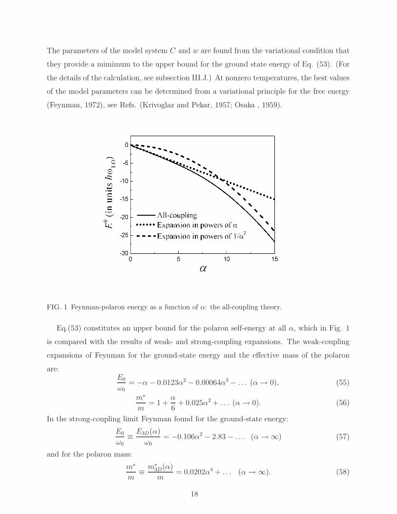
FIG. 1 Feynman-polaron energy as a function of α: the all-coupling theory.

Eq.(53) constitutes an upper bound for the polaron self-energy at all α, which in Fig. 1

is compared with the results of weak- and strong-coupling expansions. The weak-coupling

expansions of Feynman for the ground-state energy and the effective mass of the polaron

are:E0

ω0= −α − 0.0123α2 − 0.00064α3 − . . . (α→ 0), (55)

m∗

m= 1 +

α

6+ 0.025α2 + . . . (α→ 0). (56)

In the strong-coupling limit Feynman found for the ground-state energy:

E0

ω0≡ E3D(α)

ω0= −0.106α2 − 2.83 − . . . (α → ∞) (57)

and for the polaron mass:

m∗

m≡ m∗

3D(α)

m= 0.0202α4 + . . . (α→ ∞). (58)

18

Becker et al. (1983), using a Monte Carlo calculation, derived the ground-state energy of

a polaron as E0 = limβ→∞ ∆F, where ∆F = Fβ−F 0β with Fβ the free energy per polaron and

F 0β = [3/ (2β)] ln (2πβ) the free energy per electron. The value βω0 = 25, used for the actual

computation in Ref. (Becker et al., 1983), corresponds to T/TD = 0.04 (TD = ~ωLO/kB;

ωLO ≡ ω0 is the longitudinal (LO) optical phonon frequency in conventional units). The

authors of Ref. (Becker et al., 1983) actually calculated the free energy ∆F , rather than the

polaron ground-state energy. To investigate the importance of temperature effects on ∆F,

(Peeters and Devreese , 1985) considered the polaron energy as obtained by Osaka (1959),

who generalized the Feynman polaron theory to nonzero temperatures:

∆F

ω0= 3

βln

(

wv

sinhβ0v2

sinhβ0w

2

)

− 34

v2−w2

v

(

coth β0v2

− 2β0v

)

− α√2π

[1 + n (ω0)]∫ β0

0du e−u√

D(u), (59)

where β0 = βω0, n (ω) = 1/(

eβω − 1)

, and

D (u) =w2

v2

u

2

(

1 − u

β0

)

+v2 − w2

2v3

(

1 − e−vu − 4n (v) sinh2 vu

2

)

. (60)

This result is variational, with variational parameters v and w, and gives an upper bound

to the exact polaron free energy. −∆F increases with increasing temperature and the effect

of temperature on ∆F increases with increasing α. The values for the free energy obtained

analytically from the Feynman polaron model are lower than the published MC results for

α . 2 and α ≥ 4 (but lie within the 1% error of the Monte Carlo results). Since the Feynman

result for the polaron free energy is an upper bound to the exact result, we conclude that

for α . 2 and α ≥ 4 the results of the Feynman model are closer to the exact result than

the MC results of (Becker et al., 1983).

2. Diagrammatic Monte-Carlo algorithm

Mishchenko et al. (2000) performed a study of the Frohlich polaron on the basis of the

Diagrammatic Quantum Monte Carlo (DQMC) method (Prokof’ev and Svistunov , 1998).

This method is based on the direct summation of Feynman diagrams for Green’s functions in

momentum space. The basic object of their investigation is the Matsubara Green’s function

of the polaron in the momentum (k)–imaginary time (τ) representation

G(k, τ) = 〈vac|ck(τ)c†k(0)|vac〉, τ ≥ 0, (61)

19

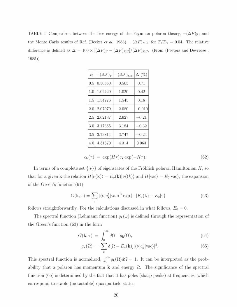
TABLE I Comparison between the free energy of the Feynman polaron theory, −(∆F )F, and

the Monte Carlo results of Ref. (Becker et al., 1983), −(∆F )MC, for T/TD = 0.04. The relative

difference is defined as ∆ = 100 × [(∆F )F − (∆F )MC]/(∆F )MC. (From (Peeters and Devreese ,

1985))

α − (∆F )F − (∆F )MC ∆ (%)

0.5 0.50860 0.505 0.71

1.0 1.02429 1.020 0.42

1.5 1.54776 1.545 0.18

2.0 2.07979 2.080 −0.010

2.5 2.62137 2.627 −0.21

3.0 3.17365 3.184 −0.32

3.5 3.73814 3.747 −0.24

4.0 4.31670 4.314 0.063

ck(τ) = exp(Hτ)ck exp(−Hτ). (62)

In terms of a complete set |ν〉 of eigenstates of the Frohlich polaron Hamiltonian H , so

that for a given k the relation H|ν(k)〉 = Eν(k)|ν((k)〉 and H|vac〉 = E0|vac〉, the expansion

of the Green’s function (61)

G(k, τ) =∑

ν

|〈ν|c†k|vac〉|2 exp−[Eν(k) − E0]τ (63)

follows straightforwardly. For the calculations discussed in what follows, E0 = 0.

The spectral function (Lehmann function) gk(ω) is defined through the representation of

the Green’s function (63) in the form

G(k, τ) =

∫ ∞

0

dΩ gk(Ω), (64)

gk(Ω) =∑

ν

δ[Ω −Eν(k)]|〈ν|c†k|vac〉|2. (65)

This spectral function is normalized,∫∞0gk(Ω)dΩ = 1. It can be interpreted as the prob-

ability that a polaron has momentum k and energy Ω. The significance of the spectral

function (65) is determined by the fact that it has poles (sharp peaks) at frequencies, which

correspond to stable (metastable) quasiparticle states.

20

If, for a given k, there is a stable state at energy E(k), the spectral function takes the

form

gk(Ω) = Z(k)0 δ[Ω − E(k)]..., (66)

where Z(k)0 is the weight of the bare-electron state. The energy Egs(k) and the weight Z

(k)0,gs

for the polaron ground state can be extracted from the Green’s function behaviour at long

times:

G(k, τ ≫ ω−10 ) → Z

(k)0 exp[−E(k)τ ]. (67)

Similarly to Eq. (61), the N -phonon Green’s function is defined:

GN(k, τ ;q1, ...,qN ) = 〈vac|dqN(τ)...dq1

(τ)cp(τ)c†p(0)d†q1(0)...d†qN

(0)|vac〉, τ ≥ 0, (68)

p = k −N∑

j−1

qj .

From the asymptotic properties of the Green’s functions (68) at long times, the characteris-

tics of the polaron ground state are found. In particular, the weight of the N -phonon state

for the polaron ground state is given by

GN(k, τ ≫ ω−10 ;q1, ...,qN) → Z

(k)N (q1, ...,qN) exp[−E(k)τ ]. (69)

A standard diagrammatic expansion of the above described Green’s functions generates a

series of Feynman diagrams. The following function is further introduced:

P (k, τ) = G(k, τ) +

∞∑

N=1

∫

dq1...dqNGN (k, τ ;q1, ...,qN), (70)

where GN are irreducible N -phonon Green’s functions (which do not contain disconnected

phonon propagators). From Eqs. (67), (69) and the completeness condition for the non-

degenerate ground state

Z(k)0 +

∞∑

N=1

∫

dq1...dqNZ(k)N (q1, ...,qN) = 1 (71)

it follows that the polaron ground state energy is determined by the asymptotic behaviour

of the function (70):

P (k, τ ≫ ω−10 ) → exp[−E(k)τ ]. (72)

The function P (k, τ) is an infinite series of integrals containing an ever increasing number

of integration variables. The essence of the DQMC method is to construct a process, which

21

generates continuum random variables (k, τ) with a distribution function that coincides

exactly with P (k, τ). Taking into account Eq. (70) and the diagrammatic rules, P (k, τ) is

identified with the distribution function

Q(y) =

∞∑

m=0

∑

ξm

∫

dx1...dxmFm(ξm, y, x1, ..., xm), (73)

where the external variables y include k, τ, α and N , while the internal variables de-

scribe the topology of the diagram (labelled with ξm), times assigned to electron-phonon

vertices and momenta of phonon propagators. The diagrammatic Monte Carlo process

is a numeric procedure, which samples various diagrams in parameter space and collects

statistics for Q(y) according to the Metropolis algorithm (Metropolis et al., 1953) is

such a way that — when the process is repeated a large number of times — the result

converges to the exact answer. The distribution function given by the convergent series

(73) is simulated within the process of sequential stochastic generation of diagrams de-

scribed by functions Fm(ξm, y, x1, ..., xm). Further, using Eq. (64), the spectral function

gk(ω) is obtained applying a stochastic optimization technique. We refer to the review

(Mishchenko and Nagaosa, 2007) for further details on the DQMC and stochastic optimiza-

tion, where information on the excited states of the polaron is also derived by the analytic

continuation of the imaginary time Green’s functions to real frequencies.

DQMC confirms that for α & 1 the bare-electron state in the polaron wave function is

no longer the dominant contribution and perturbation theory is not adequate. The bare-

electron weight Z00 for the polaron ground state, as a function of the polaron coupling

constant, rapidly vanishes for α & 3. It is suggested in (Mishchenko et al., 2000) that in

the interval 3 . α . 10 the polaron ground states smoothly transforms between weak- and

strong-coupling limits.

Below (see sections III.C, III.D, III.G) earlier analytical studies and results on Frohlich

polarons are compared with DQMC results. It would be beneficial, to have an indepen-

dent numerical check of the DQMC results. The comparison of the DQMC results for the

“low-energy” (Ω < 0) part of the spectral density 1 for the Frohlich polaron at α = 0.05

(Mishchenko et al., 2000) demonstrates perfect agreement with the perturbation theory re-

1 It is worth of noticing, that the spectral density is not identical to the optical absorption coefficient, which

is discussed below in sections III.B, III.C and III.D.

22

sult:

g0(Ω < 0) =α

2δ[Ω + α] (74)

(m and ω0 are set equal to unity). The DQMC results for the “high-energy” (Ω > 0)

part of the spectral density significantly differ from the perturbation-theory curve. This is

attributed to the fact that for the Frohlich polaron the perturbation-theory expression for

g0(Ω > 0) =α

π

θ(Ω − 1)

Ω2√

Ω − 1(75)

diverges as Ω → 1 and, consequently, the perturbation approach is no longer adequate. The

main difference between the DQMC spectrum of the Frohlich polaron and the perturbation-

theory result is the broad peak in the spectral density at Ω ∼ 3.5. This peak appears for

significantly larger values of the coupling constant and its weight grows with α, see Fig. 2.

As shown in the inset, near the threshold, Ω = 1, the spectral density behaves as√

Ω − 1.

Next to Frohlich polarons, other polaron models have been extensively investigated using

the Monte Carlo approach. In particular Alexandrov (1996) proposed a long-range discrete

Frohlich interaction as a model of the interaction between a hole and the oxygen ions in

cuprate superconductors. The essence of the model is that a charge carrier moves from site

to site on a discrete lattice (or chain in 1D) and interacts with all the ions, which reside at

the lattice sites. Numerically rigorous polaron characteristics (ground-state energy, number

of phonons in the polaron cloud, effective mass and isotope exponent) for such a lattice

polaron, valid for arbitrary EPI, were obtained using a path-integral continuous-time quan-

tum Monte Carlo technique (CTQMC) (Alexandrov and Kornilovitch , 1999; Hague et al. ,

2006a; Spencer et al. , 2005). This study leads to a “mobile small Frohlich” polaron

(IV.E.3).

Over the years the Feynman model for the Frohlich polaron has remained the most suc-

cessful approach to the problem. The analysis of an exactly solvable (“symmetrical”) 1D-

polaron model (Devreese , 1964; Devreese and Evrard , 1964, 1968), Monte Carlo schemes

(Mishchenko et al., 2000; Titantah et al., 2001) and, recently, a unifying variational ap-

proach (Cataudella et al., 2007; De Filippis et al. , 2003) demonstrate the remarkable ac-

curacy of Feynman’s path-integral method. Using the variational wave-functions, which

combine both the Landau-Pekar and the Feynman approximations, (Cataudella et al., 2007)

found in the α → ∞ limit:

E0 =(

−0.108507α2 − 2.67)

ω0. (76)

23

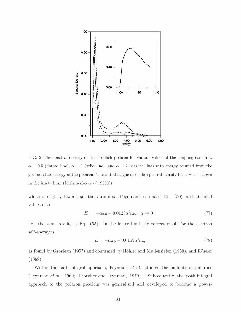
FIG. 2 The spectral density of the Frohlich polaron for various values of the coupling constant:

α = 0.5 (dotted line), α = 1 (solid line), and α = 2 (dashed line) with energy counted from the

ground-state energy of the polaron. The initial fragment of the spectral density for α = 1 is shown

in the inset (from (Mishchenko et al., 2000)).

which is slightly lower than the variational Feynman’s estimate, Eq. (50), and at small

values of α,

E0 = −αω0 − 0.0123α2ω0, α→ 0 , (77)

i.e. the same result, as Eq. (55). In the latter limit the correct result for the electron

self-energy is

E = −αω0 − 0.0159α2ω0, (78)

as found by Grosjean (1957) and confirmed by Hohler and Mullensiefen (1959), and Roseler

(1968).

Within the path-integral approach, Feynman et al. studied the mobility of polarons

(Feynman et al., 1962; Thornber and Feynman, 1970). Subsequently the path-integral

approach to the polaron problem was generalized and developed to become a power-

24

ful tool to study optical absorption and cyclotron resonance (Devreese et al. , 1972a;

Peeters and Devreese , 1986).

III. RESPONSE OF CONTINUUM POLARONS

A. Mobility

The mobility of large polarons was studied within various theoretical approaches. Frohlich

(Frohlich , 1937, 1954) pointed out the typical behavior of the large-polaron mobility

µ ∝ exp(ω0β), (79)

which is characteristic for weak coupling. Within the weak-coupling regime, the mo-

bility of the polaron was then derived, e. g., using the Boltzmann equation in

(Howarth and Sondheimer , 1953; Osaka , 1961) and starting from the LLP-transformation

in Ref. (Low and Pines, 1955). In (Langreth and Kadanoff , 1964) it was shown that for

weak coupling:

µ =e

2α[exp(ω0β) − 1]

[

1 − α

6+O(α2)

]

. (80)

A nonperturbative analysis was based on the Feynman polaron theory, where the mobility

µ of the polaron using the path-integral formalism was derived by Feynman et al. (1962)

(FHIP) as a static limit, starting from a frequency-dependent impedance function. Details

of the FHIP theory are given in (Platzman, 1963). An approximate expression for the

impedance function of a Frohlich polaron at all frequencies, temperatures and coupling

strengths was obtained in Refs. (Feynman et al., 1962; Platzman, 1963) within the path-

integral technique. Assuming the crystal to be isotropic, an alternating electric field E =

E0ex exp (iΩt) induces a current in the x-direction

j(Ω) = [z(Ω)]−1E0 exp (iΩt) . (81)

The complex function z(Ω) is called the impedance function. The electric field is considered

sufficiently weak, so that linear-response theory can be applied. The frequency-depending

mobility µ(Ω) is defined as

µ(Ω) = Re [z(Ω)]−1 . (82)

25

Taking the electric charge as unity, one arrives at j = 〈x〉, where 〈x〉 is the expectation value

of the electron displacement in the direction of the applied field: 〈x〉 = E/iΩz(Ω). In terms

of time dependent variables,

〈x(τ)〉 = −τ∫

−∞

iG(τ − σ)E(σ)dσ, (83)

where G(τ) has the inverse Fourier transform

G(Ω) =

∞∫

−∞

G(τ) exp (−iΩτ) dτ = [Ωz(Ω)]−1 . (84)

The expected displacement at time τ is

〈x(τ)〉 = Tr[

xU(τ, a)ρaU′−1(τ, a)

]

. (85)

Here, ρa is the density matrix of the system at some time a, long before the field is turned

on, and

U(τ, a) = T exp

−iτ∫

a

[Hs − xsE(s)] ds

(86)

is the unitary operator of the development of a state in time with the complete Hamiltonian

H − xE, where H is the Frohlich polaron Hamiltonian, and T is the time ordering operator

(Feynman, 1951). Primed operators are ordered antichronologically:

U ′−1(τ, a) = T′ exp

i

τ∫

a

[H ′s − x′sE

′(s)] ds

. (87)

G(τ − σ) can be represented as the second derivative

G(τ − σ) =1

2

(

∂2g

∂η∂ε

)∣

∣

∣

∣

ε=η=0

(88)

of

g = Tr[

U(b, a)ρaU′−1(b, a)

]

, b→ ∞, a→ −∞ (89)

with E(s) = εδ(s−σ)+ηδ(s−τ), E ′(s) = εδ(s−σ)−ηδ(s−τ). The initial state is chosen at

a definite temperature T , ρa ∝ exp(−βH). If the time a is sufficiently far in the past, FHIP

assume that only the phonon subsystem was in thermal equilibrium at temperature T . The

energy of the single electron and of the electron-phonon coupling are infinitesimal (of order

26

1/V ) with respect to that of the phonons. With this choice of the initial distribution, the

phonon coordinates can be eliminated from the expression (89), and the entire expression is

reduced to a double path integral over the electron coordinates only:

g =

∫ ∫

exp (iΦ)Dr(t)Dr′(t), (90)

where (taking m = 1)

Φ =

∞∫

−∞

[

r2

2− r′2

2

]

dt−∞∫

−∞

[E(t) · r(t) − E′(t) · r′(t)] dt (91)

+iα

23/2

∞∫

−∞

∞∫

−∞

[

exp(−i |t− s|) + 2P (β) cos(t− s)

|r(t) − r(s)| +exp(+i |t− s|) + 2P (β) cos(t− s)

|r′(t) − r′(s)|

−2 [exp(−i (t− s)) + 2P (β) cos(t− s)]

|r′(t) − r(s)|

]

dtds,

where P (β) =[

eβ − 1]−1

. The double path integral in (90) is over paths which satisfy the

boundary condition r(t)−r′(t) = 0 at times t approaching ±∞. The expression (90) with

(91) is supposed to be exact (Feynman et al., 1962). Clearly to provide analytical solutions

at all α presumably is impossible.

Following Feynman’s idea to describe the ground state energy properties of a polaron

by introducing a parabolic “retarded” interaction of the electron with itself (see subsection

II.D), it is assumed in (Feynman et al., 1962) that the dynamical behavior of the polaron can

be described approximately by replacing Φ of Eq. (90) by a parabolic (retarded) expression

Φ0 =

∞∫

−∞

[

r2

2− r′2

2

]

dt−∞∫

−∞

[E(t) · r(t) −E′(t) · r′(t)] dt (92)

−iC2

∞∫

−∞

∞∫

−∞

[r(t) − r(s)]2[

e−iw|t−s| + 2P (βw) cosw(t− s)]

+ [r′(t) − r′(s)]2 [e+iw|t−s| + 2P (βw) cos(t− s)

]

−2 [r′(t) − r(s)]2 [e−iw(t−s) + 2P (βw) cosw(t− s)

]

dtds.

The parameters C and w are to be determined so as to approximate Φ as closely as possible.

However, no variational principle is known for the mobility. At zero temperature, C and w

are fixed at the values, which provide the best upper bound for the polaron ground state

27

energy (53). At finite temperatures (T 6= 0) the parameters C and w are determined from the

variational principle for the polaron free energy (Feynman, 1972). This way of selection of the

model parameters C and w is based on the supposition, that “the comparison Lagrangian,

which gives a good fit to the ground-state energy at zero temperature, will also give the

dynamical behaviour of the system” (Feynman et al., 1962).

The analytical calculation of path integrals in (90) in (Feynman et al., 1962) was per-

formed to the first term in an expansion of exp [i (Φ − Φ0)]:

g =

∫ ∫

exp (iΦ0) exp [i (Φ − Φ0)]Dr(t)Dr′(t) ≈ g0 + g1, (93)

g0 =

∫ ∫

exp (iΦ0)Dr(t)Dr′(t), (94)

g1 = i

∫ ∫

exp (iΦ0) (Φ − Φ0)Dr(t)Dr′(t). (95)

Using (84) and (88), one finds from(93)

G(Ω) ≈ G0(Ω) +G1(Ω). (96)

The first term in the rhs of Eq. (96) is

G0(Ω) = iY0(Ω), Y0(Ω) = − Ω2 − w2

(Ω − iε)2[(Ω − iε)2 − v2], ε→ +0 (97)

with v2 = w2 + 4C/w. The second term in the rhs of Eq. (96) is

G1(Ω) = −iY 20 (Ω)

[

χ(Ω) − 4C

w

Ω2

Ω2 − w2

]

, (98)

χ(Ω) =

∞∫

0

(

1 − eiΩu)

ImS(u)du, (99)

S(u) =2α

3√π

eiu + 2P (β) cosu

[D(u)]3/2, (100)

D(u) =w2

v2

v2 − w2

w2v

[

1 − eivu + 4P (βv) sin2(vu

2

)]

(101)

−iu+u2

β

.

From (84) and (96), the impedance results in the form

Ωz(Ω) ≈ [G0(Ω) +G1(Ω)]−1 . (102)

Feynman et al.(1962) suggested to use this expression expanded to first order in G1(Ω):

Ωz(Ω) ≈ [G0(Ω)]−1 − [G0(Ω)]−2G1(Ω). (103)

28

Substitution of (97) and (98) into Eq.(103) leads to the final expression (Ref.

(Feynman et al., 1962)) for the impedance function of the Frohlich polaron:

Ωz(Ω) = i[

Ω2 − χ(Ω)]

. (104)

An alternative derivation of the impedance function of the Frohlich polaron, based on

simple operator techniques, was presented in (Peeters and Devreese , 1983a). The FHIP

result was worked out in (Peeters and Devreese, 1984) in detail to get a physical insight

into the scattering processes incorporated in the FHIP approximation. For sufficiently low

temperature the FHIP polaron mobility takes the form (Feynman et al., 1962)

µ =(w

v

)3 3e

4mω20αβ

eω0β exp(v2 − w2)/w2v , (105)

where v and w are variational functions of α obtained from the Feynman polaron model.

Using the Boltzmann equation for the Feynman polaron model, Kadanoff (1963) found

the mobility, which for low temperatures can be represented as follows:

µ =(w

v

)3 e

2mω0αeω0β exp(v2 − w2)/w2v , (106)

The weak-coupling perturbation expansion of the low-temperature polaron mobility as found

using the Green’s function technique (Langreth and Kadanoff , 1964) has confirmed that

the mobility derived from the Boltzmann equation is asymptotically exact for weak coupling

(α ≪ 1) and at low temperatures (T ≪ ω0). As first noticed in (Kadanoff , 1963), the

mobility of Eq. (105) differs by the factor of 3/(2βω0) from that derived using the polaron

Boltzmann equation as given by Eq. (106). 2 As follows from this comparison, the result of

(Feynman et al., 1962) is not valid when T → 0. As emphasized in (Feynman et al., 1962)

and later confirmed, in particular, in (Peeters and Devreese, 1983b, 1984) the above dis-

crepancy can be attributed to an interchange of two limits in calculating the impedance. In

FHIP, for weak electron-phonon coupling, one takes limΩ→0 limα→0, whereas limα→0 limΩ→0

should be calculated. It turns out that for the asymptotically correct result the mobility

2 In the asymptotic limit of weak electron-phonon coupling and low temperature, the FHIP polaron mobility

of Eq. (105) differs by the same factor of 3/(2βω0) from the earlier result (Howarth and Sondheimer ,

1953; Low and Pines, 1955; Osaka , 1961), which, as pointed out in Ref. (Feynman et al., 1962) and in

later publications (Kadanoff , 1963; Langreth and Kadanoff , 1964; Peeters and Devreese, 1984), is correct

for β ≫ 1.

29

at low temperatures is mainly limited by the absorption of phonons, while in the theory

of FHIP it is the emission of phonons which gives the dominant contribution as T goes to

zero (Peeters and Devreese, 1983b).

The analysis based on the Boltzmann equation takes into account the phonon emis-

sion processes whenever the energy of the polaron is above the emission threshold. The

independent-collision model, which underlies the Boltzmann-equation approach, however,

fails in the “strong coupling regime” of the Frohlich polaron, when the thermal mean free

path becomes less than the de Broglie wavelength; in this case, the Boltzmann equation

cannot be expected to be adequate (Feynman et al., 1962; Hellwarth and Biaggio , 1999).

Experimental work on alkali halides and silver halides indicates that the mobility ob-

tained from Eq. (105) describes the experimental results accurately (see (Brown , 1963,

1972) and references therein). Measurements of mobility as a function of temperature for

photoexcited electrons in cubic n-type Bi12SiO20 are explained well in terms of large polarons

within the Feynman approach (Hellwarth and Biaggio , 1999). The experimental findings

on electron transport in crystalline TiO2 (rutile phase) probed by THz time-domain spec-

troscopy were quantitatively interpreted within the Feynman model (Hendry et al., 2004).

One of the reasons for the agreement between theory based on Eq. (105) and experiment

is that in the path-integral approximation to the polaron mobility, a Maxwellian distribu-

tion for the electron velocities is assumed, when applying the adiabatic switching on of the

Frohlich interaction. Although such a distribution is not inherent in the Frohlich interac-

tion, its incorporation tends to favor agreement with experiment because other mechanisms

(interaction with acoustic phonons etc.) cause a Gaussian distribution.

B. Optical absorption at weak coupling

At zero temperature and in the weak-coupling limit, the optical absorption of a Frohlich

polaron is due to the elementary polaron scattering process with the absorption of incom-

ing photon and emission of an outgoing phonon. In the weak-coupling limit (α ≪ 1)

the polaron absorption coefficient for a many-polaron gas was first obtained by Gurevich

et al. (1962). Their optical-absorption coefficient is equivalent to a particular case of

(Tempere and Devreese , 2001) with the dynamic structure factor S(q, ω) corresponding to

the Hartree-Fock approximation. In (Tempere and Devreese , 2001) the optical absorption

30

coefficient of a many-polaron gas was shown to be given, to order α, by

Re[σ(Ω)] = n0e22

3α

1

2πΩ3

∫ ∞

0

dqq2S(q,Ω − ω0), (107)

where n0 is the density of charge carriers.

In the zero-temperature limit, starting from the Kubo formula the optical conductivity

of a single Frohlich polaron can be represented in the form

σ(Ω) = ie2

m (Ω + iδ)+

e2

m2

1

(Ω + iδ)3

∫ ∞

0

e−δt(

eiΩt − 1)

∑

q,q′

qxq′x

⟨

Ψ0|[Bq(t), B−q′(0)]|Ψ0

⟩

dt,

(108)

where δ = +0, Bq(t) = [Vqdq(t) + V ∗−qd

†−q(t)]e

iq·r(t), and |Ψ0〉 is the ground-state wave

function of the electron-phonon system. Within the weak coupling approximation, the

following analytic expression for the real part of the polaron optical conductivity results

from Eq. (108):

Reσ (Ω) =πe2

2m∗ δ (Ω) +2e2

3m

ω0α

Ω3

√

Ω − ω0Θ (Ω − ω0) , (109)

where Θ(x) = 1 if x > 0, and zero otherwise. The spectrum of the real part of the polaron

optical conductivity (109) is represented in Fig. 3.

According to Eq. (109), the absorption coefficient of light with frequency Ω > 0 by free

polarons for α → 0 takes the form

Γ(Ω) =4π

nc

2npe2αω2

0

3mΩ3(Ω/ω0 − 1)1/2 Θ (Ω − ω0) , (110)

where c is the velocity of light in vacuum, n is the refractive index of the medium, np is the

concentration of polarons. A simple derivation (Devreese et al. , 1971) using a canonical

transformation method gives the absorption coefficient of free polarons, which coincides

with the result (110). The step function in (110) reflects the fact that at zero temperature

the absorption of light accompanied by the emission of a phonon can occur only if the

energy of the incident photon is larger than that of a phonon (Ω > ω0). In the weak-

coupling limit, according to Eq. (110), the absorption spectrum consists of a “one-phonon

line”. At nonzero temperature, the absorption of a photon can be accompanied not only by

emission, but also by absorption of one or more phonons. Similarity between the temperature

dependence of several features of the experimental infrared absorption spectra in high-Tc

superconductors and the temperature dependence predicted for the optical absorption of a

31

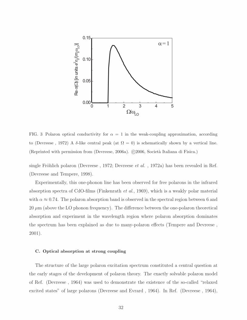
FIG. 3 Polaron optical conductivity for α = 1 in the weak-coupling approximation, according

to (Devreese , 1972) A δ-like central peak (at Ω = 0) is schematically shown by a vertical line.

(Reprinted with permission from (Devreese, 2006a). c©2006, Societa Italiana di Fisica.)

single Frohlich polaron (Devreese , 1972; Devreese et al. , 1972a) has been revealed in Ref.

(Devreese and Tempere, 1998).

Experimentally, this one-phonon line has been observed for free polarons in the infrared

absorption spectra of CdO-films (Finkenrath et al., 1969), which is a weakly polar material

with α ≈ 0.74. The polaron absorption band is observed in the spectral region between 6 and

20 µm (above the LO phonon frequency). The difference between the one-polaron theoretical

absorption and experiment in the wavelength region where polaron absorption dominates

the spectrum has been explained as due to many-polaron effects (Tempere and Devreese ,

2001).

C. Optical absorption at strong coupling

The structure of the large polaron excitation spectrum constituted a central question at

the early stages of the development of polaron theory. The exactly solvable polaron model

of Ref. (Devreese , 1964) was used to demonstrate the existence of the so-called “relaxed

excited states” of large polarons (Devreese and Evrard , 1964). In Ref. (Devreese , 1964),

32

an exactly solvable (“symmetric”) 1D-polaron model was introduced and analysed. The

further study of this model was performed in Refs. (Devreese and Evrard , 1964, 1968).

The model consists of an electron interacting with two oscillators possessing opposite wave

vectors: q and −q. The parity operator, which changes dq and d−q (and also d†q and d†−q),

commutes with the Hamiltonian of the system. Hence, the polaron states are classified into

even and odd states with eigenvalues of the parity operator +1 and −1, respectively. For

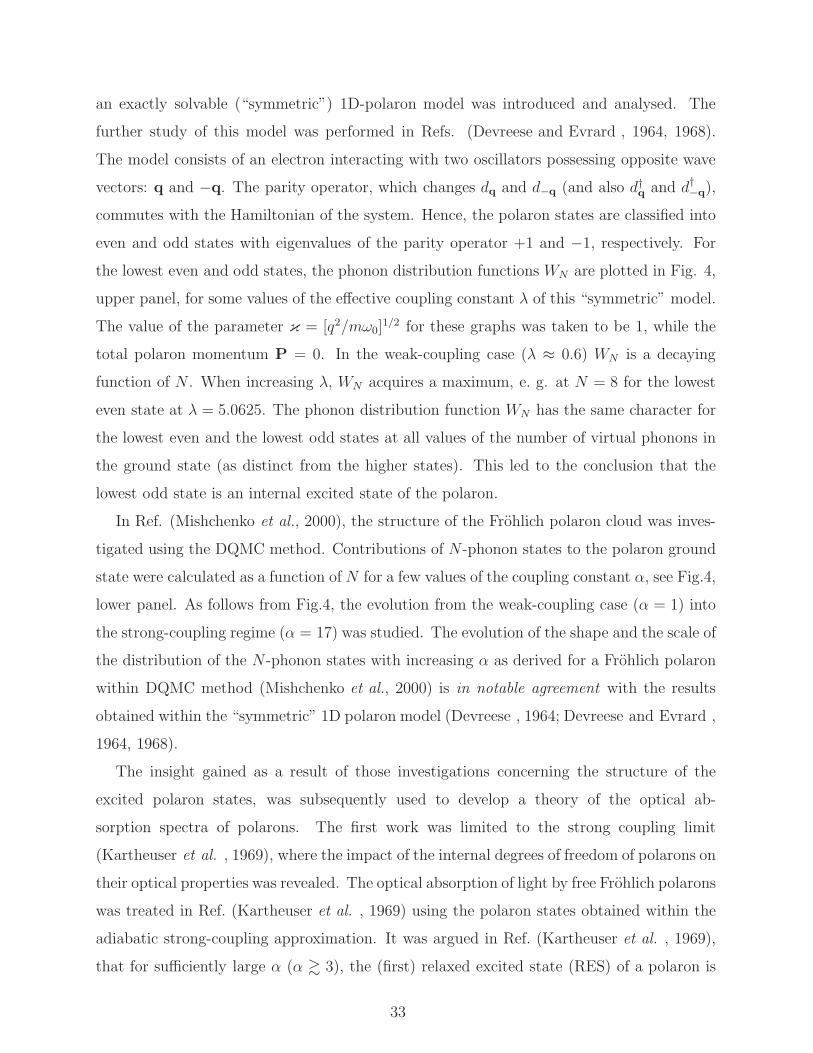
the lowest even and odd states, the phonon distribution functions WN are plotted in Fig. 4,

upper panel, for some values of the effective coupling constant λ of this “symmetric” model.

The value of the parameter κ = [q2/mω0]1/2 for these graphs was taken to be 1, while the

total polaron momentum P = 0. In the weak-coupling case (λ ≈ 0.6) WN is a decaying

function of N . When increasing λ, WN acquires a maximum, e. g. at N = 8 for the lowest

even state at λ = 5.0625. The phonon distribution function WN has the same character for

the lowest even and the lowest odd states at all values of the number of virtual phonons in

the ground state (as distinct from the higher states). This led to the conclusion that the

lowest odd state is an internal excited state of the polaron.

In Ref. (Mishchenko et al., 2000), the structure of the Frohlich polaron cloud was inves-

tigated using the DQMC method. Contributions of N -phonon states to the polaron ground

state were calculated as a function of N for a few values of the coupling constant α, see Fig.4,

lower panel. As follows from Fig.4, the evolution from the weak-coupling case (α = 1) into

the strong-coupling regime (α = 17) was studied. The evolution of the shape and the scale of

the distribution of the N -phonon states with increasing α as derived for a Frohlich polaron

within DQMC method (Mishchenko et al., 2000) is in notable agreement with the results

obtained within the “symmetric” 1D polaron model (Devreese , 1964; Devreese and Evrard ,

1964, 1968).

The insight gained as a result of those investigations concerning the structure of the

excited polaron states, was subsequently used to develop a theory of the optical ab-

sorption spectra of polarons. The first work was limited to the strong coupling limit

(Kartheuser et al. , 1969), where the impact of the internal degrees of freedom of polarons on

their optical properties was revealed. The optical absorption of light by free Frohlich polarons

was treated in Ref. (Kartheuser et al. , 1969) using the polaron states obtained within the

adiabatic strong-coupling approximation. It was argued in Ref. (Kartheuser et al. , 1969),

that for sufficiently large α (α & 3), the (first) relaxed excited state (RES) of a polaron is

33

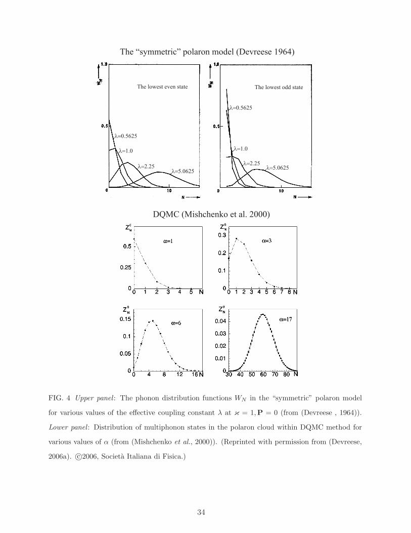
FIG. 4 Upper panel : The phonon distribution functions WN in the “symmetric” polaron model

for various values of the effective coupling constant λ at κ = 1,P = 0 (from (Devreese , 1964)).

Lower panel : Distribution of multiphonon states in the polaron cloud within DQMC method for

various values of α (from (Mishchenko et al., 2000)). (Reprinted with permission from (Devreese,

2006a). c©2006, Societa Italiana di Fisica.)

34

a relatively stable state, which gives rise to a “resonance” in the polaron optical absorption

spectrum. The following scenario of a transition, which leads to a “zero-phonon” peak in

the absorption by a strong-coupling polaron, was then suggested. If the frequency of the

incoming photon is equal to ΩRES = 0.065α2ω0, the electron jumps from the ground state

(which, at large coupling, is well-characterised by “s”-symmetry for the electron) to an ex-

cited state (“2p”), while the lattice polarization in the final state is adapted to the “2p”

electronic state of the polaron. In Ref. (Kartheuser et al. , 1969) considering the decay of

the RES with emission of one real phonon, it is argued, that the “zero-phonon” peak can

be described using the Wigner-Weisskopf formula which is valid when the linewidth of that

peak is much smaller than ω0.

For photon energies larger than ΩRES +ωLO, a transition of the polaron towards the first

scattering state, belonging to the RES, becomes possible. The final state of the optical

absorption process then consists of a polaron in its lowest RES plus a free phonon. A “one-

phonon sideband” then appears in the polaron absorption spectrum. This process is called

one-phonon sideband absorption. The one-, two-, ... K-, ... phonon sidebands of the zero-

phonon peak give rise to a broad structure in the absorption spectrum. It turns out that the

first moment of the phonon sidebands corresponds to the Franck-Condon (FC) frequency

ΩFC = 0.141α2ω0.

To summarise, following (Kartheuser et al. , 1969), the polaron optical absorption spec-

trum at strong coupling is characterised by the following features (at T = 0):

a) An absorption peak (“zero-phonon line”) appears, which corresponds to a transition

from the ground state to the first RES at ΩRES.

b) For Ω > ΩRES + ω0, a phonon sideband structure arises. This sideband structure

peaks around ΩFC. Even when the zero-phonon line becomes weak, and most oscillator

strength is in the LO-phonon sidebands, the zero-phonon line continues to determine

the onset of the phonon sideband structure.

The basic qualitative strong coupling behaviour predicted in Ref. (Kartheuser et al. ,

1969), namely, zero-phonon (RES) line with a broader sideband at the high-frequency side,

was confirmed by later studies, as discussed below.

35

D. Optical absorption at arbitrary coupling

The optical absorption of the Frohlich polaron was calculated in 1972 (Devreese , 1972;

Devreese et al. , 1972a) (“DSG”) for the Feynman polaron model using path integrals. Un-

til recently DSG combined with (Kartheuser et al. , 1969) constituted the basic picture for

the optical absorption of the Frohlich polaron. (Peeters and Devreese , 1983a) rederived the

DSG-result using the memory function formalism (MFF). The DSG-approach is successful

at weak electron-phonon coupling and is able to identify the excitations at intermediate

electron-phonon coupling (3 . α . 6). In the strong coupling limit DSG still gives an

accurate first moment for the polaron optical absorption but does not reproduce the broad

phonon sideband structure (cf. (Kartheuser et al. , 1969) and (Goovaerts et al. , 1973)). A

comparison of the DSG results with the optical conductivity spectra given by recently devel-

oped “approximation-free” numerical (Mishchenko et al. , 2003) and approximate analytical

(De Filippis et al. , 2003, 2006) approaches was carried out recently (De Filippis et al. ,

2006), see also the review articles (Cataudella et al., 2007) and (Mishchenko and Nagaosa,

2007).

The polaron absorption coefficient Γ(Ω) of light with frequency Ω at arbitrary coupling

was first derived in Ref. (Devreese et al. , 1972a). It was represented in the form

Γ(Ω) = −4π

nc

e2

m

ImΣ(Ω)

[Ω − ReΣ(Ω)]2 + [ImΣ(Ω)]2. (111)

This general expression was the starting point for a derivation of the theoretical optical

absorption spectrum of a single Frohlich polaron at all electron-phonon coupling strengths

by (Devreese et al. , 1972a). Σ(Ω) is the so-called “memory function”, which contains the

dynamics of the polaron and depends on Ω, α, temperature and applied external fields.

The key contribution of (Devreese et al. , 1972a) was to introduce Γ(Ω) in the form (111)

and to calculate ReΣ(Ω), which is essentially a (technically not trivial) Kramers–Kronig

transform of the more simple function ImΣ(Ω). Only the function ImΣ(Ω) had been derived

for the Feynman polaron (Feynman et al., 1962) to study the polaron mobility µ using the

impedance function (82): µ−1 = limΩ→0

(ImΣ(Ω)/Ω).

The basic nature of the Frohlich polaron excitations was clearly revealed through this

polaron optical absorption given by Eq. (111). It was demonstrated (Devreese et al. ,

1972a) that the FC states for Frohlich polarons are nothing else but a superposition of

36

phonon sidebands and a relatively large value of the electron-phonon coupling strength

(α > 5.9) is needed to stabilise the relaxed excited state of the polaron. It was, further,

revealed that at weaker coupling only “scattering states” of the polaron play a significant

role in the optical absorption (Devreese et al. , 1971, 1972a).

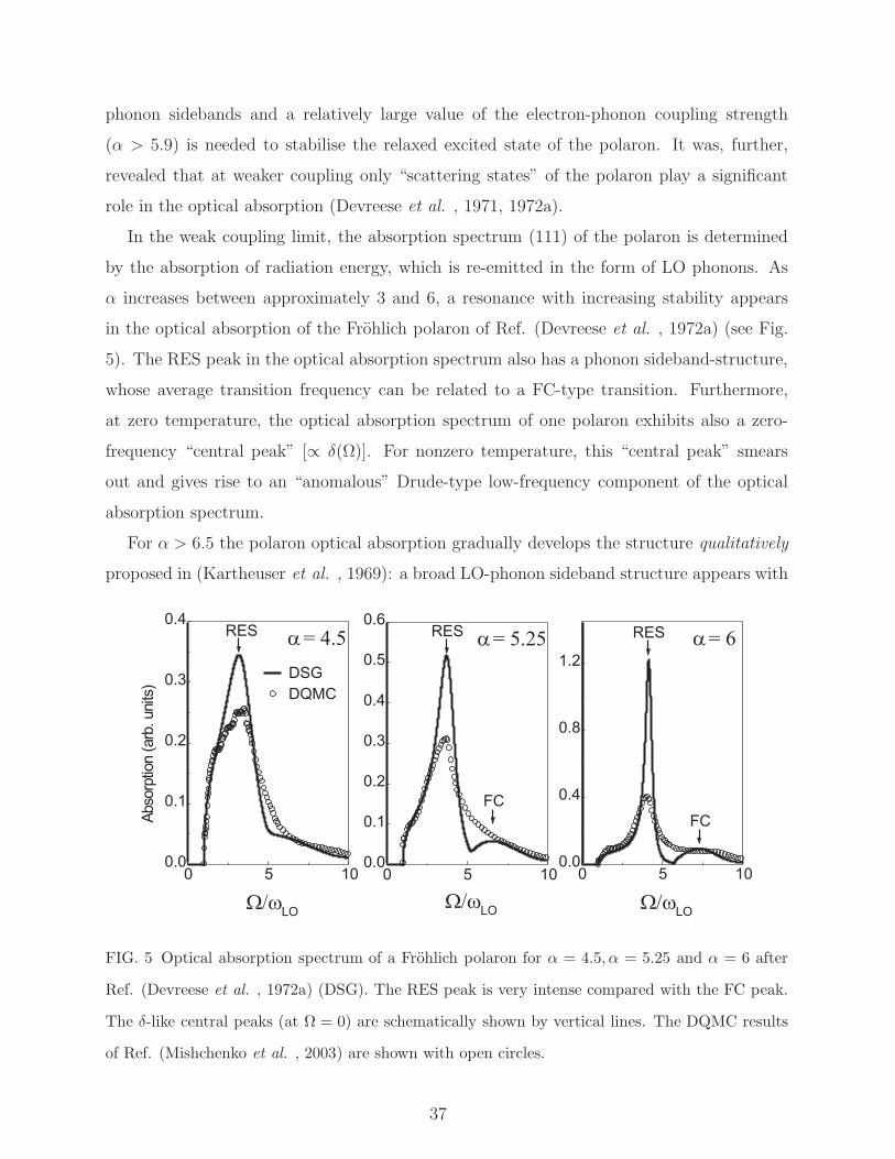
In the weak coupling limit, the absorption spectrum (111) of the polaron is determined

by the absorption of radiation energy, which is re-emitted in the form of LO phonons. As

α increases between approximately 3 and 6, a resonance with increasing stability appears

in the optical absorption of the Frohlich polaron of Ref. (Devreese et al. , 1972a) (see Fig.

5). The RES peak in the optical absorption spectrum also has a phonon sideband-structure,

whose average transition frequency can be related to a FC-type transition. Furthermore,

at zero temperature, the optical absorption spectrum of one polaron exhibits also a zero-

frequency “central peak” [∝ δ(Ω)]. For nonzero temperature, this “central peak” smears

out and gives rise to an “anomalous” Drude-type low-frequency component of the optical

absorption spectrum.

For α > 6.5 the polaron optical absorption gradually develops the structure qualitatively

proposed in (Kartheuser et al. , 1969): a broad LO-phonon sideband structure appears with

FIG. 5 Optical absorption spectrum of a Frohlich polaron for α = 4.5, α = 5.25 and α = 6 after

Ref. (Devreese et al. , 1972a) (DSG). The RES peak is very intense compared with the FC peak.

The δ-like central peaks (at Ω = 0) are schematically shown by vertical lines. The DQMC results

of Ref. (Mishchenko et al. , 2003) are shown with open circles.

37

the zero-phonon (“RES”) transition as onset. Ref. (Devreese et al. , 1972a) does not predict

the broad LO-phonon sidebands at large coupling constant, although it still gives an accurate

first Stieltjes moment of the optical absorption spectrum.

Based on (Devreese et al. , 1972a), it was argued that it is rather Holstein polarons

that determine the optical properties of the charge carriers in oxides like SrTiO3, BaTiO3

(Huybrechts and Devreese , 1975), while Frohlich weak-coupling polarons could be identi-

fied e. g. in CdO (Devreese et al. , 1971). The Frohlich coupling constants of polar semi-

conductors and ionic crystals are generally too small to allow for a static “RES”. In Ref.

(Eagles et al., 1995) the RES-peaks of Ref. (Devreese et al. , 1972a) were invoked to explain

the optical absorption spectrum of Pr2NiO4.22. The RES-like resonances in Γ(Ω), Eq. (111),

due to the zero’s of Ω − ReΣ(Ω), can effectively be displaced to smaller polaron coupling

by applying an external magnetic field B, in which case the contribution for what is for-

mally a “RES-type resonance” arises at Ω − ωc − ReΣ(Ω) = 0 (ωc = eB/m is the cyclotron

frequency). Resonances in the magnetoabsorption governed by this contribution have been

clearly observed and analysed in many solids and structures, see e. g. (Devreese, 1996, 2003;

Hodby et al., 1987; Miura et al. , 1997; Peeters and Devreese , 1986; Shi et al. , 1993) and

references therein.

Evidence for the polaron character of charge carriers in AgBr and AgCl was obtained

through high-precision cyclotron resonance experiments in external magnetic fields up to

16 T. The all-coupling magneto-absorption calculated in (Peeters and Devreese , 1986) leads

to the best quantitative agreement between theory and experiment for AgBr and AgCl.

This quantitative interpretation of the cyclotron resonance experiment in AgBr and AgCl

(Hodby et al., 1987) by the theory of (Peeters and Devreese , 1986) provided one of the most

convincing and clearest demonstrations of Frohlich polaron features in solids. The energy

spectra of polaronic systems such as shallow donors (“bound polarons”), e. g., the D0 and

D− centres, constitute the most complete and detailed polaron spectroscopy realised in the

literature (Shi et al. , 1993).

The numerical calculations of the optical conductivity for the Frohlich polaron performed

within the DQMC method (Mishchenko et al. , 2003) confirm the analytical results derived

in Ref. (Devreese et al. , 1972a) for α . 3. In the intermediate coupling regime 3 < α < 6,

the low-energy behaviour and the position of the RES-peak in the optical conductivity

spectrum of (Mishchenko et al. , 2003) follow closely the prediction of Ref. (Devreese et al. ,

38

1972a). There are some minor quantitative differences between the two approaches in the

intermediate coupling regime: the dominant (“RES”) peak is less intense in the Monte-Carlo

numerical simulations and the second (“FC”) peak develops less prominently. The following

qualitative differences exist between the two approaches: in (Mishchenko et al. , 2003), the

dominant peak broadens for α & 6 and the second peak does not develop, but gives rise

to a flat shoulder in the optical conductivity spectrum at α ≈ 6. As α increases beyond

α ≈ 6, the DSG results for the OC do not produce the broad phonon sideband spectrum of

the RES-transition that was qualitatively predicted in Ref. (Kartheuser et al. , 1969) and

obtained with DQMC.

An instructive comparison between the positions of the main peak in the optical absorp-

tion spectra of Frohlich polarons obtained within the DSG and DQMC approaches has been

performed recently (Devreese and Klimin , 2006). The main-peak positions, obtained within

DSG, have been found in good agreement with the results of DQMC for all considered values

of α. At large α the positions of the main peak in the DSG spectra are remarkably close

to those given by DQMC. The difference between the DSG and DQMC results is relatively

larger at α = 8 and for α = 9.5, but even for those values of the coupling constant the

agreement is rather good.

It is suggested that the RES-peak at α ≈ 6 in the DSG-treatment, as α increases,

gradually transforms onto a FC-peak. As stated above and in Ref. (Devreese et al. , 1972a),

DSG predicts a much too narrow FC-peak in the strong coupling limit, but still at the

“correct” frequency. The DSG spectrum also satisfies the zero and first moment sum rules

at all α as discussed below.

E. Main-peak line and strong-coupling expansion

In order to describe the OC main peak line width at intermediate electron-phonon cou-

pling, the DSG approach was modified (De Filippis et al. , 2006) to include additional dis-

sipation processes, the strength of which is fixed by an exact sum rule (Cataudella et al.,

2007).

Within the memory function formalism (MFF) (Gotze and P. Wolfle , 1972; Mori , 1965)

the interaction of the charge carriers with the free phonon oscillations is expressed in terms

39

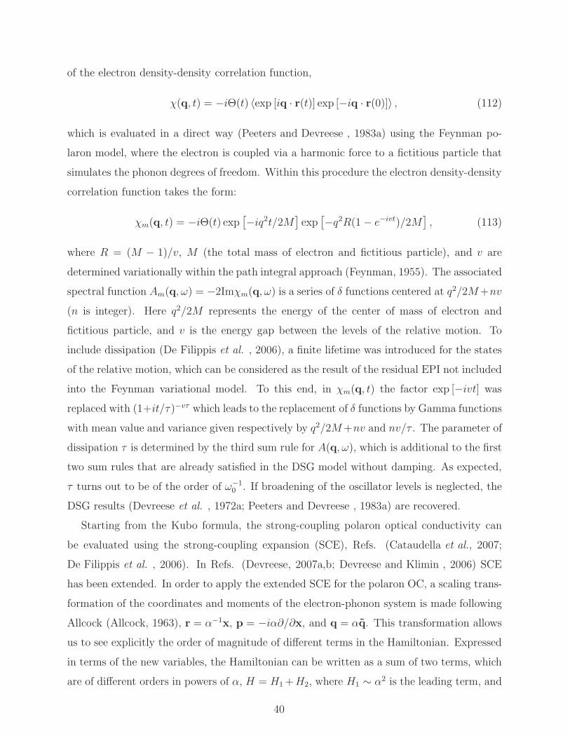
of the electron density-density correlation function,

χ(q, t) = −iΘ(t) 〈exp [iq · r(t)] exp [−iq · r(0)]〉 , (112)

which is evaluated in a direct way (Peeters and Devreese , 1983a) using the Feynman po-

laron model, where the electron is coupled via a harmonic force to a fictitious particle that

simulates the phonon degrees of freedom. Within this procedure the electron density-density

correlation function takes the form:

χm(q, t) = −iΘ(t) exp[

−iq2t/2M]

exp[

−q2R(1 − e−ivt)/2M]

, (113)

where R = (M − 1)/v, M (the total mass of electron and fictitious particle), and v are

determined variationally within the path integral approach (Feynman, 1955). The associated

spectral function Am(q, ω) = −2Imχm(q, ω) is a series of δ functions centered at q2/2M+nv

(n is integer). Here q2/2M represents the energy of the center of mass of electron and

fictitious particle, and v is the energy gap between the levels of the relative motion. To

include dissipation (De Filippis et al. , 2006), a finite lifetime was introduced for the states

of the relative motion, which can be considered as the result of the residual EPI not included

into the Feynman variational model. To this end, in χm(q, t) the factor exp [−ivt] was

replaced with (1+it/τ)−vτ which leads to the replacement of δ functions by Gamma functions

with mean value and variance given respectively by q2/2M+nv and nv/τ . The parameter of

dissipation τ is determined by the third sum rule for A(q, ω), which is additional to the first

two sum rules that are already satisfied in the DSG model without damping. As expected,

τ turns out to be of the order of ω−10 . If broadening of the oscillator levels is neglected, the

DSG results (Devreese et al. , 1972a; Peeters and Devreese , 1983a) are recovered.

Starting from the Kubo formula, the strong-coupling polaron optical conductivity can

be evaluated using the strong-coupling expansion (SCE), Refs. (Cataudella et al., 2007;

De Filippis et al. , 2006). In Refs. (Devreese, 2007a,b; Devreese and Klimin , 2006) SCE

has been extended. In order to apply the extended SCE for the polaron OC, a scaling trans-

formation of the coordinates and moments of the electron-phonon system is made following

Allcock (Allcock, 1963), r = α−1x, p = −iα∂/∂x, and q = αq. This transformation allows

us to see explicitly the order of magnitude of different terms in the Hamiltonian. Expressed

in terms of the new variables, the Hamiltonian can be written as a sum of two terms, which

are of different orders in powers of α, H = H1 +H2, where H1 ∼ α2 is the leading term, and

40

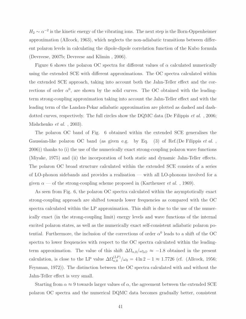
H2 ∼ α−2 is the kinetic energy of the vibrating ions. The next step is the Born-Oppenheimer

approximation (Allcock, 1963), which neglects the non-adiabatic transitions between differ-

ent polaron levels in calculating the dipole-dipole correlation function of the Kubo formula

(Devreese, 2007b; Devreese and Klimin , 2006).

Figure 6 shows the polaron OC spectra for different values of α calculated numerically

using the extended SCE with different approximations. The OC spectra calculated within

the extended SCE approach, taking into account both the Jahn-Teller effect and the cor-

rections of order α0, are shown by the solid curves. The OC obtained with the leading-

term strong-coupling approximation taking into account the Jahn-Teller effect and with the

leading term of the Landau-Pekar adiabatic approximation are plotted as dashed and dash-

dotted curves, respectively. The full circles show the DQMC data (De Filippis et al. , 2006;

Mishchenko et al. , 2003).

The polaron OC band of Fig. 6 obtained within the extended SCE generalises the

Gaussian-like polaron OC band (as given e.g. by Eq. (3) of Ref.(De Filippis et al. ,

2006)) thanks to (i) the use of the numerically exact strong-coupling polaron wave functions

(Miyake, 1975) and (ii) the incorporation of both static and dynamic Jahn-Teller effects.

The polaron OC broad structure calculated within the extended SCE consists of a series

of LO-phonon sidebands and provides a realisation — with all LO-phonons involved for a

given α — of the strong-coupling scheme proposed in (Kartheuser et al. , 1969).

As seen from Fig. 6, the polaron OC spectra calculated within the asymptotically exact

strong-coupling approach are shifted towards lower frequencies as compared with the OC

spectra calculated within the LP approximation. This shift is due to the use of the numer-

ically exact (in the strong-coupling limit) energy levels and wave functions of the internal

excited polaron states, as well as the numerically exact self-consistent adiabatic polaron po-

tential. Furthermore, the inclusion of the corrections of order α0 leads to a shift of the OC

spectra to lower frequencies with respect to the OC spectra calculated within the leading-

term approximation. The value of this shift ∆Ωn,0/ωLO ≈ −1.8 obtained in the present

calculation, is close to the LP value ∆Ω(LP )n,0 /ω0 = 4 ln 2 − 1 ≈ 1.7726 (cf. (Allcock, 1956;

Feynman, 1972)). The distinction between the OC spectra calculated with and without the

Jahn-Teller effect is very small.

Starting from α ≈ 9 towards larger values of α, the agreement between the extended SCE

polaron OC spectra and the numerical DQMC data becomes gradually better, consistent

41

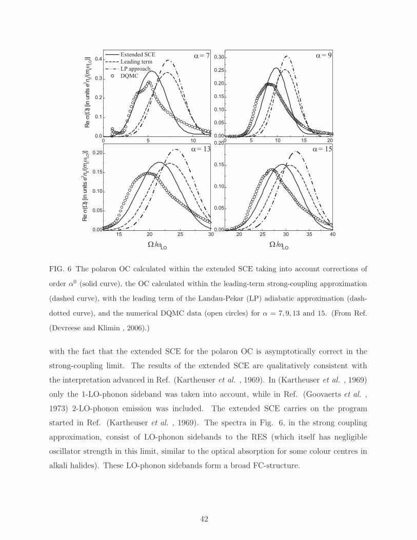
FIG. 6 The polaron OC calculated within the extended SCE taking into account corrections of

order α0 (solid curve), the OC calculated within the leading-term strong-coupling approximation

(dashed curve), with the leading term of the Landau-Pekar (LP) adiabatic approximation (dash-

dotted curve), and the numerical DQMC data (open circles) for α = 7, 9, 13 and 15. (From Ref.

(Devreese and Klimin , 2006).)

with the fact that the extended SCE for the polaron OC is asymptotically correct in the

strong-coupling limit. The results of the extended SCE are qualitatively consistent with

the interpretation advanced in Ref. (Kartheuser et al. , 1969). In (Kartheuser et al. , 1969)

only the 1-LO-phonon sideband was taken into account, while in Ref. (Goovaerts et al. ,

1973) 2-LO-phonon emission was included. The extended SCE carries on the program

started in Ref. (Kartheuser et al. , 1969). The spectra in Fig. 6, in the strong coupling

approximation, consist of LO-phonon sidebands to the RES (which itself has negligible

oscillator strength in this limit, similar to the optical absorption for some colour centres in

alkali halides). These LO-phonon sidebands form a broad FC-structure.

42

F. Comparison between optical conductivity spectra obtained by different methods

A comparison between the optical conductivity spectra obtained with the DQMC method,

extended MFF, SCE and DSG for different values of α is shown in Figs. 7, 8, taken from

Ref. (De Filippis et al. , 2006). The key results of the comparison are the following.

First, as expected, in the weak-coupling regime, both the extended MFF with phonon

broadening and DSG (Devreese et al. , 1972a) are in very good agreement with the DQMC

data (Mishchenko et al. , 2003), showing significant improvement with respect to the weak-

coupling perturbation approach (Devreese et al. , 1971; Gurevich et al. , 1962) which pro-

vides a good description of the OC spectra only for very small values of α. For 3 ≤ α ≤ 6,

DSG predicts the essential structure of the optical absorption, with a RES-transition grad-

ually building up for increasing α, but underestimates the peak width. The damping, intro-

duced in the extended MFF approach, becomes crucial in this coupling regime.

Second, comparing the peak and shoulder energies, obtained by DQMC, with the peak

energies, given by MFF, and the FC transition energies from the SCE, it is concluded

(De Filippis et al. , 2006) that as α increases from 6 to 10 the spectral weights rapidly switch

from the dynamic regime, where the lattice follows the electron motion, to the adiabatic

regime dominated by FC transitions. In the intermediate electron-phonon coupling regime,

FIG. 7 Comparison of the optical conductivity calculated with the DQMC method (circles), ex-

tended MFF (solid line) and DSG (Devreese et al. , 1972a; Peeters and Devreese , 1983a) (dotted

line), for four different values of α. The arrow indicates the lower-frequency feature in the DQMC

data. (Reprinted with permission from Ref. (De Filippis et al. , 2006). c©2006 by the American

Physical Society.)

43

6 < α < 10, both adiabatic FC and non-adiabatic dynamical excitations coexist. For still

larger coupling α & 10, the absorption spectrum consists of a broad FC-structure, built of

LO-phonon sidebands.

In summary, the accurate numerical results obtained from DQMC and from the recent

analytical approximations (De Filippis et al. , 2003, 2006) confirm the essence of the mech-

anism for the optical absorption of Frohlich polarons, proposed in Refs. (Devreese , 1972;

Devreese et al. , 1972a) combined with (Kartheuser et al. , 1969) and do add important

new insights.

G. Sum rules for the optical conductivity spectra of Frohlich polarons

In this section several sum rules for the optical conductivity spectra of Frohlich polarons

are applied to test the DSG approach (Devreese et al. , 1972a) and the DQMC results

(Mishchenko et al. , 2003). The values of the polaron effective mass for the DQMC approach

are taken from Ref. (Mishchenko et al., 2000). In Tables II and III, we show the polaron

FIG. 8 a), b) and c) Comparison of the optical conductivity calculated with the DQMC method

(circles), the extended MFF(solid line) and SCE (dashed line) for three different values of α. d)

The energy of the lower- and higher-frequency features obtained by DQMC (circles and triangles,

respectively) compared (i) with the FC transition energy calculated from the SCE (dashed line)

and (ii) with the energy of the peak obtained from the extended MFF (solid line). In the inset the

weights of Franck-Condon and adiabatically connected transitions are shown as a function of α.

We have used for η the value 1.3. (Reprinted with permission from Ref. (De Filippis et al. , 2006).

c©2006 by the American Physical Society.)

44

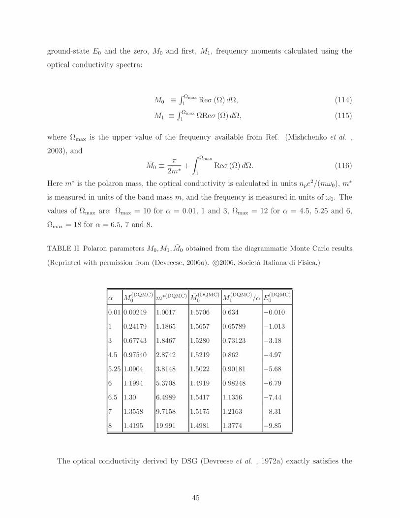
ground-state E0 and the zero, M0 and first, M1, frequency moments calculated using the

optical conductivity spectra:

M0 ≡∫ Ωmax

1Reσ (Ω) dΩ, (114)

M1 ≡∫ Ωmax

1ΩReσ (Ω) dΩ, (115)

where Ωmax is the upper value of the frequency available from Ref. (Mishchenko et al. ,

2003), and

M0 ≡π

2m∗ +

∫ Ωmax

1

Reσ (Ω) dΩ. (116)

Here m∗ is the polaron mass, the optical conductivity is calculated in units npe2/(mω0), m

∗

is measured in units of the band mass m, and the frequency is measured in units of ω0. The

values of Ωmax are: Ωmax = 10 for α = 0.01, 1 and 3, Ωmax = 12 for α = 4.5, 5.25 and 6,

Ωmax = 18 for α = 6.5, 7 and 8.

TABLE II Polaron parameters M0,M1, M0 obtained from the diagrammatic Monte Carlo results

(Reprinted with permission from (Devreese, 2006a). c©2006, Societa Italiana di Fisica.)

α M(DQMC)0 m∗(DQMC) M

(DQMC)0 M

(DQMC)1 /α E

(DQMC)0

0.01 0.00249 1.0017 1.5706 0.634 −0.010

1 0.24179 1.1865 1.5657 0.65789 −1.013

3 0.67743 1.8467 1.5280 0.73123 −3.18

4.5 0.97540 2.8742 1.5219 0.862 −4.97

5.25 1.0904 3.8148 1.5022 0.90181 −5.68

6 1.1994 5.3708 1.4919 0.98248 −6.79

6.5 1.30 6.4989 1.5417 1.1356 −7.44

7 1.3558 9.7158 1.5175 1.2163 −8.31

8 1.4195 19.991 1.4981 1.3774 −9.85

The optical conductivity derived by DSG (Devreese et al. , 1972a) exactly satisfies the

45

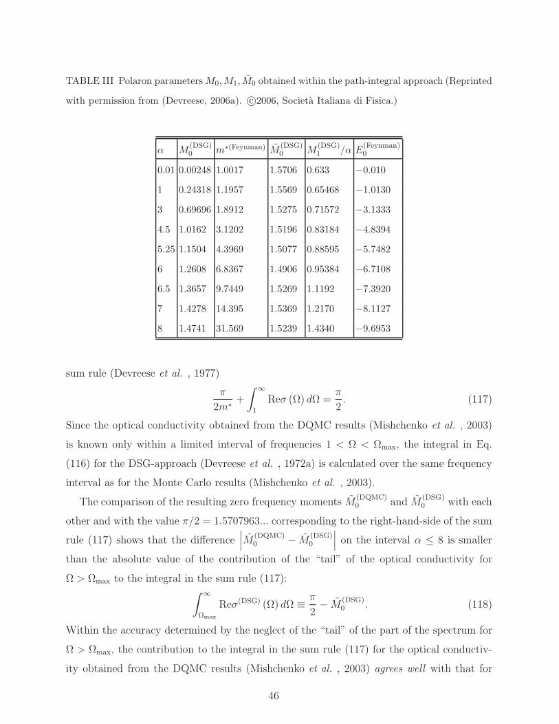
TABLE III Polaron parameters M0,M1, M0 obtained within the path-integral approach (Reprinted

with permission from (Devreese, 2006a). c©2006, Societa Italiana di Fisica.)

α M(DSG)0 m∗(Feynman) M

(DSG)0 M

(DSG)1 /α E

(Feynman)0

0.01 0.00248 1.0017 1.5706 0.633 −0.010

1 0.24318 1.1957 1.5569 0.65468 −1.0130

3 0.69696 1.8912 1.5275 0.71572 −3.1333

4.5 1.0162 3.1202 1.5196 0.83184 −4.8394

5.25 1.1504 4.3969 1.5077 0.88595 −5.7482

6 1.2608 6.8367 1.4906 0.95384 −6.7108

6.5 1.3657 9.7449 1.5269 1.1192 −7.3920

7 1.4278 14.395 1.5369 1.2170 −8.1127

8 1.4741 31.569 1.5239 1.4340 −9.6953

sum rule (Devreese et al. , 1977)

π

2m∗ +

∫ ∞

1

Reσ (Ω) dΩ =π

2. (117)

Since the optical conductivity obtained from the DQMC results (Mishchenko et al. , 2003)

is known only within a limited interval of frequencies 1 < Ω < Ωmax, the integral in Eq.

(116) for the DSG-approach (Devreese et al. , 1972a) is calculated over the same frequency

interval as for the Monte Carlo results (Mishchenko et al. , 2003).

The comparison of the resulting zero frequency moments M(DQMC)0 and M

(DSG)0 with each

other and with the value π/2 = 1.5707963... corresponding to the right-hand-side of the sum

rule (117) shows that the difference∣

∣

∣M

(DQMC)0 − M

(DSG)0

∣

∣

∣on the interval α ≤ 8 is smaller

than the absolute value of the contribution of the “tail” of the optical conductivity for

Ω > Ωmax to the integral in the sum rule (117):∫ ∞

Ωmax

Reσ(DSG) (Ω) dΩ ≡ π

2− M

(DSG)0 . (118)

Within the accuracy determined by the neglect of the “tail” of the part of the spectrum for

Ω > Ωmax, the contribution to the integral in the sum rule (117) for the optical conductiv-

ity obtained from the DQMC results (Mishchenko et al. , 2003) agrees well with that for

46

the optical conductivity found within the path-integral approach in Ref. (Devreese et al. ,

1972a). Hence, the conclusion follows that the optical conductivity obtained from the DQMC

results (Mishchenko et al. , 2003) satisfies the sum rule (117) within the aforementioned

accuracy.

H. Optical absorption spectra of continuum-polaron gas

For the weak-coupling regime, which is realized in most polar semiconductors, the ground-

state energy of a gas of interacting continuum polarons has been derived in (Lemmens et al.,

1977) by introducing a variational wave function:

|ψLDB〉 = U |φ〉 |ϕel〉 , (119)

where |ϕel〉 represents the ground-state many-body wave function for the electron (or hole)

system, |φ〉 is the phonon vacuum and U is a many-body unitary operator. U defines the

LDB-canonical transformation for a fermion gas interacting with a boson field:

U = exp

N∑

j=1

∑

q

(

fqdqeiq·rj − f ∗

qd+q e

−iq·rj)

, (120)

where rj represent the position of the N constituent electrons (or holes). The fq were

determined variationally (Lemmens et al., 1977). It may be emphasized that Eq. (120),

although it appears like a straightforward generalization of the one-particle transformation

in (Tomonaga, 1947), constitutes — especially in its implementation — a nontrivial extension

of a one-particle approximation to a many-body system. An advantage of the LDB-many-

polaron canonical transformations introduced in (Lemmens et al., 1977) for the calculation

of the ground state energy of a polaron gas is that the many-body effects are contained in

the static structure factor of the electron (or hole) system, which appears in the analytical

expression for the energy. Within the approach the minimum of the total ground-state

energy per particle for a polaron gas lies at lower density than that for the electron gas.

The non-degenerate system of interacting polarons in polar doped insulators was analysed

by Fratini and Quemerais (2000) using a simplified Feynman-type polaron model. In the

low-density limit, the ground state of the many-polaron system is the Wigner lattice of

polarons. With increasing density depending on the value of α, one of the following two

47

scenarios is possible: (i) the melting of the polaron Wigner lattice for α < α∗ and (ii) the

dissociation of the polarons for α > α∗ (Fratini and Quemerais, 2000).

The LDB-canonical transformation has been fruitfully applied in the theory of optical

absorption spectra of many-polaron systems. In (Tempere and Devreese , 2001), starting

from the LDB-many-polaron canonical transformation and the variational many-polaron

wave function introduced in (Lemmens et al., 1977), the optical absorption coefficient of

a many-polaron gas has been derived. The real part of the optical conductivity of the

many-polaron system is obtained in an intuitively appealing form, given by Eq. (107).

This approach to the many-polaron optical absorption allows one to include the many-

body effects to order α in terms of the dynamical structure factor S(k,Ω − ωLO) of the

electron (or hole) system. The experimental peaks in the mid-infrared optical absorption

spectra of cuprates (Lupi et al., 1999), and manganites (Hartinger et al., 2004) have been

adequately interpreted within this theory. The many-polaron approach describes the exper-

imental optical conductivity better than the single-polaron approximations (Emin , 1993;

Gurevich et al. , 1962). Note that in (Tempere and Devreese , 2001), like in (Eagles et al.,

1995), coexistence of small and Frohlich polarons in the same solid is involved.

The optical conductivity of a many-polaron gas was investigated in (Cataudella et al.,

1999) in a different way by calculating the correction to the dielectric function of the electron

gas, due to the electron-phonon interaction with variational parameters of a single-polaron

Feynman model. A suppression of the optical absorption of a many-polaron gas as compared

to the one-polaron optical absorption of Refs. (Devreese , 1972; Devreese et al. , 1972a) with

increasing density has been found. Such a suppression is expected because of the screening

of the Frohlich interaction with increasing polaron density.

I. Ripplopolarons

An interesting 2D system consists of electrons on films of liquid He

(Jackson and Platzman, 1981; Shikin and Monarkha, 1973). In this system the elec-

trons couple to the ripplons of the liquid He, forming “ripplopolarons”. The effective

coupling can be relatively large and self-trapping can result. The acoustic nature of the

ripplon dispersion at long wavelengths induces the self-trapping. Spherical shells of charged

particles appear in a variety of physical systems, such as fullerenes, metallic nanoshells,

48

charged droplets and neutron stars. A particularly interesting physical realization of

the spherical electron gas is found in multielectron bubbles (MEBs) in liquid helium-4.

These MEBs are 0.1 µm – 100 µm sized cavities inside liquid helium, that contain helium

vapour at vapour pressure and a nanometer-thick electron layer, anchored to the surface

of the bubble (Albrecht and Leiderer, 1987; Volodin et al., 1977). They exist as a result of

equilibrium between the surface tension of liquid helium and the Coulomb repulsion of the

electrons (Salomaa and Williams, 1981; Shikin, 1978).

Recently proposed experimental schemes to stabilize MEBs (Silvera, 2001) have stimu-

lated theoretical investigation of their properties (see e. g. (Tempere et al., 2001)). The

dynamical modes of MEB were described by considering the motion of the helium surface

(“ripplons”) and the vibrational modes of the electrons together. In particular, the case

when the ripplopolarons form a Wigner lattice was analyzed. The interaction energy be-

tween the ripplons and the electrons in the multielectron bubble is derived from the following

considerations: (i) the distance between the layer electrons and the helium surface is fixed

(the electrons find themselves confined to an effectively 2D surface anchored to the helium

surface) and (ii) the electrons are subjected to a force field, arising from the electric field

of the other electrons. To study the ripplopolaron Wigner lattice at nonzero temperature

and for any value of the electron-ripplon coupling, the variational path-integral approach

(Feynman, 1955) has been used. The destruction of the ripplopolaron Wigner lattice in a

MEB occurs through the dissociation of ripplopolarons. Below a critical pressure (on the

order of 104 Pa) the ripplopolaron solid will melt into an electron liquid. This critical pres-

sure is nearly independent of the number of electrons (except for the smallest bubbles) and

is weakly temperature dependent, up to the helium critical temperature 5.2 K. This can

be understood since the typical lattice potential well in which the ripplopolaron resides has

frequencies of the order of THz or larger, which correspond to ∼ 10 K.

The new phase that was predicted in (Tempere et al., 2003a), the ripplopolaron Wigner

lattice, will not be present for electrons on a flat helium surface. At the values of the pressing

field necessary to obtain a strong enough electron-ripplon coupling, the flat helium surface

is no longer stable against long-wavelength deformations (Gor’kov and Chernikova, 1973).

Multi-electron bubbles, with their different ripplon dispersion and the presence of stabilizing

factors such as the energy barrier against fissioning (Tempere et al., 2003b), allow for much

larger electric fields pressing the electrons against the helium surface. The regime of N , p, T

49

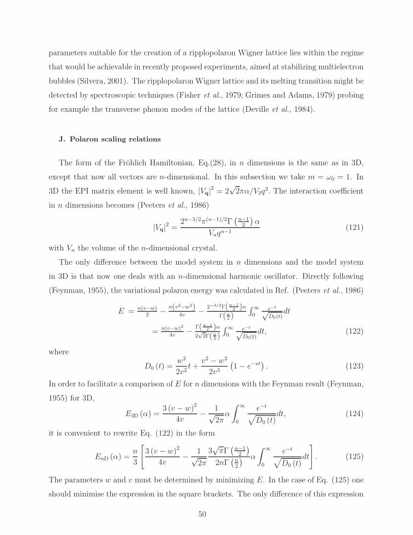
parameters suitable for the creation of a ripplopolaron Wigner lattice lies within the regime

that would be achievable in recently proposed experiments, aimed at stabilizing multielectron

bubbles (Silvera, 2001). The ripplopolaron Wigner lattice and its melting transition might be

detected by spectroscopic techniques (Fisher et al., 1979; Grimes and Adams, 1979) probing

for example the transverse phonon modes of the lattice (Deville et al., 1984).

J. Polaron scaling relations

The form of the Frohlich Hamiltonian, Eq.(28), in n dimensions is the same as in 3D,

except that now all vectors are n-dimensional. In this subsection we take m = ω0 = 1. In

3D the EPI matrix element is well known, |Vq|2 = 2√

2πα/V3q2. The interaction coefficient

in n dimensions becomes (Peeters et al., 1986)

|Vq|2 =2n−3/2π(n−1)/2Γ

(

n−12

)

α

Vnqn−1(121)

with Vn the volume of the n-dimensional crystal.

The only difference between the model system in n dimensions and the model system

in 3D is that now one deals with an n-dimensional harmonic oscillator. Directly following

(Feynman, 1955), the variational polaron energy was calculated in Ref. (Peeters et al., 1986)

E = n(v−w)2

− n(v2−w2)4v

− 2−3/2Γ(n−1

2 )α

Γ(n2 )

∫∞0

e−t√D0(t)

dt

= n(v−w)2

4v− Γ(n−1

2 )α

2√

2Γ(n2 )

∫∞0

e−t√D0(t)

dt, (122)

where

D0 (t) =w2

2v2t+

v2 − w2

2v3

(

1 − e−vt)

. (123)

In order to facilitate a comparison of E for n dimensions with the Feynman result (Feynman,

1955) for 3D,

E3D (α) =3 (v − w)2

4v− 1√

2πα

∫ ∞

0

e−t

√

D0 (t)dt, (124)

it is convenient to rewrite Eq. (122) in the form

EnD (α) =n

3

[

3 (v − w)2

4v− 1√

2π

3√πΓ(

n−12

)

2nΓ(

n2

) α

∫ ∞

0

e−t

√

D0 (t)dt

]

. (125)

The parameters w and v must be determined by minimizing E. In the case of Eq. (125) one

should minimise the expression in the square brackets. The only difference of this expression

50

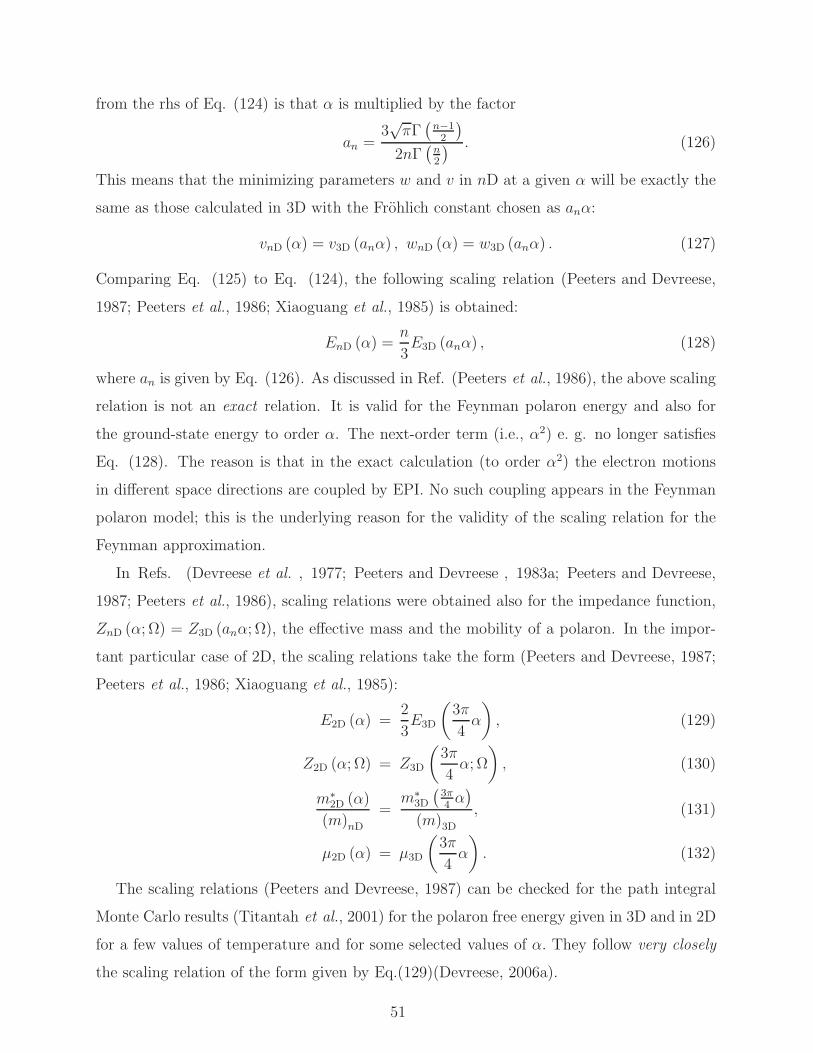
from the rhs of Eq. (124) is that α is multiplied by the factor

an =3√πΓ(

n−12

)

2nΓ(

n2

) . (126)

This means that the minimizing parameters w and v in nD at a given α will be exactly the

same as those calculated in 3D with the Frohlich constant chosen as anα:

vnD (α) = v3D (anα) , wnD (α) = w3D (anα) . (127)

Comparing Eq. (125) to Eq. (124), the following scaling relation (Peeters and Devreese,

1987; Peeters et al., 1986; Xiaoguang et al., 1985) is obtained:

EnD (α) =n

3E3D (anα) , (128)

where an is given by Eq. (126). As discussed in Ref. (Peeters et al., 1986), the above scaling

relation is not an exact relation. It is valid for the Feynman polaron energy and also for

the ground-state energy to order α. The next-order term (i.e., α2) e. g. no longer satisfies

Eq. (128). The reason is that in the exact calculation (to order α2) the electron motions

in different space directions are coupled by EPI. No such coupling appears in the Feynman

polaron model; this is the underlying reason for the validity of the scaling relation for the

Feynman approximation.

In Refs. (Devreese et al. , 1977; Peeters and Devreese , 1983a; Peeters and Devreese,

1987; Peeters et al., 1986), scaling relations were obtained also for the impedance function,

ZnD (α; Ω) = Z3D (anα; Ω), the effective mass and the mobility of a polaron. In the impor-

tant particular case of 2D, the scaling relations take the form (Peeters and Devreese, 1987;

Peeters et al., 1986; Xiaoguang et al., 1985):

E2D (α) =2

3E3D

(

3π

4α

)

, (129)

Z2D (α; Ω) = Z3D

(

3π

4α; Ω

)

, (130)

m∗2D (α)

(m)nD

=m∗

3D

(

3π4α)

(m)3D

, (131)

µ2D (α) = µ3D

(

3π

4α

)

. (132)

The scaling relations (Peeters and Devreese, 1987) can be checked for the path integral

Monte Carlo results (Titantah et al., 2001) for the polaron free energy given in 3D and in 2D

for a few values of temperature and for some selected values of α. They follow very closely

the scaling relation of the form given by Eq.(129)(Devreese, 2006a).

51

IV. DISCRETE HOLSTEIN AND FROHLICH POLARON

When the coupling with phonons increases the polaron radius decreases and becomes

of the order of the lattice constant. Then all momenta of the Brillouin zone contribute to

the polaron wave function and the effective mass approximation cannot be applied. This

regime occurs if the characteristic potential energy Ep due to the local lattice deformation

is compared or larger than the half-bandwidth D. The strong coupling regime with the

dimensionless coupling constant

λ ≡ Ep

D≥ 1 (133)

is called the small or discrete lattice polaron. In general, Ep is expressed as

Ep =1

2N

∑

q

|γ(q)|2ωq (134)

for any type of phonons involved in the polaron cloud. For the Frohlich interaction with

optical phonons one obtains Ep ≃ qde2/πκ, where qd is the Debye momentum (Alexandrov ,

1996). For example, with parameters appropriate for copper oxides ε0 ≫ ε ≃ 5 and qD ≃0.7A−1 one obtains Ep ≃ 0.6 eV (Alexandrov and Bratkovsky , 2000; Eagles , 1966). The

exact value of λc when the continuum (large) polaron transforms into the small one, depends

on the lattice structure, phonon frequency dispersions and the radius of the electron-phonon

interaction, but in most cases the transformation occurs around λc ≃ 1 (Alexandrov , 2001a).

A. Holstein model

For comparison we briefly introduce a small polaron created by a short-range EPI, which

is known as the Holstein polaron. Its main features are revealed in the simple Holstein model

(Holstein , 1959b) of two vibrating molecules and the electron hopping between them. A

simplified version of the model is defined by a two-site Hamiltonian describing the electron

tunnelling between sites 1 (“left”) and 2 (“right”) with the amplitude t and interacting with

a vibrational mode of an ion, placed at some distance in between, Fig.9:

H = t(c†1c2 + c†2c1) +Hph +He−ph, (135)

Here we take the position of an atomic level in the rigid lattice as zero, and ci annihilates

the electron on the left, i = 1, or on the right, i = 2, site.

52

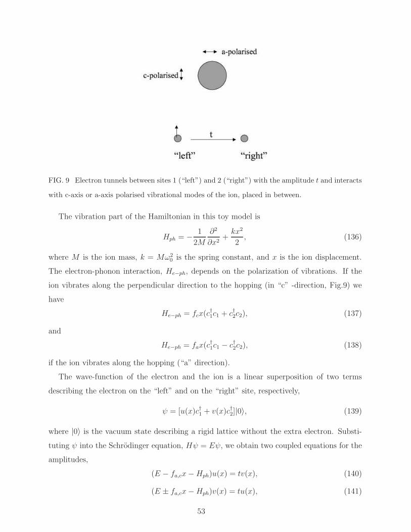
FIG. 9 Electron tunnels between sites 1 (“left”) and 2 (“right”) with the amplitude t and interacts

with c-axis or a-axis polarised vibrational modes of the ion, placed in between.

The vibration part of the Hamiltonian in this toy model is

Hph = − 1

2M

∂2

∂x2+kx2

2, (136)

where M is the ion mass, k = Mω20 is the spring constant, and x is the ion displacement.

The electron-phonon interaction, He−ph, depends on the polarization of vibrations. If the

ion vibrates along the perpendicular direction to the hopping (in “c” -direction, Fig.9) we

have

He−ph = fcx(c†1c1 + c†2c2), (137)

and

He−ph = fax(c†1c1 − c†2c2), (138)

if the ion vibrates along the hopping (“a” direction).

The wave-function of the electron and the ion is a linear superposition of two terms

describing the electron on the “left” and on the “right” site, respectively,

ψ = [u(x)c†1 + v(x)c†2]|0〉, (139)

where |0〉 is the vacuum state describing a rigid lattice without the extra electron. Substi-

tuting ψ into the Schrodinger equation, Hψ = Eψ, we obtain two coupled equations for the

amplitudes,

(E − fa,cx−Hph)u(x) = tv(x), (140)

(E ± fa,cx−Hph)v(x) = tu(x), (141)

53

where + and − in the second equation correspond to “a” and “c” polarised vibrations,

respectively. There is the exact solution for the “c” -axis polarization, when a change in the

ion position leads to the same shift of the electron energy on the left and on the right sites,

u(x) = uχn(x), (142)

v(x) = vχn(x), (143)

where u and v are constants and

χn(x) =

(

Mω0

π(2nn!)2

)1/4

Hn[(x− fc/k)(Mω0)1/2] exp[−M(x − fc/k)

2ω0/2], (144)

is the harmonic oscillator wave-function. There are two ladders of levels given by

E±n = −Ep ± t+ ω0(n+ 1/2) (145)

with Ep = f 2c /2k. Here Hn(ξ) are the Hermite polynomials, and n = 0, 1, 2, 3, ... . Hence the

c-axis single-ion deformation leads to the polaron level shift but without any renormalisation

of the hopping integral t. In contrast, a-polarized vibrations with the opposite shift of the

electron energy on the left and on the right sites, strongly renormalise the hopping integral.

There is no simple general solution of the Holstein model in this case, but one can find it in

two limiting cases, non-adiabatic, when t≪ ω0 and adiabatic, when t≫ ω0.

1. Non-adiabatic Holstein polaron

In the non-adiabatic regime the ion vibrations are fast and the electron hopping is slow.

Hence one can apply a perturbation theory in powers of t to solve(

E − fax−Hph −t−t E + fax−Hph

)[

u(x)

v(x)

]

= 0, (146)

One takes t = 0 in zero order, and obtains a two-fold degenerate ground state [ul,r(x), vl,r(x)],

corresponding to the polaron localised on the left (l) or on the right (r) sites,

ul(x) = exp

[

−Mω0

2(x+ fa/k)

2

]

,

vl(x) = 0 (147)

and

ur(x) = 0,

54

vr(x) = exp

[

−Mω0

2(x− fa/k)

2

]

(148)

with the energy E0 = −Ep + ω0/2, where Ep = f 2a/2k. The eigenstates are found as linear

superpositions of two unperturbed states,

[

u(x)

v(x)

]

= α

[

ul(x)

0

]

+ β

[

0

vr(x)

]

. (149)

Here the coefficients α and β are independent of x. The conventional secular equation for E

is obtained, multiplying the first row by ul(x) and the second row by vr(x), and integrating

over the vibration coordinate, x, each of two equations of the system. The result is

det

(

E − E0 t

t E − E0

)

= 0 (150)

with the renormalised hopping integral

t

t=

∫∞−∞ dxul(x)vr(x)∫∞−∞ dx|ul(x)|2 . (151)

The corresponding eigenvalues, E± are

E± = ω0/2 − Ep ± t. (152)

The hopping integral splits the degenerate level, as in the rigid lattice, but an effective

‘bandwidth’ 2t is significantly reduced compared with the bare one,

t = t exp(−2Ep/ω0). (153)

This polaron band narrowing originates in a small overlap integral of two displaced oscillator

wave functions ul(x) and vr(x).

2. Adiabatic Holstein polaron

In the adiabatic regime, when t ≫ ω0, the electron tunnelling is fast compared with

the ion motion. Hence one can apply the Born-Oppenheimer adiabatic approximation

(Born and Oppenheimer , 1927) taking the wave function in the form

[

u(x)

v(x)

]

= χ(x)

[

ua(x)

va(x)

]

. (154)

55

Here ua(x) and va(x) are the electron wave functions obeying the Schrodinger equation with

the frozen ion deformation x, i.e.

(

Ea(x) − fax −t−t Ea(x) + fax

)[

ua(x)

va(x)

]

= 0. (155)

The lowest energy level is found as

Ea(x) = −√

(fax)2 + t2. (156)

Ea(x) together with kx2/2 plays the role of a potential energy term in the equation for the

‘vibration’ wave function, χ(x),

[

− 1

2M

∂2

∂x2+kx2

2−√

(fax)2 + t2]

χ(x) = Eχ(x). (157)

Terms with the first and second derivatives of the electron wave-functions ua(x) and va(x) are

small compared with the corresponding derivatives of χ(x) in the adiabatic approximation,

so they are neglected in Eq.(157). As a result we arrive at the familiar double-well potential

problem, where the potential energy U(x) = kx2/2 −√

(fax)2 + t2 has two symmetric

minima, separated by a barrier. Minima are located approximately at

xm = ±fa/k (158)

in the strong-coupling limit, Ep ≫ t, and the potential energy near the bottom of each

potential well is about

U(x) = −Ep +k(|x| − fa/k)

2

2. (159)

If the barrier were impenetrable, there would be the ground state energy level E0 = −Ep +

ω0/2, the same for both wells. The underbarrier tunnelling results in a splitting of this level

2t, which corresponds to a polaron bandwidth in the lattice. It can be estimated using the

quasi-classical approximation as

t ∝ exp

[

−2

∫ xm

0

p(x)dx

]

, (160)

where p(x) =√

2M [U(x) −E0] ≈ (Mk)1/2|x− fa/k| is the classical momentum

Estimating the integral one finds the exponential reduction of the “bandwidth”,

t ∝ exp(−2Ep/ω0), (161)

56

which is the same as in the non-adiabatic regime. Holstein found corrections to this ex-

pression up to terms of the order of 1/λ2, which allowed him to improve the exponent and

estimate the pre-exponential factor as

t ≈√

Epω0

πe−g2

. (162)

Here g2 = 2Ep/ω0 and

g2 = g2

[

1 − 1

4λ2ln(4λ) − 1

8λ2

]

. (163)

A more accurate expression for t was obtained in (Alexandrov et al. , 1994a),

t ≈√

Epω0

πβ5/2λ1−β [2(1 + β)]−βe−g2

, (164)

where now g2 = g2β − [ln(2λ(1 + β))]/4λ2, and λ = Ep/t. This expression takes into

account the phonon frequency renormalisation, β ≡ ω0/ω0 =√

1 − 1/4λ2, and the anhar-

monic corrections of the order of 1/λ2 to the turning point xm in Eq.(160). The term in

front of the exponent in Eqs. (162,164) differs from t of the non-adiabatic case, Eq.(153).

It is thus apparent that the perturbation approach covers only a part of the entire lattice

polaron region, λ & 1. The upper limit of applicability of the perturbation theory is given by

t <√

Epω0. For the remainder of the region the adiabatic approximation is more appropri-

ate. A much lower effective mass of the adiabatic small polaron in the intermediate coupling

region compared with that estimated from the perturbation theory expression, Eq.(153), is

revealed in Eq.(164) (Alexandrov et al. , 1994a). The double well potential disappears at

λ = λc = 0.5, where the renormalised phonon frequency ω0 is zero.

The Holstein polaron model can be readily generalized for infinite lattices (section IV.B).

Similar models were used, for instance, in studies of dissipation (Caldeira and Leggett , 1981;

Castro Neto and Caldeira , 1991) and effects of decoherence in open quantum-mechanical

systems.

B. Lang-Firsov canonical transformation

The kinetic energy is smaller than the interaction energy as long as λ > 1. Hence a

self-consistent approach to the discrete (or lattice) polaron problem with EPI of any range

is possible with the “1/λ” expansion technique (Lang and Firsov , 1962, 1963) on infinite

lattices with any type of EPI conserving the electron site-occupation numbers, and any

57

phonon spectrum. The technique treats the electron kinetic energy as a perturbation, and

can be applied for multi-polaron systems as well (Alexandrov , 1983) (see VI.B). It is

based on the fact, known for a long time, that there is an analytical exact solution of the

any − number polaron problem in the extreme strong-coupling limit, λ → ∞. Following

Lang and Firsov one applies the canonical transformation eS to diagonalise the Hamiltonian,

Eq.(11). The diagonalisation is exact, if t(m) = 0 (or λ = ∞):

H = eSHe−S, (165)

where

S = −∑

q,i

ni [ui(q)dq −H.c.] (166)

is such that S† = −S. The electron and phonon operators are transformed as ci = eScie−S

and dq = eSdqe−S. The result is

ci = ciXi, (167)

and

dq = dq −∑

i

niu∗i (q), (168)

where Xi = exp[

∑

q ui(q)dq −H.c.]

. The Lang-Firsov transformation shifts the ions to

new equilibrium positions. In a more general sense it changes the boson vacuum. As a

result, the transformed Hamiltonian takes the following form

H =∑

i,j

σijc†icj − Ep

∑

i

ni +∑

q

ωq(d†qdq + 1/2) +

1

2

∑

i6=j

vijninj , (169)

where

σij = t(m− n)δss′X†i Xj (170)

is the renormalised hopping integral depending on the phonon operators, and

vij = Vc(m− n) − 1

N

∑

q

|γ(q)|2ωq cos[q · (m− n)] (171)

is the interaction of polarons, vij ≡ v(m− n), comprising their Coulomb repulsion and the

interaction via the lattice deformation. In the extreme infinite-coupling limit, λ → ∞, we

can neglect the hopping term of the transformed Hamiltonian. The rest has analytically

58

determined eigenstates and eigenvalues. The eigenstates |N〉 = |ni, nq〉 are sorted by the

polaron nms and phonon nq occupation numbers. The energy levels are

E = −(µ+ Ep)∑

i

ni +1

2

∑

i6=j

vijninj +∑

q

ωq(nq + 1/2), (172)

where ni = 0, 1 and nq = 0, 1, 2, 3, ....∞.

1. “1/λ” expansion and polaron band

The Hamiltonian H in zero order with respect to the hopping describes localised polarons

and independent phonons, which are vibrations of ions relative to new equilibrium positions

depending on the polaron occupation numbers. The middle of the electron band is shifted

down by the polaron level-shift Ep due to the potential well created by lattice deformation.

Importantly the phonon frequencies remain unchanged in this limit at any polaron density,

n. At finite λ and n there is a softening of phonons δω0 of the order of ω0n/λ2 (Alexandrov ,

1992a; Alexandrov and Capellmann , 1991; Alexandrov et al. , 1992; Gobel et al., 1994)

(the initial paper on the phonon renormalisation (Alexandrov and Capellmann , 1991) pre-

dicting δω0 ∝ 1/λ was subsequently corrected (Alexandrov , 1992a; Alexandrov et al. , 1992;

Gobel et al., 1994)). Interestingly the optical phonon can be mixed with a low-frequency po-

laronic plasmon forming a new excitation, “plasphon”, which was proposed in (Alexandrov ,

1992a) as an explanation of the anomalous phonon mode splitting observed in cuprates

(Rietschel et al. , 1989).

Now let us discuss the 1/λ expansion. First we restrict the discussion to a single-polaron

problem with no polaron-polaron interaction. The finite hopping term leads to the polaron

tunnelling because of degeneracy of the zero order Hamiltonian with respect to the site

position of the polaron. To see how the tunnelling occurs we apply the perturbation theory

using 1/λ as a small parameter. The proper Bloch set of N -fold degenerate zero order

eigenstates with the lowest energy (−Ep) of the unperturbed Hamiltonian is

|k, 0〉 =1√N

∑

m

c†ms exp(ik · m)|0〉, (173)

where |0〉 is the vacuum, and N is the number of sites. By applying the textbook pertur-

bation theory one readily calculates the perturbed energy levels. Up to the second order in

59

the hopping integral they are given by

Ek = −Ep + ǫk −∑

k′,nq

|〈k, 0|∑

i,j σijc†icj|k′, nq〉|2

∑

q ωqnq

, (174)

where |k′, nq〉 are the exited states of the unperturbed Hamiltonian with one electron and

at least one real phonon. The second term in this equation, which is linear with respect to

the bare hopping t(m), describes the polaron-band dispersion (Alexandrov , 2000),

ǫk =∑

m

t(m) e−g2(m) exp(−ik ·m), (175)

where

g2(m) =1

2N

∑

q

|γ(q)|2[1 − cos(q ·m)] (176)

is the band-narrowing factor at zero temperature.

The third term, quadratic in t(m) , yields a negative k-independent correction to the

polaron level-shift of the order of 1/λ2, and a small correction to the polaron band dispersion,

Eq.(175) (Alexandrov , 1992a; Gogolin , 1982; Kudinov and Firsov , 1997). The correction

to the level shift is due to polaronic hops onto a neighbouring site with no deformation

around it. As any second order correction this transition shifts the energy down by an

amount of about −t2(m)/Ep. It has little to do with the polaron effective mass and the

polaron tunneling mobility because the lattice deformation does not follow the electron.

The polaron hops back and forth many times (about eg2

) “waiting” for a sufficient lattice

deformation to appear around neighbouring site n. Only after the deformation around the

neighbouring site is created does the polaron tunnel onto the next site together with the

deformation.

2. Temperature effect on the polaron band

Let us now analyse the temperature dependence of the polaron bandwidth, which is

determined by the average of the multiphonon operator, Eq.(170),

〈〈X†i Xj〉〉 ≡

∏

q

〈〈exp[u∗i (q)d†q −H.c.] exp[uj(q)dqν −H.c.]〉〉. (177)

Here the double angular brackets correspond to quantum as well as statistical averages of

any operator A with the Gibbs distribution,

〈〈A〉〉 =∑

ν

e(Ω−Eν)/T 〈ν|A|ν〉 ≡ Tre(Ω−H)/T A, (178)

60

where Ω is the thermodynamic potential and |ν〉 are the eigenstates of H with the eigenvalues

Eν . An operator identity exp(A + B) = exp(A exp(B)exp(−[A, B]/2) is instrumental. It is

applied when the commutator [A, B] is a number. The identity allows us to write

e[u∗i (q)d†q−H.c.]e[uj(q)dq−H.c.] = eα∗d†qe−αdqe−|α|2/2 × (179)

e[ui(q)u∗j (q)−u∗

i (q)uj(q)]/2.

Quantum and statistical averages are calculated by expanding the exponents in the trace as

〈〈eα∗d†e−αd〉〉 = (1 − p)∞∑

N=0

N∑

n=0

pN(−1)n |α|2n

(n!)2N(N − 1) × ...× (N − n + 1), (180)

where we dropped the phonon and site quantum numbers for transparency. Here p =

exp(−ωqν/T ), so that a single-mode phonon partition function is Zph = 1/(1− p). Eq.(180)

can be written in the form (Lang and Firsov , 1962)

〈〈eα∗d†e−αd〉〉 = (1 − p)

N∑

n=0

(−1)n |α|2n

(n!)2pn d

n

dpn

∞∑

N=0

pN . (181)

Taking the sum over N ,∑∞

N=0 pN = 1/(1− p), and differentiating it n times yield n! in the

numerator, after which the series over n turns out equal to

〈〈eα∗d†e−αd〉〉 = e−|α|2nω , (182)

where nω = [exp(ωq/T )−1]−1 is the Bose-Einstein phonon distribution function. Collecting

all multipliers one finally obtains

〈〈σij〉〉 = T (m− n)δss′ exp

(

− 1

2N

∑

q

|γ(q)|2[1 − cos(q · m)] cothωq

2T

)

, (183)

with the zero-temperature limit given by Eq.(175).

The small-polaron band is exponentially narrow. Hence, one can raise a concern about

its existence in real solids (De Mello and Ranninger , 1998a). At zero temperature the

perturbation term of the transformed Hamiltonian conserves the momentum because all

off-diagonal matrix elements vanish,

〈k, 0|∑

i,j

σi,jc†icj|k′, 0〉 = 0 (184)

61

if k 6= k′. The emission of a single high-frequency phonon is impossible for any k because

of the energy conservation. The polaron half-bandwidth is exponentially reduced,

w ≈ De−g2

, (185)

and it is usually less than the optical phonon energy ω0 (g2 is about Dλ/ω0). Hence, there

is no damping of the polaron band at T = 0 caused by optical phonons, no matter how

strong the interaction is. The phonons “dress” the electron and coherently follow its mo-

tion. However, at finite temperatures the simultaneous emission and absorption of phonons

is possible. Moreover the polaron bandwidth shrinks with increasing temperature because

the phonon-averaged hopping integrals depend on temperature , Eq.(183). For high tem-

peratures, T ≫ ω0/2, the band narrows exponentially as w ≈ De−T/T0 , where

T−10 =

1

N

∑

q

|γ(q)|2ω−1q [1 − cos(q · m)].

On the other hand, the two-phonon scattering of polarons becomes more important with

increasing temperature. One can estimate this scattering rate by applying the Fermi-Dirac

golden rule,

1

τ= 2π

⟨

∑

q,q′

|Mqq′ |2 δ(ǫk − ǫk+q−q′)

⟩

, (186)

where the corresponding matrix element is

Mqq′ =∑

i,j

〈k + q − q′, nq − 1, nq′ + 1| σi,jc†icj |k, nq, nq′〉 .

For simplicity we consider the momentum independent γ(q) = γ0 and ωq = ω0. Expanding

σij-operators in powers of the phonon creation and annihilation operators one estimates the

matrix element of the two-phonon scattering as Mqq′ ≈ N−1wγ20

√

nq(nq′ + 1). Using this

estimate and the polaron density of states (DOS), ρp(ξ) ≡ N−1∑

k δ(ξ − ǫk) ≈ 1/2w one

obtains (Alexandrov and Mott , 1995)

1

τ≈ wγ4

0nω(1 + nω), (187)

where nω = [exp(ω0/T ) − 1]−1 is the phonon distribution function.

The polaron band is well defined, if 1/τ < w, which is satisfied for a temperature

range T ≤ Tmin ≈ ω0/ ln γ40 about half of the characteristic phonon frequency for rele-

vant values of γ20 . At higher temperatures the incoherent thermal activated hopping dom-

inates in the polaron dynamics (Holstein , 1959b; Lang and Firsov , 1962; Sewell , 1958;

62

Yamashita and Kurosawa , 1958), and the polaron states are no longer the Bloch states.

When the optical phonon frequencies are exceptionally high (i.e. about 1000K as in high-

temperature superconductors (Rietschel et al. , 1989)) lattice polarons are in the Bloch

states in the relevant range of temperatures, where the Boltzmann kinetic theory with renor-

malised energy spectrum is applied.

C. Discrete Frohlich polaron at strong coupling

The narrowing of the band and the polaron effective mass strongly depend on the range of

EPI (Alexandrov , 1996; Eagles , 1969). Let us compare the small Holstein polaron (SHP)

formed by the zero-range EPI and a small polaron formed by the long-range (Frohlich)

interaction, which we refer to as the small or discrete Frohlich polaron (SFP). We use the

real-space representation of He−ph (Alexandrov and Kornilovitch , 1999),

He−ph =∑

n,i

f(m− n)ξnni. (188)

with the normal coordinate at site n

ξn =∑

q

(2NMωq)−1/2eiq·ndq +H.c. (189)

and the force between the electron at site m and the normal coordinate ξn,

f(m) = N−1∑

q

γ(q)(Mω3q)1/2eiq·m. (190)

In general, there is no simple relation between the polaron level-shift Ep and the exponent

g2 of the mass enhancement. This relation depends on the form of EPI. Indeed for EPI with

a single dispersionless phonon mode, ωq = ω0, one obtains

Ep =1

2Mω20

∑

m

f 2(m), (191)

and

g2 =1

2Mω30

∑

m

[

f 2(m) − f(m)f(m + a)]

, (192)

where a is the primitive lattice vector. In the nearest-neighbour approximation the effective

mass renormalisation is given by m∗/m = eg2

where 1/m∗ = ∂2ǫk/∂k2 at k → 0 is the

inverse polaron mass. If the interaction is short-ranged, f(m) = κδm,0 (the Holstein model),

63

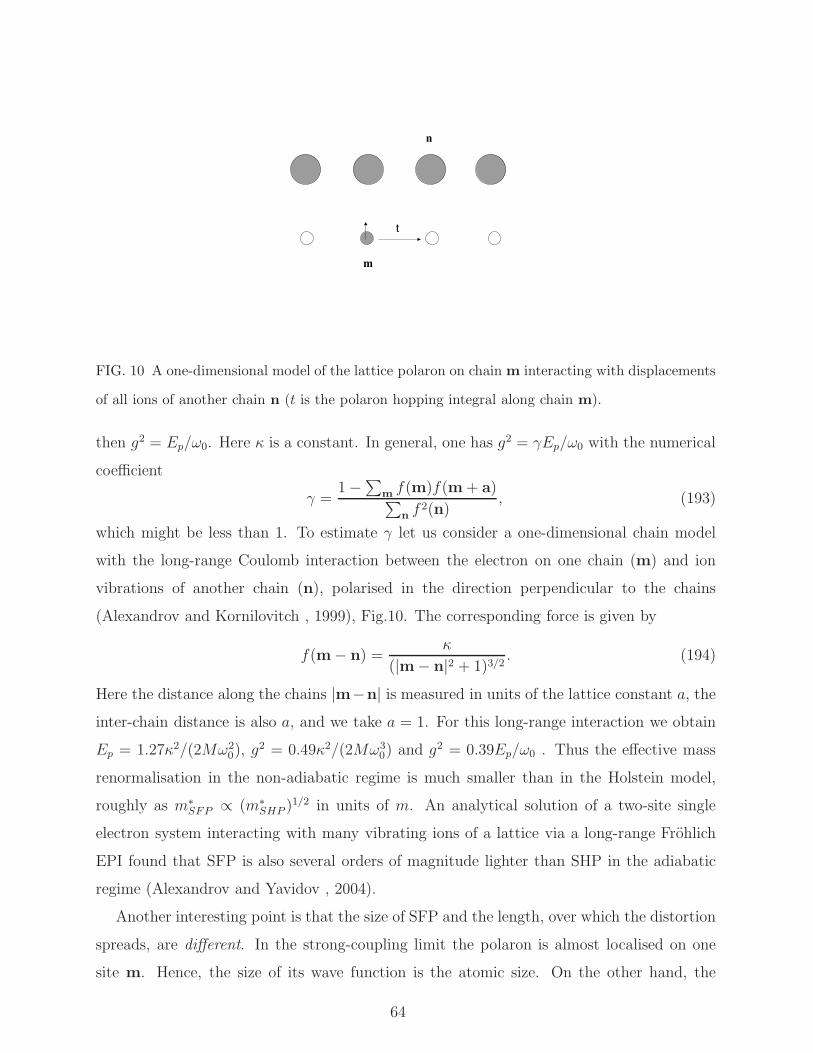
m

t

n

FIG. 10 A one-dimensional model of the lattice polaron on chain m interacting with displacements

of all ions of another chain n (t is the polaron hopping integral along chain m).

then g2 = Ep/ω0. Here κ is a constant. In general, one has g2 = γEp/ω0 with the numerical

coefficient

γ =1 −

∑

m f(m)f(m + a)∑

n f2(n)

, (193)

which might be less than 1. To estimate γ let us consider a one-dimensional chain model

with the long-range Coulomb interaction between the electron on one chain (m) and ion

vibrations of another chain (n), polarised in the direction perpendicular to the chains

(Alexandrov and Kornilovitch , 1999), Fig.10. The corresponding force is given by

f(m− n) =κ

(|m− n|2 + 1)3/2. (194)

Here the distance along the chains |m−n| is measured in units of the lattice constant a, the

inter-chain distance is also a, and we take a = 1. For this long-range interaction we obtain

Ep = 1.27κ2/(2Mω20), g

2 = 0.49κ2/(2Mω30) and g2 = 0.39Ep/ω0 . Thus the effective mass

renormalisation in the non-adiabatic regime is much smaller than in the Holstein model,

roughly as m∗SFP ∝ (m∗

SHP )1/2 in units of m. An analytical solution of a two-site single

electron system interacting with many vibrating ions of a lattice via a long-range Frohlich

EPI found that SFP is also several orders of magnitude lighter than SHP in the adiabatic

regime (Alexandrov and Yavidov , 2004).

Another interesting point is that the size of SFP and the length, over which the distortion

spreads, are different. In the strong-coupling limit the polaron is almost localised on one

site m. Hence, the size of its wave function is the atomic size. On the other hand, the

64

ion displacements, proportional to the displacement force f(m − n), spread over a large

distance. Their amplitude at a site n falls with the distance as |m− n|−3 in the one-

dimensional model, Fig.10. The polaron cloud (i.e. lattice distortion) is more extended

than the polaron itself. Such polaron tunnels with a larger probability than the Holstein

polaron due to a smaller relative lattice distortion around two neighbouring sites. For a

short-range EPI the entire lattice deformation disappears at one site and then forms at its

neighbour, when the polaron tunnels from site to site. Therefore γ = 1 and the polaron

is very heavy already at λ ≈ 1. On the contrary, if the interaction is long-ranged, only a

fraction of the total deformation changes every time the polaron tunnels from one site to its

neighbour, and γ is smaller than 1.

D. Effect of dispersive phonons

A lighter mass of SFP compared with the nondispersive SHP is a generic feature of

any dispersive electron-phonon interaction. For example, a short-range interaction with

dispersive acoustic phonons (γ(q) ∝ 1/q1/2, ωq ∝ q) also leads to a lighter polaron in the

strong-coupling regime compared with SHP (Alexandrov , 2003). Even within the Holstein

model with the local (intramolecular) EPI the dispersion of phonon frequencies is a vital

ingredient since nondispersive phonons might lead to a divergent site jump probability of

polarons (Yamashita and Kurosawa , 1958). Importantly the comprehensive studies of the

molecular Holstein Hamiltonian, in which the dispersive features of the phonon spectrum

are taken into account, found much lower values of the polaron mass compared with the

non-dispersive model (Zoli , 1998, 2000; Zoli and Das , 2004). In those studies the 1/λ

perturbation theory based on the standard Lang-Firsov (LF) and the variational (modified)

MLF transformation of the molecular Holstein Hamiltonian with dispersive phonons has

been applied for 1D, 2D and 3D lattices including the second-order corrections as in Eq.(174),

H = −t∑

〈i,j〉c†icj + gω0

∑

i

ni(di + d†i) +∑

q

ωq(d†qdq + 1/2), (195)

where dq is the Fourier transform of di. The phonon dispersion has been modeled using

the intermolecular first neighbours force constant, Mω21, which yields, for example, in 1D

case ω2q = ω2

0/2 + ω21 + (ω2

0/4 + ω20ω

21 cos q + ω2

1)1/2. MLF improves the convergence of

the 1/λ perturbation series by introducing a suitable variational parameter λq in the LF

65

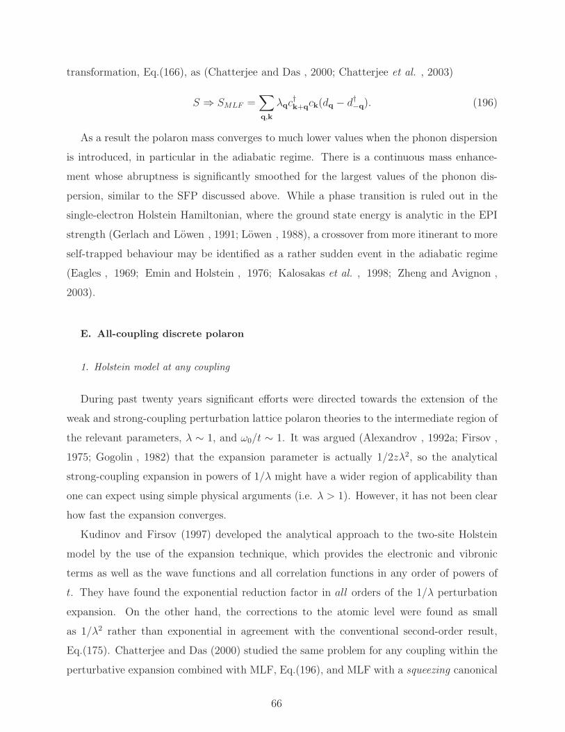
transformation, Eq.(166), as (Chatterjee and Das , 2000; Chatterjee et al. , 2003)

S ⇒ SMLF =∑

q,k

λqc†k+qck(dq − d†−q). (196)

As a result the polaron mass converges to much lower values when the phonon dispersion

is introduced, in particular in the adiabatic regime. There is a continuous mass enhance-

ment whose abruptness is significantly smoothed for the largest values of the phonon dis-

persion, similar to the SFP discussed above. While a phase transition is ruled out in the

single-electron Holstein Hamiltonian, where the ground state energy is analytic in the EPI

strength (Gerlach and Lowen , 1991; Lowen , 1988), a crossover from more itinerant to more

self-trapped behaviour may be identified as a rather sudden event in the adiabatic regime

(Eagles , 1969; Emin and Holstein , 1976; Kalosakas et al. , 1998; Zheng and Avignon ,

2003).

E. All-coupling discrete polaron

1. Holstein model at any coupling

During past twenty years significant efforts were directed towards the extension of the

weak and strong-coupling perturbation lattice polaron theories to the intermediate region of

the relevant parameters, λ ∼ 1, and ω0/t ∼ 1. It was argued (Alexandrov , 1992a; Firsov ,

1975; Gogolin , 1982) that the expansion parameter is actually 1/2zλ2, so the analytical

strong-coupling expansion in powers of 1/λ might have a wider region of applicability than

one can expect using simple physical arguments (i.e. λ > 1). However, it has not been clear

how fast the expansion converges.

Kudinov and Firsov (1997) developed the analytical approach to the two-site Holstein

model by the use of the expansion technique, which provides the electronic and vibronic

terms as well as the wave functions and all correlation functions in any order of powers of

t. They have found the exponential reduction factor in all orders of the 1/λ perturbation

expansion. On the other hand, the corrections to the atomic level were found as small

as 1/λ2 rather than exponential in agreement with the conventional second-order result,

Eq.(175). Chatterjee and Das (2000) studied the same problem for any coupling within the

perturbative expansion combined with MLF, Eq.(196), and MLF with a squeezing canonical

66

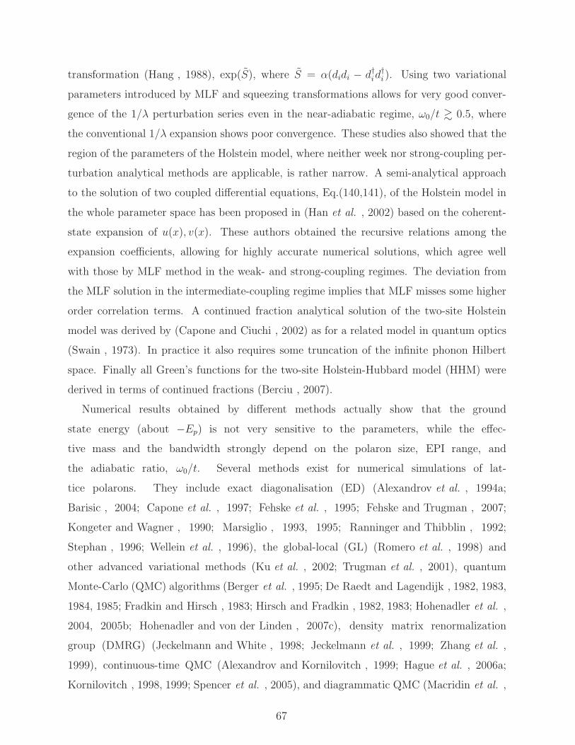
transformation (Hang , 1988), exp(S), where S = α(didi − d†id†i ). Using two variational

parameters introduced by MLF and squeezing transformations allows for very good conver-

gence of the 1/λ perturbation series even in the near-adiabatic regime, ω0/t & 0.5, where

the conventional 1/λ expansion shows poor convergence. These studies also showed that the

region of the parameters of the Holstein model, where neither week nor strong-coupling per-

turbation analytical methods are applicable, is rather narrow. A semi-analytical approach

to the solution of two coupled differential equations, Eq.(140,141), of the Holstein model in

the whole parameter space has been proposed in (Han et al. , 2002) based on the coherent-

state expansion of u(x), v(x). These authors obtained the recursive relations among the

expansion coefficients, allowing for highly accurate numerical solutions, which agree well

with those by MLF method in the weak- and strong-coupling regimes. The deviation from

the MLF solution in the intermediate-coupling regime implies that MLF misses some higher

order correlation terms. A continued fraction analytical solution of the two-site Holstein

model was derived by (Capone and Ciuchi , 2002) as for a related model in quantum optics

(Swain , 1973). In practice it also requires some truncation of the infinite phonon Hilbert

space. Finally all Green’s functions for the two-site Holstein-Hubbard model (HHM) were

derived in terms of continued fractions (Berciu , 2007).

Numerical results obtained by different methods actually show that the ground

state energy (about −Ep) is not very sensitive to the parameters, while the effec-

tive mass and the bandwidth strongly depend on the polaron size, EPI range, and

the adiabatic ratio, ω0/t. Several methods exist for numerical simulations of lat-

tice polarons. They include exact diagonalisation (ED) (Alexandrov et al. , 1994a;

Barisic , 2004; Capone et al. , 1997; Fehske et al. , 1995; Fehske and Trugman , 2007;

Kongeter and Wagner , 1990; Marsiglio , 1993, 1995; Ranninger and Thibblin , 1992;

Stephan , 1996; Wellein et al. , 1996), the global-local (GL) (Romero et al. , 1998) and

other advanced variational methods (Ku et al. , 2002; Trugman et al. , 2001), quantum

Monte-Carlo (QMC) algorithms (Berger et al. , 1995; De Raedt and Lagendijk , 1982, 1983,

1984, 1985; Fradkin and Hirsch , 1983; Hirsch and Fradkin , 1982, 1983; Hohenadler et al. ,

2004, 2005b; Hohenadler and von der Linden , 2007c), density matrix renormalization

group (DMRG) (Jeckelmann and White , 1998; Jeckelmann et al. , 1999; Zhang et al. ,

1999), continuous-time QMC (Alexandrov and Kornilovitch , 1999; Hague et al. , 2006a;

Kornilovitch , 1998, 1999; Spencer et al. , 2005), and diagrammatic QMC (Macridin et al. ,

67

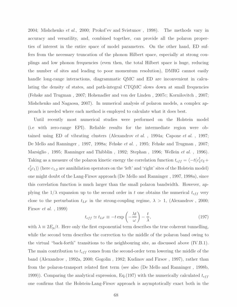
2004; Mishchenko et al., 2000; Prokof’ev and Svistunov , 1998). The methods vary in

accuracy and versatility, and, combined together, can provide all the polaron proper-

ties of interest in the entire space of model parameters. On the other hand, ED suf-

fers from the necessary truncation of the phonon Hilbert space, especially at strong cou-

plings and low phonon frequencies (even then, the total Hilbert space is huge, reducing

the number of sites and leading to poor momentum resolution), DMRG cannot easily

handle long-range interactions, diagrammatic QMC and ED are inconvenient in calcu-

lating the density of states, and path-integral CTQMC slows down at small frequencies

(Fehske and Trugman , 2007; Hohenadler and von der Linden , 2007c; Kornilovitch , 2007;

Mishchenko and Nagaosa, 2007). In numerical analysis of polaron models, a complex ap-

proach is needed where each method is employed to calculate what it does best.

Until recently most numerical studies were performed on the Holstein model

(i.e with zero-range EPI). Reliable results for the intermediate region were ob-

tained using ED of vibrating clusters (Alexandrov et al. , 1994a; Capone et al. , 1997;

De Mello and Ranninger , 1997, 1998a; Fehske et al. , 1995; Fehske and Trugman , 2007;

Marsiglio , 1995; Ranninger and Thibblin , 1992; Stephan , 1996; Wellein et al. , 1996).

Taking as a measure of the polaron kinetic energy the correlation function teff = 〈−t(c†1c2 +

c†2c1)〉 (here c1,2 are annihilation operators on the ‘left’ and ‘right’ sites of the Holstein model)

one might doubt of the Lang-Firsov approach (De Mello and Ranninger , 1997, 1998a), since

this correlation function is much larger than the small polaron bandwidth. However, ap-

plying the 1/λ expansion up to the second order in t one obtains the numerical teff very

close to the perturbation tLF in the strong-coupling regime, λ > 1, (Alexandrov , 2000;

Firsov et al. , 1999)

teff ≃ tLF ≡ −t exp

(

−λtω

)

− t

λ, (197)

with λ ≡ 2Ep/t. Here only the first exponential term describes the true coherent tunnelling,

while the second term describes the correction to the middle of the polaron band owing to

the virtual “back-forth” transitions to the neighbouring site, as discussed above (IV.B.1).

The main contribution to teff comes from the second-order term lowering the middle of the

band (Alexandrov , 1992a, 2000; Gogolin , 1982; Kudinov and Firsov , 1997), rather than

from the polaron-transport related first term (see also (De Mello and Ranninger , 1998b,

1999)). Comparing the analytical expression, Eq.(197) with the numerically calculated teff

one confirms that the Holstein-Lang-Firsov approach is asymptotically exact both in the

68

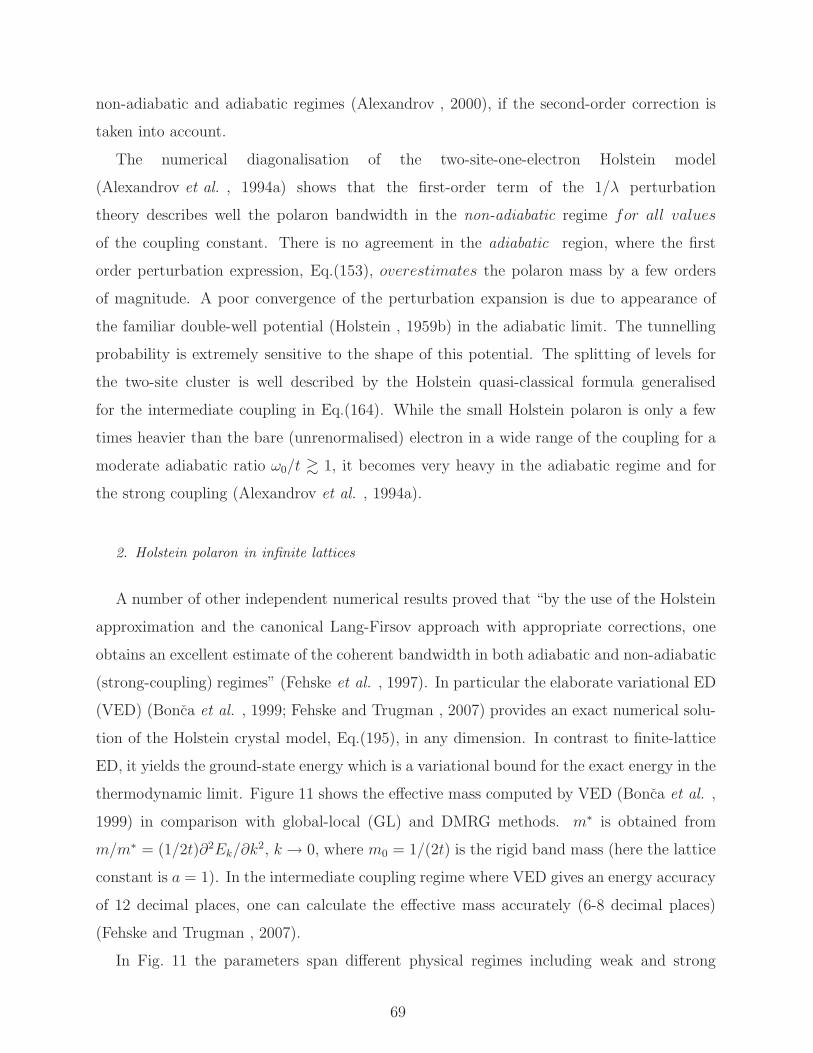
non-adiabatic and adiabatic regimes (Alexandrov , 2000), if the second-order correction is

taken into account.

The numerical diagonalisation of the two-site-one-electron Holstein model

(Alexandrov et al. , 1994a) shows that the first-order term of the 1/λ perturbation

theory describes well the polaron bandwidth in the non-adiabatic regime for all values

of the coupling constant. There is no agreement in the adiabatic region, where the first

order perturbation expression, Eq.(153), overestimates the polaron mass by a few orders

of magnitude. A poor convergence of the perturbation expansion is due to appearance of

the familiar double-well potential (Holstein , 1959b) in the adiabatic limit. The tunnelling

probability is extremely sensitive to the shape of this potential. The splitting of levels for

the two-site cluster is well described by the Holstein quasi-classical formula generalised

for the intermediate coupling in Eq.(164). While the small Holstein polaron is only a few

times heavier than the bare (unrenormalised) electron in a wide range of the coupling for a

moderate adiabatic ratio ω0/t & 1, it becomes very heavy in the adiabatic regime and for

the strong coupling (Alexandrov et al. , 1994a).

2. Holstein polaron in infinite lattices

A number of other independent numerical results proved that “by the use of the Holstein

approximation and the canonical Lang-Firsov approach with appropriate corrections, one

obtains an excellent estimate of the coherent bandwidth in both adiabatic and non-adiabatic

(strong-coupling) regimes” (Fehske et al. , 1997). In particular the elaborate variational ED

(VED) (Bonca et al. , 1999; Fehske and Trugman , 2007) provides an exact numerical solu-

tion of the Holstein crystal model, Eq.(195), in any dimension. In contrast to finite-lattice

ED, it yields the ground-state energy which is a variational bound for the exact energy in the

thermodynamic limit. Figure 11 shows the effective mass computed by VED (Bonca et al. ,

1999) in comparison with global-local (GL) and DMRG methods. m∗ is obtained from

m/m∗ = (1/2t)∂2Ek/∂k2, k → 0, where m0 = 1/(2t) is the rigid band mass (here the lattice

constant is a = 1). In the intermediate coupling regime where VED gives an energy accuracy

of 12 decimal places, one can calculate the effective mass accurately (6-8 decimal places)

(Fehske and Trugman , 2007).

In Fig. 11 the parameters span different physical regimes including weak and strong

69

0.0 1.0 2.0 3.0 4.0g

0.0

1.0

2.0

3.0

log(

m* /m

)

VEDGlobal-Localω0/ t =0.2,DMRGω0/ t =1.0, DMRGω0/ t =4.0, DMRG

FIG. 11 Logarithm of the polaron effective mass in 1D Holstein model as a function of g (after

(Fehske and Trugman , 2007)). VED results (full lines) were obtained operating repeatedly L = 20

times with the off-diagonal pieces of the Holstein Hamiltonian. For comparison GL (global-local)

results (dashed lines) are included (Romero et al. , 1998). Open symbols, indicating the value of

ω0/t, are DMRG results (Jeckelmann and White , 1998).

coupling, and low and high phonon frequency. There is good agreement between VED and

GL away from strong coupling and excellent agreement in all regimes with DMRG results.

DMRG calculations are not based on finite-k calculations due to a lack of periodic boundary

conditions, so they extrapolate the effective mass from the ground state data using chains

of different sizes, which leads to larger error bars and demands more computational effort.

There is no phase transition in the ground state of the model, but the polaron becomes

extremely heavy in the strong coupling regime. The crossover to a regime of large polaron

mass is more rapid in adiabatic regime, i.e. at small ω0/t.

Unifying systematization of the crossovers between the different polaron behaviors in

one dimension was obtained in terms of quantum to classical, weak coupling to strong

coupling, adiabatic to nonadiabatic, itinerant to self-trapped polarons and large to small

polarons (O. Barisic and S. Barisic , 2008). It was argued that the relationship between

various aspects of polaron states can be specified by five regimes: the weak-coupling regime,

the regime of large adiabatic polarons, the regime of small adiabatic polarons, the regime of

70

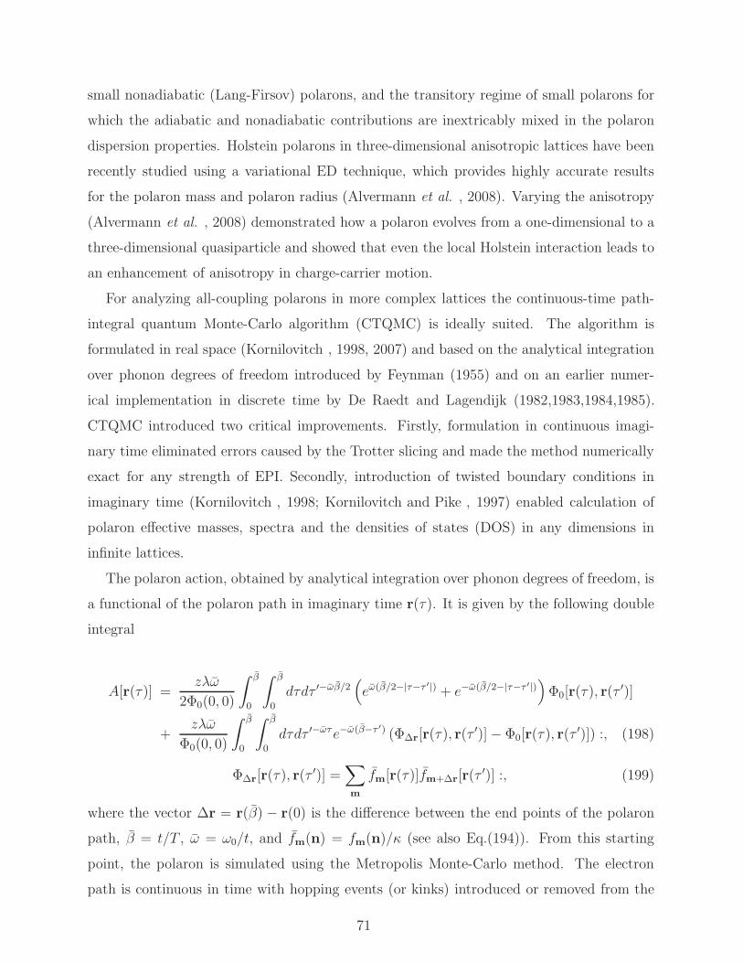
small nonadiabatic (Lang-Firsov) polarons, and the transitory regime of small polarons for

which the adiabatic and nonadiabatic contributions are inextricably mixed in the polaron

dispersion properties. Holstein polarons in three-dimensional anisotropic lattices have been

recently studied using a variational ED technique, which provides highly accurate results

for the polaron mass and polaron radius (Alvermann et al. , 2008). Varying the anisotropy

(Alvermann et al. , 2008) demonstrated how a polaron evolves from a one-dimensional to a

three-dimensional quasiparticle and showed that even the local Holstein interaction leads to

an enhancement of anisotropy in charge-carrier motion.

For analyzing all-coupling polarons in more complex lattices the continuous-time path-

integral quantum Monte-Carlo algorithm (CTQMC) is ideally suited. The algorithm is

formulated in real space (Kornilovitch , 1998, 2007) and based on the analytical integration

over phonon degrees of freedom introduced by Feynman (1955) and on an earlier numer-

ical implementation in discrete time by De Raedt and Lagendijk (1982,1983,1984,1985).

CTQMC introduced two critical improvements. Firstly, formulation in continuous imagi-

nary time eliminated errors caused by the Trotter slicing and made the method numerically

exact for any strength of EPI. Secondly, introduction of twisted boundary conditions in

imaginary time (Kornilovitch , 1998; Kornilovitch and Pike , 1997) enabled calculation of

polaron effective masses, spectra and the densities of states (DOS) in any dimensions in

infinite lattices.

The polaron action, obtained by analytical integration over phonon degrees of freedom, is

a functional of the polaron path in imaginary time r(τ). It is given by the following double

integral

A[r(τ)] =zλω

2Φ0(0, 0)

∫ β

0

∫ β

0

dτdτ ′−ωβ/2(

eω(β/2−|τ−τ ′|) + e−ω(β/2−|τ−τ ′|))

Φ0[r(τ), r(τ′)]

+zλω

Φ0(0, 0)

∫ β

0

∫ β

0

dτdτ ′−ωτe−ω(β−τ ′) (Φ∆r[r(τ), r(τ′)] − Φ0[r(τ), r(τ

′)]) :, (198)

Φ∆r[r(τ), r(τ′)] =

∑

m

fm[r(τ)]fm+∆r[r(τ′)] :, (199)

where the vector ∆r = r(β) − r(0) is the difference between the end points of the polaron

path, β = t/T , ω = ω0/t, and fm(n) = fm(n)/κ (see also Eq.(194)). From this starting

point, the polaron is simulated using the Metropolis Monte-Carlo method. The electron

path is continuous in time with hopping events (or kinks) introduced or removed from the

71

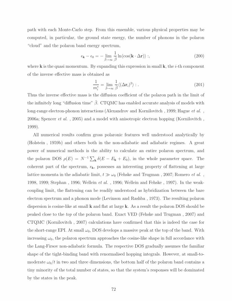
path with each Monte-Carlo step. From this ensemble, various physical properties may be

computed, in particular, the ground state energy, the number of phonons in the polaron

“cloud” and the polaron band energy spectrum,

ǫk − ǫ0 = − limβ→∞

1

βln〈cos(k · ∆r)〉 :, (200)

where k is the quasi momentum. By expanding this expression in small k, the i-th component

of the inverse effective mass is obtained as

1

m∗i

= limβ→∞

1

β〈(∆ri)

2〉 : . (201)

Thus the inverse effective mass is the diffusion coefficient of the polaron path in the limit of

the infinitely long “diffusion time” β. CTQMC has enabled accurate analysis of models with

long-range electron-phonon interactions (Alexandrov and Kornilovitch , 1999; Hague et al. ,

2006a; Spencer et al. , 2005) and a model with anisotropic electron hopping (Kornilovitch ,

1999).

All numerical results confirm gross polaronic features well understood analytically by

(Holstein , 1959b) and others both in the non-adiabatic and adiabatic regimes. A great

power of numerical methods is the ability to calculate an entire polaron spectrum, and

the polaron DOS ρ(E) = N−1∑

k δ(E − Ek + E0), in the whole parameter space. The

coherent part of the spectrum, ǫk, possesses an interesting property of flattening at large

lattice momenta in the adiabatic limit, t≫ ω0 (Fehske and Trugman , 2007; Romero et al. ,

1998, 1999; Stephan , 1996; Wellein et al. , 1996; Wellein and Fehske , 1997). In the weak-

coupling limit, the flattening can be readily understood as hybridization between the bare

electron spectrum and a phonon mode (Levinson and Rashba , 1973). The resulting polaron

dispersion is cosine-like at small k and flat at large k. As a result the polaron DOS should be

peaked close to the top of the polaron band. Exact VED (Fehske and Trugman , 2007) and

CTQMC (Kornilovitch , 2007) calculations have confirmed that this is indeed the case for

the short-range EPI. At small ω0, DOS develops a massive peak at the top of the band. With

increasing ω0, the polaron spectrum approaches the cosine-like shape in full accordance with

the Lang-Firsov non-adiabatic formula. The respective DOS gradually assumes the familiar

shape of the tight-binding band with renormalised hopping integrals. However, at small-to-

moderate ω0/t in two and three dimensions, the bottom half of the polaron band contains a

tiny minority of the total number of states, so that the system’s responses will be dominated

by the states in the peak.

72

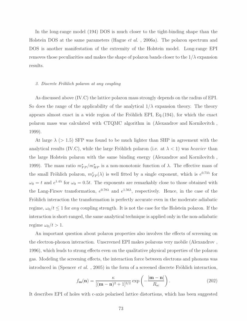
In the long-range model (194) DOS is much closer to the tight-binding shape than the

Holstein DOS at the same parameters (Hague et al. , 2006a). The polaron spectrum and

DOS is another manifestation of the extremity of the Holstein model. Long-range EPI

removes those peculiarities and makes the shape of polaron bands closer to the 1/λ expansion

results.

3. Discrete Frohlich polaron at any coupling

As discussed above (IV.C) the lattice polaron mass strongly depends on the radius of EPI.

So does the range of the applicability of the analytical 1/λ expansion theory. The theory

appears almost exact in a wide region of the Frohlich EPI, Eq.(194), for which the exact

polaron mass was calculated with CTQMC algorithm in (Alexandrov and Kornilovitch ,

1999).

At large λ (> 1.5) SFP was found to be much lighter than SHP in agreement with the

analytical results (IV.C), while the large Frohlich polaron (i.e. at λ < 1) was heavier than

the large Holstein polaron with the same binding energy (Alexandrov and Kornilovitch ,

1999). The mass ratio m∗FP/m

∗HP is a non-monotonic function of λ. The effective mass of

the small Frohlich polaron, m∗FP (λ) is well fitted by a single exponent, which is e0.73λ for

ω0 = t and e1.4λ for ω0 = 0.5t. The exponents are remarkably close to those obtained with

the Lang-Firsov transformation, e0.78λ and e1.56λ, respectively. Hence, in the case of the

Frohlich interaction the transformation is perfectly accurate even in the moderate adiabatic

regime, ω0/t ≤ 1 for any coupling strength. It is not the case for the Holstein polaron. If the

interaction is short-ranged, the same analytical technique is applied only in the non-adiabatic

regime ω0/t > 1.

An important question about polaron properties also involves the effects of screening on

the electron-phonon interaction. Unscreened EPI makes polarons very mobile (Alexandrov ,

1996), which leads to strong effects even on the qualitative physical properties of the polaron

gas. Modeling the screening effects, the interaction force between electrons and phonons was

introduced in (Spencer et al. , 2005) in the form of a screened discrete Frohlich interaction,

fm(n) =κ

[(m − n)2 + 1]3/2exp

(

−|m − n|Rsc

)

. (202)

It describes EPI of holes with c-axis polarised lattice distortions, which has been suggested

73

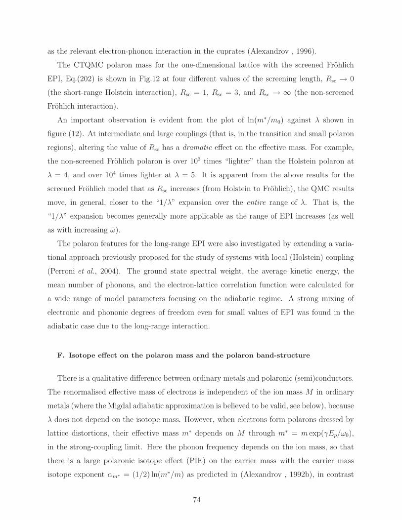
as the relevant electron-phonon interaction in the cuprates (Alexandrov , 1996).

The CTQMC polaron mass for the one-dimensional lattice with the screened Frohlich

EPI, Eq.(202) is shown in Fig.12 at four different values of the screening length, Rsc → 0

(the short-range Holstein interaction), Rsc = 1, Rsc = 3, and Rsc → ∞ (the non-screened

Frohlich interaction).

An important observation is evident from the plot of ln(m∗/m0) against λ shown in

figure (12). At intermediate and large couplings (that is, in the transition and small polaron

regions), altering the value of Rsc has a dramatic effect on the effective mass. For example,

the non-screened Frohlich polaron is over 103 times “lighter” than the Holstein polaron at

λ = 4, and over 104 times lighter at λ = 5. It is apparent from the above results for the

screened Frohlich model that as Rsc increases (from Holstein to Frohlich), the QMC results

move, in general, closer to the “1/λ” expansion over the entire range of λ. That is, the

“1/λ” expansion becomes generally more applicable as the range of EPI increases (as well

as with increasing ω).

The polaron features for the long-range EPI were also investigated by extending a varia-

tional approach previously proposed for the study of systems with local (Holstein) coupling

(Perroni et al., 2004). The ground state spectral weight, the average kinetic energy, the

mean number of phonons, and the electron-lattice correlation function were calculated for

a wide range of model parameters focusing on the adiabatic regime. A strong mixing of

electronic and phononic degrees of freedom even for small values of EPI was found in the

adiabatic case due to the long-range interaction.

F. Isotope effect on the polaron mass and the polaron band-structure

There is a qualitative difference between ordinary metals and polaronic (semi)conductors.

The renormalised effective mass of electrons is independent of the ion mass M in ordinary

metals (where the Migdal adiabatic approximation is believed to be valid, see below), because

λ does not depend on the isotope mass. However, when electrons form polarons dressed by

lattice distortions, their effective mass m∗ depends on M through m∗ = m exp(γEp/ω0),

in the strong-coupling limit. Here the phonon frequency depends on the ion mass, so that

there is a large polaronic isotope effect (PIE) on the carrier mass with the carrier mass

isotope exponent αm∗ = (1/2) ln(m∗/m) as predicted in (Alexandrov , 1992b), in contrast

74

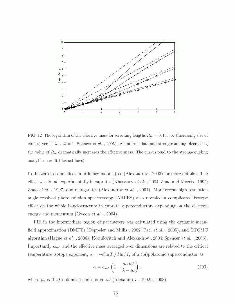
FIG. 12 The logarithm of the effective mass for screening lengths Rsc = 0, 1, 3,∞ (increasing size of

circles) versus λ at ω = 1 (Spencer et al. , 2005). At intermediate and strong coupling, decreasing

the value of Rsc dramatically increases the effective mass. The curves tend to the strong-coupling

analytical result (dashed lines).

to the zero isotope effect in ordinary metals (see (Alexandrov , 2003) for more details). The

effect was found experimentally in cuprates (Khasanov et al. , 2004; Zhao and Morris , 1995;

Zhao et al. , 1997) and manganites (Alexandrov et al. , 2001). More recent high resolution

angle resolved photoemission spectroscopy (ARPES) also revealed a complicated isotope

effect on the whole band-structure in cuprate superconductors depending on the electron

energy and momentum (Gweon et al. , 2004).

PIE in the intermediate region of parameters was calculated using the dynamic mean-

field approximation (DMFT) (Deppeler and Millis , 2002; Paci et al. , 2005), and CTQMC

algorithm (Hague et al. , 2006a; Kornilovitch and Alexandrov , 2004; Spencer et al. , 2005).

Importantly αm∗ and the effective mass averaged over dimensions are related to the critical

temperature isotope exponent, α = −d lnTc/d lnM , of a (bi)polaronic superconductor as

α = αm∗

(

1 − m/m∗

λ− µc

)

, (203)

where µc is the Coulomb pseudo-potential (Alexandrov , 1992b, 2003).

75

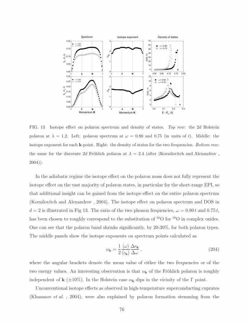
0.00

0.05

0.10

0.15

0.20

MM XX

MM XX

= 0.80 = 0.75

Spectrum

E k -

E 0, (t)

0

1

2

3

Isotope exponent

K

0.00 0.05 0.10 0.15 0.20

0

10

20

30

40

50

60

70

= 0.80 = 0.75

Density of states

DO

S, 1

/t

0.00

0.05

0.10

0.15

0.20

0.25

0.30 = 0.80 = 0.75

E K -

E 0, (t)

Momentum K

0

1

2

3

K

Momentum K0.0 0.1 0.2 0.3

0

2

4

6

8

10

12

= 0.80 = 0.75

DO

S, 1

/t

E - E0, (t)

FIG. 13 Isotope effect on polaron spectrum and density of states. Top row : the 2d Holstein

polaron at λ = 1.2. Left: polaron spectrum at ω = 0.80 and 0.75 (in units of t). Middle: the

isotope exponent for each k-point. Right: the density of states for the two frequencies. Bottom row :

the same for the discreate 2d Frohlich polaron at λ = 2.4 (after (Kornilovitch and Alexandrov ,

2004)).

In the adiabatic regime the isotope effect on the polaron mass does not fully represent the

isotope effect on the vast majority of polaron states, in particular for the short-range EPI, so

that additional insight can be gained from the isotope effect on the entire polaron spectrum

(Kornilovitch and Alexandrov , 2004). The isotope effect on polaron spectrum and DOS in

d = 2 is illustrated in Fig 13. The ratio of the two phonon frequencies, ω = 0.80 t and 0.75 t,

has been chosen to roughly correspond to the substitution of 16O for 18O in complex oxides.

One can see that the polaron band shrinks significantly, by 20-30%, for both polaron types.

The middle panels show the isotope exponents on spectrum points calculated as

αk =1

2

〈ω〉〈ǫk〉

∆ǫk∆ω

, (204)

where the angular brackets denote the mean value of either the two frequencies or of the

two energy values. An interesting observation is that αk of the Frohlich polaron is roughly

independent of k (±10%). In the Holstein case αk dips in the vicinity of the Γ point.

Unconventional isotope effects as observed in high-temperature superconducting cuprates

(Khasanov et al. , 2004), were also explained by polaron formation stemming from the

76

coupling to the particular quadrupolar Q(2)-type phonon mode (Bussmann-Holder et al. ,

2005). Polaronic isotope effects in the spectral function of strongly correlated systems were

numerically studied by (Fratini and Ciuchi , 2005) in the framework of the Holstein-Hubbard

model and by (Mishchenko and Nagaosa, 2006) using the extended t − J model including

EPI.

G. Jahn-Teller polaron

The density-displacement EPIs discussed above are not only possible types of the electron-

lattice coupling. Examples of other types are the Su-Schrieffer-Heeger (SSH) EPI (Su et al. ,

1979) ( for recent path-integral results for SSH polarons see (Zoli , 2007)), and the Jahn-

Teller (JT) EPI (Jahn and Teller , 1937). In the former, the lattice deformation is cou-

pled to electron kinetic energy, while JT involves a multidimensional electron basis and

a multidimensional representation of the deformation group. The JT interaction is active

in some molecules and crystals of high point symmetry, and it has served as a guide in

the search for high-temperature superconductivity (Bednorz and Muller , 1988). Later on

JT-type EPIs were widely discussed in connection with cuprate and other high-Tc supercon-

ductors (see, for example, (Alexandrov et al. , 1996; Gunnarsson, 1997; Mertelj et al. , 2005;

Mihailovic and Kabanov , 2001; Muller , 2000)) and colossal-magnetoresistance manganites

(see, for example, Refs. (Bussmann-Holder and Bishop , 1999; Edwards , 2002; Millis et al. ,

1995; Roder et al. , 1996; Yunoki et al. , 1998b)).

The simplest model of the JT interaction is the E ⊗ e interaction (Kanamori , 1960)

that describes a short-range coupling between twice-degenerate eg electronic levels (c1, c2)

and a local double-degenerate vibron mode (ζ, η). The Hamiltonian reads ( here we follow

(Kornilovitch , 2007))

HJT = − t∑

〈nn′〉

(

c†n′1cn1 + c†n′2cn2

)

− κ∑

n

[(

c†n1cn2 + c†n2cn1

)

ηn +(

c†n1cn1 − c†n2cn2

)

ζn

]

+∑

n

[

− 1

2M

(

∂2

∂ζ2n

+∂2

∂η2n

)

+Mω2

2

(

ζ2n + η2

n

)

]

. (205)

The symmetry of the interaction ensures the same coupling parameter κ for the two phonons.

Because the ionic coordinates of different cells are not coupled, the model describes a collec-

77

tion of separate clusters that are linked only by electron hopping. To relate the Hamiltonian

to more realistic situations, phonon dispersion should be added (Allen and Perebeinos ,

1999; Mihailovic and Kabanov , 2001).

An important property of the E ⊗ e interaction is the absence of an exact analytical

solution in the atomic limit t = 0. Here, in contrast with the Holstein and Frohlich EPI,

the atomic limit is described by two coupled partial differential equations for the electron

doublet ψ1,2(ζ, η). At large couplings, however, the elastic energy assumes the Mexican

hat shape and the phonon dynamics separates into radial oscillatory motion and azimuthal

rotary motion. This results in an additional pre-exponential factor ∝ κ in the ion overlap

integral, leading to the effective mass m∗JT/m = (2/πg)1/2 exp g2, where g2 = κ2/2Mω3

(Takada , 2000).

A path integral approach to Hamiltonian (205) was developed by Kornilovitch (2000).

Its details are found in (Kornilovitch , 2007). Because there are two electron orbitals, the

electron path must be assigned an additional orbital index (or colour) a = 1, 2. Colour 1

(or 2) of a given path segment means that it resides in the first (second) atomic orbital of

the electron doublet. There is a difference between the two phonons. Phonon ζ is coupled

to electron density, like in the Holstein case. The difference from the Holstein is that

the direction of the force changes to the opposite when the electron changes orbitals. In

contrast, phonon η is coupled to orbital changes themselves: the more often the electron

changes orbitals, the more “active” is η. Discrete orbital changes are analogous to electron

hops between discrete lattice sites, and as such are associated with “kinetic orbital energy”.

Phonon coupling to orbital changes is analogous to phonon coupling to electron hopping in

the SSH model (Su et al. , 1979).

The JT polaron properties can be calculated with no approximations using QMC algo-

rithm. The effective mass, spectrum, and density of states are obtained as for the conven-

tional lattice polarons. Most properties behave similarly to those of the d = 3 Holstein

polaron at the same phonon frequency (Kornilovitch , 2000). For example, the kinetic en-

ergy sharply decreases by absolute value between λ = 1.2 and 1.4. The JT polaron mass is

slightly larger at the small to intermediate coupling, but several times smaller at the strong

coupling. This non-monotonic behaviour of the ratio of the JT and Holstein masses was later

confirmed by accurate variational calculations (El Shawish et al. , 2003), although in that

work the JT polaron (and bipolaron) was investigated in one spatial dimension. The relative

78

lightness of the JT polaron is consistent with Takada’s result mentioned above (Takada ,

2000). Finally, the density of JT polaron states features the same peak at the top of the

band, caused by the spectrum flattening at large polaron momenta, see Fig. (13).

In summary, the local character of the JT interaction and the independence of vibrating

clusters result in the same extremity of polaron properties as in the 3d Holstein model. One

could expect that either a long-range JT interaction or phonon dispersion will soften the

sharp polaron features and make JT polarons more mobile (Kornilovitch , 2007).

V. RESPONSE OF DISCRETE POLARONS

A. Hopping mobility

Studies of lattice polarons allowed for a theoretical understanding of low mobility problem

(Ioffe , 1957) of many “poor” conductors, where an estimate of the mean-free path yields

values much lower than the lattice constant. Transport properties of lattice polarons depend

strongly on temperature. For T lower than the characteristic phonon energy polaron kinetics

is the Boltzmann kinetics of heavy particles tunnelling in the narrow band (Holstein , 1959b).

However at higher temperatures the polaron band collapses (IV.B.2), and the transport is

diffusive via thermally activated jumps of polarons from site to site (Appel , 1968; Firsov ,

1975; Holstein , 1959b; Klinger , 1979; Lang and Firsov , 1963, 1968; Mott and Davis , 1982;

Yamashita and Kurosawa , 1958).

The 1/λ perturbation expansion is particularly instrumental in calculating hopping mo-

bilities and optical absorption coefficients. Applying the canonical transformation (IV.B)

and singling out the diagonal coherent tunnelling in the polaron band one can write the

Hamiltonian as

H = Hp +Hph +Hint, (206)

where Hp =∑

k ξkc†kck is the “free” polaron contribution (here we drop the spin), Hph =

∑

q ωq(d†qdq+1/2) is the phonon part, and ξk = Z ′Ek−µ is the renormalised (polaron) band

dispersion. The chemical potential µ includes the polaron level shift −Ep, and it could also

include all higher orders in 1/λ corrections to the polaron spectrum, which are independent

79

of k, Eq.(175). The band-narrowing factor Z ′ is defined as

Z ′ =

∑

m t(m)e−g2(m) exp(−ik · m)∑

m t(m) exp(−ik · m), (207)

which is Z ′ = exp(−γEp/ω)) where γ ≤ 1 depends on the range of EPI and phonon frequency

dispersions (IV.C). The interaction term Hint comprises the polaron-polaron interaction,

Eq.(171), and the residual polaron-phonon interaction

Hp−ph ≡∑

i6=,j

[σij − 〈σij〉]c†icj , (208)

where 〈σij〉 means averaging with respect to the bare phonon distribution. In the framework

of the single-polaron problem one neglects the polaron-polaron interaction and treats Hp−ph

as a perturbation.

The motion of the small polaron at high temperatures is a random walk consisting of

steps from site to site (Holstein , 1959b). Holstein calculated the probability W for the

hop of a small polaron to a neighbouring site. He suggested that the random walk was

a Markovian process. For such processes the diffusion coefficient is given by D ≃ a2W ,

where W is the hopping probability. The only term in the polaronic Hamiltonian, which

changes the phonon occupation numbers, is the polaron-phonon interaction Hp−ph. The

nearest neighbour hopping probability in the second order is

W = 2π〈∑

j

|〈j|Hp−ph|i〉|2δ(

∑

q

ωq(njq − ni

q)

)

〉, (209)

where |i〉 and |j〉 are the eigenstates of H0 corresponding to the polaron on site i with niq

phonons in each phonon mode and the polaron on the neighbouring site j with njq phonons,

respectively. Replacing the δ function in Eq.(209) by the integral yields

W = t2e−2g2

∫ ∞

−∞dτ

[

exp

(

1

N

∑

q

|γ(q)|2[1 − cos(q · a)]cos(ωqτ)

sinh ωq

2T

)

− 1

]

e−i0+|τ |. (210)

The integration over τ is performed using a saddle-point approximation by allowing a finite

phonon frequency dispersion δω ≪ ωq. Expanding cos(ωqτ) in powers of τ , and using the

Einstein relation µ = eD/T one obtains the hopping mobility,

µh = ea2 π1/2t2

2T (EaT )1/2e−Ea/T . (211)

80

where

Ea =T

N

∑

q

|γ(q)|2[1 − cos(q · a)] tanh(ωq/4T ) (212)

is the activation energy, which is half of the polaron level shift Ep for the Holstein EPI. This

expression is applicable at T ≫ ω0/2 and t2/ω0(EaT ) ≪ 1. Importantly, increasing the EPI

range diminishes the value of Ea further. The hopping mobility µh ≡ σh/ne ∼ exp(−Ea/T )

can be below ea2 ≃ 1cm2/V s, which is the lowest limit for the Boltzmann theory to be

applied. Within the Boltzmann theory such a low mobility corresponds to the mean free

path l < a, which is not a reasonable result.

Holstein suggested that at low temperatures T < ω0/2 ln γ0, there is the ordinary Boltz-

mann transport in momentum space, but in the narrow polaron band. According to

(Holstein , 1959b), the transition from the band regime to the hopping regime occurs when

the uncertainty in the polaron energy becomes comparable to the width of the polaron

band. If phonons dominate in the scattering, the polaron mobility, µ = µt + µh decreases

when the temperature increases from zero to some Tmin, where it is at minimum, because

its Boltzmann part, µt, falls down due to an increasing number of phonons, while the hop-

ping part, µh, remains small. However µ increases above Tmin, due to the thermal activated

hopping. There is a wide temperature range around Tmin where the thermal activated hop-

ping still makes a small contribution to the conductivity, but the uncertainty in the polaron

band is already significant (Firsov , 1975, 2007). The polaron transport theory requires a

special diagrammatic technique (Firsov , 1975, 2007; Lang and Firsov , 1963, 1968) and a

conditional-probability function description (Kudinov and Firsov , 1965, 1966) in this re-

gion.

The transverse conductivity σxy and the Hall coefficient RH = σxy/Hσ2xx of lattice po-

larons can be calculated with the Peierls substitution (Peierls , 1933),

t(m − n) → t(m− n)e−ieA(m)·(m−n), (213)

which is a fair approximation if the magnetic field, B, is weak compared with the atomic field

eBa2 << 1. Here A(r) is the vector potential, which can be also time dependent. Within the

Boltzmann theory the sign of the Hall coefficient RH ≃ ±1/en depends on the type of carriers

(holes or electrons) and the Hall mobility µH ≡ RHσxx is the same as the drift mobility µt up

to a numerical factor of the order of 1. The calculations of the hopping Hall current similar to

those of the hopping conductivity (Bottger et al. , 2007; Bryksin and Firsov , 1970; Emin ,

81

1971; Friedman and Holstein , 1963) show that the Hall mobility depends on the symmetry

of the crystal lattice and has nothing in common with the hopping mobility, neither with

respect to the temperature dependence and even nor with respect to the sign. In particular

for hexagonal lattices three-site hops yield (Friedman and Holstein , 1963)

µH = ea2 π1/2t

(12EaT )1/2e−Ea/3T (214)

with the same sign for electrons and holes. The activation energy of the Hall mobility is three

times less than that of the hopping mobility. In cubic crystals, the hopping Hall effect is

governed by four-site hops. The four-site calculations in (Bryksin and Firsov , 1970; Emin ,

1971) gave the Hall mobility with the “normal” sign depending on the type of carriers.

The Hall conductivity and resistivity of strongly localized electrons at low temper-

atures and small magnetic fields strongly depend on frequency, the size of a sample

(Entin-Wohlman et al. , 1995), and on a magnetic order like, for example in ferromagnetic

(Ga,Mn)As (Burkov and Balents , 2003). In the presence of the spin-orbit interaction each

hopping path acquires a spin-dependent phase factor of the same form as that in a perpen-

dicular (to the 2D system) magnetic field, which leads to spin accumulation and spin-Hall

effects (Bottger et al. , 2007; Entin-Wohlman et al. , 2005).

B. Optical conductivity

One of the fingerprints of lattice polarons is the frequency (ω) and temperature de-

pendence of their mid-infrared (MIR) conductivity σ(ω). In the low frequency and low

temperature region, where the tunneling band transport operates (Holstein , 1959a,b), the

conductivity acquires the conventional Drude form,

σ(ω) =neµt

1 + (ωτ)2, (215)

where the transport relaxation time τ may be frequency dependent because of the narrow

band. For high (mid-infrared) frequencies, well above the polaron bandwidth (ω ≫ w) but

below the interband gap, the Drude law is not applied. In this frequency region one can

apply the generalised Einstein relation σ(ω) = eD(ω)/ω, where D(ω) = a2W (ω), and W (ω)

is the hopping probability of the absorption of the energy quantum ω (Holstein , 1959b).

The number of nearest neighbour transitions per second with the absorption of a photon of

82

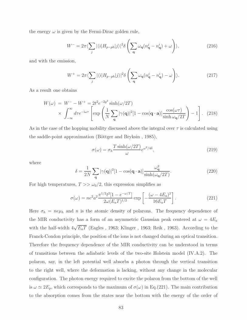
the energy ω is given by the Fermi-Dirac golden rule,

W− = 2π〈∑

j

|〈i|Hp−ph|j〉|2δ(

∑

q

ωq(njq − ni

q) + ω

)

〉, (216)

and with the emission,

W+ = 2π〈∑

j

|〈i|Hp−ph|j〉|2δ(

∑

q

ωq(njq − ni

q) − ω

)

〉. (217)

As a result one obtains

W (ω) = W− −W+ = 2t2e−2g2

sinh(ω/2T )

×∫ ∞

−∞dτe−iωτ

[

exp

(

1

N

∑

q

|γ(q)|2[1 − cos(q · a)]cos(ωτ)

sinhωq/2T

)

− 1

]

. (218)

As in the case of the hopping mobility discussed above the integral over τ is calculated using

the saddle-point approximation (Bottger and Bryksin , 1985),

σ(ω) = σhT sinh(ω/2T )

ωeω2/4δ, (219)

where

δ =1

2N

∑

q

|γ(q)|2[1 − cos(q · a)]ω2

q

sinh(ωq/2T ). (220)

For high temperatures, T >> ω0/2, this expression simplifies as

σ(ω) = ne2a2π1/2t2[1 − e−ω/T ]

2ω(EaT )1/2exp

[

−(ω − 4Ea)2

16EaT

]

. (221)

Here σh = neµh and n is the atomic density of polarons. The frequency dependence of

the MIR conductivity has a form of an asymmetric Gaussian peak centered at ω = 4Ea

with the half-width 4√EaT (Eagles , 1963; Klinger , 1963; Reik , 1963). According to the

Franck-Condon principle, the position of the ions is not changed during an optical transition.

Therefore the frequency dependence of the MIR conductivity can be understood in terms

of transitions between the adiabatic levels of the two-site Holstein model (IV.A.2). The

polaron, say, in the left potential well absorbs a photon through the vertical transition

to the right well, where the deformation is lacking, without any change in the molecular

configuration. The photon energy required to excite the polaron from the bottom of the well

is ω ≃ 2Ep, which corresponds to the maximum of σ(ω) in Eq.(221). The main contribution

to the absorption comes from the states near the bottom with the energy of the order of

83

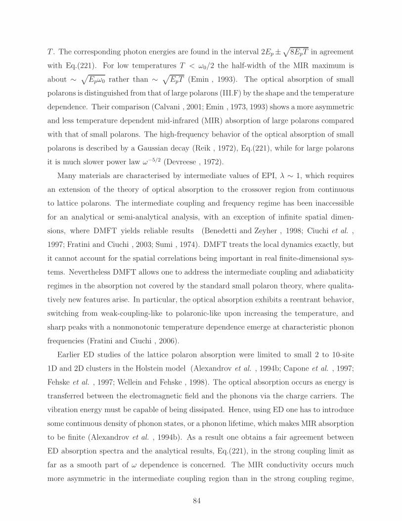
T . The corresponding photon energies are found in the interval 2Ep ±√

8EpT in agreement

with Eq.(221). For low temperatures T < ω0/2 the half-width of the MIR maximum is

about ∼√

Epω0 rather than ∼√

EpT (Emin , 1993). The optical absorption of small

polarons is distinguished from that of large polarons (III.F) by the shape and the temperature

dependence. Their comparison (Calvani , 2001; Emin , 1973, 1993) shows a more asymmetric

and less temperature dependent mid-infrared (MIR) absorption of large polarons compared

with that of small polarons. The high-frequency behavior of the optical absorption of small

polarons is described by a Gaussian decay (Reik , 1972), Eq.(221), while for large polarons

it is much slower power law ω−5/2 (Devreese , 1972).

Many materials are characterised by intermediate values of EPI, λ ∼ 1, which requires

an extension of the theory of optical absorption to the crossover region from continuous

to lattice polarons. The intermediate coupling and frequency regime has been inaccessible

for an analytical or semi-analytical analysis, with an exception of infinite spatial dimen-

sions, where DMFT yields reliable results (Benedetti and Zeyher , 1998; Ciuchi et al. ,

1997; Fratini and Ciuchi , 2003; Sumi , 1974). DMFT treats the local dynamics exactly, but

it cannot account for the spatial correlations being important in real finite-dimensional sys-

tems. Nevertheless DMFT allows one to address the intermediate coupling and adiabaticity

regimes in the absorption not covered by the standard small polaron theory, where qualita-

tively new features arise. In particular, the optical absorption exhibits a reentrant behavior,

switching from weak-coupling-like to polaronic-like upon increasing the temperature, and

sharp peaks with a nonmonotonic temperature dependence emerge at characteristic phonon

frequencies (Fratini and Ciuchi , 2006).

Earlier ED studies of the lattice polaron absorption were limited to small 2 to 10-site

1D and 2D clusters in the Holstein model (Alexandrov et al. , 1994b; Capone et al. , 1997;

Fehske et al. , 1997; Wellein and Fehske , 1998). The optical absorption occurs as energy is

transferred between the electromagnetic field and the phonons via the charge carriers. The

vibration energy must be capable of being dissipated. Hence, using ED one has to introduce

some continuous density of phonon states, or a phonon lifetime, which makes MIR absorption

to be finite (Alexandrov et al. , 1994b). As a result one obtains a fair agreement between

ED absorption spectra and the analytical results, Eq.(221), in the strong coupling limit as

far as a smooth part of ω dependence is concerned. The MIR conductivity occurs much

more asymmetric in the intermediate coupling region than in the strong coupling regime,

84

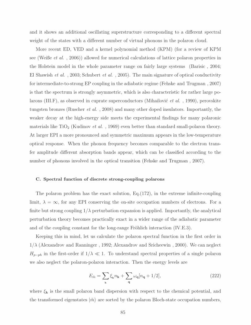
and it shows an additional oscillating superstructure corresponding to a different spectral

weight of the states with a different number of virtual phonons in the polaron cloud.

More recent ED, VED and a kernel polynomial method (KPM) (for a review of KPM

see (Weiße et al. , 2006)) allowed for numerical calculations of lattice polaron properties in

the Holstein model in the whole parameter range on fairly large systems (Barisic , 2004;

El Shawish et al. , 2003; Schubert et al. , 2005). The main signature of optical conductivity

for intermediate-to-strong EP coupling in the adiabatic regime (Fehske and Trugman , 2007)

is that the spectrum is strongly asymmetric, which is also characteristic for rather large po-

larons (III.F), as observed in cuprate superconductors (Mihailovic et al. , 1990), perovskite

tungsten bronzes (Ruscher et al. , 2008) and many other doped insulators. Importantly, the

weaker decay at the high-energy side meets the experimental findings for many polaronic

materials like TiO2 (Kudinov et al. , 1969) even better than standard small-polaron theory.

At larger EPI a more pronounced and symmetric maximum appears in the low-temperature

optical response. When the phonon frequency becomes comparable to the electron trans-

fer amplitude different absorption bands appear, which can be classified according to the

number of phonons involved in the optical transition (Fehske and Trugman , 2007).

C. Spectral function of discrete strong-coupling polarons

The polaron problem has the exact solution, Eq.(172), in the extreme infinite-coupling

limit, λ = ∞, for any EPI conserving the on-site occupation numbers of electrons. For a

finite but strong coupling 1/λ perturbation expansion is applied. Importantly, the analytical

perturbation theory becomes practically exact in a wider range of the adiabatic parameter

and of the coupling constant for the long-range Frohlich interaction (IV.E.3).

Keeping this in mind, let us calculate the polaron spectral function in the first order in

1/λ (Alexandrov and Ranninger , 1992; Alexandrov and Sricheewin , 2000). We can neglect

Hp−ph in the first-order if 1/λ ≪ 1. To understand spectral properties of a single polaron

we also neglect the polaron-polaron interaction. Then the energy levels are

Em =∑

k

ξknk +

∑

q

ωq[nq + 1/2], (222)

where ξk is the small polaron band dispersion with respect to the chemical potential, and

the transformed eigenstates |m〉 are sorted by the polaron Bloch-state occupation numbers,

85

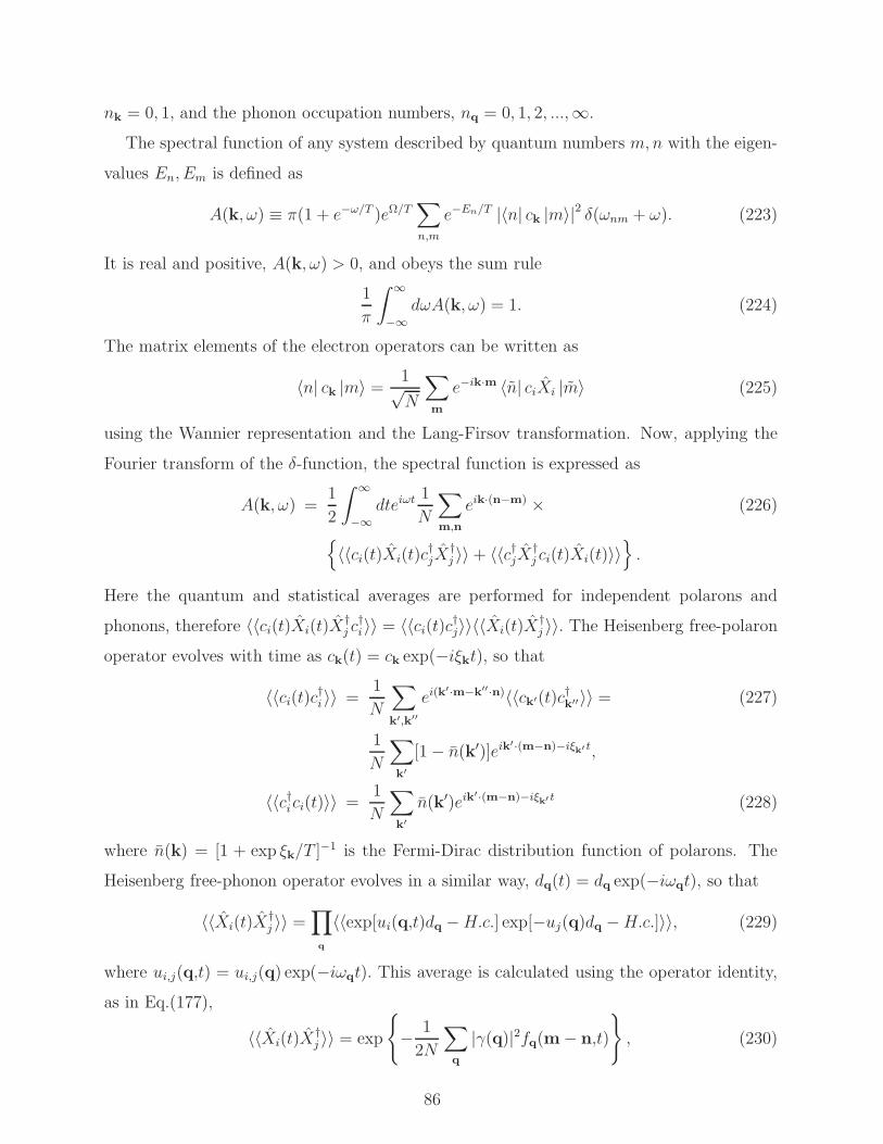
nk = 0, 1, and the phonon occupation numbers, nq = 0, 1, 2, ...,∞.

The spectral function of any system described by quantum numbers m,n with the eigen-

values En, Em is defined as

A(k, ω) ≡ π(1 + e−ω/T )eΩ/T∑

n,m

e−En/T |〈n| ck |m〉|2 δ(ωnm + ω). (223)

It is real and positive, A(k, ω) > 0, and obeys the sum rule

1

π

∫ ∞

−∞dωA(k, ω) = 1. (224)

The matrix elements of the electron operators can be written as

〈n| ck |m〉 =1√N

∑

m

e−ik·m 〈n| ciXi |m〉 (225)

using the Wannier representation and the Lang-Firsov transformation. Now, applying the

Fourier transform of the δ-function, the spectral function is expressed as

A(k, ω) =1

2

∫ ∞

−∞dteiωt 1

N

∑

m,n

eik·(n−m) × (226)

〈〈ci(t)Xi(t)c†jX

†j 〉〉 + 〈〈c†jX†

j ci(t)Xi(t)〉〉

.

Here the quantum and statistical averages are performed for independent polarons and

phonons, therefore 〈〈ci(t)Xi(t)X†j c

†i〉〉 = 〈〈ci(t)c†j〉〉〈〈Xi(t)X

†j 〉〉. The Heisenberg free-polaron

operator evolves with time as ck(t) = ck exp(−iξkt), so that

〈〈ci(t)c†i 〉〉 =1

N

∑

k′,k′′

ei(k′·m−k′′·n)〈〈ck′(t)c†k′′〉〉 = (227)

1

N

∑

k′

[1 − n(k′)]eik′·(m−n)−iξk′ t,

〈〈c†ici(t)〉〉 =1

N

∑

k′

n(k′)eik′·(m−n)−iξk′ t (228)

where n(k) = [1 + exp ξk/T ]−1 is the Fermi-Dirac distribution function of polarons. The

Heisenberg free-phonon operator evolves in a similar way, dq(t) = dq exp(−iωqt), so that

〈〈Xi(t)X†j 〉〉 =

∏

q

〈〈exp[ui(q,t)dq −H.c.] exp[−uj(q)dq −H.c.]〉〉, (229)

where ui,j(q,t) = ui,j(q) exp(−iωqt). This average is calculated using the operator identity,

as in Eq.(177),

〈〈Xi(t)X†j 〉〉 = exp

− 1

2N

∑

q

|γ(q)|2fq(m − n,t)

, (230)

86

where

fq(m,t) = [1 − cos(q · m) cos(ωqt)] cothωq

2T+ i cos(q · m) sin(ωqt). (231)

Here we used the symmetry of γ(−q) = γ(q), so that terms containing sin(q · m) have

disappeared.

To proceed with the analytical results we consider low temperatures, T ≪ ωq, when

coth(ωq/2T ) ≈ 1. Expanding the exponent in Eq.(230) and performing summation over

m,n, k′ and integration over time we arrive at (Alexandrov and Sricheewin , 2000)

A(k, ω) =

∞∑

l=0

[

A(−)l (k, ω) + A

(+)l (k, ω)

]

, (232)

where

A(−)l (k, ω) = πZ

∑

q1,...ql

∏lr=1 |γ(qr)|2(2N)ll!

× (233)

[

1 − n

(

k−l∑

r=1

qr

)]

δ

(

ω−l∑

r=1

ωqr−ξk−Plr=1

qr

)

,

A(+)l (k, ω) = πZ

∑

q1,...ql

∏lr=1 |γ(qr)|2(2N)ll!

× (234)

n

(

k+

l∑

r=1

qr

)

δ

(

ω+

l∑

r=1

ωqr−ξk+Pl

r=1qr

)

,

and Z = exp(−(2N)−1∑

q |γ(q)|2).Clearly Eq.(232) is in the form of the perturbative multi-phonon expansion. Each con-

tribution A(±)l (k, ω) to the spectral function describes the transition from the initial state

k of the polaron band to the final state k±∑l

r=1 qr with the emission (or absorption) of l

phonons.

The 1/λ expansion result, Eq.(232), is different from the conventional spectral function

of metallic electrons coupled to phonons in the Migdal-Eliashberg theory (Eliashberg , 1960;

Migdal , 1958). There is no imaginary part of the self-energy since the exponentially small

(at low temperatures) polaronic damping, Eq.(187), is neglected. Instead EPI leads to the

coherent dressing of electrons by phonons, and phonon “side-bands”. The spectral function

of the polaronic carriers comprises two different parts. The first (l = 0) k-dependent coherent

term arises from the polaron band tunnelling,

Acoh(k, ω) =[

A(−)0 (k, ω) + A

(+)0 (k, ω)

]

= πZδ(ω − ξk). (235)

87

The spectral weight of the coherent part is suppressed as Z ≪ 1. However in the case of the

Frohlich interaction the effective mass is less enhanced, since the band narrowing factor Z ′,

Eq.(207), in ξk = Z ′Ek − µ is large compared with Z (Alexandrov and Sricheewin , 2000).

The second incoherent part Aincoh(k, ω) comprises all the terms with l ≥ 1. It describes

excitations accompanied by emission and absorption of phonons. We notice that its spectral

density spreads over a wide energy range of about twice the polaron level shift Ep, which

might be larger than the unrenormalised bandwidth 2D in the rigid lattice without phonons.

On the contrary, the coherent part shows a dispersion only in the energy window of the order

of the polaron bandwidth, w = Z ′D. It is interesting that there is some k dependence of

the incoherent background as well, if the EPI matrix element and/or phonon frequencies

depend on q. Only in the Holstein model with the short-range dispersionless e-ph interaction

γ(q) =γ0 and ωq = ω0 the incoherent part is momentum independent (Mahan , 1990),

Aincoh(k, ω) = πZ

N

∞∑

l=1

γ2l0

2ll!× (236)

∑

k′

[1 − n (k′)] δ (ω−lω0−ξk′) + n (k′) δ (ω+lω0−ξk′) .

As soon as we know the spectral function, different Green’s functions (GF) are readily

obtained using their analytical properties. For example, the temperature GF is given by the

integral

G(k, ωk) =1

π

∫ ∞

−∞dω′A(k, ω′)

iωk − ω′ . (237)

where ωk = πT (2k + 1), k = 0,±1,±2, .... Calculating the integral we find in the Holstein

model (Alexandrov and Ranninger , 1992)

G(k, ωn) =Z

iωn−ξk+Z

N

∞∑

l=1

γ2l0

2ll!

∑

k′

1 − n (k′)

iωn−lω0−ξk′

+n (k′)

iωn+lω0−ξk′

. (238)

Here the first term describes the coherent tunnelling in the narrow polaron band while the

second k-independent sum describes the phonon-side bands.

D. Spectral function of discrete all-coupling polarons

The spectral function, Eq.(238), satisfies the major sum rule, Eq.(224). However the

higher-momentum integrals,∫∞−∞ dωωpA(k, ω) with p > 0, calculated using Eq.(238), differ

from the exact values (Kornilovitch , 2002) by an amount proportional to 1/λ. The difference

88

is due to a partial “undressing” of high-energy excitations in the side-bands, which is beyond

the first order 1/λ expansion. A rather accurate Green’s function of the Holstein polaron has

been recently obtained by summing all the diagrams, but with each diagram averaged over

its free propagators’ momenta (Berciu , 2006a,b). The resulting Green’s function satisfies

exactly the first six spectral weight sum rules. All higher sum rules are satisfied with great

accuracy, becoming asymptotically exact for coupling both much larger and much smaller

than the free particle bandwidth.

The spectral properties of the Holstein model in a wider parameter range have

been studied numerically using ED (see (Alexandrov et al. , 1994b; Capone et al. , 1997;

El Shawish et al. , 2003; Fehske et al. , 1997; Fehske and Trugman , 2007; Looset al. , 2006;

Ranninger and Thibblin , 1992; Schubert et al. , 2005; Wellein and Fehske , 1998), and ref-

erences therein). At the weak EPI, the electronic spectrum of 1D Holstein model is nearly

unaffected for energies below the phonon emission threshold (Fehske and Trugman , 2007).

Hence, the renormalised dispersion ǫk nearly coincides with the tight-binding cosine band

(shifted ∝ Ep) up to some kX , where the phonon energy intersects the bare electron band

with the familiar flattening effect (IV.F). Reaching the intermediate EPI (polaron crossover)

regime a coherent band separates from the rest of the spectrum [kX → π]. At the same time

its spectral weight becomes smaller and will be transferred to the incoherent part, where

several sub-bands emerge. In the strong-coupling case the coherent quasi-particle absorption

band becomes extremely narrow and its bandwidth approaches the strong-coupling result.

The incoherent part of the spectrum carries most of the spectral weight consisting of a

sequence of sub-bands separated in energy by ω0, in agreement with the analytical results.

Effects of the finite-range EPI on the spectral properties of lattice polarons have been

studied numerically by (Fehske et al. , 2002) using exact Lanczos diagonalisation method

in the framework of the 1D model of (Alexandrov and Kornilovitch , 1999). The polaron

band-structure has been calculated in agreement with the analytical and CTQMC results

IV.E.3. The optical absorption of lattice polarons with a finite-range (Frohlich-type) EPI

has been found similar to the continuous-polaron absorption (III.F) for all EPI strengths.

The polaron features due to EPIs with different coupling ranges were also investigated in

the framework of the variational approach (Perroni et al., 2005). The ground-state energy,

the spectral weight, the average kinetic energy, the mean number of phonons, and the

electron-lattice correlation function were calculated for the system with coupling to local

89

and nearest-neighbor lattice displacements and compared with the long-range case. As in

(Alexandrov and Sricheewin , 2000) a substantially different mass renormalisation compared

with the coherent weight reduction, Z ≪ Z ′, was found for the finite-range EPI.

VI. BIPOLARON

A. Polaron-polaron interaction

Polarons interact with each other, cf. Eq.(171) for small polarons. The range of the

deformation surrounding the Frohlich polarons is quite large, and their deformation fields are

overlapped at finite density. Taking into account both the long-range attraction of polarons

owing to the lattice deformations and their direct Coulomb repulsion, the residual long-range

interaction turns out rather weak and repulsive in ionic crystals (Alexandrov and Mott ,

1995). In the long-wave limit (q ≪ π/a) the Frohlich EPI dominates in the attractive part,

but polarons repel each other at large distances, |m− n| ≫ a,

v(m− n) =e2

ε0|m− n| > 0. (239)

The Frohlich EPI nearly nullifies the bare Coulomb repulsion, if ε0 ≫ 1, but cannot over-

screen it at large distances.

Considering the polaron-phonon interaction in the multi-polaron system we have to take

into account the dynamic properties of the polaron response function (Alexandrov , 2000).

One may erroneously believe that the long-range Frohlich EPI becomes a short-range (Hol-

stein) one due to screening of ionic potentials by heavy polaronic carriers. In fact, as distinct

from large polarons, small polarons cannot screen high-frequency optical vibrations because

their renormalised plasma frequency is comparable with or even less than the phonon fre-

quency in the strong-coupling regime (Alexandrov , 1992a). The small-polaron plasma fre-

quency is rather low due to the large static dielectric constant, ε0 ≫ 1, in ionic lattices and

the enhanced polaron mass m∗ ≫ m. If ω0 > ωp, the singular behaviour of the Frohlich

EPI, γ(q) ∼ 1/q, is unaffected by screening. Polarons are too slow to screen high-frequency

crystal field oscillations. As a result, EPI with high-frequency optical phonons in ionic solids

remains unscreened at any density of polarons.

Another important issue is a possibility of the Wigner crystallization of polarons. Because

the net long-range interaction is relatively weak, a relevant dimensionless parameter rs =

90

m∗ae2/ε0(4πn/3)1/3 is not very large in ionic semiconductors. The Wigner crystallization

appears around rs ≃ 100 or larger, which corresponds to the atomic density of polarons

n ≤ 10−6 with ε0 = 30 and m∗ = 5m. This estimate tells us that sufficiently mobile small

polarons can be in a liquid state (Alexandrov , 2000) at substantial doping levels, however

they can be crystallised at low doping (see III.H).

When the short-range deformation and molecular-type (i.e. Holstein) EPIs are added

to the Frohlich interaction, two polarons attract each other at a short distance of about

the lattice constant. Then, owing to a narrow band, two lattice polarons easily form a local

tightly bound state, i.e. a small bipolaron (Alexandrov and Ranninger , 1981a,b; Anderson ,

1975; Aubry , 1993; Beni et al. , 1974; Street and Mott , 1975). One can estimate the cou-

pling constant λ and the adiabatic ratio ω0/t, at which the small bipolaron “instability”

occurs (Alexandrov , 2000). The characteristic attractive potential is |v| = D/(λ − µc),

where µc is the dimensionless Coulomb repulsion, and λ includes the interaction with all

phonon modes. The radius of the potential is about a. In three dimensions a bound state

of two attractive particles appears, if |v| ≥ π2/8m∗a2. Substituting the polaron mass,

m∗ = [2a2t]−1 exp(γλD/ω0), we find

t

ω0≤ (γzλ)−1 ln

[

π2

4z(λ− µc)

]

. (240)

As a result, small bipolarons form at λ ≥ µc + π2/4z, which is almost independent of the

adiabatic ratio.

The formation of small bipolarons is closely related to a negative U -center model

(Street and Mott , 1975). Starting from initial works by Eagles (Eagles , 1969) and Legget

(Legget , 1980) this model received particular attention in connection with high-temperature

superconductivity (Micnas et al. , 1990). However, in using the negative Hubbard U model,

one has to realize that this model, which predicts a smooth crossover from Cooper pairs

to real-space pairs (Nozieres and Schmitt-Rink, 1985), cannot account for the polaron-

bipolaron crossover with the increasing EPI. The essential effect of the polaron band-

narrowing, which is responsible for high critical temperatures in the model of polaronic

superconductors (Alexandrov , 1983), is missing in the negative Hubbard U model.

91

B. Holstein bipolaron

The attractive energy of two small polarons is generally much larger than the polaron

bandwidth, which allows for a consistent treatment of small bipolarons (Alexandrov , 1983;

Alexandrov and Ranninger , 1981a,b). Under this condition the hopping term in the trans-

formed Hamiltonian H is a small perturbation of the ground state of immobile bipolarons

and free phonons,

H = H0 +Hpert, (241)

where

H0 =1

2

∑

i,j

vijc†ic

†jcjci +

∑

q,ν

ωqν [d†qνdqν + 1/2] (242)

and

Hpert =∑

i,j

σijc†icj (243)

Let us first discuss the dynamics of onsite bipolarons, which are the ground state

of the system with the Holstein non-dispersive EPI (Alexandrov and Ranninger , 1981a;

Anderson , 1975; Aubry , 1993, 1995; Beni et al. , 1974; Street and Mott , 1975). The on-

site bipolaron is formed if 2Ep > U , where U is the onsite Coulomb correlation energy (the

Hubbard U). The intersite polaron-polaron interaction, Eq.(171), is just the Coulomb repul-

sion since the phonon mediated attraction between two polarons on different sites is zero in

the Holstein model. Two or more onsite bipolarons as well as three or more polarons cannot

occupy the same site because of the Pauli exclusion principle. Hence, bipolarons repel single

polarons and each other. Their binding energy, ∆ = 2Ep − U, is larger than the polaron

half-bandwidth, ∆ ≫ w, so that there are no unbound polarons in the ground state. Hpert,

Eq.(243), destroys bipolarons in the first order. Hence it has no diagonal matrix elements.

Then the bipolaron dynamics is described by the use of another canonical transformation

exp(S2) (Alexandrov and Ranninger , 1981a), which eliminates the first order of Hpert,

(S2)fp =∑

i,j

〈f |σijc†icj|p〉

Ef − Ep

. (244)

Here Ef,p and |f〉, |p〉 are the energy levels and the eigenstates of H0. Neglecting the terms

of the order higher than (w/∆)2 one obtains

(Hb)ff ′ ≡(

eS2He−S2

)

ff ′, (245)

92

(Hb)ff ′ ≈ (H0)ff ′ − 1

2

∑

ν

∑

i6=i′,j 6=j′

〈f |σii′c†ici′|p〉〈p|σjj′c

†jcj′|f ′〉 ×

(

1

Ep −Ef ′

+1

Ep − Ef

)

.

The bipolaronic Hamiltonian Hb is defined in the subspace |f〉, |f ′〉 with no single (unbound)

polarons. On the other hand, the intermediate bra 〈p| and ket |p〉 refer to configurations

involving two unpaired polarons and any number of phonons. Hence we have

Ep −Ef = ∆ +∑

q,ν

ωqν

(

npqν − nf

qν

)

, (246)

where nf,pqν are the phonon occupation numbers (0, 1, 2, 3...∞).

The lowest eigenstates of Hb are in the subspace, which has only doubly occupied

c†msc†ms′|0〉 or empty |0〉 sites. On-site bipolaron tunnelling is a two-step transition. It

takes place via a single polaron tunneling to a neighbouring site. The subsequent tunnelling

of its “partner” to the same site restores the initial energy state of the system. There are no

real phonons emitted or absorbed because the (bi)polaron band is narrow. Hence we can

average Hb with respect to phonons,

Hb = H0 − i∑

m 6=m′,s

∑

n6=n′,s′

t(m− m′)t(n− n′) × (247)

c†mscm′sc†ns′cn′s′

∫ ∞

0

dte−i∆tΦnn′

mm′(t).

Here Φnn′

mm′(t) is a multiphonon correlator,

Φnn′

mm′(t) ≡ 〈〈X†i (t)Xi′(t)X

†j Xj′〉〉, (248)

which can be readily calculated as (Alexandrov , 1992a)

Φnn′

mm′(t) = e−g2(m−m′)e−g2(n−n′) × (249)

exp

1

2N

∑

q,ν

|γ(q,ν)|2Fq(m,m′,n,n′)cosh

[

ωqν

(

12T

− it)]

sinh[ωqν

2T

]

,

where Fq(m,m′,n,n′) = cos[q · (n′−m)]+cos[q · (n−m′)]−cos[q · (n′−m′)]−cos[q · (n−m)].

Taking into account that there are only bipolarons in the subspace, where Hb operates,

one can rewrite the Hamiltonian in terms of the creation b†m = c†m↑c†m↓ and annihilation

93

bm = cm↓cm↑ operators of singlet pairs (Alexandrov and Ranninger , 1981a):

Hb = −∑

m

[

∆ +1

2

∑

m′

v(2)(m− m′)

]

nm + (250)

∑

m 6=m′

[

tb(m −m′)b†mbm′ +1

2v(m− m′)nmnm′

]

.

Here nm = b†mbm is the bipolaron site-occupation operator, v(m− m′) = 4v(m−m′) +

v(2)(m −m′) is the bipolaron-bipolaron interaction including the direct polaron-polaron

interaction v(m −m′) and a repulsive correlation energy,

v(2)(m −m′) = 2i

∫ ∞

0

dτe−i∆τΦm′mmm′(τ). (251)

This additional repulsion appears since a virtual hop of one of two polarons of the pair

is forbidden, if the neighbouring site is occupied by another pair. The bipolaron transfer

integral, tb is of the second order in t(m)

tb(m− m′) = −2it2(m− m′)

∫ ∞

0

dτe−i∆τΦmm′

mm′(τ). (252)

The multiphonon correlator is simplified for dispersionless phonons at T ≪ ω0 as

Φmm′

mm′(t) = e−2g2(m−m′) exp[

−2g2(m −m′)e−iω0t]

,

Φm′mmm′(t) = e−2g2(m−m′) exp

[

2g2(m− m′)e−iω0t]

,

which yields (Alexandrov and Kabanov , 1986)

t(m) = −2t2(m)

∆e−2g2(m)

∞∑

l=0

[−2g2(m)]l

l!(1 + lω0/∆)(253)

and

v(2)(m) =2t2(m)

∆e−2g2(m)

∞∑

l=0

[2g2(m)]l

l!(1 + lω0/∆). (254)

When ∆ ≪ ω0, we can keep the first term only with l = 0 in the bipolaron hopping inte-

gral, Eq.(252). In this case the bipolaron half-bandwidth zt(a) is of the order of 2w2/(z∆).

However, if the bipolaron binding energy is large, ∆ ≫ ω0, the bipolaron bandwidth dra-

matically decreases proportionally to e−4g2

in the limit ∆ → ∞. This limit is not realistic

since ∆ = 2Ep − Vc < 2g2ω0. In a more realistic regime, ω0 < ∆ < 2g2ω0, Eq.(252) yields

(Alexandrov and Kabanov , 1986)

tb(m) ≈ 2√

2πt2(m)√ω0∆

exp

[

−2g2 − ∆

ω0

(

1 + ln2g2(m)ω0

∆

)]

. (255)

94

On the contrary, the bipolaron-bipolaron repulsion, Eq.(254), has no small exponent in the

limit ∆ → ∞, v(2) ∝ D2/∆. Together with the direct Coulomb repulsion the second order

v(2) ensures stability of bipolarons against clustering.

Interestingly the high-temperature behavior of the bipolaron bandwidth is just opposite

to that of the small polaron bandwidth. While the polaron band collapses with increasing

temperature (IV.B.2), the bipolaron band becomes wider (Bryksin and Gol’tsev , 1988),

tb(m) ∝ 1√T

exp

[

−Ep + ∆

2T

]

(256)

for T > ω0.

The hopping conductivity of strong-coupling on-site bipolarons in the Holstein-Hubbard

model (HHM) was found small compared with the hopping conductivity of thermally ex-

cited single polarons (Bryksin and Gol’tsev , 1988). However, as the frequency of the electric

field increases, the dominant role in the optical absorption is gradually transferred to bipo-

larons at low temperatures. Like in the single-polaron case the bipolaron optical absorption

can be estimated using the Franck-Condon principle which states that optical transitions

take place without any change in the nuclear configuration. The corresponding analysis

(Bryksin and Voloshin , 1984) shows that the absorption coefficient of light by the on-site

bipolaron has three Gaussian peaks located at frequencies Ω = 4Ea, 8Ea−U and 16Ea. The

lowest peak corresponds to the absorption by single thermally excited polarons. The highest

peak is due to the shakeoff of phonons without dissociation of the bipolaron while the main

central peak is the absorption involving dissociation. A generalisation of the Franck-Condon

principle for the optical absorption of intersite bipolarons with a finite-range EPI was given

by (Alexandrov and Bratkovsky , 1999b).

The optical absorption and single-particle spectral functions of the bipolaron in 1D HHM

in the whole range of parameters were calculated using ED on a 2-site cluster with two

electrons (Alexandrov et al. , 1994b), and more recently in (Hohenadler et al. , 2005) using

the cluster perturbation theory (CPT). The latter allowed one to calculate the spectrum

at continuous wave vectors and to find pronounced deviations (e.g. noncosine dispersions)

of the bipolaron band structure from a simple tight-binding band due to an important

contribution from the next-nearest-neighbour hoppings.

Treating phonons classically in the extreme adiabatic limit (Aubry , 1993, 1995, 2007;

Proville and Aubry , 1998, 1999) found along with the onsite bipolaron (S0) also an

95

anisotropic pair of polarons lying on two neighboring sites, i.e. the intersite bipolaron

(S1). Such bipolarons were originally hypothesized in (Alexandrov, 1991) to explain the

anomalous nuclear magnetic relaxation (NMR) in cuprate superconductors. The intersite

bipolaron could take a form of a “quadrisinglet” (QS) in 2D HHM, where the electron den-

sity at the central site is 1 and “1/4” on the four nearest neigbouring sites. In a certain

region of U , where QS is the ground state, the double-well potential barrier, which usually

pins polarons and bipolarons to the lattice, depresses to almost zero, so that adiabatic lattice

bipolarons can be rather mobile (see (Aubry , 2007) for more details).

(Sil, 1999) investigated the stability of the bipolaronic phase in HHM using a modified

Lang-Firsov variational transformation with on-site and nearest-neighbour lattice distor-

tions. There is a critical on-site Hubbard repulsion Uc below which the bipolaronic phases

are stable for a fixed electron-phonon coupling. In the absence of on-site repulsion, bipola-

ronic phases are stable over the entire range of electron-phonon coupling for one dimension,

whereas there is a critical electron-phonon coupling for formation of a stable bipolaron in

two and three dimensions. Mobile S1 bipolarons were found in 1D HHM using variational

methods also in the non- and near-adiabatic regimes with dynamical quantum phonons

(Bonca et al. , 2000; La Magna and Pucci , 1997). The intersite bipolaron with a relatively

small effective mass is stable in a wide region of the parameters of HHM due to both ex-

change and nonadiabaticity effects (La Magna and Pucci , 1997). Near the strong coupling

limit the mobile S1 bipolaron has an effective mass of the order of a single Holstein po-

laron mass, so that one should not rule out the possibility of a superconducting state of

S1 bipolarons with s or d-wave symmetry in HHM (Bonca et al. , 2000). The recent di-

agrammatic Monte Carlo study (Macridin et al. , 2004) found S1 bipolarons for large U

at intermediate and large EPI and established the phase diagram of 2D HHM, comprising

large and small unbound polarons, S0 and S1 domains. Ref. (Macridin et al. , 2004) em-

phasised that the transition to the bound state and the properties of the bipolaron in HHM

are very different from bound states in the attractive (negative U) Hubbard model without

EPI (Robaszkiewicz et al. , 1981).

The two-dimensional many-body HHM was examined within a fluctuation-based effective

cumulant approach by (Hakioglu and Zhuravlev, 1998) confirming that the numerical results

on systems with finite degrees of freedom (IV.E) can be qualitatively extended to the systems

with large degrees of freedom. When the electron-electron repulsion U is dominant, the

96

transition is to a Mott insulator; when EPI dominates, the transition is to a bipolaronic

state. In the former case, the transition was found to be second order in contrast to the

transition to the bipolaronic state, which is first order for larger values of U (Koller et al. ,

2004b).

For a very strong electron-phonon coupling polarons become self-trapped on a single

lattice site and bipolarons are on-site singlets. A finite bipolaron mass appears only in

the second order of polaron hopping, Eq.(252), so that on-site bipolarons might be very

heavy in the Holstein model with the short-range EPI. As a result the model led some

authors to the conclusion that the formation of itinerant small polarons and bipolarons in

real materials is unlikely (De Mello and Ranninger , 1997, 1998a), and high-temperature

bipolaronic superconductivity is impossible (Anderson , 1997; Chakraverty et al. , 1998).

C. Continuum Frohlich bipolaron

While polarons repel each other at large distances, two large polarons can be also bound

into a large bipolaron by an exchange interaction even without any additional EPI but

the Frohlich one (Adamowski , 1989; Bassani et al. , 1991; Hiramoto and Toyozawa , 1985;

Kashirina et al. , 2005; Kochetov et al. , 1977; Mukhomorov , 1982; Suprun and Moizhes ,

1982; Verbist et al. , 1990, 1991; Vinetskii , 1961; Vinetskii and Giterman , 1957) (see also

the reviews (Devreese, 1998; Smondyrev and Fomin, 1994)). Large bipolarons in the con-

tinuum limit are referred to as Frohlich bipolarons. Besides the Frohlich coupling constant,

α, the Frohlich bipolaron energy depends also on the dimensionless parameter U , a mea-

sure for the strength of the Coulomb repulsion between the two electrons (Verbist et al. ,

1990, 1991), U = (e2/εω0)√mω0. In the discussion of bipolarons the ratio η = ε/ε0 of the

high-frequency (electronic) and static dielectric constants is important (0 ≤ η ≤ 1). The fol-

lowing relation exists between U and α: U =√

2α1−η

. Only values of U satisfying the inequality

U ≥√

2α have a physical meaning. It was shown that bipolaron formation is favoured by

larger values of α and by smaller values of η.

Intuitive arguments suggesting that the Frohlich bipolaron is stabilised in going from

3D to 2D had been given, but the first quantitative analysis based on the Feynman path

integral was presented in Refs. (Verbist et al. , 1990, 1991). The conventional condition for

bipolaron stability is Ebip ≤ 2Epol, where Epol and Ebip denote the ground-state energies

97

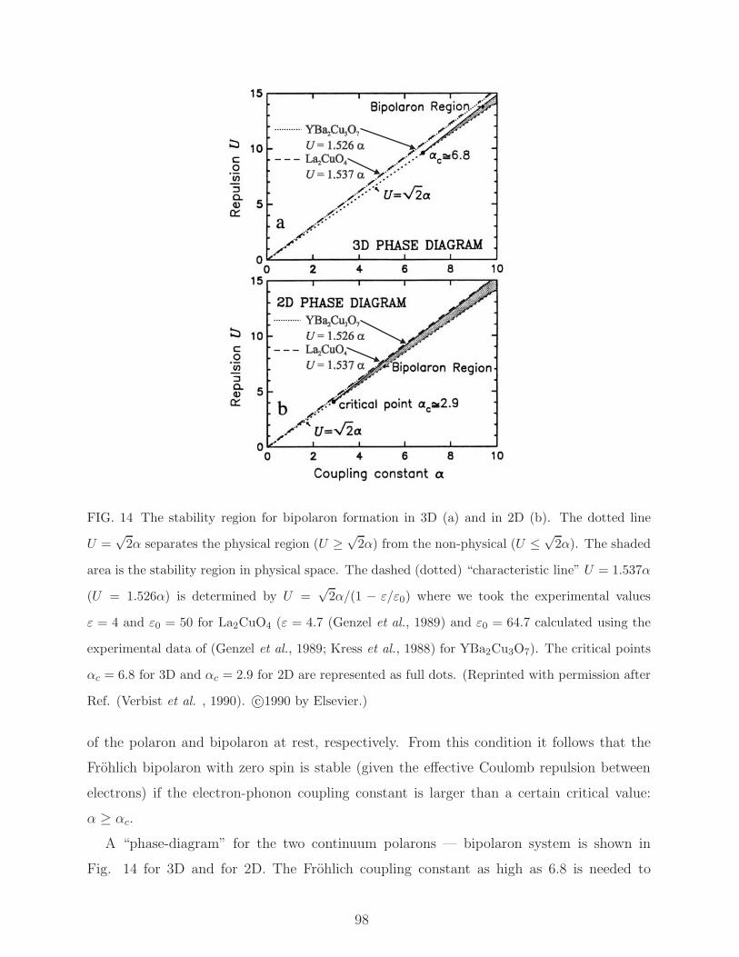
FIG. 14 The stability region for bipolaron formation in 3D (a) and in 2D (b). The dotted line

U =√

2α separates the physical region (U ≥√

2α) from the non-physical (U ≤√

2α). The shaded

area is the stability region in physical space. The dashed (dotted) “characteristic line” U = 1.537α

(U = 1.526α) is determined by U =√

2α/(1 − ε/ε0) where we took the experimental values

ε = 4 and ε0 = 50 for La2CuO4 (ε = 4.7 (Genzel et al., 1989) and ε0 = 64.7 calculated using the

experimental data of (Genzel et al., 1989; Kress et al., 1988) for YBa2Cu3O7). The critical points

αc = 6.8 for 3D and αc = 2.9 for 2D are represented as full dots. (Reprinted with permission after

Ref. (Verbist et al. , 1990). c©1990 by Elsevier.)

of the polaron and bipolaron at rest, respectively. From this condition it follows that the

Frohlich bipolaron with zero spin is stable (given the effective Coulomb repulsion between

electrons) if the electron-phonon coupling constant is larger than a certain critical value:

α ≥ αc.

A “phase-diagram” for the two continuum polarons — bipolaron system is shown in

Fig. 14 for 3D and for 2D. The Frohlich coupling constant as high as 6.8 is needed to

98

allow for bipolaron formation in 3D. The confinement of the bipolaron in two dimensions

facilitates bipolaron formation at smaller α. This can be shown using the PD-type scaling

relation between the free energies F in two dimensions F2D(α, U, β) and in three dimensions

F3D(α, U, β) (Verbist et al. , 1990, 1991),

F2D(α, U, β) =2

3F3D(

3π

4α,

3π

4U, β). (257)

According to Eq. (257), the critical value of the coupling constant for bipolaron formation

αc turns out to scale with a factor 3π/4 ≈ 2.36 or α(2D)c = α

(3D)c /2.36. From Fig. 14b it is

seen that bipolarons in 2D can be stable for α ≥ 2.9, a domain of coupling constants which

is definitely realised in several solids. The “characteristic line” U = 1.526α for the material

parameters of YBa2Cu3O7 enters the region of bipolaron stability in 2D at a value of α

which is appreciably smaller than in the case of La2CuO4. This fact suggests YBa2Cu3O7

as a good candidate for the occurrence of stable Frohlich bipolarons.

An analytical strong-coupling asymptotic expansion in inverse powers of the electron-

phonon coupling constant for the large bipolaron energy at T = 0 was derived in

(Smondyrev et al. , 1995)

E3D(α, u) = −2α2

3πA(u) − B(u) +O(α−2), (258)

where the coefficients are closed analytical functions of the ratio u = U/α:

A(u) = 4 − 2√

2u

(

1 +u2

128

)3/2

+5

8u2 − u4

512(259)

and for B(u) see the above-cited paper. The scaling relation (257) allows one to find the

bipolaron energy in two dimensions as well.

The stability of bipolarons has also been examined with the use of operator techniques

with a variational approach (Bassani et al. , 1991). The bipolaron is bound if the electron-

phonon coupling constant α is larger than ∼ 6 in three dimensions and larger than ∼ 2

in two dimensions, provided the ratio η = ε/ε0 is smaller than a critical value ηc which

depends on α. The critical value ηc is larger in the two-dimensional case than in the three-

dimensional one. The bipolaron radius is shown to be of the order of a few polaron radii.

The results of (Bassani et al. , 1991) and (Verbist et al. , 1990, 1991) tend to qualitatively

confirm each other. Furthermore, bipolaron states obtained in (Bassani et al. , 1991) under

the assumption that the total linear momentum is conserved, have intrinsically high mobility.

99

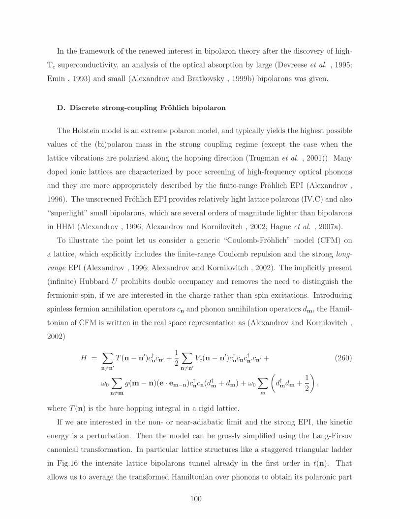
In the framework of the renewed interest in bipolaron theory after the discovery of high-

Tc superconductivity, an analysis of the optical absorption by large (Devreese et al. , 1995;

Emin , 1993) and small (Alexandrov and Bratkovsky , 1999b) bipolarons was given.

D. Discrete strong-coupling Frohlich bipolaron

The Holstein model is an extreme polaron model, and typically yields the highest possible

values of the (bi)polaron mass in the strong coupling regime (except the case when the

lattice vibrations are polarised along the hopping direction (Trugman et al. , 2001)). Many

doped ionic lattices are characterized by poor screening of high-frequency optical phonons

and they are more appropriately described by the finite-range Frohlich EPI (Alexandrov ,

1996). The unscreened Frohlich EPI provides relatively light lattice polarons (IV.C) and also

“superlight” small bipolarons, which are several orders of magnitude lighter than bipolarons

in HHM (Alexandrov , 1996; Alexandrov and Kornilovitch , 2002; Hague et al. , 2007a).

To illustrate the point let us consider a generic “Coulomb-Frohlich” model (CFM) on

a lattice, which explicitly includes the finite-range Coulomb repulsion and the strong long-

range EPI (Alexandrov , 1996; Alexandrov and Kornilovitch , 2002). The implicitly present

(infinite) Hubbard U prohibits double occupancy and removes the need to distinguish the

fermionic spin, if we are interested in the charge rather than spin excitations. Introducing

spinless fermion annihilation operators cn and phonon annihilation operators dm, the Hamil-

tonian of CFM is written in the real space representation as (Alexandrov and Kornilovitch ,

2002)

H =∑

n6=n′

T (n− n′)c†ncn′ +1

2

∑

n6=n′

Vc(n− n′)c†ncnc†n′cn′ + (260)

ω0

∑

n6=m

g(m− n)(e · em−n)c†ncn(d†m + dm) + ω0

∑

m

(

d†mdm +1

2

)

,

where T (n) is the bare hopping integral in a rigid lattice.

If we are interested in the non- or near-adiabatic limit and the strong EPI, the kinetic

energy is a perturbation. Then the model can be grossly simplified using the Lang-Firsov

canonical transformation. In particular lattice structures like a staggered triangular ladder

in Fig.16 the intersite lattice bipolarons tunnel already in the first order in t(n). That

allows us to average the transformed Hamiltonian over phonons to obtain its polaronic part

100

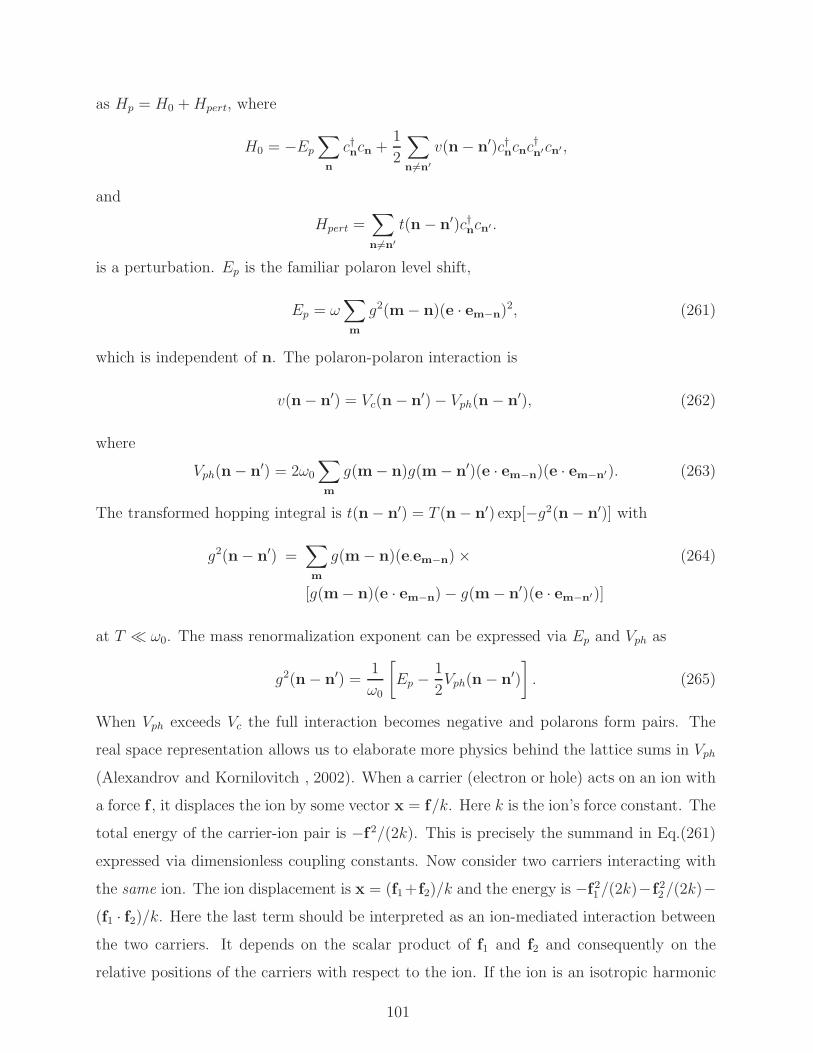
as Hp = H0 +Hpert, where

H0 = −Ep

∑

n

c†ncn +1

2

∑

n6=n′

v(n− n′)c†ncnc†n′cn′,

and

Hpert =∑

n6=n′

t(n − n′)c†ncn′ .

is a perturbation. Ep is the familiar polaron level shift,

Ep = ω∑

m

g2(m− n)(e · em−n)2, (261)

which is independent of n. The polaron-polaron interaction is

v(n− n′) = Vc(n − n′) − Vph(n− n′), (262)

where

Vph(n− n′) = 2ω0

∑

m

g(m− n)g(m− n′)(e · em−n)(e · em−n′). (263)

The transformed hopping integral is t(n− n′) = T (n− n′) exp[−g2(n− n′)] with

g2(n− n′) =∑

m

g(m− n)(e·em−n) × (264)

[g(m− n)(e · em−n) − g(m− n′)(e · em−n′)]

at T ≪ ω0. The mass renormalization exponent can be expressed via Ep and Vph as

g2(n− n′) =1

ω0

[

Ep −1

2Vph(n − n′)

]

. (265)

When Vph exceeds Vc the full interaction becomes negative and polarons form pairs. The

real space representation allows us to elaborate more physics behind the lattice sums in Vph

(Alexandrov and Kornilovitch , 2002). When a carrier (electron or hole) acts on an ion with

a force f , it displaces the ion by some vector x = f/k. Here k is the ion’s force constant. The

total energy of the carrier-ion pair is −f2/(2k). This is precisely the summand in Eq.(261)

expressed via dimensionless coupling constants. Now consider two carriers interacting with

the same ion. The ion displacement is x = (f1+f2)/k and the energy is −f21 /(2k)−f2

2 /(2k)−(f1 · f2)/k. Here the last term should be interpreted as an ion-mediated interaction between

the two carriers. It depends on the scalar product of f1 and f2 and consequently on the

relative positions of the carriers with respect to the ion. If the ion is an isotropic harmonic

101

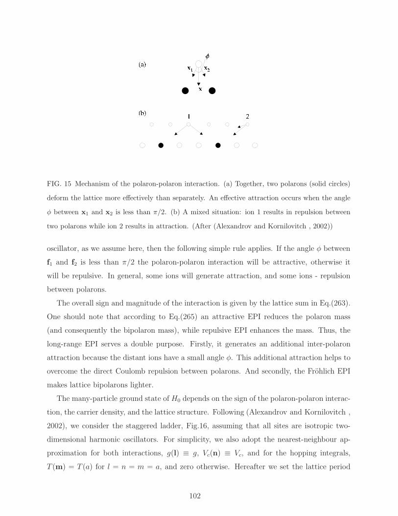
FIG. 15 Mechanism of the polaron-polaron interaction. (a) Together, two polarons (solid circles)

deform the lattice more effectively than separately. An effective attraction occurs when the angle

φ between x1 and x2 is less than π/2. (b) A mixed situation: ion 1 results in repulsion between

two polarons while ion 2 results in attraction. (After (Alexandrov and Kornilovitch , 2002))

oscillator, as we assume here, then the following simple rule applies. If the angle φ between

f1 and f2 is less than π/2 the polaron-polaron interaction will be attractive, otherwise it

will be repulsive. In general, some ions will generate attraction, and some ions - repulsion

between polarons.

The overall sign and magnitude of the interaction is given by the lattice sum in Eq.(263).

One should note that according to Eq.(265) an attractive EPI reduces the polaron mass

(and consequently the bipolaron mass), while repulsive EPI enhances the mass. Thus, the

long-range EPI serves a double purpose. Firstly, it generates an additional inter-polaron

attraction because the distant ions have a small angle φ. This additional attraction helps to

overcome the direct Coulomb repulsion between polarons. And secondly, the Frohlich EPI

makes lattice bipolarons lighter.

The many-particle ground state of H0 depends on the sign of the polaron-polaron interac-

tion, the carrier density, and the lattice structure. Following (Alexandrov and Kornilovitch ,

2002), we consider the staggered ladder, Fig.16, assuming that all sites are isotropic two-

dimensional harmonic oscillators. For simplicity, we also adopt the nearest-neighbour ap-

proximation for both interactions, g(l) ≡ g, Vc(n) ≡ Vc, and for the hopping integrals,

T (m) = T (a) for l = n = m = a, and zero otherwise. Hereafter we set the lattice period

102

a = 1. There are four nearest neighbours in the ladder, z = 4. The single-particle polaronic

Hamiltonian takes the form

Hp = −Ep

∑

n

(c†ncn + p†npn) + (266)

∑

n

[t′(c†n+1cn + p†n+1pn) + t(p†ncn + p†n−1cn) +H.c.],

where cn and pn are polaron annihilation operators on the lower and upper legs of the

ladder, respectively, Fig.16. Using Eqs.(261,263,265) one obtains Ep = 4g2ω0, t′ =

T (a) exp(−7Ep/8ω0), and t = T (a) exp(−3Ep/4ω0).

The Fourier transform of Hp yields two overlapping polaron bands,

Ep(k) = −Ep + 2t′ cos(k) ± 2t cos(k/2) (267)

with the effective mass m∗ = 2/|4t′ ± t| near their edges.

Let us now place two polarons on the ladder. The nearest neighbour interaction is

v = Vc −Ep/2, if two polarons are on different legs of the ladder, and v = Vc −Ep/4, if both

polarons are on the same leg. The attractive interaction is provided via the displacement of

the lattice sites, which are the common nearest neighbours to both polarons. There are two

such nearest neighbours for the intersite bipolaron of type A or B, Fig.16c, but there is only

one common nearest neighbour for bipolaron C, Fig.16d. When Vc > Ep/2, there are no

bound states and the multi-polaron system is a one-dimensional Luttinger liquid. However,

when Vc < Ep/2 and consequently v < 0, the two polarons are bound into an inter-site

bipolaron of types A or B.

Remarkably, bipolarons tunnel in the ladder already in the first order with respect to

the single-polaron tunnelling amplitude. This case is different from both onsite bipolarons

discussed above, and from intersite chain bipolarons of (Bonca and Trugman , 2001), where

the intersite bipolaron tunnelling appeared in the second order in t as for the on-site bipo-

larons. Indeed, the lowest-energy configurations A and B are degenerate. They are coupled

by Hpert. Neglecting all higher-energy configurations, we can project the Hamiltonian onto

the subspace containing A, B, and empty sites. The result of such a projection is the

bipolaronic Hamiltonian

Hb =

(

Vc −5

2Ep

)

∑

n

[A†nAn +B†

nBn] − t′∑

n

[B†nAn +B†

n−1An +H.c.], (268)

103

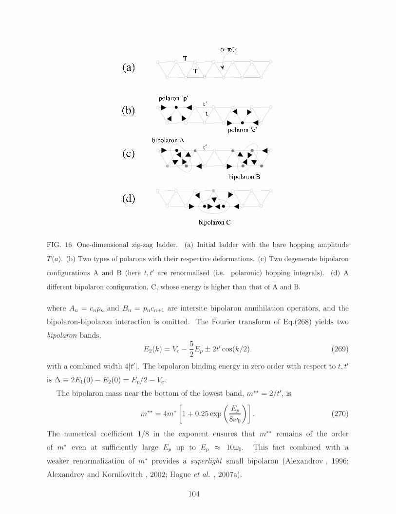
FIG. 16 One-dimensional zig-zag ladder. (a) Initial ladder with the bare hopping amplitude

T (a). (b) Two types of polarons with their respective deformations. (c) Two degenerate bipolaron

configurations A and B (here t, t′ are renormalised (i.e. polaronic) hopping integrals). (d) A

different bipolaron configuration, C, whose energy is higher than that of A and B.

where An = cnpn and Bn = pncn+1 are intersite bipolaron annihilation operators, and the

bipolaron-bipolaron interaction is omitted. The Fourier transform of Eq.(268) yields two

bipolaron bands,

E2(k) = Vc −5

2Ep ± 2t′ cos(k/2). (269)

with a combined width 4|t′|. The bipolaron binding energy in zero order with respect to t, t′

is ∆ ≡ 2E1(0) − E2(0) = Ep/2 − Vc.

The bipolaron mass near the bottom of the lowest band, m∗∗ = 2/t′, is

m∗∗ = 4m∗[

1 + 0.25 exp

(

Ep

8ω0

)]

. (270)

The numerical coefficient 1/8 in the exponent ensures that m∗∗ remains of the order

of m∗ even at sufficiently large Ep up to Ep ≈ 10ω0. This fact combined with a

weaker renormalization of m∗ provides a superlight small bipolaron (Alexandrov , 1996;

Alexandrov and Kornilovitch , 2002; Hague et al. , 2007a).

104

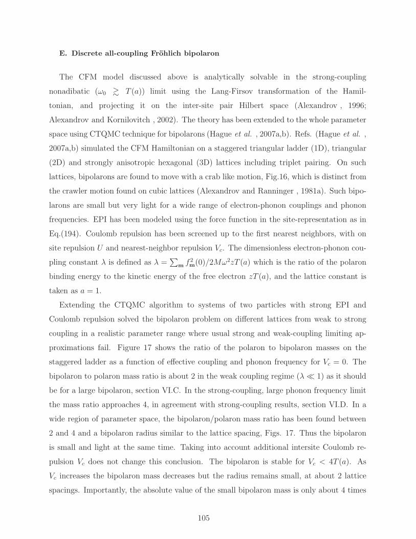
E. Discrete all-coupling Frohlich bipolaron

The CFM model discussed above is analytically solvable in the strong-coupling

nonadibatic (ω0 & T (a)) limit using the Lang-Firsov transformation of the Hamil-

tonian, and projecting it on the inter-site pair Hilbert space (Alexandrov , 1996;

Alexandrov and Kornilovitch , 2002). The theory has been extended to the whole parameter

space using CTQMC technique for bipolarons (Hague et al. , 2007a,b). Refs. (Hague et al. ,

2007a,b) simulated the CFM Hamiltonian on a staggered triangular ladder (1D), triangular

(2D) and strongly anisotropic hexagonal (3D) lattices including triplet pairing. On such

lattices, bipolarons are found to move with a crab like motion, Fig.16, which is distinct from

the crawler motion found on cubic lattices (Alexandrov and Ranninger , 1981a). Such bipo-

larons are small but very light for a wide range of electron-phonon couplings and phonon

frequencies. EPI has been modeled using the force function in the site-representation as in

Eq.(194). Coulomb repulsion has been screened up to the first nearest neighbors, with on

site repulsion U and nearest-neighbor repulsion Vc. The dimensionless electron-phonon cou-

pling constant λ is defined as λ =∑

m f 2m(0)/2Mω2zT (a) which is the ratio of the polaron

binding energy to the kinetic energy of the free electron zT (a), and the lattice constant is

taken as a = 1.

Extending the CTQMC algorithm to systems of two particles with strong EPI and

Coulomb repulsion solved the bipolaron problem on different lattices from weak to strong

coupling in a realistic parameter range where usual strong and weak-coupling limiting ap-

proximations fail. Figure 17 shows the ratio of the polaron to bipolaron masses on the

staggered ladder as a function of effective coupling and phonon frequency for Vc = 0. The

bipolaron to polaron mass ratio is about 2 in the weak coupling regime (λ≪ 1) as it should

be for a large bipolaron, section VI.C. In the strong-coupling, large phonon frequency limit

the mass ratio approaches 4, in agreement with strong-coupling results, section VI.D. In a

wide region of parameter space, the bipolaron/polaron mass ratio has been found between

2 and 4 and a bipolaron radius similar to the lattice spacing, Figs. 17. Thus the bipolaron

is small and light at the same time. Taking into account additional intersite Coulomb re-

pulsion Vc does not change this conclusion. The bipolaron is stable for Vc < 4T (a). As

Vc increases the bipolaron mass decreases but the radius remains small, at about 2 lattice

spacings. Importantly, the absolute value of the small bipolaron mass is only about 4 times

105

0 0.1 0.2 0.3 0.4 0.5

3.52.5

1.50.5 3.5

2.5 1.5

0.5

0 0.1 0.2 0.3 0.4 0.5

m*/m**

λ ω

m*/m**

FIG. 17 Polaron to bipolaron mass ratio for a range of ω = ω0/T (a) and λ on the staggered ladder.

Mobile small bipolarons are seen even in the adiabatic regime ω = 0.5 for couplings λ up to 2.5

(Reproduced from J. P. Hague et al., Phys. Rev. Lett 98, 037002 (2007), (c) American Physical

Society, 2007).

of the bare electron mass m0, for λ = ω/T (a) = 1 (see Fig. 17).

Simulations of the bipolaron on an infinite triangular lattice including exchanges and

large on-site Hubbard repulsion U = 20T (a) also lead to the bipolaron mass of about

6m0xy and the bipolaron radius Rbp ≈ 2a for a moderate coupling λ = 0.5 and a large

phonon frequency ω = T (a) (for the triangular lattice, m0xy = 1/3a2T (a)). Finally, the

bipolaron in a hexagonal lattice with out-of-plane hopping T ′ = T (a)/3 has also a light

in-plane inverse mass, m∗∗xy ≈ 4.5m0xy but a small size, Rbp ≈ 2.6a for experimentally

achievable values of the phonon frequency ω = T (a) = 200meV and EPI, λ = 0.36. Out-

of-plane m∗∗z ≈ 70m0z is Holstein like, where m0z = 1/2d2T ′, (d is the inter-plane spacing).

When bipolarons are small and pairs do not overlap, the pairs can form a BEC at TBEC =

3.31(2nB/a2√

3d)2/3/(m2/3xy m

1/3z ). If we choose realistic values for the lattice constants of 0.4

nm in the plane and 0.8 nm out of the plane, and allow the density of bosons to be nB=0.12

per lattice site, which easily avoids overlap of pairs, then TBEC ≈ 300K.

106

F. Polaronic exciton

Finally let us briefly mention works on electron-hole bound states coupled with

phonons. Such excitonic polaron states have been analysed by (Iadonisi and Bassani ,

1983, 1984, 1987). The binding energies of excitonic states in interaction with LO

phonons were computed using a phonon coherent state and applying a variational method

(Iadonisi and Bassani , 1983). Incomplete relaxation of the lattice is found. The binding en-

ergies are larger than those obtained with static dielectric screening when the polaron radius

is comparable to the exciton radius. Analysing the relative intensities of the one-phonon and

zero-phonon lines for a number of semiconductors, (Iadonisi and Bassani , 1983) observed

that the zero-phonon exciton states are generally much more probable than the phonon

replicas.

The binding energy of a core exciton, which depends on the interaction of the conduction

electron and of the core hole with the valence electrons via a Frohlich-type coupling with the

electron-hole pairs, in addition to the Coulomb attraction, was calculated within a functional

variational method (Iadonisi and Bassani , 1984). When the exciton radius is comparable

to the polaron radius, the static dielectric screening reduces and the core exciton binding

energy increases. The excitonic-polaron effective mass renormalization was analysed by

(Iadonisi and Bassani , 1984) using a variational numerical approach. Evidence for this

renormalization is found from the experimental data on polariton dispersion in hexagonal

CdS and in CuCl.

The angular momentum as a constant of the motion of a Frohlich polaron was introduced

by (Evrard et al. , 1970). Representing the excitonic polaron problem in angular coordinates

and solving it numerically, (Iadonisi et al. , 1989) showed that exciton states with various

total angular momenta L are differently affected by the interaction with LO phonons. How-

ever, when extending this approach to the bipolaron problem, the same authors found that

the Frohlich interaction is not strong enough to guarantee a stable bipolaron state at least

in the case of cubic materials.

Very recently the polaronic exciton problem has been solved using the approximation-free

DQMC technique (Burovski et al. , 2008). Numerically exact results for the wave function,

ground-state energy, binding energy and effective mass of this quasiparticle were calculated,

and the frequently used instantaneous approximation to the retarded interaction due to the

107

exchange of phonons was critically analysed.

VII. CURRENT STATUS OF POLARONS AND OPEN PROBLEMS

At present, the basic properties of single polarons are well understood theoretically, and

to a large extent they are analytically under control at all coupling. It is remarkable how

the Frohlich continuum polaron, one of the simplest examples of a Quantum Field Theoret-

ical problem, as it basically consists of a single fermion interacting with a scalar Bose field,

has resisted full analytical solution at all coupling since ∼ 1950, when its Hamiltonian was

first written. Although a mechanism for the optical absorption of Frohlich polarons was

already proposed a long time ago (Devreese et al. , 1972a; Kartheuser et al. , 1969), some

subtle characteristics were only clarified very recently (De Filippis et al. , 2006) by combin-

ing numerical DQMC studies (Mishchenko et al. , 2003) and improved analytical methods

(Cataudella et al., 2007; Devreese and Klimin , 2006) (III.F). Of special interest are several

sum rules derived for the optical conductivity spectra of arbitrary-coupling Frohlich polarons

(Devreese et al. , 1977; Lemmens et al., 1973). A variety of magneto-optical and transport-

experiments were successfully analysed with Frohlich polaron theory (see e. g. (Devreese,

2004; Hodby et al., 1987; Peeters and Devreese, 1984; Peeters and Devreese , 1986) and ref-

erences therein).

The charge carriers in a rich variety of systems of reduced dimension and dimensionality

(submicron- and nanostructures including heterojunctions, quantum wells, quantum wires,

quantum dots etc.) turn out to be Frohlich polarons. Several scaling relations were de-

rived (Peeters and Devreese, 1987), which connect polaron characteristics (the self-energy,

the effective mass, the impedance and the mobility) in different dimensions. Quite generally

confinement enhances EPI and the tendency to polaron formation. A new aspect of the po-

laron concept has been investigated for semiconductor structures at nanoscale: the exciton-

phonon states are not factorisable into an adiabatic product Ansatz, so that a non-adiabatic

treatment is needed (Fomin et al., 1998). The excitonic polarons in nanostructures lead to

the existence of phonon replicas in the luminescence ( Verzelen et al. , 2002). Experimental

evidence of the enhanced phonon-assisted absorption due to effects of non-adiabaticity has

been provided by the multi-phonon photoluminescence (PL) spectra observed under selective

excitation in self-assembled InAs/GaAs quantum dots (Garcıa-Cristobal et al., 1999) and by

108

the photoluminescence excitation (PLE) measurements on single self-assembled InAs/GaAs

(Lemaıtre et al., 2001) and InGaAs/GaAs (Zrenner et al., 2001) quantum dots. The polaron

concept was also invoked for the explanation of the PLE measurements on self-organised

InxGa1−xAs/GaAs (Heitz et al., 2001) and CdSe/ZnSe (Woggon et al., 2003) quantum dots.

The Frohlich polaron has led to many generalisations. The stability region of the

Frohlich large bipolaron is now firmly established (Bassani et al. , 1991; Verbist et al. ,

1990, 1991)(VI.C). Here the surprise is double (cf. (Devreese et al. , 1995; Verbist et al. ,

1991)): a) only in a very limited sector of the phase diagram (Coulomb repulsion versus α)

the bipolaron is stable, b) most traditional Frohlich polaron materials (alkali halides and

the like) lie completely outside (and “far” from) this bipolaron stability sector, but sev-

eral cuprate superconductors lie very close and even inside this very restricted area of the

stability diagram. The stability of a strong-coupling singlet bipolaron was studied in two-

and three-dimensional parabolic quantum dots using the Landau-Pekar variational method

(Mukhopadhyay et al. , 1996). It was shown that the confining potential of the quantum dot

reduces the stability of the bipolaron. A theory of bipolaron states in a spherical parabolic

potential well was further developed applying the Feynman variational principle. The basic

parameters of the bipolaron ground state (the binding energy, the number of phonons in the

bipolaron cloud, and the bipolaron radius were studied as a function of the radius of the

potential well (Pokatilov et al., 1999). It was found that confinement can enhance the bipo-

laron binding energy, when the radius of a quantum dot is of the same order of magnitude

as the polaron radius. A unified insight into the stability criterion for bipolaron formation

in low-dimensionally confined media was provided by (Senger and Ercelebi, 2000) using an

adiabatic variational method for a pair of electrons immersed in a reservoir of bulk LO

phonons and confined within an anisotropic parabolic potential box. Bipolaron formation in

a two-dimensional lattice with harmonic confinement, representing a simplified model for a

quantum dot, was investigated by means of QMC (Hohenadler et al. , 2007a). This method

treats all interactions exactly and takes into account quantum lattice fluctuations. Calcula-

tions of the bipolaron binding energy reveal that confinement opposes bipolaron formation

for weak electron-phonon coupling but abets a bound state at intermediate to strong cou-

pling. We also mention the exciton-polaron formation in nanostructures and quantum-light

sources studied recently by QMC in lattice models with short- or long-range carrier-phonon

interaction (see (Hohenadler et al. , 2007b), and references therein)

109

The richness and profundity of Landau-Pekar’s polaron concept is further illustrated by

its extensions to discrete (lattice) polarons. Even the simplest two-site polaron model by

Holstein (IV.A) proved to be very useful for a qualitative understanding of nontrivial fea-

tures of the polaron problem, and for obtaining some novel analytical and semi-analytical

results (see, for example, (Berciu , 2007; Han et al. , 2002; Kudinov and Firsov , 1997)).

The “1/λ” expansion technique based on the Lang-Firsov transformation (IV.B.1) and un-

biased numerical analysis of the finite and infinite Holstein and Frohlich models combining

Lanczos diagonalisations of clusters, density matrix renormalisation group, cluster pertur-

bation theory techniques, DMFT and different QMC algorithms, allowed for a description

of properties of a single lattice polaron and a lattice bipolaron. The Lang-Firsov canonical

transformation (Lang and Firsov , 1962) was proven particularly instrumental in calcula-

tion of different kinetic and optical coefficients, which can be represented as expansions in

powers of the unrenormalised hopping integral t (V). Sometimes it is possible to sum the

expansion and get results, which are valid for arbitrary values of parameters providing the

understanding of the crossover region from the Boltzmann kinetics to thermally activated

hopping (Firsov , 2007).

Recent ED (Fehske and Trugman , 2007), CTQMC (Kornilovitch , 2007) and DQMC

(Mishchenko and Nagaosa, 2007) techniques allow for determination of the ground-state and

excited states of lattice polarons with arbitrary precision in the thermodynamic limit for any

dimension and any type of lattices (IV.E.2). The spectral properties (e.g. photoemission),

optical response and thermal transport, as well as the dynamics of polaron formation in the

Holstein model have been numerically analysed for all EPI strengths and phonon frequen-

cies, including the intermediate-coupling regime (see V and (Fehske and Trugman , 2007)).

CTQMC methods have proven to be powerful and versatile tools providing unbiased results

for the polaron properties in any lattices for any-range EPI, including Jahn-Teller polarons

(IV.E). Combining the Lang-Firsov transformation and quantum Monte Carlo simulations

allows for an exact sampling without autocorrelations, which proves to be an enormous ad-

vantage for small phonon frequencies or low temperatures (Hohenadler and von der Linden ,

2007c).

Importantly, variational and numerical techniques confirmed that the Frohlich and

Holstein-Lang-Firsov theories are asymptotically exact in the weak, λ ≪ 1, and strong-

coupling, λ ≫ 1, regimes, respectively, and the polaron formation represents a contin-

110

uous crossover of the ground state (IV.E). The crossover is related to the exponential

increase of the effective mass, and the band narrowing with a strongly suppressed elec-

tronic quasiparticle residue and the Drude weight, accompanied by an increase of the

incoherent spectral weight (V.C). These features strongly depend on the phonon dis-

persion (Zoli , 1998), EPI radius (Alexandrov , 1996; Alexandrov and Kornilovitch , 1999;

Fehske et al. , 2002; Perroni et al., 2005), lattice geometry (Hague et al. , 2006a) and are

more pronounced in higher dimensions (Fehske et al. , 2002; Hague et al. , 2006a). Remark-

ably, the unscreened Frohlich EPI provides relatively light lattice polarons (IV.C), which

are several orders of magnitude lighter than the Holstein small polarons (Alexandrov , 1996;

Alexandrov and Kornilovitch , 1999) at strong coupling. This classification of weak- and

strong-coupling regimes still leaves room for continuum Frohlich polarons of not only weak

but also intermediate and - in the theoretical analysis - of strong coupling classified with

respect to the Frohlich electron-phonon coupling constant α (II.D).

While the single polaron has been actively researched for a long time and is now well un-

derstood, the multi-polaron physics has gained particular attention in the last two decades.

It has been found— unexpectedly for many researchers— that the Migdal-Eliashberg theory

breaks down already at λ ∼ 1 for any adiabatic ratio ω0/EF . The effective parameter λω0/EF

becomes large at λ & 1 since the bandwidth is narrowed and the Fermi energy, EF is renor-

malised down exponentially (Alexandrov , 1983, 2001a). Extending the BCS theory towards

the strong interaction between electrons and ion vibrations, a charged Bose gas of tightly

bound on-site small bipolarons was predicted (Alexandrov and Ranninger , 1981a), with a

further conclusion that the highest superconducting transition temperature is attained in

the crossover region of EPI strength between the BCS-like polaronic and bipolaronic super-

conductivity (Alexandrov , 1983). Subsequent studies of the Holstein-Hubbard model found

also two-site bipolarons (Aubry , 1995; Bonca et al. , 2000; La Magna and Pucci , 1997;

Macridin et al. , 2004). Taking into account that many advanced materials with low den-

sity of free carriers and poor mobility are characterized by poor screening of high-frequency

optical phonons, the Coulomb-Frohlich lattice polaron model was introduced (Alexandrov ,

1996; Alexandrov and Kornilovitch , 2002). The large Hubbard U and intersite Coulomb re-

pulsions and the unscreened Frohlich EPI provide “superlight” but small intersite bipolarons

(VI.D). More recent CTQMC simulations of intersite small bipolarons in the Coulomb-

Frohlich model (Hague et al. , 2007a) have found such quasiparticles in a wide parameter

111

range with achievable phonon frequencies and couplings. They could have a superconducting

transition in excess of room temperature.

The many-body theory for polarons has been developed for extreme weak and strong

coupling regimes. It became clear how — in the weak-coupling limit — this prob-

lem can be reduced to the study of the structure factor of a uniform electron gas

(Lemmens et al., 1977). For strong coupling the problem is reduced to an interacting

Bose gas of on-site (Alexandrov and Ranninger , 1981a) or intersite (Alexandrov , 1996;

Alexandrov and Kornilovitch , 2002; Hague et al. , 2007a) small bipolarons in the dilute

system.

While correlation effects in transport through metallic quantum dots with repulsive

electron-electron interactions received considerable attention in the past, and continue to

be the focus of intense investigations, much less has been known about a role of attractive

correlations between small polarons mediated by EPI in molecular quantum dots (MQD)

and nanowires. In the framework of the negative U Hubbard model (Alexandrov et al. ,

2003) it has been found that the attractive electron correlations within the molecule could

lead to a molecular switching effect where I-V characteristics have two branches with high

and low current at the same bias voltage. The switching phenomenon has been also pre-

dicted by a theory of correlated polaron transport with a full account of both the Coulomb

repulsion and EPI in MQD weakly coupled with electrodes (Alexandrov and Bratkovsky ,

2003; Ermakov, 2000). Ref. (Alexandrov and Bratkovsky , 2003) has shown that while the

phonon side-bands significantly modify the shape of hysteretic I-V curves in comparison with

the negative-U Hubbard model, switching remains robust. It shows up at sufficiently low

temperatures when the effective interaction of polarons in MQD is attractive and the molec-

ular level is multiply degenerate. Importantly, the switching has not been found in non-

and two-fold degenerate MQDs (Alexandrov and Bratkovsky , 2003). When the polaronic

energy shift is very large, the effective charging energy of molecules can become negative,

favoring ground states with even numbers of electrons. Ref.(Koch et al., 2006) has shown

that charge transport through such molecules is dominated by tunneling of bipolarons which

coexists with single-electron cotunneling.

The conductance of deformable molecules with a local magnetic moment has been studied

in the framework of a two-impurity Anderson model with positive and negative electron-

electron interactions and in the two-impurity Anderson-Holstein model with a single phonon

112

mode (Zitko and Bonca , 2006). It has been shown that the spin and charge Kondo effects

can occur simultaneously at any coupling strength. At finite bandwidth and strong cou-

pling the lattice effects lead to a renormalization of the effective Kondo exchange constants;

nevertheless, universal spin and charge Kondo effects still occur.

The theory of dense polaronic systems in the intermediate regime remains highly cumber-

some, in particular when EPI competes with strong electron correlations. The corresponding

microscopic models contain (extended) Hubbard, Heisenberg or double-exchange terms, and

maybe also a coupling to orbital degrees of freedom along with strong EPI, so that even

numerical solutions with the same precision as in the dilute (bi)polaron case are often prob-

lematic. A number of ED, QMC, DMFT and combined numerical results give strong evi-

dence that the tendency towards lattice polaron formation is enhanced in strongly correlated

electron systems due to a narrowing of the electron band caused by strong correlations (see

recent reviews by (Edwards , 2002; Fehske and Trugman , 2007; Hohenadler et al. , 2005b;

Hohenadler and von der Linden , 2007c) for more details). Not only antiferromagnetic cor-

relations enhance EPI, resulting in polaron formation for moderate coupling strength, but

also EPI strongly enhances spin correlations (Capone and Ciuchi , 2002; Macridin et al. ,

2006). Some of these studies show that increasing carrier density could be accompanied

by a dissociation of polarons leading to normal metallic behavior in the intermediate cou-

pling adiabatic regime (Hohenadler et al. , 2005b) that is reminiscent of the “overcrowding”

effect hypothesized by Mott (1995). On the other hand for parameters favoring small po-

larons no such density-driven crossover occurs in agreement with simple analytical arguments

(Alexandrov , 2001a). Thorough investigations of these models will definitely be a great

challenge in the near future. Here we have focused on the single and two-body problems

leaving theories of strongly-correlated polarons and their applications to high-temperature

superconductors and CMR oxides for future reviews (Alexandrov and Devreese , 2009).

Finally, exactly solvable models might give a rather limited, sometimes misleading, de-

scription of polarons in real systems. Qualitative inconsistencies can arise when coupling

is assumed to be just to one phonon mode, often taken as dispersionless, and ad-hoc ap-

proximations for EPI matrix elements are applied. Moreover electronic nanoscale disorder

and long-range strain fields can interweave with the microscopic mechanisms of polaronic

transport (Phillips et al. , 2003). Hence ab-initio calculations of the phonon spectrum, EPI

and polaron properties beyond the adiabatic Born-Oppenheimer approximation are required

113

in many cases for which the theory and experiment can be compared in detail (Banacky ,

2008; Shluger and Stoneham , 1993).

Acknowledgments

We have benefited from discussions with many colleagues. While writing this review,

conversations with Alexander Andreev, Serge Aubry, Ivan Bozovic, Alex Bratkovsky, Pe-

ter Edwards, Janez Bonca, Holger Fehske, Jim Hague, Yurii Firsov, Martin Hohenadler,

Viktor Kabanov, Pavel Kornilovitch, Wolfgang von der Linden, Peter Littlewood, Dragan

Mihailovic, John Samson, Marshall Stoneham and other participants of the European Sci-

ence Foundation workshop ”Mott’s Physics in Nanowires and Quantum Dots” (Cambridge,

UK, 31 July-2 August, 2006) were especially helpful. We like to thank Vladimir Fomin for

discussions during the preparation of this review, and to acknowledge discussions with Fons

Brosens, Dieter Bimberg, Vittorio Cataudella, Paolo Calvani, Giulio De Filippis, Roger

Evrard, Vladimir Gladilin, Giuseppe Iadonisi, Eddy Kartheuser, Serghei Klimin, Lucien

Lemmens, Andrei Mishchenko, Francois Peeters and Jacques Tempere. This work was sup-

ported in part by EPSRC under grants No. EP/C518365/1 and No. EP/D07777X/1 (UK),

IUAP, FWO-V project G.0435.03, the WOG WO.035.04N (Belgium) and the European

Commission SANDiE Network of Excellence, contract No. NMP4-CT-2004-500101.

References

Adamowski, J., 1989, Phys. Rev. B 39, 3649.

Albrecht, U., and P. Leiderer, 1987, Europhys. Lett. 3, 705.

Alexandrov , A. S., 1983, Zh. Fiz. Khim. 57, 273 [Russ. J. Phys. Chem. 57, 167].

Alexandrov, A, 1991, Physica C (Amsterdam) 182, 327.

Alexandrov, A. S., 1992a, Phys. Rev. B 46, 2838.

Alexandrov, A. S., 1992b, Phys. Rev. B 46, 14932.

Alexandrov, A. S., 1996, Phys. Rev. B 53, 2863.

Alexandrov, A. S., 1998, in Proceedings of the International School of Physics “Enrico Fermi”,

Course CXXXVI, Varenna, 1997, “Models and Phenomenology for Conventional and High-

114

Temperature Superconductivity”, edited by G. Iadonisi, J. R. Schrieffer and M. L. Chiofalo (IOS

Press, Amsterdam), 309.

Alexandrov, A. S., 2000, Phys. Rev. B 61, 12315.

Alexandrov, A. S., 2001a, Europhys. Lett. 56, 92.

Alexandrov, A. S., 2003, Theory of Superconductivity: from Weak to Strong Coupling (IoP, Bristol).

Alexandrov, A. S., and A. M. Bratkovsky, 1999a, Phys. Rev. Lett. 82, 141.

Alexandrov, A. S., and A. M. Bratkovsky, 1999b, J. Phys. Condens. Matter 48, L531.

Alexandrov, A. S., and A. M. Bratkovsky 2000, Phys. Rev. Lett. 84, 2043.

Alexandrov, A. S. and A. M. Bratkovsky, 2003, Phys. Rev. B 67, 235312.

Alexandrov, A. S., A. M. Bratkovsky, and R. S. Williams, 2003, Phys. Rev. B 67, 075301.

Alexandrov, A. S. and H. Capellmann , 1991, Phys. Rev. B 43, 2042.

Alexandrov, A. S., H. Capellmann , and U. Gobel,1992, Phys. Rev. B 46, 4374.

Alexandrov, A. S., and J. T. Devreese, 2009, Advances in Polaron Physics (Springer, Heidelberg).

Alexandrov, A. S., and V. V. Kabanov, 1986, Fiz. Tverd. Tela (St. Petersburg) 28, 1129 [Soviet

Phys. Solid St. 28, 631 ].

Alexandrov, A. S., and V. V. Kabanov, 1996, Phys. Rev. B 54, 3655.

Alexandrov, A. S., V. V. Kabanov, and D. K. Ray, 1994a, Phys. Rev. B 49, 9915.

Alexandrov, A. S., V. V. Kabanov, and D. K. Ray 1994b, Physica C (Amsterdam) 224, 247.

Alexandrov, A. S., and P. E. Kornilovitch, 1999, Phys. Rev. Lett. 82, 807.

Alexandrov, A. S., and P. E. Kornilovitch 2002, J. Phys. Condens. Matter 14, 5337.

Alexandrov, A. S., and N. F. Mott, 1994, Rep. Prog. Phys. 57, 1197.

Alexandrov, A. S., and N. F. Mott, 1995, Polarons and Bipolarons ( World Scientific, Singapore).

Alexandrov, A., and J. Ranninger, 1981a, Phys. Rev. B 23, 1796.

Alexandrov, A., and J. Ranninger, 1981b, Phys. Rev. B 24, 1164.

Alexandrov, A. S., and J. Ranninger, 1992, Phys. Rev. B 45, 13109.

Alexandrov, A. S., and C. Sricheewin, 2000, EuroPhys. Lett. 51, 188.

Alexandrov, A. S., and B. Y. Yavidov, 2004, Phys. Rev. B 69, 073101 .

Alexandrov, A. S., G. M. Zhao, H. Keller, B. Lorenz, Y. S. Wang, and C. W. Chu, 2001, Phys.

Rev. B 64, 140404(R).

Allcock, G. R., 1956, Adv. Phys. 5, 412.

Allcock, G. R., 1963, in Polarons and Excitons, edited by C. G. Kuper and G. D. Whitfield (Oliver

115

and Boyd, Edinburgh), 45.

Allen, P. B., and V. Perebeinos, 1999, Phys. Rev. B 60, 10747.

Alvermann, A., H. Fehske, and S. A. Trugman, 2008, Phys. Rev. B 78, 165106.

Anderson, P. W., 1975, Phys. Rev. Lett. 34, 953.

Anderson, P. W., 1997, The Theory of Superconductivity in the Cuprates (Princeton University

Press, Princeton, NJ).

Appel, J., 1968, in Solid State Physics edited by F. Seitz, D. Turnbull, and H. Ehrenreich (Academic

Press), 21.

Aubry, S., 1993, J. Phys. (France) IV Colloq. C2 3, 349.

Aubry, S., 1995, in Polarons and Bipolarons in High Tc Superconductors and related materi-

als edited by E. K. H. Salje, A. S. Alexandrov and W. Y.Liang (Cambridge University Press,

Cambridge), 271.

Aubry, S., 2007, in Polarons in Advanced Materials edited by A. S. Alexandrov (Canopus/Springer,

Bristol), 311.

Banacky, P., 2008, J. Phys. Chem. Sol. 69, 2696.

Barisic, O. S., 2004, Phys. Rev. B 69, 064302.

Barisic, O. S., and S. Barisic, 2008, Eur. Phys. J. B 64, 1.

Baryakhtar, V. G., E. V. Zarochentsev, and E. P. Troitskaya, 1999, Theory of Adiabatic Potential

and Atomic Properties of Simple Metals (Gordon and Breach, Amsterdam).

Bassani, F., M. Geddo, G. Iadonisi, and D. Ninno, 1991, Phys. Rev. B 43, 5296.

Becker, W., B. Gerlach, and H. Schliffke, 1983 Phys. Rev. B 28, 5735.

Bednorz, J. G., and K. A. Muller, 1988, Rev. Mod. Phys. 60, 585.

Belitz, D., and T. R. Kirkpatrick, 1994, Rev. Mod. Phys. 66, 261.

Benedetti, P., and R. Zeyher, 1998, Phys. Rev. B 58, 14320.

Beni, G., P. Pincus, and J. Kanamori, 1974, Phys. Rev. B 10, 1896.

Berciu, M., 2006a, Phys. Rev. Lett. 97, 036402.

Berciu, M., 2006b, Phys. Rev. B 74, 245104.

Berciu, M., 2007, Phys. Rev. B 75, 081101(R).

Berger, E., P. Valasek, and W. von der Linden, 1995, Phys. Rev. B 52, 4806.

Billinge , S. J. L., R. G. DiFrancesco, G. H. Kwei, J. J. Neumeier, and J. D. Thompson, 1996,

Phys. Rev. Lett. 77, 715.

116

Bogoliubov, N. N., 1950, Ukr. Math. Zh 2, 3.

Bogoliubov Jr., N. N., 1994, in Superconductivity and Strongly Correlated Electron Systems, ed. C.

Noce, A. Romano, and G. Scarpetta (World Scientific, Singapore), 107.

Bonca, J., T. Katrasnic, and S. A. Trugman, 2000, Phys. Rev. Lett. 84, 3153.

Bonca, J., and S. A. Trugman, 2001, Phys. Rev. B 64, 094507.

Bonca, J., S. A. Trugman, and I. Batistic, 1999, Phys. Rev. B 60, 1633.

Born, M., and R. Oppenheimer, 1927, Rev. Mod. Phys. 84, 457.

Bottger, H., and V. Bryksin, 1985, Hopping Conduction in Solids (Academie-Verlag, Berlin ).

Bottger, H., V. V. Bryksin, and T. Damker, 2007 in Polarons in Advanced Materials edited by A.

S. Alexandrov (Canopus/Springer, Bristol), 107.

Brosens, F., J. T. Devreese, and L. F. Lemmens, 1997a, Phys. Rev. E 55, 6795.

Brosens, F., J. T. Devreese, and L. F. Lemmens, 1997b, Phys. Rev. E 55, 227.

Brosens, F., J. T. Devreese, and L. F. Lemmens, 1998, Phys. Rev. E 58, 1634.

Brown, F. C. 1963, in Polarons and Excitons, ed. C. G. Kuper and G. D. Whitfield (Oliver and

Boyd, Edinburgh), 323.

Brown, F. C., 1972, in Point Defects in Solids, edited by J. H. Crawford and L. M. Slifkin (Plenum,

New York) 1, 537.

Bryksin, V. V., and Yu. A. Firsov, 1970, Sov. Phys. Sol. St. 12, 627.

Bryksin, V. V., and V. S. Voloshin, 1984, Fiz. Tverd. Tela (St Petersburg) 26, 2357[ Sov. Phys. Sol.

St. 26, 1429 (1984)].

Bryksin, V. V., and A. V. Gol’tsev, 1988, Fiz. Tverd. Tela (St Petersburg) 30, 1476[ Sov. Phys. Sol.

St. 30, 851 (1988)].

Burkov, A. A., and L. Balents , 2003, Phys. Rev. Lett. 91, 057202.

Burovski, E., H. Fehske, and A. S. Mishchenko, 2008, Phys. Rev. Lett. 101, 116403.

Bussmann-Holder, A., and A. R. Bishop, 1999, Phil. Mag, B 79, 119.

Bussmann-Holder, A., H. Keller, A. R. Bishop, A. Simon, R. Micnas, and K. A. Muller, 2005,

Europhys. Lett. 72, 423.

Caldeira, A. O., and A. J. Leggett, 1981, Phys. Rev. Lett. 46, 211.

Castro Neto, A. H., and A. O. Caldeira, 1991, Phys. Rev. Lett. 67, 1960.

Calvani, P., 2001, Optical Properties of Polarons (Editrice Compositori, Bologna).

Calvani, P., M. Capizzi, S. Lupi, P. Maselli, A. Paolone, R. Roy, S. W. Cheong, W. Sadowski, and

117

E. Walker, 1994, Solid State Commun. 91, 113.

Campbell, B. J., R. Osborn, D. N. Argyriou, L. Vasiliu-Doloc, J. F. Mitchell, S. K. Sinha, U. Ruett,

C. D. Ling, Z. Islam, and J. W. Lynn, 2001, Phys. Rev. B 65, 014427.

Campbell, B. J., S. K. Sinha, R. Osborn, S. Rosenkranz, J. F. Mitchell D. N. Argyriou, L. Vasiliu-

Doloc, O. H. Seeck, and J. W. Lynn, 2003, Phys. Rev. B 67, 020409.

Capone, M., and S. Ciuchi, 1997, Phys. Rev. B 65, 104409.

Capone, M., and S. Ciuchi, 2003, Phys. Rev. Lett. 91, 186405.

Capone, M., W. Stephan, and M. Grilli, 1997, Phys. Rev. B 56, 4484.

Cataudella, V., G. De Filippis, and G. Iadonisi, 1999, Eur. Phys. J. B 12, 17.

Cataudella, V., G. De Filippis, and C. A. Perroni, 2007, in Polarons in Advanced Materials edited

by A. S. Alexandrov (Canopus/Springer, Bristol), 149.

Chakraverty, B. K., J. Ranninger, and D. Feinberg, 1998, Phys. Rev. Lett. 81, 433.

Chatterjee, J., and A. N. Das, 2000, Phys. Rev. B 61, 4592.

Chatterjee, J., A. N. Das, and P. Choudhury, 2003, Solid State Commun. 126, 113.

Cheng, J.-P., B. D. McCombe, J. M. Shi, F. M. Peeters, and J. T. Devreese, 1993, Phys. Rev. B

48, 7910.

Ciuchi, S., F. de Pasquale, S. Fratini, and D. Feinberg, 1997, Phys. Rev. B 56, 4494.

De Filippis, G., V. Cataudella, V. Marigliano Ramaglia, C. A. Perroni, and D. Bercioux, 2003,

Eur. Phys. J. B 36, 65.

De Filippis, G., V. Cataudella, A. S. Mishchenko, C. A. Perroni, and J. T. Devreese, 2006, Phys.

Rev. Lett. 96, 136405.

De Mello, E. V. L., and J. Ranninger, 1997, Phys. Rev. B 55, 14872.

De Mello, E. V. L., and J. Ranninger, 1998a, Phys. Rev. B 58, 9098.

De Mello, E. V. L., and J. Ranninger, 1998b, Phys. Rev. B 58, 14625 .

De Mello, E. V. L., and J. Ranninger, 1999, Phys. Rev. B 59, 12135.

De Raedt, H., and A. Lagendijk, 1982, Phys. Rev. Lett. 49, 1522.

De Raedt, H., and A. Lagendijk, 1983, Phys. Rev. B 27, 6097.

De Raedt, H., and A. Lagendijk, 1984, Phys. Rev. B 30, 1671.

De Raedt, H., and A. Lagendijk, 1985, Phys. Rep. 127, 234.

Deppeler, A., and A. J. Millis, 2002, Phys. Rev. B 65, 224301.

Deville, G., A. Valdes, E. Y. Andrei, and F. I. B. Williams, 1984, Phys. Rev. Lett. 53, 588.

118

Devreese, J., 1963, Bull. Soc. Belge de Phys., Ser. III, no. 4, 259.

Devreese, J. T. 1964 Contribution to the polaron theory, Ph.D. Thesis (KU Leuven).

Devreese, J. T., 1972 in Polarons in Ionic Crystals and Polar Semiconductors (North-Holland,

Amsterdam), p. 83.

Devreese, J. T., 1996, in Encyclopedia of Applied Physics, edited by G. L. Trigg (VCH, Weinheim),

volume 14, 383.

Devreese, J. T., 1998, in Proceedings of the International School of Physics “Enrico Fermi”, Course

CXXXVI, Varenna, 1997, “Models and Phenomenology for Conventional and High-Temperature

Superconductivity”, edited by G. Iadonisi, J. R. Schrieffer and M. L. Chiofalo (IOS Press, Ams-

terdam), 287.

Devreese, J. T., 2003, in Lectures on the Physics of Highly Correlated Electron Systems VII, edited

by A. Avella and F. Mancini (AIP, Melville), 3.

Devreese, J. T., 2004, in Encyclopedia of Modern Optics, 5-volume set, edited by B. D. Guenther,

D. G. Steel and L. Bayvel (Academic Press), 629.

Devreese, J. T., 2005, in Encyclopedia of Physics, Third Edition, edited by R. G. Lerner and

L. Trigg (WILEY-VHC, Weinheim).

Devreese, J. T., 2006, in Proceedings of the “Enrico Fermi” Summer School, Course CLXI -

“Polarons in Bulk Materials and Systems with Reduced Dimensionality”, Varenna, June 21 -

July 1, 2005, edited by G. Iadonisi, J. Ranninger, and G. De Filippis (IOS Press, Amsterdam),

27.

Devreese, J. T., 2007, J. Phys.: Condens. Matter 19, 255201.

Devreese, J. T., 2007, in Polarons in Advanced Materials, edited by A. S. Alexandrov (Cano-

pus/Springer, Bristol,) 3.

Devreese, J., and R. Evrard, 1963, Physica Status Solidi (b) 3, 2133.

Devreese, J. T., and R. Evrard, 1964, Phys. Letters 11, 278.

Devreese, J. T., and R. P. Evrard, 1965, Physica Status Solidi (b) 9, 403.

Devreese, J. T., and R. P. Evrard, 1966, Physics Letters 23, 196.

Devreese, J. T., and R. Evrard, 1968, in Proceedings of the British Ceramic Society 10, 151

[reprinted in Path Integrals and Their Applications in Quantum, Statistical, and Solid State

Physics (NATO ASI Series B, Physics, vol. 34), edited by G. J. Papadopoulos and J. T. Devreese

(Plenum, New York), 344 1977].

119

Devreese, J. T., J. De Sitter, and M. Goovaerts, 1971 Solid State Commun. 9, 1383.

Devreese, J. T., J. De Sitter, and M. Goovaerts, 1972 Phys. Rev. B 5, 2367.

Devreese, J. T., V. M. Fomin and E. P. Pokatilov, 2006, in Handbook of Semiconductor Nanos-

tructures and Nanodevices, edited by A. A. Balandin and K. L. Wang, (American Scientific

Publishers, Los Angeles), 4, 339.

Devreese, J., W. Huybrechts, and L. Lemmens, 1971 Phys. Stat. Sol. (b) 48, 77.

Devreese, J. T., and S.N. Klimin, 2006, unpublished.

Devreese, J. T., L. Lemmens, and J. Van Royen, 1977 Phys. Rev. B 15, 1212.

Devreese, J. T., and J. Tempere, 1998, Solid State Commun. 106, 309.

Devreese, J. T., G. Verbist, and F. M. Peeters, 1995 in Polarons and Bipolarons in High-Tc

Superconductors and Related Materials, edited by E. K. H. Salje, A. S. Alexandrov, and W. Y.

Liang(Cambridge University Press, Cambridge), 385.

Dogan, F., and F. Marsiglio, 2003 Phys. Rev. B 68, 165102.

Eagles, D. M. 1963, Phys. Rev. 130, 1381.

Eagles, D. M., 1966, Phys. Rev. 145, 645.



Eagles, D. M., R. P. S. M. Lobo, and F. Gervais, 1995, Phys. Rev. B 52, 6440.

Edwards, D. M., 2002, Advan. Phys. 51, 1259.

Eliashberg, G. M., 1960, Zh. Eksp. Teor. Fiz. 38, 966 [Sov. Phys. JETP 11, 696 (1960)].

El Shawish, S., J. Bonca, L. C. Ku, and S. A. Trugman, 2003, Phys. Rev. B 67, 014301.

Emin, D., 1971, Ann. Phys. 64, 336.

Emin, D., 1973, Adv. Phys. 22, 57.

Emin, D., 1993, Phys. Rev. B 48, 13691.

Emin, D., and T. Holstein, 1976, Phys. Rev. Lett. 36, 323.

Entin-Wohlman, O., A. Aharony, Y. M. Galperin, V. I. Kozub, and V. Vinokur, 2005, Phys. Rev.

Lett. 95, 086603.

Entin-Wohlman, O., A. G. Aronov, Y. Levinson, and Y. Imry, 1995, Phys. Rev. Lett. 75, 4094.

Ermakov, V. N., 1965, Physica E 8, 99.

Evrard, R., 1965, Phys. Lett. 14, 295.

Evrard, R., E. Kartheuser and J. Devreese, 1970, Phys. Stat. Sol. 41, 431-438.

120

Fehske, H., D. Ihle, J. Loos, U. Trapper, and H. Buttner, 1994, Z. Phys. B 94, 91.

Fehske, H., H. Roder, G. Wellein, and A. Mistriotis, 1995, Phys. Rev. B 51, 16582.

Fehske, H., J. Loos, and G. Wellein, 1997, Z. Phys. B 104, 619.

Fehske, H., J. Loos, and G. Wellein, 2002, Phys. Rev. B 61, 8016.

Fehske, H., and S. A. Trugman, 2007, in Polarons in Advanced Materials edited by A. S. Alexandrov

(Canopus/Springer, Bristol), 393.

Fehske, H., G. Wellein, G. Hager, A. Weiße, and A. R. Bishop, 2004, Phys. Rev. B 69, 165115.

Feynman, R. P., 1951, Phys. Rev. 84, 108.

Feynman, R. P., 1955, Phys. Rev. 97, 660.

Feynman, R. P., 1972, Statistical Mechanics (Benjamin).

Feynman, R. P., R. W. Hellwarth, C. K. Iddings, and P. M. Platzman, 1962, Phys. Rev. 127, 1004.

Finkenrath, H., N. Uhle, and W. Waidelich, 1969, Solid State Commun. 7, 11.

Firsov, Y. A., 1975, Polarons (Nauka, Moscow ), p. 553.

Firsov, Y. A., 2007, in Polarons in Advanced Materials edited by A. S. Alexandrov (Cano-

pus/Springer, Bristol), 63.

Firsov, Y. A., V. V. Kabanov, E. K. Kudinov, and A. S. Alexandrov, 1999, Phys. Rev. B, 59,

12132.

Fisher, D. S., B. I. Halperin, and P. M. Platzman, 1979, Phys. Rev. Lett. 42, 798.

Fomin, V. M., V. N. Gladilin, J. T. Devreese, E. P. Pokatilov, S. N. Balaban, and S. N. Klimin,

1998, Phys. Rev. B 57, 2415.

Fonoberov, V. A., E. P. Pokatilov, V. M. Fomin, and J. T. Devreese, 2004, Phys. Rev. Lett. 92,

127402.

Fradkin, E., and J. E. Hirsch, 1983, Phys. Rev. B 27, 1680.

Frank, T., and M. Wagner, 1999, Phys. Rev. B 60, 3252.

Fratini, S., and S. Ciuchi, 2003, Phys. Rev. Lett. 91, 256403.

Fratini, S., and S. Ciuchi, 2005, Phys. Rev. B. 72, 235107.

Fratini, S., and S. Ciuchi, 2006, Phys. Rev. B. 74, 075101.

Fratini, S., and P. Quemerais, 2000, Eur. Phys. J. B 14, 99.

Friedman, L., and T. Holstein, 1963, Ann. Phys. 21, 494.

Frohlich, H., 1937, Proc. R. Soc. (London) Ser. A 160, 230.

Frohlich, H., 1954, Adv. Phys. 3, 325.

121

Frohlich, H., H. Pelzer, and S. Zienau, 1950, Phil. Mag. 41, 221.

Gadermaier, G., A. S. Alexandrov, V. V. Kabanov, P. Kusar, T. Mertelj, and X. Yao, C. Manzoni,

G. Cerullo, and D. Mihailovic, 2009, arXiv:0902.1636.

Garcıa-Cristobal, A., A. W. E. Minnaert, V. M. Fomin, J. T. Devreese, A. Y. Silov, J. E. M.

Haverkort, and J. H. Wolter, 1999, Physica Status Solidi (b) 215, 331.

Genzel, L., A. Wittlin, M. Bauer, M. Cardona, E. Schonherr, and A. Simon, 1989, Phys. Rev. B

40, 2170.

Gerlach, B., and H. Lowen, 1991, Rev. Mod. Phys. 63, 63.

Gladilin, V. N., S. N. Klimin, V. M. Fomin, and J. T. Devreese, 2004, Physical Review B 69,

155325 (pages 5).

Gobel, U., A. S. Alexandrov, and H. Capellmann, 1994, Zeitschrift fur Physik B 96, 47.

Gogolin, A. A., 1982, Phys.Status Solidi B 109, 95.

Goovaerts, M. J., J. De Sitter, and J. T. Devreese, Phys. Rev. 7, 2639.

Gor’kov, L. P., and D. M. Chernikova, 1973, Pis’ma Zh. Eksp. Teor. Fiz. 18, 119 [JETP Lett. 18,

68, 1973].

Gotze, W., and P. Wolfle, 1972, Phys. Rev. B 6, 1226.

Grimes, C. C., and G. Adams, 1979, Phys. Rev. Lett. 42, 795.

Grosjean, C., 1957, in Lecture Notes on Solid State Physics, edited by D. Pines, (Princeton Uni-

versity Press, Princeton), chapter 8.

Gunnarsson, O., 1997, Rev. Mod. Phys. 69, 575.

Gurari, M., 1953, Phil. Mag. 44, 329.

Gurevich, V. L., I. G. Lang, and Yu. A. Firsov, Fiz.Tverd. Tela (St. Petersburg) 4, 1252 [Sov.

Phys. Solid St. 4, 918 (1962)].

Gweon, G.-H., T. Sasagawa, S. Y. Zhou, J. Craf, H. Takagi, D. H. Lee, and A. Lanzara, 2004,

Nature (London) 430, 187.

Hague, J. P., 2003, J. Phys. Condens. Matter 15, 2535.

Hague, J. P., P. E. Kornilovitch, A. S. Alexandrov, and J. H. Samson, 2006a, Phys. Rev. B 73,

054303.

Hague, J. P., P. E. Kornilovitch, J. H. Samson, and A. S. Alexandrov, 2007, Phys. Rev. Lett. 98,

037002.

Hague, J. P., P. E. Kornilovitch, J. H. Samson, and A. S. Alexandrov, 2007, J. Phys.: Condens.

122

Matter 19, 255214.

Hakioglu, T., and M. Y. Zhuravlev, 1998, Phys. Rev. B 58, 3777.

Han, R. S., Z. J. Lin, and K. L. Wang, 2002, Phys. Rev. B 65, 174303.

Hartinger, C., F. Mayr, J. Deisenhofer, A. Loidl, and T. Kopp, 2004, Physical Review B 69,

100403(R).

Heitz, R., H. Born, F. Guffarth, O. Stier, A. Schliwa, A. Hoffmann, and D. Bimberg, 2001, Phys.

Rev. B 64, 241305(R).

Hellwege, K.-H. (editor in chief), 1982 Landolt-Bornstein Numerical Data and Functional Rela-

tionships in Science and Technology, New Series (Springer, New York), group III, Vol. 17b, p.

161.

Hendry, E., F. Wang, J. Shan, T. F. Heinz, and M. Bonn, 2004, Phys. Rev.B 69, 081101(R).

Hellwarth , R. W., and I Biaggio, 1999, Phys. Rev. B 60, 299.

Hendry, E., F. Wang, J. Shan, T. F. Heinz, and M. Bonn, 2004, Phys. Rev. B 69, 081101(R).

Hiramoto, H., and Y. Toyozawa, 1985, J. Phys. Soc. Japan 54, 245.

Hirsch, J. E., and E. Fradkin, 1982, Phys. Rev. Lett. 49, 402.

Hirsch, J. E., and E. Fradkin, 1983, Phys. Rev. B 27, 4302.

Hodby, J. W., G. P. Russell, F. M. Peeters, J. T. Devreese, and D. M. Larsen, 1987, Phys. Rev.

Lett. 58, 1471.

Hohenadler, M., M. Aichhorn, and W. von der Linden, 2005, Phys. Rev. B 71, 014302.

Hohenadler, M., H. G. Evertz, and W. von der Linden, 2004, Phys. Rev. B 69, 024301 .

Hohenadler, M., and P. B. Littlewood, 2007a, Phys. Rev. B 76, 155122.

Hohenadler, M., P. B. Littlewood, and H. Fehske, 2007b, Phys. Rev. B 76, 184303.

Hohenadler, M., D. Neuber, W. von der Linden, G. Wellein, J. Loos, and H. Fehske 2005, Phys.

Rev. B 71, 245111.

Hohenadler, M., G. Wellein, A. R. Bishop, A. Alvermann, and H. Fehske 2006, Phys. Rev. B 73,

245120.

Hohenadler, M., and W. von der Linden, 2007c, in Polarons in Advanced Materials edited by A.

S. Alexandrov (Canopus/Springer, Bristol), 463.

Hohenberg, P., and W Kohn, 1937, Proc. R. Soc. London A 136, 864.

Holstein, T., 1959, Ann. Phys. 8, 325.

Holstein, T., 1959, Ann. Phys. 8, 343.

123

Howarth, D. J., and E. H. Sondheimer, 1953, Proc. R. Soc. (London) Ser. A 219, 53.

Huybrechts , W., and J. Devreese, 1973, Phys. Rev. B 8, 5754.

Huybrechts , W., and J. Devreese, 1975, Solid State Commun. 17, 401.

Iadonisi, G., and F. Bassani, 1983, Il Nuovo Cimento 2D, 1541-1560.



Iadonisi, G., G. Strinati and F. Bassani, 1989, Phys. Stat. Sol. (b) 153, 611-622.

Ioffe, A. F., 1957, Can. Phys. 26, 582.

Itoh, N., and A. M. Stoneham, 2001, Materials Modification by Electronic Excitation(Cambridge

University Press, Cambridge).

Jackson, S. A., and P. M. Platzman, 1981, Phys. Rev. B 24, 499.

Jahn, H. A. and E. Teller, 1937, Phys. Rev. B 161, 220.

Jeckelmann, E., and S. R. White, 1998, Phys. Rev. B 57, 6376.

Jeckelmann, E., C. Zhang, and S. R. White, 1999, Phys. Rev. B 60, 7950.

Kabanov, V. V., and O. Y. Mashtakov, 1993, Phys. Rev. B 47, 6060.

Kadanoff, L. P., 1963, Phys. Rev. 130, 1364.

Kalosakas, G., S. Aubry, and G. P. Tsironis, 1998, Phys. Rev. B 58, 3094.

Kanamori, J., 1960, J. Appl. Phys. 31, S14.

Kartheuser, E., E. Evrard, and J. Devreese, 1969, Phys. Rev. Lett. 22, 94).

Kartheuser, E., 1972, in Polarons in Ionic Crystals and Polar Semiconductors, edited by J. T.

Devreese (North-Holland, Amsterdam), 717.

Kashirina, N. I., V. D. Lakhno, and V. V. Sychyov, 2005, Phys. Rev. B 71, 134301).

Khasanov, R., D. G. Eshchenko, H. Luetkens, E. Morenzoni, T. Prokscha, A. Suter, N. Garifianov,

M. Mali, J. Roos, K. Conder, and H. Keller, 2004, Phys. Rev. Lett. 92, 057602.

Klimin, S. N., F. Brosens, and J. T. Devreese, 2006, in preparation.

Klimin, S. N., V. M. Fomin, F. Brosens, and J. T. Devreese, 2004, Phys. Rev. B 69, 235324.

Klinger, M. I., 1963, Phys. Lett. 7, 102.

Klinger, M. I., 1979, Problems of polaron transport theory in semiconductors (Pergamon Press,

Oxford).

Koch, J., M. E. Raikh, and F. von Oppen, 2006, Phys. Rev. Lett. 96, 056803.

Kochetov, E. A., S. P. Kuleshov, V. A. Mateev, and M. A. Smondyrev, 1977, Teor. Mat. Fiz. 30,

124

183.

Kohn, W., and L. J. Sham, 1965, Phys. Rev. A 140, 1133.

Koller, W., D. Meyer, Y. Ono, and A. C. Hewson, 2004b, Europhys. Lett. 66, 559.

Kongeter, A., and M. Wagner, 1990, J. Chem. Phys. 92, 4003.

Kornilovitch, P. E., 1998, Phys. Rev. Lett. 81, 5382.

Kornilovitch, P. E., 1999, Phys. Rev. B. 60, 3237.

Kornilovitch, P. E., 2000, Phys. Rev. Lett. 84, 1551.

Kornilovitch, P. E., 2002, EuroPhys. Lett. 59, 735.

Kornilovitch, P. E., 2007, in Polarons in Advanced Materials edited by A. S. Alexandrov (Cano-

pus/Springer, Bristol), 191.

Kornilovitch, P. E., and E. R. Pike, 1997, Phys. Rev. B. 55, R 8634.

Kornilovitch, P. E., and A. S. Alexandrov, 2004, Phys. Rev. B. 70, 224511.

Kress, W., U. Schroder, J. Prade, A. D. Kulkarni, and F. W. de Wette, 1988, Phys. Rev. B 38,

2906.

Krivoglaz, M. A., and S. I. Pekar, 1957, Bull. Acad. Sci. U.S.S.R. 21, 1, 13, 29.

Ku, L. C., S. A. Trugman, and J. Bonca, 2002, Phys. Rev. B 65, 174306.

Kudinov , E. K., and Yu. A. Firsov, 1965, Zh. Eksp. Teor. Fiz. 49, 867 [Sov. Phys. JETP 22, 603

(1965)].

Kudinov , E. K., and Yu. A. Firsov, 1966, Fiz. Tverd. Tela (St.-Petersburg) 8, 666 [Sov. Phys.

Solid State 8, 536 (1966)].

Kudinov , E. K., and Yu. A. Firsov, 1997, Fiz. Tverd. Tela (St.-Petersburg) 39, 2159 [Phys. Solid

State 39, 1930 (1997)].

Kudinov , E. K., D. N. Mirlin, and Yu. A. Firsov, 1969, Fiz. Tverd. Tela (St.-Petersburg) 11, 2789.

La Magna, A., and R. Pucci, 1997, Phys. Rev. B 55, 14886.

Landau, L. D., 1933, Physikalische Zeitschrift der Sowjetunion 3, 664.

Landau, L. D., and S. I. Pekar, 1948, Zh. Eksp. Teor. Fiz. 18, 419.

Lang, I. G., and Y. A. Firsov, 1962, Zh. Eksp. Teor. Fiz. 43, 1843 [Sov. Phys. JETP 16, 1301

(1962)].

Lang, I. G., and Y. A. Firsov, 1963, Zh. Eksp. Teor. Fiz. 45, 378 [Sov. Phys. JETP 18, 262 (1963)].

Lang, I. G., and Y. A. Firsov, 1968, Zh. Eksp. Teor. Fiz. 54, 826 [Sov. Phys. JETP 27, 443 (1968)].

Langreth, D. C., and L. P. Kadanoff, 1964, Phys. Rev. 133, A1070.

125

Lanzara, A., P. V. Bogdanov, X. J. Zhou, S. A. Kellar, D. L. Feng, E. D. Lu, T. Yoshida, H. Eisaki,

A. Fujimori, K. Kishio, J. I. Shimoyana, T. Noda, S. Uchida, Z. Hussain, and Z. X. Shen, 2001,

Nature (London) 412, 510.

Lee, T. D., and D. Pines, 1952, Phys. Rev. 88, 960.

Lee, T. D., D. Pines, and F. Low, 1953, Phys. Rev. 90, 297.

Legget, A. J., 1980, J. Phys. (Paris) 41, C7.

Lemaıtre, A., A. D. Ashmore, J. J. Finley, D. J. Mowbray, M. S. Skolnick, M. Hopkinson, and

T. F. Krauss, 2001, Phys. Rev. B 63, 161309(R).

Lemmens, L. F., F. Brosens, and D. J. T., 1977, Physica Status Solidi (b) 82, 439.

Lemmens, L. F., J. De Sitter, and J. T. Devreese, 1973, Phys. Rev. B 8, 2717.

Levinson, Y. B., E. I. Rashba, 1973, Rep. Prog. Phys. 36, 1499.

Loos, J., M. Hohenadler, and H. Fehske, 2006, J. Phys. Condens. Matter 18, 2453.

Low, F. E., and D. Pines, 1955, Phys. Rev. 98, 414.

Lowen, H., 1988, Phys. Rev. B 37, 8661.

Lupi, S., P. Maselli, M. Capizzi, P. Calvani, P. Giura, and P. Roy, 1999, Phys. Rev. Lett. 83, 4852.

Macridin, A., B. Moritz, M. Jarrell, and T. Maier, 2006, Phys. Rev. Lett. 97, 056402.

Macridin, A., G. A. Sawatzky, and M. Jarrell, 2004, Phys. Rev. B 69, 245111 .

Mahan, G. D. 1972, in Polarons in Ionic Crystals and Polar Semiconductors ed. J. T. Devreese

(North-Holland, Amsterdam ), p. 553.

Mahan, G. D., 1990, Many-Particle Physics (Kluwer/Plenum, New York)

Marsiglio, F., 1993, Phys. Lett. A 180, 280.

Marsiglio, F., 1995, Physica C 244, 21.

Maximov, E. G., D. Yu. Savrasov, and S. Yu. Savrasov, 1997, Uspechi Fiz. Nauk. 167, 353.

Meevasana, W., N. J. C. Ingle, D. H. Lu, J. R. Shi, F. Baumberger, K. M. Shen, W. S. Lee, T. Cuk,

H. Eisaki, T. P. Devereaux, N. Nagaosa, J. Zaanen and Z. X. Shen, 2005, Phys. Rev. Lett. 96,

157003.

Mertelj, T., V. V. Kabanov, and D. Mihailovic, 2005, Phys. Rev. Lett. 94, 147003.

Metropolis, N., A. W. Rosenbluth, M. N. Rosenbluth, A. M. Teller, and E. Teller, 1953, J. Chem.

Phys. 21, 1087.

Micnas, R., J. Ranninger, and S. Robaszkiewicz, 1990, Rev. Mod. Phys. 62, 113.

Migdal, A. B., 1958, Zh. Eksp. Teor. Fiz. 34, 1438 [Sov. Phys. JETP 7, 996 (1958)].

126

Mihailovic, D., C. M. Foster, K. Voss, and A. J. Heeger, 1990, Phys. Rev. B 42, 7989.

Mihailovic, D., and V. V. Kabanov, 2001, Phys. Rev. B 63, 054505.

Millis, A. J., P. B. Littlewood, and B. I. Shraiman, 1995, Phys. Rev. Lett. 74, 5144.

Millis, A. J., B. I. Shraiman, and R. Mueller, 1996, Phys. Rev. Lett. 77, 175.

Mishchenko, A. S., and N. Nagaosa, 2004, Phys. Rev. Lett. 93, 036402.

Mishchenko, A. S., and N. Nagaosa, 2006, Phys. Rev. B 73, 092502.

Mishchenko, A. S., and N. Nagaosa, 2007, in Polarons in Advanced Materials, edited by A. S.

Alexandrov (Canopus/Springer, Bristol), 503.

Mishchenko, A. S., N. V. Prokof’ev, A. Sakamoto, and B. V. Svistunov, 1990, Phys. Rev. B 62,

6317.

Mishchenko, A. S., N. Nagaosa, N. V. Prokof’ev, A. Sakamoto, and B. V. Svistunov, 2003, Phys.

Rev. Lett. 91, 236401.

Mitra, T. K., A. Chatterjee, and S. Mukhopadhyay, 1987, Phys. Reports 153, 91.

Miura, N., H. Nojiri, P. Pfeffer, and W. Zawadzki, 1997, Phys. Rev. B 55, 13598.

Miyake, S. J., 1975, J. Phys. Soc. Jap. 38, 181.

Mori, H., 1965, Prog. Theor. Phys. 33, 423.

Mott, N. F., and E. A. Davis, 1979, Electronic processes in non-crystalline materials, (2nd edn.

Oxford University Press, Oxford).

Mukhomorov, V. K., 1982, Fiz. Tekh. Poluprovodn. (St.-Peterburg) 16, 1095 [Sov. Phys. Semi-

cond. 16, 700 (1982)].

Mukhopadhyay, S., and A. Chatterjee, 1996, J. Phys. Condens. Matter 8, 4017.

Muller, K. A., 2000, Physica C 341, 11.

Nagels, P., M. Denayer, and J. Devreese, 1963 Solid State Commun. 1, 35.

Nozieres , P., and S. Schmitt-Rink, 1985, J. Low Temp. Phys. 59, 195.

Osaka, Y., 1959, Prog. Theor. Phys. 22, 437.

Osaka, Y., 1961, Prog. Theor. Phys. 25, 517.

Paci, P., M. Capone, E. Cappelluti, S. Ciuchi, C. Grimaldi, and L. Pietronero, 2005, Phys. Rev.

Lett. 94, 036406.

Peeters, F. M., and J. T. Devreese, 1982, Phys. Status Solidi B 112, 219.

Peeters, F. M., and J. T. Devreese, 1983a, Phys. Rev. B 28, 6051.

Peeters, F. M., and J. T. Devreese, 1983b, Physica Status Solidi (b) 115, 539.

127

Peeters, F. M., and J. T. Devreese, 1984, in Solid State Physics, edited by F. Seitz and D. Turnbull,

(Academic Press, New York), 38, 81.

Peeters, F. M., and J. T. Devreese, 1985, Phys. Rev. B 31, 6826.



Peeters, F. M., W. Xiaoguang, and J. T., Devreese, 1986, Phys. Rev. B 33, 3926.

Peierls, R. E., 1933, Z. Phys. 80, 763.

Pekar, S. I. 1946, Zh. Eksp. Teor. Fiz. 16, 335.

Pekar, S. I. 1951, Research in Electron Theory of Crystals, (US AEC Transl. AEC-tr-555, Russian

edition 1951, German edition 1954).

Perroni, . A., V. Cataudella, and G. De Filippis2004, J. Phys. Condens. Matter 16, 1593.

Perroni, C. A., V. Cataudella G. De Filippis, and V. M. Ramaglia, 2005, Phys. Rev. B 71, 054301.

Phillips, J. C., A. R. Bishop, and A. Saxena, 2003, Rep. Prog. Phys. 66, 2111.

Platzman, P. M., 1963, in Polarons and Excitons, edited by C. G. Kuper and G. D. Whitfield ,

(Oliver and Boyd, Edinburgh), 123.

Pokatilov, E. P., V. M. Fomin, J. T. Devreese, S. N. Balaban, and S. N. Klimin, 1999, J. Phys.

Condens. Matter 11, 9033.

Pokatilov, E. P., S. N. Klimin, V. M. Fomin, J. T. Devreese, and F. W. Wise, 2002, Phys. Rev. B

65, 075316.

Prokof’ev, N. V., and B. V. Svistunov, 1998, Phys. Rev. Lett. 81, 2514.

Proville , L., and S. Aubry, 1998, Physica D 113, 307.

Proville , L., and S. Aubry, 1999, Eur. Phys. J. B 11, 41.

Radovic, Z., N. Bozovic, and I. Bozovic, 2008, Phys. Rev. B 77, 092508.

Ranninger, J., and U. Thibblin, 1992, Phys. Rev. B 45, 7730.

Rashba, E. I., 1957, Optika i spektroskopia 2, 75.

Rashba, E. I., 2005, in Encyclopedia of Condensed Matter Physics edited by G. F. Bassani, G. L.

Liedi, and P. Wyder (Elsevier, Amsterdam), p. 347.

Reik, H. G., 1963, Sol. St. Commun. 1, 67.

Reik, H. G., 1972 in Polarons in Ionic Crystals and Polar Semiconductors, edited by J. T. Devreese

(North-Holland, Amsterdam), p. 679.

Reznik, D., L. Pintschovius, M. Ito, S. Iikubo, M. Sato, H. Goka, M. Fujita, K. Yamada, G. D. Gu,

128

and J. M. Tranquada, 2006, Nature 440, 1170.

Rietschel, H., L. Pintschovius, and W. Reichardt, 1989, Physica C (Amsterdam) 162, 1705.

Robaszkiewicz, S., R. Micnas, and K. A. Chao, 1981, Phys. Rev. B 23, 1447.

Roder, H., J. Zang, and A. R. Bishop, 1996, Phys. Rev. Lett. 76, 1356.

Romero, A. H., D. W. Brown, and K. Linderberg, 1998, J. Chem. Phys. 109, 6540.

Romero, A. H., D. W. Brown, and K. Lindenberg 1999, Phys. Rev. B 59, 13728.

Ruscher, C. H., K. R. Dey, T. Debnath, I. Horn, R. Glaum, and A. Hussain 2008, J. Solid State

Chemistry 181, 90.

Salje, E. K. H., A. S. Alexandrov, and W. Y. Liang (eds.), 1995, Polarons and Bipolarons in

High-Tc Superconductors and Related Materials (Cambridge University Press, Cambridge).

Salomaa, M. M., and G. A. Williams, 1981, Phys. Rev. Lett. 47, 1730.

Schubert, G., G. Wellein, A. Weiße, A. Alvermann, and H. Fehske, 2005, Phys. Rev. B 72, 104304.

Schultz, T. D., 1962, in Polarons and Excitons edited by C. G. Kuper and G. D. Whitfield (Oliver

and Boyd, Edinburgh), 71.

Sendyka, T. R., W. Dmowski, T. Egami, N. Seiji, H. Yamauchi, and S. Tanaka 1995, Phys. Rev.

B 51, 6747.

Senger, R. T., and A. Ercelebi, 2000, Euro. Phys. J. B 16, 439.

Sewell, G. L., 1958, Phil. Mag. 3, 1361.

Shi, J. M., F. M. Peeters, and J. T. Devreese, 1993, Phys. Rev. B 48, 5202.

Shikin, V. B., 1978, JETP Lett. 27, 39.

Shikin, V. B., and Y. P. Monarkha, 1973, Zh. Eksp. Teor. Fiz. 65, 751 [Sov. Phys.—JETP 38, 373,

1973].

Shim, H., P. Chaudhari, G. Logvenov, and I. Bozovic, 2008, Phys. Rev. Lett. 101, 247004

Shluger, A. L., and A. M. Stoneham, 1993, J. Phys. Condens. Matter 1, 3049.

Sil, S., 1999, J. Phys.: Condens. Matter 11, 8879.

Silvera, I. F., 2001, Bull. Am. Phys. Soc. 46, 1016.

Smondyrev, M. A., and V. M. Fomin, 1994, in Polarons and Applications (Proceedings in nonlinear

science), edited by V. D. Lakhno (John Wiley & Sons, Chichester), 13.

Smondyrev, M. A., J. T. Devreese, and F. M. Peeters, 1995, Phys. Rev. B 51, 15008.

Spencer, P. E., J. H. Samson, P. E. Kornilovitch, and A. S. Alexandrov, 1995, Phys. Rev. B 71,

184310.

129

Stephan, W., 1996, Phys. Rev. B 54, 8981.

Street, R. A., and N. F. Mott, 1975 Phys. Rev. Lett. 1293, 1975.

Su, W. P., J. R. Schrieffer, and A. J. Heeger, 1979, Phys. Rev. Lett. 42, 1698.

Sumi, H., 1974, J. Phys. Soc. Jpn. 36, 770.

Suprun, S. G., and B. Y. Moizhes, 1982, Fiz. Tverd. Tela (S.-Peterburg) 24, 1571.

Swain, S., 1973, J. Phys. A 6, 192.

Takada, Y., 2000, Phys. Rev. B 61, 8631.

Tempere, J., and J. T. Devreese, 2001 Phys. Rev. B 64, 104504.

Tempere, J., S. N. Klimin, I. F. Silvera, and J. T. Devreese, 2003a, Eur. Phys. J. B 32, 329.

Tempere, J., I. F. Silvera, and J. T. Devreese, 2001, Phys. Rev. Lett. 87, 275301.

Tempere, J., I. F. Silvera, and J. T. Devreese, 2003b, Physical Review B 67(3), 035402 (pages 8).

Thornber, K. K., and R. P. Feynman, 1970, Phys. Rev. B 1, 4099.

Titantah, J. T., C. Pierleoni, and S. Ciuchi, 2001, Phys. Rev. Lett. 87, 206406.

Tokura, Y., 2000, Colossal Magnetoresistance Oxides(Gordon and Breach, New York).

Tomonaga, S., 1947, Prog. Theoret. Phys. 2, 6.

Trugman, S. A., J. Bonca, and L. C. Ku, 2001, Int. J. Mod. Phys. B 15, 2707.

Tyablikov, S. V., 1952, Zh. Eksp. Teor. Fiz 23, 381.

van Mechelen, J. L., D. van der Marel, C. Grimaldi, A. B. Kuzmenko, N. P. Armitage, N. Reyren,

H. Hagemann and I. I. Mazin, 2008, Phys. Rev. Lett. 100, 226403.

Verzelen, O., R. Ferreira, and G. Bastard, 2002, Phys. Rev. Lett. 88, 146803.

Verbist, G., F. M. Peeters, and J. T. Devreese, 1990, Sol. St. Commun. 76, 1005.

Verbist, G., F. M. Peeters, and J. T. Devreese, 1991, Phys. Rev. B 43, 2712.

Vinetskii, V. L. 1961, Zh. Eksp. Teor. Fiz. 40, 1459. [Sov. Phys. JETP 13, 1023].

Vinetskii, V. L., and M. S. Giterman, 1957, Zh. Eksp. Teor. Fiz. 33, 730.

Volodin, A. P., M. S. Khaikin, and V. S. Edelman, 1977, JETP Lett. 26, 543.

Weiße , A., G. Wellein, A. Alvermann, and H. Fehske, 2006, Rev. Mod. Phys. 78, 275.

Wellein, G., H. Roder, and H. Fehske, 1996, Phys. Rev. B 53, 9666.

Wellein, G., and H. Fehske 1997, Phys. Rev. B 56, 4513.

Wellein, G., and H. Fehske, 1998, Phys. Rev. B 58, 6208.

Woggon, U., D. Miller, F. Kalina, B. Gerlach, D. Kayser, K. Leonardi, D. Kayser and D. Hommel,

2003, Phys. Rev. B 67, 045204.

130

Xiaoguang, W., F. M. Peeters, and J. T. Devreese, 1985, Phys. Rev. B 31, 3420.

Yamashita, J., and T. Kurosawa, 1958, J. Phys. Chem. Solids 5, 34.

Yunoki, S., A. Moreo, and E. Dagotto, 1998, Phys. Rev. Lett. 81, 5612.

Zamboni, R., A. J. Pal, and C. Taliani, 1989, Solid State Commun. 70, 813.

Zhang, C., E. Jeckelmann, and S. R. White, 1999, Phys. Rev. B 60, 14092.

Zhao, G. M., and D. E. Morris, 1995, Phys. Rev. B 51, 16487.

Zhao, G.-M., K. Conder, H. Keller, and K. A. Muller, 1996, Nature (London) 381, 676.

Zhao, G.-M., M. B. Hunt, H. Keller, and K. A. Muller, 1997, Nature (London) 385, 236.

Hang, Z., 1988, Phys. Rev. B 37, 7419.

Zheng, H., and M. Avignon, 2003, Phys. Rev. B 68, 024301.

Zitko, R., and J. Bonca, 2006, Phys. Rev. B 74, 224411.

Zoli, M., 1998, Phys. Rev. B 57, 10555.

Zoli, M., 1998, Phys. Rev. B 61, 14523.

Zoli, M., 2007, in Polarons in Advanced Materials edited by A. S. Alexandrov (Canopus/Springer,

Bristol), 231.

Zoli, M., and A. N. Das, 2004, J. Phys.: Condens. Matter 16, 3597.

Zrenner, A., F. Findeis, M. Baier, M. Bichler, and G. Abstreiter, 2001, Physica B 298, 239.

131

Fröhlich polaron and bipolaron: recent developments - arXiv

Documents

Transcript of Fröhlich polaron and bipolaron: recent developments - arXiv