Some Recent Developments and Directions in Seasonal Adjustment

Some Recent Developments and Directions in SeasonalAdjustment

David F. Findley1

This article describes recent developments in software, diagnostics and research for seasonaladjustment. These include: software merging X-12-ARIMA and SEATS; improveddiagnostics for SEATS derived from finite rather than infinite filters; a diagnostic showingthe extent to which the trend delays the current business cycle information more than theseasonal adjustment; four new kinds of models for seasonal adjustment, including frequency-specific Airline models; and, finally, some methodological developments proposed for X-11method seasonal adjustments. (JEL C87, C82, C84).

Key words: Time series; X-12-ARIMA; SEATS; TSW; RunX12; trends; moving holidayeffects; sliding spans; spectrum; phase delay; RegComponent models; sampling error;seasonal heteroscedasticity; uncertainty measures.

1. Introduction

This article provides an overview of some recent areas of development in seasonal

adjustment. The emphasis is on areas connected to current and planned versions of SEATS

and X-12-ARIMA for the combination program being developed at the U.S. Census

Bureau with the support of the Bank of Spain (see Monsell, Aston, and Koopman 2003).

This program, tentatively named X-13A-S, offers the user the seasonal adjustment

methods of both programs with improved and expanded diagnostics for the model-based

seasonal adjustments. For this program, Sections 2–4 cover enhancements to regARIMA

modeling capabilities, X-12-ARIMA diagnostics for SEATS adjustments, and improved

and new diagnostics for SEATS made available by the signal extraction matrix formulas of

Bell and Hillmer (1988) and McElroy and Sutcliffe (2005). Section 5 summarizes the

features of four new classes of models for seasonal adjustment or trend estimation

presented in Bell (2004), Aston, Findley, Wills, and Martin (2004), Proietti (2004) and

Wildi (2004), which might influence the future evolution of X-13A-S or other software.

Section 6 briefly summarizes recent methodological developments directed toward

enhancing the X-11 seasonal adjustment methodology. Some important topics, such as

recent research on methods for trend estimation, receive little mention or none because of

limitations of the author’s experience and expertise.

q Statistics Sweden

1 U.S. Census Bureau, Washington, DC 20233-9100, U.S.A. Email: [email protected]: The author is indebted to William Bell, Tucker McElroy, Brian Monsell and Lars-ErikOller for their always helpful and in some cases quite extensive comments on drafts of this article. He also thanksLars Lyberg for the invitation to write such an overview article. All views expressed are the author’s and notnecessarily those of the U.S. Census Bureau.

Journal of Official Statistics, Vol. 21, No. 2, 2005, pp. 343–365

1.1. Utility software and documents

Before beginning the discussion of more technical developments in Section 2, we call

attention to some rather recent software and documents that will be useful to a broad range

of users of the current software as well as users of future versions. We start with software.

There is now a fully menu-driven version of TRAMO-SEATS with somewhat reduced

capabilities, the TSW program (Caporello and Maravall 2004) distributed by the Bank of

Spain, which is completely integrated into the Microsoft Windows operating system

environment. For X-12-ARIMA and X-13A-S, the RunX12 program of Feldpausch (2003)

distributed by the U.S. Census Bureau is a Windows interface program that enables the

user to edit or run existing spc (command) files and metafiles and invoke a (user-

specifiable) text editor to display the output files.

For the user who needs to model complex holiday effects for which the regressors

provided by X-12-ARIMA are inadequate, there is an auxiliary program named GenHol

(Monsell 2001). This program generates regressor matrices (and the spc file commands

needed to use them) for holiday effects that are different in (up to three) separate time

intervals surrounding the holiday, as happens, for example, when there is an Easter holiday

effect on Easter Sunday and Monday in addition to (and perhaps different from) the

holiday’s effect in an interval preceding the holiday. The general holiday effect model,

presented in Findley and Soukup (2000), follows the simplest model of Bell and Hillmer

(1983) in treating the effect of the holiday within an interval as constant. Lin and Liu

(2003) describe the steps of the development and successful application within X-12-

ARIMA of regressors from GenHol to the modeling and adjustment of three Chinese lunar

holidays for a variety of Taiwanese time series. The regressor produced by GenHol for an

interval will need to be modified if the daily effect of the holiday in an interval is linearly

increasing (or decreasing) or quadratic rather than constant (see Zhang, McLaren, and

Leung 2003 for examples).

On the topic of documentation to help users of the seasonal adjustment programs,

Maravall and Sanchez (2000) and Maravall (2005) give examples showing how to use the

diagnostics of TRAMO-SEATS to make decisions concerning adjustment options.

Findley and Hood (2000) do the same for X-12-ARIMA, and some of their analyses are

applicable to SEATS adjustment decisions based on diagnostics that are made available by

X-13A-S (see Section 3 below). Finally, the book by Ladiray and Quenneville (2001),

French and Spanish versions of which are available from www.census.gov/ts/papers/,

provides a very clear, complete, and elaborately illustrated presentation of the X-11

seasonal adjustment methodology of X-12-ARIMA and X-13A-S and of those of its

diagnostics that were inherited from the X-11-ARIMA program (Dagum 1980), the

foundation on which X-12-ARIMA was built.

2. RegARIMA Modeling Capabilities of X-13A-S

X-13A-S is an enhanced version of X-12-ARIMA containing the latest version of SEATS

and having time series modeling capabilities of TRAMO that were not available in version

2.10 of X-12-ARIMA (see Monsell, Aston, and Koopman 2003). These new capabilities

include an automatic regARIMA model selection procedure patterned very closely after

the procedure of TRAMO (Gomez and Maravall 2000, with additional details made

Journal of Official Statistics344

available to us by Victor Gomez and summarized in Monsell 2002). There are also

additional regressors, such as the seasonal outlier regressors of TRAMO (see Kaiser and

Maravall 2003 and Bell 1983). Only the general intervention regressor of TRAMO might

not be fully implemented at the time of the release of X-13A-S to statistical offices and

central banks for testing and evaluation in late 2005.

In the automatic model identification procedures of X-13A-S patterned after TRAMO’s,

there are certain differences from TRAMO’s procedures in the method of estimation of

ARMA parameters, in the criterion for use of the log tranformation, in the thresholds used

to include outlier regressors, in the default models for trading day and Easter holiday

effects, and in the criteria that determine when trading day, holiday, or user-defined

regressors are included in the model. As a result, X-13A-S and TRAMO make identical

regARIMA model choices only about one-fourth of the time. In the Appendix, we give

more details about these differences and about studies that have been done to compare the

automatic modeling procedure of X-13A-S with TRAMO’s. For transformation and

regressor choice, the studies suggest that the procedure of X-13-ARIMA is modestly better

(for U.S. series, at least). Some recent changes were made in the procedure for the

selection of the differencing orders and a study will soon be done to determine if it now

generally chooses the same differencings as TRAMO’s procedure.

3. Diagnostics of X-13A-S Inherited from X-12-ARIMA

The spectrum is a fundamental diagnostic for detecting the need for, or inadequacy of,

seasonal and trading day adjustments, because these effects are basically periodic with

known periods. The spectrum can also guide regARIMA modeling decisions in various

ways, as we will illustrate. X-13A-S produces log spectral plots of the (usually differenced

and log-transformed) original and seasonally adjusted series and of the irregular

component (see Findley, Monsell, Bell, Otto, and Chen 1998 and Soukup and Findley

1999; 2001 for details concerning the spectrum estimator and trading day frequencies).

Figure 1 is the spectral plot of the SEATS irregular component of monthly U.S. Exports

of Other Agricultural Material (Nonmanufactured) showing a peak at the highest seasonal

frequency, six cycles per year, associated with period two months. This suggests that

SEATS’ seasonal adjustment has not adequately removed all seasonal effects. Further

support for this interpretation will be obtained in Subsection 4.2 from a modification of a

SEATS diagnostic. For SEATS’s adjustments, residual seasonality results from an

inadequate model, which in our experience often arises from the use of too long a data

span for the estimation of model parameters when the properties of the data are changing.

Figure 2 is a spectral plot of the (differenced and log transformed) original series from

January, 1992 through September, 2001 of U.S. Shipments of Defense Communications

Equipment (Shipments for short) from the U.S. Census Bureau’s monthly Manufacturers’

Shipments, Inventories, and Orders Survey. There are small-to-moderate peaks at four of

the seasonal frequencies and a large seasonal peak at the frequency associated with

quarterly movements. These peaks confirm that the series is seasonal but also suggest that

its seasonality, being different in character at the quarterly seasonal frequency, is of a type

that cannot be well modeled by standard seasonal ARIMA models. A new type of model,

called a frequency-specific Airline model, is introduced in Section 5, where its canonical

Findley: Some Recent Developments and Directions in Seasonal Adjustment 345

seasonal adjustment for this series is compared with that of the Airline model, which

models all seasonal frequency components in the same way.

X-13A-S also includes model comparison diagnostics, such as the out-of-sample

forecast error diagnostics of X-12-ARIMA discussed in Findley et al. (1998) and Findley

(2005), and diagnostics of the stability of seasonal adjustment and trend estimates, such as

the revisions history diagnostics and sliding spans diagnostics (see Findley et al. 1998,

Hood 2002 and Findley, Monsell, Shulman, and Pugh 1990). For the sliding spans

diagnostics of SEATS estimates, a new criterion for choosing the span length is used (see

Findley, Wills, Aston, Feldpausch, and Hood 2003). The span length is determined by the

ARIMA model’s seasonal moving average parameter Q, which generally determines the

effective length of the seasonal adjustment filter. Because SEATS filters can have effective

Dec

ibel

s

10

0

–10

–20

–30

–401/12 2/12 3/12 4/12 5/12

Cycles/month

Seasonal frequencies Trading day frequencies

Fig. 2. Log spectrum of (first differences of logs of) Shipments showing a dominant peak at four cycles/year

Dec

ibel

s

–10

–20

–30

–401/12 2/12 3/12 4/12 5/12

Cycles/month

Seasonal frequencies Trading day frequencies

Fig. 1. Log spectrum of the irregular component of U.S. Exports of Agricultural Materials (Nonmanufactured).

Note the peak at 6 cycles/year suggesting the presence of a residual component with period two months


lengths much greater than X-11 filters, this modified criterion only permits standard

sliding spans comparisons to be made when Qj j , 0:685 with monthly series of length

thirteen years, a significant limitation, and research is needed to find more versatile

measures of sliding spans’ instability for model-based adjustments. However, for a large

variety of simulated series of this length whose estimated Q satisfies Qj j , 0:685;

Feldpausch, Hood, andWills (2004) show that the sliding spans statistics (and, to a slightly

lesser extent, revision histories) are much better than the other diagnostics of TRAMO and

SEATS at detecting models that yield quite inaccurate seasonal adjustments.

4. New or Improved Diagnostics of X-13A-S for SEATS Estimates

It is in the area of diagnostics that the technology of SEATS seems most conspicuously

out-of-date and, in some cases, flawed. This is mainly due to the fact that most diagnostics

provided are calculated as though an infinite or bi-infinite time series were available. Often

the diagnostics obtained this way fail to convey valuable information contained in the

corresponding diagnostics associated with the actual length of the time series. Finite-

sample analogues of the SEATS diagnostics can be obtained from the signal extraction

matrix formulas of Bell and Hillmer (1988) and McElroy and Sutcliffe (2005), which

provide the coefficients of the finite filters for frequency domain diagnostics of Subsection

4.1 below and also the covariance matrices needed for the diagnostics and tests for over- or

underestimation discussed in Subsection 4.2.

4.1. Gain and phase-delay functions of concurrent trend and seasonal adjustment filters

For seasonal adjustment and trend estimates, the filter diagnostics we now discuss can

suggest the extent of the tradeoff between smoothness and the delay or exaggeration of

business cycle components in the estimates. Findley and Martin (2005) give examples

involving competing seasonal adjustments. Here we will show how the diagnostics can

detect when a model’s trend might be less informative for recent data than its seasonal

adjustment, due to filter properties.

Using powers of the backshift operator BYt ¼ Yt21; a linear filter whose application to a

time series Yt results in an output series Zt ¼ SjcjYt2j can be expressed as the function

CðBÞ ¼ SjcjBj; i.e., Zt ¼ CðBÞYt: For monthly data, the transfer function of the filter is the

generally complex-valued periodic function defined by C e2i2p12l

� �¼ Sjcje

2i2p12jl; 26 #

l # 6;when l is in units of cycles per year. Its amplitude function,GðlÞ ¼ C e2i2p12l

� �� ; iscalled the gain function of the filter. For example, for the j-step delay filter Bj; the transfer

function is e2i2p12jl; so the gain function is constant with value 1. For the seasonal sum filter,

dSðBÞ ¼ S11k¼0B

j; the transfer function is

dS e2i2p12l

� �¼

12 e2i2p1212l

12 e2i2p12l

¼sinpl

sin p12l

� �e2i2p

125:5l ð1Þ

and the gain function is sinpl=sin p12l

�� (except at l ¼ 0 where their value is 12). For

seasonal adjustment and trend filters, C e2i2p12l

� �¼ 0 at the seasonal frequencies l ¼

^1; : : : ;^5; 6 (see Appendix C of Findley and Martin 2005), and Cð1Þ ¼ Sjcj ¼ 1:


A real-valued function fðlÞ that is defined whenever C e2i2p12l

� �– 0 and has the

property that C e2i2p12l

� �¼ ^GðlÞe i

2p12fðlÞ holds for such l is a phase function of the filter.

Here ^GðlÞ denotes a function that is real-valued, even (i.e., such that

^Gð2lÞ ¼ ^GðlÞ), and nonnegative at l ¼ 0; and whose absolute value is GðlÞ for

all l: Some values can be negative. An example is sinpl=sin p12l in (1), which changes

sign at l ¼ ^1; : : : ;^5: Thus, from (1), fdSðlÞ ¼ 25:5l is a phase function for

dSðBÞ ¼ S11k¼0B

j which is a continuous function of l:

In general, when fðlÞ is a continuous phase function for a filter with transfer function

C e2i2p12l

� �such that Cð1Þ . 0 and fð0Þ ¼ 0; then for every l – 0 for which C e2i2p

12l

� �–

0; the value of the function tðlÞ ¼ 2fðlÞ=l is interpreted as the (time) delay, or the

advance if t ðlÞ is negative, induced by the filter on the frequency component of Yt with

frequency l: (Subsection A.5 of Findley and Martin (2005) justifies this interpretation of

t ðlÞ for stationary Zt: Some numerical experiments like those of Findley (2001) for the

phase function are needed to clarify the properties of t ðlÞ for nonstationary data.) We call

t ðlÞ the phase delay function. (Rabiner and Gold (1975, p. 80) use this term for 2t ðlÞ;

which Wildi (2004, p. 50) calls the time shift.) For example, the filter Bj has a constant

phase delay of j months, and dSðBÞ ¼ S11k¼0B

j has the constant phase delay tdS ðlÞ ¼ 5:5:

Delay properties are the most useful information conveyed by the phase function, and the

phase delay function reveals delay properties more directly than the phase.

Figure 3, whose phase delays were obtained by the method of Appendix D of Findley

and Martin (2005), shows the squared gain and phase delay functions of the filters that

produce the SEATS concurrent seasonal adjustment and trend from the Airline model

ð12 BÞð12 B12ÞYt ¼ ð12 uBÞð12QBÞat ð2Þ

with u ¼ 0:8 and Q ¼ 0:4 for a series of length 109. Note that the phase delay of the trend

filter is roughly twice that of the seasonal adjustment filter and is between two and four

months over most of 0 , l # 0:5 cycles/month, the frequency interval associated with

trend and business cycle movements with periods two years or more. Consequently the

trend could have substantial timing distortions of many business cycle components.

Also, the squared gains of both filters are greater than one over much of this interval,

indicating that any business cycle components at such frequencies will be exaggerated in

the filter output (see Appendix A of Findley and Martin 2005). Where both exceed one,

the trend filter squared gain is usually substantially greater than the seasonal adjustment

filter squared gain, indicating correspondingly greater exaggeration. This phenomenon

and the greater phase delay are generally connected to the greater smoothing of the trend

filter (i.e., the greater suppression, as indicated by smaller values of the squared gain, at

higher frequencies).

The squared gains and phase delays (not shown) of the infinite concurrent filters of the

same model (calculated using formulas of Bell and Martin 2004a) are indistinguishable

from those of Figure 3, because of the rapid decay of the filter coefficients. Findley and

Martin (2005) provide a variety of examples in which the squared gains and phase delays

of the series-length filters implicitly used by SEATS differ in important ways from the

corresponding function of infinite length series, and they discuss sources of such

differences. They also argue that phase delays should only be plotted over [0,1) for


seasonal adjustment and trend filters, because delays of higher frequency components are

not of interest for business cycle analyses. That is, five-sixths of the phase-delay plot of

Figure 3 is visual “noise” whose presence results in a lack of resolution over [0, 1). (They

show in Appendix D that concurrent seasonal adjustment and trend filter phase delays tend

to 5.5 at the frequency l ¼ 6 because the filters contain dSðBÞ:)

Matrix filter formulas from Bell and Hillmer (1988) such as (3) below and from

McElroy and Sutcliffe (2005) are currently being programmed into X-13A-S so that the

coefficients of series-length concurrent and central filters, their graphs, and the graphs of

the values of their squared gains and phase delays can be produced. The analogous

calculations for X-11 filters with forecast extension are more cumbersome to produce

(see e.g., Appendix B of Findley and Martin 2005) and various strategies for providing

them are being considered.

Remark. Strictly interpreted, the phase delay of the concurrent filter provides information

about the delays in a series consisting of concurrent estimates, which is not the kind of series

produced by statistical offices. However, using TNjM to denote the trend estimate at time N

Cycles per year

Sq

uar

ed g

ain

0 1 2 3 4 5 6

0.0

0.5

1.0

1.5Seasonal adjustmentTrend

Cycles per year

Ph

ase

del

ay

0 1 2 3 4 5 6

0

1

2

3

4

5

6

Seasonal adjustmentTrend

Fig. 3. Squared gains and phase delays of concurrent SEATS seasonal adjustment and trend filters of length 109

for the Airline model with u ¼ 0:8 and Q ¼ 0:4: Note that the phase delay of the trend filter is roughly twice that

of the seasonal adjustment filter and between two and four months over most of the frequency interval [0, 1].

Consequently the trend could have large timing distortions for many business cycle components, substantially

larger than those of the seasonal adjustment


obtained from data Yt; 1 # t # M; some limited analyses kindly provided by Donald

Martin for filters from the Airline model used for Figure 3 indicate that if the phase delay is

approximately four at a business cycle frequency for the filter that produces the concurrent

trend TNjN ; then it is approximately three at this frequency for the filter that produces

TNjNþ1; two for the filter that produces TNjNþ2; : : : , and less than one and tending to zero

for the filters that produce TNjM forM $ N þ 4; with a similar pattern of decrease holding

for other business cycle phase delay values. These results suggest that concurrent phase

delays are usefully predictive. Somewhat analogously, the squared gains of the filters that

produce TNjM forM . N evolve only slowly away from the shape of the squared gain of the

concurrent filter as M increases, suggesting that this function is also predictive.

4.2. Bias-correcting modifications of SEATS’s diagnostic for over- or underestimation

and associated test statistics

We start by presenting a precise concept for an example of a diagnostic type of SEATS for

detecting over- or underestimation of the irregular component, and of the stationary

transforms of the seasonal, trend and seasonally adjusted series, from a decomposition

Yt ¼ St þ Tt þ It; 1 # t # N: This diagnostic suite is one of the few in SEATS for the

component estimates that does not assume that the estimated regARIMA model for Yt is

correct. The concept we present leads to a finite-sample-based diagnostic that does not

suffer from the strong bias (toward indicating underestimation) that can occur with

SEATS’s diagnostics with series of moderate lengths. We also present an associated test

statistic of Findley, McElroy, and Wills (2005) for testing whether overestimation or

underestimation is statistically significant.

Here we consider only the diagnostic for the irregular component It modeled as white

noise, because its formulas are simpler. McElroy and Sutcliffe (2005) provide the basic

formulas required for the stationary transforms of the other components.

First we have to address a scaling issue. The calculations that derive the canonical

models for the seasonal, trend and irregular components from the ARIMA model for Yt

produce models whose innovations variances are given in units of this model’s innovation

variance s 2a (i.e., as though this variance were one). We use s 2

I =s2a to denote the variance

specified for It in this manner. With dðBÞ denoting the differencing operator of the ARIMA

model for Yt; e.g., ð12 BÞð12 B12Þ in (2), let SW denote the autocovariance matrix of

order N 2 d of the differenced series Wt ¼ dðBÞYt; d þ 1 # t # N specified by this

ARIMA model but calculated as though s 2a were equal to one. Finally, let D denote the

N 2 d £ N matrix which transforms ½Y1; : : : ; YN�0 to W ¼ ½Wdþ1; : : : ;WN�

0: With this

notation, the vector I ¼ ½I1; : : : ; IN�0 of SEATS estimates of the irregulars has the formula

I ¼s 2

I

s 2a

D0 S21W W ð3Þ

(see (4.3) of Bell and Hillmer 1988).

Now we can state what we take to be the basic concept of SEATS’s diagnostic:

investigate the sign (and, in an unspecified way, also the size of) the difference between

the sample mean square I 2 ¼ N21SNt¼1I

2

t and its expected value N21SNt¼1EI

2

t : Here E

denotes expectation calculated for quadratic forms of the Wt ¼ dðBÞYt; d þ 1 # t # N as


if the autocovariances of theWt specified by the estimated ARIMA model for the series Yt

were correct.

Formula (3) immediately yields a formula for SI=sa; the covariance matrix of I in units

of s 2a; namely SI=sa

¼ s 2I =s

2a

� �2D0S

21W D: For 1 # t # N; we denote the t-th diagonal

entry of this matrix by s 2t =s

2a: To obtain EI

2

t ; we multiply s 2t =s

2a by the bias-corrected

maximum likelihood estimate of s 2a due to Ansley and Newbold (1981),

s2a ¼ cNðN 2 dÞ21W 0S

21W W ; with bias correction factor cN ¼ ðN 2 dÞ=ðN 2 d 2 ncoeffsÞ;

where ncoeffs denotes the number of estimated ARMA coefficients, estimated via exact

maximum likelihood estimation. Thus, with tr denoting matrix trace, i.e., the sum of the

diagnonal entries, N21SNt¼1EI

2

t ¼ s2a N21trSI=sa

� �: Our basic diagnostic is therefore

t ¼ I2 2 s 2a N21trSI=sa

� �ð4Þ

By analogy with SEATS and Maravall (2003), underestimation is indicated when

t , 0; and overestimation is indicated when t . 0; where, reformulating the description

in Marvall (2003), underestimation means inadequate suppression, and overestimation

means excessive suppression, of the complementary component to the one being

estimated, e.g., inadequate or excessive suppression of St þ Tt when estimating It:

The diagnostic provided by SEATS is effectively tSEATS ¼ I 2 2 s2a s 2

WK=s2a

� �; where

s 2WK=s

2a denotes the variance of the Wiener-Kolmogorov estimator of It from bi-infinite

data from the ARIMA model for Yt in units of s 2a: In Proposition 1 of Findley, McElroy,

and Wills (2005), it is shown that s 2WK=s

2a . s 2

t =s2a holds for all t when the model has a

moving average component. Consequently, SEATS’s diagnostic has a bias toward

indicating underestimation. For series lengths N ¼ 72; 144; the bias is shown in Tables 1

and 3 of Findley, McElroy, and Wills (2005) to strongly compromise the performance of

SEATS’s diagnostic. This is particularly the case relative to the performance of a

modification t ð2Þ of (4) obtained by using averages of I2

t and EI2

t over the more restricted

range 13 # t # N 2 12 (see Subsection 3.2 and Subsection A.3 of this reference where

approximate standard deviations for t and t ð2Þ are derived for near-Gaussian data, e.g.,

st ¼ffiffi2

ps2a

NtrS

2I=sa

22cN2c2NN2d

trSI=sa

� �2 1=2

for t ). These yield test statistics, t ¼ t=st

and the analogously defined t ð2Þ; which can be compared to the standard normal

distribution for one-sided tests of the significance of over- or underestimation. For

example, for the Export series whose spectrum in Figure 1 has a peak at the seasonal

frequency six cycles year, indicating residual seasonality in the irregular component, the

value of t ð2Þ is22.177, which has a p-value of .013 indicating significant underestimation

of the irregular component. (The value of t is20:546). Note that calculation of the trace of

S2I=sa

; and therefore of t; requires the full autocovariance matrix SI=sa; and tð2Þ requires all

but its first and last twelve rows and columns, more autocovariances than can be obtained

from standard state space algorithms.

SEATS does not have a test statistic for tSEATS and its analogues. Maravall (2003)

illustrates how such a test statistic could be obtained, but the consequences of the bias of

tSEATS shown in Findley, McElroy, and Wills (2005) indicate that such tests will often be

unreliable. These results, those of Findley and Martin (2005), and the availability of the

needed finite-filter formulas like those just presented have led us to conclude that all of the


diagnostics of SEATS that depend on Wiener-Kolmogorov (i.e., infinite-data-based)

coefficients or autocovariances should be replaced by quantities appropriate to the length

of the time series to which SEATS procedures are being applied. This is a goal the U.S.

Census Bureau is pursuing for X-13A-S.

5. New Time Series Models for Seasonal Adjustment

5.1. The RegComponent models of Bell

Bell (2004) describes methods and associated software for estimating the various model

parameters and unobserved components when observed data Yt; 1 # t # N are assumed to

have the form

Yt ¼ x0tbþXmi¼1

hitzit

where x0t is a row vector of known regression variables,b is the vector of constant regression

coefficients, hit for i ¼ 1; : : : ; m are series of known constants called “scale factors” (often

hit ¼ 1), and zit for i ¼ 1; : : : ; m are independent unobserved component series following

ARIMA models, fiðBÞdiðBÞzit ¼ uiðBÞ1it: (Sometimes, as in the first example below, a

regARIMA model is used for an unobserved component.) Such models for Yt are called

RegComponent models, or simply (ARIMA) Component modelswhen no regressors occur.

RegARIMA models are the special case with m ¼ 1; h1t ¼ 1: Bell (2004) shows how the

various types of seasonal “structural” models of Harvey (1989) can be formulated as

RegComponent models and also gives other important examples, two of which we present

below. Bell and Martin (2004b) show how the time-varying trading-day effects model of

Harvey (1989) can be formulated as a RegComponent model and they compare its

performance to that of the time-varying trading-day model considered in Bell (2004).

5.1.1. Seasonal adjustment of a time series with sampling error

For the U.S. Monthly Retail Trade Survey series of (unbenchmarked estimates) of Sales of

Drinking Places from September, 1977 through October, 1989, let Yt denote the logarithm

of the survey estimates, yt the corresponding true population quantities, and et the

sampling error in Yt as an estimate of yt: The RegComponent model for Yt considered in

Bell (2004) is, in our notation,

Yt ¼ yt þ et; ð12 BÞð12 B12Þðyt 2 x0tbÞ

¼ ð12 0:23BÞð12 0:88B12Þbt s 2b ¼ 3:97 £ 1024

ð12 0:75BÞð12 0:66B3Þð12 0:71B12Þet ¼ ð1þ 0:13BÞct s 2c ¼ 0:93 £ 1024

where x0t consists of trading day regressors. The model for et was developed given

knowledge of the survey design, and its parameters were estimated using estimates of

sampling error autocovariances. With these parameters fixed, the estimated parameters of

the regARIMA model for yt were obtained from Bell’s REGCMPNT program (which will

be made available soon). The value of b is not of concern here. From this model, a


canonical seasonal decomposition of the model for yt 2 x0tb yields a RegComponent

model Yt ¼ x0tbþ Sð1Þt þ Nð1Þt þ et: From this, the state space smoothing algorithm of the

REGCMPNT program produces an estimate Nð1Þ

t of the nonseasonal component of the

unobserved sampling-error-free series yt: This can be compared to the nonseasonal

component estimate Nð2Þ

t obtained from the alternative RegComponent model

Yt ¼ x0tbþ Sð2Þt þ Nð2Þt arising from the canonical decomposition of the directly estimated

regARIMA model for Yt;

ð12 BÞð12 B12ÞðYt 2 x0tbÞ ¼ ð12 0:29BÞð12 0:56B12Þat s 2a ¼ 6:37 £ 1024:

Figure 4 presents the graphs of the resulting nonseasonal component estimates

exp Nð1Þ

t

� �and exp N

ð2Þ

t

� �of the original data. The series exp N

ð1Þ

t

� �is smoother than

exp Nð2Þ

t

� �: Figure 12.1 of Bell (2004, p. 273) shows that its signal extraction standard

errors are larger than those of exp Nð2Þ

t

� �at all times t; as one would expect, because N

ð1Þ

t

attempts to suppress both Sð1Þt and et when estimating Nð1Þt :

5.1.2. Modeling seasonal heteroscedasticity

For the series of logarithms of U.S. Northeast region monthly total housing starts from

August, 1972 to March, 1989. Bell (2004) notes that standard ARIMA modeling

procedures without outlier identification leads to the ARIMA model ð12 BÞ �

ð12 B12ÞYt ¼ ð12 :64BÞð12 :58B12Þat with s 2a ¼ :050: However, automatic outlier

detection in X-12-ARIMA with a critical value of 3.0 leads to a regARIMA model,

ð12 BÞð12 B12ÞðYt 2 x0t~bÞ ¼ ð12 :55BÞð12 1:00B12Þat with s 2

a ¼ :024; whose

regresssors model four additive outliers for Januarys and five for Februarys, due

presumably to the effects of unusually bad or unusually good winter weather on

construction activity in these months. The value 1.00 of the seasonal moving average

parameter in the second model indicates that the seasonal pattern of the data is fixed,

whereas the coefficient .58 of the first model suggests that it is rather variable.

Time

No

nse

aso

nal

0 20 40 60 80 100 120 140

700

800

900

1000

Model with sampling error componentModel without sampling error component

Fig. 4. The graph of the nonseasonal component estimate of the unobserved sampling-error-free series, denoted

expðNð1Þ

t Þ in the text, is noticeably smoother than the graph of nonseasonal component estimate, denoted expðNð2Þ

t Þ

in the text, from the observed data model without a sampling error component


Bell (2004) then presents a Component model without regressors that includes an

observation error component for Januarys and Februarys and requires only one more

parameter than the initial Airline model instead of nine more,

Yt ¼ z1t þ h2tz2t

ð12 BÞð12 B12Þz1t ¼ ð12 :54BÞð12 1:00B12Þbt

z2t ¼ ct;s2c ¼ :12;s 2

b ¼ :023

where bt and ct are mutually independent white noise processes, and where

h2t ¼1; t , January or February

0; all other months:

(

The model for z1t is almost identical to the model obtained for the outlier corrected data

and leads to quite similar fixed seasonal factors and seasonal adjustments with moderate

exceptions for January and February. This third model is more appealing, because it avoids

the instabilities associated with the use of a fixed and somewhat arbitrarily chosen critical

value for outlier detection (not to mention instability associated with the estimation of nine

regression coefficients in this case). It also leads to seasonal factor standard errors that are

significantly larger for January and February than for the other months, as seems

appropriate, something the other models do not show.

Trimbur (2005) will provide further results for Bell’s approach to seasonal

heteroscedasticity together with the results of his study of a different, structural model-

based approach of Proietti (2004), some initial results from which we present next.

Whereas X-11 based software has always had an approach to dealing with seasonal

heteroscedasticity that is often effective (see Findley and Hood (2000) for some examples),

no versatile approach has been established for model-based seasonal adjustment.

5.2. Proietti’s seasonal specific structural models

Proietti (2004) has developed a structural-model-based approach to modeling seasonal

heteroscedasticity in which a season-specific noise process, analogous to Bell’s h2tz2t; is

added to the process governing the level changes from one period to the next. Another

such noise process can be added to the process governing the trend slope changes. We

refer the reader to Proietti’s paper for details. Thomas Trimbur kindly provided Figure 5

and the results we now summarize for eleven U.S. construction series published by the

U.S. Census Bureau. These results are taken from a preliminary version of Trimbur

(2005). These series are ones whose X-12-ARIMA seasonal adjustments are obtained by

specifying different seasonal filter lengths for some calendar months, the X-11 procedure

for dealing with calendar month heteroscedasticity.

The X-11 procedure addresses heteroscedasticity in the detrended series (the “SI”

ratios) whereas Proietti models heteroscedasticity in the levels. The log likelihood ratios

comparing Proietti’s heteroscedastic and homoscedastic local linear trend models suggest

that only three of the eleven series are heteroscedastic in Proietti’s sense. The properties of


the trend estimates of Proietti’s models that were observed for these three series are most

strongly seen in the series with the most statistically significant seasonal hetero-

scedasticity, the series of U.S. Midwest Region Total Building Permits (1992-2003) whose

model-based trends from 1995 on are shown in Figure 5, along with the X-12-ARIMA

final trend (Table D 12) obtained with a longer seasonal filter for the months December

through March than for the other months. The trend from the heteroscedastic model with

extra noise sources for December through March (and from a modification of the mean

correction of Section 4 of Proietti 2004) is notably smoother than the trend from the

homoscedastic model in most winter months, but usually somewhat less smooth than the

X-12-ARIMA trend. The trends from Proetti’s models have smaller values on average

than the X-12-ARIMA trend. This is likely a deficiency related to the fact that twelve

month sums of log seasonal factors are not required to have mean zero for either model.

5.3. Frequency-specific generalized Airline models

Aston, Findley, Wills, and Martin (2004) consider special cases of the model

ð12 BÞ2X11j¼0

Bj

!Yt ¼ ð12 BÞ2 ð1þ BÞ

Y5j¼1

12 2 cos2pj

12

� �Bþ B2

� �" #Yt

¼ ð12 uBÞð12 b0BÞ ð1þ b6BÞY5j¼1

12 2bj cos2pj

12

� �Bþ b2j B

2

� �" #1t ð5Þ

1996 1998 2000 2002 2004

9.5

10.0

10.5Trend, Seas. Het. X12 Trend

Series Trend, Seas. Hom.

Fig. 5. Logs of the original series (thin line) and three trends from 1995-2004 for U.S. Midwest-Region Total

Building Permits. The X-12-ARIMA trend (long dashes), from seasonal adjustments with longer filters for

December through January, is greater, on average, and slightly smoother than the trend (thick line) from

Proietti’s heteroscedastic model with extra noise sources for these months, which is notably smoother in these

months than the trend from Proietti’s homoscedastic model (dashes)


This eight-coefficient model is the most general form of what we call a frequency-

specific Airline model. It has an individual coefficient for each moving average factor that

corresponds to a seasonal unit root factor of the differencing operator on the left. We call

these six moving average factors seasonal frequency factors. Box-Jenkins Airline models

(2) with Q $ 0 are the special case bj ¼ Q1=12; 0 # j # 6: Aston et al. (2004) conclude

that the generalized Airline models of the form (5) which are most useful for seasonal

adjustment are those in which only two of the coefficients bj; 0 # j # 6 are distinct. The

other models have too great a tendency to have estimated coefficients equal to one in

situations in which the evidence for such a value is not strong.

Here we single out six three-coefficient frequency-specific models, denoted 5-1(3)

models, in which five seasonal frequency factors have one coefficient and the remaining

seasonal frequency factor has its individual coefficient, for example

ð12 BÞ2X11j¼0

Bj

!Yt ¼ ð12 aBÞð12 c1BÞ

£ ð1þ c2BÞY5j¼1

12 2c1 cos2pj

12

� �Bþ c21B

2

� �( )at

The situation in which a series (perhaps after taking logs and a first difference) has a

spectrum with a strong seasonal peak only at one of the seasonal frequencies, as in Figure 2

for the Shipments series, is the most easily identified one for which a 5-1 (3) frequency-

specific model is a natural alternative to the Airline model, and this situation is not

particularly rare, as Wildi (2004) also observes. Conventional seasonal ARIMA models

like the Airline model, which use the same coefficient Q1=12 for each frequency, are ill-

suited to such series.

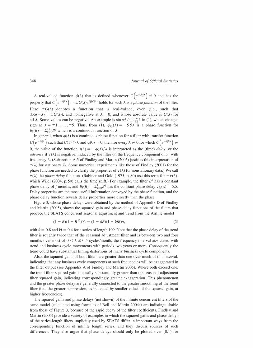
For the Shipments series, the quarterly-effect frequency, four cycles/year, is the one

associated with the c2 coefficient because this frequency has the dominant spectral peak in

Figure 2. The c1 coefficient estimate is 0.9718, close to the twelfth root of the estimated

Airline model seasonal coefficient Q (ffiffiffiffiffiffiffiffiffiffiffiffiffiffi0:666712

p¼ 0:9668). However, the c2 coefficient

estimate is 0.8086 (¼ffiffiffiffiffiffiffiffiffiffiffiffiffiffi0:078112

p). This smaller value results in the concurrent squared gains

of the 5-1 (3) model in Figure 6 having wider troughs at the four cycles/year frequency

than the Airline model’s filters and similarly for the squared gains of the symmetric filter

(see Findley, McElroy, and Wills 2005). The wider troughs indicate more suppression of

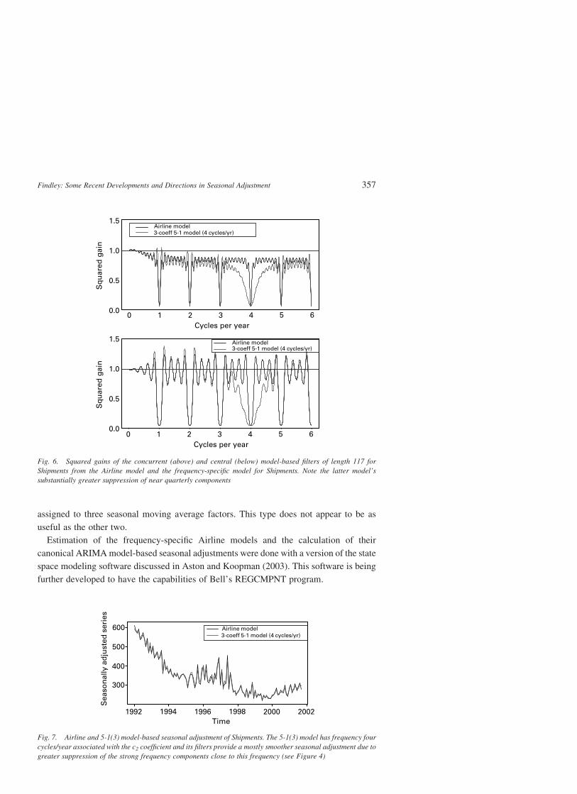
variability around this quarterly frequency. As a result, for this series, the canonical

seasonal adjustment of the 5-1(3) model is generally smoother than that of the Airline

(see Figure 7).

There are six 5-1(3) models corresponding to the available choices of season frequency

factors for c2: Analogously, there are fifteen so-called 4-2(3) models in which c2 is

assigned to two seasonal frequency factors and c1 to the other four. Aston et al. (2004) find

this to be type of three-coefficient models most frequently preferred over the Airline model

by their generalization of Akaike’s AIC that seeks to account for the increase in

uncertainty in selecting among numerous frequency-specific models and the Airline

model. Finally, there are twenty so-called 3-3(3) models in which the c1 and c2 are each


assigned to three seasonal moving average factors. This type does not appear to be as

useful as the other two.

Estimation of the frequency-specific Airline models and the calculation of their

canonical ARIMAmodel-based seasonal adjustments were done with a version of the state

space modeling software discussed in Aston and Koopman (2003). This software is being

further developed to have the capabilities of Bell’s REGCMPNT program.

0 1 2 3 4 5 60.0

0.5

1.0

1.5

0.0

0.5

1.0

1.5

Cycles per year

0 1 2 3 4 5 6Cycles per year

Sq

uar

ed g

ain

Airline model3-coeff 5-1 model (4 cycles/yr)

Sq

uar

ed g

ain

Airline model3-coeff 5-1 model (4 cycles/yr)

Fig. 6. Squared gains of the concurrent (above) and central (below) model-based filters of length 117 for

Shipments from the Airline model and the frequency-specific model for Shipments. Note the latter model’s

substantially greater suppression of near quarterly components

Time

Sea

son

ally

ad

just

ed s

erie

s

1992 1994 1996 1998 2000 2002

300

400

500

600 Airline model3-coeff 5-1 model (4 cycles/yr)

Fig. 7. Airline and 5-1(3) model-based seasonal adjustment of Shipments. The 5-1(3) model has frequency four

cycles/year associated with the c2 coefficient and its filters provide a mostly smoother seasonal adjustment due to

greater suppression of the strong frequency components close to this frequency (see Figure 4)


5.4. Wildi’s ZPC-QMP filters

The monograph by Wildi (2004) provides a radically different approach to model-based

trend estimation (and, secondarily, seasonal adjustment) which is very stimulating, also

because some new and substantial auxiliary theoretical results on frequency domain

techniques for nonstationary series are obtained. It can be argued that the long-run

behavior of any “true” ARIMA process (meaning cases like the Airline model (2) with

u ¼ 1 or Q ¼ 1 are excluded) is unlike that of any persistently seasonal economic time

series because each calendar month’s seasonal factors will change direction over time, but

Wildi emphasizes how especially ill-suited such models seem to be for the long index

series he considers, whose values are constrained to satisfy 2100 # Yt # 100: He

proposes a new class of “zero-pole-combination quasi-minimum-phase” (abbreviated

ZPC-QMP) filters with ARMA transfer functions.

The case of primary interest in Wildi (2004) is that of one-sided ZPC-QMP filters for

concurrent trend estimates. Their seventeen parameters are estimated by minimizing a

frequency domain expression, calculated from the periodogram of the time series of

interest or its differences, which estimates the mean squared difference (or revision error)

between the concurrent filter’s output and the output of a prescribed symmetric trend filter

for the given series. Constraints on the magnitude of the phase-delay (or time-shift) of the

filter can also be imposed on the estimation criterion.

If the prescribed symmetric filter is appropriate, this would seem to be more application-

appropriate criterion than maximum likelihood estimation of an ARIMA model, which is

related to minimizing the model’s mean squared one-step-ahead forecast error of the

original seasonal time series. Estimation of Wildi’s filters turns out too often to be difficult

and delicate, but for the set of series he considers, they generally yield better trends,

e.g., for turning point estimation, than the maximum likelihood based trend estimates he

investigates.

Wildi’s approach seems quite impractical for statistical offices with a large number of

time series, or with short series, but it may give indications of important limitations of

current methods and indications of how some new methods that will be useful for

statistical offices could be found.

6. Recent Developments for X-11 Filter Seasonal Adjustments

Here we call attention to two noteworthy recent research directions related to seasonal

adjustments from X-11 filters.

6.1. Shrinkage methods for X-11 seasonal factors

We start with the discussion paper of Miller and Williams (2004), which summarizes a

study of the application to X-11 seasonal factors of a “global” and a “local” shrinkage

procedure developed by the authors. It shows, through a forecasting study with a large test

set of series frequently used by academic forecasters, that the shrinkage methods lead to

seasonal adjustments from which better forecasts are obtained from certain methods that

forecast seasonal time series by (i) seasonally adjusting, (ii) forecasting the seasonally

adjusted series, and (iii) reseasonalizing these forecasts.


Findley, Wills, and Monsell (2004) investigate whether seasonal adjustment after

application of the shrinkage methods to the seasonal factors improves some of the X-12-

ARIMA Q2, M7, M8, M10, and M11 quality statistics (see Ladiray and Quenneville

2001). They find that the “local” shrinkage method of Miller and Williams, whose

statistical motivation is less clear than that of their “global” method, increases the number

of multiplicatively seasonal series with acceptable values of these statistics (defined for

this study as being any value less than 1.10) from a little over 200 to almost 250.

The shrinkage smoothes the evolution from year to year of the seasonal factors for many of

the calendar months. However, for the few series examined in detail, the resulting

seasonally adjusted series had seasonal peaks in their spectra that did not occur without

shrinkage. This suggests that shrinkage of the seasonal factor by this method often leads to

residual seasonality, a significant problem for official seasonal adjusters if not for

forecasters. The global shrinkage method provided no useful improvement to the set of

diagnostics. Thus, it remains to be seen whether shrinkage methods can be used to improve

X-11 filter-based seasonal adjustments in a way that is useful to producers of official

statistics.

6.2. Uncertainty measures

The second research direction of note is the development of methods to provide standard

errors for X-11 filter based seasonal adjustments, statistics that have always been available

for model-based method adjustments but not for X-11 adjustments. We are referring to the

method of Pfeffermann (1994) and its further development described in Scott, Sverchkov,

and Pfeffermann (2004) and to the quite different method of Bell and Kramer (1999).

These methods can take account of sampling error in the data through the use of time series

models of the sampling error like the model of Subsection 5.1.1 and the models of Nguyen,

Bell, and Gomish (2002) and Scott et al. (2004).

The Pfeffermann approach described in Scott et al. (2004) accounts for time series

uncertainty beyond sampling error, which the Bell and Kramer approach does not, by

modeling the irregular component of the unobserved sampling-error-free series with a

moving average model of order 0 # q # 3; assuming at least one such model can be found

that is not incompatible with the sampling-error autocovariances and the autocovariances

of the X-11 irregulars.

Going beyond uncertainty due to sampling error, the approach of Bell and Kramer

(1999) extends the approach of Wolter and Monsour (1981) to address uncertainty

associated with ARIMA forecast extension before application of X-11 filters in a way that

the Pfeffermann approach does not. When sampling error is negligible or not modeled, the

Bell and Kramer mean squared errors are estimates of the square of the seasonal

adjustment revisions that will occur when future data become available, to make possible

the application of more symmetric filters. Such revision estimates (and the standard error

estimates mentioned previously and also those of ARIMAmodel-based procedures) do not

account for the effect of revisions to the unadjusted data, for example revisions due to late

reporting or benchmarking.

As an alternative or complement to the procedures mentioned above, simple descriptive

statistics calculated from several years of published revisions over time to originally


published adjusted values have several useful properties. (1) They reflect the effects of

revisions to the unadjusted data as well as the effects of applying different asymmetric

filters. (2) They describe an intelligible basic type of empirical uncertainty, namely the

kinds of changes a data user will see over time. (3) They have the very important property

that they can be provided for indirectly seasonally adjusted series, e.g., sums of seasonally

adjustment component series. (Univariate time series model-based methods like that of

SEATS cannot provide plausible standard errors for indirect adjustments, nor can the

univariate methods of Pfeffermann and Bell and Kramer.) Finally, (4) they are technically

easy to produce (after the historical data are assembled).

Of course, such descriptive statistics suffer from two fundamental limitations that must

be made clear to users: they ignore both the uncertainty due to sampling error (which is

small in many high level aggregates) and the uncertainty due to the signal extraction error

that remains even when enough future data become available that further revisions are

negligible. For these reasons, they cannot be used to establish the statistical significance

of, say, an increase in the seasonally adjusted series from one month to the next. (But the

value of such significance tests is debatable for several reasons. For example, it has been

noted that the null hypothesis of no change is seldom plausible for economic time series.

See Smith 1978 for other inadequacies.) With these limitations, empirical revision

statistics may provide useful indications of basic uncertainty for seasonal adjustments

where currently none are provided, and, in the case of indirectly adjusted aggregates,

where more satisfactory measures have yet to be established.

Some branches of the U.S. Census Bureau are undertaking the preparations necessary to

enable production of robust descriptive statistics on an ongoing basis for the revisions of

some of their published (direct and indirect) seasonal adjustments or seasonally adjusted

month-to-month changes. This is being done in a spirit of experimentation to investigate

how such statistics could be used by consumers of seasonally adjusted data.

7. Some Concluding Remarks

Most of this article has been related to model-based seasonal adjustment of one kind or

another. This is a relatively young area in which there is much interest because of the

seeming simplicity and the analyzability of models and also because some of the progress

of model development in other areas of statistics (e.g., Bayesian methods) can be expected

to stimulate progress in model-based seasonal adjustment. This is therefore the area of

seasonal adjustment in which the most significant progress can be expected to occur in the

next years, in the development of better direct or indirect diagnostics for model

inadequacies, in the development and use of new models and new model fitting criteria,

and also in more effective uses of existing model types. For example, for the problem of

data spans too long for modeling with a single model or coefficient vector, the approach of

BAYSEA (Akaike 1980) could be explored. This involves estimating a model of specified

type or sometimes a set of models (see Akaike and Ishiguro 1983) over a shorter data

window which is advanced by steps of length one year through the available data. It can

also involve a method of averaging the results from different windows or different models

like that illustrated in Section 6 of Akaike and Ishiguro (1983). The Australian Bureau of


Statistics is investigating a somewhat analogous approach to estimating time-varying

trading-day effects.

Finally, the important issue of staff training for model-based seasonal adjustment must

be mentioned. The greater variety of seasonal adjustment filters available from SEATS

than from X-12-ARIMA can lead to worse results from an inadequately trained user of the

software who makes poor option choices and does not recognize this fact. (It is not enough

to check that the p-value of a model’s Ljung-Box statistic at lag 24 is greater than 0.05. For

example, models that omit significant trading day and outlier effects can have this

property.) The X-13A-S program is an important development, not only because of its

stronger suite of diagnostics but also because the user can always compare a SEATS

adjustment with an X-11 adjustment. Conversely, with this software a user of the X-12-

ARIMA approach can gradually become familiar with the alternatives made available by

model-based adjustment. Thus X-13A-S will be an important training tool, but inadequate

by itself. We expect that statistical agencies and central banks who wish to make broad use

of model-based seasonal adjustments will find it necessary to make a considerable

and sustained effort, even more than with X-12-ARIMA, to insure that enough

sufficiently trained staff is available to maintain adjustment quality when already trained

staff moves on.

Appendix: Differences between the Automatic Modeling Procedure of X-13A-S

and TRAMO

The most important automatic regARIMA model selection procedure differences from

TRAMO are that X-13A-S uses: (1) exact maximum likelihood coefficient estimates

where TRAMO uses Hannan-Risannen estimates or approximate maximum likelihood

estimates; (2) larger critical values for inclusion of outlier regressors (based on theoretical

results of Ljung 1993); (3) a theoretical value derived in Findley et al. (1998) rather than

an estimated coefficient for the length-of-month/leap-year effect component of

multiplicative trading-day models; (4) candidate intervals of lengths 1, 8, and 15 for the

Easter effect regressor instead of an interval of length 6. Also, (5) Akaike’s AIC is used

instead of individual coefficient t-statistics for inclusion of trading day and holiday

regressors.

McDonald-Johnson and Hood (2001) investigate the automatic outlier procedure of

X-13A-S (and X-12-ARIMA) and consider the effects of lower critical values like those

used by TRAMO but find them disadvantageous more often than they are advantageous.

McDonald-Johnson, Nguyen, Hood, and Monsell (2002) study other aspects of the

automatic regARIMA modeling procedure and discuss differences from TRAMO’s

procedure. The results of these and other unpublished studies done at the U.S. Census

Bureau mildly favor the automatic transformation and trading day and holiday effect

decision procedures of X-13A-S and show that TRAMO selects differencings and seasonal

differencings slightly more often than X-13A-S, whereas X-13A-S has a mild tendency to

choose ARIMA models with more coefficients. Some improvements have been made

recently to the way in which X-13A-S decides on differencing operators but a large-scale

study to see if the decisions are now the same as TRAMO’s more often has not yet been

done.


8. References

Akaike, H. (1980). Seasonal Adjustment by a Bayesian Modeling. Journal of Time Series

Analysis, 1, 1–14.

Akaike, H. and Ishiguro, M. (1983). Comparative Study of the X-11 and BAYSEA

Procedures of Seasonal Adjustment. In Applied Time Series Analysis of Economic

Data, A.Zellner (ed.). Economic Research Report ER-5, Washington: U.S. Department

of Commerce, U.S. Bureau of the Census, 17–50 Also http://www.census.gov/ts/

papers/Conference1983/AkaikeIshiguro1983.pdf

Ansley, C.F. and Newbold, P. (1981). On the Bias in Estimates of Forecast Mean Squared

Error. Journal of the American Statistical Association, 76, 569–576.

Aston, J.A., Findley, D.F., Wills, K.C., and Martin, D.E.K. (2004). Generalizations of the

Box-Jenkins’ Airline Model with Frequency-Specific Seasonal Coefficients and a

Generalization of Akaike’s MAIC. Proceedings of the 2004 NBER/NSF Time Series

Conference. [CD-ROM]. Also http://www.census.gov/ts/papers/findleynber2004.pdf

Aston, J.A.D. and Koopman, S.J. (2003). An Implementation of Component Models for

Seasonal Adjustment Using the SsfPack Software Module of Ox. Proceedings of the

13th Federal Forecasters Conference, 64–71. Also, http://www.va.gov/vhareorg/ffc/

PandP/FFC2003.pdf

Bell, W.R. (1983). A Computer Program for Detecting Outliers in Time Series.

Proceedings of the American Statistical Association, Business and Economic Statistics

Section, 634–639.

Bell, W.R. (2004). On RegComponent Time Series Models and Their Applications. In

State Space and Unobserved Component Models, A.Harvey, S.J.Koopman, and

N.Shephard (eds). Cambridge: Cambridge University Press. Also http://www.census.

gov/ts/regcmpnt/pc/.

Bell, W.R. and Hillmer, S.C. (1983). Modeling Time Series with Calendar Variation.

Journal of the American Statistical Association, 78, 526–534.

Bell, W.R. and Hillmer, S.C. (1988). A Matrix Approach to Likelihood Evaluation and

Signal Extraction for ARIMA Component Time Series Models. U.S. Bureau of the

Census, Statistical Research Division Report Number: Census/SRD/RR-88/22.

Also http://www.census.gov/srd/papers/pdf/rr88-22.pdf

Bell, W.R. and Kramer, M. (1999). Toward Variances for X-12-ARIMA Seasonal

Adjustments. Survey Methodology, 25, 13–29.

Bell, W.R. and Martin, D.E.K. (2004a). Computation of Asymmetric Signal Extraction

Filters and Mean Squared Error for ARIMA Component Models. Journal of Time Series

Analysis, 25, 603–625.

Bell, W.R. and Martin, D.E.K. (2004b). Modeling Time-Varying Trading Day Effects in

Monthly Time Series. Proceedings of the American Statistical Association: Alexandria,

VA [CD-ROM]. Also http://www.census.gov/ts/papers/jsm2004dem.pdf

Caporello, G. and Maravall, A. (2004). Program TSW. Revised Manual Version May

2004. Documentos Occasionales N8 0408, Madrid: Banco de Espana.

Dagum, E.B. (1980). The X-11-ARIMA Seasonal Adjustment Method, Catalogue No.

12-564E, Ottawa: Statistics Canada.


Feldpausch, R.M. (2003). Instructions for Installation and Use of the Windowse Interface

to X-12-ARIMA. http://www.census.gov/ts/TSMS/WIX12/winx12i.zip

Feldpausch, R.M., Hood, C.C., and Wills, K.C. (2004). Diagnostics for Model-Based

Seasonal Adjustment. Proceedings of the American Statistical Association: Alexandria,

VA [CD-ROM]. Also http://www.census.gov/ts/papers/jsm2004rmf.pdf

Findley, D.F. (2001). Discussion of Session 14: Trend Estimation. Proceedings of the

Second International Conference on Establishment Surveys. Alexandria: American

Statistical Association, 809–812.

Findley, D.F. (2005). Asymptotic Second Moment Properties of Out-of-Sample Forecast

Errors of Misspecified RegARIMA Models and the Optimality of GLS. Statistica

Sinica, 15, 447–476.

Findley, D.F. and Hood, C.C. (2000). X-12-ARIMA and Its Application to Some Italian

Indicator Series. Seasonal Adjustment Procedures – Experiences and Perspectives.

Annali di Statistica, Serie X, n. 20. Rome: Istituto Nazionali di Statistica, 231–251 Also

http://www.census.gov/ts/papers/x12istat.pdf.

Findley, D.F. and Martin, D.E.K. (2005). Frequency Domain Diagnostics of SEATS and

X-11/12-ARIMA Seasonal Adjustment Filters for Short and Moderate-Length Time

Series. (Forthcoming)

Findley, D.F., McElroy, T.S. and Wills, K.C. (2005). Modifications of SEATS’ Diagnostic

for Detecting Over- and Underestimation of Seasonal Adjustment Components

(Forthcoming). Also http://www.census.gov/ts/papers/findleymcelroywills2005.pdf

Findley, D., Monsell, B., Shulman, H., and Pugh, M. (1990). Sliding Spans Diagnostics for

Seasonal and Related Adjustments. Journal of the American Statistical Association, 85,

345–355. Also http://www.census.gov/srd/papers/pdf/rr86-18.pdf

Findley, D.F., Monsell, B.C., Bell, W.R., Otto, M.C., and Chen, B.C. (1998).

New Capabilities and Methods of the X-12-ARIMA Seasonal Adjustment Program.

Journal of Business and Economic Statistics, 16, 127–177 (with Discussion). Also

http://www.census.gov/ts/papers/jbes98.pdf

Findley, D.F. and Soukup, R.J. (2000). Modeling and Model Selection for Moving

Holidays Proceedings of the American Statistical Association, Section of the Business

and Economic Statistics. Alexandria: American Statistical Association Alexandria,

102–107. Also http://www.census.gov/ts/papers/asa00_eas.pdf.

Findley, D.F., Wills, K.C., Aston, J.A., Feldpausch, R.M., and Hood, C.C. (2003).

Diagnostics for ARIMA-Model-Based Seasonal Adjustment. Proceedings of the

American Statistical Association, Alexandria: American Statistical Association,

1459–1466 [CD-ROM]. Also http://www.census.gov/ts/papers/jsm2003dff.pdf

Findley, D.F., Wills, K.C., and Monsell, B.C. (2004). Seasonal Adjustment Perspectives

on “Damping Seasonal Factors: Shrinkage Estimators for the X-12-ARIMA Program.”

International Journal of Forecasting, 20, 551–556.

Gomez, V. and Maravall, A. (2000). Automatic Modeling Methods for Univariate Time

Series. In A Course in Time Series, R.S. Tsay, D. Pena, and G.C. Tiao (eds). New York:

John Wiley, 171–201.

Harvey, A.C. (1989). Forecasting, Structural Time Series Models, and the Kalman filter.

Cambridge: Cambridge University Press


Hood, C.C. (2002). Comparison of Time Series Characteristics for Seasonal Adjustments

from SEATS and X-12-ARIMA. Proceedings of the American Statistical Association.

Alexandria: American Statistical Association, 1485–1489 [CD-ROM]. Also http://

www.census.gov/ts/papers/choodasa2002.pdf.

Kaiser, R. and Maravall, A. (2003). Seasonal Outliers in Time Series, Estadıstica. Journal

of the Inter-American Statistical Institute, 53, 101–142.

Ladiray, D. and Quenneville, B. (2001). Seasonal Adjustment with the X-11 Method.

Lecture Notes in Statistics, No. 158. New York: Springer Verlag.

Ljung, G.M. (1993). On Outlier Detection in Time Series. Journal of the Royal Statistical

Society, Series B, 55, 559–567.

Lin, J.-L. and Liu, T.-S. (2003). Modeling Lunar Calendar Holiday Effects in Taiwan.

Taiwan Economic Policy and Forecast, 33, 1–37. Also http://www.census.gov/ts/

papers/lunar.pdf.

Maravall, A. (2002). An Application of TRAMO-SEATS: Automatic Procedure and

Sectoral Aggregation. Banco de Espana–Sevicio de Estudios, Documents de Trabajo

No. 0207. Also http://www.bde.es/informes/be/docs/dt0207e.pdf.

Maravall, A. (2003). A Class of Diagnostics in the ARIMA-Model-Based Decomposition

of a Time Series. Memorandum, Bank of Spain.

Maravall, A. and Sanchez, F.J. (2001). An Application of TRAMO-SEATS: Model

Selection and Out-of-Sample Performance. The Swiss CPI Series, Banco de Espana–

Sevicio de Estudios. Documents de Trabajo No. 0014. Also http://www.bde.es/

informes/be/docs/dt0014.pdf

McDonald-Johnson, K.M. and Hood, C.C. (2001). Outlier Selection for RegARIMA

Modeling. Proceedings of the American Statistical Association, Section of Business and

Economic Statistics. [CD-ROM Paper No. 00438]. Alexandria: American Statistical

Associaton. Also http://www.census.gov/ts/papers/asa2001kmm.pdf

McDonald-Johnson, K.M., Nguyen, T.T.T., Hood, C.C., and Monsell, B.C. (2002).

Improving the Automatic RegARIMA Model Selection Procedure of X-12-ARIMA

v0.3. Proceedings of the American Statistical Association, Section of Business and

Economic Statistics. Alexandria: American Statistical Association, 2304–2309. [CD-

ROM] Also http://www.census.gov/ts/papers/asa2002kmm.pdf

McElroy, T.S. and Sutcliffe, A. (2005). An Iterated Parametric Approach to Nonstationary

Signal Extraction. Computational Statistics and Data Analysis (Forthcoming).

Expanded version: http://www.census.gov/srd/papers/pdf/rrs2004-05.pdf

Miller, D.M. and Williams, D. (2004). Damping Seasonal Factors: Shrinkage Estimators

for the X-12-ARIMA Program. International Journal of Forecasting, 20, 529–549.

Monsell, B.C. (2001). GenHol Program and Instructions, genhol.exe and genhol.txt from

http://www.census.gov/srd/www/x12a/x12down_pc.html#x12other

Monsell, B.C. (2002). An Update on the Development of the X-12-ARIMA Seasonal

Adjustment Program. Proceedings of the 3rd International Symposium on Frontiers of

Time Series Analysis. Tokyo: Institute of Statistical Mathematics, 1–11.

Monsell, B., Aston, J., and Koopman, S. (2003). Toward X-13? Proceedings of the

American Statistical Association. Alexandria: American Statistical Association,

2870–2877. [CD-ROM]. Also, http://www.census.gov/ts/papers/jsm2003bcm.pdf.


Nguyen, T.T.T., Bell, W.R., and Gomish, J.M. (2002). Investigating Model-Based Time

Series Methods to Improve Estimates fromMonthly Value of Construction Put-in-Place

Surveys. Proceedings of the American Statistical Association, Section on Survey

Research Methods. Alexandria, VA: American Statistical Association, 2470–2475.

[CD-ROM]

Pfeffermann, D. (1994). A General Method for Estimating the Variances of X-11

Seasonally Adjusted Estimators. Journal of Time Series Analysis, 15, 85–116.

Proietti, T. (2004). Seasonal Specific Structural Time Series. Studies in Nonlinear

Dynamics and Econometrics, 8(2), Article 16. http://www.bepress.com/snde/vol8/iss2/

art16.

Rabiner, L.R. and Gold, B. (1975). Theory and Application of Digital Signal Processing.

Englewood Cliffs: Prentice Hall.

Scott, S., Sverchkov, M., and Pfeffermann, D. (2004). Variance Measures for Seasonally

Adjusted Employment and Employment Change. Proceedings of the American

Statistical Association. Alexandria: American Statistical Association [CD-ROM].

Smith, T.F.M. (1978). Principles and Problems in the Analysis of Repeated Surveys. In

Survey Sampling and Measurement, N.K. Namboodiri (ed.). New York: Academic

Press.

Soukup, R.J. and Findley, D.F. (1999). On the Spectrum Diagnostics Used by X 12

ARIMA to Indicate the Presence of Trading Day Effects after Modeling or Adjustment.

Proceedings of the American Statistical Association, Section on Business and

Economic Statistics. Alexandria, 144–149. Also http://www.census.gov/ts/papers/

rr9903s.pdf

Soukup, R.J. and Findley, D.F. (2001). Detection and Modeling of Trading Day Effects.

Proceedings of the Second International Conference on Establishment Surveys.:

American Statistical Association Alexandria, 743–753. Also http://www.census.gov/

ts/papers/ices00_td2.pdf.

Trimbur, T.M. (2005). Seasonal Heteroskedasticity and Trend Estimation in Monthly

Time Series. Proceedings of the American Statistical Association. Alexandria:

American Statistical Association [CD-ROM].

Wildi, M. (2004). Signal Extraction, Efficient Estimation, Unit Roots and Early Detection

of Turning Points. Lecture Notes in Economics and Mathematical Systems, Vol. 547.

Berlin: Springer.

Wolter, K.M. and Monsour, N.J. (1981). On the Problem of Variance Estimation for a

Deseasonalized Series. In Current Topics in Survey Sampling, D. Krewski, R. Platek,

and J.N.K. Rao (eds). New York: Academic Press, 199–226.

Zhang, X., McClaren, C.H., and Leung, C.C.S. (2003). An Easter Proximity Effect:

Modelling and Adjustment. Australian and New Zealand Journal of Statistics, 43,

269–280.

Received April 2005

Revised July 2005


Some Recent Developments and Directions in Seasonal Adjustment

Documents

Transcript of Some Recent Developments and Directions in Seasonal Adjustment