arX

iv:h

ep-t

h/02

0101

7v3

24

Sep

2009

VPI–IPPAP–01–06

The Effect of the Minimal Length Uncertainty Relation on the

Density of States and the Cosmological Constant Problem

Lay Nam Chang∗, Djordje Minic†, Naotoshi Okamura‡, and Tatsu Takeuchi§

Institute for Particle Physics and Astrophysics,

Physics Department, Virginia Tech, Blacksburg, VA 24061

(Dated: December 31, 2001; Revised: March 15, 2001; 2nd revision: September 24, 2009)

Abstract

We investigate the effect of the minimal length uncertainty relation, motivated by perturbative

string theory, on the density of states in momentum space. The relation is implemented through the

modified commutation relation [xi, pj ] = ih[(1 + βp2)δij + β′pipj]. We point out that this relation,

which is an example of an UV/IR relation, implies the finiteness of the cosmological constant.

While our result does not solve the cosmological constant problem, it does shed new light on the

relation between this outstanding problem and UV/IR correspondence. We also point out that the

blackbody radiation spectrum will be modified at higher frequencies, but the effect is too small to

be observed in the cosmic microwave background spectrum.

PACS numbers: 02.40.Gh,03.65.Sq,98.70.Vc,98.80.Es

∗ electronic address: laynam@vt.edu† electronic address: dminic@vt.edu‡ electronic address: nokamura@vt.edu§ electronic address: takeuchi@vt.edu

1

I. INTRODUCTION

In this paper, we continue our investigation [1] of the consequences of the commutation

relation

[x, p] = ih(1 + βp2) , (1)

which leads to the minimal length uncertainty relation

∆x ≥ h

2

(

1

∆p+ β ∆p

)

. (2)

As reviewed in Ref. [1], Eq. (2) has appeared in the context of perturbative string theory

[2] where it is implicit in the fact that strings cannot probe distances below the string scale

h√

β. It should be noted that the precise theoretical framework for such a minimal length

uncertainty relation is not understood in string theory. In particular, it is not clear whether

Eq. (1) represents the correct quantum mechanical implementation of Eq. (2). Indeed,

Kempf has shown that the commutation relation which implies the existence of a minimal

length is not unique [3].

Furthermore, Eq. (2) does not seem to be universally valid. For example, both in the

realms of perturbative and non-perturbative string theory (where distances shorter than

string scale can be probed by D-branes [4]), another type of uncertainty relation involving

both spatial and time coordinates has been found to hold [5]. The distinction (and relation)

between the minimal length uncertainty relation and the space-time uncertainty relation has

been clearly emphasized by Yoneya [6].

Notwithstanding these caveats, the minimum length uncertainty formula does exhibit the

basic features of UV/IR correspondence: when ∆p is large, ∆x is proportional to ∆p, a fact

which seems counterintuitive from the point of view of local quantum field theory. As is

well known, this kind of UV/IR correspondence has been previously encountered in various

contexts: the AdS/CFT correspondence [7], non-commutative field theory [8], and more

recently in the attempts to understand quantum gravity in asymptotically de Sitter spaces

[9, 10].

Moreover, it has been argued by various authors [11] that the UV/IR correspondence,

described by Eq. (2), is relevant for the understanding of the cosmological constant problem

[12]. Likewise, it has been suggested in the literature that some kind of UV/IR relation

is necessary to understand observable implications of short distance physics on inflationary

2

cosmology [3, 13].

In this paper we ask the question whether the cosmological constant problem could be

understood by utilizing a concrete UV/IR relation, such as Eq. (1). In particular, we study

the implication of the commutation relation on the effective density of states in the vacuum

and consequently on the cosmological constant problem. We point out that the commu-

tation relation implies the finiteness of the cosmological constant and the modification of

the blackbody radiation spectrum. While we do not present a solution to the cosmological

constant problem, our results offer a new perspective from which this outstanding problem

may be addressed.

II. THE CLASSICAL LIMIT AND THE LIOUVILLE THEOREM

The observation we would like to make is that the right hand side of Eq. (1) can be

considered to define an ‘effective’ value of h which is p-dependent. This means that the size

of the unit cell that each quantum state occupies in phase space can be thought of as being

also p-dependent. This will change the p-dependence of the density of states and affect the

calculation of the cosmological constant, the blackbody radiation spectrum, etc. [14]. For

this interpretation to make sense, we must first check that any volume of phase space evolves

in such a way that the number of states inside does not change with time. What we are

looking for here is the analog of the Liouville theorem. To place the discussion in a general

context, we begin by extending Eq. (1) to higher dimensions.

In D-dimensions, Eq. (1) is extended to the tensorial form [15] :

[xi, pj] = ih(δij + βp2δij + β ′pipj) . (3)

If the components of the momentum pi are assumed to commute with each other,

[pi, pj] = 0 , (4)

then the commutation relations among the coordinates xi are almost uniquely determined

by the Jacobi Identity (up to possible extensions) as

[xi, xj ] = ih(2β − β ′) + (2β + β ′)βp2

(1 + βp2)(pixj − pjxi) . (5)

3

Let us take a look at what happens in the classical limit. Recall that the quantum

mechanical commutator corresponds to the Poisson bracket in classical mechanics via

1

ih[A, B] =⇒ {A, B} . (6)

So the classical limits of Eqs. (3)–(5) read

{xi, pj} = (1 + βp2)δij + β ′pipj ,

{pi, pj} = 0 ,

{xi, xj} =(2β − β ′) + (2β + β ′)βp2

(1 + βp2)(pixj − pjxi) . (7)

The time evolutions of the coordinates and momenta are governed by

xi = {xi, H} = {xi, pj}∂H

∂pj+ {xi, xj}

∂H

∂xj,

pi = {pi, H} = −{xj , pi}∂H

∂xj. (8)

The analog of the Liouville theorem in this case states that the weighted phase space volume

dDx dDp[

1 + βp2]D−1[

1 + (β + β ′)p2]

(9)

is invariant under time evolution. To see this, consider an infinitesimal time interval δt. The

evolution of the coordinates and momenta during δt are

x′i = xi + δxi ,

p′i = pi + δpi , (10)

with

δxi =

[

{xi, pj}∂H

∂pj+ {xi, xj}

∂H

∂xj

]

δt ,

δpi =

[

−{xj , pi}∂H

∂xj

]

δt . (11)

An infinitesimal phase space volume after this infinitesimal evolution is

dDx′ dDp′ =

∣

∣

∣

∣

∣

∂(x′1, · · · , x′

D, p′1, · · · , p′D)

∂(x1, · · · , xD, p1, · · · , pD)

∣

∣

∣

∣

∣

dDx dDp . (12)

Since∂x′

i∂xj

= δij + ∂δxi∂xj

,∂x′

i∂pj

= ∂δxi∂pj

,

∂p′i∂xj

= ∂δpi∂xj

,∂p′i∂pj

= δij + ∂δpi∂pj

,(13)

4

the Jacobian to first order in δt is∣

∣

∣

∣

∣

∂(x′1, · · · , x′

D, p′1, · · · , p′D)

∂(x1, · · · , xD, p1, · · · , pD)

∣

∣

∣

∣

∣

= 1 +

(

∂δxi

∂xi+

∂δpi

∂pi

)

+ · · · . (14)

We find(

∂δxi

∂xi+

∂δpi

∂pi

)

1

δt

=∂

∂xi

[

{xi, pj}∂H

∂pj+ {xi, xj}

∂H

∂xj

]

− ∂

∂pi

[

{xj , pi}∂H

∂xj

]

=

[

∂

∂xi

{xi, pj}]

∂H

∂pj

+ {xi, pj}∂2H

∂xi∂pj

+

[

∂

∂xi

{xi, xj}]

∂H

∂xj

+{xi, xj}∂2H

∂xi∂xj−[

∂

∂pi{xj , pi}

]

∂H

∂xj− {xj , pi}

∂2H

∂pj∂xi

=

[

∂

∂xi{xi, xj}

]

∂H

∂xj−[

∂

∂pi{xj , pi}

]

∂H

∂xj

=

[

−(2β − β ′) + (2β + β ′)βp2

(1 + βp2)(D − 1) pj

]

∂H

∂xj

−[

{2β + (D + 1)β ′} pj

]

∂H

∂xj

= −[

2(D − 1)β

(

1 + (β + β ′)p2

1 + βp2

)

+ 2(β + β ′)

]

pj∂H

∂xj. (15)

Therefore, to first order in δt

dDx′ dDp′ = dDx dDp

[

1 −{

2(D − 1)β

(

1 + (β + β ′)p2

1 + βp2

)

+ 2(β + β ′)

}

pj∂H

∂xjδt

]

. (16)

On the other hand,

1 + βp′2

= 1 + β(pi + δpi)2

= 1 + β(

p2 + 2piδpi + · · ·)

= 1 + β

(

p2 − 2pi{xi, pj}∂H

∂xj

δt + · · ·)

= 1 + β

(

p2 − 2[

1 + (β + β ′)p2]

pj∂H

∂xjδt + · · ·

)

= (1 + βp2) − 2β[

1 + (β + β ′)p2]

pj∂H

∂xjδt + · · ·

= (1 + βp2)

[

1 − 2β

(

1 + (β + β ′)p2

1 + βp2

)

pj∂H

∂xjδt + · · ·

]

, (17)

and

1 + (β + β ′)p′2

= 1 + (β + β ′)(pi + δpi)2

= 1 + (β + β ′)(

p2 + 2piδpi + · · ·)

= 1 + (β + β ′)

(

p2 − 2pi{xi, pj}∂H

∂xjδt + · · ·

)

5

= 1 + (β + β ′)

(

p2 − 2[

1 + (β + β ′)p2]

pj∂H

∂xj

δt + · · ·)

=[

1 + (β + β ′)p2]

− 2(β + β ′)[

1 + (β + β ′)p2]

pj∂H

∂xjδt + · · ·

= [1 + (β + β ′)p2]

[

1 − 2(β + β ′)pj∂H

∂xjδt + · · ·

]

. (18)

Therefore, to first order in δt

[

1 + βp′2]−D+1[

1 + (β + β ′)p′2]−1

=[

1 + βp2]−D+1[

1 + (β + β ′)p2]−1

×[

1 +

{

2(D − 1)β

(

1 + (β + β ′)p2

1 + βp2

)

+ 2(β + β ′)

}

pj∂H

∂xjδt

]

. (19)

From Eqs. (16) and (19), we deduce that the weighted phase space volume Eq. (9) is invari-

ant. Note that in addition to the non-canonical Poisson brackets between the coordinates

and momenta, those among the coordinates themselves (and thus the non–commutative ge-

ometry of the problem) is crucial in arriving at this result. When β ′ = 0, Eq. (9) simplifies

todDx dDp

(1 + βp2)D. (20)

As a concrete example, consider the 1D harmonic oscillator with the Hamiltonian

H =p2

2µ+

1

2µω2x2 . (21)

The equations of motion are

x = {x, H} =1

µ(1 + βp2)p ,

p = {p, H} = −µω2(1 + βp2)x . (22)

These equations can be solved to yield

x(t) = xmax

√1 + ε

sin(√

1 + ε ωt)√

1 + ε sin2(√

1 + ε ωt),

p(t) = pmaxcos(

√1 + ε ωt)

√

1 + ε sin2(√

1 + ε ωt), (23)

where

ε = 2µEβ , xmax =

√

2E

µω2, pmax =

√

2µE . (24)

6

Note that the period of oscillation, T , is now energy (and thus amplitude) dependent:

T =2π

ω√

1 + ε. (25)

Now, consider the infinitesimal phase space volume sandwiched between the equal–energy

contours E and E + dE, and the equal–time contours t and t + dt. It is straightforward to

show that

dE dt =dx dp

1 + βp2. (26)

The left–hand side of this equation is time–independent by definition, so the right–hand side

must be also.

Finally, note that the semi–classical quantization (h → 0 limit) of the harmonic oscillator

is consistent with the full quantum mechanical result derived in our previous paper, Ref. [1].

III. DENSITY OF STATES

From this point on, we will only consider the β ′ = 0 case for the sake of simplicity.

Integrating over the coordinates, the invariant phase space volume Eq. (20) becomes

V dDp

(1 + βp2)D, (27)

where V is the coordinate space volume. This implies that upon quantization, the number

of quantum states per momentum space volume should be assumed to be

V

(2πh)D

dDp

(1 + βp2)D. (28)

Eq. (28) indicates that the density of states in momentum space must be modified by the

extra factor of (1 + βp2)−D. This factor effectively cuts off the integral beyond p = 1/√

β.

Indeed, in 3D the weight factor is1

(1 + βp2)3, (29)

the plot of which is shown in Fig. 1. We look at the consequence of this modification in

the calculation of the cosmological constant and the blackbody radiation spectrum in the

following.

7

log10(√

βp)-4 -2 2 4

0.2

0.4

0.6

0.8

1

FIG. 1: The behavior of the weight factor [1 + (√

βp)2]−3.

A. The Cosmological Constant

The cosmological constant is obtained by summing over the zero–point fluctuation ener-

gies of harmonic oscillators, each of which corresponds to a particular particle momentum

state [12]. If we assume that the zero–point energy of each oscillator is of the usual, canon-

ical, form1

2hω =

1

2

√

p2 + m2 , (30)

then, the sum over all momentum states per unit volume is (up to some prefactors)

Λ(m) =∫

d3p

(1 + βp2)3

[

1

2

√

p2 + m2

]

= 2π∫ ∞

0

p2dp

(1 + βp2)3

√

p2 + m2

=π

2β2f(βm2) , (31)

where

f(x) =

1 + x2(1 − x)

+ x2

4(1 − x)3/2 ln(

1 −√

1 − x1 +

√1 − x

)

(x ≤ 1) ,

1 − x2(x − 1)

+ x2

2(x − 1)3/2 tan−1√

x − 1 (x ≥ 1) .(32)

f(x) is a monotonically increasing function which behaves asymptotically as

f(x) ∼√

x , (33)

8

as can be gleaned from Eq. (31). In the region 0 ≤ x ≤ 1, it is well approximated by

f(x) ≈ (1 + x)0.42 . (34)

In the massless case we obtain

Λ(0) =π

2β2. (35)

As expected, due to the strong suppression of the density of states at high momenta, the

cosmological constant is rendered finite with 1/√

β acting effectively as the UV cutoff. This

result is in strong contrast to conventional calculations where the UV cutoff is an arbitrary

scale which must be introduced by hand, and where one must assume that the physics

beyond the cutoff does not contribute.

Unfortunately, since 1/√

β is the string mass scale, which we expect to be of the order

of the Planck mass Mp, this does not solve the cosmological constant problem. This is true

even if the Planck mass Mp were as low as a TeV as suggested in models with large extra

dimensions [16].

B. The Blackbody Radiation Spectrum

Taking into account the weight factor Eq. (29), the average energy in the EM field per

unit volume at temperature T is

E = 2∫ d3k

(2π)3[ 1 + β(hk)2 ]3hkc

ehkc/kBT − 1

=8π

c3

∫ ∞

0dν

1

[ 1 + β(hν/c)2 ]3

(

hν3

ehν/kBT − 1

)

≡∫ ∞

0dν uβ(ν, T ) . (36)

We see that the blackbody radiation spectrum is damped at high frequencies close to the

cutoff scale:

uβ(ν, T ) =1

[1 + (ν/νβ)2]3u0(ν, T ) , νβ ≡ c

h√

β. (37)

Here

u0(ν, T ) =8πhν3

c3

1

ehν/kBT − 1, (38)

is the regular spectral function.

9

To see the effect of this damping on the shape of the spectral function, we plot the

functions

f0(ν, T ) ≡ (ν/νβ)3

e(ν/νβ)(Tβ/T ) − 1,

fβ(ν, T ) ≡ 1

[1 + (ν/νβ)2]3f0(ν, T ) , (39)

for several values of the temperature T in Figs. 2 and 3. The temperature Tβ in the definition

of f0(ν, T ) is defined as

Tβ ≡ c

kB

√β

. (40)

As is evident from the figures, the distortion to the blackbody radiation is undetectable unless

the temperature is within a few orders of magnitude below Tβ. Given that the decoupling

temperature is on the order of an MeV [17], we do not expect the spectrum of the Cosmic

Microwave Background (CMB) to be affected in any observable way, even if 1/√

β were as

small as a TeV [16].

ν/νβ ν/νβ

T = Tβ T = 0.1Tβ

0.2 0.4 0.6 0.8 1

0.05

0.1

0.15

0.2

0.25

0.2 0.4 0.6 0.8 1

0.0002

0.0004

0.0006

0.0008

0.001

0.0012

0.0014

FIG. 2: The shape of the blackbody radiation spectrum with (solid line) and without (dashed line)

the damping factor [1 + (ν/νβ)2]−3 at temperatures T = Tβ (left) and T = 0.1Tβ (right).

IV. DISCUSSION

We have shown that Eq. (1) and its higher dimensional extensions imply that the density

of states is naturally suppressed in the ultraviolet. This suppression renders the cosmo-

logical constant finite, without affecting the blackbody radiation spectrum at observable

temperatures. The cosmological constant is still too large, however, since it is proportional

10

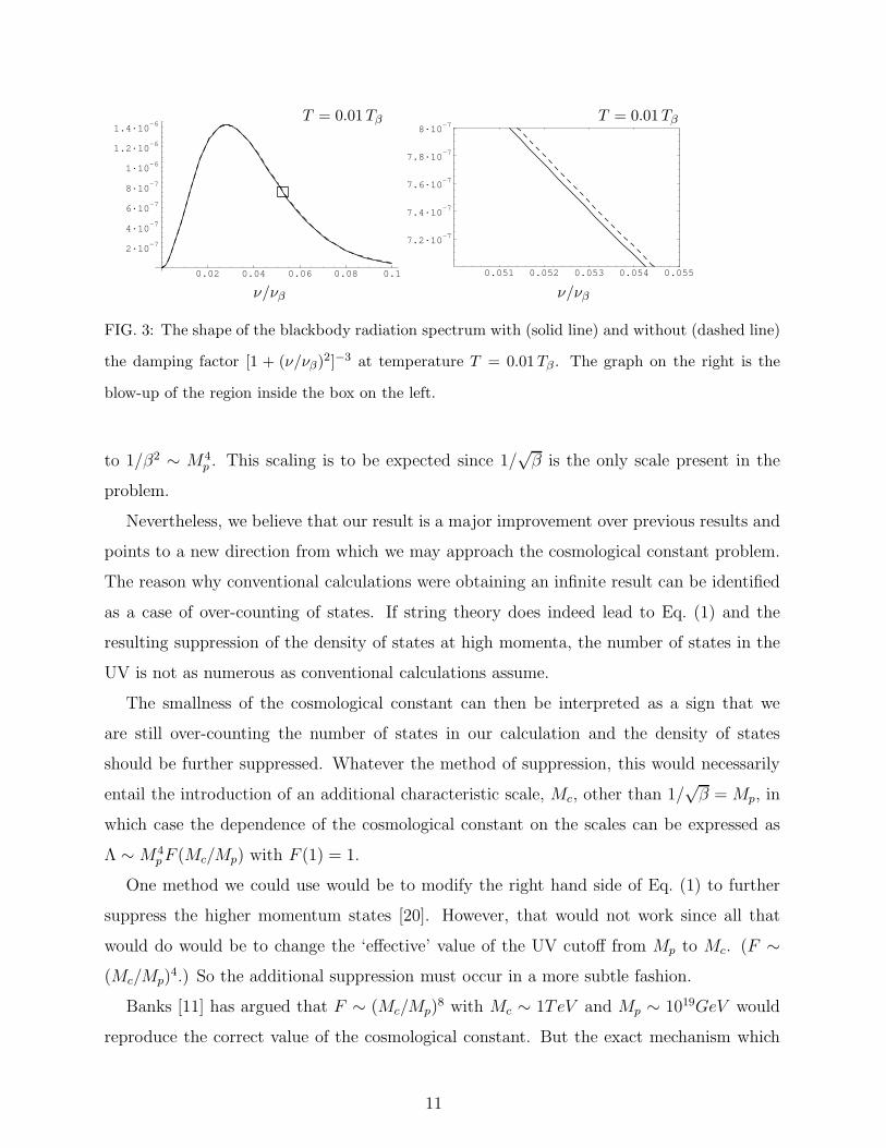
ν/νβ ν/νβ

T = 0.01Tβ T = 0.01Tβ

0.02 0.04 0.06 0.08 0.1

2·10-7

4·10-7

6·10-7

8·10-7

1·10-6

1.2·10-6

1.4·10-6

0.051 0.052 0.053 0.054 0.055

7.2·10-7

7.4·10-7

7.6·10-7

7.8·10-7

8·10-7

FIG. 3: The shape of the blackbody radiation spectrum with (solid line) and without (dashed line)

the damping factor [1 + (ν/νβ)2]−3 at temperature T = 0.01Tβ . The graph on the right is the

blow-up of the region inside the box on the left.

to 1/β2 ∼ M4p . This scaling is to be expected since 1/

√β is the only scale present in the

problem.

Nevertheless, we believe that our result is a major improvement over previous results and

points to a new direction from which we may approach the cosmological constant problem.

The reason why conventional calculations were obtaining an infinite result can be identified

as a case of over-counting of states. If string theory does indeed lead to Eq. (1) and the

resulting suppression of the density of states at high momenta, the number of states in the

UV is not as numerous as conventional calculations assume.

The smallness of the cosmological constant can then be interpreted as a sign that we

are still over-counting the number of states in our calculation and the density of states

should be further suppressed. Whatever the method of suppression, this would necessarily

entail the introduction of an additional characteristic scale, Mc, other than 1/√

β = Mp, in

which case the dependence of the cosmological constant on the scales can be expressed as

Λ ∼ M4p F (Mc/Mp) with F (1) = 1.

One method we could use would be to modify the right hand side of Eq. (1) to further

suppress the higher momentum states [20]. However, that would not work since all that

would do would be to change the ‘effective’ value of the UV cutoff from Mp to Mc. (F ∼(Mc/Mp)

4.) So the additional suppression must occur in a more subtle fashion.

Banks [11] has argued that F ∼ (Mc/Mp)8 with Mc ∼ 1TeV and Mp ∼ 1019GeV would

reproduce the correct value of the cosmological constant. But the exact mechanism which

11

would lead to such a form for F remains elusive. (See also Ref. [18] for a related discussion.)

At this point, we note that if string theory is the correct theory of gravity, modifying the

commutation relations alone would not properly take into account all of its potential effects.

It is possible that the holographic principle [19] could be of help here. Consideration of

holography in a cosmological background might naturally provide another scale other than

1/√

β, namely the size of the cosmological horizon, the Hubble radius H , related to the

cosmological constant as H2 ∼ 1/Λ. It is conceivable that due to the correct implementation

of the holographic principle in a cosmological situation, the number of fundamental degrees

of freedom contributing to the vacuum energy is determined by the density of states above

some very large momentum (which by the UV/IR correspondence (2) would be related to

the degrees of freedom at distances of the order of the cosmological horizon). If indeed the

density of states is strongly suppressed at high momenta, as argued in this paper, then the

effective number of degrees of freedom contributing to the vacuum energy density would be

very small. While these considerations are highly speculative, they seem to point to a new

promising way to approach the cosmological constant problem.

12

Acknowledgments

We would like to thank Vijay Balasubramanian, Per Berglund, Will Loinaz, Asad Naqvi,

Koenraad Schalm, Gary Shiu, Joseph Slawny, and Matthew Strassler for helpful discussions.

This research is supported in part by a grant from the US Department of Energy, DE–FG05–

92ER40709.

[1] L. N. Chang, D. Minic, N. Okamura and T. Takeuchi, Phys. Rev. D 65, 125027 (2002)

[arXiv:hep-th/0111181].

[2] D. J. Gross and P. F. Mende, Nucl. Phys. B 303, 407 (1988);

D. J. Gross and P. F. Mende, Phys. Lett. B 197, 129 (1987);

D. Amati, M. Ciafaloni and G. Veneziano, Phys. Lett. B 216, 41 (1989);

D. Amati, M. Ciafaloni and G. Veneziano, Int. J. Mod. Phys. A 3, 1615 (1988);

D. Amati, M. Ciafaloni and G. Veneziano, Phys. Lett. B 197, 81 (1987);

E. Witten, Phys. Today 49 (1997) 24.

See also, G. ’t Hooft, Int. J. Mod. Phys. A 11, 4623 (1996) [arXiv:gr-qc/9607022];

S. de Haro, JHEP 9810, 023 (1998) [arXiv:gr-qc/9806028].

[3] A. Kempf, Phys. Rev. D 63, 083514 (2001) [arXiv:astro-ph/0009209];

A. Kempf and J. C. Niemeyer, Phys. Rev. D 64, 103501 (2001) [arXiv:astro-ph/0103225];

[4] J. Polchinski, Phys. Rev. Lett. 75, 4724 (1995) [arXiv:hep-th/9510017];

M. R. Douglas, D. Kabat, P. Pouliot and S. H. Shenker, Nucl. Phys. B 485, 85 (1997)

[arXiv:hep-th/9608024].

[5] T. Yoneya, Int. J. Mod. Phys. A 16, 945 (2001) [arXiv:hep-th/0010172];

T. Yoneya, arXiv:hep-th/9707002;

M. Li and T. Yoneya, Phys. Rev. Lett. 78, 1219 (1997) [arXiv:hep-th/9611072];

M. Li and T. Yoneya, Chaos Solitons Fractals 10, 423 (1999) [arXiv:hep-th/9806240];

H. Awata, M. Li, D. Minic and T. Yoneya, JHEP 0102, 013 (2001) [arXiv:hep-th/9906248];

D. Minic, Phys. Lett. B 442, 102 (1998) [arXiv:hep-th/9808035].

[6] T. Yoneya, Prog. Theor. Phys. 103, 1081 (2000) [arXiv:hep-th/0004074].

[7] L. Susskind and E. Witten, arXiv:hep-th/9805114;

13

A. W. Peet and J. Polchinski, Phys. Rev. D 59 065011 (1999).

[8] M. R. Douglas and N. A. Nekrasov, Rev. Mod. Phys. 73, 977 (2001) [arXiv:hep-th/0106048].

[9] C. M. Hull, JHEP 9807, 021 (1998) [arXiv:hep-th/9806146];

C. M. Hull, JHEP 9811, 017 (1998) [arXiv:hep-th/9807127];

V. Balasubramanian, P. Horava and D. Minic, JHEP 0105, 043 (2001)

[arXiv:hep-th/0103171];

E. Witten, arXiv:hep-th/0106109;

A. Strominger, JHEP 0110, 034 (2001) [arXiv:hep-th/0106113].

[10] A. Strominger, JHEP 0111, 049 (2001) [arXiv:hep-th/0110087];

V. Balasubramanian, J. de Boer and D. Minic, Phys. Rev. D 65, 123508 (2002)

[arXiv:hep-th/0110108].

[11] T. Banks, Int. J. Mod. Phys. A 16 (2001) 910; arXiv:hep-th/0007146.

For other closely related attempts to understand the cosmological constant problem consult,

for example: T. Banks, arXiv:hep-th/9601151; A. G. Cohen, D. B. Kaplan and A. E. Nelson,

Phys. Rev. Lett. 82, 4971 (1999) [arXiv:hep-th/9803132]; P. Horava and D. Minic, Phys. Rev.

Lett. 85, 1610 (2000) [arXiv:hep-th/0001145]; N. Arkani-Hamed, S. Dimopoulos, N. Kaloper

and R. Sundrum, Phys. Lett. B 480, 193 (2000) [arXiv:hep-th/0001197]; S. Kachru, M. Schulz

and E. Silverstein, Phys. Rev. D 62, 045021 (2000) [arXiv:hep-th/0001206].

[12] Both observational constraints on and theoretical approaches to the cosmological constant are

reviewed in S. M. Carroll, Living Rev. Rel. 4, 1 (2001) [arXiv:astro-ph/0004075].

For some theoretical perspectives see S. Weinberg, arXiv:astro-ph/0005265; Rev. Mod. Phys.

61, 1 (1989), and E. Witten, arXiv:hep-ph/0002297.

[13] R. Easther, B. R. Greene, W. H. Kinney and G. Shiu, Phys. Rev. D 64, 103502 (2001)

[arXiv:hep-th/0104102]; R. Easther, B. R. Greene, W. H. Kinney and G. Shiu, Phys. Rev. D

67, 063508 (2003) [arXiv:hep-th/0110226].

See also, L. Mersini-Houghton, M. Bastero-Gil and P. Kanti, Phys. Rev. D 64, 043508 (2001)

[arXiv:hep-ph/0101210]; M. Bastero-Gil and L. Mersini-Houghton, Phys. Rev. D 65, 023502

(2002) [arXiv:astro-ph/0107256]; M. Bastero-Gil, P. H. Frampton and L. Mersini-Houghton,

Phys. Rev. D 65, 106002 (2002) [arXiv:hep-th/0110167].

[14] A similar observation was made in M. Lubo, arXiv:hep-th/0009162.

[15] A. Kempf, G. Mangano and R. B. Mann, Phys. Rev. D 52, 1108 (1995)

14

[arXiv:hep-th/9412167]; A. Kempf, J. Phys. A 30, 2093 (1997) [arXiv:hep-th/9604045].

[16] N. Arkani–Hamed, S. Dimopoulos and G. Dvali, Phys. Lett. B 429, 263 (1998)

[arXiv:hep-ph/9803315]; Phys. Rev. D 59, 086004 (1999) [arXiv:hep-ph/9807344]; I. An-

toniadis, N. Arkani–Hamed, S. Dimopoulos and G. Dvali, Phys. Lett. B 436, 257 (1998)

[arXiv:hep-ph/9804398].

[17] See for instance: G. F. Smoot and D. Scott, Eur. Phys. J. C C15, 145 (2000).

[18] P. Berglund, T. Hubsch and D. Minic, Phys. Lett. B 534, 147 (2002) [arXiv:hep-th/0112079];

also, P. Berglund, T. Hubsch and D. Minic, Phys. Rev. D 67, 041901 (2003)

[arXiv:hep-th/0201187].

[19] G. ’t Hooft, arXiv:gr-qc/9310026;

L. Susskind, J. Math. Phys. 36, 6377 (1995) [arXiv:hep-th/9409089].

[20] Depending on the modification, the cosmological constant may be rendered divergent. For

instance, if we adopt the commutation relations used by Kempf in Ref. [3], the cosmological

constant will diverge logarithmically.

15