EFFECT OF MICHIGAN MULTI-AXLE TRUCKS ON PAVEMENT DISTRESS Volume I – Literature Review and Analysis of In-Service Pavement Performance Data Karim Chatti, Ph.D. Anshu Manik, Ph.D. Hassan Salama, Ph.D. Syed W. Haider, Ph.D. Nicholas Brake, M.S. Chadi El Mohtar, Ph.D. Michigan State University Department of Civil and Environmental Engineering Pavement Research Center of Excellence

Final Report Volume I Project RC-1504 February 2009

Technical Report Documentation Page 1. Report No. RC-1504

2. Government Accession No.

3. MDOT Project Manager Mr. Mike Eacker 5. Report Date February 2009

4. Title and Subtitle EFFECT OF MICHIGAN MULTI-AXLE TRUCKS ON PAVEMENT DISTRESS AND PROFILE Volume I – Literature Review and Analysis of In-Service Pavement Performance Data

6. Performing Organization Code

7. Author(s) Karim Chatti, Anshu Manik, Hassan Salama, Nicholas Brake, Syed W. Haider, Chadi El Mohtar, Hyung Suk Lee

8. Performing Org. Report No.

10. Work Unit No. (TRAIS) 11. Contract No.

9. Performing Organization Name and Address Department of Civil and Environmental Engineering Michigan State University East Lansing, MI 48823

11(a). Authorization No. 13. Type of Report & Period Covered Final Report

12. Sponsoring Agency Name and Address Michigan Department of Transportation Construction & Technology Division 8885 Ricks Road Lansing, MI 48909

14. Sponsoring Agency Code

15. Supplementary Notes Volume I of III 16. Abstract With the adoption of the new mechanistic-empirical pavement design method and the employment of axle load spectra, the question of evaluating the pavement damage resulting from different axle and truck configurations has become more relevant. In particular, the state of Michigan is unique in permitting several heavy truck axle configurations that are composed of up to 11 axles, sometimes with as many as 8 axles within one axle group. Thus, there is a need to identify the relative pavement fatigue damage resulting from these multiple axle trucks. The unconfined compression cyclic load test with loading cycle that simulate different axle/truck configurations was used to examine their relative effect on permanent deformation of an asphalt mixture. Five different axle configurations and five different truck configurations were studied. Indirect tensile tests were used for studying fatigue cracking of flexible pavements. The laboratory investigation indicates that the rutting damage due to different axle configurations is approximately proportional to the number of axles, indicating that the damage per load carried is constant for individual axles. However, the same is not necessarily true for trucks with different axle configurations. The fatigue life of a typical plain concrete mixture under different truck axle configurations was determined directly from a cyclic four point beam test by using load pulses that are equivalent to the passage of an entire axle group. Full scale slab testing was performed to study joint deterioration in jointed plain concrete pavements. The laboratory investigation indicates that the fatigue damage due to different axle configurations increases with increasing number of axles within an axle group for a given stress ratio. However, the results also indicate that for the multiple axles, the damage per axle is less than the single axle for the same stress ratio. Mechanistic analysis was also carried out to substantiate laboratory results and study specific case scenarios of loading and pavement damage. 17. Key Words Multi-Axle Trucks, Michigan Trucks, Pavement Distress, Truck Factors

18. Distribution Statement No restrictions. This document is available to the public through the Michigan Department of Transportation.

19. Security Classification - report Unclassified

20. Security Classification - pageUnclassified

21. No. of Pages 82

22. Price

TABLE OF CONTENTS

LIST OF FIGURES…………………………………………………………….I-iii LIST OF TABLES………………………………………………………………I-iv CHAPTER 1: INTRODUCTION………………………………………………..I-1

1.1 BACKGROUND………………………………………………………………..I-1 1.2 RESEARCH OBJECTIVE...……………………………………………………I-1 1.3 REPORT ORGANIZATION……………………………………………………I-2

CHAPTER 2: LITERATURE REVIEW………………………………………...I-3

2.1 INTRODUCTION………………………………………………………………I-3 2.2 PREVIOUS RESEARCH: FATIGUE…………………………………………..I-3

2.2.1 Flexible Pavements ……………………………………………………….I-3 2.2.2 Rigid Pavements…………………………………………………………..I-7

2.2.2.1 Cube Testing………………………………………………………...I-7 2.2.2.2 Split Tensile Testing………………………………………………...I-7 2.2.2.3 Flexural Testing……………………………………………………..I-8

2.2.2.3.1 Variable Amplitude……………………………………………I-8 2.2.2.3.2 Material Constituents………………………………………….I-9 2.2.2.3.3 Time Dependence……………………………………………I-10

2.2.2.4 Slab Damage……………………………………………………….I-11 2.2.2.4.1 Fatigue……………………………………………………….I-11 2.2.2.4.2 Critical Location……………………………………………..I-12 2.2.2.4.3 Concrete Fatigue Models…………………………………….I-12

2.3 PREVIOUS RESEARCH: RUTTING………………………………………...I-15 2.3.1 Subgrade Strain Models…………………………………………………I-15 2.3.2 Permanent Deformation within each layer………………………………I-15

2.4 PREVIOUS RESEARCH: FAULTING………………………………………I-18 2.4.1 Aggregate Interlock Mechanism…………………………………………I-19 2.4.2 Crack Width……………………………………………………………...I-19 2.4.3 Crack Face……………………………………………………………….I-20 2.4.4 Crack Endurance…………………………………………………………I-20

2.5 FIELD STUDIES………………………………………………………………I-23

CHAPTER 3: ANALYSIS OF PERFORMANCE DATA FROM IN SERVICE PAVEMENTS…………………………………………………………………..I-25

3.1 INTRODUCTION……………………………………………………………..I-25 3.2 SITE SELECTION PROCEDURE..…………………………………………..I-25 3.3 DATA EXTRACTION AND AVAILABILITY………………………………I-26

3.3.1 Traffic Count Data……………………………………………………….I-26 3.3.2 Truck Data……………………………………………………………….I-26

I-i

3.3.3 Axle Data Analysis………………………………………………………I-32 3.3.4 Distress (DI) Data………………………………………………………..I-32 3.3.5 RQI and Rutting Data……………………………………………………I-33

3.4 PRELIMINARY ANALYSIS…………………………………………………I-33 3.4.1 Distribution of Traffic Data……………………………………………...I-33 3.4.2 Distribution of DI, RQI and Rutting Data……………………………….I-34 3.4.3 Scatter Plots of Traffic vs. Distress Data………………………………...I-35

3.5 ANALYSIS…………………………………………………………………….I-35 3.5.1 Regression Analysis……………………………………………………...I-35

3.5.1.1 Standardized Regression Coefficient………………………………I-38 3.5.2 Multicollinearity Diagnosis Tests………………………………………..I-39 3.5.3 Remedies for the Multicollinearity Problem…………………………….I-40

3.6 REGRESSION ANALYSIS RESULTS FOR FLEXIBLE PAVEMENT…….I-41 3.7 REGRESSION ANALYSIS RESULTS FOR RIGID PAVEMENT………….I-44 3.8 CONCLUSION………………………………………………………………...I-46

3.8.1 Analysis of In-service Flexible Pavement Performance Data……………I-46 3.8.2 Analysis of In-service Rigid Pavement Performance Data………………I-46 3.8.3 Recommendation for Further Analysis……...…………………………...I-46

REFERENCES……………………………………………………………….........I-47 APPENDIX A……………………………………………………………………...I-51

I-ii

LIST OF FIGURES Figure 2.1. Transverse strain versus time……………………………..………………..I-4 Figure 2.2. Types of various-amplitude fatigue loadings …………..…………….…...I-9 Figure 2.3. Effect of Air Content on Fatigue Life ………………………………...…..I-10 Figure 2.4. Comparison of Hsu Model with Previous Fatigue Data……..……………I-11 Figure 2.5. Relative Damage Levels using stress range approach along top and bottom of slab with effective built-in temperature difference of -30 Fahrenheit.…..o I-12

Figure 2.6. Comparisons of Fatigue Models……………………………………..……I-13 Figure 2.7. Effect of Crack opening on LTE………………………….…………..…...I-19 Figure 2.8. Typical load waveforms for dynamic loading.……………………………I-21 Figure 2.9. Joint Efficiency vs. Loading Cycles for different crack widths…..………I-21 Figure 2.10. Joint Efficiency vs. Joint Opening for different slab thicknesses..………I-21 Figure 2.10. LTE vs. Load Cycles for recycled slabs (top) and limestone (bottom).....I-22 Figure 3.1. Comparison between 2001 and 2002 total average daily truck traffic by

station………………..………………………………………………...….I-27 Figure 3.2. Comparison between 2001 and 2002 total average daily truck traffic by

traffic distribution …………..………….……………………………..…..I-28 Figure 3.3. Axle/truck configurations extracted from raw data……...………………..I-29 Figure 3.4. Weight and percentage of FHWA truck classes…………………………..I-29 Figure 3.5. Normality plot…………………………………………………………..…I-37 Figure 3.6. Predicted versus residual plot………………...……………………...……I-37 Figure 3.7. Cook’s distance…………………..………………………………………..I-38 Figure 3.8. Residual distribution………………………………..……………………..I-44 Figure 3.9. Residual variance……………………………………...………………….I-44

I-iii

LIST OF TABLES

Table 1.1. Michigan truck configurations……………………………………………….I-2 Table 2.1. Comparison of Test Methods ……………………….……………………….I-5 Table 2.2. Well Known Existing Fatigue Models…………………………......……….I-13 Table 2.3. Previous research involving cyclic beam fatigue testing…………………...I-14 Table 2.4. Summary of permanent deformation parameters reported in the literature...I-17 Table 2.5. Percent layer distribution of rutting in the AASHO road test...…………….I-17 Table 2.6. Limitations of the existing flexible pavement rutting models……………...I-18

Table 3.1. Number of available projects for each pavement type……………………..I-26

Table 3.2. Vehicle class definition, axle groups, and truck configuration…………….I-27Table 3.3. Axle/Truck Count and Weight for Station Number 26183049 East Direction

(Michigan Road, M-61)…………………………………………………….I-30 Table 3.4. Proportions and Average Weights for FHWA Truck Classes……………...I-31 Table 3.5. Number of weigh stations and projects…………………………………….I-31 Table 3.6. Factors used for calculating the axle traffic data…………………………...I-32 Table 3.7. Number of available subsections for each pavement type ………………….I-33 Table 3.8. Number of available projects of each pavement type for RQI……………...I-33 Table 3.9. Number of available projects of each pavement type for rutting……...……I-33 Table 3.10. Basic statistics of DI and age for all pavement types……………………...I-34 Table 3.11. Basic statistics of RQI and age for all pavement types……………………I-34 Table 3.12. Basic statistics of rutting and age for all pavement types…………………I-35 Table 3.13. Analysis of variance (ANOVA) of rigid pavement……………………….I-36 Table 3.14. Parameter Estimates for rigid pavement data……………………………..I-36 Table 3.15. Variance inflation factor…………………………………………………..I-40 Table 3.16. Effect of different truck/axle configurations on pavement rutting………..I-42 Table 3.17. Effect of different truck/axle configurations on pavement DI……………I-43 Table 3.18. Effect of different rruck/axle configurations on pavement RQI………….I-43 Table 3.19. Effect of different truck configurations on rigid pavement distress—DI and

RQI…………………………………………………………………………I-45

I-iv

CHAPTER 1 INTRODUCTION

1.1 BACKGROUND

Truck traffic is a major factor in pavement design because truck loads are the primary cause of pavement distresses. Trucks have different axle configurations that cause different levels of pavement damage. The American Association of State Highway Transportations Officials (AASHTO) pavement design guide converts different axle load configurations into a standard axle load (where one Equivalent Single Axle Load, or ESAL, is 18 kips) using the Load Equivalency Factors (LEFs) concept. These LEFs, which are based on decreases in the Pavement Serviceability Index (PSI), were developed for a limited number of pavement cross-sections, load magnitudes, load repetitions, and for one subgrade and climate. The PSI is based on the limited “functional” performance of the road surface, and accounts only to a low degree for other key performance measures such as fatigue cracking, rutting (for flexible pavements) and faulting (for rigid pavements).

Moreover, the AASHTO procedure for pavement design only accounts for single and

tandem axles used in the AASHO road test and uses extrapolation to estimate the damage due to tridem axles. Truck axle configurations and weights have significantly changed since the AASHO road study was conducted in the late 1950’s and early 1960’s. There remain concerns about the effect of newer axle configurations on pavement damage, which are unaccounted for in the AASHTO procedure.

Several researchers have investigated the pavement damage resulting from different axle

and truck configurations (Gillespie et al, 1993 Hajek, 1990, 1995, Ilves and Majidzadeh 1991), yet these studies were limited only to single, tandem, and tridem axles. The State of Michigan is unique in permitting several heavy truck axle configurations that are composed of up to 11 axles, sometimes with up to 8 axles within one axle group (as shown in Table 1.1). Therefore, there is a need to quantify the relative pavement damage resulting from these multiple axle trucks.

1.2 RESEARCH OBJECTIVE

The objective of this research study is to determine the effect of heavy multi-axle Michigan trucks on pavement distress by quantifying the effects of trucks with different axle configurations (single, tandem and multi-axles) on pavement damage; this will provide a means to:

1. differentiate between the damage caused by single and tandem axles to that caused by multi-axle trucks,

2. identify potential deficiencies in existing pavement structural designs (cross sections) relative to accounting for distress initiated by Michigan multi-axle trucks, and

3. correct the current design process accordingly.

I-1

Table 1.1. Michigan truck configurations

1.3 REPORT ORGANIZATION This report consists of four volumes: Volume I: Includes background information, literature review and statistical analyses using

truck traffic and pavement performance data from in-service pavements. Volume II: Contains the analyses pertaining to asphalt pavements, including laboratory

fatigue and rut data, and mechanistic analysis. Volume III: Contains the analyses pertaining to concrete pavements, including laboratory

fatigue and joint deterioration data, and mechanistic analysis. Volume IV: Contains the conclusions from the study, implications for design and

implementation recommendations as well as recommendations for future research. This volume is divided into three chapters: Chapter 1 presents some background information and the objective of the research study. Chapter 2 contains literature review on the effect of truck loadings on pavement fatigue, rutting and faulting. Chapter 3 includes statistical analyses of truck traffic and performance data from in-service pavements in Michigan.

I-2

CHAPTER 2 LITERATURE REVIEW

2.1 INTRODUCTION

Several factors such as traffic, environment, material and design considerations affect pavement damage over time. Traffic loads play a key role in pavement deterioration. This deterioration can take several forms of distress, such as fatigue (alligator cracking), and rutting for flexible pavements, and transverse cracking and faulting for rigid pavements. There is limited research dealing with the effect of truck configurations on pavement damage. The next sections summarize some of the research done using the mechanistic and empirical approaches (using laboratory and field data).

The mechanistic approach consists of calculating pavement primary response (stress,

strain and displacement) using analytical models and predicting pavement damage using empirical equations relating the level of stress, strain or displacement to the number of load applications to failure. Three main damage mechanisms are discussed below: Fatigue, Faulting/Joint Deterioration and Rutting.

2.2 PREVIOUS RESEARCH: FATIGUE

Fatigue is defined as the material failure occurring after many load repetitions, each of which causing stresses that are smaller in magnitude than the ultimate static strength. Fatigue failures have been observed in both flexible pavements and rigid pavements. The primary cause for fatigue damage is truck traffic. The continuous repetition of heavy axle loads over time can induce severe damage to the pavement system. Extensive research has been done in the area of fatigue for both flexible and rigid pavements.

2.2.1 Flexible Pavements Several tests have been used to measure the fatigue life of asphalt mixtures including the

repeated flexural test, direct tension test, uniaxial and triaxial tension-compression tests, diametral repeated load test (Indirect Tensile Cyclic Load Test, ITCLT), fracture test, and wheel track test (Graus et al. 1990; Matthews et al. 1993). Some of the tests use stress-controlled mode of loading while others use strain-controlled mode of loading. Different methods have been used to interpret fatigue test results including stress and strain based approaches, dissipated energy-based approach, and fracture mechanics-based approach. Matthews et al. (1993) summarized the advantages, disadvantages and limitations of these methods, as shown in Table 2.1. It is of interest to note that Matthews et al. (1993) ranked the ITCLT test as the second overall fatigue test (after the flexural beam test) among the tests investigated. One common feature among the fatigue tests reported in the literature is that they have been conducted using either a single pulse with rest period or a continuous sinusoidal load. When a vehicle travels over the pavement, a

I-3

I-4

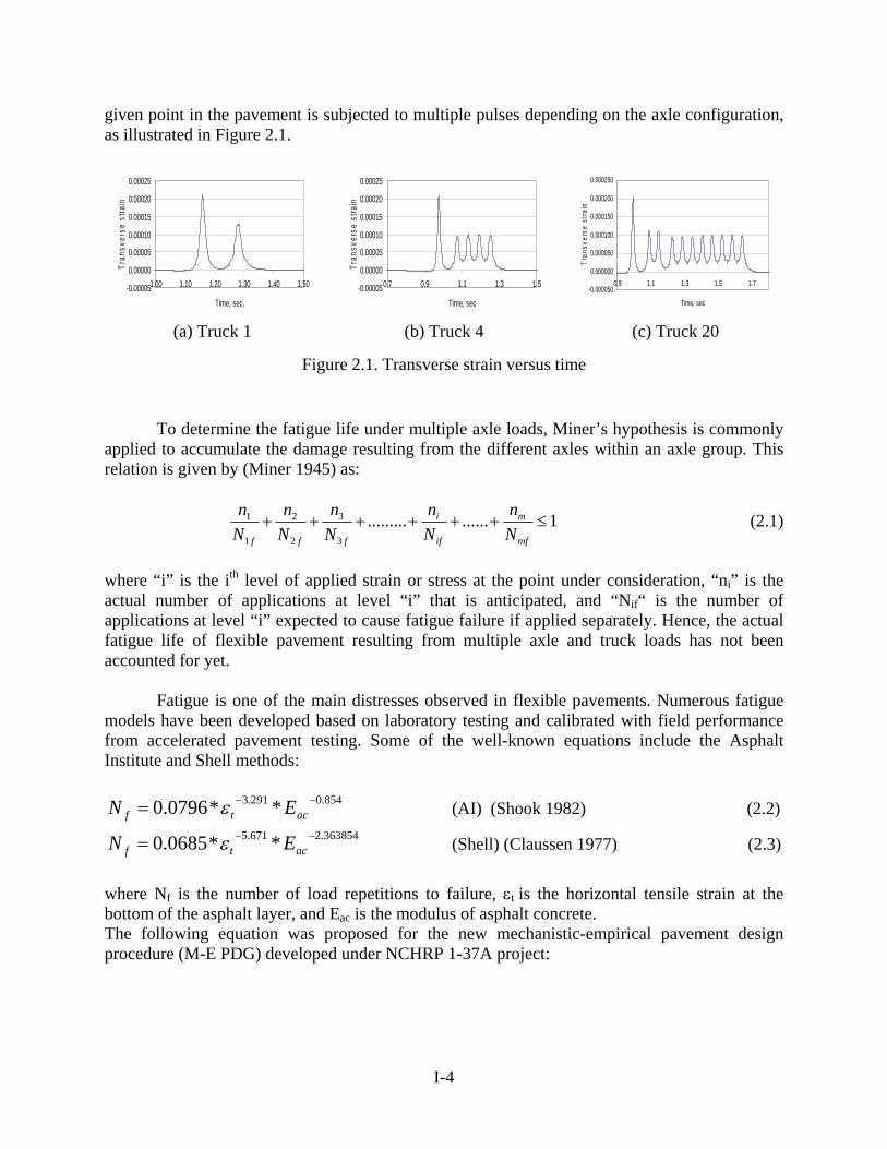
given point in the pavement is subjected to multiple pulses depending on the axle configuration, as illustrated in Figure 2.1.

-0.00005

0.00000

0.00005

0.00010

0.00015

0.00020

0.00025

1.00 1.10 1.20 1.30 1.40 1.50

Time, sec.

Tran

sver

se s

train

(a) Truck 1

-0.00005

0.00000

0.00005

0.00010

0.00015

0.00020

0.00025

0.7 0.9 1.1 1.3 1.5

Time, sec

Tran

sver

se s

train

(b) Truck 4

-0.000050

0.000000

0.000050

0.000100

0.000150

0.000200

0.000250

0.9 1.1 1.3 1.5 1.7

Time, sec

Tran

sver

se s

train

(c) Truck 20

Figure 2.1. Transverse strain versus time

To determine the fatigue life under multiple axle loads, Miner’s hypothesis is commonly applied to accumulate the damage resulting from the different axles within an axle group. This relation is given by (Miner 1945) as:

1...............3

3 ≤++++mf

m

if

i

f Nn

Nn

Nn

8540=fN

2

2

1

1 ++ff N

nNn (2.1)

where “i” is the ith level of applied strain or stress at the point under consideration, “ni” is the actual number of applications at level “i” that is anticipated, and “Nif“ is the number of applications at level “i” expected to cause fatigue failure if applied separately. Hence, the actual fatigue life of flexible pavement resulting from multiple axle and truck loads has not been accounted for yet.

Fatigue is one of the main distresses observed in flexible pavements. Numerous fatigue models have been developed based on laboratory testing and calibrated with field performance from accelerated pavement testing. Some of the well-known equations include the Asphalt Institute and Shell methods:

.0291.3 **0796. −−

act Eε (AI) (Shook 1982) (2.2)

363854.2671.50 −−=fN **0685. act Eε (Shell) (Claussen 1977) (2.3)

where Nf is the number of load repetitions to failure, εt is the horizontal tensile strain at the bottom of the asphalt layer, and Eac is the modulus of asphalt concrete. The following equation was proposed for the new mechanistic-empirical pavement design procedure (M-E PDG) developed under NCHRP 1-37A project:

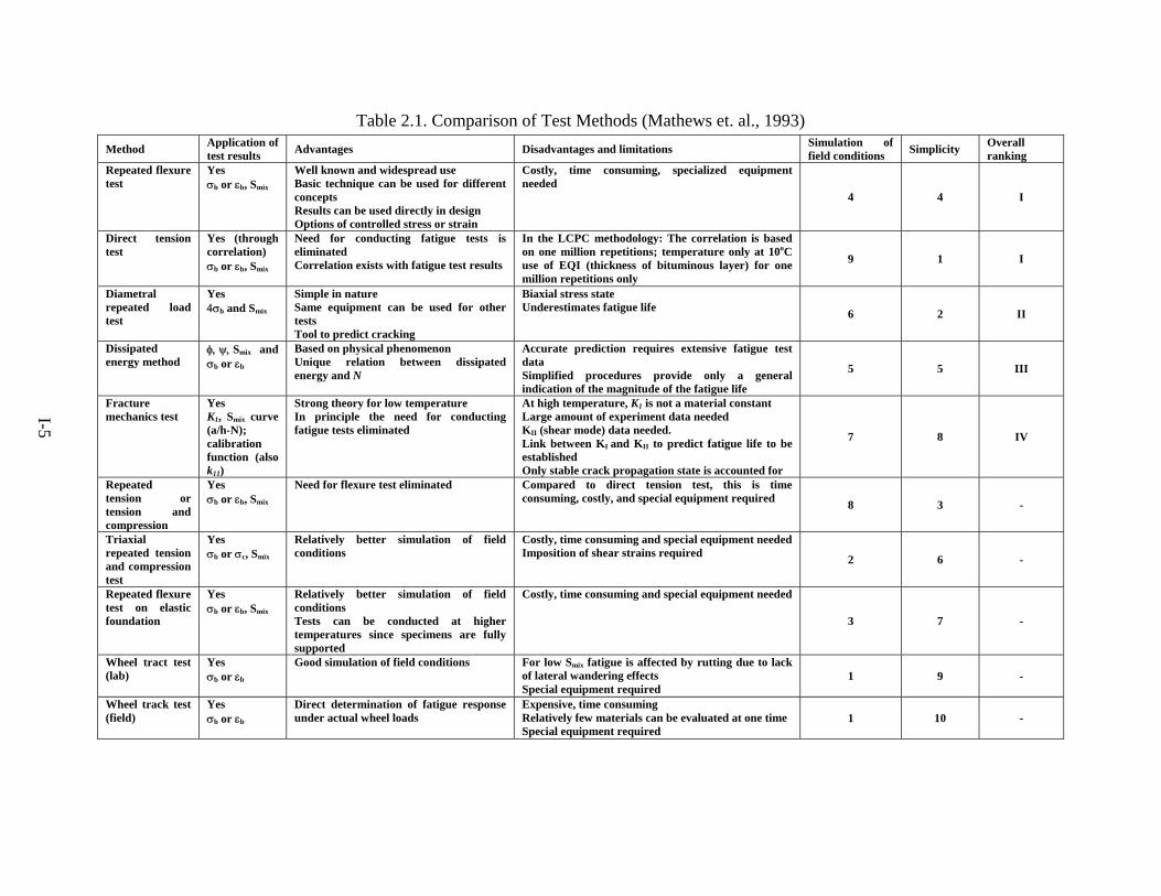
Table 2.1. Comparison of Test Methods (Mathews et. al., 1993)

Method Application of test results Advantages Disadvantages and limitations Simulation of

field conditions Simplicity Overall ranking

Repeated flexure test

Yes σb or εb, Smix

Well known and widespread use Basic technique can be used for different concepts Results can be used directly in design Options of controlled stress or strain

Costly, time consuming, specialized equipment needed

4 4 I

Direct tension test

Yes (through correlation) σb or εb, Smix

Need for conducting fatigue tests is eliminated Correlation exists with fatigue test results

In the LCPC methodology: The correlation is based on one million repetitions; temperature only at 10oC use of EQI (thickness of bituminous layer) for one million repetitions only

9 1 I

Diametral repeated load test

Yes 4σb and Smix

Simple in nature Same equipment can be used for other tests Tool to predict cracking

Biaxial stress state Underestimates fatigue life 6 2 II

Dissipated energy method

φ, ψ, Smix and σb or εb

Based on physical phenomenon Unique relation between dissipated energy and N

Accurate prediction requires extensive fatigue test data Simplified procedures provide only a general indication of the magnitude of the fatigue life

5 5 III

Fracture mechanics test

Yes K1, Smix curve (a/h-N); calibration function (also k11)

Strong theory for low temperature In principle the need for conducting fatigue tests eliminated

At high temperature, K1 is not a material constant Large amount of experiment data needed KII (shear mode) data needed. Link between KI and KII to predict fatigue life to be established Only stable crack propagation state is accounted for

7 8 IV

Repeated tension ortension and compression

σYes

b or εb, Smix

Need for flexure test eliminated Compared to direct tension test, this is time consuming, costly, and special equipment required 8 3 -

Triaxial repeated tension and compression test

Yes σb or σc, Smix

Relatively better simulation of field conditions

Costly, time consuming and special equipment needed Imposition of shear strains required 2 6 -

Repeated flexure test on elastic foundation

Yes σb or εb, Smix

Relatively better simulation of field conditions Tests can be conducted at higher temperatures since specimens are fully supported

Costly, time consuming and special equipment needed

3 7 -

Wheel tract test (lab)

Yes σb or εb

Good simulation of field conditions For low Smix fatigue is affected by rutting due to lack of lateral wandering effects Special equipment required

1 9 -

Wheel track test (field)

Yes σb or εb

Direct determination of fatigue response under actual wheel loads

Expensive, time consuming Relatively few materials can be evaluated at one time Special equipment required

1 10 -

I-5

3

24.1

5

1''

11 f

f

EKFNt

ffβ

β

σ εβ −

⎥⎦

⎤⎢⎣

⎡=

(2.4)

Where: Nf = number of repetitions to fatigue cracking, εt = tensile strain at the critical location, E = material stiffness, K1σ = laboratory calibration parameter βf1, βf2, βf3 = field calibration factors

Gillespie et al. (1993) provided the most comprehensive study related to the effect of

heavy trucks on pavement damage using mechanistic analysis. In this study, analytical models of trucks and pavement structures were developed to allow the systematic study of pavement responses to the moving, dynamic loads of various truck configurations. The truck characteristics included in this study were:

Truck type (single unit trucks, tractor-semi trailers, and multiple-trailer

configurations), Axle loads, Number of axles, Spacing between axles, Suspension type (leaf spring, air, and walking beams), and Tire parameters (single/dual configurations, radial/bias construction, and inflation

pressure).

The response was determined in both rigid and flexible pavements for various designs and parameters, with variations in road roughness and vehicle speed. Pavement responses (stresses, strains and deflections) were evaluated at different points within the pavement structure. The main conclusions of the study were:

Static axle load was found to be the unique vehicle factor that has a significant

effect on fatigue damage. Fatigue in flexible and rigid pavements vary by a factor of 1:20 over a range of

axle loads from 10 to 22 kips because fatigue damage is related to the fourth power of the loads for both pavement types.

Fatigue damage was not directly related to vehicle gross weight but varied with maximum axle loads on each vehicle configuration.

Axle spacing has a moderate effect on rigid pavement fatigue and little effect on flexible pavement fatigue.

Static load sharing in multiple axle groups affects fatigue of rigid and flexible pavements moderately.

Vehicle speed influenced rigid pavement fatigue by increasing peak dynamic loads, while flexible pavement fatigue remained fairly constant with speed.

I-6

Hajek and Agarwal (1990) highlighted the factors to be considered in calculating the Load Equivalency Factor (LEF) values of various axle configurations for flexible pavements and developed factors using different strain and deflection criteria. It was concluded that pavement response parameters such as deflections and strains have considerable influence on LEF values. Moreover, axle weight and spacing also contribute to flexible pavement fatigue damage significantly. Sebaaly and Tabatabaee (1992) studied the effect of tire parameters on flexible pavement damage and LEF, and they compared single and tandem axles of similar per-axle load level; they concluded that the passage of one tandem axle produced less fatigue damage than the passage of two single axles. Chatti and Lee (2004) studied the effects of various truck and axle configurations on flexible pavement fatigue using different summation methods (peak strain, peak-midway strain, and dissipated energy) to calculate the fatigue damage. The results indicated that the peak-midway strain method agrees reasonably well with the dissipated energy method. Moreover, Chatti and Lee recommended the use of dissipated energy method because it captures the totality of the stress strain response during the passage of the loads. 2.2.2 Rigid Pavements

Fatigue studies in concrete began in the early 20th century which was propelled by the need to improve and maintain a robust infrastructure. The first investigations of significant consequence on flexural fatigue of concrete were carried out by Illinois Department of Highways and Purdue University reported by Clemmer (1922), Older (1922, 1924), and Hatt (1924). The investigations led by these authors were used as the basis for the 1933 PCA design curve for fatigue strength of concrete pavements. Since that time, many contributions have been made in the area of concrete fatigue. 2.2.2.1 Cube Testing

Both Holmen (1982) and Tepfers (1979) investigated fatigue behavior of concrete in compression and tension, using cubes as the test specimen. Holmen concluded that the damage in concrete subjected to variable amplitude loading is not predicted well with Miner’s theory (1924). Miner’s theory assumes that the damage fraction at any stress level is linearly proportional to the ratio of number of cycles of an applied load to the total number of cycles that would produce failure at that stress level, as stated previously. The theory does not recognize the influence of the order of application of various stress levels and the damage is assumed to accumulate at the same rate for a given stress level regardless of the past stress history. Additionally, Tepfers’s investigation led him to conclude that concrete under stress reversals (tension-compression) causes more damage when compared to fatigue tests where no stress reversals are present. 2.2.2.2 Split Tensile Testing

Yun (2003) investigated the fatigue behavior in concrete through a split tensile test setup. Yun proposed an S-N curve using the laboratory tests results. Yun also concluded that the thickness of the cylinder did not significantly affect the fatigue life. Additionally, Yun noted that Miner’s hypothesis did not accurately predict the fatigue life of the cylinders under variable

I-7

amplitude loading, similar to other studies. Yun (2005) later proposed a non-linear damage model using the permanent strain history. Additionally, he concluded that Miner’s rule might be applicable to plain concrete with little error, provided the stress level remains low. He also concluded that the accumulation of damage obtained by non-linear damage theory was closer to 1 than by linear damage theory in all load cases, indicating that non-linear cumulative damage could consider the effects of magnitude and sequence under variable amplitude loading. Yun also compared the results to the flexural fatigue tests, noting that the sums of cumulative damage were greater in the flexural-tensile test than in the splitting-tensile test.

However, in concrete pavements, fatigue damage is caused by the tensile stresses generated by the flexural bending of the slab as wheel loads are placed onto them. Thus, more focus was placed on previous research related to flexural fatigue, given the similarities to actual behavior in the field. 2.2.2.3 Flexural Testing 2.2.2.3.1 Variable Amplitude

Concrete pavements are frequently subjected to heavy loads induced by truck traffic. Moreover, most of these trucks are equipped with multiple axles (tandem, tridem, quad, etc.), leading to significant stress interaction in the concrete between each of the wheels within an axle group As a result, there are many occurrences where the stress pulses induced onto the pavement will not have uniform amplitudes. Thus, to accurately assess the damage from multiple axles, variable amplitude testing is required. Hilsdorf and Kessler (1966) investigated the fatigue strength of concrete under varying flexural stresses and the effects of rest periods. The researches concluded that fatigue strength increases with increasing length of rest periods up to 5 min. They also noted that the sequence in which repeated loads of different magnitudes are applied has considerable influence on the fatigue behavior of concrete. Thus, the results were not consistent with Miners hypothesis.

Oh (1991) investigated the fatigue behavior of concrete under varying amplitudes of cyclic loading as well. He found that concrete fatigue failure is greatly affected by the magnitude and sequence of the applied variable load cycles, and Miner’s linear theory led to some errors in fatigue failure prediction of concrete materials. Oh proposed a non-linear damage theory which used the permanent strain history as a basis for damage accumulation.

I-8

Figure 2.2. Types of various-amplitude fatigue loadings (Oh, 1991)

2.2.2.3.2 Material Constituents

In the field, there is usually a large variety of possible concrete mixes to choose from for design purposes. As a designer, it is important to choose a mix that produces optimal performance and, at the same time, is economically feasible. Thus, it is important to investigate the effects of different mix components on the fatigue life of concrete.

Several studies have been done which investigated the effects of various concrete mix components, such as air content, aggregate type, and water-to-cement (w/c) ratio. Klaiber and Dah-Yin Lee (1978) concluded that air content affects the fatigue life significantly. They found that as the air content increases, the fatigue life decreases. Additionally, the crack interface will change as a result of changing the air content. The researchers also noted that fatigue behavior is slightly affected by the w/c ratio. The fatigue strength decreased at low w/c ratio (0.32). Aggregate type was also found to affect the fatigue life of concrete.

I-9

Figure 2.3. Effect of Air Content on Fatigue Life (Klaiber and Dah-Yin Lee)

2.2.2.3.3 Time Dependence

As a wheel load approaches and passes over a point in the pavement, a time dependent stress pulse ensues at that point. The magnitude and duration of the stress pulse will be dependent upon, among other things, the velocity of the vehicle. Thus, it is important to investigate the effect time has on the fatigue life of concrete. It has been observed, that the fatigue behavior of concrete is indeed affected by the rate at which the load is being applied. Several researchers have determined this through extensive laboratory experiments. Hsu (1981) proposed two equations (high cycle fatigue and low cycle fatigue) that incorporated the rate of loading, the stress ratio, and the ratio between minimum and maximum stress. The equations were substantiated by compressive and flexural tests reported in the literature. For high cycle fatigue the equation is the following:

TNRMR

log0294.0log)556.01(0662.01 −−−=σ (2.5)

For low cycle fatigue:

TRNRRMR

log)445.01(0706.0log)779.01(177.0267.060.1 −−−−−=σ (2.6)

I-10

Where: σ = maximum applied stress MR = modulus of rupture N = number of cycles to failure T = Period of one cycle R = ratio of minimum stress to maximum stress

Hsu concluded that reasonable results were produced when comparing the proposed model to previous test results. The author noted that the equation is also applicable to flexural fatigue tests.

Figure 2.4. Comparison of Hsu Model with Previous Fatigue Data (Hsu)

Zhang (1996) investigated the sustained loading effect on the fatigue life of plain concrete to establish a fundamental relationship between sustained stress and sustained time. Based on experimental results, a sustained stress-sustained time relationship was established. The author concluded that the equation predicted the previous test data reasonably well. Additionally, the author noted that the sustained loading effect is insignificant for stress ratios less than 0.75. Zhang (1996) also investigated the effects of loading frequency and stress reversal on fatigue life of plain concrete. He concluded that frequency significantly influences the fatigue life of concrete. Additionally, stress reversal causes fatigue life of concrete to decrease. 2.2.2.4 Slab Damage 2.2.2.4.1 Fatigue

The research discussed in section 2.2.2.3 only corresponds to beam testing. In reality, however, trucks traverse concrete slabs supported by soil foundations, and not simply supported

I-11

beams. Thus, it is important to compare the results from experimental flexural beam tests to experimental slab fatigue data to substantiate or disqualify the results from previous research. Roesler and Barenberg (1998) conducted fatigue and static tests on concrete slabs to determine how similar or dissimilar the results were from previous beam experiments. The authors found that the fully supported slabs had 30% higher strength than the simply supported beams. Additionally, the authors noted that when the static modulus of rupture from the slab was used, the fatigue curves for the simply supported beams and the fully supported slabs were essentially identical. 2.2.2.4.2 Critical Location

In order to properly design a pavement system for traffic loading, a designer must know the fatigue behavior of concrete and know the mechanical behavior of the system (the location where the maximum stress will occur on the slab). Traditionally, mechanistic-empirical design methods have focused on bottom-up transverse fatigue cracking induced by loads located at the mid-slab edge. However, several studies conducted in California have shown that there are transverse and longitudinal cracks surfacing around the transverse joint (Yu and Khazanovich, Armaghani, Larsen and Smith, Hatt, Hveem). The occurrence of these cracks prompted several researchers to investigate the cause behind their unique location. It was found, that upward curling of the slab due to drying shrinkage or a negative temperature gradient coupled with heavy traffic loads can cause top-down cracking near the transverse joint. Hiller and Roesler (2005) conducted an influence line analysis using a finite element program to investigate jointed concrete pavements in California. They concluded that the critical stress location cannot be easily ascertained without a detailed analysis. Furthermore, without the incorporation of an effective built-in temperature differential (EBITD), the critical stress location will be at the mid-slab edge causing bottom-up cracking, similar to traditional analysis. The researchers also noted that when incorporating the stress range approach (ratio between minimum stress and maximum stress) into the damage model and the EBITD, the critical failure location changes to a position near the transverse joint (similar to the occurrence in the field). Additionally, the authors mentioned that axle spacing (spacing between axle groups) plays a large role as well in the critical location. They noted that an axle spacing as large as 21 ft can have a significant impact on the critical failure location in the slab.

Figure 2.5. Relative damage levels using stress range approach along top and bottom of slab with

effective built-in temperature difference of -30 Fahrenheit (Hiller and Roesler)o

I-12

2.2.2.4.3 Concrete Fatigue Models

Several concrete fatigue models have been published over the years as a result of the copious research done in the area of concrete fatigue. The most well known fatigue models are listed below:

Table 2.2. Well Known Existing Fatigue Models (Smith and Roesler, 2003) 2.1

13.2log ⎟⎠⎞

⎜⎝⎛=

σMRN (2.7) Darter (1990)

588.0323.1log +⎟⎠⎞

⎜⎝⎛=

σMRN (2.8) Foxworthy (1985)

⎟⎠⎞

⎜⎝⎛−=

MRN σ61.1761.17log (2.9) Zero- Maintenance (1977)

284.4736.1log +⎟⎠⎞

⎜⎝⎛−=

MRN σ for 25.1≥

MRσ

2214.1

8127.2log−

⎟⎠⎞

⎜⎝⎛=

MRN σ for 25.1≤

MRσ (2.10)

NCHRP 1-26 (1992)

⎟⎠⎞

⎜⎝⎛−=

MRN σ1765.12810.11log

for 15.0 ≤≤MRσ (2.11)

Portland Cement Association (1963)

Where: σ = applied stress and MR = Modulus of Rupture

Figure 2.6. Comparisons of Fatigue Models (Smith and Roesler, 2003)

I-13

Table 2.3 presents a summary of previous fatigue-related studies using plain cement concrete (PCC) beams.

Table 2.3. Previous research involving cyclic beam fatigue testing

Objectives of the research Beam size (inches) Reference

Effect of stress reversal on the fatigue life of plain concrete is studied through flexural fatigue tests on plain concrete beams

4 x 4 x 20 (Zhang and Phillips 1996)

Effects of load frequency and stress reversal on fatigue life of plain concrete 4 x 4 x 20 (Zhang et al. 1996)

Sustain loading effects on the fatigue life of plain concrete 4 x 4 x 20 (Zhang et al. 1998)

Effect of water cement ratio, aggregate type and loading sequence on the fatigue properties of plain concrete

4 x 4 x 20 (Zhang et al. 1997)

The concept of equivalent fatigue life was applied to correct the effect of different stress ration between the field and the laboratory testing

6 x 6 x 36 (Suh et al. 2005)

Fatigue and static testing of concrete slab. Fatigue of slab and simply supported beam was compared.

6 x 6 x 21 (Roesler 1998; Roesler and Barenberg 1999a; Roesler and Barenberg 1999b)

Probability of fatigue failure of plain concrete 3 x 3 x 14.5 (McCall 1958) Effect of speed of testing on flexural fatigue strength of plain concrete 6 x 6 x 64 (Kesler 1953)

Effect of range of stress on fatigue strength of plain concrete beams 6 x 6 x 64 (Murdock and Kesler 1958)

Fatigue strength of concrete under varying flexural stresses 6 x 6 x 60 (Hilsdorf and Kesler 1966)

Cumulative damage theory of concrete under variable-amplitude fatigue loading 4 x 4 x 20 (Oh 1991a)

Fatigue-life distribution of concrete for various stress levels 4 x 4 x 20 (Oh 1991b)

Fatigue analysis of plain concrete in flexure 4 x 4 x 20 (Oh 1986) Fatigue flexural strength of plain concrete 4 x 4 x 20 (Shi et al. 1993) Study of the fatigue performance and damage mechanism of steel fiber reinforced concrete

4 x 4 x 16 6 x 6 x 22 (Wei et al. 1996)

Flexure fatigue life distributions and failure probability of steel fibrous concrete 4 x 4 x 20 (Singh and Kaushik 2000)

I-14

2.3 PREVIOUS RESEARCH: RUTTING

Rutting is a major failure mode for flexible pavements. Pavement engineers have been trying for years to control and arrest the development of ruts. Two approaches have been documented in the literature for mechanistic modeling of rutting. The first approach uses the sub-grade strain model, while the second approach considers permanent deformation within each layer. 2.3.1 Subgrade Strain Models The two most dominant models related to subgrade strain model are the Asphalt Institute (AI) (Shook, 1982) and Shell Petroleum (Claussen, 1977):

477.49 *10*365.1 −−= cpN ε (AI) (2.12) 47 *10*15.6 −−= cpN ε (Shell) (2.13)

Where:

NF = Number of repetitions to failure, and

εc = Vertical compressive strain at the top of the subgrade.

The rutting failures according to AI and Shell models are defined by rut depth of 13 to19 mm (0.5 to 0.75 in) and 13 mm (0.5 in), respectively. 2.3.2 Permanent Deformation within each layer Kim (1999) developed a rutting model which can account for the total rutting in all pavement layers as follow:

( )

⎟⎟⎠

⎞⎜⎜⎝

⎛⎟⎟⎠

⎞⎜⎜⎝

⎛−+++−

−++−=

SG

ACESALSGvbasev

annualAC

EEN

KVTSDHRD

ln034.0)ln(258.0)(271.0)(657.0703.2

*)ln(01.0011.0)ln(033.0016.0

883.0,

097.0, εε

(2.14)

Where: RD = Total rut depth (in) SD = Surface deflection (in) KV = Kinematic viscosity (centistoke) Tannual = Annual ambient temperature HAC =Thickness of asphalt concrete (in) N = cumulative traffic volume (ESAL) EAC = Resilient modulus of AC (psi) ESG = Resilient modulus of subgrade (psi)

basev,ε = Vertical compressive strain at the top of the base (10-3) SGv,ε = Vertical compressive strain at the top of the subgrade (10-3)

I-15

Ali and Tayabji, (2000) expanded the VESYS rutting model (Moavenzadeh 1974) so that the final form of the model includes the contribution from each pavement layer as shown below:

( ) ( )

( )Subgrade

Subgrade

Subgradei

Base

Base

Basei

AC

AC

ACi

e

k

ii

Subgrade

Subgadesubgrade

e

k

ii

Base

BaseBasee

k

ii

AC

ACACp

nh

nhnh

α

αα

α

αα

εα

µ

εα

µε

αµ

ρ

−

=

−

=

−

=

⎟⎟

⎠

⎞

⎜⎜

⎝

⎛

−+

⎟⎟⎠

⎞⎜⎜⎝

⎛

−+⎟

⎟⎠

⎞⎜⎜⎝

⎛

−=

−

−−

∑

∑∑1

1

1

1

1

1

11

,

11

,

11

,

1

11(2.15)

Where: ρp = Total cumulative rut depth (in the same units as the layer thickness, h) i = Subscript denoting load group k = Number of load groups h = layer thickness, with “AC”, “Base”, “Subgrade” subscript denoting the AC layer, the combined base/subbase layer, and the subgrade, respectively. n = number of load applications εe = Permanent deformation parameter representing the constant of proportionality between plastic and elastic strain α = Permanent deformation parameter indicating the rate of decrease in rutting as the number of load applications increases (hardening effect)

Ali et al. (1998) calibrated the model using 61 sections from the Long Term Pavement Performance (LTPP) General Pavement Study 1 (GPS-1). They calculated the permanent deformation parameters for each layer. Also, Ali and Tayabji (2000) calibrated the same model using the transverse profile from one LTPP section and came up with another set of permanent deformation parameters.

Kenis (1997) has used the Accelerated Pavement Tests (APT) performance data to

validate and calibrate the two flexible pavement-rutting models used in VESYS 5. In their study, they suggested ranges for the permanent deformation parameters of the pavement layers. Table 2.4 summarizes the calibration parameters from all three studies.

The new mechanistic design procedure developed under NCHRP 1-37A provides a

rutting model for AC layers (equation 2.16) as well as unbound layers (equation 2.17); the calibration parameters may be modified to suit local calibration within a given state or region.

339937.02734.10007.0 rNrTr

r

p βββ

ε

ε= (2.16)

Where: pε = plastic strain rε = resilient strain

T = layer temperature N = number of load repetitions βr1, βr2, βr3 = field calibration factors

I-16

⎥⎥⎦

⎤

⎢⎢⎣

⎡⎟⎟⎠

⎞⎜⎜⎝

⎛=

⎟⎠⎞

⎜⎝⎛−

βρ

εεεβδ N

r

ovsa ehN 1)( (2.17)

Where: aδ = permanent deformation for the layer N = number of load repetitions

vε = average vertical strain = thickness of the layer h

oε , ρ, β= material properties rε = resilient strain

1sβ = field calibration factor

Table 2.4. Summary of permanent deformation parameters reported in the literature Calibration Pavement layer µ α

AC 0.701 0.7 Base 0.442 0.537 Subbase 0.333 0.451

LTPP (Ali et al., 1998) Subgrade 0.021 0.752

AC 0.000103 0.1 Base 1.163 0.95

Transverse profile (Ali and Tayabji, 2000) Subgrade 0.0008 0.644

AC 0.6 to 1.0 0.5 to 0.75 Base 0.3 to 0.5 0.64 to 0.75

APT (Kenis, 1997) Subgrade 0.01 to 0.04 0.75

As mentioned previously, there are several rutting models available in the literature.

However, each rutting model has specific limitations, as listed in Table 2.6. It can be observed from the literature review that the subgrade strain model approach (AI and Shell models) are based on unreasonable assumptions, since these models account for subgrade rutting while neglecting rutting from the upper layers. Ullidtz (1987) reported that the subgrade rutting in the AASHO road test was only 9% of the total rutting as shown in Table 2.5.

Table 2.5. Percent layer distribution of rutting in the AASHO road test (Ullidtz, 1987)

Pavement layer Percent observed rutting Asphalt concrete 32

Base 14 Subbase 45 Subgrade 9

The permanent deformation model developed by Kim (1999) accounts for rutting within

all pavement layers; however, the model cannot handle different axle loads and configurations (it uses ESALs); furthermore, the model calibration was limited to specific sections (50) in the state of Michigan. The form of the second model (Ali et al., 1998) was derived in such a way that it is more applicable for use in this research, since it can accommodate different axle loads and configurations; however the calibration process of that model has several limitations as shown in Table 2.6.

I-17

Table 2.6. Limitations of the existing flexible pavement rutting models Model No.

Model name

Authors Limitations

1 AI & Shell Shook 1982; Claussen 1977

These models account only for subgrade rutting and neglect the rutting from other layers.

These models did not account for rate hardening as the number of load applications increase.

The relationship between observed rutting and rutting damage ratio did not follow the expected S-shape.

2 MSU Kim 1999

Traffic has to be in ESALs It predicts the total rutting, i.e. does not predict rutting

within each layer This model was calibrated using Michigan sections only.

3 VESYS Ali et al. 1998

Large scatter between predicted and measured rut depths.

Using this model outside the calibrated data set showed poor predictions.

The calibration procedure used total rut depth only rather than time series rut data.

4 VESYS Ali and Tayabji 2000

The calibration process was only for one section, which exhibited large amount of rutting.

Using this model for different sections gives unreasonable rut prediction.

The calibrated permanent deformation parameters were completely different from those using the maximum rut values.

The parameters can only be used for the same pavement cross-section and for similar materials.

5 VESYS Kenis, 1997 Wide range of the permanent deformation parameters, can cause large difference is rut predictions.

6 AASHTO 2002 AASHTO Calibration parameters not available yet.

2.4 PREVIOUS RESEARCH: FAULTING

Concrete pavements typically develop transverse cracks over time from repetitive traffic loads (fatigue cracking), thermal effects (curling and warping that amplifies the stress as traffic moves over the pavement) and drying shrinkage. Over time, these transverse cracks will degrade and lose their ability to transfer load through aggregate interlock. Eventually, each side of the crack will move independently of one another (no load transfer), which will result in increased slab deflections. Large slab deflections, combined with the intrusion of water into the sub-layers, can lead to a phenomenon called pumping. Pumping occurs when the slab deflects vertically and ejects a mixture of water and fine soil particles from the underlying base layers. As a result of the ejection, there is a loss of soil volume underneath the concrete slab, creating a void between the base layer and the concrete slab. Thus, the concrete slab will lose vertical elevation, and ultimately cause the crack face to fault (Raja and Snyder, 1991).

I-18

Faulting can severely reduce the ride quality of the pavement, producing unwanted noise and roughness. In order to prevent the crack from faulting, sufficient load transfer must be maintained over the course of the pavement’s life. If there is sufficient load transfer, slab deflections will be minimized, ultimately impeding the onset of a fault across the transverse crack. Extensive research has been done in the area of load transfer and joint efficiency. 2.4.1 Aggregate Interlock Mechanism

As a truck passes over a crack, the wheel load is partially transferred from one side to the other through shear forces within the aggregate particles. This transfer of load through the aggregate particles is known as Aggregate Interlock (Raja and Snyder, 1991). Aggregate Interlock is comprised of at least three significant components: (1) an initial slack or gap between crack surfaces, which exists prior to loading, (2) a sliding of the adjacent crack surfaces, and (3) in plane dilation of the crack if unrestrained, otherwise build up of normal force. (Jensen and Hansen) 2.4.2 Crack Width

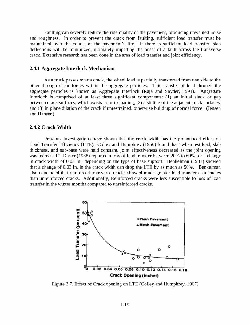
Previous Investigations have shown that the crack width has the pronounced effect on Load Transfer Efficiency (LTE). Colley and Humphrey (1956) found that “when test load, slab thickness, and sub-base were held constant, joint effectiveness decreased as the joint opening was increased.” Darter (1988) reported a loss of load transfer between 20% to 60% for a change in crack width of 0.03 in., depending on the type of base support. Benkelman (1933) showed that a change of 0.03 in. in the crack width can drop the LTE by as much as 50%. Benkelman also concluded that reinforced transverse cracks showed much greater load transfer efficiencies than unreinforced cracks. Additionally, Reinforced cracks were less susceptible to loss of load transfer in the winter months compared to unreinforced cracks.

Figure 2.7. Effect of Crack opening on LTE (Colley and Humphrey, 1967)

I-19

2.4.3 Crack Face

The time and mode of fracture will affect the LTE. If the transverse crack propagates through the aggregates, the LTE will diminish. Conversely, if the crack propagates around the aggregates, the LTE will increase. Early fractures will most likely propagate around the aggregate (depending on the aggregate) when the cement-aggregate bond is weak, producing many aggregate pullouts (Nowlen). At later times of cracking, the fracture may propagate through the aggregate, and pullouts will be diminished. Nowlen concluded that “early fracture of the joint faces with resulting aggregate pullouts contributed to high effectiveness initially, and also to endurance of good effectiveness under repeated loads.”

Additionally, the type and size of aggregate greatly affects the LTE along the crack face. Nowlen also studied the effect of coarse aggregate size on the performance of the LTE. He concluded that large coarse aggregates produce greater LTE when compared to smaller aggregate sizes, particularly for large joint openings. Buch, Fabrizzio and Hiller (2000) studied the effects of four different aggregate types on Load Transfer Efficiency. They concluded that recycled concrete pavements, comprised of relatively weak aggregate, are easily crushed, and produce the lowest LTE’s when compared to natural gravel, slag and carbonate rocks. The researchers also mentioned that natural gravel has a greater potential for higher LTE’s when compared to carbonate rocks because it is much harder. Colley and Humphrey (1956) concluded that crushed stone, which had greater angularity than natural gravel, produced higher LTE’s. Thus angularity of the aggregate also plays a role in the LTE.

2.4.4 Crack Endurance

Over time, as trucks pass over the transverse cracks, the crack will lose aggregate interlock and lose Load Transfer Efficiency. Thus, to maintain a serviceable road, and to promptly designate a time for pavement restoration, a relationship between crack degradation and truck traffic must be quantified. Several researchers have conducted experiments to investigate the performance of a crack interface by simulating a moving single axle load through two stationary hydraulic actuators on either side of the crack. The two stationary actuators apply a load pulse with a prescribed phase lag between them, in order to simulate the passage of a moving wheel load , as shown in Figure 2.8 (Colley and Humphrey; Hanekom, Horak, and Visser).

Colley and Humphrey (1956) concluded that joints with greater crack widths degraded

much more rapidly than joints with tighter crack widths (Figure 2.9). Additionally, thicker pavements for a given crack width and load, performed better than thinner pavements (Figure 2.10). The joints also performed better when using a cement treated base as compared to a natural gravel or clay base.

I-20

Figure 2.8. Typical load waveforms for dynamic loading (Colley and Humphrey; Hanekom, Horak and Visser)

Figure 2.9. Joint Efficiency vs. Loading Cycles for different crack widths (Colley and

Humphrey)

Figure 2.10. Joint Efficiency vs. Joint Opening for different slab thicknesses (Colley and

Humphrey)

I-21

Buch, Fabrizzio, and Hiller (2000) investigated the performance of a crack for different aggregate types (Figure 2.11). They concluded that “the concrete specimens containing natural aggregate products included in their study provided better crack deterioration performance than did concrete prepared using manufactured aggregates.”

Figure 2.11. LTE vs. Load Cycles for recycled slabs (top) and limestone (bottom) (Buch,

Fabrizzio, and Hiller) 2.5 FIELD STUDIES

The Ohio Department of Transportation (ODOT) recognized that their special permit data for overloaded vehicles showed that the weight for trucks traveling from Michigan to northern

I-22

Ohio cities were substantially heavier than the loads permitted in Ohio. Therefore, a field study was conducted to investigate the effect of Michigan heavy vehicles on pavement performance (Ilves and Majidzadeh 1991; Saraf et al. 1995). The following field data were collected for this study: traffic, rutting, faulting, cracking, roughness, and deflection measurements. Regression analysis of rutting data produced the following regression equation:

RUTF = 0.035+0.984 (C13) +0.03(B&C) + 0.0007 (months) (2.18)

Where: RUTF is rutting in flexible pavement, in, C13 is the number of FHWA class 13 vehicles in the lane per day, in thousands, B is the total number of FHWA classes 8 – 13 and C is the total number of FHWA classes 4-7. “months” is the number of months of testing. The conclusions of the study were: • For rigid pavements, heavy axle loads might contribute toward cracking and faulting

development, • For flexible and composite pavements, only rutting was influenced by heavy axle loads

It should be noted that this study was limited by the fact that only a limited number of roads linking the state of Ohio and Michigan were included. Furthermore, the analysis did not compare the relative damage resulting from various axle and truck configuration.

I-23

I-24

CHAPTER 3 ANALYSIS OF PERFORMANCE DATA FROM

IN SERVICE PAVEMENTS 3.1 INTRODUCTION

Michigan road regulations allow for several types of multi-axle trucks which may not be permitted on roads in several other states. The extent to which these “Michigan” trucks do contribute to the distresses observed on Michigan pavements is unknown. The Michigan Department of Transportation (MDOT) has a very comprehensive pavement surface distress database. The data include Distress Index (DI), Ride Quality Index (RQI), Rutting, as well as traffic count and weight data. Therefore, as the first step these data can be utilized to investigate the relative effect of Michigan multi-axle trucks on actual pavement damage. Moreover, the field results can be compared with the mechanistic and laboratory findings. MDOT DI includes load related distress as well as non-load distress. To facilitate comparison between field performance and mechanistic as well as laboratory results, the analysis included investigating the detailed distress files to separate load related distress and non-load related distress. 3.2 SITE SELECTION PROCEDURE The following procedure summarizes the steps used for the site selection: • Extract the stations ID’s that have available traffic for the years 2000 and 2001 from the

FHWA program (VTRIS). • Match those stations ID’s with the control sections using the Permanent Traffic Recorder,

PTR, file provided by MDOT. • Locate the stations in each county using the control section in the 2001 Physical

Reference/Control Section, PR/CS atlas and determine exactly the location of the weigh stations on the control sections.

• Traffic data in the sufficiency rating book and Michigan annual average 24-hour commercial traffic volumes maps were used to examine the variation of the traffic relative to the weigh station segment. The variation on the considered length of the control section was limited to a maximum of 10%.

• In some cases, the truck traffic data were valid only for a small portion of the control section (the weigh station segment), especially when there are several main exits and entrances on the road, as shown in figure A-1.

• In other cases, the traffic data were valid for two consecutive control sections where there are no main exits or entrances on the road, as shown in figure A-2.

Table 3.1 shows the available projects for each pavement category.

I-25

Table 3.1. Number of available projects for each pavement type

Road class Pavement type Interstate US roads Michigan roads

Total

Rigid 29 22 1 52 Flexible 9 23 21 53

Composite 27 45 5 77

3.3 DATA EXTRACTION AND AVAILABILITY 3.3.1 Traffic Count Data

The FHWA traffic data (W-2 form) classifies the traffic into13 classes. Classes 5 to 13 are for truck traffic, reported as the Average Daily Truck Traffic, ADTT count per class type. Axle spectra are also available in FHWA W-4 data forms.

3.3.2 Truck Data

Using the FHWA W-2 tables, the ADTT for class 5 through 13 were extracted for the control sections corresponding to the truck lane. Table 3.2 shows the class definition, the axle groups (number of axles within an axle group), and truck configuration for classes 5 through 13. Moreover, the improvement year of the control section was recorded from the sufficiency-rating book. The improvement year represents the most recent year the segment received significant construction work that improved the pavement condition or extended the life of the pavement. The Total Truck Traffic, TTT for classes 5 through 13 was calculated as follow:

TTT of class = ADTT of class * pavement age * 365 (3.1)

where: ADTT = average daily truck traffic of class Pavement age = year of improvement – DI survey year.

The consistency of weigh station traffic data from year to year was examined for total ADTT and individual truck classes. Figures 3.1 and 3.2 show a comparison of ADTT in 2001 and 2002 traffic data for all weigh stations in the State of Michigan. No significant change can be seen in the traffic data.

I-26

Table 3.2. Vehicle class definition, axle groups, and truck configuration

*Classes 7, 10, and 13 have three or more axle groups (multi-axle groups)

0

1,000

2,000

3,000

4,000

5,000

6,000

7,000

0 5 10 15 20 25 30 35 40 45 50 55 60 65 70 75 80 85 90

Station number

AD

TT

2002 2001

Figure 3.1. Comparison between 2001 and 2002 total average daily truck traffic by station

I-27

0.00000

0.00005

0.00010

0.00015

0.00020

0.00025

0.00030

0.00035

0 1000 2000 3000 4000 5000 6000 7000

Total ADTT

f(x)

2002 2001

Figure 3.2. Comparison between 2001 and 2002 total average daily truck traffic by traffic

distribution

Since VTRIS does not provide some essential data needed for this research, raw truck traffic data for 2000 were analyzed to determine the distribution of axle and truck configurations for all axle groups including those with a large number of axles for each weigh station. Trucks were categorized according to their largest axle group. For example, a quad axle is an axle group that has four axles that share the same weight, so that trucks with a quad-axle are all trucks that have quad axle as the largest axle group. Figure 3.3 shows the axle and truck categories used in the analysis. Table 3.3 shows an example of the extracted axle/truck information. The analysis of raw traffic data also allowed for determining the proportions of each truck type within each FHWA truck class. Table 3.4 shows the proportions, average truck weight, and the percentage of truck configurations within each class. FHWA truck class 13, which is the heaviest truck class, includes many different configurations, with most having very small numbers. Figure 3.4 shows that truck classes 7 and 12 have very small percentages (less than 0.4 %) and truck class 5 has the lowest overall average weight (6.0 tons). These trucks will not significantly contribute in explaining the pavement damage; therefore they were excluded from the analysis.

Table 3.5 shows the number of weigh stations for raw traffic and VTRIS analysis

as well as the number of projects corresponding to each one of them. More detailed information about where these stations are located on the roads, the beginning and ending, the length of each project can be found in Table A-1. Also, rut depth and traffic count for each project are shown in Table A-2.

I-28

Axle/truck Example truck configurations Axle configurations Single

Tandem

Tridem

Quad

Five

Six

Seven

Eight

I-29

05

101520

5 6 7 8 9 10 11 12 13

Truck class

ic P

erce

ntag

e an

d w

eigh

t, to

ns

2530354045

Traf

f

Per

Figure 3.3. Axle/truck configurations extracted from raw data

Figure 3.4. Weight and percentage of FHWA truck classes

centage weight

Type Configuration Count Average weight (tons) Min. weight (tons) Max. Weight (tons) St. dev. of the weight (tons)Front 23772 4.5 1.8 27.2 9.6 Single 14312 4.1 0.3 27.1 8.6

Tandem 16382 7.6 0.6 37.4 10.2Tridem 3305 10.2 0.9 26.4 13.9Quad 1267 13.1 2.3 32.3 18.1

5-Axle 652 18.3 3.5 40.4 23.36-Axle 90 24.4 7.7 37.6 11.87-Axle 317 29.9 6.0 45.2 19.5

Axles

8-Axle 214 30.7 4.7 44.6 25.31-axle 10283 8.6 3.6 105.0 19.02-axle 8103 15.8 5.5 82.7 20.53-axle 2708 22.0 5.6 64.3 29.64-axle 1265 28.8 7.2 70.6 39.65-axle 652 42.9 11.5 78.3 50.86-Axle 90 51.1 17.7 81.4 21.57-Axle 317 48.2 19.4 71.5 28.9

Trucks

8-Axle 214 46.6 13.3 64.9 35.4

Table 3.3. Axle/Truck Count and Weight for Station Number 26183049 East Direction (Michigan Road, M-61)

I-30

Table 3.4. Proportions and Average Weights for FHWA Truck Classes

FHWA class Truck configuration Truck count Total count Proportions, % Average truck weight, tons

5F1* 892451 98.5 6.0

5F12 10635 1.2 7.0

5F11 1405 0.2 6.8 5

5F111 1209

905700

0.1 7.7 6 6F2 91657 91657 100.0 13.3

7F3 6096 87.4 19.8 7

7F21 879 6975

12.6 25.6

8F11 149141 64.9 30.7

8F12 65798 28.6 15.3

8F21 7880 3.4 16.1 8

8F111 6899

229718

3.0 14.6

9F22 631743 85.6 21.4 9

9F211 106567 738310

14.4 23.0

10F23 35972 69.3 24.4

10F2111 10657 20.5 37.1

10F212** 5234 10.1 32.6 10

10F221 67

51930

0.1 29.2 11 11F1111 37790 37790 100.0 21.8 12 12F2111 1323 1323 100.0 31.2

Trucks with 8-axle*** 6987 4.4 58.3 Trucks with 7-axle 5753 3.6 68.7 Trucks with 6-axle 4284 2.7 66.5 Trucks with 5-axle 31383 19.7 61.7 Trucks with 4-axle 52190 32.8 58.5 Trucks with 3-axle 33914 21.3 51.1

13

Trucks with 2-axle 23794

158305

14.9 53.8 * FHWA class 5 front and single axle ** FHWA class 10 front, tandem, single, and tandem *** Trucks with 8-axle group as the largest group

Table 3.5. Number of weigh stations and projects

Traffic configuration Year Number of

weigh stations Number of projects Source of the data

Axle type 2000 12 29 Raw traffic data

Truck type 2000 12 29 Raw traffic data

FHWA truck classes 2001 20 52 VTRIS

I-31

3.3.3 Axle Data Analysis The axle traffic data was taken into consideration for two main reasons: 1. Some of the truck classes have more than one truck configuration under its own definition.

For instance, class 13 has six-truck configurations (axle groups 1, 2, 3, 4 and 5) as shown in Table 3. 2. After running the analysis, if one concludes that truck class 13 is more damaging, the following question will arise: Which truck type within class 13 is more damaging?

2. Running the analysis on the axle traffic data will facilitate the comparison between empirical, mechanistic, and experimental approaches because they examine the relative damage by axle type.

In axle traffic data gathering, the average daily number of single, tandem, tridem, and quad axles that passed over the sections was collected from W-4 tables that FHWA VTRIS program provides. For classes that have more than one truck type, the number of five, seven and eight-axle groups was calculated from the truck class count data based on the assumption of equal distribution among truck types within a class. Table 3.3 shows the factors for calculating the axle traffic data. Comparing the single, tandem, tridem, and quad axles from W-4 tables to the calculated ones based on the above assumption will further verify this assumption.

Table 3.6. Factors used for calculating the axle traffic data. E-18-L* Class5 Class6 Class7 Class8 Class9 Class10 Class11 Class12 Class13 Steering 0.85 1 1 1 1 1 1 1 1 1 Single 1 1 - - 1.5 1 1.6 4 3 0.57 Tandem1 1.78 - 1 - 1 1.5 1.2 - 1 0.86 Tandem2 1.44 - - - - - 0.2 - - 0.86 Tridem 2.17 - - 0.5 - - - - - 0.57 Quad 2.89 - - 0.5 - - - - - 0.57 5-axle 3.61 - - - - - - - - 0.14 7-axle 5 - - - - - 0.2 - - - 8-axle 5.78 - - - - - 0.2 - - - *E-18-L is the percentage of the actual axle group weight to the standard ESAL, 18 kips. 3.3.4 Distress (DI) Data

After matching the station ID’s with the control sections, the DI for each valid length of the control section was extracted from every tenth-of-a-mile distress data provided by MDOT. The DI was extracted from recent years (2001 and 2000). DI data from previous years (1999 to 1996) were used wherever the data for some of the control sections were not available for recent years. However, this assumes that the distribution of the truck traffic remains constant. In some cases, the DI data were also available for non-truck lanes (lanes 2 and 3). Removing this data is very important since the traffic data are for the truck lane only. Table 3.7 shows the number of subsections for each pavement category. The subsections that have the same truck traffic and the same age were summed together and the overall DI was calculated by using the same MDOT procedures (i.e. using the weighted average). Tables A-3 through A-5 show the DI and the TTT for each pavement category (see appendix A).

I-32

Table 3.7. Number of available subsections for each pavement type

Road class Pavement type Interstate US roads Michigan roads

Total

Rigid 1954 838 45 2837 Flexible 561 1102 950 2613 Composite 959 2332 80 3371

3.3.5 RQI and Rutting Data

RQI and rutting data were extracted from the MDOT PMS database. Tables 3.8 and 3.9 show the number of available projects of each pavement category for RQI and rutting, respectively. Table A-6 (appendix A) shows the details of RQI data for rigid pavement projects. Tables A-7 and A-8 show the detailed RQI and rutting data for flexible and composite pavement projects.

Table 3.8. Number of available projects of each pavement type for RQI Road class

Pavement type Interstate US roads Michigan roads

Total Rigid 28 22 1 51

Flexible 9 23 20 52 Composite 24 41 4 69

Table 3.9 Number of available projects of each pavement type for rutting

Road class Pavement type Interstate US roads Michigan roads

Total

Flexible 9 23 20 52 Composite 24 41 4 69

3.4 PRELIMINARY ANALYSIS This analysis investigates the truck traffic and DI data for the purpose of evaluating the

data and giving more insight about the distribution types as well as the nature of the relationship between them. The preliminary analysis included the distribution of each truck class, distress, and ages, for each pavement category. The relationship between the cumulative truck traffic and DI was investigated for each truck class using scatter plots.

3.4.1 Distribution of Traffic Data

The distribution of TTT for classes 5 through 13 was investigated for rigid, flexible, and composite pavements as well as by road class (interstate, US, and M-roads). The distributions did not indicate any serious problem for the truck traffic data except that there are not enough

I-33

data for class 12. Figure A-3 (Appendix A) shows a sample of the TTT data for classes 5 to 12 for rigid pavements.

3.4.2 Distribution of DI, RQI and Rutting Data

The distribution of DI, RQI and rutting data and the corresponding pavement age was investigated for all pavement types. All the distributions represent a wide range of PMS data and age except for the interstate flexible and composite roads, where the maximum age is 7 years for both pavement types. The DI’s of rigid pavements were consistent over longer age. However, flexible and composite pavements had wider DI and narrower age ranges than rigid pavements, as shown in Table 3.10. Figures A-4, A-5 and A-6 show samples of DI, RQI and rutting distributions for rigid, composite and flexible pavement data, respectively. The minimum and maximum RQI values for rigid pavements are higher than the RQI values for most of the flexible and composite pavement types. Tables 3.11 and 3.12 show the basic statistics of RQI and rutting data for all pavement types and their corresponding ages.

Table 3.10. Basic statistics of DI and age for all pavement types DI Age Pavement

type Number

of projects Min. Max. Average Std. Dev. Min. Max. Average Std. Dev. Rigid 52 0 46 12 13 0 50 19 15 Rigid -I 29 0 46 13 14 1 44 17 13 Rigid - US 22 0 42 12 12 0 50 22 18 Flexible 53 0 158 16 30 0 28 6 6 Flexible - I 9 0 11 4 4 1 7 4 3 Flexible -US 23 0 158 18 36 0 22 4 5 Flexible -M 21 0 95 20 29 1 28 8 8 Composite 77 0 285 17 40 0 33 5 6 Composite - I 27 0 21 5 5 0 7 3 2 Composite - US 45 0 208 17 31 0 33 6 7 Composite - M 5 0 285 80 120 1 25 11 11

Table 3.11. Basic statistics of RQI and age for all pavement types RQI Age Pavement

type Number of

projects Min. Max. Average Std. Dev. Min. Max. Average Std. Dev. Rigid 51 40.48 92.83 59.61 13.12 0 52 19 16 Rigid -I 28 40.48 92.83 59.33 14.59 1 44 18 14 Rigid - US 22 46.62 79.67 60.59 11.23 0 52 23 18 Flexible 52 25.84 71.41 46.18 10.81 0 30 6 6 Flexible - I 9 25.84 39.44 33.61 4.39 1 7 4 3 Flexible -US 23 28.94 60.95 46.25 9.47 0 24 5 5 Flexible -M 20 40.68 71.41 51.76 9.70 1 30 9 8 Composite 69 33.28 87.67 50.33 11.46 0 33 6 7 Composite - I 24 34.96 71.45 47.59 7.58 0 7 3 2 Composite - US 41 33.28 87.67 51.16 13.20 0 33 7 7 Composite - M 4 49.58 67.60 58.36 7.43 1 27 14 12

I-34

Table 3.12. Basic statistics of rutting and age for all pavement types Rutting Age Pavement

type Number

of projects Min. Max. Average Std. Dev. Min. Max. Average Std. Dev. Flexible 52 0.04 0.46 0.20 0.09 0 30 6 6 Flexible - I 9 0.17 0.36 0.25 0.08 1 7 4 3 Flexible -US 23 0.16 0.46 0.25 0.07 0 24 5 5 Flexible -M 20 0.04 0.31 0.12 0.06 1 30 9 8 Composite 69 0.12 0.53 0.24 0.08 0 33 6 7 Composite - I 24 0.14 0.30 0.22 0.04 0 7 3 2 Composite - US 41 0.15 0.53 0.26 0.09 0 33 7 7 Composite - M 4 0.12 0.19 0.14 0.03 1 27 14 12 3.4.3 Scatter Plots of Traffic vs. Distress Data

Scatter plots of the cumulative truck traffic per class versus DI, RQI and rutting should give some insight about which truck type/class is more correlated to the distress data. Tables A-9 through A -16 show the slope and coefficient of determination, R2, of all pavement types, as extracted from the scatter plots. Ranking the truck classes according to their respective slopes and R2 can be used to identify truck classes that have a better correlation with the DI.

3.5 ANALYSIS

This analysis investigates the data using several approaches such as univariate regression, multiple regression and ridge regression.

3.5.1 Regression Analysis A series of univariate linear regressions was used to investigate the effect of each

axle/truck configuration on rutting. The simple linear regression provides the value of the slope and the correlation coefficient of the relationship between the independent variables (axle/truck configurations) and dependent variable (DI, RQI or rutting). Univariate analysis can only partially explain pavement performance since it does not account for other variables. It was primarily used to gain insight into the data.

Multiple linear regression takes into account all specified variables at the same time. The multiple linear equations produced herein are not intended to be a universal model to predict pavement performance. Such analysis could be very helpful in comparing the relative damage from different types of axles combinations. Modeling the DI as a function of Total Truck Traffic, TTT, of classes 5 through 13 allows for determining the regression coefficient of each class. Hence, the truck classes can be ranked according to their regression coefficient. The higher the regression coefficient the more correlated the truck classes to the pavement surface distress (DI). In other words, the higher the regression coefficient, the more damage imposed from that truck class to the pavement. Some researchers [Saraf et al. 1995] have used regression coefficients to

I-35

quantify the relative damage caused by each class. The main model used in this (multiple regression) analysis is:

Yi = β0 + β1X1i+ β2X2i + ….+ β9X9 + ej ej~NIID (0, σ2) (3.2) β0 is the Y-intercept on the regression hyperplane, β1 is the standardized partial regression coefficient of y (DI) on TTT of class 5 (X1), β2 is the standardized partial regression coefficient of y (DI) on TTT of class 6 (X2),

.

.

. β9 is the standardized partial regression coefficient of y (DI) on TTT of class 13 (X9), and ej~NIID (0, σ2) is the experimental error with a mean of zero and variance of σ2

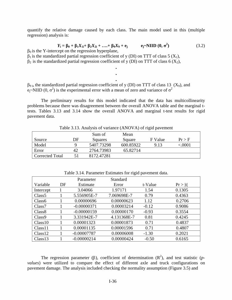
The preliminary results for this model indicated that the data has multicollinearity problems because there was disagreement between the overall ANOVA table and the marginal t-tests. Tables 3.13 and 3.14 show the overall ANOVA and marginal t-test results for rigid pavement data.

Table 3.13. Analysis of variance (ANOVA) of rigid pavement

Sum of Mean Source DF Squares Square F Value Pr > F Model 9 5407.73298 600.85922 9.13 <.0001 Error 42 2764.73983 65.82714 Corrected Total 51 8172.47281

Table 3.14. Parameter Estimates for rigid pavement data. Parameter Standard Variable DF Estimate Error t-Value Pr > |t| Intercept 1 3.04066 1.97171 1.54 0.1305 Class5 1 5.556905E-7 7.069698E-7 0.79 0.4363 Class6 1 0.00000696 0.00000623 1.12 0.2706 Class7 1 -0.00000371 0.00003214 -0.12 0.9086 Class8 1 -0.00000159 0.00000170 -0.93 0.3554 Class9 1 3.331942E-7 4.131368E-7 0.81 0.4245 Class10 1 0.00001323 0.00001873 0.71 0.4837 Class11 1 0.00001135 0.00001596 0.71 0.4807 Class12 1 -0.00007787 0.00006008 -1.30 0.2021 Class13 1 -0.00000214 0.00000424 -0.50 0.6165

The regression parameter (β), coefficient of determination (R2), and test statistic (p-

values) were utilized to compare the effect of different axle and truck configurations on pavement damage. The analysis included checking the normality assumption (Figure 3.5) and

I-36

0.0 0.2 0.4 0.6 0.8 1.0Observed Cum Prob

0.0

0.2

0.4

0.6

0.8

1.0

Expe

cted

Cum

Pro

b

Figure 3.5. Normality plot

-1 0 1 2Regression Standardized Predicted Value

-3

-2

-1

0

1

2

3

Regr

essi

on S

tand

ardi

zed

Resi

dual

Figure 3.6. Predicted versus residual plot

I-37

constant variance of the residual (Figure 3.6), as well as deleting the influential points based on Cook’s distance as shown in Figure 3.7.

Stepwise regression was also used to confirm the results from simple and multiple linear regressions. Stepwise regression is a technique for choosing the variables to include in a multivariate regression model. Forward stepwise regression starts with no model terms. At each step, it adds the most statistically significant term (the one with the highest F statistic or lowest p-value) until the addition of the next variable makes no significant difference. An important assumption behind the method is that some input variables in a multiple regression do not have an important explanatory effect on the response. Stepwise regression keeps only the statistically significant terms in the model.

0 5 10 15 20 25 30Project number

0.00

0.10

0.20

0.30

0.40

0.50

Cook

's D

ista

nce

1

25

Figure 3.7. Cook’s distance

3.5.1.1 Standardized Regression Coefficient

The standardized regression coefficient or the standardized slope has been documented as a measure to compare the relative importance of different independent variables (Dillon, W. and M. Goldstein, 1984, and Allen, J.C., 2001). Standardized slope values are determined by converting all variables (dependent and independent) into Z-scores. Having the variables in Z-score form will convert the distribution mean to zero and standard deviation to one, such that all variables will have a common measurement scale and one can determine which independent

I-38

variable is relatively more important. The following equation represents the non-standardized simple linear regression.

β XaY += (3.3)

Where:

Y = dependent variable (performance)

a = intercept

β = non-standardized slope

X = independent variable (e.g., single-tandem or multiple axle repetitions)

The following equations represent the standardized simple linear regression:

*** Xβ Y = (3.4)

xx s

XXZX −==* (3.5)

yy s

YYZY −==* (3.6)

Where:

Y* = standardized dependent variable,

β* = standardized slope,

Y = average value of dependent variable,

X* = standardized independent variable, and

X = average value of independent variable,

s = sample standard deviation

The same procedures were used to standardize the regression coefficient parameters in

multiple and stepwise regression. The standardized slope was used to compare the relative effect of the axle/truck configurations in all regression analyses presented in the following sections. Standardization of the variables in regression having a polynomial form can potentially reduce the problem of multicollinearity as well (Kim, 1999) because of implicit centering and scaling of the variables.

3.5.2 Multicollinearity Diagnosis Tests

There are several methods that can be used to diagnose the existence of multicollinearity in the data. Some of these methods are:

I-39

1. Disagreement between the F-test in the overall ANOVA table and the marginal t-tests as

mentioned before. 2. Imprecise estimation of the regression parameters (β’s); Some of the β values are

negative, which is unacceptable. 3. Large standard error for the regression parameters, which was the case for all pavement

types. 4. Variance Inflation Factor, VIF, measures how much the variance of a coefficient is

increased because of multicollinearity. Table 3.15 shows the VIF for all pavement types. VIF of 10 or more indicates serious multicollinearity problem.

Table 3.15. Variance inflation factor Rigid-

Interstate Rigid-US

roads Flexible-Interstate

Flexible-US roads

Flexible-M roads

Composite-Interstate

Composite-US roads

Class 5 16.8 16.88 218.2 29.9 31.8 6.2 6.4 Class 6 18.7 18.7 218.2 128.3 5.4 6.1 19.9 Class 7 7.8 7.8 NA 21.6 5.3 5.3 10.3 Class 8 4.8 4.8 NA 1835.3 117.3 54.8 24.9 Class 9 48.6 48.6 NA 4629.14 108.6 39.8 23.0

Class 10 26.7 26.7 NA 132.4 45.3 62.4 34.1 Class 11 35.6 35.6 NA 763.3 17.0 41.8 7.4 Class 12 25.6 25.6 NA 511.5 NA 62.6 7.7 Class 13 14.64 14.6 NA 285.9 NA 9.7 13.1

3.5.3 Remedies for the Multicollinearity Problem

There are several methods suggested in the literature to remedy the multicollinearity problem. Some of these methods are outlined below:

1. One or several predictor variables may be dropped from the model in order to reduce the

multicollinearity and standard error of the regression parameters. In our case, this method called for removing truck classes 9 and 13 from the analysis. This is not acceptable since truck class 13 includes the heaviest trucks and truck class 9 represents 33 % of the total truck population. Therefore, this method was not selected.

2. Principle component analysis can be used to form one or several composite indices based on the highly correlated predictor variables. The principle components method provides composite indices that are uncorrelated. The results from principle component analysis indicated that more than 83% of the variance can be explained by components composed of all truck classes. Therefore, this method was not selected since it lumps totally dissimilar truck configurations together, which is not desirable for meeting the objective of this research.

3. Ridge regression is one of the remedies for such a problem. Ridge regression introduces bias to the diagonal of X'X (where X is n * k matrix of independent variables, and X' is the inverse of X matrix) for calculating the regression coefficients, shrinks the coefficient values toward zero, and decreases the standard error of the coefficients. The method introduces a biasing coefficient, theta, into the regression equation, thereby reducing the

I-40

estimated coefficient error. The resulting coefficient estimates are biased, but are often more accurate than those obtained from standard multiple regression analysis. In our case, a very high value of theta was required. This will introduce significant bias, and therefore, is not acceptable.

4. Based on judgment, combine similar truck configurations.

Based on the above analyses, none of the remedies for the multicollinearity problem met the objective of this research; therefore, the analysis was done using the last method (combining similar truck configurations). Single and tandem axles/trucks were lumped together as one group and multiple axles/trucks (tridem, quad, 5-axle, 6-axle, 7-axle, and 8-axle) were lumped together as another group.

3.6 REGRESSION ANALYSIS RESULTS FOR FLEXIBLE PAVEMENTS

The most logical way to compare the effect of different correlated axle/truck configurations and truck classes was to group similar configurations together. Therefore, axles/trucks were categorized into two groups: 1) single-tandem, and 2) multiple axles/trucks. FHWA truck classes have nine different truck types (classes 5 through 13). Classes 7 and 12 were excluded based on their low percentage and class 5 was excluded due to the insignificant effect caused by its light weight. Trucks with single and tandem axles can be found in classes 6, 8, 9, 10, and 11, while trucks with multiple axles are only in class 13. A given weigh station can be the source of traffic data for several subsections based on their age; while the level of traffic is the same for these subsections, their different ages will make their cumulative traffic different.

The results from the analyses are summarized in Table 3.16. The results show that

multiple axles/trucks are significant and show higher β values than single-tandem axles/trucks, which are not significant. This indicates that rutting is more influenced by heavier loads (axle/truck gross weight), this also agrees with the analytical results of other researchers (Gillespie et al., 1993). It should be noted that the regression coefficients determined using the standardized variables, as has been done in this analysis, should be used for comparison purpose only. The magnitude of the coefficients do not have the same units as would be the regression variables namely, the number of repititions and distress were used directly. It is also important to realize that standardization of the variables leads to their scaling. Therefore, originally non-linear relationships may tend to towards being linear in the case of large standard deviation of the variables or exaggerated if the standard deviations were much smaller than one.

I-41

I-42

Table 3.16. Effect of different truck/axle configurations on pavement rutting

Simple linear regression Multiple linear regression Stepwise regression Axle/Tru

ck

Configu

rations

Independent

variables

β P- value R2 β P- value R2 β P- value R2

1 and 2 0.399 0.032 0.159 0.059 0.773 N/S* NA Axle

types 3, 4, 5, 6, 7, and 8 0.441 0.017 0.194 0.715 0.002 0.58

0.790 0.0000 0.578

1 and 2 0.283 0.137 0.079 -0.009 0.957 N/S* NA Truck

types 3, 4, 5, 6, 7, and 8 0.440 0.017 0.193 0.769 0.0006 0.584

0.695 0.0000 0.584

6, 8, 9, 10, and 11 0.395 0.004 0.156 0.073 0.6316 N/S* NA Truck

classes 13 0.537 0.0004 0.288 0.590 0.0003 0.412

0.639 0.0000 0.409

*N/S: not selected by model

It should be noted that the R2-values for simple linear regression analyses are low;

however this is expected since the individual axle/truck groups will not solely explain the distresses. A significant improvement of R2-values occurs when using multiple linear regression except for the analysis of FHWA truck classes. This refers to the fact that truck class 13 has some single and tandem axle trucks. More importantly, the main goal of using these regression models is to have a relative comparison; they are not suggested for any future prediction.

The statistical results for DI are shown in Tables 3.17. The results show the standardized

regression coefficients (β values), p-values, and R2 for DI. The β values for single-tandem axles/trucks from all three different regression methods are higher than those of multiple axles/trucks. More importantly, the p-values for multiple axles/trucks show that they are not significant (p > 0.05), suggesting that multiple axles cause less cracking damage per load carried. This conclusion agrees with the laboratory investigations conducted on the HMA mixture (Chatti and El Mohtar, 2004 and El Mohtar, 2003).

The statistical results for RQI are shown in Table 3.18. Single-tandem axles/trucks show

higher β values than multiple axle/trucks. However, even though p-values for both axle/truck configurations are significant (p<0.05), β values for multiple axles are negative. This can be interpreted to mean that pavement sections with higher proportion of multiple axles/trucks configurations tend to have lower RQI values (lower roughness), while those with a higher proportion of single and tandem axle/truck configurations tend to have higher RQI values (higher roughness). To date, no known analytical or laboratory-based investigation has been conducted to look at the effect of different axle/truck configurations on pavement roughness; therefore the results reported herein could not be independently verified. This means that, for the RQI results, there was not enough evidence to draw a firm conclusion.

Table 3.17. Effect of Different Truck/Axle Configurations on Pavement DI Simple linear regression Multiple linear regression Stepwise regression Axle/Truck

Configurations

Independent

variables β P- value R2 β P- value R2 β P- value R2

1 and 2 0.430 0.02 0.185 0.617 0.032 0.585 0.001 Axle types

3, 4, 5, 6, 7, and 8 0.265 0.164 0.070 -0.040 0.883 0.343

N/S* NA 0.342

1 and 2 0.466 0.011 0.218 0.580 0.007 0.654 0.003 Truck types

3, 4, 5, 6, 7, and 8 0.272 0.154 0.074 0.122 0.540 0.437

N/S* NA 0.427

6, 8, 9, 10, and 11 0.272 0.048 0.074 0.340 0.090 0.301 0.028 Truck classes

13 0.095 0.497 0.009 -0.053 0.790 0.092

N/S* NA 0.091

* N/S: not selected by model

Table 3.18. Effect of Different Truck/Axle Configurations on Pavement RQI

Simple linear regression Multiple linear regression Stepwise regression Axle/Truck

Configurations

Independent

variables β P- value R2 β P- value R2 β P- value R2

1 and 2 0.129 0.502 0.017 1.019 0.0006 N/S* NA Axle types

3, 4, 5, 6, 7, and 8 -0.264 0.166 0.069 -1.092 0.0003 0.424

N/S* NA NA

1 and 2 0.318 0.093 0.101 0.796 0.00020 N/S* NA Truck types

3, 4, 5, 6, 7, and 8 -0.268 0.159 0.072 -0.751 0.00037 0.473

N/S* NA NA

6, 8, 9, 10, and 11 -0.111 0.435 0.012 0.608 0.00356 0.608 0.00356 Truck classes

13 -0.423 0.002 0.179 -0.909 0.00003 0.314

-0.909 0.00003 0.314

*N/S: not selected by mode

I-43

3.7 REGRESSION ANALYSIS RESULTS FOR RIGID PAVEMENTS

Unlike for flexible pavements, rigid pavements analysis was conducted using only one independent variable, FHWA truck class. The effects of these different truck classes on rigid pavement distresses were investigated using multiple linear regression.

The regression parameter (β), coefficient of determination (R2), and test statistic (p-values) were utilized to compare the effect of different axle and truck configurations on DI and RQI. The analysis included checking the normality assumption (Figure 3.8) and constant variance of the residual (Figure 3.9).

(a) DI (b) RQI

Figure 3.8. Residual distribution

(a) DI (b) RQI

Figure 3.9. Residual variance

I-44

As mentioned above, the most logical way to compare the effect of different correlated truck configurations/truck classes was to group similar configurations together. Therefore, trucks were categorized into two groups: 1) single-tandem trucks, and 2) multiple axle trucks. FHWA truck classes have nine different truck types (classes 5 through 13). Classes 7 and 12 were excluded based on their low percentage and class 5 was excluded due to the insignificant effect caused by its light weight. Trucks with single and tandem axles can be found in classes 6, 8, 9, 10, and 11, while trucks with multiple axles are only in class 13. A given weigh station can be the source of traffic data for several subsections based on their age; while the level of traffic is the same for these subsections, their different ages will make their cumulative traffic different.

The results from the analyses are summarized in Table 3.19. The results show that single

–tandem-axle trucks are significant for distress index (cracking) (β= 0.668 and p-value = 0.000) compared to multiple axle trucks (β= 0.129 and p-value 0.294). These results fairly agree with the laboratory investigation, discussed in later volumes of this report, which showed that multiple axles are less damaging (per load carried) for fatigue cracking. Conversely, multiple-axle trucks are significant for ride quality index (pavement roughness) and show higher β values and lower P-value than single-tandem-axle trucks, which are not significant. These conclusions are based only on the analysis of in-service pavement data and need to be verified from the laboratory and mechanistic investigations.

Table 3.19. Effect of different truck configurations on rigid pavement distress—DI and RQI

DI RQI Axle/Truck

Configurations

Independent

variables β P- value R2 β P- value R2

6, 8, 9, 10, and 11 0.668 0.000 -0.007 0.961 Truck classes

13 0.129 0.294 0.569

0.655 0.000 0.424

I-45

3.8 CONCLUSION

3.8.1 Analysis of In-service Flexible Pavement Performance Data Based on the analyses of in-service pavement performance data to determine the effect of heavy multiple axle trucks on flexible pavement damage, the following main conclusions can be drawn:

1. Trucks with single and tandem axles affect pavement cracking (DI) more than those with multiple axles (tridem and higher).

2. Conversely, heavier trucks with multiple axles have more effect on rutting than those with single and tandem axles.

3. RQI results did not show enough evidence to draw a firm conclusion.

3.8.2 Analysis of In-service Rigid Pavement Performance Data Based on the analyses of in-service pavement performance data to determine the effect of heavy multiple axle trucks on rigid pavement damage, the following main conclusions can be drawn:

1. Trucks with single and tandem axles affect pavement cracking (DI) more than those with multiple axles (tridem and higher).

2. Conversely, heavier trucks with multiple axles have more effect on roughness (RQI), which is an indirect measure of faulting, than those with single and tandem axles.

3.8.3 Recommendation for Further Analysis The statistical analyses on in-service pavement performance data have not led to definitive conclusions that can be implemented in a quantitative manner. Rather, they have highlighted general apparent trends that need to be confirmed with mechanistic analyses, controlled laboratory testing, or better yet, accelerated pavement testing (APT). Volumes II and III of this report contain details of laboratory and mechanistic analyses in support of the study objectives for flexible and rigid pavements, respectively. Full-scale accelerated pavement testing (APT) was outside the scope of this study. However, it is recommended that such tests be conducted in a future study. Since MDOT does not have an APT facility, it is recommended that MDOT consider joining other State Highway Agencies (SHA) in conducting a pooled fund study to support the findings of this study using full-scale APT tests.

I-46

REFERENCES Ali, H. A., S. D Tayabji., and, F. La Torre, "Calibration of mechanistic-empirical rutting model for in-service pavements." Transportation Research Record No. 1629, 1998, pp159-168. Ali, H. A., and S. D. Tayabji, "Using transverse profile data to compute plastic deformation parameters for asphalt concrete pavements." Transportation Research Record No. 1716 , 2000, pp 89-97. Allen, J.C. (2001), “Species-Habitat Relationships For The Breeding Birds of A Longleaf Pine Ecosystem” Master of Science in Ecology, Faculty of the Virginia Polytechnic Institute and State University. Benkelman, A.C., “Tests of Aggregate Interlock at Joints and Cracks,” Engineering News Record, V. III, No. 8, Aug. 1933, pp. 227-232 Buch, N., Frabizzio, M.A., and Hiller, J.E., “Factors Affecting Shear Capacity of Transverse Cracks in Jointed Concrete Pavements (JCP),” Final report to Michigan Department of Transportation. Michigan State University, 2000 Chatti, K. and H. S. Lee, “Evaluation of Strain and Energy Based Fatigue prediction Methods for Asphalt Pavement Subjected to Multiple Axle Loading” International Journal of Pavements, 2004, Vol. 3 No. 1& 2. Chatti, K. and El Mohtar, C. (2004), “Effect of Different Axle Configurations on Fatigue Life of Asphalt Concrete Mixture” Transportation Research Record, n 1891, p 121-130 Claussen, A. I. M., J. M. Edwwareds, P. Sommer, and P. Uge 1977, "Asphalt Pavement Design -The Shell Method." Proceedings, 4th International Conference on the Structural Design of Asphalt Pavement, 1977, pp. 39-74. Clemmer, H.F., “Fatigue of Concrete,” American Society of Testing and Material, Proceedings, 22, Part II, 1922, pp. 409-419 Colley, B.E., and Humphrey, H.A., “Aggregate Interlock at Joints in Concrete Pavements,” In Highway Research Record 189, HRB, National Research Council, Washington, D.C., 1967, pp. 1-18 Darter, M.I., “Concrete Slab vs. Fatigue Models,” Proceedings, Second International Workshop on the Theoretical Design of Concrete Pavements, Siguenza, Spain Darter, M.I., and E.J. Barenberg, “Design of Zero-Maintenance Plain Jointed Concrete Pavements, Volume II Design Manual,” FHWA RD 77-112, Federal Highway Administration, Washington D.C.

I-47

Darter, M.I., “Initial Evaluation for Michigan JRCP Crack Deterioration,” Michigan Concrete Paving Association, Mahomet, Ill., Dec. 1988, rev. Feb., 1989 Dillon, W. and M. Goldstein (1984), “Multivariate Analysis Method and Applications” John Wiley & Sons. El Mohtar, C. (2003), "The Effect of Different Axle Configurations on the Fatigue Life of an Asphalt Concrete Mixtures," MS., Michigan State University, E. Lansing MI 48824. Foxworthy, P.T., Concepts for the Development of a Nondestructive Testing and Evaluation System for Rigid Airfield Pavements, Ph.D. Dissertation, University of Illinois, Urbana, IL, 1985 Gillespie, T.D., S. M. Karamihas, M. W. Sayers, and, D. Cebon, "Effects of Heavy-Vehicle Characteristics on Pavement Response and Performance." NCHRP Report 353, 1993, The University of Michigan, Transportation Research Institute, Ann Arbor, Michigan. Hajek, J. J., and A. C. Agarwal, “Influence of Axle Group Spacing on Pavement Damage” Transportation Research Record, No. 1286, 1990, pp. 138-149. Hanekom, A.C., Horak, E., Visser, A., “Aggregate Interlock Transfer Efficiency at Joints in Concrete Pavements During Dynamic Loading,” Proceedings, 7th International Conference on Concrete Pavements, Sept., 9-13, 2001, Orlando, FL Hatt, W.K., “Fatigue of Concrete,” Highway Research Board, Proceedings, 4, 1924, pp. 47-60 Hiller, J.E., Roesler, J.R., “ Transverse Joint Analysis for Mechanistic_Empirical Design of Rigid Pavments,” Transportation Research Record, No. 1809, Washington D.C., 2002, pp. 42-51 Hiller, J.E., Roesler, J.R., “Determination of Critical Concrete Pavement Damage Locations using Influence Lines,” Journal of Transportation Eng., V. 131, No. 8, 2005, pp. 599-607 Hilsdorf, H.K., and Kesler, C.E., “ fatigue Strength of Concrete under Varying Flexural Stress,” ACI Journal, Proceedings, V. 63, No. 10, Oct. 1966, pp. 1059-1076 Holmen, J.O. (1982). “Fatigue of concrete by constant and variable amplitude loading,” ACI Publication SP75-4, 1982, pp. 71-110 Hsu T.T.C., “Fatigue of Plain Concrete,” ACI Journal, 1981, V. 78, No. 4, 292-305 Ilves, G. J., and Majidzadeh, K., "Reevaluation of the Methods for Calculation of Load Equivalency and Damage Ratios,” 1991

I-48

Jensen, E.A., Hansen, W., “Mechanism of Load Transfer-Crack Width Relation in JPCP: Influence of Coarse Aggregate Properties,” Proceedings, 7th International Conference on Concrete Pavements, Sept., 9-13, 2001, Orlando, FL Kenis, W. and W. Wang, "Calibrating Mechanistic Flexible Pavement Rutting Model from Full Scale Accelerating Tests." 8th International conference on asphalt pavement, Seattle, Washington, 1997, pp. 663-672. Kesler, C.E., “Effect of Speed of Testing on Flexural Fatigue Strength of Plain Concrete,” Proceedings of the Highway Research Board, V. 32 Highway Research Board, Washington D.C., 1953 Kim, Doo-Sub, “A Standardization Technique to Reduce the Problem of Multicollinearity in Polynomial Regression Analysis”, Proceedings, Bulletin of the International Statistical Institute, 52nd Session, Volume LVIII, Finland, 1999. Kim, H. B., "Framework for incorporating rutting prediction model in the reliability-based design of flexible pavements," 1999, Ph.D. Dissertation, Department of Civil and Environmental Engineering, Michigan State University, East Lansing, MI, USA. Lee, Dah-yinn, Klaiber, F. Wayne, Coleman, Jeff W., “Fatigue Behavior of Air-Entrained Concrete,” Transportation Research Board, Washington D.C., No. 671, Jan.,1978, pp.20-23 Matthews, J. M., Monismith, C. L., and Craus, J, "Investigation of laboratory fatigue testing procedures for asphalt aggregate mixtures," Journal of Transportation Engineering, 119(4), 1993, pp.634-654. McCall, J.T. “Probability of Fatigue Failure of Plain Concrete,” Proceedings, American Concrete Institute, V. 55, No. 13, 1958, Detroit, MI Miner, M.A. Cumulative Damage in Fatigue. Transactions, American Society of Mechanical Engineers, V. 67, pp. A159-A164 Moavenzadeh, F., J. E. Soussou, H. K. Findakly, and B. Brademeyer, "Synthesis for rational design of flexible pavement," FH 11-776, Federal Highway Administration, 1974 Murdock, J.W., and C.E. Kesler, “Effect of Range of Stress on the Fatigue Strength of Plain Concrete,” Journal of the American Concrete Institute, V. 30, No.2, 1958, Detroit, MI Nowlen, W.J., “Influence of Aggregate Properties on Effectiveness of Interlock Joints in Concrete Pavements,” Journal of the PCA, Research and Development Laboratories, V. 10, No. 2, May 1968, pp.2-8

I-49

Oh, B.H., “Fatigue of Concrete by Constant and Variable Amplitude Fatigue Loading.” ACI Materials Journal, January-February, Title no. 88-M6, 1991, pp. 41-48 Older, C., “Bates Experimental Road,” State of Illinois, Department for Public Works and Buildings, Division of Highways, Bulletin No. 18, Jan 1922 Older, C., “Highway Research in Illinois,” American Society of Civil Engineers, Transactions, 87,1924, pp. 1180-1222 Raja, Z.I., and Snyder, M.B., “ Factors affecting Deterioration of Transverse Cracks in Jointed Reinforced Concrete Pavements,” Transportation Research Record 1307, TRB, National Research Council, Washington, D.C., 1991, pp.162-168 Roesler, J.R., Fatigue of Concrete Beams and Slabs, Ph.D. Dissertation, University of Illinois, Urbana, IL, 1998 Sebaaly, P. E., and Tabatabaee, N., "Effect of Tire Parameters on Pavement Damage and Load-Equivalency Factors." Journal of Transportation Engineering, 118(6), 1992, pp.805-819. Shi, X.P., Fwa, T.F., and Tan, S.A. “ Flexural Fatigue Strength of Plain Concrete,” ACI Material Journal, V. 90, No. 5, 1993, pp. 435-440 Shook, J. F., F. N. Finn, M. W. Witczak, and C. L. Monismith, "Thickness Design of Asphalt Pavement - The Asphalt Institute Method." Proceedings, 5th International Conference on the Structural Design of Asphalt Pavement, 1982 pp.17-44. Singh, S.P. and Kaushik, S.K., “Flexural Fatigue Life Distributions and Failure Probability of Steel Fibrous Concrete,” ACI Material Journal, Vol. 97, No.6, 2000, pp. 658-667 Tepfers, Ralejs, and Kutti, Thomas, “Fatigue Strength of Plain, Ordinary, and Lightweight Concrete,” ACI Journal, Proceedings, V. 76, No. 5, May 1979, pp. 635-652 Tepfers, Ralejs “Tensile Fatigue Strength of Plain Concrete,” ACI Journal, Proceedings, V. 76, No. 8, Aug 1979, pp. 919-933 Ullidtz, P. (1987), “Pavement Analysis,” Elsevier. Yun, K.K. and Kim, D.H., “Fatigue Behavior of Pavement Concrete by Splitting Tension Fatigue Test,” 82nd Transportation Research Board, Washington D.C., Jan., 2003 Zhang B., Phillips D.V. and Wu K., “Effect of Loading Frequency and Stress Reversal on Fatigue Life of Plain Concrete,” Magazine of Concrete Research, 1996, V. 48, No. 177, 361-375

I-50

APPENDIX A

Beginning of the CS

18024Location of the weigh station

Ending of the CS 18024

Segment taken into consideration

Figure A-1. Variation of the traffic along the CS # 18024

I-51

Beginning of CS # 22023

End of CS # 22023 and beginning of CS #

55021

End of CS # 55021

Location of the weigh station

Figure A-2. No variation of the traffic along two consecutive control sections (CS # 22023 and 55021)

I-52

0 2400000 4800000 7200000 9600000 12000000 14400000 16800000

0

5

10

15

20

25

30

35

Percent

cl ass50 440000 880000 1320000 1760000 2200000 2640000 3080000

0

5

10

15

20

25

30

35

Percent

cl ass6

0 80000 160000 240000 320000 400000 48

0

10

20

30

40

50

60

Percent

cl ass7

25

0 4600000 9200000 13800000 18400000 23000000 276

0

2. 5

5. 0

7. 5

10. 0

12. 5

15. 0

17. 5

20. 0

Percent

cl ass9

0 130000 260000 390000 520000 650000 78

0

5

10

15

20

25

Percent

cl ass11

N=52 N=52

Figure A-3. Distribution of to

N=52

0000 5600000 740000 1480000 2220000 2960000 3700000 44

0

5

10

15

20

Percent

cl ass8

00000 322000000 340000 680000 1020000 1360000 1700000

0

5

10

15

20

25

30

35

Percent

cl ass10

0000 910000

0 22000 44000 66000 88000 110000

0

5

10

15

20

25

30

35

Percent

cl ass12

tal truck traffic for classes 5 through 12-rigid pav

I-53

N=52

40000 5180000

N=52

N=52

2040000 2380000

N=52

N=52

132000 154000

ements

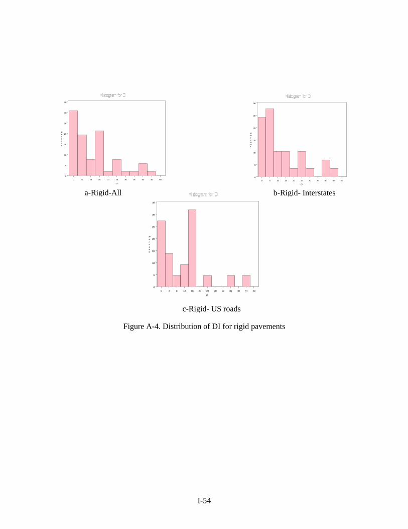
a-Rigid-All b-Rigid- Interstates

0 5 10 15 20 25 30 35 40 45 50

0

5

10

15

20

25

30

35

Percent

DI

0 4 8 12 16 20 24 28 32 36 40 44 48

0

5

10

15

20

25

30

35

Percent

DI

0 5 10 15 20 25 30 35 40 45 50

0

5

10

15

20

25

30

Percent

DI

c-Rigid- US roads

Figure A-4. Distribution of DI for rigid pavements

I-54

0 10 20 30 40 50 60 70 80 90 100

0

5

10

15

20

25

30

35

40

45

Percent

RQI

0 10 20 30 40 50 60 70 80 90 100

0

10

20

30

40

50

60

70

Percent

RQI

0 10 20 30 40 50 60 70 80 90 100

0

5

10

15

20

25

30

35

Percent

RQI

Figure A-5. Distribution of RQI for composite pavements

a-Composite-All b-Composite-Interstate

c-Composite-US roads

I-55

I-56

0 0. 05 0. 1 0. 15 0. 2 0. 25 0. 3 0. 35 0. 4 0. 45 0. 5 0. 55 0. 6

0

5

10

15

20

25

Percent

Rut t i ng

0 0. 05 0. 1 0. 15 0. 2 0. 25 0. 3 0. 35 0. 4 0. 45 0. 5 0. 55 0. 6

0 0. 05 0. 1 0. 15 0. 2 0. 25 0. 3

0

5

10

15

20

25

30

35

Percent

Rut t i ng

0. 35 0. 4 0. 45 0. 5 0. 55 0. 6

0

5

10

15

20

25

30

35

Percent

Rut t i ng

0 0. 05 0. 1 0. 15 0. 2 0. 25 0. 3 0. 35 0. 4 0. 45 0. 5 0. 55 0. 6

0

5

10

15

20

25

30

35

Percent

Rut t i ng

a-Flexible-All b-Flexible-Interstate

c-Flexible-US roads c-Flexible-US roads

Figure A-6. Distribution of rutting for flexible pavements

I-57

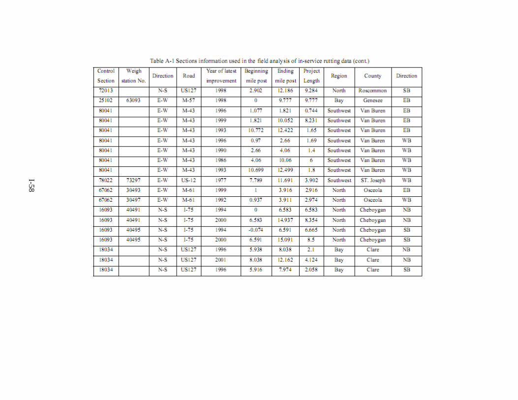
I-58

I-59

I-60

I-61

I-62

I-63

Table A-3. Rigid pavement projects

Vehic Vehi V Vehicle class Vehicle cla Age D oad Vehicle class

5 Vehicle class 6 Vehicle class 7 le class 8 cle class 9 ehicle class 10 Vehicle class 11 12 ss 13 I R class

1 43 61 72 81 485 614 156585 2409 2975 6. Inter24155 4295 270 9060 4135 295 0 115 33 28 state

2 3 46 48 60 387 421 7227 24090 278239 33 7.2 Inter059430 9755 180 2250 8490 575 0 5 2 state

3 2 31 84 38 19 16 4416 4015 104390 11 16. US r686035 7185 315 5440 63335 0600 5 0 85 oads

4 2 43 109 124 991 31 350400 6022 1138 6. Inter518500 2525 50 8300 5225 2075 5 800 15 80 state

5 2 49 12 14 112 35 3971 6825 1290 3. Inter854300 0195 410 14740 37255 3685 20 5 640 17 53 state

6 25 43 109 124 991 312 3504 6022 1138 1. Inter18500 2525 50 8300 5225 075 00 5 800 15 04 state

7 7366701 34 30 26 28 4745 6832 26 35. US r1640 0 3680 00260 4700 0 0 80 81 oads

8 418 6460 8979 515745 3832 8760 2190 241995 3 2. US r290 5 0 0 5 34 oads

9 1 13 11 430 20 67 2219 1460 6482 1. US r676080 4320 680 9920 06040 160 20 0 40 8 39 oads

10 3314 0 242360 2044 473040 7519000 210240 259880 7008 8993 3. US r20 0 0 60 8 03 oads

11 2 18 15 35 56 15 1949 5256 6745 16. US r485650 1770 330 4780 39250 7680 10 0 20 6 42 oads

12 7 51 43 100 159 44 5522 1489 1911 16. US r042675 5015 435 5210 77875 6760 45 20 140 17 22 oads

13 2 22 32 24 30 20 6570 10950 102930 30 14.8 US r124300 9950 850 0900 00300 8050 0 0 4 oads

14 1 27 20 27 29 23 4088 20440 137970 28 12.9 US r880480 5940 440 5940 12700 5060 0 0 5 oads

15 0 0 0 0 0. S 0 0 0 0 0 0 21 U roads

16 1 51 36 5 1 1 0 5292 1 0.7 US49285 100 50 5115 73740 5330 730 5 3 roads

17 6 0 0 2555 1 1. M r17520 2190 365 2555 205 2190 08 oads

18 9 14 146 21 55 10 700 18980 45698 4 0.7 Inter75280 1620 00 0240 34860 6580 80 0 2 state

19 11 88 80 120 90 36 1124 0 152570 44 15. US r258060 3300 300 4500 41780 9380 20 0 08 oads

20 8 85 14 136 97 33 1284 0 157388 44 16. US r094240 1180 4540 5100 16300 7260 80 0 66 oads

21 4 84 38 107 268 50 498225 7665 1823 15 14. nter538775 8625 325 3100 60350 3700 0 175 33 I state

22 3 83 54 88 253 66 377775 7117 1626 26. Inter356175 7675 750 1475 21875 7950 5 075 15 93 state

23 6 16 14 703 93 1277 27375 439825 5 18. Inter04075 4250 9125 9650 3550 075 50 63 state

24 6 20 15 658 14 1131 21900 306600 5 2.9 Inter22325 2575 5475 1475 0950 4175 50 4 state

25 147460 17885 365 43800 1044630 15695 29200 1460 8030 1 0.00 Interstate

26 4423800 536550 10950 1314000 31338900 470850 876000 43800 240900 30 42.22 Interstate

27 4718720 572320 11680 1401600 33428160 502240 934400 46720 256960 32 31.78 Interstate

28 142350 22995 365 49640 1063245 17885 29930 1460 11315 1 0.14 Interstate

29 4555200 735840 11680 1588480 34023840 572320 957760 46720 362080 32 26.50 Interstate

30 1073100 362810 15330 1722070 9857190 173740 97090 10220 245280 14 2.62 Interstate

I-64

31 1303050 440555 18615 2091085 11969445 210970 117895 12410 297840 17 3.20 Interstate

32 919800 310980 13140 1476060 8449020 148920 83220 8760 210240 12 15.67 Interstate

33 1328600 332150 4745 1670240 3098485 66430 109135 9490 223015 13 3.45 Interstate

34 1226400 306600 4380 1541760 2860140 61320 100740 8760 205860 12 7.68 Interstate

35 1543220 196735 22995 365365 3628100 122640 212065 30660 587650 7 0.43 US roads

36 1578990 194180 22995 273385 4928595 168630 171185 43435 651525 7 0.17 US roads

37 902280 110960 13140 156220 2816340 96360 97820 24820 372300 4 0.78 S ro U ads

38 3383550 416100 49275 585825 10561275 361350 366825 93075 1396125 15 2.15 o US r ads

39 50 167 241 250 683 669 142 0 1921 39 17.43 oa67660 9730 995 5360 2800 045 35 725 US r ds

40 74 255 182 275 868 766 3650 0 2646 50 42.03 oa64250 5000 500 5750 7000 500 0 250 US r ds

41 58 199 142 214 677 597 2847 0 2064 39 10.40 oa22115 2900 350 9485 5860 870 0 075 US r ds

42 16 28 73 83 661 208 2336 40150 7592 10 9.60 st79000 8350 00 2200 0150 050 00 00 Inter ate

43 65 112 284 324 2577 811 9110 1565 2960 25.88 s48100 4565 70 5580 9585 395 40 85 880 39 Inter tate

44 11 0 8833 8030 1204 9041 3693 1124 0 1525 44 22.83 oa25806 00 0 500 780 80 20 700 US r ds

45 88 92 157 148 105 367 1401 0 1716 48 6.32 oa30 008 856 0 68 0 92 00 9960 0 92 0 60 960 US r ds

46 3 98 54 89 42 55 766 16425 263 0. s62445 550 75 790 20130 845 50 895 3 58 Inter tate

47 1 32 18 29 14 18 255 5475 879 0. s20815 850 25 930 06710 615 50 65 1 01 Inter tate

48 3 98 54 89 42 55 766 1642 263 0. s62445 550 75 790 20130 845 50 5 895 3 00 Inter tate

49 17 24 59 509 219 187 722 6424 9459 44 37.92 st200260 41120 4220 1020 70080 9020 700 0 340 Inter ate

50 14 31 22 546 246 242 7548 4818 8158 44 45.57 st309460 47760 4840 0400 03920 5060 20 0 480 Inter ate

51 9 3 131 147 84 14 832 8760 210 12 14.87 st19800 10980 40 6060 49020 8920 20 240 Inter ate

52 00 4380 1541760 2860 100740 8760 2058 10. s1226400 3066 140 61320 60 12 25 Inter tate

I-65

Table A-4. Flexible pavement projects V 8 V V 12 R Vehicle class 5 Vehicle class 6 Vehicle class 7 ehicle class ehicle class 9 ehicle class 10 Vehicle class 11 Vehicle class Vehicle class 13 Age DI oad class

1 459170 13870 4380 34310 128480 3650 4380 0 9490 2 4.09 US roads

2 0 1 435080 64240 1460 91980 659920 93440 43800 0 18834 4 6.12 US roads

3 0 0 0 0 0 0 0 0 0 0 7.95 US roads

4 5 273750 26645 1460 31755 219365 15330 11680 365 4489 1 0.88 US roads

5 10 U 450045 101835 6570 93075 603345 73365 33945 0 1292 3 6.21 S roads

6 5 40 In 125560 12045 730 21900 96725 20440 730 36 642 1 0.84 terstate

7 5 80 I 878920 84315 5110 153300 677075 143080 5110 255 4496 7 8.26 nterstate

8 90885 5 0 I 9490 730 27010 81395 7665 1095 36 7008 1 0.76 nterstate

9 20 I 363540 37960 2920 108040 325580 30660 4380 1460 2803 4 5.05 nterstate

10 60 1 I636195 66430 5110 189070 569765 53655 7665 2555 4905 7 1.31 nterstate

11 836580 90 129210 0 179580 1031490 76650 17520 4380 4839 6 2.58 US roads

12 0 2 137240 58400 8760 26280 46720 23360 0 0 3212 8 0.82 M roads

13 5 3. 120085 51100 7665 22995 40880 20440 0 0 2810 7 72 M roads

14 0 210240 48180 4380 19710 28470 4380 0 0 4380 6 4.56 M roads

15 0 175200 40150 3650 16425 23725 3650 0 0 3650 5 0.00 M roads

16 40 11 1 U3621530 124465 4015 228855 630355 64240 12045 0 3051 0.04 S roads

17 0 987690 33945 1095 62415 171915 17520 3285 0 8322 3 5.66 US roads

18 5 509905 76285 4015 88330 686565 52195 12045 4015 33324 11 3.93 US roads

19 5 139065 20805 1095 24090 187245 14235 3285 1095 9088 3 1.21 US roads

20 473040 5 9 59130 9855 68985 167535 59130 0 0 6898 27 4.72 M roads

21 0 251850 11680 2190 9490 21170 5110 0 0 1533 2 8.25 M roads

22 5 303680 24820 1460 30660 52560 17520 0 0 5840 4 1.03 M roads

23 175920 6205 365 7665 13140 4380 0 0 1460 1 2.09 M roads

24 531440 0 43435 2555 53655 91980 30660 0 0 1022 7 2.84 M roads

25 0 99280 13870 1460 9490 30660 8030 730 0 365 2 9.52 M roads

26 0 397120 55480 5840 37960 122640 32120 2920 0 1460 8 7.94 M roads

27 595680 0 2 83220 8760 56940 183960 48180 4380 0 2190 12 1.43 M roads

28 248200 34675 3650 23725 76650 20075 1825 0 9125 5 0.85 M roads

29 90 22 4 U578160 176660 16060 417560 1373130 32120 32120 0 1043 3.61 S roads

30 34310 14600 2190 6570 11680 5840 0 0 8030 2 2.84 M roads

31 0 140160 32120 2920 13140 18980 2920 0 0 2920 4 6.22 M roads

I-66

5 80 I32 878920 84315 5110 153300 677075 143080 5110 255 4496 7 8.49 nterstate

33 730 5 0 I125560 12045 730 21900 96725 20440 36 6424 1 0.97 nterstate

34 7665 5 60 I636195 66430 5110 189070 569765 53655 255 4905 7 3.45 nterstate

35 90885 1 5 0 I 9490 730 27010 81395 7665 095 36 7008 1 0.03 nterstate

36 5475 00 7 U 1646150 56575 1825 104025 286525 29200 0 1387 5 4.50 S roads

37 0 0. 0 0 0 0 0 0 0 0 0 11 US roads

38 5475 5 5 1 231775 34675 1825 40150 312075 23725 182 15147 5 2.31 US roads

39 0 0 0 0 0 0 0 0 0 0 1.04 US roads

40 273750 5 5 0. 26645 1460 31755 219365 15330 11680 36 4489 1 95 US roads

41 0 150015 33945 2190 31025 201115 24455 11315 0 4307 1 3.30 US roads

42 25 U389820 129210 18615 192720 525600 51465 1095 0 1478 3 0.48 S roads

43 75 U447855 153300 10950 165345 521220 45990 2190 0 1587 3 0.09 S roads

44 458075 50 1 87600 3650 105850 941700 71175 54750 1825 2226 5 58.41 US roads

45 25 4 U543850 80300 1825 114975 824900 116800 54750 0 2354 5 7.76 S roads

46 0 183230 35040 1460 42340 376680 28470 21900 730 8906 2 5.34 US roads

47 0 U 91615 17520 730 21170 188340 14235 10950 365 4453 1 6.46 S roads

48 565750 5 7 54750 36500 54750 118625 27375 0 0 13687 25 7.14 M roads

49 0 7 633640 61320 40880 61320 132860 30660 0 0 15330 28 5.25 M roads

50 379600 31025 1825 38325 65700 21900 0 0 7300 5 12.87 M roads

51 455520 37230 2190 45990 78840 26280 0 0 8760 6 7.98 M roads

52 148920 20805 2190 14235 45990 12045 1095 0 5475 3 0.05 M roads

53 198560 27740 2920 18980 61320 16060 1460 0 7300 4 1.17 M roads

I-67

able A-5 Composite pavement projects Vehicle class 5 Vehicle class 6 Vehicle class 7 Vehicle class 8 Vehicle class 9 Vehicle class 10 Vehicle class 11 Vehicle class 12 Vehicle class 13 Age DI Road class

T

1 673790 67160 8030 75920 327770 26280 8030 730 170820 2 3.49343 US roads

2 774165 97090 2555 45990 245280 35770 12775 0 132860 7 22.2604 US roads

3 442380 55480 1460 26280 140160 20440 7300 0 75920 4 5.04638 US roads

4 633275 47450 5475 38325 195275 20075 5475 0 102200 5 21.7124 US roads

5 253310 18980 2190 15330 78110 8030 2190 0 40880 2 2.64367 US roads

6 229585 6935 17155 64240 1825 2190 0 4745 1 0.22222 US roads 2190

7 0 0 ads 0 0 0 0 0 0 0 0 0.21776 US ro

8 459170 128 0 s 13870 4380 34310 480 3650 4380 0 949 2 4.70936 US road

9 7576305 7 2119 602 0 0 85 s 228855 2270 566115 920 25 7227 1565 33 24.0605 US road

10 736935 1958 799 5 5 85 Int e 100740 8760 217905 955 35 7336 1 330 2441 3 0.73992 erstat

11 759930 0 35 2113 9 31 70 Int e 10293 3285 2332 350 4170 75555 1 40 2912 3 2.12459 erstat

12 1622425 0 1 0 2953 24 78 95 Int e 149723 0220 47012 580 2725 132860 1 85 4828 7 18.8595 erstat

13 927100 0 1687 13 02 40 Int e 85556 5840 268640 760 8700 75920 1 20 2759 4 9.60428 erstat

14 1158875 0 2109 1733 2 25 Int e 1069450 7300 33580 700 75 94900 1 775 3449 5 2.16537 erstat

15 0 0 Int te 0 0 0 0 0 0 0 0 0.57788 ersta

16 1197200 1 80 1956 1022 40 Int te 274480 8980 2452 400 105120 77380 0 2540 4 5.28178 ersta

17 1496500 2 00 2445 1277 50 Int te 343100 3725 3066 500 131400 96725 5 3175 5 1.93561 ersta

18 210240 1281 5 ds 44895 2190 17520 15 6570 5475 0 6022 3 10.6419 US roa

19 70080 4088 0 s 6935 1825 6205 0 6935 730 0 1679 1 4.29766 US road

20 858480 1 1 3832 21 50 s 98550 3140 854 0 50 54750 21900 90 1423 6 21.5994 US road

21 391280 2438 0 s 62780 8760 59860 20 29200 14600 0 8468 4 5.74695 US road

22 151840 8 8760 1 0 ds 24820 5840 262 0 0 3140 0 0 5110 4 2.16161 US roa

23 17520 0 5 M s 2190 365 2555 6205 2190 0 255 1 0.44605 road

24 324485 1 4664 288 255 0 Int te 43435 3870 91615 70 35 12410 5 9271 1 3.63863 ersta

25 648970 0 2 0 9329 20 2. 3 Inter te 8687 7740 18323 40 57670 24820 5110 1854 2 41 sta

26 338720 4712 25 95 Int e 54750 6570 92710 15 29930 11315 55 1105 1 0.16461 erstat

27 677440 1 0 9424 90 Int e 109500 3140 18542 30 59860 22630 5110 2211 2 2.46407 erstat

28 975280 0 1 0 5534 8 80 Int e 14162 4600 21024 860 106580 70080 1 980 4569 4 3.84401 erstat

29 1023460 0 0 8219 00 s 8030 7300 10950 80 33580 10220 0 1387 4 7.93091 US road

30 735840 0 1 0 8833 80 ds 7738 3140 12410 00 30660 11680 0 1430 4 9.71173 US roa

31 724890 00 8440 00 3285 90 9 In tate 1971 10950 179580 260 111690 1533 0 5277 6 20.618 ters

I-68

60 0 80 5264 1752 80 Int te 32 4978 16206 4380 1211 760 115340 90520 0 2452 4 6.79588 ersta

33 497860 0 80 5264 7 80 Int e 16206 4380 1211 760 115340 90520 1 520 2452 4 6.79588 erstat

34 248200 7665 5 M s 34675 3650 23725 0 20075 1825 0 912 5 3.84724 road

35 788400 0 2 0 1872 0 50 ds 24090 1900 56940 450 43800 43800 1423 30 207.697 US roa

36 105120 2496 0 s 32120 2920 75920 60 5840 5840 0 1898 4 19.2651 US road

37 562830 3321 73 70 s 37960 2920 76650 50 26280 7300 0 1817 2 3.93304 US road

38 628530 2649 73 20 s 30660 4380 71540 90 21900 7300 0 1416 2 2.53225 US road

39 356240 0 0 8263 60 s 10220 5840 7008 60 93440 73000 2920 1547 8 22.8672 US road

40 267180 619 219 70 s 76650 4380 52560 770 70080 54750 0 1160 6 21.8717 US road

41 400770 5 9296 05 s 11497 6570 78840 55 105120 82125 3285 1741 9 43.207 US road

42 188340 1 4248 146 80 ds 35040 3140 42340 60 37960 37960 0 1357 4 14.7232 US roa

43 94170 2124 73 0 ds 17520 6570 21170 30 18980 18980 0 6789 2 11.8511 US roa

44 235425 1 5310 182 25 ds 43800 6425 52925 75 47450 47450 5 1697 5 40.0743 US roa

45 781830 2 9986 70 Int e 110960 7010 231410 40 85410 32850 2920 4299 2 4.40135 erstat

46 650430 1 0 1118 11 40 Int e 143080 0220 24820 360 0230 34310 2190 3708 2 1.41915 erstat

47 378505 4869 2 32 0 s 42340 2920 54750 10 5550 16425 85 8833 1 2.60571 US road

48 3477355 3 0 3847 22 2 80 s 304045 3215 44968 830 2285 107310 2 995 7562 7 5.07817 US road

49 506620 0 1 0 1106 80 Int e 8687 4600 16863 680 52560 24090 4380 2014 2 0.98932 erstat

50 781100 8380 4 80 Int e 78840 4380 94900 40 34310 16060 1 60 1065 2 1.52444 erstat

51 914325 4 5 2007 80 Int e 442380 4895 42157 135 140160 36135 6570 4861 3 1.77338 erstat

52 1153035 5 5 1134 05 Int e 193815 2560 26389 420 64605 13140 3285 3274 3 1.03763 erstat

53 140160 85410 0 ds 29930 1460 11680 4380 3650 0 4015 2 11.1336 US roa

54 911040 2 5314 70 ds 90155 3725 80665 40 90155 9490 0 2182 13 24.6454 US roa

55 1327140 0 40 4204 0 60 ds 16644 4380 788 80 61320 21900 2277 12 18.1035 US roa

56 1266550 1 5 3905 00 s 94900 0950 766 0 50 40150 10950 0 2044 10 18.6693 US road

57 858480 1 1 3832 1 50 s 98550 3140 854 0 50 54750 21900 2 90 1423 6 13.5815 US road

58 2575440 0 3 30 114975 65 50 s 29565 9420 2562 0 164250 65700 70 4270 18 29.4917 US road

59 391280 2438 0 4 9 ads 62780 8760 59860 20 29200 1460 0 84680 6.4759 US ro

60 1565120 251120 35040 239440 975280 116800 58400 0 338720 16 22.3183 US roads

61 75920 12410 2920 13140 43800 6570 0 0 25550 2 5.74597 US roads

62 227760 37230 8760 39420 131400 19710 0 0 76650 6 10.1018 US roads

63 493480 80665 18980 85410 284700 42705 0 0 166075 13 9.30134 US roads

64 67890 6570 4380 6570 14235 3285 0 0 16425 3 21.2293 M roads

I-69

27375 0 0 136875 25 285.35 M roads 65 565750 54750 36500 54750 118625

66 429970 41610 27740 41610 90155 20805 0 0 104025 19 89.314 M roads

67 243820 3540 650 52560 715 26645 17520 5 1 1 e 5 3 1383 474 14245 3.77568 Interstat

68 1023 8030 00 9 0 13 ads 460 0 73 109500 821 80 33580 1022 0 8700 4 6.1318 US ro

69 7358 77380 1314 3 80 ads 40 0 124100 883 00 30660 116 0 143080 4 5.71886 US ro

70 2814 18980 1460 60 1 50 US ads 15 38325 16 75 3140 36 365 90885 1 6.61737 ro

71 5628 37960 292 1 2 00 US ads 30 0 76650 332 50 6280 73 730 181770 2 1.70692 ro

72 3142 15330 2190 4 0 US ads 65 35770 132 95 10950 365 365 70810 1 10.2897 ro

73 6285 30660 4380 49 00 US ads 30 71540 26 90 21900 73 730 141620 2 2.29975 ro

74 49129 67160 5840 1 597 53 10 0 In tate 0 45270 130 0 290 489 1022 162790 2 7.56976 ters

75 50662 68620 2190 15 90 62 70 0 In tate 0 5490 1408 0 780 503 876 194180 2 9.40755 ters

76 117274 166440 4051 3 796 12 75 0 In tate 5 5 47115 149 0 8115 492 438 644955 3 6.46854 ters

77 97564 214620 1533 3 754 16 65 5 In tate 5 0 72300 167 0 5345 514 328 556260 3 9.05082 ters

I-70

A-6. d RQI gid pa men ec

ection Road ear of lamprov B M ty o DI a R e I R age

Table DI an for ri ve t proj ts. Control S Y test

i ement MP E P Project Length Region Coun Direction DI Year f DI ge QI Y ar of RQ QI

09035 I75 US 19 .1 21 y 6 3 66 23 68 1. 36 2 57 .557 Bay Ba NB .28 2001 3 .47 2001 3309035 I75 US 19 1. 1 2 y 7 3 66 23 68 464 23. 64 1.7 Bay Ba SB .22 2001 3 .11 2001 3309101 US10 19 1. .6 9. 1 53 90 938 11 38 7 Bay Bay WB 1 6.85 2001 1 .59 2001 1134044 I-96 19 8 2. a 6 15 45 86 0 2. 44 844 Grand Ioni WB .80 2001 .80 2001 1534044 I-96 19 2. 5 5. a 3 17 59 84 8 .44 8 44 7 Grand Ioni WB .53 2001 .98 2001 1734044 I-96 19 8. 5 a 1 15 60 86 544 13. 44 5 Grand Ioni WB .04 2001 .74 2001 1518024 US-1 1975 0. 3 2. e 2 66 0 018 2. 89 371 Bay Clar WB 3 5.81 2001 6 .27 2001 2619033 7 (OLD 19 0. 4 8. U y on 2 52 US-12 27) 98 012 8. 53 441 niversit Clint SB .34 2001 3 .38 2001 358034 US-2 19 5. oe 1 8 56 3 9 3 0 1 5.1 University Monr NB .39 2001 .00 2001 858034 US-2 19 6. oe 3 8 50 3 93 5.1 1 1 University Monr NB .03 2001 .90 2001 858034 US-2 1995 .0 3. U y o 6 57 3 6.1 10 21 921 niversit Monr e NB 1 6.42 2001 .18 2001 658034 US-2 19 10 .6 6. U y oe 1 76 3 84 .021 16 82 661 niversit Monr NB 1 6.22 2001 7 .87 2001 1721025 2 US- 19 19 6 a 3 72 US- 41 71 0 6. 7 .197 Superior Delt NB 14.84 2001 0 .77 2001 3021025 US-1 19 0 1 6 a 2 72 US-2 02 71 - .042 6. 91 .233 Superior Delt SB 12.95 1999 8 .26 2001 3061072 US-3 20 2 3. go 46 1 01 0 3. 52 252 Grand Muske n SB 0.21 2001 0 .91 2001 061072 US-3 20 3. 3 1. go 51 1 00 252 4. 52 1 Grand Muske n SB 0.73 2001 1 .36 2001 174062 M-1 19 14 .4 ac 1 1 45 14 99 . 9984 1 35 4.451 Bay Sanil EB .08 2000 .88 2001 238103 I-94 19 0. 42 on 0 4 95 62 9. 2 8.802 University Jacks EB .72 1999 39011 US-1 19 0. 5 K zo 4 74 31 57 001 2. 45 2.544 Southwest alama o NB 15.08 2001 4 .20 2001 4439011 US-1 19 -0 5 t K zo 4 73 31 57 .002 2. 3 2.532 Southwes alama o SB 16.66 2001 4 .67 2001 4413082 I-94 198 6. 98 5 EB 14 3 0 15 75 15 6 486 9. 6 3. Southwest Calhoun .3 20 1 .00 2001 13082 I-94 1986 6.42 9.999 3.579 Southwest Calhoun WB 26.93 2001 15 80.19 2001 15 11017 I-94 1996 1.003 6.611 5.608 Southwest Berrien EB 18.63 2001 5 61.56 2001 5 11017 I-94 1996 0.888 6.604 5.716 Southwest Berrien WB 2.94 2001 5 46.76 2001 5 12033 I-69 2000 0 9.7 9.7 Southwest Branch NB 0.00 2001 1 40.48 2001 1 12033 I-69 1967 0 9.73 9.73 Southwest Branch NB 42.22 1997 30 40.48 2001 34 12033 I-69 1967 0 9.723 9.723 Southwest Branch NB 31.78 1999 32 40.48 2001 34 12033 I-69 2000 -0.008 9.626 9.634 Southwest Branch SB 0.14 2001 1 43.88 2001 1 12033 I-69 1967 -0.027 9.661 9.688 Southwest Branch SB 26.50 1999 32 43.91 2001 34

I-71

niversity Monroe NB 2.62 2001 14 56.90 2001 14 58151 I-75 1987 0 5.82 5.82 U58151 I-75 1984 5.82 11.32 5.5 University Monroe NB 3.20 2001 17 62.95 2001 17 58151 I-75 1989 11.32 15.137 3.817 University Monroe NB 15.67 2001 12 65.77 2001 12 58151 0. 11 it oe I-75 1988 079 .256 11.177 Univers y Monr SB 3.45 2001 13 57.83 2001 1358151 I- 1989 11.256 15 4 University Monroe 7.68 200 12 62.88 2 12 75 .256 SB 1 001 58034 US-23 4. 5 U rsity nro 3 5 1992 -0.062 962 .024 nive Mo e SB 0.4 1999 7 2.26 2001 958034 US-23 19 6. y nr 7 5 92 4.962 062 1.1 Universit Mo oe SB 0.1 1999 7 7.64 2001 958034 US-23 9. y nro 8 4 1995 6.062 962 3.9 Universit Mo e SB 0.7 1999 4 7.10 2001 658034 US-23 16. y r 5 6 7 1984 9.962 688 6.726 Universit Mon oe SB 2.1 1999 15 6.93 2001 161072 US-31 4. eg 1 5 1 1960 0.036 367 4.331 Grand Musk on NB 7.43 1999 39 2.31 2001 461072 US-31 1 0. 3.1 eg 4 4 2 949 039 17 3.078 Grand Musk on SB 2.03 1999 50 6.62 2001 561072 US-31 1 3. 4.3 eg 1 5 1 960 117 52 1.235 Grand Musk on SB 0.40 1999 39 1.75 2001 419022 I-9 1 7 y nto 0 5 0 6 991 0.008 .19 7.182 Universit Cli n WB 9.6 2001 10 5.23 2001 119022 I-9 8. y nto 7 6 1962 7.19 39 1.2 Universit Cli n WB 25.88 2001 39 4.08 2001 3978013 US-1 1 6. st ose 2 7 4 31 957 5.893 741 0.848 Southwe ST.J ph NB 2.83 2001 44 9.67 2001 478013 US-1 6. st se 2 7 8 31 1953 5.697 645 0.948 Southwe ST.Jo ph SB 6.3 2001 48 4.40 2001 480023 I-94 1998 est Bu 8 4 0 3.7 3.7 Southw Van ren EB 0.5 2001 3 1.84 2001 380023 I-9 13 est Bu 1 5 4 2000 3.7 .47 9.77 Southw Van ren EB 0.0 2001 1 2.64 2001 111018 I-9 2. est rie 0 4 4 1998 0 035 2.035 Southw Ber n EB 0.0 2001 3 5.44 2001 347064 I-96 1957 0. ity gst 3 9 4 0 608 0.608 Univers Livin on EB 7.92 2001 44 2.83 2001 447064 I-96 1957 0 0. ity gst 4 9 4 81 0.81 Univers Livin on WB 5.57 2001 44 1.61 2001 458152 I-7 ity nr 1 6 2 5 1989 0 4.3 4.3 Univers Mo oe NB 4.87 2001 12 5.72 2001 158152 I-75 1 - 4. y nr 1 6 2 989 0.002 25 4.252 Universit Mo oe SB 0.25 2001 12 3.63 2001 1

I-72

A-7. DI, RQI a utting lexib ave t projects.

d f latesvemen P

h Region County on r I

f QI e

Table nd r for f le p men Control Year o t BM Project

Lengt Directi DI Yeaof D

DIage RQI Year o

RQI Rag Rutting Year of

rutting Rutting

age Roa EMPSection impro t

78022 2 99 1 4 1 50 0 2 1 2 46 2 1 US-1 19 7.35 11.98 4.633 Southwest ST.Joseph EB 4.09 200 2 .0 00 0. 00 254014 1 97 2 2 1 US-13 19 7.15 11.55 4.4 Grand Mecosta SB 16.12 200 4 51.39 2001 4 0.24 2001 454014 1 01 52 7 1 US-13 20 11.5 16.09 4.545 Grand Mecosta SB 7.95 200 0 53.64 2001 0 0.23 2001 059012 1 98 893 7 m 9 US-13 19 9. 13.12 3.234 Grand Montcal NB 0.88 199 1 50.87 2001 3 0.22 2001 359012 1 98 9 9 m 1 US-13 19 9.96 13.06 3.1 Grand Montcal SB 6.21 200 3 45.72 2001 3 0.24 2001 369014 I-75 00 9 1 36 0 2 1 1 17 2 1 20 0.00 7.709 7.7 North Otsego NB 0.84 200 1 .6 00 0. 00 169014 I-75 94 9 1 1 31 2 2 1 7 27 2 1 19 7.70 13.1 5.39 North Otsego NB 8.26 200 7 .8 00 0. 00 769014 I-75 00 7 1 35 3 2 1 1 18 2 1 20 0.10 7.607 7.5 North Otsego SB 0.76 200 1 .9 00 0. 00 169014 I-75 97 7 1 19 7.60 8.707 1.1 North Otsego SB 5.05 200 4 27.82 2001 4 0.26 2001 469014 I-75 94 7 7 1 19 8.70 13.10 4.4 North Otsego SB 11.31 200 7 25.84 2001 7 0.34 2001 719033 U D 27) 95 3 3 9 1 S-127 (OL 19 8.45 13.54 5.0 University Clinton SB 2.58 200 6 37.00 2001 6 0.29 2001 618041 1 992 0 7 7 0 M-6 1 13.26 13.26 Bay Clare EB 20.82 200 8 43.89 2000 8 0.16 2000 818041 1 1993 13.267 14.367 1.1 Bay Clare EB 3.72 2000 7 41.82 2000 7 0.18 2000 7 M-618041 M-61 1992 0.047 13.256 13.209 Bay Clare WB 4.56 1998 6 42.86 2000 8 0.17 2000 8 18041 M-61 1993 13.256 14.356 1.1 Bay Clare WB 0.00 1998 5 43.55 2000 7 0.19 2000 7 72013 US127 1990 0 3 3 North Roscommon NB 10.04 2001 11 33.50 2001 11 0.22 2001 11 72013 US127 1998 3 12.165 9.165 North Roscommon NB 5.66 2001 3 28.94 2001 3 0.19 2001 3 72013 US127 1990 0.174 2.902 2.728 North Roscommon SB 3.93 2001 11 33.87 2001 11 0.19 2001 11 72013 US127 1998 2.902 12.186 9.284 North Roscommon SB 1.21 2001 3 32.30 2001 3 0.19 2001 3 74086 M-70 1973 9.921 12.426 2.505 Bay Sanilac EB 94.72 2000 27 25102 M-57 1998 0 9.777 9.777 Bay Genesee EB 8.25 2000 2 43.22 2000 2 0.14 2000 2 80041 M-43 1996 1.077 1.821 0.744 Southwest Van Buren EB 51.03 2000 4 52.43 2000 4 0.12 2000 4 80041 M-43 1999 1.821 10.052 8.231 Southwest Van Buren EB 12.09 2000 1 47.17 2000 1 0.07 2000 1 80041 M-43 1993 10.772 12.422 1.65 Southwest Van Buren EB 2.84 2000 7 42.14 2000 7 0.11 2000 7 80041 M-43 1996 0.97 2.66 1.69 Southwest Van Buren WB 9.52 1998 2 71.41 2000 4 0.07 2000 4 80041 M-43 1990 2.66 4.06 1.4 Southwest Van Buren WB 7.94 1998 8 62.29 2000 10 0.04 2000 10 80041 M-43 1986 4.06 10.06 6 Southwest Van Buren WB 21.43 1998 12 62.27 2000 14 0.08 2000 14 80041 M-43 1993 10.699 12.499 1.8 Southwest Van Buren WB 0.85 1998 5 64.42 2000 7 0.13 2000 7 78022 US-12 1977 7.789 11.691 3.902 Southwest ST.Joseph WB 43.61 1999 22 44.74 2001 24 0.22 2001 24

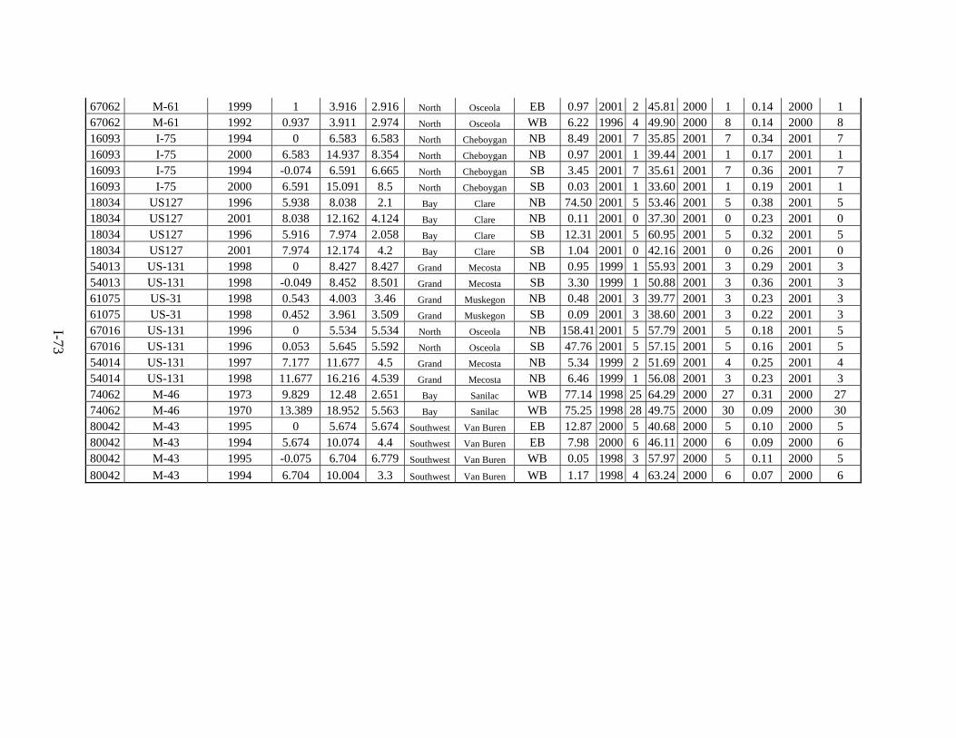
I-73

67062 M-61 1999 1 3.916 2.916 North Osceola EB 0.97 2001 2 45.81 2000 1 0.14 2000 1 67062 M-61 1992 0.937 3.911 2.974 North Osceola WB 6.22 1996 4 49.90 2000 8 0.14 2000 8 16093 I-75 1994 0 6.583 6.583 North Cheboygan NB 8.49 2001 7 35.85 2001 7 0.34 2001 7 16093 I-75 2000 6.583 14.937 8.354 North Cheboygan NB 0.97 2001 1 39.44 2001 1 0.17 2001 1 16093 I-75 1994 -0.074 6.591 6.665 North Cheboygan SB 3.45 2001 7 35.61 2001 7 0.36 2001 7 16093 I-75 2000 6.591 15.091 8.5 North Cheboygan SB 0.03 2001 1 33.60 2001 1 0.19 2001 1 18034 US127 1996 5.938 8.038 2.1 Bay Clare NB 74.50 2001 5 53.46 2001 5 0.38 2001 5 18034 US127 2001 8.038 12.162 4.124 Bay Clare NB 0.11 2001 0 37.30 2001 0 0.23 2001 0 18034 US127 1996 5.916 7.974 2.058 Bay Clare SB 12.31 2001 5 60.95 2001 5 0.32 2001 5 18034 US127 2001 7.974 12.174 4.2 Bay Clare SB 1.04 2001 0 42.16 2001 0 0.26 2001 0 54013 US-131 1998 0 8.427 8.427 Grand Mecosta NB 0.95 1999 1 55.93 2001 3 0.29 2001 3 54013 US-131 1998 -0.049 8.452 8.501 Grand Mecosta SB 3.30 1999 1 50.88 2001 3 0.36 2001 3 61075 US-31 1998 0.543 4.003 3.46 Grand Muskegon NB 0.48 2001 3 39.77 2001 3 0.23 2001 3 61075 US-31 1998 0.452 3.961 3.509 Grand Muskegon SB 0.09 2001 3 38.60 2001 3 0.22 2001 3 67016 US-131 1996 0 5.534 5.534 North Osceola NB 158.41 2001 5 57.79 2001 5 0.18 2001 5 67016 US-131 1996 0.053 5.645 5.592 North Osceola SB 47.76 2001 5 57.15 2001 5 0.16 2001 5 54014 US-131 1997 7.177 11.677 4.5 Grand Mecosta NB 5.34 1999 2 51.69 2001 4 0.25 2001 4 54014 US-131 1998 11.677 16.216 4.539 Grand Mecosta NB 6.46 1999 1 56.08 2001 3 0.23 2001 3 74062 M-46 1973 9.829 12.48 2.651 Bay Sanilac WB 77.14 1998 25 64.29 2000 27 0.31 2000 27 74062 M-46 1970 13.389 18.952 5.563 Bay Sanilac WB 75.25 1998 28 49.75 2000 30 0.09 2000 30 80042 M-43 1995 0 5.674 5.674 Southwest Van Buren EB 12.87 2000 5 40.68 2000 5 0.10 2000 5 80042 M-43 1994 5.674 10.074 4.4 Southwest Van Buren EB 7.98 2000 6 46.11 2000 6 0.09 2000 6 80042 M-43 1995 -0.075 6.704 6.779 Southwest Van Buren WB 0.05 1998 3 57.97 2000 5 0.11 2000 5 80042 M-43 1994 6.704 10.004 3.3 Southwest Van Buren WB 1.17 1998 4 63.24 2000 6 0.07 2000 6

I-74

Table A-8. DI, RQI and rutting for composite pavement projects. Control section Road Year of latest

improvement BMP EMP Project Length Region County Direction DI Year

of DI DI age RQI RQI age

RQI age Rutting Rutting

age Rutting

age

09101 US10 1999 1.918 11.508 9.59 Bay Bay EB 3.49 2001 2 42.72 2001 2 0.20 2001 2 22023 US-2 1994 0 5.104 5.104 Superior Dickinson EB 22.26 2001 7 65.12 2001 7 0.17 2001 7 22023 US-2 1997 5.104 10.996 5.892 Superior Dickinson EB 5.05 2001 4 46.76 2001 4 0.30 2001 4 22023 US-2 1994 -0.008 5.002 5.01 Superior Dickinson WB 21.71 1999 5 64.20 2001 7 0.18 2001 7 22023 US-2 1997 5.002 11.075 6.073 Superior Dickinson WB 2.64 1999 2 47.37 2001 4 0.29 2001 4 78022 US-12 2000 0 1.8 1.8 Southwest ST.Joseph EB 0.22 2001 1 63.83 2001 1 0.44 2001 1 78022 US-12 2001 1.8 3.9 2.1 Southwest ST.Joseph EB 0.22 2001 0 40.62 2001 0 0.42 2001 0 78022 US-12 1999 3.9 7.351 3.451 Southwest ST.Joseph EB 4.71 2001 2 51.49 2001 2 0.47 2001 2 78022 US-12 1968 11.984 12.242 0.258 Southwest ST.Joseph EB 24.06 2001 33 87.67 2001 33 0.52 2001 33 47066 I-96 1998 0 8.727 8.727 University Livingston EB 0.74 2001 3 37.98 2001 3 0.26 2001 3 47066 I-96 1998 0.07 8.762 8.692 University Livingston WB 2.12 2001 3 40.54 2001 3 0.24 2001 3 70024 I-196 1994 4.408 6.593 2.185 Grand Ottawa NB 18.86 2001 7 55.71 2001 7 0.22 2001 7 70024 I-196 1997 6.593 11.124 4.531 Grand Ottawa NB 9.60 2001 4 46.61 2001 4 0.25 2001 4 70024 I-196 1996 11.124 15.629 4.505 Grand Ottawa NB 2.17 2001 5 40.66 2001 5 0.23 2001 5 70024 I-196 2001 4.332 6.502 2.17 Grand Ottawa SB 0.58 2001 0 51.23 2001 0 0.24 2001 0 70024 I-196 1997 6.502 11.063 4.561 Grand Ottawa SB 5.28 2001 4 49.24 2001 4 0.22 2001 4 70024 I-196 1996 11.063 15.705 4.642 Grand Ottawa SB 1.94 2001 5 50.07 2001 5 0.22 2001 5 55022 US-2 US-41 1998 0 9.574 9.574 Superior Menominee EB 10.64 2001 3 50.40 2001 3 0.21 2001 3 55022 US-2 US-41 1998 0.03 9.588 9.558 Superior Menominee WB 4.30 1999 1 46.11 2001 3 0.24 2001 3 40012 US-131 M-66 1995 0.91 9.72 8.81 North Kalkaska NB 21.60 2001 6 45.88 2001 6 0.22 2001 6 40012 US-131 M-66 1995 0.86 9.753 8.893 North Kalkaska SB 5.75 1999 4 46.61 2001 6 0.23 2001 6 06073 US-23 1997 6.276 17.842 11.566 Bay Arenac NB 2.16 2001 4 41.17 2001 4 0.23 2001 4 74062 M-70 1999 12.426 14.984 2.558 Bay Sanilac EB 0.45 2000 1 49.58 2000 1 0.12 2000 1 25032 I-75 2000 1.1 2.384 1.284 Bay Genesee NB 3.64 2001 1 48.77 2001 1 0.16 2001 1 25032 I-75 1999 2.384 7.907 5.523 Bay Genesee NB 2.41 2001 2 47.05 2001 2 0.19 2001 2 25032 I-75 2000 0.986 2.201 1.215 Bay Genesee SB 0.16 2001 1 48.00 2001 1 0.16 2001 1 25032 I-75 1999 2.201 7.726 5.525 Bay Genesee SB 2.46 2001 2 51.16 2001 2 0.19 2001 2 38103 I-94 1995 0.011 0.62 0.609 University Jackson EB 3.84 1999 4 39011 US-131 1997 2.545 5.072 2.527 Southwest Kalamazoo NB 7.93 2001 4 56.66 2001 4 0.30 2001 4

I-75

39011 US-131 1997 2.53 5.04 2.51 Southwest Kalamazoo SB 9.71 2001 4 60.23 2001 4 0.32 2001 4 11017 I-94 1995 0 1.003 1.003 Southwest Berrien EB 20.62 2001 6 71.45 2001 6 0.26 2001 6 11017 I-94 1997 -0.007 0.888 0.895 Southwest Berrien WB 6.80 2001 4 59.20 2001 4 0.25 2001 4 11017 I-94 1997 10.052 10.672 0.62 Southwest Berrien WB 6.80 2001 4 80041 M-43 1993 10.06 10.699 0.639 Southwest Van Buren WB 3.85 1998 5 78022 US-12 1969 3.227 3.811 0.584 Southwest ST.Joseph WB 207.70 1999 30 41.86 2001 32 0.15 2001 32 78022 US-12 1995 3.811 7.789 3.978 Southwest ST.Joseph WB 19.27 1999 4 52.62 2001 6 0.21 2001 6 33031 US-127 1999 0 12.084 12.084 University Ingham NB 3.93 2001 2 38.35 2001 2 0.19 2001 2 33031 US-127 1999 0.001 12.188 12.187 University Ingham SB 2.53 2001 2 33.28 2001 2 0.19 2001 2 30062 US-12 1991 0.162 0.662 0.5 University Hillsdale EB 22.87 1999 8 30062 US-12 1993 0.662 9.362 8.7 University Hillsdale EB 21.87 1999 6 30062 US-12 1990 9.362 17.022 7.66 University Hillsdale EB 43.21 1999 9 30062 US-12 1991 0.148 0.502 0.354 University Hillsdale WB 14.72 1995 4 79.25 2001 10 0.31 2001 10 30062 US-12 1993 0.502 7.602 7.1 University Hillsdale WB 11.85 1995 2 63.04 2001 8 0.26 2001 8 30062 US-12 1990 7.602 17.002 9.4 University Hillsdale WB 40.07 1995 5 74.70 2001 11 0.30 2001 11 63022 I-96 1999 0 7.293 7.293 Metro Oakland EB 4.40 2001 2 46.14 2001 2 0.18 2001 2 63022 I-96 1999 0.023 7.083 7.06 Metro Oakland WB 1.42 2001 2 45.09 2001 2 0.14 2001 2 47014 US-23 2000 -0.005 7.738 7.743 University Livingston SB 2.61 2001 1 37.22 2001 1 0.21 2001 1 47014 US-23 1992 0.003 7.72 7.717 University Livingston NB 5.08 1999 7 81062 I-94 1999 7.426 9.112 1.686 University Washtenaw EB 0.99 2001 2 47.70 2001 2 0.21 2001 2 81062 I-94 1999 7.33 9.13 1.8 University Washtenaw WB 1.52 2001 2 47.39 2001 2 0.25 2001 2 82292 I-275 1998 3.922 6.852 2.93 Metro Wayne NB 1.77 2001 3 47.31 2001 3 0.27 2001 3 82292 I-275 1998 3.849 6.772 2.923 Metro Wayne SB 1.04 2001 3 49.10 2001 3 0.26 2001 3 21021 US-2 US-41 1999 0 3.3 3.3 Superior Delta EB 11.13 2001 2 36.67 2001 2 0.16 2001 2 21021 US-2 US-41 1986 -0.068 3.284 3.352 Superior Delta WB 24.65 1999 13 36.79 2001 15 0.19 2001 15 55021 US-2 1989 0 10.039 10.039 Superior Menominee EB 18.10 2001 12 51.11 2001 12 0.29 2001 12 55021 US-2 1989 0.048 10.219 10.171 Superior Menominee WB 18.67 1999 10 51.17 2001 12 0.28 2001 12 5071 US-131 M-66 1995 0 2.4 2.4 North Antrim NB 13.58 2001 6 46.33 2001 6 0.24 2001 6 5071 US-131 M-66 1983 2.4 3.786 1.386 North Antrim NB 29.49 2001 18 60.00 2001 18 0.24 2001 18 5071 US-131 M-66 1995 0.019 2.41 2.391 North Antrim SB 6.48 1999 4 47.80 2001 6 0.22 2001 6 5071 US-131 M-66 1983 2.41 3.653 1.243 North Antrim SB 22.32 1999 16 71.62 2001 18 0.22 2001 18

35031 US-23 1997 0 6.404 6.404 North Iosco NB 5.75 1999 2 42.13 2001 4 0.19 2001 4 35031 US-23 1993 6.404 7.298 0.894 North Iosco NB 10.10 1999 6 62.56 2001 8 0.21 2001 8

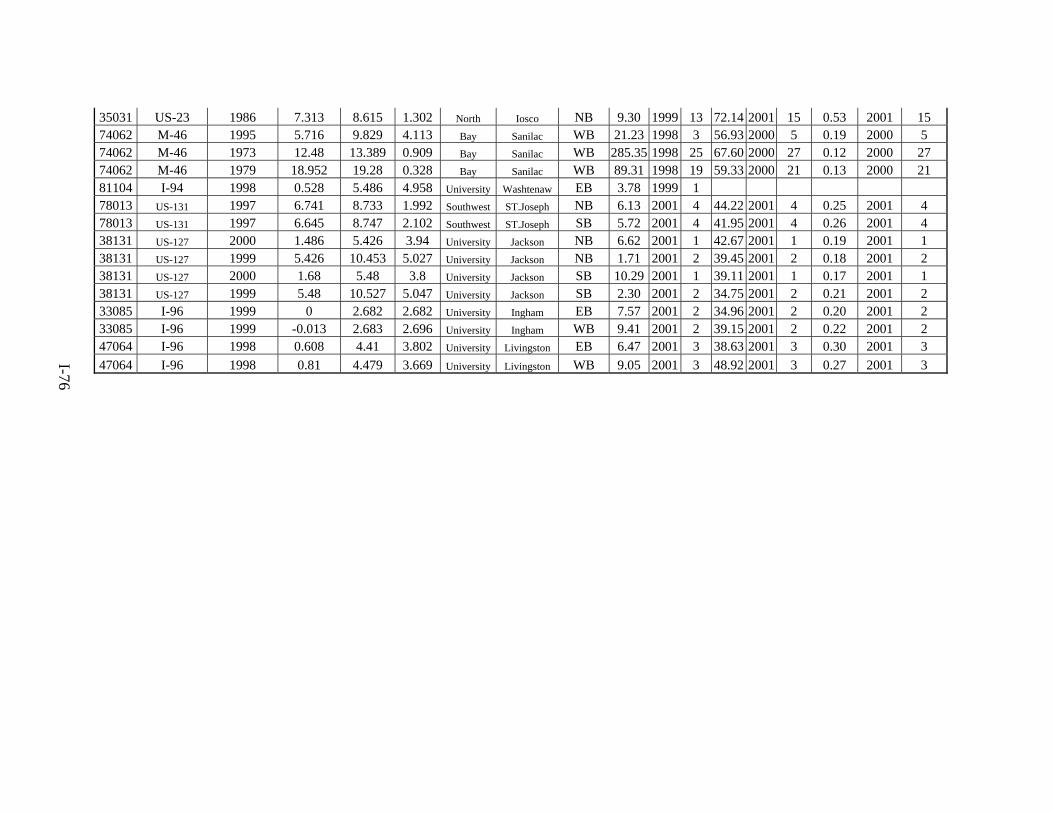
I-76

35031 US-23 1986 7.313 8.615 1.302 North Iosco NB 9.30 1999 13 72.14 2001 15 0.53 2001 15 74062 M-46 1995 5.716 9.829 4.113 Bay Sanilac WB 21.23 1998 3 56.93 2000 5 0.19 2000 5 74062 M-46 1973 12.48 13.389 0.909 Bay Sanilac WB 285.35 1998 25 67.60 2000 27 0.12 2000 27 74062 M-46 1979 18.952 19.28 0.328 Bay Sanilac WB 89.31 1998 19 59.33 2000 21 0.13 2000 21 81104 I-94 1998 0.528 5.486 4.958 University Washtenaw EB 3.78 1999 1 78013 US-131 1997 6.741 8.733 1.992 Southwest ST.Joseph NB 6.13 2001 4 44.22 2001 4 0.25 2001 4 78013 US-131 1997 6.645 8.747 2.102 Southwest ST.Joseph SB 5.72 2001 4 41.95 2001 4 0.26 2001 4 38131 US-127 2000 1.486 5.426 3.94 University Jackson NB 6.62 2001 1 42.67 2001 1 0.19 2001 1 38131 US-127 1999 5.426 10.453 5.027 University Jackson NB 1.71 2001 2 39.45 2001 2 0.18 2001 2 38131 US-127 2000 1.68 5.48 3.8 University Jackson SB 10.29 2001 1 39.11 2001 1 0.17 2001 1 38131 US-127 1999 5.48 10.527 5.047 University Jackson SB 2.30 2001 2 34.75 2001 2 0.21 2001 2 33085 I-96 1999 0 2.682 2.682 University Ingham EB 7.57 2001 2 34.96 2001 2 0.20 2001 2 33085 I-96 1999 -0.013 2.683 2.696 University Ingham WB 9.41 2001 2 39.15 2001 2 0.22 2001 2 47064 I-96 1998 0.608 4.41 3.802 University Livingston EB 6.47 2001 3 38.63 2001 3 0.30 2001 3 47064 I-96 1998 0.81 4.479 3.669 University Livingston WB 9.05 2001 3 48.92 2001 3 0.27 2001 3

I-77

Table A-9. Slope and R2 of DI for rigid pavement. Pavement type Rigid Rigid-I Rigid-US

Number of project 52 29 22 Slope R2 Slope R2 Slope R2

Class 5 2*10-6 0.42 3*10-6 0.58 2*10-6 0.21 Class 6 1*10-5 0.47 1*10-5 0.55 1*10-5 0.35 Class 7 6*10-5 0.24 6*10-5 0.27 7*10-5 0.19 Class 8 6*10-6 0.29 7*10-6 0.46 3*10-6 0.06 Class 9 9*10-7 0.43 1*10-6 0.68 8*10-7 0.84 Class 10 2*10-5 0.49 2*10-5 0.57 4*10-5 0.41 Class 11 3*10-5 0.33 4*10-5 0.67 -1*10-5 0.29 Class 12 8*10-5 0.05 2*10-4 0.23 -6*10-5 0.03 Class 13 4*10-6 0.31 4*10-6 0.34 1*10-5 0.35

TTT 7*10-7 0.57 7*10-7 0.79 6*10-7 0.2 Age 0.5544 0.45 0.5662 0.57 0.4178 0.41

Table A-10. Slope and R2 of DI for flexible pavement.

Pavement type Flexible Flexible-I Flexible-US Flexible-M Number of project 53 9 23 21

Slope R2 Slope R2 Slope R2 Slope R2

Class 5 1*10-5 0.03 1*10-5 0.74 6*10-6 0.02 9*10-5 0.35 Class 6 2*10-4 0.58 1*10-4 0.75 1*10-4 0.04 6*10-4 0.18 Class 7 1.6*10-3 0.18 1.7*10-3 0.76 3*10-4 0.002 1.9*10-3 0.51 Class 8 7*10-5 0.03 5*10-5 0.72 8*10-5 0.05 1*10-3 0.48 Class 9 3*10-5 0.07 1*10-5 0.76 4*10-5 0.19 3*10-4 0.37 Class 10 2*10-4 0.06 6*10-5 0.53 4*10-4 0.12 1.1*10-3 0.36 Class 11 9*10-4 0.17 1.1*10-3 0.64 1.3*10-3 0.38 -4*10-3 0.03 Class 12 -5*10-5 0.003 3.3*10-3 0.76 2.3*10-3 0.01

Class 13 2*10-5 0.009 2*10-5 0.74 6*10-5 0.04 5*10-4 0.58 TTT 8*10-6 0.06 4*10-6 0.76 9*10-6 0.09 6*10-5 0.46 Age 2.5886 0.31 1.2051 0.76 1.8778 0.07 3.0967 0.78

I-78

Table A-11. Slope and R2 of DI for composite pavement.

Table A-12. Slope and R2 of RQI for rigid pavement.

Pavement type Rigid Rigid-I Rigid-US Number of projects 52 29 22 Slope* R2 Slope* R2 Slope* R2

Class 5 0.0022 0.42 0.0024 0.44 0.0019 0.35 Class 6 0.0089 0.21 0.0157 0.55 -0.0006 0.00 Class 7 0.0670 0.25 0.0808 0.41 0.0117 0.01 Class 8 0.0049 0.21 0.0077 0.50 -0.0003 0.00 Class 9 0.0004 0.06 0.0003 0.05 0.0015 0.30 Class 10 0.0173 0.32 0.0185 0.48 0.0101 0.03 Class 11 0.0095 0.04 0.0083 0.03 0.0291 0.12

Pavement type Composite Composite-I Composite-US Composite-M Number of project 77 27 45 5 Slope R2 Slope R2 Slope R2 Slope R2

Class 5 1*10-6 0.001 4*10-6 0.077 2*10-6 0.01 4*10-4 0.73 Class 6 1*10-6 0.0001 7*10-6 0.202 2*10-4 0.09 4.1*10-3 0.59 Class 7 8*10-4 0.076 -6*10-5 0.027 6*10-4 0.06 6.7*10-3 0.83 Class 8 4*10-5 0.02 1*10-5 0.082 1*10-4 0.35 4.6*10-3 0.73 Class 9 -9*10-7 0.001 2*10-6 0.39 2*10-5 0.12 1.9*10-3 0.58 Class 10 -3*10-5 0.002 5*10-5 0.28 1*10-4 0.028 7.6*10-3 0.52 Class 11 -2*10-5 0.004 9*10-5 0.51 4*10-4 0.10 -5.2*10-2 0.13 Class 12 -7*10-4 0.014 4*10-4 0.42 -2*10-4 0.001 Class 13 -1*10-5 0.0023 1*10-5 0.21 2*10-5 0.01 1.8*10-3 0.83 TTT -7*10-8 0.00002 1*10-6 0.45 3*10-6 0.5 2*10-4 0.66 Age 4.548 0.488 2.0273 0.41 2.9366 0.43 10.174 0.82

I-79

Class 12 0.1108 0.09 0.1688 0.15 0.0553 0.04 Class 13 0.0049 0.44 0.0049 0.58 0.0057 0.13 TTT 0.0004 0.24 0.0004 0.26 0.0006 0.27 Age 0.4050 0.23 0.5112 0.23 0.3137 0.24

Note: TTT of each class in 1000 trucks

Table A-13. Slope and R2 of RQI for flexible pavement.

Pavement type Flexible Flexible-I Flexible-US Flexible-M Number of projects 53 9 23 21 Slope R2 Slope R2 Slope R2 Slope R2

Class 5 -0.0043 0.05 -0.0045 0.12 -0.0039 0.10 0.0065 0.02Class 6 -0.0431 0.03 -0.0504 0.14 -0.0472 0.07 0.0302 0.00Class 7 0.1879 0.02 -0.9392 0.22 -0.3568 0.04 0.1463 0.03Class 8 -0.0451 0.10 -0.0314 0.28 -0.0237 0.06 0.0403 0.01Class 9 -0.0070 0.04 -0.0066 0.16 -0.0011 0.00 0.0829 0.16Class 10 -0.0575 0.03 -0.0099 0.01 0.0142 0.00 0.1940 0.06Class 11 0.1260 0.02 -0.8706 0.33 0.2166 0.15 5.0635 0.39Class 12 -3.9352 0.15 -1.8785 0.22 -1.3042 0.03 NA NA Class 13 -0.0348 0.21 -0.0108 0.25 -0.0201 0.07 0.0124 0.00TTT -0.0033 0.09 -0.0019 0.16 -0.0022 0.07 0.0055 0.03Age 0.3330 0.04 -0.6856 0.22 -0.2669 0.02 0.3149 0.06Note: TTT of each class in 1000 trucks

I-80

Table A-14. Slope and RP

2P of rutting for flexible pavement.

Pavement type Flexible Flexible-I Flexible-US Flexible-M Number of projects 53 9 23 21 slope RP

2P slope RP

2P slope RP

2P slope RP

2P

Class 5 0.00004 0.05 0.00020 0.76 0.00000 0.00 0.00000 0.00Class 6 0.00037 0.03 0.00214 0.81 -0.00035 0.07 0.00050 0.03Class 7 -0.00005 0.00 0.03425 0.91 -0.00161 0.01 0.00222 0.17Class 8 0.00039 0.11 0.00102 0.95 -0.00014 0.04 0.00014 0.00Class 9 0.00010 0.13 0.00027 0.84 -0.00006 0.10 -0.00017 0.02Class 10 0.00069 0.06 0.00094 0.41 -0.00076 0.12 -0.00077 0.03Class 11 0.00116 0.03 0.02610 0.93 -0.00139 0.11 -0.02221 0.20Class 12 0.03299 0.15 0.06849 0.91 -0.00430 0.01 NA NAClass 13 0.00031 0.24 0.00038 0.93 -0.00013 0.05 0.00073 0.26TTT 0.00003 0.13 0.00008 0.84 -0.00001 0.03 0.00001 0.01Age -0.00145 0.01 0.02500 0.91 -0.00248 0.03 0.00268 0.11

Note: TTT of each class in 1000 trucks

I-81

Table A-15. Slope and RP

2P of RQI for composite pavement.

Pavement type Composite Composite-I Composite-US Composite-USNumber of projects 52 29 22 22 slope RP

2P slope RP

2P slope RP

2P slope RP

2P

Class 5 0.0044 0.14 0.0007 0.00 0.0050 0.20 0.0248 0.81

Class 6 0.0016 0.00 0.0025 0.01 0.0646 0.12 0.2571 0.80

Class 7 0.3158 0.14 -0.0128 0.00 0.5591 0.31 0.3810 0.82

Class 8 0.0060 0.00 -0.0047 0.00 0.0322 0.09 0.2577 0.80

Class 9 0.0016 0.03 0.0030 0.46 0.0100 0.12 0.1192 0.80

Class 10 0.0127 0.00 0.0210 0.02 0.1293 0.10 0.5214 0.79

Class 11 0.0657 0.04 0.0754 0.16 0.4025 0.31 NA NA

Class 12 0.0424 0.00 0.4932 0.23 0.4365 0.00 NA NA

Class 13 0.0020 0.00 0.0074 0.02 0.0349 0.05 0.1020 0.81

TTT 0.0015 0.08 0.0019 0.33 0.0032 0.20 0.0141 0.81

Age 0.8859 0.29 1.8936 0.17 0.9132 0.27 0.5439 0.83 Note: TTT of each class in 1000 trucks

I-82

Table A-16. Slope and RP

2P of rutting for composite pavement.

Pavement type Composite Composite-I Composite-US Composite-USNumber of projects 52 29 22 22 Slope RP

2P Slope RP

2P Slope RP

2P Slope RP

2P

Class 5 0.00003 0.15 0.00004 0.13 0.00003 0.15 -0.00006 0.19

Class 6 0.00000 0.00 0.00002 0.03 0.00007 0.00 -0.00060 0.20

Class 7 0.00120 0.04 0.00078 0.08 0.00253 0.12 -0.00084 0.18

Class 8 0.00007 0.01 0.00013 0.13 0.00012 0.02 -0.00061 0.20

Class 9 0.00000 0.00 0.00001 0.15 0.00003 0.03 -0.00028 0.21

Class 10 0.00000 0.00 0.00025 0.12 -0.00005 0.00 -0.00131 0.22

Class 11 0.00018 0.01 0.00034 0.12 0.00074 0.02 NA NA

Class 12 -0.00049 0.00 0.00177 0.11 -0.00909 0.01 NA NA

Class 13 -0.00001 0.00 0.00011 0.22 -0.00012 0.01 -0.00023 0.18

TTT 0.00001 0.05 0.00001 0.21 0.00002 0.09 -0.00003 0.19

Age 0.00161 0.02 0.00976 0.16 0.00277 0.05 -0.00109 0.15

Note: TTT of each class in 1000 trucks