Effect of distortion on optical-fiber waveguides

Journal of Russian Laser Research, Volume 33, Number 4, July, 2012

EFFECT OF DISTORTION

ON OPTICAL-FIBER WAVEGUIDES

Sushil Kumar and Vivek Singh∗

Physics Department, Faculty of ScienceBanaras Hindu University

Varanasi 221005, U.P. India∗Corresponding author e-mail: viveks @ bhu.ac.in

Abstract

We analyze the modes and coupling efficiency of asymmetric optical-fiber waveguides. We treated thestep index-asymmetric optical-fiber waveguide as a boundary-value problem and obtain the expres-sions for the modes under logical assumptions. Using these expressions, we describe the propagationconstants, mode delay, and power distribution of two asymmetric optical-fiber waveguides under con-sideration. Based on the perturbation theory, we also present the coupling coefficients of these asym-metric optical-fiber waveguides. We show that the waveguide parameters are considerably changed inthe presence of distortion, and one can tune these parameters at the desired level by choosing suitabledistortions.

Keywords: asymmetric optical-fiber waveguides, mode designation, power distribution, coupling effi-ciency.

1. Introduction

The circular optical-fiber waveguides in which the light propagates through total internal reflectionare now widely recognized for optical telecommunication [1–4]. In general, these optical-fiber waveguidessupporting many modes, which propagate through the optical fiber with different velocities, are knownas multimode fibers. These modes interfere with each other and give intermodal dispersions, which limitthe propagation bandwidth. The intermodal dispersion can be removed by suppressing the number ofmodes in the waveguide. In addition, in many practical cases, it is desired that the energy be confinedto a single mode. Generally, the suppression of modes is achieved by reducing the core diameter, and ifonly one mode is present in the waveguide, it is called the single-mode waveguide. The mode suppressioncan also be achieved by introducing a deformation in the standard (circular) shape of waveguides [5–10]as well as by replacing the constituent materials of the waveguide by some smart materials [11–13].

However, the optical waveguides are frequently used as mode coupler, switches, beam splitter, mul-tiplexer, and de-multiplexer for optical signals. Although the operation of waveguide devices is wellknown, the study of performance characteristics, which depend on many parameters such as the waveg-uide geometry, wavelength of the incident light, constituent materials data, etc., still has wide scope forimprovement. Therefore, in the present paper we took two slightly distorted (lack of azimutal symmetry)circular optical-fiber waveguide — one is asymmetric optical-fiber waveguide type I (AOFW-I) shown in

Manuscript submitted by the authors in English first on August 6, 2012 and in final form on August 14, 2012.1071-2836/12/3304-0395 c©2012 Springer Science+Business Media New York 395

Journal of Russian Laser Research Volume 33, Number 4, July, 2012

a) b)

Fig. 1. Cross-sectional view of AOFW-I (a) and AOFW-II (b).

Fig. 1a and the other is asymmetric optical-fiber waveguide type II (AOFW-II) shown in Fig. 1b. Thesedistortions are deliberately produced in the standard circular optical fiber to study their effects on thepropagation constant, mode delay, power distribution, and coupling efficiency. In Sec. 2, the character-istic equations, cutoff conditions, and mode designation for both considered waveguides are presented.The propagation constant and mode delay under certain approximations are given in Sec. 3. The powerdistribution and coupling coefficient for these waveguides are also shown in the consecutive sections;here, all the derivations in Secs. 3–5 are given only for AOFW-I. Similar derivations can also be done forAOFW-II. Finally, the paper ends with some remarks in the conclusion given in Sec. 6.

2. Characteristics Equations, Cutoff Conditions, and Mode

Designations

The cross-sectional views of the considered waveguides are shown in Fig. 1. The refractive index ofthe core region is n1 and the cladding region is n2 such that (n1 − n2)/n1 � n1. The shapes of theasymmetric cross sections [6, 7] are described by the following equations:

r = ξ e1+sin θ for AOFW-I, (1)

r = ξ e1/2 sin pθ, for AOFW-II, (2)

where ξ is the size parameter and p = 0.5. At the core–cladding boundary, we put its value equal to a,where a is a fixed constant. The normal curves of the curve presented by the above equations are givenas

r⊥ = ηcos θ

1 + sin θfor AOFW-I, (3)

r⊥ = η

[cos2 pθ

(1 + sin pθ)2

]1/p2

for AOFW-II, (4)

where η is the other size parameter.

396

Volume 33, Number 4, July, 2012 Journal of Russian Laser Research

We now want to choose an appropriate coordinate system (ξ, η, z) suitable for the analysis of thesecross sections. The direction of the wave propagation is along the z-axis, which is normal to the plane ofpaper in Fig. 1. We write the scalar Helmholtz equation of the electromagnetic-wave propagation alongthe core as follows:

∇2E + ω2μεE = 0, ∇2 =1

h1h2h3

[∂

∂ξ

(h2h3

h1

∂

∂ξ

)+

∂

∂ξ

(h1h3

h2

∂

∂η

)+

∂

∂z

(h1h2

h3

∂

∂z

)], (5)

where h1, h2, and h3 are the scale factors [14], which can be easily obtained using the equation of corecross section [Eq. (1) or (2)] along with their corresponding normal curve [Eq. (3) or (4)]. The wavefunction E may represent one of the orthogonal components of the electric and magnetic field, ω is theangular frequency of the field, μ is the permeability of the dielectric material of the core region, ε is thepermittivity of the guiding or core region, and β is the z component of the propagation constant of theguided mode.

Since the distorted part of our waveguides is of primary importance and should lie within the normalcurves, we make the approximation ξ ≈ η in order to facilitate our calculations. Thus, Eqs. (5) for theproposed structures are transformed as

1η

∂E

∂ξ+

ξ

η

∂2E

∂ξ2+

1ξ

∂E

∂η+

η

ξ

∂2E

∂η2+

ξ

η

∂2E

∂z2+ ω2με

2.718ξ

2ηE = 0 for AOFW-I, (6)

−2ξ3

∂E

∂ξ+

2ξ2

∂2E

∂ξ2− 1

2η3

∂E

∂η+

12η2

∂2E

∂η2+

25

(η

ξ

)−3/5 1ξη

∂2E

∂z2+ ω2με

(η

ξ

)−3/5 1ξη

E = 0

for AOFW-II. (7)

Now, using the method of separation of variables, we can obtain solutions of Eqs. (6) and (7) if wewrite

E = E1(ξ)E2(η) exp[i(wt − βz)]. (8)

Inserting Eq. (8) in Eqs. (6) and (7), we obtain the following set of equations:

η∂E2(η)

∂η+ η2 ∂2E2(η)

∂η2= 0 for AOFW-I, (9)

ξ∂E1(ξ)

∂ξ+ ξ2 ∂2E1(ξ)

∂ξ2+ (ω2με − β2)

2.718 ξ

2ηE1(ξ) = 0 for AOFW-I, (10)

−1η

∂E2(η)∂η

+∂2E2(η)

∂η2= 0 for AOFW-II, (11)

−1ξ

∂E1(ξ)∂ξ

+∂2E1(ξ)

∂ξ2+ (ω2με − β2)

15

(η

ξ

)−3/5

E1(ξ) = 0 for AOFW-II. (12)

Equations (9) and (11) are the same for both regions (core and cladding), and they do not contain anyparameters such as ω, μ, or ε, describing the modal behavior. We therefore concentrate only on Eqs. (10)and (12). Now the differential equations corresponding to the core ε = ε1 and the cladding region ε = ε2

397


are separately written as

ξ∂E1(ξ)

∂ξ+ ξ2 ∂2E1(ξ)

∂ξ2+ U2 2.718ξ

2ηE1(ξ) = 0 for AOFW-I (core), (13)

−1ξ

∂E1(ξ)∂ξ

+∂2E1(ξ)

∂ξ2+ U2 1

5

(η

ξ

)−3/5

E1(ξ) = 0 for AOFW-II (core), (14)

ξ∂E1(ξ)

∂ξ+ ξ2 ∂2E1(ξ)

∂ξ2− W 2 2.718ξ

2ηE1(ξ) = 0 for AOFW-I (cladding), (15)

−1ξ

∂E1(ξ)∂ξ

+∂2E1(ξ)

∂ξ2− W 2 1

5

(η

ξ

)−3/5

E1(ξ) = 0 for AOFW-II (cladding). (16)

where U2 = (ω2με1 − β2) and W 2 = (β2 − ω2με2).The solution of Eqs. (13)–(16) are written in the following ways:Field in the core region of AOFW-I, 0 ≤ ξ ≤ a,

Eξ = AJl+1

(d1

u

aξ)

cos ψ, (17)

Eη = −AJl+1

(d1

u

aξ)

sin ψ, (18)

Ez = ju

βaAJl

(d1

u

aξ)

cos(θ + ψ). (19)

Field in the cladding region of AOFW-I, ξ ≥ a,

Eξ = AJl+1(d1u)Kl+1(d1w)

Kl+1

(d1

w

aξ)

cos ψ, (20)

Eη = −AJl+1(d1u)Kl+1(d1w)

Kl+1

(d1

w

aξ)

sin ψ, (21)

Ez = jAu

βa

Jl(d1u)Kl(d1w)

Kl

(d1

w

aξ)

cos(θ + ψ). (22)

Field in the core region of AOFW-II, 0 ≤ ξ ≤ a,

Eξ = AJl(d2u

aξ) cos ψ, (23)

Eη = −AJl(d2u

aξ) sinψ, (24)

Ez = ju

βaAJl+1(d2

u

aξ) cos(θ + ψ). (25)

Field in the cladding region AOFW-II, ξ ≥ a,

Eξ = AJl(d2u)Kl(d2w)

Kl

(d2

w

aξ)

cos ψ, (26)

Eη = −AJl(d2u)Kl(d2w)

Kl

(d2

w

aξ)

sin ψ, (27)

Ez = jAu

βa

Jl+1(d2u)Kl+1(d2w)

Kl+1

(d2

w

aξ)

cos(θ + ψ). (28)

398


Here, d1 = 1.166 and d2 = 0.447, u and w are parameters defined as u = a√

k2n21 − β2 and w =

a√

β2 − k2n22, ψ denotes the phase, k = 2π/λ, where λ is the free-space wavelength, A is the constant

related to the optical power carried by the mode, J is the Bessel function for the guiding region, and K

is the modified Bessel function for the cladding regions.Using the weak guidance approximation and having in mind that tangential electric- and magnetic-

field components and their derivatives are continuous across the boundaries at ξ = a, after applying theboundary conditions with some mathematical steps, we obtain the following characteristic equations forsome low-order modes guided by the waveguides under consideration:

u

[Jl−1(d1u)Jl(d1u)

]= w

[Kl−1(d1w)Kl(d1w)

]for AOFW-I, (29)

u

[Jl(d2u)

Jl−1(d2u)

]= w

[Kl(d2w)

Kl−1(d2w)

]for AOFW-II. (30)

These are the characteristic equations for the linearly polarized (LPlm) mode. The LPlm modes count thegroup of modes appearing together as a single mode. The cutoff conditions for LP modes are obtainedfrom Eqs. (29)–(30) by putting the limiting condition β → knl

limβ→kn2

[(β2 − k2n2

2)Kl−1(β2 − k2n2

2)Kl(β2 − k2n2

2)

]→ 0. (31)

From Eqs. (29) and (31), cutoff conditions for AOFW-I can be written as

Jl−1(d1u) = 0. (32)

The lowest-order modes are characterized by l = 0 and have a cutoff equation given by

J1(d1u) = 0. (33)

This mode is labeled as the LP01 mode having a field pattern described by l = 0 and cutoff characteristicsof the first zero of the Bessel function. The next mode of the l = 0 type has a cutoff when J1(d1ua),in turn, equals zero and is called the LP02 mode. Similarly, the mode characterized by l = 1 has acutoff when J0(d1ua) = 0. A similar cutoff condition for AOFW-II is also obtained by putting Eq. (30)in Eq. (31), which is not shown here. Various cutoff conditions for LP0m, LP1m, and LP2m modes areobtained in view of the Bessel functions for both waveguides and shown in Fig. 2.

Figure 2 is used to find the cutoff values of various modes for AOWF-I and AOWF-II. These valuesare compared with the standard optical fiber waveguide (SOFW) and listed in Table 1. It is observedthat the cutoff conditions for corresponding modes decrease slightly for AOWF-I. However, these cutoffconditions for corresponding modes increase considerably in the case of AOWF-II. These changes in thecutoffs may occur because the waveguide dispersion depends on the ratio between the core radius andwavelength of the waveguide.

399


a) b)

Fig. 2. The plot of Bessel functions used for calculating the cutoff conditions for LP0m, LP1m, and LP2m modesof AOFW-I (a) and AOFW-II (b).

Table 1. The Orders of Appearance of the Modes of the Considered Waveguides.

Traditional Mode Conventional Range of V Range of V Range of VNotation Mode (AOFW-I) (SOFW) (AOFW-II)

HE11 LP01 0–2.063 0–2.405 0–5.378

TE01, TM01, HE21 LP11 2.063–3.287 2.405–3.8317 5.378–8.568

HE12 LP02 3.287–4.405 3.8317–5.135 8.568–11.48

EH11, HE31 LP21 3.287–4.735 3.8317–5.520 8.568–12.34

TE02, TM02, HE22 LP12 4.735–6.018 5.520–7.016 12.34–15.69

EH12, HE32 LP22 6.018–7.22 7.016–8.417 15.69–18.82

HE13 LP03 6.018–7.423 7.016–8.663 15.69–19.35

3. The Propagation Constant and Mode Delay

To evaluate the propagation constant β(V ) of the propagating mode, we solve the characteristicequation of a certain mode together with the equation V 2 = u2+w2, where V is the normalized frequencyparameter defined as

V =√

u2 + w2 =2πa

λ

√n2

1 − n22.

We know that the range of β for the propagating mode lies between n1k (lower-order modes) and n2k

400


(higher-order modes). Hence there are two limiting case — one is near the cutoff, when β → kn2 as wediscussed earlier, and the other one is far from the cutoff, when β → kn1, which provides

limβ→kn1

[Kl−1(β2 − k2n2

2)Kl(β2 − k2n2

2)

]≈ 1. (34)

Therefore, Eq. (29) becomes

V J0(u) = uJ1(u). (35)

Differentiating Eq. (35) with respect to the normalized frequency V with some simple algebra [3, 4] andunder the same approximations, we obtain

u0m = u∞lm exp−1/V , (36)

where u∞0m is the root of J0(u).

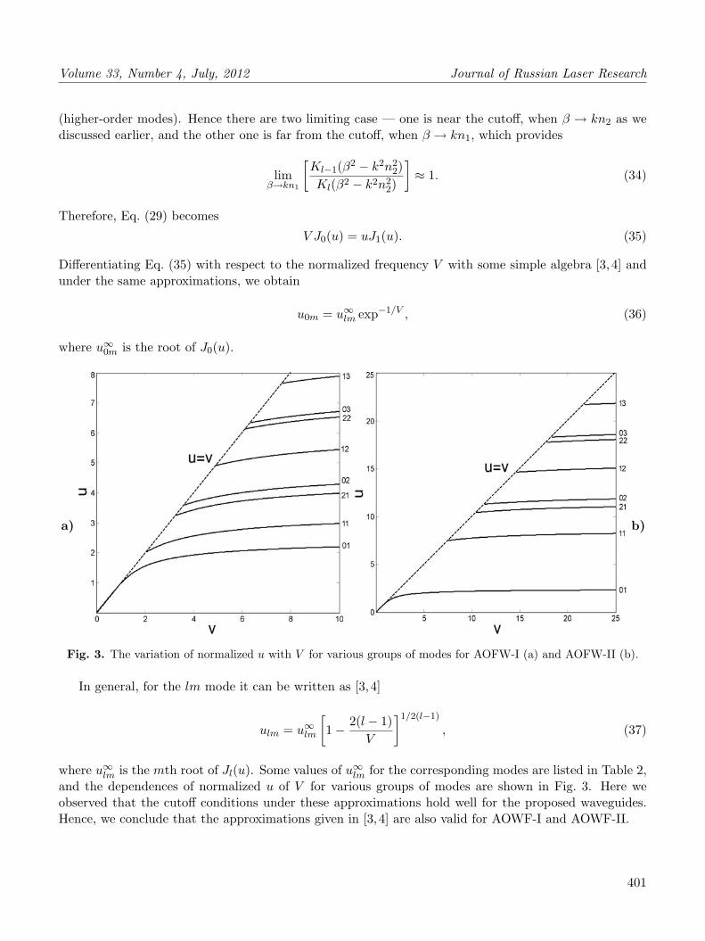
a) b)

Fig. 3. The variation of normalized u with V for various groups of modes for AOFW-I (a) and AOFW-II (b).

In general, for the lm mode it can be written as [3, 4]

ulm = u∞lm

[1 − 2(l − 1)

V

]1/2(l−1)

, (37)

where u∞lm is the mth root of Jl(u). Some values of u∞

lm for the corresponding modes are listed in Table 2,and the dependences of normalized u of V for various groups of modes are shown in Fig. 3. Here weobserved that the cutoff conditions under these approximations hold well for the proposed waveguides.Hence, we conclude that the approximations given in [3, 4] are also valid for AOWF-I and AOWF-II.

401


Table 2. Values of u∞lm.

Notation of Linearly AOFW-I AOFW-IIPolarized Modes

LP01 2.063 5.378

LP11 3.287 8.568

LP02 4.405 11.48

LP21 4.735 12.34

LP12 6.018 15.69

LP22 7.22 18.82

LP03 7.423 19.35

However, an optical fiber can be describedin terms of its baseband frequency characteristics(bandwidth), which is limited by the dispersion inthe waveguide. There are two types of dispersionspresent in a single-mode optical fiber — the mate-rial dispersion and the waveguide dispersion. Since,the waveguide dispersion is the result of the factthat the propagation characteristics of a mode is afunction of the ratio between the core radius and thewavelength, or, in other words, it depends on thestructure of the waveguide, we discuss the waveg-uide dispersion for our proposed structures. Thewaveguide dispersion can be written as [3]

d(V b)dV

= 1 −( u

V

)2(1 − 2k), (38)

where k =K2

l (dw)Kl−1(dw)Kl+1(dw)

and the normalized propagation constant b =(β2/k2) − n2

2

n21 − n2

2

.

a) b)

Fig. 4. Group delay as a function of V for AOFW-I (a) and AOFW-II (b).

Figure 4 show the variation of d(V b)/dV with V for AOFW-I and AOFW-II. It is clear that thed(V b)/dV value started from zero and tends to unity with increase in V in both considered cases. Herethe value d(V b)/dV = 0 corresponds to the velocity of the plane wave in the cladding, while its unit valuecorresponds to the velocity of the plane wave in the core region. It is also observed that the velocity ofthe plane wave for the LP01 mode in AOFW-I increases more rapidly (achieving its maximum value atV = 2.723) than the similar value for AOFW-II, which is V = 4.465. This is an important result of ourstudy and can be used in various applications.

402


4. Power Distributions

In this section, we discuss the distribution of the power that is carried by the guided mode in thecore and the cladding of the proposed step refractive-index optical fiber. After integrating the pointingvector, we obtain the amount of power carried by the core

Pcore =12

∫ 2π

0

∫ a

0ξ(EξH

∗η − EηH

∗ξ )dξ dη, (39)

and the power in the cladding given by

Pclad =12

∫ 2π

0

∫ ∞

aξ(EξH

∗η − EηH

∗ξ )dξ dη, (40)

Pt = Pcore + Pclad. (41)

The integration of Eqs. (39) and (40) for a particular mode provides us with the power transmittedthrough the core. It is written as

Pcore

Pt= 1 −

( u

V

)2[1 −

(K0(d1w)K1(d1w)

)2]

. (42)

Similarly, the power losses in the cladding are

Pclad

Pt=

( u

V

)2[1 −

(K0(d1w)K1(d1w)

)2]

. (43)

Figure 5 shows the calculated optical power in the cladding as a function of the normalized frequencyV for some lower-order modes of AOWG-I and AOWG-II. We see that at large values of V , the corecarries more and more power. It is also found that the separation of modes in AOFW-I is much smallerthan the separation of modes in AOFW-II. Therefore, if we choose the value of V ≈ 8, the AOFW-Icarries more power than the AOWF-II. The larger power losses in AOFW-II may be introduced by thelarger irregularity in its core radius.

5. Coupling Coefficients

The lossy jacket introduces some undesired losses for the core-guided mode, and these losses maybe beneficial to reduce the crosstalk between parallel optical fibers. The analysis of the mode-couplingcoefficient of the proposed asymmetric waveguides is very important for the calculation of the couplinglength and the reflectivity in the co-directional coupler.

We can write the mode-coupling coefficient as

C =ωε0

∞∫−∞

∞∫−∞

(N2 − N22 )E1 · E2 dx dy

∞∫−∞

∞∫−∞

uz(E∗1H1 + E1H∗

1 ) dx dy

, (44)

403


a) b)

Fig. 5. Variation of the normalized optical power in the cladding region as a function of V for AOFW-I (a) andAOFW-II (b).

where E1 and E2 are the electric field in the core and cladding regions, respectively. The coordinatesystems for integration of E∗

1 · E2 in AOFW-I is shown in Fig. 6. The integral field inside the core 1 isgiven as

E∗1 · E2 = E∗

x1Ex2 + E∗y1Ey2 + E∗

z1Ez2, (45)

E∗1 · E2 = |A|2 J1(d1u)

K1(d1w)J1

(d1

u

ar)

K1

(d1

w

aR

)+

(u

βa

)|A|2 J0(d1u)

K0(d1w)J0

(d1

u

ar)

×K0

(d1

w

aR

)cos(θ + ψ) cos(θ + Θ), (46)

with R =√

D2 + r2 − 2Dr cos θ ∼= D − r cos θ for D r.

Fig. 6. Systematic diagram for coupling of two AOFW-I waveguides.

Since the first term J1(.)K1(.) in Eq. (46) is smaller than J0(.)K0(.), we neglect it. Also for a small

404


angle, the value of cosine is unity, and the numerator of Eq. (44) becomes

S =

∞∫∫−∞

(N2 − N22 )E1E2 dx dy =

2π∫0

a∫0

(n21 − n2

0)|A|2 J0(d1u)K0(d1w)

J0

(d1

u

ar)

K0

(d1

w

aR

)r dr dθ.

(47)

The denominator of Eq. (44) can be written as [15]

∞∫∫−∞

uz × (E∗1H1 + E1H

∗1 ) dx dy = 4P. (48)

Putting the asymptotic value of the modified Bessel function in Eq. (47)

K0(z) ∼=√

π/2z exp(−z),

we obtain

S = (n21 − n2

0)|A|2 J0(d1u)K0(d1w)

√πa

2ωdD

2π∫−∞

a∫−∞

J0

(d1

u

aw

)exp

(d1

w

ar cos θ

)r dr dθ. (49)

Using the integral formulas of the Bessel functions [16], we rewrite Eq. (49) further as

I0(z) =1π

π∫0

exp(z cos θ) dθ, (50)

1∫0

J0(uz)I0(wz)z dz =J0(u)wI1(w) + I0w)J1(u)

u2 + w2, (51)

S = 2πa2(n21 − n2

0)|A|2 J0(d1u)K0(d1w)

√πa

2ωdDexp

(−d1

w

aD

)

× d

V 2[J0(d1u)wI1(d1w) + I0(d1w)uJ1(d1u)], (52)

where A =w

aV J0(d1u)

√2P

√μ0/ε0

πn1.

Therefore, the coupling coefficient becomes

C =(n2

1 − n20)

√μ0/ε0

n1

w2

V 4d1J20 (d1u)

J0(d1u)K0(d1w)

√πa

2ωdDexp

(−wd1D

a

)× [J0(d1u)wI1(d1w) + I0(d1w)J1(d1u)] . (53)

Curves between the RHS of Eq. (53) with the coupling length for the proposed asymmetric waveguidesare shown in Fig. 7. The dotted lines show the coupling coefficients of SOFW. It is observed that the

405

https://www.researchgate.net/publication/258951226_Optical_Waveguide_Theory?el=1_x_8&enrichId=rgreq-933623f46eea9691091615567541d3d8-XXX&enrichSource=Y292ZXJQYWdlOzI1NzU5NDgwNztBUzo5ODk2NDQ2ODY2NjM4OEAxNDAwNjA2Mzc3MjY2

https://www.researchgate.net/publication/228074113_Fundamentals_of_Optical_Waveguides?el=1_x_8&enrichId=rgreq-933623f46eea9691091615567541d3d8-XXX&enrichSource=Y292ZXJQYWdlOzI1NzU5NDgwNztBUzo5ODk2NDQ2ODY2NjM4OEAxNDAwNjA2Mzc3MjY2


a) b)

Fig. 7. Variations of the coupling coefficient with normalized coupling length of AOFW-I (a) and AOFW-II (b),where V is the parameter of the curves.

coupling coefficient decreases with increase in the coupling length, as well as the value of V . This behaviorof the waveguide may occur due to the coupling of the lower-order modes with the higher-order modes.The coupling coefficient of AOFW-I (Fig. 7a) is always smaller than the SOFW for the correspondingvalue of V . The coupling coefficient of AOFW-II (Fig. 7b) is much larger than the corresponding valueof V of SOFW. This shows that, by choosing suitable distortions, one can tune the coupling coefficientabove or below the coupling coefficient of SOFW.

6. Conclusions

In this paper, we analyzed and compared the characteristic equations, cutoff conditions, mode designa-tions, propagation constant, mode delay, power distribution, and coupling coefficient of two asymmetricaloptical-fiber waveguides. These parameters are affected by the distortion in circular optical fibers. There-fore, by introducing suitable distortion in SOFW, one can tune these parameters at desired level thatmay be used in integrated optics and optical-fiber-based sensors.

Acknowledgments

This work was supported by the DRDO (New Delhi) under Grant No. ERIP/ER/0703673/M/01/1069.The authors are grateful to Dr. B. Prasad and Dr. R. D. S. Yadava for their continuous encouragementand support in many ways. The authors also give their thanks to the learned reviewer for constructivecriticism, valuable comments, and suggestions for improvement of this paper.

References

1. E. Snitzer, J. Opt. Soc. Am, 51, 491 (1961).2. A. W. Snyder and D. J. Mitchell, J. Opt. Soc. Am, 64, 599 (1974).

406


3. D. Gloge, Appl. Opt., 10, 2252 (1971).4. C. Yeh, IEEE Trans. Education, E-30, 43 (1987).5. J. E. Goell, Bell Syst. Tech. J., 48, 2133 (1969).6. V. Singh, B. Prasad, and S. P. Ojha, Opt. Fiber Technol., 6, 290 (2000).7. M. Joshi, V. Singh, B. Prasad, and S. P. Ojha, Microwave Opt. Technol. Lett., 29, 136 (2001).8. J. R. James, I. N. L. Gallett, Proc. IEEE, 120, 1362 (1973).9. V. Singh, B. Prasad, and S. P. Ojha, J. Electromagn. Waves Appl., 17, 1025 (2003).

10. R. B. Dyott, Electron Lett., 9, 288 (1973).11. H. M. Shen and H. Y. Pao, J. Appl. Phys., 70, 6653 (1991).12. M. P. S. Rao, V. Singh, B. Prasad, et al., Photonics Optoelectron., 5, 73 (1998).13. B. Prasad, M. P. S. Rao, V. Singh, and S. P. Ojha, Opt., 110, 363, 1999.14. K. F. Riley, M. P. Hobson, and S. T. Bence, Mathematical Method for Physics and Engineering,

Cambridge University Press, Cambridge, UK (1998), p. 274.15. K. Okamoto, Fundamentals of Optical Waveguides, Academic Press, New York, USA (2006).16. A. W. Snyder and J. D. Love, Optical Waveguide Theory, Chapman and Hall, London, UK (1983).

407

https://www.researchgate.net/publication/258951226_Optical_Waveguide_Theory?el=1_x_8&enrichId=rgreq-933623f46eea9691091615567541d3d8-XXX&enrichSource=Y292ZXJQYWdlOzI1NzU5NDgwNztBUzo5ODk2NDQ2ODY2NjM4OEAxNDAwNjA2Mzc3MjY2

https://www.researchgate.net/publication/228074113_Fundamentals_of_Optical_Waveguides?el=1_x_8&enrichId=rgreq-933623f46eea9691091615567541d3d8-XXX&enrichSource=Y292ZXJQYWdlOzI1NzU5NDgwNztBUzo5ODk2NDQ2ODY2NjM4OEAxNDAwNjA2Mzc3MjY2

Effect of distortion on optical-fiber waveguides

Documents

Transcript of Effect of distortion on optical-fiber waveguides