Zoom Dependent Lens Distortion Mathematical Models

L. AlvarezCTIM, Departamento de Informatica y Sistemas.

Universidad de Las Palmas de Gran Canaria.Campus de Tafira, 35017, Las Palmas. SPAIN

lalvarez@ctim.es

L. GomezCTIM, Departamento de Ingenierıa Electronica y Automatica.

Universidad de Las Palmas de Gran Canaria.Campus de Tafira, 35017, Las Palmas. SPAIN

lgomez@ctim.es

P. HenrıquezCTIM, Departamento de Informatica y Sistemas.

Universidad de Las Palmas de Gran Canaria.Campus de Tafira, 35017, Las Palmas. SPAIN

phenriquez@ctim.es

Published in Journal of Mathematical Imaging and Vision,November 2012, Volume 44, Issue 3, pp 480-490

The final publication is available athttp://link.springer.com/article/10.1007%2Fs10851-012-0339-x

Abstract

We propose new mathematical models to study the varia-tion of lens distortion models when we change zoom set-ting in the case of zoom lenses. The new models are basedon a polynomial approximation to account for the varia-tion of the radial distortion parameters through the rangeof zoom lens settings and the minimization of a global er-ror energy measuring the distance between sequences ofdistorted aligned points and straight lines after lens dis-tortion correction. To validate the performance of themethod we present experimental results on calibration pa-

ttern images and on sport event scenarios using broadcastvideo cameras. We obtain, experimentally, that using justa second order polynomial approximation of lens distor-tion parameter zoom variation, the quality of lens distor-tion correction is as good as the one obtained individuallyframe by frame using independent lens distortion modelfor each frame.

1 Introduction

It is known that camera lens induces image distortion. Themagnitude of such distortion depends on some factors as

1

lens quality or lens zoom. One important consequence oflens distortion is that the projection of 3D straight linesin the image are curves (no longer straight lines). Usu-ally, the lens distortion models used in computer visiondepends on radial functions of image pixels coordinatesand, such models are well-known, simple and they can beestimated using just image information.

The basic standard lens distortion model used in com-puter vision (see for instance [1], [2], [3], [4]) is given bythe following expression:

x ≡ L(x) = xc +L(r)(x− xc) (1)

where x = (x,y) is the original image point (distorted),x= (x, y) is the corrected (undistorted) point, x c = (xc,yc)is the center of the camera distortion model, usually nearthe image center, r =

√(x− xc)2 +(y− yc)2 and L(r) is

the function which defines the shape of the distortionmodel. L(r) is conveniently approximated by a Taylorexpansion as

L(r) = 1+ k1r2 + k2r4 + k3r6 + · · · , (2)

where vector k = (k1,k2, . . . ,kNk )T represents the radial

distortion parameters. The complexity of the model isgiven by the number of terms of the Taylor expansion weuse to approximate L(r) (i.e. the dimension of k). Non ra-dial terms to account for tangential or decentering effects,can also be included in the models [1, 4, 5, 6], but in gen-eral, for standard camera lens these terms are neglectedbecause they are not significant.

The distortion models given by (1) are well-known,simple and can be estimated using just image information(known straight lines in the scene provide enough infor-mation for simple cases. See for instance [7, 8, 9, 10]).In particular Alvarez, Gomez and Sendra [9] propose analgebraic method to compute lens distortion models bycorrecting the line distortion induced by the lens distor-tion. Such methods are referred as non metric methodsor self-calibration methods due to they compute the dis-tortion model without any metric information of the sceneneither by means of any calibration pattern. Other meth-ods are known as metrics because they rely on some met-ric information within the image (see [11], [12]).

Apart from the above, which is normally applied tomonofocal camera, the lens zoom settings must be taken

into account in order to correctly calibrate a zoom lens ca-mera used in a real scenario. This has been specially ad-dressed within the scope of close-range photogrammetrymeasurement in the last years [13, 14, 15]. By modifyingthe focus and the zoom values, a zoom camera can be ad-justed to several fields of views, depth of fields and evenlightning conditions. Applications of zoom lenses arewidely found in 3D scene depth reconstruction [16], telep-resence [17], robot navigation [18, 19] or visual tracking[20, 21] among others. In the zoom lens value range,radial distortion may appear as barrel distortion, usuallyarising at short focal lengths, or pincushion distortion,usually arising at long focal lengths. Therefore, a modelis required to account for the variation of lens distortionthrough the zoom range lens settings.

This paper is organized as follows: Section 2 deals withthe more relevant related works devoted to lens distortionand zoom lens camera models. In section 3 we presentsome fundamental aspects about the zoom lens geometry.The proposed lens distortion model and the experimen-tal setup is discussed in Section 4. Experimental resultsare shown in Section 5, followed by some conclusions inSection 6.

2 Related works

We start by introducing some basic concepts. In this pa-per, we use the general approach to estimate L(r) by im-posing the requirement that after lens distortion correct-ion, the projection of 3D lines in the image has to be 2Dstraight lines. This approach has been succesfully usedin [2, 9] to minimize the following objective error func-tion which is expressed in terms of the distance of theprimitive points to the associated line after lens distortioncorrection,

E ({ki}) =Nl

∑l

Np(l)

∑p

dist2(L(xl,p),Sl

)Nl ·Np(l)

, (3)

where Nl is the number of line primitives detected in theimage, Np(l) is the number of extracted points associatedto a line primitive, xl,p is a primitive point associated toline Sl , L(.) is the lens distortion model given by (1) andE ({ki}) is the average of the squared distance of the prim-itive line point to a straight line after lens distortion co-

2

rrection. This error function is widely applied and theminimization can be carried out through any optimizationmethod (gradient-like).

Zoom-dependent camera calibration traditionally is de-voted to modelling the variation ot the camera parameters(matrix of the camera intrinsic parameters and the rota-tion and traslation matrices) along a predefined minimumand maximum zoom settings. See [22] for a zoom modelaccounting for the intrinsic variation only, or [23] for amodel regarding both intrinsic and extrinsic parametersvariation. In [24], authors proposed an efficient method tocalibrate a motorized zoom lens with computer-controlledaperture, zoom and focus which allows to consider thevariation of aperture along the zoom settings. Due to thecomplexity of the problem, this model is devoted to mod-elling only the intrinsic camera parameters.

To calibrate a zoom lens camera system within a a givenzoom range, a number of lens settings and the values areusually stored in a look-up table [25]. Thus, for each lenssetting, a considerable number of measurements, requir-ing a huge amount of time, have to be done. Then, thecollected data are processed using a least-squares method(Levenberg-Marquardt or other high-efficient optimiza-tion method) and, by applying a convenient model, theresult is the matrix of the camera intrinsic parameters ex-pressed as a function of the zoom setting [26, 27, 22, 28].Due to radial lens distortion varies with both changingzoom and focus, the effect of lens distortion is usuallyincluded as part of the intrinsic parameters and it is es-timated during the calibration procedure by iterativelyundistorting the images generated by the camera [27, 29].For a detailed analysis of the effect of radial lens distor-tion for consumer grade-cameras see [14], where it can beconcluded that,

• the variation of the radial distortion is non-linearwith the zoom,

• The radial distortion reaches a maximum at shortestfocal length, even in cases where zero crossings oc-cur.

Besides authors [14] show that, for medium-accuracydigital close-range photogrammetry applications, thevariation of the first radial distortion coefficient along thezoom field can be modelled by:

kc11 = d0 + d1cd2

1 , (4)

where ci is the principal distance, di are empirical coef-ficients and, for the cameras analyzed in [14], d2 rangesfrom around -0.2 to -4.1. These results are for a focussetting spanning from 5 to 21 mm.

In [30] authors discussed a method for automaticallycorrecting the radial lens distortion in a zoom lens videocamera system. The method uses 1-parameter lens dis-tortion models (i.e. only k1 is considered) and two localdifferent models to account for the barrel and pincushiondistortion. After sampling some images (video frames)with different focal lengths, authors use POVIS hardwaresystem to estimate focal length and k1 for each frame, thenleast-squares method is applied to fit a quadratic polyno-mial for the first radial distortion coefficient k1, having asa variable the inverse of the focal length f ,

k1(1/ f ) = c0 + c1(1/ f )+ c2(1/ f )−2, (5)

where {ci} represent the polynomial coefficients.In [31], a camera calibration with a depth dependent

distortion mapping is discussed. The model relies on atensor product spline using a two steps methodology: firsta standard in-plane distortion model is obtained and, asin a second step, a correction using standard linear leastsquares fitting is perfomed over the estimated distortioncoefficients to account for the focus variation.

It can be noted that to build a zoom dependent lens dis-tortion model for a set of m images, it is required to es-timate the frame-by-frame lens distortion model by mini-mizing (3) or any appropriate energy function accountingfor the deviation between distortion points and correctedones.

In what follows in this paper, we call as frame-by-framemodel to the lens distortion model estimated indepen-dently for each frame within the zoom range of interest.For a n-degree polynomial for the Taylor expansion of (1),the frame-by-frame model for m images, is the set of theradial distortion coefficients provided by minimizing (3),expressed as,

k ={(

kp1 ,k

p2 , . . .k

pn

), p = 1,2, . . . ,m

}. (6)

3 Zoom lens geometry

In this paper we assume that, after lens distortion correct-ion, camera image formation follows Pinhole projection

3

Figure 1: Pinhole projection model. f is the effective fo-cal distance.

model which is widely used in Computer Vision. In Fig-ure 1 we illustrate the basic pinhole model where f is theeffective focal distance and d is the distance of a scenepoint to the camera projection plane. Using trigonometricrelations we can obtain:

rc

f=

Rd− f

. (7)

In the case of a real zoom lens, the effective lens f de-pends on 2 adjustable lens control parameters : (1) thezoom lens setting and (2) the in-focus distance parameter,that is the distance of the projection image plane to pointsin the scene where the lens is focused. In Figure 2 we il-lustrate the basic thin lens model where we can appreciatethe variation of the effective focal distance with respect tofocused distance.

Zoom lens setting is the most significant parameter inthe effective focal distance f value. Maximum zoom lenssetting interval value is usually provided by the manu-facturer. For instance in the numerical experiments weuse a NIKKOR AF-S 18-200 lens with maximum zoomlens setting interval [18,200]. This maximum interval isobtained by adequate combination of zoom lens and in-focus distance settings and in the case we fix the in-focusdistance setting the interval of effective focal distance issmaller. As we will see in the numerical experiments suchinterval is about [20.56,127.36] for an in-focus distance of1185 mm.

Figure 2: Basic thin lens model. f ∞ is the focal distancefor points situated at infinity. f is the effective focal dis-tance when lens is focused at distance d.

4 Proposed lens distortion modeland experimental setup

The main goal of this paper is to model the variation oflens distortion model parameters with respect to effectivefocal distance f . First we observe that, using equation (7)we obtain

R = d · rc1f− rc, (8)

so, in particular, the variation of R is linear with respectto 1/ f . On the other hand we expect that for the in-focusplane, the lens distortion magnitude would depend on Rand therefore the natural choice to model the variation oflens distortion parameter ki is a function of 1/ f , that is

ki( f )≡ Pi(1/ f ), (9)

where ki( f ) represents the lens distortion parameter ki forthe effective focal length f . In fact, in [30], authors dividethe focal distance interval in 2 regions (pincushion andbarrel areas) and in each area a different polynomial ap-proximation in 1/ f variable is used to model zoom vari-ation. Probably as they use a single parameter lens dis-tortion model, to divide the focal length interval value isrequired to improve the accuracy. As we use in this papermore complex lens distortion models, we can deal with

4

the whole focal distance range without separating the in-terval in several regions and obtaining a high accuracy inthe approximation (as we will see in the numerical exper-iments).

In what follows we will assume that Pi(.) is approxi-mated by a polynomial function, that is :

Pi(x)≡ ai0 + ai

1x+ ai2x2 + ...+ ai

NxN , (10)

therefore lens distortion model depends on {a in} and we

denote by

L{ain}( f ,r) ≡ 1+P1(1/ f )r2 +P2(1/ f )r4 + · · · , (11)

the radial lens distortion model for the effective focal dis-tance f and by

x = L{ain}( f ,x), (12)

the lens distortion correction of point x using the abovelens distortion model.

We propose to estimate the polynomial coefficients{ai

n} by minimizing the error function :

EG({ai

n})=

M

∑m

Nl (m)

∑l

Np(l,m)

∑p

dist2(

L{ain}( fm,xm,l,p),Sm,l

)

M ·Nl(m) ·Np(l,m),

(13)where M is the number of images, fm is the effective fo-cal distance associated to image m, Nl(m) is the number ofline primitives detected in image m, Np(l,m) is the num-ber of extracted points associated to a particular line prim-itives, xm,l,p is a primitive point associated to line Sm,l . Weobserve that EG

({ain})

is the average of the frame dis-tortion error given by (3) when distortion coefficients areestimated using the polynomial models.

Concerning the distortion center variation with respectto the effective focal length we do not assume any modelbecause, in general, we do not expect a significant vari-ation. In particular, as we will see in the numerical ex-periments, the influence of distortion center variation isnegligible. So we assume that the lens distortion center isthe image center.

To validate the proposed model accurately we havebuilt a calibration pattern (see Figure 3) composed by acollection of 31× 23 white strips. The dimensions of the

calibration pattern is 1330× 1010 mm. The camera isfixed in front of the calibration pattern and we take a num-ber of photos by changing the zoom lens setting of the ca-mera covering its whole value interval. For each imagewe accurately estimate the edge border lines of the whitestrip (using for instance method proposed in [33]) whichprovide us with the distorted lines we use to validate theproposed model. Moreover, for each image, effective fo-cal distance is estimated using expression

f =d · rc

R+ rc, (14)

obtained from equation (7) where d is the distance fromthe camera projection plane to the calibration pattern, r c

is the distance between 2 consecutive strips in the imageand R is the distance between 2 consecutive strips in thecalibration pattern.

To summarize, the procedure we use to validate the pro-posed approach using the calibration pattern can be di-vided in the following steps :

1. We take a collection of photos of the calibration pa-ttern for a fixed in-focus distance, covering its wholezoom lens setting value interval.

2. We extract distorted lines in the image.

3. For each image we compute effective focal distanceusing equation (14).

4. We estimate zoom lens distortion polynomial coeffi-cient model by minimizing expression (13).

5. We analyze the lens distortion error obtained us-ing: (i) the proposed zoom dependent lens distor-tion model for the whole zoom lens setting interval,(ii) lens distortion model obtained independently foreach image by minimizing energy error (3) and (iii)the original lens distortion error without using anylens distortion correction.

5 Numerical Experiments

To validate the whole methodology, we have performednumerical experiments in 2 different scenarios. First we

5

Figure 3: Calibration pattern composed by a collection of31× 23 white strips.

check the accuracy of the proposed model using the ca-libration pattern we have introduced above and secondlywe apply the model to a real scenario: a video sequenceof a soccer match with a significant zoom lens variation.In Figure 4 we show video frames of both scenarios. Inthe calibration pattern experiment we use a Nikon D90camera with a NIKKOR AF-S 18-200 mm. lens, and aCCD geometry of 23.7× 15.6 mm. The resolution of thecaptured image is 4288× 2848 pixels. In the soccer videosequence, we deal with professional HD video TV camerawith frame resolution of 1920 × 1080 pixels (the class ofvideo camera typically used in broadcasting sport events).In this case, the camera manufacturer or zoom lens rangeis unknown. We estimate, for each frame, the effectivefocal distance taking into account the real dimensions ofsoccer court (which are ”a priori” known) and the sizeof the projected soccer court in the image. This size canbe computed using the homography from the image soc-cer court to the real soccer model. Such homography canbe estimated using the approach proposed in the classicalZhang calibration method [34].

We note the significant differences between the test sce-narios selected, which point out the wide possibilities ofthe proposed methodology.

For the calibration pattern, in Figure 5 we present theimage primitives used to calculate the lens distortion mo-dels to be embedded in the proposed zoom model. Itcan be seen the selected primitives for two cases corre-

sponding to a minimum zoom (zoom lens setting = 18 mmwhich corresponds to an effective focal distance f =20.55mm. measured from the calibration process, as indicatedabove) and to a maximum zoom (zoom lens setting = 200mm and an effective focal distance f =127.35 mm., mea-sured from calibration).

The image primitives consist of a set of edge points be-longing, respectively, to the horizontal and vertical whitestripes within the pattern. This can be performed usingany edge detector (see for instance [33] or [32] for furtherdetails). For instance, the number of primitives extractedwere, for the case f = 20.55 mm., 303,623 points and 103lines and for the case f = 127.35 mm., 52,433 points and18 lines. The total amount of primitive points extracted inthe 50 images we used in the experiment were 816,660.

For the case of the soccer video sequence, it can beseen in Figure 6 the primitives selected to account for theradial distortion model. In this case, the total number ofavailable primitive points is smaller than in the case of thecalibration pattern and it corresponds to the line center ofthe white strips appearing on the soccer terrain (sideline,halfway line goal line and the ones belonging to the goalbox and to the penalty box), as it can be appreciated inthe figure. Note that these primitives may not be alwaysavailable (visible), thus, calibrating this kind of imagesis a challenging problem because there are a few num-ber of visible primitives to perform the calibration. Werepresent the cases for two zoom settings, f = 45.16 mm.and f = 156.55 mm. which correspond to effective focaldistance extrema of the video sequence frame. The num-ber of primitives extracted were, for the case f = 45.16mm., 1060 extracted points and 13 lines, and 957 selectedpoints and 8 lines, for the case f = 156.55 mm. The totalamount of primitive points extracted in the 55 images weused in the experiment were 55,447.

We first evaluated the performance of the proposedzoom lens distortion model for the calibration geomet-ric pattern and, after a detailed evaluation, we applied thezoom lens distortion model to the soccer video sequence.

5.1 Results for the calibration pattern

We have to note that the calibration pattern can be seenas an ideal zoom experiment with a dense distribution ofline primitives which allow us to analyze accurately thelens distortion model behavior.

6

Figure 4: Example of image frames of test video sequences used in the numerical experiments: calibration pattern(left), real soccer match (right).

Figure 5: On the left, primitives used in the numerical experiments for the geometric pattern: top (f = 20.55 mm.), andbottom (f = 127.35 mm.). On the right, images and primitives with distortion removed applying the proposed zoommodel. We can appreciate the variation of the lens distortion models with respect to f, looking at the curvature ofimage boundary: in the case of f = 127.35 mm., the lens distortion correction is significantly smaller than in the caseof f = 20.55 mm.

7

Figure 6: On the left, primitives used in the numerical experiments for the soccer video sequence: top (f = 45.16 mm.),and bottom (f = 156.55 mm.). On the right, images and primitives with distortion removed by applying the proposedzoom model. We can appreciate the variation of the lens distortion models with respect to f, looking at the curvatureof image boundary: in the case of f = 156.55 mm., the lens distortion correction is significantly smaller than in thecase of f = 45.16 mm.

Table 1: Summary of results for the geometric pattern (RMS values).

Distortion Model Comparison Pixels Millimeters

Residue without using lens distortion model 4.2991 2.0421Residue from frame by frame model 1.8192 0.8482Residue from proposed zoom polynomial model 1.8241 0.8604

8

2142.4 2142.6 2142.8 2143 2143.2 2143.4 2143.6 2143.8 2144 2144.2 2144.41419.5

1420

1420.5

1421

1421.5

1422

1422.5

1423

1423.5

1424

1424.5

x (pixels)

y (

pix

els

)

( x0 , y

0 ) = (2144 , 1424)

0.005 0.01 0.015 0.02 0.025 0.03 0.035 0.04 0.045 0.05−0.2

0

0.2

0.4

0.6

0.8

1

1.2

1.4

1.6

1/f (mm)−1

Dis

tan

ce f

un

cti

on

err

or

(%)

Figure 7: Displacement of the center of distortion for the geometric pattern (left) and relative error improvementpercentage optimizing lens distortion center (right).

We first evaluated the influence of lens distortion centervariation through the focal distance range (f = 20.55 mm.to f = 127.35 mm.) by means of including the estimationof the center of radial distortion in the optimization pro-cedure when estimating k1 and k2 distortion coefficientsframe by frame. We used the algebraic method [9] toestimate these coefficients and, by means of the steepestdescent algorithm, we improved the solution calculatingthe RMS distance function as it was explained also in [9].According with the results obtained in this experiment wecan conclude that the variation of lens distortion centercan be neglected for 2 reasons: (i) as shown in Figure 7(left), the displacement of the center of distortion for thedistortion model (6) is very small (with a maximum normof ≈ 4 pixels) and (ii) as shown in Figure 7 (right), therelative improvement percentage of the energy error (3)when we optimize the lens distortion center with respectto take just the image center as lens distortion center isvery small (with a maximum percentage of 1.5%).

Therefore we can conclude that the influence of the lensdistortion center variation is negligible, so in what fol-

lows we will consider that the lens distortion center is theimage center.

The variation of estimated distortion coefficients alongthe zoom field using the frame by frame model can beseen in Figure 8 represented as a function of the inverse ofthe focal distance. We also represent the estimated secondorder polynomial approximation. We observe that thepolynomials fit accurately the distortion parameter dis-tribution (specially in the case of k1 which is the moreimportant parameter). Moreover, we can observe that, ingeneral, in the focal distances where k1 varies with respectto the polynomial approximation, the variation of k 2 withrespect to the polynomial move in the opposite directionsso we expect a motion compensation in terms of lens dis-tortion model correction.

Figure 9 shows the performances of the proposed zoommodel. In this figure we present for each frame : (i) theoriginal lens distortion error (3) without using any lensdistortion correction, (ii) lens distortion model obtainedindependently for each image by minimizing energy er-ror (3) and (iii) energy error (3) computed using the pro-

9

0.005 0.01 0.015 0.02 0.025 0.03 0.035 0.04 0.045 0.05−5

0

5

10

15

20x 10

−9

1/f (mm)−1

k1 (

pix

els

)

0.005 0.01 0.015 0.02 0.025 0.03 0.035 0.04 0.045 0.05−12

−10

−8

−6

−4

−2

0

2x 10

−16

1/f (mm)−1

k2 (

pix

els

)

Figure 8: Variation of estimated distortion coefficients k1 (left) and k2 (right) with the inverse of focal distance andthe estimated second order polynomial approximation. We observe that the polynomials fit accurately the distortionparameter distribution (specially in the case of k1 which is the more important parameter). Moreover the variation ofk1 and k2 with respect to the polynomials move in opposite directions so we expect a motion compensation in termsof lens distortion model correction.

10

posed polynomial zoom dependent lens distortion model.We observe that the quality of the distortion correctionobtained using the proposed zoom model is as good asthe one obtained in an independent way frame by frame.In particular, in Table 1 we summarize the RMS valuesfor the 3 models presented in Figure 9. From these re-sults, it can be appreciated that the relative RMS valuedifference between the zoom dependent proposed modeland model estimated independently frame by frame is justaround 1.43% (for the results in mm.). Due to the factthat the calibration pattern is standing in a front-parallelposition with respect to the camera projection plane, thepixels to mm. units conversion is trivial using (7). In thisexperiment, using the proposed approach, the optimizedlens distortion zoom model coefficients are given by thepolynomials:

k1 ( f ) =2.26× 10−9− 7.19× 10−7(1/ f )+ 2.14× 10−5(1/ f )2 ,k2 ( f ) =1.74×10−17+7.36×10−15(1/ f )−6.55×10−13(1/ f )2 .

5.2 Results for the soccer video sequence

The soccer video sequence we use have been taken bybroadcast video camera and it has been provided to usby MEDIAPRODUCCION S.L. company. The video se-quence is in HD resolution (1920 × 1080 pixels) and itlast 28 seconds (841 frames). The zoom settings rangesfrom 45.16 mm. to 156.55 mm. To estimate the proposedzoom dependent polynomial model we have selected 55frames covering the whole range of effective focal dis-tance. We have obtained the following polynomial modelsfor the lens distortion coefficients:

k1 ( f ) =2.65× 10−8− 8.88× 10−6(1/ f )+ 2.86× 10−4(1/ f )2 ,k2 ( f ) =1.99×10−14+3.07×10−12(1/ f )−1.04×10−10(1/ f )2 .

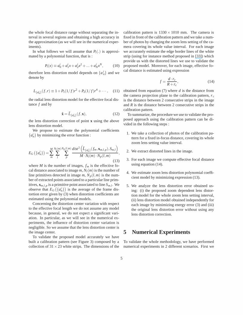
In Figure 10 the performances of the proposed zoommodel are illustrated. As in the case of the calibrationpattern experiment, we present a comparison of the lensdistortion error measures for (i) the original lens distor-tion error (3) without using any lens distortion correct-ion, (ii) lens distortion model obtained independently for

Table 2: Summary of results for the soccer video imagesset (RMS values).

Distortion Model Comparison Pixels

Residue without using lens distortion model 1.0601Residue from frame by frame model 0.5478Residue from proposed zoom polynomial model 0.5551

each image by minimizing energy error (3) and (iii) en-ergy error (3) computed using the proposed polynomialzoom dependent lens distortion model. We observe thatthe quality of the distortion correction obtained using theproposed zoom model is as good as the one obtained in anindependent way frame by frame. In particular, in Table 2we summarize the RMS values for the 3 models presentedin Figure 10. From these results, it can be appreciatedthat the relative RMS value difference between the zoomdependent proposed model and model estimated indepen-dently frame by frame is just around 1.33%. These resultsare expressed only in pixels because, as the camera is notin a front-parallel position respect to the view, we can notassociate a real single length measure (meters) to the pixelsize and so the pixel error measures can not be convertedto meter units.

One very important advantage of the proposed modelis that using the obtained polynomials we can estimatethe lens distortion model for any effective focal distancef . In particular we can obtain lens distortion models forthe whole video sequence (841 frames) in spite of just 55frames have been used to estimate the polynomials.

To illustrate the application of the proposed approachto the whole video sequence we have created a videowhere the lens distortion is corrected for each frame usingthe proposed zoom dependent polynomial model (see thisdemo video at http://www.ctim.es/demo101/).

6 Conclusions

Real applications for zoom camera demand high accuratecamera calibration estimation. Most zoom lenses presenta significant variation of lens distortion along the zoomsetting range. To study and model such variation can be

11

regarded as a relatively new and challenging field of re-search and it is a necessary step to deal with zoom lenses.In this work, new mathematical models to study the varia-tion of lens distortion models when we change zoom lenssetting have been discussed. Such mathematical modelsare based on a polynomial approximation to account forthe variation of the radial distortion parameters throughthe range of zoom lens settings and the minimization ofa global error energy measuring the distance between se-quences of distorted aligned points and straight lines afterlens distortion correction.

The numerical experiments we have performed are verypromising. We have obtained that using just a second or-der polynomial approximation of lens distortion parame-ter zoom variation, the quality of lens distortion correct-ion is as good as the one obtained individually frame byframe. In practice, this is very important because it meansthat using just 6 parameters (3 parameters for the poly-nomial associated to the first lens distortion coefficient k1

and 3 parameters for the second lens distortion coefficientk2) we can estimate the lens distortion model for any ef-fective focal distance of zoom lens.

The proposed model have been first applied to accu-rately estimate the zoom dependent lens distortion modelusing a calibration pattern. Then, for a real soccer videosequence filmed using a professional video camera, dis-tortion has been corrected and a video have been pre-sented to illustrate such distortion correction. The resultsfor both cases show the potentiality of the proposed zoomdependent model.

Acknowledgments

This research has partially been supported by theMICINN project reference MTM2010-17615 (Ministeriode Ciencia e Innovacion. Spain). We acknowledge ME-DIAPRODUCCION S.L. company who has kindly pro-vided to us with the real soccer video sequence we use inthe numerical experiments.

0.005 0.01 0.015 0.02 0.025 0.03 0.035 0.04 0.045 0.050

0.1

0.2

0.3

0.4

0.5

0.6

0.7

0.8

1/f (mm−1)

RM

S D

ista

nce f

un

cti

on

(m

m.)

Figure 9: Distance function for the geometric pattern es-timated by the three models (dashed line: original errorfunction, solid line: proposed quadratic zoom model, dot-ted line: frame by frame model (6)).

12

0.006 0.008 0.01 0.012 0.014 0.016 0.018 0.02 0.022 0.0240

0.2

0.4

0.6

0.8

1

1.2

1.4

1.6

1.8

2

1/f (mm−1)

RM

S D

ista

nc

e f

un

cti

on

(p

ixe

ls)

Figure 10: Distance function for the soccer video se-quence estimated by the three models (dashed line: orig-inal error function, solid line: proposed quadratic zoommodel, dotted line: frame by frame model (6)).

13

References

[1] Faugeras, O.: Three-Dimensional Computer Vision.MIT Press (1993)

[2] Devernay, F., Faugeras, O.: Straight lines have to bestraight. Machine Vision and Applications. 13(1), 14- 24 (2001)

[3] Faugeras, O., Luong, Q-T., Papadopoulo, T.: TheGeometry of multiple images. MIT Press (2001)

[4] Tsai, R. Y.: A versatile camera calibration techniquefor high-accuracy 3D machine vision metrology us-ing off-the-shelf tv cameras and lenses. IEEE Jour-nal of Robotics and Automation. 3(4), 323 - 344(1987)

[5] Weng, J., Cohen, P., Herniou, M.: Camera calibra-tion with distortion models and accuracy evaluation.IEEE Transactions on Pattern Analysis and MachineIntelligence. 14(10), 965 - 980 (1992)

[6] Light, D. L.: The new camera calibration system atthe U.S. geological survey. Photogrammetric Engi-neering & Remote Sensing. 58(2), 185 - 188 (1992)

[7] Wang, A., Qiu, T., Shao, L.: A simple method of ra-dial distortion correction with centre of distortion es-timation. Journal of Mathematical Imaging and Vi-sion. 35(3), 165 - 172 (2009)

[8] Rosten, E., Loveland, R.: Camera distortion self-calibration using the plumb-line constraint and min-imal Hough entropy. Machine Vision and Applica-tions. 22(1), 77 - 85 (2009)

[9] Alvarez, L., Gomez, L., Sendra, R.: An algebraicapproach to lens distortion by line rectification. Jour-nal of Mathematical Imaging and Vision. 35(1), 36 -50 (2009)

[10] Song, G-Y., Lee, J-W.: Correction of radial distor-tion based on line-fitting. International Journal ofControl, Automation and Systems. 8(3), 615 - 621(2010)

[11] Ricolfe-Viala, C., Sanchez-Salmeron, A.: Correct-ing non-linear lens distortion in cameras without us-ing a model. 42(4), 628 - 639 (2010)

[12] Li, H., Hartley, R.: A non-iterative method for cor-recting lens distortion from nine points correspon-dences. Proceedings of the International Conferenceon Computer Vision Workshop, Beijing (China)(2005)

[13] Fraser, C. S., Shortis, M. R.: Variation of distortionwithin the photographic field. Photogrammetric En-gineering Remote Sensing. 58(6), 851 - 855 (1992)

[14] Fraser, C., Al-Ajlouni, S.: Zoom-dependent ca-mera calibration in digital close-range photogram-metry. Photogrammetric Engineering Remote Sen-sing. 72(9), 1017-1026 (2006)

[15] Brauer-Burchardt, C., Heinze, M., Munkelt, C.,Kuhmstedt, P., Notni, G.: Distance dependent lensdistortion variation in 3D measuring systems usingfringe projection. In BMVC 2006, 327 - 336 (2006)

[16] Irani, M., Anandan, P.: A unified approach to mov-ing object detection in 2D and 3D scenes. IEEETransactions on Pattern Analysis and Machine In-telligence. 20(6), 577 - 589 (1998)

[17] Hampapur, A., Brown, L., Connell, J. et al.: Smartvideo surveillance: exploring the concept of multi-scale spatiotemporal tracking. IEEE Signal Process-ing Magazine. 22(2), 38 - 51 (2005)

[18] Martinez, E., Torras, C. Contour-based 3D motionrecovery while zooming. Robotics and AutonomousSystems. 44(3-4), 219 - 227 (2003)

[19] Fahn, C., Lo, C.: A high-definition human facetracking system using the fusion of omni-directionaland PTZ cameras mounted on a mobile robot. 5thIEEE Conference on Industrial Electronics and Ap-plications (ICIEA), Taichung (China), 6 - 11 (2010)

[20] Fayman, J., Sudarsky, O., Rivlin, E.: Zoom track-ing. Proceedings of the International Conference onRobotics and Automation, Leuven (Belgium). 2783- 2788 (1998)

[21] Peddigari, V., Kehtarnavaz, N.: A relational ap-proach to zoom tracking for digital still cameras.IEEE Transactions on Consumer Electronics. 51(4),1051 - 1059 (2005)

14

[22] Ergum, B.: Photogrammetric observing the varia-tion of intrinsic parameters for zoom lenses. Scien-tific Research and Essays. 5(5), 461 - 467, March(2010)

[23] Wilson, R., Shafer, S.: A perspective projection ca-mera model for zoom lenses. Proc. Second Con-ference on Optical 3-D Measurements Techniques,Switzerland, October (1993)

[24] Chen, Y., Shih, S., Hung, Y., Fuh, C.: Simple and ef-ficient method of calibrating a motorized zoom lens.Image and Vision Computing. 19(14), 1099-1110(2001)

[25] Tarabanis, K., Tsai, R., Goodman, D.: Modeling ofa computer-controlled zoom lens. In Proceedings ofIEEE International Conference on Robotics and Au-tomation. Vol. 2, 1545 - 1551 (1992)

[26] Li, M., Lavest, J.: Some aspects of zoom lenscamera calibration. IEEE Transactions on PatternAnalysis and Machine Intelligence. 18(11), 1105 -1110 (1996)

[27] Atienza, R., Zelinsky, A.: A practical zoom cameracalibration technique: an application on active vi-sion for human-robot interaction. In Proceedings ofAustralian Conference on Robotics and Automation,Sydney (Australia). 85 - 90 (2001)

[28] Sarkis, M., Senft, C., Diepold, K.: Modeling thevariation of the intrinsic parameters of an automaticzoom camera system using moving least-squares.In Proceedings of IEEE Conference on AutomationScience and Engineering (CASE), Arizona (USA)(2007)

[29] Benhimane, S., Malis, E. Self-calibration of the dis-tortion of a zooming camera by matching points atdifferent resolutions. In Proceedings of IEEE/RSJInternational Conference on Intelligent Robots andSystems, Sendai(Japan). 2307 - 2312 (2004)

[30] Kim, D., Shin, H., Oh, J., Sohn, K.: Automatic ra-dial distortion correction in zoom lens video camera.Journal of Electronic Imaging. 19(4), 43010 - 43017(2010)

[31] Hanning, T. High precision camera calibration witha depth dependent distortion mapping. In: Inter-national Conference on Visualization, Imaging andImage Processing Conference (VIIP), Palma deMallorca (Spain). 304 - 309 (2008)

[32] Aleman-Flores, M., Alvarez, L., Henrıquez, P., Ma-zorra, L.: Morphological thick line center detection.Proceedings ICIAR’2010, Springer LNCS 6111. 71- 80 (2010)

[33] Alvarez, L., Escların J., Trujillo, A.: A model basededge location with subpixel precision. ProceedingsIWCVIA 03: International WorkShop on ComputerVision and Image Analysis, Las Palmas de Gran Ca-naria (SPAIN). 29 - 32 (2003)

[34] Zhang, Z.: A flexible new technique for camera cali-bration. IEEE Transactions on Pattern Analysis andMachine Intelligence. 22(11), 1330 - 1334 (2000)

15