
effect of capillary pressure on estimation of relative - UTPedia
80
EFFECT OF CAPILLARY PRESSURE ON ESTIMATION OF RELATIVE PERMEABILITY FROM CORE FLOODING TESTS by Abdulhadi Elsounousi Khalifa Dissertation submitted in partial fulfilment of the requirement for the MSc. Petroleum Engineering JULY 2012 Universiti Teknologi PETRONAS Bandar Seri Iskandar 31750 Tronoh Perak Darul Ridzuan
-
Upload
khangminh22 -
Category
Documents
-
view
3 -
download
0
Transcript of effect of capillary pressure on estimation of relative - UTPedia
EFFECT OF CAPILLARY PRESSURE ON ESTIMATION OF RELATIVE
PERMEABILITY FROM CORE FLOODING TESTS
by
Abdulhadi Elsounousi Khalifa
Dissertation submitted in partial fulfilment of
the requirement for the
MSc. Petroleum Engineering
JULY 2012
Universiti Teknologi PETRONAS
Bandar Seri Iskandar
31750 Tronoh
Perak Darul Ridzuan
CERTIFICATE OF APPROVAL
EFFECT OF CAPILLARY PRESSURE ON ESTIMATION OF RELATIVE
PERMEABILITY FROM CORE FLOODING TESTS
by
Abdulhadi Elsounousi Khalifa
Dissertation submitted in partial fulfilment of
the requirement for the
MSc. Petroleum Engineering
JULY 2012
Approved by,
___________________________
Prof. Dr. Noaman El-Khatib
UNIVERSITI TEKNOLOGI PETRONAS
TRONOH, PERAK
JULY 2012

CERTIFICATION OF ORIGINALITY
This is to certify that we are responsible for the work submitted in this project, that
the original work is my own except as specified in the reference and
acknowledgements, and that the original work contained herein have not been
undertaken or done by unspecified sources or persons.
____________________________________________
ABDULHADI ELSOUNOUSI KHALIFA

ABSTRACT
The following investigation focuses on the impact of capillary pressure on estimation
of two phases relative permeability curves. Accurate relative permeability is a crucial
parameter for evaluating reservoir performance. The unsteady state core flooding
tests, which is considered in this study, is mostly used to measure oil-water relative
permeabilities.
The Johnson ,Bossler and Neumann (JBN) method is the conventional method for
estimating relative permeabilities from field core. The limitations in the JBN method
create an error in relative permeability curves and make it unrepresentative of a
typical core flooding test results. There are always capillary pressure effects taking
place during core flood tests. Ignoring of capillary pressure by JBN method will
influence the calculation of relative permeability curves and final saturation levels.
One dimensional numerical model with uniform initial saturation has been
implemented in this study using Eclipse 100 software to understand the relationship
between relative permeability and capillary pressure. Pressure drop and recovery
data obtained from 1-D numerical simulations are used to estimate the relative
permeabilities by JBN method. Many scenarios have been studied by running the
simulation at constant injection rate and varying the input capillary pressure.
The results obtained have shown the influence of capillary pressure on estimating
relative permeability curves. It is shown that increase in capillary pressure increases
the water relative permeability. Furthermore, the results demonstrate that the water
flooding curves differ greatly in shape and position according to the corresponding
values of capillary pressure.
Comparisons of relative permeability curves have shown that the capillary pressure
dominates the displacement process. Capillary pressure gradient will increase the
fractional flow of water and this increase in fractional flow of water results in lower
frontal water saturation, higher frontal velocity and subsequently leading to a
decrease in oil recovery.

V
ACKNOWLEDGEMENTS
First and foremost, I thank Allah for endowing me with health, patience, and
knowledge to complete this work.
I want to use this opportunity to express a heartfelt gratitude to my supervisor,
Professor Noaman El-Khatib, for offering me a thesis topic that I find very
interesting. His wealth of experience and passion for his work is a great source
of inspiration to me. Prof. El-Khatib is an enthusiastic person and his door is
always open.
I would like to recognize Dr. Ismail Bin Mohd Saaid and Dr Khalik Mohamad
Sabil for their advices and assistance during this period.
I would like to thank the PhD student at EOR center, Isa Adeeyo for his
encouragement. I thank him for his thorough guidance, inspiring discussions,
and proof reading of my thesis.
I also wish to acknowledge the UNIVERSITI TEKNOLOGI PETRONAS and the
Department of Petroleum Engineering for offering me a good working environment.
Also I would like to express my sincere gratitude to UTP and Herriot Watt lecturers
for their effort on the past courses which helped me to successfully complete this
work.
I need to say a big thanks to my adorable and devoted family, for all their
unflinching supports.
Last but not least, I would like to thank all my friends across the world, colleagues,
and classmates for their encouragement, assistance, and joyful times.
VI
Table of Contents
CHAPTER 1 ................................................................................................................ 1
INTRODUCTION ....................................................................................................... 1
1.1 BACKGROUND ......................................................................................... 1
1.2 PROBLEM STATEMENT .......................................................................... 7
1.3 OBJECTIVES .............................................................................................. 7
1.4 SCOPE OF STUDY ..................................................................................... 8
CHAPTER 2 ................................................................................................................ 9
THEORY AND LITERATURE REVIEW .................................................................. 9
2.1 MEASURING RELATIVE PERMEABILITY ........................................... 9
2.1.1 Steady State Methods ............................................................................... 9
2.1.2 Unsteady State Methods ......................................................................... 11
2.2 FLOW OF IMMISCIBLE FLUID IN POROUS MEDIA ......................... 12
2.2.1 Buckley and Leverett Theory ................................................................. 13
2.2.2 Welge Displacement Approach.............................................................. 17
2.3 THE JBN METHOD .................................................................................. 19
2.3.1 JBN DERIVATION ............................................................................... 19
2.4 EFFECT OF CAPILLARY PRESSURE ON FLUID FLOW DURING
CORE FLOODING TESTS ................................................................................... 23
CHAPTER 3 .............................................................................................................. 30
METHODOLOGY ..................................................................................................... 30
CHAPTER 4 .............................................................................................................. 33
NUMERICAL SIMULATION RESULTS AND DISCUSSION ............................. 33
4.1 ECLIPSE 100 ............................................................................................. 33
4.2 SIMULATION OF CORE FLOODING TO DETERIMINE OIL-WATER
RELATIVE PERMEABILITIES ........................................................................... 33
4.2.1 Case 1 ..................................................................................................... 38
4.2.2 Case 2 ..................................................................................................... 44
4.2.3 Case 3 ..................................................................................................... 48
4.2.4 Case 4 ..................................................................................................... 52
CHAPTER 5 .............................................................................................................. 56

VII
CONCLUSIONS AND RECOMMENDATIONS .................................................... 56
5.1 CONCLUSIONS ........................................................................................ 56
5.2 RECOMMENDATIONS ........................................................................... 57
REFERENCES ........................................................................................................... 58
APPENDICES ........................................................................................................... 61
Appendix A ........................................................................................................... 61
VIII
LIST OF FIGURES Figure 1: Capillary pressure versus water saturation [3]. ............................................ 2
Figure 2: Relative permeability curves ........................................................................ 5
Figure 3: Drainage process........................................................................................... 6
Figure 4: Imbibitions process ....................................................................................... 6
Figure 5: Steady state experiment procedure ............................................................. 10
Figure 6: Unsteady state procedure ............................................................................ 12
Figure 7: Fractional flow curve as a function of water saturation ............................. 14
Figure 8: Water saturation versus distance ................................................................ 15
Figure 9: Water saturation distribution in the displacement path .............................. 15
Figure 10 : (a) Capillary pressure versus saturation (b) Water saturation distribution
as a function of distance. ............................................................................................ 17
Figure 11: Welge graphical method ........................................................................... 18
Figure 12: Water arrives at the outlet of the core....................................................... 24
Figure 13: Water flow out of the core ....................................................................... 25
Figure 14: Relative permeability versus water saturation .......................................... 35
Figure 15: Capillary pressures versus saturation ....................................................... 36
Figure 16: One dimensional cartesian grid ................................................................ 36
Figure 17: Water injected versus oil recovery ........................................................... 39
Figure 18: Average saturation versus total water injected ......................................... 40
Figure 19: Pressure drop versus time ......................................................................... 41
Figure 20: Relative permeability curves from JBN and input relative permeability
curves ......................................................................................................................... 42
Figure 21: Water saturation versus distance .............................................................. 43
Figure 22: Water injection versus oil recovery .......................................................... 44
Figure 23: Water injection versus average saturation ................................................ 45
Figure 24: Pressure drop versus time ......................................................................... 46
Figure 25: Relative permeability curves from JBN & input relative permeability
curves for Case 2 ........................................................................................................ 47
Figure 26: Water saturation versus distance .............................................................. 47
Figure 27: Water injection versus average saturation ................................................ 48
Figure 28: Water injection versus oil recovery .......................................................... 49
Figure 29: Pressure drop versus time ......................................................................... 50
IX
Figure 30: Relative permeabilities from JBN & input relative permeabilities for
case3 ........................................................................................................................... 51
Figure 31: Water saturation versus distance .............................................................. 51
Figure 32: Water injection versus oil recovery .......................................................... 52
Figure 33: Water injected versus average saturation ................................................. 53
Figure 34: Pressure drop versus time ......................................................................... 53
Figure 35: Relative permeabilities from JBN & input relative permeabilities for
Case4 .......................................................................................................................... 54
Figure 36: Water saturation versus distance .............................................................. 55

X
LIST OF TABLES Table 1: Core properties ............................................................................................. 34
Table 2: Oil/water relative permeability .................................................................... 34
Table 3: Capillary pressures ....................................................................................... 35
XI
NOMENCLATURES
porosity
Capillary pressure
Capillary pressure of non wetting phase
Capillary pressure of wetting phase
σ Surface tension
r Radius of the pore
Ɵ Contact angle
V Fluid velocity
K Permeability
µ Viscosity of the fluid
Flow rate through the porous medium
A Cross-sectional area across which flow occurs
Effective permeability
Absolute permeability
Oil relative permeability
Effective permeability of oil
Water relative permeability
Effective permeability of water
Gas relative permeability
Effective permeability of gas
Initial water saturation
Irreducible oil saturation
Pressure drop
Total flow rate
ƒw Fractional flow of water
Average water saturation
µo Viscosity of oil
XII
µw Viscosity of water
Reservoir dip angle
g Gravitational constant
Connate water saturation
Water saturation
Water saturation at the Buckley-Leverett front
Fractional of displacing phase in flowing stream
Fractional of displaced phase in flowing stream
Cumulative injection in pore volume
Average velocity
Length
Relative injectivity
Cumulative oil recovery
Pore volume
1
CHAPTER 1
INTRODUCTION
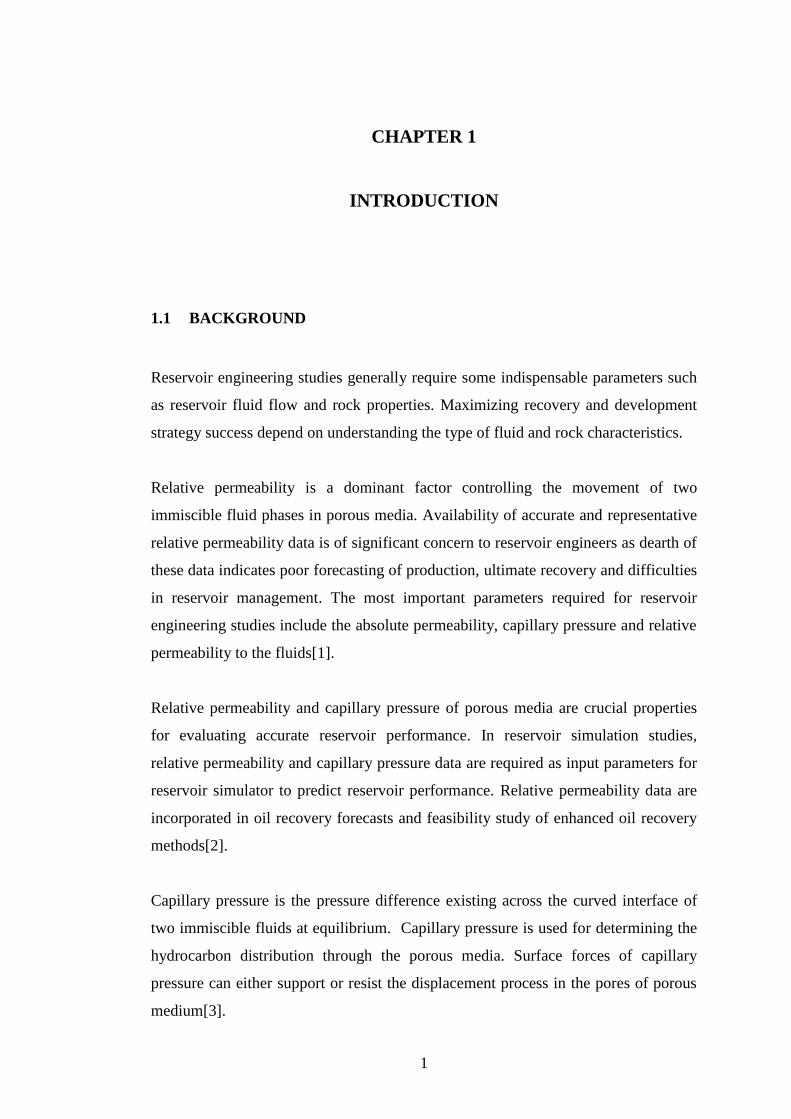
1.1 BACKGROUND
Reservoir engineering studies generally require some indispensable parameters such
as reservoir fluid flow and rock properties. Maximizing recovery and development
strategy success depend on understanding the type of fluid and rock characteristics.
Relative permeability is a dominant factor controlling the movement of two
immiscible fluid phases in porous media. Availability of accurate and representative
relative permeability data is of significant concern to reservoir engineers as dearth of
these data indicates poor forecasting of production, ultimate recovery and difficulties
in reservoir management. The most important parameters required for reservoir
engineering studies include the absolute permeability, capillary pressure and relative
permeability to the fluids[1].
Relative permeability and capillary pressure of porous media are crucial properties
for evaluating accurate reservoir performance. In reservoir simulation studies,
relative permeability and capillary pressure data are required as input parameters for
reservoir simulator to predict reservoir performance. Relative permeability data are
incorporated in oil recovery forecasts and feasibility study of enhanced oil recovery
methods[2].
Capillary pressure is the pressure difference existing across the curved interface of
two immiscible fluids at equilibrium. Capillary pressure is used for determining the
hydrocarbon distribution through the porous media. Surface forces of capillary
pressure can either support or resist the displacement process in the pores of porous
medium[3].
2
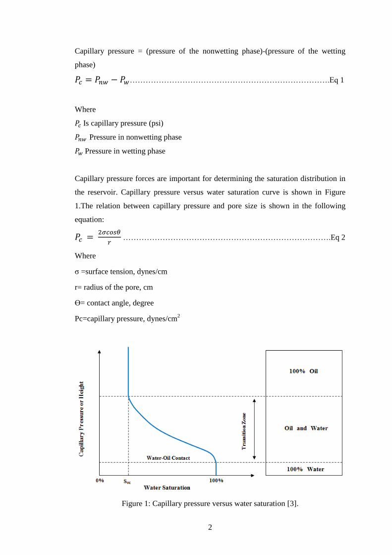
Capillary pressure = (pressure of the nonwetting phase)-(pressure of the wetting
phase)
………………………………………………………………….Eq 1
Where
Is capillary pressure (psi)
Pressure in nonwetting phase
Pressure in wetting phase
Capillary pressure forces are important for determining the saturation distribution in
the reservoir. Capillary pressure versus water saturation curve is shown in Figure
1.The relation between capillary pressure and pore size is shown in the following
equation:
…………………………………………………………………….Eq 2
Where
σ =surface tension, dynes/cm
r= radius of the pore, cm
Ɵ= contact angle, degree
Pc=capillary pressure, dynes/cm2
Figure 1: Capillary pressure versus water saturation [3].
3
Capillary pressure is used in [3]:
Fluid saturation distribution.
Reservoir fluid content.
Connate water saturation.
Input for reservoir simulation calculation.
The permeability is defined as the ability of the rock to transmit fluid through its
interconnected pore. It is a vector quantity and determines the direction flow of fluid
in the reservoir [3].
In 1856 Henry Darcy was the first engineer who illustrated mathematically the
property of the rock. He developed the fluid flow equation for a linear horizontal
system and it is given by Darcy equation [3]:
………………………………………………………….…………..Eq 3
Where
=fluid velocity, cm/sec
= Permeability, Darcy’s
μ = Viscosity of the fluid, cp
= Pressure drop per unit length, atm/cm
The apparent velocity in the previous equation can be determined by dividing flow
rate by the area (q/A), so the equation3 can be written as [3]:
…………………………………………………………………...…Eq 4
Where
q= flow rate through the porous medium, cm3/sec
A=cross-sectional area across which flow occurs, cm2
4
The relative permeability is the ability of a porous medium to transmit fluid when
more than one fluid is present in the reservoir and it is the ratio of effective
permeability to the absolute permeability. Relative permeability can be represented
by the following equation [3]:
………………………………………………………….……………..Eq 5
The relative permeability for oil, water and gas are shown in the equations below
respectively [3]:
….…………………………………………………………..………….Eq 6
…………………………………………………………………..…….Eq 7
…………………………………………………………………………Eq 8
Where
kro = relative permeability to oil
krg = relative permeability to gas
krw = relative permeability to water
k = absolute permeability
ko = effective permeability to oil for a given oil saturation
kg = effective permeability to gas for a given gas saturation
kw = effective permeability to water at some given water saturation
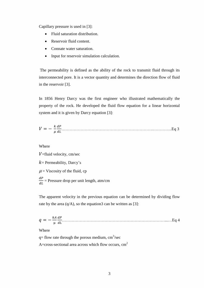
Core is usually used in the laboratory for measuring relative permeabilities of oil and
water or gas. Typical curves for relative permeability versus water saturation are
shown in Figure 2. The fluid saturations are assumed to be distributed uniformly with
respect to thickness. Flow in reservoir where uniform saturation distribution exists
over thickness of the sample can be described by either laboratory measurement or
rock relative permeability relationship. Existences of capillary and gravity forces are
very common over a range of core plug length. This results in a non-uniform water
5
saturation distribution. Hence, rock relative permeability is not generally utilized in
actual field displacement calculations [4].
Figure 2: Relative permeability curves [4].
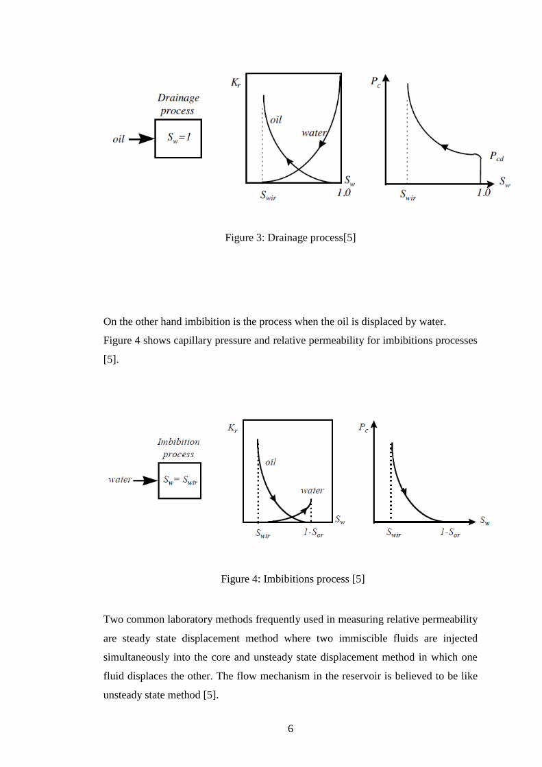
Drainage and imbibitions may be required in the estimation of relative permeability.
Capillary pressure and relative permeability for drainage processes are shown in
Figure 3. Reservoir rock was 100% saturated before oil accumulation. Oil
accumulation results in the drainage process by which the saturation of the wetting
phase (water) is reduced. The process of oil migration into the reservoir and
displaces the water is called drainage [5].
6
Figure 3: Drainage process[5]
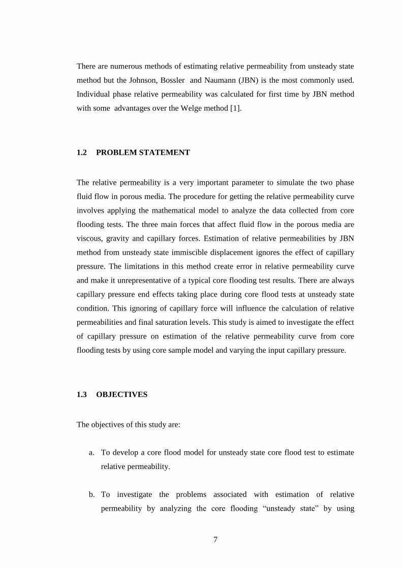
On the other hand imbibition is the process when the oil is displaced by water.
Figure 4 shows capillary pressure and relative permeability for imbibitions processes
[5].
Figure 4: Imbibitions process [5]
Two common laboratory methods frequently used in measuring relative permeability
are steady state displacement method where two immiscible fluids are injected
simultaneously into the core and unsteady state displacement method in which one
fluid displaces the other. The flow mechanism in the reservoir is believed to be like
unsteady state method [5].
7
There are numerous methods of estimating relative permeability from unsteady state
method but the Johnson, Bossler and Naumann (JBN) is the most commonly used.
Individual phase relative permeability was calculated for first time by JBN method
with some advantages over the Welge method [1].
1.2 PROBLEM STATEMENT
The relative permeability is a very important parameter to simulate the two phase
fluid flow in porous media. The procedure for getting the relative permeability curve
involves applying the mathematical model to analyze the data collected from core
flooding tests. The three main forces that affect fluid flow in the porous media are
viscous, gravity and capillary forces. Estimation of relative permeabilities by JBN
method from unsteady state immiscible displacement ignores the effect of capillary
pressure. The limitations in this method create error in relative permeability curve
and make it unrepresentative of a typical core flooding test results. There are always
capillary pressure end effects taking place during core flood tests at unsteady state
condition. This ignoring of capillary force will influence the calculation of relative
permeabilities and final saturation levels. This study is aimed to investigate the effect
of capillary pressure on estimation of the relative permeability curve from core
flooding tests by using core sample model and varying the input capillary pressure.
1.3 OBJECTIVES
The objectives of this study are:
a. To develop a core flood model for unsteady state core flood test to estimate
relative permeability.
b. To investigate the problems associated with estimation of relative
permeability by analyzing the core flooding “unsteady state” by using
8
JOHNSON, BOSSLER and NAUMANN method (JBN) which does not
consider the capillary pressure. This limitation in analyzing the core flood
data come up with the end capillary effect.
c. To demonstrate the important aspect of the error caused due to ignoring the
capillary pressure and the effect of the injection rate on the feasibility of
using the JBN to calculate the relative permeability curve.
1.4 SCOPE OF STUDY
This study addresses the determination of relative permeability from unsteady state
core flooding tests. The project focuses on understanding the relationship between
relative permeability and capillary pressure. The purpose is to check the accuracy of
estimating relative permeability from JBN method by varying the input capillary
pressure for core flood model in numerical simulation.
9
CHAPTER 2
THEORY AND LITERATURE REVIEW
This chapter gives an outline of relative permeability measurement and the effect of
capillary pressure on it.
2.1 MEASURING RELATIVE PERMEABILITY
Accurate measurement of two or three phase relative permeability is vital to reservoir
engineering application, especially in the reservoir simulation for forecasting
production and ultimate recovery. The relative permeability is the ability of the
porous medium to transmit fluid in porous media when more than one fluid is present
[6].
Knowledge of relative permeabilities is required for simulation of multiphase flow in
porous media. Relative permeability is usually obtained in the laboratory from core
flooding tests. There are numerous methods for measuring relative permeability
which can be categorized into two types: steady state and unsteady state core
flooding tests [7].
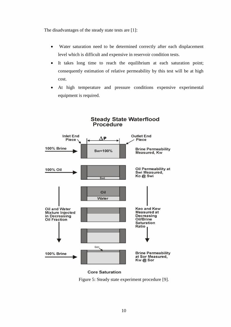
2.1.1 Steady State Methods
The two immiscible phases are simultaneously injected into the core and the
saturation and pressure drop across the core are measured as they are not changing
with time. The core inlet and outlet are connected to pressure transducer. The oil and
water are pumped into the core by metering pumps at steady flow rates. The pump
rates are adjusted to control the individual flow rate of the liquids. The procedure for
steady state tests is shown in Figure 5. End effects are prevented since the steady
state test is an equilibrium flow test which make it preferable for some investigators
[8][9].
10
The disadvantages of the steady state tests are [1]:
Water saturation need to be determined correctly after each displacement
level which is difficult and expensive in reservoir condition tests.
It takes long time to reach the equilibrium at each saturation point;
consequently estimation of relative permeability by this test will be at high
cost.
At high temperature and pressure conditions expensive experimental
equipment is required.
Figure 5: Steady state experiment procedure [9].
11
Leverett conducted relative permeability experiment on steady rate of oil and water
in unconsolidated sand column. Relative permeability and water saturation were
monitored when the steady condition had been reached. He applied the steady state
method and concluded that at low flow rate, the pressure measurement will be
affected by capillary discontinuities at the end of the core outlet. Also from his
experiment result, he concluded that the oil-water relative permeability of an
unconsolidated sand were extensively independent of the viscosity of the fluid but is
related to its pore size distribution, displacement pressure, pressure gradient and
water saturation [10].
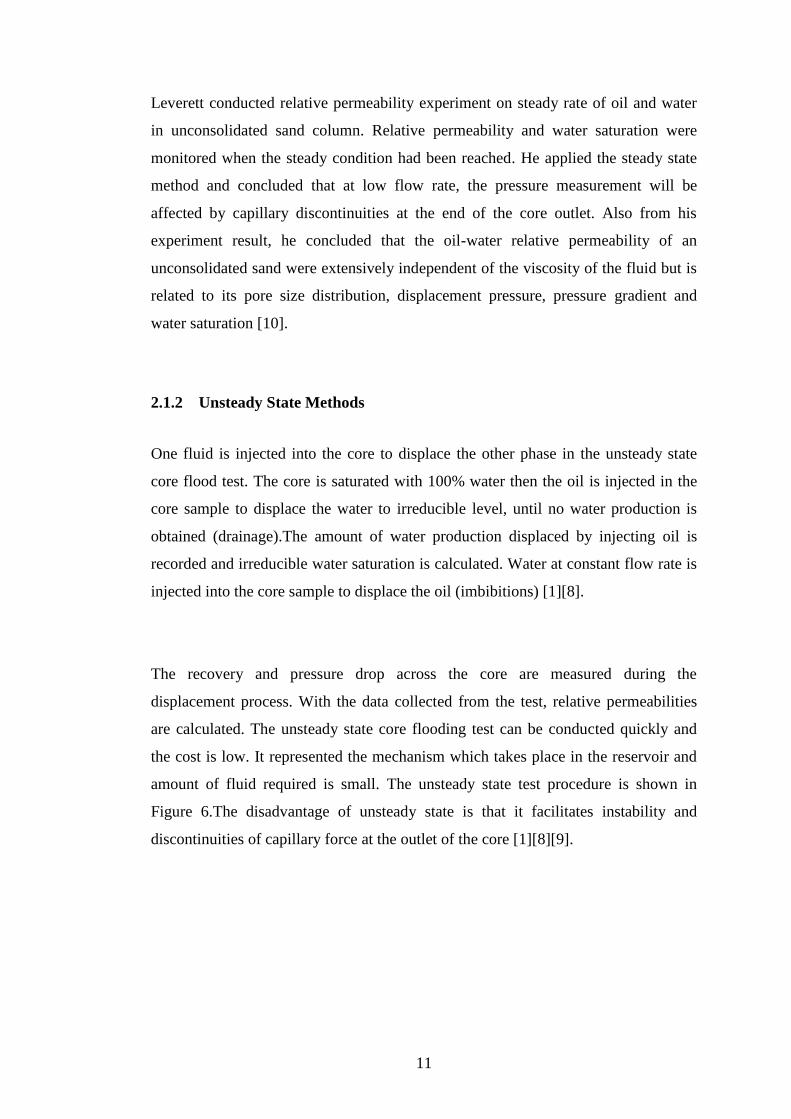
2.1.2 Unsteady State Methods
One fluid is injected into the core to displace the other phase in the unsteady state
core flood test. The core is saturated with 100% water then the oil is injected in the
core sample to displace the water to irreducible level, until no water production is
obtained (drainage).The amount of water production displaced by injecting oil is
recorded and irreducible water saturation is calculated. Water at constant flow rate is
injected into the core sample to displace the oil (imbibitions) [1][8].
The recovery and pressure drop across the core are measured during the
displacement process. With the data collected from the test, relative permeabilities
are calculated. The unsteady state core flooding test can be conducted quickly and
the cost is low. It represented the mechanism which takes place in the reservoir and
amount of fluid required is small. The unsteady state test procedure is shown in
Figure 6.The disadvantage of unsteady state is that it facilitates instability and
discontinuities of capillary force at the outlet of the core [1][8][9].
12
Figure 6: Unsteady state procedure [9].
2.2 FLOW OF IMMISCIBLE FLUID IN POROUS MEDIA
The capacity of a rock to conduct fluids is affected by the presence of immiscible
fluids for example oil and water. The process of displacing one phase by another
phase is an unsteady state displacement as the saturation of fluids changes with time
and invariably changes the relative permeabilities and pressure or phase velocities.
13
Buckley-Leverett developed one of the methods which predict displacement
performance and it is also called frontal advance method [11].
2.2.1 Buckley and Leverett Theory
In 1941 Leverett proposed the concept of boundary effect as a result of capillary
forces and figured out that the discontinuity of capillary forces at the outlet of the
core retains the wetting phase. This causes accumulation of saturation wetting phase
at the outlet and decrease in the non-wetting phase permeability [12].
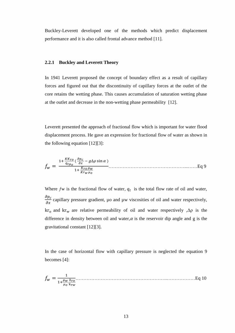
Leverett presented the approach of fractional flow which is important for water flood
displacement process. He gave an expression for fractional flow of water as shown in
the following equation [12][3]:
…………………………………………...……Eq 9
Where ƒw is the fractional flow of water, is the total flow rate of oil and water,
capillary pressure gradient, µo and µw viscosities of oil and water respectively,
and are relative permeability of oil and water respectively ,Δρ is the
difference in density between oil and water, is the reservoir dip angle and g is the
gravitational constant [12][3].
In the case of horizontal flow with capillary pressure is neglected the equation 9
becomes [4]:
………………………………………………….………………Eq 10
14
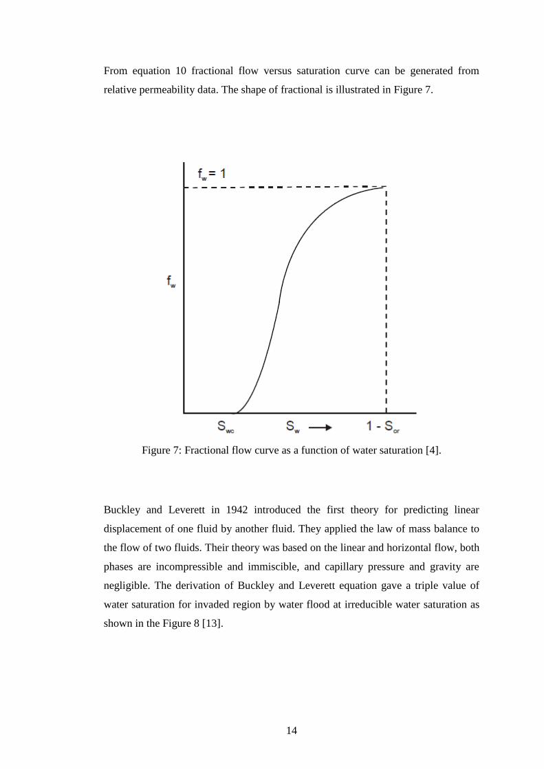
From equation 10 fractional flow versus saturation curve can be generated from
relative permeability data. The shape of fractional is illustrated in Figure 7.
Figure 7: Fractional flow curve as a function of water saturation [4].
Buckley and Leverett in 1942 introduced the first theory for predicting linear
displacement of one fluid by another fluid. They applied the law of mass balance to
the flow of two fluids. Their theory was based on the linear and horizontal flow, both
phases are incompressible and immiscible, and capillary pressure and gravity are
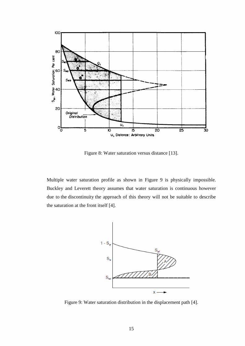
negligible. The derivation of Buckley and Leverett equation gave a triple value of
water saturation for invaded region by water flood at irreducible water saturation as
shown in the Figure 8 [13].
15
Figure 8: Water saturation versus distance [13].
Multiple water saturation profile as shown in Figure 9 is physically impossible.
Buckley and Leverett theory assumes that water saturation is continuous however
due to the discontinuity the approach of this theory will not be suitable to describe
the saturation at the front itself [4].
Figure 9: Water saturation distribution in the displacement path [4].
16
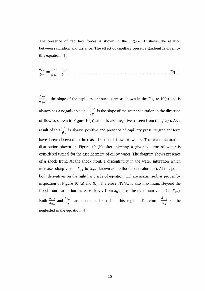
The presence of capillary forces is shown in the Figure 10 shows the relation
between saturation and distance. The effect of capillary pressure gradient is given by
this equation [4]:
…………………………………………………………………Eq 11
is the slope of the capillary pressure curve as shown in the Figure 10(a) and is
always has a negative value.
is the slope of the water saturation in the direction
of flow as shown in Figure 10(b) and it is also negative as seen from the graph. As a
result of this
is always positive and presence of capillary pressure gradient term
have been observed to increase fractional flow of water. The water saturation
distribution shown in Figure 10 (b) after injecting a given volume of water is
considered typical for the displacement of oil by water. The diagram shows presence
of a shock front. At the shock front, a discontinuity in the water saturation which
increases sharply from to , known as the flood front saturation. At this point,
both derivatives on the right hand side of equation (11) are maximised, as proven by
inspection of Figure 10 (a) and (b). Therefore ∂Pc/∂x is also maximum. Beyond the
flood front, saturation increase slowly from up to the maximum value (1 – ).
Both
and
are considered small in this region. Therefore
can be
neglected in the equation [4].
17
Figure 10 : (a) Capillary pressure versus saturation (b) Water saturation distribution
as a function of distance [4].
Fayers and Sheldon in 1959 established that if the capillary pressure is included the
triple saturation value does not exist. They also discovered that the gravity and
capillary pressure affect the Buckley and Leverett shape at low flow rate only.[14]
2.2.2 Welge Displacement Approach
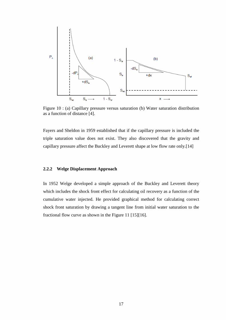
In 1952 Welge developed a simple approach of the Buckley and Leverett theory
which includes the shock front effect for calculating oil recovery as a function of the
cumulative water injected. He provided graphical method for calculating correct
shock front saturation by drawing a tangent line from initial water saturation to the
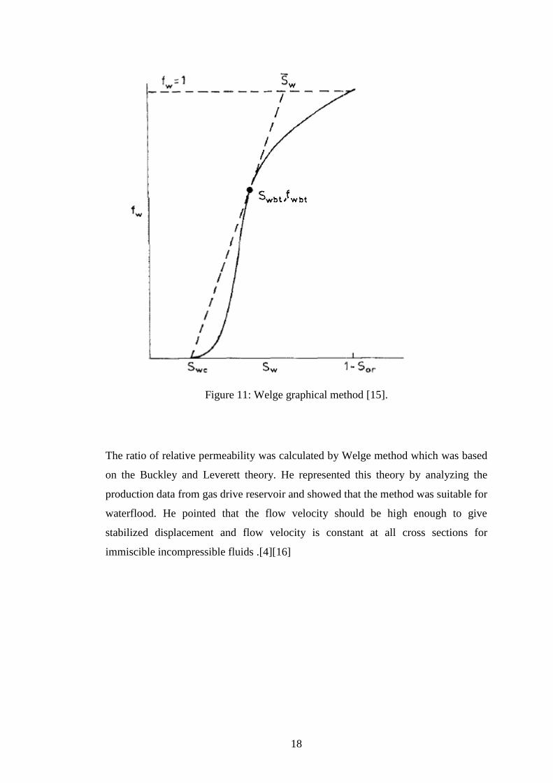
fractional flow curve as shown in the Figure 11 [15][16].
18
Figure 11: Welge graphical method [15].
The ratio of relative permeability was calculated by Welge method which was based
on the Buckley and Leverett theory. He represented this theory by analyzing the
production data from gas drive reservoir and showed that the method was suitable for
waterflood. He pointed that the flow velocity should be high enough to give
stabilized displacement and flow velocity is constant at all cross sections for
immiscible incompressible fluids .[4][16]
19
2.3 THE JBN METHOD
There are many methods for estimating the relative permeability by using unsteady
state core flooding experiments. The most commonly used method is the one
proposed by JOHNSON, BOSSLER and NAUMANN called the JBN method in
1959 which is based on Welge work .The data required for calculating the relative
permeabilities from core flooding experiments are the cumulative recovery of the
displaced phase and the pressure drops across the core section. They pointed out that
the result from their work is reliable and has agreement with direct measurement of
steady state flow tests for measuring the relative permeabilities [17].
The JBN method is less time consuming compared to other reliable methods used to
measure the relative permeability. From their results they confirmed that reliable
relative permeability can be measured from data obtained from short core samples
which is available for routine analysis [17].
2.3.1 JBN DERIVATION
The Buckley and Leverett theory (1941) was modified by Welge in 1952 to facilitate
estimation of relative permeability in laboratory core flooding displacement tests.
The work of Welge was extended by Johnson-Bossler-Naumann (JBN) 1958 for
estimation of the relative permeability from unsteady state core flood test data which
is consider in this study [17].
There are three important assumptions for JBN method [17]:
Total flow velocity is the same throughout the cross section of linear porous
body.
Flow velocity is high enough to achieve Buckley and Leverett displacement.
Capillary effect is negligible at high injection rates.
20
To overcome the capillary end effect the experiment should be done at high enough
displacement rate. At higher rate the flow will be unstable and the concept of relative
permeability will not hold. Cumulative recoveries of oil and water versus time are
measured at the outlet face of the core during the JBN method to estimate the relative
permeability curve. Some of the mathematical relations which have been developed
by Welge are required for calculation of two phase relative permeability by JBN
method as follow [17]:
=
⁄
…………………………………………………....................Eq 12
=
=
……………………………………………………………Eq 13
………………………………………………………………...…Eq 14
………………………………………………………….Eq 15
………………………………………………………………Eq 16
………...…………………………………………………….…Eq 17
The pressure drop across the core which has length L is shown as the integral
∫
……………………………………………………..………Eq 18
Substituting
from Eq16 will give,
∫
…………………………………………………………..Eq 18a
By rearranging and substituting equations 17 and 18a, the following equation is
obtained:
21
∫
=
⁄
⁄
=
…………………………….….Eq18b
Where is the relative injectivity which is the ratio of the intake capacity at any
given flood stage to the intake capacity of the system at the start of the flood. From
measurements of flow rate and pressure drop in a water flood susceptibility test,
relative injectivity function for a given type of reservoir rock can be determined [17].
Ordinary differentiation is used for equation 18b with respect to since is the
only independent variable [17],
(
)
…………………………………………………………………….Eq 19
When is equal to the reciprocal of the cumulative volume injection, the equation
19 will be written as [17],
(
)
(
)
…………………………………………………………Eq19a
From the equation 19a individual relative permeability of oil can be calculated. The
outlet face saturation is obtained by rearranging equation15 [17]:
………………………………………………..Eq15a
The relative permeability of the water at is calculated by solving equation13 [17]:
……………………………………………….....Eq 20
22
Jones and Roszelle in 1978 extended the JBN method for estimating relative
permeabilities by presenting a graphical technique to perform the essential
differentiation of the production data and the late time data analysis by their method.
They figured out that the fractional flow of displacing phase concave downward
when it is plotted against saturation. Jones and Roszell method could also be used for
experiments conducted at constant pressure drop across the core, constant rate or
changeable pressure drop and flow rate [18].
In 1984 Tao and Watson developed a Monte Carlo error analysis for JBN. The two
sources of error in relative permeability are estimation error which related to the
error included in the process of measured data to estimate relative permeability and
modeling error which is attributed to the degree where the mathematical model fails
to exhibit the physical experiment. They postulated that the use of various viscosity
ratios did not affect very much the accuracy of relative permeability and the injection
rate as well. The error will increase only when oil production or pressure drop are
reduced. They also developed the algorithms for computer implementation for JBN
method. They pointed out that the relative permeability can be estimated fairly
accurately by using linear regression or optimal spline algorithm [19][20].
In 1986 Kerig and Watson included high flexible cubic splines for estimating relative
permeability from unsteady state experiment. The error in estimating relative
permeability was greatly reduced by using cubic splines and very accurate result can
be obtained [21].
In 1988 Watson et al. introduced B-spline for use as functional representations of
relative permeability curves. They indicated that serious error may be detected when
relative permeability curves are performed with function having too few parameters.
They used both hypothetical and real experiments data for core flood test and also
pointed out that without acceptable number of parameters; large errors estimation
can occur [22].
23
2.4 EFFECT OF CAPILLARY PRESSURE ON FLUID FLOW DURING
CORE FLOODING TESTS
During core flooding test experiments in the laboratory the end effect of capillary
pressure occurs due to the discontinuity of capillary pressure when the fluid leave
the outlet of the core. This effect may lead to wrong interpretation of core flood tests
data. During displacement process the water phase will accumulate at the outlet end
of the core before the breakthrough. Sufficient water phase pressure can be achieved
when water at the outlet section of the core continues to buildup [11].
To overcome the capillary pressure end effect, wetting phase (water) is injected at
high flow rate using longer samples. On the contrary doing the core flooding tests
using high water flow rate raises concern as to whether the displacement process test
reflects what happens in the reservoir [23].
In 1956 Hadley and Handy investigated the end effect of capillary pressure in the
steady state. They studied the effect of different variables as flow rate, viscosities
and the outlet end saturation on the calculated relative permeabilities .They noticed
the saturation gradients for steady state and dynamic displacement tests. They
remarked that the pressure drop should be measured in both phases to get
representative relative permeability. Also they observed that as the flow rate is
increased the end effect of capillary pressure decreases [24].
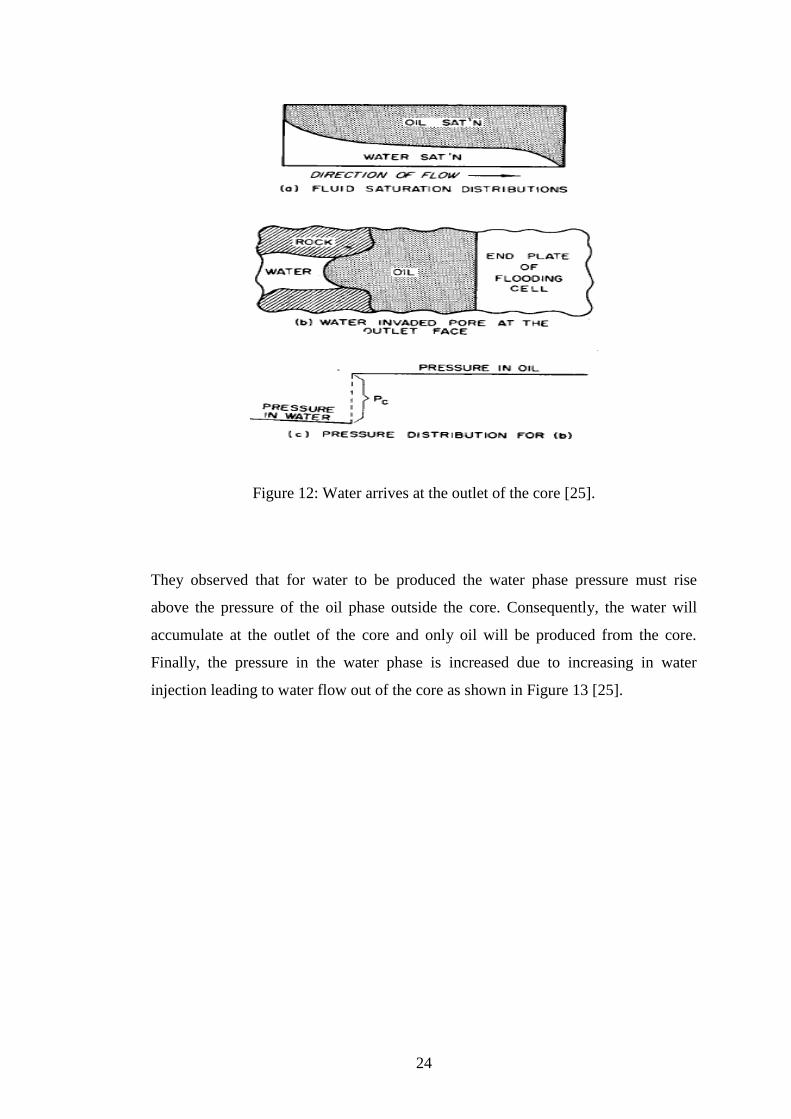
In 1958 Kyte and Rapoport studied the linear water flood behavior and end effect of
water wet porous media. Figure 12, shows the water wet core when the water first
arrives at the outlet [25].
24
Figure 12: Water arrives at the outlet of the core [25].
They observed that for water to be produced the water phase pressure must rise
above the pressure of the oil phase outside the core. Consequently, the water will
accumulate at the outlet of the core and only oil will be produced from the core.
Finally, the pressure in the water phase is increased due to increasing in water
injection leading to water flow out of the core as shown in Figure 13 [25].

25
Figure 13: Water flow out of the core [25].
Water is held back by capillary pressure at the outlet and result in apparent increased
breakthrough recovery .They reported that early breakthrough and instability may
result from high pressure drops and high flow rate [25].
In 1973 Archer and Wong stated that the JBN method gives an error in
heterogeneous cores due to ignoring capillary end effect. They indicated that the JBN
method may have irregular shapes of relative permeability curves from such system.
A computer model was proposed to history match the pressure drop and recovery for
low displacement flow rate to get the relative permeability curves. They used one
dimensional two phase mathematical model of the laboratory test conditions in their
simulation .This model allowed them to make trial and error changes in the shapes of
relative permeability curves until they get better match for laboratory production and
pressure data [26].
26
In 1979 Sigmund and McCaffery extended the approach suggested by Archer and
Wong. They performed a series of simulator calculations to investigate the effect of
capillary pressure at the outlet of the core by using an automatic history matching
technique. They pointed out that the recovery and pressure drop data obtained from
unsteady state tests are significantly affected by capillary pressure in some cases. At
drainage direction on low rate flow displacement, the calculation indicates serious
influence of capillary pressure [27].
In 1981 Batycky et al. evaluated capillary pressure and wettability for unsteady state
data by proposing method on low flow rate displacement as in situ reservoir
condition. They modified Sigmund and McCaffery simulator to reflect displacement
experiment perfectly. Capillary equilibrium was settled by stopping flow into the
core for certain time, they got extra pressure drop influenced by the capillary end
effect force .They pointed that further definition for understanding capillary pressure
end effect by using the simulator for matching the pressure drop and recovery is
needed. From their result, they observed that capillary end effect can be extended
over large part of the core when the system has strong wetting characteristics. Also
they mentioned that estimation of relative permeability from simulation when
capillary end effect is eliminated can give large error [28].
In 1985 Odeh and Dotson proposed a method for correcting Jones and Roszelle
technique by reducing the effect of flow rate and consequently reducing the errors
caused by capillary end effects in water wet systems. From their results it was shown
that at high oil saturation and high flow rate the relative permeability curves are not
strong functions of rate or less independent of the flow rate. At low oil saturation the
relative permeability curves are dependent on rate. Firstly, they calculated the
relative permeability curves by Jones and Roszelle from the data obtained from the
test and plotted
and
versus average water saturation
which is straight
line at low water saturation for high flow rate, for low flow rate straight line may not
exists. They assumed the capillary end effect will not affect the estimation of oil
27
relative permeability in this region. The straight line can be extended over the entire
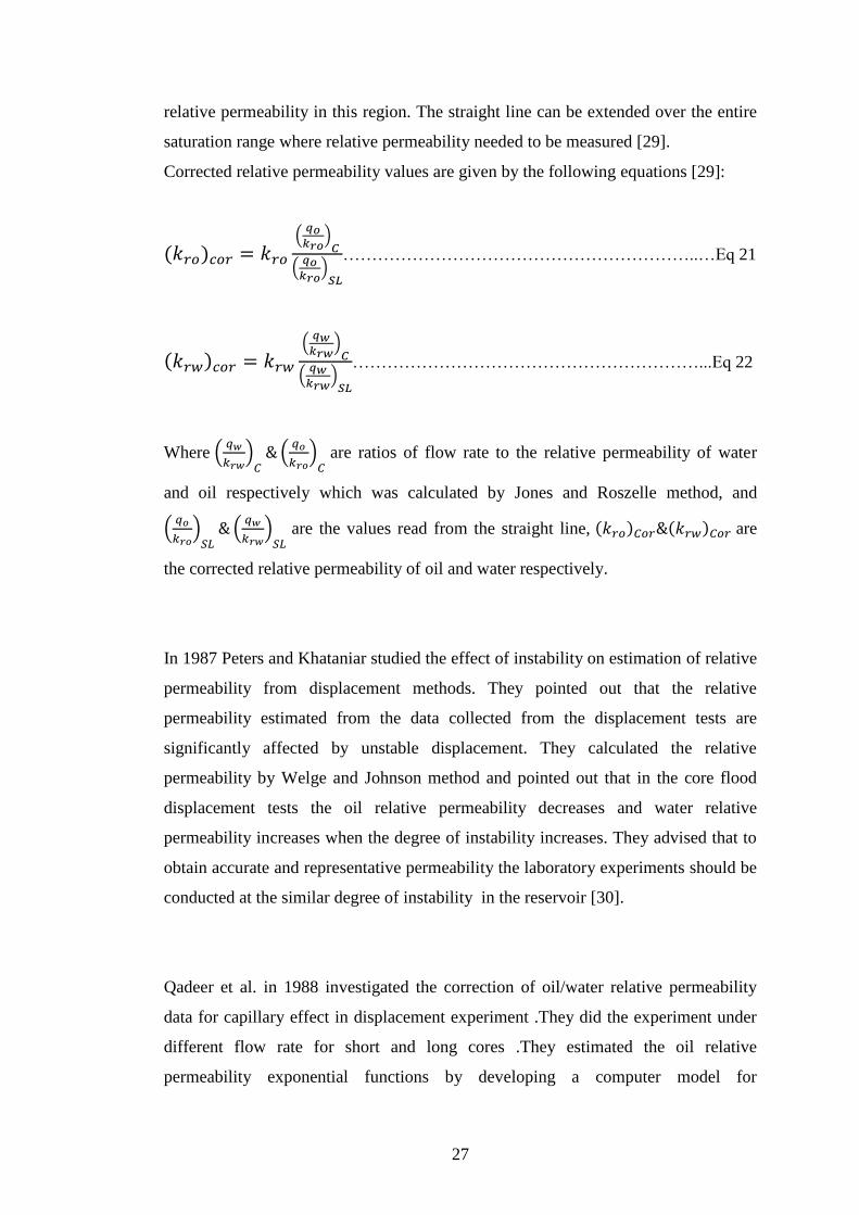
saturation range where relative permeability needed to be measured [29].
Corrected relative permeability values are given by the following equations [29]:
(
)
(
)
……………………………………………………..…Eq 21
(
)
(
)
……………………………………………………...Eq 22
Where (
) (
) are ratios of flow rate to the relative permeability of water
and oil respectively which was calculated by Jones and Roszelle method, and
(
)
(
)
are the values read from the straight line, are
the corrected relative permeability of oil and water respectively.
In 1987 Peters and Khataniar studied the effect of instability on estimation of relative
permeability from displacement methods. They pointed out that the relative
permeability estimated from the data collected from the displacement tests are
significantly affected by unstable displacement. They calculated the relative
permeability by Welge and Johnson method and pointed out that in the core flood
displacement tests the oil relative permeability decreases and water relative
permeability increases when the degree of instability increases. They advised that to
obtain accurate and representative permeability the laboratory experiments should be
conducted at the similar degree of instability in the reservoir [30].
Qadeer et al. in 1988 investigated the correction of oil/water relative permeability
data for capillary effect in displacement experiment .They did the experiment under
different flow rate for short and long cores .They estimated the oil relative
permeability exponential functions by developing a computer model for
28
displacement experiments. Their model was one dimensional two phase flow
simulator with capillary effects and a simple Buckley Leverett non capillary flow
simulator. The experiment data and the simulation model were used to investigate
the effect of rate on the parameters of relative permeability. From their results they
pointed out that the relative permeability parameters in drainage process have
functional relationships with the rate. Also, they developed regression equations for
changing saturation of non-wetting and wetting phase and find out that the end point
for relative permeability and saturation exponent for drainage process of the non-
wetting phase can be related to the dimensionless rate. They pointed out that with
increase in the rate of displacement the saturation exponent of the wetting phase
decreases [31].
In 1989 Civan and Donaldson studied relative permeability estimated from unsteady
state displacement tests with capillary pressure included. They developed a semi-
analytic method for calculating relative permeabilities which is not restricted to high
flow rate due to incorporation of capillary pressure [32].
In 1992 Chardaire-Riviere et al. developed algorithm based on optimal control
approach for automatically estimation of relative permeability and capillary pressure
in incompressible two phase flow experiment [7].
The main enhancements achieved by this algorithm are [7]:
a) The experiment can be conducted at any flow rate; consequently reservoir
flow condition can be used.
b) Estimation of relative permeability and capillary pressure from different core
sample are possible.
c) Imbibitions or drainage displacement can be used for estimation of relative
permeability with various boundary conditions.

29
In 1992 Savioli and Binder applied automatic history matching algorithm to evaluate
the effect of capillary pressure on measuring relative permeability curves. The
experimental and simulated data were tested by this algorithm. Inclusion of capillary
pressure gave good adjustment between simulated and experimental data [33].
In 1994 K. Li,P. Shen and T. Oing calculated oil –water relative permeability by
developing an analytical method that included capillary pressure. The core flooding
tests can be achieved at typical reservoir flow rate by this analytical method [34].
Qadeer, Brigham and Castanier in 2002 studied the limitations of calculating relative
permeability from unsteady state by JBN method .They used Bera sand stone core
sample in their experiments which is known to be homogeneous and strongly water
wet, also, they did simulation ,from their result they pointed out that JBN method
gave large error at low water saturation .They used CT scanner to measure the
saturation and recommended that to determine the range of the end effect of
capillary pressure and the saturation gradients in the cores ,the control experiments
should be conducted using in situ saturation measurement .They indicated that the
end point saturation and relative permeability are function of rate. From their result
relative permeability estimated by JBN method gave large error because of non-
linear flow, capillary pressure end effect and the saturation gradient [35].
30
CHAPTER 3
METHODOLOGY
This chapter describes the method that will be followed in this study to achieve the
objectives of this study that already stated.
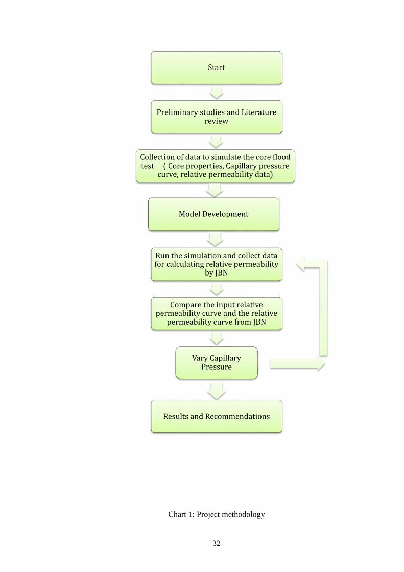
The methodology of this study is described in flow Chart 1; the study starts with the
introduction of the relative permeability and the methods of measuring the relative
permeability from core flooding tests. A literature review of the estimation of
relative permeability from core flooding tests and influence of capillary pressure on
the accuracy of the estimated relative permeability is presented.
One dimensional numerical simulation model of imbibitions unsteady state test will
be performed using input relative permeability and capillary pressure data. After
running the simulation, the data will be collected to estimate the relative permeability
by JBN method. The data required from the simulation model to calculate the
relative permeability curves are cumulative recovery of oil, pressure drop across the
core, and total water injected.
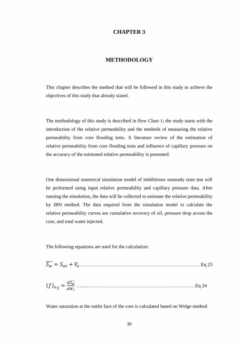
The following equations are used for the calculation:
…………….………………………………………………..….Eq 23
…..……………………………………………………………Eq 24
Water saturation at the outlet face of the core is calculated based on Welge method
31
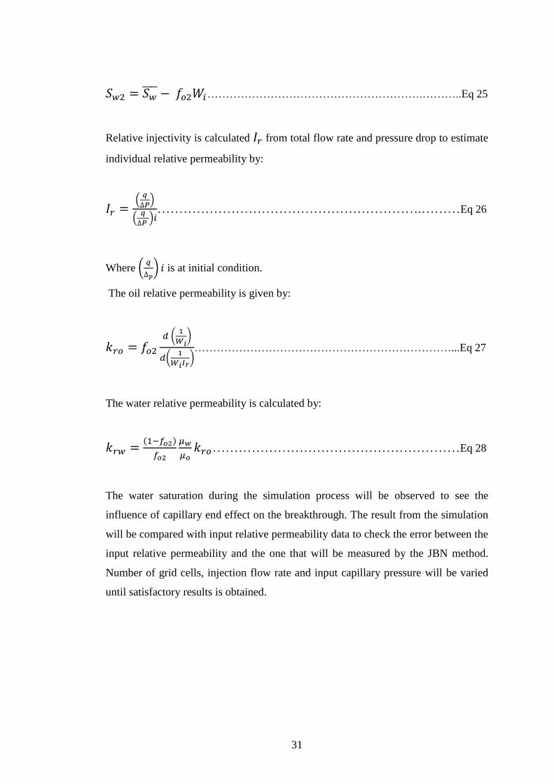
………………………………………………….………..Eq 25
Relative injectivity is calculated from total flow rate and pressure drop to estimate
individual relative permeability by:
(
)
(
)
…………………………………………………….………Eq 26
Where (
) is at initial condition.
The oil relative permeability is given by:
(
)
(
)……………………………………………………………...Eq 27
The water relative permeability is calculated by:
…………………………………………………Eq 28
The water saturation during the simulation process will be observed to see the
influence of capillary end effect on the breakthrough. The result from the simulation
will be compared with input relative permeability data to check the error between the
input relative permeability and the one that will be measured by the JBN method.
Number of grid cells, injection flow rate and input capillary pressure will be varied
until satisfactory results is obtained.
32
Chart 1: Project methodology
Start
Preliminary studies and Literature review
Collection of data to simulate the core flood test ( Core properties, Capillary pressure
curve, relative permeability data)
Model Development
Run the simulation and collect data for calculating relative permeability
by JBN
Compare the input relative permeability curve and the relative
permeability curve from JBN
Vary Capillary Pressure
Results and Recommendations
33
CHAPTER 4
NUMERICAL SIMULATION RESULTS AND DISCUSSION
4.1 ECLIPSE 100
Numerical simulation is performed in this study using a commercial black oil
simulator “Schlumberger ECLIPSE 100”.The recovery and pressure drop data from
input relative permeability and capillary pressure were obtained by the Eclipse
simulator. Four scenarios have been studied to investigate the effect of capillary
pressure on estimation relative permeability curves. The calculation of relative
permeability by JBN method and the simulation details are presented in this chapter.
4.2 SIMULATION OF CORE FLOODING TO DETERIMINE OIL-WATER
RELATIVE PERMEABILITIES
Core flooding tests is used to evaluate and determine relative permeabilities which
are required for simulation studies. Linear core was used to determine oil and water
relative permeability with unsteady state method by reducing it to irreducible oil
saturation.
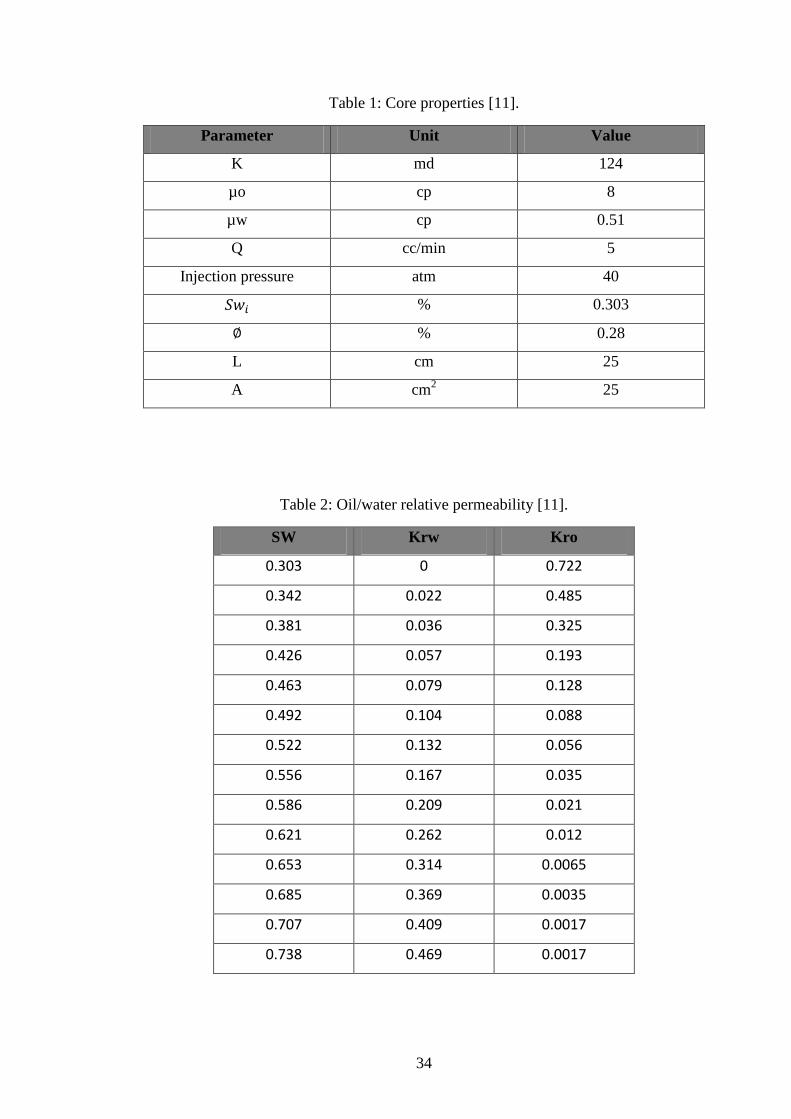
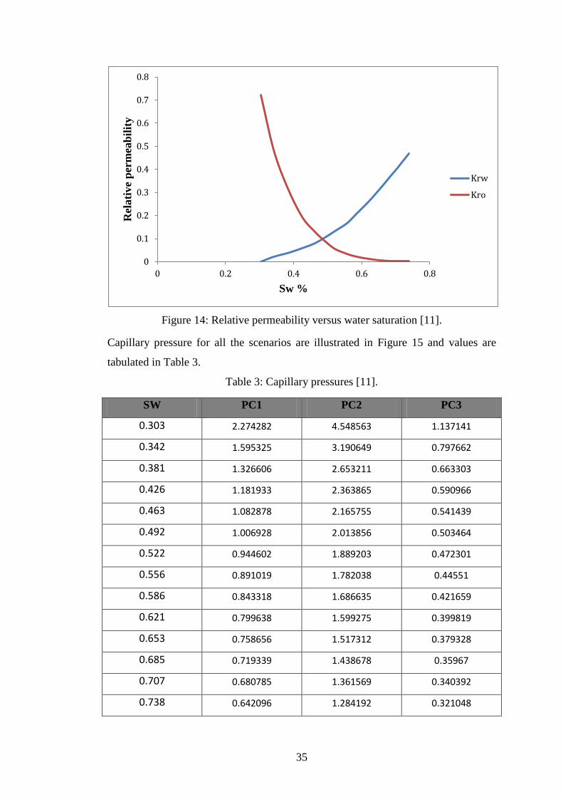
Flow is uni-directional and the core is homogeneous and isotropic. Properties of the
core are tabulated in the Table 1. The relative permeability data used in the model are
shown in Figure 14 and the values are tabulated in Table 2.
34
Table 1: Core properties [11].
Parameter Unit Value
K md 124
µo cp 8
µw cp 0.51
Q cc/min 5
Injection pressure atm 40
% 0.303
% 0.28
L cm 25
A cm2 25
Table 2: Oil/water relative permeability [11].
SW Krw Kro
0.303 0 0.722
0.342 0.022 0.485
0.381 0.036 0.325
0.426 0.057 0.193
0.463 0.079 0.128
0.492 0.104 0.088
0.522 0.132 0.056
0.556 0.167 0.035
0.586 0.209 0.021
0.621 0.262 0.012
0.653 0.314 0.0065
0.685 0.369 0.0035
0.707 0.409 0.0017
0.738 0.469 0.0017
35
Figure 14: Relative permeability versus water saturation [11].
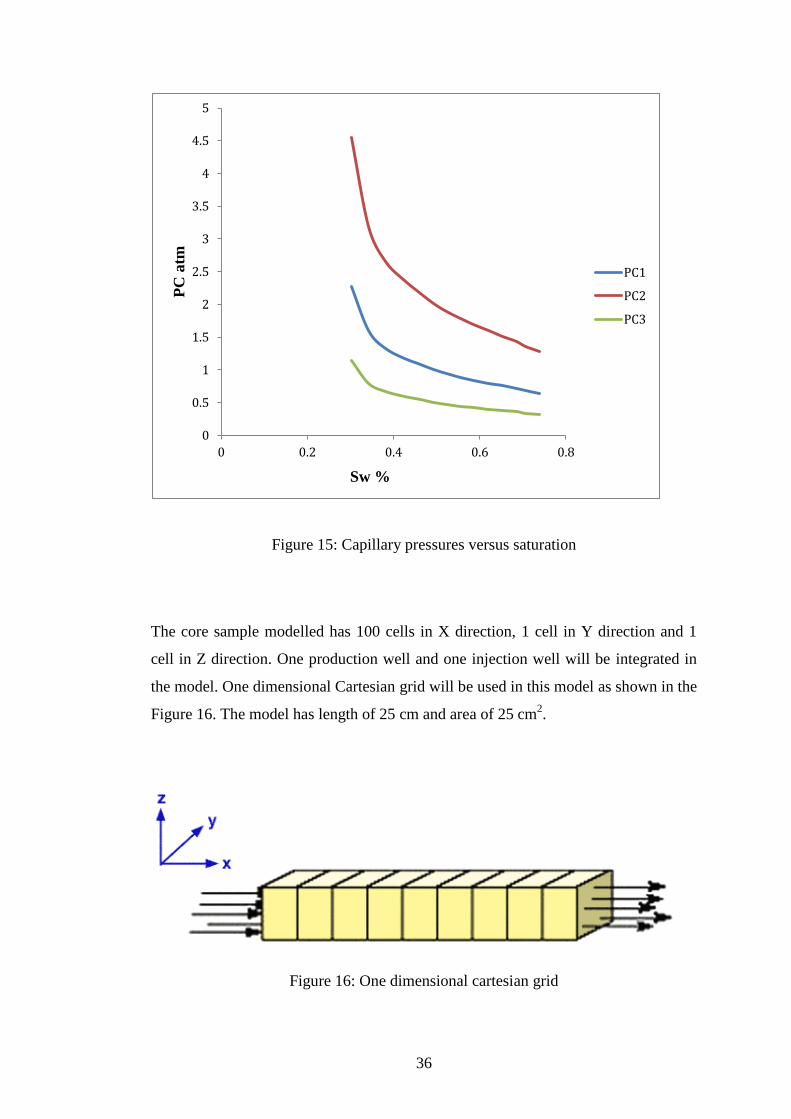
Capillary pressure for all the scenarios are illustrated in Figure 15 and values are
tabulated in Table 3.
Table 3: Capillary pressures [11].
SW PC1 PC2 PC3
0.303 2.274282 4.548563 1.137141
0.342 1.595325 3.190649 0.797662
0.381 1.326606 2.653211 0.663303
0.426 1.181933 2.363865 0.590966
0.463 1.082878 2.165755 0.541439
0.492 1.006928 2.013856 0.503464
0.522 0.944602 1.889203 0.472301
0.556 0.891019 1.782038 0.44551
0.586 0.843318 1.686635 0.421659
0.621 0.799638 1.599275 0.399819
0.653 0.758656 1.517312 0.379328
0.685 0.719339 1.438678 0.35967
0.707 0.680785 1.361569 0.340392
0.738 0.642096 1.284192 0.321048
0
0.1
0.2
0.3
0.4
0.5
0.6
0.7
0.8
0 0.2 0.4 0.6 0.8
Rel
ati
ve
per
mea
bil
ity
Sw %
Krw
Kro
36
Figure 15: Capillary pressures versus saturation
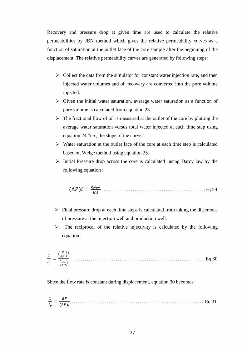
The core sample modelled has 100 cells in X direction, 1 cell in Y direction and 1
cell in Z direction. One production well and one injection well will be integrated in
the model. One dimensional Cartesian grid will be used in this model as shown in the
Figure 16. The model has length of 25 cm and area of 25 cm2.
Figure 16: One dimensional cartesian grid
0
0.5
1
1.5
2
2.5
3
3.5
4
4.5
5
0 0.2 0.4 0.6 0.8
PC
atm
Sw %
PC1
PC2
PC3
37
Recovery and pressure drop at given time are used to calculate the relative
permeabilities by JBN method which gives the relative permeability curves as a
function of saturation at the outlet face of the core sample after the beginning of the
displacement. The relative permeability curves are generated by following steps:
Collect the data from the simulator for constant water injection rate, and then
injected water volumes and oil recovery are converted into the pore volume
injected.
Given the initial water saturation, average water saturation as a function of
pore volume is calculated from equation 23.
The fractional flow of oil is measured at the outlet of the core by plotting the
average water saturation versus total water injected at each time step using
equation 24 “i.e., the slope of the curve”.
Water saturation at the outlet face of the core at each time step is calculated
based on Welge method using equation 25.
Initial Pressure drop across the core is calculated using Darcy law by the
following equation :
…………………………………….……….Eq 29
Final pressure drop at each time steps is calculated from taking the difference
of pressure at the injection well and production well.
The reciprocal of the relative injectivity is calculated by the following
equation :
(
)
(
)
…………………………………………………………..…Eq 30
Since the flow rate is constant during displacement, equation 30 becomes:
…………………………………………………………….Eq 31
38
Substituting equation 29 in equation 31 gives:
⁄ …………………………………………………………Eq 32
From simulation results, slope of the
as a function of
is calculated
and individual relative permeability of oil is obtained using equation 27.
Water relative permeability at each time steps is calculated using equation 28.
All simulation scenarios that are considered in this chapter were design to study the
effect of capillary pressure on measuring relative permeability curves. Results have
been obtained by simulation for estimation relative permeability curves by JBN
method. Different results were acquired according to different capillary pressure.
4.2.1 Case 1
The first scenario is to measure relative permeabilities by JBN method based on the
measurement of pressure drop across and the cumulative production of oil and water.
For this case the capillary pressure used is PC1 is shown in Table 3.The data file for
this case is shown in Appendix A.
The core model is flooded with water at constant flow rate of 0.0833cc/sec and
variation of pressure drop during the displacement is measured. Since the rate is
constant equation 32 becomes:
⁄ = 0.186 (atm)…………………………………… Eq 33
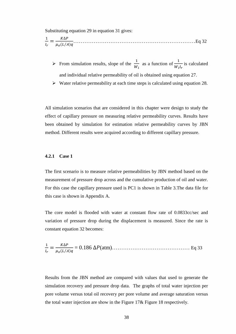
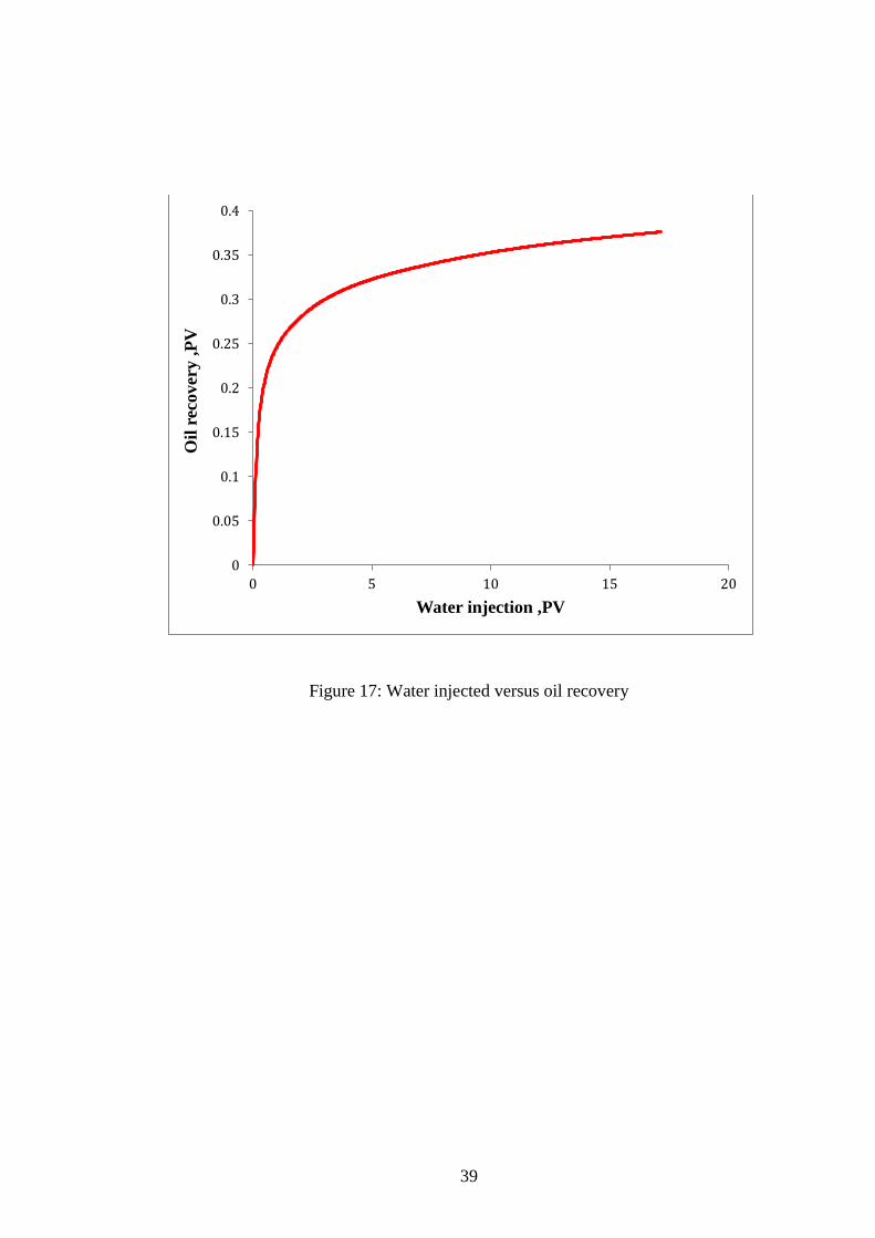
Results from the JBN method are compared with values that used to generate the
simulation recovery and pressure drop data. The graphs of total water injection per
pore volume versus total oil recovery per pore volume and average saturation versus
the total water injection are show in the Figure 17& Figure 18 respectively.
39
Figure 17: Water injected versus oil recovery
0
0.05
0.1
0.15
0.2
0.25
0.3
0.35
0.4
0 5 10 15 20
Oil
rec
over
y ,
PV
Water injection ,PV
40
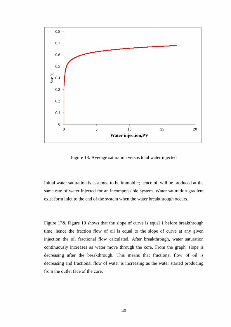
Figure 18: Average saturation versus total water injected
Initial water saturation is assumed to be immobile; hence oil will be produced at the
same rate of water injected for an incompressible system. Water saturation gradient
exist form inlet to the end of the system when the water breakthrough occurs.
Figure 17& Figure 18 shows that the slope of curve is equal 1 before breakthrough
time, hence the fraction flow of oil is equal to the slope of curve at any given
injection the oil fractional flow calculated. After breakthrough, water saturation
continuously increases as water move through the core. From the graph, slope is
decreasing after the breakthrough. This means that fractional flow of oil is
decreasing and fractional flow of water is increasing as the water started producing
from the outlet face of the core.
0
0.1
0.2
0.3
0.4
0.5
0.6
0.7
0.8
0 5 10 15 20
Sa
v %
Water injection,PV
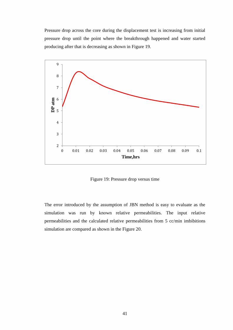
41
Pressure drop across the core during the displacement test is increasing from initial
pressure drop until the point where the breakthrough happened and water started
producing after that is decreasing as shown in Figure 19.
Figure 19: Pressure drop versus time
The error introduced by the assumption of JBN method is easy to evaluate as the
simulation was run by known relative permeabilities. The input relative
permeabilities and the calculated relative permeabilities from 5 cc/min imbibitions
simulation are compared as shown in the Figure 20.
2
3
4
5
6
7
8
9
0 0.01 0.02 0.03 0.04 0.05 0.06 0.07 0.08 0.09 0.1
DP
atm
Time,hrs
42
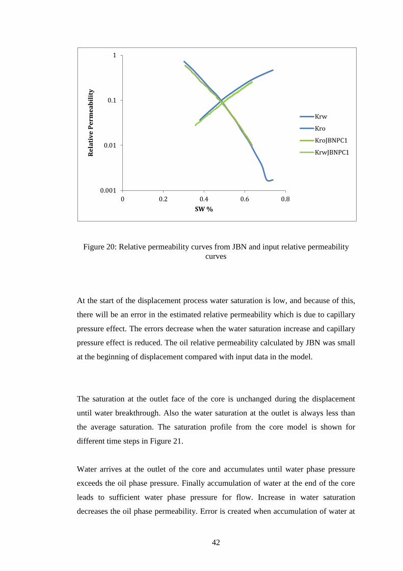
Figure 20: Relative permeability curves from JBN and input relative permeability
curves
At the start of the displacement process water saturation is low, and because of this,
there will be an error in the estimated relative permeability which is due to capillary
pressure effect. The errors decrease when the water saturation increase and capillary
pressure effect is reduced. The oil relative permeability calculated by JBN was small
at the beginning of displacement compared with input data in the model.
The saturation at the outlet face of the core is unchanged during the displacement
until water breakthrough. Also the water saturation at the outlet is always less than
the average saturation. The saturation profile from the core model is shown for
different time steps in Figure 21.
Water arrives at the outlet of the core and accumulates until water phase pressure
exceeds the oil phase pressure. Finally accumulation of water at the end of the core
leads to sufficient water phase pressure for flow. Increase in water saturation
decreases the oil phase permeability. Error is created when accumulation of water at
0.001
0.01
0.1
1
0 0.2 0.4 0.6 0.8
Re
lati
ve
Pe
rme
ab
ilit
y
SW %
Krw
Kro
KroJBNPC1
KrwJBNPC1
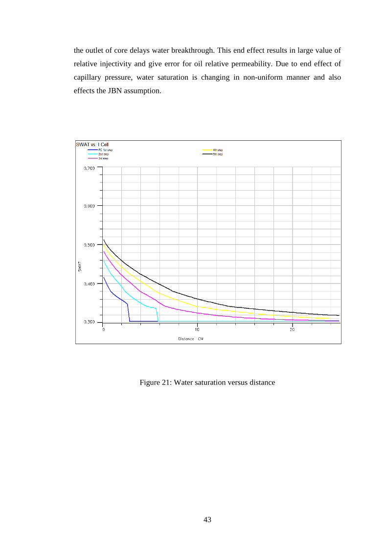
43
the outlet of core delays water breakthrough. This end effect results in large value of
relative injectivity and give error for oil relative permeability. Due to end effect of
capillary pressure, water saturation is changing in non-uniform manner and also
effects the JBN assumption.
Figure 21: Water saturation versus distance
44
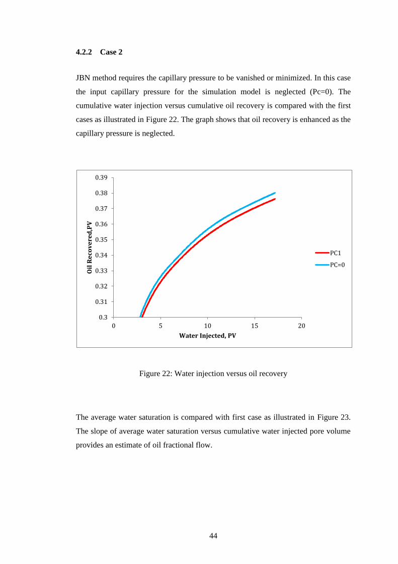
4.2.2 Case 2
JBN method requires the capillary pressure to be vanished or minimized. In this case
the input capillary pressure for the simulation model is neglected (Pc=0). The
cumulative water injection versus cumulative oil recovery is compared with the first
cases as illustrated in Figure 22. The graph shows that oil recovery is enhanced as the
capillary pressure is neglected.
Figure 22: Water injection versus oil recovery
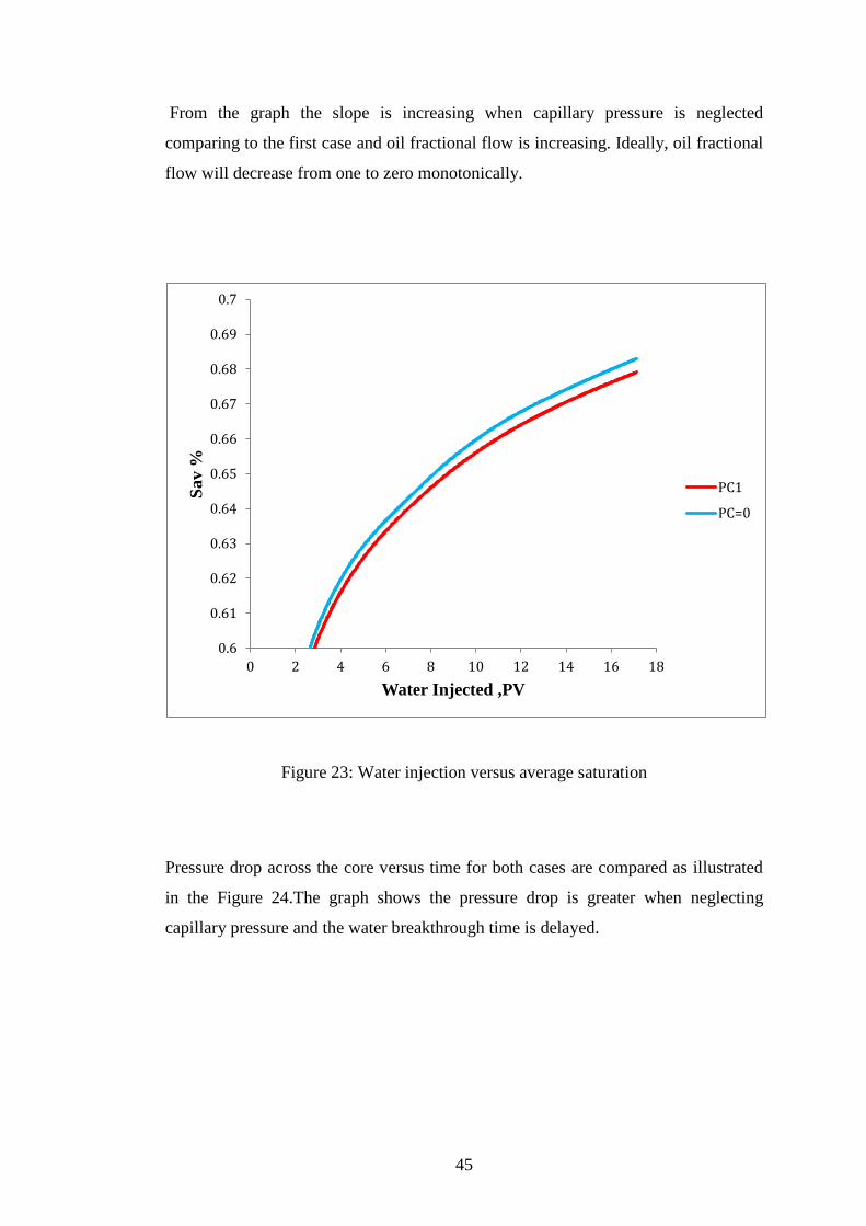
The average water saturation is compared with first case as illustrated in Figure 23.
The slope of average water saturation versus cumulative water injected pore volume
provides an estimate of oil fractional flow.
0.3
0.31
0.32
0.33
0.34
0.35
0.36
0.37
0.38
0.39
0 5 10 15 20
Oil
Re
cov
ere
d,P
V
Water Injected, PV
PC1
PC=0
45
From the graph the slope is increasing when capillary pressure is neglected
comparing to the first case and oil fractional flow is increasing. Ideally, oil fractional
flow will decrease from one to zero monotonically.
Figure 23: Water injection versus average saturation
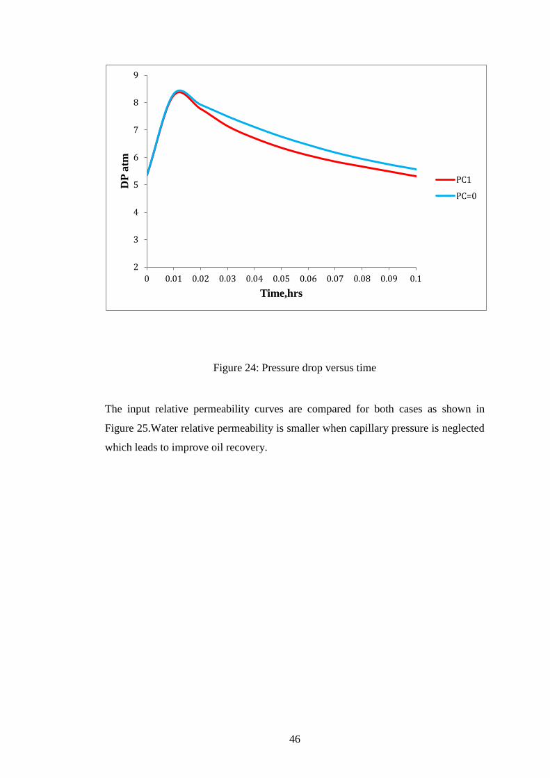
Pressure drop across the core versus time for both cases are compared as illustrated
in the Figure 24.The graph shows the pressure drop is greater when neglecting
capillary pressure and the water breakthrough time is delayed.
0.6
0.61
0.62
0.63
0.64
0.65
0.66
0.67
0.68
0.69
0.7
0 2 4 6 8 10 12 14 16 18
Sav
%
Water Injected ,PV
PC1
PC=0
46
Figure 24: Pressure drop versus time
The input relative permeability curves are compared for both cases as shown in
Figure 25.Water relative permeability is smaller when capillary pressure is neglected
which leads to improve oil recovery.
2
3
4
5
6
7
8
9
0 0.01 0.02 0.03 0.04 0.05 0.06 0.07 0.08 0.09 0.1
DP
atm
Time,hrs
PC1
PC=0
47
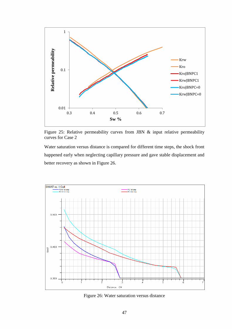
Figure 25: Relative permeability curves from JBN & input relative permeability
curves for Case 2
Water saturation versus distance is compared for different time steps, the shock front
happened early when neglecting capillary pressure and gave stable displacement and
better recovery as shown in Figure 26.
Figure 26: Water saturation versus distance
0.01
0.1
1
0.3 0.4 0.5 0.6 0.7
Rel
ati
ve
per
mea
bil
ity
Sw %
Krw
Kro
KroJBNPC1
KrwJBNPC1
KroJBNPC=0
KrwJBNPC=0
48
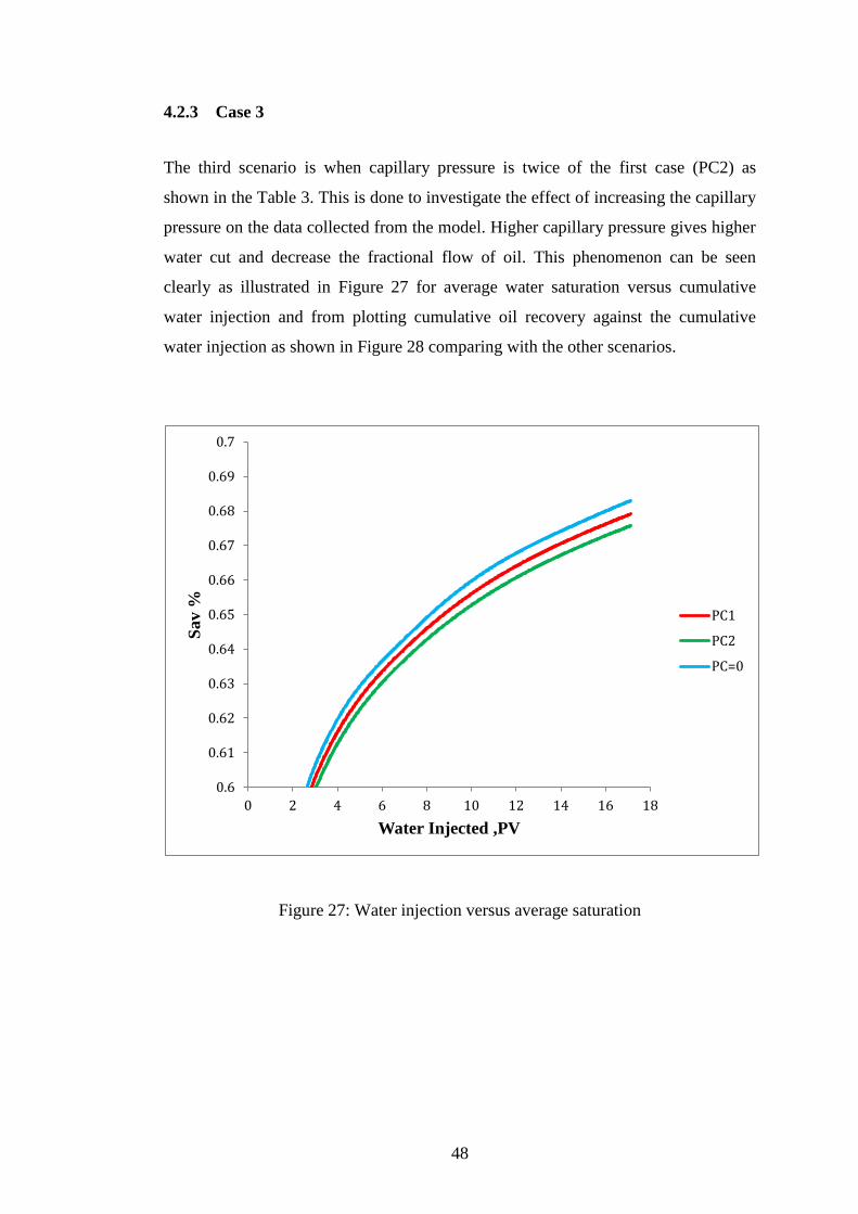
4.2.3 Case 3
The third scenario is when capillary pressure is twice of the first case (PC2) as
shown in the Table 3. This is done to investigate the effect of increasing the capillary
pressure on the data collected from the model. Higher capillary pressure gives higher
water cut and decrease the fractional flow of oil. This phenomenon can be seen
clearly as illustrated in Figure 27 for average water saturation versus cumulative
water injection and from plotting cumulative oil recovery against the cumulative
water injection as shown in Figure 28 comparing with the other scenarios.
Figure 27: Water injection versus average saturation
0.6
0.61
0.62
0.63
0.64
0.65
0.66
0.67
0.68
0.69
0.7
0 2 4 6 8 10 12 14 16 18
Sav %
Water Injected ,PV
PC1
PC2
PC=0
49
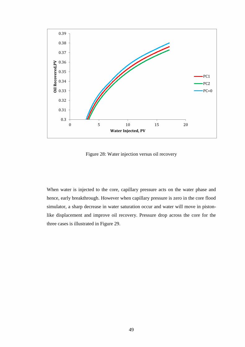
Figure 28: Water injection versus oil recovery
When water is injected to the core, capillary pressure acts on the water phase and
hence, early breakthrough. However when capillary pressure is zero in the core flood
simulator, a sharp decrease in water saturation occur and water will move in piston-
like displacement and improve oil recovery. Pressure drop across the core for the
three cases is illustrated in Figure 29.
0.3
0.31
0.32
0.33
0.34
0.35
0.36
0.37
0.38
0.39
0 5 10 15 20
Oil
Re
cov
ere
d,P
V
Water Injected, PV
PC1
PC2
PC=0
50
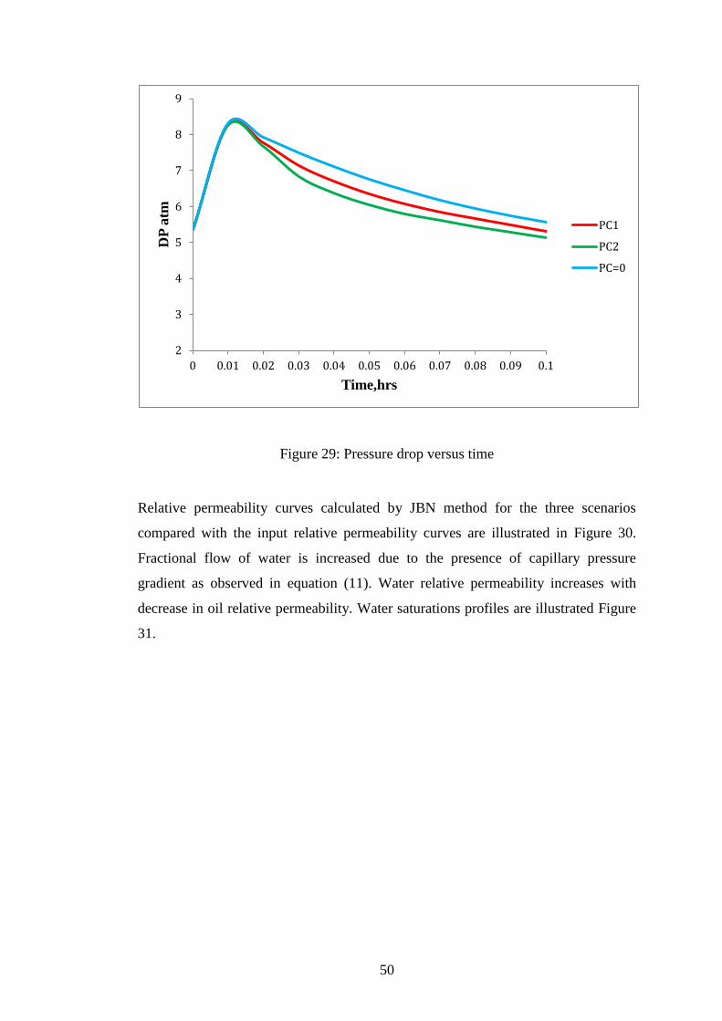
Figure 29: Pressure drop versus time
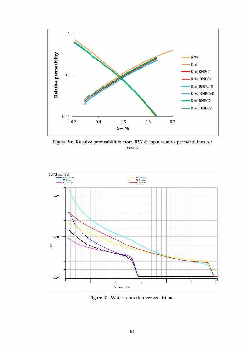
Relative permeability curves calculated by JBN method for the three scenarios
compared with the input relative permeability curves are illustrated in Figure 30.
Fractional flow of water is increased due to the presence of capillary pressure
gradient as observed in equation (11). Water relative permeability increases with
decrease in oil relative permeability. Water saturations profiles are illustrated Figure
31.
2
3
4
5
6
7
8
9
0 0.01 0.02 0.03 0.04 0.05 0.06 0.07 0.08 0.09 0.1
DP
atm
Time,hrs
PC1
PC2
PC=0
51
Figure 30: Relative permeabilities from JBN & input relative permeabilities for
case3
Figure 31: Water saturation versus distance
0.01
0.1
1
0.3 0.4 0.5 0.6 0.7
Rel
ati
ve
per
mea
bil
ity
Sw %
Krw
Kro
KroJBNPC1
KrwJBNPC1
KroJBNPC=0
KrwJBNPC=0
KroJBNPC2
KrwJBNPC2
52
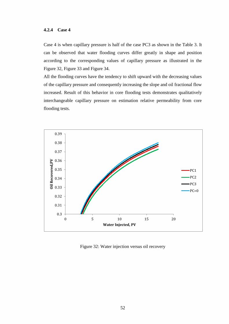
4.2.4 Case 4
Case 4 is when capillary pressure is half of the case PC3 as shown in the Table 3. It
can be observed that water flooding curves differ greatly in shape and position
according to the corresponding values of capillary pressure as illustrated in the
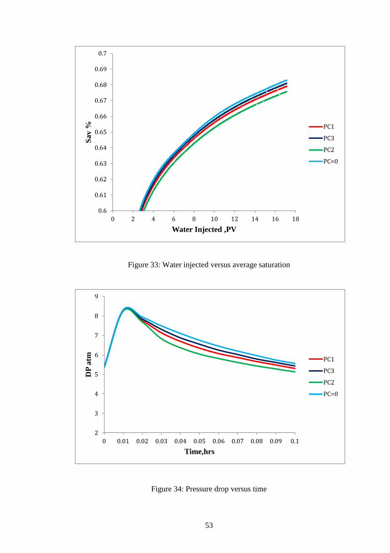
Figure 32, Figure 33 and Figure 34.
All the flooding curves have the tendency to shift upward with the decreasing values
of the capillary pressure and consequently increasing the slope and oil fractional flow
increased. Result of this behavior in core flooding tests demonstrates qualitatively
interchangeable capillary pressure on estimation relative permeability from core
flooding tests.
Figure 32: Water injection versus oil recovery
0.3
0.31
0.32
0.33
0.34
0.35
0.36
0.37
0.38
0.39
0 5 10 15 20
Oil
Re
cov
ere
d,P
V
Water Injected, PV
PC1
PC2
PC3
PC=0
53
Figure 33: Water injected versus average saturation
Figure 34: Pressure drop versus time
0.6
0.61
0.62
0.63
0.64
0.65
0.66
0.67
0.68
0.69
0.7
0 2 4 6 8 10 12 14 16 18
Sav %
Water Injected ,PV
PC1
PC3
PC2
PC=0
2
3
4
5
6
7
8
9
0 0.01 0.02 0.03 0.04 0.05 0.06 0.07 0.08 0.09 0.1
DP
atm
Time,hrs
PC1
PC3
PC2
PC=0
54
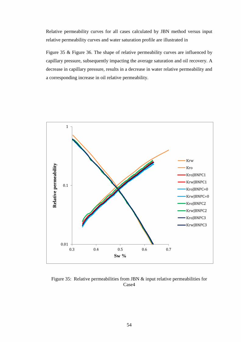
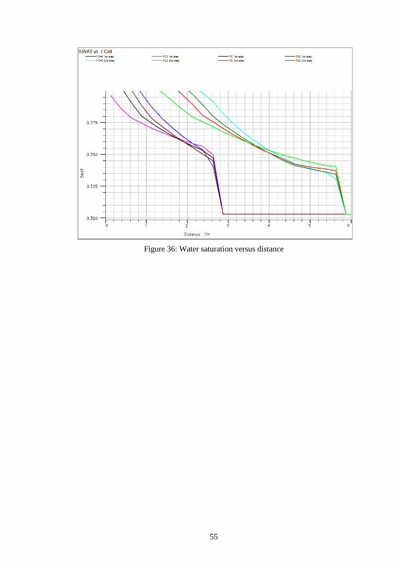
Relative permeability curves for all cases calculated by JBN method versus input
relative permeability curves and water saturation profile are illustrated in
Figure 35 & Figure 36. The shape of relative permeability curves are influenced by
capillary pressure, subsequently impacting the average saturation and oil recovery. A
decrease in capillary pressure, results in a decrease in water relative permeability and
a corresponding increase in oil relative permeability.
Figure 35: Relative permeabilities from JBN & input relative permeabilities for
Case4
0.01
0.1
1
0.3 0.4 0.5 0.6 0.7
Rel
ati
ve
per
mea
bil
ity
Sw %
Krw
Kro
KroJBNPC1
KrwJBNPC1
KroJBNPC=0
KrwJBNPC=0
KroJBNPC2
KrwJBNPC2
KroJBNPC3
KrwJBNPC3
55
Figure 36: Water saturation versus distance
56
CHAPTER 5
CONCLUSIONS AND RECOMMENDATIONS
5.1 CONCLUSIONS
In this study, numerical simulation has been used to investigate the effect of capillary
pressure on estimation relative permeability by a conventional method (JBN) from
unsteady state displacement tests which are accepted to be the closest to the flow
mechanism in the reservoirs. Influences of capillary pressure in computation of
relative permeability and saturation on core flooding displacement tests have been
addressed. The effect of capillary pressure on fluid flow in one dimensional cause
errors in the analysis of displacement data by conventional methods for estimation of
relative permeability curves.
All four study cases were investigated at various capillary pressures and their
calculated relative permeability curves by JBN method were plotted along with the
input relative permeability curves for comparison purposes.
Main conclusions based on the simulation results are:
1. Capillary pressure plays a dominate role in displacement processes and it is
responsible for trapping a large portion of oil within the pore structure of the
reservoir rocks.
2. Relative permeability calculated by JBN method is not accurate due to
capillary pressure effect. Relative permeability of oil is decreases due to this
effect.
3. Fractional oil flow is decreasing as capillary pressure increases and fractional
flow of water increases. This increase in water fractional flow results in a
lower frontal water saturation and a higher frontal velocity.
57
5.2 RECOMMENDATIONS
For future study, it is recommended to carry out core flooding experiment in the
laboratory and calculate the relative permeability from the data collect in the lab. In
the lab, distribution grooves at both ends of the core are used to distribute the fluid
evenly over the core face. Also the saturation distribution as a function of time can
be measured accurately by scanning the core during displacement process.
In order to reflect experimental cores used in lab, it is recommended to represent
cores in simulation using radial grids. An evenly distributed groove for distribution
of fluid should also be represented when carrying out simulation. This can be done
by introducing a layer of high permeability grid blocks, with zero capillary pressure
at the inlet and outlet of the core model. The simulator should be properly model at
inlet and outlet end plugs with end effect and non-linear nature of the flow near the
ends.
58
REFERENCES
[1] Bennion D.B. and Thomas F.B., “Recent Improvements in Experimental and
Analytical Technique for the Determination of Relative Permeability from
Unsteady State Flow Experiments". Socity of Petroleum Enginneer,In.SPE
10th Technical Conference June 1991 .
[2] Nordtvedt J.E, Urkedal H, Watson A.T, Ebeltoft E, Kolltveit K,Langaas K,
and Oxnevad I.E.I.,"Estimation of Relative Permeability and Capillary
Pressure Functions using Transient and Equilibrium Data from Steady –State
Experiments" SCA-9418
[3] Ahmed, T. “Reservoir Engineering Handbook” Fourth Edition, Gulf
Professional Publishing is an imprint of Elsevier,2010 .
[4] Dake, L.P. (1978) “Fundamentals of Reservoir Engineering”. Developments
in petroleum science 8, Amsterdam Boston, Elsevier.
[5] Jon Kleppe, “Review of relative permeabilities and capillary pressures”,
Handout noteTPG4150 Reservoir Recovery Techniques 2011.
[6] Yuqi D., Bolaji O.P., and Dacun L., “Literature Review on Methods to Obtain
Relative Permeability Data,” 5th Conference & Exposition on Petroleum
Geophysics, Hyderabad-2004, India PP 597-604.
[7] Chardaire-Riviere Catherine , Guy Chavent, Jerome Jaffre, Jun Liu and
Bernard J.“Simultaneous Estimation of Relative Permeabilities and Capillary
Presssure” SPE paper 19680;SPE Formation Evaluation 1992 .
[8] Djebbar Tiab and Erle C. Donaldson, “Petrophysics second Edition Theory
and Practice of Measuring Reservoir Rock and Fluid Transport
Properties,”Second Edition Gulf Professional Publishing is an imprint of
Elsevier 2004 .
[9] Paul Glover , “Relative Permeability,” Formation Evaluation MSc Course
Notes Chapter 10 : pp. 104-130. Aberdeen University Petrophysics Centre.
[10] Leverett, M. C. “Flow of Oil-Water Mixture through Unconsolidated
Sands”Trans., AIME San Antonio Meeting ,October 1939.
[11] Willhite, P.G.: “Waterflooding,” SPE Textbook Series, Vol , Richardson, TX.
1986.
[12] Leverett, M. C. “Capillary Behavior in Porous Solids,”Trans., AIME.Tulsa
Meeting, October 1941.
[13] Buckley, S, E. and Levertt, M.C., “Mechanism of fluid displacement in
sands”, SPE-942107-G. Trans AIME, 146,107-116, 1942.
59
[14] Fayers, F.J. and Sheldon, J.W.,"The Effect of Capillary Pressure and
Gravityon Two-Phase Fluid Flow in Porous Media", Trans
AIME,(1959),216,147-155 .
[15] Dake,L.P., “The Practice Of Reservoir Engineering”,(Revised Edition. ,
Elsevier, Amsterdam,1994.
[16] Welge, H. J.: “A Simplified Method for Computing Oil Recovery by Gas
or Water Drive,” Trans., AIME, (1952), 195, 91-98.
[17] Johnson, E.F., Bossler, D.P., and Naumann, V.O., Calculated of Relative
Permeabilityfrom Displacement Experiments, Trans.AIME(1959), 216. pages
370-372, .
[18] Jones, S.C., Roszelle, W.O.,”Graphical Techniques for Determining Relative
Permeability from Displacement Experiments”, JPT, May 1978, 807- 817.
[19] A.M. Tao, and A.T. Watson "Accuracy of JBN estimates of relative
permeability: part 1-error analysis". SPEJ, pp 209-214, April 1984.
[20] A.M. Tao, and A.T. Watson "Accuracy of JBN estimates of relative
permeability: part 2-algorithms". SPEJ, pp 215-222, April 1984.
[21] Kerig, P.D., Watson, A.T.: “Relative Permeability Estimation from
Displacement Experiments: An Error Analysis,” SPE Reservoir Eng., Vol. 1,
(1986), p.175–182.
[22] Watson, A.T., Richmond, P.C., Kerig, D.P., Tao, T.M.: “A Regression- Based
Methodfor Estimating Relative Permeabilities from Displacement Experiments,”
SPE ReservoirEng. Vol.3, (1988), 953–958.
[23] Mike Carlson M.R., “Practical Reservoir Simulation: using assessing, and
developing results.”Copy right 2003 by PennWell Corporation.
[24] Hadley G. F., and Handy L. L.: "A Theoretical and Experimental Study of the
Steady State Capillary End Effect," SPE 707-G, paperpresented at the 31st
Annual Fall Meeting, Los Angeles, Calif.Oct. 14-17, 1956.
[25] Kyte, J. R., and Rapoport, L. A.: "Linea,r Waterflood Behaviorand End
Effects in Water-Wet Porous Media," Trans. AIME,(1958).
[26] Archer, J.S., and Wong, S.W.: “Use of a Reservoir Simulator To
InterpretLaboratory Waterflood Data,” Soc .Pet .Eng .343-347.Dec 1973.
[27] Sigmund,P; McCaffery, F; “An improved unsteady-state procedure for
determining the Relative Permeability characteristics of heterogeneous media”; SPEJ 169, 1979.
60
[28] Batycky, J. P., McCaffery, F. G., Hodgins, P. K., and Fisher, D. B.,
"Interpreting Relative Permeability and Wettability from Unsteady-State
Displacement Measurements" SPEJ, June1981.
[29] Odeh, A. S. and Dotson, B. J.: "A method for reducing the rate effect on oil
and water relativepermeabilities calculated from dynamic displacement data",
JPT Nov., (1985), 2051–2058.
[30] Peters, E.J. and Khataniar, S.,"The effect of instability on relative permeability
curves obtained by dynamic-displacement method",SPEFE, pp. 469-
474.Dec(1987) .
[31] Qadeer, S; Dehghani,K; Ogbe, D.O; Oatermann, R.D; “Correcting Oil/Water
Relative Permeability Data for Capillary End Effect in Displacement
Experiments”;SPE 17423, 1998.
[32] Civan, Fand Donaldson, E.C.: Relative Permeability fromUnsteady-State
Displacements with Capillary Pressure Included.SPEFE (June 1989) 189-193.
[33] Savioli,G.P and Binder, M.S." The Influence of Capillary Pressure when
Determining Relative Permeability from Unsteady-state CoorFloods";SPE
23689,1992 .
[34] Li, K. Shen, P. and Qing, T. “A New Method for Calculating Oil-Water
Relative Permeabilities with Consideration of Capillary Pressure,” Mechanics
and Practice, V. 16, No. 2,1994.
[35] Qadeer, S., Brigham, W.E., and Castanier, L.M.:“Techniques to Handle
Limitations in Dynamic Relative Permeability Measurements "SUPRI TR128.
Work Performed Under Contract No . DE-FC26-01BC15311 Prepared for U .
S . Department of Energy Assistant Secretary for Fossil Energy,” 2002.
61
APPENDICES
Appendix A
EFFECT OF CAPILLARY PRESSURE ON ESTIMATION
OF RELATIVE PERMEABILITY FROM CORE FLOODING TESTS
============================================================
RUNSPEC
TITLE
2-phase
-- Number of cells
-- NX NY NZ
-- -- -- --
DIMENS
100 1 1 /
-- Phases
OIL
WATER
-- Units
LAB
-- Maximum well/connection/group values
-- #wells #cons/w #grps #wells/grp
-- ------ ------- ----- ----------
62
WELLDIMS
2 1 2 1 /
-- Unified output files
UNIFOUT
-- Simulation start date
START
1 JAN 2013 /
============================================================
====
GRID
DX
100*0.25 /
EQUALS
'DZ' 5 /
'DY' 5/
'PORO' 0.28 1 100 1 1 1 1 / MATRIX PROPERTIES
'TOPS' 0 /
'PERMX' 124 /
'PERMY' 124 /
'PERMZ' 124/
/
-- Output file with geometry and rock properties (.INIT)
INIT
63
============================================================
PROPS
-- Surface densities
-- Oil Wat
-- --- ---
DENSITY
0.76 1.09 /
-- PVT data for dead oil
-- P Bo Vis
-- ---- ---- -----
PVDO
0.00000 1.00004 8
100. 1.00002 8
3600.00 1.00000 8 /
-- PVT data for water
-- P Bw Cw Vis
-- ---- ---- ----- -----
PVTW
100.0000 1.00000 0.00E-05 0.51000 0.00E-01 /
-- Rock compressibility
-- P Cr
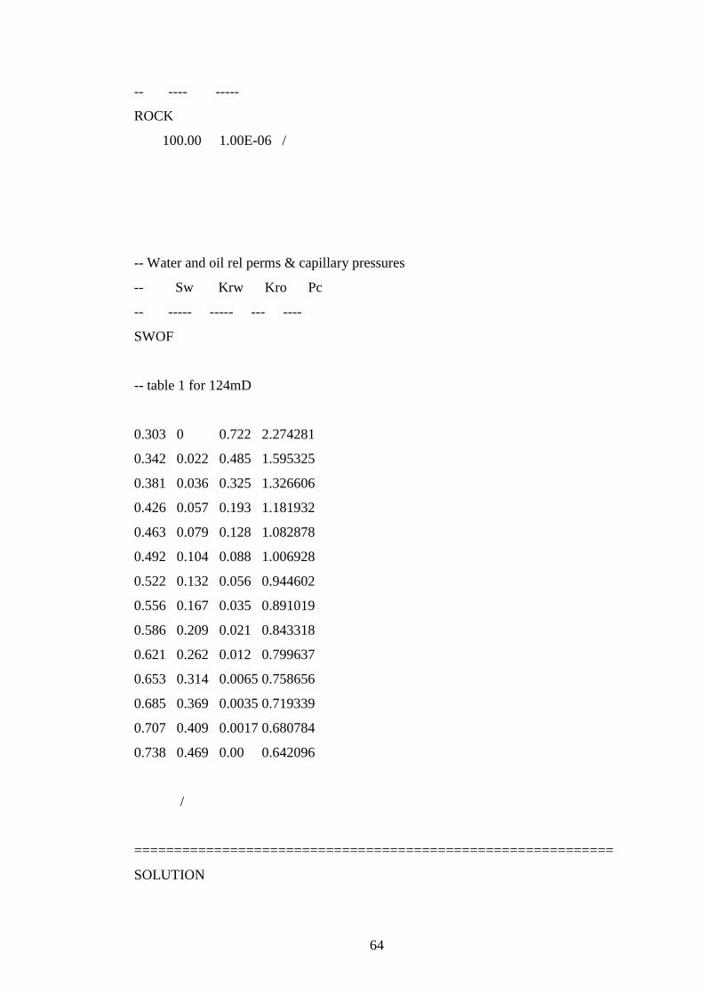
64
-- ---- -----
ROCK
100.00 1.00E-06 /
-- Water and oil rel perms & capillary pressures
-- Sw Krw Kro Pc
-- ----- ----- --- ----
SWOF
-- table 1 for 124mD
0.303 0 0.722 2.274281
0.342 0.022 0.485 1.595325
0.381 0.036 0.325 1.326606
0.426 0.057 0.193 1.181932
0.463 0.079 0.128 1.082878
0.492 0.104 0.088 1.006928
0.522 0.132 0.056 0.944602
0.556 0.167 0.035 0.891019
0.586 0.209 0.021 0.843318
0.621 0.262 0.012 0.799637
0.653 0.314 0.0065 0.758656
0.685 0.369 0.0035 0.719339
0.707 0.409 0.0017 0.680784
0.738 0.469 0.00 0.642096
/
============================================================
SOLUTION
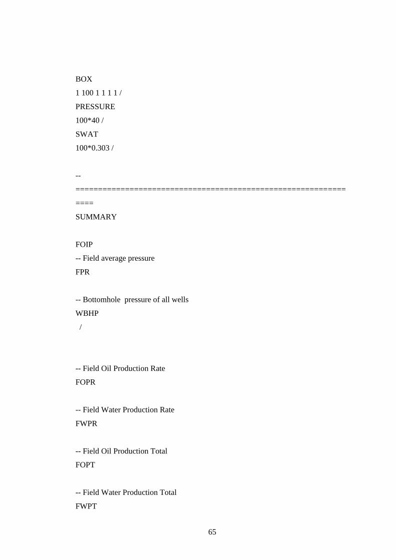
65
BOX
1 100 1 1 1 1 /
PRESSURE
100*40 /
SWAT
100*0.303 /
--
============================================================
====
SUMMARY
FOIP
-- Field average pressure
FPR
-- Bottomhole pressure of all wells
WBHP
/
-- Field Oil Production Rate
FOPR
-- Field Water Production Rate
FWPR
-- Field Oil Production Total
FOPT
-- Field Water Production Total
FWPT
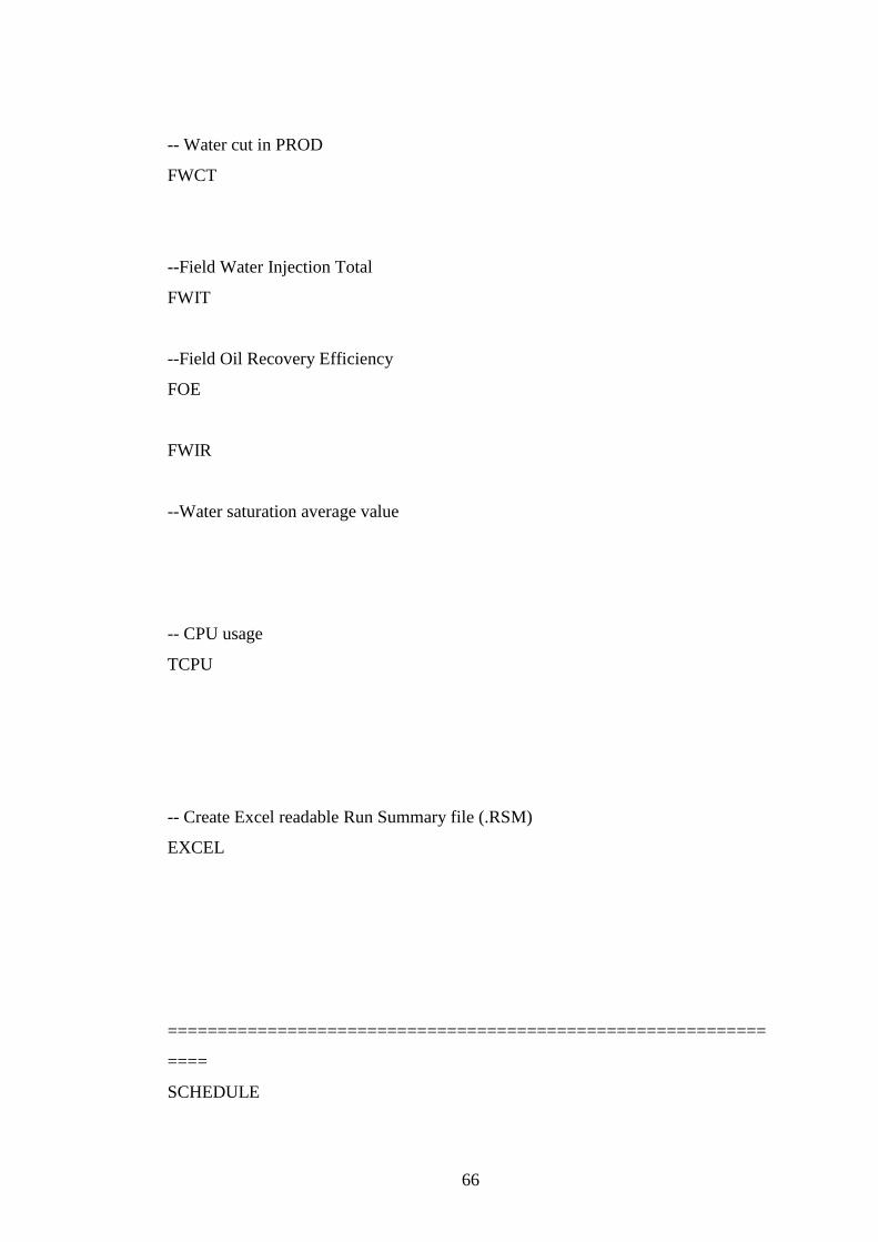
66
-- Water cut in PROD
FWCT
--Field Water Injection Total
FWIT
--Field Oil Recovery Efficiency
FOE
FWIR
--Water saturation average value
-- CPU usage
TCPU
-- Create Excel readable Run Summary file (.RSM)
EXCEL
============================================================
====
SCHEDULE
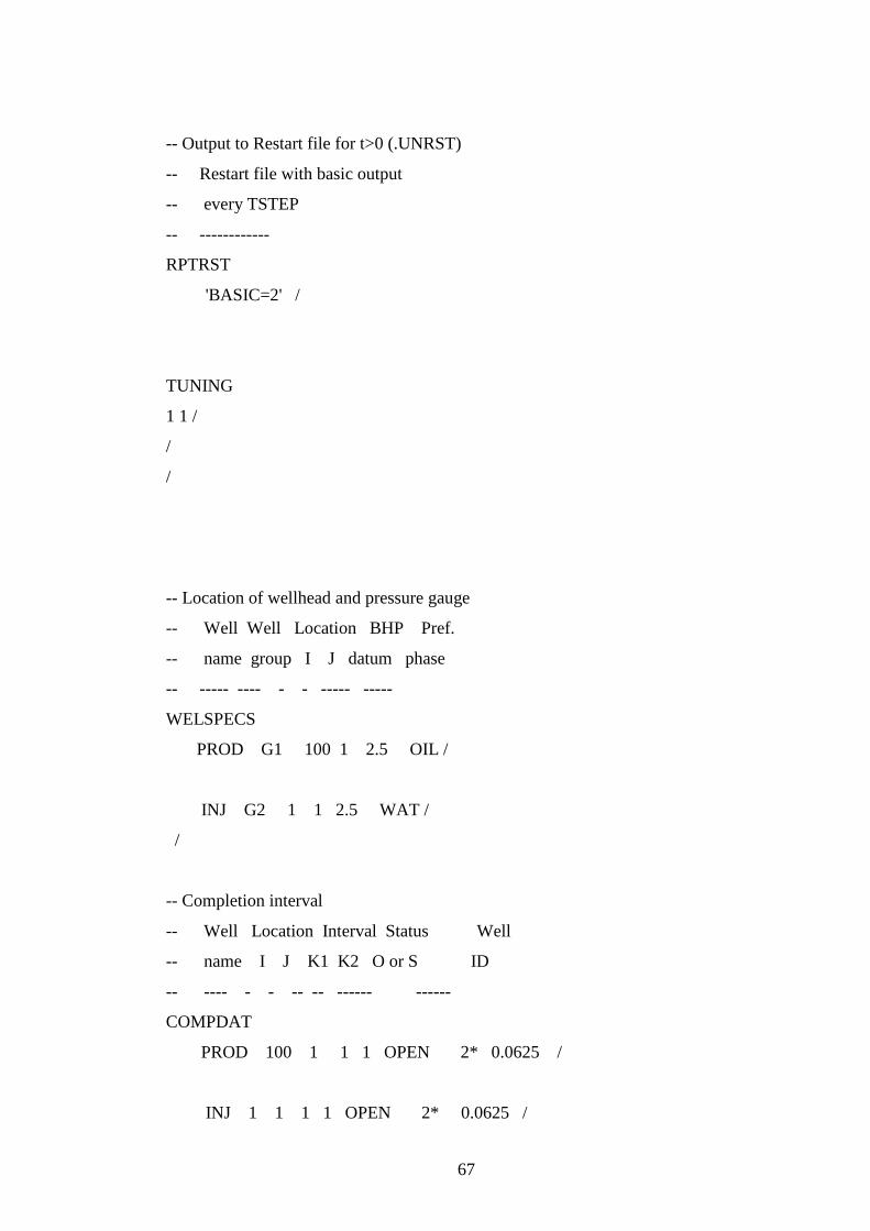
67
-- Output to Restart file for t>0 (.UNRST)
-- Restart file with basic output
-- every TSTEP
-- ------------
RPTRST
'BASIC=2' /
TUNING
1 1 /
/
/
-- Location of wellhead and pressure gauge
-- Well Well Location BHP Pref.
-- name group I J datum phase
-- ----- ---- - - ----- -----
WELSPECS
PROD G1 100 1 2.5 OIL /
INJ G2 1 1 2.5 WAT /
/
-- Completion interval
-- Well Location Interval Status Well
-- name I J K1 K2 O or S ID
-- ---- - - -- -- ------ ------
COMPDAT
PROD 100 1 1 1 OPEN 2* 0.0625 /
INJ 1 1 1 1 OPEN 2* 0.0625 /
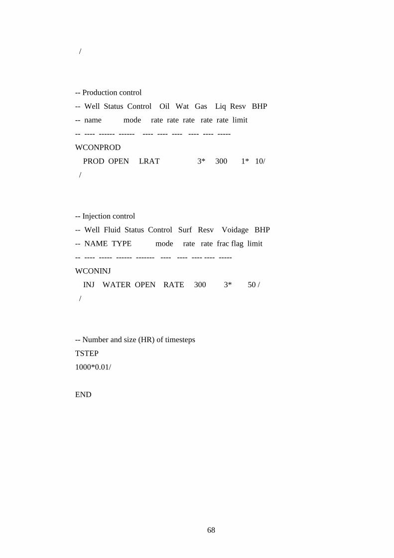
68
/
-- Production control
-- Well Status Control Oil Wat Gas Liq Resv BHP
-- name mode rate rate rate rate rate limit
-- ---- ------ ------ ---- ---- ---- ---- ---- -----
WCONPROD
PROD OPEN LRAT 3* 300 1* 10/
/
-- Injection control
-- Well Fluid Status Control Surf Resv Voidage BHP
-- NAME TYPE mode rate rate frac flag limit
-- ---- ----- ------ ------- ---- ---- ---- ---- -----
WCONINJ
INJ WATER OPEN RATE 300 3* 50 /
/
-- Number and size (HR) of timesteps
TSTEP
1000*0.01/
END