bézier method for image processing - UTPedia

i

BÉZIER METHOD FOR IMAGE PROCESSING

by

MOHD FIKRI BIN BAHARUDDIN

FINAL PROJECT REPORT

Submitted to the Electrical & Electronics Engineering Programme

in Partial Fulfillment of the Requirements

for the Degree

Bachelor of Engineering (Hons) (Electrical & Electronics Engineering)

Universiti Teknologi PETRONAS

Bandar Seri Iskandar

31750 Tronoh

Perak Darul Ridzuan

Copyright 2010

by

Mohd Fikri Bin Baharuddin, 2010

ii

CERTIFICATION OF APPROVAL

BÉZIER METHOD FOR IMAGE PROCESSING

by

MOHD FIKRI BIN BAHARUDDIN

A project dissertation submitted to the

Electrical & Electronics Engineering Programme

Universiti Teknologi PETRONAS

in partial fulfilment of the requirement for the

Bachelor of Engineering (Hons)

(Electrical & Electronics Engineering)

Approved:

________________________________________

MR. SAMSUL ARIFFIN BIN ABDUL KARIM

Project Supervisor

UNIVERSITI TEKNOLOGI PETRONAS

TRONOH, PERAK

December 2010

iii

CERTIFICATION OF ORIGINALITY

This is to certify that I am responsible for the work submitted in this project, that

the original work is my own except as specified in the references and

acknowledgements, and that the original work contained herein have not been

undertaken or done by unspecified sources or persons.

_______________________

Mohd Fikri Bin Baharuddin

iv

ABSTRACT

This project concerns about Bézier method in Computer Aided Geometric

Design (CAGD) involving Bézier Curve and Bézier Surface which widely related

to the other theorem and method. The aim of this project is to introduce the basic

of Bézier method and then generate the Bézier curves, Bézier surfaces, theory and

properties and develop Bézier method in image processing application specifically

image compression by using MATLAB. The Bézier method was widely applied in

many areas especially in Computer Aided Geometric Design (CAGD) but there is

only several application in the image processing. This project will focus on Bézier

Curve, Bézier Surface, Bernstein Polynomial, de Casteljau Algorithm,

Interpolation, Approximation, Quadtree and Parametric Line Fitting, Image

Rescaling and Image Compression application. The proof and examples of some

theory and properties as well as the application will be shown by using MATLAB

and also by using the calculation and analysis. For the main focus of this project

which is image compression by RGB Quadtree Decomposition and Parametric

Line Fitting method, the analysis have been made for four different images which

are Peppers.tiff, Baboon.tiff, Airplane.tiff and Lena.png. From the analysis which

being shown in the form of table and graph, the RGB channel threshold effect on

the resulted output images being observed.

v

ACKNOWLEDGMENT

First and foremost, praise to Allah the Almighty, who has helped and gave

me courage and strength in completing Final Year Project (FYP). Without His

permission, this FYP will not be a success. I would like to take this opportunity to

express my deepest gratitude to all parties involved in conducting this project

ranging from UTP lecturers, friend and my family who have been supportive in

helping me doing the project.

I am profoundly grateful to my supervisor, Mr. Samsul Ariffin Bin Abdul

Karim who has guided and given me opportunity to handle the project. Last but

not least, many thanks to others whose name was not mentioned in this page but

has in one way or another contributed to the accomplishment of this project.

vi

TABLE OF CONTENTS

CERTIFICATION OF APPROVAL . . . . . ii

CERTIFICATION OF ORIGINALITY . . . . . iii

ABSTRACT . . . . . . . . . iv

ACKNOWLEDGEMENT . . . . . . . v

LIST OF FIGURES . . . . . . . . xii

LIST OF TABLES . . . . . . . . xiii

LIST OF ABBREVIATIONS . . . . . . xiv

CHAPTER 1: INTRODUCTION . . . . . . 1

1.1 Background of Study . . . . 2

1.2 Problem Statement . . . . . 2

1.3 Objectives . . . . . . 2

1.4 Scope of Study . . . . . . 3

CHAPTER 2: LITERATURE REVIEW . . . . . 4

2.1 Bézier Curve . . . . . 4

2.1.1 Linear Bézier Curves . . . . 4

2.1.2 Quadratic Bézier Curves . . . 5

2.1.3 Cubic Bézier Curves . . . . 5

2.1.4 Deriving the Curve . . . . 9

2.1.5 Subdivisions and Generating New Control Points 11

2.1.6 Properties of Bézier Curves . . . 12

2.2 Bézier Surface . . . . . 13

2.2.1 Bilinear Bézier Surfaces . . . 14

2.2.2 Biquadratic Bézier Surfaces . . . 14

2.2.3 Bicubic Bézier Surfaces . . . 14

2.2.4 Properties of Bézier Surfaces . . 15

vii

2.3 Bernstein Polynomial . . . . 16

2.3.1 Properties of Bernstein Polynomials . . 17

2.4 The de Casteljau Algorithm . . . . 18

2.5 Spline . . . . . . . 18

2.6 Bernstein – Bézier – Spline . . . . 19

2.7 Image Processing . . . . . . 20

2.8 Image Compression . . . . . 21

2.9 Cubic Interpolation . . . . . 22

2.10 Image Rescaling Using Bilinear Interpolation . . 23

2.11 Cubic Bézier Curve Least Square Fitting . . 24

2.11.1 Least Square Bézier Fitting . . . 25

2.11.2 Fitting Strategy . . . . 26

2.12 Quadtree and Parametric Line Fitting . . . 28

2.13 Application: Video Data Compression . . . 30

2.14 Application: Fingerprint Data Compression . . 30

CHAPTER 3: METHODOLOGY . . . . . 31

3.1 Procedure Identifiction . . . . . 31

3.2 Tool Used . . . . . . 32

3.2.1 Software . . . . . 32

CHAPTER 4: RESULTS AND DISCUSSION . . . . 33

4.1 Linear Bézier Curve . . . . 35

4.2 Quadratic Bézier Curve . . . . . 37

4.3 Cubic Bézier Curve . . . . . 40

4.4 Bilinear Bézier Surface . . . . . 42

4.5 Biquadratic Bézier Surface . . . . 45

4.6 Bicubic Bézier Surface . . . . . 47

4.7 Bernstein Polynomial of degree 2 . . . . 48

4.8 Convex Hull Property . . . . . 48

4.9 Rotation of Cubic Bézier Curve . . . . 49

4.10 Cubic Bézier Curve with loop . . . . 50

viii

4.11 Cubic Bézier Curve with two inflection points . 50

4.12 Cubic Bézier Curve with cusp . . . . 51

4.13 Variation Diminishing Property . . . . 51

4.14 Combination of Bézier Curve . . . . 53

4.15 Combination of Bézier Surface . . . . 53

4.16 Utah Teapot . . . . . . 54

4.17 Cubic Interpolation . . . . . 56

4.18 Image Rescaling Using Bilinear Interpolation . . 59

4.19 Bézier Curve Least Square Fitting . . . 61

4.20 RGB Quadtree Decomposition and Parametric

Line Fitting . . . . . . 62

4.20.1 Uniform Threshold Variation . . 66

4.20.2 Non-uniform Threshold Variation . . 96

CHAPTER 5: CONCLUSION AND RECOMMENDATION . . 97

5.1 Conclusion . . . . . . 97

5.2 Recommendation . . . . . . 97

REFERENCES . . . . . . . . 99

APPENDICES . . . . . . . . 100

APPENDIX A: . . . . . . 102

APPENDIX B: . . . . . . 103

APPENDIX C: . . . . . . 104

ix

LIST OF FIGURES

Figure 1: Four Control Points . . . . . . 6

Figure 2: Formation of Individual Points . . . . . 6

Figure 3: Formation of the first points ��on the curve . . . 7

Figure 4: Cubic Bézier Curve Through Four Given Points . . . 21

Figure 5: Flowchart of The Project . . . . . . 31

Figure 6: Linear Curve . . . . . . . 33




Figure 10: Quadratic Curve . . . . . . . 36




Figure 14: Cubic Curve . . . . . . . 38




Figure 18: Bilinear Surface . . . . . . . 41




Figure 22: Biquadratic Surface . . . . . . 43




Figure 26: Bicubic Surface . . . . . . . 46


x



Figure 30: Bernstein Polynomial of Degree 2 . . . 48

Figure 31: Convex Hull Property . . . . . . 48

Figure 32: Rotation of Cubic Curve . . . . . . 49

Figure 33: Loop . . . . . . . . 50

Figure 34: Two Inflection Points . . . . . . 50

Figure 35: Cusp . . . . . . . . 51

Figure 36: Variation Diminishing Property . . . . . 51

Figure 37: 8 Segments of Cubic Curve . . . . . 52

Figure 38: 2 Segments of Cubic Curve . . . . . 52

Figure 39: 4 Segments of Quadratic, 2 Segments of Linear Curve . . 53

Figure 40: 2 Segments of Biquadratic Surfaces . . . . 53

Figure 41: Utah Teapot . . . . . . . 54

Figure 42: Cubic Bézier Interpolation . . . . . 56

Figure 43: Original Image Lake.tif . . . . . . 56

Figure 44: Rescale 33% . . . . . . . 57

Figure 45: Rescale 200% . . . . . . . 57

Figure 46: Original Image Mosque.jpg . . . . . 58

Figure 47: Rescale 33% . . . . . . . 58

Figure 48: Rescale 200% . . . . . . . 59

Figure 49: Circle Approximation . . . . . . 60

Figure 50: Sine Approximation . . . . . . 60

Figure 51: Five Text Approximation . . . . . . 61

Figure 52: Tangent Approximation . . . . . . 61

Figure 53: Original Image Peppers.tiff . . . . . 62

Figure 54: Decoded Image Peppers.tiff Threshold (0.3, 0.3, 0.3) . . 62


Figure 56: Original Image Baboon.tiff . . . . . 63

Figure 57: Decoded Image Baboon.tiff Threshold (0.3, 0.3, 0.3) . . 63


xi

Figure 59: Original Image Airplane.tiff . . . . . 64

Figure 60: Decoded Image Airplane.tiff Threshold (0.3, 0.3, 0.3) . . 64


Figure 62: Original Image Lena.png . . . . . . 65

Figure 63: Decoded Image Lena.png Threshold (0.3, 0.3, 0.3) . . 65



























xii
























Figure 113: Threshold Combination versus RMSE & PSNR for Peppers.tiff 94

Figure 114: Threshold Combination versus RMSE & PSNR for Baboon.tiff 94

Figure 115: Threshold Combination versus RMSE & PSNR for Airplane.tiff 95

Figure 116: Threshold Combination versus RMSE & PSNR for Lena.png 95

xiii

LIST OF TABLES

Table 1: Quantitative Analysis for Image Rescaling . . . . 61

Table 2: Quantitative Analysis for Threshold (0.3, 0.3, 0.3) . . . 66

Table 3: Quantitative Analysis for Threshold (0.5, 0.5, 0.5) . . . 66

Table 4: Non-uniform Threshold Variation . . . . . 67

Table 5: MSE, RMSE and PSNR for Peppers.tiff . . . . 84

Table 6: File Size and CR for Peppers.tiff . . . . . 84

Table 7: MSE, RMSE and PSNR for Baboon.tiff . . . . 85

Table 8: File Size and CR for Baboon.tiff . . . . . 85

Table 9: MSE, RMSE and PSNR for Airplane.tiff . . . . 86

Table 10: File Size and CR for Airplane.tiff . . . . . 86

Table 11: MSE, RMSE and PSNR for Lena.png . . . . 87

Table 12: File Size and CR for Lena.png . . . . . 87

Table 13: Comparison of Threshold and Average MSE . . . 88

Table 14: Comparison of Threshold and Average RMSE, PSNR . . 93

xiv

LIST OF ABBREVIATIONS

WxH Width x Height

MB Megabyte

KB Kilobyte

MSE Mean Squared Error

RMSE Root Mean Squared Error

PSNR Peak Signal Noise Ratio

CR Compression Ratio

R Red

G Green

B Blue

1

CHAPTER 1

INTRODUCTION

1.1 Background of Study

Originally, Bézier curves were independently developed in 1959 by Paul

de Casteljau and by Pierre Bézier about 1962. The underlying mathematical

theory is based on the concept of Bernstein polynomial [1]. The Bernstein

polynomial is important and dominant in Bézier spline models for curve and

surface design and drawing [2]. de Casteljau directly exploited this relationship,

but it was not before 1970 that R. Forrest discovered the connection between

Bézier’s work and Bernstein polynomials.

Bézier and de Casteljau developed their theories as part of CAD systems

that were built up at two French car companies, Renault and Citroën. The Renault

system UNISURF was soon described in several publications, this is the reason

that the underlying theory now bears Bézier’s name [1]. In the late sixties, the

Bézier surface description was introduced and has remained one of the most

popular schemes. When the Bézier’s work on UNISURF first published, the

remarkable spline era in computer science started.

The same situation was repeated with the discovery of Ingrid Daubechi’s

wavelets. Different wavelet splines are now well known and extensively found in

the literature. As splines are rich in properties, they provide advantages in many

important areas. Bézier and wavelet splines, can, therefore, be regarded as two

landmarks in spline theory with wide application in image processing and

machine vision [2]. Presently, Bézier curves and surfaces are extensively utilized

in many fields like industrial and computer-aided design, vector-based drawing,

font design and 3D-modelling.

2

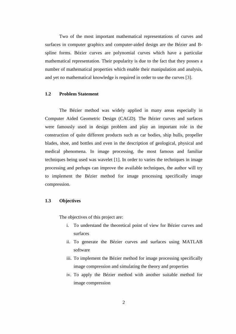
Two of the most important mathematical representations of curves and

surfaces in computer graphics and computer-aided design are the Bézier and B-

spline forms. Bézier curves are polynomial curves which have a particular

mathematical representation. Their popularity is due to the fact that they posses a

number of mathematical properties which enable their manipulation and analysis,

and yet no mathematical knowledge is required in order to use the curves [3].

1.2 Problem Statement

The Bézier method was widely applied in many areas especially in

Computer Aided Geometric Design (CAGD). The Bézier curves and surfaces

were famously used in design problem and play an important role in the

construction of quite different products such as car bodies, ship hulls, propeller

blades, shoe, and bottles and even in the description of geological, physical and

medical phenomena. In image processing, the most famous and familiar

techniques being used was wavelet [1]. In order to varies the techniques in image

processing and perhaps can improve the available techniques, the author will try

to implement the Bézier method for image processing specifically image

compression.

1.3 Objectives

The objectives of this project are:

i. To understand the theoretical point of view for Bézier curves and

surfaces

ii. To generate the Bézier curves and surfaces using MATLAB

software

iii. To implement the Bézier method for image processing specifically

image compression and simulating the theory and properties

iv. To apply the Bézier method with another suitable method for

image compression

3

1.4 Scope of Study

This project is aim to implement the Bézier method for image processing

using MATLAB. It will cover the theory and properties of Bernstein polynomial,

de Casteljau Algorithm, spline, Bézier curves, Bézier surfaces, image processing

application such as affine transformations, image rescaling, image reconstruction

and image compression. The author will try to implement Bézier method for

image processing including cubic interpolation, least square fitting and bilinear

interpolation. The author will also apply the method with quadtree decomposition

for image compression.

4

CHAPTER 2

LITERATURE REVIEW

2.1 Bézier Curve

In the mathematical field of numerical analysis, a Bézier curves is a

parametric curve important in computer graphics and related fields.

Generalizations of Bézier curves to higher dimensions are called Bézier surfaces.

‘Paths” as they are commonly referred to an image manipulation programs are

combinations of linked Bézier curves. Bézier curves are also used in animation as

a tool to control motion [4]. By simply changing the control points, the Bézier

curve will change. The examples are attached in appendices (refer Appendix A).

2.1.1 Linear Bézier Curves

A linear Bézier curve is a line segment joining two control points

��(��, ��) and ��(��, ��), parameterized by

(�), �(�) = (1 − �)(��, ��) + �(��, ��), �� ∈ [0,1] (2.1)

so that (�) = (1 − �)�� + ��, and �(�) = (1 − �)�� + ��. Letting

�(�) = ((�), �(�)), the curve can be written in the vector form

�(�) = (1 − �)�� + �� (2.2)

The curve is defined on the interval [0, 1], so the starting point of the curve

is �(0) = �� and the finishing point is �(1) = �� , that is, the Bézier

curve interpolates the first and last control points [3].

5

2.1.2 Quadratic Bézier Curves

Suppose three control points ��(��, ��), ��(��, ��) and ��(��, ��) are specified.

Then the quadratic Bézier curve is defined to be

�(�) = (1 − �)�(��, ��) + 2(1 − �)�(��, ��) + ��(��, ��) for � ∈ [0,1] (2.3)

The starting points of the curve is �(0) = �� and the finishing point is �(1) =��. The curve can be expressed in the parametric for ((�), �(�)) where

(�) = (1 − �)�� + 2(1 − �)�� + ��, (2.4) �(�) = (1 − �)�� + 2(1 − �)�� + ��, (2.5)

The triangle �� obtained by joining the control points with line segments, in

their prescribed order, is called the control polygon [3].

2.1.3 Cubic Bézier Curves

Suppose four control points ��, ��, ��, and �� are specified, then the cubic Bézier

curve is defined to be

�(�) = (1 − �)�� + 3(1 − �)�� + 3(1 − �)�� + ��, � ∈ [0,1] (2.6)

As in the quadratic case, the polygon obtained by joining the control points in the

specified order is called the control polygon.

Cubic Bézier curves provide a greater range of shapes than quadratic Bézier

curves, since they can exhibit loops, sharp corners and inflections [3].

6

2.1.4 Deriving the Curve

The first step to understand Bézier curve is knows how the curves are

geometrically formed. The construction of a Bézier curve begins with picking

three or more points, called control points. For example, we use four control

points, ��, ��, ��, and �� (refer Figure 1) to create Cubic Bézier curve [5].

Figure 1: Four Control Points

The next step is to find the points on the line segments ��, ��, and ��. This

is best done when thinking about the points as vectors. The first point is �� and it

lies �% of the way from point �� to �� (refer Figure 2).

��

��

��

Figure 2: Formation of Individual Points

0

7

This point is derived by:

�� = �� + �(�� − ��) = �� + �� − �� = (1 − �)�� + �� (2.7)

Repeating the process five more times as below;

�� (�) = (1 − �)�� + �� (�) = (1 − �)�� + �� (�) = (1 − �)�� + �� "(�) = (1 − �)�� (�) + �� (�) ��"(�) = (1 − �)�� (�) + �� (�) (2.8)

we get the other points that form Figure 3.

Figure 3: Formation of the First Points ��# on the Curve

Only ��# is on the actual curve. To find other points on the curve we repeat the

process with a different t value, ranging from 0 to 1.

��#(�) = (1 − �)��"(�) + ��"(�) (2.9)

��

��

�� # ��" ��"

��

��

��

8

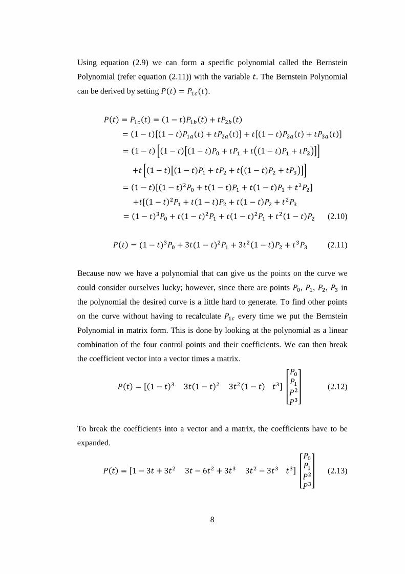
Using equation (2.9) we can form a specific polynomial called the Bernstein

Polynomial (refer equation (2.11)) with the variable �. The Bernstein Polynomial

can be derived by setting �(�) = ��#(�).

�(�) = ��#(�) = (1 − �)��"(�) + ��"(�) = (1 − �)[(1 − �)�� (�) + �� (�)] + �[(1 − �)�� (�) + �� (�)] = (1 − �) $(1 − �)%(1 − �)�� + �� + �(1 − �)�� + �� &' +� $(1 − �)%(1 − �)�� + �� + �(1 − �)�� + �� &' = (1 − �)[(1 − �)�� + �(1 − �)�� + �(1 − �)�� + ��] +�[(1 − �)�� + �(1 − �)�� + �(1 − �)�� + �� = (1 − �)�� + �(1 − �)�� + �(1 − �)�� + ��(1 − �)�� (2.10)

�(�) = (1 − �)�� + 3�(1 − �)�� + 3��(1 − �)�� + �� (2.11)

Because now we have a polynomial that can give us the points on the curve we

could consider ourselves lucky; however, since there are points ��, ��, ��, �� in

the polynomial the desired curve is a little hard to generate. To find other points

on the curve without having to recalculate ��# every time we put the Bernstein

Polynomial in matrix form. This is done by looking at the polynomial as a linear

combination of the four control points and their coefficients. We can then break

the coefficient vector into a vector times a matrix.

�(�) = [(1 − �)� 3�(1 − �)� 3��(1 − �) ��] (��) (2.12)

To break the coefficients into a vector and a matrix, the coefficients have to be

expanded.

�(�) = [1 − 3� + 3�� 3� − 6�� + 3�� 3�� − 3�� ] (��) (2.13)

9

Now the vector can be expanded to include a matrix which will isolate the �

values and allow us to quickly calculate multiple points on our Bézier curve.

�(�) = [1 � �� ] ( 1−33−1 03−63 003−3 0001) (��) (2.14)

With the matrix representation of the Bernstein Polynomial, multiple values of �

can be quickly entered and calculated using a computer to generate points on the

Bézier curve.

2.1.5 Subdivisions and Generating New Control Points

Sometimes it is useful to adjust part of a curve and not the whole thing. The

easiest way to do this is to subdivide the curve into parts and find new control

points for each of the subdivisions. To do this, take the matrix form of the

Bernstein Polynomial equation (2.14), then decide which part of the curve needs

to be changed. For this example, the curve will be divided into two equal parts. In

order to do this, the Bernstein Polynomial needs to be reparameterized, which is

easily done by adjusting � [5].

�(�) = + ,-�. + +(�� + -�) (2.15)

Taking the first part of the reparameterization of �(�), +(-�), which is the first half

of �(�), and writing in matrix form, the control points of the matrix can be

determined. Reparameterizing �(�) we get the matrix equation:

/1 �/2 (�2)� (�2)�1 ( 1−33−1 03−63 003−3 0001) (��)

10

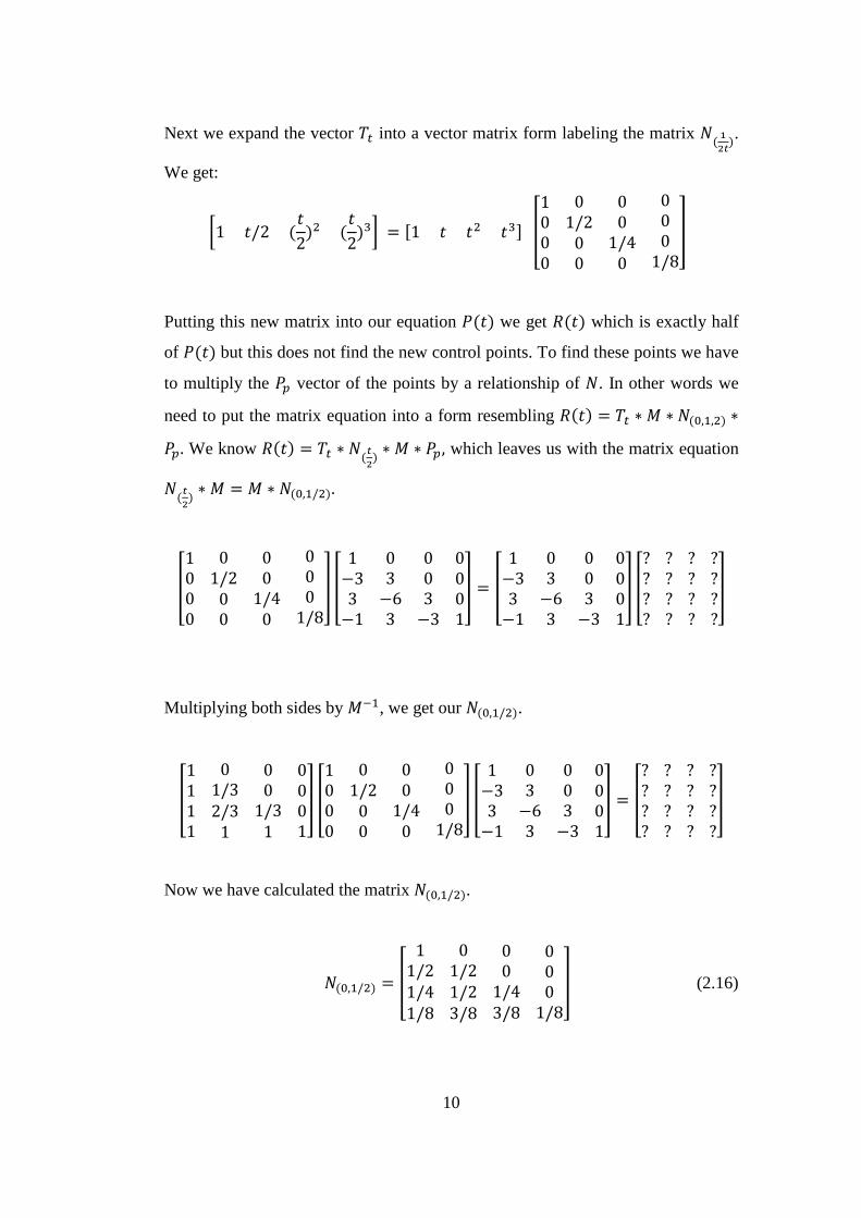
Next we expand the vector 2- into a vector matrix form labeling the matrix 3( 456). We get:

/1 �/2 (�2)� (�2)�1 = [1 � �� ] (1000 01/200 001/40 0001/8)

Putting this new matrix into our equation �(�) we get +(�) which is exactly half

of �(�) but this does not find the new control points. To find these points we have

to multiply the �9 vector of the points by a relationship of 3. In other words we

need to put the matrix equation into a form resembling +(�) = 2- ∗ ; ∗ 3(�,�,�) ∗�9. We know +(�) = 2- ∗ 3(65) ∗ ; ∗ �9, which leaves us with the matrix equation

3(65) ∗ ; = ; ∗ 3(�,�/�).

(1000 01/200 001/40 0001/8) ( 1−33−1 03−63 003−3 0001) = ( 1−33−1 03−63 003−3 0001) (???? ???? ???? ????)

Multiplying both sides by ;>�, we get our 3(�,�/�).

(1111 01/32/31 001/31 0001) (1000 01/200 001/40 0001/8) ( 1−33−1 03−63 003−3 0001) = (???? ???? ???? ????)

Now we have calculated the matrix 3(�,�/�).

3(�,�/�) = ( 11/21/41/8 01/21/23/8 001/43/8 0001/8) (2.16)

11

Using the 3(�,�/�) we found we can now multiply our control points vector �9 on

the left by 3(�,�/�) to generate our new points for +(�). This same process can be

done for +(�� + -�) to generate the 3(�,�/�) matrix which can be used to find the

new control points for the other half of the curve �(�).

3,�,45. (��) = ?@@

A��B��B��B��BCDDE (2.17)

?@@A��B��B��B��BCDD

E = ( ��1/2�� + 1/2��1/4�� + 1/2�� + 1/4��1/8�� + 3/8�� + 3/8�� + 1/8��) (2.18)

Calculating 3(45F�/�-), similarly to what we did for 3(-/�)

3(45F-/�) = (1000 1/21/200 1/41/21/40 1/83/83/81/8) (2.19)

3(45,�) = (1/8000 3/81/400 3/81/21/20 1/81/41/21 ) (2.20)

3(45F-/�) is similar to 3(45,�) as 3(-/�) is similar to 3(�,�/�). Once we have one we

can easily find the other using the matrix M. This works for any subdivision of the

original matrix and allows us to find the new control points for the subdivision.

Once the subdivisions are found we can move two of the control points, ��B or ��B, to change just part of the curve. This tool is highly practical in drafting and allows

for more complex changes.

12

2.1.6 Properties of Bézier Curves [3]

� Endpoint Interpolation Property: �(0) = �� and �(1) = �G

� Endpoint Tangent Property:

�B(0) = H(�� − ��) and �B(1) = H(�G − �G>�)

� Convex Hull Property (CHP): For all � ∈ [0,1], �(�) ∈ CH{��, … . , �G} Thus every point of a Bézier curve lies inside the convex hull of its

defining control points. The convex hull of the control points is often

referred to as the convex hull of the Bézier curve.

� Invariance under Affine Transformations: Let N be an (affine)

transformation (for example rotation, reflection, translation or scaling).

Then N ,∑ �PQPR� BP,Q(t). = ∑ NQPR� (�P)BP,Q(t) (2.21)

� Variation Diminishing Property (VDP): For a planar Bézier curve �(�),

the VDP states that the number of intersections of a given line with �(�) is

less than or equal to the number of intersections of that line with the

control polygon.

13

2.2 Bézier Surface

A species of mathematical spline used in computer graphics, computer-

aided design and finite element modeling. Bézier surface is defined by a set of

control points. Similar to interpolation in many respects, a key difference is that

the surface does not, in general, pass through the central control points; rather, it is

“stretched” toward them as though each were an attractive force. They are visually

intuitive, and for many applications [6].

A Bézier surface of order (H, U) is defined by a set of (H + 1)(U + 1)

control points VW,X. It maps the unit square into a smooth continuous surface

embedded within a space of the same dimensionality as {VW,X}. For example, if V

are all points in a four-dimensional space, then the surface will be within a four-

dimensional space [5]. A two-dimensional Bézier surface can be defined as a

parametric surface where the position of a point Y as a function of the parametric

coordinates Z, [ is given by:

Y(Z, [) = ∑ ∑ \WG]XR�GWR� (Z)\X]([)VW,X (2.22)

evaluated over the unit square where

\WG(Z) = GW ZW(1 − Z)G>W (2.23)

is a Bernstein polynomial and GW = G!W!(G>W)! is the binomial coefficient.

14

2.2.1 Bilinear Bézier Surfaces

The simple method to define bilinear Bézier surface is (linear curve)(linear curve).

So we can define bilinear Bézier surface by

_(Z, [) = (1 − Z)(1 − [)�� + (1 − Z)[�� + (1 − [)Z�� +Z[�� (2.24)

2.2.2 Biquadratic Bézier Surfaces

The simple method to define biquadratic Bézier surface is (quadratic

curve)(quadratic curve). So we can define biquadratic Bézier surface by

_(Z, [) = (1 − Z)�(1 − [)�� + (1 − Z)�2(1 − [)[�� +(1 − Z)�[�� + 2(1 − Z)Z(1 − [)�� +2(1 − Z)Z2(1 − [)[�� + 2(1 − Z)Z[�� +Z�(1 − [)�� + Z�2(1 − [)[�� + Z�[�� (2.25)

2.2.3 Bicubic Bézier Surfaces

The simple method to define bicubic Bézier surface is (cubic curve)(cubic curve).

So we can define bicubic Bézier surface by

_(Z, [) = ��(1 − Z)�(1 − [)� + 3��Z(1 − Z)�(1 − [)� +3��Z�(1 − Z)(1 − [)� + ��Z�(1 − [)� +3��(1 − Z)�[(1 − [)� + 9��Z(1 − Z)�[(1 − [)� +9��Z�(1 − Z)[(1 − [)� + 3��Z�[(1 − [)� +3��(1 − Z)�[�(1 − [) + 9��Z(1 − Z)�[�(1 − [) +9��Z�(1 − Z)[�(1 − [) + 3��Z�[�(1 − [) +��(1 − Z)�[� + 3��Z(1 − Z)�[� + 3��Z�(1 − Z)[� +��Z�[� (2.26)

15

2.2.4 Properties of Bézier Surfaces [7]

� Endpoint interpolation: Analogous to the curve case, the patch passes

through the four corner control points, that is a(0,0) = ��,� a(1,0) = �],� a(0,1) = ��,G a(1,1) = �],G

� Symmetry: We could re-index the control net so that any of the corners

corresponds to ��,� and evaluation would result in a patch with the same

shape as the original one.

� Affine invariance: Apply an affine map to the control net, and then

evaluate the patch. This surface will be identical to the surface created by

applying the same affine map to the original patch.

� Convex hull property: For (Z, [) ∈ [0,1] × [0,1], the patch a(Z, [) is in

the convex hull of the control net.

� Bilinear precision: A degree U × H patch with boundary control points

which are evenly spaced on lines connecting the corner control points, and

the interior control points are evenly-spaced on lines connecting boundary

control points on adjacent edges. This patch is identical to the bilinear

interpolant to the four corner control points.

� Tensor product: Bézier patches are in the class of tensor product surfaces.

This property allows Bézier patches to be dealt with in terms of

isoparametric curves, which in turn simplifies evaluation and other

operations.

16

2.3 Bernstein Polynomial

In the mathematical field of numerical analysis, a Bernstein polynomial is

a polynomial in the Bernstein form that is linear combination of Bernstein basis

polynomials. A numerically stable way to evaluate polynomials in Bernstein form

is de Casteljau’s algorithm. With the advent of computer graphics, Bernstein

polynomials restricted to the interval x ∈ [0, 1], became important in the form of

Bézier curves [8].

The H + 1 Bernstein basis polynomials of degree H are defined as

\W,G(�) = GW �W(1 − �)G>W, c = 0, … . , H (2.27)

A linear combination of Bernstein basis polynomials is called a Bernstein

polynomial \(�) = ∑ dW\W,GGWR� (�) (2.28)

2.3.1 Properties of Bernstein Polynomials [3]

� Partition of Unity: The Bernstein polynomials of degree n sum to one

∑ \W,G(�)GWR� = 1, � ∈ [0,1) (2.29)

� Positivity: The Bernstein polynomials are non-negative on the interval

[0, 1]

\W,G (�) ≥ 0, � ∈ [0,1] (2.30)

17

� Symmetry: \G>W,G(�) = \W,G(1 − �), for c = 0, … , H (2.31)

So, the graph of \G>W,G(�) is a reflection of the graph of \W,G(1 − �).

� Recursion: The Bernstein polynomials of degree n can be expressed in

terms of the polynomials of degree H − 1

\W,G(�) = (1 − �)\W,G>�(�) + �\W>�,G>�(�), for c = 0, … , H (2.32)

where \>�,G>�(�) = 0 and \G,G>�(�) = 0

The partition of unity and positivity properties gives rise to two important

properties of Bézier curves namely invariance under transformations and the

convex hull property. As a consequence of the symmetry property, a symmetrical

control polygon gives rise to a symmetrical curve. The recursion property gives

rise to the de Casteljau algorithm.

2.4 de Casteljau Algorithm

In the mathematical subfield of numerical analysis, de Casteljau algorithm

is a recursive method to evaluate polynomials in Bernstein form or Bézier curves.

This algorithm can also be used to split a single Bézier curve into two Bézier

curves at an arbitrary parameter value. Although the algorithm is slower when

compared with the direct approach it is numerically stable [9].

18

The de Casteljau algorithm provides a method for evaluating the point on a

Bézier curve corresponding to the parameter value � ∈ [0,1]. For the case of a

cubic Bézier curve with control points ��, ��, ��, and ��, and for a specified

parameter value � ∈ [0,1], the de Casteljau algorithm is expressed by the recursive

formula

f �W� = �W�WX = (1 − �)�WX>� + ��WF�X>�,g (2.33)

for h = 1, 2, 3 and c = 0, … , 3 − h. The formula generates a triangular set of values

as below for which �� = �(�) for the specified value of � [3].

��

2.5 Spline

In mathematics, a spline is a special function defined piecewise by

polynomials. In the computer science subfields of computer-aided design and

computer graphics, the term ‘spline’ more frequently refers to a piecewise

polynomial (parametric) curve. Splines are popular curves in these subfields

because of the simplicity of their construction, their ease and accuracy of

evaluation, and their capacity to approximate complex shapes through curve

fitting and interactive curve design [10].

19

2.6 Bernstein – Bézier – Spline

In fact, Bernstein polynomial can be thought of as the gateway to splines,

namely the Bézier spline. Bézier polynomial can be made to act in either as a

spline or non-spline. When it acts as a spline, it does piecewise approximation of a

data set with some smoothness conditions satisfying at the break points, but when

it acts as a non-spline to approximate, it does not take into consideration the

smoothness conditions to satisfy at the break points. Bézier curves is influenced

by Bernstein polynomial. As Bézier curves and surfaces are driven by Bernstein

basis, they can also be thought of, respectively, the Bernstein polynomial pieces of

curves and surfaces.

The basic philosophy behind the Bernstein polynomial approximation is

that this polynomial is very convenient to free-form drawing. In fact, some of the

properties of this Bernstein polynomial are so attractive that no sooner than the

technique was published by Bézier, it became widely popular in many industries.

In order to design the body of an automobile, Bézier developed a spline model

that became the first widely accepted spline model in computer graphics and

computer-aided design, due to its flexibility and ease over the then-used drawing

and design techniques. This model, therefore, helps to design and draw smooth

curves and surfaces of different shapes and sizes, corresponding to different

arbitrary objects, based on a set of control points.

Bézier spline model, can also be used to approximate data points

originated from different functions. Notice that Bézier spline-based drawing

technique starts from the zeroth order Bernstein approximation (which is exactly

the line drawing between control points) of the data points and goes to some

higher order (quadratic or cubic) approximation, until it mimics the shape of the

object. The Bézier splines are effective, efficient, and easy to implement, and have

a strong and elegent mathematical background as well. In computer graphics, their

significant role is well documented. Unfortunately it is not the case in image

processing and machine vision [2].

20

2.7 Image Processing

Image processing is any form of signal processing for which the input is

an image or frames of video, the output of image processing can be either an

image or a set of characteristics or parameters related to the image. Most image-

processing techniques involve treating the image as a two-dimensional signal and

applying standard signal-processing techniques to it. The typical operations

involved in image processing were denoising, compressing, reduction, rotation,

and color corrections [11].

2.8 Image Compression

Image compression is minimizing the size in bytes of a graphics file

without degrading the quality of the image to an unacceptable level. The reduction

in file size allows more images to be stored in a given amount of disk or memory

space. It also reduces the time required for images to be sent over the internet or

downloaded from web pages.

There are several different ways in which image files can be compressed.

For internet use, the two most common compressed graphic image formats are the

JPEG format and the GIF format. The JPEG method is more often used for

photographs, while the GIF method is commonly used for line art and other

images in which geometric shapes are relatively simple.

Other techniques for image compression include the use of fractal and

wavelets. These methods have not gained widespread acceptance for use on the

internet as of this writing. However, both methods offer promise because they

offer higher compressions ratio than the JPEG or GIF methods for some types of

images. Another new method that may in time replace the GIF format is the PNG

format.

21

A text file or program can be compressed without the introduction of

errors, but only up to a certain extent. This is called lossless compression. Beyond

this point, errors are introduced. In text and program files, it is crucial that

compression be lossless because a single error can seriously damage the meaning

of a text file, or cause a program not to run. In image compression, a small loss in

quality is usually not noticeable. There is no ‘critical point’ up to which

compression works perfectly, but beyond which it becomes impossible. When

there is some tolerance for loss, the compression factor can be greater than it can

where there is no loss tolerance. For this reason, graphic images can be

compressed more than text files or programs [12].

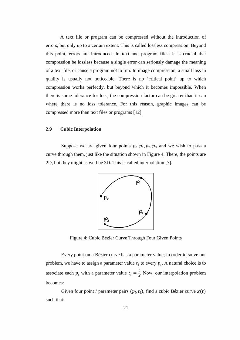
2.9 Cubic Interpolation

Suppose we are given four points ��, ��, ��, �� and we wish to pass a

curve through them, just like the situation shown in Figure 4. There, the points are

2D, but they might as well be 3D. This is called interpolation [7].

Figure 4: Cubic Bézier Curve Through Four Given Points

Every point on a Bézier curve has a parameter value; in order to solve our

problem, we have to assign a parameter value �W to every �W. A natural choice is to

associate each �W with a parameter value �W = W�. Now, our interpolation problem

becomes:

Given four point / parameter pairs (�W, �W), find a cubic Bézier curve (�)

such that:

22

(�W) = �W; c = 0,1,2,3. (2.34)

This simply states that we want the Bézier curve to pass through the data points at

the right parameter values. The desired Bézier curve will be of the form

(�) = \��(�)dj + \��(�)d� + \��(�)d� + \��(�)d� (2.35)

Writing out all interpolation conditions (2.34) yields

�� = \��(��)dj + \��(��)d� + \��(��)d� + \��(��)d� �� = \��(��)dj + \��(��)d� + \��(��)d� + \��(��)d� �� = \��(��)dj + \��(��)d� + \��(��)d� + \��(��)d� �� = \��(��)dj + \��(��)d� + \��(��)d� + \��(��)d�

These are four equations in the four unknowns d�, … , d�. In order to find a

solution, it helps to write them in matrix form:

(��) = ?@@

@A\��(��)\��(��)\��(��)\��(��) \��(��)\��(��)\��(��)\��(��) \��(��)\��(��)\��(��)\��(��) \��(��)\��(��)\��(��)\��(��)CDDDE (djd�d�d�

) (2.36)

We further abbreviate this as

� = ;\ (2.37)

The solution is now simply

\ = ;>�� (2.38)

23

2.10 Image Rescaling Using Bilinear Interpolation

In computer graphics, image scaling is the process of resizing a digital

image. Scaling is a non-trivial process that involves a trade-off between

efficiency, smoothness and sharpness. As the size of an image is increased, so the

pixels which comprise the image become increasingly visible, making the image

appears ‘soft’. Conversely, reducing an image will tend to enhance its smoothness

and apparent sharpness [13].

In mathematics, bilinear interpolation is an extension of linear

interpolation for interpolating function of two variables for example and � on a

regular grid. The key idea is to perform linear interpolation first in one direction,

and then again in the other direction. Although each step is linear in the sampled

values and in the position, the interpolation as a whole is not linear but rather

quadratic in the sample location [14].

When an image needs to be scaled up, each pixel of the original image

needs to be moved in a certain direction based on the scale constant. However,

when scaling up an image by a non-integral scale factor, there are pixels (holes)

that are not assigned appropriate pixel values. In this case, those holes should be

assigned appropriate RGB or grayscale values so that the output image does not

have non-valued pixels. Based on [15], the examples of image rescaling using

bilinear interpolation performed by using MATLAB are attached in the

appendices (refer Appendix B).

2.11 Cubic Bézier Curve Least Square Fitting

According to [16], Bézier curve is a parametric curve. A Bézier curve of

degree m can be generalized as follows:

�(�W) = ∑ ]l ]lR� �l(1 − �W)]>l�Wl, 0 ≤ �W ≤ 1, (2.39)

24

where �(�W) is an interpolated point at parameter value �W , U is degree of Bézier

curve and �l is n-o control point. To generate H points ( H is count of

interpolating points) between first and last control points inclusive, the parameter �W is uniformly divided into H − 1 intervals between 0 and 1 inclusive. Equations

of cubic Bézier curves can be derived from Eq. (2.39) as follows:

�(�W) = (1 − �W)�� + 3�W(1 − �W)�� + 3�W�(1 − �W)�� + �W�� (2.40)

Bézier curve passes through its first and last control points which are ��

and ��. The middle control points, �� and �� determine the shape of curve.

2.11.1 Least Square Bézier fitting

For data to be fit by cubic Bézier, the first and last control points of Bézier curve

are first and last point of the input data segment. The input data can be divided

into many segments or just one segment by specifying initial set of break point,

but the middle control points �� and �� for cubic Bézier must be determined. We

used least square method to find the middle control points. Least square method

gives the best value of middle control points that minimize the squared distance

between original and fitted data and is well suited for approximating data. If there

are H data points and �W and �(�W) are values of original and approximated points

respectively then we can write the least square equation as follows:

_ = ∑ [�WGWR� −�(�W)]� (2.41)

Equation above can be written as follows:

_ = ∑ [�W − (1 − �W)�� + 3�W(1 − �W)�� + 3�W�(1 − �W)�� + �W��]�GWR� (2.42)

25

�� and �� can be determined by:

p_p�� = 0

p_p�� = 0

Solving for �� and �� gives:

�� = (q�r� − q��r�) (q�q� − q��q��),s (2.43)

�� = (q�r� − q��r�) (q�q� − q��q��),s (2.44)

where

q� = 9 t �W�GWR� (1 − �W)u,

q� = 9 t �WuGWR� (1 − �W)�,

q�� = 9 t �W�GWR� (1 − �W)�,

r� = t 3�WG

WR� (1 − �W)�[�W − (1 − �W)�� − �W��], r� = t 3�W�G

WR� (1 − �W)[�W − (1 − �W)�� − �W��],

After determining the control points, Bézier curves can be fitted to large number

of original data points with very few control points using Bézier interpolation.

26

2.11.2 Fitting strategy

Suppose we have set of points (original data) v = {��, ��, … , �G} and we want to

approximate it using cubic Bézier. As in input we specify the value of limit of

error (maximum allowed square distance between original and fitted data) and

provide initial set of breakpoints. At least two breakpoints are required, the first

point and the last point of original data. Input data is divided into segments based

on initial set of breakpoints. A segment is set of all points between two

consecutive breakpoints. We have to fit each segment using cubic Bézier curve.

Now the fitting process begins. We generate H points (approximated data) w = {��, ��, … , �G} using cubic Bézier interpolation such that cubic Bézier curve

passes through breakpoints. Then we measure the error between original and

approximated (fitted) data.

When approximated data is not close enough to original data, limit of error bound

is violated then an existing segment is split (break) into two segments at a point

called new breakpoint. After splitting, number of segments are increased by one

(splitted segment is replaced by two new segments). Number of breakpoints are

also increased by one (new breakpoint is added in the set of existing breakpoints).

The point where the error is maximum between original and approximated data is

selected as new breakpoint and this point is added in the set of breakpoints.

After splitting, repeat the same fitting procedure using updated set of segments

and breakpoints until error is less than or equal to limit of error. We call this

technique as fitting break and fit strategy.

27

2.12 Quadtree and Parametric Line Fitting

Quadtree is a data structure that is widely used for image storage,

representation and processing [17, 18]. Quadtree is most often used to partition a

2-D space by recursively subdividing it into four quadrants or blocks until each

quadrant contains only pixels of one color or luminance. Recursive subdivision

may result a quadrant contains only single pixel. This conventional quadtree

decomposition has following drawbacks:

(1) The overhead of representing a single pixel by quadtree is not desirable

for image compression. It may take more space to represent a single

pixel by quadtree that without using it.

(2) Due to subdividing criteria, even if a single pixel in a quadrant is of

different color or luminance then quadtree decomposition would

divide that quadrant into four quadrants.

As a consequence of this, there may be three quadrants with same luminance

value. In other words, the boundaries between quadrants does not necessary

represent quadrant of different luminance. To overcome the first drawback; in our

method we imposed a constraint of minimum block size on quadtree

decomposition. It means that a quadrant would not be further divided into four

quadrants if its size is equal to the predefined minimum block size. The constraint

of minimum block size safeguards our method from the overhead of representing

very small quadrants (quadrants of size less than 4x4) by a quadtree. The

constraint based quadtree decomposition results in two types of quadrants:

(a) Homogeneous quadrants: quadrants that contain only pixels of one

color or luminance

(b) Non-homogeneous quadrants: quadrants that contain pixels of more

than one color or luminance

We represented only homogeneous quadrants using quadtree. Non-homogeneous

quadrants are represented by parametric line [19].

28

Parametric line is essentially a straight line obtained by linear interpolation

between two points (control points). To generate a parametric line that

interpolates n + 1 points, n line segments are used. Equation of h-o segment

between points �X and �XF� can be written as follows:

�X(�) = (1 − �)�X + ��XF�, � ∈ [0,1], 1 ≤ h ≤ n, (2.45)

where �X(�) is an interpolated point between control points �X and �XF� at

parameter value �. To generate H points between �X and �XF� inclusive, the

parameter � is divided into H − 1 intervals between 0 and 1 inclusive such that �X(0) = �X and �X(1) = �XF�. In order to represent the non-homogeneous

quadrants, we scanned the image data row wise and fitted the parametric line to

pixels of non-homogeneous quadrants. Parametric line fitting helps to further

reduce the data size in two ways. First, the parametric line fitting helps to

represent the pixels of one color/luminance with smaller data set. Second, the

parametric line fitting merges the data of a row, belong to more than one non-

homogeneous quadrant, as a single data set. This single merged row removes the

artificial boundaries between quadrants that have been imposed by quadtree

decomposition. It is very likely that at the boundaries of two adjacent non-

homogeneous quadrants, pixels have same luminance. By merging quadrants,

large number of pixels can be represented by small output data obtained from

parametric line fitting. This also solves the second drawback of conventional

quadtree representation of image [19].

2.13 Application: A New Method For Video Data Compression By

Quadratic Bézier Curve Fitting

The input points are approximated using quadratic Bézier least square

fitting. The output data consists of quadratic Bézier control points and difference

between original and fitted data. In order to understand how quadratic Bézier

curve can be used to fit video data, we need to understand the nature of video

29

data. Digital video data consists of sequence of frames which is images. Each

frame consists of rectangular 2-D array of pixels. An important factor in fitting of

data via quadratic Bézier curve is finding least number of control points [20].

Fitting process is applied to temporal data of each spatial location (, �)

individually. Let H is the number of frames in a video sequence, let x and y are

width and height of a frame respectively. At frame c, where 1 ≤ c ≤ H, let �W as

luminance or color value of a spatial location (, �). We have to approximate the H values of each spatial location by quadratic Bézier curve. As an input to

algorithm the user specifies breakpoint interval z.Luminance or color values of a

spatial location after every zth frames are taken as a breakpoint (control point).

The fitting process divides the data into segments based on breakpoints. A

segment is a set of all points (luminance or color values) between two adjacent

breakpoints. Each segment is fitted (approximated) by a quadratic Bézier curve.

The first and the last breakpoints of a segment are taken as end control points, for

example �� and ��of quadratic Bézier curve, while middle control point, ��is

obtained by least square method. Once all the three control points, ��, �� and ��are known, then approximated data of a segment using Bézier curve is obtained

using following equation:

w(�W) = (1 − �W)�� + 2�W(1 − �W)�� + �W�� (2.46)

Note that the first and last points of input data and interpolated data are always

same, because w(�W = 0) = �� and w(�W = 1) = ��. Interpolated points other than

first and last points may or may not have the same values as corresponding points

of input data. In order to reconstruct the original video data without any loss, first

interpolated frames are generated using keyframes of end control points (KFE)

and keyframes of middle control points (KFM), then adding the difference

between original and quadratic Bézier approximated (interpolated) frames other

than keyframes, frame difference (FD) to interpolated frames reproduces the

original video frames.

30

The most important application of the method is data compression. A

fundamental approach of prevalent video data compression techniques such as

MPEG-1, MPEG-2 and H.263 [21, 22] is to reduce the entropy of data by

applying Discrete Cosine Transform. Data with reduced entropy can be encoded

with less number of bits. In this method, the overall entropy of KFE, KFM and FD

is much less than the entropy of original video data. So, it can be encoded with

less number of bits. This less entropy of output data is mainly due to the fact that

quadratic Bézier curve approximates the original video data with quite good level

of accuracy.

2.14 Application: An Innovative Scheme For Effectual Fingerprint Data

Compression Using Bézier Curve Representation

This kind of application utilizes the Bézier curve representations for

effective compression of fingerprint image. It is designed in a way to preserve the

fine details in the fingerprint image such as ridge endings and bifurcations. It is

employed for achieving better compression with some cost to quality. A

fingerprint image can have hundreds of ridges each having its own structure. In

the proposed scheme, each ridge is visualized as a cubic Bézier curve and it’s

Bézier control points are determined. The set of four Bézier control points

determined, serve as compressed form of an individual ridge. So every fingerprint

image with n ridges can be compressed into a file containing 4*n Bézier control

points. A desirable property of these curves is that the curve can be translated and

rotated by performing these operations on the control points. It is sufficient to

store all the four Bézier control points instead of storing the actual Bézier curve

(ridge). The original ridge can be reproduced from these stored control points by

the properties of Bézier curve. Thus, the proposed scheme for fingerprint

compression achieves an effective reduction in the memory space required to store

the fingerprint [23].

31

CHAPTER 3

METHODOLOGY

3.1 Procedure Identification

Figure 5: Flowchart of The Project

Reviewing the Literature

Gathering Data

Understanding Bézier Curves and Surfaces

Theory Properties

Solving Equation

MATLAB Simulation

Interpolation

Data Approximation

Quadtree Decomposition Parametric Line Fitting

Image Compression

32

3.2 Tools used

3.2.1 Software

• MATLAB 7.4.0 (R2007a)

• GPL Ghostscript 8.64

• GSview 4.9

33

CHAPTER 4

RESULTS AND DISCUSSION

4.1 Linear Bézier Curve

The following figures show the examples of linear Bézier curve. The following

figures vary from its control points. The comparison between the equation and the

coding are as followed:

Equation: �(�) = (1 − �)�� + �� (4.1)

Coding: �(c) = (1 − �)∗{(1) + �∗{(2)

So, we can see that the different is �� = {(1) and �� = {(2)

� Linear Curve

Figure 6: Linear Curve

34

� Linear Curve


� Linear Curve


35

� Linear Curve


4.2 Quadratic Bézier Curve

The following figures show the examples of quadratic Bézier curve. The

following figures vary from its control points. The comparison between the

equation and the coding are as followed:

Equation: �(�) = (1 − �)�� + 2(1 − �)�� + �� (4.2)

Coding: �(c) =(1-t)^2*cx(1)+2*(1-t)*t*cx(2)+t^2*cx(3)

So, we can see that the different is �� = {(1), �� = {(2), and �� = {(3)

36

� Quadratic Curve

Figure 10: Quadratic Curve

� Quadratic Curve


37

� Quadratic Curve


� Quadratic Curve


38

4.3 Cubic Bézier Curve

The following figures show the examples of cubic Bézier curve. The following

figures vary from its control points. The comparison between the equation and the

coding are as followed:

Equation: �(�) = (1 − �)�� + 3(1 − �)�� + 3(1 − �)�� + �� (4.3)

Coding:cx(1)*(1-t)^3+3*cx(2)*t*(1-t)^2+3*cx(3)*(1-t)*t^2+cx(4)*t^3

So, we can see that the different is �� = {(1), �� = {(2), �� = {(3), and �� = {(4)

� Cubic Curve

Figure 14: Cubic Curve

39

� Cubic Curve


� Cubic Curve


40

� Cubic Curve


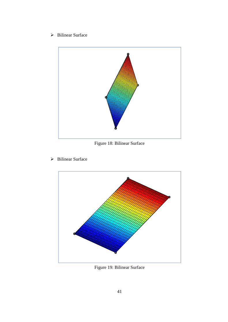
4.4 Bilinear Bézier Surface

The following figures show the examples of bilinear Bézier surface. The

following figures vary from its control points. The difference between the

equation and coding is from its control points representation:

�� = {(1,1), �� = {(1,2), �� = {(2,1), and �� = {(2,2)

41

� Bilinear Surface

Figure 18: Bilinear Surface



42





43

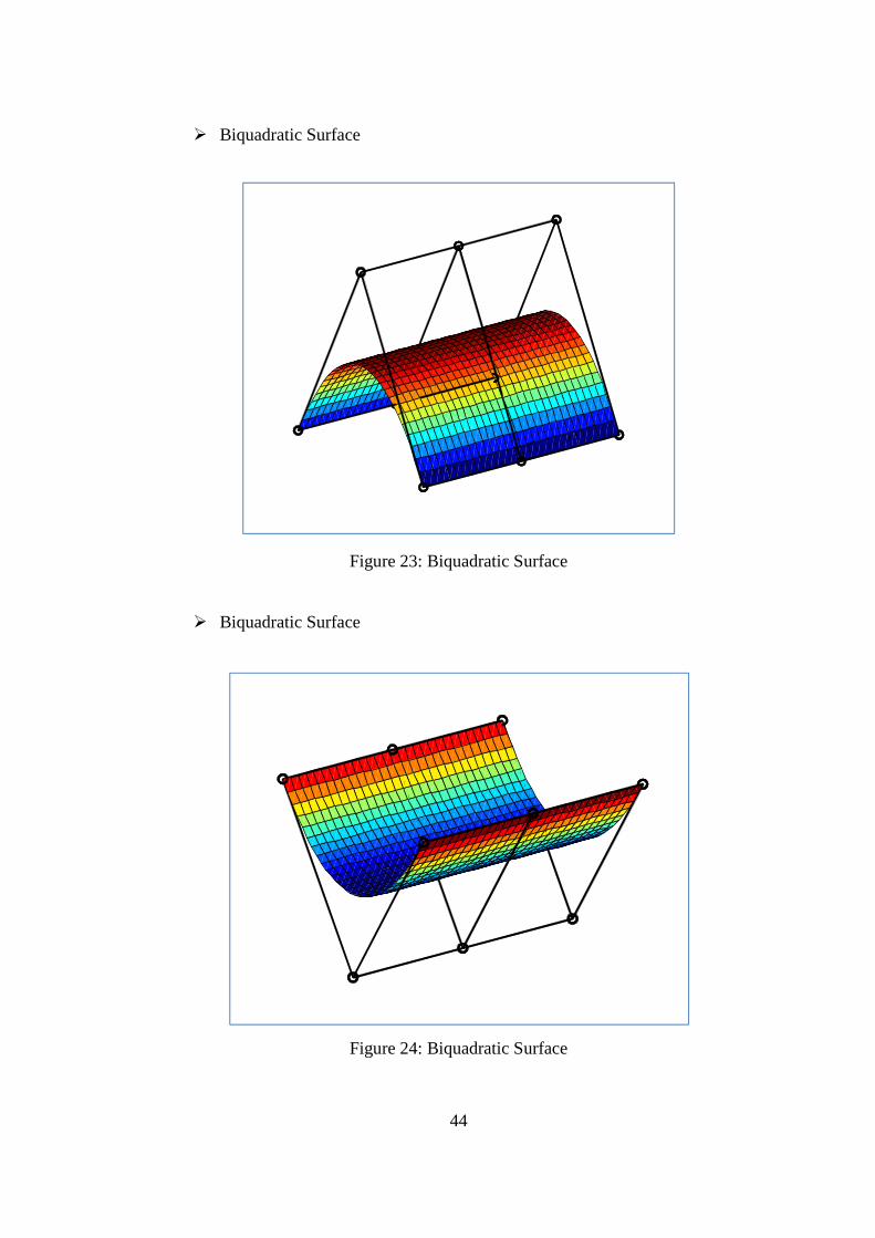
4.5 Biquadrtic Bézier Surface

The following figures show the examples of biquadratic Bézier surface. The

following figures vary from its control points. The difference between the

equation and coding is from its control points representation:

�� = {(1,1), �� = {(1,2), �� = {(1,3), �� = {(2,1), �� = {(2,2), �� = {(2,3), �� = {(3,1), �� = {(3,2), and �� = {(3,3)

� Biquadratic Surface

Figure 22: Biquadratic Surface

44





45



4.6 Bicubic Bézier Surface

The following figures show the examples of bicubic Bézier surface. The following

figures vary from its control points. The difference between the equation and

coding is from its control points representation:

�� = {(1,1), �� = {(1,2), �� = {(1,3), �� = {(1,4), �� = {(2,1), �� = {(2,2), �� = {(2,3), �� = {(2,4),

�� = {(3,1), �� = {(3,2), �� = {(3,3), �� = {(3,4), �� = {(4,1), �� = {(4,2), �� = {(4,3), and �� = {(4,4)

46

� Bicubic Surface

Figure 26: Bicubic Surface

� Bicubic Surface


47

� Bicubic Surface


� Bicubic Surface


48

4.7 Bernstein Polynomial of degree 2

This figure displayed the Bernstein Polynomial of degree 2.

� Degree 2

Figure 30: Bernstein Polynomial of Degree 2

4.8 Convex Hull Property (CHP)

� Convex Hull (The curve lies in the control polygon) [7]

Figure 31: Convex Hull Property

49

4.9 Rotation of Cubic Bézier Curve

Consider a cubic Bézier curve with vertices ��(1,0), ��(2,3), ��(5,4), and ��(2,1). [3]

Apply a rotation through an angle � 4� about the origin in the anticlockwise

direction to the curve.

�1252 0341 1111� � cos � 4�− sin � 4�0 sin � 4�cos � 4�0 001� = � 0.707−0.7070.7070.707 0.7073.5366.3642.121 1.01.01.01.0� (4.4)

The control points of the rotated curve are ��(0.707,0.707), ��(−0.707,3.536), ��(0.707,6.364), and ��(0.707,2.121). The curve and its rotated image are

illustrated in Figure 32.

� Rotation of Cubic Curve

Figure 32: Rotation of Cubic Curve

50

4.10 Cubic Bézier curve with loop

� Loop (It self-intersects) [7]

Figure 33: Loop

4.11 Cubic Bézier curve with two inflection points

� Two inflection points [7]

Figure 34: Two Inflection Points

51

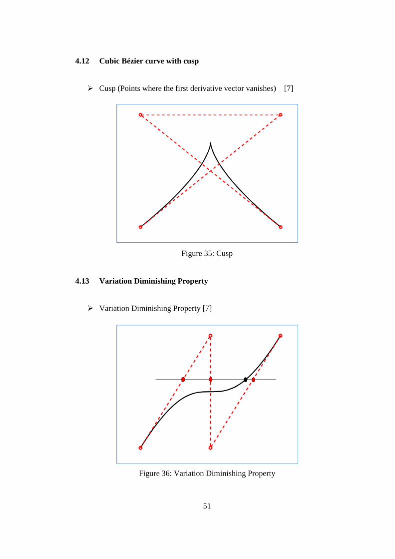
4.12 Cubic Bézier curve with cusp

� Cusp (Points where the first derivative vector vanishes) [7]

Figure 35: Cusp

4.13 Variation Diminishing Property

� Variation Diminishing Property [7]

Figure 36: Variation Diminishing Property

52

4.14 Combination of Bézier Curve

� 8 segments of Cubic Curve

Figure 37: 8 Segments of Cubic Curve

� 2 segments of Cubic Curve

Figure 38: 2 Segments of Cubic Curve

53

� 4 segments of Quadratic, 2 segments of Linear Curve

Figure 39: 4 Segments of Quadratic, 2 Segments of Linear Curve

4.15 Combination of Bézier Surface

� 2 segments of Biquadratic Surface

Figure 40: 2 Segments of Biquadratic Surface

54

4.16 Utah Teapot

The teapot data was created in 1975 by early computer graphics researcher

Martin Newell, a member of the pioneering graphic program at the University of

Utah. Newell needed a moderately simple mathematical model of a familiar object

for his work, and his wife’s teapot (a Melitta) provided a convenient solution. The

shape contains a number of elements that make it ideal for the graphics

experiments of the time. Its round, contains saddle-points, has a concave element

(the hole in the handle), and looks reasonable when displayed without a complex

surface texture [24].

Newell made the mathematical data which describes the teapot’s geometry

(largely a set of three-dimensional coordinates) publicly available and soon other

researches needed something with roughly the same characteristics that Newell

had, and using the teapot data meant they didn’t have to laboriously enter

geometric data for some other object. The actual teapot is about 30% taller than

many of its computer-generated images because the data was originally recorded

for the rectangular pixels of early displays [24].

The following figures showed the Utah teapot which being generated by

MATLAB. The model is designed by using 32 bicubic Bézier surfaces [25].

Another images for Utah teapot are attached in appendices (refer Appendix C)

� Utah Teapot

Figure 41: Utah Teapot

55

4.17 Cubic Interpolation

Let the �W be given by

�� = $−10 ' , �� = $01' , �� = $ 0−1', �� = $10',

and set �W = W�. Then the matrix M for our linear system becomes

; =?@@@@A

18271270

049290

029490

01278271 CDDDDE

Now we inverse the matrix M becomes

;>� = ( 1.0000−0.83330.33330 03.0000−1.50000 0−1.50003.00000 00.3333−0.83331.0000 ) (4.5)

With the �W given above, first we solve for - coordinate

\� = ;>�� = (−1.00001.1667−1.16671.0000 ) (4.6)

Then for �- coordinate

\� = ;>�� = ( 04.5−4.50 ) (4.7)

56

Thus, the Bézier ponts for interpolating cubic are d� = $−10 ' , d� = $1.16674.5 ' , d� = $−1.1667−4.5 ', d� = $10',

This example is outlined in Figure 42 below:

Figure 42: Cubic Bézier Interpolation

4.18 Image Rescaling Using Bilinear Interpolation

� Lake.tif

Figure 43: Original Image Lake.tif

57

Figure 44: Rescale 33%


58

� Mosque.jpg

Figure 46: Original Image Mosque.jpg


59


The comparison of WxH and file size for each images are showed as follow:

Table 1: Quantitative Analysis for Image Rescaling

Image Lake.tif Mosque.jpg Original Image WxH 720x540 500x350

File Size 2.25 MB 1.01 MB Rescale 33% WxH 238x178 165x116

File Size 264 KB 122 KB Rescale 200% WxH 140x1080 1000x700

File Size 8.98 MB 4.04 MB

60

4.19 Bézier Curve Least Square Fitting

� Circle Approximation [16]

Figure 49: Circle Approximation

� Sine Approximation (sin (x)) [16]

Figure 50: Sine Approximation

61

� Five Text Approximation [16]

Figure 51: Five Text Approximation

� Tangent Approximation (tan (x))

Figure 52: Tangent Approximation

62

4.20 RGB Quadtree Decomposition and Parametric Line Fitting

4.20.1 Uniform Threshold Variation

� Peppers.tiff

Figure 53: Original Image Peppers.tiff

Figure 54: Decoded Image Peppers.tiff Threshold (0.3, 0.3, 0.3)


63

� Baboon.tiff

Figure 56: Original Image Baboon.tiff

Figure 57: Decoded Image Baboon.tiff Threshold (0.3, 0.3, 0.3)


64

� Airplane.tiff

Figure 59: Original Image Airplane.tiff

Figure 60: Decoded Image Airplane.tiff Threshold (0.3, 0.3, 0.3)


65

� Lena.png

Figure 62: Original Image Lena.png

Figure 63: Decoded Image Lena.png Threshold (0.3, 0.3, 0.3)


66

� Threshold (0.3, 0.3, 0.3)

Table 2: Quantitative Analysis for Threshold (0.3, 0.3, 0.3)

Image Peppers.tiff Baboon.tiff Airplane.tiff Lena.png MSE R 56.0000 54.0000 56.0000 63.0000

G 68.0000 56.0000 63.0000 60.0000 B 63.0000 57.0000 58.0000 66.0000

RMSE R 7.4833 7.3485 7.4833 7.9373 G 8.2462 7.4833 7.9373 7.7460 B 7.9373 7.5498 7.6158 8.1240

PSNR R 30.6489 30.8069 30.6489 30.1374 G 29.8057 30.6489 30.1374 30.3493 B 30.1374 30.5721 30.4965 29.9354

File Size Original 35.7 KB 54.7 KB 33.7 KB 34.3 KB Decoded 34.0 KB 50.2 KB 30.9 KB 31.7 KB

� Threshold (0.5, 0.5, 0.5)

Table 3: Quantitative Analysis for Threshold (0.5, 0.5, 0.5)

Image Peppers.tiff Baboon.tiff Airplane.tiff Lena.png MSE R 107.0000 97.0000 101.0000 102.0000

G 112.0000 98.0000 108.0000 106.0000 B 99.0000 103.0000 81.0000 100.0000

RMSE R 10.3441 9.8489 10.0499 10.0995 G 10.5830 9.8995 10.3923 10.2956 B 9.9499 10.1489 9.0000 10.0000

PSNR R 27.8370 28.2631 28.0876 28.0448 G 27.6386 28.2185 27.7966 27.8777 B 28.1745 28.0024 29.0460 28.1308

File Size Original 35.7 KB 54.7 KB 33.7 KB 41.2 KB Decoded 32.8 KB 41.3 KB 28.5 KB 35.9 KB

From the quantitative analysis in two tables above, we can see the

comparison of value for MSE, RMSE and PSNR for each RGB channel and also

file size for original and decoded of the images. The compression ratio for

threshold (0.3, 0.3, 0.3) is 1.43 and for threshold (0.5, 0.5, 0.5) is 2.00 for all

images. From the above value, we can observe the best result by looking at lowest

MSE and RMSE value and highest PSNR value. The lowest MSE and RMSE and

highest PSNR determine the best quality of image compression. From the four

tested image, we can see that the best result is Baboon.tiff and if we observe the

image itself, we can see the quality is better from others.

67

4.20.2 Non-uniform Threshold Variation

For the non-uniform threshold variation, there are three patterns of

variation being used to examine and analyze the quality of the image. The lists of

non-uniform threshold being used are as followed:

Table 4: Non-uniform Threshold Variation

First Pattern Second Pattern Third Pattern 0.3, 0.5, 0.7 0.8, 0.3, 0.3 0.8, 0.8, 0.3 0.3, 0.7, 0.5 0.3, 0.8, 0.3 0.3, 0.8, 0.8 0.5, 0.3, 0.7 0.3, 0.3, 0.8 0.8, 0.3, 0.8 0.5, 0.7, 0.3 0.7, 0.3 0.5 0.7, 0.5, 0.3

The images of Peppers.tiff, Baboon.tiff, Airplane.tiff and Lena.png with

the non-uniform threshold variation are as followed:

� Peppers.tiff


68




69




70




71



� Baboon.tiff


72




73




74




75



� Airplane.tiff


76




77




78




79



� Lena.png


80




81




82




83



For all of the images with the twelve variation of threshold, the

quantitative analysis have been made including MSE, RMSE, PSNR, File size and

CR. The analysis has been arranged in the table on the next page as followed:

84

� Peppers.tiff

Table 5: MSE, RMSE and PSNR for Peppers.tiff

No. Threshold MSE RMSE PSNR

R G B R G B R G B R G B 1 0.3 0.5 0.7 62 111 145 7.874 10.536 12.042 30.2069 27.6776 26.5171 2 0.3 0.7 0.5 62 157 112 7.874 12.53 10.583 30.2069 26.1718 27.6386 3 0.5 0.3 0.7 107 71 128 10.3441 8.4261 11.314 27.837 29.6182 27.0587 4 0.5 0.7 0.3 107 157 68 10.3441 12.53 8.2462 27.837 26.1718 29.8057 5 0.7 0.3 0.5 134 71 99 11.5758 8.4261 9.9499 26.8598 29.6182 28.1745

6 0.7 0.5 0.3 134 112 63 11.5758 10.583 7.9373 26.8598 27.6386 30.1374 7 0.8 0.3 0.3 148 71 63 12.1655 8.4261 7.9373 26.4282 29.6182 30.1374 8 0.3 0.8 0.3 62 157 66 7.874 12.53 8.124 30.2069 26.1718 29.9354

9 0.3 0.3 0.8 56 68 128 7.4833 8.2462 11.314 30.6489 29.8057 27.0587

10 0.8 0.8 0.3 158 158 68 12.5698 12.57 8.2462 26.1442 26.1442 29.8057 11 0.3 0.8 0.8 62 163 161 7.874 12.767 12.689 30.2069 26.0089 26.0625

12 0.8 0.3 0.8 148 71 128 12.1655 8.4261 11.314 26.4282 29.6182 27.0587

Table 6: File Size and CR for Peppers.tiff

No. Threshold File Size CR

R G B Original Decoded R G B

1 0.3 0.5 0.7 35.7 KB 33.3 KB 1.43 2.00 3.33

2 0.3 0.7 0.5 35.7 KB 33.2 KB 1.43 3.33 2.00

3 0.5 0.3 0.7 35.7 KB 33.2 KB 2.00 1.43 3.33

4 0.5 0.7 0.3 35.7 KB 33.4 KB 2.00 3.33 1.43

5 0.7 0.3 0.5 35.7 KB 33.4 KB 3.33 1.43 2.00

6 0.7 0.5 0.3 35.7 KB 33.3 KB 3.33 2.00 1.43

7 0.8 0.3 0.3 35.7 KB 33.7 KB 5.00 1.43 1.43

8 0.3 0.8 0.3 35.7 KB 33.9 KB 1.43 5.00 1.43

9 0.3 0.3 0.8 35.7 KB 33.6 KB 1.43 1.43 5.00

10 0.8 0.8 0.3 35.7 KB 33.0 KB 5.00 5.00 1.43

11 0.3 0.8 0.8 35.7 KB 32.4 KB 1.43 5.00 5.00

12 0.8 0.3 0.8 35.7 KB 33.0 KB 5.00 1.43 5.00

85

� Baboon.tiff

Table 7: MSE, RMSE and PSNR for Baboon.tiff


R G B R G B R G B R G B 1 0.3 0.5 0.7 60 101 132 7.746 10.0499 11.4891 30.3493 28.0876 26.9251 2 0.3 0.7 0.5 58 109 103 7.6158 10.4403 10.1489 30.4965 27.7565 28.0024 3 0.5 0.3 0.7 97 60 121 9.8489 7.746 11 28.2631 30.3493 27.3029 4 0.5 0.7 0.3 97 104 61 9.8489 10.198 7.8102 28.2631 27.9605 30.2775 5 0.7 0.3 0.5 105 60 102 10.247 7.746 10.0995 27.9189 30.3493 28.0448

6 0.7 0.5 0.3 114 98 62 10.6771 9.8995 7.874 27.5618 28.2185 30.2069 7 0.8 0.3 0.3 105 56 57 10.247 7.4833 7.5498 27.9189 30.6489 30.5721 8 0.3 0.8 0.3 54 84 61 7.3485 9.1652 7.8102 30.8069 28.888 30.2775

9 0.3 0.3 0.8 54 60 108 7.3485 7.746 10.3923 30.8069 30.3493 27.7966

10 0.8 0.8 0.3 140 135 62 11.8322 11.619 7.874 26.6695 26.8275 30.2069 11 0.3 0.8 0.8 60 136 153 7.746 11.6619 12.3693 30.3493 26.7954 26.2839

12 0.8 0.3 0.8 105 60 121 10.247 7.746 11 27.9189 30.3493 27.3029

Table 8: File Size and CR for Baboon.tiff



1 0.3 0.5 0.7 54.7 KB 45.3 KB 1.43 2.00 3.33

2 0.3 0.7 0.5 54.7 KB 46.2 KB 1.43 3.33 2.00

3 0.5 0.3 0.7 54.7 KB 48.1 KB 2.00 1.43 3.33

4 0.5 0.7 0.3 54.7 KB 47.9 KB 2.00 3.33 1.43

5 0.7 0.3 0.5 54.7 KB 48.1 KB 3.33 1.43 2.00

6 0.7 0.5 0.3 54.7 KB 48.0 KB 3.33 2.00 1.43

7 0.8 0.3 0.3 54.7 KB 49.7 KB 5.00 1.43 1.43

8 0.3 0.8 0.3 54.7 KB 49.6 KB 1.43 5.00 1.43

9 0.3 0.3 0.8 54.7 KB 48.7 KB 1.43 1.43 5.00

10 0.8 0.8 0.3 54.7 KB 47.7 KB 5.00 5.00 1.43

11 0.3 0.8 0.8 54.7 KB 45.0 KB 1.43 5.00 5.00

12 0.8 0.3 0.8 54.7 KB 48.1 KB 5.00 1.43 5.00

86

� Airplane.tiff

Table 9: MSE, RMSE and PSNR for Airplane.tiff


R G B R G B R G B R G B 1 0.3 0.5 0.7 61 107 81 7.8102 10.3441 9 30.2775 27.837 29.046 2 0.3 0.7 0.5 61 134 107 7.8102 11.5758 10.3441 30.2775 26.8598 27.837 3 0.5 0.3 0.7 99 63 88 9.9499 7.9373 9.3808 28.1745 30.1374 28.686 4 0.5 0.7 0.3 98 109 58 9.8995 10.4403 7.6158 28.2185 27.7565 30.4965 5 0.7 0.3 0.5 99 63 63 9.9499 7.9373 7.9373 28.1745 30.1374 30.1374

6 0.7 0.5 0.3 95 102 58 9.7468 10.0995 7.6158 28.3536 28.0448 30.4965 7 0.8 0.3 0.3 99 63 58 9.9499 7.9373 7.6158 28.1745 30.1374 30.4965 8 0.3 0.8 0.3 61 105 58 7.8102 10.247 7.6158 30.2775 27.9189 30.4965

9 0.3 0.3 0.8 56 63 58 7.4833 7.9373 7.6158 30.6489 30.1374 30.4965

10 0.8 0.8 0.3 118 121 58 10.863 11 7.6158 27.412 27.3029 30.4965 11 0.3 0.8 0.8 61 137 107 7.8102 11.7047 10.3441 30.2775 26.7636 27.837

12 0.8 0.3 0.8 99 63 91 9.9499 7.9373 9.5394 28.1745 30.1374 28.5404

Table 10: File Size and CR for Airplane.tiff



1 0.3 0.5 0.7 33.7 KB 30.6 KB 1.43 2.00 3.33

2 0.3 0.7 0.5 33.7 KB 30.6 KB 1.43 3.33 2.00

3 0.5 0.3 0.7 33.7 KB 30.9 KB 2.00 1.43 3.33

4 0.5 0.7 0.3 33.7 KB 28.6 KB 2.00 3.33 1.43

5 0.7 0.3 0.5 33.7 KB 30.9 KB 3.33 1.43 2.00

6 0.7 0.5 0.3 33.7 KB 28.3 KB 3.33 2.00 1.43

7 0.8 0.3 0.3 33.7 KB 30.9 KB 5.00 1.43 1.43

8 0.3 0.8 0.3 33.7 KB 30.7 KB 1.43 5.00 1.43

9 0.3 0.3 0.8 33.7 KB 30.9 KB 1.43 1.43 5.00

10 0.8 0.8 0.3 33.7 KB 28.0 KB 5.00 5.00 1.43

11 0.3 0.8 0.8 33.7 KB 30.6 KB 1.43 5.00 5.00

12 0.8 0.3 0.8 33.7 KB 30.9 KB 5.00 1.43 5.00

87

� Lena.png

Table 11: MSE, RMSE and PSNR for Lena.png


R G B R G B R G B R G B 1 0.3 0.5 0.7 63 99 91 7.9373 9.9499 9.5394 30.1374 28.1745 28.5404 2 0.3 0.7 0.5 63 130 99 7.9373 11.4018 9.9499 30.1374 26.9914 28.1745 3 0.5 0.3 0.7 92 62 73 9.5917 7.874 8.544 28.4929 30.2069 29.4976 4 0.5 0.7 0.3 106 133 66 10.296 11.5326 8.124 27.8777 26.8923 29.9354 5 0.7 0.3 0.5 92 62 73 9.5917 7.874 8.544 28.4929 30.2069 29.4976

6 0.7 0.5 0.3 124 106 66 11.136 10.2956 8.124 27.1966 27.8777 29.9354 7 0.8 0.3 0.3 92 61 66 9.5917 7.8102 8.124 28.4929 30.2775 29.9354 8 0.3 0.8 0.3 63 99 66 7.9373 9.9499 8.124 30.1374 28.1745 29.9354

9 0.3 0.3 0.8 63 62 73 7.9373 7.874 8.544 30.1374 30.2069 38.8142

10 0.8 0.8 0.3 124 133 66 11.136 11.5326 8.124 27.1966 26.8923 29.9354 11 0.3 0.8 0.8 63 130 99 7.9373 11.4018 9.9499 30.1374 26.9914 28.1745

12 0.8 0.3 0.8 92 62 73 9.5917 7.874 8.544 28.4929 30.2069 29.4976

Table 12: File Size and CR for Lena.png



1 0.3 0.5 0.7 34.3 KB 30.1 KB 1.43 2.00 3.33

2 0.3 0.7 0.5 34.3 KB 30.1 KB 1.43 3.33 2.00

3 0.5 0.3 0.7 34.3 KB 31.6 KB 2.00 1.43 3.33

4 0.5 0.7 0.3 34.3 KB 30.7 KB 2.00 3.33 1.43

5 0.7 0.3 0.5 34.3 KB 31.6 KB 3.33 1.43 2.00

6 0.7 0.5 0.3 34.3 KB 30.5 KB 3.33 2.00 1.43

7 0.8 0.3 0.3 34.3 KB 31.7 KB 5.00 1.43 1.43

8 0.3 0.8 0.3 34.3 KB 31.2 KB 1.43 5.00 1.43

9 0.3 0.3 0.8 34.3 KB 31.6 KB 1.43 1.43 5.00

10 0.8 0.8 0.3 34.3 KB 30.4 KB 5.00 5.00 1.43

11 0.3 0.8 0.8 34.3 KB 29.9 KB 1.43 5.00 5.00

12 0.8 0.3 0.8 34.3 KB 31.6 KB 5.00 1.43 5.00

88

In this non-uniform threshold variation, we want to find which colour

channel most contribute to the error. We will compare the average MSE and

threshold value. By knowing this, we will consider that the threshold for that

colour channel (highest average MSE) should be the lowest compared to other

colour channels to get the better quality of image. So, the average MSE for each

variation of threshold for each images have been calculated as followed:

Table 13: Comparison of Threshold and Average MSE

No. Threshold Average MSE

R G B Peppers.tiff Baboon.tiff Airplane.tiff Lena.png 1 0.3 0.5 0.7 106 98 83 84 2 0.3 0.7 0.5 110 90 101 97 3 0.5 0.3 0.7 102 93 83 76 4 0.5 0.7 0.3 166 87 88 102 5 0.7 0.3 0.5 101 89 75 76

6 0.7 0.5 0.3 103 91 85 99 7 0.8 0.3 0.3 94 73 73 73 8 0.3 0.8 0.3 95 66 75 76

9 0.3 0.3 0.8 84 74 59 66

10 0.8 0.8 0.3 128 112 99 108 11 0.3 0.8 0.8 129 116 102 97

12 0.8 0.3 0.8 116 95 84 76

Then, we analyze the comparison between threshold and average MSE for

each images; Peppers.tiff, Baboon.tiff, Airplane.tiff and Lena.png. The average

MSE being arranged in descending order, so we can observe the highest threshold

belongs to which colour channel.

89

� Peppers.tiff

R G B Average MSE 0.5 0.7 0.3 166 0.3 0.7 0.5 110

0.3 0.5 0.7 106

0.7 0.5 0.3 103

0.5 0.3 0.7 102

0.7 0.3 0.5 101

R G B Average MSE 0.3 0.8 0.8 129 0.8 0.8 0.3 128

0.8 0.3 0.8 116

R G B Average MSE 0.3 0.8 0.3 95 0.8 0.3 0.3 94

0.3 0.3 0.8 84

- For Peppers.tiff, the Green channel contributes the highest error when its

threshold value is highest.

- So, to obtain better quality of image, the threshold value for Green channel

should be lowest compared with Red and Blue channel.

90

� Baboon.tiff

R G B Average MSE

0.3 0.5 0.7 98

0.5 0.3 0.7 93

0.7 0.5 0.3 91

0.3 0.7 0.5 90

0.7 0.3 0.5 89

0.5 0.7 0.3 87

R G B Average MSE

0.3 0.3 0.8 74

0.8 0.3 0.3 73

0.3 0.8 0.3 66

R G B Average MSE 0.3 0.8 0.8 116 0.8 0.8 0.3 112

0.8 0.3 0.8 95

- For Baboon.tiff, the Blue channel contributes the highest error when its


- So, to obtain better quality of image, the threshold value for Blue channel

should be lowest compared with Red and Green channel.

91

� Airplane.tiff

R G B Average MSE

0.3 0.7 0.5 101

0.5 0.7 0.3 88

0.7 0.5 0.3 85

0.5 0.3 0.7 83

0.3 0.5 0.7 83

0.7 0.3 0.5 75

R G B Average MSE

0.3 0.8 0.3 75

0.8 0.3 0.3 73

0.3 0.3 0.8 59

R G B Average MSE 0.3 0.8 0.8 102 0.8 0.8 0.3 99

0.8 0.3 0.8 84

- For Airplane.tiff, the Green channel contributes the highest error when its




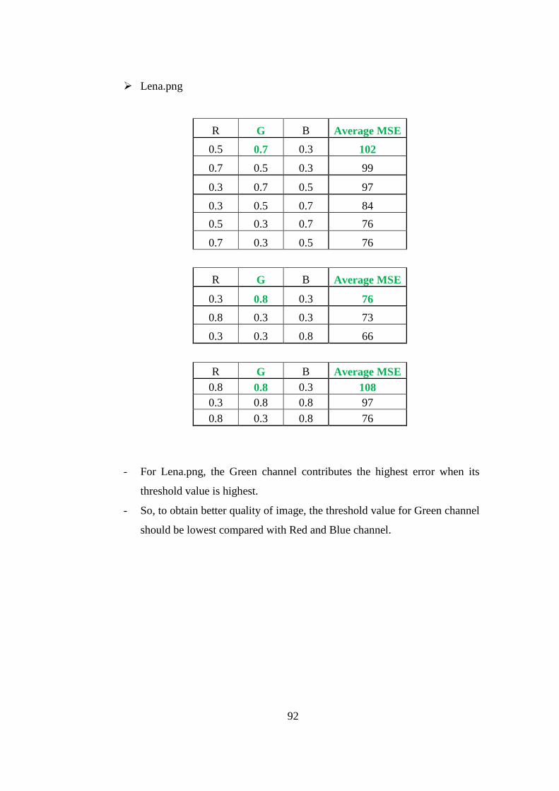
92

� Lena.png

R G B Average MSE

0.5 0.7 0.3 102

0.7 0.5 0.3 99

0.3 0.7 0.5 97

0.3 0.5 0.7 84

0.5 0.3 0.7 76

0.7 0.3 0.5 76

R G B Average MSE

0.3 0.8 0.3 76

0.8 0.3 0.3 73

0.3 0.3 0.8 66

R G B Average MSE 0.8 0.8 0.3 108 0.3 0.8 0.8 97

0.8 0.3 0.8 76

- For Lena.png, the Green channel contributes the highest error when its




93

From the analyses that have been made for non-uniform threshold

variation, we also can determine the best non-uniform threshold combination. We

can do the comparison between threshold combination and RMSE and also PSNR.

The average values of RMSE and PSNR have been calculated to determine the

best non-uniform threshold combination.

As we know, the values of MSE and RMSE are directly proportional

between each other’s and the values of MSE and PSNR are inversely proportional

between each other’s. From the quantitative analysis, the quality of images being

determined by the lowest values of MSE and RMSE and highest value of PSNR.

The average MSE and PSNR values with the respective threshold combination are

as followed:

Table 14: Comparison of Threshold and Average RMSE, PSNR

No. Threshold Peppers.tiff Baboon.tiff Airplane.tiff Lena.png

R G B RMSE PSNR RMSE PSNR RMSE PSNR RMSE PSNR 1 0.3 0.5 0.7 10.15 28.13 9.76 28.45 9.05 29.05 9.14 28.95 2 0.3 0.7 0.5 10.33 28.01 9.40 28.76 9.91 28.33 9.76 28.43 3 0.5 0.3 0.7 10.03 28.17 9.53 28.64 9.09 29.00 8.67 29.40 4 0.5 0.7 0.3 10.37 27.94 9.29 28.83 9.32 28.82 9.98 28.24 5 0.7 0.3 0.5 9.98 28.07 9.36 28.77 8.61 29.84 8.67 29.40 6 0.7 0.5 0.3 10.03 28.21 9.48 28.66 9.15 28.97 9.85 28.34 7 0.8 0.3 0.3 9.51 28.73 8.43 29.71 8.50 29.60 8.51 29.57 8 0.3 0.8 0.3 9.54 28.77 8.11 30.00 8.56 29.56 8.67 29.42 9 0.3 0.3 0.8 9.01 29.17 8.50 29.65 7.68 30.43 8.12 33.05 10 0.8 0.8 0.3 11.13 27.37 10.44 27.90 9.83 28.40 10.26 28.01 11 0.3 0.8 0.8 11.11 27.43 10.60 27.81 9.95 28.29 9.76 28.43 12 0.8 0.3 0.8 10.64 27.70 9.66 28.52 9.14 28.95 8.67 29.40

The graph of threshold combination versus RMSE & PSNR is plotted as in

the next page. From the plotted graph, we can observe the best combination of

non-uniform threshold.

94

� Peppers.tiff

Figure 113: Threshold Combination versus RMSE & PSNR for Peppers.tiff

� Baboon.tiff

Figure 114: Threshold Combination versus RMSE & PSNR for Baboon.tiff

0

5

10

15

20

25

30

35

1 2 3 4 5 6 7 8 9 10 11 12

RM

SE

& P

SN

R

Threshold Combination

RMSE

PSNR

0

5

10

15

20

25

30

35

1 2 3 4 5 6 7 8 9 10 11 12

RM

SE

& P

SN

R


RMSE

PSNR

95

� Airplane.tiff

Figure 115: Threshold Combination versus RMSE & PSNR for Airplane.tiff

� Lena.png

Figure 116: Threshold Combination versus RMSE & PSNR for Lena.png

0

5

10

15

20

25

30

35

1 2 3 4 5 6 7 8 9 10 11 12

RM

SE

& P

SN

R


RMSE

PSNR

0

5

10

15

20

25

30

35

1 2 3 4 5 6 7 8 9 10 11 12

RM

SE

& P

SN

R


RMSE

PSNR

96

From the plotted graph in the previous pages, for the Peppers.tiff image,

from Figure 113, we can see the threshold combination which achieves lowest

RMSE and highest PSNR is the ninth combination, which is 0.3, 0.3, 0.8. For the

Baboon.tiff image, from Figure 114, we can see the threshold combination which

achieves lowest RMSE and PSNR is the eighth combination, which is 0.3, 0.8,

0.3. For the Airplane.tiff image, from Figure 115, we can see the threshold

combination which achieves lowest RMSE and PSNR is the ninth combination,

which is 0.3, 0.3, 0.8. For the Lena.png image, from Figure 116, we can see the

threshold combination which achieves lowest RMSE and PSNR is the ninth

combination, which is 0.3, 0.3, 0.8.

For the RGB Quadtree Decomposition and Parametric Line Fitting method

for image compression, from the analysis and output images of variation threshold

in uniform and non-uniform patterns, we can see the quality of image Baboon.tiff

is better than others even all the Red, Green and Blue channels are at high

threshold. The Baboon.tiff image looks clear and less blur. The reason is we can

see the pure colours of the image Baboon.tiff itself which contains all of the RGB

colour components.

97

CHAPTER 5

CONCLUSION AND RECOMMENDATION

5.1 Conclusion

In summary, to define a Bézier curve of degree H, we need to choose H + 1 control points in space (+�, where � = 2 or 3) so that they roughly indicate

the shape of the desired curve while to define a Bézier surface, we need to choose (H + 1)(U + 1) control points [26]. The concept of Bézier method including

Bézier curves, Bézier surfaces, theory, properties and applications have been

generated and proved by MATLAB simulation. The quadtree decomposition and

parametric line fitting method for image compression also have been proved by

MATLAB simulation. For the image compression, we can see the quality of

image Baboon.tiff is better than others even all the Red, Green and Blue channels

are at high threshold. The reason is we can see the pure colours of the image

Baboon.tiff itself which contains all of the RGB colour components.

5.2 Recommendation

For the extension and future works, there are few recommendations that

can be done:

• For image compression using the quadtree decomposition and

parametric line fitting, we can try to use higher degree of line fitting

such as quadratic or cubic instead of parametric line fitting.

• We can try to apply filtering such as using wavelet Bior 3.5 or

Gaussian for the input image or output image of image compression

using quadtree decomposition and parametric line fitting method.

98

REFERENCES

[1] R.E. Barnhill and W. Boehm 1984, Computer Aided Geometric Design,

Amsterdam, North Holland

[2] Sambunath Biswas and Brian C. Lovell 2008, Bézier and Splines in Image

Processing and Machine Vision, London, Springer

[3] D. Marsh 2004, Applied Geometry for Computer Graphics and CAD,

Edinburgh, Springer

[4] http://en.wikipedia.org/wiki/Bézier_curve

[5] S. Kaleem and A. Abrahamsen 2000, Cubic Bézier Curves

[6] http://en.wikipedia.org/wiki/Bézier_surface

[7] G. Farin and D. Hansford 2000, The Essentials of CAGD, Arizona, A K

Peters

[8] http://en.wikipedia.org/wiki/Bernstein_polynomial

[9] http://en.wikipedia.org/wiki/De_Casteljau's_algorithm

[10] http://en.wikipedia.org/wiki/Spline_(mathematics)

[11] http://en.wikipedia.org/wiki/Image_processing

[12] http://searchcio-midmarket.techtarget.com/sDefinition/0,,sid183_gci21232

7,00.html

[13] http://en.wikipedia.org/wiki/Image_scaling

[14] http://en.wikipedia.org/wiki/Bilinear_interpolation

[15] A. Klimke, Imgrescale Version 1.0, Universität Stuttgart, 2003

[16] Dr. Murtaza Khan, Approximation of Data Using Cubic Bézier Curve

Least Square Fitting

[17] Sarah F. Frisken and Ron Perry, Simple and efficient traversal methods for

quadtrees and octrees, Journal of Graphics Tools, 7(3):1-11, 2002

[18] Hanan Samet, Data structures for quadtree approximation and

compression, Communications of the ACM, 28(9):973-993, 1985

[19] M. A. Khan, Exploiting Spline and Quadtree for Lossy Temporal Video

Data and Lossless Synthetic Image Data Compression, Keio University

99

[20] M.A. Khan, A new method for video data compression by quadratic

Bézier curve fitting, Bahrain, 2010

[21] Ghanbari, M.: Standard Codecs: Image Compression to Advanced Video

Coding, new edn. Institution Electrical Engineers (2003)

[22] Wang, Y., Ostermann, J., Zhang, Y.Q.:Video Processing and

Communications, first edn. Prentice Hall (2001)

[23] V. Perumal and Dr. J. Ramaswamy 2009, An Innovative Scheme For

Effectual Fingerprint Data Compression Using Bézier Curve

Representations, India

[24] http://design.osu.edu/Carlson/history/lesson20.html#melitta

[25] MATLAB demo, Copyright 1984-2002 The Mathworks Inc

[26] http://www.cs.mtu.edu/~shene/COURSES/cs3621/NOTES/spline/Bezier/

bezier-construct.html

100

APPENDICES

101

APPENDIX A: BÉZIER DEMO

In the following figures, we can see the changing of Bézier curve by changing the

control points.

Demo 1

Demo 2

Demo 3

102

Demo 4

Demo 5

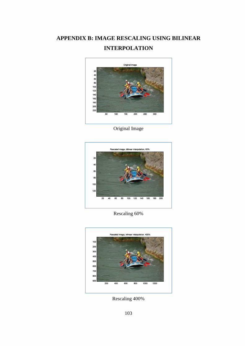
103

APPENDIX B: IMAGE RESCALING USING BILINEAR

INTERPOLATION

Original Image

Rescaling 60%

Rescaling 400%

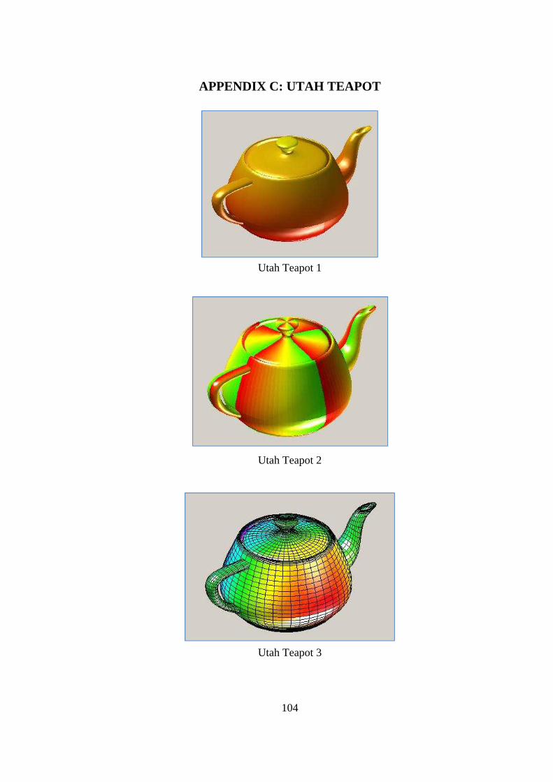
104

APPENDIX C: UTAH TEAPOT

Utah Teapot 1

Utah Teapot 2

Utah Teapot 3

bézier method for image processing - UTPedia

Documents

Transcript of bézier method for image processing - UTPedia