Introducing the Healthy Start to Life Project: economic modelling using epidemiological evidence

Mary Hedges (University of Auckland)Chris Schilling (NZ Institute of Economic Research)

2

Centre of Research Excellence

National Research Centre for Growth and Development

Fundamental processes in

developmental plasticity

Gene-environment interactions in early

life: Molecular & cellular mechanisms

Determinants of environmentally

induced developmental

mismatch

Later life effects of developmental

mismatch

Applications to agriculture and human health

Translation of our research and its impact on policy

and practice

TranslationalTheoretical

Liggins Institute, AgResearch, Landcorp, Massey University, University of Auckland. Canterbury University, Otago University

3

Theme 6: Translational Research

• Focussed on translating NRCGD research into effective policy interventions and educational practice.

• Key issue is the economic justification for a policy shift from later life interventions to early interventions.

• Must be defined in population-specific manner.• Currently two studies as a part of this theme:

– International Healthy Start to Life Project (currently in phase II)

– A healthy start to life – adolescent education for preparedness

4

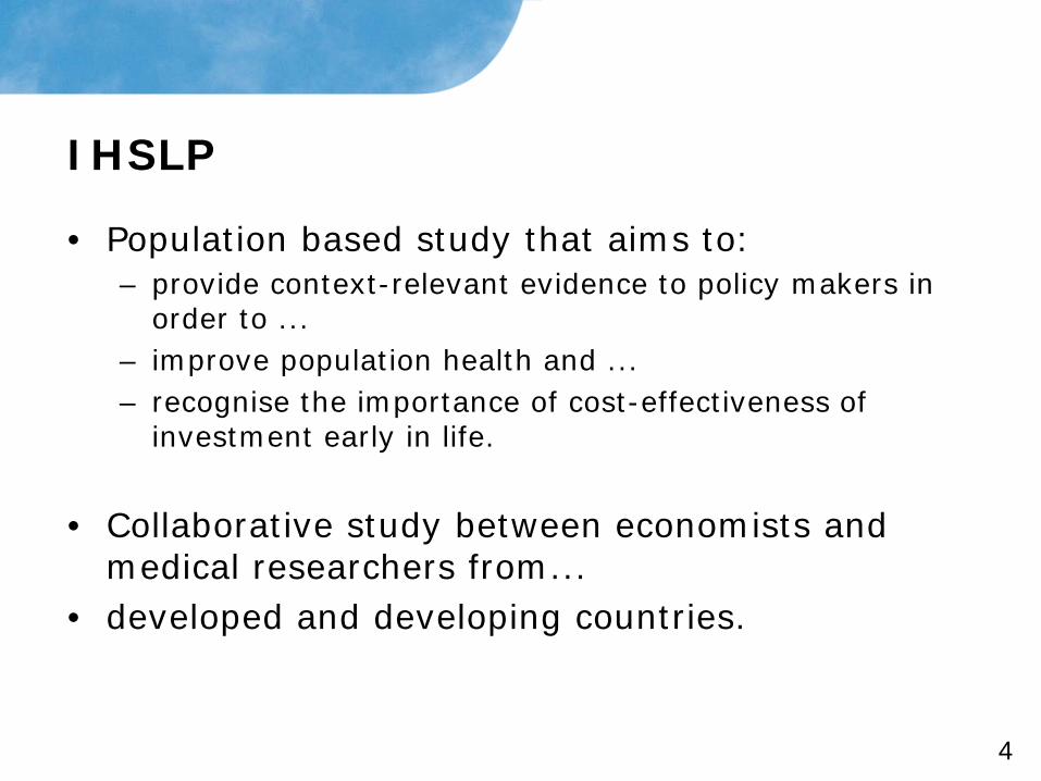
IHSLP

• Population based study that aims to:– provide context-relevant evidence to policy makers in

order to ...– improve population health and ...– recognise the importance of cost-effectiveness of

investment early in life.

• Collaborative study between economists and medical researchers from...

• developed and developing countries.

5

International Datasets

6

New Zealand Benefit

Historical International

Studies

New Zealand Context

New Zealand Now

(Growing Up)

7

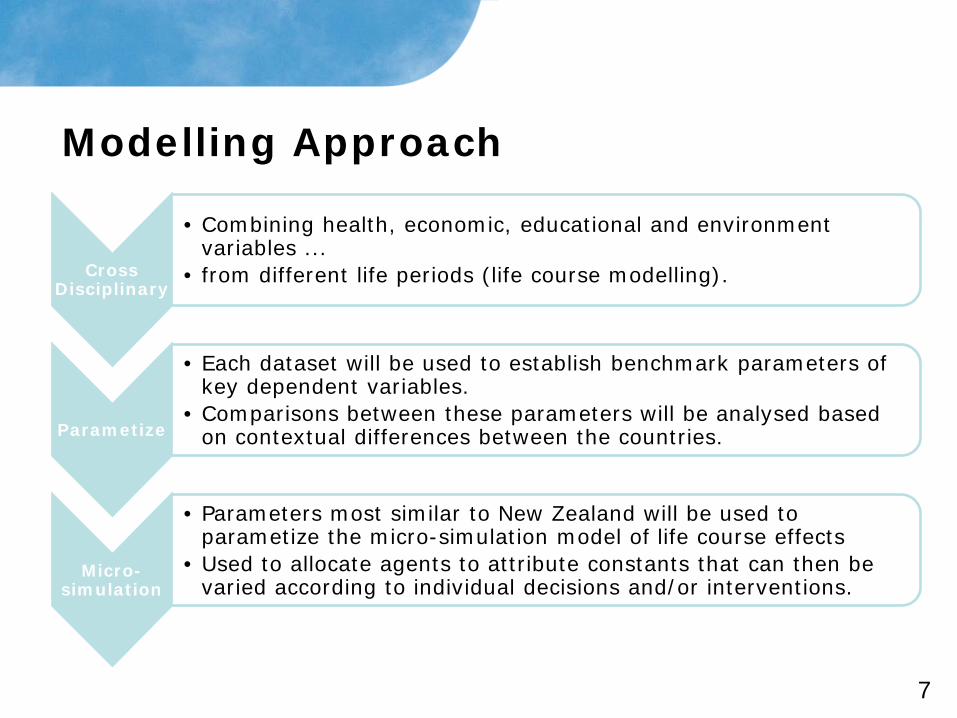
Modelling Approach

Cross Disciplinary

• Combining health, economic, educational and environment variables ...

• from different life periods (life course modelling).

Parametize

• Each dataset will be used to establish benchmark parameters of key dependent variables.

• Comparisons between these parameters will be analysed based on contextual differences between the countries.

Micro-simulation

• Parameters most similar to New Zealand will be used to parametize the micro-simulation model of life course effects

• Used to allocate agents to attribute constants that can then be varied according to individual decisions and/or interventions.

Life Course Modelling

http://www.cdphe.state.co.us/ps/mch/ArchiveFiles/life_course_fact_sheet.pdf

9

Scaling up and scaling down!

10

SCORM – A first step

• Singapore Cohort Study of the Risk factors of Myopia

• Longitudinal data set collected from 1999 that includes a wealth of demographic, socioeconomic, pre-natal and childhood characteristics.

• Short life course – pre-natal to 11 years of age• We know that low levels of cognitive ability as a

child are associated with numerous health and social outcomes later in life.

• Dependent variable childhood IQ• Can early life environment influence outcomes?

11

Sample

• Half of the sample from schools:– ranked in the bottom 20 in Singapore– ranked in the top 20 in Singapore– based on prior National Examination results

• Data included:– comprehensive peri-natal data– socio-economic data at both birth and aged 11– parent educational levels– one of the top 20 schools had additional peri-natal data

on included:• birth order, breast fed & mother’s work status.

12

Analysis - 3 stages1. Initially IQ, measured at age 11, was regressed

against a range of individual, household/socio-economic and school determinants consistent with study undertaken by Cesur & Kelly (2010)

2. Logistic regression of IQ groups was then run to identify the possible impact of interventions such as schooling

3. Multinomial logit models were then used to investigate the likelihood of moving across IQ groups and whether these movements were greater than or less than the average.

13

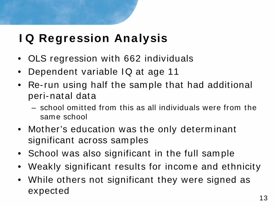
IQ Regression Analysis

• OLS regression with 662 individuals• Dependent variable IQ at age 11• Re-run using half the sample that had additional

peri-natal data– school omitted from this as all individuals were from the

same school

• Mother’s education was the only determinant significant across samples

• School was also significant in the full sample• Weakly significant results for income and ethnicity• While others not significant they were signed as

expected

IQ Regression ResultsVariables IQ Full Sample IQ Half Sample

Individual characteristics

Birth weight -0.006 (0.007) -0.003 (0.008) Birth weight squared 0.000 (0.000) 0.000 (0.000) Male -0.300 (0.872) -1.205 (1.161) Breast fed - 1.007 (1.197) Birth order - -0.936 (0.907) Chinese 2.546 (1.697) 3.676* (2.185) Malay -2.771 (1.88) -1.156 (2.644)

Household characteristics

Total combined income 1.391* (0.784) 0.504 (1.069) Father education 0.84 (0.596) 0.594 (0.803) Mother education 2.078*** (0.637) 2.709*** (0.882) Mother age -0.372 (0.872) -0.197 (1.387) Mother age squared 0.005 (0.014) 0.004 (0.023) Number of children - -1.147 (0.807) Mother working - 0.999 (1.34)

School characteristics

School dummy 5.878*** (0.982) -Observations 662 320 R squared 0.233 0.178

***, **, and * denotes significance at 1%, 5%, and 10% levels, respectively.

15

Logistic Regression of IQ Groups

• Really interested in the transition between life stages

• IQ only collected at age 11 for childrenbut given earlier results that Mother’s educaiton strongly and consistently significant it motivated us to use this as a proxy for cognition at birth.

• Mother’ education split into five categories– no formal, primary, secondary, pre-degree/diploma,

university

• Made sense to split IQ into five categories as well based on standard interpretations of IQ

16

IQ Categories1 if IQ < 90 (below average)2 if 90<=IQ<=99 (low normal or average)3 if 100<=IQ<=109 (high normal or average)4 if 110<=IQ<=119 (superior)5 if IQ=>120 (very superior)

• First applied an ordered logistic regression– appropriate given the constructed ordinal and categorical

nature of our dependent variable

• Allowed for ‘odds ratios’ to be calculated– ‘odds ratios’ are a way of comparing whether the

probability of a certain event or outcome is the same for two groups.

– An odds ratio of 1 indicates an event is equally likely in both groups/circumstances.

17

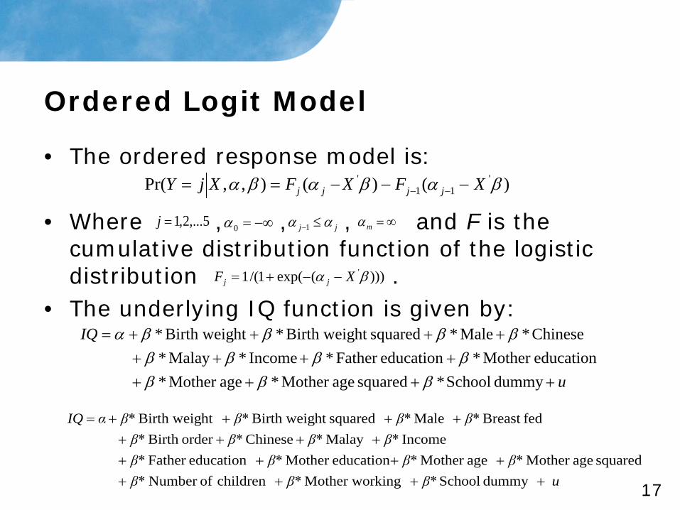
Ordered Logit Model

• The ordered response model is:

• Where , , , and F is the cumulative distribution function of the logistic distribution .

• The underlying IQ function is given by:

u β* β* β* β* β*β* β*

β* β*β*β* β* β* β* β*αIQ

++++++++

++++++++=

dummy SchoolkingMother worchildren ofNumber squared ageMother ageMother educationMother educationFather

IncomeMalay Chineseorder Birth fedBreast Malesquaredht Birth weightBirth weig

u

IQ

++++++++

++++=

dummy School*squared ageMother * ageMother * educationMother *education Father * Income*Malay *

Chinese* Male* squaredht Birth weig*ht Birth weig*

βββββββ

ββββα

)()(),,Pr( '11

' βαβαβα XFXFXjY jjjj −−−== −−

5,...2,1=j −∞=0α jj αα ≤−1 ∞=mα

)))(exp(1/(1 'βα XF jj −−+=

Logistic Regression Results

Variables Coefficients Odds-Ratio Coefficients Odds-Ratio(Full sample) (Half Sample)

Individual characteristicsBirth weight -0.001

(0.001) 1.000 -0.000

(0.001) 1.000

Birth weight squared 0.000 (0.000)

1.000 0.000 (0.000)

1.000

Male 0.087 (0.150)

1.091 0.012 (0.227)

1.012

Breast fed - - 0.274 (0.232)

1.316

Birth order - - -0.252 (0.176)

0.778

Chinese 0.331 (0.283)

1.393 0.602 (0.416)

1.827

Malay -0.373 (0.313)

0.689 -0.172 (0.505)

0.842

Household characteristicsTotal combined income

0.189 (0.135)

1.208 0.158 (0.204)

1.171

Father education 0.098 (0.102)

1.102 -0.008 (0.156)

0.992

Mother education 0.458*** (0.114)

1.581*** 0.619*** (0.179)

1.857***

Mother age -0.010 (0.146)

0.989 -0.072 (0.268)

0.931

Mother age squared 0.000 (0.002)

1.000 0.002 (0.004)

1.002

Number of children - - -0.180 (0.157)

0.835

Mother working - - 0.021 (0.259)

1.021

School characteristicsSchool dummy 1.102***

(0.171) 3.011*** - -

Observations 662 662 320 320 Pseudo R squared 0.102 0.102 0.081 0.081

CutsWhen IQ group = 1 -1.158

(2.704)-2.200(4.555)

= 2 0.027(2.700)

-0.766(4.539)

= 3 1.085(2.700)

-0.019(4.535)

= 4 3.277(2.700)

2.285(4.538)

19

Multinomial Logit Model

• This model investigates the likelihood of moving across IQ groups between birth and age 11.

• We seek to isolate the impact of environment & proxy cognition at birth by mother’s education.

• Allows us to infer,, for a given level of mothers education, how environmental factors influence the development of cognition.

• preliminary inspection shows most children are in 1 IQ group higher than their mother’s education level.

• We then focus on movements greater than or less than average movements.

Multinomial Logit Results (Above avg)

Mother education = 2 Mother education =3Above averageIndividual characteristicsBirth weight -0.001 (0.002) 0.001 (0.003)Birth weight squared 0.000 (0.000) -0.000 (0.000)Male -0.136 (0.484) 0.192 (0.256)Chinese -0.332 (0.873) 0.413 (0.553)Malay -0.536 (0.910) -0.198 (0.641)Household characteristics

Total combined income 0.568 (0.599) -0.036 (0.215)Father education 0.930 (0.423)** -0.110 (0.163)Mother age -0.205 (0.452) -0.011 (0.285)Mother age squared 0.004 (0.008) 0.000 (0.005)School characteristicsSchool dummy 1.157 (0.555)** 1.027 (0.318)***

Observations 171 331Pseudo R squared 0.154 0.106

***, **, and * denotes significance at 1%, 5%, and 10% levels, respectively.

Multinomial Logit Results (Below avg)

Below average Mother education = 2 Mother education =3Individual characteristicsBirth weight 0.016 (0.008)** 0.001 (0.004)Birth weight squared -0.000 (0.000)** -0.000 (0.000)Male 0.425 (0.571) 0.225 (0.333)Chinese -0.586 (1.138) -0.449 (0.600)Malay 0.819 (1.137) -0.313 (0.657)Household characteristics

Total combined income 0.184 (0.726) -0.460 (0.300)Father education 0.342 (0.516) -0.360 (0.223)*Mother age -0.139 (0.528) 0.018 (0.341)Mother age squared 0.003 (0.009) 0.000 (0.006)School characteristicsSchool dummy 0.723 (0.671) -1.270 (0.358)***

Observations 171 331Pseudo R squared 0.154 0.106

***, **, and * denotes significance at 1%, 5%, and 10% levels, respectively.

22

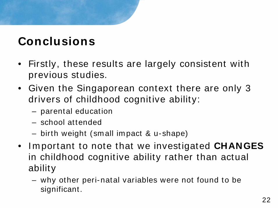
Conclusions

• Firstly, these results are largely consistent with previous studies.

• Given the Singaporean context there are only 3 drivers of childhood cognitive ability:– parental education– school attended– birth weight (small impact & u-shape)

• Important to note that we investigated CHANGESin childhood cognitive ability rather than actual ability– why other peri-natal variables were not found to be

significant.

23

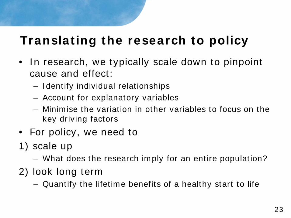
Translating the research to policy

• In research, we typically scale down to pinpoint cause and effect:– Identify individual relationships– Account for explanatory variables– Minimise the variation in other variables to focus on the

key driving factors

• For policy, we need to1) scale up

– What does the research imply for an entire population?

2) look long term– Quantify the lifetime benefits of a healthy start to life

24

Scaling up: modelling at a population level

• People are different!• Populations change

Impacts of interventions are different across cohorts

• Modelling needs to include population heterogeneity

25

Example: tobacco control

0%

5%

10%

15%

20%

25%

30%

35%

40%

0 10 20 30 40 50 60 70 80Age of life

Smoking prevalance

26

Example: tobacco control

0%

5%

10%

15%

20%

25%

30%

35%

40%

0 10 20 30 40 50 60 70 80Age of life

Smoking prevalanceAll

"Entrenched"

"Socialites"

27

Looking long term: modelling over time• Epidemiology tells us that early life matters

Benefits of an intervention today may accrue over 50 years or more• Critical periods in health development• Modelling needs to capture lifetime benefits and

costs and sum into today’s money

28

A microsimulation framework (1)

• ‘Agent’ based• Model 4 million agents rather than 1, 10 or even

10,000• Each agent is modelled individually

– Has an ethnicity, an income, a gender– Experiences different life events (e.g. birth, pregnancy,

death)– Is exposed to risk factors (e.g. smoking initiation and

cessation)

• Population is representative of wider New Zealand

See how impacts of interventions vary

29

A microsimulation framework (2)

• Based on Statistics NZ demographic data– Projects out to 2061

• Models the lifepath of each agent out for 50+ years– Include key health paths of interest e.g. smoking and

cancer– Parameterise using relative risk ratios (or odds ratios)

Models each stage of life, including long term impacts

30

Populating the model

• Longitudinal studies:– International datasets (e.g. SCORM analysis)– Growing up in NZ

• Ministry of Health data• Census and health surveys• International literature• Statistics NZ

An on-going process – “scaleable”

31

Valuing a healthy start to life

• Consider– Health care costs– Labour productivity impacts– Value of statistical life (VOSL)

32

Scenario modelling

• Scenario modelling used to estimate economic costs of intervention– Baseline scenario (without intervention) compared to

Policy scenario (with intervention)

• Sensitivity testing of key parameters– Discount rates– Econometric coefficients– Economic valuation numbers

33

What it delivers?

• An ability to make policy trade-offs• Highlight the long term benefits of early

interventions• A framework for international comparisons• Evidence

The evidence for policy makers to make decisions

34

Promoting a healthy start to life

• The epidemiology is generally accepted…• But yet translation to policy is still difficult • IHSLP is a cross disciplinary team with a focus on

policy• Our aim to promote a healthy start to life by:

– Understanding epidemiological relationships– Quantifying the implications of early life on later life– Scaling up our findings using population modelling

Robust evidence to promote a healthy start to life