Summary of Expenditures (10/1/2019 - 9/30/2020) - DC Council
Upload
khangminh22Category
view
2download
0
Durham E-Theses
Modelling Government Expenditures and Economic
Growth Nexus in Saudi Arabia: 1968 -2010
AGELI, MOHAMMED,MOOSA,O
How to cite:
AGELI, MOHAMMED,MOOSA,O (2012) Modelling Government Expenditures and Economic Growth
Nexus in Saudi Arabia: 1968 -2010, Durham theses, Durham University. Available at Durham E-ThesesOnline: http://etheses.dur.ac.uk/3534/
Use policy
The full-text may be used and/or reproduced, and given to third parties in any format or medium, without prior permission orcharge, for personal research or study, educational, or not-for-prot purposes provided that:
• a full bibliographic reference is made to the original source
• a link is made to the metadata record in Durham E-Theses
• the full-text is not changed in any way
The full-text must not be sold in any format or medium without the formal permission of the copyright holders.
Please consult the full Durham E-Theses policy for further details.

Academic Support Oce, Durham University, University Oce, Old Elvet, Durham DH1 3HPe-mail: [email protected] Tel: +44 0191 334 6107
http://etheses.dur.ac.uk
2

MODELLING GOVERNMENT EXPENDITURES AND
ECONOMIC GROWTH NEXUS IN SAUDI ARABIA:
1968-2010
by
MOHAMMED MOOSA AGELI
Thesis submitted in fulfilment of the requirements for the degree of Doctor of Philosophy at Durham University
School of Government and International Affairs Durham University
2012

i
Modelling Government Expenditures and Economic Growth Nexus in Saudi Arabia: 1968 -2010
By
Mohammed Moosa Ageli
Abstract:
Economic growth and development remains an important policy issue for most of the states in the world, which is a particular issue for late developing countries, as they have very much relied on „state‟ for economic growth and development. As a result, the experience in the 20th century demonstrates a secular increase in the growth of government expenditures all over the world. Hence, the role of government expenditures in contributing to long run economic growth continues to be an important topic and the subject of much debate.
Saudi Arabia economy is one of late developing countries. While its economy is characterised by an open and private economy, the government remains to have a large role in the economy through its expenditures financed largely by revenues generated from oil. While the Saudi economy has grown and developed, the government has also responded to the increased demand for social services such as education and healthcare in addition to other infrastructure investments for development purpose. Therefore, the process of economic growth and development has resulted in growth of government expenditures.
This research, thus, aims at modelling of government expenditures and economic growth nexus in the case o Saudi Arabia for the period of 1968-2010 by testing a number of models developed in the literature: Wagner‟s Law, Keynesian Relations and Peacock and Wiseman‟s Displacement Effect. The analysis modelled within the time series econometric techniques including co-integration test, Granger causality test and the error correction model (ECM).
The findings obtained from the analyses find that the Wagnerian proposition can explain the growth of government in Saudi Arabia, which holds for both the oil and non-oil income cases. The result indicates the existence of strong feedback causality for all the versions of Wagner‟s law in the long run. The findings also note that the three versions of Keynesian Relations found to be held for both general income and non-oil income in the case of Saudi Arabia. In addition, the findings also support for the Displacement Effect mainly due to international political developments and trends in oil prices, as such events resulted deviation from the linear growth in the government expenditures over the average growth and it is observed that government expenditure growth continued its gradual growth from the new level.
This study, thus, concludes that growing economic activity of the state has marked the Saudi Arabian economy over the period in question. While this partly can be explained due to economic reasons such as the need for economic development and responding to the demands of a growing population, but also the rentier economy nature of the Saudi political economy necessitates increasing government expenditures for political stability.

ii
DECLARATION
I hereby declare that no portion of the work that appears in this study has been used in
support of an application of another degree in qualification to this or any other university
or institution of learning.

iii
STATEMENT OF COPYRIGHT
The copyright of this thesis rests with the author. No quotation from it should be
published without his prior written consent and information derived from it should be
acknowledged.

iv
DEDICATION
I dedicate this work to my family, then to those interested in government expenditure
and economic growth.
v
ACKNOWLEDGMENT
First of all, praise is to Allah, on whom ultimately we depend for sustenance and
guidance.
I am grateful to my family for being there for me; as without their support I
would not have come thus far and for Amal.
I must express my gratitude to my supervisor, whom I consider as my brother,
Dr. Mehmet Asutay whose guidance, careful reading and constructive comments were
invaluable. His efficient contribution helped me to develop this research into its final
form.
Thank you for my Examiners, Professor Peter Jackson and Professor Habib
Ahmed, for their comments.
Many thanks, to all whose names do not appear here and without whom this
study would not have been possible.
M. M. Ageli October 2011 Durham

vi
TABLE OF CONTENTS
Abstract ................................................................................................................................................................. i Declaration ......................................................................................................................................................... ii Statement of Copyright ................................................................................................................................... iii Dedication ......................................................................................................................................................... iv Acknowledgment ............................................................................................................................................... v Table of Contents ............................................................................................................................................. vi List of Tables ...................................................................................................................................................... xi List of Figures .................................................................................................................................................. xiv
CHAPTER ONE
INTRODUCTION
1.1 Overview ..............................................................................................................................1 1.2 Aim and Objectives .............................................................................................................. 3 1.3 Significance of the Study ....................................................................................................... 4 1.4 Research Rationales .............................................................................................................. 5 1.5 Modelling and Research Method ............................................................................................ 6 1.6 Overview of the Research ..................................................................................................... 9
CHAPTER TWO
FINANCING ECONOMIC DEVELOPMENT THROUGH STATE EXPENDITURES IN LATE DEVELOPING COUNTRIES
2.1 Introduction ........................................................................................................................ 11 2.2 Late Developmentalism ........................................................................................................ 12 2.2.1 Concept ............................................................................................................................ 12 2.2.2 Lack of Private Capital ...................................................................................................... 13 2.2.3 Rationale for Public Expenditure ....................................................................................... 14 2.3 Utilisation of Government Expenditure for Economic Growth .............................................. 16 2.4 Impact of Government Expenditure on Economic Growth in Short and Long -Run ............... 20 2.5 Critical Approach to Government Expenditures .................................................................... 21 2.6 Conclusion ......................................................................................................................... .24
CHAPTER THREE
GOVERNMENT GROWTH: SURVEYING THEORIES AND MODELS 3.1 Introduction ........................................................................................................................ 26 3.2 The Perception of Government (State) Over Time ................................................................ 27 3. 3 The Economic Rationale for Government............................................................................ 28 3.3.1 Market Failure ................................................................................................................... 29 3.3.1.1 Public Goods ................................................................................................................. 30 3.3.1.2 Externalities ................................................................................................................... 30 3.3.1.3 Imperfect Market............................................................................................................ 31 3.3.1.4 Imperfect Information .................................................................................................... 32 3.3.2 Government Failure .......................................................................................................... 32 3.4 Theoretical Explanations for the Size and Growth of Government ......................................... 33

vii
3.4.1 Macroeconomic Models of Government Growth................................................................ 34 3.4.1.1 Wagner's Law of "Expending State Activity" .................................................................... 34 3.4.1.2 The Displacement Hypothesis ......................................................................................... 36 3.4.1.2.1 The Displacement Effect: Structural Break .................................................................... 39 3.4.1.2.2 The Displacement Effect: Ratchet Effect ...................................................................... 40 3.4.1.3 Keynesian Economic Growth and Government Expenditures .......................................... 40 3.4.2 Microeconomic Models of Government Growth ................................................................ 41 3.4.2.1 Baumol's Differential Productivity Growth ...................................................................... 41 3.4.2.2 Bacon and Eltis Model .................................................................................................... 42 3.4.3 Public Choice Approach to the Growth of Government ..................................................... 43 3.4.3.1 Bureaucracy and the Growth of Government ................................................................... 43 3.4.3.2Interest Groups and the Growth of Government .............................................................. 45 3.4.3.3 Median Voter and Redistributors Government Model ...................................................... 47 3.4.3.4 Fiscal Illusion ................................................................................................................. 48 3.5 The Combined Model of Government Growth ..................................................................... 48 3.6 Rentier State and Government Expansion: A Political Economy Approach ............................ 50 3.7 Surveying the Empirical Studies on Government Growth ...................................................... 52 3.8 Conclusion .......................................................................................................................... 58
CHAPTER FOUR
UNDERSTANDING GOVERNMENT EXPENDITURE: CONCEPT, DEFINITION, AND MEASUREMENT
4.1 Introduction ........................................................................................................................ 60 4.2 The Confusing of Concepts .................................................................................................. 60 4.2.1 The Concept of the State ................................................................................................... 61 4.2.2 The Concept of Government ............................................................................................. 62 4.2.3 The Concept of Public Sector ............................................................................................ 62 4.3 The Problems in the Measurement of the Government .......................................................... 63 4.3.1 Absolute or Relative Size ................................................................................................... 64 4.3.2 Normal or Real Values ...................................................................................................... 64 4.3.3 The Implications of Deflating Public Expenditures by the GDP Deflator ............................. 64 4.3.4 The Measurement of Relative Size ...................................................................................... 65 4.3.4.1 The Public Revenues Ratio.............................................................................................. 65 4.3.4.2 The Ratio of Public Expenditure ..................................................................................... 66 4.3.5 Public Employment Measurement ...................................................................................... 69 4.3.6 The Measurement of the OFF-Budget Activities of Government ......................................... 69 4.3.7 Tax Expenditure ............................................................................................................... 69 4.3.8 Law and Regulation ........................................................................................................... 70 4.4 Conclusion ......................................................................................................................... 72
CHAPTER FIVE
GOVERNMENT EXPENDITURES AND ECONOMIC DEVELOPMENT IN SAUDI ARABIA: DEVELOPMENTS AND TRENDS
5.1 Introduction ........................................................................................................................ 74 5.2. Stages of Economic Development in Saudi Arabia ................................................................ 75 5.2.1. Stages of Economic Development ..................................................................................... 76 5.2.2. Human Development Index (HDI) ................................................................................... 83 5.2.3. Budgeted Expenditures in Saudi Arabia during the Development Plans. ............................ 85 5.3. Development and Trends in Government Expenditures in Saudi Arabia ................................ 87 5.4. General Trends in Government Size .................................................................................... 93

viii
5.5. Government Social Expenditures ......................................................................................... 96 5.5.1 Education Expenditures .................................................................................................... 98 5.5.2 Social Development and Health ....................................................................................... 101 5.5.3 Community and Social Services ........................................................................................ 105 5.5.4 Social Security and Welfare .............................................................................................. 108 5.5.5 Housing and Community Development ........................................................................... 111 5.5.6 General Government Services .......................................................................................... 114 5.6 Defence Expenditures ........................................................................................................ 114 5.7 Transfer Expenditures ........................................................................................................ 117 5.8 Soverign Welafer Fund (SWF) ............................................................................................ 117 5.9 Conclusion ....................................................................................................................... 119
CHAPTER SIX
MODELLING GOVERNMENT GROWTH AND ECONOMIC GROWTH
NEXUS FOR SAUDI ARABIA
6.1 Introduction .............................................................................................................................................. 121 6.2. Modelling Wagner‟s Law ....................................................................................................................... 122 6.2.1 Peacock and Wiseman Version (1961) of Wagner‟s Law ............................................................... 123 6.2.2 Pryor version (1968) of Wagner‟s Law .............................................................................................. 124 6.2.3 Goffman (1968) and Goffman and Mahar version (1971) of Wagner‟s Law ............................ 124 6.2.4 Musgrave version (1969) of Wagner‟s Law ...................................................................................... 125 6.2.5 Gupta version (1967) of Wagner‟s Law ........................................................................................... 126 6.2.6 Mann‟s version (1980) of Wagner‟s Law .......................................................................................... 127 6.3 Modelling Peacock and Wiseman‟s Displacement Hypothesis ........................................................ 127 6.4 Modelling Keynesian Relation in Explaining Growth of Government Expenditures and Economic Growth Nexus ............................................................................................................................. 129 6.5 Identification of the Empirical Models and Data ............................................................................... 129 6.5.1 Wagner‟s Law and its Variants ............................................................................................................ 130 6.5.2 Peacock and Wiseman Models ........................................................................................................... 131 6.5.3 Modelling Keynesian Relation ............................................................................................................ 133 6.6 Estimation Proces ................................................................................................................................... 134 6.6.1 The Unit Root Test .............................................................................................................................. 134 6.6.2 Cointegration Test ................................................................................................................................ 136 6.6.3 Causality test .......................................................................................................................................... 136 6.7 Conclusion ............................................................................................................................................... 139
CHAPTER SEVEN
SEARCHING FOR WAGNER’S LAW IN SAUDI ARABIA: AN EMPIRICAL ANALYSIS
7.1 Introduction ...................................................................................................................... 140 7.2 Surveying the empirical studies on Wagner‟s Law................................................................. 140 7.3 Formulating the versions of Wagner‟s Law for Saudi Arabia ................................................. 141 7.4 The Empirical results and analysis with OLS ....................................................................... 146 7.4.1 Testing the version of Wagner‟s Law with real GDP ......................................................... 147 7.4.2 Testing the version of Wagner‟s Law with real Non-Oil GDP............................................ 151 7.5 Empirical Results of Unit Roots and Co-integration Test ..................................................... 155 7.5.1 Co-integration Test Johansen Method .............................................................................. 159 7.5.1.1 Co-integration Test with (Real GDP) ............................................................................. 160 7.5.1.2 Co-integration Test with (Real Non-Oil GDP) ............................................................... 160

ix
7.6 Causality Test for Wagner‟s Law ........................................................................................ 161 7.6.1 Granger Causality Test .................................................................................................... 162 7.6.1.1 Granger Causality Test with Real GDP .......................................................................... 162 7.6.1.2 Granger Causality Test with Real Non-Oil GDP ............................................................ 165 7.6.2 Error Correction Model (ECM) ....................................................................................... 168 7.6.2.1 Error Correction Model (ECM) with (Real GDP) ........................................................... 169 7.6.2.2 Error Correction Model (ECM) with (Real Non-Oil GDP) ............................................. 170 7.7 Contextualising the Results ................................................................................................. 171 7.8 Conclusion ........................................................................................................................ 171
CHAPTER EIGHT
LOCATING KEYNESIAN RELATIONS IN ECONOMIC GROWTH AND GOVERNEMT EXPENDITURES NEXUS IN SAUDI ARABIA
8.1 Introduction ...................................................................................................................... 174 8.2 The Keynesian Relation...................................................................................................... 175 8.3 Surveying Empirical Studies on Keynesian Relation ............................................................. 176 8.4 Formulating of the versions of Keynesian Relations and applying Econometric Methodology .............................................................................................................................................. 177 8.5 Searching for Keynesisn Relations in Saudi Arabia .............................................................. 179 8.5.1 Ordinary Least Square (OLS) Results ............................................................................... 180 8.5.1.1 Testing Keynesian Relation with Real GDP ................................................................... 180 8.5.1.2 Testing Keynesian Relation with Non-Oil Real GDP ..................................................... 181 8.5.2 Unit Roots Test.............................................................................................................. 183 8.5.3 Cointegration Test .......................................................................................................... 184 8.5.4 Causality Test ................................................................................................................. 186 8.5.4.1 Granger Causality Test for Keynesian Relation with Real GDP ...................................... 186 8.5.4.2 Granger Causality Test for Keynesian Relation with Non-Oil Real GDP ........................ 188 8.5.5 Error Correction Model (ECM) in Keynsian Relation ........................................................ 189 8.6 Conclusion ........................................................................................................................ 191
CHAPTER NINE
LOCATING DISPLACEMENT EFFECT IN THE GOVERNMENT EXPENDITURES IN SAUDI ARABIA
9.1 Introduction ...................................................................................................................... 193 9.2 The Displacement Effect Hypothesis .................................................................................. 196 9.2.1 Structural Break .............................................................................................................. 196 9.2.2 A Ratchet Effect ............................................................................................................. 197 9.2.3 Empirical Testing of Displacement Effect: Previous Studies .............................................. 197 9.3 Modelling Displacement Effect in Econometric Methodology ............................................. 198 9.4 Findings for Displacement Effect in the case of Saudi Arabia with real GDP ........................ 200 9.4.1 Peacock and Wiseman Hypothesis with real GDP and Economic and Political Dummy Variables, 1968-2010 ............................................................................................................... 200 9.4.2 Testing Displacement Effect throuth Chow Test .............................................................. 201 9.4.2.1 Testing for Displacement Effect for 1968 to 1989 with Real-GDP .................................. 202 9.4.2.2 Testing for Displacement Effect for 1990 to 2010 with Real-GDP .................................. 203 9.4.2.3 Structural Break – Chow Test with Real GDP ................................................................ 204 9.5 Findings for Displacement Effect in the case of Saudi Arabia with Non-Oil-GDP ................ 205 9.5.1 Testing for Displacement Effect for 1968 to 1989 with Non Oil real GDP......................... 206 9.5.2 Testing for Displacement Effect for 1990 to 2010 with Non Oil real-GDP ........................ 207 9.5.2 Structural Break – Chow Test with Non Oil real-GDP ...................................................... 208

x
9.6 Time Series Analysis in Locating the Displacement Effect ................................................... 208 9.6.1 Unit Roots Test............................................................................................................... 209 9.6.2 Co-integration Test ......................................................................................................... 211 9.6.2.1 Co-integration Test with real GDP ................................................................................ 212 9.6.2.2 Co-integration Test with real Non-Oil GDP .................................................................. 213 9.6.3 Causality Test .................................................................................................................. 215 9.6.3.1 Granger Causality Test .................................................................................................. 215 9.6.4 Error Correction Model (ECM) ....................................................................................... 217 9.7 Conclusion ....................................................................................................................... 219
CHAPTER TEN
DISCUSSIONS AND CONCLUSION
10.1. Overview ........................................................................................................................ 221 10.2. Summary Analysis Findings ............................................................................................. 222 10.2.1 Reflecting on the Findings ............................................................................................. 227 10.3. Policy Implications .......................................................................................................... 229 10.4 Policy Recommendations ................................................................................................. 231 10.5 Future Research ............................................................................................................... 232 10.6. Epilogue ......................................................................................................................... 233
BIBLIOGRAPHY .............................................................................................................................. 234

xi
LIST OF TABLES
Table 1.1: Six Versions of Wagner‟s Law with real GDP / Non-Oil GDP ............................................ 7 Table 1.2: Three Versions of Keynesian Relations with Real GDP/ Non-Oil GDP ........................... 7 Table 1.3: The original Version of Peacock-Wiseman with Real GDP / Non-Oil GDP ..................... 7 Table 3.1: Surveying the Empirical Studies on Growth of Government ............................................... 53 Table 4.1: The Numerators Measures ........................................................................................................... 67 Table 4.2: UK Public Expenditure Ratios 1977 and 1987 ......................................................................... 72 Table 4.3: UK Public Expenditure Ratios on Goods and Serves 1977 and 1987 .................................. 73 Table 5.1: Annual Changes in Gross Domestic Product by Sectors ............................................................ 80 Table 5.2: Financial allocation for Human (HR) Resources Developments (in billion SR) ................. 84 Table 5.3: Gross Domestic Product and Total Expenditure at Current Price ....................................... 90 Table 5.4: Gross Domestic Product and Total Expenditure at Constant Price (1999=100) ............... 92
Table 5.5: The Ratio of Public Revenue in GDP .................................................................................... 95
Table 5.6: Government Final Consumption expenditure in Purchaser‟s Value ..................................... 97 Table 5.7: The Ratio of Education Expenditures in Government Expenditure and GDP ............... 100 Table 5.8: The Ratio of Health Expenditures in Government Expenditure and GDP ...................... 104 Table 5.9: The Ratio of Community and Social Services Expenditures in Government Expenditure and GDP................................................................................................................................... 107 Table 5.10: The Ratio of Social Security and Wealfare Expenditures in Government Expenditure and GDP .......................................................................................................................................................... 110 Table 5.11: The Ratio of Housing and Community Development Expenditures in Government Expenditure and GDP................................................................................................................................... 113 Table 5.12: The Ratio of Total Expenditures (without Defence) ........................................................... 116 Table 5.13: Largest GCC SWFs by Assets under Management .............................................................. 118 Table 6.1: Six Versions of Wagner‟s Law with real GDP ........................................................................ 122 Table 6.2: Definition of Variables .............................................................................................................. 123 Table 6.3: Six Versions of Wagner‟s Law with Non-Oil Sector of real GDP ...................................... 130 Table 6.4: Six Versions of Wagner‟s Law with real Oil Sector of real GDP ........................................ 130 Table 6.5: The original Version of Peacock-Wiseman with Real GDP ................................................. 131 Table 6.6: Peacock-Wiseman Hypothesis with Real Non-Oil Sector of GDP .................................... 131 Table 6.7: The original Three Versions of Wagner‟s Law ....................................................................... 133 Table 6.8: Three Versions of Keynesian Relations with real GDP ........................................................ 133 Table 6.9: Three Versions of Keynesian Relations with real Non-Oil Sector of GDP ...................... 134 Table 7.1: Six Versions of Wagner‟s Law with real GDP ........................................................................ 142 Table 7.2: Regression results for Peacock & Wiseman Version with Real GDP................................. 147 Table 7.3: Regression results for Pryor Version with Real GDP ........................................................... 148 Table 7.4: Regression results for Guffman Version with Real GDP ..................................................... 149 Table 7.5: Regression results for Musgrave Version with Real GDP .................................................... 149 Table 7.6: Regression results for Gupta Version with Real GDP .......................................................... 150 Table 7.7: Regression results for Mann Version with Real GDP ........................................................... 151 Table 7.8: Six Versions of Wagner‟s Law with real Non-Oil Sector of GDP ...................................... 152 Table 7.9: Regression results for Peacock and Wiseman Version with Real Non-Oil GDP ............. 152 Table 7.10: Regression results for Pryor Version with Real Non-Oil GDP ......................................... 153 Table 7.11: Regression results for Guffman Version with Real Non-Oil GDP .................................. 153 Table 7.12: Regression results for Musgrave Version with Real Non-Oil GDP ................................. 154 Table 7.13: Regression results for Gupta Version with Real Non-Oil GDP ....................................... 155 Table 7.14: Regression results for Mann Version with Real Non-Oil GDP ........................................ 155 Table 7.15 A: Augmented Dickey-Fuller for stationary Unit Root Tests for Real GDP and Non Oil GDP........................................................................................................................................................... 157 Table 7.15 B: Co-integration results with real GDP ................................................................................. 158 Table 7.15 C: Co-integration results with real Non-Oil GDP ................................................................ 158 Table 7.16: Johansen Co-integration Test results with real GDP .......................................................... 160 Table 7.17: Johansen Co-integration Test results with real Non-Oil GDP .......................................... 161 Table 7.18: Granger Causality test for Peacock and Wiseman Version with real GDP ..................... 162

xii
Table 7.19: Granger Causality test for Pryor Version with real GDP ................................................... 163 Table 7.20: Granger Causality test for Goffman Version with real GDP ............................................. 163 Table 7.21: Granger Causality test for Musgrave Version with real GDP ........................................... 164 Table 7.22: Granger Causality test for Gupta Version with real GDP ................................................. 164 Table 7.23: Granger Causality test for Mann Version with real GDP ................................................... 165 Table 7.24: Granger Causality test for Peacock and Wiseman Version with real Non Oil GDP ..... 166 Table 7.25: Granger Causality test for Pryor Version with real Non Oil GDP ................................... 166 Table 7.26: Granger Causality test for Goffman Version with real Non Oil GDP............................. 167 Table 7.27: Granger Causality test for Musgrave Version with real Non Oil GDP ........................... 167 Table 7.28: Granger Causality test for Gupta Version with real Non Oil GDP ................................. 168 Table 7.29: Granger Causality test for Mann Version with real Non Oil GDP .................................. 168 Table 7.30: Causality with Error Correction Model (ECM) test with real GDP ................................. 169 Table 7.31: Causality with Error Correction Model (ECM) test with real Non-Oil GDP ................. 170 Table 8.1: The originalThree Versions of Wagner‟s Law......................................................................... 177 Table 8.2: Three Versions of Keynesian Relations with real GDP ........................................................ 177 Table 8.3: Three Versions of Keynesian Relations with real Non-Oil Sector of GDP ...................... 180 Table 8.4: Regression results for Peacock & Wiseman Version of Keynsian Relation with Real GDP ................................................................................................................................................................. 180 Table 8.5: Regression results for Goffman Version of Keynsian Relation with Real GDP .............. 181 Table 8.6: Regression results for Gupta Version of Keynsian Relation with Real GDP.................... 181 Table 8.7: Regression results for Peacock & Wiseman Version of Keynsian Relation with Real Non Oil GDP ................................................................................................................................................. 182 Table 8.8: Regression results for Goffman Version of Keynsian Relation with Real Non Oil GDP ................................................................................................................................................................. 182 Table 8.9: Regression results for Gupta Version of Keynsian Relation with Real Non Oil GDP ... 183 Table 8.10: Augmented Dickey-Fuller for stationary Unit Root Tests for Real GDP and Non-Oil GDP........................................................................................................................................................... 183 Table 8.11: Co-integration Test results with real GDP ............................................................................ 184 Table 8.12: Co-integration Test results with real Non-Oil GDP ........................................................... 184 Table 8.13: Johansen Co-integration Test results with real GDP .......................................................... 185 Table 8.14: Johansen Co-integration Test results with real Non-Oil GDP .......................................... 186 Table 8.15: Granger Causality test for Peacock and Wiseman Version with real GDP ..................... 187 Table 8.16: Granger Causality test for Goffman Version with real GDP ............................................. 187 Table 8.17: Granger Causality test for Gupta Version with real GDP .................................................. 188 Table 8.18: Granger Causality test for Peacock and Wiseman Version with real Non Oil GDP ..... 188 Table 8.19: Granger Causality test for Goffman Version with real Non Oil GDP ........................... 189 Table 8.20: Granger Causality test for Gupta Version with real Non Oil GDP ................................. 189 Table 8.21: Causality with Error Correction Model (ECM) test with (Real GDP ............................... 190 Table 8.22: Causality with Error Correction Model (ECM) test with (Real Non-Oil GDP .............. 190 Table 9.1: The original Version of Peacock-Wiseman with Real GDP ................................................. 198 Table 9.2: The Version of Peacock-Wiseman with Real Non-Oil Sector of GDP ............................. 198 Table 9.3: Displacement Effect with Political and Economic Variables (Real GDP) : 1968-2010... 201 Table 9.4: Displacement Effect with Real GDP, 1968-1989 .................................................................. 202 Table 9.5: Displacement Effect with Real GDP, 1990-2010 .................................................................. 204 Table 9.6: Residual Sum of Squares with Real GDP ................................................................................ 205 Table 9.7: Displacement Effect with non-oil real GDP 1968 to 2010 .................................................. 206 Table 9.8: Displacement Effect with non-oil real GDP 1968 to 1989 .................................................. 207 Table 9.9: Displacement Effect with non-oil real GDP 1990 to 2010 .................................................. 207 Table 9.10: Residual Sum of Squares with Non-Oil real GDP ............................................................... 208 Table 9.11: Unit Root Test for Stationary for Real GDP ........................................................................ 210 Table 9.12: Contegration Regressions Results for Real GDP ............................................................. 211
Table 9.13: Contegration Regressions Results for Real Non Oil GDP ........................................... 211
Table 9.14: Johansen Cointegration Test results (Real GDP) 1968 to 2010........................................ 213 Table 9.15: Johansen Cointegration Test results (Real GDP) 1968 to 1989......................................... 213 Table 9.16: Johansen Cointegration Test results (Real GDP) 1990 to 2010........................................ 213 Table 9.17: Johansen Cointegration Test results (Real Non Oil GDP) 1968 to 2010 ....................... 214

xiii
Table 9.18: Johansen Cointegration Test (Real Non-Oil GDP) 1968-1989 ........................................ 214 Table 9.19: Johansen Cointegration Test (Real Non-Oil GDP) 1990-2010 ......................................... 215 Table 9.20: Granger Causality test for Peacock and Wiseman Version for 1968-2010 with Real GDP ................................................................................................................................................................. 216 Table 9.21: Granger Causality test for Peacock and Wiseman Version for 1968-1989 with Real GDP ................................................................................................................................................................. 216 Table 9.22: Granger Causality test for Peacock and Wiseman Version from 1990- 2010 with Real GDP ................................................................................................................................................................. 216 Table 9.23: Granger Causality test for Peacock and Wiseman Version from 1968- 2010 with Real Non Oil GDP ................................................................................................................................................. 217 Table 9.24: Granger Causality test for Peacock and Wiseman Version from 1968-1989 with Real Non-Oil GDP ................................................................................................................................................. 217 Table 9.25: Granger Causality test for Peacock and Wiseman Version from 1990-2010 with Real Non-Oil GDP ................................................................................................................................................. 217 Table 9.26: Causality with Error Correction Model (ECM) test for 1968-2010 with Real GDP ...... 218 Table 9.27: Causality with Error Correction Model (ECM) test 1968-1989 with Real GDP ............ 218 Table 9.28: Causality with Error Correction Model (ECM) test 1990-2010 with Real GDP ............ 218 Table 9.29: Causality with Error Correction Model (ECM) test 1968-2010 with Real Non Oil GDP ................................................................................................................................................................. 219 Table 9.30: Causality with Error Correction Model (ECM) test 1968-1989 with Real Non Oil GDP ................................................................................................................................................................. 219 Table 9.31: Causality with Error Correction Model (ECM) test 1990-2010 with Real Non Oil GDP ................................................................................................................................................................. 219 Table 10.1: Summary of the main Results Theories Explaining the Government Expenditure Growth with Real GDP and Non Oil Real GDP ............................................................. 223
xiv
LIST OF FIGURES
Figure 3.1 Illustrating Displacement Effect ................................................................................................. 38 Figure 3.2 Niskanen‟s Model of Bureaucracy .............................................................................................. 44 Figure 3.3 The Combined Model ................................................................................................................... 49 Figure 5.1 The Growth in GDP .................................................................................................................... 81 Figure 5.2 The Growth in Oil Sector ............................................................................................................ 81 Figure 5.3 The Growth in Non Oil Sector ................................................................................................... 82 Figure 5.4 The Growth of Total GDP, Oil Sector and NonOil Sector .................................................. 82 Figure 5.5 Human Developments Index: Trends 1970 to 2009 ............................................................... 84 Figure 5.6 Trends in the Share of Government Expenditure in GDP .................................................... 89 Figure 5.7 The Expenditure of Education in Saudi Arabia ....................................................................... 98 Figure 5.8 The ratio of education expenditures in government expenditure in Saudi Arabia ............. 98 Figure 5.9 The ratio of Expenditure of Education in GDP in Saudi Arabia.......................................... 99 Figure 5.10 The Expenditure of Health in Saudi Arabia ......................................................................... 102 Figure 5.11 The Ratio of Health Expenditures in Government Expenditure in Saudi Arabia ......... 102 Figure 5.12 The Ratio of Health Expenditures in GDP .......................................................................... 103 Figure 5.13 Community and Social Services in Saudi Arabia .................................................................. 105 Figure 5.14 The Ratio of Community and Social Services Expenditures in Government Expenditure in Saudi Arabia ......................................................................................................................... 105 Figure 5.15 The Ratio of Community and Social Services Expenditures in GDP .............................. 106 Figure 5.16 The Expenditure of Social Security and Welfare Sector in Saudi Arabia ......................... 108 Figure 5.17 The ratio of Social Security and Welfare expenditures in government expenditure in Saudi Arabia..................................................................................................................................................... 108 Figure 5.18 The ratio of Social Security and Welfare expenditures in GDP ........................................ 109 Figure 5.19 The Expenditure of Housing and Community Development Sector in Saudi Arabia .. 111 Figure 5.20 The Ratio of Housing and Community Development Expenditures in Government Expenditure in Saudi Arabia ......................................................................................................................... 111 Figure 5.21 The ratio of housing and community development expenditures in GDP ..................... 112 Figure 5.22 The Expenditure of General Government Services in Saudi Arabia ................................ 114 Figure 5.23 The Expenditure of Defence Sector in Saudi Arabia .......................................................... 115 Figure 5.24 The Transfer Expenditure in Saudi Arabia ........................................................................... 117 Figure 9.1 Share of Government Expenditure in GDP ........................................................................... 194 Figure 9.2 Trends in the Absolute Level of Government Expenditures in Saudi Arabia .................. 195

Introduction
1
CHAPTER 1
INTRODUCTION 1.1. OVERVIEW
Economic growth and development objectives remain to be the main pillar of all
the governments in the world in general and in particular the developing countries, which
require large and sustainable capital accumulation and human resources. However, in the
initial stages of economic development, as in the case of late developing countries, capital
accumulation has generally been either non-existent or limited. Therefore, in addition to
responding to the neo-classical notion of „market failure‟, the states in developing
countries undertook the role of providing capital for economic and human development
as a result. Thus, the experience in the 20th century demonstrates a secular increase in
the growth of government expenditures all over the world. This has attracted the
attention of policy makers but also the academics. Consequently, the role of
government expenditures in contributing to long run economic growth continues to be
an important topic and the subject of much debate.
Government expenditures are resources spent to maintain the functioning of the
state and of the government as well as promoting the wellbeing of the society and the
economy as a whole. The inevitable reality of „living together‟ resulted in the rise of
„public‟ and hence „public economy‟ with the civilizational development throughout the
history. It should, however, be noted that the expanding of government activities over
time makes it increasingly difficult to distinguish which portion of government
expenditure goes to the maintaining of the government itself and which portion is
allocated for the benefit of the society and the economy more generally. Regardless of
such a debate, the experience demonstrates in most of the countries in the world that the
size of the government and more specifically the size of government expenditure is
shown to follow an upward trend in the modern history of nation states, which unlike the
empires of the past found legitimacy in delivering services to the general public for their
social welfare alongside the classical functions of the state.
The „growth of the public sector‟ or „government size‟ or „increased government
expenditures‟ has received considerable attention for several decades. In particular, the
relationship between public expenditure and national income such as GDP has been

Introduction
2
tested empirically for various countries using both time-series and cross-sectional data sets
within the context of „Wagner's Law‟. Thus, in the last few decades, considerable
attention has focused on the growth of the size of the government sector, both in
absolute terms and as a proportion of real gross domestic product or GDP. In practice,
however, economists have been more concerned with the relationship between
government expenditure and GDP.
The Kingdom of Saudi Arabia was established after the WWI as a nation state, and
since the establishment of the state, the public sector or the state has traditionally been
the generator and allocator of resources in Saudi Arabia and therefore it is the major
employer and actively encouraged the development process. This has resulted in
significant expansion of the public sector, where the public expenditure is spent on
development plan projects, the administration of the country, in meeting the welfare
needs of the society and the salaries or pensions of public sector employees. The Saudi
Arabian social formation, hence, is very much defined as a rentier state in the sense that
the state remains as the main generator of wealth and the distributor of this wealth, which
is heavily generated from the oil revenues.
Saudi Arabia being oil reach country generated huge wealth from the exploitation
of oil since 1950s. The oil shocks in 1970s and early 1980s in particular together with
continuously rising production of oil, brought the Kingdom of Saudi Arabia vast
amounts of oil money. “The Saudi economy is heavily dependent on oil with oil revenues
making up around 96% of total export earnings and around 59% of the country's GDP”
(Ministry of Economics and Planning, 2010).
The growing role of the private sector in particular since 1980s, however, is
reducing the relationship between public expenditure and the growth of non-oil sectors.
This partly can be explained with instability of public expenditures, especially during a
decline in oil prices and hence recession in 1980s. Whilst it is easy to reduce capital
expenditures without any political or social risk, Saudi Arabia sought to avoid reducing
salaries or rationalising the level of public service due to the high political and social risks.
Because of the drop and fluctuating in oil prices there is uncertainty about the
ability of the government to maintain its level of expenditure and economic policies. In
fact most of the government growth witnessed in Saudi Arabia was a result of the
government‟s expenditure from oil revenues. “In the 1970‟s and early 1980‟s oil revenues
Introduction
3
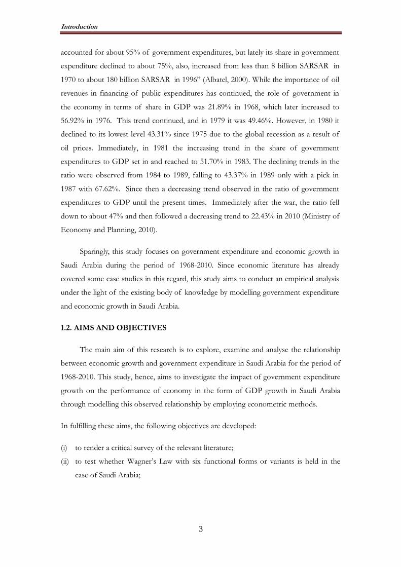
accounted for about 95% of government expenditures, but lately its share in government
expenditure declined to about 75%, also, increased from less than 8 billion SARSAR in
1970 to about 180 billion SARSAR in 1996” (Albatel, 2000). While the importance of oil
revenues in financing of public expenditures has continued, the role of government in
the economy in terms of share in GDP was 21.89% in 1968, which later increased to
56.92% in 1976. This trend continued, and in 1979 it was 49.46%. However, in 1980 it
declined to its lowest level 43.31% since 1975 due to the global recession as a result of
oil prices. Immediately, in 1981 the increasing trend in the share of government
expenditures to GDP set in and reached to 51.70% in 1983. The declining trends in the
ratio were observed from 1984 to 1989, falling to 43.37% in 1989 only with a pick in
1987 with 67.62%. Since then a decreasing trend observed in the ratio of government
expenditures to GDP until the present times. Immediately after the war, the ratio fell
down to about 47% and then followed a decreasing trend to 22.43% in 2010 (Ministry of
Economy and Planning, 2010).
Sparingly, this study focuses on government expenditure and economic growth in
Saudi Arabia during the period of 1968-2010. Since economic literature has already
covered some case studies in this regard, this study aims to conduct an empirical analysis
under the light of the existing body of knowledge by modelling government expenditure
and economic growth in Saudi Arabia.
1.2. AIMS AND OBJECTIVES
The main aim of this research is to explore, examine and analyse the relationship
between economic growth and government expenditure in Saudi Arabia for the period of
1968-2010. This study, hence, aims to investigate the impact of government expenditure
growth on the performance of economy in the form of GDP growth in Saudi Arabia
through modelling this observed relationship by employing econometric methods.
In fulfilling these aims, the following objectives are developed:
(i) to render a critical survey of the relevant literature;
(ii) to test whether Wagner‟s Law with six functional forms or variants is held in the
case of Saudi Arabia;

Introduction
4
(iii) to test if the Keynesian Relations, and the Peacock and Wiseman Hypothesis as
potential models of government expenditure growth and economic growth can
explain the experience of Saudi Arabia;
(iv) to investigate the main factors, which are important in changing the relative amount
of government expenditure in the long term; and lastly
(v) to employ econometric time series modelling in the empirical analyses of the
mentioned models.
The crucial question in this study is to find if there is a long-run relationship
between economic growth and real government expenditure. The hypothesis to test in
this study, hence, is:
Hypothesis I: There is a long-run causal relationship running from economic growth
to real government expenditures in the case of Saudi Arabia as explained by Wagner‟s
Law and Keynesian Relation;
Hypothesis II: There is a deviation from the trend in the development and growth of
government expenditures due to some social and political events as explained by
Displacement Effect;
Hypothesis III: There is a direct and long-run correlation between the government
expenditure growth and economic growth in Saudi Arabia as conceived by the Keynesian
Relationship with causality running from government expenditures to economic growth.
1.3. SIGNIFICANCE OF THE STUDY
There are a number of reasons as to why investigating the government
expenditure growth in the case of Saudi Arabia is essential. First, there is a need
to develop and analyse the relationship between government expenditure and economic
growth in particular considering that the government expenditures have shown a secular
and linear increase over the years with heavy public sector involvement in the economy.
Therefore, re-evaluating this relationship with methods of empirical testing is
particularly important to predict the new phase of the Saudi Arabian economic growth
and determine the impact of government expenditure on the economic growth in the
future.

Introduction
5
Secondly, since such an analysis has not been attempted since 1983, exploring the
impact of government expenditures on economic growth in Saudi Arabia is essential, as
since then the Saudi economy has gone through dramatic changes towards a modern
economy with increased role of private sector. However, it is still difficult to discuss
about the independent or state-free private sector, as state still remains an important
distributors of the resources in the economy. The recent disbursement and allocation of
public funds for general social welfare and increased salaries is an indication of the
continuation of a strong state in the Saudi Arabian economy.
It is, thus, important to discuss the economics and politics of public expenditure
in a rentier state such as Saudi Arabia. While the economic rationale may not suggest an
efficient use of public funds, the political economy nature of the country, being rentier,
maintains and sustains the presence of government and its expenditures in the economy
and society.
1.4. RESEARCH RATIONALE
The rationale for undertaking this study can be explained through a number of
reasoning. First, it is a reality that the government expenditure has been increasing
substantially over the years in Saudi Arabia and alludes to the expenses which the
government incurs for its own maintenance and for the society as a whole. In
supporting this statement, the data indicates that the government sector in Saudi Arabia
is a major component of GDP, accounting for more than 45% of the country's GDP in
2010. Such a growing and hegemonic economic role of the government creates academic
curiosity to study the subject matter.
It should also be mentioned that most government expenditure is financed
through revenues from oil exports, accounting for almost 88% of total government
revenues. Moreover, government expenditure has been increasing substantially over the
past few years. It is seen as the engine of economic growth and considered the leading
sector in the economy. Nevertheless, the growing government expenditure in recent
years, along with the declining oil revenues in 1980s and 1990s has largely contributed to
an accumulating national debt. However, in recent years, government managed to
increase its surplus from the oil revenues due to the recent increases in oil prices
(Ministry of Economy and Planning, 2010).

Introduction
6
One of the main issues in the rationale for this study is the opportunity to
recognize the fluctuations in oil revenues along with the large public debt. This has raised
the question of the productivity of government expenditures relative to private spending,
leading policy makers to call for an expansion of private sector at the expense of the
public sector. One of the first methods to examine the efficiency of public expenditures
is to measure its impact on economic growth as aimed at by this study.
However, the fluctuations in the oil prices in particular in the past created fiscal
tension on the government. The increase in oil prices from 1970 to the early '80s and
from 2005 to 2010 placed a huge burden on government expenditure to meet the
upcoming projects and economic development in Saudi Arabia. Therefore, as a
developing country, the Saudi government dramatically reduced the massive government
expenditures in the 1980s and since that it is making great efforts for maintaining the
growth rate of GDP. However, political economy nature of the country necessitates that
the government must distribute its wealth to the larger part of the society for its political
legitimacy, which implies the growing government expenditures. This has been the case
in the recent months, and the distributive policies in the recent months created a very
large burden on the treasury of the Kingdom.
1.5. MODELLING AND RESEARCH METHOD
There are three different theories explaining the government expenditure growth,
which are utilised in this research:
(i) Wagner‟s Law
(ii) Keynesian Relations and
(iii) The Displacement Effect Hypothesis
The relationship between government expenditure and economic growth in
Saudi Arabia during 1968 to 2010 is, thus, explored and examined by using these there
theoretical frameworks. Table 1.1, 1.2 and 1.3 summarised the six different functional
forms of Wagner‟s Law, Keynesian Relations and Displacement Effect, which are used
to model the relationship between government expenditures and real GDP and real non-
oil GDP, respectively.

Introduction
7
Table 1.1: Six Versions of Wagner’s Law with real GDP / Non-Oil GDP
No Function Version Year
Absolute Versions
1 L(GE) = α + L (Oil GDP)
Peacock-Wiseman 1967 L(GE) = α + L (Non-Oil GDP)
2 L(GEC) = α + L (Oil GDP)
Pryor 1968 L(GEC) = α + L (Non-Oil GDP)
3 L(GE) = α + L(Oil GDP / P)
Goffman 1968 L(GE) = α + L(Non-Oil GDP / P)
4 L(GE/P) = α + L (Oil GDP / P)
Gupta & Michas 1967 & 1975 L(GE/P) = α + L (Non-Oil GDP / P)
Relative Versions
5 L(GE/Oil GDP) = α + L (Oil GDP / P)
Musgrave 1969 L(GE/Oil GDP) = α + L (Non-Oil GDP / P)
6 L(GE/Oil GDP) = α + L (Oil GDP)
Mann 1980 L(GE/Oil GDP) = α + L (Non-Oil GDP)
Table 1.2: Three Versions of Keynesian Relations with Real GDP/ Non-Oil GDP
No Function Version Year
1 L(GDP) = α + β L(GE)
Peacock-Wiseman 1967 L(Non-Oil GDP) = α + β L(GE)
2 L(GDP/P) = α + β L(GE)
Goffman 1968 L(Non-Oil GDP / P) = α + β L(GE)
3 L(GDP/P) = α + β L(GE/ P)
Gupta & Michas 1967 & 1975 L(Non-Oil GDP / P) = α + β L(GE / P)
Table 1.3: The original Version of Peacock-Wiseman with Real GDP / Non-Oil GDP
Function Version Year
L(GE) = α + β L(GDP) Peacock-Wiseman 1967
L(GE) = α + β L(Non-Oil GDP)
In testing all the identified theoretical frameworks and their various forms, time
series modelling in econometrics is used through the following analyses:

Introduction
8
(i) Ordinary Least Square (OLS)
(ii) Unit Root Test
(iii) Co-integration;
(iv) Granger Causality Test
(v) Error Correction Models (ECM)
It should be mentioned that the main difficulty faced in this study is the fact that
the models under consideration mainly developed for countries where there is a different
political economy dynamic as compared to Saudi Arabia. For example, Saudi Arabia is a
rich country with large wealth created by oil exportation, while these models are based
on the experience of European countries which were and are considered mainly as
manufacturing and industrial countries.
In sum, as a method, econometric time series analysis with secondary data
utilised to explore and examine the relationship between government expenditures and
economic growth.
As to the variable definition and data sources, the data used in this study on Saudi
Arabia consist of the following variables:
(i) Real Gross Domestic Product (GDP);
(ii) Real Non-Oil Gross Domestic Product (Non-Oil GDP);
(iii) Total Real Government Expenditure (GE);
(iv) Total Real Government Expenditure on Final Consumption (GEC), it covers
expenditures on goods and services;
(v) Population (P)
The variables (GDP), (Non-Oil GDP), (GE), and (GEC), are all in real terms. In
addition, the data examined is in per capita terms, and total real government expenditure
used as ratios to GDP, which is required by some versions of Wagner's Law.
In empirically modelling this study, the following sources of secondary data were
consulted:
(i) International Financial Statistics produced by the World Bank (IFS);
Introduction
9
(ii) SAMA: Saudi Arabia Monetary Agency;
(iii) The Ministry of Planning;
(iv) International Monetary Fund (IMF)
1.6. OVERVIEW OF THE RESEARCH
This research contains ten chapters. Chapter One introduces the study, aims and
objectives, the research problem and questions and also it presents a brief research
methodology.
Chapter Two discusses financing economic development through state
expenditures in late developing countries. In the first section it discusses the late
developmentalism to explain the place of private capital and rationale for public
expenditures. In the following section it discusses the use of government expenditure
for economic growth.
Chapter Three provides a summary of the government growth theories and
models. It presents economic rationale for a government, the theoretical explanations for
the size and growth of governments and the related literatures starting with classical
studies including Wagner‟s Law and some discussion about its validity. In addition, the
Displacement Hypothesis and Keynesian Relation are explained. Furthermore, it explains
the microeconomic models in explaining the growth of government including Baumol‟s
Differential Productivity Growth and Bacon and Eltis Model. Moreover, the Public
Choice Approach to the growth of government including bureaucracy, interest groups,
median voter and redistributor‟s government model, voting bias and fiscal illusion is
discussed as part of theoretical explanations provided for the explanation of growth of
government. The chapter lastly presents the reinter state and government expansion.
Chapter Four aims to present issues related to the aspects of public
sector measurement whereby the definition and measurement of the public sector or
government expenditure is provided. In doing so, different conceptual definitions in
explaining increase in government expenditures are provided. This is followed by an
explanation of the remarkable complexity of the indicators used to measure of the size of
the public sector.

Introduction
10
Chapter Five presents the economic growth of Saudi Arabia and also the trends
and developments in government expenditures. In doing so, various measure are utilised
to present the case. The details of economic progress and growth in Saudi Arabia are
presented with the relevant stages of development.
Chapter Six describes the modelling of government expenditure and economic
development nexus for Saudi Arabia, along with the methodology that this study uses.
Ordinary Least Square (OLS), Unit Root Test, a Co-integration, and Granger Causality
Test and Error Correction Model are presented in this chapter to test for the validity of
relevant models in the case of Saudi Arabia.
Chapter Seven presents the empirical analysis for Wagner‟s Law through the six
versions of Wagner‟s Law with real GDP and real non-oil GDP. The empirical analysis
was conducted according to the methods discussed in Chapter Six after each version of
the Wagner‟s Law is presented in their functional forms.
Chapter Eight presents the empirical analysis for Keynesian Relations. After
presenting a number of empirical results from the relevant theoretical and empirical
literature on the relationship between government expenditure and economic growth,
three versions of Keynesian Relations is presented. This is followed by the presentation
of the data, and empirical analysis conducted through the use of methods mentioned in
Chapter Six.
Chapter Nine presents the empirical modelling and analysis for Displacement
Effect. It first presents the empirical results of the relevant theoretical and empirical
literature on the relationship between government expenditure and economic growth
through Peacock and Wiseman‟s Hypothesis. It also investigates the data and empirical
results and analysis by using the defined empirical methods. In addition, presents the
results of analysis presented.
Chapter Ten concludes the study by summarising the empirical findings,
comparing the results for real GDP and real non-oil GDP. The final section of the
chapter discusses some of the implications that might apply to the Saudi Arabian
economy, to identify the proper economic policy that would be appropriate for Saudi
Arabia in managing their economic growth and government expenditure.
Financing Economic Development
11
CHAPTER 2
FINANCING ECONOMIC DEVELOPMENT THROUGH STATE
EXPENDITURES IN LATE DEVELOPING COUNTRIES
2.1. INTRODUCTION
Development is the primary tool to address human suffering and requires cultural change
which deals with all sectors of society in dealing with the causes of poverty and in the provision
of social and health care. In the late twentieth century, development was an important global
concept, closely examined in multiple dimensions and levels, and seen as interconnected with
many other economic concepts such as planning, production and progress. However, concepts
of development vary according to the final objectives pursued such as increasing the national
income over a set period.This includes trying to identify the changes caused by economic
variables such as income, production, consumption, and capital formation. Means of
augmentation grow and result in automatic growth, defined as that which occurs without
government intervention or representatives in programmes and economic plans.
The most important aims of economic growth and development are to reduce
unemployment and improve citizens‟ well-being and hopes for a decent life in terms of standards
of health and education as well as social progress that allows them to contribute to the economy
and general progress of their nation‟s increasing prosperity. Thus, economic growth and
development is a comprehensive strategy aiming to change the economy and society as well as
the lives of individuals living in that particular society. However, an important part of such a
strategy is the financing economic growth and development; which has remained an important
question in developing countries since their independence (Buffie, 1984). As late development
countries, shortage of capital was initially an important bottleneck for economic development;
and hence the search for financial sources for economic growth and development constituted an
important dilemma for developing countries.
It should be noted that the studies investigating the relationship between economic
growth and finance can be classified into three: The first involves a positive relationship between
finance and economic growth. The second recognizes financing as an extremely significant
element in the development process. The third trend finds a negative relationship between
finance and economic growth (Van Wijnbergen, 1983; Buffie, 1984).
This chapter focuses on late developmentalism as a concept and policy source to explain
the weaving of private capital and rationale for public expenditures, which is extended by
Financing Economic Development
12
discussing the uses of government expenditures for economic growth. This chapter also provides
critical approaches to the issues in question. The conclusion draws this chapter to an end.
2.2. LATE DEVELOPMENTALISM
2.2.1. Concept
Developmentalism approaches aims to provide a comprehensive understanding of the
change in societies by defining development through socio-economic and human well-being
related variables beyond economic growth. It is not only an economic concept, hence, but also
takes into consideration principles of various theoretical approaches and ideologies of
development as a key strategy towards gaining economic prosperity. This is complemented by
analysing development concepts through the international economy but also through political
institutions with the objective of putting economic development in a political context, as politics
and policy making determines the nature of economic development.
The theory of development assumes that the phases of development must be compatible
with the system of each country and move in a balanced manner from one stage to another. The
map of international economies shows the huge changes that have taken place in the
international system in both geo-political and geo-economic conditions as a result of pressing
need for change through different dimensions.
Concepts of development vary depending on the final objectives pursued by doubling
national income over a certain period, including trying to explain the changes caused by the same
economic variables such as income, production, consumption, and capital formation. However,
since 1970s, the understanding of economic development changed to define it beyond economic
growth as it is recognised that economic development is a multidisciplinary and also a larger
concept compared to economic growth. Building infrastructure in the context of
underdevelopment requires measurement of productive forces and understanding the relations
and conditions of production, but at the same time change in the socio-economic and human
conditions are essential.The features of developmentalism include:
(i) Late development of the forces of production, in particular, the essential element of
„rights‟ which finds expression in the unequal relationship between people and the natural
environment in which people live.
(ii) Late emergence of an integrated and supportive cultural infrastructure. This leads to the
considerable differences in rates of literacy among developing countries as compared to
developed countries.

Financing Economic Development
13
The differences between the countries do not provide an accurate picture of the
development process, and their measurement is similarly. However, economic problems facing
any society are confined to reconciling the needs of a community and resources available to it.
Rostow (1960) states that underdeveloped countries would go through the same process
and stages of economic development until they reach the level of a mature society with rising
consumption but also level of social development. This implies that capitalism is the highest
stage of development that societies aim to reach as in industrialised democratic countries.
While developmentalism remains an important policy of developing countries, how to
finance economic development is an important issue. Considering that these are late
developmentalist states, lack of private capital in these countries resulted in finding other means
of financing economic development, which are the issues discussed in the following sections.
2.2.2. Lack of Private Capital
The development of a private sector is a key requirement for the progress of a society.
However, less developed nations failed to give this the necessary attention and so contributed to
their economic underdevelopment. This section will consider the concept of the private sector
and development, and also discusses the obstacles faced by the states.
The private sector is considered as the main aspects of the national economy which
normally provides the resources for economic growth, and such resources are utilised by the
governments to achieve economic development. This is a strategy based on the development and
industrialisation of the westerns world, and therefore as a linear modernisation, the late
developmentalist countries are also expected to go through the same stages as identified by
Rostow (1960). Thus, private capital is considered as the main locomotive of economic growth
and development. For late developmentalist countries, the lack of private sector and hence
private capital was an issue, and therefore heavy estates as a result opted as a solution in these
countries, which necessitated heavy involvement of state in economic expansion in late
developing countries. In most of the developing countries, until the privatisation policies since
1990s, state played major role in the economy. While the state involvement perceived as a
solution in the initial period after independence of these countries, by 1980s the state became an
obstacle for the economic development in these countries, and hence the Washington Consensus
in early 1980s to provide structural change through economic reform and liberalisation aiming to
strength the private sector.
In the case of the Saudi economy, as a late developmentalist country, state has been the
main economic actor generating and distributing wealth of the country. The oil wealth in the

Financing Economic Development
14
country resulted in state‟s heavy involvement in the economy, as the Saudi society did not have
any infrastructure and a viable economy when it gained independence. However, due to the need
for economic diversification, the private sector has begun to grow in recent years. As an
indication, non-oil sector grew by 9% from 2005 to 2009 to become the main engine of
expansion for the Saudi economy parallel with government expenditure (Ministry of Economic
and Planning, 2009).
The development of private sector has become important in particular with Saudi
Arabia‟s accession to the WTO in recent years, which conditions the expansion of the private
sector. As a result of the expansion of the private sector, the amount of foreign direct
investment in the Kingdom has doubled to reach 5.6 billion dollars (IMF, 2008).
The Kingdom‟s membership in the WTO did not have any sudden adverse impact on
agency agreements and the commercial sector, and this was a supporting factor in the economic
reform program adapted by Saudi Arabia. The private sector is the most important sector to
develop the economy in Saudi Arabia despite the deferred interest and the existence of some
restrictions.
The private sector‟s role in increasing productivity and investment and the provision of
employment would have been possible due to economic diversification and the WTO accession.
Over the past decade in Saudi Arabia, the government adopted several policies that would
strengthen the role of private sector in the economy. While development still requires continued
change to achieve higher rates of economic growth, expansion in private-sector investment is of
crucial importance for the development process. The Kingdom has strong economic and
physical infrastructures as well as a large domestic market, relevant institutions and modern
concepts of development management structures.
It should be noted that Saudi Arabian state has enormous resources for economic
growth and development and therefore heavily involved in the economy of the country.
However, such an expansion has resulted in inefficiency and ineffectiveness and also over waste
in the economy. Thus, there is an urgent need for the economic diversification and private sector
development in the country.
Financing Economic Development
15
2.2.3. Rationale for Public Expenditure
The lack of private sector and the private capital in the independence period of new
states resulted in governments assuming the role of private sector to raise the necessary funding
for economic growth and development. Thus, the second half of the 20th century is marked with
heavy involvement of state in the economy.
One of the most important economic phenomena, attracting the attention of economists,
is the phenomenon that any increase in public expenditure results in increases to national
income. Thus, the phenomenon of greater public expenditure increasing national income is
generally recognised phenomenon in all countries, no matter the economic system or level of
economic advancement.
The first to scrutinise the nexus between government‟s involvement in the economy and
economic growth is the German economist, Wagner (1883:8), who stated that “There is a
proportion between public expenditure and national income which may not be permanently
overstepped.” In other words, after he studied the related overheads and increases, he found that
there is a direct correlation between increases in economic activities of the state and economic
development. Moreover, it has been noted that the phenomenon of increasing public
expenditure might be due to other reasons, real and virtual, with the following being the most
important (Bailey, 2002:44)
(i) Economic reasons resulting from the increased role of the state in economic activity
to achieve overall balance of the national economy, which requires increased financial
resources, which means an increase in the volume of public expenditure.
(ii) Political reasons have been linked to the political role of the state and political
changes, which all necessarily lead to increased public expenditure.
(iii) Social reasons have been associated with an increased state role in social activity and
equitable distribution of income.
(iv) Military reasons and security needs necessitates increases in public expenditure.
(v) Administrative reasons involving large businesses run by the state require the
presence of government employees to work in the state‟s administrative structure, as
well as development, modernization and training, leading to increases in public
expenditure, and greater government work as well as the accompanying increased
expenditure.
The state, thus, actively involved in economic and social construction and structuring of
the society as a later developmentalist society as a general pattern in the post-colonial and
independence period.

Financing Economic Development
16
2.3. UTILISATION OF GOVERNMENT EXPENDITURE FOR ECONOMIC
GROWTH
There are many different opinions about the impact of government expenditure on
economic growth. Some have argued that government expenditure in all the various subdivisions
has a major impact, while another view is that there is a limited impact on some of them (Gupta
and Verhoeven, 2001).
Government expenditure, whose effects are often evident in promoting economic
growth, is an important tool to affect the economy. Government investments are initially
considered to contribute to the accumulation of capital, as well as contributing to meeting the
needs of a market economy but also aimed at generating the necessary funding for social
development of the society.
In terms of government expenditure having impact on the economy, functionally
government expenditures can be classified in the following manner, consumer expenditure,
investment expenditure; transfer expenditure.
As regards to the consumer expenditure is to be taken first. Consumption is the main
component of gross national product (GNP). It features on both sides of the equation of income
and expenditure when measuring the GNP. From this standpoint, the consumption per capita
(expenditure) is considered an income to another individual. Consumption depends heavily on
several factors, most notably income, and income is divided into consumption and savings.
Regarding the proportion of saving and consumption from society to society, some communities
tend to be more consumption-oriented and some communities are better known for their high
percentage of savings. We cannot ignore the fact that consumption is important in economic
growth, as rising consumption, especially for durable goods encourages production, which in
turn encourages increased employment and creates new businesses (Barro, 1991).
Savings further encourage investment. During economic boom years, both jobs increase
the size of expenditure for different types of consumption and investment increase. As a
consequence the value of the gross domestic product (GDP) grows. There are periods of
prosperity followed by periods of stagnation. In economic cycles periods of economic recession
are the slowing of the rate of growth of both consumer expenditure and investment expenditure.
Furthermore, there is an accompanying lack of development of alternative opportunities, leading
to increased unemployment; financial crises may lead to the loss of banks, loss of capital markets
and loss of the market‟s ability to perform its role successfully. This may lead to lower profits
and faltering stock prices, besides lower levels of real gross domestic production than normal.

Financing Economic Development
17
It is important to distinguish between savings and investment according to the factors
affecting both of them. This is crucial and important for economic analysts, some of whom
believe that investment has the more important role in economic growth and is the most prone
to volatility due to changes in expectations of investors and the multiplicity of factors that could
affect these expectations. Expenditure of wealth varies with the individual according to such
factors as age, marital status, expected changes in prices, future income, and customs and
traditions prevailing in the society.
Economists view income as more important than other factors. Functional studies have
shown that the size of consumer expenditure is directly proportional to the size of the ideal
income when other factors remain the same. There are also the differences among individuals in
terms of their commitment and their involvement in social practices and traditions such as
imitation and simulation. It has also been observed that increases in the rate of government
expenditure usually reflect increases in salaries and bonuses for staff and increases in public
services such as building and operating costs of new schools and hospitals. Thus, increased
income has many effects including an increase in the rate of personal income, increase in state
income and budget and this increase is usually inflationary because it does not reflect a real
increase in gross domestic product (GDP).
As for increasing the overall budget deficit, governments borrow from abroad or from
the private sector to cover their deficits. In both cases, the state must bear the burden of
repayment of these loans. Increases in government expenditure have a bad effect on the
economy, although governments often resort to this solution in times of economic recession to
reduce the rate of unemployment and encourage private-sector investment.
The behaviour of consumer expenditure tends to be based on habit. Once individuals
become accustomed to a certain standard of living, they will try to maintain this level despite any
drop in income. Economists are of the opinion that such behaviour is irrational.
This vision confirms the nature and simulation of consumer expenditure of family
income. Certain segments of a population will often spend more on consumption in this way if
they are of middle-range income or lower (Barro, 1991). This trend towards expenditure more in
the middle-range income bracket results in part from pressure on the family to conform to the
society in which they live. It is the result of the larger family noticing in their life what is normal
for them, and other families will tend to continue to spend on certain goods, maintaining a
family habit.

Financing Economic Development
18
On the other hand, together with the time series analysis, this has been used to clarify
cyclical movements in the average propensity to consume, whereby subjects seek to maintain a
level of consumer expenditure despite the fluctuations in income.
The level of consumption is not only current income as pointed out by Keynes (1936),
but also the greatest level of income reached in the past. Some researchers believe that consumer
expenditure has a strong negative impact on government expenditure and thus on governments‟
moves to influence economic growth (Barro, 1991).
Secondly, investment expenditure is the total expenditure by corporations, whether
governmental or private for the acquisition of assets, equipment and tools for the goal of
increasing production. Therefore, it can be said that an increase in investments is a healthy and
positive phenomenon. The reason for this is that increased investment leads to an increase in the
GDP, which in turn leads to an increase in the proportion of employed persons and therefore an
increase in income for individuals.
It is not difficult to recognise that increased investment is "a key element in the growth
of the national economy in any country, and that it can be considered as one of its important
beneficial factors" (Aschauer, 2000:391; Barro, 1991:407).
It is also important to examine extremes in positives and negatives of economic growth,
the advantages and disadvantages. Researchers like Aschauer (2000) demonstrated that public
funds might have a positive impact on growth if the growth equation has been controlled for
effectiveness and public financing. In addition, Galor and Moav (2004) suggested that the main
cause of economic growth varies at different stages of a country‟s development.
In public finance the most famous early theory is Wagner‟s law (1883) of expanding state
activity. This “law” reflects the importance of government activity and expenditure as an
inevitable feature of a progressive state (Bird, 1971). According to Al-Hakami (2002:1),
"Wagner‟s law states that government expenditure tends to rise as gross domestic product
increases because of":
(i) Expansion of "protective and administrative government functions";
(ii) Expansion of "government activities pertaining to education and culture", and
(iii) The increasing "tendency toward monopoly because of technological progress and
increasing returns to scale which need to be offset by government action."
Government expenditure has a direct impact on the operations of capital formation,
production and income, consumption and savings, as well as the distribution pattern of
investments. This as well as proved by experiments that the rate of economic growth in the
developing but also depends to a large extent on the ability of the state government expenditure

Financing Economic Development
19
on different sectors, which depend on the ability of these sectors to increase domestic
production and thus the national production and diversification of the production,
which allows the development of the state's ability on capital accumulation and the payment
of the growth rate to a remarkable level.
According to, Odedekun (1999) there is a positive relationship to spend on
infrastructure and other public expenditure on investment growth in the long term.
Lastly, governments undertake large transfer expenditure with the objective of
redistribution of national income in different forms such as education, health, public investment,
social security and social benefits. In addition, transfer expenditures can also include all expenses
paid by the government in the form of subsidies to individuals in different forms. These take
three forms:
(i) Social Benefits: for those who pay for a certain category of members of the community to
improve their social and their access to a certain standard of living. This category includes
widows, the disabled and the unemployed.
(ii) Economic Subsidies provided by the State to sectors and enterprises with a view to
reducing prices and/or increasing production of some commodities:
(a) to provide interest-free loans to some sectors;
(b) to provide direct or indirect cash subsidies;
(c) to provide benefits in kind such as providing the land needed for a project free of
charge or for a nominal fee.
(iii) Subsidies and Foreign Aid includes subsidies in the form of grants provided from one
country to another in cash or in kind. Also included are interest-free loans provided by the
state to another for political or humanitarian purposes.
All these three categories of government expenditures have different level of impact on
the economy; and therefore governments use these expenditures categories as part of its fiscal
policy.

Financing Economic Development
20
2.4. IMPACT OF GOVERNMENT EXPENDITURE ON ECONOMIC GROWTH IN SHORT AND LONG-RUN
The government expenditures through each of its categories have different impact on
economic growth. Prest (1985:7-8) commented that “expenditures may differ in their outcome in
the long run since some expenditures are expected to yield income in the longer run, like education
and public works, and others will not yield any additional income in the long run, like defence”.
As regards to the short-term economic growth, economic growth has been biased by an
increase in Aggregate Demand (AD) in the short-run and has been measured by the change in
real GDP. The main reasons for an increase in AD are as follows:
(i) Reduction of interest rates, which reduces the cost of borrowing, and thus, encourages
spending and investment.
(ii) Increased real wages, increasing disposable income, and encouraging consumer spending.
(iii) Increased government spending on development projects.
Crouch (1972) presents that the increase in AD only results in real GDP growth in the
short term. He notes that Long Run Aggregate Supply (LRAS) is inelastic; therefore higher
Aggregate Demand (AD) only causes inflation.
The long-term economic growth is biased by an increase in LRAS and AD. The main
reasons for an increase in the LRAS are as follows:
(i) New raw material;
(ii) Increases in investment;
(iii) Increases in government spending on development projects;
(iv) Increases in labour productivity.
It is common knowledge that fiscal policies cannot bring about changes in long-run
growth of output in a neoclassical growth model. The introduction of endogenous growth
models that incorporate the government sector have led to the opposite conclusion; that fiscal
policies can affect the long-run growth rate of an economy (e.g. Barro and Sala-i-Martin,
1995:539).
Over the "course of a business cycle, a rise in the budget deficit (that is, the ratio of
budget deficits to output) increases the growth rate of output and employment. By increasing
effective demand, the rise in the budget deficit increases potential business profits, thereby
stimulating investment expenditure by firms. If planned investment is greater than firms'
available savings, firms borrow from banks. However, the injection of bank credit also leads to

Financing Economic Development
21
the accumulation of financial charges that eventually slow down the expansion". The positive
effect of the budget deficit can be augmented by expansionary monetary policies that maintain
low interest rates, which would have the dual effect of providing greater monetary stimulus from
the deficit and keeping financial charges on business debt low" (Moudud, 1999:2-3). These
results accord well with the proposition that monetary policy should be designed to stimulate
growth and employment (Papadimitriou and Wray, 1994) rather than targeting inflation.
Moreover, even if productive capacity is fully utilised in the long run, government
expenditure may still have a positive role to play. "Specifically, increased government
expenditure, even deficit expenditure, may not lead to lower growth; indeed, under certain
plausible policy regimes the long-run growth rate may even rise". This can occur if government
expenditure increases either the long-run rate of profit or the social saving rate (the combined
government, business, and household saving rate). "One means of raising the social saving rate is
to increase business retained earnings, which might be accomplished through policies such as
investment tax credits, lower corporate tax rates, and accelerated deductions for capital
depreciation" (Fazzari, 1993). Combined with appropriate taxes on capital gains and „luxury‟
consumption, these policies could produce enough of an increase in the total social saving rate to
allow a fixed or modestly rising budget deficit. The consequence of this would be an increase in
the long-run growth rate.
Government expenditure can be divided into two types:
1. Consumption expenditure (expenditures on goods and services) and
2. Public investment expenditure (expenditures on infrastructure, education, public
health, research and development, and other expenditures that are conducive to
raising business productivity).
A number of empirical studies have found that a rise in public investment significantly reduces
business costs and improves business profitability, thereby raising the long-run growth rate. An
increase in the growth rate is also obtained by raising the share of investment expenditure
relative to consumption expenditure while keeping the budget deficit constant.
2.5. CRITICAL APPROACH TO GOVERNMENT EXPENDITURES
In the case of financing for development issues, despite the frequent criticism of various
funding policies for development in developing countries, shortcomings must be addressed and
criticism of government spending is important in advancing development and helping the
government to be the proper steward of public funding.

Financing Economic Development
22
Government expenditure is widely seen as having an important role in supporting
economic growth. This section aims to identify the factors determining government expenditure
efficiency and inefficiency. As discussed above, most studies did not initially find a robust
relationship between government expenditure and growth.
It should be noted that governments have also introduced performance measurement at
the organizational and individual levels to ensure that programmes and activities are
implemented efficiently and effectively with set objectives.
It is therefore important to question whether economic policies reflect the actions and
measures taken to achieve those objectives in light of the availability of human and financial
resources.
The problem of economic development facing the developing countries was itself
imposed itself through evolution from traditional concepts to the concept of sustainable
development. However, if sustainable development is itself considered an obstacle that occupies
the majority of the attention of the researcher's government (those that have reached an
advanced stage of well-being in the methods of providing for future generations) then the
situation is different to the developing countries which are still trying, with extreme difficulty, to
meet the minimum necessities of life. It therefore remains important to identify the most
efficient and effective method to address the problem and to achieve the goals according to the
nature of the economic situation caused by each of the issues posed in the past and still posed
today.
Lucas (1988:20-42) argues that "public investment in education increases the level of
human capital, and that this can be seen as a main source of long-run economic growth ".
Moreover, Barro (1990:111-125) mentions the importance of government expenditure in public
infrastructure for economic growth and Romer (1990:70-102) stresses the relevance of research
and development expenditure. "Therefore, the composition of public spending is also a relevant
issue, and if the aim is to promote growth then the focus should be put on the more productive
items in the budget, even if the balance between the various functional items of the budget varies
according to the particular circumstances and priorities of each country".
In one of the seminal contributions to endogenous growth theory, Barro (1990:103-125)
placed "fiscal policy in the central position". In providing microeconomic rationale, Romer
(1990:70-77) stressed the importance of "externalities to argue that the government has an
important role to play in the growth process".
Additionally, Kneller et al. (1999:170-191) explained these counterintuitive results as "a
failure to account for distortionary taxes. They argued that a complementary explanation is a
Financing Economic Development
23
failure to account for inefficiency. This claim was supported by a simple endogenous growth
model that explicitly considers the role of inefficiency. Particularly for developing countries, it is
very likely that inefficiency plays an even more important role than distortionary taxation due to
the income structure in these countries and the systematic occurrence of substantial
inefficiencies".
In both developed and developing countries, privatization and, in some cases,
commercialization have grown in popularity and acceptability. They have also become important
instruments that governments can use to promote economic development, improve the
production and distribution of goods and services, streamline government structures, and
reinvigorate industries controlled or managed by the state.
Over recent decades, privatization policies have been implemented all over the world
(Bortolotti and Siniscalco, 2004) and the economic literature "devoted to privatization has been
constantly increasing. The theoretical literature dealing with the relationship between
privatization and efficiency has also grown over the last twenty years, but the theoretical results
are ambivalent about the impact of ownership changes on efficiency". Although this literature
has been regularly reviewed in empirical studies devoted to privatization policies, to the best of
our knowledge there has been no survey of economic literature focusing exclusively on
theoretical studies. Such studies could be useful in assessing the pure effect of ownership
changes and would show a gradual shift from a normative to a positive analysis as the focus of
attention moves from the theory of incentives with incomplete information to political economy
issues. "The latter are obviously at the core of privatization decisions but have only recently been
analysed by the theoretical literature."
Likewise, the most serious allocation inefficiencies reflect the failure of the state to
provide a mix of goods and services consistent with any reasonable social welfare function.
Financing Economic Development
24
2.6. CONCLUSION
In this chapter, the financing of development and its importance in developing countries
and its effect on the development process is discussed. It should be concluded that development
is inevitable for the human well-being, an essential requirement in all countries in the world. But
its importance is growing in developing countries as countries seek to improve the living
standards of their residents through improved economic resource utilisation. Prest (1985) argued
that a prerequisite to the development process has been to locate, support and facilitate all
economic sectors in the country.
The economy must find and create the necessary conditions for growth, which depends
on many different ingredients, including foreign direct investment. States need to choose how
best to use those resources in order to achieve efficient use of factors of production in
production processes and thus raise the rate of economic development.
In any case, economic development is a goal of all governments throughout the world.
Over the past 25 years, it has become increasingly important to be an aggressive player in the
economically restructuring global economy of the 21st century. Rapid changes have shocked the
world. Globalization has left a gap in revenue streams. The transition from a manufacturing
economy to a service economy has created an unstable economic climate desperately trying to
create jobs and generate revenue, that this transition has taken place principally in post-industrial
societies.
Finally, with respect to proposals and recommendations relating to policy, the following
points can be considered an outline of the way in which the wheels of the economy may begin to
roll. They are:
(i) Increased investment for public and private sectors, as the economy can experiment
with public and private investment complementarily. In this case, measures should
be undertaken to promote private investment to reduce risks and provide assurances
for the public sector, and to increase revenue by expanding the market.
(ii) Adopting a gradual approach to selective trade integration processes of
unprecedented measures in order to penetrate the global economy.
(iii) Controlling volatility by coordinating functions of the actual macroeconomic
framework and by the consolidation of monetary stability to sustain growth in
investment.
(iv) Governments in developing countries should emphasize investment in research and
development activities in human capital. The criterion should be efficiency of public

Financing Economic Development
25
investment measured by the degree of economic progress made because of the
increased revenue factors in knowledge-based economies.
(v) Economic policies should be directed towards providing the necessary guarantees
for the stability and encouragement of investment.
In addition, criticism of development processes in developing countries, however
powerful, should not slow down the development process. It must be constructive, directed to
government expenditure supporting development projects, and should not diminish the role of
the private sector, which is the current key to the leadership of many government projects
through privatisation.
Economic development is a process through which state in interactions with national
private sectors achieve better economic growth and qualitatively higher levels of community life,
which remains an important policy issue still. Thus, in the late developmentalist states, such as
Saudi Arabia, there is still role for state to play in terms of creating the much-needed initial
capital in the economy for economic development. However, efficiency of such involvement in
the economy remains an important issue.

Government Growth: Theories and Models
26
CHAPTER 3
GOVERNMENT GROWTH:
SURVEYING THEORIES AND MODELS
3.1. INTRODUCTION
The growth of government and its impact on economic performance has been an
important subject area within economics and political economy studies. Over the decades, a
number of approaches, theories and models have been developed to explain the determinants of
government growth but also measure the impact of government growth on economic growth
and development. Since Wagner‟s Law of „expanding state activity‟, a number of macro and
micro-economic models have been developed to understand the relationship in question.
In particular, in late developmentalist state, the economic role of the state and the role of
the state in the economy have been crucial due to the lack of private capital for economic
growth. Therefore, compared to industrial countries where the role of the state moved to welfare
oriented concerns, in the developmentalist states the state remains an important part of the
economy despite the concerns over efficiency of the state‟s economic involvement in the
economy. For this, since 1979 Washington consensus, economies in the late developing
countries are liberalising and, hence, privatising the state economic enterprises to reduce the role
of the state in the economy.
The purpose of this chapter, hence, is to review the literature concerning economic
rationale for government but also aims to present the theoretical explanations and model to
explain the growth of government. A particular attention is given to the empirical studies aiming
to locate the relationship between government expenditures and economic growth. A number of
studies have been selected and provide observations on such growth.
The rest of the chapter is organised as follows: section one, presents government growth
and related literatures by starting with classical studies and relevant theories. Following section,
presents Wagner‟s Law, the Displacement Hypothesis, and later theoretical explanations such as
Keynesian relationship. Section three, considerers the microeconomic models such as, Baumol‟s
differential of productivity growth, Bacon, and the Eltis Model. Moreover, the Public Choice
approach to the growth of government studies is reviewed including „bureaucracy and growth of
government‟, „interest groups and growth of government‟, „median voter and redistributors‟
government model‟, and „voting bias and fiscal illusion‟. The following section reviews the
literature related to „rentier state and government expansion‟ to contextualise the case for Saudi

Government Growth: Theories and Models
27
Arabia which is a „rentier state‟ generating the wealth through oil and distributing to the larger
population. Section four presents the combined model; while section five provides the empirical
studies on the subject matter.
3.2. THE PERCEPTION OF GOVERNMENT (STATE) OVER TIME
Government has grown in all countries over the decades with the development of nation
states. However, growth in public expenditure has not been symmetrical across nations.
Depending on the economic growth level of nations, government‟s role in economy and society
has shown differences. A quick observation therefore shows a ray of government involvement in
the economy: a very heavy state involvement in the economy to very liberal economies. While
economic necessities are used to justify this, there are political reasons determining the role of
the state in the economy as well.
In an attempt to explain the state‟s role in the economy, Musgrave (1996: 250-257)
considers the relations between fiscal theory and the theory of government as it emerged from
the 18th century to date and he concludes that this relationship is observed through four
different patterns". First, there is a classical view of the service state, needed to adjust for
externality-based market failure, and to approximate a market solution. Second, there is a welfare
state, designed to correct the market-determined state of distribution, based on what society
views a fair or optimal pattern. Next is the communal model, where individuals recognize
communal as well as private concerns. Finally, the flawed state, where action of governmental
agents shifts attention from market to policy failure. While this indicates the changing political
economy over the development of economies in nation states, it also indicates changing
economic nature and role of the state in different phases of economic and political development
in nation states.
An important aspect of growth of government is, however, related to the economic
development needs of developmentalist societies. In a very euro-centric manner, the post-war
development of industrial states were taken as example in developing policies for the
underdevelopment countries through linear development model indicating that state played an
important role in the development process in Europe, which can be replicated in the developing
nations. It is therefore suggested that state in general accelerated economic development by
providing safety for increasing investment and optimal direction for growth and development by
also providing the necessary initial capital.
While classical economists aimed to limit the role of the state in the economy, the failure
of market through the beginning of the 20th century has brought the state back into the

Government Growth: Theories and Models
28
economic life beyond taxation. The Great Depression in 1929 and the collapse of the economy
in those years paved the way for the state‟s further involvement in the economy. The Keynesian
solution to the problem increased the role of the state in economy with the objective of
expanding the aggregate demand in the economy through fiscal policies to overcome the
stagnation in the economy. Keynes, therefore, suggested that the government should intervene
in the national economy to influence the overall course of spending to provide full employment,
otherwise there is recession and conditions deteriorate. This trend has led to a widening of the
scope of government action and activity throughout the government to guide all areas of
economic activity and provide for social justice in providing essential services to citizens for their
well-being and prosperity in various dimensions of their existence (Keynes, 1936).
To overcome the political and economic legacy of the grown government in the face of
inefficiency of the government involvement in the economy, in 1979 international agencies urged
the developing states to restructure their economies and liberalise their economic and financial
system as proposed as a policy under Washington Consensus. Since then about all the states in
the world involved in economic restructuring by privatising their economies, which includes
Saudi Arabia as well. While it is expected that this should result in reduced size of government,
the nature of government involvement however in regulating the economic and financial sectors
as well as social sector has been the new areas of the increased role of the state.
Lastly, since the financial crisis in 2008, a number of governments in the world in
particular in industrialised G-8 countries involved in bailing-out and transferring the ownership
of the failing financial institutions to the public sector. While this should not be considered as a
policy change, the real life consequences of such policies indicate the increased role of
government in the economy.
3.3. THE ECONOMIC RATIONALE FOR GOVERNMENT
The economic rationale for government can be understood in terms of the degree to
which government intervention improves efficiency. Importantly, however, initial stages in
economic growth and development process necessitated the public-sector investment as high
priority. In the later stages of economic growth and development, the government then
continues to supply investment but in such a stage public financing is considered as
complementary to growth in private investment.
The debate on the role of the state in the economy can be traced back to Smith (1776) in
The Wealth of Nations and Mill (1848) in Principles of Political Economy. Both Smith and Mill intended

Government Growth: Theories and Models
29
to explain the principles by which revenue and expenditure policies could be determined as part
of their wider investigation of the relationship between the government and the economy.
In Smith‟s (1776) argument the role of the government is confined to three main duties.
These are protecting the country from foreign aggressors; maintaining law and order, and
providing and producing goods that could not otherwise be produced by the private sector,
which was built on the basic theorems of welfare economics.
While the classical notion of limited role of the state could be possible until the
emergence of nation states, since mid-19th century the role of the state in the economy has
increased through various forms beyond expenditure and taxation. In particular with the
realisation of market failure and economic crisis in the beginning of the 20th century provided the
policy rationale for the increased role of the state in the economy with the objective of
correction the observed failure. On the other hand, the rise of neo-classical school of thought in
responding to the changing nature of the economy provided the theoretical and intellectual
rationale for the increased role of the state in the economy, which is discussed in detail in the
following sections.
3.3.1 Market Failure
Market failure refers to the deviation of market operation from the first best solution and
hence is marked with inefficient allocation of goods and services by a free market . "That is,
there exists another conceivable outcome where a market participant may be made better-off
without making someone else worse-off. Market failures can be viewed as scenarios where
individuals' pursuit of pure self-interest leads to results that are not efficient – that can be
improved upon from the societal point-of-view" (Stiglitz, 2000:4-5).
Smith‟s theory of laissez-faire, with the underlying premises that markets allocate
resources efficiently, leading to social welfare maximization by markets got wider acceptance
among developed countries‟ policy-makers and academicians in the centuries since he published
The Wealth of Nations. The roles of the government in many of the Western European countries
have been shaped by this philosophy. However, the realities of the market conditions and
failures in the economy and market resulted in the recognition that Simithian perfect market
conditions are not valid; as the realities indicates the impossibility of the first best choice due to
the certain prevailing conditions in the economy marked as market failures. Market failures are
used by the neo-classical school to provide rationale for the state intervention, which are
discussed in the following sections:

Government Growth: Theories and Models
30
3.3.1.1. Public Goods
Public goods have been defined by Samuelson (1954: 387) as those "which all enjoy in
common in a sense that each individual‟s consumption of such a good leads to no subtraction
from any other individual‟s consumption of that good. Therefore, by definition, public goods
either will not be supplied by the market or if supplied, are supplied in insufficient quantity. They
have two definitive properties". First, it costs nothing for an additional individual to enjoy their
benefits. Second, it is difficult to exclude individuals from the enjoyment of public goods. Thus,
it is not possible to price public goods in the market.
Samuelson (1954) argued that markets would fail to provide public goods because they
are non-excludable. However, that means it is not possible to prevent the use of the service by
those who do not pay for it, and it is nontrivial in consumption to the extent that one person‟s
consumption of the commodity does not affect any other person‟s consumption of it. However,
other users can cause congestion when using the goods and other facilities may be required. It
adds up to the government establishing effective amount of such goods provided according to
population size. The fact that private markets will not supply public goods provides a rationale
for various government activities, which includes free education, health and other welfare
services. In addition, some of the public goods perceived as merit goods, consumption of which
are encouraged due to social benefit it creates. Since the consumption of such goods also cannot
be left for the market, state is considered to provide such goods as well for the larger social
welfare.
3.3.1.2 Externalities
The private sector sells many commodities that affect people other than the purchasers.
Thus, in addition to private costs and benefits, there are social costs and benefits, which are
called „externalities‟. Externalities, hence, can lead to inefficient decisions even if perfect
competition exists as the social costs and benefits are not considered in production and pricing
decision.
Instances where one individual‟s actions impose a cost on another have been referred to
as negative externalities. An example is that without government intervention of some kind, the
level of pollution would be too high (Stiglitz, 2000). In addition, not all externalities are negative.
There are some important instances of positive externalities, where one individual‟s actions
confer a benefit upon others.
It has been, thus, argued that the economic action of a rational person may result in a
positive or a negative effect on a person or firm who does not part take in the economic activity

Government Growth: Theories and Models
31
and does not pay for the activity to occur. The positive effect is known as positive externality
and the negative one as negative externality.
If we let markets decide resource allocation in the presence of externalities, the amount
of output produced by an individual firm appears to be higher than the socially desired amount
in the case of negative externalities but lower in the case of positive externalities. This creates a
conflict with the principle of a Pareto-efficient resources allocation. The correcting mechanism is
either to reward or to penalize those who produce positive or negative externalities respectively.
This could be done by an institution which we call government.
Challenging this argument, Coase (1960) argued that, without government involvement,
optimal resource allocation is quite possible by assigning property rights. In supporting this,
Inman (1978: 687) presents his argument, as in the case of two agents linked to each other
through an external activity in a world of complete information and costless bargaining, the two
agents will strike mutually advantageous bargains for the level of the external activity. However,
considering the non-existence of perfect market, such an arrangement would not be possible,
and therefore government intervention is expected to correct such a failure.
3.3.1.3 Imperfect Market
The classical economic theory argues that Pareto-optimal resource allocation may be
achieved when price determined according to marginal cost at zero economic profit (Stiglitz,
2000). Zero economic profit eventually means that the average cost of production is equal to the
price. However, being the condition of the perfect market this may not hold when there is
oligopoly and monopoly markets or increasing returns to scale. In addition, market failure also
appears when there are few sellers or one seller in the market, or in the case when the price of a
good is greater than its marginal cost in which case the optimal level of production is less than
the socially desired one (Bailey, 2002).
In order to overcome such imperfect market conditions, government can apply many
systems to correct this market failure. While in the case of an increasing returns scale,
government intervention in the production of goods and services was justified for long periods
because of this reason. That was why government has engaged in even the developed countries
in telecommunication, postal services, electricity, and communication for long periods (Cowen
and Cramption, 2002).
In other words, government in modern economy interferes to correct the market
through regulating the market to overcome monopoly and oligopoly impacts and make sure that
natural monopolist markets produces and charges price according to the socially acceptable level.

Government Growth: Theories and Models
32
3.3.1.4 Imperfect Information
In order for an individual to obtain the maximum benefit from the consumption of a
good, he or she must possess as much information as possible about it. This makes it possible
for the individual to make an informed decision about whether to consume the goods in
question. However, in the second best solution of the market system such information is not
abundantly and freely available as suggested by the perfect market conditions. Hence, the
consumer possesses imperfect information about the goods in the market and will not be able to
make an informed decision about them (Stiglitz, 2000).
Market institutions may arise to help overcome information asymmetry such as
contingent contracts, seller reputation, and professional associations. Governments do also take
measure to moderate the consequences of asymmetric information and moral hazard by the
provision of additional information or actions through regulation and legislation (Inman, 1978:
660).
3.3.2 Government Failure
The preceding section provides rationale for the government in economic sphere of a
society by referring to the neo-classical economic theory. However, through the years, in
addition to market failure, government failure is also observed. In other words, while
government intervention was expected to overcome the market inefficiencies, government itself
was considered inefficient; and therefore with the Washington Consensus all the countries in the
world advised to reduce the role of the state in the economy by reforming and liberalising their
economies including through privatisation.
Government failures are "the public sector‟s version of market failure and happen when
a government intervention causes a more inefficient allocation of goods and resources than
would happen without that intervention" (Weimer and Vining, 2004:7-9). This was the case in
most of the economies by the 1980s, and therefore in order to reduce the efficiencies in the
economy, reducing the size of the state is considered as a panacea for the problems.
It should be noted that in particular government was considered a leading solution in
developing countries by fostering and achieving development through central planning systems.
However, the experience of the government centred economic growth did not produce much
better solution for the developing countries. In a critical position, Brown and Jackson (1990: 58)
noted that “The government failure literature discards the notion of the benevolent omniscient
economic planner serving the public interest and replaces it with a muddling, imperfect,
Government Growth: Theories and Models
33
endogenous state that serves the interests of powerful lobby groups and the private interests of
politicians and bureaucrats.”
It should be concluded that the assigned economic role for the public sector has changed
over the years depending on the political ideologies of the times in addition to the economic
necessities. For example, having some of the developing countries without any infrastructure and
sustained economic growth assuming privatisation since 1980s is an imposed political choice
rather than economic necessity. Thus, politics is an important determining factor of economic
policy choices.
3.4. THEORETICAL EXPLANATIONS FOR THE GROWTH OF GOVERNMENT
The size of government expenditure in general and in promoting economic growth in
particular has long been of interest to economists and policy-makers in both industrialised and
developing countries. In terms of government expenditure contributing to economic growth, as
Keynesian relation (1933) states its acts like an exogenous factor that can be used like a policy
instrument to determine growth.
Since this study is concerned with locating the impact of government expenditures on
economic growth in Saudi Arabia, this section aims to review the theoretical explanations and
models to identify such a relationship. These can be considered as the determining factors of
increasing government expenditure; this study however only examines the impact of government
expenditures on economic growth in the empirical sections.
This section, hence, first presents macro models developed to explain growing
government expenditures; secondly, the micro models of government growth are presented,
which is followed by the Public Choice approach to the growth of government.
The macro and micro models that we will consider in this section differ from
macroeconomic forecasting models in their analysis of public expenditure, as far as the latter take
government expenditure as exogenously determined. In this section, three different theories are
presented: (i) Wagner's Law of „Expending State Activity‟; (ii) The Displacement Effect
Hypothesis; and (iii) Keynesian Economic Growth and Government Expenditures. In addition,
two different micro models are presented: (i) Baumol‟s Differential Productivity Growth; (ii)
Bacon and Eltis‟ Model.

Government Growth: Theories and Models
34
3.4.1 Macroeconomic Models of Government Growth
In this initial section, main macroeconomic models developed to examine and explain
the growth of government expenditures are presented. The survey in this section focuses on
Wagner‟s Law, Peacock and Wiseman Hypothesis, and the Keynesian Relation. Having
government expenditures as endogenous factor is the common departuring points of these
models.
3.4.1.1. Wagner’s Law of ‘Expanding State Activity’
One of the earliest attempts to explain the growth of government in the sense of
increasing public expenditure was made by Adolph Wagner, a 19th century German economist.
His theory, which has come to be known as Wagner‟s Law, is one of the most referred to and
tested one in government growth literature.
Wagner‟s (1893) theory of The Law of Expanding State Activity pointed to the growing
importance of government activity and expenditure. In explaining his theory, Wagner (1883: 16)
stated that: “The law of increasing expansion of public, and particularly state, activities becomes
for the fiscal economy. The law of the increasing expansion of fiscal requirements, both the
state's requirements grow and, often even more so, those of local authorities, when
administration is decentralized and local government well organized." Recently there has been a
marked increase in Germany in the fiscal requirements of municipalities, especially urban ones.
“The law is the result of empirical observation in progressive countries at least in
Western European civilization; its explanation, and the causes, is the spheres of private and
public economy, especially compulsory public economy. Financial stringency may hamper the
expansion of state activities causing their extent to be conditioned by revenue, rather than the
other way round which is usual. But, in the long run the desire for the development of
progressive people will overcome these difficulties” (Wagner, 1883: 8). Thus, Wagner‟s Law
“pointed to the growing importance of government activity and expenditure as an inevitable
feature of a progressive state” (Bird, 1971: 1), which can be formally expressed as a law:
“Historically there exists a clear tendency for an expansion of public activity together with the
progress of the economy” (Biehl, 1998: 107).
Wagner (1883), thus, investigated a functional relationship between the growth of an
economy and the growth of governmental activities and observed and empirically proved that
governmental sector grows faster than that of the economy. In other words, Wagener considered
that the elasticity of government expenditures in relation to the growth of economy is higher
than the unity.
Government Growth: Theories and Models
35
Wagner also presented the motive of the government growth taking into account the
historical development of the Western governments during that century. The state activities,
according to Wagner (1890: 16), are the provision of necessary conditions for market
functioning, maintenance of law as well as order and of participating in material production.
According to Getzler (2000: 13), “Wagner was writing at a specific time and place, when
many scholars in Germany became filled with nationalism and the desire for a strong state to
heal the political and economic disorders affecting German society.” Under such influences, it is
believed that Wagner argued that the social progress of the time resulted in increasing state
activity, which in turn meant more government expenditure. Hutter (1982: 134) suggested that
“Wagner views the state, represented by the government activity, as an organic part of the social
and economic system, and he expected that the state would tend to grow proportionally with the
growth of the economy as a whole.”
Wagner offered three reasons why this development would come about with respect to
the changing and expanding functions of the state. In understanding the reasoning, it is
important to point out that these ideas were formulated in Germany in the later 19th century
which was experiencing industrialisation and hence economic growth. Not surprisingly therefore,
Wagner‟s Law was framed to refer only to states in which income was rising because of
industrialisation. The conditions under which one might expect the „Law‟ to operate would
therefore seem to be (i) rising per capita incomes; (ii) technological and institutional change of a
particular sort implying that in particular the state had an increasing role in production where
technical conditions favoured monopoly; and (iii) at least implicit democratisation of the polity
(Ghamdi , 1983) implying that Wagner saw increasing state activity in fields like education where
the social benefits of the service were not susceptible to economic evaluation.
In a more formal manner, according to Wagner (1893), growth of the public sector is due
to the above mentioned there reasons which can also be expressed in the following manner:
(i) The demand for public goods grows with the increase of population in cities, leading to
higher demand for infrastructure, leading to the growth of industrialisation and therefore
achieving a more integrated development which requires control and management of the
state and then leading to expansion of the public sector.
(ii) The more income in the economy, the greater the demand for goods of high flexibility, such
as education and the elastics of cultural goods and services that lead to a rise in government
spending.
Government Growth: Theories and Models
36
(iii) The financing of projects with long-term development goals accompanied by technical
changes lead to pressure on the state to a greater involvement in the economy, which will
have financial implications on the budget.
Over the decades, a large number of studies conducted to test the Wagner‟s Law in
different cases. As a result of this process, depending on the understanding of the concerned
scholar, different versions of Wagner‟s Law have been developed, namely: Peacock and Wiseman
(1961), Gupta (1967), Goffman (1968) and Goffman and Mahar (1971), Pryor (1968), Musgrave
(1969), and Mann (1980) versions of Wagner‟s Law. It should be noted that all these different
versions are due to the fact that in the original version, it is not clear whether Wagner was
referring to an increase in (i) absolute level of public expenditure; (ii) the ratio of total
government expenditure to GNP; or (c) the proportion of the public sector to the total
economy. Consequently, there are at least six models of Wagner's law which have also been
empirically tested. These are all explained in detail in the modelling chapter.
It should be noted that among the empirical studies, some studies have shown that
Wagner‟s law of expanding state activity holds with higher levels of economic development
(Dutt and Ghosh, 1995).
Henrekson (1993), for example, found a positive relationship between economic growth
and government expenditure in Sweden, and his result confirmed that the real GDP explained
the growth of government expenditure in the economy. In addition, Murthy (1993) found
supporting evidence in favour of Wagner‟s law using data from 1950 to 1980 in Mexico. Further
empirical studies on Wagner‟s Law is presented in a later section,
3.4.1.2. The Displacement Hypothesis
While Wagner sought to explain the trend in public expenditure, the most useful
pioneering work in Britain, that Peacock and Wiseman (1961), offered a working hypothesis to
explain the fluctuations in government expenditure over time. Peacock and Wiseman, in their
work published during the early 1960s, aimed to locate the pattern of public expenditure trends
(Peacock and Wiseman, 1961; xxiii). According to what later is known as Displacement
Hypothesis, government expenditure tends to evolve in a step-like pattern, coinciding with social
upheavals, notably wars. The disincentive effects of high marginal rates of tax, popular notions
of tolerable tax burdens and the degree of political control exercised by the citizens over their
government, encouraged by a rising output per person, are some of the major foci of study.
Peacock and Wiseman (1961:24-27) also investigated and found that "both citizens and
government hold divergent views about the desirable size of public expenditures and the

Government Growth: Theories and Models
37
possible level of government taxation. This divergence can be altered by social disturbances that
destroy established conceptions and produce a displacement effect. People will accept, in a
period of crisis, tax levels and methods of raising revenue that in quieter times would have been
thought intolerable, and this acceptance remains when the disturbance itself has disappeared."
Revenue and expenditure statistics of governments also show a displacement effect after
periods of social disturbance. Expenditures may fall when the disturbance is over, but they are
less likely to return to the old level. “The state may begin doing some of the things it might
formerly have wanted to, but for which it had hitherto felt politically unable to raise the
necessary revenues” (Peacock and Wiseman 1961: 26). Peacock and Wiseman (1961) contended
that under normal conditions of peace and economic stability, changes in public expenditure are
quite limited.
In a simple language, Displacement Hypothesis states that "the effect of public
expenditure on the time pattern will tend to be constant over time, rather than increasing, unless
major crisis periods occur which require an increase in government intervention" (Peacock and
Wiseman, 1961:24-26). The associated expansion of the public sector will not just be temporary
after such an event, since the new levels of government expenditure and taxation will be
accepted by the electors and public sector size will remain stable at a higher level until the next
shock. According to the Peacock and Wiseman model(Brown and Jackson, 1990:123-127),
therefore, the time-pattern of government expenditure normally increases stepwise, rather than
linearly. They investigated the concept that public expenditure increases stepwise during war
times due to higher military expenditures and that after a significant period military expenditures
return to their previous values. On the other hand, the government expenditure as a whole was
not restored to its earlier levels. Total government expenditures decrease after the war, but it
stabilises at a higher level compared with the pre-war period. It can also be noted that the
Peacock-Wiseman hypothesis proposed that public rationalisation during the time of expenditure
growth occurred more freely than related to the size of the ultimate government expenditures.
The entire process is depicted in Figure 3.1.

Government Growth: Theories and Models
38
Figure 3.1: Illustrating Displacement Effect
Source: Brown and Jackson (1990:126)
According to, Brown and Jackson (1990), figure 3.1 shows three possible patterns of the
influence of war expenditures on government expenditures. Figure 3.1 (a) shows that case in
which civilian public expenditures in the post-war period return to their original growth path;
whereas Figure 3.1(b) represents the case in which the trend in total public expenditure
experienced during the war period continues into the post-war period along with an upward shift
in the level of civilian public expenditures. In the final example, Figure 3.1(c), there is an increase
in post-war civilian public expenditures. This, however, is only a temporary phenomenon until

Government Growth: Theories and Models
39
the old trend line is reached. The long-term trends shown in cases 3.1(a) and 3.1(c) are thus
similar and show that there has been a permanent displacement of private by civilian public
expenditures (Brown and Jackson 1990:124-127).
It should be noted that due to such features of the Displacement Hypothesis, Brown and
Jackson (1990: 123) noted that “Peacock and Wiseman‟s study is probably one of the best-
known analyses of the time pattern of public expenditure”.
In terms of empirical contextualisation, Borcherding (1965) did not find any evidence for
a displacement effect. A new analysis focusing on the time-series behaviour of government
expenditure has developed and was tested on data from Sweden and the UK, which located
upward displacement after World War II, and good evidence against the hypothesis was found
(Henrekson, 1993). Such studies are detailed and presented in a later section,
Displacement Effect is articulated as a theory of structural break by Diamond (1977) due
to the nature and operating mechanism of the observed government expenditures. In addition,
some other contributors considered the initial jump in the government expenditures after a
social upheaval as ratchet impact. The following section explores these two features of the
Displacement Effect.
3.4.1.2.1. The Displacement Effect: Structural Break
Wars and other social and political upheavals are capable of displacing this notion of
tolerable tax rates and hence facilitating the shift in the level of government expenditures. After
such events, government expenditure may fall again, but not to their previous levels. Therefore,
public expenditure grows in a discontinuous and stepwise fashion, the steps occurring at times
of major social upheavals (Demirbas, 1999).
In other words, Peacock and Wiseman (1961:24-27) investigated that "both citizens and
government hold divergent views about the desirable size of public expenditures and the
possible level of government taxation. This divergence can be adjusted by social disturbances
that destroy established conceptions and produce a displacement effect. People will accept, in a
period of crisis, tax levels and methods of raising revenue that in quieter times would have been
intolerable, and this acceptance remains when the disturbance itself has disappeared." Thus, the
hypothesis indicates that there is the structural change in government expenditures in terms of
the trend.
In explaining the „displacement effect hypothesis‟, Henrekson (1990: 246) states that
“Peacock and Wiseman (1961), adopt a clearly inductive approach to explaining the growth of

Government Growth: Theories and Models
40
government expenditure. When Peacock and Wiseman observed that expenditures over time
appeared to outline a series of plateaus separated by peaks, and that these peaks coincided with
periods of war and preparation for war they were led to expound the „displacement effect‟
hypothesis”. Such an explanation refers to the structural break nature of the hypothesis.
Diamond (1977), therefore, presented the displacement effect as a theory of structural break. He
used the Chow test, comparing two periods separated by a social upheaval, and he found that, if
this shows significant structural change and there has been displacement.
3.4.1.2.2. The Displacement Effect: Ratchet Effect
The „ratchet effect‟ refers to the restrained ability of processes to be reversed once a
specific thing has happened. The term is used within the „displacement effect hypothesis‟ to
describe the seemingly irreversible expansion of government in times of crisis. In other words,
as explained due to the expansionary government expenditures during crises periods,
governments then have difficulty in reducing government expenditures back to the original level
after the initial temporary needs due to war, natural or economic crisis . The government‟s
exploitation of taxpayers‟ tolerance plays an important role in this process. Thus, the main
argument of the ratchet effect is that if there is a crisis and government expenditures grows as a
result, then the public expenditure might decline but not to the previous level as there would be
resistance against such a move.
According to Bird (1972), within the displacement effect, this resistance to get over
displacement effect by public expenditure returning to the original level is named as „ratchet
effect‟. However, it should be noted that Peacock and Wiseman (1979) argued that in the
extreme, the ratchet effect interpretation of the displacement effect leads to the denial of its very
existence.
3.4.1.3. Keynesian Relation: Economic Growth and Government Expenditures
Another model using Wagner‟s approach to explain economic growth and government
expenditures is associated with Keynes as was mentioned previously. Keynesian theory
articulates the idea on the role that the government expenditures or fiscal policy plays in cases
when aggregate demand in the economy is declining.
It is essential to note that Keynesian relation is related to the Wagner‟s Law, which
considers that public expenditures are income elastic. Keynesian idea of aggregate demand and
its role in the economy in stabilising the economy was central to his argument, as he considered
that total income is a function of the level of operation in any country, and hence the greater the

Government Growth: Theories and Models
41
scale of operation, the greater the total income. Therefore, he suggested expansionary economic
policies through fiscal policy for the growth of the economy, which by definition treats public
expenditure as an exogenous factor (Keynes, 1936) as oppose to other theories.
Keynes (1933) found that public expenditures could contribute positively to economic
growth and governments should use public expenditure as a tool of economic policy to manage
national economies. Keynes‟ theoretical and policy suggestions helped to get the economies of
the industrialised world out of stagnation in 1930s by heavily relying on government expenditure
to boost aggregate demand. This is expected to render economic growth through expanding the
economic activity. Therefore, it establishes a direct causality between government expenditures
and economic growth.
It should be noted that Keynesian policies very much remained as an important policy
option until 1970s, when the growing government began to be perceived as part of the
government failure as well.
3.4.2. Microeconomic Models of Government Growth
After presenting the theoretical macroeconomic models related to the growth of
government expenditures, this section considers microeconomic theoretical explanations for the
growth of government, mainly, in the western industrialised democracies.
3.4.2.1. Baumol's Differential Productivity Growth
Baumol (1967) argues for „differential productivity growth between private and public
sector. According to this explanations, there are two sectors in the economy one of it is
productive, and the other one is unproductive, namely private and public sectors respectively.
Second, the wages in the two sectors of the economy rise and fall together. Finally, the money
wages increase as rapidly as output per hour in productivity increases. Furthermore, Baumol
(1967) argues that a differential function of productivity based on these assumptions – after
developing and analysing the cost per unit of the unproductive sector – rises without limit. In
addition, there is a tendency for the outputs of the unproductive sector, whose demands are not
highly inelastic, to decline and vanish. According to Baumol (1967), in the unbalanced
productivity model – if the ratio of output of the two sectors held constant – this suggests that
more of the labour force must transfer to the non-progressive or unproductive sectors (Brown
and Jackson, 1990).
The progressive sector was characterised by cumulative increases in productivity per
man-hour that arise from economies of scale and technological change. In the non-progressive

Government Growth: Theories and Models
42
sector, labour productivity advances at a slower rate than that experienced in the progressive
sector. Baumol‟s results depend upon there being a productivity differential between the two
sectors. This does not imply, as some have incorrectly thought, that there are always zero
productivity increases in the non-progressive sector. One reason for the existence of a
productivity differential is the key role that has been played by labour inputs in the non-
progressive sector‟s goods. Baumol‟s model, thus, provides a possible explanation of public
expenditure growth, which is mainly explained by inefficiencies.
Baumol (1967) also investigated the differing inflation rates between the public and
private sector. He argued that the inflation rate for the government would be higher than that
experienced by the private sector.
In supporting „Baumol‟s Disease‟, Le Grand (1991) argued that an analysis of growth in
public sector reveals that almost half of the increase in the public sector can be attributed to
what has come to be called „Baumol‟s Disease‟.
3.4.2.2. Bacon and Eltis’ Model
Bacon and Eltis (1978) argued that Britain‟s long-term problems are reflected in high
public spending, who states that the public sector increased quickly in size through the 1960s and
early 1970s, which had to be financed by production of marketed output. Although taxes were
levied to support the public sector, the wage earners, arguments run, had either not valued the
increased social wage or had not assumed any change in the social wage, and had tacitly refused
to support the public sector (Ansari, 1994).
According to Bacon and Eltis, labour‟s concern with take-home pay led them to resist
tax increases with claims for wage increases. In Bacon and Eltis (1978), trade unions passing on
taxes to profits following a period of rapid wage increases achieved their desired position in that
model. Retained profits are the main source of investment funds in the UK, so that ultimately
the cost of the increased public sector reduces investment and there are consequent economic
problems on all fronts. On the other hand, Bacon and Eltis argue that there is a fundamental
fault in the UK economy caused by the fact that few people produce marketed goods and
services. Marketed outputs are those, which are sold, and non-marketed products are those that
are not. They have argued that the main problem with the UK economy is that an increasingly
large proportion of the nation‟s total resources have moved into the non-marketed sector.
Furthermore, they have produced figures to show that employment in the non-marketed sector
and mainly in the public sector increased by over 40 per cent between 1961 and 1975 (Bacon and
Eltis, 1978).

Government Growth: Theories and Models
43
Thus Bacon and Eltis (1978) rather than locating the reasons of increasing government
expenditures, they focused on the consequences of expanding public sector, which was
considered as an important reason for the economic difficulties in the UK by Bacon and Eltis.
3.4.3. Public Choice Approaches to the Growth of Government
In addition to the mainstream micro or macro determinants of government expenditures
and the related methods, a number of theoretical explanations are also developed by the public
choice approach, which is explored in detail. Further discussion on the empirical studies on the
topic is provided in the following section.
It should be noted that the modern public choice is a study of political mechanisms and
institutions in terms of government and individual behaviour through tools and methods of
economic analysis. In other words, as Mueller (1989: 1) stated “public choice can be defined as
the economic study of non-market decision making, or simply the application of economics of
political science”. It means that public choice takes as its province the application of economists‟
methods of a positive analysis of problems that have conventionally been regarded as those of
political science, concerning events generally in the public sector.
The subject matter of public choice is mainly political issues and the causal impact
between economics and politics. This directly refers to public sector and therefore public sector
is the natural field of study for public choice analysis, which, thus, has developed approaches in
understanding the growing size of government. The following sections present the public choice
approach to growth of government.
3.4.3.1. Bureaucracy and the Growth of Government
Public choice school with its critical approach to the public sector mainly through the
writings of Niskanen developed the understanding that one of the reasons of increasing
government size is the strong position of bureaucracy. The argument is that the government
managed to cover the bureaucracy by the use of higher bureaucrats who were intent on the
continued existence of the system for their personal benefit.
Bureaucratic responsibilities and assignments exist to attain numerous goals. However,
bureaucracies are noted for their size and complexity and bureaucrats work to become part of
the system with many rules of bureaucratic behaviour frequently tied to the letter of the law. The
presence of a large administrative authority assumes a goal of coordinating the sections in
decision-making.

Government Growth: Theories and Models
44
The bureaucracy models of Niskanen (1971) and Romer and Rosenthal (1978, 1979b,
1982:27-43), explain why the government might be larger than its optimal size or even as
expected by legislature, as legislation would prefer if it knew the unit costs of the outputs it
thought it was buying, and why the level of outputs might be larger than the median voter‟s most
preferred level. According to Niskanen (1971), the bureaucrat‟s primary purpose is to achieve
power and status, which positively correlates with the size of the budget allocated to his or her
department. Therefore, the government worker starts with the assumption that the bureaucrat‟s
objective is to maximize his or her budget, as explained in Figure 3.2.
Figure 3.2: Niskanen’s Model of Bureaucracy
Source: Niskanen‟s model (1971)
As can be seen from the Figure 3.2, if we suppose the bureaucrat knows that the sponsor
of his or her bureau‟s budget allocation will accept any project whose total benefits exceed total
costs, the bureaucrat proposes QB, the output level that maximizes the size of the bureau,
subject to the constraint that total cost (TC) is not above total benefit (TB). Thus, the solution
produced by the bureaucracy is beyond the efficient output level and hence the bureaucracy in
order to expand their size by producing inefficient outcome they use government expenditure,
which leads to the linear growth of government.
In support of the idea of the sustaining their position, Wolfinger and Rosenstone (1980:
97-1011) argued that "government workers or bureaucrats have higher voter participation rates
than do private employees but that this is not conclusive support for the salary growth assertion.
In other words, government employees have much at stake when voting, and that this explains
why participation rates are higher for government workers than for people who depend on the
private sector for their primary services."
Government Growth: Theories and Models
45
It should be noted that this explanation of the role of bureaucracy in producing an
inefficient outcome should not be limited to the central and local governments only, but this also
observed in a growth industry or in the private sector.
The theory of bureaucracy may not offer a comprehensive explanation of the growth of
government expenditure and it would be difficult to test it empirically. Mueller (1989) argued
that bureaucracy incorporates the ability to inflate both the price and quantity of their activity.
But Jackson (1990: 8) pointed out “there are no obvious measures of bureaucratic strength.”
However, the theory of bureaucracy presented by Niskanen (1971) puts forward the role of
interest of the bureaucrats. The theory that bureaucracy increases the growth of government
presumes that the bureaucracy can mislead the government about the costs of different levels of
production. Niskanen (1971) has used this assumption to analyse the penalty of pretentiousness
when bureaucrats exploit the size of their budgets. Not amazingly, the model implies larger
budgets than have been required by the governmental demanders. His study has become the
theoretical foundation for a significant section of the literature on the growth of government.
Tullock (1974) for example, in a dynamic prediction about bureaucracy considers the
extent to which bureaucrats convert their power into high wages and salaries. He notes that
bureaucracy can contract if the number of bureaucrats is falling. This can lessen the positive
influence of the goods themselves (Niskanen, 1971).
Finally, considering the impact of the bureaucratic role on the expansion of the state led
to the emergence and growth of the behavioural theory of institutions, and therefore it helps to
shed a great deal of light onto the growth of government expenditures through internal dynamics
of bureaucracy as an institution and bureaucrats as individuals.
3.4.3.2. Interest Groups and the Growth of Government
The view of the public interest and the role of interest groups are essential to what is
described as the public interest approach to the political decision making including public
expenditures. To describe government growth over time using this approach, one must certainly
argue that interest groups‟ bargaining power has developed over time; governments have become
less unified over time, or various mixtures of the two.
As the main contender, Olson (1982) argued for the growth of interest groups, however,
and Murrell (1984) presented support consistent with Olson‟s hypotheses relating to the causes
of interest group arrangement. It is thus considered that the various interest groups create
pressure on government and bureaucracy leading to growth of the government. In should be
Government Growth: Theories and Models
46
mentioned in the passing that bureaucracy is also considered as an interest group within thus
approach.
According to Olson‟s seminal theory, the steady economic situation in developed
Western countries since World War II has facilitated the growth in interest groups. “Growing
specialisation also created a host of new interest groups” (North and Wallis, 1982: 340). In other
words, the growing interest groups is seen as a reaction to the larger transaction costs of
organising in a market economy with increasing specialisation (North, 1985). The role of interest
groups can be considered as helping to develop the economies, and therefore lack of interest
groups in underdeveloped countries may help to clarify the situation of relatively poor countries.
The role of interest groups in influencing the behaviour of voters, the passage of
legislation, and operation of the bureaucracy has been widely discussed (Niskanen, 1971).
Traditional views of interest groups regard it as natural that individuals with common goals tend
to form groups to further their common interest with the objective of maximizing their welfare
by lobbying the government. In other words, the theory of interest group formation is founded
on individual self-interest, but alternative views of political motives may lead to quite different
results (Atkinson and Stiglitz, 1980).
Mueller and Murrell (1986) report investigations of empirical evidence suggesting that
interest groups have an effect on the size of government. They found a political method in
which parties supply interest groups with favours in exchange for the interest group‟s evidence.
Lybeck (1986: 88-96) found that the relative size of government in Sweden varied over time with
the relative fraction of employees who were members of interest groups. A study by McCormick
and Tollison (1981: 9-45) found that the extent of economic regulation within a state varied
directly with the number of trade associations registered in the state. In a number of cross
section econometric and sample specification studies, the number of interest groups shows as
consistently positive result, leading Mueller and Murrell (1986: 140) to suggest that those interest
groups are able to influence public policies in such a manner as to lead to increased government
size.
Hunter and Nelson (1989) have investigated evidence from Louisiana showing that
organised farmers and wealthy homeowners were able to lower their tax burdens. Rice (1986)
found evidence showing that labour unions and other interest groups were able to persuade
governments to initiate programs to counterbalance economic hardships; and also that such a
group‟s programs helped provide an explanation for the growth of government sectors in
European countries between 1950 and 1980. In a similar line, North and Wallis (1982), for

Government Growth: Theories and Models
47
example, found a correlation between the growth of government and the growth of white-collar
and managerial employment in the private sector.
The demands that interest groups put upon government are not for a redistributive
hand-out, but are to improve the transaction costs these groups stand within in an increasingly
specialised society. However, their impact on resource allocation and the pressure on the
government to act in their favour are considered as one of the reasons of growing government.
3.4.3.3. Median Voter and Redistributors Role of Government
One of the main arguments developed in public choice theory is „median voter theorem‟,
which is also employed to explain the growing size of government. The obvious point for a
public choice account of public expenditure is the median voter model, which is “the voter
whose preferences lie in the middle of the set of all voters‟ preferences. Half of voters want more
of the good, and half want less than the median voter” (Rosen, 2005:117)
Median voter theorem implies that voters have single peaked preferences, or policy bliss
points, and can be described by a distribution function arraying them in a simple two
dimensional policy space. The objective is to look into the political process closely to see how
individuals express their views on economic matters, and how that is translated into political
action, how it works with different voting rules, and whether the resolution reflects the wishes of
the public, or if the government simply imposes its will. The median voter theorem hence
implies that the preferences of the median voter determine the policy outcomes of the
governments. Since median voters act to maximise their own benefits, they prefer higher public
expenditures, which results in increased government size through redistributive policies.
However, Atkinson and Stiglitz (1980) argued that, since median income is below mean income
in virtually all societies, this would suggest that public expenditure on goods and services would
be less than the efficient level.
In support of the median voter theorem, Schneider (1994: 178) for instance, argues that
the median voter votes for the party whose political program is strongly in tune with their own
preferences. Denzau and Mackay (1976) also pointed out that benefit shares and tax share will
affect the quantity of local public goods the median voter will demand.
Pommerehne and Schneider (1978) point out that median-voter model perform better
when local institutions are consistent with their adoption. In the case of redistributive public
expenditure, the flavour of this effect is reversed. This can be seen within the model developed
by Meltzer and Richard (1978, 1983) in which there is a simple technology for income
redistribution that consists of a proportional income tax and a tax rate tied to the median voter.
In this setting, all individuals with productivity greater than or equal to the mean will vote for a

Government Growth: Theories and Models
48
tax rate of zero. Redistribution will occur only if the median voter‟s productivity income is below
the mean. The lower the productivity of the median voter the greater the redistribution will be.
In short, median voter preferences can have deterministic effect on the government
spending policies, and does result in increased government expenditures through redistributive
but also direct policies.
3.4.3.4. Fiscal Illusion
It is argued within public choice theory that fiscal illusion encourages certain
characteristics of a government‟s revenue collection system that hide the cost of public goods
leading to growing government. In other words, citizens do not realise the real costs of public
goods they demand and therefore they continue to increase their demand due to the fiscal
illusion in the sense of the tax they pay for the increased public expenditures.
Fiscal illusion states that if people do not appreciate the burden that is accruing from
government expenditure and tax relief, they may stick to the growth of the expenditure.
Congleton (2001) established that the fiscal illusion hypothesis presumes that the government
can deceive people about the true growth of government. Wagner (1976) draws attention to the
role of the tax system in fiscal illusions. In particular he considers rising revenue and postulates,
“The accuracy of a person‟s perception of the cost of government will vary inversely with the
complexity of the revenue structure” (Wagner, 1976: 52). Thus, the government size is
considered to be increasing due to the fiscal illusion people under in demanding more public
goods.
3.5. THE COMBINED MODEL OF GOVERNMENT GROWTH
The preceding section presented a number of model and theory developed over the
decades to explain the growing size of government or the increasing government expenditures.
Each of these models and theories, however, provides an explanation to the issue in question
and represents an approach, and therefore each one of these should be considered as partial
analysis.
In their attempt, however, to provide a comprehensive model, Brown and Jackson (1990)
present a combined model, which aims to explore and describe the factors that influence the
level of public expenditure in an integrated manner. The model can be explained through the
help of Figure 3.3 in four quadrants (Brown and Jackson, 1990: 143).
„Quadrant I‟ explains the the demand curve of the average voter and the average cost
curve for publicly supplied goods. In this part, we find the horizontal axes in the presentation of

Government Growth: Theories and Models
49
the tax price, the demand curve for the median voter and the average cost curve for publicly
supplied goods.
„Quadrant II‟ depicts the production of goods and services supplied. In other words, the
production function refers to the number of values and actors required in the production
process, such as technology, size of population, and the quality of services.
„Quadrant III‟ contains significant elements, namely, labour and capital. It makes use of
the input unit cost line OW0 to cost the service. if, for example, a single inputs such as labour
was used in the production of Gk then the slope of OW0 could be thought of as the wage rate,
which when multiplied by the total volume of labour inputs used would result in a value for total
cost or total expenditure (Figure 3.3). So we find that the impact of work is the amount of
labour used in the production process and has a direct impact on the total expenditures or costs
(Brown and Jackson, 1990: 145).
„Quadrant IV‟ shows how to follow up behaviour change in the total expenditure over
time through changes in the functions in the previous parts to consider what can be called
change over time or „time pattern‟ (Brown and Jackson, 1990: 144). This shows the dynamic
nature of the problem but also the on-going change in the public expenditures through the
changes take place in other variables.
Through the four quadrants in the model and the mechanism, we find that the net effect
is to show the relationship between overall spending, change over time and its impact on services
and products offered.
Figure 3.3: The Combined Model
Source: Brown and Jackson (1990)

Government Growth: Theories and Models
50
3.6. RENTIER STATE AND GOVERNMENT EXPANSION: A POLITICAL
ECONOMY APPROACH
The preceding sections present various macro, micro and public choice models in an
attempt to develop an understanding into the growth of government or the increasing public
expenditures which complemented with the combined model. However, there is an important
aspect for government growth, which is the political economy nature of it. In other words,
political economy approach can help to develop an understating beyond the functional
explanations offered by other approaches.
In the political economy approach in addition to public choice approaches, the social
formation of a society together with its political culture is considered to have important impact
on the economic performance and also on the nature of fiscal policy. In other words, the
political economy of a country also determines the size of the government in that society. In a
liberal political economy setting, the economic role of the state will be minimal while in a
socialist or welfare state setting the state will have more social role than economic role in terms
of redistribution but also regulation of the economy. The developmentalist political economy
brings about additional roles for a government in terms of undertaking the development of the
society due to the lack of private capital and lack of civil society. Furthermore, some societies are
considered as rentier state as part of their political economy in which the state remains the
generator of wealth and distributes these to the larger population and hence the rentier state
controls the entire economy and polity.
The rentier state is a state that feeds on proceeds from abroad, either from the sale of
raw materials or through the provision of services. The rentier state is a country that “receives on
a regular basis substantial amounts of external economic rent” (Mahdavy, 1970: 428). The rent
economy is then divided between the various stakeholders in the society. In general most of the
developing countries, and in particular most of the Middle Eastern states are „rentier states‟
(Shambayati, 1994: 307),
In rentier states, loyalty to the system is the most reasonable course of action for all the
economic stakehodlers as well as individual citizens. In the process, government expenditures is
used to create support but also sustain support. In this process, the state of privileges and
distributed enterprises go to pro elite, the middle classes and intellectuals, who would spoil the
shape and category of intellectual and cultural sector cash separately. The rentier state implies,
hence, that democracy is in question in such settings.
The rentier state analysis is based on the observation that the amount of money collected
by the oil-rich governments is not from taxes, but rather comes from the proceeds of natural

Government Growth: Theories and Models
51
resource extraction. According to the theory of the rentier state (Mahdavy, 1970), on condition
that the state obtains ample amounts of such income; it may not have a strong impulse for
democracy, change, and development.
As part of the articulation of rentier state, for example, in the Gulf Countries,
governments of oil-exporting countries to embark on large public expenditure programs without
the imposition of taxes. They do not fall into deficit in balances of payments and have no
financial difficulties or inflation, which the suffering states in most of the developing world, must
contend with. This does not necessarily result in a socialist system, but it can turn into what may
be considered a lucky state. The government becomes an important factor, but does not have
such a critical role in the economy. Beblawi and Luciani (1987) took this kind of state as his
point of departure and propose a new classification based on their productive functions.
Beblawi and Luciani (1987: 51) detail "the features of a rentier state. First, the rentier
economy of which the state is a subset must be one where rent situations predominate. Second,
it must be external to the economy. Furthermore, the rent must appear from external sources.
National rent, even if it were extensive enough to dominate, is not enough to typify the rentier
economy because economic rent is an income factor that only results from production and
investment at risk with respect to internal forces of production. Furthermore, the open
economy with elevated levels of distant operation is not rentier, even if it depends mainly on rent
because the majority of the society is actively involved in the creation of wealth. Finally, the
government must be the receiver of the external rent." This last point is related to the absorption
of rent into the hands of the few, to use a phrase popular among modern political scientists
(Beblawi and Luciani, 1987).
Beblawi and Luciani (1987: 224), articulating the rentier state in the case of the Gulf
region by applying their criteria consider that “the heritage long characterised by the purchase of
tribal loyalty and devotion across the country, promotes the distribution of benefits and grants
for the population” resulting ever increasing government expenditures. In supporting this, Ayubi
(1991) also considers the rentierism as part of the traditional social formation of the Arab states
in identifying the factors of production in the region.
It should be noted that the rentirer state and political economy will be particularly
important in understanding the growth of government in Saudi Arabia. However, this study is
delaminated with the search for the nexus between government expenditure growth and
economic growth and will only briefly refer to the political economy approach in reflecting on
the results.

Government Growth: Theories and Models
52
3.7. SURVEYING THE EMPIRICAL STUDIES ON GOVERNMENT GROWTH
Over the decades, interest in understanding the determining factors as to why
governments have grown in different political and economic setting. As presented above a
number of theories and models have been developed since Wagner‟s Law, but also a large body
of empirical studies conducted in the case of different countries to search for the validity of
these models and theories. With the development of knowledge in econometric modelling, the
nature of empirical studies has been sophisticated such as using time-series analysis. The
following table provides a summary of the sampled papers from the existing body of empirical
studies by referring to their methodology and the main results. Indeed, the empirical studies
cannot be limited with the ones presented, as rather large number of such studies exists, but this
list aims to provide a general understanding and pattern in government growth studies (Table
3.1).

Government Growth: Theories and Models
53
Table: 3.1. Surveying the Empirical Studies on Growth of Government
Author Version Model Econometrics Test Country Result
Kumar (2009) All Versions Log-linear /Cross &
Time Series Co-integration test
East Asian, countries
1960- 2007
Wagner‟s Law does hold East Asian countries, except for Hong Kong.
Samudram , Nair & Vaithilingam (2009)
Gupta‟s, Mann‟s & Musgrave‟s
Log-linear / Time Series Co-integration & Bounds
test Malaysia, 1970–
2004 Supporting both Keynes view and Wagner‟s Law.
Ziramba (2008) All Versions Log-linear / Time Series Co-integration & Granger non-causality test : Toda
and Yamamoto
South Africa, 1960-2006
The short-run causality find bidirectional causality, and Wagner‟s law finds no support in South Africa.
Asutay & Al Fazari (2007)
Wagner's Macroeconomic Model
Log-linear / Time Series Co-integration, Causality &
Error Correction test Oman, 1971-2002
The results do not provide evidence for the government expenditures and economic growth.
Sideris (2006) All versions except
Pryor‟s Log-linear / Time Series
Co-integration, Causality test
Greece, 1833 – 1938
The results support Wagner‟s hypothesis.
Al-Qudair (2005) P&W‟s Following
Kolluri Log-linear / Time Series
Co-integration , Granger causality & Error Correction
test
Saudi Arabia, 1970-1999
Support Wagner‟s Law, that real government expenditure has determined largely by real gross domestic product.
Dritsakis and Adamopoulos (2004)
P&W, Musgrave‟s, Goffman‟s
Log-linear / Time Series Co-integration Greece, 1960-2001 Growth in government size has positive effects on economic growth.
Wahab (2004) Musgrave‟s Log-linear / Time Series Co-integration OECD, 1950-2000 Mixed results
Halicioglu (2003) Musgrave‟s Log-linear / Time Series Co-integration Turkey, 1960-2000 Growth in government size has negative effects on economic growth.
Al Batel (2002) All Wagner's Versions Log-linear / Time Series Co-integration , Causality &
Error Correction test Saudi Arabia
1964-1998 The results suggest existence of Wagner‟s law.
Al-Faris (2002) Gupta‟s, Musgrave‟s Linear-Time Series Co-integration GCC, 1970-1997 There is a positive relation between government expenditures and GDP
Burney (2002) Musgrave‟s Log-linear / Time Series Co-integration Kuwait, 1969-1994 Growth in government size has negative effects on economic growth.
Chang (2002) All versions except
Pryor‟s Log-linear / Time Series Co-integration
6 countries, 1951-1996
Mixed results
Legrenzi, G. and Milas (2002)
All versions Linear-Time Series Co-integration Italy, 1959-1996 No support for Wagner's Law
Islam (2001) Musgrave‟s Log-linear / Time Series Co-integration USA,1929-1996
There is a positive relation between government expenditures and GDP

Government Growth: Theories and Models
54
Kolluri, Bharat R., et al. (2000)
P&W‟s Log-linear / Time Series Co-integration G7 countries, 1960-
1993
There is a positive relation between government expenditures and GDP
Asseery, et al. (1999) Goffman‟s, Musgrave‟s Log-linear / Time Series Co-integration Iraq, 1950-1980 Mixed results
Alleyne (1999) Musgrave‟s Log-linear / Time Series Co-integration 4 Caribbean
countries, 1950-1991
Growth in government size has negative effects on economic growth.
Biswal, et al. (1999) P&W‟s, Goffman‟s,
Gupta‟s Log-linear / Time Series Co-integration Canada, 1950-1995 Mixed results
Thornton (1999) P&W‟s Log-linear / Time Series Co-integration 6 develop countries,
1850-1913
There is a positive relation between government expenditures and GDP
Abizadeh & Yousefi (1998)
P&W‟s Time Series OLS South Korea, 1960-
1990
There is a positive relation between government expenditures and GDP
Azam (1998) P&W‟s following Diamond's Model
Log-linear / Time Series Using Perron's procedure , Co-integration, Causality &
Error Correction test
Malaysia, 1961- 1990
Cannot trace a structural break in total government expenditure, GNP and ratio of government expenditure in GNP to verify the Peacock –Wiseman Hypothesis.
Azam (1998) All versions except Pryor‟s & P&W‟s
Log-linear / Time Series Co-integration, Causality &
Error Correction test Malaysia, 1961 -
1990
No Causality to support Wagner's law , and Musgrave‟s, Mann‟s are not co-integrated.
Karagianni, et al. (1998)
All versions Log-linear / Time Series Co-integration EU,1949-1998 Mixed results
Kireyev (1998) All Versions Log-linear / Time Series Granger Causality test Saudi Arabia, 1969-
1997
The growth in the non-oil private GDP was significant and positively correlated with government expenditure.
Sinha (1998) All versions Log-linear / Time Series Co-integration & Granger
Causality test Malaysia, 1950-1992
Causality tests indicate the absence of short-run relationship whereas the presence of co-integration indicates long-run relationship.
Abdel-Rahman and Barry (1997)
Musgrave‟s Log-linear / Time Series Co-integration Saudi Arabia, 1970-
1991 Mixed results
Ansari, et al. (1997) Gupta‟s Log-linear / Time Series Co-integration 3 African countries,
1957-1990
No evidence supporting the existence of long-run relationship between government expenditure and national income.
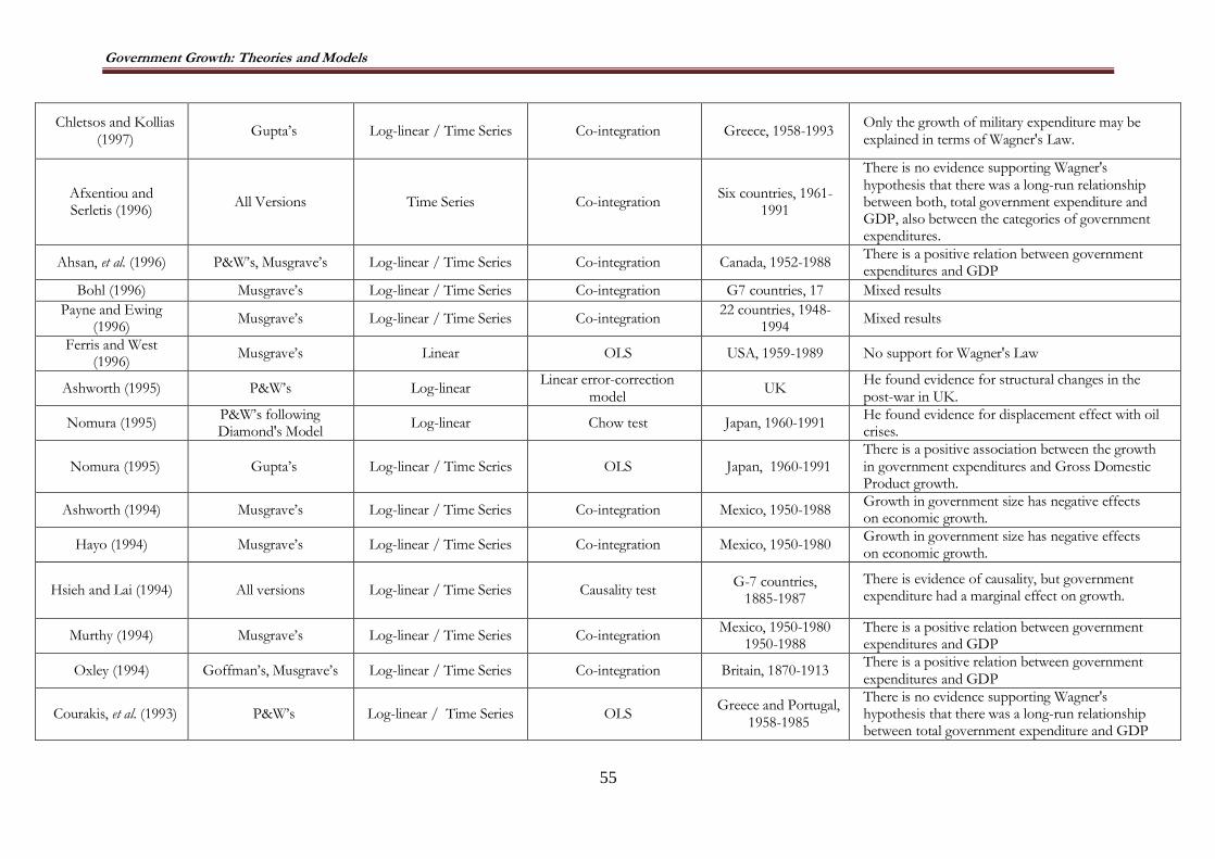
Government Growth: Theories and Models
55
Chletsos and Kollias (1997)
Gupta‟s Log-linear / Time Series Co-integration Greece, 1958-1993 Only the growth of military expenditure may be explained in terms of Wagner's Law.
Afxentiou and Serletis (1996)
All Versions Time Series Co-integration Six countries, 1961-
1991
There is no evidence supporting Wagner's hypothesis that there was a long-run relationship between both, total government expenditure and GDP, also between the categories of government expenditures.
Ahsan, et al. (1996) P&W‟s, Musgrave‟s Log-linear / Time Series Co-integration Canada, 1952-1988 There is a positive relation between government expenditures and GDP
Bohl (1996) Musgrave‟s Log-linear / Time Series Co-integration G7 countries, 17 Mixed results
Payne and Ewing (1996)
Musgrave‟s Log-linear / Time Series Co-integration 22 countries, 1948-
1994 Mixed results
Ferris and West (1996)
Musgrave‟s Linear OLS USA, 1959-1989 No support for Wagner's Law
Ashworth (1995) P&W‟s Log-linear Linear error-correction
model UK
He found evidence for structural changes in the post-war in UK.
Nomura (1995) P&W‟s following Diamond's Model
Log-linear Chow test Japan, 1960-1991 He found evidence for displacement effect with oil crises.
Nomura (1995) Gupta‟s Log-linear / Time Series OLS Japan, 1960-1991 There is a positive association between the growth in government expenditures and Gross Domestic Product growth.
Ashworth (1994) Musgrave‟s Log-linear / Time Series Co-integration Mexico, 1950-1988 Growth in government size has negative effects on economic growth.
Hayo (1994) Musgrave‟s Log-linear / Time Series Co-integration Mexico, 1950-1980 Growth in government size has negative effects on economic growth.
Hsieh and Lai (1994) All versions Log-linear / Time Series Causality test G-7 countries,
1885-1987
There is evidence of causality, but government expenditure had a marginal effect on growth.
Murthy (1994) Musgrave‟s Log-linear / Time Series Co-integration Mexico, 1950-1980
1950-1988 There is a positive relation between government expenditures and GDP
Oxley (1994) Goffman‟s, Musgrave‟s Log-linear / Time Series Co-integration Britain, 1870-1913 There is a positive relation between government expenditures and GDP
Courakis, et al. (1993) P&W‟s Log-linear / Time Series OLS Greece and Portugal,
1958-1985
There is no evidence supporting Wagner's hypothesis that there was a long-run relationship between total government expenditure and GDP
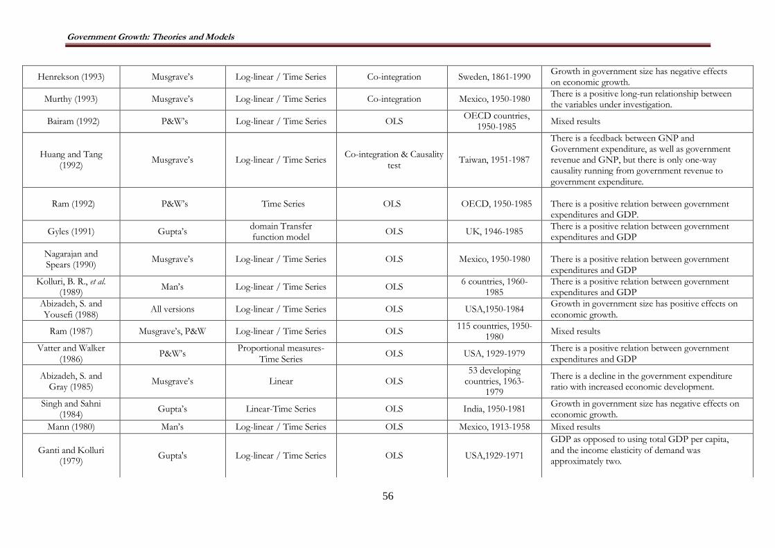
Government Growth: Theories and Models
56
Henrekson (1993) Musgrave‟s Log-linear / Time Series Co-integration Sweden, 1861-1990 Growth in government size has negative effects on economic growth.
Murthy (1993) Musgrave‟s Log-linear / Time Series Co-integration Mexico, 1950-1980 There is a positive long-run relationship between the variables under investigation.
Bairam (1992) P&W‟s Log-linear / Time Series OLS OECD countries,
1950-1985 Mixed results
Huang and Tang (1992)
Musgrave‟s Log-linear / Time Series Co-integration & Causality
test Taiwan, 1951-1987
There is a feedback between GNP and Government expenditure, as well as government revenue and GNP, but there is only one-way causality running from government revenue to government expenditure.
Ram (1992) P&W‟s Time Series OLS OECD, 1950-1985 There is a positive relation between government expenditures and GDP.
Gyles (1991) Gupta‟s domain Transfer function model
OLS UK, 1946-1985 There is a positive relation between government expenditures and GDP
Nagarajan and Spears (1990)
Musgrave‟s Log-linear / Time Series OLS Mexico, 1950-1980 There is a positive relation between government expenditures and GDP
Kolluri, B. R., et al. (1989)
Man‟s Log-linear / Time Series OLS 6 countries, 1960-
1985 There is a positive relation between government expenditures and GDP
Abizadeh, S. and Yousefi (1988)
All versions Log-linear / Time Series OLS USA,1950-1984 Growth in government size has positive effects on economic growth.
Ram (1987) Musgrave‟s, P&W Log-linear / Time Series OLS 115 countries, 1950-
1980 Mixed results
Vatter and Walker (1986)
P&W‟s Proportional measures-
Time Series OLS USA, 1929-1979
There is a positive relation between government expenditures and GDP
Abizadeh, S. and Gray (1985)
Musgrave‟s Linear OLS 53 developing
countries, 1963-1979
There is a decline in the government expenditure ratio with increased economic development.
Singh and Sahni (1984)
Gupta‟s Linear-Time Series OLS India, 1950-1981 Growth in government size has negative effects on economic growth.
Mann (1980) Man‟s Log-linear / Time Series OLS Mexico, 1913-1958 Mixed results
Ganti and Kolluri (1979)
Gupta's Log-linear / Time Series OLS USA,1929-1971
GDP as opposed to using total GDP per capita, and the income elasticity of demand was approximately two.

Government Growth: Theories and Models
57
Peacock & Wiseman (1979)
P&W‟s “while government expenditure has clearly grown over the period as a whole for all countries for which adequate statistics are available, the time pattern of growth is less regular than, and quite different from, the corresponding pattern of growth in the size of community output” (Peacock and Wiseman 1961, p. 25).
Diamond (1977) P&W‟s Log-linear Chow test He found evidence for displacement effect as a structural break.
Goffman and Mahar (1971)
Goffman‟s Proportional measures OLS 6 nations, 1940-1965
Growth in government size has negative effects on economic growth.

Government Growth: Theories and Models
58
3.8. CONCLUSION
This chapter aims to survey the relevant theories and models used in explaining growth
of government. In doing so, and in providing a foundation for the rest of the chapters, the
economic rationale for the government is discussed within various schools of thought.
In the models and theories section, Wagner‟s Law, Peacock & Wiseman‟s the
Displacement Effect and the Keynesian Approach presented as part of the macroeconomy
related models. These are three important theoretical observations on the growth of public
expenditure. The most popular one is Wagner‟s Law (1883) which states that the increased
economic activity leads to increases in government activities, which in turn result in the increase
of public expenditure. This involves the view that public expenditure can be seen as a result, or
as an internal factor of the growth of the economy. Wagner‟s (1883) law of expanding state
activity has since been empirically experienced by a number of states.
In another attempt, Peacock and Wiseman formulated the displacement effect by
analysing the time pattern of public expenditure. They found that public expenditure increases
during war or periods of social crisis. Moreover, when the war ends, or crisis is resolved, public
expenditure falls, but not to the level at the start of the emergency, with the conclusion that
growth in public expenditure occurs in stages associated with stress.
The advent of the Keynesian approach had a profound and pervasive influence on
economists and governments for many generations. Keynes (1933) found that the government
should use public expenditure as a tool of economic policy to manage a national economy and
counteract unemployment. His view found ready acceptance in a world that had not yet
recovered from the Great Depression. The Keynesian suggestion was to inject money into the
economic system. In other words, through careful consideration of the macroeconomic theories
of government growth comparable to Wagner‟s law, there appears to be a positive causal
relationship flowing from government expenditure to economic growth.
There are also the microeconomic models. These have included Baumol‟s differential of
production growth, Bacon, and the Eltis model. The results of supply side analysis are defined by
the fact that a traditional demand function for public goods always under-predicts the growth of
the public sector. An analysis of public consumption drawing support from Baumol‟s
productivity inequality model shows that this growth has exceeded the rate implied by the mutual
price and income effects. The developed model is used to explain both the relative and absolute
growth of various measures of public expenditure. Bacon and Eltis exaggerate the impact of
increases in local government employment on the national economy, because they do not allow

Government Growth: Theories and Models
59
for cheaper part-time and female labour, and they do not allow for the fact that a proportion of
the extra salaries and wages is paid back to government in taxes and rates.
This chapter, furthermore, presented four different models of the Public Choice
Approach to the growth of government. These included „bureaucracy and the growth of
government‟, „interest groups and the growth of government‟, „median voter and redistributors
government model‟, and „fiscal illusion‟.
Government expenditure increases when government allocates additional expenditure to
interest groups in order to get support from the groups. The expenditure may be on the level of
government redirecting resources from the general public interest to the interest group at the
expense of the general society. It gives us an opportunity to argue that as interest groups increase
in society, government expenditure may increase.
The median-voter model, together with the stylised fact regarding the relationship
between median and mean income, suggests that the public sector will be overly concerned with
redistribution, but may provide too few goods and services. While these consequences from the
median-voter models are suggestive, they do not give the basis for a general theory of public
expenditure determination.
In an attempt to understand government growth through political economy approach,
rentier state approach is also considered, which is particularly relevant in the case of Saudi
Arabia.
After identifying the main theoretical models, the next chapter focuses on the technical
aspect of government expenditures by discussing the definitional and measurement issues.

Understanding Government Expenditure: Concepts, Definitions, and Measurement
60
CHAPTER 4
UNDERSTANDING GOVERNMENT EXPENDITURES:
CONCEPTS, DEFINITIONS AND MEASUREMENT
4.1. INTRODUCTION
The economies of most of the countries in recent decades have been characterized by
growth in the government intervention and government expenditure expansion. Thus, due to
various reasons weather welfare state understanding or whether due to late developmentalism,
the public sector has played an important role in the economic policy making in many
countries. Wagner (1890) pointed out that the share of public sector output in the context of
economic development leads the economy to grow due to increased demand for public goods
and services. Consequently, in the process of economic development, government spending is
expected to grow. It this process, government expenditure is an endogenous factor and an
outcome, not a principle cause of growth (Wagner, 1883).
It should be noted that the nature and mechanism of government and public
expenditures differs from one country to another, as the multidimensional nature of
government intervention in the economy means that the intervention could include various
government activities (Gemmell, 1993). While most of the studies focused solely on size as
one might expect, Abizadeh and Basilevsky (1990:3) states that “the choice of different
variables would lead to a different size with distinct meaning and implications.”
This chapter, hence, presents aspects of public sector measurement accompanied by
an explanation of the concept of the public sector, or government. This is followed by an
explanation of the remarkable complexity of the indicators used to measure of the size of the
public sector.
4.2. THE CONFUSION OF CONCEPTS
It is useful to give some thought to the importance and growth of government, as it
requires clear understanding as to what we need to measure. Peters and Heisler (1983:179)
aims to make it easy when the state that the measurement should be “in forms in which data
are more readily available, in quantifiable form, ubiquitous units, and preferably in internal
form.”

Understanding Government Expenditure: Concepts, Definitions, and Measurement
61
A critical examination of the literature indicates that a number of concepts are used to
describe the government expenditure growth or government growth including „state‟, „public
sector‟, „public expenditure‟, „government expenditure‟, etc. It is clear that there is a difference
in these concepts and components in terms of size or area, and there is a difference in the
identification of these components from one country to another. According to Atkinson and
Stiglitz (1980:16) “there are several different ways in which the size of the public sector can be
measured, and there is a substantial element of arbitrariness in any definition.”
The following sections thus aim to shed some light unto these concepts in better
understanding the subject matter.
4.2.1. The Concept of the State
In an attempt to understand that conceptual issues, the first concept is to explore is
the „state‟, which is defined as the group of people associated by certain bonds governed by a
system of designated authority (Trotman and Dickenson, 1996).Beyond, this legal notion of
the state, „state‟ is also used commonly as word in political systems. It means a relationship
between geography and citizen, but also a contract between individual citizens and their
governance. According to Peters and Heisler (1983), the „state‟ refers to the relationships
between a government and its citizens.
The notion and definition of state has changed through the centuries and therefore its
impact and conceptualisation and its boundaries in economic life has changed from one
political setting to another. While communist economies experiences a heavy presence of
state in the economy, liberal capitalist economies aimed at small state in terms of state
intervention in the economy.
The nature of the political setting also defined the functions of the state in different
ways over the centuries. While classical political economists recognised the classical functions
of the state from defence to security and legal system to governance, modern welfare state
understanding as the blend of socialism and capitalism resulted in state providing public and
merit good most of the time free of charge to its citizen in developing a nation state.
In terms of the size of the government as the subject matter of this research,
measuring the size of the state is a more complicated and sophisticated matter; as the
definition states modern state is large and complex phenomenon with various economic
implications. As the constitutional economics states, then the measurement of the government

Understanding Government Expenditure: Concepts, Definitions, and Measurement
62
expenditures should start with the economic implications of the various agencies of central
authority and other agencies. However, such definitions and attempts are difficult to conduct.
4.2.2. The Concept of Government
Government is part of the composition of the state and has the authority to make and
enforce laws and regulations. Peters and Heisler (1983:184) define government as “the
institution that imparts direction to society by various means of collective decision-making and
exercises the state‟s authority on a daily basis.” As the one of the oldest political institutions in
the world, whose mission can be summarised as four fundamental tasks (World Bank, 1997):
(i) Establishing a foundation of law;
(ii) Investing in basic social services and infrastructure;
(iii) Protecting the vulnerable;
(iv) Protecting the environment.
Government thus constitutes the functional and executive articulation of the state in
economic and political system, which has particular implications for public expenditures.
However, being a different concept, it is terrible difficult to establish the demarcation lines
between the state and the government as far as public expenditures are concerned.
4.2.3. The Concept of Public Sector
There are different ways to explain the concept of the public sector. Since public
sector refers to public expenditures and incomes policies in the form of fiscal policy, Brown
and Jackson (1990:4) pointed out that “public sector economics are, therefore, the study of the
effect of public expenditure and taxes on the economy”. In other words, since the concern in
this study is related to the size of government involvement in the economy, the concept of the
public sector includes not only public expenditure but also the taxes and the creation of public
debt.
It should be noted that the multiplicity of public enterprises in each state can make the
process of measuring public sector as a difficult process (Trotman and Dickenson, 1996).In
supporting this, Aulichet al. (2001:1) notes that the concept of the public sector “represents the
activities undertaken almost solely by government agencies, and is accomplished by a mix of
departments of state, statutory authorities and other legal and political institutions.”
Since this chapter aims to identify the differences between different categories related
to the subject matter, it should be stated that there are differences between the concepts of
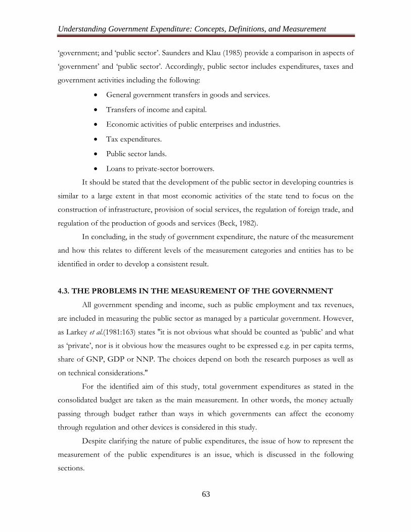
Understanding Government Expenditure: Concepts, Definitions, and Measurement
63
„government; and „public sector‟. Saunders and Klau (1985) provide a comparison in aspects of
„government‟ and „public sector‟. Accordingly, public sector includes expenditures, taxes and
government activities including the following:
General government transfers in goods and services.
Transfers of income and capital.
Economic activities of public enterprises and industries.
Tax expenditures.
Public sector lands.
Loans to private-sector borrowers.
It should be stated that the development of the public sector in developing countries is
similar to a large extent in that most economic activities of the state tend to focus on the
construction of infrastructure, provision of social services, the regulation of foreign trade, and
regulation of the production of goods and services (Beck, 1982).
In concluding, in the study of government expenditure, the nature of the measurement
and how this relates to different levels of the measurement categories and entities has to be
identified in order to develop a consistent result.
4.3. THE PROBLEMS IN THE MEASUREMENT OF THE GOVERNMENT
All government spending and income, such as public employment and tax revenues,
are included in measuring the public sector as managed by a particular government. However,
as Larkey et al.(1981:163) states ''it is not obvious what should be counted as „public‟ and what
as „private‟, nor is it obvious how the measures ought to be expressed e.g. in per capita terms,
share of GNP, GDP or NNP. The choices depend on both the research purposes as well as
on technical considerations.''
For the identified aim of this study, total government expenditures as stated in the
consolidated budget are taken as the main measurement. In other words, the money actually
passing through budget rather than ways in which governments can affect the economy
through regulation and other devices is considered in this study.
Despite clarifying the nature of public expenditures, the issue of how to represent the
measurement of the public expenditures is an issue, which is discussed in the following
sections.

Understanding Government Expenditure: Concepts, Definitions, and Measurement
64
4.3.1. Absolute or Relative Size
Using the absolute size of government expenditures may not do justice in
understanding the growing size of the public expenditures. Musgrave (1978) and Brown and
Jackson (1990) also stated that the absolute size of the public sector is a somewhat
meaningless concept. Rather, the relative size of the public sector is the typical measurement
utilised as a ratio or comparison between the estimates or the absolute measurement of the
public sector variables and the total national income. The measure of the relative size of the
public sector is not especially easy, as a ratio it involves public sector measure to total national
income, and hence the definitions of these variables are still disputed (Cullis and Jones, 1987).
4.3.2. Nominal or Real Values
Inflation has been a common economic terms and phenomenon for all the nations.
One of the main sources of the growth in public revenues and in public expenditures is clearly
inflation. The other related aspect is the relative price effect which should be taken into
account even when estimating the size by real values. As Cullis and Jones (1987)
acknowledged, we need to distinguish changes in relative prices of public services and their
volume, since prices of publicly and privately provided goods do not go up at the same rate.
Musgrave (1978:16) indicates that in fiscal policy measures, “a correction must be
made for inflation” and add that the observation on nominal levels would not be meaningful.
On the other hand, as indicated by Abizadeh and Basilevsky (1990:356), Buchanan and
Flowers and lewis-Beck and Rice favoured the nominal values, "reflect changes in prices along
with changes in government's real share in economic activity…. (while giving) a better
indication of government's scope and power vis-a-vis the national economy."
4.3.3. The Implications of Deflating Public Expenditures by the GDP Deflator.
As indicated by Monacelli and Perotti, (2006:8) "instead of the GDP deflator, one
could have used government expenditures own deflator to express government spending in
real terms. Most models predict that this action should have a positive effect on employment
and output: in a neoclassical model, this happens via a negative wealth effect on the private
sector, whereas in a 'Keynesian model', via a higher demand. Yet, if we used government
expenditures own deflator, real government expenditure would not change and we would not

Understanding Government Expenditure: Concepts, Definitions, and Measurement
65
be able to capture. Only by employing the GDP deflator will we be able to capture the positive
effect on output."
4.3.3. The Measurement of Relative Size
Since the absolute size of the public sector does not render an efficient understanding,
at least measurements can be developed to examine the direction and magnitude of change in
the public sector expenditures over time.
The measurement of the relative size of the public sector to total national income is
important in interpreting and understanding the expansion of the public sector over time. As
noted previously, one of the most important of such relative size is the proportional share of
the government in the economy, such as the proportion of government expenditure in GNP.
Nevertheless, there are some difficulties regarding the measurement of the magnitude of this
ratio as well.
4.3.3.1. The Public Revenues Ratio
One of the indicators that deserve attention in estimating the size of the government
sector is public revenue. An increase in government spending or any other part of these
financial aspects must bear in mind the growth of public revenues.
Public revenue is the sum of money levied by the state from various sources to finance
public expenditures to meet public needs. Public revenue is the financial means to enable the
state to implement public policy. There are several types of income associated with increasing
functions of the state and its intervention in economic and social affairs.
Revenues obtained from taxes are the largest sources of public revenue, and these
taxes require a strong private sector, which is obliged to pay them. The comparison between
the total taxes from the private sector renders an indication of the resources of governments
(Gillie, 1979).
There are many types of public revenue, the bulk of which is received from three main
sources. There are the fees for the provision of public services, followed by income tax, and
the third source, consists of credit and loans, domestic and external. With the increased
functions of the state, the variety of public revenues have changed and diversified.
The public revenue ratio to GDP provides an understanding on the extractive power
of the state and hence its power on the economy.

Understanding Government Expenditure: Concepts, Definitions, and Measurement
66
4.3.3.2. The Ratio of Public Expenditure
Considering that Wagner (1883) pointed out that rapid growth in public expenditure is
most often a function of a quickly growing national income, relative size of public expenditure
in terms of ratio of public expenditures to national income can be considered as an efficient
measure. In supporting this, Jackson (1980:330) noted that “the relative size of the public
sector can be simply expressed as a ratio of some absolute measure of public expenditure
divided by a national income aggregate such as GNP.”
The ratio of public expenditure involves a number of aspects beginning with
numerators measures (Cullis and Jones, 1987), which are depicted in Table 4.1:
(i) The sum of the local and central government expenditure plus the capital of corporations
(nationalised industries) and tax expenditure;
(ii) The sum of the local and central government expenditure plus the capital of corporations
(nationalised industries), but after excluding tax expenditure, despite the opinion of some
that it could be added to the miscellaneous expenses of governmental activities;
(iii) The sum of the local and central government expenditure, but after the excluding the
capital of corporations (nationalised industries) and their tax expenditure, as they are
largely autonomous;
(iv) It is similar to (iii) but excludes all expenditure on financial assets, because it reflects the
role of local and central government as financial intermediaries;
(v) Local and central government expenditure, as this figure assumes that local and central
government expenditure is less than the total spending on financial assets;
(vi) The latest measurement of the ratio of government spending, where there are attributes
and the ratio of value-added, which requires the input dimensions of the procurement
market of the expenses, detailed in this way and not as part of the spending output.

Understanding Government Expenditure: Concepts, Definitions, and Measurement
67
Table 4.1: The Numerators Measures
Measure Including Excluding
1 Local and central government expenditure Nationalized Industries
+ Tax Expenditure
--------
2 Local and central government expenditure Nationalized Industries
Tax Expenditure
3 Local and central government expenditure -------- Nationalized Industries
+ Tax Expenditure
4 Local and central government expenditure -------- All expenditures on financial assets
5 Local and central government expenditure
6 Local and central government expenditure Value – Added
Source: Cullis and Jones, (1987:69-71)
Somewhat differently, Cullis and Jones (1987) present eight possible denominators,
with six possible numerators, to measure the ratio of government expenditure, and thus the
size of government. They have noted that “While the estimate of government expenditure is
larger when selecting the appropriate numerator, the public sector appears larger by choosing
the smallest denominator” (Cullis and Jones, 1987:71). Cullis and Jones (1987:70), therefore,
state that “it is very easy to see how very differing views on the size and growth of public
sector are readily sustained.”
In identifying the difficulties in the use of such a ratio, Jackson (1980) pointed out that
the nationalised industries consume public sector resources, and thus make this ratio smaller
than the potential ratio. Therefore, Brown and Jackson (1990) suggest an expanded the ratio as
the total of public sector consumption, the total of public sector investment, government
subsidies, transfers of capital, interest on debt, and finally the net loans to the private sector.
Transfer expenditures are considered as another complicated part of the numerator of
such a ratio; as some suggests that transfer expenditures being non-economic by nature should
not be included. However, rightly so, Buchanan and Flowers, as quoted by Abizadeh and
Basilevsky (1990:356) noted that “Transfer is as much a real cost as direct outlays for tanks,
planes and paperclips. When estimating the real cost of government, the distinction between

Understanding Government Expenditure: Concepts, Definitions, and Measurement
68
productive and transfer expenditure is not useful.” Hence, in order to have a full picture of the
public sector growth, transfer expenditures should also be considered.
In all cases, change and differences in analysis and political outlook, analysts have the
opportunity to choose any measurement of the ratio of government spending which proves
useful. However, it is nonetheless quite clear that „any measure or standard for measuring the
change in the size of government is arbitrary‟ (Jackson, 1980).
The important point is that the nature of the ratio of government expenditure should
be identified. For example, Eltis (1983:79) stressed that “the expression has been made in
terms of conventional national income accounts; these are, however, not the ideal tools to use
in an examination of the influence of growth in public expenditure on the development of the
economy.” Thus, national income may be the best indicator of economic output to be used as
a denominator. Consequently, GDP can be employed as the national income aggregate
statistics in the estimation of the public expenditure ratio.
It should be noted that an additional problem with regard to figures or estimates of
national income is related to the estimation of the national income whether at factor costs and
market prices. Brown and Jackson (1990) indicated that the composition and construction of
public revenue in different countries will affect the GDP at market prices, even if they have a
similar figure at factor prices. Because of this, they preferred GDP at factor cost as the most
appropriate measurement in estimating the size of public sector through public expenditure
ratio.
Among the national income measures, Musgrave (1978:18) found that the GNP is the
favoured standard for measurement of the size of government, noting that his “inclination is
to use GNP at market price where purchases or the total expenditure ratio are concerned,
while using net national product at factor cost when dealing with transfer payments or direct
taxes.” However, Oshima (1957: 388) argued that “valuation of products at factor cost is not
suitable, since it excludes indirect taxes which are a large part of the share of government.”
Furthermore, Eltis (1983:79) suggests that “(if our goal is to measure) real resources available
for investment and consumption by the companies and workers of the private sector, then the
provision of un-marketed public services should be excluded from the output because they
can be neither invested nor privately consumed.”
As a result, even if GDP is chosen as a denominator, six different ways of interpreting
it still is an issue. However, varying percentage of increased in nominator and denominator

Understanding Government Expenditure: Concepts, Definitions, and Measurement
69
also results in unrepresentative ratio. For instance, if the government expenditure increase is
lower than the increase in the GDP or GNP, then the ratio will be lower comparatively.
4.3.4. Public Employment Measurement
Government employment can be employed as another significant indicator of the size
of government. However, one of the main difficulties found by some economists and
researchers in the field of government employment is the difficulty in separating the
employment interaction and participation between the government and the private sector,
making the expense of workers in the public sector rather difficult to estimate.
Rose (1983:165) asserted that “defining employees in terms of attributes of the
employer rather than of the employee, avoids many problems.” The difficulty that may arise is
the development of a classification for some functions not falling within any job classification,
and so may not come within the scope of the classification and thus become invisible in the
process of calculation. This can also give rise to confusion, as stated by Rose (1983:165) “if
public employment is disaggregated into functions components, the same government can be
changing in different directions at the same time.”
There are also some jobs in the public sector, with a low level of minimum income,
which are filled by individuals who do not receive a fixed wage per day, which must also be
taken into account when calculating the total number of jobs in this sector.
In short, using public employment as a measure can pose certain other difficulties in
terms of defining and understanding the various aspects of public sector employment.
4.3.5. The Measurement of the Off-Budget Activities of Government
It is clear that the assessment method and system of government expenditures must
take into account a more inclusive society, where it is necessary to identify the various
government activities and what activities add to the total government budget. The
governments use their power to issue legal and regulatory legislation to create revenues and
expenditures areas beyond the formal budget of the country, which are called off-budget
funds. The creations of such funds are sometimes due to political manoeuvre and sometime
due to the policies of the governments to circumvent rigid bureaucratic regimes.
The study of the phenomenon of off-budget activities of government is far removed
from the study of traditional data. Measures to deal with the public sector should include the

Understanding Government Expenditure: Concepts, Definitions, and Measurement
70
additional activities of governments, such as off-budget activities (Saunders and Klau, 1985).
The previous standards, such as tax expenditure, subsidies, and regulation rejected the
traditional measurement of the public sector, especially when there is difficulty in finding
estimates of the size of government. These off-budget activities are essential, constituting a
large alternative area in the performance of direct actions of the government budget.
In the case of Saudi Arabia, in particular funds in the form of sovereign wealth funds
(SWF) should be considered as an important part of government‟s increasing expenditure
power, through which government has been undertaking investments and generating wealth
beyond the state‟s budget. Considering that these SWFs have managed to pool very large
amount of funds available to be used by the state mainly for economic and financial
investments, their inclusion in the calculation of growth of government should include these
funds. Since they are investment oriented and owned and regulated by the state, it is
important that they should be considered as part of the government expenditure structure.
4.3.6. Tax Expenditure
Tax Expenditure is a term used to describe various allowances, which are used to
reduce the burden of income tax. Tax expenditure has been seen as analogous to direct
payments, or subsidies provided by the government.
Tax is a financial burden received by the state according to the rules of parliamentary
mandates, to provide the necessary funds to cover the expenses of the state so as to achieve
the economic goals of the community, that is, the economic objectives to encourage savings
and investment, to encourage some sectors of the economy, to reduce the negative effects of
economic stagnation and to curb inflationary pressures.
In addition, the government directs spending without resources and without the actual
collection or compilation of some types of expenditure in the tax system, which means it is
government-supported or subsidised, as in the case of tax expenditure. According to Saunders
and Klau (1985:79) “Tax expenditure can take various forms, such as exemptions from tax, tax
allowances, tax credits or special tax reliefs designed to assist particular groups or activities.”
In addition, the amount obtained by the government as income tax will be low and without
any charge to the direct expenditure.
Cullis and Jones (1987:75) note that “Attempts have been made to quantify some of
those implicit expenditures”, which includes tax expenditures. Gillie (1979:15) argued that

Understanding Government Expenditure: Concepts, Definitions, and Measurement
71
“There is no systematic estimate of revenue foregone because of these reliefs, but it seems
likely to be substantial.”
With the purpose of measuring the implicit expenditure, as argued by Saunders and
Klau (1985:79) “there should be agreement on what represents the normal tax structure, since
tax expenditure is usually defined as departures from the generally accepted normal or
benchmark tax structure.”
It should be noted that the traditional estimation methods of measurement, although
familiar, can only be approximate estimates of tax and tax expenditure. There are additional
problems, and in spite of the fact that increasing numbers of states find a separate system to
measure these taxes, they are exceptional budgets, as noted by Saunders and Klau (1985).
A quick review of the government expenditure growth literature, however, does not
show any study using tax expenditures as a measure of government growth.
4.3.7. Laws and Regulations
Laws and regulations are an important aspect in the organisation of public sector
activities and, therefore, the size of government. The policies that work in the regulatory
process in general have a significant impact and provide clear guidance in the private and
public sectors. As noted by Rose (1983:161), “laws are a unique resource of government”, as
through laws are regulations, government defines resources allocation in the society as well as
tax burden of the citizens. Therefore, their role goes beyond the extent to which they can be a
real alternative to direct government spending or tax measures (Brown and Jackson, 1990), as
laws and regulations have explained the importance of advancing the public sector and
performance; also, the efficiency and effectiveness of the public sector have a significant
impact on the public and the private sectors.
There are some problems related to measuring and determining the kind and quality of
laws and regulations, but that is a catalyst for regeneration and development. Moreover, laws
and regulations need to adapt to a lasting interest for economic growth and development of all
activities of the state, but are not limited only to mere work provided for under these laws;
they must take into account the rapid development of economic concepts over time. Saunders
and Klau (1985:85) argue that “attempts to estimate the economic costs of regulatory activity
in monetary terms are satisfactory”, for which various benchmarks can be developed. For
instance, if the objective is to measure the regulatory process in the economy, there are
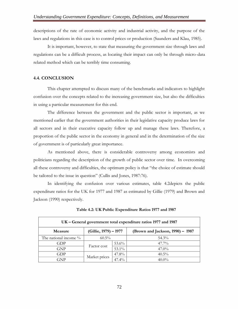
Understanding Government Expenditure: Concepts, Definitions, and Measurement
72
descriptions of the rate of economic activity and industrial activity, and the purpose of the
laws and regulations in this case is to control prices or production (Saunders and Klau, 1985).
It is important, however, to state that measuring the government size through laws and
regulations can be a difficult process, as locating their impact can only be through micro-data
related method which can be terribly time consuming.
4.4. CONCLUSION
This chapter attempted to discuss many of the benchmarks and indicators to highlight
confusion over the concepts related to the increasing government size, but also the difficulties
in using a particular measurement for this end.
The difference between the government and the public sector is important, as we
mentioned earlier that the government authorities in their legislative capacity produce laws for
all sectors and in their executive capacity follow up and manage these laws. Therefore, a
proportion of the public sector in the economy in general and in the determination of the size
of government is of particularly great importance.
As mentioned above, there is considerable controversy among economists and
politicians regarding the description of the growth of public sector over time. In overcoming
all these controversy and difficulties, the optimum policy is that “the choice of estimate should
be tailored to the issue in question” (Cullis and Jones, 1987:76).
In identifying the confusion over various estimates, table 4.2depicts the public
expenditure ratios for the UK for 1977 and 1987 as estimated by Gillie (1979) and Brown and
Jackson (1990) respectively.
Table 4.2: UK Public Expenditure Ratios 1977 and 1987
UK – General government total expenditure ratios 1977 and 1987
Measure (Gillie, 1979) – 1977 (Brown and Jackson, 1990) – 1987
The national income % 60.5% 54.3%
GDP Factor cost
53.6% 47.7%
GNP 53.1% 47.0% GDP
Market prices 47.8% 40.5%
GNP 47.4% 40.0%
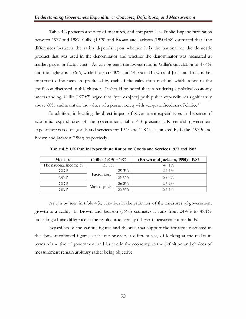
Understanding Government Expenditure: Concepts, Definitions, and Measurement
73
Table 4.2 presents a variety of measures, and compares UK Public Expenditure ratios
between 1977 and 1987. Gillie (1979) and Brown and Jackson (1990:158) estimated that “the
differences between the ratios depends upon whether it is the national or the domestic
product that was used in the denominator and whether the denominator was measured at
market prices or factor cost”. As can be seen, the lowest ratio in Gillie‟s calculation in 47.4%
and the highest is 53.6%, while these are 40% and 54.3% in Brown and Jackson. Thus, rather
important differences are produced by each of the calculation method, which refers to the
confusion discussed in this chapter. It should be noted that in rendering a political economy
understanding, Gillie (1979:7) argue that “you can[not] push public expenditures significantly
above 60% and maintain the values of a plural society with adequate freedom of choice.”
In addition, in locating the direct impact of government expenditures in the sense of
economic expenditures of the government, table 4.3 presents UK general government
expenditure ratios on goods and services for 1977 and 1987 as estimated by Gillie (1979) and
Brown and Jackson (1990) respectively.
Table 4.3: UK Public Expenditure Ratios on Goods and Services 1977 and 1987
Measure (Gillie, 1979) – 1977 (Brown and Jackson, 1990) - 1987 The national income % 33.0% 49.1%
GDP Factor cost
29.3% 24.4%
GNP 29.0% 22.9%
GDP Market prices
26.2% 26.2%
GNP 25.9% 24.4%
As can be seen in table 4.3., variation in the estimates of the measures of government
growth is a reality. In Brown and Jackson (1990) estimates it runs from 24.4% to 49.1%
indicating a huge difference in the results produced by different measurement methods.
Regardless of the various figures and theories that support the concepts discussed in
the above-mentioned figures, each one provides a different way of looking at the reality in
terms of the size of government and its role in the economy, as the definition and choices of
measurement remain arbitrary rather being objective.

Government Expenditures in Saudi Arabia: Developments and Trends
74
CHAPTER 5
GOVERNMENT EXPENDITURES AND ECONOMIC
DEVELOPMENT IN SAUDI ARABIA:
DEVELOPMENTS AND TRENDS
5.1. INTRODUCTION
Past decades have witnessed the increased role of government in most of the states in the
world and in particular in the developing countries through increased measures, procedures, and
engagement in social services but also economic activities including transfer expenditures. These
indeed have had fiscal and monetary policy implications and also raised questions about the
efficiency of government expenditures against the so-called achieved objectives.
In particular with the Keynesian policies, but also due to the realism of the need of
development in the developing countries, the government expenditures have been assigned an
important role to provide the development needs of the respective countries. Considering that
the presently developing countries have not had much private capital to finance economic
development, having the extensive involvement of state in economic development was not a
matter of choice but an imperative.
The role of government and the growth in the size of the public sector have been the
focus of attention for several decades. As mentioned in Chapter 3, Wagner initiated the initial
theorisation of the relationship between government expenditure and the GDP through what is
now known as Wagner’s Law, who, at least in the case of Germany and the Europe observed
and evidenced a strong relationship between public expenditures and economic expansion in the
form of economic growth but also economic development.
In the case of Saudi Arabia, the economic growth and development of the country has
been possible mainly due to the government expenditures which is financed through revenues
raised from the oil sector, which still dominates the economy, as Saudi Arabia is a late
developmentalist country without any private capital in its formation. Albatel (2003:77),
therefore, argues that "the government has an important influence on the economy through its
expenditure on activities including its overall development strategy financed mostly by revenues
generated from oil, under which many of the economic and social services used to be provided
to the citizens with less than their cost”.
The Kingdom of Saudi Arabia, hence, has used oil income to fund its economic growth
and development but also the country has been developing strategies to diversify sources of

Government Expenditures in Saudi Arabia: Developments and Trends
75
income in the economy away from oil dependence. It should be noted that adaptation to the
global economy and the presence of the oil, since the first five-year development plan (1970-
1975) until the seventh development plan (2000-2005) has seen sector diversification become a
more and more prominent objective.
The steps the Kingdom of Saudi Arabia has taken towards the goal of economic growth
and development involve building the infrastructure necessary to create, stimulate and activate
economic growth in non-oil sectors (Development Plan, 1970-2009). In order to organise an
efficient economic development in the country, Saudi Arabia still prepares development plans.
Planning automatically goes into every effort directed by state policy, but often it is effective only
when there is a meaningful effort for the overall development of the society’s well-being. It is
clear that development activities have achieved much through the development of plans and
obstacles have retreated after each period.
Since this study aims to examine the stated nexus between government expenditures and
economic growth in the case of Saudi Arabia, the purpose of this chapter is to outline
development and trends in economic performance, government expenditures by referring to the
stages of economic development in Saudi Arabia envisioned from the beginning. The economic
policies pursued are classified into periods, organised into general trends in GNP/GDP with
goals in human development indexed in reference to five-year plans.
It should be noted that the components of public sector/government expenditure in
Saudi Arabia have been presented in chapter four and contextualise development objectives for
Saudi Arabia.
5.2. STAGES OF ECONOMIC GROWTH IN SAUDI ARABIA
In general, the development plans that have been implemented since 1970 succeeded in
increasing economic growth and employment, and have identified areas of infrastructures and
institutions to be financed by government expenditures for supporting the economic activities
and developments, modernisation and transfer of advanced technology. The development plans
have also succeeded in achieving good levels of education and health and social services, which
are clearly reflected in the improvement of living standards for all citizens.

Government Expenditures in Saudi Arabia: Developments and Trends
76
5.2.1. Stages of Economic Development
An overview of the economic performance in table 5.1 evidences that the value of the
GDP at current prices has increased rapidly, from 22,565 million SAR in 1970 to 1,154,504
million SAR in 2005 and to 1,629,998 million SAR in 2010, at an average annual growth rate of
about 16.7% indicating an state the percentage. This is an indication of the level of economic
achievement made so far (table 5.1).
In terms of development planning, first phase covers the first three development plans,
from 1970 to 1984. Growth rate of the economy from 1970 to 1984 stood at an annual average
of 23.2% during this first phase of economic growth planning (table 5.1).
The second phase of development planning covers the development plans from the
fourth to the seventh planning, for the period from 1985 to 2005. The growth rate of the
economy was lower during the period, at an average annual rate of 4.0% (table 5.1), lower than
the previous stage.
The strategic objectives for long-term development have been formed since the
beginning of preparations for the first development plan in 1970. During the past three decades,
planning for the development in the Kingdom of Saudi Arabia has been on-going, through
harmonisation of all the conditions of interim plans to work flexibly and efficiently towards the
next phase with changes and updates, and through preparation of the subsequent plan which
comes next. The average growth rate during the seven development plans in the first year of the
Eight Development Plan (2005) stood at approximately 11.9% (table 5.1), while total exports of
9.7 billion SAR in 1970 climbed to 678.5 billion SAR in 2005 indicating another successful
performance thanks to oil exporting.
The First Development Plan for 1970-1974 called for a growth rate of real capacity of
9.8% of the GDP with an annual average (table 5.1). The actual growth rate achieved was 18.7%
which more than doubled annual average growth during that period. This was achieved due to
high oil revenues as a result of oil shock in 1973, and high oil revenues helped to increase
government spending to the actual 75.5 billion SAR, which according to the plan was expected
to be only 41.3 billion SAR, or an increase of 82.8% over government income and spending
projected (First Development Plan, 1970). This initial development is enough to understand the
crucial role played by oil in the development of the country.
The Second Development Plan covered the period of 1975-1979 and demonstrated even
further increase in government spending, and consequently spending amounted to about 684.4
billion SAR, an increase that was more than nine times that of government spending in the first

Government Expenditures in Saudi Arabia: Developments and Trends
77
development plan. This increase in government spending was result of the GDP increases due to
high oil prices and, hence revenues. However, during this period, high rates of real growth
(around 8.9%) in non-oil production sectors were also achieved as a result of initial economic
diversification attempt. During the same period, the growth of the oil sector was about 2.4%. To
further contextualise this, during the Second Development Plan, the public sector achieved that
average 5.5% real growth rates, while the private sector achieved real average annual growth of
10.1%(Ministry of Economy and Planning, 2006).
During the Third Development Plan from 1980-1984, the planned level of government
spending was 1200 billion SAR, which was nearly twice the value of actual spending during the
Second Development Plan (684.4 billion SAR). By the end of the Third Development Plan,
actual spending amounted to 1,213 billion SAR due to a sharp increase in government revenues.
During that period, the private sector increased its share in gross fixed capital formation
at current prices from 37.7 billion SAR in 1980 to 50.2 billion SAR in 1984 (Third Development
Plan, 1980), which culminated into further economic growth despite the fact the world
economies were experiencing recession due to the high oil prices. During this period, support for
the development of private sector continued with the application of economic policies aimed at
expansion of incentives given to stimulate private investment in the country.
The Fourth Development Plan, 1985-1989, saw a significant decrease in oil revenues due
to the impact of lower prices on the global market, reflected in a relative decline in total
government expenditure, to 802.1 billion SAR, contrasting with the planned 1,000 billion SAR.
This decline was a reflection of the reduction on the rates of GDP growth, as the average rate of
annual growth with real prices during the plan was only 0.6% annually during the plan period
(Fourth Development Plan, 1985).However, development efforts of the time were able to
continue supporting the economic sectors, notably agriculture, which achieved high-growth
rates, resulting in 13.4% annual average growth. Similarly, the petrochemical industries sector
achieved a quantum leap in the rate of annual growth with averaged growth rate of 47.3%.
During this period, the annual growth in oil and natural gas was 4.4% (Ministry of Economy and
Planning, 2006).
The Fourth Development Plan focused on a new strategic direction aiming at increasing
the profit generated by the oil and natural gas sector. It also became clear that there was a need
to focus on the petrochemical industry, which has a great a comparative advantage for Saudi
Arabia with high value-added. The plan also saw positive signs in terms of increase in the average
annual rate of growth of non-oil exports, which rose from 18% in the Third Development Plan

Government Expenditures in Saudi Arabia: Developments and Trends
78
to 29.3% during the Fourth Development Plan. Domestic production increased during the
period, particularly of consumer goods, and in agriculture there was increased substitution of
imports of these commodities. The period saw also increases in the share of private-sector
investment to the total, representing about 54.9% during the fourth plan, reaching 239.2 billion
SAR at constant prices of 1999(Fourth Development Plan, 1985).
In the Fifth Development Plan, 1990-1994, the average annual growth rates of the GDP
were about 4.4%, during which period the private sector achieved average annual growth of
2.1%. The rates of growth in the oil and government sectors were 9.7% and 2.9% respectively.
The high rate of growth of the oil sector and the increase in oil revenues increased the economic
growth significantly in the period in question(Fifth Development Plan, 1990).
The total value of private investments amounted to 283.6 billion SAR, growing at an
average annual rate of 5.9%, while government investments amounted to 178.8 billion SAR. The
value of total government spending amounted to 1078.1 billion SAR mainly due to the increase
in oil revenues. During the plan period, the balance of trade realised a surplus averaging around
15.6% of GDP (Ministry of Economy and Planning, 2006).
The Sixth Development Plan stretching from 1995 to 1999 focused on strategic
directions in human resource development. The plan prioritised human resource development,
job creation, and implementation of a policy of privatisation, which also took a strategic
direction of increasing the proportion of the contribution of non-oil sectors. In the
diversification of economy towards private sector certain achievements were demonstrated, as in
real GDP at 1999, the private sector’s role was 51.1% in 1969 which increased to 69.7% in 1999
(Sixth Development Plan, 1995).The Plan also concentrated on increasing the share of non-oil
sectors in real GDP from 51.2% in 1969 to 69.7% in 1999, the last year of the Sixth
Development Plan.
The Seventh Development Plan 2000-2004 set the goals of economic growth in most
non-oil sectors at an annual rate of 5.1% (table 5.1), and encouraged the private sector to achieve
a growth rate of an average annual rate of 5%. The investment sector was growing at an annual
average of 3.6% (Saudi Arabian Ministry of Economy and Planning, 2006). The non-oil sectors
during the Seventh Plan had real annual growth averaging about 3.9%; the percentage
contribution of these sectors to the GDP rose to 16.7% in 2004 (table 5.1).
The private sector had achieved a real growth rate averaging 4.3% during the Seventh
Development Plan period, 2000–2004. Its percentage share of GDP increased from 52.4% in
1999 to 54.6% in 2004, compared to the plan target of 55.4%. During the same period, private

Government Expenditures in Saudi Arabia: Developments and Trends
79
investment grew at an average annual rate of 3.5% compared to the plan target of 8.3% (Seventh
Development Plan, 2006). In addition, the seventh plan aimed at improving the current account
balance of payments deficit which was -3.0% of GDP in 1999 to a surplus of 6.9% of GDP in
2004.
The developments and trends in various dimensions of GDP are depicted in table 5.1
and Figure 5.1, Figure 5.2, Figure 5.3and Figure 5.4.As can be seen in Table 5.1; Figure 5.1,
Figure 5.2, Figure 5.3 and Figure 5.4, in 1970 the growth of GDP was about 11.9, which
increased to 200.4 in 1974 and decreased to 16.7 in 2010. Also, the growth rate of oil sector was
about 16.9%, which increased to 280.3 in 1974 and decreased to 25% in 2010. On the other
hand, the growth rate of non-oil sector was about 7.8 in 1970, which increased to 66.2 in 1974.
1n 2010 the growth rate of non-oil sector decreased to 9.1.

Government Expenditures in Saudi Arabia: Developments and Trends
80
Table 5.1: Annual Changes in Gross Domestic Product by Sectors
Source: Ministry of Economy and Planning (2010)
Year GDP
GDP Growth Rate
Oil Sector
Oil Sector Growth Rate
Non-Oil Sector
Non-Oil Sector Growth rate
1970 22,565 11.9 8,689 16.9 13,590 7.8
1971 30,497 35.2 15,186 63.9 14,938 10.1
1972 38,259 25.5 20,447 31.8 17,372 17.4
1973 53,531 40.3 30,687 48.0 22,361 29.0
1974 159,719 200.3 119,166 280.3 40,111 66.2
1975 163,670 2.4 97,568 -17.0 65,588 76.8
1976 225,347 37.6 128,476 31.6 95,963 48.3
1977 260,960 15.6 136,869 6.3 122,680 30.5
1978 272,267 4.2 120,368 -11.0 150,072 24.0
1979 375,469 38.0 187,745 56.0 185,564 21.3
1980 546,603 45.7 323,048 67.8 221,021 19.3
1981 622,175 13.9 355,736 11.5 263,802 17.9
1982 524,197 -15.9 235,975 -33.1 284,974 11.5
1983 445,210 -15.2 143,865 -36.0 297,668 4.6
1984 420,388 -5.7 120,305 -13.8 296,110 -1.0
1985 376,319 -10.6 88,286 -25.7 284,123 -2.8
1986 322,021 -14.4 61,262 -30.4 257,514 -8.2
1987 320,932 -0.4 63,390 8.4 254,089 -3.0
1988 330,518 1.5 61,711 -2.6 260,571 2.9
1989 357,065 8.7 83,847 28.6 266,478 2.5
1990 437,334 22.8 138,650 60.9 291,684 7.9
1991 491,852 12.7 156,964 13.2 327,888 12.4
1992 510,458 3.4 174,942 11.3 326,416 -1.2
1993 494,906 -3.1 147,703 -14.9 337,926 4.7
1994 503,054 1.9 146,984 -0.3 347,781 3.1
1995 533,504 6.3 163,777 10.8 362,227 4.0
1996 590,748 10.6 200,321 20.6 381,552 5.1
1997 617,902 4.6 200,941 0.8 407,861 7.1
1998 546,648 -11.9 129,480 -33.0 407,155 0.9
1999 603,589 10.7 173,102 30.2 420,853 2.9
2000 706,656 17.4 259,847 45.3 437,159 3.3
2001 686,296 -2.6 227,607 -11.6 451,556 3.9
2002 707,067 3.0 234,206 3.1 465,474 3.0
2003 804,648 13.8 291,326 25.4 505,235 6.9
2004 939,426 16.7 393,519 28.4 537,069 8.5
2005 1,182,514 26.1 618,291 45.8 595,759 9.5
2006 1,335,581 13.0 720,664 16.6 603.892 9.0
2007 1,430,547 8.0 778,353 9.5 640.395 6.3
2008 1.522.500 23.8 801.232 37.1 708.545 7.5
2009 1,614.453 -21.8 824.110 -38.8 776.697 4.7
2010 1,629.998 16.7 827.561 25.0 788.348 9.1
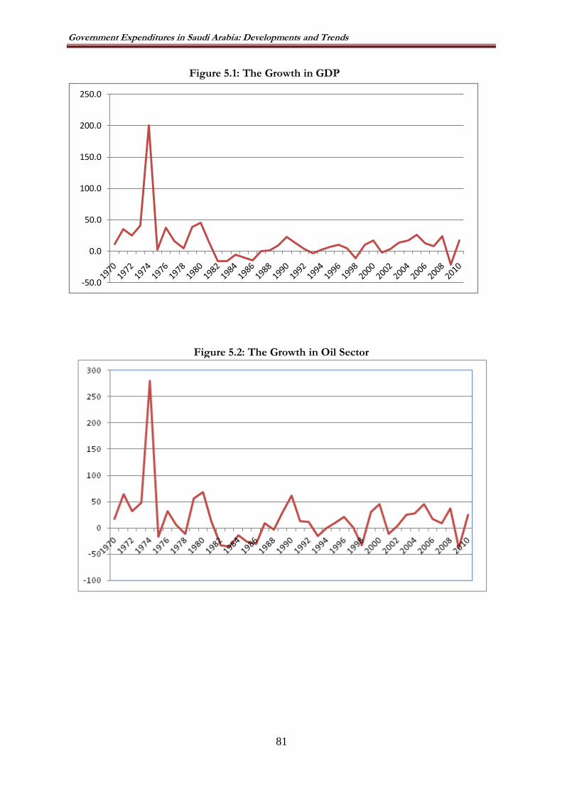
Government Expenditures in Saudi Arabia: Developments and Trends
81
Figure 5.1: The Growth in GDP
Figure 5.2: The Growth in Oil Sector
-50.0
0.0
50.0
100.0
150.0
200.0
250.0

Government Expenditures in Saudi Arabia: Developments and Trends
82
Figure 5.3: The Growth in Non-Oil Sector
Figure 5.4: The Growth of Total GDP, Oil Sector and Non Oil Sector
In sum, in terms of the consequences of economic policies of the Development Plans,
during the past development plans, including the first year of the ninth plan, the development
efforts of government resulted in the achievement of several significant economic and
developmental goals. These achievements were reflected in the increased rates of economic
growth, job opportunities, and facilitated diversified economic activities and development of
tangible and positive shifts in the economic structure. These accomplishments have manifested
themselves in the increased role of the private sector in production and investment activity, and
improved business conditions in the market economy, which were based on competition. For
the same period, the effectiveness and significance of economic, fiscal, monetary, investment and
-20
-10
0
10
20
30
40
50
60
70
80
90

Government Expenditures in Saudi Arabia: Developments and Trends
83
trade policies varied in line with the nature of the prevailing general conditions. For example,
during the First and Second Development Plans (1970-1979), which concentrated on laying
strong foundations for infrastructures, high public expenditure brought about the phenomenon
of price inflation, which peaked to reach 31.2% in (1976) as well as increased numbers of foreign
labour force personnel in the country. In the context, fiscal policy was adjusted in 1979 and 1980
when it was decided to stop increases in public expenditure.
It should be noted that government expenditure did, however, increase in the arena of
public labour training and work began on application of Saudi policy with the commencement of
the Fourth Development Plan's implementation process.
5.2.2. Human Development
While economic growth is related to the expanding capacity of the economy, economic
development includes also human development, which, according to the endogenous growth
theories, is an essential element of economic growth. Thus, development needs a focus beyond
economic growth. While economic growth is essential in generating income, human
development and well-being is also essential. With the recent changes in economic development
understanding, human development is now considered as essential. In other words, real
development is investment in human development, which in turn is society. In order to do this,
there is a significant body of opinion calling for newly re-examined plans for the overall
development of the state on the basis that such development plans are designed to, on an
objective basis, demonstrate that human development is paramount and that the development of
physical, economic and industrial infrastructures should emerge in concert with building a broad
base of human development and well-being. Mostly, industrialised countries have been
successful in invigorating their human development as well.
In reflecting the importance of human development as part of the development process,
Human Development Index or HDI was developed by UNDP, which is depended primarily on
a number of features of the human situation, the educational level, the social situation, family,
and other characteristics of the other population. HDI has become a standard for economic
development in terms of its human face, specifying that the new concept of development has a
close relationship to education (figure 5.5).
The Sixth Development Plan in Saudi Arabia (1995-2000:265) highlighted the
development of human resources as “the basic pillar for realising the objectives and aspirations
of the development process. This is attributed to the fact that education and training raise the
quality and productivity of the work force, as well as contributing to the cultural and personal
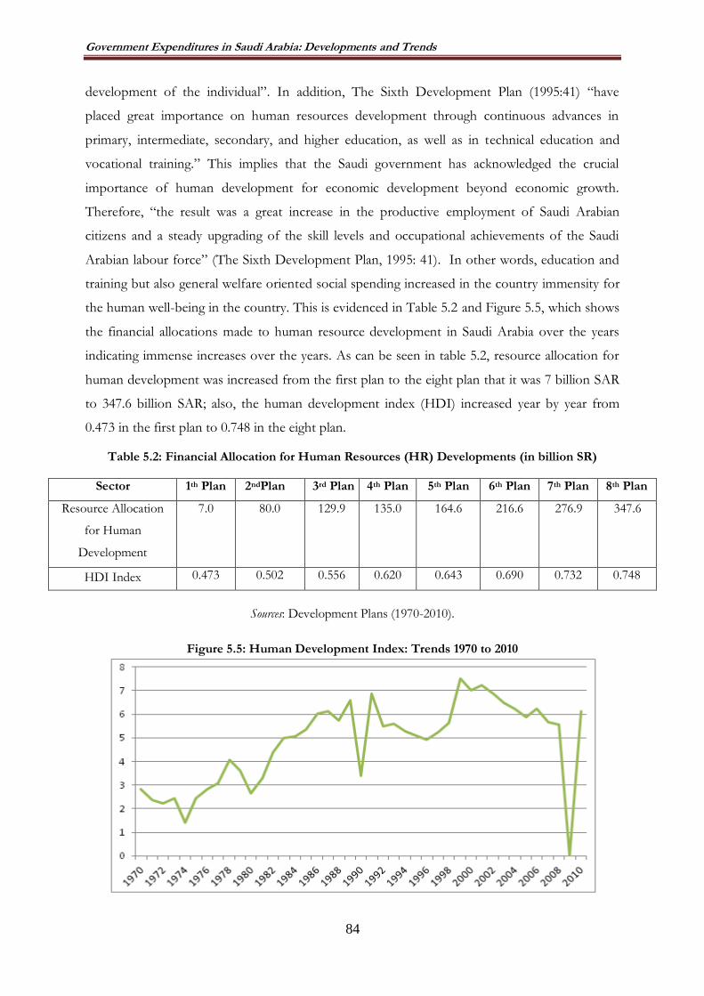
Government Expenditures in Saudi Arabia: Developments and Trends
84
development of the individual”. In addition, The Sixth Development Plan (1995:41) “have
placed great importance on human resources development through continuous advances in
primary, intermediate, secondary, and higher education, as well as in technical education and
vocational training.” This implies that the Saudi government has acknowledged the crucial
importance of human development for economic development beyond economic growth.
Therefore, “the result was a great increase in the productive employment of Saudi Arabian
citizens and a steady upgrading of the skill levels and occupational achievements of the Saudi
Arabian labour force” (The Sixth Development Plan, 1995: 41). In other words, education and
training but also general welfare oriented social spending increased in the country immensity for
the human well-being in the country. This is evidenced in Table 5.2 and Figure 5.5, which shows
the financial allocations made to human resource development in Saudi Arabia over the years
indicating immense increases over the years. As can be seen in table 5.2, resource allocation for
human development was increased from the first plan to the eight plan that it was 7 billion SAR
to 347.6 billion SAR; also, the human development index (HDI) increased year by year from
0.473 in the first plan to 0.748 in the eight plan.
Table 5.2: Financial Allocation for Human Resources (HR) Developments (in billion SR)
Sector 1th Plan 2ndPlan 3rd Plan 4th Plan 5th Plan 6th Plan 7th Plan 8th Plan
Resource Allocation
for Human
Development
7.0 80.0 129.9 135.0 164.6 216.6 276.9
347.6
HDI Index 0.473 0.502 0.556 0.620 0.643 0.690 0.732 0.748
Sources: Development Plans (1970-2010).
Figure 5.5: Human Development Index: Trends 1970 to 2010

Government Expenditures in Saudi Arabia: Developments and Trends
85
The development plans in Saudi Arabia have focused on creating opportunities to
increase economic growth and the financing of the development of public facilities and services
to improve the living standards of citizens. This is in line with the global trends, as “the structure
of government expenditure has thus shifted away from the provision of more traditional
collective goods (defence, public administration and economic services) towards those associated
with the growth of the welfare state (education, health and income maintenance), which provide
benefits on an individual rather than a collective basis and where redistributive objectives are
more important”, according to Saunders and Klau (1985:83).
5.2.3. Budgeted Expenditures in Saudi Arabia during the Development Plans.
The Saudi budget "classifies expenditures under four chapters. Chapters 1,2, and 3
include recurrent expenditures, and Chapter 4 includes capital expenditures. Within the first
three chapters, the composition has been relatively stable. Typically between 40% and 50% of
recurring expenditures is for Chapter 1, salaries. About 20% is allocated to Chapter 2, operating
expenses. The remainder, under Chapter 3, is for other expenditures" (Johany et.al, 1986:65). The
steps of "budget preparation" are following (Joharji, 2009:60-63):
1. Distribution of Budget guidelines by the Saudi Ministry of Finance.
2. Preparation of estimates by line ministries and department. The budget preparation
process starts in the line ministries and departments during the fourth month of the
fiscal year by forming an internal committee for budget preparation.
3. Submission of Budget proposal to the Ministry of Finance. The budget proposal is
typically submitted the Saudi Ministry of Finance by the deadline set in the budget
circular.
4. First sectoral negotiations of budget estimates. After receiving budget proposals
starts the review procedures and negotiation process with each line ministry or
department. The negotiation process normally takes place during August and
September.
5. First Draft of Budget review by Deputy Minister of Finance.
6. Second sectoral negotiations of budget estimates. The purpose of this round is to set
priorities for the government agencies’ requests if further reduction in the budget
estimates is needed.
7. Second Draft of Budget review by the Saudi Minister of Finance. Subsequently, a
second draft is prepared for the review by the Minister of Finance.

Government Expenditures in Saudi Arabia: Developments and Trends
86
8. Final Draft of Budget send to the council of the Ministries for submission and
approval
9. Royal approval of the budget. In this step the final approval by the Prime Ministers,
the King. This final stage normally takes place in the last two weeks of the fiscal year
and concludes with the announcement of the new budget.
When oil prices began to rise in 1970, actual revenue began to be higher than
expenditures. During the First development Plan (1970-1974), the high oil revenue helped to
increase government expenditure to the actual 75.5 billion SAR. the authorities continued to
present perfectly balanced budget. At the same time it was obvious that expenditures were
lagging far behind budgeted expenditures. Even more marked was the divergence between
expenditures and revenues. This situation was officially acknowledged in the first year of second
development plan (1975) budget.
In the Second Development Plan (1975-1979), oil revenues increased much more slowly.
At the same time , the economy was showing signs of overheating. Most obviously, the inflation
rate increased dramatically. The government followed policies which are typically prescribed for
such conditions by attempting to restrain expenditures. The government expenditure amounted
to about 684.4 billion SAR, an increase that was more than nine times that of government
expenditure in the first development plan.
During the Third Development Plan (1980-1984), the planned level of government
expenditures was 1200 billion SAR, which was nearly twice the value of actual expenditures
during the second development plan (684.4 billion SAR), both the price and quantity of oil rose
dramatically. In 1983 it was possible to reduce expenditures sufficiently that a small surplus was
realised, despite the substantial discrepancy between budget and actual revenue (Fourth
Development Plan, 1980).
The Fourth Development Plan, 1985-1989, saw a significant decrease in oil revenues due
to the impact of lower prices on the global market, reflected in a relative decline in total
government expenditure, to 802.1 billion SAR, contrasting with the planned 1,000 billion SAR.
This Plan focused on a new strategic direction aiming at increasing the profit generated by the oil
and natural gas sector. It also became clear that there was a need to focus on the petrochemical
industry, which has a great a comparative advantage for Saudi Arabia with high value-added.
(Fourth Development Plan, 1985).
In the Fifth Development Plan, 1990-1994, the government reduced the government
expenditure to faced the high expenditures in 1990 and 1991 regarding to Gulf War in those
years. The value of total government spending amounted to 1078.1 billion SAR mainly due to

Government Expenditures in Saudi Arabia: Developments and Trends
87
the increase in oil revenues. During the plan period, the balance of trade realised a surplus
averaging around 15.6% of GDP (Ministry of Economy and Planning, 2006).
The Sixth Development Plan stretching from 1995 to 1999 focused on strategic
directions in human resource development. The plan prioritised human resource development,
job creation, and implementation of a policy of privatisation, which also took a strategic
direction of increasing the proportion of the contribution of non-oil sectors (Sixth Development
Plan, 1995).
The Seventh Development Plan (2000-2004), in this plan the government tried to
intervene to push the economy by using the open economy policy.
The Eight Development Plan (2005-2009), the value of total government spending
amounted to 1784,4 billion SAR mainly due to the increase in oil revenues. The height of public
revenue in the first year of the Eighth Plan of Development was hitting 555 billion SAR
(Ministry of Economy and Planning, 2008).
"All the Development plans identify the aim of government intervention as being to raise
the standard of living and ensure equitable distribution of wealth and welfare of the citizenry.
Within the framework of national development planning, several problems affecting urban areas
were addressed" (Garba, 2004:13).
5.3. DEVELOPMENTS AND TRENDS IN GOVERNMENT EXPENDITURES IN
SAUDI ARABIA
As mentioned, Saudi Arabia is a late developmentalist country, which has witnessed the
heavy presence and intervention of state in the economy to finance economic growth and
development through the revenues raised from oil export. Being a rentier state together with
developmentalist state implies that government expenditures remains at the hearth of social and
human development, and constitutes the main locomotive for economic stimulus in the private
sector as well as conducting public sector economic activity. As a result, over the years, the
government expenditures have shown an upward trend in the economy in terms of its magnitude
and role.
In the case of the Saudi Arabian economy, thus, government expenditure increased in
the budget of the Kingdom from 6.4 billion SAR in 1970 to 8.3 billion SAR in 1971 and
multiplied by about five times in value by the end of the first development plan, up to 32 billion
SAR in 1974. Government expenditure continued to rise to 216.4 billion SAR in 1984, in order
to continue funding projects to improve education, health, housing, transportation, and
communications. The expenditure helped to support the programmes and projects of human
development and achievement of the growth objectives of the identified sectors in the plan. The

Government Expenditures in Saudi Arabia: Developments and Trends
88
total average annual growth rate in public expenditure during the actual development plan first
reached 49.5% and 42.5% and 2.8% in the second and third development plans. It was due to
growth in public expenditure during the first three development plans that many of the goals of
economic and social development were achieved, as the private capital accumulation was not
there to initiate a national economy. As a result, the size of the national economy has increased
and strengthened the capacities of new building of modern infrastructures in the key sectors of
transportation, communications, education, health, housing, agriculture and industry due to
government expenditures (Ministry of Economy and Planning, 2009).
As can be seen in Table 5.3, during the years of the Fourth Development plan, the
decline in the growth of public expenditure observed, which dropped to an average annual
capacity of 7.1%, which was the result of completion of most infrastructure projects during the
period. The expenditure for 1985 was about 184 billion SAR and fell to 149.5 billion SAR in
1989. However, 1990 and 1991 showed an increase in public expenditure and a moderate
decrease then rising in 2000 to 235.3 billion SAR and then increasing to 255.1 billion SAR in
2001 in the Seventh Development Plan. In 2003, public expenditure was about 257 billion SAR,
increasing in 2004 to 285.2 billion SAR. Public spending continued to rise in the first year of the
Eighth Development Plan, reaching 341 billion SAR (Ministry of Economy and Planning, 2008).
Regarding the components of public expenditure, the sector shares of total development
expenditure during the first plan for the development was 34.1 billion SAR, equivalent to 45.2%
of the total financial requirements of the plan. This rose to 347.2 billion SAR in the Second
Development Plan (Figure 5.6), constituting 50.7% of the total amount of the approved budget.
In the Third Development Plan, the value of the resources allocated to development was 625.2
billion SAR, or 51.6% of total public financial resources.
A better way of making meaning out of the increased government expenditures is the
traditional use of ratio of government expenditures to GDP, which is calculated in table 5.3 and
depicted in figure 5.6.

Government Expenditures in Saudi Arabia: Developments and Trends
89
Figure 5.6: Trends in the Share of Government Expenditure in GDP at Current Price
As can be seen in Table 5.3 and Figure 5.6 depending on the growth of GDP and the
growth rate of government expenditures, the ratio of government expenditures in GDP has not
shown secular trends but rather followed ups-and-downs. As can be seen, in 1970 the ratio was
about 15%, which decreased to 13.28% in 1973. However, with the enormous increases in the oil
revenues in 1974 after the first oil shock and increased GDP, the share of government
expenditures relatively fell to 8% despite showing an increase. However, increased oil revenues
encouraged government to develop infrastructure projects in line with the increased GDP and
therefore immediate adjustment witnessed in government expenditure with the share of
government expenditure increasing to 13.24% in 1975, which reached a pick at about 22.04% in
1978. However, in 1980 it declined to its lowest level14.42% since 1975 due to the global
recession as a result of oil prices. Immediately, in 1981 the increasing trend in the share of
government expenditures to GDP set in and reached to 27.04% in 1983. The declining trends in
the ratio were observed from 1984 to 1989, falling to 30.95% in 1989 only with a pick in 1987
with 32.18%. As can be seen in (Table 5.3) and (Figure 5.6), the impact of government
expenditures can immediately see in 1991 with the share of government expenditures in GDP
increasing to 32.32% . Since then, a decreasing trend observed in the ratio of government
expenditures to GDP until the present times. Immediately after the war, the ratio fell down to
about 27.56% and then followed a decreasing trend to 22.43% in 2009. In such a declining trend,
rather than government expenditures growth in absolute level declining, high increases in GDP
as the denominator due to the oil price plays an important role.
As can be seen in table 5.3, the growth of public expenditures was0.12 in 1971, which later
increased to 0.38in 1978. This trend continued, and in 1982 it was 0.13. In 1990 the decreasing
trend in the growth of government expenditures was0.09. Immediately after the war, the growth
of government expenditure fell down to about - 0.06 in 1994 and then increasing trend to 0.1 in
2010
0.00
5.00
10.00
15.00
20.00
25.00
30.00
35.00
Year
1971
1973
1975
1977
1979
1981
1983
1985
1987
1989
1991
1993
1995
1997
1999
2001
2003
2005
2007
2009

Government Expenditures in Saudi Arabia: Developments and Trends
90
Source: Ministry of Economy and Planning, (2010)
Table 5.3: Gross Domestic Product and Total Expenditure at Current Price
Year Current
GDP
The Growth of
current GDP
Government Expenditure
Government Expenditure
Growth
The Ratio of Government Expenditure/Current
GDP
1970 22,565 11.9 3,478 _ 0.15
1971 30,497 35.2 3,898 0.12 0.13
1972 38,259 25.5 4,621 0.185 0.12
1973 53,531 40.3 7,110 0.54 0.13
1974 159,719 200.3 12,321 0.73 0.08
1975 163,670 2.4 21,671 0.76 0.13
1976 225,347 37.6 34,513 0.59 0.15
1977 260,960 15.6 43,436 0.26 0.17
1978 272,267 4.2 60,020 0.38 0.22
1979 375,469 38.0 73,786 0.23 0.20
1980 546,603 45.7 78,841 0.07 0.14
1981 622,175 13.9 110,459 0.40 0.18
1982 524,197 -15.9 124,682 0.13 0.24
1983 445,210 -15.2 120,403 -0.03 0.27 1984 420,388 -5.7 115,159 -0.04 0.27
1985 376,319 -10.6 108,816 -0.06 0.29
1986 322,021 -14.4 101,057 -0.07 0.31
1987 320,932 -0.4 103,263 0.02 0.32
1988 330,518 1.5 92,823 -0.10 0.28
1989 357,065 8.7 110,498 0.19 0.31
1990 437,334 22.8 120,285 0.09 0.28
1991 491,852 12.7 158,980 0.32 0.32
1992 510,458 3.4 140,673 -0.11 0.28
1993 494,906 -3.1 122,879 -0.13 0.25
1994 503,054 1.9 115,102 -0.06 0.23
1995 533,504 6.3 118,483 0.03 0.22
1996 590,748 10.6 134,844 0.14 0.23
1997 617,902 4.6 151,043 0.12 0.24
1998 546,648 -11.9 144,993 -0.04 0.27
1999 603,589 10.7 148,892 0.03 0.25
2000 706,656 17.4 175,234 0.18 0.25
2001 686,296 -2.6 179,411 0.02 0.26
2002 707,067 3.0 175,438 -0.02 0.25
2003 804,648 13.8 188,398 0.07 0.23
2004 939,426 16.7 210,885 0.12 0.22
2005 1,182,514 26.1 257,190 0.22 0.22
2006 1,335,581 13.0 303,425 0.18 0.23
2007 1,430,547 8.0 314,768 0.04 0.22
2008 1.522.500 23.8 336,142 0.07 0.22
2009 1,614.453 -21.8 362,063 0.08 0.22 2010 1,629.998 16.7 398,352 0.10 0.24

Government Expenditures in Saudi Arabia: Developments and Trends
91
With respect to real GDP, table 5.4 depending on the growth of GDP and the growth
rate of government expenditures, the ratio of government expenditures in GDP has not shown
secular trends but rather followed ups-and-downs. As can be seen, in 1970 the ratio was about
13%, which decreased to 10% in 1973. However, with the enormous increases in the oil
revenues in 1974 after the first oil shock and increased GDP, the share of government
expenditures relatively increased to 13% despite showing an increase. However, increased oil
revenues encouraged government to develop infrastructure projects in line with the increased
GDP and therefore immediate adjustment witnessed in government expenditure with the share
of government expenditure increasing to 18% in 1975, which reached a pick at about 24% in
1978. However, in 1980 it increased but slowly to 25% since 1975 due to the global recession as
a result of oil prices. Immediately, in 1981 the increasing trend in the share of government
expenditures to GDP set in and reached to 39% in 1983. The declining trends in the ratio were
observed from 1984 to 1989, falling to 29% in 1988 only with a pick in 1987 with 36%. As can
be seen in (Table 5.4) and , the impact of government expenditures can immediately see in 1991
with the share of government expenditures in GDP decreasing to 29%. Since then, a decreasing
trend observed in the ratio of government expenditures to GDP until the present times.
Immediately after the war, the ratio increased to about 31% and then followed a increasing trend
to 37% in 2009.
The growth of public expenditures was 18.5% in 1971, which later increased to 33.5% in
1973. This trend continued, and in 1977 it was 8%. In 1990 the decreasing trend in the growth
of government expenditures was -2.5%. Immediately after the war, the growth of government
expenditure increased to about 1.9% in 1994 and then increasing trend to 1% in 2010 (Table
5.4).

Government Expenditures in Saudi Arabia: Developments and Trends
92
Table 5.4: Gross Domestic Product and Government Expenditure at Constant Price (1999=100)
Source: Ministry of Economy and Planning, (2010)
Year Real GDP The Growth of
Real GDP
Real Government Expenditure
Real Government Expenditure
Growth
The Ratio of Real Government
Expenditure/Real GDP
1970 174,469 11.35 22 -- 0.13
1971 203,960 16.90 24 18.5 0.12
1972 245,494 20.36 25 1.9 0.10
1973 301,154 22.67 30 33.5 0.10
1974 369,207 22.60 48 14.5 0.13 1975 37 3,307 1.11 66 5.4 0.18
1976 417,894 11.94 78 29.5 0.19
1977 440,704 6.89 80 8.0 0.18
1978 442,273 -0.99 107 -2.3 0.24
1979 485,366 9.74 122 -4.0 0.25 1980 517,283 6.58 129 -6.1 0.25
1981 542,093 4.80 167 -4.2 0.31
1982 485,570 -10.43 180 -1.3 0.37
1983 447,440 -7.85 176 -12.4 0.39 1984 433,793 -3.27 169 15.2 0.39
1985 408,474 -5.50 159 -4.2 0.39
1986 428,792 4.85 152 16.5 0.36
1987 412,670 -3.76 150 -0.4 0.36
1988 446,608 8.22 131 -15.6 0.29 1989 446,887 0.06 151 -7.2 0.34
1990 484,106 8.33 145 -2.5 0.30
1991 588,170 9.10 169 16.7 0.29
1992 552,625 4.63 168 6.6 0.31
1993 552,769 0.03 142 18.5 0.26 1994 556,448 0.67 132 1.9 0.24
1995 557,566 0.20 128 33.5 0.23
1996 576,433 3.38 150 14.5 0.26
1997 591,370 2.59 160 5.4 0.27
1998 608,141 2.83 158 -1.1 0.26 1999 603,589 -0.75 154 -2.8 0.26
2000 632,951 4.86 185 20.8 0.29
2001 636,417 0,55 189 0.4 0.30
2002 636,230 0.13 187 0.9 0.30 2003 686,037 7.66 198 5.6 0.29
2004 722,173 5.27 221 11.4 0.31
2005 762,277 5.55 250 12.9 0.33
2006 766,348 3.16 280 12.0 0.37
2007 802,211 2.02 286 2.4 0.36 2008 836,133 4.23 304 6.0 0.36
2009 836,938 0.10 307 1.0 0.37
2010 875,707 4.64 310 1.0 0.35

Government Expenditures in Saudi Arabia: Developments and Trends
93
5.4. GENERAL TRENDS IN GOVERNMENT REVENUES
The development of the public sector in developing countries is to a large extent seen in
terms of most economic activities of the state which tends to focus on the construction of
infrastructures, the provision of social services, and the regulation of foreign trade, and the
production of goods and services falling within the scope of the natural monopolies. This has
been the case for Saudi Arabia as well, which is mainly due to the increased the economic power
and influence of oil-producing countries as a result of rises in oil revenues. In other words, the
state is now involved in a larger set of economic activity and provides the structure of the
national economic activity. However, it is important that the role of government revenues should
be considered as an important determining factor of public expenditures in Saudi Arabia as well
as in other countries. Due to the enormous increases in public revenues, Saudi Arabian
government has managed to spend for the social and economic development of the economy.
The oil wealth was utilised by the Kingdom of Saudi Arabia since 1970sto provide the
financing power for the government to invest in infrastructure and structural projects, and the
establishment of institutions and public bodies to invest the resources of the state and its
components, which are not available in the private sector.
The first and the second development plans were characterised by a significant increase
in the general revenues under conditions on world oil markets and the increase in oil prices, with
the value of the total state revenues rising from 7.9 billion SAR in 1970 to 100.1 billion SAR in
1974, to 211.2 billion SAR in 1979. The average annual growth in revenues during the first
development plan was 77.6%, and reached 16.1% during the Second Development Plan. In the
third plan, world oil markets witnessed the negative changes that led to a decline in oil revenues
which fell by an average of -4.1% a year. Total income decreased from 348.1 billion in 1980 to
171.5 billion in 1984, and continued to decline during the years of the Fourth Development Plan,
as public revenue amounted to 133.6 billion SAR in 1985, then fell to 114.6 billion SAR in 1989.
There was an annual rate of decline of-7.7% during the plan period, and during the years of the
Fifth Development Plan, public revenues rose at an average annual rate of 2.4%, and then
continued to increase during the Sixth Development Plan at an annual average rate of 2.7%.
Income also recorded the highest increase since 1997 and amounted to 205.5 billion
SAR, which soon fell to 147.5 billion SAR in 1999. It rose in 2000 to 258.1 billion SAR at the
beginning of the Seventh Development Plan, a result of increased oil revenues, which amounted
to 214.4 billion SAR. In 2001, general revenue increased to 228.2 billion SAR, of which 183.9
billion SAR were from oil revenues. In the fourth year of the Seventh Development Plan in 2003
public revenue amounted to about 293 billion SAR and the percentage from oil revenues by

Government Expenditures in Saudi Arabia: Developments and Trends
94
78.8%. In the fifth year of the plan, 2004 revenue amounted to 392.3 billion SAR and the
proportion from oil revenues by 84.1% (table 5.5).
The height of public revenue in the first year of the Eighth Plan of Development was
hitting 555 billion SAR. With the increase in economic activity and expansion of the productive
base and services in the country, there have been increases in the value of public revenue from
other sources than oil (table 5.4); it has risen from 79.40 billion SAR in 1970 to about 171.50
billion SAR in 1984. It then started with some 392 billion SAR in 2004 and 564 billion SAR in
the first year of the Eighth Development Plan. This is due to the fluctuations that have occurred
in some items of income, such as customs revenue services, ports, airport charges and the sale of
real estate and rent, which since 1984 has declined significantly (Ministry of Economy and
Planning, 2008).
As can be seen in table 5.5, the growth of public revenue was 0.35 in 1971, which later
decreased to 0.04 in 1978. This trend continued, and in 1982 it was -0.16. In 1990 the increasing
trend in the growth of public revenue was 0.22. Immediately after the war, the growth of public
revenue fell down to about - 0.03 in 2001, and then increasing trend to 0.01 in 2010.
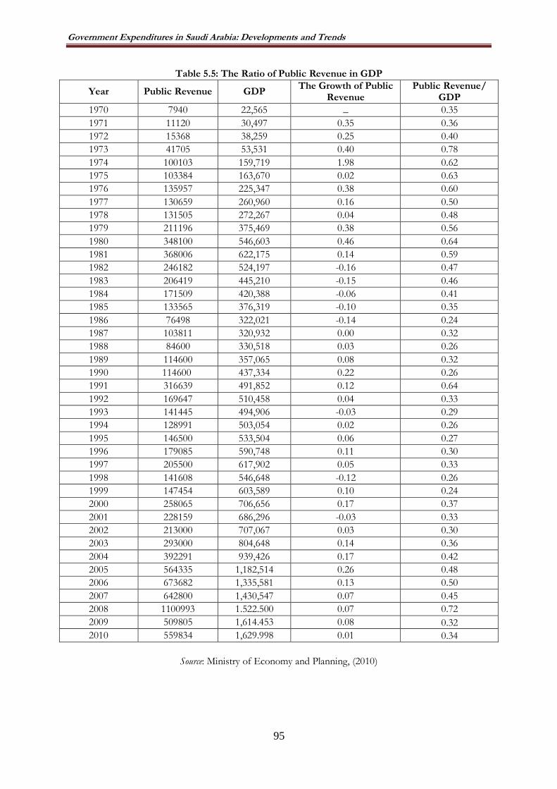
Government Expenditures in Saudi Arabia: Developments and Trends
95
Table 5.5: The Ratio of Public Revenue in GDP
Year Public Revenue GDP The Growth of Public
Revenue Public Revenue/
GDP 1970 7940 22,565 _ 0.35
1971 11120 30,497 0.35 0.36
1972 15368 38,259 0.25 0.40
1973 41705 53,531 0.40 0.78
1974 100103 159,719 1.98 0.62
1975 103384 163,670 0.02 0.63
1976 135957 225,347 0.38 0.60
1977 130659 260,960 0.16 0.50
1978 131505 272,267 0.04 0.48
1979 211196 375,469 0.38 0.56
1980 348100 546,603 0.46 0.64
1981 368006 622,175 0.14 0.59
1982 246182 524,197 -0.16 0.47
1983 206419 445,210 -0.15 0.46
1984 171509 420,388 -0.06 0.41
1985 133565 376,319 -0.10 0.35
1986 76498 322,021 -0.14 0.24
1987 103811 320,932 0.00 0.32
1988 84600 330,518 0.03 0.26
1989 114600 357,065 0.08 0.32
1990 114600 437,334 0.22 0.26
1991 316639 491,852 0.12 0.64
1992 169647 510,458 0.04 0.33
1993 141445 494,906 -0.03 0.29
1994 128991 503,054 0.02 0.26
1995 146500 533,504 0.06 0.27
1996 179085 590,748 0.11 0.30
1997 205500 617,902 0.05 0.33
1998 141608 546,648 -0.12 0.26
1999 147454 603,589 0.10 0.24
2000 258065 706,656 0.17 0.37
2001 228159 686,296 -0.03 0.33
2002 213000 707,067 0.03 0.30
2003 293000 804,648 0.14 0.36
2004 392291 939,426 0.17 0.42
2005 564335 1,182,514 0.26 0.48
2006 673682 1,335,581 0.13 0.50
2007 642800 1,430,547 0.07 0.45
2008 1100993 1.522.500 0.07 0.72
2009 509805 1,614.453 0.08 0.32 2010 559834 1,629.998 0.01 0.34
Source: Ministry of Economy and Planning, (2010)
Government Expenditures in Saudi Arabia: Developments and Trends
96
5.5. GOVERNMENT SOCIAL EXPENDITURES
The beginning of the modernisation the Kingdom of Saudi Arabia was highlighted by the
interest in the plans for human development, which is extremely important in the strategy for
overall economic and social development. The size of the many efforts and resources that have
made for the care and development of its citizens and improve living conditions reflect the
achievements made in this area during the past decades.
Considering the efforts made during the years of the Seventh Development Plan, and the
orientations of the Eighth Development Plan, this is an increasing concern. The development of
the capacity of citizens to improve living conditions is the basis for the development efforts, and
lives of individual citizens are considered as an instrument of development. Moreover, significant
progress can be measured in human development efforts, not only by the standards of local
historical comparison, but also by global standards, particularly those that have been presented in
the Human Development Reports of the annual international United Nations Development
Program (Ministry of Economy and Planning, 2006).
Development plans have made a qualitative leap in the levels of education, training,
health and social care reflected in many of the following indicators, for which developments and
trends (Table 5.6):
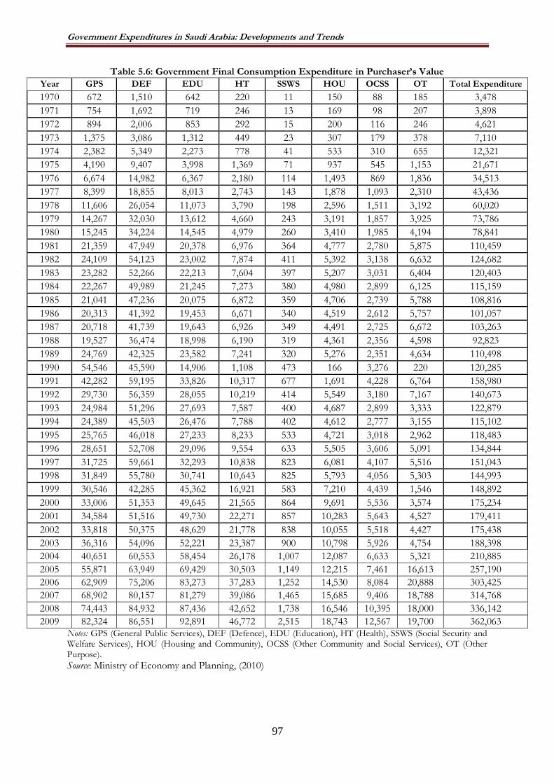
Government Expenditures in Saudi Arabia: Developments and Trends
97
Table 5.6: Government Final Consumption Expenditure in Purchaser’s Value
Year GPS DEF EDU HT SSWS HOU OCSS OT Total Expenditure
1970 672 1,510 642 220 11 150 88 185 3,478
1971 754 1,692 719 246 13 169 98 207 3,898
1972 894 2,006 853 292 15 200 116 246 4,621
1973 1,375 3,086 1,312 449 23 307 179 378 7,110
1974 2,382 5,349 2,273 778 41 533 310 655 12,321
1975 4,190 9,407 3,998 1,369 71 937 545 1,153 21,671
1976 6,674 14,982 6,367 2,180 114 1,493 869 1,836 34,513
1977 8,399 18,855 8,013 2,743 143 1,878 1,093 2,310 43,436
1978 11,606 26,054 11,073 3,790 198 2,596 1,511 3,192 60,020
1979 14,267 32,030 13,612 4,660 243 3,191 1,857 3,925 73,786
1980 15,245 34,224 14,545 4,979 260 3,410 1,985 4,194 78,841
1981 21,359 47,949 20,378 6,976 364 4,777 2,780 5,875 110,459
1982 24,109 54,123 23,002 7,874 411 5,392 3,138 6,632 124,682
1983 23,282 52,266 22,213 7,604 397 5,207 3,031 6,404 120,403
1984 22,267 49,989 21,245 7,273 380 4,980 2,899 6,125 115,159
1985 21,041 47,236 20,075 6,872 359 4,706 2,739 5,788 108,816
1986 20,313 41,392 19,453 6,671 340 4,519 2,612 5,757 101,057
1987 20,718 41,739 19,643 6,926 349 4,491 2,725 6,672 103,263
1988 19,527 36,474 18,998 6,190 319 4,361 2,356 4,598 92,823
1989 24,769 42,325 23,582 7,241 320 5,276 2,351 4,634 110,498
1990 54,546 45,590 14,906 1,108 473 166 3,276 220 120,285
1991 42,282 59,195 33,826 10,317 677 1,691 4,228 6,764 158,980
1992 29,730 56,359 28,055 10,219 414 5,549 3,180 7,167 140,673
1993 24,984 51,296 27,693 7,587 400 4,687 2,899 3,333 122,879
1994 24,389 45,503 26,476 7,788 402 4,612 2,777 3,155 115,102
1995 25,765 46,018 27,233 8,233 533 4,721 3,018 2,962 118,483
1996 28,651 52,708 29,096 9,554 633 5,505 3,606 5,091 134,844
1997 31,725 59,661 32,293 10,838 823 6,081 4,107 5,516 151,043
1998 31,849 55,780 30,741 10,643 825 5,793 4,056 5,303 144,993
1999 30,546 42,285 45,362 16,921 583 7,210 4,439 1,546 148,892
2000 33,006 51,353 49,645 21,565 864 9,691 5,536 3,574 175,234
2001 34,584 51,516 49,730 22,271 857 10,283 5,643 4,527 179,411
2002 33,818 50,375 48,629 21,778 838 10,055 5,518 4,427 175,438
2003 36,316 54,096 52,221 23,387 900 10,798 5,926 4,754 188,398
2004 40,651 60,553 58,454 26,178 1,007 12,087 6,633 5,321 210,885
2005 55,871 63,949 69,429 30,503 1,149 12,215 7,461 16,613 257,190
2006 62,909 75,206 83,273 37,283 1,252 14,530 8,084 20,888 303,425
2007 68,902 80,157 81,279 39,086 1,465 15,685 9,406 18,788 314,768
2008 74,443 84,932 87,436 42,652 1,738 16,546 10,395 18,000 336,142
2009 82,324 86,551 92,891 46,772 2,515 18,743 12,567 19,700 362,063 Notes: GPS (General Public Services), DEF (Defence), EDU (Education), HT (Health), SSWS (Social Security and Welfare Services), HOU (Housing and Community), OCSS (Other Community and Social Services), OT (Other Purpose).
Source: Ministry of Economy and Planning, (2010)

Government Expenditures in Saudi Arabia: Developments and Trends
98
5.5.1 Education Expenditures
There have been efforts and interest in development of education capacity in Saudi
Arabia, characterised by the development of human resources with continuing increases in the
number of schools and educational institutes and colleges for boys and girls, and the continuing
rise in the number of graduates and of undergraduates at different stages of development.
The importance of planning for development lies clearly in the development of human
resources - the basis of education - that give it a privileged position in terms of the objectives,
strategies and development plans initiated in 1970.It has increased and sustained allocations to
human resource development, especially after the establishment of a modern economy.
As can be seen in Table 5.5 and Figure 5.8, the state allocated 49,381 million SR in the
budget estimates for 1990/1991 for spending on education and training which represents a
48.2% proportion of the total approved expenditure for the services sectors and Development
(Figure 5.7).
Figure 5.7: The Expenditure of Education in Saudi Arabia
Figure 5.8: The Ratio of Education Expenditures in Government Expenditure in Saudi Arabia
0.00
2.00
4.00
6.00
8.00
10.00
12.00
14.00

Government Expenditures in Saudi Arabia: Developments and Trends
99
Figure 5.9: The Ratio of Expenditure of Education in GDP in Saudi Arabia
As can be seen in Table 5.7; Figure 5.8and Figure 5.9, in 1970 the ratio of education
expenditures in government expenditure was about 18.45%, which increased to 19.24% in 1986
and to 25.7% in 2010. Also, the ratio of education expenditures in GDP was about 8.24%,
which increased to 6.12% in 2010. By 1996 it had fallen to 4.9 per cent education spending has
remained relatively steady between 10 and 15 per cent for the past 40 years. In real terms, the
average annual increase in education spending between 1970 and 2010 was 4.3 per cent. Figure
5.8) shows that education spending remained almost steadily between 1970 and 1985, after which
it rose gradually until 1989, then fell very slightly, and has recently begun to increase at a faster
rate from 2007 to 2010 (Figure 5.9). However, increased oil revenues encouraged government to
develop the education sector in line with the increased GDP and therefore immediate
adjustment witnessed in government expenditure(Table 5.6).
0.00
0.02
0.04
0.06
0.08
0.10
0.12
0.14

Government Expenditures in Saudi Arabia: Developments and Trends
100
Table 5.7: The Ratio of Education Expenditures in Government Expenditure and GDP
Source: Ministry of Economy and Planning, (2010)
Year Educational
Expenditures
Government
Expenditure GDP
Education Expenditures/
Government Expenditures
Educational
Expenditures/GDP
1970 642 3,478 22,565 18.45888 2.845114
1971 719 3,898 30,497 18.44536 2.357609
1972 853 4,621 38,259 18.45921 2.229541
1973 1,312 7,110 53,531 18.45288 2.450916
1974 2,273 12,321 159,719 18.44818 1.423124
1975 3,998 21,671 163,670 18.44862 2.44272
1976 6,367 34,513 225,347 18.44812 2.82542
1977 8,013 43,436 260,960 18.44783 3.070586
1978 11,073 60,020 272,267 18.44885 4.066964
1979 13,612 73,786 375,469 18.44794 3.625333
1980 14,545 78,841 546,603 18.44852 2.660981
1981 20,378 110,459 622,175 18.44847 3.275284
1982 23,002 124,682 524,197 18.44853 4.388045
1983 22,213 120,403 445,210 18.44888 4.989331
1984 21,245 115,159 420,388 18.44841 5.053665
1985 20,075 108,816 376,319 18.44857 5.33457
1986 19,453 101,057 322,021 19.24953 6.04091
1987 19,643 103,263 320,932 19.0223 6.120611
1988 18,998 92,823 330,518 20.46691 5.747947
1989 23,582 110,498 357,065 21.34156 6.6044
1990 14,906 120,285 437,334 12.39224 3.408379
1991 33,826 158,980 491,852 21.27689 6.877272
1992 28,055 140,673 510,458 19.94341 5.496045
1993 27,693 122,879 494,906 22.5368 5.595608
1994 26,476 115,102 503,054 23.00221 5.263053
1995 27,233 118,483 533,504 22.98473 5.104554
1996 29,096 134,844 590,748 21.57753 4.925281
1997 32,293 151,043 617,902 21.38 5.226233
1998 30,741 144,993 546,648 21.20171 5.623546
1999 45,362 148,892 603,589 30.46638 7.515379
2000 49,645 175,234 706,656 28.33069 7.025342
2001 49,730 179,411 686,296 27.71848 7.246145
2002 48,629 175,438 707,067 27.71862 6.877566
2003 52,221 188,398 804,648 27.71845 6.489919
2004 58,454 210,885 939,426 27.71842 6.22231
2005 69,429 257,190 1,182,514 26.99522 5.871305
2006 83,273 303,425 1,335,581 27.44434 6.234964
2007 81,279 314,768 1,430,547 25.82188 5.681673
2008 87,436 336,142 1.522.500 26.01163 5.548821
2009 92,891 362,063 1,614.453 25.65603 5.753.713
2010 99.763 398,352 1,629.998 25.82504 6.120437

Government Expenditures in Saudi Arabia: Developments and Trends
101
5.5.2 Social Development and Health
Social development and health are foci and consistently feature in all the six five-year
plans implemented by the Saudi government.
As a result of the investment and higher support spending on development plans in the
development of social services and health sector, there has been the allocation of 3.5 billion SAR
to social development and health, which amounts to 10.3% of the total allocation plan (2005)
(Table 5.8). In the following development plan there was a higher allocation to social
development and health of 27.6 billion SAR, 8% of the total investments of the plan.
During the Third Development Plan, there was again a higher allocation to social
development and health reaching 61.9 billion SAR, or 9.8% of the total. In addition, the Fourth
Development Plan maintained the high rates of expenditure, accounting for funds allocated for
social sector development, health, of 61.9 billion SAR, or 17.7% of the total. This means that the
high share of these sectors rose to 50.7% of the total development in the Fourth Development
Plan. Moreover, in the fifth plan, the government spending as the allocation of social
development and health was 68 billion SAR, or 20% of the total, which would raise the share to
68% of the total investments for development. In the Sixth Development Plan, allocations
increased for social development and health to 87.5 billion SAR, or 20.8% of the total and,
therefore, these two sectors represent 72.3% of total investments allocated to the sectors of
development in the plan. Appropriations increased with the Seventh Development Plan’s
marked increase of the financing of human development and founded the basic education sector
and the financing of projects of social development and health, increasing again until it reached
approximately 21.5%.
The secular increase in health expenditures can be associated with a steady population
growth rate which is higher than population growth rates in most of the world, and the
considerable rise in the cost of health services which is found not just in the Kingdom but also
all over the world, all nations together paying an annual bill for health services estimated at two
trillion dollars. The trends in the health expenditures in Saudi Arabia can be seen in Figure 5.10.

Government Expenditures in Saudi Arabia: Developments and Trends
102
Figure 5.10: The Expenditure of Health in Saudi Arabia
As can be seen in Table 5.8; Figure 5.10and Figure 5.11, in 1970 the ratio of health
expenditures in government expenditure was about 6.32%, which increased to 19.24% in 1986
and to 25.7% in 2010. Also, the ratio of health expenditures in GDP was about 8.24%, which
increased to 6.12% in 2010. The ratio of health spending in government expenditure remained
almost steadily between 1970 and 1985, after which it rose gradually until 1996, then fell very
slightly, and has recently begun to increase at a faster rate from 1999 to 2010.
Figure 5.11: The Ratio of Health Expenditures in Government Expenditure in Saudi Arabia
0
10000
20000
30000
40000
50000
60000
0
2
4
6
8
10
12
14
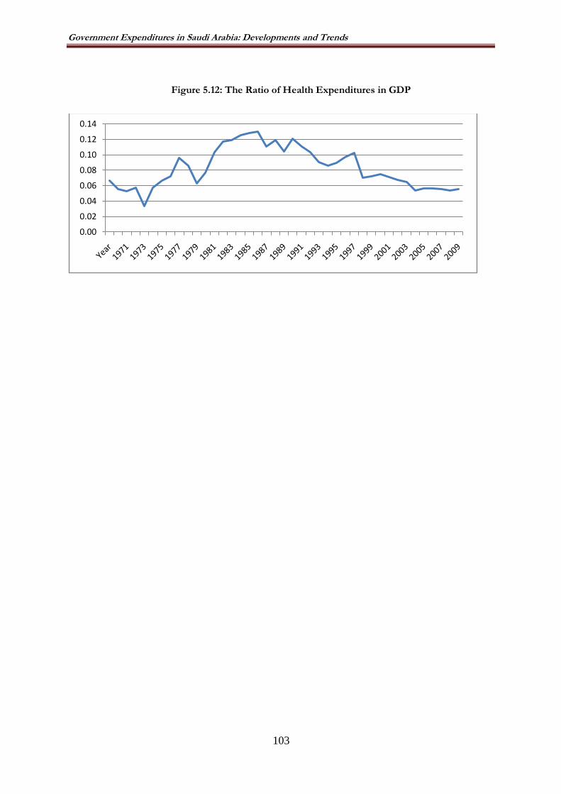
Government Expenditures in Saudi Arabia: Developments and Trends
103
Figure 5.12: The Ratio of Health Expenditures in GDP
0.00
0.02
0.04
0.06
0.08
0.10
0.12
0.14

Government Expenditures in Saudi Arabia: Developments and Trends
104
Table 5.8: Health Expenditures in Government Expenditure and GDP
Year
Health
Expenditures
Government
Expenditure GDP
Health
Expenditures/Government
Expenditures
Health
Expenditures/GDP
1970 220 3,478 22,565 6.325474 0.974961
1971 246 3,898 30,497 6.310929 0.806637
1972 292 4,621 38,259 6.318979 0.763219
1973 449 7,110 53,531 6.315049 0.838766
1974 778 12,321 159,719 6.314423 0.487105
1975 1,369 21,671 163,670 6.317198 0.836439
1976 2,180 34,513 225,347 6.31646 0.967397
1977 2,743 43,436 260,960 6.315038 1.051119
1978 3,790 60,020 272,267 6.314562 1.392016
1979 4,660 73,786 375,469 6.315561 1.241114
1980 4,979 78,841 546,603 6.315242 0.910899
1981 6,976 110,459 622,175 6.315465 1.121228
1982 7,874 124,682 524,197 6.315266 1.502107
1983 7,604 120,403 445,210 6.315457 1.707958
1984 7,273 115,159 420,388 6.315616 1.730068
1985 6,872 108,816 376,319 6.315248 1.82611
1986 6,671 101,057 322,021 6.601225 2.071604
1987 6,926 103,263 320,932 6.707146 2.15809
1988 6,190 92,823 330,518 6.668606 1.872818
1989 7,241 110,498 357,065 6.55306 2.027922
1990 1,108 120,285 437,334 6.921146 2.253353
1991 10,317 158,980 491,852 6.489496 2.097582
1992 10,219 140,673 510,458 7.264365 2.001928
1993 7,587 122,879 494,906 6.174367 1.533018
1994 7,788 115,102 503,054 6.766173 1.548144
1995 8,233 118,483 533,504 6.948676 1.543194
1996 9,554 134,844 590,748 7.085224 1.617272
1997 10,838 151,043 617,902 7.17544 1.754
1998 10,643 144,993 546,648 7.340354 1.946957
1999 16,921 148,892 603,589 11.36461 2.803398
2000 21,565 175,234 706,656 12.3064 3.051697
2001 22,271 179,411 686,296 12.4134 3.245101
2002 21,778 175,438 707,067 12.4135 3.080048
2003 23,387 188,398 804,648 12.41361 2.906488
2004 26,178 210,885 939,426 12.4134 2.786595
2005 30,503 257,190 1,182,514 11.8601 2.579504
2006 37,283 303,425 1,335,581 12.28739 2.791519
2007 39,086 314,768 1,430,547 12.4174 2.732242
2008 42,652 336,142 1.522.500 12.68869 2.81096!
2009 46,772 362,063 1,614.453 12.91819 2.89708
2010 53.661 398,352 1,629.998 13.01347 3.29209
Source: Ministry of Economy and Planning, (2010)
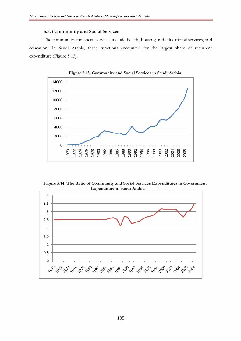
Government Expenditures in Saudi Arabia: Developments and Trends
105
5.5.3 Community and Social Services
The community and social services include health, housing and educational services, and
education. In Saudi Arabia, these functions accounted for the largest share of recurrent
expenditure (Figure 5.13).
Figure 5.13: Community and Social Services in Saudi Arabia
Figure 5.14: The Ratio of Community and Social Services Expenditures in Government Expenditure in Saudi Arabia
0
2000
4000
6000
8000
10000
12000
14000
1970
1972
1974
1976
1978
1980
1982
1984
1986
1988
1990
1992
1994
1996
1998
2000
2002
2004
2006
2008
0
0.5
1
1.5
2
2.5
3
3.5
4
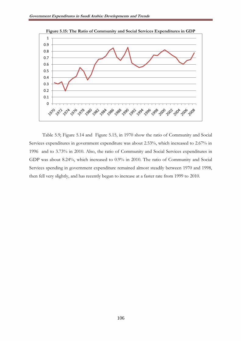
Government Expenditures in Saudi Arabia: Developments and Trends
106
Figure 5.15: The Ratio of Community and Social Services Expenditures in GDP
Table 5.9; Figure 5.14 and Figure 5.15, in 1970 show the ratio of Community and Social
Services expenditures in government expenditure was about 2.53%, which increased to 2.67% in
1996 and to 3.73% in 2010. Also, the ratio of Community and Social Services expenditures in
GDP was about 8.24%, which increased to 0.9% in 2010. The ratio of Community and Social
Services spending in government expenditure remained almost steadily between 1970 and 1998,
then fell very slightly, and has recently begun to increase at a faster rate from 1999 to 2010.
0
0.1
0.2
0.3
0.4
0.5
0.6
0.7
0.8
0.9
1

Government Expenditures in Saudi Arabia: Developments and Trends
107
Table 5.9: Community and Social Services Expenditure in Government Expenditure and GDP
Year
Community and Social Services
Expenditures
Government Expenditure
GDP
Community and Social Services
Expenditures/Government Expenditures
Community and Social Services
Expenditures/GDP
1970 88 3,478 22,565 2.53019 0.389984
1971 98 3,898 30,497 2.51411 0.321343
1972 116 4,621 38,259 2.510279 0.303197
1973 179 7,110 53,531 2.517581 0.334386
1974 310 12,321 159,719 2.51603 0.194091
1975 545 21,671 163,670 2.514882 0.332987
1976 869 34,513 225,347 2.517892 0.385627
1977 1,093 43,436 260,960 2.516346 0.418838
1978 1,511 60,020 272,267 2.517494 0.55497
1979 1,857 73,786 375,469 2.516738 0.494581
1980 1,985 78,841 546,603 2.517726 0.363152
1981 2,780 110,459 622,175 2.516771 0.44682
1982 3,138 124,682 524,197 2.516803 0.59863
1983 3,031 120,403 445,210 2.517379 0.680802
1984 2,899 115,159 420,388 2.517389 0.689601
1985 2,739 108,816 376,319 2.517093 0.72784
1986 2,612 101,057 322,021 2.58468 0.811127
1987 2,725 103,263 320,932 2.638893 0.84909
1988 2,356 92,823 330,518 2.538164 0.71282
1989 2,351 110,498 357,065 2.12764 0.658424
1990 3,276 120,285 437,334 2.723532 0.749084
1991 4,228 158,980 491,852 2.659454 0.859608
1992 3,180 140,673 510,458 2.260562 0.62297
1993 2,899 122,879 494,906 2.359231 0.585768
1994 2,777 115,102 503,054 2.412643 0.552028
1995 3,018 118,483 533,504 2.547201 0.565694
1996 3,606 134,844 590,748 2.674201 0.610413
1997 4,107 151,043 617,902 2.719093 0.664669
1998 4,056 144,993 546,648 2.797376 0.741977
1999 4,439 148,892 603,589 2.981356 0.735434
2000 5,536 175,234 706,656 3.159204 0.783408
2001 5,643 179,411 686,296 3.145292 0.82224
2002 5,518 175,438 707,067 3.145271 0.780407
2003 5,926 188,398 804,648 3.145469 0.736471
2004 6,633 210,885 939,426 3.145316 0.706069
2005 7,461 257,190 1,182,514 2.900968 0.630944
2006 8,084 303,425 1,335,581 2.66425 0.60528
2007 9,406 314,768 1,430,547 2.988233 0.657511
2008 10,395 336,142 1.522.500 3.092443 0.674328
2009 12,567 362,063 1,614.453 3.470943 0.778061
2010 14.873 398,352 1,629.998 3.733633 0.912551
Source: Ministry of Economy and Planning (2010)

Government Expenditures in Saudi Arabia: Developments and Trends
108
5.5.4 Social Security and Welfare
The growth of population and the associated welfare spending including social security
has resulted in increased government expenditures in Saudi Arabia, which is depicted in Figure
5.16.
Figure 5.16: The Expenditure of Social Security and Welfare Sector in Saudi Arabia
Figure 5.17: The Ratio of Social Security and Welfare Expenditures in Government Expenditure in Saudi Arabia
0
500
1000
1500
2000
1970
1972
1974
1976
1978
1980
1982
1984
1986
1988
1990
1992
1994
1996
1998
2000
2002
2004
2006
2008
Social Security and Welfare
0
0.1
0.2
0.3
0.4
0.5
0.6
0.7
0.8

Government Expenditures in Saudi Arabia: Developments and Trends
109
Figure 5.18: The Ratio of Social Security and Welfare Expenditures in GDP
As can be seen in Table 5.10; Figure 5.17and Figure 5.18, in 1970 the ratio of
Social Security and Welfare expenditures in government expenditure was about 0.316%,
which increased to 0.4% in 1995 and to 0.8% in 2010. Also, the ratio of Social Security
and Welfare expenditures in GDP was about 0.0487% in 1970, which increased to 0.9%
in 2010. However, increased oil revenues encouraged government to develop the Social
Security and Welfare sector in line with the increased GDP and therefore immediate
adjustment witnessed in government expenditure.
0
0.1
0.2
0.3
0.4
0.5
0.6

Government Expenditures in Saudi Arabia: Developments and Trends
110
Table 5.10: Security and Welfare Expenditure in Government Expenditure and GDP
Year
Social Security
and Welfare
Expenditures
Government
Expenditure GDP
Social Security and Welfare
Expenditures/
Government Expenditures
Social Security and
Welfare
Expenditures/GDP
1970 11 3,478 22,565 0.316274 0.048748
1971 13 3,898 30,497 0.333504 0.042627
1972 15 4,621 38,259 0.324605 0.039206
1973 23 7,110 53,531 0.323488 0.042966
1974 41 12,321 159,719 0.332765 0.02567
1975 71 21,671 163,670 0.327627 0.04338
1976 114 34,513 225,347 0.33031 0.050589
1977 143 43,436 260,960 0.32922 0.054798
1978 198 60,020 272,267 0.32989 0.072723
1979 243 73,786 375,469 0.329331 0.064719
1980 260 78,841 546,603 0.329778 0.047567
1981 364 110,459 622,175 0.329534 0.058504
1982 411 124,682 524,197 0.329639 0.078406
1983 397 120,403 445,210 0.329726 0.089171
1984 380 115,159 420,388 0.329979 0.090393
1985 359 108,816 376,319 0.329915 0.095398
1986 340 101,057 322,021 0.336444 0.105583
1987 349 103,263 320,932 0.337972 0.108746
1988 319 92,823 330,518 0.343665 0.096515
1989 320 110,498 357,065 0.289598 0.08962
1990 473 120,285 437,334 0.393233 0.108155
1991 677 158,980 491,852 0.42584 0.137643
1992 414 140,673 510,458 0.2943 0.081104
1993 400 122,879 494,906 0.325523 0.080823
1994 402 115,102 503,054 0.349255 0.079912
1995 533 118,483 533,504 0.449854 0.099906
1996 633 134,844 590,748 0.469431 0.107152
1997 823 151,043 617,902 0.544878 0.133193
1998 825 144,993 546,648 0.568993 0.15092
1999 583 148,892 603,589 0.391559 0.096589
2000 864 175,234 706,656 0.493055 0.122266
2001 857 179,411 686,296 0.477674 0.124873
2002 838 175,438 707,067 0.477662 0.118518
2003 900 188,398 804,648 0.477712 0.11185
2004 1,007 210,885 939,426 0.477511 0.107193
2005 1,149 257,190 1,182,514 0.446751 0.097166
2006 1,252 303,425 1,335,581 0.412623 0.093742
2007 1,465 314,768 1,430,547 0.465422 0.102408
2008 1,738 336,142 1.522.500 0.517043 0.132631
2009 2,515 362,063 1,614.453 0.69463 0.557803
2010 3,465 398,352 1,629.998 0.874352 0.913681
Source: Ministry of Economy and Planning, (2010)
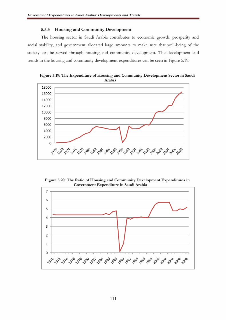
Government Expenditures in Saudi Arabia: Developments and Trends
111
5.5.5 Housing and Community Development
The housing sector in Saudi Arabia contributes to economic growth; prosperity and
social stability, and government allocated large amounts to make sure that well-being of the
society can be served through housing and community development. The development and
trends in the housing and community development expenditures can be seen in Figure 5.19.
Figure 5.19: The Expenditure of Housing and Community Development Sector in Saudi Arabia
Figure 5.20: The Ratio of Housing and Community Development Expenditures in Government Expenditure in Saudi Arabia
0
2000
4000
6000
8000
10000
12000
14000
16000
18000
0
1
2
3
4
5
6
7

Government Expenditures in Saudi Arabia: Developments and Trends
112
Figure 5.21: The Ratio of Housing and Community Development Expenditures in GDP
As can be seen in Table 5.11; Figure 5.20and Figure 5.21, in 1970 the ratio of
housing and community development expenditures in government expenditure was
about 4.31%, which increased to 4.7% in 1989 and to 5.1% in 2010. Also, the ratio of
housing and community development expenditures in GDP was about 0.66% in 1970,
which increased to 1.25% in 2010. However, increased oil revenues encouraged
government to develop the housing and community development sector in line with the
increased GDP and therefore immediate adjustment witnessed in government
expenditure.
0
0.2
0.4
0.6
0.8
1
1.2
1.4
1.6

Government Expenditures in Saudi Arabia: Developments and Trends
113
Table 5.11: The Ratio of Housing and Community Development Expenditure in Government Expenditure and GDP
Year
Housing and Community
Development Expenditures
Government Expenditure
GDP
Housing and Community Development
Expenditures/Government Expenditures
Housing and Community
Development Expenditures/GDP
1970 150 3,478 22,565 4.312823 0.664746
1971 169 3,898 30,497 4.335557 0.554153
1972 200 4,621 38,259 4.328068 0.522753
1973 307 7,110 53,531 4.317862 0.573499
1974 533 12,321 159,719 4.325948 0.333711
1975 937 21,671 163,670 4.323751 0.572493
1976 1,493 34,513 225,347 4.325906 0.662534
1977 1,878 43,436 260,960 4.323603 0.719651
1978 2,596 60,020 272,267 4.325225 0.953476
1979 3,191 73,786 375,469 4.324669 0.84987
1980 3,410 78,841 546,603 4.325161 0.623853
1981 4,777 110,459 622,175 4.324682 0.76779
1982 5,392 124,682 524,197 4.324602 1.028621
1983 5,207 120,403 445,210 4.324643 1.16956
1984 4,980 115,159 420,388 4.324456 1.18462
1985 4,706 108,816 376,319 4.324732 1.250535
1986 4,519 101,057 322,021 4.471734 1.403325
1987 4,491 103,263 320,932 4.349089 1.399362
1988 4,361 92,823 330,518 4.698189 1.319444
1989 5,276 110,498 357,065 4.774747 1.477602
1990 166 120,285 437,334 0.138006 0.037957
1991 1,691 158,980 491,852 1.063656 0.343803
1992 5,549 140,673 510,458 3.944609 1.087063
1993 4,687 122,879 494,906 3.814321 0.947049
1994 4,612 115,102 503,054 4.006881 0.9168
1995 4,721 118,483 533,504 3.984538 0.884904
1996 5,505 134,844 590,748 4.082495 0.931869
1997 6,081 151,043 617,902 4.026006 0.984137
1998 5,793 144,993 546,648 3.995365 1.059731
1999 7,210 148,892 603,589 4.842436 1.194521
2000 9,691 175,234 706,656 5.530319 1.371389
2001 10,283 179,411 686,296 5.731533 1.498333
2002 10,055 175,438 707,067 5.731369 1.422072
2003 10,798 188,398 804,648 5.731483 1.341953
2004 12,087 210,885 939,426 5.73156 1.286637
2005 12,215 257,190 1,182,514 4.749407 1.032969
2006 14,530 303,425 1,335,581 4.788663 1.087916
2007 15,685 314,768 1,430,547 4.983035 1.096434
2008 16,546 336,142 1.522.500 4.922324 1.100321
2009 18,743 362,063 1,614.453 5.176723 1.16095
2010 20.341 398,352 1,629.998 5.149466 1.25846
Source: Ministry of Economy and Planning (2010)

Government Expenditures in Saudi Arabia: Developments and Trends
114
5.5.6 General Government Services
The Government Services include all government offices. As can be seen in Figure 5.22
and table (5.5), in 1970, the expenditures for general government services were 672 SAR and it
has increased to 74,443 million SAR in 2008.
Figure 5.22: The Expenditure of General Government Services in Saudi Arabia
5.6 DEFENCE EXPENDITURES
Defence affairs are expenses related to the administration and operation of defence.
Considering the geo political importance of the Middle East and the Gulf region and the
instability associated with these regions, Saud Arabia has been investing in great amount for the
development of its defence and security forces. As mentioned previously, Gulf Wars had huge
impact and resulted in large burdens on Saudi Arabia’s budget.
As can be seen from Figure 5.23, defence affairs are expenses related to the
administration and operation of defence this amount to about 46,018 in 1995 increased to and
60,553 in the year 2004. This share increased in 1991 to 75.99% because of the effect of the
Gulf War one. The share of defence expenditure in GDP in Saudi Arabia was 13.7%, since 1971.
Defence expenditure has a large share of total government expenditure. According to statistical
report in Saudi Arabia, the annual average of defence expenditurefrom1970 to 2010 was around
46% of government expenditure (Table 5.12). The ratio of government spending on defence
fluctuated during 1990s. As we know the Gulf has witnessed three wars, which was a reason to
increase the expenditures of defence in the Gulf. .
0
10000
20000
30000
40000
50000
60000
70000
80000
1970
1972
1974
1976
1978
1980
1982
1984
1986
1988
1990
1992
1994
1996
1998
2000
2002
2004
2006
2008

Government Expenditures in Saudi Arabia: Developments and Trends
115
Figure 5.23: Defence Expenditures in Saudi Arabia
0.00
0.02
0.04
0.06
0.08
0.10
0.12
0.14
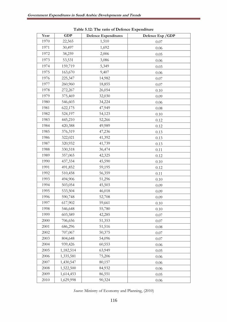
Government Expenditures in Saudi Arabia: Developments and Trends
116
Table 5.12: The ratio of Defence Expenditure
Year GDP
Defence Expenditures
Defence Exp /GDP
1970 22,565 1,510 0.07
1971 30,497 1,692 0.06
1972 38,259 2,006 0.05
1973 53,531 3,086 0.06
1974 159,719 5,349 0.03
1975 163,670 9,407 0.06
1976 225,347 14,982 0.07
1977 260,960 18,855 0.07
1978 272,267 26,054 0.10
1979 375,469 32,030 0.09
1980 546,603 34,224 0.06
1981 622,175 47,949 0.08
1982 524,197 54,123 0.10
1983 445,210 52,266 0.12
1984 420,388 49,989 0.12
1985 376,319 47,236 0.13
1986 322,021 41,392 0.13
1987 320,932 41,739 0.13
1988 330,518 36,474 0.11
1989 357,065 42,325 0.12
1990 437,334 45,590 0.10
1991 491,852 59,195 0.12
1992 510,458 56,359 0.11
1993 494,906 51,296 0.10
1994 503,054 45,503 0.09
1995 533,504 46,018 0.09
1996 590,748 52,708 0.09
1997 617,902 59,661 0.10
1998 546,648 55,780 0.10
1999 603,589 42,285 0.07
2000 706,656 51,353 0.07
2001 686,296 51,516 0.08
2002 707,067 50,375 0.07
2003 804,648 54,096 0.07
2004 939,426 60,553 0.06
2005 1,182,514 63,949 0.05
2006 1,335,581 75,206 0.06
2007 1,430,547 80,157 0.06
2008 1,522,500 84,932 0.06
2009 1,614,453 86,551 0.05
2010 1,629,998 90,324 0.06
Source: Ministry of Economy and Planning, (2010)

Government Expenditures in Saudi Arabia: Developments and Trends
117
5.7 TRANSFER EXPENDITURES
The development efforts of the Kingdom of Saudi Arabia include supporting the
government's economic activity, as well as private and social benefits through the development
plans that have been implemented. This support aims to strengthen the economic capacities of
individuals and social groups to assist in the generation of independence, and social benefits
aimed at improving the living standards of low income citizens. Development plans and financial
resources are provided for the granting of loans and social benefits for the beneficiaries.
The Kingdom of Saudi Arabia began to provide such subsidies in 1970, with 49 million
SAR, continuing to rise to the highest value in 1979, amounting to 12.9 billion SAR, dropping
subsequently to nearly 10.3 billion SAR in 2004 (Figure 5.24). Moreover, the first year of the
Eighth Development Plan saw government subsidies in 2005 of about 7.8 billion SAR (Eighth
Development Plan, 2005).
Figure 5.24: The Transfer Expenditure in Saudi Arabia
5.8 SOVERIGN WEALTH FUND (SWF)
Sovereign Wealth Funds (SWF) are government-owned investment funds composed
of financial assets such as stocks, bonds, property, metals or other financial instruments. This is
set up for a variety of macroeconomic purposes. They are commonly funded by the transfer of
foreign exchange assets that are invested long term, overseas. According to Greene and Yeager
(2008: 248) “a state-owned or influenced fund that obtains its funding from foreign-currency
reserves or commodity export revenues, through its certain instances, government budget
surpluses and pension surpluses have also been transferred to SWFs”.
SWFs are not new, and some of the longer-established funds, for example those of Saudi
Arabia, Kuwait, Abu Dhabi, and Singapore, have existed for decades. However, high oil prices,
financial globalization, and sustained, large global imbalances have resulted in the rapid
0
2
4
6
8
10
12
14
1970 -1974
1975 -1979
1980 -1984
1985 -1989
1990 -1994
1995 -1999
2000 -2004
2005 -2009

Government Expenditures in Saudi Arabia: Developments and Trends
118
accumulation of foreign assets particularly by oil exporters and several Asian countries. As a
result, the number and size of SWFs are rising fast and their presence in international capital
markets is becoming more prominent (Allen and Caruana, 2008).
Saudi Arabia, as one of the GCC countries, has been attempted to plan the economic
development utilising the finance provided by oil revenues accumulated in SWFs (Asutay, 2008).
As can be seen in Table 5.13, Saudi Arabia, with 5 SWFs, has some of the largest SWFs in the
total assets of SWFs in the GCC countries.
Table 5.13: Largest GCC SWFs by Assets under Management
Country Abbreviation Fund Name Assets (Billion Dollars) Inception Origin
United Arab Emirates
Abu Dhabi
ADIA Abu Dhabi
Investment Authority 627 1976 Oil
IPIC International
Petroleum Investment Company
48.2 1984 Oil
MDC Mubadala
Development Company
13.3 2002 Oil
ADIC Abu Dhabi
Investment Council X 2007 Oil
United Arab Emirates
Dubai ICD
Investment Corporation of Dubai
19.6 2006 Oil
United Arab Emirates
Ra's al Khaymah RIA
RAK Investment Authority
1.2 2005 Oil
United Arab Emirates –
Federal EIA
Emirates Investment Authority
X 2007 Oil
Saudi Arabia SAMA SAMA Foreign
Holdings 439.1 n/a Oil
Saudi Arabia PIF Public Investment
Fund 5.3 2008 Oil
Kuwait KIA Kuwait Investment
Authority 202.8 1953 Oil
Qatar QIA Qatar Investment
Authority 85 2003 Oil
Oman SGRF State General Reserve
Fund 8.2 1980
Oil & Gas
Oman OIF Oman Investment
Fund X 2006 Oil
Bahrain MHC Mumtalakat Holding
Company 9.1 2006 Oil
Total 1,458.8 (billion dollars)
Source: Compiled with data provided on SWF Institute website (http://www.swfinstitute.org/funds.php)

Government Expenditures in Saudi Arabia: Developments and Trends
119
SWFs are directly involved economic and financial investment and considering that they are
owned and regulated by the government, they should be incorporated into the government
growth measures as to develop a better understanding of the share of the government in the
economy. Since SWFs are not treated as part of the consolidated budget, it is important to
endogenous them in measuring the growth of government.
5.9 CONCLUSION
The preceding discussion and presentation shows that Saudi Arabian government has
extensively used government expenditures to improve the economic development of the country
and stimulate economic growth. The rentier nature of the society provides another important
motivation for the government of Saudi Arabia to extend the government expenditures;
however, economic development needs has also been an important determining factor.
One of the important findings that this chapter takes into account involves two
fundamental issues. First, there was the historical context of the development of the national
economy by the initiative of the government and its contributions to the productive sectors in it.
With the start of planning of economic and social development in 1970 with the First
Development Plan (1970-1974), and an increase in oil revenues in the third year of the plan, the
dependence on the crude oil sector has increased. However, policies and strategies are also
developed to increase production and investment in non-oil sectors, on the one hand, and to
increase the contribution of the private sector in economic growth and employment, on the
other. The second issue was linked to the development of oil resources and increased production
and export of oil in the race for development of other sectors.
In general, economic and development policies achieved further efficiency not only in
through better general economic stability internally and externally, which marked development
process over the past twenty-one years, but also in the execution of economic, social and
environmental infrastructure projects, as well as in the provision of better education, health and
environmental services to citizens. This has helped the expansion of economic activity and
acceleration of social development in general. Moreover, business conditions improved in the
market economy while efficiency performance has been enhanced in particular.
Accordingly, the government sector in the Kingdom established the foundations of
administration and economy, as they did not already exist, such as government departments,
public institutions, companies and governmental organisations, and government investments. In
addition, government involved in the development of the production activities of the public
sector in Saudi Arabia which is a major part of the overall GDP. The general climate of the Saudi
economy has improved markedly due to government investment and regulations through

Government Expenditures in Saudi Arabia: Developments and Trends
120
government expenditures and is expected to yield to government efforts aimed at improving the
investment climate and the state revenues derived from it in the future.

Modelling Government Growth and Economic Growth
121
CHAPTER 6 MODELLING GOVERNMENT GROWTH AND ECONOMIC GROWTH
NEXUS FOR SAUDI ARABIA
6.1. INTRODUCTION
As the preceding chapters demonstrated, the government expenditures play a vital role in the
economy and its growth in particular in the late developmentalist countries, which considered
government expenditures essential for economic development since the mid-20th century. It is due to
such reasons that the government expenditures are perceived by the developing countries as the
most essential instrument of the fiscal policy, which has gained importance for the decision-maker
to achieve the vision of the future of the structuring of economic policy.
As discussed previously, the Saudi Arabian economy depends on oil as the major source of
income, which is the main and essential source of financing the government and public
expenditures. The relationship between the Saudi business cycle and oil revenues is, therefore, very
strong, which means that if there is any change in this source of income, the rest of the economy
will be affected accordingly. This is true also for government expenditures, the level of which is
determined by the revenues mainly raised through oil export.
Similar to the case of any other developing nations, the Saudi government “has played a
pivotal role during the past [four] decades in economic development in the country. In addition to
providing infrastructure, establishing a modern educational system, and stabilising the economy,
the government has played a significant role in establishing large companies and reducing various
market distortions that would have worked against economic efficiency” (Albatel, 2003:82).
This chapter, hence, focuses on modelling of the government‟s growth and development in
Saudi Arabia after providing descriptive evidence for growth of government expenditures in Chapter
5. The first section in this chapter presents an overview of the Wagner Law; and then reviews all the
models derived and developed from Wagner‟s Law over the years. The second section, considers
the hypothesis; then the models derived and developed from the original Peacock and Wiseman
hypothesis are discussed and presented in econometric modelling. In doing so, all the variables are
identified and defined for the empirical work. In addition, the Keynesian Relation is examined and
the relevant modelling presented to show how the economic development and

Modelling Government Growth and Economic Growth
122
government expenditure has been modelled in the literature through aggregate supply modelling.
Since times series econometric modelling is used in this study throughout, in validating the models
tests such as Unit Root Tests, Co-integration Test, Granger Causality Tests and Error Correction
Model Test (ECM) are used which are presented in detail in this chapter.
6.2. MODELLING WAGNER’S LAW
Wagner‟s general hypothesis has provided scope for a range of different interpretations in
the existing literature. It is, consequently, possible to identify at least six of these interpretations:
Peacock and Wiseman (1961), Gupta (1967), Goffman (1968), Goffman and Mahar (1971), Pryor
(1968), Musgrave (1969), and Mann (1980). These models are depicted in Table (6.1)in a functional
form.
As discussed in the earlier chapter, there are significant differences arisen in these
interpretations of Wagner‟s Law, concerned primarily with issues that are discussed in an earlier
chapter, which includes the measurement of the economic variables in the hypothesis, the functional
form of the relationship between the key variables in Wagner‟s Law, and the nature of limits
to government growth.
Table 6.1: Six Versions of Wagner’s Law with Real GDP
No Function Version Year
1 L(GE) = α + β L(GDP) Peacock-Wiseman 1967
2 L(GEC) = α + β L(GDP) Pryor 1968
3 L(GE) = α + β L(GDP / P) Goffman 1968 4 L(GE/GDP) = α + β L(GDP / P) Musgrave 1969
5 L(GE/P) = α + β L(GDP / P) Gupta &Michas 1967 & 1975
6 L(GE/GDP) = α + β L(GDP) Mann 1980
In these formulations, the following variables are used (Table 6.2):

Modelling Government Growth and Economic Growth
123
Table 6.2: Definition of Variables
Variable Definition
The symbol (L) Natural logarithm
GE Total Government Expenditure
GEC Total Government Expenditure for consumption
GE / GDP The share of real total Government expenditure in real GDP
GE / P Total Government Expenditure per capita
GDP Gross Domestic Product
P Population
The different version of Wagner‟s law has been summarised by Mann (1980), Afxention and
Serletis (1996), and Demirbas (1999) in the use of „log-log models‟.
In conducting empirical analysis, some contributors have applied traditional regression
analysis, while others have used causality testing, and recently, co-integration analysis has appeared in
the literature. In searching for empirical validity, Wagner‟s Law has been analysed by many
researchers among others the following can be mentioned: Bird (1971), Krzyaniak (1974), Sahni and
Singh (1984), Abizadeh and gray (1985), Ram (1986, 1987), Henrekson (1992, 1993), Courakiset
al.(1993), Murthy (1993), Oxley (1994) and Ansari et al.(1997).
The six versions of Wagner‟s Law are briefly discussed in the following sub-sections with the
objective of constructing the their econometric model to test in this study for Saudi Arabia.
6.2.1. Peacock and Wiseman’s Version (1961) of Wagner’s Law
The Peacock and Wiseman explained and defined Wagner‟s Law, as “the proportion of
public expenditures to gross national product must be expected to rise over the foreseeable future”
(Peacock and Wiseman, 1961:10). Their interpretation, hence, states that the level of government
expenditure is a function of national income and can be expressed in the general relationship shown
in equation (6.1).
GE = f (GDP) f‟ > 0 & f‟‟ ≥ 0 (6.1)
where, GE represents total government expenditure, and GDP denotes Gross Domestic Product.
The logarithm form can be expressed in the following equation (6.2):
L(GE) = α + β L (GDP) + ϵ (6.2)
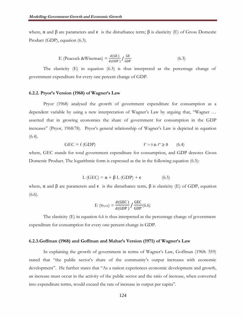
Modelling Government Growth and Economic Growth
124
where, α and β are parameters and ϵ is the disturbance term; β is elasticity (E) of Gross Domestic
Product (GDP), equation (6.3).
E (Peacock &Wiseman) = d(GE )
d(GDP )/
GE
GDP (6.3)
The elasticity (E) in equation (6.3) is thus interpreted as the percentage change of
government expenditure for every one percent change of GDP.
6.2.2. Pryor’s Version (1968) of Wagner’s Law
Pryor (1968) analysed the growth of government expenditure for consumption as a
dependent variable by using a new interpretation of Wagner‟s Law by arguing that, “Wagner …
asserted that in growing economies the share of government for consumption in the GDP
increases” (Pryor, 1968:78). Pryor‟s general relationship of Wagner‟s Law is depicted in equation
(6.4).
GEC = f (GDP) f‟ > 0 & f‟‟ ≥ 0 (6.4)
where, GEC stands for total government expenditure for consumption, and GDP denotes Gross
Domestic Product. The logarithmic form is expressed as the in the following equation (6.5):
L (GEC) = α + β L (GDP) + ϵ (6.5)
where, α and β are parameters and ϵ is the disturbance term, β is elasticity (E) of GDP, equation
(6.6).
E (Pryor) = d(GEC )
d(GDP )/
GEC
GDP(6.6)
The elasticity (E) in equation 6.6 is thus interpreted as the percentage change of government
expenditure for consumption for every one percent change in GDP.
6.2.3.Goffman (1968) and Goffman and Mahar’s Version (1971) of Wagner’s Law
In explaining the growth of government in terms of Wagner‟s Law, Goffman (1968: 359)
stated that “the public sector‟s share of the community‟s output increases with economic
development”. He further states that “As a nation experiences economic development and growth,
an increase must occur in the activity of the public sector and the ratio of increase, when converted
into expenditure terms, would exceed the rate of increase in output per capita”.

Modelling Government Growth and Economic Growth
125
Goffman‟s general relationship of Wagner‟s Law, hence, is depicted in equation (6.7).
GE = f (GDP / P) f‟ > 0 & f‟‟ ≥ 0 (6.7)
where, GE represents total government expenditure, P population, GDP represents Gross
Domestic Product and GDP/P stands for per capita GDP. The logarithm form is depicted in
equation (6.8):
L (GE) = α + β L (GDP/ P) + ϵ (6.8)
where, α and β are parameters and ϵ is the disturbance term, β is elasticity (E) of Gross Domestic
Product (GDP) per capita, equation (6.9).
E (Goffman) = d(GE )
d(GDP /P)/
GE
GDP /P (6.9)
The elasticity (E) in equation (6.9) is interpreted as the percentage change of government
expenditure for every one percent change in GDP/P.
6.2.4. Musgrave’s Version (1969) of Wagner’s Law
Musgrave (1969) investigated the validity of Wagner‟s law by looking at the ratio of
government expenditure relative to GDP per capita. He also explained the Wagner‟s law as follows:
“The proposition of expanding scale, obviously, must be interpreted as postulating a rising share of
the public sector in the economy; an absolute increase in the size of the budget can hardly fail to
result as the economy expands” (Musgrave, 1969:74).
Musgrave‟s conceptualisation of the general relationship between economic growth and
government expenditures in terms of Wagner‟s Law is depicted in equation (6.10).
GE / GDP = f (GDP / P) f‟ > 0 & f‟‟ ≥ 0 (6.10)
where, GE represents total government expenditure, P population, GDP represents Gross
Domestic Product, GE / GDP stands for the share of real total Government expenditure in real
gross domestic product and GDP / P stands for per capita GDP.
The logarithm form of equation 6.10 can be expressed as in equation (6.11):
L (GE / GDP) = α + β L (GDP/ P) + ϵ(6.11)

Modelling Government Growth and Economic Growth
126
where α and β are parameters and ϵ is the disturbance term, β is elasticity (E) of Gross Domestic
Product (GDP) per capita, equation (6.12).
The elasticity of government expenditures is estimated through equation (6.12), which implies the
percent change of the share of government expenditure in GDP for every one percent change in
GDP.
E (Musgrave) = d(GE /GDP )
d(GDP /P)/
GE /GDP
GDP /P (6.12)
6.2.5. Gupta’s Version (1967) of Wagner’s Law
Gupta (1967) explain the Wagner‟s Law by taking into account the relationship between
state activity and national income. Thus, according to Gupta (1967: 426) “Government expenditure
must increase at a rate faster than that of the national income”.
Gupta‟s general relationship of Wagner‟s law is depicted in equation (6.13).
GE / P = f (GDP / P) f‟ > 0 & f‟‟ ≥ 0 (6.13)
where, GE represents total government expenditure, P population, GDP represents Gross
Domestic Product, GE / P total Government expenditure in real gross domestic product and GDP
/ P stands for per capita GDP.
The logarithmic form can be expressed in the following form equation (6.14):
L (GE / P) = α + β L (GDP/ P) + ϵ (6.14)
where, α and β are parameters and ϵ is the disturbance term, β is elasticity (E) of Gross Domestic
Product (GDP) per capita, equation (6.15).
E (Gupta) = d(GE /P)
d(GDP /P)/
GE /P
GDP /P (6.15)
The elasticity (E) of government expenditure growth is estimated through equation (6.15),
the result of which is interpreted as the percent change of real government expenditure for every
one percent change of real GDP or GDP/P.

Modelling Government Growth and Economic Growth
127
6.2.6. Mann’s Version (1980) of Wagner’s Law
Mann (1980) analyzed the Mexican case over the period from 1925 to 1976 within Wagner‟s
Law by using six different formulations of the Law. Mann modified the Peacock and
Wiseman interpretationand called it „a structural version of Wagner‟s law‟. Thus, Mann (1980)
interpreted the Wagner‟s Law by considering that the share of public expenditure in national income
should increase at a rate higher than the rate of increase in national income. Mann‟s formulation of
Wagner‟s law translates into the functional relationship of Wagner‟s law as depicted in equation
(6.16).
GE / GDP = f (GDP) f‟ > 0 & f‟‟ ≥ 0 (6.16)
where, GE represents total government expenditure, P population, GDP represents Gross
Domestic Product, GE / GDP stands for the share of real total Government expenditure in real
gross domestic product.
Equation (6.17) expresses the logarithm form:
L (GE / GDP) = α + β L (GDP) + ϵ (6.17)
where, α and β are parameters and ϵ is the disturbance term, β is elasticity (E) of Gross Domestic
Product (GDP).
The coefficient of the independent variable in 6.17 gives the estimates of the elasticity, which
is calculated as in equation (6.18), which shows that the impact of one percent change in national
income on the share of government expenditures in the national income.
E (Mann) = d(GE /GDP )
d(GDP )/
GE /GDP
GDP (6.18)
6.3. MODELLING PEACOCK AND WISEMAN’S DISPLACEMENT HYPOTHESIS
After Wagner‟s Law in explaining the growing government in economy, Peacock and
Wiseman (1961) offered a working hypothesis to explain the fluctuations in
government expenditure over time, which emphasised the pattern of public expenditure trends
(Peacock and Wiseman, 1961; xxiii). According to the Peacock and Wiseman‟s hypothesis,
government expenditure tends to grow in a step like pattern, coinciding with social upheavals,

Modelling Government Growth and Economic Growth
128
notably wars. To support its explanatory power, Brown and Jackson (1990:123) noted, “Peacock and
Wiseman‟s study is probably one of the best-known analyses of the time pattern of public
expenditure”. The upward shift in government expenditures due to social upheaval is associated
with people‟s willingness and readiness to pay for the financing of the social upheaval including the
wars. As during such periods, it is argued that people‟s tolerable level of paying tax increases.
The pattern observed in government expenditures is further explained through the „rachet
effect‟. Bird (1972) argued that in the case of the ratchet effect, if Gross National Product or GNP
declines, then the government expenditure declines, but less than GNP. In addition, in explaining
and specifying the ratchet effect, he argued that crises are likely to have short-term implications for
the government expenditure ratio or E/GNP rather than crises leading to
a permanent upward displacement for E/GNP. In other words, after the social upheaval ceases, it
is argued that either government expenditures does not go back to its initial level before the
beginning of the social upheaval or if it does decreases, it does not decrease as much as the decrease
in the GNP. This is explained through government‟s ongoing exploitation of the increased tolerable
level of tax payment of the citizens. It should also be noted that Henrekson (1992) argued that the
E/GNP have a reduction in the short run in times of unexpectedly rapid GNP growth.
Gupta (1967) may be the first to formulate rigorous statistical tests for a displacement effect,
separately testing for a shift in the government expenditure level which is associated with the change
in the income elasticity of government expenditure with relation to economic growth.
To test the „displacement effect‟, Gupta adopted a double logarithmic functional form,
which is depicted in equation (6.19).
(GE/ P) = a + b (GNP/ P) (6.19)
Gupta‟s logarithmic form gives a constant elasticity score for the variable (GE/P) with
respect to the right hand side variable (GNP/P).Gupta shifted the original formulation adopted by
Peacock and Wiseman, because the original formulae can only explain shifts in the level of public
expenditure during wars and crises but cannot explain the shift in the level of public expenditure
during a depression since taxes are reduced in this period.

Modelling Government Growth and Economic Growth
129
6.4. MODELLING KEYNESIAN RELATION IN EXPLAINING GOVERNMENT EXPENDITURES AND ECONOMIC GROWTH NEXUS
As mentioned earlier, Wagner (1893) formulated and expressed his observation that the
public sector expanded with income growth. This relationship resulting from economic growth leads
to structural changes in the economic and social relations of society, and to the growth in aggregate
demand. In other words, government expenditures as part of fiscal policy result in expanding
economic activity. Therefore, during recession times, in the past, government expenditures used as
a stimuli to increase the economic activity in such circumstances. In a consequential manner,
increased business activity generates further revenues for government, which, in turn, provides
further opportunity space for the expansion of government.
In addition, Michas (1975) suggests that in the relationship between
government expenditure and GDP per capita, where this relationship assumes that the income
elasticity is positive, and that for the relationship itself as well as his proposal to Wagner Law to be
valid, there must be a uni-directional causal relationship from income to government
expenditure. There also needs to be a causal relationship in the opposite direction of any of the
share of government spending and GDP per capita, which corresponds with Keynesian approach to
macroeconomic policies. Recalling that, the multiplier concept in all Keynesian models is based on
this particular aspect of public expenditure. In sum, the Keynesian relation is therefore is closely
associated with growing government expenditures, which implies that as per capita income increases,
public sector‟s importance will grow (Bird, 1971:2).
6.5. IDENTIFICATION OF THE EMPIRICAL MODELS AND DATA
This study aims to model and examine the relationship between increasing government
expenditures and economic growth in Saudi Arabia for the period of 1968-2010. For this, time series
data and modelling is utilised to examine the mentioned relationship between
government expenditure and economic growth.
This study, thus, considers the 43 years period being sufficient to examine the defined
relationship between the variables described in table 6.1 above. For the purpose of this research,
mainly secondary data collected from various sources are utilised. There are four main sources
of data:
International Financial Statistics produced by the World Bank (IFS);

Modelling Government Growth and Economic Growth
130
SAMA: Saudi Arabia Monetary Agency;
The Ministry of Economy and Planning;
International Monetary Fund (IMF)
In the case of Saudi Arabia, the three models as discussed in the preceding sections are
tested, the specification of which explained in the following sections. It should be noted that each
model is tested with oil and non-oil GDP to locate and remove the impact of oil, respectively. This
provides a comparative case for capturing the impact of oil, which is the essential source of revenue.
6.5.1. Wagner’s Law and Its Variants
In testing the variants of the Wagner‟s Law, initial the non-oil GDP as explained in Table (6.3) is
used.
Table 6.3: Six Versions of Wagner’s Law with Non-Oil Sector of Real GDP
No Version Function Year
1 Peacock-Wiseman L(GE) = α + β L(Non-Oil GDP) 1967
2 Pryor L(GEC) = α + β L(Non-Oil GDP) 1968
3 Goffman L(GE) = α + β L(Non-Oil GDP / P) 1968 4 Musgrave L(GE/Non-Oil GDP) = α + β L(Non-Oil GDP / P) 1969
5 Gupta &Michas L(GE/P) = α + β L(Non-Oil GDP / P) 1967 & 1975
6 Mann L(GE/Non-Oil GDP) = α + β L(Non-Oil GDP) 1980
The research also utilises the oil sectors included GDP in searching for the growth of
government in Saudi Arabia by using the identified models in Table (6.1). These new formulations
are presented in Table (6.4).
Table 6.4: Six Versions of Wagner’s Law with Oil Sector of Real GDP
No Function Version Year
1 L(GE) = α + β L(Oil GDP) Peacock-Wiseman 1967
2 L(GEC) = α + β L(Oil GDP) Pryor 1968
3 L(GE) = α + β L(Oil GDP / P) Goffman 1968
4 L(GE/Oil GDP) = α + β L(Oil GDP / P) Musgrave 1969 5 L(GE/P) = α + β L(Oil GDP / P) Gupta &Michas 1967 & 1975
6 L(GE/Oil GDP) = α + β L(Oil GDP) Mann 1980

Modelling Government Growth and Economic Growth
131
6.5.2. Peacock and Wiseman Models
To test the „displacement effect‟ in Saudi Arabia, Gupta‟s (1967) as well as Michas‟s (1975)
double logarithmic functional form as depicted in the Table (6.5) and (6.6) is utilised. The
„displacement effect‟ is tested by reversing the Peacock-Wiseman version of Wagner‟s Law with oil
and non-oil GDP.
Table 6.5: The Original Version of Peacock-Wiseman Hypothesis with Real GDP
Function Version Year
L(GE) = α + β L(GDP) Peacock-Wiseman 1967
Table 6.6: Peacock-Wiseman Hypothesis with Non-Oil Sector Real GDP
Function Version Year
L(GE) = α + β L(Non-Oil GDP) + e Peacock-Wiseman 1967
In order to find whether there is a structural break between the two periods the observations from
1968 to 2010 were divided into two groups: from 1968 to 1989 and from 1990 to 2010.There are
several reasons for the choice of these years, which attempt to associate variations to major
economic and political event in Saudi Arabia during 1968 to 2010. After the 1973 oil shock, prices of
oil continuedrising -the oil boom began in 1974 - until early 1980‟s, expanding the government
growth in Saudi economy. In the 1976‟s the Saudi economy suffered high inflation as part of the
lagged impact of high spending resulting from oil shocks.
The world recession after 1978 and also Saudi Arabia‟s support for Iraq in its war against
Iran resulted in fiscal difficulties, as on the one had spending patter was very high, on the other
hand, oil revenues were affected. It should be noted that mega projects undertaken during those
years contributed to increased government expenditures and fiscal crisis. The decrease in oil process
in 1986, and in the 1990 Iraqi invasion of Kuwait and the war aftermath did not help to the trend in
Saudi Arabian government‟s budget. Later, in 1998, due to the decline in oil prices in 1998, Saudi
Arabia experienced its first major slowdown in economic growth since 1995, after the first Gulf
War.
From 1999 to 2001, Saudi economy was a major player in OPEC in influencing the price of
oil, because of that, government expenditure increased for education and other social sectors. In
2005, King Abdullah bin Abdul-Aziz became the King of Saudi Arabia, whose aggregate demand

Modelling Government Growth and Economic Growth
132
increasing policies pushed increasing government expenditure on the all sectors in Saudi economy.In
the recent past, five years of high oil prices from 2006 to 2010 helped the Saudi economy, but falling
oil prices and the global economic slowdown in particular since mid-2008 have severely affected
economic growth adversely.
The two periods (1968-1990 and 1991-2010), includes many significant economic and
political development for Saudi Arabia, but also this break marks the adoption of economic
liberalisation policies in Saudi Arabia, as the country followed the suit in 1990s in liberalising its
economy and financial sector, but also expressed commitment, hence, to reduce the size of the
government. Thus, thus, provides justification for structural break analysis.
In testing the potential structural breakdown in the government expenditure trend, the
Chow-test is calculated, which is a version of F- test(Equation 6.20):
knRSSRSS
kRSSRSSRSSF c
2/)(
/)(
21
21
(6.20)
The following hypotheses are developed to search for structural break due to the social
upheaval or war:
H0:βi = 0; (There is no structural break )
H1: β1 ≠ 0; (There is a structural break )
In addition, dummy variable is used to test for the structural break, which proves to be
superior over the Chow test to test for structural stability. The dummy variables were set equal to
zero for all observations except the year in which the observation goes beyond the threshold of two
standard errors. In these years, the dummy variable takes on the value of 1. However, firstly, the
Chow test applied to test for structural stability using the formula already defined in equation (6.20).
Y=αt + β1 Xi+ β2 D i + e (6.21)
whereβ = Parameter, D = Dummy Variables, y = year
The dummy variable considered in this study as the intercept dummy variable, as dummy
variables can be used to model changes in the slope of the regression line, which is known
as slope or interaction dummy variables as modelled in equation 6.21.

Modelling Government Growth and Economic Growth
133
6.5.3. Modelling Keynesian Relation
The Keynesian view postulates that government expenditure as the main component of
fiscal policy instrument can affect growth. Hence, in the original formulation, the causality runs from
government expenditure to economic growth, as explained in equation (6.22).
Yt = f xt + et (6.22)
In this study, if
Yt = ln(GDP)and, xt = ln(GE) then:
Ln (GDP) = αt + ln (GE) +et (6.23)
where GE stands for total government expenditures, GDP denotes GDP, and E is the standard
error.
The Keynesian relation is tested by reversing the three versions of Wagner‟s Law. Recall
three related versions of Wagner‟s Law as expressed in Table (6.7):
Table 6.7: The original Three Versions of Wagner’s Law No Function Version Year
1 L(GE) = α + β L(GDP) +e Peacock-Wiseman 1967
2 L(GE) = α + β L(GDP / P) + e Goffman 1968 3 L(GE/P) = α + β L(GDP / P) + e Gupta &Michas 1967 & 1975
Accordingly, table (6.8) presents the Keynesian Relations versions with real GDP:
Table 6.8: Three Versions of Keynesian Relations with Real GDP
No Function Version Year 1 L(GDP) = α + β L(GE) + e Peacock-Wiseman 1967
2 L(GDP/P) = α + β L(GE) + e Goffman 1968
3 L(GDP/P) = α + β L(GE/ P) + e Gupta &Michas 1967 & 1975
In addition, non-oil GDP is modelled as in Table (6.9) to test the variants of Keynesian
Relations.
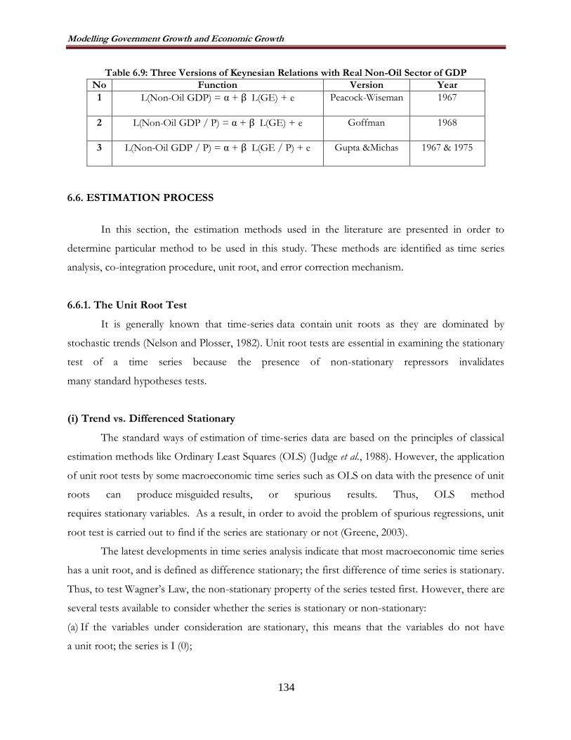
Modelling Government Growth and Economic Growth
134
Table 6.9: Three Versions of Keynesian Relations with Real Non-Oil Sector of GDP
No Function Version Year 1 L(Non-Oil GDP) = α + β L(GE) + e Peacock-Wiseman 1967
2 L(Non-Oil GDP / P) = α + β L(GE) + e Goffman 1968
3 L(Non-Oil GDP / P) = α + β L(GE / P) + e Gupta &Michas 1967 & 1975
6.6. ESTIMATION PROCESS
In this section, the estimation methods used in the literature are presented in order to
determine particular method to be used in this study. These methods are identified as time series
analysis, co-integration procedure, unit root, and error correction mechanism.
6.6.1. The Unit Root Test
It is generally known that time-series data contain unit roots as they are dominated by
stochastic trends (Nelson and Plosser, 1982). Unit root tests are essential in examining the stationary
test of a time series because the presence of non-stationary repressors invalidates
many standard hypotheses tests.
(i) Trend vs. Differenced Stationary
The standard ways of estimation of time-series data are based on the principles of classical
estimation methods like Ordinary Least Squares (OLS) (Judge et al., 1988). However, the application
of unit root tests by some macroeconomic time series such as OLS on data with the presence of unit
roots can produce misguided results, or spurious results. Thus, OLS method
requires stationary variables. As a result, in order to avoid the problem of spurious regressions, unit
root test is carried out to find if the series are stationary or not (Greene, 2003).
The latest developments in time series analysis indicate that most macroeconomic time series
has a unit root, and is defined as difference stationary; the first difference of time series is stationary.
Thus, to test Wagner‟s Law, the non-stationary property of the series tested first. However, there are
several tests available to consider whether the series is stationary or non-stationary:
(a) If the variables under consideration are stationary, this means that the variables do not have
a unit root; the series is I (0);

Modelling Government Growth and Economic Growth
135
(b) If the variables under consideration are non-stationary in its level form but stationary in its first-
difference form, the variables do have a unit root, the series is I (1). As Maddala and Kim (1998)
states then according to the null hypothesis there is a unit root in the variable and the series has first-
degree integration. Therefore, there is a need to conduct unit root analysis.
(ii) Unit Root Analysis
The most widely used Unit Root analysis tests are Dickey-Fuller (DF) and Augmented
Dickey-Fuller (ADF) (1981) tests. ADF test is performed by estimating the following equation
(6.24):
∆ Yt = a0 + a1t + a2Yt−1 + aiki=1 Yt−1 + et (6.24)
where ∆ Y = the first difference of the series; Yt = is the series under consideration (GDP,
government expenditures, or government revenues); t is the time trend, k is the number of lag and
et is a stationary random error (white noise residual).
According to Charemza and Deadman (1992: 135) “the practical rule for establishing the
value of [φ] ... is that it should be relatively small in order to save degrees of freedom, but large
enough not to allow for the existence of autocorrelation inet . For example, if for [φ] =2 the
Durbin-Watson autocorrelation statistic is low, indicating first order autocorrelation, it would be
sensible to increase m with the hope that such autocorrelation will disappear”.
The simple formula in Dickey-Fuller tests establish whether β = 1 in the model (6.25):
Yt = βYt−1+ et (6.25)
By deductingYt−1from each side of the equation in re-writing (6.25), the following form is
established:
∆Yt = Ω Yt−1+ et(6.26)
where Ω = β – 1
Testing the hypothesis with β = 1 is equivalent to testing the hypothesis Ω = 0 (Enders,
1995:221). The hypothesis are:
H0: Ω = 0
H1: Ω ≠ 0
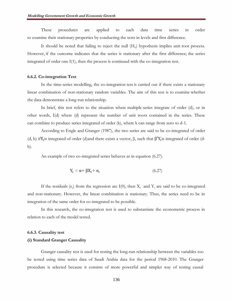
Modelling Government Growth and Economic Growth
136
These procedures are applied to each data time series in order
to examine their stationary properties by conducting the tests in levels and first difference.
It should be noted that failing to reject the null (H0) hypothesis implies unit root process.
However, if the outcome indicates that the series is stationary after the first difference; the series
integrated of order one I(1), then the process is continued with the co-integration test.
6.6.2. Co-integration Test
In the time-series modelling, the co-integration test is carried out if there exists a stationary
linear combination of non-stationary random variables. The aim of this test is to examine whether
the data demonstrate a long-run relationship.
In brief, this test refers to the situation where multiple series integrate of order (d), or in
other words, I(d) where (d) represent the number of unit roots contained in the series. These
can combine to produce series integrated of order (k), where k can range from zero to d-1.
According to Engle and Granger (1987), the two series are said to be co-integrated of order
(d, b) ifYt is integrated of order (d)and there exists a vector, β, such that β′Yt is integrated of order (d-
b).
An example of two co-integrated series behaves as in equation (6.27).
Yt = α+ βXt+ et (6.27)
If the residuals (et) from the regression are I(0), then Xt and Yt are said to be co-integrated
and non-stationary. However, the linear combination is stationary. Thus, the series need to be in
integration of the same order for co-integrated to be possible.
In this research, the co-integration test is used to substantiate the econometric process in
relation to each of the model tested.
6.6.3. Causality test
(i) Standard Granger Causality
Granger causality test is used for testing the long-run relationship between the variables too
be tested using time series data of Saudi Arabia data for the period 1968-2010. The Granger
procedure is selected because it consists of more powerful and simpler way of testing causal

Modelling Government Growth and Economic Growth
137
relationship. Assuming that the two series contain all the information necessary for prediction X
Granger-causes Y if lagged X's helps predict Y (Granger, 1980).
Causality test is required to test whether past changes in variables support changes in other
variables under the following conditions:
(a) The two variables used in the test must be stationary;
(b) The two variables are not integrated of the same order;
(c) The various economic variables are non-stationary in their respective level.
Granger (1980) causality in the models, are defined in equation (6.28) and (6.29):
tit
s
i
iytit
r
i
ixtt yxx
11
0 (6.28)
tit
s
i
ixtit
r
i
iytt xyy
11
0
(6.29)
For equation 6.28, the following hypotheses are constructed:
H0: βxt−i = 0, for i = 1, 2,............, k
H1: βxt−i ≠ 0 , for at least one i
Thus, equation 6.28 is used to test whether (Yt) Granger causes (Xt).
For equation 6.29, on the other hand, the hypotheses to be tested are:
H0: βyt − i = 0 , for i = 1, 2,............,k
H1:βyt − i ≠ 0 , for at least one i
Consequently, equation 6.29 is used to test whether (Xt) Granger causes (Yt).
In the case of this research, two fundamental issues have to be checked:
(a) To test the variables individually for the causality between the dependent variables;
(b) To check the time series properties and especially the co-integrating properties of the time series
involved. As Oskooee and Alse(1993:536) pointed out “Standard Granger or Sims tests are only
valid if the original time series from which growth rates have generated are not co-integrated.”
By following Gujarati‟s (1995) statements there are four possible results to be derived from
the causality test in the case of this study:

Modelling Government Growth and Economic Growth
138
(a) Neither variable „Granger causes‟ the other means, independence has suggested that when the
sets of GDP and GE coefficients are not statistically in both regressions;
(b) Unidirectional causality from GDP to GE implies that GDP causes GE, but not vice versa
indicating that Wagner‟s Law applies;
(c) Unidirectional causality from GE to GDP implies that is GE causes GDP, but not vice versa
indicating that Keynesian modelling is valid in this case;
(d) Bi-directional causality of each other between GDP and GE implying that GDP and GE
„Granger cause‟ each other, so either the Keynesian modelling or Wagner‟s Law is valid.
(ii) Error-Correction Models
When variables are found to be co-integrated, a mechanism is required to correct their state,
for which Engle and Granger (1987) provide such a procedure known as the „Error-Correction
Models‟ (ECM). The aim of ECM is to determine whether co–integration exists between two
variables; there must be Granger causality in at least one direction, but the most valuable aspect is
that co-integration does not reflect the direction of causality between the variables.
The ECM is expressed as in equation (6.30) and (6.31):
∆ Yt = a1 + β1ECTt−1 + δiΔni=1 Yt−1 + ΩiΔ
ni=1 Xt−1 + et (6.30)
∆ Xt = a2 + β2ECTt−1 + µiΔni=1 Yt−1 + €iΔ
ni=1 Xt−1 + et (6.31)
where (ECTt−1) is the error correction term lagged one period, is equivalent to et = Yt − α −
β Xt , which represents the disequilibrium residual of a co-integration equation (Fasana and Wang,
2001).
According to Enders (1995: 376), the causality in the ECM is applied in three stages:
(a) Joint Hypothesis:
H0:β1 = 0 , H0:δi = 0 , for all (i) in equation 6.30, or
H0:β2 = 0 , H0:µi = 0,, for all (i) in equation 6.31;
(b) Test the significance of (δi) and (µi) to check for the possibility of short run causality;
(c) Analysis of the direction of the (β′s) to see if they infer a long-run equilibrium relationship.

Modelling Government Growth and Economic Growth
139
6.7. CONCLUSION
In this chapter, the conceptual and econometric models‟ aiming to model the government
expenditures and economic growth in Saudi Arabia is presented: Wagner‟s Law, Keynesian model,
and Displacement Effect.
As regards to econometric modelling, there are three steps to test the causality between the
economic growth in GDP and government spending:
(i) to analyse the time series features to determine the degree of integration;
(ii) to determine the relationship between the two variables in the long term;
(iii) to test the direction of causality in the short and long term
In doing so, the following tests are utilised:
(i) Ordinary Least Square (OLS);
(ii) The Unit Root Test, Dickey-Fuller (ADF) test;
(iii) The Co-integration Test;
(iv) The Causality Tests, Standard Granger Causality and Error Correction Models (ECM).
In summary, this chapter describes the models used to determine the significance and
causality between the identified variables in different models used in this study with the objective of
explaining the relationship between government expenditures and economic growth over the years.
The following chapters present the applications of the models presented in this study so far in
developing the empirical findings.

Searching for Wagner’s Law in Saudi Arabia: An Empirical Analysis
140
CHAPTER 7
SEARCHING FOR WAGNER’S LAW IN SAUDI ARABIA: AN EMPRICAL ANALYSIS
7.1. INTRODUCTION
This chapter being the first empirical chapter provides the application of the
research process discussed in Chapter 6 with the objective of testing the Wagner‟s Law in
the case of Saudi Arabia. For this econometric time series analysis is utilised, for which
annual data from 1968 to 2010 were collected. Thus, an attempt is made to test the
relationship between government expenditures and economic growth by initially using
Ordinary Least Square (OLS) for both real GDP and real Non-Oil GDP in relations to
its impact on growing government and vice-versa.
In addition, as part of the time-series analysis, the stationary properties of the
data using the ADF test for real GDP and real Non-Oil GDP and other variables were
conducted. The next step in the time-series analysis is to test whether the variables in the
six versions of Wagner's Law are co-integrated. Finally, we have used the Error
Correction Model (ECM) to discuss the short run adjustment to equilibrium.
The rest of the chapter is organised as follows: section one, presents some
empirical results of relevant theoretical and empirical literature on the relationship
between government expenditure and economic growth. In section two of this chapter,
the six versions of Wagner‟s law and their formal expressions presented. Section three,
investigates the data and empirical results and analysis by using the identified methods,
which have been mentioned in Chapter Six. In addition, section four, presents the results
of the analysis by using the time series techniques, while section five, concludes the
chapters and presents the finding.
7.2. SURVEYING THE EMPIRICAL STUDIES ON WAGNER’S LAW
Extensive works have examined the relationship between government
expenditure and economic growth for all six versions of Wagner‟s Law. Early studies,
including Abizadeh and Gray (1985), Ram (1987) and Abizadeh and Yousefi (1988),
returned mixed results. The findings of these authors‟ empirical tests regarding the
validity of Wagner‟s Law differed from country to country. Some of this research
demonstrated that government expenditure growth was determined by national income
growth in developed countries, but not in less developed countries. Recent studies,

Searching for Wagner’s Law in Saudi Arabia: An Empirical Analysis
141
however, have concentrated on the long-term relationship between government
expenditure and national income. Biswal and Lee (1999) considered the relationship
between national income and government expenditure in Canada from 1950 to 1995
using Wagner‟s Law. Their results supported the model. Furthermore, Lall
(1969) examined cross-section data from 1962 to 1964 and found no support for
Wagner‟s Law in 46 developing countries. Ram (1987), who also explored the
relationship between government expenditures and GDP in 115 countries during the
period 1950–1980, obtained mixed results for Wagner‟s Law.
In the case of Saudi Arabia, Al-Hakami (2002) explored the empirical-causal
relationship between government expenditure and GDP over the period 1965–1996. He
used time-series analysis to examine the statistical characteristics of the variables. The co-
integration test – by examining the trend and pattern of the causal relationship between
the two variables – showed that the two-time series co-integrated. The findings
highlighted a causal relationship between GDP to government expenditure. Hence, the
result implies that government expenditure in oil states based on GDP is ineffective as a
policy tool, which supports Wagner's Law.
Payne and Ewing (1996) employed the error-correction model
to determine Granger causality between government expenditure and economic
growth, measured by GDP per capita. Their results supported Wagner‟s Law.
Furthermore, Burney (2002) applied Wagner‟s Law when considering the relationship
between government expenditure and economic development in Kuwait. He had
available series data from 1969 to 1994, and his findings showed support for
Wagner‟s Law over this period.
Courakiset al. (1993), Ahsanet al. (1996), Chletsos and Kollias (1997), and
Kolluriet al. (2000) supported this long-term relationship, whereas, Burney (2002) found
that the association described by Wagner‟s Law was not sufficient, accepting instead the
Keynesian interpretation. The purpose of this thesis is to test the relationship between
government expenditure and economic growth for all the six versions of Wagner‟s Law
in Saudi Arabia, one of the fastest-growing developing countries.
7.3. FORMULATING THE VERSIONS OF WAGNER’S LAW FOR SAUDI
ARABIA
As mentioned in Chapter 6, there are six versions of Wagner‟s law; as Wagner‟s
general hypothesis has provided scope for a range of different interpretations in the

Searching for Wagner’s Law in Saudi Arabia: An Empirical Analysis
142
existing literature. It is possible to identify at least six of these interpretations: Peacock
and Wiseman (1961), Gupta (1967), Goffman (1968), Goffman and Mahar (1971), Pryor
(1968), Musgrave (1969), and Man (1980), which are depicted in Table (7.1).
Table 7.1: Six Versions of Wagner’s Law with Real GDP No Function Version Year
1 L(GE) = α + β L(GDP) Peacock-Wiseman 1967
2 L(GEC) = α + β L(GDP) Pryor 1968 3 L(GE) = α + β L(GDP / P) Goffman 1968
4 L(GE/GDP) = α + β L(GDP / P) Musgrave 1969
5 L(GE/P) = α + β L(GDP / P) Gupta &Michas 1967 & 1975 6 L(GE/GDP) = α + β L(GDP) Mann 1980
where:
L Natural logarithm
GE Total Government Expenditure
GEC Total Government Expenditure for consumption
GE / GDP The share of real total Government expenditure in real GDP
GE / P Total Government Expenditure per capita
GDP Gross Domestic Product
P Population
Each of these models is discussed in the following sections:
(i) Peacock-Wiseman (1967) Version of Wagner’s Law
Peacock and Wiseman presented their version of Wagner‟s Law in 1967, which is
called the traditional version. They (1967:17) stated that “Wagner‟s argument was that
government expenditure must increase of an even faster rate than output.” This means
that the increase in total government expenditure is expected to be at a faster rate than
the growth observed in the GDP.
The functional form of Peacock and Wiseman version of Wagner‟s Law is
defined by equation (7.1):
GE = f (GDP) f‟ > 0 & f‟‟ ≥ 0 (7.1)
where: GE = Total Government Expenditure level in real terms; GDP= Gross
Domestic Product in real terms.
GE = α + β GDP + e (7.2)
The equation 7.2 is expressed in logarithm model as in equation (7.3):

Searching for Wagner’s Law in Saudi Arabia: An Empirical Analysis
143
L (GE) = α + β L (GDP) + e (7.3)
The government expenditure elasticity is then defined as:
E (Peacock & Wiseman) =
d GE
d GDP
GE
GDP
(7.4)
The elasticity (E) in equation (7.4) is thus interpreted as the percent change of
government expenditure (GE) for every one percent change of GDP.
(ii) Pryor (1968)
According to Pryor (1968:451), "Wagner asserted that in growing economies the
share of public consumption expenditures in the national income increases". This
statement can be expressed in the following functional form (Equation 7.5):
GEC = f (GDP) f‟ > 0 & f‟‟ ≥ 0 (7.5)
where: GEC = Total Government Consumption Expenditure level in real terms, and
GDP= Gross Domestic Product in real terms.
GEC = α + β GDP + e (7.6)
The equation by using logarithm model can be expressed as:
L (GEC) = α + β L (GDP) + e (7.7)
The government expenditure elasticity is then expressed as:
E (Pryor) = d(GEC )
d(GDP )/
GEC
GDP (7.8)
The elasticity (E) in equation (7.8) is thus interpreted as the percent change of
government expenditure of consumption (GEC) for every one percent change of GDP.
(iii) Goffman (1968)
Goffman (1968) introduced population into Wagner‟s Law, and therefore
considered that with the increase in per capita income government expenditures will
increase. This can be explained in the following functional form:
GE = f (GDP/ p) f‟ > 0 & f‟‟ ≥ 0 (7.9)

Searching for Wagner’s Law in Saudi Arabia: An Empirical Analysis
144
where: GE = Total Government Expenditure level in real terms; and GDP/P= Per
Capita Gross Domestic Product in real terms.
This can be transformed into the following equation:
GE = α + β GDP/ P + e (7.10)
The equation by using logarithm model can be expressed as:
L (GE) = α + β L (GDP/P) + e (7.11)
The elasticity in equation 7.11 is then expressed as:
E (Goffman) = d GE
d GDP
P
/GE
GDP
P
(7.12)
The elasticity (E) in equation 7.12 is thus interpreted as the percent change of
government expenditure (GE) for every one percent change of per capita GDP
(GDP/P).
(iv) Musgrave (1967)
Musgrave (1967) conceptualised the Wagner‟s Law as the relationship between
per capita income and the government expenditure ratio, which is expressed in the
following functional form:
GE / GDP = f (GDP/P) f‟ > 0 & f‟‟ ≥ 0 (7.13)
where: GE / GDP= the ratio of Government Expenditure level in real terms; and
GDP/P= Per Capita Gross Domestic Product in real terms.
Equation (7.13) is expressed in the following equation:
GE/GDP = α + β GDP/P + e (7.14)
Equation 7.14 is transformed by using logarithm model as in equation (7.15):
L(GE/GDP) = α + β L (GDP/P) + e (7.15)
The government expenditures elasticity in equation (7.15) is expressed as:
E (Musgrave) = d(GE /GDP )
d(GDP /P)/
GE /GDP
GDP /P (7.16)

Searching for Wagner’s Law in Saudi Arabia: An Empirical Analysis
145
The elasticity (E) in equation (7.16) is thus interpreted as the percent change of
government expenditure ratio to GDP (GE/GDP) for every one percent change of Per
Capita Gross Domestic Product (GDP/P).
(v) Gupta (1967)
Gupta in his 1967 articulation of the Wagner‟s Law, considered the relationship
between GDP and government expenditures in terms of per capita, which is explained in
the following functional format:
GE /P = f (GDP/P) f‟ > 0 & f‟‟ ≥ 0 (7.17)
where: GE/ P= Total Government Expenditure per capita in real terms; and GDP/P=
Per Capita Gross Domestic Product in real terms.
This functional relationship can be re-expressed in the following equation:
GE/P = α + β GDP/P + e (7.18)
The equation by using logarithm model is expressed in the following manner:
L (GE/P) = α + β L (GDP/P) + e (7.19)
The elasticity in the equation (7.19) can be expressed in the following equation:
E (Gupta) = d(GE /P)
d(GDP /P)/
GE /P
GDP /P(7.20)
The elasticity (E) in equation (7.20) is thus interpreted as the percent change of
government expenditure per capita (GE/P) for every one percent change of Per Capita
Gross Domestic Product (GDP/P).
(vi) Mann (1980)
Mann (1980) interpreted Wagner‟s Law as a relationship between government
expenditure ratio and GDP, which is expressed in the following functional form:
GE / GDP = f (GDP) f‟ > 0 & f‟‟ ≥ 0(7.21)
where: GE/ GDP = the ratio of Government Expenditure level in real terms; GDP =
Gross Domestic Product in real terms.

Searching for Wagner’s Law in Saudi Arabia: An Empirical Analysis
146
This can be transformed into:
GE/GDP = α + β GDP + e (7.22)
The equation by using logarithm model is expressed as below:
L(GE/GDP) = α + β L (GDP) + e (7.23)
The elasticity in equation (7.24) is explained as:
E(Mann) = d(GE /GDP )
d(GDP )/
GE /GDP
GDP(7.24)
The elasticity (E) in equation (7.24) is thus interpreted as the percent change of
the ratio of government expenditure to GDP (GE/GDP) for every one percent change
of GDP.
7.4. THE EMPIRICAL RESULTS AND ANALYSIS WITH OLS
This section of the thesis presents the research process and the analysis, which
presents the results as well in a detailed manner. It starts with describing the OLS
process:
The ordinary least square test (OLS) is employed to determine the parameters in
the equations, in which the logarithm model is utilised for the following:
(i) The parameters of the logarithm model have an explanation as elasticises;
(ii) The logarithm transformation is used when all the data are positive. According to,
Gujarati (1995), the normal regression model is obtained by taking logs of both sides of
the equation (7.25):
Y = α + β X + e (7.25)
to be:
Log Y = α + β Log X + e (7.26)
The slope is determined by as in equation (7.27):
Slope = dy
dx= β ∗
y
x (7.27)
The elasticity is:

Searching for Wagner’s Law in Saudi Arabia: An Empirical Analysis
147
E=Elasticity = d(y)
d(x)/
y
x = β (7.28)
For simplicity, E can be written as:
β = d(y)
d(x)/
y
x (7.29)
7.4.1. Testing the Versions of Wagner’s Law with Real GDP
This section provides the results of the empirical analysis by using real GDP
within the initial OLS framework as explained above. The analysis later is further
developed by employing cointegration analysis.
(i) Peacock-Wiseman (1967) Version of Wagner’s Law
According to the specification and functional and logarithmic form expressed in the
previous section, the following estimates in table (7.2) are established for the Peacock
and Wiseman version of Wagner‟s Law for the period of 1968 to 2010 for Saudi Arabia:
Table 7.2: Regression Results for Peacock & Wiseman Version with Real GDP
Versions D-Variable Constant In-Variable Coefficient R²
Peacock & Wiseman
L(GE)
-2.836
L (GDP)
1.1078
0.9016
The estimates in Table (7.2) can be expressed in the following functional form:
L(GE)= -2.836+ 1.1078 L(GDP) (7.30) (-3.85) (19.14)
The numbers between parentheses are t- statistics for each estimated measure
and intercept. In equation (7.30), to get the growth rate (elasticity), elasticity (coefficient)
is directly measured with the coefficient of GDP, namely E = 1.1078 > 0, which
indicates that the elasticity of government expenditure with respect to GDP is 1.1078. In
other words, this value means an increase of 1% unit in GDP generates a 1.1078% unit
increase in Government Expenditure (GE). The independent variable (GDP) explains
90.16% of the variations in GE, leaving only 9.84% to explain by the stochastic
disturbance term.

Searching for Wagner’s Law in Saudi Arabia: An Empirical Analysis
148
It should be noted that this finding for Saudi Arabia for the period in question is
consistent with Wagner's Law of increasing state activities, which states that the income
elasticity of demand for public goods is greater than unity. The results above show that
the expenditure elasticity with respect to GDP (β) is greater than unity (1.1078). This
study, hence, verifies Wagner‟s Law in its the traditional version as expressed by Peacock
and Wiseman (1967), which indicates that economic growth has caused government
expenditure to increase at a faster rate than that of national income.
(ii) Testing Pryor’s (1968) Version of Wagner’s Law
As defined and expressed in the previous section, the estimates for Pryor‟s
version of Wagner‟s Law through OLS are presented in Table (7.3) for Saudi Arabia for
the period of 1968-2010:
Table 7.3: Regression Results for Pryor Version with Real GDP
Versions D-Variable Constant In-Variable Coefficient R²
Pryor L(GEC)
1.307
L (GDP) 0.8078
0.8555
The results of the OLS can be written in a functional form as:
L(GEC) = 1.307+ 0.8078 L(GDP) (7.31)
(1.95) (15.39)
From equation (7.31), the impact of GDP growth on government consumption
expenditures, GEC, can be measured through the elasticity (E) or coefficient value
directly, which is 0.8078 > 0. This implies that 1% unit increase in GDP generates a
0.8078% unit increase in government expenditure for consumption (GEC). The
independent variable or GDP explains 86% of the variations in government expenditures
or as indicated by R²,leaving only 14% to be explained by the stochastic disturbance term
e, implying that there exist other factors, which explain the variations in government
expenditure for consumption. It can, therefore, be concluded that Pryor version of
Wagner‟s Law is also validated in the case of Saudi Arabia as explained.
(iii) Testing Goffman (1968) Version of Wagner Law with Real GDP
As compared to the previous two models, Goffman (1968), as discussed above,
considers GDP per capita rather than GDP level. Thus, this section utilise real GDP per
capita in searching for evidence for government growth in the case of Saudi Arabia from

Searching for Wagner’s Law in Saudi Arabia: An Empirical Analysis
149
1968 to 2010 by utilising Goffman‟s version of Wagner Law. The result can be found in
Table (7.4).
Table 7.4: Regression Results for Goffman Version with Real GDP
Versions D-Variable Constant In-Variable Coefficient R²
Goffman L(GE)
-3.119
L (GDP/P) 1.4156
0.6734
The results in Table (7.4) can be transformed into functional form as follows:
L(GE) = -3.119 + 1.4156 L (GDP/P) (7.32) (-1.97) (9.08)
The numbers between parentheses are (t- statistics) for each estimated measure
and intercept. As the results in table 7.4 for the period of 1968 to 2010 indicate the
impact of GDP per capita or the elasticity of government expenditure is identified as the
coefficient of the independent variable, which is 1.4156 > 0. This implies that 1% unit
increase in GDP per capita generates a 1.4156% unit increase in government expenditure
or GE. Thus, as predicted by the theory, when people‟s income increases their
expectations from the state do also increase, as with income increase they move to
different class segments and the demand for other types of government services beyond
the classical function increases, which results in increased government expenditures.
As the estimates in Table (7.4) depict, the independent variable (GDP/P)
explains 67.34% of the variations in government expenditures, leaving only 32.66% to be
explained by the stochastic disturbance term, or e.
It can, thus, be concluded that Goffman version of Wagner‟s Law is also
validated in the case of Saudi Arabia by using OLS estimation method.
(iv) Testing Musgrave’s (1967) Version of Wagner Law
The fourth version of Wagner‟s Law that is tested in this thesis is by Musgrave,
who considered the government growth in the form of government expenditure growth
and GDP per capita. The OLS estimates for Musgrave‟s version in the case of Saudi
Arabia for the period of 1968-2010 is depicted in Table (7.5):
Table 7.5: Regression Results for Musgrave Version Real GDP
Versions D-Variable Constant In-Variable Coefficient R²
Musgrave L(GE/GDP)
-1.7900
L (GDP/P) 0.3184
0.3200
The results are also expressed in a functional form in the following manner:

Searching for Wagner’s Law in Saudi Arabia: An Empirical Analysis
150
L(GE/GDP) = -1.7900 + 0.3184 L(GDP/P) (7.33)
(-1.98) (0.36)
The numbers between parentheses are (t- statistics) for each estimated measure
and intercept. As can be seen from the results, the coefficient of per capita GDP or
government expenditure growth rate or elasticity is 0.3184 > 0. This implies that a 1%
unit in GDP generates a 0.3184 % unit increase in the ratio of government expenditure
(GE/GDP).
Compared to the previous models, the findings for Musgrave‟s version show
lower explanatory power for the independent variable or the real per capita income, as
can be seen the GDP/P, as the explanatory variable explains only 32% of the variations
in GE, leaving only 68% to explain by the stochastic disturbance term e.
It can therefore be concluded that while Musgrave‟s version of Wagner‟s Law is
validated by this study for Saudi Arabia, due to the low R² value caution should be taken.
(v) Testing Gupta’s (1967) Version of Wagner’s Law with Real GDP
Gupta in his version (1967) of Wagner‟s Law relates the per capita GDP with per
capita government expenditures. The results for Gupta‟s version of Wagner‟s Law in the
case of Saudi Arabia for the period of 1968-2010 are depicted in Table (7.6):
Table 7.6: Regression Results for Gupta Version with Real GDP
Versions D-Variable Constant In-Variable Coefficient R²
Gupta L(GE/P)
-1.7900
L (GDP/P) 1.0318
0.7703
The results in table 7.6 can be transformed into functional form as follows:
L (GE/P) = -1.7900+ 1.0318 L(GDP/P) (7.34)
(-1.98) (11.58)
The numbers between parentheses are (t- statistics) for each estimated measure
and intercept. The estimated growth rate or elasticity of the per capita government
expenditures, as measured by coefficient value of the independent variable, namely per
capita GDP indicates E = 1.0318 > 0. This clearly shows that growth in per capita
income has strong impact on government expenditures. In other words, increase of 1%
unit in GDP generates a 1.0318% unit increase in government expenditure per capita
(GE/P). This finding is consistent with Wagner's Law of increasing state activities, which
states that the income elasticity of demand for public goods is greater than unity.

Searching for Wagner’s Law in Saudi Arabia: An Empirical Analysis
151
The results in Table (7.6) also show that the independent variable (GDP/P)
explains 77% of the variations in per capita government expenditure change, leaving only
23% to be explained by the stochastic disturbance term, e.
It can therefore be concluded that Gupta (1967) version of government
expenditure growth of Wagner‟s Law is also verified in the case of Saudi Arabia.
(vi) Testing Mann’s (1980) Version of Wagner’s Law with Real GDP
The Mann‟s version of Wagner‟s Law is tested and the following estimates were found:
L(GE/GDP) = -2.8366+ 0.10789L (GDP) (7.35)
(-3.85) (1.86)
The figures between the parentheses are (t- statistics) for each estimated measure
and intercept. In equation 7.35, for the period of 1968 to 2010, to get the growth rate
(elasticity), the estimated value of the coefficient is used as E = 0.10789 > 0, which
implies that a 1% unit in GDP generates a 0.10789% unit increase in the ratio of
Government Expenditure (GE/GDP). Thus, the independent variable or GDP explains
38% of the variations in GE/GDP, leaving only 62% to explain by the stochastic
disturbance term, e.
The results in Table (7.7) show that the expenditure elasticity with respect to
GDP (β) is greater than unity (0.10789); Wagner's Law is, thus, according to Nagarajan
and Spreares (1990) in their comments on Mann's study indicated the straight income
elasticity in order to validate the hypothesis would to be (E > 1) and the ratio income
elasticity need only be (E > 1). Importantly, since the income elasticity is greater than
zero, Wagner's Law is validated.
Table 7.7:Regression Results for Mann Version with Real GDP
Versions D-Variable Constant In-Variable Coefficient R²
Mann L(GE/GDP)
-2.8366
L (GDP) 0.10789
0.3791
7.4.2. Testing the Versions of Wagner’s Law with Non-Oil real GDP
In order to avoid the deterministic nature of the oil revenues with an attempt to
search for the impact of non-oil economic activity on government expenditures, non-oil
real GDP is utilised. All the six versions of the Wagner Law are formulated as in Table
(7.8).

Searching for Wagner’s Law in Saudi Arabia: An Empirical Analysis
152
Table 7.8: Six Versions of Wagner’s Law with Real Non-Oil Sector of GDP No Function Version Year
1 L(GE) = α + β L(Non-Oil real GDP) Peacock-Wiseman 1967
2 L(GEC) = α + β L(Non-Oil real GDP) Pryor 1968 3 L(GE) = α + β L(Non-Oil real GDP /P) Goffman 1968
4 L(GE/Non-Oil real GDP) = α + β L(Non-Oil real GDP/P) Musgrave 1969
5 L(GE/P) = α + β L(Non-Oil real GDP /P) Gupta &Michas 1975 6 L(GE/Non-Oil real GDP) = α + β L(Non-Oil real GDP) Mann 1980
(i) Testing Peacock-Wiseman (1967) Version of Wagner’s Law with Non-
Oil Real-GDP
The estimation for the Peacock and Wiseman version of the Wagner Law for the
period of 1968-2010 with non-oil real GDP is present as follows:
L(GE)=-2.2224 + 1.0936L(Non-oil real GDP ) (7.36)
(-13.46) (85.43)
As can be seen in equation (7.36), the growth rate or the elasticity value is given
by the coefficient of the independent variable, namely the non-oil real GDP which is E =
1.0936 > 0. This implies that an increase of 1% unit in Non-Oil real GDP generates a
1.0936% unit increase Government Expenditure (GE).
As can be seen in Table (7.9), the independent variable (Non-Oil real GDP)
explains 99.45% of the variations in GE, leaving only 0.55% to explain by the stochastic
disturbance term, e.
This finding in this section is consistent with Wagner‟s Law of increasing state
activities, which states that the income elasticity of demand for public goods is greater
than unity. The results above show that the expenditure elasticity with respect to Non-
Oil real GDP (β) is greater than unity (1.0936). Wagner‟s Law is, thus, according to the
traditional version, namely Peacock and Wiseman (1967) confirmed, in the sense that
economic growth indeed has caused government expenditure to increase at a faster rate
than that of national income in Saudi Arabia (Table 7.9).
Table 7.9: Regression Results for Peacock and Wiseman Version with Non-Oil real GDP
Versions D-Variable Constant In-Variable Coefficient R²
Peacock and Wiseman
L(GE)
-2.2224
L (Non-Oil GDP) 1.0936
0.9945
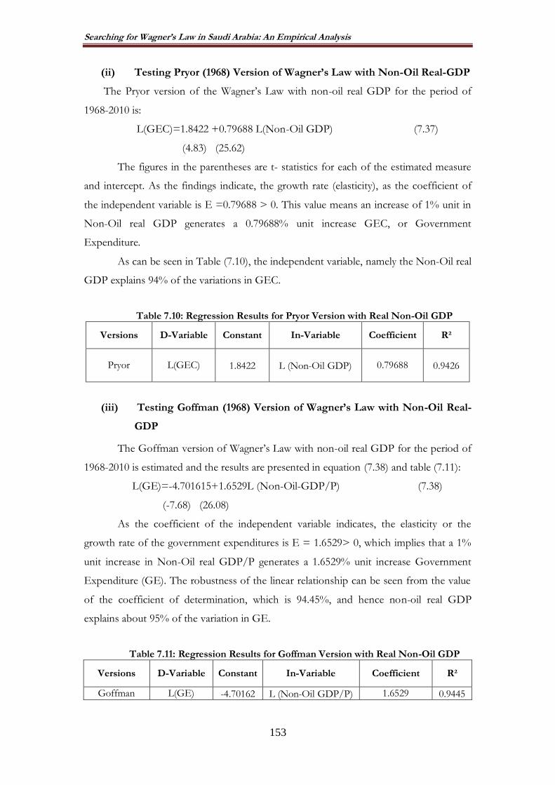
Searching for Wagner’s Law in Saudi Arabia: An Empirical Analysis
153
(ii) Testing Pryor (1968) Version of Wagner’s Law with Non-Oil Real-GDP
The Pryor version of the Wagner‟s Law with non-oil real GDP for the period of
1968-2010 is:
L(GEC)=1.8422 +0.79688 L(Non-Oil GDP) (7.37)
(4.83) (25.62)
The figures in the parentheses are t- statistics for each of the estimated measure
and intercept. As the findings indicate, the growth rate (elasticity), as the coefficient of
the independent variable is E =0.79688 > 0. This value means an increase of 1% unit in
Non-Oil real GDP generates a 0.79688% unit increase GEC, or Government
Expenditure.
As can be seen in Table (7.10), the independent variable, namely the Non-Oil real
GDP explains 94% of the variations in GEC.
Table 7.10: Regression Results for Pryor Version with Real Non-Oil GDP
Versions D-Variable Constant In-Variable Coefficient R²
Pryor L(GEC)
1.8422
L (Non-Oil GDP) 0.79688
0.9426
(iii) Testing Goffman (1968) Version of Wagner’s Law with Non-Oil Real-
GDP
The Goffman version of Wagner‟s Law with non-oil real GDP for the period of
1968-2010 is estimated and the results are presented in equation (7.38) and table (7.11):
L(GE)=-4.701615+1.6529L (Non-Oil-GDP/P) (7.38)
(-7.68) (26.08)
As the coefficient of the independent variable indicates, the elasticity or the
growth rate of the government expenditures is E = 1.6529> 0, which implies that a 1%
unit increase in Non-Oil real GDP/P generates a 1.6529% unit increase Government
Expenditure (GE). The robustness of the linear relationship can be seen from the value
of the coefficient of determination, which is 94.45%, and hence non-oil real GDP
explains about 95% of the variation in GE.
Table 7.11: Regression Results for Goffman Version with Real Non-Oil GDP
Versions D-Variable Constant In-Variable Coefficient R²
Goffman L(GE)
-4.70162
L (Non-Oil GDP/P) 1.6529
0.9445

Searching for Wagner’s Law in Saudi Arabia: An Empirical Analysis
154
(iv) Testing Musgrave (1967) Version of Wagner’s Law with Non-Oil Real-
GDP
The estimated Musgrave version of the Wagner‟s Law for the period of 1968-2010
for Saudi Arabia is presented in equation (7.39) and table (7.12):
L(GE/Non-Oil-GDP)=-2.448+0.1533L (Non-Oil-GDP/P) (7.39)
(-13.88) (8.40)
As the t-statistics between the brackets indicates, the independent variable, non-
oil real GDP per-capita, is statistically significant. As to the growth rate of the ratio of
government expenditure to non-oil real GDP, it is given by the coefficient of the
independent variable which is E =0.1533> 0, which implies that a 1% unit increase in
non-oil GDP generates a 0.1533% unit increase the ratio of Government Expenditure
(GE/Non-Oil GDP). Thus, the impact of non-oil real GDP on government expenditure
ratio is less than unit. In addition, as can be seen from table 7.12, the independent
variable (Non-Oil real GDP/P) explains 64% of the variations in GE indicating a
moderate relationship.
Table 7.12: Regression Results for Musgrave Version with Real Non-Oil GDP
Versions D-Variable Constant In-Variable Coefficient R²
Musgrave L(GE/Non-Oil
GDP)
-2.448
L (Non-Oil
GDP/P) 0.1533
0.6382
(v) Testing Gupta (1967) Version of Wagner’s Law with Non-Oil Real-
GDP
The Gupta version of Wagner‟s Law for the period of 1968-2010 for Saudi
Arabia is estimated as follows:
L(GE/P)=-2.4473+1.1531 L(Non-Oil GDP/P) (7.40)
(-13.88) (63.19)
Equation (7.40) indicates that the non-oil real GDP per-capita, as the dependent
variable, is statistically significant. The growth rate of per-capita government
expenditures as measured through the coefficient of the dependent variable is
E=1.1531>0. Accordingly, a 1% unit increase in non-oil real GDP generates a 1.1531 %
unit increase Government Expenditure per capita (GE/P). As regards to the explanatory
power of the model, as shown in Table (7.13), the independent variable (Non-Oil real
GDP/P) explains 77% of the variations in GE/P, leaving only 23% to explain by the
stochastic disturbance term, e.

Searching for Wagner’s Law in Saudi Arabia: An Empirical Analysis
155
It should be noted that this finding is consistent with Wagner‟s Law of increasing
state activities, which states the income elasticity of demand for public goods is greater
than unity.
Table 7.13: Regression Results for Gupta Version with Non-Oil real GDP
Versions D-Variable Constant In-Variable Coefficient R²
Gupta L(GE/P)
-2.4473
L (Non-Oil GDP/P) 1.1531
0.7703
(vi) Testing Mann’s (1980) Version of Wagner’s Law with Non-Oil real
GDP
Equation (7.41) and Table (7.14) presents the results of the estimated Mann‟s
version of Wagner‟s Law for the period of 1968-2010 for Saudi Arabia:
L(GE/Non-Oil real GDP)=-2.111+0.0936 L(Non-Oil real GDP) (7.41)
(-13.46) (7.31)
As can be seen, the independent variable in the form of non-oil real GDP is
statistically significant, as the t- statistics indicates. The growth rate of government
expenditure ratio or the elasticity is E =0.0936 > 0. This value means an increase of 1%
unit in non-oil real GDP generates a 0.0936% unit increase in the ratio of Government
Expenditure (GE/Non-Oil real GDP). Thus, the results show that the expenditure
elasticity with respect to Non-Oil real GDP, (β) is greater than unity. In addition, as can
be seen in table 7.14, the independent variable (Non-Oil real GDP) explains 57% of the
variations in GE/Non-Oil real GDP.
Table 7.14:Regression Results for Mann Version with Non-Oil real GDP
Versions D-Variable Constant In-Variable Coefficient R²
Mann L(GE/Non-Oil GDP)
-2.111
L (Non-Oil GDP) 0.0936
0.5719
7.5. Empirical Results of Unit Roots and Cointegration Test
The preceding section presented the findings from the simple regression analysis
as done in the original literature of each of the model presented. However, since then
the sophistication of econometric analysis has advanced and as mentioned in Chapter 6,
new methods of econometric analysis applied to the government expenditure growth
related studies.
An important part of such sophistication is the time-series analysis based on the
„unit root test‟ and „co-integration test‟. As explained in Chapter 6, the unit root test in

Searching for Wagner’s Law in Saudi Arabia: An Empirical Analysis
156
this study aims to examine the properties of time series data for each of the following:
government expenditure (LGE), gross domestic product (LGDP), gross domestic
product per capita (LGDP/P), the level of population (P), the government expenditure
ratio (LGE/GDP), and government expenditure per capita (LGE/P). Despite the
multiplicity of the unit root tests, this study utilises Dickey - Fuller test (Dickey and
Fuller: 1979), which is expressed in equation (7.42):
∆ Yt = a0 + a1t + a2Yt−1 + aiki=1 Yt−1 + et (7.42)
where:
∆ = the first difference of the series.
Yt = is the series under consideration (GDP, government expenditures, or government
revenues),
t = the time trend.
k= the number of lag.
et = is a stationary random error (white noise residual).
The hypotheses tested are:
H0: Unit root exists in Y: Y is non-stationary
H1: Unit root does not exist in Y: Y is stationary
As a rule, if we fail to reject the null hypothesis (H0), and then we have a unit
root process. If the outcome indicates that the series is stationary after the first
difference; the series integrated of order one [I(1)], then cointegration test is performed.
If the null hypothesis is accepted, the variable contains a unit root. Thus, the
Augmented-Dickey-Fuller (ADF) procedure has used to test for unit roots.
While all variables under examination are time-series variables, the time-series
properties of the series have to be examined. In order to avoid the problem of spurious
regression, each series was tested to check if they were stationary. To do so, the ADF
unit root tests is utilised with its critical value at 5% level of significance to accept or
reject the null hypothesis.
Table (7.15.A) presents the calculated t-value from ADF tests on each variable in
level and first differences in their logarithmic version. As can be seen from the depicted
results, in the case of the levels of the series, the null-hypothesis of non-stationary cannot
be rejected for any of the series. Thus, the levels of all series are non-stationary, but it is
rejected with first differences, which suggests that these variables are I (1).

Searching for Wagner’s Law in Saudi Arabia: An Empirical Analysis
157
Table 7.15.A: Augmented Dickey-Fuller for Stationary Unit Root Tests
Variables ADF(0) ADF(1)
L(GDP) -3.44 -2.746
L(GEC) -3.16 -2.067
L(GE) -3.09 -2.757
L(GE/GDP) -3.38 -1.994
L(GE/P) -3.37 -2.970
L(GDP/P) -3.44 -2.535
L(GE/Non-oil GDP) -3.32 -2.571
L(Non-Oil GDP) -3.41 -3.291
L(Non-Oil GDP/P) -3.39 -3.894
5% C-Value -3.493 -1.687
According to the result, each variable used in all six versions of Wagner‟s Law in
Saudi Arabia for the period of 1968-2010 indicates that the series are non-stationary
in level but stationary after the first difference.
Based on this test, it is concluded that all the variables tested (LGDP, LGE,
LGEC, LGE/P, LGE/GDP, LGDP/P, LNON OIL GDP, LNON OIL GDP /P and
LGE/NON OIL GDP) have contained a unit root. However, after the first difference
the unit root problem disappeared in the model. Thus, applying ADF unit root tests
(table 7.15.A), we found that each of the variables used in all six versions of Wagner‟s
Law is I(1). These results are consistent with the standard theory, which assumes that
most macroeconomic variables are not static level, but become stationary after the first
difference.
In the next step, Cointegration test is applied to examine a long-run relationship
between the variables by using OLS test, the results of which demonstrated in Table
(7.15.B) for real GDP and Table (7.15.C) for non-oil real GDP.

Searching for Wagner’s Law in Saudi Arabia: An Empirical Analysis
158
Table 7.15.B: Cointegration Results for the Versions with Real GDP
Versions Dependent Variables
Coefficient t-Stat Probability 𝐑𝟐 DW
Peacock &
Wiseman LGE 1.034 11.12 0.026 0.932 0.912
Pryor LGEC 1.157 10.86 0.041 0.863 0.920
Goffman LGE 1.342 8.15 0.013 0.781 0.793
Musgrave L(GE/GDP) 0.522 1.21 0.033 0.571 0.824
Gupta L(GE/P) 1.081 12.01 0.004 0.825 0.844
Mann (LGE/GDP) 0.287 1.92 0.029 0.497 0.885
Table 7.15.C: CointegrationResults for Non-Oil-Real GDP
Versions Dependent Variables
Coefficient T-Stat Probability 𝐑𝟐 DW
Peacock &
Wiseman LGE 1.103 50.33 0.008 0.951 0.919
Pryor LGEC 1.682 19.99 0.076 0.963 0.906
Goffman LGE 1.571 22.21 0.044 0.932 0.834
Musgrave L(GE/Non Oil-
GDP) 0.231 6.11 0.082 0.690 0.900
Gupta L(GE/P) 1.097 42.01 0.012 0.758 0.724
Mann (LGE/Non Oil-
GDP) 0.104 5.89 0.092 0.683 0.855
Table (7.15.B) and (7.15.C) present the cointegration test results for time series
for the period of 1968 to 2010 which examines the long run relationship between the
Government Expenditure (GE) and economic growth measure i.e. Real GDP and Non
Oil real-GDP in the Saudi economy. The results show that there is a long run
relationship between the Government Expenditure (GE) and Economic Growth (GDP)
for real GDP and non-oil real GDP in Saudi Arabia.
The variable used in all six versions of Wagner‟s Law for the period 1968–2010
indicates that the series are non-stationary in level, but stationary after the first
difference, which suggests that they are I(1). The estimated results given in Tables
(7.15.B) and (7.15.C) can be regarded as reliable in explaining the long-run relationship
between government expenditure and economic growth. As shown in Tables (7.15.B)
and (7.15.C), the real income elasticity for all the versions is greater than zero (i.e. more
than one in case of absolute versions and more than zero in case of relative versions for
both real GDP and Non-Oil real GDP). This confirms the validity of Wagner‟s Law in
Searching for Wagner’s Law in Saudi Arabia: An Empirical Analysis
159
relation to Saudi Arabia. In the long-run, one percent increase in GDP will lead to more
than one percent growth in total government expenditure.
It should be noted that co-integration can be conducted by using Johansen Co-
integrating test, the results of which presented in the following section.
7.5.1. Cointegration Test-Johansen Method
The concept of cointegration is that if the variables at the same level are of non-
stationary form any package of first class variables (Table 7.15.A), if possible,
to produce a linear combination is characterised by a static zero-class integrated I (0). In
this case, the integrated real-time variables of the same level cointegrated; therefore,
the level variables are not used in the regression, nor is the reduction in this case is a false
spurious. The null hypothesis is that the variables under consideration are not
cointegrated. The rejection of the null hypothesis requires that the trace value of the
cointegration test be greater than, at least one of the independent-critical values.
Therefore, the non-rejection of null hypothesis of no co-integration leads us to conclude
that there is no relationship in the long-term equilibrium between government spending
and national income. Co-integrating test in this study was conducted using the method
developed by Johansen (1988), and Johansen and Juselius (1990).
Many studies used the Engle-Granger two-step test, but there are those Sinha
(1998), Al- Hakami (2002) and Al-Qudair (2005), who used Johansen and Juselius (1990)
test, which had advantages such as it tests for all of the variables and, secondly, all
variables are treated as internal variables, so that the choice of the variable is
not absolute. This procedure is the most reliable test for cointegration.
To determine whether stochastic trends in the series displayed relate to each
other or not, cointegration test for all the six versions of Wagner‟s Law is conducted. In
addition, after determining the order of integration by the Augmented Dickey Fuller test,
it is tested whether the series is co-integrated or not, and if they are, then the
cointegrating long-run equilibrium relationship has to be determined (Brooks, 2008).
This section, hence,tests and reports the findings of the test after the
cointegration test (Real GDP) and Co-integration test (Non-Oil real GDP) by using
Johansen cointegration test.

Searching for Wagner’s Law in Saudi Arabia: An Empirical Analysis
160
7.5.1.1 Cointegration Test with (Real GDP)
The existence of a cointegration vector is pointed out by a trace test since the t-
test value exceeds the critical value of 5% level of significance. This means the
cointegration tests are statistically significant at 5% level of significance for determining
the long-run relationship between all variables. Otherwise, there is a long run equilibrium
relationship between Real GDP and Government Expenditures. All versions of
Wagner‟s Law (Peacock and Wiseman, Pryor, Goffman, Musgrave, Gupta and Mann) are
tested in this section and it is found that the trace test indicates a level of significance at
5% significance level. At the trace statistic value in Table (7.16), we can reject the null
hypothesis of cointegration in all versions of Wagner‟s Law, because the trace statistic
values are greater than the critical value of 5%.
Table 7.16: Johansen Cointegration Test Results with Real GDP
Versions Hypothesized No. of CE(s) Eigen value TraceStatistic Critical Value 5% Prob
Peacock & Wiseman
None 0.29806 22.5771 15.41 0.0000 At most 1 0.18983 8.4206 3.76 0.0000
Pryor None 0.28467 19.8538 15.41 0.0016
At most 1 0.14899 6.4532 3.76 0.0004
Goffman None 0.28090 21.6521 15.41 0.0000
At most 1 0.08098 8.1780 3.76 0.0041
Musgrave None 0.28622 21.7785 15.41 0.0000
At most 1 0.18721 8.2911 3.76 0.0008
Gupta None 0.28624 21.7771 15.41 0.0000
At most 1 0.19021 8.2061 3.76 0.0015
Mann
None 0.29806 22.5771 15.41 0.0000
At most 1 0.18983 8.4206 3.76 0.0000
The results provide definitive evidence that the real total government
expenditure (GE) and real GDP are subject to an equilibrium relationship in the long-
run.
7.5.1.2 Cointegration Test with (Non-Oil Real-GDP)
In the case of non-oil real-GDP, the Table (7.17) shows that there is a long run
equilibrium relationship between non-oil real GDP and government expenditures as
found in all versions (Peacock & Wiseman, Pryor, Goffman, Musgrave, Gupta and
Mann) of Wagner's Law at 5% levels. Thus, the null hypothesis of cointegration is
rejected in all versions of Wagner‟s Law with respect to non-oil real GDP, because the
trace statistics values are greater than the critical value of 5%. Co-integrated relationships

Searching for Wagner’s Law in Saudi Arabia: An Empirical Analysis
161
exist for all six versions of Wagner‟s Law with respect to real non-oil GDP in the case of
Saudi Arabia, an even stronger result indicating that the real total government
expenditure and real non-oil GDP are subject to an equilibrium relationship in the long-
run.
Table 7.17: Johansen Cointegration Test Results with Non-Oil Real-GDP
Versions Hypothesized No.
of CE(s) Eigen value
Trace Statistic
Critical Value 5%
Prob
Peacock & Wiseman
None 0.26793 21.0726 15.41 0.0000
At most 1 0.19341 8.5974 3.76 0.0000
Pryor None 0.24684 18.2635 15.41 0.0000
At most 1 0.15895 6.9244 3.76 0.0002
Goffman None 0.33040 17.2814 15.41 0.0000
At most 1 0.03049 1.2386 3.76 0.0007
Musgrave None 0.29277 25.0288 15.41 0.0083
At most 1 0.24370 11.1726 3.76 0.0201
Gupta None 0.29277 25.0288 15.41 0.0083
At most 1 0.24370 11.1726 3.76 0.0201
Mann
None 0.26793 21.0729 15.41 0.0026
At most 1 0.19341 8.5974 3.76 0.0066
The Johansen and Juselius (1990) test show a cointegration relationship in all
versions. Therefore, Granger-Causality thus in the framework of the Error Correction
Model will be applied.
7.6. Causality Test for Wagner’s Law
After making sure of the time series model that the variables are not stationary in
the level and stationary in the difference, and then check it all-integrated joint, it is clear,
that there is a long-term equilibrium relationship.
According to Engle and Granger (1987), the variables that integratereflect a long-
term relationship. This should be a representation of Error Correction Model (ECM),
which helps to test and evaluate the relationship in the short and long term between the
variables of the form, as it avoids problems arising from the spurious correlation.
To apply the ECM for Wagner‟s Law in Saudi Arabia, the Granger-Causality is applied as
follows:
(i) In the context, of Error Correction Model (ECM) of the variables that is cointegrated.
(ii) Standard Granger-Causal for the variables that do not cointegrated.

Searching for Wagner’s Law in Saudi Arabia: An Empirical Analysis
162
The following sections present the models and the empirical results for these two
models.
7.6.1. Granger Causality Test
The Granger Causality Test is conducted through Engle and Granger approach,
which has two phases:
(i) Assessing the relationship model equilibrium in the long term or the
joint integration.
(ii) An Error Correction Model helps to reflect on the relationship in the short term
or to reflect on the short-term volatility and also helps to locate the relationship
in the long-term.
7.6.1.1. Granger Causality Test with Real GDP
After discussing the rationale for Granger Causality Test, the following section
presents the findings for all the versions of Wagner‟s Law with real-GDP.
(i) Granger Causality Test for Peacock and Wiseman Version of Wagner’s Law, 1968-2010
Table (7.18) presents the causality test result for Peacock and Wiseman version of
the Wagner‟s Law for the period of 1968-2010 in the case of Saudi Arabia. The reported
F-statistics is a standard test for the joint hypothesis that LGDP does not Granger Cause
LGE.
As the results indicate, in Saudi Arabia, the probability for accepting the null-
hypothesis is only 0.6% while the hypothesis is rejected by 99.4%, which means that
there is a high statistical significance for LGDP causing LGE in Peacock and Wiseman‟s
Version of Wagner‟s Law in the case of Saudi Arabia, which is consistent with Wagner's
Law.
The causality from LGE to LGDP is also searched for, where the probability for
accepting the null-hypothesis is only 15.9%, while 84.1% reject the hypothesis, which
means LGE causes LGDP about 84.1% of the time.
Table 7.18: Granger Causality test for Peacock and Wiseman’s Version with Real GDP
Null Hypothesis F-Statistic Prob.
LGDP does not Granger Cause LGE 16.05 0.0060
LGE does not Granger Cause LGDP 3.6836 0.1590
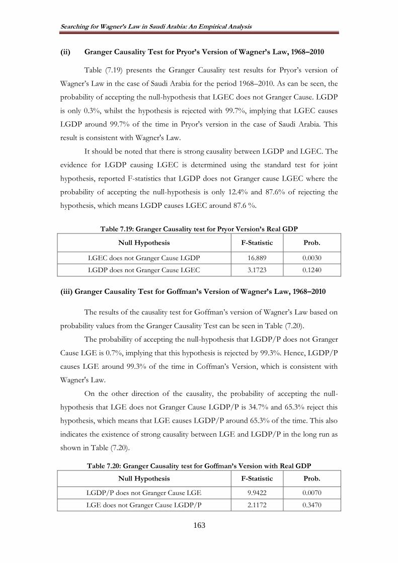
Searching for Wagner’s Law in Saudi Arabia: An Empirical Analysis
163
(ii) Granger Causality Test for Pryor’s Version of Wagner’s Law, 1968–2010
Table (7.19) presents the Granger Causality test results for Pryor‟s version of
Wagner‟s Law in the case of Saudi Arabia for the period 1968–2010. As can be seen, the
probability of accepting the null-hypothesis that LGEC does not Granger Cause. LGDP
is only 0.3%, whilst the hypothesis is rejected with 99.7%, implying that LGEC causes
LGDP around 99.7% of the time in Pryor's version in the case of Saudi Arabia. This
result is consistent with Wagner's Law.
It should be noted that there is strong causality between LGDP and LGEC. The
evidence for LGDP causing LGEC is determined using the standard test for joint
hypothesis, reported F-statistics that LGDP does not Granger cause LGEC where the
probability of accepting the null-hypothesis is only 12.4% and 87.6% of rejecting the
hypothesis, which means LGDP causes LGEC around 87.6 %.
Table 7.19: Granger Causality test for Pryor Version’s Real GDP
Null Hypothesis F-Statistic Prob.
LGEC does not Granger Cause LGDP 16.889 0.0030
LGDP does not Granger Cause LGEC 3.1723 0.1240
(iii) Granger Causality Test for Goffman’s Version of Wagner’s Law, 1968–2010
The results of the causality test for Goffman‟s version of Wagner‟s Law based on
probability values from the Granger Causality Test can be seen in Table (7.20).
The probability of accepting the null-hypothesis that LGDP/P does not Granger
Cause LGE is 0.7%, implying that this hypothesis is rejected by 99.3%. Hence, LGDP/P
causes LGE around 99.3% of the time in Coffman‟s Version, which is consistent with
Wagner's Law.
On the other direction of the causality, the probability of accepting the null-
hypothesis that LGE does not Granger Cause LGDP/P is 34.7% and 65.3% reject this
hypothesis, which means that LGE causes LGDP/P around 65.3% of the time. This also
indicates the existence of strong causality between LGE and LGDP/P in the long run as
shown in Table (7.20).
Table 7.20: Granger Causality test for Goffman’s Version with Real GDP
Null Hypothesis F-Statistic Prob.
LGDP/P does not Granger Cause LGE 9.9422 0.0070
LGE does not Granger Cause LGDP/P 2.1172 0.3470

Searching for Wagner’s Law in Saudi Arabia: An Empirical Analysis
164
(iv) Granger Causality Test for Musgrave’s Version of Wagner’s Law, 1968–2010
The results of the Granger Causality test for Musgrave‟s version of Wagner‟s Law
is presented in Table (7.21), which shows that the null-hypothesis that LGDP/P does
not Granger Causality LGE/GDP is accepted with the probability of 0.8%, whilst it is
rejected by 99.2%. This implies that LGDP/P causes LGE/GDP around 99.2% of the
time in Musgrave's version, which is consistent with the expectation of Wagner‟s Law.
It should be noted that the results in Table (7.21) also indicate strong causality
between LGE/GDP and LGDP/P in the long run. The probability of accepting the
null-hypothesis that LGE/GDP does not Granger Cause LGDP/P is 11.6%, which is
rejected by 88.4%. This means that LGE/GDP causes LGDP/P around 88.4% of the
time.
Table 7.21: Granger Causality Test for Musgrave’s Version with Real GDP
Null Hypothesis F-Statistic Prob.
LGDP/P does not Granger Cause LGE/GDP 9.5692 0.0080
LGE/GDP does not Granger Cause LGDP/P 4.3099 0.1160
(v) Granger Causality Test for Gupta’s Version of Wagner’s Law, 1968–2010
The results in Table (7.22) show the probability for accepting the null-hypothesis
that LGDP/P does not Granger cause LGE/P is only 0.3%, which means that LGDP/P
causes LGE/P around 99.7% of the time in Gupta‟s version. This, again, is consistent
with the observation of Wagner's Law.
An investigation of the opposite direction of the causality indicates the
probability of accepting the null-hypothesis that LGE/P does not Granger cause
LGDP/P is 11.6%. Hence, it can be inferred that LGE/P causes LGDP/P around
88.4% of the time suggesting a strong causality.
Table 7.22: Granger Causality Test for Gupta’s Version with Real GDP
Null Hypothesis F-Statistic Prob.
LGDP/P does not Granger Cause LGE/P 15.331 0.0030
LGE/P does not Granger Cause LGDP/P 4.3099 0.1160
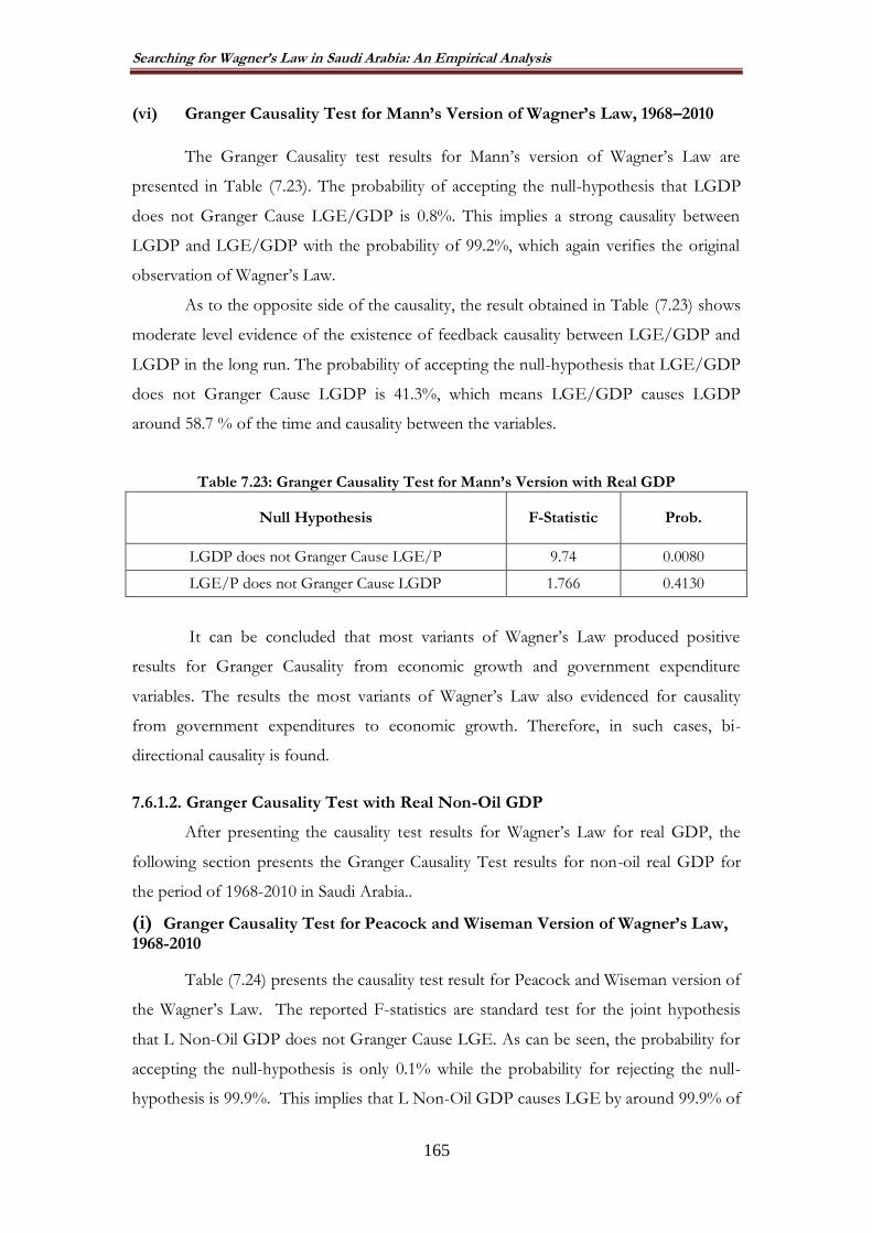
Searching for Wagner’s Law in Saudi Arabia: An Empirical Analysis
165
(vi) Granger Causality Test for Mann’s Version of Wagner’s Law, 1968–2010
The Granger Causality test results for Mann‟s version of Wagner‟s Law are
presented in Table (7.23). The probability of accepting the null-hypothesis that LGDP
does not Granger Cause LGE/GDP is 0.8%. This implies a strong causality between
LGDP and LGE/GDP with the probability of 99.2%, which again verifies the original
observation of Wagner‟s Law.
As to the opposite side of the causality, the result obtained in Table (7.23) shows
moderate level evidence of the existence of feedback causality between LGE/GDP and
LGDP in the long run. The probability of accepting the null-hypothesis that LGE/GDP
does not Granger Cause LGDP is 41.3%, which means LGE/GDP causes LGDP
around 58.7 % of the time and causality between the variables.
Table 7.23: Granger Causality Test for Mann’s Version with Real GDP
Null Hypothesis F-Statistic Prob.
LGDP does not Granger Cause LGE/P 9.74 0.0080
LGE/P does not Granger Cause LGDP 1.766 0.4130
It can be concluded that most variants of Wagner‟s Law produced positive
results for Granger Causality from economic growth and government expenditure
variables. The results the most variants of Wagner‟s Law also evidenced for causality
from government expenditures to economic growth. Therefore, in such cases, bi-
directional causality is found.
7.6.1.2. Granger Causality Test with Real Non-Oil GDP
After presenting the causality test results for Wagner‟s Law for real GDP, the
following section presents the Granger Causality Test results for non-oil real GDP for
the period of 1968-2010 in Saudi Arabia..
(i) Granger Causality Test for Peacock and Wiseman Version of Wagner’s Law, 1968-2010
Table (7.24) presents the causality test result for Peacock and Wiseman version of
the Wagner‟s Law. The reported F-statistics are standard test for the joint hypothesis
that L Non-Oil GDP does not Granger Cause LGE. As can be seen, the probability for
accepting the null-hypothesis is only 0.1% while the probability for rejecting the null-
hypothesis is 99.9%. This implies that L Non-Oil GDP causes LGE by around 99.9% of

Searching for Wagner’s Law in Saudi Arabia: An Empirical Analysis
166
the time in Peacock and Wiseman‟s Version, which is consistent with the expectations of
Wagner‟s Law.
In the feedback of causality from LGE to L Non-Oil GDP shows that the
probability for accepting the null-hypothesis is 52.6%, which means that LGE causes L
Non-Oil GDP by the probability level of 47.4% indicating a moderate level of causality.
Table 7.24: Granger Causality test for Peacock and Wiseman Version with Non- Oil Real GDP
Null Hypothesis F-Statistic Prob.
L Non-Oil GDP does not Granger Cause LGE 16.148 0.0010
LGE does not Granger Cause L Non-Oil GDP 1.2849 0.526
(ii) Granger Causality Test for Pryor’s Version of Wagner’s Law, 1968-2010
The probability for accepting null-hypothesis that LGEC does not Granger cause
LN Non-Oil real-GDP is 0.6% while it is rejected by 99.4%. The implications of this are
that LGEC causes L Non-Oil real-GDP with the probability of 99.4% in Pryor's version
of the Wagner‟s Law. This result is consistent with Wagner‟s Law to some extent.
However, there is strong feedback causality in the opposite direction between L Non-Oil
GDP and LGEC. The evidence that L Non-Oil real GDP causes LGEC is determined
by using the standard test for the joint hypothesis reported F-statistics, for which the
probability of accepting the null-hypothesis is 13.9%. Thus, L Non-Oil GDP causes
LGEC with the probability of 86.1 % as depicted in Table (7.25).
Table 7.25: Granger Causality test for Pryor Version with Non- Oil Real-GDP
Null Hypothesis F-Statistic Prob.
L Non-Oil GDP GEC does not Granger Cause L GEC 15.578 0.0060
L GEC does not Granger Cause L Non-Oil GDPGEC 3.2816 0.1390
(iii) Granger Causality Test for Goffman’s Version of Wagner’s Law, 1968-2010
Table (7.26) present the findings of the causality test based on probability values
from Granger Causality Test for Goffman‟s version of the Wagner Law. The Null-
Hypothesis that L Non-Oil GDP/P does not Granger cause LGE is accepted with the
probability of 0.1% indicating a strong case for the causality between L Non-Oil GDP/P
and LGE with a probability of 99.9%. The results indicate that Goffman‟s version of
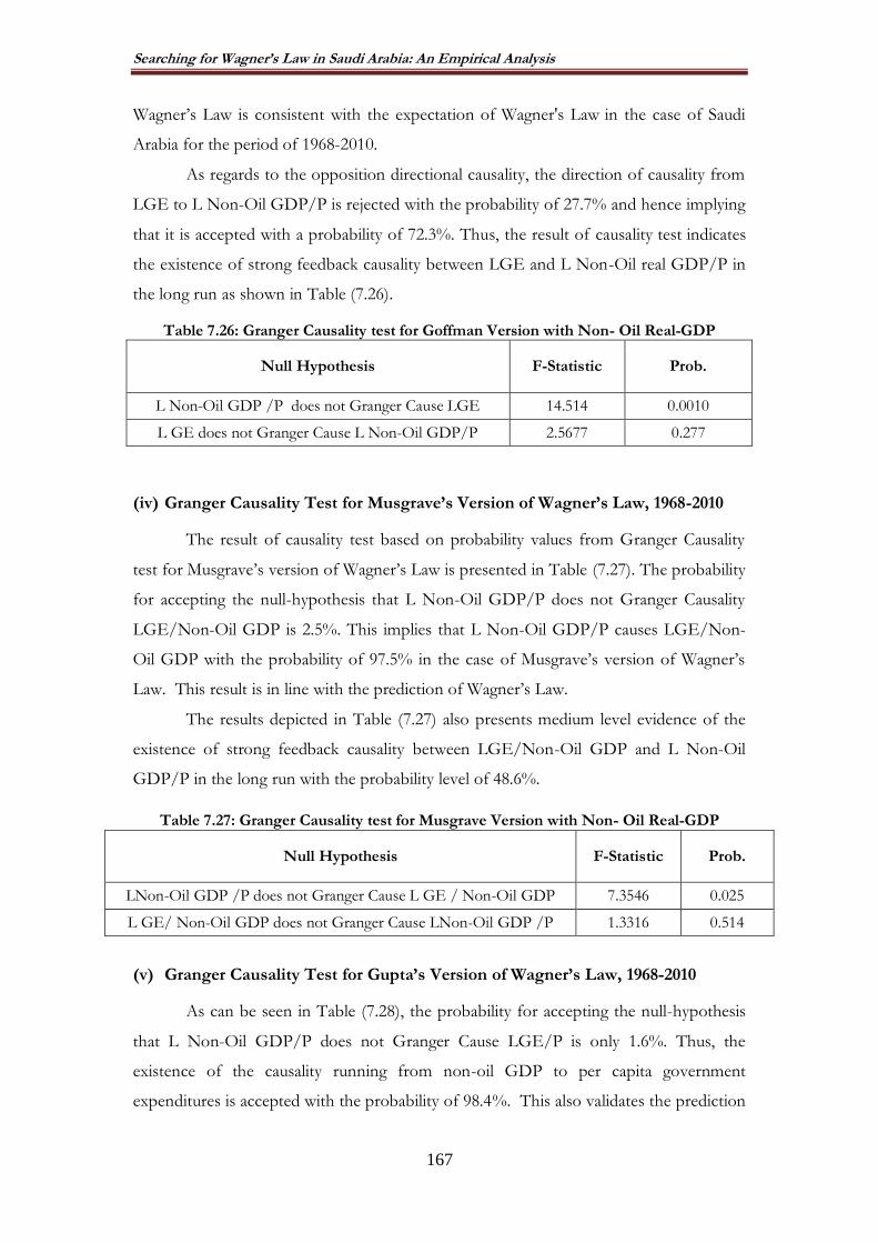
Searching for Wagner’s Law in Saudi Arabia: An Empirical Analysis
167
Wagner‟s Law is consistent with the expectation of Wagner's Law in the case of Saudi
Arabia for the period of 1968-2010.
As regards to the opposition directional causality, the direction of causality from
LGE to L Non-Oil GDP/P is rejected with the probability of 27.7% and hence implying
that it is accepted with a probability of 72.3%. Thus, the result of causality test indicates
the existence of strong feedback causality between LGE and L Non-Oil real GDP/P in
the long run as shown in Table (7.26).
Table 7.26: Granger Causality test for Goffman Version with Non- Oil Real-GDP
Null Hypothesis F-Statistic Prob.
L Non-Oil GDP /P does not Granger Cause LGE 14.514 0.0010
L GE does not Granger Cause L Non-Oil GDP/P 2.5677 0.277
(iv) Granger Causality Test for Musgrave’s Version of Wagner’s Law, 1968-2010
The result of causality test based on probability values from Granger Causality
test for Musgrave‟s version of Wagner‟s Law is presented in Table (7.27). The probability
for accepting the null-hypothesis that L Non-Oil GDP/P does not Granger Causality
LGE/Non-Oil GDP is 2.5%. This implies that L Non-Oil GDP/P causes LGE/Non-
Oil GDP with the probability of 97.5% in the case of Musgrave‟s version of Wagner‟s
Law. This result is in line with the prediction of Wagner‟s Law.
The results depicted in Table (7.27) also presents medium level evidence of the
existence of strong feedback causality between LGE/Non-Oil GDP and L Non-Oil
GDP/P in the long run with the probability level of 48.6%.
Table 7.27: Granger Causality test for Musgrave Version with Non- Oil Real-GDP
Null Hypothesis F-Statistic Prob.
LNon-Oil GDP /P does not Granger Cause L GE / Non-Oil GDP 7.3546 0.025
L GE/ Non-Oil GDP does not Granger Cause LNon-Oil GDP /P 1.3316 0.514
(v) Granger Causality Test for Gupta’s Version of Wagner’s Law, 1968-2010
As can be seen in Table (7.28), the probability for accepting the null-hypothesis
that L Non-Oil GDP/P does not Granger Cause LGE/P is only 1.6%. Thus, the
existence of the causality running from non-oil GDP to per capita government
expenditures is accepted with the probability of 98.4%. This also validates the prediction

Searching for Wagner’s Law in Saudi Arabia: An Empirical Analysis
168
of Wagner's Law. As to the oppositional causality, as the results indicate, the Granger
Causality from LGE/P to L Non-Oil GDP/P is accepted with the probability of 68.2%.
Table 7.28: Granger Causality test for Gupta Version with Real Non- Oil GD
Null Hypothesis F-Statistic Prob.
L Non-Oil GDP/P does not Granger Cause L GE/P 8.3048 0.0160
L GE/P does not Granger Cause L Non-Oil GDP/P 2.2884 0.318
(vi) Granger Causality Test for Mann’s Version of Wagner’s Law, 1968-2010
As the results in Table (7.29) shows the Granger causality from L Non-Oil GDP
to LGE/Non-Oil GDP is accepted with the probability level of 97.6%, indicating a very
strong causality, which verifies the prediction of Wagner‟s Law.
As to the opposite side of the causality, the results in Table (7.29) shows that the
causality from LGE/Non-Oil GDP to L Non-Oil GDP does not suggest a strong
relationship as the null-hypothesis accepted 52.6%, which means that LGE/Non-Oil
GDP causes L Non- Oil GDP around 47.4 % of the time in the case of Saudi Arabia.
Table 7.29: Granger Causality test for Mann Version with Real Non- Oil GDP
Null Hypothesis F-Statistic Prob.
LNon-Oil GDP does not Granger Cause L GE/Non-Oil GDP 7.4318 0.024
L GE /Non-Oil GDP does not Granger Cause LNon-Oil GDP 1.2849 0.526
It can therefore be concluded that most variant of the Wagner‟s Law produced
positive results for Granger Causality from economic growth and government
expenditure variables. The similar results in most variants of the Wagner Law are also
established for the causality from government expenditures to economic growth. In
such cases, thus, bi-directional causality is found.
The next section, extend the analysis into Error Correction Mechanism to find
out the short-run adjustment.
7.6.2. Error Correction Model (ECM)
The concept of error correction is related to cointegration, because the
cointegration relationship describes the long-run equilibrium. If a set of variables has
cointegrated, then there exists an Error Correction Model (ECM) to describe the short-
run adjustment to the equilibrium (Engle and Granger, 1987).

Searching for Wagner’s Law in Saudi Arabia: An Empirical Analysis
169
The incidence of mutual co-integration between variables indicates that the
Granger must be causal in one direction, at least, but the rules of engagement do
not refer to the direction of causality between the variables. Thus, to verify the rules of
engagement, tests of causation are tested in this section in the context of (ECM).
In addition, the t-statistics on the coefficients of the lagged error correction term
(ECTt-1) should indicate the significance of long-run causality between the two variables.
The statistical significance of the t-statistics in tests should be at most 5%.
7.6.2.1. Error Correction Model (ECM) with Real GDP
The results of ECM with real GDP is depicted in Table (7.30), which show that
there is long-run bi-directional causality that runs from GDP to GE in Peacock &
Wiseman‟s version; from GDP to GEC in Pryor‟s version; from GDP/P to GE in
Goffman‟s version;, from GDP/P to GE/GDP in Musgrave‟s version; from GDP/P to
GE/P in Gupta‟s version; and from GDP to GE/GDP in Mann‟s version. This result is
the product of the process that as depicted in Table (7.30), GE, GEC, GE/GDP, and
GE/P are all statistically significant at the 5% level. Thus, six versions of Wagner‟s Law
are found to hold in the case of Saudi Arabia.
In the Error Correction Model (ECt-1) the significant results indicate the speed of
adjustment to the long-run equilibrium, and reveal the direction of causality, which runs
from Economic Growth (GDP) to Government Expenditure (GE).
Table 7.30: Causality with ECM test with Real GDP
Versions Variables ECTt-1 t-Stat
Peacock & Wiseman
L(GE) -0.321322 -2.92
L(GDP) 0.501030 1.19
Pryor L(GEC) - 0.571306 - 3.62
L(GDP) 0.501030 1.19
Goffman L(GE) -0.21070 -2.39
L(GDP/P) 0.500729 2.09
Musgrave L(GE/GDP) -0.89640 -2.28
L(GDP/P) 0.588325 1.38
Gupta L(GE/P) -0.308073 -2.77
L(GDP/P) 0.588326 1.38
Mann
L(GE/GDP) -0.822166 -2.59
L(GDP) 0.501033 1.19

Searching for Wagner’s Law in Saudi Arabia: An Empirical Analysis
170
7.6.2.2. Error Correction Model (ECM) with Non-Oil Real-GDP
An attempt also made to find the ECM test results for non-oil real-GDP, the
results of which are depicted in Table (7.31). The results show that there is long-run bi-
directional causality that runs from Non-Oil-GDP to GE in Peacock and Wiseman
version; from Non-Oil-GDP to GEC in Pryor‟s version; from Non-Oil-GDP/P to GE
in Goffman‟s version; from Non-Oil-GDP/P to GE/ Non-Oil-GDP in Musgrave‟s
version; from Non-Oil-GDP/P to GE/P in Gupta‟s version, and from Non-Oil-GDP
to GE/ Non-Oil-GDP in Mann‟s Version of Wagner‟s Law. This result is a product of
empirical analysis which indicates that the variables used in each of the model GE, GEC,
GE/Non-Oil-GDP, and GE/P are statistically significant at the 5% level. Thus, six
versions of Wagner's Law are found to hold for non-oil-GDP in the case of Saudi
Arabia.
Table 7.31: Causality with ECM test with Non-Oil Real GDP
Versions Variables ECTt-1 T-Stat
Peacock & Wiseman
L(GE) -0.5824323 -3.52
L(Non-Oil GDP) -0.1989443 -1.67
Pryor L(GEC) -0.0344679 -0.42
L(Non-Oil GDP) 0.0861542 2.95
Goffman L(GE) 0.0534302 3.40
L(Non-Oil GDP/P) 0.0381747 3.96
Musgrave L(GE/ Non-Oil GDP) -0.0009502 -0.95
L(Non-Oil GDP/P) -0.0028346 -3.69
Gupta L(GE/P) -0.0037831 -3.07
L(Non-Oil GDP/P) -0.0028333 -3.69
Mann
L(GE/ Non-Oil GDP) -0.3834886 -3.09
L(Non-Oil GDP) -0.1989445 -1.67

Searching for Wagner’s Law in Saudi Arabia: An Empirical Analysis
171
7.7. CONTEXTUALISING THE RESULTS
Various studies have aimed to explain and validate Wagner‟s Law in many
countries either through time-series or cross section methods. Wagner (1883:8) noted
that “There is a proportion between public expenditure and national income which may
not be permanently overstepped”.
In our findings, the cointegration results suggest that Wagner‟s Law holds in
Saudi Arabia, and that there is strong feedback causality for all versions. Moreover, the
Error Correction Model (ECM) establishes that all six versions of Wagner‟s Law are
found to be significant for both real GDP and non-oil-GDP in the case of Saudi Arabia,
implying short-run adjustment process towards long-run equilibrium.
Similar results were reached, for example, by Biswal and Lee (1999). From a
different perspective, Asutay and Al Fazari (2007) investigated but provided no evidence
for the impact of government spending on GDP in Oman by using time-series data from
1971 to 2002. Their results supported causality between government expenditure and
GNP per capita.
Moreover, Abizadeh and Yousefi (1998) used Wagner‟s Law to examine
the effect of government expenditure on economic development in South Korea by
modelling the relationship through causality tests. Their research supported Wagner‟s
Law, as it studies. Furthermore, they confirmed the finding of Al-Hakami (2002) in a
trivariate model, when GDP was added. However, the results are in contrast with Al-
Hakami (2002) and Albatel (2002), who, in the case of Saudi Arabia, found that there is a
strong feedback causality that runs from government revenues to government
expenditure.
7.8. CONCLUSION
This chapter analysed empirically the relationship between government
expenditure and economic growth. Wagner‟s Law was examined – six versions that were
developed over the years – in the case of Saudi Arabia by using time-series annual data
for the period 1968–2010.
In the empirical analysis, three distinct time-series techniques were applied to test
the six versions of Wagner‟s Law by using Ordinary Least Square (OLS) for real GDP
and non-oil GDP. The unit root tests were utilised using the Augmented Dickey-Fuller
for determining the existence of stationary for real GDP and non-oil GDP. The

Searching for Wagner’s Law in Saudi Arabia: An Empirical Analysis
172
Cointegrating test for real GDP and non-oil GDP was also utilised. Finally, it was
considered the Granger causality tests and the Error Correction Model (ECM).
The results of the regression analysis – for six versions of Wagner‟s Law using
OLS for real GDP and non-oil real GDP – show that the elasticity coefficient of
government expenditure, with respect to GDP, was greater than unity in Peacock and
Wiseman (1968), Pryor (1969), Goffman (1968),and Gupta (1967). Thus, the findings in
the case of these four versions are in accordance with Wagner‟s expectation. The
empirical results also indicate that the elasticity coefficient of
government expenditure, with respect to GDP, is inelastic in the case of Musgrave‟s
(1969) and Mann‟s (1980) versions of Wagner‟s Law, although their independent variable
is still statistically significant. Nagarajan and Spreares (1990), furthermore, stated that in
order to verify Wagner‟s Law, the income elasticity needs to be E>1, i.e. greater than
unity, and the ratio income elasticity needs only be E>0, i.e. greater than zero.
According to this rule, Mann‟s version of Wagner‟s Law does not hold in the case of
Saudi Arabia.
As regards non-oil real GDP – the independent variable in the versions of
Wagner‟s Law – Peacock and Wiseman provide support for Wagner‟s Law, whilst
Pryor‟s, Musgrave‟s and Mann‟s versions do not hold for Saudi Arabia. In addition, since
elasticity is greater than unity in the results of Goffman‟s model, this version of Wagner‟s
Law is consistent for Saudi Arabia. Moreover, Gupta provides evidence for Wagner‟s
Law in the case of Saudi Arabia; the expected elasticity is higher than a unit, i.e. E>1.
Moreover, since the income elasticity needs to be higher than a unity (E > 1), and
the ratio income elasticity is expected to be higher than zero (E > 0),
Mann's version does not provide evidence for Wagner‟s Law in Saudi Arabia.
In extending the analysis, the unit root test in the form of Augmented Dickey-
Fuller is utilised to examine stationary of the time-series of all the variables. The results
indicate that the levels of all series are non-stationary, and hence all the variables are
cointegrated at first order [I (1)].
The results suggest that there is a co-integrating relationship between
government expenditure and GDP per capita, and Wagner‟s Law holds in the case of
Saudi Arabia through the cointegration analysis. Therefore, the equilibrium relationship
indicates that the major determinant of government expenditure in Saudi Arabia, in the
long run, is national income.

Searching for Wagner’s Law in Saudi Arabia: An Empirical Analysis
173
The econometric analysis further employs the Granger causality test in order to
verify the causality and its direction between the variables. The results demonstrate
statistically significant evidence in favour of per capita GDP for the long-run
relationship. In addition, it is found that Granger-causing the share of government
expenditure in GDP. This finding is consistent with the expectation of Wagner‟s Law.
Thus, the result of the causality test indicates the existence of strong feedback causality
for all versions of Wagner‟s Law in the long run.
Lastly, by using the Error Correction Model (ECM), it is established that all the
six versions of Wagner‟s Law are significant for both real GDP and non-oil-GDP in the
case of Saudi Arabia. This suggests a short-run adjustment process towards long-run
equilibrium.

Keynesian Relation: An Empirical Analysis
174
CHAPTER 8
LOCATING KEYNESIAN RELATIONS IN ECONOMICGROWTH AND GOVERNMENT EXPENDITIURES
NEXUS IN SAUDI ARABIA
8.1. INTRODUCTION
Keynesian policies are considered a new attempt in the modern times allowing
government back into economic equilibrium, as he recognised and attached important
role for fiscal policy in affecting the aggregate demand. As part of the dynamic fiscal
policy, Keynes suggested that the government should ‘revive’ the economy by
increasing public expenditure or tax cuts during economic recession, which, he
suggested would increase the aggregate demand to keep the economy moving towards
equilibrium. Thus, in the Keynesian political economy, fiscal policy and particularly
government expenditures work as an ‘invisible hand of capitalism’. Such government
intervention mostly is paid by budget deficits during recession times implying that the
government spends more than their resources (Keynes, 1936). For Keynes this did not
mean the rejection of capitalism or its working mechanism, but rather using fiscal
policy meant the salvation of capitalism. Due to such views raised by Keynes, Virginia
School and in particular Buchanan (1977) accused Keynes for the ever growing
government in the Western societies by labelling this as the ‘legacy of Keynes’.
The data used in this empirical chapter aims to analyze the relationship between
government expenditure and economic growth in Saudi Arabia within the Keynesian
relation with time series annual data for the period of 1968 to 2010. The rest of the
chapter is organised as follows: section one, presents some empirical results of relevant
theoretical and empirical literature on the relationship between government expenditure
and economic growth in Keynesian relation. Section two, presents the three versions of
Keynesian relations and their formulae. Section three, investigates the data and
empirical results and analysis by using the methods, mentioned in Chapter 6, while
section four presents the results of analysis by using the time series techniques. Lastly,
section five, concludes the chapters and presents the finding.

Keynesian Relation: An Empirical Analysis
175
8.2.THE KEYNESIAN RELATION
The Keynesian argument is in favour of effective government expenditure and
fiscal policy to stabilise the economy during recession times (Keynes, 1936). His
arguments that the government not only could but should use public expenditure as a
tool of economic policy to manage a national economy and to counteract unemployment
found ready acceptance in a world in 1930s that had not yet recovered from the great
depression.
Keynesian theory emerged in the economy through a critical period of world
history, namely between the World Wars, I and II, overshadowed by the Great
Depression. The Keynesian theory came to oppose the classical theory in the economy,
developed since Adam Smith. Keynes (1933) supported the idea that there is an effective
role to be played by fiscal policy and government expenditures for economic growth.
Keynes’ economic policy prescriptions helped the world economy to recover
after the great depression and therefore had been used as part of economic policy
making effectively until 1960s in the industrialised world. However, due to the nature of
capital shortage in the developing countries, one way or another developmentalism need
necessitated an active or passive Keynesian policy to be pursued, as with the Saudi
Arabian government’s direct involvement in the economy over the years.
It should, however, be noted that Keynes’ theory was not designed to analyse the
problems of developing countries, but focused only on the economic stagnation in the
industrialised countries in 1930s. Keynesian idea of aggregate demand and its role in the
economy in stabilising the economy was central to his argument, as he considered that
total income is a function of the level of operation in any country, and hence the greater
the scale of operation, the greater the total income. Therefore, he suggested expansionary
economic policies through fiscal policy for the growth of the economy. Due to the
nature of economic policies suggested by Keynes, it can be applied for the developing
countries which are in need of economic growth. Within such a convergence in ideas,
then Keynesian tools for developing economies can include the following:
(i) Effective demand: According to Keynes, unemployment occurs because of a
lack of effective demand and to eliminate unemployment Keynes proposed an increase
in both consumption and investment to boost the effective demand to overcome
recession and result in economic growth. Thus, the importance of aggregate demand
and expansion in national income through fiscal policies for developing countries as well.
Keynesian Relation: An Empirical Analysis
176
(ii) Marginal efficiency of capital: Keynes considered that the marginal efficiency
of capital is one of the key determinants of investment, as there is an inverse relationship
between investment and the efficiency of capital. Thus, he suggested that economic
policy making has to strike a balance in resource allocation by taking into account the
marginal efficiency of capital. This again is an issue for developing countries.
(iii) Interest rate: Keynes re-analysed the effect of the interest rate on
investment. In the classical model, the supply of funds (saving) determined the amount
of fixed business investment. That is, since all savings was placed in banks, and all
business investors are considered to be in need of borrowing funds go to the banks, the
amount of savings determine the amount that was available to invest. To Keynes, the
amount of investment was determined independently by long-term profit expectations
and, to a lesser extent, the interest rate.
In sum, a crucial aspect of Keynesian theory is its recognition of the importance
of fiscal policy in overcoming economic stagnation, by increasing spending or tax cuts.
He was convinced that otherwise the economy will be unable to correct itself. This is in
contrast to the classical theory, which is based on the principle of non-intervention.
Keynes, thus, acknowledged the occurrence of balance at any level of economic
operation, and therefore called for state intervention to treat causes of the crises that
might hinder the national economy.
8.3. SURVEYING EMPIRICAL STUDIES ON KEYNESIAN RELATION
In the relatively large body of knowledge, Ansari et al. (1997) investigated the
Granger causality test to test the income-government expenditure hypothesis for three
African countries; and found that the hypothesis of public expenditure causing national
income was not supported by the data for these African countries.
Another study by Samudramet al. (2009) tested the Keynesian Relation and
Wagner’s Law on the role of government expenditure on economic growth for Malaysia
during the period of 1970–2004. They used the Auto-Regression Distributed Lag
(ARDL) model to explain the evidence of a long run relationship between Government
Expenditure and Gross National Product (GNP). Their results show that the long run
relationship is bi-directional for GNP and Government Expenditure on administration
and health, with the structural break in 1998. Thus, they found supporting evidence by
for Keynesian Relation and Wagner’s Law.
Tang (2008) investigated the relationship between government expenditure and

Keynesian Relation: An Empirical Analysis
177
economic growth in the light of Wagner’s Law and the Keynesian Relation in Malaysia.
The results indicate that the relationship between government expenditure and economic
growth are not stable. The causality supports Wagner’s Law during 1985 to 2000, while
the Keynesian Relation was present only before 1980.
Biswalet al. (1999) tested Wagnerian versus Keynesian Relation by investigating
the relationship between national income and total government expenditure for Canada
from 1950-1995. They used the two econometric methods, Engle – Granger, two-step
Co-integration, and Error Correction Models (ECM). Their findings support the
Keynesian hypotheses, which produced evidence for short-run causation implying that
national income has increased by increase in government expenditure in the short run.
Likewise, Azam (1998) tested the Keynesian relation by reversing the Gupta’s definition
to see the effect of government expenditure on GNP. He obtained the same result by
using differenced variables.
As the recent sample literature demonstrates, the results are mixed in the case of
Keynesian relation. This study aims to contribute to the literature by searching for
evidence for Keynesian Relation in the case of Saudi Arabia.
8.4. FORMULATING THE VERSIONS OF KEYNESIAN RELATIONS AND
APPLYING ECONOMETRIC METHODOLOGY
In modelling the Keynesian Relation, three versions of Wagner’s Law as depicted
in Table 8.1 are reversed as displayed in Table 8.2. These formulations are based on real
GDP.
Table 8.1: The Original Three Versions of Wagner’s Law
No Function Version Year 1 L(GE) = α + β L(GDP) Peacock-Wiseman 1967
2 L(GE) = α + β L(GDP / P) Goffman 1968
3 L(GE/P) = α + β L(GDP / P) Gupta &Michas 1967 & 1975
Table 8.2: Three Versions of Keynesian Relations with Real GDP
No Function Version Year 1 L(GDP) = α + β L(GE) Peacock-Wiseman 1967
2 L(GDP/P) = α + β L(GE) Goffman 1968
3 L(GDP/P) = α + β L(GE/ P) Gupta &Michas 1967 & 1975
The Keynesian Relation is also formulated with non-oil GDP as in Table 8.3):

Keynesian Relation: An Empirical Analysis
178
Table 8.3: Three Versions of Keynesian Relations with Real Non-Oil Sectorof GDP
No Function Version Year 1 L(Non-Oil GDP) = α + β L(GE) Peacock-Wiseman 1967
2 L(Non-Oil GDP / P) = α + β L(GE) Goffman 1968
3 L(Non-Oil GDP / P) = α + β L(GE / P) Gupta &Michas 1967 & 1975
As regards to the econometric methodology, OLS is employed to determine the
parameters in the equations. This is followed by time-series analysis in the form of Unit
Root and cointegration test.
The Unit Root test aims to examine the properties of time series annual data for
each of the following: government expenditures (LGE), gross domestic product
(LGDP), gross domestic product per capita (LGDP/P), Population, the ratio LGE to
GDP, and government expenditure per capita (LGE/P) for the period 1968-2010. To
test the stationary time series model for the study variables, it requires the unit root test
(Enders, 1995). Despite the multiplicity of the unit root tests, Dickey-Fuller (Dickey and
Fuller: 1979) is employed which is expressed as in equation(8.1):
∆ Yt = a0 + a1t + a2Yt−1 + aiki=1 Yt−1 + et(8.1)
where:
∆ = the first difference of the series.
Yt = Is the series under consideration (GDP, government expenditures, or government
revenues);
t = the time trend;
k= the number of lag.
et= is a stationary random error (whitenoise residual).
The hypotheses for unit root tests are:
H0: Unit root exists in Y ∶ Y is non− stationary
H1: Unit root dose not exists in Y ∶ Y is stationary
Cointegration test in this study follows the method developed by Johansen
(1988), and Johansen and Juselius (1990). Many studies used the Engle Granger two-step,
but there are those who use Johansen and Juselius(1990), for so many advantages, such
as first, that tests for all the variables and, secondly, all variables are treated as internal
variables, so that the choice of the variable is not arbitrary. This procedure is the most
reliable test for cointegration. To determine whether stochastic trends in series have
related to each other or not, cointegration test is conducted for all the three versions. In
addition, after determining the order of integration by Augmented Dickey Fuller test, test

Keynesian Relation: An Empirical Analysis
179
is conducted to find whether the series are cointegrated or not, and if they are, the
cointegrating long-run equilibrium relationship has to be identified (Brooks, 2008).
According to Engle and Granger (1987), the variables that integrate common
equilibrium reflect a long-term relationship, which can be modelled through Error
Correction Model (ECM). ECM has the potential to test and assess the relationship in
the short and long term between the variables of the form, as it avoids problems arising
from the spurious correlation. To apply the ECM for Keynesian Relation in Saudi
Arabia, Granger-causality test is utilised.
As regards to the Granger Causality Test, it is conducted through Engle and
Granger approach, which has two phases:
(i) Assessing the relationship model equilibrium in the long term or the
joint integration;
(ii) An Error Correction Model helps to to reflect on the relationship in the short
term or to reflect on the short-term volatility and also helps to locate the
relationship in the long-term.
As regards to the ECM, it is related to co-integration as the co-integration
relationship describes the long run equilibrium. If a set of variables is co-integrated, then
there exists an error correction model to describe the short run adjustment to
equilibrium (Engle and Granger, 1987).
The incidence of mutual co-integration between the variable indicates that the
Granger must be causal in one direction, at least, but the rules of engagement does not
refer to the direction of causality between the variables. To verify the rules of
engagement tests of causation is conducted in the context of ECM. With regard to
periods of lag length, the same lag length is used for each version of Keynesian Relations,
as was used in co-integration.
In addition, the t-statistics on the coefficients of the lagged error correction term
(ECTt-1)indicates the significance of the long-run causality between the two variables.
The statistical significance of the t-statistics should be at most 5% level.
8.5. SEARCHING FOR KEYNESIAN RELATIONS IN SAUDI ARABIA
After identifying the econometric modelling and methodology, this section provides
the findings through each stage by commencing with the OLS results.

Keynesian Relation: An Empirical Analysis
180
8.5.1. Ordinary Least Square (OLS) Results
In presenting the results for OLS method, initially the results with real GDP is
presented in the case of three identified model as defined above.
8.5.1.1. Testing Keynesian Relation with Real GDP
In this section, the results for three identified model with real GDP is presented.
(i) Peacock-Wiseman (1967) version of Keynesian Relation
The estimated model of Peacock and Wiseman version of the Keynesian Relation
model is presented for the period of 1968-2010, as follows in equation (8.2):
L(GDP)= 3.5575+ 0.81375 L(GE) (8.2)
(7.40) (19.14)
The figures between parentheses are t- statistics for each estimated measure and
intercept, which indicates statistically significant result. The estimated results in equation
(8.2) provides the elasticity of government expenditures through its coefficient, as E
=0.81375 > 0, which implies that an increase of 1% unit in GE or government
expenditures generates a 0.81375% unit increase in the GDP. As can be seen in table
8.4., the model through independent variable explains 90.16% of the variations in GDP,
leaving only 9.84% to be explaining by the stochastic disturbance term e (table 8.4).
Table 8.4: Regression Results for Peacock & Wiseman Version of Keynesian Relation
Versions D-Variable Constant In-Variable Coefficient R²
Peacock &Wiseman
L(GDP) 3.5575 L (GE) 0.81375 0.9016
(ii) Goffman (1968) version of Keynesian Relation
The estimated Goffman version of Keynesian Relation for the period of 1968-2010
for Saudi Arabia is as follows:
L (GDP/P) = 4.792+ 0.479 L (GE) (8.3)
(8.10) (9.08)
The t- statistics are provided in the brackets below the equation (8.3); and it
indicates that GE is a statistically significant variable. The growth rate or the elasticity of
government expenditure is estimated as E =0.479 > 0. This indicates that 1% unit
increase in GE generates a 0.479% unit increase the GDP per capita (GDP/P). As
depicted in Table (8.5), the independent variable (GE) explains 67.34% of the variations
in GDP/P, leaving only 32.66% to be explaining by the stochastic disturbance term e.

Keynesian Relation: An Empirical Analysis
181
Table 8.5: Regression Results for Goffman Version of Keynesian Relation
Versions D-Variable Constant In-Variable Coefficient R²
Goffman L(GDP/P) 4.792 L (GE) 0.479 0.6734
(iii) Gupta (1967) version of Keynesian Relation
The Gupta version of the Keynesian Relation is estimated for the period of 1968-
2010 for Saudi Arabia with real GDP and the result is depicted in equation (8.4) as
follow:
L (GGDP/P) =3.663+0.747 L (GE/P) (8.4)
(6.53) (11.58)
The t- statistics in brackets show statistically significant result for per capita GE
for each estimated measure and intercept. The elasticity of GE per capita being E =0.747
implies that an increase of 1% unit in government expenditure per capita GE/P
generates a 0.747% unit increase in the GDP per capita (GDP/P). As the coefficient of
determination in Table (8.6) indicates, the independent variable (GE/P) explains 77% of
the variations in GDP/P, leaving only 23% to be explaining by the stochastic disturbance
term e (Table 8.6).
Table 8.6: Regression Results for Gupta Version of Keynesian Relation
Versions D-Variable Constant In-Variable Coefficient R²
Gupta L(GDP/P) 3.663 L (GE/P) 0.747 0.7703
8.5.1.2. Testing Keynesian Relation with Non-Oil Real GDP
This section presents the results of the OLS analysis for the Keynesian Relation
through the identified models with non-oil GDP.
(i) Peacock-Wiseman (1967) Version of Keynesian Relation
The Peacock and Wiseman version of Keynesian relation with non-oil real GDP is
presented as follows in equation (8.5):
L(Non-Oil-real GDP)=1.9866+ 0.90945L(GE) (8.5)
(16.52) (85.43)
The results, thus, indicates that GE is a statistically significant variable, with an
elasticity of 0.90 which implies that a 1% unit increase in GE generates a 0.90945 % unit
increase the non-oil real GDP. The independent variable (GE) explains 99.45% of the

Keynesian Relation: An Empirical Analysis
182
variations in non-Oil real GDP, leaving only 0.55% to be explaining by the stochastic
disturbance term e (Table 8.7).
Table 8.7: Regression Results for Peacock and Wiseman Version of Keynesian Version
Versions D-Variable Constant In-Variable Coefficient R²
Peacock &Wiseman
L(GDP) 1.9866 L (GE) 0.90945 0.9945
(ii) Goffman (1968) Version of Keynesian Relation with non-oil GDP
The Goffman version of Keynesian version is estimated for Saudi Arabia for the
period of 1968-2010 with non-oil real GDP and the results are:
L(Non-Oil realGDP/P)=3.22157+0.57139L(GE) (8.6)
(13.01) (26.08)
The t- statistics in parentheses indicates that GE is a significant variable with an
elasticity of 0.57 which implies that 1% unit increase in GE results in 0.57139% unit
increase the non-oil per capita GDP. The independent variable (GE) explains 99.45% of
the variations in Non-Oil real GDP/P, leaving only 0.55% to be explaining by the
stochastic disturbance term e (Table 8.8).
Table 8.8: Regression Results for Goffman Version of Keynesian Relation
Versions D-Variable Constan
t In-Variable Coefficient R²
Goffman L(Non-Oil real GDP/P) 3.22157 L (GE) 0.57139 0.9445
(iii) Gupta (1967) Version of Keynesian Relation with non-oil GDP
The Gupta version of Keynesian version is also estimated for Saudi Arabia for the
period in question, as follows in equation (8.7):
L(Non-Oil real GDP/P)=2.19671+0.85847 L(GE/P) (8.7)
(18.57) (63.19)
The t- statistics indicates that percapita GE is a statistically significant variable
with an estimated elasticity of E =0.85847 > 0. This value means an increase of 1% unit
in GE generates a 0.85847 % unit increase the non-oil gross GDP per capita. The results
in table 8.9 show that the GE per capita explains 99% of the variations in Non-Oil
GDP/P, leaving only 1% to be explaining by the stochastic disturbance term e (Table
8.9).

Keynesian Relation: An Empirical Analysis
183
Table 8.9: Regression Results for Gupta Version of Keynesian Relation
Versions D-Variable Constant In-Variable Coefficient R²
Gupta L(GDP/P) 2.19671 L (GE/P) 0.85847 0.9901
In overall, the OLS regression analysis produced some encouraging result
indicating the positive impact government expenditures have on economic growth or
GDP variables. However, in terms of econometric analysis, the results may suffer from
spurious regression; and therefore the time-series features have to be investigated to
overcome this in establishing robust results.
8.5.2. Unit Root Test
The theoretical explanation of Unit Root and Cointegration is explained in a
previous chapter and also above. This section provides the estimated results for Saudi
Arabian data for the period of 1968-2010.
Since all variables under examination are time-series variables; the times series
properties of the series has to be investigated to avoid the problem of spurious
regression. For this, each series are tested for stationary through apply ADF unit root
tests.
Table (8.10) presents the unit root test estimation through ADF tests In the case
of the levels of the series, the null-hypothesis of non-stationary cannot be rejected for
any of the series. Thus, it is concluded that the levels of all series are non-stationary, but
it is rejected with first differences, which suggests that these variables are integrated at
the first order or I (1).
Table 8.10: Augmented Dickey-Fuller for Stationary Unit Root Tests for Real GDP and Non-Oil GDP
Variables ADF(0) ADF(1)
L(GDP) -3.44 -2.746
L(GE) -3.09 -2.757
L(GE/P) -3.37 -2.970
L(GDP/P) -3.44 -2.535
L(Non-Oil GDP) -3.41 -3.291
L(Non-Oil GDP/P) -3.39 -3.894
5% C-Value -3.493 -1.687
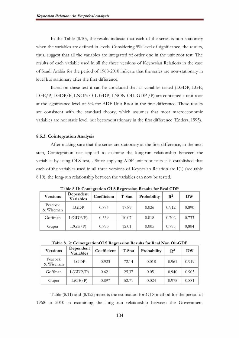
Keynesian Relation: An Empirical Analysis
184
In the Table (8.10), the results indicate that each of the series is non-stationary
when the variables are defined in levels. Considering 5% level of significance, the results,
thus, suggest that all the variables are integrated of order one in the unit root test. The
results of each variable used in all the three versions of Keynesian Relations in the case
of Saudi Arabia for the period of 1968-2010 indicate that the series are non-stationary in
level but stationary after the first difference.
Based on these test it can be concluded that all variables tested (LGDP, LGE,
LGE/P, LGDP/P, LNON OIL GDP, LNON OIL GDP /P) are contained a unit root
at the significance level of 5% for ADF Unit Root in the first difference. These results
are consistent with the standard theory, which assumes that most macroeconomic
variables are not static level, but become stationary in the first difference (Enders, 1995).
8.5.3. Cointegration Analysis
After making sure that the series are stationary at the first difference, in the next
step, Cointegration test applied to examine the long-run relationship between the
variables by using OLS test, . Since applying ADF unit root tests it is established that
each of the variables used in all three versions of Keynesian Relation are I(1) (see table
8.10), the long-run relationship between the variables can now be tested.
Table 8.11: Contegration OLS Regression Results for Real GDP
Versions Dependent Variables
Coefficient T-Stat Probability 𝐑𝟐 DW
Peacock & Wiseman
LGDP 0.874 17.89 0.026 0.912 0.890
Goffman L(GDP/P) 0.539 10.07 0.018 0.702 0.733
Gupta L(GE/P) 0.793 12.01 0.005 0.795 0.804
Table 8.12: CoinetgrationOLS Regression Results for Real Non Oil-GDP
Versions Dependent Variables
Coefficient T-Stat Probability 𝐑𝟐 DW
Peacock & Wiseman
LGDP 0.923 72.14 0.018 0.961 0.919
Goffman L(GDP/P) 0.621 25.37 0.051 0.940 0.903
Gupta L(GE/P) 0.897 52.71 0.024 0.975 0.881
Table (8.11) and (8.12) presents the estimation for OLS method for the period of
1968 to 2010 in examining the long run relationship between the Government
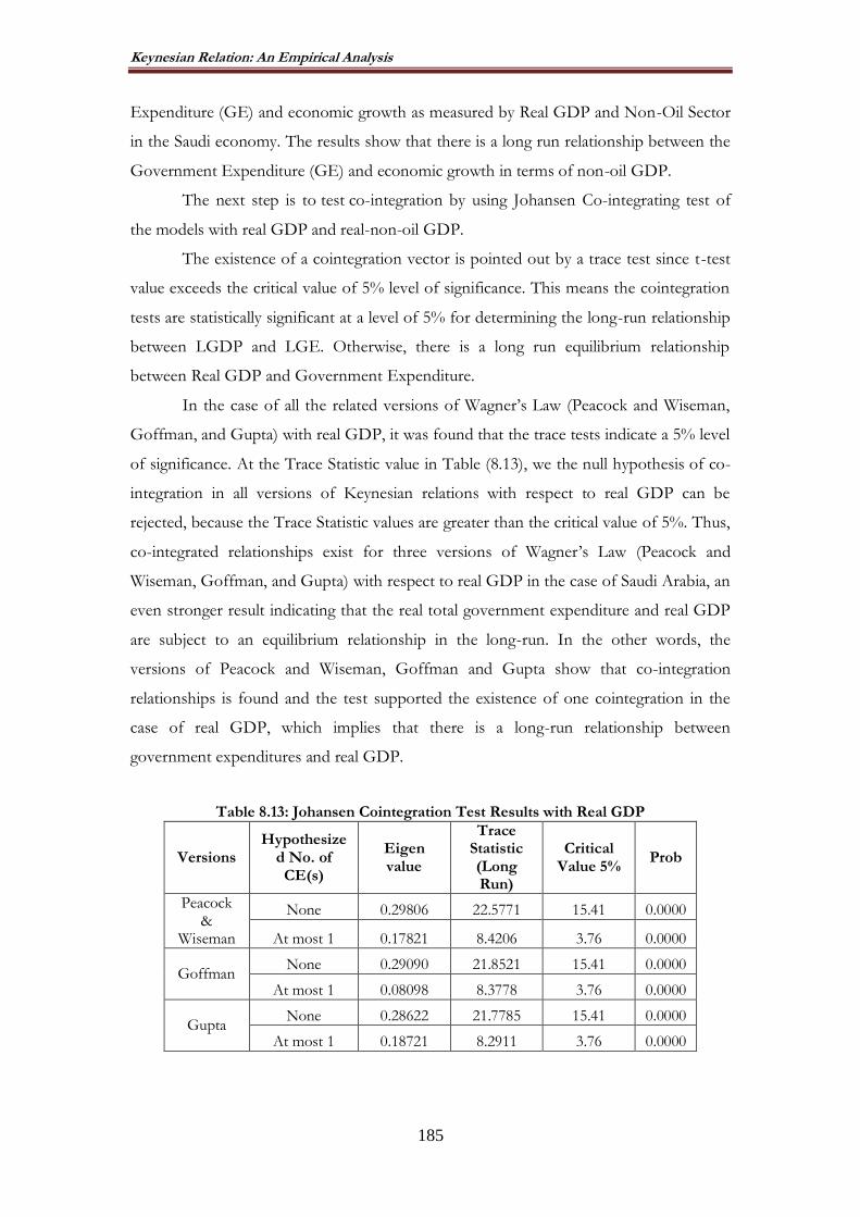
Keynesian Relation: An Empirical Analysis
185
Expenditure (GE) and economic growth as measured by Real GDP and Non-Oil Sector
in the Saudi economy. The results show that there is a long run relationship between the
Government Expenditure (GE) and economic growth in terms of non-oil GDP.
The next step is to test co-integration by using Johansen Co-integrating test of
the models with real GDP and real-non-oil GDP.
The existence of a cointegration vector is pointed out by a trace test since t-test
value exceeds the critical value of 5% level of significance. This means the cointegration
tests are statistically significant at a level of 5% for determining the long-run relationship
between LGDP and LGE. Otherwise, there is a long run equilibrium relationship
between Real GDP and Government Expenditure.
In the case of all the related versions of Wagner’s Law (Peacock and Wiseman,
Goffman, and Gupta) with real GDP, it was found that the trace tests indicate a 5% level
of significance. At the Trace Statistic value in Table (8.13), we the null hypothesis of co-
integration in all versions of Keynesian relations with respect to real GDP can be
rejected, because the Trace Statistic values are greater than the critical value of 5%. Thus,
co-integrated relationships exist for three versions of Wagner’s Law (Peacock and
Wiseman, Goffman, and Gupta) with respect to real GDP in the case of Saudi Arabia, an
even stronger result indicating that the real total government expenditure and real GDP
are subject to an equilibrium relationship in the long-run. In the other words, the
versions of Peacock and Wiseman, Goffman and Gupta show that co-integration
relationships is found and the test supported the existence of one cointegration in the
case of real GDP, which implies that there is a long-run relationship between
government expenditures and real GDP.
Table 8.13: Johansen Cointegration Test Results with Real GDP
Versions Hypothesize
d No. of CE(s)
Eigen value
Trace Statistic (Long Run)
Critical Value 5%
Prob
Peacock &
Wiseman
None 0.29806 22.5771 15.41 0.0000
At most 1 0.17821 8.4206 3.76 0.0000
Goffman None 0.29090 21.8521 15.41 0.0000
At most 1 0.08098 8.3778 3.76 0.0000
Gupta None 0.28622 21.7785 15.41 0.0000
At most 1 0.18721 8.2911 3.76 0.0000

Keynesian Relation: An Empirical Analysis
186
In the case of real non-oil GDP, the Table (8.14) shows that there is a long run
equilibrium relationship between real non oil GDP and government expenditure, or GE,
as found in Peacock and Wiseman, Goffman, and Gupta versions of Keynesian relations
at 5% levels. In other words, the null hypothesis of cointegration in all versions of
Keynesian relations with respect to real non-oil GDP, as the Trace Statistic values are
greater than the critical value of 5%.
Table 8.14: Johansen Cointegration Test Results with Real Non-Oil GDP
Versions Hypothesized No. of CE(s)
Eigen value
Trace Statistic
Critical Value 5%
Prob
Peacock & Wiseman
None 0.26793 21.0726 15.41 0.0000
At most 1 0.19341 8.5974 3.76 0.0000
Goffman None 0.33040 17.2386 15.41 0.0000
At most 1 0.03049 3.8238 3.76 0.0000
Gupta None 0.29277 25.0288 15.41 0.0000
At most 1 0.24370 11.1726 3.76 0.0000
8.5.4. Causality Test
After making sure of the time series’ model to study the variables that they are
not stationary in the level and stationary in the difference, and then check it all integrated
joint, clearly that there is a long-term equilibrium relationship. The existing relationship,
as discussed previously, is modelled through ECM and ECM in this study is applied for
Keynesian Relation in Saudi Arabia through Granger-causality test. The following is
hence the findings from Granger Causality Test.
8.5.4.1. Granger Causality Test for Keynesian Relation with Real GDP
In this section, Granger Causality results in the case of three form of Keynesian Relation
are presented with real GDP.
(i) Granger Causality in Peacock and Wiseman Version of Keynesian Relation
The probability values from Granger Causality Test are depicted in Table (8.15).
The reported F-statistics are a standard test for the joint hypothesis that economic
growth or LGDP does not Granger Cause government expenditures or LGE. The
probability for accepting the null-hypothesis is only 0.30% while the probability of
rejecting it is 99.7%. This implies that economic growth or LGDP causes government
expenditures or LGE around 99.7% of the time in Peacock and Wiseman’s Version of
Keynesian relation.

Keynesian Relation: An Empirical Analysis
187
The causality from LGE to LGDP is also searched for, where the probability for
accepting the null-hypothesis is only 15.9%, while 84.1% reject the hypothesis, which
means LGE causes LGDP about 84.1% of the time.
Table 8.15: Granger Causality test for Peacock and Wiseman Version with Real GDP
Null Hypothesis F-Statistic Prob.
LGDP does not Granger Cause LGE 3.6836 0.003
LGE does not Granger Cause LGDP 16.6836 0.159
(ii) Granger Causality in Goffman Version of Keynesian Relation
Table (8.16) presents the result of the causality test based on probability values from
the Granger Causality Test. The probability for accepting the null-hypothesis, LGE does
not Granger Cause LGDP/P is 34.7% and rejecting it is 65.3%. This means that
LGDP/P causes LGE around 65.3% of the time in the Goffman’s version of Keynesian
relation. In the other direction, the probability for accepting the null-hypothesis of LGE
does not Granger Cause LGDP/P is only 0.70% and the probability of rejecting is
99.7%, which means LGE cause LGDP/P around 99.993%. The result of causality test,
thus, indicates the existence of strong feedback causality between LGE and LGDP/P in
the long run as shown in Table (8.16).
Table 8.16: Granger Causality test for Goffman Version with Real GDP
Null Hypothesis F-Statistic Prob.
LGDP/PC does not Granger Cause LGE 2.1172 0.347
LGE does not Granger Cause LGDP/PC 9.9422 0.007
(iii) Granger Causality in Gupta Version of Keynesian Relation
The result of causality test based on probability values from Granger Causality
Test for the Gupta version of Keynesian relation is presented in Table (8.17). The null-
hypothesis that LGDP/P does not Granger Cause LGE/P is accepted with a probability
of 11.6% and is rejected by 88.4%, which indicates that LGDP/P causes LGE/P around
88.4% of the time in Gupta’s version of Keynesian relation. In the opposite direction,
the probability for accepting the null-hypothesis of LGE/P does not Granger Cause
LGDP/P is 0.10% and is rejected by 99.9%, which implies that LGE/P causes LGDP/P
around 99.9% of the time.
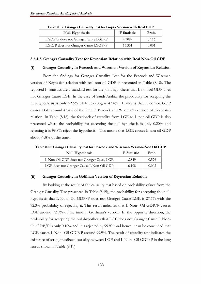
Keynesian Relation: An Empirical Analysis
188
Table 8.17: Granger Causality test for Gupta Version with Real GDP
Null Hypothesis F-Statistic Prob.
LGDP/P does not Granger Cause LGE/P 4.3099 0.116
LGE/P does not Granger Cause LGDP/P 15.331 0.001
8.5.4.2. Granger Causality Test for Keynesian Relation with Real Non-Oil GDP
(i) Granger Causality in Peacock and Wiseman Version of Keynesian Relation
From the findings for Granger Causality Test for the Peacock and Wiseman
version of Keynesian relation with real non-oil GDP is presented in Table (8.18). The
reported F-statistics are a standard test for the joint hypothesis that L non-oil GDP does
not Granger Cause LGE. In the case of Saudi Arabia, the probability for accepting the
null-hypothesis is only 52.6% while rejecting is 47.4%. It means that L non-oil GDP
causes LGE around 47.4% of the time in Peacock and Wiseman’s version of Keynesian
relation. In Table (8.18), the feedback of causality from LGE to L non-oil GDP is also
presented where the probability for accepting the null-hypothesis is only 0.20% and
rejecting it is 99.8% reject the hypothesis. This means that LGE causes L non-oil GDP
about 99.8% of the time.
Table 8.18: Granger Causality test for Peacock and Wiseman Version-Non Oil GDP
Null Hypothesis F-Statistic Prob.
L Non-Oil GDP does not Granger Cause LGE 1.2849 0.526
LGE does not Granger Cause L Non-Oil GDP 16.198 0.002
(ii) Granger Causality in Goffman Version of Keynesian Relation
By looking at the result of the causality test based on probability values from the
Granger Causality Test presented in Table (8.19), the probability for accepting the null-
hypothesis that L Non- Oil GDP/P does not Granger Cause LGE is 27.7% with the
72.3% probability of rejecting it. This result indicates that L Non- Oil GDP/P causes
LGE around 72.3% of the time in Goffman’s version. In the opposite direction, the
probability for accepting the null-hypothesis that LGE does not Granger Cause L Non-
Oil GDP/P is only 0.10% and it is rejected by 99.9% and hence it can be concluded that
LGE causes L Non- Oil GDP/P around 99.9%. The result of causality test indicates the
existence of strong feedback causality between LGE and L Non- Oil GDP/P in the long
run as shown in Table (8.19).

Keynesian Relation: An Empirical Analysis
189
Table 8.19: Granger Causality test for Goffman Version-Non Oil GDP
Null Hypothesis F-Statistic Prob.
L Non- Oil GDP/P does not Granger Cause LGE 2.5677 0.277
LGE does not Granger Cause L Non- Oil GDP/P 14.514 0.001
(iii) Granger Causality in Gupta Version of Keynesian Relation
The result of causality test based on probability values from the Granger
Causality Test presented in Table (8.20). As can be seen, the null-hypothesis that L Non-
Oil GDP/P does not Granger Cause LGE/P is only 51.4% implying that it is rejected by
48.6%. This means that L Non- Oil GDP/P causes LGE/P by around 48.6% of the
time in Gupta’s Version, which consistent with Keynesian relation suggestion. In the
oppositional direction, the probability for accepting the null-hypothesis of LGE/P does
not Granger Cause L Non- Oil GDP/P is 0.60% indicating that LGE/P causes L Non-
Oil GDP/P around 99.4% of the time.
Table 8.20: Granger Causality test for Gupta Version-Non Oil GDP
Null Hypothesis F-Statistic Prob.
L Non- Oil GDP/P does not Granger Cause LGE/P 1.3316 0.514
LGE/P does not Granger Cause L Non- Oil GDP/P 16.711 0.006
8.5.5. Error Correction Model (ECM) in Keynesian Relation
In this section, ECM is extended and analysis is presented in the following
sections with real GDP and non-oil real GDP.
(i) ECM with Real GDP
The results in Table (8.21) indicate that there is long-run unidirectional causality
that runs from GDP to GE in Peacock and Wiseman version; from GDP/P to GE in
Goffman version; from GDP/P to GE/P in Gupta version of Keynesian relation. This
is due to the fact that the variables GE and GE/P are statistically significant at the 5%
level, and the variables GDP and GDP/P are statistically insignificant at the 5% level.
Thus, three versions of Keynesian Relations are found to hold for GDP in the
case of Saudi Arabia.
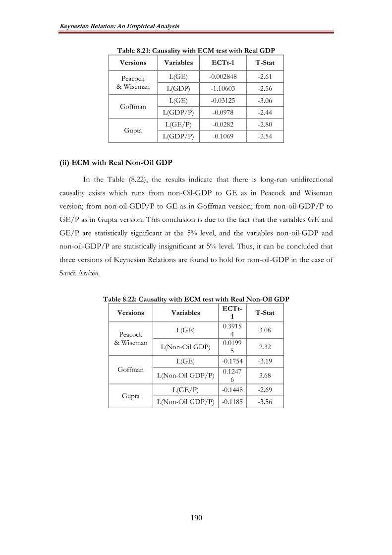
Keynesian Relation: An Empirical Analysis
190
Table 8.21: Causality with ECM test with Real GDP
Versions Variables ECTt-1 T-Stat
Peacock & Wiseman
L(GE) -0.002848 -2.61
L(GDP) -1.10603 -2.56
Goffman L(GE) -0.03125 -3.06
L(GDP/P) -0.0978 -2.44
Gupta L(GE/P) -0.0282 -2.80
L(GDP/P) -0.1069 -2.54
(ii) ECM with Real Non-Oil GDP
In the Table (8.22), the results indicate that there is long-run unidirectional
causality exists which runs from non-Oil-GDP to GE as in Peacock and Wiseman
version; from non-oil-GDP/P to GE as in Goffman version; from non-oil-GDP/P to
GE/P as in Gupta version. This conclusion is due to the fact that the variables GE and
GE/P are statistically significant at the 5% level, and the variables non-oil-GDP and
non-oil-GDP/P are statistically insignificant at 5% level. Thus, it can be concluded that
three versions of Keynesian Relations are found to hold for non-oil-GDP in the case of
Saudi Arabia.
Table 8.22: Causality with ECM test with Real Non-Oil GDP
Versions Variables ECTt-
1 T-Stat
Peacock & Wiseman
L(GE) 0.3915
4 3.08
L(Non-Oil GDP) 0.0199
5 2.32
Goffman L(GE) -0.1754 -3.19
L(Non-Oil GDP/P) 0.1247
6 3.68
Gupta L(GE/P) -0.1448 -2.69
L(Non-Oil GDP/P) -0.1185 -3.56

Keynesian Relation: An Empirical Analysis
191
8.6. CONCLUSION
In this chapter, the relationship between government expenditure and economic
growth is explored through three versions of Keynesian Relations for Saudi Arabia, using
time series annual data for the period 1968 to 2010.
In the analysis, three distinct time series techniques are applied: Initially, the
regressions analysis utilised for three versions of Keynesian Relations using Ordinary
Least Square (OLS) with real GDP and non-oil GDP. In the next step, the Unit Root
tests through Augmented Dickey-Fuller test for stationary is applied with real GDP and
non-oil GDP. In the following step, cointegrating test for real GDP and non-oil GDP.
Finally, causality tests by using Granger Causality tests are conducted together with
ECM.
In overall, the findings in this study suggest that there is a cointegrating
relationship between the share of government expenditure in national output and per
capita income. The equilibrium relationship indicates that the major determinant of
government expenditure in Saudi Arabia, in the long run, is national income. In the case
of Real GDP and Non-oil GDP, the versions of Peacock & Wiseman, Goffman and
Gupta show that co-integration relationships is found and the test supported the
existence of one cointegration.
Finally, Granger’s causality tests were used to confirm the causality direction
between the variables by using the ECM. Since there exists an ECM to describe the short
run adjustment to equilibrium, three versions of the Keynesian Relations are found to
hold for both (GDP) and (Non-Oil-GDP) in the case of Saudi Arabia.
The findings in this study verify the importance of Keynesian relation for a late
developing country such as Saudi Arabia, where the private capital for economic
development until recently was limited. The fiscal policy in the form of government
expenditures has been the engine of economic growth and development in Saudi Arabia.
The government revenues raised from oil wealth in Saudi Arabia have been the main
source of economic and social development of the country, which generated
employment and expansion of the economy as predicated by Keynes.
The findings of this research, hence, verified the validity of the Keynesian
Relation in the case of Saudi Arabia, and also indicate the importance of government
expenditure for economic development in the cases where the private capital is in short
supply as was in Saudi Arabia. This does not imply that government’s role for economic

Keynesian Relation: An Empirical Analysis
192
growth and development is applauded without any questioning, as the efficiency and
effectiveness of using government expenditure is a matter of another debate.

Displacement Effect in the Government Expenditures in Saudi Arabia: An Empirical Analysis
193
CHAPTER 9
LOCATING DISPLACEMENT EFFECT IN THE GOVERNMENT EXPENDITURES IN SAUDI ARABIA
9.1. INTRODUCTION
This chapter aims to test Peacock and Wiseman‟s (1961) „displacement effect
hypothesis‟, which originally attempted to explain the proportional increase in time
government expenditures overtime in the United Kingdom through time by making
reference to unexpected social and political events. As explained in detail in Chapter 3,
they found that government expenditure in the United Kingdom did not follow a
smooth trend, but instead deviated from the observed trends by jumping up at separate
times to respond to certain socio-political and economic events. This provided a
rationale for shift in the level of government expenditures through displacing the
previous trend.
The Peacock and Wiseman‟s (1961) „displacement effect hypothesis‟ relates to
Wagner‟s law by developing a different approach as to why government expenditures
increase. They contend that under normal conditions of peace and economic stability,
changes in public expenditure are rather limited unless some major crisis occurs, which
necessitates an increase in government intervention. In other words, Peacock and
Wiseman (1961) argue that during social and political upheavals, government
expenditures move beyond the secular trend it follows by responding to the upheavals
with increased government expenditures as required. However, they argue that the
expansion in the government expenditure will not just be temporary. In other words,
after such upheaval and crises over, the government expenditures will not go back to the
pre-crisis level. Peacock and Wiseman (1961) explain this by referring to the tolerable
level of taxation imposed on the taxpayers, as taxpayers will be more tolerable for tax
increases during social and political upheavals, which finances increased government
expenditures during such periods. However, they further argue that government
expenditure will not go back to the previous level after such upheavals as government
exploit the tolerable taxation level of the taxpayers and keep the government
expenditures at the new level. This, thus, implies that the new level of government
expenditures displaces the previous level. Consequently, the size of the public sector will
remain able at a higher level until the next shock.
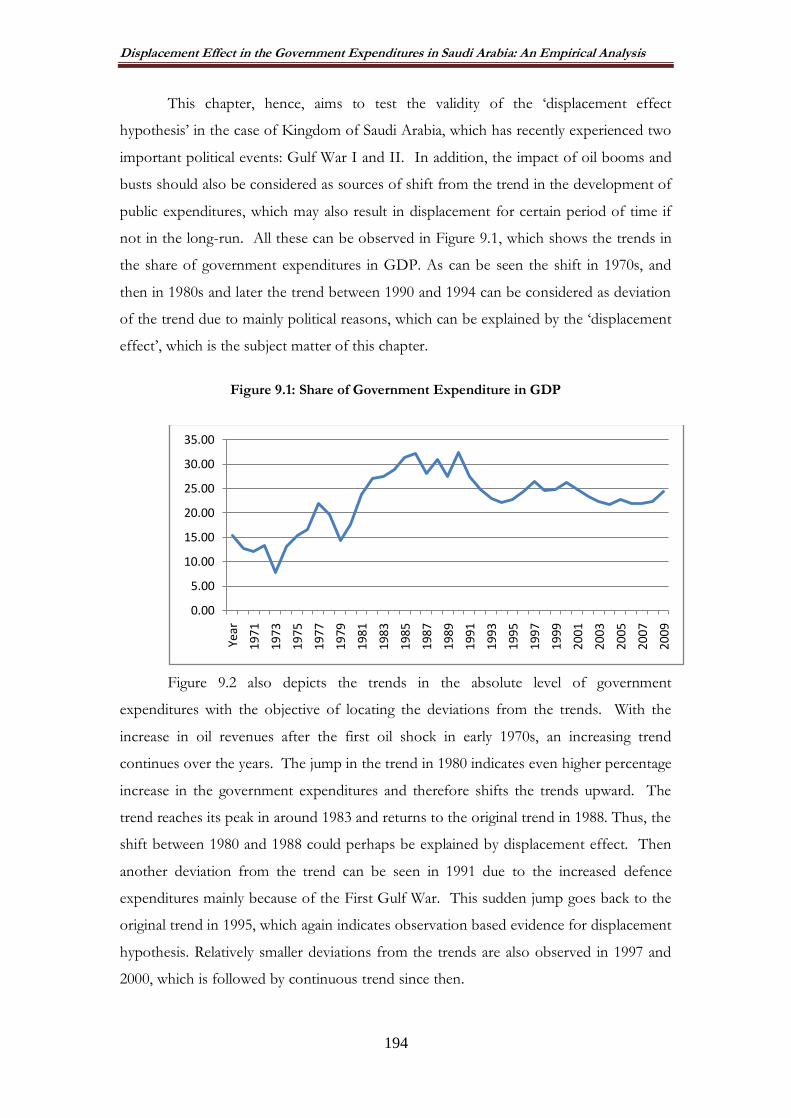
Displacement Effect in the Government Expenditures in Saudi Arabia: An Empirical Analysis
194
This chapter, hence, aims to test the validity of the „displacement effect
hypothesis‟ in the case of Kingdom of Saudi Arabia, which has recently experienced two
important political events: Gulf War I and II. In addition, the impact of oil booms and
busts should also be considered as sources of shift from the trend in the development of
public expenditures, which may also result in displacement for certain period of time if
not in the long-run. All these can be observed in Figure 9.1, which shows the trends in
the share of government expenditures in GDP. As can be seen the shift in 1970s, and
then in 1980s and later the trend between 1990 and 1994 can be considered as deviation
of the trend due to mainly political reasons, which can be explained by the „displacement
effect‟, which is the subject matter of this chapter.
Figure 9.1: Share of Government Expenditure in GDP
Figure 9.2 also depicts the trends in the absolute level of government
expenditures with the objective of locating the deviations from the trends. With the
increase in oil revenues after the first oil shock in early 1970s, an increasing trend
continues over the years. The jump in the trend in 1980 indicates even higher percentage
increase in the government expenditures and therefore shifts the trends upward. The
trend reaches its peak in around 1983 and returns to the original trend in 1988. Thus, the
shift between 1980 and 1988 could perhaps be explained by displacement effect. Then
another deviation from the trend can be seen in 1991 due to the increased defence
expenditures mainly because of the First Gulf War. This sudden jump goes back to the
original trend in 1995, which again indicates observation based evidence for displacement
hypothesis. Relatively smaller deviations from the trends are also observed in 1997 and
2000, which is followed by continuous trend since then.
0.00
5.00
10.00
15.00
20.00
25.00
30.00
35.00
Year
1971
1973
1975
1977
1979
1981
1983
1985
1987
1989
1991
1993
1995
1997
1999
2001
2003
2005
2007
2009

Displacement Effect in the Government Expenditures in Saudi Arabia: An Empirical Analysis
195
Figure 9.2: Trends in the Absolute Level of Government Expenditures in Saudi Arabia
This study, therefore, considers that Peacock and Wiseman‟s „displacement
hypothesis‟ can explain deviations from the trends, and in particular the recent wars and
other relevant events can be considered potential reasons of deviation in the Saudi
government expenditures. The data used in this study is the time series annual data for
the 1968 to 1989 period being the pre- Gulf War II, and 1990 to 2010 period being the
post-Gulf War II, which have been used to analyse the developments in government
expenditure (GE) in relation to economic growth by making particular reference to
„displacement hypothesis‟.
The rest of the chapter is organised as follows: section one, presents some
empirical results of relevant theoretical and empirical literature on the relationship
between government expenditure and economic growth in relation to „displacement
effect hypothesis.‟ Following section, presents the Peacock and Wiseman version, and
the formal explanation of the „displacement effect hypotheses‟. Section three, investigates
the data and empirical results and analysis by using displacement effect hypotheses‟.
Section four, presents the results of analysis by using the time series techniques, such as
the Ordinary Least Square (OLS), Augmented Dickey-Fuller for stationary Unit Root
Tests, Cointegration Test, Causality Granger Test, and Error Correction Model (ECM),
that for real GDP and Non-Oil GDP. While section five, concludes the chapter and
presents the finding.
0
50,000
100,000
150,000
200,000
250,000
300,000
350,000
400,000
450,000
1970
1972
1974
1976
1978
1980
1982
1984
1986
1988
1990
1992
1994
1996
1998
2000
2002
2004
2006
2008
2010

Displacement Effect in the Government Expenditures in Saudi Arabia: An Empirical Analysis
196
9.2. THE DISPLACEMENT EFFECT HYPOTHESIS
Peacock and Wiseman‟s (1961) observation on the developments of public
expenditures lead to the „displacement effect hypotheses in case of the UK. As explained
in Chapter 3 and mentioned above, the hypothesis states that due to some social and
political events and crises government expenditures, as expected, would increase in
response to the increased public expenditures during such times. However, according to
the hypothesis, after such incidences, the government expenditures would stay in the
new level rather than going back to the pre-crises level and trend, implying a shift and
displacement.
The hypothesis, however, indicates two important dimensions as discussed in the
literature; the structural break from the trend but also the ratchet impact indicating the
initial jump in the government expenditures due to such events. These are explained in
the following sections.
9.2.1. Structural Break
As explained Chapter 3, wars and other social and political upheavals are capable
of displacing this notion of tolerable tax rates and hence displacing the level of
government expenditures. After such events, government expenditure may fall again, but
not to their previous levels. Therefore, public expenditure grows in a discontinuous and
stepwise fashion, the steps occurring at times of major social upheavals (Demirbas,
1999). In other words, Peacock and Wiseman investigated that both citizens and
government hold divergent views about the desirable size of public expenditures and the
possible level of government taxation. This divergence can be adjusted by social
disturbances that destroy established conceptions and produce a displacement effect.
People will accept, in a period of crisis, tax levels and methods of raising revenue that in
quieter times would have been intolerable, and this acceptance remains when the
disturbance itself has disappeared. Thus, the hypothesis indicates that there is the
structural change aspect in government expenditures in terms of the trend.
In explaining the „displacement effect hypothesis‟, Henrekson (1990: 246) states
that “Peacock and Wiseman (1961), adopt a clearly inductive approach to explaining the
growth of government expenditure. When Peacock and Wiseman observed that
expenditures over time appeared to outline a series of plateaus separated by peaks, and
that these peaks coincided with periods of war and preparation for war they were led to
expound the „displacement effect‟ hypothesis”. Such an explanation refers to the

Displacement Effect in the Government Expenditures in Saudi Arabia: An Empirical Analysis
197
structural break nature of the hypothesis. Diamond (1977), therefore, presented the
displacement effect as a theory of structural break. He used the Chow test (1960),
comparing two periods separated by a social upheaval, and he found that, if this shows
significant structural change and there has been displacement.
9.2.2. A Ratchet Effect
As mentioned discussed in Chapter 3, the „ratchet effect‟ refers to the restrained
ability of a processes to be reversed once a specific thing has happened. The term is
used within the „displacement effect hypothesis‟ to describe the seemingly irreversible
expansion of government in times of crisis in his book. In other words, as explained due
to the expansionary government expenditures during crises periods, governments then
have difficulty in reducing government expenditures back to the original level after the
initial temporary needs due to war, natural or economic crisis. The government‟s
exploitation of taxpayers‟ tolerance plays an important role in this process. Thus, the
main argument of the ratchet effect is that if there is a crisis and government
expenditures grows as a result, then the public expenditure might decline but not to the
previous level as there would be resistance against such a move.
According to Bird (1972), within the displacement effect, this has called „ratchet
effect‟. This is due to the fact that, for Bird (1972) crises are likely to have short-term
implications for government expenditure ratio rather than leading to a permanent
upward displacement for. Thus, Bird (1972) acknowledges the ratchet effect but rejects
the displacement effect. In another study, Peacock and Wiseman (1979) argued that in
the extreme, the ratchet effect interpretation of the displacement effect leads to the
denial of its very existence.
9.2.3. Empirical Testing of Displacement Effect: Previous Studies
Gupta (1967) was the first to attempt to subject the displacement effect to
empirical testing in the case of European countries. He found significant displacement in
all cases except for Sweden after the Second World War, and also found significant
displacement caused by the Great Depression in the case of the USA and Canada.
Legrenzi (2004) argued that the displacement effect for Italy lay within a
multivariate revenue-expenditure model of government growth. His result for long-run
analysis shows the effect of GDP on the government‟s growth. Otherwise, he found that
the short-run analysis shows some evidence for the displacement effect in terms of a

Displacement Effect in the Government Expenditures in Saudi Arabia: An Empirical Analysis
198
lower resistance against tax financing of government expenditure during the Second
World War.
Another study by Henry and Olekalns (2000) investigated the Peacock and
Wiseman‟s „displacement effect‟ to explain the increases in the ratio of government
expenditure to GDP in the UK. They used a data set extending back to 1836, and found
instances where displacement may have occurred.
9.3. MODELLING DISPLACEMENT EFFECT IN ECONOMETRIC
METHODOLOGY
In an attempt to search for the „displacement effect‟ in the case of Saudi Arabia,
Peacock-Wiseman version of Wagner‟s Law is utilised, which is presented in Table (9.1)
in real GDP.
Table 9.1: The Original Version of Peacock-Wiseman with Real GDP
No Function Version Year
1 L(GE) = α + β L(GDP) Peacock-Wiseman 1967
In addition, the non-oil GDP version of the Peacock and Wiseman‟s Wagner
Law exposition is depicted in Table (9.2).
Table 9.2: The Version of Peacock-Wiseman with Real Non-Oil Sector of GDP
No Function Version Year
1 L(GE) = α + β L(Non-Oil GDP) Peacock-Wiseman 1967
In analysing the identified model, the Ordinary Least Square (OLS) test is
employed to determine the parameters in the equations. In terms of diagnosis tests, the
Durbin-Watson (DW) statistic indicates the absence of serial correlation among the
residuals; R2 reflects the regression equation‟s ability to determine the dependent
variable‟s performance in terms of explaining the observed variance in the dependent
variable. In addition, the coefficients of the logarithm model are considered as elasticises.
However, it should not be noted that the logarithm transformation is applicable only
when all the observations in the data set are positive.
As for the formal explanation of the model, according to Gujarati (1995), the
normal regression model by taking logs of both sides of the equation:

Displacement Effect in the Government Expenditures in Saudi Arabia: An Empirical Analysis
199
The normal equation of Peacock and Wiseman version of Wagner‟s Law is:
GE = f (GDP) f‟ > 0 & f‟‟ ≥ 0 (9.1)
where: GE = Total Government Expenditure level in real terms.
GDP= Gross Domestic Product in real terms.
GE = α + β GDP + e (9.2)
The equation by using logarithm model:
L (GE) = α + β L (GDP) + e (9.3)
E (Peacock & Wiseman) = d(GE )
d(GDP )/
GE
GDP (9.4)
Where: E denotes elasticity.
In order to capture the impact of political events such as Gulf War 1 and Gulf
War 2, structural break test is employed.
For this, the data is split into two groups, then the Chow test is utilised, which is
like an F- test:
knRSSRSS
kRSSRSSRSSF c
2/)(
/)(
21
21
(9.5)
The hypotheses for the Chow Test are:
H0:βi = 0; (There is no structural break )
H1: β1 ≠ 0; (There is a structural break )
It should be noted that the impact of various social, political and economic
upheavals and crises can also be captured through dummy variables. Therefore, in this
study, initially dummy variables are used to test the significance of „displacement effect‟
in the case of Saudi Arabia. The following social, political and economic upheavals and
events are considered by this study as important events causing shift in Saudi
government expenditures due to their enormity:.

Displacement Effect in the Government Expenditures in Saudi Arabia: An Empirical Analysis
200
D1973: Dummy Variables for year 1973 for the first oil shock resulting in large
revenues of the Saudi government;
D1976: Dummy Variables for year 1976 for the second oil shock which resulted in
even larger revenues for the government;
D1983: Dummy Variables for year 1983 for the global recession due to the high oil
prices which resulted in shrinking revenues for Saudi Arabia;
D1991: Dummy Variables for year 1991 indicating the beginning of the Gulf War
1;
D1997: Dummy Variables for year 1997 for the financial crisis affecting certain
parts of the world;
D2001: Dummy Variables for year 2001 for the beginning of the Gulf War 2;
D2006: Dummy Variables for year 2006 for the collapse of the Saudi stock market.
The Peacock and Wiseman version of the Wagner Law is, then, presented in its modified
version as follows:
L GE = α + β1L GDP + β2D 1973 + β3D 1976
+ β4D 1983 + β5D 1991 + β6D 1997 + β3D 2001
+ β3D 2006 + et (9.6)
9.4. FINDINGS FOR DISPLACEMENT EFFECT IN THE CASE OF SAUDI
ARABIA
After identifying the model and its particularities, Peacock and Wiseman version of
the Wagner Law is utilised to examine the validity of „displacement effect‟ in the case of
Saudi Arabia from 1968-2010. In doing so results first presented with real-GDP and
later with non-oil GDP.
9.4.1. Peacock-Wiseman Hypothesis with Real-GDP and Economic and Political
Dummy Variables, 1968-2010
In testing the „displacement effect‟, the model is expanded, as mentioned before,
with the addition of political and economic dummy variables as defined above:
L GE = α + β1L GDP + β2D 1973 + β3D 1976
+ β4D 1983 + β5D 1991 + β6D 1997 + β3D 2001
+ β3D 2006 + et (9.7)

Displacement Effect in the Government Expenditures in Saudi Arabia: An Empirical Analysis
201
The results from OLS test are presented in Table 9.3.
Table 9.3: Displacement Effect (Real GDP): 1968-2010
1968 – 2010
Variables Coefficient T-Stat Probability
C 5.006246 5.509902 0.0000
LNGDP 0.321715 3.603543 0.0010
D1973 0.778761 3.773290 0.0006
D1976 1.280299 6.966756 0.0000
D1983 0.407364 3.659938 0.0009
D1991 0.080591 0.673151 0.5055
D1997 0.111410 0.797913 0.4306
D2001 0.157782 1.072245 0.2914
D2006 0.470858 3.261902 0.0026
R-squared 0.979187 Durbin-Watson stat 1.759770
Adjusted R-squared 0.974142 F-statistic 194.0718
The results, as depicted in Table 9.3, show that all variables are significant except
for the dummy variables for Gulf War 1 in 1991, for 1997 financial crisis, and for 2001
Gulf War 2 is not.
The results indicate that the coefficient value of the GDP as being the main
independent variable gives the elasticity of government expenditure growth in relation to
realGDP: E = 0.321715> 0, which means that a 1% unit increase in GDP generates a
0.321715% unit increase GE. R2 being 97.92% indicates the strength of the model,
leaving only 2.08% to be explaining by the stochastic disturbance term, e.
These findings are consistent with Wagner's Law of increasing state activities,
which states the income elasticity of demand for public goods is greater than unity. In
addition, the findings in Table 9.3 indicate that the dummy variables, D1973, D1976,
D1983 and D2006 are statistically significant for the period 1968-2010 for Saudi Arabia.
Thus, it can be concluded that the events indicated by the significant dummy variables
have caused a change in the government expenditures in Saudi Arabia.
9.4.2. Testing Displacement Effect through Chow Test
In order to test the existence of „displacement effect‟ in the case of Saudi Arabia,
as mentioned, structural test can be used. For this, the data are split into two: 1968-1989

Displacement Effect in the Government Expenditures in Saudi Arabia: An Empirical Analysis
202
and 1990-2010. After establishing the results for the period in question with only the
relevant dummy variables, the Chow test is applied (Chow, 1960).
9.4.2.1. Testing for Displacement Effect for 1968 to 1989 with Real-GDP
The estimation for Peacock and Wiseman version of Wagner‟s Law in relation to
the „displacement effect‟ is conducted initially for only 1968-1989 period, and the results
are depicted in table 9.4. It should be noted that only the relevant variables are included
in the model, namely D1973, D1976 and D1983, as the data covers only until 1989. The
formal model is expressed as in equation 9.8.
L GE = α + β1L GDP + β2D 1973 + β3D 1976
+ β4D 1983 + et (9.8)
Where:
D1973: Dummy Variables for year (1973)
D1976: Dummy Variables for year (1976)
D1983: Dummy Variables for year (1983)
Table 9.4: Displacement Effect with Real GDP, 1968-1989
1968 – 1989
Variables Coefficient T-Stat Probability
C 0.036244 0.035622 0.9720
LNGDP 0.812822 8.102681 0.0000
D1973 0.042101 0.225312 0.8244
D1976 0.683955 4.258447 0.0005
D1983 0.418495 5.155309 0.0001
R-squared 0.990514 Durbin-Watson stat 2.773533
Adjusted R-squared 0.988281 F-statistic 443.7560
In confirming the results in Table (9.4), the findings in Table (9.4) show that
except for the dummy variable for the 1973 oil shock all the variables are significant.
The elasticity of the government expenditures in relations to GDP indicates that an
increase of 1% unit in GDP generates a 0.812822% unit increase GE. The overall

Displacement Effect in the Government Expenditures in Saudi Arabia: An Empirical Analysis
203
explanatory power of the model as explained by the R2 shows that the model is capable
of explaining 99% of the variation in the dependent variable.
This finding is consistent with Wagner‟s Law of increasing state activities, which
states the income elasticity of demand for public goods is greater than unity. In addition,
having, D1976, and D1983 dummy variables indicates an important result in terms of
displacement effect, as oil shock in 1976 generated large income for public expenditures
to expand, and 1983 global recession created fiscal crisis in Saudi Arabia as well.
Therefore, these two dummy variables help to verify displacement hypothesis in terms of
divergence of government expenditures from its trend due to economic expansion and
crisis. However, the insignificance of dummy variable for 1973 oil shock is rather
unexpected, which can be explained through initial inexperience of the government in
directing the new economic wealth to economic development through expanding
government expenditures. In other words, the social capital in terms of economic
development perhaps was much lower; and therefore the use of resources for economic
development was not prioritised.
9.4.2.2. Testing for Displacement Effect for 1990 to 2010 with Real-GDP
As part of the structural test, the second part of the data for 1990-2010 is also
examined for the presence of displacement effect, as in equation 9.9. As before, only the
relevant dummy variables are included in the equation, and the results are presented in
Table 9.5.
L GE = α + β1L GDP + β2D 1991 + β3D 1997
+ β4D 2001 + β5D 2006
+ et (9.9)
where:
D1991: Dummy Variables for year (1991)
D1997: Dummy Variables for year (1997)
D2001: Dummy Variables for year (2001)
D2006: Dummy Variables for year (2006)
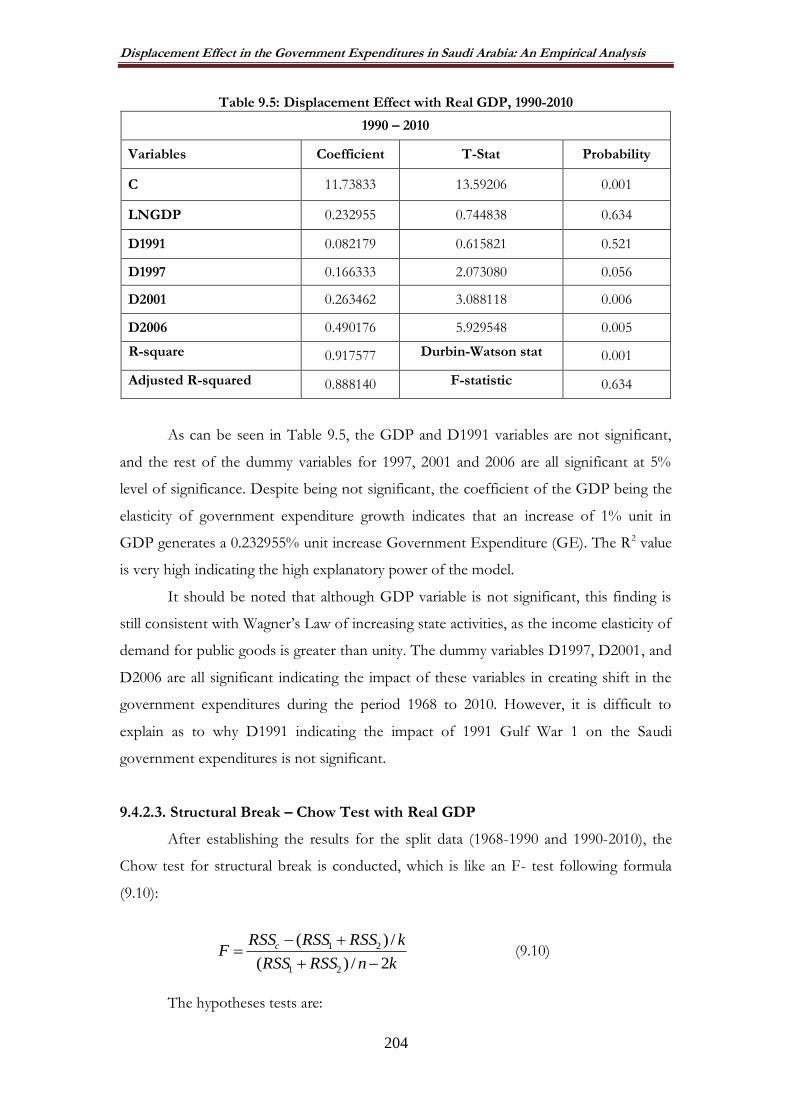
Displacement Effect in the Government Expenditures in Saudi Arabia: An Empirical Analysis
204
Table 9.5: Displacement Effect with Real GDP, 1990-2010
1990 – 2010
Variables Coefficient T-Stat Probability
C 11.73833 13.59206 0.001
LNGDP 0.232955 0.744838 0.634
D1991 0.082179 0.615821 0.521
D1997 0.166333 2.073080 0.056
D2001 0.263462 3.088118 0.006
D2006 0.490176 5.929548 0.005
R-square 0.917577 Durbin-Watson stat 0.001
Adjusted R-squared 0.888140 F-statistic 0.634
As can be seen in Table 9.5, the GDP and D1991 variables are not significant,
and the rest of the dummy variables for 1997, 2001 and 2006 are all significant at 5%
level of significance. Despite being not significant, the coefficient of the GDP being the
elasticity of government expenditure growth indicates that an increase of 1% unit in
GDP generates a 0.232955% unit increase Government Expenditure (GE). The R2 value
is very high indicating the high explanatory power of the model.
It should be noted that although GDP variable is not significant, this finding is
still consistent with Wagner‟s Law of increasing state activities, as the income elasticity of
demand for public goods is greater than unity. The dummy variables D1997, D2001, and
D2006 are all significant indicating the impact of these variables in creating shift in the
government expenditures during the period 1968 to 2010. However, it is difficult to
explain as to why D1991 indicating the impact of 1991 Gulf War 1 on the Saudi
government expenditures is not significant.
9.4.2.3. Structural Break – Chow Test with Real GDP
After establishing the results for the split data (1968-1990 and 1990-2010), the
Chow test for structural break is conducted, which is like an F- test following formula
(9.10):
knRSSRSS
kRSSRSSRSSF c
2/)(
/)(
21
21
(9.10)
The hypotheses tests are:

Displacement Effect in the Government Expenditures in Saudi Arabia: An Empirical Analysis
205
H0:βi = 0; (There is no structural break )
H1: β1 ≠ 0; There is a structural break
Table 9.6: Residual Sum of Squares with Real GDP
Source RSSc RSS1 RSS2 Df
Model 66.1080129 39.3294686 2.35229 1
Residual 7.21881508 1.91152187 0.215347 40
44.23)1(242/)35229.23295.39(
1/)35229.23295.39(1080129.66
F
After establishing the value for Chow-test, it can be concluded that since F-test
(1, 40) = 23.44 is higher than the critical value from the F-Table (5%) = 4.0847, the null
hypothesis that there is no structural break is rejected and instead the alternative
hypothesis stating that there is structural break is accepted. This implies that structural
break is a reality in the Saudi Arabian government expenditures at least in terms of 1968-
1989 and 1990-2010 period. In addition, with the existence of dummy variables and
their significance, the validity of „displacement effect‟ is verified in the case of Saudi
Arabia.
9.5. FINDINGS FOR DISPLACEMENT EFFECT IN THE CASE OF SAUDI
ARABIA WITH NON-OIL GDP
The same procedure in the previous section repeated in this section with non-oil
GDP to eliminate the impact of oil on the growth of government expenditures.
Initially, the equation in equation 9.11 is run for the entire period, 1968-2010,
with the seven variables as defined before.
L GE = α + β1L Non Oil GDP + β2D 1973 + β3D 1976
+ β4D 1983 + β5D 1991 + β6D 1997 + β3D 2001
+ β3D 2006 + et (9.11)
The results are depicted in Table 9.7:

Displacement Effect in the Government Expenditures in Saudi Arabia: An Empirical Analysis
206
Table 9.7: Displacement Effect with non-oil real GDP 1968 to 2010
1968 – 2010
Variables Coefficient T-Stat Probability
C -1.663560 0.572393 -2.906324
LN Non Oil-GDP 1.040415 0.059883 17.37416
D1973 0.189706 0.084801 2.237078
D1976 0.095467 0.106051 0.900197
D1983 -0.057862 0.049004 -1.180754
D1991 -0.054312 0.045195 -1.201744
D1997 -0.030112 0.052661 -0.571803
D2001 0.061700 0.054692 1.128137
D2006 0.144582 0.057034 2.535015
R-squared 0.997142 Durbin-Watson stat 1.269720
Adjusted R-squared 0.996449 F-statistic 1439.122
As the results, in Table 9.7 depicts, none of the variables including the GDP is
not significant, despite the fact that the coefficients values of each of the variables
indicate a certain level of impact in addition to the strong coefficient of determination as
explained by R2.
9.5.1. Testing for Displacement Effect for 1968 to 1989 with Non Oil real GDP
As part of the structural change test, Chow test, as before, the data split into two
to capture the impact of potential structural change in the government expenditures in
Saudi Arabia.
Table 9.8 shows the results for the period of 1968-1989 with the relevant dummy
variables.

Displacement Effect in the Government Expenditures in Saudi Arabia: An Empirical Analysis
207
Table 9.8: Displacement Effect with non-oil real GDP 1968 to 1989
1968 – 1989
Variables Coefficient T-Stat Probability
C -1.797123 -4.369981 0.0004
LN_NON_OIL_GDP 1.054415 24.50498 0.0000
D1973 0.175285 2.918593 0.0096
D1976 0.074266 0.982622 0.3396
D1983 -0.070775 -2.018635 0.0596
R-squared 0.998730 Durbin-Watson stat 2.773533
Adjusted R-squared 0.998431 F-statistic 3342.748
As the results in Table 9.8 demonstrates, except for D1976 all the variables are
significant with non-oil GDP having full significance and also high coefficient estimate as
compared to other variables.
9.5.2. Testing for Displacement Effect for 1990 to 2010 with Non Oil real-GDP
The same exercise repeated for the second part of the data or 1990-2010 period
and the results are depicted in Table 9.9.
Table 9.9: Displacement Effect with non-oil real GDP 1990 to 2010
1990 – 2010
Variables Coefficient T-Stat Probability
C 1.787005 4.008829 0.445767
LN Non Oil-GDP 0.787996 0.318562 2.473602
D1990 -0.057546 0.124379 -0.462665
D1997 0.017427 0.089406 0.194924
D2001 0.110417 0.092334 1.195845
D2006 0.228385 0.126219 1.809441
R-squared 0.942636 Durbin-Watson stat 1.223875
Adjusted R-squared 0.922149 F-statistic 46.01129
As the results in Table 9.9 indicate, none of the variables show any statistical
significance. It can therefore be concluded that oil revenues play an important role in

Displacement Effect in the Government Expenditures in Saudi Arabia: An Empirical Analysis
208
determining the government expenditures, as when comparing the results with the results
in the previous section the role of oil revenues is rather clear.
9.5.3. Structural Break: Chow Test with Non-Oil real GDP
After establishing the results for the split data (1968-1990 and 1990-2010), the
Chow test for structural break is conducted, which is like an F- test following formula
(9.12):
knRSSRSS
kRSSRSSRSSF c
2/)(
/)(
21
21
(9.12)
The hypotheses tests are:
H0:βi = 0; (There is no structural break )
H1: β1 ≠ 0; There is a structural break
Table 9.10: Residual Sum of Squares with Non-Oil real GDP
Source RSSc RSS1 RSS2 Df
Model 62.3715 32.4621 3.1562 1
Residual 8.04153 1.28351 0.24721 40
04.30)1(242/)1562.34621.32(
1/)1562.34621.32(3715.62
F
After establishing the value for Chow-test, it can be concluded that since F-test
(1, 40) = 30.04 is higher than the critical value from the F-Table (5%) = 4.0847, the null
hypothesis that there is no structural break is rejected and instead the alternative
hypothesis stating that there is structural break is accepted. This implies that structural
break is a reality in the Saudi Arabian government expenditures at least in terms of 1968-
1989 and 1990-2010 period. In addition, with the existence of dummy variables and
their significance, the validity of „displacement effect‟ is verified in the case of Saudi
Arabia.
9.6. TIME SERIES ANALYSIS IN LOCATING THE DISPLACEMENT
EFFECT
After conducting the research with OLS in search for displacement effect in the
case of Saudi Arabia, this section aims to further the analysis by using times-series
analysis, which includes unit root and cointegration test.

Displacement Effect in the Government Expenditures in Saudi Arabia: An Empirical Analysis
209
9.6.1. Unit Root Test
The unit root test in this section aims to examine the properties of time series
annual data for each of the government expenditures (LGE), gross domestic product
(LGDP), during the period 1968-2010 but it is applied to split data 1968-1989 to 1990-
2010 with the objective of locating the structural breakdown..
To test the stationary time series model for the study variables, it requires the
unit root test (Enders: 1995) for which Augmented Dickey-Fuller test is used as
expressed in equation 9.13:
∆ Yt = a0 + a1t + a2Yt−1 + aiki=1 Yt−1 + et (9.13)
where:
∆ = the first difference of the series.
Yt= is the series under consideration (GDP, government expenditures, or government
revenues),
t = the time trend.
k= the number of lag.
et=is stationary random error (white noise residual).
The hypotheses tests are:
H0: Unit root exists in Y , it means that ∶ Y is non − stationary
H1: Unit root dose not exists in Y , it means that ∶ Y is stationary
If the null hypothesis is rejected, it implies that the variable is non-stationary, and
hence there is a unit root process. On the other hand, if the outcome indicates that the
series are stationary after the first difference, in other words, the series integrated of
order one I(1), then co-integration test can be performed.
In this section the unit root test is performed for Peacock and Wiseman version
for real GDP and non-oil GDP firstly for 1968 to 2009, and then for the split periods:
1968 to 1989 and from 1990 to 2009. Table 9.11 presents the calculated t-value from
Augmented Dickey-Fuller for stationary unit root tests on each variable.
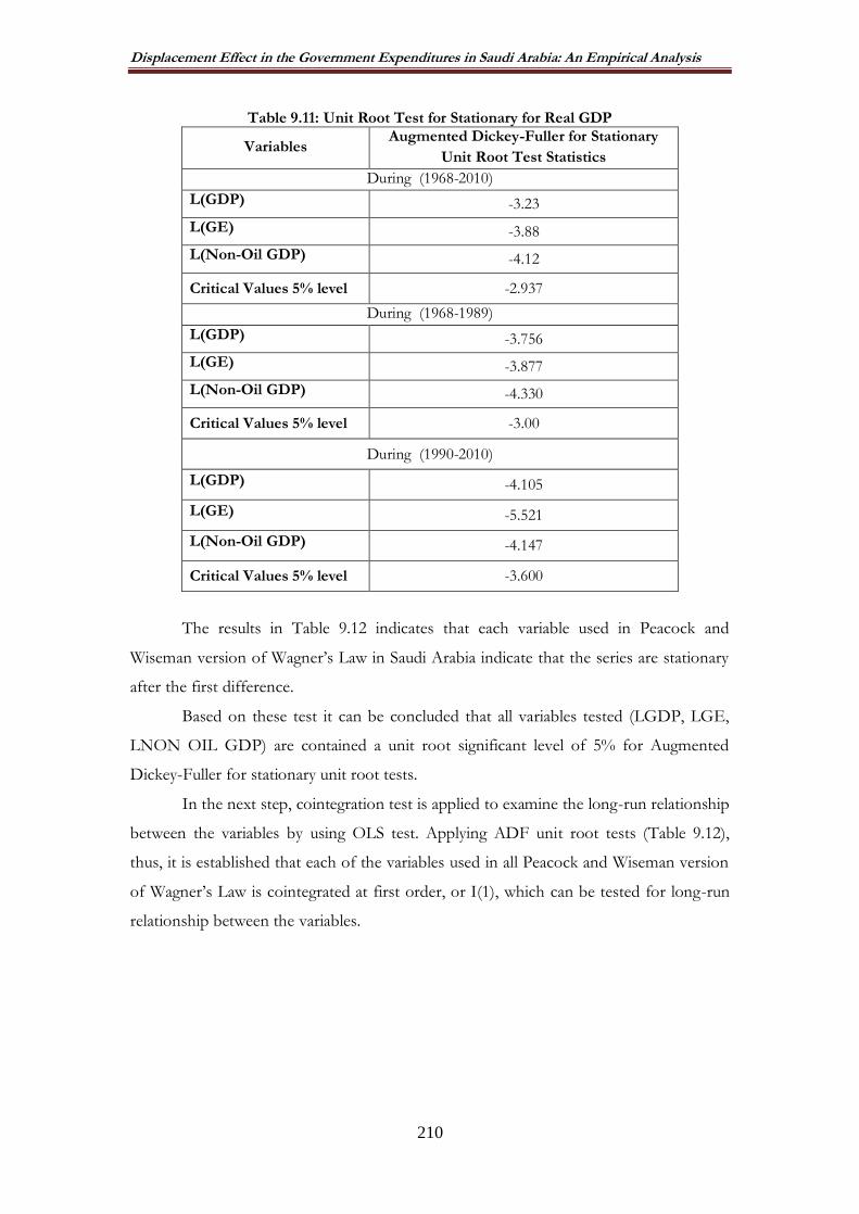
Displacement Effect in the Government Expenditures in Saudi Arabia: An Empirical Analysis
210
Table 9.11: Unit Root Test for Stationary for Real GDP
Variables Augmented Dickey-Fuller for Stationary
Unit Root Test Statistics
During (1968-2010)
L(GDP) -3.23
L(GE) -3.88
L(Non-Oil GDP) -4.12
Critical Values 5% level -2.937
During (1968-1989)
L(GDP) -3.756
L(GE) -3.877
L(Non-Oil GDP) -4.330
Critical Values 5% level -3.00
During (1990-2010)
L(GDP) -4.105
L(GE) -5.521
L(Non-Oil GDP) -4.147
Critical Values 5% level -3.600
The results in Table 9.12 indicates that each variable used in Peacock and
Wiseman version of Wagner‟s Law in Saudi Arabia indicate that the series are stationary
after the first difference.
Based on these test it can be concluded that all variables tested (LGDP, LGE,
LNON OIL GDP) are contained a unit root significant level of 5% for Augmented
Dickey-Fuller for stationary unit root tests.
In the next step, cointegration test is applied to examine the long-run relationship
between the variables by using OLS test. Applying ADF unit root tests (Table 9.12),
thus, it is established that each of the variables used in all Peacock and Wiseman version
of Wagner‟s Law is cointegrated at first order, or I(1), which can be tested for long-run
relationship between the variables.

Displacement Effect in the Government Expenditures in Saudi Arabia: An Empirical Analysis
211
Table 9.12: Contegration Regressions Results for Real GDP
Versions Dependent Variables
Coefficient T-Stat Probability 𝐑𝟐 DW
Peacock & Wiseman
LGE
1968 – 2010
0.467 4.16 0.021 0.651 0.973
1968 – 1989
1.101 14.02 0.006 0.882 0.705
1990 – 2010
0.511 0.62 0.763 0.532 0.921
Table 9.13: Cointegration Regression Results for Real Non Oil-GDP
Versions Dependent Variables
Coefficient T-Stat Probability 𝐑𝟐 DW
Peacock &
Wiseman LGE
1968 – 2010
1.024 17.12 0.004 0.932 1.171
1968 – 1989
0.987 20.44 0.000 0.929 1.913
1990 – 2010
0.663 2.74 0.002 0.961 1.192
The results in Table 9.12 and 9.13 present OLS time series results for the entire
1968-2010 and also the split periods. The results show that there is a long run
relationship between the Government Expenditure (GE) and Economic Growth (GDP)
for non-oil GDP in Saudi Arabia for the entire period as well as for the split periods as
the independent variable is significant. However, in the case of real-GDP version, the
next step is to test cointegration by using Johansen cointegrating test.
9.6.2. Cointegration Test
In this section, the cointegration test for Peacock and Wiseman version for real
GDP and non-oil GDP for the 1968 to 2010 period in Saudi Arabia is conducted; but
also the split periods (1968 to 1989 and 1990 to 2010) are also examined.
As mentioned previously, the concept of integration common that if the level
variables of the form are non-stationary any package of first class, if possible, to generate
a linear combination of these variables has characterized by a static zero-class integrated I
(0). In such a case, the integrated real-time variables of the same rank co-integrated, and
thus it can use the level variables in the regression, nor is the decline in this case a false
spurious.

Displacement Effect in the Government Expenditures in Saudi Arabia: An Empirical Analysis
212
The null hypothesis is that the variables under investigation are not co-integrated.
The rejection of the null hypothesis requires that the trace value of the co-integration test
to be greater than at least one of the different critical values. Therefore, failing to reject
the null hypothesis of no cointegration leads us to conclude that there is no relationship
in the long-term equilibrium between government spending and national income.
Cointegration test in this study is conducted by using the method developed by
Johansen (1988), and Johansen and Juselius (1990). Many studies use the Engle Granger
two-step, but there are those who used a Johansen and Juselius (1990), for so many
advantages: such as first, it tests for all of the variables and, secondly, all variables are
treated as internal variables, so that the choice of the variable is not arbitrary. This
procedure is the most reliable test for cointegration.
To determine whether stochastic trends in series have related to each other or
not, cointegration in Peacock and Wiseman version of the growth of government is
tested. In addition, after determining the order of integration by Augmented Dickey-
Fuller for stationary Unit Root Tests, co-integration of the series are tested, and if they
are, the cointegrating long-run equilibrium relationship has to be identified.
9.6.2.1. Cointegration Test with Real GDP
In the case of real GDP for the period 1968-2010, Table 9.14 shows that
cointegration relationship is found and the test supports the existence of one
cointegration equation in the relationship between LGE and LGDP. By looking at the
trace statistic value in Table 9.14, it can be concluded that the null hypothesis of no
cointegration has to be rejected in the Peacock & Wiseman version of Wagner‟s Law, as
the trace statistic values are greater than the critical value of 5%.
The existence of a co-integration vector is pointed out by a trace test since t-test
value exceeds critical value of 5% level of significance. This means the cointegration tests
are statistically significant at five per cent level for determining the long-run relationship
between LGE and LGDP.
For the period of 1968-2010 the Johansen Cointegration test includes 43
observations with exogenous or dummy variables with series D1973, D1976, D1983,
D1991, D1997, D2001, and D2006 in first differences. Peacock and Wiseman version is
tested in this section and it is found that the trace test indicates a level of significance at
5%. At the trace statistic value in Table 9.14, we can reject the null hypothesis of

Displacement Effect in the Government Expenditures in Saudi Arabia: An Empirical Analysis
213
cointegration in Peacock and Wiseman version, because the trace statistic values are
greater than the critical value of 5%.
Table 9.14: Johansen Cointegration Test results (Real GDP) 1968 to 2010
Versions Hypothesized No.
of CE(s) Eigen Value
Trace Statistic (Long Run)
Critical Value 5%
Prob
Peacock &
Wiseman
None 0.29806 22.5771 15.41 0.0000
At most 1 0.18983 8.4206 3.76 0.0000
In terms of split data, in the case of real GDP for the period of 1968 to 1989,
Table 9.15 shows that cointegration relationship is found and the test supports the
existence of no cointegration equation in the relationship between LGE and LGDP. In
the test, 22 observations included with dummy variables series of D1973, D1976, and
D1983 in their first differences, and the trace test indicates no co-integrating of 5%.
Table 9.15: Johansen Cointegration Test results (Real GDP) 1968-1989
Versions Hypothesized No. of CE(s)
Eigen Value
Trace Statistic (Long Run)
Critical Value 5%
Prob.
Peacock &
Wiseman
None 0.320153 8.233101 15.41 0.0000
At most 1 0.046326 0.901238 3.76 0.0000
On the other hand, in the case of real GDP for the period 1990-2010, Table 9.16
shows that cointegration relationship were found and the test support the existence of no
cointegration equation in the relationship between LGE and LGDP. In this test, 21
observations included with D1991, D1997, D2001, and D2006 in first differences.
Table 9.16: Johansen Cointegration Test results (Real GDP) from 1990-2010
Versions Hypothesized No. of CE(s)
Eigen Value
Trace Statistic (Long Run)
Critical Value 5%
Prob.
Peacock & Wiseman
None 0.287262 10.06590 15.41 0.0000
At most 1 0.151812 3.293070 3.76 0.0000
9.6.2.2. Cointegration Test with Real Non-Oil GDP
In the case of real non-oil GDP for the entire period of 1968 to 2010, includes
43 observations with exogenous or dummy variables with series D1973, D1976, D1983,
D1991, D1997, D2001, and D2006 in first differences, Table 9.17 shows that there is a
long run equilibrium relationship between non-oil real GDP and government
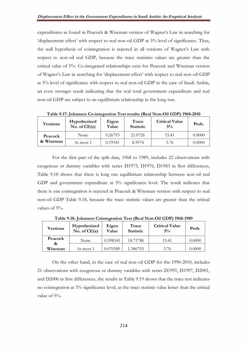
Displacement Effect in the Government Expenditures in Saudi Arabia: An Empirical Analysis
214
expenditures as found in Peacock & Wiseman version of Wagner‟s Law in searching for
„displacement effect‟ with respect to real non-oil GDP at 5% level of significance. Thus,
the null hypothesis of cointegration is rejected in all versions of Wagner‟s Law with
respect to non-oil real GDP, because the trace statistics values are greater than the
critical value of 5%. Co-integrated relationships exist for Peacock and Wiseman version
of Wagner‟s Law in searching for „displacement effect‟ with respect to real non-oil GDP
at 5% level of significance with respect to real non-oil GDP in the case of Saudi Arabia,
an even stronger result indicating that the real total government expenditure and real
non-oil GDP are subject to an equilibrium relationship in the long-run.
Table 9.17: Johansen Co-integration Test results (Real Non-Oil GDP) 1968-2010
Versions Hypothesized No. of CE(s)
Eigen Value
Trace Statistic
Critical Value 5%
Prob.
Peacock & Wiseman
None 0.26793 21.0726 15.41 0.0000
At most 1 0.19341 8.5974 3.76 0.0000
For the first part of the split data, 1968 to 1989, includes 22 observations with
exogenous or dummy variables with series D1973, D1976, D1983 in first differences,
Table 9.18 shows that there is long run equilibrium relationship between non-oil real
GDP and government expenditure at 5% significance level. The result indicates that
there is one cointegration is rejected in Peacock & Wiseman version with respect to real
non-oil GDP Table 9.18, because the trace statistic values are greater than the critical
values of 5%.
Table 9.18: Johansen Cointegration Test (Real Non-Oil GDP) 1968-1989
Versions Hypothesized No. of CE(s)
Eigen Value
Trace Statistic
Critical Value 5%
Prob.
Peacock &
Wiseman
None 0.598345 18.71788 15.41 0.0000
At most 1 0.070389 1.386793 3.76 0.0000
On the other hand, in the case of real non-oil GDP for the 1990-2010, includes
21 observations with exogenous or dummy variables with series D1991, D1997, D2001,
and D2006 in first differences, the results in Table 9.19 shows that the trace test indicates
no cointegration at 5% significance level, as the trace statistic value lesser than the critical
value of 5%.

Displacement Effect in the Government Expenditures in Saudi Arabia: An Empirical Analysis
215
Table 9.19: Johansen Cointegration Test (Real Non-Oil GDP) 1990-2010
Versions Hypothesized No.
of CE(s) Eigen value
Trace Statistic
Critical Value 5%
Prob
Peacock & Wiseman
None 0.337350 8.642084 15.41 0.0000
At most 1 0.020385 0.411915 3.76 0.0000
9.6.3. Causality Test
The econometric analysis so far indicates that there is a long-term equilibrium
relationship between government expenditures and GDP in the Peacock and Wiseman
version of the Wagner‟s Law in search for „displacement effect‟.
According to, Engle and Granger (1987), the variables that integrate towards a
common equilibrium reflects a long-term relationship, and therefore it should be a
representation of Error Correction Model (ECM), which provides the opportunity to test
and assess the relationship in the short and long term between the variables of the form.
To apply the Error Correction Model (ECM) to Peacock & Wiseman version in Saudi
Arabia, first Granger-causality has to be explored.
9.6.3.1. Granger Causality Test
In this, the Granger Causality for Peacock and Wiseman version for real GDP
and non-oil GDP for the entire period and also for the split periods are tested.
(i) Granger Causality Test with Real GDP
Table 9.20 shows the probability values from the Granger Causality Test for
Peacock and Wiseman Version for the period of 1968-2010 with Real GDP. The
reported F-statistics are standard test for the joint hypothesis that LGE does not
Granger Cause LGDP. In the case of Saudi Arabia, the probability for accepting the null-
hypothesis was only 0.36% while 99.64% reject this hypothesis, which means LGE
causes LGDP around 99.64% of the time in the Peacock and Wiseman‟s Version. In
Table 9.19, the feedback of causality from LGDP to LGE is presented where the
probability for accepting the null-hypothesis is only 23.36% while 76.64% reject the
hypothesis, which means LGDP causes LGE about 76.6% times in the case of Saudi
Arabia. It can, therefore, be concluded that there is bi-directional causality between
government expenditures and GDP in the case of Peacock and Wiseman version of
Wagner‟s Law in search of „displacement effect‟.

Displacement Effect in the Government Expenditures in Saudi Arabia: An Empirical Analysis
216
Table 9.20: Granger Causality test for Peacock and Wiseman Version for 1968-2010 with Real GDP
Null Hypothesis F-Statistic Prob.
LGE does not Granger Cause LGDP 6.65097 0.00356
LGDP does not Granger Cause LGE 1.51625 0.23360
Table 9.21 shows the probability values from the Granger Causality test for the
first part of the split data 1968 to 1989 with real GDP. The reported F-statistics are
standard test for the joint hypothesis that LGE does not Granger Cause LGDP. As can
be seen, in both cases, the probability for accepting the null-hypothesis is lesser that the
rejection value, bi-directional causality is established for 1968-1989 period.
Table 9.21: Granger Causality test for Peacock and Wiseman Version 1968-1989 with Real
GDP
Null Hypothesis F-Statistic Prob.
LGE does not Granger Cause LGDP 7.6638 0.022
LGDP does not Granger Cause LGE 4.5697 0.102
The results in Table 9.22 for the period 1990-2010, shows that LGE causes
LGDP, while the result for LGDP causing LGE is not that string albeit the results show
that LGDP causes LGE about 50% of the time.
Table 9.22: Granger Causality test for Peacock and Wiseman Version from 1990-2010 with Real GDP
Null Hypothesis F-Statistic Prob.
LGE does not Granger Cause LGDP 18.169 0.001
LGDP does not Granger Cause LGE 1.3858 0.500
(ii) Granger Causality Test with Real Non-Oil GDP
Table 9.23 shows the probability values from the Granger Causality Test for
Peacock and Wiseman version for the period of 1968-2010 with real non-oil GDP. The
reported F-statistics are standard test for the joint hypothesis indicating that LGE does
not Granger Cause L Non-Oil GDP. In the case of Saudi Arabia, the probability for
accepting the null-hypothesis was only 0.48% while 99.52% reject this hypothesis, which
means LGE causes L-Non-Oil GDP around 99.52% of the time in the Peacock and
Wiseman‟s version. In table 9.23, the feedback of causality from L-Non-Oil GDP to
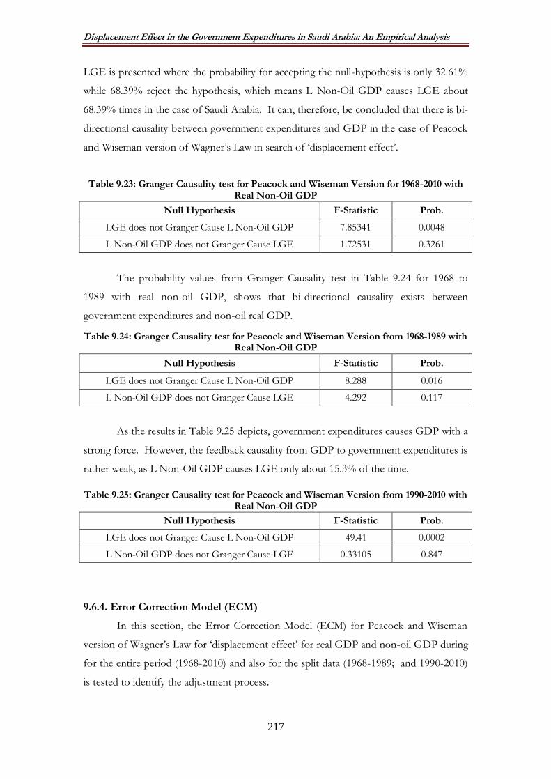
Displacement Effect in the Government Expenditures in Saudi Arabia: An Empirical Analysis
217
LGE is presented where the probability for accepting the null-hypothesis is only 32.61%
while 68.39% reject the hypothesis, which means L Non-Oil GDP causes LGE about
68.39% times in the case of Saudi Arabia. It can, therefore, be concluded that there is bi-
directional causality between government expenditures and GDP in the case of Peacock
and Wiseman version of Wagner‟s Law in search of „displacement effect‟.
Table 9.23: Granger Causality test for Peacock and Wiseman Version for 1968-2010 with Real Non-Oil GDP
Null Hypothesis F-Statistic Prob.
LGE does not Granger Cause L Non-Oil GDP 7.85341 0.0048
L Non-Oil GDP does not Granger Cause LGE 1.72531 0.3261
The probability values from Granger Causality test in Table 9.24 for 1968 to
1989 with real non-oil GDP, shows that bi-directional causality exists between
government expenditures and non-oil real GDP.
Table 9.24: Granger Causality test for Peacock and Wiseman Version from 1968-1989 with Real Non-Oil GDP
Null Hypothesis F-Statistic Prob.
LGE does not Granger Cause L Non-Oil GDP 8.288 0.016
L Non-Oil GDP does not Granger Cause LGE 4.292 0.117
As the results in Table 9.25 depicts, government expenditures causes GDP with a
strong force. However, the feedback causality from GDP to government expenditures is
rather weak, as L Non-Oil GDP causes LGE only about 15.3% of the time.
Table 9.25: Granger Causality test for Peacock and Wiseman Version from 1990-2010 with Real Non-Oil GDP
Null Hypothesis F-Statistic Prob.
LGE does not Granger Cause L Non-Oil GDP 49.41 0.0002
L Non-Oil GDP does not Granger Cause LGE 0.33105 0.847
9.6.4. Error Correction Model (ECM)
In this section, the Error Correction Model (ECM) for Peacock and Wiseman
version of Wagner‟s Law for „displacement effect‟ for real GDP and non-oil GDP during
for the entire period (1968-2010) and also for the split data (1968-1989; and 1990-2010)
is tested to identify the adjustment process.

Displacement Effect in the Government Expenditures in Saudi Arabia: An Empirical Analysis
218
(i) ECM with Real GDP
In the Table 9.26, the results for 1968 to 2010 period indicate that there is long-
run causality that runs from GDP to GE, as the coefficient is statistically significant at
5% level. Thus, Peacock and Wiseman version of Wagner‟s Law for „displacement effect‟
is found to hold for GDP in the case of Saudi Arabia.
Table 9.26: Causality with Error Correction Model (ECM) test for 1968-2010 with Real GDP
Versions Variables ECTt-1 T-Stat
Peacock & Wiseman
L(GE) -0.22349 -1.08
L(GDP) 0.67767 1.67
As the results in Table 9.27 for the period of 1968 to 1989 indicate, that there is
long-run causality that runs from GDP to GE. It can therefore be concluded that
Peacock and Wiseman version of Wagner‟s Law for „displacement effect‟ is found to
hold for GDP in the case of Saudi Arabia.
Table 9.27: Causality with ECM with Real GDP for 1968-1989
Versions Variables ECTt-1 T-Stat
Peacock & Wiseman
L(GE) -0.52349 -1.54
L(GDP) 0.86667 1.67
The results for 1990 to 2010 period indicate that there is long-run causality that
runs from GDP to GE, and therefore it can be concluded that Peacock and Wiseman
version is found to hold for GDP in the case of Saudi Arabia (Table 9.28).
Table 9.28: Causality with ECM with Real GDP for 1990-2010
Versions Variables ECTt-1 T-Stat
Peacock & Wiseman
L(GE) -0.6459957 -3.02
LGDP 1.377322 0.87
(ii) ECM with Real Non-Oil GDP
The results in Table 9.29 for the 1968 to 2010 period with real non-oil GDP
indicates that there is long-run causality that runs from non-oil-GDP to GE. Thus,
Peacock and Wiseman version is found to hold for non-oil-GDP in the case of Saudi
Arabia.

Displacement Effect in the Government Expenditures in Saudi Arabia: An Empirical Analysis
219
Table 9.29: Causality with Error Correction Model (ECM) test for 1968-2010 with Non-Oil GDP
Versions Variables ECTt-1 T-Stat
Peacock & Wiseman
L(GE) -0.7523 -0.54
L(Non-Oil GDP) 0.42890 0.78
In the Table 9.30, the results for 1968-1989 indicate that there is long-run
causality that runs from non-oil real GDP to GE showing that Peacock and Wiseman
version of Wagner‟s Law is found to hold for non-oil real GDP in the case of Saudi
Arabia.
Table 9.30: Causality with Error Correction Model (ECM) test with Non-Oil GDP
Versions Variables ECTt-1 T-Stat
Peacock & Wiseman
L(GE) -0.80127 -0.99
L(Non-Oil GDP) 0.460949 0.81
The results in Table 9.31 for the second part of the split data, 1990-2010, In the
show that there is long-run causality that runs from non-oil real-GDP to GE implying
that Peacock and Wiseman version of Wagner‟s Law for „displacement effect‟ is found to
hold for non-oil real-GDP in the case of Saudi Arabia.
Table 9.31: Causality with Error Correction Model (ECM) test with Real Non-Oil GDP
Versions Variables ECTt-1 T-Stat
Peacock & Wiseman
L(GE) -0.78442 -5.42
L(Non-Oil GDP) -0.12992 -1.43
9.7. CONCLUSION
Gupta (1967) and Diamond (1977) argued that the displacement effect leads to
the share of national income devoted to government expenditure increasing with GDP
due to further interventions during social, political and economic upheavals.
In this chapter, thus, the relationship between the government expenditure and
economic growth is examined using the Peacock & Wiseman version of Wagner‟s Law
for „displacement effect hypothesis‟ for Saudi Arabia using time series annual data for the
1968 to 2010 period but also for the split data 1968 to 1989 and 1990 to 2010 with the
objective of locating the structural change in the development and trend of government
expenditures.

Displacement Effect in the Government Expenditures in Saudi Arabia: An Empirical Analysis
220
The results through all the method used and applied to the various levels of data
indicate that there is a structural break in the trend and development of government
expenditures in Saudi Arabia.
First, the regressions for the Peacock and Wiseman of Wagner‟s Law for
„displacement effect‟ are tested by using Ordinary Least Square (OLS) for real GDP and
non-oil GDP.
Secondly, the Augmented Dickey-Fuller for stationary Unit Root Test for real
GDP and non-oil real GDP is applied. In the case, the levels of the series tested, the
null-hypothesis of non-stationary cannot be rejected for any of the series.
Third, these results suggest that there is a cointegrating relationship between
government spending and national income. The equilibrium relationship indicates that
the major determinant of government expenditure in Saudi Arabia, in the long run, is
national income.
Fourthly, Granger causality tests were employed to confirm the causality
direction between the variables. In the long run, statistically significant evidence is found
indicating government expenditures Granger causing GDP and also the feedback
causality in the GDP causing government expenditures. The similar results have been
establishing by using the ECM.
In concluding, as the empirical evidence presented in this chapter shows through
the analysis of structural break, it can be concluded that government expenditures in
Saudi Arabia has not only followed a secular growth but also experienced structural
jumps from one period to another due to certain economic reasons such as the large oil
revenues due to oil shocks, and also negative impact of world recession and also the
1997 financial crisis on fiscal policy, but also due to political reasons such as Gulf Wars
in the recent years. Further studies can be conducted through other empirical methods
to locate the beginning and ending periods of the impact of such economic, social and
political events have had on the trend and development of public expenditures in Saudi
Arabia, as this study only shows the structural breaks but not the periods of impact.
Thus, it can be concluded that this study provides initial empirical evidence in favour of
„displacement effect hypotheses of Peacock and Wiseman through using Peacock and
Wiseman version of Wagner‟s Law in different forms and through different econometric
methods.

Discussions and Conclusion
221
CHAPTER 10
DISCUSSIONS AND CONCLUSION
10.1 OVERVIEW
Government expenditures are funds spent to actualise the activity and
performance of the public sector aiming to increase the welfare of society and the
economy as a whole. However, the expansion of government activities is a political issue
as well as being an economic issue. The role of the state in economy is a subject of
debate for centuries. Regardless of the political culture of the nations, as indicated in the
literature, a secular increase has been observed in the size of public expenditures in most
of the countries in the world for different reason which ranges from welfare oriented
aims to developmentalist reasons. In addition to the large literature searching for the
determinants of increasing size of government, an equivalently large number of studies
also have looked for the relationship between government expenditures and economic
growth, as it is perceived that there is a causal relationship between government
expenditures and GDP. However, Wagner (1883) suggested that increased government
spending was because of growth in the GDP and not a cause, unlike Keynes (1933), who
believed that government expenditure is an independent factor, and a political tool to
influence growth.
It is the aim of this study to search for the perceived causal relationship between
government expenditures and economic growth in the case of Saudi Arabia., which is a
developmentalist but at the same time is a rentier state. The Saudi economy mainly
involves the exporting of oil and gas, and Saudi Arabia has the largest reserves of crude
oil in the world – an estimated 266.7 billion barrels. This is equivalent to 57% of the
reserves of the Gulf Cooperation Council countries and 29% of the total reserves of
OPEC, and accounts for 20% of world reserves (www.gulfbase.com, 2011). The
Kingdom of Saudi Arabia also ranks as the largest producer and exporter of oil in the
world where it plays a leading role in the OPEC, producing 28% of total OPEC
production. Average oil production per day in 2009 was 8.055 million barrels and in 2008
average production was 9.113 million barrels per day. In terms of its contribution to the
economy, the oil sector accounting for 90% of total export earnings, 80% of government
revenues and 45% of the gross domestic product. Due to the heavy presence of oil in the
economy, about 40% of GDP comes from the private sector (Ministry of Economy and

Discussions and Conclusion
222
Planning, 2010), which at the same time makes Saudi Arabia’s political economy as a
rentier state.
Due to the increase in oil prices in recent years but also because of the oil shocks
in 1970s, Saudi Arabia generated large wealth from oil revenues. In recent years, the
country recorded significant economic growth during the period from 2003 to late 2008
on the back of rising oil production and prices. However, in particular since Saudi Arabia
became member of WTO in 2005, Increases in foreign direct investment and
government spending to develop the contribution of non-oil sectors are large and
influential, which mainly aims to reduce the role of the state and also oil in the economy.
Thus, economic diversification led by the government has been a recent policy in
development plans as well.
It should be noted that due to the increasing oil prices, the real GDP of Saudi
Arabia rose by 4.6% in 2008 compared to 2007 when the growth rate was 3.5%, but
decreased to 0.15% in 2009 due to the global crisis. The real growth rate of the economy
is excepted to be about 3.7% in 2010 and to 4% in 2011 due to an expected global
economic recovery (www.gulfbase.com, 2011).
The Saudi economy has seen unusual changes either through mutations or
through the oil booms in the region for more than four decades (1968-2010). The
government has decided that during this period of extraordinary gains in revenues and
general economic surplus, Saudi Arabia will foster developmentalism to assure that the
future growth of the Kingdom will be through the development of physical
infrastructure and the development of human resources. However, being a rentier state,
the state’s economic role is open to question but also importantly the government failure
is something perhaps should be considered in the case of Saudi Arabia in terms of the
efficiency of government expenditures.
This chapter thus aims to provide a summary of the findings so far through the
empirical chapters but also aims to provide further meaning to the results by reflecting
on the results.
10.2 SUMMARISING THE FINDINGS
The aim of this research is to search for the causal relationships between
government expenditure and GDP, in terms of GDP and Non-oil GDP for the Saudi
Arabian economy. Hence, in addition to total GDP, non-oil GDP is also considered

Discussions and Conclusion
223
with the objective of measuring the impact of government expenditures non-oil
economy.
The empirical chapters in this research aim to estimate the economic
relationships represented in Wagner’s law in terms of the causal relationship between
government expenditures and economic growth. The empirical research was extended
by also examining Peacock and & Wiseman and Keynesian Relation as part of the
macroeconomic models within the field. It should be noted that each model tested with
overall GDP but also with non-oil GDP.
Using aggregate annual time-series data for Saudi Arabia for the period of 1968-
2010, initially the propositions of the six existing versions of Wagner’s law have been
considered using the Ordinary Least Square (OLS). The following tests were performed:
Unit Root, Co-integration, Error Correction Model (ECM), and application of Granger-
Causality-testing. The empirical results suggest that testing for the six existing versions of
Wagner’s law verifies and validates also the relationship between government
expenditure and economic growth in Saudi Arabia.
Table 10.1: Summary of the main Results Theories Explaining the Government
Expenditure Growth for real GDP and Non Oil Real GDP
Models Period Estimations Methods
Unit Root Cointegration ECM Granger Causality
Wagner's Law 1968 - 2010
Stationary in the first difference I
(1).
There is a long-run relationship
between government expenditure (GE) and economic
growth (GDP)
The long-run causality runs from GDP to Government Expenditure
Bi-directional
Keynesian Relation
1968-2010 Uni-directional
Displacement Effect
1968-2010
Bi-directional 1968-1989
1990-2010
In chapter seven, the empirical results introduced strong evidence in support of
Wagner’s Law in the case of Saudi Arabia. The results show that the elasticity of
government expenditure with respect to GDP were greater than unity in the six versions
of Wagner's law, , which leads to, good evidence of supporting Wagner's predictions.
The results of the regression analysis – for six versions of Wagner’s Law using
OLS for real GDP and non-oil real GDP – show that the elasticity coefficient of
government expenditure, with respect to GDP, was greater than unity in Peacock and

Discussions and Conclusion
224
Wiseman (1968), Pryor (1969), Goffman (1968),and Gupta (1967). Thus, the findings in
the case of these four versions are in accordance with Wagner’s expectation. The
empirical results also indicate that the elasticity coefficient of government expenditure,
with respect to GDP, is inelastic in the case of Musgrave’s (1969) and Mann’s (1980)
versions of Wagner’s Law, although their independent variable is still statistically
significant. Nagarajan and Spreares (1990), furthermore, stated that in order to verify
Wagner’s Law, the income elasticity needs to be E>1, i.e. greater than unity, and the
ratio income elasticity needs only be E>0, i.e. greater than zero. According to this rule,
Mann’s version of Wagner’s Law does not hold in the case of Saudi Arabia.
As regards non-oil real GDP – the independent variable in the versions of
Wagner’s Law – Peacock and Wiseman provide support for Wagner’s Law, whilst
Pryor’s, Musgrave’s and Mann’s versions do not hold for Saudi Arabia. In addition, since
elasticity is greater than unity in the results of Goffman’s model, this version of
Wagner’s Law is consistent for Saudi Arabia. Moreover, Gupta provides evidence for
Wagner’s Law in the case of Saudi Arabia; the expected elasticity is higher than a unit,
i.e. E>1. Moreover, since the income elasticity needs to be higher than a unity (E > 1),
and the ratio income elasticity is expected to be higher than zero (E > 0), Mann's version
does not provide evidence for Wagner’s Law in Saudi Arabia.
In extending the analysis, the unit root test in the form of Augmented Dickey-
Fuller is utilised to examine stationary of the time-series of all the variables. The results
indicate that the levels of all series are non-stationary, and hence all the variables are
cointegrated at first order [I (1)].
The results suggest that there is a co-integrating relationship between
government expenditure and GDP per capita, and Wagner’s Law holds in the case of
Saudi Arabia through the cointegration analysis. Therefore, the equilibrium relationship
indicates that the major determinant of government expenditure in Saudi Arabia, in the
long run, is national income.
The econometric analysis further employs the Granger causality test in order to
verify the causality and its direction between the variables. The results demonstrate
statistically significant evidence in favour of per capita GDP for the long-run
relationship. In addition, it is found that Granger-causing the share of government
expenditure in GDP. This finding is consistent with the expectation of Wagner’s Law.
Thus, the result of the causality test indicates the existence of strong feedback causality
for all versions of Wagner’s Law in the long run.

Discussions and Conclusion
225
Lastly, by using the Error Correction Model (ECM), it is established that all the
six versions of Wagner’s Law are significant for both real GDP and non-oil-GDP in the
case of Saudi Arabia. This suggests a short-run adjustment process towards long-run
equilibrium.
After establishing that Wagner’s Law in all version valid and can explain the
nexus between government expenditures and economic growth in Saudi Arabia, Chapter
Eight focused on testing Keynesian relation by reversing the three versions of Wagner’s,
Law, using time series annual data for the period 1968 to 2010.
In the analysis, three distinct time series techniques are applied: Initially, the
regressions analysis utilised for three versions of Keynesian Relations using Ordinary
Least Square (OLS) with real GDP and non-oil GDP. In the next step, the Unit Root
tests through Augmented Dickey-Fuller test for stationary is applied with real GDP and
non-oil GDP. In the following step, cointegrating test for real GDP and non-oil GDP.
Finally, causality tests by using Granger Causality tests are conducted together with
ECM.
In overall, the findings in this study suggest that there is a cointegrating
relationship between the share of government expenditure in national output and per
capita income. The equilibrium relationship indicates that the major determinant of
government expenditure in Saudi Arabia, in the long run, is national income. In the case
of Real GDP and Non-oil GDP, the versions of Peacock & Wiseman, Goffman and
Gupta show that co-integration relationships is found and the test supported the
existence of one cointegration.
Finally, Granger’s causality tests were used to confirm the causality direction
between the variables by using the ECM. Since there exists an ECM to describe the short
run adjustment to equilibrium, three versions of the Keynesian Relations are found to
hold for both (GDP) and (Non-Oil-GDP) in the case of Saudi Arabia.
The findings in this study verify the importance of Keynesian relation for a late
developing country such as Saudi Arabia, where the private capital for economic
development until recently was limited. The fiscal policy in the form of government
expenditures has been the engine of economic growth and development in Saudi Arabia.
The government revenues raised from oil wealth in Saudi Arabia have been the main
source of economic and social development of the country, which generated
employment and expansion of the economy as predicated by Keynes.

Discussions and Conclusion
226
The findings of this research, hence, verified the validity of the Keynesian
Relation in the case of Saudi Arabia, and also indicate the importance of government
expenditure for economic development in the cases where the private capital is in short
supply as was in Saudi Arabia. This does not imply that government’s role for economic
growth and development is applauded without any questioning, as the efficiency and
effectiveness of using government expenditure is a matter of another debate.
After establishing the validity of Keynesian Relation in the case of Saudi Arabia,
an attempt was also made in Chapter 9 to search for the validity of Peacock & Wiseman’s
‘displacement effect’. The model is expanded, as mentioned before, with the addition of
political and economic dummy variables.
In this chapter, thus, the relationship between the government expenditure and
economic growth is examined using the Peacock & Wiseman version of Wagner’s Law
for ‘displacement effect hypothesis’ for Saudi Arabia using time series annual data for the
1968 to 2010 period but also for the split data 1968 to 1989 and 1990 to 2010 with the
objective of locating the structural change in the development and trend of government
expenditures.
The results through all the method used and applied to the various levels of data
indicate that there is a structural break in the trend and development of government
expenditures in Saudi Arabia.
First, the regressions for the Peacock and Wiseman of Wagner’s Law for
‘displacement effect’ are tested by using Ordinary Least Square (OLS) for real GDP and
non-oil GDP.
Secondly, the Augmented Dickey-Fuller for stationary Unit Root Test for real
GDP and non-oil real GDP is applied. In the case, the levels of the series tested, the
null-hypothesis of non-stationary cannot be rejected for any of the series.
Third, these results suggest that there is a cointegrating relationship between
government spending and national income. The equilibrium relationship indicates that
the major determinant of government expenditure in Saudi Arabia, in the long run, is
national income.
Fourthly, Granger causality tests were employed to confirm the causality
direction between the variables. In the long run, statistically significant evidence is found
indicating government expenditures Granger causing GDP and also the feedback
causality in the GDP causing government expenditures. The similar results have been
establishing by using the ECM.

Discussions and Conclusion
227
In concluding, as the empirical evidence presented in this chapter shows through
the analysis of structural break, it can be concluded that government expenditures in
Saudi Arabia has not only followed a secular growth but also experienced structural
jumps from one period to another due to certain economic reasons such as the large oil
revenues due to oil shocks, and also negative impact of world recession and also the
1997 financial crisis on fiscal policy, but also due to political reasons such as Gulf Wars
in the recent years. Further studies can be conducted through other empirical methods
to locate the beginning and ending periods of the impact of such economic, social and
political events have had on the trend and development of public expenditures in Saudi
Arabia, as this study only shows the structural breaks but not the periods of impact.
Thus, it can be concluded that this study provides initial empirical evidence in favour of
‘displacement effect hypotheses of Peacock and Wiseman through using Peacock and
Wiseman version of Wagner’s Law in different forms and through different econometric
methods.
10.2.1. Reflecting on the Findings
In overall, the results presented in this research and summarised in this section
clearly demonstrates that government expenditures has been an important determinants
of economic growth in both the measure, namely real GDP and non-oil real GDP.
However, the results also indicate that the direction of causality worked in both ways;
while government expenditures resulted in higher economic growth; higher economic
growth in turn generated the necessary wealth for the growth in public expenditure for
economic development and welfare of the society.
While the results validates the presence of Wagner’s Law in the case of Saudi
Arabia for the period in question, the validity of the Keynesian Relation is also
established through the rigorous analysis presented in this research. Importantly, the
findings also show that Peacock & Wiseman’s ‘displacement effect’ is also verified in the
case of Saudi Arabia, as the country has gone through breaks in its economic growth and
public expenditure growth due to economic (oil shocks and global recession) but also
political events (wars).
Saudi Arabia, as mentioned, is a developmentalist rentier state, which is heavily
depended on the wealth generated from oil export. Due to having traditional modes of
production based on kinship or tribalism, in modern times this still continues to have
impact on the political economy of the country in the sense that instead of tribe, the state

Discussions and Conclusion
228
remains at the heart of developing the economy and society but also provide for the
welfare need of the society. Thus, the heavy presence of state in economy can perhaps be
justified through economic rationale by responding to the capital need of the society, it is
at the same time a cultural, traditional and historical reality and necessity.
While it is true that Saudi society and its political economy have undergone
important transformation through being party to international bodies such as WTO but
also through economic and financial liberalisation, which has resulted in a growing
bourgeoisie and expanding private sector, the traditional weight of the state is a reality
continues to exist either as a ‘benevolent administrator’ (dawlah al kareem) or a
‘leviathan’. For example, in responding to the growing political changes in the region,
Saudi government committed large public funds to overcome the financial difficulties of
individual citizens including creating jobs for the unemployed in the public sector. Thus,
regardless of assessing the economic rationale for such commitments, political necessities
create pressure for the expansion of the state’s economic involvement. It is therefore not
a surprise that the youth prefer to work in the public sector despite the expanding private
sector and the Saudization policies (Al-Shehri, 2009). Thus, the thin line between the
‘benevolent administrator’ and ‘leviathan’ is becoming rather invisible in the process of
further expansion of the state’s involvement in the economy. This is particularly
important in considering the level of economic development in Saudi Arabia and the
amount of public funds over the years allocated for this purpose. In other words, the
efficiency of the use of public funds and the effectiveness of the outcome when assessed
it clearly indicates that more could have been achieved so far.
The question, as mentioned, comes to the cultural, traditional and historical reality
of tribal and in modern times state based mode of production; it is a legacy that will
remain there for the foreseeable future, as the issue is not only a supply oriented
problem, but the general public is also toxicated with the economic and financial power
of the state and therefore consider the ‘state the father’ to deliver them with the services
and financial power they ask for. Thus, rentier economy is supported and popularised by
rentier mentality of the public, which helps to sustain the growing public expenditures in
the country despite the economic and financial liberalisation has taken place in the
country in the recent history. The recent political developments in the Arab countries
does not help to reduce the size of the state in Saudi Arabia, as further rentier oriented
spending has been promised to the society to overcome political instability in the
kingdom.
Discussions and Conclusion
229
It should, however, be noted that the development of the Saudi society has been
possible by the heavy state involvement so far. While this fact should remain in mind in
understanding the Saudi political economy, it is also important to question the efficient
use of public resources for economic development. Such questioning should also be
extended to welfare expenditures in terms of their efficiency. As observation states that
such an academic study would find the inefficiencies in the public spending whether in
economic or welfare oriented realms. This is an urgent matter requiring direct attention,
as such a study may prove that the economic development achieved so far would have
costed lesser and the welfare expenditure are economically and socially much higher than
its socially optimum level, as they are very much determined politically.
10.3. POLICY IMPLICATIONS
The policy implications of this finding imply that the fiscal stance of the state
plays an important role in the macroeconomy of the state and the welfare of the society
and individuals.
The growing public expenditures not only due to economic rationale such as
developmentalist need, but also due to public pressure indicates that stronger position
should be taken in controlling the public expenditures or at least in moderating its
expansion. While this study has not attempted the measure the efficiency and the
effectiveness of public expenditures, the observation from real life indicates that
government expenditures are inefficient and ineffective in the country, and therefore
rather than expanding the public sector further an independent private sector must be
expanded in size but also in its power. In other words, economic diversification is a need
in Saudi Arabia which should focus on creating an independent private sector, as this will
help to transform the rentier economy and rentier mentality of the society for a
productive economy and enabled and functioning individuals.
Saudi Arabia attempted to liberalise its economy and financial sector and has
been successful in this process through privatisation and other policies. In addition,
being a member of the WTO makes its necessary for the country to reduce the public
sector to prevent the crowding out impact in the economy. Therefore, rather than
increasing public spending due mainly to political pressures as in recent years, rentier
mentality has to be replaced with productive individuals in the minds of the citizens. By
the same token, the rentier expectations in the economy must be removed in favour of
independent business class. Proactively pursued economic diversification of the economy

Discussions and Conclusion
230
away from oil will be an important part of such a policy, which is, thus, essential to
prevent the state to grow further but also conduct itself with efficiency and effectives.
As part of economic and financial liberalisation and reducing the size of the
government, privatisation has been taken as an important economic policy. However,
privatisation in Saudi Arabia needs a strategy in support of the business to provide the
proper role of the private sector, in order to support the economy through the expansion
of independent private sector to complete its role and meet the requirements
of overall economic growth.
It should, however, be noted that while the role of the state in economic activity
is undergoing change, the development of the private sector is essential for the robust
nature of the state. It is expected that the development of the private sector means
assuming a great role in the future for the provision of social services such as health,
education, housing and others. It is true that the state intends to move slowly away from
sectors undertaken by the private sector, and it has taken measures
to support economic reform of the private sector.
Saudi Arabia has identified eight strategies with the objective of reducing the
public sector and expanding the private sector (Ministry of Economic and Planning,
2010).
(i) to improve the efficiency of the national economy and enhance competitiveness to
meet challenges, including with regional and international competition;
(ii) to encourage private-sector investment and encourage active participation in the
national economy, increasing the share of the private sector in the GDP to achieve
growth within the national economy;
(iii) to develop the citizens’ participation in productive economic activity rather than
sustaining rentier mentality;
(iv) to develop national capital and foreign investment locally;
(v) to increase employment opportunities, and the optimum operation performance of
the national labour force;
(vi) to continue to achieve a fair increase in per capita income through the contribution
of the private sector;
(vii) to provide services to citizens, investors in a timely fashion, and in a cost-efficient
manner, and
(viii) to rationalise public expenditure and reduce the fiscal tension on the state, and to
increase government revenues.

Discussions and Conclusion
231
As part of economic liberalisation, privatisation can help to reduce the size of
government, hence, but also helps to diversify the wealth generation in the economy. In
particular, together with other measures to create a robust private sector, privatisation
helps to withdraw the state from economic activity and can pave the way for the further
reduction of the size of the state by withdrawing the state from welfare services.
10.4 POLICY RECOMMENDATIONS
Recent development and economic policies in Saudi Arabia shows that policies,
incentives and regulatory initiatives have contributed to expand the role of the private
sector in the national economy and increase its effectiveness, leading to a steady increase
in economic efficiency of the sector. The total contribution of the private sector to the
GDP was 6.63%, and non-Oil GDP 89% at the end of the Eighth Development Plan.
This indicates that the private sector can contribute to the economy through the
opportunity spaces crated by economic diversification. Therefore, the following policy
recommendations suggested by this study:
(i) The private sectors must engage effectively in the Saudi development plan that
focuses on long-term goals. The development plan must take into account how to
form a strong relationship between all sectors and how the function of each
sector compliments the function(s) of the others.
(ii) Oil revenues must be used as an effective tool to contribute to the expansion of the
private sector;
(iii) The government should reduce its role and size to enhance and encourage the
ability of its economy to function effectively, allowing more opportunities for the
private sector in the economy.
(iv) The government should adopt creative policies that aim to achieve gradual reduction
in reliance on oil through a diversification of production within the economy. Those
policies must be constructed in a way that enables the country to face an expected
future of depletion of oil reserves. In addition, time constrains for achieving those
policies of diversifying the production of the economy need to be set.
(v) The people must understand and recognise that the majority of the existing
outcomes of ‘development’ in Saudi Arabia are the result of oil revenues and not the
outcomes of well-organised development plans and policies. Therefore, individual
citizens should take up more responsible roles in the economy and society beyond
the easy life offered by rentier mentality.
Discussions and Conclusion
232
(vi) SME development should be supported as the backbone of the stronger private
sector.
(vii) The institutional framework, which sponsors the development of the private sector
through legal reform should proactively move away from heavy bureaucracy and
red-tape and should support the developments in the private sector but also for
small businesses needs
(viii) Support for the Saudi stock market is still seen as modest on the largest Arab stock
markets. Privatisation can also exercise a significant impact on the resettlement of
capital with the creation of greater opportunities for investment while providing a
climate to attract foreign investments, primarily in order to obtain technical support,
technology, and marketing expertise.
(ix) Allowing the government to reduce its budget deficit. It would also suggest that it
does not have to continue encouraging shifts in government expenditure towards
non-oil activities.
These recommendations, however, are mostly related with the political economy
of the state, which is determined by the culture, traditional and historical forces of the
society. Thus, main changes in the political economy of the country, such as move from
rentier state, directly indicates the changes in the social formation of the society, which
may not be an easy task considering the determining forces of the social formation.
However, the country is in such a juncture that the legacies of culture, tradition and
history may not be enough to create a competitive economy, which can sustain itself
against the global forces beyond the position, provided by the oil revenues. The
economy and society needs to regenerate itself according to the global political economy
beyond the traditional modes of production and rentierism oriented distributive kinship
or tribal modes of production.
10.5 FUTURE RESEARCH
This research aimed at examining the association between government expenditures
and economic growth in Saudi Arabia. However, there is a large literature on the
determinants of increasing government expenditures. One of the research areas that can
be developed on top of this study is hence the determinants of the increasing
government expenditures in Saudi Arabia. In this, economic, political, social,
demographic and public choice related factors can be considered.

Discussions and Conclusion
233
Secondly, an attempt can be made to test the integrated model suggested by Brown
and Jackson (1990). This can help to see various factors interactively working together
leading to increase in government expenditures.
Thirdly, considering that Saudi Arabia is a rentier state, the political economy of the
Saudi rentierism through supply but also through demand side can be examined.
An extension of rentier mentality, the impact of population and welfare demand on
the Saudi public expenditure can also be an exciting study.
Importantly, however, the models suggested by public choice should be considered
as important areas of research in Saudi Arabia such as the impact of bureaucracy on the
growing size of the economy. Knowing that bureaucracy is an essential part of the state
apparatus helping to distribute the wealth created by oil, the nature and aims of the
bureaucracy in Saudi Arabia can constitute an exciting study. This can focus on the
power of the bureaucracy and their role in the budgetary decision making to locate their
role in the expansion of public expenditures.
10.6 EPILOGUE
This study aimed at exploring and examining the causal relationship between the
government expenditures and economic growth in Saudi Arabia in the period of 1968-
2010.
The foundational chapters and in particular the empirical chapters testify that the
aims of this research has been achieved and the objectives of the research have been
fulfilled.
The finds of the study clearly shows that there is a clear causal relationship
between government expenditure and the economic growth and the causality relationship
between government expenditure and the GDP supports both Wagnerian and Keynesian
Relation. The study also found that Peacock & Wiseman’s ‘displacement effect’ has been
effective in certain period of economic booms and busts but also during political turn
oils such as the case with the Gulf Wars.
This research, hence, is now considered completed at this stage; however, similar
to any other research it is a continuous process and will be extended by the relevant
future research in the field.

234
BIBLIOGRAPHY
Abdel-Rahman, A. M., and Barry, Z. (1997). "Public Investment, Government Consumption and Wagner's Law in Oil Rich Economy: Study in Co-integration and Structural Breaks", Studi Economici, (63), pp.141-158.
Abizadeh, S. and Basilevsky, A. (1990). "Measuring the Size of Government", Public Finance, (45), pp. 353-377.
Abizadeh,S.andGray,J.(1985). "Wagner's Law: A Pooled Time Series, Cross- Section Comparison", National Tax Journal, (38), pp. 209-218.
Abizadeh, S. and Yousefi, M. (1988). "An Empirical Re-Examination of Wagner's Law",Economic Letters, (26), pp. 169-173.
Abizadeh, S. and Yousefi, M. (1998). "An Empirical Analysis of South Korea's Economic Development and Public Expenditure Growth" Journal of Socio-Economics, (27), pp. 687-700.
Afexetiou, P. C. and Serletis, A. (1996). "Government Expenditures in the European Union: Do They Converge or Follow Wagner's Law",International Economic Journal, (10), pp. 33-47.
Ahsan, S. M.; Kwan, A. C., and Sahni, B. S. (1996). "Co-integration and Wagner's Hypothesis: Time Series Evidence for Canada", Applied Economics, (28), pp.1055-1058.
Al-Faris, A. F. (2002). "Public Expenditure and Economic Growth in the Gulf Cooperation Council Countries",Applied Economics, (34), pp.1187-1195.
Al-Batel, A. H. (2000). The Relationship between Government Expenditure and EconomicGrowth in Saudi Arabia. Journal of King Saud University, Administration. Scince. Vol (2), pp.173-191.
Al-Batel, A.H. (2002). "The Relationship between Government Revenue and Expenditures in Saudi Arabia",Journal of the Gulf and Arabian Peninsula.
Al-Batel, A.H. (2003). "Government Activity and Policy and Economic Development in Saudi Arabia",Journal of Economic & Administrative Science, (19), pp.77 – 100.
Al-Hakami, A.O. (2002). "Analyzing the Causal Relationship between Government Expenditure and Revenues in Saudi Arabia, Employing Co-integration and Granger Causality Models", Public Administration, (42), pp. 475-493.
Allen, M, & Caruana, J, (2008), “Sovereign Wealth Funds: A Work Agenda”, International Monetary Fund:Washington DC.
Alleyne, D. (1999). "Testing for Wagner's Law in Jamaica, Guyana, Barbados and Trinidad Tobago: Is There Spurious Relationship?", Social and Economic Studies, (48), pp.121-135.
Al-Qudair K.H.A. (2005)."The Relationship between Government Expenditure and Revenues in the Kingdom of Saudi Arabia: Testing for Co-integration and Causality", Journal of King Abdul-Aziz University, (19), pp. 31-43.
Al-Shehry, A (2009). Exploring the Perceptions of Saudi Business and the Workforce on the Saudisation Programme in the Private Sector. Unpublished Ph.D Thesis. School of Government and International Affairs, Durham University, UK.
Ansari, M.I. (1994)."Perspectives on Sustainable Development", The American Journal of Islamic Social Sciences, (11), pp. 394-402.
Ansari, M. I.; D. V. Gordon, and A. C. Akuamoah (1997). "Keynes versus Wagner: Public Expenditure and National Income for Three African Countries”,Applied Economics, (29), pp. 543-549.

235
Aschauer, D. (2000). "Public Capital and Economic Growth: Issues of Quantity, Finance and Efficiency", Economic Development and Cultural Change, (48), pp. 391-406.
Ashworth, J. (1994). "Spurious in Mexico: A Comment on Wagner's Law", Public Finance/ Finances Publiques, (49), pp. 282-286.
Asseery, A. A.; D. Law.,and N. Perdikis (1999). "Wagner's Law and Public Expenditure in Iraq: A Test Using Disaggregated Data," Applied economic letters, (6), pp. 39-44.
Asutay, M. and K. Al-Fazari (2007). "Government Expenditure and Economic Growth in Oman: Testing Wagner’s Law and Keynesian Relation". PC 2007 Conference.
Asutay, M , (2008). GCC Sovereign Wealth Funds and Their Role in the European and American Markets (2008). Equilibri, Vol. 12, No. 3, pp. 335-354.
Atkinson, A. B. and Stiglitz, J.E. (1980).Lectures in Public Economics, Maidenhead, McGraw-Hill.
Aulich, C, J Halligan & S Nutley. (2001). Australian Handbook of Public Sector,Management, Allen and Unwin, Sydney.
Ayubi, Nazih, (1991). Overstating the Arab State: Politics and Society in the Middle East.
London and New York: I.B. Tauris. pp. 1-37, 447-459.
Azam, T. L. (1998). Theorising Government Expenditure Growth in Malaysia, 1961-1990: An Econometric Analysis of Wagner's Law, Keynesian Relation and Peacock-Wiseman Hypothesis. Ph.D. Thesis. Public Sector Economics Research Centre, University of Leicester.
Bacon, R.W. and Eltisi, W.A. (1978).Britain’s economic problem: too few producers, 2edn. London: Macmillan.
Bailey, S. J. (2002).Public Sector Economics, New York, Palgrave.
Bairam, E. I. (1992). "Variable Elasticity and Wagner's Law," Public Finance, (47), pp. 491-495.
Barro R., (1990), Government spending in a simple model of endogenous growth, Journal of Political Economy, 98 (5), pp. 103-125.
Barro, R. (1991). "Economic Growth in a Cross Section of Countries",Quarterly Journal of Economics,(106), pp. 407-443.
Barro R. and X. Sala-i-Martin, (1995), Economic growth, McGraw-Hill, New York, United States, pp.539.
Baumol, W. J. (1967). "The Macroeconornics of Unbalanced Growth", American Economic Review, (57), pp. 415-26.
Beblawi, H. and G. Luciani (1987). The Rentier State. New York, NY: Croom Helm.
Beck, M. (1982). "Towards a Theory of Public Sector Growth", Public Finance, (37), pp. 163-77.
Biehl, D. (1998). "Wagner's Law: An Introduction to and a Translation of the Last Version of Adolph Wagner's Text of 1911," Public Finance/Finances Publiques, (53), pp. 102-111.
Bird, R. M. (1971). "Wagner's 'Law' of Expanding State Activity", Public Finance Quarterly, (26), pp. 1-26.
Bird, R. M. (1972). "The Displacement Effect: A Critical Note", Finanzarchiv, (30), pp. 454-463.
Biswal, B.; U. Dhawan, and H.-Y. Lee (1999). "Testing Wagner Versus Keynes Using Disaggregated Public Expenditure Data for Canada", Applied Economics, (31), pp. 1283- 1298.
Bohl, M. T. (1996). "Some International Evidence on Wagner’s Law",Public Finance/ Finance Publiques. (51), pp. 185-200.
236
Borcherding, T. E. (1965). "The Growth of Non-Federal Public Employment in the United States, 1900 to 1963".Ph.D Dissertation. Duke University.
Bortolotti, B. and Siniscalco, D. (2004) The Challenges of Privatization. An International Analysis. Oxford: Oxford University Press.
Brown, C.V. and Jackson, P.M. (1990).Public Sector Economics, Oxford, Basil Blackwell.
Brooks, C. (2008). Introductory Econometrics for Finance, Cambridge (2ed Edition).
Buchanan, J. M. (1977). Democracy in Deficit: The Political Legacy of Lord Legacy. Indianopolis, I.N.: Indiana University Press.
Buffie, E. F. (1984). "Financial Repression, the New Structuralists, and Stabilization Policy in Semi-industrialized Economics,"Journal of Development Economics, (14), pp. 305-22.
Burney, N. A. (2002). "Wagner’s Hypothesis: Evidence from Kuwait Using Co-integration Tests", Applied Economics, (34), pp. 49-57.
Chang, T. (2002). "An Econometric Test of Wagner's Law for Six Countries Based on Co-integration and Error-Correction Modelling Techniques," Applied Economics, (34), pp. 1157-1170.
Charemza, W. W. and D. F. Deadman. (1992). New Directions in Econometric Practice. Edward El gar.
Chletsos, M. and C. Kollias (1997). "Testing Wagner's Law Using Disaggregated Public Expenditure Data in the Case of Greece: 1953-1993," Applied Economics, (29), pp. 371-377.
Chow, G. C. (1960). "Tests of Equality between Sets of Coefficients in Two Linear Regressions". Econometrica, (28), pp. 591–605.
Coase, R. H. (1960). The Problem of Social Cost. Chicago, University of Chicago Press.
Congleton, R. D. (2001). "Governing the Global Environmental Commons: The Political Economy of International Environmental Treaties and Institutions,"New York: Oxford University Press.
Courakis, A. S.; F. Moura-roque, and G. Tridimas (1993). "Public Expenditure Growth in Greece and Portugal: Wagner's Law and Beyond," Applied Economics, (25), pp. 125-132.
Cowen, T. and E. Cramption (2002). Market Failure or Success: The New Debate. Northampton: Edward Elgar Publishing.
Crouch, R. L (1972). Macroeconomics. New York: Harcourt.
Cullis, J.G. and Jones, P.R. (1987). Microeconomics and the Public Economy: A Defence of Leviathan. Oxford: Basil-Blackwell.
Demirbas. S. (1999). "Cointegration Analysis-Causality Testing and Wagner’s Law: the Case of Turkey,
1950-1999," Recent Economics Discussions Papers, Dept. of Economics, University of Leicester, 99/3.
Denzau, A. and R. Mackay (1976). "Bureaucratic Discretion and Public Sector Budgets," Arizona Review, (25), pp. 1-9.
Diamond, J. (1977)."Econometric Testing of the Displacement Effect": A Reconsideration," Finanzarchiv, (35), pp. 387-404.
Diamond, J. (1977a). "Wagner’s Law and the Developing Countries,"The Developing Economies, (15), pp. 37-59.
Dickey, D. A. and W. A. Fuller. (1979). “Distribution of the Estimators for Autoregressive Time Series with a Unit Root”, Journal of the American Statistical Association, (74), pp. 427-431.

237
Dritsakis, N. and A. Adamopoulos (2004). "A Causal Relationship between Government Spending and Economic Development: An Empirical Examination of the Greek Economy," Applied Economics, (36), pp. 457-464.
Dutt, S. D. and D. Ghosh. (1995). "Are forward rates free of the risk premium?, An empirical examination," International Economic Journal, (9), pp. 49-60.
Eltis, W.A. (1983). "The growth and influence of expenditure: the United Kingdom, 1961–1979" in C.L. Taylor (ed.) (1983). Why Governments Grow: Measuring Public Sector Size. London: Sage, pp. 73–96.
Enders, W. (1995). Applied Econometric Time Series, (1ed). Wiley, J. and Sons, Inc. New York.
Engle, R. F. and C. W. J. Granger (1987). "Co-integration and Error Correction: Representation, Estimation and Testing," Econometrica, (55), pp. 251-276.
Fasana, U. and Q. Wang, (2001). "Fiscal Expenditure Policy and Non-Oil Economic Growth: Evidence from GCC Countries," IMF Working Paper 01/195 (Washington: International Monetary Fund).
Fazzari, Steven M. (1993). The Investment-Finance Link. Public Policy Brief no. 9. Annandale-on-Hudson, N.Y.: The Jerome Levy Economics Institute.
Ferris, J. S. and E. G. West (1996). "Testing Theories of Real Government Size: U.S. Experience, 1959-89," Southern Economic Journal, (62), 537-551.
Galor, O. and Moav, O. (2004). "From Physical to Human Capital: Inequality in the Process of Development, "Review of Economic Studies, (71), pp. 1001-1026.
Ganti, S. and B.R. Kolluri, (1979). "Wagner’s Law of Public Expenditures: Some Efficient Results for the United States", Public Finance.
Garba S. B. (2004). "Managing Urban Growth in the Riyadh Metropolitan Area", Saudi Arabia, Habitat International. (28) , pp. 593-60.
Getzler, J. (2000). "Law, History and the Social Sciences: Intellectual Traditions of the Late 19th and Early 20th Century Europe".
Gemmell, N. (1993). "Wagner's Law and Musgrave's Hypotheses", in N. Gernmell (ed), The Growth of the Public Sector. Edward Elgar. pp. 103-20.
Ghamdi, A. M. (1983). Public Expenditure in Saudi Arabia: Testing Wagner's Law and Critical Appraisal of Development. Ph.D. Dissertation, Fort Collins, CO: Colorado State University.
Goffman, I. J. (1968). "On the Empirical Testing of Wagner's Law: A Technical Note," Public Finance, (23), pp. 359-364.
Goffman, I. J. and D. J. Mahar (1971). "The Growth of Public Expenditures inSelected Developing Nations: Six Caribbean Countries 1940-1965,” PublicFinance/ Finances Publiques, (26), pp. 57-74.
Gillie, A. (1979). "Measuring the Government Sector and Productivity," Political Economy and Taxation, Unit 2, the Open University Press, UK.
Granger, C. W. (1980). "Testing for Causality," Journal of Economic Dynamics and Control, (2), pp. 29-352.
Greene, Edward F. and Yeager, Brian A. (2008). “Sovereign Wealth Funds: A Measured Assessment”, Capital Markets Law Journal, 3 (3), pp. 247-274.
Greene, W. H. (2003). Econometric Analysis. USA: Prentice-Hall.
Gujarati, D. N. (1995). Basic Econometrics, 3rd , ed. McGraw Hill, Inc., New York, USA.

238
Gupta, S. P. (1967). "Public Expenditure and Economic Growth: A Time-Series Analysis," Public Finance Review, (22), pp. 423-471.
Gupta S. and M. Verhoeven, (2001), The efficiency of government expenditure: experiences from Africa, Journal of Policy Modeling 23, pp. 433-467.
Gyles, A. F. (1991). "A Time-Domain Transfer Function Model of Wagner's Law: The Case of the United Kingdom Economy," Applied Economics, (23), pp. 327-330.
Halicioglu, F. (2003). "Testing Wagner’s Law for Turkey, 1960-2000,"Rev. Middle EastEcon, (1), pp. 129-140.
Hayo, B. (1994). "No Further Evidence of Wagner's Law for Mexico," Public Finance/ Finances Publiques, (49), pp. 287-294.
Henrekson, M. (1990). "The Peacock and Wiseman displacement effect. A reappraisal and a new test",European Journal of Political Economy, (6), pp. 245-26
Henrekson, M. (1992). AnEconomic Analysis of Swedish Government Expenditure. Aldershot, U.K., Brookfield, Vt. and Sydney: Ashgate. Avebury.
Henrekson, M. (1993). "Wagner's Law - a Spurious Relationship?," Public Finance/ Finances Publiques, (48), pp. 406-15.
Henry, O. and Olekalns, N. (2002). "The Effect of Recessions on the Relationship between Output Variability and Growth,"Southern Economic Journal, (68), pp. 683–92.
Howe, C. W. (1979). Natural Resource Economics. Issues, Analysis, and Policy. New York: Wiley.
Hsieh, E. and K. Lai (1994), "Government Spending and Economic Growth: The G-7". School of Business and Economics, California, CA 90032, U.C.A, Applied Economics, (26), pp. 535 - 542.
Huang, C. and D. P. Tang. (1992). "Government Revenue, Expenditure and National income: A Granger Causal Analysis of the case Taiwan", China Economic review, (3), pp. 135-148.
Hunter, W.J. and Nelson, M.A. (1989). "Interest Group Demand for Taxation," Public Choice, (62), pp. 41-61.
Hutter, M. (1982). "Early Contributions to Law and Economics: Adolph Wagner's Grundlegung," Journal of Economic Issues (pre-1986), (16), pp. 131-147.
Inman, R. P. (1978). "Testing political economy's 'as if assumption: is the median voter really decisive,"Public Choice, (33), pp. 45-65
International Monetary Fund (IMF). Government Financial Statistics Yearbook. Washington: International Monetary Fund, 1980 to 2010.
International Financial Statistics (IFS). Yearbook, World Bank .
Islam, A. M. (2001). "Wagner's Law Revisited: Co-integration and Exogeneity Tests for the USA," Applied Economic Letters, (8), pp. 509-515.
Jackson, P.M. (1980). “The Growth of the Relative Size of Public Sector,” in “Contemporary Economic Analysis, (2), ED. by. D. A. Currie and W. Peters, Croom Helm, London, UK.
Jackson, P.M. (1990). “Reflections on the Growth of Public Expenditure,” British Review of Economic Issues, Vol (12), pp. 1-15.
Johansen, S. (1988). "Statistical Analysis of Co-integration Vectors", Journal of Economic Dynamic and Control, (12), pp. 231-254.
Johansen, S. and Juselius, K. (1990). "Maximum Likelihood Estimation and Inference on Co-integration-with Application to the Demand for Money", Oxford Bulletin of Economics and Statistics, (54), pp. 325-364.

239
Johany. Ali. D,, Berne. M, and Mixon. J. M. (1986). The Saudi Arabian Economy. Taylor & Francis Group, an informa business. London.
Joharji. Ghazi A. (2009). Examining Government Expenditure and Economic Growth in Natural Resource Based Economy: Case Study of Saudi Arabia. Ph.D. Dissertation, Lebanon: American University.
Judge, G., R. C. Hill, W. E. Griffiths, H. Lutkepohl, and T.-C. Lee (1988). Introduction to the Theory and Practice of Econometrics. Canada: John Wiley& Sons.
Karagianni, S. M. Pempetzoglou, and S. Strikou (1998). "Testing Wagner's Law for the European Union Economies," The Journal of Applied Business Research, (18), pp. 107-114.
Keynes, J. (1933). "National self-sufficiency", Yale Review, (22), pp. 755-769.
Keynes, J.M. (1936). “The general theory of employment, interest and money” New York: Harcourt, Brace and Co.
Kireyev, A. (1998). "Key issues concerning non-oil sector". In Saudi Arabia Recent Economic Development Issue, (48), pp. 29-33. Washington, DC: International Monetary Fund.
Kolluri, B. R., M. J. Panik, and J. J. Sullivan (1989). "Wagner's Law of Public Expenditure Re-Visited," The Journal of Economics, (15), pp. 98-104.
Kolluri, B. R., M. J. Panik, and M. S. Wahab (2000). "Government Expenditure and Economic Growth: Evidence from G7 Countries," Applied Economics, (32), pp. 1059- 1073.
Krzyzaniak, M. (1974). The Case of Turkey, Government Expenditures, the Revenue Constraint, and Wagner's Law, Program of Development Studies, Paper No. 19. Houston (Texas): Rice University.
Kneller R., M. Bleaney and N. Gemmell, 1999, Fiscal policy and growth: evidence from OECD countries, Journal of Public Economics, 74, pp. 171-190.
Kumar, S., (2009). "Further Evidence on Public Spending and Economic Growth in East Asian Countries", MPRA Paper 19298, University Library of Munich, Germany.
Lall, S. (1969). "A Note on Government Expenditures in Developing Countries," The Economic Journal, (79), pp. 413-417.
Landau, D. (1983). "Government Expenditures and Economic Growth: A Cross Country Study," Southern Economic Journal, (49), pp. 783-92.
Larkey, P.D., Stolp, C. and Winer, M. (1981). "Theorizing about the Growth of Government: A Research Assessment,"Journal of Public Policy, (1), pp. 157-220.
Le Grand, J. (1991), "The Theory of Government Failure." British Journal of PoliticalScience, 21.
Legrenzi, G. and C. Milas (2002). "The Role of Omitted Variables in Identifying a Long-Run Equilibrium Relationship for the Italian Government Growth," International Tax and Public Finance, (9), pp. 435-449.
Legrenzi, G. (2004). "The Displacement Effect in the Growth of Government," Public Choice, (120), pp. 191-204.
Lucas R., (1988), On the mechanics of economic development, Journal of Monetary Economics, 22 (1), pp. 3-42.
Lybeck, J.A. (1986). The growth of government in developed economies. London: Gower.
Lybeck, J.A. and Henrkson. M. (1988). Explaining the Growth of the Government.New York, North-Holland.
Maddala, G. S. and I. M. Kim (1998). Unit Root, Co-integration and Structural Change, Cambridge. Cambridge University Press.

240
Mahdavy, H. (1970). The Pattern and Problems of Economic Development in Rentier States: The Case of Iran. In Studies in the Economic History of the Middle East. M. A. Cook, Oxford. Oxford University Press, pp. 37-61.
Mann, A. J. (1980). "Wagner's Law: An Econometric Test for Mexico: 1925-1976," National Tax Journal, (33), pp. 189-201.
McCormick, R. E. and R. D. Tollison. (1981). Politicians, legislation, and the Economy. Boston: Martinus Nijhoff.
Meltzer, A. H. and S. F. Richard (1978). "Why Government Grows (and Grows) in a Democracy,"Public Interest, (5), pp. II 1- 18.
Meltzer, A. H. and S. F. Richard (1983). "Tests of a Rational Theory of the Size of Government,"Public Choice, (4), pp. 403-418.
Michas, N. A. (1975). "Wagner’s Law of Public Expenditures: What Is the Appropriate Measurement for a Valid Test?," Public Finance/ Finances Publiques, (30), pp. 77-85.
Mill, J.S. (1848). Principles of Political Economy. Reprint quoted: Winch, D. (Ed.), (1970). Harmondsworth: Penguin Books.
Ministry of Economic and Planning, (2002 to 2010). Achievements of the Development Plans: Facts and Figures, Saudis Arabia.
Monacelli. T and Perotti. R. (2006). "Fiscal Policy, the Trade Balance, and the Real Exchange Rate: Implications for International Risk Sharing". IGIER, Università Bocconi and CEPR. Correspondence to: IGIER, Milan, Italy. Journal of Economic Literature. Classification Number: E52, F41, E62.
Moudud . Jamee K. (1999). "Government Spending in a Growing Economy". The Jerome Levy Economics Institute of Bard College. Public Policy Brief (52), Annandale-on-Hudson, NY .
Mueller, D.C. (1989). Public choiceII: A revised edition of Public choice. Cambridge: Cambridge University Press.
Mueller, D. C. and P. Murrell (1986). "Interest Groups and the Size of Government,"Public Choice, (48), pp. 125-45.
Murrell. P. (1984). "An Examination of the Factors Affecting the Formation of Interest Groups in OECD Countries,"Public Choice. (433), no. 2. pp. 151-71.
Murthy, N. R. V. (1993). "Further Evidence of Wagner’s Law for Mexico: An Application of Co-integration Analysis," Public Finance, (48), pp. 92-96.
Murthy, N. R. V. (1994). "Wagner’s Law, Spurious in Mexico or Misspecification: A Reply," Public Finance/ Finances Publiques, (49), pp. 295-303.
Musgrave, R. A. (1969). Fiscal Systems. New Haven and London: Yale University Press.
Musgrave, R. A. (1978). “The growth of Public Sector”, in“The Future of Fiscal Policy: Reassessment”. Ed., pp. 11-33.
Musgrave, R. A. (1996). “Principles of Budget Determination,” inH. Cameron and W. Henderson, Public Finance: Selected Readings, New York: Random House.
Nagarajan, P. and A. Spears (1990). "An Econometric Test of Wagner's Law for Mexico: A Re-Examination.," Public Finance, (45), pp. 165-168.
Nelson, C. R. and Plosser, C. I. (1982). "Trends and Random Walk in Macroeconomic Time Series: Some Evidence and Implications", Journal of Monetary Economics, (10), pp. 139-162.
Niskanen, W. A. (1971). Bureaucracy and Representative Government, Chicago: Aldine-Atherton.
Nomura, M. (1995). "Wagner's Hypothesis and Displacement Effect in Japan, 1960-1991," Public-
241
Finance, (50), pp. 121-135.
North, D.C. and Wallis, J.J. (1982). "American government expenditures: a historical perspective,"American Economic Association: Papers and Proceedings.(72), pp. 336-340.
Odedokun, M.O. (1999): How the size of the monetary sector affects economic growth, econometric evidence from industrial and developing countries. Journal of Policy Modeling, 21, 213–41.
Oshima, H. (1957). Share of Government in Gross National Product for Various Countries, The American Economic Review, (47), pp. 381-390.
Olson, M. (1982). The Rise and Decline of Nations. Yale University press.
Oskooee, B. M. and Alse, S. (1993). "Export Growth and Economic Growth: An Application of Co-integration and Error Correction Modelling,"TheJournal of Developing Areas, (27), pp. 535-542.
Oxley, L. (1994). "Co-integration, Causality and Wagner's Law: A Test for Britain 1870-1913," Scottish Journal of Political Economy, (41), pp. 286-298.
Papadimitriou, Dimitri B., and L. Randall Wray. (1994). Flying Blind: The Federal Reserve's Experiment with Unobservables. Public Policy Brief no. 15. Annandale-on-Hudson, N.Y.: The Jerome Levy Economics Institute.
Payne, J. E. and B. T. Ewing (1996). "The International Evidence on Wagner's Hypothesis: A Co-integration Analysis," Public-Finance, (51), pp. 258-274.
Peacock, A. T. and J. Wiseman (1961). The Growth of Public Expenditure in the United Kingdom. Princeton: Princeton University Press.
Peacock, A. T., and J. Wiseman (1979). “Approaches to the Analysis of Government Expenditures Growth”, Public Finance Quarterly, (7), pp. 3-23.
Peters, B. G, and M. O. Heisler (1983). Thinking about Public Sector Growth: Conceptual, Operational, Theoretical, and Policy Considerations. pp. 177-198. Beverly Hills/London/New Delhi: Sage.
Pommerehne W. and Schneider F. (1978). "Fiscal Illusion Political Institutions and local Public Spending,"International Review for Social Scinces, (31), pp. 381-408.
Prest, A. R. M. (1985). Public Finance in Developing Countries. London: Weidenfeld and Nelson.
Pryor, F. L. (1968). Public Expenditures in Communist and Capitalist Nations. London: George Allen & Unwin Ltd.
Ram, R. (1986). "Government Size and Economic Growth: A New Framework and Some Evidence from Cross-Section and Time Series Data,"The American Economic Review, (76), pp. 191-203.
Ram, R. (1987). "Wagner’s Hypothesis in Time Series and Cross Section Perspectives: Evidence from Real Data for 115 Countries, "The Review of Economics and Statistics, (69), pp. 194-204.
Ram, R. (1992). "Use of Box-Cox Models for Testing Wagner's Hypothesis: A Critical Note," Public Finance, (47), pp. 496-504.
Rice, T.W. (1986). "The Determinants of Western European Government Growth: 1950-1980,"Comparative Political Studies, (19), pp. 233-257.
Rose, R. (1983). "Disaggregating the concept of government ", in C.L. Taylor (ed),, Why Government’s Grow: Measuring Public Sector Size (Beverly Hills and London: Sage Publications), pp. 157–76.
Romer, T. and H. Rosenthal (1978). "Political Resource Allocations, Controlled Agendas, and the Status Quo,"Public Choice, (33). pp. 27-43.
Romer, P.(1990), Endogenous technological change, Journal of Political Economy, 98 (5), pp.
71-102.

242
Rosen, H. S. (2005), Public Finance, 7ed. McGraw Hill, Inc., Asia.
Rostow, W. (1960). TheStages of Economic Growth – a Non-Nommunist Manifesto. Cambridge: Cambridge University Press.
SAMA. Annual Report. The Saudi Arabia Monetary Agency (1980 to 2010).
Sammuelson, P.A. (1954). "The Pure Theory of Public Expenditure,"Review of Economics and Statistics, (36), pp-386-89.
Samudram, M., Nair, M. and Vaithilingam, S. (2009). "Keynes and Wagner on Government Expenditures and Economic Development: The Case of a Developing Economy,"Empirical Economics, (36), pp. 697-712.
Saunders, P. and F. Klau (I 985). "The Role of the Public Sector," OECD Economic Studies, No. 4.
Schneider, R.R. (1994). Idealogy and Family Change. Canadian Home Economics Journal, (44), pp. 5-7.
Shambayati, H. (1994). "The Rentier State, Interest Groups, and the Paradox of Autonomy: State and Business in Turkey and Iran," Comparative Politics, (26), pp. 307-331.
Sideris, D. (2006). "Purchasing Power Parity in economies in transition: Evidence from Central and East European countries," Applied Financial Economics, (16), pp. 135-143.
Singh, B., and B. S. Sahni (1984). "Causality between Public Expenditure and National Income," The Review of Economics and Statistics, (66), pp. 630-644.
Sinha, D. (1998). "Government Expenditure and Economic Growth in Malaysia,"Journal of Economic and Development, (23), pp. 71-80.
Smith, A. (1776). The Wealth of Nations, Reprint quoted: (1980). Vol. II. London: Dent.
Stiglitz, J.E. (2000). Economics of the Public Sector.(4th ed).New York: Norton & Company.
Tang, C.F. (2008). "Wagner law and Keynesian hypothesis: New Evidence from Recursive Regression-Based Causality Approaches,"ICFAI Journal of Public Finance, (6), pp. 29-38.
Thornton, J. (1999). "Co-integration, Causality and Wagner's Law in the 19th Century Europe," Applied Economic Letters, (6), pp. 413-16.
Trotman, and Dickenson, D.I. (1996). Economics of the Public Sector. University of Glamorgan, London.
Tullock, G. (1974). The Social Dilemma: the Economics of War and Revolution. Blacksburg: University Publications.
Van Wijnbergen, S. (1983). "Credit policy, Inflation and Growth in a Financially Repressed Economy,"Journal of Development Economics, (13), pp. 45-65.
Vatter, H. G. and J. F. Walker (1986). "Real Public Sector Employment Growth, Wagner's Law, and Economic Growth in the United States," Public Finance/ Finances Publiques, (41), pp. 116-138.
Wagner, A. (1958[1883, 1890]). "Three Extracts on Public Finance", in R. A. Musgrave and Peacock (eds) (1958), Classics in the Theory of Public Finance. London: Macmillan.
Wagner, A. (1892 and 1893). Grundlegung der Politischen Ökonomie, Erster Theil, Grundlagen der Volkswirtschaft, two parts, C. F. Winthersche Verlagsbuchhandlung, Leipzig.
Wagner, R. E. (1976). "Revenue Structure, Fiscal Illusion, and Budgetary Choice," Public Choice, (25), pp.45-61.
Wahab, M. (2004). "Economic Growth and Government Expenditure: Evidence from a New Test Specification," Applied Economics, (36), pp. 2125-2135.
Weimer and Vining (2004). Policy Analysis: Concepts and Practice.(4th Ed). Vpper Saddle River, NJ: Prentice Hall.
243
Wolfinger, R. E. and S. J. Rosenstone. (1980). Who Votes? New Haven: Yale University Press.
World Bank (2003). World Development Indicators. Washington, D.C.
Ziramba, E. (2008), "Wagner’s Law: An Econometric Test for South Africa, 1960-2006",South African Journal of Economics,(76), pp. 596-606.
http:// www.gulfbase.com [Accessed 2011].
Copyright © 2022 FDOKUMEN