
Modelling the ecological-economic impacts of restoring ...
250
Modelling the ecological-economic impacts of restoring natural capital, with a special focus on water and agriculture, at eight sites in South Africa by Douglas John Crookes December 2012 Dissertation presented for the degree of Doctor of Philosophy in Economics at Stellenbosch University Promoter: Prof. Martinus Petrus De Wit Faculty of Economic and Management Sciences
-
Upload
khangminh22 -
Category
Documents
-
view
0 -
download
0
Transcript of Modelling the ecological-economic impacts of restoring ...

Modelling the ecological-economic impacts of restoring natural capital, with a special focus on water and
agriculture, at eight sites in South Africa
by
Douglas John Crookes
December 2012
Dissertation presented for the degree of Doctor of Philosophy in Economics at
Stellenbosch University
Promoter: Prof. Martinus Petrus De Wit Faculty of Economic and Management Sciences

Declaration By submitting this thesis/dissertation electronically, I declare that the entirety of the work contained therein is my own, original work, that I am the sole author thereof (save to the extent explicitly otherwise stated), that reproduction and publication thereof by Stellenbosch University will not infringe any third party rights and that I have not previously in its entirety or in part submitted it for obtaining any qualification. December 2012 Copyright © 2012 Stellenbosch University All rights reserved
Stellenbosch University http://scholar.sun.ac.za

Abstract The restoration of natural capital has ecological, hydrological and economic benefits. Are these benefits greater than the costs of restoration when compared across a range of dissimilar sites? This study examines the impact of restoration at eight case study sites distributed throughout South Africa. The benefits of restoration include improved grazing values and crop yields, improvements in water yield and quality, soil carbon improvements, wild products, lumber, fuelwood and electricity. The impact of restoration on all forms of natural capital (i.e. cultivated, replenishable, renewable and non-renewable) is therefore quantified. The costs of restoration include depreciation on capital expenditure, labour costs, equipment and bond refinancing costs. The literature review done during this study presents three frameworks. The first framework classifies social science using the classification scheme of Burrell and Morgan. It shows that system dynamics modelling and neoclassical economics share the same epistemological and ontological characteristics, both of these fall within the naturalistic paradigm, which also characterises most of scientific research. System dynamics modelling and neoclassical economics, however, digress in the Flood and Jackson classification scheme, which is the second framework for classifying social science. Neoclassical economics is characterised by a small number of elements and few interactions between the elements. Systems dynamics modelling, on the other hand, is characterised by a large number of elements and many interactions between the elements. The nature-freedom ground motive is subject to a number of criticisms, including the fact that it introduces dualistic thinking into the analysis, as well as that it does not adequately address normative or moral issues. The framework of Dooyeweerd, the third framework, is presented as a means of transcending the nature-freedom ground motive. Although the nature-freedom ground motive is largely utilised in this study, the analysis does transcend the traditional economic approach in a number of areas. These include, for example, a focus on transdisciplinary methods, disequilibria, adopting a case study approach, and empirical estimation instead of theoretical models. The restoration case studies in this study are examples of individual complex systems. Eight system dynamics models are developed to model interactions between the economic, ecological and hydrological components of each of the case studies. The eight system dynamics models are then used to inform a risk analysis process that culminates in a portfolio mapping exercise. This portfolio mapping exercise is then used to identify the characteristics and features of the different case study sites based on the risk profile of each sites. This study is the first known application of system dynamics, risk analysis and portfolio mapping to an environmental restoration project. This framework could potentially be used by policymakers confronted with budgetary constraints to select and prioritise between competing restoration projects. Keywords: system dynamics, restoration, portfolio mapping, risk analysis, economics, ecology, hydrology, agriculture
Stellenbosch University http://scholar.sun.ac.za

JEL Classification: B1, B2, C6, O2, O3, Q
Stellenbosch University http://scholar.sun.ac.za
Opsomming Die restorasie van natuurlike kapitaal het ekologiese, hidrologiese en ekonomiese voordele. Maar is hierdie voordele groter as die kostes verbonde aan restorasie wanneer dit oor verskeie ongelyksoortige terreine vergelyk word? Hierdie studie bestudeer die impak van restorasie op agt verskillende studie terreine versprei regoor Suid-Afrika. Die voordele van restorasie sluit die volgende in: beter weiding waardes en oes opbrengste, verbeterde water lewering en water kwaliteit, verbetering van grondkoolstof, wilde produkte, hout, brandstofhout en elektrisiteit. Die impak van restorasie op alle vorme van natuurlike kapitaal (gekultiveerd, aanvulbaar, hernubaar en nie-hernubaar) is daarom gekwantifiseer. Die kostes van restorasie sluit in ‘n vermindering in kapitaal uitgawes, arbeidskoste, toerusting en verband herfinansieringskoste. Die literatuurstudie hou drie raamwerke voor. Die eerste raamwerk klassifiseer sosiale wetenskappe volgens die Burrel en Morgan klassifikasie skema. Dit wys daarop dat dinamiese stelsel modellering en neoklassieke ekonomie dieselfde epistemologiese en ontologiese eienskappe deel; beide val binne die naturalistiese paradigma, wat dan ook meeste wetenskaplike navorsing tipeer. Stelseldinamiese modellering en neoklassieke ekonomie wyk egter af na die Flood and Jackson klassifikasie skema, wat die tweede raamwerk is waarvolgens sosiale wetenskappe geklassifiseer word. Neoklassieke ekonomie word gekenmerk aan 'n klein aantal elemente en 'n beperkte hoeveelheid interaksie. Stelseldinamiese modellering het egter 'n groot aantal elemente met veel meer interaksies tussen hierdie elemente. Die natuur-vryheid grondmotief is onderworpe aan 'n aantal punte van kritiek, insluitende die feit dat dit dualistiese denke in analise inbring. Verder spreek dit ook nie voldoende die normatiewe of morele kwessies aan nie. Die raamwerk van Dooyeweerd, wat dan die derde raamwerk is, word voorgestel as 'n wyse waarop die natuur-vryheid grond-motief getransendeer kan word. Alhoewel die natuur-vryheid grondmotief grootliks gebruik word in hierdie studie, transendeer die analise die tradisionele ekonomiese benadering op 'n aantal gebiede. Hierdie gebiede sluit die volgende in: 'n fokus op transdissiplinere metodes, onewewigtigheid, 'n gevallestudie benadering, en empiriese skatting in plaas van teoretiese modelle. Die restorasie gevallestudies wat in hierdie studie gebruik word is voorbeelde van individuele komplekse sisteme. Agt dinamiese stelsel modelle word ontwikkel om die interaksies tussen ekonomiese, ekologiese en hidrologiese komponente in elke gevallestudie te modelleer. Hierdie agt stelseldinamiese modelle word dan gebruik in 'n risiko analise proses wat uitloop op 'n portefeulje plot oefening. Hierdie portefeulje plot oefening word dan gebruik om eienskappe en kenmerke van verskeie gevallestudie terreine te identifiseer gebaseer op die risiko profiel van elke terrein. Hierdie studie is die eerste bekende toepassing van dinamiese stesels, risiko analise en portefeulje plot tot 'n omgewingsrestorasie projek. Hierdie raamwerk kan potensieël gebruik word deur beleidskrywers wat met begrotings beperkinge gekonfronteer word om tussen restorasie projekte te kies en om hulle te prioritiriseer.
Stellenbosch University http://scholar.sun.ac.za

Sleutelwoorde: stelseldinamika, restorasie, portefeulje plot, risiko analiese, ekonomie, ekologie, hidrologie, landbou JEL Klassifikasie: B1, B2, C6, O2, O3, Q
Stellenbosch University http://scholar.sun.ac.za

i
Acknowledgements This study forms part of the Water Research Commission (WRC) funded contract, entitled “The Impact of Re-Establishing Indigenous Plants and Restoring the Natural Landscape on Sustainable Rural Employment and Land Productivity through Payment for Environmental Services” (WRC project K5/1803). Funding from the WRC (KSA 4: Water Utilisation in Agriculture) is gratefully acknowledged. I would also like to thank Asset Research for providing me with the bursary for this study, and for Prof. James Blignaut (project leader) and Ms Leandri van der Elst for keeping this project on track and stepping in and assisting when I was feeling frustrated and demotivated. Without James’ skilled leadership this project would not have received the commendations from the WRC that it did. I would also like to thank the ASSET core team that was also involved with supervising many of the students working on the project: Prof. Karen Elser (University of Stellenbosch), Dr David Le Maitre (CSIR), Prof. Sue Milton-Dean (University of Port Elizabeth) and Dr Steve Mitchell (University of the Free State). Without their dedication and commitment to this project it would not have been possible to obtain data for all eight studies. A special word of thanks is due to my promoter, Prof. Martin de Wit, for his useful comments and guidance during the writing of this thesis and also for giving me the freedom to pursue those areas of research that interested me. Our research collaboration currently spans over 14 years, and it continues to be a privilege to work with a man of his calibre. The following Masters students provided data for this study and also useful feedback during the model development process: Jacques Cloete (Ecology, Lephalale case study, University of the Free State), Petra de Abreu (Ecology, Oudtshoorn case study, University of Cape Town), Helanya Fourie (nee Vlok) (Economics, Agulhas case study, Beaufort West case study, University of Stellenbosch), Katie Gull (Economics, Lephalale case study, Kromme case study, University of Cape Town), Musiiwa Makumbe (Hydrology, Beaufort West case study, University of Western Cape), Dane Marx (Ecology, Drakensberg case study, University of Cape Town), Worship Mugido (Economics, Oudshoorn case study, Namaqualand case study, University of Stellenbosch) Thabisisani Ndhlovu (Ecology, Beaufort West case study, University of Stellenbosch, Megan Nowell (Ecology and hydrology, Agulhas case study, University of Stellenbosch), Marco Pauw (Ecology, Namaqualand case study, University of Stellenbosch), and Alanna Rebelo (Ecology and hydrology, Kromme case study, University of Stellenbosch). Without them this study would not have been possible. Thank you also to the various participants at the ASSET hosted workshops and colloquia that provided inputs and data for the model. As part of this Ph.D I also had the opportunity to work on the economics component of two of the case studies, the Drakensberg study and the Sand River Study. For the Drakensberg study I would like to acknowledge the assistance of Dr Terry Everson, Tony Knowles, Dr Anthony Mills, and Mahlodi Tau, and I would also like to thank the
Stellenbosch University http://scholar.sun.ac.za

ii
Okhombe Monitoring Group for their diligence in collecting restoration data from their community for so many years, and to Dr Everson for making this available to me. For the Sand River case study I thank Dr Sharon Pollard and Derick du Toit of the Association for Water and Rural Development (AWARD), Acornhoek, South Africa for hosting me in Bushbuckridge and providing project support and comments on drafts of my work. Thank you also to Bigboy for driving me around and assisting with the interviews. Thank you to those who allowed me to interview them: Pat Seoke (Plantation manager (Forestry) DAFF based on Welgevonden Plantation), David Ngobeni and Emile de Kok (MABEDI (implementing agency for small scale agricultural schemes) based in Bushbuckridge), Rogers Baloyi (Bushbuck ridge Local Municipality), Andrew Parker (CEO Sabie Sands game reserve), Mr M. Mboweni (Department of Agriculture, Nelspruit), and Marius Brundyn (DAFF (forestry), Nelspruit). I’d like to thank Albert van der Merwe from the Department of Economics, Stellenbosch University, for instilling an interest in natural resource economics that has endured for 17 years. I also thank my wife Lil, for her constant love and support, and also our son Theo, who arrived on the day I received notification that my thesis was accepted. Thank you also to my parents Barry and Pat for imparting to me the value of a good education and also for the example of restoration in action on their farm in Stanford, Western Cape, which provided inspiration to me while building the Agulhas system dynamics model. Finally, I would like to thank the Father of my Lord Jesus Christ for allowing me to work on such an interesting and worthwhile project.
Stellenbosch University http://scholar.sun.ac.za

iii
Glossary of terms and definitions Anti-positivism: Avoids searching for laws or regularities in social systems. This approach is relativistic and argues that reality is dependent on the perspectives of the individuals who are involved in the activities that are studied. It focuses on qualitative research methods. Auxiliary variable: A component of a system dynamics stock flow diagram that interacts with other components (usually through a mathematical relationship). Balancing (negative) feedback loop: A loop that features in a causal loop diagram of a system dynamics model and has the tendency to produce stable, equilibrium or goal-seeking behaviour over time. Burrell and Morgan (BM) framework: A social science classification system that distinguishes between the ontological and epistemological characteristics of social science research. It distinguishes between order and conflict, on the one hand, and objectivism and subjectivism, on the other. (See also: Order, Conflict, Objectivism and Subjectivism) Causal loop diagram (CLD): One of the basic building blocks of a system dynamics model that shows, in diagrammatic form, the key feedbacks in the system. Conflict: A type of social science research that is concerned with explaining issues related to change, conflict and compulsion. Connector: It connects components in a system dynamics model and also indicates direction of causality. Constant: An element, in a system dynamics stock flow diagram, distinguished from an auxiliary variable through the use of capitalisation (in Vensim convention). Epistemology: The philosophical study of the nature and essence of knowledge and understanding. Functionalist paradigm: One of the four sociological paradigms, which are defined by Burrell and Morgan that is characterised by seeking rational explanations of social affairs. It is a problem-orientated approach concerned with practical solutions. Flood and Jackson (FJ) classification: A framework much influenced by the work of Burrell and Morgan that focuses specifically on systems methodologies, or a ‘system of systems methodologies’. Flow: A measure of the rate at which a stock accumulates in a system dynamics model (e.g. volume of water per minute).
Stellenbosch University http://scholar.sun.ac.za

iv
Hegemonic approach: Emphasises differences in schools in contrast to the prevailing neoclassical paradigm, and focuses on ontological and epistemological aspects. Heterodox economics: A growing dissident movement within the economics profession that rejects the neoclassical, or mainstream, approach to economics. There is some debate in the literature over how to classify heterodox schools. In this study, the hegemonic approach is adopted. (See also: Hegemonic approach) Interpretative paradigm: One of the four sociological paradigms, which are defined by Burrell and Morgan, that is characterised by seeking to understand the world as it is from the perspective of the participant rather than the observer of the action. Level: See: Stock Negative loop: See: Balancing feedback loop Nominalism: Denying the existence of abstract or universal concepts and that the intellect has the power of producing them (De Wulf, 1911). What are called general ideas are only names (hence the term Nominalism). Objectivism: Objective social science implies a positivist epistemology and a realist ontology. (See also: Positivism, Realism) Ontology: The philosophical study of the nature of being. Ontological aspects are concerned with the very essence of reality – whether reality is objective, imposing itself on individuals from without, or subjective, a product of one’s mental conception. Order: A type of social science research that is concerned with explaining the nature of social order and equilibrium. Positive loop: See: Reinforcing feedback loop Positivism: The most common and widely used philosophical perspective on science. It seeks to explain the social world by exploring consistencies and causal relationships between different elements. It entails a focus on quantitative research methods. Radical humanist paradigm: One of the four sociological paradigms, which are defined by Burrell and Morgan, that is characterised by seeking ways in which humans can be freed from bonds that tie them to existing social patterns to reach their full potential. Radical structuralist paradigm: One of the four sociological paradigms, which are defined by Burrell and Morgan, that is characterised by 1) deep-seated internal contradictions and 2) the structure and analysis of power relationships.
Stellenbosch University http://scholar.sun.ac.za

v
Rate: See: Flow Realism: A philosophical concept arguing that the world of reality is consistent with the characteristics of the process of thought (De Wulf, 1911). In contrast with nominalism, this view holds that universal concepts do exist. Reinforcing (positive) feedback loop: A loop that features in a causal loop diagram of a system dynamics model and generates increasing or amplifying model behaviour. Stock: A component in a system dynamics stock flow diagram characterised by a process that accumulates (for example, water in a bath). Stock flow diagram: One of the basic building blocks of a system dynamics model representing the key linkages between the endogenous variables in the system, with a functional relationship behind each of these linkages. Shadow variable: A variable in a system dynamics stock flow diagram that links with another variable/model in a different view. In Vensim these variables are represented by the operators <> around the variable (e.g. <investment>) Subjectivism: Subjective social science implies a nominalist ontology and an anti-positivist epistemology. (See also: Nominalism, Anti-postivism) System dynamics (SD) model: A type of dynamic simulation model characterised by continuous simulation. It models how complex systems change over time, and provides a means of capturing realistic dynamic behaviour between variables, including feedback loops, delays and non-linearities. Vensim: A modelling software package, developed by Ventana systems, used to build system dynamics models.
Stellenbosch University http://scholar.sun.ac.za

vi
Table of contents List of tables .................................................................................................................. ix
List of figures .................................................................................................................. x
Chapter 1 Introduction ............................................................................................... 1
1.1 Background .................................................................................................... 1
1.1.1 What is natural capital? ............................................................................ 2
1.1.2 Rationale for restoration ........................................................................... 3
1.1.2.1 Overview ................................................................................................ 3
1.1.2.2 The economic costs of degradation ....................................................... 4
1.1.2.3 The economic benefits of restoration ................................................... 5
1.1.2.4 Project context ....................................................................................... 5
1.1.3 Management approaches to restoration .................................................. 6
1.1.3.1 Decision-making framework .................................................................. 6
1.1.3.2 Decision rules for restoration ................................................................ 7
1.1.4 Who pays for restoration? ......................................................................... 8
1.2 Research statement ....................................................................................... 8
1.3 Research philosophy ...................................................................................... 9
1.3.1 Historical development of scientific research ........................................... 9
1.3.2 Alternative paradigms of the modelling process ..................................... 10
1.4 Methodology ................................................................................................ 11
1.4.1 Definition .................................................................................................... 11
1.4.2 Justification .............................................................................................. 12
1.4.3 Types of simulation approaches .............................................................. 13
1.4.4 System dynamics modelling..................................................................... 13
1.5 Methods of data collection .......................................................................... 13
1.6 Scope and limitations of study ..................................................................... 15
1.7 Thesis outline ............................................................................................... 15
1.8 Chapter summary and conclusions .............................................................. 15
Chapter 2 Systems thinking and social theory ......................................................... 17
2.1 Introduction ................................................................................................. 17
2.2 The nature of social theory .......................................................................... 18
2.2.1 Overview of approaches .......................................................................... 18
2.2.2 Burrell and Morgan’s classification of social science............................... 19
2.2.3 Flood and Jackson classification .............................................................. 21
2.2.4 Dooyeweerdian philosophy ..................................................................... 21
2.2.5 Classification of BM in terms of Dooyeweerd’s framework .................... 24
2.3 Systems thinking and philosophy ................................................................ 25
2.3.1 What is a system? .................................................................................... 25
2.3.2 System philosophy ................................................................................... 27
2.3.3 Systems approaches ................................................................................ 28
2.3.4 Hard systems methods ............................................................................ 29
2.3.5 Mutual learning (ML) ............................................................................... 30
2.3.6 Critical systems thinking .......................................................................... 31
2.3.7 Multimodal Systems Thinking .................................................................. 31
2.3.8 Evaluation ................................................................................................ 32
2.4 Economic theory and alternative schools of thought ................................. 33
2.4.1 Overview .................................................................................................. 33
Stellenbosch University http://scholar.sun.ac.za

vii
2.4.2 Neoclassical economics ........................................................................... 33
2.4.3 Traditional heterodox schools ................................................................. 38
2.4.4 Modern schools ....................................................................................... 42
2.4.5 Summary .................................................................................................. 47
2.6 Restoration science ...................................................................................... 47
2.6.1 Overview .................................................................................................. 47
2.6.2 Ecosystem perspectives ........................................................................... 48
2.6.3 Evaluation ................................................................................................ 49
2.6.4 Classification of natural capital restoration ............................................. 50
2.7 Application: restoration and ecosystem benefits ........................................ 52
2.7.1 Overview .................................................................................................. 52
2.7.2 Ecosystem benefits .................................................................................. 52
2.7.3 Ecosystem types and restoration ............................................................ 54
2.7.4 Summary .................................................................................................. 56
2.8 Product and process development .............................................................. 56
2.8.1 Natural capital as a product ..................................................................... 56
2.8.2 System dynamics and new product development .................................. 57
2.8.3 Economics of innovation .......................................................................... 57
2.9 Chapter summary and conclusions .............................................................. 60
Chapter 3 Risk analysis ............................................................................................. 64
3.1 Introduction ................................................................................................. 64
3.2 Risk analysis ................................................................................................. 65
3.2.1 Introduction ............................................................................................. 65
3.2.2 Steps in the risk analysis process ............................................................. 65
3.3 System dynamics modelling......................................................................... 67
3.3.1 Historical development of system dynamics ........................................... 67
3.3.2 Evaluation ................................................................................................ 69
3.3.3 Recent applications .................................................................................. 73
3.3.4 Steps in the modelling process ................................................................ 77
3.3.5 Model features ......................................................................................... 86
3.3.6 Summary .................................................................................................. 90
3.4 Project portfolio management .................................................................... 91
3.5 Chapter summary and conclusions .............................................................. 95
Chapter 4 Data and integrated model ...................................................................... 96
4.1 Introduction ................................................................................................. 96
4.2 Study sites .................................................................................................... 96
4.3 Conceptual model ........................................................................................ 97
4.3.1 Model components .................................................................................. 97
4.3.2 Causal loop diagram ............................................................................... 100
4.3.3 Model description .................................................................................. 102
4.4 Data ............................................................................................................ 162
4.5 Model validation ........................................................................................ 164
4.5.1 Structure verification ............................................................................. 164
4.5.2 Parameter verification ........................................................................... 165
4.5.3 Extreme conditions ................................................................................ 165
4.5.4 Boundary adequacy ............................................................................... 167
4.5.5 Dimensional consistency........................................................................ 168
Stellenbosch University http://scholar.sun.ac.za

viii
4.5.6 Integration error test ............................................................................. 168
4.5.7 Behaviour reproduction ......................................................................... 170
4.5.8 Behaviour anomaly ................................................................................ 170
4.5.9 Family member ...................................................................................... 170
4.5.10 Surprise behaviour ............................................................................. 171
4.5.11 Sensitivity analysis ............................................................................. 171
4.5.12 Other tests ......................................................................................... 172
4.6 Chapter summary and conclusions ............................................................ 172
Chapter 5 Discussion of results............................................................................... 173
5.1 Introduction ............................................................................................... 173
5.2 System dynamics model ............................................................................ 173
5.2.1 Agulhas Plain .......................................................................................... 173
5.2.2 Beaufort West ........................................................................................ 176
5.2.3 Drakensberg ........................................................................................... 178
5.2.4 Namaqualand ......................................................................................... 180
5.2.5 Kromme .................................................................................................. 181
5.2.6 Lephalale ................................................................................................ 183
5.2.7 Oudtshoorn ............................................................................................ 184
5.2.8 Sand ........................................................................................................ 186
5.3 Forecast of payoff variables ....................................................................... 188
5.3.1 Monte Carlo simulation ......................................................................... 188
5.3.2 Sensitivity of results to restoration period ............................................ 189
5.4 Portfolio mapping ...................................................................................... 189
5.4.1 Project costs ........................................................................................... 190
5.4.2 Standard deviation ................................................................................. 191
5.4.3 Coefficient of variation .......................................................................... 191
5.5 Chapter summary and conclusions ............................................................ 192
Chapter 6 Summary and conclusions ..................................................................... 194
7. References ............................................................................................................. 198
Appendix 1: System dynamics case studies referenced for geographical map, sorted by year ........................................................................................................................ 227
Appendix 2: Geographic distribution of recent systems dynamics applications published in Science Direct journals .......................................................................... 229
Appendix 3: Participant list ........................................................................................ 230
Stellenbosch University http://scholar.sun.ac.za

ix
List of tables
Table 1 Classification of models ................................................................................. 7
Table 2 Paradigms of systems enquiry ..................................................................... 11
Table 3 The eight study sites in the research problem ............................................ 14
Table 4 Summary of the different sociological paradigms ....................................... 20
Table 5 Grouping of various systems in terms of type ............................................. 21
Table 6 Grouping of various systems in terms of the nature of participants .......... 21
Table 7 Classification of BM in context of Dooyeweerd’s modalities ...................... 24
Table 8 Hard systems modelling classified in terms of Dooyeweerd’s modalities .. 33
Table 9 Five distinguishing features of complexity economics ................................ 45
Table 10 Ontological and ethical assumptions of alternative ecosystem perspectives ......................................................................................................... 48
Table 11 Evaluation based on religious ground motives ........................................ 50
Table 12 Restoration disciplines and Dooyeweerd’s classification ........................ 51
Table 13 Main ecosystem types and their services ................................................ 53
Table 14 A conceptual framework for ecosystem management goals, outputs and benefits ................................................................................................................ 54
Table 15 Ecosystem perspectives ........................................................................... 55
Table 16 Restoration methods and CTA approaches ............................................. 55
Table 17 Example of types of innovation applied to restoration ........................... 59
Table 18 Comparison between the current study and neoclassical economics .... 62
Table 19 Strengths and weakness of alternative risk criteria ................................ 67
Table 20 Stages in system problem solving ............................................................ 70
Table 21 Comparisons between methods of problem solving ............................... 71
Table 22 Sustainability problems and relevance for system dynamics modelling . 72
Table 23 Comparison between Systems Engineering (SE) and System Dynamics (SD) methodologies .............................................................................................. 78
Table 24 Steps in the model-building process ........................................................ 79
Table 25 Summary of validation tests conducted by different authors ................. 85
Table 26 Basic entities in a stock flow diagram ...................................................... 87
Table 27 Three types of variables used in the model ............................................. 88
Table 28 Axes used in popular portfolio maps ....................................................... 94
Table 29 Steps in the risk analysis process ............................................................. 95
Table 30 Landuse and ecosystem characteristics of the eight study sites ............. 97
Table 31 Characteristics of each study site .......................................................... 100
Table 32 Land use classification for Agulhas Plain, 2010 ..................................... 103
Table 33 Landcover composition before fire event, Agulhas plain ...................... 104
Table 34 Growth rates of indigenous and alien vegetation following fire ........... 104
Table 35 Landcover composition following fire event ......................................... 104
Table 36 Comparisons between model predictions and actual landcover compositions, 2010 ............................................................................................ 105
Table 37 Bio-control agents and efficacy for selected Acacia species ................. 107
Table 38 Net water yield gain from restoration for different land use categories .... ................................................................................................................ 136
Table 39 Regression equations for water quality ................................................. 136
Stellenbosch University http://scholar.sun.ac.za
x
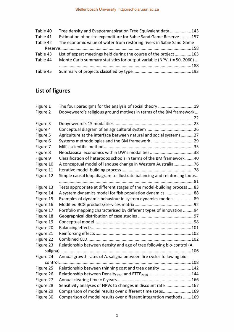
Table 40 Tree density and Evapotranspiration Tree Equivalent data .................. 143
Table 41 Estimation of onsite expenditure for Sabie Sand Game Reserve .......... 157
Table 42 The economic value of water from restoring rivers in Sabie Sand Game Reserve ............................................................................................................... 158
Table 43 List of expert meetings held during the course of the project .............. 163
Table 44 Monte Carlo summary statistics for output variable (NPV, t = 50, 2060) ... ................................................................................................................ 188
Table 45 Summary of projects classified by type ................................................. 193
List of figures
Figure 1 The four paradigms for the analysis of social theory .............................. 19
Figure 2 Dooyeweerd’s religious ground motives in terms of the BM framework ... .................................................................................................................. 22
Figure 3 Dooyeweerd’s 15 modalities ................................................................... 23
Figure 4 Conceptual diagram of an agricultural system ........................................ 26
Figure 5 Agriculture at the interface between natural and social systems ........... 27
Figure 6 Systems methodologies and the BM framework .................................... 29
Figure 7 Mill’s scientific method ............................................................................ 35
Figure 8 Neoclassical economics within DW’s modalities ..................................... 38
Figure 9 Classification of heterodox schools in terms of the BM framework ....... 40
Figure 10 A conceptual model of landuse change in Western Australia ................. 76
Figure 11 Iterative model-building process ............................................................. 78
Figure 12 Simple causal loop diagram to illustrate balancing and reinforcing loops .. .................................................................................................................. 81
Figure 13 Tests appropriate at different stages of the model-building process ..... 83
Figure 14 A system dynamics model for fish population dynamics ........................ 88
Figure 15 Examples of dynamic behaviour in system dynamics models ................. 89
Figure 16 Modified BCG products/services matrix .................................................. 92
Figure 17 Portfolio mapping characterised by different types of innovation ......... 94
Figure 18 Geographical distribution of case studies ............................................... 97
Figure 19 Conceptual model .................................................................................... 98
Figure 20 Balancing effects .................................................................................... 101
Figure 21 Reinforcing effects ................................................................................. 102
Figure 22 Combined CLD ........................................................................................ 102
Figure 23 Relationship between density and age of tree following bio-control (A. saligna) ............................................................................................................... 106
Figure 24 Annual growth rates of A. saligna between fire cycles following bio-control ................................................................................................................ 108
Figure 25 Relationship between thinning cost and tree density ........................... 142
Figure 26 Relationship between Density1991 and ETTE2008 .................................... 144
Figure 27 Annual clearing time = 0 years ............................................................... 166
Figure 28 Sensitivity analyses of NPVs to changes in discount rate ...................... 167
Figure 29 Comparison of model results over different time steps ........................ 169
Figure 30 Comparison of model results over different integration methods ....... 169
Stellenbosch University http://scholar.sun.ac.za

xi
Figure 31 Long-term clearing simulations (mean = 25, standard deviation = 13, min = 1, max = 50) ..................................................................................................... 174
Figure 32 Short-term intensive clearing of aliens (mean = 2, standard deviation = 1, min = 1, max = 5) ................................................................................................ 174
Figure 33 NPV following clearing and bio-control treatments .............................. 175
Figure 34 Sensitivity analysis for the delay in bio-control effectiveness ............... 176
Figure 35 Effect of Prosopis re-growth following rainfall on biomass NPV ........... 176
Figure 36 Effect of variations in the re-growth rate on the overall BW NPV ........ 177
Figure 37 Effect of changes in marginal price of water on BW NPV ..................... 177
Figure 38 Baseline simulation for Beaufort West, long-term clearing .................. 178
Figure 39 NPV for different ecosystem benefits associated with rehabilitation .. 179
Figure 40 Sensitivity analysis of price of water in Drakenberg .............................. 179
Figure 41 NPVs for different soil treatments at Namaqualand over a 50-year period (i = 8%) .................................................................................................... 180
Figure 42 Sensitivity analysis on variation in soil treatments, Namaqualand ....... 181
Figure 43 NPVs for restoration – Kromme ............................................................. 182
Figure 44 Sensitivity analysis for variations in the value of water, ‘no agric’ scenario .............................................................................................................. 183
Figure 45 Sensitivity analysis for variations in the value of water, ‘agric’ scenario .... ................................................................................................................ 183
Figure 46 NPVs for different management regimes, Lephalale ............................ 184
Figure 47 Sensitivity analyses of different rehabilitation method combinations . 185
Figure 48 Sensitivity analysis for Oudshoorn case study assuming treatment costs are zero. ............................................................................................................. 186
Figure 49 PV of benefits for different rehabilitation methods .............................. 186
Figure 50 Sensitivity analysis on water price, Sand river catchment .................... 187
Figure 51 Probability of project success over varying time periods (T = 5, 10 and 50 yrs) for crops (A), grazing (B) and water (C)....................................................... 189
Figure 52 Portfolio map for different ecosystem services (bubble size indicates resources committed to it) ................................................................................ 190
Figure 53 Portfolio map for different ecosystem services (bubble size indicates standard deviations) .......................................................................................... 191
Figure 54 Portfolio map for different ecosystem services (bubble size indicates coefficient of variation) ...................................................................................... 192
Stellenbosch University http://scholar.sun.ac.za

xii
List of Abbreviations ACE Association for Christian economists Ag Agulhas Ais Anthropocentric instrumental Ait Anthropocentric intrinsic (stewardship) values BCG Boston consulting group BM Burrell and Morgan BTM Benefits Transfer Method BW Beaufort West CC Christo-centric values CE Complexity economics CLD Causal loop diagram CNC Critical natural capital CST Critical systems thinking CTA Capital theory approach CV Coefficient of variation D Drakensberg DSS Decision support system DW Dooyeweerd EE Ecological economics EGS Ecosystem goods and services Eis Ecocentric instrumental values Eit Ecocentric intrinsic values EM Economic man Ep Epistemological ERE Environmental and resource economics FJ Flood and Jackson GEM General equilibrium modelling G-R Georgescu-Roegen GST General systems thinking HIE Homo institutional economicus HSM Hard systems methods IAC Irrigated annual crops IAP Invasive alien plant IP Interactive planning IPC Irrigated permanent crops IRR Internal rate of return Ka Kromme (with agriculture) Kna Kromme (no agriculture) KNP Kruger National Park Lp Lephalale MAE Mean Absolute Error ML Mutual learning approaches MSE Mean Square Error MST Multimodal systems thinking N Namaqualand
Stellenbosch University http://scholar.sun.ac.za

xiii
NC Neoclassical NM National model NPD New product development NPV Net present value Ont Ontological Ou Oudtshoorn PES Payment for Ecosystem Services PLE Public Learning Edition PPM Project portfolio management RA Risk analysis RESTORE-P model Regional Economic SysTem dynamics mOdel for the
Restoration of Ecosystems and project Prioritisation RGM Religious ground-motives S Sand SD System dynamics SDf System dynamics (Forrester variety) SE Systems Engineering SSD Social Systems Design SSGR Sabie Sand Game Reserve SSM Soft systems method TC Theo-centric values TCM Travel Cost Method TEV Total economic value TIM Technology and innovation management WA Western Australia
Stellenbosch University http://scholar.sun.ac.za

1
Chapter 1 Introduction
1.1 Background
If current trends in population growth, development and consumption continue, the earth could be confronted with a number of dire consequences including the following (TEEB, 2008):
• It is possible that 11% of the natural areas existing in 2000 will be lost by 2050, mainly due to conversion for agricultural production, impacts from climate change and expanding infrastructural requirements.
• Increased demand for agricultural land could account for almost 40% of land currently under low-impact farming being converted to intensive agricultural land use by 2050, resulting in additional biodiversity losses.
• Increasing global mobility and trade patterns increase the risk of invasive alien species impacting on food production, health and infrastructure.
In Africa, most of the 22 cases of recorded environmental conflicts between 1980 and 2005 show evidence of a connection between soil degradation and water scarcity (WBGU, 2008). Many of these conflicts also indicate the use of systematic and collective violence. Furthermore, by 2025, the number of people in southern Africa exposed to water stress (which is defined as watersheds with runoff of less than 1 000m3 per person per year) could range between 33 and 38 million (Arnell, 2004). Restoring natural capital is important ammunition in the battle against environmental degradation and the associated impacts on economic and social systems. For example, the clearing of invasive alien plants (IAPs) increases water yields and also provides the means for more sustainable agricultural practices. Restoring natural capital also enhances the ecosystem’s ability to provide a number of services such as erosion control and climate regulation, goods such as fuelwood and building materials, and other life supporting functions. (A more extensive coverage of ecosystem goods and services is developed in Chapter 2). This chapter unfolds as follows: from the outset it is important to develop a robust definition of natural capital, what it entails and what it does not. Thereafter, a detailed justification for restoration is developed, considering economic, ecological and social constraints. All decisions around restoration need to occur within a decision-making framework, and this is considered next. Sections 1.2 and 1.3 provides the research hypothesis and philosopy, and Section 1.4 presents the the proposed study approach. Section 1.5 gives the data collection methods and Section 1.6 defines the study boundaries, what will be included and what will be omitted.
Stellenbosch University http://scholar.sun.ac.za
2
1.1.1 What is natural capital?
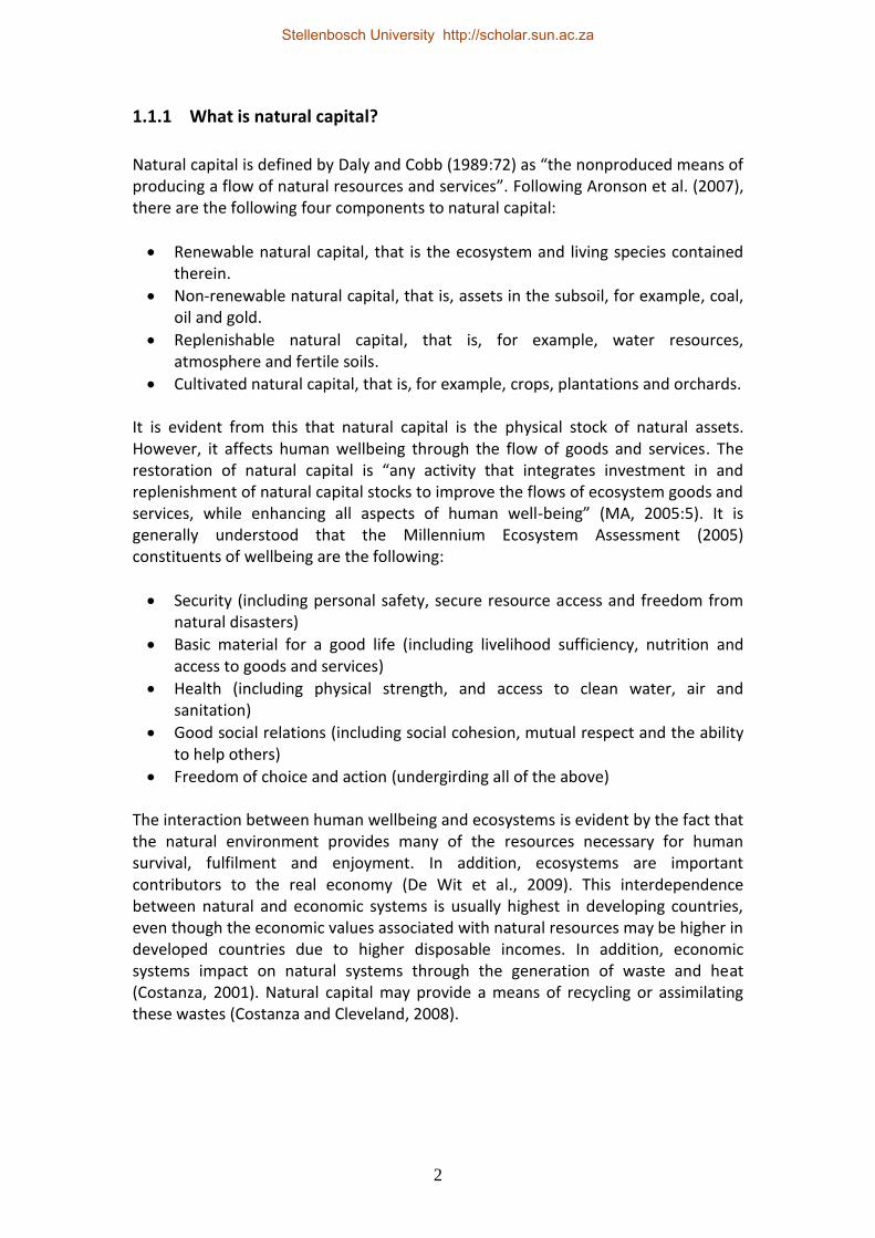
Natural capital is defined by Daly and Cobb (1989:72) as “the nonproduced means of producing a flow of natural resources and services”. Following Aronson et al. (2007), there are the following four components to natural capital:
Renewable natural capital, that is the ecosystem and living species contained therein.
Non-renewable natural capital, that is, assets in the subsoil, for example, coal, oil and gold.
Replenishable natural capital, that is, for example, water resources, atmosphere and fertile soils.
Cultivated natural capital, that is, for example, crops, plantations and orchards. It is evident from this that natural capital is the physical stock of natural assets. However, it affects human wellbeing through the flow of goods and services. The restoration of natural capital is “any activity that integrates investment in and replenishment of natural capital stocks to improve the flows of ecosystem goods and services, while enhancing all aspects of human well-being” (MA, 2005:5). It is generally understood that the Millennium Ecosystem Assessment (2005) constituents of wellbeing are the following:
Security (including personal safety, secure resource access and freedom from natural disasters)
Basic material for a good life (including livelihood sufficiency, nutrition and access to goods and services)
Health (including physical strength, and access to clean water, air and sanitation)
Good social relations (including social cohesion, mutual respect and the ability to help others)
Freedom of choice and action (undergirding all of the above) The interaction between human wellbeing and ecosystems is evident by the fact that the natural environment provides many of the resources necessary for human survival, fulfilment and enjoyment. In addition, ecosystems are important contributors to the real economy (De Wit et al., 2009). This interdependence between natural and economic systems is usually highest in developing countries, even though the economic values associated with natural resources may be higher in developed countries due to higher disposable incomes. In addition, economic systems impact on natural systems through the generation of waste and heat (Costanza, 2001). Natural capital may provide a means of recycling or assimilating these wastes (Costanza and Cleveland, 2008).
Stellenbosch University http://scholar.sun.ac.za

3
1.1.2 Rationale for restoration
1.1.2.1 Overview
Over the past century South Africa has become increasingly reliant on manufacturing and service industries (Meyer et al., 2007). However, natural capital continues to play an important role in the livelihoods of people, particularly the poor (Blignaut and Moolman, 2006). The productivity of land and the availability of water can help the poor to overcome some of the critical constraints they face in meeting their basic needs (Rosegrant et al., 2006). Like other forms of capital, natural capital may be a constraint on future development. Until recently it was treated as a free good in abundant supply. One example of natural capital as a constraint to future development is the role of water allocation in South Africa’s economic development (Backeberg, 2007). Water, health and social security are interconnected in the sense that a society’s wellbeing is linked to the availability of a clean, sustainable water supply. An example of this is the number of cholera outbreaks throughout sub-Saharan Africa. During the outbreak in KwaZulu-Natal, 113 966 people were infected and 259 lives were claimed between August 2000 and February 2002 (Cottle and Deedat, 2002). This in turn affected the extent to which the State was able to provide social assistance. Another reason for the restoration of natural capital is the economic contribution of land in South Africa. Agriculture and mining comprise less than 10% of Gross Value Added (SARB, 2008). Yet both play an important role in food security and the support of rural livelihoods. Despite shedding 140 000 regular jobs between 1988 and 1998 (Simbi and Aliber, 2000), agriculture is still a major employer of rural dwellers, with more than one million people (or 8.5% of total employment) employed in this sector as at March 2007 (StatsSA, 2007). Furthermore, World Bank (2008) figures indicate that the poverty rate in South Africa, as measured by percentage of the population below the international poverty line, has actually increased between 1995 and 2000. The linkage between increased poverty and job losses in agriculture is likely to be significant. In addition to livelihoods, land also provides a number of other economic and social benefits, such as recreation, aesthetic, tourism, hunting and cultural amenities. It has been estimated (De Wit et al., 2009) that the ecosystem services in Cape Town of natural hazard regulation, tourism and recreation, and support to the film industry provide an annual benefit of between R1.5 and R4 billion to those living in or visiting the city. A third reason for restoring natural capital is that the protection of the natural environment is a fundamental right for all South Africans, along with sustainable economic and social development. As the Constitution of the Republic of South Africa, 1996 (Act 108 of 1996) [Section 24] states:
Stellenbosch University http://scholar.sun.ac.za

4
“Everyone has the right: (a) to an environment that is not harmful to their health or well-being; and (b) to have the environment protected, for the benefit of present and future generations, through reasonable legislative and other measures that- (i) prevent pollution and ecological degradation; (ii) promote conservation; and (iii) secure ecologically sustainable development and use of natural resources while
promoting justifiable economic and social development” (RSA, 1996). South Africa is heavily dependent on fossil fuels for its energy requirements, with 93% of the electricity production being coal based (Van Heerden et al., 2006). A key consequence of this is above average per capita greenhouse gas emissions. Although a developing country, South Africa’s carbon emissions are on the level of a high income country (Van Heerden et al., 2006). Given recent electricity tariff increases and the relatively low cost of electricity production from coal, coal use is likely to remain an important source of energy in the future. But even assuming zero greenhouse gas emissions from South Africa, climate change is a global problem and the ability of the natural environment to sequester or “offset” carbon emissions remains important.
1.1.2.2 The economic costs of degradation
Degraded natural capital has various implications for socio-economic systems, including the availability of food, medicinal products, water and energy (Stocking 1999; Crookes, 2003; Blignaut and Loxton, 2007). A number of costs associated with degradation are discussed in Milton et al. (2003), including the following:
1) Excessive ploughing can replace perennial, drought-tolerant plants with drought-sensitive plants that result in forage shortages during dry periods.
2) The more degraded a landscape becomes, the less surplus a land owner has to reinvest in rehabilitation activities, resulting in a downward spiral where poor farmers become even poorer.
3) Owing to the benefits of livestock that extend beyond their cash value, stocking densities are typically higher than is sustainable resulting in serious fluctuations in livestock numbers during dry periods, which in turn affects livelihoods.
4) Not only livestock numbers are affected by degradation, but also other natural products that rural households depend on, such as building materials, fuelwood and medicinal products. Economic costs include loss of timber and beef production resulting in decreased export earnings and loss of tax revenues.
5) Mining and industrial activity such as the building of roads can also impact on degradation, by destroying vegetation and affecting surface run-off. The costs of mining (such as health costs resulting from dust) are born by local people while the benefits are exported.
6) The costs of invasive alien plants, originally imported for their perceived horticultural benefits, are substantial. For example, in South Africa the present net cost (in 1998 values) of black wattle (Acacia Mearnsii) in water lost through transpiration has been estimated at $1.4 billion. Other invasives that have
Stellenbosch University http://scholar.sun.ac.za

5
affected semiarid rangelands and river courses include lantana (Lantana camara), prickly pear cactus (Opuntia sp), and mesquite (Prosopis sp). Apart from streamflow this has also reduced biodiversity, forage biomass and livestock access.
1.1.2.3 The economic benefits of restoration
The economic arguments for conservation are quite compelling. In a review of five case studies, Balmford et al. (2002) found that sustainable management of natural resources across a range of biomes resulted in gains in Net Present Values (NPVs) of between 14% and 75% compared with unsustainable practices. While there have been a number of success stories in restoring natural capital internationally (for a discussion of the famous New York City-Catskills project, see Elliman and Berry, 2007), the results from individual studies on benefits and costs are mixed. On the benefit side, Tong et al. (2007), for example, conclude that there is a significant potential gain. They estimate an increase of 89.5% in ecosystem services value as a result of the restoration of the Sanyang wetland in China. On the other hand, costs of restoration are high and opportunity costs may often be a significant barrier to conservation on private lands (Dorrough et al., 2008). Results from South Africa indicate a significant positive benefit from restoration. In a recent study in Bushbuckridge, Blignaut and Moolman (2006) found a potential net gain in the direct consumptive use benefit of restoration of US$391/hectare, or US$ 72 million across all the land under communal management. Higgins et al. (1997a) developed a model for mountain fynbos dynamics with five sub-components (namely hydrological, fire, plant, management and economic valuation) and six value components (namely hiker visitation, ecotourist visitation, genetic storage, endemic species, wildlflower harvest and water production). They estimated that the cost of restoration could range between 0.6% and 4.76% of total value, depending on the economic valuation scenario. A preliminary review of cost-benefit studies suggests some promising results. During a study in the subtropical thicket in the Eastern Cape, Mills et al. (2007) found that the financial benefits are potentially positive, with an internal rate of return (IRR) of 9.2%. Holmes et al. (2004) also found a positive NPV in favour of both partial and full restoration of riparian habitat in North Carolina.
1.1.2.4 Project context
South Africa has a proud history of restoring natural capital. While there are some exceptions (indigenous forest rehabilitation being one), examples of restoration include the Working for Water, Working for Wetlands and Working for Fire initiatives, as well as mandatory rehabilitation of mine dumps and road servitudes. In spite of these, there has been no study to date of the economic, ecological and hydrological effects of restoration measured across a range of diverse sites. As a
Stellenbosch University http://scholar.sun.ac.za

6
result, ASSET Research, in collaboration with the Water Research Commission (WRC), initiated a project entitled “The Impact of Re-Establishing Indigenous Plants and Restoring the Natural Landscape on Sustainable Rural Employment and Land Productivity through Payment for Environmental Services” (WRC project K5/1803). As part of the project, eight sites were identified where restoration activities are taking place. A number of Masters' students in the field of hydrology, ecology and economics conducted research at these sites exploring the impacts of restoration on various ecological and economic attributes. This study builds on the work by the Masters' students and develops an integrated systems model that incorporates elements from the eight study sites. The hypothesis for this particular phase of the project is as follows: “The restoration of natural capital improves water flow and water quality, land productivity, in some instances sequesters more carbon, and, in general, improves both the socio-economic value of the land in and the surroundings of the restoration site as well as the agricultural potential of the land” (ASSET Research, 2008). The scope and specific problem statement of the study are developed and defined within the boundaries and gambit of this frame of reference.
1.1.3 Management approaches to restoration
1.1.3.1 Decision-making framework
Key to any management response is the development of a decision-making framework. A number of modelling frameworks may be used to provide decision-making support (Young et al., 2007; Crookes and De Wit, 2009), such as the following:
Landscape/system models (e.g. geographic information systems, regression models, system dynamics models, ecological footprint, key sector analysis)
Policy frameworks (e.g. environmental impact assessment, economic impact assessment, life cycle assessment)
Analytical approaches (e.g. cost-benefit analysis, multicriteria analysis, regional economic modelling, experimental methods)
Qualitative models (e.g. extended stakeholder analysis, Delphi method, mutual learning exercises)
These modelling frameworks may contain a number of different features. Following Robertshaw et al. (1978), the subsequent distinctions may be drawn (Table 1). A prescriptive model, also known as a normative model, reflects a particular value system indicating what ought to be. Descriptive models, on the other hand, focus on facts and relationships between variables, and address the so-called “what if” questions. According to Robertshaw et al. (1978), systems approaches address both these functions: descriptive approaches are used to investigate relationships
Stellenbosch University http://scholar.sun.ac.za

7
between elements, while prescriptive approaches are used to choose between alternatives. Table 1 Classification of models
Classified according to: Types
Origin Empirical – theoretical
Function Prescriptive – descriptive
Element representation Iconic – analogue – symbolic
Complexity Linear – Non-linear
Temporal characteristics Static – dynamic
Nature of changes Continuous – discrete
Execution technique Numerical – Analytical
Predictability Deterministic – probabilistic
Source: Robertshaw et al. (1978) A number of decision-making processes underlying these frameworks may also be developed (see e.g. Young et al., 2007).
1.1.3.2 Decision rules for restoration
Standard (neoclassical) economic theory argues that a restoration project should proceed if the economic benefits outweigh the economic costs. Although the restoration costs of degraded landscapes have yet to be analysed properly from an economic viewpoint, preservation of natural landscapes have been found to be less costly than the conversion of wildlands to artificial uses (Figueroa, 2007). According to Goodland and Daly (1996), natural capital restoration is justified when:
stocks of renewable and replenishable resources are used faster than they are being restored,
waste emissions exceed the capacity of the environment to absorb them,
non-renewable resources are depleted faster than technology creates sustainable alternatives.
The implicit assumption behind these criteria is that if a stock of the specified resources fall below the given thresholds then critical natural capital is being depleted. According to Farley and Brown Gaddis (2007), restoration is justified on two grounds: sustainability and desirability. In the case of sustainability, the efficiency criterion only applies to the question of how and not why. In other words, restoration should be as cost effective as possible. Desirability is a more subjective measure and the use of monetary values to prioritise restoration initiatives based on available funds can be a useful tool. In such cases efficiency implies that the total benefit of restoration should exceed the total cost.
Stellenbosch University http://scholar.sun.ac.za

8
A number of generic social, institutional and legal criteria are also relevant to the restoration of natural capital (adapted from Crookes, 2001):
security of tenure and ownership rights
sense of community
affinity with and dependence on the natural resource base
time horizon of exploitation
financial means to maintain and restore the natural resource base
legislative frameworks
traditional and customary practices
the involvement of relevant community based, local government and donor agencies
political and community willingness to restore natural capital Finally, equity criteria such as the distribution of wealth and the natural resource base among members of the community may also affect the ability of communities to restore natural capital.
1.1.4 Who pays for restoration?
In most cases natural capital and the stream of benefits that are derived from it are public goods (for example, clean air and water). This raises the question of who should pay for these restoration activities (Rees et al., 2007). If it is the State, the issue of the opportunity costs of restoration vis-á-vis other social programmes becomes relevant (Figueroa, 2007). If it is the impacter, a social criterion provides that the resource should be saved given that the social costs are tolerable. The implicit assumption, therefore, is that if the social costs are too high, the State should intervene. In development projects with broad spatial and temporal scopes, the burden of proof is on the impacter to prove that the costs of restoration are unbearably high. In the case of private (excludable, rival) goods, the user pays (Rees et al., 2007), although the distinction between public and private goods is not always clear.
1.2 Research statement
The focus of this study is driven by the underlying ASSET/WRC project (see Section 1.1.2.4). Key areas identified include the issues regarding the economic value of water and carbon sequestration, land productivity, and on- and offsite land values. The specific focus of the research is to improve the economic evaluation of a project or intervention through an interdisciplinary approach and to contrast with the traditional economic approach. Although the study does include modelling, the focus of the study is not primarily about modelling. The focus of the study is rather
Stellenbosch University http://scholar.sun.ac.za

9
on providing a framework in which resource allocation decisions can be made for restoration projects. A case study approach is utilised to apply the framework. The framework is tested at eight sites throughout South Africa where the restoration of natural capital is taking place. System dynamics modelling along with risk analysis using insights from project portfolio management (PPM) is utilised to categorise restoration projects, and the facilitation of decision-making processes regarding which projects to select under what conditions. The system dynamics modelling framework is used to model the functional relationships between water and grazing (and biophysical indicators) and changes in stocks and flows as result of degradation and restoration in respect of reference and undegraded sites and impact on agriculture. The project portfolio mapping framework is uses the outputs of the system dynamics model to classify and select restoration projects under budgetary constraints.
1.3 Research philosophy
1.3.1 Historical development of scientific research
According to Klir (1985), the nature of scientific research can be classified into three distinct periods. The first (pre-scientific) period extended until the sixteenth century and was characterised by speculation, deductive reasoning and common sense. The second (one dimensional scientific) period, from the seventeenth century until the mid-nineteenth century, was characterised by an integration of deductive reasoning and common sense with experimentation, and placed particular emphasis on the latter. A third (two dimensional scientific) period, dating from the mid-nineteenth century was characterised by the emergence of systems theory which focuses on the relational rather than the experimental aspects of science. The paradigm shift that has taken place is evident when comparing two research methodology textbooks that reflect the different time periods. The first book (Whitney 1950), initially published in 1937, emphasises the collection of data and the scientific method. Different research methods are mentioned but these are largely apportioned by discipline (e.g. sociological, philosophical and natural science). The second book (Walizer & Wienir 1978), published after the 1950s, is subtitled searching for relationships. Again, experimentation is mentioned but this only comprises a small part of the publication. Another process of scientific research that has emerged is supradisciplinary research, or any research that transcends a particular scientific discipline (Balsiger, 2004). Supradisciplinary research includes interdisciplinary, multidisciplinary and transdisciplinary research. Two aspects are important in the emergence of supradisciplinary research (Balsiger, 2004). Firstly, supradisciplinary research emerged as a means of solving problems. Secondly, systems theory as formulated by
Stellenbosch University http://scholar.sun.ac.za

10
Ludwig van Bertalanffy in 1937/8 played an important role in demonstrating that a single disciplinary approach was insufficient thereby increasing the need for collaborative approaches. Another aspect that distinguishes different categories of scientific research is scope. Roux et al. (2010) distinguish between the scope of disciplinary, interdisciplinary, multidisciplinary and transdisciplinary research as follows: disciplinary research is suitable for relatively well defined problems with limited scope; multi- and interdisciplinary research is appropriate for larger problems that require the inputs from several disciplines; and finally, transdisciplinary research addresses user inspired and context driven problems that embrace complexity and incorporate multistakeholder perspectives. Transdisciplinary research is the most recent of the supradisciplinary practices, emerging in the 1970s from interdisciplinary and multidisciplinary approaches (Balsiger, 2004). There is some overlap between the different supradisciplinary methods (Roux et al. 2010) so it is difficult to categorically state which type of scientific research this study follows. Given the complexity and user driven nature of the problem, and the nature of the participants in the research (multi-stakeholder and multi-level including policy-makers, affected parties, funders and researchers) this study is primarily transdisciplinary in nature, although it shares some characteristics with interdisciplinary research as it attempts to integrate diverse tools and frameworks within the discipline of economics.
1.3.2 Alternative paradigms of the modelling process
Linstone (1983) identifies eight paradigms of systems enquiry, namely: 1) problem solution: problems can be solved 2) problem solution: the search for the best solution 3) reduction and specialism 4) data and models 5) quantification of information 6) objectivity 7) relationship with the individual 8) time Following these paradigms, three perspectives or views on modelling may be distinguished (see Table 2). The pessimistic view argues that no analysis is useful and motivations are selfish. The optimistic perspective states that models are useful but that true objectivity is not attainable. The realistic view based on a Judeo-Christian perspective adopts an altruistic approach but argues that many solutions are beyond human comprehension. These different perspectives on modelling suggest the importance of grounding system dynamics modelling in economic theory as well as ascertaining the usefulness of this approach for addressing the research question.
Stellenbosch University http://scholar.sun.ac.za

11
Table 2 Paradigms of systems enquiry Pessimistic view Optimistic view Realistic view
There are no solutions, and investigation merely shifts the problem to a higher level.
Solutions exist to most problems, and investigation provides a means of providing solutions to these problems.
Solutions to all problems exist, but some of these may be beyond human comprehension.
Reductionism and specialism are natural human ideals in that these generate the greater chance of fame and success, and modelling is an end to this.
Modelling is a means to provide solutions to problems rather than a means to fame and success. The focus is on multidisciplinarity rather than specialism within a discipline.
Individual motivation shifts away from personal motivations of greed or fame to higher ideals of community and benevolence. Motivation for modelling is to improve wellbeing of society.
Data and models are unreliable modes of enquiry.
Data and models are imperfect, yet useful tools for enquiry.
Data and models are not enough.
Ambiguity is often more desirable than quantification.
Quantification is a tool for clarifying ambiguity.
Ambiguity is not desirable, however ultimate truth does exist although this may be beyond the determination of the individual.
Objectivity is a myth. Subjectivity guides behaviour.
Objectivity is a myth. However, the modeller is guided by problem and client interactions.
Objectivity is a myth. Truth guides behaviour.
The individual as an individual is ignored.
The individual is part of an interconnected system.
The individual has intrinsic value and is the basic building block of society.
Time is a perception. Time is fundamental to all interactions.
Time exists, but will ultimately pass away.
Source: Own analysis (used Wolstenholme (1983) for the pessimistic view)
1.4 Methodology
1.4.1 Definition
In the social sciences, the term “methodology” usually refers to the following two aspects (Jackson, 1991:3): 1) “The procedures used by a theorist in seeking to find out about reality”; and 2) The theoretical assumptions underpinning that methodology. Systems methodology also addresses two aspects (Jackson, 1991:3): 1) Methods used for gaining knowledge about systems and
Stellenbosch University http://scholar.sun.ac.za

12
2) “[T]o describe the organised set of methods an analyst employs to intervene in and change real-world problem situations”. The latter is the more normal usage in systems analysis and reflects the more practical focus of this approach. Jackson (1991) argues that these differences reflect a different emphasis rather than a real distinction: social science is strong on theory and emphasises the ontological and epistemological assumptions associated with knowledge, while having a corresponding weakness in practice. Systems analysts, however, are frequently strong on practice but neglect the underlying theory. The term "methodology" in this study refers primarily to the application of knowledge to real world problems. Where possible, however, reference is made to the underlying theoretical and philosophical foundations. This study aims at investigating the economic case for restoring natural capital. The approach is to develop a high level model for analysing decisions around natural capital restoration. A framework is needed that can account for market failures while also incorporating the complexities of supply side elements in the modelling. The approach adopted is system dynamics modelling, which incorporates mathematical rigour with the flexibility and dynamics required for complex systems. A model of this kind is used to understand why problematic behaviour is generated by finding “leverage points” in the system that causes this behaviour (Güneralp and Barlas, 2003). These leverage points are then used to formulate policies (economic or environmental) to eliminate the problem.
1.4.2 Justification
The development of computers capable of advanced simulation makes it possible to analyse complex systems and without simplifying mathematical assumptions required for traditional social models (Miller and Page, 2007:5). For example, in their publication on game theory Von Neumann and Morgenstern (1944) state: “We repeat most emphatically that our theory is thoroughly static. A dynamic theory would unquestionably be more complete and therefore preferable. But there is ample evidence from other branches of science that it is futile to try and build one as long as the static side is not thoroughly understood” (as cited in Miller and Page, 2007:84). Not only dynamics is important, but also the nature of equilibrium: “In situations in which equilibria are a possibility, understanding the dynamics is likely to be insightful. In situations where equilibria are nonexistent or transient paths are long, understanding the dynamics is critical” (Miller and Page, 2007:84). In traditional economics, theories rely on models with few agents or homogenous behaviour. For example, theories of the firm involve monopolies or cartels. Oligopolies become much more difficult to solve. Simulation modelling makes it possible to analyse these interactions (Miller and Page, 2007:84–85). Computational models also provide a way of testing economic theories and conducting repeat experiments (Miller and Page, 2007:86).
Stellenbosch University http://scholar.sun.ac.za

13
1.4.3 Types of simulation approaches
A dynamic simulation models the change in parameters over time. Robinson (2004) distinguishes between three approaches to dynamic simulation: the time-slicing approach, discrete event simulation and continuous simulation. The time-slicing approach is the simplest approach of the three and can be modelled using a spreadsheet. In a discrete event simulation, time is only measured when an event occurs. An example of this would be a traffic officer measuring when vehicles pass a checkpoint. For a continuous simulation, changes in the system are constantly monitored. System dynamics is an example of a continuous simulation, although a number of authors have looked at the interface between system dynamics and discrete event simulation (e.g. Lane, 2000a; Brailsford and Hilton, 2001; Tako and Robinson, 2009).
1.4.4 System dynamics modelling
System dynamics (SD) models changes in complex systems over time and provides a means of capturing realistic dynamic behaviour between variables, including feedback loops, delays and non-linearities. The system dynamics approach is consistent with traditional economic approaches to modelling dynamic phenomena (Smith and Van Ackere, 2002). However, the advantage of SD modelling is that it can model disequilibrium conditions as well as provide a realistic portrayal of the processes involved in decision-making (Sterman, 1987). As Sterman (1987:1573) states:
“The purpose of simulation models is to mimic the real system so that its behaviour can be anticipated or changed. Behavioural simulation models must therefore portray decision-making behaviour as it is, and not as it might be if decision-makers were omniscient optimizers. The decision-making heuristics and strategies people use, including their limitations and errors, must be modelled”.
It is not appropriate in these introductory paragraphs to provide a full evaluation of the system dynamics modelling approach, but the reader is referred to Section 3.3 for further elaboration.
1.5 Methods of data collection
The system dynamics model that will be used analyses the effects of restoration (active and passive) at eight study sites throughout South Africa (Table 3). These study sites represent a range of different biomes: two of the sites are in the Succulent Karoo, one in the Nama Karoo, two in the Fynbos biome, one in the Grassland biome and two in the Savanna biome. A common theme for all of these study sites are important linkages to agriculture and water which are key focus areas of the project.
Stellenbosch University http://scholar.sun.ac.za

14
Table 3 The eight study sites in the research problem
Study area Considerations
Agulhas Plain Existing alien clearing Tourism at De Hoop Nature Reserve Commercial flower harvesting
Beaufort West Existing Prosopis clearing Good linkages to water flows and grazing
Oudtshoorn and Calitzdorp
Degraded veld due to ostrich camps Need ostrich products with biodiversity friendly labelling for exports to the EU Need for monitoring in the area
Namakwa Sands Good existing link with restoration to obtain closure permit Aim is to improve carrying capacity for grazing
Drakensberg Communal agriculture Unsustainable forms of agriculture land use practice has led to serious degradation that impacts heavily on the water resource (both quality and quantity as well as sediment yield and the seasonality of the water flows) Ongoing restoration work over the past 10 years with data in support
Ellisras and Thabazimbi Management and clearing of indigenous bush encroachment Bush encroachment has a considerable negative impact on water levels as well as the productive capacity of the land Clearing operation with data since the mid-1990s available
Sand river Clearing of invasive alien plants to secure the flow of quality water Contested resource use: Water for agriculture (communal and commercial), the environmental reserve, domestic purposes and for aesthetic and tourism/conservation value Data since the late 1990s available plus clearing records
Krom river system Clearing of invasive alien plants and wetland restoration since 1996 Water flow and quality data available since the 1950s, yet no analysis on the effect of changes in water quality and quantity as a result of both the increase (up to 1996) and subsequent clearing of invasive aliens
Source: ASSET Research (2010) Data sources include the following: information from ecology, hydrology and economics Masters' students (providing primary data) and an expert group, including several of the supervisors of the students, that meets regularly and acts as a scientific sounding board as well as provides valuable scientific input where data from the study sites are not available. Other important sources of data for this study include various scientific publications and other third parties outside the immediate scope of the project.
Stellenbosch University http://scholar.sun.ac.za

15
1.6 Scope and limitations of study
A system dynamics model is a complex systems approach in that it models non-linear, dynamic behaviour. An advantage of the systems approach is that elements that would otherwise be excluded from the modelling framework are now included. However, given the complex nature of interactions, the study is necessarily restricted by time and space. An example of a spatial component not included in this study is the feedback arising from the destruction of natural capital in the production process used to generate revenue to fund rehabilitation work. On the temporal scale, an aspect that will need to be investigated further is whether there are any criteria for determining an optimal time period for full restoration. Failing this, a generally accepted (standardised) time period will be adopted in line with cost-benefit analyses. This study will not conduct a cost-benefit analysis per se but wil utilise total/marginal cost pricing when necessary.
1.7 Thesis outline
The structure of this study is as follows: Given the seemly unrelatedness of systems thinking and economic theory, Chapter 2 develops a classification scheme based on social science theory and applies it to systems theory, economic theory and related disciplines, and restoration science. Chapter 3 develops the methodology of building a system dynamics model, offers certain theoretical constraints and practical applications, and presents the steps in the modelling process. Chapter 4 presents the integrated systems model used to simulate the effects of the restoration of natural capital on a range of ecological, economic and hydrological impacts. Chapter 5 gives a discussion of the main results from the modelling exercise. Chapter 6 provides a summary and conclusions, and recommendations for future research.
1.8 Chapter summary and conclusions
Given the range of topics covered in this thesis, this introductory chapter sets the scene for the study by elaborating on and defining a number of concepts used in the thesis, including what is meant by restoration, an introduction to the system dynamics modelling approach, the research framework (the different types of supradisciplinary research) and also the definition of methodology in the context of this study. The chapter concludes with a brief overview of the eight case studies. There is a compelling economic case for protecting and maintaining natural capital, as well as a political argument that can be made. The chapter provides quite a broad
Stellenbosch University http://scholar.sun.ac.za

16
overview of the field of study. In the next chapter it is necessary to contextualise the research within the discipline of economics.
Stellenbosch University http://scholar.sun.ac.za

17
Chapter 2 Systems thinking and social theory
2.1 Introduction
Chapter 1 provided an overview of why restoration of natural capital is important. This chapter looks at how traditional economic theory has addressed issues related to the environment, as well as recent developments in the areas of ecological economics, resilience and complexity economics. This is important as it provides a justification for the systems approach to modelling not only economic phenomena, but also the integration of economic and environmental elements into a composite framework. The theoretical foundations of this study are rooted in several different disciplines. Firstly, it is an economics study and it is, therefore, important to ground the research in the economic and management sciences. Secondly, the modelling approach is rooted in systems theory and the literature surrounding systems philosophy needs to be addressed. Thirdly, this is an applied research topic with applications in ecological science, in particular restoration of natural capital (RNC). In order to reconcile these apparently contradicting perspectives, a framework or frameworks are needed that would enable the comparison of these disciplines on ontological and epistemological grounds. It will then be possible to identify common features between the different approaches, as well as highlight any differences and potential conflicts between the proposed methodology and the disciplinary context of the research. Key research questions for this chapter are as follows:
Is system dynamics modelling compatible with mainstream economics?
What is the disciplinary context of the research problem and is it sufficiently rooted in the economics profession?
Are there epistemological and ontological links between restoring natural capital and economics?
This chapter comprises four stages:
1) Stage 1: the presentation of social theory and the evaluation framework for the study.
2) Stage 2: an evaluation of the systems theory (the research context) and how it relates to the different disciplines within economics.
3) Stage 3: an assessment of the social aspects of restoration science and its relevance to economics.
4) Stage 4: an application of social theory to the problem of restoring natural capital and ecosystem goods and services.
Given the complexity of the reference framework, it is unlikely that a single classification framework will be sufficient. In the next section, three evaluation frameworks are presented, each with different strengths and weaknesses.
Stellenbosch University http://scholar.sun.ac.za

18
2.2 The nature of social theory
2.2.1 Overview of approaches
Modern social science research is strongly influenced by a number of dichotomies. The first is the order–conflict distinction. The second is objectivism–subjectivism distinction (see Burrell and Morgan, 1979). The third is the dualism–redemption distinction (e.g. De Raadt, 1997). Social science research is either concerned with explaining the nature of social order and equilibrium, or issues related to change, conflict and compulsion. This is the order–conflict distinction. In the objectivism–subjectivism distinction, objective social science implies a positivist epistemology and a realist ontology while subjective social science presupposes a nominalist ontology and an anti-positivist epistemology (see also Eriksson, 2003). The dualism–redemption distinction has been developed at length by a number of authors, including Francis Schaeffer and Herman Dooyeweerd. Dooyeweerd approaches the problems of ontology and epistemology from a Judeo-Christian perspective (Bergvall-Kareborn, 2001). His major work, A New Critique of Theoretical Thought, published in 1955, developed into five theories (Eriksson, 2001): (1) the theory of religious ground motives, (2) the modal theory, (3) the theory of time, (4) the entity theory or the theory of individuality structures, and (5) the social theory. The first two theories are of particular relevance to this study. The three frameworks presented for classifying social science are as follows:
1) The first is Burrell and Morgan’s (1979) classification (BM). Although this framework is now more than thirty years old, it is highly influential in classifying social science (e.g. Neuman, 2000; Jackson, 2000; Eriksson, 2003). One strength of the BM framework is that most spheres of knowledge are covered, including ontological, epistemological and methodological aspects. Another strength is that it provides comprehensive categorisation of social science research covering the interface between social, analytical, economic and the environment.
2) The second focuses specifically on systems methodologies and is the framework of Flood and Jackson (1991) (FJ). The FJ framework was much influenced by the work of BM and Morgan’s Images of Organization (2006). However, a limitation of this and the BM framework is that they are linked to the nature-freedom ground-motive (see Section 2.2.4).
3) The third framework transcends this limitation. It is the modality theory of Dooyeweerd (DW). This framework has also been widely used in systems theory and various other applications (e.g. De Raadt, 1989; Strijbos, 1995; Eriksson, 2001; Brandon and Lombardi, 2005).
Each of these frameworks will now be discussed in greater detail.
Stellenbosch University http://scholar.sun.ac.za

19
2.2.2 Burrell and Morgan’s classification of social science
The BM classification distinguishes between the epistemological, ontological and paradigmatic aspects of social research (see Figure 1 for a summary). Epistemological aspects deal with the basis of knowledge: how the world should be understood and communicated as knowledge to others. Two categories of epistemology, at opposite ends of the spectrum, are distinguished: positivism and anti-positivism. Figure 1 The four paradigms for the analysis of social theory
Key: Ep=epistemological; Ont= Ontological
Source: Based on Burrell and Morgan (1979) ‘Positivism’ is the most common and widely used philosophical perspective on science (Miller, 1987). Positivism seeks to explain the social world by exploring consistencies and causal relationships between different elements (Burrell and Morgan, 1979). Parsons (1951) argues that where the positivist scientific method is applicable, it should be used. Deviance from the positivist method in these instances “comprise the categories of ignorance and error…Beliefs which fill these gaps in positive empirical knowledge are not properly non-empirical beliefs but are scientifically inadequate empirical beliefs” (Parsons, 1951:359). Anti-positivism, on the other hand, avoids searching for laws or regularities in social systems. This approach is relativistic and argues that reality is dependent on the perspectives of the individuals who are involved in the activities that are studied. Ontological aspects are concerned with the very essence of reality – whether reality is objective, imposing itself on individuals from without, or subjective, a product of the individual's mental conception (see also Luhmann, 1995:101). Ontological concerns are at the very heart of the nature–nurture debate: whether we are created in a particular way or a product of our environment. But ontological issues are not confined to sociological systems and are also found in interactions between humans and the natural realm. For example, the study of biodiversity contains an element of realism in that it can be quantified and remains unchanged regardless of
Conflict
Order
Subjective Objective
Radical
structuralist
FunctionalistInterpretative
Radical
humanist
Ep: Anti-positivism
Ont: Nominalism
Ep: Positivism
Ont: Realism
Stellenbosch University http://scholar.sun.ac.za

20
the measurer (Mayer, 2006). However, in the realm of behavioural biology an element of nominalism could also be inferred in the sense that the interpretation of interactions between certain natural systems is subject to the perspectives of the individual observer. Both realism and nominalism have limitations (Lombardi and Basden, 1997). Realism, in its extreme, has the danger of focusing on the object at the expense of the subject. An example is the building of a road without taking the road users into account. Extreme nominalism (existentialism) has the opposite effect. There is no external reference point or standard by which views are measured or consensus is reached. The danger is therefore that the most vociferous views are addressed to the detriment of less articulate groups. Based on these ontological and epistemological dimensions, BM distinguishes between four sociological paradigms or systems of thinking) (see Figure 1). On the positivist side: functionalist and radical structuralist; on the anti-positivist side: interpretive and radical humanist. The characteristics of the four paradigms are summarised in Table 4. Table 4 Summary of the different sociological paradigms Functionalist Radical
structuralist Interpretive Radical humanist
Definition Most commonly used paradigm. Seeks rational explanations of social affairs. Problem-orientated approach concerned with practical solutions.
Radical change built on the very nature and structure of contemporary society. Focus on: 1) deep-seated internal contradictions, 2) structure and analysis of power relationships.
Seeks to understand the world as it is, from the perspective of the participant rather than the observer of the action.
Provides a crit-ique of the status quo. Society viewed as anti-human and con-cerned with ways in which humans can be freed from bonds that tie them into existing social patterns to reach their full potential.
Nature of social dynamics (order/ conflict)
Status quo, social order, consensus, social integration, solidarity, need satisfaction and actuality
Radical change, emancipation and potentiality, structural conflict, modes of domination, contradiction and deprivation
Status quo, social order, consensus, social integration and cohesion, solidarity and actuality
Radical change, modes of domination, emancipation, deprivation, and potentiality
Leading proponent
Comte; Spencer; Durkheim; Pareto
Marx; Weber; Althusser; Poul-antzas; Coletti; Dahrendorf; Rex Miliband
Kant; Dilthey; Weber; Husserl; Schultz
Kant; Hegel; Marx
Source: Based on Burrell and Morgan (1979)
Stellenbosch University http://scholar.sun.ac.za

21
2.2.3 Flood and Jackson classification
Flood and Jackson (FJ) developed a classification based on the political metaphor in terms of what they call ‘a system of systems methodologies’ (Flood and Jackson, 1991). In this classification they distinguish between simple and complex systems (see Table 5) and Unitary–Pluralist–Coercive (see Table 6). Table 5 indicates the nature of the system (in other words how complexity is perceived by participants) and Table 6 indicates the nature of the relationships between the participants (how people interact in the context of the problem). These two tables combine to give the six contexts of the system of systems methodologies, namely: simple-unitary; simple-pluralist; simple-coercive; complex-unitary; complex-pluralist; complex-coercive. Table 5 Grouping of various systems in terms of type Simple Complex
No. of elements Small Large
No. of interactions between elements Few Many
Attributes of elements Predetermined Not predetermined
Nature of interactions between elements
Highly organised Loosely organised
Nature of laws that govern behaviour Well defined Probabilistic
Source: Based on Flood and Jackson (1991) Table 6 Grouping of various systems in terms of the nature of participants Unitary Pluralist Coercive
Compatibility of interests
Share common interests
Basic compatibility of interest
Do not share common interests
Interaction between values and beliefs
Values and beliefs highly compatible
Value and beliefs diverge to some extent
Values and beliefs likely to conflict
Extent of agreement Largely agree upon ends and means
Do not necessarily agree on means and ends (compromise possible)
Do not agree on ends and means (compromise not possible)
Participation in decision-making
All participate in decision-making
All participate in decision-making
Some coerce others to accept decisions
Agreement over objectives
Act in accordance with agreed objectives
Act in accordance with agreed objectives
No agreement over objectives is possible
Source: Based on Flood and Jackson (1991)
2.2.4 Dooyeweerdian philosophy
The theory of religious ground motives recognises the dualistic thinking that has emerged as a result of ancient Greek philosophical thought, and later Thomas
Stellenbosch University http://scholar.sun.ac.za

22
Aquinas (Schaeffer, 1968). Dooyeweerd distinguishes between four religious ground motives (Eriksson, 2003): 1) The matter-form ground motive. This motive characterises all pagan ancient Greek philosophy. 2) The biblical ground motive, also known as the creation-fall-redemption ground motive. 3) The nature-grace religious ground motive, which emerged during the time of Thomas Aquinas (1225–1274) who introduced the distinction between nature (the created, earthly objects) and grace (the higher, metaphysical world). 4) The nature-freedom ground motive. When grace was eliminated, it was replaced by freedom, which characterises the modern philosophical period. This ground motive is associated with the philosophy of Immanuel Kant. Figure 2 shows how Dooyeweerds socio-religious aspects are related to the BM framework. On the horizontal axis, the subjective–objective debate in social science is illustrated. On the vertical axis the order–conflict differentiation is given. The figure indicates that the BM framework is primarily associated with the nature-freedom ground motive. Figure 2 Dooyeweerd’s religious ground motives in terms of the BM framework
Source: Adapted from Eriksson (2003) The second Dooyeweerdian theory that is relevant to this study is the modal theory (e.g. De Raadt, 1997). Dooyeweerd distinguishes 15 modalities (Figure 3) which are, in increasing order of complexity (nuclei in parenthesis): numerical (discrete quantity); spatial (continuous extension); kinetic (motion); physical (energy); biotic (vitality); psychic (feeling); analytic (distinction); historic (formative power); informatory (symbolic representation); social (social intercourse); economic (frugality); aesthetic (harmony); juridical (justice); ethical (love); and credal (faith). The framework of Dooyeweerd is subject to a number of criticisms (e.g. Brandon and Lombardi, 2005). Firstly, a hierarchical approach implies that modes far from each
Conflict
Order
Subjective Objective
Nature-freedom
NatureFreedom
Freedom
Stellenbosch University http://scholar.sun.ac.za

23
other have less influence than modes closer to each other. For example, the numerical is far removed from the ethical. However, in reality ethics and the quantitative might exert strong influence on each other such as financial reporting in the accounting and auditing professions. Furthermore, the large number of modalities makes evaluation and decision-making based on the framework difficult. Figure 3 Dooyeweerd’s 15 modalities
Source: Based on Du Plessis (2008) A strength of the framework is that this theory is based on the creation-redemption-fall religious ground motive (see also Eriksson, 2003). Thus, there is no dualistic divide between the sacred and the secular – all are intertwined. It therefore transcends the nature-freedom ground motives of the BM and FJ classifications. The shortcomings of the framework may be overcome by grouping the modalities into four categories relevant to this study. The fundamental essence of the research problem is one of utilising an analytical framework on an economy/environmental problem that exhibits considerable complexity, both in terms of dynamic behaviour as well as in the decision-making context of the problem. Using Dooyeweerd’s modalities, the following four strategic aspects relevant to this problem can be identified:1
1 Brandon and Lombardi (2005) adopt a similar approach in their assessment of sustainable development decision-making. They identify three first level aspects (natural, human and financial capital) and five second level aspects (urban development, environmental and physical quality, education and scientific development, social and economic development, and governance).
Numerical
Spatial
Kinematics
Physical
Biological
Sensitive
Analytic
Historical
Communicative
Social
Economic
Aesthetic
Juridical
Ethical
Credal
The greater the distance
between the modalities,
the less influence they
have on each other Increasing
complexity
Stellenbosch University http://scholar.sun.ac.za

24
The quantitative aspect (encompassing Dooyeweerd’s numerical, spatial and kinematic modalties)
The natural aspect (encompassing Dooyeweerd’s physical and biological modalities)
The socio-institutional (encompassing Dooyeweerd’s sensitive, analytical, formative, communicative, social and economic).
The moral aspect (encompassing Dooyeweerd’s aesthetical, juridical, ethical and credal modalities). This final aspect is included since no decision-making process is value free. The moral aspect defines the context within which policies are developed and decisions are made.
2.2.5 Classification of BM in terms of Dooyeweerd’s framework
When comparing DW’s modalities with the BM framework, it is evident that most of the lower modalities are covered (Table 7). However, and not surprising given the preceding discussion, the higher and more complex modalities are not well represented. In applying the BM framework, it should therefore be recognised that most normative aspects are not included. Table 7 Classification of BM in context of Dooyeweerd’s modalities
Strategic aspects Modalities
Quantitative Numerical
Spatial
Kinematic
Natural Physical
Biological
Socio-institutional Sensitive
Analytical
Formative
Communicative
Social
Economic
Moral Aesthetical
Juridical
Ethical
Credal Note: Shaded areas (in bold) are covered by the BM framework
Source: Own analysis In summary, all three above-mentioned frameworks contain elements that are relevant to this study. The BM framework provides an epistemological and ontological foundation, the FJ classification identifies relevant systemic aspects and the DW framework provides the normative context. It is now necessary to apply these frameworks in the context of the systems framework proposed by this study.
Stellenbosch University http://scholar.sun.ac.za

25
2.3 Systems thinking and philosophy
2.3.1 What is a system?
There are many different definitions of a ‘system’. While it will not be attempted to give a formal definition of a system, it is possible to highlight some of the complexities in understanding what a system is by considering the case of agriculture. (See e.g. Hitchins (2007) for an elaboration of the features of different definitions of a system.) Initially it appears that the literature on agricultural ‘systems’ is contradicting. For example, Holt and Schoorl (1985:78) state that “[t]he almost complete acceptance of the systems approach by agricultural professionals in planning and implementing technological change is a cause for real concern”. Bawden (1991), however, argues that agricultural science is dominated by reductionism and a focus on production. The reality is that the term ‘system’ in agriculture has two distinct meanings. Bawden (1991) terms this distinction 'ontosystemic enquiry versus episystemic enquiry'. Another way of drawing the distinction is whether the word ‘system’ is used as a noun or an adjective (Ison et al., 1997). If it relates to something that exists in the world (such as a farming system) then 'system' refers to the ontosystemic enquiry. If it is a way of thinking about reality, 'system' refers to the episystemic enquiry. It can therefore be concluded that both Holt and Schoorl, and Bawden are correct. Holt and Schoorl use the ontosystemic sense of the word and focus on the nature of reality and the systems that are used to produce the means of production. Both Bawden and Holt and Schoorl (and many other systems thinkers) are concerned with the emphasis on production systems rather than true systems science. The consequences of this thinking, Bawden (1991:2363) argues, have been
“long-term degradation of its biophysical and sociocultural environments … symptoms of serious inequities in the trade-offs between the needs of the present and those of the future are beginning to cause serious alarm as a wide spectrum of society tries to grapple with issues as complex as global warming and environmental degradation”.
The problems of degradation are aggravated in developing countries where there are aspects such as poverty, malnutrition, rapid population growth and dependence on the natural resource base. This presents agricultural science with the challenge of implementing sustainable farming practices. However, a number of different concepts of sustainability are found in the agricultural literature (Bawden, 1991) and may be distinguished in terms of productivity, social and ecological criteria. The productivity criteria emphasise agriculture as an instrument for feeding the world’s population. The ecological criteria highlight concern for disruption of biophysical and ecological balances by non-harmonious practices. Lastly, the social criteria emphasise promoting vital, coherent, rural cultures and encouraging values of stewardship and accountability.
Stellenbosch University http://scholar.sun.ac.za

26
Agriculture represents an example of the application of systems theory (the framework) with its roots in the economic and ecological context. An example of such a system represented in the ontosystemic tradition is the household model given in Figure 4. Figure 4 Conceptual diagram of an agricultural system
Source: McGregor et al. (2001) An episystemic approach to agriculture is given in Figure 5. In this figure, agriculture utilises the natural processes such as soil, water and climate processes to sustain its activities (Arrow 1). Indirectly society also enjoys the ecosystem services that the environment provides such as climate regulation, waste assimilation and nutrient cycling (Arrow 2). Modern society, in spite of its developments, is still largely agrarian and depends on the agricultural system for survival (Arrow 3). Social systems, such as the nature of farming practices, access to land, tenure and culture, and taboos all influence how farming systems operate (Arrow 4). Similarly, social systems have also influenced how we understand the natural resource base and how this is managed (Arrow 5). Finally, there is a cost to agricultural production in terms of eutrophication, erosion and other adverse impacts on the environment (Arrow 6). The implication of this is land degradation and loss of biodiversity.
CROPS LIVESTOCK
Feed, bedding
Draft, transport,
manure (fertiliser)
PHYSICAL AND ECOLOGICAL ENVIRONMENT
Weather, soil, topography, pests, diseases
HOUSEHOLD
(Land, Labour, capital)
Food, cash, fuel Food, cash, transport
MARKETS AND POLICIES
Credit, inputs, R&D, labour (off-farm work, wages), distribution, infrastructure
Goods (non-cash) Cash Labour
Stellenbosch University http://scholar.sun.ac.za

27
Figure 5 Agriculture at the interface between natural and social systems
Source: Based on Valentine (2005)
2.3.2 System philosophy
Although many of the ideas existed before then, the concept of a system emerged and became widespread in the 1950s. Three distinct fields developed (Stijbos, 2009): general systems thinking (GST), systems applications in science and technology, and systems philosophy. GST was pioneered by authors such as the biologist Ludwig von Bertalanffy (1901–1972) and economist Kenneth E. Boulding (1910–1995). The aim of this approach was to produce a unified theory of science that transcended disciplines by producing a shift away from a mechanistic view of the world (like a clock) to a more organistic, living entity (such as a cell) (e.g. Von Bertalanffy, 1973). While the proponents were unsuccessful in producing a unified science, systems thinking has permeated many disciplines, including biology, psychology, physics, information technology and economics. A second area of development was in the application of systems theory in the field of science and technology. Many large-scale models were developed in the 1960s, for example in the planning field and industrial development (Forrester 1961, 1969, 1971a). A number of successful models were developed to inform policy decisions, but some were less successful. This prompted widespread criticisms of these models, notably by Hoos (1976) and Lilienfeld (1978). There were at least two consequences of this: Firstly, these models lost favour for a number of years before a resurgence of interest returned. Secondly, a number of new ‘softer’ approaches to systems thinking surfaced at that time. A third area of development in systems thinking was in the field of systems philosophy. Early proponents such as Mario Bunge, Ervin Laszlo and Archie Bahm argued that systems philosophy was a separate discipline. Much of the early debate
NATURAL SYSTEM
SOCIAL SYSTEM
AGRICULTURAL
SYSTEM
1
23
4
56
Stellenbosch University http://scholar.sun.ac.za

28
revolved around the nature of systems thinking. Bunge argued that general systems theory was an analytical approach rather than an intuitive approach (as cited in Midgley, 2003) and was therefore closer to reductionistic science than many proponents would like to acknowledge. Lazlo, on the other hand, argued that GST was a “realist” ontology (as cited in Midgley, 2003). In other words, the world exists and is in some way ordered. Later writers would bring this assumption of realism into question. Bahm (1981) states that the majority of GST is based on the emergentist philosophy: that connections and relationships between parts should first be understood analytically and then synthetically. Modern systems thinking embodies a range of philosophical perspectives (Strijbos, 2010). One strand of systems thinking stems from the Holism philosophy of Jan C. Smuts (1870–1950). A second stems from the pragmatic school of C. West Churchman (1914–2004) and Russell L. Ackoff (1914–) which is a pantheistic perspective that rejects the notion of a personal God. A third is the scientific approach of Ludwig Von Bertalanffy (1901–1972) and Kenneth Boulding (1910–1993). The final, more recent approach is the Neo-Calvinist school, influenced by Herman Dooyeweerd (1894–1977) and Hendrik van Riessen (1911–2000) which is based on a reformed theological philosophy. In summary, there are three elements of systems philosophy that emerged: 1) the nature of systems thinking (pluralist or discipline specific), 2) the quantitative aspect (whether or not the approach may be regarded as analytical) and 3) the moral aspect (the different theistic or pantheistic perspectives). It is noted that these three elements (pluralism, analytical and moral) are common threads that have developed throughout the various disciplines associated with this study. While this study focuses on the analytical, the other elements of systems philosophy also need to be recognised.
2.3.3 Systems approaches
As indicated earlier, the classification of systems approaches using the BM framework has been undertaken by a number of authors (including Jackson (2000) and Eriksson, (2003)). This section draws heavily on those classifications, but also uses the categorisation of system approaches following Jackson (1991a) and Midgely (2003). Modern systems approaches fall into three main categories: hard systems approaches, mutual learning approaches and critical systems thinking. A fourth approach covered by Eriksson (2003) is the multimodal systems approach. A summary of the classification of these approaches in relation to the BM framework is given in Figure 6.
Stellenbosch University http://scholar.sun.ac.za

29
Figure 6 Systems methodologies and the BM framework
Key: HSM=hard systems methods, ML=Mutual learning approaches, CST=critical systems thinking. Multimodal systems thinking is not captured in this framework; Ep=epistemological; Ont= Ontological
Source: Adapted from Jackson (2000) and Eriksson (2003)
2.3.4 Hard systems methods
Hard systems methods (HSM) use quantitative techniques to solve problems where there is general agreement about the goals to be achieved. The four techniques commonly associated with this system of methods include Systems Analysis (SA), classical Operations Research (OR), Systems Engineering (SE) and System Dynamics of the Forrester variety (SDf). Jackson and Keys (1984) distinguish between OR, SE and SA as follows: Classical OR uses deterministic or stochastic techniques to solve problems that are primarily of a mechanical-unity nature. Problems are formulated based on the objectives of the system that is studied, and then represented in a quantitative model. The design that optimises the performance of the system subject to the objective of the study is then selected for implementation. SA is designed to assess the costs and other implications of the different means of achieving a goal. It is broader than classical OR with a more refined methodology. Initially it was used for wartime military operations planning but has subsequently been used in non-military applications (for example, in the hands of the RAND Corporation). SE has been defined as the approach of designing complex systems in such a way that the components making up the system fit together and operate in the most
Conflict
Order
Subjective Objective
Radical
structuralist
FunctionalistInterpretative
Radical
humanist
Ep: Anti-positivism
Ont: Nominalism
Ep: Positivism
Ont: Realism
CST
ML HSM
(empty)
Stellenbosch University http://scholar.sun.ac.za

30
efficient way. As for SA, SE is broader than OR. SE emerged in the 1950s following the work of the Bell Telephone Laboratories for the design of engineering systems. SDf also emerged in the 1950s from the work of Jay Forrester at the Massachusetts Institute of Technology (MIT). SDf uses a systems approach for solving problems and has its origins in computer simulation modelling with early applications in the engineering and industrial fields. All of these approaches have one thing in common: they address problems by selecting an efficient means of achieving a known and defined end. In terms of the BM framework these hard system approaches are rooted in the functionalist paradigm; emphasising social engineering as the basis of social change, and emphasising social order, regulation and stability in society. The epistemology is positivist and the ontology is realist (Eriksson, 2003). For the FJ framework, the problem context for these types of methodologies is the simple-unitary context, although some may be classified as complex-unitary. These methodologies assume that the objectives and problem can be well defined, and that there is agreement on these objectives (unity).
2.3.5 Mutual learning (ML)
A number of approaches emerged after the hard systems approaches fell into disrepute in the mid-seventies. In the USA, Ackoff was developing Interactive Planning (IP) (Ackoff, 1979). In Europe, Checkland was developing the soft systems method (SSM, Checkland, 1981). A third approach also emerged, namely Churchman’s Social Systems Design (SSD, see Flood and Jackson, 1991). Midgley (2003) argues that “given the 1970s backlash in the social sciences against both systems theory and practice, Checkland’s proposal for a paradigm shift was crucial in restoring the credibility of the UK systems movement”. Mutual learning (ML) approaches represent an epistemology based not on a system that should be engineered or optimised, but rather as a “process of enquiry” (Mingers and White, 2010). The mutual learning is most appropriate in contexts where the problem is “ill defined” or “messy” (Flood and Carson, 1988; Checkland and Scholes, 1990). In addition to the Soft Systems Method (SSM) and the Interactive Planning (IP) approach, a number of hard systems approaches have increasingly moved into the “soft” arena. Examples include community OR and SD models based on a social process, what Lane calls “Fin de siѐcle SD” (Lane, 1994). Examples of system dynamics models that are less objective (as per the BM definition) include the organisational learning of Senge (1990) and group decision support although Lane (1994) argues that these still fall within the functionalist paradigm. Mutual learning approaches fall within the “interpretative” paradigm of the BM framework with an anti-positivist epistemology and a nominalist ontology. Social
Stellenbosch University http://scholar.sun.ac.za

31
processes are created by the individuals concerned with very little regard for existence outside the consciousness of the individual. In terms of the FJ framework, mutual learning approaches fall into a number of categories. Churchman’s Social Systems Design is a simple–pluralist approach since there is disagreement among the participants on the goals to be achieved. The complex–pluralist approach encompasses Ackoff’s interactive planning and Checkland’s SSM. The complex–unitary approach encompasses the system dynamics approaches such as Fin de siѐcle SD and community OR.
2.3.6 Critical systems thinking
Critical systems thinking (CST) emerged in the early 1980s (e.g. Mingers, 1980) but the maturer texts emerged in the 1990s (e.g. Flood and Jackson, 1991). A useful synopsis is given in Jackson (1991b). As for soft systems methods, it found expression in the criticisms of the functionalist paradigm of systems theory and was strongly influenced by philosophers such as Habernas (Mingers, 1980). CST adopts the following as its frame of reference (Midgley, 1996):
1) critical awareness – challenging assumptions that are taken for granted; 2) emancipation – research that is focused on improvement taking into account issues of power; and 3) methodological pluralism – using a range of methods to address a variety of issues.
CST falls within the radical humanist paradigm of the Burrell and Morgan framework. A characteristic of this paradigm is a rejection of the status quo. However, a subjectivist approach is adopted which features a nominalist ontology and an anti-positivist epistemology. In terms of the Flood and Jackson classification, the CST is characterised by a simple–coercive approach to problems. Values and beliefs differ among individuals, and different groups use power to impose their constraints. CST deals with power relations. However, it is assumed that these power relations are relatively easy to identify (hence the classification as ‘simple’). Flood and Jackson (1991) do not identify a systems approach that falls within the complex–coercive category. There are very few, if any, system dynamics approaches that fall into this category. Forrester’s New Corporate Design is an example of SD modelling offering new freedoms to staff (Lane, 1994). The mediated modelling approach of Van den Belt (2004) may be an example of the radical form of learning characteristic of this approach.
2.3.7 Multimodal Systems Thinking
A fourth systems method to emerge is that of Multimodal Systems Thinking (MST). MST argues that there is ‘order within complexity’ (Mirijamdotter, 1998). It provides
Stellenbosch University http://scholar.sun.ac.za

32
a normative framework for overcoming the determinism of the hard systems method and the relativism of the soft systems method. MST was originally developed by De Raadt (1989) based on Dooyeweerd’s philosophical theory of modalities (Strijbos, 1995). Dooyeweerdian theory has been applied in a number of contexts within the systems field (Eriksson, 2001). First is the application to cybernetics undertaken by D. de Raadt and V. de Raadt. The second is the application to soft systems method pursued by B. Bergvall-Kareborn, A. Grahn, and A. Mirijamdotter. The third is applications in the information technology domain such as expert systems and multimedia exercised by Winfield. Another approach is the application to OR in general as done by S. Strijbos. MST has subsequently been renamed ‘Disclosive Systems Thinking’. However, the author of this study has not managed to locate any publications that linked Dooyeweerd’s philosophy with System Dynamics modelling. MST is the only systems approach that falls within the creation–fall–redemption religious ground motive. As such, it does not correspond well with the Burrell and Morgan (BM) framework, which is based on the nature–freedom religious ground motive. It is tempting to classify the MST in terms of the Flood and Jackson (FJ) classification as part of the complex–unity approach, since the interactions between the elements are loosely defined, and there also tends to be agreement regarding the objectives. However, the unitary view is one of ‘purposive rationality’. While MST shares some of these characteristics, De Raadt states that MST rejects the “intellectual superiority of rationality” (as cited in Strijbos, 1995). Furthermore, the FJ classification is not paradigmatically distinct from the BM framework, and therefore shares some of its limitations.
2.3.8 Evaluation
Evaluating the different systems approaches against Dooyeweerd’s modalities indicates that only Multimodal Systems Theory (MST) encompasses all 15 modalities. However, it is important to recognise that MST is based on Dooyeweerd’s modalities and is therefore, not ideologically separate. SD modelling is overwhelmingly a hard systems method and falls into many of the modalities (see Table 8). As for the BM framework, though, the higher levels of complexity are not well addressed. For example, even though it is possible to model some of the elements of the juridical modality using SDf (such as certain aspects of governance), issues such as justice, the nucleus of the modality, are not modelled.
Stellenbosch University http://scholar.sun.ac.za

33
Table 8 Hard systems modelling classified in terms of Dooyeweerd’s modalities
Strategic aspect Modality SDf modes
Quantitative Numerical √
Spatial √
Kinematic √
Natural Physical √
Biological √
Socio-institutional Sensitive √
Analytical √
Formative
Communicative √
Social √
Economic √
Moral and governance Aesthetical
Juridical √
Ethical
Credal Note: Shaded area represents domain of hard systems modelling
Source: Own analysis
2.4 Economic theory and alternative schools of thought
2.4.1 Overview
The previous section indicated that, although system dynamics modelling has elements that fall within the interpretative and radical humanist paradigms of the BM framework, SD modelling primarily falls in the functionalist paradigm, with a positivistic epistemology and realist ontology. This section evaluates the alternative schools of economic thought from ontological, epistemological and methodological perspectives to ascertain what school correlates best with the current research problem.
2.4.2 Neoclassical economics
Blaug (1985) discusses the emergence of economics prior to Adam Smith. The first is what Smith termed ‘mercantilism’ or ‘the system of commerce’. Smith criticised mercantilism as a system of protectionist fallacies promoted by merchants and manufacturers based on “the popular notion that wealth consists in money” (as quoted in Blaug, 1985:11). Smith noted that mercantilists “do set out with observing that, the wealth of a country consists, not in gold and silver only, but in its lands,
Stellenbosch University http://scholar.sun.ac.za

34
houses, and consumable goods of all different kinds; in the course of their reasoning, however, the lands, houses and consumable goods seem to slip out of their memory, and the strain of their argument frequently supposes that all wealth consists in gold and silver” (Blaug, 1985:11). Blaug (1985) argues that “it was the mercantilists who, long before Adam Smith, broke with the canonical conception of market behaviour as a moral problem and fashioned the concept of ‘economic man’” (1985:30). In contrast to mercantilism, Smith praised the physiocratic system with its imperfections as “perhaps the nearest approximation to the truth that has yet been published upon the subject of Political Economy” (Blaug, 1985:24). The physiocratic system is differentiated from the mercantilist approach by its emphasis on agriculture. Futhermore, “Quesnay’s Tableau Economique … was regarded in its day as the crowning achievement of the physiocratic school” (Blaug, 1985:25). “What it achieved was a vivid graphic picture of general interdependence by means of a drastic simplification of the economic system into three interacting sectors. Out of this emerged a conception of the closed ‘stationary state’ as a circular flow which in each period repeats itself, a conception that has ever since maintained a powerful grip upon the imagination of economics” (Blaug, 1985:25). The period 1830–1930 was the marginalist era, with figures such as Leon Walras (1834–1910) – the founder of general equilibrium theory and William Stanley Jevons (1835–1882) who stated that “value depends entirely upon utility”2. Along with the mercantilists, they placed much less emphasis on the production side of the economy (Henderson, 2008). Carl Menger (1840–1921) also contributed to the marginalist revolution with his ‘theory of derived demand’. This became the basis for much of the neoclassical synthesis, also known as ‘hydraulic Keynesianism’, that was to emerge as a result of the theory of consumption developed by John Maynard Keynes (1883–1946), the IS-LM framework of John Hicks (1904–1989) and the work of Paul Samuelson (1915–) (Hicks, 1937; Coddington, 1976; Beinhocker, 2007). Although some authors, such as Wassily Leontief (1906–1999), attempted to combine the work of the physiocrats with the marginalist economics, over the past two centuries there has emerged an emphasis on the demand side, with complexities in the supply side not well modelled. A mercantilist concept that developed considerably was the idea of rational economic man (homo economicus). This concept was not only applied in the field of neoclassical economics but also spread more widely (Hargreaves-Heap and Hollis, 1987). “Marx’s profit maximising capitalist fits the same instrumental model of rationality. Institutionalist accounts of, for instance, banks or trade unions often conceive economic bodies as unitary rational agents similarly” (Hargreaves-Heap and Hollis, 1987:54). Furthermore, social theory is also modelled as individualist in this way, including works such as Hobbes’s Leviathan and Bentham’s utilitarianism. “For example, marriage has been analysed in this spirit as an arrangement to secure the mutual benefit of exchange between two agents with different endowments” (Hargreaves-
2 The Theory of Political Economy, Ch. I, par. 2 (Jevons, [1871] 1888).
Stellenbosch University http://scholar.sun.ac.za
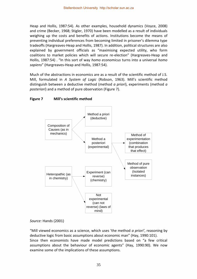
35
Heap and Hollis, 1987:54). As other examples, household dynamics (Voyce, 2008) and crime (Becker, 1968; Stigler, 1970) have been modelled as a result of individuals weighing up the costs and benefits of actions. Institutions become the means of preventing individual preferences from becoming limited in prisoner’s dilemma type tradeoffs (Hargreaves-Heap and Hollis, 1987). In addition, political structures are also explained by government officials as “maximising expected utility, who form coalitions to market policies which will secure re-election” (Hargreaves-Heap and Hollis, 1987:54) . “In this sort of way homo economicus turns into a universal homo sapiens” (Hargreaves-Heap and Hollis, 1987:54). Much of the abstractions in economics are as a result of the scientific method of J.S. Mill, formulated in A System of Logic (Robson, 1963). Mill’s scientific method distinguish between a deductive method (method a priori), experiments (method a posteriori) and a method of pure observation (Figure 7). Figure 7 Mill’s scientific method
Source: Hands (2001) “Mill viewed economics as a science, which uses ‘the method a priori’, reasoning by deductive logic from basic assumptions about economic man” (Hay, 1990:101). Since then economists have made model predictions based on “a few critical assumptions about the behaviour of economic agents” (Hay, 1990:90). We now examine some of the implications of these assumptions.
Composition of
Causes (as in
mechanics)
Heteropathic (as
in chemistry)
Method a priori
(deductive)
Method a
posteriori
(experimental)
Method of
experimentation
(combination
that produces
that effect)
Method of pure
observation
(Isolated
instances)Experiment (can
reverse)
(chemistry)
Not
experimental
(can not
reverse) (laws of
mind)
Stellenbosch University http://scholar.sun.ac.za

36
Rational economic man (homo economicus) is an abstraction that was used to simplify the model-building process. “In its ideal-type case the agent has complete, fully ordered preferences (defined over the domain of the consequences of his feasible actions), perfect information and immaculate computing power. After deliberation he chooses the action which satisfies his preferences better (or at least no worse) than any other. Here rationality is a means-to-ends notion, with no questions raised about the source or worth of preferences. This basic model is made more sophisticated … The basic vision remains, however, one of agents who are rational in the sense that they maximise an objective function subject to constraints” (Hargreaves-Heap and Hollis, 1987:54) Homo economicus is a simplistic framework that was never meant to be adopted as widely as it has been. “In his Essay on the Definition of Political Economy in 1836, Mill introduced the concept of ‘economic man’, which he took to be a partial description of man; but later economists argued that ‘economic man’ is the true nature of man, and not just an abstraction” (Hay, 1990:101). Hay (1990) further argues that there are at least two reasons why a social science should be treated differently from a physical science:
1) The basic unit of analysis is not atoms or particles, but people. “The analyst therefore has additional information besides detached observation. He can ‘get inside’ the behaviour of economic actors, and can use introspection as a source of information” (Hay, 1990:100).
2) Human actions are to be understood in terms of reasons, motives and preferences rather than by cause and effect. “The emphasis is on an individual who weighs up alternatives, and then makes a decision” (Hay, 1990:101).
Daly and Cobb (1989:37) agree: “What is emphasised is the optimal allocation of resources that can be shown to result from the mechanical interplay of individual self-interests. What is neglected is the effect on one person’s welfare on that of others through bonds of sympathy and human community, and the physical effects of one person’s production and consumption activities on others through bonds of biophysical community”. Another implicit assumption of traditional economic analysis is that it is divorced from value judgements. Robbins (1935:94) states: “While we assume that different goods have different values at different margins, we do not regard it as part of our problem to explain why these particular valuations exist. We take them as data”. De Wit (2001:32) states that “[p]ositive economics became divorced from value-judgements and too many values were treated as basic or were simply ignored … There is no real value free social science. Economy is partly ideology, and a separation of the positive from the normative in developing economic theory is impossible”. A third problem with the traditional approach is dealing with issues exogenous to the theory. “Whenever the abstracted-from elements of reality become too insistently
Stellenbosch University http://scholar.sun.ac.za

37
evident in our experience, their existence is admitted by the category ‘externality’ … Externalities do represent a recognition of neglected aspects of concrete experience, but in such a way as to minimise restructuring of the basic theory. As long as externalities involve minor details, this is perhaps a reasonable procedure. But when vital issues (e.g. the capacity of the earth to support life) have to be classed as externalities, it is time to restructure basic concepts and start with a different set of abstractions that can embrace what was previously external” (Daly and Cobb, 1989:37). The neoclassical framework has many advantages and uses in understanding and analysing economic problems. However, it is necessary to assess whether or not this framework is useful for addressing the problem proposed by this study. In order to do this, the strategic aspects identified as important for this study are revisited. First, in terms of the BM framework the neoclassical school is classified as functionalist, with a positivistic epistemology and realist ontology. The neoclassical school therefore shares many of the same epistemological and ontological characteristics of system dynamics modelling. This is promising, since it suggests a good fit between the proposed methodology of this study and mainstream economic theory. In terms of the FJ classification, the analysis framework of neoclassical economics is classified as simple unitary, since it uses abstractions to analyse economic problems. Interactions between elements are highly organised and well-defined laws govern behaviour. While system dynamics shares some of these characteristics, SD modelling fits primarily within the complex-unitary framework, with many interactions between elements and these interactions loosely organised. Fontana (2010) argues that ontologically and epistemologically the neoclassical paradigm is unable to address complexity. For example, rational economic man and the market mechanism are too limited to deal with issues such as realistic human behaviour (e.g. indecisiveness, adaptive behaviour), computational complexity (non-linear dynamics, disequilibrium) and heterogeneous agents. In terms of DW, four strategic aspects were identified as relevant to this study: quantitative, natural, socio-institutional and moral. As shown in Figure 8, evaluating neoclassical economics against these aspects indicates that within the quantitative aspect the spatial modality is not well addressed, the natural aspect is not covered at all3, while the socio-institutional aspect is mostly covered with the exception of the formative modality. In terms of the moral aspect, only the juridical aspect is covered, although even here not all elements of this aspect are included.
3 It is possible to define neoclassical economics more broadly to include those aspects that deal with the environment (e.g. Shi, 2010). A narrower definition of neoclassical economics is adopted, which focuses on the ontological and epistemological aspects of the approach. The schools of economics that address environmental issues are discussed in the next section.
Stellenbosch University http://scholar.sun.ac.za

38
Figure 8 Neoclassical economics within DW’s modalities
Strategic aspects Modality Neoclassical economics
Quantitative Numerical √
Spatial
Kinematic √
Natural Physical
Biological
Socio-institutional Sensitive √
Analytical √
Formative
Communicative √
Social √
Economic √
Moral and governance Aesthetical
Juridical √
Ethical
Credal
Source: Own analysis In summary, despite some of the limitations of NC economics, it shares many ontological and epistemological characteristics with system dynamics modelling. This is seen particularly in the way in which NC economics attempts to explain the social phenomena by investigating consistencies and causal relationships between different entities. It is now necessary to investigate whether there are links between other schools of economics and system dynamics modelling.
2.4.3 Traditional heterodox schools
Heterodox economics is a growing dissident movement that rejects the neoclassical approach (e.g. Lee, 2008; Dequech, 2008). Determining which economic schools are included in the heterodox approach is a subject of debate in the literature. Some (e.g. Davis, 2009) argue that the newer schools that emerged in the 1980s such as behavioural economics, experimental economics, game theory, neuroeconomics and complexity economics should be included in the definition of heterodox economics. Others, such as Lawson (2009), argue for a more narrow definition. Following Garnett (2006), this study distinguishes between the hegemonic approach and pluralist approach to heterodox economics. The hegemonic approach emphasises differences in schools in contrast to the prevailing neoclassical paradigm which focuses on ontological and epistemological aspects (see also Dow, 2004; Dow, 2008; Lawson, 2009). The pluralist approach, in contrast, focuses on transcending disciplinary differences between the schools.
Stellenbosch University http://scholar.sun.ac.za

39
The hegemonic approach is used in this section. Heterodox schools, according to the narrow definition include Austrian, feminist, (old) institutionalism, Marxian, post-Keynesianism and social economics (Lawson 2006). However, this study will focus on the two dominant nineteenth century schools that emerged to challenge the neoclassical paradigm, namely the Institutionalist school and the Austrian school.4 2.4.3.1 Old Institutionalist school Institutional economics was influenced by economists such as John Commons and Thorstein Veblen. The institution is the basis of analysis rather than the individual. Institutional economics emphasises the dynamic nature of institutions rather than a static, equilibrium process (Sørensen et al., 1998). Institutional economists focus on conflict rather than harmony, waste instead of efficiency, and uncertainty as opposed to perfect knowledge (Miller, 1978). The presence of power and privilege is an important area of focus, in contrast to “the machinations of the atomistic individual” (Miller, 1978). Homo institutional economicus (HIE) contrasts with the economic man (EM) of neoclassical economics as follows (Tomer 2001): while EM is self-interested, rational and unchanging; HIE is influenced by institutions and changes in line with habits and rules. HIE also has the capacity to learn from past experience. HIE is, however, not rational in the sense of being able to process information rapidly, and also does not maximise utility. In terms of the BM classification proposed earlier, institutional economics can be defined as falling within the radical structuralist paradigm (see Figure 9), with a positivist epistemology and a realist ontology. The emphasis on power and conflict clearly places it in the category of radical change social science. Furthermore, with the focus on institutions the approach falls within the objective social science category with changes in technology and the legal context determining the dynamics of the system. 2.4.3.2 Austrian school The Austrian school was influenced strongly by economists such as Carl Menger and Ludwig von Mises, who in turn was influenced by Max Webber and Immanuel Kant. The focus is on developing a value-free science of human action, called praxeology (Selgin, 1988). With the basic building block being human beings rather than institutions, Austrian economists argue that individuals are too complex to model mathematically and, therefore, reject empirical approaches. 4 A third is the Marxist school, but this largely shares the same ontological and epistemological characteristics of the other two schools and is beyond the scope of this thesis.
Stellenbosch University http://scholar.sun.ac.za

40
Figure 9 Classification of heterodox schools in terms of the BM framework
Source: Own analysis The nature of economic agents is one that seeks to understand the world system in which it operates (Selgin, 1988). Therefore, instead of the homo economicus (economic man) of neoclassical economics, Austrians prefer to think in terms homo percipiens (perceiving man) or, more importantly, homo divinans (the man who grasps the future). Austrian economics falls within the radical humanist paradigm of the BM classification (see Figure 9). The epistemology is anti-positivist and the ontology is nominalist. For example, “entrepreneurial profit and loss are subjective phenomena, having no ‘objective’ basis outside of the minds of market participants” (Selgin, 1988:28). Also, Austrian economists argue for an extreme laissez faire approach to the economy and adopt a libertarian approach in the sense of advocating the removal of government regulations. This is very much in line with the philosophy of Habernas (who also influenced Critical Systems Thinking). Habernas believed that communication is distorted by the exercise of power, and individuals have an interest in liberating themselves from the influence of this power (Adey, 2007). This is known as the emancipatory interest.
2.4.3.3 Evaluation Neither the Austrian school nor the institutional school falls within the functionalist paradigm of neoclassical economics. However, institutional economics (IE) shares the positivistic epistemology and realist ontology of the neoclassical school. An influential Post-Keynesian and institutional economist, Alfred Eichner (1938–1988), in his great work ”The Macrodynamics of Advanced Market Economies”, provides an approach to macroeconomic analysis that would be consistent with a system dynamics approach (Radzicki, 2010). The three requirements he puts forward for the construction of a macroeconomic model are:
Conflict
Order
Subjective Objective
Radical
structuralist
FunctionalistInterpretative
Radical
humanist
Austrian
(empty) Neo-classical
Institutional
Stellenbosch University http://scholar.sun.ac.za

41
1) all model variables must have real-world, measurable counterparts; 2) the theory underlying the model must be applicable at both micro- and
macro-levels; and 3) the model must represent the behaviour of the important institutions within
the system while at the same time providing a coherent explanation of the macro behaviour of the economy.
Radzicki (2008) argues that system dynamics is an approach that is well-suited for a Post-Keynesian/institutional economic context, since it is a disequilibrium approach that portrays actual human behaviour and micro-level decision-making rather than in a stylised way. Furthermore, the foundation of system dynamics is a micro-structure that explains macro-behaviour, which is consistent with a Post-Keynesian/Institutional economics approach. Austrian economics fall outside the analytical sphere with their rejection of the positive approach. Although the Austrian school argues that human behaviour is too complex to represent and solve mathematically, some argue that simulation modelling provides a means to analyse some of the assumptions of the Austrian school regarding human behaviour. For example, SD modelling can be used to model ways in which individual preferences are revised according to the manner in which the agent perceives the reaction of the environment to his or her reactions (Hinterberger, 1994). This provides an opportunity to combine the IE concept of how institutions influence behaviour with the Austrian approach that institutions are nothing more than the results of human action (e.g. Hinterberger, 1994; Radzicki, 1990). In terms of a normative assessment, it is possible to evaluate these schools against the religious ground-motives of Dooyeweerd. The neoclassical school falls within the nature ground-motive, the Austrian school within the freedom ground-motive and the institutional school within the nature-freedom ground-motive. Parts of social economics may fall within the creation-fall-redemption ground-motive, with its emphasis on ethics, morals and justice (e.g. O’Hara, 2002). Not many of the traditional economic schools address normative aspects. However, the institutional economist Eichner introduced the normative in his system classification by representing the advanced market economy as forming part of a larger social system characterised by four interacting subsystems: the economic, the political, the normative and the human development subsystem (Radzicki, 2010). In many respects the philosophy of Eichner was ahead of its time and it is sad that his life was cut short before he was able to develop many of his ideas further. In summary, the strategic aspects identified as important to this study suggest that the quantitative aspect is well represented by the institutional school. Issues of complexity are recognised by both. In terms of the FJ framework, both schools are classified as complex coercive since values and beliefs are likely to conflict and agents do not often share common interests. Some institutional economists (e.g. Swaney, 1987; Söderbaum, 1992) have attempted to address environmental
Stellenbosch University http://scholar.sun.ac.za

42
concerns, although many issues remain undealt with (Stern, 1997). The socio-institutional aspect is well represented by both schools, with the Austrian school emphasising the social aspects and institutional school the organisational aspects. The normative aspects are not so well addressed by the mainstream heterodox schools. It is concluded that while the research problem is well grounded in both the neoclassical and heterodox schools, these schools in themselves are insufficient. Therefore, it necessary to pay attention to the modern schools that have emerged.
2.4.4 Modern schools
The modern schools emerged from the limitations of the earlier schools, including a failure to adequately address complexity and a limited or deficient approach to the environment. Given the nature and complexity of the research problem and also the importance of a systems view, how the economics profession has responded to previous shortcomings is important. This section discusses four disciplines or fields of study: environmental economics, resource economics, ecological economics and complexity economics. 2.4.4.1 Economics of the environment The fields of environmental and resource economics (ERE) and ecological economics (EE) attempt to address some of the shortcomings of the traditional economics approach, including i) the argument of economics as being a value-free science, ii) the assumptions of homo economicus and iii) the issues of the environment. There is some dispute over the boundaries between the three disciplines. Van den Bergh (2000) distinguishes between the three as follows:
1) environmental economics is a discipline that explains externalities, in particular pollution;
2) resource economics concerns itself with renewable resources such as fish, water and forests; and
3) ecological economics does not presuppose a neoclassical framework for analysis and is generally more pluralistic in its approach (see also Costanza, 2003).
Others such as Pearce and Turner (1990) propose a continuum of ideologies, ranging from those within the economics framework: ‘cornucopian’ that allows substitution between natural and man-made capital, ‘accommodating’ that does not assume infinite substitution; and those outside the economics framework (ecocentric perspectives). ERE and EE both fall within the capital theory approach (CTA), while other approaches such as the institutional school fall outside the CTA (Stern, 1997). The CTA adopts an anthropocentric perspective encompassing environmental stewardship for the benefit of present and future generations (Turner et al., 2003).
Stellenbosch University http://scholar.sun.ac.za

43
2.4.4.2 Development of the systems view Costanza (2003) argues that the application of economics to the environment dates back at least to the 17th century. However, its modern roots date back to the 1960s, in particular Kenneth Boulding’s (1910–1993) seminal publication entitled The economics of the coming spaceship earth (Boulding, 1966). In this work, Boulding discusses the transition between a “cowboy economy” that is characterised by wide open spaces and abundant resources, to what he terms “spaceship earth” – a closed system where the economy and environment are characterised by a circular relationship. Boulding (1966) highlighted what is known as the first law of thermodynamics, that matter cannot be created or destroyed. Although Boulding mentions the second law of thermodynamics, it was the economist Nicolas Georgescu-Roegen (1906–1994) that developed this concept further as it relates to economy–environment interactions. Georgescu-Roegen (1993:78) defines the second law as follows: “the entropy (i.e. the amount of bound energy) of a closed system continuously increases or that the order of such a system steadily turns into disorder”. The implication is that matter continually dissipates in the economic system. In other words, the production process converts (low entropy) natural resources into high entropy resources such as waste. A number of Georgescu-Roegen’s propositions are controversial and have been challenged (e.g. Ayres, 1997). However, he is regarded as a leader in the entropic school of economics that had important implications for developing a systems understanding of economy-environment interactions. The study of resilience develops the concept of the ecosystem as a trans-scale interacting system further. “Social and ecological systems are nested in time and space from the cell to the ecosphere, with numerous non-linear feedbacks” (Holling et al., 2000:354). Perrings (1998) identifies two variants of resilience. The first is due to Pimm (1991) and is concerned with the time a system takes to return to some initial stage. The second is due to Holling (1973) and is concerned with the magnitude of the disturbance a system can absorb before switching from one state to the other. There has developed a large body of literature in both economics and ecological circles. Ecological economic applications include water systems (Brouwer and Van Ek, 2004), agroecosystems (Perrings and Stern, 2000; Di Falco and Perrings, 2005) and fisheries (Charles, 2004; Cinner and Aswani, 2007). Stern (1997) explores the application of these laws of thermodynamics and resilience within the capital theory approach (CTA). The weak sustainability criterion violates the second law of thermodynamics since a minimum quantity of energy is required to convert matter into economically beneficial goods and services. This applies equally in the case of resilience, where a minimum stock of natural capital is required to support essential life systems. Finally, weak sustainability also violates the first law of thermodynamics on the basis of mass balance.
Stellenbosch University http://scholar.sun.ac.za

44
2.4.4.3 Complexity economics 2.4.4.3.1 Definition The field of complexity economics (CE) argues that the economy is a complex adaptive system5 (Beinhocker, 2007). It is the application of the science of complexity to economic issues. A key feature of CE is that the assumption of equilibrium no longer holds. Currently there is no unified, synthetic theory of complexity economics (Beinhocker, 2007). In the philosophy of science it is regarded as a “program rather than a unified theory” (Beinhocker, 2007:19). The approach has been influenced by the classicists, in particular Adam Smith, as well as the writings of Schumpeter. 2.4.4.3.2 Contributors The writings of Adam Smith (1723–1790) have had a profound influence in a number of areas. His ideas “had an important influence on the growth of free trade in the nineteenth century” (Beinhocker, 2007:20). As a moral philosopher, his writings have also had significant influence on the nature and productivity of labour (including specialisation of labour), natural endowments and forms of trade (Goudzwaard and Van Drimmelen, 2008). Complexity theorists also argue that Smith’s contribution to the field of systems theory was fundamental.
“Writings on complexity in the social sciences go back hundreds of years, with Adam Smith’s The Wealth of Nations (1776) representing one of the earliest and most cohesive discussions of the topic. One of the prime drivers of economic theory over the past two centuries has been Smith’s concept of an ‘invisible hand’ leading collections of self-interested agents into well-formed structures that are no part of any single agent’s intention” (Miller and Page, 2007:4).
Complexity economics and ecological economics overlap in the sense that both are transdisciplinary and explore the complex linkages between ecology and economics (see e.g. Costanza, 2003). This is consistent with the early classical economists whose writings also developed in an interdisciplinary context (Dopfer, 2005). Another writer that had a significant influence on complexity economics is Joseph Schumpeter (1905–1984).
“Schumpeter’s theory of ‘the process of creative destruction’ is the principle
means by which he imports a sense of dynamic movement, and hence history, into economics. As he states, ‘capitalist reality is first and last a process of change’, and any point of static equilibrium within an economy must be understood as being a tiny subset within a bigger picture, a subset that, in practical terms, is either rare or non-existent. Schumpeter thus turns
5 Miller and Page (2007) distinguish between a complicated system and a complex system. In a complicated system the components maintain a degree of independence to the extent that eliminating one component does not fundamentally alter the behaviour of the system. A complex system, on the other hand, is characterised by strong dependencies between the components such that removing one component has a significant impact on system behaviour.
Stellenbosch University http://scholar.sun.ac.za

45
economic theory on its head. The usual neo-classical view that the economy is essentially in equilibrium, or moving towards equilibrium, is replaced with the proposal that the economy is plotting a path through time, and is ‘a history of revolutions’” (Carter, 2006:37).
2.4.4.3.3 Comparisons with mainstream economics In differentiating between traditional economics and complexity economics (Table 9), complexity economists do not reject traditional approaches:
“Theorems, equilibrium analysis, game theory, and other traditional approaches remain a part of that toolkit … In addition, Complexity researchers have imported new mathematical and statistical tools from physics, biology, and other fields to help them better understand the economy as an open, dynamic system” (Beinhocker, 2007:96)
Table 9 Five distinguishing features of complexity economics
Complexity Economics Traditional Economics
Dynamic Open, dynamic, non-linear systems, far from equilibrium
Closed, static, linear systems in equilibrium
Agents
Modelled individually; use inductive rules of thumb to make decisions; have incomplete information; are subject to errors and biases; learn and adapt over time
Modelled collectively; use complex deductive calculations to make decisions; have complete information; make no errors and have no biases; have no need for learning or adaptation (are already perfect)
Networks
Explicitly model bi-lateral interactions between individual agents; networks of relationships change over time
Assume agents only interact indirectly through market mechanisms (e.g. auctions)
Dynamic change
The process of differentiation, selection and amplification provides the system with novelty and is responsible for its growth in order and complexity
No mechanism for endogenously creating novelty, or growth in order and complexity
Emergence
No distinction between micro- and macro-economics; macro-patterns are emergent result of micro-level behaviours and interactions
Micro- and macro-economics remain separate disciplines
Source: Adapted from Beinhocker (2007)
Stellenbosch University http://scholar.sun.ac.za

46
2.4.4.3.4 Applications Durlaf (1997) discusses a number of applications of complexity theory in economics, including the following:
1) high technology industries 2) inequality 3) national security.
An elaboration of high technology industries serves as an illustration. High technology industries are frequently characterised by behaviour that contradicts traditional economic models. For example, increasing returns to scale, fixed cost in production and demand lock in. Demand lock in occurs once a particular piece of technology is purchased (e.g. motor vehicle compelled to use parts and spares that suit that particular model and make). Demand lock in is particularly prevalent in high technology industries such as the computing sector where specific platforms and operating systems (such as Windows or Mac) provide access to a particular type of technological interface. A more controversial application of complexity is in the field of inequality (Durlaf 1997). Complexity theory provides a means of explaining how some families may persist in poverty while others are always non-poor. An adult’s economic status is assumed to be the result of the interaction between formal education, peer group effects and chance. The occupational distribution of a community determines both positive and negative intergenerational feedbacks. These feedbacks, according to this approach, create incentives for economic segregation of communities, also dependent on a number of other factors such as mobility costs, preferences for certain community amenities and costs of education such as sports facilities and computers. 2.4.4.4 Evaluation The modern schools of economics are highly pluralistic in nature, and it is therefore difficult to classify them in terms of the BM framework. Ecological economics could be classified as functionalist with some areas branching into the interpretative, while complexity economics is possibly radical structuralist. In terms of the FJ framework, ecological economics is classified as complex pluralist, with basic compatibility of interest but with values and beliefs diverging to some degree. Although there is not always agreement on means and ends, compromise is possible. Complexity economics might be classified as complex coercive, with values and beliefs likely to conflict. For example, some in this approach argue that complexity conomics can successfully be included in the neoclassical toolbox; others argue that it is classified as a paradigm change; and still others that it is classified as the start of a new orthodoxy (e.g. Fontana, 2010). An attempt will not be made to categorise ecological economics and complexity economics in terms of each of the modalities of DW. However, it is possible to categorise each of these elements in terms of the strategic aspects based on each of these modalities. In terms of the quantitative aspect, both EE and CE are well
Stellenbosch University http://scholar.sun.ac.za

47
represented on all levels: the numerical, the spatial and the kinematic. In terms of the natural, those aspects of CE that are applicable to the natural environment have been subsumed into EE so that there is no distinction between CE and EE in this case. In terms of the socio-institutional aspect both are well represented, while the moral aspect is well represented by EE (even if only a minority of researchers are involved in this area) and less well-represented in CE.
2.4.5 Summary
The neoclassical economic theory that has emerged from the classical and marginalist revolution is well established in economics. Modern economic behaviour is based more on the mercantilist view of economic man, rather than the physiocrats’ systems orientated approach. An implication of this is that land is regarded as exogenous to economic theory. This study argues that much that has emerged contradicts what Adam Smith and many of the other classical writers intended. For the purposes of this study, the mercantilist-based framework is inadequate for modelling the economy-environment interactions required for the economic analysis of the impacts of the restoration of natural capital across a range of sites. At the same time, the neoclassical school contained many elements that were consistent with the proposed modelling approach. A number of alternative schools were represented which encompass different elements characteristic of the research problem, including more dynamic behaviour (institutional school), complex social interactions (Austrian school), conditions of non-linearity and disequilibrium (CE) and a more prominent role for the environment (ERE and EE).
2.6 Restoration science
2.6.1 Overview
Thus far it has been argued that systems science and the different schools of economic thought fits within the social science framework of Burrell and Morgan (BM), as well as the system framework of Flood and Jackson (FJ) and the normative framework of Dooyeweerd (DW). Much of the economic literature adopts an anthropocentric orientation, including ecological economics and environmental and resource economics (see Section 2.4.4.1). An anthropocentric approach to restoration science would therefore fit within the current research context and is consistent with the epistemological and ontological framework presented previously. However, there is much debate in the literature over whether or not the restoration of natural capital is regarded as an anthropocentric approach or an ecocentric approach. For example, Gladwin et al. (1995) argue that restoration of natural capital is primarily justified by those with an ecocentric orientation. Economic or narrowly anthropocentric values and ecocentric values are often viewed as opposing forces since much of past economic activity is believed to be the reason why restoration activities need to take place (Holl and Howarth, 2000). For
Stellenbosch University http://scholar.sun.ac.za

48
example, Jackson et al. (1995:73) argue that “restoration projects whose objective is to harvest natural products or exploit minerals to the exclusion of other values and uses are based on anthropocentric values and are unlikely to lead to good ecological restoration”. Definitions of restoration reflect this dichotomy. Bradshaw (2002), for example, adopts an ecocentric approach in his definition of restoration as the return of an ecosystem to a condition prior to its disturbance. Jackson et al. (1995:71) go further and define the restoration of natural capital as “the process of repairing damage caused by humans to the diversity and dynamics of indigenous ecosystems”. The Society for Ecological Restoration (SER) adopts a broader definition that defines restoration as “the process of assisting the recovery of an ecosystem that has been damaged, degraded or destroyed” (SER, 2004). This definition includes restoring the resilience of the ecosystem as well as its integration within a larger landscape that supports sustainable livelihoods (SER & IUCN, 2004). In order to ascertain whether or not restoration science is consistent with an anthropocentric approach, the alternative ecosystem perspectives firstly need to be compared and, secondly, it needs to be ascertained how these perspectives are linked to natural capital restoration.
2.6.2 Ecosystem perspectives
There are a number of ecosystem perspectives. Following Pearce and Turner (1990) and Gladwin et al. (1995), three classifications are distinguished, namely: technocentric, anthropocentric and ecocentric. (Table 10 gives a comparison of these three classifications.) Table 10 Ontological and ethical assumptions of alternative ecosystem perspectives
Key Assumptions Technocentrism Anthropocentrism Ecocentrism
Metaphor of earth Vast machine Life support system Mother/web of life
Perception of earth
Dead/passive Home/managed Alive/sensitive
System composition
Atomistic/parts Parts and wholes Organic/wholes
System structure Hierarchical Holarchical Heterarchical
Humans and nature
Disassociation Interdependence Indisassociation
Human role Domination Stewardship Plain member
Ethical grounding Narrow homocentric
Broad homocentric Whole earth
Time/space scales Short/near Multiscale Indefinite
Logic/reason Egoist-rational Vision/network Holism/spiritualism
Source: Gladwin et al. (1995)
Stellenbosch University http://scholar.sun.ac.za

49
The technocentric perspective adopts an extreme ‘Cornucopian’ approach (see Pearce and Turner, 1990) where the environment is assumed to be highly resilient and the focus of the economic system is on growth (maximising gross national product); resource exploitation and conversion of natural capital into productive means. The ontology of the technocentric approach is one of a vast machine that is essentially passive. While this approach could be regarded as anthropocentric, it is extremely narrow and myopic in its outlook. Restoration of natural capital is not regarded necessary, since the system is assumed to be sufficiently resilient to rebound from any impacts. Under this approach, the environment has instrumental value only in the sense of exploitation potential. The anthropocentric perspective, also known as the ‘accommodating’ approach, is a far more pluralistic approach that encompasses the various capital theory approaches (CTAs), including weak sustainability, strong sustainability and critical natural capital approaches. The earth is viewed both in terms of its instrumental value, which includes the total economic value (TEV) framework of natural resource economics, and also its intrinsic (stewardship) value (Turner et al., 2003). The anthropocentric approach encompasses both ecological economists and environmental resource economics (ERE) practitioners. Ecologists who recognise the importance of humans in ecosystem health and resilience would also fall into this category. The ecocentric perspective adopts an extreme preservationist approach. Proponents argue that society has an ethical responsibility to sustain the integrity and health of ecosystems (Purser et al., 1995). The approach advocates the view that nature has an intrinsic value based on considerations of autonomy, self-organisation and self-directedness (Swart et al., 2001). Hargrove (1992) differentiates between two philosophical schools associated with the ecocentric approach. The first is instrumental ecocentrism, following Paul Taylor and Holmes Rolston III who argues that natural entities exist for their own sakes independent of human interests. The second is intrinsic ecocentrism, following J.Baird Callicott; in this approach, entities have value independent of the valuation of a valuer. This approach includes Leopold’s land ethic, the deep ecology movement and the “eco-feminist” critique (Purser et al., 1995).
2.6.3 Evaluation
Four ecosystem perspectives can be distinguished: anthropocentric instrumental values (Ais), anthropocentric intrinsic (stewardship) values (Ait), ecocentric intrinsic values (Eit) and ecocentric instrumental values (Eis). In terms of the religious ground-motives (RGM) of Dooyeweerd, the nature realm is the realm of science, causality and the material, while freedom is the realm of culture, mind and free spirit. The dualistic approach of the nature-freedom RGM has characterised much of modern philosophy and is also the philosophy most prevalent in the ecosystem perspectives (Table 11). In terms of the creation-fall-redemption
Stellenbosch University http://scholar.sun.ac.za

50
perspective, there is much debate over whether creation should be perceived from an anthropocentric perspective, or a Christo-centric (CC) or Theo-centric (TC) perspective.6 On the one hand, creation is made for God’s glory and has value in its own right and not purely for its usefulness to humans (Walton, 2007). On the other hand, some (e.g. Keenan, 2002:189) argue that “eventually our perspective must be a human one”. This debate is seen in Reformational Christian Theology as well. Stoker (1967, as cited in Botha, 2007) argues that all realms (inanimate, vegetative, animate and human realms) have their own intrinsic value and relationship to God. Dooyeweerd (1955:548, as cited in Botha, 2007), however, argues for “an anthropocentric (con)-centring of reality in human embodiment and relations”. The categorisation in Table 11, therefore, reflects these different perspectives. Table 11 Evaluation based on religious ground motives
Dominant religious ground-motive
Nature Freedom Nature–freedom
Creation–fall– Redemption
Economic school
Anthropocentric instrumental (Ais)
Ecocentric intrinsic (Eit)
Ecocentric instrumental (Eis)
Antropocentric intrinsic (Ait); Christo-centric (CC); Theocentric (TC)
Key: Ais = Antropocentric instrumental; Eit = Ecocentric intrinsic; Eis = Ecocentric instrumental; Ait = Anthropocentric intrinsic; CC = Christo-centric; TC = Theocentric
Source: Own analysis
2.6.4 Classification of natural capital restoration
Given the preceding discussion, it is now possible to evaluate whether or not the restoration of natural capital is primarily ecocentric or anthropocentric in orientation. While it is true that restoration may be justified on ecocentric grounds, there is strong evidence to support the anthropocentric position. A study reported in Turner (2005) analysed the impact of economic indicators (such as growth, trade, per capita earnings and investment), social capital (e.g. health and education), ecological factors (air and water quality, government actions in protection treaties, and citizen participation) and land pressure (agricultural development). The factors that had a positive impact on a wetland area included environmental quality, government inclusiveness, social development and an expansion of agriculture. Turner (2005) attributes the positive impact to the expansion of agriculture causing government and society to respond with a renewed urgency to protect and restore
6 The Theo-centric or Christo-centric approach “places ultimate value on God and seeks to balance the intrinsic value of nature with issues of human need” (Walton, 2007).
Stellenbosch University http://scholar.sun.ac.za

51
wetland areas. This response, however, is more likely to occur within an enabling government context and a society that appreciates environmental quality. A number of authors advocate an integrative approach to landscape management. Holl and Howarth (2000) argue that ecologists, economists, land managers, policy makers and risk managers should be involved in developing restoration strategies. Espelta et al. (2003) argue that restoration is inextricably embedded within an economic framework. Naveh (2005) argues that restoration should occur within a landscape context that takes into consideration the human-ecological, social, economic, psychological, spiritual, aesthetic and functional aspects of using these landscapes. The following is classification based on the restoration disciplines of Armesto et al. (2007) and Dooyeweerd’s modalities (Table 12). It supports the preceding assertions that the restoration of natural capital is highly integrative. Table 12 Restoration disciplines and Dooyeweerd’s classification
Strategic aspect Modality Discipline
Quantitative Numerical Database management Architecture Landscape design Modelling Biotechnology
Spatial
Kinematic
Natural Physical Macroecology Biogeochemistry Disturbance Successional theory Alternative stable states Agroecology Landscape ecology
Biological
Socio-institutional Sensitive Macro- and micro-economy Sociology Anthropology Art
Analytical
Formative
Communicative
Social
Economic
Moral and governance Aesthetical Ethics Juridical
Ethical
Credal
Source: Own analysis based on Armesto et al. (2007)
Stellenbosch University http://scholar.sun.ac.za

52
2.7 Application: restoration and ecosystem benefits
2.7.1 Overview
In the previous section, it was ascertained that the restoration of natural capital is consistent with an integrated approach viewed from an anthropocentric perspective. However, the focus of this study is on different landuse categories, as well as different types of restoration methods. How can these different dimensions be reconciled within an anthropocentric perspective? This section demonstrates the limitations of the ecocentric approach to addressing this problem and considers an application of the anthropocentric perspective to restoration.
2.7.2 Ecosystem benefits
Restoring natural capital has an impact on ecosystem structure and process, which in turn affects ecosystem functions such as regulating, habitat, production and information, which in turn affects the production of ecosystem goods and services (De Groot et al., 2002). Ecosystem goods and services (EGS) are the annual interest arising from the stocks of natural capital that yield a flow of benefits useful to humans and other living beings (Harris et al., 2006). The ecocentric approach to restoration is primarily concerned with impacts on ecosystem structure and process, while the anthropocentric perspective is concerned with impacts on ecosystem goods and services (EGS). Apart from De Groot et al.’s (2002) classification, the Millennium Ecosystem Assessment (MA, 2005) distinguishes four types of ecosystem services:
Provisioning services relate to the products derived from ecosystems, including food, fiber and fuel, genetic resources, medicines and pharmaceuticals.
Regulating services involve the benefits derived from the regulation of ecosystem processes, such as air quality, climate, water, erosion, disease, pest and natural hazard regulation.
Cultural services are the benefits people obtain from ecosystems such as reflection, recreation, inspiration and aesthetic enjoyment, and include cultural diversity and educational values.
Supporting services are those necessary for the production of all other ecosystem services, such as soil formation, photosynthesis, primary production, nutrient cycling and water cycling.
A World Bank study (Pagiola et al., 2004) adopts many of the ecosystem services of the MA, but further categorises them by 10 ecosystem types, ranging from island habitats to forest ecosystems. Table 13, based on this categorisation, indicates that urban environments contribute the least in terms of ecosystem services, followed by
Stellenbosch University http://scholar.sun.ac.za

53
agricultural systems. The highest contributors are the natural systems such as grassland, fynbos and forest ecosystems. Table 13 Main ecosystem types and their services Ecosystem service Cult-
ivated Dry-land
Forest Urban Inland Water
Grassland Fynbos & Karoo
Freshwater • • • •
Food • • • • • • •
Timber, fuel and fiber
• • • •
Novel products • • • • •
Biodiversity regulation
• • • • • • •
Nutrient cycling • • • • • •
Air quality and climate
• • • • • • •
Human health • • • • • •
Detoxification • • • • • •
Natural hazard regulation
• • • •
Cultural and amenity
• • • • • • •
Total no. of EGS 7 8 11 6 10 10 11
Source: Based on Pagiola et al. (2004). Christensen et al. (1996) categorise ecosystem types into three categories (Table 14), namely: 1) intensive landuses that are significantly impacted by economic and development activity; 2) semi-natural landuses characterised by mixed systems with both agricultural activity and natural ecosystems; and 3) natural landuses that are characterised by wilderness areas and reserves. Following from Table 13 and Table 14, intensive landuses can be categorised as characteristic of containing moderate to low contributors to ecosystem services, seminatural landuses as high contributors to EGS, and natural landuses as very high contributors to EGS.
Stellenbosch University http://scholar.sun.ac.za

54
Table 14 A conceptual framework for ecosystem management goals, outputs and benefits Category Ecosystem type and
human use Intensity and goals of management
Ecosystem benefits
Intensive Urban; Intensive agriculture; Aquaculture and suburban; Plantation forestry; Managed pasture
Intensive management to provide food and shelter for human use
Moderate
Semi-natural Managed forestry, grazing, wildlife, and fisheries; Forest; Grassland; Woodland; Shrubland; Lakes; Streams/rivers; Wetlands; Estuaries; Oceans; Extraction; Preserves
Moderate management for sustained production of natural resources and for maintenance of ecosystem processes
High
Natural All kinds; Reserves and wild areas
Minimal management to maintain biological and habitat diversity, integrity of natural ecosystem processes and aesthetic values
Very High
Source: Christensen et al. (1996) and own analysis
2.7.3 Ecosystem types and restoration
Restoration can be either active or passive (e.g. Visser et al., 2004). Passive restoration advocates the removal of the original cause of degradation, such as overgrazing. Succession is then allowed to proceed naturally. Active restoration, on the other hand, implies the application of a number of restoration techniques, such as the propagation of plants, soil cultivation, improving soil moisture and application of mulches and fertiliser. Swart et al. (2001) have linked the ecosystem categories of Christensen et al. (1996) to a number of ‘valuation’ perspectives: functional, arcadian and wilderness views (Table 15). The functional view argues that ecosystems should have an economic value. The arcadian view is prevalent in transformed landscapes and emphasises co-operation between people and nature for the preservation and restoration of man-made ecosystems. The wilderness view argues that ecosystems are self-regulating and that there should be very little human influence in their development and management.
Stellenbosch University http://scholar.sun.ac.za

55
Table 15 Ecosystem perspectives
Ecosystem category Valuation approach Ecosystem perspective
Intensive Functional approach Strong anthropocentric
Semi-natural Arcadian approach Weak anthropocentric, stewardship
Natural Wilderness approach Ecocentric
Source: Swart et al. (2001) The method of Swart et al. (2001) partitions ecosystem categories into anthropocentric versus ecocentric approaches; with anthropocentric views for the first two ecosystem categories and ecocentric views for the third ecosystem category (Table 16). Although this is a useful approach for linking ecosystem perspectives to different landscape categories, it is problematic since it presupposes that those with an anthropocentric view do not make a contribution to natural ecosystems. In reality, total economic value (TEV) is applicable to all types of ecosystem categories. In this study an alternative classification is adopted by linking ecosystem categories to the capital theory approach (Stern, 1997). This is an anthropocentric approach (Wackernagel and Rees, 1997). Results are summarised in Table 16. Table 16 Restoration methods and CTA approaches
Ecosystem category
Inputs Outputs CTA perspective
Restoration
Intensively managed
High Manufactured products, water, food, pollutants, toxins
Weak sustainability,
Active
Semi-natural
Moderate Timber, livestock, minerals, fish, fuel, ecosystem services
Critical natural capital
Mixed
Natural Minimal Recreational and educational use, ecosystem services
Strong sustainability
Passive
* Inputs are energy, matter (soil, water), labour, etc. Source: Own analysis based on Christensen et al.’s (1996) ecosystem categories. For intensively managed areas it is assumed that natural areas are virtually non-existent. The management approach is to mitigate against externalities. A weak sustainability approach is relevant with substitution possible between natural and man-made capital. Natural capital comprises primarily agricultural systems with very little, if any, natural vegetation. For areas that have been earmarked for restoration, active restoration would be required as passive restoration is unlikely to be sufficient. Semi-natural systems include a combination of natural and artificial landscapes and therefore a critical natural capital (CNC) approach to sustainability
Stellenbosch University http://scholar.sun.ac.za

56
would be suitable. The CNC approach partitions natural capital into components that need to be maintained and those for which substitution is possible. An example of critical natural capital is the Renosterveld patches in farmland systems in the Fynbos biome. The restoration approach for this ecosystem type is mixed: some would be active and other passive. For natural landscapes such as wilderness and protected areas, a strong sustainability approach is adopted, with no net loss of natural capital allowed. Restoration in this context is likely to be passive, since the ecosystem is still intact and is assumed capable of recovering fairly quickly.
2.7.4 Summary
The argument that the restoration of natural capital is primarily an ecocentric approach is based on a (narrow) view of anthropocentrism that focuses on exploitation of natural resources rather than conservation. In the sections above, it is argued that that problem revolves around the definition of anthropocentrism. In order to eliminate confusion, two categories of anthropocentrism are distinguished: i) technocentrism and ii) (accommodating) anthropocentrism. The latter is the view adopted by the majority of economists working in the environmental field, and is highly compatible with restoration science.
2.8 Product and process development
2.8.1 Natural capital as a product
The review so far has indicated that system dynamics modelling is an analytical approach that is not only consistent with many schools of economic thought, but is also appropriate for modelling the restoration of natural capital. This is the first part of the research hypothesis, namely an assessment of the effectiveness of system dynamics modelling as a tool to model the economic, ecological and hydrological impacts of restoration. The second part of the research hypothesis relates to the ability of system dynamics modelling to classify and schedule new restoration projects. Restoration, as indicated in the previous sections, is not an end in itself, particularly if one adheres to an anthropocentric perspective. The object is the generation of ecosystem goods and services derived from the restored environment. These ecosystem goods and services are in fact new products – goods and services that would otherwise not be available in a degraded environment. In this study, three products are derived: products from cultivated natural capital (grazing values and crop values), replenishable natural capital (water yield and quality) and renewable natural capital (which encompasses a range of products including soil carbon, wild products and biomass products). Although all these products are quantified in the study, the main
Stellenbosch University http://scholar.sun.ac.za

57
focus of the analysis is on new products from cultivated and replenishable natural capital. Furthermore, while the main focus of the study is on product development, some attention is also given to process development in Section 2.8.3.
2.8.2 System dynamics and new product development
System dynamics modelling has been applied to new product or project development (e.g. Sterman, 2000; 2001), with many applications focusing on a single product or project (e.g. Cui et al., 2010; Ford & Sobek, 2005; An et al., 2007). Lyneis and Ford (2007) review system dynamics applied to project management. They argue that there are numerous examples of system dynamics and other approaches applied to multiple projects, too many to enumerate. The first to model system dynamics in a multiple-product setting was Abdel-Hamid (1993). Yaghootkar and Gil (2012) model the effect of schedule-driven project management on high performance heavy goods vehicles (‘trucks’) in a multi-project setting. Lee and Miller (2004a; 2004b) construct a number of system dynamics models in a multi-project software organisation. They argue that a multi-project environment is too complex for a system dynamics model to enable scheduling and, instead, use a method called critical chain project management to facilitate flexible scheduling. Although there is a growing body of literature applying system dynamics models in a multi-project setting, there is no known application applying system dynamics models to project management and project scheduling in a multi-project environmental context. The restoration projects of the different sites are highly diverse in nature and in the goods and services quantified. Therefore, a system dynamics model alone is unlikely to be sufficient to schedule and prioritise new restoration projects. The approach adopted in this study is to use the project portfolio management (PPM) approach in order to assess and schedule restoration projects.
2.8.3 Economics of innovation
2.8.3.1 Development of innovation in economics An excellent introduction to the economics of innovation is provided by Swann (2009). A number of classical, neoclassical and heterodox economists have all contributed to the economics of innovation. The list is not exhaustive, and for a full discussion the reader is referred to the reference cited above. Adam Smith (1723–1790) saw invention and technological change as an important generator of wealth in an economy, but argued that the division of labour was the main contributor to wealth creation rather than invention itself. John Stuart Mill (1806–1873) argued that innovation was central to wealth creation, but also concluded that invention did not necessarily lead to the improvement of the plight of the general population. Karl Marx (1818–1883) wrote of the importance of innovation in ensuring competitiveness. Alfred Marshall’s (1842–1924) contribution to innovation lies in the
Stellenbosch University http://scholar.sun.ac.za

58
theory of consumer behaviour, and the innovative consumer – one of the first economists to come up with this concept. Thorstein Veblen (1857–1929) also contributed to the theory of consumer behaviour, stating that invention could create a demand for a product where there was no original need on the part of the consumer. Joseph Schumpeter (1883–1950) was one of the most influential contributors on the economics of innovation. In his theory of ‘creative destruction’ (Schumpeter, 1942), he argues that the capitalist economy is characterised by a series of ‘revolutions’. These revolutions are the innovations that drive the capitalist economy, defined as the commercial application of something new. This innovation process “incessantly revolutionises the economic structure from within, incessantly destroying the old one, incessantly creating a new one” (Schumpeter 1942:83, his emphasis). The five areas of innovation that Schumpeter (1942:83, own summary in parenthesis) highlights are:
1) new consumer goods (product innovation) 2) new methods of production (process innovation) 3) new methods of transportation (distribution innovation) 4) new markets (market innovation) 5) new forms of industrial organisation (structural innovation)
In the 20th century, a number of other contributors developed the theory of innovation further. From the neoclassical tradition, Robert Solow (1924–) played an important role in endogenising technical change in economic growth. Other economists such as Paul Romer (1955–) and Robert Lucas Jr (1937–) built on those theories (Verspagen, 1992). From the evolutionary economics literature, Richard Nelson (1930–) and Sidney Winter (1935–) were highly influential in using the biological metaphor of evolution to explain how innovations and the economy co-evolve (e.g. Swann, 2009; Nelson and Winter, 2002). Other important contributors include E.F. Schumacher (1911–1977) and his role on the economics of sustainability, and Christopher Freeman (1921–2010) with his emphasis on the importance of applying the economics of innovation in a multidisciplinary context. Another area to emerge during the 20th century was the emphasis on ‘eco-innovations’ (Rennings, 2000). This highlights the reality that while certain innovations can have positive impacts (in both the innovation and diffusion phase, the so-called ‘double externality’ problem), in other instances these processes can result in negative impacts as well (for example, through increases in solid waste or redundant technologies). The ‘double externality’ problem reduces the incentive for firms to invest in eco-innovations and emphasises the importance of co-ordinating environmental policy and innovation policy. The vast majority of eco-innovations have occurred in the product and process realms. In a recent review of eco-innovations following the Schumpeterian classification (Hellström, 2007), 30.5% of innovations were new product developments, and 54.3% were process improvements. The development of the economics of innovation has, therefore, contributed inter alia to five main areas: 1) wealth creation; 2) competitiveness; 3) sustainability;
Stellenbosch University http://scholar.sun.ac.za

59
4) consumer theory; and 5) product and process development. It is the last concept that is further developed in the next section. 2.8.3.2 Product and process innovation In order to further develop the concepts of product and process innovation, it is important to define several innovation ‘adjectives’ (Swann, 2009; Henderson and Clark, 1990). Incremental innovation describes the progressive increase in a product or process which does not change the character of the product or process in a fundamental way. An example would be improvements in the features of a motorcycle to enable it to go faster or make less noise. Component innovation involves changing the core design concepts of a technology without changing the linkages between the core concepts and the components. Using the existing analogy, it might be the developmentof a motorcycle that runs on biofuel rather than petrol. Architectural innovation involves a fundamental change in the way that a product is assembled, while leaving the components unchanged. In the motorcycle analogy, the manufacturers develop a motorised go-cart using the engine and other components of the motorcycle. Finally, radical innovation involves fundamental improvements that alter the character of a product or process. The development of a new motorcycle that undermined the competitiveness of existing motorcycle manufacturers would be an example of this. Table 17 indicates the different approaches to ecosystem goods and services (EGS) based on the framework proposed by Henderson and Clark (1990). Table 17 Example of types of innovation applied to restoration
Process innovation
Limited Extensive
Product inno-vation
No Incremental Seeing EGS as an existing marketed product, focusing on improvements in the way EGS delivered.
Component EGS is an existing marketed product, restoration is a new process for producing that product that has not gained prominence yet.
Yes Architectural EGS is a new product that has not yet been fully exploited, but which is achievable through existing processes.
Radical EGS is a new product, and restoration is a new process to produce this product.
Source: Own analysis based on Henderson and Clark (1990) In the first (incremental) case, EGS is seen as a product that is already accepted by the market. The focus is on ensuring improvements in the way that these products are delivered to the market. An example would be building dams to provide water, or other innovative approaches to supplying EGS. The second (component) case argues that EGS is already a marketed good, but that the restoration of natural
Stellenbosch University http://scholar.sun.ac.za

60
capital represents a change in the core design concepts of supplying EGS. The third (architectural) case argues that EGS is fundamentally a new product on the market that has not yet been fully exploited, but which can be marketed without changing any of the underlying processes that produce it. In other words, existing methods of environmental supply are seen as adequate. Finally, the fourth (radical) case regards EGS as a product that has not been fully exploited to date, and could potentially undermine other existing products on the market. Radical innovation would be regarded as the Schumpeterian process of creative destruction, while Swann (2009) argues that the Adam Smith’s concept of innovation through division of labour results in incremental innovations. Hellström (2007) notes that most innovation (including eco-innovation) takes place in an incremental manner but that there is a “concomitant need to understand what types of eco-innovation can also be labelled radical innovation with high sustainability potential, and what specifically characterizes these” (Hellström, 2007:149). The kind of innovation that follows from the combination and reorganisation of existing but previously distinct knowledge competencies (attributed to Arthur Koestler) is what is required for radical innovations (Swann, 2009). 2.8.3.3 Evaluation The economics of innovation has roots in classical, neoclassical and heterodox approaches. The approach emphasises not only the importance of the price mechanism and consumer theory, but also the role of time in the analysis and multidisciplinary approaches to solving problems.
2.9 Chapter summary and conclusions
This chapter explored the development of systems theory and philosophy, and its application to economic theory and natural capital. From this assessment, a number of common features can be identified in systems practice and its applications. The first is the functionalist orientation. This is characterised by the emergence of the use of quantitative techniques in modelling. This was a feature of systems theory from the mid-1950s, and has recently experienced a renaissance with the advent of more powerful microcomputers. It is also a feature of instrumental anthropocentrism in the ecosystem literature. The second is the paradigmatic orientation. This approach focuses on the epistemological and ontological features that distinguish one discipline from another. It has had notable application in the systems literature as well as the heterodox schools. Third is the moral orientation. The application of Dooyeweerdian philosophy to systems theory is a recent development, following authors such as Strijbos and De
Stellenbosch University http://scholar.sun.ac.za

61
Raadt. The moral turn has also featured independently in economics, for example through the work of the Association for Christian Economists (ACE). Stewardship values in ecosystem approaches also reflect this development. Fourth is the critical orientation. This orientation focuses on emancipation from the prevailing orthodoxy. The heterodox schools such as the Marxists and Institutionalists are examples of early applications in economics, although in systems theory and agriculture this approach only gained strength in the 1990s. Intrinsic ecocentrism, including the fields of deep ecology and ecofeminism also reflect this orientation. The final feature is the pluralist orientation. This orientation has become a melting pot for many perspectives, including the critical theorists, heterodox economists as well as modern economic schools such as ecological economics and complexity economics. System dynamics modelling shares many of the epistemological and ontological characteristics of neoclassical economics (Table 18). Both fall into the functionalist paradigm, with a positivistic epistemology and realist ontology. The approach has the characteristic of seeking rational explanations for social affairs, and is also a problem-orientated approach concerned with practical solutions. Both approaches are concerned with the status quo, social order, consensus, social integration, solidarity, needs satisfaction and actuality. In terms of Burrell and Morgan’s classification, the modelling approach adopted in this study is highly consistent with the dominant economic paradigm prevailing today. The differences between the current approach and neoclassical economics are more apparent when comparing types of models (Robertshaw et al., 1978): the current modelling approach is empirical, non-linear, dynamic and numerical compared with neoclassical economics that is theoretical, linear, static and analytical. Another area of difference is emphasised through the work of Beed and Beed (2006), whose book, Alternatives to Economics, is a sustained criticism of the naturalist approach of neoclassical economics. Two of the criticisms mentioned by these authors include the intra-disciplinary nature of neoclassical economics and as well as its emphasis on equilibrium approaches. The present analysis transcends these limitations through a focus on transdisciplinary methods and disequilibrium (Table 18). Neoclassical economics, as indicated in Section 2.4.2, uses a number of abstractions in order to develop analytical models explaining human behaviour. The present study uses a case study approach, which Beed and Beed (2006) argue is a preferable approach to conducting economic analyses.
Stellenbosch University http://scholar.sun.ac.za

62
Table 18 Comparison between the current study and neoclassical economics
Current study Neoclassical economics
A. Burrell and Morgan
Paradigm Functionalist Functionalist
Epistemology Positivism Positivism
Ontology Realism Realism
B. Robertshaw et al.
Origin of model Empirical Theoretical
Function Prescriptive Descriptive
Complexity Non-linear Linear
Temporal characteristics Dynamic Static
Nature of changes Continuous Discrete
Execution technique Numerical Analytical
Predictability Probabilistic Deterministic
C. Flood and Jackson
System methodology Complex unitary Simple unitary
D. Beed and Beed
Disciplinarity Transdisciplinary Intra-disciplinary
Theoretical framework Case study Abstraction
Dynamic behaviour Disequilibrium Equilibrium
E. Pearce and Turner
Ecosystem perspective Anthropocentric Technocentric
F. Dooyeweerd
Religious ground-motive Nature Nature
Dooyeweerd’s aspects addressed by both
Numerical, kinematic, sensitive, analytical, communicative, social, economic, juridical
Numerical, kinematic, sensitive, analytical, communicative, social, economic, juridical
Dooyeweerd’s aspects addressed by present study only
Spatial, physical, biological
Dooyeweerd’s aspects not address by either approaches
Formative, aesthetical, ethical, credal
Formative, aesthetical, ethical, credal
G. Swann
Type of innovation A Smithian Smithian
Type of innovation B Koestlerian Sources: Own analysis based on the preceding discussion and criteria in Robertshaw et al. (1978) (see Section 1.1.3.1), Burrell and Morgan (1979), Pearce and Turner (1990), Flood and Jackson (1991), Eriksson (2003), Beed and Beed (2006) and Swann (2009). Shaded areas indicate areas of overlap between the two approaches
Another area where system dynamics and neoclassical economics digress is in the systems framework of Flood and Jackson. Neoclassical economics is a simple unitary approach, characterised by a small number of elements and few interactions
Stellenbosch University http://scholar.sun.ac.za

63
between the elements. System dynamics modelling, on the other hand, is a complex unitary approach, and shares characteristics more consistent with complexity economics (large number of elements, many interactions between elements). Both neoclassical economics and system dynamics modelling are unitary approaches, where participants act according to agreed objectives and share common interests. The anthropocentric instrumental ecosystem perspective falls within the functionalist approach, which is also the range of the total economic value framework of ecological economics. What is omitted is the intrinsic (stewardship) value, as well as ecocentric approaches. The anthropocentric intrinsic approach is highly consistent with the proposed research methodology of the present study. Table 18 also provides a comparison between this study and neoclassical economics with reference to the modalities of Dooyeweerd. There are eight areas of commonality between neoclassical economics and the proposed study approach. Importantly, the three modalities omitted from the neoclassical framework (spatial, physical and biological) are seen to be crucial to the present study. The proposed modelling approach covers 11 of Dooyeweerd’s 15 aspects. The areas not covered by the proposed modelling approach include the formative (creativity and cultural development), aesthetic (visual appeal), ethical (morality) and credal (commitment, interest and vision). These are perhaps less important in the context of the study's hypothesis and objectives. The final area of comparison is in the field of innovation. Most innovation (including neoclassical economic forms of innovation) are characterised by Smithian innovation where division of labour result in economies of scale. This study captures both Smithian and Koestlerian innovation through drawing on a range of perspectives both from within and outside the economics discipline. The literature review provides the theoretical framework for the proposed modelling approach that draws on a range of elements from transdisciplinary research. Although it shares some epistemological and ontological elements with neoclassical economics, other fields of economics relevant to the research include ecological economics, complexity economics and the economics of innovation. In the next chapter we consider the proposed modelling approach in more detail.
Stellenbosch University http://scholar.sun.ac.za

64
Chapter 3 Risk analysis
3.1 Introduction
The main objective of this study is to provide a means of selecting and prioritising restoration activities. This comprises two steps: the first is to develop a system dynamics model for eight case studies throughout South Africa where restoration is occurring; the second is using this framework to select and prioritise restoration activities. In the previous chapter, it was shown that system dynamics modelling was rooted in complexity economics, although it shared many of the epistemological and ontological characteristics of neoclassical economics. The process of selecting and prioritising projects is rooted in the economics of innovation, which also has roots in neoclassical economics as well as heterodox approaches such as evolutionary economics. In order to select and prioritise projects under a system of innovation, a decision-maker is concerned with three goals (Cooper, 2003):
1) The first is value maximisation, or the potential reward associated with a project or investment strategy.
2) The second is a balanced portfolio that takes into consideration the risks attached to those investments or projects.
3) The third is building strategy – how these aspects combine to facilitate optimal investment decision-making.
It is important to develop a risk analysis framework, which is a systematic step-by-step process in which potential risks and rewards are identified and analysed, and priorities are assigned. This is the methodology documented in this chapter. In Section 1.4.1, methodology was characterised by two perspectives: a theoretical aspect that deals with ontological and epistemological aspects, and a practical aspect. The theoretical aspects of social science were covered in Chapter 2. In this chapter the focus is on the practical aspects. A risk assessment framework is presented, including: 1) an understanding of the risk assessment process; 2) a justification for the system dynamics modelling approach as a framework for modelling environmental problems such as restoration; 3) the process of building system dynamics models including data collection methods; 4) the presentation of the strategic framework for prioritising projects based on the project portfolio management literature.
Stellenbosch University http://scholar.sun.ac.za

65
3.2 Risk analysis
3.2.1 Introduction
The risk analysis framework was first proposed by David Hertz (Hertz and Thomas, 1983). A more recent discussion of the approach is given in Aven (2003). Hertz and Thomas (1983) argue that it is insufficient to base management decisions on financial criteria (e.g. net present value, internal rate of return, payback) only. Instead, they argue that it is important to know the probability distribution of the criteria, and use both (financial and probability distribution) measures as a means to inform decision-making. The approach has been criticised for not taking the broader economic context into consideration (Van Groenendaal and Kleijnen, 1997). A number of other economic approaches are also highlighted for analysing risk, for example risk analysis based on prospect theory or utility. However, the approach is appropriate for assessing the technological or operational risk facing an organisation or institution (Van Groenendaal and Kleijnen, 1997).
3.2.2 Steps in the risk analysis process
The process entails a number of different steps (adapted from Hertz and Thomas, 1983): Step 1: Choose a strategy for the portfolio
1) Select the financial criterion (or criteria) that will be used (e.g. NPV, IRR and payback)
2) Establish the decision rules. These are the rules to screen investments based on the risk profiles of selected projects.
Farley and Brown Gaddis (2007) propose a framework used to support decisions around the restoration of natural capital. They argue that a positive NPV (or total benefits of restoration less total costs of restoration) is an appropriate measure to determine whether or not a restoration project should proceed, provided the restoration is not in the form of critical natural capital. If natural capital is critical, then restoration should proceed regardless of profitability. Critical natural capital is defined by these authors as “those components of natural capital that are essential to human survival and for which there are no adequate substitutes” (Farley and Brown Gaddis, 2007:20). It is important to recognise that, although a financial criterion is used in this study, a fundamental question that policy-makers need to ask is whether or not the restoration project constitutes critical natural capital. Step 2: Determine key success drivers
1) Identify key variables affecting each financial criterion. (Examples of factors include quantity sold per period, price per period,
Stellenbosch University http://scholar.sun.ac.za

66
development costs, the length of project life, production costs and sales costs.)
2) Develop risk profiles for each key variable. This involves identifying the range of uncertainty of each key variable, and fitting an appropriate statistical distribution to each variable. Examples of common distributions include Normal, Poisson, Uniform and Triangular. Usually, the uniform distribution is utilised if no additional information apart from the ranges in key variables is known (Van Groenendaal and Kleijnen, 2002). Step 3: Obtain a forecast for a variable of interest in terms of a probability distribution There are two techniques most commonly used to generate a forecast probability profile (Hertz and Thomas, 1983):
1) An analytical approach. Individual forecasts are combined using statistical distribution theory to obtain the mean and variance parameters of the probability distribution of the payoff measure (in this case, NPV).
2) Monte Carlo simulation. Also known as multivariate stochastic simulation, probabilistic sampling is used to map analysis inputs to analysis results (Helton and Davis, 2003). This mapping provides the basis for both uncertainty analysis as well as sensitivity analysis.
Uncertainty analysis is used to determine the probability of success of a project, as well as the volatility of the data (measured by the standard deviation or coefficient of variation). Following from this, risk and uncertainty are regarded as being synonymous (Hertz and Thomas, 1983). System dynamics modelling may be used for both risk/uncertainty analysis and sensitivity analysis. For risk analysis, a system dynamics model may be used to:
1) Dynamically model the project environment (Lee and Miller, 2004) 2) Capture project complexity (Bulbul, 2005).
Sensitivity analysis, on the other hand, is used to validate a system dynamics model (Sterman, 2000). A further elaboration of system dynamics models and the stages in the modelling process is given in the next section. Monte Carlo simulation is conducted using the Vensim DSS modelling platform. The Latin hypercube sampling method was used to sample parameter values from a given distribution (Ventana systems, 2007). This method has the advantage of being faster and producing more stable analysis outcomes compared to other sampling methods (Helton and Davis, 2003). It is important to note that an analytical approach is not always possible. It is evident that the more complex the decision-making rules underlying the problem, the further the analytical approach deviates from the simulation approach. This will be empirically verified in the next chapter.
Stellenbosch University http://scholar.sun.ac.za

67
Step 4: Generate the simulated distribution of the financial criterion
1) Calculate the mean, standard deviation and coefficient of variation of the data.
2) Use the cumulative probability distribution of the payoff variable to calculate the probability of success of the project.
The strengths and weaknesses of the different risk criteria are summarised in Table 19. Table 19 Strengths and weakness of alternative risk criteria
Criterion Strength Weakness
Variance/standard deviation
Very common measure in financial analysis. A broad measure of risk.
Not suitable for projects with highly variable means.
Coefficient of variation (CV)
Unitless measure of showing variation. Appropriate for data with highly variable means.
May be utilised for positive and ratio values only.
Probability of success
A useful criterion for measuring risk.
Project volatility not reflected in this measure.
Step 5: Utilise the risk and reward framework as a basis for selecting and prioritising between projects
3.3 System dynamics modelling
3.3.1 Historical development of system dynamics
3.3.1.1 Early system dynamics models System dynamics models emerged in the late 1950s and early 1960s pioneered by MIT Professor Jay W. Forrester. In 1961 the first book in the field was published, entitled Industrial Dynamics (Forrester, 1961). As a result of discussions with former Mayor of Boston John Collins, the book Urban dynamics was conceived, published in 1969 (Radzicki, 1997). The model dealt with macroeconomics and social issues (Forrester, 1969). It was not only controversial, but also produced counterintuitive results. For example, “a policy of building low income housing creates a poverty trap that helps to stagnate a city, while a policy of tearing down low income housing creates jobs and a rising standard of living for all of the city's inhabitants” (Radzicki, 1997).
Stellenbosch University http://scholar.sun.ac.za

68
Following discussions with the Club of Rome in 1970, the World 1 and World 2 system dynamics models were formulated, the latter published in the book World Dynamics (Forrester, 1971a). This model represented important interrelationships between world population, industrial production, pollution, resources and food (Radzicki, 1997). The model attracted considerable attention, and the Club of Rome offered to fund a subsequent revision. This work was ultimately undertaken by Donella and Dennis Meadows and their co-authors in a publication entitled, The limits to growth. This model built on Forrester’s World Dynamics model (World 2), and became known as the World 3 model (Cole, 1973). It predicted that there would “most likely be a collapse of the global economy and severe hardship for much of the world’s population in just a couple of generations if nothing were done to curtail unsustainable economic growth” (Midgley, 2003). The model had an important impact on the developing green movement and also on international policy-making (Midgley, 2003). 3.3.1.2 Criticisms of early models Industrial dynamics received a mixed reception (see for example criticisms by Ansoff and Slevin (1968) with response by Forrester (1968)). However, the models that received considerable early criticism were the World model of Forrester (1971a) and the later revisions by Meadows and co-authors. It is important to review a number of the criticisms of the early models, in particular the World models, since firstly, the current study is also an integrated economic and environmental study, and secondly, a number of the criticisms of the World models are generic criticisms that may be levelled at the modelling process in general. The World models were criticised from a number of sources. A major source of criticism of the World models came from the Sussex group that undertook a systematic and detailed study of these models (Cole et al., 1973). Lilienfeld (1978) mentions a number of these criticisms:
The model fails to capture a number of important technological and social feedback mechanisms.
“Rigid and unrealistic” assumptions such as the use of world average figures for the parameters; that low quality ores of important materials do not exist in large quantities; that there are few geographic areas left to explore; and the assumption of “fixed economically available resources”.
The system dynamics technique is rigid and contains the potential for “rounding errors”, which can be large and can influence results.
Appropriate statistical techniques have not been used.
Unrealistic results; “during computer runs some parameters take values outside those so far experienced in the world”.
Predictions of the “imminent” exhaustion of natural resources are unrealistic as technological innovations have continually falsified those predictions.
The population subsystem is based on a Malthusian approach to population and is not indicative of actual behaviour.
Stellenbosch University http://scholar.sun.ac.za

69
The capital subsystem “assumes inflexible relationships and constants throughout which make overshoot and collapse typical modes of behaviour of the model”.
As a result of these criticisms, Meadows and her co-authors revisited their model in 1992 and wrote a report entitled Beyond the limits in order to take into consideration new information that had come to light in the ensuing period (Midgley, 2003). These authors did not claim that it was possible to produce an infallible model but reinforced the conclusion that arose from the World 3 model, that action is required to prevent the limits to growth being achieved. Midgley states that “I think this conclusion is now widely accepted by these policy makers, even if short term political and economic priorities often force them to set aside longer term environmental considerations, and the work of Meadows and her colleagues has had a significant part to play in generating this consensus”. Except for the criticisms of specific models, there are more general criticisms of the modelling process. A detailed review of the various criticisms of the early models in terms of the modelling process and responses to them are given in Legasto and Marciariello (1980). One category of criticisms may be classified as problems of boundary setting (for example points 1–3 mentioned above). Another category of critisisms relates to the problem of model “validation” (e.g. points 4–6 mentioned above). Several writers, including Nordhaus (1973), emphasised this problem as “measurement without data”. Part of this criticism is related to differing paradigms held by the different proponents, for example the acceptance of statistical techniques as the only approach to verification. A further category of criticisms relates to problems with the feedback structure and disputes over the appropriate time frames (e.g. points 7 and 8 above). A number of authors have attempted to address these generic criticisms. In Section 3.3.4, some of these attempts with reference to steps in the modelling building process are revisited.
3.3.2 Evaluation
The criticisms of the early system dynamics models were non-trivial and as a result system dynamics models fell into disrepute. This was partly due to a lack of understanding of how these models were to be used; and partly because a number of models were misused and gave misleading results. A consequence of this was that system dynamics models received limited acceptance for a number of years. It is therefore important for the purposes of this study to conduct a systematic evaluation of the appropriateness of this technique. However, it should be emphasised that it is not necessary to ascertain whether or not system dynamics modelling is relevant in all circumstances, only whether or not it is applicable to the current research context. In the previous chapter systems thinking was compared with other schools within the economics profession. Given the criticisms of the approach on methodological grounds, it is now necessary to compare system dynamics modelling to other economic modelling approaches in terms of suitability to address the current problem.
Stellenbosch University http://scholar.sun.ac.za
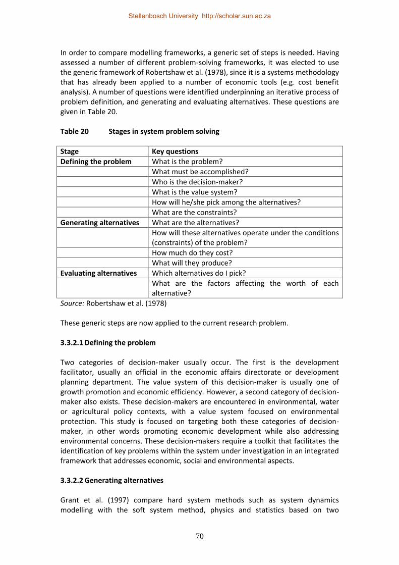
70
In order to compare modelling frameworks, a generic set of steps is needed. Having assessed a number of different problem-solving frameworks, it was elected to use the generic framework of Robertshaw et al. (1978), since it is a systems methodology that has already been applied to a number of economic tools (e.g. cost benefit analysis). A number of questions were identified underpinning an iterative process of problem definition, and generating and evaluating alternatives. These questions are given in Table 20. Table 20 Stages in system problem solving
Stage Key questions
Defining the problem What is the problem?
What must be accomplished?
Who is the decision-maker?
What is the value system?
How will he/she pick among the alternatives?
What are the constraints?
Generating alternatives What are the alternatives?
How will these alternatives operate under the conditions (constraints) of the problem?
How much do they cost?
What will they produce?
Evaluating alternatives Which alternatives do I pick?
What are the factors affecting the worth of each alternative?
Source: Robertshaw et al. (1978) These generic steps are now applied to the current research problem. 3.3.2.1 Defining the problem Two categories of decision-maker usually occur. The first is the development facilitator, usually an official in the economic affairs directorate or development planning department. The value system of this decision-maker is usually one of growth promotion and economic efficiency. However, a second category of decision-maker also exists. These decision-makers are encountered in environmental, water or agricultural policy contexts, with a value system focused on environmental protection. This study is focused on targeting both these categories of decision-maker, in other words promoting economic development while also addressing environmental concerns. These decision-makers require a toolkit that facilitates the identification of key problems within the system under investigation in an integrated framework that addresses economic, social and environmental aspects. 3.3.2.2 Generating alternatives Grant et al. (1997) compare hard system methods such as system dynamics modelling with the soft system method, physics and statistics based on two
Stellenbosch University http://scholar.sun.ac.za

71
dimensions. The first is the degree of interrelatedness of the components and the second is approaches based on the availability of data and level of understanding of the system (Table 21). Table 21 Comparisons between methods of problem solving
Level of understanding
Low High
Availability of data
High Statistics Physics
Low Soft systems analysis and simulation
System dynamics modelling
Source: Based on Grant et al. (1997) Traditional economic modelling approaches, it is suggested, fall primarily in the same category as statistics and physics, characterised by a high degree of data availability. However, more often than not when modelling environmental-social-economic systems, data is parsimonious (in particular time-series data) and approaches need to be developed that take this into consideration. Boulanger and Brechet (2005) highlight a number of sustainability problems, many of which are of relevant to the current study. These sustainability problems imply a methodological answer (Table 22). The authors identify six modelling approaches relevant to assessing these categories of problems. These include multi-agent modelling, system dynamics, Bayesian networks, optimisation, general equilibrium modelling (GEM) and econometrics. The final three columns of Table 22 compare SD modelling with two commonly-used economic modelling approaches. Boulanger and Brechet (2005) evaluate the six modelling tools based on the five methodological problems. The overall ranking of system dynamics modelling for each of the sustainability criteria is given in Table 22. These results should be interpreted with caution since all evaluations contain an element of subjectivity. However, the authors found that system dynamics performed better than both GEM and econometrics in terms of interdisciplinary potential, long-term perspective and participation; performed the same as GEM in terms of uncertainty management and local-global perspective; while econometrics performed better than SD in terms of uncertainty management and slightly worse in local-global perspective. Min Kang and Jae (2005) use a slightly different categorisation of models. Four quadrants are proposed with static/dynamic on one axis and feedback/laundry7 relationship on the other. GEMs are dynamic yet laundry; regression and correlation are static and laundry; while causal mapping is static with feedback. Computer simulation, however, is dynamic with causal feedback.
7 ‘Laundry’ is not defined by the authors, but is taken to mean linear.
Stellenbosch University http://scholar.sun.ac.za
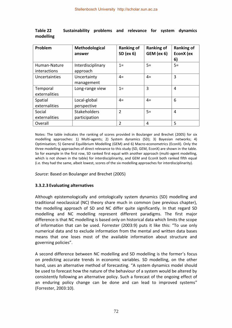
72
Table 22 Sustainability problems and relevance for system dynamics modelling
Problem Methodological answer
Ranking of SD (ex 6)
Ranking of GEM (ex 6)
Ranking of EconX (ex 6)
Human-Nature interactions
Interdisciplinary approach
1= 5= 5=
Uncertainties Uncertainty management
4= 4= 3
Temporal externalities
Long-range view 1= 3 4
Spatial externalities
Local-global perspective
4= 4= 6
Social externalities
Stakeholders participation
2 5= 4
Overall 2 4 5
Notes: The table indicates the ranking of scores provided in Boulanger and Brechet (2005) for six modelling approaches: 1) Multi-agents; 2) System dynamics (SD); 3) Bayesian networks; 4) Optimisation; 5) General Equilibrium Modelling (GEM) and 6) Macro-econometrics (EconX). Only the three modelling approaches of direct relevance to this study (SD, GEM, EconX) are shown in the table. So for example in the first row, SD ranked first equal with another approach (multi-agent modelling, which is not shown in the table) for interdisciplinarity, and GEM and EconX both ranked fifth equal (i.e. they had the same, albeit lowest, scores of the six modelling approaches for interdisciplinarity).
Source: Based on Boulanger and Brechet (2005) 3.3.2.3 Evaluating alternatives Although epistemologically and ontologically system dynamics (SD) modelling and traditional neoclassical (NC) theory share much in common (see previous chapter), the modelling approach of SD and NC differ quite significantly. In that regard SD modelling and NC modelling represent different paradigms. The first major difference is that NC modelling is based only on historical data which limits the scope of information that can be used. Forrester (2003:9) puts it like this: “To use only numerical data and to exclude information from the mental and written data bases means that one loses most of the available information about structure and governing policies”. A second difference between NC modelling and SD modelling is the former’s focus on predicting accurate trends in economic variables. SD modelling, on the other hand, uses an alternative method of forecasting. “A system dynamics model should be used to forecast how the nature of the behaviour of a system would be altered by consistently following an alternative policy. Such a forecast of the ongoing effect of an enduring policy change can be done and can lead to improved systems” (Forrester, 2003:10).
Stellenbosch University http://scholar.sun.ac.za

73
A third difference between NC modelling and SD modelling is the former’s emphasis on models based on the price mechanism. SD models, on the other hand, allow for a much broader scope of behaviour. “Inventories, backlogs, and delivery delays are the primary short-term balancing forces. Prices then change as a result of over or under supply of product” (Forrester, 2003:10). Furthermore, SD models focus on disequilibrium conditions and do not contain references to supply and demand curves as these relate to equilibrium conditions. The important point that needs to be made is that the universal rejection of neoclassical models is not advocated here. However, given the temporal and spatial scale of the current research problem, the complexity of the system (many and heterogeneous entities and complex interactions between the entities) suggests a relative strength for SD modelling in this instance.
3.3.3 Recent applications
3.3.3.1 Introduction In the previous section, it was evaluated whether or not system dynamics modelling were preferable to traditional neoclassical modelling. It was found that SD models, in theory, had a relative advantage over NC models in the area of sustainability modelling, in particular as it relates to complex systems. It is nonetheless important to ascertain whether these models are commonly used in practice to model economic and environmental systems. A search of Science Direct8 indicates that words and phrases associated with the system dynamics modelling technique is increasingly receiving attention in these publications. Assessing the usage of the key software used in system dynamics modelling during the last 10 years indicated 128 ‘hits’ for the STELLA software (since STELLA is a generic word not only used for system dynamics software, the search was narrowed down by including the company that supplies the software: HPS or isee systems), 152 ‘hits’ for Powersim and 174 ‘hits’ for Vensim software. Some of these ‘hits’ only include mentions of the technique rather than an actual modelling applications. Others include applications that are not environmentally orientated (for example, manufacturing or business). Although these are not as many as what was expected, it nonetheless indicates that the software is being used. In order to investigate actual practice, applications in
8 Although the choice of the Science Direct search engine is somewhat arbitrary, there are a number of reasons why this search engine is a useful choice for this study. Firstly, Science Direct publishes a range of journals that include agriculture, ecological, modelling and economic applications. Secondly, the premier publication Ecological Economics is also available via this search engine. Finally, while the System Dynamics Society publishes a journal System Dynamics Review which is not listed by Science Direct, it was felt that investigating publications in non-discipline specific journals would provide a better indication of the acceptability and ease of publication of system dynamics models.
Stellenbosch University http://scholar.sun.ac.za

74
three broad fields are considered. Firstly is applications in the field of economic theory. The macro economic model that was developed for the United States is described, along with other economic applications. Secondly, a comparison of recent case studies in the field of water, biodiversity and agriculture are examined to ascertain the frequency and geographical distribution of these case studies. An example of an application to agriculture is also given. Thirdly, other case studies that have only remote linkages to the project are also briefly described to indicate the universality of this technique. 3.3.3.2 Economics applications Although this is still a developing field, a number of authors have attempted to introduce the philosophy of system dynamics modelling into the realm of economic theory. Forrester, for example, argues that instead of considering economics as a social science, economics should rather be considered a systems profession similar to the engineering, management, and medical sciences.
Like the analysis and design of a chemical plant, understanding an economy should be based on understanding the internal structure of the system. The parts can then be interrelated in a simulation model to demonstrate how they interact to generate observed, economic behaviour (Forrester, 2000:21).
In this vein, SD modelling has been used to investigate a number of behavioural assumptions associated with economic theory. Two examples include Samuelson’s multiplier–accelerator model of business cycles (Low, 1980) and the Philips Curve (Forrester, 2003). The multiplier–accelerator theory as a determinant of (short-term) business cycle fluctuations states that rising demand increases production and creates jobs. The increased production results in capital expansion further creating jobs. The cycle is reversed when wage shortages drive down economic activity. The system dynamics model suggests that no plausible assumptions could result in business cycles. Rather, it is a contributing factor to the economic long wave (Forrester, 2003). Secondly, the Phillips Curve uses business cycle data to examine the relationship between inflation and unemployment. Forrester (2003:12) argues that this theory was in error since it resulted from “attributing causality to what is only a coincidental phase relationship within the complex dynamics of business cycles”. Other models incorporate alternative concepts of human decision-making rather than those of the traditional homo economicus. For example, John Morecroft develops a system dynamics model to illustrate Simon’s principle of ‘Bounded Rationality’ (Morecroft, 1983). One of the strengths of system dynamics modelling is not in the reproduction of historical data but rather in explaining outcomes based on alternative and consistent policy decisions (Forrester, 2003). The US-based system dynamics national model (NM) developed by MIT is an example of an application in this area. “Without attempting to reproduce the point-by-point behavio[u]r of the economy, the
Stellenbosch University http://scholar.sun.ac.za

75
simulation captures the major patterns in the development of the economy over almost 200 years” (Sterman, 1985:5). One area where this model has been used is in, what has been termed, Kondratiev cycles, after Kondratiev (1935). In exploring data from three Western economies (England, United States and France), Kondratiev observed not only short-term business cycle fluctuations (7–11 years) but also long-term fluctuations (averaging 50 years) in these economies. For the team based at MIT, this indicated long-term (systemic) causes for fluctuations. Some of the characteristics contributing to this long-term economic wave include: capital plant over-investment; excess borrowing used to build those capital plants and machinery; monetary policies that favour this expansion and over-investment; fluctuations in the real interest rate that accentuate cyclical activity; and changes in growth expectations (Forrester, 2003). Sterman (1985:28) states that “because the NM represents the physical structure of the economy and the decisionmaking routines used by individuals and firms to manage their affairs, it generates the multiple modes of behavio[u]r most important in modern economies, including the long wave, the business cycle, government growth and inflation, and the long-term growth of population and technology”. The model has been in development for several decades and has subsequently been generalised to capture trends beyond the United States (Forrester, 2003). Forrester (2003:14) concludes that “after many years of model development and comparison with numerous aspects of historical economic behavior, I believe that the model will pass an acceptable range of confidence tests”. 3.3.3.3 Applications in economic-environmental systems Allison and Hobbs (2004) use a combination of resilience theory and system dynamics to identify causal relations and macro level system structure in the Western Australia (WA) agricultural region. They use five ecological, social and economic variables that characterise the system. The ecological variable is the area of productive land, which in WA is classified into six major types: primary native vegetation, cropland, pastureland, commercial plantations, secondary native vegetation or regrowth, and unproductive land. The conceptual model of landuse change for this system is given in Figure 10. Other social and economic variables include the number of agricultural establishments, farmer age (discussed qualitatively), agricultural terms of trade and the wheat yield. Data used range from 1900 to 2000. As for the NM model discussed previously, not only historical data was consulted, but reference modes were interpreted with reference to Kontratiev and adaptive cycles. Evidence from the WA agricultural region suggests synchronisation of these adaptive cycles with the Kondratiev wave. The dynamics of land use change indicated a progression from primary native vegetation to a productive agricultural system. Resilience stemmed from functional reinforcement within scales and adaptive capacity between the ecological, economic and social systems. Macroeconomic conditions were the primary drivers of the dynamics of the agricultural region, but were also influenced by institutional aspects such as government, policy and markets.
Stellenbosch University http://scholar.sun.ac.za

76
Figure 10 A conceptual model of landuse change in Western Australia
Source: Allison and Hobbs (2004) In order to assess current usage of SD modelling for economic-environmental modelling, Science Direct was searched for applications in water, agriculture, biodiversity and restoration that were deemed particularly relevant to this study9. Since the current project focuses on South Africa, a specific search for applications that model a particular geographical area was done. Therefore, models that model the ‘world’ or generic studies that use hypothetical data or data that is not linked to a geographical area in the publication were excluded. In this way, 35 relevant case studies were identified, mostly published between 2000 and 2010 (see Appendix 1 for full list of case studies). Approximately half of these case studies (46 percent) used the VensimTM modelling software. This result is mainly due to the nature of the search process that was used since this author was specifically interested in Vensim applications. A notable feature of recent system dynamics applications is the wide geographical distribution of these case studies (Appendix 2). Furthermore, a number of economic-environmental modelling applications have already been done in South Africa. Higgins et al. (1997) modelled the restoration of mountain fynbos ecosystems in the Western Cape, Jogo and Hassan (2010) modelled wetland management in the Limpopo river basin, and Fleming et al. (2007) modelled cholera health risk. Other Science Direct applications by South African (or former South African) scientists on systems outside South Africa include Wise and Cacho (2005) modelling the Indonesian agroforestry sector, and Nobre et al. (2009) modelling Chinese aquaculture. A search of Science Direct publications, however, masks a potentially growing number of applications in South Africa that have not been published in these journals. One example of particular relevance to this study is the Water Research Commission study of Turpie et al. (2008). The cases of system dynamics applications have grown rapidly in recent years. For example, in terms of the Vensim models reported on earlier, 88% of the studies have taken place in the past five years. The main reason for the rapid growth in this
9 A number of economics case studies were also identified. However, many of these were generic models that addressed a theoretical question and were not for a specific geographical area.
Primary native
vegetation
Secondary native
vegetation
Unproductive land
Cropland
Pastureland
Commercial
forestry
Stellenbosch University http://scholar.sun.ac.za

77
modelling technique in recent times is more powerful personal computers enabling a wider audience to do complex simulations faster. Also, the advent of modelling software has simplified the model-building process (e.g. Voinov, 2008). The results from this assessment suggest that system dynamics models are increasingly gaining recognition as a relevant modelling technique for studying integrated economic-environmental problems. 3.3.3.4 Other applications A number of recent applications include: the following:
health services (Smith and Van Ackere, 2002)
the interrelationship between mineral policy and the resultant flow of investment (O’Reagan and Moles, 2006)
economic and political factors affecting agricultural practices (Vatn et al., 2006)
the relationship between income, population and nutrition (Fisher et al., 2003).
An interesting application (although not exclusively using the system dynamics technique of Forrester) is the dynamic systems model for the island of Crete (Perez-Trejo et al., 1993). The model explores the effects that different development scenarios might have on land degradation arising from land use changes driven by economic incentives.
3.3.4 Steps in the modelling process
3.3.4.1 Comparison between different approaches A number of authors have proposed steps to be followed in the process of building system dynamics models (e.g. Grant et al., 1997; Ford, 1999; Forrester, 2000). Table 23 compares these steps with the stages proposed in the systems engineering field. It is evident from this comparison that there is considerable uniformity on the process to be followed in building a system dynamics model. This study uses a combination of steps based on the SD stages of Ford (1999), Sterman (2000) and Grant et al. (1997). Model-building is an iterative process (Ford, 1999; Sterman, 2000; Grant et al., 1997). A model is usually built up in stages increasing in complexity (Ford, 1999). Furthermore, the stages are not always pursued sequentially, and certain stages may be repeated more than once (Grant et al., 1997). The model-building process is terminated when the model is capable of replicating the observed behaviour of the system (Ford, 1999). An illustration of the model-building process is given in Figure 11.
Stellenbosch University http://scholar.sun.ac.za

78
Table 23 Comparison between Systems Engineering (SE) and System Dynamics (SD) methodologies
SE stages (NORBE, 2004)
SD stages (Ford, 1999)
SD stages (Sterman, 2000)
SD stages (Grant et al., 1997)
1. Problem definition
1. Get acquainted with the system
1. Problem articulation
1. Conceptual model formulation
2. Goal setting 2. Be specific about the dynamic problem
2. Formulation of dynamic hypothesis
3. System synthesis 3. Construct the stock flow diagram 4. Draw the causal loop diagram 5. Estimate the parameter values
3. Formulation of a simulation model
2. Quantitative model specification
4. System analysis 6. Compare model to reference mode 7. Conduct sensitivity analysis
4. Testing
3. Model evaluation (model validation)
5. System selection 8. Test the impact of policies
5. Policy design and evaluation
4. Model use
Source: NORBE (2004), Ford (1999), Sterman (2000), Grant et al. (1997) Figure 11 Iterative model-building process
Source: Adapted from Sterman (2000) Sterman (2000) proposes a number of activities associated with each of the modelling steps (Table 24).
Problem definition
Formulation of
dynamic
hypothesis
Formulation of
simulation modelTesting
Policy design and
evaluation
Stellenbosch University http://scholar.sun.ac.za
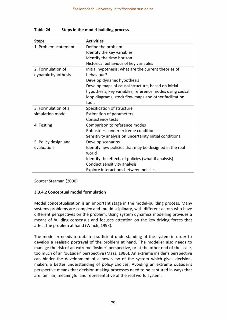
79
Table 24 Steps in the model-building process
Steps Activities
1. Problem statement Define the problem Identify the key variables Identify the time horizon Historical behaviour of key variables
2. Formulation of dynamic hypothesis
Initial hypothesis: what are the current theories of behaviour? Develop dynamic hypothesis Develop maps of causal structure, based on initial hypothesis, key variables, reference modes using causal loop diagrams, stock flow maps and other facilitation tools
3. Formulation of a simulation model
Specification of structure Estimation of parameters Consistency tests
4. Testing Comparison to reference modes Robustness under extreme conditions Sensitivity analysis on uncertainty initial conditions
5. Policy design and evaluation
Develop scenarios Identify new policies that may be designed in the real world Identify the effects of policies (what if analysis) Conduct sensitivity analysis Explore interactions between policies
Source: Sterman (2000) 3.3.4.2 Conceptual model formulation Model conceptualisation is an important stage in the model-building process. Many systems problems are complex and multidisciplinary, with different actors who have different perspectives on the problem. Using system dynamics modelling provides a means of building consensus and focuses attention on the key driving forces that affect the problem at hand (Winch, 1993). The modeller needs to obtain a sufficient understanding of the system in order to develop a realistic portrayal of the problem at hand. The modeller also needs to manage the risk of an extreme ‘insider’ perspective, or at the other end of the scale, too much of an ‘outsider’ perspective (Mass, 1986). An extreme insider's perspective can hinder the development of a new view of the system which gives decision-makers a better understanding of policy choices. Avoiding an extreme outsider's perspective means that decision-making processes need to be captured in ways that are familiar, meaningful and representative of the real world system.
Stellenbosch University http://scholar.sun.ac.za

80
According to Forrester (2000), there are three stages to conceptual model formulation. First, background knowledge on how feedback loops operate guide examination of the problem. Second, the information gathering stage takes place which might include interviews with key personnel. “These interviews are extensive and penetrating. There may be several sessions with each of many individuals. The discussions range widely from normal operations, to what is done in various kinds of crises, what is in the self interest of the individual … what would be done in hypothetical situations that may have never been experienced, and what actions are being taken to solve the serious problem facing the company” (Forrester 2000:13). Third, a case study approach is adopted where problems are described in words. A descriptive case study model is developed. “Such a descriptive case-study type of model is equivalent to a high-order nonlinear difference equation” (Forrester 2000:14). 3.3.4.3 Development of a dynamic hypothesis Kirchner (1984) distinguishes between two modelling approaches: the advocacy strategy and the strategy of multiple hypotheses. With the advocacy strategy, the strongest case is made for a particular model or theory. It is characterised by a search for confirmatory evidence. The dominant theory is only modified when doing so will result in making it more defensible. The strategy of multiple hypotheses, on the other hand, is a process of searching among a set of credible alternative hypotheses. The search is for ways of disproving a hypothesis, and this narrows down the range of options. A third approach, proposed by Sterman (2000), involves selecting a working hypothesis that explains the dynamics characterising the problem based on the feedback and stocks and flow structure of the system. The approach is dynamic because it characterises the dynamics of the stocks and flow structure of the system. It is also provisional because it is subject to revision and abandonment as a better understanding of the system and real world processes are obtained. All of these approaches have their strengths and weaknesses. Kirchner (1984) observed that at the time of publication the most common technique employed by system dynamics modellers was the advocacy strategy. There is some evidence that this still holds today. For example, Lane (2000b) argues that a ‘dynamic hypothesis’ embodies the concept that “a certain causal structure explains a certain dynamic behaviour”. He goes on to argue that “model building tests this hypothesis using rigorous formulation” (Lane, 2000b:4). However, the modeller needs to be able to adapt the modelling hypothesis if evidence from the model or from outside contradicts the hypothesis. 3.3.4.4 Quantitative model specification This involves translating the model into a simulation model. “Such a model allows the computer to act out the roles of each decision point … and feed the results to other connected decision points to become the basis for the next round of decisions” (Forrester, 2000:14). Quantification often leads to a better understanding of the structure and dynamics of a problem (Sterman, 2002) that may result in the
Stellenbosch University http://scholar.sun.ac.za
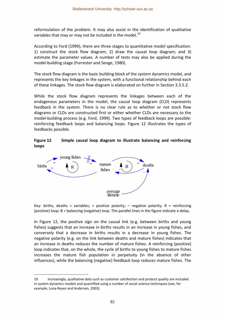
81
reformulation of the problem. It may also assist in the identification of qualitative variables that may or may not be included in the model.10 According to Ford (1999), there are three stages to quantitative model specification: 1) construct the stock flow diagram; 2) draw the causal loop diagram; and 3) estimate the parameter values. A number of tests may also be applied during the model-building stage (Forrester and Senge, 1980). The stock flow diagram is the basic building block of the system dynamics model, and represents the key linkages in the system, with a functional relationship behind each of these linkages. The stock flow diagram is elaborated on further in Section 3.3.5.2. While the stock flow diagram represents the linkages between each of the endogenous parameters in the model, the causal loop diagram (CLD) represents feedback in the system. There is no clear rule as to whether or not stock flow diagrams or CLDs are constructed first or either whether CLDs are necessary to the model-building process (e.g. Ford, 1999). Two types of feedback loops are possible: reinforcing feedback loops and balancing loops. Figure 12 illustrates the types of feedbacks possible. Figure 12 Simple causal loop diagram to illustrate balancing and reinforcing loops
Key: births, deaths = variables; + positive polarity; – negative polarity; R = reinforcing (positive) loop; B = balancing (negative) loop. The parallel lines in the figure indicate a delay.
In Figure 12, the positive sign on the causal link (e.g. between births and young fishes) suggests that an increase in births results in an increase in young fishes, and conversely that a decrease in births results in a decrease in young fishes. The negative polarity (e.g. on the link between deaths and mature fishes) indicates that an increase in deaths reduces the number of mature fishes. A reinforcing (positive) loop indicates that, on the whole, the cycle of births to young fishes to mature fishes increases the mature fish population in perpetuity (in the absence of other influences), while the balancing (negative) feedback loop reduces mature fishes. The
10 Increasingly, qualitative data such as customer satisfaction and product quality are included in system dynamics models and quantified using a number of social science techniques (see, for example, Luna-Reyes and Andersen, 2003).
young fishes
mature
fishes
+births
+deaths+
averagelifetime
-+ -
R B
Stellenbosch University http://scholar.sun.ac.za

82
direction of the arrow around the loop identifier moves in the same direction as the loop it identifies. In the above example both loops are clockwise. Estimating the parameter values in the model involves quantifying the linkages in the model. According to Graham (1980), parameter estimation techniques fall into two categories: cases where data are at the level of aggregation of the model and cases where data are below the level of aggregation of the model. Examples of the former are the most straightforward. If the model variable is quality of housing, then actual data exists on housing quality. The method of estimation is model equations. However, one of the strengths of the system dynamics modelling approach is estimating parameter values in data-poor environments. In the case where data are below the level of the model, data on housing quality do not exist. Data below the level of the variable need to be used, for example average age of household units. There are two distinct categories of methods of obtaining this information (Graham, 1980). The first category of obtaining unknown subaggregate data may be termed descriptive methods. One (time-consuming) way is to survey a number of households in the area of the study and determine the average age of the houses. Another way is expert input (asking a housing specialist or property agent the average age of houses). A third way is through visual observation. Are the houses characteristic of a particular period? Another option is to read histories of a neighbourhood to determine the average period in which houses were built. Another method is for the modeller to use his or her own experiences in estimating the average age of house. Finally, a general estimate may be obtained by picking extreme ranges for the variables (outside which the value will not fall) and then picking a value in between. This final technique seldom needs to be used. The second category of obtaining unknown subaggregate data (parameter estimates) may be termed analytical methods. Two approaches fall within this category: table functions and ad hoc approaches. Table functions use lookup tables to relate known parameter values to unknown parameter values. These lookup tables may be based on actual data, reference modes or known functional relationships. Ad hoc approaches use known data to estimate values for the unknown parameters. The data may be available or collected by the modeller. A functional relationship is then developed to relate the known data to the unknown data. One way in which this may be done is through the technique of optimisation. 3.3.4.5 Model validation The process of validation involves subjecting the model to a series of tests. Coyle and Exelby (2000:28) define validation as “the process by which we establish sufficient confidence in a model to be prepared to use it for some particular purpose”. A range of authors describe the main model tests used to validate a system dynamics model (Forrester and Senge, 1980; Richardson and Pugh, 1981; Barlas, 1989; Barlas, 1996; Sterman, 2000; Schwaninger and Groesser, 2009; Hill, 2010a; 2010b). However, it is important to emphasise that no model can be completely verified or validated – all
Stellenbosch University http://scholar.sun.ac.za

83
models are wrong since they represent limited, simplified representations of the real world (Sterman, 2000). Models, including system dynamics models, fail the extreme ‘Popperian’ approach of refutability and falsification (Sterman, 2000). However, many of these models may then be ‘saved’ by adopting an auxiliary hypothesis. This is true in other areas of science as well. Sterman (2000) gives the example of Galileo dropping balls of different weights from the leaning tower of Pisa.11 The new hypothesis of balls of different weights hitting the ground at the same time disproved the previous hypothesis that balls of different weights descend to the ground at different rates, a true ‘Popperian’ approach to science. However, the ‘new’ hypothesis was later disproved by more accurate measuring but redeemed by invoking the auxiliary hypothesis that air friction has an influence on speed of descent. The important aspect of system dynamics modelling, and models in general, is to recognise that their benefits are in their ability to assist with decision-making (Sterman, 2000). The objective for the modeller is to make the best model available for the purpose at hand in spite of its inevitable limitations. The important aspect in validation is to highlight the limitations of the model to decision-makers, so that it will not be misused and that it can be improved. The different tests used for validation are applicable at different stages in the model-building process. These include tests of model structure, model behaviour and testing a model’s policy implications (Forrester and Senge, 1980). The different tests are illustrated in Figure 13. There is no single test that serves to completely validate a model (Forrester and Senge, 1980). However, as the model passes more tests, confidence in a model gradually increases (Forrester and Senge, 1980). Figure 13 Tests appropriate at different stages of the model-building process
Source: Based on Forrester and Senge (1980) Tests of model structure include testing whether or not the model replicates the actual structure of the real world system, whether the dimensions (units) are
11 Whether or not this was in fact how Galileo conducted his experiment is subject to speculation.
Problem definitionFormulation of
model structureModel behaviour
Policy design and
evaluation
Structure verification
Extreme conditions
Parameter verification
Boundary adequacy
Dimensional consistency
Behaviour reproduction
Behaviour prediction
Behaviour anomaly
Family member
Surprise behaviour
Extreme policy
Boundary adequacy
Behaviour sensitivity
System improvement
Changed behaviour
prediction
Boundary adequacy
Policy sensitivity
STAGE
TESTS No tests identified
Stellenbosch University http://scholar.sun.ac.za

84
consistent and whether the model holds under extreme conditions (that might never occur in reality). Finally, model structure is tested to ascertain whether the level of aggregation is appropriate and that it contains all relevant parameters and feedbacks. The latter is done by comparing the model to a relevant hypothesis based on real world considerations. Tests of model behaviour include how well the model behaviour replicates the behaviour of the real world system. If anomalies occur between behaviour and reality, these need to be traced back to model assumptions. Sometimes it is also necessary to test whether or not the model contains features of a class (family) of models of which the specific model makes up a subset. Furthermore, it is necessary to understand whether surprise behaviour represents an anomaly or whether this is a feature of the model that has previously gone unnoticed. The model's resilience under extreme policy conditions related to rate equations is also tested (e.g. employment and personal savings flows fall to zero). Sensitivity of model parameters to changes in assumptions is also important, as are tests whether the model structure is adequate to address the issues it was designed for. Tests of policy implications involve testing whether the policy implications resulting from a change in a parameter value in the model replicate the policy response that a real world system would predict. Tests in this category include the system improvement test, the changed behaviour prediction test and policy sensitivity test. Not all tests are used all of the time when building system dynamics models (Forrester and Senge, 1980). Tests of model structure are most frequently used (e.g. Barlas, 1996), followed by tests of model behaviour, and finally tests of policy implications (Forrester and Senge, 1980). Given the range of tests available (Schwaninger and Groesser (2009) alone discuss 24 tests), an important validation question is: which tests are mandatory and which are for reference? In this study, a simple rule of thumb is adopted. The list of tests proposed by five leading system dynamics practitioners who have explicitly discussed a range of validation tests, were compared. The greater the number of practitioners who use a particular test the greater the weight given to the test results. This method is not without flaws since certain newer tests may have emerged that are as important as the older tests, but it provides an initial guideline nonetheless. The range of tests proposed by these authors is summarised in Table 25. Tests recommended by at least three of the five system dynamics practitioners were employed (the cells in bold), with the first four tests (structure verification, parameter verification, dimensional consistency and boundary adequacy) given the most precedence. The highlighted cells indicate which tests were actually implemented. Descriptions of each test (below) are drawn from these authors.
Stellenbosch University http://scholar.sun.ac.za

85
Table 25 Summary of validation tests conducted by different authors
Forrester and Senge (1980)
Richardson and Pugh (1981)
Sterman (2000)
Schwaninger and Groesser (2009)
Hill (2010a; 2010b)
No. used (ex 5)
Structure verification
Face validity Structure assessment
Structure examination
Structure verification (implied)
5/5
Parameter verification
Parameter values
Parameter assessment
Parameter examination
Parameter verification (implied)
5/5
Dimensional consistency
Dimensional consistency
Dimensional consistency
Dimensional consistency
Dimensional consistency
5/5
Boundary adequacy
Boundary adequacy
Boundary adequacy
Boundary adequacy
Boundary adequacy
5/5
Extreme conditions
Extreme conditions
Extreme conditions
Extreme condition
4/5
Surprise behaviour
Surprise behaviour
Surprise behaviour
Surprise behaviour
4/5
Behaviour sensitivity
Parameter sensitivity
Sensitivity analysis
Behaviour sensitivity
4/5
Behaviour reproduction
Behaviour reproduction
Behaviour reproduction
3/5
Behaviour anomaly
Behaviour anomaly
Behaviour anomaly
3/5
Family member
Family member
Family member
3/5
Integration error
Integration error
Integration error
3/5
Behaviour prediction
Behaviour anticipation
2/5
System improvement
System improvement
2/5
Extreme policy
1/5
Mass balance check
1/5
Loop dominance
1/5
Turing test 1/5 Notes: Hill (2010b) may not represent an exhaustive list of validation methods employed either by himself or Ventana Systems UK. Schwaninger and Groesser (2009) also discuss a number of context related tests that are not discussed by any of the other authors
Stellenbosch University http://scholar.sun.ac.za

86
3.3.4.6 Model use The objective of the modelling effort is to develop a model that can ultimately be used for policy design and evaluation. According to Grant et al. (1997), there are four steps within the model use phase of system development: 1) develop and execute the experimental design for the simulations; 2) analyse and interpret the simulation results; 3) examine additional management policies or situations; and 4) communication of the simulation results. In the model development phases, a runtime version of the baseline model is developed for use in policy simulations. A number of structural and dimensional consistency tests are executed to ensure that the model conforms to specifications (see Section 4.5 for an elaboration). In the model execution phase, a number of policy simulations or evaluations are undertaken depending on the objectives of the study. At the same time, the model is tested against key assumptions and extreme values (‘shocks’) (see Section 4.5). Sometimes it may be necessary to return to earlier phases of the model development process, such as reformulation of the problem statement or the dynamic hypothesis. Once a working version of the model is available that passes a satisfactory range of tests, the next step is to analyse and interpret key results. In the third step, the model is examined with the purpose of suggesting ways that the system performance may be improved by making recommendations for future interventions in the system. The limitations of the model and recommendations for future refinements are also elaborated on. Finally, model results are communicated. In a research setting, this usually means publication in a scientific journal (Grant et al., 1997). In a management framework, this implies communication of model results to those managers whose policy decisions impact on the area of study.
3.3.5 Model features
3.3.5.1 Modelling software used A number of different software packages are available to be used to model system dynamics problems. For a recent comparison between these different modelling packages see Voinov (2008). This study uses the VensimTM Simulation Environment developed by Ventana® Systems, Inc (Ventana Systems, 2007). Vensim is an interactive modelling environment that allows the development, calibration, simulation and optimisation of continuous simulation problems (Eberlein and Peterson, 1992). Some of the basic features of the modelling software include (Voinov, 2008):
stock flow modelling;
Stellenbosch University http://scholar.sun.ac.za
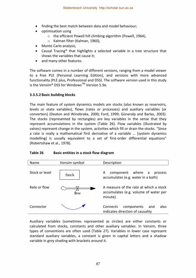
87
finding the best match between data and model behaviour;
optimisation using o the efficient Powell hill climbing algorithm (Powell, 1964), o Kalman filter (Kalman, 1960),
Monte Carlo analysis,
Causal Tracing® that highlights a selected variable in a tree structure that shows the variables that cause it;
and many other features. The software comes in a number of different versions, ranging from a model viewer to a free PLE (Personal Learning Edition), and versions with more advanced functionality (PLE plus, Professional and DSS). The software version used in this study is the Vensim® DSS for WindowsTM Version 5.9e. 3.3.5.2 Basic building blocks The main feature of system dynamics models are stocks (also known as reservoirs, levels or state variables), flows (rates or processes) and auxiliary variables (or converters) (Deaton and Winebrake, 2000; Ford, 1999; Güneralp and Barlas, 2003). The stocks (represented by rectangles) are key variables in the sense that they represent accumulations in the system (Table 26). Flow variables (illustrated by valves) represent change in the system, activities which fill or drain the stocks. “Since a rate is really a mathematical first derivative of a variable … [system dynamics modelling] is usually equivalent to a set of first-order differential equations” (Robertshaw et al., 1978). Table 26 Basic entities in a stock flow diagram
Name Vensim symbol Description
Stock or level
A component where a process accumulates (e.g. water in a bath)
Rate or flow
A measure of the rate at which a stock accumulates (e.g. volume of water per minute)
Connector
Connects components and also indicates direction of causality
Auxiliary variables (sometimes represented as circles) are either constants or calculated from stocks, constants and other auxiliary variables. In Vensim, three types of conventions are often used (Table 27). Variables in lower case represent standard auxiliary variables, a constant is given in capital letters and a shadow variable in grey shading with brackets around it.
Stock
flow
deaths
Stellenbosch University http://scholar.sun.ac.za

88
Table 27 Three types of variables used in the model
Name Vensim symbol Description Auxiliary variable
variable name A component that interacts with other components (usually through a mathematical relationship)
Constant CONSTANT Distinguished from an auxiliary variable
through the use of capitalisation Shadow variable <variable name> A variable that links with another
variable/model in a different view
An illustration of how these different entities relate to each other in a stock flow diagram is given in Figure 14. This diagram shows a simple stock flow diagram for fishes growing to maturity with a delay function associated with fisheries catch. Figure 14 A system dynamics model for fish population dynamics
Source: Millennium Institute (2010) 3.3.5.3 Dynamic behaviour Most systems exhibit multiple feedback loops (Robertshaw et al., 1978) which allow for non-linear and counterintuitive behaviour and dynamics (Forrester, 1971b). Behaviour over time is characterised both by equilibrium and non-equilibrium dynamics (Deaton and Winebrake, 2000; Radzicki, 1997). Types of dynamic behaviour include linear growth (straight line and positive slope) or decay (straight line and negative slope), exponential growth or decay (where the rate of growth or decay increases rapidly over time), logistic growth (also known as s-shaped growth, initially increasing and then declining as the population approaches carrying capacity), goal seeking behaviour (which is similar to exponential decay except that, instead of seeking a goal of zero a non-zero goal is strived towards), and oscillation and overshoot and collapse (which occurs when the system overshoots and the
Mature
FishesYoung
Fishesbirths deaths
catchBIRTH RATE
TIME FOR FISHES
TO MATURE
maturation
CARRYING
CAPACITY fish density
EFFECT OF FISHDENSITY ON DEATH
RATE
death rate
perceived mature
fishesTIME TO COUNT
FISHES
TARGET LIVE
MATURE FISHESextra fishes
TIME TO CATCH
FISHES
Stellenbosch University http://scholar.sun.ac.za

89
carrying capacity is permanently damaged, for example through overgrazing, resulting in the system being able to support a lower population than it would have initially). Examples of the different system features are given in Figure 15. For example, three types of oscillating behaviour are shown: damped, sustained and exploding. Figure 15 Examples of dynamic behaviour in system dynamics models Linear growth Linear decay
Exponential growth Exponential decay
S-Shaped growth S-Shaped decay
100
85
70
55
40 0 5 10 15 20 25
Time (Month) Current Value : Current
60
50
40
30
20 0 5 10 15 20 25
Time (Month) Current Value : Current
8,000
6,000
4,000
2,000
0 0 5 10 15 20 25
Time (Month) Current Value : Current
60
45
30
15
0 0 5 10 15 20 25
Time (Month) Current Value : Current
1,000
750
500
250
0 0 1 2 3 4 5 6 7 8 9 10 11 12
Time (Year) Current Value : Current
1,000
750
500
250
0 0 10 20 30 40 50 60 70 80 90 100
Time (Month) Current Value : Current
Stellenbosch University http://scholar.sun.ac.za

90
Goal seeking behaviour A Goal seeking behaviour B
Oscillating behaviour A Oscillating behaviour B
Oscillating behaviour C Overshoot and collapse
3.3.6 Summary
System dynamics is a technique that originates in the engineering and computational science field. In recent years, however, it has had wide-ranging applications in economic-ecological systems. Some of the problems encountered with systems analysis in the past suggest that it is less useful as a model for predictive behaviour, and rather better at exploring critical linkages, assumptions and management responses. It was argued in Chapter 2 (Section 2.4.2) that much of mainstream economics is rooted in the scientific method of J.S. Mill. This emphasises deductive reasoning and experimentation. In Chapter one, it was indicated that increasingly, scientific
60
50
40
30
20 0 5 10 15 20 25
Time (Month) Current Value : Current
40
30
20
10
0 0 5 10 15 20 25
Time (Month) Current Value : Current
100
85
70
55
40 0 5 10 15 20 25
Time (Month) Current Value : Current
200
150
100
50
0 0 5 10 15 20 25
Time (Month) Current Value : Current
40
20
0
-20
-40 0 5 10 15 20 25 30 35 40 45 50
Time (Month) Current Value : Current
1,000
750
500
250
0 0 5 10 15 20 25 30 35 40 45 50
Time (Year) Current Value : Current
Stellenbosch University http://scholar.sun.ac.za

91
research is shifting towards the search for relationships. Here, the emphasis is not strictly on Popperian “falsification” (see Section 3.3.4.5) but rather on developing a model that is able to assist decision-making. In the context of this study, the problem that is addressed is primarily applied, transdisciplinary, and characterised by non-linearity, temporal and social externalities, and multiple feedbacks. The system dynamics approach is particularly well suited to deal with problems of this nature. Although system dynamics shares many ontological and epistemological characteristics with neoclassical economics, it represents a new paradigm. This is particularly true for economics departments in South Africa that either have a pessimistic view of modelling or else hold to a traditional modelling perspective that emphasises statistical techniques for verification. Although the system dynamics modelling technique may represent a new paradigm in these contexts, there is strong evidence that the technique is gaining increased acceptance and recognition both worldwide and in South Africa. Furthermore, there are numerous case studies in the fields of agriculture, water and restoration, and economics. Although system dynamics modelling is an important tool for decision-making, it is also essential to recognise that modelling is not enough, and that one needs to be aware of the wider social and moral context of the research problem when interpreting results.
3.4 Project portfolio management
Project portfolio management (PPM) began in the field of modern portfolio theory, which was developed by Henry Markowitz, who was later awarded a Nobel Prize for his work (Wysocki, 2009). It was only during the 1990s that his theories were diversified from investments to projects (Wysocki, 2009). Today, the dominant themes of research in PPM are in the fields of New Product Development (NPD) and Technology and Innovation Management (TIM) (Hobbs, 2012). A useful definition of project portfolio management is the following: “[It] includes establishing the investment strategy of the portfolio, determining what types of projects can be incorporated in the portfolio, evaluating, and prioritizing proposed projects, constructing a balanced portfolio that will achieve the investment objectives, monitoring the performance of the portfolio, and periodically adjusting the contents of the portfolio in order to achieve the desired results” (Wysocki, 2009:536). A number of tools are available for PPM (see Cooper et al. (2001) for a review). A visually appealing and widely used tool is the portfolio mapping technique. This technique is described here and is the technique employed in the current study. Early versions of portfolio mapping emerged in 1970 in a series of popular publications by the Boston Consulting Group (Day, 1977). This framework was rapidly adopted by companies – by 1972 the approach was employed by more than
Stellenbosch University http://scholar.sun.ac.za

92
100 companies (Day, 1977). The original portfolio maps distinguished between four types of projects: Stars, Cash Cows, Dogs and Problem Children. The axes of the original maps focused on market growth rate (relative to GNP growth) and market share dominance (share relative to largest competitor). Furthermore, the original maps emphasised business units rather than projects (Cooper et al., 2001) and focused on existing businesses with known performance, strengths and weakness in contrast to the new portfolio maps that emphasise new products and projects (Cooper et al., 1997). More recent versions of portfolio maps (e.g. Matheson et al., 1989; Matheson and Menke, 1994; Cooper, 2005; Wysocki, 2009), also known as risk reward maps or bubble diagrams, contain Net Present Values of individual projects on the -xaxis, and a measure of the probability of success of each project on the y-axis (Figure 16), although there are variations on this theme. This framework has the ultimate aim of prioritising investment funds to particular projects. Figure 16 Modified BCG products/services matrix
Note: BCG classification: ?, star, cash cow, dog; Cooper classification: oysters, pearls, bread and butter, white elephant. Size of circles indicate amount of resources committed to each project.
Source: Based on Cooper (2005), Wysocki (2009) The definition of the different categories of projects is as follows (Matheson and Menke, 1994; Cooper et al., 1997; Cooper, 2005): A. Oysters These are long-shot projects with high expected payoffs but also high risk. These are projects where technical breakthroughs will pave the way for solid payoffs. Oysters require long periods of cultivation in the hopes of obtaining breakthroughs in products or processes. Significant incentives need to be given to researchers working
1
Net present value
Prob. Of
successHigh
Low
Dog/
White elephant
?
Oysters
Cash cow/
Bread and butter
Star/
Pearls
Stellenbosch University http://scholar.sun.ac.za

93
in this area. Company X in the example above is investing quite substantially into one such project. B. Pearls These are potential star products: projects with a low risk that are expected to yield a high reward. Company X has two, with relatively low investment going into them (Figure 16). Pearls require a more entrepreneurial approach. Budgets are not the key issue, since the high payoffs make virtually any budget permissible. The main focus is on development time and the promotion of flexibility to explore ways of commercialising the product. C. Bread and butter These are small, simple projects with a high likelihood of success but low reward. They include many fixes, extensions, modifications and updating of projects, or incremental improvements to a product or process. Standard project management principles apply to these projects, namely deadlines, budget parameters and traditional performance incentives. D. White elephants These are projects that consume resources and are unlikely to produce commercial value. Most companies have some of these projects and they are often difficult to kill, but Company X has too many of them. White elephants require further research in order to determine whether they are worth saving or require restructuring (for example, by using existing technology rather than new technology to develop). In addition to this information, the different bubbles may be colour coded to reflect different information: for example, project status (development, imminent or launched) or project category. In this way, the bubble diagram has the advantage of conveying a range of information to decision-makers at one time (Cooper et al., 1997) and also display portfolio balance (Cooper et al., 2001). The disadvantages of the framework include that it may be difficult to interpret and provide too much information for strategic decision-makers. In spite of these weaknesses, portfolio maps remain popular for business strategy. In a survey of different organisations, 40.6% of businesses reported using portfolio maps and they are highly recommended by managers as an effective tool for yielding correct portfolio decisions (Cooper et al., 2001). Resource allocation is dependent on the current business climate, the market share and position of the enterprise, and a number of other factors (Wysocki, 2009). In a stable industry, such as clothing manufacturing, the majority of the resources will be committed to the bread and butter projects in order to maintain market share. Some resources will be committed to pearls, and even fewer in the more risky oyster category. If the industry is in a more volatile sector, such as IT, it is likely that it will commit more resources to the pearls and the oysters, and fewer resources to the bread and butter projects. Another, but related, way of looking at portfolio mapping is through linking with the economics of innovation discussed in the previous section. A Smithian organisation (after Adam Smith’s innovation through division of
Stellenbosch University http://scholar.sun.ac.za

94
labour) will have an emphasis on projects on the left-hand side of the portfolio map (Figure 17A). The main focus of such innovations is incremental innovations to increase and maintain market share. An organisation of the Koestlerian tradition (innovation through associative thinking) will lead to more radical innovations that produce potentially higher payoffs, but at the same time also introduce potentially greater risks. An organisation focusing on radical innovations will tend to have more projects on the right-hand side of the portfolio map (Figure 17B). It is important to emphasise that no single process is likely to be optimal in all circumstances and different processes are applicable in different contexts. Figure 17 Portfolio mapping characterised by different types of innovation
The risk-reward framework for portfolio mapping is the most popular framework used by businesses (Table 28). However, a number of other axes are also used. Table 28 Axes used in popular portfolio maps Rank Type of chart Axis #1 Axis #2 %
1 Risk vs Reward Reward: NPV, IRR, benefits after years of launch, market value
Probability of success (technical, commercial)
4.4
2 Newness Technical newness Market newness 11.1
3 Ease vs Attractiveness
Technical feasibility Market attractiveness (growth potential, consumer appeal, overall attractiveness, life cycle potential)
11.1
4 Our Strengths vs Project Attractiveness
Competitive position (our relative strengths)
Project attractiveness (market growth, technical maturity, years to implementation)
11.1
5 Cost vs Timing Cost to implement Time to impact 9.7
6 Strategic vs Benefit
Strategic focus or fit Business intent, NPV, financial fit, attractiveness
8.9
7 Cost vs Benefit Cumulative reward ($) Cumulative development costs ($) 5.6
Rank ordered; last column shows percentage breakdown of portfolio map usage (as a percent of businesses using portfolio maps).
Source: Cooper et al. (2001)
Net present value
Prob. Of
successHigh
Low
Dog/
White elephant
?
Oysters
Cash cow/
Bread and butter
Star/
Pearls
A. Smithian organisation
Net present value
Prob. Of
successHigh
Low
Dog/
White elephant
?
Oysters
Cash cow/
Bread and butter
Star/
Pearls
B. Koestlerian organisation
Stellenbosch University http://scholar.sun.ac.za

95
3.5 Chapter summary and conclusions
It is useful to close this chapter by summarising how each stage in the risk assessment process was followed in the current study (Table 29). Table 29 Steps in the risk analysis process
Stage Study methodology Outcome
1. System dynamics model Develop system dynamics model that will inform other components of the risk analysis process
A system dynamics model is developed for eight case study sites throughout South Africa where restoration is occurring.
2. Choose a strategy for the portfolio
The financial criterion used for the study was determined at a strategic level at the start of the project
Following Farley and Brown Gaddis (2007), the decision rule used in this study is that the Net Present Value (NPV) of a particular project is positive.
3. Determine key success drivers
System dynamics (SD) modelling is used to determine the key tipping points in the system
The criterion that had most impact on the success or failure of the project is the price of ecosystem benefits.
4. Obtain a forecast for a variable of interest in terms of a probability distribution
Monte Carlo simulation is employed based on the set of restoration decision criteria that maximised the NPV of the project system dynamics model
Output is a set of uniform distributions for each of the project NPVs. Monte Carlo simulations based on single and multiple decision criteria are used to derive these distribution functions
5. Generate the simulated distribution of the financial criterion
Calculation Summary statistics are generated, and risk measures determined.
6. Utilise the risk and reward framework as a basis for selecting and prioritising between projects
Project portfolio management theory is used
Portfolio maps are developed for each of the risk reward profiles generated in the model.
This chapter focussed on the applied aspects of methodology by examining the risk analysis framework utilising system dynamics modelling. The framework was shown to be appropriate for transdisciplinary research integrating ecological, economic and hydrological aspects of restoration. In the next chapter, the system dynamics model and Monte Carlo simulations are validated, and some results presented.
Stellenbosch University http://scholar.sun.ac.za

96
Chapter 4 Data and integrated model
4.1 Introduction
The previous chapter described the rationale and methodology of risk analysis (RA) using the system dynamics (SD) modelling approach. Five steps required for conducting a risk analysis, were documented. Those steps were: 1) developing a system dynamics model; 2) determining the strategy for the portfolio; 3) identifying key success drivers; 4) determining the distribution of the outcome variable and risk profile of projects; and 5) using portfolio mapping in order to select and prioritise between different projects. The first step in the RA process (developing an SD model) comprises four steps: 1) model conceptualisation; 2) development of a dynamic hypothesis (Chapter 1); 3) model validation and 4) model use. Model use feeds into the identification of key success drivers (RA stage 3) and also the risk profile of the projects (RA step 4). Monte Carlo simulation based on the SD model is at the core of this integrated approach. It is used not only for the sensitivity analysis to validate the system dynamics model (SD step 3), but also RA step 3 and 4. In addition to Monte Carlo simulation, the system dynamics model is used to determine the decision rules that maximise NPV in each of the case studies. In this chapter, the RESTORE-P model (Regional Economic SysTem dynamics mOdel for the Restoration of Ecosystems and project Prioritisation) is presented with reference to each of these modelling steps.
4.2 Study sites
The RESTORE-P model is a localised system dynamics model that investigates the impacts of restoring natural capital across eight case study sites throughout South Africa (Figure 18).
The sites represent a range of vegetation types, from Nama Karoo and Succent Karoo, to Fynbos, to Savannah, Grassland and Forest (Table 30). The majority of the sites are in arid or semi-arid climatic zones, with mean annual precipitation of less than 700mm per year. Most of the restoration takes place on private land, although some have mixed landuse; others are public or communal areas. Most sites have low connectivity of the origin (measured as a rehabilitated area of less than 50km2). The extent of degradation also varies quite significantly across the sites, and although this is difficult to compare with any degree of objectivity, many sites were severely degraded. Most notable were those affected by mining activity (strip mining) and intensive ostrich farming as well as the communal grazing areas.
Stellenbosch University http://scholar.sun.ac.za

97
Figure 18 Geographical distribution of case studies
Table 30 Landuse and ecosystem characteristics of the eight study sites
Site Name Vegetation type Climatic Zone MAP
Land classification
Area rehabilitated (km
2)
Extent of degradation
S1 Namaqualand Succulent Karoo Arid 160 Private 26 Severely degraded
S2 Beaufort West Nama Karoo Arid 239 Public/Private 8 Degraded
S3 Oudtshoorn Succulent Karoo Arid 242 Private 1762 Severely degraded
S4 Lephalale Savanna Semi-arid 400 Private 9249 Degraded
S5 Agulhas Fynbos Semi-arid 478 Public/Private 548 Degraded
S6 Kromme Fynbos Semi-arid 650 Private 46 Degraded
S7 Drakensberg Grassland Temperate 900 Communal 1 Severely degraded
S8 Sand Forest/Savanna Temperate 1275 Public/Private 32 Degraded
Source: Own analysis based on Crookes (2011a); Crookes (2011b); Cloete (2012); De Abreu (2011); Ndhlovu (2011a); Nowell (2011a); Pauw (2011a); Rebelo (2012a)
4.3 Conceptual model
4.3.1 Model components
The RESTORE-P model evaluates the effects of restoration on all four forms of natural capital (see e.g. Aronson et al., 2007), namely: renewable, non-renewable,
1 Namaqualand
2 Oudtshoorn
3 Beaufort West
4 Lephalale
5 Agulhas Plain
6 Kromme river
7 Drakensberg
8 Sand river
5
3
2
1
7
48
6
Stellenbosch University http://scholar.sun.ac.za

98
replenishable and cultivated (Figure 19). Five main types of ecosystem disturbance affect the sites in various combinations. The spread of Invasive Alien Plants (IAPs), and the closely related plantation forestry (which also uses exotic species) are two dominant disturbances that affect a number of different sites. At the Agulhas and Kromme sites, Black Wattle (Acacia mearnsii) and Port Jackson (Acacia saligna) and Blue gums (Eucalyptus spp.) are major invading plants, as well as Pines (Pinus spp.). At Beaufort West, Mesquite (Prosopis spp.) is the dominant invader. At the Sand river site, a number of plantations exist, including invasives mentioned for the Agulhas and Kromme sites, as well as Bugweed (Solanum mauritianum), Lantana (Lantana camara), Guava tree (Psidium guajava), Brambles (Rubus cuneifolius), Mauritius thorn (Caesalpinia decapetala) and Prickly pear (Opuntia stricta) (Le Maitre et al., 2002). Alien species are associated with a number of negative impacts (De Wit et al., 2001), inter alia: reduction of surface streamflow, loss of biodiversity, increases in fire hazard, increases in erosion and the destabilisation of river banks. Alien species do, however, also provide a number of benefits, including (significantly in the context of this study) firewood and other biomass energy (Agulhas and Beaufort West), timber and pulp (Sand) and also nitrogen fixation (Beaufort West). Figure 19 Conceptual model
The case study at Namakwa Sands (Namaqualand) is the only example of natural capital that is not renewable. The mine produces 125 000 tons of zircon, 25 000 tons of rutile, 200 000 tons of pig iron and 200 000 tons of titania slag, but this comes at a great cost to the environment (Pauw, 2011a). The strip mining process removes natural vegetation; top soil is removed to a depth of 50 mm. The subsoil is then
S1 S2 S3 S4 S5 S6 S7 S8SITES
NON-RENEWABLE
Restoration
method
RENEWABLENATURAL
CAPITALREPLENISHABLECULTIVATED
ECOSYSTEMPRODUCTION WATERAGRICULTURE
IAPsSTRIP
MINING
UNSUST.
FARMING
UNSUST.
FORESTRY
BUSH
ENCROACHMENT
BIOMASS
Soil carbon,
wild
products
Lumber,
fuelwood,
electricity
GOODS
AND
SERVICES
Yield, quality
Game, agronomy,
horticulture,
livestock, apiculture
ECONOMICS Restoration costs Benefits
DISTURBANCE
(+)
(-)
MINING
Heavy
minerals
Capital depreciation,
labour, equipment, bond
refinancing costs
Value of improvements in
different capital classes
Stellenbosch University http://scholar.sun.ac.za

99
removed and mixed with sea water, where the mined product (heavy minerals) is then separated from the fine particles (slimes) and tailings (oversized particles). Although much of the top soil and tailings are used in the rehabilitation process, the natural vegetation is not able to fully recover. This is partly due to salination, partly leaching and partly wind erosion. As a result, a societal deadweight loss occurs, mainly affecting agricultural production in the area. Although loss of farming production is the major beneficiary of restored landscapes, farming actually causes the degradation in a number of the case studies. In Oudtshoorn, ostrich farming is a major cause of rangeland degradation (De Abreu, 2011). Ostriches strip off leaves and uproot plants, they trample soils leading to compaction and the removal of the biological crust, and they also create pathways that lead to erosion. In the Drakensberg, poor management practises such as overgrazing and burning of rangeland areas may affect species richness, the removal of vegetation cover, water infiltration rates and the occurence of erosion (Marx, 2011a). Trampling of ground, especially after rain events, creates pathways that eventually lead to erosion and dongas. At the Sand river site, it is not agriculture per se, but the canal system used to provide water for irrigated crops that has caused a number of problems. The canal system is significantly damaged and requires major repair work to fix leakages and also broken weirs (Crookes, 2011b). The consequences are that, firstly, not all irrigated crops receive water, and secondly, water users downstream of the agricultural zone do not receive the ecological reserve (the minimum water flow required to sustain ecological functioning). At the Kromme river site, farming production has resulted in eradication of large areas of the indigenous palmiet wetlands (since this area has the most fertile soil) (Rebelo, 2012a). Human intervention has also reduced the frequency of fires at the Lephalale study site, resulting in increased bush encroachment. For restoration to be effective in these areas, it is crucial that rehabilitation proceeds in conjunction with improved management practices. While there are a number of unifying characteristics that provide the basis for integration, there are also a number of unique ecosystem characteristics specific to individual case studies. The linkage between the case studies is that each is characterised by disturbance that generates an externality that impacts the functional integrity of the ecosystem. Restoration has a positive impact on the production process, which in turn improves the suite of ecosystem goods and services available (Table 31). The approach is not to focus on all EGS, but only those that were identified during the initial project scoping exercise and refined by subsequent project expert meetings, and collected by ecology, hydrology and economics students working on the different case studies. Examples of EGS included in the RESTORE-P model are improved agricultural production, improved water yield and quality, biomass fuel, soil carbon, eco-labelling and ecotourism (recreational) benefits. Each site has a unique set of ecosystem benefits that it provides. For example, at Agulhas Plain, ecosystem benefits include income from wildflower sales, fynbos products, apiculture and pollination services (Vlok, 2010;b Fourie et al., 2011). For a full list of ecosystem goods and services associated with each site, see Table 31.
Stellenbosch University http://scholar.sun.ac.za

100
Table 31 Characteristics of each study site Study site Economic
activity Disturbance Natural
capital EGS benefit from restoration
Agulhas Wild flowers Apiculture
Alien spread Renewable, replenishable
Agriculture production Water yield Firewood
Beaufort West Agriculture (Sheep, Goats)
Alien spread (Prosopis)
Renewable, replenishable, cultivated
Agriculture production Water yield Bio-electricity
Drakensberg Agriculture (Cattle, Goats)
Erosion, siltation of dams
Renewable, repenishable, cultivated
Agricultural production Agricultural services (milk, hides, etc.) Water quality Soil carbon
Namaqualand Mining Sheep farming
Destruction of natural vegetation
Renewable, non-renewable, cultivated
Agricultural production Soil carbon
Kromme river Agriculture (Sheep, Cattle, Vegetables, Honeybush tea, Fruit)
Damage to wetlands Alien infestation
Replenishable, cultivated
Agricultural production Water yield Water quality
Lephalale Agriculture (Cattle, Game production)
Reduction in fire frequency, fencing that causes bush encroachment
Renewable, cultivated
Agricultural production Game production Bio-electricity
Oudtshoorn Ostriches Destruction of natural vegetation
Renewable, cultivated
Agricultural production Soil carbon Ecolabelling
Sand river Forestry, agriculture (IACs, IAPs)
Alien spread and exotic plantations
Renewable, replenishable, cultivated
Water yield Eco-tourism
IAC = irrigated annual crops; IPC = irrigated permanent crops
4.3.2 Causal loop diagram
1. Balancing effects The causal loop diagram for each of the eight case study sites are roughly the same (Figure 20) and indicates the various feedback loops in the model. The first feedback
Stellenbosch University http://scholar.sun.ac.za

101
loop indicates the relationship between an ecosystem disturbance and the natural vegetation. An increase in unsustainable use (in the absence of restoration) creates a negative feedback loop that increases ecosystem disturbance and results in a reduction in natural capital. The more abundant the natural capital the greater the risk of unsustainable use. This is an example of a negative (or balancing) feedback loop and has the tendency to produce stable, equilibrium or goal-seeking behaviour over time. In other words, the system will stabilise but not necessarily at a sustainable level. Figure 20 Balancing effects
2. Reinforcing effects Positive (or reinforcing) feedback loops have the effect of generating, increasing or amplifying model behaviour. There are two reinforcing effects in the model: one is an ecosystem feedback loop and the other is an economic feedback loop. An increase in unsustainable use increases the ecosystem disturbance, which reduces ecosystem functionality and increases the need for restoration. An increase in restoration, on the other hand, increases natural capital. In the economic feedback loop, an increase in natural vegetation increases species composition which increases ecosystem goods and services which increases economic value. It is important to emphasise that the link between economic value and natural vegetation is a policy link and is not explicitly modelled in the system dynamics model. In other words, a positive economic value is used as a justification for payment for ecosystem services (PES) which, in turn, has the potential to further increase the area under natural vegetation.
natural capital
ecosystem
disturbance
-
Bunsustainable use
+
+
Stellenbosch University http://scholar.sun.ac.za

102
Figure 21 Reinforcing effects
A. Natural capital loop B. Economic value loop
3. Combined causal loop diagram Figure 22 indicates the combined causal loop diagram, with the balancing loop and two reinforcing loops. Figure 22 Combined CLD
4.3.3 Model description
In this section the model for each of the eight individual case studies is described, the parameter values and equations are given as well as the stock flow diagrams.
natural capital
ecosystem
functionality
restoration
-
+
ecosystem
disturbance
-
Runsustainable use
+
+natural capital
species
composition
+
ecosystem goods
and services +
economic
value
+
+
R
natural capital
ecosystem
functionality
restoration
-
+
ecosystem
disturbance -
R
-
B
species
composition
+
ecosystem goods
and services +
economic
value
+
+
R
unsustainable use
+
+
Stellenbosch University http://scholar.sun.ac.za

103
4.3.3.1 Agulhas model 1. Overview The Agulhas Plain is an area of mixed landuse (dominated by agriculture and natural vegetation situated on farmland and also in nature reserves) in the Overberg region of the Western Cape. All landuses are also invaded by invasive alien plants (IAPs) of which Acacia, Pinus and Eucalyptus species account for 93% of the invasive vegetation (Nowell 2011a). Alien species reduce the agricultural productivity of the land and result in the loss of biodiversity and reduce surface streamflow (De Wit et al. 2001). Two methods of clearing are considered in this model: physical clearing and biocontrol treatment. Fire is a natural part of the fynbos growth cycle (Higgins et al. 1997a) and also needs to be modelled. A. Fire sub-model A fire model was developed for the Agulhas plain using unpublished data provided in Nowell (2011b). Fynbos landuse is categorised as unconserved, natural and alternative. The total area of the Agulhas plain is estimated at 216 290 ha, which is marginally more than the area estimated by Fakoti (2007) (Table 32). Table 32 Land use classification for Agulhas Plain, 2010
Uncondensed area (2010, ha)
Reference
Alien vegetation (A) 67 189 Nowell (2011b)
Natural (non-conserved) (B) 84 296 Own calculation based on Nowell (2011b)
Conserved (C) 10 107 Own calculation based on Nowell (2011b)
Alternative (D) 54 698 Own calculation based on Nowell (2011b)
Total fynbos (E=B+C+D) 149 101 Novell (2011b)
Total area Agulhas plain (F=A+E) 216 290 Novell (2011b)
Area of Agulhas plain 216 000 Fakoti (2007)
The optimal fire frequency for fynbos is 15 years (Cowling, 1995, as cited in MacPherson, 2009). Therefore, a fire event is expected once every 15 years. In reality, fire events occur at different time periods depending on a range of exogenous variables which are difficult to model. In this model, a fire event is triggered when the fynbos density exceeds a specified density at the optimal fire frequency. Combining these data with data from Fakoti (2007) (Table 33), a fire event is triggered when the density of mature fynbos exceeds 33% of the total area.
Stellenbosch University http://scholar.sun.ac.za

104
Table 33 Landcover composition before fire event, Agulhas plain
Area (t=15, ha) Reference
Alien vegetation (G) 143 700 Fakoti (2007)
Total mature fynbos (F-G) 72 590 Own calculation Note: Time t=15 is period just before fire event.
Monthly cumulative growth rates for aliens and fynbos following a fire event is given in Fakoti (2007). In order to calculate annual growth rates, cumulative monthly growth rates need to be converted to monthly growth rates by taking first differences and then applying a conversion formula to convert to annual estimates. Results are shown in Table 34. Alien vegetation and fynbos grows rapidly in the first year following a fire event and then stabilises at a long-term growth rate, until the next fire. Table 34 Growth rates of indigenous and alien vegetation following fire
Growth rate p.a. (t=1)
Growth rate p.a. (t=2+)
Reference
Alien vegetation 133% 62% Own calculations based on Fakoti (2007)
Total fynbos 147% 80% Own calculations based on Fakoti (2007)
Note: Time t=1 is period following the year of a fire event.
Since growth rates and landcover data in period t=15 is now known, it is possible to work backwards to determine what the species densities are just after a fire event (i.e. at time t=0). Almost all the alien vegetation and fynbos is burnt (Table 35). This corresponds with the findings of Higgins et al. (1997a). Table 35 Landcover composition following fire event
Area (t=0, ha) (% of total)
Reference
Alien vegetation 71.93 (0.033%) Calculation
Total mature fynbos 7.84 (0.004%) Calculation
% Burnt 99.963% Calculation Note: Time t=0 is period of a fire event.
Now all that remains is to calibrate the model so that the landcover data at the start of the model simulation most closely approximates the actual landcover data in 2010. This involves shifting the time frame of the model to the period that most
Stellenbosch University http://scholar.sun.ac.za

105
closely corresponds with the 2010 data. Table 36 compares actual landcover data with model calibrated data. The calibrated model predicted that, given the prevailing landcover characteristics, the next fire event in the Agulhas plain was due to occur in 2013. In fact, a fire event occurred in 2012, suggesting that the model to some extent is able to replicate reality. B. Bio-control sub-model Bio-control was another component that was not originally included in the system dynamics model for Agulhas, but was identified during the expert input workshops as an important element to include. This analysis is by no means comprehensive and further work is required to further understand these dynamics. Table 36 Comparisons between model predictions and actual landcover compositions, 2010
Condensed area, 2010, ha
Reference
Aliens (condensed) (0.75*A) 50 392 Nowell (2011b)
Aliens (calibrated model parameter) (H)
54 755 Own calculation
Fynbos (calibrated model parameter) (I)
22 404 Own calculation
Total (J=H+I) 77 160 Own calculation
Condensed recovery as % of original area (J/F*100)
36% Calculation
Different bio-control agents are applicable to different species. Although the Agulhas Plain is invaded by a range of species, in 2000 71% of the invaded area was Acacia (Nowell, 2011a). Bio-control agents have already been released for a number of the Acacia species (Nowell, 2011a). The efficacy thereof is uncertain but different species are affected in different ways. Following the literature, bio-control is effective in three areas (Wood and Morris, 2007):
1) It reduces tree densities of those affected by bio-control agents. 2) It impacts on the growth and biomass of plant populations. 3) It impacts on pod production.
The fungal agent attacks new growth, reducing shoot production and ultimately reducing flower and seed production (Le Maitre, 2012). Seed output is reduced by as much as 60% (Wood and Morris, 2007). Mortality rate is high during years one and two after germination; from year three to year five, however, survivors are able to outgrow the fungal agent until year five; few trees survive beyond eight years of age (Le Maitre, 2012). The final result is open stands with approximately 10% of the pre-
Stellenbosch University http://scholar.sun.ac.za

106
bio-control density and other plants growing in between; prior to bio-control only dense stands formed with no plants growing underneath (Le Maitre, 2012). For the purposes of the model, the benefits of bio-control in terms of density reductions have already been taken into consideration in the historical and current Working for Water costs for clearing Acacia Saligna since they all post-date bio-control. The focus of the current model, therefore, is on the benefits of th expansion of bio-control that would ultimately target pod production. This is similar to the approach used by Higgins et al. (1997b), although their model does not take into account fire. Nowell (2011a) indicates that bio-control agents have been released for five Acacia species in the Agulhas Plain (A. saligna, A. cyclops, A. longifolia, A. melanoxylon, and A. mearnsii). For a summary of the different bio-control agents used for each of these Acacia species, and their efficacy, see Table 37. Note that these efficacy rates are applicable to specific study sites throughout South Africa and are not specific to the Agulhas plain. Excellent long-term monitoring data is available for biocontrol measures implemented against Acacia saligna at various experimental sites throughout the Western Cape (Wood and Morris, 2007), and consequently this IAP is used as a representative of the other weeds, given that the damage caused by biological control agents is comparable (see Table 37). Impacts on growth rates caused by biological control measures must take into account fire, since fire has a significant negative effect on the efficacy of bio-control (Nowell, 2011a). Regression analysis suggests the following relationship between tree age (measured in years) and tree density (measured in tonnes per hectare) (Figure 23). Figure 23 Relationship between density and age of tree following bio-control (A. saligna)
Source: Own analysis based on data in Wood and Morris (2007); Curvilinear graph from Le Maitre (2012)
y = 0.5186x
012345678
0 1 2 3 4 5 6 7
Ph
yllo
de
dry
wei
ght
(to
n/h
a)
Time (years)
Stellenbosch University http://scholar.sun.ac.za
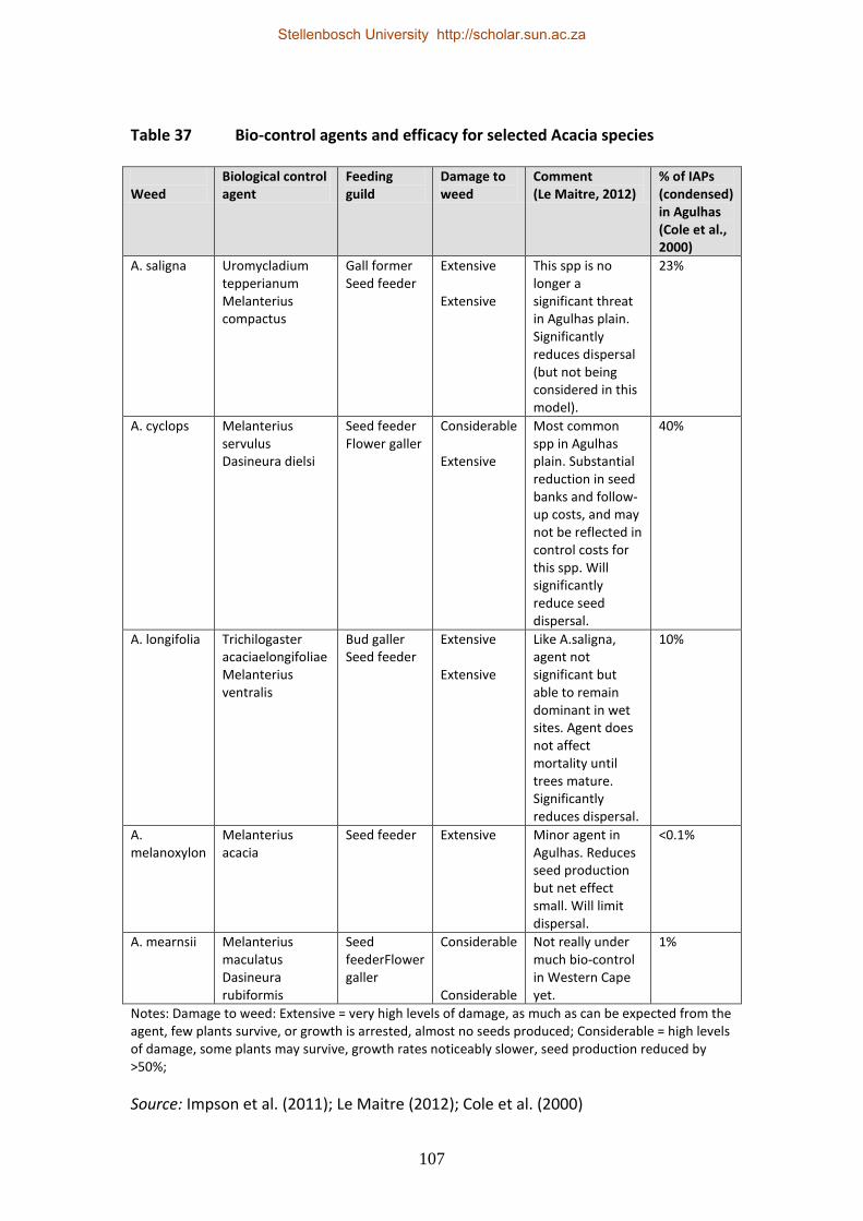
107
Table 37 Bio-control agents and efficacy for selected Acacia species Weed
Biological control agent
Feeding guild
Damage to weed
Comment (Le Maitre, 2012)
% of IAPs (condensed) in Agulhas (Cole et al., 2000)
A. saligna Uromycladium tepperianum Melanterius compactus
Gall former Seed feeder
Extensive Extensive
This spp is no longer a significant threat in Agulhas plain. Significantly reduces dispersal (but not being considered in this model).
23%
A. cyclops Melanterius servulus Dasineura dielsi
Seed feeder Flower galler
Considerable Extensive
Most common spp in Agulhas plain. Substantial reduction in seed banks and follow-up costs, and may not be reflected in control costs for this spp. Will significantly reduce seed dispersal.
40%
A. longifolia Trichilogaster acaciaelongifoliae Melanterius ventralis
Bud galler Seed feeder
Extensive Extensive
Like A.saligna, agent not significant but able to remain dominant in wet sites. Agent does not affect mortality until trees mature. Significantly reduces dispersal.
10%
A. melanoxylon
Melanterius acacia
Seed feeder Extensive Minor agent in Agulhas. Reduces seed production but net effect small. Will limit dispersal.
<0.1%
A. mearnsii Melanterius maculatus Dasineura rubiformis
Seed feederFlower galler
Considerable Considerable
Not really under much bio-control in Western Cape yet.
1%
Notes: Damage to weed: Extensive = very high levels of damage, as much as can be expected from the agent, few plants survive, or growth is arrested, almost no seeds produced; Considerable = high levels of damage, some plants may survive, growth rates noticeably slower, seed production reduced by >50%;
Source: Impson et al. (2011); Le Maitre (2012); Cole et al. (2000)
Stellenbosch University http://scholar.sun.ac.za

108
In this regression, the intercept was constrained to zero and forms the basis of determining what the annual growth in biomass would be under the controlled (experimental) environment in which high levels of biological control agents were introduced. A linear growth path is assumed primarily for simplicity and ease of calculation, but a more realistic representation for the age-biomass factor is the curvilinear line (illustrated in red in Figure 23), with biomass peaking at approximately 4–5 years after a fire and then declining. Future work would require a better refinement of the current model’s growth relationship. Using the coefficient of the regression relationship it is possible to compute the annual growth rate in density of A. saligna over the 15 years between fire regimes (Figure 24).12 Figure 24 Annual growth rates of A. saligna between fire cycles following bio-control
Source: Own calculations based on data in Wood and Morris (2007) As Figure 24 illustrates, growth rates are highest in year 1 following a fire, then steadily decline in an exponential manner until a low of just 7% per annum, before the next fire cycle. The average growth rate over the 15-year period is 31% which, if compared with the Agulhas fire model, is roughly half the long-term average growth rate for alien species (62%, see Part A, Agulhas fire sub-model). This suggests that although bio-control agents have been implemented in the Agulhas Plain, they are not yet fully effective. The time period when the long-term growth rate is achieved (31%) is roughly year 4. The model’s policy scenario for bio-control (bio-control switch=1) assumes that a broader scale inoculation programme is adopted in the Agulhas Plain. For the purposes of the model, it is assumed that the experimental sites discussed above
12 Note that here phyllode dry weight (t/ha) was used as a measure of density and it is assumed that area is held constant, while in the system dynamics model the measure of density is change in area. The same annual growth rate is achieved whether an area-based or dry weight measure is used.
0.00
0.20
0.40
0.60
0.80
1.00
1.20
1.40
0 5 10 15 20 25 30 35 40 45 50Ave
an
nu
al g
row
th r
ate
(1
/10
0)
Time (years)
Stellenbosch University http://scholar.sun.ac.za

109
represent an inoculation area of 100%. In the model, different levels of implementation are employed as sensitivity analyses, and these affect the alien growth rate in the following manner: Alien growth rate pa = long-term growth rate / (1+inoculation area (%)) Therefore, if a 100% inoculation area is adopted, Alien growth rate pa = 0.62 / (1+1) = 0.31 (which is equivalent to the estimate derived from the
literature) Innoculation costs for bio-control implementation against A. Mearnsii are obtained from De Wit et al. (2000), and inflated to 2010 values assuming an 8% inflation rate. In the absence of other data it is assumed that costs will be the same for all biological control agents. Innoculation costs are estimated at R25,43 per hectare inoculated, which is considerably less than the equivalent clearance cost of R3 696,24 per hectare (based on Fourie, 2011). The current approach is based on bio-control for A. Saligna, which is the approach that Higgins et al. (1997b) used in their bio-control system dynamics model and also for which most data exists and is probably adequate (Le Maitre, 2012). Further work, however, is required to better understand and model the effect of bio-control measures on A. cyclops in the Agulhas Plain as the costs of follow-up operations have most likely declined quite significantly. 2. Model parameters and model equations A. Parameters used in model and units Description Formula/Value Unit Reference Comment
% innoculated= 1 Dmnl Policy variable See Appendix B
Implementation cost per ha= 25.43 Rand/hectare De Wit et al., 2001
no of years of innoculations= 1 Year Policy variable
Time period that maximises NPV
lt growth rate= 0.62 1/Year Calculation based on Fakoti, 2007
biocontrol? y=1= 0 Dmnl Policy switch
delay before biocontrol takes effect= 4 Year Calculation See Appendix B
no of years to clear aliens= 50 Year Calculation
Time period that maximises NPV
total area ap 0= 216290 hectare Calculation See Appendix B
% deep sands= 0.642931 Dmnl Own calculations based on Nowell, 2011a
Share of total water released
% dryland= 0.32575 Dmnl Own calculations based Share of total
Stellenbosch University http://scholar.sun.ac.za

110
Description Formula/Value Unit Reference Comment
on Nowell, 2011a water released
% wetland= 0.0313195 Dmnl Own calculations based on Nowell, 2011a
Share of total water released
Initial fynbos= 22404.44 hectare Calculation (see Appendix B)
DISCOUNT RATE= 0.08 1/Year Mullins et al., 2007
% aliens burnt= 0.999691 Dmnl Higgins et al., 1997a
INITIAL AREA AP= 54755.4 hectare Calculation (see Appendix B)
% fynbos burnt= 0.99994 Dmnl Higgins et al., 1997a
NO OF YEARS TO CLEAR ALIENS AP= 50 Year [0,61,1]
Period that maximises NPV
proportion of alien clearance that affects fynbos= 0.0003 Dmnl Calculation
% elim= 0.09 Dmnl Own calculation based on Fourie, 2011
% eucalyptus= 0 Dmnl Le Maitre, 2012.
0 (loss of eucalyptus assumed 0 compared with baseline since Eucalptus not a target species for clearing)
% limestone= 0.07 Dmnl Own calculation based on Fourie, 2011
% mountain= 0.28 Dmnl Own calculation based on Fourie, 2011
% neutral= 0.18 Dmnl Own calculation based on Fourie, 2011
% of area belonging to landowners= 0.3 Dmnl
Own calculation based on Fourie, 2011
% restioid= 0.06 Dmnl Own calculation based on Fourie, 2011
% sand= 0.008 Dmnl Own calculation based on Fourie, 2011
% strandveld= 0.17 Dmnl Own calculation based on Fourie, 2011
% yield= 0.3333 Dmnl Le Maitre, 2011
alien water use per hectare= 7542 m3/hectare/yr
Weighted average based on Nowell, 2011a
clearing costs per ha= 3696.24 Rand/hectare
Own calculations based on Fourie, 2011
firewood r/ha lime= 204.8 Rand/hectare Fourie, 2011
firewood R/ha Strand= 184.31 Rand/hectare Fourie, 2011
Price Elim= 9.09 Rand/hectare Fourie, 2011 Wildflowers & Fynbos products
Price H&P elim= 6.23 Rand/hectare Fourie, 2011 Honey and pollination
Stellenbosch University http://scholar.sun.ac.za

111
Description Formula/Value Unit Reference Comment
price H&P eucalyptus= 490.44 Rand/hectare Fourie, 2011
Honey and pollination
price h&p lime= 16.99 Rand/hectare Fourie, 2011 Honey and pollination
Price H&P mount= 1.21 Rand/hectare Fourie, 2011
Honey and pollination
price h&p sand= 11.08 Rand/hectare Fourie, 2011 Honey and pollination
price h&p strand= 11.08 Rand/hectare Fourie, 2011
Honey and pollination
price limestone= 7.07 Rand/hectare Fourie, 2011 Wildflowers & Fynbos products
price mountain= 28.28 Rand/hectare Fourie, 2011 Wildflowers & Fynbos products
price neutral= 18.18 Rand/hectare Fourie, 2011 Wildflowers & Fynbos products
price restoid= 6.06 Rand/hectare Fourie, 2011 Wildflowers & Fynbos products
Price strand= 19.87 Rand/hectare Fourie, 2011 Wildflowers & Fynbos products
total area ap= 216290 hectare Calculation (see Appendix B)
UNIT VALUE OF WATER= 1.59 Rand/m3 Vlok, 2010a
B. Equations Description Formula/Value Unit
gr alien= alien gr % no bio*area aliens no clear hectare/Year
alien % grwth pa=
IF THEN ELSE(fire event=1,1.33,IF THEN ELSE("biocontrol? y=1"=0,lt growth rate,IF THEN ELSE(Time<2010+delay before biocontrol takes effect,lt growth rate,lt growth rate/(1+"% innoculated")))) 1/Year
alien gr % no bio= IF THEN ELSE(fire event=1,1.33,lt growth rate) 1/Year
total clearing costs=
(1-"biocontrol? y=1")*clearing costs per ha*annual clearance AP+IF THEN ELSE(Time<2010+no of years of innoculations,"biocontrol? y=1"*Implementation cost per ha*area innoculated per year,0) Rand/Year
area innoculated per year=
% innoculated*INITIAL AREA AP/no of years of innoculations hectare/Year
NO OF YEARS TO CLEAR ALIENS AP=
IF THEN ELSE("biocontrol? y=1"=1,0,no of years to clear aliens) Year [0,61,1]
area burnt= fire event*(area aliens no clear*"% aliens burnt"*(1+"alien gr % no bio")) hectare/Year
fire event= IF THEN ELSE(fynbos density>0.33,1,0) Dmnl
fynbos density= area fynbos/total area ap 0 Dmnl
water value wetland= % wetland*revenue from additional water yield Rand/Year
revenue from additional water yield= UNIT VALUE OF WATER*water yield Rand/yr
area eucalyptus= % eucalyptus*(Area Aliens Ap-condensed area no clear) hectare
net value from alien revenue firewood+water value deep sands+water Rand/Year
Stellenbosch University http://scholar.sun.ac.za

112
Description Formula/Value Unit
clearing AP= value dryland+water value wetland+Value of beekeeping+revenue from fynbos products-total clearing costs
water value dryland= % dryland*revenue from additional water yield Rand/yr
water value deep sands=
% deep sands*revenue from additional water yield Rand/yr
fire fynbos= area fire fynbos no clear hectare/Year
increase in fynbos area= area fynbos-area fynbos no clear hectare
additional water released=
baseline alien water use-alien species water extraction m3/yr
gr fynbos= fynbos % grwth pa*area fynbos no clear hectare/Year
alien species water extraction= alien water use per hectare*Area Aliens Ap m3/yr
area fynbos no clear= INTEG (gr fynbos-fire fynbos,Initial fynbos) hectare
annual clearance AP=
min(IF THEN ELSE(Time<2010+NO OF YEARS TO CLEAR ALIENS AP,INITIAL AREA AP/NO OF YEARS TO CLEAR ALIENS AP,0),gr rate aliens) hectare/Year
area fire fynbos no clear=
fire event*area fynbos no clear*"% fynbos burnt"*(1+"fynbos % grwth pa") hectare/Year
baseline alien water use=
alien water use per hectare*condensed area no clear m3/yr
area alien strandveld= % strandveld*(Area Aliens Ap-condensed area no clear) hectare
condensed area no clear= area aliens no clear*0.75 hectare
area alien limestone= ("% limestone"+"% neutral")*(Area Aliens Ap-condensed area no clear) hectare
gr alien= alien % grwth pa*area aliens no clear hectare/Year
area aliens no clear= INTEG (gr alien-fire,INITIAL AREA AP) hectare
area burnt= fire event*(area aliens no clear*"% aliens burnt"*(1+"alien % grwth pa")) hectare/Year
fire= area burnt hectare/Year
npv agulhas= NPV(net value from alien clearing AP,DISCOUNT RATE,0,1) Rand
revenue from fynbos products=
(consumption value non landowners+consumption value to landowners)/year Rand/Year
gr rate fynbos=
fynbos % grwth pa*area fynbos+annual clearance AP*proportion of alien clearance that affects fynbos hectare/Year
area fire aliens=
fire event*(Area Aliens*"% aliens burnt"*(1+"alien % grwth pa")-annual clearance AP*"% aliens burnt") hectare/Year
area fire fynbos= fire event*area fynbos*"% fynbos burnt"*(1+"fynbos % grwth pa") hectare/Year
area fynbos= INTEG (gr rate fynbos-fire loss fynbos,Initial fynbos) hectare
fynbos density= area fynbos/total area ap Dmnl
check: total= IF THEN ELSE(total area AP<216290,1,0) Dmnl
alien % grwth pa=
IF THEN ELSE(Time=2013,1.33,IF THEN ELSE(Time=2029,1.33,IF THEN ELSE(Time=2045,1.33,0.62))) 1/Year
fynbos % grwth pa= IF THEN ELSE(Time=2013,1.47,IF THEN 1/Year
Stellenbosch University http://scholar.sun.ac.za

113
Description Formula/Value Unit
ELSE(Time=2029,1.47,IF THEN ELSE(Time=2045,1.47,0.8)))
Area Aliens= INTEG (gr rate aliens-alien removal rate,INITIAL AREA AP) hectare
fire event= IF THEN ELSE(fynbos density>0.33,1,0) Dmnl
alien removal rate= annual clearance AP+area fire aliens hectare/Year
fire loss fynbos= area fire fynbos hectare/Year
Area Aliens Ap= Area Aliens*0.75 hectare
gr rate aliens= alien % grwth pa*Area Aliens hectare/Year
check: total area AP= Area Aliens+area fynbos hectare
Value of beekeeping= (value of beekeeping fynbos+value of beekeeping eucalyptus)/year Rand/Year
revenue firewood= (area alien limestone*"firewood r/ha lime"+area alien strandveld*"firewood R/ha Strand")/year Rand/Year
water yield= % yield*additional water released m3/yr
consumption value non landowners= Price strand*Strandveld Rand
consumption value to landowners=
% of area belonging to landowners*revenue from wildflower sales Rand
Elim= % elim*increase in fynbos area hectare
Limestone fynbos= % limestone*increase in fynbos area hectare
limestone total= Limestone fynbos+Neutral sand fynbos hectare
Mountain= % mountain*increase in fynbos area hectare
Neutral sand fynbos= % neutral*increase in fynbos area hectare
Restoid= % restoid*increase in fynbos area hectare
revenue from wildflower sales=
Elim*Price Elim+Limestone fynbos*price limestone+Mountain*price mountain+Neutral sand fynbos*price neutral+Restoid*price restoid Rand
sand= % sand*increase in fynbos area hectare
Strandveld= % strandveld*increase in fynbos area hectare
total clearing costs= clearing costs per ha*annual clearance AP Rand/Year
value of beekeeping eucalyptus= area eucalyptus*"price H&P eucalyptus" Rand
value of beekeeping fynbos=
Elim*"Price H&P elim"+limestone total*"price h&p lime"+Mountain*"Price H&P mount"+"price h&p sand"*sand+"price h&p strand"*Strandveld Rand
Stellenbosch University http://scholar.sun.ac.za

114
3. Stock flow diagrams A. Land use
B. Water
Area Aliens
alien removal rate
INITIAL AREA AP no of years to
clear aliens ap
Area Fynbos
gr rate aliens
gr rate fynbos
fynbos % grwth pa
alien % grwth pa
area aliens ap
fire event
fire loss fynbos
<Time>
area fire aliens % ALIENS
BURNT
% fynbos burnt
area fire fynbos
annual clearance
ap
<Time>PROPORTION OF ALIEN
CLEARANCE THATAFFECTS FYNBOStotal area ap
check: total
initial fynbosTOTAL AREA
AP 0
fynbos density
BIOCONTROL?
Y=1
LT GROWTH
RATE DELAY BEFOREBIOCONTROL TAKES
EFFECT<Time>
NO OF YEARS TO
CLEAR ALIENS
<%
INNOCULATED>
alien species water
extraction
ALIEN WATER USE
PER HECTARE
% YIELD
water yield
UNIT VALUE
OF WATER
revenue from
additional water yield
<area aliens ap>
additional water
released
Area Aliens
No Cleargr alien
<alien % grwth
pa>
fire
area burnt
<% ALIENS
BURNT>
<fire event>
<INITIAL AREA
AP>
condensed area no
clear
baseline alien water
use
% DRYLAND
% DEEP SANDS
% WETLAND
water value
dryland
water value deep
sandswater value
wetland
alien gr % no
bio
<fire event>
<LT GROWTH
RATE>
Stellenbosch University http://scholar.sun.ac.za

115
C. Fynbos
D. Firewood sub-model
elim
limestone fynbos
neutral sand fynbos
mountain
restoid
strandveld
% ELIM
% STRANDVELD
% RESTOID
% MOUNTAIN
% LIMESTONE
% NEUTRAL
limestone total
<Area Fynbos>
increase in
fynbos area
AreaFynbos No
Clear
area fire fynbos
no clear
gr fynbos
<fynbos % grwth
pa>
fire fynbos
<fire event>
<initial fynbos>
<% fynbos burnt>
revenue from
wildflower sales
<mountain>
<elim>
<restoid>
<limestone fynbos>
<neutral sand
fynbos>
PRICE STRAND
PRICE ELIM
PRICE
MOUNTAIN
PRICE RESTOID
PRICE
LIMESTONE
PRICE NEUTRAL
% OF AREABELONGING TOLANDOWNERS
consumption value to
landowners
<strandveld>
consumption value
non landowners
revenue from fynbos
products
<YEAR>
FIREWOOD R/HA
STRAND
FIREWOOD
R/HA LIME
<%
STRANDVELD>
<%
LIMESTONE>
<% NEUTRAL>
area alien
limestone
area alien
strandveld
revenue firewood<area aliens ap>
<YEAR>
<condensed area
no clear>
Stellenbosch University http://scholar.sun.ac.za

116
C. Clearing costs
D. Apiculture
total clearing costs
clearing costs per
ha
<annual
clearance ap>
<BIOCONTROL?
Y=1>
IMPLEMENTATION
COST PER HA
area innoculated
per year
<INITIAL AREA
AP>
%
INNOCULATED
NO OF YEARS OF
INNOCULATIONS<Time>
<elim><mountain><strandveld>
<increase infynbos area>
% SAND
sand <limestone total>
PRICE H&P
MOUNTPRICE H&P
ELIM
PRICE H&P
SANDPRICE H&P
STRAND
PRICE H&P
LIME
value of
beekeeping fynbos
value of beekeeping
eucalyptus
%
EUCALYPTUS
area eucalyptus
PRICE H&P
EUCALYPTUS
value of
beekeepingYEAR
<condensed area
no clear>
<area aliens ap>
Stellenbosch University http://scholar.sun.ac.za
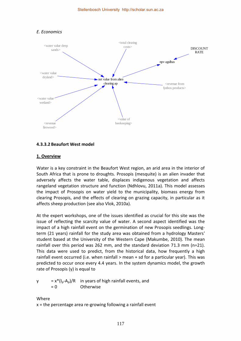
117
E. Economics
4.3.3.2 Beaufort West model 1. Overview Water is a key constraint in the Beaufort West region, an arid area in the interior of South Africa that is prone to droughts. Prosopis (mesquite) is an alien invader that adversely affects the water table, displaces indigenous vegetation and affects rangeland vegetation structure and function (Ndhlovu, 2011a). This model assesses the impact of Prosopis on water yield to the municipality, biomass energy from clearing Prosopis, and the effects of clearing on grazing capacity, in particular as it affects sheep production (see also Vlok, 2010a). At the expert workshops, one of the issues identified as crucial for this site was the issue of reflecting the scarcity value of water. A second aspect identified was the impact of a high rainfall event on the germination of new Prosopis seedlings. Long-term (21 years) rainfall for the study area was obtained from a hydrology Masters' student based at the University of the Western Cape (Makumbe, 2010). The mean rainfall over this period was 262 mm, and the standard deviation 71.3 mm (n=21). This data were used to predict, from the historical data, how frequently a high rainfall event occurred (i.e. when rainfall > mean + sd for a particular year). This was predicted to occur once every 4.4 years. In the system dynamics model, the growth rate of Prosopis (y) is equal to y = x*(Ip-Ap)/R in years of high rainfall events, and = 0 Otherwise Where x = the percentage area re-growing following a rainfall event
<revenue
firewood>
<value of
beekeeping>
<revenue from
fynbos products>
<total clearing
costs>
net value from alien
clearing ap
npv agulhas
DISCOUNTRATE
<water value deep
sands>
<water value
dryland>
<water value
wetland>
Stellenbosch University http://scholar.sun.ac.za

118
Ip = Initial area of prosopis, and Ap = the current area of prosopis R = re-growth rate, measured in years Given the low rainfall in the region, a drought year is defined to be any year that is not a high rainfall year. Water value in the model is determined by the municipal block water tariffs for Beaufort West (Vlok, 2010a). The model was adjusted so that the scarcity value of water was reflected. For example, the high rainfall block water price is R1.67/m3. However, during a drought year the water scarcity increases, so the water price rises to R2.6/m3 (data from Fourie, 2011).13 2. Model parameters and model equations A. Parameters used in model and units Description Formula/Value Unit Reference Comment
lifespan of plant= 50 Dmnl Assumption Model time period
conv: Kw to Rand= 15000 Rand/Kw Fourie, 2011
biomass included? Y=1= 1 Dmnl Policy variable Switch. 1=yes
time to clear area= 1 Year Time that maximises NPV
the larger this value, the less cleared per annum and lower impact on both area of prosopis and also quantity fed into biomass generator
water included? Y=1= 1 Dmnl Policy variable Switch. 1=yes
% area regrowth following rainfall= 1 Dmnl Assumption
regrowth rate= 1 Year Assumption
discount rate= 0.08 1/Year Mullins et al., 2007
prosopis water use= 251.9 m3/hectare Fourie, 2011
initial area= 781 hectare H.Vlok, 2010a
no of years of clearing activity= 50 Year [0,20,1] Time that maximises NPV
% condensed= 0.19 Dmnl H.Vlok, 2010a
change in grazing capacity= 0.028 LSU/hectare Ndhlovu, 2011a
clearing cost= -817.5 Rand/hectare H.Vlok, 2010a
Conv: Biomass to 900 Kw/ton*hour Fourie, 2011 ton/hour to
13 Water value for a drought event is the low drought scenario (i.e. mean difference between base tariff and drought phase 1)
Stellenbosch University http://scholar.sun.ac.za

119
Description Formula/Value Unit Reference Comment
KW= KW
price less opex= 0.345 Rand/Kw/hour Fourie, 2011
profit margin= 0.2 Dmnl Fourie, 2011
tons produced per ha= 15.7 ton/hectare Fourie, 2011
total hours per year= 8760 hour Calculation
value per LSU= 4098.73 Rand/LSU Fourie, 2011
B. Equations Description Formula/Value Unit
area condensed capital= % condensed*(initial area/time to clear area) hectare/Year
annual depreciation= capital cost/lifespan of plant Rand/Year
capital cost= power generation capital*"conv: Kw to Rand" Rand/Year
total biomass capital= area condensed capital*tons produced per ha ton/Year
power generation capital=
Biomass per hour capital*"Conv: Biomass to KW" Kw/Year
Gross profit biomass energy=
Biomass included? Y=1*(gp electricity-annual depreciation) Rand/Year
biomass per hour capital=
total biomass capital/total hours per year ton/hour/Year
condensed area prosopis= % condensed*Area prosopis hectare
npv biomass= NPV(Gross profit biomass energy,discount rate,0,1) Rand
prosopis density= condensed area prosopis/initial area*100 Dmnl
water released prosopis= cumulative area cleared*prosopis water use m3
marginal price water= IF THEN ELSE (drought event=1,2.6,1.67) Rand/m3
annual clearance=
IF THEN ELSE(Time<2010+no of years of clearing activity,Area prosopis/time to clear area, 0) hectare/Year
value of water prosopis= water included? Y=1*water released prosopis*marginal price water/year Rand/Year
drought event= 1-rainfall event prosopis Dmnl
cumulative area cleared= initial area-Area prosopis hectare
Area prosopis= INTEG (regrowth-annual clearance, initial area) hectare
regrowth=
% area regrowth following rainfall*(initial area-Area prosopis)*rainfall event prosopis/regrowth rate hectare/Year
rainfall event prosopis= IF THEN ELSE(Time/4-integer(Time/4)=0,1,0) Dmnl
npv beaufort west= NPV(economic value prosopis clearing,discount rate,0,1) Rand
area condensed cleared= % condensed*annual clearance hectare/Year
biomass per hour= total biomass/total hours per year ton/hour/Year
total additional LSU= cumulative area cleared*change in LSU/Year
Stellenbosch University http://scholar.sun.ac.za
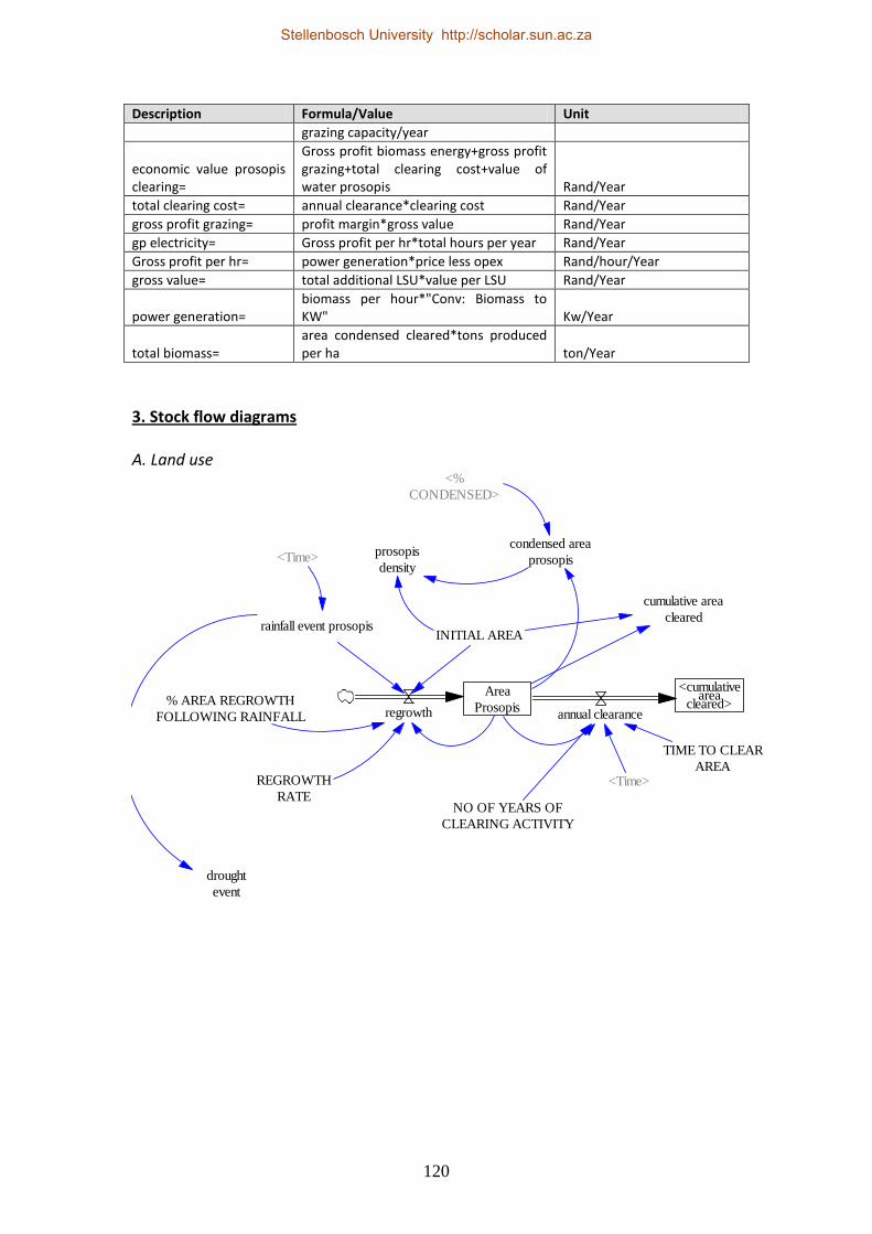
120
Description Formula/Value Unit
grazing capacity/year
economic value prosopis clearing=
Gross profit biomass energy+gross profit grazing+total clearing cost+value of water prosopis Rand/Year
total clearing cost= annual clearance*clearing cost Rand/Year
gross profit grazing= profit margin*gross value Rand/Year
gp electricity= Gross profit per hr*total hours per year Rand/Year
Gross profit per hr= power generation*price less opex Rand/hour/Year
gross value= total additional LSU*value per LSU Rand/Year
power generation= biomass per hour*"Conv: Biomass to KW" Kw/Year
total biomass= area condensed cleared*tons produced per ha ton/Year
3. Stock flow diagrams A. Land use
Area
Prosopisannual clearance
INITIAL AREA
NO OF YEARS OF
CLEARING ACTIVITY
<Time>
rainfall event prosopis
regrowth
REGROWTH
RATE
<cumulativearea
cleared>
cumulative area
cleared
% AREA REGROWTH
FOLLOWING RAINFALL
drought
event
TIME TO CLEAR
AREA
<Time>condensed area
prosopis
<%
CONDENSED>
prosopis
density
Stellenbosch University http://scholar.sun.ac.za

121
B. Grazing value
C. Clearing cost
D. Biomass electricity
CHANGE IN
GRAZING CAPACITY
total additional lsu
VALUE PER
LSU
gross value
PROFIT
MARGIN
gross profit grazing
<YEAR>
<cumulative area
cleared>
CLEARING
COST
total clearing cost
<annual
clearance>
% CONDENSED
area condensed cleared
total
biomassTONS PRODUCED
PER HA
biomass per hour
conv: biomass to
kw
power generation
price less opex
gp electricity
gross profit
biomass energy
gross profit per hr
total hours per
year
<annual
clearance>
BIOMASS
INCLUDED? Y=1
npv biomass
<DISCOUNT
RATE>
<annual
depreciation>
<financing cost
bw>
Stellenbosch University http://scholar.sun.ac.za

122
E. Water
area condensed
capital
total biomass
capital
biomass per hour
capital
power generation
capital
capital cost
CONV: KW TO
RAND
LIFESPAN OF
PLANT
annual
depreciation
<INITIAL
AREA> <TIME TO
CLEAR AREA><%
CONDENSED>
<TONS PRODUCED
PER HA>
<total hours per
year>
<conv: biomass
to kw>
financing cost bw
bond cost less
labour bw
<Time>
BOND REPAYMENT
PERIOD
PROSOPIS
WATER USE
marginal price
water
value of water
prosopis
<cumulative
area cleared>
YEARwater released
prosopis
<drought event>
WATER
INCLUDED? Y=1
Stellenbosch University http://scholar.sun.ac.za

123
F. Economics
4.3.3.3 Drakensberg model 1. Overview The Drakensberg simulation model draws heavily on an unpublished report developed for ASSET Research on the economic impact of grassland rehabilitation in the Okhombe region of KwaZulu-Natal (Crookes, 2011a). Okhombe is a communal area heavily reliant on subsistence agriculture. At the same time, grazing pressure has caused erosion of the foothills that has resulted in the soil loss and the formation of dongas. A pilot Landcare project (Everson et al., 2007) was initiated more than 10 years ago and provides an example of a payment for ecosystem services (PES) system. Community members are paid to rehabilitate degraded areas through active and passive restoration. This study considers the impact of this restoration in three areas. First, the impact of rehabilitation on improvements in grazing capacity was assessed. In a communal context, livestock provide both a wealth component and a goods and services component (Shackleton et al., 2005). The value of grazing capacity improvements as a result of rehabilitation is then the value of the marginal wealth increment as well as the value of annual livestock products (milk, meat, dung, hides, etc.) less operational costs. Second, a crucial aspect of rehabilitation in the Drakensberg is the improvements in soil stability that result. Downstream of the communal areas are several dams (such as Woodstock dam) that supply potable water to other parts of South Africa, notably Gauteng. Soil erosion from the communal areas causes siltation of dams and increases operational costs of maintenance. Soil loss was estimated using run-off data collected by community members themselves (Okhombe Monitoring Group) under the auspices of Dr Terry Everson of the University of KwaZulu-Natal (Everson, 2011a). Sediment yields were compared from before and after rehabilitation using regression relationships. The value of water improvements (R/m3) was calculated as the capital and operating cost of building and operating a dam over the estimated
<gross profit
grazing>
<gross profit
biomass energy>
<total clearing
cost>
<value of water
prosopis>
economic value prosopis
clearing
npv beaufort west
DISCOUNT
RATE
Stellenbosch University http://scholar.sun.ac.za

124
lifespan of the dam and is approximated at R4–8 per m3 over 50 years (Blignaut, 2011). A third aspect was the effect of increased soil stability on carbon storage. Percentage carbon stored in degraded, rehabilitated and pristine areas was determined from soil samples and analysed in a laboratory (Marx, 2011b). The value of carbon was estimated at R110/tonne carbon/yr (2010 values; Blignaut, 2011; based on an average price of $15/tonne carbon). Rehabilitation costs included both Working for Water costs and contractor costs (Everson, 2011b). 2. Model parameters and model equations A. Parameters used in model and units Description Formula/Value Unit Reference Comment
% of area rehabilitated= 1 Dmnl Model assumption
%C benchmark= 6.288 Dmnl Marx, 2011b
%C rehab= 1.07225 Dmnl Marx, 2011b (average)
bulk density conversion= 0.7 ton/m3 MDTP, 2007
change in gc following restoration= 0.004367 AU/hectare/Year
Own calculation based on Marx, 2011a and Everson, 2011
change in sediment volume= 0.711 m3/mm/hectare/Year
Own calculations based on Everson, 2011
contractors costs= -3380.43 rand/hectare Everson, 2011
discount rate= 0.08 1/Year Mullins et al., 2007
mean annual precipitation= 900 mm
Own calculations based on Everson, 2011
NO OF YEARS TO rehabilitate drakens= 1 Year [0,20,1] Model assumption Optimal NPV
soil volume= 5000 m3/hectare Calculation
Assumes soil depth of 50cm (Mills, 2011)
time from rehab to benchmark= 75 Dmnl Mills, 2011 (average)
Ave of range: 50-100 years
total degraded area= 90.36 hectare Bangamwabo, 2009 Bare soil.
unit price of carbon= 110 rand/ton/Year
Blignaut, 2011 (based on ave price of $15/tC
unit value livestock drakensberg= 2431.88 rand/AU
Own calculations based on Everson et al., 2007; Tau, 2011; Salomon, 2006 and Shackleton et al. 2005
unit value of 6 rand/m3 Blignaut, 2011 Ave. unit
Stellenbosch University http://scholar.sun.ac.za

125
Description Formula/Value Unit Reference Comment
water displaced=
value of water displaced, capital and operating cost over 50 years
working for water costs= -20810.5 rand/hectare Everson, 2010.
B. Equations Description Formula/Value Unit
annual area rehabilitated=
IF THEN ELSE(Time<2010+NO OF YEARS TO rehabilitate drakens,AREA rehabilitated drakens/NO OF YEARS TO rehabilitate drakens,0) hectare/Year
annual change in %C following rehabilitation=
("%C benchmark"-"%C rehab")/time from rehab to benchmark Dmnl
AREA rehabilitated drakens= % of area rehabilitated*total degraded area hectare
cumulative area rehabilitated= INTEG ( annual area rehabilitated, 0) hectare
cumulative change in gc=
cumulative area rehabilitated*change in gc following restoration AU/Year
economic value drakensberg=
livestock benefit drakensberg+soil stabilisation benefit+total rehabilitation costs Drakensberg+value of carbon benefit rand/Year
livestock benefit drakensberg=
unit value livestock drakensberg*cumulative change in gc rand/Year
npv drakensberg= NPV(economic value drakensberg,discount rate,0,1) rand
per hectare change in sediment volume=
change in sediment volume*mean annual precipitation m3/hectare/Year
rehabilitation costs per ha= contractors costs+working for water costs rand/hectare
soil stabilisation benefit=
unit value of water displaced*total change in sediment volume following rehabilitation rand/Year
tonnes carbon drakensberg=
tonnes carbon per ha*cumulative area rehabilitated Ton
tonnes carbon per ha= annual change in %C following rehabilitation*tonnes soil per hectare/100 ton/hectare
tonnes soil per hectare= soil volume*bulk density conversion ton/hectare
total change in sediment volume following rehabilitation=
cumulative area rehabilitated*per hectare change in sediment volume m3/Year
total rehabilitation costs Drakensberg=
annual area rehabilitated*rehabilitation costs per ha rand/Year
value of carbon benefit=
unit price of carbon*tonnes carbon drakensberg rand/Year
Stellenbosch University http://scholar.sun.ac.za

126
3. Stock flow diagrams A. Land use
B. Grazing capacity
area rehabilitated
drakens
NO OF YEARS TO
REHABILITATE
DRAKENS
Cumulative Area Rehabi
litatedannual area
rehabilitated
<Time>
TOTAL
DEGRADED AREA
% OF AREA
REHABILITATED
CHANGE IN GCFOLLOWING
RESTORATION
<Cumulative Area
Rehabilitated>
cumulative change
in gc
Stellenbosch University http://scholar.sun.ac.za

127
C. Soil stabilisation
D. Carbon storage
E. Clearing costs
CHANGE IN
SEDIMENT VOLUME
MEAN ANNUAL
PRECIPITATION
per hectare change in
sediment volume
<Cumulative Area
Rehabilitated>
total change in sediment
volume following
rehabilitation
tonnes soil per
hectare
SOIL VOLUME BULK DENSITY
CONVERSION
annual change in %c following
rehabilitation
tonnes carbon per ha
%C
BENCHMARK
%C REHAB
TIME FROM REHAB
TO BENCHMARK
<Cumulative Area
Rehabilitated>
tonnes carbon
drakensberg
WORKING FOR
WATER COSTS
CONTRACTORS
COSTS
rehabilitation costs
per ha
<annual area
rehabilitated>
total rehabilitation costs
drakensberg
Stellenbosch University http://scholar.sun.ac.za

128
F. Economics
4.3.3.4 Namaqualand model 1. Overview This case study focuses on the impacts of rehabilitation following heavy mineral mining at Brand-se-Baai on the West Coast of South Africa and northwest of the town of Vredendal (Pauw, 2011a). Rehabilitation is costly (Mugido and Kleynhans, 2011). The availability of data regarding the impact of different rehabilitation methods at different sites enabled a comparison of the various financial and economic benefits of restoration (namely, the value of grazing improvements and carbon storage). It was evident from the study that grazing capacity did improve following restoration. However, restoration did not result in complete recovery compared to the un-mined area, and consequently there is an unmitigated loss component associated with mining activity. The seven sites and treatments applied were (Pauw, 2011a):
1. Reference site R1, no mining, lightly grazed by wild animals. 2. Reference site R2, no mining, situated on a sheep farm and periodically
grazed at a high stocking rate. 3. Rehabilitation site S1, involves the placing of topsoil over the tailings. 4. Rehabilitation site S2, seed treatment over bare tailings. 5. Rehabilitation site S3, topsoil treatment and translocation of indigenous
species. 6. Rehabilitation site S4, seed treatment and translocation of indigenous
species.
<cumulative
change in gc>
UNIT VALUELIVESTOCK
DRAKENSBERG
<total change in sedimentvolume following
rehabilitation>
livestock benefit
drakensberg
UNIT VALUE OF
WATER DISPLACED
soil stabilisation benefit
<tonnes carbon
drakensberg>UNIT PRICE OF
CARBON
value of carbon benefit
<total rehabilitation
costs drakensberg>economic value
drakensberg
npv drakensberg
DISCOUNT
RATE
Stellenbosch University http://scholar.sun.ac.za

129
7. Rehabilitation site S5, topsoil treatment, seed treatment and translocation. Most of the rehabilitation occurred in 2001/2 with the exception of site S5 (rehabilitated in 2008), which was consequently omitted from the simulation model. 2. Model parameters and model equations A. Parameters used in model and units Description Formula/Value Unit Reference Comment
s1 unmitigated loss= -0.0135 LSU/hectare
Own calculation based on Pauw, 2011c
S2 seed gc= 0.000342 LSU/hectare Pauw, 2011c.
s2 unmitigated loss= -0.01797 LSU/hectare
Own calculation based on Pauw, 2011c.
s3 cost= 62399 Rand/hectare
Own calculation based on Mugido and Kleynhans, 2011
s4 seed + translocation gc= 0.000989 LSU/hectare Pauw, 2011c.
carbon value= 1 Dmnl Policy switch 1=yes
s4 cost= 43724 Rand/hectare
Own calculation based on Mugido and Kleynhans, 2011
discount rate= 0.08 1/Year Mullins et al., 2007
economic contribution mining= 2.80E+08 Rand/Year
Mugido and Kleynhans, 2011
s4 unmitigated loss= -0.01344 LSU/hectare
Own calculation based on Pauw, 2011c.
private benefit mining= 1 Dmnl Policy switch 1=yes
S1 topsoil gc= 0.000981 LSU/hectare Pauw, 2011c.
s2 cost= 54330 Rand/hectare
Own calculation based on Mugido and Kleynhans, 2011
s1 cost= 52170 Rand/hectare
Own calculation based on Mugido and Kleynhans, 2011
umitigated loss?= 1 Dmnl Policy switch 1=yes
s3 topsoil + translocation gc= 0.001427 LSU/hectare Pauw, 2011c
s3 unmitigated loss= -0.01038 LSU/hectare
Own calculation based on Pauw, 2011c
%C benchmark= 0.856667 Dmnl Pauw, 2011c
AREA rehabilitated Namaqualand= 2619 hectare
Area of mine (4770ha, Pauw, 2011b) less area already rehabilitated (2151ha Mugido and Kleynhans, 2011)
Potential area still to be mined by Namaqualand
bulk density conversion= 0.7 ton/m3 MDTP, 2007
Stellenbosch University http://scholar.sun.ac.za

130
Description Formula/Value Unit Reference Comment
NO OF YEARS TO rehabilitate Namaqualand= 10 Year [0,20,1] Assumption
Just under half the area of the total mine was rehabilitated (see under area rehabilitated constant) in the first 9 years of rehabilitation (Pauw, 2011a)
R/ton carbon= 110 Rand/ton/Year Blignaut, 2011 (based on ave price of $15/tC
S yes ex= 1 Dmnl Policy variable
Value between 0 and 1 representing relative share of each treatment
s+t yes= 1 Dmnl Policy variable
Value between 0 and 1 representing relative share of each treatment
s1 net sheep value per lsu= 10788.7 Rand/LSU/Year
Own calculations based on Mugido, 2011b
s2 net sheep value per lsu= 265.86 Rand/LSU/Year
Own calculations based on Mugido, 2011b
s3 net sheep value per lsu= 18825.1 Rand/LSU/Year
Own calculations based on Mugido, 2011b
s4 net sheep value per lsu= 21855.1 Rand/LSU/Year
Own calculations based on Mugido, 2011b
soil volume= 5000 m3/hectare Calculation
Assumes soil depth of 50cm (Mills, 2011)
T yes= 1 Dmnl Policy variable
Value between 0 and 1 representing relative share of each treatment
t+t yes= 1 Dmnl Policy variable
Value between 0 and 1 representing relative share of each treatment
time from rehab to benchmark= 75 Dmnl Mills, 2011 (average)
Ave of range: 50-100 years
B. Equations
Description Formula/Value Unit
% C rehab s2= 0.185833*S yes ex Dmnl
%C rehab S1= 0.3175*T yes Dmnl
Stellenbosch University http://scholar.sun.ac.za

131
Description Formula/Value Unit
%C rehab S3= 0.1425*"t+t yes" Dmnl
%C rehab S4= 0.165833*"s+t yes" Dmnl
s2 seeded= S yes ex*s2 cost Rand/hectare
s3 grazing value= s3 net sheep value per lsu*"s3 topsoil + translocation gc"*"t+t yes" Rand/hectare/Year
average unmitigated loss R/ha=
(T yes*s1 net sheep value per lsu*s1 unmitigated loss+S yes ex*s2 net sheep value per lsu*s2 unmitigated loss+"t+t yes"*s3 net sheep value per lsu*s3 unmitigated loss+"s+t yes"*s4 net sheep value per lsu*s4 unmitigated loss)/(T yes+S yes ex+"t+t yes"+"s+t yes") Rand/hectare/Year
s3 topsoil + translocation= s3 cost*"t+t yes" Rand/hectare
s4 grazing value= s4 net sheep value per lsu*"s4 seed + translocation gc"*"s+t yes" Rand/hectare/Year
net economic value Namaqualand=
annual rehabilitation cost Namaqualand+economic value carbon Namaqualand*carbon value+sheep net grazing value Namaqualand+economic contribution mining*private benefit mining+"umitigated loss?"*unmitigated loss from mining Rand/Year
npv Namaqualand= NPV(net economic value Namaqualand,discount rate,0,1) Rand
s1 grazing value= s1 net sheep value per lsu*S1 topsoil gc*T yes Rand/hectare/Year
unmitigated loss from mining=
average unmitigated loss R/ha*cumulative area rehabilitated Namaqualand Rand/Year
S1 topsoil= s1 cost*T yes Rand/hectare
s2 grazing value= s2 net sheep value per lsu*S2 seed gc*S yes ex Rand/hectare/Year
s4 seeded + translocation= s+t yes*s4 cost Rand/hectare
annual area rehabilitated Namaqualand=
IF THEN ELSE(Time<2010+NO OF YEARS TO rehabilitate Namaqualand,AREA rehabilitated Namaqualand/NO OF YEARS TO rehabilitate Namaqualand,0) hectare/Year
annual change in %C following rehabilitation=
(("%C benchmark"-"%C rehab S1")/time from rehab to benchmark+("%C benchmark"-"% C rehab s2")/time from rehab to benchmark+("%C benchmark"-"%C rehab S3")/time from rehab to benchmark+("%C benchmark"-"%C rehab S4")/time from rehab to benchmark)/(S yes ex+"s+t yes"+T yes+"t+t yes") Dmnl
annual rehabilitation cost Namaqualand=
-average rehabilitation cost Namaqualand*annual area rehabilitated Namaqualand Rand/Year
Stellenbosch University http://scholar.sun.ac.za

132
Description Formula/Value Unit
average change in sheep grazing value=
(s1 grazing value+s2 grazing value+s3 grazing value+s4 grazing value)/(S yes ex+"s+t yes"+T yes+"t+t yes") Rand/hectare/Year
average rehabilitation cost Namaqualand=
("s4 seeded + translocation"+S1 topsoil+s2 seeded+"s3 topsoil + translocation")/("s+t yes"+T yes+S yes ex+"t+t yes") Rand/hectare
cumulative area rehabilitated Namaqualand=
INTEG (Annual area rehabilitated Namaqualand, 0) hectare
economic value carbon Namaqualand=
R/ton carbon*tonnes carbon Namaqualand Rand/Year
sheep net grazing value Namaqualand=
cumulative area rehabilitated Namaqualand*average change in sheep grazing value Rand/Year
tonnes carbon Namaqualand=
Tonnes carbon per ha*cumulative area rehabilitated Namaqualand ton
tonnes carbon per ha=
annual change in %C following rehabilitation*tonnes soil per hectare/100 ton/hectare
tonnes soil per hectare= soil volume*bulk density conversion ton/hectare
3. Stock flow diagrams A. Land use
AREA
REHABILITATED
EXXARO
NO OF YEARS TO
REHABILITATE
EXXARO
CumulativeArea
RehabilitatedExxaroannual area
rehabilitated exxaro
<Time>
Stellenbosch University http://scholar.sun.ac.za

133
B. Grazing capacity
C. Rehabilitation costs
sheep net grazing
value exxaro
s3 topsoil +
translocation gc
s4 seed +
translocation gc
s1 topsoil gc
average change in
sheep grazing values2 seed gc
<T YES>
<S YES EX>
<T+T YES>
<S+T YES>
S1 NET SHEEP
VALUE PER LSU
S2 NET SHEEP
VALUE PER LSU
S3 NET SHEEP
VALUE PER LSU
S4 NET SHEEP
VALUE PER LSU
s1 grazing value
s2 grazing value
s3 grazing value
s4 grazing value
<Cumulative Area
Rehabilitated Exxaro>
s2 seeded
s3 topsoil +
translocations4 seeded +
translocation
average rehabilitation
cost exxaro
annual rehabilitation
cost exxaro
s1 topsoil
T YES
S YES EX
T+T YES
S+T YES
<annual area
rehabilitated exxaro>S1 COST
S2 COST
S3 COST
S4 COST
Stellenbosch University http://scholar.sun.ac.za

134
D. Carbon
D. Unmitigated loss
tonnes soil per
hectare
SOIL VOLUME
BULK DENSITY
CONVERSION
annual change in %c
following rehabilitation
tonnes carbon
per ha
%C
BENCHMARK
%c rehab s1
TIME FROM REHAB
TO BENCHMARK
tonnes carbon
exxaro
% c rehab s2
%c rehab s3
%c rehab s4
<T YES>
<S YES EX>
<T+T YES>
<S+T YES>
<Cumulative Area
Rehabilitated Exxaro>
R/TON
CARBON
economic value carbon
exxaro
<Cumulative Area
Rehabilitated Exxaro>
<S YES EX><S+T YES>
<T YES>
<T+T YES>
<S1 NET SHEEP
VALUE PER LSU>
<S2 NET SHEEP
VALUE PER LSU>
<S3 NET SHEEP
VALUE PER LSU>
<S4 NET SHEEP
VALUE PER LSU>
S1 UNMITIGATED
LOSS
S2 UNMITIGATED
LOSS
S3 UNMITIGATED
LOSS
S4 UNMITIGATED
LOSSaverage
unmitigated lossr/ha
unmitigated loss from
mining
Stellenbosch University http://scholar.sun.ac.za

135
E. Economics
4.3.3.5 Kromme model 1. Overview The benefits from restoration in the Kromme model consider two aspects:
1) Improvements in water yield resulting from the removal of invasive alien plants (IAPs)
2) Improvements in water quality resulting from restoring wetland function in the catchment.
A. Water yield Water yield improvements resulting from clearing IAPs is variable depending on the nature of the landuse that the land is subsequently used for (Table 38). In this study, two landuse scenarios are utilised: 1) Firstly assuming that restoration of landuse that is not in the riparian zone reverts to agriculture (‘agriculture’ scenario); 2) Assuming that the restoration of the landuse not in the riparian zone reverts to natural vegetation (‘no agriculture’ scenario). The model assumes that 90 percent of the invasion is in the riparian zone. All restoration in riparian zone reverts to natural vegetation.
<annual rehabilitation
cost exxaro>
<economic value
carbon exxaro>
<sheep net grazing
value exxaro>
net economic value
exxaro
ECONOMICCONTRIBUTION
MININGnpv exxaro
DISCOUNT
RATE
PRIVATE
BENEFIT MINING
CARBON
VALUE
<unmitigated loss
from mining>UMITIGATED
LOSS?
Stellenbosch University http://scholar.sun.ac.za

136
Table 38 Net water yield gain from restoration for different land use categories
Land use ET Gain in ET from restoration Irrigation abs Net run-off gain
mm/a mm/a mm/a mm/a m3/ha
Palmiet wetland 1 0601 440 440 4 400
Other riparian 1 3001 200 200 2 000
Fynbos 6001 660 660 6 600
Irrigated 6491 611 2004 411 4 110
Dryland (pastures) 5501 710 1694 541 5 410
Orchard 9121 348 2814 67 670
IAPs – riparian 1 5002
IAPs - non-riparian 1 2603 References: 1 Rebelo (2011)
2 Dye and Jarmain (2004)
3 Dye et al. (2001)
4 Field edge irrigation requirement for typical mix of crops (fruit, pasture, vegetables) is 650 mm/a
(DWAF, 2002), allocated as weighted average of crop category ET.
B. Water quality There is a negative relationship between wetland area and time (Table 39, equation 1). In other words, wetland area decreases over time. Although the degrees of freedom are low in this equation, the correlation coefficient is so high that the relationship is almost linear. At the same time, water treatment costs increase over time (equation 2). There are a number of reasons why treatment costs may increase (Gull, 2012a), but for the water quality component of the study it is assumed that the dominant cause of treatment cost increases is due to the decline in wetland area. The link between wetland area and savings in water treatment costs is fairly well-established in the literature (e.g. Heal, 2000; Farber et al., 2006; Barbier, 2007; De Wit et al., 2009) and represents only one aspect of the value of watershed services. Table 39 Regression equations for water quality
Dependent var
Intercept
s.e.
Independent variable
s.e.
N
Adj R2
Wetland area1 =
6.65*** 0.11 -0.29 Time** 0.04 4 0.9521
Treatment cost2 =
11.21*** 0.38 0.43 Time** 0.16 21 0.2392
References: 1 Data from Rebelo (2012b)
2 Data from Gull (2011a)
*** Significant at 1% level
** Significant at 5% level
Stellenbosch University http://scholar.sun.ac.za

137
All variables are logged and therefore indicate percentage change. In Table 39, time is the independent variable in both regression equations. It is therefore possible to solve the simultaneous equations by eliminating time, and expressing treatment costs as a function of wetland area. Solving these equations gives: ln T = 21.09 – 1.48 ln W Where T is treatment costs, measured in Rands, and W is wetland area, measured in hectares. The coefficient on wetland area is the treatment elasticity and implies that a 1% increase in wetland area results in a 1.48% decrease in treatment costs. The maximum treatment cost was R625 940.17 in 2007 (Gull, 2011a). Converting this to 2010 prices assuming a 5% inflation rate gives R724 604. Divided by the area of farmland (3 323 ha) (Rebelo, 2012b) gives the treatment costs per hectare of farmland (218.063 R/ha), which is used in the model to estimate the increase in treatment cost as a result of the expansion of agriculture. These costs represent the maximum potential benefit from water quality improvements as a result of the restoration of wetland areas in the Kromme catchment. 2. Model parameters and model equations A. Parameters used in model and units Description Formula/Value Unit Reference Comment
maintenance? (Y=1)= 1 Dmnl Policy variable Switch (1=yes)
regrowth rate= 0.1 1/Year [0,50] Model assumption
conv rate= 1 Year Model assumption
% fynbos= 0.088132 Dmnl
Own calculations based on Rebelo, 2012b
Distribution of IAPs assuming 90% of invasion riparian
% irrigated= 0.003112 Dmnl
Own calculations based on Rebelo, 2012b
Distribution of IAPs assuming 90% of invasion riparian
% orchard= 0.000355 Dmnl
Own calculations based on Rebelo, 2012b
Distribution of IAPs assuming 90% of invasion riparian
% other riparian= 0.618107 Dmnl
Own calculations based on Rebelo, 2012b
Distribution of IAPs assuming 90% of invasion riparian
% palmiet wetland= 0.281893 Dmnl
Own calculations based on Rebelo, 2012b
Distribution of IAPs assuming 90% of invasion riparian
% pastures= 0.0084 Dmnl
Own calculations based on Rebelo, 2012b
Distribution of IAPs assuming 90% of invasion riparian
annual clearing cost per ha Kromme= 10355.5 Rand/hectare
Own calculations based on Gull, 2012a
Department of Water Affairs data (Table 16) divided by condensed area
Stellenbosch University http://scholar.sun.ac.za

138
Description Formula/Value Unit Reference Comment
(Table 20) 2010 values
Discount rate= 0.08 1/Year Mullins et al., 2007
gm irrigated= 447.56 Rand/hectare
Own calculations based on Gull, 2011b and Rebelo, 2012b
gm orchards= 1807.18 Rand/hectare
Own calculations based on Gull, 2011b and Rebelo, 2012b
gm pastures= 841.28 Rand/hectare
Own calculations based on Gull, 2011b and Rebelo, 2012b
inital area palmiet= 227.504 hectare Rebelo, 2012b
percentage loss to agric per year= 0 1/Year Model assumption
This implies that all all restored land is converted to natural vegetation and not farmland
water treatment costs= 724604 Rand/Year Calculation. See Appendix F
treatment elasticity= 1.48446 Dmnl Calculation. See Appendix F
yield orchards= 670 m3/hectare Calculation. See Table x
Value of unit of water= 1.42 Rand/m3 Gull, 2011b.
Opportunity cost (ave.incremental cost) of water
yield fynbos= 6600 m3/hectare Calculation. See Table x
water treatment costs per hectare= 218.063 Rand/hectare Calculation. See Appendix F
yield pastures= 5410 m3/hectare Calculation. See Table x
yield irrigated= 4110 m3/hectare Calculation. See Table x
yield palmiet wetland= 4400 m3/hectare Calculation. See Table x
yield riparian= 2000 m3/hectare Calculation. See Table x
INITIAL AREA Kr= 4640 hectare Rebelo, 2012b
NO OF YEARS TO CLEAR ALIENS KR= 1 Year [0,50,1] Model assumption
Value that maximises NPV
B. Equations
Description Formula/Value Unit
annual clearance Kr=
IF THEN ELSE("maintenance? (Y=1)"=1,IF THEN ELSE(Area Aliens Kr<=10,"maintenance? (Y=1)"*regrowth,IF THEN ELSE(Time<2010+NO OF YEARS TO CLEAR ALIENS KR,INITIAL AREA Kr/NO OF YEARS TO CLEAR ALIENS KR+regrowth,0)),IF THEN ELSE(Time<2010+NO OF YEARS TO hectare/Year
Stellenbosch University http://scholar.sun.ac.za

139
Description Formula/Value Unit
CLEAR ALIENS KR,INITIAL AREA KrNO OF YEARS TO CLEAR ALIENS KR+regrowth,0))
additional land released= (INITIAL AREA Kr-Area Aliens Kr)/conv rate hectare/Year
total yield gain water=
area fynbos*yield fynbos+area irrigated*yield irrigated+area orchard*yield orchards+area palmiet*yield palmiet wetland+area pastures*yield pastures+area riparian*yield riparian m3/Year
value of agriculture=
gm irrigated*area irrigated+gm orchards*area orchard+gm pastures*area pastures Rand/Year
increase in costs due to expansion of agric=
(area irrigated+area orchard+area pastures)*water treatment costs per hectare Rand/Year
Area Aliens Kr= INTEG (regrowth-annual clearance Kr, INITIAL AREA Kr) hectare
regrowth= (INITIAL AREA Kr-Area Aliens Kr)*regrowth rate hectare/Year
% change in wetland area=
IF THEN ELSE(((inital area palmiet+total area palmiet)/inital area palmiet-1)*100<67.3647,((inital area palmiet+total area palmiet)/inital area palmiet-1)*100,67.3647) Dmnl
% saving in treatment costs=
% change in wetland area*treatment elasticity/100 Dmnl
annual loss to agric= loss palmiet+loss riparian hectare/Year
area fynbos= % fynbos*additional land released hectare/Year
area irrigated=
% irrigated*annual clearance Kr+"% irrigated"/("% irrigated"+"% orchard"+"% pastures")*annual loss to agric hectare/Year
area orchard=
% orchard*additional land released+"% orchard"/("% irrigated"+"% orchard"+"% pastures")*annual loss to agric hectare/Year
area palmiet= % palmiet wetland*additional land released hectare/Year
area pastures=
% pastures*additional land released+"% pastures"/("% irrigated"+"% orchard"+"% pastures")*annual loss to agric hectare/Year
area riparian= % other riparian*additional land released hectare/Year
clearing cost kromme= annual clearance Kr*annual clearing cost per ha Kromme Rand/Year
Total palmiet loss= INTEG (loss palmiet, 0) hectare
loss palmiet= percentage loss to agric per year*total area palmiet hectare/Year
loss riparian= percentage loss to agric per year*Total area riparian hectare/Year
npv kromme= NPV(total economic value kromme,discount rate,0,1) Rand
saving in water treatment costs due to wetland=
% saving in treatment costs*water treatment costs Rand/Year
Total Area Fynbos= INTEG (area fynbos, 0) hectare
Total area Irrigated= INTEG (area irrigated, 0) hectare
total area orchard= INTEG (area orchard, 0) hectare
total area palmiet= INTEG (area palmiet-loss palmiet, 0) hectare
Stellenbosch University http://scholar.sun.ac.za

140
Description Formula/Value Unit
total area pastures= INTEG (area pastures, 0) hectare
Total area riparian= INTEG (area riparian-loss riparian, 0) hectare
total economic value kromme=
value of agriculture+Value of gain in water yield+value of net saving in treatment costs-clearing cost kromme Rand/Year
total riparian loss= INTEG (loss riparian, 0) hectare
Value of gain in water yield= Value of unit of water*total yield gain water Rand/Year
value of net saving in treatment costs=
saving in water treatment costs due to wetland-increase in costs due to expansion of agric Rand/Year
3. Stock flow diagrams A. Land use
B. Agriculture
Area Aliens
Krannual clearance kr
INITIAL AREA KR
NO OF YEARS TO
CLEAR ALIENS KR
<Time>
% PALMIET
WETLAND
% OTHER
RIPARIAN
% IRRIGATED
% PASTURES% ORCHARD
Area
Orchardrate orch
Area
Pasturesrate past
Total Area
Palmietarea palmiet
Total Area
Riparianarea riparian
AreaFynbos
Krommerate fyn
Area
Irrigatedrate irr
TotalRiparian
Lossloss riparian
TotalPalmietLoss
loss palmiet PERCENTAGE LOSS
TO AGRIC PER YEAR
annual loss to agric
<annual loss to
agric>
INITAL AREA
PALMIET
% change in
wetland area
% FYNBOS
regrowth kr
REGROWTH
RATE
additional land
released
CONV RATE
MAINTENANCE?
(Y=1)mass balance
check
<Time>
<Time>
<Time>
GM IRRIGATED
GM PASTURES
GM
ORCHARDS
value of agriculture
<area irrigated>
<area pastures><area orchard>
Stellenbosch University http://scholar.sun.ac.za

141
C. Water
D. Clearing costs
E. Economics
YIELDORCHARDS
YIELDIRRIGATED
YIELD
PASTURES
YIELDPALMIET
WETLAND
YIELD
RIPARIAN
YIELD FYNBOS
total yield gain
water
Water yield
Water quality
<% change in
wetland area>TREATMENT
ELASTICITY
% saving in treatment
costs
VALUE OF UNIT
OF WATER
value of gain in water
yield
WATER
TREATMENT COSTS
saving in water treatment
costs due to wetland
WATER TREATMENT
COSTS PER HECTARE
increase in costs due to
expansion of agric
value of net saving in
treatment costs
<Total Area
Palmiet>
<Total Area
Riparian>
<Area Fynbos
Kromme>
<Area Irrigated>
<Area Orchard>
<Area Pastures>
<Area Irrigated><Area Orchard><Area Pastures>
ANNUAL CLEARINGCOST PER HA
KROMME
<annual
clearance kr>
clearing cost kromme
<value of
agriculture>
<value of gain in
water yield>
<value of net saving in
treatment costs>
<clearing cost
kromme>
total economic value
kromme
npv kromme
DISCOUNT
RATE
Stellenbosch University http://scholar.sun.ac.za
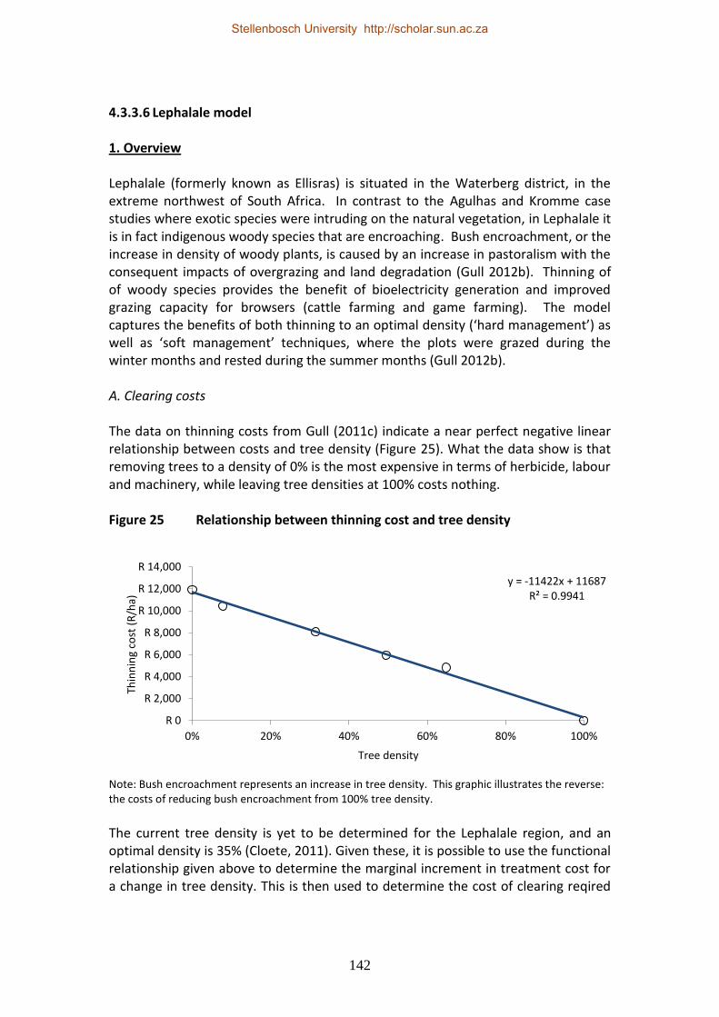
142
4.3.3.6 Lephalale model 1. Overview Lephalale (formerly known as Ellisras) is situated in the Waterberg district, in the extreme northwest of South Africa. In contrast to the Agulhas and Kromme case studies where exotic species were intruding on the natural vegetation, in Lephalale it is in fact indigenous woody species that are encroaching. Bush encroachment, or the increase in density of woody plants, is caused by an increase in pastoralism with the consequent impacts of overgrazing and land degradation (Gull 2012b). Thinning of of woody species provides the benefit of bioelectricity generation and improved grazing capacity for browsers (cattle farming and game farming). The model captures the benefits of both thinning to an optimal density (‘hard management’) as well as ‘soft management’ techniques, where the plots were grazed during the winter months and rested during the summer months (Gull 2012b). A. Clearing costs The data on thinning costs from Gull (2011c) indicate a near perfect negative linear relationship between costs and tree density (Figure 25). What the data show is that removing trees to a density of 0% is the most expensive in terms of herbicide, labour and machinery, while leaving tree densities at 100% costs nothing. Figure 25 Relationship between thinning cost and tree density
Note: Bush encroachment represents an increase in tree density. This graphic illustrates the reverse: the costs of reducing bush encroachment from 100% tree density.
The current tree density is yet to be determined for the Lephalale region, and an optimal density is 35% (Cloete, 2011). Given these, it is possible to use the functional relationship given above to determine the marginal increment in treatment cost for a change in tree density. This is then used to determine the cost of clearing reqired
y = -11422x + 11687 R² = 0.9941
R 0
R 2,000
R 4,000
R 6,000
R 8,000
R 10,000
R 12,000
R 14,000
0% 20% 40% 60% 80% 100%
Thin
nin
g co
st (
R/h
a)
Tree density
Stellenbosch University http://scholar.sun.ac.za

143
to reach the optimal tree density (assuming the current tree density exceeds the optimal tree density). B. Biomass electricity Average tree density in time period t is related to Evapotranspiration Tree Equivalents (ETTE) as follows: Densityt,i = ETTEt,i/ETTEt,100 Where ETTEt,i = Evapotranspiration Tree Equivalents for plot i in time period t, ETTEt,100 = Evapotranspiration Tree Equivalents for the 100% density plot in
time period t = 11 382 (Cloete, 2011)
Therefore, ETTEt,i = Densityt,i * 11 382 The annual increment in ETTE above the optimal density of 35% represents:
the annual growth in tree density year-on-year
the annual maintenance that is required to keep the tree density at the optimal
the additional above ground dry matter that is available each year to provide fuel for the biomass generator
To calculate the annual increment in ETTE, ETTE estimates for 1991 are compared with ETTE estimates for 2008 in order to determine the average annual growth (Table 40). Table 40 Tree density and Evapotranspiration Tree Equivalent data
Density1991 ETTE1991 ETTE2008
0% - 4 210.16
8% 894.8 3 717.7
31% 3 585 6 068.54
50% 5 638.5 10 916.54
65% 7 379 8 838.18
100% 11 382 10 207.93
Source: Cloete (2011) The relationship between ETTE1991 and Density1991 is a simple arithmetic calculation, as indicated above. The relationship between ETTE2008 and Density1991 may be calculated using regression analysis (Figure 26).
Stellenbosch University http://scholar.sun.ac.za
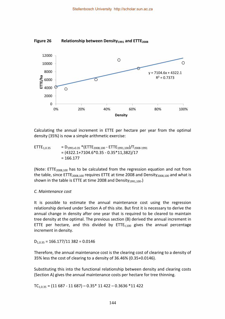
144
Figure 26 Relationship between Density1991 and ETTE2008
Calculating the annual increment in ETTE per hectare per year from the optimal density (35%) is now a simple arithmetic exercise: ETTE1,0.35 = D1991,0.35 *(ETTE2008,100 - ETTE1991,100)/T2008-1991
= (4322.1+7104.6*0.35 - 0.35*11,382)/17 = 166.177
(Note: ETTE2008,100 has to be calculated from the regression equation and not from the table, since ETTE2008,100 requires ETTE at time 2008 and Density2008,100 and what is shown in the table is ETTE at time 2008 and Density1991,100.) C. Maintenance cost It is possible to estimate the annual maintenance cost using the regression relationship derived under Section A of this site. But first it is necessary to derive the annual change in density after one year that is required to be cleared to maintain tree density at the optimal. The previous section (B) derived the annual increment in ETTE per hectare, and this divided by ETTEt,100 gives the annual percentage increment in density. D1,0.35 = 166.177/11 382 = 0.0146 Therefore, the annual maintenance cost is the clearing cost of clearing to a density of 35% less the cost of clearing to a density of 36.46% (0.35+0.0146). Substituting this into the functional relationship between density and clearing costs (Section A) gives the annual maintenance costs per hectare for tree thinning. TC1,0.35 = (11 687 - 11 687) – 0.35* 11 422 – 0.3636 *11 422
y = 7104.6x + 4322.1 R² = 0.7373
0
2000
4000
6000
8000
10000
12000
0% 20% 40% 60% 80% 100%
ETTE
/ha
Density
Stellenbosch University http://scholar.sun.ac.za

145
= 0 – (-0.0146) * 11 422 = 167 (R/ha) D. Grazing capacity As indicated in Section A of the Lephalale model description, data on the current tree density for the study area was not available at the time of the model development. The approach used was to develop a model that relates grazing capacity with tree density, and then use the model to solve for initial tree density. The equation that provided the best fit for the data was the logistic equation:
ttt xbxbxbbte
ky
33221101
(1)
Where Yt = the grazing capacity in time t measured in LSU/hectare k = the carrying capacity, measured in LSU/hectare x1t = dummy variable to reflect nature of restoration activities (0=active; 1=passive) x2t = mean annual rainfall in time t, measured in millimetres x3t = tree density expressed as a percentage Regression results are as follows:
b0 Sig b1 Sig b2 Sig b3 Sig n Adj R2
4.052 *** -2.405
*** -0.005
*** 1.147 ***
24 0.782559
(0.634)
(0.300)
(0.001)
(0.256)
*** Significant at the 1% level
Standard errors in parenthesis below each coefficient
Solving for tree density in equation (1) gives
3
22110
3
)ln(
b
XbXbbY
Yk
X
ttt
t
t
Where
tX 3 = equilibrium tree density
tY = long-term stocking rate
tX 2 = the long-term mean rainfall
Stellenbosch University http://scholar.sun.ac.za

146
2. Model parameters and model equations A. Parameters used in model and units Description Formula/Value Unit Reference Comment
long term stocking rate= 0.05 Dmnl
Schmidt et al., 1995
soft management (y=1)= 1 Dmnl Policy switch 1=yes
grazing= 1 LSU/hectare Assumption Best model fit
long term mean rainfall= 400 Dmnl Cloete, 2011
Average over 20 years (1991 - 2010)
lifespan of plant= 50 Dmnl Assumption Model time period
annual increment in tree density no maintenance= 0.0146 1/Year Calculation See Appendix G
Area of study site= 924920 hectare Gull, 2011c Municipal
coeff clearing costs= -11422.4 Rand/hectare/Year Calculation See Appendix G
coeff ette= 11382 ETTE/hectare Cloete, 2011
Evapotranspiration Tree Equivalents for 100% plot
conv ETTE to biomass= 0.002 ton/ETTE Cloete, 2011
Amount of above ground dry matter that can be removed per unit ETTE
Conv: Biomass to KW= 900 Kw/ton*hour Fourie, 2011 ton/hour to KW
conv: Kw to Rand= 15000 Rand/Kw Fourie, 2011
Biomass electricity? Y=1= 1 Dmnl Policy switch 1=yes
delay before benefits experienced= 1 Year Assumption
DISCOUNT RATE= 0.08 1/Year Mullins et al., 2007
GM R/LSU game= 9633.8 Rand/LSU/Year
Own calculations based on Gull 2011c
GM/LSU livestock= 6684.08 Rand/LSU/Year Gull, 2011c
maintenance cost= 167 Rand/hectare/Year Calculation See Appendix G
maintenance ette= 166.177 ETTE/hectare Calculation See Appendix G
MAINTENANCE? Y=0= 0 Dmnl Policy switch
optimal tree density= 0.35 Dmnl Cloete, 2011
Stellenbosch University http://scholar.sun.ac.za

147
Description Formula/Value Unit Reference Comment
Percentage livestock= 0.2 Dmnl Smit, 2011
price less opex= 0.581 Rand/Kw/hour Gull, 2011c
total hours per year= 8760 hour
Calculation (365x24)
B. Equations
Description Formula/Value Unit
Gross margin livestock=
IF THEN ELSE (Time < 2010 + delay before benefits experienced, 0, "GM/LSU livestock"*gain in grazing capacity*area livestock/(1+"soft management (y=1)")) Rand/Year
gross margin game=
IF THEN ELSE (Time < 2010 + delay before benefits experienced, 0, area game*gain in grazing capacity*"GM R/LSU game"/(1+"soft management (y=1)")) Rand/Year
Optimal Grazing capacity=
grazing/(1+EXP(4.05245-2.40525*"soft management (y=1)"-0.00487948*long term mean rainfall+1.14684*(optimal tree density+"MAINTENANCE? Y=0"*cumulative increment in tree density))) LSU/hectare
Initial grazing capacity=
grazing/(1+EXP((4.05245-2.40525*"soft management (y=1)"-0.00487948*long term mean rainfall+1.14684*initial tree density))) LSU/hectare
initial tree density=
(LN((1-long term stocking rate)/long term stocking rate)-4.05245+2.40525*0+0.00487948*long term mean rainfall)/1.14684 Dmnl
value of fuelwood=
(1-"Biomass electricity? Y=1")*total biomass*fuelwood price Rand/Year
net value lephalale=
clearing costs Lep+gross margin game+Gross margin livestock+Gross profit biomass electricity+value of fuelwood Rand/Year
Gross profit biomass electricity=
IF THEN ELSE (Time < 2010 + delay before benefits experienced, 0, "Biomass electricity? Y=1"*(gp electricity-annual depreciation))
annual depreciation= capital cost/lifespan of plant Rand/Year
area game= Area of study site*percentage game hectare
area livestock= Area of study site*Percentage livestock hectare
biomass per hour= total biomass/total hours per year ton/hour/Year
capital cost= power generation*"conv: Kw to Rand" Rand/Year
Change ETTE=
Intercept ETTE+(initial tree density-optimal tree density)*coeff ette+(1-"MAINTENANCE? Y=0")*maintenance ette ETTE/hectare
clearing costs Lep= Area of study site*clearing costs per ha Lep Rand/Year
clearing costs per ha Lep=
IF THEN ELSE(Time=2010, -(optimal tree density-initial tree density)*coeff clearing costs, -(1-"MAINTENANCE? Y=0")*maintenance cost) Rand/hectare/Year
cumulative increment in tree density=
IF THEN ELSE (Time < 2010+delay before benefits experienced, 0, annual increment in tree density no maintenance*(Time-2010-delay before benefits experienced)) Dmnl
gain in grazing Optimal Grazing capacity-Initial grazing capacity LSU/hectare
Stellenbosch University http://scholar.sun.ac.za

148
Description Formula/Value Unit
capacity=
gp electricity= Gross profit per hr*total hours per year Rand/Year
Gross profit per hr= power generation*price less opex Rand/hour/Year
npv lephalale= NPV(net value lephalale,DISCOUNT RATE,0,1) Rand
percentage game= 1-Percentage livestock Dmnl
power generation= biomass per hour*"Conv: Biomass to KW" Kw/Year
time frame over which biomass utilised= FINAL TIME-2010 Year
tons produced per ha= conv ETTE to biomass*Change ETTE ton/hectare
total biomass= tons produced per ha*Area of study site/time frame over which biomass utilised ton/Year
3. Stock flow diagrams A. Land use
AREA OF
STUDY SITE
PERCENTAGE
LIVESTOCK
percentage game
area livestock
area game
Stellenbosch University http://scholar.sun.ac.za

149
B. Grazing capacity
C. Biomass electricity
optimal grazing
capacity
initial grazing
capacity
<OPTIMAL TREE
DENSITY>
gain in grazing
capacity
<area livestock>
GM/LSU
LIVESTOCK
gross margin
livestock
ANNUAL INCREMENT INTREE DENSITY NO
MAINTENANCE
<Time>
cumulative increment in
tree density
<MAINTENANCE?
Y=0><DELAY BEFORE
BENEFITSEXPERIENCED>
<Time>
GRAZING
LONG TERM
MEAN RAINFALL
SOFT MANAGEMENT
(Y=1)
<LONG TERM
STOCKING RATE>
initial tree density
<gain in grazing
capacity>
<area game>
GM R/LSU
GAME
gross margin game
<DELAY BEFOREBENEFITS
EXPERIENCED>
<Time>
<SOFT MANAGEMENT
(Y=1)>
total biomass
tons produced per ha
biomass per hour
conv: biomass to
kw
power generation
price less opex
gp electricity lep
capital cost lep
gross profit biomass
electricity
gross profit per hr
total hours per
year
CONV: KW TO
RAND
<AREA OF
STUDY SITE>
time frame over which
biomass utilised
INTERCEPT
ETTE change ette
<OPTIMAL TREE
DENSITY>
<initial tree
density> COEFF ETTE
conv ette to
biomass
<MAINTENANCE?
Y=0>
MAINTENANCE
ETTE
<FINAL TIME>
<DELAY BEFOREBENEFITS
EXPERIENCED>
<Time>
LIFESPAN OF
PLANT
annual
depreciation lep
bond cost less
labour lep
financing cost lep
<BOND REPAYMENT
PERIOD>
BIOMASS?
Stellenbosch University http://scholar.sun.ac.za
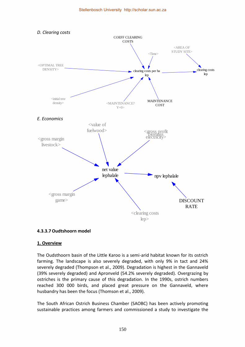
150
D. Clearing costs
E. Economics
4.3.3.7 Oudtshoorn model 1. Overview The Oudsthoorn basin of the Little Karoo is a semi-arid habitat known for its ostrich farming. The landscape is also severely degraded, with only 9% in tact and 24% severely degraded (Thompson et al., 2009). Degradation is highest in the Gannaveld (39% severely degraded) and Apronveld (54.2% severely degraded). Overgrazing by ostriches is the primary cause of this degradation. In the 1990s, ostrich numbers reached 300 000 birds, and placed great pressure on the Gannaveld, where husbandry has been the focus (Thomson et al., 2009). The South African Ostrich Business Chamber (SAOBC) has been actively promoting sustainable practices among farmers and commissioned a study to investigate the
<OPTIMAL TREE
DENSITY>
<initial tree
density>
COEFF CLEARING
COSTS
clearing costs per ha
lep
clearing costs
lep
<AREA OF
STUDY SITE>
<MAINTENANCE?
Y=0>
MAINTENANCE
COST
<Time>
<gross margin
livestock>
<gross margin
game>
<gross profitbiomass
electricity>
<clearing costs
lep>
net value
lephalale npv lephalale
DISCOUNT
RATE
<value of
fuelwood>
Stellenbosch University http://scholar.sun.ac.za

151
financial viability of rearing ostriches in small camps so that large tracts of land could be freed up for restoration (Mugido, 2011a). At the same time, the University of Cape Town conducted research on the effectiveness of different restoration treatments (De Abreu, 2011). The data collected in this study included landscape function analysis, nutrient cycling, soil stabilisation and techniques for enhancing ecosystem service delivery. This study combines these two elements into a single study. Financial values for small camp breeding (Mugido, 2011a) were combined with grazing capacity estimates for different soil treatments (ripping, micro-catchments, sowing seed and mulching) in order to determine the agricultural potential of the land following restoration. Secondly, changes in soil carbon storage for the different treatments were also used to assess the incremental value of carbon storage in the area. Thirdly, an eco-labelling premium for sustainable ostrich farming was also included, using price data from a local supermarket (Pick ’n Pay). Costs for the different treatments were derived from De Abreu (2011). 2. Model parameters and model equations A. Parameters used in model and units
Description Formula/Value Unit Reference Comment
no of years to rehabilitate= 1 Year Assumption
Time to optimise NPV
eco-labelling premium %= 0.5 Dmnl
Pick ‘n Pay retail store (27 October 2011)
Oudtshoorn (price premium on free range ostrich mince)
eco-labelling? Y=1= 1 Dmnl Policy switch 1=yes
ns gc= 0.001 LSU/hectare De Abreu, 2011
ns rehab= 0 Rand/hectare Model assumption
mu rehab= 24700 Rand/hectare Own calculation based on De Abreu, 2011
Carbon? Y=1= 1 Dmnl Policy switch 1=yes
nmu gc= 0.0032 LSU/hectare De Abreu, 2011
r gc= 0.0002 LSU/hectare De Abreu, 2011
r rehab= 1300 Rand/hectare Own calculation based on De Abreu, 2011
discount rate= 0.08 1/Year Mullins et al., 2007
mi gc= 0.0014 LSU/hectare De Abreu, 2011
mi rehab= 15400 Rand/hectare Own calculation based on De Abreu, 2011
MI yes= 0 Dmnl Policy variable
Value between 0 and 1 representing relative share of each treatment
mu gc= -0.001 LSU/hectare De Abreu, 2011
nmu rehab= 0 Rand/hectare Model assumption
s rehab= 3700 Rand/hectare Own calculation based on De Abreu, 2011
Stellenbosch University http://scholar.sun.ac.za

152
Description Formula/Value Unit Reference Comment
s gc= 0.0012 LSU/hectare De Abreu, 2011
NS yes= 0 Dmnl Policy variable
Value between 0 and 1 representing relative share of each treatment
R yes= 0 Dmnl Policy variable
Value between 0 and 1 representing relative share of each treatment
NMu yes= 1 Dmnl Policy variable
Value between 0 and 1 representing relative share of each treatment
S yes= 0 Dmnl Policy variable
Value between 0 and 1 representing relative share of each treatment
mu yes= 0 Dmnl Policy variable
Value between 0 and 1 representing relative share of each treatment
% degraded area rehabilitated= 1 Dmnl Model assumption
area oudtshoorn basin degraded= 176216 hectare Thompson et al., 2009
Only Gannaveld, Apronveld and SK Thicket (severely degraded)
Rehab %C= 0.69 Dmnl De Abreu, 2011
benchmark %C= 0.84 Dmnl De Abreu, 2011
bulk density= 0.7 ton/m3 MDTP, 2007
conv ha to m3= 5000 m3/hectare Calculation
Assumes soil depth of 50cm (Mills, 2011)
OSTRICH net VALUE PER LSU= 3219.21 Rand/LSU
Own calculation based on Mugido, 2011a
Financial model assuming 2% of natural vegetation utilised for farming
time to change to bench= 75 Year Mills, 2011 (average)
Ave of range: 50-100 years
unit value of carbon= 110 Rand/ton
Blignaut, 2011 (based on ave price of $15/tC
B. Equations
Description Formula/Value Unit
annual rehabilitation= IF THEN ELSE(Time<2010+no of years to rehabilitate,(area oudtshoorn basin hectare/Year
Stellenbosch University http://scholar.sun.ac.za

153
Description Formula/Value Unit
degraded*"% degraded area rehabilitated")/no of years to rehabilitate,0)
eco-labelling value= ostrich total additional LSU*Ecolabelling ostrich value per lsu*"eco-labelling? Y=1" Rand/Year
Ecolabelling ostrich value per lsu=
eco-labelling premium %*OSTRICH net VALUE PER LSU Rand/LSU
total value oudtshoorn=
ostrich net value+value of change in carbon+annual rehabilitation cost+"eco-labelling value" Rand/Year
no mulch gc= NMu yes*nmu gc LSU/hectare
no seed= ns rehab*NS yes Rand/hectare
no seed gc= NS yes*ns gc LSU/hectare
npv oudtshoorn= NPV(total value oudtshoorn,discount rate,0,1) Rand
seed gc= S yes*s gc LSU/hectare
mulch= mu rehab*mu yes Rand/hectare
seed= s rehab*S yes Rand/hectare
micro= mi rehab*MI yes Rand/hectare
micro gc= MI yes*mi gc LSU/hectare
no mulch= NMu yes*nmu rehab Rand/hectare
ripping gc= R yes*r gc LSU/hectare
mulch gc= mu yes*mu gc LSU/hectare
ripping= r rehab*R yes Rand/hectare
value of change in carbon= change in carbon stocks*unit value of carbon*"Carbon? Y=1" Rand/Year
average change in GC=
(micro gc+mulch gc+no mulch gc+no seed gc+ripping gc+seed gc)/(MI yes+mu yes+NMu yes+NS yes+R yes+S yes) LSU/hectare
average rehabilitation cost=
(micro+mulch+no mulch+no seed+ripping+seed)/(MI yes+mu yes+NMu yes+NS yes+R yes+S yes\ Rand/hectare
tonnes soil following rehab=
Area rehabilitated*conv ha to m3*bulk density ton
ostrich total additional LSU=
Area rehabilitated*average change in GC/year LSU/Year
annual change in %C= ("benchmark %C"-"Rehab %C")/time to change to bench Dmnl/Year
annual rehabilitation cost= -average rehabilitation cost*annual rehabilitation Rand/Year
Area rehabilitated= INTEG (annual rehabilitation, 6565) hectare
change in carbon stocks= annual change in %C*tonnes soil following rehab/100 ton/Year
ostrich net value= ostrich total additional LSU*OSTRICH net VALUE PER LSU Rand/Year
Stellenbosch University http://scholar.sun.ac.za

154
3. Stock flow diagrams A. Land use
B. Grazing capacity
Area
Rehabilitatedannual rehabilitation
AREA OUDTSHOORN
BASIN DEGRADED
% DEGRADED AREA
REHABILITATED
NO OF YEARS TO
REHABILITATE<Time>
ostrich total
additional lsuOSTRICH NET
VALUE PER LSU
ostrich net value
YEAR
<Area
Rehabilitated>
ripping gc
seed gc
mulch gcno mulch gc
micro gc
average change in
gc
no seed gc
<MI YES>
<NS YES>
<R YES>
<S YES>
<MU YES>
<NMU YES>
mi gc
ns gc
r gc
s gc
mu gc nmu gc
ECO-LABELLING
PREMIUM %
ecolabelling ostrich
value per lsu
eco-labelling value
ECO-LABELLING?
Y=1
Stellenbosch University http://scholar.sun.ac.za

155
C. Carbon
D. Area cleared
BENCHMARK
%C
TIME TO CHANGE
TO BENCH
BULK DENSITY
tonnes soil following
rehab
change in carbon
stocks
CONV HA TO
M3 UNIT VALUE OF
CARBON
value ofchange incarbon
REHAB %C
annual change in
%c
<Area
Rehabilitated>
CARBON? Y=1
ripping
seed
mulchno mulch
micro
average
rehabilitation cost
annual
rehabilitation cost
no seed<annual
rehabilitation>
NS YES
R YES
S YES
MU YES
NMU YES
MI YES
NS REHAB
R REHAB
S REHAB
MU REHAB
NMU REHAB
MI REHAB
Stellenbosch University http://scholar.sun.ac.za

156
E. Economics
4.3.3.8 Sand river model 1. Overview A. Study area The Sand river system is a water-stressed catchment in Limpopo and Mpumalanga provinces, South Africa; a sub-catchment of the Sabie River Catchment (Pollard et al., 1998). The catchment is divided into three zones (Pollard et al., 2008): Zone A, the upper catchment, where historically plantation forestry took place14; Zone B, where irrigation agriculture takes place using an outdated canal system that is in need of repair and maintenance; Zone C, the lower-end of the catchment that also receives the lowest annual rainfall. The major occupant of Zone C is Sabie Sands Game Reserve (SSGR). SSGR is reliant on water flowing from the upper catchment, but recently insufficient water is flowing to reach the reserve. A range of water supply options for the Sand river system is discussed in Crookes (2011b). Only one of these is incorporated into this simulation model, namely the complete clearance of plantations and invasive alien plants in the upper catchment region. Various methods were proposed to value the additional water released into the catchment. Originally, the intention was to conduct a contingent valuation study whereby SSGR was asked their willingness to pay for the additional water (essentially, the ecological reserve). Although SSGR was willing to provide some support to catchment management through the land tax system, and had already made some PES contributions (although the actual amount is disputed, see Crookes,
14 A decision was made to exit forestry in anticipation of the establishment of the Blyde River Canyon National Park. Neither the establishment of the park, nor the exiting of all forestry was successful, and now Government wants to review its decision to exit the forestry (Agterkamp, 2009). Furthermore, the clearance of some of the existing plantations in the catchment did not have the desired effect of increasing water supply to Zone C, largely due to the fact that the additional water was absorbed into the canal system in Zone B (Pollard, 2010).
<ostrich net value>
<value of change in
carbon>
<annual
rehabilitation cost>
total value
oudtshoorn
npv oudtshoorn DISCOUNT
RATE
<eco-labelling
value>
Stellenbosch University http://scholar.sun.ac.za

157
2011b), they were understandably unwilling to pay for water that was essentially their legal entitlement. The second method that was employed, namely the benefits transfer method, is described in the next section. B. Economic value of water, Sabie Sand Game Reserve Turpie and Joubert (2001) estimate the recreational value of rivers in the Kruger National Park (KNP) using the travel cost method (TCM). This approach asks visitors to the park questions related to on- and offsite costs incurred in visiting the KNP. We use the benefits transfer method (BTM) to estimate the value of water for SSGR based on this study. First an estimate for onsite expenditure for Kruger National Park and divided by the total area of the park to give a unit value for direct expenditure (Table 41). This is then multiplied by the area of Sabie Sands Game Reserve to give a lower bound estimate for on-site expenditure. Sabie Sands Game Reserve is a private game reserve and has a much smaller area than Kruger National Park. Consequently direct expenditure per unit area is likely to be much higher than Kruger National Park. Table 41 Estimation of onsite expenditure for Sabie Sand Game Reserve Year Value Comment/Reference
A. KNP1
Onsite expenditure KNP (R million) 2001 136 Turpie and Joubert (2001)
Onsite expenditure KNP (R million) (A) 2010 272
Converted to 2010 values assuming an 8% inflation rate
Area of KNP (million ha) (B) 2.3 Turpie and Joubert (2001)
Onsite expenditure KNP (R/ha) (C) 2010 118.202 Calculation (A/B)
Area of SSGR in SRC1 (D) 69 486 Pollard et al. (1998)
Value of on site expenditure (SSGR) (R million) 8
Calculation (C*D) Low estimate for value of on site expenditure
B. SSGR1
Onsite expenditure SSGR (R million) 1998 60 Pollard et al. (2008)2
Onsite expenditure SSGR (R million) (E) 2010 151
Converted to 2010 values assuming an 8% inflation rate
Proportion of SSGR in Sand river catchment % (F) 0.76
Calculation based on Pollard et al. (1998)
Value of onsite expenditure (SSGR) (R million) 115
Calculation (E*F) High estimate
1 KNP = Kruger National Park; SSGR = Sabie Sand Game Reserve; SRC = Sand river catchment 2 Note: Estimates of onsite visitor expenditure for SSGR are not available and consequently park income was used as a proxy.
Stellenbosch University http://scholar.sun.ac.za

158
A second approach is to use estimates of on-site expenditure from the entire Sabie Sand Game Reserve from Pollard et al. (2008) based on data from the Save the Sand Report (Pollard et al. 1998). This however needs to be apportioned to the share of the reserve that is in the Sand River Catchment assuming that the share of the expenditure is equally distributed spatially. This gives an upper bound estimate for on-site expenditure. Table 42 follows on from Table 41 and uses multipliers derived from Turpie and Joubert (2001) to estimate the recreational value of water from the upper and lower bound values of onsite expenditure. These values are then divided by the volume of water required for the ecological reserve, after accounting for losses due to degradation, to obtain unit water values for the ecological reserve. An average of lower and upper bound water values are utilised. The value of ecological reserve derived in this way is R3.99/m3 (Table 42).
Table 42 The economic value of water from restoring rivers in Sabie Sand Game Reserve 2010 Low 2010 High Reference
Onsite expenditure (R million) (A) 8 115 From previous table
Economic impact multiplier 1.96 1.96
Estimated from Turpie and Joubert (2001)
Economic impact (all expenditure related to visiting the park) (R million )(B=A*1.96) 16 225
Consumer surplus multiplier 3.74 3.74
Estimated from Turpie and Joubert (2001)
Consumer surplus (R million)(C=B*3.74) 60 842
Recreation value (R million)(D=B+C) 76 1 067
30% in lost revenues from degraded rivers (R million)(E=D*0.3) 23 320
Turpie and Joubert (2001)
Ecological reserve (M.m3/yr)(F) 43 43 Agterkamp (2009)
Value of ecological reserve (Rand/m3) (G=E/F) 0.53 7.44 Calculation
Economic value of water (SSGR) (Rand/m3) 3.99
Calculation (ave low and high values)
2. Model parameters and model equations A. Parameters used in model and units
Description Formula/Value Unit Reference Comment
Maintenance? Y=1= 1 Dmnl Policy variable 1=yes
plantation 0.1 1/Year Model assumption
Stellenbosch University http://scholar.sun.ac.za

159
Description Formula/Value Unit Reference Comment
regrowth rate=
ET forestry= 5641 m3/hectare Dye et al., 2008
lifespan of canal system= 50 Year Model assumption
Time frame of model
discount rate= 0.08 1/Year Mullins et al., 2007
ecological reserve= 4.30E+07 m3 Agterkamp, 2009
capital cost canal system= -4.3E+07 Rand Ngobeni, 2010
capital depreciation costs?= 1 Dmnl Policy variable 1=yes
unit clearing cost SRC= -1285.21 rand/hectare
Own calculations based on Pollard, 2010
2010 values. Clearing costs estimated at R21.5 million over 5 years (1997-2001) for area of aliens and plantations covering 45571 ha.
economic value forestry= -985.76 rand/hectare/Year
Own calculations based on data in Pollard et al (1998).
Unit value water IPC= 7.52 rand/m3/Year
Own calculations based on data in Pollard et al (1998) and Agterkamp (2009).
Marginal economic value
unit value water IAC= 1.99 rand/m3/Year
Own calculations based on data in Pollard et al (1998), Pollard et al (2008) and Ngobeni, 2010
UNIT VALUE WATER SSGR= 3.99 rand/m3/Year Calculation
See Appendix I
current water use iac= 9.63E+06 m3
Own calculations based on data in Pollard et al (1998), Pollard et al (2008) and Ngobeni, 2010
current water use ipc= 2.73E+06 m3
Own calculations based on data in Pollard et al (1998) and Agterkamp (2009).
efficient water use iac= 1.93E+07 m3
Own calculations based on Pollard et al., 1998; Pollard et al ., 2008
efficient water use ipc= 4.51E+06 m3
Own calculations based on Pollard et al (1998); Pollard et al (2008)
IAC improved?= 0 Dmnl Policy variable 1=yes
INITIAL AREA plantations= 2684 hectare Seoke, 2010
IPC improved?= 0 Dmnl Policy variable 1= yes
Stellenbosch University http://scholar.sun.ac.za

160
Description Formula/Value Unit Reference Comment
NO OF YEARS TO clear PLANTATIONS= 1 Year [0,20,1] Policy variable
Period that maximises NPV
B. Equations
Description Formula/Value Unit
annual clearance plantations=
IF THEN ELSE("Maintenance? Y=1"=1,IF THEN ELSE(area plantations<=10,"Maintenance? Y=1"*regrowth plantations,IF THEN ELSE(Time<2010+NO OF YEARS TO clear PLANTATIONS,INITIAL AREA plantations/NO OF YEARS TO clear PLANTATIONS+regrowth plantations,0)) hectare/Year
area plantations= INTEG (regrowth plantations-annual clearance plantations,INITIAL AREA plantations) hectare
BASE WATER flow REACHING SSGR= 2.65066e+007+1.51382e+007-water use forestry m3
clearing cost forestry= unit clearing cost SRC*annual clearance plantations rand/Year
change in area cleared= INITIAL AREA plantations-area plantations hectare
water use forestry= ET forestry*INITIAL AREA plantations m3
regrowth plantations= (INITIAL AREA plantations-area plantations)*plantation regrowth rate hectare/Year
annual depreciation= capital cost canal system/lifespan of canal system rand/Year
total clearing cost SRC=
capital depreciation costs?*annual depreciation+clearing cost forestry+opportunity cost of lost forestry rand/Year
npv sand= NPV(economic value SRC,discount rate,0,1) rand
water available from forestry= split b*(water released forestry-ER deficit) m3
split a= IF THEN ELSE(water released forestry<ER deficit,1,0) Dmnl
split b= IF THEN ELSE( water released forestry>ER deficit,1,0) Dmnl
desired water use ipc= MIN(water available from forestry,efficient water use ipc-current water use ipc) m3
total water flow ssgr= BASE WATER flow REACHING SSGR+Water allocation SSGR m3
Water available IAC= water available from forestry-water use ipc m3
Water allocation SSGR= Water available IAC-water use iac+water released to meet ecological reserve requirement m3
ER deficit= ecological reserve-BASE WATER flow REACHING SSGR m3
water forestry<deficit= split a*water released forestry m3
water released to meet ecological reserve requirement= split a*"water forestry<deficit"+split b*ER deficit m3
water released forestry= change in area cleared*forestry ET per ha m3
opportunity cost of lost forestry= economic value forestry*change in area cleared rand/Year
economic value SRC=
Unit value water IPC*water use ipc+unit value water IAC*water use iac+UNIT VALUE WATER SSGR*Water allocation SSGR+total clearing cost rand/Year
Stellenbosch University http://scholar.sun.ac.za

161
Description Formula/Value Unit
SRC
water use ipc= IF THEN ELSE("IPC improved?"=1,desired water use ipc, 0) m3
desired water use iac= MIN(Water available IAC,efficient water use iac-current water use iac) m3
water use iac= IF THEN ELSE("IAC improved?"=1,desired water use iac, 0) m3
3. Stock flow diagrams A. Land use
B. Water yield
initial area
plantations
NO OF YEARS TO
CLEAR PLANTATIONS
ET FORESTRY
water use
forestry
Area
Plantationsregrowth
plantations
PLANTATION
REGROWTH RATE
change in area cleared
annual clearance
plantations
<Time>MAINTENANCE?
Y=1
water available iacwater allocation ssgr
FORESTRY ET
PER HA
IPC
IMPROVED?
EFFICIENT
WATER USE IPCCURRENT
WATER USE IPC
desired water
use ipc
IAC
IMPROVED?
EFFICIENT
WATER USE IACCURRENT
WATER USE IAC
desired water
use iac
<change in area
cleared>
water released forestry
water use ipcwater use iac
water released to meetecological reserve
requirement
er deficit
water
forestry<deficitsplit a
split b
water available
from forestry
ECOLOGICAL
RESERVEbase water flow
reaching ssgr
total water flow
ssgr
<water use
forestry>
Stellenbosch University http://scholar.sun.ac.za

162
C. Clearing costs
D. Economics
4.4 Data
The data collection is based on document analysis, specifically the research projects of Masters' students working on the individual case studies in the model (Cloete, 2012; De Abreu, 2011; Gull, 2012a; Gull, 2012b; Marx, 2011a; Mugido, 2011a; Mugido and Kleynhans, 2011; Ndhlovu, 2011a; Nowell, 2011a; Pauw, 2011a; Rebelo, 2012a; Vlok, 2010a; Vlok, 2010b) as well as specifically commissioned studies as part of this Ph.D (Crookes, 2011a; Crookes, 2011b). Furthermore, data was also elicited from expert meetings scheduled at regular intervals throughout the year. The full list of participants and collaborators is provided in Appendix 3, comprising the core research team that originally conceptualised the project, the various supervisors of
capital cost canal
system
UNIT CLEARING
COST SRC
total cost sand
<change in area
cleared>
ECONOMIC
VALUE FORESTRYopportunity cost of lost
forestry
clearing cost forestry
CAPITALDEPRECIATION
COSTS?
LIFESPAN OFCANALSYSTEM
annual depreciation
<annual clearance
plantations>
capital financing
costsbond costs less labour component
BOND REPAYMENT
PERIOD
UNIT VALUE
WATER IPC
UNIT VALUE
WATER IAC
UNIT VALUE
WATER SSGR
economic
value src
<water use ipc>
<water use iac>
<water allocation
ssgr>
<total cost
sand>
npv sand
DISCOUNT
RATE
Stellenbosch University http://scholar.sun.ac.za

163
the Masters' students, other collaborators from various institutions with specific knowledge of the individual case study sites, and the Masters' students themselves. The eight case studies were divided into two groups of 4 case studies each, with the first tranch of students (phase 1) conducting research on the first 4 sites (Agulhas Plain, Beaufort West, Namaqualand and Oudtshoorn) during 2009–2010, and the second tranch of students (phase 2) conducting research on the remaining 4 sites (Kromme, Lephalale, Drakensberg and Sand) during 2010–2011. Seven expert meetings were held during 2009–2012 (Table 43), on average 2 per year. These meetings provided an opportunity for the students to present the results of their work on the individual study sites to the core team and groups of selected supervisors and collaborators, for discussion and comment. These meetings served to ensure that students and supervisors were all working together towards a common goal, and also provided an opportunity for integration of results and mutual learning about the contribution of other disciplines to the process. A third benefit of these meetings was they provided a means of validating the systems model that was gradually evolving and developing throughout the process. This process is elaborated on further in the next section. A final benefit of these meetings was that they ensured that students met the deadlines of the project, and that the deliverables of the project were met as far as possible. Table 43 List of expert meetings held during the course of the project
Date Venue Participants
18 May 2009 Stellenbosch University Core team, phase 1 students, selected supervisors and collaborators, PhD student
21 October 2009 Stellenbosch University Core team, phase 1 students, selected supervisors and collaborators, PhD student
17–18 March 2010 Oudtshoorn Core team, selected phase 1 and 2 students, selected collaborators, PhD student
6–7 September 2010 Stellenbosch University Core team, phase 1 and 2 students, selected supervisors and collaborators, PhD student
23–26 May 2011 Drakensberg Core team, phase 1 and 2 students, selected supervisors and collaborators, PhD student
31 October–1 November 2011
Stellenbosch University Core team, phase 2 students, selected supervisors
5–8 March 2012 Hermanus Core team, A. Rebelo, PhD student
Notes: See Appendix 3 for list of participants within each category; PhD student = D. Crookes
A number of other sources of data were also pursued by the Masters' students as well as the commissioned work, for each of the case studies. The first of these was
Stellenbosch University http://scholar.sun.ac.za

164
direct sampling methods for ecological data collection. This was undertaken by measuring sites before and after restoration against a number of ecological characteristics, such as landscape function analysis, hydrological features, grazing capacity, and many others. The second involved structured and semi-structured interviews. This was undertaken particularly in the Kromme case study (Rebelo, 2012a; Gull, 2012a), where farmers were interviewed to gather information on farm characteristics, patterns of irrigation, and revenues and costs associated with agricultural production. In addition to the expert meetings held as part of the integrated project process (see above), a range of experts was also consulted as part of the development of the individual case studies. In this way, data for the system dynamics model were both internally and externally validated. Finally, document analysis from reports and articles on individual case studies from outside the realm of the project were also consulted.
4.5 Model validation
Model validation, as discussed in the previous chapter, involves subjecting the model to a series of tests in order to ascertain whether or not it is a realistic portrayal of the system it is trying to model. In Section 3.3.4.5 it was indicated that tests of model structure were most commonly used by system dynamics modellers, followed by tests of behaviour and finally tests of policy. The tests most commonly cited in the literature included: 1) structure verification; 2) parameter verification; 3) dimensional consistency; 4) boundary adequacy; 5) extreme conditions; 6) surprise behaviour; 7) sensitivity analysis; 8) behaviour reproduction; 9) behaviour anomaly; 10) family member; 11) integration error. The first five tests are all tests of model structure, and the second six tests are tests of model behaviour. These 11 tests are the main focus of validation checks for the system dynamics model in this study.
4.5.1 Structure verification
A. Description This process involves comparing the model structure with structures prevalent in real world situations, or patterns of relationships found in the literature or through expert opinion. B. How applied The initial structure was provided from the research projects of various postgraduate students working on the case studies in the model, as discussed in Section 4.4. Further structure verification was undertaken through workshops which were held with experts in the field of ecology, hydrology and economics, knowledgeable in different parts of the system. These workshops not only enabled validation of the initial model structure, but also allowed for the development of new and more realistic structural components into the model. Two examples serve to highlight this.
Stellenbosch University http://scholar.sun.ac.za

165
The first example was the identification of the need to introduce a fire regime into the fynbos model, since this was identified as a structural feature of this particular system. The second was the inclusion of water price differentiation on the basis of climatic variation, for example during periods of drought. This was identified as a structural feature of the Beaufort West model. These and many other instances serve to illustrate the contribution of expert input in the structural development and validation of the model.
4.5.2 Parameter verification
A. Description In the same way that model structure may be compared with real world situations, model parameters (constants) may also be validated by comparing with actuality. Parameter validation is closely related to structure validation in that different parameter values influence the outcome of model structure. B. How applied Most parameter values were obtained from published literature sources, unpublished data that accompanied Masters students’ theses, or personal interviews and meetings with a range of experts. In a few cases where literature estimates were not forthcoming, parameter estimates were also selected in the model in a way that maximised net present values (NPVs) for that particular case study. One example of this is the optimal time required in order to clear invasive alien plants or to restore degraded areas.
4.5.3 Extreme conditions
A. Description This test assigns extreme, but realistic values to parameters and investigates whether or not the model responds in the expected manner. B. How applied Various extreme conditions were applied to parameters in each of the case studies in order to ascertain how the system responds. The different case studies were subjected to different tests. Therefore, a list of extreme conditions scenarios and how these impacted on the different case studies is elaborated on. Scenario 1: Number of years of clearing/rehabilitation was set to zero. Model response: Net Present Values were zero. This is in accordance with expectations but indicates that the model is able to replicate baseline conditions. An example of such a test for the Agulhas Plain model is shown in Figure 27.
Stellenbosch University http://scholar.sun.ac.za

166
Scenario 2: High initial clearing for a short period of time (No of years to clear aliens = set to a low value). Model response: for Agulhas, NPV is negative. For Beaufort West, this is positive but NPV increases with increasing clearance time. For most models, a low clearance time followed by a long maintenance period was optimal. This is in accordance with expectations, since long-term clearing is more beneficial. Scenario 3: Value of water set to zero. Model response: NPVs negative. This is also in accordance with expectations since private benefits are unlikely to exceed social benefits from restoration. Figure 27 Annual clearing time = 0 years
Scenario 4: Sensitivity of model results to changes in the discount rate. For all reasonable ranges of discount rates (4–10%), results were consistent: studies with positive NPVs remained positive and studies with negative NPVs remained negative (Figure 28). Scenario 5: For the Lephalale study, a range of other tests were also run. Sensitivity of the model to changes in optimal tree density was assessed (35%–50%), as well as sensitivity to long-term rainfall, changes in the ratio of livestock to game, and whether or not soft management was introduced. Again, results were in accordance with expectations.
area aliens
200,000
100,000
0
2010 2025 2040 2055
Time (Year)
Hec
tare
Area Aliens : Current
npv agulhas
0.2
0.1
0
2010 2025 2040 2055
Time (Year)
Ran
d
npv agulhas : Current
Stellenbosch University http://scholar.sun.ac.za

167
Figure 28 Sensitivity analyses of NPVs to changes in discount rate
4.5.4 Boundary adequacy
A. Description These comprise three separate tests, namely the structure boundary adequacy test, the behaviour boundary adequacy test and the policy boundary adequacy test, but contain essentially the same logic. The structure boundary adequacy test considers whether or not all the important elements of structure are contained in the model, and what level of aggregation is appropriate. The behaviour boundary adequacy test asks whether or not model behaviour would change significantly if boundary assumptions were changed. The policy boundary adequacy test investigates whether or not policy recommendations would change as a result of a change in the model boundary. B. How applied For the structure boundary adequacy test, exogenous variables are examined in order to ascertain whether or not they are complete, and also whether or not there are certain exogenous variables that should be endogenous. Expert meetings were used in order to determine whether or not important structural characteristics were omitted from the model, and the behaviour response was tested by investigating what changes in behaviour would result as a consequence of a change in model
Stellenbosch University http://scholar.sun.ac.za

168
structure (structure boundary adequacy). Effect of policy recommendations were also tested in this way (policy boundary adequacy). A panel of experts served to verify whether or not changes in the model structure, behaviour and policy were consistent with real world considerations.
4.5.5 Dimensional consistency
A. Description This test involves the analysis of a model’s equations in order to test whether or not the model’s dimensions (units) are consistent. Some tests are so significant that they are regarded as mandatory, and Coyle and Exelby (2000:35) regard the dimensional consistency test as being a “sine qua non”. B. How applied Most good system dynamics modelling software packages provide a means of testing the dimensional consistency of the model, Vensim DSS Version 5.9e being no exception. Dimensional consistency was checked throughout the building of the model, and the final models units satisfy the requirements.
4.5.6 Integration error test
A. Description System dynamics models use numerical integration techniques to compute the behaviour of the system, as for most models an analytical solution is not possible (Sterman, 2000). This test investigates whether or not the model is sensitive to the choice of integration method or choice of time step. The two main methods of integration in the model are the Euler method and the Runge-Kutta method. The Euler integration method is simple and usually adequate for most applications (Sterman, 2000). However, it is sometimes useful to test the sensitivity of the model to integration method, as this can highlight whether or not the assumptions underlying the method are appropriate. A description of the different integration methods and the assumptions underlying them is given in Sterman (2000). B. How applied The model uses Euler’s method of integration, and the time step is set for 1 year. The integration error test involves having the time step vary and examining whether or not the model performs as expected. Results are given in Figure 29.
Stellenbosch University http://scholar.sun.ac.za

169
Figure 29 Comparison of model results over different time steps
The sensitivity of the model to changes in integration method was also undertaken. Vensim provides the facility to select from a range of integration methods (Euler, Runge-Kutta). Comparing integration methods also did not indicate a wide deviation in values (Figure 30). Figure 30 Comparison of model results over different integration methods
npv per ha average
40,000
28,500
17,000
5,500
-6,000
2010 2015 2020 2025 2030 2035 2040 2045 2050 2055 2060
Time (Year)
Ran
d/H
ecta
re
npv per ha average : time=1
npv per ha average : time=0,5
npv per ha average
40,000
28,500
17,000
5,500
-6,000
2010 2015 2020 2025 2030 2035 2040 2045 2050 2055 2060
Time (Year)
Ran
d/H
ecta
re
npv per ha average : RK
npv per ha average : Euler
Stellenbosch University http://scholar.sun.ac.za

170
4.5.7 Behaviour reproduction
A. Description This test involves qualitative and quantitative measures for comparing how best the model is able to replicate the actual behaviour of the system. Quantitative methods include statistical measures such as using the coefficient of determination (R2), MAE (mean absolute error), MSE (mean square error) and Theil’s Inequality Statistic to investigate how much the simulation model deviates from actual values. B. How applied Time series data in support of the model is scarce. As already indicated, model calibration was undertaken through expert inputs. A number of students’ Masters' theses also generated time series information and the sub-models were constructed to replicate the time series information as far as possible. However, in reality the availability of time series data for this study was limited. Expert input also verified whether or not the model was characteristic of the underlying ecological, hydrological and economic system, and also identified dynamic behaviour of the ecological system that required inclusion in the model.
4.5.8 Behaviour anomaly
A. Description The structures in a system dynamics model contribute to the ability of a model to replicate real world systems. The importance of certain structures to the model is tested by means of modifying or deleting those relationships, and testing whether or not the model continues to perform in the manner expected. One way in which this is achieved is through loop knockout analysis in which a target relationship is eliminated and the model response is tested. B. How applied The test for behaviour anomaly was applied throughout the model-building process, through modifying and changing relationships in the model structure, and helped to analyse the effect of specific variables.
4.5.9 Family member
A. Description The family member test asks whether or not the model contains features of other instances of the same class of models the system was built to mimic. The more instances the model is able to mimic, the more generally applicable the model is.
Stellenbosch University http://scholar.sun.ac.za

171
B. How applied The RESTORE-P model is part of a model family, and is tested on eight different case studies throughout South Africa where various forms of restoration are taking place. Caution should, however, be exercised when extrapolating to other case study sites where restoration is taking place, since each site contains unique characteristics that may not be present at other sites.
4.5.10 Surprise behaviour
A. Description A surprise behaviour is a model behaviour that is not anticipated by the model analysts. Sometimes this is due to a formulation flaw in the model, and othertimes this may lead to an identification of behaviour previously unrecognised in the real world system. In the latter case confidence in the model’s usefulness is strongly enhanced. B. How applied If a test for surprise behaviour leads to unexpected results, the modeller must understand the causes of the unexpected behaviour in the model. This aspect is elaborated on in greater depth when the model results are discussed.
4.5.11 Sensitivity analysis
A. Description The SA test tests the robustness of the model to underlying assumptions. Following Sterman (2000), three types of sensitivity are distinguished: numerical sensitivity, behavioural sensitivity and policy sensitivity. Numerical sensitivity is a feature of the model, while behavioural sensitivity and especially policy sensitivity is important and requires testing. Sensitivity analysis involves testing the sensitivity of model results to changes in parameter values. B. How applied Most modelling software packages provide automated sensitivity analysis tools. Vensim DSS 5.9e is no exception. It also includes a Monte Carlo simulation technique. This enables the specification of a distribution function around a parameter of interest; and the software randomly draws a value for each parameter from the distribution and then simulates the model. This enables the generation of different trajectories from a large number of simulations, and also the confidence bounds around each trajectory. Sensitivity of results to model assumptions is further elaborated on when the model results are presented.
Stellenbosch University http://scholar.sun.ac.za

172
4.5.12 Other tests
A number of other tests such as the mass balance check were also used during model development and the outcomes supported model validation. As these tests are not the main focus of the validation exercises in the study, these will not be elaborated on.
4.6 Chapter summary and conclusions
This chapter presents an integrated SD/RA model for selecting restoration projects (the RESTORE-P model). The first component is a system dynamics model for eight case studies distributed throughout South Africa where restoration is occurring. The validation process is somewhat different from the process adopted in validating a regression model. In the latter case, a number of statistical indicators (e.g. R2, T tests, P values) are available. For a system dynamics model, the validation process involves a combination of expert input and model validation based on the response of the model to a number of structural, behavioural and policy tests. The range of tests adopted in this study is not exhaustive but are based on a range of tests recommended by experienced practitioners who have also published a list of their proposed tests. It is not possible to categorically state that the SD model passes or fails all tests (as would be the case with a range of statistical tests on a regression model). However, it is concluded that, on the basis of the tests conducted as part of this study, there is sufficient confidence in the model to proceed to using the model for a range of simulations. The outputs of the SD model feed into a risk analysis process for assigning a probability distribution to outcome variables, and culminates in a portfolio mapping exercise for prioritising restoration activities. The model is a transdisciplinary and multi-institutional exercise that draws on the expertise of many role players. In the next chapter, the model is used to address the key research questions of the study.
Stellenbosch University http://scholar.sun.ac.za
173
Chapter 5 Discussion of results
5.1 Introduction
The research hypothesis contains two elements. The first relates to the development of a system dynamics model to assess the impacts of restoring natural capital across a range of diverse sites throughout South Africa. The second relates to the strategic prioritisation of restoration projects. As a precursor to developing the model, however, it was necessary to demonstrate the relevance of this modelling approach to the problem at hand. The literature review indicated that, although very few SD applications were found that modelled restoration projects, sytem dynamics modelling has nonetheless been widely used to model ecological-, water- and agricultural-related problems, including a growing number of applications in South Africa. In the previous chapter, the integrated SD/RA model (RESTORE-P) was presented and certain validation tests were performed. In this chapter, the results from this model are provided with reference to the first and second elements of the hypothesis. Initially, the system dynamics results are communicated, followed by a risk analysis process, coupled with portfolio mapping, to facilitate the selection and prioritisation of restoration projects.
5.2 System dynamics model
5.2.1 Agulhas Plain
1. Sensitivity analysis A. Clearance time In order to ascertain the impact of clearing, sensitivity to clearance time was tested using a Monte Carlo simulation. The parameter clearance time was modelled as a normal distribution with mean 25 and standard deviation 13, with 200 simulations, minimum = 1 year and maximum = 50 years. The results indicate that 95% of clearance time falls within a narrow NPV range (Figure 31). This suggests that results are not sensitive to long-term clearance.
Stellenbosch University http://scholar.sun.ac.za

174
Figure 31 Long-term clearing simulations (mean = 25, standard deviation = 13, min = 1, max = 50)
A second simulation considered clearance time over a much shorter simulation (mean = 2, standard deviation = 1, maximum value = 5 and minimum value = 1). The results (Figure 32) suggest a much wider variation in NPV, and higher values compared to the long-term simulations. Long-term clearing is more optimal in that fire triggers regrowth of IAPs, and long-term monitoring can suppress the emergence of new growth. This suggests that short-term intensive clearing of aliens before a fire event is optimal to reduce the intensity of the fire event, followed by a long-term maintenance plan to prevent regrowth. Benefits are also realised sooner following this clearing regime. Figure 32 Short-term intensive clearing of aliens (mean = 2, standard deviation = 1, min = 1, max = 5)
Current
50% 75% 95% 100%
npv agulhas
600 M
450 M
300 M
150 M
02010 2016 2023 2029 2035 2041 2048 2054 2060
Time (Year)
Current
50% 75% 95% 100%
npv agulhas
600 M
450 M
300 M
150 M
02010 2016 2023 2029 2035 2041 2048 2054 2060
Time (Year)
Stellenbosch University http://scholar.sun.ac.za

175
B. Bio-control vs physical clearing The primary method of alien eradication in the Agulhas Plain is through physical clearing and chemical treatment. An alternative scenario considered is the utilisation of bio-control agents. Although bio-control measures have already been implemented to some extent in the Agulhas Plain, these have to-date not been completely effective (see Section 4.3.3.1 Part B). This policy scenario models the widespread introduction of bio-control into the Agulhas Plain, targeting mainly Acacia species. The baseline assumes that 100% of the area is inoculated, and the delay before the inoculation takes effect is 4 years (Section 4.3.3.1). Results are shown in Figure 33. Figure 33 NPV following clearing and bio-control treatments
Although the implementation costs are considerably less for bio-control compared with physical clearing (Section 4.3.3.1), the net present value for bio-control is less than for clearing (Figure 33). The main driver in the model is the delay before the biological agent is effective (Figure 34). For immediate effectiveness (delay = 0), NPV peaks at just under R450 million, which is greater than the NPV for clearing. However, as the effectiveness delay increases so to does NPV, and is negative for delays = 50 yrs (which is logical since only the cost is included as there is no benefit over the time frame of the model).
npv agulhas
400 M
199 M
-2 M
2010 2025 2040 2055
Time (Year)
Ran
d
npv agulhas : Clearing
npv agulhas : Bio-control
Stellenbosch University http://scholar.sun.ac.za

176
Figure 34 Sensitivity analysis for the delay in bio-control effectiveness
Note: Mean = 25, standard deviation = 13, min = 0, max = 50
5.2.2 Beaufort West
1. Develop key success drivers The effect of Prosopis regrowth on the biomass electricity is crucial to the profitability of the plant as illustrated in Figure 35. If area re-growth drops below 0.4 (40%), NPV for the biomass plant falls; for very low levels (less than 0.1), the NPV is negative. Figure 35 Effect of Prosopis re-growth following rainfall on biomass NPV
Note: Area re-growth follows random normal distribution with mean = 0.5; standard deviation = 0.25, min = 0, max = 1, n = 200
Current
50% 75% 95% 100%
npv agulhas
600 M
449.5 M
299 M
148.5 M
-2 M2010 2016 2023 2029 2035 2041 2048 2054 2060
Time (Year)
Current
50% 75% 95% 100%
npv biomass
2 M
1.45 M
900,000
350,000
-200,0002010 2016 2023 2029 2035 2041 2048 2054 2060
Time (Year)
Stellenbosch University http://scholar.sun.ac.za

177
At the same time, the overall effect of variation in the re-growth rate has very little impact on the overall Beaufort West NPV (Figure 36). Figure 36 Effect of variations in the re-growth rate on the overall BW NPV
Note: Area re-growth follows random normal distribution with mean = 0.5; standard deviation = 0.25, min = 0, max = 1, n = 200
The major factor affecting Beaufort West NPV is the value of water (Figure 37), although the NPV for BW remains positive for water prices within a 95% confidence limit (value of water normally distributed with mean = 2.13, standard deviation = 1.07, min = 0, max = 4, n = 200). Figure 37 Effect of changes in marginal price of water on BW NPV
Current
50% 75% 95% 100%
npv beaufort west
6 M
4.5 M
3 M
1.5 M
02010 2016 2023 2029 2035 2041 2048 2054 2060
Time (Year)
Current
50% 75% 95% 100%
npv beaufort west
8 M
5.9 M
3.8 M
1.7 M
-400,0002010 2016 2023 2029 2035 2041 2048 2054 2060
Time (Year)
Stellenbosch University http://scholar.sun.ac.za

178
2. Simulation that maximises NPV As was the case with the Agulhas Plain model, a long-term clearing pattern is optimal for Beaufort West (no. of years of clearing activity = 50). Although Prosopis density fluctuates (Figure 38), NPVs climb steadily. Not only does the Prosopis re-growth provide fuel to finance the biomass electricity plant, but the long-term presence of Prosopis also has a beneficial effect in terms of fixing nitrogen in the soil, which benefits grazing capacity (Ndhlovu, 2011b). Figure 38 Baseline simulation for Beaufort West, long-term clearing
5.2.3 Drakensberg
1. Simulation that maximises NPV Figure 39 summarises the net present value of ecosystem benefits over a 50-year period. It is evident that the soil stabilisation benefits associated with an improvement in water quality are vastly more beneficial compared with the benefits derived either from improvements in livestock grazing capacity or soil carbon storage improvements.
prosopis density
20
10
0
2010 2025 2040 2055
Time (Year)
Dm
nl
prosopis density : Current
npv BW
4 M
2 M
0
2010 2025 2040 2055
Time (Year)
Ran
d
npv beaufort west : Current
Stellenbosch University http://scholar.sun.ac.za

179
Figure 39 NPV for different ecosystem benefits associated with rehabilitation
2. Sensitivity analysis In contrast to the Beaufort West model, where NPV results are not sensitive to variations in the value of water, the Drakensberg model's NPV calculations are highly sensitive to water value variations (Figure 40). A higher water price is therefore crucial to a positive NPV outcome at the Drakensberg site. But is this realistic? One would expect a higher price in an area where water is relatively scarce, whereas water is scarcer in Beaufort West compared with the Drakensberg. In reality, the average water price in Beaufort West ranges from R1.67–R2.6/m3, while the value of clean water in the Drakensberg is R6/m3. Figure 40 Sensitivity analysis of price of water in Drakenberg
Note: Mean = 3.5, standard deviation = 1.75, min = 1, max = 6, n = 200
R0.00
R1.00
R2.00
R3.00
R4.00
R5.00
Grazing Soil stabilisation Carbon
R m
illio
n
Current
50% 75% 95% 100%
npv drakensberg
4 M
2 M
0
-2 M
-4 M2010 2016 2023 2029 2035 2041 2048 2054 2060
Time (Year)
Stellenbosch University http://scholar.sun.ac.za

180
The higher water price is partly explained by the remote location of the Drakensberg water source relative to the ultimate users of the water. South Africa is unique in that the areas of highest rainfall are also associated with the areas of lowest access. Distribution of urban areas is influenced by historical access to mineral resources rather than access to water. The demand for water is much higher in the Drakensberg compared with Beaufort West; also supply is inelastic, so an increase in demand tends to push prices up. In Beaufort West demand tends to be stable or declining. Secondly, the engineering costs are much higher in Drakensberg compared with Beaufort West, as water needs to be distributed thousands of kilometres to the urban areas. One would, therefore, expect a higher water value in Drakensberg compared with Beaufort West, in spite of the greater relative scarcity of water in Beaufort West.
5.2.4 Namaqualand
1. Simulation that maximises NPV A simulation model was run to estimate the effectiveness of the different soil treatments. The results, given in Figure 41, indicate that a large number of soil applications are not necessarily financially optimal. Topsoil and translocation options are the most expensive, while seeding and translocation are the most effective. Figure 41 NPVs for different soil treatments at Namaqualand over a 50-year period (i = 8%)
Note: The sites and soil treatments, in order of effectiveness are as follows: s4 (seed and translocation), s1 (topsoil), s2 (seed), s3 (topsoil and translocation).
Source: Own analysis based on data in Pauw (2011a) and Mugido and Kleynhans (2011)
-140
-120
-100
-80
-60
-40
-20
0
S1 S2 S3 S4
R m
illio
n
Net present value
Stellenbosch University http://scholar.sun.ac.za
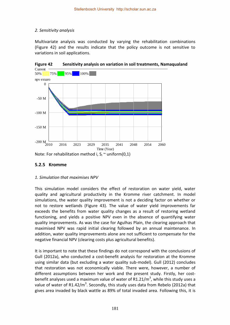
181
2. Sensitivity analysis Multivariate analysis was conducted by varying the rehabilitation combinations (Figure 42) and the results indicate that the policy outcome is not sensitive to variations in soil applications. Figure 42 Sensitivity analysis on variation in soil treatments, Namaqualand
Note: For rehabilitation method i, Si ~ uniform(0,1)
5.2.5 Kromme
1. Simulation that maximises NPV This simulation model considers the effect of restoration on water yield, water quality and agricultural productivity in the Kromme river catchment. In model simulations, the water quality improvement is not a deciding factor on whether or not to restore wetlands (Figure 43). The value of water yield improvements far exceeds the benefits from water quality changes as a result of restoring wetland functioning, and yields a positive NPV even in the absence of quantifying water quality improvements. As was the case for Agulhas Plain, the clearing approach that maximised NPV was rapid initial clearing followed by an annual maintenance. In addition, water quality improvements alone are not sufficient to compensate for the negative financial NPV (clearing costs plus agricultural benefits). It is important to note that these findings do not correspond with the conclusions of Gull (2012a), who conducted a cost-benefit analysis for restoration at the Kromme using similar data (but excluding a water quality sub-model). Gull (2012) concludes that restoration was not economically viable. There were, however, a number of different assumptions between her work and the present study. Firstly, her cost-benefit analyses used a maximum value of water of R1.21/m3, while this study uses a value of water of R1.42/m3. Secondly, this study uses data from Rebelo (2012a) that gives area invaded by black wattle as 89% of total invaded area. Following this, it is
Current
50% 75% 95% 100%
npv exxaro
0
-50 M
-100 M
-150 M
-200 M2010 2016 2023 2029 2035 2041 2048 2054 2060
Time (Year)
Stellenbosch University http://scholar.sun.ac.za

182
assumed in the simulation model that 100% of alien infestation is black wattle. Although hakea and pinus use less water than black wattle, the error margin in assuming a 100% black wattle infestation rather than an 89% black wattle infestation is less than 5%. However, Gull (2012a) uses data from McConnachie, a PhD student at Rhodes University, who models a black wattle infestation density of 66% of total infestations. There are also a number of other potential differences in assumptions, for example Gull uses average water yield changes across all landuses while water yield changes as a result of clearing aliens are measured per land use (wetland, fynbos, dryland, irrigated and orchard) for this simulation model. These effects, taken together, result in a much higher estimate for the value of additional water yield as a result of restoration compared to the estimates of Gull (2012a). Figure 43 NPVs for restoration – Kromme
Note: Values shown are at 8% discount rate. The ‘no agric’ scenario implies full restoration of wetland areas in proportion to “ideal” ratios (Rebelo, 2012a), while the ‘agric’ scenario implies the land cleared that would have been restored to wetland areas is in fact used for agriculture.
Source: Own analysis 2. Sensitivity analysis Sensitivity analysis tests the assumption of a lower unit value of water. Following Gull (2012a), a minimum unit water of R0.46/m3 (raw water tariff) is used (water price ~ normal (0.94; 0.47); max = R1.42/m3, n = 200). NPVs under the ‘no-agric’ scenario are negative in 25% of the simulations (Figure 44), but fluctuate in a fairly narrow band. By contrast, NPVs under the ‘agric’ scenario are much more sensitive to fluctuations in price, but remain positive throughout all simulations. This suggests that water yield effects are more important than prices for driving value. However, the wide range in NPV outcomes suggests that water values are nonetheless important in the model.
-200
-100
0
100
200
300
400
NPV financial NPV water quality NPV water yield
R m
illio
n
No agric
Agric
Stellenbosch University http://scholar.sun.ac.za

183
Figure 44 Sensitivity analysis for variations in the value of water, ‘no agric’ scenario
Figure 45 Sensitivity analysis for variations in the value of water, ‘agric’ scenario
5.2.6 Lephalale
1. Simulation that maximises NPV This study draws heavily on data from Gull (2011b, 2011c) and Cloete (2011). Gull (2012b) uses an excellent dataset in order to conduct a cost-benefit analysis for thinning indigenous savanna to an optimal density of 4 000 ETTE (evapotranspiration tree equivalents). As was the case for Kromme, the cost-benefit analysis for this study site did not support restoration. It is crucial to note, however, that the model did not explicitly take into account soft management15, nor the annual thinning required to maintaining tree densities at optimal levels. For this simulation, a model is developed to take into account these two aspects. Figure 46 indicates the impact of different management regimes on the net present value of restoration in Lephalale. The results indicate that no maintenance and no soft management produce results consistent with Gull (2012b). However, it is only when soft management and annual thinning of trees to the optimal density is included that a positive NPV for restoration arises. Another area of sensitivity in the model is the ratio of game to cattle farming. The simulation results show that, for restoration to be economically viable, game farming is preferable to cattle farming. Game farming is more lucrative and many farmers are switching to game. Game farms potentially occupy 80% of the area (Smit, 2011). However, if that ratio is reduced to 60% game and 40% cattle, NPVs are negative over a 50-year period (discount rate 8%).
15 Soft management involves grazing the plots during the winter months and resting them during the summer months (Gull, 2012b).
Current
50% 75% 95% 100%
npv kromme
200 M
100 M
0
-100 M
-200 M2010 2016 2023 2029 2035 2041 2048 2054 2060
Time (Year)
Current
50% 75% 95% 100%
npv kromme
400 M
285 M
170 M
55 M
-60 M2010 2016 2023 2029 2035 2041 2048 2054 2060
Time (Year)
Stellenbosch University http://scholar.sun.ac.za

184
Figure 46 NPVs for different management regimes, Lephalale Scenarios (from left to right): a. No maintenance, no soft management; b. Maintenance, no soft management; c. No maintenance, soft management; d. Maintenance, soft management
5.2.7 Oudtshoorn
1. Simulation that maximises NPV The study found that active restoration techniques were expensive and for the most part the economic value benefits were insufficient to justify them. The choice of active restoration is largely driven by cost factors. For example, the optimal active restoration method from an economic cost-benefit perspective was found to be ripping, which was also the lowest cost method (R0.13/m2) without a significant benefit. The study also looked at the effect of improved management practices (for example, rest from grazing), and found that these were the most economically viable.
npv
0
-3 B
-6 B
2010 2025 2040 2055
Time (Year)
Ran
d
npv lephalale : Current
npv
-2 B
-4 B
-6 B
2010 2025 2040 2055
Time (Year)R
and
npv lephalale : Current
npv
0
-3 B
-6 B
2010 2025 2040 2055
Time (Year)
Ran
d
npv lephalale : Current
npv
200 M
-2.9 B
-6 B
2010 2025 2040 2055
Time (Year)
Ran
d
npv lephalale : Current
Stellenbosch University http://scholar.sun.ac.za

185
2. Sensitivity analysis In some cases, passive and active restoration techniques could also be used in combination to produce a positive NPV. In order to test this, sensitivity analyses on different combinations of treatments were run (Figure 47). Results indicate that very few treatment combinations results in a positive NPV, with a wide range in values, from R60 m to –R3.0 bn over a 50-year period (discount rate = 0.08, n = 200). The model appears almost linear because benefits make very little impact on the overall cost structure. Figure 47 Sensitivity analyses of different rehabilitation method combinations
Note: For rehabilitation method i, Si ~ uniform(0,1) A second round of sensitivity analyses that was conducted, using the same assumptions around treatment costs but assuming rehabilitation costs were zero, supports this observation (Figure 48). NPVs are generally low in comparison with other case studies. Figure 49 illustrates the impact of different rehabilitation methods on the present value of benefits (excluding costs). Micro catchments and seed sowing were the most economically beneficial of the active treatments and mulching was least beneficial. Results are broadly consistent with De Abreu’s (2011) ecological assessment (micro catchments most effective, ripping least effective from an overall ecological perspective). The negative NPVs for most of the active treatments also support her conclusion that funding needs to be sourced from Government for restoration work.
Current
50% 75% 95% 100%
npv oudtshoorn
60 M
-955 M
-1.97 B
-2.985 B
-4 B2010 2016 2023 2029 2035 2041 2048 2054 2060
Time (Year)
Stellenbosch University http://scholar.sun.ac.za

186
Figure 48 Sensitivity analysis for Oudshoorn case study assuming treatment costs are zero.
Figure 49 PV of benefits for different rehabilitation methods
Note: Grazing value, carbon storage and eco-labelling benefits only
5.2.8 Sand
1. Simulation that maximises NPV The policy recommendations based on the simulation model are as follows:
Just fixing the canal system (capital depreciation costs = 1) results in a sub-optimal (negative) NPV.
Current
50% 75% 95% 100%
npv oudtshoorn
60 M
45 M
30 M
15 M
02010 2016 2023 2029 2035 2041 2048 2054 2060
Time (Year)
0
10
20
30
40
50
Micro Mulch Passive (m) Passive (s) Ripping Seed
R m
illio
n
Stellenbosch University http://scholar.sun.ac.za

187
The optimal strategy that results in the highest NPV is to clear plantations as quickly as possible (year = 1) and then maintain over 50-year period.
The improved canal system and clearance of forestry results in total water flow of 39 Mm3 to SSGR, which is slightly less than ecological reserve (43 Mm3).
Therefore, no additional water gains for Irrigated Annual Crops (IACs) and Irrigated Permanent Crops (IPCs) under the baseline (however, there may be efficiency gains which have not been captured in the model).
Lowering ecological reserve (i.e. reducing the water flowing to SSGR and increasing the water available to irrigated agriculture) results in an improvement in NPV if IPCs benefit but a decrease in NPV if IACs benefit.
This indicates the conflict of interest between meeting regulatory requirements (i.e. supplying the ecological reserve) and economic efficiency gains.
2. Sensitivity analysis Sensitivity analysis on the value of water (Figure 50) indicates that NPVs vary across a broad range, but at no time are NPVs after 50 years negative. It should also be recognised that a broad range of values were used to capture the range of estimates given in Section 4.3.3.8 (min = 0.53; max = 7.44; mean = 3.99; standard deviation = 2, random normal distribution, n = 200). Figure 50 Sensitivity analysis on water price, Sand river catchment
Current
50% 75% 95% 100%
npv sand
2 B
1.498 B
997 M
495.5 M
-6 M2010 2016 2023 2029 2035 2041 2048 2054 2060
Time (Year)
Stellenbosch University http://scholar.sun.ac.za

188
5.3 Forecast of payoff variables
5.3.1 Monte Carlo simulation
In the previous sections, a system dynamics model was developed and used to maximise the net present value of the each of the eight case studies. The interrogation of the model indicates that price, in particular the water value, is the main driver in the system. Sensitivity analysis not only serves to validate the model, but also indicates the main tipping points in the system. It indicates that there are different price sensitivities for the different case studies. In this section, this is developed further by conducting multivariate simulation on the main decision variables in the model, in order to forecast the distribution of the payoff variable, in this case NPV. Input parameters were described using the uniform distribution, with the degree of variation reflecting the uncertainty of the parameter. Parameter values for all simulations were standardised to ensure comparability across study sites. Minimum values for the price function was assumed -100% of the baseline value (i.e. zero), with maximum values equal to the baseline. Monte Carlo simulations were conducted for an ensemble of 200 realisations, for crop, water and grazing values. Uncertainties in the input parameters lead to uncertainties in the output parameters. Summary statistics for the output variables are given in Table 44. In most cases, uncertainties in the output parameters are less than uncertainties in the input parameters, since the standard deviation is less than the mean (or the coefficient of variation is less than 1). Table 44 Monte Carlo summary statistics for output variable (NPV, t = 50, 2060) Water Crop Grazing
Mean StDev CV Mean StDev CV Mean StDev CV
(Rm) (Rm) (Rm) (Rm) (Rm) (Rm)
Agulhas 176.808 116.423 0.658 375.476 0.003 0.000
Beaufort West 1.344 1.295 0.964 2.938 0.045 0.015
Drakensberg 0.222 1.154 5.200 2.185 0.003 0.001
Namaqualand -99.205 0.520 na
Kromme (a) 105.379 107.656 1.022 285.261 1.721 0.006 275.943 7.701 0.028
Kromme (na) 22.112 68.260 3.087
Lephalale -2435.787 1326.260 na
Oudtshoorn 30.745 9.050 0.294
Sand 348.348 240.607 0.691 426.167 79.997 0.188
From the output of the Monte Carlo simulations, it is also possible to compute the probability of success of a project, measured as the number of realisations (out of 200) that contain a positive NPV.
Stellenbosch University http://scholar.sun.ac.za

189
5.3.2 Sensitivity of results to restoration period
In general, the probability of success of the different projects are high (Figure 51). An important question is whether or not the time frame of study (50 years) affects the probability of success, and whether or not a shorter project payback period would affect the probability of success. Three outcomes were simulated over different time periods (T = 5yrs, 10yrs and 50yrs) and results compared (Figure 51A–C). Results indicate that crops (Figure 51A) and grazing (Figure 51B) were not, for the most part, sensitive to variations in the time period of the study. Probabilities of success remained high regardless of the time period of the analysis. For the water scenarios (Figure 51C), outcomes were sensitive to the time period. Given the importance of water in the model, this suggests that long time periods for restoration are crucial to ensure project success. Figure 51 Probability of project success over varying time periods (T = 5, 10 and 50 yrs) for crops (A), grazing (B) and water (C) A. Crops B. Grazing
C. Water
Note: Sites with no bar indicates zero probability of success over that time period.
5.4 Portfolio mapping
The object of the study is to provide a means to select and prioritise between projects. The final stage in the risk analysis process, namely portfolio mapping, provides a means to do this. Three portfolio maps are given, highlighting different aspects of portfolio risk.
Stellenbosch University http://scholar.sun.ac.za

190
5.4.1 Project costs
The standard and most commonly used portfolio map is the risk reward bubble plot (Figure 52), with the size of the bubble indicating resources committed to it. This provides the means of comparing projects by considering a range of factors (reward or payoff, probability of success and cost). It should be noted that these projects are not independent of each other, so the total resource cost will not add up to the budget. Furthermore, although some projects indicate a negative NPV, this is only because the project costs are compared with one ecosystem good at a time, rather than the entire range of EGS that are assessed for the project as a whole. Results indicate that water projects are the ‘pearl’ projects, with high expected success likelihoods and high payoffs. Grazing and crop projects are mostly the bread and butter projects. There is one white elephant, the Namaqualand mining project, with large resources committed to it. It should, however, be noted that this excludes the value of the benefits from mining, which would affect the feasibility of restoration. Mining benefits are omitted from the analysis since mineral extraction is not a renewable resource and, therefore, not sustainable under a strong sustainability perspective (see Section 2.4.4). Lephalale (grazing) is a potential oyster, with untested and therefore uncertain long-term benefits from restoration. Fairly low levels of resources are committed to this activity. Figure 52 Portfolio map for different ecosystem services (bubble size indicates resources committed to it)
Notes: The portfolio map divides the case studies into different projects based on the benefits derived from restoration: grazing benefits, water benefits and crop benefits. The same restoration costs are applicable across different projects within the same case study, but different for the different case studies. Study sites: Ag = Agulhas; BW = Beaufort West; D = Drakensberg; Ka = Kromme (agriculture); Kna = Kromme (no agric); Lp = Lephalale; N = Namaqualand; S = Sand.
In spite of the usefulness of this portfolio map, a limitation is that the risks inherent in each project outcome are not highlighted. As a result, the second portfolio map needs to be considered.
-0.2
0
0.2
0.4
0.6
0.8
1
1.2
-100000 -50000 0 50000 100000 150000
Grazing
Water
Crop
Reward (NPV)
Prob.
successHigh
LowWhite elephants Oysters
Bread and butter Pearls
BW
Lp
D
N
D
Kna
SAgKa S
Ka
R/ha
Ka
Stellenbosch University http://scholar.sun.ac.za

191
5.4.2 Standard deviation
The second portfolio map is plotted against the same two axes, but instead of the size of the bubbles representing costs of restoration, the standard deviation of each project is included (Figure 53). The standard deviation indicates the degree of volatility of the data and shows that, for the most part, the higher the potential reward the higher the risk. The projects with the most volatility are the water projects, as well as the irrigated agriculture scenario in the Sand project. Most projects with low NPV (the so called ‘bread and butter’ projects) exhibit very low project volatility. Figure 53 Portfolio map for different ecosystem services (bubble size indicates standard deviations)
Study sites: Ag = Agulhas; BW = Beaufort West; D = Drakensberg; Ka = Kromme (agriculture); Kna = Kromme (no agric); Lp = Lephalale; N = Namaqualand; S = Sand.
5.4.3 Coefficient of variation
The final portfolio map gives the coefficient of variation (CV) as bubble size, but because CVs cannot be calculated for negative means, white elephants are not shown (Figure 54). CVs are appropriate when the project means show a wide range of dispersion. The results are somewhat different from the standard deviation plots, and suggest that the Drakensberg water project and the Kromme water project (no agriculture scenario) are perhaps better classified as oysters rather than pearls, given the high degree of volatility.
-0.2
0
0.2
0.4
0.6
0.8
1
1.2
-100000 -50000 0 50000 100000 150000
Grazing
Water
Crop
Reward (NPV)
Prob.
successHigh
LowWhite elephants Oysters
Bread and butter Pearls
BW
LpN
DKna
S
AgKa
S
Ka
R/ha
Ka
Stellenbosch University http://scholar.sun.ac.za

192
Figure 54 Portfolio map for different ecosystem services (bubble size indicates coefficient of variation)
Study sites: Ag = Agulhas; BW = Beaufort West; D = Drakensberg; Ka = Kromme (agriculture); Kna = Kromme (no agric); Lp = Lephalale; N = Namaqualand; Ou = Oudtshoorn; S = Sand.
5.5 Chapter summary and conclusions
The RA process finds that no individual measure of risk (success probability, standard deviation, CV) is sufficient for selecting and classifying projects. A combination of measures provides an improved means of selection. This is then used to inform a portfolio mapping exercise, in order to classify and select restoration projects (Table 45). A summary of the classification of projects suggests that the projects with the highest potential payoffs (and, therefore, pearl projects) are the water projects, which notably are all projects where downstream water consumers benefit from the restoration project. Agulhas, Beaufort West, Kromme and Sand are all examples of this. These are potential examples of Koestlerian innovation, where a multidisciplinary approach may yield greater synergies. However, the results also indicate that water projects alone are not sufficient to mitigate the risks of the project. Table 45 shows that those projects that include agriculture (in the mix) are subject to lower risk. Firstly, Kromme without agriculture is classified as oyster (in other words, more risky) compared to Kromme (with agriculture), which is classified as a pearl. Secondly, in the Sand study, in the case where only Sabie Sand Game Reserve benefits water is a higher risk project compared with restoration where irrigated agriculture also benefits. Another restoration study which is too reliant on water for benefits is the Drakensberg study, which is also classified as an oyster. Communal agricultural benefits and carbon values are not sufficient to increase resilience in the system. Lephalale on the other hand, is too reliant on grazing, and the introduction of a biomass electricity plant could potentially mitigate that risk and even push the project into an oyster or bread and butter project.
-0.2
0
0.2
0.4
0.6
0.8
1
1.2
-100000 -50000 0 50000 100000 150000
Grazing
Water
Crop
Reward (NPV)
Prob.
successHigh
LowWhite elephants Oysters
Bread and butter Pearls
BW
D
Kna
SAg
S
Ka
R/ha
KaOu
Stellenbosch University http://scholar.sun.ac.za

193
Table 45 Summary of projects classified by type
Oyster Pearl
Bread and butter
White elephant
Description
High risk projects with uncertain merits
Projects with high likelihood of success
Essential projects that enterprises cannot do without
Projects which are preferable to avoid
Water projects D; Kna Ag, BW, Ka, S
Crop projects S Ag, Ka
Grazing projects Lp
Ou (passive only) BW, Dg, Ka N
Key: Ag = Agulhas; BW = Beaufort West; D = Drakensberg; Ka = Kromme (agriculture); Kna = Kromme (no agric); Lp = Lephalale; N = Namaqualand; Ou = Oudtshoorn; S = Sand
The bread and butter projects are mostly almost entirely crop or grazing projects, but these are only profitable if combined with either water or biomass projects. The bread and butter projects are examples of Smithian innovation, where the division of labour results in qualitative improvements in outcomes. These project benefits are essential to ensure the success of restoration activities. A diverse project portfolio requires both Koestlerian innovation and Smithian forms of innovation. The analysis of projects using portfolio mapping suggest that this approach, coupled with risk analysis and system dynamics modelling, is able to provide a means of selecting and prioritising restoration projects.
Stellenbosch University http://scholar.sun.ac.za

194
Chapter 6 Summary and conclusions The object of this study was to improve the economic evaluation of projects or interventions through an interdisciplinary approach and to contrast with the traditional economic approach. The approach adopted provides a method of classifying and prioritising restoration projects, using system dynamics (SD) modelling and risk analysis (RA) approaches as inputs into a portfolio mapping exercise that is rooted in the project portfolio management (PPM) literature. It is the first known application of these three elements in an ecological-economic problem. In order to orientate the study relative to the traditional neoclassical approach, several classification schemes were utilised. Firstly, the ontological and epistemological characteristics of the study were compared with neoclassical economics using the social science classification scheme of Burrell and Morgan (BM). The results indicated that system dynamics modelling and neoclassical economics were both largely functionalist, notably employing an analytical approach and also as an approach focused on order rather than conflict. This is the first such study to find congruency of system dynamics modelling with the neoclassical school on epistemological and ontological grounds using the BM classification. Other authors have classified system dynamics as a post-Keynesian approach in the heterodox literature. Pluralist approaches such as complexity economics and ecological economics are also supported by this approach, with numerous applications in the literature. The RA approach is also grounded in neoclassical economics, and other heterodox approaches such as evolutionary economics, through the economics of innovation. There is a growing literature base in this area, although relatively fewer applications in the environmental field. The main contribution of the latter is in the field of ‘eco-innovations’. The second evaluation framework that was employed was the framework of Flood and Jackson, which classifies systems methods based on degree of complexity in interactions between elements and also nature of interactions between participants. Here the modelling approach deviated from each other, with system dynamics classified as complexity unitary and neoclassical economics simple unitary. Robertshaw’s classification differentiates on the basis of the types of models utilised, and again the current modelling approach deviates significantly from neoclassical economics. The approach that includes the risk assessment is empirical, non-linear and dynamic and uses probabilistic methods, while neoclassical model are theoretical, descriptive, linear, static and deterministic. Beed and Beed’s distinction provides further insights into the nature of models. Here the present study is transdisciplinary, adopts a case study approach and is characterised by disequilibrium. The study then investigated restoration science in order to assess whether or not ecosystem perspectives were consistent with economic theories of human behaviour. Three ecosystem perspectives were distinguished: technocentrism, anthropocentrism and ecocentrism. The former is characterised by a resource
Stellenbosch University http://scholar.sun.ac.za

195
exploitative approach, anthropocentrism as an environmental stewardship approach and the latter as a strong preservationist approach. The current approach is largely anthropocentric in orientation. The review indicated that although restoration science is largely ecocentric in orientation, it could be demonstrated to be consistent with an anthropocentric orientation. The portfolio mapping literature is based on the theory of new project development, and is associated with the economics literature through the economics of innovation. Two types of innovation were identified, incremental innovation and radical innovation. Incremental innovation is attributed to Adam Smith and argues that innovation arises through the division of labour. Radical innovation, attributed to Arthur Koestler, results in a reorganisation of previously distinct knowledge compentencies and is usually generated by transdisciplinary research. Smithian innovation is the more common of the two approaches. This study contains elements of both Smithian and Koestlerian innovation. The literature review indicates that both system dynamics and risk analysis are well grounded in the economics literature. However, the classification scheme used in the analysis was found to be rooted in the nature-freedom religious ground-motive, which assumes a dualistic perspective. The Dooyeweerdian framework was proposed as a means of transcending this framework. The important point from this is that these modelling approaches do not address the normative aspects of restoration. These are quantitative, analytical approaches. Decision-making, on the other hand, is seldom a hard science and a number of other factors need to be taken into consideration. One of these normative factors is the issue of critical natural capital. Restoration in this case should proceed regardless of the financial and economic implications (Farley and Brown Gaddis, 2007). In transitioning from the theoretical aspects of the study to the practical, a review of the use of the system dynamics modelling approach to environment problems was conducted. An extensive body of literature on system dynamics applied to the restoration of natural capital was not found. However, a large body of literature that model water, agricultural and other environmental applications was found. There are also a growing number of applications in a South African context. The system dynamics modelling approach is a powerful tool for modelling complex systems characterised by non-linear feedbacks. The modelling approach is used in this study to model the ecological, hydrological and economic linkages for eight case studies throughout South Africa where restoration of natural capital (RNC) is taking place. The model was used for the following:
Understanding how the sub-components in each case study fitted together.
Reflecting the dynamics of the system in a more realistic manner. For example, the inclusion of a fire sub-model and also high rainfall scenarios would not be possible in a spreadsheet model.
Providing a visual framework for experts to readily understand the system in order to provide inputs on how to modify or improve it.
Stellenbosch University http://scholar.sun.ac.za

196
Understanding what the key tipping points in the system were. This turned out, surprisingly, to be price rather than time (discount rate).
Identifying policy measures that maximise Net Present Value for each of the case studies given the underlying structure of the model. For example, scenarios in which long-term restoration activity occurred as opposed to short-term high impact restoration proved to be more optimal.
The system dynamics framework also proved a useful framework for validating the model, given that very little historical or time series information was available for the study.
Monte Carlo simulation was used for validating the system dynamics model, and providing inputs into various stages of the risk analysis process. Monte Carlo simulation is preferred to model risk analysis when there are significant differences between the input shares. Shortcomings of the study that require future work include the following:
The Monte Carlo simulations assumed a uniform distribution for the input parameters. This is the preferred approach in the absence of better information about the distribution function. If time and budgetary constraints allow, however, it is preferable to conduct indepth interviews with farmers and water experts to gain a better understanding of the underlying distribution function. Future work could focus on addressing this deficiency.
This study focuses on new product development, and the process of selecting and prioritising projects. The focus is on the investment process and the factors influencing the investment decision. Future work would need to focus on the investor – his/her characteristics and motivations. For example, under what conditions would a specific investor (e.g. venture capitalists, lifestyle farmers, entrepreneurs or public sector) invest in restoration? This is an important research question that falls outside the domain of this study.
Finally, while the study has focussed primarily on factors affecting water supply, understanding water demand is an equally important in developing overall water management strategies. Estimating the slope of water demand functions presents its own unique challenges and difficulties, and may differ depending on the socioeconomic circumstances of the consumer (Jansen and Schulz, 2006). Opportunities exist for future research in this area, particularly as a number of the case studies feature communities with unmetered water supply.
The results of the portfolio analysis indicate that those projects that produce the highest potential returns for restoration activities – in other words, that fall within the ‘Oyster’ (high risk) or ‘Pearl’ (low risk) categories – are activities associated with the tertiary sector (in other words, services). In contrast, primary sector activities (such as agriculture) are important for providing stability and reducing volatility. This suggests that further research into generating returns from restoration activities should focus on the services sector (for example, ecotourism).
Stellenbosch University http://scholar.sun.ac.za

197
This study has demonstrated that there is a wide range of local level economic, ecological and hydrological benefits from restoring natural capital, which has the following policy implications:
Firstly, this suggests the merits of rolling out such projects on a wider scale throughout South Africa.
Secondly, it demonstrates the important role that water benefits provide in generating the profitability of restoration. This, in turn, has a number of additional policy implications:
o Water services are public goods, and as a result restoration should not be driven primarily from the private sector. Rather, Government should continue to play an important role, for example through the Working for Water programme.
o If the private sector is the leading agent, then incentives need to be provided in order to make this economically viable, for example through payments for ecosystem services.
Thirdly, although there are benefits associated with restoration, there are also significant costs, and appropriate funding mechanisms need to be developed. One approach to achieving this is through improving the marketability of ecosystem goods and services obtained from restoration projects. Both Government and the private sector have a role to play in this regard (Crookes and Blignaut, 2012).
In conclusion, this study provides an interdisciplinary approach to project evaluation in order to address the optimal allocation of scarce resources. It was shown that system dynamics modelling coupled with risk analysis using project portfolio mapping provides an improved means of evaluating restoration projects, as it reduces reliance on the discount rate for making project feasibility decisions. Projects are compared relative to each other and therefore the effect of discounting is virtually eliminated. The analysis not only takes into account the financial viability of the restoration project, but also potential project risks and the likelihood of technical success. Although this framework was applied in the context of restoration projects, it has potential for application in other multi-scale, multidisciplinary and multi-stakeholder projects.
Stellenbosch University http://scholar.sun.ac.za

198
7. References Abdel-Hamid, T.K. 1993. A Multiproject Perspective of Single-Project Dynamics. Journal of Systems Software, 22:151–165. Ackoff, R.L. 1979. Resurrecting the future of operations research. Journal of the Operational Research Society, 30(3):189–199. Adey, S. 2007. A Journey Without Maps: Towards Sustainable Subsistence Agriculture in South Africa. Unpublished doctoral dissertation. Wageningen: Wageningen University. Agterkamp, J.W. 2009. Allocating contested Water: A case study on the (non-) compliance with Environmental Water Allocations in the Sand sub-catchment, South Africa. Unpublished master's thesis. Wageningen: Wageningen University. Alam, M.S., Bala, B.K. and Huq, A.M.Z. 1997. Simulation of integrated rural energy system for farming in Bangladesh. Energy, 22(6):591–599. Allison, H.E. and Hobbs, R.J. 2004. Resilience, Adaptive Capacity, and the ‘Lock-in Trap’ of the Western Australian Agricultural Region. Ecology and Society, 9(1):3. An, L., Jeng, J.-J., Ren, C. and Lee, Y.M. 2007. Effective workforce life cycle management via system dynamics modelling and simulation. In Henderson, S.G., Biller, B., Hsieh, M.-H., Shortle, J., Tew, J.D. and Barton, R.R. (Eds). Proceedings of the 2007 Winter Simulation Conference. Washington D.C: IEEE. Ansoff, H.I. and Slevin, D.P. 1968. An appreciation of Industrial Dynamics. Management Science, 14(7):383–397. Armesto, J.J., Bautista, S., Del Val, E., Ferguson, B., García, X., Gaxiola, A., Godinez-Álvarez, H., Gann, G., López-Barrera, F., Manson, R., Núñez-Ávila, M., Ortiz-Arrona, C., Tognetti, P. and Williams-Liner, G. 2007. Towards an ecological restoration network: reversing land degradation in Latin America. Frontiers in Ecology and the Environment, 5(4):W1–W4. Arnell, N.W. 2004. Climate change and global water resources: SRES emissions and socio-economic scenarios. Global Environmental Change, 14:31–52. Aronson, J., Milton, S.J. and Blignaut, J.N. 2007. Restoring Natural Capital: Definitions and Rationale. In Aronson, J., Milton, S.J. and Blignaut, J.N. (Eds). Restoring natural capital: business, science, and practice. Washington D.C.: Island Press. Arquitt, S. and Johnstone, R. 2008. Use of system dynamics modelling in design of an environmental restoration banking institution. Ecological Economics, 65:63–75.
Stellenbosch University http://scholar.sun.ac.za

199
ASSET Research. 2008. The impact of re-establishing indigenous plants and restoring the natural landscape on sustainable rural employment and land productivity through payment for environmental services. Deliverable 1: Inception report. Pretoria: ASSET Research. ASSET Research. 2010. The impact of re-establishing indigenous plants and restoring the natural landscape on sustainable rural employment and land productivity through payment for environmental services. Deliverable 8b: Fieldwork: Planning report phases 1 and 2. Pretoria: ASSET Research. Aven, T. 2003. Foundations of Risk Analysis: A Knowledge and Decision-Oriented Perspective. Chichester: John Wiley & Sons. Ayres, R. 1997. Comments on Georgescu-Roegen. Ecological Economics, 22:285–287. Backeberg, G.R. 2007. Allocation of Water Use Rights in Irrigated Agriculture: Experience with Designing Institutions and Facilitating Market Processes in South Africa. Paper presented at USCID 4th International Conference on Irrigation and Drainage, Sacramento, California, 5 October. Bahm, A.J. 1981. Five Types of Systems Philosophy. International Journal of General Systems, 6(4):233–237. Bala, B.K., Satter, M.A., Halim, M.A. and Talukdar, M.S.U. 1988. Simulation of crop-irrigation systems. Agricultural Systems, 27(1):51–65. Balmford, A., Bruner, A., Cooper, P., Costanza, R., Farber, S., Green, R.E., Jenkins, M., Jefferiss, P., Jessamy, V., Madden, J., Munro, K., Myers, N., Naeem, S., Paavola, J., Rayment, M., Rosendo, S., Roughgarden, J., Trumper, K. and Turner, R.K. 2002. Economic Reasons for Conserving Wild Nature. Science, 297:950–953. Balsiger, P.W. 2004. Supradisciplinaryresearch practices: history, objectives and rationale. Futures, 36:407–421. Bangamwabo, V.M. 2009. Spatial and temporal extent of land degradation in a communal landscape of KwaZulu-Natal, South Africa. Unpublished master's thesis. Pietermaritzburg: University of KwaZulu-Natal. Barbier, E.B. 2007. Valuing ecosystem services as productive inputs. Economic Policy, 49:178–229. Barlas, Y. 1989. Theory and Methodology Multiple tests for validation of system dynamics type of simulation models. European Journal of Operational Research, 42:59–87. Barlas, Y. 1996. Formal aspects of model validity and validation in system dynamics. System Dynamics Review, 12(3):183–210.
Stellenbosch University http://scholar.sun.ac.za
200
Bawden, R.J. 1991. Systems Thinking and Practice in Agriculture. Journal of Dairy Science, 74:2362–2373. Becker, G. 1968. Crime and Punishment: An Economic Approach. Journal of Political Economy, 76(2):169–217. Beed, C. and Beed, C. 2006. Alternatives to economics: Christian socio-economic perspectives. Lanham, MD: University Press of America. Beinhocker, E.D. 2007. The Origin of Wealth. London: Random House Business Books. Bendor, T. 2009. A dynamic analysis of the wetland mitigation process and its effects on no net loss policy. Landscape and Urban Planning, 89:17–27. Bergvall-Kareborn, B. 2001. The Role of the Qualifying Function Concept in Systems Design. Systemic Practice and Action Research, 14(1):79–93. Blaug, M. 1985. Economic theory in retrospect. Cambridge: Cambridge University Press. Blignaut, J.N. 2011. Personal communication. 12 April, Pretoria. Blignaut, J.N. and Loxton, C.E. 2007. An approach to quantify the economic value of restoring natural capital: a case from South Africa. In Aronson, J., Milton, S.J. and Blignaut, J.N. (Eds). Restoring natural capital: business, science, and practice. Washington D.C.: Island Press. Blignaut, J.N. and Moolman, C. 2006. Quantifying the potential of restored natural capital to alleviate poverty and help conserve nature: A case study from South Africa. Journal for Nature Conservation, 14:237–248. Bockstael, N., Costanza, R., Strand, I., Boynton, W., Bell, K. and Wainger, L. 1995. Ecological economic modeling and valuation of ecosystems. Ecological Economics, 14:143–159. Botha, M.E. 2007. Metaphors and its moorings. Studies in the grounding of metaphorical meaning. Bern: Peter Lang AG. Boulanger, P.-M. and Brechet, T. 2005. Models for policy-making in sustainable development: The state of the art and perspectives for research. Ecological Economics, 55:337–350. Boulding, K.E. 1966. The economics of the coming spaceship Earth. In Jarrett, H. (Ed.). Environmental quality in a growing economy. Baltimore: Resources for the Future/Johns Hopkins University Press, 3–14.
Stellenbosch University http://scholar.sun.ac.za

201
Bradshaw, A.D. 2002. Introduction and Philosophy. In Perrow, M.R. and Davy, A.J. (Eds). Handbook of ecological restoration. Cambridge: Cambridge University Press. Brailsford, S.C. and Hilton, N.A. 2001. A comparison of discrete event simulation and system dynamics for modelling health care systems. In Riley, J. (Ed.). Planning for the Future: Health Service Quality and Emergency Accessibility. Glasgow: Glasgow Caledonian University. Brandon, P.S. and Lombardi, P. 2005. Evaluating sustainable development in the built environment. Oxford: Blackwell Publishing. Brouwer, R. and Van Ek, R. 2004. Integrated ecological, economic and social impact assessment of alternative flood control policies in the Netherlands. Ecological Economics, 50:1–21. Bulbul, A.A. 2005. Capturing project dynamics with a new project management tool: project management simulation model (PMSM). Paper presented at the Proceedings of the 23rd International Conference of the System Dynamics Society, Boston, MA. Available at: http://systemdynamics.org/conferences/2005/proceed/index.htm. Burrell, G. and Morgan, G. 1979. Sociological paradigms and organisational analysis. London: Heinemann. Carter, E. 2006. Joseph Schumpeter and Christian Economics. ACE Journal, 36:35–48. Charles, A.T. 2004. Sustainability and Resilience in Resource Systems: Indicator Frameworks & Policy Directions. Presented at COASTFISH 2004: First International Conference on Coastal Fisheries in Latin America and the Caribbean. Mérida, México. Checkland, P. 1981. Systems Thinking, Systems Practice. Chichester: John Wiley & Sons. Checkland, P. and Scholes, J. 1990. Soft systems methodology in action. Chichester: John Wiley & Sons. Chen, C.-H., Liu, W.-L., Liaw, S.-L. and Yu, C.-H. 2005. Development of a dynamic strategy planning theory and system for sustainable river basin land use management. Science of the Total Environment, 346:17–37. Christensen, N.L., Bartuska, A.M., Brown, J.H., Carpenter, S., D'Antonio, C., Francis, R., Franklin, J.F., MacMahon, J.A., Noss, R.F., Parsons, D.J., Peterson, C.H., Turner, M.G. and Woodmansee, R.G. 1996. The Report of the Ecological Society of America Committee on the Scientific Basis for Ecosystem Management. Ecological Applications, 6(3):665–691.
Stellenbosch University http://scholar.sun.ac.za

202
Chung, G., Lansey, K., Blowers, P., Brooks, P., Ela, W., Stewart, S. and Wilson, P. 2008. A general water supply planning model: Evaluation of decentralized treatment. Environmental Modelling & Software, 23:893–905. Cinner, J.E. and Aswani, S. 2007. Integrating customary management into marine conservation. Biological Conservation, 140:201–216. Cloete, J. 2011. No subject, email to D. Crookes [Online], 29 September. Available email: [email protected]. . Cloete, J. 2012. Restoration of an encroached semi-arid southern African savanna. An evaluation of different tree thinning treatments. Unpublished Master's thesis. Bloemfontein: University of the Free State. Coddington, A. 1976. Keynesian economics: the search for first principle. Journal of Economic Literature, 14:1258–1273. Cole, H.S.D. 1973. The structure of the world models. In Cole, H.S.D, Freeman, C., Jahoda, M. and Pavitt, K.L.R. 1973. Models of Doom: A critique of the limits to growth. New York: Universe Books. Cole, H.S.D, Freeman, C., Jahoda, M. and Pavitt, K.L.R. 1973. Models of Doom: A critique of the limits to growth. New York: Universe Books. Cole, N.S., Lombard, A.T., Cowling, R.M., Euston-Brown, D., Richardson, D.M. and Heijnis, C.E. 2000. Framework for a conservation plan for the Agulhas Plain, Cape Floristic Region, South Africa. Cape Town: Institute for Plant Conservation, University of Cape Town. Cooper, R.G. 2003. Profitable Product Innovation: The Critical Success Factors. In Shavinina, L.V. (Ed.). The International Handbook on Innovation. Amsterdam: Elsevier Science. Cooper, R.G. 2005. Portfolio management for product innovation. In Levine, H.A. (Ed.). Project portfolio management. A practical guide to selecting projects, managing portfolios, and maximising benefits. San Francisco: John Wiley & Sons, 318–355. Cooper, R., Edgett, S. and Kleinschmidt, E. 2001. Portfolio management for new product development: results of an industry practices study. R&D Management, 31(4):361–380. Cooper, R.G., Edgett, S.J. and Kleinschmidt, E.J. 1997. Portfolio management in new product development: Lessons from the leaders—I. Research Technology Management, 40(5):16–28.
Stellenbosch University http://scholar.sun.ac.za

203
Costanza, R. 2001. Visions, Values, Valuation, and the need for an Ecological Economics. BioScience, 51(6):459–468. Costanza, R. 2003. Ecological Economics is Post-Autistic. Post-autistic Economics Review, 20 (article 2). Available at: http://www.paecon.net/PAEReview/issue20/ Costanza20.htm (accessed on 17 September 2009). Costanza, R. and Cleveland, C.J. 2008. Natural capital. In Cleveland, C.J. (Ed.). Encyclopedia of Earth. Washington, D.C.: Environmental Information Coalition, National Council for Science and the Environment. Cottle, E. and Deedat, H. 2002. The Cholera Outbreak: A 2000–2002 case study of the source of the outbreak in the Madlebe Tribal Authority areas, uThungulu Region, KwaZulu-Natal. Durban: Health Systems Trust. Cowling, R.M. 1995. Fynbos: South Africa’s unique floral kingdom. Singapore: Tien Wah Press. Coyle, G. and Exelby, D. 2000. The validation of commercial system dynamics models. System Dynamics Review, 16(1):27–41. Crookes, D.J. 2001. The effects of policy tools on hunter incentives with specific reference to the Upper Guinean Forest Ecosystem, West Africa: Review of policy tools and evidence for effectiveness. London: Imperial College London. Unpublished report. Crookes, D.J. 2003. The Contribution of Livelihood Activities in Limpopo Province: Case Study Evidence from Makua and Manganeng. Development Southern Africa, 20(1):143–159. Crookes, D.J. 2011a. A Cost Benefit analysis of the impacts of grassland rehabilitation in Okhombe, Drakensberg. Pretoria: ASSET Research & Water Research Commision. Unpublished report. Crookes, D.J. 2011b. A cost benefit analysis of the impacts of water supply management in the Sand river catchment. Pretoria: ASSET Research & Water Research Commision. Unpublished report. Crookes, D.J. and Blignaut, J.N. 2012. Market challenges for the restoration of the natural environment. Pretoria: TIPS. Available at: http://www.tips.org.za/paper/policy-brief-asset-research-tips-3-market-challenges-restoration-natural-environment (accessed on 11 June 2012). Crookes, D.J. and De Wit, M.P. 2009. An evaluation of tools for an assessment of cumulative effects in socioeconomic impact studies. Journal of Environmental Assessment, Policy and Management, 11(3):311–329.
Stellenbosch University http://scholar.sun.ac.za
204
Cui, Q., Hastak, M. and Halpin, D. 2010. Systems analysis of project cash flow management strategies. Construction Management and Economics, 28:361–376. Daly, H.E. and Cobb, J. 1989. For the common good, redirecting the economy towards community, the environment and a sustainable future. London: Green. Davis, J.B. 2009. The Nature of Heterodox Economics. In Fullbrook, E. (Ed.). Ontology and Economics: Tony Lawson and His Critics. London and New York: Routledge. Day, G.S. 1977. Diagnosing the product portfolio. Journal of Marketing, 41:29–38. De Abreu, P. 2011. The effect of rehabilitation on ecosystem services in the semi-arid Succulent Karoo lowlands of the Little Karoo, South Africa. Unpublished master's thesis. Cape Town: University of Cape Town. De Groot, R.S., Wilson, M.A. and Boumans, R.M.J. 2002. A typology for the classification, description and valuation of ecosystem functions, goods and services. Ecological Economics, 41:393–408. De Raadt, J.D.R. 1989. Multi-modal systems design: a concern for the issues that matter. Systems Research, 6(1):17–25. De Raadt, J.D.R. 1997. Faith and the normative foundation of systems science. Systems Practice, 10:13–35. De Wit, M., Van Zyl, H., Crookes, D., Blignaut, J.N., Jayiya, T., Goiset, V. and Mahumani, B. 2009. Investing in Natural Assets: A business case for the environment in the City of Cape Town. Report prepared for the Environmental Resource Management Department, City of Cape Town. De Wit M.P., 2001. Economic policy making for complex and dynamic environmental problems: a conceptual framework. Doctoral Thesis: University of Pretoria. De Wit, M.P., Crookes, D.J. and Geach, B.G.S. 2000. The costs and benefits of black wattle in South Africa. Report ENV-P-C 2000-023. Pretoria: CSIR. De Wulf, M. 1911. Nominalism, Realism, Conceptualism. In The Catholic Encyclopedia. New York: Robert Appleton Company. Available at: http://www.newadvent.org/cathen/11090c.htm (accessed on 6 June 2012). Deaton, M.L. and Winebrake, J.J. 2000. Dynamic Modeling of Environmental Systems. New York: Springer. Department of Water Affairs and Forestry (DWAF). 2002. Fish to Tsitsikama water management area: Water resources situation assessment. Main report. Report Number 15000/00/0101. Pretoria: Government Printer.
Stellenbosch University http://scholar.sun.ac.za

205
Dequech, D. 2008. Neoclassical, mainstream, orthodox, and heterodox economics. Journal of Post Keynesian Economics, 30(2):279–302. Di Falco, S. and Perrings, C. 2005. Crop biodiversity, risk management and the implications of agricultural assistance. Ecological Economics, 55(4):459–466. Dooyweerd, H. 1955. A New Critique of Theoretical Thought. Translated by Freeman, D.H. and De Jongste, H. Vol. 2: The General Theory of Modal Spheres. Amsterdam: H.J. Paris. Dopfer, K. 2005. The evolutionary foundations of economics. Cambridge: Cambridge University Press. Dorrough, J., Vesk, P.A. and Moll, J. 2008. Integrating ecological uncertainty and farm-scale economics when planning restoration. Journal of Applied Ecology, 45:288–295. Dow, S.C. 2004. Roundtable: Tony Lawson’s Reorienting Economics. Journal of Economic Methodology, 11(3):307–312. Dow, S.C. 2008. A Future for Schools of Thought and Pluralism in Heterodox Economics. In Harvey, J.T. and Garnett, R.F. (Eds). Future Directions for Heterodox Economics. Michigan: University of Michigan Press. Du Plessis, C. 2008. A conceptual framework for understanding social ecological systems. In Burns, M. and Weaver, A. (Eds). Exploring sustainability science. A Southern Africa perspective. Stellenbosch: SUN Press. Durlaf, S.N. 1997. What Should Policymakers Know About Economic Complexity? Santa Fe, New Mexico: University of Wisconsin and Santa Fe Institute. Document number 97-10-080. Dye, P.J. and Jarmain, C. 2004. Water use by black wattle (Acacia mearnsii): implications for the link between removal of invading trees and catchment streamflow response. South African Journal of Science, 100:40–44. Dye, P.J., Gush, M.B., Everson, C.S., Jarmain, C., Clulow, A. and Mengistu, M. 2008. Water use in relation to biomass of indigenous tree species in woodland, forest and/or plantation conditions. Report TT361/08. Pretoria: WRC. Dye, P.J., Moses, G., Vilakazi, P., Ndlela, R. and Royappen, M. 2001. Comparative water use of wattle thickets and indigenous plant communities at riparian sites in the Western Cape and KwaZulu-Natal. WaterSA, 27:529–538. Eberlein, R.L. and Peterson, D.W. 1992. Understanding models with VensimTM. European Journal of Operational Research, 59:216–219.
Stellenbosch University http://scholar.sun.ac.za

206
Elliman, C. and Berry, N. 2007. Protecting and restoring natural capital in New York City’s watersheds to safeguard water. In Aronson, J., Milton, S.J. and Blignaut, J.N. (Eds). Restoring natural capital: business, science, and practice. Washington D.C.: Island Press. Eriksson, D.M. 2001. Multi-Modal Investigation of a Business Process and Information System Redesign: A Post-Implementation Case Study. Systems Research and Behavioral Science, 18:181–196. Eriksson, D.M. 2003. Identification of Normative Sources for Systems Thinking: An Inquiry into Religious Ground-Motives for Systems Thinking Paradigms. Systems Research and Behavioral Science, 20:475–487. Espelta, J.M., Retana, J. and Habrouk, A. 2003. An economic and ecological multi-criteria evaluation of reforestation methods to recover burned Pinus nigra forests in NE Spain. Forest Ecology and Management, 180:185–198. Everson, T.M. 2011. Okhombe monitoring group data. Pietermaritzburg: University of Kwazulu-Natal. Everson, T.M. 2010. Refs, email to D. Crookes [Online], 25 August. Available email: [email protected]. Everson, T.M., Everson, C.S. and Zuma, K.D. 2007. Community based research on the influence of rehabilitation techniques on the management of degraded catchments. Report No 1316/1/07. Pretoria: WRC. Fakoti, O.B. 2007. Monitoring the regrowth rate of alien vegetation after fire on Agulhas plain, South Africa. Unpublished master's thesis. Stellenbosch: University of Stellenbosch. Farber, S., Costanza, R., Childers, D.L., Erickson, J., Gross, K., Grove, M., Hopkinson, C.S., Kahn, J., Pincetl, S., Troy, A., Warren, P. and Wilson, M. 2006. Linking ecology and economics for ecosystem management. BioScience, 56:121–133. Farley, J. and Brown Gaddis, E.J. 2007. Restoring natural capital: an ecological economics assessment. In Aronson, J., Milton, S.J. and Blignaut, J.N. (Eds). Restoring natural capital: business, science, and practice. Washington D.C.: Island Press. Figueroa, E.B. 2007. Restoring natural capital: A mainstream economic perspective. In Aronson, J., Milton, S.J. and Blignaut, J.N. (Eds). Restoring natural capital: business, science, and practice. Washington D.C.: Island Press. Fisher, D.K., Sonka, S.T. and Westgren, R.E. 2003. Visualization and system dynamics modeling of the global appetite for protein. Computers and Electronics in Agriculture, 38:161–174.
Stellenbosch University http://scholar.sun.ac.za

207
Fleming G., van der Merwe M., and McFerren G., 2007. Fuzzy expert systems and GIS for cholera health risk prediction in southern Africa. Environmental Modelling & Software 22: 442-448 Flood, R.L. and Carson, E.R. 1988. Dealing with complexity: an introduction to the theory and application of systems science. New York: Plenum Press. Flood, R.L. and Jackson, M.C. 1991. Creative Problem Solving: Total Systems Intervention. Chichester: John Wiley & Sons. Fontana, M. 2010. Can neoclassical economics handle complexity? The fallacy of the oil spot dynamic. Journal of Economic Behavior and Organization, 76:3: 584-596. Ford, A. 1999. Modeling the environment. An introduction to systems dynamics modeling of environmental systems. Washington D.C.: Island Press. Ford D. and Sobek S. 2005. Adapting real options to new product development by modeling the second Toyota paradox. IEEE Transactions on Engineering Management, 52(2):175–185. Ford, A., Vogstad, K. and Flynn, H. 2007. Simulating price patterns for tradable green certificates to promote electricity generation from wind. Energy Policy, 35:91–111. Forrester, J.W. 1961. Industrial Dynamics. Cambridge, MA: Productivity Press. Forrester, J.W. 1968. Industrial Dynamics: A Response to Ansoff and Slevin. Management Science, 14(9):601–618. Forrester, J.W. 1969. Urban dynamics. Cambridge, MA: The M.I.T. Press. Forrester, J.W. 1971a. World dynamics. Cambridge, MA: Wright-Allen Press, Inc. Forrester, J.W. 1971b. Counterintuitive Behavior of Social Systems. Technology Review, 73(3):52–68. Forrester, J.W. 2000. From the ranch to system dynamics: an autobiography. In Bedeian, A.G. Management laureates: a collection of autobiographical essays, vol. 1. Greenwich, CT: JAI Press Forrester, J.W. 2003. Economic Theory for the New Millennium. Plenary Address at the International System Dynamics Conference, New York, 21 July 21. Forrester, J.W. and Senge, P.M. 1980. Tests for building confidence in systems dynamics models. In Legasto, A.A., Forrester, J.W. and Lyneis, J.M. (Eds). System Dynamics. TIMS Studies in the Management sciences 14. Amsterdam: North-Holland Publishing Company, 209–228.
Stellenbosch University http://scholar.sun.ac.za

208
Fourie (nee Vlok), H. 2011. CBA spreadsheets, email to D. Crookes [Online], 7 February. Available email: [email protected]. Fourie, H., De Wit, M. and Van der Merwe, A. 2011. The role and value of water in natural capital restoration on the Agulhas Plain. Economic Working Papers: 03/11. Stellenbosch: University of Stellenbosch. Garnett, R.F. 2006. Paradigms and Pluralism in Heterodox Economics. Review of Political Economy, 18(4):521–546. Georgescu-Roegen, N. 1993. The entropy law and the economic problem. In Daly, H.E. and Townsend, K.N. (Eds). Valuing the earth: economics, ecology and ethics. Massachusetts: Massachusetts Institute of Technology, 75–88. Gladwin, T.N., Kennelly, J.J. and Krause, T.-S. 1995. Shifting Paradigms for Sustainable Development: Implications for Management Theory and Research. The Academy of Management Review, 20(4):874–907. Goodland, R. and Daly, H. 1996. Environmental Sustainability: Universal and Non-Negotiable. Ecological Applications, 6(4):1002–1017. Goudzwaard, B. and Van Drimmelen, R. 2008. Market, Money, Capital. Research Paper written for economic working group of the World Council of Churches 1999–2002. Graham, A.K. 1980. Parameter estimation in system dynamics modelling. In Legasto, A.A., Forrester, J.W. and Lyneis, J.M. (Eds). System Dynamics. TIMS Studies in the Management sciences 14. Amsterdam: North-Holland Publishing Company, 125–142. Grant, W.E., Pederson, E.K. and Marin, S.L. 1997. Ecology and natural resource management. Systems analysis and simulation. New York: John Wiley and Sons Inc. Guerrin, F. 2004. Simulation of stock control policies in a two-stage production system: Application to pig slurry management involving multiple farms. Computers and Electronics in Agriculture, 45:27–50. Guimarães, V.P., Tedeschi, L.O. and Rodrigues, M.T. 2009. Development of a mathematical model to study the impacts of production and management policies on the herd dynamics and profitability of dairy goats. Agricultural Systems, 101:186–196. Gull, K. 2011a. Kromme results thus far, email to D. Crookes [Online], 20 May. Available email: [email protected]. Gull, K. 2011b. Updated Kromme output, email to D. Crookes [Online], 11 October. Available email: [email protected].
Stellenbosch University http://scholar.sun.ac.za

209
Gull, K. 2011c. Lephalale- bush encroachment, email to D. Crookes [Online], 26 October. Available email: [email protected]. Gull, K. 2012a. Water Supply in the Eastern Cape. An economic case study of land rehabilitation in the Kromme River Catchment. Unpublished master's thesis. Cape Town: University of Cape Town. Gull, K. 2012b. Economics of Restoration. The economic evaluation of restoration on the ecosystem services of encroached savanna in Lephalale. ASSET research and WRC. Unpublished report. Güneralp, B. and Barlas, Y. 2003. Dynamic modelling of a shallow freshwater lake for ecological and economic sustainability. Ecological Modelling, 167:115–138. Guo, H.C., Liu, L., Huang, G.H., Fuller, G.A., Zou, R. and Yin, Y.Y. 2001. A system dynamics approach for regional environmental planning and management: A study for the Lake Erhai Basin. Journal of Environmental Management, 61:93–111. Hands, D.W. 2001. Reflection without rules: economic methodology and contemporary science theory. Cambridge: Cambridge University Press. Hargreaves-Heap, S. and Hollis, M. 1987. Economic Man. New Palgrave Dictionary of Economics. Hampshire: Palgrave MacMillan. Hargrove, E.C. 1992. Weak anthropocentric intrinsic value. The Monist, 75(2):183–207. Harris, J.A., Hobbs, R.J., Higgs, E. and Aronson, J. 2006. Ecological Restoration and Global Climate Change. Restoration Ecology, 14(2):170–176. Hay, D.A. 1990. Economics today: a Christian critique. Grand Rapids, Michigan: W.B. Eerdmans Publishing Company. Heal, G. 2000. Nature and the Marketplace: Capturing the Value of Ecosystem Services. Washington D.C.: Island Press. Hellström, T. 2007. Dimensions of Environmentally Sustainable Innovation: the Structure of Eco-Innovation Concepts. Sustainable Development, 15:148–159. Helton, J.C. and Davis, F.J. 2003. Latin hypercube sampling and the propagation of uncertainty in analyses of complex systems. Reliability Engineering and System Safety, 81:23–69. Henderson, D.R. (ed.). 2008. William Stanley Jevons. In The Concise Encyclopaedia of Economics. Library of Economics and Liberty . Available at: http://www.econlib.org/library/Enc/bios/ Jevons.html (accessed on 8 September 2012).
Stellenbosch University http://scholar.sun.ac.za

210
Henderson, R.M. and Clark, K.B. 1990. Architectural innovation: the reconfiguration of existing product technologies and the failure of established firms. Administrative Science Quarterly, 35(1):9–30. Hertz, D.B. and Thomas, H. 1983. Risk Analysis and its Applications. New York: John Wiley & Sons. Hicks, J.R. 1937. Mr Keynes and the “classics”; a suggested interpretation. Econometrica, 5(2):147–159. Higgins, S.I., Azorin, E.J., Cowling, R.M. and Morris, M.J. 1997b. A dynamic ecological-economic model as a tool for conflict resolution in an invasie-alien-plant, biological control and native-plant scenario. Ecological Economics, 22:141–154. Higgins, S.I., Turpie, J.K., Costanza, R., Cowling, R.M., Le Maitre, D.C., Marais, C. and Midgley, G.F. 1997a. An Ecological Economic Simulation Model of Mountain Fynbos Ecosystems: Dynamics, Valuation and management. Ecological Economics, 22:155–169. Hill, A. 2010a. System Dynamics using Vensim. Salisbury: Ventana Systems UK Ltd. Hill, A. 2010b. Personal interview. 17 September, Salisbury, United Kingdom. Hinterberger, F. 1994. Self Organising systems. In Boettke, P.J. (Ed.). The Elgar Companion to Austrian Economics. Cheltenham: Edward Elgar Publishing Ltd. Hitchins, D.K. 2007. Systems Engineering: A 21st Century Systems Methodology. Chichester: John Wiley & Sons. Hobbs, B. 2012. Editorial — Special issue on project portfolio management. International Journal of Project Management, 30(5):523 – 524 Holl, K.D. and Howarth, R.B. 2000. Paying for Restoration. Restoration Ecology, 8(3):260–267. Holling, C.S., Berkes, F. and Folke, C. 2000. Science, sustainability and resource management. In Berkes, F. and Folke, C. (Eds). Linking social and ecological systems: Management practices and social mechanisms for building resilience. Cambridge: Cambridge University Press. Holling, C. S. 1973. Resilience and stability of ecological systems. Annual Review of Ecology and Systematics 4: 1-23. Holmes, T.P., Bergstrom, J.C., Huszarc, E., Kaskd, S.B. and Orr, F. 2004. Contingent valuation, net marginal benefits, and the scale of riparian ecosystem restoration. Ecological Economics, 49:19–30.
Stellenbosch University http://scholar.sun.ac.za

211
Holt, J.E. and Schoorl, D. 1985. Technological Change in Agriculture: The Systems Movement and Power. Agricultural Systems, 18:69–80. Hoos, I.R. 1976. Engineers as analysts of social systems: a critical enquiry. Journal of Systems Engineering, 4(2):81–88. Impson, F.A.C., Kleinjan, C.A., Hoffmann, J.H., Post, J.A. and Wood, A.R. 2011. Biological control of Australian Acacia species and Paraserianthes lophantha (Willd.) Nielsen (Mimosaceae) in South Africa. African Entomology, 19(2):186–207. Ison, R.L., Maiteny, P.T. and Carr, S. 1997. Systems Methodologies for Sustainable Natural Resources Research and Development. Agricultural Systems, 55(2):257–272. Jackson, L.L., Lopoukhine, N. and Hillyard, D. 1995. Ecological restoration: a definition and comments. Restoration Ecology, 3(2):71–75. Jackson, M.C. and Keys, P. 1984. Towards a system of systems methodologies. Journal of the Operational Research Society, 35:473–486. Jackson, M.C. 1991a. Systems Methodology for the Management Sciences. New York: Plenum Press. Jackson M.C. 1991b. The origins and nature of critical systems thinking. Systems Practice, 4(2):131–149. Jackson M.C. 2000. Systems Approaches to Management. London: Springer. Jansen, I.A. and Schulz, C. 2006. Water demand and the urban poor: A study of the factors influencing water consumption among households in Cape Town, South Africa. South African Journal of Economics, 74(3):593-609. Jeong, S.J., Kim, K.S. and Park, J.-W. 2009. CO2 emissions change from the sales authorization of diesel passenger cars: Korean case study. Energy Policy, 37:2630–2638. Jevons, W.S. 1888. The Theory of Political Economy, 3rd Ed. London: Macmillan. Jin, W., Xu, L. and Yang, Z. 2009. Modeling a policy making framework for urban sustainability: Incorporating system dynamics into the Ecological Footprint. Ecological Economics, 68:2938–2949. Jogo, W. and Hassan, R. 2010. Balancing the use of wetlands for economic well-being and ecological security: The case of the Limpopo wetland in southern Africa. Ecological Economics, 69:1569–1579.
Stellenbosch University http://scholar.sun.ac.za
212
Kalman, R.E. 1960. A new approach to linear filtering and prediction problems. Journal of Basic Engineering, 82(1):35–45. Keenan, J.F. 2002. Moral theological reflections. In Harrington, D.J. and Keenan, J.F. Jesus and virtue ethics: building bridges between New Testament studies and moral theology. Langham MD: Sheed and Ward. Khan, S., Yufeng, L. and Ahmad, A. 2009. Analysing complex behaviour of hydrological systems through a system dynamics approach. Environmental Modelling & Software, 24:1363–1372. Kirchner, J.W. 1984. A methodological framework for system dynamics model evaluation. Dynamica, 10(1):9–15. Klir, G.J. 1985. Architecture of systems problem solving. New York: Plenum Press. Kondratiev, N. 1935. The Long Waves in Economic Life. Review of Economic Statistics, 17:105–115. Lane, D.C. 1994. Social Theory and System Dynamics Practice. Paper presented at the 12th International Conference of the System Dynamics Society, Stirling, Scotland. Lane, D.C. 2000a. You just don’t understand me: Models of failure and success in the discourse between system dynamics and discrete event simulation. LSE Operations Research Working paper 00.34:26. Lane, D.C. 2000b. Should System Dynamics be described as a 'Hard' or 'Deterministic' Systems Approach? Systems Research and Behavioral Science, 17:3–22. Lawson, T. 2006. The nature of heterodox economics. Cambridge Journal of Economics, 30:483–505. Lawson, T. 2009. Heterodox Economics and Pluralism. In Fullbrook, E. (Ed.). Ontology and Economics: Tony Lawson and His Critics. London and New York: Routledge. Le Maitre, D. 2011. Information provided at expert meeting, 23-26 May, Drakensberg. Le Maitre, D. 2012. Biocontrol, email to D. Crookes [Online], 10 March. Available email: [email protected]. Le Maitre, D.C, Van Wilgen, B.W., Gelderblom, C.M., Bailey, C., Chapman, R.A. and Nel, J.A. 2002. Invasive alien trees and water resources in South Africa: case studies of the costs and benefits of management. Forest Ecology and Management, 160:143–159.
Stellenbosch University http://scholar.sun.ac.za

213
Lee, B. and Miller, J. 2004a. Multi-project Software Engineering Analysis Using Systems Thinking. Software Process Improvement Practice, 9:173–214. Lee, B. and Miller, J. 2004b. Multi-Project Management in Software Engineering Using Simulation Modelling. Software Quality Journal, 12(1):59-82. Lee, F.S. 2008. Heterodox economics. The Long Term View, 7(1):23–30. Legasto, A.A. and Marciariello, J. 1980. System dynamics: a critical review. In Legasto, A.A., Forrester, J.W. and Lyneis, J.M. (Eds). System Dynamics. TIMS Studies in the Management sciences 14. Amsterdam: North-Holland Publishing, 23–43. Lilienfeld, R. 1978. The rise of systems theory: an ideological analysis. New York: John Wiley & Sons. Linstone, H.A. 1983. On the management of technology: old and new perspectives, part I. Dynamica, 9(2):66–73. Liu, X., Heilig, G.K., Chen, J. and Heino, M. 2007. Interactions between economic growth and environmental quality in Shenzhen, China's first special economic zone. Ecological Economics, 62:559–570. Liu, Y., Guo, H., Yu, Y., Dai, Y. and Zhou, F. 2008. Ecological–economic modeling as a tool for watershed management: A case study of Lake Qionghai watershed, China. Limnologica, 38:89–104. Lombardi, P. and Basden, A. 1997. Environmental Sustainability and Information Systems: The Similarity. Systems Practice, 10(4):473–489. Low, G.W. 1980. The multiplier-accelerator model of business cycles interpreted from a system dynamics perspective. In Legasto, A.A., Forrester, J.W. and Lyneis, J.M. (Eds). System Dynamics. TIMS Studies in the Management sciences 14. Amsterdam: North-Holland Publishing, 107–124. Luhmann, N. 1995. Social Systems. Stanford, California: Stanford University Press. Luna-Reyes, L.F. and Andersen, D.L. 2003. Collecting and analyzing qualitative data for system dynamics: methods and models. System Dynamics Review, 19(4):271–296. Lyneis, J.M. and Ford, D.N. 2007. System dynamics applied to project management: a survey, assessment, and directions for future research. System Dynamics Review, 23(2/3):157–189. MacPherson, J. 2009. Applying Palaeoecology to Conservation: A long-term perspective or informed management of a fynbos nature reserve. Unpublished BSc (Hons) thesis. Plymouth: University of Plymouth.
Stellenbosch University http://scholar.sun.ac.za

214
Makumbe, M. 2010. Data, email to D. Crookes [Online], 7 June. available email: [email protected]. Maloti Drakensberg Transfrontier Project (MDTP). 2007. Payment for Ecosystem Services: Developing an Ecosystem Services Trading Model for the Mnweni/Cathedral Peak and Eastern Cape Drakensberg Areas. INR Report IR281. Development Bank of Southern Africa, Department of Water Affairs and Forestry, Department of Environment Affairs and Tourism, Ezemvelo KZN Wildlife, South Africa. Marx, D.L. 2011a. An assessment of the ecological impacts of community-based rehabilitation on communal grasslands in the Drakensberg foothills. Unpublished master's thesis. Cape Town: University of Cape Town. Marx, D.L. 2011b. C&N readings, email to D. Crookes [Online], 2 March. Available email: [email protected]. Mass, N.J. 1986. Methods of conceptualisation. System Dynamics Review, 2(1):76–80. Matheson, J.E. and Menke, M.M. 1994. Using decision quality principles to balance your R&D portfolio. Research Technology Management, 37(3):38–43. Matheson, J.E., Menke, M.M. and Derby, S.L. 1989. Improving the quality of R&D decision: a synopsis of the SDG approach. Journal of Science Policy & Research Management (in Japanese), 4:400–412. Mayer, P. 2006. Biodiversity – The Appreciation of Different Thought Styles and Values Helps to Clarify the Term. Restoration Ecology, 14(1):105–111. McGregor, M.J., Rola-Rubzen, M.F. and Murray-Prior, R. 2001. Micro and macro approaches for modelling decision making. Agricultural Systems, 69:63–83. Meerganz von Medeazza, G. and Moreau, V. 2007. Modelling of water–energy systems. The case of desalination. Energy, 32(6):1024–1031. Meyer, N.G., Breitenbach, M.C., Fényes, T.I. and Jooste, A. 2007. The economic rationale for agricultural regeneration and rural infrastructure investment in South Africa. Journal of Development Perspectives, 3(1):73–104. Midgley, G. 1996. What is this thing called CST? In Flood, R.L. and Romm, N.R.A. (Eds). Critical Systems Thinking: current research and practice. New York: Plenum. Midgley, G. 2003. Systems Thinking, Volumes I-IV. London: Sage Publications.
Stellenbosch University http://scholar.sun.ac.za

215
Millennium Ecosystem Assessment (MA). 2005. Ecosystems and human well-being: synthesis. Washington D.C.: Island Press. Millennium Institute. 2010. System dynamics course, Sustainability Institute,Stellenbosch, 3-14 May. Miller, J.H. and Page, S.E. 2007. Complex adaptive systems. An introduction to computational models of social life. Princeton: Princeton University Press. Miller, R.W. 1987. Fact and Method. Explanation, Confirmation and Reality in the Natural and the Social Sciences. Princeton: Princeton University Press. Miller, S.E. 1978. Institutional economics: philosophy, methodology and theory. Social Science Journal, 15:13–25. Mills, A.J., Turpie, J.K., Cowling, R.M., Marais, C., Kerley, G.I.H., Lechmere-Oertel, R.G., Sigwela, A.M., Powell, M., 2007. Assessing costs, benefits, and feasibility of restoring natural capital in subtropical thicket in South Africa. In Aronson, J., Milton, S.J. and Blignaut, J.N. (Eds). Restoring natural capital: business, science, and practice. Washington D.C.: Island Press. Mills, A. 2011. Soil carbon, email to D. Crookes [Online], 12 April. Available email: [email protected]. Milton, S.J., Dean, W.R.J. and Richardson D.M., 2003. Economic incentives for restoring natural capital in southern African rangelands. Frontiers in Ecology and the Environment, 1:247–254. Min Kang, K. and Jae, M. 2005. A quantitative assessment of LCOs for operations using system dynamics. Reliability Engineering and System Safety, 87:211–222. Mingers, J.C. 1980. Towards and appropriate social theory for applied systems thinking: critical theory and soft systems methodology. Journal of Applied Systems Analysis, 7:41–49. Mingers, J. and White, L. 2010. A Review of the Recent Contribution of Systems Thinking to Operational Research and Management Science. European Journal of Operational Research, 207(3):1147–1161. Mirijamdotter, A. 1998. A multi-modal systems extension to soft systems methodology. Unpublished doctoral dissertation. Sweden: Luleå University of Technology. Morecroft, J.D.W. 1983. System dynamics: portraying bounded rationality. Omega, 11(2):131–142.
Stellenbosch University http://scholar.sun.ac.za

216
Mugido, W. 2011a. A financial cost-benefit analysis of the implementation of a small-camp system in ostrich farming to allow veld restoration. Unpublished master's thesis. Stellenbosch: University of Stellenbosch. Mugido, W. 2011b. Oudtshoorn ostrich models, email to D. Crookes [Online], 20 April. Available email: [email protected]. Mugido, W. and Kleynhans, T.E. 2011. A financial and cost benefit analysis of veld rehabilitaion after sand dune mining. Department of Agricultural Economics, University of Stellenbosch. Unpublished research report. Mullins, D., Mosaka, D.D., Green, A.B., Downing, R. and Mapekula, P.G. 2007. A Manual for Cost Benefit Analysis in South Africa with Specific Reference to Water Resource Development. Second Edition. Report No. TT 305/07. Pretoria: WRC. Naveh, Z. 2005. Epilogue: Toward a Transdisciplinary Science of Ecological and Cultural Landscape Restoration. Restoration Ecology, 13(1):228–234. Ndhlovu, T. 2011a. Impact of Prosopis (mesquite) invasion and clearing on ecosystem structure, function and agricultural productivity in semi-arid Nama Karoo rangeland, South Africa. Unpublished master's thesis. Stellenbosch: University of Stellenbosch. Ndhlovu, T. 2011b. Personal Interview. 23 May, Drakensberg. Nelson, R.R. and Winter, S.G. 2002. Evolutionary Theorizing in Economics. The Journal of Economic Perspectives, 16(2):23–46. Neumann, W.L. 2000. Social research methods: qualitative and quantitative approaches, Fourth Edition. Boston, MA: Allyn and Bacon. Ngobeni, D. 2010. Personal Interview. 10 November, MABEDI, Bushbuckridge. Nobre, A.M., Musango, J.K., De Wit, M.P. and Ferreira, J.G. 2009. A dynamic ecological-economic modelling approach for aquaculture management. Ecological Economics, 68:3007–3017. Nordic School for Biosystems Engineering (NORBE). 2004. Introduction to Biosystems engineering. Course notes. Denmark: NOVA University Network. Nordhaus, W.D. 1973. World Dynamics: Measurement without Data. Economic Journal, 83(332):1156–1183. Nowell, M. 2011a. Determining the hydrological benefits of clearing invasive alien vegetation on the Agulhas Plain, South Africa. Unpublished master's thesis. Stellenbosch: University of Stellenbosch.
Stellenbosch University http://scholar.sun.ac.za

217
Nowell, M. 2011b. Urgent reply needed- data for Doug, email to D. Crookes [Online], 11 April. Available email: [email protected]. O’Hara, P.A. 2002. The role of institutions and the current crises of capitalism: a reply to Howard Sherman and John Henry. Review of Social Economy, 60(4):609–618. O’Reagan, B. and Moles, R. 2006. Using system dynamics to model the interaction between environmental and economic factors in the mining industry. Journal of Cleaner Production, 14:689–707. Pagiola, S., Von Ritter, K. and Bishop, J. 2004a. How much is an ecosystem worth? Assessing the economic value of conservation. Washington D.C: World Bank, The Nature Conservancy and IUCN. Parsons, T. 1951. The social system. Glencoe, Illinois: The Free Press. Patterson, T., Gulden, T., Cousins, K. and Kraev, E. 2004. Integrating environmental, social and economic systems: a dynamic model of tourism in Dominica. Ecological Modelling, 175:121–136. Pauw, M.J. 2011a. Monitoring Ecological Rehabilitation on a Coastal Mineral Sands Mine in Namaqualand, South Africa. Unpublished master's thesis. Stellenbosch: University of Stellenbosch. Pauw, M.J. 2011b. Data, email to D. Crookes [Online], 13 May. Available email: [email protected]. Pauw, M.J. 2011c. Data, email to D. Crookes [Online], 12 May. Available email: [email protected]. Pearce, D.W. and Turner, R.K. 1990. Economics of Natural Resources and the Environment. Baltimore: The Johns Hopkins University Press. Perez-Trejo, F., Clark, N. and Allen, P. 1993. An exploration of dynamical systems modelling as a decision tool for environmental policy. Journal of Environmental Management, 39:305–319. Perrings, C. 1998. Resilience in the Dynamics of Economy-Environment Systems. Environmental and Resource Economics, 11(3–4):503–520. Perrings, C. and Stern, D.I. 2000. Modelling loss of resilience in agroecosystems: Rangelands in Botswana. Environmental and Resource Economics, 16:185–210. Pimm, S. L. 1991. The balance of nature? University of Chicago Press, Chicago, Illinois, USA. Pollard, S.R. 2010. Personal interview. 8 November, AWARD, Bushbuckridge.
Stellenbosch University http://scholar.sun.ac.za
218
Pollard, S., Biggs, H. and Du Toit, D. 2008. Towards a Socio-Ecological Systems View of the Sand River Catchment, South Africa. An Exploratory Resilience Analysis. Report No TT 364/08. Pretoria: WRC. Pollard, S.R., Perez De Mendiguren, J.C., Joubert, A., Shackelton, C.M., Walker, P., Poulter, T. and White, M. 1998. Save the Sand: Phase 1. Feasibility Study: The Development of a Proposal for a Catchment Plan for the Sand River Catchment. Pretoria: Department of Water Affairs and Forestry; Department of Agriculture and Land Affairs. Portela, R. and Rademacher, I. 2001. A dynamic model of patterns of deforestation and their effect on the ability of the Brazilian Amazonia to provide ecosystem services. Ecological Modelling, 143(1–2):115–146. Powell, M. 1964. An efficient method for finding the minimum of a function of several variables without calculating derivatives. Computer Journal, 7:155–162. Purser, R.E., Park, C. and Montuori, A. 1995. Limits to Anthropocentrism: Toward an Ecocentric Organization Paradigm? The Academy of Management Review, 20(4):1053–1089. Radzicki, M.J. 1990. Institutional Dynamics, Deterministic Chaos, and Self-Organizing Systems. Journal of Economic Issues, 24(1):57–102. Radzicki, M.J. 1997. Introduction to system dynamics: a systems approach to understanding complex policy issues. Washington D.C: U.S. Department of Energy, Office of Policy and International Affairs, Office of Science & Technology Policy and Cooperation. Radzicki, M.J. 2008. Institutional Economics, Post Keynesian Economics, and System Dynamics: Three Strands of a Heterodox Economics Braid. In Harvey, J.T. and Garnett, R.F. Jr. (Eds). Future directions for heterodox economics. Ann Arbor, MI: University of Michigan Press. Radzicki, M.J. 2010. Was Alfred Eichner a System Dynamicist? In Lavoie, M., Rochon L.-P. and Seccareccia, M. (Eds). Money and Macrodynamics. Alfred Eichner and Post Keynesian Economics. Armonk, NY: M.E. Sharpe, Inc. Rebelo, A.J. 2011. ET figures, email to D. Crookes [Online], 20 October. Available email: [email protected]. Rebelo, A.J. 2012a. An Ecological and Hydrological Evaluation of the Effects of Restoration on Ecosystem Services in the Kromme River System, South Africa. Unpublished master's thesis. Stellenbosch: University of Stellenbosch.
Stellenbosch University http://scholar.sun.ac.za
219
Rebelo, A.J. 2012b. Final results, email to D. Crookes [Online], 27 February. Available email: [email protected]. Rees, W.E., Farley, J., Vesely, E.-T. and De Groot, R. 2007. Valuing natural capital and the costs and benefits of restoration. In Aronson, J., Milton, S.J. and Blignaut, J.N. (Eds). Restoring natural capital: business, science, and practice. Washington D.C.: Island Press. Rennings, K. 2000. Redefining innovation – eco-innovation research and the contribution from ecological economics. Ecological Economics, 32:319–332. Republic of South Africa (RSA). 1996. Constitution of the Republic of South Africa, Act 108 of 1996. Pretoria: Government Printer. Richardson, G.P. and Pugh, A.L. 1981. Introduction to system dynamics modelling with DYNAMO. Portland, OR: Productivity Press. Robbins, L. 1935. An essay on the nature and significance of economic science. London: Macmillan. Robertshaw, J.E., Mecca, S.J. and Rerick, M.N. 1978. Problem solving: a systems approach. New York: Petrocelli Books Inc. Robinson, S. 2004. Simulation. The practice of model development and use. Chichester: John Wiley & Sons. Robson, J.M. (Ed.). 1963. Collected Works of John Stuart Mill. Toronto: University of Toronto Press. Rosegrant, M.W., Ringler, C., Benson, T., Diao, X., Resnick, D., Thurlow, J., Torero, M. and Orden, D. 2006. Agriculture and Achieving the Millennium Development Goals. Washington: Agriculture and Rural Development Department, World Bank. Roux, D.J., Stirzaker, R.J., Breen, C.M., Lefroy, E.C. and Cresswell, H.P. 2010. Framework for participative reflection on the accomplishment of transdisciplinary research programs. Environmental Science and Policy, 13:733–741. Salomon, M. 2006. The People and their Cattle Communal Grazing in the Northern Drakensberg. Paper presented at the South African Society for Agricultural Extension Congress, May. Available at: http://www.prolinnova.net/africa/archive/2006 (accessed on 2 February 2012). Santos, M. and Cabral, J.A. 2003. Development of a stochastic dynamic model for ecological indicators’ prediction in changed Mediterranean agroecosystems of north-eastern Portugal. Ecological Indicators, 3:285–303.
Stellenbosch University http://scholar.sun.ac.za

220
Saysel, A.K. and Barlas, Y. 2001. A dynamic model of salinization on irrigated lands. Ecological Modelling, 139:177–199. Saysel, A.K., Barlas, Y. and Yenigün, O. 2002. Environmental sustainability in an agricultural development project: a system dynamics approach. Journal of Environmental Management, 64:247–260. Schaeffer, F.A. 1968. Escape from reason. London: Inter-Varsity Fellowship. Schmidt, A.G., Theron, G.K. and Van Hoven, W. 1995. A comparison of some methods used to estimate the grazing capacity of a game ranch in Northern Province, South Africa. Koedoe, 38(2):123–128. Schumpeter, J.A. 1942. Capitalism, Socialism and Democracy, 3rd ed. New York: Harper & Brothers. Schwaninger, M. and Groesser, S. 2009. System dynamics modelling: validation for quality assurance. In Meyers, R.A. (Ed.). Encyclopedia of complexity and systems science. Volume 9. New York: Springer. Selgin, G.A. 1988. Praxeology and Understanding: An Analysis of the Controversy in Austrian Economics. The Review of Austrian Economics, 2(1):19–58. Senge, P.M. 1990. The fifth discipline: the art and practice of the learning organisation. New York: Doubleday. Seoke, P. 2010. Personal Interview. 9 November, Department of Agriculture, Forestry and Fisheries, Bushbuckridge. Shackleton, C.M., Shackleton, S.E., Netshiluvhi, T.R. and Mathabela, F.R. 2005. The contribution and direct-use value of livestock to rural livelihoods in the Sand River catchment, South Africa. African Journal of Range & Forage Science, 22(2):127–140. Shi, T. and Gill, R. 2005. Developing effective policies for the sustainable development of ecological agriculture in China: the case study of Jinshan County with a systems dynamics model. Ecological Economics, 53:223–246. Shi, T. 2010. Sustainable ecological agriculture in China: bridging the gap between theory and practice. Amherst, NY: Cambria Press. Simbi, T. and Aliber, M. 2000. Agricultural Employment Crisis in South Africa. TIPS Working Paper 13. Pretoria: TIPS. Smit, G.N. 2011. Personal interview. 31 October, Stellenbosch. Smith, P.C. and Van Ackere, A. 2002. A note on the integration of system dynamics and economic models. Journal of Economic Dynamics & Control, 26:1–10.
Stellenbosch University http://scholar.sun.ac.za

221
Society for Ecological Restoration International (SER) and IUCN Commission on Ecosystem Management (IUCN). 2004. Ecological Restoration, a means of conserving biodiversity and sustaining livelihoods. Society for Ecological Restoration International, Tucson, Arizona, USA and IUCN, Gland, Switzerland. Society for Ecological Restoration International (SER). 2004. The SER International Primer on Ecological Restoration. Tucson: Society for Ecological Restoration International. Söderbaum, P. 1992. Neoclassical and institutional approaches to development and the environment. Ecological Economics, 5:127–144. Sørensen, C.G., Fountas, S., Nash, E., Pesonen, L., Bochtis, D., Pedersen, S.M., Spash, C.L. and Villena, M.G. 1998. Exploring the Approach of Institutional Economics to the Environment. Environment series number 11. Cambridge: Department of Land Economy, University of Cambridge. South African Reserve Bank (SARB). 2008. South African Reserve Bank Quarterly Bulletin, June 2008. Pretoria: SARB. StatsSA. 2007. Labour force survey. Statistical release P0210. Pretoria: Government Printer. Stave, K.A. 2003. A system dynamics model to facilitate public understanding of water management options in Las Vegas, Nevada. Journal of Environmental Management, 67:303–313. Sterman, J.D. 1985. The economic long wave: theory and evidence. Working Paper WP-1656-85. Cambridge, Massachusetts: Sloan School of Management, MIT. Sterman, J.D. 1987. Testing Behavioral Simulation Models by Direct Experiment. Management Science, 33(12):1572–1592. Sterman, J.D. 2000. Business Dynamics. Systems thinking and modelling for a complex world. Boston: Irwin McGraw-Hill. Sterman, J.D. 2001. System Dynamics modeling. Tools for learning in a complex world. California Management Review, 43(4):8–25. Sterman J.D. 2002. All models are wrong: reflections on becoming a systems scientist. System Dynamics Review, 18(4):501–531. Stern, D.I. 1997. The Capital Theory Approach to Sustainability: A Critical Appraisal. Journal of Economic Issues, 31(1):145–173.
Stellenbosch University http://scholar.sun.ac.za

222
Stigler, G. 1970. The optimum enforcement of policies. Journal of Political Economy, 78:526–536. Stocking, M. 1999. Agrodiversity: a positive means of addressing land degradation and sustainable rural livelihoods. In Conacher, A.J. (Ed.). Land Degradation: Papers Selected from Contributions to the Sixth Meeting of the International Geographical Union's Commission on Land Degradation and Desertification, Perth, Western Australia, 20-28 September. Stoker, H.G. 1967. Oorsprong en rigting. Vol. 1. Cape Town: Tafelberg Uitgewers. Strijbos, S. 1995. How Can Systems Thinking Help Us in Bridging the Gap Between Science and Wisdom? Systems Practice, 8(4):361–376. Strijbos, S. 2010. Systems thinking. In Frodeman, R., Thompson Klein, J. and Mitcham, C. (Eds). Oxford Handbook of Interdisciplinarity. Oxford, UK: Oxford University Press. Swaney, J.A. 1987. Elements of a Neoinstitutional Environmental Economics. Journal of Economic Issues, 21(4):1739–1779. Swann, G.M.P. 2009. The economics of innovation: an introduction. Cheltenham: Edward Elgar. Swart, J.A.A., Van der Windt, H.J. and Keulartz, J. 2001. Valuation of Nature in Conservation and Restoration. Restoration Ecology, 9(2):230–238. Tako, A.A. and Robinson, S. 2009. Comparing discrete-event simulation and system dynamics: users’ perceptions. Journal of the Operational Research Society, 60:296–312. Tau, M. 2011. Telephonic interview. 12 April, SANBI, Pretoria. TEEB. 2008. The economics of ecosystems and biodiversity: an interim report. Wesseling: Welzel+Hardt. Thompson, M., Vlok, J.H.J., Rouget, M., Hoffman, M.T., Balmford, A. and Cowling, R.M. 2009. Mapping grazing-induced degradation in a semi-arid environment: a rapid and cost effective approach for assessment and monitoring. Environmental Management, 43:585–596. Tomer, J. 2001. Economic Man vs. Heterodox Men: the Concepts of Human Nature in Schools of Economic Thought. Journal of Socio-Economics, 30:281–293. Tong, C., Feagin, R.A., Lu, J., Zhang, X., Zhu, X., Wang, W. and He, W. 2007. Ecosystem service values and restoration in the urban Sanyang wetland of Wenzhou, China. Ecological Engineering, 29:249–258.
Stellenbosch University http://scholar.sun.ac.za

223
Turner, R.E. 2005. On the Cusp of Restoration: Science and Society. Restoration Ecology, 13(1):165–173. Turner, R.K., Paavola, J., Cooper, P., Farber, S., Jessamy, V. and Georgiou, S. 2003. Valuing nature: lessons learned and future research directions. Ecological Economics, 46:493–510. Turpie, J.K., Clark, B.M., Cowley, P., Bornman, T & Terörde, A. 2008. Integrated ecological-economic modelling as an estuarine management tool: a case study of the East Kleinemonde Estuary. Volume II. Model construction, evaluation and user manual. WRC Report No. 1679/2/08. Pretoria. Turpie, J. and Joubert, A. 2001. Estimating potential impacts of a change in river quality on the tourism value of Kruger National Park: An application of travel cost, contingent and conjoint valuation methods. WaterSA, 27(3):387–398. Ulli-Beer, S., Andersen, D.F. and Richardson, G.P. 2007. Financing a competitive recycling initiative in Switzerland. Ecological Economics, 62:727–739. Valentine, I. 2005. An Emerging Model of a Systems Agriculturalist. Systems Research and Behavioral Science, 22:109–118. Van den Belt, M. 2004. Mediated Modeling. A Systems Dynamics Approach to Environmental Consensus Building. Washington D.C.: Island Press. Van den Bergh, J.C.J.M. 2000. Ecological economics: themes, approaches, and differences with environmental economics. Tinbergen Institute Discussion Paper TI 2000-080/3. Van Groenendaal, W.J.H. and Kleijnen, J.P.C. 1997. On the assessment of economic risk: factorial design versus Monte Carlo methods. Reliability Engineering and System Safety, 57:91–102. Van Groenendaal, W.J.H. and Kleijnen, J.P.C. 2002. Deterministic versus stochastic sensitivity analysis in investment problems: an environmental case study. European Journal of Operations Research, 141:8–20. Van Heerden, J., Blignaut, J.N., Mabugu, M., Gerlagh, R., Hess, S., Tol, R.S.J., Horridge, M., Mabugu, R., De Wit, M.P. and Letsoalo, T. 2006. Redistributing environmental tax revenue to reduce poverty in South Africa: the cases of energy and water. SAJEMS, 9(4):537–552. Vatn, A., Bakken, L., Bleken, M.A., Baadshaug, O.H., Fykse, H., Haugen, L.E., Lundekvam, H., Morken, J., Romstad, E., Rørstad, P.E., Skjelva˚g, A.O. and Sogn, T. 2006. A methodology for integrated economic and environmental analysis of pollution from agriculture. Agricultural Systems, 88:270–293.
Stellenbosch University http://scholar.sun.ac.za

224
Ventana Systems. 2007. Vensim User’s Guide Version 5. Boston, MA: Ventana Systems, Inc. Verspagen, B. 1992. Endogenous Innovation in Neo-Classical Growth Models: A Survey. Journal of Macroeconomics, 14(4):631–662. Vezjak, M., Savsek, T. and Stuhler, E.A. 1998. System dynamics of euthrophication processes in lakes. European Journal of Operational Research, 109:442–451. Videira, N., Antunes, P. and Santos, R. 2009. Scoping river basin management issues with participatory modelling: The Baixo Guadiana experience. Ecological Economics, 68:965–978. Visser, N., Botha, J.C. and Hardy, M.B. 2004. Re-establishing vegetation on bare patches in the Nama Karoo, South Africa. Journal of Arid Environments, 57:15–37. Vlok, H. 2010a. Cost-Benefit Analyses of Alien Removal and Natural Capital Restoration: Case Studies of the Agulhas Plain and Beaufort West Local Municipality. University of Stellenbosch and Western Cape Department of Agriculture, Stellenbosch. Unpublished report. Vlok, H. 2010b. The Value of Natural Capital Restoration – A Case Study of the Agulhas Plain. Unpublished master's thesis. Stellenbosch: University of Stellenbosch. Voinov, A.A. 2008. Software. In Jorgensen, S.E. and Fath, B. (Eds). Encyclopedia of Ecology. Amsterdam: Elsevier, 3270–3277. Von Bertalanffy, L. 1973. General Systems Theory. Foundations, development, applications. London: Penguins Books. Von Neumann, J. and Morgenstern, O. 1944. Theory of games and economic behavior. Princeton, NJ: Princeton University Press. Voyce, M. 2008. ‘Sexualised economics’, divorce and the division of farming property in Australia. Macquarie Law WP 2008-18. Sydney. Wackernagel, M. and Rees, W.E. 1997. Perceptual and structural barriers to investing in natural capital: Economics from an ecological footprint perspective. Ecological Economics, 20:3–24. Walizer, M.H. and Wienir, P.L. 1978. Research methods and analysis: searching for relationships. New York: Harper and Row. Walton, C. 2007. Ethics. In Weaver, J. and Hodgson, M.R. (Eds). The place of environmental theology. Whitley Trust, UK and the International Baptist Theological Seminary, Prague.
Stellenbosch University http://scholar.sun.ac.za

225
Wang, J., Lu, H. and Peng, H. 2008. System dynamics model of urban transportation system and its application. Journal of Transportation Systems Engineering and Information Technology, 8(3):83–89. WGBU (German Advisory Council on Global Change). 2008. Climate change as a security risk. London and Sterling, VA: Earthscan. Whitney, F.L. 1950. The elements of research. New Jersey: Prentice Hall. Winch, G.W. 1993. Consensus building in the planning process: benefits from a “hard” modeling approach. System Dynamics Review, 9(3):287–300. Wise, R.M. and Cacho, O.J., 2005. Tree-crop interactions and their environmental and economic implications in the presence of carbon-sequestration payments. Environmental Modelling and Software 20: 1139-1148 Wolstenholme, E.F. 1983. System dynamics: a system methodology or a system modelling technique. Dynamica, 9(2):84–90. Wood, A.R. and Morris, M.J. 2007. Impact of the gall-forming rust fungus Uromycladium tepperianum on the invasive tree Acacia saligna in South Africa: 15 years of monitoring. Biological Control, 41:68–77. World Bank. 2008. World Development Indicators 2008. Available at: http://web.worldbank.org/WBSITE/EXTERNAL/DATASTATISTICS/0,,print:Y~isCURL:Y~contentMDK:21725423~pagePK:64133150~piPK:64133175~theSitePK:239419,00.html (accessed on 5 February 2008). Wysocki, R.K. 2009. Effective Project Management: Traditional, Agile, Extreme, Fifth Edition. Indianapolis, IN: Wiley Publishing. Yaghootkar, K. and Gil, N. 2012. The effects of schedule-driven project management in multi-project environments. International Journal of Project Management, 30:127–140. Yeh, S.-C., Wang, C.-A. and Yu, H.-C. 2006. Simulation of soil erosion and nutrient impact using an integrated system dynamics model in a watershed in Taiwan. Environmental Modelling & Software, 21:937–948. Young, M.D., Hajkowicz, S., Brown Gaddis, E.J. and De Groot, R. 2007. A decision-analysis framework for proposal evaluation of natural capital restoration. In Aronson, J., Milton, S.J. and Blignaut, J.N. (Eds). Restoring natural capital: business, science, and practice. Washington D.C.: Island Press.
Stellenbosch University http://scholar.sun.ac.za

226
Zhang, X.H., Zhang, H.W., Chen, B., Chen, G.Q. and Zhao, X.H. 2008. Water resources planning based on complex system dynamics: A case study of Tianjin city. Communications in Nonlinear Science and Numerical Simulation, 13:2328–2336.
Stellenbosch University http://scholar.sun.ac.za
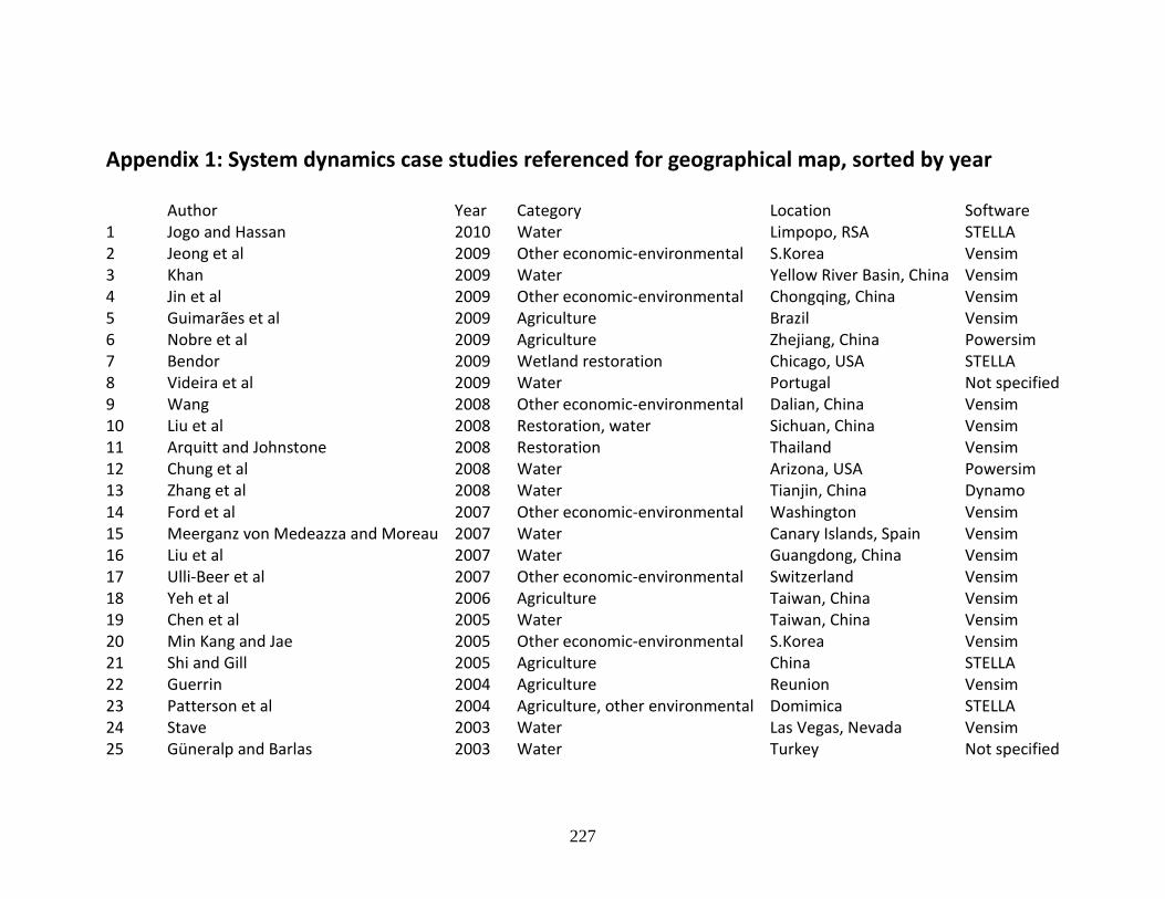
227
Appendix 1: System dynamics case studies referenced for geographical map, sorted by year Author Year Category Location Software 1 Jogo and Hassan 2010 Water Limpopo, RSA STELLA 2 Jeong et al 2009 Other economic-environmental S.Korea Vensim 3 Khan 2009 Water Yellow River Basin, China Vensim 4 Jin et al 2009 Other economic-environmental Chongqing, China Vensim 5 Guimarães et al 2009 Agriculture Brazil Vensim 6 Nobre et al 2009 Agriculture Zhejiang, China Powersim 7 Bendor 2009 Wetland restoration Chicago, USA STELLA 8 Videira et al 2009 Water Portugal Not specified 9 Wang 2008 Other economic-environmental Dalian, China Vensim 10 Liu et al 2008 Restoration, water Sichuan, China Vensim 11 Arquitt and Johnstone 2008 Restoration Thailand Vensim 12 Chung et al 2008 Water Arizona, USA Powersim 13 Zhang et al 2008 Water Tianjin, China Dynamo 14 Ford et al 2007 Other economic-environmental Washington Vensim 15 Meerganz von Medeazza and Moreau 2007 Water Canary Islands, Spain Vensim 16 Liu et al 2007 Water Guangdong, China Vensim 17 Ulli-Beer et al 2007 Other economic-environmental Switzerland Vensim 18 Yeh et al 2006 Agriculture Taiwan, China Vensim 19 Chen et al 2005 Water Taiwan, China Vensim 20 Min Kang and Jae 2005 Other economic-environmental S.Korea Vensim 21 Shi and Gill 2005 Agriculture China STELLA 22 Guerrin 2004 Agriculture Reunion Vensim 23 Patterson et al 2004 Agriculture, other environmental Domimica STELLA 24 Stave 2003 Water Las Vegas, Nevada Vensim 25 Güneralp and Barlas 2003 Water Turkey Not specified
Stellenbosch University http://scholar.sun.ac.za

228
26 Santos and Cabral 2003 Agriculture Portugal STELLA 27 Saysel et al 2002 Agriculture Turkey STELLA 28 Guo et al 2001 Water Yunan, China Not specified 29 Saysel and Barlas 2001 Water Turkey STELLA 30 Portela and Rademacher 2001 Other environmental Brazil STELLA 31 Vezjak et al 1998 Water Slovenia STELLA 32 Alam et al 1997 Agriculture Bangladesh Not specified 33 Turpie et al 1997 Other environmental Western Cape, RSA STELLA 34 Bockstael et al 1995 Water, agriculture Maryland, USA STELLA 35 Bala et al 1988 Agriculture Copenhagen Dynamo
Stellenbosch University http://scholar.sun.ac.za

229
Appendix 2: Geographic distribution of recent systems dynamics applications published in Science Direct journals
Source: Own analysis
Russia
New Zealand
Papua-New Guinea
Australia
Philippines
Japan
Brunei
Taiwan
South Korea
North Korea
Indonesia
Malaysia
Vietnam
Cambodia
LaosMyanmar
Sri Lanka
Madagascar
India
Mongolia
China
Mozambique
South Africa
Malawi
Pakistan
Zimbabwe
Botswana
Kirgistan
Tadschikistan
Somalia
Afghanistan
Tanzania
Namibia
Sambia
Kenya
Dschibuti
Qatar
Yemen
Uganda
Ethiopia
Usbekistan
Angola
Turkmenistan
Eritrea
Iran
Zaire
Saudi-Arabia
Sudan
Iraq
Kazakhstan
Azerbaijan
Congo
Argentina
Jordan
Central Africa
Chile
Gabun
Israel
Syria
Lebanon
Georgia
Cameroon
Chad
Egypt
Cyprus
Nigeria
Turkey
Benin
Togo
Ghana
Libya
Greece
Niger
Bulgaria
Ivory Coast
Burkina Faso
Liberia
Ukraine
Serbia
Romania
Tunesia
Sierra Leone
Belarus
Mali
Guinea
Brazil
Hungaria
Algeria
Lithuania
Italy
Guinea-Bissau
Estonia
Latvia
SenegalGambia
Poland
Mauretania
Finnland
Bolivia
West Sahara
Germany
Marocco
Sweden
Denmark
Spain
France
Belgium
Netherlands
Portugal
Peru
Norway
French-Guayana
United Kingdom
Guyana
Ireland
Columbia
Ecuador
Venezuela
Trinidad
Panama
Puerto Rico
Costa Rica
Dominican RepublicHaiti
Nicaragua
Jamaica
Honduras
El Salvador
Iceland
Belize
Cuba
Mexico
USA
Greenland
Canada
NepalBhutan
Bangladesh
Thailand
Uruguay
Guatemala
Kuwait
Oman
United Arab Emirates
Lesotho
Swaziland
Burundi
Rwanda
Croatia Bosnia-Herzegovina
Austria
Switzerland
Luxemburg
Moldawia
Albania
Macedonia
Montenegro
Slovenia
Czech Republic
Slovakia
Armenia
Paraguay
Surinam
VENSIM model
Agriculture
Restoration
Water
Other environmental
Stellenbosch University http://scholar.sun.ac.za
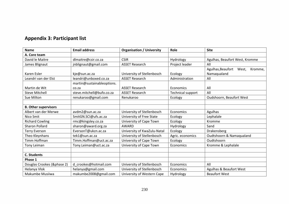
230
Appendix 3: Participant list Name Email address Organisation / University Role Site
A. Core team
David le Maitre [email protected] CSIR Hydrology Agulhas, Beaufort West, Kromme
James Blignaut [email protected] ASSET Research Project leader All
Karen Esler [email protected] University of Stellenbosch Ecology Agulhas,Beaufort West, Kromme, Namaqualand
Leandri van der Elst [email protected] ASSET Research Administration All
Martin de Wit [email protected] ASSET Research Economics All
Steve Mitchell [email protected] ASSET Research Technical support All
Sue Milton [email protected] Renukaroo Ecology Oudshoorn, Beaufort West
B. Other supervisors
Albert van der Merwe [email protected] University of Stellenbosch Economics Agulhas
Nico Smit [email protected] University of Free State Ecology Lephalale
Richard Cowling [email protected] University of Cape Town Ecology Kromme
Sharon Pollard [email protected] AWARD Hydrology Sand
Terry Everson [email protected] University of KwaZulu-Natal Ecology Drakensberg
Theo Kleynhans [email protected] University of Stellenbosch Agric. economics Oudtshoorn & Namaqualand
Timm Hoffman [email protected] University of Cape Town Ecology Oudtshoorn
Tony Leiman [email protected] University of Cape Town Economics Kromme & Lephalale
C. Students
Phase 1
Douglas Crookes (&phase 2) [email protected] University of Stellenbosch Economics All
Helanya Vlok [email protected] University of Stellenbosch Economics Agulhas & Beaufort West
Makumbe Musiiwa [email protected] University of Western Cape Hydrology Beaufort West
Stellenbosch University http://scholar.sun.ac.za
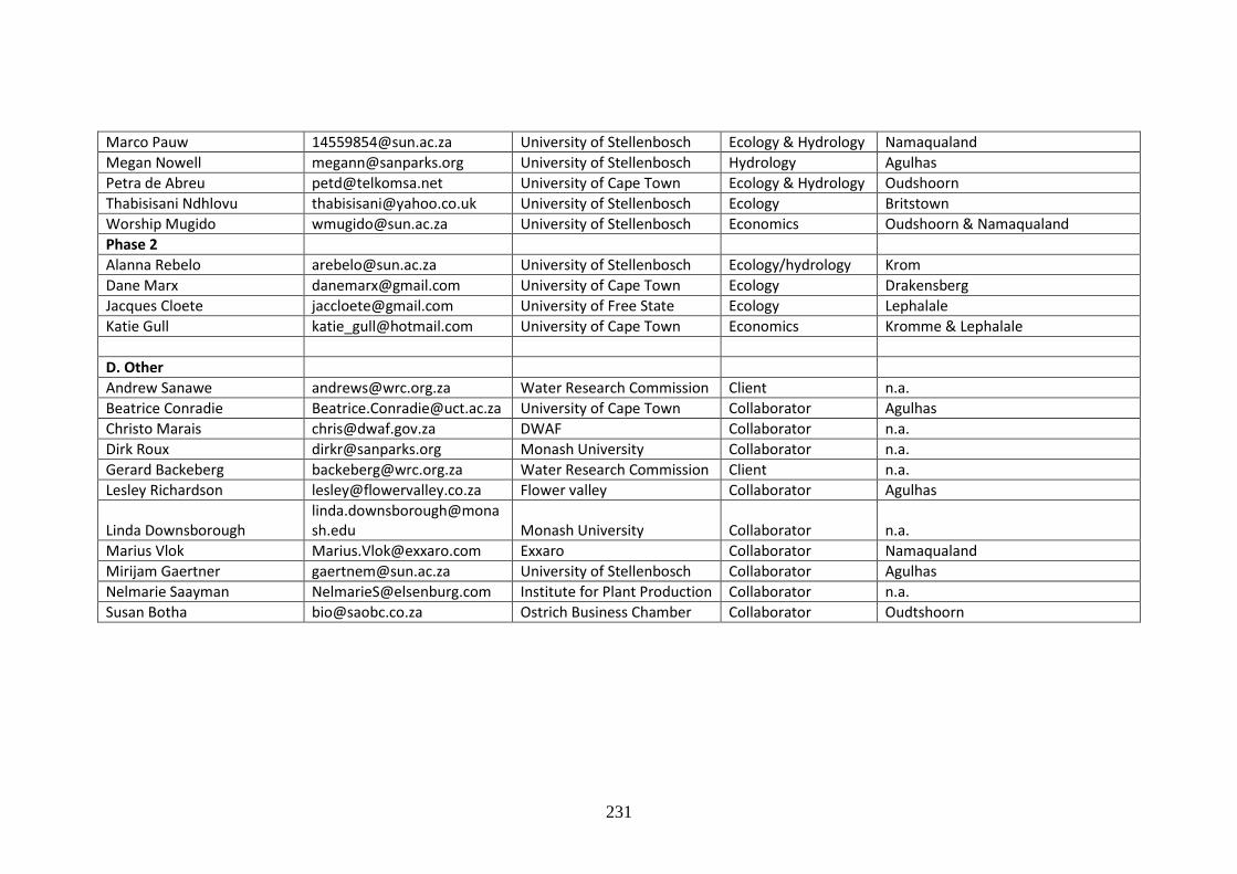
231
Marco Pauw [email protected] University of Stellenbosch Ecology & Hydrology Namaqualand
Megan Nowell [email protected] University of Stellenbosch Hydrology Agulhas
Petra de Abreu [email protected] University of Cape Town Ecology & Hydrology Oudshoorn
Thabisisani Ndhlovu [email protected] University of Stellenbosch Ecology Britstown
Worship Mugido [email protected] University of Stellenbosch Economics Oudshoorn & Namaqualand
Phase 2
Alanna Rebelo [email protected] University of Stellenbosch Ecology/hydrology Krom
Dane Marx [email protected] University of Cape Town Ecology Drakensberg
Jacques Cloete [email protected] University of Free State Ecology Lephalale
Katie Gull [email protected] University of Cape Town Economics Kromme & Lephalale
D. Other
Andrew Sanawe [email protected] Water Research Commission Client n.a.
Beatrice Conradie [email protected] University of Cape Town Collaborator Agulhas
Christo Marais [email protected] DWAF Collaborator n.a.
Dirk Roux [email protected] Monash University Collaborator n.a.
Gerard Backeberg [email protected] Water Research Commission Client n.a.
Lesley Richardson [email protected] Flower valley Collaborator Agulhas
Linda Downsborough [email protected] Monash University Collaborator n.a.
Marius Vlok [email protected] Exxaro Collaborator Namaqualand
Mirijam Gaertner [email protected] University of Stellenbosch Collaborator Agulhas
Nelmarie Saayman [email protected] Institute for Plant Production Collaborator n.a.
Susan Botha [email protected] Ostrich Business Chamber Collaborator Oudtshoorn
Stellenbosch University http://scholar.sun.ac.za