La Convention sur la diversité biologique à la croisée de quatre discours
Upload
khangminh22Category
view
3download
0
THÈSEprésentée pour obtenir le grade de docteur délivré par
Aix Marseille Université
Ecole doctorale no 251 : Sciences de l’Environnement
Spécialité “Océanographie”
présentée et soutenue publiquement le 15 Novembre 2019 à Nouméa par
Aurore RECEVEUR
Écologie spatiale du micronecton : distribution, diversité etimportance dans la structuration de l’écosystème pélagique du
Pacifique sud-ouest
JuryDr. Frédéric Ménard DR IRD Directeur de thèse
Dr. Christophe Menkes DR IRD Co-directeur de thèse
Dr. Arnaud Bertrand DR IRD Rapporteur
Dr. Ronan Fablet Prof. IMT Atlantique Rapporteur
Dr. Valérie Allain Senior Fisheries Research Scientist CPS Examinatrice
Dr. Rudy Kloser Senior Principle Research Scientist CSIRO Examinateur
Dr. Anne Lebourges-Dhaussy IR IRD Examinatrice
Dr. Claude Payri DR IRD Examinatrice
Thèse préparée au sein de la CPS et du centre IRD de Nouméa, Nouvelle-Calédonie

Résumé
L’écosystème pélagique Néo Calédonien est le théâtre d’une forte diversité de prédateurs, comme
les oiseaux marins ou les cétacés. Cette diversité est rendue possible par la grande diversité d’habitats
physiques. La récente création du Parc marin Naturel de la Mer de Corail a ouvert un besoin d’informa-
tions précises sur le fonctionnement de cet écosystème remarquable, notamment sur la dynamique du
micronecton et de son rôle central dans les réseaux trophiques, d’autant plus que ce maillon est le plus
méconnu. Dans ce contexte, cette thèse a pour objectif d’étudier la dynamique et la diversité du micro-
necton; et dans un deuxième temps d’analyser son influence sur la répartition des prédateurs. Dans le
2ème chapitre, nous avons utilisé des intensités acoustiques d’ADCP (Acoustic Doppler Current Profiler)
acquises à travers 54 campagnes réparties sur 19 ans pour évaluer les variabilités saisonnières et inter-
annuelles de micronecton et sa distribution spatiale dans la couche 20-120m. Nous avons montré une
diminution de son abondance relative de 1999 à 2007 suivie d’une augmentation jusqu’en 2017. Nous
avons également mis en évidence l’influence d’ENSO avec une augmentation de l’abondance durant les
phases El Niño. Enfin, nous avons montré une faible corrélation spatiale entre les prédictions de SEA-
PODYM, un modèle écosystémique, et nos prévisions d’intensités acoustiques. Dans le 3ème chapitre,
nous avons regardé la variabilité de la distribution verticale du micronecton et tenté d’en comprendre
les forçages physiques à travers l’analyse de données d’EK60 acquises pendant six campagnes entre 2011
et 2017. Le développement d’un cadre statistique a permis de lier les distributions verticales de micro-
necton aux conditions environnementales et de faire de la biorégionalisation. Nous avons identifié trois
régions acoustiquement homogènes : (1) au nord de 21°S avec une faible DSL (Deep Scattering Layer)
et une faible SSL (Shallow Scattering layer), (2) le coin sud-ouest (SSL intense à 80m et SSL très intense
à 30m) et (3) le coin sud-est (SSL intense et DSL très intense à 550m). Au cours du 4ème chapitre, nous
nous sommes concentrés sur la diversité du micronecton et les facteurs physiques la régissant. Pour cela,
nous avons analysé les 22 espèces les plus nombreuses, présentes dans 141 chaluts, à l’aide d’une mé-
thode multi-variée. Sept grands assemblages ont été décrits, principalement influencés par le moment
de la journée et la profondeur du chalut, puis par la température, l’oxygène et la bathymétrie. L’assem-
blage prédominant au nord était dominé par les crustacés et au sud par les céphalopodes et poissons.
Les deux chapitres suivant ont utilisé les prédictions verticales de distribution du 2ème chapitre. Nous
avons prédit l’évolution du micronecton en changement climatique dans le 5ème chapitre. Une simu-
lation océanographique régionale innovante, réalisée à partir d’un modèle biogéochimique dynamique
couplé (NEMO-PISCES), a été utilisé pour forcer la modélisation acoustique et le modèle SEAPODYM.
Les deux ont prédit une diminution moyenne de l’abondance de micronecton d’ici 2100, mais l’acous-
tique prédisait une forte augmentation pour la couche bathypélagique (environ 400-600m) alors que
SEAPODYM prédisait la plus forte diminution pour cette même couche. Les changements d’abondance
étaient majoritairement dus à la modification de la structure de la colonne d’eau, avec un approfondis-
sement de la thermocline. Enfin dans le 6ème chapitre, nous avons lié l’abondance relative des proies à la
distribution de neuf prédateurs : le thon jaune, le thon germon, la dorade coryphène (CPUE), le puffin, le
pétrel, le fou à pieds rouge (données de marquage), les dauphins, les globicéphales et les baleines à bec
(comptages par survol aérien). L’abondance des proies influençait la distribution de six des neuf préda-
teurs. Cette approche nous a permis de montrer que les données d’abondance des proies mesurées par
acoustique pouvaient améliorer les modèles de distribution des prédateurs dans une certaine mesure.
ii

Abstract
New Caledonian pelagic ecosystem has been showed to contain strong diversity of top predators, as
seabirds and cetaceans. This diversity is supported by variability in physical environment (e.g. ridges and
seamounts), offering a large diversity of habitats. The recent creation of the Natural Park of the Coral Sea
created needs of robust information on the productivity and functioning of this remarkable ecosystem,
including micronekton dynamics and their pivotal role in food webs. This food web link has been high-
lighted as the largest gap of knowledge. In this context, the PhD firstly aimed to study the biodiversity
and the functioning of micronektonic compartment through acoustics and trawl around New Caledo-
nia. In a second part, it aimed to analyze influence of prey on top predators’ distribution. In the second
chapter we used backscatter echo-intensity data of Shipboard Acoustic Doppler Current Profiler, recor-
ded during 54 cruises across 19 years to assess micronekton seasonal and inter-annual variabilities and
spatial distribution in the 20-120m layer. We showed a decrease of micronekton relative abundance until
2007 and then an increase, as well as an enhancement during El Niño events. Sea surface temperature
was the main factor driving the backscatter variability. Finally, we showed poor spatial cohesion bet-
ween SEAPODYM predictions, an ecosystem model, and our backscatter predictions. During the third
chapter, we focused on micronekton vertical distribution variability and the understanding of forcing
oceanographic parameters through analyze of EK60 from six cruises happening between 2011 and 2017.
We developed a statistical framework to link typical vertical distributions to environmental conditions
and used it to predict acoustic vertical profile over a larger area to do bio-regionalization. We found three
acoustically homogenous regions : north of 21°S with weak DSL (Deep Scattering Layer) and weak SSL
(Shallow Scattering layer), the southwest corner (intense SSL at 80m and very intense SSL at 30m) and
the southeast corner (intense SSLs and very intense DSL at 550m). During the fourth chapter, we loo-
ked at the species diversity distribution and its physical drivers. For that purpose, we analyzed the 22
most numerous species present in 141 trawls with a multi-variates method. Seven major assemblages
were identified, mainly driven by moment of the day and trawl depth, and then by temperature, oxygen
and bathymetry. Globally, predominant northern assemblages were dominated by crustaceans and sou-
thern assemblages by less crustacean and more cephalopods and fish. The last two chapters used the
methodology of the 3th. We predicted micronekton evolution in climate change in the 5th chapter. We
used an innovative oceanographic regional simulation from a coupled dynamical-biogeochemical mo-
del (NEMO-PISCES) to force acoustics modeling and SEAPODYM. Both methods predicted a micronek-
ton abundance decreasing by 2100 in the Coral Sea, but acoustics predictions showed a large increase for
the bathypelagic layer (about 400-600m) whereas SEAPODYM showed the largest decrease for this same
layer. Micronekton abundance changes were mainly driven by water column structure change, through
mainly a deepening of the thermocline. Finally, in the last chapter we linked prey relative abundance
to nine predators taxa distribution : yellowfin and albacore tuna, dolphinfish (analyzed through CPUE),
shearwater, petrel and red-footed booby (tagging data) and Delphinae, Globicephalinae and Ziphiidae
(aerial survey count). Preyscape shaped six out of nine predators distributions and we described the
nine spatial distributions. Our approach allowed us to show that prey abundance data collected using
acoustic methods can slightly improve distribution models for predators.
iii

Remerciements
Il parait que la plupart des gens ne lisent que les remerciements d’une thèse, je vais donc essayer
de soigner ceux-ci. Je voudrais commencer par remercier du fond du cœur Valérie et Christophe qui
ont monté ce projet, m’ont proposé la thèse et m’ont soutenue tout du long. Merci Christophe, depuis
presque 5 ans, de me faire partager ta passion de la science. Au début de mon stage de Master, je ne
voulais pas faire de thèse. Si jen finis une en ce moment, c’est en grande partie grâce à toi. Tu as su me
transmettre cette éternelle soif de connaissances et de compréhension du monde qui nous entoure et
qui t’anime. Tu m’as aussi appris à ne jamais être satisfaite d’une conclusion, à creuser encore et toujours
plus loin et à vouloir comprendre toujours mieux, qualité essentielle du chercheur à mon avis. Merci à
toi aussi Valérie d’avoir temporisé cette folie de Christophe et recentré les priorités. Merci d’avoir été
là au quotidien, pour me soutenir, me faire relativiser et m’offrir du chocolat. Tu m’auras aussi montré
comment être organisée et travailler en équipe. Cette faculté que tu as de pouvoir travailler avec tout le
monde m’impressionnera toujours. Merci à tous les deux d’avoir été deux sources d’inspiration si com-
plémentaires. Merci aussi pour tous ces bons moments en dehors du travail, et pour tous vos sourires.
Je voudrais ensuite remercier Fred. Merci d’avoir accepté d’être le directeur de cette thèse et de m’avoir
toujours accueillie avec beaucoup de bienveillance lors de mes passages à Marseille. Tes conseils avi-
sés lors de la relecture de mes articles m’aideront tout au long de ma carrière, j’en suis sûre. Merci de
ton implication malgré les 20 000 km de distance et ton emploi du temps parfois chargé. Enfin, merci
à toi aussi pour ta bonne humeur toujours présente. Et enfin merci à toi, la rayonnante Anne, dernier
pilier de l’encadrement de cette thèse. Merci de toutes ces connaissances sur l’acoustique que tu m’as
transmises. Merci de m’avoir montré comment faire de la très bonne science tout en gardant le sou-
rire le plus communicatif que je connaisse. Discuter de sciences et d’acoustique n’aura jamais été aussi
agréable qu’avec toi, et tu resteras toi aussi une source d’inspiration. Je continue en remerciant les deux
mathématiciens qui m’auront bien aidé, eux aussi très complémentaires. Morgan, merci de m’avoir fait
découvrir tout un panel de méthodes complexes de machine learning. Merci aussi pour tes conseils avi-
sés pendant la thèse, et tes mots toujours gentils. Merci David de m’avoir aussi montré les forces et les
possibilités énormes des méthodes plus classiques comme notre chère ACP. C’est parfois avec les plus
vieux matériaux, qu’on construit les tables les plus robustes. Merci aussi de m’avoir fait tant rire pendant
mes séjours marseillais. Merci à Elodie K. de m’avoir fait découvrir le monde de l’ADCP. Je souhaite éga-
lement remercier les membres du jury d’avoir accepté de juger ce travail et de s’être déplacés, parfois de
loin, pour assister à la soutenance.
Merci à vous, ma FEMAly de m’avoir soutenue et d’avoir cru en moi. Elodie, Annie, Valérie, Tom,
Sylvain, Bruno, Neville, François, Joe, Jed, Caro, Malo, Tim, Sifa, je vous remercie du fond du cœur pour
cette magnifique ambiance de travail. Une petite pensée pour Chloé aussi qui vient de partir et qui a
refusé d’écrire cette thèse pour 100xpf. Merci pour tous ces restaus et apéros d’équipe, de la joie que
vous avez apporté à mon quotidien. Une mention particulière pour la plus belle des partenaires de danse
tahitienne, avec qui j’adore rigoler. Un merci particulier à Dc Tom aussi, pour m’avoir appris des blagues
en anglais (dédicasse au walrus) et pour toutes nos discussions de modèles et de résidus. Tu m’auras
beaucoup appris. Merci aussi à Boris, Constance et Aymeric pour votre éternelle bonne humeur et pour
vos nombreux coups de main pour les posters, figures, dépliants, et j’en passe. Merci à toutes les pêches,
et à toute la CPS de rendre possible un environnement de travail si agréable. Une petite pensée pour
iv

mes partenaires de sport du midi. J’en profite pour remercier Simon qui m’a fait entrer à la CPS il y a
cinq ans pour mon stage de Master 2. Je suis très heureuse de te revoir d’ici quelques mois. Merci aux
équipe du MIO à Marseille et du LEMAR à Brest pour vos accueils. Un immense merci à toi, Gildas. Merci
pour ces semaines Brest, pour cette incroyable mission à Wallis, pour cette super semaine à Galway.
J’espère avoir la chance de continuer à travailler avec toi, nos discussions sur la recherche, sur mon
futur, sur la vulgarisation m’ont particulièrement marquée. Au passage, merci à l’équipage de l’Alis pour
cette mission inoubliable autour de Walis et Futuna. La météo désastreuse a largement été compensée
par la super ambiance du bateau. Je ne suis pas prête de l’oublier cette première mission en mer.
Comme il n’y a pas que le travail dans la vie, je voudrais également remercier les copains. Merci
à toi Laura, de m’avoir fait partager ta passion pour les statistiques et pour les couleurs (oui faire de
belles figures est important et mérite qu’on y passe un peu de temps). Merci aussi d’avoir encouragé
ma passion pour les enfants, c’est promis, je ne la laisserai jamais tomber. Merci ensuite à toi Elodie,
pour tout. Pour être toujours là dans les bons et les moins bons moments, merci de croire si fort en
moi et de me donner du courage. Merci aussi d’avoir partagé avec moi ta passion pour la taxonomie
du micronecton. Merci à Solène et Lauriane pour tous ces bons moments et pour votre aide pour la
relecture de mes chapitres, de chacune de vos attentions pour me donner du courage. Merci à toi aussi
Anne L. pour tes folies, pour ta passion de la science que tu transmets si bien. Tu es vraiment super forte
et j’espère être un peu comme toi un jour. Merci aussi pour tes bons ti punch. Merci à Delphine, pour
tes encouragements et puis de me motiver d’aller au sport. Merci Florence pour nos déjeuners qui m’ont
toujours sorti la tête du travail. Et pour finir merci à toi Estelle, pour nos innombrables discussions sur le
sens de la vie, pour être toujours là quand il le faut. Merci à vous Christina, Léo, Delphine, Camille, Giulia,
Ulysse, Nico, Camille, Pierre, Thomas, Thomas, Audrey, Thibault, Laurie pour ces weekends d’évasion,
pour ces parties de volley endiablées. Merci aux copains de France aussi, les fans de Céline et Johny. Merci
à toi Ludo d’avoir traversé la planète pour venir à mon mariage. Une pensée particulière à toi Maxime,
avec qui j’ai commencé à rêver d’halieutique et de stocks de poissons. Vivement notre premier projet
tous les deux. Merci à vous aussi Antoine et Margaux, les copains de prépa pour tous les bons moments.
Antoine, vivement aussi notre premier projet de sensibilisation ensemble. Et merci pour ton mail d’il y
a deux jours qui m’a fait un bien immense. Et puis, je voudrais te remercier toi Julien, qui est là depuis
le tout début. Tu as toujours cru en moi, tu m’as même trouvé mon premier stage en biologie marine.
Merci d’être toi.
Je voudrais aussi remercier ma famille. Mes quatre grands parents qui sont une source inépuisable
d’inspiration. Mes parents aussi, qui m’ont toujours poussée à viser plus haut. Merci d’avoir traversé la
France pour me faire visiter des écoles, des universités, des forums sur ‘les métiers de la mer’, de m’avoir
fait rêver. Merci aussi pour les 3 années à Mayotte qui ne sont pas pour rien dans la réalisation de cette
thèse. Et puis merci à mes trois frères, d’être toujours là et de me faire rire. Merci de me faire relativiser
quand il le faut et surtout de me supporter depuis 27 ans. Et puis aux cousins, oncles, tantes, pour tous
ces bons moments.
Les derniers remerciements iront pour toi Cyrilou. Voilà bientôt six ans que tu illumines chacune de
mes journées (ou presque) et bientôt un an que tu es devenu mon mari. Tu as été là dans les moments de
doute, tu m’as toujours soutenue et fait rire chaque jour. Et surtout, quand je me vois à travers tes yeux,
je sais que je peux y arriver. Nos discussions, parfois trop longues à mon goût, ont amplement enrichi
cette thèse et m’ont bien aidée à développer mon sens critique. Merci pour tout mon amour.
v

Scientific contributions
First author publications
Receveur, A., E. Kestenare, V. Allain, F. Menard, S. Cravatte, A. Lebourges-Dhaussy, P. Lehodey, M.
Mangeas, N. Smith, M.H. Radenac, C. Menkes. 2020. "Micronekton distribution in the southwest Pacific
(New Caledonia) inferred from Shipboard-ADCP Backscatter data". Deep Sea Research Part I. (Chapitre
2)
Receveur, A., C. Menkes, V. Allain, A. Lebourges-Dhaussy, D. Nerini, M. Mangeas, and F. Menard. 2019.
"Seasonal and spatial variability in the vertical distribution of pelagic forage fauna in the southwest Pa-
cific". Deep Sea Research Part II. (Chapitre 3)
Submitted, in revision Receveur, A., E. Vourey, A. Lebourges-Dhaussy, C.E. Menkes, F. Menard, and V.
Allain. "Micronekton Richness and Assemblages in the Natural Park of the Coral Sea". In Frontiers in
Marine Sciences. (Chapitre 4)
Submitted soon Receveur, A., T. Gorgues, C. Menkes, C. Dutheil, O. Aumont, P. Lehodey, V. Allain, F. Me-
nard, S. Nicol, and A. Lebourges-Dhaussy. "Exploring the Potential Future of the Coral Sea Micronekton".
In prep. for Global Change Biology. (Chapitre 5)
Submitted soon Receveur A., Allain V., Lebourges-Dhaussy A., Menkes C., Ménard F., Laran S., Vidal E.,
Ravache A., Hare S. , Weimerskirch H., Borsa P. Habitat predictive modelling of nine top predators with
respect to the abundance of pelagic prey in the southwest Pacific. (Chapitre 6)
Other publications
Lorrain, A., H. Pethybridge, N. Cassar, A. Receveur, V. Allain, N. Bodin, L. C.A. Bopp, Choy, L. Duffy,
B. Fry, N. Goni, D.S. Graham, A.J. Hobday, J.M. Logan, F. Menard, C. Menkes, R.J. Olson, D. Point, A.T.
Revill, C.J. Somes, J.W. Young. 2019. "Trends in Tuna Carbon Isotopes Reflect Global Changes in Pelagic
Phytoplankton Communities." Global Change Biology.
Houssard, P., A. Lorrain, L. Tremblay-Boyer, V. Allain, B. S. Graham, C. E. Menkes, H. Pethybridge, L.
Couturier, D. Point, B. Leroy, A. Receveur, B.P. Hunt, E. Vourey, S. Bonnet, M. Rodier, P. Raimbault, E.
Feunteun, P.M. Kuhnert, J.M. Munaron, B. Lebreton, T. Otake, Y. Letourneur. 2017. “"Trophic Position
Increases with Thermocline Depth in Yellowfin and Bigeye Tuna across the Western and Central Pacific
Ocean." Progress in Oceanography 154 : 49–63. https ://doi.org/10.1016/j.pocean.2017.04.008.
vi

International conferences and workshops
WGFAST, Galway, 2019 - Forecasting vertical distribution variability of pelagic forage fauna in the
south Pacific.
CLIOTOP, Taiwan, 2018 - Acoustic characterization of micronekton vertical distribution related to
the environment around New Caledonia (south-west Pacific).
WGFAST, Seattle, 2018 - Acoustic characterization of micronekton distribution in the surface layer
related to the environment across the New Caledonian economic zone (south-west Pacific).
AGU 2016, San Francisco - El Niño revisited : the influence of El Niño Southern Oscillation on the
world’s largest tuna fisheries.
Scientific reports and other presentations
Valérie Allain, Aurore Receveur, Élodie Vourey, Annie Portal, Jeff Dubosc, Laurent Millet, Damien La-
grange, Philippe Borsa, Chloé Yven, Dianne Gleeson, Elise Furlan, Jonas Bylemans, Christophe Menkes,
Gildas Roudaut et Anne Lebourges-Dhaussy, 2019. "A la découverte du micronecton de l’océan de Nouvelle-
Calédonie : les proies des thons et autres grands prédateurs marins". Note d’informations.
Valérie Allain, Christophe Menkes, Aurore Receveur, Elodie Vourey, Martine Rodier, Céline Bachelier,
Gildas Roudaut, Antoine Nowaczyk, Annie Portal et Laurent Millet, 2019. "L’exploration de l’océan de
Wallis-et-Futuna : une diversité à découvrir, des monts sous-marins à explorer". Note d’informations.
Christophe Menkes, Patrick Lehodey, Inna Senina, Thomas Gorgues, Valerie Allain et Aurore Rece-
veur, 2019. "L’impact du changement climatique sur l’écosystème de l’océan de Nouvelle-Calédonie".
Note d’informations.
Christophe Menkes, Patrick Lehodey, Inna Senina, Thomas Gorgues, Valerie Allain et Aurore Rece-
veur, 2019." L’impact du changement climatique sur l’écosystème de l’océan de Wallis-et-Futuna". Note
d’informations.
Receveur A., V. Allain. 2017. "A young scientist studies marine biodiversity in the open ocean". SPC
Fisheries Newsletter 152, 10-15.
Receveur A., S. Nicol, L. Tremblay-Boyer, C. Menkes, I. Senina and Lehodey P.. 2016. "Using SEAPO-
DYM to better understand the influence of El Niño Southern Oscillation on Pacific tuna fisheries". SPC
Fisheries Newsletter 149, 31–36.
Les six newsletters du projet BIOEPALGOS - https://fame1.spc.int/fr/projets/biopelagos
C’Nature 2019, Nouméa - Restitution publique du projet BIOPELAGOS.
vii

Le projet BIOPELAGOS
Les pays et territoires du Pacifique se caractérisent par de petites surfaces terrestres (2%) et de vastes
zones océaniques (98%) et l’océan Pacifique représente à lui seul 48% de l’océan mondial. L’océan et les
organismes vivants constituent un lien important entre tous les pays et territoires du Pacifique. Ils se par-
tagent l’océan qui est une source majeure de revenus, par exemple à travers les droits d’accès à la pêche
au thon (ces droits fournissent entre 11 et 63% des revenus annuels de pays tels que Kiribati, Tuvalu ou
les Etats fédérés de Micronésie [Bell et al., 2015]). C’est également une source essentielle de protéines
pour la sécurité alimentaire : la consommation moyenne de poisson varie de 30 à 148 kg/hab/an dans
les îles du Pacifique [Bell et al., 2011] contre une moyenne de 19 kg/hab/an pour le monde [FAO, 2016].
Enfin l’océan a une valeur culturelle et patrimoniale importante dans la région (route navigable, mytho-
logie ou encore espèces emblématiques).
L’importance de l’écosystème océanique et de sa biodiversité pour les communautés du Pacifique ne
doit donc pas être sous-estimée. Contribuant à tous les aspects de la vie, l’océan offre de nombreux ser-
vices aux populations du Pacifique, aux gouvernements (par l’accès à la pêche) et à l’emploi (à bord des
navires de pêche et dans les usines de transformation). Il contribue également aux services culturels par
la présence de mammifères marins, d’oiseaux marins, de requins et de tortues qui ont une valeur patri-
moniale et récréative (e.g. l’observation des baleines). Enfin, l’écosystème océanique lui-même contri-
bue de manière significative à la régulation du climat par sa contribution au puits de carbone océanique.
Avec une population humaine qui demeure extrêmement vulnérable aux impacts des changements cli-
matiques, ce service écosystémique traduit à lui seul le rôle crucial que jouent des écosystèmes océa-
niques pour la vitalité de la région du Pacifique et de ses habitants. Dans ce contexte, la conservation et
la gestion durable des océans est essentielle à la subsistance et au développement des pays et territoires
du Pacifique.
Le paysage océanique du Pacifique (Pacific Oceanscape en anglais) a été conçu par son excellence
Anote Tong, Président de Kiribati, au début de 2009 et le concept a été approuvé par les dirigeants du
Forum des îles du Pacifique à leur 40ème réunion en août 2009. L’objectif du cadre est d’assurer la santé
et le bien-être de l’océan et des populations par la gestion intégrée des océans, l’adaptation aux change-
ments environnementaux et climatiques. L’une des actions identifiées est l’utilisation de la planification
spatiale de l’espace marin pour améliorer la gestion des ZEE (Zone Économique Exclusive) afin de sou-
tenir le développement économique tout en maintenant les fonctions des écosystèmes et l’intégrité de
la biodiversité des zones côtières et marines. La planification spatiale de l’espace marin est un outil per-
viii

mettant d’associer un développement socio-économique durable et dans le même temps une conserva-
tion de l’environnement et de la biodiversité pour perpétuer les services que les écosystèmes fournissent
aux populations, particulièrement dans le contexte du changement climatique et du besoin critique de
stratégie de résilience. Cette planification spatiale nécessite des informations sur l’utilisation de l’océan,
l’état des écosystèmes et l’impact des perturbations de l’environnement sur ces écosystèmes. Cepen-
dant dans la plupart des pays et territoires du Pacifique, les décideurs sont confrontés à un manque
important d’informations qui empêche, entrave ou retarde leurs décisions. C’est particulièrement vrai
en ce qui concerne les zones océaniques offshore qui sont difficilement accessibles à la recherche en
comparaison des zones côtières.
C’est dans ce contexte de besoins locaux de conservation et de gestion durable qu’a été pensé le
projet BIOPELAGOS, appliqué à deux territoires français du Pacifique : la nouvelle-Calédonie et Wallis-
et-Futuna. En Nouvelle-Calédonie, après la mise en œuvre en 2014 du parc marin de la mer de corail
(catégorie VI des aires protégées de l’UICN) qui couvre l’ensemble des eaux océaniques de la ZEE, les
autorités sont en train d’élaborer un plan de gestion qui exige des informations spatiales (par exemple
répartition spatiale des usages ou des espèces). Wallis-et-Futuna a entamé des négociations avec des
entreprises de pêche étrangères en vue d’attribuer l’accès à la pêche au thon. Toutefois, aucune pêche
industrielle de thonidés industrielle hauturière n’a été pratiquée dans cette ZEE à ce jour et il n’existe
aucune information sur ses ressources pélagiques océaniques. En outre, la ZEE de Wallis-et-Futuna se
caractérise par la présence de nombreux monts sous-marins qui sont susceptibles d’avoir des niveaux
élevés de biodiversité et d’être particulièrement vulnérables à la pêche industrielle et aux autres impacts
humains.
Le projet BIOPELAGOS, co-géré par la CPS (Communauté du Pacifique) et l’IRD (Institut de Re-
cherche pour le développement) vise à apporter un soutien scientifique aux territoires français du Pa-
cifique pour contribuer à des prises de décision éclairées sur la gestion durable et la conservation de la
biodiversité de leurs écosystèmes océaniques. Le projet BIOPELAGOS a duré 3 ans (du 30 juin 2016 au
29 juin 2019) et a été financé par un programme BEST 2.0 de l’Union Européenne. Trois thématiques
étaient envisagées :
— L’acquisition de nouvelles connaissances à travers la collecte de données dans chaque territoire
pour combler les lacunes en matière de connaissances et améliorer la compréhension de la biodi-
versité et du fonctionnement de l’écosystème océanique. Pour cela, des campagnes à la mer, des
campagnes de marquage des oiseaux marins (pétrels et puffins) et du barcoding et metabarcoding
génétique ont été réalisés.
— Le renforcement des capacités humaines pour former des personnes et partager et diffuser l’in-
formation recueillie. Pour cela, une étudiante en thèse et des étudiants de niveau Master ont été
encadrés, des journées d’information auprès du grand public ont été organisées et des échanges
réguliers ont été menés avec les institutions des territoires partenaires.
— La synthèse des connaissances, pour fournir des recommandations scientifiques à l’appui de
décisions éclairées sur la conservation, la gestion durable et la résilience des écosystèmes océa-
niques. Pour cela, une base de données a été constituée rassemblant les jeux de données his-
toriques et nouvellement acquis sur le domaine océanique ; les données ont été analysées pour
comprendre les interactions trophiques et pour identifier des zones de forte biodiversité. Une
modélisation sur le changement climatique a été mise en place pour explorer les évolutions spa-
ix

tiales d’abondance du micronecton et des thons. Six notes ont été rédigées pour synthétiser les
informations les plus pertinentes pour la conservation et la gestion durable des ressources péla-
giques et ont été diffusées au niveau régional. Elle sont disponibles à l’adresse suivante : https:
//fame1.spc.int/fr/projets/biopelagos.
C’est dans le cadre de ce projet que ma thèse a été financée avec pour objectif de rassembler et
analyser l’ensemble des données récoltées sur l’écosystème pélagique pour en comprendre son fonc-
tionnement et sa diversité. Les objectifs ont été affinés au cours des premiers mois, et sont donnés à la
fin de l’introduction générale. L’inclusion de la thèse dans un projet européen m’a permis de participer
aux réunions avec les différents gestionnaires et ainsi d’appréhender les relations entre scientifiques et
décideurs. J’ai également participé à une campagne en mer de 15 jours réalisées en 2018 autour de Wal-
lis et Futuna, j’ai participé à l’encadrement d’une étudiante de Master 2, et enfin j’ai participé et mené
différentes actions de sensibilisation sur le milieu marin. Dans ce cadre, des outils pédagogiques ont été
développés et sont présentés en annexe 8 de cette thèse.
x

Table des matières
Table des matières xi
Liste des figures xv
Liste des tableaux xxv
1 Introduction 1
1.1 Contexte général : qu’est-ce qu’un écosystème pélagique? . . . . . . . . . . . . . . . . . . . . 2
1.2 Le parc marin de la mer de Corail, un écosystème riche dans une région oligotrophe . . . . 16
1.3 Les questions scientifiques de la thèse . . . . . . . . . . . . . . . . . . . . . . . . . . . . . . . . 26
1.4 Les moyens d’étude du micronecton . . . . . . . . . . . . . . . . . . . . . . . . . . . . . . . . . 26
1.5 Les outils mathématiques d’analyse . . . . . . . . . . . . . . . . . . . . . . . . . . . . . . . . . 37
1.6 Le plan de la thèse . . . . . . . . . . . . . . . . . . . . . . . . . . . . . . . . . . . . . . . . . . . 41
2 Micronekton distribution in the southwest Pacific (New Caledonia) inferred from Shipboard-
ADCP backscatter data 43
2.1 Introduction . . . . . . . . . . . . . . . . . . . . . . . . . . . . . . . . . . . . . . . . . . . . . . . 44
2.2 Material and Methods . . . . . . . . . . . . . . . . . . . . . . . . . . . . . . . . . . . . . . . . . 47
2.3 Results . . . . . . . . . . . . . . . . . . . . . . . . . . . . . . . . . . . . . . . . . . . . . . . . . . 53
2.4 Discussion . . . . . . . . . . . . . . . . . . . . . . . . . . . . . . . . . . . . . . . . . . . . . . . . 62
3 Seasonal and spatial variability in the vertical distribution of pelagic forage fauna in the south-
west Pacific 75
3.1 Introduction . . . . . . . . . . . . . . . . . . . . . . . . . . . . . . . . . . . . . . . . . . . . . . . 76
3.2 Material and Methods . . . . . . . . . . . . . . . . . . . . . . . . . . . . . . . . . . . . . . . . . 78
xi

TABLE DES MATIÈRES
3.3 Results . . . . . . . . . . . . . . . . . . . . . . . . . . . . . . . . . . . . . . . . . . . . . . . . . . 84
3.4 Discussion . . . . . . . . . . . . . . . . . . . . . . . . . . . . . . . . . . . . . . . . . . . . . . . . 92
4 Micronekton richness and assemblages in the Natural Park of the Coral Sea 103
4.1 Introduction . . . . . . . . . . . . . . . . . . . . . . . . . . . . . . . . . . . . . . . . . . . . . . . 104
4.2 Methods . . . . . . . . . . . . . . . . . . . . . . . . . . . . . . . . . . . . . . . . . . . . . . . . . 106
4.3 Results . . . . . . . . . . . . . . . . . . . . . . . . . . . . . . . . . . . . . . . . . . . . . . . . . . 111
4.4 Discussion . . . . . . . . . . . . . . . . . . . . . . . . . . . . . . . . . . . . . . . . . . . . . . . . 122
5 Exploring the potential future of the Coral Sea micronekton 133
5.1 Introduction . . . . . . . . . . . . . . . . . . . . . . . . . . . . . . . . . . . . . . . . . . . . . . . 134
5.2 Material and Methods . . . . . . . . . . . . . . . . . . . . . . . . . . . . . . . . . . . . . . . . . 136
5.3 Results . . . . . . . . . . . . . . . . . . . . . . . . . . . . . . . . . . . . . . . . . . . . . . . . . . 142
5.4 Discussion . . . . . . . . . . . . . . . . . . . . . . . . . . . . . . . . . . . . . . . . . . . . . . . . 150
6 Habitat predictive modelling of nine top predators with respect to the abundance of pelagic
prey in the southwest Pacific 157
6.1 Introduction . . . . . . . . . . . . . . . . . . . . . . . . . . . . . . . . . . . . . . . . . . . . . . . 158
6.2 Methods . . . . . . . . . . . . . . . . . . . . . . . . . . . . . . . . . . . . . . . . . . . . . . . . . 160
6.3 Results . . . . . . . . . . . . . . . . . . . . . . . . . . . . . . . . . . . . . . . . . . . . . . . . . . 166
6.4 Discussion . . . . . . . . . . . . . . . . . . . . . . . . . . . . . . . . . . . . . . . . . . . . . . . . 174
7 Conclusions et perspectives 181
7.1 Rappels des résultats principaux . . . . . . . . . . . . . . . . . . . . . . . . . . . . . . . . . . . 182
7.2 L’acoustique comme moyen d’étude . . . . . . . . . . . . . . . . . . . . . . . . . . . . . . . . . 183
7.3 La dynamique des proies mise en évidence dans le Pacifique sud-ouest . . . . . . . . . . . . 190
7.4 L’impact potentiel du changement climatique . . . . . . . . . . . . . . . . . . . . . . . . . . . 191
7.5 La gestion de l’écosystème et le parc naturel de la mer de Corail . . . . . . . . . . . . . . . . 195
7.6 Conclusion . . . . . . . . . . . . . . . . . . . . . . . . . . . . . . . . . . . . . . . . . . . . . . . . 197
8 Annexe : Sensibilisation du jeune public au milieu pélagique et à son étude 199
xii

TABLE DES MATIÈRES
8.1 Les classes rencontrées . . . . . . . . . . . . . . . . . . . . . . . . . . . . . . . . . . . . . . . . . 199
8.2 Déroulement des interventions . . . . . . . . . . . . . . . . . . . . . . . . . . . . . . . . . . . . 200
8.3 Quelques résultats . . . . . . . . . . . . . . . . . . . . . . . . . . . . . . . . . . . . . . . . . . . 209
9 Références 213
xiii

TABLE DES MATIÈRES
xiv

Liste des figures
1.1 Délimitation des couches verticales de l’écosystème pélagique. Figure extraite de Davis
et al. [2012]. . . . . . . . . . . . . . . . . . . . . . . . . . . . . . . . . . . . . . . . . . . . . . . . 3
1.2 Schéma de l’écosystème pélagique adapté au Pacifique sud (Source CPS). . . . . . . . . . . 4
1.3 Nombre d’études disponibles sur sciencedirect.com, en fonction du mot clé choisi. Les
groupes d’organismes sont classés par niveau trophique du plus élevé au plus faible, la
couleur des barres représente la taille moyenne du groupe considéré. Figure extraite de la
thèse de Anna Conchon [2016]. . . . . . . . . . . . . . . . . . . . . . . . . . . . . . . . . . . . . 6
1.4 Le nombre de publications (a) et de citations (b) par an qui ressortent d’une recherche
dans la collection de base du Web of Science pour le terme "mésopélagique" sur la période
1945-2018, effectuée le 25 février 2019. Figure extraite de Hidalgo & Browman [2019]. . . . 7
1.5 Les trois types de contrôles trophiques, l’effet de l’environnement est représenté par le vi-
sage soufflant du vent, Figure adapté d’après Cury et al. [2002]. Les tendances rouges re-
présentent l’élément déclencheur des cascades dans chaque cas de figure. . . . . . . . . . . 8
1.6 Diagramme spatio-temporel représentant la structure hiérarchique du milieu marin. La
représentation des processus physique a été adaptée de Racault et al. [2014] et les 5 échelles
ont été extraites de Hunt & Schneider [1987]. . . . . . . . . . . . . . . . . . . . . . . . . . . . . 10
1.7 Dynamiques spatio-temporelles du micronecton. La surface illustre la variation spatio-
temporelle du micronecton. Les phénomènes importants pour la compréhension et l’éva-
luation des écosystèmes, ainsi que leur extension dans le temps et dans l’espace, sont in-
diqués sur le dessus de la surface de variabilité et sont identifiés par des lettres majuscules.
Le diagramme est étendu pour illustrer l’utilisation de diverses plates-formes, leur poten-
tiel de couverture, leur chevauchement et leur caractère unique dans le temps et l’espace.
Schéma extrait de Godo et al. [2014]. . . . . . . . . . . . . . . . . . . . . . . . . . . . . . . . . . 11
1.8 Évolution de l’état des stocks mondiaux exploités de 1974 à 2015, la couleur orange montre
les stocks surexploités, la couleur bleue au-dessus du trait blanc les stocks exploités à leur
niveau maximal et la couleur bleue sous le trait blanc, les stocks sous-exploités. D’après
[FAO, 2018]. . . . . . . . . . . . . . . . . . . . . . . . . . . . . . . . . . . . . . . . . . . . . . . . 12
xv

LISTE DES FIGURES
1.9 Conséquences des activités humaines et de l’augmentation des concentrations en CO2 sur
les écosystèmes marins. Figure extraite de https ://ocean-climate.org . . . . . . . . . . . . . 14
1.10 schéma synthétique des avantages qu’offrent une AMP face au changement climatique. ©
Ivan Gromicho, KAUST . . . . . . . . . . . . . . . . . . . . . . . . . . . . . . . . . . . . . . . . . 15
1.11 Bannière et carte du parc naturel de la mer de Corail. Extrait de https://mer-de-corail.
gouv.nc/fr. . . . . . . . . . . . . . . . . . . . . . . . . . . . . . . . . . . . . . . . . . . . . . . 16
1.12 Température de surface moyenne (1998-2015) du Pacifique et principaux courants de sur-
face. Les zones en noir matérialisent les ZEE de Nouvelle-Calédonie (dans l’ouest) et de
Wallis et Futuna (au centre). Figure © CPS. . . . . . . . . . . . . . . . . . . . . . . . . . . . . . 17
1.13 Production primaire nette de surface moyenne du Pacifique Sud en couleurs. Les flèches
représentent les courants géostrophiques et les traits pleins, la profondeur de la nitracline
(ligne de concentration en nitrates égale à 1 gC/m2/jour). La partie bleue matérialise la
position du Gyre. Production primaire extraite de https://www.science.oregonstate.
edu/ocean.productivity/. . . . . . . . . . . . . . . . . . . . . . . . . . . . . . . . . . . . . . 18
1.14 Contribution relative (en pourcentage) du Trichodesmium sp. à la production primaire to-
tale. Figure extraite de Dutheil et al. [2018]. . . . . . . . . . . . . . . . . . . . . . . . . . . . . . 18
1.15 Cartes de référence du Pacifique sud-ouest (haut) et de la Nouvelle-Calédonie (bas) ex-
traite de Bonvallot et al. [2013]. Les flèches bleues représentent la circulation des eaux si-
tuées entre la surface et la thermocline (environ 120m) et les flèches rouges représentent
la circulation de surface lorsque cette dernière est différente des flèches bleues. Les abré-
viations sont : SEC (South Equatorial Current), NVJ (North Vanuatu Jet), NCJ et SCJ (North
and South Caledonian Jet), STCC (Sub Tropical Counter Current) et EAC (East Australian
Current). Les deux cartes en bas à gauche représentent la température moyenne de surface
en saison chaude (décembre à mai, gauche) et en saison froide (juin à novembre, droite). . 20
1.16 Carte de la zone économique de Nouvelle-Calédonie. Les zones discutées au cours de cette
thèse sont localisées, et les triangles gris représentent certains monts sous-marins. Carte
extraite de la thèse de Solène Derville [2018]. . . . . . . . . . . . . . . . . . . . . . . . . . . . . 21
1.17 Schéma montrant les écosystèmes récifo-lagonaire, pélagique et profonds et les échanges
autour de la Nouvelle-Calédonie. Figure extraite de l’Analyse Stratégique Régionale de Nouvelle-
Calédonie [Gardes et al., 2014]. . . . . . . . . . . . . . . . . . . . . . . . . . . . . . . . . . . . . 23
1.18 Carte montrant spatialement le nombre d’études publiées dans la mer de Corail. Extraite
de Ceccarelli et al. [2013]. . . . . . . . . . . . . . . . . . . . . . . . . . . . . . . . . . . . . . . . 24
1.19 Illustration des différentes familles présentes dans la zone avec une espèce exemple par
famille : Gonostomatidae (A, Sigmops elongatus), Sternoptychidae (B, Argyropelecus acu-
leatus), Myctophidae (C, Scopelopsis multipunctatus) et Scopelarchidae (D, Benthalbella
linguidens). Toutes les photos sont © Elodie Vourey/CPS. . . . . . . . . . . . . . . . . . . . . 25
xvi

LISTE DES FIGURES
1.20 Figure illustrant les moyens d’échantillonnage du micronecton avec (A) schématiquement
la position d’un chalut et d’un cône d’enregistrement acoustique par rapport aux couches
d’organismes micronectoniques inspirée d’une figure du projet MESOPP [Proud & Brierley
2018, http://www.mesopp.eu/project-details/] ; (B) une photo du chalut pélagique
du navire océanographique de l’IRD : l’Alis ; et (C) un schéma du positionnement des bases
acoustiques (émetteur+transducteur) sous la coque de l’Alis. . . . . . . . . . . . . . . . . . . 27
1.21 Illustration d’une onde sonore se propageant. La pression varie cycliquement comme une
onde sinusoïdale (haut) ; déplacement des particules en déphasage par rapport à la pres-
sion (bas). Figure inspirée de Simmonds & MacLennan [2005]. . . . . . . . . . . . . . . . . . 29
1.22 Exemple de représentation tridimensionnel d’un faisceau : le lobe principal du centre (in-
diqué par une flèche) a la plus grande énergie acoustique et cette énergie décroit au fur et
à mesure que l’on s’éloigne du lobe principal. Plus la surface d’émission est grande, plus le
faisceau est étroit. Figure extraite de Simmonds & MacLennan [2005]. . . . . . . . . . . . . . 30
1.23 Réponse acoustique théorique des grandes catégories de réflecteurs en fonction de la fré-
quence. Figure inspirée de Lavery et al. [2007]. . . . . . . . . . . . . . . . . . . . . . . . . . . . 33
1.24 Exemple d’enregistrement acoustique, aussi appelé échogramme. Les données ont été ex-
traites de la campagne Nectalis 4, réalisée en 2015 sur l’Alis. L’axe horizontal représente le
temps et l’axe vertical la profondeur entre 0 et 800 mètres. Les barres grises au dessus de
l’échogramme représentent les périodes de nuit. . . . . . . . . . . . . . . . . . . . . . . . . . 34
1.25 Schéma explicatif de SEAPODYM extrait de Senina et al. [2008]. . . . . . . . . . . . . . . . . 35
1.26 Identification des groupes fonctionnels de micronecton sur un schéma conceptuel. Figure
extraite de Lehodey et al. [2015]. De la surface vers la profondeur, les couches verticales
sont la couche épipélagique (couche ’1’, entre la surface et 1.5* Zeu), la couche haute méso-
pélagique (couche ’2’, entre 1.5* Zeu et 4.5* Zeu), et la couche basse mésopélagique (couche
’3’, entre 4.5* Zeu et 10.5* Zeu). Les chiffres rouge indiquent les groupes fonctionnels de mi-
cronecton basés sur leur distribution verticale et leur migration : par exemple le groupe 3.2
se situe dans la couche ’3’ de jour (basse mésopélagique) puis dans la couche ’2’ de nuit
(haute mésopélagique)... . . . . . . . . . . . . . . . . . . . . . . . . . . . . . . . . . . . . . . . . 37
1.27 Relation en le nombre de thèses en France et les taxes collectées sur les paris hippiques. Fi-
gure extraite de https://www.lemonde.fr/les-decodeurs/article/2019/01/02/correlation-ou-causalite-brillez-en-societe-avec-notre-generateur-aleatoire-de-comparaisons-absurdes_
5404286_4355770.html. . . . . . . . . . . . . . . . . . . . . . . . . . . . . . . . . . . . . . . . 38
1.28 Schéma descriptif de l’articulation de la thèse. . . . . . . . . . . . . . . . . . . . . . . . . . . . 42
2.1 Map showing cruise tracks of the R/V Alis (solid lines) with SADCP device (blue line for 150
kHz, yellow line for 75 kHz and grey line for cruises used for ADCP validation) in the New
Caledonian Exclusive Economic Zone. The background grey colors represent the seabed
depth (where lighter colors are shallower). Important areas discussed in the paper are in-
dicated in grey dashed line (panel A). Boxplot of ADCP backscatter values per cruises with
the same color code than for the map (panel B). . . . . . . . . . . . . . . . . . . . . . . . . . . 48
xvii

LISTE DES FIGURES
2.2 Diagram explaining the different steps of the analysis. For models GAMM1, GAMM2 and
SVM, purple variables are numerical and orange variables are qualitative. . . . . . . . . . . 52
2.3 ADCP backscatter (Sv) as a function of the 70 kHz EK60 echosounder Sv and the associated
linear regressions (black line) for the 150 kHz ADCP device (BB150, Nectalis 1 and 2) (left)
and the 75 kHz ADCP (OS75, Nectalis 3, 4, 5 and Puffalis) (right). Blue ticks on both axis
show the distribution of the observations. . . . . . . . . . . . . . . . . . . . . . . . . . . . . . 54
2.4 GAMM1 partial dependence plot showing the effect of the sun elevation on corrected backs-
catter values (Sv). The solid grey lines are the estimates of the smooths for the 54 simula-
tions from cross-validation and the black line is the average smooth. Blue ticks on the inner
X-axis show the distribution of the observations. . . . . . . . . . . . . . . . . . . . . . . . . . 55
2.5 GAMM1 partial dependence plot showing the effect of the month on corrected backscatter
values (Sv). The solid grey lines are the estimates of the smooths for the 54 simulations from
cross validation and the black line is the average smooth. Cold season is indicated in blue
and warm season in orange. . . . . . . . . . . . . . . . . . . . . . . . . . . . . . . . . . . . . . . 55
2.6 GAMM1 partial dependent plot terms showing the effect of year (A) and ENSO phases (B)
variables on corrected backscatter values (Sv). The solid grey lines are the estimates of
the smooths for the 54 simulations from cross validation and the black line is the average
smooth. El Niño events are indicated in blue on panel A, and La Niña events in orange. . . 56
2.7 GAMM2 partial dependent plot terms showing the effect of various continuous variables
on corrected backscatter values (Sv). The solid grey lines are the estimates of the smooths
for the 54 cross-validation simulations and the black line is the average smooth. Blue ticks
on the X-axis show the distribution of the observations. . . . . . . . . . . . . . . . . . . . . . 58
2.8 Corrected backscatter values at night predicted on average by GAMM2 and SVM1 in New
Caledonia Exclusive Economic Zone by quarter with two different thresholds applied to
variation coefficient (panel A, top row : 6%, bottom row : 2%), and the associated variation
coefficient (panel B). Warm season : DJF (December, January, February) and MAM (March,
April, May) and cold season : JJA (June, July, August) and SON (September, October, No-
vember). . . . . . . . . . . . . . . . . . . . . . . . . . . . . . . . . . . . . . . . . . . . . . . . . . 59
2.9 Corrected backscatter values predicted on average for the hybrid GAMM2/SVM model with
a variation coefficient inferior to 6% (Statistical output, Panel A, top row), and SEAPODYM-
MTL model (panel A, bottom) averaged by season. Only cells predicted by SEAPODYM-
MTL are shown in both rows of panel A. Same data averaged by month (panel B). Values on
the three panels are scaled and centered for comparison. . . . . . . . . . . . . . . . . . . . . 61
2.10 All cruises tracks colored by the year of sampling. . . . . . . . . . . . . . . . . . . . . . . . . . 70
2.11 Backscatter values averaged between 20m and 120m for each cruise using the 150 kHz
SADCP, in chronological order. G1, G2 and G3 indicate the 3 groups with abrupt changes
(see text). Top : before correction, bottom : after correction. Dashed lines are for the mean
backscatter value by ADCP devices. . . . . . . . . . . . . . . . . . . . . . . . . . . . . . . . . . 72
xviii

LISTE DES FIGURES
2.12 Backscatter predicted by the GAMM1 by the spatial term (i.e. s(lon, lat)). . . . . . . . . . . . 72
3.1 Cruise tracks of the R/V Alis with EK60 echosounder (colored lines) in the New Caledonian
Exclusive Economic Zone. Black boxes show CTD stations. The background grey colors re-
present the seabed depth (where lighter colors are shallower). Note that N1 and N2 tracks
overlap but N2 track has been slightly shifted to the north for visualization purposes. . . . . 79
3.2 Diagram explaining the different steps of the analysis. Details of the approach are provided
in the text. . . . . . . . . . . . . . . . . . . . . . . . . . . . . . . . . . . . . . . . . . . . . . . . . 82
3.3 PCA results with the two first axes (panel A) and the cumulative variance explained by the
PCA dimensions (panel B). MBC classification results : the BIC (Bayesian Information Cri-
terion) is represented as a function of the potential number of classes in black, with its
derivative curve in grey (panel C). . . . . . . . . . . . . . . . . . . . . . . . . . . . . . . . . . . 85
3.4 Classification results with the number of day and night vertical profiles in each acoustic
cluster (panel A) and the spatial position of all vertical profiles colored by the acoustic clus-
ter they belong to by day (left) and by night (right) (panel B). . . . . . . . . . . . . . . . . . . 86
3.5 Vertical profile medians for each day acoustic class. The grey ribbon is the interquartile range. 86
3.6 Vertical profile means for each night acoustic class. The grey ribbon is the interquartile range. 87
3.7 Mean SHAP values for the predictions by each environmental covariate (y-axis). . . . . . . . 88
3.8 SHAP (SHapley Additive exPlanation) values (x-axis) by covariate (y-axis) for each day clus-
ter (columns). Every observation is one dot on each row. The SHAP value (x-axis) represents
the influence of a given covariate on the prediction. The dot color represents the covariate
normalized value/level : yellow for high value (high normalized SST for example) and dark
blue for low value (low normalized SST for example). The height of one patch (the violin
shape) gives an indication of the dot density. Grey rectangles by row and by column show
the mean SHAP value by cluster and by covariate. Based on these grey rectangles, dots of
the four most important covariates by cluster are plotted in brighter colors. . . . . . . . . . 88
3.9 Same as Figure 3.8 but for the night classes. . . . . . . . . . . . . . . . . . . . . . . . . . . . . 89
3.10 Main cluster predicted for day (1st row) and night (2nd row) during the cold season (left
column) and the warm season (right column). Small black dots identify extrapolated points
(i.e. where predictions were made with at least one covariate value falling outside of the
sampled range). White areas represents non-predicted regions. . . . . . . . . . . . . . . . . . 90
3.11 N4 echogram observed (panel A) and predicted (panel B). The scatter plot of predicted
values as a function of observed values with the y = x dashed line over all data of N4 (panel
C). Boxes drawn on the plots are discussed in the main text as box (1), (2), etc. . . . . . . . . 91
3.12 Predictions of the Sv averaged over the day and the night and through the entire water co-
lumn (10-600m) for the cold season (left) and the warm season (right) (panel A). The ratio
of migrants (%) between the night and the day for the epipelagic layer (10-200m) (panel B). 92
xix

LISTE DES FIGURES
3.13 Salinity values pooled for all depths over the 12 months (x-axis, left) and oxygen values poo-
led for all depths over the 12 months (x-axis, right) as a function of temperatures values
pooled for all depths over the 12 months (y-axis). Colors represent results from k-means
clustering (i.e. water masses identified. TSW : Tropical Surface Water ; SPTWS : South Paci-
fic Tropical Water South; SPTWN : South Pacific Tropical Water North; WSPCW : Western
South Pacific Central Water ; AAIW : Antarctic Intermediate Water. . . . . . . . . . . . . . . . 98
3.14 SHAP (SHapley Additive explanation) values (x-axis) of the sun inclination covariate by
cluster : blue colors represent a strong influence of negative sun inclination values,i.e. high
probability to be in this cluster during the night, and yellow colors reflect a high probability
to be in this cluster during the day. . . . . . . . . . . . . . . . . . . . . . . . . . . . . . . . . . . 99
3.15 Distribution of values observed (yellow) and used for the prediction (blue) by variable and
by season in the XGBoost model. Blue vertical bars show the mean value of each variable
by season in the prediction dataset. . . . . . . . . . . . . . . . . . . . . . . . . . . . . . . . . . 100
4.1 Trawls spatial position coloured by the moment of the day (grey and dark crosses) in the
New Caledonian Exclusive Economic Zone. The background blue colours represent the
seabed depth (where lighter colours are shallower). Note that trawls from two cruises par-
tially overlap and for visualization purposes some trawls in the north have been slightly
shifted to the north. . . . . . . . . . . . . . . . . . . . . . . . . . . . . . . . . . . . . . . . . . . . 106
4.2 The species prevalence for each RCP (Region of Common Profile or trawls groups with
shared species’ composition) (1–7) showing the average and standard deviation of occur-
rence probability for each species. Standard deviations and means are calculated by ta-
king 500 bootstrap samples of model parameters, generating expected probability of oc-
currences for each species in each RCP. The number given in parenthesis after RCP names
is the sum of all species’ prevalence, used as proxy of species richness. All pictures are
©SPC/FEMA/Elodie Vourey. . . . . . . . . . . . . . . . . . . . . . . . . . . . . . . . . . . . . . 112
4.3 Response of each RCP (Region of Common Profile) to depth during day and night periods
(rows) (panel A), and to bathymetry, bathymetry slope, chlorophyll-a concentration, 20°C
isotherm depth, mean oxygen concentration and mean temperature during the day (grey
line) and during the night (black line) (panel B). Panel A’s black boxes show vertical layers
used for predictions in Figure 4.4. . . . . . . . . . . . . . . . . . . . . . . . . . . . . . . . . . . 113
4.4 Most probable predicted RCP (Region of Common Profile), for three different vertical layers :
0-80, 80-250 and 250-600m (columns) and for day and night periods during cold and warm
seasons (rows) for the whole New Caledonian EEZ (panel A) and mean probabilities of each
RCP by month with warm season in light grey and cold season in dark grey (panel B). See
Figure 1 for the location of the various reefs and islands names. . . . . . . . . . . . . . . . . 115
4.5 Proxy for the species richness predicted in the whole studied area, for three different verti-
cal layers (panel A) and on average between 0 and 600m (panel B). Black triangles indicate
the location of seamounts according to Allain et al. [2008]. . . . . . . . . . . . . . . . . . . . . 116
xx
LISTE DES FIGURES
4.6 Response of each species to depth according to day (light grey line) and night (dark grey
line). Coloured box around species name indicate the identified migratory behaviour and
no clear vertical behaviour identified has no colour. . . . . . . . . . . . . . . . . . . . . . . . 117
4.7 Spatial distribution of occurrence probability predicted per species, on average between
day and night and for all depth with a 10m vertical resolution between 10 and 600m. Grey
points show raw observed data in number of specimens per m3. . . . . . . . . . . . . . . . . 120
4.8 Tracks of the 5 Nectalis cruises. . . . . . . . . . . . . . . . . . . . . . . . . . . . . . . . . . . . . 128
4.10 BIC (Bayesian information criteria) function of number of clusters or RCPs. . . . . . . . . . 128
4.11 Residuals plots checking : qqline (left) and residuals function of fitted values (right). . . . . 128
4.9 Raw trawls data species composition and their RCP corresponding. . . . . . . . . . . . . . . 129
4.12 Spatial auto-correlation by species, horizontal axis is the distance in km. . . . . . . . . . . . 130
4.13 Last decree (16-08-2018) identifying strict nature reserve (category I, none human activities
authorized, according to IUCN protected area classification or 1-No take-No go according
to Horta e Costa et al. [2016]) in the Natural Park of the Coral Sea in New Caledonia (from
https://mer-de-corail.gouv.nc/en).ReferredtoFigureA1forlocalization. . . 130
5.1 Modeling framework. . . . . . . . . . . . . . . . . . . . . . . . . . . . . . . . . . . . . . . . . . . 137
5.2 Comparison between the NEMO-PISCES outputs (first column) and the WOA2009 (Word
Ocean Atlas, extrapolated observed data, https://www.nodc.noaa.gov/OC5/WOA09/pr_
woa09.html) (second column) dataset for three variables : the temperature (first row), the
salinity (second row) and the oxygen concentration (third row), averaged over the top 700m
of the ocean. Difference in percentage between two are shown too (thids column). . . . . . 141
5.3 Spatial anomalies (future – present) of environmental variables for the 4 climate models. . 143
5.4 Main vertical acoustic classes (panel A) and spatial pattern of these classes for the present
(first row) and for the CTL simulation and the 4 climate models (panel B) during day (left
column) and night (right column). . . . . . . . . . . . . . . . . . . . . . . . . . . . . . . . . . . 144
5.5 Important variables represents by SHAP values (x-axis) in acoustics predictions for the
present (first line) and for the 4 future predictions (second line). . . . . . . . . . . . . . . . . 146
5.6 Spatial anomalies (future – present) for the epipelagic zone (1.5* euphotic depth) for the
mean acoustic value (first row) and the SEAPODYM biomass (second row). . . . . . . . . . . 147
5.7 Spatial anomalies (future - present) for the mesopelagic zone (1.5*Zeu - 4.5*Zeu) for the
mean acoustic value (first row) and the SEAPODYM biomass (second row). . . . . . . . . . . 148
5.8 Spatial anomalies (future – present) for the bathypelagic zone (4.5* euphotic depth – 10.5*
euphotic depth) for the mean acoustic value (first row) and the SEAPODYM biomass (se-
cond row). . . . . . . . . . . . . . . . . . . . . . . . . . . . . . . . . . . . . . . . . . . . . . . . . 149
xxi

LISTE DES FIGURES
5.9 NASC spatial anomalies (future – present) by month averaged over the complete vertical
layer (10-600m). . . . . . . . . . . . . . . . . . . . . . . . . . . . . . . . . . . . . . . . . . . . . . 149
6.1 Raw data for the nine predators included in the study. Top : Albacore (ALB) and yellow-
fin (YFT) tuna and dolphin fish (DOL) catch per unit of effort (CPUE) in number of fish
caught per 100 hooks. Middle : Delphininae (DELPH), Globicephalinae (GLOB) and Zi-
phiidae (ZIPH) cetacean counts in number of animals. Bottom : wedge-tailed shearwater
(WTSH), Tahiti petrel (TAPET) and red foot booby (RFBO) foraging behavior positions from
tagging data. . . . . . . . . . . . . . . . . . . . . . . . . . . . . . . . . . . . . . . . . . . . . . . . 161
6.2 Spatial patterns of environmental variables averaged from 2011 to 2017 and over all months.167
6.3 Spatial patterns of NASC values during the day (first row), during the night (second row)
and on average between day and night (third row) integrated over four vertical layers : 0-
30 m (first column), 0-200 m (second column), 200-400 m (third column) and 400-600 m
(fourth column). . . . . . . . . . . . . . . . . . . . . . . . . . . . . . . . . . . . . . . . . . . . . 168
6.4 Predators’ modelled responses to NASC variations (CPUE for tuna and dolphin fish, animal
counts for cetacean, and foraging probability for seabirds). Colors indicate different vertical
layers for tuna and cetacean, and time of day for seabirds. The solid grey ribbons show the
confidence limits of the model and are twice the standard error. Stars colored by the factor
(vertical layer or moment) show the significant level : two stars (**) for highly significant
(p-value < 0.01), one star (*) for slightly significant (p-value between 0.01 and 0.1) and no
star for non-significant. . . . . . . . . . . . . . . . . . . . . . . . . . . . . . . . . . . . . . . . . 169
6.5 Predators’ modelled responses (by rows) to four environmental variables (by columns). The
solid grey ribbons show the confidence limits of the model and are twice the standard error.
Stars show the significant level : two stars (**) for highly significant (p-value < 0.01), one star
(*) for slightly significant (p-value between 0.01 and 0.1) and no star for non-significant. . . 171
6.6 Spatial predictions for the nine predators included in this study. Top : predictions of Al-
bacore (ALB) and yellowfin (YFT) tuna catch per unit of effort (CPUE) in number of fish
caught per 100 hooks. Middle : predictions of Delphininae (DELPH), Globicephalinae (GLOB)
and Ziphiidae (ZIPH) cetacean count.Bottom : predictions of wedge-tailed shearwater (WTSH),
Tahiti petrel (TAPET) and red footed booby (RFBO) foraging behavior probability. . . . . . 172
6.7 Standard error (SE) predicted by the models (grey ribbons on Figure 2 and 3) for the nine
spatial predictions in the same unit than for Figure 6.6. . . . . . . . . . . . . . . . . . . . . . 173
6.8 75% (dark brown) and 50% (light brown) kernel densities for each predators (panel A) and
normalized predicted number of predators (i.e. number of 75% predator predicted occur-
rences divided by the total number of predicted occurrences per cell) (panel B). Grey tri-
angles indicate the location of a selection of seamounts gathered from [Allain et al., 2008]. 174
7.1 Distributions spatiales de l’écho intensité acoustique (Sv) prédites à partir des données
d’EK60 (haut) et d’ADCP (bas) en moyenne sur la couche 20-120m. . . . . . . . . . . . . . . 184
xxii

LISTE DES FIGURES
7.2 Illustration des différent outils acoustiques existant. Figure extraite de Benoit-Bird & Law-
son [2016]. . . . . . . . . . . . . . . . . . . . . . . . . . . . . . . . . . . . . . . . . . . . . . . . . 186
7.3 Schéma explicatif de l’étude envisagée pour mieux comprendre le lien composition en
espèces-acoustique. . . . . . . . . . . . . . . . . . . . . . . . . . . . . . . . . . . . . . . . . . . 188
7.4 Deux exemples d’échogrammes montrant une réponse rapide des couches de proies à une
prédation par des baleines (A) et non précisé (B). Figures extraites de Benoit-Bird & Lawson
[2016] (A) et de Godo et al. [2014] (B). . . . . . . . . . . . . . . . . . . . . . . . . . . . . . . . . 189
7.5 Plan d’échantillonnage des campagnes MARACAS 7B et 7C et localisation de la zone d’étude
dans le sud de la grande terre. Les transects et stations seront répétés encore 1 fois en sep-
tembre 2019 (MARACAS 7D). . . . . . . . . . . . . . . . . . . . . . . . . . . . . . . . . . . . . . 191
7.6 Schéma conceptuel du flux d’informations dans un système couplé observation-modélisation.
Les flèches épaisses indiquent les sorties des modèles et des observations, et les flèches
minces représentent les paramètres des modèles, les éléments du plan d’échantillonnage
et de son interprétation. (a) L’intensité acoustique mesurée sur diverses plates-formes est
répartie en groupes taxonomiques, fonctionnels ou en espèces. (b) Les méthodes établies
dans le domaine des pêcheries sont utilisées pour obtenir des indices d’abondance relative.
(c) Comparaison des données modélisées et d’observations en terme de valeurs acous-
tiques ou de biomasses. La comparaison peut aider au choix des plates-formes d’obser-
vation et du plan d’échantillonnage. (d) Le modèle d’observation. (e) les modèles écosys-
témiques, avec l’étape d’optimisation des paramètres (assimilation des données). Figure
adaptée de Handegard et al. [2013]. . . . . . . . . . . . . . . . . . . . . . . . . . . . . . . . . . 193
7.7 Schéma représentant les 5 zones identifiées au cours de la thèse. . . . . . . . . . . . . . . . . 196
7.8 Carte du Pacifique montrant les points prévisionnels d’échantillonnage des campagnes
WARMALIS. Les couleurs du fond de carte représentent la biomasse de micronecton (g/m2)
prédite par SEAPODYM en moyenne entre 2011 et 2017. Les polygones hachurés montrent
les zones où des études sur le micronecton ont déjà été publiées récemment. . . . . . . . . 198
8.1 Poster de l’écosystème pélagique (avant positionnement des animaux (A) puis une fois
complété (B)) et poster de l’échantillonnage biologique (poisson entier sans les pictogramme
(C) puis avec pictogrammes (D)). . . . . . . . . . . . . . . . . . . . . . . . . . . . . . . . . . . . 201
8.2 Bac avec les colorants montrant le déplacement des masses d’eau. . . . . . . . . . . . . . . . 202
8.3 Deux exemples de pages du quizz mis en place pour les élèves de troisième. . . . . . . . . . 203
8.4 Atelier sur l’écosystème pélagique. . . . . . . . . . . . . . . . . . . . . . . . . . . . . . . . . . . 205
8.5 Atelier taxonomie. . . . . . . . . . . . . . . . . . . . . . . . . . . . . . . . . . . . . . . . . . . . 206
8.6 Démonstration au cours de l’atelier otolithe. . . . . . . . . . . . . . . . . . . . . . . . . . . . . 207
8.7 Atelier marquage des thons. . . . . . . . . . . . . . . . . . . . . . . . . . . . . . . . . . . . . . . 208
xxiii

LISTE DES FIGURES
8.8 Atelier physique. . . . . . . . . . . . . . . . . . . . . . . . . . . . . . . . . . . . . . . . . . . . . 209
8.9 Photo de groupe avec les élèves de 3ème du collège de Tuband. . . . . . . . . . . . . . . . . . 211
xxiv
Liste des tableaux
1.1 Biens et services fournis par la biodiversité marine. Tableau adapté d’après Beaumont et al.
[2007] . . . . . . . . . . . . . . . . . . . . . . . . . . . . . . . . . . . . . . . . . . . . . . . . . . . 4
1.2 Typologie des espèces marines de plus de 1cm. Les espèces sont regroupées selon leur éco-
logie et leur capacité à se déplacer. Tableau adapté d’après Davis et al. [2012]. . . . . . . . . 6
1.3 Caractéristiques des masses d’eau autour de la Nouvelle-Calédonie, avec σ la densité rela-
tive définie comme la densité absolue moins 1000, T la température, S la salinité, O2 l’oxy-
gène et la profondeur moyenne de la couche dans la ZEE. TSW : Tropical Surface Water ;
SPTWS :South Pacific Tropical Water South ; SPTWN : South Pacific Tropical Water North ;
WSPCW : Western South Pacific Central Water ; AAIW : Antarctic Intermediate Water. Ta-
bleau adapté de Gasparin et al. [2014]. . . . . . . . . . . . . . . . . . . . . . . . . . . . . . . . 19
2.1 Number of 10km transects per season, warm season : DJF (December, January, February)
and MAM (March, April, May) ; and cold season : JJA (June, July, August) and SON (Sep-
tember, October, November) and per year. Italic numbers are with the ADCP 75 kHz plain
numbers are for the ADCP 150 kHz. . . . . . . . . . . . . . . . . . . . . . . . . . . . . . . . . . 47
2.2 Environmental variable summary with unit, source and resolutions detailed for each va-
riable. Variables with an asterisk (*) were downloaded via the Copernicus portal, CMEMS
(Copernicus Marine Environment Monitoring Service) (http://copernicus.eu/main/
marine-monitoring). Variables with (C) are climatologic. . . . . . . . . . . . . . . . . . . . 50
2.3 Linear regression analysis outputs including the intercept, the slope, the slope standard
error and p-value, the deviance explained (or R2) and the number of observations for each
ADCP device. . . . . . . . . . . . . . . . . . . . . . . . . . . . . . . . . . . . . . . . . . . . . . . 54
2.4 Model summary with the model name, the response variable, the explicative variables, the
total deviance explained (or R2) and the rank of importance by variable. All predictors were
significant in the GAMMs output (p-values < 0.05). An asterisk (*) indicates that an auto-
correlative model is nested into the GAMM. . . . . . . . . . . . . . . . . . . . . . . . . . . . . 56
xxv

LISTE DES TABLEAUX
2.5 Details on the cruise used in the paper, with the cruise name, the index number used in the
main text, the date of start and end, the number of 5 minutes bins, the quarter, the total
distance of the cruise, the ADCP device and the DOI for each cruise. Warm season : DJF
(December, January, February) and MAM (March, April, May) and cold season : JJA (June,
July, August) and SON (September, October, November). . . . . . . . . . . . . . . . . . . . . . 69
3.1 Details on the cruises used in the paper, with the cruise name, the date of start and end,
the number of 0.1nm bins, and the DOI of each cruise. . . . . . . . . . . . . . . . . . . . . . . 79
3.2 Environmental variable summary with unit, source and resolutions. Variables with an as-
terisk (*) were downloaded via the Copernicus portal, CMEMS (Copernicus Marine Envi-
ronment Monitoring Service) (http://copernicus.eu/main/marine-monitoring). Va-
riables with a temporal resolution ‘clim’ are climatologic. Details on the variables and on
the sources are provided in the main text. Water masses names are for TSW : Tropical Sur-
face Water ; SPTWS : South Pacific Tropical Water South; SPTWN : South Pacific Tropical
Water North; WSPCW : Western South Pacific Central Water ; AAIW : Antarctic Intermediate
Water. . . . . . . . . . . . . . . . . . . . . . . . . . . . . . . . . . . . . . . . . . . . . . . . . . . . 80
3.3 Details of parameters and formulas used for metric calculations. sv is the linear measure of
the volume backscattering strength (m-1), z is the depth (m) and all integrals are calculated
between the first depth level (10m) and the deepest depth (600m). . . . . . . . . . . . . . . . 83
3.4 Parameters for profiles. Details of calculations are given in Table 3. . . . . . . . . . . . . . . . 87
4.1 Summary of environmental variables with unit, source, and resolutions. Variables with a
temporal resolution ‘Clim’ are climatological data (2000-2018). Details on the variables and
on the sources are provided in the main text. . . . . . . . . . . . . . . . . . . . . . . . . . . . . 108
4.2 Comparison of the vertical behaviour per species between our results and the literature ,
ordered and coloured by taxonomic group. For migrant species, the first depth range given
is during the day and the second one during the night. Green colour indicate agreement
between our results and the literature review. . . . . . . . . . . . . . . . . . . . . . . . . . . . 118
4.3 AUC (Area Under the Curve) values by species, higher the AUC, better the model is at pre-
dicting species occurrence. Species name are coloured by taxonomic group (blue for fish,
purple for mollusc and orange for crustacean). . . . . . . . . . . . . . . . . . . . . . . . . . . 121
4.4 Family found in trawls arranged by alphabetic order with ‘N’ the total number of indivi-
duals, ‘W’ the total weight (g). . . . . . . . . . . . . . . . . . . . . . . . . . . . . . . . . . . . . . 127
5.1 Ocean-Atmosphere coupled models and their related modelisation centers used in this study.138
5.2 Covariates used as forcing for SEAPODYM and for the acoustic modeling. . . . . . . . . . . 139
5.3 Correlations between SEAPODYM outputs and acoustic modeling outputs. (*) indicates si-
gnificant results for a 0.01 threshold. . . . . . . . . . . . . . . . . . . . . . . . . . . . . . . . . . 145
xxvi

LISTE DES TABLEAUX
5.4 Coral sea mean anomalies (i.e. future – present) for the three vertical layers and on average
for SEAPODYM and for acoustic modeling. The average value is also done in percentage
(i.e. (future-present)/future). . . . . . . . . . . . . . . . . . . . . . . . . . . . . . . . . . . . . . 147
6.1 Predators variable summary with the species, the code used for figures, the unit, the num-
ber of observations (N), the data source, the time of day, year and month sampled. . . . . . 162
6.2 Environmental variable summary with unit, source and resolutions detailed for each va-
riable. . . . . . . . . . . . . . . . . . . . . . . . . . . . . . . . . . . . . . . . . . . . . . . . . . . . 164
6.3 Details of distribution models, with predator taxa, response variable, link function, distri-
bution, offset to correct for sampling effort , explicative variables, and details of the nested
model. . . . . . . . . . . . . . . . . . . . . . . . . . . . . . . . . . . . . . . . . . . . . . . . . . . 165
6.4 Total deviance explained (second column) by model and for five explicative variables orde-
red by the importance of their influence. Italic names show non-significant variables and
bold names emphasize NASC’s rank. All values are percentages. . . . . . . . . . . . . . . . . 170
8.1 Tableau récapitulant les accueils de classe auxquels j’ai participé. . . . . . . . . . . . . . . . 200
xxvii

LISTE DES TABLEAUX
xxviii

Chapitre 1
Introduction
Sommaire
1.1 Contexte général : qu’est-ce qu’un écosystème pélagique? . . . . . . . . . . . . . . . . . . 2
1.1.1 La diversité de ses habitants . . . . . . . . . . . . . . . . . . . . . . . . . . . . . . . . 2
1.1.2 Les contrôles trophiques qui régissent l’écosystème . . . . . . . . . . . . . . . . . . 7
1.1.3 L’hétérogénéité spatio-temporelle des processus marins . . . . . . . . . . . . . . . . 7
1.1.4 Les écosystèmes marins sous pression au cœur des préoccupations environne-
mentales . . . . . . . . . . . . . . . . . . . . . . . . . . . . . . . . . . . . . . . . . . . . 10
1.2 Le parc marin de la mer de Corail, un écosystème riche dans une région oligotrophe . . 16
1.2.1 La circulation océanique du Pacifique sud . . . . . . . . . . . . . . . . . . . . . . . . 17
1.2.2 Le milieu physique autour de la Nouvelle-Calédonie . . . . . . . . . . . . . . . . . . 19
1.2.3 Un point de rencontre de nombreuses espèces . . . . . . . . . . . . . . . . . . . . . 22
1.2.4 La gestion actuelle . . . . . . . . . . . . . . . . . . . . . . . . . . . . . . . . . . . . . . 25
1.3 Les questions scientifiques de la thèse . . . . . . . . . . . . . . . . . . . . . . . . . . . . . . 26
1.4 Les moyens d’étude du micronecton . . . . . . . . . . . . . . . . . . . . . . . . . . . . . . . 26
1.4.1 Les chaluts . . . . . . . . . . . . . . . . . . . . . . . . . . . . . . . . . . . . . . . . . . . 27
1.4.2 L’acoustique active . . . . . . . . . . . . . . . . . . . . . . . . . . . . . . . . . . . . . . 28
1.4.3 Les modèles . . . . . . . . . . . . . . . . . . . . . . . . . . . . . . . . . . . . . . . . . . 34
1.5 Les outils mathématiques d’analyse . . . . . . . . . . . . . . . . . . . . . . . . . . . . . . . 37
1.5.1 Analyses univariées . . . . . . . . . . . . . . . . . . . . . . . . . . . . . . . . . . . . . . 39
1.5.2 Analyses multivariées . . . . . . . . . . . . . . . . . . . . . . . . . . . . . . . . . . . . 40
1.5.3 Et le machine learning dans tout ça ? . . . . . . . . . . . . . . . . . . . . . . . . . . . 40
1.5.4 Validation et utilisation des modèles . . . . . . . . . . . . . . . . . . . . . . . . . . . 40
1.6 Le plan de la thèse . . . . . . . . . . . . . . . . . . . . . . . . . . . . . . . . . . . . . . . . . 41
1

CHAPITRE 1. INTRODUCTION
Écologie spatiale du micronecton : distribution, diversité et importance dans la structu-
ration de l’écosystème pélagique du Pacifique sud-ouest
Ce chapitre introductif vise à situer le contexte écologique et scientifique dans lequel s’inscrit ce tra-
vail de thèse. Dans un premier temps, nous donnerons des éléments de compréhension sur la structure
et le fonctionnement d’un écosystème pélagique, puis sur les menaces qui pèsent dessus. Dans un se-
cond temps, nous décrirons les différents maillons de l’écosystème pélagique du Pacifique sud-ouest,
puis nous détaillerons sa gestion. Ensuite nous aborderons les questions scientifiques de cette thèse. Fi-
nalement, nous résumerons les outils utilisés pour répondre à ces questions, en détaillant les moyens
d’observation, les outils d’analyse(s) et nous finirons par la présentation du plan du manuscrit.
1.1 Contexte général : qu’est-ce qu’un écosystème pélagique?
1.1.1 La diversité de ses habitants
Le terme « écosystème » naît en 1935, défini par Arthur George Tansley. Il propose ce terme pour
remplacer « communauté biotique » ou « biome » qui n’incluent que les êtres vivants dans leurs défini-
tions [Tansley, 1935]. Il argumente notamment que, même si ce sont les animaux qui sont au centre de
l’intérêt humain, ils forment un tout avec leur environnement physique qui les contrôle et qu’on ne peut
donc pas les en dissocier. Ce sont ces écosystèmes ainsi formés qui, du point de vue de l’écologiste, sont
les unités de base de la nature à la surface de la terre. Ces systèmes peuvent être de toutes sortes et de
toutes tailles. L’humain isole ces systèmes pour pouvoir les définir, les décrire et les comprendre. Cepen-
dant il est important de garder à l’esprit que ces systèmes ne sont pas seulement inclus dans d’autres
systèmes plus grands, mais se chevauchent, s’imbriquent et interagissent les uns avec les autres. L’iso-
lement est en partie artificiel, mais c’est la seule façon possible de procéder. Tansley [1935] inclut égale-
ment pour la première fois la notion d’interaction entre les composants qui organisent les écosystèmes.
Ces interactions permettent à l’écosystème d’atteindre un état relativement stable : les biomasses des
différents compartiments sont régulées grâce aux interactions avec les compartiments qui l’entourent.
Ces interactions sont pour la plupart trophiques et environnementales. La définition actuelle proposée
par l’Organisation des Nations Unies (ONU) en 2000 d’un écosystème se rapproche fortement de la défi-
nition de Tansley de 1935 : « complexe dynamique composé de plantes, d’animaux, de micro-organismes
et de la nature morte environnante agissant en interaction en tant qu’unité fonctionnelle » [Millennium
Ecosystem Assessment, 2005]. Les écosystèmes sont définis la plupart du temps par leur position géogra-
phique, on sépare souvent dans un premier temps les écosystèmes marins des écosystèmes terrestres.
Cette thèse s’est concentrée sur un écosystème marin en particulier : l’écosystème pélagique, océanique
ou encore appelé de haute mer.
Le domaine océanique est le plus vaste de la planète, environ 14 milliards de km3, il inclue toute la
colonne d’eau de tous les océans et mers du globe. Il commence là où le domaine néritique se termine,
c’est-à-dire au-delà du plateau continental et ne comprend pas le domaine benthique, c’est-à-dire les
organismes et milieu à proximité du fond (Figure 1.1). Comme expliqué dans le paragraphe précédent,
ces limites sont très arbitraires mais servent à mieux définir les milieux d’études.
2
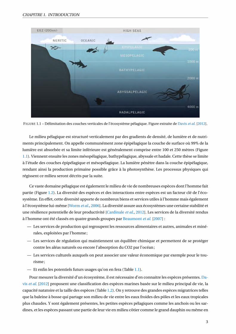
CHAPITRE 1. INTRODUCTION
FIGURE 1.1 – Délimitation des couches verticales de l’écosystème pélagique. Figure extraite de Davis et al. [2012].
Le milieu pélagique est structuré verticalement par des gradients de densité, de lumière et de nutri-
ments principalement. On appelle communément zone épipélagique la couche de surface où 99% de la
lumière est absorbée et sa limite inférieure est généralement comprise entre 100 et 250 mètres (Figure
1.1). Viennent ensuite les zones mésopélagique, bathypélagique, abyssale et hadale. Cette thèse se limite
à l’étude des couches épipélagique et mésopélagique. La lumière pénètre dans la couche épipélagique,
rendant ainsi la production primaine possible grâce à la photosynthèse. Les processus physiques qui
régissent ce milieu seront décrits par la suite.
Ce vaste domaine pélagique est également le milieu de vie de nombreuses espèces dont l’homme fait
partie (Figure 1.2). La diversité des espèces et des interactions entre espèces est un facteur clé de l’éco-
système. En effet, cette diversité apporte de nombreux biens et services utiles à l’homme mais également
à l’écosystème lui-même [Worm et al., 2006]. La diversité assure aux écosystèmes une certaine stabilité et
une résilience potentielle de leur productivité [Cardinale et al., 2012]. Les services de la diversité rendus
à l’homme ont été classés en quatre grands groupes par Beaumont et al. [2007] :
— Les services de production qui regroupent les ressources alimentaires et autres, animales et miné-
rales, exploitées par l’homme;
— Les services de régulation qui maintiennent un équilibre chimique et permettent de se protéger
contre les aléas naturels ou encore l’absorption du CO2 par l’océan;
— Les services culturels auxquels on peut associer une valeur économique par exemple pour le tou-
risme;
— Et enfin les potentiels futurs usages qu’on en fera (Table 1.1).
Pour mesurer la diversité d’un écosystème, il est nécessaire d’en connaitre les espèces présentes. Da-
vis et al. [2012] proposent une classification des espèces marines basée sur le milieu principal de vie, la
capacité natatoire et la taille des espèces (Table 1.2). On y retrouve des grandes espèces migratrices telles
que la baleine à bosse qui partage son milieu de vie entre les eaux froides des pôles et les eaux tropicales
plus chaudes. Y sont également présentes, les petites espèces pélagiques comme les anchois ou les sar-
dines, et les espèces passant une partie de leur vie en milieu côtier comme le grand dauphin ou même en
3

CHAPITRE 1. INTRODUCTION
FIGURE 1.2 – Schéma de l’écosystème pélagique adapté au Pacifique sud (Source CPS).
TABLEAU 1.1 – Biens et services fournis par la biodiversité marine. Tableau adapté d’après Beaumont et al. [2007] .
Catégorie Biens ou servicesApprovisionnement alimentaire
Service de productionMatières premièresRégulation des gaz et du climatPrévention des perturbations (protection contre les inondations et tempêtes)Service de régulationStockage et recyclage des déchetsPatrimoine culturel et identitéLoisirsSensation de bien-être (avantages de non-utilisation)
Service immatériels
Bénéfices cognitifs (e.g. éducation, recherche)Valeur d’usage de l’option Avantages futurs inconnus et spéculatif
4

CHAPITRE 1. INTRODUCTION
eau douce comme l’anguille. Cette classification ne prend pas en compte les relations trophiques entre
espèces qui sont matérialisées par les flèches blanches sur la Figure 1.2, et qui sont donc nombreuses et
complexes. L’image de la chaîne trophique du petit poisson qui est mangé par le moyen poisson qui est
lui-même mangé par le gros poisson a depuis plusieurs années laissé la place à cette représentation de
réseau trophique où toutes les espèces sont inter-connectées. Une autre classification fréquente des es-
pèces est basée sur leur niveau trophique, on retrouve communément les producteurs primaires en bas
de la pyramide (phytoplancton), puis les consommateurs primaires (zooplancton), les prédateurs in-
termédiaires (micronecton) et les prédateurs supérieurs (ou « top predators », e.g. thon). Si on considère
l’énergie totale disponible d’un niveau trophique (i.e. 100%), en moyenne 10% est effectivement converti
en biomasse dans le niveau suivant, avec une variation comprise entre 1 et 20% [Pomeroy, 1979], il s’agit
de la loi de Lindeman. Ce taux de transfert d’énergie s’explique par deux raisons principales : (1) il y a
une perte d’énergie à chaque niveau par la respiration et l’excrétion et (2) les consommateurs du niveau
suivant n’assimilent pas toute la matière organique disponible. Dans les écosystèmes marins, la taille
d’un organisme peut être un meilleur prédicteur de sa position trophique que sa taxonomie [Jennings
et al., 2001]. Ce constat a donné naissance à la théorie des spectres de taille qui dit que le nombre d’indi-
vidus par niveau trophique est de plus en plus petit au fur et à mesure que l’on s’élève dans la pyramide
trophique et que cette réduction de nombre est compensée par une augmentation de la taille [Boudreau
et al., 1991]. La théorie du spectre de taille est de plus en plus utilisée pour paramétrer les modèles de
réseau trophique [Blanchard et al., 2011; Maury et al., 2007]. Bien que cette approche ne donne pas né-
cessairement un aperçu des interactions au niveau des espèces, elle présente l’avantage de reposer sur
des relations écologiques et physiologiques qui sont largement applicables à l’ensemble des taxons et
des régions.
En dénombrant les interactions trophiques correspondant à chaque espèce (Figure 1.2), les poissons
volants, les calamars et les crevettes sont les espèces qui arrivent en tête avec pas moins de 9 interactions
pour chaque espèce. Ce constat met en avant le rôle clé du micronecton dans le réseau alimentaire :
ce sont ces espèces qui font le lien entre les organismes de niveaux trophiques inférieurs influencés
fortement par l’environnement et tous les prédateurs supérieurs. Nous nous sommes particulièrement
intéressés à cet échelon trophique au cours de la thèse. Le micronecton est composé de tous les orga-
nismes mesurant entre 1 et 20cm et constitue la nourriture des prédateurs supérieurs. On y retrouve une
grande diversité d’espèces : des poissons, des crustacés, des mollusques ou encore des organismes géla-
tineux. Le micronecton inclut également un grand nombre d’organismes de façon transitoire lors de leur
développement larvaire et juvénile, et pas uniquement d’espèces pélagiques. On retrouve par exemple
de nombreuses larves de poissons récifaux dans le micronecton [Allain et al., 2012]. Malgré le rôle pri-
mordial de ce groupe , il est encore le maillon le moins étudié de l’écosystème marin [Conchon, 2016].
Comme le montre le nombre d’études disponibles en fonction de certains mots clés, le micronecton ar-
rive en dernière position (Figure 1.3) [St. John et al., 2016]. L’intérêt pour ce compartiment encore très
peu étudié est cependant en train de grandir, notamment car il représente potentiellement une nouvelle
ressource alimentaire importante (Figure 1.4) [Hidalgo & Browman, 2019].
5

CHAPITRE 1. INTRODUCTION
TABLEAU 1.2 – Typologie des espèces marines de plus de 1cm. Les espèces sont regroupées selon leur écologie etleur capacité à se déplacer. Tableau adapté d’après Davis et al. [2012].
Groupe d’espèces Description Exemple d’espèces
Espèces pélagiques très mobiles Espèces qui voyagent sur de trèsgrandes distances de façon saison-nière ou au cours de leur vie. Cegroupe se compose principalementd’oiseaux et de grands cétacés
AlbatrosBaleine à bosse
Grand pélagique océanique Espèces de taille raisonnable qui ha-bitent principalement des eaux océa-niques et sont capables d’effectuerdes mouvements importants sur despériodes relativement courtes.
ThonRequin océanique
Petits pélagiques océaniques Espèces relativement petites qui ne sedéplacent que sur de petites distancesdans des eaux à prédominance océa-nique.
Dorade coryphèneRaie pélagique
Grands pélagiques littoraux Espèces pélagiques de grande taille li-mitées aux zones littorales pendantla plus grande partie ou la totalité deleur vie et capables de se déplacermodestement.
Grand dauphin
Petits pélagiques littoraux Petites espèces pélagiques limitéesaux zones littorales pendant touteleur durée de vie et capables de se dé-placer modestement.
SardineMaquereau
Espèces pélagiques diadromes Espèces anadromes qui migrent entredes distances importantes entre lesrivières d’eau douce et l’océan péla-gique.
SaumonAnguille
FIGURE 1.3 – Nombre d’études disponibles sur sciencedirect.com, en fonction du mot clé choisi. Les groupesd’organismes sont classés par niveau trophique du plus élevé au plus faible, la couleur des barres représente lataille moyenne du groupe considéré. Figure extraite de la thèse de Anna Conchon [2016].
6

CHAPITRE 1. INTRODUCTION
FIGURE 1.4 – Le nombre de publications (a) et de citations (b) par an qui ressortent d’une recherche dans la col-lection de base du Web of Science pour le terme "mésopélagique" sur la période 1945-2018, effectuée le 25 février2019. Figure extraite de Hidalgo & Browman [2019].
1.1.2 Les contrôles trophiques qui régissent l’écosystème
Nous avons vu dans la section précédente que les biomasses des espèces d’un écosystème étaient
régulées en partie par les interactions alimentaires. Ces interactions sont également appelées contrôles
trophiques et on en distingue généralement trois modèles (Figure 1.5) [Cury et al., 2002]. Le contrôle
par le haut (ou top down control) est un écosystème où c’est la biomasse de l’échelon n qui contrôle la
biomasse de l’échelon n-1 : si les prédateurs diminuent, les proies augmentent car elles sont moins man-
gées, le zooplancton diminue car il est plus mangé et le phytoplancton lui augmente. On peut voir que
dans ce cas de figure, les réponses sont inversées pour chaque échelon trophique. Le contrôle par le bas
(ou bottom-up control) est comme son nom l’indique, un système où c’est la production primaire qui
régit tous les échelons : si cette dernière diminue, la biomasse de zooplancton diminue elle aussi, et par
cascade, celle des proies et des prédateurs. Dans ce cas, c’est l’environnement qui est le régulateur prin-
cipal de l’écosystème. Ce type de contrôle existe notamment dans l’upwelling du Pérou où l’on observe
une alternance entre anchois et sardines. Ces deux espèces n’ayant pas le même habitat optimal, l’abon-
dance de leur population respective s’alterne au cours du temps dues à des variations de conditions
environnementales. Même si l’effet exact des facteurs environnementaux contrôlant cette alternance
n’est pas encore parfaitement compris, l’impact du phénomène ENSO (El Niño Southern Oscillation)
a été largement montré [e.g. Bertrand et al. 2004,Chavez et al. 1999,Chavez et al. 2003]. La pression de
pêche très forte dans cette région se rajoute aux facteurs environnementaux. Les fortes variations de
biomasses pouvant passer de centaines de milliers de tonnes à pratiquement zéro dans les cas extrêmes
[Lluch-Belda et al., 1989] peuvent avoir un effet dramatique sur les populations humaines exploitants ces
ressources [Allison et al., 2009; Barange et al., 2014; Bell et al., 2011]. Dans les zones moins productives
et plus diversifiées en terme de proies, le lien à l’environnement des proies est encore plus complexe à
comprendre et les connaissances sur ces contrôles sont encore assez limitées [St. John et al., 2016].
1.1.3 L’hétérogénéité spatio-temporelle des processus marins
La complexité de ces systèmes est accrue par la forte variabilité spatio-temporelle des processus phy-
siques, de l’influence de ces processus sur les échelons trophiques, et des interactions entre espèces. De
plus, la tridimensionnalité du milieu marin, et particulièrement sa composante verticale, complique en-
7

CHAPITRE 1. INTRODUCTION
FIGURE 1.5 – Les trois types de contrôles trophiques, l’effet de l’environnement est représenté par le visage souf-flant du vent, Figure adapté d’après Cury et al. [2002]. Les tendances rouges représentent l’élément déclencheurdes cascades dans chaque cas de figure.
8

CHAPITRE 1. INTRODUCTION
core la compréhension des processus. La majeure partie de l’écosystème marin est plongée dans le noir
et subit des fortes pressions, rendant cet espace inaccessible aux moyens d’échantillonnage tradition-
nels. Finalement, la complexité de ce tableau est encore accrue par les interactions entre les espèces et
l’environnement qui sont changeantes au cours du cycle de vie d’une espèce. Une espèce va être man-
gée par différentes espèces au cours de son cycle de vie par exemple. On peut citer le cas étonnant de la
morue de mer du nord qui peut se nourrir de ses propres juvéniles (cannibalisme) [Folkvord, 1991]. En-
fin, les conditions océanographiques favorables au stade larvaire sont souvent différentes des conditions
favorables au stade adulte.
Hunt & Schneider [1987] proposèrent un découpage des échelles temporelles et spatiales des pro-
cessus adapté au milieu marin : on y retrouve l’échelle fine (inférieure à 1km), l’échelle grossière (de
1 à 10km), la méso échelle (de 10km à 1000km), la macro échelle (de 1000km à 10000km) et enfin la
méga échelle (supérieure à 10000km) (Figure 1.6). Ces échelles spatiales sont associées à leurs gammes
temporelles respectives. Comme on peut voir avec les quelques exemples de phénomènes physiques su-
perposés, les échelles physiques prédéfinies chevauchent les phénomènes physiques mais comme pour
le découpage vertical du milieu (Figure 1.1), elles permettent de mieux définir et classer les différents
processus. Plus les échelles sont petites, plus les phénomènes sont instables et donc compliqués à pré-
dire.
Avec son temps de croissance rapide (1-2 jours), la dynamique du phytoplancton est étroitement
liée à la dynamique des nutriments dont la distribution tridimensionnelle est influencée par les proces-
sus physiques. Ainsi, on retrouve par exemple une forte production primaire dans les upwellings, où la
remontée de nutriments, calquée sur celle des températures plus fraiches des couches profondes, en-
richit la surface. L’influence de la physique sur le zooplancton est plus complexe et on observe dès ce
niveau trophique, une décorrélation spatio-temporelle des processus [Smeti et al., 2015]. Cette décorré-
lation s’amplifie avec le niveau trophique, et il est souvent complexe de comprendre ce qui conditionne
la dynamique spatio-temporelle des prédateurs supérieurs [Bellier et al., 2012; Godo et al., 2014; McHu-
ron, 2018; Scales et al., 2017], d’autant qu’à cette dynamique océanique s’ajoutent les comportements
biologiques des animaux tels que migrations entre habitats de ponte et d’alimentation par exemple.
Le micronecton a-t-il aussi une dynamique spatio-temporelle complexe? La Figure 1.7 regroupe les
processus dynamiques majeurs du micronecton à toutes les échelles spatiotemporelles identifiées par
les polygones noirs et les moyens d’échantillonnage identifiés par les rectangles bleus et gris, et le noir en
trait gras. A échelle journalière, les migrations nycthémérales sont majoritaires (Diel Vertical Migration
ou DVM). Chaque jour, la majorité des espèces de micronecton parcourent verticalement des centaines
de mètres, migrant du domaine mésopélagique où elles résident durant le jour à la zone épipélagique
où elles passent la nuit. Ce mouvement est aujourd’hui reconnu comme la plus grande migration ani-
male au monde [Hays, 2003] et a été observé dans tous les océans de la planète [Bianchi & Mislan, 2016;
Klevjer et al., 2016]. Cette migration verticale est généralement expliquée comme une échappatoire à la
prédation visuelle pendant la journée. La nuit, les organismes remontent en surface pour s’alimenter
[Pearre, 2003]. Le micronecton a également une dynamique saisonnière [e.g. Harding et al. 2011] et est
sensible aux variations océanographiques interannuelles [Chavez et al., 2003; Staby et al., 2011]. Cepen-
dant, l’intérêt récent (Figure 1.4) que nous portons au micronecton restreint la couverture temporelle des
données disponibles pour étudier des tendances sur le long terme. La difficulté d’observation et d’échan-
tillonnage sur lesquelles nous reviendrons dans cette introduction complexifie également l’étude de cet
9

CHAPITRE 1. INTRODUCTION
FIGURE 1.6 – Diagramme spatio-temporel représentant la structure hiérarchique du milieu marin. La représen-tation des processus physique a été adaptée de Racault et al. [2014] et les 5 échelles ont été extraites de Hunt &Schneider [1987].
échelon trophique (par exemple les phénomènes I, H et G ne sont recoupés par aucun moyen d’étude sur
la Figure 1.7). Au niveau mondial, la biomasse estimée d’organismes mésopélagiques varie grandement.
En 1980, Gjøsaeter & Kawaguchi [1980] estimaient la biomasse totale de micronecton à environ 1Gt, es-
timation basée sur des données de chalutage. Depuis cette estimation a été revue à la hausse : en 2014
Irigoien et al. [2014] proposèrent une estimation entre 14.3 et 19.5Gt d’après des mesures acoustiques.
Cependant une étude récente de modélisation a remis en question ces estimations, avec une biomasse
modélisée de 2.4Gt [Anderson et al., 2019]. Enfin, Proud et al. [2018b] ont développé un modèle pour
calculer la biomasse de micronecton à partir de données d’acoustique active (38kHz) acquises dans les
couches profondes. Leurs estimations varient globalement entre 1.8Gt et 16Gt. D’après leurs conclu-
sions, la présence/absence et le volume de la vessie natatoire, la distribution des tailles et le ratio de la
forme des organismes sont des facteurs clés à déterminer pour améliorer l’estimation de biomasse.
1.1.4 Les écosystèmes marins sous pression au cœur des préoccupations environnemen-
tales
De nombreuses menaces affectent ces écosystèmes
Ayant présenté les contraintes naturelles imposées aux écosystèmes marins, nous présentons main-
tenant les pressions anthropiques. En effet, depuis plusieurs années les sonnettes d’alarme sont tirées
quant à l’état de santé général des écosystèmes marins. Deux faits majeurs, étroitement liés, reviennent
régulièrement : l’effondrement des stocks de poissons exploités et la baisse globale de biodiversité, ca-
taloguée comme la sixième extinction majeure que connaîtra notre planète [Barnosky et al., 2011; Davis
et al., 2018]. Alors que la population humaine augmente rapidement, avec près de 9.7 milliards d’habi-
tants prévus pour 2050 [Barnosky et al., 2012], les pressions induites sur les écosystèmes augmentent
10

CHAPITRE 1. INTRODUCTION
FIGURE 1.7 – Dynamiques spatio-temporelles du micronecton. La surface illustre la variation spatio-temporelledu micronecton. Les phénomènes importants pour la compréhension et l’évaluation des écosystèmes, ainsi queleur extension dans le temps et dans l’espace, sont indiqués sur le dessus de la surface de variabilité et sont identi-fiés par des lettres majuscules. Le diagramme est étendu pour illustrer l’utilisation de diverses plates-formes, leurpotentiel de couverture, leur chevauchement et leur caractère unique dans le temps et l’espace. Schéma extrait deGodo et al. [2014].
11

CHAPITRE 1. INTRODUCTION
FIGURE 1.8 – Évolution de l’état des stocks mondiaux exploités de 1974 à 2015, la couleur orange montre les stockssurexploités, la couleur bleue au-dessus du trait blanc les stocks exploités à leur niveau maximal et la couleur bleuesous le trait blanc, les stocks sous-exploités. D’après [FAO, 2018].
conjointement. Les activités anthropiques affectent directement ou indirectement la presque totalité du
milieu marin. Une étude récente a calculé que seulement 13.2% de l’océan était encore vierge de tout
trace anthropique [Jones et al., 2018]. Des chercheurs ont récemment trouvé des micro-plastiques dans
des organismes micronectoniques présents jusqu’à 1000 mètres de profondeur [Choy et al., 2019]. Lotze
& Worm [2009] ont montré que les abondances des 256 espèces analysées avaient décliné en moyenne
de 89% par rapport à leur niveau historique. A travers des modèles, Christensen et al. [2014] arrivent au
même constat avec une division par trois de la biomasse des prédateurs à l’échelle globale ces 100 der-
nières années. Le niveau moyen de biodiversité est lui aussi en train de diminuer à une vitesse record
[Butchart et al., 2010; Pimm et al., 1995]. Les menaces principales aboutissant à ces résultats alarmants
peuvent être classées en trois catégories : les activités de pêche, la pollution et les destructions d’habitat
et enfin le changement climatique.
Les premières traces d’apparition de la pêche remontent à plus de 40 000 ans [Thomazi, 1951], et
depuis cette période les techniques de pêche n’ont fait que s’améliorer, si bien qu’aujourd’hui le rapport
pression de pêche /poissons laisse peu de chance aux poissons. Petit à petit, l’amélioration des tech-
niques de pêche et des bateaux a rendu possible la pêche de plus en plus loin du port d’attache : tous
les océans ont progressivement été exploités et on a pu pêcher de plus en plus profond. L’usage grandis-
sant des DCP (Dispositifs de Concentration de Poissons) utilisé principalement pour la pêche au thon
a permis de concentrer la ressource et de pêcher de manière bien plus efficace, parfois au détriment
de nombreuses captures accessoires [Escalle et al., 2018]. Soixante pourcent des ressources marines se-
raient exploitées à leur niveau maximal et 30% surexploitées (Figure 1.8). Les espèces exploitées sont de
plus en plus nombreuses, mais le niveau trophique moyen des captures est de plus en plus bas [Pauly
et al., 1998]. Une revue a même récemment publié une série d’articles qui évaluent le potentiel du mi-
cronecton comme ressource alimentaire [Hidalgo & Browman, 2019].
La destruction d’habitats par les engins trainant en contact avec le fond est une autre menace im-
portante qui pèse sur les écosystèmes marins, impactant particulièrement les stades critiques de vie
12

CHAPITRE 1. INTRODUCTION
comme le les stades larvaires/juvéniles. Cependant, cette menace est plus présente en milieu côtier [Gib-
son et al., 2007; Le Pape et al., 2007].
Enfin, le changement climatique global menace lui aussi ces écosystèmes (Figure 1.9). Dans les éco-
systèmes pélagiques, l’augmentation de température de l’océan impacte majoritairement la distribution
spatiale des espèces ainsi que leur métabolisme. Une étude récente a montré que les biomasses des es-
pèces seraient de plus en plus impactées au fur et à mesure que leur niveau trophique s’élève [Lotze
et al., 2019]. Les nouvelles conditions environnementales peuvent être physiologiquement tolérables,
permettant l’acclimatation (un ajustement de la physiologie par exemple un changement de tolérance
à l’oxygène par l’individu) ou l’adaptation (une abondance et une reproduction accrues avec certains
génotypes changeant au fil des générations) des espèces. Si au contraire un habitat devient inadéquat
pour une population donnée, la taille de la population peut diminuer à mesure que la performance éco-
physiologique (les taux métaboliques ou la croissance par exemple) diminue [Hillebrand et al., 2018;
Portner, 2001], les espèces peuvent également migrer vers des eaux plus froides [Pecl et al., 2017] ou
encore subir une extinction locale [Parmesan, 2006]. L’effet sur les changements de distribution a été
étudié par un grand nombre d’études et un consensus s’accorde sur la prévision d’un grand nombre de
disparitions dans les régions tropicales et subpolaires et des apparitions d’espèces en zone Arctique et
Antarctique [e.g. Cheung et al. 2009; Pecl et al. 2017]. L’impact physiologique du changement climatique
sur les espèces de poisson est lui encore très peu appréhendé.
Le micronecton a une faible capacité natatoire, et a donc peu de chance de pouvoir migrer à de
grandes échelles spatiales pour échapper au réchauffement des températures. Il est donc plus probable
que ces espèces connaissent des changements métaboliques ou des extinctions. Actuellement, l’impact
sur le micronecton est encore peu compris. Bryndum-Buchholz et al. [2019] ont prédit une diminution
de la biomasse d’environ 15% pour les organismes dont la taille varie entre 0 et 30 cm pour l’ensemble
du Pacifique Sud et Lefort et al. [2015] une diminution d’environ 20% pour l’ensemble du Pacifique. Ces
études se basent sur des modèles, et à notre connaissance, aucune étude ne mesure l’impact du chan-
gement climatique sur le micronecton à travers des données. Les impacts potentiels du changement
climatique sur les prédateurs à travers des changements de micronecton sont encore, eux aussi, peu
étudiés, majoritairement dû à un manque de connaissance sur le micronecton [St. John et al., 2016].
Une prise de conscience globale place aujourd’hui ces menaces au cœur des préoccupations poli-
tiques
Aujourd’hui la question de l’urgence climatique et de ses impacts néfastes pour les écosystèmes
semble être une évidence. Pourtant, vers le début des années 1900, à l’époque des premiers travaux por-
tant sur l’impact climatique d’une hausse du gaz carbonique (CO2) dans l’atmosphère, Walter Nernst,
prix Nobel de chimie, proposa de brûler du charbon pour réchauffer l’atmosphère et ainsi améliorer le
confort humain. Il avança également comme argument qu’une augmentation de CO2 dans l’atmosphère
allait doper la production primaire et donc l’état de santé des végétaux. En 1940, des scientifiques mon-
trèrent pour la première fois qu’une augmentation de la concentration de CO2 pouvait entraîner une
augmentation de température [Plass, 1956a,b]. La première preuve d’accumulation du CO2 dans l’atmo-
sphère fut ensuite apportée en 1960 par Keeling [1960] qui mesura quotidiennement les concentrations
de CO2 à Hawaï et en Antarctique. Les préoccupations écologiques apparurent dans les années 1960-70,
13

CHAPITRE 1. INTRODUCTION
FIGURE 1.9 – Conséquences des activités humaines et de l’augmentation des concentrations en CO2 sur les éco-systèmes marins. Figure extraite de https ://ocean-climate.org
avec la création des premières ONG environnementales (WWF, Greenpeace, etc.), puis avec le premier
sommet de la Terre à Stockholm en 1972 qui marqua le début des préoccupations à l’échelle internatio-
nale.
En 1988 se crée le Groupe d’experts intergouvernemental sur l’évolution du climat (GIEC) (en anglais
Intergovernmental Panel on Climate Change, IPCC), organisme intergouvernemental ouvert à tous les
pays membres de l’ONU et regroupant actuellement 195 États. Il a pour objectif de fournir aux décideurs
des évaluations scientifiques régulières de l’état actuel des connaissances sur le changement climatique.
En 1992, au sommet de la Terre de Rio, ces préoccupations s’étendent à l’écologie et à la conservation
de la biodiversité à grande échelle. Parmi les accords signés à l’issue de cette rencontre figure la Conven-
tion sur la diversité biologique, première du genre, à l’échelle mondiale, à être consacrée au maintien
et à l’utilisation durable de la biodiversité (conserver la diversité ; utiliser la diversité de façon durable ;
partager les avantages de la diversité de façon juste et équitable). Cet accord a très vite bénéficié d’une
large acceptation : il a été signé sur place par plus de 150 gouvernements et compte désormais plus de
180 états membres. Il est entré en vigueur le 29 décembre 1993. En avril 2002, la Convention des parties
s’est engagée à réduire sensiblement, d’ici à 2010, le taux de perte de biodiversité au niveau mondial,
régional et national afin de contribuer à la réduction de la pauvreté et au bénéfice de toute vie sur Terre
(Objectif 2010). Cet objectif a ensuite été approuvé par le Sommet mondial pour le développement du-
rable et l’Assemblée générale de l’ONU et a été intégré en tant que nouvel objectif dans les objectifs
du Millénaire pour le développement [Millennium Ecosystem Assessment, 2005]. Finalement, en 2010
la 65ème session de l’Assemblée générale de l’ONU officialise la création de l’IPBES (Intergovernmental
Science-Policy Platform on Biodiversity and Ecosystem Services ou Plateforme intergouvernementale sur
la biodiversité et les services écosystémiques), équivalent du GIEC mais appliqué à la biodiversité et
regroupant 195 états. Très récemment en juin 2019, un atelier de l’IPBES s’est déroulé à Nouméa pour
proposer des pistes d’adaptation du plan global au contexte Océanien. Les discussions se sont focalisées
sur les moyens d’incorporer les connaissances et savoir-faire traditionnels pour la conservation [Payri &
Vidal, 2019].
En 2020, se tiendra à Marseille le Congrès mondial de la nature de l’IUCN (International Union for
14

CHAPITRE 1. INTRODUCTION
FIGURE 1.10 – schéma synthétique des avantages qu’offrent une AMP face au changement climatique. © IvanGromicho, KAUST
Conservation of Nature ou Union Internationale pour la conservation de la nature), annoncé comme
le plus grand événement mondial consacré à la biodiversité. Il a pour principal objectif la mobilisation
de tous les acteurs concernés par ce sujet à quelques mois de la COP15 de la biodiversité qui aura lieu
en Chine et qui devrait adopter un nouveau cadre international pour la prochaine décennie. De nom-
breuses solutions pour préserver l’état de santé des écosystèmes marins ont été proposées au cours de
ces différents sommets, nous en détaillerons deux qui incluent le micronecton : l’approche écosysté-
mique des pêches et la mise en place d’Aires Marines Protégées (AMPs, ou Marine Protected Areas MPAs).
Nous avons vu précédemment que la pression de pêche affecte grandement les espèces marines, et
pas uniquement les espèces exploitées, mais bien toute la structure de l’écosystème à travers les diffé-
rentes interactions trophiques. La gestion écosystémique des pêches propose de minimiser les impacts
de la pêche tout en maximisant la résilience des écosystèmes [Gascuel et al., 2016; Worm et al., 2009].
La mise en place réelle de cette approche nécessite la définition d’indicateurs concret sur l’impact d’une
pêcherie sur son écosystème. Pour cela il est nécessaire de développer des connaissances pertinentes sur
les mécanismes et les processus écologiques qui façonnent les interactions prédateur-proie à l’échelle
de l’écosystème [Christensen et al., 1996; Koslow, 2009] .
La mise en place d’AMPs est une autre solution très en vogue qui est fortement recommandée comme
outil de conservation des espèces [Christie et al., 2017; Davidson & Dulvy, 2017; Ehler & Douvere, 2009].
La convention sur la diversité biologique définit une AMP comme "Toute zone dans ou à proximité du
milieu marin, ainsi que la flore, la faune et les caractéristiques historiques et culturelles associées, qui
a été délimitée par voie législative ou par d’autres moyens comme la coutume, de sorte que sa biodi-
versité marine et/ou côtière bénéficie d’un niveau de protection supérieur à son environnement". Il a
été avancé que les AMP pouvaient être un moyen efficace de conservation des espèces contre le chan-
gement climatique [Roberts et al., 2017] à travers notamment leur rôle de stockage et de source poten-
tielle de diversité génétique, de carbone, de prédateurs, de micronecton . . . (Figure 1.10). Cependant,
une AMP peut prendre des formes très différentes et la présence d’une AMP ne garantit pas forcément
15

CHAPITRE 1. INTRODUCTION
FIGURE 1.11 – Bannière et carte du parc naturel de la mer de Corail. Extrait de https://mer-de-corail.gouv.
nc/fr.
une protection totale des espèces s’y trouvant [Horta e Costa et al., 2016]. Par ailleurs, dû à un manque
de connaissances des écosystèmes, il a été montré qu’à échelle globale, ces AMP ne couvraient pas les
zones de fortes biodiversités [Lindegren et al., 2018]. Plus récemment, des AMP pélagiques ont été mises
en place pour la conservation d’espèces pélagiques telles que les thons, avec des avis scientifiques miti-
gés quant au niveau réel d’efficacité pour la protection [Davis et al., 2012; Game et al., 2009; Kaplan et al.,
2010].
Dans le Pacifique sud-ouest, la plus grande aire marine protégée française a vu le jour en Nouvelle-
Calédonie en 2014 : le parc naturel de la mer de Corail. Sa surface recouvre toute la zone économique
exclusive (ZEE) de la Nouvelle-Calédonie en dehors des eaux provinciales (Figure 1.11). Selon la défini-
tion donnée plus haut dans cette section, la zone est en effet délimitée par voie législative et représente
donc bien, en ce sens, une Aire Marine Protégée. Cependant, le niveau de protection qui s’y applique est
très variable, aujourd’hui seules de petites zones sont classées en réserve intégrale.
1.2 Le parc marin de la mer de Corail, un écosystème riche dans une région
oligotrophe
Les paragraphes qui suivent s’attacheront à décrire de manière succincte le milieu physique et les
espèces du parc de la mer de Corail. Nous décrirons notamment les connaissances scientifiques man-
quantes et qui sont nécessaires pour développer une bonne gestion de ce milieu.
16
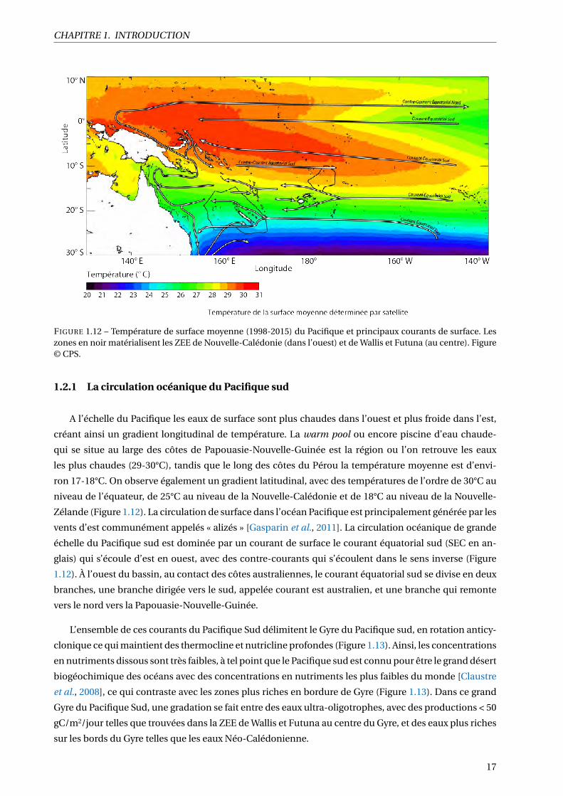
CHAPITRE 1. INTRODUCTION
FIGURE 1.12 – Température de surface moyenne (1998-2015) du Pacifique et principaux courants de surface. Leszones en noir matérialisent les ZEE de Nouvelle-Calédonie (dans l’ouest) et de Wallis et Futuna (au centre). Figure© CPS.
1.2.1 La circulation océanique du Pacifique sud
A l’échelle du Pacifique les eaux de surface sont plus chaudes dans l’ouest et plus froide dans l’est,
créant ainsi un gradient longitudinal de température. La warm pool ou encore piscine d’eau chaude-
qui se situe au large des côtes de Papouasie-Nouvelle-Guinée est la région ou l’on retrouve les eaux
les plus chaudes (29-30°C), tandis que le long des côtes du Pérou la température moyenne est d’envi-
ron 17-18°C. On observe également un gradient latitudinal, avec des températures de l’ordre de 30°C au
niveau de l’équateur, de 25°C au niveau de la Nouvelle-Calédonie et de 18°C au niveau de la Nouvelle-
Zélande (Figure 1.12). La circulation de surface dans l’océan Pacifique est principalement générée par les
vents d’est communément appelés « alizés » [Gasparin et al., 2011]. La circulation océanique de grande
échelle du Pacifique sud est dominée par un courant de surface le courant équatorial sud (SEC en an-
glais) qui s’écoule d’est en ouest, avec des contre-courants qui s’écoulent dans le sens inverse (Figure
1.12). À l’ouest du bassin, au contact des côtes australiennes, le courant équatorial sud se divise en deux
branches, une branche dirigée vers le sud, appelée courant est australien, et une branche qui remonte
vers le nord vers la Papouasie-Nouvelle-Guinée.
L’ensemble de ces courants du Pacifique Sud délimitent le Gyre du Pacifique sud, en rotation anticy-
clonique ce qui maintient des thermocline et nutricline profondes (Figure 1.13). Ainsi, les concentrations
en nutriments dissous sont très faibles, à tel point que le Pacifique sud est connu pour être le grand désert
biogéochimique des océans avec des concentrations en nutriments les plus faibles du monde [Claustre
et al., 2008], ce qui contraste avec les zones plus riches en bordure de Gyre (Figure 1.13). Dans ce grand
Gyre du Pacifique Sud, une gradation se fait entre des eaux ultra-oligotrophes, avec des productions < 50
gC/m2/jour telles que trouvées dans la ZEE de Wallis et Futuna au centre du Gyre, et des eaux plus riches
sur les bords du Gyre telles que les eaux Néo-Calédonienne.
17

CHAPITRE 1. INTRODUCTION
FIGURE 1.13 – Production primaire nette de surface moyenne du Pacifique Sud en couleurs. Les flèches repré-sentent les courants géostrophiques et les traits pleins, la profondeur de la nitracline (ligne de concentration ennitrates égale à 1 gC/m2/jour). La partie bleue matérialise la position du Gyre. Production primaire extraite dehttps://www.science.oregonstate.edu/ocean.productivity/.
FIGURE 1.14 – Contribution relative (en pourcentage) du Trichodesmium sp. à la production primaire totale. Figureextraite de Dutheil et al. [2018].
Le Pacifique sud-ouest reste une région oligotrophe où la croissance du phytoplancton est majoritai-
rement limitée par l’azote. La présence de nombreuses espèces de phytoplancton diazotrophes permet
néanmoins d’enrichir légèrement ce milieu naturellement pauvre [Berthelot et al., 2015a, 2017; Bonnet
et al., 2016]. En effet, les espèces diazotrophes fixent le diazote (N2) atmosphérique dissous dans l’océan
et excrètent en retour de l’azote bio-assimilable (principalement sous forme d’ammonium NH4+, essen-
tiel dans la croissance du phytoplancton Berthelot et al. [2015b]) par les autres espèces phytoplancto-
niques. La multitude d’îles ensemencent le milieu en fer, élément essentiel aux espèces diazotrophes
[Dutheil et al., 2018; Shiozaki et al., 2014]. Ainsi, cette partie du Pacifique sud, la mer de Corail, est moins
oligotrophe que les eaux situées plus à l’est dans le centre du grand gyre [Ceccarelli et al., 2013; Menkes
et al., 2015]. Une étude de modélisation a permis d’estimer à 30% la part de production primaire dûe à
la présence de ces diazotrophes (Figure 1.14) [Dutheil et al., 2018]. Dans le même temps Bonnet et al.
[2017] ont montré que les plus forts taux de fixation mesurés à l’échelle du globe se situaient dans le
Pacifique sud-ouest. C’est dans ce contexte biogéochimique que se situe la Nouvelle-Calédonie.
18

CHAPITRE 1. INTRODUCTION
TABLEAU 1.3 – Caractéristiques des masses d’eau autour de la Nouvelle-Calédonie, avecσ la densité relative définiecomme la densité absolue moins 1000, T la température, S la salinité, O2 l’oxygène et la profondeur moyenne dela couche dans la ZEE. TSW : Tropical Surface Water ; SPTWS :South Pacific Tropical Water South ; SPTWN : SouthPacific Tropical Water North ; WSPCW : Western South Pacific Central Water ; AAIW : Antarctic Intermediate Water.Tableau adapté de Gasparin et al. [2014].
Surface Upper Thermocline Lower Thermocline IntermediateTSW SPTWN SPTWS WSPCW AAIW
σ(kg.m-3) >24 ∼24.5 ∼25.3 ∼26.3 ∼27T (°C) 28 22 19.5 14.5 5.5
S 34.5 35.9 35.65 35.25 34.45O2 (µmol.kg-1) 200 120 175 180 180
Profondeur (m) 40 220 130 360 530
1.2.2 Le milieu physique autour de la Nouvelle-Calédonie
La Nouvelle-Calédonie se situe dans le Pacifique sud-ouest entre l’Australie et le Vanuatu, dans le sud
de la mer de Corail. Un zoom atour de la Nouvelle-Calédonie fait apparaître une circulation océanique
plus complexe qu’à grande échelle (Figure 1.15). Les eaux superficielles de la ZEE sont sous l’influence de
deux grands systèmes de courants très distincts. Au sud, le STCC (Sub Tropical Counter Current), branche
du Courant Est Australien (EAC), amène de l’eau froide et salée tandis que de l’eau d’origine équatoriale,
chaude et peu salée, pénètre au nord de la ZEE par le biais du Courant Equatorial Sud (SEC) [Bonvallot
et al., 2013; Cravatte et al., 2015; Kessler & Cravatte, 2013]. Ce dernier se divise en deux en arrivant sur la
grande terre (voir Figure 1.16 pour la localisation de la grande terre) : une branche monte vers le nord et
crée le NCJ (North Caledonian Jet) et possiblement une branche part vers le sud : le SCJ (South Caledo-
nian Jet). Sur la côte est, une zone de downwelling (plongée des eaux chaudes de surface) est associé à la
convergence géostrophique des eaux à la côte [Cravatte et al., 2015; Marchesiello et al., 2010]. Sur la côté
ouest, les courants, associés à des forts alizés ponctuels, créent parfois une zone d’upwelling (remontée
d’eaux froides et riches en nutriments) dans la partie sud de la côte [Alory et al., 2006; Cravatte et al.,
2015; Marchesiello et al., 2010]. L’upwelling, particulièrement présent pendant la saison chaude entre
novembre et avril est visible sur la température de surface et pourrait enrichir localement le milieu pé-
lagique en nutriments jusqu’à une centaine de kilomètre au large de la barrière de corail mais de façon
intermittente [Hénin & Cresswell, 2005].
On retrouve principalement 5 masses d’eau dans la ZEE qui se différencient par leur densité et par
leur concentration en oxygène (Table 1.3). En surface, on retrouve majoritairement la TSW (Tropical
Surface Water) qui est chaude et oxygénée et qui arrive de l’est. Aux alentours de la thermocline, deux
masses d’eau aux caractéristiques bien différentes sont présentes : la SPTWN (South Pacific Tropical Wa-
ter North) qui est une masse d’eau chaude, salée et relativement peu oxygénée venant du Pacifique est,
vers la Polynésie ; et la SPTWS (South Pacific Tropical Water South) qui est plus froide, moins salée et plus
oxygénée. Cette dernière masse d’eau provient de la zone de convergence subtropicale qui est proche de
la Nouvelle-Zélande [Gasparin et al., 2014]. En dessous, entre 300 et 400 mètres, les eaux de "basse ther-
mocline" sont composées majoritairement par la WSPCW (Western South Pacific Central Water), masse
d’eau froide arrivant du sud. Enfin, sous la thermocline la masse d’eau AAIW (Antarctic Intermediate
Water) est majoritaire et est composée d’eau froide et peu salée arrivant d’Antarctique.
Enfin, la zone économique de Nouvelle-Calédonie est également sujette à une forte activité tour-
19

CHAPITRE 1. INTRODUCTION
FIGURE 1.15 – Cartes de référence du Pacifique sud-ouest (haut) et de la Nouvelle-Calédonie (bas) extraite de Bon-vallot et al. [2013]. Les flèches bleues représentent la circulation des eaux situées entre la surface et la thermocline(environ 120m) et les flèches rouges représentent la circulation de surface lorsque cette dernière est différente desflèches bleues. Les abréviations sont : SEC (South Equatorial Current), NVJ (North Vanuatu Jet), NCJ et SCJ (Northand South Caledonian Jet), STCC (Sub Tropical Counter Current) et EAC (East Australian Current). Les deux cartesen bas à gauche représentent la température moyenne de surface en saison chaude (décembre à mai, gauche) eten saison froide (juin à novembre, droite).
20

CHAPITRE 1. INTRODUCTION
FIGURE 1.16 – Carte de la zone économique de Nouvelle-Calédonie. Les zones discutées au cours de cette thèsesont localisées, et les triangles gris représentent certains monts sous-marins. Carte extraite de la thèse de SolèneDerville [2018].
21

CHAPITRE 1. INTRODUCTION
billonnaire [Keppler et al., 2018]. Au nord de la zone, ces tourbillons dits de méso-échelle, de l’ordre de
la centaine de kilomètres, sont épars et de courte durée, et n’affectent que les 200 premiers mètres de la
colonne d’eau. Au sud de la zone par contre, le cisaillement latéral entre le STCC et SCJ, crée des tour-
billons plus nombreux et plus énergiques. Les tourbillons de méso-échelle sont omniprésents, avec des
durées de vie d’environ 5 mois et affectent les propriétés de l’eau jusqu’à une profondeur d’au moins 500
mètres et contribuent au mélange des eaux comprises entre la thermocline et la surface.
Comme décrit en section 1.2.1, la température moyenne de l’eau de surface est d’environ 25°C, mais
oscille entre 27°C l’été (entre décembre et mai) et 22°C l’hiver (entre juin et novembre) (Figure 1.15). La
grande terre joue un rôle de barrière physique à la circulation des masses d’eau, et un décalage des tem-
pératures de surface est présent entre la côte est et la côte ouest avec des températures en moyenne plus
chaude sur la côte est. C’est pendant la saison froide et dans le sud que la concentration en chlorophylle
est plus forte en lien avec la structure verticale des eaux de surface. En hiver, la colonne d’eau est peu
stratifiée et donc plus homogène avec probablement plus de nutriments dans la couche euphotique.
En été, elle est fortement stratifiée avec des eaux globalement plus pauvres sauf durant les évènements
ponctuels d’upwelling du sud-ouest calédonien.
Tous ces paramètres océanographiques sont influencés par le phénomène ENSO (El Niño Southern
Oscillation) même si son influence est moins forte qu’à l’équateur. Les effets d’ENSO en Nouvelle-Calédonie
sont inversés par rapport au niveau du Pacifique équatorial. Les eaux sont globalement plus froides et
plus productives pendant El Niño et inversement pendant La Niña [Dandonneau & Gohin, 1984; Del-
croix & Lenormand, 1997; Radenac et al., 2012]. Le signal reste cependant limité avec des baisses de
température de surface d’en moyenne 0.5°C dans la ZEE et des vents légèrement accru durant El Niño.
La bathymétrie de la ZEE de Nouvelle-Calédonie est complexe, avec une grande variété de forma-
tions. On y retrouve notamment trois rides continentales (la ride de Lord Howe et la ride de Fairway
à l’ouest de la grande terre, et la ride de Norfolk qui est dans le prolongement de la grande terre) des
rides volcaniques et des bassins sédimentaires (comme le grand bassin de la Nouvelle-Calédonie juste
à l’ouest de la grande terre). Dans ces trois formations, de nombreux monts sous-marins sont présents
(Figure 1.16). On retrouve enfin une fosse de subduction dans l’est de la grande terre : la fosse des Nou-
velles Hybrides qui descend jusqu’à 7000 mètres. Des récifs isolés sont présents en grand nombre dans
le milieu océanique, on notera notamment : les récifs de Chesterfield dans le nord-ouest, le plateau de
Bellona au sud de ces derniers, les atolls d’Entrecasteaux au nord de la Grande Terre, le récif Pétrie juste
à l’est de ces derniers, et les récifs d’Astrolabe au nord des îles Loyautés.
1.2.3 Un point de rencontre de nombreuses espèces
La bathymétrie complexe ainsi que les nombreux récifs éloignés offrent un nombre incroyable d’ha-
bitats différents pour les espèces évoluant dans ce milieu pélagique. Par ailleurs, le lagon de Nouvelle-
Calédonie est le plus grand lagon fermé au monde et est également très diversifié [Garcia et al., 2018]. Les
échanges entre ce milieu lagonaire et le milieu pélagique sont nombreux, avec par exemple un apport de
nutriments du lagon vers l’océan, ou un passage des larves de poissons récifaux par une phase pélagique
[Allain et al., 2012] (Figure 1.17). La "neige pélagique" permet également d’enrichir le milieu benthique.
Les nombreux monts sous-marins abritent également des communautés encore mal-connues.
22

CHAPITRE 1. INTRODUCTION
FIGURE 1.17 – Schéma montrant les écosystèmes récifo-lagonaire, pélagique et profonds et les échanges autourde la Nouvelle-Calédonie. Figure extraite de l’Analyse Stratégique Régionale de Nouvelle-Calédonie [Gardes et al.,2014].
23

CHAPITRE 1. INTRODUCTION
FIGURE 1.18 – Carte montrant spatialement le nombre d’études publiées dans la mer de Corail. Extraite de Cecca-relli et al. [2013].
La méga faune est particulièrement riche dans la zone [Laran et al., 2016b; Tittensor et al., 2010;
Worm et al., 2003]. On y retrouve de nombreuses espèces emblématiques comme les oiseaux marins
[Borsa et al., 2010, 2014, 2015; Weimerskirch et al., 2017], raies, requins [Bakker et al., 2017; Boussarie
et al., 2018; Ceccarelli et al., 2013], tortues et cétacés [Derville et al., 2018; Garrigue et al., 2015]. Les res-
sources marines exploitées sont majoritairement composées du thon blanc et du thon jaune, complé-
tées par le thon obèse, la bonite à ventre rayée, la dorade coryphène, les poissons à rostre pour en citer
quelques-unes [WCPFC, 2018]. Certaines espèces comme le puffin Fouquet ou la baleine à bosse ne sont
présentes que pendant leur saison de reproduction, stade critique du cycle de vie, alors que d’autres
espèces sont présentes toute l’année. Globalement, la mer de Corail reste relativement peu étudiée en
comparaison d’autres zones, et les études existantes se concentrent sur des petites régions comme les
Chesterfields, comme le montre le répartition spatiale des articles sur la zone (Figure 1.18).
Toutes ces espèces se partagent les ressources alimentaires disponibles dans la zone. Les espèces de
micronecton sont elles aussi très diversifiées d’après des études de contenus stomacaux de leurs pré-
dateurs [Allain et al., 2012; Olson et al., 2014; Williams et al., 2014; Young et al., 2010] et de chalutages
pélagiques [Grandperrin et al., 1999; Menkes et al., 2015; Young et al., 2011]. Une étude globale a classé
le milieu mésopélagique de la mer de Corail comme une région dominée par les poissons lanternes
[Sutton et al., 2017], en accord avec les précédents résultats [Grandperrin, 1975; Vourey et al., 2017] qui
avaient identifié les Gonostomatidae, Sternoptychidae, Myctophidae (poissons lanternes) et Scopelar-
chidae comme les familles dominantes dans la mer de Corail (Figure 1.19). Globalement, les espèces pré-
sentes dans la région sont relativement bien caractérisées, cependant deux synthèses regroupant toutes
les connaissances de la région sur le milieu pélagique ont identifié le micronecton comme le maillon tro-
phique le plus méconnu [Ceccarelli et al., 2013; Gardes et al., 2014]. Ce constat local rejoint un constat
global sur le manque crucial de connaissances concernant le micronecton [Hidalgo & Browman, 2019;
St. John et al., 2016].
Une première étude sur la dynamique du micronecton en Nouvelle-Calédonie a émis l’hypothèse
24
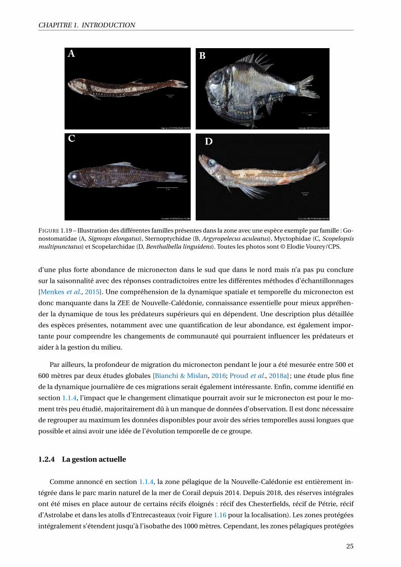
CHAPITRE 1. INTRODUCTION
FIGURE 1.19 – Illustration des différentes familles présentes dans la zone avec une espèce exemple par famille : Go-nostomatidae (A, Sigmops elongatus), Sternoptychidae (B, Argyropelecus aculeatus), Myctophidae (C, Scopelopsismultipunctatus) et Scopelarchidae (D, Benthalbella linguidens). Toutes les photos sont © Elodie Vourey/CPS.
d’une plus forte abondance de micronecton dans le sud que dans le nord mais n’a pas pu conclure
sur la saisonnalité avec des réponses contradictoires entre les différentes méthodes d’échantillonnages
[Menkes et al., 2015]. Une compréhension de la dynamique spatiale et temporelle du micronecton est
donc manquante dans la ZEE de Nouvelle-Calédonie, connaissance essentielle pour mieux appréhen-
der la dynamique de tous les prédateurs supérieurs qui en dépendent. Une description plus détaillée
des espèces présentes, notamment avec une quantification de leur abondance, est également impor-
tante pour comprendre les changements de communauté qui pourraient influencer les prédateurs et
aider à la gestion du milieu.
Par ailleurs, la profondeur de migration du micronecton pendant le jour a été mesurée entre 500 et
600 mètres par deux études globales [Bianchi & Mislan, 2016; Proud et al., 2018a] ; une étude plus fine
de la dynamique journalière de ces migrations serait également intéressante. Enfin, comme identifié en
section 1.1.4, l’impact que le changement climatique pourrait avoir sur le micronecton est pour le mo-
ment très peu étudié, majoritairement dû à un manque de données d’observation. Il est donc nécessaire
de regrouper au maximum les données disponibles pour avoir des séries temporelles aussi longues que
possible et ainsi avoir une idée de l’évolution temporelle de ce groupe.
1.2.4 La gestion actuelle
Comme annoncé en section 1.1.4, la zone pélagique de la Nouvelle-Calédonie est entièrement in-
tégrée dans le parc marin naturel de la mer de Corail depuis 2014. Depuis 2018, des réserves intégrales
ont été mises en place autour de certains récifs éloignés : récif des Chesterfields, récif de Pétrie, récif
d’Astrolabe et dans les atolls d’Entrecasteaux (voir Figure 1.16 pour la localisation). Les zones protégées
intégralement s’étendent jusqu’à l’isobathe des 1000 mètres. Cependant, les zones pélagiques protégées
25

CHAPITRE 1. INTRODUCTION
intégralement sont encore relativement limitées spatialement. Des informations scientifiques solides
sont maintenant nécessaires pour délimiter d’autres zones d’intérêt prioritaire pour la conservation des
espèces et de tout l’écosystème pélagique en général.
1.3 Les questions scientifiques de la thèse
Comme nous l’avons vu tout au long de cette introduction, les écosystèmes pélagiques ont un fonc-
tionnement très complexe, notamment au niveau des interactions trophiques. La variabilité des échelles
spatio-temporelles auxquelles ces processus interviennent rajoute une complexité difficile à appréhen-
der. Cependant, une bonne compréhension des processus contrôlant le milieu et les espèces est néces-
saire pour la mise en place de moyens de gestion efficace quant à la protection des espèces. Dans le
monde et autour de la Nouvelle-Calédonie, le maillon du réseau trophique pélagique le moins connu est
le micronecton. Dans un objectif de compréhension du fonctionnement de l’écosystème, nous avons
donc choisi dans cette thèse de nous concentrer majoritairement sur son rôle en répondant aux ques-
tions suivantes :
— Quelle est la dynamique spatiale et temporelle du micronecton dans la ZEE de Nouvelle-Calédonie?
— Quels facteurs environnementaux contrôlent cette dynamique ?
— Quelles sont les espèces qui composent le micronecton?
— Est-il possible de quantifier les dynamiques spatiotemporelles au niveau spécifique?
— Est-il possible de prédire le devenir du micronecton dans un contexte de changement climatique ?
— Comment le micronecton influence par sa dynamique temporelle et sa distribution spatiale les
prédateurs supérieurs?
— Comment les informations collectées peuvent servir pour la gestion du parc marin de la mer de
Corail ?
Pour répondre à ces 7 questions, plusieurs outils d’observation et d’analyse ont été utilisés, les deux
parties suivantes ont pour objectif de les décrire succinctement. Nous finirons cette introduction géné-
rale par présenter le plan de la thèse.
1.4 Les moyens d’étude du micronecton
Comprendre le fonctionnement et estimer la diversité du micronecton dépend fortement de notre
capacité à accéder aux espèces. Comme décrit au cours de cette introduction, le domaine pélagique
est vaste spatialement et verticalement et les capacités d’étude du micronecton dépendent fortement
de l’échantillonnage in situ. Pour étudier ce micronecton plusieurs méthodes s’offrent à nous, qui se
séparent en deux grands groupes : méthodes d’observation directes dans leur milieu et modélisations.
L’observation permet d’accéder à un certain nombre de paramètres in situ, aux résolutions spatiale et
temporelle accessibles par la méthode utilisée. Ces observations sont limitées par la technique qui peut
être biaisée comme nous le verrons plus loin, par leur coût et le temps nécessaire pour les réaliser. Ces
observations peuvent se faire avec prélèvement (méthode intrusive) ou sans prélèvement biologique
26

CHAPITRE 1. INTRODUCTION
FIGURE 1.20 – Figure illustrant les moyens d’échantillonnage du micronecton avec (A) schématiquement laposition d’un chalut et d’un cône d’enregistrement acoustique par rapport aux couches d’organismes mi-cronectoniques inspirée d’une figure du projet MESOPP [Proud & Brierley 2018, http://www.mesopp.eu/project-details/] ; (B) une photo du chalut pélagique du navire océanographique de l’IRD : l’Alis ; et (C) unschéma du positionnement des bases acoustiques (émetteur+transducteur) sous la coque de l’Alis.
(méthode non intrusive). Ces données d’observation à la mer sont ponctuelles dans le temps et dans
l’espace. Elles présentent un certain nombre de biais et d’incertitudes que nous allons présenter.
Par contraste, la modélisation permet d’accéder à des données prédites en continu spatialement et
temporellement. Cependant, ces données reposent sur de multiples hypothèses de modélisation. Par
ailleurs, les données prédites ont une erreur associée difficile à estimer car souvent les prédictions ne
sont pas directement comparables aux observations. Nous allons voir pourquoi dans les paragraphes
qui suivent. Nous ne présenterons que les outils qui ont servi dans cette thèse, sans faire une description
exhaustive de tous les moyens d’observation et de modélisation du micronecton qui existent.
1.4.1 Les chaluts
La méthode traditionnelle d’échantillonnage du micronecton est le chalut pélagique (Filet schéma-
tisé sur la Figure 1.20A et photo sur la Figure1.20B). Cette méthode a pour grand avantage de permettre
l’identification taxonomique des individus capturés, ainsi qu’un dénombrement direct de l’abondance
et de la biomasse par espèce. Cependant, le chalutage a également plusieurs inconvénients. Le phé-
nomène d’évitement peut créer un fort biais, avec une surreprésentation des espèces à faible capacité
natatoire et une sous-représentation des espèces capables d’éviter le chalut. En moyenne, le phénomène
d’évitement a pour conséquence une sous-estimation de la biomasse [Kaartvedt et al., 2012; Kloser et al.,
2009]. Par ailleurs, le maillage choisi sélectionne également certaines espèces et surtout une gamme de
tailles, ce qui biaise l’estimation de biomasse. Enfin, le chalutage est un processus pouvant être long à
mettre en place, notamment pour chaluter à des profondeurs dépassant les 200 mètres. A titre d’exemple,
27

CHAPITRE 1. INTRODUCTION
sur le navire océanographique de l’IRD basé à Nouméa, l’Alis, un chalutage à 500 mètres de 30 minutes
prend plus de deux heures de mise en œuvre. Cette complexité de mise en place rend le nombre de cha-
luts limités dans le temps et dans l’espace, cela rend difficile également la capture d’organismes repérés à
un temps t, qui peuvent se disperser ou changer de profondeur au cours de l’opération. Pour toutes ces
raisons, avoir une vue d’ensemble de la distribution de l’abondance du micronecton reste compliqué
avec l’aide du chalut seul.
1.4.2 L’acoustique active
L’acoustique est l’outil essentiel utilisé dans cette thèse pour comprendre les dynamiques du mi-
cronecton. Pour bien comprendre les forces et faiblesses des différents résultats, il est nécessaire de
comprendre les bases de son fonctionnement. Ces dernières sont décrites succinctement dans les pa-
ragraphes suivant, en se basant sur l’ouvrage de référence : Simmonds & MacLennan [2005].
On distingue deux types d’acoustique : les systèmes acoustiques actifs qui émettent des ondes so-
nores et reçoivent les signaux réfléchis, et l’acoustique passive qui écoute (via un hydrophone) les sons
émis naturellement dans le milieu, comme par des mammifères marins ou par des phénomènes phy-
siques (pluie, séisme) ou des sons anthropiques (passage d’un sous-marin...). On ne parlera dans ce
document que d’acoustique active et ce ne sera plus précisé dans la suite du manuscrit. L’acoustique est
aujourd’hui un outil largement répandu pour l’étude du milieu pélagique, mais son histoire débute dans
les années 1830 avec les premières mesures de célérité du son dans l’eau. Cent ans plus tard, le premier
échogramme de poissons est enregistré avec une seule fréquence et un seul faisceau. Aujourd’hui, les
sonars ont plusieurs fréquences voire sont large bande, ils peuvent être multi faisceaux et leur capacité
à mettre en évidence aussi bien les structures physiques, les échelons trophiques intermédiaires que les
prédateurs en font des outils clefs pour les approches écosystémiques.
Principes généraux
Le principal avantage de l’acoustique est sa large couverture spatiale avec une résolution fine : le si-
gnal acoustique émis par un sonar (pour sound navigation and ranging) est enregistré en continu le long
du trajet des bateaux, avec une cadence d’émission élevée (typiquement, toutes les secondes). La portée
verticale maximale du signal dépend de l’engin acoustique et de sa fréquence, du navire et de la météo,
mais on peut atteindre de l’ordre de 1000 mètres à 38 kHz avec une résolution verticale de la donnée
brute d’une dizaine de centimètres. De plus, l’échantillonnage se fait de manière non intrusive, c’est-à-
dire sans déranger les espèces présentes. La couverture totale temporelle dépend, elle, de la durée de la
campagne. L’inconvénient majeur de l’acoustique réside dans notre incapacité à identifier les espèces
responsables de l’écho acoustique, particulièrement dans des milieux complexes avec de grands mé-
langes d’espèces comme le sont les milieux hauturiers où l’on rencontre essentiellement du micronec-
ton. Dans des cas relativement simple (i.e. composé d’un faible nombre d’espèces), on peut différencier
des organismes (2 tailles d’euphausiacés ou de myctophidés, séparation poissons/crustacés/méduses,
par exemple) à partir de méthodes basées sur une approche multi fréquentielle [De Robertis et al., 2010;
Kloser et al., 2002; McQuinn et al., 2013]. Mais dans la majorité des cas, une estimation exhaustive des
espèces présentes nécessite de compléter l’échantillonnage acoustique par des méthodes intrusives de
28

CHAPITRE 1. INTRODUCTION
FIGURE 1.21 – Illustration d’une onde sonore se propageant. La pression varie cycliquement comme une ondesinusoïdale (haut) ; déplacement des particules en déphasage par rapport à la pression (bas). Figure inspirée deSimmonds & MacLennan [2005].
collecte d’organismes. De ce fait, l’estimation d’une biomasse reste très compliquée avec l’usage seul de
l’acoustique.
Propagation d’une onde acoustique
La vitesse de propagation (ou célérité) d’une onde dépend de la densité du milieu dans lequel elle
se propage, soit de la cohésion entre ses particules, de leur capacité à se transmettre les petites com-
pressions/dilatations que produit l’onde en se propageant (Figure 1.21). Une onde sonore se déplace
donc plus rapidement dans les milieux denses : elle se déplace à environ 1 500m/s dans l’eau de mer
et à environ 340m/s dans l’air. Le produit de la densité et de la célérité du son, dans un milieu, s’ap-
pelle son impédance. La densité du milieu océanique n’est pas constante et varie avec la température
ou la pression. Une relation simplifiée permet de calculer la célérité du son dans l’eau en fonction des
caractéristiques du milieu de propagation (c en m/s) :
c = 1449.2+4.6T−0.055T2 +0.00029T3 + (1.34–0.01T)∗ (S −35)+0.016z
Avec T la température (°C), S la salinité (ppm) et z la profondeur (m).
La longueur d’onde λ (m) (Figure 1.21) se calcule ainsi : λ = c/ f , avec f la fréquence (Hz) de l’onde
(Figure 1.21). Pour une vitesse donnée, plus la fréquence est élevée et plus la longueur d’onde est faible.
Les variations locales de pression créées dans le milieu par le déplacement d’une onde sonore (Fi-
gure 1.21) correspondent à un flux d’énergie par unité de temps, appelée intensité de l’onde. L’intensité
I est proportionnelle au carré de la pression locale p : I = p2
ρ.c , avec ρ la densité et c la célérite de l’onde
dans le milieu de propagation. Lorsque l’onde incidente I1 rencontre un obstacle ayant une impédance
différente de celle de l’eau, elle se réfléchit en partie et le récepteur mesure l’intensité réfléchie I2. La
mesure réalisée s’exprime en termes de ratio de l’intensité réfléchie sur l’intensité incidente. Ce rap-
port est exprimé en décibels, c’est-à-dire dans une échelle logarithmique qui facilite la manipulation de
données dans une très grande dynamique, qui peut être de plus d’une dizaine d’ordres de grandeurs en
acoustique : r (dB) = 10log10
(I2I1
)29

CHAPITRE 1. INTRODUCTION
FIGURE 1.22 – Exemple de représentation tridimensionnel d’un faisceau : le lobe principal du centre (indiqué parune flèche) a la plus grande énergie acoustique et cette énergie décroit au fur et à mesure que l’on s’éloigne dulobe principal. Plus la surface d’émission est grande, plus le faisceau est étroit. Figure extraite de Simmonds &MacLennan [2005].
Fonctionnement d’un échosondeur
L’échosondeur est un cas particulier de sonar avec un faisceau acoustique dirigé verticalement (Fi-
gure 1.20C). Un échosondeur est composé d’un émetteur, d’un récepteur, d’un transducteur, d’une hor-
loge de synchronisation et d’un système d’enregistrement et de visualisation. L’émetteur envoie un si-
gnal électrique avec une certaine fréquence de tir et durée d’impulsion au transducteur. Le transducteur
converti le signal électrique en signal acoustique, il transmet l’onde acoustique en faisant légèrement
vibrer le milieu. Le transducteur a également le rôle inverse, il transforme le signal acoustique reçu en
signal électrique à destination du récepteur.
Le transducteur est directionnel, il concentre l’onde acoustique selon une direction principale : les
ondes émises se propagent selon un faisceau acoustique principal qui concentre le maxium de l‘énergie
et dont l’axe est perpendiculaire au plan du transducteur, et des lobes secondaires dans des directions
latérales qui concentrent des niveaux d’énergie beaucoup plus bas (Figure 1.22). L’ouverture du faisceau,
les niveaux et orientations des lobes latéraux, dépendent de la surface du transducteur et de la fréquence
émise : (i) à une fréquence donnée, plus le transducteur est grand, plus il est directif ; et (ii) pour une taille
de transducteur donnée, sa directivité est d’autant plus grande que la fréquence est haute.
Lors de la propagation de l’onde acoustique dans l’espace et dans le temps, la forme conique du
faisceau principal induit une augmentation du volume échantillonné et une diminution de l’intensité
acoustique qu’il faut corriger. L’absorption moléculaire du milieu transmetteur (liée à la viscosité et
conduction thermique) diminue également l’intensité acoustique avec la profondeur. Ces deux effets
de perte d’intensité du signal acoustique sont compensés par l’application d’un gain proportionnel à la
distance de la cible détectée par le transducteur (Time Variable Gain, TVG). La mesure du temps que met
l’onde à revenir au récepteur permet de calculer cette distance de la cible à l’émetteur.
L’onde émise par le transducteur est rétrodiffusée par des cibles (i.e. tout objet dont la densité est
différente de celle de l’eau). Lorsqu’une seule cible est présente dans le faisceau acoustique, on me-
sure un écho de cible individuelle (ou backscattering cross-section σbs) en m2 [Maclennan et al., 2002].
Elle représente l’aire d’un réflecteur standard qui produirait un signal équivalent au signal reçu et est
plus souvent exprimée en échelle logarithmique (Target Strength ou TS). Lorsque les cibles sont agré-
gées selon diverses structures (couches, bancs) ou qu’elles sont trop nombreuses pour être seules dans
le faisceau, il y a dans le volume échantillonné un ensemble de cibles que l’on ne peut pas séparer les
30

CHAPITRE 1. INTRODUCTION
unes des autres dans le signal. L’analyse des données acoustiques est basée sur un principe de linéa-
rité : on considère que l’écho provenant d’un volume échantillonné résulte de la combinaison linéaire
des contributions des cibles individuelles qui s’y trouvent. La somme des σbs des cibles individuelles in-
cluses dans le volume V0, divisée par ce volume, fournit le sv, le coefficient de rétrodiffusion volumique
(ou volume bascattering coefficient en m2/m3) : c’est la surface totale réfléchissante par unité de volume.
Comme le σbs, le sv s’exprime surtout sous sa forme logarithmique Sv. On peut également intégrer les
valeurs de sv sur une gamme de profondeurs z1 et z2, pour mesurer le coefficient de rétrodiffusion ou
surface totale réfléchissante par unité de surface, le sa (ou area backscattering coefficient, en m2/m2) et
son équivalent logarithmique Sa [Maclennan et al., 2002]. Le NASC (Nautical Area Scattering Coefficient,
ou sA, en m2/nm2) enfin, est l’expression du sa pour un carré d’un mile nautique de côté. C’est cette
grandeur qui est utilisée comme indicateur de biomasse dans la plupart des études.
Toutes ces valeurs sont reliées les unes aux autres selon les formules suivantes :
σbs =I2
I1; TS = 10∗ l og10(σbs)
sv =∑σbsV0
; Sv = 10∗ log10(sv )
sa =∫ z2
z1svd z ; Sa = 10∗ log10(sa)
NASC = 4π(1852)2 ∗ sa
Ces équations montrent que l’intensité acoustique mesurée est proportionnelle au nombre de cibles
échantillonnées et donc qu’elle peut être utilisée comme un indicateur linéairement lié au nombre de
cibles détectées, c’est-à-dire à leur abondance. Afin que ces mesures soient comparables d’une cam-
pagne à l’autre ou d’un navire à l’autre et deviennent indépendantes du sondeur scientifique utilisé,
il faut en début de chaque campagne réaliser une calibration des sondeurs suivant le protocole décrit
dans Foote et al. [1987]. Une telle procédure n’est pas encore réalisable pour les ADCP (Acoustic Doppler
Current Profiler).
Rétrodiffusion d’une onde acoustique
En cas de réflexion sur une cible, la part de l’onde qui est réfléchie en direction de l’émetteur-récepteur
est la part rétro-diffusée. L’intensité de l’onde rétrodiffusée par une cible individuelle est fonction de son
impédance et du rapport entre la longueur L de la cible et la longueur λ de l’onde, donc de la fréquence
f de l’onde incidente.
Si la cible est très petite par rapport à la longueur d’onde acoustique incidente (L « λ), elle se com-
porte comme un point source pour l’onde diffusée et la diffusion est omnidirectionnelle, limitant sa
détection dans la direction du récepteur. L’énergie de l’écho est déterminée par le volume et non par la
forme de la cible et suit la loi de diffusion de Rayleigh : elle est proportionnelle à ( dλ )4 avec d la racine
cubique du volume de la cible et d « λ (Figure 1.23 dans la partie linéairement croissante des courbes
pour les crustacés, méduses, céphalopodes).
Si au contraire la cible est très grande en comparaison de la longueur d’onde (L » λ), seule la portion
de l’objet présente dans le volume de l’onde réfléchit le signal, dans une direction privilégiée. L’onde est
31

CHAPITRE 1. INTRODUCTION
alors rétrodiffusée par la surface plutôt que par son volume. Si la surface est plate, la diffusion se fait avec
un angle de réflexion égal à celui d’incidence. Par exemple, une onde qui arrive perpendiculaire à une
surface plane, est entièrement rétrodiffusée de manière perpendiculaire vers le récepteur (cas le plus
simple). L’énergie rétrodiffusée ne dépend pas directement de la fréquence, mais de la taille et surtout
de la forme de la cible. On parle de diffusion géométrique (zone où la courbe devient indépendante de la
fréquence sur la Figure 1.23), elle survient à des fréquences plus hautes que la figure pour les copépodes,
euphausiacés, ptéropodes : à partir d’environ 40kHz par exemple pour les calmars (courbe verte, Figure
1.23).
Pour résumer, l’énergie rétrodiffusée par une cible de petite taille augmente rapidement avec la fré-
quence, alors que pour les cibles de grande taille la forme de la cible a de l’importance et par là même son
orientation vis-à-vis de l’onde incidente. La fréquence d’acquisition doit être choisie en fonction du type
et de la taille des organismes recherchés (Figure 1.23). Dans cette thèse nous avons uniquement utilisé la
fréquence 38kHz qui est la fréquence avec une portée verticale la plus grande (800 mètres en moyenne).
De plus, cette fréquence permet de cibler les espèces micronectoniques [Davison et al., 2015a; Proud
et al., 2018b]. Les autres fréquences disponibles (70kHz, 120kHz et 200kHz) ciblent également des orga-
nismes d’intérêt, mais leurs portées verticales sont plus faibles (respectivement 450, 250 et 120 mètres).
Les cibles gazeuses (e.g. organismes gélatineux, poissons à vessie natatoire...) génèrent une diffusion
de forte intensité à une fréquence spécifique du fait d’un phénomène de résonance. A l’état d’équilibre,
la pression du gaz de la cible a une pression équivalente à la pression environnante, mais lorsque l’onde
acoustique perturbe la cible gazeuse en la faisant osciller, la pression se met à varier. Le changement de
pression induit un état oscillatoire de la cible gazeuse autour de son état d’équilibre selon la fréquence
de l’onde ; c’est la résonance.
La Figure 1.23 montre bien l’importance de la fréquence dans l’intensité de la réponse acoustique
(Sv) mesurée pour un type d’organisme donné. La réponse en fréquence obtenue en enregistrant plu-
sieurs fréquences en même temps, est donc une information importante pour la détermination de la
nature de la cible. Des sondeurs ‘large bande’ ont d’ailleurs été développés afin de passer de mesures à
plusieurs fréquences ponctuelles à des mesures continues dans des plages de fréquences afin de mieux
localiser les fréquences de résonance, les fréquences de transition entre zone de Rayleigh et zone géo-
métrique, espacements des maximums et minimums locaux lorsqu’il y a des ondulation [Blanluet et al.,
2019]. Ceci devrait aider à la reconnaissance des organismes mais c’est un champ de recherches en plein
développement. Les données présentées dans cette thèse sont uniquement des données à 38kHz, mais
la Figure 1.23 met bien en évidence des biais dans les données acoustiques : à une fréquence unique,
certains organismes sont bien détectés mais d’autres ne le sont pas ou mal ; si la fréquence d’enregistre-
ment correspond au pic de résonance d’un type d’organisme, le signal rétrodiffusé sera dominé par cet
organisme qui masquera les autres. Toutefois de faibles diffuseurs peuvent tout de même être détectés
s’ils sont seuls dans une zone. Ainsi et malgré les limites que l’on vient de mentionner, l’acoustique est
un outil précieux en écologie pour déterminer les densités et les distributions spatiales des divers orga-
nismes qui sont présents dans le milieu, étudier leurs interactions et leurs comportements à différentes
échelles spatiales et temporelles.
La figure 1.24 donne un exemple d’enregistrement acoustique à une fréquence donnée (38kHz) :
l’axe vertical matérialise la profondeur, entre 0 et 800 mètres et l’axe horizontal le temps. Les fortes in-
32
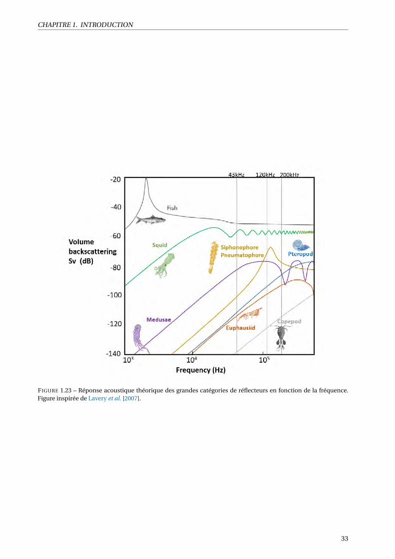
CHAPITRE 1. INTRODUCTION
FIGURE 1.23 – Réponse acoustique théorique des grandes catégories de réflecteurs en fonction de la fréquence.Figure inspirée de Lavery et al. [2007].
33

CHAPITRE 1. INTRODUCTION
FIGURE 1.24 – Exemple d’enregistrement acoustique, aussi appelé échogramme. Les données ont été extraites de lacampagne Nectalis 4, réalisée en 2015 sur l’Alis. L’axe horizontal représente le temps et l’axe vertical la profondeurentre 0 et 800 mètres. Les barres grises au dessus de l’échogramme représentent les périodes de nuit.
tensités acoustiques sont en jaune, les moyennes en vert et le bleu foncé traduit un vide acoustique. Les
migrations nycthémérales abordées en section 1.1.3 sont bien visibles sur cet enregistrement : de nuit,
les fortes densités de micronecton sont concentrées entre 0 et 200 mètres (périodes identifiées par les
barres grises au dessus de l’échogramme) alors que de jour les densités sont plus diffuses et le maximum
plutôt autour de 600mètres. On peut voir que pendant la journée, les couches ne s’arrêtent pas toutes
à la même profondeur : une fine couche se retrouve à 400 mètres, une deuxième vers 500 mètres, une
autre rejoint la couche présente de nuit également à 600 mètres, une dernière couche descend jusqu’à
780 mètres et une dernière couche reste dans les 200 premiers mètres.
1.4.3 Les modèles
Une autre méthode d’étude du micronecton est l’utilisation de modèles déterministes. Les modèles
sont nombreux et leurs fonctionnements très divers (basés sur les interactions trophiques, basés sur
la taille des organismes, individu-centré ou non . . . ). Les modèles spatiaux de dynamique des écosys-
tèmes et des populations permettent de prédire des processus dans l’espace et le temps qu’il est difficile
d’observer directement. Nous ne détaillerons ici que le modèle utilisé dans cette thèse : SEAPODYM
pour "Spatial Ecosystem And POpulation DYnamics Model" [Lehodey et al., 2008]. Il comporte plusieurs
composantes, chacune modélisant un échelon trophique particulier : le zooplancton, le micronecton
[Lehodey et al., 2015, 2010] et les prédateurs supérieurs (majoritairement les thons) [Lehodey, 2001; Le-
hodey et al., 2013]. SEAPODYM est composé d’un ensemble de modèles eulériens qui décrit l’évolution
temporelle de variables en tous points d’un domaine spatial, avec une composante verticale. Il n’est pas
individu-centré car on ne suit pas des cohortes ou des individus. Il est basé sur un ensemble d’équations
(eulériennes) d’advection-diffusion-réaction qui codent les différents processus de dynamique spatiale
34

CHAPITRE 1. INTRODUCTION
FIGURE 1.25 – Schéma explicatif de SEAPODYM extrait de Senina et al. [2008].
et temporelle des populations. Le modèle de diffusion saisit la dispersion aléatoire d’une population; le
modèle d’advection sert à conditionner les mouvements en fonction des courants et du gradient de qua-
lité de l’habitat. Les données hydrodynamiques (température et courants) et biogéochimiques (oxygène
et production primaire) sont utilisées pour simuler la distribution du micronecton. Ensuite, cette distri-
bution de micronecton ainsi que les variables environnementales sont utilisées pour estimer l’habitat de
reproduction et le transport de larves et de juvéniles pour des prédateurs supérieurs comme les thons.
Le modèle crée un indice d’habitat avec des formules empiriques basées sur la densité de micronecton
et l’environnement puis simule la biomasse et le mouvement du thon dans l’espace et le temps (Figure
1.25) pour différentes cohortes d’âge. Il est donc important de simuler avec précision le micronecton afin
d’avoir une bonne représentation des prédateurs supérieurs. Les prédictions de biomasse et de captures
des prédateurs sont ensuite comparées aux données observées de captures et cette comparaison sert à
optimiser les différents paramètres du modèle de thon. La validation du modèle de micronecton est plus
compliquée due à l’absence de données de comparaison.
Le modèle micronectonic (SEAPODYM-MTL pour Mid Trophic Level) sépare le micronecton en 6
groupes basés sur leurs comportements verticaux. La colonne d’eau est divisée en trois couches verti-
cales selon la profondeur de la couche euphotique (Zeu) : la couche épipélagique (entre la surface et 1.5*
35

CHAPITRE 1. INTRODUCTION
Zeu), la couche haute mésopélagique (entre 1.5* Zeu et 4.5* Zeu), et la couche basse mésopélagique (entre
4.5* Zeu et 10.5* Zeu). Les groupes de micronecton sont ensuite divisées selon leur couche de résidence
pendant la nuit et le jour (Figure 1.26). On retrouve les trois groupes résidents dans chacune des couches
(1.1, 2.2, et 3.3 sur la Figure 1.26), le groupe qui migre de la couche haute mésopélagique à la couche
épipélagique (2.1), le groupe qui migre de la couche basse mésopélagique à la couche épipélagique (3.1)
et enfin le groupe qui migre de la couche basse à la couche haute mésopélagique (3.2). Ce modèle de
micronecton simule des biomasses, et comme nous l’avons vu dans les deux paragraphes précédents, il
est très compliqué d’obtenir des biomasses de micronecton qui ne sont pas biaisées par l’outil d’échan-
tillonnage. Il est donc très compliqué d’optimiser le modèle de micronecton en fonction de données
observées et également de valider ses prédictions.
En 2015, Lehodey et al. [2015] propose une méthode d’optimisation de SEAPODYM-MTL basée sur
les données acoustiques, notamment pour optimiser les transferts d’énergie. Le paramètre E définit le
pourcentage d’énergie qui est transféré de la production primaire au micronecton, et ne peut donc pas
être optimisé car il nécessiterait une biomasse absolue. Les autres paramètres sont les paramètres E’n
qui définissent la redistribution de E aux différents compartiments de micronecton, la somme des E’n
vaut 1. Comme ces paramètres sont relatifs les uns aux autres, ils peuvent être estimés en comparant les
valeurs acoustiques intégrées dans les couches verticales les unes aux autres : les coefficients de trans-
fert d’énergie sont optimisés pour s’adapter aux rapports relatifs de biomasse en micronecton (via les
valeurs de NASC) entre les couches qui changent pendant les périodes diurnes et nocturnes. La part
d’organismes migrant est ainsi optimisée avec des valeurs d’acoustique mais la biomasse absolue des
couches et sa distribution spatiale ne l’est pas.
Au cours de cette thèse, nous comparerons les prédictions de biomasse micronectonic faites par
SEAPODYM et les informations tirées de l’acoustique. Pour cela, le signal acoustique sera analysé par
des méthodes statistiques qui sont présentées succinctement dans le paragraphe suivant.
36

CHAPITRE 1. INTRODUCTION
FIGURE 1.26 – Identification des groupes fonctionnels de micronecton sur un schéma conceptuel. Figure extraitede Lehodey et al. [2015]. De la surface vers la profondeur, les couches verticales sont la couche épipélagique(couche ’1’, entre la surface et 1.5* Zeu), la couche haute mésopélagique (couche ’2’, entre 1.5* Zeu et 4.5* Zeu),et la couche basse mésopélagique (couche ’3’, entre 4.5* Zeu et 10.5* Zeu). Les chiffres rouge indiquent les groupesfonctionnels de micronecton basés sur leur distribution verticale et leur migration : par exemple le groupe 3.2 sesitue dans la couche ’3’ de jour (basse mésopélagique) puis dans la couche ’2’ de nuit (haute mésopélagique)...
1.5 Les outils mathématiques d’analyse
Les modèles déterministes/empiriques comme SEAPODYM offrent une couverture spatio-temporelle
extensive pouvant être adaptée à la question posée, ils fonctionnent en mettant en équation des proces-
sus écologiques connus et quantifiables. Les modèles statistiques, eux, ajustent une relation entre une
quantité mesurée et des variables explicatives. Dormann et al. [2012] résume cette dualité : il écrit que
dans les modèles statistiques, les paramètres n’ont pas de signification écologique définie à priori et
les processus sont implicites. En revanche, les modèles empiriques basés sur des processus mécanistes
sont formalisés mathématiquement avec des paramètres explicitement énoncés qui ont une interpréta-
tion écologique claire définie à priori. Dans un modèle statistique, il n’y a pas à priori de lien de causalité
entre la quantité mesurée et les variables explicatives mais la mise en évidence de relations statistiques.
Ces relations doivent ensuite être appuyées par des processus écologiques pour être vérifiées. La Figure
1.27 montre par exemple une excellente relation (corrélation de 0.79) entre le nombre de thèses par an
et les taxes collectées par l’état sur les paris hippiques. Peut-on pour autant en conclure que les taxes sur
les paris hippiques financent les thèses en France? Toute relation statistique identifiée, pour être validée,
doit donc s’appuyer sur des concepts fondamentaux écologiques ou sur un grand nombre d’études faites
sur une autre espèce ou dans un autre endroit.
La définition d’un modèle statistique est « une description mathématique approximative de la réalité,
c’est-à-dire du mécanisme qui a généré les observations, sans description à priori de ces mécanismes.
Un modèle statistique permet d’ajuster des relations entres paramètres sans que ces relations soient
connues à priori.
Dans la grande majorité des cas, les modèles statistiques impliquent une variable de réponse (ou
37
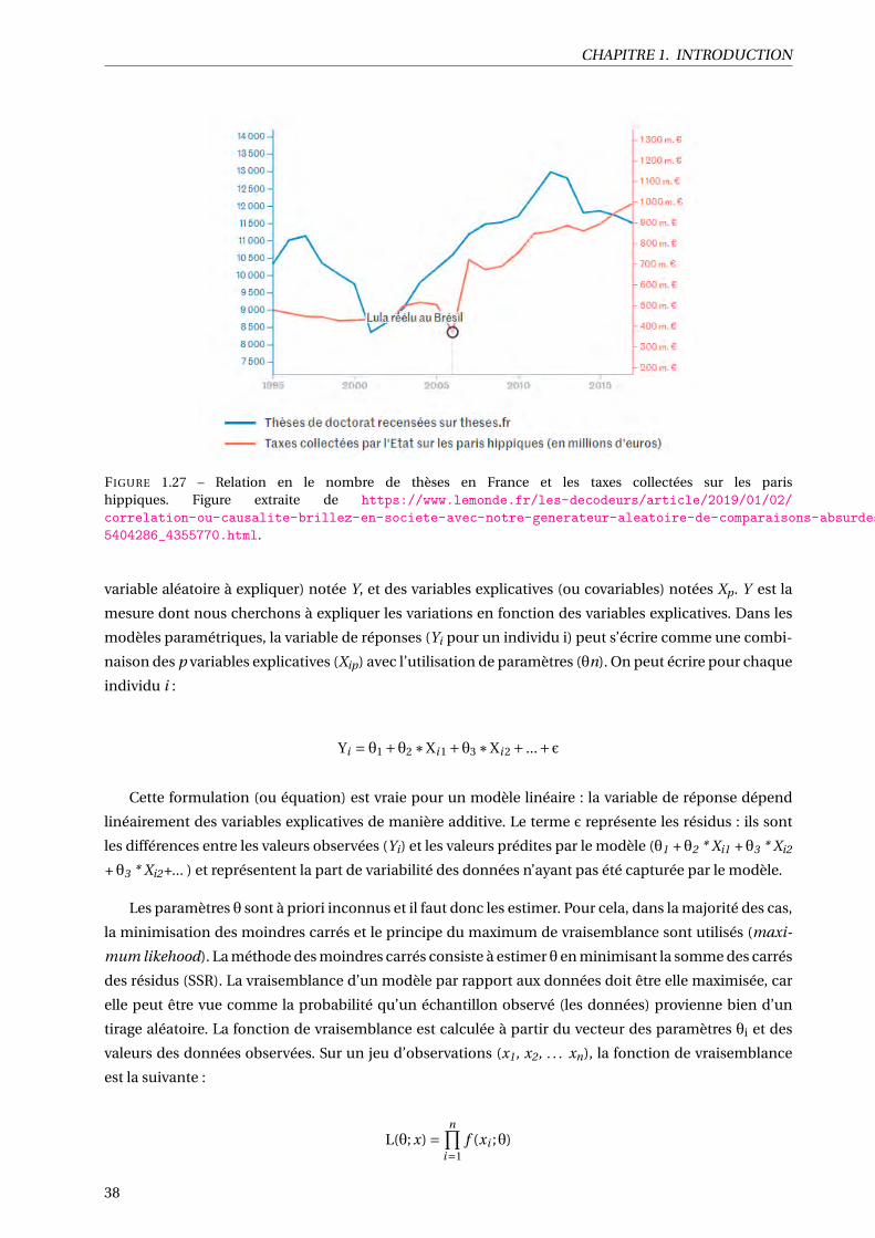
CHAPITRE 1. INTRODUCTION
FIGURE 1.27 – Relation en le nombre de thèses en France et les taxes collectées sur les parishippiques. Figure extraite de https://www.lemonde.fr/les-decodeurs/article/2019/01/02/
correlation-ou-causalite-brillez-en-societe-avec-notre-generateur-aleatoire-de-comparaisons-absurdes_
5404286_4355770.html.
variable aléatoire à expliquer) notée Y, et des variables explicatives (ou covariables) notées Xp. Y est la
mesure dont nous cherchons à expliquer les variations en fonction des variables explicatives. Dans les
modèles paramétriques, la variable de réponses (Yi pour un individu i) peut s’écrire comme une combi-
naison des p variables explicatives (Xip) avec l’utilisation de paramètres (θn). On peut écrire pour chaque
individu i :
Yi = θ1 +θ2 ∗Xi 1 +θ3 ∗Xi 2 + ...+ε
Cette formulation (ou équation) est vraie pour un modèle linéaire : la variable de réponse dépend
linéairement des variables explicatives de manière additive. Le terme ε représente les résidus : ils sont
les différences entre les valeurs observées (Yi) et les valeurs prédites par le modèle (θ1 + θ2 * Xi1 + θ3 * Xi2
+ θ3 * Xi2+... ) et représentent la part de variabilité des données n’ayant pas été capturée par le modèle.
Les paramètres θ sont à priori inconnus et il faut donc les estimer. Pour cela, dans la majorité des cas,
la minimisation des moindres carrés et le principe du maximum de vraisemblance sont utilisés (maxi-
mum likehood). La méthode des moindres carrés consiste à estimer θ en minimisant la somme des carrés
des résidus (SSR). La vraisemblance d’un modèle par rapport aux données doit être elle maximisée, car
elle peut être vue comme la probabilité qu’un échantillon observé (les données) provienne bien d’un
tirage aléatoire. La fonction de vraisemblance est calculée à partir du vecteur des paramètres θi et des
valeurs des données observées. Sur un jeu d’observations (x1, x2, . . . xn), la fonction de vraisemblance
est la suivante :
L(θ; x) =n∏
i=1f (xi ;θ)
38

CHAPITRE 1. INTRODUCTION
où f (xi ;θ) est la densité de la loi Normale sur x. L’objectif sera de trouver un estimateur de θ (noté
θ′) qui maximise la fonction de vraisemblance à partir du jeu d’observations de départ. Pour maximi-
ser cette fonction, on trouve des valeurs de θ pour lesquels la dérivée de la fonction de vraisemblance est
nulle. On peut ainsi ajuster une relation statistique, basée sur des paramètres estimés par cette méthode,
entre une variable de réponse et des variables explicatives. Les différentes manières d’ajuster cette rela-
tion sont détaillées ci-dessous, sans en faire une liste exhaustive, mais en mettant l’accent sur les outils
utilisés pendant cette thèse. On retrouve deux grands groupes d’analyses : uni-variés (une seule variable
de réponse) et multi-variés (plusieurs variables de réponse).
1.5.1 Analyses univariées
Le modèle linéaire (gaussien) de base. À la fois le plus simple, le plus ancien et le plus connu des mo-
dèles statistiques, il englobe essentiellement la régression linéaire, l’analyse de variance et l’analyse de
covariance. Dans ce modèle, les variables explicatives (qualitatives ou quantitatives) sont liées à la va-
riable de réponse de manière linéaire et additive. Il se base sur une hypothèse de distribution Gaussienne
de ses résidus.
Le modèle linéaire généralisé. Il généralise le précédent à deux niveaux : d’une part, la loi des erreurs
n’est plus nécessairement gaussienne, mais doit appartenir à l’une des lois de la famille exponentielle ;
d’autre part, la liaison linéaire entre l’espérance de la variable réponse et les variables explicatives se fait
à travers une fonction particulière appelée fonction de lien (spécifiée à priori).
Les modèles non linéaires. De façon très générale, il s’agit de modèles permettant d’expliquer la va-
riable réponse au moyen des variables explicatives à travers une fonction quelconque inconnue, souvent
non paramétrique. Les GAM (pour Generalized Additive Models) font partis de cette famille et modélisent
la variable réponse avec une somme de fonctions de lissage non-linéaires des variables explicatives [Has-
tie & Tibshirani, 1995; Wood, 2006]. Les fonctions de lissage (ou spline en anglais) sont découpées en
parties et les points de jonctions entre les parties sont des nœuds (le nombre maximal de nœuds est sou-
vent un paramètre à renseigner à priori). Entre chaque nœud, des fonctions souvent polynomiales, sont
ajustées.
Les modèles mixtes. Les modèles mixtes, comme leur nom l’indique, mixent plusieurs types de mo-
dèles. Dans notre cas, le modèle GAM est combiné avec un autre modèle qui prend en compte la coli-
néarité [Wood et al., 2012]. Dans le cas où la variable de réponse a une dimension spatiale ou temporelle,
sa répétition n est liée à sa répétition n-1 car elle est proche de cette dernière temporellement ou spatia-
lement. Il faut prendre en compte cette autocorrélation mathématiquement avant d’ajuster la relation
aux variables explicatives. On dit parfois qu’un autre modèle est emboité dans le premier pour gérer
l’autocorrélation.
Les modèles par arbre de régression et de classification. Ces méthodes consistent à découper une po-
pulation en plusieurs groupes en fonction des variables explicatives qui discrétisent au mieux la variable
39

CHAPITRE 1. INTRODUCTION
de réponse. Ces modèles sont non linéaires. On parle d’arbre de régression en présence d’une variable
réponse quantitative et d’arbre de classification en présence d’une variable réponse qualitative.
1.5.2 Analyses multivariées
L’analyse en composante principale (ACP). L’ACP consiste à transformer des variables corrélées en
nouvelles variables décorrélées les unes des autres dans un nouvel espace. Ces nouvelles variables sont
nommées « composantes principales », ou axes principaux et sont orthogonales entres elles. Elle est ma-
joritairement utilisée pour réduire le nombre de variables et rendre l’information moins redondante. On
dit aussi qu’on projette l’ensemble des variables dans un nouvel espace réduit. Le meilleur ajustement
des axes est trouvé en utilisant la vraisemblance. Souvent, une classification basée sur une minimisation
des distances est réalisée dans cet espace réduit.
Les modèles multivariés. Contrairement à l’ACP, les modèles multivariés ne vont pas simplement ré-
duire l’espace mais réduire cet espace en fonction d’autres variables comme pour les modèles linéaire,
GLM et GAM. Dans ce cas, la variable de réponse est multivariée, c’est-à-dire que la variable mesurée
pour un individu est composée d’un vecteur de valeurs (contre une seule valeur en analyse uni-variée)
[Foster et al., 2013; Ward et al., 2015].
1.5.3 Et le machine learning dans tout ça?
Le machine learning est de plus en plus présent dans le monde de l’analyse de données. Malgré ça,
il n’est pas simple d’en trouver et d’en donner une définition claire. On pourrait le définir comme un
ensemble de méthodes heuristiques (i.e. vraies dans les faits mais qu’on ne peut pas démontrer) per-
mettant d’approximer des observations par apprentissage. Concrètement, les statistiques « classiques »
sont basées sur des hypothèses de distribution des données relativement à des lois de probabilités sur
lesquelles on peut calculer des seuils de significativité, alors que les méthodes de machine learning fonc-
tionnent uniquement avec de l’apprentissage. Par exemple en 2017, un algorithme de machine learning
(AlphaGo, propriété de Google) a battu le champion du monde du jeu de Go. La version suivante de ce
programme (AlphaGo Zero) a ensuite battu 100 parties à zéro AlphaGo. AlphaGo Zero a appris tout seul
à jouer au jeu de Go, sans intervention humaine, en s’entrainant contre lui même [Silver et al., 2017].
Ces algorithmes sont plus puissants que les algorithmes classiques mais souvent vus comme des boites
noires souffrant d’un manque de compréhension.
1.5.4 Validation et utilisation des modèles
Une fois le modèle ajusté, il existe une relation statistique capable de calculer une valeur de la va-
riable réponse pour tout vecteur des variables explicatives. En prédisant sur la base des valeurs explica-
tives observées, on obtient une valeur prédite comparable à la valeur observée. La différence de l’une à
l’autre est appelée résidu. C’est la part de la variance que le modèle ne peut expliquer, due à du bruit
et/ou à un lien avec une variable qui n’a pas été inclue dans le modèle. Tout modèle statistique nécessite
40

CHAPITRE 1. INTRODUCTION
de faire des hypothèses sur la distribution de ses résidus qu’il faut donc vérifier ensuite. On y retrouve
surtout : l’indépendance des résidus 2 à 2, la bonne distribution des résidus, l’indépendance des rési-
dus vis-à-vis des valeurs prédites (appelée hétéroscédasticité), l’absence de sur-dispersion pour les lois
discrètes (e.g. Poisson, binomiale). Une fois que le modèle est validé, il peut être utilisé comme outils de
prédiction. Dans le cas où les valeurs des variables explicatives sortent des gammes échantillonnées, on
parle d’extrapolation.
1.6 Le plan de la thèse
Nous avons analysé des données d’acoustique et de chaluts avec les outils présentés précédem-
ment pour répondre aux questions scientifiques de la thèse. Pour mémoire ces questions portaient sur la
compréhension de la dynamique spatiotemporelle du micronecton; des paramètres environnementaux
contrôlant cette dynamique, de la description des espèces de micronecton et enfin du rôle joué par le
micronecton dans son écosystème. Ce manuscrit s’articule autour de 5 chapitres (Figure 1.28) :
Le travail du chapitre 2 se concentre sur la distribution spatiale et temporelle du micronecton dans
une couche superficielle entre 20 et 120 mètres. Pour cela, 19 ans de données acoustiques d’un échoson-
deur non calibré largement répandu ont été analysées dans un premier modèle pour estimer l’évolution
de l’abondance du micronecton entre 1999 et 2017 dans la ZEE calédonienne. L’influence du phénomène
ENSO a également été étudiée ainsi que le cycle nycthéméral jour/nuit. Un deuxième modèle statistique
nous a ensuite permis d’analyser l’influence de paramètres environnementaux sur la valeur moyenne
acoustique de nuit uniquement. Nous nous sommes servis de ce modèle pour prédire une valeur acous-
tique moyenne dans la zone que nous avons comparé avec les prédictions de biomasse de micronecton
de SEAPODYM-MTL sur la même couche verticale.
Au cours du chapitre 3, nous nous sommes focalisés sur la distribution verticale du micronecton.
Pour cela, les données de six campagnes acoustiques utilisant un échosondeur calibré ont été analysées.
Une méthodologie statistique relativement complexe a permis de décrire la variabilité de la distribution
verticale du micronecton et également de la relier à certains paramètres environnementaux. Encore une
fois, des prédictions de distribution verticale ont été faites sur toute la zone.
Dans le chapitre 4, nous avons analysé des données de chaluts réalisés dans la zone entre 2011 et
2017. Cette étude a permis d’identifier et de décrire les assemblages dominants d’espèces de micronec-
ton. L’influence de quelques paramètres environnementaux sur la probabilité de présence de ces assem-
blages a été également investiguée. Enfin, la distribution spatiale des assemblages a été prédite dans la
zone, de nuit et de jour et à différentes profondeurs.
Pour le chapitre 5, nous avons utilisés le cadre statistique du chapitre 3 pour prédire ce que pourrait
devenir les distributions verticales dans un contexte de changement climatique en se basant sur une
simulation régionale d’un modèle biogéochimique. Nous avons également étudié quels seraient les fac-
teurs environnementaux les plus influents. Les prédictions acoustiques en changement climatique ont
été encore une fois comparées aux prédictions issues du modèle SEAPODYM-MTL.
Finalement, le cadre statistique du chapitre 2 a de nouveau été utilisé pour le chapitre 6. Nous en
41

CHAPITRE 1. INTRODUCTION
FIGURE 1.28 – Schéma descriptif de l’articulation de la thèse.
avons utilisé les prédictions spatio-temporelles, conjointement avec des variables environnementales,
pour comprendre les facteurs contrôlant la dynamique de neuf prédateurs supérieurs (trois espèces de
poissons pélagiques, trois guildes de cétacés et trois espèces d’oiseaux marins). Des modèles statistiques
ont permis de mesurer l’influence de la distribution du micronecton par rapport à l’influence de facteurs
abiotiques sur la distribution de ces prédateurs. Les prédictions spatiales des neuf prédateurs ont ensuite
été combinées en un indice unique pour identifier des zones d’intérêt en matière de conservation et
potentiellement utiles aux gestionnaires du parc marin.
Les résultats majeurs de la thèse sont résumés et discutés dans le chapitre 7 et plusieurs pistes de
recherches futures sont avancées.
42

Chapitre 2
Micronekton distribution in the southwest
Pacific (New Caledonia) inferred from
Shipboard-ADCP backscatter data
Sommaire
2.1 Introduction . . . . . . . . . . . . . . . . . . . . . . . . . . . . . . . . . . . . . . . . . . . . . 44
2.2 Material and Methods . . . . . . . . . . . . . . . . . . . . . . . . . . . . . . . . . . . . . . . 47
2.2.1 Acoustic data . . . . . . . . . . . . . . . . . . . . . . . . . . . . . . . . . . . . . . . . . 47
2.2.2 Environmental data . . . . . . . . . . . . . . . . . . . . . . . . . . . . . . . . . . . . . 49
2.2.3 Statistical model and analysis . . . . . . . . . . . . . . . . . . . . . . . . . . . . . . . . 51
2.2.4 SEAPODYM simulation . . . . . . . . . . . . . . . . . . . . . . . . . . . . . . . . . . . 53
2.3 Results . . . . . . . . . . . . . . . . . . . . . . . . . . . . . . . . . . . . . . . . . . . . . . . . 53
2.3.1 Comparison to EK60 values . . . . . . . . . . . . . . . . . . . . . . . . . . . . . . . . . 53
2.3.2 Temporal variability of backscatter . . . . . . . . . . . . . . . . . . . . . . . . . . . . 54
2.3.3 Estimating ecological relationships . . . . . . . . . . . . . . . . . . . . . . . . . . . . 55
2.3.4 Predicted spatial distribution . . . . . . . . . . . . . . . . . . . . . . . . . . . . . . . . 57
2.3.5 Comparison with SEAPODYM-MTL . . . . . . . . . . . . . . . . . . . . . . . . . . . . 59
2.4 Discussion . . . . . . . . . . . . . . . . . . . . . . . . . . . . . . . . . . . . . . . . . . . . . . 62
2.4.1 ADCP-EK60 comparison . . . . . . . . . . . . . . . . . . . . . . . . . . . . . . . . . . . 62
2.4.2 Environmental predictors . . . . . . . . . . . . . . . . . . . . . . . . . . . . . . . . . . 63
2.4.3 Variability of acoustic backscatters in the New Caledonian EEZ . . . . . . . . . . . . 65
2.4.4 Interest for ecosystem modeling . . . . . . . . . . . . . . . . . . . . . . . . . . . . . . 66
2.4.5 Conclusions and perspectives . . . . . . . . . . . . . . . . . . . . . . . . . . . . . . . 67
43

CHAPITRE 2. MICRONEKTON DISTRIBUTION IN THE SOUTHWEST PACIFIC (NEW CALEDONIA)INFERRED FROM SHIPBOARD-ADCP BACKSCATTER DATA
Abstract
Acoustic data is an invaluable data source for characterizing the distribution and abundance of mid-
trophic level organisms (micronekton). These organisms play a pivotal role in the ecosystem as preys
of top predators and as predators of low-trophic level organisms. Though it cannot provide an absolute
biomass estimate, the Shipboard ADCP (Acoustic Doppler Current Profiler) acoustic backscatter signal
intensity may be a useful proxy to investigate variability in distribution and relative density of micronek-
ton. This study uses data from 19 years (1999 - 2017) across 54 cruises of acoustic recording from ADCP
in the New-Caledonia oceanic sub-tropical EEZ (Exclusive Economic Zone) to assess micronekton sea-
sonal and interannual variabilities and spatial distribution. The dataset is composed of two different
ADCPs with a 150 kHz for the first period followed by a 75 kHz ADCP for the latest years. We examine the
20-120m averaged scattering layer. Using a few cruises with concurrent EK60 measurements, we propose
that the backscatters from the ADCPs and 70 kHz EK60 are closely linked allowing to use the backscatter
signal of both ADCPs in a combined dataset over the full time series. We then design a GAMM (Generali-
zed Additive Mixed Model) model that takes into account the two ADCP devices as well as the temporal
variability. After accounting for the device effect, we show that the acoustic signal is mainly driven by
diel vertical migration, season, year as well as ENSO (El Niño-Southern Oscillation). In a second step,
a consensus model between two statistical approaches (GAMM and SVM) (Support Vector Machine) is
constructed linking the night 20-120m backscatter to the oceanographic and geographic environment.
The model shows that sea-surface temperature is the main factor driving the backscatter variability in
the EEZ with enhanced backscatter during austral summer in the northern part of the EEZ. We show that
such acoustic density differs significantly spatially and temporally from micronekton biomass predic-
ted for the same period by the SEAPODYM-MTL (Mid Trophic Level) ecosystemic model. The seasonal
cycle given by ADCP data lags the SEAPODYM-MTL seasonal cycle by around 3 months. Reasons to ex-
plain these differences and further needs in observation and modelling are explored in the discussion.
In addition to providing new insights for micronekton dynamics in the EEZ needed for ecosystem-based
fisheries management, the data may also help improving our ability to model that key trophic compart-
ment.
Keywords : Micronekton ; southwest Pacific Ocean ; SEAPODYM ; acoustic ; ecosystem
2.1 Introduction
In the western Pacific, marine pelagic predators, in particular tuna, are a major food and economic
resource for small island developing states [Bell et al., 2015]. Tuna distribution variability in space and
time has been linked to oceanographic factors (e.g. temperature, depth and oxygen) or to biological fac-
tors (e.g. age and reproduction) [Brill et al., 2005; Young et al., 2011]. However, the presence and the
availability of forage fauna remains a key driver of tuna distribution [Bertrand et al., 2002a; Duffy et al.,
2017; Olson et al., 2014].
Tuna forage fauna is mostly composed of micronekton, which are mid-trophic level organisms com-
prising crustaceans, molluscs, gelatinous organisms and fish measuring between 1 and 20cm [Bertrand
et al., 2002a; Young et al., 2015]. Distributed in the upper 1000m of the water column [Gjøsaeter & Ka-
44

CHAPITRE 2. MICRONEKTON DISTRIBUTION IN THE SOUTHWEST PACIFIC (NEW CALEDONIA)INFERRED FROM SHIPBOARD-ADCP BACKSCATTER DATA
waguchi, 1980], micronekton is layer-distributed [Burgos & Horne, 2008]. Layer vertical positions are in-
fluenced by physical-chemical properties of the water mass such as oxygen or temperature [Klevjer et al.,
2016], or by the presence of predators [Benoit-Bird et al., 2017]. Micronekton abundance is also influen-
ced by environmental conditions such as primary production [Escobar-Flores et al., 2013; Irigoien et al.,
2014] or the presence of eddies or fronts [Behagle et al. 2016, Sabarros et al. 2009]. A large proportion of
micronekton organisms undertakes diel vertical migrations (DVM), moving from the mesopelagic zone
(200-1000m), where they stay during the day, to the more productive surface layer (0-200m) during the
night [Pearre, 2003]. Diel vertical migrations are observed across all the oceans [Bianchi & Mislan 2016,
Klevjer et al. 2016] and are recognized today as the biggest biomass movement on earth [Hays, 2003]. In
addition to their pivot role between low trophic-level organisms and top predators [Bedford et al. 2015,
Giménez et al. 2018], micronekton actively contribute to the downward flux of nutrients and particulate
organic matter by their diel vertical migration [Ariza et al., 2016; Drazen & Sutton, 2017; Kiko et al., 2017].
Understanding the dynamics of micronekton in the water column and its horizontal spatial distri-
bution at different scales remains challenging. Net trawling is the traditional sampling approach [Potier
et al., 2014]. However, trawl data are size and species dependent and because of net avoidance behavior
of organisms, obtaining an unbiased quantitative estimate with trawls is challenging [Heino et al., 2011;
Kaartvedt et al., 2012]. Further, trawl data are temporally and spatially discrete data, which complicates
their use in attempting to have an overview of the area considered. For the last fifty years, net sampling
has been complemented by the use of underwater sound measurement [Benoit-Bird & Lawson, 2016] as
micronekton layers scatter sound. Scientific echosounders are a powerful tool to study the distribution
and behavior of pelagic biota [Cade & Benoit-Bird, 2015; Kloser et al., 2002].For all echosounders, orga-
nisms’ biomass estimation needs the knowledge of community species composition with net sampling
and their target strength. The use of several frequencies is recommended to achieve a better discrimi-
nation between species or group of species [Davison et al., 2015b]. Calibrated echosounders are widely
used to study the organisms’ distribution through the water column.
Compared to the sampling coverage by scientific echosounders, the one available from shipboard
un-calibrated Acoustic Doppler Current Profiler (hereafter ADCP) is potentially huge. Given that the
ADCP, initially devoted to measuring current velocities, has been used routinely for several decades to
sample currents, the data provided by these instruments are potentially useful over relatively long per-
iods and large spatial scale. Since Flagg & Smith [1989] proposed a method to use ADCP echo intensity
and convert it as a proxy of abundance, a number of subsequent studies have investigated the distribu-
tion, the dynamic and the variability of scattering layers in the pelagic ocean using ADCP records [Che-
reskin & Tarling 2007; Radenac et al. 2010; Smeti et al. 2015]. Due to the lack of calibration, ADCP data
must be numerous to overcome the potential device biases such as the temperature dependence. Seve-
ral studies have successfully compared ADCP and calibrated echosounder [Brierley et al., 1998; Fiedler
et al., 1998; Gostiaux & van Haren, 2010; Griffiths, 2010; Lee et al., 2004]. They suggest that ADCP provides
a proxy of relative density of combined zooplankton and micronekton [Flagg & Smith, 1989; Lee et al.,
2004; Radenac et al., 2010].
Net sampling and acoustic data provide critical information to calibrate and validate ecosystem mo-
dels including a representation of mid-trophic functional groups [Handegard et al., 2013]. Such models
allow for estimating, at regional to global scales, the biomass of micronekton based on key biological
processes and ecological principles such as growth and mortality rates with temperature. SEAPODYM is
45

CHAPITRE 2. MICRONEKTON DISTRIBUTION IN THE SOUTHWEST PACIFIC (NEW CALEDONIA)INFERRED FROM SHIPBOARD-ADCP BACKSCATTER DATA
a Spatial Ecosystem and Population Dynamics Model where both micronekton groups and predator fish
(e.g. tuna) population dynamics are described [Lehodey et al., 2008, 2010]. A method has been developed
to assimilate biomass observations in this model for the estimation of energy transfer efficiency coeffi-
cients between micronekton groups, i.e. migrant and resident. It has been demonstrated using acoustic
data directly, assuming for the sake of simplicity that acoustic signal and biomass are directly propor-
tional [Lehodey et al., 2015]. To explore the interest of using existing abundant archived ADCP data in a
future data assimilation ecosystem modeling framework, we investigate a 19-year time series of ADCP
data, collected through 54 oceanographic cruises in the New Caledonian EEZ.
New Caledonian Exclusive Economic Zone is located in the Coral Sea, at the southwestern edge of the
Pacific Ocean. New Caledonia and the nearby Vanuatu Archipelago create an obstacle to the westward
South Equatorial Current (SEC), the dominant feature of water circulation for the surface, thermocline
and intermediate waters. The SEC is divided into zonal jets when encountering the New Caledonian
islands and finally, waters above the thermocline diverge into two branches around 15°S when reaching
the Australian coast [Cravatte et al., 2015]. In this region, the general circulation models are prone to
shear instabilities and high eddy kinetic energy is observed [Qiu et al., 2009; Rousselet et al., 2016]that
may influence on deep-living organisms distribution [Behagle et al., 2014; Tew Kai & Marsac, 2010]. On
the western barrier reef of New Caledonia’s main island, strong wind episodes during Austral summer
also create upwelling conditions cooling the sea surface temperature and creating vertical movement of
nutrients [Alory et al., 2006; Ganachaud et al., 2010; Marchesiello et al., 2010]. Excluding the very coastal
areas, the New Caledonian EEZ is regarded as oligotrophic with a higher productivity zone south of 22°S
[Ceccarelli et al., 2013; Dandonneau & Gohin, 1984].
The active management of the recently created Coral Sea Natural Park (Decree 2014-1063/GNC)
creates a need for robust information on the productivity and functioning of this remarkable ecosys-
tem, including micronekton dynamics and its pivotal role in food webs. Micronekton taxonomy, dis-
tribution and biomass are still poorly known in the Coral Sea [Ceccarelli et al., 2013] and in the New
Caledonian EEZ [Gardes et al., 2014]. Top predator diet studies [Allain et al., 2012; Olson et al., 2014;
Williams et al., 2014; Young et al., 2010] and trawl data analyses [Grandperrin et al., 1999; Menkes et al.,
2015; Young et al., 2011] emphasized a high diversity level of macro-zooplankton and micronekton with
a dominance of Gonostomatidae, Sternoptychidae, Myctophidae, Scopelarchidae and Phosichthyidae
[Ceccarelli et al., 2013; Grandperrin, 1975; Sutton et al., 2017; Vourey et al., 2017].
Behind this diversity description, the amount of data collected specifically to study micronekton to-
gether with co-located oceanographic conditions are still rare [Menkes et al., 2015; Smeti et al., 2015].
In the New Caledonian EEZ, the poor data coverage prohibits a comprehensive description of the pe-
lagic ecosystem, including the main seasonal patterns of micronekton and their relationships with its
oceanographic drivers. In the present paper, we focus on the analysis of the spatial and seasonal varia-
bility of acoustic backscatter collected around New Caledonia and its relationships with oceanographic
conditions, assuming that backscatter values are a relevant proxy for micronekton relative abundance.
Our objectives are four-fold. Firstly, we propose a simple approach of inter-calibration between various
instruments. We describe diel vertical migration, seasonal cycles and multi-year trends in backscatter
data. Then, the effect of environmental variables (bathymetry, distance to the closest coast, sea surface
temperature, chlorophyll-a and depth of the thermocline) on backscatter values is investigated through
statistical models providing backscatter predictions at the scale of the EEZ. Finally, we compare acous-
46

CHAPITRE 2. MICRONEKTON DISTRIBUTION IN THE SOUTHWEST PACIFIC (NEW CALEDONIA)INFERRED FROM SHIPBOARD-ADCP BACKSCATTER DATA
tic data from the ADCP model to micronekton outputs of SEAPODYM simulations. In the discussion,
pathways are proposed to progress on the observation, understanding and modelling of micronekton.
2.2 Material and Methods
Micronekton dynamics are usually studied with calibrated echosounder devices such as the SIMRAD
EK60 echosounder. Therefore, EK60 backscatter values are comparable to any other backscatter value
from other EK60 survey. The un-calibrated ADCP is usually switched-on for current measurements on-
board oceanographic vessels : for the New Caledonian region, only 6 cruises have collected acoustics
data using the EK60, while 54 cruises have recorded ADCP data. Hence, despite the lack of calibration,
ADCP offers longer time series and wider spatial coverage than calibrated acoustic data for our zone.
2.2.1 Acoustic data
TABLEAU 2.1 – Number of 10km transects per season, warm season : DJF (December, January, February) and MAM(March, April, May) ; and cold season : JJA (June, July, August) and SON (September, October, November) and peryear. Italic numbers are with the ADCP 75 kHz plain numbers are for the ADCP 150 kHz.
DJF MAM JJA SON1999 0 0 0 712000 0 79 0 02001 17 68 0 392002 7 59 0 02003 100 0 213 2902004 244 68 77 962005 19 35 0 02006 0 0 0 602007 0 64 117 02008 0 262 110 02009 0 0 0 02010 0 124 0 02011 135 0 192 782012 0 83 50 + 56 1482013 30 1 40 722014 70 0 0 942015 0 0 0 902016 51 134 50 1702017 0 0 62 217
We gathered historical ADCP data from 54 cruises on board the R/V Alis in the New-Caledonia EEZ
between 156°E–174°E and 14°S–27°S, from 1999 to 2017 (Figure 2.1, Table 2.1 and Appendix 2.4.5). Two
profilers were used : a 150 kHz BroadBand ADCP (BBADCP), from 1999 to May 2012, and an Ocean Sur-
veyor 75 kHz NarrowBand ADCP (NBADCP) from October 2012 to 2017.
All ADCP data were processed using the freely available CODAS software (http://currents.soest.
hawaii.edu), applying the procedure described in Hummon & Firing [2003]. The echo intensity (Ea), in
counts, recorded by the ADCP was converted to backscatter coefficient (Sv in dB.re.m2) using the stan-
47

CHAPITRE 2. MICRONEKTON DISTRIBUTION IN THE SOUTHWEST PACIFIC (NEW CALEDONIA)INFERRED FROM SHIPBOARD-ADCP BACKSCATTER DATA
FIGURE 2.1 – Map showing cruise tracks of the R/V Alis (solid lines) with SADCP device (blue line for 150 kHz, yellowline for 75 kHz and grey line for cruises used for ADCP validation) in the New Caledonian Exclusive EconomicZone. The background grey colors represent the seabed depth (where lighter colors are shallower). Important areasdiscussed in the paper are indicated in grey dashed line (panel A). Boxplot of ADCP backscatter values per cruiseswith the same color code than for the map (panel B).
dard equation of sonar given by RDI [1998] for a NB-ADCP. Deines [1999] transformed this equation for
a BB-ADCP, subsequently rearranged by Gostiaux & van Haren [2010] (Appendix 2.4.5). 150 kHz ADCP
backscatter data also had to be corrected due to a technical bias : due to two technical interventions,
the mean level of backscatter values changed abruptly two times. Cruises were grouped in order to have
constant mean Sv across groups (i.e. Group1 : Wespalis1 to Mareva1; Group2 : Secalis4 to Secargo ; and
Group3 : Nectalis1 to Momalis) (Appendix 2.4.5). The maximum depth reached between these cruises
groups are statistically different according to a Wilcoxon test (p-value < 0.05 for Group1-Group2, Group1-
Group3 and Group2-Group3) showing that backscatter values changes are due to technical bias and
not due to some environmental changes. We adjusted backscatter values on a similar mean level across
groups by adding offsets (Appendix 2.4.5). The final vertical resolution (bin) was 8m for the 150 kHz and
16m for the 75 kHz, both starting at 16m depth and ending on at 300m for the 150 kHz and at 700m for
the 75 kHz, with a time resolution of 5 min.
WWe selected the surface layer (20-120 m) only, because of the limited vertical range of the 150 kHz
48

CHAPITRE 2. MICRONEKTON DISTRIBUTION IN THE SOUTHWEST PACIFIC (NEW CALEDONIA)INFERRED FROM SHIPBOARD-ADCP BACKSCATTER DATA
ADCP : its initial vertical range was 300 m, but the depth actually reached after several years was limited
to 120 m due to a decrease in the power of the device. Analyses were done on a thicker layer (20-200
m) with fewer cruises and conclusions were similar, so the 20-120 m layer was kept and considered re-
presentative of the epipelagic zone (0-200 m). Sv data were transformed into a linear scattering measure
(sv = 10 Sv10 ) before to be depth-averaged over 20-120 meters. In order to remove phenomena happening
at high spatiotemporal scales [Escobar-Flores et al., 2018], the linear scattering measure was also ave-
raged along survey traces every 10km that corresponds approximately to 10 initial points with a vessel
speed around 7 knots (13km.h-1). Sensitivity studies with different spatial resolution (5, 10 and 20 km)
as well as by analyzing the median value rather than the mean, and all results lead to the same conclu-
sions (not shown). Then, the logarithmic value (Sv = 10l og (sv )) was calculated and used for all following
analysis (Sv_ADCP, in dB.re.m2) (Appendix 2.4.5).
To analyze the complete time series (from 1999 to 2017), the two ADCP frequencies needed to be
analyzed together to look for a potential long temporal trend. For that purpose, we offered a method
to replace the two ADCP signals on a similar mean level by comparing to the EK60 data. Both instru-
ments, were used simultaneously during six cruises : Nectalis 1 through 5 and Puffalis (cruises numbers
33, 35, 45, 46, 51, 52 in Appendix 2.4.5). During these cruises, EK60 calibration was performed according
to the Foote et al. [1987] method at the beginning of each cruise. As for ADCP, the mean value of EK60
Sv of the 70 kHz frequency was calculated in the 20-120m layer, with a 10km resolution. Two linear re-
gressions were fitted between the Sv_ADCP values (one regression for each device : 150 kHz and 75 kHz)
and the Sv_EK60 values (70 kHz). By comparing the two ADCP frequencies to the same EK60 frequency,
we assumed that a part of each ADCP signal was correlated to the EK60. Based on the assumption that
backscatter echo-intensities of EK60 70 kHz were comparable between the 6 cruises due to calibration
step, an ‘ADCP corrected value’ relative to the EK60 70 kHz value could be calculated. For the rest of
the text, the ‘corrected backscatter’ (Sv_ADCP_corrected) corresponded to the Sv_ADCP corrected with one of
the two linear regressions with EK60 values. These regressions were used to adjusted on the same mean
backscatter level the two ADCP frequencies and therefore to average predictions (Figure 2.2).
The comparison with the EK60 data made it possible to treat together the two groups of cruises car-
ried out with the two ADCPs. The adjustment from Sv_ADCP to Sv_EK60 was made globally for each group,
assuming that the 38 cruises (150 kHz) on the one hand and the 16 others (75 kHz) on the other were
comparable. Indeed, in a group, it is considered that variations in Sv values between cruises are due so-
lely to biological and environmental effects and not to a "device effect" such as technical dependence
on temperature. The influence of ambient temperature on the backscatter calculation (Appendix 2.4.5)
was tested and found to be negligible (not shown). Many previous studies have used a similar approach
[e.g. Ashjian et al. 2002, Bianchi & Mislan 2016, Blanc et al. 2008, Chereskin & Tarling 2007, Kaneda et al.
2002, Liljebladh & Thomasson 2001, Radenac et al. 2010, Tarling et al. 2001].
2.2.2 Environmental data
A suite of available environmental variables was selected to explore the physical drivers of backscat-
ter data. For each backscatter location, environmental variables were obtained at the matching sampling
position and date when data were available. Where real date data were not available, climatologic data
were used (Table 2.2).
49

CHAPITRE 2. MICRONEKTON DISTRIBUTION IN THE SOUTHWEST PACIFIC (NEW CALEDONIA)INFERRED FROM SHIPBOARD-ADCP BACKSCATTER DATA
The bathymetry was extracted from a 500m resolution dataset [ZoNéCo, 2013], and the Euclidean
distance to the closest coastline or shallow reef (0-30m) was calculated from a coastline-reef shapefile
[Andréfouët et al., 2008]. Sun elevation was calculated for all points with an adapted version [Blanc &
Wald, 2012] of the formula given by Michalsky [1988], a function of spatial position and date. Sun eleva-
tion negative value are for Night period (from -90° to 0°) and positive value for Day (from 0° to 90°).
Several products were tested for zonal and meridional currents : a mean absolute geostrophic cur-
rent climatology, based on 1000m-Argo floats combined with geostrophic currents computed from the
CSIRO Atlas of the Regional Sea (CARS2009) [Kessler & Cravatte, 2013], a seasonal ADCP current cli-
matology [Cravatte et al., 2015], the ARMOR3D gridded weekly velocities derived from satellite and in
situ observations [Guinehut et al., 2004, 2012; Mulet et al., 2012] and the MERCATOR-OCEAN GLORYS
ocean reanalysis. Other oceanographic physical parameters used were the sea level anomaly [Pujol et al.,
2016],the sea surface temperature [Reynolds et al., 2007], and the depth of the 20°C isotherms calcula-
ted from the ARMOR3D dataset. We used surface vector winds from Cross-Calibrated Multi-Platform
(CCMP-v2), produced using satellite, moored buoy, and model [Wentz et al., 2015]. One biological para-
meter was extracted from GlobColour project : surface chlorophyll-a [Saulquin et al., 2009]. These geo-
graphic parameters and environmental dataset are detailed in Table 2.2.
To assess ENSO effect, the Oceanic Niño Index (ONI) [3 month running mean of ERSST.v5 SST ano-
malies in the Niño 3.4 region (5°N-5°S, 120°-170°W)] (http://origin.cpc.ncep.noaa.gov/products/
analysis_monitoring/ensostuff/ONI_v5.php) was used. ENSO phases were defined with a 0.7 thre-
shold on : months with an ONI above 0.7 were classified as El Niño and months with an ONI below -0.7
as La Niña.
TABLEAU 2.2 – Environmental variable summary with unit, source and resolutions detailed for each variable. Va-riables with an asterisk (*) were downloaded via the Copernicus portal, CMEMS (Copernicus Marine EnvironmentMonitoring Service) (http://copernicus.eu/main/marine-monitoring). Variables with (C) are climatologic.
Variable name Unit SourceTemporalresolution
Spatialresolution
Bathymetry km ZoNeCo, 2013 - 500 mDistance to the closest land or reef km from coastline and reef shapefiles - ¼°Sun elevation ° Calculated from position and date - -3D geostrophic zonal and meridionalcurrents 30-100m mean
cm/sARGO floats and CSIRO Atlas of the Regional Sea(CARS2009)
Annual (C) ¼°
SADCP zonal and meridional currents25-100m mean
cm/s Large ADCP dataset Quarter (C) ¼°
Surface zonal and meridional seawatervelocity (*)
m/s MERCATOR GLORYS2V4 Day ¼°
Zonal and meridional geostrophiccurrents 20-110m mean (*)
m/s ARMOR3D Week ¼°
Sea Surface Temperature (SST) (*) °CAdvanced Very High Resolution Radiometer(AVHRR) infrared satellite
Day ¼°
Chlorophyll-a (*) mg/m3GlobColour-Processors versions :MODIS 2014.0.1/VIIRSN 2014.0.2
Day ¼°
Sea Level Anomaly (SLA) (*) mDT all-sat-merged Global Ocean GriddedSSALTO/DUACS Sea Surface Height L4 product
Day ¼°
Zonal and meridional winds (*) m/s Cross-Calibrated Multi-Platform (CCMP-v2) Week ¼°Depth of the 20 degrees isotherm(D20) (*)
m ARMOR3D Week ¼°
50

CHAPITRE 2. MICRONEKTON DISTRIBUTION IN THE SOUTHWEST PACIFIC (NEW CALEDONIA)INFERRED FROM SHIPBOARD-ADCP BACKSCATTER DATA
2.2.3 Statistical model and analysis
GAM (Generalized Additive Models) [Hastie & Tibshirani, 1995] and SVM (Support Vector Machine)
[Cortes & Vapnik, 1995] statistical models were used to investigate variability of backscatter echo-intensities
in the New Caledonian EEZ. We studied the temporal variability (daily, monthly, multi-annually varia-
bility) in a first step and the relationships between backscatter values and environmental variables in a
second step to avoid collinearity problems (e.g. between SST and month) (Figure 2.2). Each model used
has specific advantages : GAM allows to rank the variables by relevance and to highlight the relationships
between the response variables and the predictors (explanatory variables), which is interesting from an
ecological point of view. However, GAM is difficult to tune while respecting strong assumptions (e.g.
absence of autocorrelation in residuals, error distributed normally). SVM, as the state-of-the-art classifi-
cation and regression algorithm, has been applied in various scientific domains and especially in ecolo-
gical niche modeling [Drake et al., 2006; Palialexis et al., 2011]. For this method there is no requirement
concerning predictors’ distributions or autocorrelation [Hegel et al., 2010]. Yet, it remains difficult to in-
terpret the SVM results and there is no straightforward method for explaining the results and rank the
predictors by relevance. To interpret ecological phenomena, partial dependence plots were produced by
environment variables to visually explore the marginal effect of a given variable on the backscatter value
while other variable are fixed to their mean values [Friedman, 2001]. SVM partial dependence plots were
not presented as strong interactions exist between predictors [Goldstein et al., 2015]. Subsequent models
were fitted both GAMM and SVM, excluding each of the remaining terms, one at a time, to assess per-
centage of variation explained by predictor and we classified predictors, according to their importance
in the model.
To account for autocorrelation between consecutive backscatter values we used a Generalized Addi-
tive Mixed Model (GAMM). We nested an autocorrelation structure of order 1 (i.e. a 10km autocorrelation
structure, Ménard & Marchal, 2003), with a random effect fitted by cruises dealing with the correlation
structure [Dormann et al., 2007; Wood, 2006]. The absence of collinearity was checked in residuals. We
used a Gaussian family with an identity link function and adopted restricted maximum likelihood (RML)
as the smoothness selection criteria [Wood, 2011]. All splines were fitted with a maximum knot number
of 10 to keep a relatively simple relationship. SVM uses a functional relationship to map data onto a new
hyperspace in which complex patterns can be more simply represented [Drake et al., 2006; Muller et al.,
2001]. SVM parameters were tuned (Gaussian kernel, gamma = 0.1 and cost = 10) by cross validation
[Browne & Cudeck, 1989]. We calculated the root mean square error (RMSE) on the evaluation dataset by
removing data from each of the 54 cruises one by one.
To account for the potential difference between the two ADCP devices, we included an ADCP de-
vice effect in all models (GAMM and SVM). Therefore, backscatter values were predicted for each ADCP
device, BB150 and OS75 respectively. We then corrected the predicted Sv using the corresponding EK60
linear regressions, and finally averaged the corrected predicted values from the two devices (Figure 2.2).
The effect of the ADCP device included in the each models is different. For the GAMM, it is a ‘fixed effect’,
meaning that relationships between backscatter and covariates have the same shape but with an offset
function of the ADCP device. For the SVM approach, ADCP effect is included as a binary variables (-1/1)
and fitted relationships linked to ADCP device have different shapes.
We explored visually the temporal dynamic over the entire time series (1999-2017) with GAMM out-
51

CHAPITRE 2. MICRONEKTON DISTRIBUTION IN THE SOUTHWEST PACIFIC (NEW CALEDONIA)INFERRED FROM SHIPBOARD-ADCP BACKSCATTER DATA
puts. In a first step, GAMM1 allowed us to investigate relationships between Sv_ADCP values and a set of
temporal and spatial predictors. Six predictors were tested : the ADCP effect (BB150 or OS75) and the
ENSO phase (Neutral, Niño or Niã) as qualitative variables and sun elevation (proxy for the moment of
the day), year, month, latitude and longitude as quantitative variables (Figure 2.2, step 1). Year variable
was smoothed with a cubic spline and month with a cyclic cubic spline. Latitude and longitude were fit-
ted inside the same isotropic spline [Wood et al., 2012] with a Gaussian process model smoothing basis
[Golding & Purse, 2016; Miller et al., 2013]. This spatial term was added to fit the mean spatial distribution
pattern to account for difference in surveys spatial localisation across years (Appendix 2.10).
In a second step, environmental variables described in Table 2.2 (i.e. bathymetry, distance to the
coast/reef, sun elevation, 4 currents sources, SST, chlorophyll-a, SLA, winds and d20) and a fix effect of
the ADCP device were included in GAMM2 and SVM (Figure 2.2, step 2) independently of a month or
year variables. All variables were smoothed with cubic splines. Predictions were done on climatological
environmental variables with a ¼° resolution grid (explicative variables resolution) and then averaged
between models leading to a hybrid GAMM2-SVM prediction. A measure of the coherence between the
two models was estimated through the variation coefficient (i.e. standard deviation divided by mean),
which ranged from 0 to 7%. We applied two different standard deviation thresholds (6%, 2%) : the lower
the variation coefficient threshold is, the higher the confidence is in the prediction, but the lower the
number of cells predicted is. We used two statistical models to compare large spatial predictions, com-
bine common patterns [Oppel et al., 2012] and to ensure that conclusions are robust to the underlying
statistical assumptions. Before constructing models, we confirmed that collinearity was not apparent
among the predictors using variance inflation factors (VIF) [O’brien, 2007] and Spearman correlations
between each pair of covariates. We considered covariates were not collinear when both Spearman cor-
relations were inferior to 0.5 and VIF were inferior to 3.
The GAMM1 assesses the seasonal cycle by fitting a ‘month’ variable as a continuous variable. GAMM2-
SVM does not use a temporal variable to explicit seasonality but use relationships with environmental
variables (such as SST) in which seasonality is inherent to predict backscatter values at each point and
finally the seasonal cycle is assessed by averaging all EEZ predicted values by month.
All statistical analyses were performed with R (version 3.5.0, R Core Team 2016). GAMMs were fitted
using the gamm function of R package mgcv [Wood, 2017]. SVM was fitted using the svm function of R
e1071 package [Meyer et al., 2017].
FIGURE 2.2 – Diagram explaining the different steps of the analysis. For models GAMM1, GAMM2 and SVM, purplevariables are numerical and orange variables are qualitative.
52

CHAPITRE 2. MICRONEKTON DISTRIBUTION IN THE SOUTHWEST PACIFIC (NEW CALEDONIA)INFERRED FROM SHIPBOARD-ADCP BACKSCATTER DATA
2.2.4 SEAPODYM simulation
The sub-model of SEAPODYM for mid-trophic levels (MTL) simulates several functional groups of
micronekton for the oceanic epi- and mesopelagic layers [Lehodey et al., 2015, 2010]. The spatial and
temporal dynamics of production and biomass are modelled with a system of advection-diffusion-reaction
equations driven by ocean temperature, horizontal currents, primary production and euphotic depth.
Currently, there are six groups of micronekton defined according to the Diel Vertical Migration (DVM)
patterns of mesopelagic organisms between three broad epipelagic, upper and lower mesopelagic verti-
cal layers. The euphotic depth Zeu is used to define the depth boundaries of the vertical layers : 0-1.5*Zeu
for the epipelagic layer, 1.5-4.5*Zeu for the mesopelagic layer and 4.5-10.5*Zeu for the bathypelagic layer.
In New Caledonia, Zeu is around 70-75m hence the epipelagic layer in the model occupies the top 110m.
During the day, only the epipelagic group inhabits the epipelagic layer, but during the night, it also in-
cludes the migrant upper-mesopelagic and highly migrant lower mesopelagic groups.
We compared the predicted backscatter to SEAPODYM-MTL modelled micronekton biomass. We
used SEAPODYM-MTL micronekton simulation for the 1999-2017 period. The biomass of micronekton
groups inhabiting the epipelagic layer at night was extracted at the date and places of the ADCP data.
Values were centered (the mean was subtracted) and scaled (divided by the standard deviation) for both
SEAPODYM and acoustics models. Biomass values were compared along the tracks by calculating corre-
lations, and distribution patterns compared over the whole New Caledonian EEZ.
2.3 Results
A total of 89530km of survey track across 435 days (288 days for the 150 kHz and 147 for the 75 kHz
ADCP) over 19 years were analyzed in this study. All quarters were sampled at least nine times during
the study period (Table 2.1 and Appendix 2.4.5) and the whole Exclusive Economic Zone was surveyed
at least once except a small area in the south east corner of the EEZ, and an area in the south west below
Chesterfield Reefs (Figure 1.1).
2.3.1 Comparison to EK60 values
We compared the un-calibrated ADCP acoustic data to the calibrated EK60 echosounder data. Two
cruises were available with concomitant 150 kHz Sv_ADCP and Sv_EK60 records (1110 paired values) and
four cruises with 75 kHz Sv_ADCP and Sv_EK60 (1955 paired values). For both ADCP frequencies, correla-
tions between mean 20-120m Sv_ADCP and Sv_EK60 were significant and higher than 0.8 (Figure 2.3). The
two regressions were significant (p-values <0.01) and had different slopes : 1.05 (standard error 0.017) for
the 75 kHz ADCP and 0.72 (standard error 0.012) for the 150 kHz ADCP (Table 2.3). For the 75 kHz, the
data scatterplot from Nectalis 4 and Puffalis on one side, and from Nectalis 3 and Nectalis 5 on the other
side, could warrant the estimation of different intercepts (Figure 2.3).
53

CHAPITRE 2. MICRONEKTON DISTRIBUTION IN THE SOUTHWEST PACIFIC (NEW CALEDONIA)INFERRED FROM SHIPBOARD-ADCP BACKSCATTER DATA
FIGURE 2.3 – ADCP backscatter (Sv) as a function of the 70 kHz EK60 echosounder Sv and the associated linearregressions (black line) for the 150 kHz ADCP device (BB150, Nectalis 1 and 2) (left) and the 75 kHz ADCP (OS75,Nectalis 3, 4, 5 and Puffalis) (right). Blue ticks on both axis show the distribution of the observations.
TABLEAU 2.3 – Linear regression analysis outputs including the intercept, the slope, the slope standard error andp-value, the deviance explained (or R2) and the number of observations for each ADCP device.
ADCP device Intercept Slope Slope standard error Slope p-valueDevianceexplained
n
OS75 -11.32 1.05 0.017 <2e-16 67 1955BB150 -14.64 0.72 0.012 <2e-16 76 1110
2.3.2 Temporal variability of backscatter
Temporal variability of backscatter micronekton was analyzed at three scales : daily, monthly and
yearly using a GAMM including all Sv_ADCP values (night and day) as a function of ADCP device, sun ele-
vation, year, ENSO phase, month and location (latitude and longitude) with a nested auto-correlative
model (Figure 2.2, left part). In this model, the largest part of the variance was explained by the sun
elevation (Table 2.4). Sv_ADCP in the 20-120m layer was higher during the night than during the day (res-
pectively -69dB and -75dB) (Figure 2.4), with a 6dB difference. The usual value used as a density proxy is
the linear value (sv), so a 6dB difference meaned that the micronekton density was about 4 times higher
during the night than during the day in the 20-120m layer. Sv_ADCP values were constant during the night,
but started to decrease at dawn when the sun elevation exceeds -20°. The variance explained by the sun
elevation demonstrated the important impact of the diel vertical migration in the 20-120m layer. The
second most important variable was the effect of the ADCP device (Table 2.4).
Month was the third variable explaining the variance of Sv_ADCP (Table 2.4). The seasonal cycle dis-
played a maximum in March (-70.8dB), and a minimum in September (-74.3dB), with two superimposed
relative maxima in July and November (-71.8dB and -72.8dB respectively) (Figure 2.5). The difference
between extreme values was about 3.5dB, meaning there was in average 2 times more biomass during
March than during September, 1.6 more in July and 1.4 more in November compared to September. The
54

CHAPITRE 2. MICRONEKTON DISTRIBUTION IN THE SOUTHWEST PACIFIC (NEW CALEDONIA)INFERRED FROM SHIPBOARD-ADCP BACKSCATTER DATA
54 cross-validation simulations (Figure 2.5) confirmed the robustness of the seasonal cycle.
The variance explained putted the year variable at the 5th rank and ENSO at the 6th rank (Table 2.4).
The relationship between the Sv_ADCP and the year was non-linear with a minimum and a maximum
(Figure 2.6 A). Predicted Sv_ADCP were about -73dB in 1999, decreased to a minimum of -75dB in 2007
and reached a maximum of -71.5dB in 2017. So, on average the acoustic density decreased by 1.6% bet-
ween 1999 and 20017 and then increased by 2.2% between 2007 and 2017. The ENSO phase effect was
significant in the GAMM1 : Sv_ADCP was twice as high during El Niño phase than during a neutral phase
(Figure 2.6B), and the Sv_ADCP during La Niña phase was not significantly different from the value during
the neutral phase.
FIGURE 2.4 – GAMM1 partial dependence plot showing the effect of the sun elevation on corrected backscattervalues (Sv). The solid grey lines are the estimates of the smooths for the 54 simulations from cross-validation andthe black line is the average smooth. Blue ticks on the inner X-axis show the distribution of the observations.
FIGURE 2.5 – GAMM1 partial dependence plot showing the effect of the month on corrected backscatter values(Sv). The solid grey lines are the estimates of the smooths for the 54 simulations from cross validation and theblack line is the average smooth. Cold season is indicated in blue and warm season in orange.
2.3.3 Estimating ecological relationships
To investigate the impact of environmental variables on Sv_ADCP, values during the night only (Sv_ADCP_night)
were fitted through both a GAMM2 (with a nested auto-correlative model) and a SVM with environmen-
55

CHAPITRE 2. MICRONEKTON DISTRIBUTION IN THE SOUTHWEST PACIFIC (NEW CALEDONIA)INFERRED FROM SHIPBOARD-ADCP BACKSCATTER DATA
TABLEAU 2.4 – Model summary with the model name, the response variable, the explicative variables, the totaldeviance explained (or R2) and the rank of importance by variable. All predictors were significant in the GAMMsoutput (p-values < 0.05). An asterisk (*) indicates that an auto-correlative model is nested into the GAMM.
Model Response variableExplicative
variablesDevianceexplained
Rank ofimportance by variable
Sun elevation 1year 5
month 3Lat * lon 4
ENSO_phase 6
GAMM1 (*) Sv_ADCP
ADCP_device
63.9
2SST 2D20 4
Log_chloro 3Bathy 5
Dist_coast 6
GAMM2 (*) Sv_ADCP_NIGHT
ADCP_device
58.1
1SST 2D20 3
Log_chloro 6Bathy 4
Dist_coast 5
SVM Sv_ADCP_NIGHT
ADCP_device
77.9
1
FIGURE 2.6 – GAMM1 partial dependent plot terms showing the effect of year (A) and ENSO phases (B) variableson corrected backscatter values (Sv). The solid grey lines are the estimates of the smooths for the 54 simulationsfrom cross validation and the black line is the average smooth. El Niño events are indicated in blue on panel A, andLa Niña events in orange.
tal variables and an effect on ADCP device (150 kHz or 75 kHz) (Figure 2.2, right part). We focused this
part of the study on nighttime values to reveal the potential influence of environmental parameters that
could have been masked by the strong impact of the sun elevation on backscatter. The night signal was
preferred over the day signal as in the layer 20-120m it better represents the micronekton community
by accumulating both permanent epipelagic organisms and migrating organisms coming from deeper
layers.
Based on Spearman correlation tests and VIF, depth of isotherm 20°C (d20) and SLA were correlated,
which required selecting only one of those variables to be included in the model. As SLA was not signi-
ficant for the GAMM2, we chose to keep d20 in the final model. The zonal and meridional currents and
56

CHAPITRE 2. MICRONEKTON DISTRIBUTION IN THE SOUTHWEST PACIFIC (NEW CALEDONIA)INFERRED FROM SHIPBOARD-ADCP BACKSCATTER DATA
wind data were un-significant in the GAMM2 ; relationships were flat thus they were not considered fur-
ther in the models (GAMM2 and SVM). The final models included SST, chlorophyll-a, depth of the 20°C
isotherm, distance to the coast/reef, bathymetry and the effect of the ADCP device for both SVM and
GAMM2.
After considering the ADCP device effect, the two statistical methods mostly agreed on the relative
contribution of variables (Table 2.4) with SST demonstrating the main effect among the oceanographic
variables. The contribution rank of the chlorophyll-a was different between the GAMM2 and the SVM :
chlorophyll-a was the second most important variable for the GAMM2 and the last (6th) for the SVM.
Then, in descending order of importance, we found the 20°C isotherm depth, the bathymetry and the
distance to the closest coast/reef.
The relationship between backscatter value and distance to the closest reef/coast was linearly de-
creasing, with higher values closer to the coast (Figure 2.7A). The influence of the bathymetry was not
linear, but an optimum of the 20-120m backscatter value was observed over a sea floor at 1800m depth
(Figure 2.7B). Relationship with SST was increasing non-linearly, with a first optimum around 24°C and
a rise from 26 to 31°C (Figure 2.7C). The chlorophyll-a concentration relationship was also increasing;
the backscatter value was higher with higher chlorophyll-a concentration (Figure 2.7D). The relationship
with the 20°C isotherm depth was decreasing : the mean backscatter value was higher when the isotherm
was shallower (Figure 2.7E). All relationships were significant according to GAMM outputs and the va-
riability through cross validation was small over almost all the variable ranges showing robustness of the
model (Figure 2.7).
2.3.4 Predicted spatial distribution
Predicted distribution patterns of the GAMM2-SVM hybrid-model backscatter during the four quar-
ters are shown on Figure 2.8. We defined the austral summer or the warm season as the DJF (December,
January and February) and MAM (March, April and May) quarter periods and the austral winter or the
cold season as JJA (June, July and August) and SON (September, October and November) quarters. This
definition was chosen relative to the common knowledge of these seasons in New Caledonia [Cravatte
et al., 2015]. Spatial predictions were highly homogenous across one season (DJF is very similar to MAM
and identically for JJA and SON) (Figure 2.8A).
Generally, values were higher during the warm season. During this season the distributions showed
aggregations of high values in the central part of the EEZ in a wide strip area with a south-east to north-
west orientation encompassing the main island and the Loyalty islands where there was a high confi-
dence in the predictions (refer to Figure 2.1 for islands and reefs names). The values were particularly
high north of 22°S (Figure 2.8A, DJF and MAM) and around the Chesterfield Reefs. There were lower va-
lues in the southeastern corner of the EEZ. The channel between the group made of Chesterfield Reefs,
Bellona, Fairway-Landsdowne, and the main island was also predicted to have lower values.
During the cold season, there were lower values in the north close to the coast of the main island and
in the south along the edges of the EEZ (Figure 2.8A, JJA and SON). Highest values during the cold season
were located south of 20°S, south of the main island, south of the Chesterfield Reefs and north of the
southeast corner of the EEW where there was a higher prediction divergence between the GAMM2 and
57

CHAPITRE 2. MICRONEKTON DISTRIBUTION IN THE SOUTHWEST PACIFIC (NEW CALEDONIA)INFERRED FROM SHIPBOARD-ADCP BACKSCATTER DATA
FIGURE 2.7 – GAMM2 partial dependent plot terms showing the effect of various continuous variables on correctedbackscatter values (Sv). The solid grey lines are the estimates of the smooths for the 54 cross-validation simulationsand the black line is the average smooth. Blue ticks on the X-axis show the distribution of the observations.
SVM and thus less confidence was given to results in this area. Along the southwest main island coast,
high values were farther to the coast than during the warm season.
There was good agreement between the predictions of the two models (variation coefficient ranges
from 0 to 7 %) for most of the New Caledonian EEZ (Figure 2.8B). However, discrepancies between the
GAMM2 and SVM were observed in some areas, with relatively high model variation coefficients in the
north of the EEZ, in the north of the southeastern corner of the EEZ and the Fairway-Landsdowne Bank
for the cold season; and, the north of the main island for the warm season. Using a 6% threshold for the
variation coefficient removed only 0.17% of the cells (0.084% for DJF, 0.034% for MAM, 0.53% for JJA and
0.042% for SON) whereas 28% of cells were removed for a 2% threshold for the variation coefficient (31%
for DJF, 30% for MAM, 27% for JJA and 22% for SON).
58

CHAPITRE 2. MICRONEKTON DISTRIBUTION IN THE SOUTHWEST PACIFIC (NEW CALEDONIA)INFERRED FROM SHIPBOARD-ADCP BACKSCATTER DATA
FIGURE 2.8 – Corrected backscatter values at night predicted on average by GAMM2 and SVM1 in New CaledoniaExclusive Economic Zone by quarter with two different thresholds applied to variation coefficient (panel A, toprow : 6%, bottom row : 2%), and the associated variation coefficient (panel B). Warm season : DJF (December,January, February) and MAM (March, April, May) and cold season : JJA (June, July, August) and SON (September,October, November).
2.3.5 Comparison with SEAPODYM-MTL
Correlation between the observed 20-120m backscatter and the SEAPODYM-MTL values, extracted
at the dates and locations of the cruise tracks was close to zero and non-significant, suggesting an ab-
sence of direct coherence between the two sources. We then compared the seasonal patterns of the out-
put of the GAMM2-SVM gridded predicted model of backscatter to the seasonal SEAPODYM-MTL out-
puts. The warm and cold seasons were calculated as the averages of the two quarters composing each
season. Within each season, we kept the data with CV <= 6% to keep the largest dataset in the hybrid
model.
During the cold season (June to November) the GAMM2-SVM and the SEAPODYM-MTL models sho-
wed different spatial patterns (Figure 2.9A). In SEAPODYM-MTL simulations, high values were located
in the southern part of the EEZ in oceanic waters close to the EEZ boundary while in the GAMM2-SVM,
this area was characterized by low values, and high values were close to the main island southern coast.
However, in the two cases, values were low in the northern part. During the warm season (December
59

CHAPITRE 2. MICRONEKTON DISTRIBUTION IN THE SOUTHWEST PACIFIC (NEW CALEDONIA)INFERRED FROM SHIPBOARD-ADCP BACKSCATTER DATA
to May), SEAPODYM-MTL spatial distribution pattern was similar to the SEAPODYM-MTL austral win-
ter pattern with enhanced values. The difference between SEAPODYM-MTL and the GAMM2-SVM pre-
dictions based on observed acoustic data was stronger during the warm season than during the cold
season with higher values around islands and reefs in the GAMM2-SVM predictions. For the two sea-
sons, SEAPODYM-MTL spatial distribution showed a north-south gradient that the acoustic data does
not show. The spatial structures provided by the GAMM2-SVM predictions were spatially more detai-
led than in SEAPODYM-MTL. For the two seasons, the Spearman correlations were very low (< 0.2). In
SEAPODYM-MTL, the predicted biomass level changed but the spatial distribution staid similar over
seasons, whereas in the GAMM2-SVM predictions, a spatial distribution change over the seasonal cycle
was observed as well as a change in the mean level.
The seasonal cycle coming from our GAMM2-SVM hybrid model showed increased acoustic density
during austral summer and decreased density during austral winter (Figure 2.9B). The seasonal cycle
showed a 3 months lag between the GAMM2-SVM predictions and the SEAPODYM-MTL and seasonal
variability was much weaker in SEAPODYM-MTL than in the GAMM2-SVM predictions. The peak was
in December for SEAPODYM-MTL (averaged scaled values over the EEZ) while the highest peak was in
February on average for the GAMM2-SVM outputs (Figure 2.9B). The seasonal cycle from acoustic data
was mainly driven by change in the North of the EEZ while the SEAPODYM seasonal cycle seemed to be
due to change in the biomass level in both the north and the south (Figure 2.9A).
60

CHAPITRE 2. MICRONEKTON DISTRIBUTION IN THE SOUTHWEST PACIFIC (NEW CALEDONIA)INFERRED FROM SHIPBOARD-ADCP BACKSCATTER DATA
FIGURE 2.9 – Corrected backscatter values predicted on average for the hybrid GAMM2/SVM model with a varia-tion coefficient inferior to 6% (Statistical output, Panel A, top row), and SEAPODYM-MTL model (panel A, bottom)averaged by season. Only cells predicted by SEAPODYM-MTL are shown in both rows of panel A. Same data avera-ged by month (panel B). Values on the three panels are scaled and centered for comparison.
61

CHAPITRE 2. MICRONEKTON DISTRIBUTION IN THE SOUTHWEST PACIFIC (NEW CALEDONIA)INFERRED FROM SHIPBOARD-ADCP BACKSCATTER DATA
2.4 Discussion
Backscatter values from 54 ADCP surveys at 75 kHz and 150 kHz over 19 years (1999-2017) were used
to examine micronekton dynamics in the upper 120m of the ocean in the New Caledonian EEZ (south-
west Pacific), assuming that micronekton density was proportional to the backscatter values. A strong
diel signal was found as well as a clear seasonal cycle, an effect of El Nino and a longer-term temporal
trend. The link to environmental variables such as SSTs, surface chlorophyll, depth of 20°C isotherm,
bathymetry, and distance to coast were studied. A hybrid model constructed with two statistical models
(GAMM2 and SVM) was used for predictive statistical modelling of backscatter values. A large variabi-
lity in spatial distribution was found over seasons. Those spatial distributions were quite different from
separate SEAPODYM-MTL model simulations.
2.4.1 ADCP-EK60 comparison
The lag between mean ADCP levels was relatively large, about 20dB. Due to the absence of similar
offset among EK60 Nectalis data (Figure 2.3), this lag was linked to the reported ADCP device change
and not to a biological effect. High positive correlations between the 70 kHz Sv_EK60 and the 150 kHz
and 75 kHz Sv_ADCP have been previously observed in other regions [Brierley et al., 1998; Griffiths, 1996].
Based on the positive correlations, data from both ADCP devices could be combined and analyzed as
one dataset when adjusted to a common EK60 reference. With this methodology, we studied data from
ADCP at different frequencies to obtain a long time series for the present region (19 years by aggregating
the data from the two devices including 12 years for the 150 kHz and 7 years for the 75 kHz).
Although the relationships with the EK60 reference signal allowed combining data from the two
ADCP devices, uncertainty remained among cruises using the same ADCP device. By analyzing the 54
cruises together, the methodology assumed that cruises performed with each ADCP device (38 cruises
for the 150 kHz and 16 cruises for the 75 kHz) were comparable, i.e. that relationships found between Sv
and environmental variables or across time were due to biological change and were not linked to a de-
vice temperature dependence for example. We based this hypothesis on previous studies where several
ADCP cruises are aggregated to analyze them together [e.g. Ashjian et al. 2002, Bianchi & Mislan 2016,
Blanc et al. 2008, Chereskin & Tarling 2007, Kaneda et al. 2002, Liljebladh & Thomasson 2001, Radenac
et al. 2010, Tarling et al. 2001]). Moreover, regression curves for EK60 signal for one cruise (one color
on Figure 2.3) were linear whereas the cruises covered areas including large variations of temperature,
particularly between the north and the south of the EEZ (Figure 2.1). This analysis indicated a constant
survey dependent shift rather than an environmental effect such as a device dependence to tempera-
ture. Finally, we had no other choice than using a unique set of estimated regression parameters for all
the cruises as only 6 cruises with EK60 data were available. For future studies using S-ADCPs, we would
recommend recording EK60 reference transects at least once a year for calibration.
While the size-range of organisms detected by ADCP was not defined precisely, both ADCP devices
were thought to detect a broad range of organisms from macro-zooplankton to micronekton in the 20-
120m layer. Smeti et al. [2015] using data from zooplankton nets and TAPS (Tracor Acoustic Profiling
System) concluded 150 kHz ADCP is appropriate to detect organisms such as macro-zooplankton. The
62

CHAPITRE 2. MICRONEKTON DISTRIBUTION IN THE SOUTHWEST PACIFIC (NEW CALEDONIA)INFERRED FROM SHIPBOARD-ADCP BACKSCATTER DATA
very high correlations of the ADCP signal with EK60 at various frequencies as presented in Menkes et al.
[2015] and in the present study confirm the contribution of the micronekton to the 70 and 75 kHz ADCP
backscatter.
2.4.2 Environmental predictors
All relationships between ADCP backscatter and environmental variables had relatively simple and
smooth shapes.
The relationship between SST and Sv was increasing and non-linear, reaching a first maximum at
23.5°C and then a second above 26°C after a significant rising slope. There were fewer SST values sampled
above 28°C, and so the relationship had to be taken with caution above 28°C. This type of relationship
with two temperature optimums could express contrasted situations either spatially, e.g. as in Boersch-
Supan et al. [2017] or by season as observed in the Gulf of Maine [Hazen et al., 2009]. In the present study,
it seemed due to a clear difference between warm and cold seasons but also between north and south
regions.
The relationship between backscatter and chlorophyll-a (proxy of primary production) showed an
increase with a plateau in higher values. Escobar-Flores et al. [2013] found a strong correlation to chlorophyll-
a (used as a proxy for the primary productivity) and the acoustic backscatter at the scale of the entire
south Pacific. However, they obtained a bell-shaped relationship instead of the plateau predicted in our
study. Their maximum backscatter was obtained for about 0.5 mg.mm-3 chlorophyll-a concentration,
very similar to the found asymptotic chlorophyll-a concentration value. At the global scale, a similar
strong positive link was found between the 38kHz acoustic backscatter (EK60 echosounder) in the me-
sopelagic layer and satellite derived primary production [Irigoien et al., 2014]. However, Boersch-Supan
et al. [2017] in the Indian Ocean and Hazen & Johnston [2010] in the central equatorial Pacific did not find
such significant relationships suggesting that they may be ecosystem or region dependent. In any case,
understanding the mechanisms that link chlorophyll or primary productivity and micronekton requires
the understanding of the intermediate zooplankton compartment ; hence measuring at the same time
phytoplankton, zooplankton and micronekton is required to better understand the interaction processes
in the lower trophic compartments.
We found that the backscatter decreased gradually with increasing distance to the coast. Especially,
the backscatter values increased close to the reef during the warm season (DJF and MAM). This pattern
was seen both for the main island and for the Chesterfield Reefs. It could be linked to an intensification
of primary productivity close to the coast, and conversely more oceanic patchiness offshore [Escobar-
Flores et al., 2013]. Shallow waters offer a reduced habitat for mesopelagic organisms and induce a den-
sification of the different functional groups that they constitute [Escobar-Flores et al., 2018; Lehodey
et al., 2010]. Low backscatter values far to the reef can also be linked to change in species composition,
with species responding differently to acoustic frequencies. For example, in the Southern Ocean, a clear
change in species composition was observed between the neritic zone and the oceanic zone [Duhamel
et al., 2000; Koubbi et al., 2011]. In the Southern California Bight, Davison et al. [2015b] observed what
they called a “seasonal basin effect” that they found to be consistent with blooms of the siphonophore
Nanomia bijuga. In the Southern Ocean between New Zealand and the Ross Sea, Escobar-Flores et al.
63

CHAPITRE 2. MICRONEKTON DISTRIBUTION IN THE SOUTHWEST PACIFIC (NEW CALEDONIA)INFERRED FROM SHIPBOARD-ADCP BACKSCATTER DATA
[2018] found that while the backscatter (38 kHz) consistently and significantly decreased from north
to south, higher biomass of mesopelagic fish were estimated from net sampling in the central region.
Clearly, in absence of in situ sampling the acoustic data alone could be misleading and this was discus-
sed further in the modelling section below.
Bathymetry and distance to the coast were not correlated because of the New Caledonian EEZ com-
plex topography. Relationship between the backscatter and bottom depth showed an optimum around
2000m depth. The areas with a bottom depth between 1500m and 2500m were located between the main
island and the Loyalty islands and south the main islands as well as around Chesterfield, Bellona, Fair-
way and Lansdowne and they did include seamounts. Seamounts can have an aggregation effect for
micronekton as demonstrated by other studies, but it highly depends on the type of seamount (e.g. sea-
mount shape, seamount depth, upwelling presence) and the type of organisms as not all species are
aggregating around seamounts [Drazen et al., 2011; Morato et al., 2008, 2010]. From our study, we could
not conclude of any direct seamount aggregation effect. A better characterization of these seamounts
would be necessary, including variables such as distance to the seamount and typology, e.g. depth of the
summit, shallow or deep and sharp or flat morphology.
Higher backscatter values were found when the 20°C isotherm was closer to the surface, but with
a larger confidence interval before 150m depth and after 250m where sampled values were more scat-
tered. The depth of the 20°C isotherm was a proxy for the thermocline location. A deep 20°C isotherm
(and thus thermocline) likely limits possible nutrients inputs in the euphotic surface layer [Kessler &
Cravatte, 2013]. On the contrary, the closer it is to the surface, the higher the vertical mixing is in the
surface layers bringing more nutrients to the photic layer, and the more productive the surface layer is.
This productivity increase propagated through the food web as potentially detected here and in other
studies [Benoit-Bird & McManus, 2012; Lebourges-Dhaussy et al., 2014]. Therefore, together with bio-
geochemical variables and sea surface temperature, the 20°C isotherm appeared an interesting proxy of
the thermocline in the context of climate change to understand and monitor the impacts of increased
temperature and vertical stratification of the water column on prey availability for top predators [Cec-
carelli et al., 2013; Choy et al., 2016]. The 20°C isotherm is also used to characterize mesoscale activity
with deeper closed-contours of 20°C isotherm characterizing anticyclonic “downwelling-type” eddies
and shallower 20°C closed-contours isotherms characterizing cyclonic “upwelling-type” eddies. Eddy
activity is relatively important around New Caledonia as mentioned in introduction. Previous studies
have demonstrated a positive impact of eddies on the primary production [Chelton et al., 2011; Gaube
& McGillicuddy, 2017; McGillicuddy et al., 2007] and some impacts on zooplankton [Goldthwait & Stein-
berg, 2008; Hauss et al., 2016; Lebourges-Dhaussy et al., 2014]. The relationship with micronekton was
less clear and sometimes contradictory or specifically related to observed eddies [Behagle et al., 2014;
Brandt, 1983; Griffiths & Wadley, 1986; Sabarros et al., 2009]. Further studies to determine how eddies
could affect the backscatter and the micronekton should include specific metrics to eventually propose
a typology.
Finally, we did not test a possible effect associated to the dissolved oxygen concentration because
oxygen is not limiting in this sub-tropical zone. Furthermore, oxygen is especially important for the
maximum depth of migration [Bertrand et al., 2010; Bianchi et al., 2013b; Maas et al., 2014] which is
not a parameter that we consider in this study limited to the nighttime abundance in the 20-120m layer.
64
CHAPITRE 2. MICRONEKTON DISTRIBUTION IN THE SOUTHWEST PACIFIC (NEW CALEDONIA)INFERRED FROM SHIPBOARD-ADCP BACKSCATTER DATA
2.4.3 Variability of acoustic backscatters in the New Caledonian EEZ
Mean spatial distribution
Without independent dataset to validate our predicted distributions, the use of two different mo-
deling approaches offered an alternative to assess the prediction robustness. GAMMs have been largely
used to explain backscatter value variability with environmental data [Bertrand et al., 2004; Boersch-
Supan et al., 2017; Escobar-Flores et al., 2018; Hazen & Johnston, 2010]. Machine learning algorithms
like SVM have been used for species distribution modeling [Drake et al., 2006] but not yet applied to
acoustic data. One major difference between models was how they dealt with interaction terms : GAMM
relationships between Sv and environmental variables had the same shape for the two ADCP devices,
whereas SVM relationships had different shapes. The underlying assumption was that depending on
the ADCP frequency, organisms could respond differently and thus could show different responses to
oceanographic variables. As we did not know what the reality was and as quadratic errors for the two
models were very close, assuming common patterns seemed to be a reasonable way : the use of the two
methods concurrently increased the confidence that we had in predictions. Moreover, predicted spatial
patterns were also coherent with the one based on GAMM1 that included latitude and longitude instead
of environmental predictive variables (Appendix 2.4.5). However, acoustic data remained relatively com-
plicated to analyze due to the high collinearity level that was difficult to include in statistical models and
to understand due to a persistent uncertainty about which organisms were measured.
The two approaches, GAM and SVM, generally agreed with some exceptions. Both models predicted
higher backscatter close to the reefs during the warm season and in the southern part of the EEZ during
the cold season. These areas were characterized by high chlorophyll-a concentration, warm waters, close
to the coast and an optimum bathymetry. The main island western coast seemed to be a favorable habitat
all year long. On the contrary, low predicted backscatter values in the south of the EEZ during the austral
winter (Figure 2.8A) were in the highest chlorophyll-a concentration waters. The SST may be too low,
despite the high chlorophyll-a concentration, to be favorable to backscatter values. The combination of
all those intertwined environmental parameters determined the value of the backscatter at a specific
location and time and defined the micronekton habitat.
The areas where the two models diverged the most were the northern part of the southeast corner
of the EEZ, the Fairway-Landsdowne Banks, and the northern part of the EEZ. Those areas had been
all sampled several times (Figure 1.1). The variability predicted by the models could be linked to the
variability in oceanographic variables used as predictors or in observed scattering values.
Temporal variability
Not surprisingly, the largest variability in abundance of micronekton in the observed layer (20-120
m) was associated to the DVM, which is a well-known ubiquitous phenomenon [Bianchi & Mislan, 2016].
Sun elevation was found to explain the largest part of Sv_ADCP variability with higher values during the
night than during the day. Sv_ADCP became constant across a 24 hours cycle when sun elevation was lower
than -20° for the night and higher than 10° for the day. The sun elevation thresholds values were close to
the values used in SEAPODYM-MTL to define a ‘night period’ and a ‘day period’ [Lehodey et al., 2015].
65
CHAPITRE 2. MICRONEKTON DISTRIBUTION IN THE SOUTHWEST PACIFIC (NEW CALEDONIA)INFERRED FROM SHIPBOARD-ADCP BACKSCATTER DATA
The difference in the mean backscatter value between Night and Day was coherent with previous results
[Domokos, 2009].
Backscatter echo intensity was globally higher during the warm season (February-March) and lower
during the cold season (July-August) with a clear seasonal cycle both by the GAMM1 results (Figure 2.5)
and the second hybrid GAMM2/SVM, thus providing a robust result. The secondary peaks in the seaso-
nal cycle could be linked to different rates of recruitment and mortality according to the species and so
different optima inducing different peaks in species abundance over the year. This hypothesis was rein-
forced by the fact that areas predicted as favorable habitat changed across years (Figure 2.8A), and may
be due to favorable habitat for different species. Such variability could be expected given the high diver-
sity of micronekton observed in the region, with more than 480 species of fishes, crustaceans, squids and
gelatinous organism [Payri, 2018].
A significant influence of ENSO on the acoustic densities was detected in the EEZ, with higher values
during El Niño compared to La Niña or neutral years. We showed that micronekton density increased
with both increasing surface chlorophyll-a and SST (Figure 2.7). El Niño is characterized by colder SSTs
[Delcroix & Lenormand, 1997] but more productive waters in New Caledonian EEZ [Dandonneau & Go-
hin, 1984; Radenac et al., 2012]. Therefore, we suggested that the chlorophyll effect (positive anomaly) as-
sociated to El Niño was stronger than the temperature (negative anomaly) effect to explain higher backs-
catter during El Niño. Additionally, we knew that ENSO may impact micronekton species, especially on
their recruitment [Hewitt et al., 2003; Quetin & Ross, 2003]. Such mechanisms also likely occured in New
Caledonian waters.
An interesting long-term temporal trend was also observed over the 1999-2017 time period, with 8
years of acoustic density decrease from 1999 to 2007, followed by 8 years of increase from 2007 to 2015
(Figure 2.6). This trend was possibly link to IPO/PDO cycle (Interdecadal Pacific Oscillation/Pacific De-
cadal Oscillation). The PDO fluctuations have basin wide effects on sea surface temperature and thermo-
cline slope that are similar to El Niño (warm phase) and La Niña (cold phase) but on an approximately
10 years cycle [Mantua & Hare, 2002]. A PDO warm period started in 2008 that coincided with the in-
creasing trend of backscatter values. However, we did not identify any related long-term anomaly in the
oceanographic variables used as predictors in this study, and the shift in backscatter after 2007 remained
unexplained.
2.4.4 Interest for ecosystem modeling
The predicted backscatter had been compared to the micronekton biomass outputs predicted by the
ecosystem model SEAPODYM for the functional groups inhabiting the epipelagic layer during nighttime.
If we assumed that backscatter was directly proportional to the biomass of all micronekton organisms
included in these functional groups, a good match between the two products would provide confidence
in the results of both the ecosystem model and the statistical approach used to inter-calibrate and merge
a large volume of acoustic data collected with ADCP. This was not the case. There was some consistency
between predicted backscatter and biomass during the cold season, but overall common spatial patterns
were weak and the seasonality predicted from the ecosystem model was also weaker and shifted in time
in comparison to the statistical predictions. The micronekton SEAPODYM biomass distribution in the
66

CHAPITRE 2. MICRONEKTON DISTRIBUTION IN THE SOUTHWEST PACIFIC (NEW CALEDONIA)INFERRED FROM SHIPBOARD-ADCP BACKSCATTER DATA
epipelagic layer at night was close to the average distribution of chlorophyll-a with higher productivity
in the southern region (Figure 2.9), but a delayed seasonal peak (Nov-Dec) of five months relatively to the
peak of chlorophyll-a that occurs around July-August [Condie & Dunn, 2006; Smeti, 2015]. The predicted
average backscatter had a seasonal peak in the warmest months (Feb-Mar) and higher values in average
in the northern warmer region.
For a better understanding of these results, it seemed essential to characterize the community of
mesozooplankton and micronekton species in these regions and seasons, the target strengths of domi-
nant species at different frequencies and their cycles of abundances. It was possible for instance that
the observed discrepancy between these model outputs was due to seasonal blooms of gas-bearing si-
phonophores [Davison et al., 2015a; Proud et al., 2018b] or similar organisms that have strong acoustic
resonance but low energy (carbon) content. Conversely large biomass of mesopelagic fish without gas-
filled swimbladders can be present but transparent to the acoustic signal [Foote, 1980]. Trawl data would
be needed to validate or invalidate such hypothesis. Continue to validate ecosystem model is another
essential task. SEAPODYM-MTL advection model may appear too simple to take into account the spatial
variation of observed micronekton distribution across seasons, based on our acoustic estimates. Im-
plementing a zooplankton compartment in SEAPODYM-MTL may improve that model by giving more
flexibility to the model to better fit observed backscatter values.
Compare ecosystem model outputs with equivalent observations such as acoustic is challenging. The
biomass of taxonomic groups defined in ecosystem models need to be converted into measures suitable
for comparison, in that case target strength, by making simple approximations of target shape and as-
sumptions regarding density and sound speed contrasts [Lavery et al., 2007; Scoulding et al., 2015]. This
approach still requires collecting in situ data to attribute which part of the ecosystem model biomass
is observable or not with a given acoustic frequency. A multi-platform of observation combining nets,
acoustic and imagery techniques and eDNA appears necessary to achieve this goal [Handegard et al.,
2013; Lehodey et al., 2015].
2.4.5 Conclusions and perspectives
Our results brought additional evidence that ADCP echosounders were valuable data source for stu-
dying micronekton variability through time and space. The access to a large historical ADCP acoustic
database was of primary interest, especially in the context of the climate change, to explore past varia-
bility of macro-zooplankton and micronekton. We provided an approach to merge two un-calibrated
acoustic datasets using a recent reference calibrated dataset. Key environmental predictors such as SST,
chlorophyll-a, thermocline depth, bathymetry and distance to coast seemed sufficient to statistically
predict the backscattering intensity recorded from ADCP in the New Caledonian EEZ. The temporal and
spatial variability of the signal had been analyzed and provided interesting result at seasonal, inter-
annual (ENSO) and long-term scales. Finally, we showed that a state-of-the-art model (SEAPODYM-
MTL) did not always reproduce our acoustic estimates. To be fully comparable with ecosystem model
outputs, a research effort on the development of acoustic observation models must be promoted. Acous-
tic data need to be complemented with multiple observation platforms to reduce overall bias in esti-
mates of micronekton biomass and use those estimates to assess, initiate and assimilate into ecosystem
models.
67

CHAPITRE 2. MICRONEKTON DISTRIBUTION IN THE SOUTHWEST PACIFIC (NEW CALEDONIA)INFERRED FROM SHIPBOARD-ADCP BACKSCATTER DATA
Continuous and long-term monitoring at various spatial and temporal scales has multiple applica-
tions in the domains of ecosystem-based fishery management, marine spatial planning, conservation
and monitoring of the climate change [Kloser et al., 2009].
The case of New Caledonia and the implementation of the Coral Sea Natural Park (https://mer-de-corail.
gouv.nc/) provide a good example of close link between science and management. Observed and pre-
dicted distributions of micronekton along with knowledge of top predators distributions are central to
refining management and conservation measures in such a vast oceanic region. Cooperation and coor-
dination at a larger international scale is also highly desirable, e.g. through the Global Ocean Observing
System (GOOS), to model and forecast the impact of the climate change on the functioning of the eco-
systems and to propose eventually long term mitigation and conservation measures [Bax et al., 2018;
Muller-Karger et al., 2018].
68

CHAPITRE 2. MICRONEKTON DISTRIBUTION IN THE SOUTHWEST PACIFIC (NEW CALEDONIA)INFERRED FROM SHIPBOARD-ADCP BACKSCATTER DATA
Appendix
Appendix A
TABLEAU 2.5 – Details on the cruise used in the paper, with the cruise name, the index number used in the maintext, the date of start and end, the number of 5 minutes bins, the quarter, the total distance of the cruise, the ADCPdevice and the DOI for each cruise. Warm season : DJF (December, January, February) and MAM (March, April,May) and cold season : JJA (June, July, August) and SON (September, October, November).
Cruisename
Indexnumber
Start EndNumberof 5 min
binsQuarter
Totaldistance
(km)
ADCPdevice
DOI
wespalis1 1 14/10/1999 09/11/1999 1051 SON 2365 BB150 10.17600/99100110wespalis2 2 13/04/2000 10/05/2000 785 MAM 2355 BB150 10.17600/100040frontalis1 3 29/03/2001 25/04/2001 1065 MAM 1387 BB150 10.17600/1100030diapalis1 4 25/10/2001 30/10/2001 1347 SON 509 BB150 10.17600/1100100diapalis2 5 10/12/2001 21/12/2001 1710 DJF 518 BB150 10.17600/1100140diapalis3 6 18/01/2002 21/01/2002 368 DJF 111 BB150 10.17600/2100010diapalis4 7 04/04/2002 08/04/2002 862 MAM 336 BB150 10.17600/2100120diapalis5 8 21/05/2002 26/05/2002 1362 MAM 531 BB150 10.17600/2100130diapalis7 9 03/02/2003 12/02/2003 1824 DJF 1401 BB150 10.17600/3100020diapalis8 10 10/06/2003 13/06/2003 575 JJA 438 BB150 10.17600/3100080secalis1 11 04/07/2003 17/07/2003 1527 JJA 1952 BB150 10.17600/3100090
pil2 12 28/07/2003 31/07/2003 515 JJA 653 BB150 nonebula4a 136 25/08/2003 27/08/2003 568 JJA 655 BB150 none
diapalis9 14 08/10/2003 15/10/2003 1370 SON 1197 BB150 10.17600/3100120nor1 15 20/10/2003 06/11/2003 4396 SON 3528 BB150 10.17600/3100030
teralis1 16 08/12/2003 21/12/2003 474 DJF 623 BB150 nonepil3 17 28/01/2004 01/02/2004 155 DJF 383 BB150 10.17600/4100010pvs1 18 11/02/2004 19/02/2004 1895 DJF 2498 BB150 10.17600/4100080
frontalis2 19 02/04/2004 29/04/2004 887 MAM 1515 BB150 10.17600/4100040bula5a 20 31/05/2004 02/06/2004 578 MAM 691 BB150 10.17600/4100060bula5r 21 16/06/2004 18/06/2004 536 JJA 721 BB150 10.17600/4100060
salomon 22 14/10/2004 22/11/2004 734 SON 2107 BB150 10.17600/4100090pvs3 23 26/11/2004 02/12/2004 1017 SON 1369 BB150 10.17600/4100120
secalis2 24 08/12/2004 21/12/2004 2157 DJF 2726 BB150 10.17600/4100110mareva1 25 28/02/2005 06/03/2005 713 DJF 1380 BB150 10.17600/5100020secalis4 26 08/11/2006 21/11/2006 752 SON 1781 BB150 10.17600/6100120
bsmf 27 03/05/2007 31/05/2007 938 MAM 1417 BB150 10.17600/7100030flusec 28 12/08/2007 28/08/2007 1736 JJA 2599 BB150 10.17600/7100060
zonalis 29 01/03/2008 14/03/2008 3287 MAM 2900 BB150 10.17600/8100060concalis 30 27/04/2008 11/05/2008 3059 MAM 2709 BB150 10.17600/8100010gyrafort 31 01/06/2008 22/06/2008 1586 JJA 2056 BB150 10.17600/8100040secargo 32 07/05/2010 18/05/2010 2583 MAM 2480 BB150 10.17600/10100020
nectalis1 33 30/07/2011 15/08/2011 3756 JJA 3683 BB150 10.17600/11100050sprayalis2 34 17/10/2011 20/10/2011 745 SON 741 BB150 10.17600/11100110nectalis2 35 26/11/2011 14/12/2011 4649 SON 4052 BB150 10.17600/11100070
essaiglider 36 06/05/2012 08/05/2012 284 MAM 198 BB150 10.17600/12100040geodeva5 37 10/05/2012 19/05/2012 475 MAM 852 BB150 nonemomalis1 38 23/05/2012 07/06/2012 1418 MAM 2202 BB150 none
ipod 39 05/08/2012 11/08/2012 1770 JJA 1051 OS75 10.17600/12100080bifurcation 40 01/09/2012 14/09/2012 1818 SON 2250 OS75 10.17600/10100020sprayalis3 41 01/10/2012 03/10/2012 261 SON 664 OS75 10.17600/12100110
spot1 42 07/10/2012 10/10/2012 787 SON 554 OS75 10.17600/12100120polynesie2013 43 17/02/2013 20/07/2013 1019 DJF 1236 OS75 none
loss 44 29/10/2013 04/11/2013 1680 SON 1528 OS75 10.17600/13100090nectalis3 45 21/11/2014 08/12/2014 4454 SON 3824 OS75 10.17600/14004900nectalis4 46 19/10/2015 25/10/2015 1810 SON 1505 OS75 10.17600/15004000
69

CHAPITRE 2. MICRONEKTON DISTRIBUTION IN THE SOUTHWEST PACIFIC (NEW CALEDONIA)INFERRED FROM SHIPBOARD-ADCP BACKSCATTER DATA
chest1 47 05/11/2015 24/11/2015 1352 SON 2148 OS75 10.17600/15004500comeva1 48 25/03/2016 08/04/2016 1433 MAM 2371 OS75 10.17600/16003500kanacono 49 23/08/2016 29/08/2016 725 JJA 845 OS75 10.17600/16003900
carioca 50 03/09/2016 01/10/2016 698 SON 2184 OS75 10.17600/16004000nectalis5 51 23/11/2016 06/12/2016 1750 SON 2604 OS75 10.17600/16004200puffalis 52 18/03/2017 31/03/2017 1669 MAM 1854 OS75 10.17600/17003300
maracas3 53 07/08/2017 09/08/2017 261 JJA 769 OS75 10.17600/17003700kanadeep 54 31/08/2017 26/09/2017 1278 JJA 4526 OS75 10.17600/17003800
FIGURE 2.10 – All cruises tracks colored by the year of sampling.
Appendix B
We determined the vertical profiles of scattering volume (Sv) from shipboard ADCP using two sepa-
rate equations depending on the ADCP data mode acquisition.
For 150 kHz Broadband ADCP measurements between 1999 and 2012, the echo intensity was conver-
ted into Scattering Volume (Sv, in dB) using the equation (2.1) from Deines [1999] modified by Gostiaux
& van Haren [2010] as :
Sv = C+ log10[(Tx +283.16)R2 −LDBM −PDBW +2αR+10log10[10(Kc Ea )/10 −10(Kc Enoi se )/10] (2.1)
70

CHAPITRE 2. MICRONEKTON DISTRIBUTION IN THE SOUTHWEST PACIFIC (NEW CALEDONIA)INFERRED FROM SHIPBOARD-ADCP BACKSCATTER DATA
where Ea is the ADCP raw echo intensity (counts) and Enoise is the noise (counts), Tx is the tempera-
ture of the transducer (°C), LDBM is 10log10(transmit pulse in meter), PDBW is 10log10(transmit power,
in Watts) R is depth along the beam (m), α is sound absorption coefficient (dB/m) in water calculated
using the World Ocean Atlas 2005 density climatology [Antonov et al., 2006; Locarnini et al., 2006]. These
parameters are recorded during acquisition. Kx = 127.3/Te with Te (in °K) is the temperature of the elec-
tronic system [RDI, 1998] taken here as Tx. Kc is a conversion factor for echo intensity (in dB/counts).
For the constants C and PDBW, we used the default parameters given in Deines (1999)’s table 1 (C=-153.3
and PDBW =23.8 in dB). To evaluate Enoise, we estimated the minimum of the echo intensities Ea at each
vertical profile when the ship was on station. Indeed, Heywood et al. [1991] discussed a bias between on
station signal versus underway signal during which that noise level increased and they finally only used
on-station signal to estimate Enoise (we also found a similar bias in our dataset). We then averaged these
minima over each entire cruise to obtain Enoise.
For Ocean Surveyor 75 kHz Narrowband ADCP measurements between 2012 and 2017, the echo in-
tensity was converted into Scattering Volume (Sv, in dB) using the standard sonar equation given by RDI
[1998] :
Sv = log10[4.47∗10−20K2Ks(Tx +273.16)(10(Kc Enoi se )/10 −1)R2
cPK1 ∗10−2αR/10(2.2)
with the same notation as Equation 2.1. K2 is a system noise factor (K2 = 2.5, dimensionless) and Ks is
the ratio of system bandwidth to the square of transducer diameter (Ks = 1.09*105 at 75 kHz) ; K2 and Ks
are taken from RDI [1998]. We must emphasize that K1 in equation 2.2 is unavailable for our instrument
and our contacts with RDI could not help us to determine its value. RDI [1998] provides a way to calculate
that coefficient which depends on the power voltage supply of the instrument used. In the absence of
further information on that voltage supply from RDI, we took 220V, which is the power supply onboard
the R/V Alis. Choosing a different voltage will offset the backscatter similarly for all cruises using NB 75
kHz.
Figure 2.4.5 (top) shows the 20-120m depth-averaged backscatter for 150 kHz BB ADCP by cruise
ordered chronologically. Surprisingly, one can note two abrupt changes in backscatters delineating 3
groups of cruises. Group1 includes cruises from Westpalis1 (1999) to Mareva1 (2005). Group 2 includes
Secalis4 (2006) to Secargo (2010) and group 3, Nectalis1 (2011) to Momalis1 (2012) (Figure 2.4.5). Each
shift corresponded to a specific intervention on the instrument (e.g, changes in the deck unit and beam
repairs, D. Varillon, pers. communication). These shifts, if kept, prevents to merge all the cruises to
conduct a global analysis of the dataset. For each group, we calculated mean backscatter by averaging all
cruises of a given group for the 20-120m layer. Then, offsets for groups 2 and 3 were calculated separately,
relative to group 1 as : α2 = Sv1−Sv
2and α3 = Sv
1−Sv3
, considering group 1 as the reference. We added
the offset of each cruise according to their group ( α2 for group 2 and α3 for group 3). This choice of group
1 as the reference is arbitrary, as we do not have means to calibrate the instruments. However, it is a mean
to make data of all cruises coherent and the choice of the reference group does not have any impact on
the analysis. A qualitative validation of our method is shown on Figure 2.4.5. Using offsets present two
advantages : it does not change the variability into the dataset, nor the function of distribution.
Once corrected, the distribution of the mean Sv values of the cruises do not present any obvious
71

CHAPITRE 2. MICRONEKTON DISTRIBUTION IN THE SOUTHWEST PACIFIC (NEW CALEDONIA)INFERRED FROM SHIPBOARD-ADCP BACKSCATTER DATA
“group biases” (Figure 2.11, bottom) thus giving us reasonable confidence in considering all the cruises
in our dataset for our analysis.
FIGURE 2.11 – Backscatter values averaged between 20m and 120m for each cruise using the 150 kHz SADCP, inchronological order. G1, G2 and G3 indicate the 3 groups with abrupt changes (see text). Top : before correction,bottom : after correction. Dashed lines are for the mean backscatter value by ADCP devices.
Appendix C
FIGURE 2.12 – Backscatter predicted by the GAMM1 by the spatial term (i.e. s(lon, lat)).
72

Inter-chapter
Chapter 2 evaluated seasonal, interannual and spatial variability of micronecton relative abundance
in the 20-120m layer. For that, we used ADCP data acquired through 54 cruises over 19 years. We detected
a decrease in the relative abundance of micronecton in the New Caledonian EEZ from 1999 to 2007 fol-
lowed by an increase. We also highlighted the influence of ENSO with an increase in abundance during
the El Niño phases. Finally, we showed poor spatial cohesion between SEAPODYM predictions, an eco-
system model, and our echo intensity predictions. The ADCP comparison to EK60 data increased spatial
and temporal coverage by combining two ADCP frequencies. However, this method did not allow us to
inter-calibrate cruises inside each frequency. Moreover, the limited vertical range constrained analysis to
the top 120meters of the water column. As such, we could not explore potential variability in the vertical
distribution of micronekton. The third chapter tackled these two last limitations of non-calibration and
restricted vertical range by using EK60 data. EK60 records need a calibration step to be able to analyze
the data and therefore cruises recording EK60 are less frequent. However, the calibration step allows ro-
bust comparisons between cruises. While the second chapter focused on long-term variability, the third
chapter focused on seasonal variability. In addition, the third chapter studied the micronekton vertical
distribution between 0 and 600meters and its spatial and seasonal variability.
73

CHAPITRE 2. MICRONEKTON DISTRIBUTION IN THE SOUTHWEST PACIFIC (NEW CALEDONIA)INFERRED FROM SHIPBOARD-ADCP BACKSCATTER DATA
74

Chapitre 3
Seasonal and spatial variability in the
vertical distribution of pelagic forage fauna
in the southwest Pacific
Sommaire
3.1 Introduction . . . . . . . . . . . . . . . . . . . . . . . . . . . . . . . . . . . . . . . . . . . . . 76
3.2 Material and Methods . . . . . . . . . . . . . . . . . . . . . . . . . . . . . . . . . . . . . . . 78
3.2.1 Acoustic data . . . . . . . . . . . . . . . . . . . . . . . . . . . . . . . . . . . . . . . . . 78
3.2.2 Environmental data . . . . . . . . . . . . . . . . . . . . . . . . . . . . . . . . . . . . . 80
3.2.3 Statistical methods . . . . . . . . . . . . . . . . . . . . . . . . . . . . . . . . . . . . . . 81
3.3 Results . . . . . . . . . . . . . . . . . . . . . . . . . . . . . . . . . . . . . . . . . . . . . . . . 84
3.3.1 Main patterns of MTLOs vertical distribution . . . . . . . . . . . . . . . . . . . . . . 84
3.3.2 Environmental influence on the vertical distribution . . . . . . . . . . . . . . . . . . 87
3.3.3 Prediction at a larger spatial scale . . . . . . . . . . . . . . . . . . . . . . . . . . . . . 90
3.4 Discussion . . . . . . . . . . . . . . . . . . . . . . . . . . . . . . . . . . . . . . . . . . . . . . 92
3.4.1 Methodological framework . . . . . . . . . . . . . . . . . . . . . . . . . . . . . . . . . 93
3.4.2 Acoustically based regionalization . . . . . . . . . . . . . . . . . . . . . . . . . . . . . 94
3.4.3 Environmental drivers of the MTLOs vertical distribution . . . . . . . . . . . . . . . 94
3.4.4 Conclusion and perspectives . . . . . . . . . . . . . . . . . . . . . . . . . . . . . . . . 96
75

CHAPITRE 3. SEASONAL AND SPATIAL VARIABILITY IN THE VERTICAL DISTRIBUTION OF PELAGICFORAGE FAUNA IN THE SOUTHWEST PACIFIC
Abstract
Acoustic data are an invaluable source of information for characterizing the distribution and abun-
dance of mid-trophic level organisms (MTLOs) in the ocean. These organisms play a key role in the eco-
system as prey of top predators and as predators of lower trophic level organisms, as well as in carbon
export towards deeper layers. This study used 38 kHz-EK60 acoustic echosounder data from six cruises
spanning 2011-2017 to explore the seasonal and spatial variability of MTLOs’ 10-600m vertical distribu-
tion in the New Caledonian (South Pacific) Exclusive Economic Zone. A total of 16715 acoustic vertical
profiles were clustered into homogeneous groups. Two small shallow scattering layers (SSLs) between
0 and 100m, and one large deep scattering layer (DSL) at around 550m depth characterized the mean
MTLOs’ vertical distribution. A machine-learning model (eXtreme Gradient tree Boosting algorithm, XG-
Boost) was fitted to explain the acoustic profiles clusters with environmental variables as predictors. Sun
inclination was the most important factor in structuring the vertical profile shapes due to the diel ver-
tical migration signal, followed by the mean oxygen value of the top 600m. Bathymetry, 20°C isotherm
depth, 0-600m mean temperature and euphotic depth were the next most significant variables. Wind,
surface chlorophyll-a, SST, and mean salinity had a lower influence on the shape of the vertical profiles.
The model was then used to construct vertical echograms at the scale of the New Caledonian EEZ, sho-
wing an accuracy up to 87% in cross validation. Across the EEZ, the shape of vertical acoustic profiles
were comparable, though layer echo intensities varied spatially with a marked north-south gradient that
remained relatively constant seasonally. The vertically-averaged acoustic values were characterized by
a maximum to the south of the EEZ in summer, mainly driven by high oxygen values as well as shallow
euphotic depth. We also estimated a migrant proportion between day DSL and night SSL of about 75%.
Our methodology offers a promising approach for analyzing the vertical control of the environment on
MTLOs for other oceanic provinces, while also providing a framework to investigate the corresponding
trophic interactions between MTLOs and their predators feeding at different depths and times. Moreo-
ver, our findings stress the need to consolidate knowledge on species composition in order to optimize
acoustic data interpretation.
Keywords : Micronekton, echosounder, Pacific Ocean, mesopelagic zone, sound scattering layer, envi-
ronment
3.1 Introduction
In pelagic ecosystems, mid-trophic level organisms (MTLOs), also referred to as micronekton, are
composed of crustaceans, molluscs, gelatinous organisms and fish with size ranging from 1 to 20cm long
[Bertrand et al., 2002a; Young et al., 2015]. MTLOs play an important role as intermediate components
between lower trophic levels (phytoplankton and zooplankton) and predators including commercially
targeted fish species [Bertrand et al., 2002a; Duffy et al., 2017; Olson et al., 2014] as well as emblematic
endangered marine species [Lambert et al., 2014; Miller et al., 2018]. The feeding habitats and vertical
behaviors of predators through the water column are very diverse [e.g. Benoit-Bird & McManus, 2012;
Choy et al., 2017]. Moreover, the habitat depth range of a specific predator may change spatially, as a
function of prey distribution or due to physiological tolerance to environmental parameters [Houssard
76

CHAPITRE 3. SEASONAL AND SPATIAL VARIABILITY IN THE VERTICAL DISTRIBUTION OF PELAGICFORAGE FAUNA IN THE SOUTHWEST PACIFIC
et al., 2017; Schaefer & Fuller, 2010; Schaefer et al., 2007]. Ecosystem Based Fishery Management (EBFM)
aims to develop relevant knowledge on ecological mechanisms and processes that shape such predator-
prey interactions [Christensen et al., 1996; Koslow, 2009]. To date, most of the studies assessing the in-
fluence of prey distribution on predator distribution at a regional scale used ecosystem models outputs
[e.g. Lambert et al., 2014; Miller et al., 2018]. Observations and data on the vertical distribution of prey
are still lacking, although they could greatly contribute to calibrate state-of-the-art ecosystem models
that inform EBFM [Fulton et al., 2005; Lehodey et al., 2010; Maury, 2010; Pauly et al., 2000; Shin & Cury,
2001].
MTLOs are usually aggregated into layers and these layers are present everywhere from the surface
down to 2000m depth [Opdal et al., 2008]. The thickness of a single layer ranges from a few meters to
tens of meters, and the layer can horizontally spread over hundreds of kilometers [Benoit-Bird et al.,
2017]. MTLOs layers residing in the epipelagic zone (0-200m) refer to Shallow Scattering Layers (SSL) and
the ones residing in the mesopelagic zone (200-1000m) refer to Deep Scattering Layers (DSL). The layer
aggregation of pelagic organisms is a highly organized process of many individuals reacting to predation
pressure as well as to environmental resources such as food availability or oxygen concentration [Benoit-
Bird et al., 2017; Ritz et al., 2011].The MTLOs layer characteristics (depth, echo intensity, composition
and number of layers) vary geographically and seasonally [e.g. Escobar-Flores et al., 2018]. The DSL
depth has been linked to various environmental variables such as seawater density [Godo et al., 2012] or
oxygen concentration [Bianchi et al., 2013a; Klevjer et al., 2016]. Primary production and sea temperature
also affect the DSL and SSL echo intensity [Escobar-Flores et al., 2013; Irigoien et al., 2014] and DSL is
sometimes split into more than one layer composed with different species [Ariza et al., 2016; Benoit-Bird
& Au, 2004].
Day DSL and night SSL are connected through diel vertical migration (DVM), a well-known pheno-
menon observed at the global scale [Bianchi & Mislan, 2016; Klevjer et al., 2016]. DVM is recognized
today as the world’s largest animal movement [Hays, 2003]. DVM patterns relate to population-wide mo-
vements in the water column, with ascents and descents of a large proportion of the MTLOs from the
mesopelagic zone, where they remain during day time, toward the more productive 0-200m layer where
they feed during the night [Pearre, 2003]. By daily migrating between surface and deep waters, MTLOs
actively contribute to the downward flux of nutrients and particulate organic matter via their respiration
and excretion processes [Ariza et al., 2015; Drazen & Sutton, 2017]. Quantifying the proportion of MTLOs
performing DVM and identifying the environmental drivers can thus contribute to a better understan-
ding of the overall role of DVM in the carbon cycle [Aumont et al., 2018; Belcher et al., 2019].
Data from scientific calibrated echosounders can provide us a proxy of the vertical distribution of
SSL and DSL [Kloser et al., 2002]. Single-frequency acoustic data from echosounders at 38 kHz and lower
frequencies can typically describe both SSL and DSL down to 1000m, encompassing the entire DVM. Be-
cause they vary widely in two dimensions (depth and time/distance), echograms are complex to analyze
in relation to a varying multi variate environment. Most studies simplify information contained in the
depth profile of an echogram through few metrics and analyze them through time together with envi-
ronmental variables. For instance, acoustic backscatter has been studied using invariant depth-averaged
vertical layers (e.g. 0-200m and 200-1000m) [e.g. Bedford et al., 2015; Behagle et al., 2014; Doray et al.,
2009]. Other studies extracted schools or layers and studied these layers’ depth, thickness and echo in-
tensity [Burgos & Horne, 2008; Proud et al., 2018a]. These methods provide information on the layer echo
77

CHAPITRE 3. SEASONAL AND SPATIAL VARIABILITY IN THE VERTICAL DISTRIBUTION OF PELAGICFORAGE FAUNA IN THE SOUTHWEST PACIFIC
intensity variability but not on the vertical structure variability. Behagle et al. [2016] and Boersch-Supan
et al. [2017] classified vertical acoustic profiles but they did not actually test the influence of environ-
mental parameters on their classification results.
To our knowledge, there is not actually any robust method that statistically links the whole MTLOs’
vertical distribution to environmental variables. We attempted to fill part of this gap in the present study,
by designing a method to link the acoustic MTLOs’ vertical distribution to oceanographic conditions;
and using this method to predict MTLOs vertical echograms in un-sampled areas with similar environ-
mental conditions. We used acoustic vertical profiles as sampling units from six cruises, and classified
them into clusters to first describe the main vertical profile modes. We then modeled, with a machine
learning algorithm, clusters as a function of environmental variables to understand the main links bet-
ween oceanographic factors and vertical distribution. We finally predicted vertical echograms and mi-
grant proportion between SSL and DSL at the scale of the New Caledonian EEZ in un-sampled regions
where oceanographic data were available.
3.2 Material and Methods
Our study area fell within the New Caledonian Exclusive Economic Zone (EEZ), a region of more than
1.4 million km2. Recent studies have provided an overview of the physical and biological oceanographic
context in the New Caledonian EEZ [Ceccarelli et al., 2013; Menkes et al., 2015]. Studies specifically fo-
cusing on micronekton have explored species richness and diversity in the region, identifying more than
480 MTLOs species [e.g. Grandperrin, 1975; Payri et al., 2019], as well as the spatial-temporal MTLOs
distribution averaged in the 20-120m layer [Receveur et al., n.d.]. We focused on the MTLOs vertical dis-
tribution aspect on the present study.
3.2.1 Acoustic data
We gathered data from 6 cruises on board the R/V Alis in the New-Caledonia EEZ between 156°E–175°E
and 14°S–27°S from 2011 to 2017 (Figure 3.1, Table 3.1). During the cruises, in situ acoustic data were
recorded continuously using an EK60 echosounder (SIMRAD Kongsberg Maritime AS, Horten, Norway)
connected to 4 split-beam transducers at 38, 70, 120 and 200 kHz. EK60 calibration was performed accor-
ding to Foote et al. [1987] for each cruise. In the present study, we used the 38 kHz only. The hull-mounted
transducer was 4m below the surface and a layer of 6m below the transducer face was deleted from the
records (data collection started at 10m below the surface). The maximum detection range was 800m for
all the surveys except for N1 cruise, where the records were limited to 600m depth. For consistency, the
analyses were thus limited to 600m.
All raw acoustic data were processed with the open-source Matecho software [Perrot et al., 2018]. A
first cleaning step removed ghost bottom echoes. Then, four semi-automatic cleaning filters were ap-
plied to : (i) remove acoustic device interference (‘un-parasite’ Matecho filter), (ii) remove attenuated
signals (‘white pings’ filter), (iii) remove elevated signals (‘deep spike’ filter) and (iv) reduce background
noise [De Robertis & Higginbottom, 2007]. Details of filter parameters could be found in Behagle et al.
[2016] and Perrot et al. [2018]. After data cleaning, the echo-integration was done on cells of 1m-deep and
78

CHAPITRE 3. SEASONAL AND SPATIAL VARIABILITY IN THE VERTICAL DISTRIBUTION OF PELAGICFORAGE FAUNA IN THE SOUTHWEST PACIFIC
0.1nm-long, providing for each integrated cell the volume backscattering strength Sv data (dB.re.1.m-1)
(hereafter referred to as echo intensity), the linear measure of the volume backscattering strength sv (m-1)
(sv = 10Sv10 ) and the area backscattering strength Sa (dB.re.1.m2.m-2) a proxy for the MTLOs biomass [Iri-
goien et al., 2014] [Maclennan et al., 2002]. We used the linear form sv when arithmetic operations were
necessary.
Vertical profiles were smoothed using a locally polynomial quantile regression [Koenker, 2004] to
remove high-frequency peaks (e.g. interferences or very small schools that create peaks in an acoustic
profile) that were considered non-interpretable in the present study. Each vertical profile ranging from
10 to 600 m was averaged in 4-m vertical bins keeping the 0.1-nm horizontal resolution. Correlations bet-
ween consecutive vertical profiles were high for distances ranging from 0.1 to 0.4 nm and decreased after.
We then selected one profile out of four to limit autocorrelation effects. The final dataset was composed
of 16715 vertical profiles.
FIGURE 3.1 – Cruise tracks of the R/V Alis with EK60 echosounder (colored lines) in the New Caledonian ExclusiveEconomic Zone. Black boxes show CTD stations. The background grey colors represent the seabed depth (wherelighter colors are shallower). Note that N1 and N2 tracks overlap but N2 track has been slightly shifted to the northfor visualization purposes.
TABLEAU 3.1 – Details on the cruises used in the paper, with the cruise name, the date of start and end, the numberof 0.1nm bins, and the DOI of each cruise.
Cruise name Start End Number of 0.1nm bins DOINectalis 1 (N1) 30/07/2011 15/08/2011 3681 10.17600/11100050Nectalis 2 (N2) 26/11/2011 14/12/2011 2896 10.17600/11100070Nectalis 3 (N3) 21/11/2014 08/12/2014 3617 10.17600/14004900Nectalis 4 (N4) 19/10/2015 25/10/2015 1034 10.17600/15004000Nectalis 5 (N5) 23/11/2016 06/12/2016 3989 10.17600/16004200Puffalis (PUFF) 18/03/2017 31/03/2017 1498 10.17600/17003300
79

CHAPITRE 3. SEASONAL AND SPATIAL VARIABILITY IN THE VERTICAL DISTRIBUTION OF PELAGICFORAGE FAUNA IN THE SOUTHWEST PACIFIC
3.2.2 Environmental data
Table 3.2 displays the environmental variables (and their spatial resolution) selected to explore the
physical drivers of the MTLOs’ vertical distribution. For each vertical profile, environmental data were
extracted at the dates and positions of the acoustic samples.
Bathymetry data were extracted from the ZoNéCo database at a 500m spatial resolution [ZoNéCo,
2013]. Sun inclination was calculated as a function of spatial position and date, with negative values for
nights and positive values for days [Blanc & Wald, 2012; Michalsky, 1988]. Twilight periods were arbitra-
rily determined when sun inclination was in the range -10° and 10°. These were removed from the final
dataset. During these periods, as organisms actively swim up or down, organisms’ orientation changes
in the water column, creating strong variability in backscatter [McGehee et al., 1998; Zedel et al., 2005].
Hence, migration vertical profiles are highly changeable.
TABLEAU 3.2 – Environmental variable summary with unit, source and resolutions. Variables with an asterisk(*) were downloaded via the Copernicus portal, CMEMS (Copernicus Marine Environment Monitoring Service)(http://copernicus.eu/main/marine-monitoring). Variables with a temporal resolution ‘clim’ are climatolo-gic. Details on the variables and on the sources are provided in the main text. Water masses names are for TSW :Tropical Surface Water ; SPTWS : South Pacific Tropical Water South; SPTWN : South Pacific Tropical Water North;WSPCW : Western South Pacific Central Water ; AAIW : Antarctic Intermediate Water.
Variable name Unit SourceTemporalresolution
Spatialresolution
Bathymetry km ZoNéCo, 2013 - 500 mSun elevation ° Calculated from position and date - -
Sea Surface Temperature(SST) (*)
°CAdvanced Very High ResolutionRadiometer (AVHRR) infrared
satelliteDay ¼°
Depth of the 20 degreesisotherm (D20) (*)
m ARMOR3D Week ¼°
Depth of euphotic depth m MERCATOR GLORYS2V4 Week ¼°
Norm of winds (*) m/sCross-Calibrated Multi-Platform
(CCMP-v2)Week ¼°
Norm of geostrophiccurrents (*)
m/s ARMOR3D Week ¼°
Chlorophyll-a (*) mg/m3GlobColour-Processors versions :MODIS 2014.0.1/VIIRSN 2014.0.2
Day ¼°
Proportion of TSWwater mass
% CARS and ARMOR3D Clim ½°
Proportion of SPTWNwater mass
% CARS and ARMOR3D Clim ½°
Proportion of SPTWSwater mass
% CARS and ARMOR3D Clim ½°
Proportion of WSPCWwater mass
% CARS and ARMOR3D Clim ½°
Proportion of AAIWwater mass
% CARS and ARMOR3D Clim ½°
Water column oxygen µmol/kg CARS Clim ½°Water columntemperature
°C ARMOR3D Clim ½°
Water column salinity m3/kg ARMOR3D Clim ½°
80

CHAPITRE 3. SEASONAL AND SPATIAL VARIABILITY IN THE VERTICAL DISTRIBUTION OF PELAGICFORAGE FAUNA IN THE SOUTHWEST PACIFIC
Inter-annual surface variables
Sea Surface Temperature (SST) was taken from the NOAA OI SST High Resolution Dataset at a daily
resolution [Reynolds et al., 2007]. The depth of the 20°C isotherm and the surface geostrophic ocean
velocity amplitude were extracted from the Armor3D dataset [Guinehut et al., 2012] available at a weekly
time scale. The depth of the euphotic zone was extracted from the MERCATOR GLORYS2V4 reanalysis
[Garric et al., 2017] at a weekly resolution. Surface wind amplitudes were obtained from Cross-Calibrated
Multi-Platform [CCMP-v2, Wentz et al., 2015] datasets at a weekly resolution. Surface chlorophyll-a was
extracted from GLOBCOLOUR [Saulquin et al., 2009] at a daily resolution. All section 3.2.2 variables were
extracted on a ¼° spatial grid. We used these variables as environmental covariates for modeling acoustic
profiles (see section 3.2.3).
3D ocean datasets
In addition to surface values, Armor3D provided an ocean reanalysis of observed vertical profiles of
ocean temperature (T) and salinity (S) [Guinehut et al., 2012]. Armord3D was used rather than CTD field
data, because CTD casts were only taken at a limited number of sampling stations (156 stations, Figure 1).
However we systematically checked the matching between CTDs and Armor3D data (correlation of 0.99
for temperature values and 0.96 for salinity values). We extracted the oxygen (O2) vertical distribution
from the climatological dataset CARS [Ridgway et al., 2002] as inter-annual data are not available. We
also checked the matching between CTDs and CARS data and we found a correlation of 0.74. We used
the 6-606m monthly averages of seasonal temperature, salinity and oxygen (30m vertical resolution) at a
1/2° spatial resolution as environmental variables for modeling acoustic profiles (see section 3.2.3).
Water masses
Water masses describe bodies of water with homogenous physical properties, and constitute a syn-
thetic way of understanding the physical oceanography. Water masses can be defined in terms of tem-
perature, salinity (hence density) and oxygen values and have been described in the south west Pacific
[Gasparin et al., 2014; Germineaud et al., 2016]. We pooled temperature, salinity and oxygen values for
all depths in the top 606m (with a 30m vertical resolution) as derived from Armor3D and CARS (Appen-
dix 3.13). We then classified data with a k-means algorithm [Hartigan & Wong, 1979] and identified five
distinct water masses corresponding to those identified by Gasparin et al. [2014] and Germineaud et al.
[2016] (Appendix 3.13). The cluster results were transformed into water mass covariates by calculating,
for each acoustic profile, the proportion in depth occupied by the corresponding water mass in the water
column.
3.2.3 Statistical methods
Figure 3.2 displayed the schematic framework of the analyses, considering one acoustic vertical pro-
file as the sampling unit (one ‘observation’ hereafter). We first reduced the vertical dimension by prin-
cipal component analysis and then classified the acoustic profiles in homogenous groups using their
81

CHAPITRE 3. SEASONAL AND SPATIAL VARIABILITY IN THE VERTICAL DISTRIBUTION OF PELAGICFORAGE FAUNA IN THE SOUTHWEST PACIFIC
FIGURE 3.2 – Diagram explaining the different steps of the analysis. Details of the approach are provided in thetext.
principal coordinates as variables. In the last step, we fitted a machine-learning type model to link verti-
cal profile clusters to environmental variables.
Noise reduction and classification
A Principal Component Analysis [PCA, Jolliffe, 2011] allowed to reduce the dimensions of observa-
tions (from 146 depths per profile to a smaller number per profile) (Figure 3.2, left panel, step 1). Vertical
acoustic profiles were then grouped using a model-based clustering (MBC) (Figure 3.2, left panel, step
2). As PCA brings similar observations closer in new space, we performed clustering based on the density
of points. Each cluster was centered around points (i.e. the clusters’ center) where the point density was
the highest in the PCA space [Fraley & Raftery, 2002]. We maximized the Bayesian Information Criteria
(BIC) [Raftery, 1995] to select the appropriate number of clusters. BIC values as a function of the number
of classes were plotted, and we added the BIC values derivative to better identify discontinuities.
Metrics on vertical profiles
Acoustic metrics were calculated using sv (linearized backscatter) according to Urmy et al. [2012]. We
calculated the mean backscatter value over the entire vertical profile (called ‘density’) and a mean depth
location calculated by the average sampled depths weighted by their sv values (called ‘center of mass’).
We calculated a proxy of the acoustic aggregation rate over the water column : a high value corresponds
to high backscatter concentrated over short depth ranges in the vertical profiles (called ‘aggregation’).
These metrics are detailed in Table 3.3 (see also Urmy et al. 2012).
82

CHAPITRE 3. SEASONAL AND SPATIAL VARIABILITY IN THE VERTICAL DISTRIBUTION OF PELAGICFORAGE FAUNA IN THE SOUTHWEST PACIFIC
TABLEAU 3.3 – Details of parameters and formulas used for metric calculations. sv is the linear measure of thevolume backscattering strength (m-1), z is the depth (m) and all integrals are calculated between the first depthlevel (10m) and the deepest depth (600m).
Name Metric Formula Parameters Unit
DensityMean volume
backscattering strength10∗ log10
( ∫sv (z)d z
H
)H=146 dB re 1 m-1
Center of mass Mean vertical localization∫
Z.sv (z)d z∫sv (z)d z
- m
Aggregation Index of aggregation∫
sv (z)2d z
(∫
sv (z)d z)2 - m-1
Environmental factors driving the acoustic clusters
A machine-learning model was fitted to link the acoustic clusters to environmental covariates (Fi-
gure 3.2, left panel, step 3). We used the XGBoost algorithm (eXtreme Gradient tree Boosting), which is
an optimized distributed gradient boosting designed to be highly efficient, flexible and portable [Chen
& Guestrin, 2016]. XGBoost uses machine-learning algorithms under the Gradient Boosting framework.
The basic idea is to incrementally create new sub-models that improve the residuals or errors of prior
sub-models, and then merge sub-models together to make the final prediction. Gradient boosting uses
a gradient descent algorithm to minimize the loss when adding new models. We used cross-validation
(CV) to tune parameters [Browne & Cudeck, 1989], with the proportion of well-classified observations in
the validation dataset as the criterion. The model was first fitted on a training dataset (75% of randomly
selected profiles) and then tested on a validation dataset (the remaining 25% of data). To prevent over-
fitting, XGBoost parameters were set equal to 0.3 for the learning rate and to six maximum tree depths.
Environmental variables listed in section 3.2.2 were included as covariates.
To rank the importance of covariates, SHapley Additive exPlanation (SHAP) values were computed
[Lundberg et al., 2018] for the overall model and for each cluster. SHAP values indicated how much a
given covariate value could change the predicted value compared to the prediction done without this
covariate [Lundberg & Lee, 2017]. For instance, a high SHAP value for a given covariate value indicates a
strong significance in the prediction. For a given prediction, the difference between the value predicted
by the model (i.e. the set of probabilities to be in each acoustic cluster) and the predicted value without
one covariate was calculated. To take into account the integration order of the remaining covariates,
all possible orders of covariate inputs were tested for predictions. Then, all differences were added to
calculate SHAP values. Following the same process, SHAP values were calculated for other covariates. By
averaging SHAP values by covariate across all observations, the explanatory variables in the final model
were ranked.
In the same way, SHAP values were averaged by covariates across groups of observations (for example
acoustic clusters) to determine the importance of each explanatory variable for those groups. To visualize
the importance of variables by cluster in the predicted observations, we first normalized and centered
the covariates. Then we plotted, by acoustic cluster and for each covariate, SHAP values for each predic-
ted value associated with that covariate, with color coding for the normalized covariate value (green to
yellow, see Figure 3.8 and section 3.3.2 for a complete interpretation).
83

CHAPITRE 3. SEASONAL AND SPATIAL VARIABILITY IN THE VERTICAL DISTRIBUTION OF PELAGICFORAGE FAUNA IN THE SOUTHWEST PACIFIC
Model predictions
We next used the model as a predictive tool (Figure 3.2, right panel) based on the climatology of all
explanatory variables computed on a given spatial cell (latitude and longitude resolution of ¼°). The
distribution of prediction dataset values were similar to observation dataset values (Appendix 3.15). For
each spatial cell, the model predicted the probability to belong to each acoustic cluster. Two alternative
approaches were considered to finally allocate one acoustic profile per cell : 1) we selected the acoustic
cluster with the highest probability ; and 2) we calculated each mean vertical profile by cluster, and then
we averaged the mean vertical profiles of clusters weighted by their predicted probability (Figure 3.2,
right).
The second option allowed us to predict acoustic values for all EEZ cells by month, during day and
night, and at each depth. We then estimated echograms for the whole EEZ and produced maps of the
integrated 10-600m acoustic value by season. Finally, we quantified the proportion of migrant MTLOs
(%) with :
Mp = sNv − sd
v
snv
with Mp representing the proportion of migrants, svn the mean sv for a given vertical layer (e.g. 10-
200m) during the night in m-1 and svd the mean sv for the same layer during the day.
Statistical analyses were performed using [R Core Team, 2018] version 3.5.0. Classification was car-
ried out using the library mclust [Scrucca et al., 2016] with the "VVV" option. Extreme gradient boosting
tree was carried out with the xgboost package [Chen et al., 2018].
3.3 Results
The six cruises provided a dataset covering the two mains seasons as well as most of the New Caledo-
nian EEZ. Cruises N2, N2 and N5 were carried out during the warm season (December-May), and N1 and
N4 during the cold season (June-November) (Table 3.1). The New Caledonian EEZ was reasonably well
sampled, with cruise tracks for N1 and N2 covering the northern region, N3 the west, N4 the south-west,
N5 the south-east, and Puffalis close to the coast (Figure 3.1). The full dataset encompassed more than
17500km (i.e. about 9500nm), including 16715 vertical profiles of 146 depth points in the 10-600m depth
range.
3.3.1 Main patterns of MTLOs vertical distribution
The first two axes of the PCA accounted for 64.3% of the variability and revealed two high density
regions of acoustic profiles well separated on the first axis. Within these regions a secondary maximum
appeared, separated on the second axis (Figure 3.3A). The first axis split night from day profiles (50%),
and the second axis split the vertical profiles geographically : those located in the north from those loca-
ted in the south of the EEZ (14.3%). The cumulative variance explained by the axes increased relatively
84

CHAPITRE 3. SEASONAL AND SPATIAL VARIABILITY IN THE VERTICAL DISTRIBUTION OF PELAGICFORAGE FAUNA IN THE SOUTHWEST PACIFIC
FIGURE 3.3 – PCA results with the two first axes (panel A) and the cumulative variance explained by the PCA dimen-sions (panel B). MBC classification results : the BIC (Bayesian Information Criterion) is represented as a functionof the potential number of classes in black, with its derivative curve in grey (panel C).
quickly (Figure 3.3B). We thus kept the first 11 PCA components for the MBC classification step, as these
11 dimensions (instead of the initial 146 depths) contributed to 90% of the vertical profile shapes. Ba-
sed on the BIC curve and its derivative function, 10 clusters were chosen rather than two or four which
are the three first peaks highlighted by the derivative curve. Two or four clusters appeared too low to
represent correctly the high diversity in acoustic vertical profile shape observed among the 16715 obser-
vations (Figure 3.3C). Moreover, the BIC increased quickly between one and 10 clusters, after which the
rate of decrease was smaller. Finally, 10 clusters allowed us to keep the number of cluster interpretable.
Day and night profiles were almost perfectly separated into different acoustic clusters. Six clusters
were mainly composed of day profiles (light grey bar on Figure 3.4A, referred as ‘day group’ hereafter)
and four clusters were composed mainly of night profiles (dark grey bar on Figure 3.4A, referred as ‘night
group’ hereafter). The number of acoustic profiles per cluster ranged from 277 to 2065, with one cluster
indicative of very insignificant specific features : cluster 10 contained less than 300 vertical profiles, while
the other clusters described frequent features with more than 1000 profiles per cluster. The spatial distri-
bution of the acoustic clusters indicated a north-south separation for both day and night groups (Figure
3.4B) with day clusters 1 and 6 and night cluster 5 in the north, and clusters 7 (day), 4 and 8 (night) in the
south of the EEZ.
Among the six day clusters (Figure 3.5), we observed persistent detections at 20-80m, which were
composed of non-migrant MTLOs staying within the 0-150m zone during the day. DSLs were located
between 450 and 600m depth. Cluster 10 displayed an intermediate layer in the 350-400m range. Cluster
9 had the highest density and cluster 6 the lowest, showing a very flat profile indicative of a near empty
water column (Table 3.4). The center of mass of the clusters varied according to the echo intensity of the
SSL and DSL : the shallowest center of mass (338.2m) of cluster 2 was due to a strong SSL, while cluster 10
85

CHAPITRE 3. SEASONAL AND SPATIAL VARIABILITY IN THE VERTICAL DISTRIBUTION OF PELAGICFORAGE FAUNA IN THE SOUTHWEST PACIFIC
FIGURE 3.4 – Classification results with the number of day and night vertical profiles in each acoustic cluster (panelA) and the spatial position of all vertical profiles colored by the acoustic cluster they belong to by day (left) and bynight (right) (panel B).
FIGURE 3.5 – Vertical profile medians for each day acoustic class. The grey ribbon is the interquartile range.
86

CHAPITRE 3. SEASONAL AND SPATIAL VARIABILITY IN THE VERTICAL DISTRIBUTION OF PELAGICFORAGE FAUNA IN THE SOUTHWEST PACIFIC
FIGURE 3.6 – Vertical profile means for each night acoustic class. The grey ribbon is the interquartile range.
TABLEAU 3.4 – Parameters for profiles. Details of calculations are given in Table 3.
Day Day Night Night Night Day Day Night Day Day1 2 3 4 5 6 7 8 9 10
N observations 2065 1805 1010 2919 2787 1878 1116 1538 1320 277Density (dB) -75.6 -75.2 -72.7 -71.7 -74.0 -76.8 -75.3 -71.4 -75.0 -75.7Center of mass (m) 369.3 338.2 144.3 174.7 152.7 339.6 375.0 187.0 385.2 408.5Aggregation (m-1) 1.28 1.18 2.55 1.72 1.63 1.02 1.63 1.36 0.96 1.84
had the deepest mass center (408.5m) due to an intense DSL. For other clusters, the center of mass varied
between 340 and 385m depth, indicating an almost equivalent ratio between DSL and SSL intensities.
Clusters 7 and 10 were the most aggregated clusters (aggregation index greater than 1.5). Indeed, these
two clusters showed a narrower DSL than the other clusters. Cluster 9 showed a more gradual change
in DSL intensity than other clusters (Figure 3.5) and a very small aggregation index (Table 4), indicating
a diffuse vertical distribution through the water column. In addition, profiles of cluster 9 were mainly
located at the beginning or at the end of transects (Figure 3.4B).
The shape variability among clusters of the night vertical profiles (Figure 3.6) was concentrated on
the epipelagic zone (0-200m). Two clusters had two well-marked SSL (clusters 4 and 8) and other clusters
had one high peak only (cluster 3). Clusters 4 and 8 had the highest densities (Table 3.4) and were found
in the south (Figure 3.4B). By contrast, cluster 5 had the smallest densities and was mainly found in the
north. The deepest mass center was 187m for cluster 8 and the shallowest was 144m for cluster 3, which
had a very intense SSL. Clusters 4 and 8 in the south of the EEZ had, on average, a deeper mass center
than other clusters. Cluster 8 was the most aggregated, and cluster 5 ranked second. Clusters 3 and 4
were less aggregated.
3.3.2 Environmental influence on the vertical distribution
The relationships between acoustic clusters and environmental covariates were examined using XG-
Boost modelling (Figure 3.2, left panel, step 3). Among the 16 explanatory variables, the least important
covariates were the proportion of the five water masses and ocean currents. They were removed from the
final model as all five together increased the success rate of the model (i.e. the rate of the well-classified
87

CHAPITRE 3. SEASONAL AND SPATIAL VARIABILITY IN THE VERTICAL DISTRIBUTION OF PELAGICFORAGE FAUNA IN THE SOUTHWEST PACIFIC
profiles from the validation dataset) by 1% only. The success rate of the most parsimonious model rea-
ched 87%.
The most influential variable on the profile shape was sun inclination (Figure 3.7). This major effect
was due to the DVM signal. The second most influencing variable was oxygen followed by bathymetry,
20°C isotherm depth, mean temperature over 6-606m and euphotic depth. Wind, chlorophyll-a, and SST
ranked then. Mean salinity was the last one.
FIGURE 3.7 – Mean SHAP values for the predictions by each environmental covariate (y-axis).
FIGURE 3.8 – SHAP (SHapley Additive exPlanation) values (x-axis) by covariate (y-axis) for each day cluster (co-lumns). Every observation is one dot on each row. The SHAP value (x-axis) represents the influence of a givencovariate on the prediction. The dot color represents the covariate normalized value/level : yellow for high value(high normalized SST for example) and dark blue for low value (low normalized SST for example). The height ofone patch (the violin shape) gives an indication of the dot density. Grey rectangles by row and by column showthe mean SHAP value by cluster and by covariate. Based on these grey rectangles, dots of the four most importantcovariates by cluster are plotted in brighter colors.
As the sun inclination influence is obvious by comparing day and night clusters, we removed it from
Figures 3.8 and 3.9 to clarify and simplify them. The SHAP values of sun inclination were presented in
Appendix 3.14.
For the acoustic cluster 1, significant covariates were bathymetry, mean temperature, euphotic depth
and SST (Figure 3.8). The high values of mean temperature and SST had a strong influence on this clus-
88

CHAPITRE 3. SEASONAL AND SPATIAL VARIABILITY IN THE VERTICAL DISTRIBUTION OF PELAGICFORAGE FAUNA IN THE SOUTHWEST PACIFIC
ter (green and yellow colors indicating high temperature values together with high SHAP value), as well
as values of deep bathymetry. High oxygen, bathymetry, deep euphotic depth and weak wind contribu-
ted significantly to the profiles of cluster 2. For cluster 6, low oxygen and shallow euphotic depth were
important, as well as mixed bathymetry values. The shallowest values of bathymetry, relatively deep va-
lues of euphotic depth, low chlorophyll-a and high oxygen shaped vertical profiles of cluster 7. Profiles
of cluster 9 were mainly influenced by intermediate values of sun inclination (Appendix 3.14) as well as
low mean oxygen, bathymetry, deep euphotic depth, and strong wind. Finally, profiles of cluster 10 were
mostly influenced by deep 20°C isotherm depth.
FIGURE 3.9 – Same as Figure 3.8 but for the night classes.
For the night group, the oxygen level influenced all clusters except cluster 8, with low oxygen values
for cluster 5, and high oxygen values for clusters 3 and 4 (Figure 3.9). The bathymetry shaped all clus-
ters except cluster 9 with a large diversity of values. Deep 20°C isotherm depth acted on cluster 3. Quite
warm temperatures were important for cluster 5 and extremely cold temperatures for clusters 3 and 4.
The deep euphotic depth impacted cluster 8 and strong winds clusters 5 and 8. Very low chlorophyll-
a concentration had a strong influence on cluster 8 and relatively high chlorophyll-a concentration on
cluster 5. Quite warm SST drove cluster 4. Finally, mean salinity did not influence any cluster.
Generally, the low oxygen values influenced clusters in the north of the EEZ (clusters 1, 5, 6), and high
oxygen and low chlorophyll-a were significant for clusters in the south (clusters 2, 4, 7 and 8). Bathymetry
and oxygen influenced almost all clusters, while the impact of other covariates was more variable among
clusters.
89

CHAPITRE 3. SEASONAL AND SPATIAL VARIABILITY IN THE VERTICAL DISTRIBUTION OF PELAGICFORAGE FAUNA IN THE SOUTHWEST PACIFIC
FIGURE 3.10 – Main cluster predicted for day (1st row) and night (2nd row) during the cold season (left column)and the warm season (right column). Small black dots identify extrapolated points (i.e. where predictions weremade with at least one covariate value falling outside of the sampled range). White areas represents non-predictedregions.
3.3.3 Prediction at a larger spatial scale
Acoustic regionalization
Figure 3.10 displayed the spatial distribution of the most probable acoustic clusters by season and
by day and night. Day distribution was patchier than night distribution. During the day, cluster 1 domi-
nated in the north during the warm season with a southward extension of its spatial range during the
cold season. Cluster 2 occurred in the south during the two seasons. The southwest corner was partially
invaded by cluster 7 during the warm season. Cluster 10 was present during the warm season scattered
in isolated patches east of Chesterfield reefs (refer to Figures 3.1 for feature names). At night, cluster 5
dominated in the north of the EEZ, and cluster 4 in the south. The cluster distribution patterns were very
similar during both seasons ; however, a small southward extension of cluster 5 was predicted during the
warm season. Cluster 3 patches was present in the west of Main Island during the east season but in the
east of Main Island during the warm season. Cluster 8 was mainly in the north during the warm season.
Vertical predictions of MTLOs distribution
Following section 3.2.3, for each spatial cell, we calculated an average vertical acoustic profile by
weighting each mean clusters’ vertical profile by the probability of cluster occurrence predicted by the
model. After estimating the quality of predictions for a given transect, we predicted acoustic vertical
profiles at the scale of the New Caledonian EEZ, and integrated values for the 10-600m vertical layer as
well as the 10-200m vertical layer to calculate a migrant’s proportion.
90

CHAPITRE 3. SEASONAL AND SPATIAL VARIABILITY IN THE VERTICAL DISTRIBUTION OF PELAGICFORAGE FAUNA IN THE SOUTHWEST PACIFIC
For illustration, we selected N4 track that encompassed 1034 observations. A visual comparison of
the predicted reconstructed echogram versus the observed echogram indicated that the method repro-
duced the main patterns of the observed echogram (Figures 3.11A and 3.11B). Dynamics of some small
layers were replicated, as in box (2) where the shallowest SSL became more intense, or in box (3) where
the shallowest SSL connected with the deepest SSL. However, some other features were not well repro-
duced, as for boxes (1) or (5) where predicted values did not replicate observed changes. Finally in box
(4), there was an observed intensification of the deepest SSL whereas the model predicted an intensifi-
cation of the shallowest SSL. The high correlation between observed and predicted Sv values pooled for
all depths for the N4 cruise (Figure 3.11C, correlation = 0.88, p-value < 0.0001) indicated again that the
methodology could be used to predict echograms in non-sampled areas if the range of environmental
variables was similar to sampled data.
By averaging predicted acoustic values in the whole water column (10-600m), we proposed an in-
tegrated view of the spatial and seasonal variations of the MTLOs’ distribution (Figure 3.12). The mean
backscatter maximum always occurred in the south of the EEZ, extending toward the north during the
warm season.
The proportion of MTLOs migrating within the epipelagic (10-200m) during the night showed a larger
part of migrant population below 20°S, especially in the southeast (Figure 3.12B). Migrant proportion
varied spatially spanning a range from 75% in the north to 85% in the south with mean values around
78%.
FIGURE 3.11 – N4 echogram observed (panel A) and predicted (panel B). The scatter plot of predicted values as afunction of observed values with the y = x dashed line over all data of N4 (panel C). Boxes drawn on the plots arediscussed in the main text as box (1), (2), etc.
91

CHAPITRE 3. SEASONAL AND SPATIAL VARIABILITY IN THE VERTICAL DISTRIBUTION OF PELAGICFORAGE FAUNA IN THE SOUTHWEST PACIFIC
FIGURE 3.12 – Predictions of the Sv averaged over the day and the night and through the entire water column (10-600m) for the cold season (left) and the warm season (right) (panel A). The ratio of migrants (%) between the nightand the day for the epipelagic layer (10-200m) (panel B).
3.4 Discussion
By analyzing six cruises of EK60 vertical profiles, we provided new insights into the spatiotemporal
MTLOs’ vertical distribution in the New Caledonian EEZ. We proposed a statistical framework to link
MTLOs’ vertical distribution to oceanographic conditions. This framework allowed us to predict acous-
tic vertical distribution with some success in un-sampled areas. Sun inclination and the mean oxygen
concentration were the main factors driving the acoustic vertical profile shape. Three homogeneous
acoustic based regions were identified in the New Caledonian EEZ : the north with weak DSL and SSL
during the cold season and stronger DSL during the warm season; the southwest corner with strong DSL
and SSL and a center of gravity deeper than in the west ; and the southeast corner with strong SSL and the
shallowest center of gravity. Northern vertical distribution was mainly influenced by low mean oxygen
values, and southwest distributions were mainly influenced by waters with deep chlorophyll maxima
and high oxygen concentration. Due to this spatial pattern of vertical distributions, there were generally
more MTLOs in the south of the New Caledonian EEZ than in the north and the migrant’s proportion
was about 78%.
92

CHAPITRE 3. SEASONAL AND SPATIAL VARIABILITY IN THE VERTICAL DISTRIBUTION OF PELAGICFORAGE FAUNA IN THE SOUTHWEST PACIFIC
3.4.1 Methodological framework
Behagle et al. [2016] performed classification of acoustic vertical profiles but they did not statistically
link clusters to environmental covariates. Proud et al. [2018a] developed an innovative approach and
classified acoustic layers below 200m to investigate the MTLOs’ vertical distribution variability. Using
a 38 kHz global dataset, they identified six spatially-coherent regional clusters using estimated proba-
bility distributions of local SSL depth and of echo intensity. They mapped the clusters at a global scale
and matched them with Longhurst’s provinces [Longhurst, 1995, 2007]. In our work, we fitted relation-
ships between mean MTLOs’ vertical distribution and environmental covariates and were able to predict
vertical acoustic profiles in un-sampled areas and so at a larger spatial scale than cruise tracks.
Our proposed methodological framework treated the vertical acoustic profiles as the sampling unit.
We thus kept all the shape information contained by the profiles ; echo intensity and location of interme-
diate layers or moderate peaks were taken into account in the analyses. The PCA allowed us to represent
the profile data in a lower-dimensional space, reducing the degrees of freedom while keeping 90% of
the variability of the raw dataset. This lower-dimensional space was then grouped into 10 clusters that
captured the large variabilities of vertical shapes and identify three large homogeneous regions. Clusters
were then used in a machine learning algorithm, an approach still underused in analyses of marine data
despite their efficiency [De’ath, 2007; Elith et al., 2008]. These approaches are often seen as ‘black boxes’
and the interpretation of the results remains challenging. Here, we obtained a high performance level
(87% in cross validation) for the XGBoost modelling. At the same time, the importance of each cova-
riate was ranked, and we evaluated how they influenced each acoustic cluster through SHAP values that
have been shown to be reliable indicators of covariate influence (compare to Gain, split count or Saabas)
[Lundberg & Lee, 2017]. However, the use of SHAP values did not allow us to explore the degree of the
interactions among covariates.
The XGBoost model predicted the probability of belonging to a given acoustic cluster based on a vec-
tor of covariate values. We could do that when the range of covariate values used for the model prediction
were similar to the range covered by the initial data used to build the model. Expected for extremely low
values of temperature, oxygen and salinity and for shallow waters, covariates ranges used for prediction
were well sampled (Appendix 3.15). Regions where predictions were done out of the covariate range sam-
pled were relatively small, mainly around the Main Island, and extreme northern and southern parts of
the EEZ in the cold season (Figure 3.10, black points). The narrow range of un-sampled covariate va-
lues even for the two widely different seasons suggests that observational sampling was sufficient for the
current purpose of the paper.
Using the predicted probabilities at a given point, we reconstructed an acoustic profile by weighting
the mean cluster profiles by these probabilities for each point, leading to a complete 3-D reconstruction
of acoustic profiles in the EEZ. Despite that correlation between pooled observed and reconstructed
backscatter values was high, the variability inside the scatter plot remained relatively high (Figure 3.11C).
Predicted values could vary from +- 10dB for an observed value, pointing out to the limits of the model
in terms of reproducing the exact variability. Yet, the main strength of the model was to reproduce the
MTLOs’ vertical distribution patterns in space and time rather than predict echo-intensities per se. A
change of a few dB in the backscatter values may result in large biomass changes [Proud et al., 2018b].
Indeed, for layers dominated by Myctophids, a 10dB change with a 38 kHz frequency could translate into
93

CHAPITRE 3. SEASONAL AND SPATIAL VARIABILITY IN THE VERTICAL DISTRIBUTION OF PELAGICFORAGE FAUNA IN THE SOUTHWEST PACIFIC
a three-fold increase in animal density [Benoit-Bird, 2009].
In addition, the use of the 38kHz frequency could help in detecting organisms with a swimbladder
(mostly fish) while excluding other organisms without gas-filled swimbladders [Davison et al., 2015a].
Foote [1980] even showed that more than 95% of the organisms’ backscatter at 38 kHz was produced by
gas-filled swimbladders of fish and gas-filled pneumatophores of siphonophores. One major limitation
of our study was the inability to determine if changes in layer intensity and depth position were due to
changes in MTLOs’ quantity or in MTLOs’ compositions. Developing a similar method including orga-
nisms’ composition would be of great interest. Some efficient algorithms already exist [e.g. Ariza et al.,
2016; Behagle et al., 2017; Kloser et al., 2016; Korneliussen et al., 2008] based on two or three frequencies
that allow for distinguishing among different types of organisms in echograms. Going further into such
analysis would require an extensive program of in situ sampling with appropriate trawls to identify the
species composition of the different layers. So far, with the in situ samplers available and given the spe-
cies diversity already observed [Ceccarelli et al., 2013][Payri et al., 2019], it is unlikely that such a goal can
be met in the near future in the New Caledonian region or in the Coral Sea in general.
3.4.2 Acoustically based regionalization
Studies of biogeography require methods that partition large areas into distinct regions with homo-
geneous biological and/or physical oceanographic conditions [e.g. Longhurst, 1995, 2007]. Our findings
provide evidence that statistical new tools used on acoustic recordings are valuable for conducting regio-
nalization that take into account the MTLOs’ distribution in the water column. Several studies already
include information on mesopelagic organisms [Sutton et al., 2017], even SSL depth and echo intensity
[Proud et al., 2017, 2018a]. Our methodological framework is reproducible at a global scale, and contri-
butes to the general effort for partitioning the mesopelagic domain using acoustic information on the
MTLOs’ vertical distribution. Such an expansion would require the acquisition of acoustic data on a
large scale and on a ‘routine’ basis, as is done for other variables on ship of opportunity.
3.4.3 Environmental drivers of the MTLOs vertical distribution
Physiological tolerance varies by species [Duffy et al., 2017]. Hence, direct relationships between
acoustics echo-intensities and environmental covariates are complex to understand due to the high spe-
cies diversity including MTLOs. In this section, we made some hypothesis based on the literature about
environmental effects on MTLO dynamics without analyzing them by species.
Role of the most significant covariates
Sun inclination was by far the most important covariate influencing acoustic vertical profiles. Indeed,
the DVM pattern impacts drastically the shape of the vertical profiles at night and during the day. MTLOs
ascents and descents depend strongly on light intensity, with migrating organisms generally going up to
the surface at night to feed, and returning back to deep layers during the day to avoid visual predation
[Benoit-Bird & Au, 2004; Hays, 2003].
94

CHAPITRE 3. SEASONAL AND SPATIAL VARIABILITY IN THE VERTICAL DISTRIBUTION OF PELAGICFORAGE FAUNA IN THE SOUTHWEST PACIFIC
The oxygen concentration averaged over the 6-606m water column was the second most important
covariate influencing the vertical profiles. We found that vertical profiles with higher mean density were
influenced by high oxygen values, therefore we added the oxygen influence on the mean echo intensity
in addition to the influence on MTLOs’ residing depth previously demonstrated. Indeed, in the South
Pacific, the lower vertical expansion of the MTLOs’ daytime and nighttime SSL is limited by the depth
of the oxygen minimum [Bertrand et al., 2010], and Bianchi et al. [2013a] demonstrated at a global scale
that the higher the oxygen concentration, the deeper the DSL daytime depth.
Our results are in contrast with the widespread hypothesis that low oxygen concentrations provide
a refuge from large visual predators and so enhance acoustic values [Bianchi et al., 2013b; Steinberg
et al., 2008]. As there is no oxygen minimum zone in the region, MTLOs may go deeper in the water
column during the day to minimize predatory pressure and so search for the oxygenated zone during the
night to replenish any oxygen depletion developed during their diurnal stay. Therefore, oxygenated water
would attract more MTLOs and so would enhance the acoustic values as we shown here. The fact that
mean oxygen was more important among night clusters reinforced this hypothesis. As oxygen minimum
zones are predicted to expand both spatially and vertically in the future (Keeling et al., 2010), the direct
impacts on predator distribution [Stramma et al., 2012] are likely to be heightened by changes in prey
distribution.
Bathymetry was the third important variable that influenced vertical profiles (Figure 3.7). The topo-
graphy of the deep ocean floor is complex around New Caledonia [Gardes et al., 2014], with the presence
of three ridges, numerous seamounts with a high shape diversity, one trench and some sedimentary ba-
sins. The presence of seamounts, distance to the coast, differences in the topography of the ocean floor
between the north and south New Caledonian EEZ did affect MTLOs vertical distribution. The highest
10-600m mean predicted acoustic values occurred in the southeast corner, which was characterized by
a variable topography with both shallow and deep bottom depths (Figure 3.12). Shallow waters offer
lower-quality habitat for mesopelagic organisms and may induce a densification of MTLOs in the upper
layers of the water column [Escobar-Flores et al., 2018]. In addition, the southeast corner of the EEZ has a
high density of seamounts that can enhance the mean backscatter values. Seamount impacts on MTLOs
dynamics are a function of the type of seamount (e.g. isolated or not, shape, depth, upwelling, currents)
and of the organisms that aggregate around seamounts [e.g. Drazen et al., 2011; Morato et al., 2008, 2010;
Rogers, 2018].
Other environmental drivers of MTLOs vertical distribution
The deep euphotic zone had a strong influence on clusters with a deeper mass center (clusters 7, 8
and 9). A deep euphotic zone indicates a deep chlorophyll maximum characterizing oligotrophic areas
and dominated by vertical processes with nutrients coming from deep waters. Given that three clusters
showed more intense deep SSL compare to other clusters, we assume that a deep euphotic zone allowed
ecosystem organization around the chlorophyll maximum with deep zooplankton maxima and, in turn,
deep SSL.
Mean temperature and SST also impacted acoustic clusters. Spatial patterns of the mean tempera-
ture showed a strong north-south gradient, with one front well delimited around 20°S [Menkes et al.,
95

CHAPITRE 3. SEASONAL AND SPATIAL VARIABILITY IN THE VERTICAL DISTRIBUTION OF PELAGICFORAGE FAUNA IN THE SOUTHWEST PACIFIC
2015]. This north-south separation coincides with the spatial distribution of the predicted acoustic clus-
ters (Figure 3.10). We hypothesized that mean temperature was simply a measure of hydrographic fea-
tures that likely reflected different oceanographic conditions. Therefore, mean temperature appeared to
delimit large homogeneous regions (the north from the south of the EEZ) rather than having a direct
impact on organisms.
A deep 20°C isotherm strongly impacted profiles of clusters in the south during the warm season.
The depth of the 20°C isotherm is a proxy of thermocline location : a deeper 20°C isotherm is associated
with higher stratification and limits nutrient inputs in the euphotic surface layer [Kessler & Cravatte,
2013; Le Borgne et al., 2011]. Conversely, a 20°C isotherm close to the surface boosts vertical transport
of nutrients to the euphotic layer, and could potentially stimulate the trophic web through enhancing
phytoplankton, zooplankton and micronekton production [Benoit-Bird & McManus, 2012; Lebourges-
Dhaussy et al., 2014]. We emphasized that the link to the isotherm depth was not causal (isotherm depths
do not act on animals) but instead reflected different oceanographic conditions. Isotherm depth is a
proxy for the presence of eddies. Keppler et al. [2018] identified two areas relative to eddies : a smaller
number of eddies with a longer lifetime in the southern portion of the EEZ part compared to the northern
part, with a clear limit at 20°S that corresponds with the spatial delimitation of Figure 3.10.
High values of surface chlorophyll-a concentration had a strong influence on profiles, with the hi-
ghest echo intensities at the surface layer. We suggested that the enhancement of primary production
at the surface during the day could be associated with enhanced zooplankton production, leading to an
increase in MTLOs’ density in that part of the water column. The trophic link of a positive relationship
between primary production and mesopelagic organisms had been found previously [Escobar-Flores
et al., 2013; Irigoien et al., 2014], but at a much wider scale.
Finally, we did not find any effect of the water mass proportions in the New Caledonian EEZ while
previous studies [Behagle et al., 2016; Jungblut et al., 2017; Sutton et al., 2017] documented this factor as
significant. Water masses are often linked to biogeographical provinces [Briggs & Bowen, 2012] at a wide
spatial scale. We hypothesized that the size of New Caledonian EEZ and the lack of contrasting water
masses precluded the detection of a significant effect in our case.
3.4.4 Conclusion and perspectives
While acoustics provides a useful avenue for routine measurement of crucial trophic compartments,
it remains that analyses of such datasets depend on knowledge of the species giving rise to the analyzed
signal. Indeed, it is crucial to increase our understanding of the actual relationships between acoustic
output and true species composition and density. So far, in our region, the lack of adequate in situ sam-
pling is a major limitation to our understanding of the ecological processes based on acoustic data.
Our findings highlighted the importance of environmental variables characterizing the structure of
the water column, such as the mean oxygen, the euphotic depth (as a proxy for the vertical structure of
primary production) and the 20°C isotherm depth (as a proxy for the functioning of ocean dynamics such
as upwelling or down welling). Investigating the links between the 3-D oceanographic conditions and
the MTLOs’ dynamics requires information on the physics, biogeochemistry and biology of the upper
(< 1000m) water column. Accessing 3-D high-resolution oceanographic data or models to understand
96

CHAPITRE 3. SEASONAL AND SPATIAL VARIABILITY IN THE VERTICAL DISTRIBUTION OF PELAGICFORAGE FAUNA IN THE SOUTHWEST PACIFIC
complex interactions at the acoustic data acquisition scale is not yet possible. For instance, we did not
find a satisfying 3-D biogeochemical model estimating the values of primary production that matched
with our in situ data. Consolidating and validating coupled dynamical-biogeochemical 3-D models will
strongly contribute to a better comprehension of the pelagic ecosystem.
Variability in MTLOs’ layer depths during day and night impacts predator-prey interactions, inclu-
ding the predators’ energy budget allocated to feeding. For active vertically migrating predators, the pos-
sibility to feed in shallow, warm, and rich water brings energetic savings [Hazen et al., 2015]. Acous-
tic data are extremely helpful for analyzing predator-prey interactions on a wide scale [Bertrand et al.,
2003; Koslow, 2009]. Indeed, acoustics recorded continuously along vessels’ tracks allow building da-
tasets with a better coverage than trawl data or predators’ stomach content, for example. However, the
surface sampled along the tracks remains small compared to the surface of predators feeding. Our model
gave the possibility to fill gaps around acoustic cruise tracks while keeping all the information contained
on acoustic profiles. Then, by averaging vertical predictions on a specific vertical layer (e.g. 0-30m to link
to seabirds foraging compartment), we offer an innovative method to predict a proxy of prey biomass
(through echo intensity) that could be used in predator niche modeling on large spatial and temporal
scales [Briand et al., 2011; Lambert et al., 2014; Miller et al., 2018].
Further, our method may provide a valuable contribution to assess the climate change impact on
MTLOs, and consequently on the whole pelagic ecosystem. The increase in ocean temperature, the ex-
tension of low-oxygen zones [Bindoff et al., 2007; Doney et al., 2012] as well as the possible decrease of
the primary production [Bopp et al., 2013] predicted under future scenarios of environmental change
will have dramatic effects on MTLOs distribution (i.e. layer position, abundance and biomass). Our mo-
del, including predictive oceanographic variables could help to predict changes in MTLOs vertical dis-
tribution for the next 100 years using climate change scenarios as Proud et al. [2017] did.
97

CHAPITRE 3. SEASONAL AND SPATIAL VARIABILITY IN THE VERTICAL DISTRIBUTION OF PELAGICFORAGE FAUNA IN THE SOUTHWEST PACIFIC
Appendix
FIGURE 3.13 – Salinity values pooled for all depths over the 12 months (x-axis, left) and oxygen values pooled forall depths over the 12 months (x-axis, right) as a function of temperatures values pooled for all depths over the12 months (y-axis). Colors represent results from k-means clustering (i.e. water masses identified. TSW : TropicalSurface Water ; SPTWS : South Pacific Tropical Water South; SPTWN : South Pacific Tropical Water North; WSPCW :Western South Pacific Central Water ; AAIW : Antarctic Intermediate Water.
98

CHAPITRE 3. SEASONAL AND SPATIAL VARIABILITY IN THE VERTICAL DISTRIBUTION OF PELAGICFORAGE FAUNA IN THE SOUTHWEST PACIFIC
FIGURE 3.14 – SHAP (SHapley Additive explanation) values (x-axis) of the sun inclination covariate by cluster :blue colors represent a strong influence of negative sun inclination values,i.e. high probability to be in this clusterduring the night, and yellow colors reflect a high probability to be in this cluster during the day.
99

CHAPITRE 3. SEASONAL AND SPATIAL VARIABILITY IN THE VERTICAL DISTRIBUTION OF PELAGICFORAGE FAUNA IN THE SOUTHWEST PACIFIC
FIGURE 3.15 – Distribution of values observed (yellow) and used for the prediction (blue) by variable and by seasonin the XGBoost model. Blue vertical bars show the mean value of each variable by season in the prediction dataset.
100

Inter-chapter
Chapter 3 evaluated the seasonal and spatial variability of micronekton vertical distribution. For that,
we used EK60 data acquired through six cruises. Sun inclination was the most structuring variable for
vertical distribution. Mean oxygen and bathymetry were the next most important drivers of micronek-
ton vertical distribution. We identified three acoustically homogenous regions : north of 21°S with low
Deep Scattering Layer (DSL) and low Shallow Scattering Layer (SSL) ; the southwest corner (high SSL at
80m and very high SSL at 30m) ; and, the southeast corner (high SSLs and very high DSL at 550m). These
regions stayed relatively stable across seasons. Due to variable vertical distributions, mean echo inten-
sity of the southern EEZ region was always higher than in the north. We also approximated the migrant
proportion of the region, about 75%. However, due to the absence of information about species compo-
sition, we cannot conclude if echo intensity changes were linked to real micronekton abundance change
or species composition changes modifying the acoustic signal. To answer this question, the next chapter
focuses on characterizing micronecton species assemblages. For that, we analyzed trawl data collected
during the six cruises used for the analysis of the EK60 data.
101

CHAPITRE 3. SEASONAL AND SPATIAL VARIABILITY IN THE VERTICAL DISTRIBUTION OF PELAGICFORAGE FAUNA IN THE SOUTHWEST PACIFIC
102

Chapitre 4
Micronekton richness and assemblages in
the Natural Park of the Coral Sea
Sommaire
4.1 Introduction . . . . . . . . . . . . . . . . . . . . . . . . . . . . . . . . . . . . . . . . . . . . . 104
4.2 Methods . . . . . . . . . . . . . . . . . . . . . . . . . . . . . . . . . . . . . . . . . . . . . . . 106
4.2.1 Sample collection . . . . . . . . . . . . . . . . . . . . . . . . . . . . . . . . . . . . . . . 106
4.2.2 Environmental variables . . . . . . . . . . . . . . . . . . . . . . . . . . . . . . . . . . . 107
4.2.3 Statistical analysis . . . . . . . . . . . . . . . . . . . . . . . . . . . . . . . . . . . . . . 108
4.3 Results . . . . . . . . . . . . . . . . . . . . . . . . . . . . . . . . . . . . . . . . . . . . . . . . 111
4.3.1 Trawl dataset . . . . . . . . . . . . . . . . . . . . . . . . . . . . . . . . . . . . . . . . . 111
4.3.2 Assemblage description . . . . . . . . . . . . . . . . . . . . . . . . . . . . . . . . . . . 111
4.3.3 Environmental variables influencing assemblages . . . . . . . . . . . . . . . . . . . 113
4.3.4 Spatial and temporal distribution of predicted assemblages . . . . . . . . . . . . . . 114
4.3.5 Vertical and spatial distribution per species . . . . . . . . . . . . . . . . . . . . . . . 116
4.4 Discussion . . . . . . . . . . . . . . . . . . . . . . . . . . . . . . . . . . . . . . . . . . . . . . 122
4.4.1 Statistical framework . . . . . . . . . . . . . . . . . . . . . . . . . . . . . . . . . . . . . 122
4.4.2 Eco-regionalization of prey communities . . . . . . . . . . . . . . . . . . . . . . . . . 123
4.4.3 Micronektonic species behaviour . . . . . . . . . . . . . . . . . . . . . . . . . . . . . 124
4.4.4 Link to acoustics . . . . . . . . . . . . . . . . . . . . . . . . . . . . . . . . . . . . . . . 125
4.4.5 Natural Park of the Coral Sea management . . . . . . . . . . . . . . . . . . . . . . . . 125
4.4.6 Conclusion . . . . . . . . . . . . . . . . . . . . . . . . . . . . . . . . . . . . . . . . . . . 126
103

CHAPITRE 4. MICRONEKTON RICHNESS AND ASSEMBLAGES IN THE NATURAL PARK OF THECORAL SEA
Abstract
Mesopelagic resources are central to the ecosystem but remain poorly studied mainly due to the lack
of data. This paper investigated the richness and assemblages of micronekton organisms and their ha-
bitat in the Natural Park of the Coral Sea around New Caledonia (southwest Pacific) using data from 141
pelagic trawls. A total of 67 130 micronekton individuals (fish, crustaceans, and molluscs) were collec-
ted, with 421 species identified, among 237 genus and 161 families. In the analyses we focused on 22
species, each were present in more than 33 trawls (i.e. in more than 25% of the total number of trawls)
and studied their spatial distribution and vertical dynamic behaviour. Community structure was inves-
tigated through Region of Common Profile (RCP), an innovative statistical multivariate method allowing
to study both species assemblages and environmental conditions influence on species occurrence pro-
bability. Seven major assemblages were identified, mainly driven by time of the day and depth. Environ-
mental variables such as mean oxygen concentration, mean temperature and bathymetry, also influen-
ced micronekton assemblages, inducing a north/south distribution pattern. Two major day-assemblages
were identified, both distributed over the whole EEZ but segregated by depth, one in waters shallower
than 250m and the other one in deeper waters. The four night-assemblages were also mostly segregated
by depths, with two community changes at approximately 80m and 250m, as well as spatially. The pre-
dominant 0-80m northern assemblage was dominated by crustacean whereas the southern assemblage
was dominated by one crustacean species, three cephalopod species and four fish species. The 80-250m
assemblages were characterized by more cephalopod and fish species in the south than in the north.
Generally, the northwest part of the EEZ was more diverse than the southwest part. Based on our results,
we identified three important areas to be considered for speical management measures as part of the
Natural Park of the Coral Sea.
Keywords : Micronekton, richness, assemblages, Southwest Pacific Ocean, mesopelagic zone
4.1 Introduction
Marine biodiversity is predicted to decrease in the coming years at the global scale [Garcia Molinos
et al., 2016; Worm & Lotze, 2016] with human activities such as fishing, pollution and habitat perturba-
tion, identified as key drivers of this decrease [Diaz et al., 2019; Lotze et al., 2006]. Climate change, ano-
ther main threat to marine diversity is causing large modifications is species spatial distribution [Cheung
et al., 2009; Hillebrand et al., 2018; Lotze et al., 2019; Pecl et al., 2017] and therefore induces local changes
in assemblages composition [Dornelas et al., 2014].
This global loss of biodiversity is threatening the ecosystem functioning as well as the services they
provide, essential for human well-being [Beaumont et al., 2007; Cardinale et al., 2012; Hannah et al.,
2013; Worm et al., 2006]. Marine Protected Areas (MPAs) and Large-scale Marine Protected Areas (LSM-
PAs) have been identified as key species conservation tools [Christie et al., 2017; Davidson & Dulvy, 2017;
Ehler & Douvere, 2009], as well as to mitigate the effects of climate change [Roberts et al., 2017]. In the
vast pelagic domain, MPAs have been offered as tool to protect migratory species [Davis et al., 2012].
However, it has been emphasized that at the global scale the current level of protection of marine eco-
systems spatially mismatched the important regions in terms of diversity, for instance main diversity
104

CHAPITRE 4. MICRONEKTON RICHNESS AND ASSEMBLAGES IN THE NATURAL PARK OF THECORAL SEA
hotspots are mostly outside protected areas [Lindegren et al., 2018]. This relatively inefficient global ma-
nagement could be explained by the knowledge gap in marine species ecology (especially environmental
drivers of their spatial distribution) and species interactions (trophic or others) [Dornelas et al., 2014].
Therefore, climate change impacts could be mitigated by improving the understanding of species opti-
mal environmental conditions and by including it in global strategic frameworks for management and
conservation [Glover et al., 2018; Pecl et al., 2017]. However, this should not be limited to a small number
of species, as it is often the case, but it should target to encompass the whole species assemblages [Fisher
et al., 2011].
In pelagic ecosystems, mid-trophic level organisms (MTLOs), also referred to as micronekton, in-
clude crustaceans, molluscs, gelatinous organisms and fish with size ranging from 1 to 20cm long [e.g.
Young et al., 2015]. Micronekton species play a central role in the pelagic ecosystem as food of predators
including commercially targeted species such as tuna [Bertrand et al., 2002a; Duffy et al., 2017; Olson
et al., 2014] and emblematic marine species such as seabirds, cetaceans and sharks [Lambert et al., 2014;
Miller et al., 2018]. Hence, micronekton diversity directly impacts predators diet [Duffy et al., 2017; Port-
ner et al., 2017]. Micronekton performs daily migrations between the surface layer (0-200m), where they
stay during the night, and the mesopelagic layer (200-1000m), where they stay during the day to avoid
visual predation. This largely participates to the downward flux of nutrients and particulate organic mat-
ter via respiration and excretion processes [Ariza et al., 2015; Drazen & Sutton, 2017; Hidaka et al., 2001].
This Diel Vertical Migration pattern (DVM) is observed in the world ocean [Bianchi & Mislan, 2016; Klev-
jer et al., 2016] and is performed by a large majority of species (75% of organisms in the southwest Pacific
according to Receveur et al. 2019). Despite their important role, the dynamic of micronektonic species in
their environment is still poorly understood [Hidalgo & Browman, 2019; St. John et al., 2016]. In particu-
lar, species vertical behaviour (e.g. percentage of individuals performing DVM) is one knowledge gap to
solve in order to include micronekton into biogeochemical models of carbon cycle [Aumont et al., 2018].
The large intrinsic micronekton diversity [Olivar et al., 2017], and the poor observation level complicate
a complete understanding of the mesopelagic species ecology. Indeed, each micronektonic species has
a specific habitat that is challenging to identify [Duffy et al., 2017].
In the New Caledonian Exclusive Economic Zone (EEZ), located in the Coral Sea at the south-western
edge of the Pacific Ocean, top predator diet studies [Allain et al., 2012; Olson et al., 2014; Williams et al.,
2014; Young et al., 2010] and trawl data analyses [Grandperrin et al., 1999; Menkes et al., 2015; Young
et al., 2011] revealed a high diversity of micronekton organisms [Payri et al., 2019]. This high diversity
also supports high richness of top predators species [Ceccarelli et al., 2013; Laran et al., 2016b], with the
presence of several species of cetaceans [Garrigue et al., 2015; Mannocci et al., 2014b], sharks [Bakker
et al., 2017; Boussarie et al., 2018] and seabirds [Borsa et al., 2014, 2015; Weimerskirch et al., 2017]). Mo-
reover, the seabed topography is complex around New Caledonia [Gardes et al., 2014], with the presence
of three ridges, numerous seamounts with a high shape diversity, one trench and some sedimentary
basins. Such bathymetry offers large habitats diversity that could enhance micronekton diversity and
biomass as demonstrated for seamounts [Drazen et al., 2011; Morato et al., 2010] and ridges [Hudson
et al., 2014; Laptikhovsky et al., 2017].
The Natural Park of the Coral Sea was recently created in oceanic waters of New Caledonia (Decree
2014-1063/GNC). However, robust scientific information on the productivity and functioning of this pe-
lagic ecosystem, including micronekton dynamics and role in food webs, are still lacking [Ceccarelli et al.,
105

CHAPITRE 4. MICRONEKTON RICHNESS AND ASSEMBLAGES IN THE NATURAL PARK OF THECORAL SEA
2013; Gardes et al., 2014]. Hence, additional information on micronekton assemblages and diversity will
contribute to designing the Natural Park management plan, accounting for the conservation of the food
stock of all top predators. In this context, the large diversity of predators and micronekton makes the
New Caledonian EEZ the perfect case study to understand the pelagic ecosystem functioning and to
implement efficient management tool. Using data from 141 mesopelagic trawls conducted in New Ca-
ledonian EEZ in 2011–2016, we applied Region of Common Profile (RCP) methodology to quantitatively
characterize the micronektonic assemblages, to identify the environmental conditions influencing those
assemblages and to determine their spatial distribution. RCP also allowed the description of the vertical
distribution of the most abundant species as well as their spatial distribution.
4.2 Methods
4.2.1 Sample collection
We gathered data from five cruises (Nectalis 1 to 5, DOIs : 10.17600/11100050, 10.17600/11100070,
10.17600/14004900, 10.17600/15004000, 10.17600/16004200) on board the R/V Alis in the New Caledo-
nian Exclusive Economic Zone, covering the area between 156°E–175°E and 14°S–27°S over the period
2011 to 2016 (Figure 4.1A). The sampling strategy of the five cruises aimed at covering both spatially and
temporally the whole New Caledonian EEZ (Appendix 4.8). Nectalis 2, Nectalis 3 and Nectalis 5 were car-
ried out during the warm season (December-May), and Nectalis 1 and Nectalis 4 during the cold season
(June-November). Moreover, Nectalis 1 and Nectalis 2 covered the northern region, Nectalis 3 the west,
Nectalis 4 the south-west and Nectalis 5 the south-east. Acoustic data were recorded continuously du-
ring cruises using an EK60 echosounder (SIMRAD Kongsberg Maritime AS, Horten, Norway) connected
to four split-beam transducers at 38, 70, 120 and 200 kHz.
FIGURE 4.1 – Trawls spatial position coloured by the moment of the day (grey and dark crosses) in the New Cale-donian Exclusive Economic Zone. The background blue colours represent the seabed depth (where lighter coloursare shallower). Note that trawls from two cruises partially overlap and for visualization purposes some trawls inthe north have been slightly shifted to the north.
Micronekton organisms were sampled at each station with a mid-water trawl with a 10 mm mesh.
106

CHAPITRE 4. MICRONEKTON RICHNESS AND ASSEMBLAGES IN THE NATURAL PARK OF THECORAL SEA
Vertical and horizontal mouth opening of about 10 m were monitored with trawl opening sensors (Scan-
mar, Asgardstrand, Norway). Horizontal tows were conducted to target aggregations visually detected
with the EK60 echosounder, both during day and night periods (Figure 4.1B). Once the net was stabili-
zed at the echo depth, based on Scanmar depth positioning information, it was towed for about 30min
with a vessel speed around 3-4 knots. One or two trawls were conducted at each station, at depth varying
between 10 and 590m during the day and between 10 and 520m during the night. Organisms collected
were quickly sorted by broad taxon (e.g. Crustacea, Actinopterygii, Cephalopoda) onboard the vessel and
immediately frozen at -20°C.
In the laboratory, specimens were defrosted and identified to the lowest possible taxon based on
morphologic criteria and using identification keys. Identified specimens were counted and weighted.
Gelatinous organisms were removed from analysis as accurate counts and weights cannot be recorded
due to the fragility of those organisms and their high percentage of water. Indeed, they are easily dama-
ged during trawling and freezing, limiting the accuracy of the identification. Individuals from colonies
were separated, making the counting of organisms imprecise and thawing make them loose their water
content such that weighting was non representative of the fresh wet weight.
The volume filtered by the net was calculated as V = SD, with S = hv and D = Rc,
c = 2t an−1(√
a1a
)and
a =[
si n(
l at2−l at12
)]2 + cos(l at1)cos(l at2)[
si n(
lon2−lon22
)]2
Where V is the volume filtered (m3), S is the net mouth opening (m2), h and v are the net horizontal
and vertical mouth opening (m), D is the distance covered by the trawl (m), R = 6371e3 is the earth radius,
lat1, lat2, lon1, lon2 are the latitude and longitude of the start and the end of the set at the chosen depth
(radian). More details about Nectalis 1 and Nectalis 2 are given in Menkes et al. [2015].
4.2.2 Environmental variables
Environmental variables were selected to explore the sampling conditions of micronekton assem-
blages (Table 4.1). For each trawl, environmental data were extracted at the date and position of the
sample.
107

CHAPITRE 4. MICRONEKTON RICHNESS AND ASSEMBLAGES IN THE NATURAL PARK OF THECORAL SEA
TABLEAU 4.1 – Summary of environmental variables with unit, source, and resolutions. Variables with a temporalresolution ‘Clim’ are climatological data (2000-2018). Details on the variables and on the sources are provided inthe main text.
Variable name Unit SourceTemporalresolution
Spatialresolution
Moment - Sun inclination calculated - -Trawl depth m Measured with Scanmar sensors - -Bathymetry km ZoNéCo 2013 - 500 mBathymetry slope ° ZoNéCo 2013 - 500 m20°C isotherm depth m ARMOR3D Week ¼°
Chlorophyll-a mg/m3GlobColour-Processors versions :MODIS 2014.0.1/VIIRSN 2014.0.2
Day ¼°
Mean temperature °C ARMOR3D Clim ½°Mean oxygen µmol/kg CARS Clim ½°
Sun inclination was calculated as a function of spatial position and date [Blanc & Wald, 2012; Mi-
chalsky, 1988] and trawl were categorized into ‘Day’ and ‘Night’ periods (negative values corresponding
to Night and positive values to Day). Bathymetry data was extracted from the ZoNéCo database at a
500m spatial resolution [ZoNéCo, 2013]. Slope of bottom was calculated as the spatial derivate of the
bathymetry.
The depth of the 20°C isotherm (referred as ‘isotherm depth’ hereafter) were extracted from the Ar-
mor3D dataset [Guinehut et al., 2012] available at a weekly time scale. Chlorophyll-a surface concen-
tration was extracted from GLOBCOLOUR [Saulquin et al., 2009] at a daily resolution. All variables were
extracted on a ¼° spatial grid.
Armor3D provided an ocean reanalysis of observed vertical profiles of ocean temperature (T) [Gui-
nehut et al., 2012] and CARS vertical distribution of oxygen concentration (O2) [Ridgway et al., 2002].
As inter-annual data were not available for CARS, we used the climatology calculated between 2000 and
2018 for these two data. Armord3D and CARS were used rather than in situ field data, because CTD
casts were only taken at a limited number of sampling stations. However we systematically checked the
matching between CTDs and Armor3D temperature (correlation of 0.99) and between CTDs and CARS
oxygen (correlation of 0.74). We used the 0-600m (the trawl depth range) averages of climatologic tem-
perature and oxygen concentration (30m vertical resolution) at a 1/2° spatial resolution.
We checked the absence of collinearity between variables by ensuring that Spearman correlations
were below 0.5.
4.2.3 Statistical analysis
Methodological background
Commonly used methods to study species assemblages or to do regionalization are mostly based on
dissimilarity metrics between sites [Gotelli & Ellison, 2012] allowing to group sites with similar species
composition. The link between the groups and the environmental parameters is done in a second step,
often by fitting a model between groups and environmental variables or by averaging variables by group
108

CHAPITRE 4. MICRONEKTON RICHNESS AND ASSEMBLAGES IN THE NATURAL PARK OF THECORAL SEA
[e.g. Ariza et al., 2016; Olivar et al., 2012; Williams & Koslow, 1997]. However, firstly such approaches do
not allow understanding the links between species composition and the environmental conditions [Hill
et al., 2017]. Secondarily, methods based on dissimilarity metrics implicitly assume a mean-variance re-
lationships (e.g. linear) that is not true [Warton & Hui, 2017; Warton et al., 2012]. To oppose these two
large limits, the use of model-based approach allows to explore species assemblages and the response of
species abundance to environmental variables in only one step [Warton et al., 2015b]. This method also
allows to check the quality of the model and predictions by looking at residuals [Warton et al., 2015a].
Therefore, in the present study, assemblages and environment influence was tested using the RCP (Re-
gion of Common Profiles) method, a model-based approach [Foster et al., 2013].RCP method is based
on multivariate generalized linear models (GLMs) and aims at simultaneously group trawls of similar
species composition and describes assemblages’ variability using environmental variables [Hill et al.,
2017].
One RCP was defined as a group of trawls where the probability to observe one species assemblage
was approximately constant among trawls and distinct from other groups of trawls [Foster et al., 2013].
To link with other more commonly used methods, RCPs could be viewed as clusters of trawls, but in a
probabilistic world. The probability for one trawl to belong to one RCP varied according to environmen-
tal variables. The method had the great advantage to allow predictions of RCP’s where trawls are absent.
Model parametrization
One assemblage, also called ‘RCP’, is defined as a group of trawls where the probability to observe
one species assemblage was approximately constant among trawls and distinct from other groups of
trawls [Foster et al., 2013]. To link with other more commonly used methods, RCPs could be viewed as
clusters of trawls, but in a probabilistic world. The method offered the advantage to do predictions of
RCP’s where trawls are absent.
The model predicts two outputs : (1) the probability of observing each RCP based on a set of en-
vironmental values and (2) each RCP composition, i.e. probabilities of observing each species by RCP
and.
For one species, the probability to belong to one RCP is called species prevalence. The sum of species
prevalence by RCP was considered to be a proxy of species richness. This prevalence sum ranged from
zero (if no species were predicted to be present) to n, the total number of species (if all species were
predicted to be present with a probability of one). The higher this sum is, the higher the probability of
species occurrence is and, therefore, hereafter, we used ‘species richness’ to speak about this sum of
prevalence values.
Only specimens identified at the species level were considered to fit the model. The response va-
riable was the number of individuals by species and by trawl, that we modelled using RCP methodology
with a Negative Binomial sampling distribution and a log link function. The model was estimated with
maximum penalized likelihood. The number of individuals by species and by trawl was explained as a
function of the time of the day (categorical variable with two levels, day and night), and seven quan-
titative variables (trawl depth, bathymetry, slope, chlorophyll-a concentration, isotherm depth, mean
oxygen concentration and mean temperature) (Table 4.1).
109

CHAPITRE 4. MICRONEKTON RICHNESS AND ASSEMBLAGES IN THE NATURAL PARK OF THECORAL SEA
Trawls were different in terms of duration (from 16min to 56min). Moreover, the total number of
sampled individuals strongly varied among trawls (from 1 to 1544), mostly due to acoustic detection
targeted or not. To take into account these two factors showing a variability of sampling effort among
trawls, we added by trawl the total number of individuals divided by the volume filtered as a sampling
factor [Foster, 2017].
We used the Bayesian Information Criteria (BIC) [Hui et al., 2015; Raftery, 1995] and our personal
knowledge of the region based on acoustics data analyses [Receveur et al., 2019, n.d.] to select the appro-
priate number of RCPs.
Model predictions
To visually explore environmental drivers on the occurrence probability by RCP, partial dependence
plots were produced. Hence, we fixed all environmental variables to their mean values expect one, and
we then predicted RCPs probabilities for the remaining variable increasing from its minimal value to its
maximal [Friedman, 2001].
We then spatially predicted RCPs probabilities for the whole New Caledonian EEZ. It required the
calculation of the climatology of the two inter-annual variables (e.g. chlorophyll-a concentration and
isotherm depth) and coupled with the four other variables (mean oxygen concentration, mean tempe-
rature, moment of the day, trawl depth, bathymetry and slope) we predicted at a 1/4° spatial resolution
the probability of each cell of the grid to belong to each RCP. We only predicted RCPs probabilities wi-
thin the range of values of each environmental variable. For example mean temperature associated to
trawls ranged between 15.6°C and 24.3°C, so predictions were only performed within this range to avoid
extrapolation. We then extracted the most probable RCP by grid cell. We also calculated mean richness
for each spatial cell by averaging RCP species richness weighted by RCP presence probability.
To improve our understanding of species ecology, we calculated occurrence probability of each spe-
cies by grid cell by : multiplying RCP presence probability by species prevalence inside this RCP, and
summed across all RCPs. With this technic, we were able to predict occurrence probability of one species
function of varying environmental conditions [Foster et al., 2013; Hill et al., 2017].
Model validation
As described in the previous paragraph, we calculated species occurrence probability based on a
set of environmental variables. To validate these predicted probabilities, we did 4-fold cross validation
[Browne & Cudeck, 1989].The model was first fitted on a training dataset (75% of randomly selected
trawls) and then tested on a validation dataset (the remaining 25% of trawls) four times. The Area Under
the Curve (AUC) was then calculated by species (a species was ‘present’ with a predicted probability
higher than 0.5). AUC indicates the probability that the model predicts a presence when a presence was
observed (called a true positive). It gives a measure of the model robustness to predict the presence of
the considered species : the higher the AUC, the better the model prediction.
Following Hill et al. 2017, we performed 500 bootstrap optimization with random first values to avoid
110
CHAPITRE 4. MICRONEKTON RICHNESS AND ASSEMBLAGES IN THE NATURAL PARK OF THECORAL SEA
drawing broad conclusions based on a local likelihood maximum and to measure the method’s accuracy.
The species profile of each RCP was then averaged between the 500 simulations.
Statistical analyses were performed using R [R Core Team, 2018] version 3.5.0. RCP models were car-
ried out using the RCPmod package [Foster, 2017; Foster et al., 2013].
4.3 Results
4.3.1 Trawl dataset
After removing gelatinous organisms, the total number of specimens was 35,180 weighting about
50kg and ordered in 624 taxa (i.e. a mix of specimens identified at different taxonomic levels as family,
genus, species). A total of 252 species among 152 genus and 77 families were identified. Myctophidae, Eu-
phausiidae, Sternoptychidae, Pyroteuthidae, Oplophoridae and Gonostomatidae were the most abun-
dant families, with more than 500 specimens among all trawls (Appendix 4.4).
The full dataset encompassed 141 trawls in the 10-600m depth range. Three trawls were removed be-
cause of technical problems during trawling, and three more because no specimen were identified at the
species level. We kept 22 species that occurred in more than 25% of the trawls (i.e. in more than 33 trawls
out of 135). The cumulative abundance of these 22 species corresponded to 64% of the total abundance
sampled (22 473 individuals out of 35 180) and 55% of the total weight sampled (27.1kg over 49.6kg). We
removed nine additional trawls for which none of the 22 most frequent species were sampled, and three
additional trawls because environmental variables were not available at the sampling location. There-
fore, the final dataset analysed was composed of 123 trawls with the abundance of 22 species. Most of
the night trawls were conducted between 0 and 250m depth whereas day trawls usually ranged between 0
and 600m (Figure 4.1B). The 22 species retained for the assemblage analyses belong to the Myctophidae,
Euphausiidae, Sternoptychidae, Oplophoridae, Gonostomatidae, Cranchiidae, Phrosinidae, Hydromyli-
dae, Phronimidae and Pyroteuthidae families (Appendix 4.9).
4.3.2 Assemblage description
Doing 7, 12, 14 or 15 RCPs had smaller BIC values compared to surrounding RCPs numbers (Appendix
4.10). Moreover, in the New Caledonian EEZ, Receveur et al. 2019 highlighted three large homogenous
regions at the New Caledonian EEZ scale. Based on BIC curve and to be able to compare to acoustics
region, we chose to separate the trawls dataset in seven RCPs. The RCP model diagnostic plots indicated
that the model was adequate to describe variation in data (e.g. independence of observed data, good resi-
duals distribution, and residuals’ independence to fitted values) (Appendix 4.11). There was no evidence
of residual spatial auto-correlation by species (Appendix 4.12).
Assemblages were splited into two groups : i) RCP1 and RCP5, which demonstrated the lowest species
richness (3.1 and 4.1 respectively) with few species dominating and ii) RCP2, RCP3, RCP4, RCP6 and
RCP7, which were richer (species richness above 6) (Figure 4.2). RCP1 was mainly composed by Phrosina
semilunata (crustacean) and Cranchia Scabra (mollusc) and RCP5 by the crustacean Janicella spinicauda
111

CHAPITRE 4. MICRONEKTON RICHNESS AND ASSEMBLAGES IN THE NATURAL PARK OF THECORAL SEA
FIGURE 4.2 – The species prevalence for each RCP (Region of Common Profile or trawls groups with shared species’composition) (1–7) showing the average and standard deviation of occurrence probability for each species. Stan-dard deviations and means are calculated by taking 500 bootstrap samples of model parameters, generating ex-pected probability of occurrences for each species in each RCP. The number given in parenthesis after RCP namesis the sum of all species’ prevalence, used as proxy of species richness. All pictures are ©SPC/FEMA/Elodie Vourey.
112

CHAPITRE 4. MICRONEKTON RICHNESS AND ASSEMBLAGES IN THE NATURAL PARK OF THECORAL SEA
FIGURE 4.3 – Response of each RCP (Region of Common Profile) to depth during day and night periods (rows)(panel A), and to bathymetry, bathymetry slope, chlorophyll-a concentration, 20°C isotherm depth, mean oxygenconcentration and mean temperature during the day (grey line) and during the night (black line) (panel B). PanelA’s black boxes show vertical layers used for predictions in Figure 4.4.
and Thysanopoda tricuspidata as well as few fish species (Hygophum reinhardtii and Symbolophorus
evermanni) and one mollusc (Liocranchia reinhardti).
Almost all species were dominant for RCP3, except the three Argyropelecus sp. and Pterygioteuthis
sp.. RCP2 looked like RCP3 but with a smaller total richness, with especially less fish. RCP4 had high
probabilities for almost all crustacean species, and for the three Argyropelecus sp.. RCP6 had three crus-
tacean species with large prevalence, three fish and one mollusc. Two Pterygioteuthis sp., Liocranchia
reinhardti, Thysanopoda tricuspidata, were especially dominant in RCP7.
4.3.3 Environmental variables influencing assemblages
Probability of RCPs’ presence was especially driven by the depth and the moment of the day (Figure
4.3A). During the day, mainly 2 RCP were observed : RCP1 was found in the top 300m of the water column
and RCP4 was found in waters deeper than 300m. At night, layers deeper than 200m were mainly occu-
pied by RCP4 too. For RCP1, probability of presence in relation to environmental variables were mostly
constant, supporting the large effect of depth. Mean oxygen concentration above 190µmol/kg favoured
RCP1 presence. Variables influencing RCP4 were shaped and different between day and night. During
the night, RCP4 optimal values were for intermediate bathymetry, slope and mean temperature and for
high chlorophyll-a concentration, high mean oxygen concentration and deep 20°C isotherm depth. In
this RCP4, optimal values were opposite during the day for slope, chlorophyll-a concentration and mean
oxygen concentration values.
113

CHAPITRE 4. MICRONEKTON RICHNESS AND ASSEMBLAGES IN THE NATURAL PARK OF THECORAL SEA
Among the RCPs found in the top 200m during the night, RCP7 was found mainly in waters with
deep bathymetry, and high oxygen concentration whereas RCP5 was found in waters with low oxygen
concentration during day (Figure 4.3B). RCP2 and RCP3 were found between 80 and 400m during the
night. Deep bathymetry and warm mean temperature were important for RCP2 whereas cold tempera-
ture, low oxygen values and shallow bathymetry were the factors influencing RCP3. Finally, RCP6 was
found at a very low probability in the whole water column during both day and night, and was driven by
very shallow 20°C isotherm depth, and high mean oxygen and warm mean temperature.
4.3.4 Spatial and temporal distribution of predicted assemblages
Based on RCPs depth distribution (Figure 4.3A), we selected three vertical layers to predict RCPs pro-
babilities on a 1/4° spatial grid, and to examine spatial extend of species assemblages. The maximum
probability of presence for RCP5 and RCP7 was for depth between 0 and 80m, while for RCP2 and it was
between 80 and 250m, and for RCP4 below 250m. Therefore we averaged predictions over these three
vertical layers. By averaging RCP predicted probabilities for the entire New Caledonian EEZ by month,
we assessed the seasonal cycle of each RCP probability.
During the day, RCP1 dominated almost the whole EEZ between 0 and 250m, except for the extreme
north (RCP5), and the region around Chesterfield/Bellona reef for the whole water column (RCP6) (Fi-
gure 4.4A). RCP4 occupied the entire EEZ below 250m, except for the Chesterfield/Bellona area (RCP6).
Night predictions were more partitioned and there were differences among the three vertical layers with
a general north/south splitting. Over 0-80m, RCP5 dominated the area north of 21°S and RCP7 domi-
nated the southern east area during two seasons. The southwest corner was dominated by RCP5 during
the warm season (e.g. from December to May) and RCP3 during the cold season (e.g. from June to No-
vember). Between 80 and 250m, RCP2 prevailed during the warm season whereas RCP3 prevailed during
the cold season. The 250-600m spatial distribution at night was very close to the day for the same layer
with a domination of RCP4. RCP2 was the most probable assemblage at night, and RCP6 at day around
Chesterfield/Bellona reef.
The predicted seasonal cycle of RCPs also showed the dominance of RCP1 between 0 and 250m and
RCP4 below during almost all the year during the day. RCP4 dominated all year long at night below 250m
too. However, at night, there was switch between RCP5 and RCP3 in the surface layer and between RCP2
and RCP3 in the 80-250m layer (Figure 4.4B).
Between 0 and 80m, the species richness was higher in the area south of 21°S and was especially high
in the Chesterfield/Bellona reefs region and in Entrecasteaux reefs, located at the north of the main is-
land. The 80-250m spatial distribution of richness showed larger values in the northwest compared to
the southeast and was also higher around Chesterfield/Bellona reefs. In the 250-600m layer, the value of
the richness around Chesterfield/Bellona was similar to the value in shallower layers, but it was lower
than in the surrounding area at 250-600m, and more generally richness was higher in the south than in
the north (Figure 4.5A). When averaging richness on 0-600m, the richness was higher than in surroun-
ding seascape for two seamounts alignments north of the Chesterfield reefs and north of the Loyalties
Islands (Figure 4.5B). This richness enhancement was mainly due to 80-250m and 250-600m layers. The
mean richness in the southeast trench was low as well as around the Chesterfield/Bellona reefs.
114

CHAPITRE 4. MICRONEKTON RICHNESS AND ASSEMBLAGES IN THE NATURAL PARK OF THECORAL SEA
FIGURE 4.4 – Most probable predicted RCP (Region of Common Profile), for three different vertical layers : 0-80,80-250 and 250-600m (columns) and for day and night periods during cold and warm seasons (rows) for the wholeNew Caledonian EEZ (panel A) and mean probabilities of each RCP by month with warm season in light grey andcold season in dark grey (panel B). See Figure 1 for the location of the various reefs and islands names.
115

CHAPITRE 4. MICRONEKTON RICHNESS AND ASSEMBLAGES IN THE NATURAL PARK OF THECORAL SEA
FIGURE 4.5 – Proxy for the species richness predicted in the whole studied area, for three different vertical layers(panel A) and on average between 0 and 600m (panel B). Black triangles indicate the location of seamounts accor-ding to Allain et al. [2008].
4.3.5 Vertical and spatial distribution per species
The diel vertical behaviour of the 22 focus species was studied using the day and night occurrence
profiles (Figure 4.6) to identify resident (overlay of day and night curves) ; migrant (differing day and
night curves differed) ; and weakly migrant species (night curve only slightly different from the day curve,
assuming that only part of the population migrated).
The previously described DVM behaviour of some species were confirmed by comparing results from
this study with literature results (Table 4.2). For instance, Thysanopoda tricuspidata was found to have a
migrant behaviour from 400-600m at day to 0-200m at night as previously shown by Grandperrin [1975]
and Legand et al. [1972]. Similarly, two Pterygioteuthis species were classified as migrant from day 200-
500m to night 0-200m, as mentioned by Roper & Young [1975] and in the Tree of Life website (http:
//tolweb.org/Cephalopoda). The resident behaviour in waters deeper than 300m for the three hat-
chetfish Argyropelecus species and the highly migrant behaviour below 600m at day to 0-200m at night
for the lanternfish Hygophum reinhardtii and Symbolophorus evermanni were confirmed ( Davison et al.
2015b; Grandperrin 1975; Legand et al. 1972). Fishbase (https://www.fishbase.se/search.php) as-
signs the lanternfish Lobianchia gemellarii as migrant (juveniles in the 25-100m layer and adults in the
200-300m layer at night), and we identified for this species slightly larger probabilities in the 200-400m
layer at night, likely indicating the presence of adult specimens.
116

CHAPITRE 4. MICRONEKTON RICHNESS AND ASSEMBLAGES IN THE NATURAL PARK OF THECORAL SEA
FIG
UR
E4.
6–
Res
po
nse
ofe
ach
spec
ies
tod
epth
acco
rdin
gto
day
(lig
htg
rey
lin
e)an
dn
igh
t(d
ark
grey
line)
.Co
lou
red
box
aro
un
dsp
ecie
sn
ame
ind
icat
eth
eid
enti
fied
mig
rato
ryb
ehav
iou
ran
dn
ocl
ear
vert
ical
beh
avio
ur
iden
tifi
edh
asn
oco
lou
r.
117

CHAPITRE 4. MICRONEKTON RICHNESS AND ASSEMBLAGES IN THE NATURAL PARK OF THECORAL SEA
TABLEAU 4.2 – Comparison of the vertical behaviour per species between our results and the literature , orderedand coloured by taxonomic group. For migrant species, the first depth range given is during the day and the secondone during the night. Green colour indicate agreement between our results and the literature review.
Species Own resultsLiteratureresults
Literature reference
Janicellaspinicauda
Migrant 400-600to 0-200m
- -
Oplophorusgracilirostris
Weakly migrant 400-600to 200-400m
- -
Phronimasedentaria
Deep residentMigrant 225-450mto 0-110m
(Grandperrin, 1975 ;Legand et al., 1972)
Phrosinasemilunata
?0-400m, mostly day
Migrant 200-500mto 0-200m
(Grandperrin,1975)
Thysanopodamonacantha
Weakly migrant 400-600to 200-400m
Resident300-800m
(Grandperrin, 1975 ;Legand et al., 1972)
C
Thysanopodatricuspidata
Migrant 400-600to 0-200m
Migrant 400-800mto 0-200m
(Grandperrin, 1975 ;Legand et al., 1972)
Cranchiascabra
?0-400m, mostly day
Deep resident (Boyle and Rodhouse, 2008)
Hydromylesglobulosus
Migrant 400-600to 0-100m
- -
Liocranchiareinhardti
Surface resident Migrant (Young, 1978)
Pterygioteuthisgiardi
Migrant 400-600to 0-200m
Migrant 200-500mto 0-200m
(Roper and Young, 1975)M
Pterygioteuthismicrolampas
Migrant 400-600to 0-100m
Migrant 200-500mto 0-200m
Tree of Life webpage
Argyropelecusaculeatus
Deep residentNon migrant200-500m
(Grandperrin, 1975 ;Legand et al., 1972)
Argyropelecushemigymnus
Deep residentNon migrant200-500m
(Davison et al., 2015 ;Grandperrin, 1975 ;Smith and Heemstra, 1986)
Argyropelecussladeni
Deep residentNon migrant200-500m
(Grandperrin, 1975 ;Legand et al., 1972)
Bolinichthyslongipes
Migrant +600mto 0-200m
Migrant +500to 0-200m
Fishbase
Ceratoscopeluswarmingii
Migrant 400-600mto 0-200m
Migrant +500to 0-200m
(Grandperrin,1975 ;Legand et al., 1972)
Diaphusperspicillatus
Migrant 400-600mto 0-200m
Migrant 300-400to 0-200m
(Brodeur et al., 2005;Grandperrin, 1975 ;Legand et al., 1972)
Gonostomaatlanticum
Weakly migrant 400-600to 200-400m
Migrant +500to 0-200m
(Grandperrin,1975 ;Legand et al., 1972)
Hygophumhygomii
Migrant 400-600mto 0-200m
Migrant 600-800mto 0-200m
Fishbase
Hygophumreinhardtii
Migrant + 600mto 0-200m
Migrant +1,000mto 0-200m
Fishbase
Lobianchiagemellarii
Weakly migrant400-600 to200-400m
Migrant 300-800mto 25-100m (juv)and 200-300m (adults)
Fishbase
F
Symbolophorusevermanni
Migrant + 600mto 0-200m
Migrant 700-900mto 0-200m
(Brodeur et al., 2005;Grandperrin, 1975 ;Legand et al., 1972)
118
CHAPITRE 4. MICRONEKTON RICHNESS AND ASSEMBLAGES IN THE NATURAL PARK OF THECORAL SEA
For other species, findings provided information differing from information available in the litera-
ture. It was for instance the case for the crustacean Thysanopoda monacantha, classified as resident in
the literature, and defined as a weak migrant according to our data. Phronima sedentaria was identified
as migrant [Grandperrin, 1975; Legand et al., 1972], but was found to be resident in the present study.
On the contrary, Liocranchia reinhardti was classified here as surface resident whereas it was previously
classified as migrant in Young [1978]. The probability of presence of the two species Phrosina semilunata
and Cranchia scabra was higher during the day than during the night in the 10-200m layer, precluding
their classification as surface resident, contrary to Boyle & Rodhouse [2008] who classified Cranchia sca-
bra as deep resident and to Grandperrin [1975] who classified Phrosina semilunata as migrant.
Finally, the average spatial distribution over the 10-600m depth layer and over day and night was
investigated for each of the 22 species (Figure 4.7).
First, regarding crustacean species, Janicella spinicauda was predicted to be more abundant in shal-
low waters, especially around Chesterfield reefs and in the north of the main island. On the contrary,
Oplophorus gracilirostris and Thysanopoda monacantha were predicted to be absent around Chester-
field reefs, with the former more abundant north of 20°S and the latter south of 20°S. Phrosina semilu-
nata was found in shallow waters close to the coast, and more abundant in the south than in the north.
Finally, Thysanopoda tricuspidata was mainly predicted in the extreme north of the EEZ.
Second, regarding molluscs, Cranchia scabra had higher probability of presence in the southern part
of the EEZ, with a homogenous repartition in the south. Pterygioteuthis giardi was also predicted to be
more abundant in the south, but with a more patchy distribution and especially in deeper waters. To the
contrary, Hydromyles globulosus was predicted to be more abundant in the north. Spatial patterns were
weaker for Liocranchia reinhardti and Pterygioteuthis microlampas, with the first one being slightly more
abundant north of 20°S and the second around Chesterfield reefs.
Finally among fishes, three hatchetfish Argyropelecus aculeatus, A. hemigymnus and A. sladeni were
predicted to have the same spatial patterns, with a higher abundance in regions characterized by high
bathymetry slope and lower abundance around Chesterfield. Specifically, regarding the Chesterfield, Bo-
linichthys longipes, Ceratoscopelus warmingii, Diaphus perspicillatus, Hygophum hygomii, Hygophum
reinhardtii and Symbolophorus evermanni were mainly predicted as abundant in this region whereas Go-
nostoma atlanticum and Lobianchia gemellarii were predicted to be absent. The two latter species had
similar spatial distribution, found homogeneously all over in the New Caledonian EEZ but with a slightly
higher probability in the southwest corner of the EEZ. Ceratoscopelus warmingii, Diaphus perspicillatus
and Hygophum hygomii were predicted as rare almost everywhere but with slightly higher probability of
presence in the south of the EEZ. To finish, Bolinichthys longipes, Symbolophorus evermanni and Hygo-
phum reinhardtii were predicted as more abundant in the northwest compared to the southeast.
Based on the AUC criterion (Table 4.3), predictions of spatial distribution should be considered with
caution for a number of species. For instance, Cranchia scabra, Oplophorus gracilirostris, Janicella spini-
cauda and Phronima sedentaria. Thysanopoda monacantha and Hydromyles globulosus had the smallest
AUC of all species. In general, the spatial distribution of fish species were better fitted than crustacean
and molluscs species. In particular, observations badly fitted predictions for Phronima sedentaria, Thy-
sanopoda tricuspidata and Ceratoscopelus warmingii (indicated as grey points on Figure 4.7).
119

CHAPITRE 4. MICRONEKTON RICHNESS AND ASSEMBLAGES IN THE NATURAL PARK OF THECORAL SEA
FI G
UR
E4.7
–Sp
atialdistrib
utio
no
foccu
rrence
pro
bab
ilityp
redicted
per
species,o
naverage
betw
eend
ayan
dn
ight
and
for
alldep
thw
itha
10mverticalreso
lutio
nb
etween
10an
d600m
.Grey
po
ints
show
rawo
bserved
data
inn
um
ber
ofsp
ecimen
sp
erm
3.
120

CHAPITRE 4. MICRONEKTON RICHNESS AND ASSEMBLAGES IN THE NATURAL PARK OF THECORAL SEA
TABLEAU 4.3 – AUC (Area Under the Curve) values by species, higher the AUC, better the model is at predictingspecies occurrence. Species name are coloured by taxonomic group (blue for fish, purple for mollusc and orangefor crustacean).
Species AUCArgyropelecus aculeatus 0.91Argyropelecus hemigymnus 0.90Bolinichthys longipes 0.88Hygophum hygomii 0.88Argyropelecus sladeni 0.86Diaphus perspicillatus 0.84Pterygioteuthis giardi 0.84Symbolophorus evermanni 0.84Hygophum reinhardtii 0.81Ceratoscopelus warmingii 0.80Pterygioteuthis microlampas 0.80Thysanopoda tricuspidata 0.80Lobianchia gemellarii 0.79Phrosina semilunata 0.78Gonostoma atlanticum 0.72Liocranchia reinhardti 0.70Cranchia scabra 0.69Oplophorus gracilirostris 0.69Janicella spinicauda 0.67Phronima sedentaria 0.67Thysanopoda monacantha 0.60Hydromyles globulosus 0.53
121
CHAPITRE 4. MICRONEKTON RICHNESS AND ASSEMBLAGES IN THE NATURAL PARK OF THECORAL SEA
4.4 Discussion
Community ecology (species assemblages) and ecosystem ecology (physical processes driving in-
teractions with species) are primordial to the understanding of complex ecosystem functioning [Lo-
reau, 2010]. The present study described the richness and community structure of micronektonic as-
semblages and their habitat in the New Caledonian EEZ (southwest Pacific). A focus was made on the
22 most frequent species (out of 250 identified) to adequately model their spatial distribution. Seven
major assemblages were identified, mainly driven by the moment of the day and the depth of sam-
pling. Environmental variables such as mean oxygen concentration, mean temperature and bathymetry
also influenced micronekton assemblages and induced a north/south distribution of those assemblages.
Only two major day assemblages were identified, both covering the whole EEZ, but segregated by depth
layers : one in waters shallower than 250m and the other one in deeper waters (down to 600m). The
four night communities were more diverse with a more patchy spatial distribution and two community
changes along depth, at approximately 50m and 200m. The predominant night northern assemblage
(RCP5) at 30m was dominated by crustacean whereas the southern assemblage (RCP7) was dominated
by one crustacean, three cephalopod and four fish species. The 150m night assemblages were charac-
terized by more cephalopods and fish in the south than in the north. Generally, assemblages’ spatial
distribution indicated that the northwest part of the EEZ was more diverse than the southwest region.
Finally, our data allowed to describe the spatial distribution of 22 frequent species, as well as their vertical
behaviour.
4.4.1 Statistical framework
From our knowledge, previous studies on micronekton mostly used clustering methods based on va-
rious dissimilarity metrics [e.g. Drazen et al., 2011; Eduardo et al., 2018; Flynn et al., 2018; Parker et al.,
2015]. An alternative is offered here to classify trawl data in homogenous groups and at the same time to
study links between these groups and environmental drivers. We confirmed Hill et al. 2017 conclusions
about capabilities of RCP method and we extended the application domain moving from demersal fish of
Kerguelen Plateau to micronektonic communities in a subtropical region. RCP species profiles allowed to
assess which species and environmental variables drive these assemblages. The method was especially
useful for micronekton species that had a complex vertical habitat and behaviour. Indeed, the approach
allowed to take into account the DVM signal by including moment of the day and trawl depth, as well as
to look at the influence of oceanographic parameters on more subtle variations in assemblages. Moreo-
ver, the prediction of species occurrence probability was predicted for all 0-600m depths and therefore
incomplete dataset composed by small observations number (e.g. missing sample depths) could be used
to assess species vertical habitat. Hence, the model was no longer limited to the depth sampled only, as
presented by Williams & Koslow [1997] or Nishikawa et al. [2001]. A complete description of vertical ha-
bitat by species could be especially useful to integrate in biogeochemical models for example [Aumont
et al., 2018].
Given that rare species (i.e. present in less than 33 trawls) had being removed from analysis, it was
assumed that part of the information was missing when compiling richness. To verify the validity of
the results using this limited dataset, the same methodology was applied on a dataset keeping all the
122

CHAPITRE 4. MICRONEKTON RICHNESS AND ASSEMBLAGES IN THE NATURAL PARK OF THECORAL SEA
252 observed species. This resulted in richness map was very similar to Figure 4.5, which validated the
spatial predictions of micronekton richness based on the most frequent species only.
There was no link between the total numbers of observations and the model ability to efficiently
predict the probability of presence (quantified by AUC). For example Phronima sedentaria had the third
worse AUC whereas it was the third most frequent species. It was assumed that species with small AUC,
such as Phronima sedentaria, had large environmental tolerance, at least for variables included in the
RCP model. This large tolerance windows complicated the fit of the relationships between environmen-
tal gradient and the probability of presence. Therefore, to improve predictions of spatial distribution for
these species, sampling may need to be performed in more contrasted environmental conditions.
4.4.2 Eco-regionalization of prey communities
It should be noted that the trawl used in this study did not allow to sample micronekton communities
at the surface (i.e. the top 10m), resulting in the likely absence of an important community, as previously
shown in the southern ocean [Flores et al., 2014]. Moreover, mid-water trawls are known to select some
species due to net avoidance behavior by some organisms and to select some specific size ranges of
organisms [Heino et al., 2011; Kaartvedt et al., 2012]. This trawl selectivity will have to be tested by using
different trawls to sample same layers [De Robertis et al., 2017]. Finally, as the trawl stay open for setting
and hauling, layers sampled could be mixed with other layers during these two periods.
During the night, communities of the northern region were relatively stable across seasons, as well as
the ones in the southeast region but below 250m. To the contrary, communities in the southwest changed
above 250m during the night across seasons. Those differences could be explained by environmental
conditions, as the assemblages predicted in the south of 21°S were supported by high oxygen values and
cold temperature whereas northern assemblage were supported by low oxygen and warm temperature.
The north-south transition observed between the communities RCP5 and RCP3-RCP7 at night in the
surface layer around latitude 21°S appear to be mainly linked to a thermal gradient. Spatial patterns of
the mean temperature in the New Caledonian EEZ showed a strong north-south gradient, well delimi-
ted around 21°S [Menkes et al., 2015]. Mean temperature may therefore be a measure of hydrographic
features that likely reflected different oceanographic conditions. Therefore, 0-600m mean temperature
appeared to delimit large homogeneous regions rather than having a direct impact on organisms. The
0-600m averaged oxygen concentration was another important variable influencing community’s pro-
bability of presence. The link between oxygen concentration and micronekton vertical distribution has
been studied previously using acoustic estimates. For instance in the South Pacific, the lower vertical
expansion of micronekton layers was found to be limited by the minimum oxygen depth [Bertrand et al.,
2010]. Bianchi et al. [2013b] demonstrated at a global scale that the higher the oxygen concentration at
depth, the deeper the micronekton deep layer daytime depth. Results from the present study, as well as
from Suntsov & Domokos [2013] in the north Pacific showed that oxygen also influenced the micronek-
ton species composition with higher oxygen values linked to richer community with a larger proportion
of molluscs.
In addition to oceanographic parameters, we observed that micronekton assemblages were influen-
ced by bathymetry which is very diverse in New Caledonia with ridges, seamounts, trenches and sedi-
123

CHAPITRE 4. MICRONEKTON RICHNESS AND ASSEMBLAGES IN THE NATURAL PARK OF THECORAL SEA
mentary basins [Gardes et al., 2014]. Shallower waters offer lower-quality habitat for mesopelagic orga-
nisms and may induce an organisms densification in the upper layers of the water column [Escobar-
Flores et al., 2018]. Spatial predictions of richness showed a higher richness around seamounts in the
north, especially in the 80- 600m depth layer.
Climate change will have a profound impact on ecosystem structure [Lotze et al., 2019], but impacts
on the micronekton component are largely unknown [St. John et al., 2016]. Based on this study, the pre-
dicted decrease of oxygen concentration [Stramma et al., 2008, 2010] should favour RCP2 and RCP5 in
the future whereas the predicted temperature increase [Bopp et al., 2013] should favour RCP3. Moreover,
changes in oxygen minimal depth would change the vertical distribution of prey communities, poten-
tially making them more vulnerable to epipelagic predators [Olson et al., 2014; Stramma et al., 2010]. As
predictions of future marine oceanographic conditions are becoming more and more precise and realis-
tic, one next step could be to forecast future communities by forcing the RCP model with climate change
model outputs, both with present and future simulations to measure communities changes.
The stronger latitudinal shift in micronekton assemblages, compared to a longitudinal one, found in
this study, mirrored Flynn & Marshall [2013] and [Flynn et al., 2018] bio-regionalization of the eastern
Australia region. Communities described here were in agreement with previous studies in the Coral Sea,
with the dominant fish species belonging to the families Gonostomatidae, Sternoptychidae, and Mycto-
phidae [Flynn & Paxton, 2012; Grandperrin, 1975; Sutton et al., 2017]. However, the 22 most abundant
species identified were completely different from the 20 most abundant species described in the sou-
thern of Tasmania, even if some species were found in both studies (Argyropelecus aculeatus, Argyrope-
lecus hemigymnus, Ceratoscopelus warmingii) [Williams & Koslow, 1997]. Some other common species
in this study were also found in Hawaiian waters (18°N-21°N) (e.g. Bolinichthys longipes, Ceratoscopelus
warmingii, Diaphus perspicillatus, Gonostoma atlanticum and Janicella spinicauda) [De Forest, 2009;
Drazen et al., 2011; Reid et al., 1991] or close to Papua New Guinea (0-20°N) (e.g. Bolinichthys longipes,
Cranchia scabra, Diaphus perspicillatus, Hygophum reinhardtii and Symbolophorus evermanni). Given
those similarities and differences, an analysis at the scale of the Pacific Ocean would be a large impro-
vement for the understanding of prey distribution. The ability of RCP method to take into account a
sampling artefact would allow to inter-calibrate various sampling tools, making such a regional study
relevant.
4.4.3 Micronektonic species behaviour
Vertical behaviours and spatial distribution of the 22 most frequent species were investigated in the
New Caledonian EEZ. Specifically, regarding the vertical behaviour, previously described vertical beha-
viour was confirmed for nine species ; new vertical behaviour was described for three species, and verti-
cal behaviour was refined for the nine remaining species. This indicated that the RCP method appear to
be a valuable technique to analyse micronekton species data and to determine their vertical behaviour.
Predictions of the spatial distribution patterns were very similar to the bathymetry pattern, highlighting
the importance of this parameter in species distribution, but also in assemblage composition.
Eleven species (Argyropelecus aculeatus, A. sladeni, Cranchia scabra, Hydromyles globulosus, Lio-
cranchia reinhardti, Oplophorus gracilirostris, Phronima sedentaria, Phrosina semilunata, Pterygioteu-
124

CHAPITRE 4. MICRONEKTON RICHNESS AND ASSEMBLAGES IN THE NATURAL PARK OF THECORAL SEA
this giardia, P. microlampas, and Thysanopoda tricuspidata) had been observed in predators’ stomach
content in the western and central Pacific Ocean database of the Pacific Community (SPC; http://www.
spc.int/ofp/PacificSpecimenBank) [Sanchez et al., 2018] (e.g. Coryphaena hippurus, Kajikia audax,
Katsuwonus pelamis, Lampris guttatus, Sphyraena barracuda, Thunnus albacares, Thunnus obesus, and
Xiphias gladius). Lanternfish species (or Myctophidae) are also a non-negligible part of predators’ diet
[Brodeur et al., 2005; Williams et al., 2014], and while Myctophidae are found very often in stomach
contents (Elodie Vourey, pers. com.) their quick digestion limited their identification at the specific le-
vel and explained their absence in the previously cited species list.. The 22 most frequent micronekton
species found in this study were also observed in other predators diet studies in the Pacific Ocean [Kuh-
nert et al., 2012; Olson et al., 2014; Portner et al., 2017; ?], corroborating the importance of this group in
the pelagic ecosystem and reinforcing the need for a better understanding of their dynamics [St. John
et al., 2016]. Understanding how sensitive all micronekton species are to oceanographic variables (phy-
sical and biogeochemical) is needed to fully evaluate the impact that climate change could have on top
predators’ food [Choy et al., 2016].
4.4.4 Link to acoustics
Two previous studies analysed the acoustic data from the same Nectalis surveys, to link the mean 20-
120m acoustic echo-intensity and the 0-600m vertical acoustic profiles to environmental conditions [Re-
ceveur et al., 2019, n.d.]. The latter proposed a bio-regionalization of New Caledonian EEZ based on the
micronekton vertical distribution and identified 3 homogenous regions during the day : i) north of 21°S
with a weak Deep Scattering Layer (DSL) and a weak Shallow Scattering layer (SSL) ; ii) south of 21°S and
west of 165°E (intense SSL at 80m and very intense SSL at 30m) ; and iii) south of 21°S and east of 165°E
(intense SSL and very intense DSL at 550m). The spatial extent of assemblages found in the present study
corresponded to the three homogenous regions defined based on acoustic profiles. This result reinforced
the useful contribution of acoustics data to characterize mesopelagic organisms’ distribution. However,
gelatinous organisms are known to be responsible of a significant part of the acoustic signal [Proud &
Brierley, 2018; Warren, 2001]. Therefore the development of methods capable to include gelatinous or-
ganisms in trawl analyses is crucial to compare acoustics and trawl data. Therefore, a study focusing on
the direct link between trawl content and multi-frequency acoustic signal is needed to fully understand
these complex links and to be able to quantify a total micronekton biomass for the region. For this type
of study, it will be necessary to group species that respond in the same way acoustically (e.g. ’fluid-like’,
’no gaz’...). However, in order to compile biomass estimation from acoustic data, the knowledge of com-
munity’s species composition and of their target strength is primordial. Given the high species richness
found in this study, going further into transforming acoustic signal into biomass appeared very complex
in the region [Fielding, 2004; Godo et al., 2009].
4.4.5 Natural Park of the Coral Sea management
The creation of the Natural Park of the Coral Sea is recent (2014) and the management plan is still
under development, specifically more focus have been made on isolated reefs and islands and less focus
on the oceanic areas (https://mer-de-corail.gouv.nc/en). Recently, Chesterfield, Bellona, Entre-
125
CHAPITRE 4. MICRONEKTON RICHNESS AND ASSEMBLAGES IN THE NATURAL PARK OF THECORAL SEA
casteaux, Petrie and Astrolabe (see Figure 4.1 for location of those features) have been classified as strict
nature reserves (category I of “no human activities authorized” according to IUCN protected area classi-
fication or “1-No take-No go” according to Horta e Costa et al. [2016] classification), but this only includes
shallow waters inside reefs (Appendix 4.13). Based on results from this study, Petrie, Astrolabe and En-
trecasteaux reefs seem to aggregate a high number of mesopelagic organisms’ in the 0-80m layer. Hence,
these areas appear to be good candidates to implement a higher degree of protection level on offshore
areas as well. For instance, it could be done by extending the existing “strict nature reserve” classifica-
tion to the pelagic domain around reefs/atolls. The southeastern part of the EEZ (south of 22°S and east
of 165°E) could be another area of interest for management as the RCP7 micronekton assemblage was
composed of a large number of species identified as preys for top predator species, important for the
pelagic ecosystem.
4.4.6 Conclusion
By analysing the abundance of the 22 most frequent species collected in 123 pelagic trawls, and with
the help of an innovative multivariate statistical approach, variability in micronektonic assemblages
around New Caledonia was measured and linked to oceanographic drivers. The largest variability high-
lighted was function of depth dur to DVM. Further, the method must help to isolate areas that may be
regarded as priority conservation areas. The method must finally be a valuable contribution to assess
the climate change impact on micronectonic assemblages and distribution, a crucial knowledge conse-
quently for the whole pelagic ecosystem.
126

CHAPITRE 4. MICRONEKTON RICHNESS AND ASSEMBLAGES IN THE NATURAL PARK OF THECORAL SEA
Appendix
TABLEAU 4.4 – Family found in trawls arranged by alphabetic order with ‘N’ the total number of individuals, ‘W’the total weight (g).
Family N W Family N WAcanthephyridae 28 110,6 Melamphaidae 1 0,9Amarsipidae 2 2,1 Molidae 9 1,14Ancistrocheiridae 7 11,3 Monacanthidae 7 2Anoplogastridae 1 0,6 Myctophidae 20529 31702,48Bathylagidae 3 2,9 Nemichthyidae 2 1,5Bathysauridae 1 5,2 Nomeidae 24 241,6Benthesicymidae 38 18 Notosudidae 40 137,9Bramidae 34 250,3 Ommastrephidae 123 4046,5Bregmacerotidae 1 1,5 Onychoteuthidae 11 17,3Carangidae 302 4316,1 Opisthoproctidae 22 132,7Carinariidae 5 6,7 Oplophoridae 903 638,53Cavoliniidae 13 3,31 Ostraciidae 9 4,7Chiasmodontidae 3 2,7 Oxycephalidae 51 5,46Chlopsidae 14 98,3 Pandalidae 1 0,4Chtenopterygidae 2 2,1 Paralepididae 18 60,8Cirrhitidae 7 1 Penaeidae 151 172,9Cliidae 55 4,85 Pholidoteuthidae 9 66,4Cranchiidae 393 451,24 Phosichthyidae 249 104,15Cystisomatidae 7 9,6 Phronimidae 191 25,8Dalatiidae 11 1375,8 Phronimidae 630 210.37Derichthyidae 1 0,5 Platyscelidae 207 42,97Diretmidae 15 13,9 Priacanthidae 8 10,9Emmelichthyidae 14 19,3 Pronoidae 8 1,4Engraulidae 116 123,2 Pterotracheidae 3 5,8Enoploteuthidae 349 730,2 Pyroteuthidae 1471 626,59Epigonidae 3 2,8 Radiicephalidae 2 2,7Euphausiidae 6642 1115,16 Scinidae 40 3,7Evermannellidae 1 0,8 Scombridae 4 26,2Fistulariidae 1 0,6 Scombrolabracidae 5 160,8Gempylidae 200 247,39 Scopelarchidae 12 46,1Gonostomatidae 765 1530,2 Sergestidae 86 22,85Grammicolepididae 3 4,4 Spirulidae 29 113,8Histioteuthidae 7 69,7 Sternoptychidae 3829 2660,72Howellidae 3 9,9 Stomiidae 288 811,2Hydromylidae 378 9,46 Syngnathidae 2 1Lampridae 1 0,7 Thalassocarididae 119 10,8Lanceolidae 1 0,2 Thysanoteuthidae 1 6,9Lycoteuthidae 1 1,6 Xiphiidae 1 55,9
127

CHAPITRE 4. MICRONEKTON RICHNESS AND ASSEMBLAGES IN THE NATURAL PARK OF THECORAL SEA
FIGURE 4.8 – Tracks of the 5 Nectalis cruises.
FIGURE 4.10 – BIC (Bayesian information criteria) function of number of clusters or RCPs.
FIGURE 4.11 – Residuals plots checking : qqline (left) and residuals function of fitted values (right).
128

CHAPITRE 4. MICRONEKTON RICHNESS AND ASSEMBLAGES IN THE NATURAL PARK OF THECORAL SEA
FIG
UR
E4.
9–
Raw
traw
lsd
ata
spec
ies
com
po
siti
on
and
thei
rR
CP
corr
esp
on
din
g.
129

CHAPITRE 4. MICRONEKTON RICHNESS AND ASSEMBLAGES IN THE NATURAL PARK OF THECORAL SEA
FIGURE 4.12 – Spatial auto-correlation by species, horizontal axis is the distance in km.
FIGURE 4.13 – Last decree (16-08-2018) identifying strict nature reserve (category I, none human activities au-thorized, according to IUCN protected area classification or 1-No take-No go according to Horta e Costa et al.[2016]) in the Natural Park of the Coral Sea in New Caledonia (from https://mer-de-corail.gouv.nc/en)
.ReferredtoFigureA1forlocalization.
130

Inter-chapter
Chapter 4 described spatial variability of micronekton species assemblages. We analyzed, with a
multi-variate method, data from 123 trawls done in the New Caledonian EEZ between 2011 and 2016. As
for the analyses of acoustic data, time of day was one of the most influencial variables on species compo-
sition, together with trawl depth. Other environmental variables such as mean oxygen, mean tempera-
ture and bathymetry, also influenced micronekton assemblages and induced a north/south distribution
pattern of those assemblages. The two day-time assemblages were relatively invariant spatially, one in
waters shallower than 250m, and the other one in deeper waters. The four night-time assemblages were
also mostly different function of depths, with two community changes at approximately 80m and 250m.
Globally, northern assemblages were dominated by crustacean species whereas southern assemblages
were more dominated by cephalopods and fish species. The spatial distribution of fitted assemblages
were closely similar to the spatial predictions of acoustics classes. The three first chapters focused on
analysing data to fully understand micronekton dynamics, spatially, vertically, temporally and in term of
species assemblages. The next two chapters place micronekton in a broader context. The next chapter
compares two approaches to predict micronekton abundance in a climate change context.
131

CHAPITRE 4. MICRONEKTON RICHNESS AND ASSEMBLAGES IN THE NATURAL PARK OF THECORAL SEA
132

Chapitre 5
Exploring the potential future of the Coral
Sea micronekton
Sommaire
5.1 Introduction . . . . . . . . . . . . . . . . . . . . . . . . . . . . . . . . . . . . . . . . . . . . . 134
5.2 Material and Methods . . . . . . . . . . . . . . . . . . . . . . . . . . . . . . . . . . . . . . . 136
5.2.1 Dynamical and Biogeochemical ocean future states . . . . . . . . . . . . . . . . . . 137
5.2.2 SEAPODYM simulation . . . . . . . . . . . . . . . . . . . . . . . . . . . . . . . . . . . 138
5.2.3 Acoustic modeling . . . . . . . . . . . . . . . . . . . . . . . . . . . . . . . . . . . . . . 139
5.2.4 SEAPODYM and acoustic estimates comparison . . . . . . . . . . . . . . . . . . . . 140
5.3 Results . . . . . . . . . . . . . . . . . . . . . . . . . . . . . . . . . . . . . . . . . . . . . . . . 142
5.3.1 Climate experiments . . . . . . . . . . . . . . . . . . . . . . . . . . . . . . . . . . . . . 142
5.3.2 Micronekton vertical distribution . . . . . . . . . . . . . . . . . . . . . . . . . . . . . 142
5.4 Discussion . . . . . . . . . . . . . . . . . . . . . . . . . . . . . . . . . . . . . . . . . . . . . . 150
5.4.1 Main limitations . . . . . . . . . . . . . . . . . . . . . . . . . . . . . . . . . . . . . . . 150
5.4.2 Change in physical oceanography . . . . . . . . . . . . . . . . . . . . . . . . . . . . . 151
5.4.3 Change in micronekton . . . . . . . . . . . . . . . . . . . . . . . . . . . . . . . . . . . 152
5.4.4 Improve prediction reliability . . . . . . . . . . . . . . . . . . . . . . . . . . . . . . . . 153
5.4.5 Conclusions and perspectives . . . . . . . . . . . . . . . . . . . . . . . . . . . . . . . 154
133

CHAPITRE 5. EXPLORING THE POTENTIAL FUTURE OF THE CORAL SEA MICRONEKTON
Abstract
Despite its predominant role in the pelagic ecosystem and its potential role as proteins source, stu-
dies about the mesopelagic orgranism at global scale are recent and insufficient to fully understand its
dynamic. Due to this weak understanding of the mesopelagic organisms present dynamics, the potential
impact of climate change is even less known and understood. The complexity to measure these orga-
nisms could explain this lack. Bias-adjusted regional climate simulations of ocean dynamics had been
performed with the coupled model NEMO-PISCES in present-day and future conditions (RCP.8.5 sce-
nario). The future surface and lateral oceanic boundary conditions were generated from four CMIP5
models. Then, using these simulations, 1) ecosystem climate simulations have been performed from the
ecosystem model SEAPODYM, and 2) a 3D statistical model based on present-day acoustic data was used
to explore the future of micronekton. The NEMO-PISCES simulations showed a good representation of
main oceanic characteristics (i.e. temperature, salinity, oxygen concentration), condition necessary for
the micronekton growth. The 3D statistical model projected a decrease of micronekton abundance in
epipelagic layer and an increase in bathypelagic layer. The main drivers of these changes for the Coral Sea
were the change in 20°C isotherm depth and in salinity. The SEAPODYM projections were coherent with
statistical projections for epipelagic layer, but the trend was opposite for the micronekton abundance
change in mesopelagic and bathypelagic layers. The difference projections between the two modelling
tools highlighted the need of more analyze to explore the changes of micronekton abundance in glo-
bal warming context. Nevertheless the possible decrease of micronekton abundanc in epipelagic layere
predicted by both tools highlighted the crucial need to establish management areas for this potentially
important resource in the future.
Keywords : Micronekton, echosounder, Coral Sea, climate change,SEAPODYM model
5.1 Introduction
Recently, mesopelagic community have been highlighted as a potential food resource, especially for
aquaculture with large uncertainty of its global biomass ranging from 0.5 to 19.5 billion metric tons [e.g.
Anderson et al., 2019; Irigoien et al., 2014; Proud et al., 2017, 2018b]. Mesopelagic species play a central
role in the pelagic ecosystem too, acting noticeably as food for predators that include commercially tar-
geted species [Bertrand et al., 2002a; Duffy et al., 2017; Olson et al., 2014] as well as emblematic marine
species [Lambert et al., 2014; Miller et al., 2018]. Some of the mesopelagic species compose the micro-
nekton, which is known to migrate daily between the surface layer (0-200m), where they stay during the
night, and the mesopelagic layer (200-1000m), where they stay during the day to avoid visual predation.
Thus, micronekton largely participate to the downward flux of nutrients and particulate organic matter
via respiration and excretion processes [Ariza et al., 2015; Drazen & Sutton, 2017]. This well-known mi-
grating comportment is called Diel Vertical Migration (DVM) and is observed at the global scale [Bianchi
& Mislan, 2016; Klevjer et al., 2016].
The Coral Sea ecosystem has been classified as a hotspot of species richness [Tittensor et al., 2010]
found in prey communities [e.g. Allain et al., 2012; Olson et al., 2014; Williams et al., 2014; Young et al.,
2010] and in top predators communities with cetaceans [Mannocci et al., 2014b], sharks [Boussarie et al.,
134

CHAPITRE 5. EXPLORING THE POTENTIAL FUTURE OF THE CORAL SEA MICRONEKTON
2018] and seabirds [Weimerskirch et al., 2017]. The Coral Sea is located in the southwest Pacific and co-
vers more than 4 700 000 km2, making it the second largest tropical area marginal sea after the Philip-
pine Sea [Ceccarelli et al., 2013]. The South Equatorial Current (SEC), entering between New Caledonia
and the Solomon Islands, dominates Coral Sea oceanic circulation. When reaching the Australian coast,
waters above the thermocline diverge into two branches around 15°S : one forming the Gulf of Papua
Current (GPC) flowing northward along the coast of Queensland and the other feeding the southward
flowing East Australian Current (EAC) [Cravatte et al., 2015; Kessler & Cravatte, 2013]. Water are mainly
regarded as oligotrophic, with a higher productivity zone south of 22°S [Dandonneau & Gohin, 1984]. Its
food web included in the ARCH (Archipelagic Deep Basins) region, was expected to have a low in 2035
and a moderate in 2100 vulnerability to climate change [Bell et al., 2013].
Despite its predominant role in the pelagic ecosystem and its potential role as proteins source, stu-
dies about the mesopelagic at global scale are recent (Figure 1 from Hidalgo & Browman 2019) and insuf-
ficient to fully understand its dynamic [Glover et al., 2018; St. John et al., 2016]. Most of the micronektonic
species are currently not commercially exploited and hence scientific cruises are needed to collect data.
The large intrinsic diversity level including crustaceans, molluscs, gelatinous organisms and fish [Olivar
et al., 2017] makes it challenging to have a complete understanding of micronektonic species ecology
[Duffy et al., 2017]. Species are usually sampled with mesopelagic trawls and calibrated echosounders
that are complex and difficult to compare. The transformation of acoustic backscatter into mesopela-
gic biomass needs the knowledge of the species composition, their size and the target strength of each
species detected [Davison et al., 2015a; Proud et al., 2018b]. Therefore, extracting relationships between
mesopelagic organisms’ biomass and environment is hard with acoustic. Trawl data are size and/or spe-
cies dependent and because of net avoidance behavior of organisms, obtaining an unbiased quantitative
estimate with trawls is even more challenging than with acoustic data [Heino et al., 2011; Kaartvedt et al.,
2012]. Moreover, trawl data are temporally and spatially discrete, and understanding a relationship bet-
ween one micronektonic species and its environment would require a very high number of trawls. For
these reasons, the actual understanding of the optimal environmental conditions for the micronekton,
even for small spatial region, is poorly developed [St. John et al., 2016]. Despite the above mentioned li-
mitations, analyzing the whole micronekton vertical distribution rather than the integrated backscatter
echo intensity value, allows us to develop an innovate statistical framework to assess the 3D distribution
of micronekton from environmental conditions [Receveur et al., 2019]. The latter studies thus provide a
technical framework to explore how changes in the future environmental conditions may change micro-
nekton distribution in the future.
Upper trophic levels models are another solution to assess the evolution of micronekton biomass
and spatial distribution. Micronektonic comportment is implemented in some ecosystem models. For
instance, a fully coupled end-to-end ecosystem model combining the ocean general circulation model
NEMO [Madec & team, 2008] for the ocean dynamics, PISCES for the biogeochemistry and lower trophic
level organisms (phytoplankton and zooplankton) [Aumont et al., 2015] and APECOSM for the upper
trophic level organisms [Maury, 2010] was developed. An end-to-end model was used in Aumont et al.
[2018] to study the impact of DVM on carbon cycle and oxygen concentration. Lefort et al. [2015] used a
similar modeling framework (NEMO-PISCES-APECOSM) to predict the evolution of biomass, maximum
body size and spatial distribution of pelagic communities in 2100. The latter study showed a global de-
crease of biomass with a spatial shift to Arctic region, a decrease of growth rate and maximum size for
135
CHAPITRE 5. EXPLORING THE POTENTIAL FUTURE OF THE CORAL SEA MICRONEKTON
epipelagic and mesopelagic communities in central oceans. Spatial Ecosystem and Population Dyna-
mics Model (SEAPODYM) is another model implementing a micronekton compartment [Lehodey et al.,
2015, 2008, 2010]. This model uses the simulated micronekton mainly to predict tuna biomass and spa-
tial distribution following climate change scenarios in support of pacific islands resource management
[Johnson et al., 2018; Senina et al., 2016]. To the authors knowledge, these upper trophic levels models
have never been used in published literature to study changes in micronekton spatial distribution or
quantity.
To predict these changes, the ocean dynamic models composing the fully coupled end-to-end eco-
system models need to be forced by atmospheric fields, which are generally extracted from the Coupled
Model Intercomparison Project (CMIP) database [Taylor et al., 2011]. Unfortunately the CMIP5 models
exhibit substantial present-day climatological biases in the Pacific : an equatorial cold tongue penetra-
ting too far westward [Li & Xie, 2013; Li et al., 2015; Richter, 2015; Zuidema et al., 2016] and a South Pa-
cific Convergence Zone (SPCZ) too zonal and extending too far eastward [Brown et al., 2010; Grose et al.,
2014]. Therefore directly forcing an ocean model with the CMIP atmospheres boundary conditions will
induce systematic biases as those seen in the ocean models of CMIP5. Theses biases also impact upper
trophic levels predictions [Payne et al., 2016]. In the atmosphere, a commonly-used strategy to partly
alleviate this problem is to add “climate change anomalies” to the observed signal over the present day
[e.g. Dutheil et al., 2019].
Hence, in the present study, we developed a framework to project the change of micronekton spa-
tial distribution and quantities in 2100 based on realistic physical simulations. For that, we performed
four climate simulations with the NEMO-PISCES model, one present-day simulation, and four climate-
change simulations forced with the climate trends extracted from four CMIP5 models. Based on these
simulations, we extracted the future oceanic conditions (e.g. temperature, salinity, dissolved oxygen
concentration) to simulate micronekton spatial distribution change with two highly different tools : the
SEAPODYM mid-trophic levels model and an acoustically based statistical model. This methodology al-
lows to address the following questions : What are the changes in micronekton spatial distribution in the
Coral Sea? What are the parameters driving these changes ? And what are the differences in the micro-
nekton projections between the SEAPODYM model and an acoustically based statistical model ?
5.2 Material and Methods
The predictions of future evolution of micronekton requires the future dynamical and biogeochemi-
cal states of the ocean as a prerequisite. The method used to derive future ocean states was described in
section 5.2.1. SEAPODYM was then used to compute future micronekton biomass following the set-up
described in section 5.2.2. In addition to the projection made using the SEAPODYM model, the present
study also used [Receveur et al., 2019] analyzes to produce another projected future micronekton bio-
mass from a statistical model. As acoustic data collection, statistical methods and validation were pre-
sented in details in Receveur et al. [2019], section 5.2.3 presented only the main information needed to
comprehend the method.
136

CHAPITRE 5. EXPLORING THE POTENTIAL FUTURE OF THE CORAL SEA MICRONEKTON
FIGURE 5.1 – Modeling framework.
5.2.1 Dynamical and Biogeochemical ocean future states
Despite their ability in producing a consistent global warming trend for the future, global coupled
climate models are known to display significant biases in the mean state as well as in the variability of
the ocean for the historical and present periods along with regional discrepancies for the future climate.
Those discrepancies, particularly significant for biogeochemical projections, arise from dynamical mo-
del differences [Wang et al., 2014] and from biogeochemical model differences [Laufkötter et al., 2015].
Therefore, their projected dynamical and biogeochemical ocean states should be used with caution at re-
gional scale. To be able to pin point changes of realistic biogeochemical regional structures in response
to future climates, we proposed an alternative method using a single physical-biogeochemical ocean
model. This model, NEMO-PISCES [Aumont et al., 2015], was forced with mixed forcing fields composed
of realistic atmospheric forcings, based on an improved ERA-interim reanalysis (DFS5 : Drakkar Forcing
Sets, Brown et al. 2010) to which atmospheric trends extracted from global coupled climate models for
the RCP8.5 scenario were added for the future climate. With this method, we produced simulations of
the dynamic and biogeochemical state of the ocean for the future (2011-2100) period using different at-
mospheric trends from different climate coupled models applied to the same physical-biogeochemical
model. The method advantages were to constrain the mean spatial patterns of the ocean forcing fields to
remain close to the observations and to retain the desired observed modes of variability while having the
changes induced by the anthropogenic perturbations. In this study, we choose to focus on the long term
climatic trends leaving out any inter-annual to decadal climate modulation. To that end, we removed
variations equal to shorter than 15 years by using a 31-years Hanning filter applied on the four selec-
ted coupled climate models (Table 5.1) atmospheric outputs (i.e. zonal and meridional wind stresses, air
temperature and humidity at 2 meters, shortwave radiation and longwave radiations, snowfall and preci-
pitation). We then constructed four sets of atmospheric forcing fields, in which the low frequency trends
137

CHAPITRE 5. EXPLORING THE POTENTIAL FUTURE OF THE CORAL SEA MICRONEKTON
TABLEAU 5.1 – Ocean-Atmosphere coupled models and their related modelisation centers used in this study.
Modeling centers Coupled modelsInstitut Pierre Simon Laplace (IPSL) IPSL-CM5A-MR
Geophysical Fluid Dynamics Laboratory (NOAA GFDL) GFDL-ESM2GJapan Agency for Marine-Earth Science and Technology, Atmosphere and
Ocean Research Institute (The University of Tokyo), and National Institute forEnvironmental Studies (MIROC)
MIROC-ESM
Max Planck Institute for Meteorology (MPI-M) MPI-ESM-MR
from the four coupled-models had been added to the atmospheric reanalysis product DFS5 (cycled 3
times to cover the 90 years future period). Thus, the seasonal to decadal variability of this forcing dataset
was fully constrained by the reanalysis and was repeated unchangingly in the future while the climatic
trends over the 2011-2100 period were imposed from the coupled models. A control simulation (CTL)
using unaltered atmospheric reanalysis product DFS5 cycled three times had also been run to account
for model drifts. These atmospheric inputs were then used to force our physical-biogeochemical model.
We finally obtained five simulations of the dynamics and biogeochemistry covering the 1979-2100 time
period : one control (CTL) without including any climate change scenario and four simulations corres-
ponding to the four atmospheric forcings built from four CMIP5 climate models projections (Table 5.1
and Figure 5.1).
5.2.2 SEAPODYM simulation
The sub-model of SEAPODYM-MTL (for Mid Trophic Level) simulates several functional groups of
micronekton for the oceanic epi, meso and bathy pelagic layers [Lehodey et al., 2015, 2010]. The spatial
and temporal dynamics of production and biomass are modelled with a system of advection-diffusion-
reaction equations driven by ocean temperature, horizontal currents, primary production and euphotic
depth (Table 5.2). Currently, there are six groups of micronekton defined according to the Diel Vertical
Migration (DVM) patterns of mesopelagic organisms between three broad epipelagic, upper and lower
mesopelagic vertical layers. The euphotic depth Zeu is used to define the depth boundaries of the verti-
cal layers, i.e., 0-1.5*Zeu for the epipelagic layer, 1.5-4.5*Zeu for the mesopelagic layer and 4.5-10.5*Zeu
for the bathypelagic layer. The average euphotic depth for the region, as calculated from the historical
simulation NEMO-PISCES is 105m, therefore 1.5Zeu corresponds to about 160m, 4.5Zeu to 470m and
10.5Zeu to 1100m. During the day, only the epipelagic group inhabits the epipelagic layer and during the
night, it also includes the migrant upper-mesopelagic and highly migrant lower mesopelagic groups. The
mesopelagic layer is inhabited by the mesopelagic and the migrant mesopelagic during the day and the
mesopelagic and migrant bathypelagic during the night. Finally, the bathypelagic is inhabited by bathy-
pelagic, migrant bathypelagic and highly migrant bathypelagic during the day and only by bathypelagic
during the night (see Figure 1.26 in PhD Introduction).
SEAPODYM simulations were forced by the five physical-biogeochemical outputs obtained from the
method presented in section 5.2.1 : CTL, IPSL, GFDL, MIROC and MPI (Figure 5.1). Complementing the
control simulation without climate change trend, we carried out four climate change simulations from
the four climate models spanning the future under the RCP8.5 scenario, all over the 2000-2100 period.
From those, we calculated one present climatology over the 2000-2009 period from the CTL simulation,
138

CHAPITRE 5. EXPLORING THE POTENTIAL FUTURE OF THE CORAL SEA MICRONEKTON
TABLEAU 5.2 – Covariates used as forcing for SEAPODYM and for the acoustic modeling.
Variable SEAPODYM Acoustic modelCurrents Average by vertical layer -Winds - SurfaceTemperature Average by vertical layer Average over 0-600mOxygen Average by vertica layer Average over 0-600mSalinity - Average over 0-600mPrimary production Surface SurfaceEuphotic depth To define layers YesIsotherm depth - YesBathymetry - YesSun inclination To define periods Yes
and four futures climatology over the 2090-2099 period calculated from the four climate change simula-
tions. Spatial resolution was 1°.
5.2.3 Acoustic modeling
Data collection
The steps of that section are similar to Receveur et al. [2019] in which the detailed methodology is gi-
ven. In short, we gathered data from six cruises on board the R/V Alis between 156°E–175°E and 14°S–27°S
from 2011 to 2017. During cruises, in situ acoustic data were recorded continuously using an EK60 echo-
sounder (SIMRAD Kongsberg Maritime AS, Horten, Norway) connected to four split-beam transducers,
we only used in the present study the 38 kHz. EK60 calibration was performed according to Foote et al.
[1987] for each cruise. After data processing, the echo-integration was done providing the volume backs-
cattering strength Sv data (dB.R.1.m-1) referred to echo intensity hereafter), the linear measure of the
volume backscattering strength sv (m-1) (sv = 10Sv10 ) and the Nautical Area Scattering Coefficient (NASC),
sA (m2nmi-2) a proxy for the micronekton biomass [Irigoien et al., 2014][Maclennan et al., 2002]. The final
dataset was then composed of 16715 vertical profiles ranging between 10 and 600m, with a 4m vertical
bin and a 0.1nm horizontal bin.
Transition periods at dawn and dusk had voluntarily been excluded from the final dataset, when
organisms’ orientation changes as organisms actively swim up or down, creating strong variability in
backscatter [McGehee et al., 1998; Zedel et al., 2005].
Statistical analysis of acoustic vertical profiles
The vertical dimension of acoustic profiles was reduced with a Principal Component Analysis (PCA)
[Jolliffe, 2011] : from 146 depths per profile to 11 coordinates. Then vertical profiles were classified using
their PCA coordinates based on density points : each cluster was centered where the observations density
was the highest [Fraley & Raftery, 2002]. Based on the Bayesian Information Criteria [Raftery, 1995], 10
clusters were done. Only frequent clusters were shown and discussed in the present study.
Finally, we calculated climatology for the physical CTL simulation over the 2000-2009 period. The
139

CHAPITRE 5. EXPLORING THE POTENTIAL FUTURE OF THE CORAL SEA MICRONEKTON
10 clusters were statistically linked to 9 environmental covariates extracted from the previous described
climatology through XGBoost algorithm (eXtreme Gradient tree Boosting) : sun inclination, bathymetry,
chlorophyll-a, depth of the 20°C isotherm, euphotic depth, norm of the winds, and the mean 0-600m
values of oxygen, temperature and salinity.
We then used the XGBoost model as a predictive tool. As for SEAPODYM, we calculated the four fu-
tures climatology over the 2090-2099 period calculated from the four climate change simulations of all
explanatory variables on a regular spatial grid with a resolution of ¼°. The model predicted the probabi-
lity to belong to each acoustic cluster (i.e. a vector of 10 probabilities). Two alternative approaches were
considered to finally allocate one acoustic profile per cell : 1) we selected the acoustic cluster with the
highest probability and 2) we calculated each mean vertical profile by cluster, and then we averaged the
mean vertical profiles of clusters weighted by their predicted probability. The second option allowed us
to predict acoustic values for all EEZ cells by month, during day and night, and at each depth. We then
estimated acoustics values for the whole EEZ and produced maps of the integrated acoustic value for
different vertical layers for the present period as well as for the future period.
To rank the importance of environmental covariates, SHapley Additive exPlanation (SHAP) values
were computed [Lundberg et al., 2018]. SHAP values indicated how much a given covariate value could
change the predicted value compared to the prediction done without this covariate [Lundberg & Lee,
2017]. For instance, a high SHAP value for a given covariate value indicates a strong significance on the
prediction. By averaging SHAP values by covariate across all predictions, we could rank the explanatory
variables for the present predictions and the four models climate change predictions.
5.2.4 SEAPODYM and acoustic estimates comparison
The 38 kHz NASC values was used as a proxy of micronekton biomass for the present study [Irigoien
et al., 2014] and predicted spatial patterns were directly compared to SEAPODYM-MTL biomass outputs.
We assumed that even if NASC was not a direct measure of micronekton biomass, they could be used
for qualitative comparisons between the future and the present period for example, or between vertical
layers.
SEAPODYM vertical epi, meso and bathypelagic layers are calculated as a function of the eupho-
tic depth (section 5.2.2). We similarly integrated modelled acoustic values over the same vertical layers
for comparisons. Climate change anomalies were calculated by subtracting future from present values.
Correlations were calculated.
140

CHAPITRE 5. EXPLORING THE POTENTIAL FUTURE OF THE CORAL SEA MICRONEKTON
FIGURE 5.2 – Comparison between the NEMO-PISCES outputs (first column) and the WOA2009 (Word Ocean At-las, extrapolated observed data, https://www.nodc.noaa.gov/OC5/WOA09/pr_woa09.html) (second column)dataset for three variables : the temperature (first row), the salinity (second row) and the oxygen concentration(third row), averaged over the top 700m of the ocean. Difference in percentage between two are shown too (thidscolumn).
141

CHAPITRE 5. EXPLORING THE POTENTIAL FUTURE OF THE CORAL SEA MICRONEKTON
5.3 Results
5.3.1 Climate experiments
Control of the biogeochemical simulation
In this subsection we aimed at validating the NEMO-PISCES simulation over the present-day per-
iod by comparing NEMO-PISCES to WOA2009 real data. In the southwestern Pacific, the observations
showed a maximum south of New-Caledonia, and a south-north gradient for temperature, salinity and
oxygen concentration (Figure 5.2). The three variables showed modeled values and spatial structures in
good agreement with observations. Nevertheless, the NEMO-PISCES simulation tended to overestimate
about 10% temperature observed values (Figure 5.2c), about 5% oxygen concentrations (Figure 5.2f),
while the difference between salinity modeled values and observations was less than 2% (Figure 5.2i).
Future oceanographic conditions in the Coral Sea
Generally, the four climate experiments agreed on future evolution compared to the CTL situation
for the environmental covariates, especially for the oxygen, the chlorophyll-a, the euphotic depth, the
temperature and the 20°C isotherm depth (Figure 5.3). IPSL and MIROC predicted more pronounced
changes than GFDL and MPI. Oxygen was predicted to decrease in the 4 experiments, chlorophyll-a was
predicted to increase slightly in the north of the Coral Sea and to decreases below 25°S as well as in the
small northwest corner (close to the Papua New Guinee). Changes in euphotic depth were naturally anti-
correlated to chlorophyll changes : a deeper euphotic depth south of 25°S and for Papua New Guinee
EEZ where the chlorophyll-a decreased and a shallower euphotic depth in the remaining part of the
Coral Sea where increased chlorophyll were simulated. Expectedly, mean temperature was predicted to
increase almost everywhere in climate change experiments, with an anomaly reaching or exceeding 2°C.
20°C isotherm depth was predicted to deepen with a higher trend (> 100m) in the south of the Coral Sea.
Salinity predictions were more variable among climate experiments : GFDL forcing predicted an increase
of the salinity for almost all the studied region whereas the three other models predicted a salinity drop
for almost all the region, with only a small rise in the south for IPSL and MPI and also a small rise in the
northeast for IPSL. Winds were predicted to reinforce strongly for MIROC and MPI, slightly for GFDL and
a strong increase in the south and a weak decrease in the north were simulated for IPSL.
5.3.2 Micronekton vertical distribution
Modeling framework validation
The classification step for observed profiles separated almost perfectly day and night profiles into
different acoustic clusters (Figure 5.4A). Among day clusters, we observed persistent detections located
at 20-100m, which were composed of non-migrant micronekton staying within surface zone during the
day. These detections would correspond to SEAPODYM-MTL epipealagic resident group. DSLs (Deep
Scattering Layers) were located between 450 and 600m depth at day. Cluster 10 displayed an interme-
142

CHAPITRE 5. EXPLORING THE POTENTIAL FUTURE OF THE CORAL SEA MICRONEKTON
FIGURE 5.3 – Spatial anomalies (future – present) of environmental variables for the 4 climate models.
143

CHAPITRE 5. EXPLORING THE POTENTIAL FUTURE OF THE CORAL SEA MICRONEKTON
FIGURE 5.4 – Main vertical acoustic classes (panel A) and spatial pattern of these classes for the present (first row)and for the CTL simulation and the 4 climate models (panel B) during day (left column) and night (right column).
144

CHAPITRE 5. EXPLORING THE POTENTIAL FUTURE OF THE CORAL SEA MICRONEKTON
TABLEAU 5.3 – Correlations between SEAPODYM outputs and acoustic modeling outputs. (*) indicates significantresults for a 0.01 threshold.
Epipelagic Mesopelagic BathypelagicControl 0.74 (*) 0.16 (*) -0.1
GFDL 0.64 (*) 0.12 (*) -0.01IPSL 0.48 (*) -0.27 (*) -0.24 (*)
MIROC 0.58 (*) -0.28 (*) -0.1Future
MPI 0.71 (*) 0.02 0.25 (*)
diate layer in the 350-400m range. The variability of the vertical profiles shapes among the night clusters
was concentrated in the epipelagic zone (0-200m). The two most important had two SSL (Shallow Scat-
tering Layer).
As explained in the section 5.2.3, the relationships between acoustic clusters and environmental co-
variates were examined using XGBoost modelling. Covariates used to fit the model were extracted from
the control simulation. Then, the most probable cluster was predicted over an area covering the whole
Coral Sea based on CTL simulation variablesand on the four future simulations variables (Figure 5.4B).
The XGBoost modeling predicted the cluster number with a success rate of 84% in cross validation, i.e.
84% of the observations were well-classified in the validation dataset. We also showed previously that the
model was able to predict main patterns of the micronekton vertical distribution [Receveur et al., 2019].
The CTL simulation showed a dominance of clusters 6 in the north and 1 in the south for day-time
and clusters 5 in the north and 4 on the south for night time (Figure 5.4B). Future predictions agreed
on the spatial expansion of cluster 10 during the day and of cluster 5 during the night. GFDL, IPSL and
MIROC showed a large expansion of cluster 10 in the south and small changes in the north. MPI also
showed a movement of cluster 6 spatial distribution southward. IPSL and MIROC showed a small sou-
thward expansion of cluster 7. For the night, the four climate models showed a southward expansion of
cluster 5.
Concerning future vertical distribution, during the day, the most predicted cluster (10) showed wea-
ker SSL and narrower but more intense DSL compare to CTL vertical distribution. This future cluster also
had a supplementary layer at 380m. The other cluster in expansion in the future (7) had also a more in-
tense DSL as well as a more intense SSL. For the night, acoustic vertical profiles mostly predicted in the
future showed (cluster 5) both weaker DSL, weaker SSL at 80m and especially a significantly weaker SSL
at 30m than present vertical profiles (cluster 4) (Figure 5.4A). In conclusion, climate change seemed to
consistently favor some acoustic vertical distributions (7, 10 and 5) and to disadvantage others (1 and 4).
Future change according to acoustic modeling and SEAPODYM
The importance order of forcing variables changed between the present and future acoustic simula-
tion (Figure 5.5). Wind was the most important covariate structuring the present predictions whereas the
20°C isotherm depth became the most important for three future predictions (GFDL, IPSL and MIROC)
over four. The mean salinity took the second place for the same 3 climate models despite it was only
the fourth for CTL. Finally, the mean 0-600m temperature became more important in future simulations
than for the present-day simulation.
145

CHAPITRE 5. EXPLORING THE POTENTIAL FUTURE OF THE CORAL SEA MICRONEKTON
FIGURE 5.5 – Important variables represents by SHAP values (x-axis) in acoustics predictions for the present (firstline) and for the 4 future predictions (second line).
As explained in section 5.2.3, the model predicted the probability to belong in each acoustic cluster
for a given spatial cell. By averaging vertical profiles of clusters weighted by their probabilities, we rebuilt
the 38 kHz complete vertical distribution for the whole zone (see also Receveur et al. 2019 for additional
information on the method). We integrated these predicted NASC values on the same vertical layers than
SEAPODYM used to predict the forage biomass for the present and the future periods.
Predictions of SEAPODYM biomass and NASC values were well correlated in the control simulation in
epipelagic layer, however correlations were smaller for mesopelagic and bathypelagic layers (Table 5.3).
Therefore, we only found a consensus between SEAPODYM and acoustics predictions for the epipelagic
layer.
On average for the three vertical layers, both SEAPODYM and acoustics modeling predicted a drop in
micronekton quantities, ranged from -0.39 to -0.49 g/m2 for SEAPODYM and from -0.06 to -0.45 m2/nmi2
for predicted NASC values (Table 5.4). SEAPODYM and acoustics predictions agreed on the change sign
for epipelagic and mesopelagic layers but strongly disagreed for the bathypelagic layer.
Epipelagic layer In general, both acoustics and SEAPODYM predicted a drop of values in the south of
the Coral Sea and a rise in the north for the epipelagic layer (Figure 5.6) with good predictions agreement
across climate models. Values between SEAPODYM and acoustics were correlated significantly for this
layer in future simulations even if correlations for the future period were smaller than for the present for
the four models (Table 5.3). Acoustic predictions showed a limit at 20°S for the four models. Maximum
increase were predicted in Fijian economic zone for the IPSL model. GFDL predicted larger increases
in the north of Vanuatu. MIROC and MPI mainly agreed with a slight increase between Vanuatu and
Fiji. Below 20°S, the four models predictions showed a strong decrease except for the southeast corner
146

CHAPITRE 5. EXPLORING THE POTENTIAL FUTURE OF THE CORAL SEA MICRONEKTON
TABLEAU 5.4 – Coral sea mean anomalies (i.e. future – present) for the three vertical layers and on average forSEAPODYM and for acoustic modeling. The average value is also done in percentage (i.e. (future-present)/future).
Epipelagic Mesopelagic Bathypelagic Mean Mean (%)GFDL -0.072 -0.064 -1.3 -0.48 -29.5IPSL -0.089 -0.049 -1.28 -0.47 -26.7
MIROC -0.055 -0.022 -1.25 -0.44 -19.1SEAPODYM
MPI 0.0031 0.029 -1.20 -0.39 -15.8GFDL -0.22 -0.015 0.16 -0.024 -0.75IPSL -0.25 -0.035 0.042 -0.081 -2.4
MIROC -0.38 -0.055 0.14 -0.099 -3.1Acoustic
MPI -0.32 -0.069 -0.19 -0.19 -8.8
FIGURE 5.6 – Spatial anomalies (future – present) for the epipelagic zone (1.5* euphotic depth) for the mean acous-tic value (first row) and the SEAPODYM biomass (second row).
in MPI model. SEAPODYM predictions showed similar spatial patterns with the presence of the 20°S
limit for GFDL, IPSL and MIROC predictions. GFDL and IPSL predicted an increase for New Caledonian,
Vanuatu and Fijian EEZs and MIROC and MPI also predicted an increase for Salomon islands and Papua
New Guinee EEZs (Figure 5.6). GFDL, IPSL and MIROC for the acoustic modeling and the four climate
models for SEAPODYM showed a decrease of the biomass in the epipelagic layer (Table 5.4).
Mesopelagic layer Correlations were smaller for mesopelagic compared to epipelagic layer even if they
were still significant for the future periods (Table 5.3). IPSL and MIROC were anti-correlated according
to acoustics predictions. Acoustic predictions were also less heterogeneous between models than for the
epipelagic layer (Figure 5.7). GFDL and MIROC showed an increase in the southeast corner not shown by
the two other models. IPSL was the only model showing an increase in the north. SEAPODYM predictions
were more consistent among models with a large northwest increase, mainly around Solomon Islands.
The rise pattern spread toward the southeast until New Caledonian EEZ. Like for the epipelagic layer,
GFDL, IPSL and MIROC for the acoustic modeling and the four climate models for SEAPODYM showed a
147

CHAPITRE 5. EXPLORING THE POTENTIAL FUTURE OF THE CORAL SEA MICRONEKTON
FIGURE 5.7 – Spatial anomalies (future - present) for the mesopelagic zone (1.5*Zeu - 4.5*Zeu) for the mean acousticvalue (first row) and the SEAPODYM biomass (second row).
decrease of the biomass (Table 5.4). For all decreases, the drop was smaller than for the epipelagic layer.
Bathypelagic layer Correlations were almost all null for models for the future periods in bathypela-
gic layer (Table 5.3). Spatial patterns were very different between SEAPODYM and acoustics predictions
(Figure 5.8). The four models predicted a decrease of the micronekton biomass for the whole Coral Sea
in SEAPODYM, with larger decrease in the north and in the south bands compare to the band compri-
sed between 15°S and 25°S. On the contrary, acoustics predictions showed a strong increase of values,
especially below 25°S for MIROC and GFDL, and between 15°S and 20°S for GFDL. IPSL also showed a
crescent shape of increase around Fiji. This time, all SEAPODYM simulations had a negative drop and all
acoustics modeling simulations had a positive drop except for MPI (Table 5.4).
Seasonal cycle By integrating predicted acoustic NASC between 10 and 600m, change in acoustics
predictions according to the month were assessed. Increase above 20°S were stronger between March
and September, i.e. during the austral winter. During the austral summer (November-March), the main
change was a drop in the New Caledonian EEZ (Figure 5.9). There was no change in spatial distribution
predicted by SEAPODYM across seasons, only differences in the biomass predicted (not shown).
148

CHAPITRE 5. EXPLORING THE POTENTIAL FUTURE OF THE CORAL SEA MICRONEKTON
FIGURE 5.8 – Spatial anomalies (future – present) for the bathypelagic zone (4.5* euphotic depth – 10.5* euphoticdepth) for the mean acoustic value (first row) and the SEAPODYM biomass (second row).
FIGURE 5.9 – NASC spatial anomalies (future – present) by month averaged over the complete vertical layer (10-600m).
149

CHAPITRE 5. EXPLORING THE POTENTIAL FUTURE OF THE CORAL SEA MICRONEKTON
5.4 Discussion
We used bias-adjusted atmospheric outputs of four (IPSL, GFDL, MIROC and MPI) climate models
for the next 100 years under RCP8.5 scenario to force the PISCES-NEMO dynamical-biogeochemical mo-
del. These model outputs were then used as inputs of two ecosystem models of micronekton to unders-
tand the potential futures of this trophic compartment. The first model was a statistical model linking
observed profiles of acoustic relative abundance of micronekton. The second one was the micronekton
component of the population dynamics SEAPODYM model. With these two models, we evaluated the
response of Coral Sea marine micronekton to changes of temperature, oxygen, salinity, winds, 20°C iso-
therm depth, euphotic depth and primary production resulting from a range of climate change forcings.
In agreement with previous climate modeling studies, we reported profound modifications of the eco-
system structure, such as micronekton biomass decrease and geographical shift predicted both by SEA-
PODYM and acoustic modeling albeit with uncertainties related to the different models and forcings. The
strongest difference between SEAPODYM and acoustic predictions occurred for the bathypelagic verti-
cal layer both in term of biomass and of spatial patterns. Changes in the water column vertical structure
seemed to create change in acoustic vertical structure. Uncertainties within climate model forcings were
reported to be less impacting than differences between micronekton model types.
5.4.1 Main limitations
Acoustic modeling
The acoustic modeling framework created depth-dependent acoustic clusters by linking observed
acoustic vertical profiles and the present-day environment. That model constrained the micronekton fu-
ture projections as we predicted the probability to belong to the present-day clusters given the evolution
of the environment under climate change. Hence, the method could not create new vertical distribu-
tions in the future but could only show increased or decreased proportion for each cluster given future
environments.
Moreover, the XGBoost model predicted the probability of belonging to a given acoustic cluster based
on a vector of covariate values, therefore the range of covariate values used for the model prediction had
to be similar to the range covered by the initial data used to build the model. Globally, the dataset used
for control predictions was reasonably sampled with observed covariates values whereas future condi-
tions were less sampled. Future values of low mean oxygen, high mean temperature and deep isotherm
depth were the most badly sampled covariates for future predictions. By using determinist equation,
SEAPODYM overpassed this issue.
In addition, the 38kHz frequency detected mostly organisms with a swimbladder (mostly fish) while
excluding other organisms without gas-filled swimbladders [Davison et al., 2015a,b]. Foote [1980] even
showed that more than 95% of the organisms’ backscatter at 38 kHz was produced by gas-filled swim-
bladders of fish and gas-filled pneumatophores of siphonophores. If climate change favors some species
compared to others, our analysis of acoustics cannot capture such effect. We used the 38 kHz NASC to
have an overview of the micronekton total biomass in the Coral Sea and the NASC predicted would cer-
150

CHAPITRE 5. EXPLORING THE POTENTIAL FUTURE OF THE CORAL SEA MICRONEKTON
tainly slightly change if species composition changed. However, we assumed that spatial patterns and
the sign of the change were realistic.
The next step to validate our acoustics prediction would require an extensive program of in situ sam-
pling with appropriate trawls to identify the species composition of the different layers. This would al-
low to link species to their environmental tolerances and so predict species distribution in a climate
change context. However, new conditions may be physiologically tolerable, allowing acclimatization (an
adjustment of physiology like oxygen tolerance by individual) or adaptation (increased abundance and
reproduction with some genotypes changes over generations), or may be intolerable, creating migration,
change in phenology, or local extinction [Parmesan, 2006]. So far, given the micronekton species diver-
sity already observed [Ceccarelli et al., 2013; Payri et al., 2019], it is unlikely that the climate change effect
understanding on individual species can be met in the near future in the Coral Sea.
SEAPODYM modeling
SEAPODYM-MTL is a complex model based on advection-diffusion equations and we could not di-
rectly link biomass changes to oceanographic changes as we did with acoustic modeling.
SEAPODYM bathypelagic layer is comprised between 4.5Zeu and 10.5Zeu, i.e. on average 470m and
1100m for the Coral Sea. Acoustics vertical profiles ranged from 10m to 600m. Therefore, the SEAPODYM
‘bathypelagic layer’ has 500m more than the acoustics ‘bathypelagic layer’, that could explain the large
differences between NASC predictions and SEAPODYM outputs. However, Receveur et al. [2019] conclu-
ded that for the region, vertical profiles until 600m were enough to take into account the complete DSL
comportment.
Overall, to the authors knowledge the present study provided a first assessment of the possible change
of the mesopelagic compartment in the future in the Coral Sea.
5.4.2 Change in physical oceanography
By using realistic atmospheric forcings to which climate change trends were added, the common
biases of fully coupled climate models at regional scale were minimized. The future simulations forced
by those “hybrid” atmospheric forcings were therefore minimizing the ocean biases in the Coral Sea
region.
Predicted change of mean temperature mostly agreed with previous published work about tempe-
rature changes, even if most of the studies were about SST change [Le Borgne et al., 2011]. For example,
Ceccarelli et al. [2013] reported a SST rise of 3.2°C by 2100, which was in accordance with present results.
Spatial patterns of chlorophyll-a change showed a delimitation at about 25°S that more or less mat-
ched the limits described by Jitts [1965]. He divided the Coral Sea into two regions based on their produc-
tivity, with a boundary at 20°S ; the central Coral Sea (264mgC.m-2.d-1) and the less oligotrophic southern
Coral Sea (360mgC.m-2.d-1). Menkes et al. [2015] confirmed this spatial pattern with more chlorophyll-a
below 22°S. Based on this study results, the oligotrophic waters were predicted to become less oligotro-
151
CHAPITRE 5. EXPLORING THE POTENTIAL FUTURE OF THE CORAL SEA MICRONEKTON
phic to the north and on the contrary, relatively richer waters to the south were predicted to become
poorer. Therefore, the Coral Sea was predicted to become more homogenous in term of primary produc-
tion (i.e. the rich south was predicted to become poorer in the future and the poor north was predicted
to become richer in the future).
The decrease of chlorophyll-a in the Coral Sea south deepened the euphotic depth and the increase
in the north resulted in a shallower euphotic depth. For the region, Bopp et al. [2013] mapped a decrease
of the integrated net primary productivity change of about 100gC.m-2.y-1 by 2100 for the RCP8.5 scenario,
with an homogeneous decrease for the whole Coral Sea. The present study showed that such pattern may
be more contrasted than previously published : the chlorophyll-a increase found above 25°S has never
been shown before to our knowledge.
We found a decrease of about 3.4% of mean oxygen by 2100 on average among the 4 climate models,
which was coherent with the 5% given by Ceccarelli et al. [2013]. Bopp et al. [2013] mapped a decrease of
about 10 µmol/L at 200-600m that was fully coherent with our oxygen predictions.
We did not find any study showing climate change effect on salinity and wind that were also the most
spatially variable covariates among the 4 climate models for the future (Figure 5.2). Mean salinity was
also the second most driving covariate in micronekton future spatial change for the four climate models.
For the future, validate the evolution of these two variables in climate change is crucial.
5.4.3 Change in micronekton
As said in the section 5.4.1, climate change could create favorable or un-favorable environmental
conditions for the mix of species composing micronekton [Pecl & Jackson, 2008; Pecl et al., 2017]. If a
habitat becomes unsuitable for a given population, population size may decline as eco-physiological
performance (e.g. metabolic rates or growth) is negatively affected [Hillebrand et al., 2018; Portner, 2001]
or species may shift their distribution to cooler waters [Pecl et al., 2017]. The large diversity of species
strongly complicated the assessment of climate change impact on micronekton.
Strong discrepancies appeared between SEAPODYM and acoustics modeling, across the four climate
models and across vertical layers in the present study. SEAPODYM and acoustics modeling agreed on the
predicted decrease of micronekton abundance on average for the whole Coral Sea. They both showed an
increase of micronekton abundance in the north of the Coral Sea and a decrease in the south for the epi-
pelagic layer. They also agreed to conclude that climate change impacts were completely different bet-
ween epipelagic and bathypelagic layers.Bryndum-Buchholz et al. [2019] predicted a biomass decrease
of about 15% for organisms with a length ranged from 0 to 30cm for the whole South Pacific Ocean and
Lefort et al. [2015] an approximately 20% decrease for the whole Pacific Ocean. SEAPODYM predicted
changes (-13.2%, -2.6% and -70.4% respectively for the epipelagic, mesopelagic and bathypelagic layers)
and acoustics predicted changes (-6.6%, -5.7% and +2.6% respectively for the epipelagic, mesopelagic
and bathypelagic layers) globally agreed on the sign of the change, but showed a large variability. Ho-
wever, unlike our study, these previous studies did not include the vertical structure of the micronekton
that was shown to be important.
The increase of epipelagic micronekton biomass matched the region that predicted higher chlorophyll-
152

CHAPITRE 5. EXPLORING THE POTENTIAL FUTURE OF THE CORAL SEA MICRONEKTON
a by 2100 (Figures 5.3 and 5.6). We suggested that the enhancement of primary production could be
associated with enhanced zooplankton production, leading to an increase in micronekton density in
that part of the water column. The trophic link of a positive relationship between primary production
and mesopelagic organisms had been found previously [Escobar-Flores et al., 2013; Irigoien et al., 2014].
Positive anomalies NASC values in the epipelagic layer also matched with relatively high salinity anoma-
lies values (Figures 5.3 and 5.6). Salinity is often linked to water mass, and so this positive link between
high salinity and high NASC values could be due to the enhancement of a specific water mass as it had al-
ready been demonstrated in other places [e.g. Behagle et al., 2016; Jungblut et al., 2017; Sutton & Beckley,
2017]. A focused analysis on water masses and their links to micronekton would be needed to validate
this hypothesis.
Largest change in acoustics modeling for the bathypelagic layer (Figure 5.8) coincided spatially with
a deeper 20°C isotherm depth predicted (stronger for the MIROC simulation as for acoustics’ prediction)
together with low wind. Weak winds and deep isotherm are often linked to oceanic conditions charac-
terized by small mix rate between mixed layer and deeper layer. We assumed that deep isotherm could
create a physical barrier for micronekton, which more stay in the epipelagic layer. However, this effect
was not show by SEAPODYM MTL model.
By doing niche modeling, spatial distribution of top predators in climate change could be assessed
[Block et al., 2011; Hazen et al., 2012]. However, these studies did not take into account the potential
change in predators prey spatial distribution that could highly influence predators spatial distribution
[e.g. Hazen et al., 2009; Lambert et al., 2014; Miller et al., 2018; Schick & Lutcavage, 2009]. We have shown
in the Coral sea that the prey spatial distribution are likely to change. Spatial predictions or predators
with climate change would hence need the integration of their prey spatial distribution in the future.
5.4.4 Improve prediction reliability
Correlations between SEAPODYM predictions and acoustic modeling predictions were good (signi-
ficant and superior to 0.5) for the epipelagic layer both for present and future periods but were small
(inferior to 0.3) for the mesopelagic and bathypelagic layers. The large difference between SEAPODYM
and acoustics predictions in the mesopelagic layer highlighted the need to develop tools assessing cli-
mate change impact on mesopelagic components.
More and more recent articles published global analyses of the climate change impact on ocean bio-
mass and trophic interaction. They showed a decline of the global marine animal biomass under all sce-
narios, and a stronger decline for high trophic level organisms (i.e. top predators) [Bryndum-Buchholz
et al., 2019; Cheung et al., 2016; Lotze et al., 2019]. For that, they all used ensemble projections from
several global marine ecosystem models forced with several Earth system models under at least two
climate change scenarios. Studies using ecosystemic models size structured concluded for the same de-
crease [Blanchard et al., 2012; Carozza et al., 2019; Christensen et al., 2014; Fernandes et al., 2013; Lefort
et al., 2015]. Tittensor et al. [2018] offered a method to homogenous forcing oceanographic data to be
able to compare outputs from different ecosystem models and so to measure the predictions variabi-
lity across different ecosystem models. However, large incertitude gap remained in these models [Payne
et al., 2016].
153

CHAPITRE 5. EXPLORING THE POTENTIAL FUTURE OF THE CORAL SEA MICRONEKTON
Studies about biodiversity changes in marine ecosystem using real in situ data are more common
than studies about quantity potential change using in situ data [Garcia Molinos et al., 2016; Hillebrand
et al., 2018; Worm & Lotze, 2016]. In situ diversity data are often easier to understand and to analyze re-
garding to environmental data than in situ quantity data for micronekton. However, more study using in
situ data are needed to improve our understanding of marine ecosystems, their services and their pos-
sible change in climate change [St. John et al., 2016]. We argue that, before developing ensemble model
as advised by Chen & Guestrin [2016], it is essential to first develop predictions based on real data. It is
also crucial to enhance knowledge about micronekton species physiological tolerance to environmental
data to predict potential changes in species compositions.
We assumed for our study that the NASC was directly proportional to the biomass of all micronek-
ton organisms included in SEAPODYM functional groups and we found a good match between the two
products for the epipelagic layer, which provided confidence in the results of the ecosystem model. Ho-
wever, the common spatial patterns for the mesopelagic and bathypelagic layers were weak, even for the
present period. To fully be able to compare acoustics data and ecosystemic models outputs as SEAPO-
DYM MTL, it seemed essential to characterize the community of micronekton species in these different
vertical layers, and the target strengths of dominant species. It is possible for instance that the observed
discrepancy between these model outputs was due to a dominant species with strong acoustic resonance
but low energy (carbon) content that dominated NASC values [Davison et al., 2015a; Proud et al., 2018b].
Conversely large biomass of mesopelagic fish without gas-filled swimbladders can be present but trans-
parent to the acoustic signal [Foote, 1980]. SEAPODYM-MTL model structure also may appear too simple
to take into account the spatial variation of observed micronekton distribution across seasons, based on
our acoustic estimates. For instance, implementing a zooplankton compartment in SEAPODYM-MTL
may improve that model by giving more flexibility to the model to better fit with our predicted NASC
values.
5.4.5 Conclusions and perspectives
We predicted a decrease of micronekton biomass in the Coral Sea by 2100 both in an ecosystemic
model and based on statistical models working with acoustics data. For that, we used an innovative phy-
sical modeling based on the NEMO-PISCES coupling. Future predictions for the epipelagic mostly agreed
whereas SEAPODYM and acoustics data hugely differed for the bathypelagic layer, even for the present
period. We emphasized the necessity to do more predictions about micronekton that has a key role in the
pelagic ecosystem in a climate change context. Ecosystem models have to be tuned with external data
[Lehodey et al., 2015] and predictions have to be compared with real in situ data. We reinforced Han-
degard et al. [2013] conclusions for the development of observation models and for the improvement of
observation-model links.
154

Inter-chapter
Chapter 5 offered two 3-dimensional techniques to predict micronekton evolution in response to
climate change, using four different oceanographic models to ensure conclusions were robust to the
underlying physical predictions. We used an innovative oceanographic regional simulation from a cou-
pled dynamical-biogeochemical model (NEMO-PISCES) to force biological modeling. One method was
based on statistical modelling using available acoustic data and the other one on the outputs of SEAPO-
DYM, an end-to-end ecosystemic model. A deeper 20°C isotherm depth and salinity change drove mi-
cronekton change in the Coral Sea by 2100. The two methods predicted a mean decrease of micronekton
abundance, though uncertainty in predictions varied depending on the vertical layer considered. Micro-
nekton’s epipelagic SSL abundance increased north of 21°S and decreased south of this limit, both for
acoustic and SEAPODYM predictions. Predictions of mesopelagic layer micronekton abundance increa-
sed by 2100 according to SEAPODYM, whilst no clear patterns were apparent based on acoustic data.
Finally, there was a large inconsistency in predictions for the bathypelagic layer. We concluded on the
importance to develop more frameworks and methods to compare between acoustic data and forage
ecosystemic model outputs in order to be able to predict micronekton change. Chapter 6 also compares,
in a certain way, the use of forage ecosystemic model outputs and acoustic based prey layers but in the
context of prey-predator relationships. In the next chapter, we conducted a similar analysis but using
acoustics values to incorporate prey relative abundance into nine predators’ niche models.
155

CHAPITRE 5. EXPLORING THE POTENTIAL FUTURE OF THE CORAL SEA MICRONEKTON
156

Chapitre 6
Habitat predictive modelling of nine top
predators with respect to the abundance of
pelagic prey in the southwest Pacific
Sommaire
6.1 Introduction . . . . . . . . . . . . . . . . . . . . . . . . . . . . . . . . . . . . . . . . . . . . . 158
6.2 Methods . . . . . . . . . . . . . . . . . . . . . . . . . . . . . . . . . . . . . . . . . . . . . . . 160
6.2.1 Predator data collection . . . . . . . . . . . . . . . . . . . . . . . . . . . . . . . . . . . 160
6.2.2 Explicative variables . . . . . . . . . . . . . . . . . . . . . . . . . . . . . . . . . . . . . 163
6.2.3 Statistical analysis . . . . . . . . . . . . . . . . . . . . . . . . . . . . . . . . . . . . . . 165
6.3 Results . . . . . . . . . . . . . . . . . . . . . . . . . . . . . . . . . . . . . . . . . . . . . . . . 166
6.3.1 Data collection . . . . . . . . . . . . . . . . . . . . . . . . . . . . . . . . . . . . . . . . 166
6.3.2 Environmental drivers of predator distribution . . . . . . . . . . . . . . . . . . . . . 168
6.3.3 Spatial distribution predictions . . . . . . . . . . . . . . . . . . . . . . . . . . . . . . . 172
6.4 Discussion . . . . . . . . . . . . . . . . . . . . . . . . . . . . . . . . . . . . . . . . . . . . . . 174
6.4.1 Sources of uncertainty . . . . . . . . . . . . . . . . . . . . . . . . . . . . . . . . . . . . 175
6.4.2 Environmental drivers of predators distribution . . . . . . . . . . . . . . . . . . . . . 177
6.4.3 Predator niche modeling . . . . . . . . . . . . . . . . . . . . . . . . . . . . . . . . . . 178
6.4.4 Conclusions and perspectives for the Natural Park of the Coral Sea . . . . . . . . . 179
157

CHAPITRE 6. HABITAT PREDICTIVE MODELLING OF NINE TOP PREDATORS WITH RESPECT TOTHE ABUNDANCE OF PELAGIC PREY IN THE SOUTHWEST PACIFIC
Abstract
Developing habitat predictive models of both predators and prey species is a fundamental goal in
marine spatial ecology, as marine species are often highly mobile and difficult to monitor. In this study,
the spatial distribution of nine top-predator groups was analyzed throughout the New Caledonian pela-
gic waters, including three fish species, three cetacean guilds and three seabird species : albacore tuna
(ALB), yellowfin tuna (YFT), dolphinfish (DOL), Delphininae (DELPH), Globicephalinae (GLOB), Ziphii-
dae (ZIPH), wedge-tailed shearwater (WTSH), Tahiti petrel (TAPET) and red-footed booby (RFBO). Spa-
tial distribution and environmental relationships were analysed using catch per unit effort for tuna and
dolphinfish, aerial counts for cetaceans, and tracking data identifying foraging behaviour for seabirds.
Predator distributions were modelled in relation to static predictors (bathymetry), dynamic predictors
(SST, chlorophyll and 20°C isotherm depth) and acoustically derived preyscapes. Preyscapes influenced
six out of nine predator distributions (ALB, YFT, DOL, DELPH, WTSH and RFBO). Therefore, it appears
that acoustically-derived prey abundance estimates can improve distribution models for some preda-
tors. Predicted spatial distributions of fishes (ALB, YFT and DOL) did not overlap, whereas those of ceta-
cean (DELPH, GLOB and ZIPH) were more similar. WTSH, TAPET and RFBO spatial distributions slightly
differed, even if conclusions are limited by the relatively small datasets collected for TAPET and RFBO.
By combining the predicted maps of distribution for the nine predators, we identified regions concen-
trating a number of predators that may be regarded as interesting areas for management purposes. This
study constitutes a first step towards an integrated description of marine top predators’ distribution in
the New Caledonian pelagic ecosystem.
Keywords : Micronekton, top predators, Southwest Pacific Ocean, niche modeling, habitat, Natural
Park of the Coral Sea
6.1 Introduction
Ecosystem based fisheries management (EBFM) aims at developing relevant knowledge on ecologi-
cal mechanisms and processes that shape predator-prey interactions [Christensen et al., 1996; Koslow,
2009]. It values habitat, embraces a multispecies perspective, and is committed to understanding eco-
system processes [Garcia et al., 2003]. However, one of EBFM’s major challenge is the definition of effi-
cient and comparable indicators integrating the ecosystem complexity [Garcia & Cochrane, 2005; Garcia
et al., 2003]. This pelagic ecosystem complexity results both from the numerous interactions across spe-
cies, and from the variability of spatiotemporal scales at which interactions take place. Understanding
ecological processes at an ecosystemic level that underpin species distribution patterns and their ocea-
nographic drivers remains challenging [e.g. Briscoe et al., 2016; Carroll et al., 2017; Wiens, 1989].
In addition, the variety of observation systems complicates the production of relevant EBFM indi-
cators. Within marine top predators, commercially exploited fish species are often studied using catch
data [e.g. Lan et al., 2018], non-target species using by-catch data [e.g. Escalle et al., 2018] and on-board
observer data [e.g. Lopez et al., 2003]. For species of special interest like cetacean or seabirds, datasets
also comprise detailed counts carried out by scientific observers from boats or aircrafts, but are based
on a great variety of sampling strategies. Data collection from citizen science is sometimes an alternative
158

CHAPITRE 6. HABITAT PREDICTIVE MODELLING OF NINE TOP PREDATORS WITH RESPECT TOTHE ABUNDANCE OF PELAGIC PREY IN THE SOUTHWEST PACIFIC
approach to produce these datasets [e.g. Delavenne et al., 2017; Derville et al., 2018]. The movements of
marine predators are also followed with tagging approaches, which include a great variety of methods
(e.g. spaghetti marks, archival marks, telemetry) [e.g. Abecassis et al., 2015; Block et al., 2011; Leroy et al.,
2016]. All the above-listed data types measure different predators’ behaviors (e.g. foraging, migrating,
resting) at variable spatio-temporal scales : from a few seconds to several years, and from a few centime-
ters to thousands of kilometers. Scientific effort is needed to develop a modeling framework to fill data
gaps in time and space, to undertake integrated analyses of species distributions, and therefore acquire
a realistic overview of the pelagic ecosystem functioning [Bax et al., 2019].
In addition, while most of the predators vertical and horizontal movements are motivated by fo-
raging behavior [Lehodey & Maury, 2010], measures of prey availability are often lacking in predators
niche modeling [Robinson et al., 2011]. Most studies of predators’ spatial distributions only rely on ocea-
nographic (e.g. SST, oxygen, chlorophyll-a) and static (e.g. depth, bottom slope) variables. At fine spatial
scale, predator-prey relationships have been studied with the use of acoustics [e.g. Bertrand et al., 2002a;
Lezama-Ochoa et al., 2010] ; but to date, most of the studies assessing the influence of prey distribution
on predator distribution at a regional scale used ecosystem models [e.g. Briand et al., 2011; Lambert
et al., 2014; Miller et al., 2018]. The lack of real prey data in predators niche modelling could be explained
by the large variability in predators diet [Duffy et al., 2015; Olson et al., 2014; Potier et al., 2007], as well
as the difficulty to quantify prey abundance and characterize its dynamics.
Oceanic pelagic prey abundance and diversity are often investigated using meso-pelagic trawls (Sut-
ton et al., 2010) and stomach content data [e.g. Annasawmy et al., 2018; Ménard et al., 2013; Portner
et al., 2017]. However, the net avoidance behavior of organisms introduces a bias in abundance esti-
mates derived from trawl data [Heino et al., 2011; Kaartvedt et al., 2012]. In addition, trawls or stomach
data estimations are spatially discrete, hampering extrapolation at scales larger than the surroundings of
the sample position. For the last fifty years, net sampling has been supplemented with underwater sound
measurement [Benoit-Bird & Lawson, 2016], scientific echosounders being a powerful tool to study prey
distribution and behavior [Cade & Benoit-Bird, 2015; Kloser et al., 2002]. Although species composition
and species target strength have to be exactly known to calculate an absolute prey biomass [Davison
et al., 2015a; Proud et al., 2018b], the acoustic echo-intensity can be used as useful proxy of prey relative
abundance [Irigoien et al., 2014]. As scientific echosounders record echo intensity continuously during
surveys at sea, acoustic data have a larger spatial extent and are less scattered than trawl data.
To give an overview of predator-prey spatial distribution relationships, acoustic data can be interpo-
lated on a regular grid, and then matched with various predators’ distribution data. Moreover, the feeding
habitats and vertical behaviors of predators through the water column are very diverse [e.g. Benoit-Bird
& McManus, 2012; Choy et al., 2017] and may change spatially, as a function of prey distribution or due
to physiological tolerance to environmental parameters [Houssard et al., 2017; Schaefer & Fuller, 2010;
Schaefer et al., 2007]. Taking into account the vertical structure of preys is therefore necessary to fully
understand predator-prey relationships [Louzao et al., 2019b] as these are strongly layered in the ocean
[Opdal et al., 2008].
In the present study, we developed a method to combine environmental variables and vertically-
structured prey abundance with top-predator abundance/occurrence data. As a result, the influence of
prey abundance on predator distribution was assessed in comparison with oceanographic drivers. We
159

CHAPITRE 6. HABITAT PREDICTIVE MODELLING OF NINE TOP PREDATORS WITH RESPECT TOTHE ABUNDANCE OF PELAGIC PREY IN THE SOUTHWEST PACIFIC
used nine predators taxa in New Caledonian Economic Zone (EEZ), located in the Coral Sea at the south-
western edge of the Pacific Ocean. Around New Caledonia, a large species richness of top predators has
been highlighted with for example the presence of 27 species of cetaceans [Garrigue & Poupon, 2013;
Laran et al., 2016a] or 17 species of seabirds [Borsa et al., 2014, 2015; Laran et al., 2016a; Weimerskirch
et al., 2017]. This high predator diversity is supported by a large diversity among prey species demonstra-
ted through predator diet studies [Allain et al., 2012; Olson et al., 2014; Williams et al., 2014; Young et al.,
2010] and trawl data analyses [Grandperrin et al., 1999; Menkes et al., 2015; Young et al., 2011].
The recent creation of the Natural Park of the Coral Sea (Decree 2014-1063/GNC) covering the whole
NC EEZ has led to a need for robust scientific information on the functioning of its remarkable pelagic
ecosystem. In this context, distribution models were built for two tuna species and dolphinfish through
catch data, three cetacean taxa through aerial survey count data and three seabird species through tag-
ging data. Predators abundance/occurrence data were statistically modeled in relation to three main
biophysical oceanographic variable (SST, chlorophyll, 20°C isotherm depth), bathymetry, as well as one
biotic prey variable (acoustics echo intensity integrated over different depth layers). We described the
importance of prey relative abundances on predator abundance/occurrence. Finally, the relationships
were used to predict spatial distributions of the nine predators and the overlap between those were dis-
cussed to identify areas of special interest for management.
6.2 Methods
Statistical models were fitted over a measure of predators’ occurrence or abundance as a function
of explicative variables including oceanographic conditions and prey distribution. All data used in the
models were gathered in the New Caledonian Exclusive Economic Zone (EEZ), covering the area between
156°E–175°E and 14°S–27°S (Figure 6.1).
6.2.1 Predator data collection
Tuna and dolphinfish
Daily catch rates of albacore (ALB) and yellowfin (YFT) tuna and dolphinfish (DOL) were obtained
from the logbooks covering 100% of the longline fleets in New Caledonia [WCPFC, 2018] (Table 6.1). The
logbooks provided information on a daily basis : name of vessel, date and location (latitude and longi-
tude) of the fishing set, number of specimens captured according to commercial category and number
of hooks.
Cetaceans
Cetacean counts were obtained from the REMMOA aerial surveys conducted in the New Caledo-
nian EEZ between October and December 2014 (Table 6.1). More than 30 000 km were surveyed over
a total surface area of 542 300 km2 (39% of the EEZ) (see Figure 4 in Laran et al. 2016a) at a ground
speed of 167 km.h-1. A line-transect methodology was used to count cetaceans [Buckland et al., 2001],
160

CHAPITRE 6. HABITAT PREDICTIVE MODELLING OF NINE TOP PREDATORS WITH RESPECT TOTHE ABUNDANCE OF PELAGIC PREY IN THE SOUTHWEST PACIFIC
FIGURE 6.1 – Raw data for the nine predators included in the study. Top : Albacore (ALB) and yellowfin (YFT) tunaand dolphin fish (DOL) catch per unit of effort (CPUE) in number of fish caught per 100 hooks. Middle : Delphi-ninae (DELPH), Globicephalinae (GLOB) and Ziphiidae (ZIPH) cetacean counts in number of animals. Bottom :wedge-tailed shearwater (WTSH), Tahiti petrel (TAPET) and red foot booby (RFBO) foraging behavior positionsfrom tagging data.
161

CHAPITRE 6. HABITAT PREDICTIVE MODELLING OF NINE TOP PREDATORS WITH RESPECT TOTHE ABUNDANCE OF PELAGIC PREY IN THE SOUTHWEST PACIFIC
TABLEAU 6.1 – Predators variable summary with the species, the code used for figures, the unit, the number ofobservations (N), the data source, the time of day, year and month sampled.
Taxon Code Unit N SourceMoment ofthe day
Year range Month
Albacore tuna ALBNumber per100 hook
13158 Catch Unknown 2010-2017 1 to 12
Yellowfin tuna YFTNumber per100 hook
13158 Catch Unknown 2010-2017 1 to 12
Dolphinfish DOLNumber per100 hook
13158 Catch Unknown 2010-2017 1 to 12
Delphininae DELPHNumber along10km segment
47Aerialsurvey
Day 201410, 11and 12
Globicephalinae GLOBNumber along10km segment
46Aerialsurvey
Day 201410, 11and 12
Ziphiidae ZIPHNumber along10km segment
37Aerialsurvey
Day 201410, 11and 12
Wedge-tailedshearwater
WTSHOccurrence offoraging behavior
7413 TaggingDay andnight
2017 3 and 4
Tahiti petrel TAPETOccurrence offoraging behavior
745 TaggingDay andnight
20178, 9, 10and 11
Red-footedboody
RFBOOccurrence offoraging behavior
3588 TaggingDay andnight
2012 5 and 6
from high-wing double engine aircrafts equipped with bubble windows, allowing a vertical observa-
tion of the sea surface. For each observation, group sizes were recorded at the lowest taxonomic level
possible, alongside observation conditions (Beaufort sea-state, glare severity, turbidity, and cloud co-
verage). Animal observations were summed over 10 km segments of effort with homogenous weather
conditions. Only segments with good weather conditions allowing detection were kept. The angle to
the track line was also recorded for each observation, used with the flight altitude to calculate the per-
pendicular distance from the track line. Data are available on the PELAGIS Observatory website (http:
//www.observatoire-pelagis.cnrs.fr).
As the number of observations per species was relatively small , we grouped observations into trophic
guilds based on morphological features, as defined by [Lambert et al., 2014]. These authors used diving
abilities as a proxy for energetic requirements to classify cetacean species into three guilds : Ziphiidae
(ZIPH), Globicephalinae (GLOB) and Delphininae (DELPH) [Mannocci et al., 2014a,b]. The DELPH guild
was composed of Lagenodelphis hosei, Stenella attenuate, Stenella longirostris, Tursiops truncates, Tur-
siops aduncus and large and small delphininae unidentified. The GLOB guild was composed of Globice-
phala macrorhynchus, Grampus griseus, Pseudorca crassidens, Peponocephala electra and Pseudorca sp..
Finally, the ZIPH guild was composed of Indopacetus pacificus, Ziphius cavirostris, Mesoplodon sp., and
Ziphiidae sp..
Seabirds
Seabird data were obtained from tagging programs carried out during the breeding season of each
species, in 2012 for red-footed booby (RFBO), and in 2017 for wedge-tailed shearwater (WTSH) and Tahiti
162

CHAPITRE 6. HABITAT PREDICTIVE MODELLING OF NINE TOP PREDATORS WITH RESPECT TOTHE ABUNDANCE OF PELAGIC PREY IN THE SOUTHWEST PACIFIC
petrel (TAPET) (Table 6.1). For wedge-tailed shearwater, GPS-loggers were put on breeding adults during
the chick-rearing period at four breeding sites. One study colony was located on Main Island of New-
Caledonia, Pindaï (21.354°S, 164.954°E), where 37 breeders were equipped. The two other study sites
were located in offshore islets : Mato islet (22.55°S, 166.80°E), where 20 breeders were equipped, and
Canard islet (22.31°S, 166.31°E), where 11 breeders were equipped. Tahiti petrel were tagged at Canard
islet and red-footed booby in the Chesterfield reef complex (19.3°S, 158.2°E).
Breeding adults were fitted with either 4.5 g Ecotone, 6 g Lotek, 5 g Pathtrack or 12.5 g TechnoSmart
GPS-loggers, all representing less than 3% of animals’ body weight (413 ± 40 g), so as not to modify their
behaviour. The lightest GPS-loggers (Ecotone, Lotek and Pathtrack) were attached to three tail feathers
using Tesa® tape, while the heaviest GPS-loggers (Technosmart) were back-mounted to not unbalance
their flight. Locations were recorded every 15 minutes. Birds were captured by hand at their burrow en-
trance before feeding their chicks. Colonies were monitored every night to recapture birds for logger
recovery.
The Expectation Maximization binary Clustering (EMbC) algorithm [Garriga et al., 2016] was used to
determine bird behaviour during their foraging trips. EMbC is a variant of the Expectation maximization
algorithm in Maximum Likelihood Estimation of Gaussian Mixture Models : it is a robust multivariate
clustering algorithm based on trajectory sinuosity and speed to identify animal behaviour. It assumes
that wide turning angles between consecutive locations indicate a foraging behaviour, while fast and
straight bouts are associated with commuting movement. EMbC assigned one of the four behaviours
to each GPS location : resting (low speed, small turning angle), commuting (high speed, small turning
angle), extensive search (high speed, wide turning angle) or intensive foraging (low speed, wide turning
angle). Movement bouts including at least three consecutive ‘Intensive foraging’ locations were then
conserved as ‘presence of foraging’ locations, while the others were considered as ‘absence of foraging’
locations for further analysis.
6.2.2 Explicative variables
Table 6.2 displays the environmental variables (and their spatial resolution) selected to explore dri-
vers of predator abundance or occurrence. For each predator value, environmental data were extrac-
ted/predicted at the date and position of the observations.
Enviromental data
Bathymetry data were extracted from the ZoNéCo database at a 500m spatial resolution [ZoNéCo,
2013]. Sea Surface Temperature (SST) was extracted from the NOAA OI SST High Resolution Dataset at a
daily resolution [Reynolds et al., 2007]. The depth of the 20°C isotherm was extracted from the Armor3D
dataset [Guinehut et al., 2012] available at a weekly time scale. Surface chlorophyll-a was extracted from
GLOBCOLOUR [Saulquin et al., 2009] at a daily resolution. All variables were extracted on a ¼° spatial
grid.
163

CHAPITRE 6. HABITAT PREDICTIVE MODELLING OF NINE TOP PREDATORS WITH RESPECT TOTHE ABUNDANCE OF PELAGIC PREY IN THE SOUTHWEST PACIFIC
TABLEAU 6.2 – Environmental variable summary with unit, source and resolutions detailed for each variable.
Variable name Unit SourceTemporalresolution
Spatialresolution
Bathymetry km ZoNéCo 2013 - 500 mSea SurfaceTemperature
°CAdvanced Very High ResolutionRadiometer (AVHRR) infrared satellite
Day ¼ degrees
Chlorophyll-a mg/m3GlobColour-Processors versions :MODIS 2014.0.1/VIIRSN 2014.0.2
Day ¼ degrees
Depth of the 20°Cisotherm
m ARMOR3D Week ¼ degrees
NASC m2/nmi2 Receveur et al. 2019 Day ¼ degrees
Prey data
Acoustic data (collection, processing, statistical models and outputs including validation) are pre-
sented in details in Receveur et al. [2019] (also Chapter 2). Hereafter, only the main information from
those chapter are summarized.
Data were gathered from six cruises on board the R/V Alis in the New Caledonian EEZ over the period
2011 to 2017 where in situ acoustic data were recorded continuously using an EK60 echosounder (SIM-
RAD Kongsberg Maritime AS, Horten, Norway). Raw acoustic data were processed with the open-source
Matecho software [Perrot et al., 2018]. After data cleaning, the echo-integration of the 38kHz frequency
was performed on cells of 1m-deep and 0.1nm-long, providing for each integrated cell the volume backs-
cattering strength Sv data (dB.R.1.m-1) and the Nautical Area Scattering Coefficient (NASC) sA (m2.nmi-2)
a proxy for the prey biomass [Irigoien et al., 2014] [Maclennan et al., 2002]. The final dataset was com-
posed of 16,715 vertical profiles ranging between 10 and 600m, with a 4m vertical bin and a 0.1nm hori-
zontal bin only composed by day and night profiles (profiles from dawn and dusk were removed when
organisms actively swim up or down, creating strong variability in backscatter values).
Acoustic vertical profiles were statistically linked to environmental conditions [Receveur et al., 2019].
Using that model, a NASC vertical profiles were calculated, based on the environmental variables at a
given position (in space and time). For each predator abundance/occurrence position, NASC profiles
were predicted and then integrated over different vertical layers : 0-30m, 0-200m (i.e. epipelagic or ‘epi’),
200-400m (i.e. upper mesopelagic or ‘up_ meso’) and 400-600m (i.e. lower mesopelagic or ‘low_ meso’).
The vertical layer was then chosen depending on the predator. As the exact time of the day of catch
data (ALB, YFT and DOL) was unknown, we first averaged NASC between day and night. Based on publi-
shed knowledge of vertical habitats, epipelagic layer was kept for DOL [Furukawa et al., 2014; Lin et al.,
2019], epipelagic and upper mesopelagic layers for YFT [Dagorn et al., 2006; Schaefer et al., 2009] and
epipelagic and upper and lower mesopelagic layers for ALB [Williams et al., 2014]. For cetacean (DELPH,
GLOB and SIPH), aerial surveys were conducted during the day, so we took NASC values for the day per-
iod only. As vertical habitats of cetacean guilds were unknown, epipelagic, upper and lower mesopelagic
layers were included. For seabirds (WTSH, TAPET and RFBO), GPS recorded the time of the day of loca-
tions. Based on their latitude/longitude, we calculated sun inclination at the time of each location [Blanc
& Wald, 2012; Michalsky, 1988]. NASC values were then predicted based on this information and 0-30m
integrated NASC layer was used, where seabirds dive and feed (Table 6.3).
164

CHAPITRE 6. HABITAT PREDICTIVE MODELLING OF NINE TOP PREDATORS WITH RESPECT TOTHE ABUNDANCE OF PELAGIC PREY IN THE SOUTHWEST PACIFIC
TABLEAU 6.3 – Details of distribution models, with predator taxa, response variable, link function, distribution,offset to correct for sampling effort , explicative variables, and details of the nested model.
TaxaResponsevariable
Linkfunction
Distribution Offset Explicative variables Nested model
ALBCatch fishnumber
logNegativebinomial
Log(hooksnumber)
SST, log_chlorophyll,d20, bathy, year, (lon,lat)
NASC_day_night bylayer(epi, up_meso,low_meso)
Random effectby vessel
YFTCatch fishnumber
logNegativebinomial
Log(hooksnumber)
SST, log_chlorophyll,d20,bathy, year, (lon,lat)
NASC_day_night bylayer(epi, up_meso)
Random effectby vessel
DOLCatch fishnumber
logNegativebinomial
Log(hooksnumber)
SST, log_chlorophyll,d20, bathy, year, (lon,lat)
NASC_day_night_epi
Random effectby vessel
DELPH,GLOBand ZIPH
Animalcount
logNegativebinomial
Log(sampledsurface)
SST, log_chlorophyll,d20, bathy
NASC_day by layer(epi,up_meso, low_meso)
-
WTSH,TAPETandRFBO
Foragingoccurence
cloglog Binomial -
SST, log_chlorophyll,d20, bathy
NASC_day_0-30m bymoment(day, night)
Random effectby individualwith anautocorrelation
6.2.3 Statistical analysis
GAMs (Generalized Additive Models) [Hastie & Tibshirani, 1995] were used to examine relationships
between predator abundance/occurrence and a suite of predictors. In GAMs, the response variable de-
pends linearly on unknown smooth functions of some covariates, here the explicative variables descri-
bed in Table 6.2 (e.g. bathymetry, SST, chlorophyll-a, d20 and NASC). Before constructing models, we
confirmed that collinearity was not apparent among the predictors using Spearman correlations bet-
ween each pair of covariates. We considered that covariates were not collinear when Spearman correla-
tions were below 0.5 [Louzao et al., 2011]. All variables were smoothed with cubic splines with a maxi-
mum knot number of eight to prevent overfitting. All GAMs were fitted in R (version 3.5.0, R Core Team
2018) using the mgcv package (Wood, 2017) .
Partial dependence plots were produced for each environment variable to visually explore their mar-
ginal effect on the response variable while other variables were fixed to their mean values [Friedman,
2001]. Models were fitted successively, excluding each of the remaining terms one at a time, to assess
the percentage of variation explained by each predictor and to classify predictors according to the ma-
gnitude of their influence in the model. The nine GAMs were constructed differently depending on the
nature of the response variable, and therefore were different for fish, cetacean and seabirds (Table 6.3).
165

CHAPITRE 6. HABITAT PREDICTIVE MODELLING OF NINE TOP PREDATORS WITH RESPECT TOTHE ABUNDANCE OF PELAGIC PREY IN THE SOUTHWEST PACIFIC
Tuna and dolphinfish models
For tuna and dolphinfish, the response variable was the number of animals caught. A negative bino-
mial distribution was used and the mean of the response variable was related to the additive predictor
by a log-link function (Table 6.3). To take into account the variability in fishing effort between trips, the
logarithm of the number of hooks was added as an offset. A random effect by vessel was also fitted to deal
with the variability in catchability between vessels. The year was also added as a continuous explicative
variable to assess a possible change across years. Finally, a spatial smoothing in latitude and longitude
was added to limit spatial autocorrelation. From this model, catch was predicted and then divided by the
number of hooks in order to show CPUE, a fish abundance proxy.
Cetaceans models
For cetaceans, the response variable was the number of animals counted along the track of the air-
planeper segments of approximately 10 km. A negative binomial distribution was used and the mean
of the response variable was related to the additive predictor by a log-link function (Table 6.3). For each
guild, we used a unique effective strip width (ESZ) estimated by Laran et al. [2016a] [Marques & Buckland,
2004]. The ESZ could be interpreted as the effective distance from the plane at which animals could be
detected. The sampled surface area for each single transect was the transect length multiplied by twice
the corresponding associated ESW. The log-transformed sampled surface area was added as an offset in
the model to account for the variability in sampled effort. Using this model, the number of individuals
was predicted, and then divided by the surface in order to have an animal number by km2.
Seabirds models
For seabirds, the response variable was the presence/absence of foraging behavior. We used a bino-
mial distribution and the mean of the response variable was related to the additive predictor by a log-
log-link function (Table 6.3). To account for autocorrelation between consecutive behaviors, we used a
Generalized Additive Mixed Model (GAMM). We nested an autocorrelation structure of order three with
a random effect fitted by individual to deal with the correlation structure [Dormann et al., 2007; Wood,
2006]. Using this model, the occurrence probability of animals foraging was predicted.
6.3 Results
6.3.1 Data collection
Predators data
ALB, YFT and DOL datasets were composed of 13,158 observations, ranging from 117 to 648 observa-
tions per month between 2011 and 2017. Number of fish caught by 100 hooks ranged between 0 and 5.5
(ALB), 0 and 2.4 (YFT) and 0 and 1.6 (DOL). The EEZ was used almost entirely by fishing vessels except
166

CHAPITRE 6. HABITAT PREDICTIVE MODELLING OF NINE TOP PREDATORS WITH RESPECT TOTHE ABUNDANCE OF PELAGIC PREY IN THE SOUTHWEST PACIFIC
FIGURE 6.2 – Spatial patterns of environmental variables averaged from 2011 to 2017 and over all months.
for the southeast corner (Figure 6.1). Data for cetacean were more spatially sparse, with a lower spatial
and temporal coverage than catch data. Number of animals counted for DELPH ranged from 1 to 100,
from 1 to 230 for GLOB (with only two very large groups), and from 1 to 6 for ZIPH (Figure 6.1). Moreover,
surveys only took place during three months in 2014. Concerning seabirds, month sampled were limited
by the breading season of each species, when animals were present in New Caledonia (Table 6.1). The
number of foraging occurrences largely differed, with more than 7,000 observations for WTSH (including
2659 foraging behaviors), more than 3,000 for RFBO (including 1,064 foraging behaviors), and less than
1,000 for TAPET (including 234 foraging behaviors). The observations of TAPET and RFBO were spatially
limited to the proximity of the unique colony where they were tagged (in the south for TAPET and in the
northwest for RFBO).
Environmental and prey layers
Mean 20°C isotherm depth was shallow in the south and deep in the north with deepest values found
west of the Chesterfield reef complex (Figure 6.2). Waters had relatively warmer SST in the north and
colder SST in the south. Chlorophyll concentrations were high close to coast and reefs, and generally
higher in the south than in the north. Bathymetry is complex in the EEZ, with deep waters in the north
and the southeast, shallower waters in the southwest corner and below Main Island.
NASC values were integrated over different vertical layers and for different time periods. As for SST
and the 20°C isotherm depth, NASC spatial distribution showed a strong longitudinal gradient, especially
during the night (Figure 6.3). During the day, between 0 and 30 m, the largest NASC values were close to
the coast of the Main Island and the Loyalty Islands. The 0-200m and 400-600m integrated NASC were
higher in the south than in north, with the exception of the waters southeast of the Main Island that
had weaker NASC values than the rest of the southern region. At the opposite, this same area had higher
NASC values than the surrounding southern region in the 200-400m vertical layer during the day. During
167

CHAPITRE 6. HABITAT PREDICTIVE MODELLING OF NINE TOP PREDATORS WITH RESPECT TOTHE ABUNDANCE OF PELAGIC PREY IN THE SOUTHWEST PACIFIC
FIGURE 6.3 – Spatial patterns of NASC values during the day (first row), during the night (second row) and onaverage between day and night (third row) integrated over four vertical layers : 0-30 m (first column), 0-200 m(second column), 200-400 m (third column) and 400-600 m (fourth column).
the night, NASC values were higher in the south than in north for the four vertical layers considered, with
values almost twice as high in south. After averaging day and night predictions, mean NASC night-day
patterns were similar to night patterns.
6.3.2 Environmental drivers of predator distribution
Link to prey distribution
We checked residuals for the nine models using the quantile residuals [Dunn & Smyth, 1996] : resi-
duals variances were constant, residuals were independent, and neither predicted values and residuals
nor explicative variables and residuals were statistically linked.
Total deviance explained by model ranged from 10.7% (TAPET) to 58.6% (RFBO), with an average of
30% (Table 6.4). The NASC variable had a relatively small influence in all models. It ranked second for
WTSH, three for DOL and RFBO. Then, it was at the fourth place for YFT and DELPH, and at the last
position for ALB, GLOB (non-significant), ZIPH (non-significant) and TAPET (non-significant).
ALB and DOL had bell-shaped relationships to NASC values. ALB optimum were around 1.5 for the
lower mesopelagic layer and around 3.5m2/nmi2 for the epipelagic layer. DOL optimum was 3.2m2/nmi2
for the epipelagic layers (Figure 6.4). The two YFT relationships to NASC were decreasing, more quickly
for the upper mesopelagic than for the epipelagic. For the three species, the influence of NASC was rela-
tively small compared to the total deviance explained (Table 6.4).
Relationships to NASC were weak and non-significant for GLOB and ZIPH (Figure 6.4) and deviance
explained by NASC variable was low for the three cetacean taxa (Table 6.4). DELPH was linked to upper
mesopelagic NASC with a positive relationship.
168

CHAPITRE 6. HABITAT PREDICTIVE MODELLING OF NINE TOP PREDATORS WITH RESPECT TOTHE ABUNDANCE OF PELAGIC PREY IN THE SOUTHWEST PACIFIC
FIGURE 6.4 – Predators’ modelled responses to NASC variations (CPUE for tuna and dolphin fish, animal countsfor cetacean, and foraging probability for seabirds). Colors indicate different vertical layers for tuna and cetacean,and time of day for seabirds. The solid grey ribbons show the confidence limits of the model and are twice thestandard error. Stars colored by the factor (vertical layer or moment) show the significant level : two stars (**) forhighly significant (p-value < 0.01), one star (*) for slightly significant (p-value between 0.01 and 0.1) and no star fornon-significant.
169
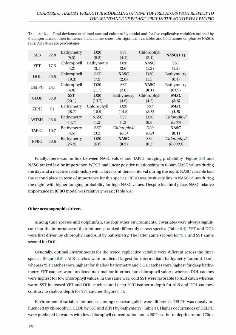
CHAPITRE 6. HABITAT PREDICTIVE MODELLING OF NINE TOP PREDATORS WITH RESPECT TOTHE ABUNDANCE OF PELAGIC PREY IN THE SOUTHWEST PACIFIC
TABLEAU 6.4 – Total deviance explained (second column) by model and for five explicative variables ordered bythe importance of their influence. Italic names show non-significant variables and bold names emphasize NASC’srank. All values are percentages.
ALB 22.8Bathymetry
(9.3)D20(8.3)
SST(4.1)
Chlorophyll(2.1)
NASC(1.1)
YFT 17.5Chlorophyll
(4.2)Bathymetry
(3.1)D20(2.6)
NASC(1.3)
SST(1.2)
DOL 29.5Chlorophyll
(19.3)SST(7.9)
NASC(2.0)
D20(1.5)
Bathymetry(0.4)
DELPH 25.1Chlorophyll
(4.8)D20(1.7)
SST(2.0)
NASC(0.1)
Bathymetry(0.09)
GLOB 33.9SST
(20.1)D20
(13.7)Bathymetry
(4.9)Chlorophyll
(4.2)NASC(3.6)
ZIPH 51Bathymetry
(28.7)Chlorophyll
(18.9)D20
(14.5)SST(8.8)
NASC(1.6)
WTSH 25.6Bathymetry
(14.7)NASC(1.5)
SST(1.3)
D20(0.8)
Chlorophyll(0.05)
TAPET 10.7Bathymetry
(4.5)SST(3.2)
Chlorophyll(0.5)
D20(0.2)
NASC(0.1)
RFBO 58.6Bathymetry
(26.9)D20(6.8)
NASC(0.5)
SST(0.2)
Chlorophyll(0.0003)
Finally, there was no link between NASC values and TAPET foraging probability (Figure 6.4) and
NASC ranked last by importance. WTSH had linear positive relationships to 0-30m NASC values during
the day and a negative relationship with a large confidence interval during the night. NASC variable had
the second place in term of importance for this species. RFBO was positively link to NASC values during
the night, with higher foraging probability for high NASC values. Despite his third place, NASC relative
importance in RFBO model was relatively weak (Table 6.4).
Other oceanographic drivers
Among tuna species and dolphinfish, the four other environmental covariates were always signifi-
cant but the importance of their influence ranked differently across species (Table 6.4). YFT and DOL
were first driven by chlorophyll and ALB by bathymetry. The latter came second for YFT and SST came
second for DOL.
Generally, optimal environments for the tested explicative variable were different across the three
species (Figure 6.5) : ALB catches were predicted largest for intermediate bathymetry (around 4km),
whereas YFT catches were highest for shallow bathymetry and DOL catches were highest for deep bathy-
metry. YFT catches were predicted maximal for intermediate chlorophyll values, whereas DOL catches
were highest for low chlorophyll values. In the same way, cold SST were favorable to ALB catch whereas
warm SST increased YFT and DOL catches ; and deep 20°C isotherm depth for ALB and DOL catches,
contrary to shallow depth for YFT catches (Figure 6.5).
Environmental variables influences among cetacean guilds were different : DELPH was mostly in-
fluenced by chlorophyll, GLOB by SST and ZIPH by bathymetry (Table 4). Higher occurrences of DELPH
were predicted in waters with low chlorophyll concentration and a 20°C isotherm depth around 170m.
170

CHAPITRE 6. HABITAT PREDICTIVE MODELLING OF NINE TOP PREDATORS WITH RESPECT TOTHE ABUNDANCE OF PELAGIC PREY IN THE SOUTHWEST PACIFIC
FIGURE 6.5 – Predators’ modelled responses (by rows) to four environmental variables (by columns). The solid greyribbons show the confidence limits of the model and are twice the standard error. Stars show the significant level :two stars (**) for highly significant (p-value < 0.01), one star (*) for slightly significant (p-value between 0.01 and0.1) and no star for non-significant.
GLOB were predicted to be more abundant when the 20°C isotherm depth was extreme (very shallow
or very deep), and both in waters with SST around 24°C and with SST warmer than 27°C. Finally, ZIPH
were predicted abundance was especially high in waters with a bathymetry around 3km and with large
chlorophyll concentrations (Figure 6.5).
The three seabirds species foraging behavior were primarily influenced by bathymetry, but with
contrasting optimal values : WTSH and RFBO mostly fed in deep waters while TAPET fed in shallow
waters (Figure 6.5). Secondarily, WTSH foraging behavior was influenced by NASC values integrated bet-
ween 0 and 30m deep, and in a third place by warm SST. TAPET was also predicted to be more likely to
feed in waters with warm SST. Finally, RFBO foraging behavior was also influenced by the 20°C isotherm
depth, with more feeding predicted to occur in extreme values (very shallow or very deep isotherm).
171

CHAPITRE 6. HABITAT PREDICTIVE MODELLING OF NINE TOP PREDATORS WITH RESPECT TOTHE ABUNDANCE OF PELAGIC PREY IN THE SOUTHWEST PACIFIC
6.3.3 Spatial distribution predictions
Based on environmental and NASC layers, we predicted the spatial distribution of the nine predators
in the New Caledonian EEZ. In order to avoid predictive extrapolation, we limited predictions to sampled
environmental variable ranges.
Predators spatial distribution
ALB, YFT and DOL CPUE spatial predictions did not spatially overlap. High ALB CPUE were predicted
overall west of the diagonal marked by the Main Island. The largest CPUE were predicted west of Ches-
terfield reef complex (Figure 6.6), with the exception of a small area directly surrounding the Chesterfield
and Bellona reefs. On the opposite, high predicted YFT CPUE were found in this small area. The highest
YFT CPUE were predicted close to the lagoon, around the Main Island and to a lesser extent around the
Loyalty Islands. Finally, the EEZ southeast corner, and around the Loyalty Islands were predicted favo-
rable to DOL CPUE. Standard error predicted by models were larger in the southeast for YFT and DOL
predictions, and in the south for ALB predictions (Figure 6.7).
FIGURE 6.6 – Spatial predictions for the nine predators included in this study. Top : predictions of Albacore (ALB)and yellowfin (YFT) tuna catch per unit of effort (CPUE) in number of fish caught per 100 hooks. Middle : predic-tions of Delphininae (DELPH), Globicephalinae (GLOB) and Ziphiidae (ZIPH) cetacean count.Bottom : predictionsof wedge-tailed shearwater (WTSH), Tahiti petrel (TAPET) and red footed booby (RFBO) foraging behavior proba-bility.
172
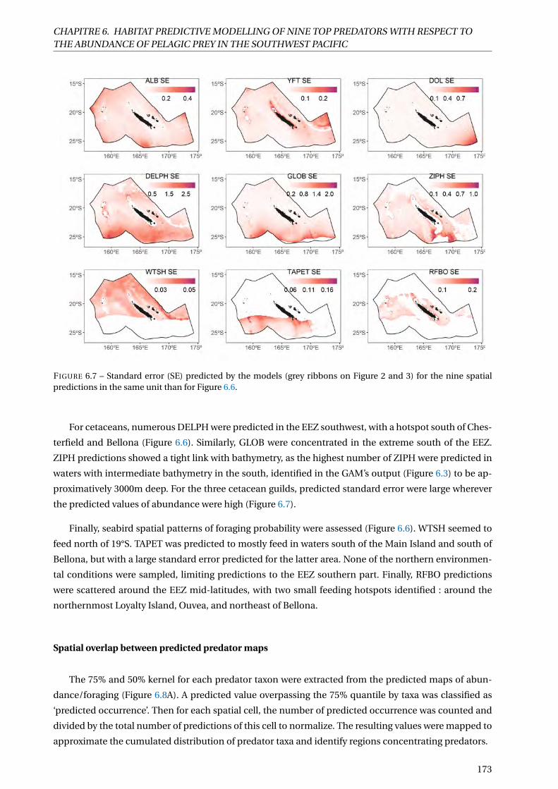
CHAPITRE 6. HABITAT PREDICTIVE MODELLING OF NINE TOP PREDATORS WITH RESPECT TOTHE ABUNDANCE OF PELAGIC PREY IN THE SOUTHWEST PACIFIC
FIGURE 6.7 – Standard error (SE) predicted by the models (grey ribbons on Figure 2 and 3) for the nine spatialpredictions in the same unit than for Figure 6.6.
For cetaceans, numerous DELPH were predicted in the EEZ southwest, with a hotspot south of Ches-
terfield and Bellona (Figure 6.6). Similarly, GLOB were concentrated in the extreme south of the EEZ.
ZIPH predictions showed a tight link with bathymetry, as the highest number of ZIPH were predicted in
waters with intermediate bathymetry in the south, identified in the GAM’s output (Figure 6.3) to be ap-
proximatively 3000m deep. For the three cetacean guilds, predicted standard error were large wherever
the predicted values of abundance were high (Figure 6.7).
Finally, seabird spatial patterns of foraging probability were assessed (Figure 6.6). WTSH seemed to
feed north of 19°S. TAPET was predicted to mostly feed in waters south of the Main Island and south of
Bellona, but with a large standard error predicted for the latter area. None of the northern environmen-
tal conditions were sampled, limiting predictions to the EEZ southern part. Finally, RFBO predictions
were scattered around the EEZ mid-latitudes, with two small feeding hotspots identified : around the
northernmost Loyalty Island, Ouvea, and northeast of Bellona.
Spatial overlap between predicted predator maps
The 75% and 50% kernel for each predator taxon were extracted from the predicted maps of abun-
dance/foraging (Figure 6.8A). A predicted value overpassing the 75% quantile by taxa was classified as
‘predicted occurrence’. Then for each spatial cell, the number of predicted occurrence was counted and
divided by the total number of predictions of this cell to normalize. The resulting values were mapped to
approximate the cumulated distribution of predator taxa and identify regions concentrating predators.
173

CHAPITRE 6. HABITAT PREDICTIVE MODELLING OF NINE TOP PREDATORS WITH RESPECT TOTHE ABUNDANCE OF PELAGIC PREY IN THE SOUTHWEST PACIFIC
FIGURE 6.8 – 75% (dark brown) and 50% (light brown) kernel densities for each predators (panel A) and normalizedpredicted number of predators (i.e. number of 75% predator predicted occurrences divided by the total number ofpredicted occurrences per cell) (panel B). Grey triangles indicate the location of a selection of seamounts gatheredfrom [Allain et al., 2008].
Maps of the normalized predicted cumulated occurrence of taxa showed a slight north-south gra-
dient, with relatively higher numbers of predators taxa in the south where there are numerous seamounts
(Figure 6.8B). A large region northeast of the Main Island, covering the Petrie and Astrolabe reefs, was
identified with a relatively high predicted occurrence of predator taxa, as well as in the region surroun-
ding the Chesterfield reefs.
6.4 Discussion
Understanding the ecological processes that underpin species distribution patterns is a fundamental
goal in spatial ecology. In the present study, the distribution of nine groups of top predators was modelled
to provide a multi-trophic assessment of the ecological niches of pelagic communities. Previous studies
in New Caledonia have focused on specific taxa, such as seabirds [Benoit & Bretagnolle, 2002; Robinet
et al., 1997], cetaceans [Derville, 2018; Garrigue et al., 2015], shark [Boussarie et al., 2018] and albacore
[Briand et al., 2011; Williams et al., 2014]. This study therefore provides the first step towards an integra-
ted view of multiple marine predator distributions across the New Caledonian pelagic ecosystem. Nine
top predators were analysed at the same time : albacore tuna, yellowfin tuna, dolphinfish, Delphininae,
Globicephalinae, Ziphiidae, wedge-tailed shearwater, Tahiti petrel and red-footed booby. Prey relative
abundance data collected using acoustic methods (NASC) was tested together with static (bathymetry)
and dynamic oceanographic descriptors (SST, chlorophyll and 20°C isotherm depth) to improve pre-
dator distribution models. Preyscape affected six predator distribution patterns out of nine (ALB, YFT,
DOL, DELPH, WTSH and RFBO). Spatial distributions predicted for ALB, YFT and DOL did not overlap.
DELPH, GLOB and ZIPH predictions were concentrated in the south whereas WTSH used the north of
the EEZ to feed. The small datasets for TAPET and RFBO made complicated robust conclusions.
174

CHAPITRE 6. HABITAT PREDICTIVE MODELLING OF NINE TOP PREDATORS WITH RESPECT TOTHE ABUNDANCE OF PELAGIC PREY IN THE SOUTHWEST PACIFIC
6.4.1 Sources of uncertainty
Predators’ dynamics
Fishing vessels in New Caledonia are relatively homogeneous in term of fishing capabilities and only
include long-liners [WCPFC, 2018]. By including vessel random effect, we took into account potential
variability of fishing power between vessels due to different vessel sizes for example, or to more or less
efficient hooks, or to differences in hooks fishing depth. By including the effort (number of hooks here)
as an offset, we transformed catches into CPUE therefore used as a proxy of fish abundance accounting
for effort. CPUE are also linked to fishing power of vessels and species catchability. Hence, large CPUE
changes can be erroneously measured where only small abundance changes exist [Kleiber & Maunder,
2008]. However, given the large sample used and the precautions by including a vessels random effect,
our CPUE predictions could constituted a robust proxy to species abundances.
Cetacean distributions were assessed through counting performed during the REMMOA aerial sur-
veys [Laran et al., 2016a]. This relatively low-cost method can be advantageously implemented with a
great flexibility, which allows a quick reaction to changing weather conditions [Mannocci et al., 2013].
However, compared to CPUE data for instance, REMMOA surveys only occurred once in New Caledo-
nian EEZ and only spanned three months. The surveys gave a snapshot of animal presence and partial
distribution over a short period. Moreover, cetaceans are highly mobile predators and their behaviors
were not identified by observers. Animals could have been travelling between two favorable habitats
when there were detected and therefore the oceanographic conditions attributed to that group were not
necessarily optimal habitats. We assumed that to improve our niche modeling and therefore to have a
better comprehension of species habitats, more cruises are needed to overpass the “snapshot problem”.
Moreover, the aerial surveys had three other major limitations : observers do not detect animals under
the surface, observers may miss some animals at the surface, and observers may miss-recognize species
[Pollock et al., 2006]. To deal with the miss-recognizing, planes could be equipped with camera taking
pictures upon detection.
Finally, seabird feeding behaviors were analyzed with tracking data. As seabirds spend most of their
time at sea in order to forage during the breeding season, we assumed that the foraging probability was
a good indicator of seabird probabilit of presence and therefore of the seabirds’ distributions during the
breeding season. Another limitation of tagging data is the commonly small sample sizes that badly cap-
ture inter-individual behavioural variability. For instance, we used data from 47 individuals for WTSH,
the largest seabirds’ dataset, while up to 500,000 wedge-tailed shearwaters pairs are estimated to breed in
New Caledonia. In addition, uncertainty may come from the clustering step (EMbC, Garriga et al. 2016)
to identify the behavior of seabirds based on their sinuosity and speed. A sensitivity analysis of EMbC
parameters would certainly help to identify robust foraging patterns. By selecting only the intensive fo-
raging observations occurring for more than three consecutives positions, we offered an approach to
filter-out the shortest foraging bouts and to ensure that the animals were truly foraging when classified
as such.
175

CHAPITRE 6. HABITAT PREDICTIVE MODELLING OF NINE TOP PREDATORS WITH RESPECT TOTHE ABUNDANCE OF PELAGIC PREY IN THE SOUTHWEST PACIFIC
Prey layer distribution
Previous studies have emphasized the large added value in collecting acoustic data simultaneously
with megafauna observations [Louzao et al., 2019a], which is made possible by using monitoring systems
such as integrated oceanographic surveys [Doray et al., 2018]. Our study suggested an alternative whe-
reby prey abundance is estimated during surveys focusing on low trophic levels, and then subsequently
compared to a large number of predators observations coming from other surveys. Such approach is not
applicable with other more discrete prey sampling techniques (Torres et al. 2008, trawling, i.e.). It pro-
vided a suitable dataset for modelling predator distribution in relation to their prey without observing
predators and prey at the same time.
The strength of our acoustics modeling framework was the possibility to average prey relative abun-
dances over different vertical layers. Therefore, prey layers could be adapted to the predators’ vertical
feeding habitats that most illuminate prey-predator relationships. The differences in spatial patterns
during the day of integrated NASC values over layers 0-30 m and 0-200 m (Figure 6.3) supported the
importance to extract specific vertical layers to analyze prey-predator relationships. Integrating more 3-
dimensional biotic and abiotic variables in predator niche modeling is a necessity to be able to define
3-dimensional oceanographic habitats used by marine species [Brodie et al., 2018; Lambert et al., 2014;
Louzao et al., 2019b].
All prey layers were based on Receveur et al. [2019] methodology who used a statistical framework to
link acoustics vertical profile to environmental variables. The present study assumed that predicted mi-
cronekton vertical distribution were realistic and so was the micronekton relative abundance variation.
They showed that for a given observed acoustic value (measured through the backscatter echo intensity,
Sv), the predicted echo intensity could vary +/-10dB, which could result in large biomass changes[Benoit-
Bird, 2009; Proud et al., 2018b]. They also demonstrated that predicted echo-intensity variations mat-
ched observed echo-intensity variations (see Figure 11 in Receveur et al. 2019) that were needed in
the present study. Indeed, to assess NASC’s influence on predators’ behaviour, we presumed that rea-
listic spatial, vertical and temporal NASC gradients were more informative than exact absolute NASC
values.Receveur et al. [2019] noticed that the use of the 38kHz frequency favored detection of organisms
with swimbladders (mostly fish) while excluding other organisms without gas-filled swimbladders [Da-
vison et al., 2015a], which may bias spatial variations of prey species composing predators’ diets. Never-
theless, given the large diversity in predator’s diets [Duffy et al., 2015; Olson et al., 2014; Williams et al.,
2014] and the difficulty to transform acoustic signal into species biomass [Davison et al., 2015a; Proud
et al., 2018b], we used NASC values as an overall proxy of the relative abundance of prey available for
all predators. Going further into acoustic signal separation into species groups (as fish, gelatinous, crus-
tacean) would allow to link each predator to their favorite preys. However, given the diversity of preys
present in the region (Chapter 3), assigning acoustic intensity to prey species will constitute a real chal-
lenge.
The last limitation was the potential absence of organism shoals. Indeed, our framework firstly clus-
tered all vertical profiles into ten groups, allowing to keep only persistent structure in prey vertical dis-
tribution but removing less frequent features as shoals. Previous studies highlighted the importance of
shoal formations in the feeding behavior of some predators [Benoit-Bird et al., 2013; Bertrand et al.,
2002a, 2014; Carroll et al., 2017; Ménard & Marchal, 2003; Williams et al., 2014]. As we removed shoals
176

CHAPITRE 6. HABITAT PREDICTIVE MODELLING OF NINE TOP PREDATORS WITH RESPECT TOTHE ABUNDANCE OF PELAGIC PREY IN THE SOUTHWEST PACIFIC
from our prey layers, we were not able to test their influence on predators’ distribution. Moreover, we
were not able to analyze the fine spatial scale that we removed from the acoustic signal, although it is
known to be an important component of foraging behaviors [Benoit-Bird & Au, 2003; Bertrand et al.,
2014; Grados et al., 2016].
Finally, developing predictive models of habitat use is challenging for species that forage in marine
environments, as both predators and prey are often highly mobile and difficult to monitor. Previous
studies incorporated SEAPODYM prey population dynamics outputs [Lehodey & Maury, 2010; Lehodey
et al., 2008] to their predator niche models for tuna [Briand et al., 2011], seabird [Miller et al., 2018] and
cetacean [Lambert et al., 2014]. The statistical method developed here based on observed acoustics is an
alternative to using such modelled prey distribution from population dynamics model. The approach
allowed to study predator-prey relationships at a regional scale, but required the acoustic observation at
this vast spatial scale. Conductingmore acoustic surveys would allow to refine prey distribution models
and therefore would improve prey implementation into predator niche models.
6.4.2 Environmental drivers of predators distribution
Tuna and dolphinfish species were strongly influenced by SST, as shown previously by Kleisner et al.
[2010]. YFT and DOL prefered warm SST, whereas ALB’s optimal temperatures were colder [Bertrand
et al., 2002b]. For foraging, ALB and DOL were linked to NASC values with a bell-shaped relationship
whereas YFT was negatively linked to NASC values (Figure 6.2). ALB’s relationships to NASC values were
in total agreement with previous results found in the New Caledonian EEZ using the SEAPODYM out-
puts as prey data source. Briand et al. 2011 showed a negative relationship to upper mesopelagic layer
(that they called ‘mesopelagic’) and a bell relationship to epipelagic layer. In order to explain the nega-
tive relationship to upper mesopelagic prey, they assumed that the increase in prey abundance induces
a competition for baited hooks placed in this layer ; a hypothesis confirmed by another albacore study in
French Polynesia [Bertrand et al., 2002b]. This hypothesis would explain the two YFT negative relation-
ships to NASC values.
ALB, YFT and DOL were shown to utilize comparable foraging resources and have similar niches
[Teffer et al., 2015], especially for YFT and DOL in the Pacific [Young et al., 2010]. We showed a different
result with a relatively weak distribution overlap between the three species (expect for DOL and YFT east
of Main Island, Figure 6.8A) and different relationships to environmental predictors (Figures 6.2 and 6.3).
We hypothesized that at the Pacific Ocean scale, ALB, YFT and DOL have similar large distribution but
at a regional scale, the three species divided the space and the foraging resource. Bertrand et al. [2002a]
showed that tuna were more abundant in waters rich in prey and with favorable hydrological conditions
at a regional scale, and were attracted by small prey patches at a small scale in the southeast Pacific. We
confirmed this result at a regional scale for ALB, but we found that YFT was more attracted by waters
with relatively low prey abundance. Finally, the 20°C isotherm depth was relatively important for the two
tuna species. The 20°C isotherm depth is a proxy for vertical habitat change, and is strongly linked to
catchability changes. Therefore, part of the abundance changes linked to the 20°C isotherm depth may
reflect catchability changes rather than a true ecological relationship.
REMMOA surveys of cetaceans were performed in several other places (French Polynesia, Mozam-
177

CHAPITRE 6. HABITAT PREDICTIVE MODELLING OF NINE TOP PREDATORS WITH RESPECT TOTHE ABUNDANCE OF PELAGIC PREY IN THE SOUTHWEST PACIFIC
bique channel, Bay of Biscay, French Antilles. . . ) and cetacean niche modeling has been published for
all these other regions [Lambert et al., 2016, 2014; Mannocci et al., 2013, 2014a, 2015]. In New Caledo-
nia, bathymetry strongly influenced GLOB and ZIPH distribution, as also shown by Laran et al. [2016b]
in the bay of Biscay. Relationships to NASC values were non-significant for GLOB and ZIPH, whereas it
was significant for DELPH, although only explaining a small part of the total explained deviance. Mo-
reover, the shapes of the NASC relationships were different from those found by Lambert et al. [2014] in
the Indian Ocean and in French Polynesia using SEAPODYM outputs. The cetacean dataset was certainly
too small to fit relevant predator-prey spatial relationships. The positive relationships between epipela-
gic and upper mesopelagic NASC and DELPH and GLOB counts, and between mesopelagic and ZIPH
counts suggests that vertical foraging habitats of ZIPH species were probably deeper than that of DELPH
and GLOB. This result would confirm previous conclusions from the East Atlantic [Lambert et al., 2014].
Finally, seabird relationships to oceanographic conditions were in agreement with previous results
acquired nearby in Australia [McDuie et al., 2018]. Bathymetry had the strongest influence on either of
the three species [Catry et al., 2009]. WTSH and RFBO seemed to have similar foraging habitats in deep
waters and with high chlorophyll concentration, whereas TAPET preferred shallow waters. The three
species were predicted to feed more in warm waters. Relationships to the 20°C isotherm depth were
mostly negative for WTSH and RFBO. Fronts of oceanic eddies have been shown to largely influence
seabirds’ foraging behavior [Jaquemet et al., 2014; McDuie et al., 2018; McDuie & Congdon, 2016; Tew Kai
& Marsac, 2010; Tew Kai et al., 2009] and the 20°C isotherm depth is a proxy to characterize these meso-
scale features.
WTSH relationship to NASC values was positive only during the day : the higher the NASC values, the
higher the foraging probability was. This night-day difference in NASC relationships showed that WTSH
may be visually searching for food during the day and can locate prey strong concentrations of prey at
the surface, whereas during the night they might be using other feeding technics. TAPET did not target
region with high prey abundance but stayed in shallows waters with high chlorophyll concentration. The
facilitation of seabird foraging in association with other top predators has been observed in different
regions, increasing seabirds’ foraging probability when other predators are present [Miller et al., 2018;
Weimerskirch et al., 2005]. At the regional scale, we did not find similar results with a globally low overlap
between seabirds and tuna/cetacean spatial distributions.
6.4.3 Predator niche modeling
In addition to the uncertainty due to the source of predators and prey data, the nine GAMs also had
their own limitations. For cetaceans, the small number of observations did not allow us to split analyzes
at species level. In order to increase the dataset power to study cetacean-prey relationships, it was neces-
sary to group cetacean species into three trophic guilds based on [Lambert et al., 2014; Mannocci et al.,
2014b; Weimerskirch et al., 2005]. This approach may be disadvantageous as it could smooth out some
relationships to environmental conditions, by mixing together potentially different species-specific op-
timal habitats. In addition, even when pooling data into wider groups, the observations of cetaceans,
TAPET and RFBO were too few to robustly evaluate the influence of NASC, resulting in a relatively low
effect of NASC compared to other oceanographic variables.
178

CHAPITRE 6. HABITAT PREDICTIVE MODELLING OF NINE TOP PREDATORS WITH RESPECT TOTHE ABUNDANCE OF PELAGIC PREY IN THE SOUTHWEST PACIFIC
In order to limit correlations between variables, to measure the influence of prey distribution and
to compare this influence between species, we included the same four abiotic variables together with
NASC for the nine predators. The models may have benefited from the inclusion of other environmental
factors such as oxygen, which is known to be important for tuna habitat [Bertrand et al., 2002a; Cayré &
Marsac, 1993]. Increasing the number of environmental variables also may help to better model preda-
tors optimal habitats. Concerning prey, vertical integral of NASC values were included as a proxy of prey
abundance. As the method used originally predicted vertical profiles, Receveur et al. [2019], relate pre-
dator abundance/foraging to the depth of NASC maximal value would be useful to understand vertical
predator habitat- vertical prey habitat relationships [Boyd et al., 2015].
Finally, we proposed a relatively simple method, the “quantile method”, to measure species’ niche
overlap. In a recent review describing a large panel of metrics used to measure species niche overlapping
[Carroll et al., 2019], we found that all metrics needed the same quantity/variable for the two species to
measure their distribution overlap (often presence probability Abrams 1980; Swanson et al. 2015). We did
not find any metrics dealing with different responses measured for the two species of interest. We think
that a crucial development would be to find new metrics allowing to deal with different data-sources,
considering that current study methods are strongly species dependent. The ability to cross data from
different domains has to be enhanced through new statistical frameworks.
6.4.4 Conclusions and perspectives for the Natural Park of the Coral Sea
In the present study, we developed a methodological approach to implement preyscape predictors
as well as oceanographic conditions into nine predator niche models. We managed to describe the rela-
tionship between prey and predator distributions only when the predators’ datasets were large enough.
Based on the predicted spatial distributions of predators, we highlighted potential pelagic predator hots-
pots : around the Loyalty Islands, around Petrie reef, around the Chesterfield reefs, and in the seamount
region southeast of the Main Island. More scientific surveys, especially for cetacean and seabird, are nee-
ded to confirm the relevance of these regions for conservation. Most of these areas (Chesterfield, Bellona,
Entrecasteaux, Petrie and Astrolabe) have been classified into strict marine reserve (category I, none hu-
man activities authorized, according to IUCN protected area classification or “1-No take-No go” Horta e
Costa et al. 2016), but only shallow waters up to 1000m bottom depth are protected. However, our results
suggest that predators also aggregate in deeper pelagic waters. Those areas, therefore appear as good
candidates to implement a higher level of protection into offshore waters. For instance, we suggest that
protected areas could be extended from the existing strict marine reserves to the pelagic domain around
reefs/atolls. Finally, the present analysis focused on nine predators, but a variety of other taxa are still
lacking to provide an exhaustive overview of the pelagic ecosystem. Adding turtles, sharks, humpback
whales, other seabirds such as frigates, and other commercially exploited fish species will be necessary
for a complete management of the Natural Park of the Coral Sea.
179

CHAPITRE 6. HABITAT PREDICTIVE MODELLING OF NINE TOP PREDATORS WITH RESPECT TOTHE ABUNDANCE OF PELAGIC PREY IN THE SOUTHWEST PACIFIC
180

Chapitre 7
Conclusions et perspectives
Sommaire
7.1 Rappels des résultats principaux . . . . . . . . . . . . . . . . . . . . . . . . . . . . . . . . 182
7.2 L’acoustique comme moyen d’étude . . . . . . . . . . . . . . . . . . . . . . . . . . . . . . . 183
7.2.1 Comparaison EK60-ADCP . . . . . . . . . . . . . . . . . . . . . . . . . . . . . . . . . . 184
7.2.2 Compréhension des espèces associées au signal acoustique . . . . . . . . . . . . . 187
7.2.3 La fine échelle . . . . . . . . . . . . . . . . . . . . . . . . . . . . . . . . . . . . . . . . . 188
7.3 La dynamique des proies mise en évidence dans le Pacifique sud-ouest . . . . . . . . . . 190
7.4 L’impact potentiel du changement climatique . . . . . . . . . . . . . . . . . . . . . . . . . 191
7.5 La gestion de l’écosystème et le parc naturel de la mer de Corail . . . . . . . . . . . . . . 195
7.6 Conclusion . . . . . . . . . . . . . . . . . . . . . . . . . . . . . . . . . . . . . . . . . . . . . . 197
181

CHAPITRE 7. CONCLUSIONS ET PERSPECTIVES
L’objectif de ce travail de thèse était d’examiner le fonctionnement de l’écosystème pélagique dans
le Pacifique sud-ouest et plus particulièrement la dynamique des organismes de niveaux trophiques in-
termédiaires (ou micronecton). A partir de l’analyse de données acoustiques, nous avons développé une
méthode de suivi du micronecton dans l’espace et dans le temps en relation avec l’environnement. Cette
méthodologie mise en place, nous l’avons utilisée pour décrire la dynamique spatiale et temporelle du
micronecton autour de la Nouvelle-Calédonie et les facteurs environnementaux qui la contrôlent. Nous
avons ensuite mis en évidence les espèces majoritaires de ce compartiment. Finalement, deux études
ont replacé la dynamique de ce compartiment dans un contexte plus général : le devenir du micronec-
ton de la zone face au changement climatique, et l’influence de ce compartiment sur la distribution des
prédateurs supérieurs qui s’en nourrissent.
7.1 Rappels des résultats principaux
Au cours du chapitre 2, nous utilisons les données d’un échosondeur non calibré (ADCP) largement
répandu pour analyser 19 ans de données acoustiques et ainsi évaluer l’évolution de l’abondance re-
lative du micronecton dans la ZEE Calédonienne. Deux fréquences distinctes (150kHz et 75kHz) sont
utilisées conjointement pour obtenir une série temporelle continue entre 1999 et 2017 dans la couche
20-120m. En comparant le signal ADCP à des mesures simultanées d’un autre sondeur dédié et calibré
pour les estimations de biomasse (EK60) à 70 kHz, nous montrons que les signaux d’ADCP à 150kHz et à
75kHz y sont étroitement liés. La variabilité du signal acoustique est majoritairement due aux migration
nycthémérales, puis à l’année (avec une diminution globale du micronecton de 1999 à 2007 puis une ré-
augmentation jusqu’en 2017) et enfin au cycle d’ENSO (avec en moyenne plus de micronecton pendant
les phases El Niño). Le lien avec les paramètres environnementaux met en évidence une distribution
spatiale saisonnière variable : durant l’été, le micronecton se concentre autour des côtes, alors que pen-
dant l’hiver il se concentre plutôt dans le nord de la zone économique exclusive et à l’ouest de la grande
terre. Cette distribution spatiale du micronecton en surface de nuit, ainsi que son cycle saisonnier sont
différents de ceux prédits par le modèle de dynamique de population SEAPODYM-MTL.
Nous nous sommes ensuite concentrés dans le chapitre 3 sur la compréhension de la distribution
verticale du micronecton à travers l’analyse de 6 campagnes d’enregistrement d’EK60 et encore une fois
des facteurs océanographiques la contrôlant. Nous avons développé une méthodologie statistique ori-
ginale qui a permis d’identifier trois zones homogènes en terme de distribution verticale : une zone au
nord de 20°S, une zone au sud de cette limite et à l’est de 165°E (quart sud-est), et une dernière zone
également au sud de 20°S et à l’ouest de 165°E (quart sud-ouest). La zone nord est caractérisée par des
faibles densités de micronecton à la fois en surface et en profondeur, de jour et de nuit, et une plus faible
proportion d’organismes migrants que dans le sud. Cette zone est majoritairement influencée par des
faibles concentrations en oxygène et des fortes températures de surface. Dans les deux régions du sud,
la distribution verticale de nuit est plus dense en micronecton en surface et en profondeur que dans le
nord. Durant le jour, la distribution du micronecton du quart sud-ouest est plus dense en profondeur
(vers 550 mètres) alors que dans le quart sud-est, la densité est plus forte entre 0 et 50 mètres. Ces deux
régions du sud sont majoritairement influencées par de fortes concentrations en oxygène et une forte
salinité. Dans le sud, la densité intégrée entre 0 et 600 mètres est globalement plus élevée que dans le
nord avec une proportion de migrants plus importante.
182

CHAPITRE 7. CONCLUSIONS ET PERSPECTIVES
Le chapitre 4 nous a permis d’analyser des données de composition en espèces issues de 141 cha-
luts réalisés dans la zone entre 2011 et 2016. Cette étude a aboutit à la description de sept assemblages
dominants d’espèces de micronecton. La profondeur de chalutage ainsi que le moment de la journée
sont les paramètres dominants dans la différentiation des assemblages. De jour, deux assemblages sont
identifiés : un premier au-dessus de 350 mètres dominé par une espèce de crustacé et une espèce de mol-
lusque, et un second en dessous de 350 mètres très diversifié avec une domination de plusieurs espèces
de poissons. Quatre assemblages nocturnes se partagent la couche 0-250 mètres, avec deux change-
ments de communauté à environ 80m et 250m. Les assemblages du nord sont dominés par des espèces
de crustacés, tandis que les assemblages du sud sont dominés davantage par les espèces de céphalo-
podes et les espèces de poissons. Les prévisions spatiales de distribution des communautés de micro-
necton sont étroitement liées aux prévisions des distributions spatiales des écorégions acoustiques.
Dans le chapitre 5, nous avons exploré des scénarios d’évolution des distributions verticales et des
abondances de micronecton issues du chapitre 3 dans un contexte de changement climatique. Pour cela,
nous avons utilisé deux approches : la modélisation acoustique et le modèle SEAPODYM. Pour la couche
épipélagique, les deux méthodes prédisent en moyenne pour toute la zone une diminution de l’abon-
dance de micronecton. Cependant des différences spatiales sont présentes : une légère augmentation est
prévue au nord de 20°S contre une plus forte diminution au sud. Pour les deux couches verticales infé-
rieures (couches mésopélagiques haute et basse), les prévisions divergent fortement entre modélisation
acoustique et SEAPODYM. Nous montrons au cours de ce chapitre que les divergences de prédictions
sont encore trop grandes entre les deux moyens d’études du micronecton. Une validation plus fréquente
des sorties de modèles écosystémiques avec comparaison aux données acoustiques d’observation est
nécessaire pour améliorer la robustesse et notre confiance en ces projections.
Enfin, au cours du chapitre 6, nous nous sommes penchés sur la compréhension des facteurs, bio-
tiques et abiotiques, contrôlant la dynamique spatiale de neuf prédateurs supérieurs (trois espèces de
poissons pélagiques, trois groupes de cétacés et trois espèces d’oiseaux marins). L’influence de la dis-
tribution des proies sur les prédateurs est significative pour six prédateurs sur neuf et a donc permis
d’améliorer significativement la modélisation de leurs distributions spatiales. Cependant, cette analyse
a aussi montré que l’influence du micronecton dans les modèles de niche des prédateurs restait relative-
ment faible en comparaison des autres variables abiotiques. Finalement, les prédictions spatiales de ces
neuf prédateurs ont été combinées et ont permis de proposer des zones possiblement sensibles pour la
conservation de ces espèces, zones qui pourront être utile dans la planification spatiale des activités du
parc naturel de la mer de Corail.
7.2 L’acoustique comme moyen d’étude
L’avantage de l’acoustique est sa large gamme d’échantillonnage temporelle (de la seconde à l’in-
terannuel) et spatiale (du mètre à des milliers de kilomètres) pour peu que les supports d’observations
(e.g. navires, mouillages) le permettent. Nous nous sommes concentrés au cours de cette thèse sur les
gammes intermédiaires d’échelles spatio-temporelles : nous avons quantifié la distribution horizontale
du micronecton à une résolution de l’ordre de 20km, la distribution verticale à une résolution de l’ordre
de 5-10m, et la dynamique temporelle aux échelles journalière, saisonnière et inter annuelle (environ 20
183

CHAPITRE 7. CONCLUSIONS ET PERSPECTIVES
FIGURE 7.1 – Distributions spatiales de l’écho intensité acoustique (Sv) prédites à partir des données d’EK60 (haut)et d’ADCP (bas) en moyenne sur la couche 20-120m.
ans). Dans une synthèse récente sur le potentiel de l’acoustique dans la compréhension des processus
écologiques, Benoit-Bird & Lawson [2016] identifient neuf questions auxquelles l’acoustique peut appor-
ter des éléments de réponse. Au cours de ce travail de thèse, nous avons confirmé l’utilité de l’acoustique
pour apporter des éléments de réponse aux cinq questions suivantes :
— Biogéographie et distribution spatiale à grande échelle : où trouve t’on des animaux dans l’océan?
— Interactions biophysiques : comment l’environnement conditionne-t-il la répartition des animaux
dans la mer ?
— Dynamique temporelle : quand, pourquoi et comment les animaux se déplacent-ils ?
— Sciences du climat : comment les écosystèmes réagissent-ils au changement climatique ?
— Interactions prédateur-proies : comment les animaux trouvent-ils leur alimentation?
L’acoustique est donc un moyen d’étude puissant, non intrusif, qui mériterait d’être encore plus large-
ment utilisé.
7.2.1 Comparaison EK60-ADCP
L’utilisation d’un engin non calibré a permis de réunir 54 campagnes couvrant 19 années et un cycle
saisonnier complet (tous les mois ont été échantillonnés au moins deux fois). L’étude de l’influence du
phénomène ENSO sur le micronecton par exemple nécessite de telle série temporelle car il faut échan-
tillonner plusieurs fois chaque phase pour que les résultats soient robustes ; son cycle étant compris
entre 3 et 7 ans avec une moyenne à 3.5 ans. De même, l’étude de l’impact sur le micronecton du chan-
gement climatique nécessitera des séries temporelles de données les plus longues possibles.
184

CHAPITRE 7. CONCLUSIONS ET PERSPECTIVES
Cependant, les différences de prédictions spatiales obtenues avec les données d’ADCP et d’EK60
posent question (Figure 7.1). Plusieurs hypothèses sont envisagées pour les expliquer.
— La différence entre les fréquences d’échantillonnages des deux engins : dans le cas de l’EK60, seul
la fréquence 38kHz est utilisée dans cette thèse alors que le travail sur l’ADCP utilise les fréquences
75kHz et 150kHz, ramenées à un équivalent 70kHz. Cela pourrait expliquer une partie de la diffé-
rence entre les prédictions spatiales car les fréquences ne détectent pas exactement les mêmes
organismes. Cependant, les résultats du chapitre 1 montrent bien que les signaux des différentes
fréquences sont corrélés entres eux et donc qu’une partie des organismes détectés est commune.
Cette explication pourrait donc expliquer des légères différences, mais pas l’amplitude des diffé-
rences que l’on observe sur la Figure 7.1.
— On peut également se demander si les données des six campagnes menées avec l’EK60 sont suffi-
santes pour mesurer la dynamique captées par les 54 campagnes d’ADCP.
— L’absence d’inter-calibration des campagnes ADCP questionne également. En effet, des différences
de niveaux moyens apparaissent entre campagnes dans les valeurs d’ADCP qui ne reflètent pas les
différences de niveau moyen des valeurs d’EK60 (Figure 2.3). Est-il possible d’analyser ensemble
toutes les campagnes si elles ne sont pas calibrées? Le chapitre 2 montre qu’il est possible de
construire un modèle mixant des campagnes d’ADCP et combinant jusqu’à deux fréquences dif-
férentes. De nombreux articles ont validé les valeurs de l’ADCP grâce à une comparaison aux don-
nées d’EK60 [Brierley et al., 1998; Fiedler et al., 1998; Griffiths, 1996; Lee et al., 2004] ou par rap-
port aux données de chaluts [Fielding, 2004; Heywood et al., 1991; Luo et al., 2000; Ressler, 2002].
L’analyse conjointe de plusieurs campagnes a également déjà été faite par Bianchi et al. [2013a] et
Bianchi & Mislan [2016] sur 389 campagnes effectuées à l’échelle mondiale avec des fréquences
allant de 38 à 150 kHz, ou encore par Chereskin & Tarling [2007] qui ont analysés ensemble 127
campagnes. Nous avons-nous même utilisé la méthode proposée par Gostiaux & van Haren [2010]
permettant d’utiliser des valeurs ADCP non calibrées lorsque l’intensité de l’écho est supérieure
d’au moins 10 dB au niveau de bruit. Cependant, cela pourrait expliquer une partie des différences
de prédiction entre EK60 et ADCP.
— Enfin, il est également possible qu’une partie de la différence s’explique par les méthodologies
statistiques : pour l’ADCP (chapitre 2), les données sont moyennées entre 20 et 120 mètres et
c’est cette valeur moyenne qui est expliquée en fonction de paramètres environnementaux. Dans
l’étude avec l’EK60 (chapitre 3), c’est tout le profil vertical qui est analysé et lié à l’environnement.
Ces profils sont d’abord classés en 10 classes et ce sont ces 10 classes qui sont modélisées en fonc-
tion de l’environnement. La valeur acoustique est ensuite reconstruite avec une moyenne des pro-
fils acoustiques de chaque classe, pondérée par la probabilité d’être dans cette classe. Le passage
par les 10 classes réduit fortement la variance intrinsèque des données d’écho-intensité acous-
tique (Sv). De nuit notamment, les profils verticaux ne sont groupés qu’en 4 classes. Les valeurs
reconstruites sont dans la gamme maximale des combinaisons linéaires de ces 4 profils verticaux
moyens, d’où la grande homogénéité spatiale de la Figure 7.1 de nuit. Finalement de nuit dans le
nord de la zone, quasiment toutes les cellules spatiales sont prédites comme appartenant à une
même classe acoustique, limitant fortement les potentielles différences de patterns spatiaux.
Pour améliorer la cohérence spatiale entre les deux prédictions, plusieurs pistes pourraient être en-
visagées. Premièrement, rendre disponible de manière plus systématique les données d’EK60, comme
c’est le cas avec l’ADCP, permettrait de réaliser des comparaisons sur plus de campagnes et ainsi de
185

CHAPITRE 7. CONCLUSIONS ET PERSPECTIVES
FIGURE 7.2 – Illustration des différent outils acoustiques existant. Figure extraite de Benoit-Bird & Lawson [2016].
valider ou invalider l’utilisation de l’ADCP. Les données ADCP, collectées d’une manière relativement
routinière, sont en effet accessibles à la communauté scientifique grâce à un effort de coordination
permettant le stockage national et international (voir notamment https://data.ifremer.fr/SISMER
pour les données françaises et https://currents.soest.hawaii.edu/docs/adcp_doc/adcp_data/
index.html pour des données internationales). Même si la transformation des données brutes en don-
nées acoustiquement analysables nécessite une transformation (cf chapitre 2), ces bases permettent
d’envisager des études à grande échelle. Par exemple, une étude globale sur la variabilité des profon-
deurs de migration a notamment été possible grâce à ces bases globales de données d’ADCP [Bianchi &
Mislan, 2016]. A notre connaissance, les bases similaires regroupant les données d’EK60 sont plus res-
treintes spatialement à certaines régions (http://imos.org.au/facilities/shipsofopportunity/
bioacoustic/u par exemple pour l’Australie). Les analyses globales se basent souvent sur un faible
nombre de campagnes [e.g. Irigoien et al., 2014; Klevjer et al., 2016].
Il serait donc utile de développer des bases similaires à l’ADCP pour encourager le partage de don-
nées et les analyses grandes échelles. Il serait également nécessaire de développer des méthodes de ca-
libration adaptées à l’ADCP, en l’absence d’EK60. Enfin, augmenter le nombre de classes de la méthode
de traitement des données EK60 permettrait d’incorporer plus de variabilité dans les valeurs d’écho-
intensités acoustiques (Sv) dans le modèle, et donc prédire une plus grande variabilité. Des contrastes
spatiaux à plus fine échelle pourraient apparaitre dans les prédictions du nord de la zone durant la nuit.
186

CHAPITRE 7. CONCLUSIONS ET PERSPECTIVES
7.2.2 Compréhension des espèces associées au signal acoustique
La non-identification des espèces a également limité l’utilisation de l’acoustique seule pour com-
prendre la dynamique du micronecton, laissant toujours en suspens si les variations prédites d’écho
intensité étaient dues à des changements d’abondance ou de communautés. En effet, à une fréquence
donnée (cf Figure 1.23) un changement de Sv peut se traduire par un changement de densité des orga-
nismes (équation du Sv) mais aussi par un changement des organismes présents. L’étude du chapitre
4 nous apporte des éléments de réponse montrant qu’effectivement les communautés varient dans la
zone, même si ces variations sont relativement faibles (les 7 communautés identifiées se ressemblent).
De jour par exemple, une seule communauté est prédite dans toute la ZEE alors que des variations appa-
raissent dans la densité acoustique, traduisant certainement des changements d’abondance de micro-
necton.
Une possibilité pour répondre plus pertinemment à ces questions serait de classer le signal acous-
tique en groupes d’organismes [De Robertis et al., 2010; Kloser et al., 2002; McQuinn et al., 2013]. Cela
est possible en utilisant seulement 2 fréquences, comme le proposent par exemple Behagle et al. [2017]
avec l’utilisation du 38kHz et 120kHz pour différencier les ‘fluid-like’ (organismes composés en majo-
rité d’eau) des ‘gas-bearing’ (organismes à vessie natatoire). Malgré tout, cette classification limiterait
l’étude des distributions verticales aux 200 premiers mètres de la colonne d’eau, portée maximale du
120kHz. Cela fait apparaitre une deuxième limite de ces études : l’utilisation de seulement deux engins
acoustiques (EK60 et ADCP), placés tous deux sous la coque d’un navire océanographique. L’utilisation
conjointe de plusieurs outils d’échantillonnage acoustique permettrait une meilleur couverture spatio-
temporelle, notamment sur la verticale (Figure 7.2). L’objectif serait d’avoir plusieurs fréquences dispo-
nibles en profondeur. Pour cela, l’utilisation d’un mouillage serait appropriée pour avoir des mesures en
un seul point ou bien des profileurs acoustiques pour avoir des données en station. Toutes les analyses
de cette thèse ont débuté à 10m sous la surface car les sondeurs de coque sont sous la coque du bateau et
qu’il faut y ajouter une zone aveugle. Positionner un mouillage qui ‘regarde’ vers la surface comme l’en-
gin numéro 5 de la Figure 7.2 permettrait également d’intégrer la couche de subsurface (0-10m) dans les
analyses. Enfin, le déploiement d’un véhicule autonome type glider permettrait d’acquérir des données
continues spatialement et donc complémentaires de celles obtenues en station avec le profileur.
Aller plus loin pour comprendre le lien acoustique-chalut
Le chapitre 4 utilise une méthode d’analyse multivariées : un individu (un chalut en l’occurrence) est
un vecteur (sa composition en espèces) au lieu d’être une valeur unique (analyse univariée). Une pro-
chaine étude pourrait utiliser le même cadre statistique en analysant en parallèle la réponse acoustique
moyenne de la couche échantillonnée et sa composition en espèces (Figure 7.3). Il faudrait extraire la
réponse acoustique moyenne de chaque couche échantillonnée par chalut. Puis, il faudrait faire deux
analyses RCP en parallèle : une avec la composition en groupes acoustiques (par exemple ’fluid like’, ’no
gaz’ ..) (de manière similaire au travail du chapitre 3) et une autre avec la valeur moyenne de 2, 3 ou 4
fréquences par chalut. Cela permettrait de classer de manière indépendante l’acoustique et les espèces.
Une comparaison des RCP obtenues permettrait alors de conclure si la réponse en fréquence moyenne
d’une couche peut être utilisée pour caractériser sa composition en espèce. Cela permettrait également
187

CHAPITRE 7. CONCLUSIONS ET PERSPECTIVES
FIGURE 7.3 – Schéma explicatif de l’étude envisagée pour mieux comprendre le lien composition en espèces-acoustique.
de mieux comprendre une réponse acoustique en fonction d’une composition spécifique. Cela rejoin-
drait des études déjà existantes comme celle d’ Ariza et al. [2016], en ajoutant un cadre de modélisation
permettant d’aller plus loin dans la compréhension des phénomènes significatifs et dans l’extrapolation
des résultats. Compte tenu de l’importance du gélatineux dans la rétrodiffusion acoustique, et en parti-
culier des siphonophores [Proud et al., 2018b], il serait primordial d’inclure les gélatineux dans ce type
d’étude.
7.2.3 La fine échelle
L’acoustique permet également d’observer des comportements, surtout alimentaires, à très fine échelle
[Bertrand et al., 2014] comme on peut l’observer sur les deux échogrammes de la Figure 7.4. Sur cette Fi-
gure, deux exemples d’enregistrements acoustiques montrent des comportements alimentaires de pré-
dateurs supérieurs et une réaction immédiate des proies ciblées par le prédateur avec un changement
de distribution verticale. La campagne PUFFALIS a été réalisée conjointement à une campagne à terre
de marquage d’oiseaux marins, l’objectif était d’échantillonner les proies en même temps que les com-
portements d’alimentation des oiseaux autour de la colonie. Cependant les oiseaux s’alimentent sur des
échelles temporelles trop courtes et rapides pour que le bateau puisse les suivre. La complexité des ma-
nipulations en station allongeait le temps de travail par station (environ 6 heures par station), et ne per-
mettait donc pas la mobilité nécessaire pour suivre les oiseaux ou même atteindre des zones d’alimen-
tation. Et enfin, la couche de surface 0-10m sur laquelle la plupart des oiseaux se nourrissent n’est pas
bien échantillonnée par le sondeur qui se situe déjà à 3m de profondeur. Pourtant échantillonner acous-
tiquement et par chalut des couches où les oiseaux se nourrissent aurait été utile pour une meilleure
188

CHAPITRE 7. CONCLUSIONS ET PERSPECTIVES
FIGURE 7.4 – Deux exemples d’échogrammes montrant une réponse rapide des couches de proies à une prédationpar des baleines (A) et non précisé (B). Figures extraites de Benoit-Bird & Lawson [2016] (A) et de Godo et al. [2014](B).
189

CHAPITRE 7. CONCLUSIONS ET PERSPECTIVES
compréhension des proies recherchées par les oiseaux. Avec de telles données, des modèles liant le si-
gnal acoustique multifréquence et la composition des espèces pourraient également être mis en place
pour prédire à plus large échelle les zones d’alimentation potentielle des oiseaux à partir de l’environne-
ment et de l’acoustique.
7.3 La dynamique des proies mise en évidence dans le Pacifique sud-ouest
Dans les chapitres 2 et 3, nous avons étudié les facteurs influençant la distribution spatiale, verticale
et temporelle du micronecton. On a notamment prédit plus de micronecton dans le sud de la ZEE que
dans le nord (Chapitre 3) avec des variations à plus fine échelle comme une plus forte abondance de
micronecton près des côtes (Chapitre 2).
La bathymétrie est un paramètre qui est revenu régulièrement comme facteur influençant le micro-
necton (chapitres 2, 3 et 4). Plusieurs raisons ont été avancées au cours des discussions, notamment un
potentiel effet des monts sous-marins. Cependant, cette piste est toujours restée en suspens, faute de
manque de données plus fines autour des monts. Un problème de définition des monts (surface, hau-
teur, forme) est également souvent revenu, compliquant leur caractérisation. D’après la littérature, l’in-
fluence d’un mont sous-marin sur les communautés de micronecton est complexe et dépend fortement
de la hauteur du mont et de sa forme [Drazen et al., 2011; Morato et al., 2008, 2010]. De plus, les espèces
ne sont pas toutes influencées de la même manière par un mont [Annasawmy et al., 2019]. Les échelles
spatiales de travail ne permettaient pas d’étudier un phénomène qui se produit à très fine échelle spa-
tiale. Au cours de l’hiver austral 2019 (juin, juillet, août et septembre), sept campagnes sont conduites
spécifiquement autour de monts sous-marins dans la ZEE Néo-Calédonienne avec un échantillonnage
acoustique très serré (campagnes SEAMOUNTS et MARACAS). Au cours de quatre de ces campagnes,
des chalutages ont été effectués autour des monts (Figure 7.5). Toutes les données récoltées en cours de
traitement pourront certainement permettre de mieux comprendre la distribution des espèces autour
des monts et des possibles changements d’abondance.
La concentration en oxygène est un autre paramètre qui est ressorti régulièrement dans nos résultats.
Une analyse conjointe des données de CTD et d’acoustique (non présentée dans ce manuscrit) a mis en
évidence une forte relation positive entre la valeur de rétrodiffusion de volume (Sv) et la concentration
en oxygène. Ces conclusions rejoignent celles de la littérature où la distribution verticale du micronec-
ton a été liée à la structure verticale de l’oxygène à plusieurs reprises [e.g. Bertrand et al., 2010; Bianchi
et al., 2013b]. La figure 5.3 montre une baisse de la concentration en oxygène liée au changement cli-
matique dans tout le Pacifique sud-ouest, en accord avec la tendance prédite à l’échelle globale [Keeling
et al., 2010]. La concentration en oxygène reste un paramètre compliqué à mesurer sur de larges échelles
spatiales (pas d’image satellite par exemple) et via des procédures à la mer assez lourdes. Sa modélisa-
tion n’est pas évidente non plus, avec de grandes variations dans les projections des conditions futures.
Vu l’importance de cette variable pour la dynamique du micronecton, continuer l’effort de mesures et
améliorer les modèles sont essentiels.
Enfin, la température apparaît à plusieurs reprises comme déterminante pour le micronecton. Comme
pour l’oxygène, le profil vertical de la température est déterminant dans la distribution verticale du mi-
190

CHAPITRE 7. CONCLUSIONS ET PERSPECTIVES
FIGURE 7.5 – Plan d’échantillonnage des campagnes MARACAS 7B et 7C et localisation de la zone d’étude dans lesud de la grande terre. Les transects et stations seront répétés encore 1 fois en septembre 2019 (MARACAS 7D).
cronecton. La température semble aussi jouer un rôle dans la délimitation de larges zones homogènes
dans la ZEE avec un front de température délimité vers 20°S. Au nord de cette limite on retrouve la masse
d’eau, SPTWN (South Pacific Tropical Water North) qui est une masse d’eau chaude, salée et relative-
ment peu oxygénée venant de la Polynésie. Au sud, on détecte plutôt la SPTWS (South Pacific Tropical
Water South) qui est plus froide, moins salée et plus oxygénée. Cette masse d’eau semble plus favorable
au micronecton.
7.4 L’impact potentiel du changement climatique
L’étude de l’impact potentiel du changement climatique sur les proies a été menée à partir de deux
approches (Chapitre 5). Nous avons prédit en moyenne une baisse d’abondance des proies entre 0 et
1000m, résultat en accord avec les études globales d’impact du changement climatique sur les écosys-
tèmes [Kwiatkowski et al., 2019; Lotze et al., 2019] et les études par bassin [Bryndum-Buchholz et al.,
2019; Lefort et al., 2015]. Cette diminution moyenne est comprise entre -4% (acoustique) et -22% (SEA-
PODYM) mais avec une forte variabilité selon la couche verticale (-7%, -6% et +2% respectivement pour
les couches épipélagique, mésopélagique haute et mésopélagique basse pour l’acoustique et -2%, +3%
et -69% respectivement pour les mêmes couches dans SEAPODYM).
Il apparait notamment que la diminution de la couche mésopélagique basse (ou bathypélagique,
d’environ 500 à 1000m) contrôle la diminution moyenne dans SEAPODYM et que cette diminution d’abon-
dance de la couche mésopélagique basse est en forte contradiction avec les prédictions des valeurs
acoustiques. A notre connaissance, peu d’études prennent en compte la distribution verticale du mi-
191

CHAPITRE 7. CONCLUSIONS ET PERSPECTIVES
cronecton dans les études d’impact du changement climatique. Lefort et al. [2015], à partir des sorties
du modèle écosystémique APECOSM, séparent les organismes en trois groupes : la communauté épipé-
lagique, la communauté mésopélagique et la communauté migrante. Cependant, tous les organismes
de plus de 2cm sont analysés ensemble : on ne peut donc pas différencier le micronecton des prédateurs
supérieurs. Les auteurs montrent une diminution de la biomasse du groupe migrant en 2100 (environ
-15%) et des biomasses des groupes épipélagique et mésopélagique (environ -30%) par rapport aux an-
nées 2000. Ils lient les différences entre groupes aux changements de taille moyenne : une diminution de
1.3cm des tailles moyennes de la communauté migrante contre une diminution de 2.1cm et 5cm pour les
deux autres communautés. La communauté migrante verrait également sa production d’œufs augmen-
ter (+4.5%). La baisse de taille moyenne est liée à la baisse de production primaire : quand la disponibi-
lité en nourriture baisse, les organismes réduisent l’énergie allouée à leur croissance et conservent cette
l’énergie pour le maintien des fonctions vitales de base [Maury et al., 2007]. Toutes ces conclusions font
apparaitre la complexité des changements potentiels pour chaque espèce. La modélisation déterministe
(comme SEAPODYM ou APECOSM) se base sur la mise en équation de ces processus. Certains processus
peuvent être mal pris en compte, voire absents, et biaiser les résultats des prédictions de micronecton.
Il apparait donc essentiel de valider d’une manière ou d’une autre ces prédictions.
Les paramètres de ces modèles sont optimisés et les prédictions validées en comparant les sorties
à des observations de terrain pour quasiment tous les niveaux trophiques : la télédétection par satel-
lite et les mesures directes en mer fournissent des informations sur les niveaux trophiques inférieurs, et
les données de pêches fournissent des informations sur les espèces exploitées. L’efficacité de ces com-
paraisons a été montrée pour modéliser correctement les prédateurs supérieurs [Anderson et al., 2017;
Tittensor et al., 2018]. Cependant, ces modèles souffrent d’un manque d’observations pour les niveaux
dits intermédiaires, qui sont mal échantillonnés par les méthodes conventionnelles. Les données acous-
tiques semblent bien adaptées pour valider les sorties de modèles déterministes grâce notamment à leur
large couverture spatiotemporelle. Mais d’une part un travail d’homogénéisation entre les données pré-
dites par les modèles et les données observées est nécessaire pour une bonne comparaison et d’autre
part il sera nécessaire de mieux comprendre les relations entre signal acoustique et biomasse réelle.
Le développement d’un modèle d’observation
Plusieurs pistes ont été proposées pour améliorer l’incorporation des données acoustiques dans les
modèles écosystémiques [Handegard et al., 2013]. Pour ce faire, il est nécessaire de définir des normes
de métadonnées et ainsi faciliter la mutualisation des données acoustiques comme proposé récem-
ment par exemple, avec un format standard Netcdf [e.g. Haris et al., 2018]. Il est également impor-
tant de mettre en place systématiquement des capteurs acoustiques dans les programmes d’observa-
tion à grande échelle. L’acquisition croissante de données permettrait le développement d’un "acoustic-
based coupled observation and modeling system" que l’on pourrait traduire par un système couplé
observation-modélisation basé sur l’acoustique (Figure 7.6).
Les intensités acoustiques peuvent être transformées en biomasse à deux conditions : connaître la
réponse acoustique par espèce et être capable de donner la proportion d’espèces ou de taxons pré-
sent dans la couche échantillonnée. Pour ce deuxième objectif, on peut échantillonner directement la
couche avec un autre engin d’échantillonnage (un chalut par exemple), ou utiliser l’acoustique multi-
192

CHAPITRE 7. CONCLUSIONS ET PERSPECTIVES
FIGURE 7.6 – Schéma conceptuel du flux d’informations dans un système couplé observation-modélisation. Lesflèches épaisses indiquent les sorties des modèles et des observations, et les flèches minces représentent les pa-ramètres des modèles, les éléments du plan d’échantillonnage et de son interprétation. (a) L’intensité acoustiquemesurée sur diverses plates-formes est répartie en groupes taxonomiques, fonctionnels ou en espèces. (b) Lesméthodes établies dans le domaine des pêcheries sont utilisées pour obtenir des indices d’abondance relative.(c) Comparaison des données modélisées et d’observations en terme de valeurs acoustiques ou de biomasses. Lacomparaison peut aider au choix des plates-formes d’observation et du plan d’échantillonnage. (d) Le modèled’observation. (e) les modèles écosystémiques, avec l’étape d’optimisation des paramètres (assimilation des don-nées). Figure adaptée de Handegard et al. [2013].
193

CHAPITRE 7. CONCLUSIONS ET PERSPECTIVES
fréquences, ou encore identifier un comportement spécifique à une espèce (forme du banc et caractère
migratoire par exemple) (Figure 7.6, cadre A). Ensuite, l’intensité acoustique peut être transformée en
biomasse, notamment grâce aux connaissances des index de réflexion individuels (TS) des espèces ex-
ploitées dont la gestion se fait grâce aux campagnes acoustiques (Figure 7.6, cadre B). Cette biomasse
peut alors être comparée aux biomasses prédites par les modèles (Figure 7.6, bas du cadre C). Cepen-
dant, malgré toutes les avancées technologiques récentes (véhicules autonomes, acquisition en large
bande. . . ), la transformation de l’intensité acoustique en biomasse reste délicate notamment à cause du
manque d’identification taxonomique précise des espèces présentes et du manque de connaissances
des TS de chaque type d’organisme et encore plus compliquée dans une région telle que la Nouvelle-
Calédonie où la diversité d’espèces est très forte.
Une autre possibilité pour valider les prédictions issues des modèles écosystémiques serait de trans-
former les biomasses prédites pas les modèles en intensité acoustique, et ensuite de comparer ces inten-
sités acoustiques prédites aux intensités acoustiques mesurées, qualifiée de comparaison dans l’espace
des observations (Figure 7.6, haut du cadre C). Contrairement à la méthode de comparaison des bio-
masses, cette méthode n’exige pas que l’intensité acoustique soit répartie par espèce ou par taxon avant
la comparaison. Cependant, les réponses acoustiques de chaque groupe modélisé doivent être connues,
ce qui n’est pas simple dans le cas de la Nouvelle-Calédonie où on observe une grande diversité d’or-
ganismes aux propriétés rétro-diffusantes différentes [Fielding, 2004; Godo et al., 2009]. Néanmoins, la
transformation de biomasse en intensité acoustique reste plus simple que l’inverse [Handegard et al.,
2013]. On suppose initialement des relations linéaires entre biomasse et intensité acoustique, et de ma-
nière itérative on optimise la composition en taxons pour obtenir une intensité acoustique totale proche
de celle mesurée.
Pour initialiser cette optimisation à partir de composition en taxons observées, Handegard et al.
[2013] proposent l’identification de zones d’intérêt : le délimitation de zones spatiales réduites où concen-
trer les efforts d’échantillonnage pour caractériser au mieux les populations de micronecton présentes.
Le nombre de points d’intérêt serait à définir en fonction de la complexité de l’écosystème. Au vu des ré-
sultats de la thèse, au moins 5 points d’échantillonnages seraient nécessaires dans la zone économique
exclusive de Nouvelle-Calédonie (Figure 7.7).
L’utilisation d’un tel cadre permettrait de mieux lier les prédictions issues des modèles comme SEA-
PODYM aux observations de terrain et donc de réduire l’incertitude qui existe dans les prédictions fu-
tures de micronecton dans un contexte de changement climatique.
Lehodey et al. [2015] propose une autre approche : la redistribution entre les différents comparti-
ments de micronecton de l’énergie totale venant de la production primaire est optimisée sur la base des
proportions des valeurs de NASC moyens entre les groupes (Figure 1.26). Cependant, la valeur absolue
de l’énergie totale venant de la production primaire n’est pas optimisée, il faudrait pour cela calculer une
valeur absolue de biomasse à partir des données d’acoustique, ce qui n’est pas encore possible en l’état.
194

CHAPITRE 7. CONCLUSIONS ET PERSPECTIVES
7.5 La gestion de l’écosystème et le parc naturel de la mer de Corail
L’acoustique est régulièrement mise en avant comme outil de gestion efficace pour la gestion éco-
systémique des pêches [Koslow, 2009; Melvin et al., 2016; Trenkel et al., 2011]. Son efficacité a notam-
ment été démontrée pour le suivi des stocks de poissons d’intérêt commercial (le hareng, la sardine,
l’anchois, le lieu sont quelques exemples), et pour comprendre les relations proies-prédateurs. Le cas de
la Nouvelle-Calédonie sort largement de ce cadre : aucun stock de poisson n’y est géré par acoustique.
Nos campagnes scientifiques avaient pour objectif de comprendre la dynamique du micronecton, proies
des prédateurs, dans leur environnement. Nous avons aussi confirmé que l’échantillonnage acoustique
pouvait aider à comprendre les relations prédateurs-proies. Néanmoins, la compréhension des proces-
sus régissant la dynamique de l’écosystème pélagique dans son ensemble pourrait être largement amé-
liorer avec des campagnes écosystémiques. Dans ce cadre-là, des mesures sont menées en même temps
sur un maximum de compartiments biologiques (producteurs primaires, secondaires, proies et préda-
teurs), comme c’est le cas durant les campagnes PELGAS conduites dans le golfe de Gascogne [Certain
et al., 2011] et dans sa partie Espagnole [Louzao et al., 2019a,b].
Malgré l’ambition et le fort potentiel de l’acoustique pour aider à caractériser un écosystème et pour
gérer les pêcheries de manière écosystémique, son utilisation dans le calcul d’indicateurs de la santé
des écosystèmes est compliquée [Trenkel et al., 2011]. Dans une région comme la ZEE de Nouvelle-
Calédonie, il semble actuellement quasiment impossible d’utiliser des indicateurs acoustiques. La pre-
mière limite vient de la définition de niveaux de références : pour que l’indicateur soit utile, il faut pou-
voir le comparer à une valeur de base (souvent mesurée à un autre endroit ou à un autre moment de
référence) qui est souvent méconnue [Rochet & Trenkel, 2003]. La première campagne réalisée avec un
sondeur EK60 dans la zone date de 2011, ce qui est loin d’être une période "historique". Par ailleurs, les
indicateurs sont surtout adaptés à des régions avec un petit nombre d’espèces et/ou à des régions où la
gestion des stocks se fait par campagne acoustique [Trenkel et al., 2011]. Le signal acoustique nécessite
d’être discrétisé un minimum en taxon, ce qui n’est pas le cas.
L’analyse conjointe des données de deux engins acoustiques, associée à (i) l’analyse des données de
chalutage, (ii) les sorties d’un modèle écosystémique, et (iii) l’étude des distributions de neuf prédateurs
supérieurs, nous ont permis de proposer cinq zones dont la dynamique semble relativement homogène.
Les limites de ces zones se déplacent au cours des saisons, et nous présentons ici une situation moyenne
(Figure 7.7).
Globalement le nord de la ZEE est influencé par une masse d’eau chaude venant de l’équateur,
pauvre en production primaire. Cette zone est relativement pauvre en micronecton avec une majorité
d’espèces de poisson. En 2100, le micronecton serait légèrement favorisé. Elle est enfin la zone privilé-
giée d’alimentation des oiseaux marins et on y retrouve du thon blanc en grande quantité dans l’ouest.
Le sud de la ZEE est caractérisé par une plus grande proportion d’organismes migrants et se sépare
en deux zones : le sud-est et le sud-ouest. Le sud-est est influencé par une masse d’eau froide et oxygénée
venant d’Antarctique. On y retrouve une forte densité de micronecton entre 400 et 600mètres, caractéri-
sée par une grande richesse spécifique. Ce sont les poissons et les crustacés qui y sont majoritaires et on y
retrouve surtout des dauphins et les deux espèces de thon (thon germon et thon jaune). Le micronecton
de cette zone aurait tendance à voir son abondance diminuer en 2100.
195

CHAPITRE 7. CONCLUSIONS ET PERSPECTIVES
FIGURE 7.7 – Schéma représentant les 5 zones identifiées au cours de la thèse.
Au sud-est, c’est la couche de sub-surface (10-30m) qui est enrichie pendant le jour, notamment due
à de fortes concentrations en chlorophylle. Le micronecton de cette région aurait une tendance négative
face au changement climatique. Ce sont les mollusques qui semblent dominés, et le mahi-mahi (dorade
coryphène), les globicéphales et les baleines à bec chez les prédateurs supérieurs.
La région autour des Chesterfield se démarque du reste de la zone : on y retrouve des couches de
micronecton qu’on ne trouve pas ailleurs comme celle entre 350 et 400m de jour. Une nouvelle espèce de
Polyipnus sp. (poisson hache d’argent de la famille des Sternoptychidae) y a été découverte au cours des
missions Nectalis (Elodie Vourey, Pers. Comm. description en cours). La faible profondeur de l’isotherme
20°C y est un paramètre environnemental important, indicateur de beaucoup de mélange de la colonne
d’eau, et est également certainement lié à la faible bathymétrie. Les cétacés semblent y être très présents,
ce qui a déjà été observé dans le cas des baleines à bosses [Derville, 2018].
Enfin, nous avons identifié une enveloppe autour de la grande terre, s’arrêtant au niveau des îles
Loyautés. Comme pour les récifs des Chesterfield, la composition en espèces de micronecton y est diffé-
rente des eaux qui l’entourent, et le chapitre 2 montre un potentiel enrichissement d’espèces de micro-
necton résonnant à 75 et 150kHz. Cette zone est influencée par des apports lagonaires et donc riche en
chlorophylle. On y retrouve des thons jaunes et du mahi-mahi en grande quantité. Cette zone englobe
les récifs Pétrie et Entrecasteaux que nous avons identifiés comme zone potentielle de concentration en
prédateurs supérieurs et donc potentiellement en zone d’intérêt pour la conservation.
Cette délimitation a été rendue possible grâce notamment à l’utilisation conjointe d’outils statis-
196

CHAPITRE 7. CONCLUSIONS ET PERSPECTIVES
tiques. Toutes les données disponibles étaient dispersées et il aurait été compliqué d’arriver à une com-
préhension intégrative du milieu en se basant uniquement sur les données brutes éparses dans le temps
et l’espace. Ces outils d’analyses ont des limites et peuvent introduire des biais qu’il faut garder à l’esprit
lors de l’interprétation des résultats. Cependant, ils sont nécessaires à la compréhension et à la synthèse
des dynamiques. Les résultats issus des extrapolations statistiques que nous avons menées ont notam-
ment permis de travailler à l’échelle de toute la ZEE de Nouvelle-Calédonie et de recouper les informa-
tions sur l’abondance des proies, la composition en espèces et, avec plus de difficulté, sur la distribution
des prédateurs supérieurs.
7.6 Conclusion
En conclusion, ce travail de thèse a permis de mieux comprendre la dynamique spatiotemporelle
des espèces composant le micronecton dans le Pacifique sud-ouest et les processus physiques le contrô-
lant. Ces travaux ont également apporté une première pierre dans la caractérisation de l’écosystème
pélagique dans son ensemble. Nous avons proposé des méthodes pour replacer le micronecton dans
un contexte de changement climatique et comme proies des prédateurs supérieurs. Ces deux dernières
études méritent de nouveaux développements pour confirmer les résultats obtenus. Tout le travail de
thèse s’est concentré sur la zone économique exclusive de Nouvelle-Calédonie. En 2020, 2021 et 2022
des campagnes similaires seront réalisées dans tout le Pacifique ouest (Figure 7.8). Les méthodes déve-
loppées au cours de cette thèse pourraient servir à plus large échelle, pour identifier des bio-régions.
197

CHAPITRE 7. CONCLUSIONS ET PERSPECTIVES
FIGURE 7.8 – Carte du Pacifique montrant les points prévisionnels d’échantillonnage des campagnes WARMA-LIS. Les couleurs du fond de carte représentent la biomasse de micronecton (g/m2) prédite par SEAPODYM enmoyenne entre 2011 et 2017. Les polygones hachurés montrent les zones où des études sur le micronecton ontdéjà été publiées récemment.
198

Chapitre 8
Annexe : Sensibilisation du jeune public au
milieu pélagique et à son étude
Un objectif du projet BIOPELAGOS était la vulgarisation des résultats et la sensibilisation du jeune
public au milieu marin. Comme c’est par ailleurs un sujet qui me tient à cœur, j’y ai investi du temps
et de l’énergie, complétant ainsi mon travail de transmission des connaissances issues de la recherche.
Cette annexe a pour objectif de présenter rapidement le public accueilli, les outils pédagogiques mis en
place au cours du projet et enfin de donner quelques remarques personnelles. Cela permettra également
d’avoir un document de référence pour remettre en place ce genre d’activités.
8.1 Les classes rencontrées
J’ai participé au cours de ces trois dernières années à 12 interventions (Table 8.1). Chaque interven-
tion dure en moyenne 4 heures, mais il y a, au préalable, au moins le même temps de préparation. Par
ailleurs, chaque nouvel outil pédagogique a demandé bien plus de temps pour son développement, afin
de proposer une activité de qualité et accessible à ce genre de public. Les élèves venaient majoritaire-
ment du collège de Tuband (collège de Nouméa avec une population culturellement très mixée), mais
nous avons également accueilli des élèves de Kindy School (maternelle privée bilingue) ou encore d’une
école primaire (école publique Charles Bichon). Au cours de la mission embarquée dans la ZEE de Wallis
et Futuna, nous avons également pu intervenir dans le collège de Futuna et faire venir sur le bateau des
lycéens de Wallis. En novembre 2018, j’ai également participé à un forum/atelier des femmes au sein du
collège de Tuband. Nous étions 12 femmes à témoigner des difficultés rencontrées dans nos différents
milieux en tant que femme et nous étions surtout présentes pour répondre aux questions des élèves.
Ce panel de classes et de lieux a permis de rencontrer et de discuter avec des jeunes de cultures et de
milieux très variés et ainsi de se faire une idée assez représentative de la perception qu’ont les jeunes de
leur environnement marin et de la science.
199

CHAPITRE 8. ANNEXE : SENSIBILISATION DU JEUNE PUBLIC AU MILIEU PÉLAGIQUE ET À SONÉTUDE
TABLEAU 8.1 – Tableau récapitulant les accueils de classe auxquels j’ai participé.
Date Etablissement NiveauAge deseleves
Nombred’élèves
Lieud’intervention
05/08/2016 Kindy school Moyenne section 4-5 ans 14 CPS12/05/2017 Collège portes de fer 3ème 14-15 ans 16 CPS23/06/2017 Ecole charles bichon CE2 7-8 ans 24 CPS07/06/2018 Lycée grand Nouméa 6ème à la 3ème 11-15 ans +- 30 Lycée10/07/2018 Collège de Futuna 3ème 15 ans 20 Collège
10/07/2018 Lycée de Wallis2nde, 1ère etterminale
16-18ans +- 40 Alis
29/11/2018 Collège Tuband 6ème à la 3ème 11-15 ans +- 30 Collège
06/03/2019Conseil municipal
junior4ème 13-14 ans +- 50 CPS
19/03/2019 Collège Tuband 6ème 11-12 ans 21 CPS03/06/2019 Collège Tuband 5ème 12-13 ans 22 CPS25/06/2019 Collège Tuband 4ème 13-14 ans 18 CPS11/07/2019 Collège Tuband 3ème 14-15 ans 22 CPS
8.2 Déroulement des interventions
L’objectif de ces interventions était double : apporter des connaissances sur le milieu pélagique qu’ils
ont peu l’occasion de découvrir et leur faire découvrir les métiers de la recherche. Les ateliers et outils
mis en place avaient donc ce double objectif : dans chacun des cas, nous nous demandions "quelles
informations sur le milieu pélagique nous voulons leurs apporter" et "quel(le) métier/tâche scientifique
nous voulons leur montrer". La section qui suit présente les outils.
8.2.1 Les outils pédagogiques développés
Le poster de l’écosystème
Alors qu’une partie des jeunes naviguent sur le lagon régulièrement, ils côtoient nettement moins
souvent le milieu pélagique. Un des premiers objectifs a donc été de faire un bilan non exhaustif des or-
ganismes vivant en milieu pélagique, au moins pendant une partie de leur cycle de vie. Comme pour tous
les outils, nous voulions construire un support facilement déplaçable pour pouvoir l’utiliser en dehors
de la CPS. La manière la plus parlante de présenter les espèces de cet écosystème étant de les montrer,
nous nous sommes tournés vers un poster. Ce poster ne présente bien sûr qu’une petite partie des es-
pèces, mais a le grand avantage de balayer tous les échelons trophiques et positionne verticalement les
espèces en fonction de leurs habitats (Figure 8.1). Par ailleurs ce poster est interactif : au début l’océan
est vide, seules les silhouettes des animaux sont présentes (Figure 8.1A). L’océan se remplie au cours de
la discussion avec les jeunes, les animaux sont placés au fur et à mesure (Figure 8.1B). Cela permet de
discuter de la biologie, de l’écologie et de la distribution spatiale de chaque espèce au fur et à mesure.
Les silhouettes blanches peuvent également aider pendant le déroulement de l’activité comme nous le
verrons plus bas.
200

CHAPITRE 8. ANNEXE : SENSIBILISATION DU JEUNE PUBLIC AU MILIEU PÉLAGIQUE ET À SONÉTUDE
FIGURE 8.1 – Poster de l’écosystème pélagique (avant positionnement des animaux (A) puis une fois complété (B))et poster de l’échantillonnage biologique (poisson entier sans les pictogramme (C) puis avec pictogrammes (D)).
Le poster de l’échantillonnage biologique
Après avoir abordé la diversité des espèces présentes dans ce vaste milieu, nous voulions abordé
les moyens d’étude. Contrairement aux espèces lagonaires, il est complexe d’observer les espèces péla-
giques dans leur milieu naturel. L’échantillonnage biologique est une des sources essentielles d’infor-
mations concernant la biologie des organismes pélagiques et constituent par ailleurs un part non né-
gligeable du métier de technicien. Cette fois lors de la conception du poster, nous avons voulu illustrer
ce qui se passe réellement au port lors de l’échantillonnage : le poisson est initialement entier (Figure
8.1C), et on doit l’ouvrir au fur et à mesure pour y découvrir des organes/parties d’intérêt (Figure 8.1D).
Souvent les jeunes n’ont aucune idée de ce qui peut être prélevé, la peau du thon jaune peut être en-
levée du poster, partie par partie, et le dessin de l’organe qui apparait en dessous les aide à deviner de
quel organe/partie il s’agit. On y retrouve : un muscle, un otolithe, une branchie, l’épine dorsale, le foie,
une gonade, l’estomac, du sang, une vertèbre et même une marque électronique. Autour du thon, on
retrouve les étapes de la vie du thon pour lesquelles on cherche des indices : son origine et ses migra-
tions, sa reproduction, sa croissance, son régime alimentaire et la présence potentielle de contaminants.
Quand une partie de peau est enlevée et l’organe/partie découvert, on vient associer le ou les picto-
grammes correspondant aux informations que l’on peut en tirer. Par exemple, la gonade nous renseigne
sur la reproduction (stade de maturité, sexe), l’estomac sur le régime alimentaire, ou encore le sang sur
les migrations et les contaminants.
Concrètement, tous les éléments sont aimantés : un aimant plat très fin est collé sous le poster,
201

CHAPITRE 8. ANNEXE : SENSIBILISATION DU JEUNE PUBLIC AU MILIEU PÉLAGIQUE ET À SONÉTUDE
des petits bouts d’aimant plats sont collés sous les parties de peau qui peuvent s’enlever, et les picto-
grammes sont collés sur des aimants plus épais qui les mettent en relief. Lorsque le poster est entière-
ment construit, on voit à la fois les organes/parties qui peuvent être échantillonnés et aussi à quoi ils
peuvent servir. Bien sur, des explications sont nécessaires en parallèle pour que les jeunes comprennent
bien.
Ce poster est en téléchargement libre à cette adresse https://www.spc.int/DigitalLibrary/
Doc/FAME/Posters/Anon_19_enquete_thon_A4.pdf avec une plaquette explicative à cette adresse
https://www.spc.int/DigitalLibrary/Doc/FAME/Posters/Anon_19_enquete_thon.pdf.
Les masses d’eau
FIGURE 8.2 – Bac avec les colorants montrant le déplacement des masses d’eau.
L’étude de l’écosystème pélagique commence avec la compréhension des processus océanographiques.
La circulation globale et ses moteurs m’ont toujours fascinés. C’est donc cette connaissance du mouve-
ment des masses d’eau que j’ai voulu transmettre à travers cet atelier. Pour cela, avec l’aide de nombreux
tutoriels sur internet et après de nombreux essais infructueux, j’ai mis en place une petite expérience
pour visualiser le mouvement de deux masses d’eau (Figure 8.2). Dans ce petit bac transparent (l’ex-
périence serait plus visible avec un bac plus grand), l’eau est initialement homogène et à température
ambiante. Sur la droite du bac, une bouteille glacée est positionnée pour refroidir l’eau de cette partie
du bac. Puis des gouttes de colorant alimentaire sont directement incorporés dans le bac : du colorant
jaune sur la gauche et du colorant bleu le long de la bouteille glacée. En quelques minutes, le colorant
bleu se retrouve tout au fond du bac, montrant que l’eau froide est plus dense (donc plus lourde) et se
retrouve au fond et le colorant jaune reste dans la partie haute du bac. Avant d’arriver à l’état d’équilibre
comme sur la photo, on observe le ’glissement’ de la masse d’eau chaude sur la masse d’eau froide et
l’absence de mélange : le colorant jaune qui tombe ne pénètre pas dans la couche froide, mais reste à la
surface de la couche profonde.
202

CHAPITRE 8. ANNEXE : SENSIBILISATION DU JEUNE PUBLIC AU MILIEU PÉLAGIQUE ET À SONÉTUDE
FIGURE 8.3 – Deux exemples de pages du quizz mis en place pour les élèves de troisième.
Le quizz des troisièmes
Lors de la venue de la première classe de troisième (12 mai 2017), nous avions choisi de séparer la
matinée en deux temps : deux premières heures de présentation pour leur apporter des connaissances
avant de faire deux heures d’ateliers pour replacer ses connaissances dans leurs contextes de manière
interactive. Pour garder leur attention durant les présentations, nous avions mis en place un quizz dont
les réponses étaient données au cours des présentations (Figure 8.3). Les présentations portaient sur
diverses sujets : la CPS et le projet BIOPELAGOS, la physique, le micronecton, les thons et les oiseaux
marins. Le quizz enchainait donc les questions sur ces différentes thématiques. Il y avait des questions
très ciblées avec des réponses à choix multiples mais aussi des questions très ouvertes pour les faire
réfléchir (par exemple, "Qu’est-ce-que le mot phénomène El Niño évoque pour vous?" ou encore "Quelle
est la source d’énergie qui permet aux vents de souffler, aux océans de bouger, à la vie de se développer
dans l’océan et sur terre ?"). Un accent était mis sur les outils d’analyses, avec des questions sur une CTD
(sonde pour Conductivity Temperature Depth), un échogramme acoustique, les données de marquage,
les otolithes.
Cependant, les présentations proposées étaient surement trop longues et il n’est pas simple de gar-
der l’attention de ce jeune public, en particulier lorsqu’ils sont en dehors de leur salle de classe. Malgré
le mot ’quizz’, les élèves m’ont demandé si cela allait être noté et leur investissement est largement re-
tombé lorsque j’ai répondu par la négative. Nous n’avons pas réitéré cette expérience même avec les
classes suivantes de troisième, et nous avons ensuite privilégié tous les ateliers interactifs où les jeunes
pouvaient être acteurs des connaissances.
203

CHAPITRE 8. ANNEXE : SENSIBILISATION DU JEUNE PUBLIC AU MILIEU PÉLAGIQUE ET À SONÉTUDE
8.2.2 Les méthodes/ateliers mis en place
Nous avons donc choisi de mener uniquement des ateliers interactifs plutôt que des présentations
plus formelles. Nous avons construit une demi-journée type où la classe est séparée en quatre groupes
et chaque groupe tourne entre quatre ateliers. Au total, nous avons construit cinq ateliers et nous en
choisissions quatre parmi eux en fonction du public accueillit et des collègues présents pouvant ani-
mer ses ateliers. Globalement, le déroulement est toujours le même : il y a un atelier pour poser le
cadre de l’écosystème pélagique et ses moyens d’études, et trois autres ateliers plus vivants avec des
jeux/manipulations que les élèves mettent en œuvre eux mêmes.
L’écosystème pélagique
Cet atelier a pour objectif de poser un cadre, de faire du lien avec les trois autres. Le plan de cet atelier
reprend le plan de l’introduction générale de cette thèse, ou plutôt, j’ai repris le plan de cet atelier dans
mon introduction de thèse. Nous abordons dans un premier temps les habitants de l’écosystème péla-
gique, puis les menaces et enfin nous tentons de déterminer quelles solutions pourraient être apportées.
L’animation débute avec un brainstorming des espèces vivant en haute mer qu’on ne retrouve pas dans
le lagon. Les silhouettes blanches du poster sont évidemment une grande aide pour deviner les espèces.
A partir de la classe de 6ème, je cache le poster pour ne pas que les silhouettes empêchent les élèves de
réfléchir par eux mêmes. Une fois toutes les espèces du poster à leurs places (comme sur la Figure 8.1B),
j’introduis la notion de réseau trophique et le principe du ’qui mange qui’, et je ré-enlève chacune des
espèces au fur et à mesure que l’on monte dans la pyramide trophique.
Nous commençons tout naturellement avec le phytoplancton et la production primaire. Nous dis-
cutons ensuite du zooplancton puis du micronecton. Une manière de leur montrer l’importance de ce
dernier groupe, est d’enlever le phytoplancton, le zooplancton, les méduses, les calmars, les poissons
volants et les poissons hache et de leurs montrer que toutes les espèces restantes sur le poster (presque
toutes) dépendent de ce micronecton. Et donc que même si l’homme ne les consomme pas directement,
toutes les espèces que nous mangeons ou que nous aimons observer (baleines ou dauphins) dépendent
fortement et directement de la présence de ces petites espèces.
Le thème des oiseaux marins amène beaucoup de questionnement. Les élèves ont l’air de savoir que
certains oiseaux sont marins et d’autres non, mais peu d’élèves peuvent expliquer ce qui différencie vrai-
ment ces deux groupes. Lorsque nous cherchions ensemble quelles espèces d’oiseaux marins pouvaient
être présent sur le poster, le pigeon est souvent arrivé en première position jusqu’en classe de quatrième
(et pourtant nous ne vivons pas à Paris).
Une fois que les espèces pélagiques et le réseau trophique sont compris, nous passons aux menaces
(Figure 8.4). Je rajoute alors simplement trois grandes cartes A4 sur le mur à coté du poster où le nom
de chacune des menaces est inscrit (pollution, sur-pêche et changement climatique) une fois la me-
nace identifiée par les élèves. Nous discutons ensuite sans support, des leviers d’action possible à notre
échelle contre la pollution et le changement climatique. Finalement, j’aborde les différentes mesures de
gestion des pêcheries en commençant toujours par un brainstorming. Les mesures de limite de taille
(minimale et maximale) arrivent souvent en première position, surement car cette mesure est très uti-
204

CHAPITRE 8. ANNEXE : SENSIBILISATION DU JEUNE PUBLIC AU MILIEU PÉLAGIQUE ET À SONÉTUDE
FIGURE 8.4 – Atelier sur l’écosystème pélagique.
lisée pour les espèces récifales en Nouvelle Calédonie. La notion de quotas et de limite de nombres de
bateaux par licences arrive souvent en deuxième position. Par contre, la délimitation d’aires marines
protégées n’est que peu proposée par les élèves.
Je leur explique alors que toutes ces mesures nécessitent des connaissances solides sur la biologie
et l’écologie de chaque espèce, et que pour en apprendre d’avantage, l’échantillonnage biologique est
une source inestimable d’informations. La connaissance des migrations est par exemple nécessaire pour
délimiter des zones protégées, la quantité de mâles et de femelles, le taux de reproduction, la vitesse
de croissance pour la mise en place des quotas, ou encore que les analyses chimiques permettent de
s’assurer que le poisson est sain à la consommation.
Cet atelier brosse donc un tableau du fonctionnement de l’écosystème pélagique, des menaces et
des solutions et chacun des trois autres ateliers de la matinée est replacé dans son contexte. L’avantage
d’avoir un atelier dédié à l’explication du contexte est de laisser plus de temps aux autres ateliers pour
expérimenter, jouer, manipuler. En donnant tout le raisonnement en une fois aux élèves, cela clarifie
également le message et leur permet de mieux suivre, de le comprendre et donc de le retenir.
La taxonomie
Au cours de cet atelier, les élèves sont sensibilisés au travail de laboratoire et à la taxonomie du mi-
cronecton. L’atelier commence avec une identification de requin à l’aide d’une clé d’identification sim-
plifiée (Figure 8.1). Cette démarche permet de faire manipuler aux élèves les critères morphologiques
du requin dont une représentation simplifiée accompagne la clé d’identification. S’en suit une discus-
sion sur le rôle de la taxonomie : pourquoi est-ce important de pouvoir nommer ce qui nous entoure.
Pour finir, les élèves observent des spécimens de micronecton à la loupe et au microscope. Cela leur per-
205

CHAPITRE 8. ANNEXE : SENSIBILISATION DU JEUNE PUBLIC AU MILIEU PÉLAGIQUE ET À SONÉTUDE
FIGURE 8.5 – Atelier taxonomie.
met de mettre en œuvre les apprentissages qu’ils ont suivi sur les manipulations en laboratoire pendant
leurs cours de SVT. Des poissons haches sont notamment observés pour faire le lien avec le poster de
l’écosystème pélagique où ils apparaissent.
Les otolithes
L’extraction d’otolithes a toujours beaucoup de succès. L’animation débute avec des images A4 de
coupe transverale de tronc d’arbres, les élèves reconnaissent rapidement la coupe d’arbre et savent que
l’on peut connaitre l’âge de l’arbre en comptant les cernes. On leur montre ensuite des images A4 de
coupes d’otolithes bien choisies où l’otolithe ressemble fortement à la coupe d’arbre, pour leur faire
comprendre que l’on peut connaître l’âge du poisson avec une coupe d’otolithe. Pour les plus âgés (à
partir de la 5ème), l’animation continue avec l’exécution d’un petit logiciel développé par l’IUEM qui
permet de lire plusieurs lames d’otolithes d’une espèce à la suite (téléchargeable sur ce lien https://
www-iuem.univ-brest.fr/intranet/communication/ressources-danimations-et-mediations/
animation-sclerochronologie). Le logiciel affiche une photo de lame d’otolithe, et les élèves doivent
entrer l’âge qu’ils estiment donner au poisson. Ensuite, le logiciel donne la réponse de l’âge du pois-
son ainsi que sa taille. Les élèves peuvent alors placer sur une grille qu’on leur distribue une vingtaine
de couples (age du poisson-taille du poisson) et ainsi construire une courbe taille-âge. Cette étape leur
permet de comprendre explicitement l’intéret de l’analyse d’otolithes.
La dernière partie de l’atelier est celle qui connait généralement le plus grand succès : chaque bi-
nôme a une tête de poisson (souvent des mulets dont les otolithes sont gros) et doit retrouver les deux
otolithes dans la tête du poisson. L’animateur leur montre au préalable un exemple pour savoir où cher-
cher (Figure 8.6). Passé un petit moment de dégout, notamment chez les adolescents, les élèves mettent
toute leur énergie pour trouver ces précieux otolithes qu’ils peuvent ramener avec eux.
206

CHAPITRE 8. ANNEXE : SENSIBILISATION DU JEUNE PUBLIC AU MILIEU PÉLAGIQUE ET À SONÉTUDE
FIGURE 8.6 – Démonstration au cours de l’atelier otolithe.
Le jeu de rôle du tagging
Le dernier atelier porte sur la mise en place du marquage des thons. Il commence avec une courte
vidéo (4 min) où toutes les étapes d’une campagne de marquage de la CPS sont montrées. La vidéo n’a
ni paroles ni musique, et la personne qui anime doit donc d’écrire les étapes successives. Le bateau est
d’abord filmé, avec les différents postes de travail. On y voit le capitaine qui commande le bateau, les
marins qui observent l’océan pour détecter les bancs et qui agitent une cloche lorsqu’ils en détectent
un. On voit ensuite le maitre des appâts qui les lancent à la mer pour attirer les thons, et le coup de
pêche peut commencer. Les pêcheurs à la canne remontent le poisson sur le pont ; puis le scientifique le
mesure, le marque et le remet à l’eau.
Une fois que la vidéo est terminée, le jeu de rôle peut commencer. Tout d’abord, les rôles sont dis-
tribués entre les élèves. Pour les plus jeunes, une couronne avec leur rôle est distribuée (comme sur la
photo 8.7). Ensuite, avec plus ou moins d’aide en fonction de l’âge des élèves, ils doivent reproduire un
coup de pêche. Un élève pilote donc le bateau, un autre tient des jumelles et doit sonner une cloche lors-
qu’il repère un banc, un maître des appâts lance des petites poissons en caoutchouc. Puis les pêcheurs
entrent en action et doivent attraper des poissons posés sur un support ; qu’ils passent au scientifique.
Le scientifique identifie l’espèce, le mesure, le marque et le rejette à l’eau. Un assistant scientifique doit
écrire ces informations sur une feuille.
Il est possible pour les plus grands d’ajouter une partie réflexion : un certain nombre de poissons
sont cachés sous un drap, nous leurs donnons le nombre de poissons marqués qui ont été recapturés et
ils peuvent alors calculer le nombre de poissons total qu’il y a sous le drap. Les 4èmes et les 3èmes pouvaient
deviner la formule, mais nous la donnions aux plus jeunes.
Cet atelier a été animé pour des élèves de la moyenne section de maternelle à la troisièmes. Comme
pour les autres ateliers, la manière d’apporter les connaissances et d’animer l’atelier changent en fonc-
tion de l’âge des élèves mais l’outil reste identique.
207

CHAPITRE 8. ANNEXE : SENSIBILISATION DU JEUNE PUBLIC AU MILIEU PÉLAGIQUE ET À SONÉTUDE
FIGURE 8.7 – Atelier marquage des thons.
La physique
Cet atelier n’a été mis en place que pour des troisièmes car il aborde des notions plus compliquées à
appréhender. L’atelier commence avec l’animation présentée plus haut où les élèves observent simple-
ment le mouvement des colorants simulant les masses d’eau chaude et froide. S’ensuit une discussion
pour les amener à la notion de densité et des paramètres pouvant faire varier cette densité (Figure 8.8).
Ensuite, l’animateur leur explique que grâce à ces différences de densité, les masses d’eau plongent à cer-
tains endroits du globe et remontent à d’autres. Les élèves dessinent alors la circulation thermo-haline
globale (le ’tapis roulant’ de l’océan). Le changement climatique et ses processus physiques sont aussi
abordés au cours de cet atelier par la visualisation de cartes de SST dans le présent et dans le futur.
Finalement, des cartes (de la taille de cartes à jouer) avec différents engins d’observations leurs sont
montrées (un mouillage ancré, un satellite, un filet à plancton, une CTD, un éléphant de mer avec une
sonde accorchée à la tête, une bouée dérivante et un glider). Ces cartes doivent être replacées sur une
grille temps-espace en fonction des échelles spatiotemporelles que ces engins peuvent mesurer.
208

CHAPITRE 8. ANNEXE : SENSIBILISATION DU JEUNE PUBLIC AU MILIEU PÉLAGIQUE ET À SONÉTUDE
FIGURE 8.8 – Atelier physique.
8.3 Quelques résultats
Pour conclure cette partie, je mets quelques constats personnels fait au cours de ces ateliers afin de
proposer une sorte d’évaluation-bilan de cette approche de vulgarisation que nous avons mis en place.
J’ai spécialement organisé les quatre dernières interventions : un accueil de classes de la sixième à la
troisième en deux mois. Je voulais essayer de comprendre l’évolution des connaissances et du compor-
tement de l’enfant qui grandit et pouvoir proposer des pistes d’adaptation des outils et des messages
au public rencontré. La partie qui suit a donc pour objectif de donner quelques résultats qui pourraient
aider à la mise en place d’interventions plus systématiques. Tous ces résultats se basent sur des obser-
vations faites sur un nombre restreint d’élèves et n’engagent que moi. J’ai essayé de dégager des faits qui
me semblaient représentatifs de tous les élèves rencontrés.
8.3.1 Sur les développement de l’enfant
J’ai noté un net changement dans le comportement et dans les capacités de réflexion des élèves
entre les 6èmes, 5èmes d’un côté et les 4èmes, 3èmes de l’autre. Jusqu’en 5ème les élèves sont très spontanés
et donnent à peu près toutes idées qui leurs passent par la tête. A partir de la 4ème, les élèvent donnent
moins de réponses mais ces dernières sont plus réfléchies. Les 3èmes sont encore moins spontanés, et
réfléchissent à chacune de leurs réponses. J’ai eu le sentiment que la peur de la moquerie des autres les
bloquait. Ils ne veulent plus se démarquer des autres et ne cherchent donc plus à donner de réponse.
Par conséquent, l’intérêt de ce genre d’intervention est limité car les élèves ne cherchent plus vraiment
à comprendre. A mon sens, la classe idéale pour faire ce genre d’intervention est donc la 4ème où l’on
retrouve une alliance parfaite entre la curiosité, la spontanéité et les capacités de réflexion.
Des différences de comportement entre fille et garçon apparaissent. Un exemple qui m’a marqué
s’est passé avec la classe de CE2 (environ 8 ans). Lors du jeu de rôle sur le marquage, un scientifique a
209

CHAPITRE 8. ANNEXE : SENSIBILISATION DU JEUNE PUBLIC AU MILIEU PÉLAGIQUE ET À SONÉTUDE
pour mission de mesurer, marquer et remettre le poisson à l’eau. Un assistant scientifique doit noter les
informations sur une fiche. Parmi tous les rôles (dont capitaine, pêcheur et scientifique par exemple),
la majorité des filles voulaient être assistante. Elles aimaient remplir les fiches proprement et que ces
dernières soient belles. J’ai pourtant essayé de les encourager à faire pêcheur, capitaine, ou scientifique
en leurs expliquant les taches très intéressantes que ces métiers impliquaient, mais elles insistaient pour
être assistante et se battaient pour ce poste. Je constate une auto-censure des filles sur des métiers à tort
attribués aux hommes et je me demande quelles actions nous pourrions mettre en place pour palier à ce
constat.
Un peu plus tard, une bonne majorité des collégiennes étaient capable de citer les baleines et les
dauphins comme habitants de l’écosystème alors que les garçons parlaient de Mahi-mahi (le nom local
de la dorade coryphène), de thons et de coup de pêche. De la même manière, comment réussir à dé-
sexifier certaines activités comme la pêche reste une question importante.
8.3.2 Sur leurs connaissances
Le principe général de la photosynthèse est abordé en classe de sixième pour la première fois et
est revu en cinquième. Il semble effectivement important de rappeler ces notions au cours de tous les
niveaux car le terme photosynthèse (lors des discussions sur le phytoplancton) n’est apparut qu’avec les
quatrièmes et une bonne explication de la photosynthèse n’a été donné que par des élèves de troisième.
C’est finalement la répétition au fil des années de collège qui permet aux élèves de maitriser cette notion
et d’être capable de la ré-investir en dehors du contexte de leur classe de SVT.
De la même manière, j’étais assez étonnée que des élèves de cinquième ne puissent pas vraiment
différencier les mammifères marins des autres espèces. Un élève a par exemple parlé de baleine à écailles
en cinquième. De manière générale, et jusqu’à la troisième les élèves ne semblent pas très familiers au
milieu marin. La source principale de connaissances est l’alimentation, les élèves connaissaient souvent
les poissons consommés régulièrement en Nouvelle-Calédonie. Jusqu’à la troisième, ils avaient du mal
à différencier les espèces du lagon des espèces pélagiques. Comme citée plus tôt dans cette annexe, la
différence fondamentale entre un pigeon et une mouette ou un puffin n’était pas toujours pas maitrisée.
J’étais également surprise de la méconnaissance du changement climatique en sixième et en cin-
quième. Parmi tous les élèves de ces deux niveaux, un seul a été capable de me parler du changement
climatique (un deuxième a cité le "sur-chauffage" de la terre et n’était donc pas bien loin de l’idée). Les
quatrièmes et les troisièmes étaient plus conscients de cette problématique. Lorsque finalement je leurs
donnais la réponse et que nous discutions des choses que nous pourrions faire à notre échelle pour limi-
ter cette menace, là encore ce n’était pas simple. Le lien entre l’énergie (essence, électricité) et le change-
ment climatique n’est pas du tout compris en sixième et cinquième et n’est pas facilement explicité par
les quatrièmes et troisièmes.
Au contraire, la pollution, et notamment le plastique, est connue par tous. Connaissez-vous l’histoire
de la tortue qui mange un sac plastique en la confondant avec une méduse ? Et bien absolument tous les
élèves que j’ai rencontré connaissent cette histoire et me l’ont cité dans les deux premières minutes
de la discussion sur les menaces. Je pense que c’est dû à plusieurs facteurs : la tortue est un animal
relativement emblématique, facilement identifiable et très présent en NC, le cas est concret et met en
210

CHAPITRE 8. ANNEXE : SENSIBILISATION DU JEUNE PUBLIC AU MILIEU PÉLAGIQUE ET À SONÉTUDE
scène un objet du quotidien, le sac. Contrairement au changement climatique, cette image parle aux
élèves. Je pense qu’il serait intéressant de mener une étude sur la manière dont cette publicité/image a
été diffusée ces dernières années, et de s’en inspirer pour faire passer d’autres messages cruciaux.
Au niveau de la surpêche, les élèves avaient des idées assez claires. Encore une fois, le contexte lo-
cal aide. Dans tous les niveaux, ils étaient capable de citer de nombreuses mesures pour préserver la
ressource, avec même parfois quelques réflexions enfantines naïves mais criantes de vérités comme cet
élève de sixième "si on pêche presque tous les adultes trop vite, on ne les laisse pas assez longtemps dans
l’eau pour qu’ils grandissent et aient des bébés, et alors ils disparaissent et on ne peut plus en manger".
Pour conclure, je pense qu’il serait intéressant d’ajouter quelques connaissances sur le milieu marin
et sur le changement climatique au programme du collège, d’autant plus dans une île comme la Nouvelle
Calédonie où la population dépend fortement de l’océan (voir description du projet BIOPELAGOS au
début de ce manuscrit). Je pense que des évènements comme la fête de la science sont également des
évènements parfaitement adaptés pour faire passer ces messages. J’ai personnellement beaucoup aimé
mener ces différentes activités, et côtoyer ces jeunes de tout horizon culturel qui font la richesse de la
Nouvelle-Calédonie. J’espère que la description des ateliers pourra inspirer d’autres équipes à les mettre
en place.
FIGURE 8.9 – Photo de groupe avec les élèves de 3ème du collège de Tuband.
211

CHAPITRE 8. ANNEXE : SENSIBILISATION DU JEUNE PUBLIC AU MILIEU PÉLAGIQUE ET À SONÉTUDE
212

Chapitre 9
Références
Bibliographie
Abecassis, Melanie, Polovina, Jeffrey, Baird, Robin W., Copeland, Adrienne, Drazen, Jeffrey C., Domokos,
Reka, Oleson, Erin, Jia, Yanli, Schorr, Gregory S., Webster, Daniel L., & Andrews, Russel D. 2015. Cha-
racterizing a Foraging Hotspot for Short-Finned Pilot Whales and Blainville’s Beaked Whales Located
off the West Side of Hawai‘i Island by Using Tagging and Oceanographic Data. PLOS ONE, 10(11),
e0142628. 159
Abrams, Peter. 1980. Some Comments on Measuring Niche Overlap. Ecology, 61(1), 44–49. 179
Allain, Valerie, Fernandez, Emilie, Hoyle, Simon D., Caillot, Sylvain, Jurado-Molina, Jesus, Andréfouët,
Serge, & Nicol, Simon J. 2012. Interaction between Coastal and Oceanic Ecosystems of the Western
and Central Pacific Ocean through Predator-Prey Relationship Studies. PLoS ONE, 7(5), e36701. 5, 22,
24, 46, 105, 134, 160
Allain, Valérie, Kerandel, Julie-Anne, Andréfouët, Serge, Magron, Franck, Clark, Malcolm, Kirby, David S.,
& Muller-Karger, Frank E. 2008. Enhanced seamount location database for the western and central
Pacific Ocean : Screening and cross-checking of 20 existing datasets. Deep Sea Research Part I : Ocea-
nographic Research Papers, 55(8), 1035–1047. xx, xxii, 116, 174
Allison, Edward H., Perry, Allison L., Badjeck, Marie-Caroline, Adger, W. Neil, Brown, Katrina, Conway,
Declan, Halls, Ashley S., Pilling, Graham M., Reynolds, John D., Andrew, Neil L., & Dulvy, Nicholas K.
2009. Vulnerability of national economies to the impacts of climate change on fisheries. Fish and
Fisheries, 10(2), 173–196. 7
Alory, Gaël, Vega, Andres, Ganachaud, Alexandre, & Despinoy, Marc. 2006. Influence of upwelling, sub-
surface stratification, and heat fluxes on coastal sea surface temperature off southwestern New Cale-
donia. Journal of Geophysical Research, 111, C07023. 19, 46
Anderson, Sean C., Cooper, Andrew B., Jensen, Olaf P., Minto, Cóilín, Thorson, James T., Walsh, Jessica C.,
Afflerbach, Jamie, Dickey-Collas, Mark, Kleisner, Kristin M., Longo, Catherine, Osio, Giacomo Chato,
213

CHAPITRE 9. RÉFÉRENCES
Ovando, Daniel, Mosqueira, Iago, Rosenberg, Andrew A., & Selig, Elizabeth R. 2017. Improving esti-
mates of population status and trend with superensemble models. Fish and Fisheries, 18(4), 732–741.
192
Anderson, Thomas R., Martin, Adrian P., Lampitt, Richard S., Trueman, Clive N., Henson, Stephanie A., &
Mayor, Daniel J. 2019. Quantifying carbon fluxes from primary production to mesopelagic fish using
a simple food web model. ICES Journal of Marine Science, 76(3), 690–701. 10, 134
Andréfouët, S., chagnaud, N., Chauvin, C., & Kranenburg, C.J. 2008. Atlas of French Overseas Coral Reefs.
50
Annasawmy, P., Ternon, J.F., Marsac, F., Cherel, Y., Béhagle, N., Roudaut, G., Lebourges-Dhaussy, A., De-
marcq, H., Moloney, C.L., Jaquemet, S., & Ménard, F. 2018. Micronekton diel migration, community
composition and trophic position within two biogeochemical provinces of the South West Indian
Ocean : Insight from acoustics and stable isotopes. Deep Sea Research Part I : Oceanographic Research
Papers. 159
Annasawmy, Pavanee, Ternon, Jean-François, Cotel, Pascal, Cherel, Yves, Romanov, Evgeny V., Roudaut,
Gildas, Lebourges-Dhaussy, Anne, Ménard, Fréderic, & Marsac, Francis. 2019. Micronekton distribu-
tions and assemblages at two shallow seamounts of the south-western Indian Ocean : Insights from
acoustics and mesopelagic trawl data. Progress in Oceanography, 102161. 190
Antonov, J. I, Locarnini, R. A., Boyer, T. P., Mishonov, A. V., & Garcia, H. E. 2006. World Ocean Atlas 2005,Sa-
linity. Noaa atlas nesdis 62 edn. Vol. 2. 71
Ariza, A., Garijo, J.C., Landeira, J.M., Bordes, F., & Hernández-León, S. 2015. Migrant biomass and respira-
tory carbon flux by zooplankton and micronekton in the subtropical northeast Atlantic Ocean (Canary
Islands). Progress in Oceanography, 134, 330–342. 77, 105, 134
Ariza, A., Landeira, J. M., Escánez, A., Wienerroither, R, Aguilar de Soto, N., Røstad, A., Kaartvedt, S.,
& Hernández-León, S. 2016. Vertical distribution, composition and migratory patterns of acoustic
scattering layers in the Canary Islands. Journal of Marine Systems, 157, 82–91. 45, 77, 94, 109, 188
Ashjian, Carin J., Smith, Sharon L., Flagg, Charles N., & Idrisi, Nasseer. 2002. Distribution, annual cycle,
and vertical migration of acoustically derived biomass in the Arabian Sea during 1994–1995. Deep Sea
Research Part II : Topical Studies in Oceanography, 49(12), 2377–2402. 49, 62
Aumont, O., Ethé, C., Tagliabue, A., Bopp, L., & Gehlen, M. 2015. PISCES-v2 : an ocean biogeochemical
model for carbon and ecosystem studies. Geoscientific Model Development, 8(8), 2465–2513. 135, 137
Aumont, Olivier, Maury, Olivier, Lefort, Stelly, & Bopp, Laurent. 2018. Evaluating the potential impacts of
the diurnal vertical migration by marine organisms on marine biogeochemistry. 74. 77, 105, 122, 135
Bakker, Judith, Wangensteen, Owen S., Chapman, Demian D., Boussarie, Germain, Buddo, Dayne, Gut-
tridge, Tristan L., Hertler, Heidi, Mouillot, David, Vigliola, Laurent, & Mariani, Stefano. 2017. Environ-
mental DNA reveals tropical shark diversity in contrasting levels of anthropogenic impact. Scientific
Reports, 7(1), 16886. 24, 105
214

CHAPITRE 9. RÉFÉRENCES
Barange, M., Merino, G., Blanchard, J. L., Scholtens, J., Harle, J., Allison, E. H., Allen, J. I., Holt, J., & Jen-
nings, S. 2014. Impacts of climate change on marine ecosystem production in societies dependent on
fisheries. Nature Climate Change, 4(3), 211–216. 7
Barnosky, Anthony D., Matzke, Nicholas, Tomiya, Susumu, Wogan, Guinevere O. U., Swartz, Brian, Quen-
tal, Tiago B., Marshall, Charles, McGuire, Jenny L., Lindsey, Emily L., Maguire, Kaitlin C., Mersey, Ben,
& Ferrer, Elizabeth A. 2011. Has the Earth’s sixth mass extinction already arrived? Nature, 471(7336),
51–57. 10
Barnosky, Anthony D., Hadly, Elizabeth A., Bascompte, Jordi, Berlow, Eric L., Brown, James H., Fortelius,
Mikael, Getz, Wayne M., Harte, John, Hastings, Alan, Marquet, Pablo A., Martinez, Neo D., Mooers,
Arne, Roopnarine, Peter, Vermeij, Geerat, Williams, John W., Gillespie, Rosemary, Kitzes, Justin, Mar-
shall, Charles, Matzke, Nicholas, Mindell, David P., Revilla, Eloy, & Smith, Adam B. 2012. Approaching
a state shift in Earth’s biosphere. Nature, 486(7401), 52–58. 10
Bax, Nicholas J., Appeltans, Ward, Brainard, Russell, Duffy, J. Emmett, Dunstan, Piers, Hanich, Quentin,
Harden Davies, Harriet, Hills, Jeremy, Miloslavich, Patricia, Muller-Karger, Frank Edgar, Simmons, Sa-
mantha, Aburto-Oropeza, O., Batten, Sonia, Benedetti-Cecchi, Lisandro, Checkley, David, Chiba, Sa-
nae, Fischer, Albert, Andersen Garcia, Melissa, Gunn, John, Klein, Eduardo, Kudela, Raphael M., Mar-
sac, Francis, Obura, David, Shin, Yunne-Jai, Sloyan, Bernadette, Tanhua, Toste, & Wilkin, John. 2018.
Linking Capacity Development to GOOS Monitoring Networks to Achieve Sustained Ocean Observa-
tion. Frontiers in Marine Science, 5. 68
Bax, Nicholas J, Miloslavich, Patricia, Muller-Karger, Frank E., Allain, Valerie, Appeltans, Ward, dawn
Batten, Sonia, Benedetti-Cecchi, Lisandro, Buttigieg, Pier Luigi, Chiba, Sanae, Costa, Daniel P, Duffy,
J. Emmett, Dunn, Daniel, Johnson, Craig R., Kudela, Raphael M., Obura, David, Rebelo, Lisa-Maria,
Shin, Yunne, Simmons, Samantha E., & Tyack, Peter lloyd. 2019. A Response to Scientific and Societal
Needs for Marine Biological Observations. Frontiers in Marine Science, 6, 22. 159
Beaumont, N. J., Austen, M. C., Atkins, J. P., Burdon, D., Degraer, S., Dentinho, T. P., Derous, S., Holm, P.,
Horton, T., van Ierland, E., Marboe, A. H., Starkey, D. J., Townsend, M., & Zarzycki, T. 2007. Identifi-
cation, definition and quantification of goods and services provided by marine biodiversity : implica-
tions for the ecosystem approach. Marine Pollution Bulletin, 54(3), 253–265. xxv, 3, 4, 104
Bedford, M, Melbourne-Thomas, J, Corney, S, Jarvis, T, Kelly, N, & Constable, A. 2015. Prey-field use by
a Southern Ocean top predator : enhanced understanding using integrated datasets. Marine Ecology
Progress Series, 526, 169–181. 45, 77
Behagle, Nolwenn, du Buisson, Louis, Josse, Erwan, Lebourges-Dhaussy, Anne, Roudaut, Gildas, & Mé-
nard, Frédéric. 2014. Mesoscale features and micronekton in the Mozambique Channel : An acoustic
approach. Deep Sea Research Part II : Topical Studies in Oceanography, 100, 164–173. 46, 64, 77
Behagle, Nolwenn, Cotté, Cédric, Ryan, Tim E., Gauthier, Olivier, Roudaut, Gildas, Brehmer, Patrice,
Josse, Erwan, & Cherel, Yves. 2016. Acoustic micronektonic distribution is structured by macroscale
oceanographic processes across 20–50°S latitudes in the South-Western Indian Ocean. Deep Sea Re-
search Part I : Oceanographic Research Papers, 110, 20–32. 45, 78, 93, 96, 153
215
CHAPITRE 9. RÉFÉRENCES
Behagle, Nolwenn, Cotté, Cédric, Lebourges-Dhaussy, Anne, Roudaut, Gildas, Duhamel, Guy, Brehmer,
Patrice, Josse, Erwan, & Cherel, Yves. 2017. Acoustic distribution of discriminated micronektonic orga-
nisms from a bi-frequency processing : The case study of eastern Kerguelen oceanic waters. Progress
in Oceanography, 156, 276–289. 94, 187
Belcher, Anna, Saunders, Ryan A., & Tarling, Geraint A. 2019. Respiration rates and active carbon flux of
mesopelagic fishes (Family Myctophidae) in the Scotia Sea, Southern Ocean. Marine Ecology Progress
Series, 610, 149–162. 77
Bell, Johann D., Johnson, Johanna E., & Hobday, Alistair James. 2011. Vulnerability of Tropical Pacific
Fisheries and Aquaculture to Climate Change. SPC FAME Digital Library. Google-Books-ID : anVzlUv_-
864C. viii, 7
Bell, Johann D., Ganachaud, Alexandre, Gehrke, Peter C., Griffiths, Shane P., Hobday, Alistair J., Hoegh-
Guldberg, Ove, Johnson, Johanna E., Le Borgne, Robert, Lehodey, Patrick, Lough, Janice M., Matear,
Richard J., Pickering, Timothy D., Pratchett, Morgan S., Gupta, Alex Sen, Senina, Inna, & Waycott, Mi-
chelle. 2013. Mixed responses of tropical Pacific fisheries and aquaculture to climate change. Nature
Climate Change, 3(6), 591–599. 135
Bell, Johann D., Allain, Valerie, Allison, Edward H., Andréfouët, Serge, Andrew, Neil L., Batty, Michael J.,
Blanc, Michel, Dambacher, Jeffrey M., Hampton, John, Hanich, Quentin, Harley, Shelton, Lorrain,
Anne, McCoy, Michael, McTurk, Nicholas, Nicol, Simon, Pilling, Graham, Point, David, Sharp, Mi-
chael K., Vivili, Paula, & Williams, Peter. 2015. Diversifying the use of tuna to improve food security
and public health in Pacific Island countries and territories. Marine Policy, 51, 584–591. viii, 44
Bellier, Edwige, Monestiez, Pascal, Certain, Grégoire, Chadoeuf, Joël, & Bretagnolle, Vincent. 2012. De-
composing the heterogeneity of species distributions into multiple scales : a hierarchical framework
for large-scale count surveys. Ecography, 35(9), 839–854. 9
Benoit, Mireille Pandolfi, & Bretagnolle, Vincent. 2002. Seabirds of the Southern Lagoon of New Caledo-
nia ; Distribution, Abundance and Threats. Waterbirds, 25(2), 202–213. 174
Benoit-Bird, K. J., & McManus, M. A. 2012. Bottom-up regulation of a pelagic community through spatial
aggregations. Biology Letters, 8(5), 813–816. 64, 76, 96, 159
Benoit-Bird, Kelly J. 2009. The effects of scattering-layer composition, animal size, and numerical density
on the frequency response of volume backscatter. ICES Journal of Marine Science : Journal du Conseil.
94, 176
Benoit-Bird, Kelly J., & Au, Whitlow W. L. 2003. Prey dynamics affect foraging by a pelagic predator (Ste-
nella longirostris) over a range of spatial and temporal scales. Behavioral Ecology and Sociobiology,
53(6), 364–373. 177
Benoit-Bird, Kelly J., & Au, Whitlow W.L. 2004. Diel migration dynamics of an island-associated sound-
scattering layer. Deep Sea Research Part I : Oceanographic Research Papers, 51(5), 707–719. 77, 94
Benoit-Bird, Kelly J., & Lawson, Gareth L. 2016. Ecological Insights from Pelagic Habitats Acquired Using
Active Acoustic Techniques. Annual Review of Marine Science, 8(1), 463–490. xxiii, 45, 159, 184, 186,
189
216

CHAPITRE 9. RÉFÉRENCES
Benoit-Bird, Kelly J., Battaile, Brian C., Heppell, Scott A., Hoover, Brian, Irons, David, Jones, Nathan, Ku-
letz, Kathy J., Nordstrom, Chad A., Paredes, Rosana, Suryan, Robert M., Waluk, Chad M., & Trites, An-
drew W. 2013. Prey Patch Patterns Predict Habitat Use by Top Marine Predators with Diverse Foraging
Strategies. PLOS ONE, 8(1), e53348. 176
Benoit-Bird, Kelly J., Moline, Mark A., & Southall, Brandon L. 2017. Prey in oceanic sound scattering
layers organize to get a little help from their friends. Limnology and Oceanography, 62(6), 2788–2798.
45, 77
Berthelot, H., Moutin, T., L’Helguen, S., Leblanc, K., Hélias, S., Grosso, O., Leblond, N., Charrière, B., &
Bonnet, S. 2015a. Dinitrogen fixation and dissolved organic nitrogen fueled primary production and
particulate export during the VAHINE mesocosm experiment (New Caledonia lagoon). Biogeosciences,
12(13), 4099–4112. 18
Berthelot, H., Benavides, M., Moisander, P. H., Grosso, O., & Bonnet, S. 2017. High-nitrogen fixation rates
in the particulate and dissolved pools in the Western Tropical Pacific (Solomon and Bismarck Seas).
Geophysical Research Letters, 44(16), 8414–8423. 18
Berthelot, Hugo, Bonnet, Sophie, Camps, Mercedes, Grosso, Olivier, & Moutin, Thierry. 2015b. Assess-
ment of the dinitrogen released as ammonium and dissolved organic nitrogen by unicellular and fila-
mentous marine diazotrophic cyanobacteria grown in culture. Frontiers in Marine Science, 2. 18
Bertrand, A., Bard, F.-X., & Josse, E. 2002a. Tuna food habits related to the micronekton distribution in
French Polynesia. Marine Biology, 140(5), 1023–1037. 44, 76, 105, 134, 159, 176, 177, 179
Bertrand, Arnaud, Josse, Erwan, Bach, Pascal, Gros, Philippe, & Dagorn, Laurent. 2002b. Hydrological and
trophic characteristics of tuna habitat : consequences on tuna distribution and longline catchability.
Canadian Journal of Fisheries and Aquatic Sciences, 59(6), 1002–1013. 177
Bertrand, Arnaud, Josse, Erwan, Bach, Pascal, & Dagorn, Laurent. 2003. Acoustics for ecosystem re-
search : lessons and perspectives from a scientific programme focusing on tuna-environment rela-
tionships. Aquatic Living Resources, 16(3), 197–203. 97
Bertrand, Arnaud, Segura, Marceliano, Gutiérrez, Mariano, & Vásquez, Luis. 2004. From small-scale ha-
bitat loopholes to decadal cycles : a habitat-based hypothesis explaining fluctuation in pelagic fish
populations off Peru. Fish and fisheries, 5(4), 296–316. 7, 65
Bertrand, Arnaud, Ballón, Michael, & Chaigneau, Alexis. 2010. Acoustic Observation of Living Organisms
Reveals the Upper Limit of the Oxygen Minimum Zone. PLoS ONE, 5(4), e10330. 64, 95, 123, 190
Bertrand, Arnaud, Grados, Daniel, Colas, François, Bertrand, Sophie, Capet, Xavier, Chaigneau, Alexis,
Vargas, Gary, Mousseigne, Alexandre, & Fablet, Ronan. 2014. Broad impacts of fine-scale dynamics on
seascape structure from zooplankton to seabirds. Nature Communications, 5, 5239. 176, 177, 188
Bianchi, Daniele, & Mislan, K. A. S. 2016. Global patterns of diel vertical migration times and velocities
from acoustic data : Global patterns of diel vertical migration. Limnology and Oceanography, 61(1),
353–364. 9, 25, 45, 49, 62, 65, 77, 105, 134, 185, 186
217

CHAPITRE 9. RÉFÉRENCES
Bianchi, Daniele, Stock, Charles, Galbraith, Eric D., & Sarmiento, Jorge L. 2013a. Diel vertical migration :
Ecological controls and impacts on the biological pump in a one-dimensional ocean model. Global
Biogeochemical Cycles, 27(2), 478–491. 77, 95, 185
Bianchi, Daniele, Galbraith, Eric D., Carozza, David A., Mislan, K. A. S., & Stock, Charles A. 2013b. In-
tensification of open-ocean oxygen depletion by vertically migrating animals. Nature Geoscience, 6(7),
545–548. 64, 95, 123, 190
Bindoff, N. L., Willebrand, J., Artale, V., Cazenave, A., Gregory, J. M., Gulev, S., Hanawa, K., Le Quere,
C., Levitus, S., Nojiri, Y., Shum, CK., Talley, LD., & Unnikrishnan, AS. 2007. Observations : Oceanic
Climate Change and Sea Level. Pages 385–432 of : Climate Change 2007 : The Physical Science Basis :
Contribution of Working Group I to the Fourth Assessment Report of the Intergovernmental Panel on
Climate Change, cambridge univ. press edn. S Solomon, D Qin, M Manning, Z Chen, M Marquis, et al.
97
Blanc, Ph., & Wald, L. 2012. The SG2 algorithm for a fast and accurate computation of the position of the
Sun for multi-decadal time period. Solar Energy, 86(10), 3072–3083. 50, 80, 108, 164
Blanc, Silvia, Baqués, Michele, & Etcheverry de Milou, Marta I. 2008. Examining the plankton acoustic
response with a vessel mounted ADCP across oceanic fronts located in the Drake Passage. Asociación
Argentina de Geofísicos y Geodestas, 33, 110–121. 49, 62
Blanchard, J., Jennings, S., Holmes, R., Harle, J., Merino, G., Allen, J.I., J., Holt, Dulvy, N.K., & Barange, M.
2012. Potential consequences of climate change for primary production and fish production in large
marine ecosystems. Philosophical Transactions of the Royal Society B : Biological Sciences, 367(1605),
2979–2989. 153
Blanchard, Julia L., Law, Richard, Castle, Matthew D., & Jennings, Simon. 2011. Coupled energy pathways
and the resilience of size-structured food webs. Theoretical Ecology, 4(3), 289–300. 5
Blanluet, Arthur, Doray, Mathieu, Berger, Laurent, Romagnan, Jean-Baptiste, Le Bouffant, Naig, Lehuta,
Sigrid, & Petitgas, Pierre. 2019. Characterization of sound scattering layers in the Bay of Biscay using
broadband acoustics, nets and video. PLoS ONE, 14(10). 32
Block, B. A., Jonsen, I. D., Jorgensen, S. J., Winship, A. J., Shaffer, S. A., Bograd, S. J., Hazen, E. L., Foley,
D. G., Breed, G. A., Harrison, A.-L., Ganong, J. E., Swithenbank, A., Castleton, M., Dewar, H., Mate, B. R.,
Shillinger, G. L., Schaefer, K. M., Benson, S. R., Weise, M. J., Henry, R. W., & Costa, D. P. 2011. Tracking
apex marine predator movements in a dynamic ocean. Nature, 475(7354), 86–90. 153, 159
Boersch-Supan, Philipp H., Rogers, Alex D., & Brierley, Andrew S. 2017. The distribution of pelagic sound
scattering layers across the southwest Indian Ocean. Deep Sea Research Part II : Topical Studies in
Oceanography, 136, 108–121. 63, 65, 78
Bonnet, Sophie, Berthelot, Hugo, Turk-kubo, Kendra, Cornet-Barthaux, Veronique, Fawcett, Sarah,
Berman-Frank, Ilana, BARANI, Aude, Gregori, Gerald, Dekaezemacker, Julien, BENAVIDES, Mar, &
Capone, Douglas G. 2016. Diazotroph derived nitrogen supports diatom growth in the South West
Pacific : A quantitative study using nanoSIMS. Limnology and Oceanography, 61(5), 1549–1562. 18
218

CHAPITRE 9. RÉFÉRENCES
Bonnet, Sophie, Caffin, Mathieu, Berthelot, Hugo, & Moutin, Thierry. 2017. Hot spot of N2 fixation in the
western tropical South Pacific pleads for a spatial decoupling between N2 fixation and denitrification.
Proceedings of the National Academy of Sciences, 114(14), E2800–E2801. 18
Bonvallot, Jacques, Gay, Jean-Christophe, & Habert, Elisabeth. 2013. Atlas de la Nouvelle-Calédonie. Ird
Éditions/congrès de la nouvelle-calédonie edn. IRD INSTITUT. IRD Orstom. xvi, 19, 20
Bopp, L., Resplandy, L., Orr, J. C., Doney, S. C., Dunne, J. P., Gehlen, M., Halloran, P., Heinze, C., Ilyina, T.,
Séférian, R., Tjiputra, J., & Vichi, M. 2013. Multiple stressors of ocean ecosystems in the 21st century :
projections with CMIP5 models. Biogeosciences, 10(10), 6225–6245. 97, 124, 152
Borsa, Philippe, Pandolfi, Mireille, Andréfouët, Serge, & Bretagnolle, Vincent. 2010. Breeding Avifauna
of the Chesterfield Islands, Coral Sea : Current Population Sizes, Trends, and Threats. Pacific Science,
64(2), 297–314. 24
Borsa, Philippe, Corbeau, Alexandre, Mcduie, Fiona, Renaudet, Ludovic, & Weimerskirch, Henri. 2014.
Mouvements en mer des puffins fouquets reproducteurs de la colonie de Gouaro Deva (Nouvelle-
Calédonie) : compte rendu de mission, 25 février–14 mars 2014. Ph.D. thesis, IRD, Noumea; CNRS,
Chize ; James Cook University, Cairns ; Societe caledonienne d’ornithologie, Noumea. 24, 105, 160
Borsa, Philippe, Congdon, Brad, & Weimerskirch, H. 2015. Mouvements en mer des puffins fouquets de la
colonie de Temrock (Nouvelle-Calédonie) : compte rendu de mission, 28 novembre–08 décembre 2014.
Ph.D. thesis, IRD Institut de recherche pour le developpement. 24, 105, 160
Boudreau, P. R., Dickie, L. M., & Kerr, S. R. 1991. Body-size spectra of production and biomass as system-
level indicators of ecological dynamics. Journal of Theoretical Biology, 152(3), 329–339. 5
Boussarie, Germain, Bakker, Judith, Wangensteen, Owen S., Mariani, Stefano, Bonnin, Lucas, Juhel, Jean-
Baptiste, Kiszka, Jeremy J., Kulbicki, Michel, Manel, Stephanie, Robbins, William D., Vigliola, Laurent,
& Mouillot, David. 2018. Environmental DNA illuminates the dark diversity of sharks. Science Ad-
vances, 4(5), eaap9661. 24, 105, 134, 174
Boyd, Charlotte, Castillo, Ramiro, Hunt, George L., Punt, André E., VanBlaricom, Glenn R., Weimerskirch,
Henri, & Bertrand, Sophie. 2015. Predictive modelling of habitat selection by marine predators with
respect to the abundance and depth distribution of pelagic prey. Journal of Animal Ecology, 84(6),
1575–1588. 179
Boyle, Peter, & Rodhouse, Paul. 2008. Cephalopods : Ecology and Fisheries. 1 edn. Wiley-Blackwell. 119
Brandt, S. B. 1983. Temporal and spatial patterns of lanternfish (family Myctophidae) communities as-
sociated with a warm-core eddy. Marine Biology, 74(3), 231–244. 64
Briand, Karine, Molony, Brett, & Lehodey, Patrick. 2011. A study on the variability of albacore (Thunnus
alalunga) longline catch rates in the southwest Pacific Ocean : Albacore longline fishery and environ-
ment. Fisheries Oceanography, 20(6), 517–529. 97, 159, 174, 177
Brierley, Andrew S, Brandon, Mark A, & Watkins, Jonathan L. 1998. An assessment of the utility of an
acoustic Doppler current profiler for biomass estimation. Deep Sea Research Part I : Oceanographic
Research Papers, 45(9), 1555–1573. 45, 62, 185
219

CHAPITRE 9. RÉFÉRENCES
Briggs, John C., & Bowen, Brian W. 2012. A realignment of marine biogeographic provinces with parti-
cular reference to fish distributions : Marine biogeographic provinces. Journal of Biogeography, 39(1),
12–30. 96
Brill, Richard W., Bigelow, Keith A., Musyl, Michael K., Fritsches, Kerstin A., & Warrant, Eric J. 2005. Bigeye
Tuna ( Thunnus Obesus ) Behavior and Physiology and Their Relevance to Stock Assessments and
Fishery Biology. Col. Vol. Sci. Pap. ICCAT, 57(2), 142–161. 44
Briscoe, Dana K., Hobday, Alistair J., Carlisle, Aaron, Scales, Kylie, Eveson, J. Paige, Arrizabalaga, Haritz,
Druon, Jean Noel, & Fromentin, Jean-Marc. 2016. Ecological bridges and barriers in pelagic ecosys-
tems. Deep Sea Research Part II : Topical Studies in Oceanography. 158
Brodeur, Richard, Yamamura, Orio, Dower, John, Mackas, David, Iguchi, Naoki, Kawaguchi, Kouichi,
Miyashita, Kazushi, Toczko, Sean, & Yamamura, Orio. 2005. Micronekton of the North Pacific. 125
Brodie, Stephanie, Jacox, Michael G., Bograd, Steven J., Welch, Heather, Dewar, Heidi, Scales, Kylie L.,
& Maxwell, Sara M. 2018. Integrating Dynamic Subsurface Habitat Metrics Into Species Distribution
Models. Frontiers in Marine Science, 5, 15. 176
Brown, Josephine R., Power, Scott B., Delage, Francois P., Colman, Robert A., Moise, Aurel F., & Murphy,
Bradley F. 2010. Evaluation of the South Pacific Convergence Zone in IPCC AR4 Climate Model Simu-
lations of the Twentieth Century. Journal of Climate, 24(6), 1565–1582. 136, 137
Browne, M.W., & Cudeck, R. 1989. Single Sample Cross-Validation Indices for Covariance Structures.
Multivariate Behavioral Research, 24(4), 445–455. 51, 83, 110
Bryndum-Buchholz, Andrea, Tittensor, Derek P., Blanchard, Julia L., Cheung, William W. L., Coll, Marta,
Galbraith, Eric D., Jennings, Simon, Maury, Olivier, & Lotze, Heike K. 2019. Twenty-first-century cli-
mate change impacts on marine animal biomass and ecosystem structure across ocean basins. Global
Change Biology, 25(2), 459–472. 13, 152, 153, 191
Buckland, Stephen Terrence, Anderson, David R., Burnham, Kenneth Paul, Laake, Jeffrey Lee, Borchers,
David Louis, & Thomas, Leonard. 2001. Introduction to Distance Sampling : Estimating Abundance of
Biological Populations. Oxford, New York : Oxford University Press. 160
Burgos, Julian M., & Horne, John K. 2008. Characterization and classification of acoustically detected fish
spatial distributions. ICES Journal of Marine Science, 65(7), 1235–1247. 45, 77
Butchart, Stuart H. M., Walpole, Matt, Collen, Ben, Strien, Arco van, Scharlemann, Jörn P. W., Almond,
Rosamunde E. A., Baillie, Jonathan E. M., Bomhard, Bastian, Brown, Claire, Bruno, John, Carpenter,
Kent E., Carr, Geneviève M., Chanson, Janice, Chenery, Anna M., Csirke, Jorge, Davidson, Nick C., Den-
tener, Frank, Foster, Matt, Galli, Alessandro, Galloway, James N., Genovesi, Piero, Gregory, Richard D.,
Hockings, Marc, Kapos, Valerie, Lamarque, Jean-Francois, Leverington, Fiona, Loh, Jonathan, Mc-
Geoch, Melodie A., McRae, Louise, Minasyan, Anahit, Morcillo, Monica Hernández, Oldfield, Thoma-
sina E. E., Pauly, Daniel, Quader, Suhel, Revenga, Carmen, Sauer, John R., Skolnik, Benjamin, Spear,
Dian, Stanwell-Smith, Damon, Stuart, Simon N., Symes, Andy, Tierney, Megan, Tyrrell, Tristan D., Vié,
Jean-Christophe, & Watson, Reg. 2010. Global Biodiversity : Indicators of Recent Declines. Science,
328(5982), 1164–1168. 12
220

CHAPITRE 9. RÉFÉRENCES
Cade, David E., & Benoit-Bird, Kelly J. 2015. Depths, migration rates and environmental associations of
acoustic scattering layers in the Gulf of California. Deep Sea Research Part I : Oceanographic Research
Papers, 102, 78–89. 45, 159
Cardinale, Bradley J., Duffy, J. Emmett, Gonzalez, Andrew, Hooper, David U., Perrings, Charles, Venail,
Patrick, Narwani, Anita, Mace, Georgina M., Tilman, David, Wardle, David A., Kinzig, Ann P., Daily,
Gretchen C., Loreau, Michel, Grace, James B., Larigauderie, Anne, Srivastava, Diane S., & Naeem, Sha-
hid. 2012. Biodiversity loss and its impact on humanity. Nature, 486(7401), 59–67. 3, 104
Carozza, David A., Bianchi, Daniele, & Galbraith, Eric D. 2019. Metabolic impacts of climate change on
marine ecosystems : Implications for fish communities and fisheries. Global Ecology and Biogeogra-
phy, 28(2), 158–169. 153
Carroll, Gemma, Cox, Martin, Harcourt, Robert, Pitcher, Benjamin J, Slip, David, & Jonsen, Ian. 2017. Hie-
rarchical influences of prey distribution on patterns of prey capture by a marine predator. Functional
Ecology, 11. 158, 176
Carroll, Gemma, Holsman, Kirstin K., Brodie, Stephanie, Thorson, James T., Hazen, Elliott L., Bograd,
Steven J., Haltuch, Melissa A., Kotwicki, Stan, Samhouri, Jameal, Spencer, Paul, Willis-Norton, Ellen, &
Selden, Rebecca L. 2019. A review of methods for quantifying spatial predator–prey overlap. Global
Ecology and Biogeography, 0(0). 179
Catry, Teresa, Ramos, Jaime A., Corre, Matthieu Le, & Phillips, Richard A. 2009. Movements, at-sea distri-
bution and behaviour of a tropical pelagic seabird : the wedge-tailed shearwater in the western Indian
Ocean. Marine Ecology Progress Series, 391, 231–242. 178
Cayré, Patrice, & Marsac, Francis. 1993. Modelling the yellowfin tuna (Thunnus albacares) vertical dis-
tribution using sonic tagging results and local environmental parameters. Aquatic Living Resources,
6(1), 1–14. 179
Ceccarelli, Daniela M., McKinnon, A. David, Andréfouët, Serge, Allain, Valerie, Young, Jock, Gledhill, Da-
niel C., Flynn, Adrian, Bax, Nicholas J., Beaman, Robin, Borsa, Philippe, Brinkman, Richard, Busta-
mante, Rodrigo H., Campbell, Robert, Cappo, Mike, Cravatte, Sophie, D’Agata, Stéphanie, Dichmont,
Catherine M., Dunstan, Piers K., Dupouy, Cécile, Edgar, Graham, Farman, Richard, Furnas, Miles, Gar-
rigue, Claire, Hutton, Trevor, Kulbicki, Michel, Letourneur, Yves, Lindsay, Dhugal, Menkes, Christophe,
Mouillot, David, Parravicini, Valeriano, Payri, Claude, Pelletier, Bernard, Richer de Forges, Bertrand,
Ridgway, Ken, Rodier, Martine, Samadi, Sarah, Schoeman, David, Skewes, Tim, Swearer, Steven, Vi-
gliola, Laurent, Wantiez, Laurent, Williams, Alan, Williams, Ashley, & Richardson, Anthony J. 2013. The
Coral Sea. Pages 213–290 of : Advances in Marine Biology, vol. 66. Elsevier. xvi, 18, 24, 46, 64, 78, 94,
105, 135, 151, 152
Certain, G., Masse, J., Canneyt, O. Van, Petitgas, P., Doremus, G., Santos, M. B., & Ridoux, V. 2011. Inves-
tigating the coupling between small pelagic fish and marine top predators using data collected from
ecosystem-based surveys. Marine Ecology Progress Series, 422, 23–39. 195
Chavez, F P, Strutton, P G, Friederich, G E, Feely, R A, Feldman, G C, Foley, D G, & McPhaden, M J. 1999.
Biological and Chemical Response of the Equatorial Pacific Ocean to the 1997–98 El Nin~o. 286, 6. 7
221

CHAPITRE 9. RÉFÉRENCES
Chavez, Francisco P, Ryan, John, & Lluch-Cota, Salvador E. 2003. From Anchovies to Sardines and Back :
Multidecadal Change in the Pacific Ocean. Science, 299(5604), 217–221. 7, 9
Chelton, D. B., Gaube, P., Schlax, M. G., Early, J. J., & Samelson, R. M. 2011. The Influence of Nonlinear
Mesoscale Eddies on Near-Surface Oceanic Chlorophyll. Science, 334(6054), 328–332. 64
Chen, Tianqi, & Guestrin, Carlos. 2016. XGBoost : A Scalable Tree Boosting System. Pages 785–794 of :
Proceedings of the 22Nd ACM SIGKDD International Conference on Knowledge Discovery and Data Mi-
ning. KDD ’16. New York, NY, USA : ACM. 83, 154
Chen, Tianqi, He, Tong, Benesty, Michael, Khotilovich, Vadim, Tang, Yuan, Cho, Hyunsu, Chen, Kailong,
Mitchell, Rory, Cano, Ignacio, Zhou, Tianyi, Li, Mu, Xie, Junyuan, Lin, Min, Geng, Yifeng, Li, Yutian, &
implementation), XGBoost contributors (base XGBoost. 2018. xgboost : Extreme Gradient Boosting. 84
Chereskin, T. K., & Tarling, G. A. 2007. Interannual to diurnal variability in the near-surface scattering
layer in Drake Passage. ICES Journal of Marine Science, 64(9), 1617–1626. 45, 49, 62, 185
Cheung, William W. L., Frölicher, Thomas L., Asch, Rebecca G., Jones, Miranda C., Pinsky, Malin L., Rey-
gondeau, Gabriel, Rodgers, Keith B., Rykaczewski, Ryan R., Sarmiento, Jorge L., Stock, Charles, & Wat-
son, James R. 2016. Building confidence in projections of the responses of living marine resources to
climate change. ICES Journal of Marine Science, 73(5), 1283–1296. 153
Cheung, William W.L., Lam, Vicky W.Y., Sarmiento, Jorge L., Kearney, Kelly, Watson, Reg, & Pauly, Da-
niel. 2009. Projecting global marine biodiversity impacts under climate change scenarios. Fish and
Fisheries, 10(3), 235–251. 13, 104
Choy, C. Anela, Haddock, Steven H. D., & Robison, Bruce H. 2017. Deep pelagic food web structure
as revealed by in situ feeding observations. Proceedings of the Royal Society B : Biological Sciences,
284(1868), 20172116. 76, 159
Choy, C. Anela, Robison, Bruce H., Gagne, Tyler O., Erwin, Benjamin, Firl, Evan, Halden, Rolf U., Hamil-
ton, J. Andrew, Katija, Kakani, Lisin, Susan E., Rolsky, Charles, & Houtan, Kyle S. Van. 2019. The vertical
distribution and biological transport of marine microplastics across the epipelagic and mesopelagic
water column. Scientific Reports, 9(1), 1–9. 12
Choy, Ca, Wabnitz, Ccc, Weijerman, M, Woodworth-Jefcoats, Pa, & Polovina, Jj. 2016. Finding the way to
the top : how the composition of oceanic mid-trophic micronekton groups determines apex predator
biomass in the central North Pacific. Marine Ecology Progress Series, 549, 9–25. 64, 125
Christensen, Norman L., Bartuska, Ann M., Brown, James H., Carpenter, Stephen, D’Antonio, Carla,
Francis, Rober, Franklin, Jerry F., MacMahon, James A., Noss, Reed F., Parsons, David J., Peterson,
Charles H., Turner, Monica G., & Woodmansee, Robert G. 1996. The Report of the Ecological Society of
America Committee on the Scientific Basis for Ecosystem Management. Ecological Applications, 6(3),
665–691. 15, 77, 158
Christensen, Villy, Coll, Marta, Piroddi, Chiara, Steenbeek, Jeroen, Buszowski, Joe, & Pauly, Daniel. 2014.
A century of fish biomass decline in the ocean. Marine Ecology Progress Series, 512, 155–166. 12, 153
222

CHAPITRE 9. RÉFÉRENCES
Christie, Patrick, Bennett, Nathan J., Gray, Noella J., Wilhelm, T. ‘Aulani, Lewis, Nai‘a Lewis, Parks, John,
Ban, Natalie C., Gruby, Rebecca L., Gordon, Lindsay, Day, Jon, Taei, Sue, & Friedlander, Alan M. 2017.
Why people matter in ocean governance_ Incorporating human dimensions into large-scale marine
protected areas. Marine Policy, 84, 273–284. 15, 104
Claustre, H., Sciandra, A., & Vaulot, Daniel. 2008. Introduction to the special section Bio-optical and bio-
geochemical conditions in the South East Pacific in late 2004 : the BIOSOPE program. Biogeosciences
Discussions, 5(1), 605–640. 17
Conchon, Anna. 2016. Modélisation du zooplancton et du micronecton marins. Sciences agricoles, Uni-
versité de La Rochelle. xv, 5, 6
Condie, Scott A., & Dunn, Jeff R. 2006. Seasonal characteristics of the surface mixed layer in the Australa-
sian region : implications for primary production regimes and biogeography. Marine and Freshwater
Research, 57(6), 569–590. 67
Cortes, Corinna, & Vapnik, Vladimir. 1995. Support-vector networks. Machine Learning, 20(3), 273–297.
51
Cravatte, Sophie, Kestenare, Elodie, Eldin, Gérard, Ganachaud, Alexandre, Lefevre, Jérome, Marin, Fré-
déric, Menkes, Christophe, & Aucan, Jérôme. 2015. Regional circulation around New Caledonia from
two decades of observations. Journal of Marine Systems, 148, 249–271. 19, 46, 50, 57, 135
Cury, Philippe, Shannon, Lynne, & Shin, Yunne-Jai. 2002. The functionnning of marine ecosystems. In :
FAO Fisheries Report, vol. 658. Reykjavik, Iceland : FAO. xv, 7, 8
Dagorn, Laurent, Holland, Kim N., Hallier, Jean-Pierre, Taquet, Marc, Moreno, Gala, Sancho, Gorka, Itano,
David G., Aumeeruddy, Riaz, Girard, Charlotte, Million, Julien, & Fonteneau, Alain. 2006. Deep diving
behavior observed in yellowfin tuna (Thunnus albacares). Aquatic Living Resources, 19(1), 85–88. 164
Dandonneau, Yves, & Gohin, Francis. 1984. Meridional and seasonal variations of the sea surface chloro-
phyll concentration in the southwestern tropical Pacific (14 to 32°S, 160 to 175°E). Deep Sea Research,
31(12), 1377–1393. 22, 46, 66, 135
Davidson, Lindsay N. K., & Dulvy, Nicholas K. 2017. Global marine protected areas to prevent extinctions.
Nature Ecology & Evolution, 1(2), 0040. 15, 104
Davis, Matt, Faurby, Søren, & Svenning, Jens-Christian. 2018. Mammal diversity will take millions of
years to recover from the current biodiversity crisis. Proceedings of the National Academy of Sciences,
115(44), 11262–11267. 10
Davis, Tim K, Martin, Sarah, Mees, Chris, Chassot, & Kaplan, David. 2012. A review of the conservation
benefits of marine protected areas for pelagic species associated with fisheries. ISSF Technical Report.
International Seafood Sustainability Foundation, Virginia, USA. xv, xxv, 3, 6, 16, 104
Davison, P. C., Koslow, J. A., & Kloser, R. J. 2015a. Acoustic biomass estimation of mesopelagic fish :
backscattering from individuals, populations, and communities. ICES Journal of Marine Science, 72(5),
1413–1424. 32, 67, 94, 135, 150, 154, 159, 176
223

CHAPITRE 9. RÉFÉRENCES
Davison, Peter, Lara-Lopez, Ana, & Anthony Koslow, J. 2015b. Mesopelagic fish biomass in the southern
California current ecosystem. Deep Sea Research Part II : Topical Studies in Oceanography, 112, 129–
142. 45, 63, 116, 150
De Forest, Lisa. 2009. The influence of a Hawaiian seamount on mesopelagic micronekton. Ph.D. thesis.
124
De Robertis, Alex, & Higginbottom, Ian. 2007. A post-processing technique to estimate the signal-to-
noise ratio and remove echosounder background noise. ICES Journal of Marine Science, 64(6), 1282–
1291. 78
De Robertis, Alex, McKelvey, Denise R., & Ressler, Patrick H. 2010. Development and application of an
empirical multifrequency method for backscatter classification. Canadian Journal of Fisheries and
Aquatic Sciences, 67(9), 1459–1474. 28, 187
De Robertis, Alex, Taylor, Kevin, Williams, Kresimir, & Wilson, Christopher D. 2017. Species and size
selectivity of two midwater trawls used in an acoustic survey of the Alaska Arctic. Deep Sea Research
Part II : Topical Studies in Oceanography, 135, 40–50. 123
De’ath, Glenn. 2007. Boosted Trees for Ecological Modeling and Prediction. Ecology, 88(1), 243–251. 93
Deines, K.L. 1999. Backscatter estimation using Braodband Acoustic Doppler Current Profiles. 48, 70
Delavenne, J., Lepareur, F., Witté, I., Touroult, J., Lambert, C., Pettex, E., Virgili, A., & Siblet, J.-P. 2017.
Spatial conservation prioritization for mobile top predators in French waters : Comparing encounter
rates and predicted densities as input. Deep Sea Research Part II : Topical Studies in Oceanography.
159
Delcroix, Thierry, & Lenormand, Olivier. 1997. ENSO signals in the vicinity of New Caledonia, South
Western Pacific. Oceanologica Acta, 20(3), 481–491. 22, 66
Derville, Solene. 2018. Spatial ecology of humpback whales in breeding areas : habitats, distribution and
movements in the South Pacific. Ecologie Marine, Paris, France. xvi, 21, 174, 196
Derville, Solene, Torres, Leigh G, Iovan, Corina, & Garrigue, Claire. 2018. Finding the right fit : Compara-
tive cetacean distribution models using multiple data sources and statistical approaches. biodiversity
research, 00, 1–17. 24, 159
Diaz, Sandra, Settele, Josef, & Brondizio, Eduardo. 2019. Summary for policymakers of the global assess-
ment report on biodiversity and ecosystem services of the Intergovernmental Science-Policy Platform on
Biodiversity and Ecosystem Services. Tech. rept. IPBES/7/10/Add.1. Intergovernmental Science-Policy
Platform on Biodiversity and Ecosystem Services (IPBES), Paris, France. 104
Domokos, RéKa. 2009. Environmental effects on forage and longline fishery performance for albacore
(Thunnus alalunga) in the American Samoa Exclusive Economic Zone. Fisheries Oceanography, 18(6),
419–438. 66
Doney, Scott C., Ruckelshaus, Mary, Emmett Duffy, J., Barry, James P., Chan, Francis, English, Chad A.,
Galindo, Heather M., Grebmeier, Jacqueline M., Hollowed, Anne B., Knowlton, Nancy, Polovina, Jeffrey,
224

CHAPITRE 9. RÉFÉRENCES
Rabalais, Nancy N., Sydeman, William J., & Talley, Lynne D. 2012. Climate Change Impacts on Marine
Ecosystems. Annual Review of Marine Science, 4(1), 11–37. 97
Doray, Mathieu, Petitgas, Pierre, Nelson, Laetitia, Mahévas, Stéphanie, Josse, Erwan, & Reynal, Lionel.
2009. The influence of the environment on the variability of monthly tuna biomass around a moored,
fish-aggregating device. ICES Journal of Marine Science, 66(6), 1410–1416. 77
Doray, Mathieu, Petitgas, Pierre, Romagnan, Jean Baptiste, Huret, Martin, Duhamel, Erwan, Dupuy,
Christine, Spitz, Jérome, Authier, Matthieu, Sanchez, Florence, Berger, Laurent, Dorémus, Ghislain,
Bourriau, Paul, Grellier, Patrick, & Massé, Jacques. 2018. The PELGAS survey : Ship-based integrated
monitoring of the Bay of Biscay pelagic ecosystem. Progress in Oceanography, 166, 15–29. 176
Dormann, Carsten, McPherson, Jana, Araújo, Miguel, Bivand, Roger, Bolliger, Janine, Carl, Gudrun, Da-
vies, Richard, Hirzel, Alexandre, Jetz, Walter, Daniel Kissling, W., Kühn, Ingolf, Ohlemüller, Ralf, Peres-
Neto, Pedro, Reineking, Björn, Schröder, Boris, Schurr, Frank, & Wilson, Robert. 2007. Methods to
account for spatial autocorrelation in the analysis of species distributional data : a review. Ecography,
30(5), 609–628. 51, 166
Dormann, Carsten F., Schymanski, Stanislaus J., Cabral, Juliano, Chuine, Isabelle, Graham, Catherine,
Hartig, Florian, Kearney, Michael, Morin, Xavier, Römermann, Christine, Schröder, Boris, & Singer,
Alexander. 2012. Correlation and process in species distribution models : bridging a dichotomy. Jour-
nal of Biogeography, 39(12), 2119–2131. 37
Dornelas, Maria, Gotelli, Nicholas J., McGill, Brian, Shimadzu, Hideyasu, Moyes, Faye, Sievers, Caya, &
Magurran, Anne E. 2014. Assemblage Time Series Reveal Biodiversity Change but Not Systematic Loss.
Science, 344(6181), 296–299. 104, 105
Drake, John M., Randin, Christophe, & Guisan, Antoine. 2006. Modelling ecological niches with support
vector machines. Journal of Applied Ecology, 43(3), 424–432. 51, 65
Drazen, Jeffrey C., & Sutton, Tracey T. 2017. Dining in the Deep : The Feeding Ecology of Deep-Sea Fishes.
Annual Review of Marine Science, 9(1), 337–366. 45, 77, 105, 134
Drazen, Jeffrey C., De Forest, Lisa G., & Domokos, Reka. 2011. Micronekton abundance and biomass
in Hawaiian waters as influenced by seamounts, eddies, and the moon. Deep Sea Research Part I :
Oceanographic Research Papers, 58(5), 557–566. 64, 95, 105, 122, 124, 190
Duffy, Leanne M, Olson, Robert J, Lennert-Cody, Cleridy E, Galván-Magaña, Felipe, Bocanegra-Castillo,
Noemi, & Kuhnert, Petra M. 2015. Foraging ecology of silky sharks, Carcharhinus falciformis, captured
by the tuna purse-seine fishery in the eastern Pacific Ocean. Marine Biology, 23. 159, 176
Duffy, Leanne M., Kuhnert, Petra M., Pethybridge, Heidi R., Young, Jock W., Olson, Robert J., Logan,
John M., Goñi, Nicolas, Romanov, Evgeny, Allain, Valerie, Staudinger, Michelle D., Abecassis, Melanie,
Choy, C. Anela, Hobday, Alistair J., Simier, Monique, Galván-Magaña, Felipe, Potier, Michel, & Ménard,
Frederic. 2017. Global trophic ecology of yellowfin, bigeye, and albacore tunas : Understanding pre-
dation on micronekton communities at ocean-basin scales. Deep Sea Research Part II : Topical Studies
in Oceanography, 140, 55–73. 44, 76, 94, 105, 134, 135
225

CHAPITRE 9. RÉFÉRENCES
Duhamel, G., Koubbi, P., & Ravier, C. 2000. Day and night mesopelagic fish assemblages off the Kerguelen
Islands (Southern Ocean). Polar Biology, 23(2), 106–112. 63
Dunn, Peter K., & Smyth, Gordon K. 1996. Randomized Quantile Residuals. Journal of Computational
and Graphical Statistics, 5(3), 236–244. 168
Dutheil, Cyril, Aumont, Olivier, Gorgues, Thomas, Lorrain, Anne, Bonnet, Sophie, Rodier, Martine, Du-
pouy, Cécile, Shiozaki, Takuhei, & Menkes, Christophe. 2018. Modelling N2 fixation related to Tricho-
desmium sp. : driving processes and impacts on primary production in the tropical Pacific Ocean.
Biogeosciences, 15, 20. xvi, 18
Dutheil, Cyril, Bador, M., Lengaigne, M., Lefevre, J., Jourdain, N. C., Vialard, J., Jullien, S., Peltier, A., &
Menkes, C. 2019. Impact of surface temperature biases on climate change projections of the South
Pacific Convergence Zone. Climate Dynamics. 136
Eduardo, Leandro Nole, Frédou, Thierry, Lira, Alex Souza, Ferreira, Beatrice Padovani, Bertrand, Arnaud,
Ménard, Frederic, & Frédou, Flávia Lucena. 2018. Identifying key habitat and spatial patterns of fish
biodiversity in the tropical Brazilian continental shelf. Continental Shelf Research, 30. 122
Ehler, Charles, & Douvere, Fanny. 2009. Marine Spatial Planning : a step-by-step approach toward
ecosystem-based management. Intergovernmental Oceanographic Commission and Man and the Bios-
phere Programme. Report. Unesco. 15, 104
Elith, J., Leathwick, J. R., & Hastie, T. 2008. A working guide to boosted regression trees. Journal of Animal
Ecology, 77(4), 802–813. 93
Escalle, Lauriane, gaertner, daniel, chavance, pierre, Murua, Hilario, Simier, Monique, pascual alayon,
Pedro Jose, & Ménard, Frederic. 2018. Catch and bycatch captured by tropical tuna purse-seine fishery
in whale and whale shark associated sets : comparison with free school and FAD sets. Biodiversity and
Conservation, 35. 12, 158
Escobar-Flores, P, O’Driscoll, Rl, & Montgomery, Jc. 2013. Acoustic characterization of pelagic fish dis-
tribution across the South Pacific Ocean. Marine Ecology Progress Series, 490, 169–183. 45, 63, 77, 96,
153
Escobar-Flores, Pablo C., O’Driscoll, Richard L., & Montgomery, John C. 2018. Predicting distribution
and relative abundance of mid-trophic level organisms using oceanographic parameters and acoustic
backscatter. Marine Ecology Progress Series, 592, 37–56. 49, 63, 65, 77, 95, 124
FAO. 2016. La situation mondiale des pêches et de l’aquaculture 2016. Contribuer à la sécurité alimentaire
et à la nutrition de tous. Tech. rept. Rome. viii
FAO. 2018. The state of world fisheries and aquaculture. Meeting the sustainable development goals. Tech.
rept. Rome. xv, 12
Fernandes, Jose A., Cheung, William W. L., Jennings, Simon, Butenschön, Momme, Mora, Lee de, Fröli-
cher, Thomas L., Barange, Manuel, & Grant, Alastair. 2013. Modelling the effects of climate change on
the distribution and production of marine fishes : accounting for trophic interactions in a dynamic
bioclimate envelope model. Global Change Biology, 19(8), 2596–2607. 153
226

CHAPITRE 9. RÉFÉRENCES
Fiedler, Paul C, Barlow, Jay, & Gerrodette, Tim. 1998. Dolphin prey abuindance determined from acoustic
backscatter data in eastern Pacific surveys. Fishery Bulletin, 96, 237–247. 45, 185
Fielding, S. 2004. The biological validation of ADCP acoustic backscatter through direct comparison
with net samples and model predictions based on acoustic-scattering models. ICES Journal of Marine
Science, 61(2), 184–200. 125, 185, 194
Fisher, Rebecca, Knowlton, Nancy, Brainard, Russell E., & Caley, M. Julian. 2011. Differences among
Major Taxa in the Extent of Ecological Knowledge across Four Major Ecosystems. PLOS ONE, 6(11),
e26556. 105
Flagg, Charles N., & Smith, Sharon L. 1989. On the use of the acoustic Doppler current profiler to measure
zooplankton abundance. Deep Sea Research Part A. Oceanographic Research Papers, 36(3), 455–474.
45
Flores, Hauke, Hunt, Brian P.V., Kruse, Svenja, Pakhomov, Evgeny A., Siegel, Volker, van Franeker, Jan A.,
Strass, Volker, Van de Putte, Anton P., Meesters, Erik H.W.G., & Bathmann, Ulrich. 2014. Seasonal
changes in the vertical distribution and community structure of Antarctic macrozooplankton and mi-
cronekton. Deep Sea Research Part I : Oceanographic Research Papers, 84, 127–141. 123
Flynn, A. J., Kloser, R. J., & Sutton, C. 2018. Micronekton assemblages and bioregional setting of the Great
Australian Bight : A temperate northern boundary current system. Deep Sea Research Part II : Topical
Studies in Oceanography, 157-158, 58–77. 122, 124
Flynn, Adrian J., & Marshall, N. Justin. 2013. Lanternfish (Myctophidae) Zoogeography off Eastern Aus-
tralia : A Comparison with Physicochemical Biogeography. PLOS ONE, 8(12), e80950. 124
Flynn, Adrian J., & Paxton, John R. 2012. Spawning aggregation of the lanternfish Diaphus danae (family
Myctophidae) in the north-western Coral Sea and associations with tuna aggregations. Marine and
Freshwater Research, 63(12), 1255. 124
Folkvord, Arild. 1991. Growth, survival and cannibalism of cod juveniles (Gadus morhua) : effects of feed
type, starvation and fish size. Aquaculture, 97(1), 41–59. 9
Foote, K G, Knudsen, H P, & Vestnes, G. 1987. Calibration of acoustic instruments for fish density estima-
tion : a practical guide. Cooperative research report / International Council for the Exploration of the
Sea, 144. 31, 49, 78, 139
Foote, Kenneth G. 1980. Importance of the swimbladder in acoustic scattering by fish : A comparison
of gadoid and mackerel target strengths. The Journal of the Acoustical Society of America, 67(6), 2084–
2089. 67, 94, 150, 154
Foster, Scott D. 2017. RCPmod : Regions of Common Profiles Modelling with Mixtures-of-Experts. 110,
111
Foster, S.D., Givens, G.H., Dornan, G.J., Dunstan, P.K., & Darnell, R. 2013. Modelling biological regions
from multi-species and environmental data. Environmetrics, 24(7), 489–499. 40, 109, 110, 111
Fraley, Chris, & Raftery, Adrian. 2002. Model-Based Clustering, Discriminant Analysis, and Density Esti-
mation. Journal of the American Statistical Association, 97(458), 611–631. 82, 139
227

CHAPITRE 9. RÉFÉRENCES
Friedman, Jerome H. 2001. Greedy Function Approximation : A Gradient Boosting Machine. The Annals
of Statistics, 29(5), 1189–1232. 51, 110, 165
Fulton, Elizabeth A., Smith, Anthony D. M., & Punt, André E. 2005. Which ecological indicators can
robustly detect effects of fishing? ICES Journal of Marine Science, 62(3), 540–551. 77
Furukawa, Seishiro, Tsuda, Yuichi, Nishihara, Gregory N., Fujioka, Ko, Ohshimo, Seiji, Tomoe, Seitaro,
Nakatsuka, Naoyuki, Kimura, Hideaki, Aoshima, Takashi, Kanehara, Hisao, Kitagawa, Takashi, Chiang,
Wei-Chuan, Nakata, Hideaki, & Kawabe, Ryo. 2014. Vertical movements of Pacific bluefin tuna (Thun-
nus orientalis) and dolphinfish (Coryphaena hippurus) relative to the thermocline in the northern
East China Sea. Fisheries Research, 149, 86–91. 164
Game, Edward T., Grantham, Hedley S., Hobday, Alistair J., Pressey, Robert L., Lombard, Amanda T., Beck-
ley, Lynnath E., Gjerde, Kristina, Bustamante, Rodrigo, Possingham, Hugh P., & Richardson, Anthony J.
2009. Pelagic protected areas : the missing dimension in ocean conservation. Trends in Ecology &
Evolution, 24(7), 360–369. 16
Ganachaud, Alexandre, Vega, Andrés, Rodier, Martine, Dupouy, Cécile, Maes, Christophe, Marchesiello,
Patrick, Eldin, Gerard, Ridgway, Ken, & Le Borgne, Robert. 2010. Observed impact of upwelling events
on water properties and biological activity off the southwest coast of New Caledonia. Marine Pollution
Bulletin, 61(7-12), 449–464. 46
Garcia, Jessica, Pelletier, Dominique, Carpentier, Liliane, Roman, William, & Bockel, Thomas. 2018.
Scale-dependency of the environmental influence on fish b-diversity : Implications for ecoregiona-
lization and conservation. Journal of Biogeography, 1–15. 22
Garcia, Serge M., & Cochrane, Kevern L. 2005. Ecosystem approach to fisheries : a review of implemen-
tation guidelines. ICES Journal of Marine Science, 62(3), 311–318. 158
Garcia, S.M, Zerbi, A., Aliaume, C., Do Chi, T., & Lasserre, G. 2003. The ecosystem approach to fisheries.
Issues, terminology, principles, institutional foundations, implementation and outlook. FAO Fisheries
Technical Paper, 71. 158
Garcia Molinos, Jorge, Halpern, Benjamin S., Schoeman, David S., Brown, Christopher J., Kiessling, Wolf-
gang, Moore, Pippa J., Pandolfi, John M., Poloczanska, Elvira S., Richardson, Anthony J., & Burrows,
Michael T. 2016. Climate velocity and the future global redistribution of marine biodiversity. Nature
Climate Change, 6(1), 83–88. 104, 154
Gardes, Lionel, Tessier, Emmanuel, Allain, Valerie, Alloncle, Neil, Baudat-Franceschi, Julien, Butaud,
Jean-Francois, Collot, Julien, Etaix-Bonnin, Regis, Hubert, Antonin, Jourdan, Hervé, Loisier, Aude,
Menkes, Christophe, Payri, Claude, Rouillard, Pierrick, Samadi, Sarah, Vidal, Eric, & Yokohama, Yanick.
2014. Analyse stratégique de l’Espace maritime de la Nouvelle-Calédonie - vers une gestion intégrée.
Tech. rept. Agence des aires marines protégées / Gouvernement de la Nouvelle-Calédonie éditeurs.
xvi, 23, 24, 46, 95, 105, 106, 124
Garric, Gilles, Parent, Laurent, Greiner, Eric, Drévillon, Marie, Hamon, Mathieu, Lellouche, Jean-Michel,
Régnier, Charly, Desportes, Charles, Le Galloudec, Olivier, Bricaud, Clement, Drillet, Yann, Hernandez,
Fabrice, & Le Traon, Pierre-Yves. 2017. Performance and quality assessment of the global ocean eddy-
permitting physical reanalysis GLORYS2V4. vol. 19. 81
228

CHAPITRE 9. RÉFÉRENCES
Garriga, Joan, Palmer, John R. B., Oltra, Aitana, & Bartumeus, Frederic. 2016. Expectation-Maximization
Binary Clustering for Behavioural Annotation. PLOS ONE, 11(3), e0151984. 163, 175
Garrigue, C., & Poupon, M. 2013. Guide d’identification Des Mammifères Marins de Nouvelle-Calédonie.
Editions opération cétacés edn. 160
Garrigue, Claire, Clapham, Phillip J., Geyer, Ygor, Kennedy, Amy S., & Zerbini, Alexandre N. 2015. Satellite
tracking reveals novel migratory patterns and the importance of seamounts for endangered South
Pacific humpback whales. Royal Society Open Science, 2(11), 150489. 24, 105, 174
Gascuel, Didier, Coll, Marta, Fox, Clive, Guénette, Sylvie, Guitton, Jérome, Kenny, Andrew, Knittweis,
Leyla, Nielsen, J. Rasmus, Piet, Gerjan, Raid, Tiit, Travers-Trolet, Morgane, & Shephard, Samuel. 2016.
Fishing impact and environmental status in European seas : a diagnosis from stock assessments and
ecosystem indicators. Fish and Fisheries, 17(1), 31–55. 15
Gasparin, Florent, Ganachaud, Alexandre, & Maes, Christophe. 2011. A western boundary current east of
New Caledonia : Observed characteristics. Deep Sea Research Part I : Oceanographic Research Papers,
58(9), 956–969. 17
Gasparin, Florent, Maes, Christophe, Sudre, Joel, Garcon, Veronique, & Ganachaud, Alexandre. 2014. Wa-
ter mass analysis of the Coral Sea through an Optimum Multiparameter method. Journal of Geophysi-
cal Research : Oceans, 119(10), 7229–7244. xxv, 19, 81
Gaube, Peter, & McGillicuddy, Dennis J. 2017. The influence of Gulf Stream eddies and meanders on
near-surface chlorophyll. Deep Sea Research Part I : Oceanographic Research Papers, 122, 1–16. 64
Germineaud, Cyril, Ganachaud, Alexandre, Sprintall, Janet, Cravatte, Sophie, Eldin, Gérard, Alberty, Ma-
rion S., & Privat, Emilien. 2016. Pathways and Water Mass Properties of the Thermocline and Interme-
diate Waters in the Solomon Sea. Journal of Physical Oceanography, 46(10), 3031–3049. 81
Gibson, R. N., Atkinson, R. J. A., Gordon, J. D. M., Atkinson, R. J. A., & Gordon, J. D. M. 2007. Oceanography
and Marine Biology : An Annual Review, Volume 45. CRC Press. 13
Giménez, Joan, Marçalo, Ana, García-Polo, Manuel, García-Barón, Isabel, Castillo, Juan José, Fernández-
Maldonado, Carolina, Saavedra, Camilo, Santos, M. Begoña, & de Stephanis, Renaud. 2018. Feeding
ecology of Mediterranean common dolphins : The importance of mesopelagic fish in the diet of an
endangered subpopulation. Marine Mammal Science, 34(1), 136–154. 45
Gjøsaeter, J., & Kawaguchi, K. 1980. A Review of the World Resources of Mesopelagic Fish. Food & Agricul-
ture Org. Google-Books-ID : Zw0A_veImj8C. 10, 44
Glover, Adrian G, Wiklund, Helena, Chen, Chong, & Dahlgren, Thomas G. 2018. Managing a sustainable
deep-sea ‘blue economy’ requires knowledge of what actually lives there. eLife, 7(e41319). 105, 135
Godo, O. R., Handegard, N. O., Browman, H. I., Macaulay, G. J., Kaartvedt, S., Giske, J., Ona, E., Huse, G.,
& Johnsen, E. 2014. Marine ecosystem acoustics (MEA) : quantifying processes in the sea at the spatio-
temporal scales on which they occur. ICES Journal of Marine Science, 71(8), 2357–2369. xv, xxiii, 9, 11,
189
229

CHAPITRE 9. RÉFÉRENCES
Godo, Olav R., Samuelsen, Annette, Macaulay, Gavin J., Patel, Ruben, Hjøllo, Solfrid Sætre, Horne, John,
Kaartvedt, Stein, & Johannessen, Johnny A. 2012. Mesoscale Eddies Are Oases for Higher Trophic Ma-
rine Life. PLoS ONE, 7(1), e30161. 77
Godo, Olav Rune, Patel, Ruben, & Pedersen, Geir. 2009. Diel migration and swimbladder resonance
of small fish : some implications for analyses of multifrequency echo data. ICES Journal of Marine
Science : Journal du Conseil, 66(6), 1143–1148. 125, 194
Golding, Nick, & Purse, Bethan V. 2016. Fast and flexible Bayesian species distribution modelling using
Gaussian processes. Methods in Ecology and Evolution, 7, 598–608. 52
Goldstein, Alex, Kapelner, Adam, Bleich, Justin, & Pitkin, Emil. 2015. Peeking Inside the Black Box : Visua-
lizing Statistical Learning With Plots of Individual Conditional Expectation. Journal of Computational
and Graphical Statistics, 24(1), 44–65. 51
Goldthwait, Sarah A., & Steinberg, Deborah K. 2008. Elevated biomass of mesozooplankton and enhan-
ced fecal pellet flux in cyclonic and mode-water eddies in the Sargasso Sea. Deep Sea Research Part II :
Topical Studies in Oceanography, 55(10-13), 1360–1377. 64
Gostiaux, Louis, & van Haren, Hans. 2010. Extracting Meaningful Information from Uncalibrated Backs-
cattered Echo Intensity Data. Journal of Atmospheric and Oceanic Technology, 27(5), 943–949. 45, 48,
70, 185
Gotelli, Nicholas J., & Ellison, Aaron M. 2012. A Primer of Ecological Statistics. Second edition edn. Oxford,
New York : Oxford University Press. 108
Grados, Daniel, Bertrand, Arnaud, Colas, François, Echevin, Vincent, Chaigneau, Alexis, Gutiérrez, Dimi-
tri, Vargas, Gary, & Fablet, Ronan. 2016. Spatial and seasonal patterns of fine-scale to mesoscale upper
ocean dynamics in an Eastern Boundary Current System. Progress in Oceanography, 142, 105–116. 177
Grandperrin, R. 1975. Structures trophiques aboutissant aux thons de longue ligne dans le Pacifique sud-
ouest tropical. PhD, Aix Marseille Universite. 24, 46, 78, 116, 119, 124
Grandperrin, R., Auzende, J.M., Lafoy, Y., Lafoy, Y., Richer de Forges, B., Seret, B., Van Beuque, S., & Virly,
S. 1999. Swath-mapping and related deep-sea trawling in the southeastern part of the economic zone
of New Caledonia. 24, 46, 105, 160
Griffiths, F. B., & Wadley, V. A. 1986. A synoptic comparison of fishes and crustaceans from a warm-
core eddy, the East Australian Current, the Coral Sea and the Tasman Sea. Deep Sea Research Part A.
Oceanographic Research Papers, 33(11-12), 1907–1922. 64
Griffiths, G. 1996. Comparison of acoustic backscatter measurements from a ship-mounted Acoustic
Doppler Current Profiler and an EK500 scientific echo-sounder. ICES Journal of Marine Science, 53(2),
487–491. 62, 185
Griffiths, Huw J. 2010. Antarctic Marine Biodiversity – What Do We Know About the Distribution of Life
in the Southern Ocean? PLOS ONE, 5(8), e11683. 45
230
CHAPITRE 9. RÉFÉRENCES
Grose, Michael R, Brown, Jaclyn N, Narsey, Sugata, Brown, Josephine R, Murphy, Bradley F, Langlais, Clo-
thilde, Gupta, Alex Sen, Moise, Aurel F, & Irving, Damien B. 2014. Assessment of the CMIP5 global
climate model simulations of the western tropical Pacific climate system and comparison to CMIP3.
Int. J. Climatol., 18. 136
Guinehut, S., Le Traon, P.Y., Larnicol, G., & Philipps, S. 2004. Combining Argo and remote-sensing data
to estimate the ocean three-dimensional temperature fields—a first approach based on simulated ob-
servations. Journal of Marine Systems, 46(1-4), 85–98. 50
Guinehut, S., Dhomps, A.-L., Larnicol, G., & Le Traon, P.-Y. 2012. High Resolution 3-D temperature and
salinity fields derived from in situ and satellite observations. Ocean Science Discussions, 9(2), 1313–
1347. 50, 81, 108, 163
Handegard, Nils Olav, Buisson, Louis du, Brehmer, Patrice, Chalmers, Stewart J, De Robertis, Alex, Huse,
Geir, Kloser, Rudy, Macaulay, Gavin, Maury, Olivier, Ressler, Patrick H, Stenseth, Nils Chr, & Godø,
Olav Rune. 2013. Towards an acoustic-based coupled observation and modelling system for moni-
toring and predicting ecosystem dynamics of the open ocean. Fish and Fisheries, 14(4), 605–615. xxiii,
45, 67, 154, 192, 193, 194
Hannah, Lee, Ikegami, Makihiko, Hole, David G., Seo, Changwan, Butchart, Stuart H. M., Peterson,
A. Townsend, & Roehrdanz, Patrick R. 2013. Global Climate Change Adaptation Priorities for Biodi-
versity and Food Security. PLOS ONE, 8(8), e72590. 104
Harding, Jeffrey A., Ammann, Arnold J., & MacFarlane, R. Bruce. 2011. Regional and seasonal patterns of
epipelagic fish assemblages from the central California Current. Fishery Bulletin, 109(3), 261–281. 9
Haris, K., Kloser, R., & Ryan, T. 2018. IMOS SOOP-BA NetCDF Conventions (Version 2.2). Integrated
Marine Observing System : CSIRO Report EP185001. 192
Hartigan, J. A., & Wong, M. A. 1979. Algorithm AS 136 : A K-Means Clustering Algorithm. Journal of the
Royal Statistical Society. Series C (Applied Statistics), 28(1), 100–108. 81
Hastie, Trevor, & Tibshirani, Robert. 1995. Generalized Additive Models. Encyclopedia of Statistical
Sciences. 39, 51, 165
Hauss, Helena, Christiansen, Svenja, Schütte, Florian, Kiko, Rainer, Edvam Lima, Miryam, Rodrigues,
Elizandro, Karstensen, Johannes, Löscher, Carolin R., Körtzinger, Arne, & Fiedler, Björn. 2016. Dead
zone or oasis in the open ocean? Zooplankton distribution and migration in low-oxygen modewater
eddies. Biogeosciences, 13(6), 1977–1989. 64
Hays, Graeme C. 2003. A review of the adaptive significance and ecosystem consequences of zooplank-
ton diel vertical migrations. Pages 163–170 of : Migrations and Dispersal of Marine Organisms. Sprin-
ger. 9, 45, 77, 94
Hazen, El, Friedlaender, As, Thompson, Ma, Ware, Cr, Weinrich, Mt, Halpin, Pn, & Wiley, Dn. 2009. Fine-
scale prey aggregations and foraging ecology of humpback whales Megaptera novaeangliae. Marine
Ecology Progress Series, 395, 75–89. 63, 153
231

CHAPITRE 9. RÉFÉRENCES
Hazen, Elliott L., & Johnston, David W. 2010. Meridional patterns in the deep scattering layers and top
predator distribution in the central equatorial Pacific : Deep scattering layers in the central equatorial
Pacific. Fisheries Oceanography, 19(6), 427–433. 63, 65
Hazen, Elliott L., Jorgensen, Salvador, Rykaczewski, Ryan R., Bograd, Steven J., Foley, David G., Jonsen,
Ian D., Shaffer, Scott A., Dunne, John P., Costa, Daniel P., Crowder, Larry B., & Block, Barbara A. 2012.
Predicted habitat shifts of Pacific top predators in a changing climate. Nature Climate Change, 3(3),
234–238. 153
Hazen, Elliott L., Friedlaender, Ari Seth, & goldbogen, Jeremy Arthur. 2015. Blue whales (Balaenoptera
musculus) optimize foraging efficiency by balancing oxygen use and energy gain as a function of prey
density. Science Advances, 1. 97
Hegel, Troy, Cushman, Samuel, Evans, Jeffrey, & Huettmann, Falk. 2010. Current State of the Art for Sta-
tistical Modelling of Species Distributions. Pages 273–311 of : Cushman, Samuel, & Huettmann, Falk
(eds), Spatial Complexity, Informatics, and Wildlife Conservation. Tokyo : Springer Japan. 51
Heino, M, Porteiro, F M, Sutton, T T, Falkenhaug, T, Godø, O R, & Piatkowski, U. 2011. Catchability of pe-
lagic trawls for sampling deep-living nekton in the mid-North Atlantic. ICES Journal of Marine Science,
68(2), 377–389. 45, 123, 135, 159
Hewitt, Roger P, Demer, David A, & Emery, Jennifer H. 2003. An 8-year cycle in krill biomass density in-
ferred from acoustic surveys conducted in the vicinity of the South Shetland Islands during the austral
summers of 1991–1992 through 2001–2002. Aquatic Living Resources, 16, 205–213. 66
Heywood, K. J., Scrope-Howe, S., & Barton, E. D. 1991. Estimation of zooplankton abundance from ship-
borne ADCP backscatter. Deep Sea Research Part I : Oceanographic Research Papers, 38. 71, 185
Hidaka, Kiyotaka, Kawaguchi, Kouichi, Murakami, Masahiro, & Takahashi, Mio. 2001. Downward trans-
port of organic carbon by diel migratory micronekton in the western equatorial Paci"c : its quantitative
and qualitative importance. Deep-Sea Research I, 48, 1923–1939. 105
Hidalgo, Manuel, & Browman, Howard I. 2019. Developing the knowledge base needed to sustainably
manage mesopelagic resources. ICES Journal of Marine Science, 76(3), 609–615. xv, 5, 7, 12, 24, 105,
135
Hill, Nicole A., Foster, Scott D., Duhamel, Guy, Welsford, Dirk, Koubbi, Philippe, & Johnson, Craig R. 2017.
Model-based mapping of assemblages for ecology and conservation management : A case study of
demersal fish on the Kerguelen Plateau. Diversity and Distributions, 23(10), 1216–1230. 109, 110, 122
Hillebrand, Helmut, Brey, Thomas, Gutt, Julian, Hagen, Wilhelm, Metfies, Katja, Meyer, Bettina, & Lewan-
dowska, Aleksandra. 2018. Climate Change : Warming Impacts on Marine Biodiversity. Pages 353–373
of : Salomon, Markus, & Markus, Till (eds), Handbook on Marine Environment Protection : Science,
Impacts and Sustainable Management. Cham : Springer International Publishing. 13, 104, 152, 154
Hénin, Christian, & Cresswell, G R. 2005. Upwelling along the western barrier reef of New Caledonia.
Marine and Freshwater Research, 56, 1005–1010. 19
232
CHAPITRE 9. RÉFÉRENCES
Horta e Costa, Bárbara, Claudet, Joachim, Franco, Gustavo, Erzini, Karim, Caro, Anthony, & Gonçalves,
Emanuel J. 2016. A regulation-based classification system for Marine Protected Areas (MPAs). Marine
Policy, 72, 192–198. xxi, 16, 126, 130, 179
Houssard, Patrick, Lorrain, Anne, Tremblay-Boyer, Laura, Allain, Valérie, Graham, Brittany S., Menkes,
Christophe E., Pethybridge, Heidi, Couturier, Lydie I.E., Point, David, Leroy, Bruno, Receveur, Aurore,
Hunt, Brian P.V., Vourey, Elodie, Bonnet, Sophie, Rodier, Martine, Raimbault, Patrick, Feunteun, Eric,
Kuhnert, Petra M., Munaron, Jean-Marie, Lebreton, Benoit, Otake, Tsuguo, & Letourneur, Yves. 2017.
Trophic position increases with thermocline depth in yellowfin and bigeye tuna across the Western
and Central Pacific Ocean. Progress in Oceanography, 154, 49–63. 76, 159
Hudson, Jeanna M, Steinberg, DeborahK., Sutton, Tracey T., Graves, John E., & Latour, Robert J. 2014.
Myctophid feeding ecology and carbon transport along the northern Mid-Atlantic Ridge. Deep Sea
Research Part I : Oceanographic Research Papers, 93, 104–116. 105
Hui, Francis K.C., Taskinen, Sara, Pledger, Shirley, Foster, Scott D., & Warton, David I. 2015. Model-based
approaches to unconstrained ordination. Methods in Ecology and Evolution, 6(4), 399–411. 110
Hummon, Julia M., & Firing, Eric. 2003. A Direct Comparison of Two RDI Shipboard ADCPs : A 75-kHz
Ocean Surveyor and a 150-kHz Narrow Band*. Journal of Atmospheric and Oceanic Technology, 20(6),
872–888. 47
Hunt, G.L., & Schneider, D.C. 1987. Scale-dependent processes in the physical and biological enironment
of marine birds. In : Seabirds : Feeding Ecology and Role in Marine Ecosystems. Cambridge University
Press. Google-Books-ID : FSU9AAAAIAAJ. xv, 9, 10
Irigoien, Xabier, Klevjer, T. A., Røstad, A., Martinez, U., Boyra, G., Acuña, J. L., Bode, A., Echevarria, F.,
Gonzalez-Gordillo, J. I., Hernandez-Leon, S., Agusti, S., Aksnes, D. L., Duarte, C. M., & Kaartvedt, S.
2014. Large mesopelagic fishes biomass and trophic efficiency in the open ocean. Nature Communi-
cations, 5. 10, 45, 63, 77, 79, 96, 134, 139, 140, 153, 159, 164, 186
Jaquemet, S., Ternon, J.F., Kaehler, S., Thiebot, J.B., Dyer, B., Bemanaja, E., Marteau, C., & Le Corre, M.
2014. Contrasted structuring effects of mesoscale features on the seabird community in the Mozam-
bique Channel. Deep Sea Research Part II : Topical Studies in Oceanography, 100, 200–211. 178
Jennings, Simon, Pinnegar, John K., Polunin, Nicholas V. C., & Boon, Trevor W. 2001. Weak cross-species
relationships between body size and trophic level belie powerful size-based trophic structuring in fish
communities. Journal of Animal Ecology, 70(6), 934–944. 5
Jitts, H. R. 1965. The summer characteristics of primary productivity in the Tasman and Coral seas.
Marine and Freshwater Research, 16(2), 151–162. 151
Johnson, Johanna, Allain, Valerie, johann, Bell, Lehodey, Patrick, Nicol, Simon, & Senina, Inna. 2018. Ef-
fects of Climate Change on Ocean Fisheries Relevant to the Pacific Islands. PACIFIC MARINE CLIMATE
CHANGE REPORT CARD, 177–188. 136
Jolliffe, Ian. 2011. Principal Component Analysis. Pages 1094–1096 of : Lovric, Miodrag (ed), International
Encyclopedia of Statistical Science. Berlin, Heidelberg : Springer Berlin Heidelberg. 82, 139
233

CHAPITRE 9. RÉFÉRENCES
Jones, Kendall R., Klein, Carissa J., Halpern, Benjamin S., Venter, Oscar, Grantham, Hedley, Kuempel,
Caitlin D., Shumway, Nicole, Friedlander, Alan M., Possingham, Hugh P., & Watson, James E. M. 2018.
The Location and Protection Status of Earth’s Diminishing Marine Wilderness. Current biology : CB,
28(15), 2506–2512.e3. 12
Jungblut, Simon, Nachtsheim, Dominik A., Boos, Karin, & Joiris, Claude R. 2017. Biogeography of top
predators – seabirds and cetaceans – along four latitudinal transects in the Atlantic Ocean. Deep Sea
Research Part II : Topical Studies in Oceanography. 96, 153
Kaartvedt, Stein, Staby, Arved, & Aksnes, Dag L. 2012. Efficient trawl avoidance by mesopelagic fishes
causes large underestimation of their biomass. Marine Ecology Progress Series, 456, 1–6. 27, 45, 123,
135, 159
Kaneda, A et al, Takeoka, H., & Koizumi, Y. 2002. Periodic Occurrence of Diurnal Signal of ADCP Backs-
catter Strength in Uchiumi Bay, Japan. Estuarine, Coastal and Shelf Science, 55, 323–330. 49, 62
Kaplan, David M., Chassot, Emmanuel, Gruss, Arnaud, & Fonteneau, Alain. 2010. Pelagic MPAs : the devil
is in the details. Trends in Ecology & Evolution, 25(2), 62–63 ; author reply 63–64. 16
Keeling, Charles D. 1960. The Concentration and Isotopic Abundances of Carbon Dioxide in the Atmos-
phere. Tellus, 12(2), 200–203. 13
Keeling, Ralph F., Körtzinger, Arne, & Gruber, Nicolas. 2010. Ocean Deoxygenation in a Warming World.
Annual Review of Marine Science, 2(1), 199–229. 190
Keppler, Lydia, Cravatte, Sophie, Chaigneau, Alexis, Pegliasco, Cori, Gourdeau, Lionel, & Singh, Awnesh.
2018. Observed Characteristics and Vertical Structure of Mesoscale Eddies in the Southwest Tropical
Pacific. Journal of Geophysical Research : Oceans, 123(4), 2731–2756. 22, 96
Kessler, William S., & Cravatte, Sophie. 2013. Mean circulation of the Coral Sea. Journal of Geophysical
Research : Oceans, 118(12), 6385–6410. 19, 50, 64, 96, 135
Kiko, R., Biastoch, A., Brandt, P., Cravatte, S., Hauss, H., Hummels, R., Kriest, I., Marin, F., McDonnell, A.
M. P., Oschlies, A., Picheral, M., Schwarzkopf, F. U., Thurnherr, A. M., & Stemmann, L. 2017. Biological
and physical influences on marine snowfall at the equator. Nature Geoscience, 10(11), 852–858. 45
Kleiber, Pierre, & Maunder, Mark N. 2008. Inherent bias in using aggregate CPUE to characterize abun-
dance of fish species assemblages. Fisheries Research, 93(1), 140–145. 175
Kleisner, Kristin M., Iii, John F. Walter, Diamond, Sandra L., & Die, David J. 2010. Modeling the spatial
autocorrelation of pelagic fish abundance. Marine Ecology Progress Series, 411, 203–213. 177
Klevjer, T. A., Irigoien, X., Røstad, A., Fraile-Nuez, E., Benítez-Barrios, V. M., & Kaartvedt., S. 2016. Large
scale patterns in vertical distribution and behaviour of mesopelagic scattering layers. Scientific Re-
ports, 6, 19873. 9, 45, 77, 105, 134, 186
Kloser, R J, Ryan, T, Sakov, P, Williams, A, & Koslow, J A. 2002. Species identification in deep water using
multiple acoustic frequencies. Canadian Journal of Fisheries and Aquatic Sciences, 59(6), 1065–1077.
28, 45, 77, 159, 187
234

CHAPITRE 9. RÉFÉRENCES
Kloser, Rudy J., Ryan, Tim E., Young, Jock W., & Lewis, Mark E. 2009. Acoustic observations of micro-
nekton fish on the scale of an ocean basin : potential and challenges. ICES Journal of Marine Science,
66(6), 998–1006. 27, 68
Kloser, Rudy J., Ryan, Tim E., Keith, Gordon, & Gershwin, Lisa. 2016. Deep-scattering layer, gas-bladder
density, and size estimates using a two-frequency acoustic and optical probe. ICES Journal of Marine
Science : Journal du Conseil, 73(8), 2037–2048. 94
Koenker, Roger. 2004. Quantile regression for longitudinal data. Journal of Multivariate Analysis, 91(1),
74–89. 79
Korneliussen, Rolf J., Diner, Noel, Ona, Egil, Berger, Laurent, & Fernandes, Paul G. 2008. Proposals for the
collection of multifrequency acoustic data. ICES Journal of Marine Science : Journal du Conseil, 65(6),
982–994. 94
Koslow, J Anthony. 2009. The role of acoustics in ecosystem-based fishery management. ICES Journal of
Marine Science, 66, 966–973. 15, 77, 97, 158, 195
Koubbi, Philippe, Moteki, Masato, Duhamel, Guy, Goarant, Anne, Hulley, Percy-Alexander, O’Driscoll, Ri-
chard, Ishimaru, Takashi, Pruvost, Patrice, Tavernier, Eric, & Hosie, Graham. 2011. Ecoregionalization
of myctophid fish in the Indian sector of the Southern Ocean : Results from generalized dissimilarity
models. Deep Sea Research Part II : Topical Studies in Oceanography, 58(1), 170–180. 63
Kuhnert, Petra M, Duffy, Leanne M, Young, Jock W, & Olson, Robert J. 2012. Predicting fish diet compo-
sition using a bagged classification tree approach : a case study using yellowfin tuna (Thunnus alba-
cares). Marine Biology, 159(1), 87–100. 125
Kwiatkowski, Lester, Aumont, Olivier, & Bopp, Laurent. 2019. Consistent trophic amplification of marine
biomass declines under climate change. Global Change Biology, 25(1), 218–229. 191
Lambert, C., Laran, S., David, L., Dorémus, G., Pettex, E., Van Canneyt, O., & Ridoux, V. 2016. How does
ocean seasonality drive habitat preferences of highly mobile top predators ? Part I : The north-western
Mediterranean Sea. Deep Sea Research Part II : Topical Studies in Oceanography. 178
Lambert, Charlotte, Mannocci, Laura, Lehodey, Patrick, & Ridoux, Vincent. 2014. Predicting Cetacean
Habitats from Their Energetic Needs and the Distribution of Their Prey in Two Contrasted Tropical
Regions. PLoS ONE, 9(8), e105958. 76, 77, 97, 105, 134, 153, 159, 162, 176, 177, 178
Lan, Kuo-Wei, Lee, Ming-An, Chou, Chin-Pei, & Vayghan, Ali Haghi. 2018. Association between the inter-
annual variation in the oceanic environment and catch rates of bigeye tuna (Thunnus obesus) in the
Atlantic Ocean. Fisheries Oceanography, 1–13. 158
Laptikhovsky, V., Boersch-Supan, P., Bolstad, K., Kemp, K., Letessier, T., & Rogers, A.D. 2017. Cephalopods
of the Southwest Indian OceanRidge : A hotspot of biological diversity and absence of endemism. Deep
Sea Research Part II : Topical Studies in Oceanography, 136, 98–107. 105
Laran, S., Hamani, V., Authier, M., Dorémus, G., Van Canneyt, O., Ridoux, V., & Watremez, P. 2016a. Dis-
tribution et abondance de la mégafaune marine dans le sud-ouest du Pacifique. Campagne REMMOA -
Nouvelle-Calédonie et Wallis et Futuna. Rapport final pour l’Agence des aires marines protégées. Tech.
rept. 160, 166, 175
235

CHAPITRE 9. RÉFÉRENCES
Laran, Sophie, Pettex, Emeline, Authier, Matthieu, Blanck, Aurélie, David, Léa, Dorémus, Ghislain, Fal-
chetto, Hélene, Monestiez, Pascal, Van Canneyt, Olivier, & Ridoux, Vincent. 2016b. Seasonal distribu-
tion and abundance of cetaceans within French waters- Part I : The North-Western Mediterranean,
including the Pelagos sanctuary. Deep Sea Research Part II : Topical Studies in Oceanography, 141,
20–30. 24, 105, 178
Laufkötter, C., Vogt, M., Gruber, N., Aita-Noguchi, M., Aumont, O., Bopp, L., Buitenhuis, E., Doney, Scott,
Dunne, J., Hashioka, T., Hauck, Judith, Hirata, T., John, J., Le Quéré, C., Lima, I. D., Nakano, H., Séférian,
R., Totterdell, I., Vichi, M., & Völker, Christoph. 2015. Drivers and uncertainties of future global marine
primary production in marine ecosystem models. Biogeosciences, 12, 6955–6984. 137
Lavery, Andone C., Wiebe, Peter H., Stanton, Timothy K., Lawson, Gareth L., Benfield, Mark C., & Co-
pley, Nancy. 2007. Determining dominant scatterers of sound in mixed zooplankton populations. The
Journal of the Acoustical Society of America, 122(6), 3304. xvii, 33, 67
Le Borgne, Robert, Allain, Valérie, Griffiths, Shane P., Matear, Richard J., McKinnon, A. David, Richard-
son, Anthony J., & Young, Jock W. 2011. Vulnerability of open ocean food webs in the tropical Pacific
to climate change. In : Vulnerability of tropical Pacific fisheries and aquaculture to climate change.
Secretariat of the Pacific Community, New Caledonia. 96, 151
Le Pape, O., Gilliers, C., Riou, P., Morin, J., Amara, R., & Désaunay, Y. 2007. Convergent signs of degrada-
tion in both the capacity and the quality of an essential fish habitat : state of the Seine estuary (France)
flatfish nurseries. Hydrobiologia, 588(1), 225–229. 13
Lebourges-Dhaussy, A., Huggett, J., Ockhuis, S., Roudaut, G., Josse, E., & Verheye, H. 2014. Zooplankton
size and distribution within mesoscale structures in the Mozambique Channel : A comparative ap-
proach using the TAPS acoustic profiler, a multiple net sampler and ZooScan image analysis. Deep Sea
Research Part II : Topical Studies in Oceanography, 100, 136–152. 64, 96
Lee, Kyounghoon, Mukai, Tohru, Kamg, Donhyug, & Iida, Kohji. 2004. Application of acoustic Doppler
current profiler combined with a scientific echo sounder for krill Euphausia pacifica density estima-
tion. Fisheries science, 70, 1051–1060. 45, 185
Lefort, Stelly, Aumont, Olivier, Bopp, Laurent, Arsouze, Thomas, Gehlen, Marion, & Maury, Olivier. 2015.
Spatial and body-size dependent response of marine pelagic communities to projected global climate
change. Global Change Biology, 21(1), 154–164. 13, 135, 152, 153, 191, 192
Legand, M., Bourret, M., Fourmanoir, P., Grandperrin, R., Gueredrat, René, Michel, A., Rangurel, P., Re-
pelin, R., & Roger, C. 1972. Relations trophiques et distributions verticales en milieu pélagique dans
l’Océan Pacifique intertropical. Cah. O.R.S.T.O.M., sér. Océanogr.,, X(4), 303–393. 116, 119
Lehodey, P., Conchon, A., Senina, I., Domokos, R., Calmettes, B., Jouanno, J., Hernandez, O., & Kloser, R.
2015. Optimization of a micronekton model with acoustic data. ICES Journal of Marine Science, 72(5),
1399–1412. xvii, 34, 36, 37, 46, 53, 65, 67, 136, 138, 154, 194
Lehodey, Patrick. 2001. The pelagic ecosystem of the tropical Pacific Ocean : dynamic spatial modelling
and biological consequences of ENSO. Progress in Oceanography, 49(1), 439–468. 34
236
CHAPITRE 9. RÉFÉRENCES
Lehodey, Patrick, & Maury, Olivier. 2010. CLimate Impacts on Oceanic TOp Predators (CLIOTOP) : Intro-
duction to the Special Issue of the CLIOTOP International Symposium, La Paz, Mexico, 3–7 December
2007. Progress in Oceanography, 86(1), 1–7. 159, 177
Lehodey, Patrick, Senina, Inna, & Murtugudde, Raghu. 2008. A spatial ecosystem and populations dyna-
mics model (SEAPODYM) – Modeling of tuna and tuna-like populations. Progress in Oceanography,
78(4), 304–318. 34, 46, 136, 177
Lehodey, Patrick, Murtugudde, Raghu, & Senina, Inna. 2010. Bridging the gap from ocean models to
population dynamics of large marine predators : A model of mid-trophic functional groups. Progress
in Oceanography, 84(1), 69–84. 34, 46, 53, 63, 77, 136, 138
Lehodey, Patrick, Senina, Inna, Calmettes, Beatriz, Hampton, John, & Nicol, Simon. 2013. Modelling the
impact of climate change on Pacific skipjack tuna population and fisheries. Climatic Change, 119(1),
95–109. 34
Leroy, Bruno, Peatman, Thomas, Usu, Thomas, Caillot, Sylvain, Moore, Brad, Williams, Ashley, & Nicol,
Simon. 2016. Interactions between artisanal and industrial tuna fisheries : Insights from a decade of
tagging experiments. Marine Policy, 65, 11–19. 159
Lezama-Ochoa, Ainhoa, Boyra, Guillermo, Goñi, Nicolas, Arrizabalaga, Haritz, & Bertrand, Arnaud. 2010.
Investigating relationships between albacore tuna (Thunnus alalunga) CPUE and prey distribution in
the Bay of Biscay. Progress in Oceanography, 86(1), 105–114. 159
Li, Gen, & Xie, Shang-Ping. 2013. Tropical Biases in CMIP5 Multimodel Ensemble : The Excessive Equa-
torial Pacific Cold Tongue and Double ITCZ Problems. Journal of Climate, 27(4), 1765–1780. 136
Li, Gen, Du, Yan, Xu, Haiming, & Ren, Baohua. 2015. An Intermodel Approach to Identify the Source of
Excessive Equatorial Pacific Cold Tongue in CMIP5 Models and Uncertainty in Observational Datasets.
Journal of Climate, 28(19), 7630–7640. 136
Liljebladh, Bengt, & Thomasson, Maria A. 2001. Krill behaviour as recorded by acoustic doppler current
profilers in the Gullmarsfjord. Journal of Marine Systems, 27, 301–313. 49, 62
Lin, Shian-Jhong, Musyl, Michael K., Wang, Sheng-Ping, Su, Nan-Jay, Chiang, Wei-Chuan, Lu, Ching-
Ping, Tone, Kazuki, Wu, Chang-Ying, Sasaki, Akira, Nakamura, Itsumi, Komeyama, Kazuyoshi, & Ka-
wabe, Ryo. 2019. Movement behaviour of released wild and farm-raised dolphinfish Coryphaena hip-
purus tracked by pop-up satellite archival tags. Fisheries Science, 85(5), 779–790. 164
Lindegren, Martin, Holt, Ben G., MacKenzie, Brian R., & Rahbek, Carsten. 2018. A global mismatch in the
protection of multiple marine biodiversity components and ecosystem services. Scientific Reports,
8(1), 4099. 16, 105
Lluch-Belda, D., Crawford, R. J. M., Kawasaki, T., MacCall, A. D., Parrish, R. H., Schwartzlose, R. A., &
Smith, P. E. 1989. World-wide fluctuations of sardine and anchovy stocks : the regime problem. South
African Journal of Marine Science, 8(1), 195–205. 7
Locarnini, R. A., Mishonov, A. V., Antonov, J. I., Boyer, T. P., & Garcia, H. E. 2006. World Ocean Atlas 2005,
Temperature. Noaa atlas nesdis 61 edn. Vol. 1. 71
237

CHAPITRE 9. RÉFÉRENCES
Longhurst, Alan. 1995. Seasonal cycles of pelagic production and consumption. Progress in Oceanogra-
phy, 36(2), 77–167. 93, 94
Longhurst, Alan. 2007. Ecological Geography of the Sea. Academic press edn. Elsevier. 93, 94
Lopez, A, Pierce, G. J, Santos, M. B, Gracia, J, & Guerra, A. 2003. Fishery by-catches of marine mammals in
Galician waters : results from on-board observations and an interview survey of fishermen. Biological
Conservation, 111(1), 25–40. 158
Loreau, Michel. 2010. From Populations to Ecosystems : Theoretical Foundations for a New Ecological
Synthesis (MPB-46). Monographs in Population Biology. Princeton University Press. 122
Lotze, Heike K., & Worm, Boris. 2009. Historical baselines for large marine animals. Trends in Ecology &
Evolution, 24(5), 254–262. 12
Lotze, Heike K., Lenihan, Hunter S., Bourque, Bruce J., Bradbury, Roger H., Cooke, Richard G., Kay, Mat-
thew C., Kidwell, Susan M., Kirby, Michael X., Peterson, Charles H., & Jackson, Jeremy B. C. 2006. De-
pletion, Degradation, and Recovery Potential of Estuaries and Coastal Seas. Science, 312(5781), 1806–
1809. 104
Lotze, Heike K., Tittensor, Derek P., Bryndum-Buchholz, Andrea, Eddy, Tyler D., Cheung, William W. L.,
Galbraith, Eric D., Barange, Manuel, Barrier, Nicolas, Bianchi, Daniele, Blanchard, Julia L., Bopp,
Laurent, Büchner, Matthias, Bulman, Catherine M., Carozza, David A., Christensen, Villy, Coll, Marta,
Dunne, John P., Fulton, Elizabeth A., Jennings, Simon, Jones, Miranda C., Mackinson, Steve, Maury,
Olivier, Niiranen, Susa, Oliveros-Ramos, Ricardo, Roy, Tilla, Fernandes, José A., Schewe, Jacob, Shin,
Yunne-Jai, Silva, Tiago A. M., Steenbeek, Jeroen, Stock, Charles A., Verley, Philippe, Volkholz, Jan, Wal-
ker, Nicola D., & Worm, Boris. 2019. Global ensemble projections reveal trophic amplification of ocean
biomass declines with climate change. Proceedings of the National Academy of Sciences, 201900194.
13, 104, 124, 153, 191
Louzao, Maite, Pinaud, David, Péron, Clara, Delord, Karine, Wiegand, Thorsten, & Weimerskirch, Henri.
2011. Conserving pelagic habitats : seascape modelling of an oceanic top predator. Journal of Applied
Ecology, 48(1), 121–132. 165
Louzao, Maite, Valeiras, Xulio, García-Barcelona, Salvador, González-Quirós, Rafael, Nogueira, Enrique,
Iglesias, Magdalena, Bode, Antonio, Vázquez, José Antonio, Murcia, José Luis, Saavedra, Camilo,
Pierce, Graham J., Fernández, Ruth, García-Barón, Isabel, & Santos, M. Begoña. 2019a. Marine me-
gafauna niche coexistence and hotspot areas in a temperate ecosystem. Continental Shelf Research.
176, 195
Louzao, Maite, García-Baró, Isabel, Rubio, Anna, Martínez, Udane, Vázquez, José Antonio, Murcia,
José Luis, Nogueira, Enrique, & Boyra, Guillermo. 2019b. Understanding the 3D environment of pela-
gic predators from multidisciplinary oceanographic surveys to advance ecosystem-based monitoring.
Marine Ecology Progress Series. 159, 176, 195
Lundberg, Scott M, & Lee, Su-In. 2017. A Unified Approach to Interpreting Model Predictions. Pages
4765–4774 of : Guyon, I., Luxburg, U. V., Bengio, S., Wallach, H., Fergus, R., Vishwanathan, S., & Garnett,
R. (eds), Advances in Neural Information Processing Systems 30. Curran Associates, Inc. 83, 93, 140
238

CHAPITRE 9. RÉFÉRENCES
Lundberg, Scott M., Erion, Gabriel G., & Lee, Su-In. 2018. Consistent Individualized Feature Attribution
for Tree Ensembles. arXiv :1802.03888 [cs, stat]. arXiv : 1802.03888. 83, 140
Luo, Jiangang, Ortner, Peter B, Forcucci, David, & Cummings, Shailer R. 2000. Diel vertical migration of
zooplankton and mesopelagic fish in the Arabian Sea. Deep-Sea Research II, 47, 1451–1473. 185
Maas, A. E., Frazar, S. L., Outram, D. M., Seibel, B. A., & Wishner, K. F. 2014. Fine-scale vertical distribution
of macroplankton and micronekton in the Eastern Tropical North Pacific in association with an oxygen
minimum zone. Journal of Plankton Research, 36(6), 1557–1575. 64
Maclennan, David N., Fernandes, Paul G., & Dalen, John. 2002. A consistent approach to definitions and
symbols in fisheries acoustics. ICES Journal of Marine Science, 59(2), 365–369. 30, 31, 79, 139, 164
Madec, Gurvan, & team, NEMO. 2008. NEMO ocean engine. Note du Pole de mod ^ elisation de l’Institut
Pierre-Simon Laplace No 27 ´ 27. Institut Pierre-Simon Laplace (IPSL). 135
Mannocci, Laura, Monestiez, Pascal, Bolaños-Jiménez, Jaime, Dorémus, Ghislain, Jeremie, Stéphane, La-
ran, Sophie, Rinaldi, Renato, Van Canneyt, Olivier, & Ridoux, Vincent. 2013. Megavertebrate commu-
nities from two contrasting ecosystems in the western tropical Atlantic. Journal of Marine Systems,
111-112, 208–222. 175, 178
Mannocci, Laura, Catalogna, Maxime, Dorémus, Ghislain, Laran, Sophie, Lehodey, Patrick, Massart,
Wendy, Monestiez, Pascal, Van Canneyt, Olivier, Watremez, Pierre, & Ridoux, Vincent. 2014a. Predic-
ting cetacean and seabird habitats across a productivity gradient in the South Pacific gyre. Progress in
Oceanography, 120, 383–398. 162, 178
Mannocci, Laura, Laran, Sophie, Monestiez, Pascal, Dorémus, Ghislain, Van Canneyt, Olivier, Watremez,
Pierre, & Ridoux, Vincent. 2014b. Predicting top predator habitats in the Southwest Indian Ocean.
Ecography, 37(3), 261–278. 105, 134, 162, 178
Mannocci, Laura, Monestiez, Pascal, Spitz, Jérome, & Ridoux, Vincent. 2015. Extrapolating cetacean den-
sities beyond surveyed regions : habitat-based predictions in the circumtropical belt. Journal of Bio-
geography, 42(7), 1267–1280. 178
Mantua, Nathan J., & Hare, Steven R. 2002. The Pacific Decadal Oscillation. journal of oceanography, 58,
35–44. 66
Marchesiello, Patrick, Lefevre, Jérome, Vega, Andres, Couvelard, Xavier, & Menkes, Christophe. 2010.
Coastal upwelling, circulation and heat balance around New Caledonia’s barrier reef. Marine Pollution
Bulletin, 61(7-12), 432–448. 19, 46
Marques, F. F. C., & Buckland, Stephen Terrence. 2004. Covariate models for the detection function. Pages
pp31–47 of : Buckland, S. T., Anderson, D. R., Burnham, K. P., Laake, J. L., Borchers, D. L., & Thomas, L.
(eds), Advanced Distance Sampling. United Kingdom : Oxford University Press. 166
Maury, Olivier. 2010. An overview of APECOSM, a spatialized mass balanced “Apex Predators ECOSystem
Model” to study physiologically structured tuna population dynamics in their ecosystem. Progress in
Oceanography, 84(1), 113–117. 77, 135
239

CHAPITRE 9. RÉFÉRENCES
Maury, Olivier, Shin, Yunne-Jai, Faugeras, Blaise, Ben Ari, Tamara, & Marsac, Francis. 2007. Modeling
environmental effects on the size-structured energy flow through marine ecosystems. Part 2 : Simula-
tions. Progress in Oceanography, 74(4), 500–514. 5, 192
McDuie, F, Weeks, Sj, & Congdon, Bc. 2018. Oceanographic drivers of near-colony seabird foraging site
use in tropical marine systems. Marine Ecology Progress Series, 589, 209–225. 178
McDuie, Fiona, & Congdon, Bradley C. 2016. Trans-equatorial migration and non-breeding habitat of
tropical shearwaters : implications for modelling pelagic Important Bird Areas. Marine Ecology Pro-
gress Series, 550, 219–234. 178
McGehee, D.E., O’Driscoll, R.L., & Traykovski, L.V. Martin. 1998. Effects of orientation on acoustics scat-
tering from Antarctic krill at 120 kHz. Deep Sea Research Part II, 45, 1273–1294. 80, 139
McGillicuddy, D. J., Anderson, L. A., Bates, N. R., Bibby, T., Buesseler, K. O., Carlson, C. A., Davis, C. S.,
Ewart, C., Falkowski, P. G., Goldthwait, S. A., Hansell, D. A., Jenkins, W. J., Johnson, R., Kosnyrev, V. K.,
Ledwell, J. R., Li, Q. P., Siegel, D. A., & Steinberg, D. K. 2007. Eddy/Wind Interactions Stimulate Extra-
ordinary Mid-Ocean Plankton Blooms. Science, 316(5827), 1021–1026. 64
McHuron, Elizabeth A. 2018. Constrained by consistency ? Repeatability of foraging behavior at multiple
timescales for a generalist marine predator. Marine Biology, 165(122), 1–13. 9
McQuinn, Ian H., Dion, Maxime, & St. Pierre, Jean-François. 2013. The acoustic multifrequency classi-
fication of two sympatric euphausiid species (Meganyctiphanes norvegica and Thysanoessa raschii),
with empirical and SDWBA model validation. ICES Journal of Marine Science, 70(3), 636–649. 28, 187
Melvin, Gary D., Kloser, Rudy, & Honkalehto, Taina. 2016. The adaptation of acoustic data from commer-
cial fishing vessels in resource assessment and ecosystem monitoring. Fisheries Research, 178, 13–25.
195
Menkes, C.E., Allain, V., Rodier, M., Gallois, F., Lebourges-Dhaussy, A., Hunt, B.P.V., Smeti, H., Pagano, M.,
Josse, E., Daroux, A., Lehodey, P., Senina, I., Kestenare, E., Lorrain, A., & Nicol, S. 2015. Seasonal ocea-
nography from physics to micronekton in the south-west Pacific. Deep Sea Research Part II : Topical
Studies in Oceanography, 113, 125–144. 18, 24, 25, 46, 63, 78, 95, 105, 107, 123, 151, 160
Meyer, David, Dimitriadou, Evgenia, Hornik, Kurt, Weingessel, Andreas, & Leisch, Friedrich. 2017. e1071 :
Misc Functions of the Department of Statistics, Probability Theory Group (Formerly : E1071), TU Wien.
52
Michalsky, Joseph J. 1988. The Astronomical Almanac’s algorithm for approximate solar position
(1950–2050). Solar Energy, 40(3), 227–235. 50, 80, 108, 164
Millennium Ecosystem Assessment. 2005. Ecosystems and Human Well-Being : Current State and Trends :
Findings of the Condition and Trends Working Group. Island Press. 2, 14
Miller, David L, Burt, M Louise, Rexstad, Eric A, & Thomas, Len. 2013. Spatial models for distance sam-
pling data : recent developments and future directions. Methods in Ecology and Evolution, 4, 1001–
1010. 52
240

CHAPITRE 9. RÉFÉRENCES
Miller, Mark G. R., Carlile, Nicholas, Phillips, Joe Scutt, McDuie, Fiona, & Congdon, Bradley C. 2018. Im-
portance of tropical tuna for seabird foraging over a marine productivity gradient. Marine Ecology
Progress Series, 586, 233–249. 76, 77, 97, 105, 134, 153, 159, 177, 178
Ménard, F, & Marchal, Emile. 2003. Foraging behaviour of tuna feeding on small schooling Vinciguerria
nimbaria in the surface layer of the equatorial Atlantic Ocean. Aquatic Living Resources, 16(3), 231–
238. 51, 176
Ménard, Frédéric, Potier, Michel, Jaquemet, Sébastien, Romanov, Evgeny, Sabatié, Richard, & Cherel,
Yves. 2013. Pelagic cephalopods in the western Indian Ocean : New information from diets of top
predators. Deep Sea Research Part II : Topical Studies in Oceanography, 95, 83–92. 159
Morato, T, Varkey, Da, Damaso, C, Machete, M, Santos, M, Prieto, R, Pitcher, Tj, & Santos, Rs. 2008. Evi-
dence of a seamount effect on aggregating visitors. Marine Ecology Progress Series, 357, 23–32. 64, 95,
190
Morato, Telmo, Hoyle, Simon D., Allain, Valerie, & Nicol, Simon J. 2010. Seamounts are hotspots of pelagic
biodiversity in the open ocean. Proceedings of the National Academy of Sciences, 107(21), 9707–9711.
64, 95, 105, 190
Mulet, S., Rio, M.-H., Mignot, A., Guinehut, S., & Morrow, R. 2012. A new estimate of the global 3D geo-
strophic ocean circulation based on satellite data and in-situ measurements. Deep Sea Research Part
II : Topical Studies in Oceanography, 77-80, 70–81. 50
Muller, K.-R., Mika, S., Ratsch, G., Tsuda, K., & Scholkopf, B. 2001. An introduction to kernel-based lear-
ning algorithms. IEEE Transactions on Neural Networks, 12(2), 181–201. 51
Muller-Karger, Frank E., Miloslavich, Patricia, Bax, Nicholas J., Simmons, Samantha, Costello, Mark J.,
Sousa Pinto, Isabel, Canonico, Gabrielle, Turner, Woody, Gill, Michael, Montes, Enrique, Best, Benja-
min D., Pearlman, Jay, Halpin, Patrick, Dunn, Daniel, Benson, Abigail, Martin, Corinne S., Weather-
don, Lauren V., Appeltans, Ward, Provoost, Pieter, Klein, Eduardo, Kelble, Christopher R., Miller, Ro-
bert J., Chavez, Francisco P., Iken, Katrin, Chiba, Sanae, Obura, David, Navarro, Laetitia M., Pereira,
Henrique M., Allain, Valerie, Batten, Sonia, Benedetti-Checchi, Lisandro, Duffy, J. Emmett, Kudela,
Raphael M., Rebelo, Lisa-Maria, Shin, Yunne, & Geller, Gary. 2018. Advancing Marine Biological Obser-
vations and Data Requirements of the Complementary Essential Ocean Variables (EOVs) and Essential
Biodiversity Variables (EBVs) Frameworks. Frontiers in Marine Science, 5. 68
Nishikawa, Jun, Nishida, Shuhei, Moku, Masatoshi, Hidaka, Kiyotaka, & Kawaguchi, Kouichi. 2001. Bio-
mass, Abundance, and Vertical Distribution of Micronekton and Large Gelatinous Zooplankton in the
Subarctic Pacific and the Bering Sea during the Summer of 1997. Journal of Oceanography, 57(3), 361–
375. 122
O’brien, Robert M. 2007. A Caution Regarding Rules of Thumb for Variance Inflation Factors. Quality &
Quantity, 41(5), 673–690. 52
Olivar, M P, Bernal, A, & Molı, B. 2012. Vertical distribution, diversity and assemblages of mesopelagic
fishes in the western Mediterranean. Deep Sea Research Part I : Oceanographic Research Papers, 62,
53–69. 109
241

CHAPITRE 9. RÉFÉRENCES
Olivar, M. Pilar, Hulley, P. Alexander, Castellón, Arturo, Emelianov, Mikhail, López, Cristina, Tuset, Víc-
tor M., Contreras, Tabit, & Molí, Balbina. 2017. Mesopelagic fishes across the tropical and equatorial
Atlantic : Biogeographical and vertical patterns. Progress in Oceanography, 151, 116–137. 105, 135
Olson, Robert J, Duffy, Leanne M., Kuhnert, Petra M., Galván-Magaña, Felipe, Bocanegra-Castillo, Noemi,
& Alatorre-Ramírez, V. 2014. Decadal diet shift in yellowfin tuna Thunnus albacares suggests broad-
scale food web changes in the eastern tropical Pacific Ocean. Marine Ecology Progress Series, 497,
157–178. 24, 44, 46, 76, 105, 124, 125, 134, 159, 160, 176
Opdal, A.F., Godø, O.R., Bergstad, O.A., & Fiksen, ø. 2008. Distribution, identity, and possible processes
sustaining meso- and bathypelagic scattering layers on the northern Mid-Atlantic Ridge. Deep Sea
Research Part II : Topical Studies in Oceanography, 55(1-2), 45–58. 77, 159
Oppel, Steffen, Meirinho, Ana, Ramírez, Iván, Gardner, Beth, O’Connell, Allan F., Miller, Peter I., & Lou-
zao, Maite. 2012. Comparison of five modelling techniques to predict the spatial distribution and
abundance of seabirds. Biological Conservation, 156, 94–104. 52
Palialexis, A., Georgakarakos, S., Karakassis, I., Lika, K., & Valavanis, V. D. 2011. Prediction of marine
species distribution from presence–absence acoustic data : comparing the fitting efficiency and the
predictive capacity of conventional and novel distribution models. Hydrobiologia, 670(1), 241–266. 51
Parker, Melanie L., Fraser, William R., Ashford, Julian, Patarnello, Tomaso, Zane, Lorenzo, & Torres, Jo-
seph J. 2015. Assemblages of micronektonic fishes and invertebrates in a gradient of regional warming
along the Western Antarctic Peninsula. Journal of Marine Systems, 152, 18–41. 122
Parmesan, Camille. 2006. Ecological and Evolutionary Responses to Recent Climate Change. Annual
Review of Ecology, Evolution, and Systematics, 37(1), 637–669. 13, 151
Pauly, Daniel, Christensen, Villy, Dalsgaard, Johanne, Froese, Rainer, & Torres, Francisco. 1998. Fishing
Down Marine Food Webs. Science, 279(5352), 860–863. 12
Pauly, Daniel, Christensen, Villy, & Walters, Carl. 2000. Ecopath, Ecosim, and Ecospace as tools for eva-
luating ecosystem impact of fisheries. ICES Journal of Marine Science, 57(3), 697–706. 77
Payne, Mark R., Barange, Manuel, Cheung, William W. L., MacKenzie, Brian R., Batchelder, Harold P.,
Cormon, Xochitl, Eddy, Tyler D., Fernandes, Jose A., Hollowed, Anne B., Jones, Miranda C., Link, Ja-
son S., Neubauer, Philipp, Ortiz, Ivonne, Queirós, Ana M., & Paula, José Ricardo. 2016. Uncertainties
in projecting climate-change impacts in marine ecosystems. ICES Journal of Marine Science, 73(5),
1272–1282. 136, 153
Payri, Claude. 2018. Nouvelle-Calédonie, Archipel de corail. 1ère édition edn. hors collection. IRD Edi-
tions/Solaris. 66
Payri, Claude, & Vidal, Eric. 2019. Biodiversity, a pressing need for action in Oceania. Noumea 2019.
Presses universitaires de la nouvelle-calédonie (punc) edn. Noumea, New Caledonia : Claude E. Payri
and Eric Vidal. 14
Payri, Claude E., Allain, Valérie, Aucan, Jérome, David, Corine, David, Victor, Dutheil, Cyril, Loubersac,
Lionel, Menkes, Christophe, Pelletier, Bernard, Pestana, Gilles, & Samadi, Sarah. 2019. Chapter 27 -
242

CHAPITRE 9. RÉFÉRENCES
New Caledonia. Pages 593–618 of : Sheppard, Charles (ed), World Seas : an Environmental Evaluation
(Second Edition). Academic Press. 78, 94, 105, 151
Pearre, Sifford. 2003. Eat and run? The hunger/satiation hypothesis in vertical migration : history, evi-
dence and consequences. Biological Reviews of the Cambridge Philosophical Society, 78(1), 1–79. 9,
45, 77
Pecl, Gretta T., & Jackson, George D. 2008. The potential impacts of climate change on inshore squid :
biology, ecology and fisheries. Reviews in Fish Biology and Fisheries, 18(4), 373–385. 152
Pecl, Gretta T., Araújo, Miguel B., Bell, Johann D., Blanchard, Julia, Bonebrake, Timothy C., Chen, I.-
Ching, Clark, Timothy D., Colwell, Robert K., Danielsen, Finn, Evengård, Birgitta, Falconi, Lorena, Fer-
rier, Simon, Frusher, Stewart, Garcia, Raquel A., Griffis, Roger B., Hobday, Alistair J., Janion-Scheepers,
Charlene, Jarzyna, Marta A., Jennings, Sarah, Lenoir, Jonathan, Linnetved, Hlif I., Martin, Victoria Y.,
McCormack, Phillipa C., McDonald, Jan, Mitchell, Nicola J., Mustonen, Tero, Pandolfi, John M., Pet-
torelli, Nathalie, Popova, Ekaterina, Robinson, Sharon A., Scheffers, Brett R., Shaw, Justine D., Sorte,
Cascade J. B., Strugnell, Jan M., Sunday, Jennifer M., Tuanmu, Mao-Ning, Vergés, Adriana, Villanueva,
Cecilia, Wernberg, Thomas, Wapstra, Erik, & Williams, Stephen E. 2017. Biodiversity redistribution
under climate change : Impacts on ecosystems and human well-being. Science, 355(6332), eaai9214.
13, 104, 105, 152
Perrot, Yannick, Brehmer, Patrice, Habasque, Jeremie, Roudaut, Gildas, Behagle, Nolwenn, Sarré, Ab-
doulaye, & Lebourges-Dhaussy, Anne. 2018. Matecho : An Open-Source Tool for Processing Fisheries
Acoustics Data. Acoustics Australia, 8. 78, 164
Pimm, Stuart L., Russell, Gareth J., Gittleman, John L., & Brooks, Thomas M. 1995. The Future of Biodi-
versity. Science, 269(5222), 347–350. 12
Plass, G. N. 1956a. The influence of the 15µcarbon-dioxide band on the atmospheric infra-red cooling
rate. Quarterly Journal of the Royal Meteorological Society, 82(353), 310–324. 13
Plass, Gilbert N. 1956b. The Carbon Dioxide Theory of Climatic Change. Tellus, 8(2), 140–154. 13
Pollock, Kenneth H., Marsh, Helene D., Lawler, Ivan R., & Alldredge, Mathew W. 2006. Estimating Animal
Abundance in Heterogeneous Environments : An Application to Aerial Surveys for Dugongs. Journal
of Wildlife Management, 70(1), 255–262. 175
Pomeroy, Lawrence R. 1979. Secondary Production Mechanisms of Continental Shelf Communities.
Pages 163–186 of : Livingston, Robert J. (ed), Ecological Processes in Coastal and Marine Systems. Ma-
rine Science. Boston, MA : Springer US. 5
Portner, Elan J., Polovina, Jeffrey J., & Choy, C. Anela. 2017. Patterns in micronekton diversity across
the North Pacific Subtropical Gyre observed from the diet of longnose lancetfish ( Alepisaurus ferox ).
Deep Sea Research Part I : Oceanographic Research Papers, 125, 40–51. 105, 125, 159
Portner, H. 2001. Climate change and temperature-dependent biogeography : oxygen limitation of ther-
mal tolerance in animals. Naturwissenschaften, 88(4), 137–146. 13, 152
243

CHAPITRE 9. RÉFÉRENCES
Potier, Michel, Marsac, Francis, Cherel, Yves, Lucas, Vincent, Sabatie, Richard, Maury, Olivier, & Ménard,
Frederic. 2007. Forage fauna in the diet of three large pelagic fishes (lancetfish, swordfish and yellowfin
tuna) in the western equatorial Indian Ocean. Fisheries Research, 83, 60–72. 159
Potier, Michel, Bach, Pascal, Ménard, Frédéric, & Marsac, Francis. 2014. Influence of mesoscale features
on micronekton and large pelagic fish communities in the Mozambique Channel. Deep Sea Research
Part II : Topical Studies in Oceanography, 100, 184–199. 45
Proud, R., & Brierley, A.S. 2018. Modelisation of potential habitats of the main mesopelagic fish according
to environmental parameters. Report from the EU-H2020 MESOPP project MESOPP-18-0004. xvii, 27,
125
Proud, Roland, Cox, Martin J., & Brierley, Andrew S. 2017. Biogeography of the Global Ocean’s Mesope-
lagic Zone. Current Biology, 27(1), 113–119. 94, 97, 134
Proud, Roland, Cox, Martin J., le guen, Camille, & Brierley, Andrew S. 2018a. Fine-scale depth structure of
pelagic communities throughout the global ocean based on acoustic sound scattering layers. Marine
Ecology Progress Series, 598, 35–48. 25, 77, 93, 94
Proud, Roland, Handegard, Nils Olav, Kloser, Rudy J, Cox, Martin J, Brierley, Andrew S, & Handling edi-
tor : David Demer. 2018b. From siphonophores to deep scattering layers : uncertainty ranges for the
estimation of global mesopelagic fish biomass. ICES Journal of Marine Science. 10, 32, 67, 93, 134, 135,
154, 159, 176, 188
Pujol, Marie-Isabelle, Faugere, Yannice, Taburet, Guillaume, Dupuy, Stéphanie, Pelloquin, Camille,
Ablain, Michael, & Picot, Nicolas. 2016. DUACS DT2014 : the new multi-mission altimeter data set
reprocessed over 20 years. Ocean Science, 12(5), 1067–1090. 50
Qiu, Bo, Chen, Shuiming, & Kessler, William S. 2009. Source of the 70-Day Mesoscale Eddy Variability in
the Coral Sea and the North Fiji Basin*. Journal of Physical Oceanography, 39(2), 404–420. 46
Quetin, Langdon B., & Ross, Robin M. 2003. Episodic recruitment in Antarctic krill Euphausia superba in
the Palmer LTER study region. Marine Ecology Progress Series, 25, 185–200. 66
R Core Team. 2018. R : A Language and Environment for Statistical Computing. 84, 111, 165
Racault, Marie-Fanny, Platt, Trevor, Sathyendranath, Shubha, Agirbas, Ertugrul, Martinez Vicente, Victor,
& Brewin, Robert. 2014. Plankton indicators and ocean observing systems : support to the marine
ecosystem state assessment. Journal of Plankton Research, 36(3), 621–629. xv, 10
Radenac, Marie-Hélene, Plimpton, Patricia E., Lebourges-Dhaussy, Anne, Commien, Ludivine, & McPha-
den, Michael J. 2010. Impact of environmental forcing on the acoustic backscattering strength in the
equatorial Pacific : Diurnal, lunar, intraseasonal, and interannual variability. Deep Sea Research Part
I : Oceanographic Research Papers, 57(10), 1314–1328. 45, 49, 62
Radenac, Marie-Hélene, Léger, Fabien, Singh, Awnesh, & Delcroix, Thierry. 2012. Sea surface chlorophyll
signature in the tropical Pacific during eastern and central Pacific ENSO events. Journal of Geophysical
Research : Oceans, 117(C4). 22, 66
244

CHAPITRE 9. RÉFÉRENCES
Raftery, Adrian. 1995. Bayesian Model Selection in Social Research (with Discussion by Andrew Gelman
& Donald B. Rubin, and Robert M. Hauser). Peter v. marsden edn. Sociological Methodology. Oxford,
U.K : Blackwells. 82, 110, 139
RDI, Instruments. 1998. Calculating Absolute Backscatter in Narrowband ADCPs. 48, 71
Receveur, A., Menkes, C., Allain, V., Lebourges-Dhaussy, A., Nerini, D., Mangeas, M., & Menard, F. 2019.
Seasonal and spatial variability in the vertical distribution of pelagic forage fauna in the southwest
Pacific. Deep Sea Research Part II. 105, 110, 111, 125, 135, 136, 139, 145, 146, 151, 164, 176, 179
Receveur, Aurore, Kestenare, Elodie, Allain, Valerie, Menard, Frederic, Cravatte, Sophie, Lebourges-
Dhaussy, Anne, Lehodey, Patrick, Mangeas, Morgan, Smith, Neville, Radenac, Marie Helene, & Menkes,
Christophe. Micronekton distribution in the southwest Pacific (New Caledonia) inferred from
Shipboard-ADCP backscatter data. Deep Sea Research Part I : Oceanographic Research Papers. 78,
110, 125
Reid, S. B., Hirota, J., Young, R. E., & Hallacher, L. E. 1991. Mesopelagic-boundary community in Hawaii :
Micronekton at the interface between neritic and oceanic ecosystems. Marine Biology, 109(3), 427–
440. 124
Ressler, Patrick H. 2002. Acoustic backscatter measurements with a 153 kHz ADCP in the northeastern
Gulf of Mexico : determination of dominant zooplankton and micronekton scatterers. 17. 185
Reynolds, Richard W., Smith, Thomas M., Liu, Chunying, Chelton, Dudley B., Casey, Kenneth S., & Schlax,
Michael G. 2007. Daily High-Resolution-Blended Analyses for Sea Surface Temperature. Journal of
Climate, 20(22), 5473–5496. 50, 81, 163
Richter, Ingo. 2015. Climate model biases in the eastern tropical oceans : causes, impacts and ways
forward. Wiley Interdisciplinary Reviews : Climate Change, 6(3), 345–358. 136
Ridgway, K. R., Dunn, J. R., & Wilkin, J. L. 2002. Ocean Interpolation by Four-Dimensional Weighted
Least Squares—Application to the Waters around Australasia. Journal of Atmospheric and Oceanic
Technology, 19(9), 1357–1375. 81, 108
Ritz, David A., Hobday, Alistair J., Montgomery, John C., & Ward, Ashley J. W. 2011. Chapter Four - Social
Aggregation in the Pelagic Zone with Special Reference to Fish and Invertebrates. Pages 161–227 of :
Lesser, Michael (ed), Advances in Marine Biology. Advances in Marine Biology, vol. 60. Academic Press.
77
Roberts, Callum M., O’Leary, Bethan C., McCauley, Douglas J., Cury, Philippe Maurice, Duarte, Carlos M.,
Lubchenco, Jane, Pauly, Daniel, Sáenz-Arroyo, Andrea, Sumaila, Ussif Rashid, Wilson, Rod W., Worm,
Boris, & Castilla, Juan Carlos. 2017. Marine reserves can mitigate and promote adaptation to climate
change. Proceedings of the National Academy of Sciences, 114(24), 6167–6175. 15, 104
Robinet, Olivier, Sirgouant, Serge, & Bretagnolle, Vincent. 1997. Marine Birds of d’Entrecasteaux Reefs
(New Caledonia, Southwestern Pacific) : Diversity, Abundance, Trends and Threats. Colonial Water-
birds, 20(2), 282–290. 174
245

CHAPITRE 9. RÉFÉRENCES
Robinson, L. M., Elith, J., Hobday, A. J., Pearson, R. G., Kendall, B. E., Possingham, H. P., & Richardson,
A. J. 2011. Pushing the limits in marine species distribution modelling : lessons from the land present
challenges and opportunities. Global Ecology and Biogeography, 20(6), 789–802. 159
Rochet, Marie-Joëlle, & Trenkel, Verena M. 2003. Which community indicators can measure the impact
of fishing? A review and proposals. Canadian Journal of Fisheries and Aquatic Sciences, 60(1), 86–99.
195
Rogers, Alex D. 2018. Chapter Four - The Biology of Seamounts : 25 Years on. Pages 137–224 of : Sheppard,
Charles (ed), Advances in Marine Biology, vol. 79. Academic Press. 95
Roper, Clyde F. E., & Young, R. E. 1975. Vertical distribution of pelagic cephalopods. Smithsonian Contri-
butions to Zoology, 1–51. 116
Rousselet, L., Doglioli, A.M., Maes, C., Blanke, B., & Petrenko, A. A. 2016. Impacts of mesoscale activity
on the water masses and circulation in the Coral Sea. Journal of Geophysical Research : Oceans, 121.
46
Sabarros, Ps, Ménard, F, Lévénez, Jj, Tew-Kai, E, & Ternon, Jf. 2009. Mesoscale eddies influence distribu-
tion and aggregation patterns of micronekton in the Mozambique Channel. Marine Ecology Progress
Series, 395, 101–107. 45, 64
Sanchez, C., Roupsard, F., Caillot, S., Allain, V., Bell, L., Brogan, D., Fukufoka, S., Hosken, M., Leroy, B.,
Park, T., Peatman, T., Portal, A., Receveur, A., Smith, N., & Vourey, E. 2018. Project 35b : WCPFC Tuna
Tissue Bank. 125
Saulquin, Bertrand, Gohin, Francis, & Garello, Rene. 2009. Regional objective analysis for merging ME-
RIS, MODIS/Aqua and SeaWiFS Chlorophyll-a data from 1998 to 2008 on the European Atlantic Shelf
at a resolution of 1.1Km. Oceans 2009 - Europe, 1(2), 1165–1174. 50, 81, 108, 163
Scales, Kylie L., Hazen, Elliott L., Jacox, Michael G., Edwards, Christopher A., Boustany, Andre M., Oliver,
Matthew J., & Bograd, Steven J. 2017. Scale of inference : on the sensitivity of habitat models for wide-
ranging marine predators to the resolution of environmental data. Ecography, 40(1), 210–220. 9
Schaefer, Kurt M, & Fuller, Daniel W. 2010. Vertical movements, behavior, and habitat of bigeye tuna
(Thunnus obesus) in the equatorial eastern Pacific Ocean, ascertained from archival tag data. Marine
Biology, 157, 2625–2642. 77, 159
Schaefer, Kurt M., Fuller, Daniel W., & Block, Barbara A. 2007. Movements, behavior, and habitat utili-
zation of yellowfin tuna (Thunnus albacares) in the northeastern Pacific Ocean, ascertained through
archival tag data. Marine Biology, 152(3), 503–525. 77, 159
Schaefer, Kurt M., Fuller, Daniel W., & Block, Barbara A. 2009. Vertical Movements and Habitat Utilization
of Skipjack (Katsuwonus pelamis), Yellowfin (Thunnus albacares), and Bigeye (Thunnus obesus) Tunas
in the Equatorial Eastern Pacific Ocean, Ascertained Through Archival Tag Data. Pages 121–144 of :
Nielsen, Jennifer L., Arrizabalaga, Haritz, Fragoso, Nuno, Hobday, Alistair, Lutcavage, Molly, & Sibert,
John (eds), Tagging and Tracking of Marine Animals with Electronic Devices. Reviews : Methods and
Technologies in Fish Biology and Fisheries. Dordrecht : Springer Netherlands. 164
246

CHAPITRE 9. RÉFÉRENCES
Schick, R. S., & Lutcavage, M. E. 2009. Inclusion of prey data improves prediction of bluefin tuna (Thun-
nus thynnus) distribution. Fisheries Oceanography, 18(1), 77–81. 153
Scoulding, Ben, Chu, Dezhang, Ona, Egil, & Fernandes, Paul G. 2015. Target strengths of two abundant
mesopelagic fish species. The Journal of the Acoustical Society of America, 137(2), 989–1000. 67
Scrucca, Luca, Fop, Michael, Murphy, T. Brendan, & Raftery, Adrian E. 2016. mclust 5 : Clustering, Classi-
fication and Density Estimation Using Gaussian Finite Mixture Models. The R Journal, 8(1), 289–317.
84
Senina, I., Lehodey, P., Calmettesa, Beatriz, Nicol, S., Caillot, S., Hampton, J., & Williams, P. 2016. Predic-
ting skipjack tuna dynamics and effects of climate change using SEAPODYM with fishing and tagging
data. Tech. rept. SC12 EB-WP-01. Twelfth Regular Session of the Scientific Committee of the WCPFC.
Bali, Indonesia. 3–11 August. 136
Senina, Inna, Sibert, John, & Lehodey, Patrick. 2008. Parameter estimation for basin-scale ecosystem-
linked population models of large pelagic predators : Application to skipjack tuna. Progress in Ocea-
nography, 78(4), 319–335. xvii, 35
Shin, Yunne-Jai, & Cury, Philippe. 2001. Exploring fish community dynamics through size-dependent
trophic interactions using a spatialized individual-based model. Aquatic Living Resources, 14(2), 65–
80. 77
Shiozaki, Takuhei, Kodama, Taketoshi, & Furuya, Ken. 2014. Large-scale impact of the island mass effect
through nitrogen fixation in the western South Pacific Ocean. Geophysical Research Letters, 41(8),
2907–2913. 18
Silver, David, Schrittwieser, Julian, Simonyan, Karen, Antonoglou, Ioannis, Huang, Aja, Guez, Arthur, Hu-
bert, Thomas, Baker, Lucas, Lai, Matthew, Bolton, Adrian, Chen, Yutian, Lillicrap, Timothy, Hui, Fan,
Sifre, Laurent, van den Driessche, George, Graepel, Thore, & Hassabis, Demis. 2017. Mastering the
game of Go without human knowledge. Nature, 550(7676), 354–359. 40
Simmonds, John, & MacLennan, David N. 2005. Fisheries acoustics : theory and practice. 2. ed edn. Fish
and aquatic resources series, no. 10. Oxford : Blackwell Science. OCLC : 248766613. xvii, 28, 29, 30
Smeti, Houssem. 2015. Physical forcing of zooplankton in the upper oligotrophic ocean off Bermuda (nor-
thwestern Atlantic) and New Caledonia (southwestern Pacific) from acoustics and net measurements.
Ph.D. thesis, Aix Marseille, Mqrseille. 67
Smeti, Houssem, Pagano, Marc, Menkes, Christophe, Lebourges-Dhaussy, Anne, Hunt, Brian P. V., Allain,
Valerie, Rodier, Martine, de Boissieu, Florian, Kestenare, Elodie, & Sammari, Cherif. 2015. Spatial and
temporal variability of zooplankton off New Caledonia (Southwestern Pacific) from acoustics and net
measurements. Journal of Geophysical Research : Oceans, 120(4), 2676–2700. 9, 45, 46, 62
St. John, Michael A., Borja, Angel, Chust, Guillem, Heath, Michael, Grigorov, Ivo, Mariani, Patrizio, Mar-
tin, Adrian P., & Santos, Ricardo S. 2016. A Dark Hole in Our Understanding of Marine Ecosystems and
Their Services : Perspectives from the Mesopelagic Community. Frontiers in Marine Science, 3. 5, 7,
13, 24, 105, 124, 125, 135, 154
247
CHAPITRE 9. RÉFÉRENCES
Staby, A, Røstad, A, & Kaartvedt, S. 2011. Long-term acoustical observations of the mesopelagic fish Mau-
rolicus muelleri reveal novel and varied vertical migration patterns. Marine Ecology Progress Series,
441, 241–255. 9
Steinberg, Deborah K., Cope, Joseph S., Wilson, Stephanie E., & Kobari, T. 2008. A comparison of meso-
pelagic mesozooplankton community structure in the subtropical and subarctic North Pacific Ocean.
Deep Sea Research Part II : Topical Studies in Oceanography, 55(14), 1615–1635. 95
Stramma, Lothar, Johnson, Gregory C., Sprintall, Janet, & Mohrholz, Volker. 2008. Expanding Oxygen-
Minimum Zones in the Tropical Oceans. Science, 320(5876), 655–658. 124
Stramma, Lothar, Schmidtko, Sunke, Levin, Lisa A., & Johnson, Gregory C. 2010. Ocean oxygen minima
expansions and their biological impacts. Deep Sea Research Part I : Oceanographic Research Papers,
57(4), 587–595. 124
Stramma, Lothar, Prince, Eric D., Schmidtko, Sunke, Luo, Jiangang, Hoolihan, John P., Visbeck, Martin,
Wallace, Douglas W. R., Brandt, Peter, & Körtzinger, Arne. 2012. Expansion of oxygen minimum zones
may reduce available habitat for tropical pelagic fishes. Nature Climate Change, 2(1), 33–37. 95
Suntsov, Andrey, & Domokos, Réka. 2013. Vertically migrating micronekton and macrozooplankton com-
munities around Guam and the Northern Mariana Islands. Deep Sea Research Part I : Oceanographic
Research Papers, 71, 113–129. 123
Sutton, Alicia L., & Beckley, Lynnath E. 2017. Vertical structuring of epipelagic euphausiid assemblages
across a thermohaline front in the south-east Indian Ocean. Journal of Plankton Research, 1–16. 153
Sutton, Tracey T., Clark, Malcolm R., Dunn, Daniel C., Halpin, Patrick N., Rogers, Alex D., Guinotte, John,
Bograd, Steven J., Angel, Martin V., Perez, Jose Angel A., Wishner, Karen, Haedrich, Richard L., Lindsay,
Dhugal J., Drazen, Jeffrey C., Vereshchaka, Alexander, Piatkowski, Uwe, Morato, Telmo, Błachowiak-
Samołyk, Katarzyna, Robison, Bruce H., Gjerde, Kristina M., Pierrot-Bults, Annelies, Bernal, Patricio,
Reygondeau, Gabriel, & Heino, Mikko. 2017. A global biogeographic classification of the mesopelagic
zone. Deep Sea Research Part I : Oceanographic Research Papers, 126, 85–102. 24, 46, 94, 96, 124
Swanson, Heidi K., Lysy, Martin, Power, Michael, Stasko, Ashley D., Johnson, Jim D., & Reist, James D.
2015. A new probabilistic method for quantifying n-dimensional ecological niches and niche overlap.
Ecology, 96(2), 318–324. 179
Tansley, A. G. 1935. . Ecology, 16(3), 284–307. 2
Tarling, G A, Matthews, J B L, David, P, Guerin, O, & Buchholz, F. 2001. The swarm dynamics of northern
krill (Meganyctiphanes norvegica) and pteropods (Cavolinia inyexa) during vertical migration in the
Ligurian Sea observed by an acoustic Doppler current pro"ler. 16. 49, 62
Taylor, Karl E., Stouffer, Ronald J., & Meehl, Gerald A. 2011. An Overview of CMIP5 and the Experiment
Design. Bulletin of the American Meteorological Society, 93(4), 485–498. 136
Teffer, Amy K., Staudinger, Michelle D., & Juanes, Francis. 2015. Trophic niche overlap among dolphinfish
and co-occurring tunas near the northern edge of their range in the western North Atlantic. Marine
Biology, 162(9), 1823–1840. 177
248

CHAPITRE 9. RÉFÉRENCES
Tew Kai, Emilie, & Marsac, Francis. 2010. Influence of mesoscale eddies on spatial structuring of top
predators’ communities in the Mozambique Channel. Progress in Oceanography, 86(1-2), 214–223.
46, 178
Tew Kai, Emilie, Rossi, Vincent, Sudre, Joel, Weimerskirch, Henri, Lopez, Cristobal, Hernandez-Garcia,
Emilio, Marsac, Francis, & Garçon, Veronique. 2009. Top marine predators track Lagrangian coherent
structures. Proceedings of the National Academy of Sciences, 106(20), 8245–8250. 178
Thomazi, A. 1951. Histoire de la pêche, des âges de la pierre à nos jours. Géocarrefour, 26(2), 207–207. 12
Tittensor, Derek P., Mora, Camilo, Jetz, Walter, Lotze, Heike K., Ricard, Daniel, Berghe, Edward Vanden,
& Worm, Boris. 2010. Global patterns and predictors of marine biodiversity across taxa. Nature,
466(7310), 1098–1101. 24, 134
Tittensor, Derek P., Eddy, Tyler D., Lotze, Heike K., Galbraith, Eric D., Cheung, William, Barange, Ma-
nuel, Blanchard, Julia L., Bopp, Laurent, Bryndum-Buchholz, Andrea, Büchner, Matthias, Bulman, Ca-
therine, Carozza, David A., Christensen, Villy, Coll, Marta, Dunne, John P., Fernandes, Jose A., Fulton,
Elizabeth A., Hobday, Alistair J., Huber, Veronika, Jennings, Simon, Jones, Miranda, Lehodey, Patrick,
Link, Jason S., Mackinson, Steve, Maury, Olivier, Niiranen, Susa, Oliveros-Ramos, Ricardo, Roy, Tilla,
Schewe, Jacob, Shin, Yunne-Jai, Silva, Tiago, Stock, Charles A., Steenbeek, Jeroen, Underwood, Phi-
lip J., Volkholz, Jan, Watson, James R., & Walker, Nicola D. 2018. A protocol for the intercomparison of
marine fishery and ecosystem models : Fish-MIP v1.0. Geoscientific Model Development, 11(4), 1421–
1442. 153, 192
Torres, Leigh G., Read, Andrew J., & Halpin, Patrick. 2008. Fine-scale habitat modeling of a top marine
predator : do prey data improve predictive capacity ? Ecological Applications : A Publication of the
Ecological Society of America, 18(7), 1702–1717. 176
Trenkel, Vm, Ressler, Ph, Jech, M, Giannoulaki, M, & Taylor, C. 2011. Underwater acoustics for ecosystem-
based management : state of the science and proposals for ecosystem indicators. Marine Ecology
Progress Series, 442, 285–301. 195
Urmy, S. S., Horne, J. K., & Barbee, D. H. 2012. Measuring the vertical distributional variability of pelagic
fauna in Monterey Bay. ICES Journal of Marine Science, 69(2), 184–196. 82
Vourey, Elodie, Dupouy, Cyndie, & Harold, Antony scott. 2017. A new species of Polyipnus (Stomiiformes :
Sternoptychidae) from the Western South Pacific. Zootaxa, 4263(3), 567–577. 24, 46
Wang, Chunzai, Zhang, Liping, Lee, Sang-Ki, Wu, Lixin, & Mechoso, Carlos R. 2014. A global perspective
on CMIP5 climate model biases. Nature Climate Change, 4(3), 201–205. 137
Ward, Eric J., Jannot, Jason E., Lee, Yong-Woo, Ono, Kotaro, Shelton, Andrew O., & Thorson, James T. 2015.
Using spatiotemporal species distribution models to identify temporally evolving hotspots of species
co-occurrence. Ecological Applications, 25(8), 2198–2209. 40
Warren, J. 2001. In situ measurements of acoustic target strengths of gas-bearing siphonophores. ICES
Journal of Marine Science, 58(4), 740–749. 125
249

CHAPITRE 9. RÉFÉRENCES
Warton, David I., & Hui, Francis K. C. 2017. The central role of mean-variance relationships in the analysis
of multivariate abundance data : a response to Roberts (2017). Methods in Ecology and Evolution,
8(11), 1408–1414. 109
Warton, David I., Wright, Stephen T., & Wang, Yi. 2012. Distance-based multivariate analyses confound
location and dispersion effects : Mean-variance confounding in multivariate analysis. Methods in Eco-
logy and Evolution, 3(1), 89–101. 109
Warton, David I., Foster, Scott D., De’ath, Glenn, Stoklosa, Jakub, & Dunstan, Piers K. 2015a. Model-based
thinking for community ecology. Plant Ecology, 216(5), 669–682. 109
Warton, David I., Blanchet, F. Guillaume, O’Hara, Robert B., Ovaskainen, Otso, Taskinen, Sara, Walker,
Steven C., & Hui, Francis K. C. 2015b. So Many Variables : Joint Modeling in Community Ecology.
Trends in Ecology & Evolution, 30(12), 766–779. 109
WCPFC. 2018. Annual report to the commission. Part 1 : information of fisheries, research, and statistics.
New Caledonia. In : SC14-AR/CCM-15. 24, 160, 175
Weimerskirch, Henri, Corre, Matthieu Le, Jaquemet, Sébastien, & Marsac, Francis. 2005. Foraging stra-
tegy of a tropical seabird, the red-footed booby, in a dynamic marine environment. Marine Ecology
Progress Series, 288, 251–261. 178
Weimerskirch, Henri, Borsa, Philippe, Cruz, Sebastian, de Grissac, Sophie, Gardes, Lionel, Lallemand,
Joëlle, Corre, Matthieu Le, & Prudor, Aurélien. 2017. Diversity of migration strategies among great
frigatebirds populations. Journal of Avian Biology, 48(1), 103–113. 24, 105, 135, 160
Wentz, F.J., Scott, R. Hoffman, Leidner, M., Atlas, R., & Ardizzone, J. 2015. Remote Sensing Systems Cross-
Calibrated Multi-Platform (CCMP) 6-hourly ocean vector wind analysis product on 0.25 deg grid. 50,
81
Wiens, J. A. 1989. Spatial Scaling in Ecology. Functional Ecology, 3(4), 385–397. 158
Williams, A, & Koslow, J A. 1997. Species composition, biomass and vertical distribution of micronekton
over the mid-slope region off southern Tasmania, Australia. Marine Biology, 130, 259–276. 109, 122,
124
Williams, Rob, Grand, Joanna, Hooker, Sascha K., Buckland, Stephen T., Reeves, Randall R., Rojas-Bracho,
Lorenzo, Sandilands, Doug, & Kaschner, Kristin. 2014. Prioritizing global marine mammal habitats
using density maps in place of range maps. Ecography, 37(3), 212–220. 24, 46, 105, 125, 134, 160, 164,
174, 176
Wood, Simon. 2006. Generalized additive models : an introduction with R. CRC press. 39, 51, 166
Wood, Simon N. 2011. Fast stable restricted maximum likelihood and marginal likelihood estimation of
semiparametric generalized linear models : Estimation of Semiparametric Generalized Linear Models.
Journal of the Royal Statistical Society : Series B (Statistical Methodology), 73(1), 3–36. 51
Wood, Simon N. 2017. Generalized Additive Models : An Introduction with R, Second Edition. Chapman
& Hall/CRC Texts in Statistical Science, no. 2. 52
250

CHAPITRE 9. RÉFÉRENCES
Wood, Simon N, Scheipl, Fabian, & Faraway, Julian J. 2012. Straightforward intermediate rank tensor
product smoothing in mixed models. Statistics and Computing, 23(3), 341–360. 39, 52
Worm, Boris, & Lotze, Heike K. 2016. Chapter 13 - Marine Biodiversity and Climate Change. Pages 195–
212 of : Letcher, Trevor M. (ed), Climate Change (Second Edition). Boston : Elsevier. 104, 154
Worm, Boris, Lotze, Heike K., & Myers, Ransom A. 2003. Predator diversity hotspots in the blue ocean.
Proceedings of the National Academy of Sciences, 100(17), 9884–9888. 24
Worm, Boris, Barbier, Edward B., Beaumont, Nicola, Duffy, J. Emmett, Folke, Carl, Halpern, Benjamin S.,
Jackson, Jeremy B. C., Lotze, Heike K., Micheli, Fiorenza, Palumbi, Stephen R., Sala, Enric, Selkoe, Kim-
berley A., Stachowicz, John J., & Watson, Reg. 2006. Impacts of Biodiversity Loss on Ocean Ecosystem
Services. Science, 314(5800), 787–790. 3, 104
Worm, Boris, Hilborn, Ray, Baum, Julia K., Branch, Trevor A., Collie, Jeremy S., Costello, Christopher,
Fogarty, Michael J., Fulton, Elizabeth A., Hutchings, Jeffrey A., Jennings, Simon, Jensen, Olaf P., Lotze,
Heike K., Mace, Pamela M., McClanahan, Tim R., Minto, Cóilín, Palumbi, Stephen R., Parma, Ana M.,
Ricard, Daniel, Rosenberg, Andrew A., Watson, Reg, & Zeller, Dirk. 2009. Rebuilding Global Fisheries.
Science, 325(5940), 578–585. 15
Young, Jock W., Lansdell, Matt J., Campbell, Robert A., Cooper, Scott P., Juanes, Francis, & Guest, Mi-
chaela A. 2010. Feeding ecology and niche segregation in oceanic top predators off eastern Australia.
Marine Biology, 157(11), 2347–2368. 24, 46, 105, 134, 160, 177
Young, Jock W., Hunt, Brian P.V., Cook, Timothée R., Llopiz, Joel K., Hazen, Elliott L., Pethybridge, Heidi R.,
Ceccarelli, Daniela, Lorrain, Anne, Olson, Robert J., Allain, Valerie, Menkes, Christophe, Patterson,
Toby, Nicol, Simon, Lehodey, Patrick, Kloser, Rudy J., Arrizabalaga, Haritz, & Anela Choy, C. 2015. The
trophodynamics of marine top predators : Current knowledge, recent advances and challenges. Deep
Sea Research Part II : Topical Studies in Oceanography, 113, 170–187. 44, 76, 105
Young, J.W., Hobday, A.J., Campbell, R.A., Kloser, R.J., Bonham, P.I., Clementson, L.A., & Lansdell, M.J.
2011. The biological oceanography of the East Australian Current and surrounding waters in relation
to tuna and billfish catches off eastern Australia. Deep Sea Research Part II : Topical Studies in Oceano-
graphy, 58(5), 720–733. 24, 44, 46, 105, 160
Young, Richard Edward. 1978. Vertical distribution and photosensitive vesicles of pelagic cephalopods
from Hawaiian waters. FISHERY BULLETIN, 76(3), 583–615. 119
Zedel, Len, Patro, Ranjan, & Knutsen, Tor. 2005. Fish behaviour and orientation-dependent backscatter
in acoustic Doppler profiler data. ICES Journal of Marine Science, 62, 1191–1201. 80, 139
ZoNéCo. 2013. L’atlas bathymétrique de la Nouvelle-Calédonie. 50, 80, 108, 163, 164
Zuidema, Paquita, Chang, Ping, Medeiros, Brian, Kirtman, Ben P., Mechoso, Roberto, Schneider, Ed-
win K., Toniazzo, Thomas, Richter, Ingo, Small, R. Justin, Bellomo, Katinka, Brandt, Peter, de Szoeke,
Simon, Farrar, J. Thomas, Jung, Eunsil, Kato, Seiji, Li, Mingkui, Patricola, Christina, Wang, Zaiyu, Wood,
Robert, & Xu, Zhao. 2016. Challenges and Prospects for Reducing Coupled Climate Model SST Biases in
the Eastern Tropical Atlantic and Pacific Oceans : The U.S. CLIVAR Eastern Tropical Oceans Synthesis
Working Group. Bulletin of the American Meteorological Society, 97(12), 2305–2328. 136
251
Copyright © 2022 FDOKUMEN