ecological risk assessment in-valley disposal alternative
288
APPENDIXG ECOLOGICAL RISK ASSESSMENT IN-VALLEY DISPOSAL ALTERNATIVE
-
Upload
khangminh22 -
Category
Documents
-
view
0 -
download
0
Transcript of ecological risk assessment in-valley disposal alternative

APPENDIXG
ECOLOGICAL RISK ASSESSMENT IN-VALLEY DISPOSAL ALTERNATIVE


TABLE OF CONTENTS
SLDFR Final EIS Appendix G G-i
Appendix G Ecological Risk Assessment, In-Valley Disposal Alternative .................................... G-1
G1 Introduction............................................................................................. G-1
G1.1 Objectives of Evaluation............................................................. G-1 G1.2 General Approach ....................................................................... G-1 G1.3 Terminology................................................................................ G-2
G2 Site Characterization and Environmental Setting ................................... G-2
G2.1 Site Characterization for Proposed Evaporation Basins ............. G-3 G2.2 Water Quality.............................................................................. G-3 G2.3 Ecological Setting ....................................................................... G-3
G3 Chemicals of Potential Ecological Concern ......................................... G-16
G3.1 Selenium ................................................................................... G-16 G3.2 Other Constituents of Potential Ecological Concern ................ G-22
G4 Primary Exposure Pathways ................................................................. G-24
G4.1 Conceptual Site Model.............................................................. G-24 G4.2 Bioaccumulation in the Aquatic Food Web.............................. G-25 G4.3 Assessment and Measurement Endpoints................................. G-27
G5 Exposure Assessment............................................................................ G-28
G5.1 Concentrations in Water ........................................................... G-28 G5.2 Concentrations in Plant and Invertebrate Tissue ...................... G-28 G5.3 Bird Exposure ........................................................................... G-35
G6 Effects Assessment ............................................................................... G-44
G7 Results and Discussion ......................................................................... G-44
G7.1 Selenium Concentrations in Water, Plant, and Invertebrate Tissue ........................................................................................ G-44
G7.2 Avian Toxicity Thresholds for Selenium.................................. G-45 G7.3 Effects Characterization............................................................ G-54 G7.4 Uncertainty................................................................................ G-60
G8 References............................................................................................. G-62

TABLE OF CONTENTS
SLDFR Final EIS Appendix G G-ii
Tables G-1 Bird Categories
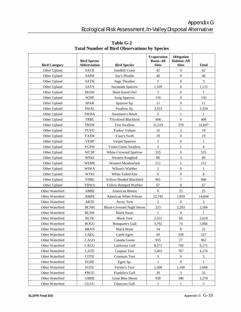
G-2 Total Number of Bird Observations by Species
G-3 Bird Density in Central Valley Evaporation Basins
G-4 Bird Dietary Composition Data
G-5 Estimated Dietary Composition for Bird Categories
G-6 Predicted Selenium Concentrations in Influent Water and Dietary Tissue
G-7 Predicted Average Selenium Concentration in Diet of Each Bird Category
G-8 Dietary Selenium Concentrations Associated with Adverse Reproductive Effects in Birds
G-9 Selenium Concentrations in Bird Eggs Collected from Kesterson Reservoir, 1983–1985
G-10 Estimated Total Number of Birds Assuming Mean Density
G-11 Estimated Total Number of Birds Assuming Median Density
Figures G1 Conceptual Site Exposure Model, In-Valley Disposal Alternative
G-2 Bivariate Fit of Log Vegetation [Se] By Log Water [Se]
G-3 Bivariate Fit of Log Nektos [Se] By Log Water [Se]
G-4 Bivariate Fit of Log Benthos [Se] By Log Water [Se]
G-5 Percentage of Fertile Eggs Hatched vs. Selenium Concentration in Diet of Mallard Ducks
G-6 Percentage Survival of Mallard Ducklings to 6 Days of Age vs. Selenium Concentration in Diet of Parents
G-7 Number of 6-Day-Old Mallard Ducklings Produced per Hen vs. Selenium (as Selenomethionine) Concentration in Diet
Attachments G1 Bird Density Histograms

TABLE OF CONTENTS
SLDFR Final EIS Appendix G G-iii
Acronyms BCF bioconcentration factor
CDFG California Department of Fish and Game
EC electrical conductivity
EC10 effects concentration to 10 percent of the population
EIS Environmental Impact Statement
LOAEL lowest-observable-adverse-effect level
µg/L microgram(s) per liter
mg/kg milligram(s) per kilogram
mg/L milligram(s) per liter
NOAEL no-observable-adverse-effect level
ppb part(s) per billion
ppm part(s) per million
ppt part(s) per thousand
Se selenium
Service U.S. Fish and Wildlife Service
TDS total dissolved solids
USEPA U.S. Environmental Protection Agency


Appendix G Ecological Risk Assessment, In-Valley Disposal Alternative
SLDFR Final EIS Appendix G G-1
APPENDIX G ECOLOGICAL RISK ASSESSMENT, IN-VALLEY DISPOSAL ALTERNATIVE
G1 INTRODUCTION This report evaluates the potential for adverse ecological effects to avian receptors due to increased selenium (Se) exposure that may result from creation of the evaporation basins proposed with the In-Valley Disposal Alternative. Once Se enters the aquatic environment, it has the potential to bioaccumulate in primary and secondary consumers (e.g., zooplankton and benthic invertebrates), and biomagnify as it reaches top-level predators (e.g., predatory fish, birds, and mammals). Biomagnification is a form of bioaccumulation in which the concentration of a chemical in a higher-trophic-level organism is greater than the concentration in the food that this organism consumes. This phenomenon has been observed to result in a two- to sixfold increase in Se concentrations between primary producers and forage fish (Lemly 1999).
Se is an essential element necessary for proper enzyme formation and function (Eisler 1985). However, chronic exposure to significantly elevated Se levels in the diet or water can also cause severe toxicological effects, including death. The concentration range separating effects of Se deficiency from those of toxicity (i.e., selenosis) is very narrow (Luoma and Presser 2000). With the exception of mortality, the two major toxicological effects to aquatic organisms from chronic exposure are reproductive effects and teratogenesis (i.e., malformations in developing fetus). Excessive Se contamination is often associated with localized extinction of certain species and reduction in biodiversity. Based on field and laboratory studies with fish and wildlife, it is apparent that elevated Se concentrations in environmental media, including dietary components, can cause reproductive abnormalities. These abnormalities include congenital malformations, selective bioaccumulation by the organism, and growth retardation (Eisler 1985).
The primary guidance documents used to develop the approach for this evaluation were the Guidelines for Ecological Risk Assessment (U.S. Environmental Protection Agency [USEPA] 1998), Ecological Risk Assessment Guidance for Superfund (USEPA 1997), and Guidance for Ecological Risk Assessment at Hazardous Waste Sites and Permitted Facilities (Cal-EPA 1996).
G1.1 Objectives of Evaluation The primary objectives of this evaluation were to:
• Identify groups of ecological receptors most likely to be exposed to Se in the evaporation basins.
• Identify potential toxicological effects of Se.
• Provide estimates of probable adverse effects due to Se exposure via the food chain.
• Identify other water quality constituents that have potential to cause adverse effects to ecological receptors using evaporation basins.
G1.2 General Approach Water quality modeling results were reviewed and the ecological setting was evaluated to develop a conceptual site model and identify potentially complete exposure pathways for the chemicals present. Assessment and measurement endpoints were identified for each ecological group likely to be exposed. To evaluate toxicity to receptors exposed to the Se via

Appendix G Ecological Risk Assessment, In-Valley Disposal Alternative
SLDFR Final EIS Appendix G G-2
bioaccumulation, plant and invertebrate tissue concentrations were estimated using available data on Se bioaccumulation in existing Central Valley evaporation basins. A literature search on Se toxicity was conducted to determine probable effects of predicted plant and invertebrate tissue concentrations on upper trophic level receptors.
It should be noted that this assessment was conducted under the assumption that no mitigation habitat is provided. Although the evaporation basins would be designed to minimize bird use, it is assumed that all birds using the evaporation basins would be obtaining 100 percent of their food from the evaporation basins. Therefore, no dietary dilution of Se concentrations would occur, and the risk assessment results would represent the worst-case scenario. The results of this risk assessment will be used as a tool to help determine mitigation requirements to reduce the risk of Se toxicity to populations of birds utilizing the evaporation basins.
G1.3 Terminology Several terms used throughout this section are defined below:
Direct toxicity refers to adverse effects to an organism caused by contact between the organism and contaminated environmental media, i.e., water or sediment.
Acute toxicity refers to adverse effects, often lethality, that occur from short-term exposure to a chemical (usually less than 96 hours).
Chronic toxicity refers to sublethal adverse effects (such as reduced growth or reproduction) during long-term exposure.
Bioconcentration is the process by which living organisms can retain and concentrate chemicals present in their surrounding medium (usually water).
Bioaccumulation is the process by which living organisms can retain and concentrate chemicals both directly from their surrounding environment (i.e., from water, bioconcentration) and indirectly from sediments, soil, and their food.
Biomagnification is a form of bioaccumulation in which the concentration of a chemical in a higher-trophic-level organism (predatory fish, bird, or mammal) is greater than the concentration in the lower trophic level food items that this organism consumes.
A food-web receptor is an ecological receptor whose primary exposure to chemicals occurs by way of diet, i.e., bioaccumulation. Most food-web receptors evaluated in ecological risk assessment are birds and mammals.
Ecological risk assessment is a process that evaluates the likelihood that adverse ecological effects may occur as a result of exposure to one or more stressors (USEPA 1997).
The exposure, or dose, represents the average amount of a chemical that an individual member of a population ingests. The exposure is a function of a receptor’s foraging behavior and depends on life-history strategies such as dietary preferences, food ingestion rates, and seasonal behavior.
G2 SITE CHARACTERIZATION AND ENVIRONMENTAL SETTING Data have been collected on existing sediment and water quality as well as on the ecology and biology of the areas that would be affected by construction of the evaporation basins.

Appendix G Ecological Risk Assessment, In-Valley Disposal Alternative
SLDFR Final EIS Appendix G G-3
Evaporation basins have been used in the San Joaquin Valley for about two decades as a means of disposal of irrigation drainwater. About 4,000 acres of evaporation basins are currently in operation within the valley.
G2.1 Site Characterization for Proposed Evaporation Basins It is estimated that a total of approximately 2,870 acres (average wetted area under typical conditions) to 3,290 acres (maximum wetted area under wet conditions) of evaporation basin will be needed for the four basin sites. This acreage is a gross estimate and is based on the flow of water being provided by the reuse areas. The final areas will be fine-tuned based upon the flow from the reuse areas and the amount of water treatment provided to the influent. Four areas are under investigation for four evaporation basins that would be located adjacent to the reuse facilities:
• Northerly Reuse Area (Evaporation Basin A)
• Westlands North Reuse Area (Evaporation Basin B)
• Westlands Central Reuse Area (Evaporation Basin C)
• Westlands South Reuse Area (Evaporation Basin D)
Section 2.4.1.3 provides a summary description of the evaporation basins. Figure 2.4-1 shows the generalized areas under consideration for selection of specific sites for the evaporation basins. The figure also shows the proximity of the evaporation basins to the reuse areas.
G2.2 Water Quality Typical ranges for water quality parameters expected to occur in the water flowing into the proposed evaporation basins are presented in Section 5.2.4 and Appendix C of the Environmental Impact Statement (EIS). Constituents present at high concentrations include Se, boron, molybdenum, and salinity. Mean Se concentrations in influent water are predicted to be approximately 10 micrograms per liter (µg/L). Molybdenum concentrations are expected to range from approximately 170 to 690 µg/L, and boron concentrations from 31,000 to 52,000 µg/L. Total dissolved solids (TDS) in influent water is predicted to range from approximately 24,000 to 32,000 milligrams per liter (mg/L). As water evaporates from the basins, concentrations of these constituents are expected to become more concentrated.
G2.3 Ecological Setting
G2.3.1 General Habitat Evaporation basins are used for disposal of agricultural drainwater, and the areas adjacent to the evaporation basins are typically utilized for irrigated agriculture. In general, they are comprised of evaporation basins hydrologically interconnected by the main drainage conveyance facilities. The basins are generally sited and constructed above the 100-year flood level, and a network of levees and the topographic characteristics of the area would protect the evaporation basins from being inundated with floodwater. Each individual evaporation basin is made up of a series of levees constructed of consolidated soil. Interior levee slopes are typically 3:1 or less. Drainwater

Appendix G Ecological Risk Assessment, In-Valley Disposal Alternative
SLDFR Final EIS Appendix G G-4
flowing into the evaporation basin and between basin cells is regulated by a series of valves and control weirs.
The evaporation basins collect and store subsurface agricultural drainwater, which evaporates, concentrating salts and other constituents such as Se. They are operated as a closed hydrologic unit, have no surface water discharge, and typically have extremely high concentrations of salts and other constituents. For example, in the Tulare Lake Drainage Basin, salinity ranged from 20 percent of seawater (10 microSiemens per centimeter electrical conductivity [EC], or approximately 7 parts per thousand [ppt]) to 6 times seawater (300 microSiemens per centimeter EC, or approximately 210 ppt) (Euliss, Jarvis, and Gilmer 1991). Since salts tend to concentrate in evaporation basins over time, the biota will show a change to more hypersaline adapted organisms as the salt concentration increases.
The high salinity in evaporation basins creates harsh aquatic environments. Most of the aquatic organisms present have limited osmoregulatory abilities and the high concentration of dissolved minerals is likely the most important factor determining biological characteristics of these systems (Parker and Knight 1992). Due to this situation, species diversity within evaporation basins is very low. However, since evaporation basins have extensive surface areas relative to storage volumes, receive direct sunlight throughout the day, and receive irrigation drainage rich in nutrients, the basins exhibit very high primary productivity (Parker and Knight 1992), which is typical of shallow, saline aquatic systems in general.
G2.3.2 Plant Communities Widgeongrass (Ruppia maritima), a submergent macrophyte, is frequently the dominant macrophyte present in the basins, covering up to 80 percent of the surface of the basins in some cases (Parker and Knight 1992). Algae are very common in evaporation basins and typical species include Dunaliella, Chaetoceros sp., Nitzchia sp., cyanobacteria, and Synechoccus Nageli (Tanner, Glenn, and Moore 1999).
G2.3.3 Invertebrate Communities Waterboatmen (Trichorixa reticulata), midges (Tanypus sp., Tanypus grodhausi Sublette), damselflies (Enallagma iile), brine flies (Ephydra sp.), and brine shrimp (Artemia franciscana franciscana) are the dominant macroinvertebrates present in evaporation basins. At lower salinity levels, waterboatmen are the most dominant species. In some basins, waterboatmen made up 70 to 90 percent of total macroinvertebrate density (Parker and Knight 1992). In another study, waterboatmen and T. grodhausi made up 96.3 percent of total dry mass (Euliss, Jarvis, and Gilmer 1991). At higher salinities (greater than 50 ppt), brine flies and brine shrimp were co-dominant, although waterboatmen were also present (Fan et al. 2002).
G2.3.4 Bird Communities Evaporation basins support a relatively diverse group of birds, including grebes, gulls, waterfowl, terns, shorebirds, and passerines. Raptors such as owls, kestrels, and hawks may feed on birds that forage in evaporation basins. Black-necked stilts (Himantopus mexicanus), American avocets (Recurvirostra americana), eared grebes (Podiceps nigricollis), ruddy ducks (Oxyura jamaicensis), and Wilson’s phalaropes (Phalaropus tricolor) tolerate hypersaline

Appendix G Ecological Risk Assessment, In-Valley Disposal Alternative
SLDFR Final EIS Appendix G G-5
environments, forage on brine shrimp, and are common in evaporation basins in the Central Valley (Hanson Environmental 2003).
Historical survey data for birds from various sites in the Central Valley were collected by H.T. Harvey & Associates, Fresno, CA, and Hanson Environmental, Inc, Walnut Creek, CA, between 1993 and 2003 (Hanson Environmental 2003; H.T. Harvey & Associates, 1996a, 1996b, 1998, 2000, 2001a, 2001b, 2001c, 2001d, 2001e, 2002a, 2002b, 2002c, 2002d, 2002e). These records include ten evaporation basins and eight associated mitigation sites, and each site was surveyed for 2 to 11 years in an approximate interval of every 2 weeks, though most mitigation sites were not surveyed during the winter months (Nov-Jan).
The size of basins varied significantly. For evaporation basins, the size ranged from 20 acres (Westlake Farms, Experimental Evaporation Pond) to 1,793 acres (Tulare Lake Drainage District, South Basin Evaporation Pond). For mitigation sites, the size ranged from 8 acres (Britz, Alternative Wetland) to 640 acres (Westlake Farms, Section 23). For this analysis, the general size of the site was considered, rather than the flooded acreage (which varies by season), in the calculation of bird density. Hence, the basin size was assumed to be fixed in all historical surveys for each site.
The data analysis was discretized into four seasons: spring migration (Feb-Apr), breeding (May-Jul), fall migration (Aug-Oct), and winter (Nov-Jan); and six bird categories as described in Table G-1: dabblers, divers, breeding shorebirds, nonbreeding shorebirds, upland birds, and other waterbirds. These categories are broken down based on distinct types of foraging behavior, dietary composition, and seasonal use patterns and, therefore, address different potentials for Se exposure. Species assigned to each of the bird categories are listed in Table G-2.
For each individual survey, the number of birds from a given bird category (all species within that category) were summed up and then divided by the corresponding site acreage. Hence, the unit of analysis was birds per acre (or more precisely, birds per acre per survey). The results are summarized in Table G-3.
It should be noted that each survey was considered as an equal-weighted data point, given that the number of surveys was fairly similar across all sites. However, the result is that sites that were surveyed more frequently are more heavily weighted in the analysis. It was also assumed that the duration of time spent observing birds during each survey was similar, and that the times of day surveys occurred was similar, although little information on survey methods or duration was available in the monitoring reports.
The histograms of bird density (in birds/acre) indicate that the data distribution is highly skewed (see histograms in Attachment G1). Therefore, an appropriate measure of central tendency is the sample median, rather than the sample mean (which may be affected by extremely high measurements). The median is defined as the middle measurement in an ordered set of data, that is, just as many observations are larger than the median as smaller. The median of a highly skewed distribution is generally smaller than the arithmetic mean. The median and mean bird densities presented in Table G-3 represent the bird densities (of all bird species within the relevant bird category) at a given time.

Appendix G Ecological Risk Assessment, In-Valley Disposal Alternative
SLDFR Final EIS Appendix G G-6
Table G-1 Bird Categories
Guild Description Dabblers (surface-feeding waterfowl) Dabblers generally occur in shallower water than divers. They feed
mostly on vegetation or very small invertebrates. Divers Divers generally occur in open water and forage beneath the surface,
most often on benthic invertebrates. Divers tend to occur most frequently in evaporation basins during the nonbreeding season.
Breeding shorebirds (likely to breed at evaporation basins)
Breeding shorebirds include those that are known to breed on the edges of evaporation basin sites that have been monitored in the Central Valley. Black-necked stilts and American avocets are long-legged waders. Killdeer and snowy plover exhibit foraging patterns similar to short-legged waders.
Nonbreeding shorebirds (not likely to breed at evaporation basins)
Long-legged waders are those species with a mean tarsal length greater than 2 inches (5 centimeters). Long-legged waders, in general, share feeding habitats and display similar foraging methods. These species tend to concentrate at the water’s edge or in shallow waters where they probe in the substrate for invertebrate prey. Long-legged waders include whimbrels, greater yellowlegs, dowitchers, plovers, long-billed curlew, and godwits. Short-legged waders are those species with a mean tarsal length less than 2 inches (5 centimeters). These species tend to forage on exposed tidal flats at slightly higher intertidal elevations than long-legged waders, where they also feed on invertebrate prey. Short-legged waders include sandpipers and sanderlings. Phalaropes have a foraging style that is distinct from other shorebirds. They typically forage for aquatic invertebrates by paddling in a circle in shallow open water.
Other waterbirds These species include all other waterbird species that were observed in the evaporation basins, including gulls, terns, egrets, and herons. Gulls and terns are ecologically and taxonomically related, and tend to congregate in flocks on tidal flats, open water, pilings, or seawalls. However, gulls feed from the surface of the water and terns dive from the air to capture their prey. Both feed on a variety of fish that occupy the upper water column. In addition, gulls forage on a wide variety of food sources.
upland birds These species include all upland bird species that were observed around evaporation basins. These species include all upland bird species that were observed around evaporation basins, including gulls, terns, and phalaropes. These species are not expected to obtain a significant amount of their diet within the evaporation basins. However, some raptor species may feed on waterbirds and shorebirds.

Appendix G Ecological Risk Assessment, In-Valley Disposal Alternative
SLDFR Final EIS Appendix G G-7
Table G-2 Total Number of Bird Observations by Species
Bird Category Bird Species Abbreviation Bird Species
Evaporation Basin–All
Sites
Mitigation Habitat–All
Sites Total Dabbler AMCO American Coot 131,932 28,419 160,351 Dabbler AMWI American Wigeon 5,546 599 6,145 Dabbler BWTE Blue-Winged Teal 71 192 263 Dabbler CITE Cinnamon Teal 19,120 15,378 34,498 Dabbler COMO Common Moorhen 2 107 109 Dabbler DABB Dabbling Duck Sp. 24,723 123 24,846 Dabbler EUWI Eurasian Wigeon 6 1 7 Dabbler GADW Gadwall 35,127 5,639 40,766 Dabbler GWTE Green-Winged Teal 7,297 5,214 12,511 Dabbler MALL Mallard 22,226 26,156 48,382 Dabbler NOPI Northern Pintail 16,383 9,874 26,257 Dabbler NOSH Northern Shoveler 462,878 10,832 473,710 Dabbler TEAL Teal Species 537 6 543
Diver AECH Aechmophorus Sp. 12 0 12 Diver AYTH Aythya Sp. 1 0 1 Diver BUFF Bufflehead 5,118 4 5,122 Diver CANV Canvasback 1,295 0 1,295 Diver CLGR Clark's Grebe 487 2 489 Diver COGO Common Goldeneye 333 0 333 Diver COLO Common Loon 4 0 4 Diver COME Common Merganser 1,906 11 1,917 Diver DCCO Double-Crested Cormorant 9,647 56 9,703 Diver EAGR Eared Grebe 284,703 57 284,760 Diver GRSC Greater Scaup 11 0 11 Diver GRSP Grebe Species 400 0 400 Diver HOGR Horned Grebe 10 0 10 Diver HOME Hooded Merganser 6 0 6 Diver LESC Lesser Scaup 9,337 9 9,346 Diver OLDS Long-Tailed Duck 14 0 14 Diver PBGR Pied-Billed Grebe 1,716 164 1,880 Diver RBME Red-Breasted Merganser 2 0 2 Diver REDH Redhead 21,361 483 21,844 Diver RNDU Ring-Necked Duck 474 4 478 Diver RUDU Ruddy Duck 444,487 333 444,820 Diver SUSC Surf Scoter 38 0 38 Diver WEGR Western Grebe 517 0 517
Breeding Shorebird AMAV American Avocet 329,523 79,610 409,133 Breeding Shorebird BNST Black-Necked Stilt 203,587 35,382 238,969 Breeding Shorebird KILL Killdeer 5,638 3,399 9,037 Breeding Shorebird SNPL Snowy Plover 19,231 1,228 20,459

Appendix G Ecological Risk Assessment, In-Valley Disposal Alternative
SLDFR Final EIS Appendix G G-8
Table G-2 Total Number of Bird Observations by Species
Bird Category Bird Species Abbreviation Bird Species
Evaporation Basin–All
Sites
Mitigation Habitat–All
Sites Total Nonbreeding Shorebird AMGP American Golden Plover 1 1 2 Nonbreeding Shorebird BASA Baird's Sandpiper 282 9 291 Nonbreeding Shorebird BBPL Black-Bellied Plover 66,941 6,300 73,241 Nonbreeding Shorebird BLTU Black Turnstone 3 0 3 Nonbreeding Shorebird COSN Common Snipe 16 7 23 Nonbreeding Shorebird CUSA Curlew Sandpiper 1 0 1 Nonbreeding Shorebird DOWI Dowitcher Sp. 33,763 72,670 106,433 Nonbreeding Shorebird DUNL Dunlin 177,623 17,451 195,074 Nonbreeding Shorebird GPSP Golden-Plover Species 7 0 7 Nonbreeding Shorebird GRYE Greater Yellowlegs 23,861 7,561 31,422 Nonbreeding Shorebird JURE Juv. Recurvirostridae 96 1,346 1,442 Nonbreeding Shorebird LBDO Long-Billed Dowitcher 73,627 1,019 74,646 Nonbreeding Shorebird LEGP Lesser Golden-Plover 5 0 5 Nonbreeding Shorebird LESA Least Sandpiper 178,686 14,324 193,010 Nonbreeding Shorebird LEYE Lesser Yellowlegs 539 127 666 Nonbreeding Shorebird LOCU Long-Billed Curlew 13,690 6,833 20,523 Nonbreeding Shorebird MAGO Marbled Godwit 2,160 66 2,226 Nonbreeding Shorebird PESA Pectoral Sandpiper 14 2 16 Nonbreeding Shorebird PGPL Pacific Golden-Plover 5 2 7 Nonbreeding Shorebird PHAL Phalarope Sp. 10,608 0 10,608 Nonbreeding Shorebird REKN Red Knot 135 20 155 Nonbreeding Shorebird REPH Red Phalarope 3 1 4 Nonbreeding Shorebird RUFF Ruff 41 5 46 Nonbreeding Shorebird RUTU Ruddy Turnstone 31 7 38 Nonbreeding Shorebird SAND Sanderling 1,027 15 1,042 Nonbreeding Shorebird SAPI Sandpiper Sp. 493 0 493 Nonbreeding Shorebird SBDO Short-Billed Dowitcher 26 1 27 Nonbreeding Shorebird SEPL Semipalmated Plover 1,134 346 1,480 Nonbreeding Shorebird SESA Semipalmated Sandpiper 35 6 41 Nonbreeding Shorebird SORA Sora 0 47 47 Nonbreeding Shorebird SOSA Solitary Sandpiper 1 0 1 Nonbreeding Shorebird SPSA Spotted Sandpiper 80 13 93 Nonbreeding Shorebird STSA Stilt Sandpiper 45 4 49 Nonbreeding Shorebird TURN Turnstone Species 1 0 1 Nonbreeding Shorebird WELE Western/Least Sandpiper 45,701 2,009 47,710 Nonbreeding Shorebird WESA Western Sandpiper 357,272 83,506 440,778 Nonbreeding Shorebird WHIM Whimbrel 6,607 15,597 22,204 Nonbreeding Shorebird WILL Willet 10,320 504 10,824 Nonbreeding Shorebird WIPH Wilson's Phalarope 165,186 552 165,738 Nonbreeding Shorebird WRSA White-Rumped Sandpiper 1 0 1

Appendix G Ecological Risk Assessment, In-Valley Disposal Alternative
SLDFR Final EIS Appendix G G-9
Table G-2 Total Number of Bird Observations by Species
Bird Category Bird Species Abbreviation Bird Species
Evaporation Basin–All
Sites
Mitigation Habitat–All
Sites Total Nonbreeding Shorebird YELL Yellowlegs Sp. 390 0 390
Other Upland AMCR American Crow 5 0 5 Other Upland AMKE American Kestrel 5 0 5 Other Upland AMPI American Pipit 3,609 107 3,716 Other Upland BASW Bank Swallow 1,064 57 1,121 Other Upland BBSP Blackbird Sp. 1,382 5 1,387 Other Upland BHCO Brown-Headed Cowbird 35 0 35 Other Upland BLPH Black Phoebe 46 0 46 Other Upland BRBL Brewer's Blackbird 2,614 3 2,617 Other Upland BUOR Bullock's Oriole 1 0 1 Other Upland BUOW Burrowing Owl 30 0 30 Other Upland CLSW Cliff Swallow 16,770 1,748 18,518 Other Upland CORO Common Raven 247 0 247 Other Upland EUST European Starling 2 0 2 Other Upland FALC Large Falco Sp. 1 0 1 Other Upland FEHA Ferruginous Hawk 4 0 4 Other Upland FOSP Fox Sparrow 1 0 1 Other Upland GCSP Golden-Crowned Sparrow 3 0 3 Other Upland HOFI House Finch 265 0 265 Other Upland HOLA Horned Lark 2,713 31 2,744 Other Upland HOSP House Sparrow 30 1 31 Other Upland HUMM Hummingbird Sp. 2 0 2 Other Upland LISP Lincoln's Sparrow 2 0 2 Other Upland LOSH Loggerhead Shrike 99 0 99 Other Upland MAWR Marsh Wren 136 0 136 Other Upland MERL Merlin 8 0 8 Other Upland MODO Mourning Dove 4 0 4 Other Upland MOPL Mountain Plover 22 0 22 Other Upland NOHA Northern Harrier 368 1 369 Other Upland NOMO Northern Mockingbird 1 0 1 Other Upland NRWS N. Rough-Winged Swallow 124 16 140 Other Upland PEFA Peregrine Falcon 68 1 69 Other Upland PRFA Prairie Falcon 11 1 12 Other Upland RCKI Ruby-Crowned Kinglet 1 0 1 Other Upland RLHA Rough-Legged Hawk 1 0 1 Other Upland RNPH Ring-Necked Pheasant 1 0 1 Other Upland ROWR Rock Wren 6 0 6 Other Upland RTHA Red-Tailed Hawk 96 0 96 Other Upland RUHU Rufous Hummingbird 0 1 1 Other Upland RWBL Red-Winged Blackbird 1,594 17 1,611
Appendix G Ecological Risk Assessment, In-Valley Disposal Alternative
SLDFR Final EIS Appendix G G-10
Table G-2 Total Number of Bird Observations by Species
Bird Category Bird Species Abbreviation Bird Species
Evaporation Basin–All
Sites
Mitigation Habitat–All
Sites Total Other Upland SACR Sandhill Crane 42 0 42 Other Upland SAPH Say's Phoebe 40 0 40 Other Upland SATH Sage Thrasher 5 0 5 Other Upland SAVS Savannah Sparrow 1,109 6 1,115 Other Upland SEOW Short-Eared Owl 1 0 1 Other Upland SOSP Song Sparrow 156 0 156 Other Upland SPAR Sparrow Sp. 11 0 11 Other Upland SWAL Swallow Sp. 3,333 1 3,334 Other Upland SWHA Swainson's Hawk 0 1 1 Other Upland TRBL Tricolored Blackbird 408 0 408 Other Upland TRSW Tree Swallow 31,319 378 31,697 Other Upland TUVU Turkey Vulture 16 2 18 Other Upland VASW Vaux's Swift 19 0 19 Other Upland VESP Vesper Sparrow 1 0 1 Other Upland VGSW Violet-Green Swallow 3 1 4 Other Upland WCSP White-Crowned Sparrow 555 0 555 Other Upland WEKI Western Kingbird 86 3 89 Other Upland WEME Western Meadowlark 211 1 212 Other Upland WIWA Wilson's Warbler 1 0 1 Other Upland WTKI White-Tailed Kite 8 0 8 Other Upland YHBL Yellow-Headed Blackbird 961 7 968 Other Upland YRWA Yellow-Rumped Warbler 67 0 67
Other Waterbird AMBI American Bittern 0 25 25 Other Waterbird AMPE American White Pelican 12,745 1,859 14,604 Other Waterbird ARTE Arctic Tern 2 0 2 Other Waterbird BCNH Black-Crowned Night Heron 223 2,283 2,506 Other Waterbird BLSW Black Swan 1 0 1 Other Waterbird BLTE Black Tern 2,551 68 2,619 Other Waterbird BOGU Bonaparte's Gull 3,792 74 3,866 Other Waterbird BRAN Black Brant 14 8 22 Other Waterbird CAEG Cattle Egret 69 258 327 Other Waterbird CAGO Canada Goose 935 27 962 Other Waterbird CAGU California Gull 8,572 700 9,272 Other Waterbird CATE Caspian Tern 3,403 767 4,170 Other Waterbird COTE Common Tern 3 0 3 Other Waterbird EGRE Egret Sp. 1 0 1 Other Waterbird FOTE Forster's Tern 1,568 1,100 2,668 Other Waterbird FRGU Franklin's Gull 30 3 33 Other Waterbird GBHE Great Blue Heron 938 340 1,278 Other Waterbird GLGU Glaucous Gull 1 1 2

Appendix G Ecological Risk Assessment, In-Valley Disposal Alternative
SLDFR Final EIS Appendix G G-11
Table G-2 Total Number of Bird Observations by Species
Bird Category Bird Species Abbreviation Bird Species
Evaporation Basin–All
Sites
Mitigation Habitat–All
Sites Total Other Waterbird GREG Great Egret 1,060 1,128 2,188 Other Waterbird GRHE Green Heron 1 12 13 Other Waterbird GULL Gull Sp. 1,417 130 1,547 Other Waterbird GWFG Greater White-Fronted Goose 623 163 786 Other Waterbird HEGU Herring Gull 835 128 963 Other Waterbird LEBI Least Bittern 0 2 2 Other Waterbird LETE Least Tern 142 7 149 Other Waterbird LTJA Long-Tailed Jaeger 2 0 2 Other Waterbird OSPR Osprey 3 0 3 Other Waterbird RBGU Ring-Billed Gull 10,359 6,570 16,929 Other Waterbird RNPA Red-Necked Phalarope 42,923 292 43,215 Other Waterbird ROGO Ross's Goose 59 0 59 Other Waterbird SAGU Sabine's Gull 8 0 8 Other Waterbird SNEG Snowy Egret 6,199 5,199 11,398 Other Waterbird SNGO Snow Goose 41 5 46 Other Waterbird TUSW Tundra Swan 10 0 10 Other Waterbird VIRA Virginia Rail 0 31 31 Other Waterbird WFIS White-Faced Ibis 834 5,773 6,607

Appendix G Ecological Risk Assessment, In-Valley Disposal Alternative
SLDFR Final EIS Appendix G G-12
Evaporation basins in California receive use by much higher numbers of nonbreeding birds than breeding birds. An estimated 10 to 12 million waterfowl winter or pass through the Central Valley of California each year (Heinz and Fitzgerald 1993a). Ruddy ducks, eared grebes, and American coots (Fulica americana) are the most abundant species that winter on large, open, and deep agricultural evaporation basins in the San Joaquin Valley (Gordus, Shivaprasad, and Swift 2002). Generally, overwintering birds arrive in the Central Valley in the fall and migrate north in early spring. The degree of site fidelity exhibited by overwintering waterfowl in the Central Valley is not well documented. Understanding the movement of individuals on a daily basis is dependent on radio telemetry studies. Previous studies have shown strong site fidelity by female northern pintails on a regional basis, but on a smaller scale, movements can be highly flexible depending on prey abundance and other factors (Cox and Afton 2000). Pintails studied on National Wildlife Refuges during the winter tend to make extensive daily flights between feeding sites, but choose the same sites consistently among years (Cox and Afton 2000).
Nonbreeding shorebirds, on the other hand, are more abundant within the Pacific Flyway during short, intense migratory periods during the fall and spring. Some species are known to overwinter in the Central Valley.
In general, the degree of site fidelity in birds is thought to be linked most closely to the predictability or physical stability of a site or food source (Ehrlich, Dobkin, and Wheye 1988). Birds tend to have higher levels of fidelity to foraging grounds during the breeding season when they have an established nesting site. Individuals may range farther in search of food during the winter period when a mate or nestlings are not dependent.
G2.3.5 Special-Status Species Three Federally and State-listed species are known to occur in or around existing Central Valley evaporation basins (Hanson Environmental 2003; Appendix P4, Comment Letter S-06):
• American peregrine falcon (Falco peregrinus anatum)
• California least tern (Sterna antillarum browni)
• Swainson’s hawk (Buteo swainsoni)
Twelve Federal and State species of special concern are known to occur or have potential to occur in or around existing Central Valley evaporation basins:
Species with Both Federal and State Species of Concern Status • Tricolored blackbird (Agelaius tricolor) (nesting sites only)
• Western burrowing owl (Athene cunicularia hypugea) (nesting sites only)
• Ferruginous hawk (Buteo regalis) (wintering only)
• Black tern (Chlidonias niger) (nesting sites only)
• Long-billed curlew (Numenius americanus) (nesting sites only)
• White-faced ibis (Plegadis chihi) (nesting sites only)

Table G-3Bird Density in Central Valley Evaporation Basins
Britz, Evaporation
Pond
Lost Hills, Evaporation
Basin
Rainbow Ranch Evaporation
Basin, Evaporation
Pond
Tulare Drainage District,
Hacienda
Tulare Drainage
District, North Basin
Evaporation Pond
Tulare Drainage
District, South Basin
Evaporation Pond
Westlake Farms,
Experimental Evaporation
Pond
Westlake Farms, North Evaporation
Basin
Westlake Farms, South Evaporation
Basin
Westlake Farms, South Evaporation
Basin, Cell A1A
Britz, Alternative
Wetland
Britz, Compensation
Site
Lost Hills, Alternative
Wetland
Lost Hills, Experimental Alternative
Habitat
Tulare Drainage District,
Compensation Habitat
Westlake Farms,
Section 16
Westlake Farms,
Section 23
Westlake Farms,
Section 3
Size (Acres) 25 345 100 1,108 264 1,793 20 260 740 52 8 10 130 120 307 135 740 68Year 1994 - 2003 1996 - 2003 1994 - 1997 1998 - 2002 1998 - 2002 1998 - 2002 1993 - 2001 1993 - 2003 1993 - 2003 1995 - 2003 1996 - 2002 1995 - 2002 1999 - 2003 1997 - 1998 1998 - 2002 1993 - 2001 1995 - 2001 1993 - 2002
Season Bird CategoryMean - 2 Std Dev
Mean - 1 Std Dev Mean
Mean + 1 Std Dev
Mean + 2 Std Dev
Mean - 2 Std Dev
Mean - 1 Std Dev Mean
Mean + 1 Std Dev
Mean + 2 Std Dev
Dabblers 0.000 0.000 1.474 3.941 6.408 0.115 0.003 0.083 1.236 5.375 0.923 3.136 1.023 0.574 3.008 0.000 0.000 3.021 7.078 11.136 3.350 5.500 1.057 1.350 0.315 2.778 0.877 5.629Divers 0.000 0.000 1.748 3.987 6.226 0.042 1.655 2.412 2.218 3.541 3.224 1.972 0.420 1.023 3.204 0.000 0.000 0.016 0.070 0.124 0.000 0.000 0.021 0.000 0.000 0.012 0.002 0.039Breeding Shorebirds 0.000 0.000 0.493 1.653 2.812 0.261 0.249 0.851 0.520 1.454 0.116 0.391 0.611 0.464 0.347 0.000 0.000 2.360 6.140 9.920 1.563 5.225 0.560 1.800 0.653 0.949 0.149 5.472Nonbreeding Shorebirds 0.000 0.000 1.244 3.451 5.659 0.097 0.183 1.368 1.924 2.630 0.427 0.305 2.493 2.082 0.679 0.000 0.000 7.601 22.574 37.548 0.600 29.738 2.443 0.667 0.828 7.181 0.892 11.312Other Uplands 0.000 0.000 0.082 0.529 0.975 0.000 0.000 0.000 0.213 0.930 0.088 0.000 0.000 0.000 0.000 0.000 0.000 0.020 0.104 0.188 0.000 0.000 0.000 0.000 0.191 0.000 0.000 0.000Other Waterbirds 0.000 0.000 0.035 0.165 0.294 0.009 0.001 0.081 0.062 0.015 0.030 0.060 0.049 0.016 0.046 0.000 0.000 0.259 0.881 1.503 0.025 0.769 0.051 0.033 0.001 0.318 0.027 0.441Dabblers 0.000 0.000 0.458 1.513 2.567 0.033 0.002 0.016 0.446 2.949 0.145 0.436 0.474 0.102 0.879 0.000 0.000 1.234 2.831 4.428 2.035 2.300 0.741 1.817 0.134 0.896 0.199 1.722Divers 0.000 0.000 0.187 0.692 1.197 0.006 0.019 0.026 0.409 0.412 0.642 0.115 0.058 0.056 0.544 0.000 0.000 0.019 0.074 0.129 0.008 0.002 0.036 0.019 0.000 0.012 0.002 0.052Breeding Shorebirds 0.000 0.000 0.702 1.794 2.887 0.418 0.094 0.963 1.401 2.359 1.248 0.493 0.793 0.355 0.294 0.000 0.000 2.404 5.643 8.881 2.168 3.136 1.323 2.079 1.745 1.458 0.189 5.177Nonbreeding Shorebirds 0.000 0.000 0.894 3.063 5.231 0.067 0.042 1.937 1.729 2.107 1.978 0.435 1.610 0.598 0.146 0.000 0.000 2.068 7.965 13.863 0.152 4.378 1.186 1.873 0.839 1.276 0.132 4.398Other Uplands 0.000 0.000 0.075 0.349 0.622 0.000 0.000 0.000 0.343 0.582 0.220 0.000 0.000 0.000 0.000 0.000 0.000 0.012 0.073 0.134 0.000 0.000 0.000 0.000 0.121 0.000 0.000 0.000Other Waterbirds 0.000 0.000 0.110 0.464 0.818 0.024 0.002 0.037 0.114 0.070 0.127 0.164 0.083 0.064 0.430 0.000 0.000 0.456 1.402 2.347 0.055 0.769 0.114 0.377 0.007 0.503 0.058 1.103Dabblers 0.000 0.000 0.954 2.582 4.211 0.091 0.008 0.196 2.732 2.538 2.753 1.045 0.655 0.172 0.617 0.000 0.000 1.450 4.352 7.254 1.133 1.600 0.228 0.028 0.000 0.957 0.194 2.830Divers 0.000 0.000 0.697 2.424 4.151 0.026 0.545 0.854 1.147 0.947 1.484 0.745 0.156 0.251 1.483 0.000 0.000 0.012 0.044 0.076 0.000 0.017 0.003 0.042 0.000 0.003 0.003 0.026Breeding Shorebirds 0.000 0.000 1.218 3.546 5.874 0.170 0.083 1.934 2.587 3.644 1.426 1.305 0.984 0.828 0.807 0.000 0.000 1.961 6.581 11.200 0.675 1.250 0.580 0.067 0.176 0.639 0.332 4.590Nonbreeding Shorebirds 0.000 0.000 2.295 5.646 8.997 2.193 0.049 3.819 3.887 6.266 2.381 0.828 3.942 1.190 0.980 0.000 0.000 4.930 14.996 25.062 0.692 4.508 3.699 0.106 0.484 2.124 1.576 10.340Other Uplands 0.000 0.000 0.080 0.479 0.877 0.000 0.000 0.000 0.067 0.855 0.134 0.000 0.000 0.000 0.000 0.000 0.000 0.004 0.033 0.062 0.000 0.000 0.000 0.000 0.130 0.000 0.000 0.000Other Waterbirds 0.000 0.000 0.462 1.802 3.141 0.076 0.002 0.628 0.547 0.434 0.397 1.230 0.500 0.226 0.519 0.000 0.000 0.865 2.781 4.698 0.025 0.458 0.390 0.306 0.000 0.624 0.189 1.892Dabblers 0.000 0.000 1.355 4.948 8.541 0.110 0.034 0.200 2.418 1.876 1.977 4.057 0.199 0.471 1.806 0.000 0.000 2.396 4.794 7.191 - - 1.019 0.475 - - - 2.584Divers 0.000 0.000 1.972 5.306 8.639 0.078 1.330 3.789 1.637 2.089 1.808 2.404 0.786 1.040 5.379 0.000 0.000 0.069 0.215 0.361 - - 0.000 0.017 - - - 0.077Breeding Shorebirds 0.000 0.000 0.625 2.370 4.115 0.062 0.125 0.781 0.729 0.857 0.098 1.375 0.792 0.587 0.485 0.000 0.000 1.569 4.097 6.625 - - 0.000 0.317 - - - 1.744Nonbreeding Shorebirds 0.000 0.000 2.957 19.246 35.535 0.220 0.057 2.150 1.968 3.654 0.550 10.663 3.683 2.213 1.056 0.000 0.000 4.421 9.711 15.000 - - 0.100 1.692 - - - 4.876Other Uplands 0.000 0.000 0.053 0.238 0.423 0.000 0.000 0.000 0.072 0.533 0.055 0.000 0.000 0.000 0.000 0.000 0.000 0.000 0.000 0.000 - - 0.000 0.000 - - - 0.000Other Waterbirds 0.000 0.000 0.159 0.945 1.730 0.000 0.004 0.045 0.178 0.056 0.041 0.690 0.132 0.062 0.158 0.000 0.000 0.714 1.535 2.356 - - 0.000 0.000 - - - 0.799
Bird Density (Median Number of Birds per Acre per Survey)
Britz, Evaporation
Pond
Lost Hills, Evaporation
Basin
Rainbow Ranch Evaporation
Basin, Evaporation
Pond
Tulare Drainage District,
Hacienda
Tulare Drainage
District, North Basin
Evaporation Pond
Tulare Drainage
District, South Basin
Evaporation Pond
Westlake Farms,
Experimental Evaporation
Pond
Westlake Farms, North Evaporation
Basin
Westlake Farms, South Evaporation
Basin
Westlake Farms, South Evaporation
Basin, Cell A1A
Britz, Alternative
Wetland
Britz, Compensation
Site
Lost Hills, Alternative
Wetland
Lost Hills, Experimental Alternative
Habitat
Tulare Drainage District,
Compensation Habitat
Westlake Farms,
Section 16
Westlake Farms,
Section 23
Westlake Farms,
Section 3
Size (Acres) 25 345 100 1,108 264 1,793 20 260 740 52 8 10 130 120 307 135 740 68Year 1994 - 2003 1996 - 2003 1994 - 1997 1998 - 2002 1998 - 2002 1998 - 2002 1993 - 2001 1993 - 2003 1993 - 2003 1995 - 2003 1996 - 2002 1995 - 2002 1999 - 2003 1997 - 1998 1998 - 2002 1993 - 2001 1995 - 2001 1993 - 2002
Season Bird Category 10% 25%Median (50%) 75% 90% 10% 25%
Median (50%) 75% 90%
Dabblers 0.000 0.039 0.412 1.556 4.607 0.080 0.000 0.020 1.005 4.091 0.248 1.975 0.504 0.502 1.327 0.108 0.410 1.535 4.070 7.485 2.188 2.150 1.073 1.350 0.235 1.963 0.419 4.691Divers 0.000 0.163 1.012 2.536 4.482 0.000 1.339 1.915 2.395 3.201 3.068 0.925 0.252 0.853 2.462 0.000 0.000 0.000 0.000 0.049 0.000 0.000 0.000 0.000 0.000 0.000 0.000 0.000Breeding Shorebirds 0.000 0.002 0.121 0.534 1.323 0.080 0.180 0.635 0.482 1.189 0.076 0.000 0.058 0.319 0.000 0.030 0.179 0.951 2.322 7.860 1.375 4.550 0.335 1.800 0.557 0.700 0.089 3.485Nonbreeding Shorebirds 0.000 0.000 0.262 1.419 4.034 0.000 0.054 0.975 1.286 2.045 0.235 0.000 0.508 1.466 0.000 0.009 0.216 1.566 6.747 24.860 0.250 25.950 1.296 0.667 0.469 1.237 0.203 6.588Other Upland Birds 0.000 0.000 0.000 0.000 0.099 0.000 0.000 0.000 0.116 0.466 0.036 0.000 0.000 0.000 0.000 0.000 0.000 0.000 0.000 0.007 0.000 0.000 0.000 0.000 0.150 0.000 0.000 0.000Other Waterbirds 0.000 0.000 0.000 0.018 0.067 0.000 0.000 0.000 0.031 0.011 0.015 0.000 0.004 0.005 0.000 0.000 0.000 0.045 0.250 0.728 0.000 0.200 0.019 0.033 0.000 0.093 0.007 0.294Dabblers 0.000 0.000 0.070 0.350 1.301 0.000 0.000 0.000 0.330 2.343 0.076 0.100 0.288 0.051 0.337 0.010 0.132 0.608 1.657 3.500 1.625 1.600 0.642 0.967 0.073 0.726 0.116 1.213Divers 0.000 0.000 0.016 0.156 0.469 0.000 0.001 0.010 0.284 0.239 0.451 0.000 0.013 0.013 0.077 0.000 0.000 0.000 0.008 0.059 0.000 0.000 0.015 0.000 0.000 0.000 0.000 0.007Breeding Shorebirds 0.014 0.104 0.308 0.753 1.831 0.320 0.072 0.620 0.704 1.864 0.739 0.150 0.331 0.283 0.125 0.055 0.506 1.431 2.900 5.760 1.750 2.900 1.231 2.308 1.775 1.267 0.097 4.206Nonbreeding Shorebirds 0.000 0.000 0.032 0.451 3.332 0.000 0.003 0.130 1.182 0.621 0.581 0.000 0.094 0.057 0.000 0.000 0.000 0.176 1.279 4.695 0.000 0.300 0.719 0.200 0.256 0.052 0.002 0.529Other Upland Birds 0.000 0.000 0.000 0.000 0.207 0.000 0.000 0.000 0.203 0.369 0.019 0.000 0.000 0.000 0.000 0.000 0.000 0.000 0.000 0.000 0.000 0.000 0.000 0.000 0.050 0.000 0.000 0.000Other Waterbirds 0.000 0.000 0.019 0.096 0.248 0.000 0.000 0.010 0.065 0.025 0.069 0.050 0.019 0.035 0.125 0.000 0.005 0.111 0.450 1.271 0.000 0.200 0.092 0.117 0.000 0.244 0.043 0.728Dabblers 0.000 0.000 0.201 1.231 3.286 0.000 0.000 0.170 2.610 2.167 2.936 0.250 0.327 0.085 0.019 0.000 0.013 0.500 1.890 3.544 0.500 1.300 0.081 0.025 0.000 0.170 0.062 1.706Divers 0.000 0.000 0.091 0.657 2.086 0.000 0.009 0.180 0.777 0.479 1.076 0.000 0.033 0.034 0.019 0.000 0.000 0.000 0.006 0.044 0.000 0.000 0.000 0.017 0.000 0.000 0.000 0.000Breeding Shorebirds 0.000 0.041 0.417 1.534 3.414 0.120 0.041 1.610 2.440 2.390 0.880 0.000 0.429 0.519 0.096 0.000 0.000 0.254 1.958 5.404 0.000 0.200 0.200 0.058 0.112 0.033 0.039 1.162Nonbreeding Shorebirds 0.000 0.029 0.741 3.496 6.910 0.080 0.009 3.280 3.212 4.612 1.713 0.000 2.863 0.704 0.038 0.000 0.000 0.815 5.353 16.885 0.000 0.000 0.600 0.000 0.015 0.478 0.172 5.426Other Upland Birds 0.000 0.000 0.000 0.000 0.087 0.000 0.000 0.000 0.007 0.477 0.006 0.000 0.000 0.000 0.000 0.000 0.000 0.000 0.000 0.000 0.000 0.000 0.000 0.000 0.111 0.000 0.000 0.000Other Waterbirds 0.000 0.000 0.088 0.435 1.180 0.000 0.000 0.290 0.310 0.246 0.136 0.100 0.106 0.097 0.154 0.000 0.028 0.289 0.834 2.150 0.000 0.350 0.369 0.250 0.000 0.259 0.112 1.015Dabblers 0.000 0.034 0.231 1.288 3.196 0.040 0.003 0.100 1.890 1.867 1.707 0.550 0.092 0.241 0.346 0.082 0.592 1.853 3.143 7.407 - - 1.019 0.475 - - - 1.956Divers 0.000 0.160 0.991 2.460 3.558 0.000 0.826 3.320 1.651 2.133 1.802 0.275 0.546 0.843 2.346 0.000 0.000 0.015 0.029 0.329 - - 0.000 0.017 - - - 0.015Breeding Shorebirds 0.000 0.000 0.166 0.570 1.269 0.000 0.119 0.560 0.577 0.576 0.091 0.000 0.215 0.507 0.000 0.000 0.007 0.199 2.636 5.485 - - 0.000 0.317 - - - 0.279Nonbreeding Shorebirds 0.000 0.012 0.577 2.588 5.150 0.000 0.023 1.300 1.887 3.068 0.445 0.000 2.000 1.385 0.000 0.116 0.636 2.375 7.121 13.349 - - 0.100 1.692 - - - 2.603Other Upland Birds 0.000 0.000 0.000 0.000 0.129 0.000 0.000 0.000 0.031 0.443 0.022 0.000 0.000 0.000 0.000 0.000 0.000 0.000 0.000 0.000 - - 0.000 0.000 - - - 0.000Other Waterbirds 0.000 0.000 0.010 0.069 0.259 0.000 0.000 0.000 0.071 0.023 0.025 0.000 0.046 0.021 0.000 0.000 0.066 0.493 1.029 2.065 - - 0.000 0.000 - - - 0.588
Number of Surveys
Season All Sites
Britz, Evaporation
Pond
Lost Hills, Evaporation
Basin
Rainbow Ranch Evaporation
Basin, Evaporation
Pond
Tulare Drainage District,
Hacienda
Tulare Drainage
District, North Basin
Evaporation Pond
Tulare Drainage
District, South Basin
Evaporation Pond
Westlake Farms,
Experimental Evaporation
Pond
Westlake Farms, North Evaporation
Basin
Westlake Farms, South Evaporation
Basin
Westlake Farms, South Evaporation
Basin, Cell A1A All Sites
Britz, Alternative
Wetland
Britz, Compensation
Site
Lost Hills, Alternative
Wetland
Lost Hills, Experimental Alternative
Habitat
Tulare Drainage District,
Compensation Habitat
Westlake Farms,
Section 16
Westlake Farms,
Section 23
Westlake Farms,
Section 3
Spring Migration (Feb-Apr) 402 39 44 26 26 27 26 48 60 60 46 184 10 16 26 1 19 36 27 49
Breeding(May-Jul) 455 55 56 33 30 30 30 53 60 60 48 297 32 45 38 7 30 47 38 60
Fall Migration (Aug-Oct) 395 32 41 17 30 30 30 49 60 59 47 133 15 12 12 3 4 24 18 45
Winter(Nov-Jan) 339 24 31 15 28 27 28 42 51 52 41 28 0 0 2 1 0 0 0 25
Spring Migration (Feb-Apr)
Breeding(May-Jul)
Fall Migration (Aug-Oct)
Winter(Nov-Jan)
Evaporation Basin Mitigation Habitat
Evaporation Pond Mitigation Habitat
All Sites4,707
1993 - 2003
All Sites1,518
1993 - 2003
Spring Migration (Feb-Apr)
Breeding(May-Jul)
Fall Migration (Aug-Oct)
Winter(Nov-Jan)
Evaporation Pond Mitigation Habitat
All Sites4,707
1993 - 2003
All Sites1,518
1993 - 2003
SLDFR Final EIS Table G-3 G-13

Appendix G Ecological Risk Assessment, In-Valley Disposal Alternative
SLDFR Final EIS Appendix G G-14
[This page left intentionally blank]

Appendix G Ecological Risk Assessment, In-Valley Disposal Alternative
SLDFR Final EIS Appendix G G-15
Species with State Species of Special Concern Status Only • Sharp-shinned hawk (Accipiter striatus) (nesting only)
• Golden eagle (Aquila chrysaetos) (nesting and wintering sites)
• Short-eared owl (Asio flammeus) (nesting sites only)
• Northern harrier (Circus cyaneus) (nesting sites only)
• Loggerhead shrike (Lanius ludovicianus) (nesting sites only)
• California gull (Larus californicus) (nesting sites only)
All of these listed species and species of special concern have the potential to forage and/or overwinter in or near evaporation basins. The breeding distribution of the following species of special concern is also known to encompass the Central Valley: tricolored blackbird, western burrowing owl, black tern, white-faced ibis, northern harrier, and loggerhead shrike. Tricolored blackbirds, black tern, white-faced ibis, and northern harrier prefer freshwater marshes as nesting habitat. Loggerhead shrikes nest in shrubs or trees. Both of these habitat types are typically absent from the vicinity of evaporation basins. Therefore, of the abovementioned species of special concern, only the western burrowing owl has the potential to nest in the vicinity of evaporation basins. Federally and State-listed species are discussed individually below, as well as the western burrowing owl, which has the potential to nest in the area.
G2.3.5.1 American Peregrine Falcon This raptor has been recently delisted from the federal Endangered Species Act, but is still listed as a State endangered species. Peregrines generally nest on protected ledges of high cliffs in woodland, forest, and coastal habitats. However, pairs are also known to nest on human-made structures such as bridges and buildings (CDFG 2003). Peregrine falcons are known to exhibit high nest site fidelity. Peregrine falcons forage over most wetland habitats, including salt ponds, that harbor many bird species it uses as prey. Peregrines prey on bird species such as ducks, shorebirds, and doves (Goals Project 2000). However, this species does not nest in the Central Valley.
G2.3.5.2 Swainson’s Hawk The Swainson’s hawk is listed as threatened under the California Endangered Species Act. They eat mice, gophers, ground squirrels, rabbits, large arthropods, amphibians, reptiles, birds, and, rarely fish. They may also walk on ground to catch invertebrates and other prey. Their typical habitat is open desert, grassland, or cropland containing scattered, large trees or small groves, but they are usually found near water in the Central Valley (CDFG 2003). Swainson’s hawks nest in open riparian habitat, in scattered trees or small groves in sparsely vegetated flatlands. This species is an uncommon breeding resident and migrant in the Central Valley (CDFG 2003).

Appendix G Ecological Risk Assessment, In-Valley Disposal Alternative
SLDFR Final EIS Appendix G G-16
G2.3.5.3 Burrowing Owl The western burrowing owl (Athene cunicularia hypurgea) is designated as a California Department of Fish and Game (CDFG) and U.S. Fish and Wildlife Service (Service) species of concern. Burrowing owls prefer annual and perennial grasslands, typically with sparse or nonexistent tree or shrub canopies. In California, they are found in close association with California ground squirrel burrows (Spermophilus beecheyi), which provide them with year-round shelter and seasonal nesting habitat. Burrowing owls also use human-made structures such as culverts, debris piles, or openings beneath pavement as shelter and nesting habitat (CDFG 1995). Burrowing owl populations have been on the decline due to diminishing habitat (CDFG 1995) and burrowing mammal control (Zarn 1974). Burrowing owls exhibit a high degree of nest site fidelity and as habitat becomes increasingly fragmented and isolated by development, these sites become increasingly inhospitable for breeding burrowing owls.
G3 CHEMICALS OF POTENTIAL ECOLOGICAL CONCERN This section summarizes the potential effects that may occur as a result of exposure to Se and other water constituents. Occurrence of effects depends on the level and duration of exposure and the sensitivity of the species.
Although arsenic, boron, mercury, and other elements found in agricultural drainwater are known to adversely affect fish and wildlife species, Se is generally considered the most harmful drainwater contaminant in the San Joaquin Valley. While other trace elements such as arsenic, boron, and molybdenum may also occur at elevated concentrations in drainwater, they generally do not occur at concentrations associated with adverse effects (Ohlendorf and Hothem 1995; Hothem and Welsh 1994; Skorupa and Ohlendorf 1991). No significant risk of adverse effects to wildlife as a result of exposure to these other constituents within evaporation basin water has been documented (Hanson Environmental 2003).
Toxic chemicals have a variety of different modes of action. Combinations may work additively, synergistically, or antagonistically to cause toxic effects. Some chemicals are more likely to cause acute effects, while others are more likely to cause chronic problems through bioaccumulation and food-chain transfer. Examples of chronic effects include mutagenic, carcinogenic, or teratogenic effects, as well as changes in behavior and decreased reproduction.
G3.1 Selenium Once Se enters the aquatic environment, it has the potential to bioaccumulate in primary and secondary consumers (e.g., zooplankton, benthic invertebrates), and biomagnify as it reaches top-level predators (e.g., predatory fish, birds and mammals). This phenomenon has been observed to result in a two- to six-fold increase in Se concentrations between primary producers and forage fish (Lemly 1999).
G3.1.1 Environmental Chemistry Se can exist in several oxidation states (IV, VI, 0, -II) as well as in organic and inorganic forms, and can exist as a dissolved species, or can be attached to suspended particulate matter in the

Appendix G Ecological Risk Assessment, In-Valley Disposal Alternative
SLDFR Final EIS Appendix G G-17
water column, or to bedded sediment and detritus. The following oxidation states can occur in the dissolved phase:
• Selenide or organo-selenium (-II), substituting for S (-II) in proteins seleno-methionine, or seleno-cysteine
• Selenite, SeO3-2 (IV), an analog to sulfite
• Selenate (VI), an analog to sulfate
• Elemental Se, which has low solubility although it may exist as a suspended colloidal species
The reduced organic, elemental, or selenite forms of inorganic Se are converted to the selenite or selenate forms through the oxidation process. Methylation is the process by which inorganic or organic Se is converted to an organic form that contains one or more methyl groups (usually resulting in a volatile form). Assimilative reduction is the process in which oxidized forms are taken into cells and reduced to organic species such as seleno-methionine and seleno-cysteine. These organo-Se forms can then be released to the water column following death or depuration. These processes are responsible for converting relatively less bioavailable inorganic forms of Se to highly bioavailable organic forms.
Four oxidation and methylation processes also contribute to the bioavailability of Se in aquatic systems:
• Oxidation and methylation of inorganic and organic Se by plant roots and microorganisms
• Biological mixing and associated oxidation of sediments that results from burrowing of benthic invertebrates and foraging activities of wildlife
• Physical agitation and chemical oxidation associated with water circulation and mixing (e.g., wind, current, stratification)
• Oxidation of sediments through plant photosynthesis (Lemly 1999)
G3.1.2 Toxicity Se is an essential element necessary for proper enzyme formation and function. Insufficient Se in the diet may have harmful and sometimes fatal consequences on terrestrial and aquatic organisms. Se is an essential nutrient with dietary concentrations ranging from 0.05 to 0.3 milligram per kilogram (mg/kg). The amount of Se required in the diet of a particular species is dependent on the amount of Vitamin E in the diet (Ohlendorf 1989). Studies on animals, including humans, indicate that Se deficiency can cause susceptibility to cancer, arthritis, hypertension, heart disease, and possibly periodontal disease and cataracts (Eisler 1985).
However, chronic exposure to significantly elevated Se levels in the diet or water can also cause severe toxicological effects, including death. The concentration range separating effects of Se deficiency from those of toxicity (i.e., selenosis) is very narrow (Luoma and Presser 2000). With the exception of mortality, the two major toxicological effects to aquatic organisms from chronic exposure are reproductive effects and teratogenesis (i.e., malformations in developing fetus or embryo). Excessive Se contamination is often associated with localized extinction of certain species and reduction in biodiversity. Based on field and laboratory studies with fish and wildlife, it is apparent that elevated Se concentrations in environmental media, including dietary

Appendix G Ecological Risk Assessment, In-Valley Disposal Alternative
SLDFR Final EIS Appendix G G-18
components, can cause reproductive abnormalities. These abnormalities include congenital malformations, selective bioaccumulation by the organism, and growth retardation (Eisler 1985).
Many studies have been conducted on the adverse effects of elevated Se concentrations to wildlife. Some of these studies were performed in the field, in habitats similar to that which is proposed for the evaporation basins, and others were performed in a laboratory environment. Under both In-Valley Disposal Alternative conditions, the organic form of Se, i.e., selenomethionine (the most bioavailable form), has proven to be more toxic than inorganic Se (e.g., sodium selenate and sodium selenite). Selenates are relatively soluble compounds, while elemental Se and selenites are virtually insoluble (Goyer 1986). However, adverse reproductive effects have been produced with both inorganic and organic forms in the laboratory.
G3.1.2.1 Mechanism of Action The major organs affected by subchronic and chronic exposure to Se appear to be the liver, skin, blood, central nervous system, and endocrine system (ATSDR 2001). Chronic selenosis can result in teratogenic and mutagenic effects in wildlife, including aquatic-dependant birds. The exact mechanism of action of Se is not completely understood, and information specific to birds is scarce. At high exposure levels, Se can replace sulfur in biomolecules (i.e., amino acids and proteins), and this substitution is believed to be a mechanism of toxicity (ATSDR 2001). Once absorbed into the blood, Se rapidly becomes protein-bound. Because it is an essential nutrient, Se is incorporated into selenoproteins through a specific selenocysteine tRNA. It is found as selenocysteine in glutathione peroxidase and is incorporated into other proteins, such as tetraiodothyronine deiodinase and selenoprotein (WHO 1996). Glutathione peroxidase (the Se-containing enzyme) destroys hydrogen peroxide in cells, causing tissue peroxide levels in the body to decrease. Animal studies suggest that the cytotoxicity of Se results from the pro-oxidant catalytic activity of the selenide anions, which produce reactive metabolites such as super oxide anions and hydrogen peroxide. In addition, selenomethionine has been shown to randomly substitute for methionine in protein synthesis, which is another mechanism for subchronic or chronic toxicity (ATSDR 2001).
G3.1.2.2 Potential Adverse Effects Aquatic invertebrates and aquatic-dependent birds that forage on invertebrates in evaporation basins, such as black-necked stilts and American avocets (members of the Recurvirostridae family, or recurvirostrids), comprise the focus of this toxicological evaluation, as well as waterfowl (e.g., mallards). Additionally, dose-response information pertaining to chickens, quails, and other birds was reviewed due to the paucity of dietary studies conducted on wild birds in the field.
Aquatic Invertebrates Limited data exist on the adverse effects of Se to invertebrates in the field, but these organisms appear to be rather insensitive to Se exposure. Aquatic invertebrates, such as daphnids (Daphnia magna) and midges (Chironomus riparius), can tolerate exposure to waterborne Se concentrations that have been shown to cause adverse effects in fish and bioaccumulate through the food chain. Because these aquatic invertebrates generally are not sensitive to the toxic effects

Appendix G Ecological Risk Assessment, In-Valley Disposal Alternative
SLDFR Final EIS Appendix G G-19
of Se, they have the capacity to accumulate this chemical to high levels in their tissues. However, tissue concentrations of 14.7 and 31.7 mg/kg in daphnids have been correlated with reduced grown and reproduction, respectively (Ohlendorf 2003). In addition, significant reductions in growth were observed in midges exposed to about 10 mg/kg in plant substrate.
Under laboratory conditions, selenite proved to be more toxic than selenate to aquatic invertebrates, causing lethal and sublethal (e.g., reproductive impairment) effects (Ohlendorf 2003). Toxicity was found to increase with increasing exposure durations up until roughly 2 weeks. Some examples of toxicity test results are presented below to provide a range of the levels of Se associated with mortality in aquatic invertebrates.
Invertebrate Species Exposure Duration Endpoint Concentrations (µg/L) Hyalella azteca 96 hours Lethality – LC50 340–760 Hyalella azteca 14 days Lethality – LC50 70 Daphnia magna 96 hours Lethality – LC50 710 Daphnia magna 14 days Lethality – LC50 430
As presented in Ohlendorf (2003).
Aquatic Birds Chronic effects of Se exposure in birds include decreased egg weight, reduced hatching success, embryo deformities, and offspring mortality. A significant portion of the Se consumed by birds is transferred to their offspring and can kill developing embryos in the egg or induce lethal or sublethal teratogenic deformities. Adults that experience dietary exposure may suffer complete reproductive failure without exhibiting clinical symptoms themselves (Lemly 1999).
In addition to lethality, Se exposure can induce sublethal changes in birds, including emaciation, liver lesions, and atrophy of feather follicles and lymphoid tissues. Studies have shown that excess Se in the diet actually alters feather structure on a microscopic level, decreasing the capacity for water repellence (O’Toole and Raisbeck 1997).
Reproductive and developmental changes that can affect a species at the population level occur from chronic exposure to Se. Female birds with excess Se in their diet just prior to egg-laying have been shown to transfer Se to the eggs at harmful levels (Ohlendorf 2003). Examples of effects on growth and reproduction include reduced egg hatchability (embryo mortality), egg infertility, teratogenesis, and increased juvenile mortality. Egg fertility and egg hatchability are distinct endpoints because the former implies an effects mechanism acting on an adult, and the latter on embryonic physiology (Ohlendorf 2003). Furthermore, egg fertility does not appear to be as sensitive an endpoint as egg hatchability (Heinz et al. 1987; Smith et al. 1988; Heinz and Hoffman 1996, 1998).
Chronic selenosis usually results in multiple congenital malformations; some examples of gross abnormalities associated with embryo development are anophthalmia (absence of the globe and ocular tissue from the orbit), incomplete beak development, and brain and foot defects. Examples of teratogenic effects that are less apparent include an enlarged heart, edema, gastroschisis (open fissure of the abdomen), and liver disorders (Hanson Environmental 2003).
The available literature indicates that avian embryos are very sensitive to Se exposure. Sensitivity to Se exposure can vary substantially even in closely related species, like stilts and

Appendix G Ecological Risk Assessment, In-Valley Disposal Alternative
SLDFR Final EIS Appendix G G-20
avocets. Existing toxicity data indicate that mallards are more sensitive to Se than avocets and stilts (Ohlendorf 2003). Unpublished data collected by Skorupa et al. indicate that the reproductive toxicity EC50 for stilts would be overly protective of avocets, but may not be adequately protective of other aquatic-dependant species. The unpublished data that support this idea were collected from several species of waterfowl, as well as stilts and avocets. The EC50 for overt teratogenesis was estimated to be 31 mg Se/kg egg tissue of dabbling ducks, whereas, the respective EC50s for stilts and avocets are 58 and 105 mg Se/kg egg tissue. These results indicate that ducks may be twice as sensitive to Se exposure as recurvirostrids, and avocets are relatively insensitive to selenosis (Skorupa 1998). The species examined in this study can be summarized as “sensitive” (duck), “average” (stilt), and “tolerant” (avocet) (Ohlendorf 2003).
Other studies have shown that growth of mallard ducklings is less sensitive to dietary Se exposure than growth of chickens and Japanese quails (Heinz, Hoffman, and Gold 1988). Mallards were found to be less sensitive to sodium selenite than chickens or quails in a study conducted by Heinz et al. (1987). O’Toole and Raisbeck (1997) conducted a literature review on the various sensitivities of bird species to embryonic effects related to Se and ranked the following birds in order of most sensitive to least sensitive: chicken > quail > mallard > black-crowned night heron = screech owl. A recent publication by Byron et al. (2003) confirmed this hierarchy of avian sensitivity levels and concluded that mallards are the most sensitive wild species, while stilts and killdeer are moderately sensitive and avocets are the least sensitive. Based on the sensitivity information discussed above pertaining to stilts and avocets, embryo toxicity in recurvirostrids would likely be less sensitive than for mallards, chickens, and quails, but similar to night herons, screech owls, and killdeer.
As previously stated, organic forms of Se generally have a greater capacity for toxicity than inorganic forms. However, the level of dietary exposure may influence the toxicity potential for inorganic forms of Se. Selenomethionine appears to be more toxic to mallard ducklings than sodium selenite at lower concentrations (i.e., 10 mg/kg dry weight in diet; Heinz et al. 1987). However, other studies indicate that sodium selenite is as toxic, or even slightly more toxic, than selenomethionine to mallard ducklings at highly elevated concentrations (i.e., 40 mg/kg dry weight in diet; Heinz et al. 1988). In addition, selenomethionine has been reported to be more toxic than selenocysteine (Heinz, Hoffman, and Gold 1989).
Mammals Ingestion of Se in dietary items has been shown to cause congenital malformations in rodents and livestock. Generally, offspring of females chronically exposed to Se in their diet were emaciated and unable to nurse. In another study, mice given Se in drinking water reproduced normally for three generations, but had fewer and smaller litters. Pups were runts with high mortality before weaning, and most survivors were infertile (Eisler 1985).
G3.1.3 Accumulation and Elimination This section describes the processes of uptake, accumulation, and elimination of Se by organisms. These processes are important in determining the exposure and effects of Se on various ecological receptor groups. Accumulation refers to the amount of Se that is retained in tissues after ingestion, absorption, metabolism, and excretion. The rate of accumulation is influenced by factors such as foraging strategy, dietary composition, the form of Se the organism

Appendix G Ecological Risk Assessment, In-Valley Disposal Alternative
SLDFR Final EIS Appendix G G-21
ingests, and the ability of the organism to absorb, metabolize, and excrete Se. The predominant form of Se in oxidized surface water is predicted to be selenate. Selenate can be converted to less soluble forms such as selenite and elemental Se in reducing conditions. Although elemental Se may be immobilized in sediments and assimilated by some bivalves, assimilation of Se in this form is less efficient than organic Se (Luoma et al. 1992).
G3.1.3.1 Foraging Strategy A study conducted on bivalves in Grizzly Bay reported the highest accumulation of Se in the Asian clam (Potamocorbula amurensis), a suspension feeder found in high abundance in the Bay (Schlekat et al. 2000). Lower Se concentrations were detected in crustaceans (Baines, Fisher, and Stewart 2002). These data correspond to Se concentrations measured in fish species that consume these organisms. For example, tissue residues in sturgeon (which mainly consume clams) were much higher than in striped bass (which mainly consume crustaceans).
Luoma et al. (1992) studied the effects of Se exposure on another common bivalve in the Bay, the balthic clam (Macoma balthica). The balthic clam is a deposit feeder with suspension feeding capabilities. Like the Asian clam, the balthic clam primarily consumes benthic and suspended microorganisms (diatoms) and detritus. The results of this study showed that organic Se present in diatoms was retained much more efficiently than elemental Se. Additionally, the average absorption efficiency of organic Se was 86 percent, which indicates that Se is persistent in the digestive tract of bivalves following consumption of microorganisms. Little information is available on the detrital pathway, although Se uptake via this pathway is expected to be less efficient than uptake from living plant material (Luoma and Presser 2000).
G3.1.3.2 Ingestion, Absorption, and Metabolism Se compounds are biotransformed through incorporation into amino acids or proteins (as discussed above under Section G3.1.2.1, Mechanism of Action) or through methylation. Plants and animals can produce methylated forms of Se, such as dimethyl selenide, from inorganic Se, as well as some organic forms. The formation of methylated Se compounds by animals is believed to be one mechanism of detoxification, as the toxicity of dimethyl selenide is 500 to 1,000 times lower than the toxicity of selenide (Se2-) (Nagpal and Howell 2001; ATSDR 2001).
Selenate and selenomethionine are believed to be absorbed by the intestine without changes to their original chemical forms, while selenite and selenocysteine are metabolized during absorption (ATSDR 2001). After absorption, these compounds are biotransformed into excretable metabolites, such as methylated selenides (WHO 1996).
G3.1.3.3 Detoxification and Elimination In the body, Se (as selenides) can react with heavy metals (arsenic, cadmium, copper, mercury, and zinc) to form metal selenides, which have low solubility and affect absorption and distribution processes within the body (Goyer 1986). The formation of metallic selenides can aid in detoxification, reducing the magnitude of adverse effects. For example, Stanley et al. (1994) demonstrated that dietary exposure of mallards to arsenic can alleviate the toxic effects of selenomethionine, such as impaired reproduction and reduced duckling growth and survival. The results of a study conducted by Heinz and Hoffman (1998) indicate that methylmercury chloride

Appendix G Ecological Risk Assessment, In-Valley Disposal Alternative
SLDFR Final EIS Appendix G G-22
and selenomethionine may have antagonistic effects on adult mallards and syngergistic effects on ducklings.
Most (49-70 percent) Se is excreted in urine (WHO 1996). Although waterbirds rapidly accumulate Se, rapid depuration also occurs with low dietary Se concentrations. This process would reduce the potential for adverse effects in transient and migratory species (Hanson Environmental 2003).
Elimination rates for Se also vary among aquatic organisms and are another major determinant of the time required for and the magnitude of bioaccumulation. The time for 50 percent excretion of accumulated Se has ranged from 13 to 181 days in various species of marine and freshwater fauna. Time for 50 percent excretion in 30-day elimination trials was approximately 15 days from the gills and erythrocytes (i.e., red blood cells); however, essentially no elimination occurred from the spleen, liver, kidney, or muscle. Studies on crustaceans have revealed higher Se concentrations in fecal pellets than in the actual diet. Therefore, fecal pellets may represent a possible biological mechanism for downward vertical transport of Se in marine and freshwater environments (Eisler 1985).
Experiments suggest that Se concentrations in fish tissue resulting from dietary uptake do not reach equilibrium until at least 90 days of constant exposure (Reclamation 2001). Evaluation of water and tissue data collected in the Central Valley indicate that Se concentrations in fish tissue were best predicted using the average water concentration 1 to 7 months prior to collection of the fish sample. Se concentrations in aquatic invertebrate tissue were best predicted using the average water concentration 30 to 60 days prior to collection of the fish sample (Reclamation 2001).
G3.2 Other Constituents of Potential Ecological Concern Trace elements such as arsenic, boron, and molybdenum have been documented to occur at elevated concentrations in drainwater. However, they generally do not occur in evaporation basins at concentrations associated with adverse effects (Ohlendorf and Hothem 1995; Hothem and Welsh 1994; Skorupa and Ohlendorf 1991), and no significant risk of adverse effect to wildlife as a result of exposure to these constituents within evaporation basin water has been documented (Hanson Environmental 2003). However, the potential for these elements to cause adverse ecological effect to wildlife utilizing evaporation basins has not been ruled out. In addition, the high levels of salinity that generally occur in evaporation basins may result in adverse effects to wildlife. Potential effects of these constituents on birds are discussed briefly in the following sections, but a quantitative assessment was not conducted as part of this evaluation.
G3.2.1 Arsenic Signs of inorganic trivalent arsenite poisoning in birds include muscular incoordination, debility, slowness, jerkiness, falling hyperactivity, fluffed feathers, drooped eyelid, huddled position, unkempt appearance, loss of righting reflex, immobility, and seizures. Arsenic typically acts by destroying the blood vessels that line the gut, resulting in decreased blood pressure and shock. Arsenic is a teratogen (a substance that causes developmental malformations) and carcinogen, and malformations through placental barrier transfer and fetal death has been noted. Arsenic has the potential to bioaccumulate, but is not known to biomagnify (Eisler 1988).
Appendix G Ecological Risk Assessment, In-Valley Disposal Alternative
SLDFR Final EIS Appendix G G-23
In the Grasslands Wildlife Management Area in the San Joaquin Valley only 2 of 64 eggs analyzed for arsenic in 1986 contained detectable levels of arsenic. Results of laboratory studies indicate that the embrotoxicity threshold for dietary exposure to arsenic is greater than 1.3 mg/kg (Ohlendorf and Hothem 1995).
G3.2.2 Boron Boric acid accumulates in the brain, liver, kidney, and white muscle. Forty-eight-hour symptoms of boron toxicosis include diarrhea, ataxia, incoordination, hypertonia, and sometimes death. Consumption causes decrease in growth, decreased hematocrit and hemoglobin, decreased liver and spleen weights, reduced egg fertility, and increased embryo mortality (Sample et al. 1997). Boron is a potent teratogen to domestic chicken embryos when injected into eggs. Injection of boron into the yolk sac of chicken embryos during the first 96 hours produced a wide range of developmental abnormalities, including rumplessness, facial defects, and melanin formations. Consumption of boron by mallards adversely affected mallard growth, behavior, and brain biochemistry (Eisler 1990).
Boron concentrations predicted in the influent water to the evaporation basins range from 30,000 to 52,000 µg/L. Boron concentrations measured in the eggs of aquatic birds in the Tulare Basin have been substantially lower than the adverse-effect thresholds determined in laboratory studies (CH2M Hill et al. 1993). Boron concentrations in water were significantly higher at Kesterson Reservoir than at reference sites, and at one basin the mean concentration in widgeongrass was high enough to potentially impair avian reproduction (Ohlendorf and Hothem 1995). Boron concentrations in eggs of shorebirds and ducks collected at the Grasslands area were below levels associated with reduced hatchability in laboratory mallards (Ohlendorf and Hothem 1995).
G3.2.3 Molybdenum Molybdenum is found in all living organisms and is considered to be an essential or beneficial micronutrient. However, molybdenum poisoning has been reported in several areas of the world. Molybdenum poisoning in chickens results in reduced egg production, severe growth depression, weight loss, and mortality (Eisler 1989). Molybdenum concentrations predicted in the influent water to the evaporation basins range from 170 to 690 µg/L. Elevated levels of molybdenum in bird eggs collected from evaporation basins are usually well below thresholds for avian embryotoxicity (Skorupa and Ohlendorf 1991).
G3.2.4 Salinity Sodium concentrations in influent water to the proposed evaporation basins are expected to range from approximately 4,000 to 9,500 mg/L. TDS concentrations are predicted to range from approximately 24,000 to 52,000 mg/L. As water evaporates, salinity concentrations within the basins are likely to increase over time. Elevated levels of salinity have the potential to cause salt toxicosis and feather encrustation in aquatic birds (Gordus et al. 2002; CH2M Hill et al. 1993; Hanson Environmental 2003). The risk of salt encrustation is more likely to occur during very cold weather, and impacts of salt encrustation appear to pose greater risk for less mobile, relatively sedentary species such as ruddy ducks (Gordus et al. 2002; Hanson Environmental 2003). Ingestion of highly saline water may cause elevated reduced growth rates and increased

Appendix G Ecological Risk Assessment, In-Valley Disposal Alternative
SLDFR Final EIS Appendix G G-24
mortality in ducklings (Hanson Environmental 2003; Gordus et al. 2002). An EC of 70,000 micromhos per centimeter (approximately 50,000 mg/L TDS) has been identified as the threshold for high risk of salt encrustation during winter months when temperatures are at or below 32°F (Hanson Environmental 2003; Gordus et al. 2002).
Salt toxicosis has been documented in ruddy ducks using an agricultural evaporation basin near Lost Hills in the San Joaquin Valley (Gordus et al. 2002). Dead birds collected in December 1998 and January 1999 were found to contain sodium concentrations in the brain ranging from 1,890 to 3,670 parts per million (ppm) wet weight. Sodium concentration thresholds considered diagnostic of salt toxicosis range from 1,900 to 2,000 ppm wet weight (Gordus et al. 2002). Although concentrations of other elements such as Se, cadmium, iron, and zinc were also elevated in bird tissue, concentrations of these elements did not exceed levels associated with adverse effects (Gordus et al. 2002). Therefore, salinity was determined to be the cause of mortality. The TDS concentration measured in basin water in October 1998 was 120,000 mg/L, and the EC was 100,000 micromhos per centimeter.
G4 PRIMARY EXPOSURE PATHWAYS Since many environmental factors can have a significant effect on the mechanism by which waterborne Se is transferred to wildlife, concentrations of dissolved Se measured in surface water are often not useful for predicting exposure to upper trophic levels. For example, uptake of selenite from solution was too slow to account for the high tissue residues measured in clams (Macoma balthica) and Mediterranean mussels (Mytilus galloprovincialis) (Luoma et al. 1992). In fact, the uptake rate of dissolved selenite was responsible for less than 5 percent of the tissue residues of Se measured in clams. When Se is absent in surface water but present in sediment, it can still be transferred through the food chain. Se uptake by rooted plants and benthic invertebrates are two primary pathways that facilitate Se movement through the food chain. Long-term cycling of potentially toxic Se concentrations is highly dependent upon these pathways. Ingestion of rooted plants and benthic invertebrates often represents a source of continuous exposure to fish and wildlife, even when surface water is characterized by very low Se concentrations (Lemly 1999).
Some studies have generated data that show a statistical correlation between Se concentrations in surface water and biota. For example, a study on evaporation basins in the Tulare Lake basin provided evidence to suggest that Se in water was a better indicator of Se in eggs of black-necked stilt than was Se in sediment (Hamilton and Lemly 1999). Based on the available literature, however, estimation of Se uptake through measured concentrations in sediment or surface water alone are not good predictors of bioaccumulation, as dietary exposure is usually responsible for the largest proportion of Se accumulation (Luoma and Presser 2000).
G4.1 Conceptual Site Model For effects to occur, a receptor and a complete exposure pathway must be present. An exposure pathway is only considered complete when all four of the following elements are present: site-related source of a chemical, a mechanism of release of the chemical from the source to the environment, a mechanism of transport of the chemical to the ecological receptor, and a route by which the receptor is exposed to the chemical.

Appendix G Ecological Risk Assessment, In-Valley Disposal Alternative
SLDFR Final EIS Appendix G G-25
The exposure routes associated with the complete pathways include sediment ingestion, water ingestion, direct contact, and food-web exposure. The conceptual site model (Figure G-1) was developed to provide a schematic representation of the links between sources, release and transport mechanisms, affected media, exposure routes, and potentially exposed ecological receptors. Although several complete exposure pathways may exist, not all pathways are comparable in magnitude or significance. The significance of a pathway as a mode of exposure depends on the identity and nature of the chemicals involved, the magnitude of the likely exposure dose, and the specific characteristics of the biological receptors. For birds and mammals, ingestion is generally the most significant exposure pathway. Dermal contact is expected to be insignificant relative to ingestion, and unquantifiable due to the frequent movement, ranging habits, and furry or feathery outer skin of most wildlife species.
G4.2 Bioaccumulation in the Aquatic Food Web The adverse effects associated with bioaccumulative chemicals relate to their propensity to transfer through the food web and accumulate preferentially in tissue. Basic routes of exposure to bioaccumulative compounds by organisms are the transport of dissolved contaminants in water across biological membranes and ingestion of contaminated food or sediment particles, with subsequent transport across the gut. For upper-trophic-level species, ingestion of contaminated food is the predominant route of exposure. Uptake through ingestion of or direct exposure to water or sediment can also be important (USEPA 2000). Se bioavailability in sediment is affected by factors such as diagenesis (physical and chemical changes during deposition and consolidation); sorption/desorption interactions with organic matter, sulfides, and carbonates; and physical attributes of the particle (Burton 2001).
Se accumulates in the organs of biological systems to differing degrees. Crustaceans usually accumulate the highest Se levels in their exoskeletons, while the visceral mass and gills of mollusks usually contain the highest levels. In marine shrimps that were exposed to Se through their diet, highest concentrations were observed in the viscera and exoskeleton, suggesting that ingested Se is readily transferred from internal to external tissues. Highest Se concentrations in fish were found in the liver, kidney, and gills. Similarly, the highest concentrations in birds and mammals are often found in the liver and kidneys. However, Se concentrations in the muscle tissue of Hawaiian coots (Fulica americana alai) have been detected at sufficiently elevated levels to warrant the posting of consumption advisories (Eisler 1985).

Appendix G Ecological Risk Assessment, In-Valley Disposal Alternative
SLDFR Final EIS Appendix G G-26

Appendix G Ecological Risk Assessment, In-Valley Disposal Alternative
SLDFR Final EIS Appendix G G-27
G4.3 Assessment and Measurement Endpoints Ecological risk assessment involves multiple species that are likely to be exposed to differing degrees and respond differently to the same contaminant. It is not practical or possible to directly evaluate risks to all of the individual components of the ecosystem that could be adversely affected by contaminants from the site. Instead, assessment endpoints focus the risk assessment on components of the ecosystem that are judged to have high potential for adverse effects. USEPA defines an assessment endpoint as an “explicit expression of an environmental value to be protected” (USEPA 1997). Assessment endpoints define both the valued ecological entity at the site and a characteristic of the entity to protect, such as individual survival, population success, production per unit area, or changes in species distribution in an ecosystem community. Generally, each assessment endpoint includes a guild or a functional group within an ecosystem, rather than one particular species. However, for purposes of evaluation, a representative or surrogate species is selected. When threatened or endangered species are present, it is often appropriate to define assessment endpoints based on protection of an individual. Other assessment endpoints are typically defined on the basis of protection of a population or a community.
The selection of assessment endpoints depends on the following:
• The contaminants present and their concentrations
• Mechanisms of toxicity of the contaminants to different groups of organisms
• Potentially complete and significant exposure pathways
• Ecologically relevant receptor groups that are potentially sensitive if highly exposed to the contaminant
• Societally significant valued resources (such as protected species)
USEPA defines measurement endpoints as “a measurable ecological characteristic that is related to the valued characteristic chosen as the assessment endpoint and is a measure of biological effects (e.g., mortality, reproduction, growth)” (USEPA 1997). Measurement endpoints can include measures of exposure or effect and are frequently numerical expressions of observations that can be compared statistically to a control or reference site or scientific study to predict adverse responses to a site-specific chemical.
In this evaluation, effects to populations of avian receptors are the primary concern. Although benthic and aquatic invertebrates may experience toxic effects due to concentrations of Se and other constituents, these organisms are not considered appropriate assessment endpoints. Rather, the evaporation basins will be designed and managed to minimize populations of invertebrates to decrease the food supply and discourage the utilization of the basins by birds. Fish are not expected to occur in evaporation basins due to high salinities and lack of hydrologic connection with natural water bodies. Few occurrences of mammals have been documented at other existing evaporation basins; therefore, mammals are not considered an appropriate assessment endpoint in this evaluation.

Appendix G Ecological Risk Assessment, In-Valley Disposal Alternative
SLDFR Final EIS Appendix G G-28
The assessment endpoints defined in this evaluation include the following:
• Protection of populations of migratory ducks, waterfowl, and other birds likely to overwinter or forage but not breed at the proposed evaporation basins
• Protection of populations of shorebirds such as stilts and avocets, and other birds likely to nest, breed, and forage at the proposed evaporation basins
• Protection of individuals of threatened or endangered raptor species such as the American peregrine falcon that are likely to prey on aquatic birds that forage at evaporation basins
The measurement endpoint used in this evaluation consisted of predicting Se concentrations in the tissue of dietary items (plants and invertebrates), and comparing these predicted tissue concentrations to dietary thresholds associated with adverse effects in avian receptors. A literature search was conducted to identify Se dietary thresholds associated with adverse effects, including acute effects such as adult and chick mortality, as well as chronic sublethal effects such as reduced reproduction and embryo deformities.
G5 EXPOSURE ASSESSMENT Only potentially complete exposure pathways are considered relevant in an ecological risk assessment, as effects cannot occur without exposure. The exposure routes associated with the complete pathways include sediment and water ingestion, direct contact (dermal exposure), and food-web exposure (bioaccumulation) for wildlife. For higher-trophic-level receptors, the exposure dose is estimated as a function of the chemical concentrations in the water, several other parameters related to biotransfer through the food web, and the manner in which receptors use the habitat (e.g., behavior, dietary composition, food ingestion rates, etc).
In this evaluation, only food-web exposure to avian receptors is evaluated quantitatively. A substantial amount of data are available that link dietary tissue concentrations to effects in birds. Therefore, the exposure assessment for this evaluation consists of predicting average Se concentrations in plant and invertebrate tissue. In the effects assessments, predicted plant and invertebrate tissue concentrations are used to determine whether adverse effects are likely in birds feeding at the evaporation basins.
G5.1 Concentrations in Water Invertebrates are assumed to be exposed to the Se concentrations in influent water (CWATER). It is assumed that Se concentrations in influent water will be representative of typical Se concentrations throughout the evaporation basins. The methods used to predict Se concentrations in influent water to the four proposed evaporation basins are described in Section 5.0 of the EIS. The Se concentration of 10 µg/L used in this evaluation is representative of the final effluent conditions predicted.
G5.2 Concentrations in Plant and Invertebrate Tissue It is possible to predict concentrations in invertebrate prey in the evaporation basins based on concentrations of Se predicted in the water and sediments of the evaporation basins. However, a large amount of uncertainty may be related to these predictions, due to various factors including:

Appendix G Ecological Risk Assessment, In-Valley Disposal Alternative
SLDFR Final EIS Appendix G G-29
• Limited information on the speciation of Se expected to be present in influent water
• Limited information on the speciation of Se expected to be present in water and sediments throughout the evaporation basin
• Spatial and temporal variation in factors that affect bioavailability, such as salinity, dissolved oxygen, sulfides, etc.
• Fluctuations in Se concentrations and bioavailability over time
• Chemical interactions with other constituents
• Highly variable Se bioaccumulation in different plant and invertebrate species
• Differences in primary production and algal biomass in various systems
• Length of exposure duration for prey species
Monitoring reports available for existing evaporation basins are based on untreated effluent, which may have very different speciation compositions than the treated influent to the proposed evaporation basins. Even if the speciation of Se in the treated influent to the basins could be predicted with a reasonable amount of certainty, it is difficult to predict what will happen to the Se speciation when the water flows through the basin. Because speciation is dependent on various chemical and physical parameters that are characteristic of conditions in the evaporation basins, the speciation will eventually change if the residence time is long enough. Alaimo et al. (1994) measured Se speciation in four evaporation basins, and found that speciation varied considerably. In the Westlake Farms basins (where the total Se concentration in water was 4.3 µg/L), the Se was measured as 100 percent selenate (the least bioavailable form). In contrast, the Se in the Bowman Farms evaporation basins was found to be 78 percent organic selenide (the most bioavailable form), even though the total Se concentration (10.8 µg/L) was in the same range of that in the Westlake Farms basin. Total Se concentrations in the Lost Hills Water District and Sumner Peck Ranch basins were substantially higher (320 and 679 µg/L, respectively). The Lost Hills basin contained all three forms of Se (selenate, selenite, and organic selenide), while only selenate and selenite were measured in the Sumner Peck Ranch basin water. These data demonstrate that no typical Se speciation distribution can be assumed for conditions in evaporation basins.
Amweg et al. (2003) investigated Se bioavailability and bioaccumulation in the effluent of a pilot-scale algal-bacterial Se reduction system similar to the treatment system proposed for the In-Valley Disposal Alternative. This study measured concentrations of organo-Se and selenate (combined analysis) and selenite in treatment effluent, as well as tissue concentrations in two species of invertebrates (Lumbriculus variegatus and Helisoma sp.). It should be noted that these species are standard toxicity test organisms and are not representative of invertebrate species typically found in large numbers in evaporation basins. Using these data, bioconcentration factors (BCFs) were calculated. The BCF is defined as the ratio of the average Se concentration in biota tissue (dry weight) to the average dissolved Se concentration in water. Concentrations in aquatic invertebrates are estimated by multiplying the water concentration by the BCF:
Cinv (mg Se/kg tissue (dw)) = Cw (mg/L) × BCF (L/kg)
BCFs based on the Amweg et al. (2003) study results were calculated to be 603 for Lumbriculus variegatus and 618 for Helisoma sp. The Amweg study measured only total Se concentrations in
Appendix G Ecological Risk Assessment, In-Valley Disposal Alternative
SLDFR Final EIS Appendix G G-30
water, not dissolved concentrations. However, because the treated effluent includes a filtration step, it is assumed that most of the total Se is present in the dissolved form.
Subsequent to completion of this study, the design of the treatment system has been modified, and due to these modifications it is expected that bioavailability of Se in the final effluent will be lower than that measured by Amweg et al. In addition, Se bioaccumulation varies considerably among different invertebrate species, and BCFs calculated for Lumbriculus variegatus and Helisoma sp. may not be representative of BCFs for species more typically found in evaporation basins.
Fan et al. (2002) investigated Se bioavailability and bioaccumulation in agricultural drainwater and evaporation basins in the San Joaquin Valley. This study analyzed total Se concentrations in surface water, microphytes, macroinvertebrates, and fish. Water column macroinvertebrates primarily included brine shrimp (Artemia franciscana franciscana) and water boatmen (Corixidae). Benthic macroinvertebrates primarily included midge larvae (Chironomidae), and brine fly larvae (Edaphae). Using these data, the average water-to-invertebrate BCF calculated for all samples in both evaporation basins was 1,565.
However, the authors noted that Se concentrations in tissue did not correlate well with waterborne Se concentrations. (Use of BCFs to predict tissue concentrations assumes a linear relationship between Se concentrations in water and tissue.)
Ohlendorf (2003) reported that among the invertebrates samples at Kesterson Reservoir, Se concentrations were highest in benthic species such as midge larvae (Chironomidae), and lowest in aquatic species such as waterboatmen (Coroxidae). Se bioaccumulation factors for invertebrate samples at Kesterson ranged from 168 to 3,700, with a mean of 1,090 (Ohlendorf 2003). Most aquatic insects collected at Kesterson Reservoir in 1983, including damselfly nymphs (Zygoptera), dragonfly nymphs (Anisoptera), and midge larvae (Chirononmidae), averaged more than 100 mg/kg Se. Water boatmen contained lower concentrations (geometric mean of about 20 mg/kg). Se concentrations in water entering Kesterson Reservoir during 1983 to 1985 averaged about 300 µg/L Se. Waterborne Se concentrations generally decreased as water moved through a series of basins, but water in the downstream basins still contained 50 to 200 µg/L Se. BCFs were calculated by dividing the Se concentrations in biota by those in water samples collected at the same sites and times in 1983 (Ohlendorf 1989). Most biota at Kesterson Reservoir accumulated Se concentrations to levels more than 1,000 times the concentration in water and some more than 5,000 times (Ohlendorf and Hothem 1995).
The use of BCFs assumes a linear relationship between Se concentration in water and Se concentration in tissue. However, the true relationship is expected to be logarithmic, with the ratio of Se concentration in tissue to the Se concentration in water decreasing at higher concentrations. Therefore, a regression equation based on data collected at varying Se concentrations is expected to more accurately predict bioaccumulation. Also, because birds within the various bird categories described in Table G-1 differ considerably with regard to foraging habitats and dietary composition, the Se bioaccumulation prediction for this evaluation has been broken down by different types of dietary components – plant matter, nektonic invertebrates, and benthic invertebrates.
Moore et al. (1990) compiled historical data on Se concentrations in water, plants, and invertebrates of evaporation basins in the San Joaquin Valley. These data were extracted from a

Appendix G Ecological Risk Assessment, In-Valley Disposal Alternative
SLDFR Final EIS Appendix G G-31
wide variety of sources including scientific journals, technical reports, and lay publications published by public agencies, universities, private organizations, and individuals. These data, as well as the more recent data collected by Fan et al. (2002) (described above), were used in this evaluation to develop regression equations to predict bioaccumulation for each of the dietary components (plant matter, nektonic invertebrates, and benthic invertebrates). Data for widgeongrass were used to represent Se uptake in plants, data for waterboatmen were used to represent Se uptake in nektonic invertebrates, and data for fly larvae (all available species) were used to represent Se uptake in benthic invertebrates. For nektonic and benthic invertebrates, the data set used to develop the regression equations was limited to Se concentrations in water that were no greater than 20 parts per billion (ppb). Because the Se concentrations of water entering the evaporation basins are expected to be approximately 10 ppb, data that were representative of these conditions were used for the regression equation. However, for vegetation not enough data were available within this range to develop a regression equation with high confidence (the r2 value was less than 0.25).
It should be noted that for this analysis, the raw data sets were not readily available and the mean Se concentrations for each study site were used. The regression was weighted by the sample sizes for the tissue samples from each site. As a result, it is likely that the r2 values obtained are higher than would have been the case if the raw data had been used (variability would have been greater).
G5.2.1 Vegetation Historical data for widgeongrass from Moore et al. (1990) were used to represent Se uptake in plants. Initially, the data set was limited to Se concentrations in water that were no greater than 20 ppb. However, not enough data were available within this range to develop a regression equation with high confidence (the r2 value was less than 0.25). Therefore, a regession equation with the entire data set (all available concentrations) was developed. Results are shown on Figure G-2, and the following predictive equation was calculated:
Veg [Se] = 10 1.8985 + 0.7350 Log10
Water [Se]
Where:
Veg [Se] = Vegetation tissue Se concentration in mg/kg dry weight
Water [Se] = Total recoverable waterborne Se concentration in mg/L
At a water concentration of 10 µg/L total Se, the predicted Se concentration in plant tissue would be 2.7 mg/kg.

Appendix G Ecological Risk Assessment, In-Valley Disposal Alternative
SLDFR Final EIS Appendix G G-32
Figure G-2 Bivariate Fit of Log Vegetation [Se] By Log Water [Se]
-1
-0.5
0
0.5
1
1.5
2
Log
Veg
[Se]
-3.5 -3 -2.5 -2 -1.5 -1 -0.5 0 .5Log Water [Se]
Linear Fit
Linear Fit Log Veg [Se] = 1.8984682 + 0.7350269 Log Water [Se]
Summary of Fit
Rsquare 0.72979
RSquare Adj 0.707273
Root Mean Square Error 2.082061
Mean of Response 0.721051
Observations (or Sum Wgts) 238.5
Analysis of Variance Source DF Sum of Squares Mean Square F Ratio
Model 1 140.49644 140.496 32.4100
Error 12 52.01971 4.335 Prob > F
C. Total 13 192.51615 0.0001
Parameter Estimates Term Estimate Std Error t Ratio Prob>|t|
Intercept 1.8984682 0.246881 7.69 <.0001
Log Water [Se] 0.7350269 0.129111 5.69 0.0001
0
10
20
30
40
50
60
Veg
etat
ion
[Se]
-0.25 0 .25 .5 .75 1 1.25Water [Se]

Appendix G Ecological Risk Assessment, In-Valley Disposal Alternative
SLDFR Final EIS Appendix G G-33
G5.2.2 Nektonic Invertebrates Historical data for waterboatmen (Chorixids) from Moore et al. (1990), as well as the more recent data collected by Fan et al. (2002) were used to represent Se uptake in nektonic invertebrates. Because the Se concentrations of water entering the evaporation basins are expected to be approximately 10 ppb, data that were representative of these conditions (Se concentrations no greater than 20 µg/L in water) were used for the regression equation. Results are shown on Figure G-3, and the following predictive equation was calculated:
Nektos [Se] = 10 2.0804 + 0.5711 Log10
Water [Se]
Where:
Nektos [Se] = Nektos tissue Se concentration in mg/kg dry weight
Water [Se] = Total recoverable waterborne Se concentration in mg/L
At a water concentration of 10 µg/L total Se, the predicted Se concentration in nektonic invertebrate tissue would be 8.7 mg/kg.

Appendix G Ecological Risk Assessment, In-Valley Disposal Alternative
SLDFR Final EIS Appendix G G-34
Figure G-3 Bivariate Fit of Log Nektos [Se] By Log Water [Se]
0
2.5
5
7.5
10
12.5
15
Nek
tos
[Se]
0 .005 .01 .015 .02Water [Se]
Linear Fit
Linear Fit Log Nektos [Se] = 2.0803684 + 0.5711376 Log Water [Se]
Summary of Fit Rsquare 0.816157 RSquare Adj 0.797772 Root Mean Square Error 0.659202 Mean of Response 0.678347 Observations (or Sum Wgts) 180.5 Analysis of Variance Source DF Sum of Squares Mean Square F Ratio Model 1 19.291334 19.2913 44.3942 Error 10 4.345466 0.4345 Prob > F C. Total 11 23.636800 <.0001 Parameter Estimates Term Estimate Std Error t Ratio Prob>|t| Intercept 2.0803684 0.216067 9.63 <.0001 Log Water [Se] 0.5711376 0.085719 6.66 <.0001
0
0.25
0.5
0.75
1
1.25
Log
Nek
tos
[Se]
-3.5 -3 -2.5 -2 -1.5Log Water [Se]

Appendix G Ecological Risk Assessment, In-Valley Disposal Alternative
SLDFR Final EIS Appendix G G-35
G5.2.3 Benthic Invertebrates Historical data for fly larvae (all available species) from Moore et al.(1990), as well as the more recent data collected by Fan et al. (2002) were used to represent Se uptake in benthic invertebrates. Because the Se concentrations of water entering the evaporation basins are expected to be approximately 10 ppb, data that were representative of these conditions (Se concentrations no greater than 20 µg/L in water) were used for the regression equation. Results are shown on Figure G-4, and the following predictive equation was calculated:
Benthos [Se] = 10 2.8625 + 0.8345 Log10
Water [Se]
Where:
Benthos [Se] = Benthos tissue Se concentration in mg/kg dry weight
Water [Se] = Total recoverable waterborne Se concentration in mg/L
At a water concentration of 10 µg/L total Se, the predicted Se concentration in nektonic invertebrate tissue would be 15.6 mg/kg.
G5.3 Bird Exposure For this evaluation it is assumed that the avian receptors obtain 100 percent of their food from the evaporation basins, and that they feed primarily on plants, nektonic invertebrates, and benthic invertebrates. Exposure to Se via incidental ingestion of water and sediment is assumed to be negligible compared to the dose received via food consumption.
To identify representative dietary compositions for each of the bird categories described in Table G-1, it was necessary to conduct a literature review of data on dietary composition for bird species in each of the categories considered for this analysis. The results of this review are presented in Table G-4. For each bird category, all species with at least 10 observances at all existing evaporation basins for all surveys (see Table G-2) were considered for dietary composition and included in Table G-4. Species with less than 10 observances were considered infrequent users of evaporation basins. For each bird species within each category, dietary data specific to Central Valley evaporation basins were considered primarily, when available, and data collected from other locations were considered secondarily. Because dietary composition for some species is known to change considerably during the breeding season, the data were separated into breeding season and nonbreeding season data.

Appendix G Ecological Risk Assessment, In-Valley Disposal Alternative
SLDFR Final EIS Appendix G G-36
Figure G-4 Bivariate Fit of Log Benthos [Se] By Log Water [Se]
0
10
20
30
40
50
Ben
thos
[Se]
0 .005 .01 .015 .02Water [Se]
Linear Fit
Linear Fit Log Benthos [Se] = 2.8625227 + 0.8345153 Log Water [Se]
Summary of Fit Rsquare 0.810551 RSquare Adj 0.78687 Root Mean Square Error 0.922559 Mean of Response 0.758121 Observations (or Sum Wgts) 117.5 Analysis of Variance Source DF Sum of Squares Mean Square F Ratio Model 1 29.131702 29.1317 34.2277 Error 8 6.808924 0.8511 Prob > F C. Total 9 35.940626 0.0004 Parameter Estimates Term Estimate Std Error t Ratio Prob>|t| Intercept 2.8625227 0.369631 7.74 <.0001 Log Water [Se] 0.8345153 0.142641 5.85 0.0004
0
0.5
1
1.5
Log
Ben
thos
[Se]
-3.5 -3 -2.5 -2 -1.5Log Water [Se]

Table G-4Bird Dietary Composition Data
Guild Species Common NameBenthic
InvertebratesNektonic
InvertebratesTerrestrial
Invertebrates Plants Fish
Unspecified Animal
MaterialBenthic
InvertebratesNektonic
InvertebratesTerrestrial
Invertebrates Plants Fish
Unspecified Animal
MaterialBenthic
InvertebratesNektonic
InvertebratesTerrestrial
Invertebrates Plants Fish
Unspecified Animal
MaterialBenthic
InvertebratesNektonic
InvertebratesTerrestrial
Invertebrates Plants Fish
Unspecified Animal
MaterialAnas acuta Northern pintail 1, 98 41.7 -g 8.6 -g 61 -b, 49.5 -g 29 -b, 0.2 -g 77 -bAnas americana American wigeon 60 97 -b 3 -b 62 to 81 -b 18 to 41 -bAnas clypeata Northern shoveler 20, 98 4.5 -g 87.7 -g 7.5 -g 0.3 -g 94 -g 5 -g 55 -g 7 -g 10 -g 7 -gAnas crecca Green-winged teal 45 62.3 -a 37.6 -a 90.7 -c 9.3 -cAnas cyanoptera Cinnamon teal 29 11 -d 89 -d 33 -d 67 -dAnas discolor Blue-winged teal 78 9 to 15 -b 85 to 91 -b 46 to 99 -b 1 to 54 -b
Anas platyrhynchus Mallard 19 30 -c 70 -c 74 -c 26 -cAnas strepera Gadwall 49 42 to 54 -a 23 to 46 -a 95 to 97 -a 3 to 5 -a Fulica americana American coot 6 11 -a 89 -aMelanitta perspicillata Surf scoter 83 100 -h 90 -h 7 -hMergus merganser Common merganser 54 5.9 -e 82.5 -e 11.6 -ePhalacrocorax auritus
Double-crested cormorant 38 99 -a 1 -a
Aechmorphorus clarkii Clark's grebe 86 81 to 100 -aAechmorphorus occidentalis Western grebe 86 81 to 100 -aAythya affinis Lesser Scaup 2 90 -d 10 - d 75 -a 25 -aAythya americana Redhead 95 77 -g 23 -g 70Aythya collaris Ring-necked Duck 40 25 -a 65 -a 10 -a 38 62Aythya marila Greater Scaup 46 25 -b 70 -bAythya valisineria Canvasback 61 90 -a 10 -a 90 10Bucephala albeola Bufflehead 30 66.8 --a 3.6 -a 9.5 -a 16.6 -a 3.3 -a
Bucephala clangula Common Goldeneye 24 8.1 -a 31.4 -a 7.7 -a 46 -a 6.1 -a
Clangula hyemalisLong-tailed duck (Oldsquaw) 74 100 -a 99 -a 1 -a
Oxyura jamaicensis Ruddy duck 4, 96, 97, 98 85 -a 15 -a 53.4-g, 89.3-g36.7 -g, 1.4 -g, 92 -a
9.8 -g, 8.5 -g, 8 -a 95 -k 5 -k 57 -k 43 -k
Podiceps auritus Horned grebe 85 35 -c 35 -c 28 to 34.6 -c
Podiceps nigricollis Eared grebe 14 100 -a
Podilymbus podiceps Pied-billed grebe 65 74.8 -f 20.2 -f
Actitis macularia Spotted sandpiper 68Arenaria interpres Ruddy turnstone 66 97.3 -a 2.7 -a 70 30Tringa flavipes Lesser yellowlegs 91 75 to 80 -c 20 - 25 -c
Tringa melanoleuca Greater yellowlegs 26 60 to 65 -a 23 to 30 -a 6 to 10 -aCaladris alba Sanderling 53 >95
Calidris alpina Dunlin 92 73 to 75 -f 19 to 50 -f 70 -f 60 -f, 42 -f Calidris bairdii Baird's sandpiper 59 100 -aCalidris canutus Red Knot 37 100 -a
Calidris himantopus Stilt sandpiper 47 90 -a 10 -a 29.9 -a 70.1 -aCalidris mauri Western sandpiper 93 100 -aCalidris melanotos Pectoral sandpiper 42 50 to 78 22 to 50 76.8 -a12.7 -a 10.5 -aCalidris minutilla Least Sandpiper 13 54 -f 24 -f 19 -f
Calidris pusillaSemipalmated sandpiper 34 60 to 85 -a 15 to 20 -a 0 to 10 -a 60 to 85 -a 15 to 20 -a 0 to 10 -a
Catoptrophorus semipalmatus Willet 51Charadrius semipalmatus Semipalmated plover 67 78 to 100 -a 0 to 15 -a 0 to 8 -a
Gallinago gallinago Common snipe 63 6 to 8 -d 25 to 56 -d 46 to 66 -dLimnodromus griseus Short-billed dowitcher 44 54 - a 3 -a 29 -a 12 -aLimnodromus scolopaceus Long-billed dowitcher 88 5 -h 15 -a 71 -a 12 -hLimosa fedoa Marbled godwit 35 14 to 97 -c 33 to 86 -cNumenius americanus Long-billed curlew 21 94 -a 7 -a
Numenius phaeopus Whimbrel 84 64 -a 11 -a 25 -a 37 -a 1 -a 62 -a
Phalaropus lobatus Red-necked phalarope 79 100 -f
Phalaropus tricolor Wilson's phalrope 11 34 to 66 -f 11 -f
Philomachus pugnax Ruff 96 100
Pluvialis squatarola Black-bellied plover 71 100 -cCharadrius alexandrinus Snowy plover 69
Charadrius vociferus Killdeer 43 0 to 2 -f 98 to 100 -fHimantopus mexicanus Black-necked stilt 75, 97 ~63 to 79 -j ~21 to 35 -j ~ 0 to 2 -j 7.9 -a 85.1 -a 1.1 -a 3.2 -a 2.7 -aRecurvirostra americana American avocet 76, 97 ~84 to 96 -j ~3 to 13 -j ~1 to 3 -j 8.6 - j 41.2 - j 34.9 - j 14.5 - j
Table G-4 G-37
BirdCentral Valley Data - Breeding Season
Dietary Composition (percent) Dietary Composition (percent)Central Valley Data - Nonbreeding Season Other Data - Nonbreeding Season
Reference Number*
Dietary Composition (percent) Dietary Composition (percent)Other Data - Breeding Season
Dabblers
Divers
Nonbreeding Shorebirds
Breeding Shorebirds
SLDFR Final EIS

Appendix G Ecological Risk Assessment, In-Valley Disposal Alternative
SLDFR Final EIS Appendix G G-38
[This page left intentionally blank]
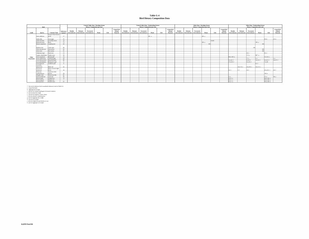
Table G-4Bird Dietary Composition Data
Guild Species Common NameBenthic
InvertebratesNektonic
InvertebratesTerrestrial
Invertebrates Plants Fish
Unspecified Animal
MaterialBenthic
InvertebratesNektonic
InvertebratesTerrestrial
Invertebrates Plants Fish
Unspecified Animal
MaterialBenthic
InvertebratesNektonic
InvertebratesTerrestrial
Invertebrates Plants Fish
Unspecified Animal
MaterialBenthic
InvertebratesNektonic
InvertebratesTerrestrial
Invertebrates Plants Fish
Unspecified Animal
Material
BirdCentral Valley Data - Breeding Season
Dietary Composition (percent) Dietary Composition (percent)Central Valley Data - Nonbreeding Season Other Data - Nonbreeding Season
Reference Number*
Dietary Composition (percent) Dietary Composition (percent)Other Data - Breeding Season
Anser albifronsGreater white-fronted goose 27 100 - a 100 -a
Ardea alba Great egret 55 90 -b 10 -b Ardea herodias Great blue heron 10 mostlyBranta bernicla Brant 73 100 -a 100 -aBranta canadensis Canada goose 62 100 100
Bubulcus ibis Cattle egret 89 100Chen caerulescens Snow goose 63 100Chen rossii Ross' goose 81 100
Chlidonias niger Black tern 23 30 -e 93 -e
Cygnus columbianus Tundra swan 50 1.3 -a 98.7 -aLarus argentatus Herring gull 72 86 to 100 -a 0 to 14 -aLarus californicus California gull 94 77 -c 5 -c 5 -c Larus delawarensis Ring-billed gull 80 5 to 42 -f 0 to 8 -f 5 to 31 -f 0 to 61 -f 2 to 97 -fLarus philadelphia Bonaparte's gull 9 17 to 93 -f 0 to 33 -f 7 to 50Larus pipixcan Franklin's gull 8 61 -fLaterallus jamaicensis Black rail 25 14 to 73 -c 14 to 95 -c 16 to 51 -cNycticorax nycticorax
Black-crowned night-heron 16 21 -f 5 -f 16 -f 29 to 59 -f 30 -f
Pelecanus erythrorhyncos
American white pelican 28 100 -a
Plegadis chihi White-faced ibis 82Sterna antillarum Least tern 90 5 -a 57 -a 38 -aSterna caspia Caspian tern 15 0 to 2 -a 98 to 100 -aSterna elegans Elegant tern 7 0 to 1 -a 99 to 100 -aSterna forsteri Forster's tern 57 0 to 1 -a 99 to 100 -a
* - See end of reference list for numbered references cited in Table G-4a - unspecified unitsb - aggregate percentagesc - percent by volume (esophageal of stomach contents)d - percent total dry weighte - percent by frequency of prey choicef - percent stomach containing itemg - percent aggregate dry weighth - percent wet weightj - percent weight not specified dry or wetk - percent aggregate wet weight
Other Waterbirds
SLDFR Final EIS
Appendix G Ecological Risk Assessment, In-Valley Disposal Alternative
SLDFR Final EIS Appendix G G-40
[This page left intentionally blank]

Appendix G Ecological Risk Assessment, In-Valley Disposal Alternative
SLDFR Final EIS Appendix G G-41
Dietary composition percentages used for this evaluation are presented in Table G-5, and discussed in the following sections. The following equation is used to calculate the average dietary Se concentration for each bird category:
BXgroup = (Pv * Veg [Se]) + (Pn * Nektos [Se]) + (Pb * Benthos [Se])
Where:
BXgroup = Average dietary concentration for birds within the category being considered (mg Se/kg tissue (dry weight))
Pv = Proportion of diet from vegetation
Pn = Proportion of diet from nektonic inverts
Pb = Proportion of diet from benthic invertebrates
Table G-5 Estimated Dietary Composition for Bird Categories
Dietary Composition (Percent) Breeding Season Nonbreeding Seasons
Bird Category B
enth
ic
Inve
rteb
rate
s
Nek
toni
c In
vert
ebra
tes
Plants Source Ben
thic
In
vert
ebra
tes
Nek
toni
c In
vert
ebra
tes
Plants Source
Dabblers (except for Northern Shoveler)
77 8 15
Estimated from data presented in
Table G-4 (no Central Valley data)
42 9 49
Euliss et al. (1991)
(Central Valley data on northern
pintail)
Northern Shoveler 0 100 0
Estimated from data presented in
Table G-4 and
Euliss et al. (1991)
5 88 7
Euliss et al. (1991)
(Central Valley data)
Divers 85 0 15 Brua (2002)
(Ruddy duck at Tulare Basin)
53 37 10
Euliss et al. (1991)
(Central Valley data on ruddy
duck)
Shorebirds (“Breeding” and “Nonbreeding)
96 4 0
Cooper et al. (unpublished)
(Central Valley stilts and avocets)
96 4 0
Cooper et al. (unpublished)
(Central Valley stilts and avocets)

Appendix G Ecological Risk Assessment, In-Valley Disposal Alternative
SLDFR Final EIS Appendix G G-42
G5.3.1 Dabblers For dabblers, no studies were found on dietary composition conducted in the Central Valley during the breeding season. Central Valley data collected during other seasons indicate that plants make up approximately 61 to 97 percent of the diet of the dabbler species investigated, but little information is available on nektonic or benthic invertebrates in the diet. A review of dietary data collected from other areas indicates that, in general, dabblers forage primarily on plant material during most seasons. However, during the breeding season, benthic and/or nektonic invertebrates can compose up to 100 percent of the diet. Northern shovelers tend to feed primarily on invertebrates throughout the year, and are not typical of other dabblers in this respect. Therefore, for the purposes of the exposure and risk analysis, the northern shoveler will be evaluated separately from other birds in the “dabbler” category.
Euliss et al. 1991 collected dietary composition data on northern pintails during September through March (fall and winter seasons), but no data for spring or summer (breeding season). A review of the data presented by Euliss et al. (1991) indicates that during October 100 percent of the diet was plant material. September was the only other fall month for which data were collected, and these data indicate that approximately 43 percent of the diet was plant material, 43 percent was benthic invertebrates, and 14 percent was nektonic invertebrates. During winter, Euliss et al. (1991) presented data for the three months of January, February, and March. During January, 100 percent of the diet was composed of vegetation. However, during February, approximately 11 percent of the diet was benthic invertebrates, and 18 percent was nektonic invertebrates. During March, approximately 75 percent of the diet was benthic invertebrates and 8 percent was unspecified animal material. No data were collected during November or December by Euliss et al., but it is assumed that the diet during this time would be close to 100 percent plant material.
Based on the data presented by Euliss et al. (1991), the aggregated percent dry weight dietary data for northern pintails collected over the entire study period (September–March) are used to represent dietary composition for dabblers during the nonbreeding seasons (August–April): 42 percent benthic invertebrates, 9 percent nektonic invertebrates, and 49 percent plant material (see Table G-5).
The data presented in Table G-4 indicate that at least some dabbler species (blue-winged teal, mallard, and gadwall) tend to eat higher quantities of invertebrates during the breeding season than during other periods of the year. In most cases, the types of invertebrates or animal material were not specified. Therefore, the following dietary composition for dabblers are used during the breeding season (May–July): 77 percent benthic invertebrates, 8 percent nektonic invertebrates, and 15 percent plant material (see Table G-5). While data presented in Table G-4 indicate that the blue-winged teal may consume a higher percentage of invertebrates (85 to 91 percent) during the breeding season, this species is infrequently observed at evaporation basins compared to other dabbler species (see Table G-2).
The Euliss et al. (1991) study also included data on the dietary composition of northern shovelers foraging at evaporation basins. Again, no data for spring or summer were presented. However, data from other areas indicate that during the breeding season, this species consumed 94 percent benthic invertebrates and 5 percent unspecified animal material. Because this species has been observed to forage primarily on nektonic species in Central Valley evaporation basins, it is

Appendix G Ecological Risk Assessment, In-Valley Disposal Alternative
SLDFR Final EIS Appendix G G-43
reasonable to assume that during the breeding season, northern shovelers foraging at evaporation basins in the Central Valley may consume up to 100 percent nektonic invertebrates.
Based on the data presented by Euliss et al. (1991), aggregated percent dry weight dietary data for northern shovelers collected over the entire study period (September–March) are used to represent dietary composition for this species during the nonbreeding seasons (August–April): 5 percent benthic invertebrates, 88 percent nektonic invertebrates, and 7 percent plant material (see Table G-5).
G5.3.2 Divers The Euliss et al. (1991) study included data on the dietary composition of ruddy ducks foraging at evaporation basins. Again, no data for spring or summer were presented in this study. However, data collected at evaporation basins in Tulare Basin indicate that this species consumed 85 percent benthic invertebrates and 15 percent plant matter during March and April, right before the breeding season (Brua 2002). Data collected from other areas indicate that other species of divers consume 65 to 100 percent nektonic invertebrates during the breeding season (see Table G-4). The long-tailed duck was reported to consume 100 percent nektonic invertebrates; however, this species was infrequently observed at evaporation basins compared to other species of divers (see Table G-2). Therefore, the data collected for the ruddy duck at Tulare Basin are used to represent the dietary composition of divers at evaporation basins during the breeding season (see Table G-5).
Based on the data presented by Euliss et al. (1991), aggregated percent dry weight dietary data for ruddy ducks collected over the entire study period (September–March) are used to represent dietary composition for divers during the nonbreeding seasons (August–April): 53 percent benthic invertebrates, 37 percent nektonic invertebrates, and 10 percent plant material (see Table G-5).
G5.3.3 Shorebirds (“Breeding” and “Nonbreeding”) Cooper et al. (unpublished) collected data on the dietary composition of the American avocet and black-necked stilt foraging at San Joaquin Valley evaporation basins. The report does not present numbers for dietary percentages; data are presented in charts and graphs from which the reader must estimate numerical percentages. 1992 data for the American avocet indicated that benthic invertebrates composed approximately 96 percent of the diet. For the black-necked stilt, benthic invertebrates composed approximately 63 and 79 percent of the diet in 1991 and 1992, respectively. Although data from other locations (see Table G-4) indicate that the diet of these two species may be composed of a larger percentage of nektonic invertebrates in some cases, site-specific data were preferred for this evaluation. To be adequately protective of all shorebird species, the assumed dietary composition is 96 percent benthic invertebrates, 4 percent nektonic invertebrates throughout the year (both breeding and nonbreeding seasons) (see Table G-5). These values apply to both “breeding shorebirds” (those species that are expected to breed at evaporation basins) and to “nonbreeding shorebirds” (those species that are expected to forage but are not likely to breed at evaporation basins).

Appendix G Ecological Risk Assessment, In-Valley Disposal Alternative
SLDFR Final EIS Appendix G G-44
G5.3.4 Other Waterbirds and Upland Birds Dietary composition data for birds in the “other waterbirds” category are presented in Table G-4. A review of these data indicates that many of these species feed primarily on fish or terrestrial plants and invertebrates, and it is unlikely that aquatic invertebrates and plants from the evaporation basins would compose a high percentage of their diets. Similarly, it is expected that birds categorized as “upland birds” in Table G-2 obtain most of their food from terrestrial sources. Therefore, no quantitative evaluation of risks was conducted for the species categorized as “other waterbirds” or “upland birds” as these species are unlikely to experience significant exposure to Se via feeding on plants or invertebrates at evaporation basins. An exception is for raptors that may potentially be affected by feeding on waterbirds contaminated with Se from evaporation basins. Potential effects to raptors are addressed in Section G7.2.3.
G6 EFFECTS ASSESSMENT The effects assessment is a qualitative and quantitative description of the relationship between the predicted chemical concentration or dose and the nature of possible effects elicited in exposed receptors, populations, or ecological communities. In this evaluation, predicted plant and invertebrate tissue concentrations are used to determine whether adverse effects are likely in birds feeding at the evaporation basins.
As described in Section G4.3, the assessment endpoints defined in this evaluation include the following:
• Protection of populations of migratory ducks, waterfowl, and other birds likely to overwinter or forage but not breed at the proposed evaporation basins
• Protection of populations of shorebirds such as stilts and avocets, and other birds likely to nest, breed, and forage at the proposed evaporation basins
• Protection of individuals of threatened or endangered raptor species such as the American peregrine falcon that are likely to prey on aquatic birds that forage at evaporation basins
The measurement endpoint used in this evaluation consisted of predicting Se concentrations in the plant and invertebrate tissue, and comparing these predicted tissue concentrations to dietary thresholds associated with adverse effects in avian receptors. A literature search was conducted to identify Se dietary thresholds associated with adverse effects, including acute effects such as adult and chick mortality, as well as chronic sublethal effects such as reduced reproduction and embryo deformities. Duration of exposure was also considered, as birds that are nesting and breeding at the site are likely to receive longer-term, continuous exposure than birds that are overwintering or resting at the evaporation basins.
G7 RESULTS AND DISCUSSION
G7.1 Selenium Concentrations in Water, Plant, and Invertebrate Tissue Table G-6 presents the predicted Se concentrations in influent water and plant, nektonic invertebrate, and benthic invertebrate tissue for the proposed evaporation basins.

Appendix G Ecological Risk Assessment, In-Valley Disposal Alternative
SLDFR Final EIS Appendix G G-45
Table G-6 Predicted Selenium Concentrations in Influent Water and Dietary Tissue
[Se] in Influent Water (µg/L) [Se] in Plant Tissue (mg/kg dry weight)
[Se] in Nektonic Invertebrate Tissue (mg/kg dry weight)
[Se] in Benthic Invertebrate Tissue (mg/kg dry weight)
10 2.7 8.7 15.6
Table G-7 presents the average predicted Se concentrations in the dietary items of each bird category. These estimates were calculated based on the estimated dietary composition of each bird category, as described in Section G5.3.
Table G-7 Predicted Average Selenium Concentration in Diet of Each Bird Category
Average Dietary [Se] (mg/kg dry weight)
Bird Category Breeding Season Nonbreeding Seasons Dabblers (except for Northern Shoveler) 13.1 8.7
Northern Shoveler 8.7 8.6 Divers 13.7 11.8
Shorebirds (“Breeding” and “Nonbreeding”) 15.3 15.3
The following sections describe the Se levels associated with acute and chronic toxicity in birds, and characterize the potential effects likely to occur in the proposed evaporation basins.
G7.2 Avian Toxicity Thresholds for Selenium A literature search was conducted to identify Se dietary thresholds associated with adverse effects, including acute effects such as adult and chick mortality, as well as chronic sublethal effects such as reduced reproduction and embryo deformities. Avian feeding studies indicate that dietary Se concentrations that cause avian mortality are much higher than concentrations causing reproductive impairment (Peterson and Nebeker 1992). Of the reproductive effects studied, reduced egg hatchability is believed to be a more sensitive endpoint than teratogenesis.
Little quantitative information is available on potential Se-related effects to birds that utilize evaporation basins outside the breeding season, as migratory resting habitat or for overwintering (Hanson Environmental 2003; CH2M HILL 1993). Potential nonlethal effects may include weight loss, atrophy of feather follicles, and atrophy of lymphoid tissue (Hanson Environmental 2003). It is unknown whether these effects are likely to contribute to lower reproductive success. However, at high Se concentrations in dietary items, lethal effects are also possible.
The following sections describe the results of the literature search on Se toxicity. First, data on reproductive effects are described. These are the types of effects most often documented for Se, and are most relevant to birds that are likely to breed at the proposed evaporation basins. In the next section, data on mortality associated with Se exposure are summarized. In areas with high
Appendix G Ecological Risk Assessment, In-Valley Disposal Alternative
SLDFR Final EIS Appendix G G-46
Se concentrations, lethal effects may be relevant both for migratory birds that receive relatively short term exposure, as well as for nesting birds that receive longer term exposure.
G7.2.1 Reproductive Effect Thresholds Threshold effect levels for Se exposure have been estimated for breeding birds in the San Joaquin Valley (Hanson Environmental 2003). Thresholds have been developed for waterborne Se, dietary items (aquatic plants and invertebrates), and avian egg tissues. The incidence of adverse effects is likely to increase at concentrations in exceedance of these threshold levels. The majority of these thresholds correspond to bird tissue concentrations, primarily in eggs. Although many of these data were reviewed and are presented below, the objective of the current evaluation is to identify dietary Se concentrations that correspond to adverse effects in waterbirds.
G7.2.1.1 Concentrations in Dietary Components Se concentrations in dietary components of aquatic birds at Kesterson Reservoir and the San Luis Drain were highly elevated in the 1980s. Se concentrations measured in algae, rooted plants, net plankton, and various aquatic insects ranged from 20 to 332 mg/kg dry weight (Ohlendorf 2002). Total Se concentrations measured in aquatic invertebrates from 1983 through 1985 ranged from 45 to 215 mg/kg at Kesterson (Williams, Hothem, and Ohlendorf 1989). These concentrations are well above dietary levels estimated in the laboratory. Current Service guidelines indicate that the background concentration of Se in dietary components is <3 mg/kg dry weight, while concentrations between 3 to 7 mg/kg dry weight have the potential to cause adverse effects. Lemly (1996) reviewed data on Se toxicity and assigned a hazard ranking for dietary toxicity and reproductive failure in fish and aquatic birds from ingestion of Se-contaminated macroinvertebrates. A Se concentration of 2 to 3 mg/kg (dry weight) was assigned a hazard ranking of minimal toxicity, 3 to 4 mg/kg was assigned a hazard ranking of low toxicity, 4 to 5 mg/kg was assigned a hazard ranking of moderate toxicity, and greater than 5 mg/kg was assigned a hazard ranking of high toxicity. Peterson and Nebeker (1992) described the results of several comprehensive reviews on the effects of Se on animals. They concluded that it is widely agreed that chronic exposure to Se dietary concentrations greater than 5 mg/kg can result in adverse effects to birds and mammals. Dietary concentrations in exceedance of 7 mg/kg (i.e., the toxicity threshold) are associated with a high probability of adverse reproductive effects in birds (Byron et al. 2003).
Based on the studies discussed above, the significance threshold used to determine potential for adverse reproductive effects in this evaluation is a predicted average invertebrate tissue concentration exceeding 4 mg/kg Se (dry weight). The results of several dietary studies are provided in Table G-8.
It should be noted that no data exist that relate dietary Se concentrations to birds most likely to nest and breed at the site (recurvorostrids such as stilts and avocets). However, the egg tissue data presented below do include results of studies conducted on recurvorostrids, which indicates that birds in this family may be less sensitive to Se than some of the species included in the studies list in Table G-8.

Appendix G Ecological Risk Assessment, In-Valley Disposal Alternative
SLDFR Final EIS Appendix G G-47
Table G-8 Dietary Selenium Concentrations Associated with Adverse Reproductive Effects in Birds
Bird Species
Life Stage Endpoint Duration
Threshold Concentrations (dry weight) Reference
Mallard embryo hatching success chronic
NOAEL = 3.5 mg selenomethionine/kg feed LOAEL = 7 mg selenomethionine/kg
feed
Stanley et al. 1996
Mallard embryo hatching success chronic EC10 = 4.87 mg Se/kg feed
(form of Se not specified) Ohlendorf 2003
Mallard embryo hatching success chronic EL = 3 to 5 mg selenomethionine/kg feed
Heinz and Fitzgerald 1993a,b
Mallard embryo/ duckling
hatching success/ survival
chronic - 0 to 6
days old EL = 10 mg selenomethionine/kg feed Heinz and
Hoffman 1996
Mallard duckling
survival/ number
produced per hen
chronic – 0 to 21 days
EL = 10 mg selenomethionine/kg feed NOAEL = 10 mg sodium selenite/kg feed LOAEL = 25 mg sodium selenite/kg feed
Heinz et al. 1987
Mallard duckling survival chronic -
0 to 6 weeks old
NOAEL = 20 mg selenomethionine/kg feed LOAEL = 40 mg
selenomethionine/kg feed
Heinz, Hoffman, and Gold 1988
Mallard duckling survival Chronic 0 to 6 days
old
NOAEL = 4 mg selenomethionine/kg feed LOAEL = 8 mg selenomethionine/kg feed
Heinz, Hoffman, and Gold 1989
Chicken embryo hatching success chronic LOAEL = 5 mg sodium selenite/kg feed Ort and Latshaw
1978 Black-
Crowned Night Heron
embryo hatching success chronic NOAEL = 3.3 mg selenomethionine/kg
feed Smith et al. 1988
Japanese Quail embryo hatching
success chronic EL = 6 mg sodium selenite/kg feed El-Begearmi, Sunde, and
Ganther 1977
Japanese Quail embryo hatching
success chronic EL = 5 mg selenomethionine/kg feed Martin 1988, as cited in Heinz
1996 EL = effect level LOAEL = lowest-observable-adverse-effect level NOAEL = no-observable-adverse-effect level

Appendix G Ecological Risk Assessment, In-Valley Disposal Alternative
SLDFR Final EIS Appendix G G-48
Data from several studies were used to develop dose-response relationships for reproductive effects based on dietary Se concentrations. Because a substantial number of studies were conducted on mallards, only data on this species were used in the data set. Three endpoints were evaluated: percentage of fertile eggs hatched, percentage survival of ducklings to 6 days of age, and number of 6-day old ducklings produced per hen. Measured values for each of these endpoints were plotted against dietary Se concentrations on Figures G-5, G-6, and G-7.
For the endpoint of percentage eggs hatched, data were sufficient to evaluate two forms of Se: selenomethionine and sodium selenite. Figure G-5 shows that the percentage of fertile eggs hatched begins to decrease when the dietary concentration of selenomethionine exceeds approximately 4 mg/kg, and when the dietary concentration of sodium selenite exceeds approximately 8 mg/kg. Hatching success decreases by approximately 50 percent when the dietary concentration of selenomethionine reaches about 8 mg/kg, and hatching success is close to zero at a dietary selenomethionine concentration of 16 mg/kg. This endpoint is less sensitive to sodium selenate in the diet; at 25 mg/kg a decrease in hatching success of approximately 10 percent was exhibited. However, selenomethionine is the form of Se that occurs predominantly in invertebrate tissue. The fitted regression equations calculated based on the data are:
• Selenomethionine: Percent Eggs Hatched = 150.2 - 84.06 * exp(0.03547*[Se])
• Sodium selenite: Percent Eggs Hatched = 123.6 - 53.67 * exp(0.01087*[Se])
For the other two endpoints (percentage survival of ducklings to 6 days of age, and number of 6-day-old ducklings produced per hen), data were sufficient to evaluate only one form of Se: selenomethionine. Figure G-6 shows that the percentage survival begins to decrease when the dietary concentration of selenomethionine exceeds approximately 8 mg/kg, and survival is close to zero at a dietary selenomethionine concentration of 16 mg/kg. Figure G-7 shows that the number of surviving ducklings per hen begins to decrease when the dietary concentration of selenomethionine exceeds approximately 4 mg/kg, and survival is close to zero at a dietary selenomethionine concentration of 16 mg/kg. The fitted regression equations calculated based on the data are:
• Percent Survival = 105.8 - 5.058 * exp(0.1901*[Se])
• Number of Ducklings = 17.32 - 8.634 * exp(0.04374*[Se])

Appendix G Ecological Risk Assessment, In-Valley Disposal Alternative
SLDFR Final EIS Appendix G G-49
0
10
20
30
40
50
60
70
80
0 5 10 15 20 25 30Selenium Concentration in Diet (mg/kg dry weight)
Perc
ent E
ggs
Hat
ched
Selenomethionine Sodium seleniteFitted Selenomethionine Fitted Sodium selenite
Sources: Heinz et al. 1987, 1989 Figure G-5 Percentage of Fertile Eggs Hatched vs. Selenium Concentration in Diet of Mallard Ducks
0
20
40
60
80
100
120
0 2 4 6 8 10 12 14 16 18Selenium Concentration in Feed (mg/kg dry weight)
Perc
enta
ge S
urvi
val
Selenomethionine Fitted Selenomethionine
Source: Heinz et al. 1989 Figure G-6 Percentage Survival of Mallard Ducklings to 6 Days of Age vs. Selenium Concentration in
Diet of Parents

Appendix G Ecological Risk Assessment, In-Valley Disposal Alternative
SLDFR Final EIS Appendix G G-50
0
1
2
3
4
5
6
7
8
9
10
0 2 4 6 8 10 12 14 16 18 Selenium Concentration (mg/kg dry weight)
Num
ber o
f Duc
klin
gsSelenomethionine Fitted Selenomethionine
Sources: Heinz et al. (1989)
Figure G-7 Number of 6-Day-Old Mallard Ducklings Produced per Hen vs. Selenium (as Selenomethionine) Concentration in Diet
G7.2.1.2 Concentrations in Egg Tissue Eggs of various bird species were collected from Kesterson Reservoir from 1983 through 1985 (Ohlendorf and Hothem 1995). Mean Se concentrations in these eggs ranged from 3.2 to 180 mg/kg dry weight. Table G-9 provides the ranges of Se concentrations in eggs of waterbirds collected from Kesterson during this 3-year time period. Embryo deformities and malformations were observed at Kesterson during this time period. In fact, of the 578 nests monitored at Kesterson, including nests of waterbirds and some terrestrial species, at least 39 percent contained at least one dead or deformed embryo or chick. A direct correlation was found between Se concentrations in eggs and these adverse effects, such that embryo death or deformity increased and hatching success decreased as Se concentrations increased (Ohlendforf and Hothem 1995).
The effects concentration to 10 percent of the population (EC10) in egg tissue corresponding to teratogenesis in mallards, stilts, and avocets vary substantially, with EC10s of 23 mg/kg, 37 mg/kg, and 74 mg/kg, respectively (Ohlendorf, in press, as cited in Hanson Environmental 2003). Teratogenesis is a severe response and, therefore, it is a relatively insensitive endpoint. More subtle developmental effects, such as reduced hatchability, are expected to provide better estimates of chronic exposure levels (Heinz 1996; Skorupa 1998; Ohlendorf 2003). Some recent studies provide data to support the idea that reduced egg hatchability is a more sensitive endpoint than teratogenesis. For example, an EC10 of 16 mg/kg based on reduced hatchability was reported for mallards (Fairbrother et al. 1996, as cited in Hanson Environmental 2003). In

Appendix G Ecological Risk Assessment, In-Valley Disposal Alternative
SLDFR Final EIS Appendix G G-51
addition, Ohlendorf (2003) calculated a geometric mean egg Se threshold level (EC10) of 12.5 mg/kg from the available data on mallards.
Table G-9 Selenium Concentrations in Bird Eggs Collected from
Kesterson Reservoir, 1983–1985
Species Egg Concentrations (mg/kg dry weight)
Eared grebe (Podilymbus nigricollis) 44–130 Mallard (Anas platyrhynchos) 3.6–31
Cinnamon teal (Anas cyanoptera) 3.9–37 Gadwall (Anas strepera) 7.3–33
American coot (Fulica americana) 17–74 Killdeer (Charadrius vociferus) 14–180
Black-necked stilt (Himantopus mexicanus) 4.3–100 American avocet (Recurvirostra americana) 3.2–88
Forster’s tern (Sterna forster) 6.7–18
Skorupa and Ohlendorf (1991) established two linear regression models to evaluate the relationships between (1) waterborne Se and concentrations in the food chain and (2) dietary Se and mean egg Se residues. The first model incorporated field data from evaporation basins within the San Joaquin Valley, and the second model was based on laboratory studies with farm-raised mallards exposed to selenomethionine in their diet. The results of the regression analysis indicated that water-borne Se concentrations of 0.5–2.3 µg/L represent the range not exceeding the egg tissue threshold level of 3 mg/kg dry weight (0.9 mg/kg wet weight). At the time the models were established, this level was assumed to equal the natural background concentration because embryo deformities were seen in only 3 of 55 populations of birds at this concentration (Hanson Environmental. 2003). However, the egg tissue threshold level of 3 mg/kg dry weight was later re-evaluated (as discussed below) based on a more robust and current data set.
Subsequent to the analysis of additional egg tissue data for stilts and avocets in relation to the incidence of reproductive effects, Skorupa (1998) calculated a threshold level of 6 mg Se/kg egg tissue dry weight. This threshold level represents an upper bound estimate of safe exposure levels for stilt embryos based on a no-observed-effect concentration for reproductive effects and is currently proposed by the Service as the threshold level for Se in avian egg tissue. This value was applied to the regression model to generate the Service recommended chronic water quality criterion of 2 µg/L for the protection of waterbirds. Current guidelines (Service) indicate that the respective background concentrations of Se in water (as total recoverable Se) and waterbird eggs are <2 µg/L and <6 mg/kg dry weight. Concentrations in water between 2 to 5 µg/L and in eggs between 6 to 10 mg/kg dry weight have the potential to cause effects. Finally, Se concentrations in exceedance of 5 µg/L in water and 10 mg/kg dry weight in egg tissue are associated with a high probability of adverse effects in birds (Byron et al. 2003). The current USEPA ambient water quality criterion for chronic Se exposure of 5 µg/L is above the recommended Service criterion (i.e., “no effects” threshold level) of 2 µg/L.
Appendix G Ecological Risk Assessment, In-Valley Disposal Alternative
SLDFR Final EIS Appendix G G-52
Brix (2000) evaluated the scientific justification used to establish the egg Se threshold level of 6 mg/kg dry weight proposed by the Service in an effort to develop an alternative threshold level. Brix (2000) derived dose-response relationships for the laboratory data available for mallards and dose-response relationships for existing field data for mallards and recurvirostrids, and then compared the results. By pooling the laboratory data for mallards, Brix (2000) established a dose-response relationship for duckling mortality and teratogenicity. The findings of this study indicate that conservative threshold levels (EC10s) are 16 mg/kg dry weight for chick mortality (i.e., reduced hatchability) and 26 mg/kg dry weight for teratogenic effects. The threshold level for chick mortality is more than two times greater than the level developed by Skorupa (1998) of 6 mg/kg dry weight, but the levels for teratogenesis are fairly similar (i.e., 26 mg/kg versus 23 mg/kg in the Skorupa [1998] study). Brix (2000) cites the main reason for the discrepancy between the two chick mortality threshold levels as the use of field data (in the Skorupa [1998] study), which is not a Se-specific endpoint due to the numerous other factors that could contribute to chick mortality. These confounding factors inherent in the field data are attributed to the much lower threshold level. Some of the confounding factors cited in the study include the presence of other contaminants, predators, weather, and starvation.
G7.2.2 Mortality Thresholds Heinz and Fitzgerald (1993b) evaluated the effects of overwinter exposure to Se on reproduction of mallards. Forty pairs of mallards were fed a dietary concentration of 15 mg/kg Se as selenomethionine for about 21 weeks during winter. The dietary concentration of 15 mg/kg Se was selected to represent a severe, prolonged exposure that would be likely to result in sublethal reproductive effects, without causing significant mortality in adults. However, four adults died during the 21 weeks of treatment. The Se treatment was discontinued at the start of the breeding season. Treated females lost weight, and their egg laying was delayed. During the first 2 weeks of egg laying, the hatching success in the treated group was lower than that in the control group, and a few of the early eggs contained deformed embryos. However, Se was quickly depurated from tissues, and after a period of about 2 weeks off the Se-treated diet, reproductive success returned to a level comparable to that of the control group (Heinz and Fitzgerald 1993b).
A concentration of 80 ppm sodium selenite in the diet of 6-week-old mallard ducklings resulted in 97.5 percent mortality by 6 weeks. A concentration of 80 ppm selenomethionine in the diet of 6-week-old mallard ducklings resulted in 100 percent mortality by 6 weeks. At 40 ppm, these two forms of Se resulted in 25 percent and 12.5 percent mortality, respectively. No mortality occurred at 20 ppm (Heinz, Hoffmann, and Gold 1988).
Eleven out of 12 adult mallards fed a diet containing 100 ppm Se as sodium selenate died within 16 to 39 days. One of 20 adult mallards fed a diet containing 25 ppm Se died at 57 days (Heinz 1987).
Adult male mallards were fed diets containing 0, 10, 20, 40, and 80 mg/kg Se as selenomethionine, with 20 birds in each treatment group. After 1 week of treatment, body weights were significantly lower in the 20, 40, and 80 mg/kg treatment groups, but not in the 10 mg/kg group. Mortality began in the 40 and 80 mg/kg treatment groups during the third week of treatment. By the fourth week, mortality in birds fed 80 mg/kg Se was significantly greater than at 10 or 20 mg/kg Se. By the eighth week, all birds in the 80 mg/kg treatment group had died. Mortality occurred by the 16th week in 19 out of 20 birds in the 40 mg/kg treatment group,

Appendix G Ecological Risk Assessment, In-Valley Disposal Alternative
SLDFR Final EIS Appendix G G-53
but the one survivor died 5 days after treatment ended. Mortality among mallards fed 20 mg/kg Se was significantly greater than the control group by the 13th week, and 25 percent died by the 16th week. No mortality occurred among birds fed 10 mg/kg Se during the 16-week treatment period. Mallards that died from Se treatments were severely emaciated. The lowest dietary concentration of Se associated with significant weight loss or mortality was 20 mg/kg (Heinz and Fitzgerald 1993a).
Based on results in this study and previous studies conducted, Heinz and Fitzgerald (1993a) concluded that the dietary threshold of Se causing weight loss and mortality in adult mallards is likely to be between 10 and 15 mg/kg dry weight. The threshold may be higher during warm weather. Diseases and other natural stressors, such as migration, breeding, and food shortages, may also affect the threshold. In addition, differences are likely to occur in the toxicity of different forms of Se, as well as differences in the sensitivity of various bird species (Heinz and Fitzgerald 1993a).
In another study conducted on adult male mallards over a 21-week warm weather period (March to July), groups of 21 birds each were fed diets containing 0, 10, 20, 40, and 80 mg/kg Se as selenomethionine. All ducks receiving 80 mg/kg Se died, and 15 percent of ducks receiving 40 mg/kg Se died during the treatment period. The authors hypothesized that the lower threshold for mortality observed in the Heinz and Fitzgerald (1993a) study may have been due to increased stress of cold temperatures (Albers et al. 1996).
In 16- and 20-week studies, no adverse effects on mortality rates, body weight, or food consumption were observed among Japanese quail administered a concentration of 6 ppm Se as sodium selenite in their diet. Increased mortality at 12 weeks, reduced egg production and hatchability, and increased deformities were observed among Japanese quail administered a concentration of 12 ppm Se as sodium selenite in their diet (El-Begearmi et al. 1977).
G7.2.3 Potential Effects to Raptors Predatory birds may feed on aquatic birds that forage on invertebrates in the evaporation basins. Aquatic birds that obtain a large amount of their diet from evaporation basins are likely to contain elevated Se levels in their tissue. Therefore, predatory birds are likely to receive Se exposure by feeding on these birds. American peregrine falcons (Falco peragrinus) have been observed feeding on shorebirds at the Tulare Lake Drainage District evaporation basins (Hanson Environmental 2003). Two sick American peregrine falcons were recovered during mid-summer 1992, and blood and feather samples collected from these birds contained elevated Se levels. One birds was too weak to fly. Both birds experienced full recovery after being fed a diet containing a normal Se concentration (Hanson Environmental 2003).
Santolo et al. (1999) investigated effects on reproduction in captive American kestrels (Falco sparverius) fed 6 and 12 mg/kg selenomethionine for 11 weeks. No statistically significant difference was observed between these groups and the control group in terms of percentage of pairs that laid eggs, numbers of pairs that were fertile, or hatchability of fertile eggs. The percentage of the total number of fertile eggs produced was lower in the group fed the 12 mg/kg Se diet than in the other two groups, but the difference was not statistically significant. The authors indicated that results were not conclusive regarding Se embryotoxicity, but suggested

Appendix G Ecological Risk Assessment, In-Valley Disposal Alternative
SLDFR Final EIS Appendix G G-54
that kestrels may be less sensitive to Se than are aquatic species such as mallards (Santolo et al. 1999).
Peregrine falcons are in the same family as kestrels (Falconidae), but feed primarily on birds, while the kestrels also feed on worms, insects, amphibians, reptiles, and small mammals (USEPA 1993). The size of the kestrel’s territory in winter has been estimated to range from approximately 10 to 452 hectares, and the territory size in summer has been estimated to range from approximately 21 to 500 hectares (USEPA 1993).
G7.3 Effects Characterization This section describes probable ecological effects predicted to occur in each bird category as a result of Se exposure at the proposed evaporation basins. Probable effects are determined by comparing the predictive average dietary concentrations with toxicity threshold data.
To estimate the number of birds in each category that would be exposed to Se at the proposed evaporation basins, the total size of the evaporation basins was multiplied by the bird density calculated using historical data (see Table G-3). Estimates were made for average conditions, when the total evaporation basin area would be approximately 2,870 acres, and for wet conditions, when the maximum total evaporation basin area would be approximately 3,290 acres. As discussed in Section G2.3.4, the median bird density is expected to best represent the central tendency. However, the mean would better account for pulses in densities, such as those that would occur during migrations. As there is uncertainty about how long individual birds would be likely to stay at the evaporation basins during the migration seasons (several days or several weeks), it may be useful to take into account temporary increases in densities. Therefore, the total number of birds in each category that would be expected to utilize the evaporation basins during each season were calculated using both the mean and the median bird densities, and results are presented in Tables G-10 and G-11, respectively.

Appendix G Ecological Risk Assessment, In-Valley Disposal Alternative
SLDFR Final EIS Appendix G G-55
Table G-10 Estimated Total Number of Birds Assuming Mean Density
Estimated Total Number of Birds (assuming mean density)
Season Bird Category
2,870 Acres Total Evaporation Basins
(average wetted area)
3,290 Acres Total Evaporation Basins
(maximum wetted area)Dabblers 4,232 4,851 Divers 5,018 5,752
Breeding Shorebirds 1,415 1,622 Nonbreeding Shorebirds 3,570 4,092
Upland Birds 235 270
Spring Migration (Feb-Apr)
Other Waterbirds 101 116 Dabblers 1,315 1,508 Divers 537 616
Breeding Shorebirds 2,015 2,310 Nonbreeding Shorebirds 2,567 2,942
Upland Birds 217 248
Breeding (May-Jul)
Other Waterbirds 316 362 Dabblers 2,739 3,140 Divers 2,001 2,294
Breeding Shorebirds 3,496 4,008 Nonbreeding Shorebirds 6,586 7,550
Upland Birds 230 264
Fall Migration (Aug-Oct)
Other Waterbirds 1,326 1,520 Dabblers 3,890 4,459 Divers 5,660 6,488
Breeding Shorebirds 1,794 2,057 Nonbreeding Shorebirds 8,487 9,729
Upland Birds 152 174
Winter (Nov-Jan)
Other Waterbirds 456 523

Appendix G Ecological Risk Assessment, In-Valley Disposal Alternative
SLDFR Final EIS Appendix G G-56
Table G-11 Estimated Total Number of Birds Assuming Median Density
Estimated Total Number of Birds (assuming median density)
Season Bird Category
2,870 Acres Total Evaporation Basins
(average wetted area)
3,290 Acres Total Evaporation Basins
(maximum wetted area)Dabblers 1,181 1,354 Divers 2,904 3,329
Breeding Shorebirds 347 398 Nonbreeding Shorebirds 751 860
Upland Birds 0 0
Spring Migration (Feb-Apr)
Other Waterbirds 0 0 Dabblers 201 230 Divers 47 53
Breeding Shorebirds 883 1,012 Nonbreeding Shorebirds 92 105
Upland Birds 0 0
Breeding (May-Jul)
Other Waterbirds 55 63 Dabblers 578 662 Divers 261 299
Breeding Shorebirds 1,198 1,373 Nonbreeding Shorebirds 2,127 2,438
Upland Birds 0 0
Fall Migration (Aug-Oct)
Other Waterbirds 254 291 Dabblers 662 759 Divers 2,843 3,259
Breeding Shorebirds 477 547 Nonbreeding Shorebirds 1,656 1,898
Upland Birds 0 0
Winter (Nov-Jan)
Other Waterbirds 29 33

Appendix G Ecological Risk Assessment, In-Valley Disposal Alternative
SLDFR Final EIS Appendix G G-57
G7.3.1 Dabblers As presented in Table G-7, mean dietary Se concentrations for dabblers foraging solely at the proposed evaporation basins are estimated to be 8.7 mg/kg dry weight during the nonbreeding seasons and 13.1 mg/kg dry weight during the breeding season. Because most dabblers are expected to forage at the evaporation basins primarily during the nonbreeding season, the effects assessment focuses on this period.
The data summarized in Section G7.2.2 indicate that the threshold for significant increases in adult mortality during winter is likely to be between 10 and 15 mg/kg, and probably varies depending on factors such as bird species and physical stresses such as weather. The average dietary Se concentrations predicted for dabblers during the nonbreeding seasons are below this range. Data indicate that during late spring as the breeding season approaches, dabblers tend to eat more invertebrates rather than plants. Assuming that during this period the average dietary Se concentrations approaches 13.1 mg/kg dry weight, some potential for effects to adult dabblers may occur. However, Heinz and Fitzgerald (1999b) found that a dietary concentration of 15 mg/kg Se was associated with the death of 10 percent of adult mallards over a 21-week period, longer than most dabblers would typically be expected to forage at evaporation basins during late spring as the breeding season approaches.
Although the proposed evaporation basins are not expected to provide appropriate breeding habitat for dabblers because vegetation is controlled to minimize nesting habitat, it is possible that some individuals will nest close by and may forage primarily at the evaporation basins during the breeding season. Individual dabblers foraging primarily on invertebrates at evaporation basins during the breeding season are expected to have an average dietary Se concentration of approximately 13.1 mg/kg dry weight, which exceeds the threshold for reproductive effects (approximately 4 mg/kg) and may also cause loss of body weight and possibly mortality in adults over an extended period (several months).
As described in Section G7.2.1.1, Figure G-5 shows that the percentage of fertile eggs hatched begins to decrease when the dietary concentration of selenomethionine exceeds approximately 4 mg/kg. Hatching success decreases by approximately 50 percent when the dietary concentration of selenomethionine reaches about 10 mg/kg, and hatching success is close to zero at a dietary selenomethionine concentration of 16 mg/kg. Figure G-6 shows that the percentage of survival of ducklings begins to decrease when the dietary concentration of selenomethionine exceeds approximately 8 mg/kg, and survival is close to zero at a dietary selenomethionine concentration of 16 mg/kg. Figure G-7 shows that the number of surviving ducklings per hen begins to decrease when the dietary concentration of selenomethionine exceeds approximately 4 mg/kg, and survival is close to zero at a dietary selenomethionine concentration of 16 mg/kg. Based on these findings, significant decreases in reproduction (at least 50 percent reduction), and possibly elimination of successful reproduction, would be expected in birds that obtain 100 percent of their food from the evaporation basins for a period of at least several weeks during the breeding season.
As described in Section 5.3.1, the diet of the northern shoveler is atypical of other dabblers, as it tends to forage primarily on nektonic invertebrates year-round. Mean dietary Se concentrations for northern shovelers foraging solely at the proposed evaporation basins are estimated to be 8.6 mg/kg dry weight during the nonbreeding seasons and 8.7 mg/kg dry weight during the

Appendix G Ecological Risk Assessment, In-Valley Disposal Alternative
SLDFR Final EIS Appendix G G-58
breeding season. Therefore, the northern shoveler population would be unlikely to experience lethal effects due to Se concentrations in diet, but northern shoveler individuals nesting close by and foraging primarily at evaporation basins during the breeding season may experience some decrease in reproductive success.
As shown in Table G-10, the number of dabblers estimated to be present at the proposed evaporation basins (assuming mean densities) ranges from 1,315 during the breeding season under average conditions to 4,851 during spring migration under wet conditions (maximum wetted area). As shown in Table G-11, the number of dabblers estimated to be present at the proposed evaporation basins (assuming median densities) ranges from 201 during the breeding season under average conditions to 1,354 during spring migration under wet conditions (maximum wetted area). As can be seen from Table G-2, approximately 64% of the dabblers observed at evaporation basins are northern shovelers (the total count of northern shovelers over the monitoring period was 462,878, while the total count for all dabblers was 725,848.
If it is assumed that the dabblers present during breeding season obtain all of their food from the evaporation basins with an average concentration of 13.1 mg/kg Se for dabblers other than the northern shoveler, and 8.7 mg/kg for the northern shoveler, it would be expected that approximately 60 (assuming median densities under average conditions) to 473 (assuming mean densities and maximum wetted area) individuals would experience a significant decrease in reproductive success, and some may also experience loss of body weight and possibly death. Dabblers present during other times of the year would not be expected to experience significant effects.
G7.3.2 Divers As presented in Table G-7, mean dietary Se concentrations for divers foraging solely at the proposed evaporation basins are estimated to be 11.8 mg/kg dry weight during the nonbreeding seasons and 13.7 mg/kg dry weight during the breeding season. Similarly to dabblers, most divers are expected to forage at the evaporation basins primarily during the nonbreeding season.
The average dietary Se concentrations predicted for divers during both the nonbreeding and breeding seasons are within the range likely to cause a low level of adult mortality (10 to 15 mg/kg). Based on data collected by Heinz and Fitzgerald (1993b), a concentration of approximately 15 mg/kg Se would be expected to result in the death of approximately 10 percent of adults over a period of several months.
Although the proposed evaporation basins are not expected to provide appropriate breeding habitat for divers because vegetation is controlled to minimize nesting habitat, it is possible that some individuals will nest close by and may forage primarily at the evaporation basins during the breeding season. Individual divers foraging primarily on invertebrates at evaporation basins during the breeding season are expected to have an average dietary Se concentration of approximately 13.7 mg/kg dry weight, which would be expected to decrease reproductive success by close to 100 percent.
As shown in Table G-10, the number of divers estimated to be present at the proposed evaporation basins (assuming mean densities) ranges from 537 during the breeding season under average conditions to 6,488 during winter under wet conditions (maximum wetted area). As shown in Table G-11, the number of divers estimated to be present at the proposed evaporation

Appendix G Ecological Risk Assessment, In-Valley Disposal Alternative
SLDFR Final EIS Appendix G G-59
basins (assuming median densities) ranges from 47 during the breeding season under average conditions to 3,329 during spring migration under wet conditions (maximum wetted area).
If it is assumed that the divers present during breeding season obtain all of their food from the evaporation basins with an average concentration of 13.7 mg/kg Se, it would be expected that approximately 47 (assuming median densities under average conditions) to 537 (assuming mean densities and maximum wetted area) individuals would experience a significant decrease in reproductive success, and some may also experience loss of body weight and possibly death. If it is assumed that the divers present during winter or spring migration season (up to 6,488 during winter under wet conditions) are obtaining all of their food from the evaporation basins with an average concentration of 11.8 mg/kg Se over a period of at least several months, it is possible that a small proportion of these individuals (less than 10 percent of the total number of individuals present, or up to 649) may experience loss of body weight and possibly death.
G7.3.3 Shorebirds (“Breeding” and “Nonbreeding”) As presented in Table G-7, mean dietary Se concentrations for shorebirds foraging solely at the proposed evaporation basins are estimated to be 15.3 mg/kg dry weight during both the breeding and the nonbreeding seasons. This means that all types of shorebirds (both “breeding” and “nonbreeding”) feeding primarily at the proposed evaporation basins for at least several months at a time may experience an increase in mortality due to elevated Se concentrations in their diets. Based on data collected by Heinz and Fitzgerald (1993b), a concentration of approximately 15 mg/kg Se would be expected to result in the death of approximately 10 percent of adults.
Because those shorebirds likely to breed at the evaporation basins (avocets, black-necked stilts, killdeer, and snowy plovers) are more likely to forage there than “nonbreeding” shorebirds, these species are more likely to experience increased mortality. In addition, the average predicted dietary concentration of 15.3 mg/kg Se is high enough to decrease reproductive success by close to 100 percent.
As shown in Table G-10, the number of breeding shorebirds estimated to be present at the proposed evaporation basins (assuming mean densities) ranges from 1,415 during the spring migration season under average conditions to 4,008 during fall migration under wet conditions (maximum wetted area). As shown in Table G-11, the number of breeding shorebirds estimated to be present at the proposed evaporation basins (assuming median densities) ranges from 347 during the spring migration season under average conditions to 1,373 during spring migration under wet conditions (maximum wetted area).
If it is assumed that the breeding shorebirds present during breeding season are obtaining all of their food from the evaporation basins with an average concentration of 15.3 mg/kg Se, it would be expected that approximately 883 to 2,310 individuals would experience a significant decrease in reproductive success, and some (about 10 percent or less) may also experience loss of body weight and possibly death. If it is assumed that the breeding shorebirds present during winter or spring and fall migration seasons are obtaining all of their food from the evaporation basins with an average concentration of 15.3 mg/kg Se over a period of at least several months, it is possible that small proportion (about 10 percent or less) of these individuals may experience loss of body weight and possibly death.

Appendix G Ecological Risk Assessment, In-Valley Disposal Alternative
SLDFR Final EIS Appendix G G-60
As shown in Table G-10, the number of nonbreeding shorebirds estimated to be present at the proposed evaporation basins (assuming mean densities) ranges from 2,567 during the breeding season under average conditions to 9,729 during winter under wet conditions (maximum wetted area). As shown in Table G-11, the number of breeding shorebirds estimated to be present at the proposed evaporation basins (assuming median densities) ranges from 92 during the breeding season under average conditions to 2,438 during fall migration under wet conditions (maximum wetted area).
If it is assumed that the nonbreeding shorebirds present during breeding season are obtaining all of their food from the evaporation basins with an average concentration of 15.3 mg/kg Se for a period of at least several months, it would be expected that approximately 883 (assuming median densities under average conditions) to 2,310 (assuming mean densities and maximum wetted area) individuals would experience a significant decrease in reproductive success, and some (about 10 percent or less of the total number of individuals present) may also experience loss of body weight and possibly death. If it is assumed that the nonbreeding shorebirds present during winter or spring and fall migration seasons (up to 9,729 during winter assuming maximum wetted area) are obtaining all of their food from the evaporation basins with an average concentration of 15.3 mg/kg Se over a period of at least several months, it is possible that small proportion (about 10 percent or less of the total number of individuals present, or up to 973) of these individuals may experience loss of body weight and possibly death.
G7.3.4 Other Waterbirds and Upland Birds As discussed in Section G5.3.4, dietary composition data for birds in the “other waterbirds” category are presented in Table G-4. A review of these data indicates that many of these species feed primarily on fish or terrestrial plants and invertebrates, and it is unlikely that aquatic invertebrates and plants from the evaporation basins would compose a high percentage of their diets over an extended period of time. Similarly, it is expected that birds categorized as “upland birds” in Table G-2 obtain most of their food from terrestrial sources. In addition, the numbers of “upland birds” and “other waterbirds” observed are relatively low compared to the number of birds in other categories (see Tables G-10 and G-11). Therefore, no quantitative evaluation of risks was conducted for the species categorized as “other waterbirds” or “upland birds” as these species are unlikely to experience significant exposure to Se via feeding on plants or invertebrates at evaporation basins, in comparison to the other bird categories.
An exception is raptors that may potentially be affected by feeding on waterbirds contaminated with Se from evaporation basins. Raptors that obtain a significant portion of their prey in the form of birds that forage on evaporation basins may also experience toxicosis and/or mortality. However, due to their large foraging ranges, it is unlikely that raptors would obtain 100 percent of their prey from the evaporation basins.
G7.4 Uncertainty Any evaluation of ecological effects has a number of limitations, including the degree of success in meeting objectives, range of conditions over which conclusions can be applied, and certainty with which conclusions can be drawn (USEPA 1989). The conclusions of an effects assessment are useful once they have been placed into perspective relative to the uncertainties associated

Appendix G Ecological Risk Assessment, In-Valley Disposal Alternative
SLDFR Final EIS Appendix G G-61
with the evaluation. The major sources of uncertainty pertinent to this evaluation are discussed below.
G7.4.1 General Sources of Uncertainty Due to the multiplicity of potential receptor species and general lack of knowledge regarding their life cycles, feeding habits, and relative toxicological sensitivity, the uncertainty surrounding estimates of ecological effects may be substantial. Most of the criteria and parameters used in this assessment are intended to provide a conservative (high end) evaluation of potential effects. The measurement endpoints utilized are chemical-specific and, as such, cannot address the additive, antagonistic, or synergistic effects of the mixtures of chemicals typically found in the environment. Furthermore, they do not account for many site-specific conditions regulating chemical contact and bioavailability, the potential toxicity of other constituents that were not quantified, or the pervasive influence of physical stressors associated with short-term and long-term disruption by human activities.
G7.4.2 Specific Sources of Uncertainty In addition to the broadly influential general sources discussed above, several discrete sources of uncertainty are described below.
G7.4.2.1 Temporal and Spatial Distribution of Selenium Concentrations in Water Because this ecological evaluation is based on predicted concentrations of Se in water, all results are based on the accuracy of the water quality modeling results. Assumptions and uncertainties in the water quality modeling of influent Se concentrations are described in detail in Appendix C. In addition, it was assumed that the influent Se concentrations would be representative of Se concentrations in water throughout the evaporation basins. Se concentrations in water are likely to change as the water flows through the system, due to factors such as partitioning and bioaccumulation. However, it is difficult to quantitatively predict changes in concentrations.
G7.4.2.2 Selenium Speciation and Bioavailability Limited information is available to predict what forms of Se will exist in the proposed evaporation basins. Even if the speciation of Se in the treated influent to the basins could be predicted with a reasonable amount of certainty, it is difficult to predict what will happen to the Se speciation when the water flows through the basin. Because speciation is dependent on various chemical and physical parameters that are characteristic of conditions in the evaporation basins, the speciation is likely to eventually change if the residence time is long enough.
G7.4.2.3 Species Sensitivity No data could be found that relate dietary Se concentrations to effects to the birds species most likely to nest and breed at the site (recurvorostrids such as stilts and avocets). However, available egg tissue effects data do include results of studies conducted on recurvorostrids, which indicates that birds in this family may be less sensitive to Se than some other species such as mallards (Ohlendorf 2003). Sensitivity to Se exposure can vary substantially even in closely related
Appendix G Ecological Risk Assessment, In-Valley Disposal Alternative
SLDFR Final EIS Appendix G G-62
species, like stilts and avocets. The EC50 for overt teratogenesis was estimated to be 31 mg Se/kg egg tissue of dabbling ducks, whereas, the respective EC50s for stilts and avocets are 58 and 105 mg Se/kg egg tissue. These results indicate that ducks may be twice as sensitive to Se exposure as recurvirostrids, and avocets are relatively insensitive to selenosis (Skorupa 1998). The species examined in this study can be summarized as “sensitive” (duck), “average” (stilt), and “tolerant” (avocet) (Ohlendorf 2003).
The toxicity data used in this assessment were based mainly on studies conducted on mallards; therefore, potential effects to recurvorostrids such as stilts and avocets may be overpredicted.
G7.4.2.4 Exposure Assessment This evaluation assumed that birds nesting at the evaporation basins would be ingesting food obtained from the evaporation basins only. If adjacent foraging habitat is available, it is likely that birds would obtain a portion of their food from areas with lower Se concentration, and exposure would be lower than predicted in this assessment.
In addition, a significant amount of uncertainty exists regarding the duration of time that migrating and wintering birds would spend at one location. At the range of Se concentrations predicted to occur in the proposed evaporation basins, it is expected that several weeks to several months of continuous exposure would be required for individual birds to experience adverse effects. It was assumed (as a worst-case scenario) that most birds at the site would spend a sufficient amount of time at the site to allow for Se concentrations to accumulate in their tissues.
Although predictions of bird density are based on a substantial amount of historical monitoring data at existing evaporation basins, uncertainty exists in these predictions. Bird densities varied considerably at different evaporation basins, as shown in Table G-3. Densities may also vary from year to year and depending on factors such as nearby habitats and food availability.
This evaluation also assumed that the dietary compositions of all bird species and all individuals within each bird category would be identical. However, dietary composition is likely to vary considerably, depending on numerous factors such as species, food availability, and time of year. In general, this evaluation assumed dietary composition that would predict Se exposure at the high end of the range (i.e., more consumption of benthic invertebrates, which accumulate higher Se levels).
Se exposure in birds is a function of two main factors: Se concentration in dietary items and food ingestion rates. Ingestion rates may vary substantially among species and at different times of the year. However, ingestion rates were not considered in this evaluation.
G8 REFERENCES Agency for Toxic Substances and Disease Registry (ATSDR). 2001. Toxicological profile for
selenium. Draft for public comment. Update. U.S. Department of Health and Human Services, Public Health Service, Atlanta, GA.
Alaimo, J., R.S. Ogle, and A.W. Knight. 1994. Selenium uptake by larval Chironmus decorus from a Ruppia Maritima-based benthic/detrital substrate. Archives of Environmental Contamination and Toxicology 27: 441-448.

Appendix G Ecological Risk Assessment, In-Valley Disposal Alternative
SLDFR Final EIS Appendix G G-63
Albers, P.H., D.E. Green, and C.J. Sanderson. 1996. Diagnostic Criteria for Selenium toxicosis in aquatic birds: dietary exposure, tissue concentrations, and macroscopic effects. Journal of Wildlife Diseases 32(3): 468-485.
Amweg, E.L., D.L. Stuart, and D.P. Weston. 2003. Comparative bioavailability of selenium to aquatic organisms after biological treatment of agricultural drainage water. Aquatic Toxicology 63:13-25.
Baines, S.B., N.S. Fisher, and R. Stewart. 2002. Assimilation and retention of selenium and other trace elements from crustacean food by juvenile striped bass (Morono saxatilis) Limnology and Oceanography 47 (3): 646-655.
Brix, K.V., D.K. DeFrost, A. Fairbrother, and W.J. Adams. 2000. Critical review of tissue-based selenium toxicity thresholds for fish and birds. Planning for End Land Uses in Mine Reclamation, Proceedings of the Twenty-fourth Annual British Columbia Mine Reclamation Symposium, June, pp. 220-230.
Burton, G.A., Jr. 2001. Moving beyond sediment quality values and simple laboratory toxicity tests. SETAC Globe 2(2): 26-27.
Byron, E.R., H.M. Ohlendorf, G.M. Santolo, S.M. Benson, P.T. Zawislanski, T.K. Tokunaga, and M. Delamore. 2003. Ecological risk assessment example: waterfowl and shorebirds feeding in ephemeral pools at Kesterson Reservoir, CA. In Handbook of Ecotoxicology, 2nd edition, D.J. Hoffman, ed., pp. 985-1014. Boca Raton, FL: Lewis Publishers, Inc.
California Department of Fish and Game (CDFG). 1995. Staff report on burrowing owl mitigation. Sacramento, California. September.
California Department of Fish and Game (CDFG). 2003. Habitat Conservation Planning Branch web site. http://www.dfg.ca.gov/hcpb/species/t_e_spp/tespp.shtml.
California Environmental Protection Agency (Cal-EPA). 1996. Guidance for ecological risk assessment at hazardous waste sites and permitted facilities. Department of Toxic Substance Control, Human and Ecological Risk Division. June.
CH2M Hill, H.T. Harvey and Associates, and G.L. Horner. 1993. Cumulative Impacts of Agriculture Evaporation Basins on Wildlife. Technical report prepared for Department of Water Resources. February.
Cooper, R.J., C.S. McCasland, and D.A. Barnum. Unpublished. Dietary ecology of shorebirds using evaporation ponds of the San Joaquin Valley, California, with implications for use of pesticides to limit toxic exposure. Draft final report submitted to California Department of Water Resources, Fresno, CA.
Cox, R.R., Jr. and A.D. Afton. 2000. Predictable interregional movements by female northern pintails during winter. Waterbirds 23(2): 258-269.
Ehrlich, P.R., D.S. Dobkin, and D. Wheye. 1988. The Birder’s Handbook. New York: Simon and Schuster.
Eisler, R. 1985. Selenium hazards to fish, wildlife, and invertebrates: a synoptic review. U.S. Fish and Wildlife Service Biological Report 85 (1.5). Washington, D.C.

Appendix G Ecological Risk Assessment, In-Valley Disposal Alternative
SLDFR Final EIS Appendix G G-64
Eisler, R. 1988. Arsenic hazards to fish, wildlife, and invertebrates: a synoptic review. Biological Report 85(1.12), Contaminant Hazard Reviews. January.
Eisler, R. 1989. Molybdenum hazards to fish, wildlife, and invertebrates: a synoptic review. Biological Report 85(1.19), Contaminant Hazard Reviews. August.
Eisler, R. 1990. Boron hazards to fish, wildlife, and invertebrates: a synoptic review. Biological Report 85(1.20), Contaminant Hazard Reviews. April.
El-Begearmi, M. M., M. L. Sunde, and H. E. Ganther. 1977. A mutual protective effect of mercury and selenium in Japanese quail. Poultry Science 56:313-322.
Euliss, N.H. Jr., R.L. Jarvis, and D.S. Gilmer. 1991. Standing crops and ecology of aquatic invertebrates in agricultural drainwater basins in California. Wetlands 11:179-190.
Fan, T.W.M., S.J. Teh, D.E. Hinton, and R.M. Higashi. 2002. Selenium biotransformations into proteinaceous forms by foodweb organisms of selenium-laden drainage water in California. Aquatic Toxicology 57:65-84.
Goals Project. 2000. Baylands ecosystem species and community profiles: life histories and environmental requirements of key plants, fish, and wildlife. Prepared by the San Francisco Bay Area Wetlands Ecosystem Goals Project. P.R. Olofson, editor. San Francisco Bay Regional Water Quality Control Board, Oakland, CA.
Gordus, A.G., H.L. Shivaprasad, and P.K. Swift. 2002. Salt toxicosis in ruddy ducks that winter on an agricultural evaporation basin in California. Journal of Wildlife Diseases 38(1):124-131.
Goyer, R.A. 1986. Toxic effects of metals. In Casarett and Doull’s Toxicology – The Basic Science of Poisons, 3rd edition, C.D. Klasssen, ed. pp. 582-635. New York, NY: MacMillan Publishing Company.
H.T. Harvey & Associates. 1996a. Britz, Inc. Mitigation Assessment Report. October 15.
H.T. Harvey & Associates. 1996b. Westlake Farms, Inc. Mitigation Assessment Report. December 10.
H.T. Harvey & Associates. 1998. Final Rainbow Ranch Mitigation Assessment and Technical Report. January 26.
H.T. Harvey & Associates. 2000. Britz, Inc. 2000 Biannual Wildlife Monitoring Report. August 3.
H.T. Harvey & Associates. 2001a. Britz, Inc. 2000-2001 Biannual Wildlife Monitoring Report. May 1, 2001.
H.T. Harvey & Associates. 2001b. Britz, Inc. 2001 Biannual Wildlife Monitoring Report. December.
H.T. Harvey & Associates. 2001c. Draft Westlake Farms, Inc. 2001 Biannual Wildlife Monitoring Report. December 20.
H.T. Harvey & Associates. 2001d. Draft Lost Hills Water District 2001 Annual Wildlife Monitoring Report. December 20.

Appendix G Ecological Risk Assessment, In-Valley Disposal Alternative
SLDFR Final EIS Appendix G G-65
H.T. Harvey & Associates. 2001e. Lost Hills Water District Mitigation Assessment and Technical Report. March 23.
H.T. Harvey & Associates. 2002a. Britz, Inc. 2001-2002 Biannual Wildlife Monitoring Report. May 1.
H.T. Harvey & Associates. 2002b. Draft Westlake Farms, Inc. 2001-2002 Biannual Wildlife Monitoring Report. May 9.
H.T. Harvey & Associates. 2002c. Britz, Inc. 2002 Biannual Wildlife Monitoring Report. December 24.
H.T. Harvey & Associates. 2002d. Draft Lost Hills Water District 2002 Biannual Wildlife Monitoring Report. December 24.
H.T. Harvey & Associates. 2002e. Draft Westlake Farms, Inc. 2002 Biannual Wildlife Monitoring Report. December 24, 2002.
Hamilton, S.J. and A.D. Lemly. 1999. Water-sediment controversy in setting environmental standards for Se. Ecotoxicology and Environmental Safety 44: 227-235.
Hanson Environmental, Inc. 2003. Performance Assessment of Mitigation Actions Implemented at the Tulare Lake Drainage District Evaporation Basins: 1993–2001. Technical report prepared for Tulare Lake Drainage District for Submittal to California Regional Water Quality Control Board–Central Valley Region. March.
Heinz, G. H. 1996. Selenium in birds. In Environmental Contaminants in Wildlife Interpreting Tissue Concentrations, W. N. Beyer, G. H. Heinz, and A. W. Redmon-Norwood, eds., pp. 447-458. Boca Raton, FL: Lewis Publishers, Inc.
Heinz, G.H. and D.J. Hoffman. 1996. Comparison of the effects of seleno-L-methionine, seleno-DL-methionine, and selenized yeast on reproduction of mallards. Environmental Pollution 91: 169-175.
Heinz, G.H. and D.J. Hoffman. 1998. Methylmercury chloride and selenomethionine interactions on health and reproduction in mallards. Environmental Toxicology and Chemistry 17:139-145.
Heinz, G.H. and M.A. Fitzgerald. 1993a. Overwinter survival of mallards fed selenium. Archives of Environmental Contamination and Toxicology 25: 90-94.
Heinz, G.H. and M.A. Fitzgerald. 1993b. Reproduction of mallards following overwinter exposure to selenium. (unpublished) (Cited from Heinz and Fitzgerald 1993a).
Heinz, G.H., D.J. Hoffman, A.J. Krynitsky, and D.M.G. Weller. 1987. Reproduction in mallards fed selenium. Environmental Toxicology and Chemistry 6: 423-433.
Heinz, G.H., D.J. Hoffman, and L.G. Gold. 1988. Toxicity of organic and inorganic selenium to mallard ducklings. Archives of Environmental Contamination and Toxicology 17: 561-568.
Heinz, G.H., D.J. Hoffman, and L.G. Gold. 1989. Impaired reproduction of mallards fed an organic form of selenium. Journal of Wildlife Management 53: 418-428.

Appendix G Ecological Risk Assessment, In-Valley Disposal Alternative
SLDFR Final EIS Appendix G G-66
Hothem, R.L. and D. Welsh. 1994. Contaminants in eggs of aquatic birds from the grasslands of central California. Archives of Environmental Contamination and Toxicology 27:180-185.
Lemly, A.D. 1999. Selenium transport and bioaccumulation in aquatic ecosystems: a proposal for water quality criteria based on hydrological units. Ecotoxicology and Environmental Safety 42: 150-156.
Luoma, S.N. and T.S. Presser. 2000. Forecasting selenium discharges to the San Francisco Bay-Delta Estuary: ecological effects of a proposed San Luis Drain Extension. U.S. Geological Survey Open-File Report 00-416.
Luoma, S.N., C. Johns, N. Fisher, N.A. Steinberg, R.S., Oremland, and J.R. Reinfelder. 1992. Determination of Se bioavailability to a benthic bivalve from particulate and solute pathway. Environmental Science and Technology 26: 485-491.
Moore, S.B., J. Winckel, S.J. Detwiler, S.A. Klasing, P.A. Gaul, N.R. Kanim, B.E. Kesser, A.B. Debevec, K. Beardsley, and L.K. Puckett. 1990. Fish and Wildlife Resources and Agricultural Drainage in the San Joaquin Valley, California. Volume II. San Joaquin Valley Drainage Program, Sacramento, CA.
Nagpal N K and K. Howell. 2001. Water Quality Guidelines for Selenium, Technical Appendix. National Library of Canada Cataloguing in Publication Data.
O’Toole, D. and M.F. Raisbeck. 1997. Magic numbers, elusive lesions. Comparative aspects of selenosis in waterfowl and mammals. Chapter 19 in Environmental Chemistry of Selenium, W. T. Frankenberger and R.A. Engberg, eds, pp. 355-395. Books in Soils, Plants, and the Environment, Volume 64. New York, NY: Marcel Dekker, Inc.
Ohlendorf, H.M. 1989. Bioaccumulation and effects of selenium in wildlife. In Selenium in Agriculture and the Environment, L.W. Jacobs, ed., pp. 133-177. SSSA Special Publication No. 23. American Society of Agronomy and Soil Science Society of America, Madison, WI.
Ohlendorf, H.M., 2002. The birds of Kesterson Reservoir: a historical perspective. Aquatic Toxicology 57 (1-2):1-10.
Ohlendorf, H.M. 2003. Ecotoxicology of selenium. In Handbook of Ecotoxicology, 2nd edition, D.J. Hoffman, ed., pp. 465-500. Boca Raton FL: Lewis Publishers, Inc.
Ohlendorf, H. M. and R. L. Hothem. 1995. Agricultural drainwater effects on wildlife in Central California. In Handbook of Ecotoxicology, 2nd edition, D.J. Hoffman, ed., pp. 577-595.
Ort, J.F. and J.D. Latshaw. 1978. The toxic level of sodium selenite in the diet of laying hens. Journal of Nutrition 108: 1114-1120.
Parker, M.S. and A.W. Knight 1992. Aquatic invertebrates inhabiting saline evaporation ponds in the southern San Joaquin Valley, California. Bulletin of Southern California Academy of Science 98(1): pp. 39-43.
Peterson, J.A. and A.V. Nebeker. 1992. Estimations of waterborne selenium concentrations that are toxicity thresholds for wildlife. Archives of Environmental Contamination and Toxicology 23:154-162.

Appendix G Ecological Risk Assessment, In-Valley Disposal Alternative
SLDFR Final EIS Appendix G G-67
Sample, B.E., G. W. Suter II, M. B. Sheaffer, D. S. Jones, and R. A. Efroymson. 1997. Ecotoxicological Profiles for Selected Metals and Other Inorganic Chemicals. September.
Santolo, G.M., J.T. Yamamoto, J.M. Pisenti, and B.W. Wilson. 1999. Selenium accumulation and effects on reproduction in captive American kestrels fed selenomethionine. Journal of Wildlife Management 63:502-511.
Schlekat C.E., P.R. Dowdle, B.G. Lee, S.N. Luoma, and R.S. Oremland. 2000. Bioavailability of particle-associated Se to the bivalve Potamocorbula amurensis. Environmental Science and Technology 34 (21): 4504-4510.
Skorupa, J.P. 1998. Selenium poisoning of fish and wildlife in nature: lessons from twelve real-world examples. In Environmental Chemistry of Selenium, W.T. Frankenberger and R.A. Engberg, eds., pp. 315-354. New York, NY: Marcel Dekker, Inc.
Skorupa, J.P. and H.M. Ohlendorf. 1991. Contaminants in drainage water and avian risk thresholds. In The Economics and Management of Water and Drainage in Agriculture, A. Dinar and D. Zilberman, eds., pp. ???. Boston, MA: Kluwer Academic Publishers.
Smith, G.J., G.H. Heinz, D.J. Hoffman, J.W. Spann, and A.J. Krynitsky. 1988. Reproduction in black-crowned night-herons fed selenium. Lake Reservoir Management 4:175-180.
Stanley, T.R., Jr., G.J. Smith, D.J. Hoffman, G.H. Heinz, and R. Rosscoe. 1996. Effects of boron and selenium on mallard reproduction and duckling growth and survival. Environmental Toxicology and Chemistry 15(7):1124-1132.
Stanley, T.R., Jr., J.W. Spann, G.J. Smith, and R. Roscoe, 1994. Main and interactive effects of arsenic and selenium on mallard reproduction and duckling growth and survival. Archives of Environmental Contamination and Toxicology 26: 444-451.
Tanner, R., E.P. Glenn, and D. Moore. 1999. Food chain organisms in hypersaline, industrial evaporation ponds. Water Environment Research 71:494-505.
U.S. Environmental Protection Agency (USEPA). 1989. Evaluation of the Apparent Effects Threshold (AET) Approach for Assessing Sediment Quality, Report of the Sediment Criteria Subcommittee, Science Advisory Board. SAB-EETFC-89-027.
USEPA. 1993. Wildlife Exposure Factors Handbook. Volumes I and II. EPA/600/R-93/187a. ORD, Washington, DC. December.
USEPA. 1997. Ecological Risk Assessment Guidance for Superfund: Process for Designing and Conducting Ecological Risk Assessments. Interim Final. Environmental Response Team. June.
USEPA. 1998. Guidelines for Ecological Risk Assessment. EPA/630/R-95/002F. Final. Risk Assessment Forum, Washington DC. April.
USEPA. 2000. Bioaccumulation testing and interpretation for the purpose of sediment quality assessment: status and needs. EPA-823-R-00-001. Office of Water. February.
U.S. Fish and Wildlife Service (Service). 2003. Sacramento Fish and Wildlife Office, Endangered Species Information. http://sacramento.fws.gov/es/spp_info.htm.

Appendix G Ecological Risk Assessment, In-Valley Disposal Alternative
SLDFR Final EIS Appendix G G-68
Williams, M. L., R. L. Hothem, and H. M. Ohlendorf. 1989. Recruitment failure in American avocets and black-necked stilts nesting at Kesterson Reservoir, California, 1984-1985. The Condor 91:797.802.
World Health Organization (WHO). 1996. Guidelines for drinking-water quality, 2nd edition. Volume 2. Health criteria and other supporting information. Pages 328-338.
Zarn, M. 1974. Borrowing owl, Report no. 11. Habitat management service for unique or endangered species. U.S. Department of the Interior, Bureau of Land Management, Denver, CO.

Appendix G Ecological Risk Assessment, In-Valley Disposal Alternative
SLDFR Final EIS Appendix G G-69
References Cited in Table G-4
References from The Birds of America 1. Austin, J.E., and M.R. Miller. 1995. Northern pintail (Anas acuta). The Birds of North
America 163, A. Poole and F. Gill, editors. The American Ornithologists Union and Cornell Laboratory of Ornithology and the Academy of Natural Sciences.
2. Austin, J.E., C.M. Custer, and A.D. Afton. 1998. Lesser scaup (Aythya affinis). The Birds of North America 338, A. Poole and F. Gill, editors. The American Ornithologists Union and Cornell Laboratory of Ornithology and the Academy of Natural Sciences.
3. Beedy, E.C., and W.J. Hamilton III. 1999. Tricolored blackbird (Agelaius tricolor). The Birds of North America 423, A. Poole and F. Gill, editors. The American Ornithologists Union and Cornell Laboratory of Ornithology and the Academy of Natural Sciences.
4. Brua, R.S. 2002. Ruddy duck (Oxyura jamaicenses). The Birds of North America 696, A. Poole and F. Gill, editors. The American Ornithologists Union and Cornell Laboratory of Ornithology and the Academy of Natural Sciences.
5. Bull, E.L., and C.T. Collins. 1993. Vaux’s swift (Chaetura vauxi). The Birds of North America 77, A. Poole and F. Gill, editors. The American Ornithologists Union and Cornell Laboratory of Ornithology and the Academy of Natural Sciences.
6. Brisbin, I.L., Jr., and T.B. Mowbray. 2002. American coot (Fulica americana). The Birds of North America 697, A. Poole and F. Gill, editors. The American Ornithologists Union and Cornell Laboratory of Ornithology and the Academy of Natural Sciences.
7. Burness, G.P., K. LeFevre, and C.T. Collins. 1999. Elegant tern (Sterna elegans). The Birds of North America 404, A. Poole and F. Gill, editors. The American Ornithologists Union and Cornell Laboratory of Ornithology and the Academy of Natural Sciences.
8. Burger, J., and M. Gochfeld. 1994. Franklin’s gull (Larus pipixcan). The Birds of North America 116, A. Poole and F. Gill, editors. The American Ornithologists Union and Cornell Laboratory of Ornithology and the Academy of Natural Sciences.
9. Burger, J., and M. Gochfeld. 2002. Bonaparte’s gull (Larus philadelphia). The Birds of North America 634, A. Poole and F. Gill, editors. The American Ornithologists Union and Cornell Laboratory of Ornithology and the Academy of Natural Sciences.
10. Butler, R.W. 1992. Great blue heron (Ardea herodias). The Birds of North America 25, A. Poole, P. Stettenheim, and F. Gill, editors. The American Ornithologists Union and Cornell Laboratory of Ornithology and the Academy of Natural Sciences.
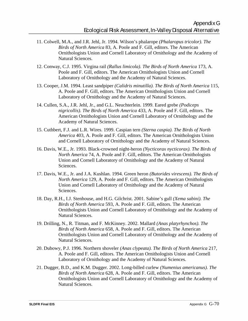
Appendix G Ecological Risk Assessment, In-Valley Disposal Alternative
SLDFR Final EIS Appendix G G-70
11. Colwell, M.A., and J.R. Jehl, Jr. 1994. Wilson’s phalarope (Phalaropus tricolor). The Birds of North America 83, A. Poole and F. Gill, editors. The American Ornithologists Union and Cornell Laboratory of Ornithology and the Academy of Natural Sciences.
12. Conway, C.J. 1995. Virgina rail (Rallus limicola). The Birds of North America 173, A. Poole and F. Gill, editors. The American Ornithologists Union and Cornell Laboratory of Ornithology and the Academy of Natural Sciences.
13. Cooper, J.M. 1994. Least sandpiper (Calidris minutilla). The Birds of North America 115, A. Poole and F. Gill, editors. The American Ornithologists Union and Cornell Laboratory of Ornithology and the Academy of Natural Sciences.
14. Cullen, S.A., J.R. Jehl, Jr., and G.L. Neuchterlein. 1999. Eared grebe (Podiceps nigricollis). The Birds of North America 433, A. Poole and F. Gill, editors. The American Ornithologists Union and Cornell Laboratory of Ornithology and the Academy of Natural Sciences.
15. Cuthbert, F.J. and L.R. Wires. 1999. Caspian tern (Sterna caspia). The Birds of North America 403, A. Poole and F. Gill, editors. The American Ornithologists Union and Cornell Laboratory of Ornithology and the Academy of Natural Sciences.
16. Davis, W.E., Jr. 1993. Black-crowned night-heron (Nycticorax nycticorax). The Birds of North America 74, A. Poole and F. Gill, editors. The American Ornithologists Union and Cornell Laboratory of Ornithology and the Academy of Natural Sciences.
17. Davis, W.E., Jr. and J.A. Kushlan. 1994. Green heron (Butorides virescens). The Birds of North America 129, A. Poole and F. Gill, editors. The American Ornithologists Union and Cornell Laboratory of Ornithology and the Academy of Natural Sciences.
18. Day, R.H., I.J. Stenhouse, and H.G. Gilchrist. 2001. Sabine’s gull (Xema sabini). The Birds of North America 593, A. Poole and F. Gill, editors. The American Ornithologists Union and Cornell Laboratory of Ornithology and the Academy of Natural Sciences.
19. Drilling, N., R. Titman, and F. McKinney. 2002. Mallard (Anas platyrhynchos). The Birds of North America 658, A. Poole and F. Gill, editors. The American Ornithologists Union and Cornell Laboratory of Ornithology and the Academy of Natural Sciences.
20. Dubowy, P.J. 1996. Northern shoveler (Anas clypeata). The Birds of North America 217, A. Poole and F. Gill, editors. The American Ornithologists Union and Cornell Laboratory of Ornithology and the Academy of Natural Sciences.
21. Dugger, B.D., and K.M. Dugger. 2002. Long-billed curlew (Numenius americanus). The Birds of North America 628, A. Poole and F. Gill, editors. The American Ornithologists Union and Cornell Laboratory of Ornithology and the Academy of Natural Sciences.

Appendix G Ecological Risk Assessment, In-Valley Disposal Alternative
SLDFR Final EIS Appendix G G-71
22. Dugger, B.D., K.M. Dugger, and L.H. Fredrickson. 1994. Hooded merganser (Lophodytes cucullatus). The Birds of North America 98, A. Poole and F. Gill, editors. The American Ornithologists Union and Cornell Laboratory of Ornithology and the Academy of Natural Sciences.
23. Dunn, E.H., and D.J. Agro. 1995. Black tern (Chlidonias niger). The Birds of North America 147, A. Poole and F. Gill, editors. The American Ornithologists Union and Cornell Laboratory of Ornithology and the Academy of Natural Sciences.
24. Eadie, J.M., M.L. Mallory, and H.G. Lumsden. 1995. Common goldeneye (Bucephala clangula). The Birds of North America 170, A. Poole and F. Gill, editors. The American Ornithologists Union and Cornell Laboratory of Ornithology and the Academy of Natural Sciences.
25. Eddleman, W.R., R.E. Flores, and M.L. Legare. 1994. Black rail (Laterallus jamaicensis). The Birds of North America 123, A. Poole and F. Gill, editors. The American Ornithologists Union and Cornell Laboratory of Ornithology and the Academy of Natural Sciences.
26. Elphick, C.S., and T.L. Tibbitts. 1998. Greater yellowlegs (Tringa melanoleuca). The Birds of North America 355, A. Poole and F. Gill, editors. The American Ornithologists Union and Cornell Laboratory of Ornithology and the Academy of Natural Sciences.
27. Ely, C.R., and A.X. Dzubin. 1994. Greater white-fronted goose (Anser albifrons). The Birds of North America 131, A. Poole and F. Gill, editors. The American Ornithologists Union and Cornell Laboratory of Ornithology and the Academy of Natural Sciences.
28. Evans, R.M., and F.L. Knopf. 1993. American white pelican (Pelecanus erythrorhynchos). The Birds of North America 57, A. Poole and F. Gill, editors. The American Ornithologists Union and Cornell Laboratory of Ornithology and the Academy of Natural Sciences.
29. Gammonley, J.H. 1996. Cinnamon teal (Anas cyanoptera). The Birds of North America 209, A. Poole and F. Gill, editors. The American Ornithologists Union and Cornell Laboratory of Ornithology and the Academy of Natural Sciences.
30. Gauthier, G. 1993. Bufflehead (Bucephala albeola). The Birds of North America 67, A. Poole and F. Gill, editors. The American Ornithologists Union and Cornell Laboratory of Ornithology and the Academy of Natural Sciences.
31. Gibbs, J.P., F.A. Reid, and S.M. Melvin. 1992. Least bittern (Ixobrychus exilis). The Birds of North America 17, A. Poole, P. Stettenheim, and F. Gill, editors. The American Ornithologists Union and Cornell Laboratory of Ornithology and the Academy of Natural Sciences.
32. Gibbs, J.P., S. Melvin, and F.A. Reid. 1992. American bittern (Botaurus lentiginosus). The Birds of North America 18, A. Poole, P. Stettenheim, and F. Gill, editors. The American Ornithologists Union and Cornell Laboratory of Ornithology and the Academy of Natural Sciences.

Appendix G Ecological Risk Assessment, In-Valley Disposal Alternative
SLDFR Final EIS Appendix G G-72
33. Gochfeld, M., and J. Burger. 1994. Black skimmer (Rynchops niger). The Birds of North America 108, A. Poole and F. Gill, editors. The American Ornithologists Union and Cornell Laboratory of Ornithology and the Academy of Natural Sciences.
34. Gratto-Trevor, C.L. 1992. Semipalmated sandpiper (Calidris pusilla). The Birds of North America 6, A. Poole, P. Stettenheim, and F. Gill, editors. The American Ornithologists Union and Cornell Laboratory of Ornithology and the Academy of Natural Sciences.
35. Gratto-Trevor, C.L. 2000. Marbled godwit (Limosa fedoa). The Birds of North America 492, A. Poole and F. Gill, editors. The American Ornithologists Union and Cornell Laboratory of Ornithology and the Academy of Natural Sciences.
36. Hamas, M.J. 1994. Belted kingfisher (Ceryle alcyon). The Birds of North America 84, A. Poole and F. Gill, editors. The American Ornithologists Union and Cornell Laboratory of Ornithology and the Academy of Natural Sciences.
37. Harrington, B.A. 2001. Red knot (Calidris canutus). The Birds of North America 563, A. Poole and F. Gill, editors. The American Ornithologists Union and Cornell Laboratory of Ornithology and the Academy of Natural Sciences.
38. Hatch, J.J. and D.V. Weseloh. 1999. Double-crested cormorant (Phalocrocorax auritus). The Birds of North America 441, A. Poole and F. Gill, editors. The American Ornithologists Union and Cornell Laboratory of Ornithology and the Academy of Natural Sciences.
39. Hepp, G.R., and F.C. Bellrose. 1995. Wood duck (Aix sponsa). The Birds of North America 169, A. Poole and F. Gill, editors. The American Ornithologists Union and Cornell Laboratory of Ornithology and the Academy of Natural Sciences.
40. Hohman, W.L., and R.T. Eberhardt. 1998. Ring-necked duck (Aythya collaris). The Birds of North America 329, A. Poole and F. Gill, editors. The American Ornithologists Union and Cornell Laboratory of Ornithology and the Academy of Natural Sciences.
41. Hohman, W.L., and S.A. Lee. 2001. Fulvous whistling-duck (Dendrocygna bicolor). The Birds of North America 562, A. Poole and F. Gill, editors. The American Ornithologists Union and Cornell Laboratory of Ornithology and the Academy of Natural Sciences.
42. Holmes, R.T., and F.A. Pitelka. 1998. Pectoral sandpiper (Calidris melanotos). The Birds of North America 348, A. Poole and F. Gill, editors. The American Ornithologists Union and Cornell Laboratory of Ornithology and the Academy of Natural Sciences.
43. Jackson, B.J.S., and J.A. Jackson. 2000. Killdeer (Charadrius vociferus). The Birds of North America 517, A. Poole and F. Gill, editors. The American Ornithologists Union and Cornell Laboratory of Ornithology and the Academy of Natural Sciences.

Appendix G Ecological Risk Assessment, In-Valley Disposal Alternative
SLDFR Final EIS Appendix G G-73
44. Jehl, J.R., Jr., J. Klima, and R.E. Harris. 2001. Short-billed dowitcher (Limnodromus griseus). The Birds of North America 564, A. Poole and F. Gill, editors. The American Ornithologists Union and Cornell Laboratory of Ornithology and the Academy of Natural Sciences.
45. Johnson, K. 1995. Green-winged teal (Anas crecca). The Birds of North America 193, A. Poole and F. Gill, editors. The American Ornithologists Union and Cornell Laboratory of Ornithology and the Academy of Natural Sciences.
46. Kessel, B., D.A. Rocque, and J.S. Barclay. 2002. Greater scaup (Aythya marila). The Birds of North America 650, A. Poole and F. Gill, editors. The American Ornithologists Union and Cornell Laboratory of Ornithology and the Academy of Natural Sciences.
47. Klima, J., and J.R. Jehl, Jr. 1998. Stilt sandpiper (Calidris himantopus). The Birds of North America 341, A. Poole and F. Gill, editors. The American Ornithologists Union and Cornell Laboratory of Ornithology and the Academy of Natural Sciences.
48. Knopf, F.L. 1996. Mountain plower (Charadrius montanus). The birds of North America 211, A. Poole and F. Gill, editors. The American Ornithologists Union and Cornell Laboratory of Ornithology and the Academy of Natural Sciences.
49. Leschack, C.R., S.K. McKnight, and G.R. Hepp. 1997. Gadwall (Anas strepera). The Birds of North America 283, A. Poole and F. Gill, editors. The American Ornithologists Union and Cornell Laboratory of Ornithology and the Academy of Natural Sciences.
50. Limpert, R.J., and S.L. Earnst. 1994. Tundra swan (Cygnus columbianus). The Birds of North America 89, A. Poole and F. Gill, editors. The American Ornithologists Union and Cornell Laboratory of Ornithology and the Academy of Natural Sciences.
51. Lowther, P.E., H.D. Douglas III, and C.L. Gratto-Trevor. 2001. Willet (Catoptrophorus semipalmatus). The Birds of North America 579, A. Poole and F. Gill, editors. The American Ornithologists Union and Cornell Laboratory of Ornithology and the Academy of Natural Sciences.
52. MacWhirter, R.B., and K.L. Bildstein. 1996. Northern harrier (Circus cyaneus). The Birds of North America 210, A. Poole and F. Gill, editors. The American Ornithologists Union and Cornell Laboratory of Ornithology and the Academy of Natural Sciences.
53. MacWhirter, B., P. Austin-Smith, Jr., and D. Kroodsma. 2002. Sanderling (Calidris alba). The Birds of North America 653, A. Poole and F. Gill, editors. The American Ornithologists Union and Cornell Laboratory of Ornithology and the Academy of Natural Sciences.
54. Mallory, M., and K. Metz. 1999. Common merganser (Mergus merganser). The Birds of North America 442, A. Poole and F. Gill, editors. The American Ornithologists Union and Cornell Laboratory of Ornithology and the Academy of Natural Sciences.
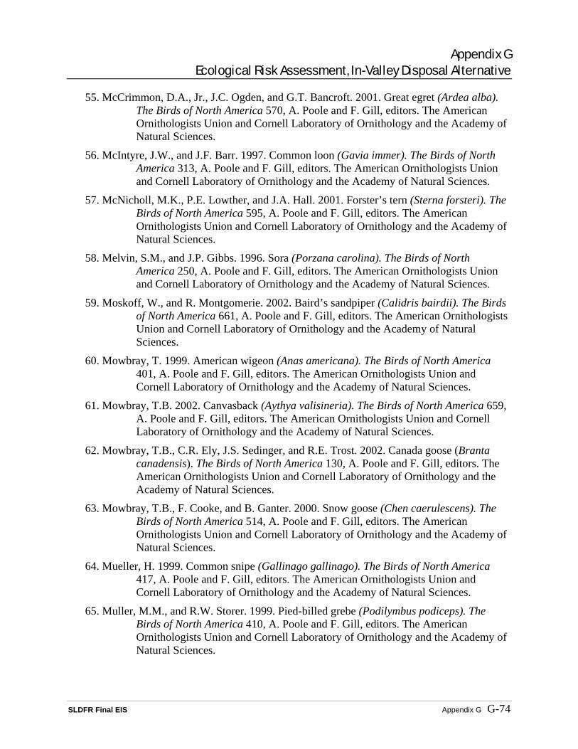
Appendix G Ecological Risk Assessment, In-Valley Disposal Alternative
SLDFR Final EIS Appendix G G-74
55. McCrimmon, D.A., Jr., J.C. Ogden, and G.T. Bancroft. 2001. Great egret (Ardea alba). The Birds of North America 570, A. Poole and F. Gill, editors. The American Ornithologists Union and Cornell Laboratory of Ornithology and the Academy of Natural Sciences.
56. McIntyre, J.W., and J.F. Barr. 1997. Common loon (Gavia immer). The Birds of North America 313, A. Poole and F. Gill, editors. The American Ornithologists Union and Cornell Laboratory of Ornithology and the Academy of Natural Sciences.
57. McNicholl, M.K., P.E. Lowther, and J.A. Hall. 2001. Forster’s tern (Sterna forsteri). The Birds of North America 595, A. Poole and F. Gill, editors. The American Ornithologists Union and Cornell Laboratory of Ornithology and the Academy of Natural Sciences.
58. Melvin, S.M., and J.P. Gibbs. 1996. Sora (Porzana carolina). The Birds of North America 250, A. Poole and F. Gill, editors. The American Ornithologists Union and Cornell Laboratory of Ornithology and the Academy of Natural Sciences.
59. Moskoff, W., and R. Montgomerie. 2002. Baird’s sandpiper (Calidris bairdii). The Birds of North America 661, A. Poole and F. Gill, editors. The American Ornithologists Union and Cornell Laboratory of Ornithology and the Academy of Natural Sciences.
60. Mowbray, T. 1999. American wigeon (Anas americana). The Birds of North America 401, A. Poole and F. Gill, editors. The American Ornithologists Union and Cornell Laboratory of Ornithology and the Academy of Natural Sciences.
61. Mowbray, T.B. 2002. Canvasback (Aythya valisineria). The Birds of North America 659, A. Poole and F. Gill, editors. The American Ornithologists Union and Cornell Laboratory of Ornithology and the Academy of Natural Sciences.
62. Mowbray, T.B., C.R. Ely, J.S. Sedinger, and R.E. Trost. 2002. Canada goose (Branta canadensis). The Birds of North America 130, A. Poole and F. Gill, editors. The American Ornithologists Union and Cornell Laboratory of Ornithology and the Academy of Natural Sciences.
63. Mowbray, T.B., F. Cooke, and B. Ganter. 2000. Snow goose (Chen caerulescens). The Birds of North America 514, A. Poole and F. Gill, editors. The American Ornithologists Union and Cornell Laboratory of Ornithology and the Academy of Natural Sciences.
64. Mueller, H. 1999. Common snipe (Gallinago gallinago). The Birds of North America 417, A. Poole and F. Gill, editors. The American Ornithologists Union and Cornell Laboratory of Ornithology and the Academy of Natural Sciences.
65. Muller, M.M., and R.W. Storer. 1999. Pied-billed grebe (Podilymbus podiceps). The Birds of North America 410, A. Poole and F. Gill, editors. The American Ornithologists Union and Cornell Laboratory of Ornithology and the Academy of Natural Sciences.

Appendix G Ecological Risk Assessment, In-Valley Disposal Alternative
SLDFR Final EIS Appendix G G-75
66. Nettleship, D.N. 2000. Ruddy turnstone (Arenaria interpres). The Birds of North America 537, A. Poole and F. Gill, editors. The American Ornithologists Union and Cornell Laboratory of Ornithology and the Academy of Natural Sciences.
67. Nol, E., and M.S. Blanken. 1999. Semipalmated plover (Charadrius semipalmatus). The Birds of North America 444, A. Poole and F. Gill, editors. The American Ornithologists Union and Cornell Laboratory of Ornithology and the Academy of Natural Sciences.
68. Oring, L.W., E.M. Gray, and J.M. Reed. 1997. Spotted sandpiper (Actitis macularia). The Birds of North America 289, A. Poole and F. Gill, editors. The American Ornithologists Union and Cornell Laboratory of Ornithology and the Academy of Natural Sciences.
69. Page, G.W., J.S. and J.C. Warriner, and P.W.C. Paton. 1995. Snowy plover (Charadrius alexandrinus). The Birds of North America 154, A. Poole and F. Gill, editors. The American Ornithologists Union and Cornell Laboratory of Ornithology and the Academy of Natural Sciences.
70. Parsons, K.C., and T.L. Master. 2000. Snowy egret (Egretta thula). The Birds of North America 489, A. Poole and F. Gill, editors. The American Ornithologists Union and Cornell Laboratory of Ornithology and the Academy of Natural Sciences.
71. Paulson, D.R. 1995. Black-bellied plover (Pluvialis squatarola). The Birds of North America 186, A. Poole and F. Gill, editors. The American Ornithologists Union and Cornell Laboratory of Ornithology and the Academy of Natural Sciences.
72. Pierotti, R.J., and T.P. Good. 1994. Herring gull (Larus argentatus). The Birds of North America 124, A. Poole and F. Gill, editors. The American Ornithologists Union and Cornell Laboratory of Ornithology and the Academy of Natural Sciences.
73. Reed, A., D.H. Ward, D.V. Derksen, and J.S. Sedinger. 1998. Brant (Branta bernicla). The Birds of North America 337, A. Poole and F. Gill, editors. The American Ornithologists Union and Cornell Laboratory of Ornithology and the Academy of Natural Sciences.
74. Robertson, G.J., and J-P.L. Savard. 2002. Long-tailed duck (Clangula hyemalis). The Birds of North America 651, A. Poole and F. Gill, editors. The American Ornithologists Union and Cornell Laboratory of Ornithology and the Academy of Natural Sciences.
75. Robinson, J.A., J.M. Reed, J.P. Skorupa, and L.W. Oring. 1999. Black-necked stilt (Himantopus mexicanus). The Birds of North America 449, A. Poole and F. Gill, editors. The American Ornithologists Union and Cornell Laboratory of Ornithology and the Academy of Natural Sciences.
76. Robinson, J.A., L.W. Oring, J.P. Skorupa, and R. Boettcher. 1997. American avocet (Recurvirostra americana). The Birds of North America 275, A. Poole and F. Gill, editors. The American Ornithologists Union and Cornell Laboratory of Ornithology and the Academy of Natural Sciences.

Appendix G Ecological Risk Assessment, In-Valley Disposal Alternative
SLDFR Final EIS Appendix G G-76
77. Rodgers, J.A., Jr., and H.T. Smith. 1995. Little blue heron (Egretta caerulea). The Birds of North America 145, A. Poole and F. Gill, editors. The American Ornithologists Union and Cornell Laboratory of Ornithology and the Academy of Natural Sciences.
78. Rohwer, F.C., W.P. Johnson, and E.R. Loos. 2002. Blue-winged teal (Anas discors). The Birds of North America 625, A. Poole and F. Gill, editors. The American Ornithologists Union and Cornell Laboratory of Ornithology and the Academy of Natural Sciences.
79. Rubega, M.A., D. Schamel, and D.M. Tracy. 2000. Red-necked phalarope (Phalaropus lobatus). The Birds of North America 538, A. Poole and F. Gill, editors. The American Ornithologists Union and Cornell Laboratory of Ornithology and the Academy of Natural Sciences.
80. Ryder, J.P. 1993. Ring-billed gull (Larus delawarensis). The Birds of North America 33, A. Poole, P. Stettenheim, and F. Gill, editors. The American Ornithologists Union and Cornell Laboratory of Ornithology and the Academy of Natural Sciences.
81. Ryder, J.P., and R.T. Alisauskas. 1995. Ross’ goose (Chen rossii). The Birds of North America 162, A. Poole and F. Gill, editors. The American Ornithologists Union and Cornell Laboratory of Ornithology and the Academy of Natural Sciences.
82. Ryder, R.R., and D.E. Manry. 1994. White-faced ibis (Plegadis chihi). The Birds of North America 130. A. Poole and F. Gill, editors. The American Ornithologists Union and Cornell Laboratory of Ornithology and the Academy of Natural Sciences.
83. Savard, J-P.L., D. Bordage, and A. Reed. 1998. Surf scoter (Melanitta perspicillata). The Birds of North America 363, A. Poole and F. Gill, editors. The American Ornithologists Union and Cornell Laboratory of Ornithology and the Academy of Natural Sciences.
84. Skeel, M.A., and E.P. Mallory. 1996. Whimbrel (Numenius phaeopus). The Birds of North America 219, A. Poole and F. Gill, editors. The American Ornithologists Union and Cornell Laboratory of Ornithology and the Academy of Natural Sciences.
85. Stedman S.J. 2000. Horned grebe (Podiceps auritus). The Birds of North America 505, A. Poole and F. Gill, editors. The American Ornithologists Union and Cornell Laboratory of Ornithology and the Academy of Natural Sciences.
86. Storer, R.W., and G.L. Nuechterlein. 1992. Western grebe (Aechmophorus occidentalis) and Clark’s grebe (Aechmophorus clarkii). The Birds of North America 26. A. Poole, P. Stettenheim, and F. Gill, editors. The American Ornithologists Union and Cornell Laboratory of Ornithology and the Academy of Natural Sciences.
87. Tacha, T.C., S.A. Nesbitt, and P.A. Vohs. 1992. Sandhill crane (Grus canadensis). The Birds of North America 31, A. Poole, P. Stettenheim, and F. Gill, editors. The American Ornithologists Union and Cornell Laboratory of Ornithology and the Academy of Natural Sciences.

Appendix G Ecological Risk Assessment, In-Valley Disposal Alternative
SLDFR Final EIS Appendix G G-77
88. Takekawa, J.Y. and N. Warnock. 2000. Long-billed dowitcher (Limnodromus scolopaceus). The Birds of North America 493, A. Poole and F. Gill, editors. The American Ornithologists Union and Cornell Laboratory of Ornithology and the Academy of Natural Sciences.
89. Telfair, R.C., II. 1994. Cattle egret (Bubulcus ibis). The Birds of North America 113, A. Poole and F. Gill, editors. The American Ornithologists Union and Cornell Laboratory of Ornithology and the Academy of Natural Sciences.
90. Thompson, B.C., J.A. Jackson, J. Burger, L.A. Hill, E.M. Kirsch, and J.L. Atwood. 1997. Least tern (Sterna antillarum). The Birds of North America 290, A. Poole and F. Gill, editors. The American Ornithologists Union and Cornell Laboratory of Ornithology and the Academy of Natural Sciences.
91. Tibbitts, T.L. and W. Moskoff. 1999. Lesser yellowlegs (Tringa flavipes). The Birds of North America 427, A. Poole and F. Gill, editors. The American Ornithologists Union and Cornell Laboratory of Ornithology and the Academy of Natural Sciences.
92. Warnock, N.D., and R.E. Gill. 1996. Dunlin (Calidris alpina). The Birds of North America 203, A. Poole and F. Gill, editors. The American Ornithologists Union and Cornell Laboratory of Ornithology and the Academy of Natural Sciences.
93. Wilson, W.H. 1994. Western sandpiper (Calidris mauri). The Birds of North America 90, A. Poole and F. Gill, editors. The American Ornithologists Union and Cornell Laboratory of Ornithology and the Academy of Natural Sciences.
94. Winkler, D.W. 1996. California gull (Larus californicus). The Birds of North America 259, A. Poole and F. Gill, editors. The American Ornithologists Union and Cornell Laboratory of Ornithology and the Academy of Natural Sciences.
95. Woodin, M.C., and T.C. Michot. 2002. Redhead (Aythya Americana). The Birds of North America 695, A. Poole and F. Gill, editors. The American Ornithologists Union and Cornell Laboratory of Ornithology and the Academy of Natural Sciences.
Other References 96. Beintema, A.J., J.B. Thissen, D. Tensen, and G.H. Visser. 1991. Feeding ecology of
Charadriiform chicks in agricultural grassland. Ardea 79:31-44.
97. Cooper, R.J., C.S. McCasland, and D.A. Barnum. Unpublished. Dietary Ecology of Shorebirds Using Evaporation Ponds of the San Joaquin Valley, California: With Implications for Use of Pesticides to Limit Toxic Exposure. Draft Final Report Submitted to California Department of Water Resources, Fresno, CA, Department of Biology, California State University, Humboldt, CA.
98. Euliss, N.H., R.L. Jarvis, and D.S. Gilmer, 1991. Feeding ecology of waterfowl wintering on evaporation ponds in California. Condor 93:582-590.
99. Hohman, W.L., C.D. Ankney, and D.L. Roster, 1992. Body condition, food habits, and molt status of late-wintering ruddy ducks in California. Southwestern Naturalist 37(3):268-273.


AttachmentG1
Bird Density Histograms


Page G1-1 of G1-16 SLDFR Final EIS Attachment G-1
Pond Type=Evaporation Pond, Season=(1) Spring Migration, Bird Category=(1) Dabbler Distributions Birds/Acre
0.10
0.30
0.50
0.70
Pro
babi
lity
-1 0 1 2 3 4 5 6 7 8 9 1011 121314
Quantiles 100.0% maximum 13.500 99.5% 13.289 97.5% 9.766 90.0% 4.607 75.0% quartile 1.556 50.0% median 0.412 25.0% quartile 0.039 10.0% 0.000 2.5% 0.000 0.5% 0.000 0.0% minimum 0.000 Moments Mean 1.4744398 Std Dev 2.4668189 Std Err Mean 0.1230337 upper 95% Mean 1.7163115 lower 95% Mean 1.232568 N 402
Pond Type=Evaporation Pond, Season=(1) Spring Migration, Bird Category=(2) Diver Distributions Birds/Acre
0.10
0.30
0.50
0.70
Pro
babi
lity
0 10 20
Quantiles 100.0% maximum 20.30099.5% 14.00797.5% 7.09490.0% 4.48275.0% quartile 2.53650.0% median 1.01225.0% quartile 0.16310.0% 0.0002.5% 0.0000.5% 0.0000.0% minimum 0.000Moments Mean 1.7484753Std Dev 2.238743Std Err Mean 0.1116584upper 95% Mean 1.9679842lower 95% Mean 1.5289664N 402
Pond Type=Evaporation Pond, Season=(1) Spring Migration, Bird Category=(3) Breeding Shorebird Distributions Birds/Acre
0.20
0.40
0.60
0.80
Pro
babi
lity
0 10
Quantiles 100.0% maximum 18.05099.5% 4.47997.5% 3.15390.0% 1.32375.0% quartile 0.53450.0% median 0.12125.0% quartile 0.00210.0% 0.0002.5% 0.0000.5% 0.0000.0% minimum 0.000Moments Mean 0.4930844Std Dev 1.1594457Std Err Mean 0.0578279upper 95% Mean 0.6067681lower 95% Mean 0.3794007N 402

Page G1-2 of G1-16 SLDFR Final EIS Attachment G-1
Pond Type=Evaporation Pond, Season=(1) Spring Migration, Bird Category=(4) Nonbreeding Shorebird Distributions Birds/Acre
0.10
0.30
0.50
0.70
Pro
babi
lity
0 10
Quantiles 100.0% maximum 16.896 99.5% 12.165 97.5% 7.925 90.0% 4.037 75.0% quartile 1.419 50.0% median 0.272 25.0% quartile 0.000 10.0% 0.000 2.5% 0.000 0.5% 0.000 0.0% minimum 0.000 Moments Mean 1.251029 Std Dev 2.2058674 Std Err Mean 0.1100187 upper 95% Mean 1.4673144 lower 95% Mean 1.0347436 N 402
Pond Type=Evaporation Pond, Season=(1) Spring Migration, Bird Category=(5) Other Upland Distributions Birds/Acre
0.25
0.50
0.75
1.00
Pro
babi
lity
0 1 2 3 4 5 6 7 8
Quantiles 100.0% maximum 7.643999.5% 1.992297.5% 1.073190.0% 0.102775.0% quartile 0.000050.0% median 0.000025.0% quartile 0.000010.0% 0.00002.5% 0.00000.5% 0.00000.0% minimum 0.0000Moments Mean 0.0834219Std Dev 0.4479047Std Err Mean 0.0223395upper 95% Mean 0.127339lower 95% Mean 0.0395048N 402
Pond Type=Evaporation Pond, Season=(1) Spring Migration, Bird Category=(6) Other Waterbird Distributions Birds/Acre
0.25
0.50
0.75
1.00
Pro
babi
lity
0 1
Quantiles 100.0% maximum 1.580099.5% 0.749097.5% 0.236190.0% 0.052375.0% quartile 0.011450.0% median 0.000025.0% quartile 0.000010.0% 0.00002.5% 0.00000.5% 0.00000.0% minimum 0.0000Moments Mean 0.0266974Std Dev 0.1107138Std Err Mean 0.0055219upper 95% Mean 0.0375529lower 95% Mean 0.0158419N 402

Page G1-3 of G1-16 SLDFR Final EIS Attachment G-1
Pond Type=Evaporation Pond, Season=(2) Breeding, Bird Category=(1) Dabbler Distributions Birds/Acre
0.20
0.40
0.60
0.80
Pro
babi
lity
0 1 2 3 4 5 6 7 8
Quantiles 100.0% maximum 7.6477 99.5% 7.3420 97.5% 3.2923 90.0% 1.3010 75.0% quartile 0.3500 50.0% median 0.0700 25.0% quartile 0.0000 10.0% 0.0000 2.5% 0.0000 0.5% 0.0000 0.0% minimum 0.0000 Moments Mean 0.4582912 Std Dev 1.0544652 Std Err Mean 0.0494341 upper 95% Mean 0.5554392 lower 95% Mean 0.3611432 N 455
Pond Type=Evaporation Pond, Season=(2) Breeding, Bird Category=(2) Diver Distributions Birds/Acre
0.25
0.50
0.75
1.00
Pro
babi
lity
0 1 2 3 4 5 6
Quantiles 100.0% maximum 5.500099.5% 3.737797.5% 1.449190.0% 0.468875.0% quartile 0.156250.0% median 0.016225.0% quartile 0.000010.0% 0.00002.5% 0.00000.5% 0.00000.0% minimum 0.0000Moments Mean 0.1872679Std Dev 0.5046821Std Err Mean 0.0236599upper 95% Mean 0.2337643lower 95% Mean 0.1407714N 455
Pond Type=Evaporation Pond, Season=(2) Breeding, Bird Category=(3) Breeding Shorebird Distributions Birds/Acre
0.10
0.30
0.50
Pro
babi
lity
0 1 2 3 4 5 6 7 8
Quantiles 100.0% maximum 8.477499.5% 7.275997.5% 3.966690.0% 1.831175.0% quartile 0.752750.0% median 0.307725.0% quartile 0.104310.0% 0.01452.5% 0.00000.5% 0.00000.0% minimum 0.0000Moments Mean 0.7019918Std Dev 1.092294Std Err Mean 0.0512075upper 95% Mean 0.8026249lower 95% Mean 0.6013586N 455

Page G1-4 of G1-16 SLDFR Final EIS Attachment G-1
Pond Type=Evaporation Pond, Season=(2) Breeding, Bird Category=(4) Nonbreeding Shorebird Distributions Birds/Acre
0.20
0.40
0.60
0.80
Pro
babi
lity
0 10
Quantiles 100.0% maximum 16.758 99.5% 12.463 97.5% 8.582 90.0% 3.332 75.0% quartile 0.577 50.0% median 0.070 25.0% quartile 0.003 10.0% 0.000 2.5% 0.000 0.5% 0.000 0.0% minimum 0.000 Moments Mean 0.9380664 Std Dev 2.1668951 Std Err Mean 0.1015856 upper 95% Mean 1.1377027 lower 95% Mean 0.73843 N 455
Pond Type=Evaporation Pond, Season=(2) Breeding, Bird Category=(5) Other Upland Distributions Birds/Acre
0.25
0.50
0.75
1.00
Pro
babi
lity
0 .5 1 1.5 2 2.5 3
Quantiles 100.0% maximum 2.787999.5% 2.061297.5% 0.853090.0% 0.217675.0% quartile 0.004150.0% median 0.000025.0% quartile 0.000010.0% 0.00002.5% 0.00000.5% 0.00000.0% minimum 0.0000Moments Mean 0.0784756Std Dev 0.2740236Std Err Mean 0.0128464upper 95% Mean 0.1037214lower 95% Mean 0.0532298N 455
Pond Type=Evaporation Pond, Season=(2) Breeding, Bird Category=(6) Other Waterbird Distributions Birds/Acre
0.25
0.50
0.75
1.00
Pro
babi
lity
0 .5 1 1.5 2 2.5 3 3.5
Quantiles 100.0% maximum 3.365499.5% 1.112797.5% 0.453790.0% 0.189975.0% quartile 0.050050.0% median 0.007825.0% quartile 0.000010.0% 0.00002.5% 0.00000.5% 0.00000.0% minimum 0.0000Moments Mean 0.0633509Std Dev 0.1988419Std Err Mean 0.0093219upper 95% Mean 0.0816703lower 95% Mean 0.0450316N 455

Page G1-5 of G1-16 SLDFR Final EIS Attachment G-1
Pond Type=Evaporation Pond, Season=(3) Fall Migration, Bird Category=(1) Dabbler Distributions Birds/Acre
0.10
0.30
0.50
0.70
Pro
babi
lity
-1 0 1 2 3 4 5 6 7 8 9 1011 121314
Quantiles 100.0% maximum 13.950 99.5% 11.645 97.5% 4.722 90.0% 3.286 75.0% quartile 1.231 50.0% median 0.201 25.0% quartile 0.000 10.0% 0.000 2.5% 0.000 0.5% 0.000 0.0% minimum 0.000 Moments Mean 0.9542645 Std Dev 1.6282335 Std Err Mean 0.0819253 upper 95% Mean 1.11533 lower 95% Mean 0.7931991 N 395
Pond Type=Evaporation Pond, Season=(3) Fall Migration, Bird Category=(2) Diver Distributions Birds/Acre
0.20
0.40
0.60
0.80
Pro
babi
lity
0 10
Quantiles 100.0% maximum 18.34699.5% 15.50897.5% 5.01990.0% 2.08675.0% quartile 0.65750.0% median 0.09125.0% quartile 0.00010.0% 0.0002.5% 0.0000.5% 0.0000.0% minimum 0.000Moments Mean 0.6973686Std Dev 1.7267979Std Err Mean 0.0868846upper 95% Mean 0.8681841lower 95% Mean 0.5265532N 395
Pond Type=Evaporation Pond, Season=(3) Fall Migration, Bird Category=(3) Breeding Shorebird Distributions Birds/Acre
0.20
0.40
0.60
0.80
Pro
babi
lity
0 5 10 15 20 25 30
Quantiles 100.0% maximum 31.90099.5% 13.07497.5% 6.29490.0% 3.41475.0% quartile 1.53450.0% median 0.41725.0% quartile 0.04110.0% 0.0002.5% 0.0000.5% 0.0000.0% minimum 0.000Moments Mean 1.2182151Std Dev 2.3276693Std Err Mean 0.1171178upper 95% Mean 1.448469lower 95% Mean 0.9879612N 395

Page G1-6 of G1-16 SLDFR Final EIS Attachment G-1
Pond Type=Evaporation Pond, Season=(3) Fall Migration, Bird Category=(4) Nonbreeding Shorebird Distributions Birds/Acre
0.10
0.30
0.50
0.70
Pro
babi
lity
0 5 10 15 20 25
Quantiles 100.0% maximum 25.883 99.5% 18.197 97.5% 11.430 90.0% 6.942 75.0% quartile 3.655 50.0% median 0.846 25.0% quartile 0.080 10.0% 0.000 2.5% 0.000 0.5% 0.000 0.0% minimum 0.000 Moments Mean 2.36909 Std Dev 3.338068 Std Err Mean 0.1679564 upper 95% Mean 2.6992929 lower 95% Mean 2.0388871 N 395
Pond Type=Evaporation Pond, Season=(3) Fall Migration, Bird Category=(5) Other Upland Distributions Birds/Acre
0.25
0.50
0.75
1.00
Pro
babi
lity
0 1 2 3 4
Quantiles 100.0% maximum 4.700899.5% 4.400197.5% 0.985690.0% 0.103875.0% quartile 0.010050.0% median 0.000025.0% quartile 0.000010.0% 0.00002.5% 0.00000.5% 0.00000.0% minimum 0.0000Moments Mean 0.0863742Std Dev 0.400007Std Err Mean 0.0201265upper 95% Mean 0.125943lower 95% Mean 0.0468054N 395
Pond Type=Evaporation Pond, Season=(3) Fall Migration, Bird Category=(6) Other Waterbird Distributions Birds/Acre
0.20
0.400.600.80
Pro
babi
lity
0 10
Quantiles 100.0% maximum 15.45099.5% 7.56197.5% 2.70490.0% 1.03475.0% quartile 0.31950.0% median 0.03625.0% quartile 0.00010.0% 0.0002.5% 0.0000.5% 0.0000.0% minimum 0.000Moments Mean 0.3814525Std Dev 1.0902423Std Err Mean 0.054856upper 95% Mean 0.4892997lower 95% Mean 0.2736054N 395

Page G1-7 of G1-16 SLDFR Final EIS Attachment G-1
Pond Type=Evaporation Pond, Season=(4) Winter, Bird Category=(1) Dabbler Distributions Birds/Acre
0.20
0.40
0.60
0.80
Pro
babi
lity
0 5 10 15 20 25 30
Quantiles 100.0% maximum 30.150 99.5% 30.115 97.5% 8.243 90.0% 3.196 75.0% quartile 1.288 50.0% median 0.231 25.0% quartile 0.034 10.0% 0.000 2.5% 0.000 0.5% 0.000 0.0% minimum 0.000 Moments Mean 1.3554905 Std Dev 3.5925974 Std Err Mean 0.1951231 upper 95% Mean 1.739299 lower 95% Mean 0.9716819 N 339
Pond Type=Evaporation Pond, Season=(4) Winter, Bird Category=(2) Diver Distributions Birds/Acre
0.10
0.30
0.50
0.70
Pro
babi
lity
0 10 20
Quantiles 100.0% maximum 22.32799.5% 22.17997.5% 13.99090.0% 3.55875.0% quartile 2.46050.0% median 0.99125.0% quartile 0.16010.0% 0.0002.5% 0.0000.5% 0.0000.0% minimum 0.000Moments Mean 1.971963Std Dev 3.3337385Std Err Mean 0.1810638upper 95% Mean 2.3281168lower 95% Mean 1.6158091N 339
Pond Type=Evaporation Pond, Season=(4) Winter, Bird Category=(3) Breeding Shorebird Distributions Birds/Acre
0.25
0.50
0.75
1.00
Pro
babi
lity
0 10 20
Quantiles 100.0% maximum 21.10099.5% 17.77597.5% 3.54890.0% 1.26975.0% quartile 0.57050.0% median 0.16625.0% quartile 0.00010.0% 0.0002.5% 0.0000.5% 0.0000.0% minimum 0.000Moments Mean 0.6251144Std Dev 1.7449691Std Err Mean 0.0947737upper 95% Mean 0.811535lower 95% Mean 0.4386938N 339
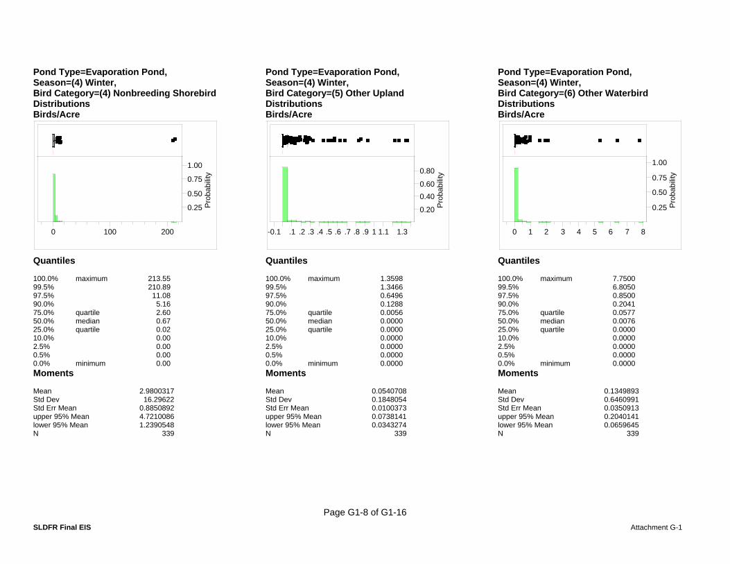
Page G1-8 of G1-16 SLDFR Final EIS Attachment G-1
Pond Type=Evaporation Pond, Season=(4) Winter, Bird Category=(4) Nonbreeding Shorebird Distributions Birds/Acre
0.25
0.50
0.75
1.00
Pro
babi
lity
0 100 200
Quantiles 100.0% maximum 213.55 99.5% 210.89 97.5% 11.08 90.0% 5.16 75.0% quartile 2.60 50.0% median 0.67 25.0% quartile 0.02 10.0% 0.00 2.5% 0.00 0.5% 0.00 0.0% minimum 0.00 Moments Mean 2.9800317 Std Dev 16.29622 Std Err Mean 0.8850892 upper 95% Mean 4.7210086 lower 95% Mean 1.2390548 N 339
Pond Type=Evaporation Pond, Season=(4) Winter, Bird Category=(5) Other Upland Distributions Birds/Acre
0.20
0.400.60
0.80
Pro
babi
lity
-0.1 .1 .2 .3 .4 .5 .6 .7 .8 .9 1 1.1 1.3
Quantiles 100.0% maximum 1.359899.5% 1.346697.5% 0.649690.0% 0.128875.0% quartile 0.005650.0% median 0.000025.0% quartile 0.000010.0% 0.00002.5% 0.00000.5% 0.00000.0% minimum 0.0000Moments Mean 0.0540708Std Dev 0.1848054Std Err Mean 0.0100373upper 95% Mean 0.0738141lower 95% Mean 0.0343274N 339
Pond Type=Evaporation Pond, Season=(4) Winter, Bird Category=(6) Other Waterbird Distributions Birds/Acre
0.25
0.50
0.75
1.00
Pro
babi
lity
0 1 2 3 4 5 6 7 8
Quantiles 100.0% maximum 7.750099.5% 6.805097.5% 0.850090.0% 0.204175.0% quartile 0.057750.0% median 0.007625.0% quartile 0.000010.0% 0.00002.5% 0.00000.5% 0.00000.0% minimum 0.0000Moments Mean 0.1349893Std Dev 0.6460991Std Err Mean 0.0350913upper 95% Mean 0.2040141lower 95% Mean 0.0659645N 339

Page G1-9 of G1-16 SLDFR Final EIS Attachment G-1
Pond Type=Mitigation Habitat, Season=(1) Spring Migration, Bird Category=(1) Dabbler Distributions Birds/Acre
0.10
0.30
0.50
0.70
Pro
babi
lity
0 5 10 15 20 25
Quantiles 100.0% maximum 25.700 99.5% 25.700 97.5% 17.162 90.0% 7.485 75.0% quartile 4.070 50.0% median 1.535 25.0% quartile 0.410 10.0% 0.108 2.5% 0.000 0.5% 0.000 0.0% minimum 0.000 Moments Mean 3.020666 Std Dev 4.0576141 Std Err Mean 0.2991313 upper 95% Mean 3.6108556 lower 95% Mean 2.4304764 N 184
Pond Type=Mitigation Habitat, Season=(1) Spring Migration, Bird Category=(2) Diver Distributions Birds/Acre
0.200.400.60
0.80
Pro
babi
lity
0 .1 .2 .3 .4 .5
Quantiles 100.0% maximum 0.5000099.5% 0.5000097.5% 0.1750390.0% 0.0490075.0% quartile 0.0000050.0% median 0.0000025.0% quartile 0.0000010.0% 0.000002.5% 0.000000.5% 0.000000.0% minimum 0.00000Moments Mean 0.0158541Std Dev 0.0541178Std Err Mean 0.0039896upper 95% Mean 0.0237257lower 95% Mean 0.0079825N 184
Pond Type=Mitigation Habitat, Season=(1) Spring Migration, Bird Category=(3) Breeding Shorebird Distributions Birds/Acre
0.20
0.40
0.60
0.80
Pro
babi
lity
0 5 10 15 20 25
Quantiles 100.0% maximum 23.80999.5% 23.80997.5% 14.07490.0% 7.86075.0% quartile 2.32250.0% median 0.95125.0% quartile 0.17910.0% 0.0302.5% 0.0000.5% 0.0000.0% minimum 0.000Moments Mean 2.3604088Std Dev 3.7797156Std Err Mean 0.2786443upper 95% Mean 2.9101774lower 95% Mean 1.8106402N 184

Page G1-10 of G1-16 SLDFR Final EIS Attachment G-1
Pond Type=Mitigation Habitat, Season=(1) Spring Migration, Bird Category=(4) Nonbreeding Shorebird Distributions Birds/Acre
0.20
0.40
0.60
0.80
Pro
babi
lity
-10 0 10 20 30 40 50 60 70 80 90 110 130
Quantiles 100.0% maximum 123.13 99.5% 123.13 97.5% 51.79 90.0% 24.94 75.0% quartile 6.77 50.0% median 1.59 25.0% quartile 0.25 10.0% 0.03 2.5% 0.00 0.5% 0.00 0.0% minimum 0.00 Moments Mean 7.6370776 Std Dev 15.005055 Std Err Mean 1.1061873 upper 95% Mean 9.8195984 lower 95% Mean 5.4545568 N 184
Pond Type=Mitigation Habitat, Season=(1) Spring Migration, Bird Category=(5) Other Upland Distributions Birds/Acre
0.20
0.40
0.60
0.80
Pro
babi
lity
0 .1 .2 .3 .4 .5 .6 .7
Quantiles 100.0% maximum 0.7263899.5% 0.7263897.5% 0.3490090.0% 0.0988675.0% quartile 0.0148550.0% median 0.0000025.0% quartile 0.0000010.0% 0.000002.5% 0.000000.5% 0.000000.0% minimum 0.00000Moments Mean 0.0334171Std Dev 0.0930638Std Err Mean 0.0068608upper 95% Mean 0.0469535lower 95% Mean 0.0198808N 184
Pond Type=Mitigation Habitat, Season=(1) Spring Migration, Bird Category=(6) Other Waterbird Distributions Birds/Acre
0.200.400.60
0.80
Pro
babi
lity
0 1 2 3 4 5 6
Quantiles 100.0% maximum 6.300099.5% 6.300097.5% 1.544990.0% 0.487075.0% quartile 0.200050.0% median 0.022625.0% quartile 0.000010.0% 0.00002.5% 0.00000.5% 0.00000.0% minimum 0.0000Moments Mean 0.2096202Std Dev 0.5940506Std Err Mean 0.043794upper 95% Mean 0.2960263lower 95% Mean 0.1232142N 184

Page G1-11 of G1-16 SLDFR Final EIS Attachment G-1
Pond Type=Mitigation Habitat, Season=(2) Breeding, Bird Category=(1) Dabbler Distributions Birds/Acre
0.10
0.30
0.50
Pro
babi
lity
-1 0 1 2 3 4 5 6 7 8 9 10
Quantiles 100.0% maximum 9.5000 99.5% 8.8140 97.5% 6.0550 90.0% 3.5000 75.0% quartile 1.6568 50.0% median 0.6081 25.0% quartile 0.1317 10.0% 0.0098 2.5% 0.0000 0.5% 0.0000 0.0% minimum 0.0000 Moments Mean 1.2340286 Std Dev 1.5970284 Std Err Mean 0.092669 upper 95% Mean 1.4164022 lower 95% Mean 1.0516551 N 297
Pond Type=Mitigation Habitat, Season=(2) Breeding, Bird Category=(2) Diver Distributions Birds/Acre
0.20
0.400.60
0.80
Pro
babi
lity
0 .1 .2 .3 .4 .5
Quantiles 100.0% maximum 0.5147199.5% 0.4210397.5% 0.1882290.0% 0.0588275.0% quartile 0.0075550.0% median 0.0000025.0% quartile 0.0000010.0% 0.000002.5% 0.000000.5% 0.000000.0% minimum 0.00000Moments Mean 0.0189218Std Dev 0.0552085Std Err Mean 0.0032035upper 95% Mean 0.0252263lower 95% Mean 0.0126172N 297
Pond Type=Mitigation Habitat, Season=(2) Breeding, Bird Category=(3) Breeding Shorebird Distributions Birds/Acre
0.10
0.30
0.50
0.70
Pro
babi
lity
0 5 10 15 20 25 30
Quantiles 100.0% maximum 29.10399.5% 24.89597.5% 11.58290.0% 5.76075.0% quartile 2.90050.0% median 1.43125.0% quartile 0.50610.0% 0.0552.5% 0.0000.5% 0.0000.0% minimum 0.000Moments Mean 2.4039595Std Dev 3.2387086Std Err Mean 0.1879289upper 95% Mean 2.7738057lower 95% Mean 2.0341134N 297

Page G1-12 of G1-16 SLDFR Final EIS Attachment G-1
Pond Type=Mitigation Habitat, Season=(2) Breeding, Bird Category=(4) Nonbreeding Shorebird Distributions Birds/Acre
0.200.400.60
0.80
Pro
babi
lity
0 10 20 30 40 50 60
Quantiles 100.0% maximum 61.900 99.5% 49.569 97.5% 19.511 90.0% 4.840 75.0% quartile 1.326 50.0% median 0.235 25.0% quartile 0.015 10.0% 0.000 2.5% 0.000 0.5% 0.000 0.0% minimum 0.000 Moments Mean 2.1334192 Std Dev 5.9197928 Std Err Mean 0.3435012 upper 95% Mean 2.8094332 lower 95% Mean 1.4574051 N 297
Pond Type=Mitigation Habitat, Season=(2) Breeding, Bird Category=(5) Other Upland Distributions Birds/Acre
0.20
0.40
0.60
0.80
Pro
babi
lity
0 .1 .2 .3 .4 .5 .6 .7 .8
Quantiles 100.0% maximum 0.8000099.5% 0.7510097.5% 0.3491990.0% 0.0931175.0% quartile 0.0222250.0% median 0.0000025.0% quartile 0.0000010.0% 0.000002.5% 0.000000.5% 0.000000.0% minimum 0.00000Moments Mean 0.0352318Std Dev 0.0990397Std Err Mean 0.0057469upper 95% Mean 0.0465417lower 95% Mean 0.0239219N 297
Pond Type=Mitigation Habitat, Season=(2) Breeding, Bird Category=(6) Other Waterbird Distributions Birds/Acre
0.20
0.40
0.60
0.80
Pro
babi
lity
0 1 2 3 4 5 6 7 8
Quantiles 100.0% maximum 8.161899.5% 7.200597.5% 3.235690.0% 1.002975.0% quartile 0.295250.0% median 0.073525.0% quartile 0.000010.0% 0.00002.5% 0.00000.5% 0.00000.0% minimum 0.0000Moments Mean 0.3675578Std Dev 0.8692883Std Err Mean 0.0504412upper 95% Mean 0.4668267lower 95% Mean 0.2682889N 297
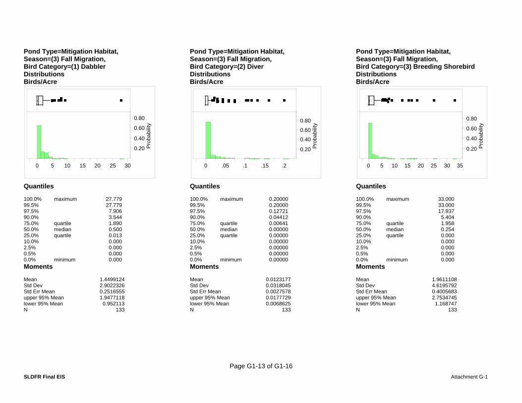
Page G1-13 of G1-16 SLDFR Final EIS Attachment G-1
Pond Type=Mitigation Habitat, Season=(3) Fall Migration, Bird Category=(1) Dabbler Distributions Birds/Acre
0.20
0.40
0.60
0.80
Pro
babi
lity
0 5 10 15 20 25 30
Quantiles 100.0% maximum 27.779 99.5% 27.779 97.5% 7.906 90.0% 3.544 75.0% quartile 1.890 50.0% median 0.500 25.0% quartile 0.013 10.0% 0.000 2.5% 0.000 0.5% 0.000 0.0% minimum 0.000 Moments Mean 1.4499124 Std Dev 2.9022326 Std Err Mean 0.2516555 upper 95% Mean 1.9477118 lower 95% Mean 0.952113 N 133
Pond Type=Mitigation Habitat, Season=(3) Fall Migration, Bird Category=(2) Diver Distributions Birds/Acre
0.20
0.40
0.60
0.80
Pro
babi
lity
0 .05 .1 .15 .2
Quantiles 100.0% maximum 0.2000099.5% 0.2000097.5% 0.1272190.0% 0.0441275.0% quartile 0.0064150.0% median 0.0000025.0% quartile 0.0000010.0% 0.000002.5% 0.000000.5% 0.000000.0% minimum 0.00000Moments Mean 0.0123177Std Dev 0.0318045Std Err Mean 0.0027578upper 95% Mean 0.0177729lower 95% Mean 0.0068625N 133
Pond Type=Mitigation Habitat, Season=(3) Fall Migration, Bird Category=(3) Breeding Shorebird Distributions Birds/Acre
0.20
0.40
0.60
0.80
Pro
babi
lity
0 5 10 15 20 25 30 35
Quantiles 100.0% maximum 33.00099.5% 33.00097.5% 17.93790.0% 5.40475.0% quartile 1.95850.0% median 0.25425.0% quartile 0.00010.0% 0.0002.5% 0.0000.5% 0.0000.0% minimum 0.000Moments Mean 1.9611108Std Dev 4.6195792Std Err Mean 0.4005683upper 95% Mean 2.7534745lower 95% Mean 1.168747N 133

Page G1-14 of G1-16 SLDFR Final EIS Attachment G-1
Pond Type=Mitigation Habitat, Season=(3) Fall Migration, Bird Category=(4) Nonbreeding Shorebird Distributions Birds/Acre
0.20
0.40
0.60
0.80
Pro
babi
lity
-10 0 10 20 30 40 50 60 70 80 90
Quantiles 100.0% maximum 84.074 99.5% 84.074 97.5% 34.007 90.0% 16.979 75.0% quartile 5.654 50.0% median 0.882 25.0% quartile 0.041 10.0% 0.000 2.5% 0.000 0.5% 0.000 0.0% minimum 0.000 Moments Mean 5.1246229 Std Dev 10.294896 Std Err Mean 0.8926807 upper 95% Mean 6.8904336 lower 95% Mean 3.3588123 N 133
Pond Type=Mitigation Habitat, Season=(3) Fall Migration, Bird Category=(5) Other Upland Distributions Birds/Acre
0.20
0.40
0.60
0.80
Pro
babi
lity
-0.05 0 .05 .1 .15 .2 .25 .3 .35 .4
Quantiles 100.0% maximum 0.3676599.5% 0.3676597.5% 0.2998990.0% 0.1040275.0% quartile 0.0148150.0% median 0.0000025.0% quartile 0.0000010.0% 0.000002.5% 0.000000.5% 0.000000.0% minimum 0.00000Moments Mean 0.0247104Std Dev 0.0637395Std Err Mean 0.0055269upper 95% Mean 0.0356431lower 95% Mean 0.0137776N 133
Pond Type=Mitigation Habitat, Season=(3) Fall Migration, Bird Category=(6) Other Waterbird Distributions Birds/Acre
0.20
0.400.600.80
Pro
babi
lity
0 10
Quantiles 100.0% maximum 16.52999.5% 16.52997.5% 4.82690.0% 2.11575.0% quartile 0.60050.0% median 0.14225.0% quartile 0.00310.0% 0.0002.5% 0.0000.5% 0.0000.0% minimum 0.000Moments Mean 0.6497741Std Dev 1.6849457Std Err Mean 0.1461033upper 95% Mean 0.9387809lower 95% Mean 0.3607673N 133

Page G1-15 of G1-16 SLDFR Final EIS Attachment G-1
Pond Type=Mitigation Habitat, Season=(4) Winter, Bird Category=(1) Dabbler Distributions Birds/Acre
0.100.200.300.400.50
Pro
babi
lity
-2 0 2 4 6 8 10
Quantiles 100.0% maximum 9.1029 99.5% 9.1029 97.5% 9.1029 90.0% 7.4074 75.0% quartile 3.1434 50.0% median 1.8529 25.0% quartile 0.5919 10.0% 0.0824 2.5% 0.0000 0.5% 0.0000 0.0% minimum 0.0000 Moments Mean 2.3964892 Std Dev 2.3972794 Std Err Mean 0.4530432 upper 95% Mean 3.3260571 lower 95% Mean 1.4669212 N 28
Pond Type=Mitigation Habitat, Season=(4) Winter, Bird Category=(2) Diver Distributions Birds/Acre
0.20
0.40
0.60
0.80
Pro
babi
lity
-0.1 0 .1 .2 .3 .4 .5 .6
Quantiles 100.0% maximum 0.5882499.5% 0.5882497.5% 0.5882490.0% 0.3294175.0% quartile 0.0294150.0% median 0.0147125.0% quartile 0.0000010.0% 0.000002.5% 0.000000.5% 0.000000.0% minimum 0.00000Moments Mean 0.0693978Std Dev 0.1456012Std Err Mean 0.027516upper 95% Mean 0.125856lower 95% Mean 0.0129395N 28
Pond Type=Mitigation Habitat, Season=(4) Winter, Bird Category=(3) Breeding Shorebird Distributions Birds/Acre
0.10
0.30
0.50
0.70
Pro
babi
lity
-2 0 2 4 6 8 10
Quantiles 100.0% maximum 9.647199.5% 9.647197.5% 9.647190.0% 5.485375.0% quartile 2.636050.0% median 0.198525.0% quartile 0.007410.0% 0.00002.5% 0.00000.5% 0.00000.0% minimum 0.0000Moments Mean 1.5685574Std Dev 2.5283117Std Err Mean 0.477806upper 95% Mean 2.5489343lower 95% Mean 0.5881805N 28

Page G1-16 of G1-16 SLDFR Final EIS Attachment G-1
Pond Type=Mitigation Habitat, Season=(4) Winter, Bird Category=(4) Nonbreeding Shorebird Distributions Birds/Acre
0.10
0.30
0.50
0.70
Pro
babi
lity
-5 0 5 10 15 20 25
Quantiles 100.0% maximum 21.721 99.5% 21.721 97.5% 21.721 90.0% 13.484 75.0% quartile 7.533 50.0% median 2.544 25.0% quartile 0.721 10.0% 0.324 2.5% 0.000 0.5% 0.000 0.0% minimum 0.000 Moments Mean 4.7167192 Std Dev 5.4814583 Std Err Mean 1.0358982 upper 95% Mean 6.8422068 lower 95% Mean 2.5912315 N 28
Pond Type=Mitigation Habitat, Season=(4) Winter, Bird Category=(5) Other Upland Distributions Birds/Acre
0.25
0.50
0.75
1.00
Pro
babi
lity
-0.25 0 .25 .5 .75 1 1.25
Quantiles 100.0% maximum 099.5% 097.5% 090.0% 075.0% quartile 050.0% median 025.0% quartile 010.0% 02.5% 00.5% 00.0% minimum 0Moments Mean 0Std Dev 0Std Err Mean 0upper 95% Mean 0lower 95% Mean 0N 28
Pond Type=Mitigation Habitat, Season=(4) Winter, Bird Category=(6) Other Waterbird Distributions Birds/Acre
0.20
0.40
0.60
0.80
Pro
babi
lity
-0.5 0 .5 1 1.5 2 2.5
Quantiles 100.0% maximum 2.235399.5% 2.235397.5% 2.235390.0% 1.708875.0% quartile 0.507450.0% median 0.169125.0% quartile 0.044110.0% 0.00002.5% 0.00000.5% 0.00000.0% minimum 0.0000Moments Mean 0.4180672Std Dev 0.6001307Std Err Mean 0.113414upper 95% Mean 0.6507736lower 95% Mean 0.1853609N 28

APPENDIXH
Geology and Seismicity


TABLE OF CONTENTS
SLDFR Final EIS Appendix H H-i
H1 Affected Environment ................................................................................................... H-1
H1.1 Great Valley Geomorphic Province........................................................ H-1 H1.2 Coast Ranges Geomorphic Province ...................................................... H-3 H1.3 Seismotectonic Setting............................................................................ H-4 H1.4 Seismicity................................................................................................ H-5
H1.4.1 1857 Fort Tejon Earthquake.................................................... H-5 H1.4.2 1868 Hayward Earthquake ...................................................... H-6 H1.4.3 1889 Collinsville Earthquake .................................................. H-6 H1.4.4 1906 San Francisco Earthquake .............................................. H-6 H1.4.5 1857, 1881, 1901, 1922, 1934, 1966, and 2004 Parkfield
Earthquakes ............................................................................. H-6 H1.4.6 1983 Coalinga Earthquake ...................................................... H-7 H1.4.7 1985 North Kettleman Hills Earthquake................................. H-7 H1.4.8 1989 Loma Prieta Earthquake ................................................. H-7 H1.4.9 2003 San Simeon Earthquake ................................................. H-7 H1.4.10 Contemporary Seismicity ........................................................ H-8
H1.5 Significant Faults .................................................................................... H-8 H1.5.1 San Andreas Fault Zone .......................................................... H-8 H1.5.2 Hayward Fault ....................................................................... H-10 H1.5.3 Concord-Green Valley Fault ................................................. H-10 H1.5.4 Coast Range-Sierran Block Boundary .................................. H-11 H1.5.5 Sacramento-San Joaquin River Delta Faults ......................... H-12 H1.5.6 Coast Range-Sierran Block Boundary South of the Delta .... H-13 H1.5.7 Mount Diablo ‘Blind’ Thrust ................................................ H-13 H1.5.8 Greenville Fault..................................................................... H-14 H1.5.9 Ortigalita Fault ...................................................................... H-15 H1.5.10 Mount Oso Anticline............................................................. H-15 H1.5.11 San Juan Fault ....................................................................... H-15 H1.5.12 La Panza Thrust..................................................................... H-16 H1.5.13 Rinconada Fault..................................................................... H-16 H1.5.14 Nacimiento Fault ................................................................... H-17 H1.5.15 Oceanic/West Huasna Fault .................................................. H-17 H1.5.16 Cambria Fault ........................................................................ H-17 H1.5.17 Hosgri Fault........................................................................... H-18
H2 References ................................................................................................................... H-18

TABLE OF CONTENTS
SLDFR Final EIS Appendix H H-ii
Acronyms Delta Sacramento-San Joaquin River Delta
Ma million years old
ML Richter local magnitude
MM Modified Mercalli Intensity
MCE maximum credible earthquake
CRSB Coast-Range Sierran Block Boundary
PKHF Pittsburg-Kirby Hills fault

Appendix H Geology and Seismicity
SLDFR Final EIS Appendix H H-1
H1 AFFECTED ENVIRONMENT The following paragraphs discuss the geologic conditions and hazards that may be encountered during the construction and implementation of the alternatives for the San Luis Drainage Feature Re-evaluation. The focus of this appendix is the geologic and seismic characteristics of the Great Valley and the Coast Ranges geomorphic provinces, which may influence the selection of a preferred alternative due to the geologic conditions and potential geologic hazards associated with these regions.
H1.1 Great Valley Geomorphic Province The existing San Luis Drain is situated near the western margin of San Joaquin Valley (Figure 9-1), which comprises the southern region of the Great Valley geomorphic province (Harden 1998). The Great Valley Province is one of the largest agricultural basins in the world and comprises the Sacramento Valley in the north and San Joaquin Valley in the south, separated by the San Joaquin-Sacramento River Delta (the Delta).
The San Joaquin Valley is an asymmetrical topographic and structural basin with the axis offset to the west (Figure 9-2), and a gentle topographic downward slope to the north. The valley encompasses approximately 10,000 square miles and is bounded to the east by the Sierra Nevada Range, to the west by the Central Coast Ranges, to the south by the Tehacapi Mountains of the Transverse Ranges geomorphic province, and to the north by the Delta. The Sierra Nevada is composed of igneous and metamorphic rocks of pre-Tertiary age. The granitic rocks of the Sierra Nevada comprise the basement complex beneath the Great Valley. Overlying the basement complex is approximately 9,200 meters (30,000 feet) of Late Cenozoic sedimentary deposits in central and northern San Joaquin Valley. The present-day basin evolved from a late Jurassic to middle Tertiary (40-150 million years old [Ma]) marine fore-arc basin (Castillo and Zoback 1994). In the late Tertiary (25-30 Ma), a change in the relative motion between the Pacific and North American plates resulted in the gradual uplift of the Coast Ranges and the eventual isolation of the basin from the ocean. More recent Miocene and lower Pliocene sediments were derived from the neighboring Coast Ranges and the Sierra Nevada (Perkins 1987). By the late Pliocene (2-3 Ma), subaerial depositional conditions prevailed and Sierra Nevada-derived sediments were deposited in the basins (Bartow 1987).
A veneer of Quaternary alluvial and lacustrine sediments cover the Cenozoic rocks of the Great Valley (Figure 9-3). Along the western margin of the valley, these deposits were deposited primarily in alluvial fan settings. At the distal edges of these fans the deposits are commonly alluvial flood plain, lacustrine, and alluvial channel in origin (Lettis 1982). In central San Joaquin Valley these deposits tend to consist mostly of unconsolidated silty sands, poorly graded sands, clayey sands, silts, and sandy clays at shallow depths. The silty sands, clayey sands, and poorly graded sands tend to be the major water-bearing units beneath the valley (Ferriz 2001). To a lesser extent, groundwater has been encountered in sandy silt and sandy clay layers, but these tend to be poor groundwater-producing zones. Organic soils make up the upper 3 meters (10 feet) of the valley in some areas; however, through the intensive farming conducted in the region, the organic soils are missing or vacant in areas south of the Delta. Along the western and southern boundaries of the valley, farming in areas has been limited due to the buildup of salts and drainwater containing selenium (Se) in the soil (see Section 6.1). Concentrations of salts and

Appendix H Geology and Seismicity
SLDFR Final EIS Appendix H H-2
Se and drainage problems within the western and southern areas of the valley would likely increase over time should the treatment and drainage of irrigation water within these areas not be implemented.
Coarser sediments from fluvial processes are mostly located on the eastern part of the valley and are associated with large alluvial fans that extend from the Sierra Nevada to the trough (topographic low point) of the valley (Poland and Lofgren 1984). The west side of San Joaquin Valley receives less rainfall due to the rain shadow effect from the Coast Ranges and, therefore, the soils are generally more fine-grained.
The Delta region consists of a low triangular area between Sacramento to the north, Stockton to the south, and Suisun Bay to the west. The Delta is located approximately 80 km (50 miles) from the Pacific Ocean and is currently growing inland as sediments are being deposited around its margins. Recent studies indicate that the Delta grows and recedes during periods of high and low sea level resulting from glacial and interglacial periods (Knowles and Cayan 2002). The sediments deposited in the Delta are a mix of glacially-derived fluvial deposits and marine-estuarine-deltaic deposits (Norris and Webb 1990).
The central and northern San Joaquin Valley groundwater-bearing units are comprised of several interbedded and unconsolidated layers of coarse- and fine-grained sediments. The groundwater-bearing sedimentary deposits beneath the valley can be subdivided into two principal hydrologic units: an upper unit and a lower unit (Ferriz 2001). The upper unit consists of a semiconfined aquifer system, which extends from the ground surface to the top of the Corcoran Clay Unit, at depths ranging from the ground surface to approximately 275 meters (900 feet) below the ground surface. The lower unit is considered to be a confined aquifer, which extends from below the Corcoran Clay Unit to the deep saline groundwater-bearing units and ranges in thickness between 61 to 610 meters (200 and 2,000 feet). The Corcoran Clay Unit has an average thickness of (20 meters) 65 feet and is the principal confining layer beneath nearly half of San Joaquin Valley (Ferriz 2001; Poland and Lofgren 1984).
The San Joaquin Valley drains by way of the San Joaquin, Merced, Tuolomne, Stanislaus, and Calaveras rivers through the Delta. In central San Joaquin Valley, the Kings, Kaweah, and Tule rivers naturally drain toward a large basin located between the towns of Kettleman City and Stratford, which until recently contained Tulare Lake. Within the southern end of San Joaquin Valley, the Kern River until recently drained into Lake Buena Vista. Tulare Lake and Lake Buena Vista were both seasonal lakes. Water from the rivers that formed both of the lakes has been diverted for agricultural use, through flood control measures (i.e., dam and canal construction). The former Tulare Lake and Lake Buena Vista lake beds are now used for agriculture.
Overdraft of shallow groundwater resources within San Joaquin Valley began in the middle 1920s when an estimated 2,025,000 acre-feet was pumped from the shallow subsurface strata for irrigation purposes. The amount of overdraft continued to increase and by the 1940s an estimated 3,000,000 acre-feet was removed from the shallow aquifers on a yearly basis. By 1966 the amount of groundwater overdraft exceeded 9,720,000 acre-feet/year (Poland and Lofgren 1984). Removal of such large volumes of groundwater resulted in dramatic subsidence within several areas of the Southern San Joaquin Valley (Holzer 1984). Through the importation of large amounts of surface water beginning in 1968 from the California Aqueduct, and other irrigation projects, overdraft of the groundwater supplies decreased sharply.

Appendix H Geology and Seismicity
SLDFR Final EIS Appendix H H-3
H1.2 Coast Ranges Geomorphic Province The Ocean, Delta-Chipps Island, and Delta-Carquinez Disposal options all traverse the Coast Ranges geomorphic province (Figure 9-1). Physiographically, the Coast Ranges can be divided into two subprovinces, the northern and southern subprovinces separated by San Francisco Bay and the Delta. The latter represents the only major breach in the Coast Ranges and allows drainage of the Sierra Nevada and the Sacramento-San Joaquin Valley. The division of the Coast Ranges into two subprovinces is more for convenience rather than driven by geologic or physiographic differences. The only major geologic difference between the two subprovinces is that south of San Francisco Bay, the Coast Ranges are predominantly located to the west of the San Andreas fault, while the entire northern subprovince is located to the east of the main San Andreas fault. Several secondary faults of the San Andreas fault system do however traverse the Coast Ranges between San Francisco Bay and Cape Mendocino.
Four main orogenic (mountain-building) episodes have been proposed for evolution of the Coast Ranges (Norris and Webb 1990):
1. Early (?) Cretaceous mountain-building accompanied by granitic intrusion in the Salinian block (located to the west of the San Andreas), and by metamorphism of older rocks
2. Early Tertiary thrusting of rocks of the Great Valley Group over Franciscan basement
3. Followed by strike-slip faulting along the San Andreas fault system
4. The Late Pliocene and Pleistocene formation of the present-day Coast Ranges
The Coast Range orogeny is responsible for the topography that is seen today in the Coast Ranges. Earlier deformation involved compression across the Coast Ranges, resulting in uplift of the ranges and corresponding depression of intervening basins (Norris and Webb 1990). Erosion from the ranges quickly filled the basins with terrestrial clastic sediments such as the Livermore Gravels that outcrop on the southern side of Mount Diablo. Deformation during this orogenic episode, however, was dominated by the right-lateral strike-slip movement on faults of the San Andreas system. The total amount of movement on these faults is considerable; however, estimates of the absolute amount of movement on individual faults, in particular the San Andreas, are contentious.
The Coast Ranges are underlain by uplifted and intensely deformed Upper Jurassic (150 Ma) and younger rocks of the Franciscan Formation and the Salinian metamorphic and granitic complex, which are in fault contact with the less deformed Great Valley sediments (Figure 9-3). The Coast Ranges are characterized by elongate topographic and lithologic strips underlain by discrete basement blocks separated by major structural discontinuities. To the east is the Coast Ranges-Sierran block boundary zone (buried beneath the sediments of the Great Valley province). The major boundary to the west is the San Andreas fault zone separating Franciscan Formation rocks from the Salinian assemblage. The pervasive late Cenozoic deformation observed within the Coast Ranges is due to compression orthogonal to the Pacific-North American plate contact, i.e., perpendicular to the strike of the San Andreas fault system. Ophiolites of the Coast Ranges are deformed by a series of thrust faults. The majority of these faults, although exhibiting extensive evidence for late Tertiary and early Quaternary movement, now appear to be inactive, or at least significantly less active than the strike-slip faults of the San Andreas system.

Appendix H Geology and Seismicity
SLDFR Final EIS Appendix H H-4
The Diablo Range, at the northern end of which the Delta-Carquinez and Delta-Chipps Island Disposal Alternatives cross, extends from the Delta, south for 210 km (130 miles) along the western side of the San Joaquin Valley to just north of Coalinga (Figure 9-4). The range is up to 48 km (30 miles) wide and reaches a maximum elevation of 1,598 meters (5,243 feet) at San Benito Mountain. Rocks of the Mesozoic Great Valley rest upon Franciscan basement along the San Joaquin Valley margin throughout the Diablo Range. This contact is often a thrust fault (Irwin 1990). Younger Paleocene to Pleistocene sedimentary units from are widely distributed along the margins of the range and also in some intermontane areas, like the Livermore basin. Despite the Diablo Range containing rocks of every Tertiary epoch, nowhere in the range is a complete Tertiary sequence located.
The Diablo Range is separated from the remainder of the Coast Ranges by faults of the San Andreas system. The Calaveras fault separates the Mount Diablo massif from the remainder of the East Bay Hills. Mount Diablo is separated from the southern extension of the Diablo Range by the Livermore Valley, an east-west-trending thrust-bounded Cenozoic basin. To the east, the Diablo Range is bounded by the Coast Range-Sierran block boundary zone (CRSB) that is, in general, created by a series of blind and partially concealed thrust faults (Wong et al. 1988; Unruh and Moores 1992). In the area of Mount Diablo, the main east bounding structure is the San Joaquin fault (Sowers, Noller, and Unruh 1992).
The general structural pattern of the Diablo Range is a series of large anticlinal folds, cored by Franciscan rocks, aligned in an en echelon manner and separated by synclines containing younger rocks. This sequence of folds is cored by, and often dissected by, a series of thrust faults that verge both to the east and the west. These thrust faults are, in turn, truncated by or offset by contemporary strike-slip movement on the northwest-striking, right-lateral faults of the San Andreas fault system. Along-strike complexities along these strike-slip faults give rise to areas of compression (restraining left-steps) or extension (releasing right-steps). An example of the former is the Mount Diablo uplift (Unruh and Sawyer 1997; Unruh and Lettis 1998).
The Ocean Disposal Alternative crosses the southern Coast Ranges. West of the San Andreas fault, this part of the Coast Ranges is underlain by the Salinian block (Figure 9-3) consisting of granitic and crystalline metamorphic basement rocks with a thin cover of Mesozoic and Cenozoic sediments bounded by the Rinconada fault to the west (Clark et al. 1994). Unlike the remainder of the Coast Ranges, there is little internal deformation and low rates of contemporary seismicity within the Salinian block (Clark et al. 1994; Page, Thompson, and Coleman 1998). Historical seismicity is concentrated along the bounding faults. To the west, the Salinian block is bordered by the Rinconada fault with the Coastal Franciscan domain. This tectonic block consists of predominantly Franciscan Complex basement, bounded to the west by the San Gregorio-San Simeon-Hosgri fault system. Many faults and folds that exhibit late Cenozoic movement traverse this domain. Contemporary seismicity rates are considerably higher than for the Salinian block and, although predominantly diffuse in nature, epicenters can, in some cases, be shown to be aligned along specific faults.
H1.3 Seismotectonic Setting The California Coast Ranges are a domain of right-lateral strike-slip faulting (Figure 9-4), dominated by the San Andreas fault system, that accommodates about 75 percent of the motion between the Pacific and North American plates (Wallace 1990). In addition to the right-lateral

Appendix H Geology and Seismicity
SLDFR Final EIS Appendix H H-5
strike-slip deformation, compression oriented normal to the plate boundary is transferred east of the main strike-slip faults by means of east-west to east-northeast-directed crustal shortening. Locally, within the Coast Ranges, this shortening is oriented more northeast-southwest and is accommodated as a series of folds and thrusts along the CRSB zone along the western margin of the Great Valley (Wakabayashi and Smith 1994). These thrusts and folds trend subparallel to the faults of the San Andreas system. In contrast, regional shortening within the Coast Ranges themselves, for example in the Mount Diablo and Mount Oso regions, has a more northerly orientation, resulting in folds and thrust that are oriented at an oblique angle to the main strike-slip faults. These tectonic features are discussed in more detail in the following sections.
H1.4 Seismicity The historical earthquake record for the San Joaquin Valley and much of California only extends to the mid-1800s, coinciding with the influx of miners and settlers during the Gold Rush (Wong and Ely 1983). Until adequate seismographic coverage came into existence in southern California in the 1930s, earthquake detection was generally limited to those events that produced felt or physical effects. Earthquakes as small as Richter local magnitude (ML) 3 were probably not completely observed throughout the San Joaquin Valley until about 1960. Thereafter, seismographic coverage in southern California improved significantly, and currently earthquakes as small as ML 1.5 can be detected for most portions of the San Joaquin Valley.
The San Luis Drain Feature Re-evaluation is located in an area that historically has not been seismically active (Figure 9-5). In general, the largest historical earthquakes have generally occurred along the valley margins. A historical catalog was compiled for the study region and the epicentral locations are shown on Figure 9-5.
The catalog was compiled from the following data sources: the National Earthquake Information Center’s Preliminary Determination of Epicenters; Stover, Reagor, and Algermission’s U.S. historical catalog; the catalog of the California Division of Mines and Geology, 1735–1974; the catalog of the Decade of North American Geology; and the Northern California Seismic Network and the Southern California Earthquake Center catalogs. The resulting catalog (1864–2004) of approximate ML 3 and greater is shown on Figure 9-5. The most significant of these events are annotated and discussed in more detail below.
H1.4.1 1857 Fort Tejon Earthquake At about 8:00 am (PST) on 9 January 1857, the largest earthquake within the study region ruptured the San Bernardino, Mohave, Carrizo, and Cholame segments of the San Andreas fault. A moment magnitude (M) 8 has been estimated for the event based on the rupture length, average slip, and based on comparison to the 1906 earthquake in northern California (Sieh 1978). The earthquake epicenter was located near Fort Tejon (Real et al. 1978), approximately 72 km west-southwest of the site. Fort Tejon was destroyed (maximum Modified Mercalli Intensity [MMI] IX) and the effects were felt over an area of at least 350,000 km2 (Townley and Allen 1939). The site likely experienced a maximum intensity of MM VII-IX (Stover and Coffman 1993). Instances of fissuring, sand blows, and hydrologic changes were reported from Sacramento to the Colorado River delta. One report describes liquefaction in the region between Stockton and Sacramento (Stover and Coffman 1993). Surface rupture extended over a distance of 230 km, possibly as great as 360 km, from San Bernardino to San Benito County. Offset
Appendix H Geology and Seismicity
SLDFR Final EIS Appendix H H-6
channels and alluvial deposits are evidence for at least 7 meters of right-lateral slip during the 1857 event (Grant and Sieh 1993).
H1.4.2 1868 Hayward Earthquake This ML 6.8 earthquake probably occurred on the southern Hayward fault. It was one of the most destructive in California history because it occurred in a populated area. Significant damage was sustained in towns along the fault in the eastern San Francisco Bay area, as well as in San Francisco and San Jose.
H1.4.3 1889 Collinsville Earthquake Of all known earthquakes of M 6.0 or greater in the San Francisco Bay region, this earthquake occurred closest to the project alignment (Figure 9-5). It may have been associated with the Pittsburg-Kirby Hills fault (PKHF). In Collinsville, a house was toppled over from ground shaking. In Antioch, many chimneys toppled and two small fissures were reported on Main Street. Toppozada et al. (1981) estimated the magnitude of the earthquake to be ML 6 while Ellsworth (1990) estimated the event to be M 6 ¼.
H1.4.4 1906 San Francisco Earthquake The M 7.9 Great San Francisco earthquake of 1906, centered near Olema, was arguably the most destructive historical earthquake to have occurred in northern California. It was felt from southern Oregon to south of Los Angeles, and as far east as central Nevada. It ruptured the northernmost 430 km of the San Andreas fault, from San Juan Bautista to the Mendocino Triple Junction. Damage was widespread in northern California and injury and loss of life was particularly severe. Ground shaking and fire caused the deaths of more than 3,000 people and injured approximately 225,000. Damage from shaking was most severe in areas of saturated or loose, young soils.
H1.4.5 1857, 1881, 1901, 1922, 1934, 1966, and 2004 Parkfield Earthquakes Seven earthquakes of approximately M 6.0 occurred along the Parkfield segment of the San Andreas fault since 1857. The January 1857 earthquake has been considered a foreshock to the 1857 Fort Tejon M 8 earthquake. The 2 February 1881 event knocked down a few chimneys in Imusdale, which would later become Parkfield. The 3 March 1901 earthquake was accompanied by some ground cracking and landsliding. The 10 March 1922 earthquake caused only minor damage because of the sparse population in the area at the time. The 8 June 1934 earthquake caused toppling of chimneys in the town of Parkfield and minor damage to nearby bridges. The 27 June 1966 earthquake caused minor damage to roads and bridges in the area around the town of Parkfield. The 29 September 2004 earthquake caused little damage but was well-monitored because it was an event that was long anticipated by scientists. Because of the similarities in magnitude, location, and rupture propagation, Bakun and McEvilly (1984) suggested that these events are characteristic of earthquake activity along the Parkfield segment of the San Andreas fault.

Appendix H Geology and Seismicity
SLDFR Final EIS Appendix H H-7
H1.4.6 1983 Coalinga Earthquake The M 6.4 mainshock of a sequence of earthquakes occurred on 2 May 1983 near the town of Coalinga beneath the Coalinga anticline (Figure 9-5). More than 6,000 aftershocks were recorded over a 4-month period, with seven greater than M 5. The town of Coalinga was heavily damaged; a four-block industrial area downtown was destroyed. Numerous houses and public buildings suffered significant damage (Stover and Coffman 1993). Although no surface faulting was associated with the mainshock, Anticline Ridge, northeast of Coalinga, was uplifted by 0.5 meter (Stein and Ekström 1992). Surface rupture occurred along about 3 km of the Nunez fault, northwest of Coalinga, associated with an aftershock of M 5.2 in June 1983 (Rymer, Harms, and Clark 1984).
H1.4.7 1985 North Kettleman Hills Earthquake A M 6.2 earthquake occurred beneath the Kettleman Hills North Dome anticline on 4 August, 1985. Over 400 aftershocks were recorded in a 4-week period following the mainshock (Ekström et al. 1992). Buildings and water lines in the town of Avenal suffered significant damage. Minor damage was more widespread throughout the region and the earthquake was felt over much of central and southern California (Stover and Coffman 1993).
H1.4.8 1989 Loma Prieta Earthquake The 17 October 1989 M 6.9 Loma Prieta earthquake occurred on or adjacent to the southern Santa Cruz segment of the San Andreas fault. The cities of Los Gatos, Watsonville, and Santa Cruz were hard hit with damage, as were San Francisco and Oakland. Shaking was felt throughout the San Francisco Bay area and as far away as San Diego and Nevada. While the Loma Prieta earthquake was one of the most expensive natural disasters in U.S. history, causing in excess of $6 billion damage, the loss of life was significantly less than in 1906. Sixty-two people died and about 3,500 were injured. About 12,000 people were displaced from their homes. As in the 1906 earthquake, the worst damage from shaking occurred to buildings on unconsolidated or saturated soils, with unreinforced masonry walls or improperly designed structures.
H1.4.9 2003 San Simeon Earthquake The 22 December 2003 M 6.5 San Simeon earthquake was centered in a mountainous region of the central California coast, nucleating about 11 km (7 miles) northeast of the town of San Simeon and at a depth of about 7 km (4 miles). The earthquake was caused by a unilaterally southeast-propagating rupture of a northwest-striking, probably northeast-dipping, blind reverse fault (Hardebeck et al. 2004). A blind fault ruptures only in the subsurface and deforms the surface through folding rather than faulting. Peak slip on the fault plane was about 2.8 meters (Ji et al. 2004). The upward projection of the fault plane is roughly coincident with the surface trace of the Oceanic fault, making it a likely candidate for the source (Figure 9-4). However, the source may as likely be a previously unidentified blind reverse fault parallel to the Oceanic fault (Hardebeck et al. 2004; Hauksson 2004). The San Simeon earthquake produced no coseismic surface faulting. However, strong ground shaking induced some ground deformation. Liquefaction and lateral spreading occurred in Paso Robles, Oceano, and the Salinas River,

Appendix H Geology and Seismicity
SLDFR Final EIS Appendix H H-8
primarily in artificial fill, and shaking-induced settlement caused cracking in paved roads. Shaking triggered numerous small landslides, especially along highways cut in steep slopes, and some larger surficial slides within the highly susceptible Franciscan formation. Concentration of energy caused some cracking and extension on ridge tops, which may have contributed to damage to buildings located there. Damage to human-made structures included cracking in dams, bridges, and roadways. The most severe damage to buildings occurred in unreinforced masonry buildings with little or no seismic retrofitting.
H1.4.10 Contemporary Seismicity The contemporary seismicity along the margins of the Central Valley and within the Coast Ranges provinces is characterized by linear alignments of epicenters along the main faults of the San Andreas fault system, most prominently the San Andreas, Calaveras, Hayward, Nacimiento, and Hosgri faults (Hill et al. 1991) (Figure 9-5). Seismicity along the western margin of the Central Valley (the CRSB) is more diffuse and clustered as aftershock sequences around the epicenters of the 1983 Coalinga and 1985 Kettleman Hills mainshocks. Earthquake focal mechanisms in the Coast Ranges exhibit predominantly right-lateral strike-slip faulting along the faults of the San Andreas system and reverse/thrust faulting in the intervening areas consistent with observed folds that are underlain by reverse/thrust faults (Hill et al. 1991). Focal mechanisms also exhibit reverse/thrust faulting along the CRSB boundary zone indicative of the fold and thrust deformation occurring along the west side of the Central Valley (Wong et al. 1988). Maximum focal depths, which indicate the thickness of the seismogenic brittle crust, are typically in the 12 to 15 km range beneath the Coast Ranges and gradually deepen eastward to the Sierra Nevada to as much as 40 km (Hill et al. 1991)
H1.5 Significant Faults The southern San Joaquin Valley is surrounded by a number of active and potentially active faults, some of which have generated large, damaging earthquakes during historic time. The most significant of these are shown on Figure 9-4 for each fault. Maximum earthquake magnitude estimates for each fault are based on the Working Group for Northern California Earthquake Potential (WGNCEP 1996), Working Group for California Earthquake Probabilities (WGCEP 1999), and empirical relationships amongst fault rupture length, fault rupture area, and maximum magnitude (Wells and Coppersmith 1994) (Table 9-1). The most significant Quaternary faults within 100 km of the project are discussed in brief detail below.
H1.5.1 San Andreas Fault Zone The dominant active fault structure in this region is the San Andreas fault (Figure 9-4). It extends from the Gulf of California, Mexico, to Point Delgada on the Mendocino Coast in northern California, a total distance of 1,200 km (745 miles). The San Andreas fault accommodates the majority of the motion between the Pacific and North American plates. This fault is the largest active fault in California and is responsible for the largest known earthquake in Northern California, the 1906 M 7.9 San Francisco earthquake (Wallace 1990). Movement on the San Andreas fault is right-lateral strike-slip, with a total offset of some 560 km (348 miles) (Irwin 1990). In northern California, the San Andreas fault is clearly delineated, striking northwest, approximately parallel to the vector of plate motion between the Pacific and North American

Appendix H Geology and Seismicity
SLDFR Final EIS Appendix H H-9
plates. Over most of its length, the San Andreas fault has a relatively simple, linear fault trace. Immediately south of the Bay, however, the fault splits into a number of branch faults or splays, including the Calaveras and Hayward faults (each is discussed below). In the Bay Area, the main trace of the San Andreas fault forms a linear depression along the Peninsula, occupied by the Crystal Springs and San Andreas Lake reservoirs. Geomorphic evidence for multiple episodes of Holocene faulting includes fault scarps in Holocene deposits, right-laterally offset streams, shutter ridges, and closed linear depressions (Wallace 1990). The 1906 earthquake resulted from rupture of the fault from San Juan Bautista north to Point Delgada, a distance of approximately 475 km (295 miles). The average amount of slip on the fault during this earthquake was 5.1 meters (17 feet) in the area to the north of the Golden Gate and 2.5 meters (8 feet) in the Santa Cruz Mountains (WGNCEP 1996).
Based on differences in geomorphic expression, fault geometry, paleoseismic chronology, slip rate, seismicity, and historic fault ruptures, the San Andreas fault is divided into a number of fault segments. Each of these segments is capable of rupturing either independently or in conjunction with adjacent segments. In the Bay Area, these segments include the Santa Cruz Mountains, the Peninsula, and the North Coast segments. These segments have estimated maximum earthquakes of M 7.2, 7.3, and 7.7, respectively. The North Coast segment may also be subdivided into two shorter segments with a boundary at Point Arena. These northern and southern North Coast segments are capable of generating earthquakes of M 7.5 and 7.7, respectively. The North Coast segment, or an adjacent fault branch, was the source of the August 18, 1999 M 5.0 earthquake located near Bolinas.
South of the Golden Gate, the fault slip rate is 17 - 3/+ 7 mm/yr (Hall, Wright, and Clahan 1999). North of the Golden Gate, the slip rate increases to 24 ± 5 mm/yr (Niemi and Hall 1992). WGCEP (1999) assigns a recurrence interval of 361 years to a M 7.9 1906-type event on the San Andreas fault, with a 21 percent probability of a M 6.7 or larger earthquake on the San Andreas in northern California in the time period 2000 to 2030. Recent investigations by Niemi (2002) indicate that the repeat time for large earthquakes on the North Coast segment may be less than 250 years.
The fault segments nearest to the San Luis Drainage Feature Re-Evaluation are the Carrizo, Cholame, Parkfield, and Creeping segments. The 1857 M 8 Fort Tejon earthquake ruptured these fault segments and parts of neighboring segments between the Coachella Valley and San Benito. From empirical relations between fault length and earthquake magnitude (Wells and Coppersmith 1994), the Carrizo, Cholame, and Parkfield fault segments have calculated maximum earthquakes of M 7.6, 7.2, and 6.5 respectively. The 1857 M 8 rupture is considered the maximum credible earthquake (MCE) for this reach of the San Andreas fault. The creeping segment of the fault is not considered to be an independent seismic source; it is undergoing aseismic creep, i.e., slow steady movement without generating earthquakes. The rate of creep is equivalent to the long-term geologic slip rate; therefore, no buildup of strain occurs along this section of the fault.
The Ocean Disposal Alternative crosses the San Andreas fault at the boundary between the Parkfield and Cholame segments. This part of the fault ruptured during the 1857 Fort Tejon earthquake. Estimates of lateral displacement during this earthquake are at least 7 meters (Grant and Sieh 1993)
Appendix H Geology and Seismicity
SLDFR Final EIS Appendix H H-10
H1.5.2 Hayward Fault The Hayward fault extends for about 100 km from the area of Mount Misery, east of San Jose, to Point Pinole on San Pablo Bay (Figure 9-4). At Point Pinole, the Hayward fault extends northward into San Pablo Bay. The northern continuation of this fault system is the Rodgers Creek fault(Figure 9-4). The two faults are separated by a 5-km-wide (3-mile-wide) right step beneath San Pablo Bay (the Rodgers Creek fault is discussed below). Systematic right-lateral geomorphic offsets and creep offset of cultural features have been well documented along the entire length of the fault (Lienkaemper 1992). The last major earthquake on the Hayward fault, in October 1868, occurred along the southern segment of the fault. This M 6.8 event caused toppling of buildings in Hayward and other localities within about 5 km (3 miles) of the fault. The surface rupture associated with this earthquake is thought to have extended for approximately 30 km (19 miles), from Warm Springs to San Leandro, with a maximum reported displacement of 1 meter. The Hayward fault is considered the most likely source of the next major earthquake in the Bay Area (WGCEP 1999). As well as undergoing coseismic ruptures, the Hayward fault also moves by aseismic creep. Measurements along the fault over the last two decades show that the creep rate is 5 to 9 mm/yr (Lienkaemper and Galehouse 1997).
Recent research of historical documents has led to the conclusion that an earthquake in 1836, previously thought to have occurred on the northern Hayward fault, probably occurred elsewhere and not on the Hayward fault (Toppozada and Borchardt 1998). This observation increases the time since the last earthquake on this segment of the fault. Recent paleoseismic trenching along the northern Hayward fault indicates that the last surface rupturing earthquake along this part of the fault was sometime between 1626 and 1724 (Lienkaemper et al. 1997). This study also indicated at least four surface-rupture earthquakes occurred in the last 2,250 years. The WGCEP (1999) assigns maximum earthquakes of M 6.6 and 6.9, and recurrence intervals of 387 and 371 years, for the northern and southern segments of the Hayward fault, respectively. Rupture of the entire fault zone would generate an earthquake of M 7.1. Using more recent rupture area – magnitude relationships, M 6.9, 7.1, and 7.3 were assigned to rupture of the northern and southern segments, and entire Hayward fault, respectively. A third Hayward fault segment – the southeast extension – was also incorporated that has an estimated maximum earthquake of M 6.5. This part of the fault has a slip rate of 3 ± 2 mm/yr. The WGCEP (1999) considers the Hayward-Rodgers Creek fault system the most likely source of the next M 6.7 or larger earthquake in the Bay Area, with a 32 percent probability of occurring in the time period 2000 to 2030. Our model also incorporates a scenario where the Hayward fault ruptures along with the Rodgers Creek fault. Rupture of the entire length of both faults would generate a maximum earthquake of M 7.6. Rupture of the Rodgers Creek fault and the northern segment of the Hayward fault would generate a maximum event of M 7.4.
H1.5.3 Concord-Green Valley Fault The Concord fault, and its continuation on the northern side of Suisun Bay, the Green Valley fault, is a northwest-striking right-lateral strike-slip fault of the San Andreas system (Figure 9-4). The Concord fault extends for 18 km (11 miles) along the eastern margin of Ygnacio Valley, from the northern slopes of Mount Diablo to Suisun Bay. North of the Bay, the Green Valley fault extends northward for a distance of approximately 43 km (27 miles). The northern end of the Green Valley fault is defined by a change in fault strike and a gap in microseismicity

Appendix H Geology and Seismicity
SLDFR Final EIS Appendix H H-11
(WGCEP 1999). The WGCEP (1999) also included the Cordelia fault within the Concord-Green Valley fault system.
Both the Concord and Green Valley faults exhibit aseismic creep at the rate of 3 to 6 mm/yr (Galehouse 1992). Relatively few paleoseismic data exist for either fault. Wills, Snyder, and Borchardt (1994) showed 30 to 60 meters (98 to 196 feet) of right-lateral offset has occurred across the Concord fault during the Holocene (the last 10,000 years). Snyder, Borchardt, and Wills (1994) estimate a slip rate range of 2.6 to 10.8 mm/yr. The WGCEP (1999) has assigned a slip rate of 4 ± 2 mm/yr for the Concord and 5 ± 2 mm/yr for the Green Valley fault. Baldwin, Koehler, and Barron (2001) calculate a slip rate of 3.8 to 4.8 mm/yr for both the Concord and southern Green Valley faults. Based on differences in geomorphic expression, fault geometry, paleoseismic chronology, slip rate, and seismicity, the Concord-Green Valley fault is divided into three fault segments: the Concord fault, the southern Green Valley fault, and northern Green Valley fault. The segment boundary between the Concord and Green Valley faults is taken to be the middle of Suisun Bay. The boundary between the southern and northern Green Valley segments is located at the northern end of Green Valley, north of Cordelia. Independent rupture of the Concord and Green Valley faults would generate maximum earthquakes of M 6.5 and 7.0, respectively. The Green Valley fault may also rupture as independent north and south segments, generating maximum earthquakes of M 6.7each. A rupture along the entire length of both faults would generate a maximum earthquake of M 7.1. The Delta-Carquinez Strait Disposal Alternative crosses the Concord fault.
H1.5.4 Coast Range-Sierran Block Boundary The CRSB is a complex zone of thrust faulting that forms the boundary between the Coast Range block and Sierran basement rocks that are concealed beneath the Great Valley sedimentary rocks of the Sacramento and San Joaquin valleys (Figure 9-4). The basal detachment within the CRSB is a low-angle, west-dipping thrust accommodating eastward thrusting of the Coast Range block over the Sierran block. Above this detachment is a complex array of west-dipping thrusts and east-dipping back-thrusts. The CRSB extends for over 500 km (311 miles), from near Red Bluff in the northern Sacramento Valley to Wheeler Ridge in the southern San Joaquin Valley (Wakabayashi and Smith 1994; Wong, Ely, and Kollman 1988).
The CRSB was the probable source of the two M 6¼ to 6½ 1892 Vacaville-Winters earthquakes and the 1983 M 6.5 Coalinga earthquake (Wong, Ely, and Kollman 1988; Unruh and Moores 1992 O’Connell, Unruh, and Block 2001). Although the faults themselves do not rupture to the surface, the CRSB is marked along much of its length by an alignment of fault-propagation folds that form a series of low hills along the western side of the Sacramento and San Joaquin valleys (e.g., the Kettleman Hills). This relatively simple geomorphic expression is interrupted by the Delta where the CRSB takes a right-step between the Montezuma Hills to the north and the Los Medanos Hills to the south (Wakabayashi and Smith 1994). This complexity is most likely due to left-stepping restraining bends along right-lateral strike-slip faults that belong to the San Andreas fault system (Unruh et al. 1997; Wakabayashi and Smith 1994).
Based on differences in geomorphic expression and fault geometry, Wakabayashi and Smith (1994) divided the CRSB into a number of segments. WGNCEP (1996) has since modified this segmentation model, using the rupture geometry of the 1983 Coalinga earthquake as a “characteristic” event. Recent investigations by Unruh and Hector (1999) and O’Connell, Unruh,

Appendix H Geology and Seismicity
SLDFR Final EIS Appendix H H-12
and Block (2001) have further refined the segmentation of the CRSB in the region surrounding the Delta. These faults are discussed in the following sections. The CRSB faults are considered independent seismogenic sources, capable of generating maximum earthquake in the range M 6.5 to 7.0. Where no further information is available, fault activity is expressed in terms of slip rate as determined by Wakabayashi and Smith (1994) and refined by WGNCEP (1996). The preferred geologic slip rate is 1.5 ±0.5 mm/yr.
The Ocean Disposal Alternative crosses the Kettleman Hills segments of the CRSB. This segment is capable of generating a MCE of M 6.8. The Delta-Carquinez and Delta-Chipps Island Disposal Alternatives cross the Delta fault segments of the CRSB.
H1.5.5 Sacramento-San Joaquin River Delta Faults Recent investigations in the Delta region have revealed a number of Quaternary active thrust faults beneath a series of right-stepping en echelon anticlines to the north of Mount Diablo (Unruh and Hector 1999; Weber-Band 1998) (Figure 9-4). These faults include the Roe Island thrust, Potrero Hills thrust fault, PKHF, and the Midland fault.
Previous seismic source models for the Delta region have assumed a through-going buried or blind thrust fault representing the local continuation of the CRSB through the central part of the Delta (Wakabayashi and Smith 1994). The lack of Coalinga-type anticlines through the Delta region suggests that blind thrusts of the CRSB, if present, must have lower slip rates than the “type” structures of the CRSB to the south. Unruh and Lettis (1998) proposed an alternative kinematic model for the deformation in this region that does not involve a through-going CRSB thrust structure; instead, they have a series of smaller, less active thrust faults.
The Roe Island thrust underlies the asymmetric Roe Island anticline in Suisun Bay (Figure 9-4). This fold and underlying thrust fault are well documented from gas exploration wells and seismic reflection data (Unruh and Hector 1999). The northeast-dipping thrust fault is considered capable of generating a maximum earthquake of M 5.5 to M 6.0 (Unruh and Hector 1999). Slip-rate estimates range from 0.3 to 0.7 mm/yr, with a preferred value of 0.5 mm/yr.
Unruh and Hector (1999) interpret the Los Medanos thrust to underlie the asymmetric, southwest-tilted Los Medanos and Concord anticlines (Figure 9-4). Based on an estimate of potential fault rupture area from the length of the overlying folds and the down-dip width from structural cross sections, Unruh et al. (1997) estimate a maximum earthquake magnitude of M 6 for the Los Medanos thrust fault. However, due to uncertainties of fault geometry and the interaction of the fault with neighboring faults, namely the Roe Island thrust to the northwest and the PKHF to the east, the maximum event for the Los Medanos thrust ranges from M 5¾ to M 6¼. Estimates for the slip rate on the Los Medanos thrust range from 0.3 to 0.7 mm/yr. Although they have slightly different geometries, the Los Medanos and Rose Island thrusts may merge at a common decollement horizon; thus, a possibility exists that they may rupture simultaneously, generating a maximum earthquake of M 6.6.
The Potrero Hills thrust fault underlies the north-tilted Potrero Hills anticline, located just south of Fairfield (Figure 9-4). Unruh and Hector (1999) consider this fault capable of generating a maximum earthquake of M 6. Estimates of fault slip-rate range from 0.1 to 0.6 mm/yr, with 0.3 mm/yr representing the best estimate for the long-term slip rate.

Appendix H Geology and Seismicity
SLDFR Final EIS Appendix H H-13
The PKHF is a right-lateral tear fault that bounds the eastern margin of a series of folds and thrusts in the Grizzly Bay-Van Sickle Island area (Unruh et al. 1997) (Figure 9-4). The PKHF is highlighted by a linear alignment of microseismicity, which is unusual in that it occurs to depths of 20 to 25 km (12 to 16 miles) rather than the typical 15 km (9 miles) observed throughout most of coastal California (Wong et al.1988). Weber-Band (1998) argued that the PKHF is an east-dipping reverse fault, however, focal mechanisms indicate that the movement on the fault is almost pure right-lateral strike-slip. The 1889 M 6 Antioch earthquake may possibly have occurred on the PKHF (Unruh and Lettis 1998). Empirical relations among fault length, fault rupture area, and earthquake magnitude indicate that the maximum earthquake for the PKHF is M 6.7. Estimates for the slip rate of the PKHF range from 0.3 to 0.7 mm/yr. (Clark Fenton, URS, pers. comm., 2002)
The Midland fault is a west-dipping fault located along the eastern margin of the Montezuma Hills (Figure 9-4). This fault accommodated subsidence of the Sacramento basin during early Tertiary time. Based on detailed analysis of seismic reflection data, late Cenozoic reactivation of the Midland fault to accommodate reverse slip and horizontal crustal shortening has occurred (Weber-Band 1998). This reverse reactivation of the Midland fault has resulted in uplift of the eastern Montezuma Hills. From the offset of known Cenozoic reflectors, the Midland fault is estimated to have a slip rate of 0.1 to 0.6 mm/yr with a preferred estimate of 0.15 mm/yr (Jeff Unruh, William Lettis and Associates, Inc., pers. comm., 1999). The maximum earthquake for the Midland fault is M 6.3 ± 0.3.
H1.5.6 Coast Range-Sierran Block Boundary South of the Delta Previous models for segmentation of the CRSB south of the Sacramento River inferred a continuous zone of faulting along the eastern side of the Diablo Range (Wakabayashi and Smith 1994; WGNCEP 1996). More recent studies have shown that the regional fault geometry is more complex. Instead of one, continuous through-going fault zone, there is in fact a broad zone of en echelon folds and thrusts, including the Mount Diablo blind thrust, between the Delta and the Livermore Valley (Figure 9-4). The CRSB sensu stricto begins again along the eastern range front of the Altamont Hills. Two segments of this southern part of the CRSB are of importance to ground shaking hazard to the In-Delta storage project. These are the range front faults west of Tracy (herein called the ‘Tracy segment’) and the range front faults west of Vernalis (the ‘Vernalis’ segment). The geometry of these structures is not known, but from analogy with other sections of the CRSB, it is assumed that these are west-dipping blind thrusts located beneath east-facing monoclinal warps (a fault-propagation fold geometry). Assuming a 15° dip and a ‘Coalinga-type’ geometry (fault extending from a 4- to 10-km [2.5- to 6-mile] depth), the Tracy and Vernalis blind thrusts are considered capable of generating maximum earthquakes of M 6.8 and 6.6, respectively. Rupture of both segments would generate a maximum earthquake of M 7.0. The slip rate for these faults is between 0.29 and 2.3 mm/yr, with a preferred estimate of 0.42 mm/yr based on vertical separation rates calculated by Sowers and Ludwig (2000).
H1.5.7 Mount Diablo ‘Blind’ Thrust The Mount Diablo thrust fault is a northeast-dipping, southwest propagating thrust fault beneath the Mount Diablo anticline (Figure 9-4). Unruh and Sawyer (1995) proposed that slip on the northern Greenville fault appears to die out northward because the fault steps left to the
Appendix H Geology and Seismicity
SLDFR Final EIS Appendix H H-14
northwest across Mount Diablo to join with the right-lateral Concord fault. This model argues that the Mount Diablo anticline is a contractional left-stepover between the Greenville and Concord faults. Unruh and Sawyer (1995) specifically proposed that Mount Diablo is an asymmetric, southwest-vergent fault-propagation fold underlain by a northeast-dipping blind thrust fault that links the northern Greenville fault to the Concord fault.
Long-term average Quaternary shortening rates across the Mount Diablo region, estimated from construction of balanced cross sections, are 3.4 ± 0.9 mm/yr (Unruh and Sawyer 1997). Considering the likely fault geometry, an average slip rate for the Mount Diablo thrust would be approximately 4.1 ± 1.4 mm/yr. This blind thrust fault is capable of generating a maximum earthquake of M 6.9. Along-strike complexities indicate that the Mount Diablo thrust may be segmented, with the segments separated by northeast-striking tear faults. If this is the case, then the maximum earthquake for each segment would be M 6.2 to 6.6. Based on an average coseismic slip during the maximum event and the calculated slip rate, Unruh and Sawyer (1997) proposed an average recurrence of approximately 230 to 740 years for the Mount Diablo thrust.
H1.5.8 Greenville Fault The north-northwest- to northwest-striking Greenville fault is a strike-slip fault of the San Andreas system in the northern Diablo Range (Figure 9-4). The fault extends from Bear Valley to just north of Livermore Valley. Evidence for right-lateral displacement on the Greenville fault includes right-laterally offset drainages and sidehill benches, and right-lateral surface offsets observed along traces of the fault following the January 1980 Livermore earthquake sequence (Hart 1981). Seismicity associated with the fault is characterized by a subvertical alignment of hypocenters extending to depths of approximately 17 km (11 miles) at the latitude of Livermore Valley (Hill, Eaton, and Jones 1990). Focal mechanisms indicate primarily right-lateral strike-slip motion on northwest-striking nodal planes (Oppenheimer and Macgregor-Scott 1992). The Greenville fault generally is assumed to continue north of Livermore Valley as the Marsh Creek-Clayton system; however, the well-defined surface trace of the fault dies out or diminishes markedly several km north of Livermore Valley. The Marsh Creek-Clayton fault system is considerably less active than the northern Greenville fault east of Livermore. The restraining step-over model of Unruh and Sawyer (1997) indicates that slip from the Greenville fault is transferred to the Concord fault, and therefore the Clayton-Marsh Creek fault is either inactive or not part of the Greenville fault system.
Available data on the late Quaternary slip rate of the Greenville fault are sparse and have significant uncertainties. Based on correlation of terraces south of Livermore Valley offset by the Greenville fault, Wright et al. (1982) documents approximately 90 meters (295 feet) of Pleistocene displacement. The deformed terraces were estimated by Wright et al. (1982) to be 125,000 to 180,000 years old, based on soil profile development, thus implying a slip rate of 0.5 to 0.7 mm/yr. Paleoseismic trench investigations across one strand of the northern Greenville fault document evidence for Holocene surface-rupturing events. Wright et al. (1982) estimated a horizontal slip rate of approximately 0.1 to 0.3 mm/yr using an assumed 1:3 ratio of vertical to horizontal separation.. The WGNCEP (1996) assigned a maximum earthquake of M 6.9 and a minimum slip rate of 2 mm/yr to the Greenville fault. The recurrence interval is estimated to be on the order of 550 years. Recent investigations indicate a 70 km (43-mile) length for the active Greenville fault (Unruh and Sawyer 1998; Sawyer and Unruh 2002). Preliminary Holocene slip
Appendix H Geology and Seismicity
SLDFR Final EIS Appendix H H-15
rate estimates from a site at the northern end of the Livermore Valley are 4.1 ± 1.8 mm/yr (Sawyer and Unruh 2002).
H1.5.9 Ortigalita Fault The Ortigalita fault is a 66-km-long (41-mile-long), north-northwest-striking, right-lateral strike-slip fault located in the southern Diablo Range. The fault extends from Panoche to southeast of Mount Stakes. It consists of two distinct geometric sections, separated by a 5-km-wide (3-mile-wide) right-step across San Luis Reservoir. Much of the fault is delineated by persistent microseismicity and is marked by geomorphic evidence for recent strike-slip faulting, including deflected drainages, shutter ridges, sidehill benches, and vegetation lineaments (Anderson, LaForge, and Anders 1982; Anderson and Piety 2001). Paleoseismic trenching investigations have estimated a slip rate of 0.5 to 2.5 mm/yr for the fault north of San Luis Reservoir. South of the reservoir, the slip rate is considerably less, approximately 0.2 to 1.0 mm/yr (Anderson and Piety 2001). The maximum earthquake for rupture of the entire Ortigalita fault is M 7.4. Independent rupture of the northern segment would generate a maximum earthquake M 7.0 while the southern segment would generate a maximum earthquake of M 7.2. The geometric complexity of the southern part of the Ortigalita fault, generally forming 17- to 27-km-long fault strands, would more likely rupture as smaller earthquakes, of M 6.5 to 6.7.
H1.5.10 Mount Oso Anticline The Mount Oso anticline is located in the left-step between the Ortigalita and Greenville faults (Figure 9-4). The location of this fold, in what is considered a restraining step between two active right-lateral strike-slip faults, indicates that it may be undergoing active contractional deformation. In addition, the southwest-vergent geometry of this fold suggests that it may be underlain by a northwest-dipping blind thrust, similar to that beneath Mount Diablo (Jeff Unruh, Willam Lettis & Associates, Inc., pers. comm., 2002). The geometry and activity of this structure is the subject of speculation. Without further information, this zone was assigned a probability of activity of 0.5. Conservatively, the entire zone beneath Mount Oso between the Greenville and Ortigalita faults was assumed to be underlain by a blind thrust dipping at 20°. The fault was also assumed capable of generating a similar size MCE to the Mount Diablo blind thrust (M 6.9).
H1.5.11 San Juan Fault The San Juan fault splays from the San Andreas just to the north of Cholame (Figure 9-4). This right-lateral strike-slip fault is approximately 86-km-long (53-mile-long), running along the western side of the Carrizo plain, at the foot of the La Panza range. The fault is a broad, complex zone, of en echelon fault strands. The northern extent of this fault, namely the Red Hills and Gillis Canyon faults, have ruptured during Holocene time (Jennings 1994). Although only the northern part of this fault zone displays evidence for recent activity, in the absence of detailed geologic or paleoseismic data, the entire fault zone was conservatively assumed to be active and capable of generating a MCE of M 7¼.

Appendix H Geology and Seismicity
SLDFR Final EIS Appendix H H-16
H1.5.12 La Panza Thrust The La Panza thrust is a northwest-striking, northeast-dipping reverse fault along the southwestern margin of the La Panza Range (Figure 9-4). Jennings (1994) depicts the La Panza thrust as being Quaternary in age, i.e., it cuts Pleistocene deposits. The fault is approximately 71 km long (44 miles) and consists of two sections, a 38-km-long (24-mile-long) southeast and 33-km-long (21-mile-long) northwest section, separated by a prominent right bend. No paleoseismic data indicate timing of recent movement on the La Panza thrust; therefore, it is assumed that the entire fault ruptures at once, generating a MCE of M 7¼.
H1.5.13 Rinconada Fault The Rinconada fault extends from near King City, along the western side of the Salinas Valley to the Rinconada Mine at the southern end of the Santa Margarita Valley (Figure 9-4). Jennings (1994) shows the Rinconada fault as a right-lateral strike-slip fault of late Quaternary age (i.e., cuts Pleistocene deposits). Based on fault geometry and geomorphic expression, the Rinconada fault can be divided into three segments. Hart (1985) defined them as the Espinosa segment between King City and Lake San Antonio, the San Marcos segment between Lake San Antonio and Paso Robles, and the Rinconada segment between Paso Robles and Rinconada Mine. Hart (1985) also includes the southern Nacimiento fault between Rinconada Mine and Big Pine as the southernmost segment of the Rinconada fault. The southern Nacimiento fault is in fact a southwest-dipping thrust fault with no geomorphic evidence of recent movement. Unlike the rest of the Rinconada fault, which forms a basin-bounding range front, the southern Nacimiento fault traverses the uplands of the Sierra Madre Mountains. Therefore, the southern Nacimiento fault is concluded to not be part of the Rinconada fault zone and to be inactive. Thus, the southern end of the Rinconada fault coincides with the southern end of the Santa Margarita Valley, where it apparently truncates against a southwest-dipping thrust fault.
Analysis of aerial photographs and a field reconnaissance along the Rinconada segment reveal plentiful geomorphic evidence for latest Pleistocene and possibly even Holocene movement. The fault is marked by prominent southwest-facing fault scarps, right-laterally deflected drainages, scarps on alluvium, spring lines, and vegetation/tonal lineaments.
Geometric complexities and changing geomorphic character of the Rinconada fault suggests that it ruptures as discrete segments. The youthful geomorphology along the Rinconada segment indicates that it apparently either more active (has a higher slip rate), or has ruptured more recently, than the San Marcos segment immediately to the north. The increase in range front height from the San Marcos to the Espinoza segment indicates a greater amount of displacement on the Espinoza segment. However, without site-specific paleoseismic data the Rinconada fault has to be considered capable of experiencing a multisegment rupture. Rupture of the Rinconada segment alone would generate an earthquake of M 7. Rupture of both the Rinconada and the San Marcos segments would generate an earthquake of M 7¼. Rupture of all three segments would generate an earthquake of M 7½. In accordance with WGCEP (1995), rupture of the entire Rinconada fault generating a M 7½ is considered as the MCE.

Appendix H Geology and Seismicity
SLDFR Final EIS Appendix H H-17
H1.5.14 Nacimiento Fault The Nacimiento fault extends from near Point Lopez, south of Big Sur, southeast to near San Luis Obispo, where it merges with the Oceanic/Huasna fault systems (Figure 9-4). The Nacimiento fault comprises a complex zone of anastamosing fault strands that mark the boundary between the coastal Franciscan block and the interior Salinian granitic terrane. This zone consists of numerous, predominantly northwest-striking faults with long complex histories of strike-slip. normal, and reverse movement. Although no evidence for Quaternary movement exists along any of these faults (Clark et al. 1994), low to moderate seismicity along this fault trend suggests that it is a potentially active structure that is releasing at least some of the strain accumulation across the central Coast Ranges. The southern continuation of the Nacimiento fault depicted by Jennings (1994) is actually a southwest-dipping thrust fault that shows no evidence of Quaternary movement. No contemporary seismicity occurs along this southern continuation of the Nacimiento fault (Jennings 1994). The structural complexity of the Nacimiento fault zone and the lack of geologic or geomorphic evidence for Quaternary movement along the southern portion of the fault indicates that it is unlikely the Nacimiento fault would rupture in a single, through-going event. Contemporary seismicity along the fault between Point Lopez and San Luis Obispo, however, indicates that the Nacimiento fault is likely active. Rupture of the entire fault would generate an earthquake of M 7¼. However, based on the lack of evidence for activity of the southern part of the fault it is more likely that the fault breaks as shorter segments with little of no surface expression. A conservative estimate for such an event would be a MCE of M 6½ to 7.
H1.5.15 Oceanic/West Huasna Fault The Oceanic fault is a long, complex series of fault strands that bounds the eastern side of the Los Osos Valley and separates the San Luis and Santa Lucia Ranges. Jennings (1994) shows the Oceanic fault as a 28-km-long (17-mile-long), Pleistocene active fault. The West Huasna may be southern continuation of the Oceanic fault. Anderson and LaForge (1985) indicate that the West Huasna fault may offset Pleistocene sands and gravels. The Oceanic fault’s position at the base of the prominent Santa Lucia Range front, the offset of late Pleistocene deposits, and contemporary seismicity along the Oceanic/West Huasna trend indicate that the faults are active (Clark et al., 1994). Rupture of the Oceanic fault would generate a MCE of M 6¾. The 2003 M 6.5 San Simeon earthquake may have occurred on this fault. The fault source for that earthquake was a blind reverse fault that projects upward to the Oceanic fault (Hardebeck et al., 2004). However, the geometry of the earthquake source suggests it may have occurred on a previously unidentified fault parallel to the Oceanic fault.
H1.5.16 Cambria Fault The Cambria fault is a small west-dipping thrust or reverse fault that splays from the Oceanic/West Huasna fault to the south of the Ocean Disposal Corridor alignment (Figure 9-4). The fault extends from Pismo Creek in the south to Cambria. The San Luis Drainage Feature Re-evaluation Ocean Disposal Corridor crosses the Cambria fault about 3 km (2 miles) east of Point Estero. Clark et al. (1994) suggest that the association with contemporary seismicity and reported offset of late Pleistocene deposits indicate that the Cambria fault is a potentially active

Appendix H Geology and Seismicity
SLDFR Final EIS Appendix H H-18
structure. Based on a mapped fault length of 63 km (39 miles), the MCE for the Cambria fault is estimated as M 7.1.
H1.5.17 Hosgri Fault The Hosgri fault is part of a large right-lateral strike-slip fault system, including the San Simeon, Sur/Palo Colorado, and San Gregorio faults (Figure 9-4). The majority of this fault system lies offshore and, therefore, has had relatively little study. The Hosgri fault lies entirely offshore, and has recently been mapped using seismic reflection data (Steritz and Luyendyk 1994). It extends from near Point Conception in the south, to near Point Estero, north of Estero Bay. Jennings (1994) only shows a 32-km-long (20-mile-long) section of the fault as having Holocene displacement. Although the fault is predominantly right-lateral strike-slip, portions of it exhibit high-angle reverse displacements on seismic reflection profiles (Steritz and Luyendyk 1994). The entire Hosgri fault zone is approximately 120 km long (74 miles), however, the complex geometry and discontinuous nature of the fault zone suggests that it does not rupture in a single through-going event. Assuming that the 32-km-long (20-mile-long) Holocene active section depicted by Jennings (1994) is a typical rupture segment, this would indicate that the Hosgri fault is capable of generating an earthquake of M 6¾. Rupture of the entire 120-km (74-mile) fault length would generate an earthquake of M 7½. The structural complexity of the fault zone indicates that this is not a likely event. WGCEP (1995) models the Hosgri as a two 60-km-long (37-mile-long) segments, each capable of generating an earthquake of M 7¼, which is adopted here as the MCE for the Hosgri fault.
H2 REFERENCES Anderson, L.W. and L.A. Piety. 2001. Geologic seismic source characterization of the San Luis-
O’Neill area, eastern Diablo Range, California for B.F. Sisk and O’Neill Forebay dams, San Luis Unit, Central Valley Project, California. Bureau of Reclamation, Seismotectonic Report 2001-2.
Anderson, L.W. and R. LaForge. 1985. Seismotectonic study for Twitchell Dam, Santa Maria Project, California. Bureau of Reclamation, Seismotectonic Report 85-1.
Anderson, L.W., R. LaForge, and M.H. Anders. 1982. Seismotectonic study of the San Luis Area, Eastern Diablo Range, California for San Luis Dam, O’Neill Dam, Los Banos Detention Dam, and Little Panoche Detention Dam, San Luis Unit, Central Valley Project. Bureau of Reclamation, Seismotectonic Report 82-2.
Bakun, W.H. and T.V. McEvilly. 1984. Recurrence models and the Parkfield, California, earthquakes. Journal of Geophysical Research 89:3,051-3,058.
Baldwin, J.N., R.D. Koehler, and A. Barron. 2001. Paleoseismic Feasibility Study of the Green Valley Fault, San Francisco Bay Area, California. Final Technical Report for U.S. Geological Survey, National Earthquake Hazard Reduction Program, Award Number 01 -HQGR-0.
Bartow, J.A. 1987. Cenozoic nonmarine sedimentation in the San Joaquin Basin, central California. In Cenozoic Basin Development of Coastal California, R.A. Ingersoll and W.G. Ernst, eds., pp. 146-171. New Jersey:Prentice-Hall.

Appendix H Geology and Seismicity
SLDFR Final EIS Appendix H H-19
Castillo, D.A. and M.D. Zoback. 1994. Systematic variations in stress state in the southern San Joaquin Valley: inferences based on well-bore data and contemporary seismicity. Bulletin of the American Association of Petroleum Geologists 78:1257-1275.
Clark, D.G., D.B. Slemmons, S.J. Caskey, and D.M. dePolo. 1994. Seismotectonic framework of coastal central California. In Seismotectonics of the Central California Coast Ranges, I.B. Alterman, R.B., McMullen, L.S. Cluff, and D.B. Slemmons, eds., pp. 9-30. Geological Society of America Special Paper 292.
Ekström, G., R.S. Stein, J.P. Eaton, and D. Eberhart-Phillips. 1992. Seismicity and geometry of a 110-km-long blind thrust fault. 1: The 1985 Kettleman Hills, California, earthquake. Journal of Geophysical Research 97:4843-4864.
Ellsworth, W.L. 1990. Earthquake history, 1769-1989. In The San Andreas fault system, R.E. Wallace, ed., pp. 153-187. U.S. Geological Survey Professional Paper 1515.
Ferriz, H. 2001. Groundwater resources of Northern California: An overview. In Engineering Geology Practice in Northern California, H. Ferriz and R. Anderson, eds., pp. 19-47. AEG Special Publication 12/California Geological Survey Bulletin 210.
Galehouse, J. 1992. Creep rates and creep characteristics of eastern San Francisco Bay Area faults: 1979-1992. In Proceedings of the Second Conference on Earthquake Hazards in the Eastern San Francisco Bay Area, G. Borchardt, S.E. Hirschfeld, J.J. Lienkaemper, P. McClellan, P.L. Williams, and I.G. Wong, eds., pp. 45-53. California Department of Conservation, Division of Mines and Geology.
Grant, L.B. and K. Sieh. 1993. Stratigraphic evidence for seven meters of dextral slip on the San Andreas fault during the 1857 earthquake in the Carrizo Plain. Bulletin of the Seismological Society of America 83:619-635.
Hall, N.T., R.H. Wright, and K.B. Clahan. 1999. Paleoseismic studies of the San Francisco Peninsula segment of the San Andreas fault zone near Woodside, California. Journal of Geophysical Research 104:23,215-23,236.
Hardebeck, J.L., J. Boatwright, D. Dreger, R. Goel, V. Graizer, K. Hudnut, C. Ji, L. Jones, J. Langbein, J. Lin, E. Roeloffs, R. Simpson, K. Stark, R. Stein, and J.C. Tinsley. 2004. Preliminary report on the 22 December 2003, M 6.5 San Simeon, California earthquake. Seismological Research Letters 75(2): 155-172.
Harden, D.R. 1998. California Geology. Prentice Hall.
Hart, E.W. 1981. Greenville fault. California Division of Mines and Geology, Fault Evaluation Report 117.
Hart, E.W. 1985. Rinconada fault (Espinosa and San Marcos segments), Monterey and San Luis Obispo Counties. California Division of Mines and Geology, Fault Evaluation Report 125.
Hauksson, E. 2004. Analysis of earthquake data from the greater Los Angeles basin and adjacent offshore area, southern California. U.S. Geological Survey Final Technical Report: 04HQGR0052, January 1-December 31.
Appendix H Geology and Seismicity
SLDFR Final EIS Appendix H H-20
Holzer, T.L. 1984. Ground failure induced by groundwater withdrawal from unconsolidated sediment. In Man-induced Subsidence, Reviews in Engineering Geology, Volume VI, T.L. Holzer, ed., pp. 67-105. Geological Society of America, Boulder, Colorado.
Hill, D.P., J.P. Eaton, and L.M. Jones. 1990. Seismicity, 1980-86. In The San Andreas Fault System, R.E. Wallace, ed., pp. 115-151. U.S Geological Survey Professional Paper 1515.
Hill, D.P., J.P. Eaton, W.L. Ellsworth, R.S. Cockerham,F.W. Lester, and E.J. Corbett. 1991. The seismotectonic fabric of central California. In Neotectonics of North America, Decade of North American Geology, D.B. Slemmons, E.R. Engdahl, M.R. Zoback, and D.D. Blackwell,eds.,pp. 107-132.: Geological Society of America.
Irwin, W.P. 1990. Geology and plate tectonic development. In The San Andreas Fault System, California, R.E. Wallace, ed., pp. 61-80. U.S. Geological Survey Professional Paper 1515.
Jennings, C.W. 1994. Fault activity map of California and adjacent areas. California Division of Mines and Geology, California Geologic Data Map Series, Map No. 6, 1:750,000 scale.
Ji, C., K.L. Larson, Y. Tan, K.W. Hudnut, and K. Choi. 2004. Slip history of 2003 San Simeon earthquake constrained by combining 1-Hz GPS, strong motion, and teleseismic data. Geophysical Research Letters 31(17): L17608. DOI:10.1029/2004GL020448.
Knowles, N. and D.R. Cayan. 2002. Potential effects of global warming on the Sacramento/San Joaquin watershed and the San Francisco estuary. Geophysical Research Letters 29:38-1–38-4.
Lettis, W.R. 1982. Late Cenozoic stratigraphy and structure of the western margin of the central San Joaquin Valley, California. U.S. Geological Survey, Open-File Report 82-526.
Lienkaemper, J.J. 1992. Map of recently active traces of the Hayward fault, Alameda and Contra Costa counties, California. U.S. Geological Survey Miscellaneous Field Studies Map MF-2196, 1:24,000 scale.
Lienkaemper, J.J. and J.S. Galehouse. 1997. Revised long-term creep rates on the Hayward fault, Alameda and Contra Costa Counties, California. U.S. Geological Survey Open-File Report 97-690.
Lienkaemper, J.J., K.I. Kelson, W.R. Lettis, D.P. Schwartz, J. Southon, and P.L. Williams. 1997. The northern Hayward fault, CA: Preliminary timing of paleoearthquakes. EOS, Transactions of the American Geophysical Union, Supplement 78:F439.
Niemi, T.M. 2002. Determination of high resolution paleoearthquake chronology for the northern San Andreas fault at the Vedanta Marsh site, Marin County, CA, Annual Summary Report. Prepared for U.S. Geological Survey, National Earthquake Hazards Reduction Program, Award 01-HQ-GR-0194 (http://erp-web.er.usgs.gov/reports/annsum/vol43/nc/01HQGR0194.htm p).
Niemi, T.M. and N.T. Hall. 1992. Late Holocene slip rate and recurrence of great earthquakes on the San Andreas fault in northern California. Geology 20:195-198.

Appendix H Geology and Seismicity
SLDFR Final EIS Appendix H H-21
Norris, R.M. and R.W. Webb. 1990. Geology of California. New York: John Wiley & Sons.
O’Connell, D.R.H., J.R. Unruh, and L.V. Block. 2001. Source characterization and ground-motion modeling of the 1892 Vacaville-Winters earthquake sequence, California. Bulletin of the Seismological Society of America 91:1,471-1,497.
Oppenheimer, D.H. and N. Macgregor-Scott. 1992. The seismotectonics of the eastern San Francisco Bay region. In Proceedings of the Second Conference on Earthquake Hazards in the Eastern San Francisco Bay Area, G. Borchardt, S.E. Hirschfeld, J.J. Lienkaemper, P. McClellan, P.L. Williams, and I.G. Wong, eds., pp. 11-16. California Department of Conservation, Division of Mines and Geology.
Page, B.M., G.A. Thompson, and R.G. Coleman. 1998. Late Cenozoic tectonics of the central and southern Coast Ranges of California. Geological Society of America Bulletin 110:846-876.
Perkins, J.A. 1987. Provenance of the Upper Miocene and Pliocene Etchegoin Formation: Implications for paleogeography of the late Miocene of Central California, Unpublished MSc thesis, San Jose State University, CA.
Poland J.F. and B.E. Lofgren. 1984. Guidebook to Studies of Land Subsidence due to Groundwater Withdrawal, Case History 9.13, San Joaquin Valley, California, USA. UNESCO Publishers.
Real, C.R., T.R. Toppozada, and D.L. Parke. 1978. Earthquake catalog of California, January 1, 1900–December 31, 1974. California Division of Mines and Geology Special Publication 52.
Rymer, M.J., K.K. Harms, and M.M. Clark. 1984. Surface faulting associated with the June 11 aftershock of the May 2, 1983, Coalinga earthquake. In Coalinga, California, Earthquake of May 2, 1983, R.E. Scholl and J.L. Stratta, eds., pp. 57-60. Earthquake Engineering Research Institute Reconnaissance Report 84-03.
Sawyer, T.L. and J.R. Unruh. 2002. Paleoseismic investigation of the Holocene slip rate on the Greenville fault, eastern San Francisco Bay area, California. Report prepared for U.S. Geological Survey, National Earthquake Hazards Reduction Program, Award No. 00HQGR0055.
Sieh, K.E. 1978. Slip along the San Andreas Fault associated with the great 1857 earthquake. Bulletin of the Seismological Society of America 68:1421-1448.
Snyder, D.L., G. Borchardt, and C.J. Wills. 1994. Initial paleoseismic study of the Concord fault, California. EOS, Transactions of the American Geophysical Union, Supplement 75:684.
Sowers, J.M. and K.R. Ludwig. 2000. Quaternary Deformation along the East Front of the Diablo Range near Tracy, California: Year 2, Annual Summary Report. Prepared for U.S. Geological Survey, National Earthquake Hazard Reduction Program, Award # 99-HQ-GR-0101.

Appendix H Geology and Seismicity
SLDFR Final EIS Appendix H H-22
Sowers, J.M., J.S. Noller, and J.R. Unruh. 1992. Quaternary deformation and blind-thrust faulting on the east flank of the Diablo Range near Tracy, California. In Proceedings of the Second Conference on Earthquake Hazards in the Eastern San Francisco Bay Area, G. Borchardt, S.E. Hirschfeld, J.J. Lienkaemper, P. McClellan, P.L. Williams, and I.G. Wong, eds., pp. 377-383. California Department of Conservation, Division of Mines and Geology.
Stein, R.S. and G.T. Ekström. 1992. Seismicity and geometry of a 110-km-long blind thrust fault. 2: Synthesis of the 1982-85 California earthquake sequence. Journal of Geophysical Research 97:4865-4883.
Steritz, J.W. and B.P. Luyendyk. 1994. Hosgri fault zone, offshore Santa Maria basin, California. In Seismotectonics of the Central California Coast Ranges, I.B. Alterman, R.B. McMullen, L.S. Cluff, and D.B. Slemmons, eds., pp. 191-209. Geological Society of America Special Paper 292.
Stover, C.W. and J.L. Coffman. 1993. Seismicity of the United States 1568-1989 (Revised). U.S. Geological Survey Professional Paper 1527.
Toppozada, T.R. and G. Borchardt. 1998. Re-evaluation of the 1836 “Hayward fault” and 1838 San Andreas fault earthquakes. Bulletin of the Seismological Society of America 88:140-159.
Toppozada, T.R., C.R. Real, and D.L. Parke. 1981. Preparation of isoseismial maps and summaries of reported effects of the pre-1900 California earthquakes. California Division of Mines and Geology Open-File Report 81-11.
Towney, S.D. and M.W. Allen. 1939. Descriptive catalog of earthquakes of the Pacific coast of the United States 1769 to 1928. Bulletin of the Seismological Society of America 29.
Unruh, J.R. and E.M. Moores. 1992. Quaternary blind thrusting in the southwestern Sacramento Valley, California. Tectonics 11:192-203.
Unruh, J.R. and S.T. Hector. 1999. Subsurface characterization of the Potrero-Ryer Island thrust system, western Sacramento-San Joaquin Delta, northern California. William Lettis and Associates, Inc., Final Technical Report. Prepared for U.S. Geological Survey, National Earthquake Hazards Reduction Program, Award No. 1434-HQ-96-GR-02724.
Unruh, J.R. and T.L. Sawyer. 1995. Late Cenozoic growth of the Mount Diablo fold-and-thrust belt, central Contra Costa County, California, and implications for transpressional deformation of the northern Diablo Range. Bulletin of the American Association of Petroleum Geologists 79.
Unruh, J.R. and T.L. Sawyer. 1997. Assessment of blind seismogenic sources, Livermore Valley, eastern San Francisco Bay region. William Lettis and Associates, Inc., Final Report to U.S. Geological Survey, National Earthquake Hazards Reduction Program, Award No. 1434-95-G-2611.

Appendix H Geology and Seismicity
SLDFR Final EIS Appendix H H-23
Unruh, J.R. and T.L. Sawyer. 1998. Paleoseismic investigation of the northern Greenville fault, eastern San Francisco Bay Area, California. William Lettis and Associates, Inc., Final Technical Report. Prepared for U.S. Geological Survey, National Earthquake Hazards Reduction Program, Award No. 1434-HQ-97-GR-03146.
Unruh, J.R. and W.R. Lettis. 1998. Kinematics of transpressional deformation in the eastern San Francisco Bay region, California. Geology 26:19-22.
Unruh, J.R., G.D. Simpson,, C.S. Hitchcock, and W.R. Lettis. 1997. Seismotectonic evaluation Stony Gorge and East Park Dams, Orland Project, Monticello Dam, Solano Project, North Coast Ranges, California. William Lettis & Associates, Inc., Final Report prepared for Bureau of Reclamation.
Wakabayashi, J. and D.L. Smith. 1994. Evaluation of recurrence intervals, characteristic earthquakes and slip-rates associated with thrusting along the Coast Range-Central Valley geomorphic boundary. Bulletin of the Seismological Society of America 84:1960-1970.
Wallace, R.E. 1990. The San Andreas Fault System, California. U.S. Geological Survey Professional Paper 1515.
Weber-Band, J. 1998. Neotectonics of the Sacramento-San Joaquin Delta area, east-central Coast Ranges, California. Unpublished PhD dissertation, University of California, Berkeley.
Wells, D.L. and K.J. Coppersmith. 1994. New empirical relationships among magnitude, rupture length, rupture width, rupture area, and surface displacement. Bulletin of the Seismological Society of America 84:974-1002.
Wills, C.J., D.L. Snyder, and G. Borchardt. 1994. Preliminary results of paleoseismic studies of the Concord fault at Galindo Creek, Concord, California. In Proceedings of the Workshop on Paleoseismology, 18-22 September 1994, Marshall, California, C.S. Prentice, D.P. Schwartz, and R.S. Yeats, eds., pp. 200-201. U.S. Geological Survey Open-File Report 94-568.
Wong, I.G. and R.W. Ely. 1983. Historical seismicity and tectonics of the Coast Ranges-Sierra block boundary: Implications to the 1983 Coalinga earthquakes. In The 1983 Coalinga, California Earthquakes, J. Bennet and R. Sherburne, eds., pp. 89-104. California Division of Mines and Geology Special Publication 66.
Wong, I.G., R.W. Ely, and A.C. Kollmann. 1988. Contemporary seismicity and tectonics of the Northern and Central Coast Ranges-Sierran Block Boundary zone, California. Journal of Geophysical Research 93:7,813-7,833.
Working Group on California Earthquake Probabilities (WGCEP). 1999. Earthquake probabilities in the San Francisco Bay region: 2000 to 2030 – A summary of findings. U.S. Geological Survey Open-File Report 99-517.
Working Group for California Earthquake Probabilities (WGCEP). 1995. Seismic hazards in Southern California: probable earthquakes, 1994 to 2024. Bulletin of the Seismological Society of America 85:379-439.

Appendix H Geology and Seismicity
SLDFR Final EIS Appendix H H-24
Working Group on Northern California Earthquake Potential (WGNCEP). 1996. Database of potential sources for earthquakes larger than magnitude 6 in Northern California. U.S. Geological Survey Open-File Report 96-705.
Wright, R.H., D.H. Hamilton, T.D. Hunt, M.L. Traubenik, and R.J. Shlemon. 1982. Character and activity of the Greenville structural trend. In Proceedings. Conference on Earthquake Hazards in the Eastern San Francisco Bay Area, E.W. Hart, S.E. Hirschfeld, and S.S. Schulz, eds., pp. 187-196. California Division of Mines and Geology Special Publication 62.

APPENDIXI
Land and Soil Resources of the San Luis Unit


TABLE OF CONTENTS
SLDFR Final EIS Appendix I I-i
Appendix I Land and Soil Resources of the San Luis Unit ............................................................. I-1
I1 Evaporation Basins ...................................................................................I-1
I2 Salt Sink Areas..........................................................................................I-2
I2.1 Evidence for Further Salt Sink Development ...............................I-2 I2.2 Recent Studies of Salt Sink Potential............................................I-3 I2.3 Identification of Potential Salt Sink Areas....................................I-4 I2.4 Land Retirement Effects on Vast Majority of the Area of
Potential Effect..............................................................................I-6 I2.5 Summary .......................................................................................I-6
I3 Reuse Areas ..............................................................................................I-7
I4 Salt Balance and Storage of Salts .............................................................I-7
I5 Use of Retired Drainage-Impaired Lands .................................................I-8
I5.1 Dryland Farming, Grazing, and Wildlife Habitat Lands ..............I-8 I5.2 Dry Farmed Grain Land................................................................I-9 I5.3 Supplemental Irrigation for Limited Crop Production..................I-9
I6 Salt and Drainwater Management Scenarios ............................................I-9
I6.1 Recycling of Drainwater Over Large Areas ...............................I-10 I6.2 Shallow Groundwater Management ...........................................I-10
I7 Upland Soil Salt Balance ........................................................................I-10
I8 Soil Salt Balance in the Area of Potential Effect ....................................I-11
I9 Estimates of Groundwater Pumping Drainage Relief (GPDR) ..............I-14
I10 Soil Salinity in Drainage-Impaired Areas...............................................I-15
I11 Reclamation Standards and Criteria for Land Evaluation ......................I-17
I12 Land Use .................................................................................................I-17
I13 Construction-Related Land and Soil Effects...........................................I-20
I14 References...............................................................................................I-22
TABLE OF CONTENTS
SLDFR Final EIS Appendix I I-ii
Tables I-1 Westlands Salt Balance (Salt imports 800 pounds/AF [0.4 tons/AF] or 320,000
tons/year [800,000 AF/year])
I-2 Soil Salinity Profile for Upland Areas
I-3 Area of Potential Effect Soil Salinity Summary
I-4 Reclamation Irrigation Suitability Standards, San Luis Unit 1978
I-5 Land Use Summary
I-6 Crop Summary Data, Westlands Water District
I-7 Construction Effects and Mitigation Methods
Attachments I1 Prime Farmland Listing by County
I2 Farmland Soils of Statewide Importance by County
I3 Map of Prime and Statewide Important Farmland in the San Luis Unit
I4 Salt Sink Evaluation Map
I5 Watsuit Model Output
I6 EM38 Meter Calibration Graphs
I7 NRCS Soil Salinity, Landform, and Drainage Maps of the San Luis Unit
I8 Natural Drainage Maps for Northern Drainage-Impaired Areas

TABLE OF CONTENTS
SLDFR Final EIS Appendix I I-iii
Acronyms AF acre-foot or acre-feet
APE area of potential effect
CPT cone penetrometer testing
CV% coefficient of variation expressed as a percentage
dS/m deciSiemen(s) per meter
EC electrical conductivity
ECe electrical conductivity of the soil saturation extract
ECsw electrical conductivity of soilwater
EM38 electromagnetic instrument used to measure soil salinity
Emh EM38 meter reading in the horizontal, effective depth 0 to 3 feet
Emv EM38 meter reading in the vertical, effective depth 0 to 5 feet
EIS Environmental Impact Statement
ET evapotranspiration by plants
FSI Farmland of Statewide Importance
GPDR groundwater pumping drainage relief
mS/m milliSiemen(s) per meter
NRCS Natural Resources Conservation Service
pHp pH paste
Reclamation Bureau of Reclamation
Unit San Luis Unit
vadose zone The substrata layers between the saturated zone (water table) and the bottom of the root zone
Westlands Westlands Water District


Appendix I Land and Soil Resources of the San Luis Unit
SLDFR Final EIS Appendix I I-1
APPENDIX I LAND AND SOIL RESOURCES OF THE SAN LUIS UNIT
The lands and soils of the San Luis Unit (the Unit) are a valuable natural resource. Nearly all the lands in the survey area are considered either Prime Farmland or Farmland of Statewide Importance (FSI). Due to increasing drainage problems and associated deteriorating soil salinity conditions, the Natural Resources Conservation Service (NRCS) has removed about 120,000 acres from the Prime Farmland category since 1985. Although these lands are no longer considered to be Prime Farmland, they are still considered to be FSI by the State of California. Attachment I1 lists all the Prime Farmlands and Attachment I2 lists the FSI by county. Current maps of the Unit (Attachment I3) indicate about 55 percent of the lands are Prime Farmland, about 40 percent are FSI, and less than 5 percent are uncategorized lands. Uncategorized lands consist of stream channels, sediment basins, feedlots, steep areas, very heavy fine textured soils of the valley basin, and highly saline lands (electrical conductivity of the soil saturation extract [Ece] over 16 deciSiemens per meter [dS/m]). Since nearly all the lands of the Unit are either Prime Farmland or FSI, this effect analysis for lands and soil resources covers the entire Unit. While some of the area is well suited for irrigation, the lower portions of the Unit are affected by shallow groundwater and would require artificial drainage to maintain high potential productivity and Prime Farmland status.
The areas affected by shallow groundwater are termed the area of potential effect (APE). Although the APE would be farmed less intensively during the 50-year life of this analysis, it is important that land productivity and soil quality be maintained at a level that would permit production of food on these lands in the future when the value of food products increases due to increasing world population pressures. Nearly all effects to groundwater, water quality, and water supplies would eventually and primarily affect the productivity of valuable land and soil resources. Remedial measures, including land retirement, on-farm drainwater source control, drainwater reuse, and construction-related effects have the potential to adversely affect land productivity if not done in a technically sound manner.
Environmental effects to land and soil resulting from various action alternative features are discussed below.
I1 EVAPORATION BASINS Site selection criteria for evaporation basins or “ponds” indicate that these ponds would be sited on lands that are some of the least productive for irrigated farming in the area. These lands would be further degraded to the point that future irrigation would be precluded. In the event the evaporation basins are no longer needed, they could be either capped with 2 to 3 feet of cover and used for dryland activities, or the salts could be scraped off the surface of the ponds and landfilled at another site. Salt harvesting and sale is another possibility. In either scenario a very large quantity of soluble salt would remain in the soils. Although leaching of these salts is possible, it would be very expensive and would contribute a tremendous, salt, selenium, and boron load to discharge facilities.
Current plans call for salts collected in evaporation basins to be scraped off, isolated, consolidated, and buried in one end of the basin. Eventually, it is hoped salts could be harvested and sold.
Evaporative concentration of salts could also result in concentration of toxic elements. Water treatment plants are planned to reduce selenium and nitrate levels; however, high levels of

Appendix I Land and Soil Resources of the San Luis Unit
SLDFR Final EIS Appendix I I-2
elements such as such molybdenum, mercury, nickel, and boron could complicate salt disposal and management of evaporation basin salts. The chemical reduction and lowering of pH associated with selenium removal could also affect the toxicity of other elements in the evaporation basin waters, which in turn could complicate management procedures and increase costs.
I2 SALT SINK AREAS Salt sinks are usually barren or nearly barren areas with little or no vegetation. Surface soil salts are very high. Since no plants are usually present to use the soil water, the subsoil is often moist below a depth of 3 inches or so. Soil salinity often decreases with depth. Shallow groundwater is often present at depths shallower than 6 feet. The high soil salinity tends to impart a soft or very friable flocculated condition to the surface soil. The salty surface soil of this type is subject to wind erosion. Surrounding lands may be damaged by windborne salts from the salt sink area. The salt sink will continue to expand until surface evaporation comes into balance with recharge, or the source of recharge is controlled by artificial drainage, canal lining, or shallow groundwater pumping to reduce or eliminate the source of recharge. In some cases land retirement or a reduction of deep percolation in the source area would be needed to arrest salt sink development. Salt sink areas would greatly exceed salinity levels considered for Prime Farmland or FSI.
Currently, Westland’s Water District (Westlands) has about 700 acres of salt sinks. These areas have been caused by deep cuts for land leveling of fields, canal seepage, and salt concentration in reuse areas, or in some cases are remnants of natural subsurface discharges and associated salinity in basin rim locations. One salt sink is the result of an abandoned evaporation basin.
I2.1 Evidence for Further Salt Sink Development In his March 26, 1991, Travel Report (Busch 1991) Bureau of Reclamation (Reclamation) Drainage Engineer Leo Busch indicated he believed that potential existed for development of 10,000 to 20,000 acres of salt sinks in the San Luis Unit. The trip report further stated: “These areas are normally associated with lateral groundwater movement that is decreased or stopped by downslope impedance.” Following field inspection of potential salt sink areas Mr. Busch had the following conclusions: “Definite evidence of salt sink potential was observed in the field. The degree of this problem will be determined by the source control measures practiced upslope. These measures are especially important in the areas above potential areas of salt sinks due primarily to increased hydraulic gradient due to excessive deep percolation water, combined with the funneling effect of the sand stringers. These stringers tend to concentrate subsurface flows and hydraulic energy which magnify the potential for the creation of salt sinks.”
In recent years incipient salt sink areas are beginning to develop in interfan and mid-fan topographic positions. Growers in some of these areas (e.g., Red Rock Ranch) have installed drains and salt harvesting facilities to restore the lands to a more productive state. Other growers have installed drains and reuse areas but currently have no salt disposal or harvesting facilities. In these situations salt sinks tend to form near the tail of reuse fields or on the lower fields in the reuse field sequence. Attachment I4 indicates the location of some existing salt sinks (E), existing reuse areas (R), and some potential salt sink areas (P). This drawing is intended to show

Appendix I Land and Soil Resources of the San Luis Unit
SLDFR Final EIS Appendix I I-3
examples of some affected areas and is not intended to be a comprehensive inventory of all potential areas in the Unit.
I2.2 Recent Studies of Salt Sink Potential Multiple water pressure readings at 23 cone penetrometer testing (CPT) sites indicated upward gradients at 15 sites, downward gradients at 2 sites, and nearly no gradient at 6 sites. The CPT pressure measurements were done in successive sandy layers to a depth of 50 feet. Some of the CPT logs also indicated groundwater salinity discontinuities in coarse textured layers, which suggest low salinity recharge from upslope areas moving in preferential flow paths. Virtually all CPT and drill logs indicated multiple fine-textured barriers and/or confining layers, and a few sites indicated nearly all fine-textured material to a depth of 50 feet. The shallow aquifer is often described as semiconfined. This term implies that upward gradients exist in at least part of the APE. In areas where a barrier to downward flow exists and a discontinuous shallow confining layer is above the barrier, salt sinks could form in areas where the discontinuous confining later is absent. Data from Appendix E Groundwater Resources seem to indicate that some subsurface drainwater samples had rather low chloride concentrations especially in central and southern areas of Westlands, suggesting that the primary source of these waters is not deep percolation from irrigation but is canal seepage, floodwater recharge, or recharge from other water sources that have somehow bypassed root zone evapotranspiration processes and moved directly into shallow aquifers. In some cases these waters appear to have moved laterally several miles from the potential recharge sources.
Generally, salt sink areas tend to form where subsurface drainwaters from upslope carried in coarse-textured preferential flow paths encounter a lateral barrier of fine-textured soils or other flow restriction. In the absence of artificial drains, or in some areas, increased shallow groundwater pumping the drainwaters tend to rise to near the ground surface and greatly increase bare soil evaporation potential.
A description of one salt sink area (about 40 acres in size) and the remedial measures taken to improve the situation (Red Rock Ranch) is given in the California Vegetable Grower (Thompson 1998) In this case eucalyptus (red gum) trees were used to intercept a portion of the upslope lateral flows. The variety of red gum used was specifically developed to withstand western San Joaquin valley soil salinity and climatic factors. Extensive drainage systems were also installed. Several other cases of the use of trees to intercept upslope flows were also noted in the San Luis Unit. These treelines should work as biological interceptors until soil salinity becomes limiting for tree growth. Based on EM38 surveys of existing treelines at Red Rock Ranch and the Panoche reuse area, it appears this variety of red gum trees can tolerate a soil salinity of about ECe 10 dS/m before growth is restricted. Estimated tree diameter at breast height was reduced about 6.6 percent per ECe unit until with an ECe of about 25 dS/m all the red gum trees were dead. Athel trees appear much more salt tolerant. Red gum trees at the Panoche reuse area also showed classic boron toxicity symptoms on the leaves. Soil boron content appears to be the more limiting than soil salinity for red gum growth in northerly areas.
Some of the land retirement alternatives would tend to deliver additional water supplies to upslope lands that were formerly in Priority 2 water supply areas, which will increase deep percolation on these lands and may also reduce the historically high groundwater pumping demands in these areas. Since large acreages of lands will be retired in the APE, groundwater

Appendix I Land and Soil Resources of the San Luis Unit
SLDFR Final EIS Appendix I I-4
pumping will sharply decrease in the APE. A reduction in groundwater pumping will reduce the vertical drainage relief in these areas. Increased subsurface flows moving downslope from well-drained lands could encounter lateral barriers and increase the size, severity, and number of salt sinks relative to existing conditions.
Salt sink areas are also expected to increase under the No Action Alternative relative to the existing situation, since the effects of recent water transfers to upslope lands have not yet fully affected downslope areas. However, groundwater pumping to irrigate a portion of the 65,000 acres of acquired lands that are not eligible for Central Valley Project water would limit the potential for salt sink development on many lands.
I2.3 Identification of Potential Salt Sink Areas Attachment I4 (intended to show examples of some affected areas and not to be a comprehensive inventory of all potential areas in the San Luis Unit) indicates the location of some existing salt sinks (E) and some potential salt sinks (P). Current reuse areas are designated with an (R) on the map. The (N) designations indicate that salt sink potential only exists with the No Action Alternative at the site. Circled designations indicate higher potential for salt sink development due to increased recharge anticipated from upslope irrigation and reduced groundwater pumping in retired areas. More than 100 potential and existing salt sink areas were identified. The reuse areas are located in areas with current drainage problems and could also be potential salt sink areas if the drains were plugged and/or the reuse area abandoned. Ground-truthing activities removed some of the potential sites initially designated on the map. The most common reason for removal was an observation well was sited in a location that would tend to give false positive (too shallow) results for shallow groundwater levels. In some cases current crop condition or EM survey indicated nonsaline conditions in area originally designated as highly saline. The following criteria were used to identify existing salt sink areas:
• Salts visible on the soil surface
• Little or no vegetation or severely stressed vegetation
• Temperature adjusted (25°C) EM38 horizontal readings over 500 milliSiemens per meter (mS/m)
• Surface soil ECe over 30 dS/m
• Recent aerial photography indicating high salts on soil surface
Potential salt sink areas were identified using the following indicators:
• Relatively steep groundwater gradients that suddenly flatten.
• Relatively steep topographic gradients that suddenly flatten.
• Aerial photo or drill log indicates some soil surface salt accumulation, but soil salinity information is not available or measured soil salinity values do not meet the criteria for salt sinks.
• Recent April observation well groundwater readings shallower than 4 feet and do not subside below 6 feet in October.

Appendix I Land and Soil Resources of the San Luis Unit
SLDFR Final EIS Appendix I I-5
• Recent October groundwater levels shallower than 5 feet.
• Hydrologic model indicates bare soil evaporation potential in general area.
• Hydrologic model indicates water table 7 feet or shallower in the general area on nonirrigated land or indicates groundwater levels of 2 to 3 feet on irrigated lands.
• Grower reports of equipment bog down in springtime unless cultural operations are delayed.
• Existing drainage system sumps handle unusually large volumes of drainwater for the area drained, and tend to keep running even when the drained field is fallowed.
• CPT logs from June 2003 indicate groundwater readings shallower than 5 feet and/or artesian pressure potentials at shallow depth.
• Reclamation drill logs indicate groundwater levels shallower than 4 feet in June 2004 and/or upward groundwater gradients.
• Existing drainwater reuse area.
• NRCS soil survey data indicate soils with ECe levels over 16 ds/m in the top meter of soil.
• Field inspection indicated visual evidence of surface salt accumulation or poor crop conditions.
I2.3.1.1 Quantification of Adverse Effects Associated with Salt Sinks Strictly speaking, evaporation basins and salt-harvesting facilities are salt sinks; however, the salts are under control in these areas and selenium hazards are reduced and/or mitigated for. In uncontrolled salt sinks, the salts may accumulate in irregular polygons where an 80-acre salt sink may render a much larger area unproductive due to isolation of better lands and field size issues. Prevailing winds can blow the salts to other nearby lands and cause severe damage. Bare soil evaporation and associated soil surface salt deposition processes can also lead to accumulation of harmful trace elements on the soil surface. Soil samples collected in salt sink areas had high soluble selenium concentrations. Based on the information presented above, salt sink areas are rated two times more adverse than evaporation basins and salt harvesting facilities for the land and soil resources effects analysis.
The size of the existing 18 salt sink areas range from about 10 to 80 acres with an average size of roughly 40 acres. The average size of the salt sinks is expected to expand under some alternatives.
Since the acreage of salt sinks is difficult to predict, often no remediation or mitigation measures are undertaken. The grower has probably retired the land and would have no income from farming to finance remediation or mitigation measures. The grower or land owner is generally not responsible for the increase in upslope flows causing the problem on his lands; therefore, the salt sink problem should be addressed as a regional problem. One way to handle the problem would be to assess a fee to all growers in contributing drainage areas to create a fund that could be used to remediate or mitigate salt sink conditions that may develop over time.

Appendix I Land and Soil Resources of the San Luis Unit
SLDFR Final EIS Appendix I I-6
I2.4 Land Retirement Effects on Vast Majority of the Area of Potential Effect Reclamation’s land retirement demonstration area research indicates that shallow groundwaters have receded about 14 inches per year since the lands were retired from irrigation. Surface soil salinity has also decreased indicating the absence of bare soil evaporation from the water table. The demonstration area is located on basin and basin rim lands and is isolated from recharge from actively irrigated areas by many miles of retired lands. Field estimates of specific yield and pumping-induced drainage indicate that in the absence of recharge from lateral flows the water table depths on most retired lands should subside between 2 and 3 feet per year following cessation of irrigation. Based on this rate of groundwater subsidence, nearly all lands on lower-alluvial fans and basin rims should not be subject to any bare soil evaporation potential 2 years following land retirement. Extensive drill and CPT logs from 2003–2004 drainage and land investigations generally indicate shallow groundwater levels somewhat deeper than expected in areas in the vicinity of retired lands.
The HydroFocus groundwater model predicts that groundwater levels would subside following land retirement on the vast majority of APE lands as long as groundwater pumping at the safe yield rate is continued.
Reclamation’s land retirement research on Basin rim lands seems to indicate that groundwater levels would recede following land retirement and that bare soil evaporation would not occur. Based on Reclamation’s land retirement research, HydroFocus groundwater modeling results, and the implementation of source control measures on upland areas under some of the action alternatives, it is believed the potential for salt sink development in the 50-year effects analysis period is more on the order of 6,000 acres rather than the 10,000–20,000 acres predicted by Reclamation Drainage Engineer Leo Busch in 1991. Salt sink analysis based entirely on HydroFocus modeling groundwater levels in the northern areas would indicate about 5,000 acres of retired lands would develop salt sinks by the year 2050 (all retired lands with shallow groundwater levels of 7 feet or less). Scaling of this acreage outside of the model area to the entire district would indicate about 12,000 acres of potential salt sinks. This approach was not used since conditions on the Arroyo Pasajero fan, Cantua Creek fan, and the interfan area may not have the same salt sink potential as the modeled area (Panoche and Little Panoche Creek fans). The model also predicted shallow groundwater levels on the eastern boundary of the modeled area. These areas may not represent retired lands since they tend to overly basin alluvium of mixed sources and border on irrigated areas.
I2.5 Summary The salt sink analysis has found some widely scattered areas that appear to have the potential for salt sink development after land retirement. These areas are mostly in interfan areas and relatively high on the alluvial fans. About 1.5 percent (6,000 acres) of the APE is predicted to have good potential for salt sink development. The current area of salt sinks consists of 18 widely scattered areas, comprising a total of about 700 acres of land. Salt sink areas will not qualify for FSI due to very high soil salinity levels.

Appendix I Land and Soil Resources of the San Luis Unit
SLDFR Final EIS Appendix I I-7
I3 REUSE AREAS These areas would be sited on FSI. Although these lands would increase in soil salinity due to irrigation with water high in total dissolved solids, salinity would not increase to the point that the lands would be too saline to be classified as FSI. Reclamation design criteria provide for an excellent deep artificial drainage system complete with water-level control capability. Short irrigation runs, large heads of water, and basins leveled to uniform grades would facilitate relatively high application efficiencies. Drainwater bypass criteria and operational flexibility would also permit these lands to be managed for soil salinity control. In the event these lands are converted back to commercial farmland, the versatile deep drainage system would permit a relatively rapid leaching of active root zone salts down to levels associated with Prime Farmlands.
Several existing reuse areas are located in the APE. The location of these areas is designated with an (R) on the salt sink evaluation drawing (Attachment I4). Some of these facilities have sequential reuse systems, salt disposal and harvesting facilities, as well as selenium treatment facilities; however, most of the areas are one stage reuse with salt-tolerant crops and grasses. Salt tends to accumulate in these reuse areas. Currently, growers have the option of expanding the reuse areas; however, at some point the salt disposal question will have to be addressed. Salt levels on most reuse area lands would still qualify these lands for the FSI category. Concentrating/harvesting/selling salts has some potential; however, this solution has not been fully explored. These reuse systems could also be incorporated into San Luis Drainage Feature Re-evaluation reuse areas for Out-of-Valley and In-Valley-Disposal Alternatives. Most of these areas are located in shallow groundwater problem areas and would be likely locations for salt sink development if drainage facilities were plugged and/or the reuse areas abandoned.
I4 SALT BALANCE AND STORAGE OF SALTS Although regional salt balance is not a stated goal of the drainage program, it does have an important influence on future land productivity. Most of the salts imported in San Luis Canal water supplies are currently being stored in drainage-study-area soils, vadose zones, and aquifers. Eventually, the aquifers will become too saline for irrigation use and pumping for irrigation will cease. Following cessation of irrigation pumping, water levels will rise and drainage problems could be much worse. A cursory salt balance is presented in Table I-1.

Appendix I Land and Soil Resources of the San Luis Unit
SLDFR Final EIS Appendix I I-8
Table I-1 Westlands Salt Balance
(Salt imports 800 pounds/AF [0.4 tons/AF] or 320,000 tons/year [800,000 AF/year])
Alternative Salts Removed Disposal Method No Action 5,000 Salt harvesting Delta Disposal 354,000 tons Discharge in Delta Ocean Disposal 354,000 tons Discharge in ocean In-Valley Disposal 354,000 tons Salt burial, isolation In-Valley/Water Quality Land Retirement 282,000 tons Salt burial, isolation
In-Valley/Water Needs Land Retirement 153,000 tons Salt burial, isolation
In-Valley/Drainage Area Land Retirement 0 None, all salts stored in aquifers or
salt sinks
The data presented above are based on a post reuse area drainwater salt concentration of 20,000 parts per million or 27.2 tons/acre-feet (AF). All the Out-of-Valley Alternatives would provide a positive salt balance for the San Joaquin Valley. The In-Valley Disposal Alternative could also provide a positive salt balance if salts were marketed, sold, and transported out of the valley.
I5 USE OF RETIRED DRAINAGE-IMPAIRED LANDS Several options for uses of retired lands have been discussed. Effects associated with different post-retirement land uses are presented below.
I5.1 Dryland Farming, Grazing, and Wildlife Habitat Lands Retired lands could be used for habitat mitigation for effects on wildlife from evaporation basins. Reclamation is currently evaluating a 2,000-acre demonstration area in Westlands. Soil data from the baseline, 3-year, and 5-year soil sampling events indicate that soil salinity is decreasing at the site, especially in surface soil layers. The depth to shallow groundwater has receded by approximately 14 inches per year to well below the 7-foot target groundwater level (Lee 2003) to prevent bare ground evaporation from the water table, and upflux and deposition of salts on the soil surface. Electromagnetic salinity surveys indicate that areas of wildlife habitat are slightly lower in salinity than buffer zone lands that have received a small amount of supplemental irrigation water and are used for barley production.
Based on the data to date, it appears that the vast majority of retired lands that are used for grazing or wildlife habitat would not be physically damaged. To date, no occurrence of harmful levels of salinity, boron, or selenium have been observed or measured on surface soils at the land retirement demonstration area. Although these lands would not be damaged, they would not qualify as FSI since they would no longer be irrigated. Saturation extract data from the 3 and 5 year soil-sampling events are presented below:

Appendix I Land and Soil Resources of the San Luis Unit
SLDFR Final EIS Appendix I I-9
Parameter Average of all sites
(0-1 foot) ECe 4.2 dS/m
Boron 3.7 mg/L Selenium 4.6 µg/L
I5.2 Dry Farmed Grain Land Preliminary data from dry land barley fields grown in buffer strips at the land retirement demonstration site indicate that the shallow groundwater level has receded and soil salinity has decreased. Lands used for dryland grain would probably be summer-fallowed to accumulate enough moisture for a viable crop. Dryland grain fields (no summer fallow) planted in January 2004 (dry year) produced very little grain. Most fields did not appear to be worth harvesting. Strip-cropping may be desirable to reduce wind erosion potential and blowing dust. Summer fallowing would store moisture for the crop from the previous year, facilitate weed control, and discourage buildup of plant diseases and harmful insect infestations.
I5.3 Supplemental Irrigation for Limited Crop Production Grainlands on Reclamation’s Westlands land retirement demonstration site have occasionally received small amounts of irrigation water to supplement rainfall for barley production. Despite the water applications (which average about 4 inches per year), the water table has receded about 14 inches per year at the site. Soil salinity has also decreased on these lands; however, EM38 ground surveys indicate they are slightly more saline than lands used for nonirrigated wildlife habitat. Limited irrigation would permit growing a viable small grain crop on an annual basis. If grain were grown on an annual basis, occasional summer fallowing or rotation with other low water use winter crops would be desirable. Water applications should not exceed 6 inches per year. Possible rotation crops for small grains would be oat/vetch hay or possibly dry peas or lentils. The recent increased development of dairies near the APE may increase the demand for winter forage mixes and grains that are chopped for silage. For most years, 6 inches of well-timed irrigation would permit a marketable crop of winter forage on retired lands.
Under the No Action Alternative it is assumed that 10 percent of lands acquired by Westlands (65,000 acres) on average could be irrigated with groundwater or other non-Central Valley Project sources. Salt-tolerant, relatively low-water-use crops (such as cotton, sugar beets, and small grains) could be grown with groundwater. Use of groundwater for irrigation would also help relieve drainage problems in the APE.
I6 SALT AND DRAINWATER MANAGEMENT SCENARIOS Some of the alternatives contain on-farm salt and groundwater management scenarios designed to reduce the volume of drainwater needing expensive treatment. Possible effects of these scenarios are presented below.

Appendix I Land and Soil Resources of the San Luis Unit
SLDFR Final EIS Appendix I I-10
I6.1 Recycling of Drainwater Over Large Areas Blending of drainwater with good quality surface water supplies is generally not recommended by salinity experts. The utility of the surface water for irrigation is greatly affected. Although annual leaching fractions should be adequate to ensure no permanent soil damage, the use of blended water for salt-sensitive vegetable crops and early crop irrigation of many sensitive and moderately sensitive crops could reduce yields.
I6.2 Shallow Groundwater Management This option would permit growers to use water table control structures to raise the water table during periods when crops can safely use higher salinity water. Some crops such as cotton, sugar beets, small grains, and alfalfa seed can use large quantities of shallow groundwater with little effect on yield. The grower would then lower the water table and leach any accumulated salts prior to planting other most salt-sensitive crops.
I7 UPLAND SOIL SALT BALANCE These areas are not affected by shallow groundwater, and no upflux of salts is anticipated. The net downward flow would provide a favorable regular soil salinity profile. The cropwater use distribution pattern is assumed to be 40, 30, 20, and 10 from the first 4 feet of soil depth. (The first foot of soil supplies 40 percent of the crop’s water use and the second foot 30 percent, etc.) Natural drainage rates are estimated at about 0.3 foot per year. Growers have an incentive to maintain high irrigation efficiencies on these lands, since water supplies are often limited and costs to pump groundwater are high. A gypsum baseload is not assumed in the top 3 feet of soil (active root zone); however, residual gypsum is present in some soils near the foothills and in substrata materials below the active root zone. In any case, any gypsum present would be discounted when crop salt tolerance tables are used. Therefore, the most common condition (no residual gypsum in the active root zone) is assumed for well-drained middle and upper alluvial fans. Based on an average irrigation application of about 30 inches per year and a 3.6-inch-deep percolation below the root zone, a 12 percent leaching fraction is assumed. The irrigation water is comprised of 88 percent surface water from the San Luis Canal and 12 percent groundwater. A weighted average electrical conductivity (EC) is estimated at 0.9 dS/m for the water. Salt balance calculations assume the soil water salinity is 200 percent of the saturation extract value. Every effort should be made to irrigate these lands as efficiently as possible since a portion of the deep percolation from upslope lands would move laterally downslope and contribute to salt sink formation on lower lands. The soil salinity profile for the upland areas is shown in Table I-2.

Appendix I Land and Soil Resources of the San Luis Unit
SLDFR Final EIS Appendix I I-11
Table I-2 Soil Salinity Profile for Upland Areas
Depth (inches)
Leaching Fraction (%)
Ecsw* (dS/m)
ECe (dS/m)
Depth Average (inches) ECe
1 100 0.90 0.45 0-12 0.54 12 72 1.25 0.63 12-24 0.85 24 42 2.14 1.07 24-36 1.56 36 22 4.09 2.05 36-48 2.78 48 12 7.50 3.50 48-60 3.50 60 12 7.5 3.50 0-36 0.98
*Ecsw = electrical conductivity of soil water
Although the mass balance equations show the ECe values of less than 1.0 for the top 24 inches of soil, actual soil salinity measurements would probably be slightly higher due to annual fertilizer applications and the tendency for saturation extracts to dissolve a small amount of residual salts not present in the soil water. Based on the factors discussed, the average ECe of the active root zone at upland sites is estimated at about 1.2 dS/m in the 0- to 36-inch active root zone. This level of salinity is suitable for the growth of all climatically adapted crops including all salt-sensitive vegetables and orchard crops.
The average ECe associated with fan terrace lands is assumed to be about 3.2 dS/m due to the presence of residual gypsum at many of these sites. For crop salt-tolerance estimation purposes, the gypsum component of the soil ECe was subtracted from the actual EC present at field soil-water moisture levels.
The agricultural research service program Watsuit was also used to evaluate soil salinity on the well-drained upland areas. Even with leaching fractions as low as 5 percent, active root zone salinity values remained below an ECe value of 1.0 dS/m when 100 percent San Luis Canal water was assumed for irrigation supply. Examples of Watsuit output are found in Attachment I5.
I8 SOIL SALT BALANCE IN THE AREA OF POTENTIAL EFFECT Current soil salinity was measured at many sites in the APE. Although these sites tend to be clustered in certain areas on and near the proposed reuse areas and land retirement areas, they do give an indication of the current soil salinity and salt distribution of lands in the APE. Soil salinity measurements were made with an EM38 ground conductivity meter. The meter readings were adjusted based on soil texture, temperature, and moisture content, and calibrated to laboratory-determined ECe values obtained at a limited number of sites. An ECe/Emh correlation graph is presented in Attachment I6. A graph comparing ECe values predicted by Emetrsp with laboratory-determined saturation extract ECe values at calibration sites is also presented. The Reclamation EM38 calibration program Emetrsp was used for ECe estimations presented later on in Table I-3 since insufficient calibration site data were available at low salinity ranges to make a San Luis Drainage Feature Re-evaluation-specific correlation. Over 10,000 individual EM38 measurements were made in the APE during the Reconnaissance and Feasibility land investigations. A summary of the APE soil salinity measurements collected in Reconnaissance surveys are listed below in Table I-3.

Appendix I Land and Soil Resources of the San Luis Unit
SLDFR Final EIS Appendix I I-12
Table I-3 Area of Potential Effect Soil Salinity Summary
Site Location/Number
Number of Observations
Emh avg (ms/m)
Emv avg (ms/m)
Emh CV (%)
Est. ECe 0-36”
(dS/m) Field Use Red Rock Reuse slu1 18 364.9 411.8 6.8 16.5 RU
Slu2 23 367.6 386.4 27.5 17.9 RU Slu3 41 111.4 148.1 11.3 6.61 CA Slu5 19 276.7 280.7 19.0 14.7 RU Slu6 16 259.5 279 10.0 12.9 RU Slu7 16 376.9 386.3 9.0 18.8 RU Slu8 15 334.2 373.1 17.2 16.7 RU Slu9 5 120 170 Nr 5.2 CA
Panoche Reuse T1 50 163.1 206.9 18.6 7.9 RU T2 16 197.6 236.4 9.3 9.7 RU T3 28 327.6 352.3 15.5 21.9 RU T3a 8 216 211 9.1 11.5 RU T4 43 205.7 234.4 22.7 11.0 RU T5 31 166.4 222.6 13.2 6.3 RU T6 26 182.5 238.9 15.6 7.9 RU T7 30 235.6 276.6 15.4 12.3 RU T8 23 276.1 306.0 12.6 17.4 RU T9 44 190.7 226.6 24.5 10.5 RU T10 29 227.9 263.6 13.3 9.6 RU
Rs-03-12 10 77.1 96.7 11.5 3.8 CA Rs-03-11 9 113.9 140.2 5.1 7.6 CA Rs-03-12a 15 84.9 117.6 7.6 4.6 CA Rs-03-13 9 53.7 92.1 20.4 1.2 CA Rs-03-17 12 110.8 139.8 13.1 4.5 CA Rs-03-09 8 91.3 117.1 6.6 5.1 CA Rs-03-15 10 112 168.2 9.7 4.2 CA
Rum1 10 92.4 126.2 19.9 4.1 CA Rum2 8 102.3 155.4 5.2 9.1 CA RT1 9 77.8 130.4 26.8 2.8 CA Rt15 7 54.6 101.3 15.3 1.5 CA
Rt15b 8 67.4 119.9 12.1 2.8 CA Ren1 8 86.3 117.9 29.0 7.1 CA Ren2 5 78 83.8 4.4 5.0 CA Ren5 8 150.4 209.4 7.6 8.4 CA Ren6 8 115.5 138.3 5.3 6.0 CA Ren7 10 55.2 77.7 6.4 2.0 CA Ren8 8 142.4 204.1 10.1 6.3 CA Ren9 8 97.4 106.4 11.7 6.4 CA Pru1 60 266.6 348 14.7 14.4 RU Pru2 36 506.3 565.3 20.2 26.1 RU

Appendix I Land and Soil Resources of the San Luis Unit
SLDFR Final EIS Appendix I I-13
Table I-3 Area of Potential Effect Soil Salinity Summary
Site Location/Number
Number of Observations
Emh avg (ms/m)
Emv avg (ms/m)
Emh CV (%)
Est. ECe 0-36”
(dS/m) Field Use Pru3 8 101.5 139 7.9 2.4 CA Pru4 30 454.3 550.1 15.2 20.2 RU Pru5 15 162.2 278.2 5.3 5.8 RU Pru6 42 225.8 319.7 14.6 8.6 RU Pru7 9 421.9 506 12.4 21.8 RU Pru8 8 100.1 109.5 7.9 3.6 CA
Rs-03-01 8 107.6 173.6 6.2 3.8 CA Rs-03-02 8 157.1 201.4 87.6 8.3 CA
CA = commercial agricultural use RU = reuse facility Soil Sampling Summary: Although the soil sampling sites were not selected in a strictly random manner, they do represent over 1,700 individual soil salinity measurements. Most of the data from reconnaissance studies were collected in a stratified random manner from a 100-foot-diameter area surrounding a central calibration site. A statistical summary of the data collected in Reconnaissance level investigations is presented below:
• Commercial cropland: CA
• Number of sites: 25
• Average ECe 0 to 3 feet: 4.90 dS/m
• 95 percent confidence interval: 4.03–5.75 dS/m
Existing reuse areas only (RU):
• Number of sites: 23
• Average ECe 0 to3 feet: 13.9 dS/m
• 95 percent confidence interval: 11.7–16.2 dS/m
Feasibility Study Salinity Data: The following statistical summary is for all soil salinity transect data collected for reuse area feasibility level studies. Transects were typically conducted from the head of the field to the tail of the field to get a complete picture of soil salinity conditions in the field. Data from current reuse areas are not included. The mean values are affected by some highly saline areas of retired land that are included. The median or geometric mean values are probably the best representations of current soil salinity conditions on APE lands. Each transect represents an average salinity of from 12 to 40 EM38 measurements.
• All lands including retired lands: ECe summary
• Number of transects: 172
• Average: 7.46 dS/m

Appendix I Land and Soil Resources of the San Luis Unit
SLDFR Final EIS Appendix I I-14
• 95 percent confidence interval: 6.76–8.16 dS/m
• Median: 6.9 dS/m
• Geomean: 5.9 dS/m
A portable EC meter was used to measure shallow groundwater salinity at many substrata permeability testing sites. A summary of data collected to date (representing more northerly areas) is presented below:
• Number of observations: 85
• Average specific conductance: 13,050
• 95 percent confidence interval: 10,330–15,770
• Median: 8,300
• Geomean: 7,920
I9 ESTIMATES OF GROUNDWATER PUMPING DRAINAGE RELIEF (GPDR) Many Environmental Impact Statement (EIS) narratives including this document describe the GPDR as natural drainage; however, it is important to understand that only a very small component of this drainage is truly natural drainage. Most of the drainage is induced by groundwater pumping.
Based on the groundwater resources analysis, feasibility study drainage investigations to date, and data from an intensively monitored land retirement site located on lower alluvial fans and basin rim landform areas, it appears that GPDR drainage rates range from less than 0.1 to about 0.3 foot per year in the San Luis Unit. Many relative barriers in the upper semiconfined aquifer affect natural drainage rates. Reclamation soil scientists noted only slightly moist to moist conditions below wet zones on well over 50 percent of the drill logs on recent drilling investigations on or near potential reuse areas. NRCS soil scientists and State of California drillers report similar findings, indicating that these zones were either not saturated or were possibly previously saturated, but the specific yield was so low that the soil seemed near or below field capacity. In either case a relative barrier to downward deep percolation is indicated. The first barrier to vertical flow and the head on the barrier would control the natural drainage rates in the Unit as long as sufficient pumping below the Corcoran clay continues to facilitate some natural drainage below the semiconfined aquifer. Attachment I7 contains NRCS maps of soil salinity, landform type, and drainage conditions in the Unit.
The depth to water table was measured at nearly all drill sites. A summary of data collected to date (mostly in the northern APE) is presented below:
• Number of observations: 44
• Average depth to groundwater: 8.57 feet
• 95 percent confidence interval: 7.05–10.09 feet
The depth to shallow groundwater was measured in the spring in April and May 2003 before the summer irrigation season. The drill holes commonly remained open during the 1- to 2-hour

Appendix I Land and Soil Resources of the San Luis Unit
SLDFR Final EIS Appendix I I-15
hydraulic conductivity testing period; however, some of the water table levels were measured after a 12-hour period (overnight). In some cases the water level in the drill holes rose following the overnight period. All borings were located at the edge of the fields just outside of the farmed area.
The average GPDR value for Westlands lands is estimated by HydroFocus at 0.25 foot per year, while the average value for the Northerly Area is estimated at 0.23 foot per year. One factor in this analysis is the flux across the Corcoran clay layer. This flux is partially dependent on the number of wells and associated gravel packs penetrating the Corcoran clay as well as the hydraulic head on the Corcoran layer. Many of the upslope lands without a drainage problem were traditionally in a Priority 2 or Priority 3 water availability status, which encourages the installation and pumping of wells and the use of groundwater for irrigation. The heavy demand for groundwater and the presence of many wells below the Corcoran clay in this area and the potential for lateral downslope relief would tend to permit natural drainage rates in the range of 0.3 to 0.4 foot per year, while lands such as the retired lands near the lower alluvial fans and basin rims would have a rate more in the range of 0.1 AF/year. Lands in the interfan areas and lower alluvial fans most likely to be artificially drained would probably have intermediate natural drainage rates in the 0.2 foot per year range. It should be noted, however, that some of these areas are most vulnerable to canal seepage and recharge from upslope lateral flow. Based on this analysis, GRDR is estimated to average about 0.2 foot per year on lands that would be drained, about 0.2 foot per year on lands that would be irrigated and not drained, and about 0.15 foot per year on reuse areas. All well-drained lands above the San Luis Canal should have a GRDR of about 0.3 foot per year or greater. HydroFocus provided vertical drainage rates for the northern APE. It should be noted that these estimates are for natural drainage below a depth of 50 feet. Many APE areas contain restrictive clay barriers that restrict natural drainage at depths shallower than 50 feet. A copy of the HydroFocus natural drainage rate map is provided as Attachment I8.
I10 SOIL SALINITY IN DRAINAGE-IMPAIRED AREAS Soil salinity and crop adaptability modeling data developed by Steve Hatchett of Western Resource Economics for Section 12, Agricultural Production and Economics of this EIS were used to predict qualitative soil salinity and cropping pattern changes for the areas affected by shallow groundwater (APE). This model is referred to as the APSIDE model in this EIS. The APSIDE model uses inputs from the HydroFocus regional groundwater model as well as soil and economics relationships developed for the San Luis Unit.
Although this model was not comprehensively reviewed, inputs to the model, and the general assumptions and soil relationships used, were evaluated. It was determined that the model output could be reliably used to estimate soil salinity trends, however, the following changes to APSIDE model inputs were recommended:
• The average growing season depth to groundwater for the drained condition should be 5 feet below grade, while the average growing season depth for the irrigated undrained condition should be about 4 feet below grade. Source control from irrigated lands tends to favor shallow drainage systems or force growers to regulate deeper drainage systems. Crops would consume some of the shallow groundwater as evapotranspiration (ET). The original calculations assumed a shallow groundwater depth of 6 feet below grade during the growing

Appendix I Land and Soil Resources of the San Luis Unit
SLDFR Final EIS Appendix I I-16
season. Based on a clay to clay loam substrata texture, upflux for the drained condition would be about 20 percent of ET, while upflux from the irrigated undrained condition would be about 25 percent of ET (ASCE 1990, Figure 12-8, page 251).
• The natural drainage value for lower alluvial fans should be about 0.15 to 0.2 foot per year rather than the 0.25 foot originally assumed.
• The model uses a gypsum baseload concept, which is considered valid in the saline soils. The ECe data presented as model output are based on the relationship of ECsw = 2ECe. Since the model works from a soil-water basis, no gypsum adjustment is needed for crop salt-tolerance estimates. It should be noted that measured ECe values from soil samples collected in irrigated fields may be 1 to 3 dS/m higher than values predicted by the model due to increased gypsum dissolution in the saturation extract, which is considerably more dilute than soil-water concentrations.
• A uniform salinity profile is assumed for drainage-impaired lands. This assumption is judged valid for drained lands due to the continuous upflux of water and salt from the water table balanced by downward flow following irrigation events. Some of the undrained irrigated lands may even exhibit inverted soil salinity profiles where the surface salts are higher than subsoil salts. When this condition occurs, then the grower could elect to either install drains or temporarily idle the lands until the water table subsides and rainfall can leach the seedbed, or grow only very salt-tolerant, low-water-use crops such as barley that would tolerate saline conditions at equilibrium with the very low natural drainage rates (0.1 to 0.20 foot per year). Very careful irrigation management, scheduling, and water application efficiencies will be needed on undrained, irrigated lands in the APE.
Soil Scientist Dr. David Miller of Grant Davids Engineering reviewed the model in more detail. His recommendations are as follows:
• Specific yield values for the model input should be reduced from 13 to 10 percent, and more documentation on specific yield estimation procedures and assumptions should be available for review.
This recommendation was followed, and Reclamation technical staff have prepared further documentation of specific yield findings to date. Specific yield data are from four drill logs and extensive hydraulic conductivity testing. Generally, bulk densities of the active root zone are in the 1.2 to 1.4 specific gravity range. Below this depth the density increases to a specific gravity of about 1.5 to 1.8. Total porosities in the substrata are in the 30 to 40 percent range. Estimated specific yields on soil samples from 4 drill cores are based on the difference of drained-out field moisture levels and total porosity indicate a range of specific yields from 6 to 17 percent, with an average value of 56 samples of 11.1 percent. U.S. Geological Survey data on deeper borings indicates total porosity values averaging about 40 percent at depths from 50 to 500 feet. Specific yield data (mostly from the 4- to 12-foot-deep zone) based on correlations with extensive hydraulic conductivity testing are presented below:

Appendix I Land and Soil Resources of the San Luis Unit
SLDFR Final EIS Appendix I I-17
U.S. Department of Agriculture Texture
Average Hydraulic Conductivity (inches/hour)
Specific Yield (percent)
Clay 0.58 8 Silty clay 1.2 11
Silty clay loam 1.6 13 Loam, silt loam, fsl, scl 4.0 17
Loamy sands 5.0 18 The average specific yields in the 4- to 12-foot-deep zones are about 14 percent. The average specific yield in the 0- to 5-foot-deep zone is estimated at about 10.7 percent, although it is noted that ET processes typically deplete soil moisture and greatly increase the effective soil storage.
The HydroFocus groundwater model inputs into the APSIDE model assume an upflux of 1 AF/year to bare soil evaporation processes when the depth to shallow groundwater is 4 feet or less. The salt sink analysis in the land and soil resources analysis assumes higher upflux quantities and, therefore, increased bare soil evaporation potential when predicted water tables are shallower than 4 feet.
I11 RECLAMATION STANDARDS AND CRITERIA FOR LAND EVALUATION Reclamation classified the San Luis Unit prior to delivery of Central Valley Project water supplies. The specifications presented below in Table I-4 were used to classify the lands. Only the standards most applicable to this EIS are presented. Salinity standards have been converted from “percent salt” to ECe to be consistent with other soil salinity data presented in this report. The Irrigation Suitability land classification acreages presented in this EIS are based on these standards. Other factors, such as soil texture and slope, are also considered in Reclamation’s land classification system.
Table I-4 Reclamation Irrigation Suitability Standards, San Luis Unit 1978
Land Characteristic Class 1 Class 2 Class 3 Class 4 Irrigation Suitability Rating Excellent Good Fair Marginal Soil Salinity (ECe) Surface Less than 4 Less than 8 Less than 12 Less than 15 Subsoil Less than 4 Less than 8 Less than 12 Less than 25 Alkalinity, Soil Reaction pHp Surface Less than 8.3 Less than 8.7 Less than 9.0 Less than 9.0 Subsoil Less than 8.5 Less than 9.0 Less than 9.4 Less than 9.4 Slope < 4 percent < 8 percent < 12 percent Up to 25 percent Drainage Requirements None Slight Moderate High PHp = pH paste
I12 LAND USE The survey area has been intensively irrigated for many years and agriculture has been the dominant land use. Two aspects of land use are evaluated in this section. The first analysis addresses land use in the general sense. Broad categories of general land use include Irrigated

Appendix I Land and Soil Resources of the San Luis Unit
SLDFR Final EIS Appendix I I-18
cropland; Dryland cropland; Urban lands, such as commercial, residential, and industrial; Developed lands of Lemoore Naval Air Station including the operational area were placed in this category; Wildlife habitat, including long-term fallow, recreational, and endangered species habitat management areas; and Municipal uses such as highways, transportation corridors, detention basins, and evaporation basins. Water conveyance, storage, treatment, reuse, and disposal facilities were also broadly categorized as municipal use. The irrigated area includes many small right-of-way ditches and drains; therefore, the actual irrigated acreage is somewhat smaller than the amounts presented in Table I-5.
County maps, recent aerial photos, and Westlands maps were used for this analysis. Several pending actions that could affect land use, such as the sale of the Broadview Water District lands and various land retirement scenarios, were also considered in this analysis. The level of land retirement was assumed to be about 109,000 acres for the No Action Alternative and about 2,100 acres for existing conditions (2001). Some land uses could fall into two categories: for example, the current Arroyo Pasajero sediment basins could be used for wildlife habitat, while its primary use would be considered as a flood control and sediment detention facility (municipal use).
Features such as proposed reuse sites were only considered for the action alternatives. Table I-5 presents a summary of the broad land use categories by alternative.
Table I-5 Land Use Summary
Alternative
Retired Land
(K ac.)
Irrigated Cropland
(K ac.)
Dryland Cropland
(K ac.)
Dryland Pasture (K. ac.)
Wildlife Habitat (K ac.)
Municipal (K ac.)
Urban (K ac.)
Existing 3 710 1 1 1 0 0 No Action 109 625 25 25 25 18 12
Out-of-Valley 44 672 7 7 7 25 12 In-Valley 44 667 7 7 7 30 12
Groundwater Quality Land Retirement
94 619 18 18 18 45 12
Water Needs Land
Retirement 194 518 46 55 46 53 12
Drainage-Impaired
Area Land Retirement
308 406 86 97 86 45 12
K ac. = 1,000 acres
The second category of land use includes review of qualitative trends in cropping patterns. Much of this analysis is based on output from the agricultural production model (APSIDE), land suitability factors, and anticipated future water supplies. Existing cropping pattern trends were modified based on the above factors. Although economic factors were not directly input into the analysis, it is assumed that they are reflected in Westlands cropping pattern trends. Table I-6 presents current cropping patterns and trends for the San Luis Unit (Westlands 2001). Changes in

Appendix I Land and Soil Resources of the San Luis Unit
SLDFR Final EIS Appendix I I-19
cropping patterns by alternative are presented in the agricultural production and economics analysis in Section 12 of the EIS.
Table I-6 Crop Summary Data, Westlands Water District
Crop 1978 acres 1990 acres 2001 acres General Trend Alfalfa hay 13,771 10,716 9,701 Decrease Cotton 272,061 235,290 188,569 Decrease Orchards, vineyards 13,012 25,139 59,495 Increase Small grain 129,130 34,994 50,631 Decrease-stable Tomatoes 30,224 95,159 85,122 Increase- stable Other vegetables 37,839 73,706 88,088 Increase Sugar beets 6,746 7,393 5,007 Variable-stable Other Field crops 16,584 14,206 7,484 Decrease Alfalfa seed 17,337 10,716 2,214 Decrease Fallow, idle 36,335 52,544 73,802 increase Double crop 9,021 7,069 12,873 Variable
Several local zoning ordinances, laws, Westlands policies, and restrictions imposed by the authorizing legislation for the Unit also affect the land use analysis, some of which are briefly described below:
• Williamson Act. This California tax law gave agricultural producers a tax break if they agree to keep their lands in agriculture for a specified period of time. This law can affect landowner’s land use decisions, since a penalty for conversion of agricultural lands to other uses may apply.
• County Zoning Ordinances. These ordinances can restrict the types of land use and development in unincorporated portions of the survey area. The vast majority of the survey area is currently zoned for agriculture. Land retirement as well as other proposed land uses for retired lands are inconsistent with current zoning.
• County General Plans. County land use plans designate broad uses that are subsequently implemented through zoning. County plans for Fresno, Merced, and Kings counties call for the San Luis Unit lands to be used for agriculture. Provisions for limited expansion of urban areas in and around small farming communities, limited farm labor housing on farms, and light industrial uses supporting agriculture (e.g., cotton gins, food sorting, and packing) are included in the plans. The Natural Vegetation/Wildlife Element in county general plans encourages preservation of existing wildlife areas in their natural state and calls for the management of vegetation and wildlife resources in a responsible and productive manner.
• Authorizing Legislation for the San Luis Unit. This legislation contained land ownership restrictions such as acreage limitation provisions and restrictions on crop types grown on newly irrigated lands. An understanding of these provisions is needed to evaluate land use trends in the Unit. Repayment specialists (Phillips 2003) from Reclamation’s Fresno office

Appendix I Land and Soil Resources of the San Luis Unit
SLDFR Final EIS Appendix I I-20
were consulted to determine the affect the action alternatives may have on contract or authorizing legislation factors related to land use.
• Westlands Water Priority System. This system generally resulted in more water being applied to downslope drainage-impaired lands (Priority 1). The more productive lands on the upper fans were mostly in Priority 2 areas that had limited surface-water supplies, especially in dry years. Landowners could not purchase Priority 1 downslope lands to move water to their more productive upslope lands. Portions of this policy have been repealed by Westlands, with the net result of water moving upslope into the well-drained Priority 2 areas. This move has reduced water supply uncertainty in the upslope areas, which in turn has encouraged more long-term land use decisions such as planting orchards and vineyards on land that was formerly used intermittently for field crops.
• Farmland Protection Policy Act. This act requires that all National Environmental Policy Act evaluations consider and document the effect of action alternatives on prime and unique farmlands. Much of the land and soil analyses presented in this EIS are in response to this requirement. Local NRCS personnel (Arroues, pers comm., 2003) were consulted on several occasions to assist with the scope and effect analysis presented in this EIS. A listing of important farmlands in western Fresno, Kings, and western Merced counties is presented in Attachment I2. A soil map showing the location and extent of these lands is also provided in Attachment I6. Estimates of acres were based on a visual estimation from this map.
• Wildlife Habitat Conservation Plans or Natural Community Conservation Plans. These plans are prepared to offset or mitigate for certain types of development or continuing effects on wildlife habitat. For example, Reclamation set aside several small wildlife conservation areas bordering the San Luis Canal. These areas were planted with quailbush or other plants that are considered beneficial to wildlife. It is possible that some action alternatives could preclude the use of some of these sites for wildlife habitat.
The U.S. Fish and Wildlife Service and private parties agree to wildlife habitat conservation plans as a way to offset and mitigate the effects of certain ongoing actions on endangered species. A number of these plans cover areas in the Unit. Each plan was evaluated individually to determine if any significant effects would occur from any of the action alternatives.
The California Department of Fish and Game and landowners enter into natural community conservation plans to preserve unique natural vegetative communities. None of these plans are currently in effect for the Unit.
I13 CONSTRUCTION-RELATED LAND AND SOIL EFFECTS The various action alternatives include many features such as open canals, buried pipelines, evaporation basins, reuse areas, treatment plants, pumping stations, tunnels, and outfall facilities. Types of environmental effects on land resources associated with reuse areas and evaporation basins have already been discussed. Conveyance facilities and associated features also affect land and soil resources. Where possible, existing facilities would be rehabilitated and used for the action alternatives; however, some new conveyance facilities would be required for all of the action alternatives.

Appendix I Land and Soil Resources of the San Luis Unit
SLDFR Final EIS Appendix I I-21
All conveyance routes were compared to NRCS (1986, 1990, 2003) soil survey maps to determine what types of soils were affected. Land uses were also estimated from these surveys, although in some cases the aerial photography was over 10 years old. To supplement the office evaluation, the main out-of-valley conveyance routes were spot-checked in the field to determine potential land and soil effects. Environmentally sensitive areas such as wetlands and coastal areas were given a priority for on-site inspection. Some of the findings of the spot checks are presented below:
• Many new permanent crops such as vineyards and orchards have been developed in areas that appear to be on the Ocean Disposal Alternative conveyance route. Pipelines installed in these areas would probably destroy a sizeable acreage of orchards and vineyards. These vineyards could be replanted or the landowners would need to be compensated for their loss. Pipeline construction could also destroy some native oak trees in range and forest areas.
• The Ocean Disposal Alternative pipeline skirts a few miles of habitat for the endangered snowy plover. The pipeline may have to be located in upslope areas away from the coastline.
• The Delta-Chipps Island and Delta-Carquinez Strait Disposal Alternatives outfall routes are located on railroad right-of-ways in some sensitive areas, but in other areas they appear to be on tidal wetlands. Some of these wetlands already support large active and inactive military and industrial complexes. Therefore, the pipeline route appears to be somewhat consistent with current and past activities in the area. The pipeline trench in some areas may have to be drained due to shallow groundwater at excavation depth. A small portion of adjacent wetland area may also be drained temporarily during construction activities.
At this stage of the study, conveyance effects were handled somewhat generically, since the construction-related effects listed in Table I-7 are common to most conveyance features and are typically mitigatable.
Table I-7 Construction Effects and Mitigation Methods
Effects Mitigation Methods Canals Severance of land uses or ownerships Provide bridges and crossings. Canal seepage Provide toe drains if needed.
Use membrane linings under concrete. Canal is source of noxious weeds Control weeds on canal banks. Canal is attractive nuisance for children Fence and post canal. Control access. Canal bank erosion Plant grasses on canal bank. Use erosion control
methods before grass is established. Pipelines Destruction of current permanent crops Replant orchards, compensate landowner. Backfill less productive than original soil Stockpile topsoil and replace in proper position. Grassland or crop destroyed Reseed range land.
Compensate landowner for destroyed crops. Temporary exclusion of grazing animals Compensate landowner. Construction activities create excessive dust Uses water trucks to wet down areas for dust abatement. Temporary drainage of wetlands during construction Rewet area as soon as possible following construction.

Appendix I Land and Soil Resources of the San Luis Unit
SLDFR Final EIS Appendix I I-22
I14 REFERENCES American Society of Civil Engineers (ASCE). 1990. Manual #17, Agricultural Salinity
Assessment and Management.
Arroues, K.D. 2003. Soil Scientist, NRCS, Hanford Office. Personal communication with Joe Brummer, Soil Scientist, Bureau of Reclamation, Denver Office, April 2003.
Bureau of Reclamation (Reclamation). 1991. Draft Environmental Impact Statement, San Luis Drainage Program, Central Valley Project, California. Sacramento, CA. December.
Reclamation. 2002. Plan Formulation Report, San Luis Drainage Feature Re-evaluation. December.
Busch L. and J. Brummer. 1991. Bureau of Reclamation Travel Report, Field Inspection, San Luis Unit.
Lee, S. 2003. Hydrologist, Bureau of Reclamation, Fresno, CA; lead researcher on Reclamation’s Westlands Land Retirement Demonstration Area. Personal communication with Joe Brummer, Soil Scientist, Bureau of Reclamation, Denver Office, April 2003.
Natural Resources Conservation Service (NRCS). 1986. Soil Survey of Kings County, California. September.
NRCS. 1990. Soil Survey of Merced County, California.
NRCS. 2003. Soil Survey of Western Fresno County, California. Unpublished.
Phillips, R. 2003. Acreage Limitation Specialist, Bureau of Reclamation, Fresno, CA. Personal communication with Joe Brummer, Bureau of Reclamation Technical Services Center, Denver, CO. March.
Thompson, W. 1998. California Vegetable Journal 3:6, October.
Westlands Water District. 2001. Annual crop acreage report. Available online at www.westlandswater.org.
Westlands Water District. 2002. Annual crop acreage report. Available online at www.westlandswater.org.

Attachment I1
Prime Farmland Listing by County


SLDFR Final EIS Att_I1
Table I1-I Prime Farmland Soils
Fresno County, California Map Unit Map Unit Name
115 Bolfar Loam, Drained, 0 to 1 Percent Slopes 311 Bisgani Sandy Loam, Drained, 0 to 1 Percent Slopes 320 Elnido Sandy Loam, Drained, 0 to 1 Percent Slopes 325 Palazzo Sandy Loam, Drained, 0 to 1 Percent Slopes 406 Guijarral Sandy Loam, Drained, 2 to 5 Percent Slopes 412 Yribarren Clay Loam, 0 to 2 Percent Slopes 414 Dospalos Clay Loam, Drained, 0 to 1 Percent Slopes 415 Dospalos Clay, Drained, 0 to 1 Percent Slopes 425 Kimberlina Sandy Loam, 0 to 2 Percent Slopes 426 Kimberlina Sandy Loam, 2 to 5 Percent Slopes 436 Panoche Loam, 0 to 2 Percent Slopes 437 Panoche Sandy Loam, 0 to 2 Percent Slopes 438 Panoche Loam, 2 to 5 Percent Slopes 442 Panoche Clay Loam, 0 to 2 Percent Slopes 445 Excelsior Sandy Loam, 0 to 2 Percent Slopes 447 Excelsior Sandy Loam, Sandy Substratum, 0 to 2 Percent Slopes 448 Excelsior Sandy Loam, Sandy Substratum, 0 to 1 Percent Slopes, Eroded 451 Milham Sandy Loam, 0 to 2 Percent Slopes 452 Milham Sandy Loam, 2 to 5 Percent Slopes 454 Polvadero Sandy Loam, 0 to 2 Percent Slopes 455 Polvadero Sandy Loam, 2 to 5 Percent Slopes 459 Ciervo Clay, 0 to 2 Percent Slopes 466 Paver Clay Loam, 0 to 2 Percent Slopes 468 Deldota Clay, Partially Drained, 0 to 1 Percent Slopes 474 Westhaven Loam, 0 to 2 Percent Slopes 477 Westhaven Clay Loam, 0 to 2 Percent Slopes 479 Cerini Sandy Loam, 0 to 2 Percent Slopes 479 Cerini Clay Loam, 0 to 2 Percent Slopes 481 Cerini Caly Loam, 2 to 5 Percent Slopes 488 Wasco Sandy Loam, 0 to 2 Percent Slopes 469 Wasco Sandy Loam, 2 to 5 Percent Slopes 490 Cerini Sandy Loam, Subsided, 0 to 5 Percent Slopes 491 Cerini Clay Loam, Subsided, 0 to 5 Percent Slopes 492 Panoche Loam, Subsided, 0 to 5 Percent Slopes 493 Panoche Clay Loam, Subsided, 0 to 5 Percent Slopes 823 Ayar Clay, 5 to 6 Percent Slopes 849 Chaqua Loam, 2 to 8 Percent Slopes 851 Los Banos Clay Loam, 0 to 2 Percent Slopes 852 Los Banos Clay Loam, 2 to 8 Percent Slopes 853 Los Banos-Plieto Complex, 2 to 8 Percent Slopes 863 Vernalis Loam, 0 to 2 Percent Slopes 872 Vernalis Loam, 2 to 5 Percent Slopes

SLDFR Final EIS Att_I1
Table I1-2 Prime Farmland Soils
Kings County, California Map Unit Map Unit Name
102 Avenal Loam, 0 to 5 Percent Slopes 108 Corona Silt Loam 120 Grangeville Fine Sandy Loam, Partially Drained 131 Kimberlina Fine Sandy Loam, Sandy Substratum 144 Milham Sandy Loam, Silty Substratum 147 Nord Fine Sandy Loam 149 Nord Complex 150 Panoche Loam 165 Twisselman Silty Clay 174 Wasco Sandy Loam, 0 to 5 Percent Slopes 176 Westhaven Loam, 0 to 2 Percent Slopes 177 Westhaven Loam, 2 to 5 Percent Slopes

SLDFR Final EIS Att_I1
Table I1-3 Prime Farmland Soils
Merced County, California Map Unit Map Unit Name
106 Anela Gravelly Loam, 0 to 2 Percent Slopes 109 Apollo Clay Loam, 2 to 8 Percent Slopes (where slope is 4.6 % or less) 116 Arbuckle Variant Sandy Loam 123 Ayar Clay, 5 to 8 Percent Slopes (where slope is 6 % or less) 131 Ballvar Loam, 2 to 8 Percent Slopes (where slope is 6 % or less) 132 Ballvar-Pedcat, Eroded Association, 0 to 5 Percent Slopes (Ballvar Soil only) 137 Bisgani Loamy Sand, Partially Drained 139 Bolfar Clay Loam, Partially Drained 144 Capay Clay Loam 145 Capay Clay 149 Chaqual Loam, 2 to 8 Percent Slopes (where slope is 6 % or less) 154 Cole Variant Clay Loam, 2 to 5 Percent Slopes 161 Damluis Clay Loam, 0 to 2 Percent Slopes 163 Damluis Gravelly Clay Loam, 0 to 2 Percent Slopes 164 Damluis Gravelly Clay Loam, 2 to 8 Percent Slopes (where slope is 6 % or less) 167 Deldota Clay, Partially Drained 170 Dospalos Clay Loam, Partially Drained 171 Dospalos Clay, Partially Drained 174 Dospalos-Urban Land Complex, Partially Drained (Dospalos Soil only) 178 Elnido Sandy Loam, Partially Drained 180 Elnido Clay Loam, Partially Drained 181 Escano Clay Loam, Partially Drained 192 Henmel Clay Loam, Partially Drained 193 Herito Loam 206 Los Banos Clay Loam, 0 to 2 Percent Slopes 207 Los Banos Clay Loam, 2 to 8 Percent Slopes (where slope is 6 % or less) 209 Los Banos-Plieto Clay Loam, 2 to 8 Percent Slopes (where slope is 6 % or less) 210 Los Banos Variant Gravelly Sandy Clay Loam 228 Palazzo Sandy Loam, Partially Drained 229 Paver Clay Loam, 0 to 2 Percent Slopes 230 Paver Clay Loam, 2 to 5 Percent Slopes 246 San Emigdio Fine Sandy Loam 247 San Emigdio Loam 253 Stanislaus Clay Loam 254 Stanislaus Clay Loam, Wet 255 Stanislaus-Dosamigos-Urban Land Complex (Stanislaus and Dosamigos Soils only) 263 Vernalis Loam, 2 to 5 Percent Slopes 274 Woo Loam, 0 to 2 Percent Slopes 275 Woo Loam, Gravelly Substratum, 0 to 2 Percent Slopes 278 Woo Sandy Clay Loam, 0 to 2 Percent Slopes 277 Woo Clay Loam, 0 to 2 Percent Slopes 278 Woo Clay Loam, 2 to 5 Percent Slopes 279 Woo Clay Loam, Wet, 0 to 2 Percent Slopes 280 Woo Clay, 0 to 2 Percent Slopes 281 Woo-Anela-Urban Land Complex, 0 to 2 Percent Slopes (Woo and Anela Soils only) 282 Woo-Urban Land Complex, 0 to 2 Percent Slopes (Woo Soil only)


Attachment I2
Farmland Soils of Statewide Importance by County


SLDFR Final EIS Att_I2
Table I2-1 Farmland Soils of Statewide Importance Fresno County, California; Western Part
Map Unit Map Unit Name 101 Armona Loam, Partially Drained, 0 to 1 Percent Slopes 120 Altaslough Clay Loam, 0 to 1 Percent Slopes 130 Gepford Clay, 0 to 1 Percent Slopes 282 Tachi Clay, 0 to 1 Percent Slopes 285 Tranquillity-Tranquillity Wet Complex, Saline-Sodic, 0 to 1 Percent Slopes 286 Tranquillity Clay, Saline-Sodic, Wet, 0 to 1 Percent Slopes 404 Milham-Guijarral Association, 5 to 15 Percent Slopes 405 Polvadero-Guijarral Complex, 5 to 15 Percent Slopes 434 Lethent Clay Loam, Wet, 0 to 1 Percent Slopes 435 Lethent Clay Loam, 0 to 1 Percent Slopes 453 Milham Sandy Loam, 5 to 9 Percent Slopes 461 Ciervo Clay, Saline-Sodic, Wet, 0 to 1 Percent Slopes 462 Ciervo, Wet-Ciervo Complex, Saline-Sodic, 0 to 1 Percent Slopes 470 Chateau Clay, Partially Drained, 0 to 1 Percent Slopes 472 Wekoda Clay, Partially Drained, 0 to 1 Percent Slopes 475 Posochanet Clay Loam, Saline-Sodic, Wet, 0 to 1 Percent Slopes 476 Posochanet Clay Loam, Saline-Sodic, 0 to 2 Percent Slopes 480 Calflax Clay Loam, Saline-Sodic, 0 to 2 Percent Slopes 482 Calflax Clay Loam, Saline-Sodic, Wet, 0 to 2 Percent Slopes

SLDFR Final EIS Att_I2
Table I2-2 Farmland Soils of Statewide Importance
Kings County, California Map Unit Map Unit Name
101 Armona Loam, Partially Drained 103* Boggs Sandy Loam, Partially Drained 104 Cajon Sandy Loam 112 Excelsior Sandy Loam 113* Garces Loam 115* Gepford Clay, Partially Drained 116* Gepford Clay, Sandy Substratum, Partially Drained 117* Goldberg Loam, Drained 118 Goldberg Loam, Partially Drained 119 Grangeville Sandy Loam, Saline-Alkali 121 Grangeville Fine Sandy Loam, Saline-Alkali, Partially Drained 125 Houser Fine Sandy Loam, Drained 126 Houser Clay, Partially Drained 130 Kimberlina Fine Sandy Loam, Saline-Alkali 134 Lakeside Loam, Partially Drained 135 Lakeside Clay Loam, Drained 136 Lakeside Clay, Partially Drained 137 Lemoore Sandy Loam, Partially Drained 138 Lethent Fine Sandy Loam 139 Lethent Clay Loam 140 Melga Silt Loam 148 Nord Fine Sandy Loam, Saline-Alkali 151 Panoche Clay Loam, Saline-Alkali 153 Pitco Clay, Partially Drained 155 Rambla Loamy Sand, Drained 158 Remnoy Very Fine Sandy Loam (if ripped) 162 Sandridge Loamy Fine Sand 136 Tulare Clay, Partially Drained 164* Tulare Variant Clay, Partially Drained 166* Twisselman Silty Clay, Saline-Alkalli 168 Vanguard Sandy Loam, Partially Drained 175 estcamp Loam, Partially Drained 178 Westhaven Clay Loam, Saline-Alkali, 0 to 2 Percent Slopes 180 Yout Fine Sandy Loam (if ripped) * This unit is of statewide importance if the saturation extrace is less than 16 mmhos/cm, the pH is less than 9.0, and the ESP is less than 25.

SLDFR Final EIS Att_I2
Table I2-3 Farmland Soils of Statewide Importance
Merced County, California Map Unit Map Unit Name
113 Alros Clay Loam, Partially Drained 117 Arburua Loam, 2 to 8 Percent Slopes 140 Bolfar Clay Loam, Hummocky 146 Carranza Gravelly Loam, 0 to 2 Percent Slopes 147 Carranza Gravelly Clay Loam, 2 to 8 Percent Slopes 150 Chateau Clay, Partially Drained 153 Chinvar Loam 162 Damluis Clay Loam, 2 to 8 Percent Slopes 166 Damluis Variant Clay Loam 168 Dosamigos Clay Loam, Partially Drained 169 Dosamigos Clay, Partially Drained 172 Dospalos Clay, Hummocky 173 Dospalos-Bolfar Complex, Occasionally Flooded 175 Edminster Loam 176 Edminster-Kesterson Complex 177 Edminster Variant Sand 198 Kesterson Sandy Loam 200 Kesterson Loam, Ponded 201 Kesterson-Edminster Complex 212 Marcuse Clay, Leveled 239 Plieto Gravelly Clay Loam, 8 to 15 Percent Slopes 258 Trulae Silty Clay, Partially Drained 266 Volta Clay Loam, Partially Drained 267 Wekoda Clay Loam, Partially Drained 285 Yokut Sandy Loam 286 Yokut Loam


Attachment I3
Map of Prime and Statewide Important Farmland in the San Luis Unit

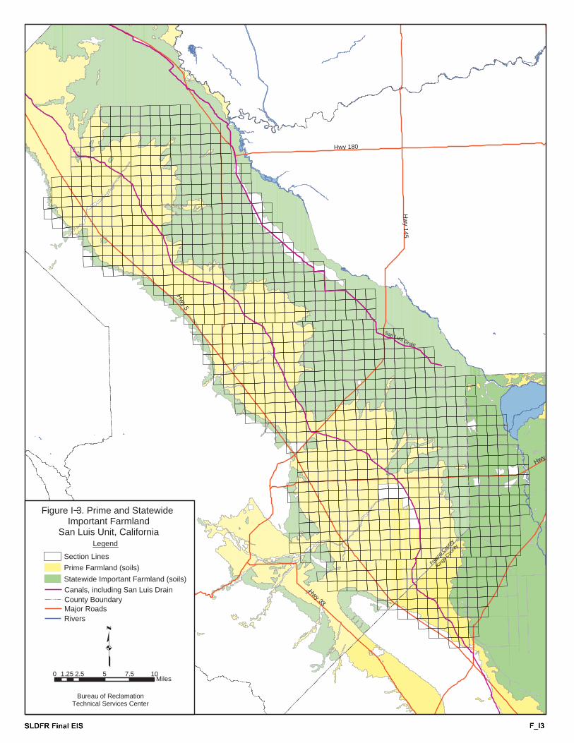
Kings C
ount
y
Fres
no C
ount
y
San Luis Drain
Hw
y 5
Hwy 180
Hw
y 145
Hwy 198
Hwy 33
Hwy 1
q0 2.5 5 7.5 101.25
Miles
Bureau of ReclamationTechnical Services Center
Figure I−3. Prime and Statewide Important Farmland
San Luis Unit, California
Section Lines
Prime Farmland (soils)
Statewide Important Farmland (soils)
Legend
Rivers
Canals, including San Luis Drain
Major RoadsCounty Boundary


Attachment I4
Salt Sink Evaluation Map


SLDFR Final EIS F_I4
Attachment I4


Attachment I5
Watsuit Model Output


SLDFR Final EIS Att_I5
The EC and ion concentrations given on these tables are on a soil-water basis. To estimate equivalent saturation extract levels, divide the tabular concentration values by two.
Note: All concentrations are in meq/L Case ID: Westlands Alluvial Upland areas Amendments: None Leaching fraction treatment: 0.05
Depth LF "1/LF" Ca Mg Na+K Cl CO3 HCO3 SO4 0 1.00 1.00 1.86 1.25 3.04 2.84 0.45 1.92 0.941 0.62 1.61 3.49 2.02 4.90 4.58 0.43 3.88 1.522 0.33 3.03 5.04 3.79 9.21 8.61 0.44 6.15 2.853 0.14 7.14 5.45 8.93 21.71 20.29 0.47 8.62 6.714 0.05 20.00 4.60 25.00 60.80 56.80 0.64 14.16 18.80
Depth pH Ca/Mg Sum Cat. EC SAR Lime Gypsum
0 8.22 1.490 6.15 0.64 2.37 -0.76 0.001 7.65 1.732 10.41 1.02 2.88 -1.72 0.002 7.36 1.331 18.04 1.71 4.27 -1.71 0.003 7.29 0.610 36.09 3.43 7.89 2.41 0.004 7.34 0.184 90.40 8.47 15.39 17.40 0.00
Case ID: Westlands Alluvial Upland areas Amendments: None Leaching fraction treatment: 0.10
Depth LF "1/LF" Ca Mg Na+K Cl CO3 HCO3 SO4 0 1.00 1.00 1.86 1.25 3.04 2.84 0.45 1.92 0.941 0.64 1.56 3.50 1.95 4.75 4.44 0.43 3.86 1.472 0.37 2.70 5.08 3.38 8.22 7.68 0.43 6.03 2.543 0.19 5.26 5.69 6.58 16.00 14.95 0.45 7.92 4.954 0.10 10.00 5.76 12.50 30.40 28.40 0.49 10.37 9.40
Depth pH Ca/Mg Sum Cat. EC SAR Lime Gypsum
0 8.22 1.490 6.15 0.64 2.37 -0.76 0.001 7.65 1.791 10.20 1.00 2.80 -1.78 0.002 7.35 1.504 16.67 1.58 3.89 -2.11 0.003 7.26 0.865 28.27 2.68 6.29 0.10 0.004 7.24 0.461 48.66 4.64 9.80 5.24 0.00


Attachment I6
EM38 Meter Calibration Graphs


SLDFR Final EIS Att_I6
Soil salinity calibration curve, San Luis Reuse sites, EMTERSP program
y = 0.9031x + 1.3906R2 = 0.7941
0
2
4
6
8
10
12
14
16
0 2 4 6 8 10 12 14
Predicted ECe (ds/m)
Lab
Ece
(ds/
m)
Lab eCe Linear (Lab eCe)
Soil Salinity Relationships, San Luis Reuse Areas
y = 0.0143x + 6.1345
R2 = 0.7955
0
2
4
6
8
10
12
14
16
0 100 200 300 400 500 600
EMh @15c (ms/m)
ECe
(ds/
m)
eCe Linear (eCe)

Attachment I7
NRCS Soil Salinity, Landform, and Drainage Maps of the San Luis Unit


SLDFR Final EIS Att_I7 Figures


SLDFR Final EIS Att_I7 Figures


SLDFR Final EIS Att_I7 Figures


SLDFR Final EIS Att_I7 Figures


SLDFR Final EIS Att_I7 Figures


Attachment I8
Natural Drainage Map for Northern Drainage-Impaired Areas


SLDFR Final EIS Att_I8

APPENDIXJ
Implementation of In-Valley Alternatives


TABLE OF CONTENTS
SLDFR Final EIS Appendix J J-i
Appendix J Implementation of In-Valley Alternatives...................................................................... J-1
J1 Feasibility Designs and Cost Estimates ....................................................J-1
J2 Permitting..................................................................................................J-1
J3 Final Design ..............................................................................................J-2
J4 Land Acquisition.......................................................................................J-2
J5 Phased Construction..................................................................................J-2
J6 Environmental Mitigation.........................................................................J-3
J7 Evaluation of Innovative Technologies ....................................................J-4
Attachment J1 Mitigation for Selenium-Related Effects of Evaporation Basins
TABLE OF CONTENTS
SLDFR Final EIS Appendix J J-ii
Acronyms µg/L micrograms per liter
AH alternative habitat
AX alternative habitat dietary exposure
Regional Board Regional Water Quality Control Board
BX evaporation basin dietary exposure
CH compensation habitat
DS dilution standard
EH evaporation basin acreage
ENH enhancement habitat
HU habitat utility
K coefficient of relative habitat attractiveness
mg/kg milligrams per kilogram
mg/L milligrams per liter
NA Northerly Area
OH other habitat
ppm parts per million
Reclamation Bureau of Reclamation
RO reverse osmosis
ROD Record of Decision
Se selenium
TDS total dissolved solids
Unit San Luis Unit
WC Westlands Central
Westlands Westlands Water District
WN Westlands North
WS Westlands South

Appendix J Implementation of In-Valley Alternatives
SLDFR Final EIS Appendix J J-1
APPENDIX J IMPLEMENTATION OF IN-VALLEY ALTERNATIVES
Preliminary implementation schedules for the In-Valley Alternatives are shown in Section 2 of the main report (Figures 2.4-4, 2.5-2, 2.6-2, and 2.7-2). These alternatives are composed of the following common drainage service components:
• Collection System: Closed pipelines that collect drainwater from farm lands in Westlands and convey it to reuse facilities; a combination of closed pipelines and open ditches that collect drainwater and convey it to reuse facilities in the Northerly Area.
• Reuse Facilities: Farm lands that reuse the collected drainwater to irrigate salt-tolerant crops. Drainwater from these facilities is collected by tile drains for treatment and disposal.
• Conveyance System: Closed pipelines that convey drainwater from the reuse facilities to the treatment and disposal areas.
• Reverse Osmosis (RO) Treatment: Desalination of drainwater to recover high-quality product water, which can be reused for irrigation or other beneficial use.
• Selenium (Se) Biotreatment: Saline concentrate waste stream from RO is treated to remove Se.
• Evaporation Basins: Treated effluent from biotreatment is discharged to evaporation basins to precipitate salts for in-place disposal.
• Evaporation Basin Mitigation: Constructed or enhanced wetland habitats sited and managed to reduce or compensate for adverse effects to waterbirds from operation of the evaporation basins.
The differences among the In-Valley Alternatives are simply the number, size, and locations of these components, which are determined by the amount and location of future retired lands. Consequently, most aspects of drainage service construction and operation will be the same among these alternatives.
Implementation activities include feasibility designs and cost estimates, permitting, final design, land acquisition, phased construction, environmental mitigation, and evaluation of innovative technologies.
J1 FEASIBILITY DESIGNS AND COST ESTIMATES This activity evaluates technical feasibility of the alternatives and generates cost estimates for construction and operation. Feasibility evaluation includes field investigations, data analysis, engineering designs, quantity estimates, and cost estimates. The cost estimates are used to obtain authorization and funding from Congress to construct the project. The feasibility design will also include a more detailed plan and schedule than is presented herein for all of the subsequent implementation activities. This activity is currently under way for the In-Valley Alternatives and is scheduled for completion in 2006.
J2 PERMITTING One or more of the components of drainage service will require permits to construct and/or operate. Notable among these, evaporation systems require permits from the Regional Water Quality Control Board (Regional Board), which also identify initial mitigation measures. The

Appendix J Implementation of In-Valley Alternatives
SLDFR Final EIS Appendix J J-2
Bureau of Reclamation (Reclamation) or local partners will apply for the necessary permits upon selection of the final drainage service alternative. The length of time to complete the permitting process is uncertain but may take about 2 years. The regulatory environment and compliance requirements described in Section 4 of the main report are addressed through the permitting process.
J3 FINAL DESIGN A final design of the drainage service project will commence when the final alternative is selected in the Record of Decision (ROD) in 2006. The final design builds upon the feasibility design but is more detailed and comprehensive. The product of final design consists of several packages of written engineering specifications and drawings that are used for contracting and construction of the project. Some components or packages of the final design will be completed before others, which will enable the contracting and construction process to begin before final design of the entire project is completed in 2008.
J4 LAND ACQUISITION Implementation of drainage service will require the acquisition of easements and real estate property to construct and operate the various components of drainage service. Construction of collection and conveyance systems can likely be accomplished by granting easements. Land area needed for reuse, treatment, disposal, and mitigation components will require the purchase of land to construct and operate these facilities. Leasing of lands or other contractual arrangements with local districts and farmers may also be considered. If the selected drainage service alternative includes land retirement, steps can be undertaken immediately for the purpose of retiring these lands from irrigated agricultural production. Where technically feasible, retired lands will be used for project facilities, reducing overall land acquisition requirements. Land retirement will occur concurrently with permitting and final design activities for drainage service facilities.
J5 PHASED CONSTRUCTION Specifications and drawings produced in final design are used to prepare bid and contract documents for the various components and phases of drainage service to be constructed. The implementation schedules shown in Section 2 of the main report (Figures 2.4-4, 2.5-2, 2.6-2, and 2.7-2) assume that construction activities gradually start after the ROD in 2006 and level out at a spending rate of approximately $100 million per year until completion. For all In-Valley Alternatives, it is anticipated that initial construction efforts will begin in the Northerly Area to meet discharge requirements, and proceed southward through the San Luis Unit (Unit).
• Northerly Area Construction: A large portion of the Northerly Area is currently drained. Local farming districts have constructed and are operating collection and reuse components of drainage service. Implementation of Federal drainage service will expand the existing collection and reuse infrastructure and add the treatment, disposal, and mitigation components. Construction of treatment, disposal, and initial mitigation components would receive highest priority to accommodate existing drainage flows and are expected to be completed in 2009.
Appendix J Implementation of In-Valley Alternatives
SLDFR Final EIS Appendix J J-3
• Westlands Water District (Westlands) Construction: Initial construction efforts will focus on construction of collection and reuse components. Completion of these components will permit partial implementation of drainage service because it is anticipated that collection and reuse facilities may operate at least 2 years while conveyance, treatment, disposal, and mitigation systems are being constructed.
Construction of drainage service components in Westlands will likely proceed simultaneously with the Northerly Area but will take several years longer to complete because Westlands covers a much larger area and does not have significant existing drainage infrastructure. Among the drainage service alternatives for Westlands, the In-Valley Disposal Alternative provides drainage service to the largest geographic area, requires the largest constructed facilities, and will require more years to construct than the Land Retirement Alternatives.
Although Reclamation will construct various components of drainage service, it is up to the individual farmer or Westlands to install on-farm, subsurface tile drains to collect the drainwater and pump it into the Federal collection system for further reuse, treatment, and disposal. It is anticipated that not all eligible farmers in Westlands will utilize the drainage service. It is also assumed that farmers who choose to install tile drains will do so gradually over the 50-year planning period. Therefore, drainage service components will be constructed in two or more phases to meet the projected capacity requirements over the 50-year planning period. For example, the initial construction phase may only install about 50 percent of the total projected capacity needed over 50 years. After about 20 years, a second construction phase will install the additional capacity needed for full buildout. Only the initial construction phase for Westlands is shown in the implementation schedules in Section 2 of the main report (Figures 2.4-4, 2.5-2, 2.6-2, and 2.7-2).
The phased construction of drainage service in Westlands reduces the overall cost of construction and provides greater flexibility in responding to changes in drainage quality and quantity over time. Phased implementation also permits monitoring of environmental impacts of evaporation basins and refinement of mitigation measures to reduce and compensate for these impacts, and continuing evaluation and incorporation of technical innovations to improve or optimize the treatment and disposal systems.
J6 ENVIRONMENTAL MITIGATION Reclamation anticipates adverse effects to waterbirds during operation of the evaporation basins. A conceptual phased mitigation, monitoring, and adaptive management approach for the In-Valley Alternatives is shown in Attachment J1, Figure J-1. The phased adaptive management approach is described in more detail in Attachment J1. Evaluation and quantification of potential environmental impacts is subjective and uncertain. Likewise, the effectiveness of potential mitigation measures to reduce and compensate for these impacts is uncertain. Initial mitigation and monitoring measures will be implemented during the first phase of construction of drainage service components.
Operation of the evaporation basins and mitigation facilities will be closely monitored and modified as needed to reduce and compensate for the environmental effects. Changes to the construction and operation of these facilities will be implemented as part of the phased construction process. It is anticipated that monitoring impacts and modification of operations and

Appendix J Implementation of In-Valley Alternatives
SLDFR Final EIS Appendix J J-4
facilities will be repeated during the life of the project. This iterative continual process of implementing environmental mitigation is referred to as adaptive management and consists of the following steps:
1. Implement initial mitigation measures. The mitigation facilities described in the initial plan will be constructed during the first phase of drainage service.
2. Monitor environmental impacts and effectiveness of mitigation measures for the constructed facilities. Monitoring activities will include tracking the concentrations and fate of drainwater contaminants in the evaporation basins (including groundwater monitoring wells), field observations of waterbird use and data collection of Se bioaccumulation at the evaporation basins and mitigation facilities, and measurements of the effectiveness of the mitigation measures to reduce and compensate for impacts.
3. Analyze and modify mitigation measures as appropriate. Data collected from monitoring activities will be evaluated to determine actual environmental impacts and mitigation requirements. The effectiveness of existing mitigation measures will be analyzed. Modifications will be implemented to address and conform to actual field conditions. Modifications may include changes to the design and operation of the evaporation basins as well as the mitigation facilities. Individual mitigation measures may be increased, decreased, or modified depending on their effectiveness and need.
4. Repeat Steps 2 and 3 throughout the life of the project.
J7 EVALUATION OF INNOVATIVE TECHNOLOGIES The primary barrier to achieving in-valley drainage service during the past 30 years has been the lack of affordable technologies to reduce or eliminate the associated environmental impacts. Recent advances in technologies for desalination and Se removal have significantly reduced the treatment costs and potential impacts of releasing irrigation drainwater into the environment. These treatment technologies have been implemented and proven at other locations, field-tested at the San Luis Unit, and are now integral components of all In-Valley Alternatives.
As part of the overall implementation strategy, Reclamation continues to monitor and investigate enhancements to these technologies as well as other innovative technologies that can potentially lower the costs and environmental risks of drainage service. Evaluation and implementation of innovative technologies occur through a process of technology review, laboratory and field studies, and demonstration:
• Technology Review: Reclamation staff monitors technological developments and consults with outside researchers; they review ongoing research and determine potential applicability to drainwater treatment and disposal.
• Laboratory and Field Studies: Bench- and pilot-scale studies are conducted to gather performance and operation data to assist in the designs for full-scale implementation of reuse, RO treatment, Se biotreatment, and evaporation disposal of drainwater. Reclamation is currently performing laboratory and field investigations for all of these components and will continue to evaluate these and other innovative technologies during implementation of drainage service as funding permits.

Appendix J Implementation of In-Valley Alternatives
SLDFR Final EIS Appendix J J-5
• Demonstration: Reclamation is also developing plans for a larger demonstration facility in the Northerly Area as an intermediate step towards implementation of drainage service. The demonstration facility would receive drainwater from existing reuse sites and provide RO treatment, Se biotreatment, and evaporation disposal. This facility would be used to optimize the existing systems to site-specific conditions and evaluate technology enhancements to be used in the full-scale design.
The current status and potential implementation of innovative technologies for each of the treatment and disposal components is described below:
• RO Treatment: Conventional RO treatment has been pilot-tested in the San Luis Unit and found to be effective in desalinating the drainwater. Product water recovery, however, is limited to about 50 percent of the influent feedwater due to high calcium concentrations. Reclamation is collaborating with PCI Membranes and WaterTech Partners to evaluate the patented DP3RO process, which removes calcium from the RO feedwater to increase product water recovery up to about 90 percent. A laboratory bench-scale study was completed and a pilot study is being conducted from September 2004 to March 2006. Based on the results of this pilot study, a technical and economic analysis will determine whether this innovative technology should be added as a pretreatment step to RO. This determination will likely be made by August 2006.
Reclamation is also evaluating recent technological advancements related to boron removal. Membrane manufacturers have announced a new generation of membranes that are effective in separating boron during RO treatment. Also, a new ion exchange resin was recently field-tested for boron removal from RO product water in the Unit. This information will be reviewed and perhaps more field studies will be performed to determine whether either of these options should be incorporated into the RO treatment process by August 2006.
• Se Treatment: Reclamation has conducted bench- and pilot-scale studies of the patented ABMet® biotreatment process to remove Se from the RO concentrate and found this technology to be superior in performance to all other available technologies. An additional pilot study of this technology will be conducted in 2005 and 2006 to incorporate recent design improvements in an effort to optimize the treatment process and maximize Se removal.
Se speciation studies are currently underway to quantify and characterize the residual Se in the treated effluent and the Se that is removed from the drainwater and stored within the bioreactor tanks of the treatment system. This information will be used to assess potential post-treatment operations to render the residual Se less bioavailable, and to assess potential beneficial uses or disposal methods of the Se that is removed from the drainwater.
Bench- and pilot-scale studies will be performed in 2005 to evaluate biological oxidation as a method of converting organic residual Se into less bioavailable inorganic forms. The results of all of the above studies will be published in May 2006. The results will be used to perform full-scale designs, determine Se disposal requirements, and reduce uncertainty of environmental impacts of the treated effluent.
• Evaporation Technologies: The In-Valley Alternatives incorporate evaporation basins as the final step in the treatment and disposal process of drainwater. This method has proven effective at existing basins in the Unit for concentrating drainwater and precipitating salts for

Appendix J Implementation of In-Valley Alternatives
SLDFR Final EIS Appendix J J-6
final disposal. A variety of innovative technologies to increase the evaporation rate have been or are currently being tested at locations within and outside of the Unit. These technologies include dewvaporation, Solar Bee mixers, salt-gradient solar ponds, wind turbines, and different configurations of sprinkler systems. Reclamation is monitoring, reviewing, and in some cases funding research on these evaporation technologies for applicability to the Unit.
By August 2006, recommendations will be made as to whether any of these options should be incorporated into the full-scale design of evaporation basins or if on-site field investigations should be pursued. Reclamation constructed small evaporation basins in the Northerly Area for the purpose of monitoring Se bioaccumulation, but enhanced evaporation is not being studied at this site.
Manipulation and recovery of precipitated salts for beneficial reuse is another area of interest that is being evaluated in conjunction with evaporation technologies. Field studies are needed to determine whether salt recovery is technically and economically feasible in the Unit. Reclamation is consulting with technology vendors and seeking funding for field studies in 2005 and 2006. If successful, a salt recovery process will be incorporated into the full-scale design and implementation of evaporation technologies.

Attachment J1 Mitigation for Selenium-Related Effects of Evaporation Basins


TABLE OF CONTENTS
SLDFR Final EIS Appendix J J1-i
J1.1 Evaporation Basin Design And Management Objectives.......................J1-3
J1.2 Alternative Habitat..................................................................................J1-4
J1.2.1 Dilution Standard ........................................................................J1-6 J1.2.2 Coefficient of Relative Habitat Attractiveness ...........................J1-6 J1.2.3 Estimation of Dietary Selenium..................................................J1-9 J1.2.4 Estimated Alternative Habitat Acreage ....................................J1-10
J1.3 Compensation Habitat...........................................................................J1-10
J1.3.1 Predicted Selenium Concentration in Dietary Tissue at Evaporation Basins ...................................................................J1-12
J1.3.2 Predicted Selenium Concentration in Bird Egg Tissue at Evaporation Basins ...................................................................J1-12
J1.3.3 Relative Habitat Utility (HU)....................................................J1-12 J1.3.4 Acres of Evaporation Basin (EH) .............................................J1-12 J1.3.5 Compensation Coefficient (CC) ...............................................J1-12 J1.3.6 Estimated Compensation Habitat Acreage ...............................J1-13
J1.4 Initial Estimate ......................................................................................J1-14
J1.5 Adaptive Management Contingency Allowance ..................................J1-14
J1.6 Mitigation Estimates for all In-Valley Alternatives..............................J1-17
J1.7 Mitigation Site Selection.......................................................................J1-17
J1.8 Mitigation Site Evaluation Factors .......................................................J1-20
J1.8.1 Initial Review General Site Characteristics ..............................J1-20 J1.8.2 Mitigation Habitat Types and Bird Guilds................................J1-20 J1.8.3 Specific Mitigation Site Layout and Design Planning
Factors.......................................................................................J1-23
J1.9 Mitigation Site Options.........................................................................J1-23
J1.9.1 Initial Site Review Assumptions...............................................J1-23 J1.9.2 Inventory of Potential Mitigation Areas ...................................J1-24
J1.10 References.............................................................................................J1-27

TABLE OF CONTENTS
SLDFR Final EIS Appendix J J1-ii
Tables J-1 Estimated Area of Alternative Habitat Based on Dilution to 10 mg/kg Se in Diet –
In-Valley Disposal Alternative
J-2 Estimated Area of Compensation Habitat – In-Valley Disposal Alternative
J-3 Mitigation Estimates for All In-Valley Alternatives
J-4 Mitigation Planning Considerations for Targeted Bird Guild Functions
J-5 Potential Mitigation Areas – Initial Review First-Cut Summary List
Figures J-1 In-Valley Alternative (Mitigation Facilities Only), Conceptual Planned
Development through Phase 1 of Project Implementation (2007–2027)
J-2 Conceptual Mitigation Framework Plan – Concepts and Interactions
J-3 Mitigation Components – Expanded Description and Examples

Attachment J1 Mitigation for Selenium-Related Effects of Evaporation Basins
SLDFR Final EIS Appendix J J1-1
This attachment summarizes the mitigation habitat acreage estimation approach used for planning and cost-estimating purposes for the In-Valley Alternatives. This attachment addresses only mitigation for selenium (Se)-related effects due to operation of evaporation basins associated with these alternatives and does not include mitigation for reuse areas or other facilities. The approach presented below was developed by Reclamation in coordination with the SLDFR Mitigation Work Group.
A number of options are available for mitigation of Se-related effects due to construction of new evaporation basins under each of the In-Valley Alternatives. Habitat may be created to mitigate for adverse physiological and reproductive effects to waterfowl and shorebirds exposed to elevated levels of Se within the evaporation basins. Construction of Se-safe alternative habitat mitigation facilities would provide attractive, uncontaminated alternative foraging and nesting habitat, thus reducing overall contaminant exposure in the landscape surrounding the basins. Compensation habitat would support additional birds to replace those adversely affected by evaporation basins. A conceptual phased mitigation, monitoring, and adaptive management approach is shown in Figure J-1.
The Mitigation Work Group generally agreed that if vertical walls and water depth greater than 4 feet could be ensured for the proposed evaporation basins, little or no use by shorebirds or dabblers would be expected to occur (historical bird monitoring data are not available for basins with vertical walls). However, certain evaporation basin cells may dry out during some periods (such as during the transition from a wet year to a dry year). During transitional periods when some pond cells would have shallow water, some shorebirds/dabblers could be affected. Therefore, some limited mitigation may be necessary for time periods and locations where drawdown occurs. If, for example, pond cells are drawn down or dry out during the late spring (the breeding season), large numbers of shorebirds and dabblers might forage in the shallow water, potentially resulting in increased exposure during the most sensitive time (when reproductive effects could occur). However, if cells are dried out in late summer, increased exposure could be avoided during the reproductive season as well as during the migration seasons, when shorebirds and dabblers are present in larger numbers and may be more sensitive due to stress.
For purposes of estimating mitigation acreage, it was assumed that the size of the area to be affected by low water levels would be the difference in area between the “maximum” wetted area (average under wet year conditions) and “average” wetted area (average water year conditions). For the In-Valley Disposal Alternative, this difference would be 3,290 acres minus 2,870 acres, or 420 acres. It was agreed that, provided Reclamation could ensure vertical side walls and water depths of 4 feet in the remaining pond cells, mitigation requirements for shorebirds and dabblers could be limited to the area of cells that may be dried out.

Attachment J1 Implementation of In-Valley Alternatives
SLDFR Final EIS Appendix J J1-2
Figure J-1
In-Valley Alternative (Mitigation Facilities Only) Conceptual Planned Development through Phase 1 of Project Implementation (2007–2027)

Attachment J1 Implementation of In-Valley Alternatives
SLDFR Final EIS Appendix J J1-3
The approach to estimate the amount of mitigation habitat needed is to first determine the acreage of alternative habitat sufficient to dilute the dietary Se concentration to 10 milligrams per kilogram (mg/kg) (the low end of the threshold range for adult mortality) for breeding shorebirds, nonbreeding shorebirds,1 and dabblers. Assuming this amount of alternative habitat would be created, the amount of compensation habitat acreage likely to be needed under the assumed conditions of drawdown was then calculated. This compensation (or contingency) habitat would mitigate for effects during the breeding season if such conditions were to occur.
The approach for planning and cost-estimating is to calculate an initial estimate of combined alternative and compensation habitat acreage, plus an adaptive management/contingency allowance that would be implemented if effects are greater than predicted, due to unexpected circumstances relating to any of the various parameter values that were used in the initial estimate. For example, if monitoring results indicate that effects are greater than expected due to higher than expected bird densities in the drawn-down cells, additional mitigation would be triggered and implemented as part of the adaptive management/contingency allowance. The feasibility planning estimate that would be used for cost-estimating purposes would include both the initial estimate and the adaptive management/contingency allowance.
J1.1 EVAPORATION BASIN DESIGN AND MANAGEMENT OBJECTIVES Preliminary designs and costs for evaporation basins assume the following features:
Design Features • Bottoms of basins would be constructed using natural clay liners compacted from native soils
to reduce overall permeability of foundation soils.
• Basins would be constructed with side slopes close to vertical, with ramps to allow exit by wildlife, and with no interior levees.
• Evaporation basins would consist of sequential evaporation cells that diminish in size as the drainage flows toward the terminal cell where final salt precipitation occurs.
• Basins would be located where underlying groundwater is not potable and not considered to be a source of drinking water (i.e., total dissolved solids [TDS] > 3,000 milligrams per liter [mg/L]).
• Basins would be located above the 100-year floodplain or would be constructed to prevent overtopping during 100-year flood events.
• Basins would be located on existing retired lands where practical.
• Basins would be located in areas with flat or gently sloping terrain (as close to level as possible).
1 As used in this appendix, “breeding shorebirds” refers to species that are expected to breed at evaporation basins, and “nonbreeding shorebirds” refers to species that are expected to forage but are not likely to breed at evaporation basins.

Attachment J1 Implementation of In-Valley Alternatives
SLDFR Final EIS Appendix J J1-4
• Basins would not be located within native or natural habitat types used by endangered or protected species.
• Most basins would be surrounded by reuse areas, which would act as a buffer zone to nearby commercial irrigated agriculture.
Management Measures • Wells would be established near each basin site to verify and monitor groundwater
conditions before, during, and after evaporation basin installation.
• Management techniques would be implemented to minimize adverse biological effects associated with wildlife exposure to Se, including maintaining basin depths of >4 feet, controlling aquatic and terrestrial vegetation to avoid nesting habitat, and hazing of waterfowl. During periods of drawdown, affected cells would be actively managed and monitored. Portable pumps would be utilized to minimize the presence of shallow water or mudflats in receding cells, and the frequency of hazing in these transitional areas would be increased.
• Basin operational design would include provisions to evacuate individual evaporation basin cells if inflow is not sufficient to maintain a 4-foot minimum depth.
• Se concentrations within basin waters would be maintained below levels designated as hazardous waste.
• Se concentrations within precipitated salts and sediments would be maintained below levels designated as hazardous waste.
• Site closure would entail in-place burial of precipitated salts, placement of low-permeability soil cap, grading to control runoff and ponding of precipitation, establishment of vegetation to minimize erosion, and long-term monitoring of selected biota and the underlying groundwater.
• Methods to minimize invertebrate populations in evaporation basins would be explored, and results would be used in adaptive management.
• Measures such as intensive hazing and salinity management would be implemented to minimize potential for salt encrustation and salt toxicosis to wintering birds, particularly on cold nights.
J1.2 ALTERNATIVE HABITAT Alternative habitat is defined as year-round, Se-safe wetland habitat that is located in the same “functional landscape” as the evaporation basin. The functional landscape of an evaporation basin is defined as a limited radius (approximately 1 to 3 kilometers) around a basin within which the presence of alternative habitat, in combination with hazing and other management actions, is very likely to significantly dilute the contaminant exposure of birds attracted to the basin. The purpose of alternative habitat is not necessarily to reduce the number of breeding and nonbreeding birds using an evaporation basin, but rather to reduce the relative proportion of feeding time that the birds, whatever their number, allocate to evaporation basins versus “clean”

Attachment J1 Implementation of In-Valley Alternatives
SLDFR Final EIS Appendix J J1-5
wetlands. These wetlands would require a safe and reliable freshwater source. Development of alternative habitat is a preemptive strategy.
Other elements of the mitigation strategy include: (1) reducing the amount of waterbird use at the evaporation basins by implementing design and management actions to decrease the basins’ attractiveness to birds; and (2) developing compensation habitat (i.e., additional breeding habitat) on an as-needed basis to directly offset actual or estimated unavoidable waterbird losses by providing additional high-quality nesting habitat during the breeding season.
Minimal nesting habitat currently exists for dabblers, divers, and nonbreeding shorebirds near the proposed evaporation facilities. Therefore, creation of additional shallow open or emergent wetlands and vegetated upland nesting habitat near evaporation basins during the breeding season would be avoided as its presence would only serve to attract breeding birds to the general vicinity of the basins, thereby increasing the potential for reproductive effects due to Se exposure. Similarly, no deepwater alternative habitat would be created for divers, as this could result in attracting more diving birds to the vicinity of the evaporation basins during the breeding season. Only compensation habitat would be provided for divers.
The approach presented here is to estimate the amount of alternative habitat sufficient to dilute the dietary Se concentration to 10 mg/kg (the low end of the threshold range for adult mortality) for all shorebirds and dabblers. The Service protocol for estimating alternative habitat, Alternative Habitat Protocol for Drainwater Evaporation Basins (Service 1995a), was used for these calculations, with some modifications as described below.
The Service protocol determines the maximum proportion of an avian population’s diet (Qmax) that can come from the evaporation basin without exceeding a toxicity threshold. Qmax is established using the following formula:
Qmax = (DS - AX) / (BX - AX)
Where:
Qmax = Maximum proportion of an avian population’s diet that can be obtained from the Se-contaminated evaporation basin without exceeding the dilution standard (DS)
DS = Dilution standard
AX = Alternative habitat dietary exposure = Average Se concentration of dietary items obtained from the alternative habitat (AH)
BX = Evaporation Basin Dietary Exposure = Average Se concentration of dietary items obtained from the evaporation basin (EH)
Once Qmax has been established, the next step is to calculate the minimum amount of alternative habitat required to not exceed the DS. If the size of an evaporation basin and the information needed to estimate Qmax are known, the minimum amount of alternative habitat required (AHmin) can be estimated using the following equation:
AH = (1-Qmax)(EH) / (Qmax)(K)
Where:
AH = Minimum alternative habitat obligation
EH = Evaporation basin acreage

Attachment J1 Implementation of In-Valley Alternatives
SLDFR Final EIS Appendix J J1-6
K = Coefficient of Relative Habitat Attractiveness
It should be noted that the alternative habitat protocol (Service 1995a) is based on protection of the reproductive health of birds likely to breed at the evaporation basins. However, birds that overwinter or periodically forage (but do not breed) at the evaporation basins may also experience adverse effects from ingestion of Se. Therefore, these types of birds were also considered in this evaluation.
J1.2.1 Dilution Standard The protocol defines the dilution standard (DS) as the maximum safe dietary Se exposure for waterbirds on a long-term basis. A DS of 2.6 parts per million (ppm) dietary Se was derived from risk relationships presented in the Cumulative Impacts Report for Tulare Basin Evaporation Basins (CH2M Hill et al. 1993). However, for this evaluation, the objective is to provide enough alternative habitat to dilute the concentrations to below the threshold for adult mortality. Generally, mortality due to high dietary Se is preceded by severe weight loss. Several studies provide data on dietary Se concentrations associated with weight loss. Heinz and Fitzgerald (1993) found that after 1 week of treatment, body weights of adult male mallards were significantly depressed when dietary Se concentrations were 20, 40, and 80 mg/kg, but not when the dietary Se concentration was 10 mg/kg. Albers et al. (1996) reported that adult male mallards fed 40 and 80 mg/kg Se in food experienced significant weight loss as compared to mallards fed 0, 10, and 20 mg/kg Se in food. Heinz et al. (1987) reported no effects on weight in adult mallards fed 1, 5, or 10 mg/kg Se in food and weight loss in mallards fed 25 mg/kg Se. Heinz, Hoffman, and Gold (1989) found that adult female mallards consuming 16 mg/kg Se in their diet experienced temporary weight loss but those consuming 8 mg/kg Se were unaffected. Heinz and Hoffman (1996) reported that no mallards fed 10 mg/kg dry weight in the diet exhibited physiological symptoms.
Based on the evidence presented above, 10 mg/kg is considered the highest dietary Se concentration at which no significant change in body weight or increase in mortality would be expected to occur in adult mallards using the evaporation basins for foraging. Therefore, 10 mg/kg was selected as the DS value for birds likely to be foraging but not breeding at the evaporation basins.
J1.2.2 Coefficient of Relative Habitat Attractiveness The coefficient of relative habitat attractiveness (K) used in the protocol is the ratio of bird density at mitigation habitat to the bird density at evaporation basins. The value of K combines the net effect of all factors that influence the relative propensity of alternative habitat versus evaporation basins to attract foraging birds. As the relative attractiveness of alternative habitat increases, K increases. Any actions that improve the attractiveness of alternative habitat or diminish the attractiveness of evaporation basin habitat will function to increase the value of K. Factors that diminish the attractiveness of evaporation basin habitat such as the physical design, the way water is managed, invertebrate management, and intensity of hazing will increase the value of K. As K increases, the acreage of alternative habitat needed to meet the DS decreases.
Bird community usage of evaporation basins was analyzed using historical survey data, as discussed in Appendix G, Section G2.3.4. The data analysis was divided into four seasons:

Attachment J1 Implementation of In-Valley Alternatives
SLDFR Final EIS Appendix J J1-7
spring migration (February through April), breeding (May through July), fall migration (August through October), and winter (November through January). The data analysis was also divided into six bird categories (as described in Appendix G, Table G-1): dabblers, divers, breeding shorebirds, nonbreeding shorebirds, upland birds, and other waterbirds. These categories are based on distinct types of foraging behavior, dietary composition, and seasonal use patterns and therefore address different potentials for Se exposure. Species assigned to each of the bird categories are listed in Appendix G, Table G-2. It should be noted that while Appendix G addressed risks to the northern shoveler separately from other birds in the dabbler category due to differences in feeding behavior, for purposes of this mitigation analysis the northern shoveler is included in the dabbler category. As shown in Table G-7, predicted dietary Se concentrations for the northern shoveler are lower than those for the dabbler for both the breeding and nonbreeding seasons; therefore, when shovelers are lumped with other dabblers the resulting risk predictions for shovelers are likely to be somewhat overestimated (erring on the protective side).
The histograms of bird density (in birds/acre) indicate that the data distribution is highly skewed. Therefore, an appropriate measure of central tendency is the sample median, rather than the sample mean (which may be affected by extremely high measurements). The median is defined as the middle measurement in an ordered set of data, that is, just as many observations are larger than the median measurement as smaller. The median of a highly skewed distribution is generally smaller than the arithmetic mean. The median and mean bird densities presented in Appendix G, Table G-3 represent the bird densities (of all bird species within the relevant bird category) at a given time. Although the median may be considered a more representative value, the mean was used for the mitigation calculations as it resulted in higher acreage of mitigation (a more conservative estimate).
The category of birds addressed in the alternative habitat protocol (Service 1995a) is the breeding shorebirds, or birds that are likely to breed at evaporation basins. The categories of birds not addressed in the protocol are birds not likely to breed at the evaporation basins, including dabblers, divers, nonbreeding shorebirds, other waterbirds, and upland birds. However, mitigation is also proposed for dabblers, divers, and nonbreeding shorebirds, as these types of birds may be affected by exposure to Se at evaporation basins.
No mitigation is proposed for other waterbirds or upland birds because they are not expected to receive significant exposure to Se in the evaporation basins. Dietary composition data for birds in the “other waterbirds” category are presented in Appendix G, Table G-4. A review of these data indicates that many of these species feed primarily on fish or terrestrial plants and invertebrates, and it is unlikely that aquatic invertebrates and plants from the evaporation basins would compose a high percentage of their diets. Similarly, it is expected that birds categorized as “upland birds” in Appendix G, Table G-2 obtain most of their food from terrestrial sources. Therefore, no quantitative evaluation of risks was conducted for the species categorized as other waterbirds or upland birds, as these species are unlikely to experience significant exposure to Se via feeding on plants or invertebrates at evaporation basins.
Using the bird monitoring data (both mean and median values for bird densities presented in Appendix G, Table G-3), values for K were calculated, as presented in Table J-1. The value of K was calculated as the ratio of bird density at mitigation habitat to the bird density at evaporation basins. It should be noted that a default K value of 1 is used for divers in these calculations. This assumes that divers will be equally likely to utilize evaporation basins and mitigation habitat.

Attachment J1 Implementation of In-Valley Alternatives
SLDFR Final EIS Appendix J J1-8
Because existing mitigation habitats are managed for shorebirds that prefer shallow water, insufficient data exist to determine an empirical K value for divers.
Table J-1 Estimated Area of Alternative Habitat Based on Dilution to 10 mg/kg Se in Diet –
In-Valley Disposal Alternative DS (Dilution Standard) mg/kg Se in dietary tissue
Bird Category Breeding Season Nonbreeding Seasons Dabblers 10 10 Divers NA NA Nonbreeding Shorebirds 10 10 Breeding Shorebirds 10 10
AX (Se Concentration in Alternative Habitat) Dietary Tissue (mg/kg Se) Water (mg/L total Se)
Benthic InvertebratesNektonic
Invertebrates Plants 2.3 2.3 0.49 0.0010
Breeding Season Average Dietary Composition (percent)
Bird Category Benthic InvertebratesNektonic
Invertebrates Plants AX (Average Dietary
Concentration) Dabblers 77 8.0 15 2.0 Nonbreeding Shorebirds 96 4.0 0.0 2.3 Breeding Shorebirds 96 4.0 0.0 2.3 Nonbreeding Seasons Average Dietary Composition (percent)
Benthic
Invertebrates Nektonic
Invertebrates Plants AX (Average Dietary
Concentration) Dabblers 42 9.0 49 1.4 Nonbreeding Shorebirds 96 4.0 0.0 2.3 Breeding Shorebirds 96 4.0 0.0 2.3
BX (Se Concentration in Evaporation Basin) Dietary Tissue (mg/kg Se) Water (mg/L total Se)
Benthic InvertebratesNektonic
Invertebrates Plants 16 8.7 2.7 0.010
Breeding Season Average Dietary Composition (percent)
Bird Category Benthic InvertebratesNektonic
Invertebrates Plants BX (Average Dietary
Concentration) Dabblers 77 8.0 15 13 Divers 85 0.0 15 14 Nonbreeding Shorebirds 96 4.0 0.0 15 Breeding Shorebirds 96 4.0 0.0 15 Nonbreeding Seasons Average Dietary Composition (percent)
Benthic
Invertebrates Nektonic
Invertebrates Plants BX (Average Dietary
Concentration) Dabblers 42 9.0 49 8.7 Divers 53 37 10 12 Nonbreeding Shorebirds 96 4.0 0.0 15 Breeding Shorebirds 96 4.0 0.0 15

Attachment J1 Implementation of In-Valley Alternatives
SLDFR Final EIS Appendix J J1-9
Table J-1 (concluded) Estimated Area of Alternative Habitat Based on Dilution to 10 mg/kg Se in Diet –
In-Valley Disposal Alternative K (Relative habitat attractiveness) unitless ratio
Assuming Median Densities Spring Migration Breeding Fall Migration Winter
Dabblers 3.7 8.7 2.5 8.0 Divers 1.0 1.0 1.0 1.0 Nonbreeding Shorebirds 6.0 5.5 1.1 4.1 Breeding Shorebirds 7.9 4.6 0.6 1.2 Assuming Mean Densities Spring Migration Breeding Fall Migration Winter Dabblers 2.0 2.7 1.5 1.8 Divers 1.0 1.0 1.0 1.0 Nonbreeding Shorebirds 6.1 2.3 2.1 1.5 Breeding Shorebirds 4.8 3.4 1.6 2.5
EH (Acres of Evaporation basin) Maximum Drawdown Area (total) 420
Qmax (Proportion of Diet from evap basins) (DS-AX)/(BX-AX) Spring Migration Breeding Fall Migration Winter
Dabblers 1.2 0.72 1.2 1.2 Nonbreeding Shorebirds 0.59 0.59 0.59 0.59 Breeding Shorebirds 0.59 0.59 0.59 0.59
AH (Acres of Alternative Habitat) (1-Q)(EH)/(Q)(K) Assuming Median Densities Spring Migration Breeding Fall Migration Winter
Dabblers 0.0 19 0.0 0.0 Nonbreeding Shorebirds 49 52 260 71 Breeding Shorebirds 37 62 480 240 Assuming Mean Densities Spring Migration Breeding Fall Migration Winter Dabblers 0.0 61 0.0 0.0 Nonbreeding Shorebirds 48 130 140 200 Breeding Shorebirds 61 85 180 120 Note: The most conservative value for AH for all bird categories and seasons (the shaded value of 480 acres) was selected for mitigation planning purposes
J1.2.3 Estimation of Dietary Selenium Invertebrates are assumed to be exposed to the Se concentrations in influent water (CWATER) for the respective evaporation basin or mitigation habitat. It is assumed that Se concentrations in influent water will be representative of typical Se concentrations throughout the evaporation basins and mitigation habitats. In accordance with the project description presented in Volume I, Section 2, the Se concentrations in treated water entering the evaporation basins will be no greater than 10 micrograms per liter (µg/L); therefore, it is assumed that CWATER will equal 10 µg/L. For this analysis it is conservatively assumed that average Se in source water for all alternative habitat will be 1 µg/L, based on historical water quality for the Delta-Mendota Canal. (Se concentrations in source water for mitigation habitat in areas other than the Northerly Area are likely to be substantially lower than 1 µg/L.)

Attachment J1 Implementation of In-Valley Alternatives
SLDFR Final EIS Appendix J J1-10
Predicted Se concentrations in plants and invertebrate prey in evaporation basins are discussed in Appendix G, Section G5.2. Avian exposure to Se from evaporation basins is discussed in Appendix G, Section G5.3.
J1.2.4 Estimated Alternative Habitat Acreage Table J-1 presents ranges of calculated alternative habitat acreage requirements (based on median and mean densities) for the proposed evaporation basins under the In-Valley Disposal Alternative for each bird category and season. As explained in Section J1.2, no deepwater alternative habitat would be created for divers, as this could result in attracting more diving birds to the vicinity of the evaporation basins during the breeding season. Only compensation habitat would be used for divers. It should be noted that the estimated alternative habitat acreage does not include nesting habitat, and additional acreage would be required to provide both vegetated and open nesting areas appropriate for the various types of birds. To estimate the amount of nesting habitat to be provided, a wetted foraging area to nest area ratio of approximately 2 to 1 could be used for each type of nesting habitat (open habitat for breeding shorebirds and vegetated habitat for nonbreeding shorebirds, dabblers, and divers).
J1.3 COMPENSATION HABITAT The premise of the Compensation Habitat Protocol for Drainwater Evaporation Basins (Service 1995b) is to calculate the “take” of birds, or estimate the number of individuals lost from the population due to Se toxicity from evaporation basins. The amount of compensation habitat required is based on the estimate of “take,” and the amount of additional “clean” habitat necessary to replace the birds lost. This protocol requires measurement of Se concentrations in tissues of adult female birds or eggs collected from evaporation basin sites. Therefore, strict implementation of this protocol requires that evaporation basins already exist. Because the proposed In-Valley Disposal Alternative evaporation basins do not yet exist, this protocol had to be modified to estimate the amount of compensation habitat that would be needed after implementation of alternative habitat.
To calculate the amount of compensation habitat necessary to mitigate for residual effects after creation of 480 acres of shallow-water alternative habitat, it was first necessary to calculate the average diluted dietary Se concentration for each bird category. Because the alternative habitat is expected to reduce the average dietary Se concentration below the weight loss/mortality threshold for breeding shorebirds, nonbreeding shorebirds, and dabblers during all seasons, no effects (on a population level) to these bird categories are expected to occur during the nonbreeding season. As shown in Table J-1, the maximum acreage calculation for the breeding season is based on mean densities for all types of birds considered. Therefore, only the breeding season was evaluated for residual effects to breeding shorebirds, nonbreeding shorebirds, and dabblers, assuming mean densities.
The diluted dietary Se concentrations (a weighted average of dietary Se concentrations at the alternative habitat and the evaporation basins) were calculated for each bird category using the following equation:
Diluted Dietary Se Concentration = (K(AH)(AX) + (EH)(BX)) / (K(AH) + EH)

Attachment J1 Implementation of In-Valley Alternatives
SLDFR Final EIS Appendix J J1-11
To estimate the predicted Se concentrations in tissues of eggs at the proposed evaporation basins, the predicted Se concentration in dietary tissue was multiplied by a factor of two, following guidance provided in the alternative habitat protocol (Service 1995a).
The following paragraphs describe each of the parameters included in the compensation habitat calculations, as shown in Table J-2.
Table J-2 Estimated Area of Compensation Habitat – In-Valley Disposal Alternative
Predicted Se Concentration in Average Diluted Dietary Tissue
Breeding Season, Assuming Mean Density and 480 acres Alternative
Habitat
Average Dietary Concentration
(mg/kg Se) Dabblers Diluted 4.7
Divers Not diluted (no deepwater alternative
habitat) - breeding season 14 Nonbreeding Shorebirds Diluted 5.9 Breeding Shorebirds Diluted 5.0
Predicted Average Se Concentration in Bird Egg Tissue (mg/kg Se) Dabblers 9.5 Divers 27 Nonbreeding Shorebirds 12 Breeding Shorebirds 9.9
HU (Relative habitat utility) (1/K) unitless ratio Breeding Season, Assuming Mean Density
Dabblers 0.37 Divers 1.0 Nonbreeding Shorebirds 0.43 Breeding Shorebirds 0.29
EH (Acres of Evaporation basin) Max Drawdown Area (shorebirds/dabblers) 420 Maximum Deep Area (divers) 3290
CC (Compensation Coefficient ) Breeding Season, Assuming Mean Density Dabblers 0.070 Divers 0.063 Nonbreeding Shorebirds 0.082 Breeding Shorebirds 0.056
Acres of Compensation Habitat Needed Breeding Season, Assuming Mean Density
Dabblers 29 Divers 210 Nonbreeding Shorebirds 34 Breeding Shorebirds 23

Attachment J1 Implementation of In-Valley Alternatives
SLDFR Final EIS Appendix J J1-12
J1.3.1 Predicted Selenium Concentration in Dietary Tissue at Evaporation Basins This value is identical to BX described under the alternative habitat calculations in Section J1.2.
J1.3.2 Predicted Selenium Concentration in Bird Egg Tissue at Evaporation Basins To estimate the predicted Se concentrations in tissues of eggs at the proposed evaporation basins, the predicted average dietary Se concentration (as described above) was multiplied by a factor of two, following guidance provided in the alternative habitat protocol (Service 1995a).
J1.3.3 Relative Habitat Utility (HU) This value is the inverse of K described under the alternative habitat calculations in Section J1.2. It should be noted that a default Habitat Utility value of 1 is used for divers in these calculations. This assumes that divers will be equally likely to utilize evaporation basins and mitigation habitat. Because existing mitigation habitats are managed for shorebirds that prefer shallow water, insufficient data exist to determine an empirical HU value for divers.
J1.3.4 Acres of Evaporation Basin (EH) This value is identical to that described under the alternative habitat calculations in Section J1.2.
J1.3.5 Compensation Coefficient (CC) The compensation coefficient is calculated by multiplying HU by the amount of reduction (fraction lost) expected to occur in the population of birds at the evaporation basins. The compensation habitat protocol (Service 1995b) accounts only for losses due to decreased reproduction in breeding birds, using the following equation:
CC = HU [F1 (L1) + F2 (L2) + F3 (L3) + F4 (L4) + F5 (L5)]
Where:
CC = The multiple of an evaporation basin’s acreage that, on average, would be necessary in compensation habitat to replace lost production
F1 = The proportion of randomly sampled eggs containing 0 to 5 ppm Se
F2 = The proportion of randomly sampled eggs containing 5.1 to 20 ppm Se
F3 = The proportion of randomly sampled eggs containing 21 to 40 ppm Se
F4 = The proportion of randomly sampled eggs containing 41 to 70 ppm Se
F5 = The proportion of randomly sampled eggs containing 71 or more ppm Se
L1 = The proportion of production lost when egg contamination is from 0 to 5 ppm Se (L1 = 0)
L2 = The proportion of production lost when egg contamination is from 5.1 to 20 ppm Se (L2 = 0.1889)
L3 = The proportion of production lost when egg contamination is from 21 to 40 ppm Se (L3 = 0.2551)

Attachment J1 Implementation of In-Valley Alternatives
SLDFR Final EIS Appendix J J1-13
L4 = The proportion of production lost when egg contamination is from 41 to 70 ppm Se (L4 = 0.5083)
L5 = The proportion of production lost when egg contamination is from 71 or more ppm Se (L5 = 0.9261)
However, in this case, the equation was simplified because the average predicted egg tissue concentration was used. Therefore, the equation can be presented as:
CC = HU ( Lx)
Where Lx is selected as L1, L2, L3, L4 or L5 depending on the value of the average predicted egg tissue concentration. As 100 percent of the eggs are assumed to contain the average predicted egg tissue concentration, the “proportion of randomly sampled eggs” is assumed to be equal to 1 and drops out of the equation.
Because the compensation habitat protocol (Service 1995b) does not account for adult mortality, the calculations for divers were modified to account for potential mortality. To make these calculations, some assumptions had to be made in terms of the length of stay of individual birds. The following assumptions were used in the calculations:
• For predicted Se concentrations of 10 to 30 mg/kg in invertebrate prey, data indicate that approximately 25 percent mortality is likely to occur after about 16 weeks.
• It is assumed that approximately 25 percent of the migratory birds using the evaporation basins would stay longer than 16 weeks. Therefore, the proportion of production lost would be 0.0625 (0.25 x 0.25 = 0.0625).
The first assumption is based on toxicity data described in Appendix G, Section G7.2.2. It should be noted that because no alternative habitat would be provided for diving ducks, they are not likely to nest near the evaporation basins and therefore would not experience reproductive impacts. This assumption would be tested through monitoring and adaptive management. Because the average predicted Se dietary concentration for divers is slightly higher during the breeding season than the nonbreeding seasons due to dietary differences, the breeding season dietary concentration was used in the compensation habitat calculations to be conservative.
J1.3.6 Estimated Compensation Habitat Acreage As shown in Table J-2, the total amount of estimated compensation habitat acreage (wetted area) would be 210 acres of deepwater habitat for divers and 34 acres of shallow-water habitat for breeding shorebirds, nonbreeding shorebirds, and dabblers. It should be noted that this estimate does not include nesting habitat, and additional acreage would be required to provide both vegetated and open nesting areas appropriate for the various types of birds. To estimate the amount of open nesting habitat required for breeding shorebirds, a wetted foraging area to nest area ratio of approximately 2 to 1 was used to design the Tulare Lake Drainage District mitigation habitats (Hanson Environmental 2003). Although existing mitigation habitats generally do not include nesting habitat for nonbreeding shorebirds, dabblers, or divers (which require vegetated nesting different from the open habitat required by breeding shorebirds), a 2 to 1 ratio could also be used for these types of birds to develop a rough estimate of total upland nesting habitat acreage.

Attachment J1 Implementation of In-Valley Alternatives
SLDFR Final EIS Appendix J J1-14
J1.4 INITIAL ESTIMATE The assumed area likely to be affected by low water levels would be the difference in area between the “maximum” wetted area (average under wet year conditions) and “average” wetted area (average water year conditions). For the In-Valley Disposal Alternative, this difference would be 3,290 acres minus 2,870 acres, or 420 acres. This appendix provides estimates of alternative and compensation mitigation acreage that could be necessary under these conditions for each of the In-Valley Alternatives.
Habitat may be created to mitigate for adverse physiological and reproductive effects to waterfowl and shorebirds exposed to elevated levels of Se within the evaporation basins. Construction of Se-safe alternative mitigation facilities would provide attractive, uncontaminated alternative foraging and nesting habitat, thus reducing overall contaminant exposure in the landscape surrounding the basins. Compensation habitat would support additional birds to replace those adversely affected by evaporation basins.
The proposed approach to estimate the amount of mitigation habitat needed is to first determine the acreage of alternative habitat sufficient to dilute the dietary Se concentration to 10 mg/kg (the low end of the threshold range for adult mortality) for breeding shorebirds, nonbreeding shorebirds, and dabblers. Assuming this amount of alternative habitat would be created, the amount of compensation habitat acreage likely to be needed under the assumed conditions of drawdown was then calculated. This compensation habitat would compensate for effects during the breeding season if such conditions were to occur. Calculations and parameter values for alternative and compensation habitat acreages for the In-Valley Disposal Alternative under the initial estimate are presented in Tables J-1 and J-2, respectively. Estimated acreages for all In-Valley Alternatives are summarized in Table J-3.
It should be noted that these estimates are driven by the low K value (0.6) for breeding shorebirds during the fall migration period. This K value is based on data for existing alternative habitats, which are designed to attract shorebirds during the breeding season and are not necessarily managed for the fall migration season. The K value could potentially be increased by examining the factors that affect shorebird use of alternative habitat during the fall migration season, and designing and managing the proposed alternative habitat accordingly.
J1.5 ADAPTIVE MANAGEMENT CONTINGENCY ALLOWANCE The methods described above are used to calculate the initial estimate of mitigation habitat for planning and costing purposes. However, considerable uncertainty exists regarding these estimates, and a phased adaptive management approach will be used to determine if additional mitigation is necessary, or if less mitigation is necessary for future phases. The first phase of implementation will be for the Northerly Area evaporation basins. If monitoring results indicate that the initial amount of mitigation is not sufficient, a decision would be made to construct additional contingency mitigation habitat for the Northerly Area, and also to incorporate additional mitigation into planning for future phases. On the other hand, if monitoring results indicate that effects were overestimated and more than enough mitigation was provided, adjustments will be made for future phases to reduce the amount of mitigation.
To allow for adaptive management, it is assumed that approximately twice the amount of mitigation acreage calculated under the initial estimate could be necessary to allow for greater-

Attachment J1 Implementation of In-Valley Alternatives
SLDFR Final EIS Appendix J J1-15
than-expected effects due to a variety of circumstances that could occur. Rather than attempting to calculate a precise amount of “contingency” acreage, it is recognized that considerable uncertainty exists in several of the assumptions that went into calculation of the initial estimate, and doubling the acreage estimate to calculate the feasibility planning estimate is expected to allow for adaptive management in case effects are greater than predicted. The estimated acreage for the adaptive management/contingency allowance would be added to the initial estimate to calculate the feasibility planning estimate that would be used for cost-estimating purposes. These estimates are summarized in Table J-3 for all In-Valley Alternatives.
Table J-3 Mitigation Estimates for All In-Valley Alternatives
Proposed Evaporation Basin Acreage Initial Estimate
Alternative
Maximum Wetted
Evaporation Basin Acres
Average Wetted
Evaporation Basin Acres
Difference between
Maximum and Average Acres
Shallow Water Alternative
Habitat Acres
Deep Water Compensation Habitat Acres
Shallow Water Compensation Habitat Acres
Total Estimated Acreage of
Initial Mitigation
Habitat
In-Valley Disposal
Alternative 3290 2870 420 480 210 34 724
In-Valley/ Groundwater Quality Land Retirement Alternative
2890 2530 360 410 180 30 620
In-Valley/ Water Needs
Land Retirement Alternative
2150 1880 270 310 130 22 462
In-Valley/ Drainage-
Impaired Area Land
Retirement Alternative
1270 1110 160 180 79 13 270

Attachment J1 Implementation of In-Valley Alternatives
SLDFR Final EIS Appendix J J1-16
Table J-3 Mitigation Estimates for All In-Valley Alternatives (concluded)
Adaptive Management/Contingency Allowance Total Feasibility Planning Estimate
Alternative
Shallow Water
Alternative Habitat Acres
Deep Water Compensation Habitat Acres
Shallow Water
Compensation Habitat Acres
Total Estimated Acreage of
Contingency Allowance Mitigation
Habitat
Shallow Water
Alternative Habitat Acres
Deep Water Compensation Habitat Acres
Shallow Water
Compensation Habitat Acres
Total Estimated Acreage of Feasibility Planning
Mitigation Habitat
In-Valley Disposal
Alternative 480 210 34 724 960 420 68 1448
In-Valley/ Groundwater Quality Land Retirement Alternative
410 180 30 620 820 360 60 1240
In-Valley/ Water Needs
Land Retirement Alternative
310 130 22 462 620 260 44 924
In-Valley/ Drainage-Impaired
Area Land Retirement Alternative
180 79 13 270 360 160 26 540
Attachment J1 Implementation of In-Valley Alternatives
SLDFR Final EIS Appendix J J1-17
J1.6 MITIGATION ESTIMATES FOR ALL IN-VALLEY ALTERNATIVES Table J-3 compares initial estimates, adaptive management/contingency allowances, and feasibility planning estimate mitigation acreages for all In-Valley Alternatives.
J1.7 MITIGATION SITE SELECTION This section describes mitigation site evaluation criteria and presents the results of an initial review of potential mitigation site areas. The initial site review provides a starting point for identifying higher-priority cost-effective locations for more detailed investigations in later mitigation planning stages. Sites identified in this initial review only represent potential locations for mitigation facilities and do not imply any specific lands available for mitigation development.
The basic mitigation framework shown in Figure J-2 shows relationships among mitigation issues and illustrates how various components—including the initial site review—fit as part of overall mitigation plans. Interactions among major mitigation components may also help to identify and evaluate environmental or economic trade-offs between options or different combinations of features.
Concepts presented in Figure J-2 are ordered from the left to the right side of the diagram. Phases indicated on the left side represent possible staged implementation. Mitigation phases are not yet defined and may or may not align with major project construction phases. Global factors shown in the first column represent major assumptions or criteria that are the basis for all subsequent mitigation plans. A prominent example is the operating criterion that the treatment process will discharge water with less than 10 µg/L Se into the evaporation basins, otherwise the mitigation components are no longer valid. In effect, these stop-gap factors could trigger contingency actions and, from a planning perspective, may help to address uncertainties. Other possible global conditions may warrant review. Mitigation sites are highlighted to indicate where this initial site review fits. Options or possible trade-offs among components may warrant further evaluation. Cost factors shown on the right side indicate total mitigation costs will include facilities construction, operation, monitoring, and contingency factors for each phase. Consideration for performance monitoring, adjustments, and contingency allowances are illustrated with the reminder that no open-ended commitments can be accounted in feasibility costs, so limitations must be projected in advance.
Mitigation components shown in the Figure J-2 are expanded in Figure J-3 to provide more detail and examples of each category. Project design and operational features have potential to reduce mitigation site needs by addressing impact concerns directly. For example, constructing vertical side walls and maintaining depths greater than 4 feet at the evaporation basins serve as mechanisms to directly mitigate certain classes of bird habitat hazards. The difference in cost between incorporating these measures into project plans versus viable lower-cost alternatives will represent a mitigation cost. Costs for all project design and operational mitigation measures must be accounted over the full design life of the project facilities.

Attachment J1 Implementation of In-Valley Alternatives
SLDFR Final EIS Appendix J J1-18
Figure J-2 Conceptual Mitigation Framework Plan – Concepts and Interactions

Attachment J1 Implementation of In-Valley Alternatives
SLDFR Final EIS Appendix J J1-19
Mitigation Components
Measures established as part of overall project evaporation facilities and mitigation habitat sites – design, construction, management:
Follow-up monitoring & adaptive adjustment measures:
PROJECT DESIGN & OPERATIONS – Features incorporated into project facilities for mitigation goals ↓ ↓ ↓ Current measures: (a) Vertical or near-vertical sides at evaporation basins to minimize shorebird exposure (b) Maintaining evaporation basin water depths at 4 feet to reduce shorebird, dabbling duck use (c) Manage aquatic food sources and wetland crops to discourage diving and dabbling duck use (d) Use hazing, ribbons, fencing, water control to deter bird use or reduce hazard risks
MITIGATION SITE PLAN DEVELOPMENT – Based on defined habitat types and functional objectives ↓ ↓ ↓ Mitigation habitat types: AH = Alternative habitat CH = Compensation habitat OH = Other habitat (banked compensation allowance) ENH = Enhancement habitat Bird guilds: Breeding and non-breeding shorebirds, dabbling ducks, and diving ducks Site habitat functions: Deepwater over-wintering CH, shallow-water nesting CH, and shallow-water AH
MONITORING AND ADAPTIVE MANAGEMENT – Facility operations, mitigation sites, defined biological criteria ↓ ↓ ↓ Current examples: Evaporation facility monitoring:
- Operations monitoring - Biological monitoring
Mitigation site monitoring:
- Site management to maintain identified habitat functions
- Mitigation measurement and performance criteria
Contingencies and adaptive management plans:
- On-site contingency plans - Mitigation expansion within pre-
defined allowances
↕ ↕ ↕
The mitigation components shown are inter-related and may influence future planning stages. In particular, monitoring and performance evaluations conducted for the initial mitigation phase may result in changes in the conditions or criteria applied to subsequent adaptive mitigation development stages.
Figure J-3
Mitigation Components Applied in Feasibility Planning Mitigation site planning considerations including defined mitigation habitat types (AH, CH, OH, ENH), bird guilds (shorebirds, dabblers, divers, other waterbirds), and seasonal habitat functions shown in the center column of Figure J-3 are described in more detail in Section J1.8. These considerations are the prominent aspects of the risk assessment and protocol efforts; however, site characteristics and practical management factors also contribute to effective mitigation.

Attachment J1 Implementation of In-Valley Alternatives
SLDFR Final EIS Appendix J J1-20
Project design and operational features, shown in the left-hand column, include vertical side walls, water depths, food source controls, hazing, and other deterrent methods to reduce impacts at the evaporation basins. Examples of monitoring and adaptive management plans are shown in the right-hand column. These measures are the least well-defined, because they depend on specific characteristics of the mitigation facilities and phased implementation that are still undetermined. Some assumptions may have to be applied to develop cost estimates for these components. The last row of Figure J-3 emphasizes the interactions between mitigation components and reference criteria defined in the risk assessment and/or protocols. Each mitigation component category could affect the total mitigation area.
Mitigation site selection could also be reviewed iteratively with respect to defined protocols. For example, creating new habitat on leveled cropland could be more expensive and have greater uncertainty and risks than enhancing or restoring habitat on more suitable lands. Site enhancement could be applied on an opportunity basis to contribute to mitigation objectives. Monitoring conducted during one phase to confirm performance could also provide data to revise criteria applied in subsequent phases. The three mitigation components shown in Figure J-3 reflect a tiered process moving from generic, typical concepts in each category to specific sites and more complete mitigation plans. Each of the components included in this framework should be tracked and advanced in a systematic, practical, and effective way in order to meet the feasibility re-evaluation objectives.
J1.8 MITIGATION SITE EVALUATION FACTORS Evaluation factors were developed for the feasibility planning to characterize sites based on identified mitigation criteria. These factors are also hierarchical and have three basic tiers starting with initial review general characteristics and moving to specific features for target habitat functions and more detailed site-specific design planning investigations.
J1.8.1 Initial Review General Site Characteristics This first tier was applied in the initial site review. These evaluation factors start with the proximity to proposed project facilities, service areas, and related habitat considerations including general information available on existing land uses, land retirement implications, land availability, and any identified cost factors.
Potential sites were identified for preliminary review before undertaking detailed site-specific investigations. The initial site review also took advantage of soils characterization and permeability testing completed for the reuse and evaporation basin feasibility studies. Certain assumptions regarding hydrology, permeability, water supply, and groundwater conditions were applied that will require detailed review and confirmation for selected high-priority sites. A full list of prospective mitigation sites and findings from initial field review evaluations are summarized in the following section on mitigation site options.
J1.8.2 Mitigation Habitat Types and Bird Guilds Mitigation habitat types and bird guilds have been the primary topics of the ongoing risk assessment and protocol review efforts. These habitat types and guilds are only briefly described here to indicate how this array of factors will be used to formulate specific site features that can

Attachment J1 Implementation of In-Valley Alternatives
SLDFR Final EIS Appendix J J1-21
be applied as a second tier in feasibility planning evaluations and cost estimates. This information is necessary to move beyond using “typical” features as a rough unit area cost basis.
Mitigation Habitat Types Habitat types are operationally defined from the standpoint of how they were used in the initial site review and considerations for further planning.
• Alternative Habitat (AH) – The functional objectives for AH include attracting birds away from the hazard exposure by providing more attractive habitat in the nearby landscape and diluting the dietary toxin intake by providing a clean alternative food source. Proximity to the evaporation basins is a critical factor. The site evaluation criteria considered only AH sites located within a 1-mile boundary.
Alternative habitat is not applicable for dabbling or diving ducks and is directed solely to mitigate for breeding and non-breeding shorebirds. The evaporation side walls and depths described previously result in smaller AH site areas to function only during times of inadvertent drawdown of an evaporation basin. As a result, the AH habitat site operations will be closely coordinated with monitoring plans as integral components of the evaporation facility operations.
• Compensation Habitat (CH) or Other Habitat (OH) – Impacts that deplete migratory bird populations require CH habitat to replenish lost birds. Although CH sites may be located anywhere within an impacted range, establishing CH is defined as a retroactive measure, to be implemented after losses are known. To address the operational definition of CH, the concept of OH was used in the site evaluations to denote areas potentially suitable as an allowance or banked habitat that could contribute to estimated CH objectives.
Since CH is designed to support additional birds to replace those adversely affected by evaporation facilities, preference is given to sites at least 3 miles from the facilities. Compensation habitat includes both shallow-water and deepwater components as specified in Section J1.3.
• Enhancement Habitat (ENH) – Enhancing existing undeveloped lands or restoring marginal depleted habitat can provide a more practical and cost-effective means to contribute toward mitigation objectives. For example, creating new habitat on leveled cropland could be more expensive and have greater uncertainty risk than enhancing or restoring habitat on more suitable lands.
The proximity requirements for AH pose a practical limitation, and potential ENH sites are primarily considered to count toward CH objectives. Potential ENH sites are evaluated individually based on development and management conditions or factors such as proximity to water supplies or other existing resources.
Target Bird Guilds and Seasonal Habitat Considerations Mitigation habitat estimates for defined bird guilds (functional groups) were derived based on different exposure pathways and habitat needs including seasonal factors such as feeding, nesting, or overwintering patterns, as discussed at the beginning of this attachment. Example bird varieties and habitat characteristics are described in Table J-4 based on information from the

Attachment J1 Implementation of In-Valley Alternatives
SLDFR Final EIS Appendix J J1-22
completed risk assessment (Appendix G). Possible implications for planning mitigation habitat sites are also described for each guild category.
Table J-4 Mitigation Planning Considerations for Targeted Bird Guild Functions
Bird Guild Categories and Habitat Characteristics
Considerations for Alternative Habitat (AH), Compensation Habitat (CH), Other Habitat (OH), or Enhancement Habitat (ENH) Sites
Shorebirds1
Examples – stilts, avocets, plovers, sandpipers, phalaropes, dunlins Shorebirds require shallow wetlands and pond margins for foraging and adjacent shoreline areas for nesting/roosting
Mitigation estimates were derived for AH and CH for the In-Valley Alternatives. Evaporation basin plans limited AH to residual impacts during unavoidable drawdown. Breeding and non-breeding shorebird habitat features have fairly well-defined characteristics. Mitigation AH, CH/OH, or ENH appears possible, although sites conditions may affect benefits and costs.
Dabblers2
Examples – shovelers, mallards, teal, coots, wigeon, pintails, gadwalls Dabblers feed in shallow-water areas or in mats of floating vegetation and rest in open water, emergent marsh areas, or close to vegetated uplands
Mitigation estimates were derived for deepwater CH, primarily for overwintering. For AH, the ability to manage open-water habitat to attract dabblers away from evaporation sites is not promising and AH was eliminated. Mitigation deepwater CH/OH or ENH appears possible depending on site conditions and associate functions for seasonal migration, nesting and overwintering patterns.
Divers2
Examples – ruddy duck, redhead, grebes Divers swim and dive to feed on plants or aquatic invertebrates and rest in open water or emergent marsh but do not tend to nest in this area
Mitigation estimates were derived for deepwater CH, primarily for overwintering. For AH, the ability to create open-water habitat to attract divers away from evaporation sites is not promising and AH was eliminated. Mitigation deepwater CH/OH or ENH appears possible depending on site conditions and associated functions for seasonal migration, nesting, and overwintering patterns.
Other waterbirds1
Examples – gulls, pelicans, terns, egrets, herons Exposure is not well-defined, although most forage for fish, frogs, or crayfish
Significant use/exposure has not been reported and this group was eliminated from mitigation analysis. Food sources (primarily fish prey) are not expected to occur at project evaporation basin facilities. Any identified threatened or endangered species would be addressed through the Endangered Species Act coordination process and are not included in the mitigation site planning.
Upland birds1
Examples – swallows, killdeer, some raptors, and songbirds, or identified special-status species of interest Exposure and impacts are not defined and may not affect mitigation plans
Significant use/exposure has not been reported and this group was eliminated from mitigation analysis. The evaporation facilities will not have significant habitat or hazard exposure for upland bird varieties. Any identified threatened or endangered species would be addressed through the Endangered Species Act coordination process and are not included in the mitigation site planning.
1 May include breeding, migrating, overwintering, and year-round resident species. 2 Generally limited to migrating and overwintering species. Although some species nest in limited numbers in the project area,
most migrate to preferred breeding areas to the north or would not find suitable nesting habitat at proposed treatment evaporation facilities.

Attachment J1 Implementation of In-Valley Alternatives
SLDFR Final EIS Appendix J J1-23
J1.8.3 Specific Mitigation Site Layout and Design Planning Factors The third tier of feasibility site evaluations will involve developing more detailed site-specific features for a selected short list of promising, high-priority mitigation options. This will take place during later feasibility planning stages.
The array of mitigation types and bird guilds will require more detailed review to eliminate and reconcile overlapping seasonal site factors or habitat characteristics and formulate distinct site features for critical habitat functions. This information can then be used to develop criteria for breakdown specific sites into manageable habitat units (e.g., open water, riparian, marsh wetlands, seasonal wetland). Most promising sites can also be characterized with respect to land uses, proximity and connectivity factors, available water supplies, and active management factors that influence practical and effective mitigation strategies.
From there, additional site engineering factors include overall mitigation facility area, cell breakdown, earthwork, water controls, and long-term operations and management requirements. These practical site considerations are essential to develop and sustain fully functional and effective mitigation facilities.
J1.9 MITIGATION SITE OPTIONS The initial site inventory review is intended to identify all site areas with potential for mitigation purposes. A full working inventory list and site characteristics are described as a basis for further refinement. The total mitigation habitat needs and actual sites remain to be determined. As a result, sites identified for initial review encompass a greater total area than is estimated to be needed to provide flexibility in further screening and formulating options for site selection.
J1.9.1 Initial Site Review Assumptions Potential mitigation site areas identified in the initial site inventory were screened against general factors such as proximity to proposed project facilities, land uses or land retirement plans, existing habitat, and water supply and conveyance, and local groundwater conditions. Other specific assumptions and evaluation factors applied to prioritize sites are described as follows.
• Initial site review only concerns the potential Se bioaccumulation or related impacts to birds at the proposed evaporation facilities. The biological treatment process will lower Se concentrations in water entering the evaporation facilities to less than 10 µg/L.
• Total site areas for the defined mitigation habitat types—shallow-water AH, shallow-water CH, and deepwater CH—are based on the analysis presented in Sections J1.2 and J1.3. The site review considered a sufficient area to accommodate the total area for both the initial areas and a contingency/adaptive management allowance.
• By definition, AH will have to be established at each of the evaporation facilities in proportion to the evaporation basin size. One possible exception is under investigation for the Northerly Area, where the availability of suitable quality water supply is questionable and CH may be used in place of AH. By definition, AH sites are located within 1 mile of evaporation facilities.
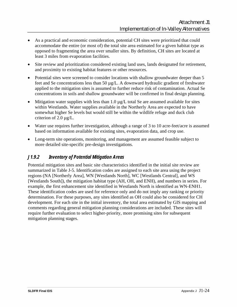
Attachment J1 Implementation of In-Valley Alternatives
SLDFR Final EIS Appendix J J1-24
• As a practical and economic consideration, potential CH sites were prioritized that could accommodate the entire (or most of) the total site area estimated for a given habitat type as opposed to fragmenting the area over smaller sites. By definition, CH sites are located at least 3 miles from evaporation facilities.
• Site review and prioritization considered existing land uses, lands designated for retirement, and proximity to existing habitat features or other resources.
• Potential sites were screened to consider locations with shallow groundwater deeper than 5 feet and Se concentrations less than 50 µg/L. A downward hydraulic gradient of freshwater applied to the mitigation sites is assumed to further reduce risk of contamination. Actual Se concentrations in soils and shallow groundwater will be confirmed in final design planning.
• Mitigation water supplies with less than 1.0 µg/L total Se are assumed available for sites within Westlands. Water supplies available in the Northerly Area are expected to have somewhat higher Se levels but would still be within the wildlife refuge and duck club criterion of 2.0 µg/L.
• Water use requires further investigation, although a range of 3 to 10 acre-feet/acre is assumed based on information available for existing sites, evaporation data, and crop use.
• Long-term site operations, monitoring, and management are assumed feasible subject to more detailed site-specific pre-design investigations.
J1.9.2 Inventory of Potential Mitigation Areas Potential mitigation sites and basic site characteristics identified in the initial site review are summarized in Table J-5. Identification codes are assigned to each site area using the project regions (NA [Northerly Area], WN [Westlands North], WC [Westlands Central], and WS [Westlands South]), the mitigation habitat type (AH, OH, and ENH), and numbers in series. For example, the first enhancement site identified in Westlands North is identified as WN-ENH1. These identification codes are used for reference only and do not imply any ranking or priority determination. For these purposes, any sites identified as OH could also be considered for CH development. For each site in the initial inventory, the total area estimated by GIS mapping and comments regarding general mitigation planning considerations are included. These sites will require further evaluation to select higher-priority, more promising sites for subsequent mitigation planning stages.

Attachment J1 Implementation of In-Valley Alternatives
SLDFR Final EIS Appendix J J1-25
Table J-5 Potential Mitigation Areas – Initial Review First-Cut Summary List
Area ID Description and notes on potential mitigation areas Areas estimated by GIS Acres
Northerly Area (NA)
NA-TE – Northerly Area treatment & evaporation facilities total potential suitable area 1454
NA-AH1 Conceptual AH area within 1 mile east of the NA treatment area. Area could shift to use some NA-OH1 site lands within proximity to the west. Area identified by Panoche Water District. Shifting this AH to the NA-OH1 would be closer to the San Luis National Wildlife Refuge.
676
NA-OH1 Conceptual OH area to the west side of the NA treatment area. Part of this area could convert to AH as needed. Area identified by Panoche Water District.
1904
NA-OH2 Area formerly part of Broadview Water District included as potential OH mitigation mainly because lands within this district are currently retired from irrigation service.
9709
NA-ENH1 Area between existing drainwater reuse lands currently occupied by private duck hunting clubs may have potential for habitat enhancement as part of mitigation plans.
395
NA-ENH2 Corridor habitat enhancement along Little Panoche Creek. Area shown assumes ¼ mile wide stream corridor – actual area could change as appropriate. This is a very small ephemeral drainage that appears to have minimal enhancement potential.
1143
Westlands North (WN)
WN-TE – Westlands North treatment & evaporation facilities total potential suitable area ~1440
WN-AH1 Conceptual AH area ½ mile wide around the north and east side of WN treatment area to take advantage of existing wildlife habitat (Mendota Wildlife Management Area) to the east.
~1440
WN-AH2 Other potential AH lands within 1 mile boundary around the WN treatment area. ~2262
WN-OH1 Retired lands between Westlands boundary and proposed Reuse Area O. Future land use questionable due to close proximity to Mendota.
1600
WN-OH2 Conceptual OH area located between the WN treatment AH proximity lands and the Westlands boundary along the Mendota Wildlife Management Area.
~1920
WN-OH3 Other potential OH area south of WN treatment area. Could overlap or shift with the identified enhancement areas WN-ENH6 and WN-ENH7 to the south and east.
~3531
WN-OH4 Located along the Westlands east boundary, San Luis Drain, and Reuse Area L. Area also borders enhancement area WN-ENH6 and could shift.
5924
WN-ENH1 Corridor habitat enhancement along Panoche Creek. Area shown assumes ¼ mile wide stream corridor – actual area could change as appropriate. This existing stream corridor would have greatest potential if combined with WN-ENH2 development.
3000
WN-ENH2 Area identified as potential Panoche Creek flood control detention pond in Westlands plan. If constructed, the facilities could be enhanced as part of mitigation plan components.
4840
WN-ENH3 Mendota Pool seasonal flood pool area could have potential for enhancing the existing habitat as part of comprehensive mitigation plan components.
4288
WN-ENH4 Corridor habitat enhancement along San Joaquin River. Area shows ½ mile wide corridor in the seasonal flood backwater zone – actual area could vary as appropriate.
3093
WN-ENH5 Corridor habitat enhancement along San Joaquin River. Area shown assumes ¼ mile wide stream corridor – actual area could change as appropriate.
2206

Attachment J1 Implementation of In-Valley Alternatives
SLDFR Final EIS Appendix J J1-26
Table J-5 (continued) Potential Mitigation Areas – Initial Review First-Cut Summary List
Area ID Description and notes on potential mitigation areas Areas estimated by GIS Acres
Westlands North (WN)
WN-ENH6 Area identified as possible storage reservoir in Westlands plans. If constructed, the reservoir site could be enhanced as part of comprehensive mitigation plans.
4186
WN-ENH7 Area identified to indicate potential for habitat enhancement of lands within the existing Mendota Wildlife Management Area to contribute toward mitigation plans. Other similar lands may have the same potential for mitigation purposes. See also WN-ENH8.
1485
WN-ENH8 Area identified to indicate potential for habitat enhancement of lands outside the existing Mendota Wildlife Management Area to contribute toward mitigation plans. Other similar lands may have the same potential for mitigation purposes. Both WN-ENH7 and WN-ENH8 could offer long-term management and water supply advantages.
1182
WN-ENH9 Corridor habitat enhancement along Fresno Slough and James Bypass. Area shown assumes ¼ mile wide stream corridor – actual area could change as appropriate.
6397
Westlands Central (WC)
WC-TE – Westlands Central treatment & evaporation facilities total potential suitable area 2862
WC-AH1 Conceptual AH area within 1 mile of north and east side of WC treatment area and near the eastern boundary of Westlands.
~2560
WC-AH2 Other potential AH within 1 mile boundary around the WC treatment and reuse areas. ~3170
WC-OH1 Area between Reuse Area H and the east Westlands boundary and near undeveloped lands along Fresno Sough.
3670
WC-OH2 Area bordered on 3 sides by Westlands boundary and located just north of the proposed WC treatment and evaporation area south of Fresno Sough.
~2245
WC-OH3 Conceptual OH area located between the WC treatment area, potential AH mitigation area, and Westlands boundary. Area could shift with other nearby project features.
~2560
WC-OH4 Area bordered on 3 sides by Westlands boundary and just to the east of the WC treatment area. Area could shift with other nearby project features.
1253
WC-OH5 Includes 2 sections on the west side of the WC treatment area. OH could shift to other retired lands in nearby vicinity depending on mitigation objectives and cost factors.
2285
WC-ENH1 Undeveloped area between Westlands boundary and Fresno Slough could offer opportunity for enhancement as part of mitigation plan components.
2914
WC-ENH2 Corridor habitat enhancement along Kings River to Fresno Slough. Area shows ¼ mile wide stream corridor – actual area could change as appropriate.
2535
WC-ENH3 Corridor habitat enhancement along Cantua Creek. Area shown assumes ¼ mile wide stream corridor. This is a very small drainage with limited enhancement potential.
1048
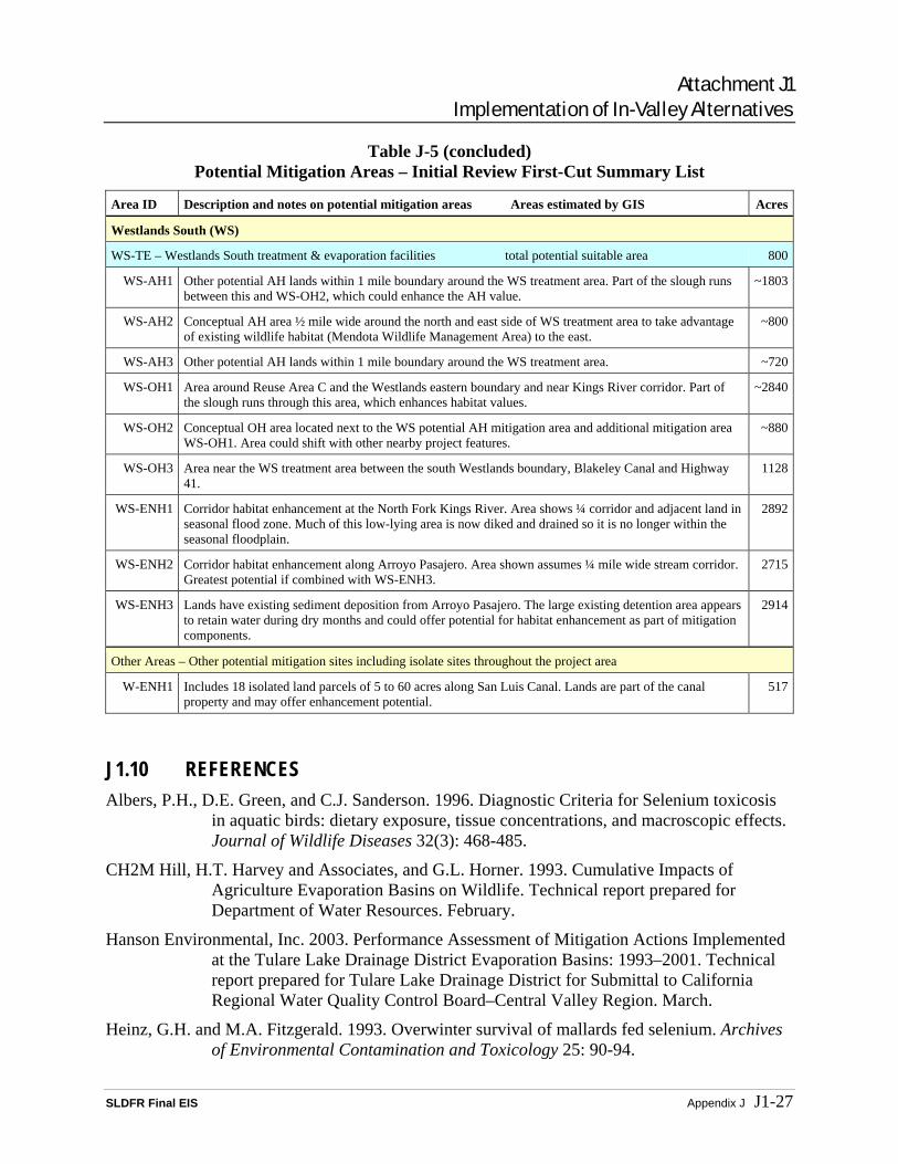
Attachment J1 Implementation of In-Valley Alternatives
SLDFR Final EIS Appendix J J1-27
Table J-5 (concluded) Potential Mitigation Areas – Initial Review First-Cut Summary List
Area ID Description and notes on potential mitigation areas Areas estimated by GIS Acres
Westlands South (WS)
WS-TE – Westlands South treatment & evaporation facilities total potential suitable area 800
WS-AH1 Other potential AH lands within 1 mile boundary around the WS treatment area. Part of the slough runs between this and WS-OH2, which could enhance the AH value.
~1803
WS-AH2 Conceptual AH area ½ mile wide around the north and east side of WS treatment area to take advantage of existing wildlife habitat (Mendota Wildlife Management Area) to the east.
~800
WS-AH3 Other potential AH lands within 1 mile boundary around the WS treatment area. ~720
WS-OH1 Area around Reuse Area C and the Westlands eastern boundary and near Kings River corridor. Part of the slough runs through this area, which enhances habitat values.
~2840
WS-OH2 Conceptual OH area located next to the WS potential AH mitigation area and additional mitigation area WS-OH1. Area could shift with other nearby project features.
~880
WS-OH3 Area near the WS treatment area between the south Westlands boundary, Blakeley Canal and Highway 41.
1128
WS-ENH1 Corridor habitat enhancement at the North Fork Kings River. Area shows ¼ corridor and adjacent land in seasonal flood zone. Much of this low-lying area is now diked and drained so it is no longer within the seasonal floodplain.
2892
WS-ENH2 Corridor habitat enhancement along Arroyo Pasajero. Area shown assumes ¼ mile wide stream corridor. Greatest potential if combined with WS-ENH3.
2715
WS-ENH3 Lands have existing sediment deposition from Arroyo Pasajero. The large existing detention area appears to retain water during dry months and could offer potential for habitat enhancement as part of mitigation components.
2914
Other Areas – Other potential mitigation sites including isolate sites throughout the project area
W-ENH1 Includes 18 isolated land parcels of 5 to 60 acres along San Luis Canal. Lands are part of the canal property and may offer enhancement potential.
517
J1.10 REFERENCES Albers, P.H., D.E. Green, and C.J. Sanderson. 1996. Diagnostic Criteria for Selenium toxicosis
in aquatic birds: dietary exposure, tissue concentrations, and macroscopic effects. Journal of Wildlife Diseases 32(3): 468-485.
CH2M Hill, H.T. Harvey and Associates, and G.L. Horner. 1993. Cumulative Impacts of Agriculture Evaporation Basins on Wildlife. Technical report prepared for Department of Water Resources. February.
Hanson Environmental, Inc. 2003. Performance Assessment of Mitigation Actions Implemented at the Tulare Lake Drainage District Evaporation Basins: 1993–2001. Technical report prepared for Tulare Lake Drainage District for Submittal to California Regional Water Quality Control Board–Central Valley Region. March.
Heinz, G.H. and M.A. Fitzgerald. 1993. Overwinter survival of mallards fed selenium. Archives of Environmental Contamination and Toxicology 25: 90-94.

Attachment J1 Implementation of In-Valley Alternatives
SLDFR Final EIS Appendix J J1-28
Heinz, G.H. and D.J. Hoffman. 1996. Comparison of the effects of seleno-L-methionine, seleno-DL-methionine, and selenized yeast on reproduction of mallards. Environmental Pollution 91: 169-175.
Heinz, G.H., D.J. Hoffman, A.J. Krynitsky, and D.M.G. Weller. 1987. Reproduction in mallards fed selenium. Environmental Toxicology and Chemistry 6: 423-433.
Heinz, G.H., D.J. Hoffman, and L.G. Gold. 1989. Impaired reproduction of mallards fed an organic form of selenium. Journal of Wildlife Management 53: 418-428.
Service. 1995a. Alternative Habitat Protocol for Drainwater Evaporation Basins. U.S Fish and Wildlife Service. March.
Service. 1995b. Compensation Habitat Protocol for Drainwater Evaporation Basins. U.S Fish and Wildlife Service. January.

APPENDIXK
Land Retirement Analysis


TABLE OF CONTENTS
SLDFR Final EIS Appendix K K-i
Appendix K Land Retirement Alternatives....................................................................................... K-1
K1 Land Retirement Alternatives ................................................................. K-1
K1.1 Refinement and Optimization Process........................................ K-2 K1.2 Selected Land Retirement Scenarios .......................................... K-5
K2 Out-of-Valley Disposal Alternatives with Land Retirement .................. K-6

TABLE OF CONTENTS
SLDFR Final EIS Appendix K K-ii
Tables K-1 San Luis Drainage Alternative Cost Comparison Annual Equivalent Costs
K-2 San Luis Drainage Alternative cost Comparison Annual Equivalent Costs
Acronyms EIS Environmental Impact Statement
PFR Plan Formulation Report
ppb parts per billion
Reclamation Bureau of Reclamation
Se selenium
Unit San Luis Unit
Westlands Westlands Water District

Appendix K Land Retirement Analysis
SLDFR Final EIS Appendix K K-1
APPENDIX K LAND RETIREMENT ALTERNATIVES
K1 LAND RETIREMENT ALTERNATIVES Westlands Water District (Westlands) and several environmental and other interests in the San Luis Unit (the Unit) requested that the Bureau of Reclamation (Reclamation) include a land retirement alternative in the Environmental Impact Statement (EIS). Specifically, these interests suggested that Reclamation consider the Westlands proposed land retirement plan or an alternative that retires sufficient lands to eliminate the drainage problem in the Unit. The land retirement analysis in the 2002 Plan Formulation Report (PFR) was broadened to respond to requests from stakeholders and interested agencies. Preliminary alternatives were developed, refined, and optimized based on specific criteria. The optimization process led to the selection of three additional alternatives that incorporated land retirement. The rationale for eliminating other land retirement alternatives is provided in this section as well.
On February 5, 2004, Reclamation submitted to the Court an Amended Plan of Action for Drainage to the San Luis Unit. The Amended Plan of Action states that Reclamation will continue to refine and evaluate all five alternatives (including No Action) described in the PFR for inclusion in the EIS. Additionally, Reclamation will formulate alternative(s) that use land retirement as a method to control drainage need, by comparing costs, benefits, and effects for alternatives with different amounts of land retirement.
In October 2003, Reclamation began land retirement alternatives development by meeting with project stakeholders to define the parameters that would constitute a complete land retirement program and the range of sizes (acreage) for alternatives. Stakeholders included representatives from San Luis Unit districts (San Luis Water District, Broadview Water District, Westlands Water District, and Panoche Water and Drainage District), San Joaquin River Exchange Contractors Water Authority, and environmental and Delta interests (Environmental Defense, Contra Costa County, Contra Costa Water District). The initial range of alternatives included alternatives based on the following reports and comments provided by the stakeholders:
• Westside Regional Drainage Plan (San Joaquin River Exchange Contractors Water Authority et al. 2003) including lands within Westlands and the Northerly Area.
• U.S. Fish and Wildlife Service comments on the PFR, including an alternative that would retire all drainage-impaired lands in the San Luis Unit
• “Drainage Without a Drain” concept proposed by a coalition of environmental groups and local agencies downstream of the San Joaquin Valley1
The Project Team refined the initial alternatives developed from the public outreach process to arrive at complete alternatives that include the disposal of any residual drainwater. Factors considered included:
• Amount of land retirement
• Land retirement implementation method
• Future retired land use and ownership
1 The Bay Institute, Contra Costa County, Contra Costa County Water Agency, Contra Costa Water District, and Environmental Defense.

Appendix K Land Retirement Analysis
SLDFR Final EIS Appendix K K-2
• Future use of water currently used to irrigate land that would be retired
• Extent of drainage reduction measures including irrigation efficiencies and groundwater pumping
• Inclusion of drainage service components necessary to provide a complete disposal alternative
By December 2003, the following five concepts were identified for further refinement and optimization:
• Locally Preferred 1: Westside Regional Drainage Plan
• Locally Preferred 2: Optimized Retirement
• Reclamation 1: Federal Management
• Reclamation 2: Maximum Retirement
• Environmental: Drainage Without a Drain
K1.1 Refinement and Optimization Process Beginning in December 2003, Reclamation refined the alternatives by determining how the cost, benefit, and potential environmental effects of the resulting drainage service plan compared to previous alternatives using a variety of modeling and analysis tools. Using an iterative evaluation process, Reclamation considered the following factors for varied levels of land retirement:
• Improved irrigation efficiency balanced with deep percolation rates to maintain salt balance in the root zone.
• The amount of drainage to be expected under the different land retirement scenarios using the regional groundwater model.
• Estimated costs of drainage service for the land retirement scenarios using engineering cost curves, which calculated the cost for each component of drainage service (e.g., collector system, treatment system, and disposal) for a corresponding drainage rate.
• The economic benefits of each scenario to provide another measure to select a final set of alternatives for analysis.
• Indicators of environmental effect (such as acres of reuse and evaporation basins needed, or amount of drainwater reclaimed for irrigation) for each scenario.
Reclamation developed and analyzed potential alternatives that include combinations of land retirement, source reduction (including reduced percolation losses from irrigation, and drainwater recycling and reuse), and treatment and disposal. These potential alternatives, called land retirement scenarios, were compared primarily using costs. Scenarios mix different levels of land retirement, source reduction, and treatment/disposal. Alternatives that provided for partial retirement of drainage-impaired lands were further evaluated to balance the amount of land retired with the implementation of drainage-reduction measures to improve farm profits. The primary drainage-reduction measure evaluated was increases in irrigation efficiencies.

Appendix K Land Retirement Analysis
SLDFR Final EIS Appendix K K-3
Because the cost of selenium (Se) removal from drainwater is high, Reclamation developed a land retirement alternative that was based on retiring lands with high Se concentrations in the shallow groundwater and that used groundwater well monitoring data to estimate the Se concentration in shallow groundwater. Several different groundwater concentrations were used as criteria for selecting land retirement areas. The alternatives were assessed based on the amount of land that would be retired and the potential decrease in Se concentration in drainwater. In addition, the effect of retiring lands already acquired by Westlands because of drainwater quality was also evaluated.
Another two-step process was used to evaluate, compare, and screen land retirement scenarios. The first step covered a fairly wide range of retirement and source control combinations and was used to:
• Screen out scenarios that were clearly inferior (e.g., more costly for the same or less benefit).
• Screen out scenarios that were technically impractical or questionable.
• Identify potential scenarios that might be more effective and/or less costly.
The second step evaluated four scenarios in comparison to the In-Valley Disposal Alternative, including the change in applied water.
K1.1.1 First Screening Step Three land retirement levels and three levels of increased irrigation efficiencies were evaluated. The three retirement levels were:
• Lands retired as in the In-Valley Disposal Alternative (approximately 44,100 acres within Westlands drainage-impaired area)
• 200,000 acres retired within the Westlands drainage-impaired area
• All drainage-impaired lands in the San Luis Unit retired (298,000 acres in Westlands and 45,000 acres in the Northerly Area)
Three increased irrigation efficiency rates were evaluated for the first two retirement levels (because with all drainage-impaired lands retired, reducing drainage with source controls is not needed).
The following conclusions were drawn from this screening:
• Comparison of the cost for land retirement (land acquisition and land management costs) versus the cost for collection, treatment, and disposal indicated that land retirement was more costly. In other words, it cost more to avoid the drainage through land retirement than to collect, treat, and dispose of the drainwater.
• Further analysis is needed to estimate the value of water that land retirement makes available for other uses, which should be factored into a comparison of final alternatives.
• Root zone salinity analysis indicated that Level 2 deep percolation reduction (i.e., increased irrigation efficiency) probably does not allow for salinity balance in the root zone for the drainage-impaired area. Level 2 deep percolation reduction was eliminated from further consideration.

Appendix K Land Retirement Analysis
SLDFR Final EIS Appendix K K-4
• Level 1 deep percolation reduction did appear to be technically feasible and cost-effective, but root zone salinity balance in the Westlands drainage-impaired area could be achieved only with extremely careful management. It was agreed to include Level 1 reduction in further screening of scenarios, although questions were raised about the practicality of growers being able to achieve deep percolation rates of 0.27 foot/year.
• Full retirement of drainage-impaired lands eliminated the need for drainage service, but the 200,000-acre retirement level did not. Analysis of additional intermediate levels of retirement was suggested to see if some acreage less than full retirement could eliminate the need for drainage in Westlands.
• Other implications besides cost and drainage volume were requested for consideration in the land retirement scenario screening. Specifically, a scenario could target retirement of lands based on Se concentrations in shallow groundwater. Two target levels were suggested: greater than 20 parts per billion (ppb) and greater than 50 ppb Se in shallow groundwater.
Retirement of the remaining 35,000 acres of lands in the northerly San Luis Unit (lands other than the 10,000 acres in Broadview Water District) was not included in scenarios for further analysis. This Project Team decision was supported by a variety of factors, including the following:
• Initial screening showed land retirement to be more costly than drainage service. Consequently, land retirement combined with the Out-of-Valley Alternatives was also not cost-effective.
• Northerly Unit lands already have a substantial investment in installed drainage system components (drains, collector system, recirculation systems, reuse areas, etc.). These systems have been funded using a variety of local funding and State and Federal grants, loans, and bond funds. Repayment of the remaining obligation from the 12 million dollars funded from the State Revolving Loan funds would add to the cost of land retirement.
• Other non-Unit lands in the Northerly Area could not be retired under the current San Luis Unit authorization. Retirement of the remaining northerly Unit lands would result in approximately 36,000 acres of lands outside the Unit needing drainage service. Drainage flows would continue to occur on these lands including seepage into deep open drains, drainwater and tailwater (from continued non-Unit farms) that is not able to be recycled, and runoff from storm events. In the absence of drainage service, these uncontrolled flows would continue downstream and could reach the adjacent wildlife refuges or the San Joaquin River, resulting in adverse effects to water quality and wildlife.
K1.1.2 Second Screening Results Four scenarios were evaluated and compared to the In-Valley Disposal Alternative in this screening:
• Revision of the In-Valley Disposal Alternative to include Level 1 deep percolation reduction and 55,311 total acres retired in Westlands (including lands for project facilities).

Appendix K Land Retirement Analysis
SLDFR Final EIS Appendix K K-5
• Retirement of all lands in Westlands with Se concentration greater than 50 ppb and implementing Level 1 deep percolation reduction. Total land retired would be 88,576 acres in Westlands and the 10,000 acres of Broadview Water District in the Northerly Area.
• Retirement of all lands in Westlands with Se concentration greater than 20 ppb and implementing Level 1 deep percolation reduction. Total land retired would be 129,051 acres in Westlands and the 10,000 acres of Broadview Water District in the Northerly Area.
• Retirement of 198,000 acres within the drainage-impaired area of Westlands plus 10,000 acres in the Northerly Area. Implementation of Level 1 deep percolation reduction.
Some additional groundwater modeling analysis was performed to see if the need for drainage could be eliminated by combinations of deep percolation reduction and land retirement (less than complete retirement of all lands in the drainage-impaired area). Only a few combinations were tested, but it appeared that eliminating all need for current or future drainage service in the Unit could only be assured by retiring all drainage-impaired lands.
K1.2 Selected Land Retirement Scenarios Based on the screening of the many combinations of land retirement and other drainwater reduction measures, three land retirement scenarios were selected (as variations on the In-Valley Disposal Alternative) as reasonable alternatives for analysis in the EIS. All three assume 10,000 acres would be retired in Broadview Water District in the Northerly Area. The first of the three scenarios would retire land with Se concentration greater than 50 ppb in shallow groundwater (approximately 83,100 acres in Westlands). The second would retire land in Westlands up to the level at which the water made available could be used to fulfill other irrigation demands in the San Luis Unit (195,000 acres). The third would retire the entire drainage-impaired area in Westlands (298,000 acres). All three are assumed to be variations of the original In-Valley Disposal Alternative and, therefore, the methods of collection, treatment, and disposal of drainwater for the three In-Valley Land Retirement Alternatives are essentially the same as the In-Valley Disposal Alternative.
K1.2.1 In-Valley/Groundwater Quality Land Retirement Alternative This alternative consists of retiring all the lands in Westlands with Se concentration greater than 50 ppb in the shallow groundwater and lands acquired by Westlands (83,100 acres). It would also retire 10,000 acres in Broadview Water District in the Northerly Area for a total of 93,100 acres of land retirement. This alternative would also include irrigation system improvements to reduce deep percolation to shallow groundwater. Lands remaining in production within the drainage-impaired area would be eligible for drainage service.
K1.2.2 In-Valley/Water Needs Land Retirement Alternative This alternative would retire enough lands to meet the internal water use needs of the San Luis Unit (195,000 acres). This value would include lands with Se concentrations greater than 20 ppb in Westlands, lands acquired by Westlands, and 10,000 acres in Broadview Water District. The alternative would include irrigation system improvements to reduce deep percolation to shallow

Appendix K Land Retirement Analysis
SLDFR Final EIS Appendix K K-6
groundwater. Lands remaining in production within the drainage-impaired area would be eligible for drainage service.
K1.2.3 In-Valley/Drainage-Impaired Area Land Retirement Alternative This alternative consists of retiring 308,000 acres, including all the drainage-impaired lands in Westlands – approximately 298,000 acres. The Northerly Area (non-Westlands) is excluded from land retirement except for 10,000 acres in Broadview Water District, and drainage collection, treatment, and disposal facilities would be avoided in the Westlands drainage-impaired areas. Water made available from this alternative would exceed the agricultural water required by the remaining lands within the Unit, and would be available for reallocation to other purposes.
K2 OUT-OF-VALLEY DISPOSAL ALTERNATIVES WITH LAND RETIREMENT Based on the screening of the many combinations of land retirement and other drainwater reduction measures, three land retirement scenarios were selected as partial alternatives for analysis in the EIS. As indicated above, these alternatives are all variations of the original In-Valley Disposal Alternative. The collection, treatment, and disposal of drainwater collected from drained lands are essentially the same as the In-Valley Disposal Alternative, except that the amount of drainage would vary depending on the amount of drainage-impaired land that would be retired. All three land retirement alternatives assume that 10,000 acres of the Broadview Water District, located in the Northerly Area would be retired.
Preliminary analyses of various land retirement scenarios were conducted during the plan formulation process to compare the costs of retiring varying amounts of drainage-impaired lands versus the cost of providing drainage service to those same lands. These initial analyses were based on comparing the In-Valley Disposal Alternative with land retirement to the least expensive Out-of-Valley Disposal Alternative (Chipps Island) with the same level of land retirement. The analyses indicated that the In-Valley Disposal Alternative was consistently less expensive than the least expensive Out-of-Valley Disposal Alternative, regardless of the amount of land retirement. Consequently, it was assumed that since land retirement costs were greater than the corresponding savings of reduced treatment and disposal costs for the In-Valley Disposal Alternative, land retirement would be even less cost-effective for any Out-of-Valley Disposal Alternative.
However, as the cost estimates of various project features were refined for the Feasibility Study, the cost differences between the alternatives changed. The most notable changes that occurred as feature costs changed were (1) the costs of the In-Valley Disposal Alternative increased, (2) the cost of the conveyance systems for all of the Out-of-Valley Disposal Alternatives decreased, and (3) the Ocean Disposal Alternative became the least expensive Out-of-Valley Disposal Alternative. As a result of these changes, it was decided to conduct another brief analysis of land retirement with the Ocean Disposal Alternative to determine if a more thorough analysis would be required.
Two land retirement scenarios were analyzed for comparison with the In-Valley/Land Retirement Alternatives. The first scenario analyzed assumed essentially the same amount of land retirement as the In-Valley/Water Supply Land Retirement Alternative (195,000 acres

Appendix K Land Retirement Analysis
SLDFR Final EIS Appendix K K-7
retired in Westlands and 10,000 acres in the Broadview Water District). The second scenario assumed retirement of all drainage-impaired lands in Westlands, or 298,000 acres plus 10,000 in Broadview. These analyses indicated that, even though the cost differences between the various alternatives were much closer than they had been previously, the In-Valley Disposal Alternative was still consistently less expensive than the least costly Out-of-Valley Disposal Alternative, regardless of the amount of land retirement. Consequently, the Out-of-Valley Disposal Alternatives with additional land retirement were not carried forward into this EIS for full analysis. The results of this analysis are summarized in Tables K-1 and K-2.

Appendix K Land Retirement Analysis
SLDFR Final EIS Appendix K K-8
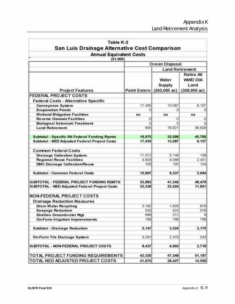
Appendix K Land Retirement Analysis
SLDFR Final EIS Appendix K K-9


APPENDIXL
Regulatory Environment and Compliance Requirements


TABLE OF CONTENTS
SLDFR Final EIS Appendix L L-i
Appendix L Regulatory Environment and Compliance Requirements...........................................L-1
L1 Environmental Compliance Regulations .................................................L-1 L2 Biological Resource Legislation and Requirements ................................L-1
L2.1 Fish and Wildlife Coordination Act .........................................L-1 L2.2 Migratory Bird Treaty Act .......................................................L-2 L2.3 Endangered Species Act...........................................................L-2 L2.4 California Endangered Species Act..........................................L-3 L2.5 Magnuson-Stevens Fishery Conservation and
Management Act ......................................................................L-3 L2.6 California Fish and Game Code (Section 1601)
Streambed Alteration Agreement.............................................L-3 L2.7 Executive Order 11990 (Protection of Wetlands) ....................L-3 L2.8 Executive Order 13186 (Responsibilities of Federal
Agencies to Protect Migratory Birds) ......................................L-4 L2.9 Marine Mammal Protection Act (16 United States Code
1361-1407) ...............................................................................L-4 L2.10 National Marine Sanctuaries Act (16 United States Code
1431 et seq.) .............................................................................L-5 L3 Disposal/Discharge-Related Requirements, Permits, and/or
Approvals.................................................................................................L-6 L3.1 Clean Water Act .......................................................................L-6 L3.2 Rivers and Harbors Act of 1899...............................................L-9 L3.3 Safe Drinking Water Act..........................................................L-9 L3.4 Underground Injection Control Program ...............................L-10 L3.5 Resource Conservation and Recovery Act.............................L-10 L3.6 California Porter-Cologne Water Quality Act .......................L-10 L3.7 California Toxic Pits Control Act ..........................................L-11 L3.8 California Hazardous Waste Control Act...............................L-11 L3.9 California Hazardous Waste Management Act ......................L-11 L3.10 California Toxic Injection Well Control Act .........................L-11 L3.11 Federal and State Deep-Well Injection Regulations ..............L-12 L3.12 California Water Conservation and Water Bond Laws..........L-12 L3.13 Surface Water Rights and Compliance ..................................L-12 L3.14 Groundwater Rights and Management and Compliance........L-12
L4 Bay/Delta/Coastal Requirements, Permits, and/or Approvals...............L-13 L4.1 Coastal Zone Management Act and Coastal Zone Act
Reauthorization Amendments of 1990...................................L-13 L4.2 California Coastal Commission .............................................L-13 L4.3 San Francisco Bay Conservation and Development
Commission............................................................................L-14 L5 Land Use and Regional, County, and Local Requirements, Permits,
and/or Approvals....................................................................................L-14 L5.1 California State Lands Commission Lease and Permit ..........L-14 L5.2 California Department of Transportation Encroachment
Permit .....................................................................................L-14

TABLE OF CONTENTS
SLDFR Final EIS Appendix L L-ii
L5.3 California County Permits......................................................L-15 L5.4 Reclamation Board Encroachment Permit .............................L-15 L5.5 State, Areawide, and Local Plan and Program
Consistency ............................................................................L-15 L5.6 Coordination with Related Federal, State, and Local
Programs.................................................................................L-15 L5.7 San Joaquin Valley Air Pollution Control District
Conservation Management Plans ...........................................L-16 L6 Additional Environmental Legislation and Requirements.....................L-16
L6.1 Central Valley Project Improvement Act...............................L-16 L6.2 Clean Air Act .........................................................................L-17 L6.3 National Historic Preservation Act of 1966 ...........................L-17 L6.4 Wild and Scenic Rivers Act of 1968......................................L-17 L6.5 California Wild and Scenic Rivers Act ..................................L-18 L6.6 Wilderness Act of 1964, as Amended....................................L-18 L6.7 Federal Water Project Recreation Act....................................L-18 L6.8 Executive Order 11988, Floodplain Management .................L-18 L6.9 Executive Order 12898, Environmental Justice .....................L-19 L6.10 Indian Trust Assets.................................................................L-19 L6.11 Executive Order 13007 (Indian Sacred Sites on Federal
Land) ......................................................................................L-19 L6.12 American Indian Religious Freedom Act...............................L-19 L6.13 Farmland Protection Policy Act and Farmland
Preservation............................................................................L-19 L6.14 Earthquake Hazards Reduction Act of 1977 (Public Law
95-124) ...................................................................................L-20 L6.15 National Earthquake Loss Reduction Program ......................L-20 L6.16 Executive Order 12699 Seismic Safety of Federal and
Federally Assisted or Regulated New Building Construction ...........................................................................L-21
L6.17 1998 California Building Code ..............................................L-22 L6.18 California Public Resources Code § 25523(a); 20
California Code of Regulations § 1752(b) and (c). 1972 Alquist-Priolo Earthquake Fault Zoning Act (amended 1994).......................................................................................L-22
L6.19 California Public Resources Code Chapter 7.8, 1990 Seismic Hazards Mapping Act ...............................................L-23
L6.20 Historic Structures – California Public Resources Code Section 5028...........................................................................L-23

TABLE OF CONTENTS
SLDFR Final EIS Appendix L L-iii
Acronyms Basin Plan Water Quality Control Plan for the Sacramento River and San
Joaquin River Basins
BMPs best management practices
CBC California Building Code
CDFG California Department of Fish and Game
CEQA California Environmental Quality Act
CWA Clean Water Act
DHS California Department of Health and Safety
EFH Essential Fish Habitat
EIS Environmental Impact Statement
EPA U.S. Environmental Protection Agency
ESA Endangered Species Act
FEMA Federal Emergency Management Agency
NEHRP National Earthquake Hazards Reduction Program
NEP National Earthquake Loss Reduction Program
NEPA National Environmental Policy Act
NOAA National Oceanic and Atmospheric Administration
NPDES National Pollution Discharge Elimination System
RCRA Resource Conservation and Recovery Act
Regional Board San Francisco Bay Regional Water Quality Control Board
State Board California State Water Resources Control Board
SWPPP Storm Water Pollution Prevention Plan
UIC Underground Inspection Control (Program)
USACE U.S. Army Corps of Engineers


Appendix L Regulatory Environment and Compliance Requirements
SLDFR Final EIS Appendix L L-1
APPENDIX L REGULATORY ENVIRONMENT AND COMPLIANCE REQUIREMENTS
Construction and operation of any of the action alternatives under consideration would be subject to numerous regulatory compliance actions that are in place to safeguard the human and biological environment. This appendix explains the legislation and regulatory requirements, and several require Reclamation to obtain, or ensure that, the applicable approvals are obtained.
L1 Environmental Compliance Regulations The National Environmental Policy Act (NEPA) and the California Environmental Quality Act (CEQA) apply to actions that a Federal or State agency may undertake directly, approve by issuing a permit or other authorization, or fund wholly or in part. NEPA provides a commitment that Federal agencies will consider the environmental effects of their actions. It requires that an Environmental Impact Statement (EIS) be prepared for all major Federal actions with significant environmental effects. The CEQA requirements are similar to the NEPA requirements and require the preparation on an Environmental Impact Report for major State actions significantly affecting the quality of the physical and social environment. Both NEPA and CEQA require that an agency consider the environmental effects of its actions at the earliest point in time in which the analysis is meaningful. NEPA and CEQA are intended to inform decision makers and the public of the environmental consequences of the proposed action, provide an analysis of alternatives, and ensure consideration of mitigation options. Under both statutes, the environmental documentation and analysis are circulated for public review and comment before a final document is completed and before a decision is made to approve the proposed action or other alternative.
• CEQA Compliance: This document has been written to facilitate State and local agencies using the document to meet their CEQA obligations.
• NEPA Compliance: The Draft EIS is being circulated for public review. Following the Final EIS and signature of the Record of Decision, Reclamation will have fully complied with NEPA.
L2 Biological Resource Legislation and Requirements Both the Federal and State governments have enacted biological resource legislation and requirements to ensure that projects do not needlessly harm these resources. The major biological resource legislative requirements applicable to the alternatives under consideration are discussed below.
L2.1 Fish and Wildlife Coordination Act The Fish and Wildlife Coordination Act (Public Law 85-624) mandates that conservation, rehabilitation, and enhancement of fish and wildlife resources receive equal consideration and be coordinated with other features of water resource development programs and provide an opportunity for the “appropriate wildlife agencies” (U.S. Fish and Wildlife Service [Service] and the National Oceanic and Atmospheric Administration [NOAA] Fisheries) to consult on Federal water development projects or on non-Federal projects that require a Federal permit or license. The agencies are provided the opportunity to conduct surveys and investigations to determine the potential damage to fish and wildlife resources with project implementation and to identify the
Appendix L Regulatory Environment and Compliance Requirements
SLDFR Final EIS Appendix L L-2
mitigation measures that should be undertaken. The findings are incorporated into an official Section 2(b) report. The Coordination Act Report is provided as Appendix M1.
Compliance: Specific activities, including the draft Coordination Act Report, are described in Section 21.2.4.
Similarly, Sections 13450 et seq. of the California Fish and Game Code provide opportunities for the California Department of Fish and Game (CDFG) to report its recommendations for wildlife conservation and development, and the expected results, and, describe the damage to wildlife attributable to the project and the measures proposed for mitigating or compensating for these damages. These provisions, however, do not apply to fish in irrigation canals or works, or to mammals destroyed or birds killed while damaging crops.
Compliance: CDFG will have an opportunity to provide input through their review of the Coordination Act Report.
L2.2 Migratory Bird Treaty Act The Migratory Bird Treaty Act prohibits the intentional or unintentional taking of migratory birds except under specific authorized and permitted activities. The Service has indicated that operation of the evaporation basins to dispose of subsurface agricultural drainage could result in the incidental take of migratory birds (including the American avocet, black-necked stilt, gadwall, mallard, northern pintail, and snowy plover), in violation of this act. The Service has recommended that lands producing drainwater exceeding threshold levels for agricultural toxicants should either be retired from irrigated agriculture or the drainwater be disposed of in a manner that avoids wildlife contact, such as deep-well injection or treatment to render the drainage harmless to the environment. The Service has developed protocols that provide guidance criteria for agricultural drainage basin operations. These criteria include design criteria to prevent waterfowl attraction and to require substitute wetlands for mitigation.
Compliance: Reclamation is designing the In-Valley Disposal Alternatives to minimize waterfowl attraction and to provide alternative and compensation wetlands to reduce the incidental take of protected migratory waterbirds.
L2.3 Endangered Species Act The Federal Endangered Species Act (ESA), as amended (16 United States Code 1536), establishes a national program for the conservation of threatened and endangered species of fish, wildlife, and plants and the preservation of the ecosystems upon which they depend. Section 7(a)(2) of the ESA requires Federal agencies to consult with the Service and/or NOAA Fisheries on any activities that may affect any species listed as threatened or endangered or designated critical habitat. These potential effects require initiation of the Section 7 consultation process.
Compliance: A list of Federal and State threatened, endangered, proposed, candidate, rare, species of concern, and/or species of special concern that may occur in the project area was obtained from the Service and NOAA Fisheries and is included as Appendix F. Pursuant to Section 7 of the ESA, information addressing potential adverse effects on listed and proposed species will be incorporated into the NEPA document. Based on Reclamation’s effects

Appendix L Regulatory Environment and Compliance Requirements
SLDFR Final EIS Appendix L L-3
determination, formal consultation with the Service and NOAA Fisheries may be requested in compliance with Section 7.
L2.4 California Endangered Species Act The California ESA is similar to the Federal ESA.
Compliance: A list of State threatened, endangered, proposed, candidate, rare, species of concern, and/or species of special concern that may occur in the project area were requested from the CDFG. Information addressing potential effects on listed and proposed species will be incorporated into the NEPA document, as appropriate, and provided to the CDFG for their analysis and comment.
L2.5 Magnuson-Stevens Fishery Conservation and Management Act The Magnuson-Stevens Fishery Conservation and Management Act requires all Federal agencies to consult with NOAA Fisheries on all actions or proposed actions, permitted, funded, or undertaken by an agency, that may adversely affect Essential Fish Habitat (EFH). EFH is defined as “those waters and substrate necessary to fish for spawning, breeding, feeding, or growth to maturity.” Only species managed under a Federal fishery management plan are covered. Species for which this act applies for this project are Sacramento River winter-run salmon, Central Valley spring-run salmon, Central Valley fall/late fall-run salmon, and Central Valley steelhead. Consultation generally requires that an EFH Assessment be prepared and submitted to NOAA Fisheries. Information that is normally included in an EFH Assessment will be incorporated into the NEPA document.
Compliance: None of the alternatives would affect the species subject to this act.
L2.6 California Fish and Game Code (Section 1601) Streambed Alteration Agreement Pursuant to Section 1601 of the California Fish and Game Code, before any State or local governmental agency or public utility begins a construction project that will (1) divert, obstruct, or change the natural flow or the bed, channel, or bank of any river, stream, or lake; (2) use materials from a streambed; or (3) result in the disposal or deposition of debris, waste, or other material containing crumbled, flaked, or ground pavement where it can pass into any river, stream, or lake, it must first notify the CDFG of the proposed project. Based on the notification materials submitted to the CDFG, the CDFG will determine if the proposed project may affect fish or wildlife resources. If the CDFG determines that the proposed project may substantially adversely affect existing fish or wildlife resources, a Lake or Streambed Alteration Agreement will be required, unless the proposed project is otherwise exempt.
Compliance: Not applicable to Reclamation; however, comments from CDFG will be considered in the Final EIS.
L2.7 Executive Order 11990 (Protection of Wetlands) Executive Order 11990 (Protection of Wetlands) requires Federal agencies to take actions to minimize the destruction, loss, or degradation of wetlands, and to preserve and enhance the

Appendix L Regulatory Environment and Compliance Requirements
SLDFR Final EIS Appendix L L-4
natural and beneficial values of wetlands when undertaking Federal activities and programs. Any agency considering a proposal that might affect wetlands must evaluate factors affecting wetland quality and survival. These factors should include the proposal’s effects on the public health, safety, and welfare due to modifications in water supply and water quality; maintenance of natural ecosystems and conservation of flora and fauna; and other recreational, scientific, and cultural uses.
Compliance: Action alternative facilities could be sited so as to avoid and minimize impacts to wetland resources.
L2.8 Executive Order 13186 (Responsibilities of Federal Agencies to Protect Migratory Birds)
Executive Order 13186 requires all Federal agencies taking actions that have, or are likely to have, a measurable negative effect on migratory bird populations to develop and implement a Memorandum of Understanding with the Service to promote the conservation of migratory bird populations. The order requires departments and agencies of the Federal government, to the extent practicable and permitted by budgetary limits and in harmony with their agency’s missions, to (1) avoid or minimize the negative effect of their actions on migratory birds, (2) restore and enhance the habitat of migratory birds, (3) prevent or abate the pollution or detrimental alteration of the environment for the benefit of migratory birds, (4) incorporate migratory bird habitat and population conservation measures, principles, and practices into their agency activities and planning efforts, and (5) minimize the intentional and unintentional take of species of concern during the conduct of agency actions. A number of other measures to promote the protection and conservation of migratory bird resources are also directed under the order.
Compliance: If actions implemented under the selected alternative are determined to have measurable negative effects on migratory birds, Reclamation will develop and implement an appropriate Memorandum of Understanding with the Service as prescribed in the order.
L2.9 Marine Mammal Protection Act (16 United States Code 1361-1407) In 1972, the Marine Mammal Protection Act was passed by the U.S. Congress to protect the many mammals that live in the world’s oceans. This legislation is the basis for policies preventing the harassment, capture, injury, or killing of all species of whales, dolphins, seals, and sea lions, as well as walruses, manatees, dugongs, sea otters, and polar bears.
The law sets up a management regime to reduce marine mammal mortalities and injuries in their interactions with fisheries (gear entanglement, etc.); regulates scientific research in the wild; establishes basic requirements for public display of captive marine mammals; addresses issues specific to the tuna fishery in the eastern tropical Pacific Ocean where dolphins associate with tuna and are harassed, injured, and sometimes killed by fishing practices there; creates a management regime for native subsistence hunting of marine mammals in Alaska; and regulates the import and export of marine mammals and their products.
The primary government agency responsible for enforcing this act is NOAA Fisheries. Under this act, NOAA Fisheries is responsible for the management and conservation of whales and dolphins (cetaceans) and pinnipeds other than the walrus. Walruses, manatees and dugongs (sirenians), sea otters, and polar bears are under the jurisdiction of the Service.

Appendix L Regulatory Environment and Compliance Requirements
SLDFR Final EIS Appendix L L-5
This act underwent some significant changes in its 1994 amendments, especially with respect to switching the emphasis on pinnipeds from protection to management.
Compliance: No marine mammals would be affected by the Ocean Disposal Alternative or other action alternatives.
L2.10 National Marine Sanctuaries Act (16 United States Code 1431 et seq.) The National Marine Sanctuaries Act was enacted in 1972 to designate and manage areas of the marine environment with special national significance due to their conservation, recreational, ecological, historical, scientific, cultural, archeological, educational, or aesthetic qualities as national marine sanctuaries. Day-to-day management of national marine sanctuaries has been delegated by the Secretary of Commerce to the National Marine Sanctuary Program. National Marine Sanctuary Program regulations are codified at 15 CFR Part 922. In general, regulations are used by the Program to implement the National Marine Sanctuaries Act and national marine sanctuary management plans. Each sanctuary has its own set of regulations within 15 CFR Part 922.
Monterey Bay National Marine Sanctuary is a Federally protected marine area offshore of California’s central coast. Stretching from Marin to Cambria, the Sanctuary encompasses a shoreline length of 276 miles and 5,322 square miles of ocean. Supporting one of the world's most diverse marine ecosystems, it is home to numerous mammals, seabirds, fishes, invertebrates, and plants in a remarkably productive coastal environment. The Sanctuary was established for the purpose of resource protection, research, education, and public use of this national treasure. The Sanctuary is part of a system of 13 National Marine Sanctuaries administered by NOAA. The Sanctuary focuses attention of the area’s resources and qualities.
The highest priority management goal of the Sanctuary is the protection of its marine environment, resources, and qualities. Many of the activities that affect the Sanctuary’s marine environment are presently governed by existing State and Federal regulations under the jurisdiction of many different agencies. When this complexity occurs, a National Marine Sanctuary may serve the function of coordinating the activities of these management and regulatory agencies by specifically taking steps to (NOAA 1992):
• Coordinate policies and procedures among the agencies sharing responsibility for protection and management of resources.
• Encourage participation by interested agencies and organization in the development of procedures to address specific management concerns (e.g., monitoring and emergency response programs).
• Develop an effective and coordinated program for the enforcement of Sanctuary regulations.
• Enforce Sanctuary regulations in addition to other regulations already in place.
• Promote public awareness of, and voluntary compliance with, Sanctuary regulation and objectives, through education and interpretive programs stressing resource sensitivity and wise use.
• Ensure that the Sanctuary’s water quality is maintained at a level consonant with Sanctuary designation.

Appendix L Regulatory Environment and Compliance Requirements
SLDFR Final EIS Appendix L L-6
• Establish memoranda of agreement and other mechanisms for coordination among all the agencies participating in Sanctuary management.
• Ensure that the appropriate management agency incorporates research results and scientific data into effective resource protection strategies.
• Reduce threats to Sanctuary resources and qualities.
Based on the analysis presented in the Final EIS, the Ocean Disposal Alternative would be consistent with the goals of the Monterey Bay National Marine Sanctuary.
L3 Disposal/Discharge-Related Requirements, Permits, and/or Approvals Both the Federal and State governments have enacted disposal/discharge-related legislation and requirements to ensure that projects do not needlessly harm the environment. The major legislative requirements applicable to the alternatives under consideration are discussed below. Reclamation will commit to compliance with applicable Federal, State, and local legislation, requirements, permits, and approvals.
L3.1 Clean Water Act The Clean Water Act (CWA) gave the U.S. Environmental Protection Agency (EPA) the authority to develop a program to make all waters of the United States “fishable and swimmable.” The CWA has an antidegradation policy imposed by the EPA. Except under certain specified conditions, States must maintain levels of water quality established in 1977. This program has included identifying existing and proposed beneficial uses and methods to protect and/or restore those beneficial uses. In California, the EPA has designated planning and permitting authority to the California Environmental Protection Agency, which is comprised of the State Water Resources Control Board (State Board) and nine Regional Water Quality Control Boards (Regional Boards).
The CWA contains many provisions, including provisions that regulate the discharge of pollutants into waterbodies. The discharges may be direct flows from point sources, such as an effluent from a wastewater treatment plant, or a nonpoint source, such as eroded soil particles from a construction site. Numerous provisions could affect implementation of the proposed project. The following focuses on the main provisions that require compliance.
Every 2 years, the State Board submits a report on the State’s water quality to the EPA pursuant to CWA Section 305(b). The report provides water quality information to the general public and serves as the basis for the EPA’s National Water quality Inventory Report to Congress. Section 303(d) requires States to develop a list of waterbodies that, after application of technology-based effluent controls, will not achieve water quality objectives and to develop a prioritization schedule for conducting total maximum daily load studies to allocate pollutant discharges from each source such that water quality objectives will be achieved. This list is included in the Section 305(b) report. The Section 303(d) list identifies impaired waterbodies and sources of contamination, such as mine drainage, agricultural drainage, urban and industrial runoff, and municipal and industrial wastewater discharges for each contaminant. In California, the EPA has designated planning and permitting authority to the California Environmental Protection Agency, which is comprised of the State Board and nine Regional Boards. The State Board is responsible

Appendix L Regulatory Environment and Compliance Requirements
SLDFR Final EIS Appendix L L-7
for the triennial review process and for developing the Section 303(d) list. In May 2003, the EPA approved a new Section 303(d) list submitted by the State Board that includes 685 surface waters that are currently listed as not meeting water quality standards.
The EPA also has developed the National Guidance on Water Quality Criteria under Section 304 (a) for pollutants to protect human health and aquatic life. Relevant pollutants are identified under Section 307 of the CWA.
Section 320 of the CWA promulgates the National Estuary Program, which provides for long-term management of 28 estuaries in the United States, including the San Francisco Bay-Delta and Morro Bay. The EPA administers the program, but decisions and activities are carried out by committees of local government officials, private citizens, and representatives from other Federal agencies, academic institutions, industry, and estuary user groups. Each estuary program group works to create and implement a formal management plan to restore and protect the estuary. The Morro Bay National Estuary Program has a Comprehensive Conservation and Management Plan in place, and the San Francisco Estuary Project has one in progress.
Morro Bay was established as California’s first State Estuary in 1994 and was accepted into the National Estuary Program in October 1995. The Comprehensive Conservation and Management Plan identifies goals of the Morro Bay National Marine Estuary Program (2000) as follows:
• Slow the process of bay sedimentation through implementation of management measures, which address erosion and sediment transport.
• Re-establish healthy steelhead trout habitat in Chorro and Los Osos creeks through measures including reduction of sediment loading in gravels, stabilization of riparian corridors, removal or mitigation of migration barriers, improvement of water quality, and restoration and maintenance of adequate freshwater flow.
• Ensure that bay water remains of sufficient quality to support a viable commercial shellfish and mariculture industry, safe recreational uses, healthy eelgrass beds, and thriving fish and shellfish populations.
• Ensure the integrity of the broad diversity of natural habitats and associated native wildlife species in the bay and watershed.
• Maintain watershed functional integrity through appropriate management of fires, grazing, riparian corridors, and impervious surfaces.
• Protect social, economic, and environmental benefits provided by the bay and watershed, including agriculture and fisheries, through comprehensive resource management planning.
• Promote public awareness and involvement in estuarine management issues through outreach, educational programs, and use of volunteers in ongoing bay monitoring and other programs.
The Ocean Disposal Alternative would be consistent with the goals of the Morro Bay National Estuary Program.
Under Section 401, the State Board, acting for the EPA, certifies that Federally licensed or funded projects are consistent with maintenance or attainment of water quality standards. The need for Section 401 certification is required for Section 404 permits (as well as Rivers and

Appendix L Regulatory Environment and Compliance Requirements
SLDFR Final EIS Appendix L L-8
Harbors Act Section 10 permits) and will need to be determined on a site-specific basis. Section 404 identifies conditions under which a regulatory permit is required for activities that result in the placement of dredged or fill materials into waters of the United States (which includes wetlands). The U.S. Army Corps of Engineers (USACE) administers the regulatory program. Section 401 water quality certification will be requested from the applicable Regional Board for Section 404/Section 10 activities, and other regulated activities (unless water quality certification has been waived, i.e., applicable primarily to Section 404/Section 10 general or nationwide permits, or otherwise determined not to be required). If certification is issued or waived, the State would certify that the proposed work would not violate State water quality standards.
Section 402 regulates discharges of any pollutant, or combination of pollutants, notwithstanding Section 301 (a), upon condition that such discharge will meet all applicable requirements under Sections 301, 302, 307, 308, and 403. Stormwater discharges from construction activities and discharges of wastewaters are regulated by this section of the CWA. The applicable Regional Board regulates this section of the CWA. Section 402 (l)(1) excludes permit requirements under Section 402 for discharges composed entirely of return flows from irrigated agriculture except as provided in Section 307 for a toxic pollutant injurious to human health. The Delta and Ocean Disposal Alternatives will need to apply for and obtain a National Pollution Discharge Elimination System (NPDES) permit in compliance with CWA Section 402. The State Board has been designated in the Basin Plan for the Central Valley Regional Board as the appropriate permitting agency for Delta discharge alternatives. Discharges to the ocean would be regulated either by the State Board or by the Central Coast Regional Board. In either case, the discharge permits will be in compliance with the requirements of Section 402.
Stormwater discharges from construction activities involving a total of 1 acre of disturbed land must be authorized by a Section 402 NPDES general permit. Reclamation will require that a Stormwater Pollution Prevention Plan (SWPPP) be developed, and implemented that specifies best management practices (BMPs) that will prevent all construction pollutants from contacting stormwater and address measures that will control erosion and keep sediment from moving off site into receiving waters. A Notice of Intent to utilize the NPDES General Permit for Stormwater Discharges Associated with Construction Activity (Water Quality Order 99-08-DWQ) and a site map showing the proposed activities and control measures will be submitted to the State Board to comply with the filing requirements for the General Permit. In addition, a SWPPP will be developed and maintained on site prior to construction. The SWPPP will be available at all construction sites during construction and available to contractors and representatives of the State Board or local agencies.
The SWPPP will include (1) the identification of pollutant sources that may affect the quality of stormwater associated with construction activity, (2) the identification of stormwater pollution prevention measures and BMPs that would be utilized to reduce pollutants in stormwater discharges during and after construction, and (3) a list of responsible parties. Therefore, the SWPPP will include a description of potential pollutants to stormwater from erosion, management of any dredged sediments, and any hazardous materials that may be on site during construction (including vehicle and equipment fuels). The SWPPP will also include details of how sediment and erosion control practices outlined above would be implemented.
Regulation of wastewaters would require either a separate Federal or State permit (called Waste Discharge Requirements). The applicable Regional Board could, however, waive regulation for

Appendix L Regulatory Environment and Compliance Requirements
SLDFR Final EIS Appendix L L-9
those activities where no effect on water quality is expected. A Waste Discharge Requirements permit/waiver will be requested from the applicable Regional Board for dewatering and depressurization activities. If issued or waived, the State will certify that the proposed work will not violate State water quality standards.
Section 403 addresses ocean discharge criteria. No permit under Section 402 for a discharge into the territorial sea, the waters of the contiguous zone, or the oceans will be issued, after promulgation of guidelines established under Subsection (c) of this section, except in compliance with such guidelines.
Reclamation will make application to the USACE for CWA Section 404 authorization for activities that are regulated by the USACE and will result in the deposition of dredged or fill materials into waters of the United States. Either an individual, general, or nationwide permit may apply, depending on the ultimate parameters of the proposed project. If the proposed work can be accomplished under a general or nationwide permit, it will be prosecuted pursuant to the general or nationwide permit conditions and BMPs applicable at the time of authorization. If an individual permit is required, a public notice is generally issued by the USACE requesting public comment on the proposed action (but this requirement may be foregone due to the extensive public involvement effort that has been conducted for this project). After the close of the public notice comment period, all comments received would be forwarded to Reclamation for response. The USACE would ultimately prepare a “finding of fact” and make a determination whether to issue a permit, with or without special conditions, for the proposed work.
L3.2 Rivers and Harbors Act of 1899 Section 10 of the Rivers and Harbors Act of 1899, as amended, prohibits the unauthorized obstruction or alteration of any navigable water of the United States without authorization by the USACE. Such activity requires a permit from the USACE.
L3.3 Safe Drinking Water Act The Safe Drinking Water Act (Public Law 99-339) became law in 1974 and was reauthorized in 1986 and again in August 1996. Through this act, the United States Congress gave the EPA the authority to set standards for contaminants in drinking water supplies. Amendments to this act provide more flexibility, more State responsibility, and more problem prevention approaches. The law changes the standard-setting procedure for drinking water and establishes a State Revolving Loan Fund to help public water systems improve their facilities and to ensure compliance with drinking water regulations and to support State drinking water program activities.
Under the provisions of this act, the California Department of Health Services (DHS) has the primary enforcement responsibility. The California Health and Safety Code establishes this authority and stipulates drinking water quality and monitoring standards. To maintain primacy, a State’s drinking water regulations cannot be less stringent than the Federal standards.

Appendix L Regulatory Environment and Compliance Requirements
SLDFR Final EIS Appendix L L-10
L3.4 Underground Injection Control Program The Underground Injection Control (UIC) Program, part of the Safe Drinking Water Act, provides the Federal authority for regulating deep-well injection. This program establishes a scheme for the regulation of public drinking water systems and sets minimum standards for drinking water supplies. The UIC Program utilizes the very complex operating, tracking, and monitoring requirements set up under the Federal hazardous waste statutes. Disposal of hazardous waste into an injection well generally requires compliance with both the Federal and State regulatory schemes: compliance with the UIC Program, including Federal operating permit, a hazardous waste facilities permit from the DHS, and submission of a hydrological assessment report to the DHS and the Regional Board.
L3.5 Resource Conservation and Recovery Act The Resource Conservation and Recovery Act (RCRA) applies to agricultural operations, and, in general, comprehensively regulates the design and operation of surface impoundments. It regulates hazardous waste and the generation, transportation, treatment, storage, and disposal of that waste. It excludes from its hazardous waste regulations “irrigation return flows.” To the extent that the RCRA does apply to subsurface drainwater, the concentrations of toxins found in the Central Valley’s drainwater already exceed or are approaching the threshold levels that would subject evaporation basins to the highly complex standards for design and operation, and that may subject the growers to the rather onerous controls that apply to “generators” or “transporters” of hazardous waste. These controls include, primarily, requirements to test and monitor the waste stream.
L3.6 California Porter-Cologne Water Quality Act The Porter-Cologne Water Quality Act provides a comprehensive water quality control scheme that is administered by the State Board and the Regional Board. The jurisdiction of this act extends to all “waters of the State,” including surface and subsurface waters, and saline waters. Unlike the CWA, the Porter-Cologne Act does not exclude irrigation return flows from its purview. The State Board establishes policy guidelines while the Regional Boards adopt Water Quality Control Plans (Basin Plans) and develop waste discharge limitations as necessary to protect beneficial uses.
This act requires anyone discharging or proposing to discharge waste within any region of the State to file a report with the Regional Board describing the action taken and to comply with such other requirements as established by the regional Basin Plans. The Regional Boards have promulgated requirements for discharges to their respective waterways for the major aggravating constituents in agricultural drainwater to comply with the provisions of the CWA. The criteria can be numerical or based upon biological assessment methods, for all priority pollutants for which the EPA has published criteria under Section 304(a) of the CWA. The Regional Boards must also comply with the CWA antidegradation policy, which requires the Regional Boards to, at a minimum, (1) maintain whatever water quality is necessary to protect existing instream uses and (2) preserve the quality of waters that exceed levels necessary to support the propagation of fish, wildlife, and recreation.

Appendix L Regulatory Environment and Compliance Requirements
SLDFR Final EIS Appendix L L-11
The serious problem associated with ponding drainwater laden with high concentrations of selenium and arsenic is, if that if they are high enough to meet the hazardous waste threshold, then they are subject not only to the Regional Board requirements but also to the more stringent requirements established under the Hazardous Waste Management Act administered by the DHS.
The real regulatory problem with the disposal of hazardous drainage centers around the Federal policy of treating surface impoundments as the “least favored method” of disposal and the State statutory policy of generally prohibiting the development of new hazardous waste impoundments. The State Hazardous Waste Management Act prohibits the disposal of hazardous agricultural drainwater in evaporation basins beyond 1990 unless it is treated. Drainwater is not deemed to be treated if it contains any persistent or biocumulative toxic substances in excess of the DHS soluble threshold limit concentrations.
L3.7 California Toxic Pits Control Act The Toxic Pits Control Act was enacted to prevent environmental contamination from leaking waste impoundments. It prohibits the discharge of liquid hazardous wastes into an evaporation basin if the basin or the land beneath it already contains hazardous wastes and the basin is within ½ mile upgradient from a potential source of drinking water. The discharge of hazardous drainwater to evaporation basins located in other areas may be permitted after submission of a hydrogeologic assessment report to the DHS and the Regional Board, and compliance with this act’s many design, operation, and maintenance regulations, including the use of double liners and leachate collection systems and the monitoring of groundwater. The drainwater ponded may not contain selenium, arsenic, or other bioaccumulative constituents in excess of the DHS soluble threshold limit concentrations.
L3.8 California Hazardous Waste Control Act The Hazardous Waste Control Act is the State’s counterpart to the Federal RCRA statute. It comprehensively regulates “hazardous” waste.
L3.9 California Hazardous Waste Management Act The Hazardous Waste Management Act of 1986, an amendment to the Hazardous Waste Control Act, is significant in that it generally prohibits land disposal of liquid wastes and hazardous wastes after 1990, except for “treated” hazardous waste or solid waste generated in the cleanup of a contaminated site. This act prohibits the land disposal of hazardous waste beyond May 8, 1990, unless it is treated. Thus, unless “treated” or excepted by another provision, an agricultural waste discharge will have to comply with the exemption criteria of this act.
L3.10 California Toxic Injection Well Control Act The State has authority to regulate the deep-well injection of hazardous waste under the Toxic Injection Well Control Act and the Hazardous Waste Management Act. The Toxic Pits Control Act is inapplicable here as it only attempts to regulate surface impoundments. Both this act and the Hazardous Waste Management Act recognize the increased occasion of contaminant

Appendix L Regulatory Environment and Compliance Requirements
SLDFR Final EIS Appendix L L-12
migration from land treatment facilities, such as injection wells, and, therefore, provide authority for State regulation.
L3.11 Federal and State Deep-Well Injection Regulations Injection wells are regulated by the EPA, DHS, and Regional Board. The Federal regulatory authority is extensive and very complex. Certain wells are subject to EPA’s UIC Program, while others are subject to the State’s regulatory scheme. Some wells are subject to both the Federal and State requirements. Both regulatory schemes require permits for construction of a well and include a complex set of criteria and rules for operation. The Federal UIC Program utilizes the very complex operating, tracking, and monitoring requirements set up under the Federal hazardous waste statutes.
Disposal of hazardous waste into an injection well generally requires compliance with both the Federal and State regulatory schemes: compliance with the Federal UIC Program, including Federal operating permit, a hazardous waste facilities permit from the DHS, and submission of a hydrological assessment report to the DHS and the Regional Board.
L3.12 California Water Conservation and Water Bond Laws The Water Conservation and Water Quality Bond Law of 1986 was passed to provide funds for the construction of “cost effective containment structures and treatment facilities for the treatment, storage and disposal of agricultural drainage water”. The fund was established to provide monies to assist local agencies in their water conservation programs and “to aid in the construction of drainage water management units for the treatment, storage, or disposal of agricultural drainage water ….” The term “drainage water management units” includes treatment facilities to remove or substantially reduce the level of constituents that pollute or threaten to pollute State waters, evaporation basins, and injection wells.
Other State bond laws working on similar principles are the Clean Water Bond Laws of 1970, 1974, 1984, and the State Water Pollution Control Revolving Fund; Clean Water and Conservation Bond Law of 1978; and Department of Water Resources and State Board Loans for Recharge and Irrigation Drainage.
L3.13 Surface Water Rights and Compliance Applies to all projects that involve any change to surface water rights and/or existing diversions.
L3.14 Groundwater Rights and Management and Compliance Actions may be subject to a county ordinance, approval by a local agency or district, or the terms of judicial adjudication, if they involve: (1) the use, replenishment, transfer, or sale of groundwater; (2) the use of a groundwater basin for storage; or, (3) the construction, abandonment, or destruction of a well.

Appendix L Regulatory Environment and Compliance Requirements
SLDFR Final EIS Appendix L L-13
L4 Bay/Delta/Coastal Requirements, Permits, and/or Approvals Both the Federal and State governments have enacted legislation and requirements to ensure that projects do not needlessly harm Bay/Delta/coastal resources. Major legislative requirements applicable to the alternatives under consideration in this EIS are discussed below.
L4.1 Coastal Zone Management Act and Coastal Zone Act Reauthorization Amendments of 1990
The Coastal Zone Management Act and the Coastal Zone Reauthorization Act Amendments of 1990 make Federal funds available to encourage States to develop comprehensive management programs in an effort to increase the effective management, beneficial use, protection, and development of the coastal zone. These acts apply to all actions that are located within a designated coastal zone. Sections 307(c)(1) and (2) state that any Federal agency whose activities directly affect the coastal zone will, to the maximum extent practicable, be consistent with approved State management programs. In other words, Federal actions must conform to the requirements of State-approved programs.
Thus, any applicant seeking a permit or license to conduct an activity affecting land and water uses in a State’s coastal zone must certify to the Federal permit or licensing agency that the activity will be conducted in a manner consistent with the State-approved program.
L4.2 California Coastal Commission The California Coastal Commission was established by voter initiative in 1972 (Proposition 20) and made permanent by the Legislature in 1976 (the Coastal Act). The primary mission of the Commission, as the lead agency responsible for carrying out California’s Federally approved coastal management program, is to plan for and regulate land and water uses in the coastal zone consistent with the policies of the Coastal Act.
The Commission is one of California’s two designated coastal management agencies for the purpose of administering the Federal Coastal Zone Management Act in California. The most significant provisions of this Federal act give State coastal management agencies regulatory control (Federal consistency review authority) over all Federal activities and Federally licensed, permitted or assisted activities, wherever they may occur (i.e., landward or seaward of the respective coastal zone boundaries fixed under State law) if the activity affects coastal resources. Examples of such Federal activities include outer continental shelf oil and gas leasing, exploration, and development; designation of dredge material disposal sites in the ocean; military projects at coastal locations; CWA Section 404 permits; certain Service permits; National Park projects; highway improvement projects assisted with Federal funds; and commercial space launch projects on Federal lands. Federal consistency is an extremely important coastal management tool because it is often the only review authority over Federal activities affecting coastal resources given to any State agency. The San Francisco Bay Conservation and Development Commission has this authority within San Francisco Bay, while the Coastal Commission exercises this authority relative to the rest of California’s coastal zone.
Either commission’s jurisdiction in the coastal zone (which is specifically mapped) is broad and applies to all private and public entities and covers virtually all manner of development

Appendix L Regulatory Environment and Compliance Requirements
SLDFR Final EIS Appendix L L-14
activities, including any division of land, a change in the intensity of use of State waters and of public access to them. The Coastal Act includes specific policies (see Division 20 of the Public Resources Code) relating to public access and recreation, lower cost visitor accommodations, terrestrial and marine habitat protection, visual resources, landform alteration, agricultural lands, commercial fisheries, industrial uses, water quality, offshore oil and gas development, transportation, development design, power plants, ports, universities, and public works. These policies constitute the statutory standards applied to planning and regulatory decisions pursuant to the Coastal Act.
L4.3 San Francisco Bay Conservation and Development Commission The San Francisco Bay Conservation and Development Commission regulates all filling and dredging in San Francisco Bay (which includes San Pablo and Suisun bays, sloughs, and certain creeks and tributaries that are part of the Bay system, salt ponds and certain other areas that have been diked off from the Bay). It provides protection to Suisun Marsh, the largest remaining wetland in California, by administering the Suisun Marsh Preservation Act in cooperation with local governments. It regulates new development within the first 100 feet inland from the Bay to ensure that maximum feasible public access to the Bay is provided. It minimizes pressures to fill the Bay by ensuring that the limited amount of shoreline area suitable for high priority water-oriented uses is reserved for ports, water-related industries, water-oriented recreation, airports, and wildlife areas. The Commission pursues an active planning program to study Bay issues so that Commission plans and policies are based upon the best available current information. It administers the Federal Coastal Zone Management Act within the San Francisco Bay segment of the California coastal zone to ensure that Federal activities reflect Commission policies. It participates in the regionwide State and Federal program to prepare a Long Term Management Strategy for dredging and dredge material disposal in San Francisco Bay. It participates in California’s oil spill prevention and response planning program.
L5 Land Use and Regional, County, and Local Requirements, Permits, and/or Approvals
Both the Federal and State governments have enacted land use and regional, county, and local legislation and requirements to ensure that projects do not needlessly harm the environment. These major requirements are discussed below.
L5.1 California State Lands Commission Lease and Permit The California State Lands Commission requires a real estate lease or permit for placement of project facilities on State lands. This lease or permit does not apply to Federal agencies.
L5.2 California Department of Transportation Encroachment Permit A California Department of Transportation encroachment permit would be required for any project that would include an area within, under, or over a State highway right-of-way, including opening or excavating a State roadway for any purpose; placing, changing, or renewing an encroachment; planting or tampering with vegetation growing along any State roadway;

Appendix L Regulatory Environment and Compliance Requirements
SLDFR Final EIS Appendix L L-15
constructing and maintaining road approaches or connections to the right-of-way on any State roadway; and conducting any activity that affects the use of the roadway.
L5.3 California County Permits Reclamation will coordinate with local building and planning departments to ensure that project actions involving grading and earthmoving activities, activities within local road right-of-ways, building of a structure or significant modification or renovation of an existing structure, and construction inconsistent with local land use designations are consistent with local regulations. However, Reclamation does not need to obtain local permits and approvals for the project.
L5.4 Reclamation Board Encroachment Permit Reclamation will coordinate with the Reclamation Board to ensure the project is consistent with the Board’s regulations regarding (1) the placement, construction, reconstruction, removal, or abandonment of any landscaping, culvert, bridge, conduit, fence, projection, fill, embankment, building, structure, obstruction, or encroachment within an area under the jurisdiction of the Reclamation Board, including designated floodways, project levees and areas between levees, and streams within the Central Valley; or (2) work of any kind within an area with an adopted flood control plan. Reclamation does not need to obtain a permit from the Board for the project.
L5.5 State, Areawide, and Local Plan and Program Consistency Agencies must consider the consistency of a proposed action with approved State and local plans and laws. Given the extremely large number of State and local jurisdictions within the project area, not all of the individual plans and laws were reviewed. In accordance with Executive Order 12372, this environmental document is being prepared with input from the Cooperating Agencies and Consulting Agencies. During the NEPA review period, the environmental document will be circulated to the appropriate State agencies and to the State Clearinghouse for review and consultation.
L5.6 Coordination with Related Federal, State, and Local Programs Reclamation will conduct a formal coordination process to identify other programs that could significantly affect the assumptions, implementation, or effectiveness of the proposed project. In addition, Reclamation will actively include interested or affected parties or programs as part of its Public Involvement Program for the proposed project. Programs will include the following:
• The Westside Integrated Resources Plan
• Various Central Valley Project Yield Improvement studies
• Land retirement studies and implementation
• San Joaquin Valley Drainage Implementation Program
• Grassland Bypass Project and related studies
Appendix L Regulatory Environment and Compliance Requirements
SLDFR Final EIS Appendix L L-16
L5.7 San Joaquin Valley Air Pollution Control District Conservation Management Plans
Current rulemaking in the San Joaquin Valley Air Pollution Control District requires owners and operators of agricultural operations in the San Joaquin Valley to develop and implement Conservation Management Practice plans to reduce particulate matter less than 10 microns in diameter fugitive dust from on-farm sources such as unpaved roads and equipment yards, land preparation, harvest activities, and other cultural practices. Examples of the practices required under this program include activities that reduce or eliminate the need to move or disturb the soil, protect the soil from wind erosion, equipment modifications, application of dust suppressants, speed reductions and unpaved roads, alternatives to burning brush/prunings, and activities that reduce chemical applications.
Compliance: Implementation of San Joaquin Valley Air Pollution Control District Rule 4550 Conservation Management Practices by agricultural operations, as discussed in Section 11.2.11, reduces the potential for cumulative effects to air quality.
L6 Additional Environmental Legislation and Requirements During the NEPA and CEQA environmental documentation process, the following additional environmental legislation and/or requirements will also be addressed.
L6.1 Central Valley Project Improvement Act This act amends the previous authorizations of the California Central Valley Project to include fish and wildlife protection, restoration, and mitigation as project purposes having equal priority with irrigation and domestic uses and fish and wildlife enhancement as a project purpose equal to power generation. Section 3406(b) directs the Secretary to develop and implement a program to ensure that natural production of anadromous fish in Central Valley rivers and streams will be sustainable, and authorizes acquisition of a water supply to supplement the quantity of water dedicated to fish and wildlife purposes utilizing the following options:
• Improvements in or modifications of the operations of the project
• Water banking
• Conservation
• Transfers
• Conjunctive use
• Temporary and permanent land fallowing
Section 3408 (j) directs the Secretary to submit a plan to increase the yield of the Central Valley Project by the amount dedicated to fish and wildlife purposes, using the following options:
• Improvements in, modification of, or additions to the facilities and operations of the project
• Conservation
• Transfers
Appendix L Regulatory Environment and Compliance Requirements
SLDFR Final EIS Appendix L L-17
• Conjunctive use
• Purchase of water
• Purchase and idling of agricultural land
• Direct purchase of water rights
Compliance: Each of the action alternatives includes some amount of drainwater recycling (conservation) and permanent agricultural land retirement.
L6.2 Clean Air Act The Clean Air Act, as amended, requires that any Federal entity engaged in an activity that may result in the discharge of air pollutants must comply with all applicable air pollution control laws and regulations (Federal, State, or local).
Compliance: Construction-related effects on air quality would be mitigated (see Section 11.2.11), and the design and operation of the treatment facilities evaporation basins for the In-Valley Disposal Alternatives would avoid emissions.
L6.3 National Historic Preservation Act of 1966 Section 106 of the National Historic Preservation Act requires that Federal agencies evaluate the effects of Federal undertakings on historical, archeological, and cultural resources and afford the Advisory Council on Historic Preservation and State Historic Preservation Officer opportunities to comment on the proposed undertaking. The first step in the process is to identify cultural resources included on (or eligible for inclusion on) the National Register of Historic Places that are located in or near the project area. The second step is to identify the possible effects of proposed actions.
Compliance: Reclamation will examine whether feasible alternatives exist that would avoid such effects. If an effect cannot reasonably be avoided, measures could be taken to minimize or mitigate potential adverse effects.
L6.4 Wild and Scenic Rivers Act of 1968 The Wild and Scenic Rivers Act designates qualifying free-flowing river segments as wild, scenic, or recreational. This act establishes requirements applicable to water resource projects affecting wild, scenic, or recreational rivers within the National Wild and Scenic Rivers System, as well as rivers designated on the National Rivers Inventory. Under this act, a Federal agency may not assist the construction of a water resources project that would have a direct and adverse effect on the free-flowing, scenic, and natural values of a wild or scenic river. If the project would affect the free-flowing characteristics of a designated river or unreasonably diminish the scenic, recreational, and fish and wildlife values present in the area, such activities should be undertaken in a manner that would minimize adverse effects and should be developed in consultation with the appropriate Federal agency having administrative responsibility (e.g., National Park Service).

Appendix L Regulatory Environment and Compliance Requirements
SLDFR Final EIS Appendix L L-18
Compliance: None of the alternative features would affect any rivers that are designated as wild, scenic, or recreational.
L6.5 California Wild and Scenic Rivers Act The California Wild and Scenic Rivers Act is similar to the Federal Wild and Scenic Rivers Act and it applies to projects that are located on a California-designated wild and scenic river.
Compliance: None of the alternative features would affect any rivers that are California-designated as wild, scenic, or recreational.
L6.6 Wilderness Act of 1964, as Amended The Wilderness Act establishes requirements applicable to water resource projects affecting designated wilderness. Under this act, a Federal agency may not assist the construction of a water resources project that would have a direct and adverse effect on designated wilderness. If the project would affect a designated wilderness or unreasonably diminish the scenic, recreational, and fish and wildlife values present in the area, such activities should be undertaken in a manner that would minimize adverse effects and should be developed in consultation with the appropriate Federal agency having administrative responsibility (e.g., National Park Service, U.S. Forest Service, U.S. Fish and Wildlife Service, etc.).
Compliance: None of the alternative features would affect any designated wilderness areas or unreasonably diminish the scenic recreational, and fish and wildlife values present in the area.
L6.7 Federal Water Project Recreation Act Section 4(f) of the Federal Water Project Recreation Act establishes requirements applicable to water resource projects affecting Section 4(f) lands. Under this act, a Federal agency may not assist the construction of a water resources project that would have a direct and adverse effect on Section 4(f) lands. If the project would affect these lands or unreasonably diminish the scenic, recreational, and fish and wildlife values present in the area, such activities should be undertaken in a manner that would minimize adverse effects and should be developed in consultation with the appropriate Federal agency having administrative responsibility (e.g., National Park Service).
Compliance: The evaporation basins for the In-Valley Disposal Alternatives would be located and designed to discourage wildlife use. Potential mitigation areas would encourage wildlife use and could provide recreational value.
L6.8 Executive Order 11988, Floodplain Management If a Federal agency program will affect a floodplain, the agency must consider alternatives to avoid adverse effects in the floodplain or to minimize potential harm. Executive Order 11988 requires Federal agencies to evaluate the potential effects of any actions they might take in a floodplain and to ensure that planning, programs, and budget requests reflect consideration of flood hazards and floodplain management.
Compliance: The design and location of the alternatives would take into consideration flood hazards and floodplain management.

Appendix L Regulatory Environment and Compliance Requirements
SLDFR Final EIS Appendix L L-19
L6.9 Executive Order 12898, Environmental Justice Executive Order 12898 requires each Federal agency to achieve environmental justice as part of its mission, by identifying and addressing disproportionately high and adverse human health or environmental effects, including social and economic effects, of its programs, policies, and activities on minority populations and low-income populations of the United States.
There are no significant adverse effects to environmental justice from the action alternatives.
L6.10 Indian Trust Assets The United States Government’s trust responsibility for Indian resources requires Reclamation and other agencies to take measures to protect and maintain trust resources. These responsibilities include taking reasonable actions to preserve and restore tribal resources. Indian Trust Assets are legal interests in property and rights held in trust by the United States for Indian tribes or individuals. Indian reservations, rancherias, and allotments are common Indian Trust Assets.
Compliance: The alternative alignments would be further than 8 miles from the nearest Indian rancheria. Reclamation will continue to review any changes in the alternative alignments throughout the planning process to determine whether consultation would be necessary in the future.
L6.11 Executive Order 13007 (Indian Sacred Sites on Federal Land) Executive Order 13007 provides that in managing Federal lands, each Federal agency with statutory or administrative responsibility for management of Federal lands will, to the extent practicable and as permitted by law, accommodate access to and ceremonial use of Indian sacred sites by Indian religious practitioners, and avoid adversely affecting the physical integrity of such sacred sites.
Compliance: Reclamation would, to the extent practicable and as permitted by law, allow access to and ceremonial use of Indian sacred sites.
L6.12 American Indian Religious Freedom Act The American Indian Religious Freedom Act applies to all actions that are located on Federal land, sponsored by a Federal agency, or funded with Federal monies; and that could involve adverse effects on the observance of traditional Native American Religions.
Compliance: The alternatives would not involve adverse effects on the observance of traditional Native American religions.
L6.13 Farmland Protection Policy Act and Farmland Preservation Two policies require Federal agencies to include assessments of the potential effects of a project on prime and unique farmland. These policies are the Farmland Protection Policy Act of 1981, and the Memoranda on Farmland Preservation, dated August 30, 1976, and August 11, 1980, respectively, from the President’s Council on Environmental Quality. Under requirements set

Appendix L Regulatory Environment and Compliance Requirements
SLDFR Final EIS Appendix L L-20
forth in these policies, Federal agencies must determine these effects before taking any action that could result in converting designated prime or unique farmland for nonagricultural purposes. If implementing a project would adversely affect farmland preservation, the agencies must consider alternatives to lessen those effects. Federal agencies also must ensure that their programs, to the extent practicable, are compatible with State, local, and private programs to protect farmland. The Natural Resources Conservation Service is the Federal agency responsible for ensuring that these laws and polices are followed.
Compliance: Two of the In-Valley Disposal Alternatives (the In-Valley Disposal and In-Valley/Groundwater Quality Land Retirement Alternatives) would increase the productivity of project land meeting the criteria for Prime Farmland. However, the In-Valley/Water Needs Land Retirement and In-Valley/Drainage-Impaired Area Land Retirement Alternatives would remove large acreages from irrigated production and would not be in compliance with the Farmland Protection Policy Act and Farmland Preservation. The Out-of-Valley Disposal Alternatives would not remove lands from irrigated production because they would not include evaporation basins and not incorporate additional land retirement.
L6.14 Earthquake Hazards Reduction Act of 1977 (Public Law 95-124) In October 1977, Congress passed the Earthquake Hazards Reduction Act (Public Law 95-124) to “reduce the risks to life and property from future earthquakes in the United States through the establishment and maintenance of an effective earthquake hazards reduction program.” To accomplish this, this act established the National Earthquake Hazards Reduction Program (NEHRP). This program was significantly amended in November 1990 by the National Earthquake Hazards Reduction Program Act (Public Law 101-614) by refining the description of the agency responsibilities, program goals and objectives.
The four NEHRP agencies are the Federal Emergency Management Agency (FEMA), National Institute of Standards and Technology, National Science Foundation, and United States Geological Survey.
To meet the above goal, NEHRP’s mission includes improved understanding, characterization and prediction of hazards and vulnerabilities; improved model building codes and land use practices; risk reduction through post-earthquake investigations and education; development and improvement of design and construction techniques; improved mitigation capacity; and accelerated application of research results. This act designates FEMA as the lead agency of the program, and assigns several planning, coordinating and reporting responsibilities.
Compliance: Facilities would be designed to current building and seismic design codes and should reduce the risk to life and property from future earthquakes.
L6.15 National Earthquake Loss Reduction Program The National Earthquake Loss Reduction Program (NEP) was formed as a result of the report “Strategy for National Earthquake Loss Reduction” prepared by the Office of Science and Technology Policy in April 1996. The NEP “aims to focus scarce research and development dollars on the most effective means for saving lives and property and limiting the social disruptions from earthquakes, coordinate Federal earthquake mitigation research and development and emergency planning in a number of agencies beyond those in NEHRP to avoid

Appendix L Regulatory Environment and Compliance Requirements
SLDFR Final EIS Appendix L L-21
duplication and ensure focus on priority goals, and cooperate with the private sector and with State and local jurisdictions to apply effective mitigation strategies and measures.” The NEP does not replace NEHRP, but encompasses a wider range of earthquake hazard reduction activities than those supported by the NEHRP agencies, and provides a framework within which these activities can be more effectively coordinated.
FEMA’s earthquake program was established in 1977, under the authority of the Earthquake Hazards Reduction Act of 1977, enacted as Public Law 101-614. FEMA serves as lead agency among the four primary NEHRP Federal partners, responsible for planning and coordinating the Program.
Mitigation involves developing and implementing strategies for reducing losses from earthquakes by incorporating principles of seismic safety into public and private decisions regarding the siting, design, and construction of structures (i.e., updating building and zoning codes and ordinances to enhance seismic safety), and regarding buildings’ nonstructural elements, contents and furnishings.
In addition to the above actions, a number of FEMA guidelines cover seismic hazards and design strategies for various types of buildings, including the seismic rehabilitation of existing buildings (FEMA-273 and FEMA-274) and seismic design for both new and existing steel moment buildings (FEMA-350 through FEMA-354).
Compliance: Alternative features would be designed to incorporate the principles of seismic safety into the siting, design, and construction of structures.
L6.16 Executive Order 12699 Seismic Safety of Federal and Federally Assisted or Regulated New Building Construction
The purposes of these requirements are to reduce risks to the lives of occupants of buildings owned by the Federal Government, leased for Federal uses or purchased or constructed with Federal assistance and to persons who would be affected by the failures of Federal buildings in earthquakes, to improve the capability of essential Federal buildings to function during or after an earthquake, and to reduce earthquake losses of public buildings, all in a cost-effective manner. A building means any structure, fully or partially enclosed, used or intended for sheltering persons or property.
Each Federal agency responsible for the design and construction of each new Federal building has to ensure that the building is designed and constructed in accord with appropriate seismic design and construction standards. This requirement pertains to all building projects for which detailed plans and specifications were initiated subsequent to the issuance of the order.
Additionally, each Federal agency responsible for the construction and lease of a new building has to also ensure that the building is designed and constructed in accord with appropriate seismic design and construction standards. Local building codes are used in design and construction and augmented when necessary to achieve appropriate seismic design and construction standards.
According to Office of Management and Budget Circular A-119 of January 17, 1980, entitled “Federal Participation in the Development and Use of Voluntary Standards,” nationally recognized private sector standards and practices will be used unless the responsible agency

Appendix L Regulatory Environment and Compliance Requirements
SLDFR Final EIS Appendix L L-22
finds that none is available that meets its requirements. This circular states that design criteria should consider the seismic hazards in various areas of the country, as shown in the most recent edition of the American National Standards Institute Standards A58, Minimum Design Loans for Buildings and Other Structures, or subsequent maps adopted for Federal use. Local building codes determined by the responsible agency or by the Interagency Committee for Seismic Safety in Construction to provide adequately for seismic safety, or special seismic standards and practices required by unique agency mission needs, may be used.
Compliance: Reclamation would ensure that the design and construction of new facilities are in accordance with appropriate seismic design and construction standards.
L6.17 1998 California Building Code The California Building Code (CBC) contains the minimum standards for design and construction in California. Local standards other than the CBC may be adopted if those standards are stricter. Reclamation will consider these standards in the design of project facilities. The CBC involves the standards associated with seismic engineering detailed in the Uniform Building Code of 1997. California has not adopted the Uniform Building Code of 2000.
Compliance: Facilities would be designed to current building and seismic design codes.
L6.18 California Public Resources Code § 25523(a); 20 California Code of Regulations § 1752(b) and (c). 1972 Alquist-Priolo Earthquake Fault Zoning Act (amended 1994)
The Alquist-Priolo Earthquake Fault Zoning Act was passed in 1972 to mitigate the hazard of surface faulting to structures for human occupancy. This State law was a direct result of the 1971 San Fernando Earthquake, which was associated with extensive surface fault ruptures that damaged numerous homes, commercial buildings, and other structures. Surface rupture is the most easily avoided seismic hazard.
This act’s main purpose is to prevent the construction of buildings used for human occupancy on the surface trace of active faults. The Act only addresses the hazard of surface fault rupture and is not directed toward other earthquake hazards. The Seismic Hazards Mapping Act, passed in 1990, addresses nonsurface fault rupture earthquake hazards, including liquefaction and seismically induced landslides.
The law requires the State Geologist to establish regulatory zones (known as Earthquake Fault Zones) around the surface traces of active faults and to issue appropriate maps. (“Earthquake Fault Zones” were called “Special Studies Zones” prior to January 1, 1994.) The maps are distributed to all affected cities, counties, and State agencies for their use in planning and controlling new or renewed construction. Local agencies must regulate most development projects within the zones. Projects include all land divisions and most structures for human occupancy. Single family wood-frame and steel-frame dwellings up to two stories not part of a development of four units or more are exempt. However, local agencies can be more restrictive than State law requires.
Before a project can be permitted, cities and counties must require a geologic investigation to demonstrate that proposed buildings will not be constructed across active faults. An evaluation and written report of a specific site must be prepared by a licensed geologist. If an active fault is

Appendix L Regulatory Environment and Compliance Requirements
SLDFR Final EIS Appendix L L-23
found, a structure for human occupancy cannot be placed over the trace of the fault and must be set back from the fault (generally 50 feet).
Earthquake Fault Zones are regulatory zones around active faults. The zones are defined by turning points connected by straight lines. Most of the turning points are identified by roads, drainages, and other features on the ground. Earthquake Fault Zones are plotted on topographic maps at a scale of 1 inch equals 2,000 feet. The zones vary in width, but average about one-quarter mile wide.
A fault is a fracture in the crust of the earth along which rocks on one side have moved relative to those on the other side. Most faults are the result of repeated displacements over a long period of time. A fault trace is the line on the earth’s surface defining the fault. For the purposes of the Act, an active fault is one that has ruptured in the last 11,000 years.
Effective June 1, 1998, the Natural Hazards Disclosure Act requires that sellers of real property and their agents provide prospective buyers with a “Natural Hazard Disclosure Statement” when the property is being sold lies within one or more state-mapped hazard areas, including Earthquake Fault Zones.
Compliance: A geologic investigation would be conducted prior to construction to ensure that facilities would not be constructed across active faults. If an active fault is to be crossed, facilities could be designed to ensure that they could withstand the seismic hazard.
L6.19 California Public Resources Code Chapter 7.8, 1990 Seismic Hazards Mapping Act
This law addresses shaking, landsliding, and liquefaction hazards. It expands from the surface fault-rupture hazard addressed in the Alquist-Priolo Act to other seismic hazards including shaking, landsliding, and liquefaction. This act requires the State Geologist to prepare seismic hazard maps that cities and counties must then use in preparing their general plan safety elements, and in regulating new development to avoid or mitigate these seismic hazards. The California Geological Survey (formerly the California Division of Mines and Geology) has adopted regulations for the mapping process under 14 California Code of Regulations.
The Seismic Hazards Mapping Act of 1990 allows the lead agency to withhold permits until geologic investigations are conducted and mitigation measures are incorporated into plans. The Seismic Hazards Mapping Act not only addresses seismically induced hazards, but also includes such things as expansive soils, settlement, and slope stability. If required, cities and counties can adopt more stringent criteria and policies as they see fit.
Compliance: Site-specific geotechnical investigations would be required to identify and subsequently mitigate for areas of potential seismic hazards.
L6.20 Historic Structures – California Public Resources Code Section 5028 Enacted following the 1989 Loma Prieta Earthquake, Historic Structures provides that structures listed on the National Register, the California Register, or a local historic register, damaged by an earthquake or other natural disaster, may not be demolished, destroyed, or significantly altered unless the structure presents an imminent threat to public safety or its demolition or alteration has been approved by the State Historic Preservation Officer.

Appendix L Regulatory Environment and Compliance Requirements
SLDFR Final EIS Appendix L L-24
It is important to note that for any Federally assisted project, Section 106 of the National Historic Preservation Act requires Federal review of the project’s effects on historic resources and requires that demolitions proposed for reimbursement by FEMA be reviewed for their effect on properties either listed in the National Register or eligible for listing.
Compliance: In the event that an earthquake or other natural disaster damages a structure listed on the National Register, Reclamation would coordinate with appropriate State and Federal agencies prior to demolition.