Labour Economics xxx (2014) xxx–xxx

LABECO-01299; No of Pages 11

Contents lists available at ScienceDirect

Labour Economics

j ourna l homepage: www.e lsev ie r .com/ locate / labeco

Earnings and labour market volatility in Britain, with atransatlantic comparison

Lorenzo Cappellari a,c, Stephen P. Jenkins b,c,d,⁎a Dipartimento di Economia e Finanza, Università Cattolica di Milano, Largo Gemelli 1, 20123 Milano, Italyb Department of Social Policy, London School of Economics, Houghton Street, London WC2A 2AE, UKc Institute for the Study of Labor (IZA), Schaumburg-Lippe-Strasse 5-9, 53113 Bonn, Germanyd Institute for Social and Economic Research (ISER), University of Essex, Wivenhoe Park, Colchester, Essex CO4 3SQ UK

H I G H L I G H T S

• New evidence about earnings instability for Britain• Findings for men and women, employed workers and all workers• Between 1992 and 2008, earnings volatility was constant for both sexes• Between 192 and 2008, labour market volatility declined for both sexes• This decline is related to changes in employment attachment• British trends differ from their US counterparts

⁎ Corresponding author at: Department of Social PolicHoughton Street, London WC2A 2AE, UK. Tel.: +44 20 79

E-mail addresses: lorenzo.cappellari@unicatt.it (L. Cap(S.P. Jenkins).

http://dx.doi.org/10.1016/j.labeco.2014.03.0120927-5371/© 2014 Elsevier B.V. All rights reserved.

Please cite this article as: Cappellari, L., Jenkin(2014), http://dx.doi.org/10.1016/j.labeco.20

a b s t r a c t

a r t i c l e i n f o

Article history:Received 12 October 2013Received in revised form 17 March 2014Accepted 31 March 2014Available online xxxx

JEL classification:J41C46

Keywords:Earnings instabilityEarnings volatilityLabour market volatility

We contribute new evidence about earnings and labour market volatility in Britain over the period 1992–2008,for women as well as men, and provide transatlantic comparisons (Most research about volatility refers to earn-ings volatility for USmen.). Earnings volatility declined slightly for bothmen andwomen over the period but thechanges are not statistically significant. When we look at labour market volatility, i.e. also including individualswith zero earnings in the calculations, there is a statistically significant decline in volatility for both womenand men, with the fall greater for men. Using variance decompositions, we demonstrate that the fall in labourmarket volatility is largely accounted for by changes in employment attachment rates. We show that volatilitytrends in Britain, and what contributes to them, differ from their US counterparts in several respects.

© 2014 Elsevier B.V. All rights reserved.

1. Introduction

There is a substantial literature for the USA analysing trends in earn-ings instability using a range of measures and data sets, with a criticalissue being whether instability has been increasing in parallel with thewell-known rise in cross-sectional earnings inequality. The balanceof evidence suggests that, at least for men, earnings instability grewover the 1970s through to the 1990s but levelled off thereafter —

y, London School of Economics,55 6527.pellari), s.jenkins@lse.ac.uk

s, S.P., Earnings and labourma14.03.012

which is in contrast to the emphasis on ever-growing instability (andconsequential greater income risk) that is emphasized in popular ac-counts such as those by Gosselin (2008) and Hacker (2008). Earningsinequality in Britain has also increased over the last three decades,for both men and women. For example, the ratio of the 90th per-centile to the 10th percentile increased during the 1980s (by 2.4and 1.9 percentage points per year for full-time men and womenrespectively) and the 1990s (1.1 and 1.0 percentage points peryear), and continued to increase during the 2000s albeit at a de-creasing rate (0.7 and 0.3 percentage points per year): see Machin(2011: Table 11.1). However, there is little evidence about whathappened to earnings instability in Britain, especially in the 1990sand 2000s. This paper provides a transatlantic perspective on

rket volatility in Britain,with a transatlantic comparison, Labour Econ.

2 L. Cappellari, S.P. Jenkins / Labour Economics xxx (2014) xxx–xxx

earnings and labour market instability and its trends, with new ev-idence for Britain for the period 1992–2008.

There are several reasons for interest in longitudinal earnings insta-bility (See the reviews by inter alia Gottschalk and Moffitt 2009 andMoffitt and Gottschalk, 2012.). First, information about the longitudinalearnings processes contributes to understanding of the causes of the risein inequality in the cross-section (more on this in Section 2). Second, theinformation helps understanding of other aspects of household behav-iour. Consumption smoothing is greater in the face of transitory incomeshocks compared to permanent shocks (Friedman, 1957; Attanasio andWeber, 2010). Third, there is much interest in earnings and income sta-bility from a normative perspective. An increase in instability increaseslongitudinal mobility (re-ranking in the earnings distribution) and alsoequalizes lifetime incomes, aspects that are often viewed as welfare-improving (Shorrocks, 1978; Gottschalk and Spolaore, 2002). Fourth,much of the research interest in earnings instability is undoubtedly be-cause of its connection with income risk. This is emphasized in thebooks by Hacker (2008) and Gosselin (2008) though, as many econo-mists have emphasised, assessments of the welfare consequences ofgreater instability also need to take into account the extent to whichearnings changes reflect voluntary decisions by workers and their fam-ilies and the extent to which they are insurable in principle and antici-pated and insured against in practice. See the caveats expressed by,for example, Celik et al. (2012), Dahl et al. (2011), Dynan et al. (2012),Moffitt andGottschalk (2012), and Shin and Solon (2011). For structuralmodels aiming to identify income risk, see Blundell et al. (2008) andCunha et al. (2005).

The substantial body of research about earnings instability about theUSA does not exist in the same form for most other countries, and yetcross-national comparisons help benchmark estimates of levels andtrends for each country, and raise questions about similarities and dif-ferences in labour markets and other institutions. Most of the US re-search on earnings volatility has been based on the Panel Study ofIncome Dynamics and matched data from the Current PopulationSurvey (with recent research also drawing on administrative recorddata). We argue below that the survey data we use, from the BritishHousehold Panel Survey, are of high quality and compare well with USsurvey data. They are therefore a good source for examining volatilityfor the first time for Britain and also for undertaking transatlanticcomparisons.

Earnings instability has been characterized in three ways in theliterature — using transitory variances estimated from parametricmodels of earnings dynamics or their non-parametric counterparts, orusingmeasures of ‘volatility’ that summarize the dispersion across indi-viduals of short-run earnings changes (see below for more discussion).In this paper, our evidence for Britain about levels and trends in earn-ings instability is based on measures of volatility. There are no previousestimates that we are aware of; so our first contribution is this newevidence.

Weusemultiplemeasures in order to check the robustness of our es-timates of trends. Our headline results are based on the standard devia-tion (or variance) of two-year earnings changes. In addition to themethodological advantages of this measure (discussed in the nextSection), use of this volatility measure leads to the further contributionsof our paper.

Second, we examine not only earnings volatility among workerswith positive earnings in two consecutive years (as in most previousstudies), but also the volatility among all workers, including thosegaining or losing a job or remaining without a job. This simply cannotbe done if one follows the ‘transitory variances’ approach to measuringinstability literature (see below) because it uses log(earnings)measureswhich are undefined if earnings are zero. Our research follows Ziliaket al. (2011) who in turn used the volatility measure proposed byDynan et al. (2012) that allows one to ‘include the zeros’. For brevity,we use the term ‘earnings volatility’ to refer to volatility amongworkerswith positive earnings at the two time points, and we use the term

Please cite this article as: Cappellari, L., Jenkins, S.P., Earnings and labourma(2014), http://dx.doi.org/10.1016/j.labeco.2014.03.012

‘labour market volatility’ to refer to volatility among all potentialworkers, i.e. including individuals with zero earnings as well as thosewith positive earnings.

Third, and related, we provide estimates about volatility trends forwomen as well as men. This is appropriate given the secular increasein women's employment rates over the last few decades and the grow-ing importance of women's earnings to total household income. Likemost US studies of earnings instability of all three types, those using vol-atility measures have either focused on men only (e.g. Cameron andTracy, 1988; Celik et al., 2012; Juhn and McCue, 2012; Shin and Solon,2011; Shin, 2012) or examined household heads (mostly men) andtheir spouses (Dahl et al., 2011; Dynan et al., 2012). Indeed, Dynanet al. (2012) restrict their attention to household heads belonging tohouseholds that do not experience a change in head or residential mo-bility (they were primarily interested in the volatility of family incomerather than of earnings). Only Ziliak et al. (2011) study volatility forUS men and women regardless of headship status in a systematic man-ner. Some comparisons of volatility in theUSA and EU countries are pre-sented in an OECD report (2011) and its background working paper(Venn, 2011), but the focus is on a single volatility measure and esti-mates for men and women are not provided separately.

We show that earnings volatility in Britain declined slightly for bothmen andwomenbetween 1992 and 2008 but the changes are not statis-tically significant. When we widen the scope to look at labour marketvolatility, we find that there is a statistically significant declineover the period for both women and men, with the fall greater formen. Using variance decompositions, we demonstrate that the mainfactor accounting for the downward trend in labour market volatilityis a secular decline in the proportions of workers moving into and outof employment combined with greater employment attachment, andsuggest a business cycle explanation for this. The flat trend in earningsvolatility is not attributable to factors related to job-changing that offseteach other, or to changes in part- and full-time working, or secular im-provements in educational qualifications. We show that these findingsabout British trends differ from those for the USA in several respects.In particular there has been no fall in labour market volatility in theUSA as there has been in Britain and trends in employment attachmentrates are quite different.

2. Methods for measurement of earnings instability

Earnings instability has long been associatedwith the transitory var-iance of earnings, and estimated using both parametric model-basedand non-model-based methods. There is a long tradition of fitting para-metric models of earnings dynamics, from the pioneering research byLillard andWillis (1978) onwards. Applications of this variance compo-nent approach include Abowd and Card (1989), Baker (1997), Bakerand Solon (2003), Haider (2001), Guvenen (2009), Hause (1980),Lillard and Willis (1978), Lillard and Weiss (1979), MaCurdy (1982),and Moffitt and Gottschalk (2011, 2012). All this research uses US orCanadian data. Applications to British men's earnings data are Dalyand Valletta (2008), Dickens (2000), Kalwij and Alessie (2007), andRamos (2003). An excellent review of variance component modellingand recent extensions is provided by Meghir and Pistaferri (2011).

To fix ideas, suppose that the dynamics of earnings can be describedusing the canonical random effects model:

yit ¼ ui þ vit : ð1Þ

The logarithm of earnings for person i in year t, yit, is equal to a fixed‘permanent’ random individual-specific component, ui, with mean zeroand constant variance σu

2 (common to all individuals), plus a year-specific idiosyncratic random component with mean zero and varianceσvt

2 (common to all individuals) that is uncorrelated with ui. Thus, totalinequality as measured by variance of log income, σt

2, is equal to thesum of the variance of ‘permanent’ individual differences plus the

rket volatility in Britain,with a transatlantic comparison, Labour Econ.

3L. Cappellari, S.P. Jenkins / Labour Economics xxx (2014) xxx–xxx

variance of ‘transitory’ shocks:

σ2t ¼ σ2

u þ σ2vt: ð2Þ

Assuming that permanent differences are relatively fixed over time,changes over time in cross-sectional income inequality arise mostlythrough changes in the variance of the transitory component. The inter-pretation of this latter component as idiosyncratic unpredictable in-come change leads to the association of changes in the transitoryvariance with changes in income risk.

Of course, theparametricmodels cited above usemuchmore sophis-ticated specifications than Eq. (1), for instance, allowing the permanentcomponent to follow a randomwalk or have individual-specific rates ofgrowth; allowing for persistence in transitory shocks described by alow-order autoregressive moving average process; and also allowingfor calendar-time variation in the transitory and permanent compo-nents' shares of total earnings inequality by including year-specific‘factor loading’ on each component.

At the same time, the parametric variance components modellingapproach has potential weaknesses. Guvenen (2009) and Doris et al.(2013) draw attention to the difficulties of differentiating betweenmodel specifications when using the panel data sets on earnings thatare typically available. Also, robust identification is difficult without rel-atively long panels. Similarly, Shin and Solonmake the case that model-based ‘estimates of trends can be sensitive to arbitrary variations inmodel specification’ (2011: 975), making reference to the finding ofBaker and Solon (2003) that specifications used in previous workwere rejected by their more general specification fitted to rich adminis-trative data. To illustrate this point further, we note that the estimatedtime paths of the transitory earnings variance are quite different in theRamos (2003) and Daly and Valletta (2008) studies for Britain despiteonly relatively minor differences in model specification.

All of the studies cited so far in this Section consider men's earningsand so women's earnings are not analysed. Also, all refer to workerswith positive earnings and any additional labour market instability as-sociated with movements into or out of employment is not captured.

Model-based estimates of the transitory variance have been supple-mented by non-parametric estimation approaches, notably by whatMoffitt and Gottschalk (2012) refer to as a ‘window averaging’method(otherwise known as theGottschalk andMoffitt (1994) ‘BPEA’method).See also their more recently proposed ‘approximate non-parametric’method (Moffitt and Gottschalk, 2012).

Shin and Solon (2011) argue that the window averaging methodprovides biased estimates of the transitory variance on the groundsthat it also reflects (unobserved) changes over time in the contributionof the permanent component of the total earnings variance. In short,any descriptive measure is likely to capture permanent as well astransitory shocks. But Shin and Solon do not see this as a problem:‘[b]ecause permanent shocks … are even more consequential thantransitory ones, it makes sense to include them in a measure of earn-ings volatility’ (2011: 976), and they argue for ‘transparent methodsthat focus on simple measures of dispersion in year-to-year earningschanges’ (2011: 973).

There is now a growing number of papers about the USA usingthese measures of earnings volatility in addition to Shin and Solon'sown research: see Cameron and Tracy (1988), Celik et al. (2012),Congressional Budget Office (2008), Dahl et al. (2011), DeBacker et al.(2013), Dynan et al. (2012), Juhn and McCue (2012), Shin and Solon(2011), Shin (2012), and Ziliak et al. (2011). In the spirit of this litera-ture, our research also employs ‘simple measures’ but studies Britain,for which there are no previous estimates. We consider both men andwomen, and both earnings and labour market volatility.

In a companion paper (Cappellari and Jenkins, 2013a), we derive es-timates of trends in transitory earnings variances for Britishmen and forwomen using parametric variance component models and find broadlysimilar trends to those reported below for earnings volatility. Window-

Please cite this article as: Cappellari, L., Jenkins, S.P., Earnings and labourma(2014), http://dx.doi.org/10.1016/j.labeco.2014.03.012

averaging estimates of transitory variances for men also show the sametrends as those we report later in this paper for earnings volatility(Jenkins, 2011a,b).

3. Data and measures of volatility

3.1. Data

We use data from waves 1–18 (survey years 1991–2008) of theBritish Household Panel Survey (BHPS). The BHPS is a householdpanel with design features similar to those of the US Panel Study ofIncome Dynamics (PSID). Some relevant BHPS–PSID differences arediscussed below. The original BHPS respondents were a nationally-representative sample of the private household population of GreatBritain (England, Wales, and Scotland) in 1991. The survey re-interviewed respondents annually thereafter in the autumn of eachyear, through to 2008 which was the final year of the survey andhence also the last year covered by our analysis. Although a large frac-tion of the BHPS sample was included in the panel survey that replacedthe BHPS (Understanding Society), the first interviews in the new sur-vey were in 2010, and households were interviewed throughout theyear rather than in the autumn (so their first interview in the new sur-vey was 18 months or more after the final BHPS interview, rather thanaround one year later). In any case, suitable earnings data fromUnderstanding Society had not been released when we began ourresearch.

Our analysis of earnings instability is based on individual-level earn-ings changes between two consecutive years t − 1 and t, for t = 1992,…, 2008. We focus on working-age individuals in employment ornon-employment. More specifically, we work with samples that ex-clude individuals who were (i) aged either less than 16 years or aged60 years or more at t or t − 1; (ii) non-respondents (did not provide afull, telephone or proxy interviews at t or t − 1); (iii) self-employed ateither t or t − 1; or (iv) a full-time student at either t or t − 1.

The age selection is similar to that of Ziliak et al. (2011). Althoughthe age range is wider than those used by, for example, Shin andSolon (2011) and others who use a bottom age limit of 25 years, ourchoice is effectively the same because we also drop individuals in edu-cation (We repeated the main analyses dropping all individuals agedless than 25 years and the findings were the same.). Regarding thetop age limit, note that the State Retirement Pension (SRP) age in theUK was 60 years for women and 65 years for men over this period,and that a significant proportion of men and women leave the labourmarket before the SRP age (Office for National Statistics, 2013). Wedrop self-employed individuals, as do all studies of earnings instabilitythat we are aware of (whether model- or non-model-based), becauseof concerns that self-employment earnings data are less accurate thanemployment earnings data due to a combination of higher rates of re-sponse error and higher rates of item non-response. For discussion ofself-employment earnings and non-response in the BHPS, see Jenkins(2011a: Chapter 4).

The total base sample size for the period as a whole was an unbal-anced panel of around 6357 men (43,880 person-years) and 6697women (54,130 person-years). This corresponds to subsamples foreach (t − 1, t) year pair of between 2000 and 2600 men, and between2600 and 3300 women. The BHPS sample sizes for men are largerthan those used in Shin and Solon's (2011) study of US men's earningsvolatility using PSID data (ranging between about 1000 and 2000 indi-viduals per year-pair). The sample sizes are substantially smaller thanthose derived from matched-CPS data (Ziliak et al., 2011 report samplesizes of men and women combined of between 10,000 and 30,000 foreach year pair) or from longitudinally-linked administrative recorddata (Congressional Budget Office, 2008; Dahl et al., 2011 use Continu-ous Work History Sample data comprising more than 700,000 individ-uals for each year pair). Given BHPS sample sizes, we report standarderrors for our headline estimates (as did Shin and Solon, 2011), and

rket volatility in Britain,with a transatlantic comparison, Labour Econ.

4 L. Cappellari, S.P. Jenkins / Labour Economics xxx (2014) xxx–xxx

use only relatively coarse subgroupbreakdowns in our volatility decom-position analysis (Section 5).

Sample attrition is a negligible issue for the analysis. This is becausewave-on-wave retention rates are very high in the BHPS (95% orgreater), and we are considering two-year changes only. Weights thatadjust for non-response and post-stratification grossing-up to matchpopulation totals are supplied with the BHPS, but their use makes littledifference to earnings volatility estimates and so for brevity we reportonly results based on unweighted data (sensitivity analyses are report-ed in Appendix A).

The quality of our earningsmeasures benefits from the BHPS design:interviews are sought with all individuals aged 16 or more years withina household. Hence information about earnings is gathered from theearner himself or herself, by contrast with the practice of the US PSIDor CPS, each of which uses a single household informant to report oneach household member's earnings. The BHPS practice is likely to im-prove reporting accuracy especially for women's earnings since house-hold headship in couple households is typically attributed to men. Inaddition, earnings data are not top-coded in the BHPS, also by contrastwith the PSID and CPS.

Our principal measure of earnings is earnings from employment inthe pay period most recent to the annual BHPS interview, convertedto amonthly amount pro rata (BHPS variable pay g). Themeasure refersto amain job,whether part-timeor full-time, and does not include earn-ings from any second or other jobs (which are less well measured).Nominal amounts are converted to 2011 prices using the consumerprice index (UK Office for National Statistics series D7BT). Earningsvalues are positive for workers and zero for non-workers.

Our earnings measure differs from the ‘annual earnings’ measuresused in US studies of earnings volatility. Although a measure of ‘annuallabour income’ is released in the BHPS files, arguably this measure is in-herently less accurate than the current earnings measure because it isestimated by the survey producers from responses to a series of ques-tions about last earnings received (as above) and retrospective recallquestions about circumstances during the reference period: numbersof weeks worked, dates of job changes (if any) and the earnings re-ceived when beginning a new job or jobs. The BHPS emphasis on cur-rent earnings is in line with virtually all UK household surveys.

Although the BHPS current earnings variable is of better quality thanthe BHPS annual labour income variable, its use is potentially problem-atic if used for comparisons with the USA. Because some people do notwork all year round, there is a greater chance of finding zero earningsvalueswith a current earningsmeasure than an annualmeasure. Put an-other way, some of what may be counted as labour market volatilitywhen a current measure is used would contribute to earnings volatilitywere an annual measure to be used. To minimize the chances of theproblem contaminating our transatlantic comparisons, we use annualearnings measures for these after first demonstrating that our principalfindings about British volatility trends are the same regardless ofwhether a current or annual measure is used.

Respondentswithmissing values on the BHPSmonthly (and annual)earnings variables have values imputed by the survey producers using aregression-based cross-wave predictive mean matching procedure. Inline with the concern expressed by US researchers about measurementerror and hence spurious earnings instability being introduced by item-response imputation (‘allocated earnings’ in US jargon), the results thatwe report in the main text are based on samples from which imputedobservations are dropped.We show in Appendix A that including obser-vations with imputed earnings in the calculations changes results verylittle.

To ensure that longitudinal earnings changes reflect genuine insta-bility rather than systematic lifecycle variation, many US studies age-adjust earnings or earnings changes: observed earnings (or earningschanges) are regressed on a polynomial in age, and subsequent analysisis of earnings residuals.We show in Appendix A that volatility estimatesbased on age-adjusted and raw earnings changes are very similar in our

Please cite this article as: Cappellari, L., Jenkins, S.P., Earnings and labourma(2014), http://dx.doi.org/10.1016/j.labeco.2014.03.012

data set and so we focus on unadjusted estimates in the main text. Ob-serve in addition that the BHPS following rule ensures that the averageagewithin each of our two-year sub-samples changes little over the 18-year period, reducing the likelihood that estimates of volatility trendsare driven by sample ageing. For men, the average age increases from36 in the 1992 subsample to 40 in the 2008 subsample; for womenthe corresponding averages are 37 and 40 years.

Many US studies of earnings instability use samples from which thetop and bottom one per cent of positive earnings observations aredropped (e.g. Shin and Solon, 2011; Celik et al., 2012; Moffitt andGottschalk, 2012). The motivation is to reduce the influence of top-coding (not relevant in the BHPS case) and of outlier observations.Like Dahl et al. (2011: 753), our preliminary analysis suggested thattrimming made little difference to estimated trends in earnings volatil-ity and so for brevity the results reported below refer to estimates basedon untrimmed distributions. An additional reason for not trimming thedata is that we are interested in labour market volatility as well as earn-ings volatility and, for the commonly-used arc standard deviation mea-sure of volatility (see below), observationsmoving fromemployment tonon-employment or vice versa are attributed with earnings changevalues that would be at risk of being dropped were trimming to beemployed although they are genuine. Hence, rather than trimming thedata to reduce the influence of outliers,we employ a number of earningsinstability measures that are more robust to the influence of outliersthan the standard deviation in order to check the sensitivity of ourresults.

3.2. Measures of volatility

The principal measure of volatility used in this paper is the standarddeviation of the arc percentage change in individual earnings betweentwo years t − 1 and t, I, a measure also used by Dahl et al. (2011),Dynan et al. (2012), and Ziliak et al. (2011):

I ¼ffiffiffiffiffiffiffiffiffiffiffiffiffiffiffiffiffiffiffiffiffiffiffiffiffiffiffiffiffiffiffiffiffiffiffiffiffiffiffiffiffiffiffiffiffiffiffiffiffiffiffiffiffiffiffiffiffiffiffiffiffiffiVariance 100 Eit−Eit−1ð Þ=Eiτ½ �

q; ð3Þ

where Eiτ = (Eit − 1 + Eit) / 2 for each individual i with earnings Eit inyear t. Eiτ is the two-year longitudinal average of person i's earnings. Ifan individual is notworking at both t− 1 and t, his or her arc percentagechange value is set equal to zero. Individual earnings changes are there-fore bounded above by 200% and below by−200%. The aggregate mea-sure of volatility, I, is bounded below by zero, which corresponds to the(unlikely) case in which the arc percentage change in earnings isthe same for every individual; otherwise, the greater is the dispersion(variance) of individual earnings changes, the greater is volatility mea-sured by I. Inmost of our analysis, the standarddeviation is used to sum-marize dispersion rather than the variance because the former leads to avolatilitymeasure that is in the samemetric as earnings levels and earn-ings changes (Dynan et al., 2012). However, we do use the variancewhen decomposing total volatility into within- and between-groupcomponents because the standard deviation is not additively decom-posable (see below).

Measure I has the advantage that it can be used to summarize bothearnings volatility and labour market volatility, precisely becausezero-earnings values can be included in the measure. Shin and Solon(2011) and subsequent research (e.g. Celik et al., 2012; Shin, 2012;Ziliak et al., 2011) also summarize earnings volatility using the standarddeviation of the distribution of changes in log(earnings), S:

S ¼ffiffiffiffiffiffiffiffiffiffiffiffiffiffiffiffiffiffiffiffiffiffiffiffiffiffiffiffiffiffiffiffiffiffiffiffiffiffiffiffiffiffiffiffiffiffiffiffiffiffiffiffiffiffiffiffiffiffiffiffiffiffiffiffiVariance log Eitð Þ− log Eit−1ð Þ½ �

q: ð4Þ

S is defined only forworkerswith positive earnings at both t− 1 andt. If the distribution of earnings changes primarily consists of relatively

rket volatility in Britain,with a transatlantic comparison, Labour Econ.

5L. Cappellari, S.P. Jenkins / Labour Economics xxx (2014) xxx–xxx

small values, then S ≈ I. We confirm below that S and I provide verysimilar estimates of earnings volatility trends in Britain.

As summary measures of dispersion in a distribution, the standarddeviation and variance are known to be potentially sensitive to outliers.We check the robustness of our estimates of trends by presentingmoreinformation about the complete distribution of earnings changes at eacht –we track quantiles of the earnings change distribution over time (asdid Shin and Solon, 2011 andDahl et al., 2011) – andwe also present es-timates for two other summary indices. The absolute Gini coefficient(one-half of Gini's mean difference) of the earnings change distribution,A, is a monotonic transformation of the ‘L2 moment’, a measure of dis-persion based on order statisticswith desirable properties such as great-er robustness to outliers compared to the variance: see Hosking (1990)for details. We also provide estimates of the proportion of personsexperiencing a year-on-year earnings change greater than 20% in mag-nitude, P. A volatility measure of this form was used by Dahl et al.(2011), Monti and Gathright (2013), OECD (2011), and Venn (2011).P is analogous to a headcount measure of poverty (because it only de-pends on the prevalence of earnings changes larger than some thresh-old value) rather than a measure of inequality of earnings changes per

(a) Men

(b) Women

0

10

20

30

40

50

60

70

SD

(arc

per

cent

age

chan

ge),

%

1992 1994 1996 1998 2000 2002 2004 2006 2008

Earnings volatility Labour market volatility

0

10

20

30

40

50

60

70

SD

(arc

per

cent

age

chan

ge),

%

1992 1994 1996 1998 2000 2002 2004 2006 2008

Earnings volatility Labour market volatility

Fig. 1. Earnings and labour market volatility for British men and women, 1992–2008.Notes: authors' estimates are from BHPS data (unweighted, not age-adjusted, excludingimputed earnings values). The measure of volatility is I (see main text). Error bars showpoint-wise 95% confidence intervals, calculated using bootstrap standard errors (1000replications) accounting for survey clustering and stratification. Year labels refer to yeart for earnings changes between t − 1 and t.

Please cite this article as: Cappellari, L., Jenkins, S.P., Earnings and labourma(2014), http://dx.doi.org/10.1016/j.labeco.2014.03.012

se. However, it can also be interpreted as being another measurewhich downweights very large earnings changes (since all arc percent-age changes greater than 20% are treated the same).

4. Volatility trends: Britain, 1992–2008

Our headline estimates of trends in earnings and labour market vol-atility are shown in Fig. 1 for men and women (These are based on theBHPS current earningsmeasure; estimates based on annual earnings arepresented later.). Volatility is summarized using the standard deviationof the arc percentage changes in earnings (I). In each chart, the lowerline summarizes earnings volatility (calculated for annual subsampleswith positive earnings in both years) and the upper line summarizes la-bourmarket volatility (calculated for samples also including individualswith zero earnings). The vertical bars show 95% confidence intervalsaround each year's volatility estimate, derived using bootstrap esti-mates of standard errors that take account of the BHPS survey design(clustering and stratification).

For both men and women, there is no significant change in earningsvolatility over the period 1992–2008. Formen, the estimate of I for 1992is 27.9% (standard error: 1.83) and for 2008, 25.1% (s.e.: 1.33),representing a decline of 2.8 percentage points or around 3% butwhich does not differ significantly from zero (t-statistic for test ofnon-zero difference assuming independence = 1.3). Earnings volatilityis slightly greater for women than for men, but the trend is also flat. I isestimated to be 31.3% (s.e.: 1.11) for 1992 and 29.9% (s.e.: 1.00) for2008, a decline of 1.4 percentage points or about 4.6% which does notdiffer significantly from zero (t-statistic = 0.96).

By contrast with earnings volatility, labour market volatilitydeclined significantly over the period as a whole for both men andwomen. For men, we estimate that I fell from 63.8% (s.e.: 1.08) in1992 to 43.6% (s.e.: 1.73) in 2008, which is a decline of 20 percentagepoints, or some 32%. The change in I is significantly different from zero(t-statistic = 9.9). For women, there is also a statistically significantdecline (t-statistic = 5.7) but the size of the change is smaller: from66.3% (s.e.: 1.40) in 1992 to 54.0% (s.e.: 1.62) in 2008, which is a fall of12.3 percentage points or 18%. For men, the rate of decline is fastest inthe early-1990s, and slowed thereafter but, for women, there is nosimilar pattern in the trend. For both sexes, there are year-to-year fluc-tuations in I, and most of these are within the bounds of samplingvariability.

The estimates of volatility levels and trends shown in Fig. 1 arerobust to whether individuals with imputed earnings are includedin the estimation samples, whether there is age-adjustment ofraw earnings changes, or whether sample weights are used: seeAppendix Figs. A1 and A2. For example, the inclusion of imputedearnings observations increases volatility estimates (as expected),but the impact is very small.

The estimates of downward trends are also unaffected by the choiceof index used to summarize volatility. Appendix Figs. A3 and A4 displayestimates of labour market volatility for men and women respectivelycalculated using the standard deviation of the arc percentage earningschanges (I), the absolute Gini coefficient (A), and the percentage of indi-viduals with an earnings change greater than 20% inmagnitude (P). Themain impact of using A and P rather than I is that the magnitude of thefall in volatility is smaller, reflecting the fact that the former two indicesgive a lower weight to large earnings changes including the change im-puted when there is a change in labour force attachment. See Cappellariand Jenkins (2013b) for more discussion.

Fig. 2 shows trends in the quantiles of earnings change distributionsfor earners and all individuals, and by sex. Six quantiles are plotted;three below the median (the 5th, 10th, and 25th percentiles) andthree above the median (the 75th, 90th, and 95th percentiles). The me-dian change is not plotted in order not to obscure the plot lines (it isslightly above zero in each case; mean changes are shown later). It isclear that the flat trend in aggregate earnings volatility for men and

rket volatility in Britain,with a transatlantic comparison, Labour Econ.

(a) Men with positive earnings at both year t–1 and year t

(b) Women with positive earnings at bothyear t–1 and year t

(c) All men – including those with zeroearnings at either year t–1 or year t

(d) All women – including those with zeroearnings at either year t–1 or year t

-200

-100

0

100

200A

rc p

erce

ntag

e ch

ange

(%

)

1992 1994 1996 1998 2000 2002 2004 2006 2008

p5 p10 p25p75 p90 p95

-200

-100

0

100

200

Arc

per

cent

age

chan

ge (

%)

1992 1994 1996 1998 2000 2002 2004 2006 2008

p5 p10 p25p75 p90 p95

-200

-100

0

100

200

Arc

per

cent

age

chan

ge (

%)

1992 1994 1996 1998 2000 2002 2004 2006 2008

p5 p10 p25p75 p90 p95

-200

-100

0

100

200

Arc

per

cent

age

chan

ge (

%)

1992 1994 1996 1998 2000 2002 2004 2006 2008

p5 p10 p25p75 p90 p95

Fig. 2.Quantiles of the distributions of earnings changes for British men andwomen, including and excludingmenwith zero earnings. Notes: Authors' estimates are from BHPS data. Yearlabels refer to year t for earnings changes between t−1 and t.

6 L. Cappellari, S.P. Jenkins / Labour Economics xxx (2014) xxx–xxx

women reflects flat trends in all sections of the earnings change distri-bution; it is not a matter, say, of there being a decline in large earningschanges being offset by a rise in small earnings changes. Turning to la-bour market volatility for men, we see that the faster rate of decline ob-served in the 1990s in aggregate volatility is due to a marked declineduring this period in themagnitude of earnings increases and decreasesfor the individuals near the tails of the distribution. For women, forwhom labourmarket volatility declinedmore continuously over the pe-riod as a whole, we see that this reflects a decline in the magnitude ofearnings increases and earnings decreases for the individuals near theextremes of the distribution (as for men but to a greater extent), butthis decline occurred over the whole period (unlike for men).

Do these time-series patterns for men and women reflect what ishappening to earnings changes among individuals with a job at both t− 1 and t, to the earnings changes associated with transitions into andout of employment, or to the proportions of individuals retaining, los-ing, or gaining employment? The contrasting trends for earnings and la-bour market volatility suggest that trends in employment transitionsand the earnings changes associated with them are the relevant factors.The volatility decomposition analysis presented in the nextSection provides a formal framework for answering these questions.

5. Accounting for volatility trends: decomposition analysis

We exploit the fact that, for a population of individuals that is ex-haustively classified into a set of mutually-exclusive groups, the vari-ance of a quantity for the population at a particular date, V, is equal tothe sum of the ‘within-group’ variance plus the ‘between-group’ vari-ance (See Celik et al., 2012; Ziliak et al., 2011.). The within-group vari-ance is the weighted sum of the variances within each group, where a

Please cite this article as: Cappellari, L., Jenkins, S.P., Earnings and labourma(2014), http://dx.doi.org/10.1016/j.labeco.2014.03.012

group's weight is equal to the group's size expressed as a proportionof the total population size (the subgroup ‘population share’). Thebetween-group variance is the variance in the population that wouldarise were each individual to be attributed with the mean value of thequantity for his or her group.

We decompose labourmarket volatilitymeasured by the variance ofindividuals' arc percentage change in earnings (V= I2), and four groupsof individuals are defined depending on employment attachment at t−1 and at t:

• Group ‘11’: with positive earnings at both t− 1 and at t, andwith var-iance V11, meanM11, and subgroup population share P11.

• Group ‘00’: with zero earnings at both t− 1 and at t, andwith varianceV00, meanM00, and subgroup population share P00.

• Group ‘01’: movers from non-employment to employment, and withvariance V01, meanM01, and subgroup population share P01.

• Group ‘10’: movers from employment to non-employment, and withvariance V10, meanM10, and subgroup population share P10.

The arc percentage earnings change is zero for every group memberof group 00, and henceM00 = 0 as well. For every member of group 01,the arc percentage change is +200 and hence M01 equals +200. Simi-larly, M10 = −200. The population mean arc percentage earningschange, M, equals P11M11 + P00M00 + P01M01 + P10M10 = P11M11 +200(P01 − P10), where P11 + P00 + P01 + P10 = 1. Since V00 = V01 =V10 = 0, the within-group variance is equal to V11 weighted by its pop-ulation share P11. The remainder of the total variance is accounted for bythe four group-specific terms that comprise the between-group vari-ance: for each group, the term is the square of the difference betweenthe group's mean and the population mean, weighted by the group'spopulation share.

rket volatility in Britain,with a transatlantic comparison, Labour Econ.

(a) Men

(b) Women

0

1000

2000

3000

4000

5000

Var

ianc

e an

d va

rianc

e co

ntrib

utio

ns

1992 1994 1996 1998 2000 2002 2004 2006 2008

Variance (total) P11V11 P00M2

P01(200 - M)2 P10(200 + M)2 P11(M11 - M)2

0

1000

2000

3000

4000

5000

Var

ianc

e an

d va

rianc

e co

ntrib

utio

ns

1992 1994 1996 1998 2000 2002 2004 2006 2008

Variance (total) P11V11 P00M2

P01(200 - M)2 P10(200 + M)2 P11(M11 - M)2

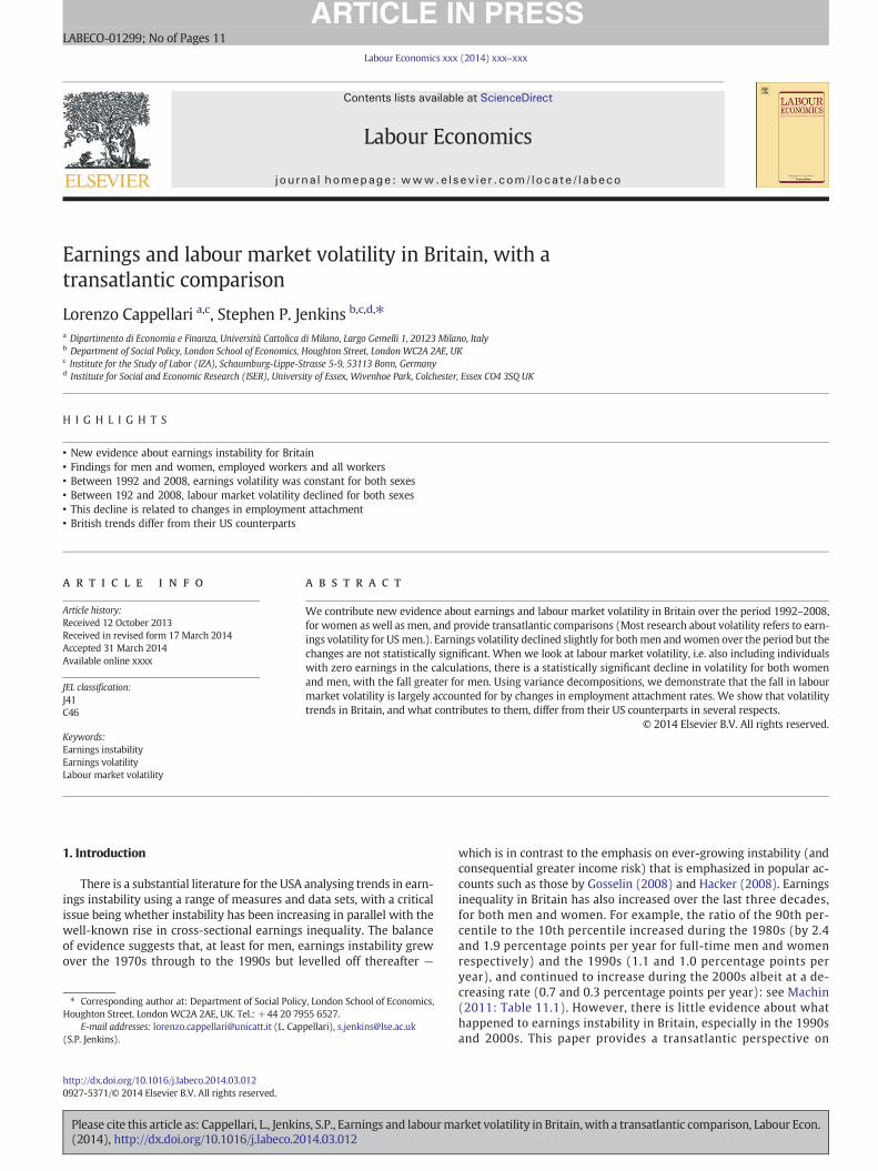
Fig. 3. Decomposition of labour market volatility by employment attachment, Britishmen and women. Notes: Authors' estimates are from BHPS data. The measure of volatilityis V= I2 (see main text). The decomposition formula is shown in Eq. (3). The values of thevariance and variance contributions, and the latter expressed as a share of the total variance,are tabulated by year and sex in Cappellari and Jenkins (2013b: Appendix Table A1).

(b) Women

(a) Men

0

10

20

30

40

50

60

70

80

90

100

Per

cent

age

1992 1994 1996 1998 2000 2002 2004 2006 2008P11 P01 P10 P00 M11

0

10

20

30

40

50

60

70

80

90

100

Per

cent

age

1992 1994 1996 1998 2000 2002 2004 2006 2008P11 P01 P10 P00 M11

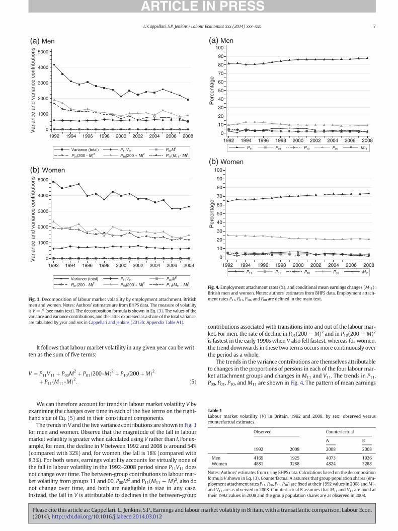
Fig. 4. Employment attachment rates (%), and conditional mean earnings changes (M11):British men and women. Notes: authors' estimates from BHPS data. Employment attach-ment rates P11, P01, P10, and P00 are defined in the main text.

Table 1Labour market volatility (V) in Britain, 1992 and 2008, by sex: observed versuscounterfactual estimates.

Observed Counterfactual

A B

1992 2008 2008 2008

Men 4169 1925 4073 1926Women 4881 3288 4824 3288

Notes: Authors' estimates from using BHPS data. Calculations based on the decompositionformula V shown in Eq. (3). Counterfactual A assumes that group population shares (em-ployment attachment rates P11, P00, P10, P10) are fixed at their 1992 values in 2008 andM11

and V11 are as observed in 2008. Counterfactual B assumes that M11 and V11 are fixed attheir 1992 values in 2008 and the group population shares are as observed in 2008.

7L. Cappellari, S.P. Jenkins / Labour Economics xxx (2014) xxx–xxx

It follows that labourmarket volatility in any given year can bewrit-ten as the sum of five terms:

V ¼ P11V11 þ P00M2 þ P01 200–Mð Þ2 þ P10 200þMð Þ2

þ P11 M11–Mð Þ2: ð5Þ

We can therefore account for trends in labour market volatility V byexamining the changes over time in each of the five terms on the right-hand side of Eq. (5) and in their constituent components.

The trends in V and thefive variance contributions are shown in Fig. 3for men and women. Observe that the magnitude of the fall in labourmarket volatility is greater when calculated using V rather than I. For ex-ample, for men, the decline in V between 1992 and 2008 is around 54%(compared with 32%) and, for women, the fall is 18% (compared with8.3%). For both sexes, earnings volatility accounts for virtually none ofthe fall in labour volatility in the 1992–2008 period since P11V11 doesnot change over time. The between-group contributions to labour mar-ket volatility from groups 11 and 00, P00M2 and P11(M11 − M)2, also donot change over time, and both are negligible in size in any case.Instead, the fall in V is attributable to declines in the between-group

Please cite this article as: Cappellari, L., Jenkins, S.P., Earnings and labourma(2014), http://dx.doi.org/10.1016/j.labeco.2014.03.012

contributions associated with transitions into and out of the labour mar-ket. For men, the rate of decline in P01(200−M)2 and in P10(200+M)2

is fastest in the early 1990s when V also fell fastest, whereas for women,the trend downwards in these two terms occursmore continuously overthe period as a whole.

The trends in the variance contributions are themselves attributableto changes in the proportions of persons in each of the four labour mar-ket attachment groups and changes in M11 and V11. The trends in P11,P00, P01, P10, and M11 are shown in Fig. 4. The pattern of mean earnings

rket volatility in Britain,with a transatlantic comparison, Labour Econ.

8 L. Cappellari, S.P. Jenkins / Labour Economics xxx (2014) xxx–xxx

changes among group 11 is a flat inverse U-shape for both men andwomen:M11 rises from less than 5% per year during the early 1990s toaround 5% for the decade between the mid-1990s and mid-2000s, andthen declines to less than 5% per year again subsequently.

The most perceptible changes over time are in the group populationshares (employment attachment rates). Specifically, the proportion ofmen in group 11 rises from just below 81% at the start of the 1990s toaround 86% at the start of the 2000s, after which the rate of increase issomewhat smaller (the group's share is 88% in 2008). The rise primarilyreflects a shift from the proportion of men in group 00: the share de-creases from just over 13% in 1994 to around 9% in the late-2000s ac-companied by decreases in the shares in the other two groups. Thepopulation share of group 01 falls from just over 3% in 1994 to justover 1% in 2008; for group 10, the corresponding change is from justover 3% to just over 2%. For women, the rise in the population share ofgroup 11 is more continuous over the period, increasing from around66% in 1994 to 73% in 2008, matched by a decline in the proportion ingroup 00 from around 25% at the start of the 1990s to around 20% in2008, together with small declines in the other two groups' shares(from just under 5% in 1994 to just under 3% in 2008 for group 01and from just under 5% in 1994 to just under 4% for group 10). Forbrevity, annual estimates of V11 are not reported; we report thechanges between 1992 and 2008 in Table 1. The direction of changesover the years in earnings volatility calculated using V11 is of courseidentical to the direction of changes for I summarized in Fig. 1, butthe magnitude of the estimated decline over the period is greaterfor V11 than I. The fall in V11 between 1992 and 2008 is −15% formen (compared with −3% for I), and −18% for women (comparedwith −8%).

We illustrate the importance of the trends in group populationshares for explaining trends in labour market volatility with a counter-factual exercise. Using Eq. (5), we can ask what labour market volatilitywould have been in 2008 were group population shares to haveremained as they were in 1992 while M11 and V11 take their observedvalues for the two years (counterfactual A) or, instead, we can askwhat labour market volatility would have been in 2008 if M11 and V11

were to have remained as they were in 1992 but group populationshares take their observed values in the two years (counterfactual B).The results are summarized in Table 1. If population shares are fixedas in A, then the observed changes in group 11's mean and variance ofearnings changes would have reduced labourmarket volatility between1992 and 2008, but only slightly: just over 2% of the observed change inV for men, and just over 1% of the observed change for women. In con-trast, counterfactual B shows that changes in the group populationshares with M11 and V11 fixed generate estimates for V for 2008 thatare virtually identical to those that are observed.

Assembling the evidence, the story that emerges for both men andwomen is that earnings volatility trends make a negligible contributionto labour market volatility trends between 1992 and 2008. The within-group variance contribution is constant over time, because a small fall inearnings volatilitywas offset by an increase in the proportion of individ-ualswhoare employed for two consecutive years. Instead, the decline inlabourmarket volatility is primarily accounted for by the declines in theproportions of individualsmaking transitions into or out of employmentbetween two consecutive years. Although these two groups' populationshares are small in every year, they are used in the variance decomposi-tion formula to weight a group average earnings change (200% or−200%) that is very large by comparison with the average earningschange in the population as awhole. Thefinding that labourmarket vol-atility trends in Britain are not attributable to earnings volatility trendsis of course consistent with what was shown by the trends in quantilesof earnings change distributions presented earlier. The advantage of theapproach used in this Section based on the variance as a summary indexis that it provides an exact decomposition of the various contributions;the potential disadvantage of the decomposition formula is the particu-lar way in which it aggregates the various components.

Please cite this article as: Cappellari, L., Jenkins, S.P., Earnings and labourma(2014), http://dx.doi.org/10.1016/j.labeco.2014.03.012

What are the drivers of the observed trends? For earnings volatility,the question is morewhy it hardly changed over the 1992–2008 period.One possible answer is that it reflects the net outcome of offsettingchanges for different groups. Celik et al. (2012) analysed whether thiswas the case in the USA, distinguishing between workers who stayedwith the same employer and workers who changed jobs from oneyear to the next. Using variance decompositions of the type describedabove, Celik et al. found higher volatility levels among job-changers(as expected), but there was no clear cut association between trendsin earnings volatility and changes in job-change rates. We find thesame result for Britain (results not shown). Moreover, we also find nosystematic explanation for theflat trend in terms of changes in the prev-alence of part- and full-timework attachment, or the secular increase inthe fraction of workers with educational qualifications to university en-trance standard. See Cappellari and Jenkins (2013b) for details.

The downward trend in labour market volatility is correlated withthe improvement in macroeconomic conditions from the early-1990sthrough to 2008. The UK economy experienced a serious downturn atthe start of the 1990s, but this was followed by recovery at a steadyrate until the turn of the 2000s and then at a slower rate until theonset of the Great Recession. Unemployment rates around 10% in1992 and 1993 (following two consecutive quarters of negative GDPgrowth in 1991), but around 5% in 2000 and then steady until theyrose sharply in 2008 with the return of negative GDP growth (Greggand Wadsworth, 2010: Figure 1). The association between labour mar-ket volatility and macroeconomic conditions arises from changes in la-bour market attachment since earnings volatility is flat throughout theperiod. The rise in P11 from the mid-1990s – greater employmentattachment – is consistent with the decline in both involuntary and vol-untary annual job separation rates between 1997 and 2008 reported bythe Office for National Statistics (2011: Figure 1). And the decline in P00is consistent with the decline in the fraction of individuals unemployedfor more than a year between 1993 and the mid-2000s (Gregg andWadsworth 2010: Figure 3).

The trends in P01 and P10 are consistent with other evidence forBritain about how labour market flow transition rates changed withthe macroeconomic cycle between 1992 and 2008. Annual transitionrates between unemployment (U), inactivity (N), and employment(E), estimated from Labour Force Survey data, are shown by Elsbyet al. (2011, Figure 7) (See also Smith, 2011 who estimates monthlyflow transition rates using BHPS data.). For example, Elsby et al. showtransition rate UE rising over the period and transition rate EU falling.These same patterns are apparent in our BHPS data once we use labourmarket state definitions corresponding to theirs and take account ofother definitional differences. For instance note that P00, P10, P01, P11are population shares not transition rates, we define employment interms of having earnings or not (rather than using ILO definitions),and our estimation sample excludes virtually all individuals under theage of 25 (Elsby et al. include all individuals aged 16 and over, andpool data for men and women). We return to the relationship withthe business cycle in the transatlantic comparison in the next Section.

6. Britain in comparison with the USA

Wehave shown that, for bothmen andwomen, earnings volatility inBritain changed little between the early-1990s and the late-2000s,whereas labour market volatility for both sexes fell over the same peri-od. How do these results compare with those for the USA?

To answer this question, we switch to using volatility estimates forBritain that are based on annual earnings measures because they areused in US studies. This switch is insubstantial because our headlinefindings for Britain are the same regardless of whether a current or an-nual earningsmeasure is used. See Appendix Figs. A5 and A6. As expect-ed, earnings volatility is larger if calculated using the annual earningsmeasure rather than current earnings (but the increase is small) andthere is also no trend upwards or downwards over time. Labourmarket

rket volatility in Britain,with a transatlantic comparison, Labour Econ.

9L. Cappellari, S.P. Jenkins / Labour Economics xxx (2014) xxx–xxx

volatility is also greater when the annual earnings measure is used(more obviously for women than for men), but both measures show asimilar downward trend over the period. Trends in employment attach-ment are also similar for the two earnings measures.

The US literature on volatility provides estimates for the period fromthe early 1970s through to 2008 (A useful table summarizing the find-ings of US studies of longitudinal earnings instability is provided byDynan et al., 2012, Table 3b.). Virtually all studies show that earningsvolatility for men increased during the 1970s, but then levelled offsomewhat through to the early- to mid-1980s or fell slightly. Findingsabout what happened thereafter depend on the data set used: in partic-ular, estimates derived from the Panel Study of Income Dynamics sug-gest a rise in volatility (Celik et al., 2012; Shin and Solon, 2011)whereas those derived using administrative record data or survey datalinked to administrative record data suggesting that volatility eitherremained flat (Celik et al., 2012; Dahl et al., 2011; DeBacker et al.,2013) or at least appear not to have risen (Juhn and McCue, 2012;Monti and Gathright, 2013). Our summary judgment is that there isno clear cut evidence for a trend in men's earnings volatility in theUSA between the beginning of the 1990s and 2008 (i.e. we give lessweight to the PSID estimates), a result which is the same as our finding

(a) Men

(b) Women

0

10

20

30

40

50

60

70

80

90

Per

cent

age

1992 1994 1996 1998 2000 2002 2004 2006 2008

Labour market volatility (GB) Earnings volatility (GB)Labour market volatility (US) Earnings volatility (US)

0

10

20

30

40

50

60

70

80

90

Per

cent

age

1992 1994 1996 1998 2000 2002 2004 2006 2008

Labour market volatility (GB) Earnings volatility (GB)Labour market volatility (US) Earnings volatility (US)

Fig. 5. Earnings and labour market volatility for men and women, Britain and the USA.Notes: The measure of volatility is I (see main text). The earnings volatility estimates forBritain (‘GB’) are based on the BHPS measure of ‘annual labour income’ (Comparisons ofestimates based on current and annual earnings measures are shown in AppendixFigs. A5 and A6). The earnings volatility estimates for the USA (‘US’) are derived frommatched CPS data, and are shown as the ‘baseline series’ in Ziliak et al. (2011: Figures 1and 3) which also cover 1973–1991. The discontinuity in the US series at 1995 reflects amajor redesign of the CPS.

Please cite this article as: Cappellari, L., Jenkins, S.P., Earnings and labourma(2014), http://dx.doi.org/10.1016/j.labeco.2014.03.012

for Britain. However, there is much less US evidence about labour mar-ket volatility or earnings volatility for women.

To continue with our transatlantic comparisons, we thereforefocus on the estimates from the US study by Ziliak et al. (2011)for the period 1992–2008. Only their research provides volatilityestimates for men and women separately, and for labour marketvolatility as well as earnings volatility. However, to avoid relianceon a single study, we draw on other research where possible. Ourtransatlantic comparisons of earnings and labour market volatilityare summarized in Fig. 5.

What is clear from the graphs is that earnings volatility is withouttrend in both Britain and the USA. In addition, the eye is struck by theapparently substantially greater magnitude of earnings volatility levelsin the USA. Ziliak et al. (2011) estimate I to hover just above 50% forUS men whereas the British estimate is around 30%. The correspondingestimates for women are between 55% and 60% in the USA but around40% in Britain. Some caution is required when comparing earnings vol-atility levels, however, because other US studies suggest that estimatesof the same volatility measure differ across data sets and samples. Forexample, Celik et al. (2012, Figure 1) using matched-CPS data reportlevels of S for US men that are around 10 percentage points lowerthan the corresponding estimates of Ziliak et al. (2011, Figure 3), thoughalso with a relatively flat trend (with one exception discussed shortly).The reason for the differences may be the use of different samples(Ziliak, Hardy, and Bollinger use men aged 16–60; Celik et al. use menaged 25–59). Also, the two studies report rather different CPS matchrates. Either or both of these factors is also likely to be responsible forthe fact that Celik et al. (2012: Figure 1) report a substantial spike in-crease in men's earnings volatility between 2007 and 2008, whereasZiliak et al. (2011: Figure 3) report virtually no change over the sameinterval.

Celik et al. (2012: Figure 1) also report two series of estimates formen based on Survey of Income Program and Participation panels(but a discontinuous series) and LEHD data derived from unemploy-ment insurance administration records. Over the 1990s and 2000s, theSIPP series for S tracks the matched-CPS one, but estimates for eachyear are about 5 percentage points smaller (the LEHD estimates areabout 10 percentage points larger than the matched-CPS ones), butthe level is always above 30%. This is the level of our British estimatesof S for men (see Appendix Fig. A3), although based on current ratherthan annual earnings (and survey rather than administrative data).The transatlantic differential in earnings volatility levels is confirmed ifP is used as the volatility measure: see OECD (2011: Figure 3.1) formen and women combined.

In sum, it appears that earnings volatility levels for men are greaterin the USA than in Britain — this is shown by all the data sources withthe exception of the discontinuous SIPP series.

Turning to labour market volatility rather than earnings volatili-ty, it is clear that volatility levels are substantially greater in the USAthan in Britain and there is a downward trend in Britain that doesnot occur in the USA: see Fig. 5. According to Ziliak et al. (2011),labour market volatility in the USA hardly changed over the1992–2008 period, remaining at about 75% for men and just under85% for women. In Britain, labour market volatility fell for bothsexes. The transatlantic differential is about 10 percentage pointsat the beginning of the 1990s for men (less for women) but around30 percentage points by 2008. Again we may ask whether the com-parisons are robust to choice of measure and data set, and the prob-lem is that few other estimates are available. We are aware only ofthe estimates of I for US men provided by Celik et al. (2012:Figure 2), derived from matched-CPS data. These confirm the trans-atlantic differential and difference in trend. Celik et al.'s estimatesfor the 1990s and 2000s range between 60% and 70%, i.e. around10 percentage points lower than those of Ziliak et al. (2011) – seeour comments above – but are still well above our correspondingBritish estimates (and with a different trend).

rket volatility in Britain,with a transatlantic comparison, Labour Econ.

(a) Men

(b) Women

0

10

20

30

40

50

60

70

80

90

100

Per

cent

age

1992 1994 1996 1998 2000 2002 2004 2006 2008P11 (GB) P01 (GB) P10 (GB) P00 (GB)P11 (US) P01 (US) P10 (US) P00 (US)

0

10

20

30

40

50

60

70

80

90

100

Per

cent

age

1992 1994 1996 1998 2000 2002 2004 2006 2008P11 (GB) P01 (GB) P10 (GB) P00 (GB)P11 (US) P01 (US) P10 (US) P00 (US)

Fig. 6. Employment attachment rates (%) for men andwomen, Britain and the USA. Notes:Employment attachment rates P11, P01, P10, and P00, are defined in the main text. See alsothe notes to Fig. 5.

10 L. Cappellari, S.P. Jenkins / Labour Economics xxx (2014) xxx–xxx

One additional US feature that many researchers have pointedto is that earnings volatility for men is higher during recessions:see e.g. Cameron and Tracy (1988), Celik et al. (2012), Shinand Solon (2011), Ziliak et al. (2011). Similarly, Moffitt andGottschalk (2012) report that the transitory variance of men'searnings is larger in recessions (Although these papers point tothe empirical association, none of them discuss the reasons whyit may arise.). In contrast, Ziliak et al. (2011) using their full runof data from the early 1970s report that women's earnings volatility islower during recessions.

Ascertaining whether a relationship between volatility and reces-sions also holds for Britain is constrained by the fact that the period ofobservation (1992–2008) is shorter than the period spanned by theUS PSID and matched-CPS data sets (back to the start of the 1970s). In-deed, the period covered by the BHPS spans only one cycle from troughto trough. However, since the decline in labour market volatility inBritain is correlated with macroeconomic recovery, there is some sortof business cycle story at play. This must arise via changes in employ-ment attachment, since earnings volatility is flat through the period.And it is in trends in employment attachment rates that another inter-esting transatlantic contrast appears. See Fig. 6 which compares Ziliaket al. (2011) estimates of employment attachment rateswith our Britishestimates.

For British men, the proportion of individuals with two consecutiveyears in employment (P11) fell slightly during the early-1990s recession

Please cite this article as: Cappellari, L., Jenkins, S.P., Earnings and labourma(2014), http://dx.doi.org/10.1016/j.labeco.2014.03.012

and then recovered to around 90% by 2000 and then remained constantthereafter. The proportion of men with two consecutive years not inemployment (P00) rose in the recession to reach around 10% and thenfell back again,while the proportionsmoving into or out of employmentdeclined slightly. This picture is in sharp contrast to that for USmen, forwhom P11 fell continuously throughout the period and P00 increased(P01 and P10 are relatively small and did not change much in absoluteterms.). Put another way, employment attachment rates for the USandBritishmen appear to be similar at the start of the 1990s butmarkeddifferences open up by 2008. Fig. 6 shows this is the case for women aswell as men.

Wehave not foundother studies that allowus to directly benchmarkthese trends. However, the estimated declines in P01 and P10 for the USA(which are not very perceptible in Fig. 6 given the scales used) are con-sistent with the declining rates of job separations and hires reported byHyatt and Spletzer (2013) using three administrative data sets (similaradministrative data do not exist for the UK). As discussed in the previ-ous Section, trends in employment rates are related to underlying la-bour market flow transition rates, and we note that there is evidencethat levels and trends in labourmarket transition rates differed betweenthe USA and the UK over this period. According to Elsby et al. (2013:Figure 2), UE and EU transition rates levels are substantially lower inthe UK than the USA and, moreover, the upward trend in the UErate is greater in the UK than the USA. Our findings are thus alsoconsistent with the OECD's conclusion, based on a different sum-mary measure of volatility, that ‘[c]ountries with the most dynamiclabour markets – as measured by hiring, firing and quit rates – tendto have a relatively low incidence of earnings volatility’ (OECD,2011: 154).

7. Summary and conclusions

We have argued that straightforward measures of volatility providea means to examine not only instability in earnings among those whoare employed, but also instability in the labour market as a whole, i.e.also including workers without a job. This same property makes thesemeasures well-suited to analyse volatility for women as well as men(virtually all previous studies of earnings instability of all kinds havebeen for men only). Using BHPS data, we have provided new British ev-idence about earnings and labour market volatility for both men andwomen.

Wehave shown that in Britain, and for both sexes, earnings volatilitychanged little between 1992 and 2008, but there was a fall in labourmarket volatility. Although earnings volatility trends over this periodappearflat in both theUSA and Britain, the decline in labourmarket vol-atility that occurred in Britain is not apparent in the USA. And, in so faras there is a relationship between volatility and the business cycle, it ap-pears to arise in Britain via changes in employment attachment ratesrather than in changes in earnings volatility as in the USA. In any case,there are intriguing transatlantic differences in the trends in employ-ment attachment rates.

Our research leaves a number of unresolved questions. For example,what explains the transatlantic differences in levels and trends in vola-tility that we have identified? Regarding levels, it is often said that theUS labour market is more flexible than the British one, with employ-ment arrangements less governed by collective bargaining arrange-ments, employment protection legislation, and so on (Nickell, 1997).One might conjecture that this labour market flexibility is reflected inrelatively greater instability in earnings and employment attachmentfor US workers compared to their British counterparts. Our estimatesare consistent with this hypothesis but, as we have pointed out, differ-ent data sets (and samples) can tell different stories. Explaining the dif-ferences in trends in volatility is a harder task. Our decompositionanalysis suggests that differences in aggregate trends can arise via mul-tiple routes: differences in trends in earnings volatility, mean earnings

rket volatility in Britain,with a transatlantic comparison, Labour Econ.

11L. Cappellari, S.P. Jenkins / Labour Economics xxx (2014) xxx–xxx

changes, and labour market attachment rates. Further work is requiredto disentangle the roles of the various elements.

Another outstanding question is: what has happened to earningsand labourmarket volatility in the period after the onset of theGreat Re-cession, not covered by the data sets for Britain or the USA that werecited in this paper? For Britain, a promising source for future work onearnings and labourmarket volatility is the panel data version of theAn-nual Survey of Hours and Employment, also employed in its earlier guise(as the New Earnings Survey panel) by Dickens (2000) and Kalwij andAlessie (2007) to fit parametric earnings component models.

Acknowledgements

The research for this paper was supported by a British AcademySmall Research Grant (award SG110858) and by core funding of the Re-search Centre onMicro-Social Change at the Institute for Social and Eco-nomic Research by the University of Essex and the UK Economic andSocial Research Council (award RES-518-28-001). For comments anddiscussion, we thank the editor and two anonymous referees, JohnMicklewright, Berkay Özcan, Lucinda Platt, Jim Spletzler, and audiencesat RHUL, ISER/Essex, CEP/LSE, Girona, EALE2013, ESPE2013, and the2013 IZA/SoLE Transatlantic meeting. Bradley Hardy kindly providedthe statistics underlying the charts in Ziliak et al. (2011).

Appendix A. Supplementary data

Supplementary data to this article can be found online at http://dx.doi.org/10.1016/j.labeco.2014.03.012.

References

Abowd, J., Card, D., 1989. On the covariance structure of earnings and hours changes.Econometrica 57, 411–445.

Attanasio, O., Weber, G., 2010. Consumption and saving: models of intertemporal alloca-tion and their implications for public policy. J. Econ. Lit. 48, 693–751.

Baker, M., 1997. Growth-rate heterogeneity and the covariance structure of life-cycleearnings. J. Labor Econ. 15, 338–375.

Baker, M., Solon, G., 2003. Earnings dynamics and inequality among Canadian men,1976–1992: evidence from longitudinal income tax records. J. Labour Econ. 21,289–321.

Blundell, R., Pistaferri, L., Preston, I., 2008. Consumption inequality and partial insurance.Am. Econ. Rev. 98, 1887–1921.

Cameron, S. and Tracy, J. (1988). ‘Earnings variability in the United States: an examinationusingmatched-CPS data’. Unpublished paper. NewYork: Federal Reserve BankofNewYork. http://www.newyorkfed.org/research/economists/tracy/earnings_variability.pdf, last accessed 12 March 2014.

Cappellari and Jenkins (2013a). ‘Trends in the transitory variance of earnings: evidencefor British men and women’, unpublished paper, LSE and Università Cattolica, Milano.

Cappellari, L., Jenkins, S.P., 2013a. Earnings and labour market volatility in Britain. Work-ing Paper 2013-10Institute for Social and Economic Research, University of Essex,Colchester (https://www.iser.essex.ac.uk/publications/working-papers/iser/2013-10,last accessed 12 March 2014).

Celik, S., Juhn, C.,McCue, K., Thompson, J., 2012. Recent trends in earnings volatility: evidencefrom survey and administrative data. B. E. J. Econ. Anal. Policy 12, 2 ((Contributions),Article 1).

Congressional Budget Office, 2008. Recent Trends in the Variability of Individual Earningsand Household Income. Congressional Budget Office, Washington DC (http://www.cbo.gov/publication/41714, last accessed 12 March 2014).

Cunha, F., Heckman, J., Navarro, S., 2005. Separating uncertainty from heterogeneity in lifecycle earnings. Oxf. Econ. Pap. 57, 191–261.

Dahl, M., DeLeire, T., Schwabisch, J.A., 2011. Estimates of year-to-year volatility in earn-ings and in household incomes from administrative, survey, and matched data.J. Hum. Resour. 46, 750–774.

Daly, M.C., Valletta, R.G., 2008. Cross-national trends in earnings inequality and instability.Econ. Lett. 99, 215–219.

DeBacker, J., Heim, B., Panousi, V., Ramnath, S., Vidangos, I., 2013. Rising inequality:transitory or permanent? New evidence from a panel of U.S. tax returns. Brook.Pap. Econ. Act. 67–142 (Spring).

Dickens, R., 2000. The evolution of individual male earnings in Great Britain: 1975–95.Econ. J. 110, 27–49.

Doris, A., O'Neill, D., Sweetman, O., 2013. Identification of the covariance structure ofearnings using the GMM estimator. J. Econ. Inequal. 11, 343–372.

Please cite this article as: Cappellari, L., Jenkins, S.P., Earnings and labourma(2014), http://dx.doi.org/10.1016/j.labeco.2014.03.012

Dynan, K.E., Elmendorf, D.W., Sichel, D.E., 2012. The evolution of household income vola-tility. B. E. J. Econ. Anal. Policy 12, 2 ((Advances), Article 3).

Elsby, M.W.L., Smith, J.C., Wadsworth, J., 2011. The role of worker flows in the dynamicsand distribution of UK unemployment. Oxf. Rev. Econ. Policy 27, 338–363.

Elsby, M.W.L., Hobijn, B., Sahin, A., 2013. Unemployment dynamics in the OECD. Rev.Econ. Stat. 95, 530–548.

Friedman, M., 1957. A Theory of the Consumption Function. Princeton University Press,Princeton.

Gosselin, P., 2008. High Wire: the Precarious Financial Lives of American Families. BasicBooks, New York.

Gottschalk, P., Moffitt, R.A., 1994. The growth of earnings instability in the U.S. labourmarket. Brook. Pap. Econ. Act. 2, 217–272.

Gottschalk, P., Spolaore, E., 2002. On the evaluation of economic mobility. Rev. Econ. Stud.69, 191–208.

Gregg, P., Wadsworth, J., 2010. Unemployment and inactivity in the 2008–2009 recession.Econ. Labour Mark. Rev. 4, 44–50.

Guvenen, F., 2009. An empirical investigation of labour income processes. Rev. Econ. Dyn.12, 58–79.

Hacker, J.S., 2008. The Great Risk Shift (revised and expanded edition). Oxford UniversityPress, Oxford.

Haider, S.J., 2001. Earnings instability and earnings inequality of males in the UnitedStates: 1967–1991. J. Labor Econ. 19, 799–836.

Hause, J.C., 1980. The fine structure of earnings and the on-the-job training hypothesis.Econometrica 48, 1013–1029.

Hosking, J.R.M., 1990. L-moments: analysis and estimation of distributions using linearcombinations of order statistics. J. R. Stat. Soc. Ser. B 52, 105–124.

Hyatt, H.R., Spletzer, J.R., 2013. The recent decline in employment dynamics. IZA J. LaborEcon. 2 (Article 5).

Jenkins, S.P., 2011a. Changing Fortunes: IncomeMobility and Poverty Dynamics in Britain.Oxford University Press, Oxford.

Jenkins, S.P., 2011b. Has the instability of personal incomes been increasing? Natl. Inst.Econ. Rev. 218 (1), R33–R43.

Juhn, C., McCue, K., 2012. Recent trends in earnings volatility: evidence from surveys andadministrative data. B. E. J. Econ. Anal. Policy 12, 2 ((Contributions), Article 1).

Kalwij, A., Alessie, R., 2007. Permanent and transitory wages of British men, 1975–2001:year, age and cohort effects. J. Appl. Econ. 22, 1063–1093.

Lillard, L., Weiss, Y., 1979. Components of variation in panel earnings data: American sci-entists, 1960–1970. Econometrica 47, 437–454.

Lillard, L., Willis, R., 1978. Dynamic aspects of earnings mobility. Econometrica 46,985–1012.

Machin, S., 2011. Changes in UK wage inequality over the last forty years. Chapter 11. In:Gregg, P., Wadsworth, J. (Eds.), The Labour Market in Winter. The State of WorkingBritain. Oxford University Press, Oxford, pp. 155–169.

MaCurdy, T., 1982. The use of time series processes to model the error structure of earn-ings in a longitudinal data analysis. J. Econ. 18, 83–114.

Meghir, C., Pistaferri, L., 2011. Earnings, consumption and lifecycle choices. In:Ashenfelter, O., Card, D. (Eds.), Handbook of Labour Economics, vol. 4B. Elsevier,Amsterdam.

Moffitt, R.A., Gottschalk, P., 2011. Trends in the covariance structure of earnings in theU.S.:1969–1987 (‘Rediscovered Classics’ section reproduction of John Hopkins Universityworking paper from 1995). J. Econ. Inequal. 9, 439–459.

Moffitt, R.A., Gottschalk, P., 2012. Trends in the transitory variance of male earnings.Methods and evidence. J. Hum. Resour. 47, 204–236.

Monti, H., Gathright, G., 2013. Measuring earnings stability using survey and administra-tive data. Paper Presented at the 2013 SoLE Meetings (http://www.sole-jole.org/13516.pdf, last accessed 12 March 2014).

Nickell, S., 1997. Unemployment and labour market rigidities: Europe versus NorthAmerica. J. Econ. Perspect. 11, 55–74.

OECD, 2011. Earnings volatility: causes and consequences. Employment Outlook 2011.OECD, Paris, pp. 153–190.

Office for National Statistics, 2013. Pension trends, chapter 4: the labour market andretirement, 2013 edition. http://www.ons.gov.uk/ons/dcp171766_297899.pdf(last accessed 12 March 2014).

Office for National Statistics, 2011. Reasons for leaving last job. http://www.ons.gov.uk/ons/dcp171776_241679.pdf (last accessed 12 March 2014).

Ramos, X., 2003. The covariance structure of earnings in Britain, 1991–1999. Economica70, 353–374.

Shin, D., 2012. Trends in men's earnings volatility: evidence from the National Longitudi-nal Survey of Youth, 1985–2009. B. E. J. Econ. Anal. Policy 12, 2 ((Topics), Article 2).

Shin, D., Solon, G., 2011. Trends in men's earnings volatility: what does the Panel Study ofIncome Dynamics show? J. Public Econ. 95, 973–982.

Shorrocks, A., 1978. Income inequality and income mobility. J. Econ. Theory 19, 376–393.Smith, J.C., 2011. The ins and outs of UK unemployment. Econ. J. 121, 402–444.Venn,D., 2011. Earnings volatility and its consequences for households. Social, Employment

and Migration Working Papers, No. 125OECD, Paris.Ziliak, J.P., Hardy, B., Bollinger, C., 2011. Earnings volatility in America: evidence from

matched CPS. Labour Econ. 18, 742–754.

rket volatility in Britain,with a transatlantic comparison, Labour Econ.